A TRMM-CALIBRATED INFRARED RAINFALL ALGORITHM

APPLIED OVER BRAZIL

A. J. Negri "1, L. Xu 2 , and R. F. Adler _

_Laboratory for Atmospheres

NASA/Goddard Space Flight Center, Greenbelt, MD 20771

2 Dept. of Hydrology and Water Resources, U. Arizona, Tucson, AZ 85721

Journal of Geophysical Research

Submitted to the special issue on LBA

12/2/00

* Corresponding author address: Andrew J. Negri,

NASA/GSFC, Code 912, Greenbelt, MD 20771 ;

email: negri @agnes.gsfc.nasa.gov

https://ntrs.nasa.gov/search.jsp?R=20010016103 2018-05-20T13:27:41+00:00Z

ABSTRACT

The development of a satellite infrared technique for estimating convective and stratiform

rainfall and its application in studying the diurnal variability of rainfall in Amazonia are

presented. The Convective-Stratiform Technique, calibrated by coincident, physically retrieved

rain rates from the TRMM Microwave Imager (TMI), is applied during January to April 1999

over northern South America. The diurnal cycle of rainfall, as well as the division between

convective and stratiform rainfall is presented. Results compare well (a one-hour lag) with the

diurnal cycle derived from TOGA radar-estimated rainfall in Rondonia. The satellite estimates

reveal that the convective rain constitutes, in the mean, 24% of the rain area while accounting for

67% of the rain volume. The effects of geography (rivers, lakes, coasts) and topography on the

diurnal cycle of convection are examined. In particular, the Amazon River, downstream of

Manaus, is shown to both enhance early morning rainfall and inhibit afternoon convection.

Monthly estimates from this technique, dubbed CST/TMI, are verified over a dense rain gage

network in the state of Ceara, in northeast Brazil. The CST/TMI showed a high bias equal to

+33% of the gage mean, indicating that possibly the TMI estimates alone are also high. The root

mean square difference (after removal of the bias) equaled 36.6% of the gage mean. The

correlation coefficient was 0.77 based on 72 station-months.

1. Introduction

In this paper, we present the application of and results from a satellite infrared (IR) technique

for estimating rainfall over northern South America. Our objectives are to examine the diurnal

variability of rainfall and to investigate the relative contributions from the convective and

stratiform components. There is a paucity of hourly-reporting rainfall stations in northern South

America in general and the Amazon Basin in particular. Hence, most of the literature describing

the diurnal cycle of rainfall in this region has necessarily used satellite observations as a proxy

for rainfall. One notable exception is Kousky (1980), who examined the diurnal cycle of rainfall

in northeast Brazil from l0 years of gage observations. Estimates from IR-only methods include

Meisner and Arkin (1987), who found a pronounced maximum in IR cloudiness at 1800 LT over

the interior of summertime South America. Janowiak and Arkin (1991) examined the period

1986-1989 for seasonal and interannual variations in estimated rainfall. Horel et al. (1989)

looked at 15 years of twice-daily out-going longwave radiation measurements to describe the

annual cycle of convection in the Amazon Basin. More recently, Garreaud and Wallace (1997)

examined 9 years of high spatial resolution IR data to define the diurnal march of deep

convection over the tropical Americas and surrounding waters.

With the launch of the Special Sensor Microwave Imager (SSM/I) in 1987, microwave (MW)

algorithms were developed and applied. Examples include Negri et al. (1994), a 5-year

climatology of warm-season tropical rainfall, and Negri et al. (2000), and a 10-year climatology

over northern South America. Using four SSM/I observations per day, they showed dramatic

differencesin afternoonversusmorning rain estimates.Methodologyusing a combinationof

MW andIR includeHuffman et al. (1995, 1997) who made global, monthly rain estimates from

a merger of IR, MW, gage and models. Other techniques adjust existing IR techniques by the

MW measurements. Examples include Negri et al. (1993), a 3-year, warm-season study over

Mexico, and Xu et al. (1999, 2000) who adjust the GOES Precipitation Index (GPI) by MW

observations from SSM/I in an attempt to improve monthly rainfall estimates. Recently, the

Passive Microwave and Infrared Algorithm (MIRA) [Todd et al., 2000] attempts to estimate

small-scale rainfall. In the forerunner of the research described in this paper, Anagnostou et al.

(1999) trained IR observations with three months of SSM/I observations to deduce the diurnal

cycle of rainfall over northern South America.

In this study, we apply the Convective-Stratiform Technique (CST) of Adler and Negri,

[1988]. The parameters of the original technique were recalibrated using coincident rainfall

estimates derived from the Tropical Rain Measuring Mission (TRMM) Microwave Imager

(TMI) and GOES IR (11 lam) observations. Henceforth, we refer to this new technique as the

CST/TMI.

2.0 Data and Methodology

In this study, we apply the Convective-Stratiform Technique (CST) of Adler and Negri,

[1988]. In short, the CST locates, in an array of IR data, all local minima in the brightness

temperature field. After an empirical screening to remove thin, non-raining cirrus, the remaining

2

minima are assumed centers of convective rain. A stratiform rain assignment, based on the mode

temperature of each cloud system, completes the rain estimation. The parameters of the original

technique were recalibrated using coincident rainfall estimates derived from the application of

the Goddard Profiling (GPROF) algorithm to TMI brightness temperatures [Kummerow and

Giglio, 1994; Kummerow et al., 1996]. We use an improved algorithm for convective/stratiform

division in the GPROF as described by Olson et al., [2000].

Over northern South America, the GOES-east observes every 30 rain; therefore, we were

able to match a TMI image with an IR image within a 15 min window. Calibration was

performed over land only, from 12N to 18S and from 82W to 34W. The TMI rain estimates

contain the distribution of total surface rainfall as well as the classification of convective and

stratiform rain. The matched data (165 TRMM overpasses) are in the period from January to

April, 1999, the first two months of which coincide with the period of the Large-Scale

Biosphere-Atmosphere (LBA) experiment in Brazil.

The goal of the recalibration is to determine parameters so that the CST will be able to

reproduce the total rain volume, total rain area, and the TMI-observed division between

convective and stratiform rain. We adjust the CST on a statistical basis, over the 4-month

calibration period, without explicit constraints on instantaneous rain estimates. The recalibration

takes the following form:

3

a) determination of convective cores using a discriminant analysis. This is based on the

identification of points of local IR temperature minimum (T,n_o) and the computation of the

deviation of the Tm_nfrom the background temperature (defined as the average temperature of the

eight surrounding pixels). Figure 1 shows the analysis of Tmi n in the 2-dimensional space defined

by IR temperature and the deviation of the Tm_nfrom the background. Points are defined by the

corresponding TMI-retrieved rain rate as either convective (C) or non-convective (N). Plotted

data represents a 1% random subset of the total dataset used to derive the discriminant line. T,,_.

points above and to the left of the discriminant lines are deemed convective. The resultant

discriminant lines are defined by:

1.25. T.,,o - 3.16.Deviation _<254.7 and Deviation _<2.23

b) determination of the convective rain area assigned to each Tm,o. This is based on the

computation of c_, the constant of proportionality between the total convective area in the TMI

estimates and the parameter }_(Tc_,,ua- Train). For a given convective Tram, O_• (Tc_ooj - Tmin) is the

number of pixels to which we assign a convective rain rate centered on the Tmi n. In this study

Tcjoud is a constant set to 253 K, a commonly used threshold for convective clouds. Based on the

rain area determined from the TRMM convective area estimates, o_ - 0.61. For Tin,, = 203 for

example, 32 pixels (4 by 4 km) would be assigned the convective rain rate.

c) determination of the mean convective rain rate. We set the convective rain rate equal

to the conditional rain rate of the TMI/GPROF estimates, namely 18.9 mm h -]. This allows the

total convective rain volume derived from CST/TMI to equal that calculated from the TMI

alone.

d) determination of the threshold temperature to define the stratiform rain area. We

choose a threshold such that the total cloud area colder than this threshold (excluding those

pixels already assigned convective rain) is equal to the stratiform rain area derived by

TMI/GPROF. This threshold, calculating using cumulative area matching, was found to be 219

K.

e) determination of the mean stratiform rain rate. As in the case of determining the

convective mean rain rate, the conditional TMI/GPROF stratiform rain rate of 2.6 mm h-; was

used. This forces the total stratiform rain volume from CST/TMI to equal that of the TMI alone,

integrated over the 4-month calibration period.

In summary, the CST/TMI finds local IR minima, decides if they are convective features,

then assigns a rain area and rainrate based on the TMI calibration parameters. A stratiform rain

area is then defined, and a lower rain rate is assigned to those cloud pixels colder than the

stratiform IR threshold and not previously assigned convective rain. We have chosen two rain

rates to make the technique simple and efficient. An example of the instantaneous application of

this technique is shown in Figure 2. The four panels indicate (clockwise from the upper left): a

GOES IR image of southwestern Brazil; the CST/TMI rainfall estimate; the rain rate from the

5

TRMM radar algorithm 2A25; and the GPROF-retrieved rain rate applied to the TMI brightness

temperatures. For reference, the outline of the TMI swath appears on all images.

3. Results

3.1 The Diurnal Cycle in the TOGA Radar Area

Rain estimates over northern South America (12N to 18S, 82W to 34W) were made from 30

rain interval GOES data for the period January-April, 1999. The first two months of this period

coincided with the LBA experiment in Rondonia, (southwestern Brazil). TOGA radar data

provided a comparison between the mean radar rain rates and convective/stratiform division with

those estimated by the CST. The satellite estimates were matched in both time (5 min) and space

(accounting [br bad and missing data) to the gage-calibrated radar estimates [Anagnoustou et al.,

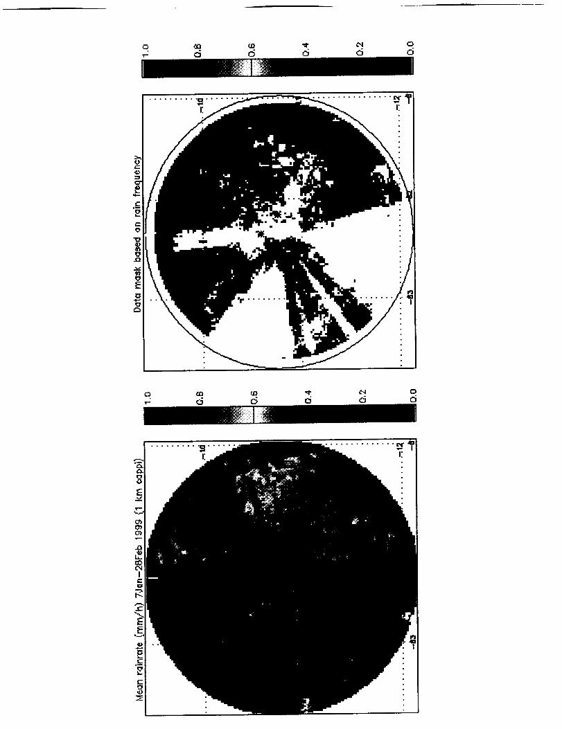
2000]. Figure 3 (left) displays the mean rain rate (ram h -_) from the TOGA radar at 1 km height

for the period 7 Jan to 28 Feb 1999. The asterisks mark the location of the four main clusters of

rain gages. Problems with beam blockage and ground clutter along several azimuths necessitated

the creation of a quality control mask (Figure 3, right). This mask represents the frequency of

occurrence of rainfall in the interval 7-13%. (Higher than 13% was determined to be ground

clutter; lower than 7% was beam blockage). Instantaneous radar estimates were averaged only

within the confines of this mask, and it is apparent that problems remain with the radar data.

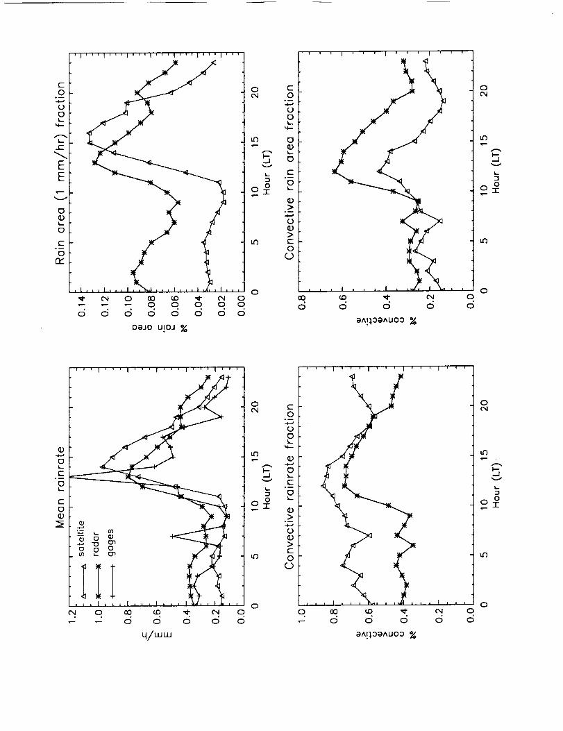
Figure 4 shows the diurnal variation of four rain parameters during the experiment period of

7 Jan to 28 Feb 1999. The upper left panel of the figure displays the unconditional rain rate for

6

the CST/TMI estimates (green), TOGA radar (red) and rain gages (blue). The upper right panel

shows the percent of the radar area covered by rain greater than 1 mm h -_. The lower left panel

tracks the variation of the convective rain rate (the percent of the rain volume due to convective

rain). Finally, the lower right panel reveals the variation of the percent of the rain area due to

convective rain. The satellite estimates of the mean rain rate (top left) are in good agreement

with both the radar and gages. They lag the radar (and gage) estimates by one hour, essentially

missing the earliest stages of convection. By comparison, results using a simple threshold

method (the GOES Precipitation Index or GPI, not plotted) showed a three-hour lag in the

maximum rainfall. The mean values of the satellite, gage and radar estimates are, respectively,

0.35, 0.35 and 0.43 mm h -_. Compared to the radar estimates, the CST/TMI overestimates the

fractional convective rain volume (bottom left) by a factor of 1.36, while underestimating the

fractional convective area (bottom right) by a factor of 1.57. An underestimation of the total rain

area by a factor of 1.52 is also noted. Despite the biases, the phase of all four of the satellite-

estimated parameters seems to well represent (within an hour of the maximum), the phase of the

radar-derived rainfall. The satellite estimates reveal that the convective rain constitutes, in the

mean, 24% of the rain area while accounting for 67% of the rain volume.

3.2 Results for Northern South America

Figure 5 shows the application of the CST/TMI to 30 min interval data from January-April

1999 over the northern portion of South America. Results (in mm h l) are binned into hourly

categoriesandadjustedfor local time (3 zones).The final paneldisplaysthemeanrain ratefor

theentire4-monthperiod. Amongtheinterestingfeaturesrevealedin this presentationare:

• The development of afternoon (12 - 20 LT) squall lines along the Northeast Brazilian

coast. Such squall lines were studied by Garstang et al., [ 1990].

• A morning maximum and afternoon minimum in rainfall along the Amazon River east of

Manaus. This is described in more detail in the next section;

• A morning rain maximum in the Gulf of Panama, no doubt in response to a land breeze

along the highly convergent coastline;

• The onset of deep convection in the Amazon Basin around 13 LT, maximizing at 15-16

LT;

• A late evening (23 LT) to early-morning (05 LT) maximum along the eastern slopes of

the southern Andes Mountains, possibly the result of a mountain/valley circulation:

• An afternoon (13-18 LT) maximum along the western slopes of the southern Andes.

Many more small-scale features are revealed when these 24 images are viewed in time-

sequence. A QuickTime '_' movie of this sequence is available by contacting the first author. An

alternate method of displaying these hourly data is shown in Figure 6, the arithmetic difference

of the CST/TMI estimates at 18 LT and 06 LT. These times correspond with the overpass times

of the Special Sensor Microwave Imager (SSM/I). Areas with an afternoon maximum are

displayed in yellow to red shades, while areas of morning maximum appear blue to purple. In an

8

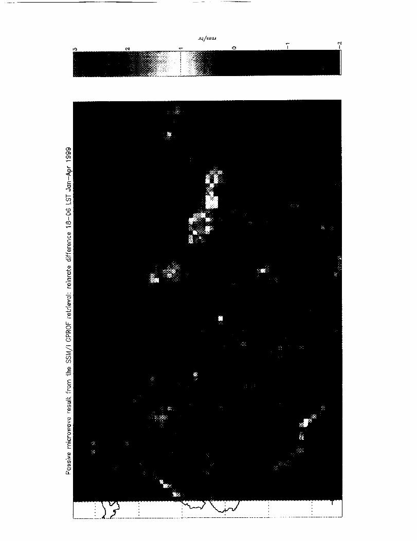
effort to validate these results, we present Figure 7, the estimated rainfall difference (18 -06 LT)

derived from the application of the GPROF algorithm to SSM/I brightness temperatures from the

Fl3 DMSP satellite. Spatial resolution is 0.5 ° and the temporal sampling is about 20

observations/month at both 18 and 06 LT. Note the similarity of features, particularly along the

coasts and rivers, which lend credibility to the IR estimates.

3.3 Effects of the Amazon River on the Rainfall

Figure 8 is a blow-up of the mean hourly estimates in Figure 5, along the confluence of the

Negro and Solim6es Rivers near Manaus, Amazonia, Brazil. Here we find a late-evening (00

LT) rainfall maximum that elongates and moves westward along the river until about l0 LT.

Convection begins by 12 LT, and there is a pronounced minimum in rainfall along the river from

about 15 to 18 LT.

Figure 9 is a time/latitude display of the mean estimated rain rate for January-April, 1999

(left) and January-April, 2000 (right) for a cross-section through the Amazon River at 56W. The

mean position of the Amazon River at this longitude is noted. Downstream of where the Negro

and Solim6es Rivers merge, we find an early morning (3 LT) maximum along the river. Rainfall

avoids the river in the afternoon (12 LT and later). The river seems to be generating a land/river

circulation, which enhances early morning rainfall but inhibits afternoon rainfall along the river.

Such phenomenon have been studied by Oliveira & Fitzjarrald, [1993]. The pattern is

9

duplicated a year later, January-April, 2000 (right), demonstratingthe repeatability of the

phenomenon.

3.4 Diurnal curves for other regions

Buoyed by the success of the technique in an area with ground-truth, we examine the diurnal

variation of rainfall in other regions. In Figure 10, we display a time series of the estimated total,

convective and stratiform rain rates (mm/h) for three regions of interest. In the region

encompassing much of the Amazon Basin (top), peak convective rainfall occurs at 15-16 LT.

The convective rainfall comprises about 74% of the total rainfall at the time of the maximum,

and 67% overall. The stratiform estimates lag the convective by two hours. Estimates for a

smaller subset of the Amazon Basin, along the Amazon R. (downstream of the confluence of the

Negro and Solim6es Rivers) are shown in the middle panel of Fig. 3. A pronounced rainfall

maximum at 3 LT is noted. The bottom panel of Fig. 3 shows the diurnal curve for the northeast

Brazil area, where coastal squall lines form almost daily. The peak estimated rainfall is 1.3

mm/h at 17 LT, and at the maximum, has a percentage of convective rainfall of 65%. The

stratiform lags the convective by 2 h.

3.5 Monthly Verification in the State of Ceara, Brazil

Figure 11 is an example of the monthly rainfall (April 2000) in the state of Ceara in northeast

Brazil. Monthly rainfall is highest along the coast, and tapers off as one moves inland, until

10

higherelevationsarereachedin the southernpart of thestate. This gagedatawasaveragedin

the nine 1° squaresoutlined in the figure for comparison to the area-averagedCST/TMI

estimates.Figure 12showsa scatterplotof theestimatesversusthegagesfor thewet seasonfor

two years(January-April,1999-2000).Standarddeviationsof themeangagerainfall for thenine

grid squaresin Fig. I I areplotted to demonstratethe high spatial variability of rainfall. The

CST/TMI shows a bias (+33% of the gagemean). The root meansquaredifference after

removalof thebias(RMSD-br) is 36.6%of thegagemean,but thetechniqueis not specifically

calibratedin thisregion. We areencouragedby thehighcorrelationcoefficientof 0.77.

4. Conclusions

In this paper, we have presented results from a satellite infrared technique for estimating

rainfall over northern South America. The parameters of the technique were calibrated using

coincident rainfall estimates derived from the application of the GPROF algorithm to TRMM

Microwave Imager brightness temperatures. Our objectives were to examine the diurnal

variability of rainfall at high space and time resolution, and to investigate the relative

contributions from the convective and stratiform components. TOGA radar data during the LBA

experiment provided radar ground truth for both the CST rainfall and convective/stratiform

estimates.

The diurnal cycle of rainfall in the LBA radar area was constructed. The peak satellite-

estimated rainfall lagged the radar by one hour. Identification of the onset of convection was the

11

primary cause of this lag. Estimates of the division of rainfall into convective and stratiform

components were also accomplished. The phase of these components agreed with the radar

estimates, though the convective volume (area) was overestimated (underestimated). The satellite

estimates revealed that the convective rain constitutes, in the mean, 24% of the rain area while

accounting for 67% of the rain volume. Local circulations were found to play a major role in

modulating the rainfall and its diurnal cycle. These included land/sea circulations (notably along

the northeast Brazilian coast and in the Gulf of Panama), mountain/valley circulations (along the

Andes Mountains), and circulations associated with the presence of rivers. This last category

was examined in detail along the Amazon R. east of Manaus. There we found an early morning

rainfall maximum along the river (3 LT at 56W). Rainfall avoids the river in the afternoon (12

LT and later. The width of the river seems to be generating a land/river circulation that enhances

early morning rainfall but inhibits afternoon rainfall.

Verification of the monthly CST/TMI results was performed using rain gages in the northeast

Brazilian state of Ceara. The CST/TMI showed a high bias equal to +33% of the gage mean.

The root mean square difference after removal of the bias was 36.6% of the gage mean. We were

encouraged by the high correlation coefficient of 0.77 for a technique is not specifically

calibrated in this region.

Perhaps the most important future application of this technique may be assessing the impact

of deforestation on the both the rainfall and it's diurnal cycle. We intend to run the CST/TMI for

a full year, and compare monthly and seasonal total and hourly rain estimates with maps of

12

forestedanddeforestedregionsof Amazonia. We hopethat circulationslike that describedover

theAmazonRiver will exist over theseregions,andmanifestthemselvesin thesatelliterainfall

estimates. A secondapplication involves the application of this techniqueto global, high-

resolution,geosynchronousIR datasets(Janowiaket al., 2001).

Acknowledgements. This research was funded by the Atmospheric Dynamics and

Thermodynamics Program at NASA Headquarters. The continued support of Dr. Ramesh Kakar

is appreciated. We would like to thank Geraldo Ferriera of FUNCEME (Meteorology and Water

Resources Foundation of Ceara, Brazil) for providing the raingage data. We also would like to

thank Dr. Emmanouil Anagnostou and Dr. Carlos Morales of the University of Connecticut for

processing and providing the gage-calibrated TOGA radar estimates.

13

References

Adler, R.F. and A.J.Negri, 1988: A satellite infrared technique to estimate tropical convective

and stratiform rainfall. J. Appl. Meteor., 27, 30-5 I.

Anagnostou, E. N., A. J. Negri, and R. F. Adler, 1999: A satellite infrared technique for diurnal

rainfall variability studies. J. Geophys. Res., 104, 31,477-31,488.

Anagnostou, E. and C. Morales, 2000: Rainfall Estimation from TOGA Radar Observations

during TRMM-LBA Field Campaign. AGU (Fall meeting-Atmospheric Sciences).

Garreaud, R. D. and J. M. Wallace, 1997: The diurnal march of convective cloudiness over the

Americas. Mon. Wea. Rev., 125, 3157-3171.

Garstang, M., H. L. Massie, Jr., J. Halverson, S. Greco, and J. Scala, 1990: Amazon coastal

squall lines. Part I: Structure and kinematics. Mon. Wea. Rev., 122, 608-622.

Horel, J. D., A. N. Hahmann, and J. E. Geisler, 1989: An investigation of the annual cycle of

convective activity over the Tropical Americas. J. Climate, 2, 1388-1403.

14

Huffman,G. J., R. F. Adler, B. Rudolf, U. Schneider, and P. R. Keehn, 1995: Global

precipitation estimates based on a technique for combining satellite-based estimates, rain

gauge analysis, and NWP model precipitation information. J. Climate, 8, 1284-1295.

Huffman, G. J., R. F. Adler, P. Arkin, A. Chang, R. Ferraro, A. Gruber, J. Janowiak, A. McNab,

B. Rudolf, and U. Schneider, 1997: The Global Precipitation Climatology Project (GPCP)

combined precipitation dataset. Bull. Amer. Meteor. Soc., 78, 5-20.

Janowiak, J. E. and P. A. Arkin, 1991" Rainfall variations in the tropics during 1986-1989 as

estimated from observations of cloud-top temperature. J. Geophys. Res., 96, 3359-3373.

Janowiak, J. E., Y. Yarosh, and R. J. Joyce, 2001: A real-time global half-hourly pixel-resolution

infrared data set and its applications. Bull. Amer. Meteor. Soc., 82, (in press).

Kousky, V. E., 1980: Diurnal rainfall variation in Northeast Brazil. Mon. Wea. Rev., 108, 488-

498.

Kummerow, C. and L. Giglio, 1994: A passive microwave technique for estimating rainfall and

vertical structure information from space, Part I: algorithm description. J. Appl. Meteor., 33, 3-

18.

15

Kummerow,C.,W. S.Olson,andL. Giglio, 1996:A simplifiedschemefor obtaining

precipitationandverticalhydrometeorprofiles from passivemicrowavesensors.IEEE Trans.

Geosci. Remote Sensing, 34, 1213-1232.

Meisner, B. N. and P. A. Arkin, 1987: Spatial and annual variations in the diurnal cycle of large-

scale tropical convective cloudiness and precipitation. Mon. Wea. Rev., 115, 2009-2032.

Negri, A. J., R. F. Adler, R. A. Maddox, K. W. Howard, and P. R. Keehn, 1993: A regional

rainfall climatology over Mexico and the southwest United States derived from passive

microwave and geosynchronous infrared data. J. Climate, 6, 2144-2161.

Negri, A. J., R. F. Adler, E. J. Nelkin, and G. J. Huffman, 1994: Regional rainfall climatologies

derived from Special Sensor Microwave Imager (SSM/I) data. Bull. Amer. Meteor. Soc., 75,

1165-1182.

Negri, A. J., E. N. Anagnostou, and R. F. Adler, 2000: A 10-year climatology of Amazonian

rainfall derived from passive microwave satellite observations, J. Appl. Meteor., 39, 42-56.

16

Oliveira and D. Fitzjarrald, 1993:The Amazonriver breezeand the local boundarylayer: I.

Observations.Boundary Layer Met. 63, 141-162.

Olson, W., Y. Hong, C.D. Kummerow, and J. Turk, 2000: A texture-polarization method for

estimating convective/stratiform precipitation area coverage from passive microwave

radiometer data, J. Appl. Meteor., (submitted).

Todd, M. C., C. Kidd, D. Kniveton, and T. J. Bellerby, 2000: A combined satellite infrared and

passive microwave technique for estimation of small scale rainfall. J. Atmos. Oceanic

Technol., 17, (in press).

Xu, L., X. Gao, S. Sorooshian, P. Arkin, and B. Imam, 1999: A microwave infrared threshold

technique to improve the GOES Precipitation Index. J. Appl. Meteor., 38, 569-579.

Xu, L., X. Gao, S. Sorooshian, and B. Imam, 2000: Parameter estimation of GOES precipitation

index at different calibration time scales. J. Geophys. Res., 105, 20,131-20,143.

17

Figure Captions

Figure 1. Discriminant analysis of IR temperature minima (Train) in the 2-dimensional space

defined by IR brightness temperature and the deviation of the Tn,_, from the background.

Points are defined by the corresponding TMI-retrieved rain rate as either convective (C) or

non-convective (N) rain. Plotted data represents a 1% random subset of the total dataset used

to derive the discriminant line.

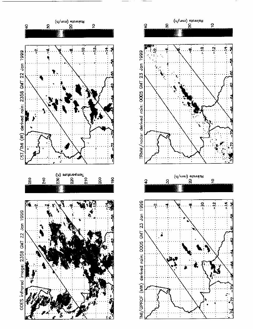
Figure 2. An example of the application of the CST/TMI to one IR image. The outline of the

TMI swath is overlain on all images.

(Upper left): GOES IR image of southwestern Brazil scanned at 2358 GMT 22 Jan 1999;

(Upper right): CSTfrMI rainfall estimate. Convective cores (green) have a mean rain rate of

t8.9 mm h -_ while stratiform rain areas (purple) have a mean rain rate of 2.6 mm h_;

(Lower left): Rain rate retrieved by application of the GPROF algorithm to the TMI

microwave brightness temperatures. Overpass occurred 7 min after the time of the GOES

image;

(Lower right): Rain rate from the TRMM radar algorithm 2A25.

Figure 3. TOGA radar at 1 km height for the period 7 Jan to 28 Feb 1999. The asterisks mark

the locations of the four main clusters of rain gages.

(Left): Mean rain rate (mm h _)

18

(Right): Quality control maskappliedto accountfor missingor bad azimuthsand ground

clutter.

Figure4. Thediurnalvariationof four rain parametersin theperiod7 Janto 28 Feb1999.

(Upper left): The unconditionalrain rate for the CST/TMI estimates(green),TOGA radar

(red)andrain gages(blue).

(Upperright): The variationthe fractionof theradarareacoveredby rain greaterthan 1mm

h-l).

(Lower left): The variation of the percent of the rain volume due to convective rain.

(Lower right): The variation of the percent of the rain area due to convective rain.

Figure 5. Application of the CST/TMI to 30 min interval data from January-April 1999. Results

(mm h -l) are binned into hourly categories and adjusted for local time (3 zones). The final

panel displays the mean rain rate for the entire 4-month period.

Figure 6. The arithmetic difference of the CST/TMI estimates at 18 LT and 06 LT for the

period January-April, 1999. Areas with an afternoon maximum are displayed in yellow to red

shades, while areas of morning maximum appear blue to purple. Units are mm h _.

Figure 7. Same as Figure 4 except the rainfall estimates are derived from the application of the

GPROF algorithm to SSM/I brightness temperatures from the F13 satellite. Spatial

19

resolution is 0.5" and the temporal sampling is about 20 observations/month at both 18 and

06 LT.

Figure 8. A blow-up of the mean hourly estimates (mm h -_) in Figure 3, along the confluence of

the Negro and Solim6es Rivers near Manaus, Amazonia, Brazil.

Figure 9. A time/latitude display of the mean estimated rain rate (mm hl) for a cross-section

through the Amazon River at 56W.

(Left): January-April, 1999

(Right): January - April 2000

Figure 10. The diurnal cycle of CST/TMI rain estimates for three regions of South America:

(Top): the Amazon Basin (0-10 S, 50-75W)

(Middle): the Amazon River (2-3 S, 55-59 W)

(Bottom): the northeast Brazilian coast (2-5 S, 42-50 W)

Figure 11. Monthly gage rainfall for April 2000 in the state of Ceara in northeast Brazil.

Figure 12. Scatterplot of CST/TMI versus gage rain estimates of monthly rainfall, averaged to 1°

squares, for the 8 months January-April, 1999-2000. The vertical lines with bars represent

20

onestandarddeviationof themeangage-averagedrainfall for thenineoutlined 1° squaresin

Figure 11.

21

25

vv

,.- 20

(D..

E

'- 15"o¢-

o

u0

m 10

E£

i,

t-O

°_

_ 5oo_>

O

0

180

C

C CC

C

CC

C

N C

200

oc

C

C

N

N

CNC

CN

ccN

C N

N N cNN N

I_ NcNc N N

C NN N

Nc _

N :CN _ CCNI_I _N

220 240

Temperoture (K)

NN

260

Figure 1

• . . ° ° ° ,

.... 1'" .... r. " "''..1,_" i. I: I1 l: I I

: ,,,,, d..... :...... : ....... _..: ..... :...... : ..... ;.

: : : ,_ ....

: : ..... i ..... _."m,,...: ...... :..

..... :. ,...1 : . . .: • .....

, , °

..... • ..... %° •!..... . .i !

,°o° ° ...... _

• . ,:..... ..',

i__,._l,_/_m_• o'_

i._ ._ i

0

JN/LUWrdI

0

_ ° o • . ° ° ° • °_° ° °

_1 o cO _D•- ',- _ 0 0 0

• •

o o d o o o

ogJo uloJ

C4 00 0

0 0

0 c-O

0

o o

0

c0

¢.p

oQ0d d d

aA!1OgAUO0

d0d

0c_

u_

#==._

ooT

If)

0

0L.

E

0

c0q_

¢'_ o aod o

4/ww

do0

0 c-O

°_

0

r

o

©>

°m

0(D>c0

00 00 co .y" _I o

d d d d d

_^!_0_^uoo %

o

u_

ooi-

u_

o

u'_ c) LL'_ C>_- ,-- c_ c_

O I_rI I

ON

m_qrm.

Em

o

u_c_ c_

O !TI I

O

LL_

8,9rm.

IIIjllljllllllljlll j

0 (X) _ID _" C'4 0_- o d d do

(_l/ww) a_,0Ju!0_l

0

Lr)

0

(D

>

o.c(1)

0

h_

0

IIIJlllJlllJlllllll

it.i i

_ ..

o 00 co _ c4 0_- d c_ o o d

(4/ww) o_oJu!oa

0 ,_

i--

0

o

-4,-"

C

ID

i5

0

•-- ,- d d

(4/LUUJ) g_,OJU!Oa

0

Lr)

o

Ceara gages Apr 2000

-3

-4

-5

-6

-7

-8

226

i

175 22377

219

.... 268

190:

134

220 195151

155 130 174

95

150 48

176 77 78 5845

99 11_

15398

154

•.,.s+............. (---+++.f........................ +.+.....215 204 • 168

21_ 135 191

183i 100

: 171 :; _ 171

1Q5 176 180 :

168 209 iO 4157

157131

100

132 20414,5

97165

222 193202

12,,

1,111 78J 1

137

182,

192103

101

10t

136

198

217

133 208204

_51 2?2_48

11_II02 231!

217 _;

27_228

163 :

228

248

8 238

.............:::......................202

183 16

89

233

162 B224_25

229

194 165

.........................199110

136 163

139

125

27!_

: .... JB.4 ..........................................

144

-41 -40 -39 -38 -37

Figure 11

500

400

EE

v 300

o

c

fll0

E

0"_0o_ 200c

oCIC

IO0

0

0

1-degree averaged monthly rainfall over Ceoro, Brazil

J =Jan

F=Feb

M =Mar

A=Apr

M

M

i

- M I_ d- M

-- @" F!

j -"

F MJ

d M

A d

AA FJNum = 72

J Gage mean = 151.2F_J Sat. mean = 201.6

F Bias = 50.4 (33.3%)J J RMSD (br) = 55.4 ( 36.6%',

Correl. = 0.766

I I i , I i I i [ I I I I [ I I i I I I I I i i , I , I I ] i i i , , i I i J I I.I I I i I I I I

1O0 200 500 400 500

CST/TMI estimated rainfall (ram)

Figure 12