A Tutorial of AMPL for Linear Programmings ∗

Illinois Institute of Technology

Applied Mathematics

Hongwei Jin

A20288745

April 30, 2014

∗Project of MATH 535, Spring 2014

Contents

1 Introduction 1

1.1 AMPL . . . . . . . . . . . . . . . . . . . . . . . . . . . . . . . . . . . . . . . . . . . . 1

1.2 Solvers . . . . . . . . . . . . . . . . . . . . . . . . . . . . . . . . . . . . . . . . . . . . 2

1.3 Install and Run . . . . . . . . . . . . . . . . . . . . . . . . . . . . . . . . . . . . . . . 4

2 AMPL Syntax 5

2.1 Model Declaration . . . . . . . . . . . . . . . . . . . . . . . . . . . . . . . . . . . . . 5

2.2 Data Assignment . . . . . . . . . . . . . . . . . . . . . . . . . . . . . . . . . . . . . . 8

2.3 Solve . . . . . . . . . . . . . . . . . . . . . . . . . . . . . . . . . . . . . . . . . . . . . 9

2.4 Display . . . . . . . . . . . . . . . . . . . . . . . . . . . . . . . . . . . . . . . . . . . 10

2.5 Advanced AMPL Feature . . . . . . . . . . . . . . . . . . . . . . . . . . . . . . . . . 11

3 Example: Capacity Expansion Problem 13

3.1 Problem Definition . . . . . . . . . . . . . . . . . . . . . . . . . . . . . . . . . . . . . 13

3.2 Model Definition . . . . . . . . . . . . . . . . . . . . . . . . . . . . . . . . . . . . . . 15

3.3 Transfer into AMPL . . . . . . . . . . . . . . . . . . . . . . . . . . . . . . . . . . . . 15

4 Summarization 16

Reference 17

1 Introduction

1.1 AMPL

AMPL is a comprehensive and powerful algebraic modeling language for linear and nonlinear op-

timization problems, in discrete or continuous variables. Developed at Bell Laboratories, AMPL

lets you use common notation and familiar concepts to formulate optimization models and exam-

ine solutions, while the computer manages communication with an appropriate solver. AMPL’s

flexibility and convenience render it ideal for rapid prototyping and model development, while its

speed and control options make it an especially efficient choice for repeated production runs.

According to the statistics of NEOS [1], AMPL is the most commonly used mathematical

modeling language submitted to the server.

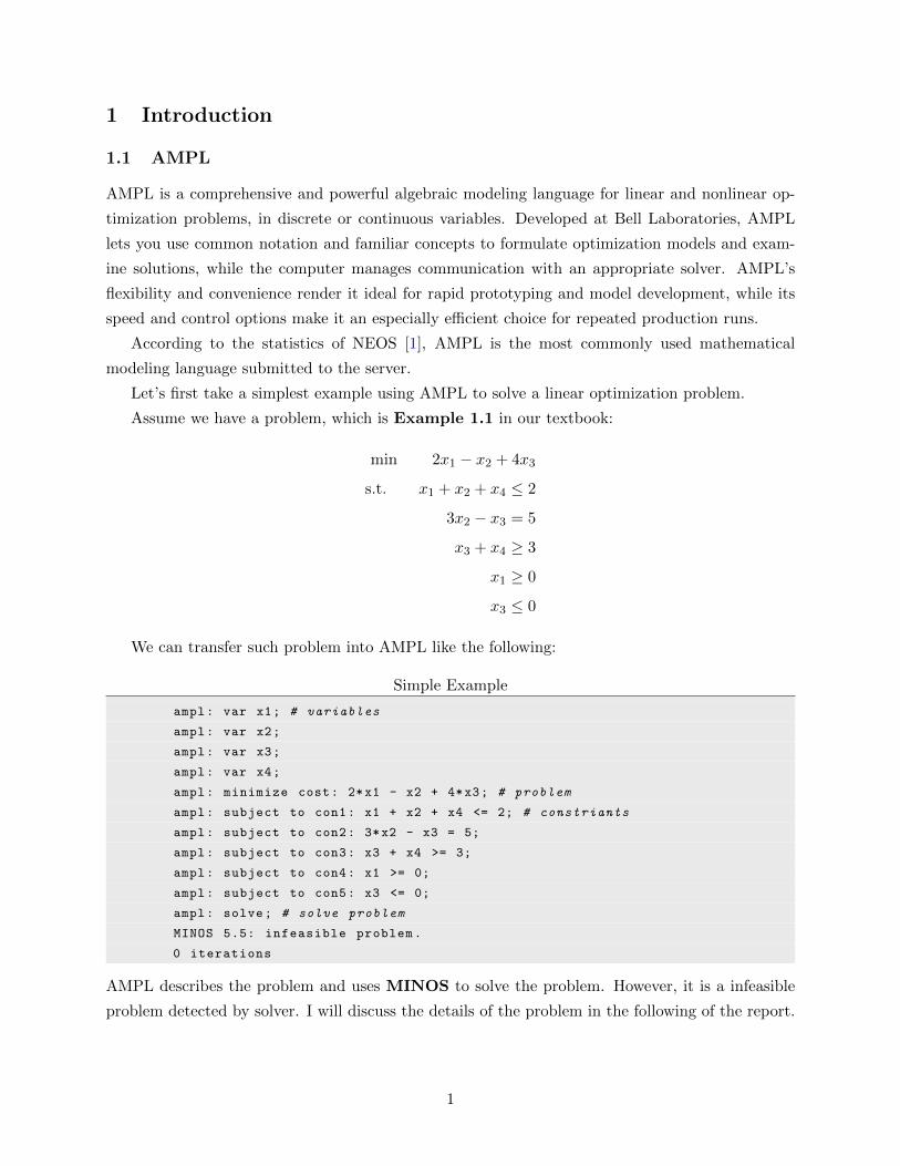
Let’s first take a simplest example using AMPL to solve a linear optimization problem.

Assume we have a problem, which is Example 1.1 in our textbook:

min 2x1 − x2 + 4x3

s.t. x1 + x2 + x4 ≤ 2

3x2 − x3 = 5

x3 + x4 ≥ 3

x1 ≥ 0

x3 ≤ 0

We can transfer such problem into AMPL like the following:

Simple Example

ampl: var x1; # variables

ampl: var x2;

ampl: var x3;

ampl: var x4;

ampl: minimize cost: 2*x1 - x2 + 4*x3; # problem

ampl: subject to con1: x1 + x2 + x4 <= 2; # constriants

ampl: subject to con2: 3*x2 - x3 = 5;

ampl: subject to con3: x3 + x4 >= 3;

ampl: subject to con4: x1 >= 0;

ampl: subject to con5: x3 <= 0;

ampl: solve; # solve problem

MINOS 5.5: infeasible problem.

0 iterations

AMPL describes the problem and uses MINOS to solve the problem. However, it is a infeasible

problem detected by solver. I will discuss the details of the problem in the following of the report.

1

1.2 Solvers

A solver is an application which really solves the problem, and achieves its result. There are many

solvers working with AMPL. AMPL takes MINOS as its default solver, and of course, if you want

to change the solver, you may put solver option in command.

ampl: option solver; # display current solver

option solver minos;

ampl: option solver CPLEX; # change to CPLEX

ampl: option solver;

option solver CPLEX;

As we all know, there are many algorithms approaching solving problems. Here is a list of algorithms

commonly used in solvers [2] for different type of problems.

• Linear (simplex): Linear objective and constraints, by some version of the simplex method.

• Linear (interior): Linear objective and constraints, by some version of an interior (or

barrier) method.

• Network: Linear objective and network flow constraints, by some version of the network

simplex method.

• Quadratic: Convex or concave quadratic objective and linear constraints, by either a simplex-

type or interior-type method.

• Nonlinear: Continuous but not all-linear objective and constraints, by any of several meth-

ods including reduced gradient, quasi-newton, augmented Lagrangian and interior-point. Un-

less other indication is given (see below), possibly optimal over only some local neighborhood.

– Nonlinear convex: Nonlinear with an objective that is convex (if minimized) or con-

cave (if maximized) and constraints that define a convex region. Guaranteed to be

optimal over the entire feasible region.

– Nonlinear global: Nonlinear but requiring a solution that is optimal over all points in

the feasible region.

• Complementarity: Linear or nonlinear as above, with additional complementarity condi-

tions.

• Integer linear: Linear objective and constraints and some or all integer-valued variables,

by a branch-and-bound approach that applies a linear solver to successive subproblems.

• Integer nonlinear: Continuous but not all-linear objective and constraints and some or all

integer-valued variables, by a branch-and-bound approach that applies a nonlinear solver to

successive subproblems.

2

Different solvers have their own feature, some may mainly focus on linear optimization, some

may suitable for solving non-linear optimization problem, which depend on the complex algorithms

implemented inside them.

Here are some commonly used solver compatible with AMPL:

• CPLEX: The IBM ILOG CPLEX Optimizer solves integer programming problems, very large

linear programming problems using either primal or dual variants of the simplex method or

the barrier interior point method, convex and non-convex quadratic programming problems,

and convex quadratically constrained problems (solved via second-order cone programming,

or SOCP).

• MINOS: MINOS is a software package for solving large-scale optimization problems (linear

and nonlinear programs). It is especially effective for linear programs and for problems with

a nonlinear objective function and sparse linear constraints (e.g., quadratic programs).

• Gurobi: The Gurobi Optimizer is a state-of-the-art solver for mathematical programming. It

includes the following solvers: linear programming solver (LP), quadratic programming solver

(QP), quadratically constrained programming solver (QCP), mixed-integer linear program-

ming solver (MILP), mixed-integer quadratic programming solver (MIQP), and mixed-integer

quadratically constrained programming solver (MIQCP). The solvers in the Gurobi Optimizer

were designed from the ground up to exploit modern architectures and multi-core processors,

using the most advanced implementations of the latest algorithms.

• CLP/CBC: CLP(COIN-OR LP) is an open-source linear programming solver written in

C++. It is published under the Common Public License so it can be used in commercial

software without any of the contamination issues of the GNU General Public License. CLP

is primarily meant to be used as a callable library, although a stand-alone executable version

can be built. It is designed to be as reliable as any commercial solver (if not quite as fast)

and to be able to tackle very large problems.

• SNOPT: SNOPT is for the solution of nonlinearly constrained optimization problems. SNOPT

is suitable for large nonlinearly constrained problems with a modest number of degrees of

freedom. SNOPT implements a sequential programming algorithm that uses a smooth aug-

mented Lagrangian merit function and makes explicit provision for infeasibility in the original

problem and in the quadratic programming subproblems.

• KNITRO: KNITRO is for the solution of general non-convex, nonlinearly constrained opti-

mization problems. KNITRO can also be effectively used to solve simpler classes of problems

such as unconstrained problems, bound constrained problems, linear programs (LPs) and

quadratic programs (QPs). KNITRO offers both interior-point and active-set methods.

In Table 1 summarize all commonly used solver for different optimization problems.

In this report, it applies CPLEX as its default solver.

3

Table 1: Solver for problem types

LP MILP QP MIQP NLP MINLP

CPLEX * * * *

MINOS * * * * * *

Gurobi * * * *

CLP/CBC * * * *

SNOPT * * * * * *

KNITRO * * * * * *

lpsolve * *

1.3 Install and Run

Notice AMPL and some other solvers are for commercial usage. However, they also provide a

student version, for whom working on AMPL and other solvers to do coursework or simple research

project.

One from AMPL:

http://www.ampl.com/DOWNLOADS/.

Choose the compatible version to download, meanwhile, it is recommended to download some

student version of solvers working with AMPL. A much easy and useful link

http://ampl.com/try-ampl/download-a-demo-version/

contains both AMPL, solver and examples. If you want to run those examples, you need to use

command line to locate your directory and type in the following command:

$ ampl modinc -

This will include all the files in the EXAMPLES and MODELS directories, such that you can

include those files without change directory. Also for the convenience of changing workspace,

recommended to add the ampl and solvers into system PATH.

Another source is from netlib: http://www.netlib.org/ampl/student/, which is repository

of mathematical softwares. Size-limited versions of AMPL and certain solvers are available free

for download from this page. These versions have no licensing requirements or expiration date.

However they are strictly limited in the size of problem that can be sent to a solver:

• For linear problems, 500 variables and 500 constraints plus objectives.

• For nonlinear problems, 300 variables and 300 constraints plus objectives.

A online demo can also apply AMPL and other solvers to solve problems build with AMPL. The

AMPL [3] also provide a free cloud optimization service that makes AMPL and many solvers

available for trial through an online scheduler and contributed workstations at various locations.

The online version also has size limitations.

4

After setting up all the environment, you can try the simplex example at the beginning of the

report. If you get the same result as showed before, you can continue to next part. Otherwise, you

need to be carefully to set up the environment.

You can refer to the Appendix 1, it will help you to set the AMPL working step by step, also

it will give you example of running AMPL and GLPK1 on Linux system as well.

2 AMPL Syntax

Typically, a complete AMPL program will contain three parts: model(.mod file), data(.dat file)

and running command(.run file). Model is a description of the mathematical model, it will include

variables, parameters, objective function, constraints etc. Data is a specific set of exact data used

in the model, mostly, it is for parameters defined in the model. Running command is to integrate

both model and data file into the command, and also set proper options of AMPL and solver,

display the result.

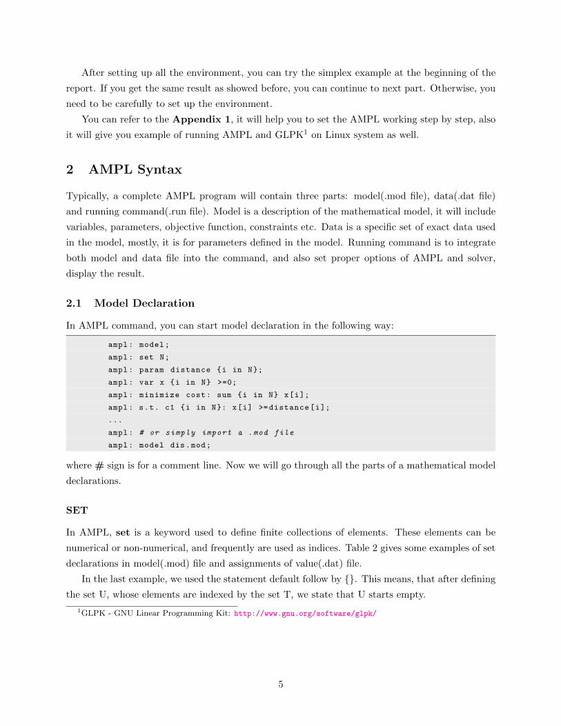
2.1 Model Declaration

In AMPL command, you can start model declaration in the following way:

ampl: model;

ampl: set N;

ampl: param distance {i in N};

ampl: var x {i in N} >=0;

ampl: minimize cost: sum {i in N} x[i];

ampl: s.t. c1 {i in N}: x[i] >=distance[i];

...

ampl: # or simply import a .mod file

ampl: model dis.mod;

where # sign is for a comment line. Now we will go through all the parts of a mathematical model

declarations.

SET

In AMPL, set is a keyword used to define finite collections of elements. These elements can be

numerical or non-numerical, and frequently are used as indices. Table 2 gives some examples of set

declarations in model(.mod) file and assignments of value(.dat) file.

In the last example, we used the statement default follow by {}. This means, that after defining

the set U, whose elements are indexed by the set T, we state that U starts empty.

1GLPK - GNU Linear Programming Kit: http://www.gnu.org/software/glpk/

5

Table 2: set examples

.mod FILE .dat FILE

param n; param n:= 4;

set P := 1..n;

set Q; set Q:= 1 2 3 4;

set R; set R := rainy, cloudy, sunny;

param t; param t := 1000;

set T := 1..t;

set U{T} default {};

Table 3: param example

.mod FILE .dat FILE

param m1; param m1 := 1 1.2 2 1.5 3 1.4;

param m2; param m2 :=

1 1.2

2 1.5

3 1.4;

set M; set M:= a b c d;

set 0; set O:= e f g;

param p{M,O}; param p:

a b c d :=

e 1 5 3 2

f 4 3 1 0

g 3 2 7 8;

param n; param n:= 3;

set M; set M:= a b c d;

set 0; set O:= e f g;

set N; set N:= {1..n};param q{M,O,N}; param q:

[*,*,1]: a b c d :=

e 30 10 8 10

f 22 7 10 7

g 19 11 12 10

6

PARAM

Typically, in a mathematical model, parameters are important to it. Most of the analyses of model

are focus on parameters. In AMPL, it use param to declare parameters. The parameter entity is

used to hold constant values. Table 3 shows some examples of parameter declarations (.mod file)

and the corresponding assignment of values (.run file). In general, parameters can be indexed with

Cartesian product of sets. Which we can use cost to declare that.

VAR

Variables are the fundamental stuff we need to solve in a mathematical model. AMPL uses var as

its keyword to declare variables. Variables are the AMPL entities representing the actual variables

in our mathematical program. We can illustrate the declaration of variables in a .mod file (you can

also do this in a .run file) through examples. Table 4 shows some examples of var declaration.

Table 4: var example

.mod file

var x;

var x{N};var x{1..n} >= 0 <= 1;

var x{1..n,M} integer;

var x{M,O,N} binary;

Notice all the declarations are in .mod files. Bound constraints over the variables can be

imposed in the declaration of the variables in the .mod file. In the third example in Table 4

we imposed upper and lower bounds over the vector of variables x during the declaration of the

variables.

Also by default the variables are assumed to be real numbers, if your problem requires that a

variable or vector of variables is restricted to be integer or binary you should write the command

integer or binary in front the declaration of the variable. Just like the last two examples in Table

4. Again, variables can be indexed with Cartesian product of sets.

MAXIMIZE / MINIMIZE

The objective function is what we want to minimize or maximize. In AMPL, it applies keyword

minimize and maximize to set the objective function. Following with minimize or maximize, you

should also to define a name of the objective function, such as cost, profit. Then to write down the

formula of the objective. Table 5 shows some examples.

7

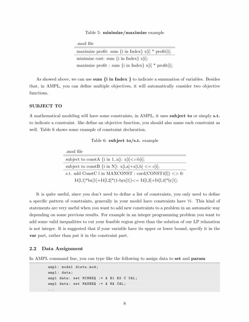
Table 5: minimize/maximize example

.mod file

maximize profit: sum {i in Index} x[i] * profit[i];

minimize cost: sum {i in Index} x[i];

maximize profit : sum {i in Index} x[i] * profit[i];

As showed above, we can use sum {i in Index } to indicate a summation of variables. Besides

that, in AMPL, you can define multiple objectives, it will automatically consider two objective

functions.

SUBJECT TO

A mathematical modeling will have some constraints, in AMPL, it uses subject to or simply s.t.

to indicate a constraint. like define an objective function, you should also name each constraint as

well. Table 6 shows some example of constraint declaration.

Table 6: subject to/s.t. example

.mod file

subject to constA {i in 1..n}: x[i]<=b[i];

subject to constB {i in N}: x[i,a]+x[i,b] <= c[i];

s.t. add ConstC l in MAXCONST : card(CONST4[l]) <> 0:

I4[l,1]*bx[1]+I4[l,2]*(1-bys[1])<= I4[l,3]+I4[l,4]*ly[1];

It is quite useful, since you don’t need to define a list of constraints, you only need to define

a specific pattern of constraints, generally in your model have constraints have ∀i. This kind of

statements are very useful when you want to add new constraints to a problem in an automatic way

depending on some previous results. For example in an integer programming problem you want to

add some valid inequalities to cut your feasible region given than the solution of our LP relaxation

is not integer. It is suggested that if your variable have its upper or lower bound, specify it in the

var part, rather than put it in the constraint part.

2.2 Data Assignment

In AMPL command line, you can type like the following to assign data to set and param

ampl: model dietu.mod;

ampl: data;

ampl data: set MINREQ := A B1 B2 C CAL;

ampl data: set MAXREQ := A NA CAL;

...

8

ampl: # import data specification from a .dat file:

ampl: data dietu.dat;

It is straight forward, however, sometimes you need to specify a large data, for example a time

sequence. You can use ”{ }” to indicate a list:

ampl: set TIME := {1..100}

which means a time sequence from 1 to 100, increasing 1 at a time.

Also mostly a two-dimension set or parameter are needed. AMPL has a gentle feature to handle

such problem. One option is to specify two dimension data as a list of pairs.

ampl data: set LINKS :=

(GARY ,DET) (GARY ,LAN) (GARY ,STL) (GARY ,LAF) (CLEV ,FRA)

(CLEV ,DET) (CLEV ,LAN) (CLEV ,WIN) (CLEV ,STL) (CLEV ,LAF)

(PITT ,FRA) (PITT ,WIN) (PITT ,STL) (PITT ,FRE) ;

Another option is to specify it with ∗ taking the place of elements which can be replaced with

others.

ampl data: set LINKS :=

(*,FRA) CLEV PITT (*,DET) GARY CLEV (*,LAN) GARY CLEV

(*,WIN) CLEV PITT (*,LAF) GARY CLEV (*,FRE) PITT

(*,STL) GARY CLEV PITT ;

Such kind of feature is much more useful in a situation with sparse matrix data. And also for high

dimension data, which is much larger than 2, you can take the advantage of it.

2.3 Solve

After setting up all the model and data, you need to run command to solve problem.

ampl: model diet.mod;

ampl: data diet.dat;

ampl: solve;

MINOS 5.5: optimal solution found.

6 iterations , objective 88.2

It will output some basic result. If the problem is infeasible or unbounded, the solver will also

output some information, just like the example showed at the beginning.

AMPL use MINOS as its default solver, if you want to change it to CPLEX, you can type

like the following:

ampl: model diet.mod;

ampl: data diet.dat;

ampl: option solver cplex;

ampl: solve;

CPLEX 12.6.0.0: optimal solution; objective 88.2

1 dual simplex iterations (0 in phase I)

Different solver will have different algorithms to apply, the output may have some differences.

9

2.4 Display

Now you can get the model solved, and you want to know what is the optimal solution, display

command can display some detailed information of the result.

ampl: # Print out the value of the objective function

ampl: display _objname , _obj;

: _objname _obj :=

1 Total_Cost 88.2

;

ampl: # print out by obj name

ampl: display Total_Cost;

Total_Cost = 88.2

ampl: # Print out names , values and reduced costs

ampl: display _varname , _var , _var.rc;

: _varname _var _var.rc :=

1 "Buy[’BEEF ’]" 0 1.3

2 "Buy[’CHK ’]" 0 0.07

3 "Buy[’FISH ’]" 0 1.03

4 "Buy[’HAM ’]" 0 1.63

5 "Buy[’MCH ’]" 46.6667 -2.22045e-16

6 "Buy[’MTL ’]" 0 0.1

7 "Buy[’SPG ’]" 0 0.1

8 "Buy[’TUR ’]" 0 1.23

;

ampl: # print out by variable name

ampl: display Buy;

Buy [*] :=

BEEF 0

CHK 0

FISH 0

HAM 0

MCH 46.6667

MTL 0

SPG 0

TUR 0

;

ampl: # print out constriant name , lower bound , upper bound , and its dual.

ampl: display _conname ,_con.lb,_con.ub, _con.dual;

: _conname _con.lb _con.ub _con.dual :=

1 "Diet[’A’]" 700 10000 0

2 "Diet[’B1 ’]" 700 10000 0

3 "Diet[’B2 ’]" 700 10000 0.126

4 "Diet[’C’]" 700 10000 0

;

It is much flexible of display options. Generic synonyms such as obj, var, con is enough for us

to get the solution. If an analysis based on the optimal solution, you may need to add some suffix

10

to show much more of the result, lower bound(.lb), upper bound(.ub), reduced cost(.rc) and so on.

If you want to save the result into a file, you can use ”>” to a specific file. Foe every model

solve, it will replace the data inside it, unless you set a sequence of problems to solve using for or

repeat. For example:

ampl: model diet.mod;

ampl: data diet.dat;

ampl: solve;

ampl: display _obj > diet.out;

ampl: display _varname , _var > diet.out;

And in the file diet.out, we will have:

_obj [*] :=

1 88.2

;

: _varname _var :=

1 "Buy[’BEEF ’]" 0

2 "Buy[’CHK ’]" 0

3 "Buy[’FISH ’]" 0

4 "Buy[’HAM ’]" 0

5 "Buy[’MCH ’]" 46.6667

6 "Buy[’MTL ’]" -1.07823e-16

7 "Buy[’SPG ’]" -1.32893e-16

8 "Buy[’TUR ’]" 0

;

2.5 Advanced AMPL Feature

FOR / REPEAT

In some model, you will repeat the model again with modifying some parameters, thus a loop

command is useful in such situations. These are looping commands to repeatedly perform tasks

until some condition holds. The for statement executes a statement or collection of statements for

each member of some set (remember that such members can be numerical or non-numerical). Here

are some example:

for {1..4} {

solve problem1;

let p1[1] := p1 [1]+1;

solve problem2;

let p2[1] := p2 [1]+1;

}

In general, the for statement syntax is:

for {i in N} {

11

...

}

In the case of the repeat statement, the iterations continue as long as some logical condition holds.

Here is an example:

repeat while T[2]. dual > 0 {..};

repeat until T[2]. dual =0 {..};

repeat {..} while T[2]. dual >0 ;

repeat {..} until T[2]. dual >0;

Here, the loop body is inside the {}. All these four statements are different. When the body

appears after the while or until statement, the validation of the condition is made before the a

pass through the body commands. When the body appears before the while or until the validation

is performed after an execution of the body commands.

The while statement repeats while the validation condition holds; on the contrary the until

statement repeats while condition is false. In our example, while the dual variable corresponding to

the constraint T[2] is greater than zero the loop continues. In the until statement, so long as the

dual variable corresponding to constraint T[2] is different from zero, the loop execution continues.

As additional information, the command let is used to change the value of an entity. For

example, if you have a flag and you want to update his value to 1, you just have to type:

let flag:= 1;

IF-THEN-ELSE

This statement is used to describe conditional expressions; its general syntax is as follows:

if (logicalcondition1) then {

..

}

else if (logical condition2) then {

..

}

else {

..

}

The logical condition is any statement that can be true or false. For example a < 100, b[1] < 1 and

b[2] < 1, b[1] < 1 or b[2] < 1. Note that there is no semicolon (;) after the brackets that enclose the

body. The semicolon just follows commands. If the body is a single command you do not need to

use brackets.

Above all, we have show all the basic syntax of AMPL for LP, such as set, param, var,

minimize/maximize, subject to, let, solve, display, for/repeat, while, until, if else and

12

so on. Some of the previous example is from a tutorial contributed by Tulia Herrera1 A detailed

description syntax is already include in the bible book of AMPL [4].

3 Example: Capacity Expansion Problem

3.1 Problem Definition

I will represent an example of stochastic programming. Stochastic programming is a framework

for modeling optimization problems that involve uncertainty. Whereas deterministic optimization

problems are formulated with known parameters, real world problems almost invariably include

some unknown parameters.

The following example is from ORMM2, and it is similar with Example 6.5 [5], but with data

assigned.

A company will supply electricity to three demanders from two electric generators. The unit

cost of supplying each customer from each generator site is given below.

Table 7: Transport Cost

Transportation Cost Dem. 1 Dem. 2 Dem. 3

Gen. 1 4.3 2 0.5

Gen. 2 7.7 3 1

The amounts required by the three demanders is uncertain. Each demand has three levels with

amounts and probabilities given below. The probability distributions are independent.

Table 8: Demand and Probability of each Demander

Demand/Prob Dem. 1 Dem. 2 Dem. 3

Level d1 P(d1) d2 P(d2) d3 P(d3)

1 900 0.35 900 0.35 900 0.35

2 1000 0.55 1000 0.55 1100 0.55

3 1300 0.1 1250 0.1 1400 0.1

To supply the electricity, the company will install capacity at the two generators. The first-

stage decisions are x1 and x2 , the installed capacity at the two generators. The unit costs of

installed capacity are 400 and 350 at generator 1 and 2 respectively. The total capacity cannot

exceed 10,000.

1AMPL Tutorial: http://www.columbia.edu/~dano/courses/4600/lectures/6/AMPLTutorialV2.pdf2Operation Research Models and Methods - Stochastic Programming: https://www.me.utexas.edu/~jensen/

ORMM/computation/unit/mp_add/subunits/stochastic/capacity.html

13

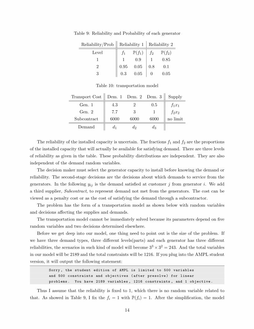
Table 9: Reliability and Probability of each generator

Reliability/Prob Reliability 1 Reliability 2

Level f1 P(f1) f2 P(f2)

1 1 0.9 1 0.85

2 0.95 0.05 0.8 0.1

3 0.3 0.05 0 0.05

Table 10: transportation model

Transport Cost Dem. 1 Dem. 2 Dem. 3 Supply

Gen. 1 4.3 2 0.5 f1x1

Gen. 2 7.7 3 1 f2x2

Subcontract 6000 6000 6000 no limit

Demand d1 d2 d3

The reliability of the installed capacity is uncertain. The fractions f1 and f2 are the proportions

of the installed capacity that will actually be available for satisfying demand. There are three levels

of reliability as given in the table. These probability distributions are independent. They are also

independent of the demand random variables.

The decision maker must select the generator capacity to install before knowing the demand or

reliability. The second-stage decisions are the decisions about which demands to service from the

generators. In the following yij is the demand satisfied at customer j from generator i. We add

a third supplier, Subcontract, to represent demand not met from the generators. The cost can be

viewed as a penalty cost or as the cost of satisfying the demand through a subcontractor.

The problem has the form of a transportation model as shown below with random variables

and decisions affecting the supplies and demands.

The transportation model cannot be immediately solved because its parameters depend on five

random variables and two decisions determined elsewhere.

Before we get deep into our model, one thing need to point out is the size of the problem. If

we have three demand types, three different levels(parts) and each generator has three different

reliabilities, the scenarios in such kind of model will become 33× 32 = 243. And the total variables

in our model will be 2189 and the total constraints will be 1216. If you plug into the AMPL student

version, it will output the following statement:

Sorry , the student edition of AMPL is limited to 500 variables

and 500 constraints and objectives (after presolve) for linear

problems. You have 2189 variables , 1216 constraints , and 1 objective.

Thus I assume that the reliability is fixed to 1, which there is no random variable related to

that. As showed in Table 9, I fix the fi = 1 with P(fi) = 1. After the simplification, the model

14

will become much smaller that before. 27 scenarios, 27*9+2 = 245 variables and 27*5+1=136

constraints.

3.2 Model Definition

Let’s define xi be the capacity installed in generator i, let ysij be the amount transposed from

generator i to demander j at scenario s, let zj be the capacity transfered from subcontract to

demander j at scenario s.

And also let ci be the parameter of installation cost of each generator; let P(s) be the probability

of scenario s, which is a Cartesian product of probabilities of three demanders in three levels; let gj

be the cost of transpose from subcontract to demand j, which is fixed 6000 in this example. The

problem can be formed as:

min

2∑i=1

cixi +∑s∈S

P(s)

2∑i=1

3∑j=1

(fijysij + gjz

sj )

s.t.

2∑i=1

xi ≤ 10000

3∑j=1

ysi,j ≤ xi, ∀i, s

2∑i=1

ysi,j ≥ dj,s, ∀j, s

xi ≥ 0, ∀i

ysij ≥ 0, ∀i, j

zsj ≥ 0, ∀j

3.3 Transfer into AMPL

A proper way of programming with AMPL is to figure out all the parameters, variables, objective

and constraints. Here are steps you can follow to get hand on AMPL:

1. Identify the variables in the model. In this example x,y, z are the variables.

2. Identify the indices of each variable, understand what those mean. For example, xi where i

is the index of generator; ysij where i is the index of generator, j is the index of demander

and s is the index of scenario.

3. Identify the set involved in the model, and define them at .mod file. In this example gener-

ator, demander and scenario are three main set in our problem.

4. Write down the parameter, variable declaration in .mod file according to the set already

defined.

15

5. Write down problem objective and constraint. Taking advantage of set you defined, just write

down the form of each constraint, especially constraints with ∀ in it. For example:

# constraint of suppling from generators must

# larger than it distributed to demander

s.t. supply_constraint {g in Generator , s in Scenarios }:

sum {d in Demander} y[g, d, s] <= x[g];

indicate the second constraint of the problem for all j and s.

6. Assign data to parameters and sets.

7. Write down a command(.run) file, which include both model and data files, and set proper

options, display options, and reset data if need.

A detailed implementation and commands can be found in Appendix 2.

For this problem we can get the optimal cost is 1277842.605 with x = (0, 3400) decision made at

the first stage. In the simplified problem, since the transport costs of first generator are larger then

the second one, it makes sense that set the second one into a certain amount. For the second stage,

if extra demand needed, transpose from subcontract. Such scenario has much lower probability.

4 Summarization

This is a simple tutorial of AMPL. At the end of the tutorial, you should already know how to

build a mathematical model using AMPL, and solve it. A lot of advanced topics of AMPL are not

covered in the report, such as compound data specification, data access from database, network

programming, piecewise LP and nonlinear programming. Besides, solver, like CPLEX, has its own

features, it can work be separated from AMPL, and using other modeling language, such as GAMS.

It also has features like analysis of problems, presolve problem, duality analysis and so on.

Besides our textbook [5], for quick study of LP, you can refer a textbook contributed by Ma-

tousek, Jirı and Gartner, Bernd [6]; for applications and algorithms of operation research, you can

refer a book contributed by Winston [7]; for typical models of optimization, you can refer a book

written by Jensen [8], and also available online https://www.me.utexas.edu/~jensen/ORMM/. For

detailed syntax of AMPL, check its book online http://www.ampl.com/BOOK/, it is free for down-

load.

16

References

[1] NEOS. Neos statistics. http://www.neos-server.org/neos/, June 2014.

[2] AMPL. All solvers for ampl. http://ampl.com/products/solvers/all-solvers-for-ampl/,

June 2014.

[3] AMPL. Try ampl! http://www.ampl.com/TRYAMPL/startup.html, June 2014.

[4] Rober Fourer, D Gay, and Brian W Kernighan. A Mathematical Programming Language (Second

Edition). Duxbury Press, Pacific Grove, 2002.

[5] Dimitris Bertsimas and John N Tsitsiklis. Introduction to linear optimization. 1997.

[6] Jirı Matousek and Bernd Gartner. Understanding and using linear programming, volume 168.

Springer, 2007.

[7] Wayne L Winston and Jeffrey B Goldberg. Operations research: applications and algorithms.

1994.

[8] Paul A Jensen and Jonathan F Bard. Operations research models and methods. John Wiley &

Sons Incorporated, 2003.

17

Appendix 1: Step by Step Setting up AMPL(student edition)

The following steps are working for Windows systems.

Step 1: Download the resource from http://ampl.com/dl/demo/ampl-demo-mswin.zip.

Step 2: Unzip it into a directory you want to install, for example in the desktop. Now you will

see a list of files and directories. In my example:

Directory of C:\ Users\Hongwei Jin\Desktop\ampl -demo -mswin\ampl -demo

04/30/2014 01:19 AM <DIR > .

04/30/2014 01:19 AM <DIR > ..

02/21/2014 03:52 PM 868 ,352 ampl.exe

02/21/2014 03:52 PM 94,208 ampltabl.dll

02/21/2014 03:52 PM 362 ,496 cplex.exe

02/21/2014 03:52 PM 13 ,430 ,784 cplex1260.dll

02/21/2014 03:52 PM 5,932 exhelp32.exe

02/21/2014 03:52 PM 233 ,472 gurobi.exe

02/21/2014 03:52 PM 8 ,241,672 gurobi56.dll

02/21/2014 03:52 PM 30 kestrelkill

02/21/2014 03:52 PM 78 kestrelret

02/21/2014 03:52 PM 79 kestrelsub

02/21/2014 03:52 PM 3,213 LICENSE.txt

02/21/2014 03:52 PM 188 ,416 lpsolve.exe

02/21/2014 03:52 PM 393 ,216 minos.exe

04/30/2014 01:19 AM <DIR > MODELS

02/21/2014 03:52 PM 53 modinc

02/21/2014 03:52 PM 4,415 README

02/21/2014 03:52 PM 88,054 README.cplex.txt

02/21/2014 03:52 PM 4,780 README.gurobi.txt

02/21/2014 03:52 PM 12,736 readme.sw

02/21/2014 03:52 PM 69,632 sw.exe

04/30/2014 01:19 AM <DIR > TABLES

19 File(s) 24 ,001 ,618 bytes

4 Dir(s) 55 ,729 ,176 ,576 bytes free

Notice besides the ampl application, it also include student edition solvers, such as cplex, gurobi,

lpsolve, minos. If you have other solvers just put the executable file in the same directory. Sub-

directories include all example in the AMPL book [4]. It is a fast way to get started.

Step 3: Use Windows CMD.exe get to the directory of AMPL, type ampl modinc -:

C:\ Users\Hongwei Jin\Desktop\ampl -demo -mswin\ampl -demo >ampl modinc -

ampl:

You will see AMPL is running.

Step 4: Example Test. You can try examples in the sub-directory, since you already include

the sub-directories by ampl modinc -, you can type in AMPL to specify model and data and to

solve. One example will be the following:

ampl: model prod.mod;

ampl: data prod.dat;

ampl: solve;

MINOS 5.5: optimal solution found.

2 iterations , objective 192000

ampl: display _varname , _var;

: _varname _var :=

1 "X[’bands ’]" 6000

2 "X[’coils ’]" 1400

;

Step 5: Basically, you can run AMPL to solve problem by step 4, however, it is tedious to get

into that directory every time. You can add this directory path into your system path environment

such that you can run AMPL any where. But if you need to run examples, you need to get into

this directory.

Commends:

> Download source from netlib are almost the same, the only different is you need to download

AMPL and solver one by one and extract them into a same directory.

> Other systems are just similar with Windows. But if you have a 64 bit Linux system, you

wouldn’t able to run AMPL. What you need to do is install a 32 bit support lib, named

libc6-i386, after that make AMPL executable by

hjin15@hjin15 -mint ~/ampl/ampl -demo/ampl $ chmod x ampl

hjin15@hjin15 -mint ~/ampl/ampl -demo/ampl $ ./ampl modinc -

ampl:

> A GLPK (GNU Linear Programming Kit) is available for Linux systems. It can work with

AMPL as well. Define a model file:

# short.mod

var x1;

var x2;

maximize obj: 0.6 * x1 + 0.5 * x2;

s.t. c1: x1 + 2 * x2 <= 1;

s.t. c2: 3 * x1 + x2 <= 2;

solve;

display x1 , x2;

end;

Install GLPK on Linux system, it usually called: glpk-utils. After that you can solve this

short model by using glpk as well.

hjin15@hjin15 -mint ~ $ glpsol --math short.mod

GLPSOL: GLPK LP/MIP Solver , v4.45

Parameter(s) specified in the command line:

--math short.mod

Reading model section from short.mod ...

9 lines were read

Generating obj...

Generating c1...

Generating c2...

Model has been successfully generated

GLPK Simplex Optimizer , v4.45

3 rows , 2 columns , 6 non -zeros

Preprocessing ...

2 rows , 2 columns , 4 non -zeros

Scaling ...

A: min|aij| = 1.000e+00 max|aij| = 3.000e+00 ratio = 3.000e+00

Problem data seem to be well scaled

Constructing initial basis ...

Size of triangular part = 2

* 0: obj = 0.000000000e+00 infeas = 0.000e+00 (0)

* 2: obj = 4.600000000e-01 infeas = 0.000e+00 (0)

OPTIMAL SOLUTION FOUND

Time used: 0.0 secs

Memory used: 0.1 Mb (114811 bytes)

Display statement at line 8

x1.val = 0.6

x2.val = 0.2

Model has been successfully processed

where –math indicate that the model is described by AMPL.

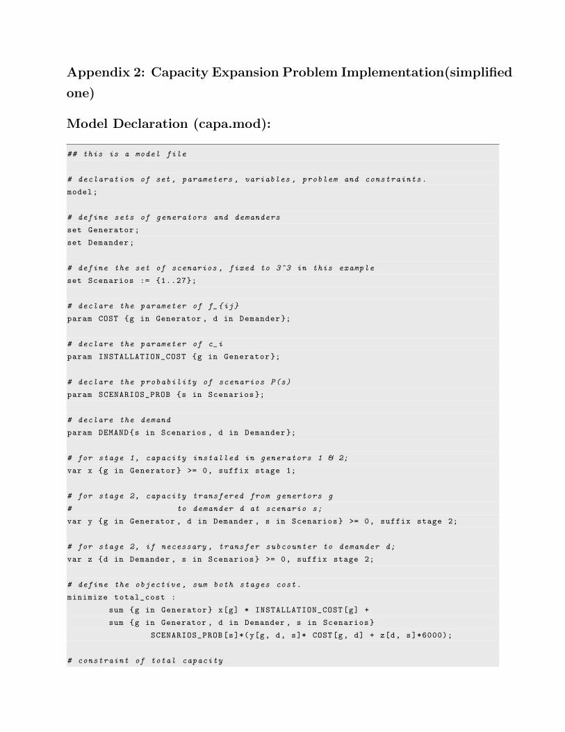
Appendix 2: Capacity Expansion Problem Implementation(simplified

one)

Model Declaration (capa.mod):

## this is a model file

# declaration of set , parameters , variables , problem and constraints.

model;

# define sets of generators and demanders

set Generator;

set Demander;

# define the set of scenarios , fixed to 3^3 in this example

set Scenarios := {1..27};

# declare the parameter of f_{ij}

param COST {g in Generator , d in Demander };

# declare the parameter of c_i

param INSTALLATION_COST {g in Generator };

# declare the probability of scenarios P(s)

param SCENARIOS_PROB {s in Scenarios };

# declare the demand

param DEMAND{s in Scenarios , d in Demander };

# for stage 1, capacity installed in generators 1 & 2;

var x {g in Generator} >= 0, suffix stage 1;

# for stage 2, capacity transfered from genertors g

# to demander d at scenario s;

var y {g in Generator , d in Demander , s in Scenarios} >= 0, suffix stage 2;

# for stage 2, if necessary , transfer subcounter to demander d;

var z {d in Demander , s in Scenarios} >= 0, suffix stage 2;

# define the objective , sum both stages cost.

minimize total_cost :

sum {g in Generator} x[g] * INSTALLATION_COST[g] +

sum {g in Generator , d in Demander , s in Scenarios}

SCENARIOS_PROB[s]*(y[g, d, s]* COST[g, d] + z[d, s]*6000);

# constraint of total capacity

s.t. total_capacity :

sum {g in Generator} x[g] <=10000;

# constraint of suppling from generators must larger than it distributed to demander

s.t. supply_constraint {g in Generator , s in Scenarios }:

sum {d in Demander} y[g, d, s] <= x[g];

# for each demander , either from generator or subcontract must meet the requirement

s.t. demand_constraint {d in Demander , s in Scenarios }:

sum {g in Generator} y[g, d, s] + z[d, s]>= DEMAND[s, d];

Data specification (capa.dat)

## this is a data file

# set all the data according to the variables.

data;

set Generator := g1 g2;

set Demander := d1 d2 d3;

param COST:

d1 d2 d3 :=

g1 4.3 2 0.5

g2 7.7 3 1;

param INSTALLATION_COST :=

g1 400

g2 350;

# The probability is calculated by Cartesian product of three

# different demander ’s probability.

param SCENARIOS_PROB :=

1 0.042875

2 0.067375

3 0.01225

4 0.067375

5 0.105875

6 0.01925

7 0.01225

8 0.01925

9 0.0035

10 0.067375

11 0.105875

12 0.01925

13 0.105875

14 0.166375

15 0.03025

16 0.01925

17 0.03025

18 0.0055

19 0.01225

20 0.01925

21 0.0035

22 0.01925

23 0.03025

24 0.0055

25 0.0035

26 0.0055

27 0.001;

param DEMAND:

d1 d2 d3:=

1 900 900 900

2 900 900 1100

3 900 900 1400

4 900 1000 900

5 900 1000 1100

6 900 1000 1400

7 900 1250 900

8 900 1250 1100

9 900 1250 1400

10 1000 900 900

11 1000 900 1100

12 1000 900 1400

13 1000 1000 900

14 1000 1000 1100

15 1000 1000 1400

16 1000 1250 900

17 1000 1250 1100

18 1000 1250 1400

19 1300 900 900

20 1300 900 1100

21 1300 900 1400

22 1300 1000 900

23 1300 1000 1100

24 1300 1000 1400

25 1300 1250 900

26 1300 1250 1100

27 1300 1250 1400

;

Command file (capa.run)

## this is a command file

# reset all the previous parameters variable and data.

reset;

# include model and data file

include capa.mod;

include capa.dat;

# show running time

option times 1;

# show model statistics , variable number , constraint number etc.

option show_stats 1;

# set solver option

option solver cplex;

# presolve the problem to reduce the number of constriants

option presolve 1;

solve;

# show objective value

display _obj;

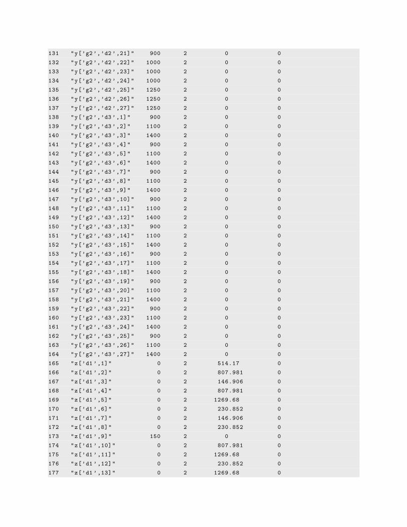
# show variable value , stage , reduced cost ,

display _varname , _var , _var.stage , _var.rc;

Display output:

# incremental total

#phase seconds memory memory

#execute 0.0156001 275512 275512

#execute 0 0 275512

#execute 0 0 275512

#execute 0 0 275512

#compile 0 0 275512

#genmod 0 75648 351160

#merge 0 2056 353216

#collect 0 15432 368648

245 variables , all linear

136 constraints , all linear; 461 nonzeros

136 inequality constraints

1 linear objective; 245 nonzeros.

#presolve 0 34848 403496

#output 0 0 403496

CPLEX 12.6.0.0: #Total 0.0156001

optimal solution; objective 1277842.605

163 dual simplex iterations (0 in phase I)

#execute 0.0156001 6704 410200

_obj [*] :=

1 1277840

;

#execute 0 4624 414824

### E:\ Dropbox\GitHub\AMPL -project\draft/capa.run :23(511) display ...

: _varname _var _var.stage _var.rc _var.dual :=

1 "x[’g1 ’]" 0 1 46.6 0

2 "x[’g2 ’]" 3400 1 0 0

3 "y[’g1 ’,’d1 ’,1]" 0 2 0 0

4 "y[’g1 ’,’d1 ’,2]" 0 2 0 0

5 "y[’g1 ’,’d1 ’,3]" 0 2 0 0

6 "y[’g1 ’,’d1 ’,4]" 0 2 0 0

7 "y[’g1 ’,’d1 ’,5]" 0 2 0 0

8 "y[’g1 ’,’d1 ’,6]" 0 2 0 0

9 "y[’g1 ’,’d1 ’,7]" 0 2 0 0

10 "y[’g1’,’d1 ’,8]" 0 2 0 0

11 "y[’g1’,’d1 ’,9]" 0 2 0 0

12 "y[’g1’,’d1 ’,10]" 0 2 0 0

13 "y[’g1’,’d1 ’,11]" 0 2 0 0

14 "y[’g1’,’d1 ’,12]" 0 2 0 0

15 "y[’g1’,’d1 ’,13]" 0 2 0 0

16 "y[’g1’,’d1 ’,14]" 0 2 0 0

17 "y[’g1’,’d1 ’,15]" 0 2 0 0

18 "y[’g1’,’d1 ’,16]" 0 2 0 0

19 "y[’g1’,’d1 ’,17]" 0 2 0 0

20 "y[’g1’,’d1 ’,18]" 0 2 0 0

21 "y[’g1’,’d1 ’,19]" 0 2 0 0

22 "y[’g1’,’d1 ’,20]" 0 2 0 0

23 "y[’g1’,’d1 ’,21]" 0 2 0 0

24 "y[’g1’,’d1 ’,22]" 0 2 0 0

25 "y[’g1’,’d1 ’,23]" 0 2 0 0

26 "y[’g1’,’d1 ’,24]" 0 2 0 0

27 "y[’g1’,’d1 ’,25]" 0 2 0 0

28 "y[’g1’,’d1 ’,26]" 0 2 0 0

29 "y[’g1’,’d1 ’,27]" 0 2 0 0

30 "y[’g1’,’d2 ’,1]" 0 2 0.1029 0

31 "y[’g1’,’d2 ’,2]" 0 2 0.1617 0

32 "y[’g1’,’d2 ’,3]" 0 2 0.0294 0

33 "y[’g1’,’d2 ’,4]" 0 2 0.1617 0

34 "y[’g1’,’d2 ’,5]" 0 2 0.2541 0

35 "y[’g1’,’d2 ’,6]" 0 2 0.0462 0

36 "y[’g1’,’d2 ’,7]" 0 2 0.0294 0

37 "y[’g1’,’d2 ’,8]" 0 2 0.0462 0

38 "y[’g1’,’d2 ’,9]" 0 2 0.0084 0

39 "y[’g1’,’d2 ’,10]" 0 2 0.1617 0

40 "y[’g1’,’d2 ’,11]" 0 2 0.2541 0

41 "y[’g1’,’d2 ’,12]" 0 2 0.0462 0

42 "y[’g1’,’d2 ’,13]" 0 2 0.2541 0

43 "y[’g1’,’d2 ’,14]" 0 2 0.3993 0

44 "y[’g1’,’d2 ’,15]" 0 2 0.0726 0

45 "y[’g1’,’d2 ’,16]" 0 2 0.0462 0

46 "y[’g1’,’d2 ’,17]" 0 2 0.0726 0

47 "y[’g1’,’d2 ’,18]" 0 2 0.0132 0

48 "y[’g1’,’d2 ’,19]" 0 2 0.0294 0

49 "y[’g1’,’d2 ’,20]" 0 2 0.0462 0

50 "y[’g1’,’d2 ’,21]" 0 2 0.0084 0

51 "y[’g1’,’d2 ’,22]" 0 2 0.0462 0

52 "y[’g1’,’d2 ’,23]" 0 2 0.0726 0

53 "y[’g1’,’d2 ’,24]" 0 2 0.0132 0

54 "y[’g1’,’d2 ’,25]" 0 2 0.0084 0

55 "y[’g1’,’d2 ’,26]" 0 2 0.0132 0

56 "y[’g1’,’d2 ’,27]" 0 2 0.0024 0

57 "y[’g1’,’d3 ’,1]" 0 2 0.124338 0

58 "y[’g1’,’d3 ’,2]" 0 2 0.195388 0

59 "y[’g1’,’d3 ’,3]" 0 2 0.035525 0

60 "y[’g1’,’d3 ’,4]" 0 2 0.195388 0

61 "y[’g1’,’d3 ’,5]" 0 2 0.307038 0

62 "y[’g1’,’d3 ’,6]" 0 2 0.055825 0

63 "y[’g1’,’d3 ’,7]" 0 2 0.035525 0

64 "y[’g1’,’d3 ’,8]" 0 2 0.055825 0

65 "y[’g1’,’d3 ’,9]" 0 2 0.01015 0

66 "y[’g1’,’d3 ’,10]" 0 2 0.195388 0

67 "y[’g1’,’d3 ’,11]" 0 2 0.307038 0

68 "y[’g1’,’d3 ’,12]" 0 2 0.055825 0

69 "y[’g1’,’d3 ’,13]" 0 2 0.307038 0

70 "y[’g1’,’d3 ’,14]" 0 2 0.482488 0

71 "y[’g1’,’d3 ’,15]" 0 2 0.087725 0

72 "y[’g1’,’d3 ’,16]" 0 2 0.055825 0

73 "y[’g1’,’d3 ’,17]" 0 2 0.087725 0

74 "y[’g1’,’d3 ’,18]" 0 2 0.01595 0

75 "y[’g1’,’d3 ’,19]" 0 2 0.035525 0

76 "y[’g1’,’d3 ’,20]" 0 2 0.055825 0

77 "y[’g1’,’d3 ’,21]" 0 2 0.01015 0

78 "y[’g1’,’d3 ’,22]" 0 2 0.055825 0

79 "y[’g1’,’d3 ’,23]" 0 2 0.087725 0

80 "y[’g1’,’d3 ’,24]" 0 2 0.01595 0

81 "y[’g1’,’d3 ’,25]" 0 2 0.01015 0

82 "y[’g1’,’d3 ’,26]" 0 2 0.01595 0

83 "y[’g1’,’d3 ’,27]" 0 2 0.0029 0

84 "y[’g2’,’d1 ’,1]" 900 2 0 0

85 "y[’g2’,’d1 ’,2]" 900 2 0 0

86 "y[’g2’,’d1 ’,3]" 900 2 0 0

87 "y[’g2’,’d1 ’,4]" 900 2 0 0

88 "y[’g2’,’d1 ’,5]" 900 2 0 0

89 "y[’g2’,’d1 ’,6]" 900 2 0 0

90 "y[’g2’,’d1 ’,7]" 900 2 0 0

91 "y[’g2’,’d1 ’,8]" 900 2 0 0

92 "y[’g2’,’d1 ’,9]" 750 2 0 0

93 "y[’g2’,’d1 ’,10]" 1000 2 0 0

94 "y[’g2’,’d1 ’,11]" 1000 2 0 0

95 "y[’g2’,’d1 ’,12]" 1000 2 0 0

96 "y[’g2’,’d1 ’,13]" 1000 2 0 0

97 "y[’g2’,’d1 ’,14]" 1000 2 0 0

98 "y[’g2’,’d1 ’,15]" 1000 2 0 0

99 "y[’g2’,’d1 ’,16]" 1000 2 0 0

100 "y[’g2 ’,’d1 ’,17]" 1000 2 0 0

101 "y[’g2 ’,’d1 ’,18]" 750 2 0 0

102 "y[’g2 ’,’d1 ’,19]" 1300 2 0 0

103 "y[’g2 ’,’d1 ’,20]" 1300 2 0 0

104 "y[’g2 ’,’d1 ’,21]" 1100 2 0 0

105 "y[’g2 ’,’d1 ’,22]" 1300 2 0 0

106 "y[’g2 ’,’d1 ’,23]" 1300 2 0 0

107 "y[’g2 ’,’d1 ’,24]" 1000 2 0 0

108 "y[’g2 ’,’d1 ’,25]" 1250 2 0 0

109 "y[’g2 ’,’d1 ’,26]" 1050 2 0 0

110 "y[’g2 ’,’d1 ’,27]" 750 2 0 0

111 "y[’g2 ’,’d2 ’,1]" 900 2 0 0

112 "y[’g2 ’,’d2 ’,2]" 900 2 0 0

113 "y[’g2 ’,’d2 ’,3]" 900 2 0 0

114 "y[’g2 ’,’d2 ’,4]" 1000 2 0 0

115 "y[’g2 ’,’d2 ’,5]" 1000 2 0 0

116 "y[’g2 ’,’d2 ’,6]" 1000 2 0 0

117 "y[’g2 ’,’d2 ’,7]" 1250 2 0 0

118 "y[’g2 ’,’d2 ’,8]" 1250 2 0 0

119 "y[’g2 ’,’d2 ’,9]" 1250 2 0 0

120 "y[’g2 ’,’d2 ’,10]" 900 2 0 0

121 "y[’g2 ’,’d2 ’,11]" 900 2 0 0

122 "y[’g2 ’,’d2 ’,12]" 900 2 0 0

123 "y[’g2 ’,’d2 ’,13]" 1000 2 0 0

124 "y[’g2 ’,’d2 ’,14]" 1000 2 0 0

125 "y[’g2 ’,’d2 ’,15]" 1000 2 0 0

126 "y[’g2 ’,’d2 ’,16]" 1250 2 0 0

127 "y[’g2 ’,’d2 ’,17]" 1250 2 0 0

128 "y[’g2 ’,’d2 ’,18]" 1250 2 0 0

129 "y[’g2 ’,’d2 ’,19]" 900 2 0 0

130 "y[’g2 ’,’d2 ’,20]" 900 2 0 0

131 "y[’g2 ’,’d2 ’,21]" 900 2 0 0

132 "y[’g2 ’,’d2 ’,22]" 1000 2 0 0

133 "y[’g2 ’,’d2 ’,23]" 1000 2 0 0

134 "y[’g2 ’,’d2 ’,24]" 1000 2 0 0

135 "y[’g2 ’,’d2 ’,25]" 1250 2 0 0

136 "y[’g2 ’,’d2 ’,26]" 1250 2 0 0

137 "y[’g2 ’,’d2 ’,27]" 1250 2 0 0

138 "y[’g2 ’,’d3 ’,1]" 900 2 0 0

139 "y[’g2 ’,’d3 ’,2]" 1100 2 0 0

140 "y[’g2 ’,’d3 ’,3]" 1400 2 0 0

141 "y[’g2 ’,’d3 ’,4]" 900 2 0 0

142 "y[’g2 ’,’d3 ’,5]" 1100 2 0 0

143 "y[’g2 ’,’d3 ’,6]" 1400 2 0 0

144 "y[’g2 ’,’d3 ’,7]" 900 2 0 0

145 "y[’g2 ’,’d3 ’,8]" 1100 2 0 0

146 "y[’g2 ’,’d3 ’,9]" 1400 2 0 0

147 "y[’g2 ’,’d3 ’,10]" 900 2 0 0

148 "y[’g2 ’,’d3 ’,11]" 1100 2 0 0

149 "y[’g2 ’,’d3 ’,12]" 1400 2 0 0

150 "y[’g2 ’,’d3 ’,13]" 900 2 0 0

151 "y[’g2 ’,’d3 ’,14]" 1100 2 0 0

152 "y[’g2 ’,’d3 ’,15]" 1400 2 0 0

153 "y[’g2 ’,’d3 ’,16]" 900 2 0 0

154 "y[’g2 ’,’d3 ’,17]" 1100 2 0 0

155 "y[’g2 ’,’d3 ’,18]" 1400 2 0 0

156 "y[’g2 ’,’d3 ’,19]" 900 2 0 0

157 "y[’g2 ’,’d3 ’,20]" 1100 2 0 0

158 "y[’g2 ’,’d3 ’,21]" 1400 2 0 0

159 "y[’g2 ’,’d3 ’,22]" 900 2 0 0

160 "y[’g2 ’,’d3 ’,23]" 1100 2 0 0

161 "y[’g2 ’,’d3 ’,24]" 1400 2 0 0

162 "y[’g2 ’,’d3 ’,25]" 900 2 0 0

163 "y[’g2 ’,’d3 ’,26]" 1100 2 0 0

164 "y[’g2 ’,’d3 ’,27]" 1400 2 0 0

165 "z[’d1 ’,1]" 0 2 514.17 0

166 "z[’d1 ’,2]" 0 2 807.981 0

167 "z[’d1 ’,3]" 0 2 146.906 0

168 "z[’d1 ’,4]" 0 2 807.981 0

169 "z[’d1 ’,5]" 0 2 1269.68 0

170 "z[’d1 ’,6]" 0 2 230.852 0

171 "z[’d1 ’,7]" 0 2 146.906 0

172 "z[’d1 ’,8]" 0 2 230.852 0

173 "z[’d1 ’,9]" 150 2 0 0

174 "z[’d1 ’,10]" 0 2 807.981 0

175 "z[’d1 ’,11]" 0 2 1269.68 0

176 "z[’d1 ’,12]" 0 2 230.852 0

177 "z[’d1 ’,13]" 0 2 1269.68 0

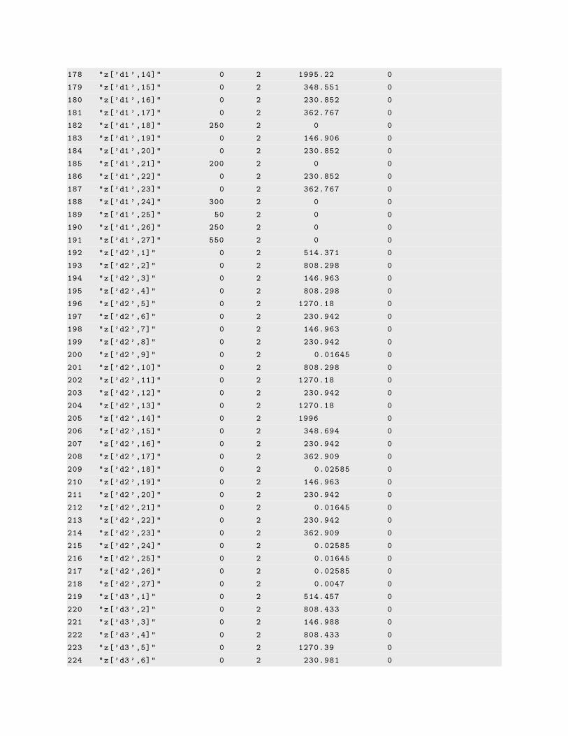
178 "z[’d1 ’,14]" 0 2 1995.22 0

179 "z[’d1 ’,15]" 0 2 348.551 0

180 "z[’d1 ’,16]" 0 2 230.852 0

181 "z[’d1 ’,17]" 0 2 362.767 0

182 "z[’d1 ’,18]" 250 2 0 0

183 "z[’d1 ’,19]" 0 2 146.906 0

184 "z[’d1 ’,20]" 0 2 230.852 0

185 "z[’d1 ’,21]" 200 2 0 0

186 "z[’d1 ’,22]" 0 2 230.852 0

187 "z[’d1 ’,23]" 0 2 362.767 0

188 "z[’d1 ’,24]" 300 2 0 0

189 "z[’d1 ’,25]" 50 2 0 0

190 "z[’d1 ’,26]" 250 2 0 0

191 "z[’d1 ’,27]" 550 2 0 0

192 "z[’d2 ’,1]" 0 2 514.371 0

193 "z[’d2 ’,2]" 0 2 808.298 0

194 "z[’d2 ’,3]" 0 2 146.963 0

195 "z[’d2 ’,4]" 0 2 808.298 0

196 "z[’d2 ’,5]" 0 2 1270.18 0

197 "z[’d2 ’,6]" 0 2 230.942 0

198 "z[’d2 ’,7]" 0 2 146.963 0

199 "z[’d2 ’,8]" 0 2 230.942 0

200 "z[’d2 ’,9]" 0 2 0.01645 0

201 "z[’d2 ’,10]" 0 2 808.298 0

202 "z[’d2 ’,11]" 0 2 1270.18 0

203 "z[’d2 ’,12]" 0 2 230.942 0

204 "z[’d2 ’,13]" 0 2 1270.18 0

205 "z[’d2 ’,14]" 0 2 1996 0

206 "z[’d2 ’,15]" 0 2 348.694 0

207 "z[’d2 ’,16]" 0 2 230.942 0

208 "z[’d2 ’,17]" 0 2 362.909 0

209 "z[’d2 ’,18]" 0 2 0.02585 0

210 "z[’d2 ’,19]" 0 2 146.963 0

211 "z[’d2 ’,20]" 0 2 230.942 0

212 "z[’d2 ’,21]" 0 2 0.01645 0

213 "z[’d2 ’,22]" 0 2 230.942 0

214 "z[’d2 ’,23]" 0 2 362.909 0

215 "z[’d2 ’,24]" 0 2 0.02585 0

216 "z[’d2 ’,25]" 0 2 0.01645 0

217 "z[’d2 ’,26]" 0 2 0.02585 0

218 "z[’d2 ’,27]" 0 2 0.0047 0

219 "z[’d3 ’,1]" 0 2 514.457 0

220 "z[’d3 ’,2]" 0 2 808.433 0

221 "z[’d3 ’,3]" 0 2 146.988 0

222 "z[’d3 ’,4]" 0 2 808.433 0

223 "z[’d3 ’,5]" 0 2 1270.39 0

224 "z[’d3 ’,6]" 0 2 230.981 0

225 "z[’d3 ’,7]" 0 2 146.988 0

226 "z[’d3 ’,8]" 0 2 230.981 0

227 "z[’d3 ’,9]" 0 2 0.02345 0

228 "z[’d3 ’,10]" 0 2 808.433 0

229 "z[’d3 ’,11]" 0 2 1270.39 0

230 "z[’d3 ’,12]" 0 2 230.981 0

231 "z[’d3 ’,13]" 0 2 1270.39 0

232 "z[’d3 ’,14]" 0 2 1996.33 0

233 "z[’d3 ’,15]" 0 2 348.754 0

234 "z[’d3 ’,16]" 0 2 230.981 0

235 "z[’d3 ’,17]" 0 2 362.97 0

236 "z[’d3 ’,18]" 0 2 0.03685 0

237 "z[’d3 ’,19]" 0 2 146.988 0

238 "z[’d3 ’,20]" 0 2 230.981 0

239 "z[’d3 ’,21]" 0 2 0.02345 0

240 "z[’d3 ’,22]" 0 2 230.981 0

241 "z[’d3 ’,23]" 0 2 362.97 0

242 "z[’d3 ’,24]" 0 2 0.03685 0

243 "z[’d3 ’,25]" 0 2 0.02345 0

244 "z[’d3 ’,26]" 0 2 0.03685 0

245 "z[’d3 ’,27]" 0 2 0.0067 0

;

#execute 0 30288 445112