A tutorial on how (not) to over-interpret STRUCTURE ... · A tutorial on how (not) to over-interpret STRUCTURE/ADMIXTURE bar plots. Daniel Falush1*, Lucy van Dorp2,3, Daniel J Lawson4

A tutorial on how (not) to over-interpret STRUCTURE/ADMIXTURE bar plots.

Daniel Falush1*, Lucy van Dorp2,3, Daniel J Lawson4

Abstract

Genetic clustering algorithms, implemented in popular programs such as STRUCTURE and

ADMIXTURE, have been used extensively in the characterisation of individuals and populations

based on genetic data. A successful example is reconstruction of the genetic history of African

Americans who are a product of recent admixture between highly differentiated populations.

Histories can also be reconstructed using the same procedure for groups which do not have

admixture in their recent history, where recent genetic drift is strong or that deviate in other ways

from the underlying inference model. Unfortunately, such histories can be misleading. We have

implemented an approach (available at www.paintmychromsomes.com) to assessing the goodness

of fit of the model using the ancestry “palettes” estimated by CHROMOPAINTER and apply it to both

simulated and real examples. Combining these complementary analyses with additional methods

that are designed to test specific hypothesis allows a richer and more robust analysis of recent

demographic history based on genetic data.

1 Milner Centre for Evolution, University of Bath.

2 University College London. Dept. Genetics, Evolution and Environment. London, UK.

3 Centre for Mathematics and Physics in the Life Sciences and Experimental Biology (CoMPLEX),

University College London. London, UK.

4 University of Bristol, School of Social and Community Medicine, Bristol, UK.

*To whom correspondence should be addressed,

Milner Centre for Evolution

Department of Biology & Biotechnology

University of Bath, 4 South, Lab 0.39

Claverton Down

Bath, BA2 7AY

United Kingdom

[email protected]

.CC-BY-NC 4.0 International licenseauthor/funder. It is made available under aThe copyright holder for this preprint (which was not peer-reviewed) is the. https://doi.org/10.1101/066431doi: bioRxiv preprint

http://www.paintmychromsomes.com/

https://doi.org/10.1101/066431

http://creativecommons.org/licenses/by-nc/4.0/

STRUCTURE/ADMIXTURE are excellent tools for analysing recent admixture between

differentiated groups

Model-based clustering has become a popular approach to visualizing the genetic ancestry of

humans and other organisms. Pritchard et al. (2000) introduced a Bayesian algorithm STRUCTURE for

defining populations and assigning individuals to them. FRAPPE and ADMIXTURE were later

implemented based on a similar underlying inference model but with algorithmic refinements that

allow them to be run on datasets with hundreds of thousands of genetic markers (Alexander et al.,

2009; Tang et al., 2005). One motivating example was African Americans. The “admixture model” of

STRUCTURE assumes that each individual has ancestry from one or more of K genetically distinct

sources. In the case of African Americans, the most important sources are West Africans, who were

brought to the Americas as slaves, and European settlers. The two groups are thought to have been

previously separated with minimal genetic contact for tens of thousands of years. This means that

their history can be separated into two phases, a “divergence phase” lasting thousands of years of

largely independent evolution and an “admixture phase”, in which large populations met and

admixed within the last few hundred years. The source populations are described as being

“ancestral”, to capture the idea that most of the ancestors of modern African Americans that lived

500 years ago would have be members of African or European populations, with similar genetic

profiles to Africans and Europeans within contemporary datasets.

Pritchard et al. hoped that STRUCTURE would be “flexible enough to permit appropriate clustering

for a wide range of datasets”, but also emphasized that the output should be interpreted with care

since “clusters may not correspond to real populations”. Many subsequent users of the algorithm,

such as Evanno et al. (2005) have been less reticent and for example made a considerable effort to

“detect the true number of clusters (K)”, assuming implicitly that such a quantity was biologically

meaningful. In practice, rigorous estimation of K is a difficult statistical problem, even if the

assumptions of the underlying model are assumed to hold. Pritchard et al. suggest a heuristic

approach based on comparing “model probabilities” estimated in runs of the model for different

values of K. A widely used modification of the protocol was suggested by Evanno et al. (2005) while

Alexander et al. (2009) suggest a cross validation approach, using consistency between different

runs of the algorithm at a particular value of K as an indication of validity.

When the STRUCTURE admixture model is applied to a dataset consisting of genetic markers from

West Africans, African Americans and Europeans it infers two ancestral populations. Each of the

Europeans and Africans is assigned a great majority of their ancestry from one of them. Africans are

inferred to have an average of 18% ancestry from the European cluster but with substantial inter-

individual variation (Falush et al., 2003). This and other successful examples of inference (Rosenberg

et al., 2001; Rosenberg et al., 2002; Tishkoff et al., 2009), have lead researchers to use STRUCTURE

or ADMIXTURE according to a protocol that can be summarized as follows:

(1) Estimate K using a refined statistical procedure.

(2) Assume that this is the true value of K.

(3) Assume each of the K ancestral population existed at some point in the past.


https://doi.org/10.1101/066431


(4) Assume that modern individuals were produced by recent mixing of these ancestral

populations.

There are genetic differences amongst both the Africans and the Europeans who contributed to

African American ancestry, e.g. reflecting genetic variation between regions within Europe and

Africa, but these are subtle relative to the magnitude of the differences between continents. For the

purpose of analysing recent African American admixture it is therefore reasonable to add the

following assumptions to the protocol:

(3a) Neglect the possibility an ancestral population might itself be admixed.

(3b) Label ancestral populations based on the locations they are currently most frequent in.

(3c) Do not ask how the inferred ancestral populations are related to each other.

Qualitatively different historical scenarios can give indistinguishable STRUCTURE/ADMIXTURE

plots

Versions of the protocol are often applied with limited prior knowledge about how the groups in a

sample are related to each other. Many real population histories are not neatly separable into

divergence and admixture phases but the methods can be applied to all datasets to produce

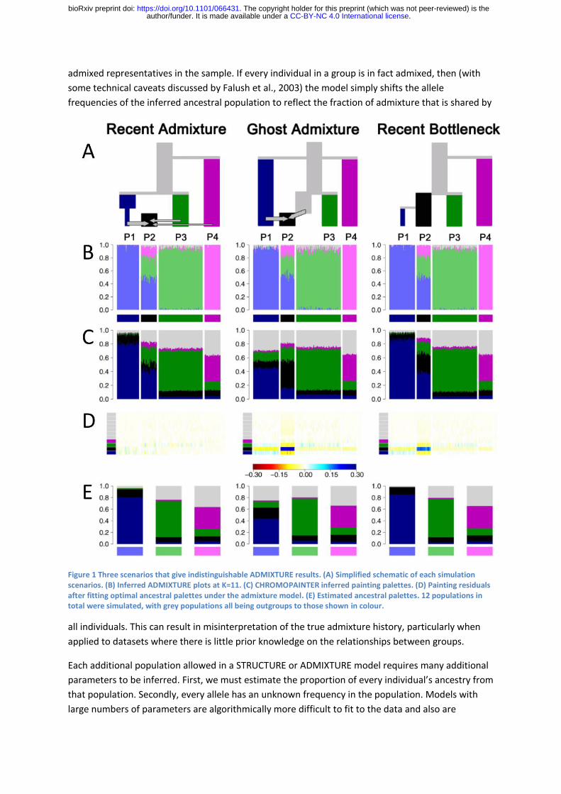
ancestry bar plots. Figure 1 shows admixture histories inferred by STRUCTURE for three scenarios.

Note that these simulations were performed with 12 populations but only results for the four most

relevant populations are shown. The “Recent Admixture” scenario represents a history qualitatively

similar to African Americans. The true history is that P2 is an admixture of P1, P3 and P4.

ADMIXTURE, interpreted according to the above protocol, infers that this is what happened and

estimates approximately correct admixture proportions, with the light green ancestral population

contributing a higher proportion than the light pink one (true admixture proportions 35% and 15%

respectively).

In the “Ghost Admixture” scenario, P2 is instead formed by a 50% -50% admixture between P1 and

an unsampled “ghost” population, which is most closely related to P3. Here, the relative proportions

of inferred ancestry are very similar but in this case the difference between the amount of ancestry

inferred from the light green and light pink ancestral population reflects a difference in the

phylogenetic distances of P3 and P4 to the true admixing source. In the “Recent Bottleneck”

scenario, P1 is a sister population to P2 that underwent a strong recent bottleneck. Members of P2

are once again inferred to be admixed, while P1 receives its own ancestry component.

In order to understand these results, it is useful to think of STRUCTURE and ADMIXTURE as

algorithms that parsimoniously explain variation between individuals rather than as parametric

models of divergence and admixture. If admixture events or genetic drift affect all members of the

sample equally, then there is no variation between individuals for the model to explain. For example,

non-African humans have a few percent Neanderthal ancestry, but this is invisible to STRUCTURE or

ADMIXTURE since it does not result in differences in ancestry profile between individuals. The same

reasoning helps to explain why for most datasets –even in species such as humans where mixing is

commonplace - each of the K populations is inferred by STRUCTURE/ADMIXTURE to have non-


https://doi.org/10.1101/066431


admixed representatives in the sample. If every individual in a group is in fact admixed, then (with

some technical caveats discussed by Falush et al., 2003) the model simply shifts the allele

frequencies of the inferred ancestral population to reflect the fraction of admixture that is shared by

Figure 1 Three scenarios that give indistinguishable ADMIXTURE results. (A) Simplified schematic of each simulation scenarios. (B) Inferred ADMIXTURE plots at K=11. (C) CHROMOPAINTER inferred painting palettes. (D) Painting residuals after fitting optimal ancestral palettes under the admixture model. (E) Estimated ancestral palettes. 12 populations in total were simulated, with grey populations all being outgroups to those shown in colour.

all individuals. This can result in misinterpretation of the true admixture history, particularly when

applied to datasets where there is little prior knowledge on the relationships between groups.

Each additional population allowed in a STRUCTURE or ADMIXTURE model requires many additional

parameters to be inferred. First, we must estimate the proportion of every individual’s ancestry from

that population. Secondly, every allele has an unknown frequency in the population. Models with

large numbers of parameters are algorithmically more difficult to fit to the data and also are


https://doi.org/10.1101/066431


penalized in statistical comparisons to prevent overfitting. For example, because the number of

parameters increases with the number of loci, the algorithms can fail to detect subtle population

structure even in relatively simple scenarios if the number of loci is very large (Lawson et al., 2012).

In practice, the best that can be expected, even if the models converge on good solutions and K is

estimated sensibly, is that the algorithms choose the smallest number of ancestral populations that

can explain the most salient variation in the data. Unless the demographic history of the sample is

particularly simple, the value of K inferred according to any statistically sensible criterion is likely to

be smaller than the number of distinct drift events that have significantly impacted the sample.

What the algorithm often does is in practice use variation in admixture proportions between

individuals to approximately mimic the effect of more than K distinct drift events without estimating

ancestral populations corresponding to each one.

To be specific, in the Ghost Admixture scenario, the ghost population is modelled as a mix of the

sampled populations it is most closely related to, rather than being given its own ancestral

population. In the Recent Bottleneck scenario, the genetic drift shared by P1 and P2 is modelled by

ADMIXTURE by assigning both populations some ancestry from the light blue ancestral population.

The strong recent drift specific to P1 is approximately modelled by assigning more light blue ancestry

to P1 than to P2, thereby making P1 more distinct from the other populations in the sample. An

alternative outcome in both scenarios would be for ADMIXTURE to infer a higher value of K and to

include an extra ancestral population for P2. The algorithm is more likely to infer this solution if

there was stronger genetic drift specific to P2 or if members of the population made up a greater

overall proportion of the sample.

A visualization of the goodness of fit of admixture models using chromosome painting

We have implemented an approach that uses painting “palettes” calculated by CHROMOPAINTER

(Lawson et al., 2012) to assess the goodness of fit of a recent admixture model to the underlying

genetic data. CHROMOPAINTER uses haplotype information to identify fine-scale ancestry

information by identifying, for each individual, which of the other individual(s) in the sample are

most closely related for each stretch of genome. The palettes (Figure 1C) constitute the proportion

of ancestry that comes from each of the labelled populations plotted as a distinct colour. In this

manuscript we use sampling labels but if these are not available or are not predictive of genetic

relationships, it is possible to use fineSTRUCTURE (Lawson et al. 2012) to cluster individuals into

genetically homogeneous groups based on their inferred painting profiles, thus generating labels.

We assume that there are more labelled populations P than there are ancestral populations K. The

painting palettes can be thought of as a way of representing the information that the genetic data

provides on shared ancestry between populations. There is no underlying historical or evolutionary

model assumed by this representation, except that each labelled populations is homogeneous in its

ancestry profile.

The palettes are distinct for the three simulated scenarios, demonstrating that it is possible to

distinguish between them using genetic data and that the palettes provide complementary

information to the ADMIXTURE plots (Figure 1B compared to Figure 1C). In order to more directly

relate the results of STRUCTURE/ADMIXTURE to the painting palettes, we assume that each


https://doi.org/10.1101/066431


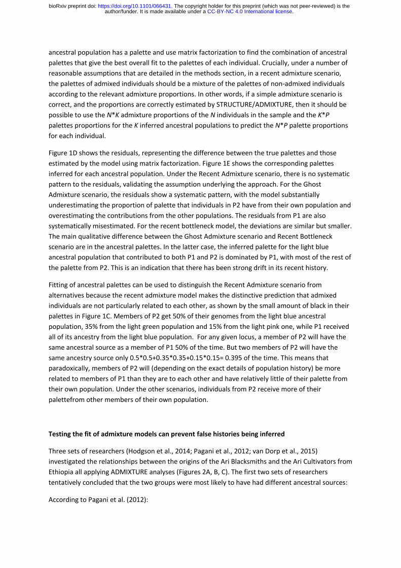
ancestral population has a palette and use matrix factorization to find the combination of ancestral

palettes that give the best overall fit to the palettes of each individual. Crucially, under a number of

reasonable assumptions that are detailed in the methods section, in a recent admixture scenario,

the palettes of admixed individuals should be a mixture of the palettes of non-admixed individuals

according to the relevant admixture proportions. In other words, if a simple admixture scenario is

correct, and the proportions are correctly estimated by STRUCTURE/ADMIXTURE, then it should be

possible to use the N*K admixture proportions of the N individuals in the sample and the K*P

palettes proportions for the K inferred ancestral populations to predict the N*P palette proportions

for each individual.

Figure 1D shows the residuals, representing the difference between the true palettes and those

estimated by the model using matrix factorization. Figure 1E shows the corresponding palettes

inferred for each ancestral population. Under the Recent Admixture scenario, there is no systematic

pattern to the residuals, validating the assumption underlying the approach. For the Ghost

Admixture scenario, the residuals show a systematic pattern, with the model substantially

underestimating the proportion of palette that individuals in P2 have from their own population and

overestimating the contributions from the other populations. The residuals from P1 are also

systematically misestimated. For the recent bottleneck model, the deviations are similar but smaller.

The main qualitative difference between the Ghost Admixture scenario and Recent Bottleneck

scenario are in the ancestral palettes. In the latter case, the inferred palette for the light blue

ancestral population that contributed to both P1 and P2 is dominated by P1, with most of the rest of

the palette from P2. This is an indication that there has been strong drift in its recent history.

Fitting of ancestral palettes can be used to distinguish the Recent Admixture scenario from

alternatives because the recent admixture model makes the distinctive prediction that admixed

individuals are not particularly related to each other, as shown by the small amount of black in their

palettes in Figure 1C. Members of P2 get 50% of their genomes from the light blue ancestral

population, 35% from the light green population and 15% from the light pink one, while P1 received

all of its ancestry from the light blue population. For any given locus, a member of P2 will have the

same ancestral source as a member of P1 50% of the time. But two members of P2 will have the

same ancestry source only 0.5*0.5+0.35*0.35+0.15*0.15= 0.395 of the time. This means that

paradoxically, members of P2 will (depending on the exact details of population history) be more

related to members of P1 than they are to each other and have relatively little of their palette from

their own population. Under the other scenarios, individuals from P2 receive more of their

palettefrom other members of their own population.

Testing the fit of admixture models can prevent false histories being inferred

Three sets of researchers (Hodgson et al., 2014; Pagani et al., 2012; van Dorp et al., 2015)

investigated the relationships between the origins of the Ari Blacksmiths and the Ari Cultivators from

Ethiopia all applying ADMIXTURE analyses (Figures 2A, B, C). The first two sets of researchers

tentatively concluded that the two groups were most likely to have had different ancestral sources:

According to Pagani et al. (2012):


https://doi.org/10.1101/066431


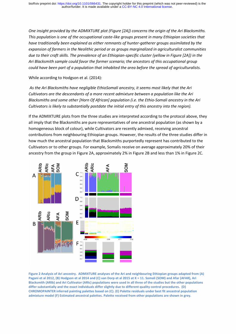
One insight provided by the ADMIXTURE plot (Figure [2A]) concerns the origin of the Ari Blacksmiths.

This population is one of the occupational caste-like groups present in many Ethiopian societies that

have traditionally been explained as either remnants of hunter-gatherer groups assimilated by the

expansion of farmers in the Neolithic period or as groups marginalized in agriculturalist communities

due to their craft skills. The prevalence of an Ethiopian-specific cluster (yellow in Figure [2A]) in the

Ari Blacksmith sample could favor the former scenario; the ancestors of this occupational group

could have been part of a population that inhabited the area before the spread of agriculturalists.

While according to Hodgson et al. (2014):

As the Ari Blacksmiths have negligible EthioSomali ancestry, it seems most likely that the Ari

Cultivators are the descendants of a more recent admixture between a population like the Ari

Blacksmiths and some other [Horn Of African] population (i.e. the Ethio-Somali ancestry in the Ari

Cultivators is likely to substantially postdate the initial entry of this ancestry into the region).

If the ADMIXTURE plots from the three studies are interpreted according to the protocol above, they

all imply that the Blacksmiths are pure representatives of one ancestral population (as shown by a

homogeneous block of colour), while Cultivators are recently admixed, receiving ancestral

contributions from neighbouring Ethiopian groups. However, the results of the three studies differ in

how much the ancestral population that Blacksmiths purportedly represent has contributed to the

Cultivators or to other groups. For example, Somalis receive on average approximately 20% of their

ancestry from the group in Figure 2A, approximately 2% in Figure 2B and less than 1% in Figure 2C.

Figure 2 Analysis of Ari ancestry. ADMIXTURE analyses of the Ari and neighbouring Ethiopian groups adapted from (A) Pagani et al 2012, (B) Hodgson et al 2014 and (C) van Dorp et al 2015 at K = 11. Somali (SOM) and Afar (AFAR), Ari Blacksmith (ARIb) and Ari Cultivator (ARIc) populations were used in all three of the studies but the other populations differ substantially and the exact individuals differ slightly due to different quality control procedures. (D) CHROMOPAINTER inferred painting palettes based on (C). (E) Palette residuals under best fit ancestral population admixture model (F) Estimated ancestral palettes. Palette received from other populations are shown in grey.


https://doi.org/10.1101/066431


In fact, as was demonstrated by the third set of authors (van Dorp et al., 2015) based on several

additional analyses, this history is false and the totality of evidence from the genetic data shows that

the true history is analogous to the Recent Bottleneck Scenario of Figure 1A. The Blacksmiths and

the Cultivators diverged from each other, principally by a bottleneck in the Blacksmiths, which was

likely a consequence of their marginalised status. Once this drift is accounted for the Blacksmiths

and Cultivators have almost identical inferred ancestry profiles and admixture histories. In our

analysis, a strong deviation from a simple admixture model can be seen in the residual palettes,

which imply that the inferred ancestral palettes substantially underestimate the drift in the Ari

Blacksmiths (Figure 2E).

Sample sizes can substantially affect clustering and ancestral population inference

The alert reader will have noticed a difference between the results inferred for the simulated Recent

Bottleneck Scenario and the real Ari data. In the real data (Figure 2), the Ari Blacksmiths have the

largest residuals, which imply that their genetic drift is much stronger than predicted based on the

ancestral palettes. For the simulated data, the light blue ancestral palette (Figure 1E) incorporates

strong drift in its recent history and the largest residuals are found in P2 which is analogous to the

Ari Cultivators. This difference is due to sample size. In the real data, there are many more

Cultivators than Blacksmiths, while in the simulations, P1, which is analogous to the Blacksmiths has

more sample members. Sample size influences the results because the ancestral palettes are

calculated based on minimizing the sum of residuals over all of the individuals, giving more weight to

larger populations.

The results obtained by STRUCTURE/ADMIXTURE are themselves also greatly affected by sample size

(Puechmaille 2016). Specifically, groups that are numerically small with respect to other groups in

the sample or have undergone little population-specific drift of their own are likely to be fit as mixes

of multiple drifted groups, rather than given their own ancestral population. Indeed, if an ancient

sample is put into a dataset of modern individuals, the ancient sample is typically represented as an

admixture of the modern populations (e.g. Rasmussen et al. 2010, Skoglund et al. 2012), which can

happen even if the individual sample is older than the split date of the modern populations and thus

cannot be admixed. A similar effect can happen when a source population is put into a dataset with

two or more drifted sink populations. The source can be represented as a mix, even though there is

no mixture within its history.

The sensitivity of STRUCTURE/ADMIXTURE to sample size and to strong genetic drift allows the

addition of two more to the above protocol:

(0) Make sure to over-sample your favourite group.

(1a) If your favourite group does not have its own population, increase K until it does.

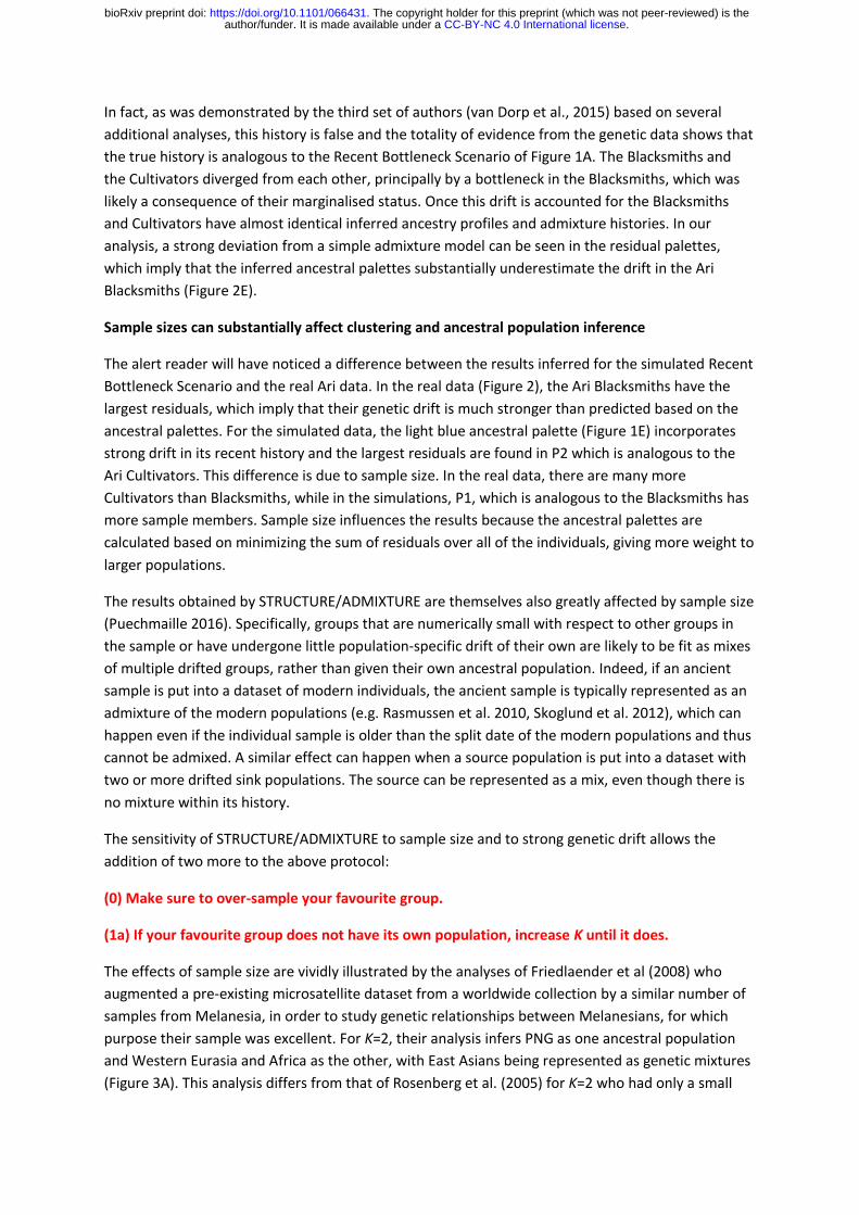
The effects of sample size are vividly illustrated by the analyses of Friedlaender et al (2008) who

augmented a pre-existing microsatellite dataset from a worldwide collection by a similar number of

samples from Melanesia, in order to study genetic relationships between Melanesians, for which

purpose their sample was excellent. For K=2, their analysis infers PNG as one ancestral population

and Western Eurasia and Africa as the other, with East Asians being represented as genetic mixtures

(Figure 3A). This analysis differs from that of Rosenberg et al. (2005) for K=2 who had only a small


https://doi.org/10.1101/066431


number of Melanesians in their sample, and who found Native Americans rather than Melanesians

to be the unadmixed group (Figure 3F). For K=6, both models distinguish between all 5 continental

groups (Americans, Western Eurasians, Africans East Asians, Oceanians), however Rosenberg et al.

split Native American groups into two ancestral populations (not presented here), while

Friedlaender et al. infer that Melanesians have two ancestral populations, with pure representatives

in Bourganville and New Britain (Figure 3B). A third result for K=6 was found by Rosenberg et al.

(2002), who found the Kalash, an isolated population in Pakistan, to be the sixth cluster.

It is tempting to attribute the global clustering results of Friedlaender et al. as being due to peculiar

sampling but for K=2, the results of Rosenberg et al. (2005) are actually odder, if interpreted literally,

since they imply a continuous admixture cline between Africa and the Americas. From almost any

perspective, the most important demographic event that has left a signature in the dataset is the

out-of-Africa bottleneck. This is not taken by STRUCTURE to be the event at K=2 in either of the

analyses or of others with similar datasets because sub-Saharan Africans constitute only a small

proportion of the sample.

Some even more peculiar results are obtained for an analysis that focused on Melanesian

populations, leaving in only East Asian populations and a single European population, namely the

French. Friedlander et al.’s purpose in presenting this analysis was to analyse the fine-scale

relationships amongst the Melanesians, while detecting admixture e.g. from Colonial settlers. Our

purpose here is to ask what the results imply, when interpreted literally, about the relationships

between Melanesians, East Asians and Europeans. For all values from K=2 to K=9, the French

population is inferred to be a mixture between an East Asian population and a Melanesian one. For

K=7 to K=9, the model is more specific, fitting the European population as a mixture of East Asian

population and one from New Guinea (Figure 3D, 3E). Only for K=10 do the French form their own

cluster and in this case they are inferred to have variable levels of admixture from East Asians (Figure

3C).

Once again, it is tempting to write these results off as being the product of an inappropriate

sampling scheme, but instead imagine that there was an environmental catastrophe that spared the

people of Melanesia and a few lucky others. In this case, the analysis would become a faithful

sampling of the people of the world and the results would become the world’s genetic history. This

exercise is relevant in particular because human history is in fact full of episodes in which groups

such as the Bantu and the Han have used technological, cultural or military advantage or virgin

territory to multiply until they make up a substantial fraction of the world’s population. The history

of the world told by STRUCTURE or ADMIXTURE is thus a tale that is skewed towards populations

that have grown from small numbers of founders, with the bottlenecks that that implies. Even if the

sampling is strictly proportional to modern population sizes, it is a winner’s history.

Other genetic analysis methods have similar peculiarities. Principle Components Analysis (PCA) is

closely related to the STRUCTURE model in the information that it uses, both in theory (Lawson et

al., 2012) and in practice (Patterson et al., 2006) and has also been shown theoretically to be

affected by sample size (McVean, 2009). Friedlaender et al. plot a neighbour-joining tree calculated

based on Fst values between populations which instructively exaggerates the effect of drift (Figure

3G). Africa and the Middle East together make a small part of the diversity which is dominated by

the isolated populations of Native Americans and PNG. If enough individuals are present in the


https://doi.org/10.1101/066431


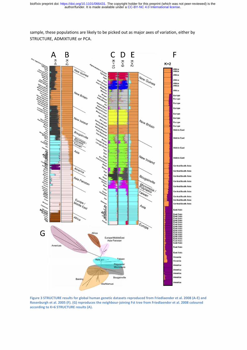
sample, these populations are likely to be picked out as major axes of variation, either by

STRUCTURE, ADMIXTURE or PCA.

Figure 3 STRUCTURE results for global human genetic datasets reproduced from Friedlaender et al. 2008 (A-E) and Rosenburgh et al. 2005 (F). (G) reproduces the neighbour-joining Fst tree from Friedlaender et al. 2008 coloured according to K=6 STRUCTURE results (A).


https://doi.org/10.1101/066431


Summarizing but not over-simplifying complex datasets

Notwithstanding the pitfalls we have described, there is tremendous value in summarizing data

based on a handful of major axes of variation. Identifying these axes is a first step in historical

reconstruction and in asking whether they can in fact be related to specific historical bottlenecks,

expansions or migrations or whether they instead reflect continuously acting processes. PCA is

effective for representing two or three axes of variation but becomes unwieldy for four or more and

suffers from similar interpretation issues as STRUCTURE/ADMIXTURE. We finish this article by

attempting to describe variation within a recently published Indian dataset.

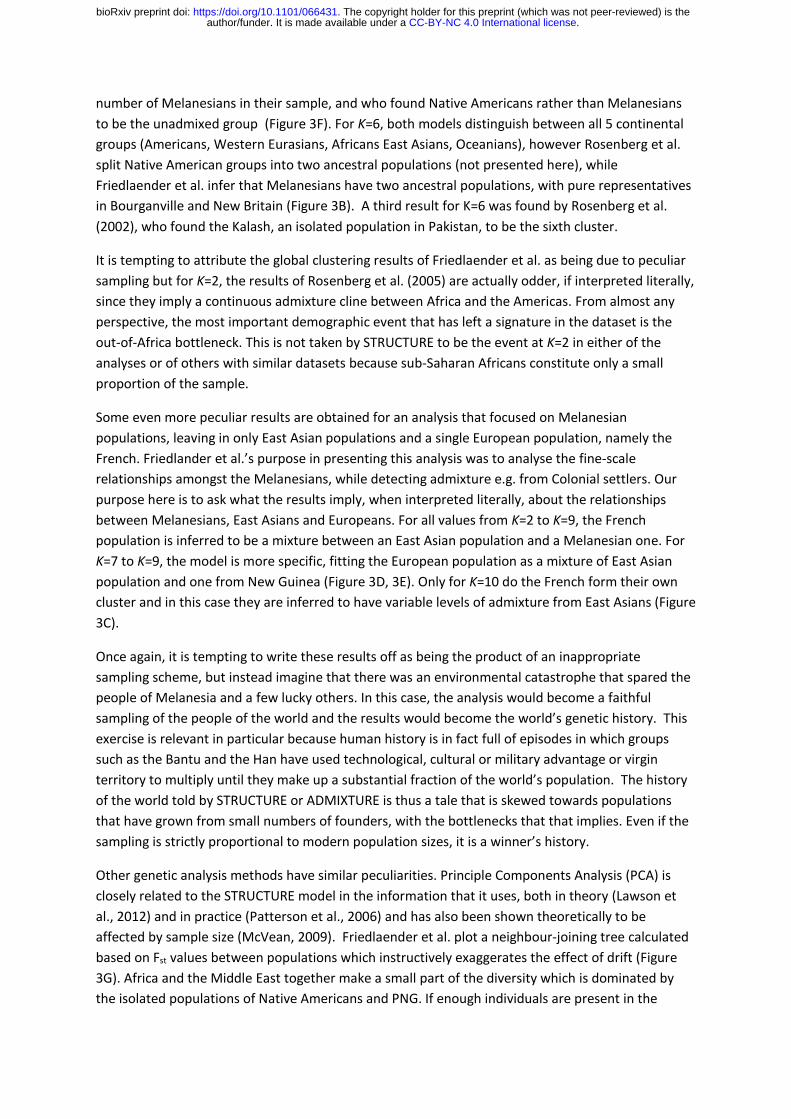
Basu et al. (2016) used an ADMIXTURE plot with K=4 to summarize variation amongst continental

Indians from 19 populations. The four ancestral populations were labelled Ancestral North India

(ANI), Ancestral South India (ASI), Ancestral Tibeto-Burman (ATB) and Ancestral Austro-Asiatic (AAA),

as shown in Figure 4A. The overall fit to the CHROMOPAINTER painting palette is poor (Figure 4B)

principally due to individuals receiving much more of their palette from their own population than

predicted by the best-fit model, as indicated by the blue in the diagonals of the residual matrix.

Predominantly ASI populations have the largest residuals followed by AAA, ATB and then ANI. The

most likely explanation for these residuals is genetic drift specific to the labelled populations,

although populations can also diverge from each other by admixture with ghost populations. In any

case, the results show that many of these populations have undergone significant demographic

events of their own and are not simply recent mixtures between large ancestral populations. In

some of the population, such as the Kharti (KSH), there is substantial variation between individuals

in the proportion of the within-population painting palettes contribution, which is likely to reflect

recent relatedness between members of the sample.

The large proportion of the painting palette that members of ASA and ATB population receive from

their own population makes the rest of their palette hard to interpret. We have therefore attempted

to estimate what the painting palettes would look like if the drift specific to individual populations

had not occurred. Specifically, we replace the within-population palette proportion for each

individual with the value predicted based on the ancestral palettes and rescale the remaining

palettes so that the whole palette continues to sum to one. We then re-estimate the ancestral

palette and iterate until convergence. The resulting palette is shown in Figure 4C. The ancestral

palettes estimated by this method are substantially altered, particularly for ASI and AAA populations

(compare Figure 4D and 4E). The results of this procedure should be interpreted with caution – for

example because they are highly dependent on how the labelled populations are defined – but have

proven informative for this dataset. More rigorous approaches to excluding population-specific drift

are described by van Dorp et al. (2015)

Once population specific drift is accounted for, there is good evidence for four ancestry components,

as can be seen by eye inspecting the palettes. For example, the four ATB populations each have

higher proportions of all four ATB population palettes than any of the non-ATB populations. It is also

possible to make deductions about the relationships between the ancestral populations. The ASI and

ANI populations are relatively closely related, with high sharing of palettes between them, while ATB

and AAA are more distantly related to each other and to ANI and ASI. These results validate the

claim made by Basu et al. that variation within the Indian populations they sampled should not be

thought of as a predominantly mixture between ANI and ASI.


https://doi.org/10.1101/066431


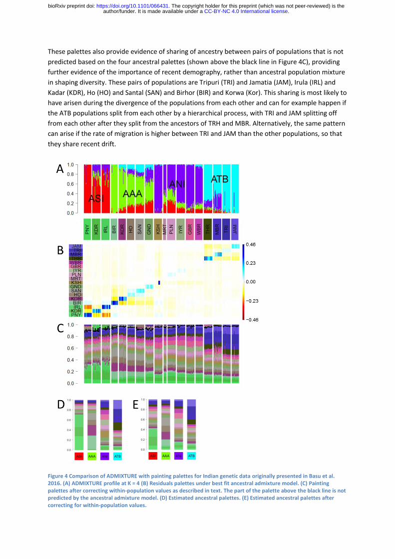
These palettes also provide evidence of sharing of ancestry between pairs of populations that is not

predicted based on the four ancestral palettes (shown above the black line in Figure 4C), providing

further evidence of the importance of recent demography, rather than ancestral population mixture

in shaping diversity. These pairs of populations are Tripuri (TRI) and Jamatia (JAM), Irula (IRL) and

Kadar (KDR), Ho (HO) and Santal (SAN) and Birhor (BIR) and Korwa (Kor). This sharing is most likely to

have arisen during the divergence of the populations from each other and can for example happen if

the ATB populations split from each other by a hierarchical process, with TRI and JAM splitting off

from each other after they split from the ancestors of TRH and MBR. Alternatively, the same pattern

can arise if the rate of migration is higher between TRI and JAM than the other populations, so that

they share recent drift.

Figure 4 Comparison of ADMIXTURE with painting palettes for Indian genetic data originally presented in Basu et al. 2016. (A) ADMIXTURE profile at K = 4 (B) Residuals palettes under best fit ancestral admixture model. (C) Painting palettes after correcting within-population values as described in text. The part of the palette above the black line is not predicted by the ancestral admixture model. (D) Estimated ancestral palettes. (E) Estimated ancestral palettes after correcting for within-population values.


https://doi.org/10.1101/066431


Finally, we can ask whether the variation in ancestry proportions in the ADMIXTURE plots are likely

to be indicative of a history of admixture between populations. For example, ADMIXTURE assigns

nearly 100% ASI ancestry to Paniya (PNY), while KDR and IRL are inferred to be admixed (Figure 4A)

but this result is suspicious because of the tendency documented above for ADMIXTURE to assign

pure ancestry components to highly drifted populations like PNY. Once population specific drift is

accounted for, the palette for PNY actually has slightly less overall ASI ancestry than KDR and IRL

(Figure 4C). PCA also makes PNY the most strongly differentiated population according to the

relevant Principal Component (see Figure 2, Basu et al.) but this may be based on PNY specific drift

being incorporated into the component and should not be thought of as providing independent

confirmation of the ADMIXTURE results. Thus the evidence that PNY is a less admixed representative

of a putative ancestral ASI population than KDR or IRL is weak.

For AAA and ANI, an admixture cline does appear to be a real feature of the data, as indicated by

variation between the labelled populations in the overall proportion of the palette that comes from

other AAA and ANI populations, respectively (Figure 4C). The palettes are consistent with the

ADMIXTURE result in implying that Birhor (BIR) have the most AAA ancestry of any population. For

ANI, ADMIXTURE finds that KSH receive almost all of their ancestry from ANI while Gujarati Brahmin

(GBR) are more admixed but once the high relatedness of some KSH is accounted for along with

other population specific drift, it is difficult to discern differences between the palettes of these two

populations.

Overall, these results show that in recent history, genetic drift has been at least as important in

shaping variation within these populations as admixture. A simple history comprising a

differentiation phase followed by a mixture phase is false and inferences based on this model are

liable to be misleading. Other, qualitatively different scenarios should also be considered, such as

one in which in which the processes of mixture and divergence in ancient history was similar to that

in recent history and the differentiation into four major ancestries reflects sustained differences in

connectedness between populations. It is beyond the scope of this manuscript to test this or other

models. The popularity of STRUCTURE and its descendants as unsupervised clustering methods is

justified but even if interpreted carefully their use should represent the beginning of a detailed

demographic and historical analysis, not the end.

Materials and Methods

Simulations

Figure 1A illustrates the demographic histories behind three simulation scenarios: “Recent

Admixture”, “Ghost Admixture” and “Recent Bottleneck”. “Ghost Admixture” and “Recent

Bottleneck” are based on full simulations described in van Dorp et al. 2015 aimed to capture global

population genetic diversity with an emphasis on exploring population structure in “Ethiopian-like”

simulated groups, here represented as P1-P4. For our purposes we instead employ these simulations

to assess how differences in demographic histories impact on inferred ADMIXTURE profiles.

For the “Recent Bottleneck” and “Ghost Admixture” simulations 13 populations, each containing 100

individuals were simulated using the approximate coalescence simulation software MaCS (Chen et


https://doi.org/10.1101/066431


al. 2010) under histories that differ in how P2 relates to P1 (Figure 1A). Specifically, “Recent

Bottleneck” equates to the “MA” simulations of van Dorp et al. 2015 where P1 splits from P2

(analogously Pop5b splits from Pop5) 20 generations ago followed immediately by a strong

bottleneck in P2. “Ghost Admixture” equates to the “RN” simulations of van Dorp et al. 2015 where

P1 splits from P2 (analogously Pop5b splits from Pop5) 1700 generations ago after which migrants

from P1 form approximately 50% of P2 over a period of 200-300 generations. Although simulating

100 individuals in each population, we perform subsequent ADMIXTURE and CHROMOPAINTER

analyses on a subset of these using only 35 individuals from P1, 25 individuals from P2, 70 individuals

from P3 and 25 individuals from P4, so as to approximately mimic sample sizes in the true data. This

leaves an ‘excess’ of simulated individuals. For simplicity and ease of interpretation only P1-P4 are

depicted in Figure 1 with all other populations coloured grey.

For the “Recent Admixture” scenario we implement a simulation technique adapted from that

applied in Leslie et al. 2015, which sub-samples chromosomes from the ‘excess’ individuals

simulated under the “Recent Bottleneck” scenario. This method explicitly mixes chromosomes from

different populations based on a set of user-defined proportions, analogous to an instantaneous

admixture event. Importantly for our purposes, this simulation method allows direct assessment of

how well ADMIXTURE recapitulates these proportions, an objective which is more difficult to achieve

using more complex simulation techniques. Using this approach we simulate admixed chromosomes

of P2 by mixing chromosomes of 20 ‘excess’ individuals from each of P1 (50%), P3 (35%) and P4

(15%) based on an admixture event occurring λ=15 generations ago. In particularly to simulate a

haploid admixed chromosome and as in Leslie et al. 2015 we first sample a genetic distance x from

an exponential distribution with rate 0.15 (λ/100). The first x cM of the simulated chromosome is

composed of the first x cM of chromosomes selected randomly, but without overlap, from ‘excess’

individuals of P1, P3 and P4 according to the defined proportions. This process is repeated using a

new genetic distance sampled from the same exponential distribution (rate=0.15) and continued

until an entire simulated chromosome is generated. This method is then re-employed to generate a

set of 20 haploid chromosomes for a single individual and then repeated 70 times to generate 70

haploid autosomes. Diploid individuals are constructed by joining two full sets of haploid

chromosomes, resulting in 35 simulated Pop2 individuals in total. All other populations are

simulated using MaCS as in the “Ghost Admixture” and “Recent Bottleneck” scenarios.

For each simulation scenario we apply ADMIXTURE (Alexander et al. 2010) to the sampled

individuals from every simulated group. SNPs were first pruned to remove those in high linkage

disequilibrium (LD) using PLINK v1.07 (Purcell et al. 2007) so that no two SNPs within 250kb have a

squared correlation coefficient (r2) greater than 0.1. ADMIXTURE was then run with default values

for multiple values of K, and the resultant admixture profiles plotted where K=11 (Figure 1B and

Figure 2C). In addition for each scenario we applied CHROMOPAINTER to paint all individuals in

relation to all others using default values for the CHROMOPAINTER mutation/emission (“-M” switch)

and switch (“-n” switch) rates. We sum the total proportion of genome-wide DNA each recipient

individual is painted by each donor group and plot the inferred contributions for each recipient as a

painting palette (as in Figure 1C and Figure 2D).

Estimation of ancestral palettes


https://doi.org/10.1101/066431


Define 𝐴 as the 𝑁 ×𝐾 admixture proportion matrix, where there are N individuals in the sample and

K ancestral populations used in the ADMIXTURE analysis. Let 𝐶 be the 𝑁 × 𝑃 matrix of individual

palettes from the CHROMOPAINTER painting, and 𝑋 be the 𝐾 × 𝑃 matrix of the palettes for each

ancestral population. Then we seek solutions for 𝑋 that minimise the squared prediction error of the

form:

𝐴𝑋 = 𝐶.

We define 𝐵 = (𝐴𝑇𝐴)−1𝐴𝑇. Then, 𝐵𝐴𝑋 = (𝐴𝑇𝐴)−1𝐴𝑇𝐴𝑋 = 𝑋, leading to the solution

𝑋 = (𝐴𝑇𝐴)−1𝐴𝑇𝐶.

Note that there is no guarantee that 𝑋 will be positive. Negative elements would imply a poor fit of

the admixture model, and alternative minimization strategies might be employed to find 𝑋 subject

to the constraint. Further, if the matrix 𝐴𝑇𝐴 is rank deficient its inverse will not exist. This should

only be the case if 𝐾 is chosen too large, or there are genuine symmetries in the data.

For a recent admixture model, long haplotypes are inherited from each of the donating populations

in a given admixture proportion. If we assume that ancestral boundaries can be inferred then,

excluding drift in either SNP frequency or haplotype structure, the palettes of admixed individuals

are (by definition) a mixture with the same ancestry proportions as the SNPS under which admixture

is inferred.

Acknowledgements

This paper was stimulated by a discussion with Chuck Langley and also by the 2016 Workshop for

Population and Speciation Genomics, Cesky Krumlov. We thank Jonathan Pritchard for suggesting

the residuals plot and Analabha Basu, Kimberly Gilbert, Matthew Hahn, Razib Khan, Partha

Majumder, Iain Mathieson, and Matthew Stephens for comments. D.F. is funded by a Medical

Research Council Fellowship as part of the MRC CLIMB consortium for microbial bioinformatics

(grant number MR/M501608/1). LvD is supported by CoMPLEX via EPSRC (grant number

EP/F500351/1). DJL is supported by Wellcome Trust and Royal Society grant WT104125AIA.

Alexander, D. H., J. Novembre, and K. Lange, 2009, Fast model-based estimation of ancestry in unrelated individuals: Genome Research, v. 19, p. 1655-1664.

Basu, A., N. Sarkar-Roy, and P. Majumder, 2016, Genomic reconstruction of the history of extant populations of India reveals five distinct ancestral components and a complex structure: Proceedings of the National Academy of Sciences of the United States of America, v. 113, p. 1594-1599.

Chen, G., P. Marojoram, J. Wall, 2009, Fast and felxible simulation of DNA sequence data: Genome Research, v. 19, p. 136-142.

Evanno, G., S. Regnaut, and J. Goudet, 2005, Detecting the number of clusters of individuals using the software STRUCTURE: a simulation study: Molecular Ecology, v. 14, p. 2611-2620.

Falush, D., M. Stephens, and J. K. Pritchard, 2003, Inference of population structure using multilocus genotype data: Linked loci and correlated allele frequencies: Genetics, v. 164, p. 1567-1587.

Friedlaender, J., F. Friedlaender, F. Reed, K. Kidd, J. Kidd, G. Chambers, R. Lea, J. Loo, G. Koki, J. Hodgson, D. Merriwether, and J. Weber, 2008, The genetic structure of Pacific islanders: Plos Genetics, v. 4.


https://doi.org/10.1101/066431


Hodgson, J. A., C. J. Mulligan, A. Al-Meeri, and R. L. Raaum, 2014, Early Back-to-Africa Migration into the Horn of Africa: Plos Genetics, v. 10, p. 18.

Lawson, D. J., G. Hellenthal, S. Myers, and D. Falush, 2012, Inference of Population Structure using Dense Haplotype Data: Plos Genetics, v. 8.

Leslie, S., B. Winney, G. Hellenthal, D. Davison, A. Boumertit, T. Day, K. Hutnik, E. C. Royrvik, B. Cunliffe, D. J. Lawson, D. Falush, C. Freeman, M. Pirinen, S. Myers, M. Robinson, P. Donnelly, W. Bodmer, C. Wellcome Trust Case, and G. Int Multiple Sclerosis, 2015, The fine-scale genetic structure of the British population: Nature, v. 519, p. 309-+.

McVean, G., 2009, A Genealogical Interpretation of Principal Components Analysis: Plos Genetics, v. 5.

Pagani, L., T. Kivisild, A. Tarekegn, R. Ekong, C. Plaster, I. G. Romero, Q. Ayub, S. Q. Mehdi, M. G. Thomas, D. Luiselli, E. Bekele, N. Bradman, D. J. Balding, and C. Tyler-Smith, 2012, Ethiopian Genetic Diversity Reveals Linguistic Stratification and Complex Influences on the Ethiopian Gene Pool: American Journal of Human Genetics, v. 91, p. 83-96.

Patterson, N., A. Price, and D. Reich, 2006, Population structure and eigenanalysis: Plos Genetics, v. 2, p. 2074-2093.

Pritchard, J. K., M. Stephens, and P. Donnelly, 2000, Inference of population structure using multilocus genotype data: Genetics, v. 155, p. 945-959.

Purcell, S., B. Neale, K. Todd-Brown, L. Thomas, M. Ferreira et al. 2007, PLINK: a toolset for whole-genome association and population-based linkage analysis: Am J Hum Genet, 81, p. 559-575.

Puechmaille, S.J, 2016 The program structure does not reliably recover the correct population structure when sampling is uneven: subsampling and new estimators alleviate the problem. Molecular Ecology Resources 16, p. 608-627.

Rasmussen, M., et al. 2010, Ancient human genome sequence of an extinct Palaeo-Eskimo, Nature p. 757-762.

Rosenberg, N., T. Burke, K. Elo, M. Feldmann, P. Freidlin, M. Groenen, J. Hillel, A. Maki-Tanila, M. Tixier-Boichard, A. Vignal, K. Wimmers, and S. Weigend, 2001, Empirical evaluation of genetic clustering methods using multilocus genotypes from 20 chicken breeds: Genetics, v. 159, p. 699-713.

Rosenberg, N., S. Mahajan, S. Ramachandran, C. Zhao, J. Pritchard, and M. Feldman, 2005, Clines, clusters, and the effect of study design on the inference of human population structure: Plos Genetics, v. 1, p. 660-671.

Rosenberg, N., J. Pritchard, J. Weber, H. Cann, K. Kidd, L. Zhivotovsky, and M. Feldman, 2002, Genetic structure of human populations: Science, v. 298, p. 2381-2385.

Skoglund, P., Malmström, H., Raghavan, M., Storå, J., Hall, P., Willerslev E., Gilbert, M. T. P., Götherström, A., Jakobsson, M., 2012, Origins and Genetic Legacy of Neolithic Farmers and Hunter-Gatherers in Europe. Science, 336, p. 466-469

Tang, H., J. Peng, P. Wang, and N. Risch, 2005, Estimation of individual admixture: Analytical and study design considerations: Genetic Epidemiology, v. 28, p. 289-301.

Tishkoff, S., F. Reed, F. Friedlaender, C. Ehret, A. Ranciaro, A. Froment, J. Hirbo, A. Awomoyi, J. Bodo, O. Doumbo, M. Ibrahim, A. Juma, M. Kotze, G. Lema, J. Moore, H. Mortensen, T. Nyambo, S. Omar, K. Powell, G. Pretorius, M. Smith, M. Thera, C. Wambebe, J. Weber, and S. Williams, 2009, The Genetic Structure and History of Africans and African Americans: Science, v. 324, p. 1035-1044.

van Dorp, L., D. Balding, S. Myers, L. Pagani, C. Tyler-Smith, E. Bekele, A. Tarekegn, M. G. Thomas, N. Bradman, and G. Hellenthal, 2015, Evidence for a Common Origin of Blacksmiths and Cultivators in the Ethiopian Ari within the Last 4500 Years: Lessons for Clustering-Based Inference: Plos Genetics, v. 11, p. 49.


https://doi.org/10.1101/066431


Documents

A tutorial on how (not) to over-interpret STRUCTURE ... · A tutorial on how (not) to over-interpret STRUCTURE/ADMIXTURE bar plots. Daniel Falush1*, Lucy van Dorp2,3, Daniel J Lawson4