A Two Hundred-Year Statistical History

of the Gerrymander∗

Stephen Ansolabehere† Maxwell Palmer‡

May 16, 2015

Abstract

In this paper we assess the geographic compactness of every congressional district used acrossU.S. history. Using the original gerrymander as a standard and a variety of compactness mea-sures, we assess changes in geographic gerrymandering over time and analyze the effect of keyvoting rights laws and court cases on compactness. We find that approximately 20% of all dis-tricts are less compact than the original gerrymander. This pattern has been fairly steady overthe past 200 years, but has worsened since the 1970s. We also show a strong relationship be-tween non-compact districts and Democratic vote share in Congressional elections; Democraticdistricts tend to be less compact than Republican districts.

∗Prepared for presentation at the Congress & History Conference, Vanderbilt University, May 22-23, 2015.†Professor of Government, Harvard University. sda@gov.harvard.edu.‡Assistant Professor of Political Science, Boston University. mbpalmer@bu.edu.

1

1 Introduction

Geographic compactness of legislative districts has long served as a way to identify where map-

makers have manipulated district boundaries to favor one interest, social group, or political party

over others. Most states today have some form of compactness criterion, down to legislation of the

use of specific formulas for assessing compactness. At the federal level, the Apportionment Act of

1911 states that congressional districts are to consist of “contiguous and compact territory,” though

that language was eventually dropped in the Apportionment Act of 1941. While compactness may

itself be a desirable feature of districts (say because it minimizes travel time), significant deviations

from compactness are taken as indicative of other forms of political manipulation of the election

laws, such as favoring one of the political parties or interfering with the representation of one social

group or interest.1 How closely districts comport with this standard, then, is informative about the

extent to which states comply with this broad districting principles and it is a key piece of evidence

in detecting political manipulation of legislative boundaries.

This paper presents an historical assessment of the geographic compactness of all congressional

districts from the 1st Congress to the present. We do so with an eye toward three specific questions

regarding compactness as a stand-alone districting principle and as an indicator of other sorts of

manipulations. First, how compact are districts compared with a standard of what constitutes

a non-compact boundary? Second, is compactness indicative of racial gerrymanders? Third, is

compactness indicative of partisan gerrymanders?

In offering this assessment, we introduce a standard for what constitutes a minimum acceptable

level of compactness. Generally, there exists no accepted statistical or legal standard for measur-

ing whether a district is non-compact (see Niemi et al. 1990). The legal literature on legislative

districting has generally sought such a standard, but usually gets no farther than a subjective as-

sessment of ugliness (see Polsby and Popper 1993). Pildes and Niemi (1993) offer a comparison of

the compactness of every U.S. House district drawn during the 1991-1992 redistricting cycle. Their

analysis offers an enlightening comparison of the compactness of various districts in that cycle of

apportionment, but it offers no metric against which to measure whether a district was unusually

1For a general discussion of districting principles and practices see Butler and Cain (1992); also see Levitt (2010).

2

misshapen. How bad is bad? We invoke an historical standard which has become synonymous

with political manipulation of legislative district boundaries: the shape of the 1812 Massachusetts

Senate district, the Gerrymander. If there is a district whose shape defines a gerrymander, it is the

original beast itself.

We compare the compactness of every congressional district in U.S. history against the shape

of the original gerrymander. One in five Congressional Districts, 20 percent of all districts ever

drawn, are less compact than the original gerrymander. That frequency of non-compact districts

has increased somewhat since the mid-1960s. Twin federal actions dramatically altered the practice

of districting. First, in 1964, the Supreme Court required extensive redrawing of districts to comply

with the standard of one-person-one-vote. Second, beginning in 1970s, the federal Voting Rights

Act compelled creation of minority districts. Both requirements are thought to have contributed

to the growing distortion of legislative district boundaries (Pildes and Niemi 1993; Ansolabehere

and Snyder Jr. 2008). It is difficult to say what one would expect if, say, districts were drawn

arbitrarily (see Chen and Rodden 2013), however the high rate of non-compactness historically

— 20 percent of all congressional districts — suggests that states typically do not comport with

the most basic standards of compactness when drawing district boundaries. Other factors might

have contributed to the increasing distortion of district boundaries, including the introduction of

computerized districting and the increased partisan rancor in U. S. politics.

Interestingly, the compactness of the original gerrymander suggests a readily acceptable stan-

dard for measuring and assessing the compactness of legislative districts. Existing measures of

district compactness have different scales and “ideal districts” that must be understood to inter-

pret a particular compactness result. For example, with the Reock measure, a perfectly circular

district would receive a score of “1”, a perfect square a score of “.64”, and less compact districts

receive smaller scores. With the Schwartzberg perimeter measure, a perfect circle would receive

a score of 1, and less compact districts receive higher scores. With other measures, such as the

ratio of the district area to the perimeter, there is no “ideal” district shape to use as a benchmark;

districts are only assessed relative to each other. Here, we propose that the original gerrymander

be the standard for measuring district compactness for all measures. We adjust and scale every

3

measure such that the compactness score of the original gerrymander is always “1,” higher scores

are less compact, and lower scores are more compact.

This standardizing approach offers four distinct advantages. First, all measures, regardless of

how they are calculated, are interpreted in the same way, and on the same scale. This makes

it easier to understand what a compactness measure means relative to an established baseline.

Second, we can more easily compare different measures of the same district. A district may be non-

compact on one measure, but compact on another. The common scale allows for direct comparisons

between these measures. Third, we have a clear reference district that is well-known and easy to

visualize. When we say a district scores “1.25” on a given measure, we can interpret that as “this

district is 25% worse than the original gerrymander.” Fourth, we can use the score of the original

gerrymander as a cutoff for identifying unambiguous gerrymanders. If a district is worse that the

original gerrymander across some set of measures, we can classify it as a gerrymander as well.

Compactness itself may not be of great concern. Rather, non-compactness is usually a red flag.

It indicates that something unusual happened to district boundaries, and suggests that districts

may have been drawn to favor one social group or political party. Specifically, non-compactness is

often taken as facial evidence that the districts were drawn so that one party might gain electoral

advantages over others, as in the original gerrymander or in the 2012 Florida congressional districts,2

or discriminating against racial groups, as in the first case of racial districting Gomillion v. Lightfoot

(364 U. S. 399 (1960)).

Compactness can be immediately informative about individual districts. If a district’s bound-

ary is determined to be unusually distorted, a court or other analyst might then examine other

characteristics of the district and neighboring districts, such as racial or partisan composition, to

determine whether the non-compactness might have had the effect of diluting the vote of certain

groups of individuals in the are affected by the district. One may also determine the relation-

ship between the characteristics of suspect districts and the political orientation of the legislature

that drew the district. For example, is a Democratically controlled legislature more likely to cre-

2See Romo v. Detzner decided July 10, 2014, in the Circuit Court of the Second Judicial Ciruit in and forLeon, County, Florida, 2012-CA-412 http://www.floridaredistricting.org/documents/Romo_Final_Judgment_

10-Jul-2014.pdf.

4

ate misshapen Republican districts, say because of packing of the opposition party, or misshapen

Democratic districts, say, to increase the number of potential Democratic districts. We examine the

connection between the non-compactness of a district and the extent to which it tilts toward one of

the parties, and whether that slant is a function of who drew the districts (a court, a commission, or

a legislature. Throughout the extensive literature on districting and gerrymandering several factors

are thought to contribute to the characteristics of districts and the structure of representation. The

most prominent of these is: the number of districts (Young 1988; Gilligan and Matsusaka 2006),

unified government (Cox and Katz 1999, 2002), population density (Chen and Rodden 2013), racial

composition (Owen and Grofman 1988; Lublin 1997; Friedman and Holden 2008), and partisanship

and incumbency protection (Ansolabehere and Snyder 2012; Rush 2000; Forgette and Platt 2005).

2 Measuring Compactness

A substantial literature considers the problem of measuring district compactness. Young (1988)

and Niemi et al. (1990) examine a wide variety of methods to measure compactness. Here, we seek

to build on Altman (1998), which analyzes the historical compactness of districts in the context of

districting principles and voting rights challenges.

The literature generally divides methods into several categories, including dispersion, which

assesses the general shape and area of the district, regularity of the perimeter, which penalizes

districts for contorted borders, and population distribution, which takes populations concentration

into account when evaluating the district’s shape. As our goal here is an historical assessment of

district compactness, we are unable to consider compactness measures of this third category due

to data availability. Thus, we focus on the area and perimeter of congressional districts to assess

compactness.

Our analysis below focuses on four key methods for measuring compactness.3 First, we use two

measures of dispersion, Reock and the convex hull ratio, to examine the shape of districts. Reock

(1961) compares the area of the district to the area of the minimum bounding circle that encloses

3One future goal of this project is to calculate every feasible compactness measure for every district, including allmeasures listed in Young (1988) and Niemi et al. (1990).

5

the district. The “ideal” district is a circle, with a perfect score of 1; a square has a score of 0.63.

The convex hull ratio uses a similar approach, but substitutes the minimum bounding circle for the

minimum bounding convex polygon. With this measure, any convex polygon is equally ideal, but

districts with significant protrusions or curves are non-compact. The top half of Figure 2 illustrates

these measures.4

One of the drawbacks of these dispersion measures is that some states, due to borders or

coastlines, are non-compact themselves, and as a result some districts within them will receive

low compactness scores, regardless of how the district borders are drawn. This is a particularly

important problem when we seek to compare district compactness across states, or when we use

the average compactness of a state plan to compare states. As a result, we implement an adjusted

version of Reock and the convex hull ratio that excludes areas outside of the state’s borders from the

area of the minimum bounding circle or convex polygon. For example, in Figure 2, the minimum

bounding circle encloses the district, but also includes part of New Hampshire at the top, and the

Atlantic ocean to the right of the district. The Reock measure includes these areas, but the adjusted

Reock measure excludes them, and only includes the area of state within the circle, shaded in gray.

This method of adjusting the minimum bounding geometry is used in some state compactness

statutes, such as Michigan.5

The second set of measures examines the perimeter of the district. Schwartzberg (1965) and

Polsby-Popper (1991) measure how effectively the perimeter of a district captures the area of a

district. Districts with smooth perimeters are more compact than those with contorted borders,

and the most compact possible district is a circle. Schwartzberg measures the ratio of the perimeter

of the district to the perimeter of a circle with the same area. Polsby-Popper measures the ratio

of the area of the district to the area of a circle with the same perimeter. These two measures are

closely related. As Polsby and Popper (1991) point out when proposing their measure, they are

mathematically equivalent.6 However, they are often used as two separate measures of compactness.

The bottom half of Figure 2 illustrates these two measures.

4Some districts are non-contiguous due to islands or other geographic features. For these districts, we drawseparate bounding circles or convex polygons for each individual feature.

5Mich. Comp. L. §§3.63, 4.261, see http://redistricting.lls.edu/states-MI.php#criteria6Polsby-Popper = 1/(Schwartzberg2) (see Polsby and Popper 1991, note 204).

6

Like the dispersion measures, perimeter-based measures are also particularly sensitive to state

borders. In particular, the convoluted coastlines of states such as Maine, Maryland, Virginia,

and Louisiana produce coastal districts with extraordinarily low Polsby-Popper and Schwartzberg

scores. Furthermore, these scores are extremely sensitive to the resolution of the map. The more

detailed the map, the greater the district perimeter. Unlike the dispersion measures, however, there

is not an easy adjustment to correct for complex geography. As a result, we must be more careful

when using perimeter-based compactness scores, to ensure that non-compactness is due to political

rather than coastal geography.

As discussed throughout the literature, no one measure of compactness is optimal. Each measure

has its advantages in detecting certain forms of non-compactness, and its disadvantages in missing

others. For example, a spiral shaped district will be relatively compact using both of the dispersion

measures, but extremely non-compact on the perimeter measures (Young 1988). A triangle is

perfectly compact using the convex hull ratio, but non-compact using Reock. As a result, multiple

criteria are desirable for assessing non-compactness and gerrymandering (Edwards and Polsby 1991;

Niemi et al. 1990).

2.1 Data

We use the United States Congressional District Shapefiles assembled by Lewis et al. (2013) to

measure the compactness of every congressional district from the 1st Congress to the present.

Lewis et al. (2013) provide separate shapefiles for each Congress, such that we can measure not

only the districts produced following the decennial censuses, but districts created through mid-

decade redistrictings and districts that change mid-decade due to legal challenges and court orders.

To measure the compactness of each district, we used ArcGIS and the Python module ArcPy

to measure the area and perimeter for each district and calculate the minimum bounding circles

and convex polygons (and the state-boundary-adjusted variants) used in our dispersion measures.

These tools allow us to automate much of the work involved in calculating compactness measures,

a substantial advantage over the more limited tools available in the 1980s and 1990s when the

compactness literature was largely developed. Table 1 shows the distribution of each compactness

7

measure.

While most congressional districts now are defined every ten years, historically many districts

persisted with the same boundaries for much longer periods, while others might only be used for

one or two Congresses as a result of mid-cycle redistricting or voting rights litigation. From 1789

through 2013, 9,276 different districts have been used over a total of 34,996 district-Congresses.7

However, of these 9,276 different districts, many are close variants of each other, as some districts

changed minimally following redistricting. We use district-Congress as the unit of analysis. By using

district-Congress instead of district, districts that are used for longer time periods are weighted

more heavily than districts that are used for a single congress.8

Table 1: Distribution of Compactness Measures For All Congressional Districts

Percentile

Measure Mean SD 10% 25% 50% 75% 90%

Reock 0.405 0.110 0.260 0.326 0.408 0.481 0.547Reock Adj. 0.526 0.147 0.340 0.424 0.518 0.622 0.719Convex Hull Ratio 0.760 0.106 0.620 0.697 0.768 0.840 0.889Convex Hull Ratio Adj. 0.809 0.107 0.664 0.746 0.822 0.888 0.935Polsby-Popper 0.293 0.158 0.080 0.178 0.287 0.401 0.511Schwartzberg 2.381 1.875 1.399 1.580 1.866 2.369 3.532

Statistics based on 34,996 observations. Each observation is a district-Congress. Ex-cludes single-district states.

3 District-Level Results

We begin with the original gerrymander, our baseline for assessing district compactness. While the

origin of the Gerrymander is well known, it is often incorrectly described as a congressional district

instead of a state senate district. The original gerrymander, upon which the famous cartoon is

based, was a Massachusetts Senate district. Figure 1 shows the infamous gerrymander cartoon, the

7These counts exclude at-large districts. Multi-member districts are counted as single districts.8Additionally, using district as the observation would overrepresent districts that change very slightly over time,

because each would appear as a separate observation. This choice also keeps the number of observations constantwhen we analyze the data by congress.The results are very similar when we use the district as the unit of observationinstead.

8

actual Massachusetts Senate District, and the 2nd Congressional District, which is often confused

with the original gerrymander. The only difference between the original gerrymander and the

congressional district is the town of Salisbury, the “head” of the gerrymander. While the original

gerrymander is not a congressional district, we will use it, rather than the “headless” congressional

district, as our baseline due to its well its identifiable shape and its recognition as an effective

political gerrymander.9

Figure 1: The Original Gerrymander

“The Gerry-mander. A newspecies of of Monster, which ap-peared in Essex South District inJanuary last.” Boston Sentinel

Actual map of the original ger-rymander, a Massachusetts StateSenate district drawn in 1812.

Map of the Massachusetts 2ndCongressional District, 13thCongress.

We use this original gerrymander as a standard by which we assess all other districts. Rather

than compare districts to some ideal geometry, whether a circle, square, or other desirable shape, we

compare districts to this gerrymandered (by definition) shape. By standardizing our compactness

measurements relative to the original gerrymander, we are able to analyze different measures using

a common scale and shared interpretation. While any district (or shape) could be selected as a

standard, we believe that the original gerrymander is an extremely effective choice. As a deliberate,

unambiguous, and successful political gerrymander (Griffith 1907), the original gerrymander offers

9As discussed in Griffith (1907), the original gerrymander is not in fact the first political gerrymander in theUnited States. Several congressional and state legislative districts were drawn prior to the original gerrymander thatwe would consider to be gerrymanders, and even some colonial districts were gerrymandered as well.

9

a useful and interpretable standard: any district worse than the original gerrymander across some

set of compactness measures should be considered gerrymandered as well. The use of the phrase

“some set of compactness measures’; reflects that multiple criteria are desirable for assessing district

compactness. Districts that are bad on one measure may be good on others. However, compactness

measures generally correlate, and a district that scores poorly on a number of different measures is

a likely gerrymander. Figure 2 illustrates the compactness of the original gerrymander using the

Reock, convex hull ratio (and their adjusted variants), Polsby-Popper, and Schwartzberg measures.

Table 2 reports the raw scores for the original gerrymander for each measure.

Table 2: Compactness Score for the Original Gerrymander

Measure Score

Reock 0.289Reock Adjusted 0.396Convex Hull Ratio 0.494Convex Hull Ratio Adjusted 0.539Polsby-Popper 0.095Schwartzberg 3.247

Using the compactness results for the original gerrymander, we standardize the results for all

other districts by dividing the district’s result by the compactness score of the original gerryman-

der.10 The higher the score, the less compact (the more non-compact) the district. A score less

than one means that the district is more compact than the original gerrymander on that measure,

while scores greater than 1 mean the district is less compact. Table 3 reports the standardized

distributions for each measure. This allows for better interpretability between measures than in

Table 1. For example, the average district is 16% better than the original gerrymander using Reock,

but 52% better using the convex hull ratio. All of the subsequent analyses of compactness use these

standardized measures.

10For measures such as Schwartzberg, where higher scores indicate lower compactness, we divide the score of theoriginal gerrymander by the district’s score.

10

Reock Convex Hull

Polsby-Popper Schwartzberg

Figure 2: Illustrations of Compactness Measures using the Original Gerrymander

The top two maps illustrate measures of dispersion: Reock and convex hull ratio.They are defined as the ratio of the area of the district to the area of the boundinggeometry. The circle/polygon outline define this geometry. The light gray areawithin these outlines defines the area of the bounding geometry that is within theborders of the state. This area is used in the adjusted measures. The bottom twomaps illustrate measures of perimeter. Polsby-Popper is the ratio of the districtarea to the area of a circle with the same perimeter. Schwartzberg is the ratio ofthe perimeter of the district to the perimeter of a circle with the same area.

11

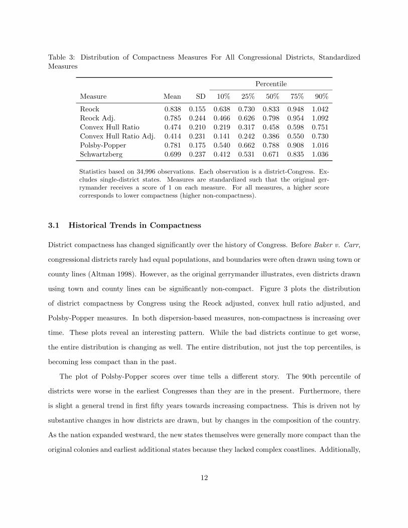
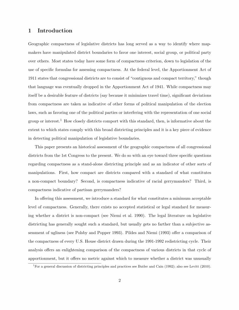
Table 3: Distribution of Compactness Measures For All Congressional Districts, StandardizedMeasures

Percentile

Measure Mean SD 10% 25% 50% 75% 90%

Reock 0.838 0.155 0.638 0.730 0.833 0.948 1.042Reock Adj. 0.785 0.244 0.466 0.626 0.798 0.954 1.092Convex Hull Ratio 0.474 0.210 0.219 0.317 0.458 0.598 0.751Convex Hull Ratio Adj. 0.414 0.231 0.141 0.242 0.386 0.550 0.730Polsby-Popper 0.781 0.175 0.540 0.662 0.788 0.908 1.016Schwartzberg 0.699 0.237 0.412 0.531 0.671 0.835 1.036

Statistics based on 34,996 observations. Each observation is a district-Congress. Ex-cludes single-district states. Measures are standardized such that the original ger-rymander receives a score of 1 on each measure. For all measures, a higher scorecorresponds to lower compactness (higher non-compactness).

3.1 Historical Trends in Compactness

District compactness has changed significantly over the history of Congress. Before Baker v. Carr,

congressional districts rarely had equal populations, and boundaries were often drawn using town or

county lines (Altman 1998). However, as the original gerrymander illustrates, even districts drawn

using town and county lines can be significantly non-compact. Figure 3 plots the distribution

of district compactness by Congress using the Reock adjusted, convex hull ratio adjusted, and

Polsby-Popper measures. In both dispersion-based measures, non-compactness is increasing over

time. These plots reveal an interesting pattern. While the bad districts continue to get worse,

the entire distribution is changing as well. The entire distribution, not just the top percentiles, is

becoming less compact than in the past.

The plot of Polsby-Popper scores over time tells a different story. The 90th percentile of

districts were worse in the earliest Congresses than they are in the present. Furthermore, there

is slight a general trend in first fifty years towards increasing compactness. This is driven not by

substantive changes in how districts are drawn, but by changes in the composition of the country.

As the nation expanded westward, the new states themselves were generally more compact than the

original colonies and earliest additional states because they lacked complex coastlines. Additionally,

12

as the number of districts increased, the effect of coastal districts in Massachusetts/Maine, Virginia,

Maryland, and elsewhere on average compactness diminished. Within the last fifty years, however, a

similar trend is evident on this measure as in the others — there is an increase in non-compactness

throughout most of the distribution. This shift, however, is largest among the bottom of the

distribution. This is likely due to the fact that the very worst districts — the aforementioned

coastal districts — remain relatively constant across the entire time period. However, as with the

other two measures, even the best districts are getting less compact.

While the trend generally persists across the entire time period, it is strongest in recent decades.

Table 4 reports averages for each standardized measure for three time periods: 1941–1970 (dis-

tricts drawn before Wesberry v. Sanders took effect), 1971–2000 (districts drawn before Shaw v.

Reno took effect), and 2001–2013 (district drawn after Shaw v. Reno). Across all measures, non-

compactness has increased, and the differences between these averages are highly significant for all

time periods and measures.

Table 4: Compactness by Era

Time Period Reock Convex Hull Polsby-Popper

1942–1971 0.773 0.386 0.763n = 6356 (0.003) (0.003) (0.002)

1972–2001 0.823 0.502 0.834n = 6430 (0.003) (0.003) (0.002)

2002–2013 0.887 0.593 0.859n = 2568 (0.005) (0.006) (0.002)

Mean and standard distribution of standardized Reock, convex hull ratio, andPolsby-Popper scores for congressional districts by time period. From each timeperiod to the next, the difference in means for each measure are significant atp < .01.

3.2 Using the Standard to Identify Gerrymandered Districts

In this section we use the standard of the original gerrymander to identify potentially gerryman-

dered districts. Rather than use the compactness measurements of the original gerrymander to

13

10

25

50

75 90

0

0.25

0.5

0.75

1

1.25

1791 1811 1831 1851 1871 1891 1911 1931 1951 1971 1991 2011

Non

−co

mpa

ctne

ss

Reock (Adjusted)

10

25

50

75

90

0

0.25

0.5

0.75

1

1.25

1791 1811 1831 1851 1871 1891 1911 1931 1951 1971 1991 2011

Non

−co

mpa

ctne

ss

Convex Hull Ratio (Adjusted)

10 25 50 75 90

0

0.25

0.5

0.75

1

1.25

1791 1811 1831 1851 1871 1891 1911 1931 1951 1971 1991 2011

Non

−co

mpa

ctne

ss

Polsby−Popper

Figure 3: Historical Trends in District Compactness

These graphs plot the distribution of each compactness measure by Congress.Each line shows how the specified percentile changes over time. Higher scorescorrespond to less compact districts. In the last 50 years, districts are signifi-cantly less compact than in the past.

14

standardize the measurements for all other districts, we use the original gerrymander’s compact-

ness scores as cutoff. Figure 4 plots the percentage of districts in each congress with worse scores

than the original gerrymander for Reock (adjusted), the convex hull ratio (adjusted), and Polsby-

Popper. All three measures generally correlate, with the exception of Polsby-Popper in the first fifty

year (see discussion in §3.1). In the last fifty years, we see a substantial increase in the percentage

of districts worse than the original gerrymander under all three measures.

Table 5 reports the number and percentage of all congressional districts that are worse than

the original gerrymander. Overall, 28% of all congressional districts are less compact than the

original gerrymander on at least one of our three measures, but only 1% are worse on all three

of the compactness measures used in this paper. This highlights the importance of using multiple

criteria to assess non-compactness: of the districts that are worse on one measure, only 11% are

worse on a second measure.

CH

PP

Reock

0

0.1

0.2

0.3

0.4

1791 1811 1831 1851 1871 1891 1911 1931 1951 1971 1991 2011

% L

ess

Com

pact

than

Sta

ndar

d

Figure 4: Districts Less Compact Than the Standard

Each line plots the percentage of districts in each congress that are worse thanthe original gerrymander (standardized score greater than 1) for the specifiedmeasure. CH =Convex hull ratio; PP=Polsby-Popper.

Table 6 divides the non-compactness results in Table 5 by measure. The second column gives

the number and percentage of districts that are worse than the original gerrymander on each of the

three measures. The set of columns on the right then show the percentage of these districts that

15

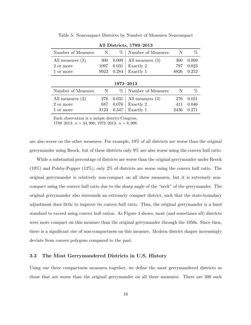
Table 5: Noncompact Districts by Number of Measures Noncompact

All Districts, 1789–2013

Number of Measures N % Number of Measures N %

All measures (3) 300 0.009 All measures (3) 300 0.0092 or more 1097 0.031 Exactly 2 797 0.0231 or more 9923 0.284 Exactly 1 8826 0.252

1973–2013

Number of Measures N % Number of Measures N %

All measures (3) 276 0.031 All measures (3) 276 0.0312 or more 687 0.076 Exactly 2 411 0.0461 or more 3123 0.347 Exactly 1 2436 0.271

Each observation is a unique district-Congress.1789–2013: n = 34, 996; 1973–2013: n = 8, 998.

are also worse on the other measures. For example, 19% of all districts are worse than the original

gerrymander using Reock, but of these districts only 9% are also worse using the convex hull ratio.

While a substantial percentage of districts are worse than the original gerrymander under Reock

(19%) and Polsby-Popper (12%), only 2% of districts are worse using the convex hull ratio. The

original gerrymander is relatively non-compact on all three measures, but it is extremely non-

compact using the convex hull ratio due to the sharp angle of the “neck” of the gerrymander. The

original gerrymander also surrounds an extremely compact district, such that the state-boundary

adjustment does little to improve its convex hull ratio. Thus, the original gerrymander is a hard

standard to exceed using convex hull ration. As Figure 4 shows, most (and sometimes all) districts

were more compact on this measure than the original gerrymander through the 1950s. Since then,

there is a significant rise of non-compactness on this measure. Modern district shapes increasingly

deviate from convex polygons compared to the past.

3.3 The Most Gerrymandered Districts in U.S. History

Using our three compactness measures together, we define the most gerrymandered districts as

those that are worse than the original gerrymander on all three measures. There are 300 such

16

Table 6: Percentage of Congressional Districts Worse than Original Gerrymander, by CompactnessMeasure

Worse than Within-groupMeasure Gerrymander Reock CH PP

Reock Adj. 0.191 — 0.087 0.122(6671) (581) (812)

Convex Hull Ratio Adj. 0.017 0.983 — 0.514(591) (581) (304)

Polsby-Popper 0.116 0.200 0.075 —(4058) (812) (304)

Worse on Any Measure 0.284 0.672 0.060 0.409(9923) (6671) (591) (4058)

The second column gives the percentages and numbers (below) of congressional districtsless compact than the original gerrymander by the measure listed in the first column.The three columns on the right gives the percentages and numbers (below) of districtsless compact than the original gerrymander by compactness measure within the groupthat are less compact by the measure in the first column. Each observation is a uniquedistrict-Congress, n = 34, 996.

district-Congresses, representing 109 unique districts. Figure 5 displays some of these districts.

The set of the most gerrymandered districts includes some well-known examples of gerrymandering,

such as the Illinois 4th “earmuffs” and the Maryland 3rd “pinwheel,” but also includes some less

recognized gerrymanders including the MA 9th district. Most of the 109 districts that are worse

than the original gerrymander on all three measures are recent; only 16 of the districts were drawn

before the 103rd Congress. New York (18), Florida (14), California (13), and Texas (12) appear on

the list the most times, and Florida has the highest percentage of district-Congresses on the list;

6% of all district-Congresses in Florida are less compact on all three measures than the original

gerrymander.

3.4 Compactness and Competition

The incidence of highly non-compact congressional districts has increased over the past 50 years.

That trend may be worrisome in and of itself, but it might also be indicative of deeper changes

in our politics. Geographic non-compactness of districts has long been thought to signal political

17

FL-3 (1993-1995) NY-12 (1993-1997) CA-23 (2003-2011)

FL-17 (1993-1995) LA-4 (1993) FL-22 (2003-2011)

IL-4 (1993-2001) GA-13 (2003-2005) MD-3 (2013)

TX-25 (1993-1995) IL-17 (2003-2011) MA-9 (1993-2001)

CA-12 (1983) AZ-2 (2005-2011) PA-12 (2005-2011)

Figure 5: Examples of Highly-Gerrymandered Districts

18

manipulation to favor one party over another, for example. Certainly that is the story of Elbridge

Gerry’s handiwork in 1811. In this section we present a first look at the connection between

non-compactness and partisanship using the measures developed here.

We examine the relationship between partisanship and non-compactness at the individual dis-

trict level. Using U. S. House election data from 1972 to 2008, we find that Democratic vote share

is highly correlated with district non-compactness. We focus on the post 1970 period to set aside

the problem of unequal population. Table 7 presents results from regressions of Democratic vote

share in congressional elections on our measures of compactness. There is a strong relationship

between the performance of Democratic candidates and the non-compactness of the district. The

more Democratic the district, the less compact the district.

There are many possible explanations for this regularity. The geographic distribution of par-

tisans is one possibility. Chen and Rodden (2013) argue that there is a natural tendency for

Democrats to have less compact districts because they are more heavily concentrated in urban

areas. This can produce a partisan bias at the state level in favor of Republicans. The creation of

majority-minority districts under the Voting Rights Act is another possibility (Pildes and Niemi

1993). The method of redistricting (state legislature, commission, or courts) may also play a role

in the creation of non-compact Democratic districts (Carson, Crespin, and Williamson 2014). Non-

compact districts may be the product of Democratic gerrymanders, where Democratic state legis-

latures have drawn convoluted lines to benefit themselves. In other cases, non-compact Democratic

districts may be drawn in Republican gerrymanders, where Democrats are packed into serpentine

districts to reduce their electoral influence in neighboring districts.

Explaining the origins of this relationship awaits further investigation. Whatever the causes of

the correlation between Democratic vote share and non-compactness of districts, the existence of

such a relationship reveals that non-compactness can be indicative of political concerns and electoral

outcomes. As a legal criterion, then, insistence on compactness may have important implications

for the political fairness of legislative districts, individually and whole plans.

19

Table 7: Regressions of Democratic Vote Share on Compactness

(1) (2) (3) (4) (5) (6)Reock Convex Poslby- Reock Convex Polsby-

Hull Popper Hull Popper

Dem. vote % 0.122*** 0.121*** 0.0624*** 0.195*** 0.209*** 0.108***(0.012) (0.010) (0.006) (0.0169) (0.015) (0.009)

Observations 7,981 7,981 7,981 6,912 6,912 6,912R-squared 0.252 0.243 0.343 0.267 0.259 0.361Uncontested Elections Yes Yes Yes No No NoState-Congress FE Yes Yes Yes Yes Yes Yes

This table displays OLS results from regressing Democratic vote share in congressional elec-tions on standardized measures of district compactness, using state-congress fixed effects. In-cludes U.S. House general election results for from 1972–2008. The first three models includeall elections; the last three exclude uncontested races. At-large elections are excluded.Standard errors in parentheses. *** p<0.01, ** p<0.05, * p<0.1

4 Conclusion

The geographic configuration of legislative districts is one of the most immediate tests of the

integrity of the districting process: we know a gerrymander when we see it. Even though people

commonly conjecture such a casual standard, it is evident that state legislators, courts, and others

involved in the districting process have struggled to establish clear guidelines for the geographic

compactness of districts. We have proposed one such standard, the configuration of the original

gerrymander. The everyday meaning of the term gerrymander and the manipulations that lie

behind it are embodied in the geographic features of the map itself. By measuring those features

and applying them to the history of all congressional districts, much can be learned about the

integrity of the districting process in the United States and how it has changed.

We do not intend this as a bright line standard that any court or legislature could adopt. Rather

it serves as a guide post, a marker that should raise concerns. There maybe other lower or higher

thresholds, perhaps derived from other districts that have been accepted in a legal setting or in

common parlance as examples of districting gone awry. Our purpose has been to lay down one such

20

marker – to our thinking the most obvious one – and to see where it leads.

Importantly, it appears that the geographic integrity of congressional districts has worsened in

the United States since the 1960s. This certainly fits the common perception and much popular

writing on the matter. But it is a social scientific question as to why that worsening has occurred.

Was it the one-person, one-vote rule? The Voting Rights Act? The increased involvement of the

courts? It is also an open question as to what the increasing non-compactness of congressional

districts indicates. Is this a sign that representation is getting worse because there is increased

manipulation of districts to favor one party over another? Has the creation of majority minority

districts contributed to non-compactness, and if so, in what respects has that improved or distorted

representation? These are important, unanswered questions, and certainly the next step in the quest

to understand how the structure of representation has changed in the United States over the course

of its history.

Whatever the answer to these questions, though, maintaining geographic compactness of dis-

tricts has long been embraced as a traditional districting principle. Over the arc of U.S. history

there was a steady state in the distribution of compactness and non-compactness, but that steady

state was disrupted in the 1960s. The political process today is engaged in a protracted struggle

to find a new balance among the various principles that guide districting, including geographic in-

tegrity. The patterns found here indicate a steady move away from geographic compactness as such

a principle. There may be a reassertion of this criterion, as has been seen in states like Florida and

in some recent federal court cases (such as Page v. Virginia Board of Elections), or the nation may

shift toward a different conception of representation in which compactness, although a standard,

is valued little. The historical trajectory certainly suggests that we are on the latter path. It is

up to the legislatures and the courts in the United States to determine whether geography will

remain a meaningful basis for representation, and if so what will be the criterion for representation

of geographic areas in the United States.

21

References

Altman, Micah. 1998. “Traditional districting principles: judicial myths vs. reality.” Social ScienceHistory 22 (2): 159–200.

Ansolabehere, Stephen, and James M Snyder. 2012. “The Effects of Redistricting on Incumbents.”Election Law Journal 11 (4): 409–502.

Ansolabehere, Stephen, and James M. Snyder Jr. 2008. The End of Inequality: One Person, OneVote and the Transformation of American Politics. New York, NY: W.W. Norton & Company.

Butler, David, and Bruce E Cain. 1992. Congressional Redistricting: Comparative and TheoreticalPerspectives. Prentice Hall.

Carson, Jamie L, Michael H Crespin, and Ryan Dane Williamson. 2014. “Re-evaluating the Effectsof Redistricting on Electoral Competition, 1972-2012.” State Politics & Policy Quarterly 14 (2):165–177.

Chen, Jowei, and Jonathan Rodden. 2013. “Unintentional gerrymandering: Political geography andelectoral bias in legislatures.” Quarterly Journal of Political Science 8 (3): 239–269.

Cox, Gary W, and Jonathan N Katz. 1999. “The reapportionment revolution and bias in UScongressional elections.” American Journal of Political Science 43 (3): 812–841.

Cox, Gary W, and Jonathan N Katz. 2002. Elbridge Gerry’s Salamander: the Electoral Conse-quences of the Reapportionment Revolution. Cambridge, UK: Cambridge Univ Press.

Edwards, Paul S, and Nelson W Polsby. 1991. “Introduction: The Judicial Regulation of PoliticalProcesses-In Praise of Multiple Criteria.” Yale L & Pol’y Rev.

Forgette, Richard, and Glenn Platt. 2005. “Redistricting principles and incumbency protection inthe U.S. Congress.” Political Geography 24 (November): 934–951.

Friedman, John N, and Richard T Holden. 2008. “Optimal gerrymandering: sometimes pack, butnever crack.” The American Economic Review 98 (1): 113–144.

Gilligan, Thomas W, and John G Matsusaka. 2006. “Public choice principles of redistricting.”Public Choice 129 (3-4): 381–398.

Griffith, Elmer Cummings. 1907. “The Rise and Development of the Gerrymander.”.

Levitt, Justin. 2010. A Citizen’s Guide To Redistricting. 2nd ed. Brennan Center for Justice.

Lewis, Jeffrey B., Brandon DeVine, Lincoln Pitcher, and Kenneth C. Martis. 2013. “Digital Bound-ary Definitions of United States Congressional Districts, 1789-2012. [Data file and code book].Retrieved from http://cdmaps.polisci.ucla.edu on July 21, 2014.”.

Lublin, David Ian. 1997. The Paradox of Representation: Racial Gerrymandering and MinorityInterests in Congress. Princeton, NJ: Princeton University Press.

22

Niemi, Richard G., Bernard Grofman, Carl Carlucci, and Thomas Hofeller. 1990. “Measuring com-pactness and the role of a compactness standard in a test for partisan and racial gerrymandering.”The Journal of Politics 52 (4): 1155-1181.

Owen, Guillermo, and Bernard Grofman. 1988. “Optimal partisan gerrymandering.” Political Ge-ography Quarterly 7 (1): 5–22.

Pildes, Richard H, and Richard G Niemi. 1993. “Expressive Harms, ”Bizarre Districts,” and VotingRights: Evaluating Election-District Appearances after Shaw v. Reno.” Michigan Law Review92: 483–587.

Polsby, Daniel D., and Robert D. Popper. 1991. “The Third Criterion: Compactness as a proceduralsafeguard against partisan gerrymandering.” Yale Law & Policy Review 9 (2): 301–353.

Polsby, Daniel D, and Robert D Popper. 1993. “Ugly: An Inquiry into the Problem of RacialGerrymandering under the Voting Rights Act.” Michigan Law Review 92 (3): 652–682.

Reock, Ernest C. 1961. “A note: Measuring compactness as a requirement of legislative apportion-ment.” Midwest Journal of Political Science 5 (1): 70–74.

Rush, Mark E. 2000. “Redistricting and partisan fluidity: do we really know a gerrymander whenwe see one?” Political Geography 19 (2): 249–260.

Schwartzberg, Joseph E. 1965. “Reapportionment, gerrymanders, and the notion of compactness.”Minn. L. Rev. 50: 443.

Young, H P. 1988. “Measuring the compactness of legislative districts.” Legislative Studies Quarterly13 (1): 105–115.

23