A Uniﬁed Approach for Fault Tolerance and Dynamic Power

IEEE TRANSACTIONS ON COMPUTER-AIDED DESIGN OF INTEGRATED CIRCUITS AND SYSTEMS, VOL. 25, NO. 1, JANUARY 2006 111

A Unified Approach for Fault Tolerance andDynamic Power Management in Fixed-Priority

Real-Time Embedded SystemsYing Zhang and Krishnendu Chakrabarty, Senior Member, IEEE

Abstract—This paper investigates an integrated approach forachieving fault tolerance and energy savings in real-time em-bedded systems. Fault tolerance is achieved via checkpointing,and energy is saved using dynamic voltage scaling (DVS). Theauthors present a feasibility analysis for checkpointing schemesfor a constant processor speed as well as for variable processorspeeds. DVS is then carried out on the basis of the feasibilityanalysis. The authors incorporate important practical issues suchas faults during checkpointing, rollback recovery time, memoryaccess time, and energy needed for checkpointing, as well asDVS and context switching overhead. Numerical results basedon real-life checkpointing data and processor data sheets showthat compared to fault-oblivious methods, the proposed approachsignificantly reduces power consumption and guarantees timelytask completion in the presence of faults.

Index Terms—Checkpointing, dynamic voltage scaling (DVS),fault tolerance, real-time scheduling.

I. INTRODUCTION

MANY embedded systems in use today rely on dynamicpower management (DPM) techniques, where the op-

erating system (OS) is responsible for managing system-levelpower consumption. There are two main types of DPM tech-niques. The first includes selective shut-off or slow down ofsystem components that are idle or underutilized [1]. The sec-ond, termed as dynamic voltage scaling (DVS), refers to thedynamic control of the supply voltage level for the various com-ponents in a system [2]. DVS has emerged as a popular solutionto the problem of reducing power consumption during systemoperation [3]–[5]. Many embedded processors such as the IntelXScale PXA260 [6], the Motorola 6805 [7], the TransmetaCrusoe [8], and the AMD K-6 [9] are now equipped with theability to dynamically scale the processor frequency by adjust-ing the operating voltage.

A large number of embedded systems are also designed forreal-time use [10], where a missed deadline can result in ca-

Manuscript received August 26, 2003; revised March 8, 2004. This work wassupported by the Defense Advance Research Projects Agency (DARPA) andadministered by the Army Research Office under Emergent Surveillance PlexusMURI Award DAAD19-01-1-0504. Parts of this paper were presented at theIEEE/ACM International Conference on Computer-Aided Design (ICCAD),San Jose, CA, 2003, and at the IEEE/ACM Design, Automation and Test inEurope (DATE) Conference, Paris, France, 2004. This paper was recommendedby Associate Editor R. Gupta.

Y. Zhang is with Guidant Corporation, St. Paul, MN 55112 USA.K. Chakrabarty is with Department of Electrical and Computer Engineering,

Duke University, Durham, NC 27708 USA (e-mail: [email protected]).Digital Object Identifier 10.1109/TCAD.2005.852657

tastrophic consequences. When DVS is employed to achieveenergy saving for real-time systems, a reduction in voltage re-sults in a corresponding drop in the processor speed, hencethe capability of the system to meet task deadlines might beundermined [11]. A number of techniques have been proposedrecently to balance real-time responsiveness with low-energytask execution [12]–[15].

Embedded systems are often deployed in harsh operationalenvironments. Many of these systems tend to be situated atremote and inaccessible locations; hence, repair and mainte-nance are often difficult and sometimes even impossible. Thisnecessitates the use of fault-tolerant techniques.

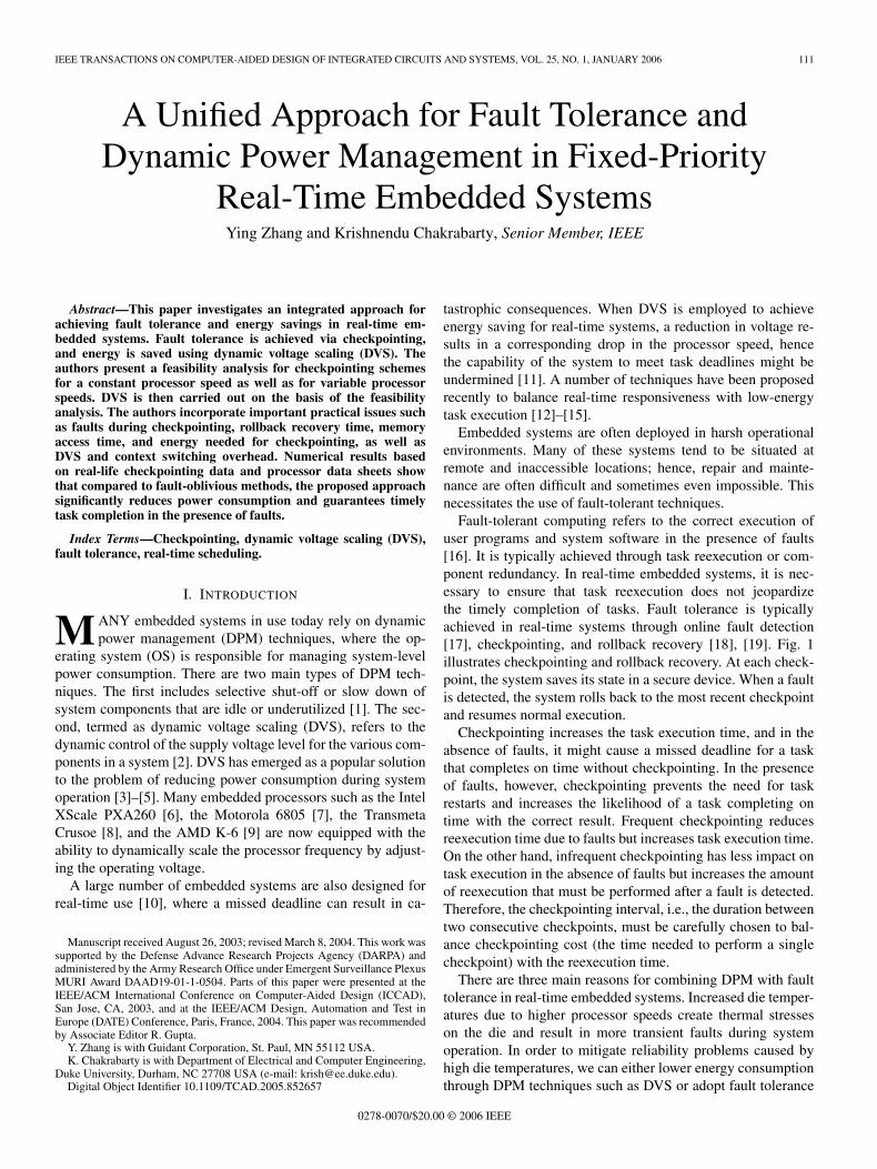
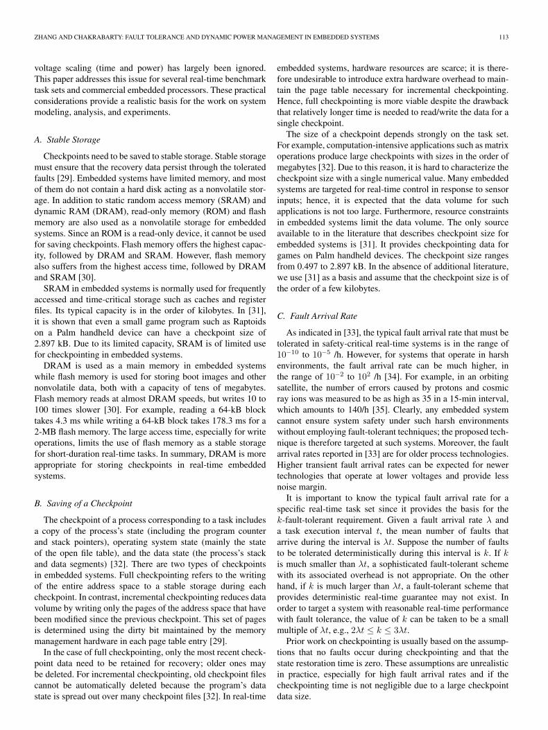
Fault-tolerant computing refers to the correct execution ofuser programs and system software in the presence of faults[16]. It is typically achieved through task reexecution or com-ponent redundancy. In real-time embedded systems, it is nec-essary to ensure that task reexecution does not jeopardizethe timely completion of tasks. Fault tolerance is typicallyachieved in real-time systems through online fault detection[17], checkpointing, and rollback recovery [18], [19]. Fig. 1illustrates checkpointing and rollback recovery. At each check-point, the system saves its state in a secure device. When a faultis detected, the system rolls back to the most recent checkpointand resumes normal execution.

Checkpointing increases the task execution time, and in theabsence of faults, it might cause a missed deadline for a taskthat completes on time without checkpointing. In the presenceof faults, however, checkpointing prevents the need for taskrestarts and increases the likelihood of a task completing ontime with the correct result. Frequent checkpointing reducesreexecution time due to faults but increases task execution time.On the other hand, infrequent checkpointing has less impact ontask execution in the absence of faults but increases the amountof reexecution that must be performed after a fault is detected.Therefore, the checkpointing interval, i.e., the duration betweentwo consecutive checkpoints, must be carefully chosen to bal-ance checkpointing cost (the time needed to perform a singlecheckpoint) with the reexecution time.

There are three main reasons for combining DPM with faulttolerance in real-time embedded systems. Increased die temper-atures due to higher processor speeds create thermal stresseson the die and result in more transient faults during systemoperation. In order to mitigate reliability problems caused byhigh die temperatures, we can either lower energy consumptionthrough DPM techniques such as DVS or adopt fault tolerance

0278-0070/$20.00 © 2006 IEEE

112 IEEE TRANSACTIONS ON COMPUTER-AIDED DESIGN OF INTEGRATED CIRCUITS AND SYSTEMS, VOL. 25, NO. 1, JANUARY 2006

Fig. 1. Illustration of checkpointing and rollback recovery.

techniques such as checkpointing. Better still, a combination ofDVS and checkpointing can be used to reduce energy consump-tion and improve the run time reliability of the system.

The second reason for combining DVS with adaptive check-pointing is motivated by the need to meet task deadlines inreal-time systems. Checkpointing provides an effective methodto reduce reexecution time in the presence of faults. DVS canalso be used to enhance fault tolerance in a real-time system.If faults occur frequently, the processor speed can be scaled updynamically (within limits imposed by higher die temperatures)and more slack can be provided to the task, which allowsmore time for rollback recovery. Hence, a combination ofcheckpointing and DVS can be used to increase the likelihoodof timely task completion in the presence of faults and trade offenergy with fault tolerance.

The third motivation arises from shrinking process technolo-gies in the nanotechnology realm. Lower processor voltagesare likely to lead to lower noise margins and more transientfaults caused in part by single-event upsets [26]. Hence, a DPMframework, in which DVS techniques are tied to system-levelfault tolerance, are of particular interest for embedded systems.

DPM and fault tolerance for embedded real-time systemshave largely been studied as separate problems in the literature.DVS techniques for power management do not consider faulttolerance [3]–[5], [12]–[15], and checkpoint placement strate-gies for fault tolerance do not address DPM [20]–[22]. It isonly recently that an attempt has been made to combine faulttolerance with DPM [23], [24].

In [23], adaptive checkpointing is combined with DVS forsoft real-time systems. In [24], the analysis is based on theearliest-deadline-first (EDF) scheduling strategy; however, anumber of simplifying assumptions are made, e.g., a task issubject to at most one fault occurrence before its deadline andalways resumes execution after rollback with the maximumprocessor speed. In addition, it is assumed in [24] that theprocessor is capable of adjusting its speed continuously in therange [Smin, Smax], the checkpointing cost is dependent onprocessor speed, and the state restoration cost is zero. Finally,faults during checkpointing and state restoration are not con-sidered in [24], task priorities are assumed to be dynamic, andsimulation results are presented only for simple task sets andhypothetical processor models.

In contrast to [24], this paper focuses on fixed-priority real-time systems and relaxes the restriction that no faults occurduring checkpointing and state restoration. Although the EDFpolicy is used in some real-time systems, fixed-priority assign-ments are adopted in many real-time scheduling algorithms of

practical interest due to their low overhead and predictability[25]. The number of fault occurrences in this paper is not lim-ited to one, and voltage scaling and state restoration costs are in-corporated in the analysis. Simulation results are presented forbenchmark task sets and commercial embedded processors witha discrete set of voltage/speed settings. Typical parameters usedin the simulation experiments are based on realistic scenarios.

The integrated approach presented here provides fault toler-ance and DPM in hard real-time embedded systems. Feasibilitytests for fixed-priority real-time systems with checkpointingunder constant processor speed are presented first. We considerjob-oriented feasibility tests, in which the goal is to tolerate kfault occurrences for each job, where an appropriate value ofk is determined based on the task execution time and typicalfault arrival rates. Hyperperiod-oriented feasibility tests arethen presented, in which the goal is to tolerate up to k fault oc-currences in a hyperperiod. The value of k in this case dependson the length of the hyperperiod and typical fault arrival rates.Following this, we extend these feasibility tests to variable-speed processors. The above feasibility analyses provide thecriteria under which checkpointing can provide fault toleranceand real-time guarantees. Based on the feasibility analyses re-sults, an on-line dynamic speed-scaling scheme is developed toreduce energy during task execution by exploiting the availableslack. The proposed approach is compared with a recent fault-oblivious DVS scheme, referred to as voltage scaling for lowpower (VSLP) [5], in the presence of fault occurrences.

It was assumed throughout that faults are intermittent ortransient in nature and that permanent faults are handledthrough manufacturing testing or field testing techniques [27].Typical examples of transient faults include errors caused bycosmic rays and high-energy particles in nanotechnology withshrinking processes [26]. We assume that these faults affectthe processor either during normal operation or during memorywrites for checkpointing. In the latter case, the fault makes thecheckpoint invalid.

The rest of the paper is organized as follows. Section IIdiscusses practical issues related to checkpointing and DVS inreal-time embedded systems. These include the size of check-points, the type of stable storage for the checkpoints, memoryaccess time and power models, and the time and power neededfor voltage scaling. Section III provides off-line feasibilityanalysis for checkpointing under constant processor speed inreal-time systems. Section IV extends these results to a systemwith a variable-speed processor. Experimental results based onrepresentative parameter values from Section II are presentedin Section V, and Section VI presents conclusions.

II. PRACTICAL ISSUES IN CHECKPOINTING AND DVS

This section reviews some practical issues for checkpointingand DVS in real-time embedded systems. The goal here is notto present a comprehensive survey of checkpointing and DVS,for which the reader is referred to [1], [11], and [28]. Rather,the objective here is to identify practical issues and parametervalues that must be considered for analysis and for meaningfulsimulation experiments. While prior work on DVS has some-times been based on realistic processor models, the cost of

ZHANG AND CHAKRABARTY: FAULT TOLERANCE AND DYNAMIC POWER MANAGEMENT IN EMBEDDED SYSTEMS 113

voltage scaling (time and power) has largely been ignored.This paper addresses this issue for several real-time benchmarktask sets and commercial embedded processors. These practicalconsiderations provide a realistic basis for the work on systemmodeling, analysis, and experiments.

A. Stable Storage

Checkpoints need to be saved to stable storage. Stable storagemust ensure that the recovery data persist through the toleratedfaults [29]. Embedded systems have limited memory, and mostof them do not contain a hard disk acting as a nonvolatile stor-age. In addition to static random access memory (SRAM) anddynamic RAM (DRAM), read-only memory (ROM) and flashmemory are also used as a nonvolatile storage for embeddedsystems. Since an ROM is a read-only device, it cannot be usedfor saving checkpoints. Flash memory offers the highest capac-ity, followed by DRAM and SRAM. However, flash memoryalso suffers from the highest access time, followed by DRAMand SRAM [30].

SRAM in embedded systems is normally used for frequentlyaccessed and time-critical storage such as caches and registerfiles. Its typical capacity is in the order of kilobytes. In [31],it is shown that even a small game program such as Raptoidson a Palm handheld device can have a checkpoint size of2.897 kB. Due to its limited capacity, SRAM is of limited usefor checkpointing in embedded systems.

DRAM is used as a main memory in embedded systemswhile flash memory is used for storing boot images and othernonvolatile data, both with a capacity of tens of megabytes.Flash memory reads at almost DRAM speeds, but writes 10 to100 times slower [30]. For example, reading a 64-kB blocktakes 4.3 ms while writing a 64-kB block takes 178.3 ms for a2-MB flash memory. The large access time, especially for writeoperations, limits the use of flash memory as a stable storagefor short-duration real-time tasks. In summary, DRAM is moreappropriate for storing checkpoints in real-time embeddedsystems.

B. Saving of a Checkpoint

The checkpoint of a process corresponding to a task includesa copy of the process’s state (including the program counterand stack pointers), operating system state (mainly the stateof the open file table), and the data state (the process’s stackand data segments) [32]. There are two types of checkpointsin embedded systems. Full checkpointing refers to the writingof the entire address space to a stable storage during eachcheckpoint. In contrast, incremental checkpointing reduces datavolume by writing only the pages of the address space that havebeen modified since the previous checkpoint. This set of pagesis determined using the dirty bit maintained by the memorymanagement hardware in each page table entry [29].

In the case of full checkpointing, only the most recent check-point data need to be retained for recovery; older ones maybe deleted. For incremental checkpointing, old checkpoint filescannot be automatically deleted because the program’s datastate is spread out over many checkpoint files [32]. In real-time

embedded systems, hardware resources are scarce; it is there-fore undesirable to introduce extra hardware overhead to main-tain the page table necessary for incremental checkpointing.Hence, full checkpointing is more viable despite the drawbackthat relatively longer time is needed to read/write the data for asingle checkpoint.

The size of a checkpoint depends strongly on the task set.For example, computation-intensive applications such as matrixoperations produce large checkpoints with sizes in the order ofmegabytes [32]. Due to this reason, it is hard to characterize thecheckpoint size with a single numerical value. Many embeddedsystems are targeted for real-time control in response to sensorinputs; hence, it is expected that the data volume for suchapplications is not too large. Furthermore, resource constraintsin embedded systems limit the data volume. The only sourceavailable to in the literature that describes checkpoint size forembedded systems is [31]. It provides checkpointing data forgames on Palm handheld devices. The checkpoint size rangesfrom 0.497 to 2.897 kB. In the absence of additional literature,we use [31] as a basis and assume that the checkpoint size is ofthe order of a few kilobytes.

C. Fault Arrival Rate

As indicated in [33], the typical fault arrival rate that must betolerated in safety-critical real-time systems is in the range of10−10 to 10−5 /h. However, for systems that operate in harshenvironments, the fault arrival rate can be much higher, inthe range of 10−2 to 102 /h [34]. For example, in an orbitingsatellite, the number of errors caused by protons and cosmicray ions was measured to be as high as 35 in a 15-min interval,which amounts to 140/h [35]. Clearly, any embedded systemcannot ensure system safety under such harsh environmentswithout employing fault-tolerant techniques; the proposed tech-nique is therefore targeted at such systems. Moreover, the faultarrival rates reported in [33] are for older process technologies.Higher transient fault arrival rates can be expected for newertechnologies that operate at lower voltages and provide lessnoise margin.

It is important to know the typical fault arrival rate for aspecific real-time task set since it provides the basis for thek-fault-tolerant requirement. Given a fault arrival rate λ anda task execution interval t, the mean number of faults thatarrive during the interval is λt. Suppose the number of faultsto be tolerated deterministically during this interval is k. If kis much smaller than λt, a sophisticated fault-tolerant schemewith its associated overhead is not appropriate. On the otherhand, if k is much larger than λt, a fault-tolerant scheme thatprovides deterministic real-time guarantee may not exist. Inorder to target a system with reasonable real-time performancewith fault tolerance, the value of k can be taken to be a smallmultiple of λt, e.g., 2λt ≤ k ≤ 3λt.

Prior work on checkpointing is usually based on the assump-tions that no faults occur during checkpointing and that thestate restoration time is zero. These assumptions are unrealisticin practice, especially for high fault arrival rates and if thecheckpointing time is not negligible due to a large checkpointdata size.


D. Cost of Voltage Scaling

The voltage scaling cost for DVS in real-time embeddedsystems has attracted relatively little attention in prior workon task scheduling and DPM. It is now recognized, however,that these costs cannot be ignored for real-time and power-constrained embedded systems [12].

Four typical real-time task sets are described in [12]: a ge-neric avionics platform (GAP), an inertial navigation system(INS), a computerized numerical control (CNC), and a flightcontrol system. The execution times for the tasks range from35 to 720 µs for CNC, 1 to 9 ms for GAP, 1.18 to 100.28 msfor INS, and 10 to 60 ms for flight control. In [36], sometask sets for real-time multimedia applications are presented.The typical execution times for those tasks range from 1.4 to50.4 ms. We therefore see that the execution times of tasksin real-time applications range from microseconds to millisec-onds. As discussed next, the execution times of these tasks mustbe viewed in the context of typical voltage scaling overheads.

The voltage scaling costs for embedded processors havebeen documented in a number of recent papers. The worstcase voltage transition time for the ARM8 microprocessor coreranges from 10 [37] to 520 µs [38]. The time taken by a Powerpersonal computer (PC)-embedded processor to switch between0.9 and 1.95 V is 105 µs [39]. The StrongArm 1100 processortakes 250 µs to switch from a 1.5-V supply voltage to a 1.23-Vsupply voltage [40].

We note that the voltage scaling time is in the order ofhundreds of microseconds for typical embedded processors.Hence, for short-duration real-time tasks such as CNC, wherethe execution time is also in the order of tens of microseconds,it might be counterproductive to employ DVS. The relativeDVS time penalty is so high for CNC that the energy savingsdue to DVS are counterbalanced by the adverse impact onreal-time responsiveness due to voltage scaling times. Mostpapers in the DVS literature that use CNC as a benchmarkdo not consider this issue. Even for longer-duration real-timetasks (with an execution time greater than 1 ms), the consid-eration of DVS overheads leads to more accurate conclusions.In this paper, we incorporate the times and energy overheadsdue to voltage scaling in the general theoretical framework.We also include these considerations in the simulations basedon real-time benchmark task sets and commercial embeddedprocessors.

III. FEASIBILITY ANALYSIS UNDER CONSTANT SPEED

We are given a set Γ = τ1, τ2, . . . , τn of n periodicreal-time tasks, where task τi is modeled by a tuple τi =(Ti,Di, Ei). The elements of the tuple are defined as follows:Ti is the period of τi and Di is its deadline (Di ≤ Ti), andEi is the execution time of τi under fault-free conditions. Letthe time required to store a checkpoint be Cs and the timerequired to retrieve a checkpoint be Cr. We make the followingassumptions related to task execution and fault arrivals: 1) thetask set Γ is scheduled using fixed-priority methods such asthe rate-monotonic scheme or the deadline-monotonic scheme[25]; 2) the task set Γ is schedulable under fault-free conditions;

3) the priority of tasks is in decreasing order of the index i,i.e., task τi has higher priority than task τj if i < j; 4) eachinstance of the task is released at the beginning of the period;5) the checkpointing intervals for the same task are equal; and6) faults are detected as soon as they occur.

In [41], a feasibility analysis is provided under the as-sumption that two successive faults arrive with a minimuminterarrival time TF . This implies that the time between theoccurrences of two faults is at least TF . This assumption is notpractical for realistic applications, where the fault occurrencecan be bursty or memoryless. For example, it is difficult toobtain a minimum interarrival time for a typical Poisson arrivalprocess. Therefore, we focus here on tolerating up to a givennumber of faults during task execution. No additional assump-tion is made regarding fault arrivals.

Since the task set is periodic, the total execution time isinfinite if we consider an unlimited number of periods. Wetherefore need to identify an appropriate k-fault-tolerant condi-tion for a shorter time duration. Here, we provide two solutionscorresponding to two different fault-tolerance requirements.One is to tolerate k faults for each job, termed as job-orientedfault tolerance; the other is to tolerate k faults within a hyper-period (defined as the least common multiple of all the taskperiods [25]), termed as hyperperiod-oriented fault tolerance. Inpractical situations, the choice of an appropriate fault tolerancecriterion can be made based on the needs of the real-timeapplication and a realistic fault arrival rate.

The rest of this section is organized as follows. Section III-Aconsiders k fault tolerance for a single job. Section III-Breviews feasibility analysis based on time-demand analysis fora task set under fault-free conditions [25]. This analysis isextended in Section III-C to incorporate fault arrivals underthe job-oriented fault model. Finally, Section III-D analyzes ahyperperiod-oriented fault tolerance for a task set.

A. Feasibility Analysis for a Single Job

We first consider the case of a single job. Suppose the check-pointing interval is ∆ = E/(m+ 1), where m is the numberof checkpoints inserted equidistantly during the computationtime to tolerate k faults in one job. The objective here is to findthe optimal checkpointing interval to minimize the worst caseresponse time in case of faults.

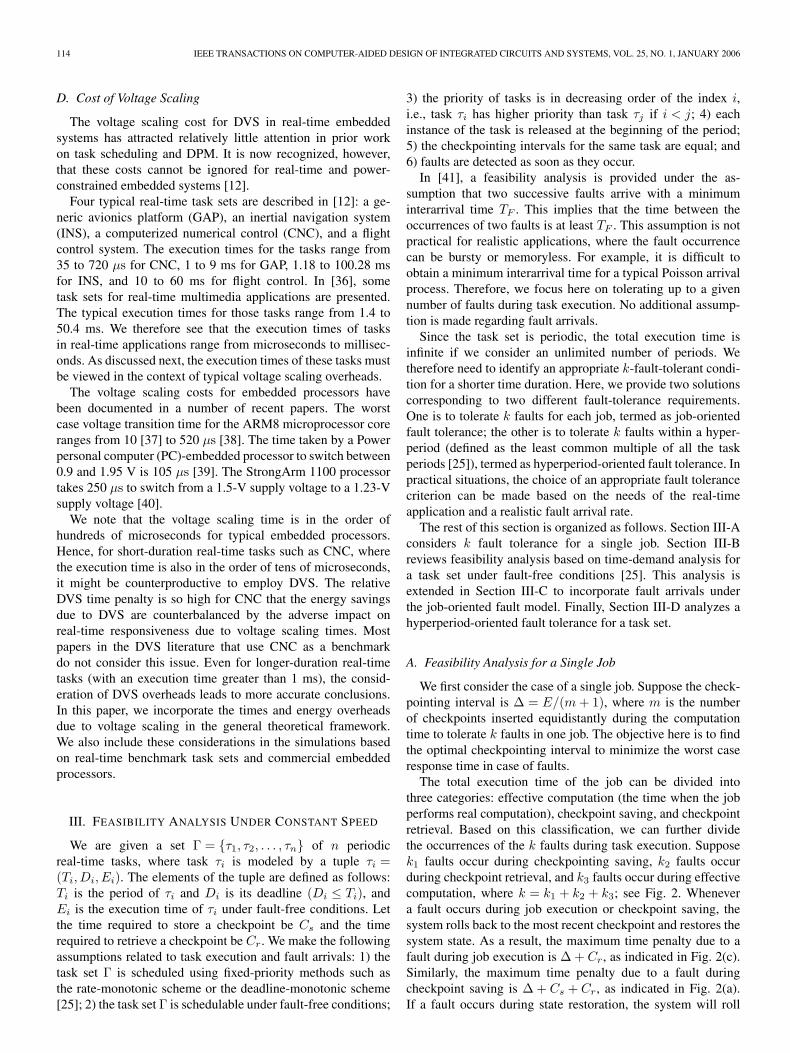
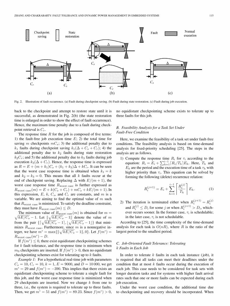
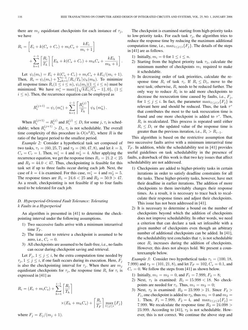
The total execution time of the job can be divided intothree categories: effective computation (the time when the jobperforms real computation), checkpoint saving, and checkpointretrieval. Based on this classification, we can further dividethe occurrences of the k faults during task execution. Supposek1 faults occur during checkpointing saving, k2 faults occurduring checkpoint retrieval, and k3 faults occur during effectivecomputation, where k = k1 + k2 + k3; see Fig. 2. Whenevera fault occurs during job execution or checkpoint saving, thesystem rolls back to the most recent checkpoint and restores thesystem state. As a result, the maximum time penalty due to afault during job execution is ∆+ Cr, as indicated in Fig. 2(c).Similarly, the maximum time penalty due to a fault duringcheckpoint saving is ∆+ Cs + Cr, as indicated in Fig. 2(a).If a fault occurs during state restoration, the system will roll


Fig. 2. Illustration of fault occurrence. (a) Fault during checkpoint saving. (b) Fault during state restoration. (c) Fault during job execution.

back to the checkpoint and attempt to restore state until it issuccessful, as demonstrated in Fig. 2(b) (the state restorationtime is enlarged in order to show the effect of fault occurrence).Hence, the maximum time penalty due to a fault during check-point retrieval is Cr.

The response time R for the job is composed of five terms:1) the fault-free job execution time E; 2) the total time forsaving m checkpoints mCs; 3) the additional penalty due tok1 faults during checkpoint saving k1(∆ + Cs + Cr); 4) theadditional penalty due to k2 faults during state restorationk2Cr; and 5) the additional penalty due to k3 faults during jobexecution k3(∆ + Cr). Hence, the response time is expressedas R = E + (m+ k1)Cs + (k1 + k3)∆ + kCr. It can be seenthat the worst case response time is obtained when k1 = kand k2 = k3 = 0. This means that all k faults occur at theend of checkpoint saving. Replacing ∆ with E/(m+ 1), theworst case response time Rworst case is further expressed asRworst case(m) = E + k(Cs + Cr) +mCs + kE/(m+ 1). Inthis expression, E, k, Cs, and Cr are constants, and m is avariable. We are aiming to find the optimal value of m suchthat Rworst case is minimized. To satisfy the deadline constraint,they must have Rworst case(m) ≤ D.

The minimum value of Rworst case(m) is obtained for m =√kE/Cs − 1. Let ‖√kE/Cs − 1‖ denote the value of m

from the pair √kE/Cs − 1, √

kE/Cs − 1 that mini-mizes Rworst case. Furthermore, since m is a nonnegative in-teger, we have m∗ = max‖√kE/Cs − 1‖, 0. Let f(m∗) =Rworst case(m∗)−D.

If f(m∗) ≤ 0, there exist equidistant checkpointing schemesfor k fault tolerance, and the response time is minimum whenm0 checkpoints are inserted. If f(m∗) > 0, then no equidistantcheckpointing schemes exist for tolerating up to k faults.Example 1: For a hypothetical real-time job with parameters

Cs = 10, Cr = 10, k = 1, E = 9000, and D = 10 000, we getm∗ = 29 and f(m∗) = −390. This implies that there exists anequidistant checkpointing scheme to tolerate a single fault forthis job, and the worst case response time is minimized when29 checkpoints are inserted. Now we change k from one tothree, i.e., the system is required to tolerate up to three faults.Then, we get m∗ = 51 and f(m∗) = 89.23. Since f(m∗) > 0,

no equidistant checkpointing scheme exists to tolerate up tothree faults for this job.

B. Feasibility Analysis for a Task Set UnderFault-Free Condition

Here, we examine the feasibility of a task set under fault-freeconditions. The feasibility analysis is based on time-demandanalysis for fixed-priority scheduling [25]. The steps in theanalysis are as follows.

1) Compute the response time Ri for τi according to theequation: Ri = Ei +

∑i−1h=1Ri/ThEh. Here, Th and

Eh are the period and the execution time of a task τh withhigher priority than τi. This equation can be solved byforming the following (delete) recurrence relation:

R(j+1)i = Ei +

i−1∑h=1

⌈R

(j)i

Th

⌉Eh. (1)

2) The iteration is terminated either when R(j+1)i = R

(j)i

and R(j)i ≤ Di for some j or when R

(j+1)i > Di, which-

ever occurs sooner. In the former case, τi is schedulable;in the later case, τi is not schedulable.

According to [25], the time complexity of the time-demandanalysis for each task is O(nR), where R is the ratio of thelargest period to the smallest period.

C. Job-Oriented Fault Tolerance: Toleratingk Faults in Each Job

In order to tolerate k faults in each task instance ( job), itis required that all tasks can meet their deadlines under thecondition that at most k faults occur during the execution ofeach job. This case needs to be considered for task sets withlonger duration tasks and for systems with higher fault arrivalrates such that one or more faults can be expected during eachjob execution.

Under the worst case condition, the additional time dueto checkpointing and recovery should be incorporated. When


there are mj equidistant checkpoints for each instance of τj ,we have

Ri =[Ei + k(Cs + Cr) +miCs +

kEi

mi + 1

]

+i−1∑h=1

⌈Ri

Th

⌉ [Eh + k(Cs + Cr) +mhCs +

kEh

mh + 1

].

Let ψi(mi) = Ei + k(Cs + Cr) +miCs + kEi/(mi + 1).Then, Ri = ψi(mi) +

∑i−1h=1Ri/Thψh(mh). To minimize

all response times Ri(1 ≤ i ≤ n), ψi(mi)(1 ≤ i ≤ n) must beminimized. We have m∗

i = max‖√

kEi/Cs − 1‖, 0, (1 ≤i ≤ n). Then, the recurrence equation can be employed as

R(j+1)i = ψi (m∗

i ) +i−1∑h=1

⌈R

(j)i

Th

⌉ψh (m∗

h) .

When R(j+1)i = R

(j)i and R

(j)i ≤ Di for some j, τi is sched-

ulable; when R(j+1)i > Di, τi is not schedulable. The overall

time complexity of this procedure is O(n2R), where R is theratio of the largest period to the smallest period.Example 2: Consider a hypothetical task set composed of

two tasks, τ1 = (60, 25, 7) and τ2 = (80, 47, 8), and let k = 3,Cs = Cr = 1. Then, m∗

1 = 4 and m∗2 = 4. After applying the

recurrence equation, we get the response times R1 = 21.2 < 25and R2 = 44.0 < 47. Thus, checkpointing is feasible for thistask set if up to three faults occur during each job. Next, thecase of k = 4 is examined. For this case, m∗

1 = 4 and m∗2 = 5.

The response times are R1 = 24.6 < 25 and R2 = 50.9 > 47.As a result, checkpointing is not feasible if up to four faultsneed to be tolerated for each job.

D. Hyperperiod-Oriented Fault Tolerance: Toleratingk Faults in a Hyperperiod

An algorithm is presented in [41] to determine the check-pointing interval under the following assumptions.

1) Two successive faults arrive with a minimum interarrivaltime TF .

2) The time cost to retrieve a checkpoint is assumed to bezero, i.e., Cr = 0.

3) All checkpoints are assumed to be fault-free, i.e., no faultscan occur during checkpoint saving and retrieval.

Let Fj , 1 ≤ j ≤ i, be the extra computation time needed byτj , 1 ≤ j ≤ i, if one fault occurs during its execution. Here, Fj

is also the checkpointing interval for τj . When there are mj

equidistant checkpoints for τj , the response time Ri for τi isexpressed in [41] as

Ri = (Ei +miCs) +i−1∑h=1

⌈Ri

Th

⌉

×(Eh +mhCs) +⌈Ri

TF

⌉max1≤j≤i

Fj

where Fj = Ej/(mj + 1).

The checkpoint is examined starting from high-priority tasksto low-priority tasks. For each task τj , the algorithm tries toreduce the response time by reducing the maximum additionalcomputation time, i.e., max1≤j≤iFj. The details of the stepsin [41] are as follows.

1) Initially, mi = 0 for 1 ≤ i ≤ n.2) Starting from the highest priority task τ1, calculate the

minimum number of checkpoints m1 required to makeit schedulable.

3) In decreasing order of task priorities, calculate the re-sponse time Ri of task τi. If Ri ≤ Di, move to thenext task; otherwise, Ri needs to be reduced further. Theonly way to reduce Ri is to add more checkpoints todecrease the reexecution time caused by faults, i.e., Fj ,for 1 ≤ j ≤ i. In fact, the parameter max1≤j≤iFj isrelevant here and should be reduced. Thus, the task τ ∗

that contributes the most to the task reexecution time isfound and one more checkpoint is added to τ ∗. Then,Ri is recalculated. This process is repeated until eitherRi ≤ Di or the updated value of the response time isgreater than the previous iteration, i.e., Ri > Ri−1.

This algorithm is based on the restrictive assumption thattwo successive faults arrive with a minimum interarrival timeTF . In addition, while the schedulability test in [41] providesuseful guidelines on task schedulability in the presence offaults, a drawback of this work is that two key issues that affectschedulability are not addressed.

1) Checkpoints are added to higher-priority tasks in certainiterations in order to satisfy deadline constraints for allthe tasks. These higher-priority tasks, however, have mettheir deadline in earlier iterations. The addition of morecheckpoints to them inevitably changes their responsetimes. As a result, it is necessary to trace back to recal-culate their response times and adjust their checkpoints.This issue has not been addressed in [41].

2) It is necessary to determine a bound on the number ofcheckpoints beyond which the addition of checkpointsdoes not improve schedulability. In other words, we needa criterion that can declare a task set infeasible with agiven number of checkpoints even though an arbitrarynumber of additional checkpoints can be added. In [41],the schedulability test concludes that τi is not schedulableonce Ri increases during the addition of checkpoints.However, this does not always hold. We present a coun-terexample below.

Example 3: Consider two hypothetical tasks τ1 = (100, 18,7.999) and τ2 = (101, 21, 8), and let TF = 102, Cs = 0.1, andCr = 0. We follow the steps from [41] as shown below.

1) Initially, m1 = m2 = 0, and F1 = 7.999, F2 = 8;2) Next, τ1 is examined: R1 = 15.998 < 18. No check-

points are needed for τ1. Thus, m1 = m2 = 0;3) Next, τ2 is examined: R2 = 23.999 > 21. Since F2 >

F1, one checkpoint is added to τ2, thus m1 = 0 and m2 =1. Then, F1 = 7.999, F2 = 4, and max1≤j≤2Fj =7.999. We recalculate the response time R2 = 24.098 >23.999. According to [41], τ2 is not schedulable. How-ever, this is not correct. We continue the above step and


find F1 > F2, then one more checkpoint is added to τ1;as a result, m1 = 1 and m2 = 1. Then, F1 = 7.999/(1 +1) = 3.9995, F2 = 4, andmax1≤j≤2Fj = 4. We recal-culate the response time of τ1 and τ2 : R1 = 12.0985 <18 and R2 = 20.199 < 21, which implies that both tasksare schedulable.

It is required here that the tasks meet their deadlines underthe condition that at most k faults occur during a hyperperiod.Furthermore, as indicated in Section II, in order to make themodel more practical for real-time embedded systems, the tworestrictive assumptions of zero state-restoration time and fault-free checkpointing are removed. Based on the schedulabilitytest in [41], we incorporate the state-restoration time, takeinto account faults during checkpointing, and solve the twoaforementioned problems as follows.

The response time Ri for τi is expressed as

Ri = (Ei +miCs) +i−1∑h=1

⌈Ri

Th

⌉(Eh +mhCs)

+ k(Cs + Cr) + k max1≤j≤i

Fj

where Fj = Ej/(mj + 1).The problem of recalculating response times due to the

addition of checkpoints to higher-priority tasks can be solvedusing a recursive method. Any time the number of checkpointsfor a task is increased, all the lower-priority tasks need to bereexamined. The second problem is more complicated since theresponse time Ri for task τi does not decrease monotonicallywhen more checkpoints are added to higher-priority tasks. Sup-pose that inmax1≤h≤iFh we find that task τh1 contributes themost to the response time Ri and add one more checkpoint toτh1. After recalculating Ri, we might find that Ri has increased.In this situation, it cannot be simply claimed that the task is notschedulable, as has been shown in Example 3.

We solve the second problem by determining a bound onthe number of checkpoints such that if the task set cannot bemade schedulable using this number of checkpoints it cannot bescheduled by adding more checkpoints. Both the checkpointingcost and the timing constraints must be taken into account.1) Bound Based on Checkpointing Tradeoffs: The effect of

adding more checkpoints is twofold. First, it increases theexecution time due to the checkpoint saving cost, which runscontrary to the goal of reducing the response time. On the otherhand, it decreases reexecution due to a fault, which helps inreducing the response time. Suppose the task execution timeis E and m checkpoints have already been added. If anothercheckpoint is now added, the reduction of reexecution timeunder the k-fault-tolerance requirement is simply

kE

(m+ 1)− kE

(m+ 2)=

kE

[(m+ 1)(m+ 2)].

We combine the two impacts of checkpointing on the reexe-cution time to define the tradeoff function tr(m) as tr(m) =Cs − kE/[(m+ 1)(m+ 2)]. If tr(m) < 0, then adding onemore checkpoint can potentially reduce the response time;

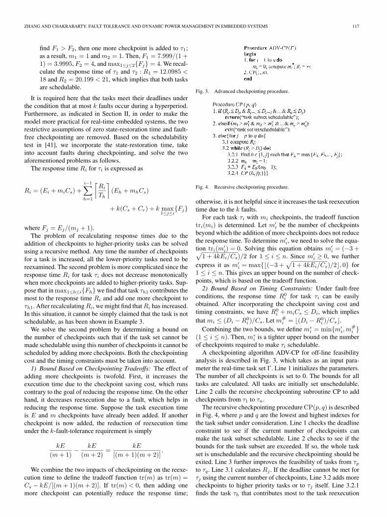
Fig. 3. Advanced checkpointing procedure.

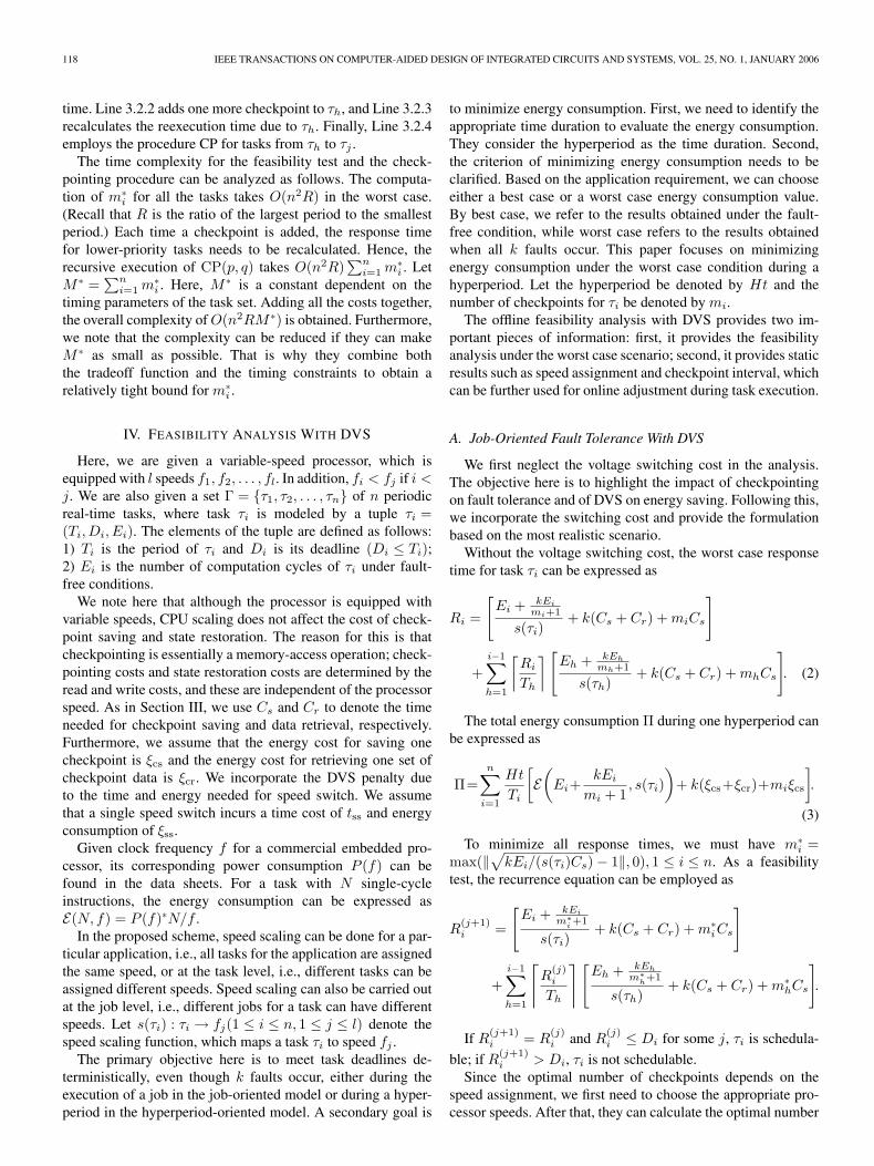
Fig. 4. Recursive checkpointing procedure.

otherwise, it is not helpful since it increases the task reexecutiontime due to the k faults.

For each task τi with mi checkpoints, the tradeoff functiontri(mi) is determined. Let m′

i be the number of checkpointsbeyond which the addition of more checkpoints does not reducethe response time. To determine m′

i, we need to solve the equa-tion tri(m′

i) = 0. Solving this equation obtains m′i = (−3 +√

1 + 4kEi/Cs)/2 for 1 ≤ i ≤ n. Since m′i ≥ 0, we further

express it as m′i = max(−3 +

√1 + 4kEi/Cs)/2, 0 for

1 ≤ i ≤ n. This gives an upper bound on the number of check-points, which is based on the tradeoff function.2) Bound Based on Timing Constraints: Under fault-free

conditions, the response time R0i for task τi can be easily

obtained. After incorporating the checkpoint saving cost andtiming constraints, we have R0

i +miCs ≤ Di, which impliesthat mi ≤ (Di −R0

i )/Cs. Let m#i = (Di −R0

i )/Cs.Combining the two bounds, we define m∗

i = minm′i,m

#i

(1 ≤ i ≤ n). Then, m∗i is a tighter upper bound on the number

of checkpoints required to make τi schedulable.A checkpointing algorithm ADV-CP for off-line feasibility

analysis is described in Fig. 3, which takes as an input para-meter the real-time task set Γ. Line 1 initializes the parameters.The number of all checkpoints is set to 0. The bounds for alltasks are calculated. All tasks are initially set unschedulable.Line 2 calls the recursive checkpointing subroutine CP to addcheckpoints from τ1 to τn.

The recursive checkpointing procedureCP(p, q) is describedin Fig. 4, where p and q are the lowest and highest indexes forthe task subset under consideration. Line 1 checks the deadlineconstraint to see if the current number of checkpoints canmake the task subset schedulable. Line 2 checks to see if thebounds for the task subset are exceeded. If so, the whole taskset is unschedulable and the recursive checkpointing should beexited. Line 3 further improves the feasibility of tasks from τp

to τq. Line 3.1 calculates Rj . If the deadline cannot be met forτj using the current number of checkpoints, Line 3.2 adds morecheckpoints to higher priority tasks or to τj itself. Line 3.2.1finds the task τh that contributes most to the task reexecution


time. Line 3.2.2 adds one more checkpoint to τh, and Line 3.2.3recalculates the reexecution time due to τh. Finally, Line 3.2.4employs the procedure CP for tasks from τh to τj .

The time complexity for the feasibility test and the check-pointing procedure can be analyzed as follows. The computa-tion of m∗

i for all the tasks takes O(n2R) in the worst case.(Recall that R is the ratio of the largest period to the smallestperiod.) Each time a checkpoint is added, the response timefor lower-priority tasks needs to be recalculated. Hence, therecursive execution of CP(p, q) takes O(n2R)

∑ni=1 m

∗i . Let

M ∗ =∑n

i=1 m∗i . Here, M ∗ is a constant dependent on the

timing parameters of the task set. Adding all the costs together,the overall complexity of O(n2RM ∗) is obtained. Furthermore,we note that the complexity can be reduced if they can makeM ∗ as small as possible. That is why they combine boththe tradeoff function and the timing constraints to obtain arelatively tight bound for m∗

i .

IV. FEASIBILITY ANALYSIS WITH DVS

Here, we are given a variable-speed processor, which isequipped with l speeds f1, f2, . . . , fl. In addition, fi < fj if i <j. We are also given a set Γ = τ1, τ2, . . . , τn of n periodicreal-time tasks, where task τi is modeled by a tuple τi =(Ti,Di, Ei). The elements of the tuple are defined as follows:1) Ti is the period of τi and Di is its deadline (Di ≤ Ti);2) Ei is the number of computation cycles of τi under fault-free conditions.

We note here that although the processor is equipped withvariable speeds, CPU scaling does not affect the cost of check-point saving and state restoration. The reason for this is thatcheckpointing is essentially a memory-access operation; check-pointing costs and state restoration costs are determined by theread and write costs, and these are independent of the processorspeed. As in Section III, we use Cs and Cr to denote the timeneeded for checkpoint saving and data retrieval, respectively.Furthermore, we assume that the energy cost for saving onecheckpoint is ξcs and the energy cost for retrieving one set ofcheckpoint data is ξcr. We incorporate the DVS penalty dueto the time and energy needed for speed switch. We assumethat a single speed switch incurs a time cost of tss and energyconsumption of ξss.

Given clock frequency f for a commercial embedded pro-cessor, its corresponding power consumption P (f) can befound in the data sheets. For a task with N single-cycleinstructions, the energy consumption can be expressed asE(N, f) = P (f)∗N/f .

In the proposed scheme, speed scaling can be done for a par-ticular application, i.e., all tasks for the application are assignedthe same speed, or at the task level, i.e., different tasks can beassigned different speeds. Speed scaling can also be carried outat the job level, i.e., different jobs for a task can have differentspeeds. Let s(τi) : τi → fj(1 ≤ i ≤ n, 1 ≤ j ≤ l) denote thespeed scaling function, which maps a task τi to speed fj .

The primary objective here is to meet task deadlines de-terministically, even though k faults occur, either during theexecution of a job in the job-oriented model or during a hyper-period in the hyperperiod-oriented model. A secondary goal is

to minimize energy consumption. First, we need to identify theappropriate time duration to evaluate the energy consumption.They consider the hyperperiod as the time duration. Second,the criterion of minimizing energy consumption needs to beclarified. Based on the application requirement, we can chooseeither a best case or a worst case energy consumption value.By best case, we refer to the results obtained under the fault-free condition, while worst case refers to the results obtainedwhen all k faults occur. This paper focuses on minimizingenergy consumption under the worst case condition during ahyperperiod. Let the hyperperiod be denoted by Ht and thenumber of checkpoints for τi be denoted by mi.

The offline feasibility analysis with DVS provides two im-portant pieces of information: first, it provides the feasibilityanalysis under the worst case scenario; second, it provides staticresults such as speed assignment and checkpoint interval, whichcan be further used for online adjustment during task execution.

A. Job-Oriented Fault Tolerance With DVS

We first neglect the voltage switching cost in the analysis.The objective here is to highlight the impact of checkpointingon fault tolerance and of DVS on energy saving. Following this,we incorporate the switching cost and provide the formulationbased on the most realistic scenario.

Without the voltage switching cost, the worst case responsetime for task τi can be expressed as

Ri =

[Ei + kEi

mi+1

s(τi)+ k(Cs + Cr) +miCs

]

+i−1∑h=1

⌈Ri

Th

⌉ [Eh + kEh

mh+1

s(τh)+ k(Cs + Cr) +mhCs

]. (2)

The total energy consumption Π during one hyperperiod canbe expressed as

Π=n∑

i=1

Ht

Ti

[E(Ei+

kEi

mi + 1, s(τi)

)+ k(ξcs+ξcr)+miξcs

].

(3)

To minimize all response times, we must have m∗i =

max(‖√kEi/(s(τi)Cs)− 1‖, 0), 1 ≤ i ≤ n. As a feasibilitytest, the recurrence equation can be employed as

R(j+1)i =

[Ei + kEi

m∗i+1

s(τi)+ k(Cs + Cr) +m∗

iCs

]

+i−1∑h=1

⌈R

(j)i

Th

⌉ [Eh + kEh

m∗h+1

s(τh)+ k(Cs + Cr) +m∗

hCs

].

If R(j+1)i = R

(j)i and R

(j)i ≤ Di for some j, τi is schedula-

ble; if R(j+1)i > Di, τi is not schedulable.

Since the optimal number of checkpoints depends on thespeed assignment, we first need to choose the appropriate pro-cessor speeds. After that, they can calculate the optimal number


of checkpoints, insert these values in (2), and carry out thefeasibility test.1) Application-Level Speed Scaling—All Tasks Have the

Same Speed: Here, all tasks have the same speed f ∗ ands(τ1) = s(τ2) = · · · = s(τn) = f ∗, where f ∗ ∈ f1, f2, . . . ,fl. Then, (2) is simplified as

R(j+1)i =

[Ei + kEi

m∗i+1

f ∗ + k(Cs + Cr) +m∗iCs

]

+i−1∑h=1

⌈R

(j)i

Th

⌉ [Eh + kEh

m∗h+1

f ∗ + k(Cs + Cr) +m∗hCs

].

For each given speed f ∗, in order to minimize all re-sponse times, we must have m∗

i = max(‖√

kEi/(f ∗Cs)− 1‖,0), 1 ≤ i ≤ n. The iterative method described in Section III-Acan be used here. To examine the feasibility for each task, allpossible speeds have to be examined. There are l possibilitiesin total. The lowest speed that satisfies the timing constraints isselected to minimize energy consumption.2) Task-Level Speed Scaling—Different Tasks Can Have

Different Speeds: To obtain an optimal solution, a straight-forward solution is to use an exhaustive search method.Since each task can be run at l speeds, there are ln possi-ble speed combinations for n tasks. Given a speed assign-ment, in order to minimize all response times, we must havem∗

i = max(‖√

kEi/(s(τi)Cs)− 1‖, 0), 1 ≤ i ≤ n. The feasi-bility test is performed according to (2). Meanwhile, the energyconsumption is calculated from (3). The speed combinationthat satisfies the timing constraints with the minimum energyconsumption is chosen as the optimal solution.

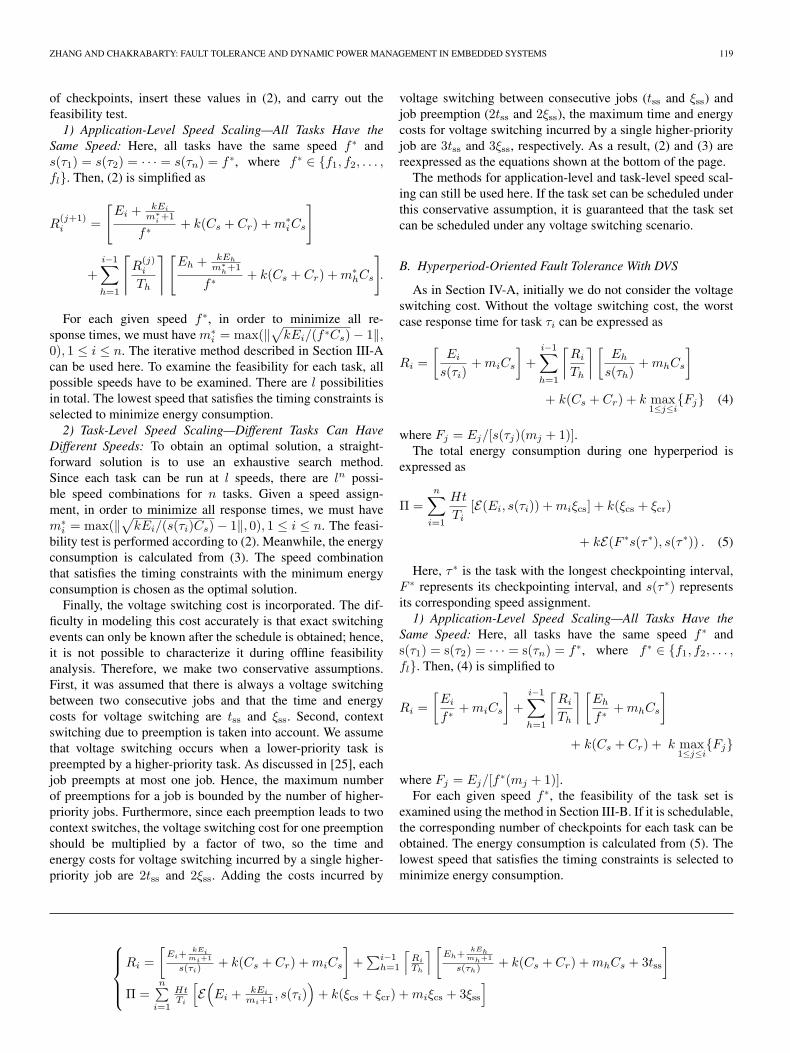
Finally, the voltage switching cost is incorporated. The dif-ficulty in modeling this cost accurately is that exact switchingevents can only be known after the schedule is obtained; hence,it is not possible to characterize it during offline feasibilityanalysis. Therefore, we make two conservative assumptions.First, it was assumed that there is always a voltage switchingbetween two consecutive jobs and that the time and energycosts for voltage switching are tss and ξss. Second, contextswitching due to preemption is taken into account. We assumethat voltage switching occurs when a lower-priority task ispreempted by a higher-priority task. As discussed in [25], eachjob preempts at most one job. Hence, the maximum numberof preemptions for a job is bounded by the number of higher-priority jobs. Furthermore, since each preemption leads to twocontext switches, the voltage switching cost for one preemptionshould be multiplied by a factor of two, so the time andenergy costs for voltage switching incurred by a single higher-priority job are 2tss and 2ξss. Adding the costs incurred by

voltage switching between consecutive jobs (tss and ξss) andjob preemption (2tss and 2ξss), the maximum time and energycosts for voltage switching incurred by a single higher-priorityjob are 3tss and 3ξss, respectively. As a result, (2) and (3) arereexpressed as the equations shown at the bottom of the page.

The methods for application-level and task-level speed scal-ing can still be used here. If the task set can be scheduled underthis conservative assumption, it is guaranteed that the task setcan be scheduled under any voltage switching scenario.

B. Hyperperiod-Oriented Fault Tolerance With DVS

As in Section IV-A, initially we do not consider the voltageswitching cost. Without the voltage switching cost, the worstcase response time for task τi can be expressed as

Ri =[

Ei

s(τi)+miCs

]+

i−1∑h=1

⌈Ri

Th

⌉[Eh

s(τh)+mhCs

]


Fj (4)

where Fj = Ej/[s(τj)(mj + 1)].The total energy consumption during one hyperperiod is

expressed as

Π =n∑

i=1

Ht

Ti[E(Ei, s(τi)) +miξcs] + k(ξcs + ξcr)

+ kE(F ∗s(τ ∗), s(τ ∗)) . (5)

Here, τ ∗ is the task with the longest checkpointing interval,F ∗ represents its checkpointing interval, and s(τ ∗) representsits corresponding speed assignment.1) Application-Level Speed Scaling—All Tasks Have the

Same Speed: Here, all tasks have the same speed f ∗ ands(τ1) = s(τ2) = · · · = s(τn) = f ∗, where f ∗ ∈ f1, f2, . . . ,fl. Then, (4) is simplified to

Ri =[Ei

f ∗ +miCs

]+

i−1∑h=1

⌈Ri

Th

⌉ [Eh

f ∗ +mhCs

]


Fj

where Fj = Ej/[f ∗(mj + 1)].For each given speed f ∗, the feasibility of the task set is

examined using the method in Section III-B. If it is schedulable,the corresponding number of checkpoints for each task can beobtained. The energy consumption is calculated from (5). Thelowest speed that satisfies the timing constraints is selected tominimize energy consumption.

Ri =[

Ei+kEi

mi+1

s(τi)+ k(Cs + Cr) +miCs

]+

∑i−1h=1

⌈Ri

Th

⌉ [Eh+

kEhmh+1

s(τh) + k(Cs + Cr) +mhCs + 3tss

]

Π =n∑

i=1

HtTi

[E(Ei + kEi

mi+1 , s(τi))+ k(ξcs + ξcr) +miξcs + 3ξss

]


2) Task-Level Speed Scaling—Different Tasks Can HaveDifferent Speeds: To obtain an optimal solution, a straightfor-ward solution is to use an exhaustive method. Since each taskcan be run at l speeds, there are ln possible speed combinationsfor n tasks. For each speed combination, the feasibility test isperformed according to (4). The method in Section III-B isemployed and the corresponding number of checkpoints is ob-tained. Energy consumption is calculated from (5). The speedcombination that satisfies the timing constraints with the mini-mum energy consumption is chosen as the optimal solution.

Next, the voltage switching cost is incorporated. As in thejob-oriented case, the switching cost between two jobs and theswitching cost due to preemption are incorporated. Based onthis, (4) and (5) are reexpressed as

Ri =[

Ei

s(τi)+miCs

]+

i−1∑h=1

⌈Ri

Th

⌉ [Eh

s(τh) +mhCs + 3tss]


Fj

Π =n∑

i=1

HtTi[E(Ei, s(τi)) +miξcs + 3ξss] + k(ξcs + ξcr)

+ kE(F ∗s(τ ∗), s(τ ∗))

.

The methods for application-level and task-level speed scal-ing can again be used here. If the task set can be scheduledunder this conservative assumption, it is guaranteed that thetask set can be scheduled under any other voltage switchingscenario.

C. Heuristic Method Based on a Genetic Algorithm (GA)

As expected, the exhaustive method for task-level speedscaling is very time consuming. For instance, we carried outsimulation for a real-time application composed of 17 taskswith three variable speeds. The exhaustive search method ex-amined all 317 speed combinations and took 63 h of CPU timeon a Pentium IV PC with a 1.4-GHz processor and 256-MBmemory. It is therefore obvious that the exhaustive method canonly be applied to moderate-sized problem instances. When thesize of the task set or the number of processor speeds is large,a heuristic method needs to be employed to obtain accept-able performance with low computation cost. Heuristics basedon GAs have been used to solve a number of combina-torial search problems. We use a GA-based heuristic here fortask-level speed scaling. It is applicable for both job- andhyperperiod-oriented cases. The solution is approximate. Alter-native heuristic approaches can also be developed to solve thisproblem. However, since the focus of this paper is not on thecomparison between heuristic approaches, an investigation intoother heuristic techniques is left for future work.

We choose a GA based on two reasons. First, they aretargeting a multiobjective optimization problem for which re-searchers have often used GAs by formulating the problem interms of two-priority optimizations. The primary objective hereis to meet task deadlines deterministically, even though k faultsoccur, either during the execution of a job in the job-orientedmodel or during a hyperperiod in the hyperperiod-orientedmodel. A secondary goal is to minimize energy consumption.

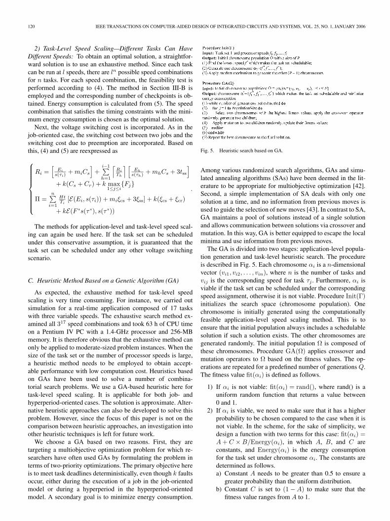
Fig. 5. Heuristic search based on GA.

Among various randomized search algorithms, GAs and simu-lated annealing algorithms (SAs) have been deemed in the lit-erature to be appropriate for multiobjective optimization [42].Second, a simple implementation of SA deals with only onesolution at a time, and no information from previous moves isused to guide the selection of new moves [43]. In contrast to SA,GA maintains a pool of solutions instead of a single solutionand allows communication between solutions via crossover andmutation. In this way, GA is better equipped to escape the localminima and use information from previous moves.

The GA is divided into two stages: application-level popula-tion generation and task-level heuristic search. The procedureis described in Fig. 5. Each chromosome αi is a n-dimensionalvector (vi1, vi2, . . . , vin), where n is the number of tasks andvij is the corresponding speed for task τj . Furthermore, αi isviable if the task set can be scheduled under the correspondingspeed assignment, otherwise it is not viable. Procedure Init(Γ)initializes the search space (chromosome population). Onechromosome is initially generated using the computationallyfeasible application-level speed scaling method. This is toensure that the initial population always includes a schedulablesolution if such a solution exists. The other chromosomes aregenerated randomly. The initial population Ω is composed ofthese chromosomes. Procedure GA(Ω) applies crossover andmutation operators to Ω based on the fitness values. The op-erations are repeated for a predefined number of generations Q.The fitness value fit(αi) is defined as follows.

1) If αi is not viable: fit(αi) = rand(), where rand() is auniform random function that returns a value between0 and 1.

2) If αi is viable, we need to make sure that it has a higherprobability to be chosen compared to the case when it isnot viable. In the scheme, for the sake of simplicity, wedesign a function with two terms for this case: fit(αi) =A+ C ×B/Energy(αi), in which A, B, and C areconstants, and Energy(αi) is the energy consumptionfor the task set under chromosome αi. The constants aredetermined as follows.a) Constant A needs to be greater than 0.5 to ensure a

greater probability than the uniform distribution.b) Constant C is set to (1−A) to make sure that the

fitness value ranges from A to 1.


c) Constant B is set to the value of the energy con-sumption under fault-free conditions using some well-known schemes such as VSLP.

d) A chromosome αi with low-energy consumptionEnergy(αi) has a high fitness value, which makes itmore likely to be selected.

The choice of the value for A is based on preprocessingusing a large number of experiments. It has to tradeoff betweentask feasibility and energy consumption. If A is too small(i.e., slightly greater than 0.50), then energy consumption playsa more important role and the difference between a viablechromosome and that which is not viable is not significant; ifA is too large, then the effect of energy consumption becomessmall in the selection procedure. Based on experiments withrandom task sets, we choose A = 0.6 and C = 0.4 for theGA-based algorithm.

The mutation and crossover operators used in the procedureare defined as follows.

1) Crossover: find an index randomly; then one child keepsthe information of its parent to the left of the index andfills the right with the other parent chromosome, and theother child keeps the information of its parent to theright of the index and fills the left with the other parentchromosome.

2) Mutation: choose a certain number of bits from twochildren randomly and replace them with a differentinformation.

The choices for the number of generations Q and the pop-ulation size P are also based on experiments. For the bench-marks in this paper, Q = 1000 yields good results. The valueof P depends on the size of the task set and on the number ofspeeds.

The complexity of this heuristic method is linear with thenumber of generations Q and the population size P . In the17-task, three-speed example for which the exhaustive methodtook 63 h, the heuristic method takes only 3 min. While theproposed GA-based technique is found to yield good results inSection V, it is particularly difficult to establish a theoreticalbasis that explains its effectiveness for this problem. By theirvery nature, it is very hard to theoretically justify the suitabilityof GAs for a given optimization problem, or explain analyti-cally why they work well. As a result, it is typical in the areaof evolutionary algorithms to demonstrate the suitability of aGA-based approach for a problem experimentally.

D. Job-Level Online Speed Scaling

As discussed in Sections IV-A and IV-B, the speed assign-ment and the checkpointing interval are determined via off-linefeasibility analysis. A static sequence of jobs is obtained andtheir parameters such as release times and execution times areknown a priori under the worst case. However, if only suchstatic measures are used during run time, it will not be possibleto make use of idle intervals. Clearly, further energy saving ispossible through additional online speed scaling.

The on-line speed scaling procedure, done at the job level,is adaptive with respect to fault occurrence. It makes use of

a simple run-time adaptation mechanism. The key features ofthis procedure are: 1) once a job completes, the release time ofthe next job is adjusted dynamically during run time and 2) theprocessor is run at an appropriate speed such that the current jobcompletes either before its deadline or before the static releasetime of the next job, whichever is sooner.

V. NUMERICAL RESULTS

This section compares the performance of the energy-awarefault-tolerance scheme with the DVS technique proposed in[5], referred to as VSLP. In the absence of any publishedexperimental results on energy-aware fault tolerance, we areonly able to compare the approach with DVS schemes thatdo not consider fault occurrences. On the other hand, currentfault-tolerant schemes do not incorporate DVS, which makesthem energy inefficient. We therefore compare the approachwith fault-tolerant schemes that do not consider energy. Thegoal here is to highlight the impact of fault occurrences on afault-oblivious DVS scheme and quantify the energy saving ofthe scheme over a DVS-oblivious checkpointing scheme.

We use the following notation to refer to the various typesof fault tolerance and energy-aware fault tolerance schemes:1) JFTC: job-oriented fault tolerance under constant speed;2) JFTA: job-oriented fault tolerance with application-levelspeed scaling; 3) JFTT: job-oriented fault tolerance with task-level speed scaling; 4) HFTC: hyperperiod-oriented fault tol-erance under constant speed; 5) HFTA: hyperperiod-orientedfault tolerance with application-level speed scaling; and6) HFTT: hyperperiod-oriented fault tolerance with task-levelspeed scaling.

Since the VSLP scheme presented in [5] does not providefault tolerance, we assume that it simply reexecutes a jobwhen a fault occurs. As for the DVS-oblivious constant-speedschemes (JFTC and HFTC), it was assumed that the tasks areexecuted under the highest processor speed. Furthermore, sinceJFTA is a special case of JFTT and HFTA is a special caseof HFTT, the other schemes were compared with the JFTT andHFTT schemes. For both cases, we first show that JFTT andHFTT can schedule task sets even when the VSLP cannot doso, that these schemes can save more energy via checkpointingin the presence of faults, and finally that these schemes can alsosave energy via DVS compared to the DVS-oblivious schemes.

Two low-power embedded processors were chosen for theexperiments: the Intel XScale PXA260 [6] and the Trans-meta Crusoe [8]. The parameter values that are listed in datasheets were used. The frequencies, voltages, and correspond-ing power consumptions for these processors are listed inTable I.

We evaluate the schemes on three real-life task sets. Thesetask sets include a CNC task set [44], an inertial navigationsystem (INS) task set [45], and a generic aviation platform(GAP) task set [46], respectively. The characteristics of thethree task sets are listed in Table II. The task execution timesfor these task sets are assumed for a nominal CPU frequencyof 200 MHz.

The choices of k are based on the characteristics of the tasksets and typical fault arrival rates. For the job-oriented case, the


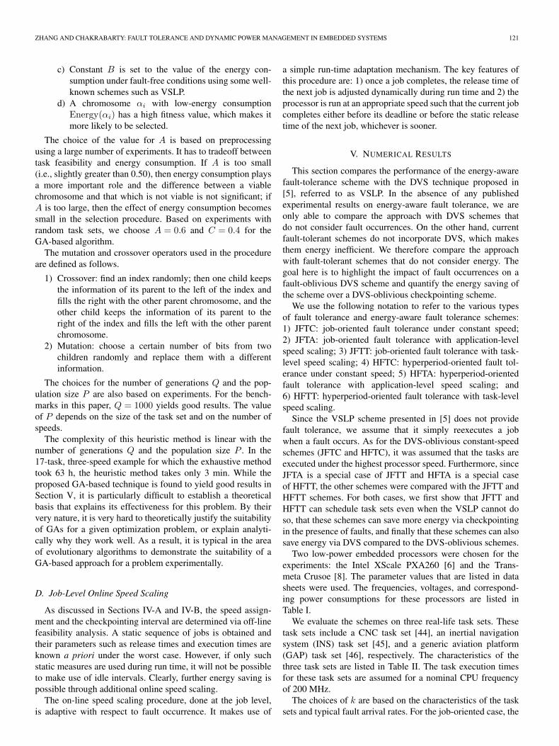
TABLE IPROCESSOR FREQUENCIES, VOLTAGES, AND POWER [6], [8]

TABLE IICHARACTERISTICS OF THE BENCHMARKS

TABLE IIIJFTT PERFORMANCE COMPARISON USING INTEL XScale

typical value of k should be relatively small since each taskinstance is short. It is therefore enough to require that eachtask instance tolerate one fault (k = 1). Therefore, we choosek = 1 for INS and GAP. In addition, since the execution timesand periods for CNC are extremely short, it is impractical toincorporate job-oriented fault tolerance for this task set. For thehyperperiod-oriented case, since a hyperperiod can be as longas hundreds of seconds, it is reasonable to choose a larger valueof k. For example, the hyperperiod for GAP is 118 s. If weassume that the fault arrival rate is as high as 140/h, as in [34],then the number of faults during this hyperperiod can be as highas 5. In the experiments for the hyperperiod-oriented case, wetherefore set the values of k to 1, 2, and 4 for CNC, INS, andGAP, respectively.

Based on the discussion in Section II, it was assumed thatthe checkpoint size is 5 kB and that checkpoint data are savedin DRAM. Based on the typical access speeds of DRAMdescribed in Section II, the time to read or write a checkpointof size 5 kB is assumed to be 0.4 ms. We choose a powerconsumption value of 400 mW for the DRAM [47]. Hence,the energy consumption for saving or retrieving a checkpoint is160 µJ. In addition, based on data provided in the literature in[37]–[40], it was assumed that a single DVS transition takes100 µs and consumes 30 µJ. We further classify the simulationinto two categories: zero DVS cost and nonzero DVS cost. Thisclassification is done in order to highlight the effect of DVScost on the task set feasibility and the energy consumption. Forsome processors, it has been reported that task execution canproceed concurrently with voltage scaling [48]; hence, we alsoconsider the case of zero voltage switching time.

Since the number of tasks for CNC and INS is relativelysmall, the simulation results for CNC and INS are obtainedusing the exhaustive search method. The simulation results forGAP are obtained using the heuristic method. Typical DVS

costs due to context switching have also been considered inthese experiments.

A. JFTT Results Based on Data Sheetsof the Intel XScale Processor

The simulation results for zero voltage-scaling cost areshown in Table III. The last two columns of the table show theenergy saving of JFTT compared to VSLP and JFTC, respec-tively. In the table, E13 = (E1 − E3)/E1 × 100% and E23 =(E2 − E3)/E2 × 100%. It can be seen that JFTT saves as muchas 17% more energy compared to VSLP. The performances ofJFTC and JFTT are comparable. This is because JFTT has tooften run at the highest processor speed to ensure timely taskcompletion. As a result, the energy saving is not so significant.

Next, we assume nonzero DVS cost. The performance com-parisons are also shown in Table III. From Table III, it can beseen that JFTT saves approximately 15% more energy com-pared to VSLP. The performances of JFTT and JFTC are onceagain comparable.

B. JFTT Results Based on Data Sheetsof the Transmeta Crusoe Processor

Since the Transmeta Crusoe processor consumes more powercompared to the Intel XScale processor, the checkpointingenergy is relatively small in this case compared to the taskexecution energy. The performance gain of JFTT over VSLPis therefore more significant in this case. Furthermore, since thepower consumption varies more for different processor speeds,it is expected that JFTT can achieve more energy saving thanthe DVS-oblivious JFTC scheme.

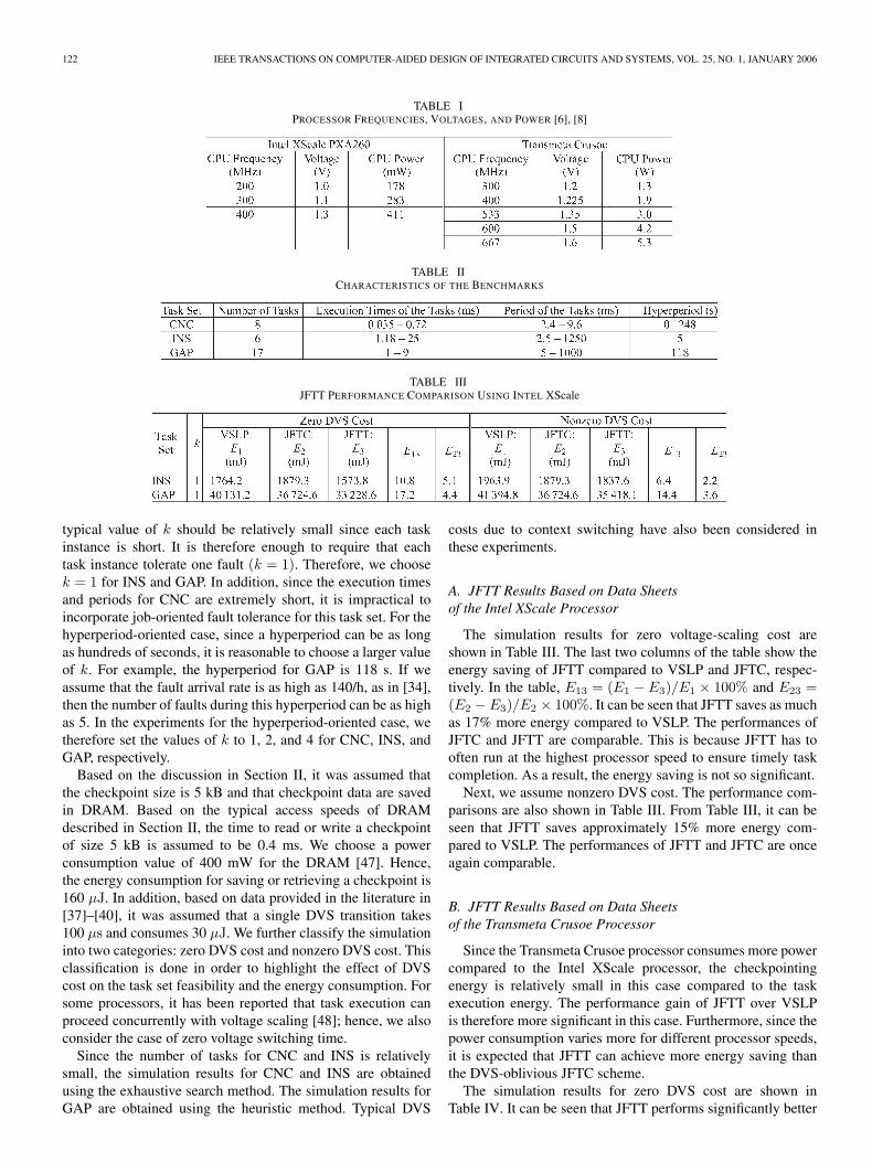
The simulation results for zero DVS cost are shown inTable IV. It can be seen that JFTT performs significantly better


TABLE IVJFTT PERFORMANCE COMPARISON USING TRANSMETA CRUSOE

TABLE VHFTT PERFORMANCE COMPARISON USING INTEL XScale

TABLE VIHFTT PERFORMANCE COMPARISON USING TRANSMETA CRUSOE

than VSLP. For example, the energy saving for GAP is as highas 33.2%. Next, we compare JFTT and JFTC. As expected,JFTT saves much more energy. For example, JFTT saves 51.9%energy over JFTC for INS. This is because JFTT can scaledown the processor speed more often when faults occur lessfrequently.

Finally, we examine the case of nonzero DVS cost. Theperformance comparisons are also shown in Table IV. JFTTsaves up to 33.6% energy compared to VSLP and up to 51.6%energy compared to JFTC.

C. HFTT Results Based on Data Sheetsof the Intel XScale Processor

The performance comparison for zero DVS cost is shown inTable V. In the table, “NF” denotes that the task set cannotbe feasibly scheduled. HFTT performs better than VSLP andHFTC in all cases. First, HFTT saves more energy when allschemes are feasible. The energy saving for HFTT over VSLPis as high as 53.9%, and it is as high as 15.6% over HFTC.Second, HFTT and HFTC tolerate more faults compared toVSLP. For example, when k is greater than one for INS andGAP, VSLP is not feasible while both HFTT and HFTC stillguarantee the feasibility.

The performance comparison for nonzero DVS cost is alsoshown in Table V. HFTT saves as much as 49.9% in energy

compared to VSLP. The performances of HFTT and HFTCare comparable.

D. HFTT Results Based on Data Sheetsof the Transmeta Crusoe Processor

The performance comparison for zero DVS cost is shown inTable VI. HFTT outperforms VSLP and HFTC in all cases. Theenergy saving for HFTT over VSLP is as high as 79.0%, and itis as high as 45.7% over HFTC.

The performance comparison for nonzero DVS cost is alsoshown in Table VI. HFTT saves as much as 77.3% in energyover VSLP, and as much as 42.1% in energy over HFTC.

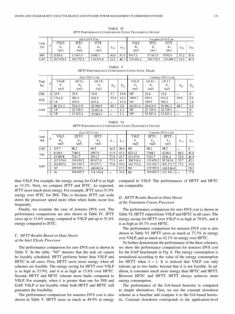
To further demonstrate the performance of the three schemes,we show the performance comparison for nonzero DVS costfor the GAP benchmark in Fig. 6. The energy consumption isnormalized according to the value of the energy consumptionfor HFTT when k = 1. It is noticed that VSLP can onlytolerate up to two faults, beyond that it is not feasible. In ad-dition, it consumes much more energy than HFTC and HFTT.Between HFTC and HFTT, HFTT always achieves moreenergy consumption.

The performance of the GA-based heuristic is comparedto simple alternatives. First, we use the constant slowdownscheme as a baseline and compare it to the GA-based heuris-tic. Constant slowdown corresponds to the application-level


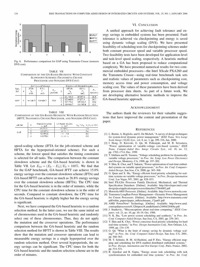
Fig. 6. Performance comparison for GAP using Transmeta Crusoe (nonzeroDVS cost).

TABLE VIICOMPARISON OF THE GA-BASED HEURISTIC WITH CONSTANT

SLOWDOWN SCHEMES (TRANSMETA CRUSOE

PROCESSOR AND NONZERO DVS COST)

TABLE VIIICOMPARISON OF THE GA-BASED HEURISTIC WITH RANDOM SELECTION

(HFTT, TRANSMETA CRUSOE PROCESSOR, AND NONZERO DVS COST)

speed-scaling scheme (JFTA for the job-oriented scheme andHFTA for the hyperperiod-oriented scheme). For such ascheme, the lowest speed that satisfies the timing constraintsis selected for all tasks. The comparison between the constantslowdown scheme and the GA-based heuristic is shown inTable VII. Let E03 = (E0 − E3)/E0 × 100%. We find thatfor the GAP benchmark, GA-based JFTT can achieve 15.0%energy savings over the constant slowdown scheme (JFTA) andGA-based HFTT can achieve as much as 26.8% energy savingsover the constant slowdown scheme (HFTA). The CPU timefor the GA-based heuristic is in the order of minutes, while theCPU time for the constant slowdown scheme is in the order ofseconds. Compared to constant slowdown, the CPU time forthe GA-based heuristic is slightly higher but the energy savingis significant.

Next, we have compared the GA-based heuristic to a randomselection method. In the latter case, we use the same initial setof chromosomes used in the GA-based heuristic and randomlyselect one of these chromosomes. Thus, they do not applythe mutation and the crossover operations. The performancecomparison between the GA-based heuristic and the randomselection method for HFTT is shown in Table VIII. The resultsshow that the mutation and crossover operations can lead tomeasurable energy savings in a single hyperperiod over therandom selection method. Over several hyperperiods, the en-ergy savings can be significant. The CPU times for both theGA-based heuristic and the random selection scheme are in theorder of minutes.

VI. CONCLUSION

A unified approach for achieving fault tolerance and en-ergy savings in embedded systems has been presented. Faulttolerance is achieved via checkpointing and energy is savedusing dynamic voltage scaling (DVS). We have presentedfeasibility-of-scheduling tests for checkpointing schemes underboth constant processor speed and variable processor speed.Two feasibility tests have been developed for application-leveland task-level speed scaling, respectively. A heuristic methodbased on a GA has been proposed to reduce computationalcomplexity. We have presented numerical results for two com-mercial embedded processors—the Intel XScale PXA260 andthe Transmeta Crusoe—using real-time benchmark task setsand realistic values of parameters such as checkpointing cost,memory access time and power consumption, and voltagescaling cost. The values of these parameters have been derivedfrom processor data sheets. As part of a future work, Weare developing alternative heuristic methods to improve theGA-based heuristic approach.

ACKNOWLEDGMENT

The authors thank the reviewers for their valuable sugges-tions that have improved the content and presentation of thepaper.

REFERENCES

[1] L. Benini, A. Bogliolo, and G. De Micheli, “A survey of design techniquesfor system-level dynamic power management,” IEEE Trans. Very LargeScale Integr. (VLSI) Syst., vol. 8, no. 3, pp. 299–316, Jun. 2000.

[2] I. Hong, D. Kirovski, G. Qu, M. Potkonjak, and M. B. Srivastava,“Power optimization of variable-voltage core-based systems,” IEEETrans. Comput.-Aided Des. Integr. Circuits Syst., vol. 18, no. 12,pp. 1702–1714, Dec. 1999.

[3] T. Ishihara and H. Yasuura, “Voltage scheduling problem for dynamicallyvariable voltage processors,” in Proc. Int. Symp. Low Power Electronicsand Design, Monterey, CA, 1998, pp. 197–202.

[4] Y. Shin, K. Choi, and T. Sakurai, “Power optimization of real-time embed-ded systems on variable speed processors,” in Proc. Int. Conf. Computer-Aided Design, San Jose, CA, 2000, pp. 365–368.

[5] G. Quan and X. Hu, “Energy efficient fixed-priority scheduling for real-time systems on variable voltage processors,” in Proc. Design AutomationConf., Las Vegas, NV, 2001, pp. 828–833.

[6] Intel PXA26x Processor Family Electrical, Mechanical, and ThermalSpecification Datasheet. [Online]. Available: http://developer.intel.com/design/pca/applicationsprocessors/datashts/27864002.pdf

[7] Motorola 6805 Processor. [Online]. Available: http://www.motorola.com[8] Transmeta LongRun Power Management—Dynamic Power Management

for Crusoe Processors. [Online]. Available: http://www.transmeta.com/pdf/white_papers/paper_mfleischmann_17jan01.pdf

[9] AMD PowerNow! Technology. [Online]. Available: http://www.amd.com/epd/processors/6.32bitproc/8.amdk6fami/x24404/24404a.pdf

[10] J. Stankovic, “Misconceptions about real-time computing,” IEEE Com-puter, vol. 21, no. 10, pp. 10–19, Oct. 1988.

[11] N. K. Jha, “Low power system scheduling and synthesis,” in Proc. Int.Conf. Computer-Aided Design, San Jose, CA, 2001, pp. 259–263.

[12] Y. Shin and K. Choi, “Power conscious fixed priority scheduling for hardreal-time systems,” in Proc. Design Automation Conf., New Orleans, LA,1999, pp. 134–139.

[13] G. Qu “What is the limit of energy saving by dynamic voltage scal-ing?” in Proc. Int. Conf. Computer-Aided Design, San Jose, CA, 2001,pp. 560–563.

[14] M. T. Schmitz, B. M. Al-Hashimi, and P. Eles, “Energy efficient map-ping and scheduling for DVS enabled distributed embedded systems,”in Proc. Design, Automation and Test Europe Conf., Paris, France, 2002,pp. 514–521.

[15] R. Jejurikar and R. Gupta, “Energy aware task scheduling with tasksynchronization for embedded real time systems,” in Proc. Int. Conf.


Compilers, Architecture and Synthesis Embedded Systems, Grenoble,France, 2002, pp. 164–169.

[16] D. Siewiorek and R. Swarz, Reliable Computer Systems: Design andEvaluation. Natick, MA: A. K. Peters, Ltd., 1998.

[17] K. G. Shin and Y.-H. Lee, “Error detection process—Model, design andits impact on computer performance,” IEEE Trans. Comput., vol. C-33,no. 6, pp. 529–540, Jun. 1984.

[18] K. M. Chandy, J. C. Browne, C. W. Dissly, and W. R. Uhrig, “Analyticmodels for rollback and recovery strategies in data base systems,” IEEETrans. Softw. Eng., vol. 1, no. 1, pp. 100–110, Mar. 1975.

[19] D. K. Pradhan and N. H. Vaidya, “Roll-forward and rollback recovery:Performance reliability trade-off,” IEEE Trans. Comput., vol. 46, no. 3,pp. 372–378, Mar. 1997.

[20] K. Shin, T. Lin, and Y. Lee, “Optimal checkpointing of real-time tasks,”IEEE Trans. Comput., vol. 36, no. 11, pp. 1328–1341, Nov. 1987.

[21] A. Ziv and J. Bruck, “An on-line algorithm for checkpoint placement,”IEEE Trans. Comput., vol. 46, no. 9, pp. 976–985, Sep. 1997.

[22] S. W. Kwak, B. J. Choi, and B. K. Kim, “An optimal checkpointing-strategy for real-time control systems under transient faults,” IEEE Trans.Reliab., vol. 50, no. 3, pp. 293–301, Sep. 2001.

[23] Y. Zhang and K. Chakrabarty, “Energy-aware adaptive checkpointingin embedded real-time systems,” in Proc. Design, Automation and TestEurope Conf., Munich, Germany, 2003, pp. 918–923.

[24] R. Melhem, D. Mosse, and E. N. Elnozahy, “The interplay of power man-agement and fault recovery in real-time systems,” IEEE Trans. Comput.,vol. 53, no. 2, pp. 217–231, Feb. 2004.

[25] J. W. Liu, Real-Time Systems. Upper Saddle River, NJ: Prentice-Hall,2000.

[26] E. Dupont, M. Nicolaidis, and P. Rohr, “Embedded robustness IPs fortransient-error-free ICs,” IEEE Des. Test. Comput., vol. 19, no. 3, pp. 54–68, May–Jun. 2002.

[27] M. L. Bushnell and V. D. Agrawal, Essentials of Electronic Testing.Norwell, MA: Kluwer, 2000.

[28] E. N. Elnozahy, Y. M. Wang, and D. B. Johnson, “A survey of rollback-recovery protocols in message-passing systems,” ACM Comput. Surv.,vol. 34, no. 3, pp. 375–408, Sep. 2002.

[29] E. N. Elnozahy, D. B. Johnson, and W. Zwaenepoel, “The performance ofconsistent checkpointing,” in Proc. Symp. Reliable Distributed Systems,Houston, TX, 1992, pp. 39–47.

[30] J. L. Hennessy and D. A. Patterson, Computer Architecture: A Quantita-tive Approach. San Mateo, CA: Morgan Kaufmann, 2002.

[31] C.-Y. Lin, S.-Y. Kuo, and Y. Huang, “A checkpointing tool for Palmoperating system,” in Proc. Dependable Systems and Networks, Göteborg,Sweden, 2001, pp. 71–76.

[32] J. S. Plank, M. Beck, G. Kingsley, and K. Li, “Libckpt: Transparentcheckpointing under Unix,” in Proc. Usenix Technical Conf., NewOrleans, LA, 1995, pp. 213–223.

[33] C. M. Krishna and A. D. Singh, “Reliability of checkpointed real-timesystems using time redundancy,” IEEE Trans. Reliab., vol. 42, no. 3,pp. 427–435, Sep. 1993.

[34] S. Punnekkat, A. Burns, and R. Davis, “Probabilistic scheduling guaran-tees for fault-tolerant real-time systems,” in Proc. Int. Conf. DependableComputing Critical Applications, San Jose, CA, 1999, pp. 361–378.

[35] A. Campbell, P. McDonald, and K. Ray, “Single event upset rates inspace,” IEEE Trans. Nucl. Sci., vol. 39, no. 6, pp. 1828–1835, Dec. 1992.

[36] D. Shin, S. Lee, and J. Kim, “Intra-task voltage scheduling for low-energyhard real-time applications,” IEEE Des. Test. Comput., vol. 18, no. 2,pp. 20–30, Mar.–Apr. 2001.

[37] T. Pering, T. Burd, and R. Broderson, “The simulation and evaluationof dynamic voltage scaling algorithms,” in Proc. Int. Symp. Low PowerElectronics and Design, Monterey, CA, 1998, pp. 76–81.

[38] T. Burd and R. Broderson, “Design issues for dynamic voltage scaling,”in Proc. Int. Symp. Low Power Electronics and Design, Rapallo, Italy,2000, pp. 9–14.

[39] K. Nowka, G. Carpenter, E. M. Donald, H. Ngo, B. Brock, K. Ishii,K. Nguyen, and J. Burns, “A 0.9 V to 1.95 V dynamic voltage-scalableand frequency-scalable 32b PowerPC processor,” in Proc. IEEE Int. Solid-State Circuits Conf., San Francisco, CA, 2002, pp. 340–341.

[40] D. Grunwald, P. Levis, C. Morrey, III, M. Neufeld, and K. Farkas, “Poli-cies for dynamic clock scheduling,” in Proc. Symp. Operating SystemsDesign and Implementation, San Diego, CA, 2000, pp. 73–86.

[41] S. Punnekkat, A. Burns, and R. Davis, “Analysis of checkpointing forreal-time systems,” Real-Time Syst. J., vol. 20, no. 1, pp. 83–102,Jan. 2001.

[42] R. P. Dick, “Multiobjective synthesis of low-power real-time distrib-uted embedded systems,” Ph.D. dissertation, Dept. Elect. Eng., PrincetonUniv., Princeton, NJ, Nov. 2002.

[43] E. Aarts and J. Korst, Simulated Annealing and Boltzmann Machines.Chichester, U.K.: Wiley, 1989.

[44] N. Kim, M. Ryu, S. Hong, M. Saksena, C. Choi, and H. Shin, “Visualassessment of a real-time system design: Case study on a CNC controller,”in Proc. Real-Time Systems Symp., Washington, DC, 1996, pp. 300–310.

[45] D. Katcher, H. Arakawa, and J. Strosnider, “Engineering and analysisof fixed priority schedulers,” IEEE Trans. Softw. Eng., vol. 19, no. 9,pp. 920–934, Sep. 1993.

[46] D. C. Locke, D. Vogel, and T. Mesler, “Building a predictable avionicsplatform in Ada: A case study,” in Proc. Real-Time Systems Symp., SanAntonio, TX, 1991, pp. 181–189.

[47] T. Simunic, L. Benini, P. Glynn, and G. D. Micheli, “Event-driven powermanagement,” IEEE Trans. Comput.-Aided Des. Integr. Circuits Syst.,vol. 20, no. 7, pp. 840–857, Jul. 2001.

[48] T. D. Burd, T. A. Pering, A. J. Stratakos, and R. W. Brodersen, “Adynamic voltage scaled microprocessor system,” IEEE J. Solid-StateCircuits, vol. 35, no. 11, pp. 1571–1580, Nov. 2000.

Ying Zhang received the B.S. and M.S. degreesin electronic engineering from Tsinghua University,Beijing, China, in 1997 and 1999, respectively, andthe Ph.D. degree in electrical and computer engineer-ing from Duke University, Durham, NC, in 2004.

He is currently a Senior Software engineer withthe Research and Development Department, GuidantCorporation, St. Paul, MN. His research interestsinclude real-time scheduling, low-power design, andfault tolerance.

Krishnendu Chakrabarty (S’92–M’96–SM’00)received the B.Tech. degree from the Indian Insti-tute of Technology, Kharagpur, India, in 1990, andthe M.S.E. and Ph.D. degrees, all from the Univer-sity of Michigan, Ann Arbor, in 1992 and 1995,respectively.

He is currently an Associate Professor of Elec-trical and Computer Engineering at Duke Univer-sity, Durham, NC. From 2000 to 2002, he was alsoa Mercator Visiting Professor at the University ofPotsdam, Germany. He is a coauthor of two books,

Microelectrofluidic Systems: Modeling and Simulation (Boca Raton, FL: CRCPress, 2002) and Test Resource Partitioning for System-on-a-Chip (Norwell,MA: Kluwer, 2002), and the Editor of SOC (System-on-a-Chip) Testing forPlug and Play Test Automation (Norwell, MA: Kluwer, 2002). He is alsoa coauthor of the forthcoming book Scalable Infrastructure for DistributedSensor Networks (London, U.K.: Springer). He has published over 190 papersin journals and refereed conference proceedings, and he holds a U.S. patentin integrated circuit testing. His current research projects include design andtesting of system-on-chip integrated circuits, embedded real-time systems, dis-tributed sensor networks, design automation of microfluidics-based biochips,and microfluidics-based chip cooling.

Dr. Chakrabarty is the recipient of the National Science Foundation EarlyFaculty (CAREER) Award, the Office of Naval Research Young InvestigatorAward, the Best Paper Award at the 2001 Design, Automation and Test inEurope (DATE) Conference, and the Humboldt Research Fellowship, awardedby the Alexander von Humboldt Foundation, Germany. He is a DistinguishedVisitor of the IEEE Computer Society from 2005 to 2007. He is an Asso-ciate Editor of the IEEE TRANSACTIONS ON COMPUTER-AIDED DESIGN

OF INTEGRATED CIRCUITS AND SYSTEMS, an Associate Editor of IEEETRANSACTIONS ON VERY LARGE SCALE INTEGRATION (VLSI) SYSTEMS,an Editor of the Journal of Electronic Testing: Theory and Applications(JETTA), and an Associate Editor for the ACM Journal on Emerging Technolo-gies in Computing Systems. He serves on the Editorial Board of Sensor Lettersand the Journal of Embedded Computing. He serves as a Subject Area Editorfor the International Journal of Distributed Sensor Networks. He has alsoserved as an Associate Editor of the IEEE TRANSACTIONS ON CIRCUITS AND

SYSTEMS II: ANALOG AND DIGITAL SIGNAL PROCESSING. He is a Memberof ACM and ACM SIGDA, and a Member of Sigma Xi. He serves as Vice Chairof Technical Activities of the IEEE Test Technology Technical Council and isa Member of the program committees of several IEEE/ACM conferences andworkshops. He served as the Tutorial Cochair for the 2005 IEEE InternationalConference on VLSI Design and is a designated Program Cochair for the 2005IEEE Asian Test Symposium.

Documents

A Uniﬁed Approach for Fault Tolerance and Dynamic Power