A unified framework for high-dimensional analysis ofM-estimators with decomposable regularizers

Sahand Negahban1 Pradeep Ravikumar2

Martin J. Wainwright1,3 Bin Yu1,3

Department of EECS1 Department of CS2 Department of Statistics3

UC Berkeley UT Austin UC Berkeley

October 2010

Abstract

High-dimensional statistical inference deals with models in which the the number of parame-ters p is comparable to or larger than the sample size n. Since it is usually impossible to obtainconsistent procedures unless p/n→ 0, a line of recent work has studied models with various typesof low-dimensional structure (e.g., sparse vectors; block-structured matrices; low-rank matrices;Markov assumptions). In such settings, a general approach to estimation is to solve a regu-larized convex program (known as a regularized M -estimator) which combines a loss function(measuring how well the model fits the data) with some regularization function that encouragesthe assumed structure. This paper provides a unified framework for establishing consistency andconvergence rates for such regularized M -estimators under high-dimensional scaling. We stateone main theorem and show how it can be used to re-derive some existing results, and also toobtain a number of new results on consistency and convergence rates. Our analysis also identifiestwo key properties of loss and regularization functions, referred to as restricted strong convexityand decomposability, that ensure corresponding regularized M -estimators have fast convergencerates, and which are optimal in many well-studied cases.

1 Introduction

High-dimensional statistics is concerned with models in which the ambient dimension of the problemp may be of the same order as—or substantially larger than—the sample size n. While its rootsare quite old, dating back to classical random matrix theory and high-dimensional testing problems(e.g, [26, 46, 58, 82]), the past decade has witnessed a tremendous surge of research activity. Rapiddevelopment of data collection technology is a major driving force: it allows for more observationsto be collected (larger n), and also for more variables to be measured (larger p). Examples are ubiq-uitous throughout science: astronomical projects such as the Large Synoptic Survey Telescope [1]produce terabytes of data in a single evening; each sample is a high-resolution image, with severalhundred megapixels, so that p ≫ 108. Financial data is also of a high-dimensional nature, withhundreds or thousands of financial instruments being measured and tracked over time, often atvery fine time intervals for use in high frequency trading. Advances in biotechnology now allowfor measurements of thousands of genes or proteins, and lead to numerous statistical challenges(e.g., see the paper [6] and references therein). Various types of imaging technology, among themmagnetic resonance imaging in medicine [44] and hyper-spectral imaging in ecology [38], also leadto high-dimensional data sets.

1

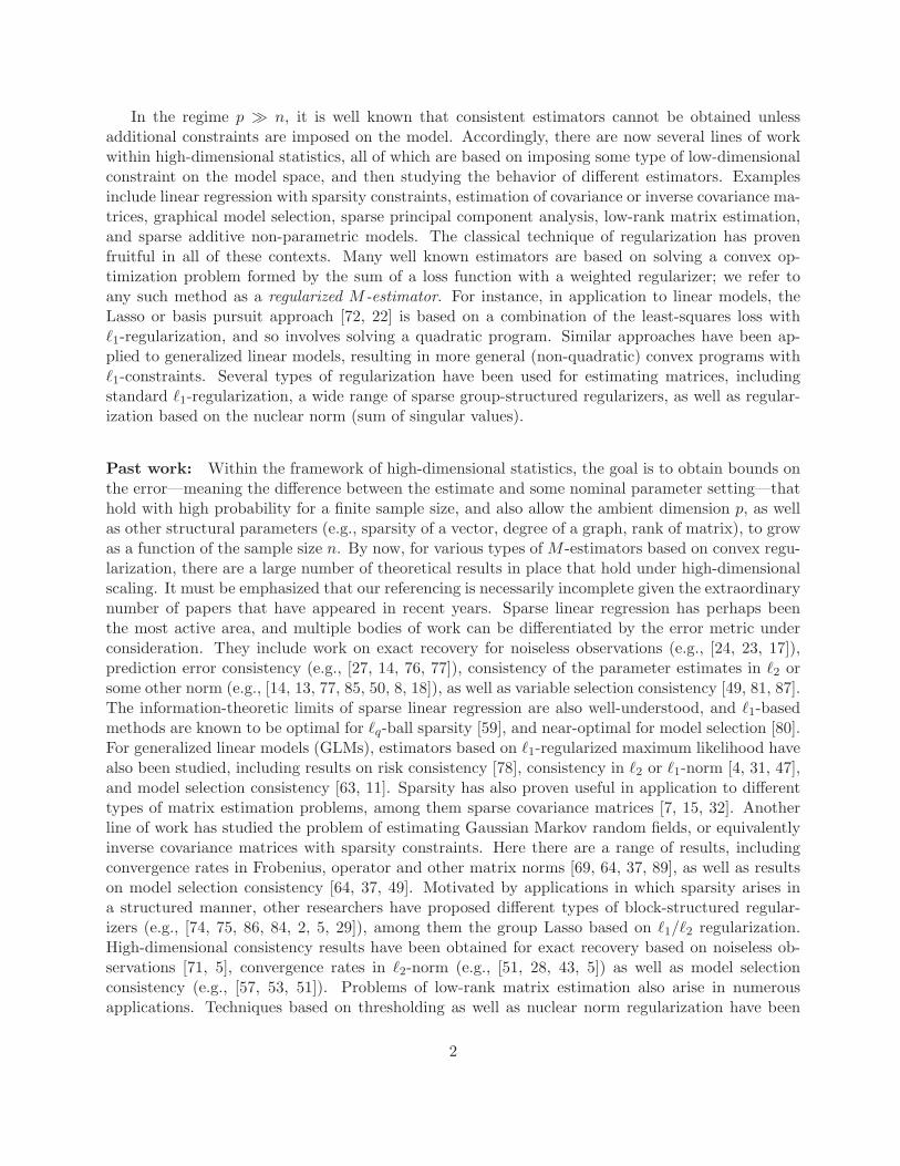
In the regime p ≫ n, it is well known that consistent estimators cannot be obtained unlessadditional constraints are imposed on the model. Accordingly, there are now several lines of workwithin high-dimensional statistics, all of which are based on imposing some type of low-dimensionalconstraint on the model space, and then studying the behavior of different estimators. Examplesinclude linear regression with sparsity constraints, estimation of covariance or inverse covariance ma-trices, graphical model selection, sparse principal component analysis, low-rank matrix estimation,and sparse additive non-parametric models. The classical technique of regularization has provenfruitful in all of these contexts. Many well known estimators are based on solving a convex op-timization problem formed by the sum of a loss function with a weighted regularizer; we refer toany such method as a regularized M -estimator. For instance, in application to linear models, theLasso or basis pursuit approach [72, 22] is based on a combination of the least-squares loss withℓ1-regularization, and so involves solving a quadratic program. Similar approaches have been ap-plied to generalized linear models, resulting in more general (non-quadratic) convex programs withℓ1-constraints. Several types of regularization have been used for estimating matrices, includingstandard ℓ1-regularization, a wide range of sparse group-structured regularizers, as well as regular-ization based on the nuclear norm (sum of singular values).

Past work: Within the framework of high-dimensional statistics, the goal is to obtain bounds onthe error—meaning the difference between the estimate and some nominal parameter setting—thathold with high probability for a finite sample size, and also allow the ambient dimension p, as wellas other structural parameters (e.g., sparsity of a vector, degree of a graph, rank of matrix), to growas a function of the sample size n. By now, for various types of M -estimators based on convex regu-larization, there are a large number of theoretical results in place that hold under high-dimensionalscaling. It must be emphasized that our referencing is necessarily incomplete given the extraordinarynumber of papers that have appeared in recent years. Sparse linear regression has perhaps beenthe most active area, and multiple bodies of work can be differentiated by the error metric underconsideration. They include work on exact recovery for noiseless observations (e.g., [24, 23, 17]),prediction error consistency (e.g., [27, 14, 76, 77]), consistency of the parameter estimates in ℓ2 orsome other norm (e.g., [14, 13, 77, 85, 50, 8, 18]), as well as variable selection consistency [49, 81, 87].The information-theoretic limits of sparse linear regression are also well-understood, and ℓ1-basedmethods are known to be optimal for ℓq-ball sparsity [59], and near-optimal for model selection [80].For generalized linear models (GLMs), estimators based on ℓ1-regularized maximum likelihood havealso been studied, including results on risk consistency [78], consistency in ℓ2 or ℓ1-norm [4, 31, 47],and model selection consistency [63, 11]. Sparsity has also proven useful in application to differenttypes of matrix estimation problems, among them sparse covariance matrices [7, 15, 32]. Anotherline of work has studied the problem of estimating Gaussian Markov random fields, or equivalentlyinverse covariance matrices with sparsity constraints. Here there are a range of results, includingconvergence rates in Frobenius, operator and other matrix norms [69, 64, 37, 89], as well as resultson model selection consistency [64, 37, 49]. Motivated by applications in which sparsity arises ina structured manner, other researchers have proposed different types of block-structured regular-izers (e.g., [74, 75, 86, 84, 2, 5, 29]), among them the group Lasso based on ℓ1/ℓ2 regularization.High-dimensional consistency results have been obtained for exact recovery based on noiseless ob-servations [71, 5], convergence rates in ℓ2-norm (e.g., [51, 28, 43, 5]) as well as model selectionconsistency (e.g., [57, 53, 51]). Problems of low-rank matrix estimation also arise in numerousapplications. Techniques based on thresholding as well as nuclear norm regularization have been

2

studied for different statistical models, including compressed sensing [66, 40, 67], matrix comple-tion [19, 33, 34, 65, 52], multitask regression [83, 54, 68, 12, 3], and system identification [25, 54, 42].Finally, although the primary emphasis of this paper is on high-dimensional parametric models, reg-ularization methods have also proven effective for a class of high-dimensional non-parametric modelsthat have a sparse additive decomposition (e.g., [62, 48, 35, 36]). Again, regularization methodshave been been shown to achieve minimax-optimal rates in this setting [60].

Our contributions: As we have noted previously, almost all of these estimators can be seenas particular types of regularized M -estimators, with the choice of loss function, regularizer andstatistical assumptions changing according to the model. This methodological similarity suggestsan intriguing possibility: is there a common set of theoretical principles that underlies analysis ofall these estimators? If so, it could be possible to gain a unified understanding of a large collectionof techniques for high-dimensional estimation.

The main contribution of this paper is to provide an affirmative answer to this question. Inparticular, we isolate and highlight two key properties of a regularized M -estimator—namely, a de-composability property for the regularizer, and a notion of restricted strong convexity that dependson the interaction between the regularizer and the loss function. For loss functions and regulariz-ers satisfying these two conditions, we prove a general result (Theorem 1) about consistency andconvergence rates for the associated estimates. This result provides a family of bounds indexed bysubspaces, and each bound consists of the sum of approximation error and estimation error. Thisgeneral result, when specialized to different statistical models, yields in a direct manner a largenumber of corollaries, some of them known and others novel. In addition to our framework andmain result (Theorem 1), other new results include minimax-optimal rates for sparse regression overℓq-balls (Corollary 3), a general oracle-type result for group-structured norms with applications togeneralized ℓq-ball sparsity (Corollary 4), as well as bounds for generalized linear models underminimal assumptions (Corollary 5), allowing for both unbounded and non-Lipschitz functions. Inconcurrent work, a subset of the current authors have also used this framework to prove severalresults on low-rank matrix estimation using the nuclear norm [54], as well as optimal rates for noisymatrix completion [52]. Finally, en route to establishing these corollaries, we also prove some newtechnical results that are of independent interest, including guarantees of restricted strong convexityfor group-structured regularization (Proposition 1) and for generalized linear models (Proposition 2).

The remainder of this paper is organized as follows. We begin in Section 2 by formulating theclass of regularized M -estimators that we consider, and then defining the notions of decomposabilityand restricted strong convexity. Section 3 is devoted to the statement of our main result (Theorem 1),and discussion of its consequences. Subsequent sections are devoted to corollaries of this main resultfor different statistical models, including sparse linear regression (Section 4), estimators based ongroup-structured regularizers (Section 5), estimation in generalized linear models (Section 6), andlow-rank matrix estimation (Section 7).

2 Problem formulation and some key properties

In this section, we begin with a precise formulation of the problem, and then develop some keyproperties of the regularizer and loss function.

3

2.1 A family of M-estimators

Let Zn1 := Z1, . . . , Zn denote n observations drawn i.i.d. according to some distribution P, and sup-pose that we are interested in estimating some parameter θ of the distribution P. Let L : R

p ×Zn → R

be some loss function that, for a given set of observations Zn1 , assigns a cost L(θ;Zn1 ) to any parame-ter θ ∈ R

p. We assume that that the population risk R(θ) = EZn1[L(θ;Zn1 )] is independent of n, and

we let θ∗ ∈ arg minθ∈Rp

R(θ) be a minimizer of the population risk. As is standard in statistics, in order

to estimate the parameter vector θ∗ from the data Zn1 , we solve a convex program that combines theloss function with a regularizer. More specifically, let r : R

p → R denote a regularization function,and consider the regularized M -estimator given by

θλn ∈ arg minθ∈Rp

L(θ;Zn1 ) + λnr(θ)

, (1)

where λn > 0 is a user-defined regularization penalty. Throughout the paper, we assume that theloss function L is convex and differentiable, and that the regularization function r is a norm.

Our goal is to provide general techniques for deriving bounds on the difference between anysolution θλn to the convex program (1) and the unknown vector θ∗. In this paper, we derive boundson the norm ‖θλn − θ∗‖⋆, where the error norm is induced by an inner product 〈·, ·〉⋆ on R

p. Mostoften, this error norm will either be the Euclidean ℓ2-norm on vectors, or the analogous Frobeniusnorm for matrices, but our theory also applies to certain types of weighted norms. In addition,we provide bounds on the quantity r(θλn − θ∗), which measures the error in the regularizer norm.In the classical setting, the ambient dimension p stays fixed while the number of observations ntends to infinity. Under these conditions, there are standard techniques for proving consistency andasymptotic normality for the error θλn − θ∗. In contrast, the analysis of this paper is all within ahigh-dimensional framework, in which the tuple (n, p), as well as other problem parameters, suchas vector sparsity or matrix rank etc., are all allowed to tend to infinity. In contrast to asymptoticnormality, our goal is to obtain explicit finite sample error bounds that hold with high probability.

Throughout the paper, we make use of the following notation. For any given subspace A ⊆ Rp,

we let A⊥ be its orthogonal complement, as defined by the inner product 〈·, ·〉⋆—namely, the setA⊥ :=

v ∈ R

p | 〈v, u〉⋆ = 0 for all u ∈ A. In addition, we let ΠA : R

p → A denote the projectionoperator, defined by

ΠA(u) := arg minv∈A

‖u− v‖⋆ , (2)

with the projection operator ΠA⊥ defined in an analogous manner.

2.2 Decomposability

We now motivate and define the decomposability property of regularizers, and then show how itconstrains the error in the M -estimation problem (1). This property is defined in terms of a pairof subspaces A ⊆ B of R

p. The role of the model subspace A is to capture the constraints specifiedby the model; for instance, it might be the subspace of vectors with a particular support (seeExample 1), or a subspace of low-rank matrices (see Example 3). The orthogonal complement B⊥

is the perturbation subspace, representing deviations away from the model subspace A. In the idealcase, we have B⊥ = A⊥, but our definition allows for the possibility that B is strictly larger than A.

4

Definition 1. A norm-based regularizer r is decomposable with respect to the subspace pairA ⊆ B if

r(α+ β) = r(α) + r(β) for all α ∈ A and β ∈ B⊥. (3)

In order to build some intuition, let us consider the ideal case A = B for the time being, so that thedecomposition (3) holds for all pairs (α, β) ∈ A × A⊥. For any given pair (α, β) of this form, thevector α + β can be interpreted as perturbation of the model vector α away from the subspace A,and it is desirable that the regularizer penalize such deviations as much as possible. By the triangleinequality, we always have r(α+ β) ≤ r(α) + r(β), so that the decomposability condition (3) holdsif and only the triangle inequality is tight for all pairs (α, β) ∈ (A,A⊥). It is exactly in this settingthat the regularizer penalizes deviations away from the model subspace A as much as possible.

In general, it is not difficult to find subspace pairs that satisfy the decomposability property.As a trivial example, any regularizer is decomposable with respect to A = R

p and its orthogonalcomplement A⊥ = 0. As will be clear in our main theorem, it is of more interest to find subspacepairs in which the model subspace A is “small”, so that the orthogonal complement A⊥ is “large”.Recalling the projection operator (2), of interest to us is its action on the unknown parameterθ∗ ∈ R

p. In the most desirable setting, the model subspace A can be chosen such that ΠA(θ∗) ≈ θ∗

and ΠA⊥(θ∗) ≈ 0. If this can be achieved with the model subspace A remaining relatively small, thenour main theorem guarantees that it is possible to estimate θ∗ at a relatively fast rate. The followingexamples illustrate suitable choices of the spaces A and B in three concrete settings, beginning withthe case of sparse vectors.

Example 1. Sparse vectors and ℓ1-norm regularization. Suppose the error norm ‖ · ‖⋆ is the usualℓ2-norm, and that the model class of interest is the set of s-sparse vectors in p dimensions. For anyparticular subset S ⊆ 1, 2, . . . , p with cardinality s, we define the model subspace

A(S) :=α ∈ R

p | αj = 0 for all j /∈ S. (4)

Here our notation reflects the fact that A depends explicitly on the chosen subset S. By construction,we have ΠA(S)(θ

∗) = θ∗ for any vector that is supported on S.

Now define B(S) = A(S), and note that the orthogonal complement with respect to the Eu-clidean inner product is given by

B⊥(S) = A⊥(S) =β ∈ R

p | βj = 0 for all j ∈ S. (5)

This set corresponds to the perturbation subspace, capturing deviations away from the set of vectorswith support S. We claim that for any subset S, the ℓ1-norm r(α) = ‖α‖1 is decomposable withrespect to the pair (A(S), B(S)). Indeed, by construction of the subspaces, any α ∈ A(S) can bewritten in the partitioned form α = (αS , 0Sc), where αS ∈ R

s and 0Sc ∈ Rp−s is a vector of zeros.

Similarly, any vector β ∈ B⊥(S) has the partitioned representation (0S , βSc). Putting together thepieces, we obtain

‖α+ β‖1 = ‖(αS , 0) + (0, βSc)‖1 = ‖α‖1 + ‖β‖1,

showing that the ℓ1-norm is decomposable as claimed. ♦

5

As a follow-up to the previous example, it is also worth noting that the same argument showsthat for a strictly positive weight vector ω, the weighted ℓ1-norm ‖α‖ω :=

∑pj=1 ωj |αj | is also de-

composable with respect to the pair (A(S), B(S)). For another natural extension, we now turn tothe case of sparsity models with more structure.

Example 2. Group-structured norms. In many applications, sparsity arises in a more structuredfashion, with groups of coefficients likely to be zero (or non-zero) simultaneously. In order to modelthis behavior, suppose that the index set 1, 2, . . . , p can be partitioned into a set of T disjointgroups, say G = G1, G2, . . . , GT . With this set-up, for a given vector ~ν = (ν1, . . . , νT ) ∈ [1,∞]T ,the associated (1, ~ν)-group norm takes the form

‖α‖G,~ν :=

T∑

t=1

‖αGt‖νt . (6)

For instance, with the choice ~ν = (2, 2, . . . , 2), we obtain the group ℓ1/ℓ2-norm, corresponding to theregularizer that underlies the group Lasso [84]. The choice ~ν = (∞, . . . ,∞) has also been studiedin past work [75, 53].

We claim that the norm ‖ · ‖G,~ν is again decomposable with respect to appropriately definedsubspaces. Indeed, given any subset SG ⊆ 1, . . . , T of group indices, say with cardinality sG = |SG |,we can define the subspace

A(SG) :=α ∈ R

p | αGt = 0 for all t /∈ SG, (7)

as well as its orthogonal complement with respect to the usual Euclidean inner product

A⊥(SG) = B⊥(SG) :=α ∈ R

p | αGt = 0 for all t ∈ SG. (8)

With these definitions, for any pair of vectors α ∈ A(SG) and β ∈ B⊥(SG), we have

‖α+ β‖G,~ν =∑

t∈SG

‖αGt + 0Gt‖νt +∑

t∈Sc

‖0Gj + βGt‖νt = ‖α‖G,~ν + ‖β‖G,~ν , (9)

thus verifying the decomposability condition. ♦

Example 3. Low-rank matrices and nuclear norm. Now suppose that each parameter Θ ∈ Rp1×p2

is a matrix; this corresponds to an instance of our general set-up with p = p1p2, as long as weidentify the space R

p1×p2 with Rp1p2 in the usual way. We equip this space with the inner product

〈〈Θ, Γ〉〉 := trace(ΘΓT ), a choice which yields the Frobenius norm

‖Θ‖⋆ :=√

〈〈Θ, Θ〉〉 =

√√√√p1∑

j=1

p2∑

k=1

Θ2jk (10)

as the induced norm. In many settings, it is natural to consider estimating matrices that arelow-rank; examples include principal component analysis, spectral clustering, collaborative filter-ing, and matrix completion. In particular, consider the class of matrices Θ ∈ R

p1×p2 that have

6

rank r ≤ minp1, p2. For any given matrix Θ, we let row(Θ) ⊆ Rp2 and col(Θ) ⊆ R

p1 denote itsrow space and column space respectively. Let U and V be a given pair of r-dimensional subspacesU ⊆ R

p1 and V ⊆ Rp2 ; these subspaces will represent left and right singular vectors of the tar-

get matrix Θ∗ to be estimated. For a given pair (U, V ), we can define the subspaces A(U, V ) andB⊥(U, V ) of R

p1×p2 given by

A(U, V ) :=Θ ∈ R

p1×p2 | row(Θ) ⊆ V, col(Θ) ⊆ U, and (11a)

B⊥(U, V ) :=Θ ∈ R

p1×p2 | row(Θ) ⊆ V ⊥, col(Θ) ⊆ U⊥. (11b)

Unlike the preceding examples, in this case, we have A(U, V ) 6= B(U, V ). However, as is requiredby our theory, we do have the inclusion A(U, V ) ⊆ B(U, V ). Indeed, given any Θ ∈ A(U, V ) andΓ ∈ B⊥(U, V ), we have ΘTΓ = 0 by definition, and hence 〈〈Θ, Γ〉〉 = trace(ΘTΓ) = 0. Consequently,we have shown that Θ is orthogonal to the space B⊥(U, V ), implying the claimed inclusion.

Finally, we claim that the nuclear or trace norm r(Θ) = |||Θ|||1, corresponding to the sum ofthe singular values of the matrix Θ, satisfies the decomposability property with respect to the pair(A(U, V ), B⊥(U, V )). By construction, any pair of matrices Θ ∈ A(U, V ) and Γ ∈ B⊥(U, V ) haveorthogonal row and column spaces, which implies the required decomposability condition—namely|||Θ + Γ|||1 = |||Θ|||1 + |||Γ|||1. ♦

A line of recent work (e.g., [21, 20]) has studied matrix problems involving the sum of a low-rankmatrix with a sparse matrix, along with the regularizer formed by a weighted sum of the nuclearnorm and the elementwise ℓ1-norm. By a combination of Examples 1 and Example 3, this regularizeralso satisfies the decomposability property with respect to appropriately defined subspaces.

2.3 A key consequence of decomposability

Thus far, we have specified a class (1) of M -estimators based on regularization, defined the notion ofdecomposability for the regularizer and worked through several illustrative examples. We now turnto the statistical consequences of decomposability—more specifically, its implications for the errorvector ∆λn = θλn − θ∗, where θ ∈ R

p is any solution of the regularized M -estimation procedure (1).Letting 〈·, ·〉 denote the usual Euclidean inner product, the dual norm of r is given by

r∗(v) := supu∈Rp\0

〈u, v〉r(u)

. (12)

It plays a key role in our specification of the regularization parameter λn in the convex program (1),in particular linking it to the data Zn1 that defines the estimator.

Lemma 1. Suppose that L is a convex function, and consider any optimal solution θ to the opti-mization problem (1) with a strictly positive regularization parameter satisfying

λn ≥ 2 r∗(∇L(θ∗;Zn1 )). (13)

Then for any pair (A,B) over which r is decomposable, the error ∆ = θλn − θ∗ belongs to the set

C(A,B; θ∗) :=∆ ∈ R

p | r(ΠB⊥(∆)) ≤ 3r(ΠB(∆)) + 4r(ΠA⊥(θ∗)). (14)

7

r(∆B⊥)

r(∆B)

r(∆B⊥)

r(∆B)

(a) (b)

Figure 1. Illustration of the set C(A,B; θ∗) in the special case ∆ = (∆1,∆2,∆3) ∈ R3 and regularizer

r(∆) = ‖∆‖1, relevant for sparse vectors (Example 1). This picture shows the case S = 3, so thatthe model subspace is A(S) = B(S) = ∆ ∈ R

3 | ∆1 = ∆2 = 0, and its orthogonal complementis given by A⊥(S) = B⊥(S) = ∆ ∈ R

3 | ∆3 = 0. (a) In the special case when θ∗ ∈ A(S) so thatr(ΠA⊥(θ∗)) = 0, the set C(A,B; θ∗) is a cone. (b) When θ∗ does not belong to A(S), the setC(A,B; θ∗) is enlarged in the co-ordinates (∆1,∆2) that span B⊥(S). It is no longer a cone, but isstill a star-shaped set.

We prove this result in Appendix A.1. It has the following important consequence: for any decom-posable regularizer and an appropriate choice (13) of regularization parameter, we are guaranteedthat the error vector ∆ belongs to a very specific set, depending on the unknown vector θ∗. Asillustrated in Figure 1, the geometry of the set C depends on the relation between θ∗ and the modelsubspace A. When θ∗ ∈ A, then we are guaranteed that r(ΠA⊥(θ∗)) = 0. In this case, the con-straint (14) reduces to r(ΠB⊥(∆)) ≤ 3r(ΠB(∆)), so that C is a cone, as illustrated in panel (a).In the more general case when θ∗ /∈ A and r(ΠA⊥(θ∗)) 6= 0, the set C is not a cone, but rather astar-shaped set excluding a small ball centered at the origin (panel (b)). As will be clarified in thesequel, this difference (between θ∗ ∈ A and θ∗ /∈ A) plays an important role in bounding the error.

2.4 Restricted strong convexity

We now turn to an important requirement of the loss function, and its interaction with the statis-tical model. Recall that ∆ = θλn − θ∗ is the difference between an optimal solution θλn and thetrue parameter, and consider the loss difference L(θλn ;Zn1 ) − L(θ∗;Zn1 ). To simplify notation, we

frequently write L(θλn)−L(θ∗) when the underlying data Zn1 is clear from context. In the classicalsetting, under fairly mild conditions, one expects that that the loss difference should converge tozero as the sample size n increases. It is important to note, however, that such convergence on itsown is not sufficient to guarantee that θλn and θ∗ are close, or equivalently that ∆ is small. Rather,the closeness depends on the curvature of the loss function, as illustrated in Figure 2. In a desirablesetting (panel (a)), the loss function is sharply curved around its optimum θλn , so that having a

8

θ∗ θλn

dL

∆

θ∗ θλn

dL

∆

(a) (b)

Figure 2. Role of curvature in distinguishing parameters. (a) Loss function has high curvature around

∆. A small excess loss dL = |L(θλn) − L(θ∗)| guarantees that the parameter error ∆ = θλn

− θ∗ isalso small. (b) A less desirable setting, in which the loss function has relatively low curvature aroundthe optimum.

small loss difference |L(θ∗) −L(θλn)| translates to a small error ∆ = θλn − θ∗. Panel (b) illustratesa less desirable setting, in which the loss function is relatively flat, so that the loss difference can besmall while the error ∆ is relatively large.

The standard way to ensure that a function is “not too flat” is via the notion of strong convexity—in particular, by requiring that there exist some constant γ > 0 such that

δL(∆, θ∗;Zn1 ) := L(θ∗ + ∆;Zn1 ) − L(θ∗;Zn1 ) − 〈∇L(θ∗;Zn1 ),∆〉 ≥ γ‖∆‖22 (15)

for all ∆ ∈ Rp in a neighborhood of θ∗. When the loss function is twice differentiable, restricted

strong convexity amounts to a uniform lower bound on the eigenvalues of the Hessian ∇2L.

Under classical “fixed p, large n” scaling, the loss function will be strongly convex under mildconditions. For instance, suppose that population function R(θ) := EZn

1[L(θ;Zn1 )] is strongly convex,

or equivalently, that the Hessian ∇2R(θ) is strictly positive definite in a neighborhood of θ∗. As aconcrete example, when the loss function L is defined based on negative log likelihood of a statisticalmodel, then the Hessian ∇2R(θ) corresponds to the Fisher information matrix, a quantity whicharises naturally in asymptotic statistics. If the dimension p is fixed while the sample size n goes toinfinity, standard arguments can be used to show that (under mild regularity conditions) the randomHessian ∇2L(θ;Zn1 ) converges to ∇2R(θ) = EZn

1[∇2L(θ;Zn1 )] uniformly for all θ in a neighborhood

of θ∗.Whenever the pair (n, p) both increase in such a way that p > n, the situation is drastically

different: the p×p Hessian matrix ∇2L(θ;Zn1 ) will always be rank-deficient. As a concrete example,consider linear regression based on samples Zi = (yi, xi) ∈ R × R

p, for i = 1, 2, . . . , n. Using theleast-squares loss L(θ;Zn1 ) = 1

2n‖y−Xθ‖22, the p× p Hessian matrix ∇2L(θ;Zn1 ) = 1

nXTX has rank

at most n, meaning that the loss cannot be strongly convex when p > n. In the high-dimensionalsetting, a typical loss function will take the form shown in Figure 3(a): while curved in certaindirections, it will be completely flat in a large number of directions. Thus, it is impossible toguarantee global strong convexity.

9

(a) (b)

Figure 3. (a) Illustration of a generic loss function in the high-dimensional p > n setting:it is curved in certain directions, but completely flat in others. (b) Illustration of the setK(δ;A,B, θ∗) = C(A,B; θ∗) ∩ ∆ ∈ R

p | ‖∆‖⋆ = δ over which restricted strong convexity musthold. It is the intersection of a ball of radius δ with the star-shaped set C(A,B, θ∗).

In summary, we need to relax the notion of strong convexity by restricting the set of directionsfor which condition (15) holds. We formalize this idea as follows:

Definition 2. For a given set S, the loss function satisfies restricted strong convexity (RSC)with parameter κL > 0 if

L(θ∗ + ∆;Zn1 ) − L(θ∗;Zn1 ) − 〈∇L(θ∗;Zn1 ),∆〉︸ ︷︷ ︸δL(∆, θ∗; Zn

1 )

≥ κL ‖∆‖2⋆ for all ∆ ∈ S. (16)

It remains to specify suitable choices of sets S for this definition. Based on our discussion ofregularizers and Lemma 1, one natural candidate is the set C(A,B; θ∗). As will be seen, this choiceis suitable only in the special case θ∗ ∈ A, so that C is a cone, as illustrated in Figure 1(a). In themore general setting (θ∗ /∈ A), the set C is not a cone, but rather contains an ‖ · ‖⋆-ball of somepositive radius centered at the origin. In this setting, even in the case of least-squares loss, it isimpossible to certify RSC over the set C, since it contains vectors in all possible directions.

For this reason, in order to obtain a generally applicable theory, it is essential to further restrictthe set C, in particular by introducing some tolerance δ > 0, and defining the set

K(δ;A,B, θ∗) := C(A,B; θ∗) ∩θ ∈ R

p | ‖∆‖⋆ = δ. (17)

As illustrated in Figure (3)(b), the set K(δ) consists of the intersection of the sphere of radius δin the error norm ‖ · ‖⋆ with the set C(A,B; θ∗). As long as the tolerance parameter δ is suitablychosen, the additional sphere constraint, in conjunction with C, excludes many directions in space.The necessity of this additional sphere case—essential for the inexact case θ∗ /∈ A—does not appearto have been explicitly recognized in past work, even in the special case of sparse vector recovery.

10

3 Bounds for general M-estimators

We are now ready to state a general result that provides bounds and hence convergence rates forthe error ‖θλn − θ∗‖⋆, where θλn is any optimal solution of the convex program (1). Although itmay appear somewhat abstract at first sight, we illustrate that this result has a number of concreteand useful consequences for specific models. In particular, we recover as an immediate corollarythe best known results about estimation in sparse linear models with general designs [8, 50], aswell as a number of new results, including minimax-optimal rates for estimation under ℓq-sparsityconstraints, as well as results for sparse generalized linear models, estimation of block-structuredsparse matrices and estimation of low-rank matrices.

Let us recall our running assumptions on the structure of the convex program (1).

(G1) The loss function L is convex and differentiable.

(G2) The regularizer is a norm, and is decomposable with respect to a subspace pair A ⊆ B.

The statement of our main result involves a quantity that relates the error norm and the regularizer:

Definition 3 (Subspace compatibility constant). For any subspace B of Rp, the subspace com-

patibility constant with respect to the pair (r, ‖ · ‖⋆) is given by

Ψ(B) := infc > 0 | r(u) ≤ c ‖u‖⋆ for all u ∈ B

. (18)

This quantity reflects the degree of compatibility between the regularizer and the error norm overthe subspace B. As a simple example, if B is a s-dimensional co-ordinate subspace, with regularizerr(u) = ‖u‖1 and error norm ‖u‖⋆ = ‖u‖2, then we have Ψ(B) =

√s.

With this notation, we now come to the main result of this paper:

Theorem 1 (Bounds for general models). Under conditions (G1) and (G2), consider the convexprogram (1) based on a strictly positive regularization constant λn ≥ 2r∗(∇L(θ∗;Zn1 )). Define thecritical tolerance

δn := infδ>0

δ | δ ≥ 2λn

κLΨ(B) +

√2λnr(ΠA⊥(θ∗))

κL, and RSC holds over K(δ;A,B, θ∗).

. (19)

Then any optimal solution θλn to the convex program (1) satisfies the bound ‖θλn − θ∗‖⋆ ≤ δn.

Remarks: We can gain intuition by discussing in more detail some different features of this result.

(a) It should be noted that Theorem 1 is actually a deterministic statement about the set of op-timizers of the convex program (1) for a fixed choice of λn. Since this program is not strictlyconvex in general, it may have multiple optimal solutions θλn , and the stated bound holds forany of these optima. Probabilistic analysis is required when Theorem 1 is applied to particularstatistical models, and we need to verify that the regularizer satisfies the condition

λn ≥ 2r∗(∇L(θ∗;Zn1 )), (20)

11

and that the loss satisfies the RSC condition. A challenge here is that since θ∗ is unknown, it isusually impossible to compute the quantity r∗(∇L(θ∗;Zn1 )). Instead, when we derive consequencesof Theorem 1 for different statistical models, we use large deviations techniques in order to providebounds that hold with high probability over the data Zn1 .

(b) Second, note that Theorem 1 actually provides a family of bounds, one for each pair (A,B) ofsubspaces for which the regularizer is decomposable. For any given pair, the error bound is thesum of two terms, corresponding to estimation error Eerr and approximation error Eapp, given by(respectively)

Eerr :=2λnκL

Ψ(B), and Eapp :=

√2λnr(ΠA⊥(θ∗))

κL. (21)

As the dimension of the subspace A increases (so that the dimension of A⊥ decreases), theapproximation error tends to zero. But since A ⊆ B, the estimation error is increasing at thesame time. Thus, in the usual way, optimal rates are obtained by choosing A and B so as tobalance these two contributions to the error. We illustrate such choices for various specific modelsto follow.

A large body of past work on sparse linear regression has focused on the case of exactly sparseregression models for which the unknown regression vector θ∗ is s-sparse. For this special case, recallfrom Example 1 in Section 2.2 that we can define an s-dimensional subspace A that contains θ∗.Consequently, the associated set C(A,B; θ∗) is a cone (see Figure 1(a)), and it is thus possible toestablish that restricted strong convexity (RSC) holds without any need for the additional toleranceparameter δ defining K. This same reasoning applies to other statistical models, among them group-sparse regression, in which a small subset of groups are active, as well as low-rank matrix estimation.The following corollary provides a simply stated bound that covers all of these models:

Corollary 1. If, in addition to the conditions of Theorem 1, the true parameter θ∗ belongs to A andthe RSC condition holds over C(A,B, θ∗), then any optimal solution θλn to the convex program (1)satisfies the bounds

‖θλn − θ∗‖⋆ ≤2λnκL

Ψ(B), and (22a)

r(θλn − θ∗) ≤ 6λnκL

Ψ2(B). (22b)

Focusing first on the bound (22a), it consists of three terms, each of which has a natural interpre-tation:

(a) The bound is inversely proportional to the RSC constant κL, which measures the curvatureof the loss function in a restricted set of directions.

(b) The bound is proportional the subspace compatibility constant Ψ(B) from Definition 3, whichmeasures the compatibility between the regularizer r and error norm ‖ · ‖⋆ over the subspaceB.

(c) The bound also scales linearly with the regularization parameter λn, which must be strictlypositive and satisfy the lower bound (20).

12

The bound (22b) on the error measured in the regularizer norm is similar, except that it scalesquadratically with the subspace compatibility constant. As the proof clarifies, this additional de-pendence arises since the regularizer over the subspace B is larger than the norm ‖ · ‖⋆ by a factorof at most Ψ(B) (see Definition 3).

Obtaining concrete rates using Corollary 1 requires some work in order to provide control onthe three quantities in the bounds (22a) and (22b), as illustrated in the examples to follow.

4 Convergence rates for sparse linear regression

In order to illustrate the consequences of Theorem 1 and Corollary 1, let us begin with one ofthe simplest statistical models, namely the standard linear model. It is based on n observationsZi = (xi, yi) ∈ R

p×R of covariate-response pairs. Let y ∈ Rn denote a vector of the responses, and

let X ∈ Rn×p be the design matrix, where xi ∈ R

p is the ith row. This pair is linked via the linearmodel

y = Xθ∗ + w, (23)

where θ∗ ∈ Rp is the unknown regression vector, and w ∈ R

n is a noise vector. Given the observationsZn1 = (y,X) ∈ R

n × Rn×p, our goal is to obtain a “good” estimate θ of the regression vector θ∗,

assessed either in terms of its ℓ2-error ‖θ − θ∗‖2 or its ℓ1-error ‖θ − θ∗‖1.It is worth noting that whenever p > n, the standard linear model (23) is unidentifiable, since

the rectangular matrix X ∈ Rn×p has a nullspace of dimension at least p−n. Consequently, in order

to obtain an identifiable model—or at the very least, to bound the degree of non-identifiability—itis essential to impose additional constraints on the regression vector θ∗. One natural constraint isthat of some type of sparsity in the regression vector; for instance, one might assume that θ∗ has atmost s non-zero coefficients, as discussed at more length in Section 4.2. More generally, one mightassume that although θ∗ is not exactly sparse, it can be well-approximated by a sparse vector, inwhich case one might say that θ∗ is “weakly sparse”, “sparsifiable” or “compressible”. Section 4.3is devoted to a more detailed discussion of this weakly sparse case.

A natural M -estimator for this problem is the constrained basis pursuit or Lasso [22, 72], ob-tained by solving the ℓ1-penalized quadratic program

θλn ∈ arg minθ∈Rp

1

2n‖y −Xθ‖2

2 + λn‖θ‖1

, (24)

for some choice λn > 0 of regularization parameter. Note that this Lasso estimator is a par-ticular case of the general M -estimator (1), based on the loss function and regularization pairL(θ;Zn1 ) = 1

2n‖y −Xθ‖22 and r(θ) =

∑pj=1 |θj | = ‖θ‖1. We now show how Theorem 1 can be

specialized to obtain bounds on the error θλn − θ∗ for the Lasso estimate.

4.1 Restricted eigenvalues for sparse linear regression

We begin by discussing the special form of restricted strong convexity for the least-squares lossfunction that underlies the Lasso. For the quadratic loss function L(θ;Zn1 ) = 1

2n‖y − Xθ‖22, the

first-order Taylor series expansion from Definition 2 is exact, so that

δL(∆, θ∗;Zn1 ) = 〈∆, 1

nXTX〉∆ =

1

n‖X∆‖2

2.

13

This exact relation allows for substantial theoretical simplification. In particular, in order to estab-lish restricted strong convexity (see Definition 2) for quadratic losses, it suffices to establish a lowerbound on ‖X∆‖2

2/n, one that holds uniformly for an appropriately restricted subset of p-dimensionalvectors ∆.

As previously discussed in Example 1, for any subset S ⊆ 1, 2, . . . , p, the ℓ1-norm is decom-posable with respect to the subspace A(S) = α ∈ R

p | αSc = 0 and its orthogonal complement.When the unknown regression vector θ∗ ∈ R

p is exactly sparse, it is natural to choose S equal tothe support set of θ∗. By appropriately specializing the definition (14) of C, we are led to considerthe cone

C(S) :=∆ ∈ R

p | ‖∆Sc‖1 ≤ 3‖∆S‖1

. (25)

See Figure 1(a) for an illustration of this set in three dimensions. With this choice and the quadraticloss function, restricted strong convexity with respect to the ℓ2-norm is equivalent to requiring thatthe design matrix X satisfy the condition

‖Xθ‖22

n≥ κL ‖θ‖2

2 for all θ ∈ C(S). (26)

This is a type of restricted eigenvalue (RE) condition, and has been studied in past work on basispursuit and the Lasso (e.g., [8, 50, 59, 76]). It is a much milder condition than the restrictedisometry property [18], since only a lower bound is required, and the strictly positive constant κLcan be arbitrarily close to zero. Indeed, as shown by Bickel et al. [8], the restricted isometry property(RIP) implies the RE condition (26), but not vice versa. More strongly, Raskutti et al. [61] giveexamples of matrix families for which the RE condition (26) holds, but the RIP constants tend toinfinity as (n, |S|) grow. One could also enforce that a related condition hold with respect to theℓ1-norm—viz.

‖Xθ‖22

n≥ κ′L

‖θ‖21

|S| for all θ ∈ C(S). (27)

This type of ℓ1-based RE condition is less restrictive than the corresponding ℓ2 version (26); see vande Geer and Buhlmann [77] for further discussion.

It is natural to ask whether there are many matrices that satisfy these types of RE condi-tions. This question was addressed by Raskutti et al. [59, 61], who showed that if the designmatrix X ∈ R

n×p is formed by independently sampling each row Xi ∼ N(0,Σ), referred to asthe Σ-Gaussian ensemble, then there are strictly positive constants (κ1, κ2), depending only on thepositive definite matrix Σ, such that

‖Xθ‖2√n

≥ κ1 ‖θ‖2 − κ2

√log p

n‖θ‖1 for all θ ∈ R

p (28)

with probability greater than 1 − c1 exp(−c2n). In particular, the results of Raskutti et al. [61]imply that this bound holds with κ1 = 1

4λmin(√

Σ) and κ2 = 9√

maxj=1,...,p

Σjj , but sharper results are

possible.The bound (28) has an important consequence: it guarantees that the RE property (26) holds1

with κL = κ1

2 > 0 as long as n > 64(κ2/κ1)2 s log p. Therefore, not only do there exist matrices

1To see this fact, note that for any θ ∈ C(S), we have ‖θ‖1 ≤ 4‖θS‖1 ≤ 4√

s‖θS‖2. Given the lower bound (28),

for any θ ∈ C(S), we have the lower bound ‖Xθ‖2√n

≥˘

κ1 −4κ2

q

s log pn

¯

‖θ‖2 ≥ κ1

2‖θ‖2, where final inequality follows

as long as n > 64(κ2/κ1)2 s log p.

14

satisfying the RE property (26), but it holds with high probability for any matrix random sampledfrom a Σ-Gaussian design. Related analysis by Zhou [88] extends these types of guarantees to thecase of sub-Gaussian designs.

4.2 Lasso estimates with exact sparsity

We now show how Corollary 1 can be used to derive convergence rates for the error of the Lassoestimate when the unknown regression vector θ∗ is s-sparse. In order to state these results, werequire some additional notation. Using Xj ∈ R

n to denote the jth column of X, we say that X iscolumn-normalized if

‖Xj‖2√n

≤ 1 for all j = 1, 2, . . . , p. (29)

Here we have set the upper bound to one in order to simplify notation as much as possible. This par-ticular choice entails no loss of generality, since we can always rescale the linear model appropriately(including the observation noise variance) so that it holds.

In addition, we assume that the noise vector w ∈ Rn is zero-mean and has sub-Gaussian tails,

meaning that there is a constant σ > 0 such that for any fixed ‖v‖2 = 1,

P[|〈v, w〉| ≥ t

]≤ 2 exp

(− δ2

2σ2

)for all δ > 0. (30)

For instance, this condition holds in the special case of i.i.d. N(0, σ2) Gaussian noise; it alsoholds whenever the noise vector w consists of independent, bounded random variables. Under theseconditions, we recover as a corollary of Theorem 1 the following result:

Corollary 2. Consider an s-sparse instance of the linear regression model (23) such that X satisfiesthe RE condition (26), and the column normalization condition (29). Given the Lasso program (24)

with regularization parameter λn = 4σ√

log pn , then with probability at least 1− c1 exp(−c2nλ2

n), any

solution θλn satisfies the bounds

‖θλn − θ∗‖22 ≤ 64σ2

κ2L

s log p

n, and (31a)

‖θλn − θ∗‖1 ≤ 24σ

κLs

√log p

n. (31b)

Although these error bounds are known from past work [8, 50, 76], our proof illuminates the un-derlying structure that leads to the different terms in the bound—in particular, see equations (22a)and (22b) in the statement of Corollary 1.

Proof. We first note that the RE condition (27) implies that RSC holds with respect to the sub-space A(S). As discussed in Example 1, the ℓ1-norm is decomposable with respect to A(S) and itsorthogonal complement, so that we may set B(S) = A(S). Since any vector θ ∈ A(S) has at most

s non-zero entries, the subspace compatibility constant is given by Ψ(A(S)) = supθ∈A(S)\0

‖θ‖1

‖θ‖2=

√s.

The final step is to compute an appropriate choice of the regularization parameter. The gradientof the quadratic loss is given by ∇L(θ; (y,X)) = 1

nXTw, whereas the dual norm of the ℓ1-norm is

15

the ℓ∞-norm. Consequently, we need to specify a choice of λn > 0 such that

λn ≥ 2 r∗(∇L(θ∗;Zn1 )) = 2∥∥ 1

nXTw

∥∥∞

with high probability. Using the column normalization (29) and sub-Gaussian (30) conditions, for

each j = 1, . . . , p, we have the tail bound P[|〈Xj , w〉/n| ≥ t

]≤ 2 exp

(− nt2

2σ2

). Consequently, by

union bound, we conclude that P[‖XTw/n‖∞ ≥ t

]≤ 2 exp

(− nt2

2σ2 +log p). Setting t2 = 4σ2 log p

n , wesee that the choice of λn given in the statement is valid with probability at least 1−c1 exp(−c2nλ2

n).Consequently, the claims (31a) and (31b) follow from the bounds (22a) and (22b) in Corollary 1.

4.3 Lasso estimates with weakly sparse models

We now consider regression models for which θ∗ is not exactly sparse, but rather can be approximatedwell by a sparse vector. One way in which to formalize this notion is by considering the ℓq “ball” ofradius Rq, given by

Bq(Rq) := θ ∈ Rp |

p∑

i=1

|θi|q ≤ Rq, where q ∈ [0, 1] is parameter.

In the special case q = 0, this set corresponds to an exact sparsity constraint—that is, θ∗ ∈ B0(R0)if and only if θ∗ has at most R0 non-zero entries. More generally, for q ∈ (0, 1], the set Bq(Rq)enforces a certain decay rate on the ordered absolute values of θ∗.

In the case of weakly sparse vectors, the constraint set C takes the form

C(A,B; θ∗) = ∆ ∈ Rp | ‖∆Sc‖1 ≤ 3‖∆S‖1 + 4‖θ∗Sc‖1

. (32)

It is essential to note that—in sharp contrast to the case of exact sparsity—the set C is no longera cone, but rather contains a ball centered at the origin. To see the difference, compare panels (a)and (b) of Figure 1. As a consequence, it is never possible to ensure that ‖Xθ‖2/

√n is uniformly

bounded from below for all vectors θ in the set (32). For this reason, it is essential that Theorem 1require only that such a bound only hold over the set K(δ), formed by intersecting C with a sphericalshell ∆ ∈ R

p | ‖∆‖⋆ = δ.

The random matrix result (28), stated in the previous section, allows us to establish a form ofRSC that is appropriate for the setting of ℓq-ball sparsity. More precisely, as shown in the proof ofthe following result, it guarantees that RSC holds with a suitably small δ > 0. To the best of ourknowledge, the following corollary of Theorem 1 is a novel result.

Corollary 3. Suppose that X satisfies the condition (28) and the column normalization condi-tion (29); the noise w is sub-Gaussian (30); and θ∗ belongs to Bq(Rq) for a radius Rq such that√Rq

( log pn

) 12− q

4 = o(1). Then if we solve the Lasso with regularization parameter λn = 4σ√

log pn ,

there are strictly positive constants (c1, c2) such that any optimal solution θλn satisfies

‖θλn − θ∗‖22 ≤ 64Rq

(σ2

κ21

log p

n

)1− q2

(33)

with probability at least 1 − c1 exp(−c2nλ2n).

16

Remarks: Note that this corollary is a strict generalization of Corollary 2, to which it reduceswhen q = 0. More generally, the parameter q ∈ [0, 1] controls the relative “sparsifiability” of θ∗, withlarger values corresponding to lesser sparsity. Naturally then, the rate slows down as q increasesfrom 0 towards 1. In fact, Raskutti et al. [59] show that the rates (33) are minimax-optimal overthe ℓq-balls—implying that not only are the consequences of Theorem 1 sharp for the Lasso, butmore generally, no algorithm can achieve faster rates.

Proof. Since the loss function L is quadratic, the proof of Corollary 2 shows that the stated choice

λn = 4√

σ2 log pn is valid with probability at least 1 − c exp(−c′nλ2

n). Let us now show that the

RSC condition holds. We do so via condition (28), in particular showing that it implies the RSCcondition over an appropriate set as long as ‖θ − θ∗‖2 is sufficiently large. For a threshold τ > 0 tobe chosen, define the thresholded subset

Sτ :=j ∈ 1, 2, . . . , p | |θ∗j | > τ

. (34)

Now recall the subspaces A(Sτ ) and A⊥(Sτ ) previously defined, as in equations (4) and (5) ofExample 1 with S = Sτ . The following lemma, proved in Appendix B, provides sufficient conditionsfor restricted strong convexity with respect to these subspace pairs:

Lemma 2. Under the assumptions of Corollary 3 and the choice τ = λnκ1

, then the RSC conditionholds with κL = κ1/4 over the set K(δ;A(Sτ ), B(Sτ ), θ

∗) for all tolerance parameters

δ ≥ δ∗ :=4κ2

κ1

√log p

nRq τ

1−q (35)

This result guarantees that we may apply Theorem 1 with over K(δ∗) with κL = κ1/4, from whichwe obtain

‖θ − θ∗‖2 ≤ max

δ∗,

8λnκ1

Ψ(A(Sτ )) +

√8λn ‖θ∗Sc

τ‖1

κ1

. (36)

From the proof of Corollary 2, we have Ψ(A(Sτ )) =√Sτ . It remains to upper bound the cardinality

of Sτ in terms of the threshold τ and ℓq-ball radius Rq. Note that we have

Rq ≥p∑

j=1

|θ∗j |q ≥∑

j∈Sτ

|θ∗i |q ≥ τ q|Sτ |, (37)

whence |Sτ | ≤ τ−q Rq for any τ > 0. Next we upper bound the approximation error ‖θ∗Scτ‖1, using

the fact that θ∗ ∈ Bq(Rq). Letting Scτ denote the complementary set Sτ\1, 2, . . . , p, we have

‖θ∗Scτ‖1 =

∑

j∈Scτ

|θ∗j | =∑

j∈Scτ

|θ∗j |q|θ∗j |1−q ≤ Rq τ1−q. (38)

Setting τ = λn/κ1 and then substituting the bounds (37) and (38) into the bound (36) yields

‖θ − θ∗‖2 ≤ max

δ∗, 8

√Rq

(λnκ1

)1−q/2+

√8Rq

(λnκ1

)2−q

≤ max

δ∗, 16

√Rq

(λnκ1

)1−q/2.

Under the assumption√Rq

( log pn

) 12− q

4 = o(1), the critical δ∗ in the condition (35) is of lower orderthan the second term, so that the claim follows.

17

5 Convergence rates for group-structured norms

The preceding two sections addressed M -estimators based on ℓ1-regularization, the simplest typeof decomposable regularizer. We now turn to some extensions of our results to more complexregularizers that are also decomposable. Various researchers have proposed extensions of the Lassobased on regularizers that have more structure than the ℓ1 norm (e.g., [75, 84, 86, 47, 5]). Suchregularizers allow one to impose different types of block-sparsity constraints, in which groups ofparameters are assumed to be active (or inactive) simultaneously. These norms naturally arise inthe context of multivariate regression, where the goal is to predict a multivariate output in R

m onthe basis of a set of p covariates. Here it is natural to assume that groups of covariates are usefulfor predicting the different elements of the m-dimensional output vector. We refer the reader tothe papers papers [75, 84, 86, 47, 5] for further discussion and motivation of such block-structurednorms.

Given a collection G = G1, . . . , GT of groups, recall from Example 2 in Section 2.2 the def-inition of the group norm ‖ · ‖G,~ν . In full generality, this group norm is based on a weight vector~ν = (ν1, . . . , νT ) ∈ [1,∞]T , one for each group. For simplicity, here we consider the case when νt = νfor all t = 1, 2, . . . , T , and we use ‖ · ‖G,ν to denote the associated group norm. As a natural gener-alization of the Lasso, we consider the block Lasso estimator

θ ∈ arg minθ∈Rp

1

n‖y −Xθ‖2

2 + λn‖θ‖G,ν, (39)

where λn > 0 is a user-defined regularization parameter. Different choices of the parameter ν yielddifferent estimators, and in this section, we consider the range ν ∈ [2,∞]. This range covers the twomost commonly applied choices, ν = 2, often referred to as the group Lasso, as well as the choiceν = +∞.

5.1 Restricted strong convexity for group sparsity

As a parallel to our analysis of ordinary sparse regression, our first step is to provide a conditionsufficient to guarantee restricted strong convexity for the group-sparse setting. More specifically,we state the natural extension of condition (28) to the block-sparse setting, and prove that it holdswith high probability for the class of Σ-Gaussian random designs. Recall from Theorem 1 that thedual norm of the regularizer plays a central role. For the block-(1, ν)-regularizer, the associateddual norm is a block-(∞, ν∗) norm, where (ν, ν∗) are conjugate exponents satisfying 1

ν + 1ν∗ = 1.

Letting ε ∼ N(0, Ip×p) be a standard normal vector, we consider the following condition. Supposethat there are strictly positive constants (κ1, κ2) such that, for all ∆ ∈ R

p, we have

‖X∆‖2√n

≥ κ1‖∆‖2 − κ2ρG(ν∗)√

n‖∆‖1,ν where ρG(ν∗) := E

[max

t=1,2,...,T‖εGt‖ν∗

]. (40)

To understand this condition, first consider the special case of T = p groups, each of size one, sothat the group-sparse norm reduces to the ordinary ℓ1-norm. (The choice of ν ∈ [2,∞] is irrelevantwhen the group sizes are all one.) In this case, we have

ρG(2) = E[‖w‖∞] ≤√

3 log p,

using standard bounds on Gaussian maxima. Therefore, condition (40) reduces to the earlier con-dition (28) in this special case.

18

Let us consider a more general setting, say with ν = 2 and T groups each of size m, so thatp = Tm. For this choice of groups and norm, we have ρG(2) = E

[max

t=1,...,T‖wGt‖2

]where each sub-

vector wGt is a standard Gaussian vector with m elements. Since E[‖wGt‖2] ≤√m, tail bounds for

χ2-variates yield ρG(2) ≤ √m+

√3 log T , so that the condition (40) is equivalent to

‖X∆‖2√n

≥ κ1‖∆‖2 − κ2

[√m

n+

√3 log T

n

]‖∆‖G,2 for all ∆ ∈ R

p.

Thus far, we have seen the form that condition (40) takes for different choices of the groups andparameter ν. It is natural to ask whether there are any matrices that satisfy the condition (40).As shown in the following result, the answer is affirmative—more strongly, almost every matrixsatisfied from the Σ-Gaussian ensemble will satisfy this condition with high probability. (Here werecall that for a non-degenerate covariance matrix, a random design matrix X ∈ R

n×p is drawnfrom the Σ-Gaussian ensemble if each row xi ∼ N(0,Σ), i.i.d. for i = 1, 2, . . . , n.)

Proposition 1. For a design matrix X ∈ Rn×p from the Σ-ensemble, there are constants (κ1, κ2)

depending only Σ such that condition (40) holds with probability greater than 1 − c1 exp(−c2n).

We provide the proof of this result in Appendix C.1. This condition can be used to show thatappropriate forms of RSC hold, for both the cases of exactly group-sparse and weakly sparse vectors.As with ℓ1-regularization, these RSC conditions are much milder than analogous RIP conditions(e.g., [28, 71, 5]), which require that all sub-matrices up to a certain size are close to isometries.

5.2 Convergence rates

Apart from RSC, we impose one additional condition on the design matrix. For a given group Gof size m, let us view XG as an operator from ℓmν → ℓn2 , and define the associated operator norm|||XG|||ν→2 := max

‖θ‖ν=1‖XG θ‖2. We then require that

|||XGt |||ν→2√n

≤ 1 for all t = 1, 2, . . . , T . (41)

Note that this is a natural generalization of the column normalization condition (29), to which itreduces when we have T = p groups, each of size one. As before, we may assume without lossof generality, rescaling X and the noise as necessary, that condition (41) holds with constant one.Finally, we define the maximum group size m = max

t=1,...,T|Gt|. With this notation, we have the

following novel result:

Corollary 4. Suppose that the noise w is sub-Gaussian (30), and the design matrix X satisfiescondition (40) and the block normalization condition (41). If we solve the group Lasso with

λn ≥ 2σ

m1−1/ν

√n

+

√log T

n

, (42)

then with probability at least 1 − 2/T 2, for any group subset SG ⊆ 1, 2, . . . , T with cardinality|SG | = sG, any optimal solution θλn satisfies

‖θλn − θ∗‖22 ≤ 4λ2

n

κ2LsG +

4λnκL

∑

t/∈SG

‖θ∗Gt‖ν . (43)

19

Remarks: Since the result applies to any ν ∈ [2,∞], we can observe how the choices of differentgroup-sparse norms affect the convergence rates. So as to simplify this discussion, let us assumethat the groups are all of equal size so that p = mT is the ambient dimension of the problem.

Case ν = 2: The case ν = 2 corresponds to the block (1, 2) norm, and the resulting estimator isfrequently referred to as the group Lasso. For this case, we can set the regularization parameter as

λn = 2σ√

mn +

√log Tn

. If we assume moreover that θ∗ is exactly group-sparse, say supported on

a group subset SG ⊆ 1, 2, . . . , T of cardinality sG , then the bound (43) takes the form

‖θ − θ∗‖22 = O

(sG mn

+sG log T

n

). (44)

Similar bounds were derived in independent work by Lounici et al. [43] and Huang and Zhang [28]for this special case of exact block sparsity. The analysis here shows how the different terms arise,in particular via the noise magnitude measured in the dual norm of the block regularizer.

In the more general setting of weak block sparsity, Corollary 4 yields a number of novel re-sults. For instance, for a given set of groups G, we can consider the block sparse analog of theℓq-“ball”—namely the set

Bq(Rq;G, 2) :=

θ ∈ R

p |T∑

t=1

‖θGt‖q2 ≤ Rq

.

In this case, if we optimize the choice of S in the bound (43) so as to trade off the estimation andapproximation errors, then we obtain

‖θ − θ∗‖22 = O

(Rq

[m

n+

log T

n

]1− q2),

which is a novel result. This result is a generalization of our earlier Corollary 3, to which it reduceswhen we have T = p groups each of size m = 1.

Case ν = +∞: Now consider the case of ℓ1/ℓ∞ regularization, as suggested in past work [75]. In

this case, Corollary 4 implies that ‖θ − θ∗‖22 = O

(sm2

n + s log Tn

). Similar to the case ν = 2, this

bound consists of an estimation term, and a search term. The estimation term sm2

n is larger by afactor of m, which corresponds to amount by which an ℓ∞ ball in m dimensions is larger than thecorresponding ℓ2 ball.

We provide the proof of Corollary 4 in Appendix C.2. It is based on verifying the conditionsof Theorem 1: more precisely, we use Proposition 1 in order to establish RSC, and we provide alemma that shows that the regularization choice (42) is valid in the context of Theorem 1.

6 Convergence rates for generalized linear models

The previous sections were devoted to the study of high-dimensional linear models, under eithersparsity constraints (Section 4) or group-sparse constraints (Section 5). In these cases, the quadratic

20

loss function allowed us to reduce the study of restricted strong convexity to the study of restrictedeigenvalues. However, the assumption of an ordinary linear model is limiting, and may not besuitable in some settings. For instance, the response variables may be binary as in a classificationproblem, or follow another type of exponential family distribution (e.g., Poisson, Gamma etc.) Itis natural then to consider high-dimensional models that involve non-quadratic losses. This sectionis devoted to an in-depth analysis of the setting in which the real-valued response y ∈ Y is linkedto the p-dimensional covariate x ∈ R

p via a generalized linear model (GLM) with canonical linkfunction. This extension, though straightforward from a conceptual viewpoint, introduces sometechnical challenges. Restricted strong convexity (RSC) is a more subtle condition in this setting,and one of the results in this section is Proposition 2, which guarantees that RSC holds with highprobability for a broad class of GLMs.

6.1 Generalized linear models and M-estimation

We begin with background on generalized linear models. Suppose that conditioned on the covariatevector, the response variable has the distribution

P(y | x; θ∗, σ) ∝ exp

y 〈θ∗, x〉 − ψ(〈θ∗, x〉)

c(σ)

(45)

Here the scalar σ > 0 is a fixed and known scale parameter, whereas the vector θ∗ ∈ Rp is fixed but

unknown, and our goal is to estimate it. The function ψ : R 7→ R is known as the link function. Weassume that ψ is defined on all of R; otherwise, it would be necessary to impose constraints on thevector 〈θ∗, x〉 so as to ensure that the model was meaningfully defined. From standard propertiesof exponential families [10], it follows that ψ is infinitely differentiable, and its second derivative ψ′′

is strictly positive on the real line.

Let us illustrate this set-up with some standard examples:

Example 4.(a) The model (45) includes the usual linear model as a special case. In particular,let the response y take values in Y = R, define the link function ψ(u) = u2/2 and set c(σ) = σ2,where σ is the standard deviation of the observation noise. The conditional distribution (45) takesthe form

P(y | x; θ∗, σ) ∝ exp

y 〈θ∗, x〉 − (〈θ∗, x〉)2/2

σ2

.

In this way, we recognize that conditioned on x, the response y has a Gaussian distribution withmean 〈θ∗, x〉 and variance σ2.

(b) For the logistic regression model, the response y takes binary values (Y = 0, 1), and the linkfunction is given by ψ(u) = log(1 + exp(u)). There is no scale parameter σ for this model, andwe have

P(y | x; θ∗) = expy〈θ∗, x〉 − log(1 + exp(〈θ∗, x〉))

,

so that conditioned on x, the response y is a Bernoulli variable with P(y = 1 | x; θ∗) = exp(〈θ∗,x〉)1+exp(〈θ∗,x〉) .

21

(c) In the Poisson model, the response y takes a positive integer value in Y = 0, 1, 2, . . ., and theconditional distribution of the response given the covariate takes the form

P(y | x; θ∗) = expy〈θ∗, x〉 − exp(〈θ∗, x〉)

,

corresponding to a GLM with link function ψ(u) = exp(u).♦

We now turn to the estimation problem of interest in the GLM setting. Suppose that wesample n i.i.d. covariate vectors xipi=1 from some distribution over R

p. For each i = 1, . . . , n,we then draw an independent response variable yi ∈ Y according to the distribution P(y | xi; θ∗),Given the collection of observations Zn1 := (xi, yi)ni=1, the goal is to estimate the parameter vectorθ∗ ∈ R

p. When θ∗ is an s-sparse vector, it is natural to consider the estimator based on ℓ1-regularizedmaximum likelihood—namely, the convex program

θλn ∈ arg minθ∈Rp

−〈θ, 1

n

n∑

i=1

yixi〉 +1

n

n∑

i=1

ψ(〈θ, xi〉

)

︸ ︷︷ ︸L(θ;Zn

1 )

+λn‖θ‖1

. (46)

This estimator is a special case of our M -estimator (1) with r(θ) = ‖θ‖1.

6.2 Restricted strong convexity for GLMs

In order to leverage Theorem 1, we need to establish that an appropriate form of RSC holds forgeneralized linear models. In the special case of linear models, we exploited a result in randommatrix theory, as stated in the bound (28), in order to verify these properties, both for exactlysparse and weakly sparse models. In this section, we state an analogous result for generalized linearmodels. It applies to models with sub-Gaussian behavior (see equation (30)), as formalized by thefollowing condition:

(GLM1) The rows xi, i = 1, 2, . . . , n of the design matrix are i.i.d. samples from a zero-meandistribution with covariance matrix cov(xi) = Σ such that λmin(Σ) ≥ κℓ > 0, and for anyv ∈ R

p, the variable 〈v, xi〉 is sub-Gaussian with parameter at most κu‖v‖22.

We recall that RSC involves lower bounds on the error in the first-order Taylor series expansion—namely, the quantity

δL(∆, θ∗;Zn1 ) := L(θ∗ + ∆;Zn1 ) − L(θ∗;Zn1 ) − 〈∇L(θ∗;Zn1 ),∆〉.When the loss function is more general than least-squares, then the quantity δL cannot be reducedto a fixed quadratic form, Rather, we need to establish a result that provides control uniformly overa neighborhood. The following result is of this flavor:

Proposition 2. For any minimal GLM satisfying condition (GLM1) , there exist positive constantsκ1 and κ2, depending only on (κℓ, κu) and ψ, such that

δL(∆, θ∗;Zn1 ) ≥ κ1‖∆‖2

‖∆‖2 − κ2

√log p

n‖∆‖1

for all ‖∆‖2 ≤ 1. (47)

with probability at least 1 − c1 exp(−c2n).

22

Note that Proposition 2 is a lower bound for an an empirical process; in particular, given theempirical process δL(∆, θ∗;Zn1 ), ∆ ∈ R

p, it yields a lower bound on the infimum over ‖∆‖2 ≤ 1.The proof of this result, provided in Appendix D.1, requires a number of techniques from empiricalprocess theory, among them concentration bounds, the Ledoux-Talagrand contraction inequality,and a peeling argument. A subtle aspect is the use of an appropriate truncation argument to dealwith the non-Lipschitz and unbounded functions that it covers.

In the current context, the most important consequence of Proposition 2 is that it guaranteesthat GLMs satisfy restricted strong convexity for s-sparse models as long as n = Ω(s log p). Thisfollows by the same argument as in the quadratic case (see Section 4.1).

6.3 Convergence rates

We now use Theorem 1 and Proposition 2 in order to derive convergence rates for the GLMLasso (46). In addition to our sub-Gaussian assumptions on the covariates (Condition (GLM1)),we require the following mild regularity conditions on the link function:

(GLM2) For some constant Mψ > 0, at least one of the following two conditions holds:

(i) The Hessian of the cumulant function is uniformly bounded: ‖ψ′′‖∞ ≤Mψ, or

(ii) The covariates are bounded (|xij | ≤ 1), and

E[max|u|≤1

[ψ′′(〈θ∗, x〉 + u)]α]≤Mψ for some α ≥ 2. (48)

Whereas condition (GLM1) applies purely to the random choice of the covariates xini=1, con-dition (GLM2) also involves the structure of the GLM. Straightforward calculations show that thestandard linear model and the logistic model both satisfy (GLM2) (i), whereas the Poisson modelsatisfies the moment condition when the covariates are bounded. The following result provides con-vergence rates for GLMs; we state it in terms of positive constants (c0, c1, c2, c3) that depend on theparameters in conditions (GLM1) and (GLM2) .

Corollary 5. Consider a GLM satisfying conditions (GLM1) and (GLM2) , and suppose that

n > 9κ22 s log p. For regularization parameter λn = c0

√log pn , any optimal solution θλn to the GLM

Lasso satisfies the bound

‖θλn − θ∗‖22 ≤ c1

s log p

n(49)

with probability greater than 1 − c2/nα.

The proof, provided in Appendix D.2, is based on a combination of Theorem 1 and Proposition 2,along with some tail bounds to establish that the specified choice of regularization parameter λn issuitable. Note that up to differences in constant factors, the rate (49) is the same as the ordinarylinear model with an s-sparse vector.

7 Convergence rates for low rank matrices

Finally, we consider the implications of our main result for the problem of estimating a matrixΘ∗ ∈ R

p1×p2 that is either exactly low rank, or well-approximated by low rank matrices. Suchestimation problems arise in various guises, including principal component analysis, multivariateregression, matrix completion, and system identification.

23

7.1 Matrix-based regression and examples

In order to treat a range of instances in a unified manner, it is helpful to set up the problem ofmatrix regression. For a pair of p1 × p2 matrices Θ and X, recall the usual trace inner product〈〈X, Θ〉〉 := trace(XTΘ). In terms of this notation, we then consider an observation model in whicheach observation yi ∈ R is a noisy version of such an inner product. More specifically, for eachi = 1, . . . , n, we let Xi ∈ R

p1×p2 denote a matrix, and define

yi = 〈〈Xi, Θ∗〉〉 + wi, for i = 1, 2, . . . , n, (50)

where wi ∈ R is an additive observation noise. When the unknown matrix Θ∗ has low rank structure,it is natural to consider the estimator

Θλn ∈ arg minΘ∈Rp1×p2

1

2n

n∑

i=1

(yi − 〈〈Xi, Θ)〉〉

)2+ λn |||Θ|||1

, (51)

using the nuclear norm |||Θ|||1 =∑minp1,p2

j=1 σj(Θ) for regularization. Note that the estimator (51)is a special case of our general estimator (1). From the computational perspective, it is an in-stance of a semidefinite program [79], and there are a number of efficient algorithms for solving it(e.g., [9, 41, 45, 55, 56]).

Let us consider some examples to illustrate applications covered by the model (51).

Example 5.(a) Matrix completion [19, 52, 65, 68, 70]: Suppose that one observes a relativelysmall subset of the entries of a matrix Θ∗ ∈ R

p1×p2 . These observations may be uncorrupted, or(as is relevant here) corrupted by additive noise. If n entries are observed, then one has accessto the samples yi = Θ∗

a(i)b(i) + wi for i = 1, 2, . . . , n, where (a(i), b(i)) corresponds to the matrix

entry associated with observation i. This set-up is an instance of the model (50), based on theobservation matrices Xi = Ea(i)b(i), corresponding to the matrix with one in position (a(i), b(i))and zeroes elsewhere.

(b) Multivariate regression [54, 68, 83]: Suppose that for j = 1, 2, . . . , p2, we are given a regressionproblem in p1 dimensions, involving the unknown regression vector θ∗j ∈ R

p1 . By stacking theseregression vectors as columns, we can form a p1 × p2 matrix

Θ∗ =[θ∗1 θ∗2 · · · θ∗p2

]

of regression coefficients. A multivariate regression problem based on N observations then takesthe form Y = ZΘ∗ + W , where Z ∈ R

N×p1 is the matrix of covariates, and Y ∈ RN×p2 is the

matrix of response vectors. In many applications, it is natural to assume that the regressionvectors θ∗j , j = 1, 2, . . . , p2 are relatively similar, and so can be modeled as lying within orclose to a lower dimensional subspace. Equivalently, the matrix Θ∗ is either exactly low rank,and approximately low rank. As an example, in multi-view imaging, each regression problem isobtained from a different camera viewing the same scene, so that one expects substantial sharingamong the different regression problems. This model can be reformulated as an instance of theobservation model (50) based on n = N p2 observations; see the paper [54] for details.

24

(c) Compressed sensing [16, 54, 66]: The goal of compressed sensing to estimate a parameter vectoror matrix based on noisy random projections. In the matrix variant [66], one makes noisy obser-vations of the form (50), where each Xi is a standard Gaussian random matrix (i.e., with i.i.d.N(0, 1) entries).

(d) System identification in autoregressive processes [25, 54, 42]: Consider a vector-valued stochasticprocess that is evolves according to the recursion Zt+1 = Θ∗Zt + Vt, where Wt ∼ N(0, ν2).Suppose that we observe a sequence (Z1, Z2, . . . , ZN ) generated by this vector autoregressive(VAR) process, and that our goal is to estimate the unknown system matrix Θ∗ ∈ R

p×p, wherep1 = p2 = p in this case. This problem of system identification can be tackled by solving aversion of the M -estimator (51) with n = N p observations, based on suitable definitions of thematrices Xi.

♦

7.2 Restricted strong convexity for matrix estimation

Let us now consider the form of restricted strong convexity (RSC) relevant for the estimator (51). Inorder to do so, we first define an operator X : R

p1×p2 → Rn. This operator plays an analogous role

to the design matrix in ordinary linear regression, and is defined elementwise by [X(Θ)]i = 〈〈Xi, Θ〉〉.Using this notation, the observation model can be re-written in a vector form as y = X(Θ∗) + w,and the estimator (51) takes the form

Θλn ∈ arg minΘ∈Rp1×p2

1

2n‖y − X(Θ)‖2

2︸ ︷︷ ︸

L(Θ;Zn1 )

+λn |||Θ|||1︸ ︷︷ ︸r(Θ)

.

Note that the Hessian of this quadratic loss function L is given by the operator 1n(X ⊗ X), and the

RSC condition amounts to establishing lower bounds of the form 1√n‖X(∆)‖2 ≥ κL‖∆‖2 that hold

uniformly for a suitable subset of matrices ∆ ∈ Rp1×p2 .

Recall from Example 3 that the nuclear norm is decomposable with respect to subspaces ofmatrices defined in terms of their row and column spaces. We now show how suitable choices leadto a useful form of RSC for recovering near low-rank matrices. Given a rank k matrix Θ∗ ∈ R

p1×p2 ,let Θ∗ = UΣV T be its singular value decomposition (SVD), so that U ∈ R

p1×k and V ∈ Rp2×k are

orthogonal, and Σ ∈ Rk×k has the singular values of Θ∗ along its diagonal, ordered from largest

to smallest. For each integer ℓ = 1, 2, . . . , k, let U ℓ ∈ Rp1×ℓ denote the submatrix of left singular

vectors associated with the top ℓ singular values, and define the submatrix V ℓ ∈ Rp2×ℓ similarly. As

discussed in Example 3 of Section 2.2, the nuclear norm r(Θ) = |||Θ|||1 is decomposable with respectto the subspaces Aℓ = A(U ℓ, V ℓ) and B = B(U ℓ, V ℓ). Recalling the definition (17) of the set K, amatrix ∆ belongs to K(δ;Aℓ, Bℓ,Θ∗) if and only if |||∆|||F = δ, and

|||Π(Bℓ)⊥(∆)|||1 ≤ 3|||ΠBℓ(∆)|||1 + 4

k∑

j=ℓ+1

σj(Θ∗),

and the RSC condition amounts to requiring

1√n‖X(∆)‖2 ≥ κL‖∆‖2 for all ∆ ∈ K(δ;Aℓ, Bℓ,Θ∗). (52)

25

This RSC condition can be shown to hold with high probability for different instantiations of theobservation model (50). It is relatively straightforward to show [54] that it holds for multivariateregression and system identification of autoregressive models, as discussed in parts (b) and (d)of Example 5. For the case of compressed sensing, it has been shown that RIP conditions holdfor certain types of sub-Gaussian matrices [66, 16]; other authors have imposed RIP conditions inthe setting of multivariate regression [68]. As in the case of linear regression, RIP conditions aresufficient to guarantee the RSC property, but are much more restrictive in general. For instance, itis possible to construct sequences of models where the RIP constants tend to infinity while the RSCcondition holds [54]. Even more strikingly, for the case of matrix completion, it is never possiblefor the RIP condition to hold; however, a fruitful version of restricted strong convexity does exist,and can be used to derive minimax-optimal bounds, up to logarithmic factors, for noisy matrixcompletion [52].

8 Discussion

In this paper, we have presented a unified framework for deriving convergence rates for a class ofregularized M -estimators. The theory is high-dimensional and non-asymptotic in nature, meaningthat it yields explicit bounds that hold with high probability for finite sample sizes, and revealsthe dependence on dimension and other structural parameters of the model. Two properties ofthe M -estimator play a central role in our framework. We isolated the notion of a regularizerbeing decomposable with respect to a pair of subspaces, and showed how it constrains the errorvector—meaning the difference between any solution and the nominal parameter—to lie within avery specific set. This fact is significant, because it allows for a fruitful notion of restricted strongconvexity to be developed for the loss function. Since the usual form of strong convexity cannothold under high-dimensional scaling, this interaction between the decomposable regularizer and theloss function is essential.

Our main result (Theorem 1) provides a deterministic bound on the error for a broad classof regularized M -estimators. By specializing this result to different statistical models, we derivedvarious explicit convergence rates for different estimators, including some known results and a rangeof novel results. We derived convergence rates for sparse linear models, both under exact andapproximate sparsity assumptions; our results for models with ℓq-ball are novel, and have beenproven minimax-optimal elsewhere [59]. For generalized linear models with sparsity, we derived aconvergence rate that covers a wide range of models, and also proved a novel technical result onrestricted strong convexity that holds under relatively mild conditions. In the case of sparse groupregularization, we established a novel upper bound of the oracle type, with a separation between theapproximation and estimation error terms. For matrix estimation, the framework described here hasbeen used to derive bounds on Frobenius error that are known to be minimax-optimal [52, 54, 68].

There are a variety of interesting open questions associated with our work. In this paper, forsimplicity of exposition, we have specified the regularization parameter in terms of the dual normr∗ of the regularizer. In many cases, this choice leads to convergence rates that are known tobe minimax-optimal, including linear regression over ℓq-balls (Corollary 3) for sufficiently smallradii, and various instances of low-rank matrix regression. In other cases, some refinements of ourconvergence rates are possible; for instance, for the special case of linear sparsity regression (i.e., anexactly sparse vector, with a constant fraction of non-zero elements), our rates are sub-optimal by alogarithmic factor. However, optimal rates can be obtained by a more careful analysis of the noise

26

term, which allows for a slightly smaller choice of the regularization parameter. Similarly, thereare other non-parametric settings in which a more delicate choice of the regularization parameteris required [36, 60]. Last, we suspect that there are many other statistical models, not discussedin this paper, for which this framework can yield useful results. Some examples include differenttypes of hierarchical regularizers and/or overlapping group regularizers [29, 30], as well as methodsusing combinations of decomposable regularizers, such as the fused Lasso [73], and work on matrixdecomposition [21, 20].

Acknowledgements

All authors were partially supported by NSF grants DMS-0605165 and DMS-0907632. BY acknowl-edges additional support from NSF-grant SES-0835531 (CDI); MJW and SN acknowledge additionalsupport from the NSF grant CDI-0941742, and AFOSR grant 09NL184; and PR acknowledges ad-ditional support from NSF grant IIS-101842. We thank a number of people, including Arash Amini,Francis Bach, Garvesh Raskutti, Alexandre Tsybakov, and Sara van de Geer, for helpful discussions.

A Proofs related to Theorem 1

In this section, we collect the proofs of Lemma 1 and our main result. All our arguments in thissection are deterministic, and so we adopt the shorthand L(θ∗) = L(θ∗;Zn1 ). For an arbitrary vector∆ ∈ R

p, we also use the simpler notation

∆A := ΠA(∆), ∆A⊥ := ΠA⊥(∆), ∆B := ΠB(∆), and ∆B⊥ := ΠB⊥(∆).

Both proofs make use of the function F : Rp → R given by

F(∆) := L(θ∗ + ∆) − L(θ∗) + λnr(θ∗ + ∆) − r(θ∗)

. (53)

In addition, we exploit the following fact: since F(0) = 0, the optimal error ∆ = θ− θ∗ must satisfyF(∆) ≤ 0.

A.1 Proof of Lemma 1

Note that the function F consists of two parts: a difference of loss functions, and a difference ofregularizers. In order to control F , we require bounds on these two quantities:

Lemma 3 (Deviation inequalities). For any decomposable regularizer and p-dimensional vectors θ∗

and ∆, we have

r(θ∗ + ∆) − r(θ∗) ≥ r(∆B⊥) − r(∆B) − 2r(θ∗A⊥). (54)

Moreover, as long as λn ≥ 2r∗(∇L(θ∗)) and L is convex, we have

L(θ∗ + ∆) − L(θ∗) ≥ −λn2

[r(∆B

)+ r

(∆B⊥

)]. (55)

27

Proof. By triangle inequality, we have

r(θ∗ + ∆

)= r

(θ∗A + θ∗A⊥ + ∆B + ∆B⊥

)

≥ r(θ∗A + ∆B⊥

)− r

(θ∗A⊥ + ∆B

)

≥ r(θ∗A + ∆B⊥

)− r

(θ∗A⊥

)− r

(∆B

).

By decomposability applied to θ∗A and ∆B⊥ , we have r(θ∗A + ∆B⊥

)= r

(θ∗A

)+ r

(∆B⊥

), so that

r(θ∗ + ∆

)≥ r

(θ∗A

)+ r

(∆B⊥

)− r

(θ∗A⊥

)− r

(∆B

). (56)

Similarly, by triangle inequality, we have r(θ∗) ≤ r(θ∗A

)+ r

(θ∗A⊥

). Combining this inequality with

the bound (56), we obtain

r(θ∗ + ∆

)− r(θ∗) ≥ r

(θ∗A

)+ r

(∆B⊥

)− r

(θ∗A⊥

)− r

(∆B

)−

r(θ∗A

)+ r

(θ∗A⊥

)

= r(∆B⊥

)− r

(∆B

)− 2r

(θ∗A⊥

),

which yields the claim (54).Turning to the loss difference, using the convexity of the loss function L, we have

L(θ∗ + ∆) − L(θ∗) ≥ 〈∇L(θ∗),∆〉 ≥ −|〈∇L(θ∗),∆〉|.

Applying the (generalized) Cauchy-Schwarz inequality with the regularizer and its dual, we obtain

|〈∇L(θ∗),∆〉| ≤ r∗(∇L(θ∗)) r(∆) ≤ λn2

[r(∆B

)+ r

(∆B⊥

)],

where the final equality uses triangle inequality, and the assumed bound λn ≥ 2r∗(∇L(θ∗)). Con-sequently, we conclude that L(θ∗ + ∆) − L(θ∗) ≥ −λn

2

[r(∆B

)+ r

(∆B⊥

)], as claimed.

We can now complete the proof of Lemma 1. Combining the two lower bounds (54) and (55),we obtain

0 ≥ F(∆) ≥ λnr(∆B⊥) − r(∆B) − 2r(θ∗A⊥)

− λn

2

[r(∆B

)+ r

(∆B⊥

)]

=λn2

r(∆B⊥) − 3r(∆B) − 4r(θ∗A⊥)

,

from which the claim follows.

A.2 Proof of Theorem 1

For an error tolerance δ > 0 as given in the theorem, we are concerned with the behavior of thefunction F previously defined (53) over the set

K(δ;A,B, θ∗) :=∆ ∈ R

p | ‖∆‖⋆ = δ∩ C(A,B; θ∗), (57)

where

C(A,B; θ∗) :=∆ ∈ R

p | r(∆B⊥

)≤ 3r

(∆B

)+ 4r

(θ∗A⊥

). (58)

Since the subspace pair (A,B) and true parameter θ∗ remain fixed throughout this analysis, weadopt the shorthand notation K(δ) and C for the remainder of this proof.

The following lemma shows that it suffices to control the sign of the function F over the set (57).

28

Lemma 4. If F(∆) > 0 for all vectors ∆ ∈ K(δ), then ‖∆‖⋆ ≤ δ.

Proof. We first claim that C is star-shaped, meaning that if ∆ ∈ C, then the entire line t∆ | t ∈ (0, 1)connecting ∆ with the all-zeroes vector is contained with C. This property is immediate wheneverθ∗ ∈ A, since C is then a cone, as illustrated in Figure 1(a). Now consider the general case, whenθ∗ /∈ A. We first observe that for any t ∈ (0, 1),

ΠB(t∆) = arg minβ∈B

‖t∆ − β‖⋆ = t arg minβ∈B

‖∆ − β

t‖⋆ = tΠB(∆),

using the fact that β/t also belongs to the subspace B. The equality ΠB⊥(t∆) = tΠB⊥(∆) followssimilarly. Consequently, for all ∆ ∈ C, we have

r(ΠB⊥(t∆)) = r(tΠB⊥(∆))(i)= t r(ΠB⊥(∆))

(ii)

≤ t3 r(ΠB(∆)) + 4r(ΠA⊥(θ∗))

where step (i) uses the fact that any norm is positive homogeneous,2 and step (ii) uses the inclusion∆ ∈ C. We now observe that 3 t r(ΠB(∆)) = 3 r(ΠB(t∆)), and that 4t r(ΠA⊥(θ∗)) ≤ 4r(ΠA⊥(θ∗)),since t ∈ (0, 1), so that

r(ΠB⊥(t∆)) ≤ 3 r(ΠB(t∆)) + t 4ΠA⊥(θ∗) ≤ 3 r(ΠB(t∆)) + 4r(ΠA⊥(θ∗)).

We have thus shown that t∆ ∈ C, and hence that C is star-shaped.

Turning to the lemma itself, we prove the contrapositive statement: in particular, we show that iffor some optimal solution θ, the associated error vector ∆ = θ−θ∗ satisfies the inequality ‖∆‖⋆ > δ,then there must be some vector ∆ ∈ K(δ) such that F(∆) ≤ 0. If ‖∆‖⋆ > δ, then the line joining∆ to 0 must intersect the set K(δ) at some intermediate point t∗∆, for some t∗ ∈ (0, 1). Since theloss function L and regularizer r are convex, the function F is also convex for any choice of theregularization parameter, so that by Jensen’s inequality,

F(t∗∆

)= F

(t∗∆ + (1 − t∗) 0

)≤ t∗F(∆) + (1 − t∗)F(0)

(i)= t∗F(∆),

where equality (i) uses the fact that F(0) = 0 by construction. But since ∆ is optimal, we musthave F(∆) ≤ 0, and hence F(t∗∆) ≤ 0 as well. Thus, we have constructed a vector ∆ = t∗∆ withthe claimed properties, thereby establishing Lemma 4.

We now exploit Lemma 4 in order to prove Theorem 1. More specifically, it suffices to establisha lower bound on F(∆) over K(δ) for the specified critical radius δ > 0. For an arbitrary ∆ ∈ K(δ),we have

F(∆) = L(θ∗ + ∆) − L(θ∗) + λnr(θ∗ + ∆) − r(θ∗)

(i)

≥ 〈∇L(θ∗),∆〉 + κL‖∆‖2⋆ + λn

r(θ∗ + ∆) − r(θ∗)

(ii)

≥ 〈∇L(θ∗),∆〉 + κL‖∆‖2⋆ + λn

r(∆B⊥) − r(∆B) − 2r(θ∗A⊥)

,

2Explicitly, for any norm and non-negative scalar t, we have ‖tx‖ = t‖x‖.

29

where inequality (i) holds because the RSC condition holds over K(δ), and inequality (ii) followsfrom the bound (54).

By the Cauchy-Schwarz inequality applied to the regularizer r and its dual r∗, we have thebound |〈∇L(θ∗),∆〉| ≤ r∗(∇L(θ∗)) r(∆). Since λn ≥ 2r∗(∇L(θ∗)) by assumption, we conclude that|〈∇L(θ∗),∆〉| ≤ λn

2 r(∆), and hence that

F(∆) ≥ κL‖∆‖2⋆ + λn

r(∆B⊥) − r(∆B) − 2r(θ∗A⊥)

− λn

2r(∆)

By triangle inequality, we have

r(∆) = r(∆B⊥ + ∆B) ≤ r(∆B⊥) + r(∆B),

and hence, following some algebra

F(∆) ≥ κL‖∆‖2⋆ + λn

1

2r(∆B⊥) − 3

2r(∆B) − 2r(θ∗A⊥)

≥ κL‖∆‖2⋆ −

λn2

3r(∆B) + 4r(θ∗A⊥)

. (59)

Now by definition (18) of the subspace compatibility, we have the inequality r(∆B) ≤ Ψ(B)‖∆B‖⋆.Since the projection ∆B = ΠB(∆) is defined in terms of the norm ‖ · ‖⋆, it is non-expansive. Since0 ∈ B, we have

‖∆B‖⋆ = ‖ΠB(∆) − ΠB(0)‖⋆ ≤ ‖∆ − 0‖⋆ = ‖∆‖⋆.

Combining with the earlier bound, we conclude that r(∆B) ≤ Ψ(B)‖∆‖⋆. Substituting into thelower bound (59), we obtain

F(∆) ≥ κL‖∆‖2⋆ −

λn2

3Ψ(B) ‖∆‖⋆ + 4r(θ∗A⊥)

.

This is a strictly positive definite quadratic form in ‖∆‖⋆, and so will be positive for ‖∆‖⋆ sufficientlylarge; in particular, following some algebra, we find that it suffices to have ‖∆‖⋆ ≥ 1

κL

2λnΨ(B) +√

2κLλnr(θ∗A⊥). This completes the proof of Theorem 1.

B Proof of Lemma 2

For any ∆ in the set C(Sτ ), we have

‖∆‖1 ≤ 4‖∆Sτ ‖1 + 4‖θ∗Scτ‖1 ≤

√|Sτ |‖∆‖2 + 4Rq τ

1−q ≤ 4√Rq τ

−q/2 ‖∆‖2 + 4Rq τ1−q,

where we have used the bounds (37) and (38). Therefore, for any vector ∆ ∈ C(Sτ ), the condi-tion (28) implies that

‖X∆‖2√n

≥ κ1 ‖∆‖2 − κ2

√log p

n

√Rq τ

−q/2 ‖∆‖2 +Rq τ1−q

= ‖∆‖2

κ1 − κ2

√Rq log p

nτ−q/2

− κ2

√log p

nRq τ

1−q.

30

By our choices τ = λnκ1

and λn = 4σ√

log pn , we have κ2

√Rq log p

n τ−q/2 = κ2

(8σ)q/2

√Rq

( log pn

)1− q2 ,

which is less than κ1/2 under the stated assumptions. Thus, we obtain the lower bound

‖X∆‖2√n

≥ κ1

2

‖∆‖2 −

2κ2

κ1

√log p

nRq τ

1−q.

Finally, recalling the choice δ∗ = 4κ2

κ1

√log pn Rq τ

1−q previously specified (35), then we have

‖X∆‖2√n

≥ κ1

2

‖∆‖2 −

‖∆‖2

2

=

κ1

4‖∆‖2

for any ∆ ∈ C(Sτ ) with ‖∆‖2 ≥ δ∗, as claimed.

C Proofs for group-sparse norms

In this section, we collect the proofs of results related to the group-sparse norms in Section 5.

C.1 Proof of Proposition 1

The proof of this result follows similar lines to the proof of condition (28) given by Raskutti etal. [61], hereafter RWY, who established this result in the special case of the ℓ1-norm. Here wedescribe only those portions of the proof that require modification. For a radius t > 0, define theset

V (t) :=θ ∈ R

p | ‖Σ1/2θ‖2 = 1, ‖θ‖G,ν ≤ t,

as well as the random variable M(t;X) := 1− infθ∈V (t)‖Xθ‖2√

n. The argument in Section 4.2 of RWY

makes use of the Gordon-Slepian comparison inequality in order to upper bound this quantity.Following the same steps, we obtain the modified upper bound

E[M(t;X)] ≤ 1

4+

1√n

E[

maxj=1,...,T

‖wGj‖ν∗

]t,

where w ∼ N(0,Σ). The argument in Section 4.3 uses concentration of measure to show that thissame bound will hold with high probability for M(t;X) itself; the same reasoning applies here.Finally, the argument in Section 4.4 of RWY uses a peeling argument to make the bound suitablyuniform over choices of the radius t. This argument allows us to conclude that

infθ∈Rp

‖Xθ‖2√n

≥ 1

4‖Σ1/2θ‖2 − 9 E

[max

j=1,...,T‖wGj

‖ν∗]‖θ‖G,ν for all θ ∈ R

p

with probability greater than 1 − c1 exp(−c2n). Recalling the definition of ρG(ν∗), we see that inthe case Σ = Ip×p, the claim holds with constants (κ1, κ2) = (1

4 , 9). Turning to the case of generalΣ, let us define the matrix norm |||A|||ν∗ := max

‖β‖ν∗=1‖Aβ‖ν∗ . With this notation, some algebra shows

that the claim holds with κ1 = 14λmin(Σ

1/2) and κ2 = 9 maxt=1,...,T

|||(Σ1/2)Gt |||ν∗ .

31

C.2 Proof of Corollary 4

In order to prove this claim, we need to verify that Theorem 1 may be applied. Doing so requiresdefining the appropriate model and perturbation subspaces, computing the compatibility constant,and checking that the specified choice (42) of regularization parameter λn is valid. For a givensubset SG ⊆ 1, 2, . . . , T, define the subspaces

A(SG) :=θ ∈ R

p | θGt = 0 for all t /∈ SG, and A⊥(SG) :=

θ ∈ R

p | θGt = 0 for all t ∈ SG.

As discussed in Example 2, the block norm ‖ · ‖G,ν is decomposable with respect to these subspaces.Let us compute the regularizer-error compatibility function, as defined in equation (18), that relatesthe regularizer (‖ · ‖G,ν in this case) to the error norm (here the ℓ2-norm). For any ∆ ∈ A(SG), wehave

‖∆‖G,ν =∑

t∈SG

‖∆Gt‖ν(a)

≤∑

t∈SG

‖∆Gt‖2 ≤√s ‖∆‖2,

where inequality (a) uses the fact that ν ≥ 2.

Finally, let us check that the specified choice of λn satisfies the condition (20). As in the proofof Corollary 2, we have ∇L(θ∗;Zn1 ) = 1

nXTw, so that the final step is to compute an upper bound

on the quantity

r∗(1

nXTw) =

1

nmax

t=1,...,T‖(XTw)Gt‖ν∗

that holds with high probability.

Lemma 5. Suppose that X satisfies the block column normalization condition (41), and the obser-vation noise is sub-Gaussian (30). Then we have

P

[max

t=1,...,T‖XTGtw

n‖ν∗ ≥ 2σ

m1−1/ν

√n

+

√log T

n

]≤ 2 exp

(− 2 log T

). (60)

Proof. Throughout the proof, we assume without loss of generality that σ = 1, since the general re-sult can be obtained by rescaling. For a fixed group G of size m, consider the submatrix XG ∈ R

n×m.

We begin by establishing a tail bound for the random variable ‖XTGwn ‖ν∗ .

Deviations above the mean: For any pair w,w′ ∈ Rn, we have

∣∣∣∣‖XTGw

n‖ν∗ − ‖X

TGw

′

n‖ν∗

∣∣∣∣ ≤1

n‖XT

G(w − w′)‖ν∗ =1

nmax‖θ‖ν=1

〈XG θ, (w − w′)〉.

By definition of the (ν → 2) operator norm, we have

1

n‖XT

G(w − w′)‖ν∗ ≤ 1

n|||XG|||ν→2 ‖w − w′‖2

(i)

≤ 1√n‖w − w′‖2,

32

where inequality (i) uses the block normalization condition (41). We conclude that the function

w 7→ ‖XTGwn ‖ν∗ is a Lipschitz with constant 1/

√n, so that by Gaussian concentration of measure for

Lipschitz functions [39], we have

P

[‖X

TGw

n‖ν∗ ≥ E

[‖X

TGw

n‖ν∗

]+ δ

]≤ 2 exp

(− nδ2

2

)for all δ > 0. (61)

Upper bounding the mean: For any vector β ∈ Rm, define the zero-mean Gaussian random variable

Zβ = 1n〈β,XT

Gw〉, and note the relation ‖XTGwn ‖ν∗ = max

‖β‖ν=1Zβ . Thus, the quantity of interest is the

supremum of a Gaussian process, and can be upper bounded using Gaussian comparison principles.For any two vectors ‖β‖ν ≤ 1 and ‖β′‖ν ≤ 1, we have

E

[(Zβ − Zβ′)2

]=

1

n2‖XG(β − β′)‖2

2

(a)

≤ 2

n

|||XG|||2ν→2

n‖β − β′‖2

2

(b)

≤ 2

n‖β − β′‖2

2,

where inequality (a) uses the fact that ‖β − β′‖ν ≤√

2, and inequality (b) uses the block normal-ization condition (41).

Now define a second Gaussian process Yβ =√

2n 〈β, ε〉, where ε ∼ N(0, Im×m) is standard Gaus-

sian. By construction, for any pair β, β′ ∈ Rm, we have E

[(Yβ − Yβ′)2

]= 2

n‖β − β′‖22 ≥ E[(Zβ − Zβ′)2],

so that the Sudakov-Fernique comparison principle [39] implies that

E

[‖X

TGw

n‖ν∗

]= E

[max

‖β‖ν=1Zβ

]≤ E

[max

‖β‖ν=1Yβ

].

By definition of Yβ , we have

E

[max

‖β‖ν=1Yβ

]=

√2

nE

[‖ε‖ν∗

]=

√2

nE

[( m∑

j=1

|εj |ν∗)1/ν∗

]

≤√

2

nm1/ν∗(

E[|ε1|ν∗])1/ν∗

,

using Jensen’s inequality, and the concavity of the function f(t) = t1/ν∗

for ν∗ ∈ [1, 2]. Finally, we

have(E[|ε1|ν

∗])1/ν∗ ≤

√E[ε21] = 1 and 1/ν∗ = 1 − 1/ν, so that we have shown that

E

[max

‖β‖ν=1Yβ

]≤ 2

m1−1/ν

√n

. (62)

Finally, combining the bound (62) with the concentration statement (61), we obtain

P

[‖X

TGw

n‖ν∗ ≥ 2

m1−1/ν

√n

+ δ

]≤ 2 exp

(− nδ2

2

).

33

We now apply the union bound over all groups, and set δ2 = 4 log Tn to conclude that

P

[max

t=1,...,T‖XTGtw

n‖ν∗ ≥ 2

m1−1/ν

√n

+

√log T

n

]≤ 2 exp

(− 2 log T

),

as claimed.

D Proofs related to generalized linear models

In this section, we collect the proofs of several results concerning generalized linear models.

D.1 Proof of Proposition 2

Applying a second-order Taylor expansion to the negative log likelihood (46) between θ∗ + ∆ andθ∗, we conclude that for some v ∈ [0, 1],

δL(∆, θ∗;Zn1 ) := L(θ∗ + ∆) − L(θ∗) − 〈∇L(θ∗),∆〉 =1

n

n∑

i=1

ψ′′(〈θ∗, xi〉 + v〈∆, xi〉)〈∆, xi〉2. (63)

We now lower bound the right-hand side by a suitably truncated version. For a truncation level

− τ2−τ τ

2 τ

ϕτ (u)

u

Figure 4. Illustration of truncation function ϕτ . It agrees with u2 for all |u| ≤ τ2, and then tapers

off so that it is zero for all |u| ≥ τ . By construction, it is a Lipschitz function.

τ > 0 to be chosen shortly (see equation (67)), define the functions

ϕτ (u) =

u2 if |u| ≤ τ2 ,

(τ − u)2 if τ2 ≤ |u| ≤ τ

0 otherwise

, and ατ (u) =

u for |u| ≤ τ ,

0 otherwise.(64)

Let us focus on a given term Ai := ψ′′(〈θ∗, xi〉+ v〈∆, xi〉)〈∆, xi〉2. Introducing a second trunca-

tion level T ≥ τ , consider the event:

|〈θ∗, xi〉| > T or |〈∆, xi〉| > τ. (65)

Case 1: If the event (65) holds, then we use the lower bound Ai ≥ 0.

34

Case 2: If the event (65) does not hold, then the definitions (64) of the truncation functions ensurethat

〈θ∗, xi〉 = αT (〈θ∗, xi〉), 〈∆, xi〉 = ατ (〈∆, xi〉), and 〈∆, xi〉2 = ϕτ (〈∆, xi〉),and thus that

Ai = ψ′′(〈θ∗, x〉 + v〈∆, xi〉)〈∆, xi〉2 = ψ′′(αT (〈θ∗, xi〉) + vατ (〈∆, xi〉)

)ϕτ

(〈∆, xi〉

).

In order to combine the two cases, let I [|〈θ∗, x〉| ≤ T ] be a 0, 1-valued indicator function, andnote that ϕτ

(〈∆, xi〉I [|〈θ∗, xi〉| ≤ T ]

)= 0 whenever the event (65) holds. With this notation, we

have established the lower bound

ψ′′(〈θ∗, x〉 + v〈∆, xi〉)〈∆, xi〉2 ≥ ψ′′

(αT (〈θ∗, xi〉) + vατ (〈∆, xi〉)

)ϕτ

(〈∆, xi〉I [|〈θ∗, xi〉| ≤ T ]

).

Defining the constant Lψ(T ) := min|u|≤2T

ψ′′(u) and recalling that T ≥ τ by choice, we have

ψ′′(αT (〈θ∗, xi〉)+vατ (〈∆, xi〉))≥ Lψ(T ) for any sample. Consequently, summing over all n samples,

we conclude that

δL(∆, θ∗;Zn1 ) ≥ Lψ(T )1

n

n∑

i=1

ϕτ(〈∆, xi〉I [|〈θ∗, xi〉| ≤ T ]

)

︸ ︷︷ ︸bEn

[ϕτ

(〈∆,x〉I [|〈θ∗,x〉|≤T ]

)]

(66)

where we have used En to denote empirical expectation over the n samples. We now define the

constantK3 := max1, 16κ2u log(24κ2

u

κ2ℓ

), and for a given ℓ2-radius δ ∈ (0, 1], we choose the truncation

parameters as

T 2 := K3 and τ2(δ) := K3δ2. (67)

Based on the lower bound (66), in order to prove the result, it suffices to show that there existstrictly positive constants κ1 and κ2, depending only on ψ and the covariance matrix Σ of thecovariates, such that for any fixed δ ∈ (0, 1], we have

En

[ϕτ(δ)

(〈∆, x〉I [|〈θ∗, x〉| ≤ T ]

)]≥ κ1 ‖∆‖2

‖∆‖2 − κ2

√log p

n‖∆‖1

∀ ‖∆‖2 = δ (68)

with high probability. In fact, it is enough to prove the claim (68) for ‖∆‖2 = δ = 1. To reducefrom the general case, suppose that the claim (68) holds for δ = 1. For any vector ∆ with ‖∆‖2 = δ,we can apply the claim to the rescaled vector ∆ = ∆/‖∆‖2, thereby obtaining

En

[ϕτ(1)

(〈∆/‖∆‖2, x〉I [|〈θ∗, x〉| ≥ T ]

)]≥ κ1

1 − κ2

√log p

n

‖∆‖1

‖∆‖2

. (69)

Note that from the definition (64), for any c > 0 and z ∈ R, we have the homogeneity propertyϕc(cz) = c2ϕ1(z). Multiplying both sides of the bound (69) by δ2 = ‖∆‖2

2 and using this homogene-ity property yields the claim.

35

Consequently, for the remainder of the proof, we restrict our attention to δ = 1, and and thetruncation level τ = τ(1) = K3. We use S2(1) to denote the spherical shell with ℓ2-radius one, andS1(t) :=

∆ ∈ R

p | ‖∆‖1 = t

to denote the ℓ1-sphere of radius t to be chosen. For each ∆ ∈ Rp,

let us introduce the notation3

f∆(x) := 〈∆, x〉 I [|〈θ∗, x〉| ≤ T ], and g∆(x) := ϕτ(f∆(x)

). (70)

For each radius t > 0, define the event

E(t) :=

En

[g∆(x)

]< κ1

[1 − κ2

√log p

nt

], for some ∆ ∈ S1(t) ∩ S2(1)

.

Our goal is to show that the probability of this event is very small, and we do so via the followingtwo steps:

(a) First, we show that with the truncation parameters (67), for any fixed ∆ ∈ S2(1), we have

E[g∆(x)] ≥ κℓ2. (71)

(b) Second, defining the random variable Z(t) := sup∆∈S2(1) ∩ S1(t)

∣∣En[g∆(x)

]− E[g∆(x)]

∣∣, we prove

the tail bound

P

[Z(t) ≥ κℓ

4+ 50K3 κu

√log p

nt

]≤ c1 exp

(− c2n− c′2t log p

). (72)

In conjunction, equations (71) and (72) imply that P[E(t)] ≤ c1 exp(−c2n − c′2t log p). This resultimplies the claim of Proposition 2 with slightly different constants ci by a peeling argument (seeRaskutti et al. [61] for details).

Let us first prove the lower bound (71). By assumption (GLM1), for any ∆ ∈ S2(1), we haveE[〈∆, x〉2] ≥ κℓ‖∆‖2

2 = κℓ, so that it suffices to show that

Ex

[〈∆, x〉2 − g∆(x)

)]≤ κℓ

2. (73)

Note that g∆(x) ≥ 0 for all x, and g∆(x) = 〈∆, x〉2 for all x such |〈θ∗, x〉| ≤ T and |〈∆, x〉| ≤ τ2 .

Therefore, by union bound, we have

Ex

[〈∆, x〉2 − g∆(x)

)]≤ Ex

[〈∆, x〉2I [|〈θ∗, x〉| ≥ T ]

]+ Ex

[〈∆, x〉2I [|〈∆, x〉| ≥ τ

2]].

We bound each of the two terms on the right-hand side in turn. By the Cauchy-Schwarz inequality,

Ex

[〈∆, x〉2I [|〈θ∗, x〉| ≥ T ]

]≤

√Ex

[〈∆, x〉4

] √P[|〈θ∗, x〉| ≥ T ].

3Although f∆ and g∆ also depend on (θ∗, T ) and (θ∗, T, τ), these quantities remain fixed throughout the argument,so that we omit the dependence.

36

By our assumptions, the variables 〈θ∗, x〉 and 〈∆, x〉 are both zero-mean and sub-Gaussian with

parameter κ2u. Consequently, we have Ex

[〈∆, x〉4

]≤ 3κ4

u and P[|〈θ∗, x〉| ≥ T ] ≤ 2 exp(− T 2

2κ2u), and

thus

Ex

[〈∆, x〉2I [|〈θ∗, x〉| ≥ T ]

]≤ 6κ2

u exp(− T 2

4κ2u

). (74)

A similar argument for the other term yields

Ex

[〈∆, x〉2I [|〈∆, x〉| ≥ τ

2]]≤ 6κ2

u exp(− τ2

16 κ2u

). (75)

With δ = 1, the specified choices (67) τ2 = T 2 = K3 guarantee that each of these terms is at mostκℓ4 , which completes the proof of the lower bound (73), and hence (71).

Now let us prove the tail bound (72). For any ∆ ∈ S2(1), we have ‖g∆‖∞ ≤ τ2 = K3. Therefore,

by the Azuma-Hoeffding inequality, for any z > 0, we have P[Z(t) ≥ E[Z(t)] + z] ≤ 2 exp(− nz2

4K23

).

Setting z∗(t) = κℓ4 + 2K3 κu

√log pn t, we obtain

P[Z(t) ≥ E[Z(t)] + z∗(t)]] ≤ 2 exp

−n(κℓ4 + 2K3 κu

√log pn t

)2

4K23

≤ 2 exp

(− nκ2

ℓ

64K23

− κ2ut log p

).

(76)

Consequently, in order to establish the claim (72), it suffices to show that

E[Z(t)] ≤ 48K3 κu t

√log p

n. (77)

Letting εini=1 be an i.i.d. sequence of Rademacher variables, a standard symmetrization argu-ment [39] yields

E[Z(t)] ≤ 2 Ex,ε

[sup

∆∈S2(1)∩S1(t)

∣∣ 1n

n∑

i=1

εig∆(xi)∣∣] = 2 Ex,ε

[sup

∆∈S2(1)∩S1(t)

∣∣ 1n

n∑

i=1

εiϕτ(f∆(xi)

)∣∣],

where the final step uses the definition (70) of g∆. By the definition (64), the function ϕτ isLipschitz with parameter at most L = 2τ = 2

√K3 ≤ 2K3, and ϕτ (0) = 0. Therefore, by the

Ledoux-Talagrand contraction inequality (see [39], p. 112), we have

E[Z(t)] ≤ 8 K3 Ex,ε

[sup

∆∈S2(1)∩S1(t)

∣∣ 1n

n∑

i=1

εif∆(xi)∣∣]

= 8 K3 Ex,ε

[sup

∆∈S2(1)∩S1(t)

∣∣⟨ 1

n

n∑

i=1

εixiI [|〈θ∗, xi〉| ≤ T ], ∆⟩∣∣

]

≤ 8 K3 t Ex,ε

∥∥ 1

n

n∑

i=1

εixiI [|〈θ∗, xi〉| ≤ T ]∥∥∞. (78)

37

Finally, let us upper bound the remaining expectation. For each fixed index j = 1, . . . , p, define thevariable uij := xijI [|〈θ∗, xi〉| ≤ T ], and note that by definition, we have 1

n

∑ni=1 u

2ij ≤ 1

n

∑ni=1 x

2ij .

Since the variables xij , i = 1, 2, . . . , n are i.i.d zero-mean sub-Gaussian with parameter at mostκ2u, standard bounds for the norms of sub-Gaussian vectors yields

P[| 1n

n∑

i=1

u2ij | ≥ 2κ2

u

]≤ P

[| 1n

n∑

i=1

x2ij | ≥ 2κ2

u

]≤ 2 exp(−cn).

Thus, if we define the event T :=| 1n

∑ni=1 u

2ij | ≤ 2κ2

u for all j = 1, 2, . . . , p, then the union bound

implies that

P[T ] ≥ 1 − 2 exp(−cn+ log p)(i)

≥ 1 − 2 exp(−c′n),

where inequality (i) follows since n ≫ log p. Conditionally on T , the variable 1n

∑ni=1 εiuij is sub-

Gaussian with parameter at most 2κ2un . Since ‖ 1

n

∑ni=1 εiui‖∞ is the maximum of p such terms, known

bounds on expectations of sub-Gaussian maxima (e.g., see Ledoux and Talagrand [39], p. 79) yield

E∥∥ 1n

∑ni=1 εiui

∥∥∞ ≤ 6κu

√log pn . Combining with the earlier bound (78) yields the claim (77).

D.2 Proof of Corollary 5

For a given support set S, recall the subspaces A(S) and B(S) first defined in Example 1. Recallfrom our discussion following Proposition 2 that, as long as n > 9κ2

2 |S| log p, restricted strongconvexity with some κL > 0 holds for the pair A = B for all vectors ∆ ∈ C(A;B; θ∗)∩ ‖∆‖2 ≤ 1.Since ΠA⊥(θ∗) = 0, Theorem 1 implies that, for a given valid choice of λn— meaning that it satisfiesthe bound (20)— any solution θλn satisfies the bound

‖θλn − θ∗‖2 ≤ 2Ψ(A(S))

κLλn. (79)

As calculated previously, for the combination of ℓ1-norm as regularizer and ℓ2-norm as error metric,we have Ψ(A(S)) =

√|S|.

The only remaining step is to verify that the specified choice of λn satisfies the condition (20).We compute the loss gradient ∇L(θ∗;Zn1 ) = − 1

n

∑ni=1 xi

(yi−ψ′(〈θ∗, xi〉)

), as before, the dual norm

of the ℓ1-norm is the ℓ∞-norm. The following result yields the requisite control on the ℓ∞-norm ofthis loss gradient:

Lemma 6. Under conditions (GLM1) and (GLM2), there are universal positive constants (c1, c2)such that

P

[‖∇L(θ∗;Zn1 )‖∞ ≥ c1

√log p

n

]≤ c2n.

Combining this claim with the earlier bound (79) yields the claim of Corollary 5.

In order to complete the proof, it remains to prove Lemma 6. For a fixed index j ∈ 1, 2, . . . , p,we begin by establishing an upper bound on the moment generating function of the sum 1

n

∑ni=1 Vij ,

38

where Vij := xij(yi − ψ′(〈θ∗, xi〉)

). Let us condition on xini=1 to start, so that yi is drawn from the

exponential family with parameter 〈θ∗, xi〉. For any t ∈ R, we compute the cumulant function

log E[exp(tVij) | xi] = logE[exp(txijyi)] exp(−txijψ′(〈θ∗, xi〉))

= ψ(txij + 〈θ∗, xi〉) − ψ(〈θ∗, xi〉) − ψ′(〈θ∗, xi〉)(txij

).

Consequently, by second-order Taylor series expansion, we have

log E[exp(tVij) | xi] =t2

2x2ijψ

′′(〈θ∗, xi〉 + vi txij) for some vi ∈ [0, 1].

Since this upper bound holds for each i = 1, 2, . . . , n, we have shown that

1

n

n∑

i=1

log E[exp(tVij) | xi] ≤t2

2

1

n

n∑

i=1

x2ijψ

′′(〈θ∗, xi〉 + vi txij). (80)

At this point, we split the analysis into two cases, depending on whether condition (i) or (ii) holdsin assumption (GLM2) .

Case (i): Using the uniform bound on the second derivative, we obtain

1

n

n∑

i=1

log E[exp(tVij) | xi] ≤t2‖ψ′′‖∞

2

1

n

n∑

i=1

x2ij

.

For each index j, the variables xijni=1 are i.i.d., zero-mean and sub-Gaussian with parameter atmost κu (by assumption (GLM1)). Consequently, we have E[x2

ij ] ≤ κ2u. Since the squared variables

are sub-exponential, and we have the tail bound

P[1

n

n∑

i=1

x2ij ≥ 2κ2

u] ≤ 2 exp(−n/4). (81)

Now define the event E =

maxj=1,...,p

1n

∑ni=1 x

2ij ≤ 2κ2

u

. By combining union bound with the tail

bound (81), we have

P[Ec] ≤ 2 exp(−n/2 + log p) ≤ 2 exp(−cn), (82)

where we have used the fact that n≫ log p. Conditioned on the event E , we have

1

n

n∑

i=1

log E[exp(tVij) | xi] ≤ t2‖ψ′′‖∞κ2u for each j = 1, 2, . . . , p.

By the Chernoff bound, we obtain P[| 1n

∑ni=1 Vij | ≥ t | E

]≤ 2 exp

(− n t2

‖ψ′′‖∞κ2u

). Combining this

bound with the union bound yields

P[ maxj=1,...,p

| 1n

n∑

i=1

Vij | ≥ δ | E ] ≤ 2 exp(− n

δ2

‖ψ′′‖∞κ2u

+ log p). (83)

39

Setting δ∗ =√

2‖ψ′′‖∞κ2u

log pn , and putting together the pieces yields

P

[maxj=1,...,p

| 1n

n∑

i=1

Vij | ≥ δ∗] ≤ P[Ec] + P

[maxj=1,...,p

| 1n

n∑

i=1

Vij | ≥ δ∗ | E]

≤ c1 exp(−c2 log p),

where the final inequality combines the bounds (82) and (83). Since p≫ n in the regime of interest,the claim follows.

Case (ii): In this case, we assume that the model c satisfies conditions GLM (ii). Let us take |t| ≤ 1in our calculations above. Since |xij | ≤ 1 by assumption, from the bound (80), we have

1

n

n∑

i=1

log E[exp(tVij) | xi] ≤t2

2

1

n

n∑

i=1

max|z|≤1

ψ′′(〈θ∗, xi〉 + z)

︸ ︷︷ ︸Ui

.

For a constant c0, define the event E ′(c0) :=| 1n

∑ni=1 Ui| ≤ c20

. By the condition GLM (ii),

the random variables Ui are non-negative, i.i.d., and have a bounded αth moment. Therefore, byChebyshev’s inequality, as long the constant c0 is chosen sufficiently large, there is a positive constantc1 such that P[E ′(c0)] ≥ 1 − c1/n

α. From the upper bound (80), we conclude that

1

n

n∑

i=1

log E[exp(tVij) | E ′(c0)

]≤ c20t

2

2for all |t| ≤ 1.

Consequently, for any δ > 0, the Chernoff bound implies that

P[| 1n

n∑

i=1

Uij | ≥ δ | E ′(c0)]≤ 2 exp

n(c20t2

2− tδ

)for all |t| ≤ 1.

For any δ ∈ [0, c20], we may set t = δc20

≤ 1 to obtain P[| 1n

∑ni=1 Uij | ≥ δ E ′(c0)

]≤ 2 exp

(− nδ2

2c20

).

Since this bound holds for each j = 1, . . . , p, the union bound implies that

P[‖∇L(θ∗;Zn1 )‖∞ ≥ δ | E ′(c0)

]≤ 2 exp

(− nδ2

2c20+ log p) for all δ ∈ [0, c20].

We now set δ = 2c0

√log pn ; this choice is less than c20 since n≫ log p. With this choice, we obtain

P

[‖∇L(θ∗;Zn1 )‖∞ ≥ 2c0

√log p

n| E ′

]≤ 2 exp

(− 2 log p) ≤ 2

n,

where the final inequality holds since p≫ n in the regime of interest.

40

References

[1] Large Synoptic Survey Telescope, 2003. URL: www.lsst.org.

[2] F. Bach. Consistency of the group Lasso and multiple kernel learning. Journal of Machine LearningResearch, 9:1179–1225, 2008.

[3] F. Bach. Consistency of trace norm minimization. Journal of Machine Learning Research, 9:1019–1048,June 2008.

[4] F. Bach. Self-concordant analysis for logistic regression. Electronic Journal of Statistics, 4:384–414,2010.

[5] R. G. Baraniuk, V. Cevher, M. F. Duarte, and C. Hegde. Model-based compressive sensing. Technicalreport, Rice University, 2008. Available at arxiv:0808.3572.

[6] P. J. Bickel, J. B. Brown, H. Huang, and Q. Li. An overview of recent developments in genomics andassociated statistical methods. Phil. Trans. Royal Society A, 367:4313–4337, 2009.

[7] P. J. Bickel and E. Levina. Covariance regularization by thresholding. Annals of Statistics, 36(6):2577–2604, 2008.

[8] P. J. Bickel, Y. Ritov, and A. Tsybakov. Simultaneous analysis of Lasso and Dantzig selector. Annalsof Statistics, 37(4):1705–1732, 2009.

[9] S. Boyd and L. Vandenberghe. Convex optimization. Cambridge University Press, Cambridge, UK, 2004.

[10] L.D. Brown. Fundamentals of statistical exponential families. Institute of Mathematical Statistics,Hayward, CA, 1986.

[11] F. Bunea. Honest variable selection in linear and logistic regression models via ℓ1 and ℓ1+ℓ2 penalization.Electronic Journal of Statistics, 2:1153–1194, 2008.

[12] F. Bunea, Y. She, and M. Wegkamp. Adaptive rank penalized estimators in multivariate regression.Technical report, Florida State, 2010. available at arXiv:1004.2995.

[13] F. Bunea, A. Tsybakov, and M. Wegkamp. Aggregation for gaussian regression. Annals of Statistics,35(4):1674–1697, 2007.

[14] F. Bunea, A. Tsybakov, and M. Wegkamp. Sparsity oracle inequalities for the Lasso. Electronic Journalof Statistics, pages 169–194, 2007.

[15] T. Cai and H. Zhou. Optimal rates of convergence for sparse covariance matrix estimation. Techni-cal report, Wharton School of Business, University of Pennsylvania, 2010. available at http://www-stat.wharton.upenn.edu/ tcai/paper/html/Sparse-Covariance-Matrix.html.

[16] E. Candes and Y. Plan. Tight oracle bounds for low-rank matrix recovery from a minimal number ofrandom measurements. Technical Report arXiv:1001.0339v1, Stanford, January 2010.

[17] E. Candes and T. Tao. Decoding by linear programming. IEEE Trans. Info Theory, 51(12):4203–4215,December 2005.

[18] E. Candes and T. Tao. The Dantzig selector: Statistical estimation when p is much larger than n. Annalsof Statistics, 35(6):2313–2351, 2007.

[19] E. J. Candes and B. Recht. Exact matrix completion via convex optimization. Found. Comput. Math.,9(6):717–772, 2009.

41

[20] E. J. Candes, Y. Ma X. Li, and J. Wright. Stable principal component pursuit. In InternationalSymposium on Information Theory, June 2010.

[21] V. Chandrasekaran, S. Sanghavi, P. A. Parrilo, and A. S. Willsky. Rank-sparsity incoherence for matrixdecomposition. Technical report, MIT, June 2009. Available at arXiv:0906.2220v1.

[22] S. Chen, D. L. Donoho, and M. A. Saunders. Atomic decomposition by basis pursuit. SIAM J. Sci.Computing, 20(1):33–61, 1998.

[23] D. L. Donoho. Compressed sensing. IEEE Trans. Info. Theory, 52(4):1289–1306, April 2006.

[24] D. L. Donoho and J. M. Tanner. Neighborliness of randomly-projected simplices in high dimensions.Proceedings of the National Academy of Sciences, 102(27):9452–9457, 2005.

[25] M. Fazel. Matrix Rank Minimization with Applications. PhD thesis, Stanford, 2002. Available online:http://faculty.washington.edu/mfazel/thesis-final.pdf.

[26] V. L. Girko. Statistical analysis of observations of increasing dimension. Kluwer Academic, New York,1995.

[27] E. Greenshtein and Y. Ritov. Persistency in high dimensional linear predictor-selection and the virtueof over-parametrization. Bernoulli, 10:971–988, 2004.

[28] J. Huang and T. Zhang. The benefit of group sparsity. The Annals of Statistics, 38(4):1978–2004, 2010.

[29] L. Jacob, G. Obozinski, and J. P. Vert. Group Lasso with Overlap and Graph Lasso. In InternationalConference on Machine Learning (ICML), pages 433–440, 2009.

[30] R. Jenatton, J. Mairal, G. Obozinski, and F. Bach. Proximal methods for hierarchical sparse coding.Technical report, HAL-Inria, 2010. available at inria-00516723.

[31] S. M. Kakade, O. Shamir, K. Sridharan, and A. Tewari. Learning exponential families in high-dimensions:Strong convexity and sparsity. In AISTATS, 2010.

[32] N. El Karoui. Operator norm consistent estimation of large-dimensional sparse covariance matrices.Annals of Statistics, 36(6):2717–2756, 2008.

[33] R. H. Keshavan, A. Montanari, and S. Oh. Matrix completion from few entries. Technical report,Stanford, January 2009. Preprint available at http://arxiv.org/abs/0901.3150.

[34] R. H. Keshavan, A. Montanari, and S. Oh. Matrix completion from noisy entries. Technical report,Stanford, June 2009. Preprint available at http://arxiv.org/abs/0906.2027v1.

[35] V. Koltchinskii and M. Yuan. Sparse recovery in large ensembles of kernel machines. In Proceedings ofCOLT, 2008.

[36] V. Koltchinskii and M. Yuan. Sparsity in multiple kernel learning. Technical report, Georgia Tech.,April 2010.

[37] C. Lam and J. Fan. Sparsistency and rates of convergence in large covariance matrix estimation. Annalsof Statistics, 37:4254–4278, 2009.

[38] D. Landgrebe. Hyperspectral image data analsysis as a high-dimensional signal processing problem.IEEE Signal Processing Magazine, 19(1):17–28, January 2008.

[39] M. Ledoux and M. Talagrand. Probability in Banach Spaces: Isoperimetry and Processes. Springer-Verlag, New York, NY, 1991.

42

[40] K. Lee and Y. Bresler. Guaranteed minimum rank approximation from linear observations by nu-clear norm minimization with an ellipsoidal constraint. Technical report, UIUC, 2009. Available atarXiv:0903.4742.

[41] Z. Lin, A. Ganesh, J. Wright, L. Wu, M. Chen, and Y. Ma. Fast convex optimization algorithms forexact recovery of a corrupted low-rank matrix. Technical Report UILU-ENG-09-2214, Univ. Illinois,Urbana-Champaign, July 2009.

[42] Z. Liu and L. Vandenberghe. Interior-point method for nuclear norm optimization with application tosystem identification. SIAM Journal on Matrix Analysis and Applications, 31(3):1235–1256, 2009.

[43] K. Lounici, M. Pontil, A. B. Tsybakov, and S. van de Geer. Taking advantage of sparsity in multi-tasklearning. Technical Report arXiv:0903.1468, ETH Zurich, March 2009.

[44] M. Lusting, D. Donoho, J. Santos, and J. Pauly. Compressed sensing MRI. IEEE Signal ProcessingMagazine, 27:72–82, March 2008.

[45] R. Mazumber, T. Hastie, and R. Tibshirani. Spectral regularization algorithms for learning large incom-plete matrices. Technical report, Stanford, July 2009.

[46] M. L. Mehta. Random matrices. Academic Press, New York, NY, 1991.

[47] L. Meier, S. van de Geer, and P. Buhlmann. The group lasso for logistic regression. Journal of the RoyalStatistical Society, Series B, 70:53–71, 2008.

[48] L. Meier, S. van de Geer, and P. Buhlmann. High-dimensional additive modeling. Annals of Statistics,37:3779–3821, 2009.

[49] N. Meinshausen and P. Buhlmann. High-dimensional graphs and variable selection with the Lasso.Annals of Statistics, 34:1436–1462, 2006.

[50] N. Meinshausen and B. Yu. Lasso-type recovery of sparse representations for high-dimensional data.Annals of Statistics, 37(1):246–270, 2009.

[51] Y. Nardi and A. Rinaldo. On the asymptotic properties of the group lasso estimator for linear models.Electronic Journal of Statistics, 2:605–633, 2008.

[52] S. Negahban and M. J. Wainwright. Restricted strong convexity and (weighted) matrix completion:Optimal bounds with noise. Technical report, UC Berkeley, August 2010.

[53] S. Negahban and M. J. Wainwright. Simultaneous support recovery in high-dimensional regression:Benefits and perils of ℓ1,∞-regularization. IEEE Transactions on Information Theory, 2010. To appear.

[54] S. Negahban and M. J. Wainwright. Estimation of (near) low-rank matrices with noiseand high-dimensional scaling. Annals of Statistics, To appear. Originally posted ashttp://arxiv.org/abs/0912.5100.

[55] Y. Nesterov. Gradient methods for minimizing composite objective function. Technical Report 76, Centerfor Operations Research and Econometrics (CORE), Catholic University of Louvain (UCL), 2007.

[56] Y. Nesterov. Primal-dual subgradient methods for convex problems. Mathematical Programming A,120(1):261–283, 2009.

[57] G. Obozinski, M. J. Wainwright, and M. I. Jordan. Union support recovery in high-dimensional multi-variate regression. Annals of Statistics, 2010. To appear.

43

[58] L. A. Pastur. On the spectrum of random matrices. Theoretical and Mathematical Physics, 10:67–74,1972.

[59] G. Raskutti, M. J. Wainwright, and B. Yu. Minimax rates of estimation for high-dimensional linearregression over ℓq-balls. Technical Report arXiv:0910.2042, UC Berkeley, Department of Statistics, 2009.

[60] G. Raskutti, M. J. Wainwright, and B. Yu. Minimax-optimal rates for sparse additive models overkernel classes via convex programming. Technical Report http://arxiv.org/abs/1008.3654, UC Berkeley,Department of Statistics, August 2010.

[61] G. Raskutti, M. J. Wainwright, and B. Yu. Restricted eigenvalue conditions for correlated Gaussiandesigns. Journal of Machine Learning Research, 11:2241–2259, August 2010.

[62] P. Ravikumar, H. Liu, J. Lafferty, and L. Wasserman. SpAM: sparse additive models. Journal of theRoyal Statistical Society, Series B, 2010. To appear.

[63] P. Ravikumar, M. J. Wainwright, and J. Lafferty. High-dimensional ising model selection using ℓ1-regularized logistic regression. Annals of Statistics, 38(3):1287–1319, 2010.

[64] P. Ravikumar, M. J. Wainwright, G. Raskutti, and B. Yu. High-dimensional covariance estimation: Con-vergence rates of ℓ1-regularized log-determinant divergence. Technical report, Department of Statistics,UC Berkeley, September 2008.

[65] B. Recht. A simpler approach to matrix completion. Journal of Machine Learning Research, 2010.Posted as arXiv:0910.0651v2.

[66] B. Recht, M. Fazel, and P. Parrilo. Guaranteed minimum-rank solutions of linear matrix equations vianuclear norm minimization. SIAM Review, Vol 52(3):471–501, 2010.

[67] B. Recht, W. Xu, and B. Hassibi. Null space conditions and thresholdsfor rank minimization. Technical report, U. Madison, 2009. Available athttp://pages.cs.wisc.edu/ brecht/papers/10.RecXuHas.Thresholds.pdf.

[68] A. Rohde and A. Tsybakov. Estimation of high-dimensional low-rank matrices. Technical ReportarXiv:0912.5338v2, Universite de Paris, January 2010.

[69] A. J. Rothman, P. J. Bickel, E. Levina, and J. Zhu. Sparse permutation invariant covariance estimation.Electronic Journal of Statistics, 2:494–515, 2008.

[70] N. Srebro, N. Alon, and T. S. Jaakkola. Generalization error bounds for collaborative prediction withlow-rank matrices. In Neural Information Processing Systems (NIPS), Vancouver, Canada, December2005.

[71] M. Stojnic, F. Parvaresh, and B. Hassibi. On the reconstruction of block-sparse signals with an optimalnumber of measurements. IEEE Transactions on Signal Processing, 57(8):3075–3085, 2009.

[72] R. Tibshirani. Regression shrinkage and selection via the lasso. Journal of the Royal Statistical Society,Series B, 58(1):267–288, 1996.

[73] R. Tibshirani, M. Saunders, S. Rosset, J. Zhu, and K. Knight. Sparsity and smoothness via the fusedLasso. J. R. Statistical Soc. B, 67:91–108, 2005.

[74] J. A. Tropp, A. C. Gilbert, and M. J. Strauss. Algorithms for simultaneous sparse approximation.Signal Processing, 86:572–602, April 2006. Special issue on ”Sparse approximations in signal and imageprocessing”.

44

[75] B. Turlach, W.N. Venables, and S.J. Wright. Simultaneous variable selection. Technometrics, 27:349–363,2005.

[76] S. van de Geer. The deterministic lasso. In Proc. of Joint Statistical Meeting, 2007.

[77] S. van de Geer and P. Buhlmann. On the conditions used to prove oracle results for the lasso. ElectronicJournal of Statistics, 3:1360–1392, 2009.

[78] S. A. van de Geer. High-dimensional generalized linear models and the lasso. The Annals of Statistics,36:614–645, 2008.

[79] L. Vandenberghe and S. Boyd. Semidefinite programming. SIAM Review, 38:49–95, 1996.

[80] M. J. Wainwright. Information-theoretic bounds on sparsity recovery in the high-dimensional and noisysetting. IEEE Trans. Info. Theory, 55:5728–5741, December 2009.

[81] M. J. Wainwright. Sharp thresholds for high-dimensional and noisy sparsity recovery using ℓ1-constrainedquadratic programming (Lasso). IEEE Trans. Information Theory, 55:2183–2202, May 2009.

[82] E. Wigner. Characteristic vectors of bordered matrices with infinite dimensions. Annals of Mathematics,62:548–564, 1955.

[83] M. Yuan, A. Ekici, Z. Lu, and R. Monteiro. Dimension reduction and coefficient estimation in multi-variate linear regression. Journal Of The Royal Statistical Society Series B, 69(3):329–346, 2007.

[84] M. Yuan and Y. Lin. Model selection and estimation in regression with grouped variables. Journal ofthe Royal Statistical Society B, 1(68):49, 2006.

[85] C. H. Zhang and J. Huang. The sparsity and bias of the lasso selection in high-dimensional linearregression. Annals of Statistics, 36(4):1567–1594, 2008.

[86] P. Zhao, G. Rocha, and B. Yu. Grouped and hierarchical model selection through composite absolutepenalties. Annals of Statistics, 37(6A):3468–3497, 2009.

[87] P. Zhao and B. Yu. On model selection consistency of Lasso. Journal of Machine Learning Research,7:2541–2567, 2006.

[88] S. Zhou. Restricted eigenvalue conditions on subgaussian random matrices. Technical report, Departmentof Mathematics, ETH Zurich, December 2009.

[89] S. Zhou, J. Lafferty, and L. Wasserman. Time-varying undirected graphs. In 21st Annual Conferenceon Learning Theory (COLT), Helsinki, Finland, July 2008.

45