A unifying statistical framework for dynamic structuralequation models with latent variables

Dario Cziraky∗

Department of Statistics, London School of Economics,Houghton Street, WC2A 2AE, London

Abstract

The paper proposes a unifying statistical framework for dynamic latent variable modelsbased on a general dynamic structural equation model (DSEM). The DSEM model is spec-ified to encompass virtually all dynamic linear models (with or without latent variables)as special cases. A statistical framework for the analysis of the DSEM model is suggestedby making distributional assumptions about its exogenous components and measurementerrors. It is shown how the general model can be formulated following different tradi-tions in the literature. The resulting forms of the general model are compared and it issuggested that some forms are more suitable for particular applications and estimationmethods.

Keywords: Dynamic latent variable models; structural equations, errors-in-variables

∗E-mail: D.Ciraki@lse.ac.uk; tel.:(+44) 20 7955 6014.

1

1 Introduction

The literature on dynamic latent variable models can be broadly classified into three tra-

ditions. The first tradition emerged from econometrics literature on the errors-in-variable

models and regression with measurement error (Cheng and Van Ness 1999, Wansbeek and

Meijer 2000). The second one is closely linked to covariance structure methods and gen-

eralised method of moments, streaming from the psychometrics and multivariate statistics

(Joreskog 1981, Bartholomew and Knott 1999, Skrondal and Rabe-Hesketh 2004). Finally, the

third tradition based on estimation of the models written in “state-space form” emerged from

control engineering and was adopted in econometrics owing to the suitability of the Kalman

filter algorithm for estimation of various econometric models written in the “state space form”

(Harvey 1989, Durbin and Koopman 2001).

This threefold and apparently diverging developments did not facilitate advance of dynamic

latent variable models matching the expanding literature on static latent variable models (see

e.g. Skrondal and Rabe-Hesketh (2004) for a comprehensive review). Consequently, specific

empirical applications became linked with particular estimation methods and a lack of a more

general framework hindered estimation of more elaborate empirical models. For example, the

DYMIMIC model of Engle et al. (1985) permits dynamics in the endogenous latent variables but

does not allow exogenous latent variables, which facilitated a number of empirical applications

in which substantive problems had to be limited to static, perfectly observable exogenous

variables.

Aside of seemingly diverging and specific directions in the development of particular esti-

mation methods, a notable lack of cross-referencing among the three main traditions can be

observed in different streams of literature. In summary, an encompassing statistical framework

that unifies different traditions in development of estimation methods would facilitate both

developments of estimation methods and implementation of more general empirical models.

In this paper a unifying statistical framework for dynamic latent variable models is pro-

posed. A general dynamic structural or simultaneous equation model (DSEM) is suggested as

an encompassing model including virtually all dynamic linear models (with or without latent

variables) as special cases. We develop a statistical framework by making distributional as-

sumptions about the exogenous components and the measurement errors in the general DSEM

model. We then show how the general model can be formulated following the three main tradi-

tions and compare the models resulting from such formulations by referring to their stochastic

properties. In particular, we show that different approaches do not necessarily result in identical

reparametrisation of the general model, rather some additional or different statistical assump-

tions need to be made to make different models equivalent. Finally, we suggest that some

forms are suitable for particular estimation methods and briefly discuss the implications for the

development of such methods.

2

The paper is organised as follows. In section §2 a general DSEM model is specified for

a particular time t and the corresponding expression is derived for a time series process

t = 1, 2, . . . , T , addressing problem of reducing the model with general dynamics. Section

§3 develops a statistical framework for the analysis of DSEM models based on distribution

theory of normal linear forms. Special forms of the general model corresponding to different

traditions in the literature are analysed in sections §3.1–section §3.5, and the validity of different

specifications and choice of possible estimators is discussed. Finally, section §4 compares the

three main forms of the model and discusses their specifics in relation to the choice of possible

estimation methods.

2 General dynamic structural equation model (DSEM)

In this section we consider a dynamic simultaneous equation model with latent variables

(DSEM). A DSEM(p, q) model at any time period t using the “t-notation” as

ηt =

p∑j=0

B jηt−j +

q∑j=0

Γ jξt−j + ζt (1)

y t = Λyηt + εt (2)

x t = Λxξt + δt (3)

where ηt =(η

(1)t , η

(2)t , . . . , η

(m)t

)′and ξt =

(ξ

(1)t , ξ

(2)t , . . . , ξ

(g)t

)′are vectors of possibly unob-

served (latent) variables, y t =((y

(1)t , y

(2)t , . . . , y

(n)t

)′and x t =

(x

(1)t , x

(2)t , . . . , x

(k)t

)′are vectors

of observable variables, and B j (m×m), Γ j (m×g), Λx (k×g), and Λy (n×m) are coefficient

matrices. The contemporaneous and simultaneous coefficients are in B0, and Γ 0, while B1,

B2, . . . , Bp, and Γ 1, Γ 2, . . . , Γ q contain coefficients of the lagged variables.

The DSEM model (1)–(3) can be viewed either as a dynamic generalisation of the static

structural equation model with latent variables (SEM) or a generalised dynamic simultaneous

equation model with unobservable variables. The static SEM (LISREL) model (Joreskog 1970,

Joreskog 1981) is thus a special case of (1)–(3) with B j = Γ j = 0 , for j > 0. Moreover,

the general DSEM encompasses virtually all static or dynamic linear models, which can be

specified by imposing zero restrictions on its parameter matrices. Table 1 lists the most common

multivariate models and shows how they can be specified as special (restricted) cases of the

general DSEM model (1)–(3).

The idea behind the SEM model was to combine multiple-indicator factor-analytic mea-

surement model for the latent variables with a structural equation model thus allowing for

the measurement error in all variables in the structural model (Joreskog 1970, Joreskog 1981,

Bartholomew and Knott 1999, Skrondal and Rabe-Hesketh 2004). The static SEM model can

be written as a special case of (1)–(3), i.e.,

3

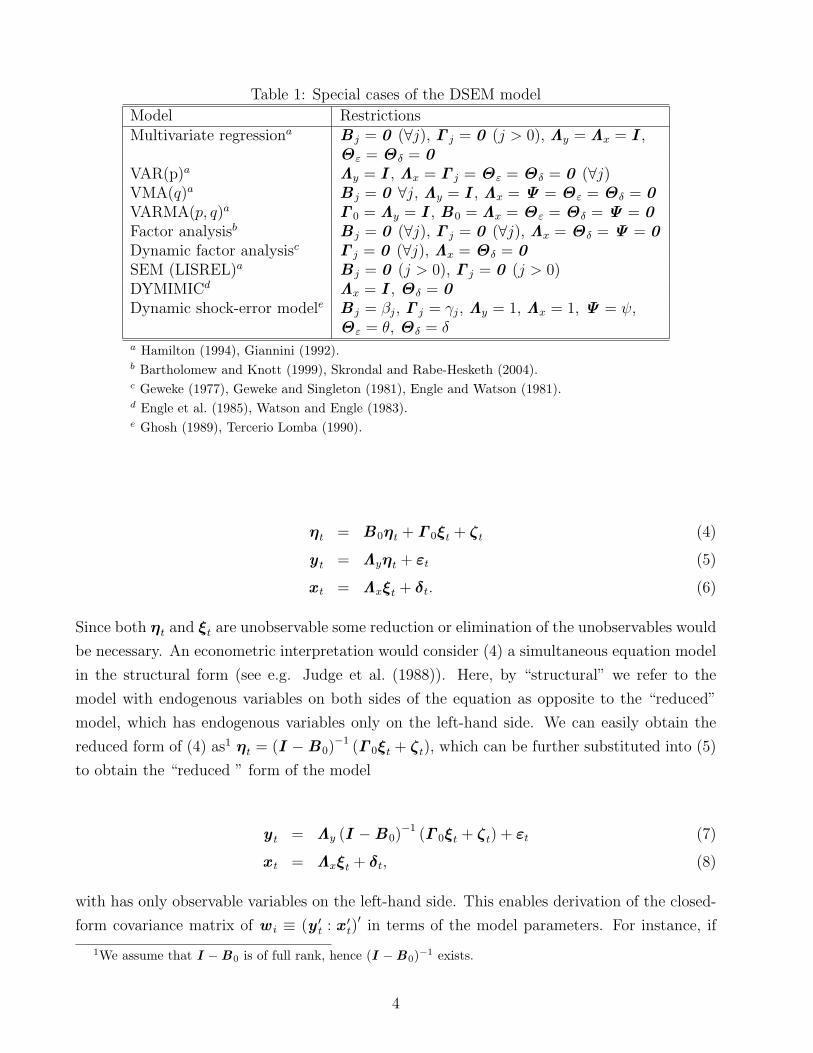
Table 1: Special cases of the DSEM model

Model RestrictionsMultivariate regressiona B j = 0 (∀j), Γ j = 0 (j > 0), Λy = Λx = I ,

Θε = Θδ = 0VAR(p)a Λy = I , Λx = Γ j = Θε = Θδ = 0 (∀j)VMA(q)a B j = 0 ∀j, Λy = I , Λx = Ψ = Θε = Θδ = 0VARMA(p, q)a Γ 0 = Λy = I , B0 = Λx = Θε = Θδ = Ψ = 0Factor analysisb B j = 0 (∀j), Γ j = 0 (∀j), Λx = Θδ = Ψ = 0Dynamic factor analysisc Γ j = 0 (∀j), Λx = Θδ = 0SEM (LISREL)a B j = 0 (j > 0), Γ j = 0 (j > 0)DYMIMICd Λx = I , Θδ = 0Dynamic shock-error modele B j = βj, Γ j = γj, Λy = 1, Λx = 1, Ψ = ψ,

Θε = θ, Θδ = δa Hamilton (1994), Giannini (1992).b Bartholomew and Knott (1999), Skrondal and Rabe-Hesketh (2004).c Geweke (1977), Geweke and Singleton (1981), Engle and Watson (1981).d Engle et al. (1985), Watson and Engle (1983).e Ghosh (1989), Tercerio Lomba (1990).

ηt = B0ηt + Γ 0ξt + ζt (4)

y t = Λyηt + εt (5)

x t = Λxξt + δt. (6)

Since both ηt and ξt are unobservable some reduction or elimination of the unobservables would

be necessary. An econometric interpretation would consider (4) a simultaneous equation model

in the structural form (see e.g. Judge et al. (1988)). Here, by “structural” we refer to the

model with endogenous variables on both sides of the equation as opposite to the “reduced”

model, which has endogenous variables only on the left-hand side. We can easily obtain the

reduced form of (4) as1 ηt = (I −B0)−1 (Γ 0ξt + ζt), which can be further substituted into (5)

to obtain the “reduced ” form of the model

y t = Λy (I −B0)−1 (Γ 0ξt + ζt) + εt (7)

x t = Λxξt + δt, (8)

with has only observable variables on the left-hand side. This enables derivation of the closed-

form covariance matrix of w i ≡ (y ′t : x ′t)′ in terms of the model parameters. For instance, if

1We assume that I −B0 is of full rank, hence (I −B0)−1 exists.

4

w i ∼ N (µ,Σ), it follows that (T − 1)S ∼ W (T − 1,Σ ), where S = 1T−1

∑Ti=1 w iw

′i is the

empirical covariance matrix, and W denotes the Wishart distribution.2

However, the same approach cannot be straightforwardly applied to the DSEM model (1)–

(3), which contains lagged latent variables. Namely, the reduction from (4)–(6) to (7)–(8) would

not eliminate the lagged values of ηt.

The likelihood function for a sample of T observations generated by a dynamic model

specified for a typical time point t (i.e. in “t-notation), such as (1)–(3), can be obtained

recursively by sequential conditioning (Hamilton 1994, p. 118). In this approach we would

write down the probability density function of the first sample observation (t = 1) conditional

on the initial r = max(p, q) observations and then obtain the density for the second sample

observation (t = 2), conditional on the the first, etc. until the last observation (t = T ). The

likelihood function would then be obtained as a product of the T sequentially derived conditional

densities, assuming conditional independence of the successive observations. However, this

approach is not feasible for complex multivariate dynamic models with latent variables as

sequential conditioning soon becomes intractable.

An alternative approach leading to an equivalent expression for the likelihood function would

be to assume that the observed sample came from a T -variate (e.g. Gaussian) distribution,

having multivariate density function, from which the sample likelihood immediately follows

(Hamilton 1994, p. 119). This approach might not be easily applicable to dynamic latent

variable models for which we generally wish to obtain the likelihood in separated form, i.e.,

with all unknown parameters placed in the covariance matrix, separated from the observed

data vectors. Without such separation we would be left with T “missing” observations on the

latent vectors ηt and ξt instead of only their unknown second moment matrices.

We can solve this problem by specifying a DSEM model (1)–(3) for the time series process

that started at time t = 1 and was observed till time t = T using a “T -notation” defined in

Table 2. The vector ∗T1 can then be taken as a single realization from a T -variate distribution.

Working with the model in T -notation will enable us to “reduce” the model (1)–(3) and

obtain a closed form covariance structure and hence a closed form likelihood of the general

DSEM model.

We make the following simplifying assumption about the pre-sample (initial) observations.

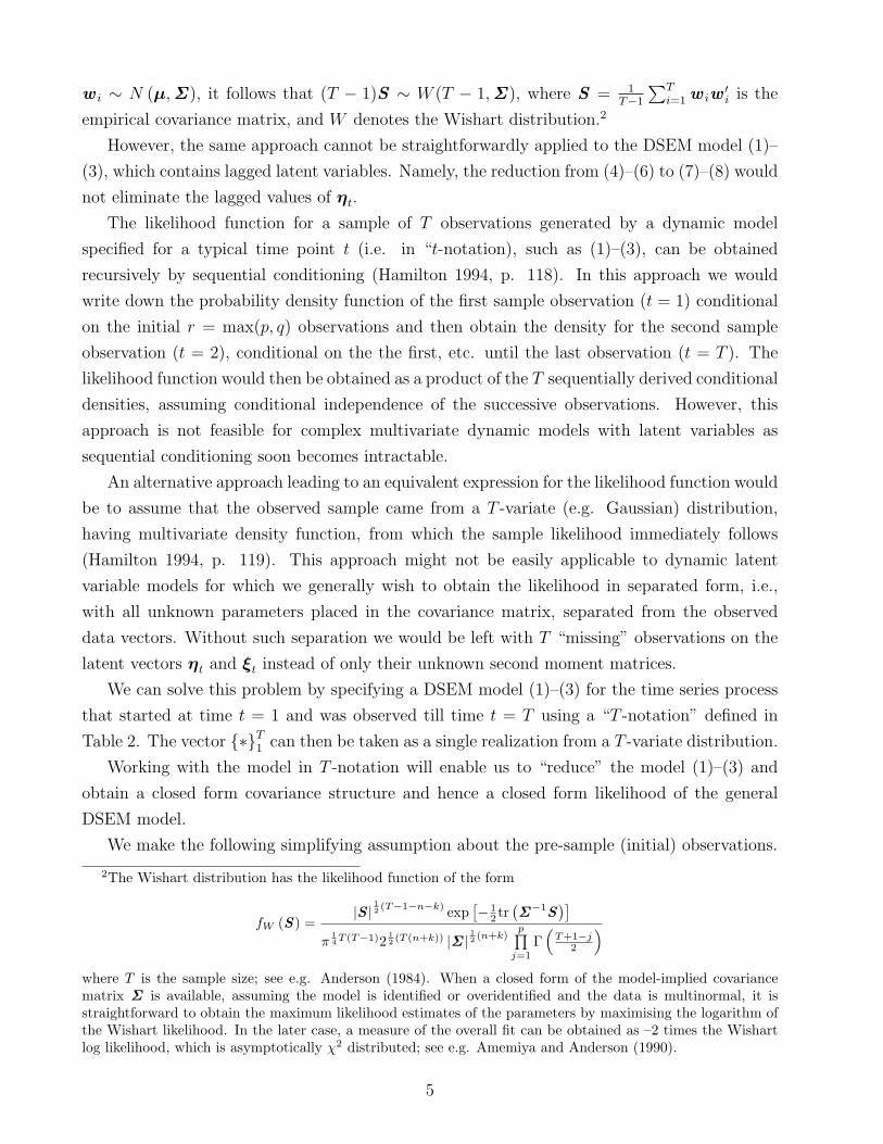
2The Wishart distribution has the likelihood function of the form

fW (S) =|S | 12 (T−1−n−k) exp

[− 12 tr

(Σ−1S

)]

π14 T (T−1)2

12 (T (n+k)) |Σ | 12 (n+k)

p∏j=1

Γ(

T+1−j2

)

where T is the sample size; see e.g. Anderson (1984). When a closed form of the model-implied covariancematrix Σ is available, assuming the model is identified or overidentified and the data is multinormal, it isstraightforward to obtain the maximum likelihood estimates of the parameters by maximising the logarithm ofthe Wishart likelihood. In the later case, a measure of the overall fit can be obtained as –2 times the Wishartlog likelihood, which is asymptotically χ2 distributed; see e.g. Amemiya and Anderson (1990).

5

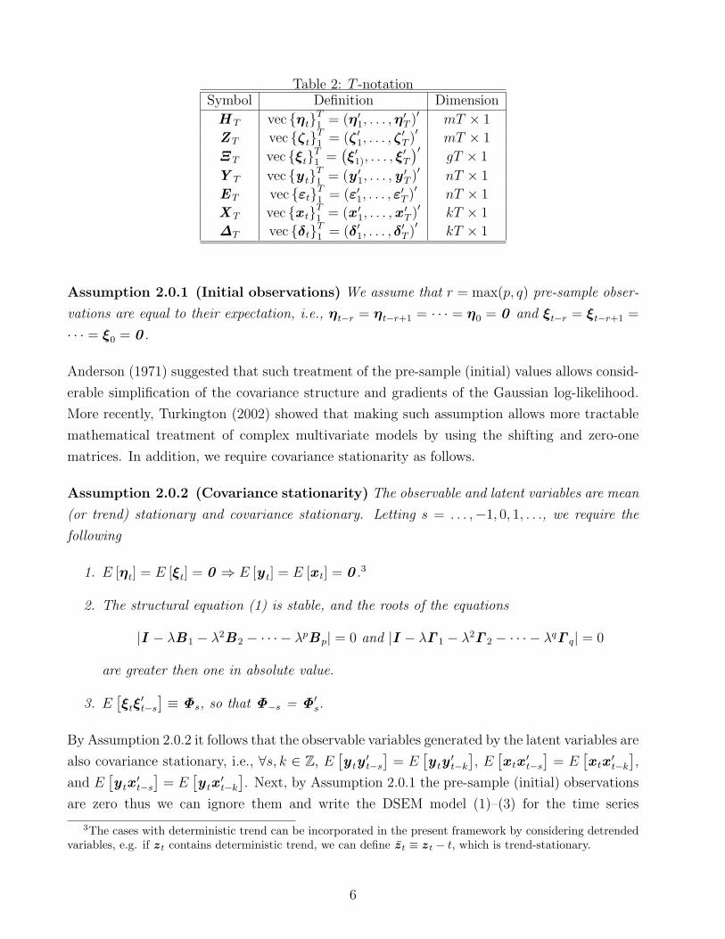
Table 2: T -notationSymbol Definition Dimension

H T vec ηtT1 = (η′1, . . . , η

′T )′ mT × 1

Z T vec ζtT1 = (ζ ′1, . . . , ζ

′T )′

mT × 1

Ξ T vec ξtT1 =

(ξ′1), . . . , ξ

′T

)′gT × 1

Y T vec y tT1 = (y ′1, . . . ,y

′T )′ nT × 1

ET vec εtT1 = (ε′1, . . . , ε

′T )′ nT × 1

X T vec x tT1 = (x ′1, . . . ,x

′T )′ kT × 1

∆T vec δtT1 = (δ′1, . . . , δ

′T )′

kT × 1

Assumption 2.0.1 (Initial observations) We assume that r = max(p, q) pre-sample obser-

vations are equal to their expectation, i.e., ηt−r = ηt−r+1 = · · · = η0 = 0 and ξt−r = ξt−r+1 =

· · · = ξ0 = 0 .

Anderson (1971) suggested that such treatment of the pre-sample (initial) values allows consid-

erable simplification of the covariance structure and gradients of the Gaussian log-likelihood.

More recently, Turkington (2002) showed that making such assumption allows more tractable

mathematical treatment of complex multivariate models by using the shifting and zero-one

matrices. In addition, we require covariance stationarity as follows.

Assumption 2.0.2 (Covariance stationarity) The observable and latent variables are mean

(or trend) stationary and covariance stationary. Letting s = . . . ,−1, 0, 1, . . ., we require the

following

1. E [ηt] = E [ξt] = 0 ⇒ E [y t] = E [x t] = 0 .3

2. The structural equation (1) is stable, and the roots of the equations

|I − λB1 − λ2B2 − · · · − λpBp| = 0 and |I − λΓ 1 − λ2Γ 2 − · · · − λqΓ q| = 0

are greater then one in absolute value.

3. E[ξtξ

′t−s

] ≡ Φs, so that Φ−s = Φ′s.

By Assumption 2.0.2 it follows that the observable variables generated by the latent variables are

also covariance stationary, i.e., ∀s, k ∈ Z, E[y ty

′t−s

]= E

[y ty

′t−k

], E

[x tx

′t−s

]= E

[x tx

′t−k

],

and E[y tx

′t−s

]= E

[y tx

′t−k

]. Next, by Assumption 2.0.1 the pre-sample (initial) observations

are zero thus we can ignore them and write the DSEM model (1)–(3) for the time series

3The cases with deterministic trend can be incorporated in the present framework by considering detrendedvariables, e.g. if z t contains deterministic trend, we can define z t ≡ z t − t, which is trend-stationary.

6

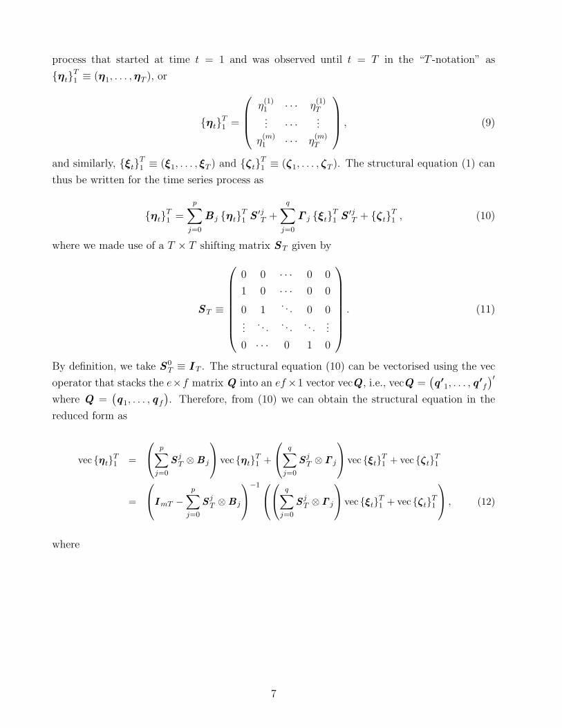
process that started at time t = 1 and was observed until t = T in the “T -notation” as

ηtT1 ≡ (η1, . . . , ηT ), or

ηtT1 =

η(1)1 · · · η

(1)T

... · · · ...

η(m)1 · · · η

(m)T

, (9)

and similarly, ξtT1 ≡ (ξ1, . . . , ξT ) and ζtT

1 ≡ (ζ1, . . . , ζT ). The structural equation (1) can

thus be written for the time series process as

ηtT1 =

p∑j=0

B j ηtT1 S ′j

T +

q∑j=0

Γ j ξtT1 S ′j

T + ζtT1 , (10)

where we made use of a T × T shifting matrix ST given by

ST ≡

0 0 · · · 0 0

1 0 · · · 0 0

0 1. . . 0 0

.... . . . . . . . .

...

0 · · · 0 1 0

. (11)

By definition, we take S 0T ≡ I T . The structural equation (10) can be vectorised using the vec

operator that stacks the e×f matrix Q into an ef×1 vector vecQ , i.e., vecQ =(q 01, . . . , q

0f

)′where Q =

(q1, . . . , q f

). Therefore, from (10) we can obtain the structural equation in the

reduced form as

vec ηtT1 =

p∑

j=0

S jT ⊗B j

vec ηtT

1 +

q∑

j=0

S jT ⊗ Γ j

vec ξtT

1 + vec ζtT1

=

ImT −

p∑

j=0

S jT ⊗B j

−1

q∑

j=0

S jT ⊗ Γ j

vec ξtT

1 + vec ζtT1

, (12)

where

7

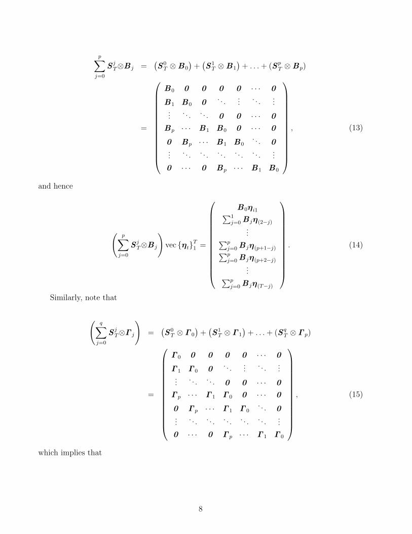
p∑j=0

S jT⊗B j =

(S 0

T ⊗B0

)+

(S 1

T ⊗B1

)+ . . . + (S p

T ⊗Bp)

=

B0 0 0 0 0 · · · 0

B1 B0 0. . .

.... . .

......

. . . . . . 0 0 · · · 0

Bp · · · B1 B0 0 · · · 0

0 Bp · · · B1 B0. . . 0

.... . . . . . . . . . . . . . .

...

0 · · · 0 Bp · · · B1 B0

, (13)

and hence

(p∑

j=0

S jT⊗B j

)vec ηtT

1 =

B0ηi1∑1j=0 B jη(2−j)

...∑pj=0 B jη(p+1−j)∑pj=0 B jη(p+2−j)

...∑pj=0 B jη(T−j)

. (14)

Similarly, note that

(q∑

j=0

S jT⊗Γ j

)=

(S 0

T ⊗ Γ 0

)+

(S 1

T ⊗ Γ 1

)+ . . . + (S q

T ⊗ Γ p)

=

Γ 0 0 0 0 0 · · · 0

Γ 1 Γ 0 0. . .

.... . .

......

. . . . . . 0 0 · · · 0

Γ p · · · Γ 1 Γ 0 0 · · · 0

0 Γ p · · · Γ 1 Γ 0. . . 0

.... . . . . . . . . . . . . . .

...

0 · · · 0 Γ p · · · Γ 1 Γ 0

, (15)

which implies that

8

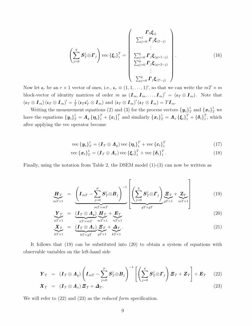
(q∑

j=0

S jT⊗Γ j

)vec ξtT

1 =

Γ 0ξi1∑1j=0 Γ jξ(2−j)

...∑qj=0 Γ jξ(q+1−j)∑qj=0 Γ jξ(q+2−j)

...∑qj=0 Γ jξ(T−j)

. (16)

Now let ιr be an r× 1 vector of ones, i.e., ιr ≡ (1, 1, . . . , 1)′, so that we can write the mT ×m

block-vector of identity matrices of order m as (Im, Im, . . . , Im)′ = (ιT ⊗ Im). Note that

(ιT ⊗ Im) (ιT ⊗ Im)′ = 1T

(ιT ι′T ⊗ Im) and (ιT ⊗ Im)′ (ιT ⊗ Im) = TIm.

Writing the measurement equations (2) and (3) for the process vectors y t1T and x t1

T we

have the equations y t1T = Λy ηtT

1 + εtT1 and similarly x t1

T = Λx ξtT1 + δtT

1 , which

after applying the vec operator become

vec y t1T = (I T ⊗Λy) vec ηtT

1 + vec εtT1 (17)

vec x t1T = (I T ⊗Λx) vec ξtT

1 + vec δtT1 . (18)

Finally, using the notation from Table 2, the DSEM model (1)-(3) can now be written as

H T︸︷︷︸mT×1

=

(ImT −

p∑j=0

S jT⊗B j

)−1

︸ ︷︷ ︸mT×mT

(q∑

j=0

S jT⊗Γ j

)

︸ ︷︷ ︸gT×gT

Ξ T︸︷︷︸gT×1

+ ZT︸︷︷︸mT×1

(19)

Y T︸︷︷︸nT×1

= (I T ⊗Λy)︸ ︷︷ ︸nT×mT

H T︸︷︷︸mT×1

+ ET︸︷︷︸nT×1

(20)

X T︸︷︷︸kT×1

= (I T ⊗Λx)︸ ︷︷ ︸kT×gT

Ξ T︸︷︷︸gT×1

+ ∆T︸︷︷︸kT×1

. (21)

It follows that (19) can be substituted into (20) to obtain a system of equations with

observable variables on the left-hand side

Y T = (I T ⊗Λy)

(ImT −

p∑j=0

S jT⊗B j

)−1 [(q∑

j=0

S jT⊗Γ j

)Ξ T + Z T

]+ ET (22)

X T = (I T ⊗Λx)Ξ T + ∆T . (23)

We will refer to (22) and (23) as the reduced form specification.

9

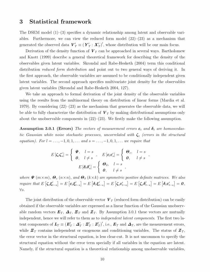
3 Statistical framework

The DSEM model (1)–(3) specifies a dynamic relationship among latent and observable vari-

ables. Furthermore, we can view the reduced form model (22)–(23) as a mechanism that

generated the observed data V ′T ≡ (Y ′

T : X ′T )′, whose distribution will be our main focus.

Derivation of the density function of V T can be approached in several ways. Bartholomew

and Knott (1999) describe a general theoretical framework for describing the density of the

observables given latent variables. Skrondal and Rabe-Hesketh (2004) term this conditional

distribution reduced form distribution and point out to two general ways of deriving it. In

the first approach, the observable variables are assumed to be conditionally independent given

latent variables. The second approach specifies multivariate joint density for the observables

given latent variables (Skrondal and Rabe-Hesketh 2004, 127).

We take an approach to formal derivation of the joint density of the observable variables

using the results from the multinormal theory on distribution of linear forms (Mardia et al.

1979). By considering (22)–(23) as the mechanism that generates the observable data, we will

be able to fully characterize the distribution of V T by making distributional assumptions only

about the unobservable components in (22)–(23). We firstly make the following assumption.

Assumption 3.0.1 (Errors) The vectors of measurement errors εt and δt are homoscedas-

tic Gaussian white noise stochastic processes, uncorrelated with ζt (errors in the structural

equation). For l = . . . ,−1, 0, 1, . . . and s = . . . ,−1, 0, 1, . . . we require that

E [ζlζ′s] =

Ψ , l = s

0 , l 6= s, E [εlε

′s] =

Θε, l = s

0 , l 6= s,

E [δlδ′s] =

Θδ, l = s

0 , l 6= s,

where Ψ (m×m), Θε (n×n), and Θδ (k×k) are symmetric positive definite matrices. We also

require that E[ζtξ

′t−s

]= E

[εtξ

′t−s

]= E

[δtξ

′t−s

]= E

[ζtε

′t−s

]= E

[ζtδ

′t−s

]= E

[δtε

′t−s

]= 0 ,

∀s.

The joint distribution of the observable vector V T (reduced form distribution) can be easily

obtained if the observable variables are expressed as a linear function of the Gaussian unobserv-

able random vectors ET , ∆T , Ξ T and Z T . By Assumption 3.0.1 these vectors are mutually

independent, hence we will refer to them as to independent latent components. The first two la-

tent components of LT ≡ (E ′T : ∆′

T : Ξ ′T : Z ′

T )′, i.e., ET and ∆T , are the measurement errors,

while Ξ T contains independent or exogenous and conditioning variables. The status of Z T ,

the error vector in the structural equation, is less clear-cut. It is not uncommon to specify the

structural equation without the error term specially if all variables in the equation are latent.

Namely, if the structural equation is a theoretical relationship among unobservable variables,

10

hence something that is assumed to be true in population but is not directly observable, then

it might be dubious what is the source of such error. A reasonable explanation would be that

Z T contains all other un-modelled variables, hence it is itself a latent variable. Clearly, to

justify the omission of such other variables we need to make very strict assumptions about Z T

requiring it to be a homoscedastic white noise process uncorrelated with independent variables

and measurement errors. Thus, statistical properties of Z T should be the same as those of a

classical stochastic error term, though Z T might be interpreted as a composite of “irrelevant”

latent variables.

To fully characterize the distribution of the observable variables we only need to make

additional assumptions about the marginal multinormal densities for the independent latent

components.

Assumption 3.0.2 (Distribution) Let Ξ T ∼ NgT (0 ,ΣΞ), Z T ∼ NmT (0 , I T ⊗Ψ), ET ∼NnT (0 , I T ⊗Θε), and ∆T ∼ NkT (0 , I T ⊗Θδ). Since ET , ∆T , Ξ T , and Z T are mutually

independent, E [Ξ TZ′T ], E [Ξ TE

′T ], E [Z TE

′T ], E [Ξ T∆

′T ], and E [Z T∆

′T ] are all zero with

joint density

ET

∆T

Ξ T

Z T

︸ ︷︷ ︸LT

∼ N(n+k+g+m)T

0 ,

I T ⊗Θε 0 0 0

0 I T ⊗Θδ 0 0

0 0 ΣΞ 0

0 0 0 I T ⊗Ψ

︸ ︷︷ ︸ΣL

. (24)

Given Assumptions 3.0.1 and 3.0.2 we can infer the distribution of any linear form in LT

using the following result from the multinormal theory.

Proposition 3.0.3 If x ∼ Np (µ,Σ ) and if y = Ax + c, where A is any q × p matrix and c

is any q-vector, then y ∼ Nq (Aµ + c,AΣA′).

Proof See Theorem 3.1.1. and Theorem 3.2.1 of Mardia et al. (1979, pg. 61-62).

Q.E.D.

Using the above result, and defining the following notation makes possible to obtain different

versions of the general DSEM model as simple linear forms in LT .

Definition 3.0.4 (Parameters) Using the simplifying notation

11

A(1)Ξ︸︷︷︸

nT×mT

≡ (I T ⊗Λy)︸ ︷︷ ︸(nT×mT )

(ImT −

p∑j=0

S jT⊗B j

)−1

︸ ︷︷ ︸mT×mT

and A(2)Ξ︸︷︷︸

mT×gT

≡q∑

j=0

S jT⊗Γ j

︸ ︷︷ ︸mT×gT

⇒ A(1)Ξ A

(2)Ξ︸ ︷︷ ︸

nT×gT

,

we define the following matrices of parameters

P ≡(

A(1)Ξ A

(2)Ξ A

(1)Ξ

I T ⊗Λx 0

), K S ≡

(I (n+k)T P

0 I (g+m)T

), KR ≡

(I (n+k)T P

).

Denote a linear form by F(∗)T and consider the following two forms

F(S)T = K SLT (25)

F(R)T = KRLT . (26)

It is easy to see that (26) corresponds to the reduced model (22)–(23) hence F(R)T = V T

can be interpreted as the observable data generated by the linear form KRLT . On the other

hand, F(S)T includes the latent variables Ξ T and Z T as endogenous or dependent. Models with

both observable and latent variables treated as endogenous are commonly termed “structural”

(Ainger et al. 1984, Cheng and Van Ness 1999, Wansbeek and Meijer 2000), though this can

be easily confused with the structural form of the simultaneous equation system we referred to

previously. To avoid confusion with terminology, we will refer to (26) as the reduced structural

latent form (RSLF) model while we will term (25) structural latent form (SLF) model. The

emphases on both models being “latent” will distinguish these forms from the errors-in-variables

models that we will analyse in section §3.4.

We treat all variables except Ξ t as random, while we will consider both cases with random

and fixed Ξ t. The later case requires special consideration as it is obviously not encompassed

by the Assumptions 3.0.1 and 3.0.2, which assume random Ξ t. The model with fixed Ξ t is

generally known as the functional model (Wansbeek and Meijer 2000, p. 11) in which no explicit

assumptions regarding the distribution of Ξ T are made and its elements are considered to be

unknown fixed parameters or “incidental parameters” (Cheng and Van Ness 1999, p. 3).

Since we can assume that the observable data V T were generated by linear forms (25)

and (26), or equivalently by the reduced-form equations (22) and (23), we can let F(S)T ≡

(Y ′T : X ′

T : Ξ ′T : Z ′

T ) and F(R)T ≡ (Y ′

T : X ′T ). Hence the distribution of the observable vari-

ables will be the same as the distribution of the linear form form F(R)T . Now, by Proposition

(3.0.3) it follows that

12

F(S)T ∼ N(n+k+g+m)T (0 ,K SΣLK

′S) (27)

F(R)T ∼ N(n+k)T (0 ,KRΣLK

′R) (28)

The difference between the structural (25) and the reduced (26) form is important insofar

(26) does not model latent variables, i.e., it takes all latent components as independent or

exogenous. It might be appealing to think of the reduced model (26) as conditional (on latent

variables), however, this turns out to be a marginal model with Ξ T and Z T marginalized or

integrated out of the likelihood, as we will show in section §3.1.

A common argument in the literature (Aigner et al. 1984, Wansbeek and Meijer 2000) used

to justify this marginalization is unobservability of the latent variables that necessitates their

removal from the model and focusing on (26) rather then on (25). This justification is apparently

motivated by the choice of the estimation methods (e.g. Wishart maximum likelihood), which

can handle only the reduced form model (26). However, recursive estimation methods using the

Kalman filter (Kalman 1960) and the expectation maximisation (EM) algorithm (Dampster et

al. 1977) are potentially capable of handling models such as (25) and estimating the values of

the unobservable variables (Harvey 1989, Durbin and Koopman 2001).

Therefore, marginalization of this kind might not be justified in general, and this matter

requires a more formal approach. To tackle this issue, we firstly define the notion of weak

exogeneity on the lines of Engle et al. (1983) as follows.

Definition 3.0.5 (Weak exogeneity) Let x and z be random vectors with joint density

function fxz (x , z ; ω), which can be factorised as the product of the conditional density function

of x given z and the marginal density function of z ,

fxz (x , z ; ω) = fx|z (x |z ; ω1) fz (z ; ω2) , (29)

where ω ≡ (ω′1 : ω′

2)′ is the parameter vector and Ω1 and Ω2 are parameter spaces of ω1 and

ω2, respectively, with product parameter space Ω1×Ω2 = (ω1, ω2) : ω1 ∈ Ω1, ω2 ∈ Ω2 such

that ω1 and ω2 have no elements in common, i.e., ω1 ∩ ω2 = φ. Then, z is weakly exogenous

for ω1.

The practical implication of Definition 3.0.5 is that if z is weakly exogenous for ω1, the

joint density fx|z (x |z ; ω1) contains all information about ω1 and thus the marginal density of

z fz (z ; ω2) is uninformative about ω1. The following definition partitions the parameters of

the DSEM model (1)–(3) into non-overlapping sub-vectors.

Definition 3.0.6 Parameters Let the vector θ include all unknown parameters of the DSEM

model (1)–(3). We define the following partition

13

θ ≡ (θ′(Bi) : θ′(Γj) : θ′(Λy) : θ′(Λx) : θ′(Φj) : θ′(Ψ) : θ′(Θε) : θ′(Θδ)

)′. (30)

where θ(Bi) ≡ vecB i, θ(Γj) ≡ vecΓ j, θ(Λy) ≡ vecΛy, θ(Λx) ≡ vecΛx, θ(Φj) ≡ vechΦj,

θ(Ψ) ≡ vechΨ , θ(Θε) ≡ vech θε, and θ(Θδ) ≡ vech θδ; i = 0, . . . , p, j = 0, . . . q.4

3.1 Structural latent form (SLF)

Given the linear form (25) or the SLF model, we are now interested whether the conditional

model for the observable variables (V T ) given the latent variables contains sufficient informa-

tion to identify and estimate the model parameters.

By Assumption 3.0.2 and Proposition 3.0.3 the log-likelihood function of the SLF model is

of the form

`S

(F

(S)T ; θ

)= α− 1

2ln |K SΣLK

′S| −

1

2trL′(L)

T (K SΣLK′S)−1

F(S)T , (31)

where α ≡ −(n + k + g + m)T2

ln(2π). The following proposition shows that the log-likelihood

(31) can be decomposed into conditional and marginal log-likelihoods hence the likelihood can

be expressed as the product of the form given in Definition 3.0.5.

Proposition 3.1.1 (Likelihood decomposition) Let (31) be the log-likelihood of the struc-

tural model (25), i.e., the joint log-likelihood of the random vector F(S)T . Denote the condi-

tional log-likelihood of V T given Ξ T and Z T by `V |Ξ,Z (V T |Ξ T ,Z T ; θ1), and the marginal

log-likelihoods of Ξ T and Z T by `Ξ (Ξ T ; θ2) and `Z (Z T ; θ3), respectively. Then (31) can be

factorised as

`S

(F

(S)T ; θ

)= `V |Ξ,Z (V T |Ξ T ,Z T ; θ1) + `Ξ (Ξ T ; θ2) + `Z (Z T ; θ3) , (32)

where θ1 ≡(θ′(Bi) : θ′(Γj) : θ′(Λy) : θ′(Λx) : θ′(Θε) : θ′(Θδ)

)′, θ2 ≡ θ(Φj), and θ3 ≡ θ(Ψ). There-

fore, Ξ T and Z T are weakly exogenous for θ1.

Proof See Appendix A.

Proposition 3.1.1 has some interesting implications. Firstly, if all variables were observable, a

conditional model with the log-likelihood `V |Ξ,Z (V T |Ξ T ,Z T ; θ1) would provide all information

about the the parameters of interest. As remarked above, some recursive algorithms might

handle certain special cases with Ξ T and Z T unobservable, hence by Proposition 32 methods

based on the conditional likelihood might be justified.

4We make use of the vech operator for the symmetric matrices, which stacks the columns on and below thediagonal.

14

However, larger models might contain too many unknowns which renders the conditional

model unfeasible. The commonly used covariance structure and GMM estimators (Hall 2005)

require a likelihood in the separated form since these methods aim at minimising the distance

between the theoretical and empirical moments. Naturally, to make GMM-type of methods

feasible, full separation of the latent and observable variables is necessary. This means the

“modelled” variables must be observable and expressible as functions of unobservable variables

and unknown parameters.

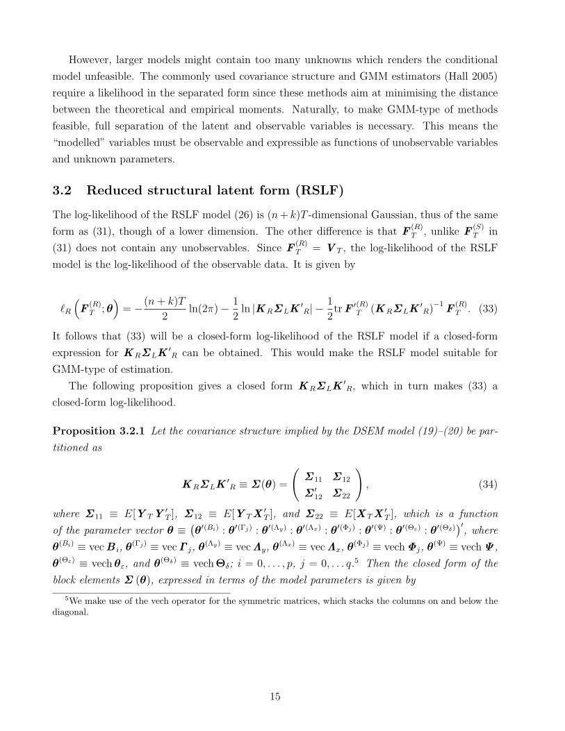
3.2 Reduced structural latent form (RSLF)

The log-likelihood of the RSLF model (26) is (n + k)T -dimensional Gaussian, thus of the same

form as (31), though of a lower dimension. The other difference is that F(R)T , unlike F

(S)T in

(31) does not contain any unobservables. Since F(R)T = V T , the log-likelihood of the RSLF

model is the log-likelihood of the observable data. It is given by

`R

(F

(R)T ; θ

)= −(n + k)T

2ln(2π)− 1

2ln |KRΣLK

′R| − 1

2trF ′(R)

T (KRΣLK′R)−1

F(R)T . (33)

It follows that (33) will be a closed-form log-likelihood of the RSLF model if a closed-form

expression for KRΣLK′R can be obtained. This would make the RSLF model suitable for

GMM-type of estimation.

The following proposition gives a closed form KRΣLK′R, which in turn makes (33) a

closed-form log-likelihood.

Proposition 3.2.1 Let the covariance structure implied by the DSEM model (19)–(20) be par-

titioned as

KRΣLK′R ≡ Σ (θ) =

(Σ 11 Σ 12

Σ ′12 Σ 22

), (34)

where Σ 11 ≡ E[Y TY′T ], Σ 12 ≡ E[Y TX

′T ], and Σ 22 ≡ E[X TX

′T ], which is a function

of the parameter vector θ ≡ (θ′(Bi) : θ′(Γj) : θ′(Λy) : θ′(Λx) : θ′(Φj) : θ′(Ψ) : θ′(Θε) : θ′(Θδ)

)′, where

θ(Bi) ≡ vecB i, θ(Γj) ≡ vecΓ j, θ(Λy) ≡ vecΛy, θ(Λx) ≡ vecΛx, θ(Φj) ≡ vechΦj, θ(Ψ) ≡ vechΨ ,

θ(Θε) ≡ vech θε, and θ(Θδ) ≡ vechΘδ; i = 0, . . . , p, j = 0, . . . q.5 Then the closed form of the

block elements Σ (θ), expressed in terms of the model parameters is given by

5We make use of the vech operator for the symmetric matrices, which stacks the columns on and below thediagonal.

15

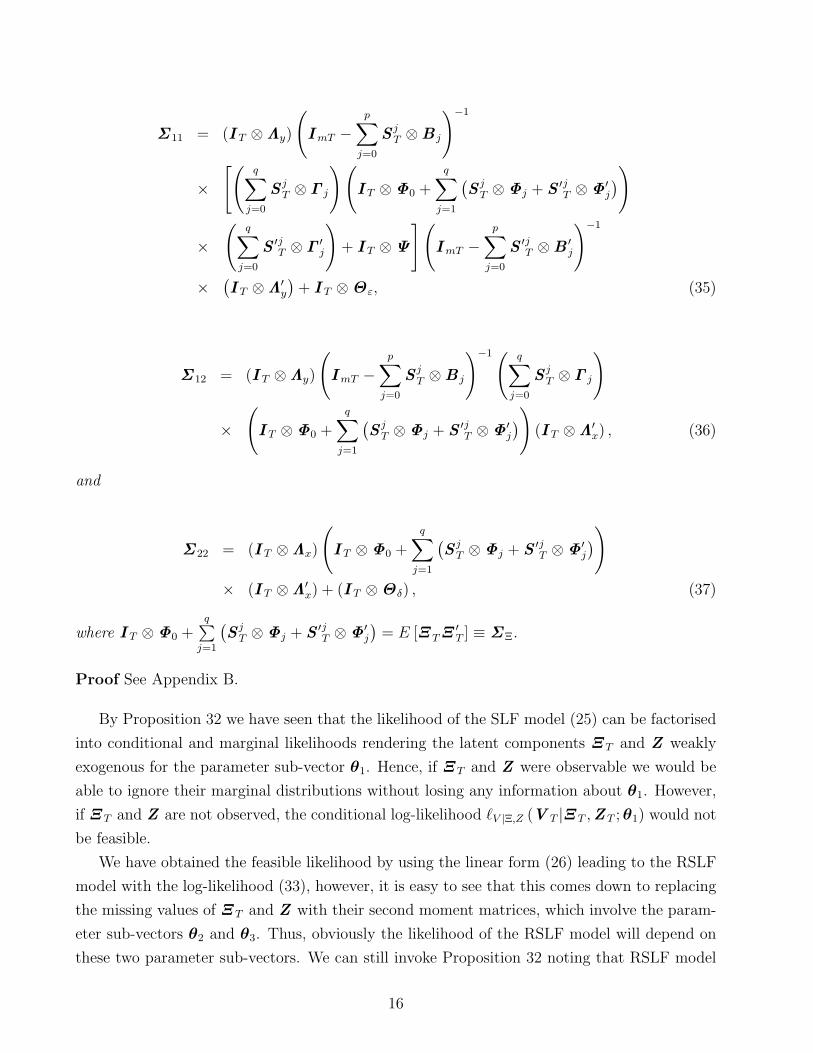
Σ 11 = (I T ⊗Λy)

(ImT −

p∑j=0

S jT ⊗B j

)−1

×[(

q∑j=0

S jT ⊗ Γ j

)(I T ⊗Φ0 +

q∑j=1

(S j

T ⊗Φj + S ′jT ⊗Φ′

j

))

×(

q∑j=0

S ′jT ⊗ Γ ′

j

)+ I T ⊗Ψ

](ImT −

p∑j=0

S ′jT ⊗B ′

j

)−1

× (I T ⊗Λ′

y

)+ I T ⊗Θε, (35)

Σ 12 = (I T ⊗Λy)

(ImT −

p∑j=0

S jT ⊗B j

)−1 (q∑

j=0

S jT ⊗ Γ j

)

×(I T ⊗Φ0 +

q∑j=1

(S j

T ⊗Φj + S ′jT ⊗Φ′

j

))

(I T ⊗Λ′x) , (36)

and

Σ 22 = (I T ⊗Λx)

(I T ⊗Φ0 +

q∑j=1

(S j

T ⊗Φj + S ′jT ⊗Φ′

j

))

× (I T ⊗Λ′x) + (I T ⊗Θδ) , (37)

where I T ⊗Φ0 +q∑

j=1

(S j

T ⊗Φj + S ′jT ⊗Φ′

j

)= E [Ξ TΞ

′T ] ≡ ΣΞ.

Proof See Appendix B.

By Proposition 32 we have seen that the likelihood of the SLF model (25) can be factorised

into conditional and marginal likelihoods rendering the latent components Ξ T and Z weakly

exogenous for the parameter sub-vector θ1. Hence, if Ξ T and Z were observable we would be

able to ignore their marginal distributions without losing any information about θ1. However,

if Ξ T and Z are not observed, the conditional log-likelihood `V |Ξ,Z (V T |Ξ T ,Z T ; θ1) would not

be feasible.

We have obtained the feasible likelihood by using the linear form (26) leading to the RSLF

model with the log-likelihood (33), however, it is easy to see that this comes down to replacing

the missing values of Ξ T and Z with their second moment matrices, which involve the param-

eter sub-vectors θ2 and θ3. Thus, obviously the likelihood of the RSLF model will depend on

these two parameter sub-vectors. We can still invoke Proposition 32 noting that RSLF model

16

(26) is a simple reducing linear transformation of the SLF model (25) to justify estimation of

θ1 using the RSLF likelihood. However, in this case we will also need to estimate θ2 and θ3.

In conclusion, while weak exogeneity in the sense of Definition 3.0.5 holds, we still need to

estimate θ2 and θ3 along θ1, which will require additional knowledge about θ in the form of

parametric restrictions, which cannot be inferred from data alone.

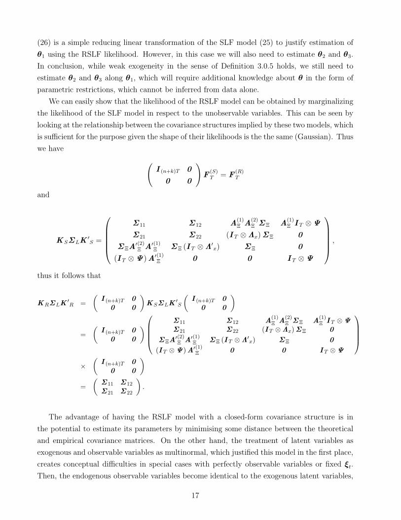
We can easily show that the likelihood of the RSLF model can be obtained by marginalizing

the likelihood of the SLF model in respect to the unobservable variables. This can be seen by

looking at the relationship between the covariance structures implied by these two models, which

is sufficient for the purpose given the shape of their likelihoods is the the same (Gaussian). Thus

we have

(I (n+k)T 0

0 0

)F

(S)T = F

(R)T

and

K SΣLK′S =

Σ 11 Σ 12 A(1)Ξ A

(2)Ξ ΣΞ A

(1)Ξ I T ⊗Ψ

Σ 21 Σ 22 (I T ⊗Λx)ΣΞ 0

ΣΞA′(2)Ξ A′(1)

Ξ ΣΞ (I T ⊗Λ′x) ΣΞ 0

(I T ⊗Ψ)A′(1)Ξ 0 0 I T ⊗Ψ

,

thus it follows that

KRΣLK′R =

(I (n+k)T 0

0 0

)K SΣLK

′S

(I (n+k)T 0

0 0

)

=(

I (n+k)T 00 0

)

Σ11 Σ12 A(1)Ξ A

(2)Ξ ΣΞ A

(1)Ξ I T ⊗Ψ

Σ21 Σ22 (I T ⊗Λx)ΣΞ 0

ΣΞA′(2)Ξ A′(1)

Ξ ΣΞ (I T ⊗Λ′x) ΣΞ 0

(I T ⊗Ψ)A′(1)Ξ 0 0 I T ⊗Ψ

×(

I (n+k)T 0

0 0

)

=(

Σ11 Σ12

Σ21 Σ22

).

The advantage of having the RSLF model with a closed-form covariance structure is in

the potential to estimate its parameters by minimising some distance between the theoretical

and empirical covariance matrices. On the other hand, the treatment of latent variables as

exogenous and observable variables as multinormal, which justified this model in the first place,

creates conceptual difficulties in special cases with perfectly observable variables or fixed ξt.

Then, the endogenous observable variables become identical to the exogenous latent variables,

17

which contradicts the statistical assumptions behind the RSLF model. It is thus appealing to

entertain the idea behind the errors-in-variables or measurement-errors models (Cheng and Van

Ness 1999) where different approach is taken. We will consider this approach in the following

section by firstly placing it in the same framework with the models discussed so far.

3.3 A restricted RSLF

The approach taken in the errors-in-variables literature is to estimate the structural model (1)

by replacing each latent variable by a single noisy indicator or a “proxy” variable. Usually,

some form of instrumental variables (e.g. other noisy indicators of the latent variables) are

used in estimation with the aim of correcting the resulting errors-in-variables bias, and the

focus is on evaluating and correcting the bias induced by the measurement error (Cheng and

Van Ness 1999).

We will refer to the transformed model in which latent variables are replaced by observable

but noisy indicators as the observed form (OF) model. To study the OF model we will firstly

place it into the general DSEM framework, where each latent variable is measured by multiple

indicators. Choosing one indicator per latent variable and normalizing its coefficient (loading)

to unity leads to a restricted covariance structure and is thus a special case of the (unrestricted)

DSEM covariance structure (34) considered above. Clearly, the unit-loading constrains can be

used to fix the metric of the latent variable, which has only a re-scaling effect, without affecting

the value of the likelihood function.

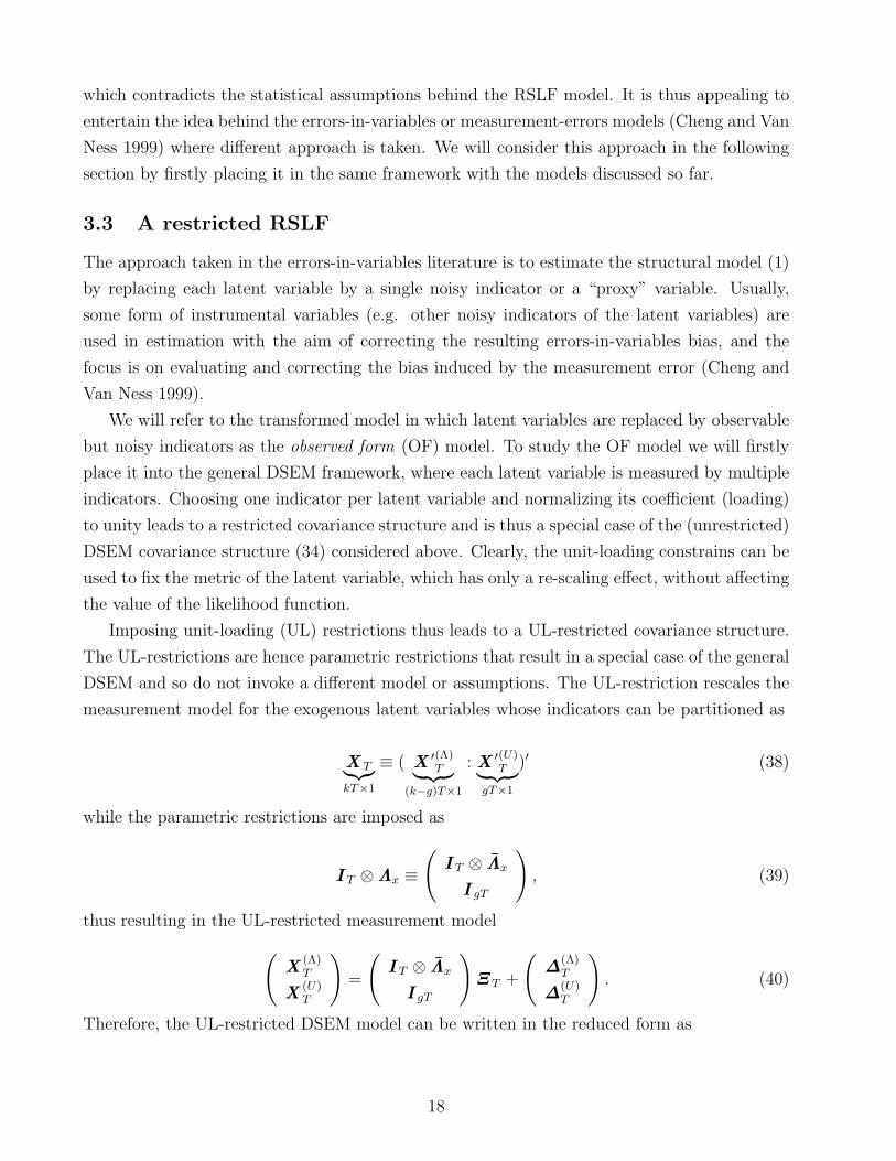
Imposing unit-loading (UL) restrictions thus leads to a UL-restricted covariance structure.

The UL-restrictions are hence parametric restrictions that result in a special case of the general

DSEM and so do not invoke a different model or assumptions. The UL-restriction rescales the

measurement model for the exogenous latent variables whose indicators can be partitioned as

X T︸︷︷︸kT×1

≡ ( X ′(Λ)T︸ ︷︷ ︸

(k−g)T×1

: X ′(U)T︸ ︷︷ ︸

gT×1

)′ (38)

while the parametric restrictions are imposed as

I T ⊗Λx ≡(

I T ⊗ Λx

I gT

), (39)

thus resulting in the UL-restricted measurement model

(X

(Λ)T

X(U)T

)=

(I T ⊗ Λx

I gT

)Ξ T +

(∆

(Λ)T

∆(U)T

). (40)

Therefore, the UL-restricted DSEM model can be written in the reduced form as

18

Y T = (I T ⊗Λy)

(ImT −

p∑j=0

S jT⊗B j

)−1 [(q∑

j=0

S jT⊗Γ j

)Ξ T + Z T

]+ ET (41)

X(Λ)T =

(I T ⊗ Λx

)Ξ T + ∆

(Λ)T (42)

X(U)T = Ξ T + ∆

(U)T , (43)

where we partitioned X T into a gT×1 vector X(U)T and a (k−g)T×1 vector X

(Λ)T . Correspond-

ingly, we have partitioned ∆T into sub-vectors ∆(U)T and ∆

(Λ)T . We partition the measurement

error covariance matrix I T ⊗Θδ as

I T ⊗Θδ ≡(

I T ⊗Θ(ΛΛ)δδ I T ⊗Θ

(ΛU)δδ

I T ⊗Θ(UΛ)δδ I T ⊗Θ

(UU)δδ

), (44)

so ΣL is partitioned as

ΣL =

I T ⊗Θε 0 0 0 0

0 I T ⊗Θ(ΛΛ)δδ I T ⊗Θ

(ΛU)δδ 0 0

0 I T ⊗Θ(UΛ)δδ I T ⊗Θ

(UU)δδ 0 0

0 0 0 ΣΞ 0

0 0 0 0 I T ⊗Ψ

. (45)

Now, if we define

KR ≡(

I (n+k)T P)

, P ≡

A(1)Ξ A

(2)Ξ A

(1)Ξ

I T ⊗ Λx 0

I gT 0

, (46)

it follows that

F(R)T = KRLT , (47)

thus the density of the restricted RSLF model is the same as of the unrestricted model but

with different parametrisation, i.e.,

F(R)T ∼ N(n+k)T

(0 , KRΣLK

′R

), (48)

hence we have the log-likelihood of the form

`R

(F

(R)T ; θ

)= −(n + k)

T

2ln(2π)− 1

2ln

∣∣∣KRΣLK′R

∣∣∣− 1

2tr F

′(R)T

(KRΣLK

′R

)−1

F(R)T . (49)

Next, we partition the covariance matrix (34) corresponding to the partition of the data

vector(Y T : X

(Λ)T : X

(U)T

)as

19

K′RΣLKR ≡

(Σ 11 Σ 12

Σ′12 Σ 22

)=

ΣY Y Σ(Λ)Y X Σ

(U)Y X

Σ(Λ)XY Σ

(Λ,Λ)XX Σ

(ΛU)XX

Σ(U)XY Σ

(UΛ)XX Σ

(UU)XX

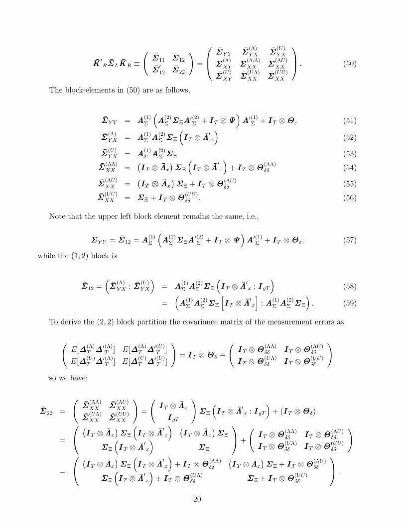
. (50)

The block-elements in (50) are as follows,

ΣY Y = A(1)Σ

(A

(2)Σ ΣΞA

′(2)Σ + I T ⊗Ψ

)A′(1)

Σ + I T ⊗Θε (51)

Σ(Λ)Y X = A

(1)Σ A

(2)Σ ΣΞ

(I T ⊗ Λ

′x

)(52)

Σ(U)Y X = A

(1)Σ A

(2)Σ ΣΞ (53)

Σ(ΛΛ)XX =

(I T ⊗ Λx

)ΣΞ

(I T ⊗ Λ

′x

)+ I T ⊗Θ

(ΛΛ)δδ (54)

Σ(ΛU)XX =

(IT ⊗ Λx

)ΣΞ + I T ⊗Θ

(ΛU)δδ (55)

Σ(UU)XX = ΣΞ + I T ⊗Θ

(UU)δδ . (56)

Note that the upper left block element remains the same, i.e.,

ΣY Y = Σ 12 = A(1)Σ

(A

(2)Σ ΣΞA

′(2)Σ + I T ⊗Ψ

)A′(1)

Σ + I T ⊗Θε, (57)

while the (1, 2) block is

Σ 12 =(Σ

(Λ)Y X : Σ

(U)Y X

)= A

(1)Σ A

(2)Σ ΣΞ

(I T ⊗ Λ

′x : I gT

)(58)

=(A

(1)Σ A

(2)Σ ΣΞ

[I T ⊗ Λ

′x

]: A

(1)Σ A

(2)Σ ΣΞ

). (59)

To derive the (2, 2) block partition the covariance matrix of the measurement errors as

(E[∆

(Λ)T ∆′(Λ)

T ] E[∆(Λ)T ∆′(U)

T ]

E[∆(U)T ∆′(Λ)

T ] E[∆(U)T ∆′(U)

T ]

)= I T ⊗Θδ ≡

(I T ⊗Θ

(ΛΛ)δδ I T ⊗Θ

(ΛU)δδ

I T ⊗Θ(UΛ)δδ I T ⊗Θ

(UU)δδ

)

so we have:

Σ 22 =

(Σ

(ΛΛ)XX Σ

(ΛU)XX

Σ(UΛ)XX Σ

(UU)XX

)=

(I T ⊗ Λx

I gT

)ΣΞ

(I T ⊗ Λ

′x : I gT

)+ (I T ⊗Θδ)

=

(I T ⊗ Λx

)ΣΞ

(I T ⊗ Λ

′x

) (I T ⊗ Λx

)ΣΞ

ΣΞ

(I T ⊗ Λ

′x

)ΣΞ

+

(I T ⊗Θ

(ΛΛ)δδ I T ⊗Θ

(ΛU)δδ

I T ⊗Θ(UΛ)δδ I T ⊗Θ

(UU)δδ

)

=

(I T ⊗ Λx

)ΣΞ

(I T ⊗ Λ

′x

)+ I T ⊗Θ

(ΛΛ)δδ

(I T ⊗ Λx

)ΣΞ + I T ⊗Θ

(ΛU)δδ

ΣΞ

(I T ⊗ Λ

′x

)+ I T ⊗Θ

(UΛ)δδ ΣΞ + I T ⊗Θ

(UU)δδ

.

20

Finally, note that the marginal covariance structure of Y T and X(Λ)T , i.e.,

(ΣY Y Σ

(Λ)Y X

Σ(Λ)XY Σ

(ΛΛ)XX

)

is given by

A

(1)Σ

(A

(2)Σ ΣΞA

′(2)Σ + I T ⊗Ψ

)A′(1)

Σ + I T ⊗Θε A(1)Σ A

(2)Σ ΣΞ

(I T ⊗ Λ

′x

)(I T ⊗ Λx

)ΣΞA

′(2)Σ A′(1)

Σ

(I T ⊗ Λx

)ΣΞ

(I T ⊗ Λ

′x

)+ I T ⊗Θ

(ΛΛ)δδ

(60)

3.4 Observed form (OF)

Suppose we wish to estimate the DSEM model with the unobservable Ξ T but instead specify

the model by replacing Ξ T with its noisy indicators X(U)T . This would lead to the model with

errors in the variables (EIV). Such model can be interpreted in two ways. Firstly, we can arrive

at such model if instead of the true Ξ T we mistakenly include in the model its noisy indicators,

thus introducing the additional error due to mis-measurement (noise), which gives

Y T = A(1)Ξ

[A

(2)Ξ

(X

(U)T −∆

(U)T

)

︸ ︷︷ ︸Ξ T

+ ZT ] + ET (61)

X(Λ)T =

(I T ⊗ Λx

) (X

(U)T −∆

(U)T

)

︸ ︷︷ ︸Ξ T

+∆(Λ)T (62)

X(U)T = X

(U)T . (63)

Alternatively, we can specify the model in its latent form, and use a trivial identity and re-write

it as an EIV model, i.e.,

Y T = A(1)Ξ A

(2)Ξ

(Ξ T + ∆

(U)T −∆

(U)T

)

︸ ︷︷ ︸X (U)

T −∆(U)

T

+A(1)Ξ Z T + ET (64)

X(Λ)T =

(I T ⊗ Λx

) (Ξ T + ∆

(U)T −∆

(U)T

)

︸ ︷︷ ︸X (U)

T −∆(U)

T

+∆(Λ)T (65)

X(U)T =

(Ξ T + ∆

(U)T −∆

(U)T

)

︸ ︷︷ ︸X (U)

T −∆(U)

T

+∆(U)T . (66)

21

In either case, we obtain a DSEM model in the observed form (OF), which can be seen as a

linear transform

KRLT =

I nT 0 0 A(1)Ξ A

(2)Ξ A

(1)Ξ

0 I (k−g)T 0 I T ⊗ Λx 0

0 0 I gT I gT 0

ET

∆(Λ)T

∆(U)T

Ξ T

Z T

≡

Y T

X(Λ)T

X(U)T

. (67)

We will inspect the OF model (67) by comparing its likelihood function to that of the UL-

restricted latent form model considered in previous section. In order to do so we will need a

simple result on the variance decomposition summarised in the following lemma.

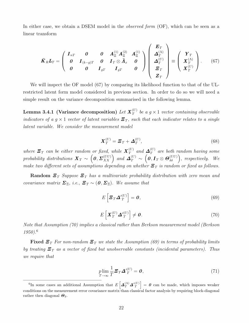
Lemma 3.4.1 (Variance decomposition) Let X(U)T be a g× 1 vector containing observable

indicators of a g × 1 vector of latent variables Ξ T , such that each indicator relates to a single

latent variable. We consider the measurement model

X(U)T = Ξ T + ∆

(U)T , (68)

where Ξ T can be either random or fixed, while X(U)T and ∆

(U)T are both random having some

probability distributions X T ∼(0 ,Σ

(UU)XX

)and ∆

(U)T ∼

(0 , I T ⊗Θ

(UU)δδ

), respectively. We

make two different sets of assumptions depending on whether Ξ T is random or fixed as follows.

Random Ξ T Suppose Ξ T has a multivariate probability distribution with zero mean and

covariance matrix ΣΞ, i.e., Ξ T ∼ (0 ,ΣΞ). We assume that

E[Ξ T∆

′(U)T

]= 0 , (69)

E[X

(U)T ∆′(U)

T

]6= 0 . (70)

Note that Assumption (70) implies a classical rather than Berkson measurement model (Berkson

1950).6

Fixed Ξ T For non-random Ξ T we state the Assumption (69) in terms of probability limits

by treating Ξ T as a vector of fixed but unobservable constants (incidental parameters). Thus

we require that

p limT→∞

1

TΞ T∆

′(U)T = 0 , (71)

6In some cases an additional Assumption that E[∆

(Λ)T ∆′(U)

T

]= 0 can be made, which imposes weaker

conditions on the measurement error covariance matrix than classical factor analysis by requiring block-diagonalrather then diagonal Θδ.

22

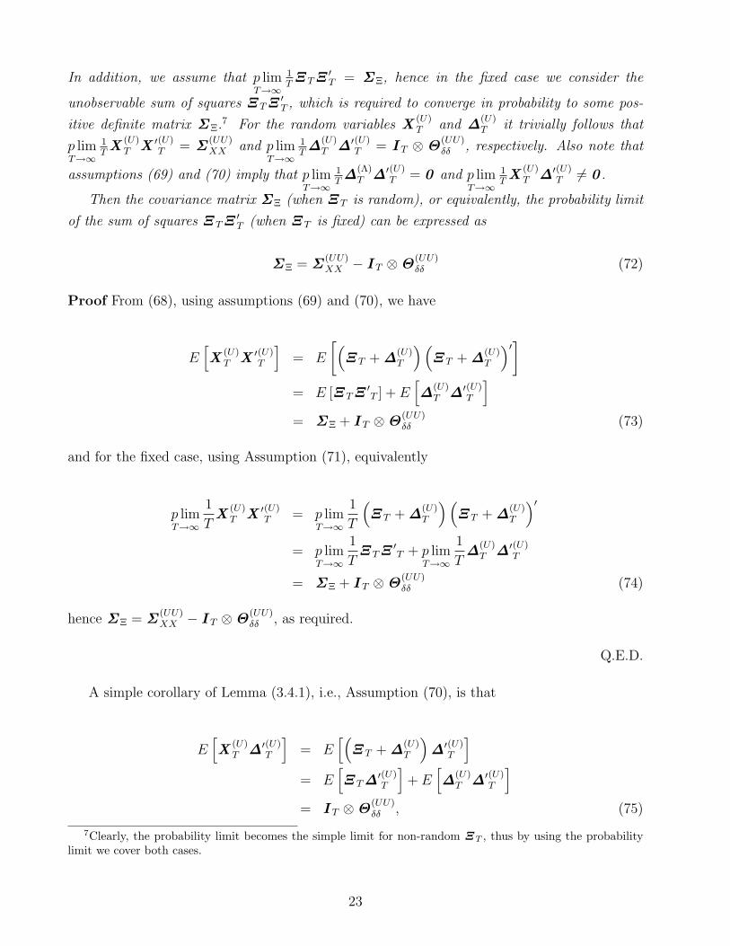
In addition, we assume that p limT→∞

1TΞ TΞ

′T = ΣΞ, hence in the fixed case we consider the

unobservable sum of squares Ξ TΞ′T , which is required to converge in probability to some pos-

itive definite matrix ΣΞ.7 For the random variables X(U)T and ∆

(U)T it trivially follows that

p limT→∞

1TX

(U)T X ′(U)

T = Σ(UU)XX and p lim

T→∞1T∆

(U)T ∆′(U)

T = I T ⊗Θ(UU)δδ , respectively. Also note that

assumptions (69) and (70) imply that p limT→∞

1T∆

(Λ)T ∆′(U)

T = 0 and p limT→∞

1TX

(U)T ∆′(U)

T 6= 0 .

Then the covariance matrix ΣΞ (when Ξ T is random), or equivalently, the probability limit

of the sum of squares Ξ TΞ′T (when Ξ T is fixed) can be expressed as

ΣΞ = Σ(UU)XX − I T ⊗Θ

(UU)δδ (72)

Proof From (68), using assumptions (69) and (70), we have

E[X

(U)T X ′(U)

T

]= E

[(Ξ T + ∆

(U)T

)(Ξ T + ∆

(U)T

)′]

= E [Ξ TΞ′T ] + E

[∆

(U)T ∆′(U)

T

]

= ΣΞ + I T ⊗Θ(UU)δδ (73)

and for the fixed case, using Assumption (71), equivalently

p limT→∞

1

TX

(U)T X ′(U)

T = p limT→∞

1

T

(Ξ T + ∆

(U)T

)(Ξ T + ∆

(U)T

)′

= p limT→∞

1

TΞ TΞ

′T + p lim

T→∞

1

T∆

(U)T ∆′(U)

T

= ΣΞ + I T ⊗Θ(UU)δδ (74)

hence ΣΞ = Σ(UU)XX − I T ⊗Θ

(UU)δδ , as required.

Q.E.D.

A simple corollary of Lemma (3.4.1), i.e., Assumption (70), is that

E[X

(U)T ∆′(U)

T

]= E

[(Ξ T + ∆

(U)T

)∆′(U)

T

]

= E[Ξ T∆

′(U)T

]+ E

[∆

(U)T ∆′(U)

T

]

= I T ⊗Θ(UU)δδ , (75)

7Clearly, the probability limit becomes the simple limit for non-random Ξ T , thus by using the probabilitylimit we cover both cases.

23

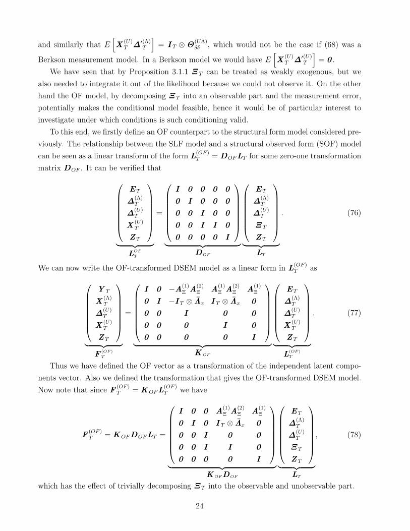
and similarly that E[X

(U)T ∆′(Λ)

T

]= I T ⊗Θ

(UΛ)δδ , which would not be the case if (68) was a

Berkson measurement model. In a Berkson model we would have E[X

(U)T ∆′(U)

T

]= 0 .

We have seen that by Proposition 3.1.1 Ξ T can be treated as weakly exogenous, but we

also needed to integrate it out of the likelihood because we could not observe it. On the other

hand the OF model, by decomposing Ξ T into an observable part and the measurement error,

potentially makes the conditional model feasible, hence it would be of particular interest to

investigate under which conditions is such conditioning valid.

To this end, we firstly define an OF counterpart to the structural form model considered pre-

viously. The relationship between the SLF model and a structural observed form (SOF) model

can be seen as a linear transform of the form L(OF )T = DOFLT for some zero-one transformation

matrix DOF . It can be verified that

ET

∆(Λ)T

∆(U)T

X(U)T

Z T

︸ ︷︷ ︸LOF

T

=

I 0 0 0 0

0 I 0 0 0

0 0 I 0 0

0 0 I I 0

0 0 0 0 I

︸ ︷︷ ︸DOF

ET

∆(Λ)T

∆(U)T

Ξ T

Z T

︸ ︷︷ ︸LT

. (76)

We can now write the OF-transformed DSEM model as a linear form in L(OF )T as

Y T

X(Λ)T

∆(U)T

X(U)T

Z T

︸ ︷︷ ︸F (OF )

T

=

I 0 −A(1)Ξ A

(2)Ξ A

(1)Ξ A

(2)Ξ A

(1)Ξ

0 I −I T ⊗ Λx I T ⊗ Λx 0

0 0 I 0 0

0 0 0 I 0

0 0 0 0 I

︸ ︷︷ ︸K OF

ET

∆(Λ)T

∆(U)T

X(U)T

Z T

︸ ︷︷ ︸L(OF )

T

. (77)

Thus we have defined the OF vector as a transformation of the independent latent compo-

nents vector. Also we defined the transformation that gives the OF-transformed DSEM model.

Now note that since F(OF )T = KOFL

(OF )T we have

F(OF )T = KOFDOFLT =

I 0 0 A(1)Ξ A

(2)Ξ A

(1)Ξ

0 I 0 I T ⊗ Λx 0

0 0 I 0 0

0 0 I I 0

0 0 0 0 I

︸ ︷︷ ︸K OFDOF

ET

∆(Λ)T

∆(U)T

Ξ T

Z T

︸ ︷︷ ︸LT

, (78)

which has the effect of trivially decomposing Ξ T into the observable and unobservable part.

24

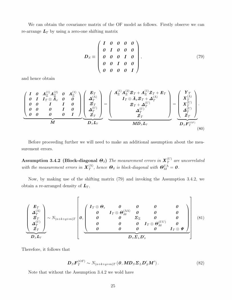
We can obtain the covariance matrix of the OF model as follows. Firstly observe we can

re-arrange LT by using a zero-one shifting matrix

DS ≡

I 0 0 0 0

0 I 0 0 0

0 0 0 I 0

0 0 I 0 0

0 0 0 0 I

, (79)

and hence obtain

I 0 A(1)Ξ A

(2)Ξ 0 A

(1)Ξ

0 I I T ⊗ Λx 0 00 0 I I 00 0 0 I 00 0 0 0 I

︸ ︷︷ ︸M

ET

∆(Λ)T

Ξ T

∆(U)T

Z T

︸ ︷︷ ︸DSLT

=

A(1)Ξ A

(2)Ξ Ξ T + A

(1)Ξ Z T + ET

I T ⊗ ΛxΞ T + ∆(Λ)T

Ξ T + ∆(U)T

∆(U)T

Z T

︸ ︷︷ ︸MDSLT

=

Y T

X(Λ)T

X(U)T

∆(U)T

Z T

︸ ︷︷ ︸DSF

(OF )T

.

(80)

Before proceeding further we will need to make an additional assumption about the mea-

surement errors.

Assumption 3.4.2 (Block-diagonal Θδ) The measurement errors in X(U)T are uncorrelated

with the measurement errors in X(Λ)T , hence Θδ is block-diagonal with ΘUΛ

δδ = 0 .

Now, by making use of the shifting matrix (79) and invoking the Assumption 3.4.2, we

obtain a re-arranged density of LT ,

ET

∆(Λ)T

Ξ T

∆(U)T

Z T

︸ ︷︷ ︸DSLT

∼ N(n+k+g+m)T

0 ,

I T ⊗Θε 0 0 0 0

0 I T ⊗Θ(ΛΛ)δδ 0 0 0

0 0 ΣΞ 0 0

0 0 0 I T ⊗Θ(UU)δδ 0

0 0 0 0 I T ⊗Ψ

︸ ︷︷ ︸DSΣLD

′S

(81)

Therefore, it follows that

DSF(OF )T ∼ N(n+k+g+m)T (0 ,MDSΣLD

′SM

′) . (82)

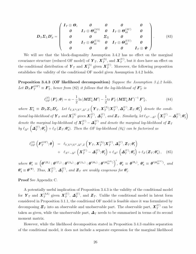
Note that without the Assumption 3.4.2 we wold have

25

DSΣLD′S =

I T ⊗Θε 0 0 0 0

0 I T ⊗Θ(ΛΛ)δδ 0 I T ⊗Θ

(ΛU)δδ 0

0 0 ΣΞ 0 0

0 I T ⊗Θ(UΛ)δδ 0 I T ⊗Θ

(UU)δδ 0

0 0 0 0 I T ⊗Ψ

. (83)

We will see that the block-diagonality Assumption 3.4.2 has no effect on the marginal

covariance structure (reduced OF model) of Y T , X(Λ)T , and X

(U)T , but it does have an effect on

the conditional distribution of Y T and X(Λ)T given X

(U)T . Moreover, the following proposition

establishes the validity of the conditional OF model given Assumption 3.4.2 holds.

Proposition 3.4.3 (OF likelihood decomposition) Suppose the Assumption 3.4.2 holds.

Let DSF(OF )T ≡ F ∗

T , hence from (82) it follows that the log-likelihood of F ∗T is

`(S)OF (F ∗

T ; θ) = α− 1

2ln |MΣ ∗

LM′| − 1

2trF ∗

T (MΣ ∗LM

′)−1F ′∗

T , (84)

where Σ ∗L ≡ DSΣLD

′S. Let `Y,XΛ|XU ,∆U ,Z

(Y T ,X

(Λ)T |X (U)

T ,∆(U)T ,Z T ; θ∗1

)denote the condi-

tional log-likelihood of Y T and X(Λ)T given X

(U)T , ∆

(U)T , and Z T . Similarly, let `XU−∆U

(X

(U)T −∆

(U)T ; θ∗2

)

denote the marginal log-likelihood of X(U)T −∆

(U)T and denote the marginal log-likelihood of Z T

by `∆U

(∆

(U)T ; θ∗3

)+ `Z (Z T ; θ∗4). Then the OF log-likelihood (84) can be factorised as

`(S)OF

(F

(OF )T ; θ

)= `Y,XΛ|XU ,∆U ,Z

(Y T ,X

(Λ)T |X (U)

T ,∆(U)T ,Z T ; θ∗1

)

+ `XU−∆U

(X

(U)T −∆

(U)T ; θ∗2

)+ `∆U

(∆

(U)T ; θ∗3

)+ `Z (Z T ; θ∗4) , (85)

where θ∗1 ≡(θ′(Bi) : θ′(Γj) : θ′(Λy) : θ′(Λx) : θ′(Θε) : θ′(Θ

(ΛΛ)δδ )

)′, θ∗2 ≡ θ(Φj), θ∗3 ≡ θ′(Θ

(UU)δδ ), and

θ∗4 ≡ θ(Ψ). Thus, X(U)T , ∆

(U)T , and Z T are weakly exogenous for θ∗1.

Proof See Appendix C.

A potentially useful implication of Proposition 3.4.3 is the validity of the conditional model

for Y T and X(ΛΛ)T given X

(U)T , ∆

(U)T , and Z T . Unlike the conditional model in latent form

considered in Proposition 3.1.1, the conditional OF model is feasible since it was formulated by

decomposing Ξ T into an observable and unobservable part. The observable part, X(U)T can be

taken as given, while the unobservable part, ∆T needs to be summarised in terms of its second

moment matrix.

However, while the likelihood decomposition stated in Proposition 3.4.3 enables separation

of the conditional model, it does not include a separate expression for the marginal likelihood

26

of X T . Instead, (85) includes marginal likelihood of the decomposed Ξ T into the observable

and unobservable parts, i.e., the marginal likelihood of X(U)T − ∆

(U)T . It thus follows that

conditioning on X T in the OF model would be valid in the sense of Definition 3.0.5 if the

Assumption 3.4.2 holds, and if ∆(U)T is known or observable (the same goes for Z T , which is

always unobservable but can be taken as zero). Not knowing ∆(U)T necessitates estimation of

its covariance matrix as an additional matrix of parameters θ(UU)δδ . For random X

(U)T this leads

us back to the reduced-type of a model and we next show the OF model in the reduced form

has the same likelihood (in expectation or in probability limit) as the RSLF model.

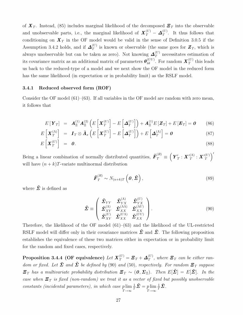
3.4.1 Reduced observed form (ROF)

Consider the OF model (61)–(63). If all variables in the OF model are random with zero mean,

it follows that

E [Y T ] = A(1)Ξ A

(2)Ξ

(E

[X

(U)T

]− E

[∆

(U)T

])+ A

(1)Ξ E [Z T ] + E [ET ] = 0 (86)

E[X

(Λ)T

]= I T ⊗ Λx

(E

[X

(U)T

]− E

[∆

(U)T

])+ E

[∆

(Λ)T

]= 0 (87)

E[X

(U)T

]= 0 . (88)

Being a linear combination of normally distributed quantities, F(R)

T ≡(Y ′

T : X ′(Λ)T : X ′(U)

T

)′

will have (n + k)T -variate multinormal distribution

F(R)

T ∼ N(n+k)T

(0 , Σ

), (89)

where Σ is defined as

Σ ≡

ΣY Y Σ(Λ)

Y X Σ(U)

Y X

Σ(Λ)

XY Σ(ΛΛ)

XX Σ(ΛU)

XX

Σ(U)

XY Σ(UΛ)

XX Σ(UU)

XX

. (90)

Therefore, the likelihood of the OF model (61)–(63) and the likelihood of the UL-restricted

RSLF model will differ only in their covariance matrices Σ and Σ . The following proposition

establishes the equivalence of these two matrices either in expectation or in probability limit

for the random and fixed cases, respectively.

Proposition 3.4.4 (OF equivalence) Let X(U)T = Ξ T + ∆

(U)T , where Ξ T can be either ran-

dom or fixed. Let Σ and Σ be defined by (90) and (50), respectively. For random Ξ T suppose

Ξ T has a multivariate probability distribution Ξ T ∼ (0 ,ΣΞ). Then E[Σ ] = E[Σ ]. In the

case when Ξ T is fixed (non-random) we treat it as a vector of fixed but possibly unobservable

constants (incidental parameters), in which case p limT→∞

1TΣ = p lim

T→∞1TΣ .

27

Proof See Appendix D.

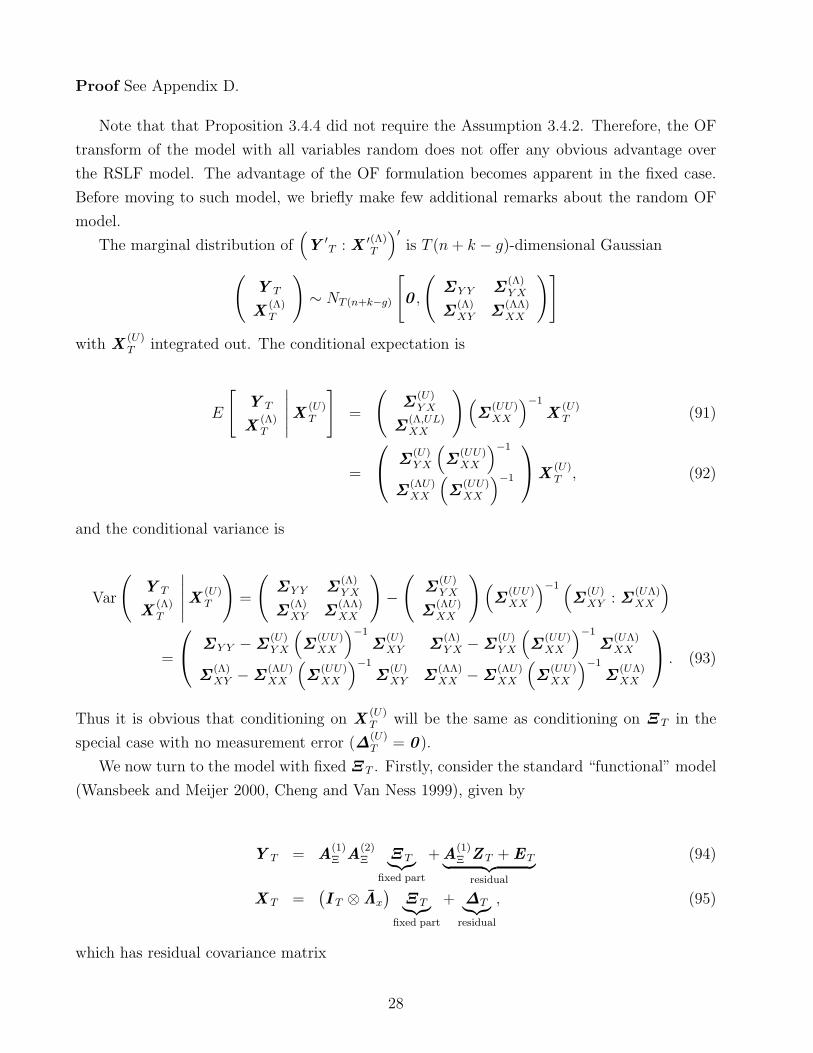
Note that that Proposition 3.4.4 did not require the Assumption 3.4.2. Therefore, the OF

transform of the model with all variables random does not offer any obvious advantage over

the RSLF model. The advantage of the OF formulation becomes apparent in the fixed case.

Before moving to such model, we briefly make few additional remarks about the random OF

model.

The marginal distribution of(Y ′

T : X ′(Λ)T

)′is T (n + k − g)-dimensional Gaussian

(Y T

X(Λ)T

)∼ NT (n+k−g)

[0 ,

(ΣY Y Σ

(Λ)Y X

Σ(Λ)XY Σ

(ΛΛ)XX

)]

with X(U)T integrated out. The conditional expectation is

E

[Y T

X(Λ)T

∣∣∣∣∣X(U)T

]=

(Σ

(U)Y X

Σ(Λ,UL)XX

) (Σ

(UU)XX

)−1

X(U)T (91)

=

Σ

(U)Y X

(Σ

(UU)XX

)−1

Σ(ΛU)XX

(Σ

(UU)XX

)−1

X

(U)T , (92)

and the conditional variance is

Var

(Y T

X(Λ)T

∣∣∣∣∣X(U)T

)=

(ΣY Y Σ

(Λ)Y X

Σ(Λ)XY Σ

(ΛΛ)XX

)−

(Σ

(U)Y X

Σ(ΛU)XX

)(Σ

(UU)XX

)−1 (Σ

(U)XY : Σ

(UΛ)XX

)

=

ΣY Y −Σ

(U)Y X

(Σ

(UU)XX

)−1

Σ(U)XY Σ

(Λ)Y X −Σ

(U)Y X

(Σ

(UU)XX

)−1

Σ(UΛ)XX

Σ(Λ)XY −Σ

(ΛU)XX

(Σ

(UU)XX

)−1

Σ(U)XY Σ

(ΛΛ)XX −Σ

(ΛU)XX

(Σ

(UU)XX

)−1

Σ(UΛ)XX

. (93)

Thus it is obvious that conditioning on X(U)T will be the same as conditioning on Ξ T in the

special case with no measurement error (∆(U)T = 0 ).

We now turn to the model with fixed Ξ T . Firstly, consider the standard “functional” model

(Wansbeek and Meijer 2000, Cheng and Van Ness 1999), given by

Y T = A(1)Ξ A

(2)Ξ Ξ T︸︷︷︸

fixed part

+A(1)Ξ Z T + ET︸ ︷︷ ︸

residual

(94)

X T =(I T ⊗ Λx

)Ξ T︸︷︷︸

fixed part

+ ∆T︸︷︷︸residual

, (95)

which has residual covariance matrix

28

ΩF =

(A

(1)Ξ (I T ⊗Ψ)A

(1)Ξ + I T ⊗Θε 0

0 I T ⊗Θδ

), (96)

and hence the density function

(Y T

X T

)∼ N(n+k−g)T

[(A

(1)Ξ A

(2)Ξ Ξ T

(I T ⊗Λx)Ξ T

),

(A

(1)Ξ (I T ⊗Ψ)A(1)

Ξ + I T ⊗Θε 00 I T ⊗Θδ

)].

(97)

The log-likelihood of the functional model is then

`Y,X|Ξ (Y T ,X T |Ξ T ; θ) = −(n + k)T

2ln(2π)− 1

2ln |ΩF |

−1

2tr

(Y T −A

(1)Ξ A

(2)Ξ Ξ T

X T − (I T ⊗Λx)Ξ T

)′

Ω−1F

(Y T −A

(1)Ξ A

(2)Ξ Ξ T

X T − (I T ⊗Λx)Ξ T

.

)(98)

Note that the log-likelihood (98) includes Ξ T , which is unobservable.

Next, consider the OF-transformed model

Y T = A(1)Ξ A

(2)Ξ

(X

(U)T −∆

(U)T

)+ A

(1)Ξ Z T + ET

= A(1)Ξ A

(2)Ξ X

(U)T +

(A

(1)Ξ Z T −A

(1)Ξ A

(2)Ξ ∆

(U)T + ET

)

︸ ︷︷ ︸U (Y )

T

(99)

X(Λ)T =

(I T ⊗ Λx

) (X

(U)T −∆

(U)T

)+ ∆

(Λ)T

=(I T ⊗ Λx

)X

(U)T +

(∆

(Λ)T − (

I T ⊗ Λx

)∆

(U)T

)

︸ ︷︷ ︸U (X)

T

(100)

X(UL)T = X

(UL)T −∆

(UL)T + ∆

(UL)T

= X(UL)T , (101)

and denote the covariance matrix of the residuals U(Y )T and U

(X)T in (99) and (100) by

(ΩY Y Ω

(Λ)Y X

Ω(Λ)XY Ω

(ΛΛ)XX

). (102)

Therefore, the distribution of the OF functional model is given by

(Y T

X(Λ)T

)∼ N(n+k−g)T

[(A

(1)Ξ A

(2)Ξ X

(U)T(

I T ⊗ Λx

)X

(U)T

),

(ΩY Y Ω

(Λ)Y X

Ω(Λ)XY Ω

(ΛΛ)XX

)], (103)

29

and the log-likelihood

`Y,XΛ|XU

(Y T ,X

(Λ)T |X (U)

T ; θ)

= − (n+k)T2 ln(2π)− 1

2 ln

∣∣∣∣∣

(ΩY Y Ω

(Λ)Y X

Ω(Λ)XY Ω

(ΛΛ)XX

)∣∣∣∣∣

−12tr

(Y T −A

(1)Ξ A

(2)Ξ X

(U)T

X(Λ)T − (

I T ⊗ Λx

)X

(U)T

)′(ΩY Y Ω

(Λ)Y X

Ω(Λ)XY Ω

(ΛΛ)XX

)−1 (Y T −A

(1)Ξ A

(2)Ξ X

(U)T

X(Λ)T − (

I T ⊗ Λx

)X

(U)T

)

(104)

The structure of (102) for the special case with I T ⊗Θ(ΛU)δδ = 0 (i.e. under Assumption 3.4.2)

is given by the following proposition.

Proposition 3.4.5 Assume I T ⊗Θ(ΛU)δδ = 0 . Then the block-elements of (102) are given by

ΩY Y = A(1)Ξ

(A

(2)Ξ

(I T ⊗Θ

(UU)δδ

)A′(2)

Ξ + I T ⊗Ψ)A′(1)

Ξ + I T ⊗Θε (105)

Ω(Λ)Y X = A

(1)Ξ A

(2)Ξ

(I T ⊗Θ

(UU)δδ

)(I T ⊗ Λ

′x

)(106)

Ω(ΛΛ)XX =

(I T ⊗ Λx

) (I T ⊗Θ

(UU)δδ

)(I T ⊗ Λ

′x

)+ I T ⊗Θ

(ΛΛ)δδ , (107)

and Ω(Λ)XY = Ω ′(Λ)

Y X . Furthermore, it follows that

(ΩY Y Ω

(Λ)Y X

Ω(Λ)XY Ω

(ΛΛ)XX

)= KRDSΣLD

′SK

′R, (108)

where

DS ≡

I 0 0 0 0

0 I 0 0 0

0 0 I 0 0

0 0 0 0 I

. (109)

Proof See Appendix E.

Using the above result, we can thus simplify the log-likelihood of the functional OF model as

`Y,Xλ|XU

(Y T ,X

(Λ)T |X (U)

T ; θ)

= − (n+k−g)T2 ln(2π)− 1

2 ln∣∣∣KRDSΣLD

′SK

′R

∣∣∣

−12tr

(Y T −A

(1)Ξ A

(2)Ξ X

(U)T

X(Λ)T − (

I T ⊗ Λx

)X

(U)T

)′ (KRDSΣLD

′SK

′R

)−1(

Y T −A(1)Ξ A

(2)Ξ X

(U)T

X(Λ)T − (

I T ⊗ Λx

)X

(U)T

).

(110)

Therefore, the log-likelihood (110) of the functional OF model has gT unknowns less then

the log-likelihood of the functional model in latent form as a consequence of not having to

estimate Ξ T .

30

3.5 State-space form (SSF)

Various special cases of the general DSEM model have been analysed in the “state-space” form

including dynamic factor model and DYMIMIC model (Engle and Watson 1981, Watson and

Engle 1983) and the shock-error model (Aigner et al. 1984, Ghosh 1989, Terceiro Lomba 1990).

The motivation behind casting particular dynamic models in state-space form is primarily in the

possibility of using the Kalman filter algorithm (Kalman 1960) for estimation of the unknown

parameters.8

The state-space model can be specified in its basic form as

ϑt = Hϑt−1 + w t, (111)

W t = Fϑt + u t, (112)

where (111) is the state equation, (112) is the measurement equation, ϑt is the possibly un-

observable state vector, and H is the transition matrix (Harvey 1989, Durbin and Koopman

2001).9 The specification (111)–(112) is particularly appealing for dynamic models involving

unobservable variables since the state equation can contain dynamic unobservable variables

and the measurement equation can link them with the observable indicators. These attractive

properties of the Kalman filter resulted in numerous empirical papers in the applied statistics

and econometric literature. Harvey (1989, p. 100), for example, calls the state-space form “an

enormously powerful tool which opens the way to handling a wide range of time series models”.

To enable estimation of a statistical model by Kalman filter, it is necessary to formulate

it in the state-space. We will show that a state-space representation of the general DSEM

model (1)–(3) and hence of all its special cases listed in Table 1 exists. In addition, it can be

verified that for the transition matrix H to be non-singular we will need to make the following

assumption.10

Assumption 3.5.1 Let ξt follow a VAR(q) process with q ≥ 1

ξt =

q∑j=1

Rjξt−j + υt, (113)

8The Kalman filter was developed by Rudolph E. Kalman as a solution to discrete data linear filtering problemin control engineering. The filter is based on a set of recursive equations, which allow efficient estimation ofthe state of the process by minimising the mean of the squared error. The Kalman filter recursive algorithmproved to be considerably simpler then the previously available (non-recursive) filters such as the Winer filter,see Brown (1992) for a review.

9A simple generalisation of the measurement equation is to include a vector of observable regressors.10Since the state-space representation is achieved by dynamically linking the current state with the past-

period state via a first-order Markov process, the first equation (for time t) is the actual model, while the restof the stacked elements (for time t− 1, t− 2, . . . , t− q) of ϑt are set trivially equal to themselves as they appearin both ϑt and ϑt−1. Hence, if any of the elements of ϑt cannot be related to an element of ϑt−1 (such as inthe case of white unobservable regressors) the transition matrix H will contain a row of zeros and thus it willbe singular.

31

with the roots of |I − λR1 − λ2R2 − · · · − λqRq| = 0 greater then one in absolute value and υt

is a Gaussian zero-mean homoscedastic white noise process with E[υtυ′t] = Συ.

Definition 3.5.2 Let Π j ≡ (I − B0)−1B j, Gj ≡ (I −B0)

−1(Γ j + Γ 0Rj), and K t ≡(I −B0)

−1(ζt + Γ 0υt), where B j, Γ j, and ζt are defined as in (1)–(3).

The following result establishes the existence of the state-space form of the general DSEM

model given Assumption 113.

Proposition 3.5.3 Let ξt be generated by a VAR (q) process as in (113). Then the general

DSEM model (1)–(3) can be written in the state-space form (111)–(112) as

ηt

ξt

ηt−1

ξt−1...

ηt−r+1

ξt−r+1

=

Π 1 G1 · · · Π r−1 Gr−1 Π r Gr

0 R1 · · · 0 Rr−1 0 Rr

I 0 · · · 0 0 0 00 I · · · 0 0 0 0...

.... . .

......

......

0 0 · · · I 0 0 00 0 · · · 0 I 0 0

ηt−1

ξt−1

ηt−2

ξt−2...

ηt−r

ξt−r

+

K t

υt

00...00

, (114)

and

(y t

x t

)=

(Λy 0 · · · 0

0 Λx · · · 0

)

ηt

ξt

ηt−1

ξt−1...

ηt−r

ξt−r

+

(εt

δt

), (115)

where r = max(p, q), with notation defined in 3.5.2.

Proof See Appendix F.

While Proposition 3.5.3 gives the state-space form of the general DSEM model, it is not

immediately clear how the state-space form compares with the forms considered earlier. Namely,

the SSF model (114) is in a recursive form required for the Kalman filter, hence it is specified

in t-notation. On the other hand the T -notation (Table 2) we used to analyse the statistical

properties of other DSEM forms leads to a closed-form rather then a recursive form of the

model. Nevertheless, we can write the SSF model (114) for the process (t = 1, 2 . . . , T ) and

compare its likelihood with those of the other forms of the model. In the context of the RSLF

model, for example, this would call for additional modelling of the VAR(q) process for Ξ T ,

32

thereby increasing the dimensionality of the multivariate density function from (n + k)T to

(n + k + g)T . However, we will show that such extended model can still be reduced to the

(n + k)T -dimensional model.

Given the VAR(q) process for Ξ T (Assumption 113), the SLF model will have to include

an additional equation for Ξ T . The structural equation remains as before and it can be reduce

as

H T =

(p∑

j=0

S jT⊗B j

)H T +

(q∑

j=0

S jT⊗Γ j

)Ξ T + ZT

=

(ImT −

p∑j=0

S jT⊗B j

)−1 [(q∑

j=0

S jT⊗Γ j

)Ξ T + ZT

]. (116)

A T -notation equivalent of the VAR(q) model (113) can be written as

Ξ T =

(q∑

j=1

S jT⊗Rj

)Ξ T + ΥT =

(I gT −

q∑j=1

S jT⊗Rj

)−1

︸ ︷︷ ︸A(3)

Σ

ΥT . (117)

Finally, the measurement equations as as before

Y T = (I T ⊗Λy)H T + ET (118)

X T = (I T ⊗Λx)Ξ T + ∆T . (119)

Substituting (116) and (117) in (118) and (119), respectively, we obtan the reduced SSF

model

(H T

Ξ T

)=

p∑j=0

S jT⊗B j

q∑j=0

S jT⊗Γ j

0q∑

j=1S j

T⊗Rj

(H T

Ξ T

)+

(ZT

ΥT

)

=

ImT −p∑

j=0S j

T⊗B j −q∑

j=0S j

T⊗Γ j

0 I gT −q∑

j=1S j

T⊗Rj

−1

(ZT

ΥT

), (120)

where the inverse of the matrix of parameters in (120) is given by11

11We make use of the result

(D11 D12

0 D22

)−1

=(

D−111 −D−1

11 D12D−122

0 D−122

).

33

(ImT −

p∑j=0

S jT⊗B j

)−1 (ImT −

p∑j=0

S jT⊗Bj

)−1 (q∑

j=0

S jT⊗Γ j

)(I gT −

q∑j=1

S jT⊗Rj

)−1

0

(I gT −

q∑j=1

S jT⊗Rj

)−1

, (121)

therefore the reduced SSF model becomes

Y T = (I T ⊗Λy)

(ImT −

p∑j=0

S jT⊗B j

)−1

×

(q∑

j=0

S jT⊗Γ j

)(I gT −

q∑j=1

S jT⊗Rj

)−1

ΥT + ZT

+ ET (122)

X T = (I T ⊗Λx)

(I gT −

q∑j=1

S jT⊗Rj

)−1

ΥT + ∆T . (123)

Using the simplifying notation from Definition 3.0.4 we can write (122) and (123) as

Y T = A(1)Σ A

(2)Σ A

(3)Σ ΥT︸ ︷︷ ︸Ξ T

+A(1)Σ ZT + ET (124)

X T = (I T ⊗Λx)A(3)Σ ΥT︸ ︷︷ ︸Ξ T

+∆T (125)

Next, we consider the covariance structure of Ξ T , which can be easily obtained from the

reduced form T -notation expression (117). The following lemma gives the required expression.

Lemma 3.5.4 Consider the VAR process (117). By Assumption 3.5.1, E[υtυ′t] = Συ ⇒

E [ΥTΥ′T ] ≡ I T⊗Συ. Then ΣΞ = A

(3)Σ (I T ⊗Συ)A

′(3)Σ , where A

(3)Σ ≡ (I gT −

q∑j=1

S jT⊗Rj)

−1.

Proof Since Ξ T = A(3)Σ ΥT and E [Ξ TΞ

′T ] ≡ ΣΞ, we have ΣΞ = A

(3)Σ E [ΥTΥ

′T ]A′(3)

Σ =

A(3)Σ E [ΥTΥ

′T ]A′(3)

Σ = A(3)Σ (I T ⊗Συ)A

′(3)Σ , as required.

Q.E.D

To examine the likelihood of the SSF model firstly note that the reduced SSF model (120)

is (n + k)T -dimensional, thus the SSF likelihood will be (n + k)T -variate Gaussian, thus of the

same form and dimension as the likelihood of the RSLF model given by (33). Recall that by

Assumption (113) as shown in (117), the Ξ T process can be expressed as a linear function of

34

the residual vector ΥT . Defining LSSFT ≡ (E ′

T : ∆′T : Υ ′

T : Z′T )′, assuming ΥT is Gaussian

and independent of other latent components it follows that

ET

∆T

ΥT

ZT

︸ ︷︷ ︸LSSF

T

∼ N(n+k+g+m)T

0 ,

I T ⊗Θε 0 0 0

0 I T ⊗Θδ 0 0

0 0 I T ⊗Συ 0

0 0 0 I T ⊗Ψ

︸ ︷︷ ︸Σ SSF

. (126)

Now, by letting

K SSF =

(I nT 0 A

(1)Σ A

(2)Σ A

(3)Σ A

(1)Σ

0 I kT (I T ⊗Λx)A(3)Σ 0

), (127)

the reduced SSF model (122)–(123) can be written as a linear form in LSSFT , i.e., as K SSFLSSF

T .

Therefore, by Proposition 3.0.3 it follows that

LSSFT ∼ N(n+k+g+m)T (0 ,ΣSSF ) ⇒ K SSFLSSF

T ∼ N(n+k)T (0 ,K SSFΣSSFK ′SSF ) .

Finally, since Ξ T is a VAR(q) process by Assumption 3.5.1 whose covariance structure, by

Lemma 3.5.4, is ΣΞ = A(3)Σ (I T ⊗Συ)A

′(3)Σ , we can parametrise ΣL as

ΣL =

I T ⊗Θε 0 0 0

0 I T ⊗Θδ 0 0

0 0 A(3)Σ (I T ⊗Συ)A

′(3)Σ︸ ︷︷ ︸

ΣΞ

0

0 0 0 I T ⊗Ψ

. (128)

Therefore, modelling the Ξ T process as a VAR(q) imposes the parametrisation ΣΞ =

A(3)Σ (I T ⊗Συ)A

′(3)Σ on ΣL. Hence with such structure imposed on ΣL it can be easily verified

that K SSFΣSSFK ′SSF = KRΣLK

′R, thus the likelihood of the reduced SSF model (122)–

(123) is equal to the likelihood of the RSLF model (26) with the covariance matrix of Ξ T

parametrised as A(3)Σ (I T ⊗Συ)A

′(3)Σ .

4 Comparison of different forms

There are several possible criteria on which to compare different forms of the general DSEM

model. We have seen that different forms of the general model discussed in this paper are not

35

identical re-arrangements of the same model in the statistical sense. Rather different assump-

tions about the modelled variables had to be made as well as some specific parametrisations

needed to be considered. In this respect, while substantively we are dealing with the same

model, its different forms might favour certain estimation methods and applications over the

others. In particular, we would be interested in the criteria such as 1) choice of estimation

method, 2) identification of the parameters, and 3) statistical assumptions about modelled

variables. We will look into some of these criteria, in turn, by focusing on particular forms of

the general model.

RSLF model. The RSLF model (section §3.2) has appealing implications when repeated

observations on the time series process F(R)iT are available. Consider N independent realizations

of F(R)iT are being observed. Then the log-likelihood (33) can be written for a single realization

as

`R

(F

(R)iT ; θ

)= −(n + k)T

2ln(2π)− 1

2ln |KRΣLK

′R| − 1

2trF ′(R)

iT (KRΣLK′R)−1

F(R)iT , (129)

thus for N independent realizations, the log-likelihood becomes

`R

(F

(R)NT ; θ

)= −(n + k)NT

2ln(2π)− N

2ln |KRΣLK

′R| − 1

2trF ′(R)

NT (KRΣLK′R)−1

F(R)NT ,

(130)

where F(R)NT ≡ (F

(R)1T , . . . ,F

(R)NT ). Now, ignoring the constant term and rearranging the matrices

under the trace, and multiplying by −2/N yields

ln |KRΣLK′R|+ 1

2tr (KRΣLK

′R)−1 1

NF

(R)NTF

′(R)NT , (131)

which can be minimised to obtain the maximum likelihood estimates of the model parameters.

Inspecting (131), we can observe that that N−1F(R)NTF

′(R)NT is the empirical covariance matrix of

the observable data, hence making (131) is a closed form likelihood. The log-likelihood (131) is

asymptotically equivalent to the Wishart log-likelihood of (N − 1)−1F(R)NTF

′(R)NT , the empirical

covariance matrix of the observable data.

Alternatively, an assumption that the observable variables are multivariate Gaussian along

with the independence of the N realizations (hence independence of the columns of F(R)NTF

′(R)NT

would imply a Wishart distribution of (N−1)−1F(R)NTF

′(R)NT , hence a log-likelihood different from

(131) only in a scaling constant.

The availability of the closed-form covariance structure 3.2.1 implied by the RSLF model

also motivates generalised methods of moments or weighted least squares type of estimators.

Consider a quadratic form in a positive definite matrix W ,

36

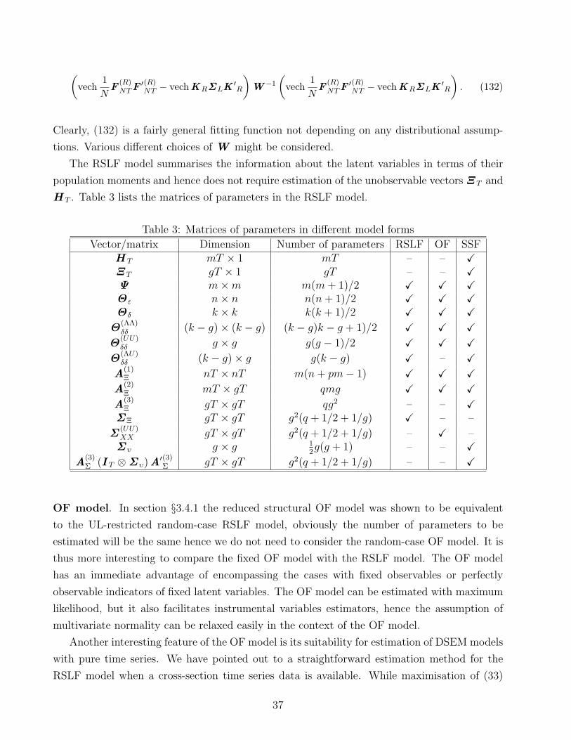
(vech

1N

F(R)NTF ′(R)

NT − vechKRΣLK′R

)W −1

(vech

1N

F(R)NTF ′(R)

NT − vechKRΣLK′R

). (132)

Clearly, (132) is a fairly general fitting function not depending on any distributional assump-

tions. Various different choices of W might be considered.

The RSLF model summarises the information about the latent variables in terms of their

population moments and hence does not require estimation of the unobservable vectors Ξ T and

H T . Table 3 lists the matrices of parameters in the RSLF model.

Table 3: Matrices of parameters in different model forms

Vector/matrix Dimension Number of parameters RSLF OF SSFH T mT × 1 mT – – XΞ T gT × 1 gT – – XΨ m×m m(m + 1)/2 X X XΘε n× n n(n + 1)/2 X X XΘδ k × k k(k + 1)/2 X X X

Θ(ΛΛ)δδ (k − g)× (k − g) (k − g)k − g + 1)/2 X X X

Θ(UU)δδ g × g g(g − 1)/2 X X X

Θ(ΛU)δδ (k − g)× g g(k − g) X – X

A(1)Ξ nT × nT m(n + pm− 1) X X X

A(2)Ξ mT × gT qmg X X X

A(3)Ξ gT × gT qg2 – – X

ΣΞ gT × gT g2(q + 1/2 + 1/g) X – –

Σ(UU)XX gT × gT g2(q + 1/2 + 1/g) – X –Συ g × g 1

2g(g + 1) – – X

A(3)Σ (I T ⊗Συ)A

′(3)Σ gT × gT g2(q + 1/2 + 1/g) – – X

OF model. In section §3.4.1 the reduced structural OF model was shown to be equivalent

to the UL-restricted random-case RSLF model, obviously the number of parameters to be

estimated will be the same hence we do not need to consider the random-case OF model. It is

thus more interesting to compare the fixed OF model with the RSLF model. The OF model

has an immediate advantage of encompassing the cases with fixed observables or perfectly

observable indicators of fixed latent variables. The OF model can be estimated with maximum

likelihood, but it also facilitates instrumental variables estimators, hence the assumption of

multivariate normality can be relaxed easily in the context of the OF model.

Another interesting feature of the OF model is its suitability for estimation of DSEM models

with pure time series. We have pointed out to a straightforward estimation method for the

RSLF model when a cross-section time series data is available. While maximisation of (33)

37

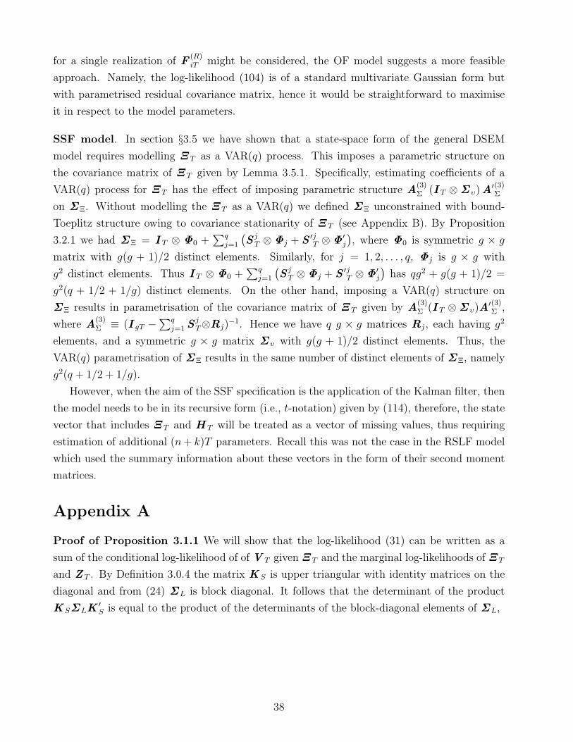
for a single realization of F(R)iT might be considered, the OF model suggests a more feasible

approach. Namely, the log-likelihood (104) is of a standard multivariate Gaussian form but

with parametrised residual covariance matrix, hence it would be straightforward to maximise

it in respect to the model parameters.

SSF model. In section §3.5 we have shown that a state-space form of the general DSEM

model requires modelling Ξ T as a VAR(q) process. This imposes a parametric structure on

the covariance matrix of Ξ T given by Lemma 3.5.1. Specifically, estimating coefficients of a

VAR(q) process for Ξ T has the effect of imposing parametric structure A(3)Σ (I T ⊗Συ)A

′(3)Σ

on ΣΞ. Without modelling the Ξ T as a VAR(q) we defined ΣΞ unconstrained with bound-

Toeplitz structure owing to covariance stationarity of Ξ T (see Appendix B). By Proposition

3.2.1 we had ΣΞ = I T ⊗ Φ0 +∑q

j=1

(S j

T ⊗Φj + S ′jT ⊗Φ′

j

), where Φ0 is symmetric g × g

matrix with g(g + 1)/2 distinct elements. Similarly, for j = 1, 2, . . . , q, Φj is g × g with

g2 distinct elements. Thus I T ⊗ Φ0 +∑q

j=1

(S j

T ⊗Φj + S ′jT ⊗Φ′

j

)has qg2 + g(g + 1)/2 =

g2(q + 1/2 + 1/g) distinct elements. On the other hand, imposing a VAR(q) structure on

ΣΞ results in parametrisation of the covariance matrix of Ξ T given by A(3)Σ (I T ⊗Συ)A

′(3)Σ ,

where A(3)Σ ≡ (I gT −

∑qj=1 S

jT⊗Rj)

−1. Hence we have q g × g matrices Rj, each having g2

elements, and a symmetric g × g matrix Συ with g(g + 1)/2 distinct elements. Thus, the

VAR(q) parametrisation of ΣΞ results in the same number of distinct elements of ΣΞ, namely

g2(q + 1/2 + 1/g).

However, when the aim of the SSF specification is the application of the Kalman filter, then

the model needs to be in its recursive form (i.e., t-notation) given by (114), therefore, the state

vector that includes Ξ T and H T will be treated as a vector of missing values, thus requiring

estimation of additional (n + k)T parameters. Recall this was not the case in the RSLF model

which used the summary information about these vectors in the form of their second moment

matrices.

Appendix A

Proof of Proposition 3.1.1 We will show that the log-likelihood (31) can be written as a

sum of the conditional log-likelihood of of V T given Ξ T and the marginal log-likelihoods of Ξ T

and Z T . By Definition 3.0.4 the matrix K S is upper triangular with identity matrices on the

diagonal and from (24) ΣL is block diagonal. It follows that the determinant of the product

K SΣLK′S is equal to the product of the determinants of the block-diagonal elements of ΣL,

38

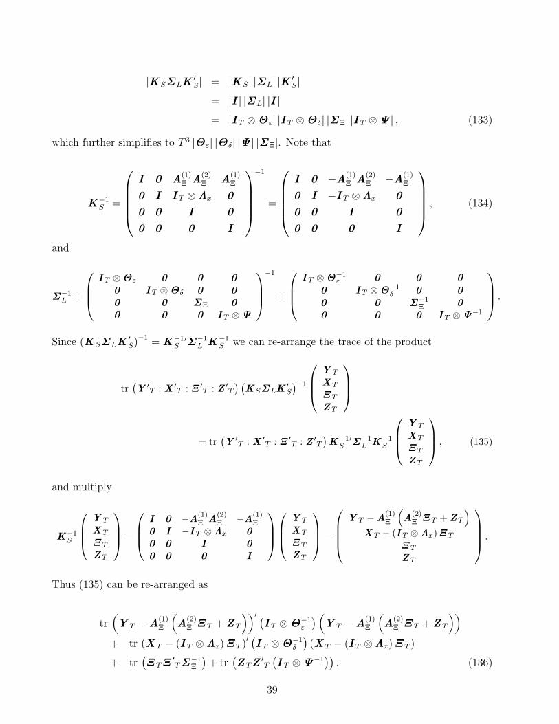
|K SΣLK′S| = |K S| |ΣL| |K ′

S|= |I | |ΣL| |I |= |I T ⊗Θε| |I T ⊗Θδ| |ΣΞ| |I T ⊗Ψ | , (133)

which further simplifies to T 3 |Θε| |Θδ| |Ψ | |ΣΞ|. Note that

K−1S =

I 0 A(1)Ξ A

(2)Ξ A

(1)Ξ

0 I I T ⊗Λx 0

0 0 I 0

0 0 0 I

−1

=

I 0 −A(1)Ξ A

(2)Ξ −A

(1)Ξ

0 I −I T ⊗Λx 0

0 0 I 0

0 0 0 I

, (134)

and

Σ−1L =

I T ⊗Θε 0 0 00 I T ⊗Θδ 0 00 0 ΣΞ 00 0 0 I T ⊗Ψ

−1

=

I T ⊗Θ−1ε 0 0 0

0 I T ⊗Θ−1δ 0 0

0 0 Σ−1Ξ 0

0 0 0 I T ⊗Ψ−1

.

Since (K SΣLK′S)−1

= K−1S′Σ−1

L K−1S we can re-arrange the trace of the product

tr(Y ′

T : X ′T : Ξ ′

T : Z ′T

) (K SΣLK

′S

)−1

Y T

X T

Ξ T

Z T

= tr(Y ′

T : X ′T : Ξ ′

T : Z ′T

)K−1

S′Σ−1

L K−1S

Y T

X T

Ξ T

Z T

, (135)

and multiply

K−1S

Y T

X T

Ξ T

Z T

=

I 0 −A(1)Ξ A

(2)Ξ −A

(1)Ξ

0 I −I T ⊗Λx 00 0 I 00 0 0 I

Y T

X T

Ξ T

Z T

=

Y T −A(1)Ξ

(A

(2)Ξ Ξ T + Z T

)

X T − (I T ⊗Λx)Ξ T

Ξ T

Z T

.

Thus (135) can be re-arranged as

tr(Y T −A

(1)Ξ

(A

(2)Ξ Ξ T + Z T

))′ (I T ⊗Θ−1

ε

) (Y T −A

(1)Ξ

(A

(2)Ξ Ξ T + Z T

))

+ tr (X T − (I T ⊗Λx)Ξ T )′(I T ⊗Θ−1

δ

)(X T − (I T ⊗Λx)Ξ T )

+ tr(Ξ TΞ

′TΣ

−1Ξ

)+ tr

(Z TZ

′T

(I T ⊗Ψ−1

)). (136)

39

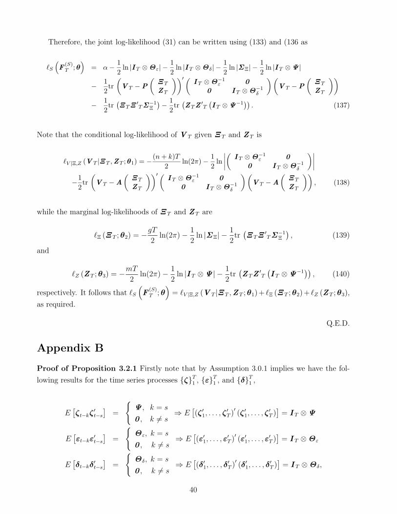
Therefore, the joint log-likelihood (31) can be written using (133) and (136 as

`S

(F

(S)T ; θ

)= α− 1

2ln |I T ⊗Θε| − 1

2ln |I T ⊗Θδ| − 1

2ln |ΣΞ| − 1

2ln |I T ⊗Ψ |

− 12tr

(V T −P

(Ξ T

Z T

))′(I T ⊗Θ−1

ε 0

0 I T ⊗Θ−1δ

)(V T −P

(Ξ T

Z T

))

− 12tr

(Ξ TΞ ′

TΣ−1Ξ

)− 12tr

(Z TZ ′

T

(I T ⊗Ψ−1

)). (137)

Note that the conditional log-likelihood of V T given Ξ T and Z T is

`V |Ξ,Z (V T |Ξ T ,Z T ; θ1) = −(n + k)T2

ln(2π)− 12

ln∣∣∣∣(

I T ⊗Θ−1ε 0

0 I T ⊗Θ−1δ

)∣∣∣∣

−12tr

(V T −A

(Ξ T

Z T

))′(I T ⊗Θ−1

ε 0

0 I T ⊗Θ−1δ

)(V T −A

(Ξ T

Z T

)), (138)

while the marginal log-likelihoods of Ξ T and Z T are

`Ξ (Ξ T ; θ2) = −gT

2ln(2π)− 1

2ln |ΣΞ| − 1

2tr

(Ξ TΞ

′TΣ

−1Ξ

), (139)

and

`Z (Z T ; θ3) = −mT

2ln(2π)− 1

2ln |I T ⊗Ψ | − 1

2tr

(Z TZ

′T

(I T ⊗Ψ−1

)), (140)

respectively. It follows that `S

(F

(S)T ; θ

)= `V |Ξ,Z (V T |Ξ T ,Z T ; θ1)+ `Ξ (Ξ T ; θ2)+ `Z (Z T ; θ3),

as required.

Q.E.D.

Appendix B

Proof of Proposition 3.2.1 Firstly note that by Assumption 3.0.1 implies we have the fol-

lowing results for the time series processes ζT1 , εT

1 , and δT1 ,

E[ζt−kζ

′t−s

]=

Ψ , k = s

0 , k 6= s⇒ E

[(ζ ′1, . . . , ζ

′T )′(ζ ′1, . . . , ζ

′T )

]= I T ⊗Ψ

E[εt−kε

′t−s

]=

Θε, k = s

0 , k 6= s⇒ E

[(ε′1, . . . , ε

′T )′(ε′1, . . . , ε

′T )

]= I T ⊗Θε

E[δt−kδ

′t−s

]=

Θδ, k = s

0 , k 6= s⇒ E

[(δ′1, . . . , δ

′T )′(δ′1, . . . , δ

′T )

]= I T ⊗Θδ,

40

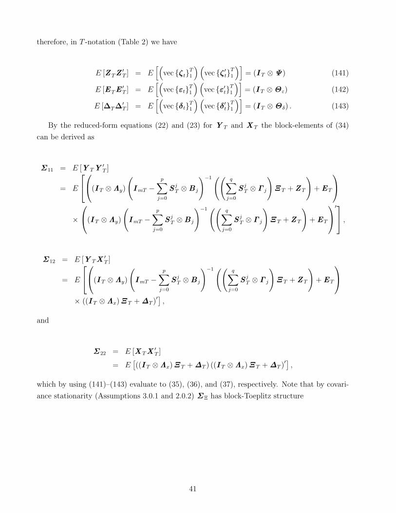
therefore, in T -notation (Table 2) we have

E [Z TZ′T ] = E

[(vec ζtT

1

)(vec ζ ′tT

1

)]= (I T ⊗Ψ) (141)

E [ETE′T ] = E

[(vec εtT

1

)(vec ε′tT

1

)]= (I T ⊗Θε) (142)

E [∆T∆′T ] = E

[(vec δtT

1

)(vec δ′tT

1

)]= (I T ⊗Θδ) . (143)

By the reduced-form equations (22) and (23) for Y T and X T the block-elements of (34)

can be derived as

Σ 11 = E [Y TY′T ]

= E

(I T ⊗Λy)

(ImT −

p∑j=0

S jT ⊗B j

)−1 ((q∑

j=0

S jT ⊗ Γ j

)Ξ T + Z T

)+ ET

×(I T ⊗Λy)

(ImT −

p∑j=0

S jT ⊗B j

)−1 ((q∑

j=0

S jT ⊗ Γ j

)Ξ T + Z T

)+ ET

′ ,

Σ 12 = E [Y TX′T ]

= E

(I T ⊗Λy)

(ImT −

p∑j=0

S jT ⊗B j

)−1 ((q∑

j=0

S jT ⊗ Γ j

)Ξ T + Z T

)+ ET

× ((I T ⊗Λx)Ξ T + ∆T )′],

and

Σ 22 = E [X TX′T ]

= E[((I T ⊗Λx)Ξ T + ∆T ) ((I T ⊗Λx)Ξ T + ∆T )′

],

which by using (141)–(143) evaluate to (35), (36), and (37), respectively. Note that by covari-

ance stationarity (Assumptions 3.0.1 and 2.0.2) ΣΞ has block-Toeplitz structure

41

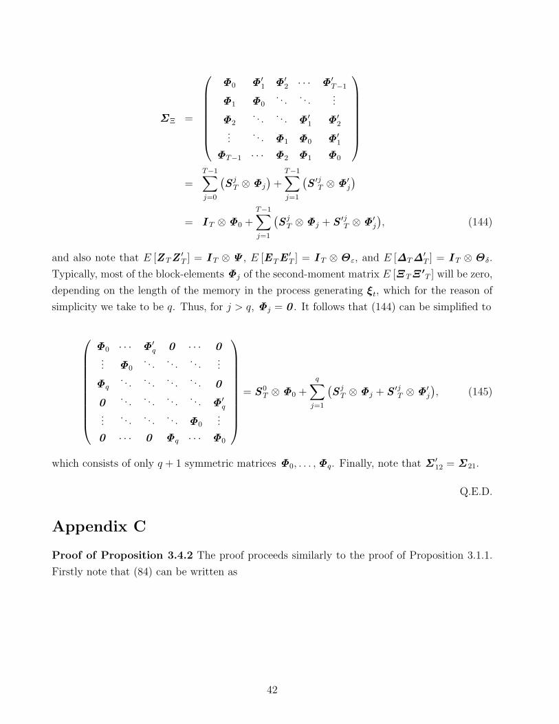
ΣΞ =

Φ0 Φ′1 Φ′

2 · · · Φ′T−1

Φ1 Φ0. . . . . .

...

Φ2. . . . . . Φ′

1 Φ′2

.... . . Φ1 Φ0 Φ′

1

ΦT−1 · · · Φ2 Φ1 Φ0

=T−1∑j=0

(S j

T ⊗Φj

)+

T−1∑j=1

(S ′j

T ⊗Φ′j

)

= I T ⊗Φ0 +T−1∑j=1

(S j

T ⊗Φj + S ′jT ⊗Φ′

j

), (144)

and also note that E [Z TZ′T ] = I T ⊗Ψ , E [ETE

′T ] = I T ⊗Θε, and E [∆T∆

′T ] = I T ⊗Θδ.

Typically, most of the block-elements Φj of the second-moment matrix E [Ξ TΞ0T ] will be zero,

depending on the length of the memory in the process generating ξt, which for the reason of

simplicity we take to be q. Thus, for j > q, Φj = 0 . It follows that (144) can be simplified to

Φ0 · · · Φ′q 0 · · · 0

... Φ0. . . . . . . . .

...

Φq. . . . . . . . . . . . 0

0. . . . . . . . . . . . Φ′

q...

. . . . . . . . . Φ0...

0 · · · 0 Φq · · · Φ0

= S 0T ⊗Φ0 +

q∑j=1

(S j

T ⊗Φj + S ′jT ⊗Φ′

j

), (145)

which consists of only q + 1 symmetric matrices Φ0, . . . ,Φq. Finally, note that Σ ′12 = Σ 21.

Q.E.D.

Appendix C

Proof of Proposition 3.4.2 The proof proceeds similarly to the proof of Proposition 3.1.1.

Firstly note that (84) can be written as

42

`(S)OF

(F

(OF )T ; θ

)= −(n + k + g + m)T

2ln(2π)− 1

2ln |MΣ ∗

LM′|

−1

2tr

(Y ′

T : X ′(Λ)T : X ′(U)

T : ∆′(U)T : Z ′

T

)(MΣ ∗

LM′)−1

Y T

X(Λ)T

X(U)T

∆(U)T

Z T

, (146)

which can be rearranged by following the same procedure we used to derive (137) as

− (n+k+g+m)T2 ln(2π)

−12 ln

∣∣∣∣∣

(I T ⊗Θε 0

0 I T ⊗Θ(ΛΛ)δδ

)∣∣∣∣∣−12 ln

∣∣∣I T ⊗Θ(UU)δδ

∣∣∣− 12 ln |ΣΞ| − 1

2 ln |I T ⊗Ψ |

−12tr

(Y T

X(Λ)T

)− A

X(U)T

∆(U)T

Z T

′(I T ⊗Θ−1

ε 0

0 I T ⊗Θ(ΛΛ)δδ

−1

)

(Y T

X(Λ)T

)− A

X(U)T

∆(U)T

Z T

−12tr

((I : −I )

(X

(U)T

∆(U)T

)(X ′(U)

T : ∆′(U)T

)(I−I

)Σ−1

Ξ

)

−12tr

(∆

(U)T ∆′(U)

T

(I T ⊗Θ

(UU)δδ

)−1)− 1

2tr(Z TZ ′

T

(I T ⊗Ψ−1

)),

(147)

where

A ≡(

A(1)Ξ A

(2)Ξ −A

(1)Ξ A

(2)Ξ A

(1)Ξ

I T ⊗ Λx 0 0

). (148)

Note that A(1)Ξ A

(2)Ξ Ξ T = A

(1)Ξ A

(2)Ξ X

(U)T −A

(1)Ξ A

(2)Ξ ∆

(U)T . Finally, we can observe that

`Y,XΛ|XU ,∆U ,Z

(Y T ,X

(Λ)T |X (U)

T ,∆(U)T ,Z T ;θ∗1

)= − (n+k−g)T

2 ln(2π)

−12 ln

∣∣∣∣∣

(I T ⊗Θε 0

0 I T ⊗Θ(ΛΛ)δδ

)∣∣∣∣∣

−12tr

(Y T

X(Λ)T

)− A

X(U)T

∆(U)T

Z T

′

×(

I T ⊗Θ−1ε 0

0 I T ⊗Θ(ΛΛ)δδ

−1

)

(Y T

X(Λ)T

)− A

X(U)T

∆(U)T

Z T

(149)

is the conditional log-likelihood of Y T and X(Λ)T given X

(U)T , ∆

(U)T , and Z T . The marginal

log-likelihoods of X(U)T −∆

(U)T , `∆U , and Z T are given by

43

`M

(X

(U)T −∆

(U)T ;θ∗2

)= −gT

2ln(2π)− 1

2ln |ΣΞ|

− 12tr

((I : −I )

(X

(U)T

∆(U)T

)(X ′(U)

T : ∆′(U)T

)(I−I

)Σ−1

Ξ

), (150)

`M

(∆

(U)T ; θ∗3

)= −gT

2ln(2π)−1

2ln

∣∣∣I T ⊗Θ(UU)δδ

∣∣∣−1

2tr

(∆

(U)T ∆′(U)

T

(I T ⊗Θ

(UU)δδ

)−1)

, (151)

and

`M (Z T ; θ∗4) = −mT

2ln(2π)− 1

2ln |I T ⊗Ψ | − 1

2tr

(Z TZ

′T

(I T ⊗Ψ−1

)), (152)

respectively. Hence (84) factorise into (85), as required.

Q.E.D.

Appendix D

Proof of Proposition 3.4.4 We will compare (90) and (50) by comparing their corresponding

block-elements in expectation and probability limit. Recall that by Lemma (3.4.1) we have

ΣΞ = Σ(UU)XX − I T ⊗Θ

(UU)δδ . Therefore, we can evaluate the block elements of (90) as follows.

44

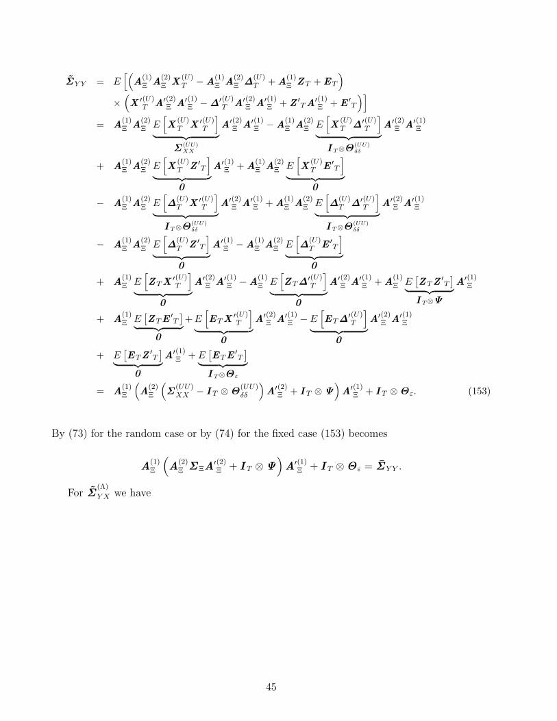
ΣY Y = E[(

A(1)Ξ A

(2)Ξ X

(U)T −A

(1)Ξ A

(2)Ξ ∆

(U)T + A

(1)Ξ Z T + ET

)

×(X ′(U)

T A′(2)Ξ A′(1)

Ξ −∆′(U)T A′(2)

Ξ A′(1)Ξ + Z ′

TA′(1)Ξ + E ′

T

)]

= A(1)Ξ A

(2)Ξ E

[X

(U)T X ′(U)

T

]

︸ ︷︷ ︸Σ (UU)

XX

A′(2)Ξ A′(1)

Ξ −A(1)Ξ A

(2)Ξ E

[X

(U)T ∆′(U)

T

]

︸ ︷︷ ︸I T⊗Θ (UU)

δδ

A′(2)Ξ A′(1)

Ξ

+ A(1)Ξ A

(2)Ξ E

[X

(U)T Z ′

T

]

︸ ︷︷ ︸0

A′(1)Ξ + A

(1)Ξ A

(2)Ξ E

[X

(U)T E ′

T

]

︸ ︷︷ ︸0

− A(1)Ξ A

(2)Ξ E

[∆

(U)T X ′(U)

T

]

︸ ︷︷ ︸I T⊗Θ (UU)

δδ

A′(2)Ξ A′(1)

Ξ + A(1)Ξ A

(2)Ξ E

[∆

(U)T ∆′(U)

T

]

︸ ︷︷ ︸I T⊗Θ (UU)

δδ

A′(2)Ξ A′(1)

Ξ

− A(1)Ξ A

(2)Ξ E

[∆

(U)T Z ′

T

]

︸ ︷︷ ︸0

A′(1)Ξ −A

(1)Ξ A

(2)Ξ E

[∆

(U)T E ′

T

]

︸ ︷︷ ︸0

+ A(1)Ξ E

[Z TX ′(U)

T

]

︸ ︷︷ ︸0

A′(2)Ξ A′(1)

Ξ −A(1)Ξ E

[Z T∆′(U)

T

]

︸ ︷︷ ︸0

A′(2)Ξ A′(1)

Ξ + A(1)Ξ E

[Z TZ ′

T

]︸ ︷︷ ︸

I T⊗Ψ

A′(1)Ξ

+ A(1)Ξ E

[Z TE ′

T

]︸ ︷︷ ︸

0

+E[ETX ′(U)

T

]

︸ ︷︷ ︸0

A′(2)Ξ A′(1)

Ξ − E[ET∆′(U)

T

]

︸ ︷︷ ︸0

A′(2)Ξ A′(1)

Ξ

+ E[ETZ ′

T

]︸ ︷︷ ︸

0

A′(1)Ξ + E

[ETE ′

T

]︸ ︷︷ ︸

I T⊗Θε

= A(1)Ξ

(A

(2)Ξ

(Σ

(UU)XX − I T ⊗Θ

(UU)δδ

)A′(2)

Ξ + I T ⊗Ψ)A′(1)

Ξ + I T ⊗Θε. (153)

By (73) for the random case or by (74) for the fixed case (153) becomes

A(1)Ξ

(A

(2)Ξ ΣΞA

′(2)Ξ + I T ⊗Ψ

)A′(1)

Ξ + I T ⊗Θε = ΣY Y .

For Σ(Λ)

Y X we have

45

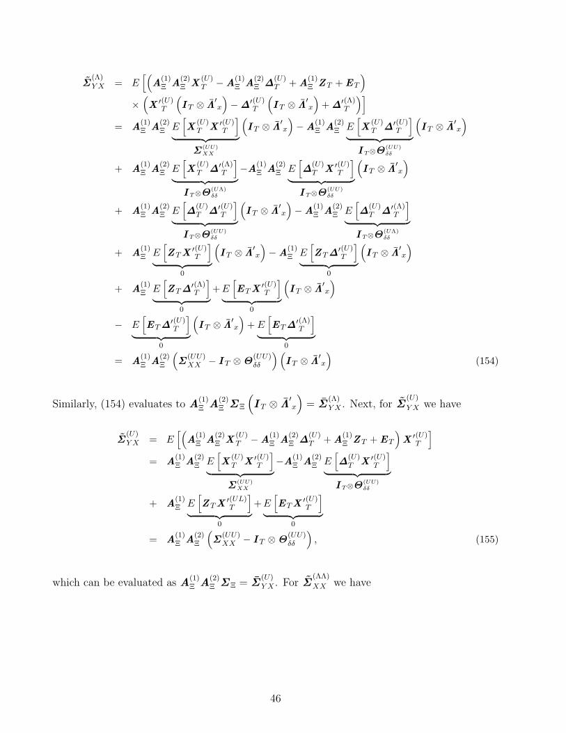
Σ(Λ)Y X = E

[(A

(1)Ξ A

(2)Ξ X

(U)T −A

(1)Ξ A

(2)Ξ ∆

(U)T + A

(1)Ξ Z T + ET

)

×(X ′(U)

T

(I T ⊗ Λ

′x

)−∆′(U)

T

(I T ⊗ Λ

′x

)+ ∆′(Λ)

T

)]

= A(1)Ξ A

(2)Ξ E

[X

(U)T X ′(U)

T

]

︸ ︷︷ ︸Σ (UU)

XX

(I T ⊗ Λ

′x

)−A

(1)Ξ A

(2)Ξ E

[X

(U)T ∆′(U)

T

]

︸ ︷︷ ︸I T⊗Θ (UU)

δδ

(I T ⊗ Λ

′x

)

+ A(1)Ξ A

(2)Ξ E

[X

(U)T ∆′(Λ)

T

]

︸ ︷︷ ︸I T⊗Θ (UΛ)

δδ

−A(1)Ξ A

(2)Ξ E

[∆

(U)T X ′(U)

T

]

︸ ︷︷ ︸I T⊗Θ (UU)

δδ

(I T ⊗ Λ

′x

)

+ A(1)Ξ A

(2)Ξ E

[∆

(U)T ∆′(U)

T

]

︸ ︷︷ ︸I T⊗Θ (UU)

δδ

(I T ⊗ Λ

′x

)−A

(1)Ξ A

(2)Ξ E

[∆

(U)T ∆′(Λ)

T

]

︸ ︷︷ ︸I T⊗Θ (UΛ)

δδ

+ A(1)Ξ E

[Z TX ′(U)

T

]

︸ ︷︷ ︸0

(I T ⊗ Λ

′x

)−A

(1)Ξ E

[Z T∆′(U)

T

]

︸ ︷︷ ︸0

(I T ⊗ Λ

′x

)

+ A(1)Ξ E

[Z T∆′(Λ)

T

]

︸ ︷︷ ︸0

+E[ETX ′(U)

T

]

︸ ︷︷ ︸0

(I T ⊗ Λ

′x

)

− E[ET∆′(U)

T

]

︸ ︷︷ ︸0

(I T ⊗ Λ

′x

)+ E

[ET∆′(Λ)

T

]

︸ ︷︷ ︸0

= A(1)Ξ A

(2)Ξ

(Σ

(UU)XX − I T ⊗Θ

(UU)δδ

)(I T ⊗ Λ

′x

)(154)

Similarly, (154) evaluates to A(1)Ξ A

(2)Ξ ΣΞ

(I T ⊗ Λ

′x

)= Σ

(Λ)Y X . Next, for Σ

(U)

Y X we have

Σ(U)Y X = E

[(A

(1)Ξ A

(2)Ξ X

(U)T −A

(1)Ξ A

(2)Ξ ∆

(U)T + A

(1)Ξ Z T + ET

)X ′(U)

T

]

= A(1)Ξ A

(2)Ξ E

[X

(U)T X ′(U)

T

]

︸ ︷︷ ︸Σ (UU)

XX

−A(1)Ξ A

(2)Ξ E

[∆

(U)T X ′(U)

T

]

︸ ︷︷ ︸I T⊗Θ (UU)

δδ

+ A(1)Ξ E

[Z TX ′(UL)

T

]

︸ ︷︷ ︸0

+E[ETX ′(U)

T

]

︸ ︷︷ ︸0

= A(1)Ξ A

(2)Ξ

(Σ

(UU)XX − I T ⊗Θ

(UU)δδ

), (155)

which can be evaluated as A(1)Ξ A

(2)Ξ ΣΞ = Σ

(U)Y X . For Σ

(ΛΛ)

XX we have

46

Σ(ΛΛ)XX = E

[((I T ⊗ Λx

)X

(U)T − (

I T ⊗ Λx

)∆

(U)T + ∆

(Λ)T

)

×(X ′(U)

T

(I T ⊗ Λ

′x

)−∆′(U)

T

(I T ⊗ Λ

′x

)+ ∆′(Λ)

T

)]

=(I T ⊗ Λx

)E

[X

(U)T X ′(U)

T

]

︸ ︷︷ ︸Σ (UU)

XX

(I T ⊗ Λ

′x

)− (

I T ⊗ Λx

)E

[X

(U)T ∆′(U)

T

]

︸ ︷︷ ︸I T⊗Θ (UU)

δδ

(I T ⊗ Λ

′x

)

+(I T ⊗ Λx

)E

[X

(U)T ∆′(Λ)

T

]

︸ ︷︷ ︸I T⊗Θ (UΛ)

δδ

− (I T ⊗ Λx

)E

[∆

(U)T X ′(U)

T

]

︸ ︷︷ ︸I T⊗Θ (UU)

δδ

(I T ⊗ Λ

′x

)

+(I T ⊗ Λx

)E

[∆

(U)T ∆′(U)

T

]

︸ ︷︷ ︸I T⊗Θ (UU)

δδ

(I T ⊗ Λ

′x

)− (

I T ⊗ Λx

)E

[∆

(U)T ∆′(Λ)

T

]

︸ ︷︷ ︸I T⊗Θ (UΛ)

δδ

+ E[∆

(Λ)T X ′(U)

T

]

︸ ︷︷ ︸I T⊗Θ (ΛU)

δδ

(I T ⊗ Λ

′x

)−E

[∆

(Λ)T ∆′(U)

T

]

︸ ︷︷ ︸I T⊗Θ (ΛU)

δδ

(I T ⊗ Λ

′x

)+ E

[∆

(Λ)T ∆′(Λ)

T

]

︸ ︷︷ ︸I T⊗Θ (ΛΛ)

δδ

=(I T ⊗ Λx

) (Σ

(UU)XX − I T ⊗Θ

(UU)δδ

)(I T ⊗ Λ

′x

)+ I T ⊗Θ

(ΛΛ)δδ , (156)

which becomes(I T ⊗ Λx

)ΣΞ

(I T ⊗ Λ

′x

)+I T⊗Θ

(ΛΛ)δδ = Σ

(ΛΛ)XX . Similarly, for Σ

(ΛU)

XX it follows

that

Σ(ΛU)XX = E

[((I T ⊗ Λx

)X

(U)T − (

I T ⊗ Λx

)∆

(U)T + ∆

(Λ)T

)X ′(U)

T

]

=(I T ⊗ Λx

)E

[X

(U)T X ′(U)

T

]

︸ ︷︷ ︸Σ (UU)

XX

− (I T ⊗ Λx

)E

[∆

(U)T X ′(U)

T

]

︸ ︷︷ ︸I T⊗Θ (UU)

δδ

+E[∆

(Λ)T X ′(U)

T

]

︸ ︷︷ ︸I T⊗Θ (ΛU)

δδ

=(I T ⊗ Λx

) (Σ

(UU)XX − I T ⊗Θ

(UU)δδ

)+ I T ⊗Θ

(ΛU)δδ , (157)

which evaluates to(I T ⊗ Λx

)ΣΞ + I T ⊗Θ

(ΛU)δδ = Σ

(ΛU)XX . Finally,

Σ(UU)

XX = E[X

(UL)T X ′(UL)

T

]= Σ

(UU)XX , (158)

thus trivially we have Σ(UU)

XX = Σ(UU)XX . Therefore, E[Σ ] = E[Σ ] or p lim

T→∞1/T Σ = p lim

T→∞1/T Σ ,

as required.

Q.E.D.

Appendix E

Proof of Proposition 3.4.5 We firstly derive (105)–(107) from (99)–(101) using Assumption

3.0.1. For ΩY Y we have

47

ΩY Y = E[(

A(1)Ξ Z T −A

(1)Ξ A

(2)Ξ ∆

(U)T + ET

)(Z ′

TA′(1)Ξ −∆′(U)

T A′(2)Ξ A′(1)

Ξ + E ′T

)]

= A(1)Ξ E

[Z T∆′(U)

T

]

︸ ︷︷ ︸0

A′(2)Ξ A′(1)

Ξ + A(1)Ξ E

[Z TZ ′

T

]︸ ︷︷ ︸

I T⊗Ψ

A′(1)Ξ + A

(1)Ξ E

[Z TE ′

T

]︸ ︷︷ ︸

0

+ E[ET∆′(U)

T

]

︸ ︷︷ ︸0

A′(2)Ξ A′(1)

Ξ + A(1)Ξ A

(2)Ξ E

[∆

(U)T ∆′(U)

T

]

︸ ︷︷ ︸I T⊗Θ (UU)

δδ

A′(2)Ξ A′(1)

Ξ

− A(1)Ξ A

(2)Ξ E

[∆

(U)T Z ′

T

]

︸ ︷︷ ︸0

A′(1)Ξ −A

(1)Ξ A

(2)Ξ E

[∆

(U)T E ′

T

]

︸ ︷︷ ︸0

+E[ETZ ′

T

]︸ ︷︷ ︸

0

A′(1)Ξ + E

[ETE ′

T

]︸ ︷︷ ︸

I T⊗Θε

= A(1)Ξ

(A

(2)Ξ

(I T ⊗Θ

(UU)δδ

)A′(2)

Ξ + I T ⊗Ψ)A′(1)

Ξ + I T ⊗Θε, (159)

which gives (105). Next, for Ω(Λ)Y X we have

Ω(Λ)Y X = E

[(A

(1)Ξ Z T −A

(1)Ξ A

(2)Ξ ∆

(U)T + ET

)(∆′(Λ)

T −∆′(U)T

(I T ⊗ Λ

′x

))]

= A(1)Ξ E

[Z T∆′(Λ)

T

]

︸ ︷︷ ︸0

−A(1)Ξ E

[Z T∆′(U)

T

]

︸ ︷︷ ︸0

(I T ⊗ Λ

′x

)−A

(1)Ξ A

(2)Ξ E

[∆

(U)T ∆′(Λ)

T

]

︸ ︷︷ ︸I T⊗Θ (UΛ)

δδ

+ A(1)Ξ A

(2)Ξ E

[∆

(U)T ∆′(U)

T

]

︸ ︷︷ ︸I T⊗Θ (UU)

δδ

(I T ⊗ Λ

′x

)+ E

[ET∆′(Λ)

T

]

︸ ︷︷ ︸0

−E[ET∆′(U)

T

]

︸ ︷︷ ︸0

(I T ⊗ Λ

′x

)

= A(1)Ξ A

(2)Ξ

(I T ⊗Θ

(UU)δδ

)(I T ⊗ Λ

′x

)−A

(1)Ξ A

(2)Ξ

(I T ⊗Θ

(UΛ)δδ

), (160)

which, since I T ⊗Θ(ΛU)δδ = 0 , yields (106). Finally, Ω

(ΛΛ)XX can be evaluated as

Ω(ΛΛ)XX = E

[(∆

(Λ)T − (

I T ⊗ Λx

)∆

(U)T

)(∆′(Λ)

T −∆′(U)T

(I T ⊗ Λ

′x

))]

= E[∆

(Λ)T ∆′(Λ)

T

]

︸ ︷︷ ︸I T⊗Θ (ΛΛ)

δδ

−E[∆

(Λ)T ∆′(U)

T

]

︸ ︷︷ ︸I T⊗Θ (ΛU)

δδ

(I T ⊗ Λ

′x

)− (

I T ⊗ Λx

)E

[∆

(U)T ∆′(Λ)

T

]

︸ ︷︷ ︸I T⊗Θ (UΛ)

δδ

+(I T ⊗ Λx

)E

[∆

(U)T ∆′(U)

T

]

︸ ︷︷ ︸I T⊗Θ (UU)

δδ

(I T ⊗ Λ

′x

)

= I T ⊗Θ(ΛΛ)δδ +

(I T ⊗Θ

(ΛU)δδ

)(I T ⊗ Λ

′x

)− (

I T ⊗ Λx

) (I T ⊗Θ

(UΛ)δδ

)

+(I T ⊗ Λx

) (I T ⊗Θ

(UU)δδ

)(I T ⊗ Λ

′x

), (161)

yielding (107) again by noting that I T ⊗Θ(ΛU)δδ = 0 . Secondly, we derive (108) as follows. By

Definition 3.0.4,

48

KR ≡(

I 0 A(1)Ξ A

(2)Ξ A

(1)Ξ

0 I I T ⊗ Λx 0

), (162)

hence

DSΣLD′S ≡

I T ⊗Θε 0 0 0

0 I T ⊗Θ(ΛΛ)δδ 0 0

0 0 I T ⊗Θ(UU)δδ 0

0 0 0 I T ⊗Ψ

, (163)

where ΣL is defined as in (24). Finally, premultiplying and postmultiplying (163) by (162)

yields (108), as required.

Q.E.D.

Appendix F

Proof of Proposition 3.5.3 We will show that the general DSEM model (1)–(2) can be

written in the state-space form (111)–(112). Firstly, the structural part of the general DSEM

model (1) and the VAR(q) process for ξt (113) can be written as a system

(ηt

ξt

)=

(B0 Γ 0

0 0

)(ηt

ξt

)

+

(B1 Γ 1

0 R1

)(ηt−1

ξt−1

)+ . . . +

(B r Γ r

0 Rr

)(ηt−r

ξt−r

)+

(ζt

υt

), (164)

or equivalently as

((I −B0) −Γ 0

0 I

)(ηt

ξt

)=

(B1 Γ 1

0 R1

)(ηt−1

ξt−1

)

+ . . . +

(B r Γ r

0 Rr

) (ηt−r

ξt−r

)+

(ζt

υt

). (165)

Therefore, the reduced form of (164) is

(ηt

ξt

)=

((I −B0) −Γ 0

0 I

)−1 [(B1 Γ 1

0 R1

)(ηt−1

ξt−1

)

+ . . . +

(B r Γ r

0 Rr

)(ηt−r

ξt−r

)+

(ζt

υt

)]. (166)

49

Note that

((I −B0) −Γ 0

0 I

)−1

=

((I −B0)

−1 (I −B0)−1 Γ 0

0 I

),

hence

((I −B0)

−1 (I −B0)−1 Γ 0

0 I

)(B j Γ j

0 Rj

)

=

((I −B0)

−1 B j (I −B0)−1 Γ j + (I −B0)

−1 Γ 0Rj

0 Rj

), (167)

and

((I −B0)

−1 (I −B0)−1 Γ 0

0 I

)(ζt

υt

)=

((I −B0)

−1 ζt + (I −B0)−1 Γ 0υt

υt

). (168)

Therefore, using (167) and (168), the reduced form of the system (164) can be written as

(ηt

ξt

)=

(Π 1 G1

0 R1

)(ηt−1

ξt−1

)+ . . . +

(Π r Gr

0 Rr

)(ηt−r

ξt−r

)+

(K t

υt

). (169)

making use of the notation from Definition 3.5.2. Finally, we stack the current and lagged ηt

and ξt into a single column vector, collect all coefficient matrices in a single block matrix, and

stack the residuals into a single as

ϑt ≡

ηt

ξt

ηt−1

ξt−1...

ηt−r+1

ξt−r+1

,H ≡

Π 1 G1 · · · Π r−1 Gr−1 Π r Gr

0 R1 · · · 0 Rr−1 0 Rr

I 0 · · · 0 0 0 00 I · · · 0 0 0 0...

.... . .

......

......

0 0 · · · I 0 0 00 0 · · · 0 I 0 0

,wt ≡

K t

υt

00...00

, (170)

and

W t ≡(

y t

x t

), F ≡

(Λy 0 · · · 0

0 Λx · · · 0

), u t ≡

(εt

δt

),

therefore, (169) can be written in the state space form (111)–(112), as required.

Q.E.D.

50

References

Aigner, D.J. and Goldberger, A.S., Eds. (1977), Latent Variables in Socio-economic Models.

Amsterdam: North-Holland.

Aigner, D.J., Hsiao, C., Kapteyn, A., and Wansbeek, T. (1984), Latent variable models in

econometrics. In: Griliches, Z. and Intriligator, M., Eds. Handbook of Econometrics. Ams-

terdam: North-Holland.

Amemiya, Y. and Anderson, T.W. (1990), Asymptotic chi-square tests for a large class of factor

analysis models. Annals of Statistics, 18(3), 1453–1463.

Anderson, T.W. (1971), An Introduction to Multivariate Statistical Analysis. 2nd ed. New York:

Wiley.

Anderson, T.W. (1989), Linear latent variable models and covariance structures. Journal of

Econometrics, 41, 91–119.

Anderson, T.W. (1971), The Statistical Analysis of Time Series. New York: Wiley.

Anderson, T.W. and Amemiya, Y. (1988), The asymptotic normal distribution of estimators

in factor analysis under general conditions. Annals of Statistics, 16(2), 759–771.

Bartholomew, D.J. and Knott, M. (1999), Latent Variable Models and Factor Analysis. 2nd ed.

London: Arnold.

Berkson, J. (1950), Are there two regressions? Journal fo the American Statistical Association,

45, 164–180.

Brown, R.G. and Hwang, P.Y.C. (1992), Introduction to Random Signals and Applied Kalman

Filtering. New York: John Wiley.

Cheng, C.L. and Van Ness, J.W. (1999), Statistical Regression with Measurement Error. Arnold:

London.

Cziraky, D. (2004), LISREL 8.54: A programme for structural equation modelling with latent

variables, Journal of Applied Econometrics, 19, 135–141.

Cziraky, D. (2004d), Estimation of a dynamic structural equation model with latent variables.

In Ferligoj, A. and Mrvar, A. (Eds.), Developments in Applied Statistics, Metodoloski zvezki,

1(1), 185–204.

51

Dampster, A.P., Laird, N.M., and Rubin, D.B. (1977), Maximum likelihood estimation from in-

complete data via the EM algorithm (with discussion). Journal of the Royal Statiscal Society,

Series B, 39, 1–38.

Durbin, J. and Koopman, S.J. (2001), Time Series Analysis by State Space Methods. Oxford:

Oxford University Press.

Du Toit, S.H.C. and Brown, M.W. (2001), The covariance structure of a vector ARMA time

series. In Cudeck, R., Du Toit, S.H.C., and Sorbom, D. (Eds.), Structural Equation Modeling:

Present and Future. Lincolnwood: Scientific Software International, 279–314.

Engle, R.F., Hendry, D.F, and Richard, J.F. (1983), Exogeneity. Econometrica, 51, 277–304.

Engle, R.F. and Watson, M. (1981), A one-factor multivariate time-series model of metropolitan

wage rates. Journal of the American Statistical Association, 76(376), 774–781.

Engle, R.F., Lilien, D.M., and Watson, M. (1985), A DYMIMIC model of housing price deter-

mination. Journal of Econometrics, 28, 307–326.

Ghosh, D. (1989), Maximum likelihood estimation of the dynamic shock-error model. Journal

of Econometrics, 41, 121–143.

Geweke, J. (1977), The dynamic factor analysis of economic time series. In: Aigner, D.J. and

Goldberger, A.S. (Eds.) Latent Variables in Socio Economic Models. Amsterdam: North

Holland.

Geweke, J.F. and Singleton, K.J. (1981), Maximum likelihood “confirmatory” factor analysis

of economic time series. International Economic Review, 22(1), 37–54.

Giannini, C. (1992), Topics in Structural VAR Econometrics. New York: Springer-Verlag.

Hall, A.R. (2005), Generalized Method of Moments. Oxford: Oxford University Press.

Hamilton, J. (1994), Time Series Analysis. New Jersey: Princeton University Press.

Harvey, A.C. (1989), Forecasting, Structural Time Series Models and the Kalman Filter. Cam-

bridge: Cambridge University Press.

Joreskog, K.G. (1969), A general approach to confirmatory maximum likelihood factor analysis.

Psychometrika, 34, 183–202.

Joreskog, K.G. (1970), A general method for analysis of covariance structures. Biometrika,

57(2), 239–251.

52

Joreskog, K.G. (1973), A general method for estimating a linear structural equation system.

In Goldberger, A.S. and Duncan, O.D. (Eds.), Structural Equation Models in the Social

Sciences. Chicago: Academic Press, 85–112.

Joreskog, K.G. (1981), Analysis of covariance structures. Scandinavian Journal of Statistics, 8,

65–92.

Judge, G.G., Hill, R.C., Griffiths, Lutkepohl, H., and Lee, C.-T. (1988), Introduction to the

Theory and Practice of Econometrics. New York: John Wiley.

Kalman, R.E. (1960), A new approach to linear filtering and prediction problems. Journal of

Basic Engineering, Transactions of the ASME Series D, 82, 35-45.

Magnus, J.R. and Neudecker, H. (1988), Matrix Differential Calculus with Applications in

Statistics and Econometrics. Chichester: Wiley.

Mardia, K.V., Kent, J.T., and Bibby, J.M. (1979), Multivariate Analysis. London: Academic

Press.

Maravall, A. (1979), Identification in Dynamic Shock-error Models. New York: Springer-Verlag.

Maravall, A. and Aigner, D.J. (1977), Identification of the dynamic shock-error model: The

case of dynamic regression. In: Aigner, D.J. and Goldberger, A.S., Eds. Latent Variables in

Socio-economic Models. Amsterdam: North-Holland.

Skrondal, A. and Rabe-Hesketh, S. (2004), Generalized Latent Variable Modeling: Multilevel,

Longitudinal, and Structural Equation Models. Chapman and Hall/CRC.

Terceiro Lomba, J. (1990), Estimation of Dynamic Econometric Models with Errors in Vari-

ables. Berlin: Springer-Verlag.

Turkington, D. (2002), Matrix Calculus and Zero-One Matrices: Statistical and Econometric

Applications. Cambridge: Cambridge University Press.

Wansbeek, T. and Meijer, E. (2000), Measurement Error and Latent Variables in Econometrics.

Amsterdam: North Holland.

Watson, M.W. and Engle, R.F. (1983), Alternative algorithms for the estimation of dynamic

factor, MIMIC and varying coefficient regression models. Journal of Econometrics, 23, 385–

400.

Zellner, A. (1970), Estimation of regression relationships containing unobservable independent

variables. International Economic Review, 11(3), 441–454.

53