A user-friendly approach to stochastic mortalitymodelling

Helena Aro Teemu PennanenDepartment of Mathematics and Systems Analysis

Helsinki University of TechnologyPL 1100, 02015 TKK

[haro,teemu]@math.hut.fi

Abstract

This paper proposes a general approach to stochastic mortality modelling,where the logit transforms of annual survival probabilities in different agegroups are modelled by linear combinations of user-specified basis functions.The flexible construction allows for an easy incorporation of population-specific characteristics and user preferences into the model. Moreover, thestructure enables the assignment of tangible demographic interpretations tothe risk factors of the model. Survivor numbers are assumed to be binomiallydistributed, and, under very general assumptions, the resulting log-likelihoodfunction in model calibration is shown to be strictly concave. This facilitatesthe use of convex optimization tools, and guarantees that the underlying riskfactors are well-defined. We fit two versions of the model intoFinnish adult(18-100 years) population and mortality data, and present simulations for thefuture development of Finnish life spans.

Keywords: Mortality risk, longevity risk, survival rates, stochastic modelling,convexity

1 Introduction

General longevity has improved significantly over the 20th century, with unexpect-edly high increases in life spans. Mortality has not only been falling unpredictablyin general, but there have also been considerable fluctuations in the rate of improve-ment over time. In addition, the changes in mortality rates across different agegroups have also displayed different behavior. The pensions industry as well as na-tional social security systems incur the costs of unpredictably improved longevity,as they need to pay out benefits for much longer than was anticipated. The effectsof mortality risk on demographics and fiscal sustainability have been studied e.g.in [2, 1].

1

As the effects of factors such as medical advances, environmental changesor lifestyle issues on mortality remain unpredictable, life and pensions insuranceindustry as well as national pensions funds have become increasingly aware ofthe need for longevity risk management. Consequently, several new financial in-struments have been introduced for the management of mortality risk; see e.g.[5, 4, 17, 22]. The mathematical tools for pricing and hedging of such products arestill rather under-developed, compared with more traditional financial instruments.The markets for these new securities would benefit from well-founded models formortality risk management.

This paper proposes a general approach, where the logistic transforms of an-nual survival probabilities in different age groups are modelled by linear combi-nations of basis functions specified by the user. The flexible constructionallowspopulation-specific characteristics as well as user views and preferences to be in-corporated into the model. The structure also enables the assignment of tangibledemographic interpretations to the risk factors of the model. Survivor numbersare assumed to be binomially distributed, which, under very general assumptionsabout the basis functions, results in a strictly convex log likelihood function whencalibrating the model. This guarantees the uniqueness of risk factors, andfacili-tates the use of convex optimization tools in the estimation of risk factor values bythe maximum likelihood method.

Several models have been proposed for capturing the uncertainty in future de-velopment of mortality rates; see [10] for a recent review. The earliest and stillwidely popular discrete-time model with one stochastic factor was introduced byLee and Carter [20] in 1992. It was followed by a number of modifications (seee.g. [7, 21, 6, 16, 15]), varying the original model and addressing its shortcomings.Models with multiple stochastic factors were subsequently proposed by Renshawand Haberman [25] and Cairns et al. [9], with extensions incorporating cohort ef-fects by Renshaw and Haberman [26] and Cairns et al. [11]. Currie etal. [12] haveapplied penalized splines in mortality modelling. In addition, although mortalitydata is generally published on discrete time intervals, rendering the discrete-timeframework a natural choice for practical implementations, the development of mor-tality has also been considered in continuous time (see e.g. [23, 13, 14]).

In the modelling approach proposed in this paper, the logit transforms of sur-vival rates are modelled by linear combinations of user-specified basis functionson the age groups. The weights of the basis functions are the stochastic risk fac-tors capturing the uncertainty in the future survival rates. As the number of basisfunctions as well as their properties, such as piecewise linearity, continuityandsmoothness can be chosen by the user, population specific characteristics as wellas user preferences and other expert opinions can be taken into account.

An appropriate choice of basis functions ensures that the factors of themodelhave an easy interpretation, for instance as the logit transforms of the survivalprobabilities in certain cohorts, which facilitates the assessment of the model, andenables the study of the relationships between survival rates and economic factors.This is a central issue in e.g. the engineering of mortality-linked securities.

2

The chosen model is fitted into data by the maximum log-likelihood method,assuming deaths to be binomially distributed. This results in a strictly concave loglikelihood function to be maximized. This feature not only means that the riskfactors are well-defined, but also enables the use of convex optimization tools inmodel calibration.

As an example, we study Finnish adult (from 18 to 100 years) longevity. Wechoose piecewise linear basis functions, and consider two exemplary models withtwo and three basis functions, respectively. Using the resulting model, we presentsimulations for future development of Finnish survival rates and cohortsizes withsome promising results.

The rest of this paper is organized as follows. Section 2 presents the modellingprocedure. Section 3 illustrates the modeling procedure by fitting two models toFinnish adult population data. The resulting models are analyzed in terms of his-torical data as well as in simulations. Section 4 concludes.

2 Model specification

Let E(x, t) be the number of individuals aged[x, x + 1) years at the beginning ofyeart in a given population. Our aim is to model the values ofE(x, t) over timet = 0, 1, 2, . . . for a given setX ⊂ N of ages. We assume that the conditionaldistribution ofE(x+1, t+1) givenE(x, t) is binomial:

E(x+1, t+1) ∼ Bin(E(x, t), p(x, t)), (1)

wherep(x, t) is thesurvival probability, the probability that an individual agedxand alive at the beginning of yeart is still alive at the end of that year. Althoughprevious literature predominantly applies the Poisson distribution to the numbersof deaths during a year, the binomial distribution is more realistic in a discrete timeframework. We adopt a discrete time framework from the beginning since mostavailable data sets are for yearly observations and it is the yearly values that areof interest in many applications. The distinction between binomial and Poissondistributions becomes important especially whenE(x, t) is small as is often thecase in older age groups and in the small populations of countries such as Finland.

A stochastic mortality model is obtained by modelling the survival probabili-ties p(x, t) as stochastic processes. The future values ofE(x+1, t+1) are thenobtained by sampling fromBin(E(x, t), p(x, t)). The uncertainty in the future val-ues ofp(x, t) represents the systematic risk in future values ofE(x, t). Even if the’true’ survival probabilities were known, future population sizes wouldstill be ran-dom. However, as the population grows, the fractionE(x+1, t+1)/[E(x, t)p(x, t)]converges in distribution to constant1. For large populations, the population dy-namics is thus well described byE(x+1, t+1) = E(x, t)p(x, t), and the mainuncertainty comes from unpredictable variations in the future values ofp(x, t).

3

We propose to model the logistic probabilities by

logit p(x, t) := ln( p(x, t)

1 − p(x, t)

)

=

n∑

i=1

vi(t)φi(x), (2)

whereφi are user-definedbasis functionsand vi are stochasticrisk factors thatvary over time. In other words, in this frameworkp(x, t) = pv(t)(x), wherev(t) =(v1(t), . . . , vn(t)) andpv : X → (0, 1) is the parametric function defined for eachv ∈ R

n by

pv(x) =exp (

∑ni=1 viφi(x))

1 + exp(∑n

i=1 viφi(x)). (3)

Modelling the vector of risk factorsv = (v1, . . . , vn) as a real-valued stochasticprocess impliesp(x, t) ∈ (0, 1), guaranteeing that they are indeed probabilities.

With appropriate choices of the basis functionsφi(·) one can incorporate cho-sen properties ofp(·, t) in the model. For example, one may wish to construct amodel where the probabilitiesp(x, t) behave continuously or smoothly across ages.This can be achieved simply by choosing continuous or smooth basis functions, re-spectively.

Another natural requirement is that the basis functions be sufficiently indepen-dent in the sense that they each contain features that cannot be represented by theother basis functions. The functionsφi arelinearly independenton a setA ⊂ X ofage groups if the only vectorv ∈ R

n that satisfies

n∑

i=1

viφi(x) = 0 ∀x ∈ A

is the zero vectorv = 0. A violation of this condition would mean that the set ofbasis functions is redundant in the sense that we could remove at least one basisfunction without affecting the range of possible survival probabilities onA in themodel.

The choice of the basis functions also determines the interpretation of the riskfactors. If, for example, the basis functions are such thatφk(x) = 1 butφi(x) = 0for i 6= k for a certain agex, then the risk factorvk(t) equals the logistic survivalprobability inx in the yeart. Such concrete interpretations facilitate the modellingof future values of the risk factors. For example, one may be able to deduce de-pendencies between betweenv and certain economic factors such as investmentreturns. Such dependencies play a crucial role in asset and liability management ofinsurance companies as well as in pricing and hedging of mortality-linked securi-ties.

Example 1 When the survival probabilities are given by(3) the logisticmortalityratesq(x, t) := 1 − p(x, t) are given by

logit q(x, t) = − logit p(x, t) = −n

∑

i=1

wi(t)φi(x).

4

In [9], Cairns et al. introduced the model

logit q(x, t) = κ1(t) + κ2(t)(x − x̄),

whereκ1 andκ2 follow a two-dimensional random walk, and̄x is the mean ageoverX. This fits our framework withn = 2, vi = −κi , φ1(x) = 1 andφ2(x) =(x − x̄). The parameterv1 can be interpreted as the general level of mortality,while v2 describes how mortality rates change with age. In this case, the basisfunctions are not only linearly independent onX but alsoorthogonal:

∑

x∈X

φ1(x)φ2(x) = 0.

Example 2 Following Lee and Carter [20], we could model the mortality rates by

logit q(x, t) = β1(x) + β2(x)κt,

where the functionsβi as well as the historical valuesκt are obtained from the sin-gular value decomposition of the matrix of historical death rates. In our frameworkthis corresponds ton = 2, ϕi = βi, v2 = −κt and the first risk factorv1 beingequal to constant−1. We will, however, deviate from the calibration procedure of[20].

Once the basis functionsφi have been chosen, the vectorv = (v1, . . . , vn) ofrisk factors is modelled as a multivariate stochastic process in discrete time. Thesimplest (nontrivial) choice would be to modelv as a random walk with a drift,but one could also use more sophisticated models developed in the broad rangeof literature on econometric modelling. The model specification could be basedsolely on the user’s views about the future development of survival probabilities,on historical data, or on both. The historical values of the risk factorsv(t) =(v1(t), . . . , vn(t)) can be easily constructed by maximum likelihood estimation asfollows.

Given the historical values ofE(x, t), the log-likelihood function for yearlyvalues ofv(t) can be written using (1) and (3) as

lt(v) = ln∏

x∈X

(

E(x, t)

E(x+1, t+1)

)

pv(x)E(x+1,t+1)(1 − pv(x))E(x,t)−E(x+1,t+1)

=∑

x∈X

{E(x+1, t+1)[ln pv(x) − ln(1 − pv(x))] + E(x, t) ln(1 − pv(x))} + ct

=∑

x∈X

[

E(x+1, t+1)∑

i

viφi(x) − E(x, t) ln(1 + eP

iviφi(x))

]

+ ct (4)

where

ct =∑

x∈X

ln

(

E(x, t)

E(x+1, t+1)

)

.

5

Maximizing lt(v) overv ∈ Rn gives an estimate of the factor vectorv(t) for year

t. In general, the maximization requires techniques of numerical optimization, butthe following result significantly facilitates the task.

Proposition 3 The log-likelihood functionlt : Rn → R is concave. If the basis

functionsφi are linearly independent on the set of ages

A(t) = {x |E(x, t) > 0},

thenlt is strictly concave.

Proof. The log-likelihood function in (4) can be written as

lt(v) = ft(Φv),

where the functionsΦ : Rn → R

A(t) andf : RA(t) → R are defined by

Φv =

[

n∑

i=1

viφt(x)

]

x∈A(t)

andft(z) =

∑

x∈A(t)

[E(x+1, t+1)z(x) − E(x, t)ϕ(z(x))] + ct

whereϕ(z) = ln(1 + ez). For convexity, it suffices to show thatΦ is linear andft

is convex. For strict convexity, it suffices to show thatf is strictly convex and thatΦ is injective.

The linearity ofΦ is clear and the injectivity ofΦ is equivalent to the linearindependence condition. To finish the proof it suffices to show thatϕ is strictlyconvex onR since that implies thatft is strictly convex onRA(t). The secondderivative ofϕ can be written as

ϕ′′(z) =ez

(1 + ez)2,

which is strictly positive onR. This completes the proof; see e.g. [27, Theo-rem 2.13]. �

Concavity implies that local maxima oflv are true maximum likelihood esti-mators. Strict concavity implies that the estimator is unique; see e.g. [27, Theo-rem 2.6]. Besides guaranteeing well defined estimators, convexity facilitates thenumerical maximization oflt. There exists a wide literature on numerical tech-niques for convex optimization; see e.g. [3, 24].

We end this section by a brief summary of our modelling procedure.

1. Choose a set{φi}ni=1 of basis functions that is rich enough to allow for a

description of features of interest in the survival probability curvep(x., t).

6

2. Construct historical values ofv(t) from data using maximum likelihood es-timation.

3. Model the future development ofv(t) as a stochastic process, using its his-torical values and/or expert information.

4. The future survival probabilities are given by

p(x, t) = logit−1(

∑

i

vi(t)φi(x)))

=[

1 + exp(

−∑

i

vi(t)φi(x))]

−1

5. The future population sizesE(x+1, t+1) are obtained by sampling fromBin(E(x, t), p(x, t)) or simply byE(x+1, t+1) = E(x, t)p(x, t), if we areonly interested in the systematic risk in future values ofE(x, t).

3 Modelling Finnish adult mortality

As an example, we construct two stochastic mortality models using the frameworkpresented in the previous section, and fit the models into Finnish population andmortality data. The first, simpler model comprises two linear basis functions andtwo stochastic risk factors, while the second one has three piecewise linearbasisfunctions and three risk factors.

We employ population and mortality data for Finnish adults, obtained fromthe the Human Mortality Database1. We use data covering age groups from 18to 100 and years 1900 to 2007 in the fitting of our models. The population datais recorded as the annual age-specific population sizesE(x, t) at the beginning ofyeart, separately for males and females.

The yearly values of the risk factorsv were obtained by maximizing the log-likelihood functions (4) using Matlab Optimization Toolbox.

3.1 Two-parameter model

We first consider a two-factor model with two linear basis functions, which are ofthe form

φ1(x) = 1 −x − 18

82and φ2(x) =

x − 18

82.

Consequently, their linear combination∑2

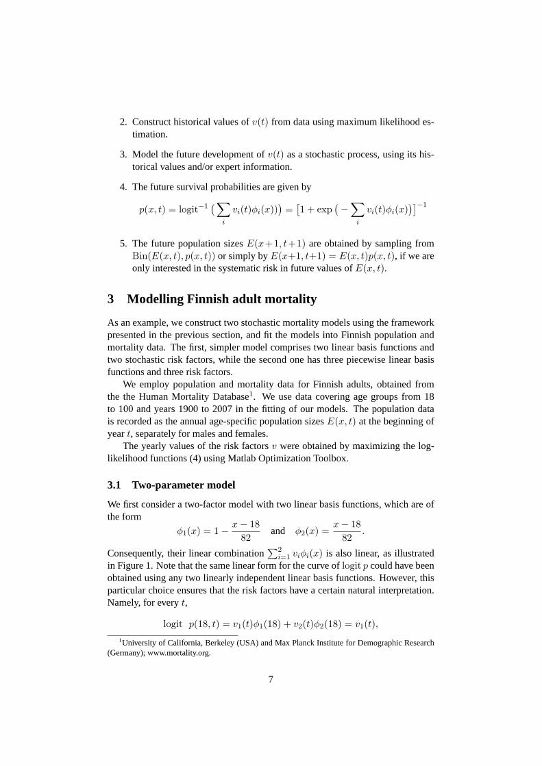
i=1 viφi(x) is also linear, as illustratedin Figure 1. Note that the same linear form for the curve oflogit p could have beenobtained using any two linearly independent linear basis functions. However, thisparticular choice ensures that the risk factors have a certain natural interpretation.Namely, for everyt,

logit p(18, t) = v1(t)φ1(18) + v2(t)φ2(18) = v1(t),

1University of California, Berkeley (USA) and Max Planck Institute for Demographic Research(Germany); www.mortality.org.

7

and, similarly,logit p(100, t) = v2(t). Hence, the risk factors are the logit survivalprobabilities of ages18 and100.

This interpretation will be useful when assessing estimation results for histori-cal values ofv, and the general validity of the model in this particular population.In addition, expert views on the future development of mortality in these age groupsmay be incorporated into the model when choosing the appropriate stochasticpro-cess that governs the evolution of the risk factors. Furthermore, in the engineeringof mortality-linked securities this feature facilitates, for instance, the assessment ofvarious other instruments for hedging purposes.

40 60 80 100x

0.2

0.4

0.6

0.8

1.0

SiviΦiHxL

Φ2HxL

Φ1HxL

Figure 1: Linear basis functions and an exemplary linear combination∑2

i=1 viφi(x) withv1 = 0.6 andv2 = 0.2.

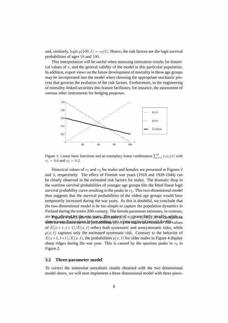
Historical values ofv1 andv2 for males and females are presented in Figures 2and 3, respectively. The effect of Finnish war years (1918 and 1939-1944) canbe clearly observed in the estimated risk factors for males. The dramatic dropinthe wartime survival probabilities of younger age groups tilts the fitted linear logitsurvival probability curve resulting in the peaks inv2. This two-dimensional modelthus suggests that the survival probabilities of the oldest age groups would havetemporarily increased during the war years. As this is doubtful, we conclude thatthe two-dimensional model is be too simple to capture the population dynamics inFinland during the entire 20th century. The female parameter estimates, in contrast,are less affected by the war years. The values ofv1 grows fairly steadily, whilev2

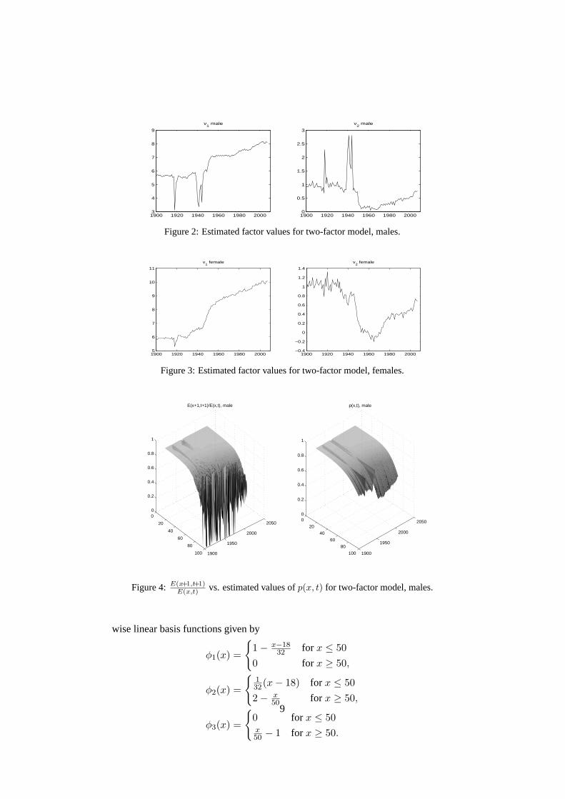
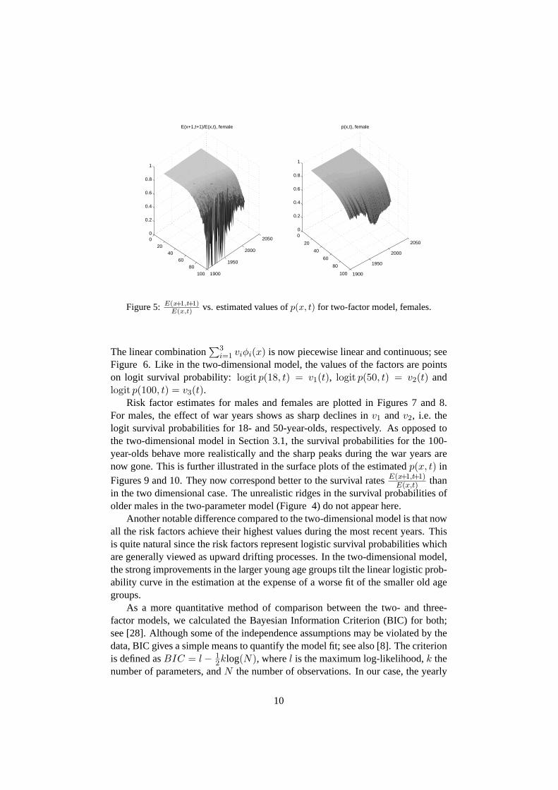
shows some fluctuations before settling into a growing trend around the 60s.Figures 4 and 5 plot the survivals ratiosE(x+1, t+1)/E(x, t) in comparison

with the estimated survival probabilitiesp(x, t) for males and females. The valuesof E(x+1, t+1)/E(x, t) reflect both systematic and nonsystematic risks, whilep(x, t) captures only the estimated systematic risk. Contrary to the behavior ofE(x+1, t+1)/E(x, t), the probabilitiesp(x, t) for older males in Figure 4 displaysharp ridges during the war year. This is caused by the spurious peaksin v2 inFigure 2.

3.2 Three-parameter model

To correct the somewhat unrealistic results obtained with the two dimensionalmodel above, we will next implement a three dimensional model with three piece-

8

1900 1920 1940 1960 1980 20003

4

5

6

7

8

9

v1 male

1900 1920 1940 1960 1980 20000

0.5

1

1.5

2

2.5

3

v2 male

Figure 2: Estimated factor values for two-factor model, males.

1900 1920 1940 1960 1980 20005

6

7

8

9

10

11

v1 female

1900 1920 1940 1960 1980 2000−0.4

−0.2

0

0.2

0.4

0.6

0.8

1

1.2

1.4

v2 female

Figure 3: Estimated factor values for two-factor model, females.

0

20

40

60

80

100 1900

1950

2000

2050

0

0.2

0.4

0.6

0.8

1

E(x+1,t+1)/E(x,t), male

0

20

40

60

80

100 1900

1950

2000

2050

0

0.2

0.4

0.6

0.8

1

p(x,t), male

Figure 4: E(x+1,t+1)E(x,t) vs. estimated values ofp(x, t) for two-factor model, males.

wise linear basis functions given by

φ1(x) =

{

1 − x−1832 for x ≤ 50

0 for x ≥ 50,

φ2(x) =

{

132(x − 18) for x ≤ 50

2 − x50 for x ≥ 50,

φ3(x) =

{

0 for x ≤ 50x50 − 1 for x ≥ 50.

9

0

20

40

60

80

100 1900

1950

2000

20500

0.2

0.4

0.6

0.8

1

E(x+1,t+1)/E(x,t), female

0

20

40

60

80

100 1900

1950

2000

2050

0

0.2

0.4

0.6

0.8

1

p(x,t), female

Figure 5: E(x+1,t+1)E(x,t) vs. estimated values ofp(x, t) for two-factor model, females.

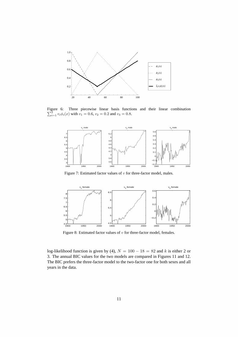
The linear combination∑3

i=1 viφi(x) is now piecewise linear and continuous; seeFigure 6. Like in the two-dimensional model, the values of the factors are pointson logit survival probability: logit p(18, t) = v1(t), logit p(50, t) = v2(t) andlogit p(100, t) = v3(t).

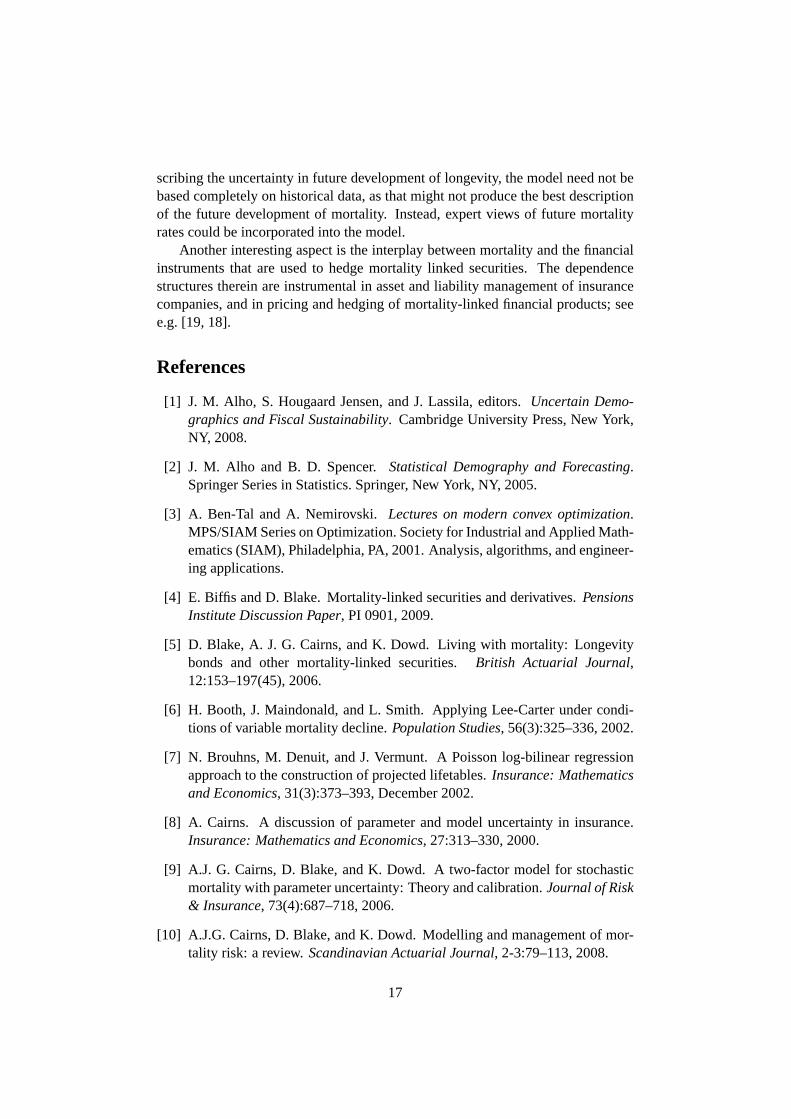
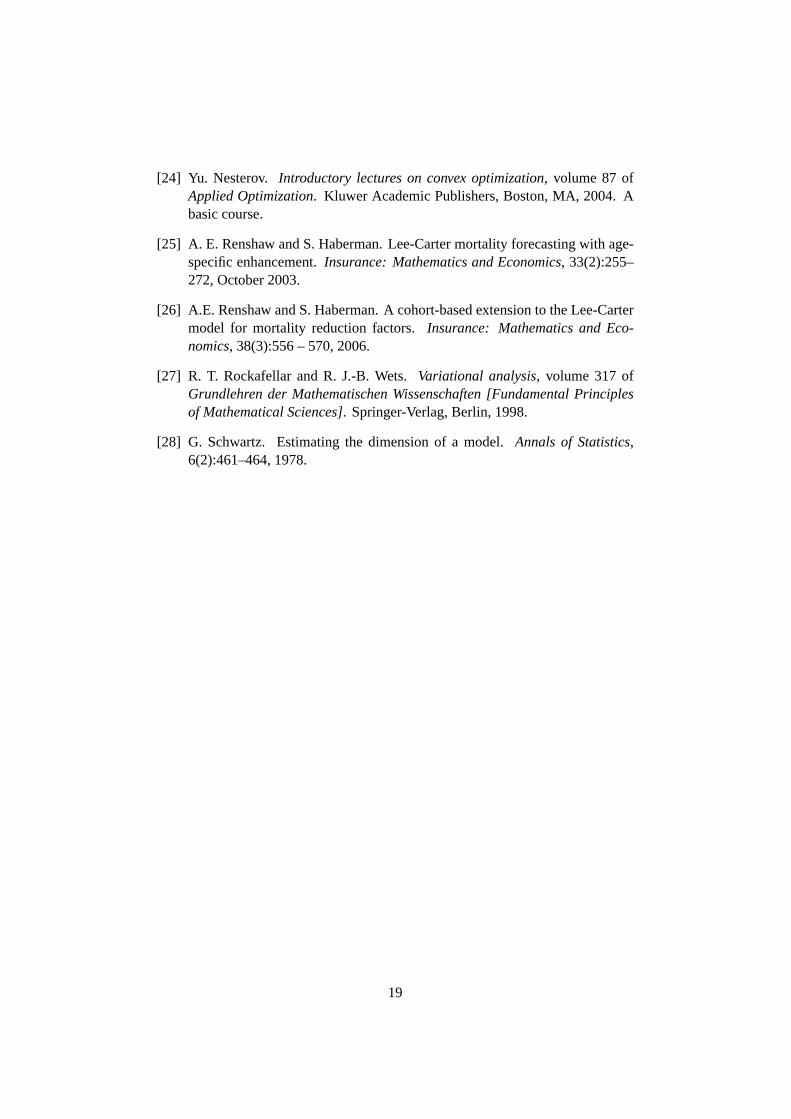
Risk factor estimates for males and females are plotted in Figures 7 and 8.For males, the effect of war years shows as sharp declines inv1 andv2, i.e. thelogit survival probabilities for 18- and 50-year-olds, respectively.As opposed tothe two-dimensional model in Section 3.1, the survival probabilities for the 100-year-olds behave more realistically and the sharp peaks during the war years arenow gone. This is further illustrated in the surface plots of the estimatedp(x, t) inFigures 9 and 10. They now correspond better to the survival ratesE(x+1,t+1)

E(x,t) thanin the two dimensional case. The unrealistic ridges in the survival probabilities ofolder males in the two-parameter model (Figure 4) do not appear here.

Another notable difference compared to the two-dimensional model is that nowall the risk factors achieve their highest values during the most recent years. Thisis quite natural since the risk factors represent logistic survival probabilities whichare generally viewed as upward drifting processes. In the two-dimensional model,the strong improvements in the larger young age groups tilt the linear logistic prob-ability curve in the estimation at the expense of a worse fit of the smaller old agegroups.

As a more quantitative method of comparison between the two- and three-factor models, we calculated the Bayesian Information Criterion (BIC) for both;see [28]. Although some of the independence assumptions may be violated bythedata, BIC gives a simple means to quantify the model fit; see also [8]. The criterionis defined asBIC = l − 1

2klog(N), wherel is the maximum log-likelihood,k thenumber of parameters, andN the number of observations. In our case, the yearly

10

20 40 60 80 100

0.2

0.4

0.6

0.8

1.0

SiviΦiHxL

Φ3HxL

Φ2HxL

Φ1HxL

Figure 6: Three piecewise linear basis functions and their linear combination∑2

i=1 viφi(x) with v1 = 0.6, v2 = 0.2 andv3 = 0.8.

1900 1950 2000

3

3.5

4

4.5

5

5.5

6

6.5

7

v1 male

1900 1950 2000

3.6

3.8

4

4.2

4.4

4.6

4.8

5

5.2

v2 male

1900 1950 2000−0.2

−0.1

0

0.1

0.2

0.3

0.4

0.5

0.6

v3 male

Figure 7: Estimated factor values ofv for three-factor model, males.

1900 1950 20004.5

5

5.5

6

6.5

7

7.5

8

v1 female

1900 1950 20004.5

5

5.5

6

6.5

v2 female

1900 1950 2000

−0.2

0

0.2

0.4

0.6

v3 female

Figure 8: Estimated factor values ofv for three-factor model, females.

log-likelihood function is given by (4),N = 100 − 18 = 82 andk is either 2 or3. The annual BIC values for the two models are compared in Figures 11 and 12.The BIC prefers the three-factor model to the two-factor one for both sexes and allyears in the data.

11

0

20

40

60

80

100 1900

1950

2000

20500

0.2

0.4

0.6

0.8

1

E(x+1,t+1)/E(x,t), male

0

20

40

60

80

100 19001920

19401960

19802000

20200

0.2

0.4

0.6

0.8

1

p(x,t), male

Figure 9: Estimated values ofE(x+1,t+1)E(x,t) vs. p(x, t) for three-factor model, males.

0

20

40

60

80

100 1900

1950

2000

2050

0

0.2

0.4

0.6

0.8

1

E(x+1,t+1)/E(x,t), female

0

20

40

60

80

100 1900

1950

2000

2050

0

0.2

0.4

0.6

0.8

1

p(x,t), female

Figure 10: Estimated values ofE(x+1,t+1)E(x,t) vs. p(x, t) for three-factor model, females.

3.3 Modelling the risk factors

To obtain a stochastic mortality model, we model the vectorv of risk factors as amultivariate stochastic process. In order to capture the dependencies between maleand female mortality, we model the joint behavior of all the risk factors as a singlemultivariate process.

In this study, the risk factors are modelled as a simple multivariate Brownianmotion (random walk) with drift. The combined vector of female and male riskfactorsv(t) satisfies

∆v(t) = µ + CZ(t), (5)

whereZ(t) aren-dimensional independent standard Gaussian random variables,and vectorµ ∈ R

n and matrixC ∈ Rn×n are parameters of the model. Here

n is the total number of the risk factors for females and males. Vectorµ gives

12

1900 1910 1920 1930 1940 1950 1960 1970 1980 1990 2000−9000

−8000

−7000

−6000

−5000

−4000

−3000

−2000

−1000

0BIC, males

2−factor model3−factor model

Figure 11: Annual BIC values, males.

1900 1910 1920 1930 1940 1950 1960 1970 1980 1990 2000−3000

−2500

−2000

−1500

−1000

−500

0BIC, females

2−factor model3−factor model

Figure 12: Annual BIC values, females.

the drift and matrixC the volatility of the risk factors, i.e.E(∆v(t)) = µ andVar(∆v(t)) = CCT . The volatility matrixC can be chosen e.g. as the Choleskyfactor of the covariance matrixVar(∆v(t)).

We choose to model Finnish mortality in relatively stable conditions, and there-fore use historical values of the risk factors only from the period 1960-2007 incalibration of the processes. In the two-parameter model, the estimated risk factorvalues for both males and females show an upward trend from year 1960 onwards.In the case of the two-factor model we obtain, for the combined vector of female(f) and male (m) risk factorsv = (vf

1 , vf2 , vm

1 , vm2 )

µ =

0.03110.01530.02070.0128

, σ =

0.07990.06370.05350.0626

13

and

R =

1.0000 −0.6890 0.4051 −0.3565−0.6890 1.0000 −0.3279 0.66550.4051 −0.3279 1.0000 −0.6605−0.3565 0.6655 −0.6605 1.0000

,

whereσ andR give the standard deviations and correlations of∆v so that

Var(∆v) = diag(σ)R diag(σ).

For the three-parameter model with the vectorv = (vf1 , vf

2 , vf3 , vm

1 , vm2 , vm

3 ) ofcombined male and female risk factors, we obtain

µ =

0.00970.02520.01710.00750.01960.0116

, σ =

0.11490.03520.06620.07650.03720.0728

and

R =

1.0000 0.1246 0.1277 0.1341 0.1690 −0.05730.1246 1.0000 −0.3064 −0.2564 0.4259 −0.17410.1277 −0.3064 1.0000 0.1067 0.0528 0.62820.1341 −0.2564 0.1067 1.0000 −0.4031 0.16250.1690 0.4259 0.0528 −0.4031 1.0000 −0.3214−0.0573 −0.1741 0.6282 0.1625 −0.3214 1.0000

.

3.4 Simulations

We applied the the two models presented in Section 3.2 to simulate male survivalprobabilities and cohort sizes 30 years into the future. The processv(t) was mod-elled as a random walk with a drift as described in the previous section. A sampleof 10000 scenarios forv was generated using Latin hypercube sampling, and theprobabilitiesp(x, t) were then calculated from each simulated path ofv(t). Thenumber of survivorsE(x+1, t+1) in each cohort was approximated by its ex-pected valueE(x, t)p(x, t).

Cohorts aged 30 and 65 in the final observation year 2007 were chosenasreference cohorts. Figures 13 and 14 plot the development of the medians and90% confidence intervals forp(x0 + t, t) and cohort sizesE(x0 + t, t). Figures15 and 16 give the corresponding results for the three-factor model. Inthe threefactor model, the younger reference cohort displays a notable kink in thesurvivalprobability curves, which results from the cohort shifting from one partof thepiecewise linear logit probability curve to another during the simulation period.For the younger cohort, the cohort size estimates for the two-factor modelin the

14

final simulation year are slightly below that of the three-factor model. For the olderreference cohort the difference, albeit hardly notable, is the other way round.

Figure 17 plots the density function of the survival probability of the youngerreference cohort for the three-factor model at the end of the simulation period i.e.60-year-old males in year 2037.

2010 2015 2020 2025 2030 2035

0.992

0.993

0.994

0.995

0.996

0.997

0.998

0.999

Year (t)

p(30

+t,t)

p(30+t,t), males

2010 2015 2020 2025 2030 2035

3.1

3.15

3.2

3.25

3.3

3.35

3.4

x 104

Year (t)

E(30

+t,t)

E(30+t,t), males

Figure 13: Medians and 90% confidence intervals for survivalratesp(x0, t) and cohortsizesE(x0, t). Cohort aged 30 in 2007, male. Two-factor model.

2010 2015 2020 2025 2030 2035

0.78

0.8

0.82

0.84

0.86

0.88

0.9

0.92

0.94

0.96

0.98

Year (t)

p(65

+t,t)

p(65+t,t), males

2010 2015 2020 2025 2030 2035

0.2

0.4

0.6

0.8

1

1.2

1.4

1.6

1.8

2

x 104

Year (t)

E(65

+t,t)

E(65+t,t), males

Figure 14: Medians and 90% confidence intervals for survivalratesp(x0, t) and cohortsizesE(x0, t). Cohort aged 65 in 2007, male. Two-factor model.

4 Conclusions

This paper proposed a flexible but simple framework for stochastic mortality mod-elling. The framework allows for risk factors with tangible interpretations, andguarantees that the parameter estimates are well-defined. Two- and three-factorversions of the model were fitted into Finnish adult population and mortality data,and the factors were modelled as a simple random walk process with a drift. Us-ing the resulting models, future values of death probabilities and cohort sizes weresimulated with plausible results.

15

2010 2015 2020 2025 2030 20350.992

0.993

0.994

0.995

0.996

0.997

0.998

Year (t)

p(30

+t,t)

p(30+t,t), males

2010 2015 2020 2025 2030 20353.1

3.15

3.2

3.25

3.3

3.35

3.4

x 104

Year (t)

E(3

0+t,t

)

E(30+t,t), males

Figure 15: Medians and 90% confidence intervals for survivalratesp(x0 + t, t) and cohortsizesE(x0 + t, t). Cohort aged 30 in 2007, male. Three-factor model.

2010 2015 2020 2025 2030 2035

0.75

0.8

0.85

0.9

0.95

Year (t)

p(65

+t,t

)

p(65+t,t), males

2010 2015 2020 2025 2030 2035

0.2

0.4

0.6

0.8

1

1.2

1.4

1.6

1.8

2

x 104

Year (t)

E(6

5+t,t

)E(65+t,t), males

Figure 16: Medians and 90% confidence intervals for survivalratesp(x0 + t, t) and cohortsizesE(x0 + t, t). Cohort aged 65 in 2007, male. Three-factor model.

0.984 0.986 0.988 0.99 0.992 0.994 0.996 0.998 1

Figure 17: Distribution of the survival probability of 60-year-olds in year 2037.

In real-life applications, modelling of the risk factors should receive more at-tention. A straightforward extension would be to use more flexible econometricmodels. For example, by allowing heavy tailed distributions one might be able tobetter capture the effects of epidemics or natural disasters on mortality. When de-

16

scribing the uncertainty in future development of longevity, the model need not bebased completely on historical data, as that might not produce the best descriptionof the future development of mortality. Instead, expert views of future mortalityrates could be incorporated into the model.

Another interesting aspect is the interplay between mortality and the financialinstruments that are used to hedge mortality linked securities. The dependencestructures therein are instrumental in asset and liability management of insurancecompanies, and in pricing and hedging of mortality-linked financial products; seee.g. [19, 18].

References

[1] J. M. Alho, S. Hougaard Jensen, and J. Lassila, editors.Uncertain Demo-graphics and Fiscal Sustainability. Cambridge University Press, New York,NY, 2008.

[2] J. M. Alho and B. D. Spencer.Statistical Demography and Forecasting.Springer Series in Statistics. Springer, New York, NY, 2005.

[3] A. Ben-Tal and A. Nemirovski. Lectures on modern convex optimization.MPS/SIAM Series on Optimization. Society for Industrial and Applied Math-ematics (SIAM), Philadelphia, PA, 2001. Analysis, algorithms, and engineer-ing applications.

[4] E. Biffis and D. Blake. Mortality-linked securities and derivatives.PensionsInstitute Discussion Paper, PI 0901, 2009.

[5] D. Blake, A. J. G. Cairns, and K. Dowd. Living with mortality: Longevitybonds and other mortality-linked securities.British Actuarial Journal,12:153–197(45), 2006.

[6] H. Booth, J. Maindonald, and L. Smith. Applying Lee-Carter under condi-tions of variable mortality decline.Population Studies, 56(3):325–336, 2002.

[7] N. Brouhns, M. Denuit, and J. Vermunt. A Poisson log-bilinear regressionapproach to the construction of projected lifetables.Insurance: Mathematicsand Economics, 31(3):373–393, December 2002.

[8] A. Cairns. A discussion of parameter and model uncertainty in insurance.Insurance: Mathematics and Economics, 27:313–330, 2000.

[9] A.J. G. Cairns, D. Blake, and K. Dowd. A two-factor model for stochasticmortality with parameter uncertainty: Theory and calibration.Journal of Risk& Insurance, 73(4):687–718, 2006.

[10] A.J.G. Cairns, D. Blake, and K. Dowd. Modelling and management of mor-tality risk: a review.Scandinavian Actuarial Journal, 2-3:79–113, 2008.

17

[11] A.J.G. Cairns, D. Blake, K. Dowd, G. D. Coughlan, D. Epstein, A. Ong,and I Balevich. A quantitative comparison of stochastic mortality modelsusing data from England and Wales and the United States.Pensions InstituteDiscussion Paper, PI 0701, 2007.

[12] I. D. Currie, M. Durban, and P. H. C. Eilers. Smoothing and forecastingmortality rates.Statistical Modelling: An International Journal, 4(4):279 –298, 2004.

[13] M. Dahl. Stochastic mortality in life insurance: market reserves andmortality-linked insurance contracts.Insurance: Mathematics and Eco-nomics, 35(1):113 – 136, 2004.

[14] M. Dahl and T. Moller. Valuation and hedging of life insurance liabilitieswith systematic mortality risk. Insurance: Mathematics and Economics,39(2):193–217, October 2006.

[15] P. De Jong and L Tickle. Extending the Lee-Carter model of mortality pro-jection. Mathematical Population Studies, 13:1–18, 2006.

[16] A. Delwarde, M. Denuit, and P. Eilers. Smoothing the Lee-Carter and Pois-son log-bilinear models for mortality forecasting: A penalised log-likelihoodapproach.Statistical Modelling, 7:29–48, 2007.

[17] K. Dowd, D. Blake, A.J.G Cairns, and P. Dawson. Survivor swaps. TheJournal of Risk and Insurance, 73(1):1–17, 2006.

[18] P. Hilli, M. Koivu, and T. Pennanen. Cash-flow based valuation ofpensionliabilities. Submitted.

[19] P. Hilli, M. Koivu, and T. Pennanen. Optimal construction of a fund of funds.Submitted.

[20] R.. Lee and L. Carter. Modeling and forecasting U.S. mortality.Journal ofthe American Statistical Association, 87(419):659–671, 1992.

[21] R. Lee and T. Miller. Evaluating the performance of the Lee-Carter methodfor forecasting mortality.Demography, 38(4):537–549, 2001.

[22] Y. Lin and S. H. Cox. Securitization of mortality risks in life annuities.TheJournal of Risk and Insurance, 72(2):227–252, 2005.

[23] M.A. Milevsky and S.D. Promislow. Mortality derivatives and the optionto annuitise. Insurance: Mathematics and Economics, 29(3):299 – 318,2001. Papers presented at the 4th IME Conference, Universitat de Barcelona,Barcelona, 24-26 July 2001.

18

[24] Yu. Nesterov. Introductory lectures on convex optimization, volume 87 ofApplied Optimization. Kluwer Academic Publishers, Boston, MA, 2004. Abasic course.

[25] A. E. Renshaw and S. Haberman. Lee-Carter mortality forecasting with age-specific enhancement.Insurance: Mathematics and Economics, 33(2):255–272, October 2003.

[26] A.E. Renshaw and S. Haberman. A cohort-based extension to the Lee-Cartermodel for mortality reduction factors.Insurance: Mathematics and Eco-nomics, 38(3):556 – 570, 2006.

[27] R. T. Rockafellar and R. J.-B. Wets.Variational analysis, volume 317 ofGrundlehren der Mathematischen Wissenschaften [Fundamental Principlesof Mathematical Sciences]. Springer-Verlag, Berlin, 1998.

[28] G. Schwartz. Estimating the dimension of a model.Annals of Statistics,6(2):461–464, 1978.

19