A User Manual for Benefit Cost Analysis

Using Microsoft Excel

Canesio Predo National Abaca Research Center

Leyte State University Baybay, Leyte, Philippines

David James Ecoservices Pty Ltd

NSW, Australia

ECONOMY AND ENVIRONMENT PROGRAM FOR SOUTHEAST ASIA

April 2006

A User Manual for Benefit Cost Analysis Using Microsoft Excel

Canesio Predo and David James Preface This manual has been prepared with support provided by the Economy and Environment Programme for South East Asia (EEPSEA) to enhance the capacity of researchers in carrying out practical applications of BCA using spreadsheet modelling and analysis. The frameworks and analyses presented are based on core concepts and theory of BCA, with applications that relate primarily to environmental and natural resource management. The manual demonstrates approaches and techniques using simple examples and case studies typical of those found in most countries in the South East Asian region. Preliminary versions of the manual have been used in training programs by EEPSEA. The authors gratefully acknowledge the many useful suggestions for expansion and improvement offered by participants, now incorporated in the present version. There are several reasons for preparing a manual that relies on Microsoft Excel as the main vehicle. Excel is a powerful, user-friendly tool that helps to foster a disciplined approach to the analysis required. In BCA applications, it allows researchers to construct appropriate evaluation frameworks and carry out extensive computations easily and rapidly. Most operations can be performed by drawing on the many functions and mathematical procedures contained in Excel, including those commonly used in BCA evaluations. The formulae, functions and results in Excel are transparent. Researchers can therefore review their work, making improvements or corrections where warranted. Resource persons providing guidance to researchers additionally have a means of seeing, in detail, how particular analyses have been carried out, enabling them to make constructive comments and suggestions, as the case may be. One of the strongest features of Excel, as indeed with all spreadsheet software programs, is the facility to conduct simulation modelling and sensitivity analyses. An effective platform is available through which to assess the implications of changes in assumptions, variables and model parameters. The following guidelines, instructions and worked examples have been specially designed for researchers with no prior experience in spreadsheet modelling or Excel. However, even experienced users may discover new concepts, techniques and applications to assist them in their work. The authors encourage the interested researcher to follow the text with diligence, and reap the rewards of acquiring skills that have become essential in practical applications of BCA frameworks and methods.

2

I. Introduction to Excel Microsoft Excel is a software product that falls into the general category of spreadsheets. Excel is one of several spreadsheet products that you can run on your PC. You might have heard the terms "spreadsheet" and "worksheet". People generally use them interchangeably. To remain consistent with Microsoft and other publishers the term worksheet refers to the row-and-column matrix sheet on which you work upon and the term spreadsheet refers to this type of computer application. In addition, the term workbook will refer to the book of pages that is the standard Excel document. The workbook can contain worksheets, chart sheets, or macro modules.

Basic features of MS Excel

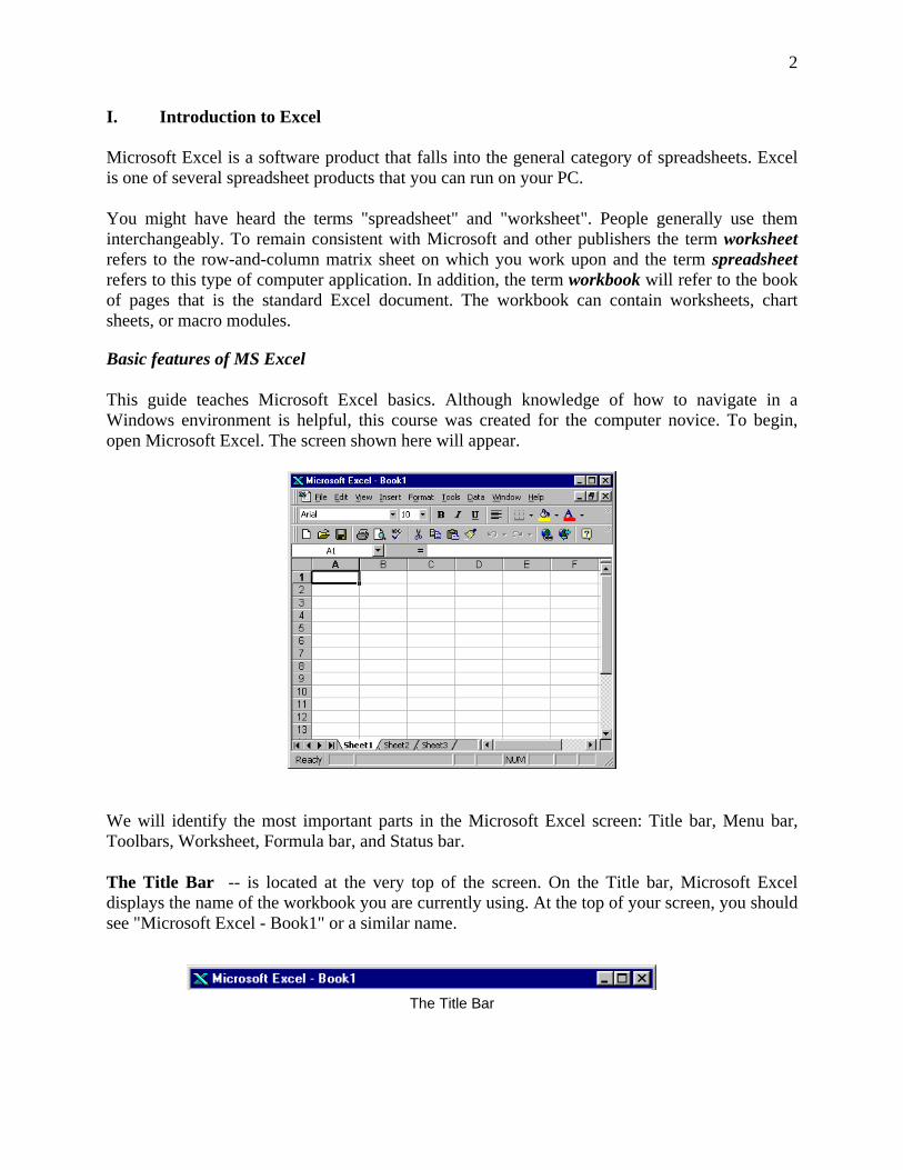
This guide teaches Microsoft Excel basics. Although knowledge of how to navigate in a Windows environment is helpful, this course was created for the computer novice. To begin, open Microsoft Excel. The screen shown here will appear.

We will identify the most important parts in the Microsoft Excel screen: Title bar, Menu bar, Toolbars, Worksheet, Formula bar, and Status bar.

The Title Bar -- is located at the very top of the screen. On the Title bar, Microsoft Excel displays the name of the workbook you are currently using. At the top of your screen, you should see "Microsoft Excel - Book1" or a similar name.

The Title Bar

3

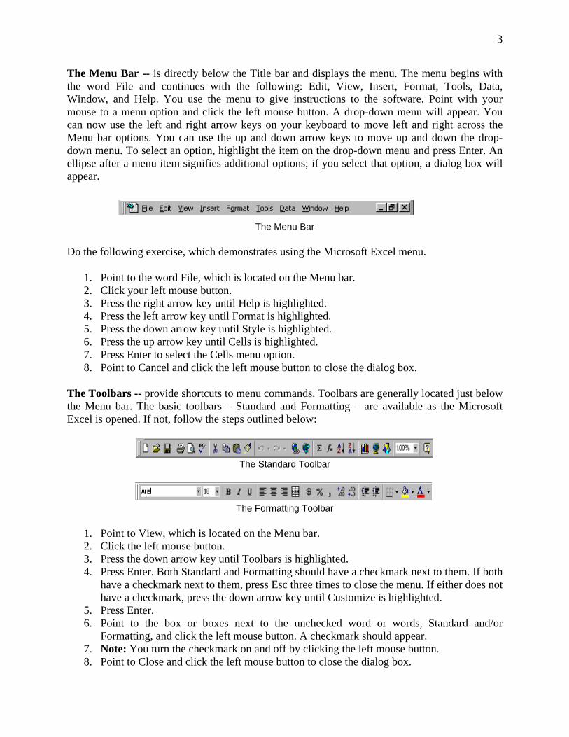
The Menu Bar -- is directly below the Title bar and displays the menu. The menu begins with the word File and continues with the following: Edit, View, Insert, Format, Tools, Data, Window, and Help. You use the menu to give instructions to the software. Point with your mouse to a menu option and click the left mouse button. A drop-down menu will appear. You can now use the left and right arrow keys on your keyboard to move left and right across the Menu bar options. You can use the up and down arrow keys to move up and down the drop-down menu. To select an option, highlight the item on the drop-down menu and press Enter. An ellipse after a menu item signifies additional options; if you select that option, a dialog box will appear.

The Menu Bar

Do the following exercise, which demonstrates using the Microsoft Excel menu.

1. Point to the word File, which is located on the Menu bar. 2. Click your left mouse button. 3. Press the right arrow key until Help is highlighted. 4. Press the left arrow key until Format is highlighted. 5. Press the down arrow key until Style is highlighted. 6. Press the up arrow key until Cells is highlighted. 7. Press Enter to select the Cells menu option. 8. Point to Cancel and click the left mouse button to close the dialog box.

The Toolbars -- provide shortcuts to menu commands. Toolbars are generally located just below the Menu bar. The basic toolbars – Standard and Formatting – are available as the Microsoft Excel is opened. If not, follow the steps outlined below:

The Standard Toolbar

The Formatting Toolbar

1. Point to View, which is located on the Menu bar. 2. Click the left mouse button. 3. Press the down arrow key until Toolbars is highlighted. 4. Press Enter. Both Standard and Formatting should have a checkmark next to them. If both

have a checkmark next to them, press Esc three times to close the menu. If either does not have a checkmark, press the down arrow key until Customize is highlighted.

5. Press Enter. 6. Point to the box or boxes next to the unchecked word or words, Standard and/or

Formatting, and click the left mouse button. A checkmark should appear. 7. Note: You turn the checkmark on and off by clicking the left mouse button. 8. Point to Close and click the left mouse button to close the dialog box.

4

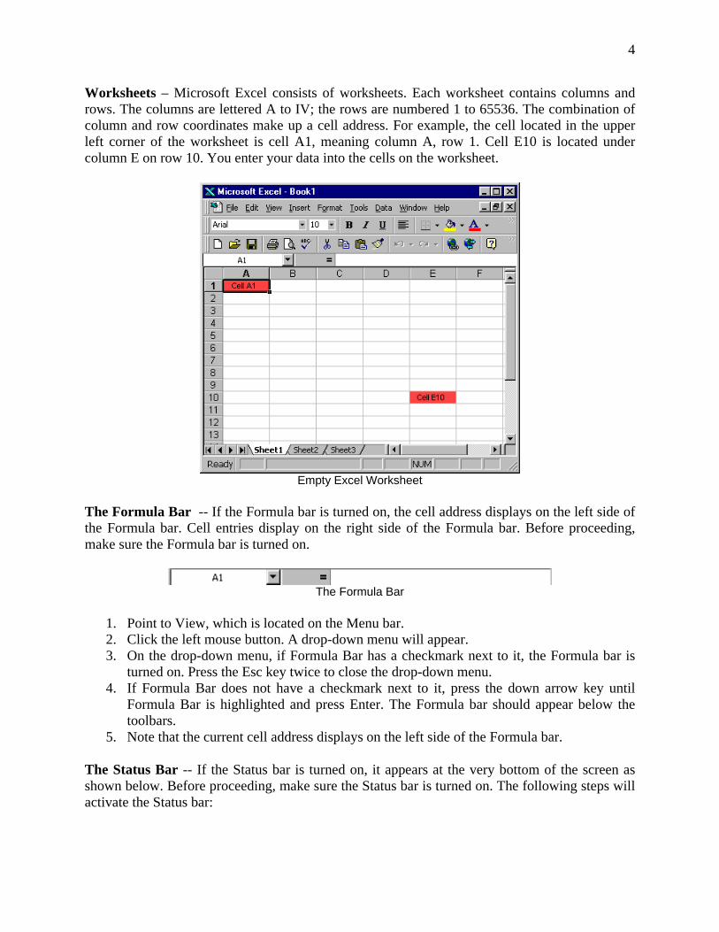
Worksheets – Microsoft Excel consists of worksheets. Each worksheet contains columns and rows. The columns are lettered A to IV; the rows are numbered 1 to 65536. The combination of column and row coordinates make up a cell address. For example, the cell located in the upper left corner of the worksheet is cell A1, meaning column A, row 1. Cell E10 is located under column E on row 10. You enter your data into the cells on the worksheet.

Empty Excel Worksheet

The Formula Bar -- If the Formula bar is turned on, the cell address displays on the left side of the Formula bar. Cell entries display on the right side of the Formula bar. Before proceeding, make sure the Formula bar is turned on.

The Formula Bar

1. Point to View, which is located on the Menu bar. 2. Click the left mouse button. A drop-down menu will appear. 3. On the drop-down menu, if Formula Bar has a checkmark next to it, the Formula bar is

turned on. Press the Esc key twice to close the drop-down menu. 4. If Formula Bar does not have a checkmark next to it, press the down arrow key until

Formula Bar is highlighted and press Enter. The Formula bar should appear below the toolbars.

5. Note that the current cell address displays on the left side of the Formula bar.

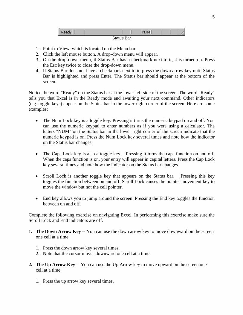
The Status Bar -- If the Status bar is turned on, it appears at the very bottom of the screen as shown below. Before proceeding, make sure the Status bar is turned on. The following steps will activate the Status bar:

5

Status Bar

1. Point to View, which is located on the Menu bar. 2. Click the left mouse button. A drop-down menu will appear. 3. On the drop-down menu, if Status Bar has a checkmark next to it, it is turned on. Press

the Esc key twice to close the drop-down menu. 4. If Status Bar does not have a checkmark next to it, press the down arrow key until Status

Bar is highlighted and press Enter. The Status bar should appear at the bottom of the screen.

Notice the word "Ready" on the Status bar at the lower left side of the screen. The word "Ready" tells you that Excel is in the Ready mode and awaiting your next command. Other indicators (e.g. toggle keys) appear on the Status bar in the lower right corner of the screen. Here are some examples:

• The Num Lock key is a toggle key. Pressing it turns the numeric keypad on and off. You can use the numeric keypad to enter numbers as if you were using a calculator. The letters "NUM" on the Status bar in the lower right corner of the screen indicate that the numeric keypad is on. Press the Num Lock key several times and note how the indicator on the Status bar changes.

• The Caps Lock key is also a toggle key. Pressing it turns the caps function on and off.

When the caps function is on, your entry will appear in capital letters. Press the Cap Lock key several times and note how the indicator on the Status bar changes.

• Scroll Lock is another toggle key that appears on the Status bar. Pressing this key

toggles the function between on and off. Scroll Lock causes the pointer movement key to move the window but not the cell pointer.

• End key allows you to jump around the screen. Pressing the End key toggles the function

between on and off.

Complete the following exercise on navigating Excel. In performing this exercise make sure the Scroll Lock and End indicators are off.

1. The Down Arrow Key -- You can use the down arrow key to move downward on the screen one cell at a time.

1. Press the down arrow key several times. 2. Note that the cursor moves downward one cell at a time.

2. The Up Arrow Key -- You can use the Up Arrow key to move upward on the screen one cell at a time.

1. Press the up arrow key several times.

6

2. Note that the cursor moves upward one cell at a time.

3. The Right and Left Arrow Keys -- You can use the right and left arrow keys to move right or left one cell at a time.

1. Press the right arrow key several times. 2. Note that the cursor moves to the right. 3. Press the left arrow key several times. 4. Note that the cursor moves to the left.

4. Page Up and Page Down -- The Page Up and Page Down keys move the cursor up and down one page at a time.

1. Press the Page Down key. 2. Note that the cursor moves down one page. 3. Press the Page Up key. 4. Note that the cursor moves up one page.

5. The End Key -- The End key, used in conjunction with the arrow keys, causes the cursor to move to the far end of the spreadsheet in the direction of the arrow.

The Status Bar showing End Key

1. Press the End key. 2. Note that "END" appears on the Status bar in the lower right corner of the screen. 3. Press the right arrow key. 4. Note that the cursor moves to the farthest right area of the screen. 5. Press the END key again. 6. Press the down arrow key. Note that the cursor moves to the bottom of the screen. 7. Press the End key again. 8. Press the left arrow key. Note that the cursor moves to the farthest left area of the screen. 9. Press the End key again. 10. Press the up arrow key. Note that the cursor moves to the top of the screen.

Note: If you have entered data into the worksheet, the End key moves you to the end of the data area.

6. The Home Key -- The Home key, used in conjunction with the End key, moves you to cell A1 -- or to the beginning of the data area if you have entered data.

1. Move the cursor to column J. 2. Stay in column J and move the cursor to row 20. 3. Press the End key. 4. Press Home. 5. You should now be in cell A1.

7

7. Scroll Lock -- Scroll Lock moves the window, but not the cell pointer.

The Status Bar showing Scroll Lock

1. Press the Page Down key. 2. Press Scroll Lock. Note "SCRL" appears on the Status bar in the lower right corner of the

screen. 3. Press the up arrow key several times. Note that the cursor stays in the same position and

the window moves upward. 4. Press the down arrow key several times. Note that the cursor stays in the same position

and the window moves downward. 5. Press Scroll Lock to turn the scroll lock function off. 6. Press End. 7. Press Home. You should be in cell A1.

Working with Cells and Ranges A cell is a single element in a worksheet that can hold a value, text, or a formula. A cell is identified by its address, which consists of its column letter and row number. For example, cell D12 is the cell in the fourth column and the twelfth row. A group of cells is called a range. You designate a range address by specifying its upper-left cell address and its lower-right cell address, separated by a colon. Here are some examples of range addresses:

A1:B1 Two cells that occupy one row and two columns C24 A range that consists of a single cell A1:A100 100 cells in column A A1:D416 Cells (four rows by four columns) C1:C65536 An entire column of cells; this range also can be expressed as C:C A6:IV6 An entire row of cells

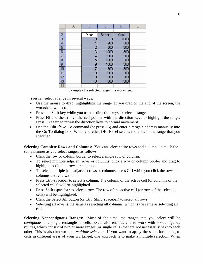
Selecting Ranges: To perform an operation on a range of cells in a worksheet, you must select the range of cells first. For example, if you want to make the text bold for a range of cells, you must select the range and then click the Bold button on the Formatting toolbar (or, use any of several other methods to make the text bold). When you select a range, the cells appear highlighted in light blue-gray. The exception is the active cell, which remains its normal color. The figure below shows an example of a selected range in a worksheet.

8

Example of a selected range in a worksheet.

You can select a range in several ways: • Use the mouse to drag, highlighting the range. If you drag to the end of the screen, the

worksheet will scroll. • Press the Shift key while you use the direction keys to select a range. • Press F8 and then move the cell pointer with the direction keys to highlight the range.

Press F8 again to return the direction keys to normal movement. • Use the Edit Go To command (or press F5) and enter a range’s address manually into

the Go To dialog box. When you click OK, Excel selects the cells in the range that you specified.

Selecting Complete Rows and Columns: You can select entire rows and columns in much the same manner as you select ranges, as follows:

• Click the row or column border to select a single row or column. • To select multiple adjacent rows or columns, click a row or column border and drag to

highlight additional rows or columns. • To select multiple (nonadjacent) rows or columns, press Ctrl while you click the rows or

columns that you want. • Press Ctrl+spacebar to select a column. The column of the active cell (or columns of the

selected cells) will be highlighted. • Press Shift+spacebar to select a row. The row of the active cell (or rows of the selected

cells) will be highlighted. • Click the Select All button (or Ctrl+Shift+spacebar) to select all rows. • Selecting all rows is the same as selecting all columns, which is the same as selecting all

cells.

Selecting Noncontiguous Ranges: Most of the time, the ranges that you select will be contiguous -- a single rectangle of cells. Excel also enables you to work with noncontiguous ranges, which consist of two or more ranges (or single cells) that are not necessarily next to each other. This is also known as a multiple selection. If you want to apply the same formatting to cells in different areas of your worksheet, one approach is to make a multiple selection. When

9

the appropriate cells or ranges are selected, the formatting that you select is applied to them all. A noncontiguous range selected in a worksheet is shown below:

Example of selected cells in noncontiguous ranges.

You can select a noncontiguous range in several ways:

• Hold down Ctrl while you drag the mouse to highlight the individual cells or ranges. • From the keyboard, select a range as described previously (using F8 or the Shift key).

Then, press Shift+F8 to select another range without canceling the previous range selections.

• Select Edit Go To and then enter a range’s address manually into the Go To dialog box. Separate the different ranges with a comma. When you click OK, Excel selects the cells in the ranges that you specified (see Figure above).

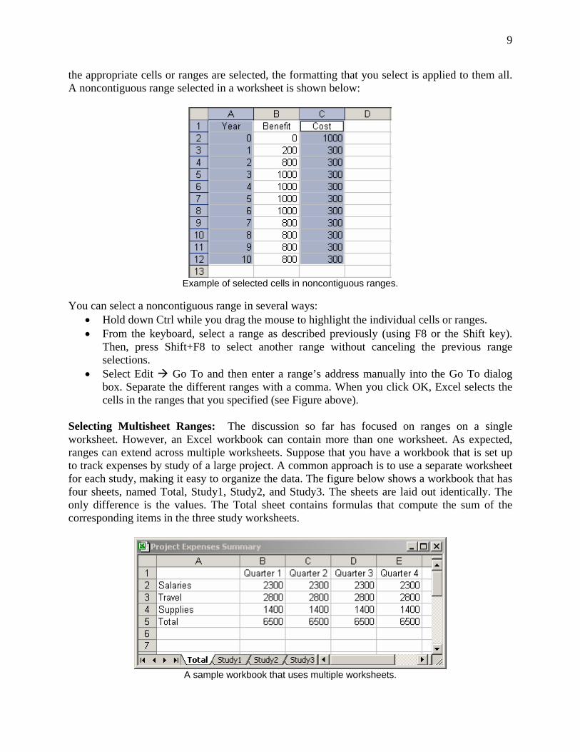
Selecting Multisheet Ranges: The discussion so far has focused on ranges on a single worksheet. However, an Excel workbook can contain more than one worksheet. As expected, ranges can extend across multiple worksheets. Suppose that you have a workbook that is set up to track expenses by study of a large project. A common approach is to use a separate worksheet for each study, making it easy to organize the data. The figure below shows a workbook that has four sheets, named Total, Study1, Study2, and Study3. The sheets are laid out identically. The only difference is the values. The Total sheet contains formulas that compute the sum of the corresponding items in the three study worksheets.

A sample workbook that uses multiple worksheets.

10

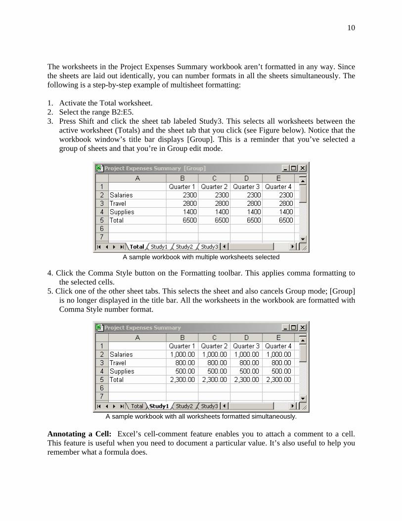
The worksheets in the Project Expenses Summary workbook aren’t formatted in any way. Since the sheets are laid out identically, you can number formats in all the sheets simultaneously. The following is a step-by-step example of multisheet formatting: 1. Activate the Total worksheet. 2. Select the range B2:E5. 3. Press Shift and click the sheet tab labeled Study3. This selects all worksheets between the

active worksheet (Totals) and the sheet tab that you click (see Figure below). Notice that the workbook window’s title bar displays [Group]. This is a reminder that you’ve selected a group of sheets and that you’re in Group edit mode.

A sample workbook with multiple worksheets selected

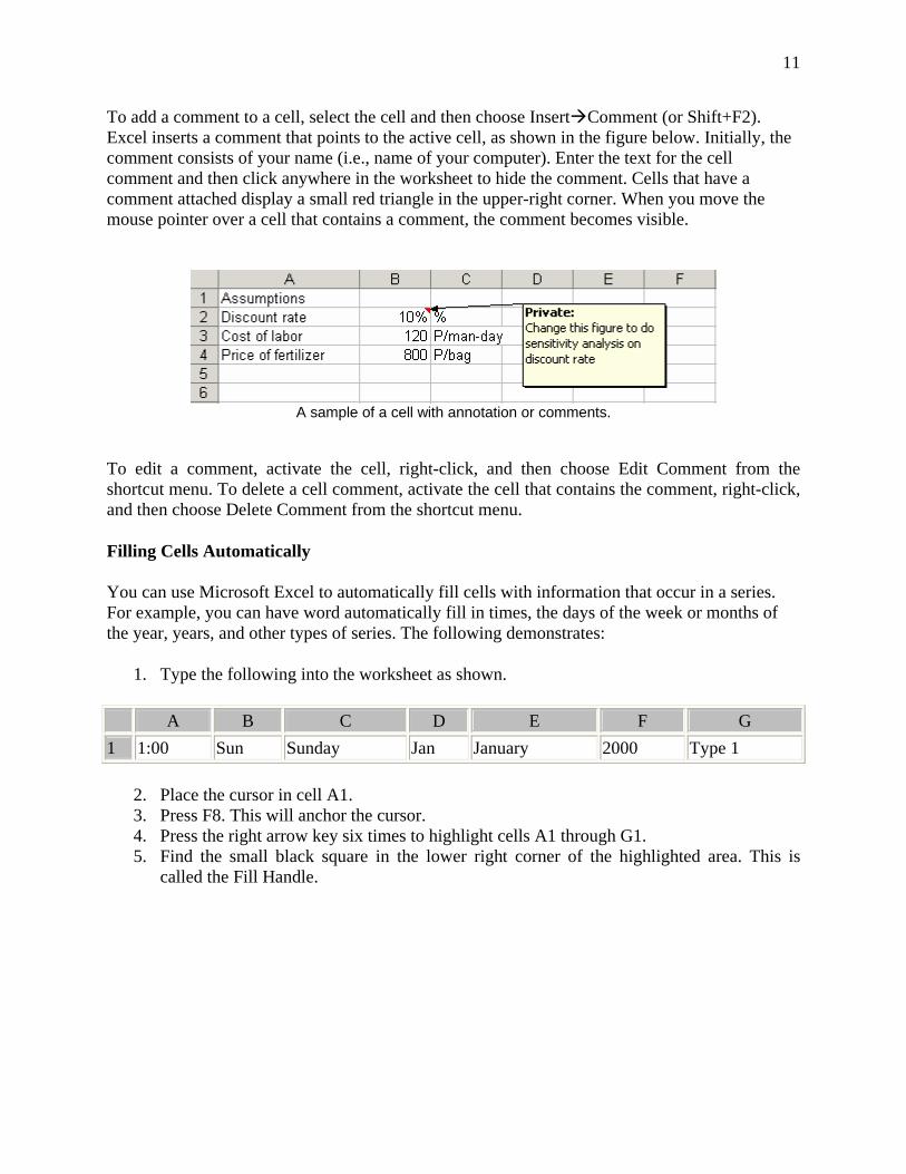
4. Click the Comma Style button on the Formatting toolbar. This applies comma formatting to

the selected cells. 5. Click one of the other sheet tabs. This selects the sheet and also cancels Group mode; [Group]

is no longer displayed in the title bar. All the worksheets in the workbook are formatted with Comma Style number format.

A sample workbook with all worksheets formatted simultaneously.

Annotating a Cell: Excel’s cell-comment feature enables you to attach a comment to a cell. This feature is useful when you need to document a particular value. It’s also useful to help you remember what a formula does.

11

To add a comment to a cell, select the cell and then choose Insert Comment (or Shift+F2). Excel inserts a comment that points to the active cell, as shown in the figure below. Initially, the comment consists of your name (i.e., name of your computer). Enter the text for the cell comment and then click anywhere in the worksheet to hide the comment. Cells that have a comment attached display a small red triangle in the upper-right corner. When you move the mouse pointer over a cell that contains a comment, the comment becomes visible.

A sample of a cell with annotation or comments.

To edit a comment, activate the cell, right-click, and then choose Edit Comment from the shortcut menu. To delete a cell comment, activate the cell that contains the comment, right-click, and then choose Delete Comment from the shortcut menu.

Filling Cells Automatically

You can use Microsoft Excel to automatically fill cells with information that occur in a series. For example, you can have word automatically fill in times, the days of the week or months of the year, years, and other types of series. The following demonstrates:

1. Type the following into the worksheet as shown.

A B C D E F G 1 1:00 Sun Sunday Jan January 2000 Type 1

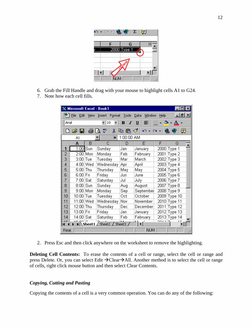
2. Place the cursor in cell A1. 3. Press F8. This will anchor the cursor. 4. Press the right arrow key six times to highlight cells A1 through G1. 5. Find the small black square in the lower right corner of the highlighted area. This is

called the Fill Handle.

12

6. Grab the Fill Handle and drag with your mouse to highlight cells A1 to G24. 7. Note how each cell fills.

2. Press Esc and then click anywhere on the worksheet to remove the highlighting.

Deleting Cell Contents: To erase the contents of a cell or range, select the cell or range and press Delete. Or, you can select Edit Clear All. Another method is to select the cell or range of cells, right click mouse button and then select Clear Contents. Copying, Cutting and Pasting Copying the contents of a cell is a very common operation. You can do any of the following:

13

• Copy a cell to another cell. • Copy a cell to a range of cells. The source cell is copied to every cell in the destination

range. • Copy a range to another range. Both ranges must be the same size.

Copying a cell normally copies the cell contents, any formatting that is applied to the original cell (including conditional formatting and data validation), and the cell comment (if it has one). When you copy a cell that contains a formula, the cell references in the copied formulas are changed automatically to be relative to their new destination. Copying consists of two steps although shortcut methods exist: 1. Select the cell or range to copy (the source range) and copy it to the Clipboard. 2. Move the cell pointer to the range that will hold the copy (the destination range) and paste

the Clipboard contents. If you find that pasting overwrote some essential cells, choose Edit Undo (or press Ctrl+Z). Because copying is used so often, Excel provides many different methods as follows: Copying by using toolbar buttons: The Standard toolbar has two buttons that are relevant to

copying: the Copy icon ( ) and the Paste icon ( ). Follow the steps below to copy a cell or range of cells by using toolbar buttons: 1. Highlight cell or range of cells to be copied, say A7 to B9. To do this, place the cursor in cell

A7. Press F8. Press the down arrow key twice. Press the right arrow key once. A7 to B9 should be highlighted. Or highlight cell range A7 to B9 by clicking the mouse on cell A7. While holding the left mouse button at cell A7 drag it down to A9 and then to the right at B9.

2. Click on the Copy icon, which is located on the Formatting toolbar. Use the arrow key or mouse to move the cursor to cell C7.

3. Click on the Paste icon, which is located on the Formatting toolbar 4. Press Esc to exit the Copy mode. Copying by using menu commands: You can use the following menu commands for copying and pasting: • Highlight cell or range of cells to be copied. Then click Edit Copy -- Copies the selected

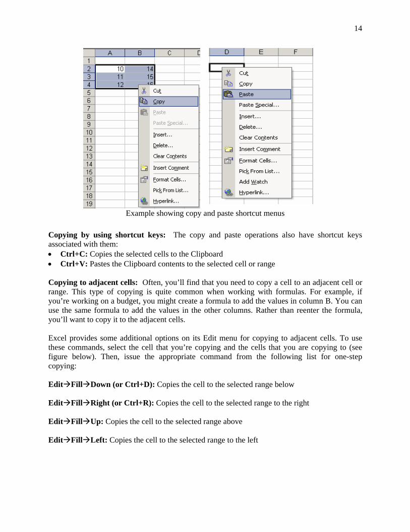
cells to the Windows Clipboard and the Office Clipboard • Click Edit Paste: Pastes the Windows Clipboard contents to the selected cell or range Copying by using shortcut menus: Select the cell or range to copy (A2:B4), right-click, and then choose Copy from the shortcut menu. Then, select the cell (D2) in which you want the copy to appear, right-click, and choose Paste from the shortcut menu (see figure below).

14

Example showing copy and paste shortcut menus

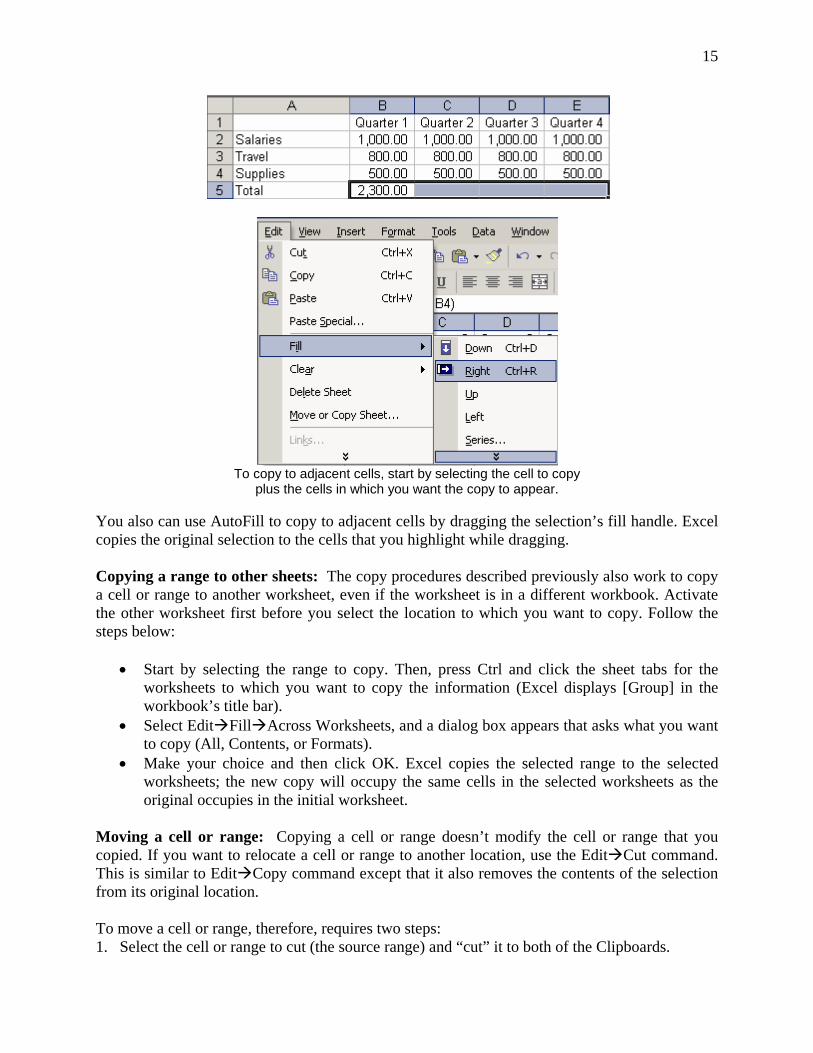
Copying by using shortcut keys: The copy and paste operations also have shortcut keys associated with them: • Ctrl+C: Copies the selected cells to the Clipboard • Ctrl+V: Pastes the Clipboard contents to the selected cell or range Copying to adjacent cells: Often, you’ll find that you need to copy a cell to an adjacent cell or range. This type of copying is quite common when working with formulas. For example, if you’re working on a budget, you might create a formula to add the values in column B. You can use the same formula to add the values in the other columns. Rather than reenter the formula, you’ll want to copy it to the adjacent cells. Excel provides some additional options on its Edit menu for copying to adjacent cells. To use these commands, select the cell that you’re copying and the cells that you are copying to (see figure below). Then, issue the appropriate command from the following list for one-step copying: Edit Fill Down (or Ctrl+D): Copies the cell to the selected range below Edit Fill Right (or Ctrl+R): Copies the cell to the selected range to the right Edit Fill Up: Copies the cell to the selected range above Edit Fill Left: Copies the cell to the selected range to the left

15

To copy to adjacent cells, start by selecting the cell to copy

plus the cells in which you want the copy to appear.

You also can use AutoFill to copy to adjacent cells by dragging the selection’s fill handle. Excel copies the original selection to the cells that you highlight while dragging. Copying a range to other sheets: The copy procedures described previously also work to copy a cell or range to another worksheet, even if the worksheet is in a different workbook. Activate the other worksheet first before you select the location to which you want to copy. Follow the steps below:

• Start by selecting the range to copy. Then, press Ctrl and click the sheet tabs for the worksheets to which you want to copy the information (Excel displays [Group] in the workbook’s title bar).

• Select Edit Fill Across Worksheets, and a dialog box appears that asks what you want to copy (All, Contents, or Formats).

• Make your choice and then click OK. Excel copies the selected range to the selected worksheets; the new copy will occupy the same cells in the selected worksheets as the original occupies in the initial worksheet.

Moving a cell or range: Copying a cell or range doesn’t modify the cell or range that you copied. If you want to relocate a cell or range to another location, use the Edit Cut command. This is similar to Edit Copy command except that it also removes the contents of the selection from its original location. To move a cell or range, therefore, requires two steps: 1. Select the cell or range to cut (the source range) and “cut” it to both of the Clipboards.

16

2. Select the cell that will hold the moved cell or range (the destination range) and paste the contents of one of the Clipboards. The destination range can be on the same worksheet or in a different worksheet—or in a different workbook.

Note that you also can move a cell or range by dragging it. Select the cell or range that you want to move and then slide the mouse pointer to any of the selection’s four borders. The mouse pointer turns into an arrow pointing up and to the left. Drag the selection to its new location and release the mouse button. Copy and Paste Special: Excel contains two more versatile ways to paste information. You can use the Office Clipboard to copy and paste multiple items, or you can use the Paste Special dialog box to paste information in distinctive ways. • The Edit Paste Special command is a much more versatile version of the Edit Paste

command. • For the Paste Special command to be available, you need to copy a cell or range to the

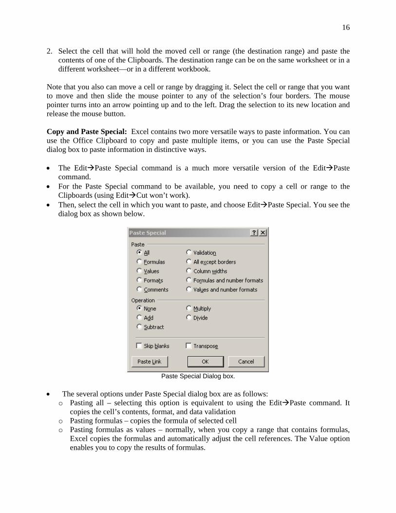
Clipboards (using Edit Cut won’t work). • Then, select the cell in which you want to paste, and choose Edit Paste Special. You see the

dialog box as shown below.

Paste Special Dialog box.

• The several options under Paste Special dialog box are as follows:

o Pasting all – selecting this option is equivalent to using the Edit Paste command. It copies the cell’s contents, format, and data validation

o Pasting formulas – copies the formula of selected cell o Pasting formulas as values – normally, when you copy a range that contains formulas,

Excel copies the formulas and automatically adjust the cell references. The Value option enables you to copy the results of formulas.

17

o Pasting cell formats only – copy only the formatting applied in the selected cell or range to the destination cell or range.

o Pasting cell comments – copy only the cell comments from a cell or range; doesn’t copy cell contents or formatting

o Pasting validation criteria – copy the data validation command created in the selected cell or range to another cell or range

o Skipping borders when pasting – this is to avoid pasting the border of selected cell or range

o Pasting column widths – copy column width information from one column to another o Performing mathematical operations without formulas – perform an arithmetic operation

without using formulas. For example, you can copy a range to another range and select the multiply operation. Excel multiplies the corresponding values in the source range and the destination range and replaces the destination range with the new values.

o Skipping blanks when pasting – this prevents Excel from overwriting cell contents in your paste area with blank cells from the copied range.

o Transposing a range – changes the orientation of the copied range. For instance, rows become column and columns become rows. Any formulas in the copied range are adjusted so that they work properly when transposed.

Elementary Formulae All formulas in Excel must begin with an equal sign (=). When a formula is entered into a cell, the formula itself is displayed in the formula bar when that cell is highlighted, and the result of the formula is displayed in the actual cell. When you are typing in formulas, do not type spaces; Excel will delete them.

In Microsoft Excel, you can enter numbers and mathematical formulas into cells. When a number is entered into a cell, you can perform mathematical calculations such as addition, subtraction, multiplication, and division. Use the following to indicate the type of calculation you wish to perform:

+ Addition - Subtraction * Multiplication / Division ^ Exponential

The following exercises demonstrate how to create formula and perform mathematical calculations.

Addition (+)

1. Move the cursor to cell A1. 2. Type 1. 3. Press Enter. 4. Type 1 in cell A2.

18

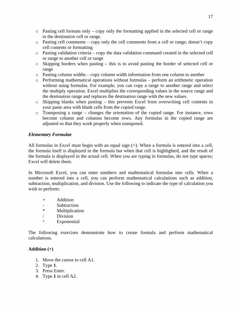
5. Press Enter. 6. Type =A1+A2 in cell A3. 7. Press Enter. 8. Note that cell A1 has been added to cell A2 and the result is shown in cell A3.

Place the cursor in cell A3 and look at the Formula bar.

Subtraction (-)

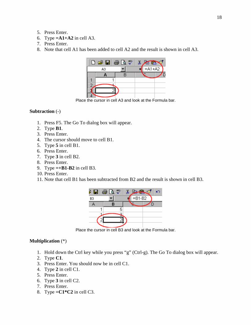
1. Press F5. The Go To dialog box will appear. 2. Type B1. 3. Press Enter. 4. The cursor should move to cell B1. 5. Type 5 in cell B1. 6. Press Enter. 7. Type 3 in cell B2. 8. Press Enter. 9. Type =+B1-B2 in cell B3. 10. Press Enter. 11. Note that cell B1 has been subtracted from B2 and the result is shown in cell B3.

Place the cursor in cell B3 and look at the Formula bar.

Multiplication (*)

1. Hold down the Ctrl key while you press “g” (Ctrl-g). The Go To dialog box will appear. 2. Type C1. 3. Press Enter. You should now be in cell C1. 4. Type 2 in cell C1. 5. Press Enter. 6. Type 3 in cell C2. 7. Press Enter. 8. Type =C1*C2 in cell C3.

19

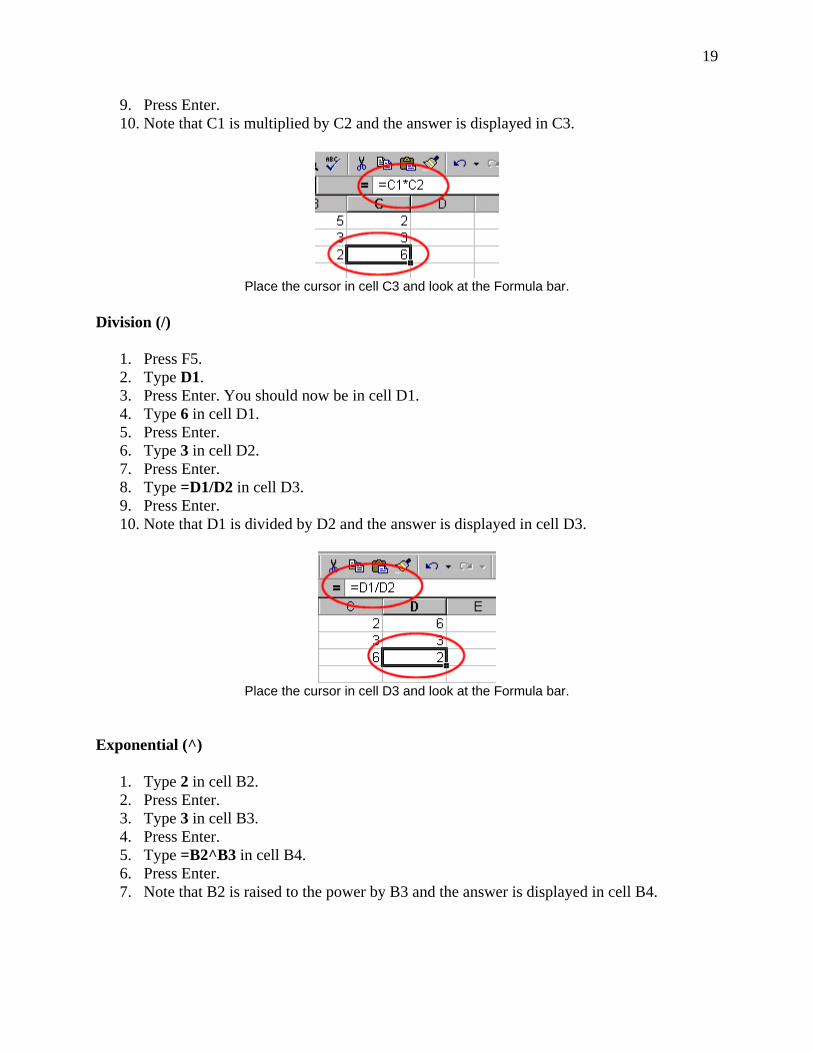
9. Press Enter. 10. Note that C1 is multiplied by C2 and the answer is displayed in C3.

Place the cursor in cell C3 and look at the Formula bar.

Division (/)

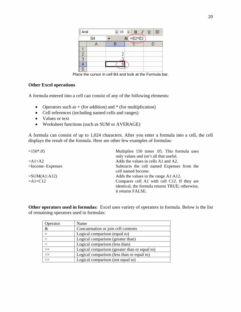
1. Press F5. 2. Type D1. 3. Press Enter. You should now be in cell D1. 4. Type 6 in cell D1. 5. Press Enter. 6. Type 3 in cell D2. 7. Press Enter. 8. Type =D1/D2 in cell D3. 9. Press Enter. 10. Note that D1 is divided by D2 and the answer is displayed in cell D3.

Place the cursor in cell D3 and look at the Formula bar.

Exponential (^)

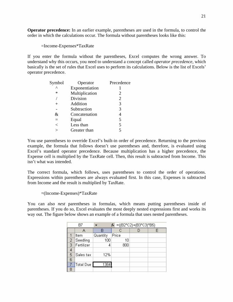
1. Type 2 in cell B2. 2. Press Enter. 3. Type 3 in cell B3. 4. Press Enter. 5. Type =B2^B3 in cell B4. 6. Press Enter. 7. Note that B2 is raised to the power by B3 and the answer is displayed in cell B4.

20

Place the cursor in cell B4 and look at the Formula bar.

Other Excel operations A formula entered into a cell can consist of any of the following elements:

• Operators such as + (for addition) and * (for multiplication) • Cell references (including named cells and ranges) • Values or text • Worksheet functions (such as SUM or AVERAGE)

A formula can consist of up to 1,024 characters. After you enter a formula into a cell, the cell displays the result of the formula. Here are other few examples of formulas: =150*.05 Multiplies 150 times .05. This formula uses

only values and isn’t all that useful. =A1+A2 Adds the values in cells A1 and A2. =Income–Expenses Subtracts the cell named Expenses from the

cell named Income. =SUM(A1:A12) Adds the values in the range A1:A12. =A1=C12 Compares cell A1 with cell C12. If they are

identical, the formula returns TRUE; otherwise, it returns FALSE.

Other operators used in formulas: Excel uses variety of operators in formula. Below is the list of remaining operators used in formulas:

Operator Name & Concatenation or join cell contents = Logical comparison (equal to) > Logical comparison (greater than) < Logical comparison (less than) >= Logical comparison (greater than or equal to) <= Logical comparison (less than or equal to) <> Logical comparison (not equal to)

21

Operator precedence: In an earlier example, parentheses are used in the formula, to control the order in which the calculations occur. The formula without parentheses looks like this:

=Income-Expenses*TaxRate If you enter the formula without the parentheses, Excel computes the wrong answer. To understand why this occurs, you need to understand a concept called operator precedence, which basically is the set of rules that Excel uses to perform its calculations. Below is the list of Excels’ operator precedence.

Symbol Operator Precedence ^ Exponentiation 1 * Multiplication 2 / Division 2 + Addition 3 - Subtraction 3 & Concatenation 4 = Equal 5 < Less than 5 > Greater than 5

You use parentheses to override Excel’s built-in order of precedence. Returning to the previous example, the formula that follows doesn’t use parentheses and, therefore, is evaluated using Excel’s standard operator precedence. Because multiplication has a higher precedence, the Expense cell is multiplied by the TaxRate cell. Then, this result is subtracted from Income. This isn’t what was intended. The correct formula, which follows, uses parentheses to control the order of operations. Expressions within parentheses are always evaluated first. In this case, Expenses is subtracted from Income and the result is multiplied by TaxRate.

=(Income-Expenses)*TaxRate You can also nest parentheses in formulas, which means putting parentheses inside of parentheses. If you do so, Excel evaluates the most deeply nested expressions first and works its way out. The figure below shows an example of a formula that uses nested parentheses.

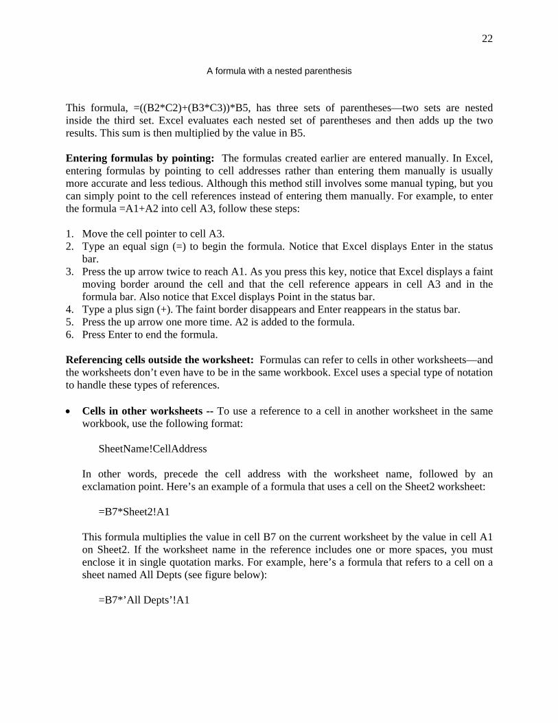
22

A formula with a nested parenthesis This formula, =((B2*C2)+(B3*C3))*B5, has three sets of parentheses—two sets are nested inside the third set. Excel evaluates each nested set of parentheses and then adds up the two results. This sum is then multiplied by the value in B5. Entering formulas by pointing: The formulas created earlier are entered manually. In Excel, entering formulas by pointing to cell addresses rather than entering them manually is usually more accurate and less tedious. Although this method still involves some manual typing, but you can simply point to the cell references instead of entering them manually. For example, to enter the formula =A1+A2 into cell A3, follow these steps: 1. Move the cell pointer to cell A3. 2. Type an equal sign (=) to begin the formula. Notice that Excel displays Enter in the status

bar. 3. Press the up arrow twice to reach A1. As you press this key, notice that Excel displays a faint

moving border around the cell and that the cell reference appears in cell A3 and in the formula bar. Also notice that Excel displays Point in the status bar.

4. Type a plus sign (+). The faint border disappears and Enter reappears in the status bar. 5. Press the up arrow one more time. A2 is added to the formula. 6. Press Enter to end the formula. Referencing cells outside the worksheet: Formulas can refer to cells in other worksheets—and the worksheets don’t even have to be in the same workbook. Excel uses a special type of notation to handle these types of references. • Cells in other worksheets -- To use a reference to a cell in another worksheet in the same

workbook, use the following format:

SheetName!CellAddress

In other words, precede the cell address with the worksheet name, followed by an exclamation point. Here’s an example of a formula that uses a cell on the Sheet2 worksheet:

=B7*Sheet2!A1

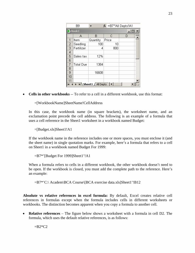
This formula multiplies the value in cell B7 on the current worksheet by the value in cell A1 on Sheet2. If the worksheet name in the reference includes one or more spaces, you must enclose it in single quotation marks. For example, here’s a formula that refers to a cell on a sheet named All Depts (see figure below):

=B7*’All Depts’!A1

23

• Cells in other workbooks -- To refer to a cell in a different workbook, use this format:

=[WorkbookName]SheetName!CellAddress

In this case, the workbook name (in square brackets), the worksheet name, and an exclamation point precede the cell address. The following is an example of a formula that uses a cell reference in the Sheet1 worksheet in a workbook named Budget:

=[Budget.xls]Sheet1!A1

If the workbook name in the reference includes one or more spaces, you must enclose it (and the sheet name) in single quotation marks. For example, here’s a formula that refers to a cell on Sheet1 in a workbook named Budget For 1999:

=B7*’[Budget For 1999]Sheet1’!A1

When a formula refers to cells in a different workbook, the other workbook doesn’t need to be open. If the workbook is closed, you must add the complete path to the reference. Here’s an example:

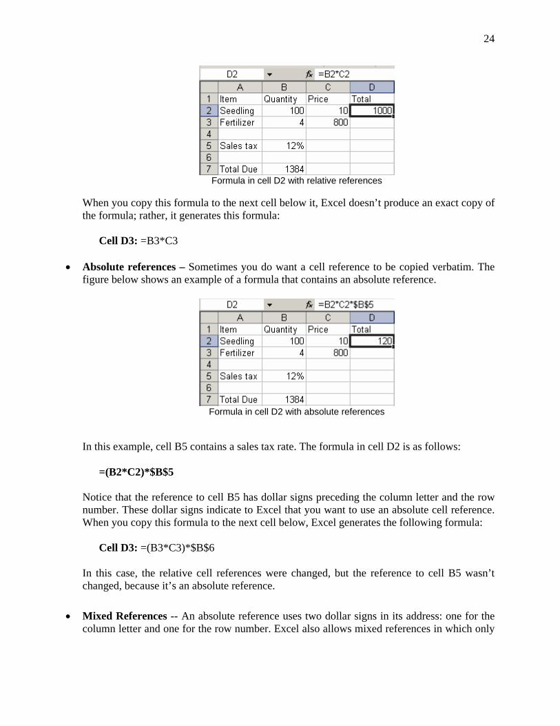
=B7*’C:\ Academ\BCA Course\[BCA exercise data.xls]Sheet1’!B12 Absolute vs relative references in excel formula: By default, Excel creates relative cell references in formulas except when the formula includes cells in different worksheets or workbooks. The distinction becomes apparent when you copy a formula to another cell. • Relative references – The figure below shows a worksheet with a formula in cell D2. The

formula, which uses the default relative references, is as follows:

=B2*C2

24

Formula in cell D2 with relative references

When you copy this formula to the next cell below it, Excel doesn’t produce an exact copy of the formula; rather, it generates this formula:

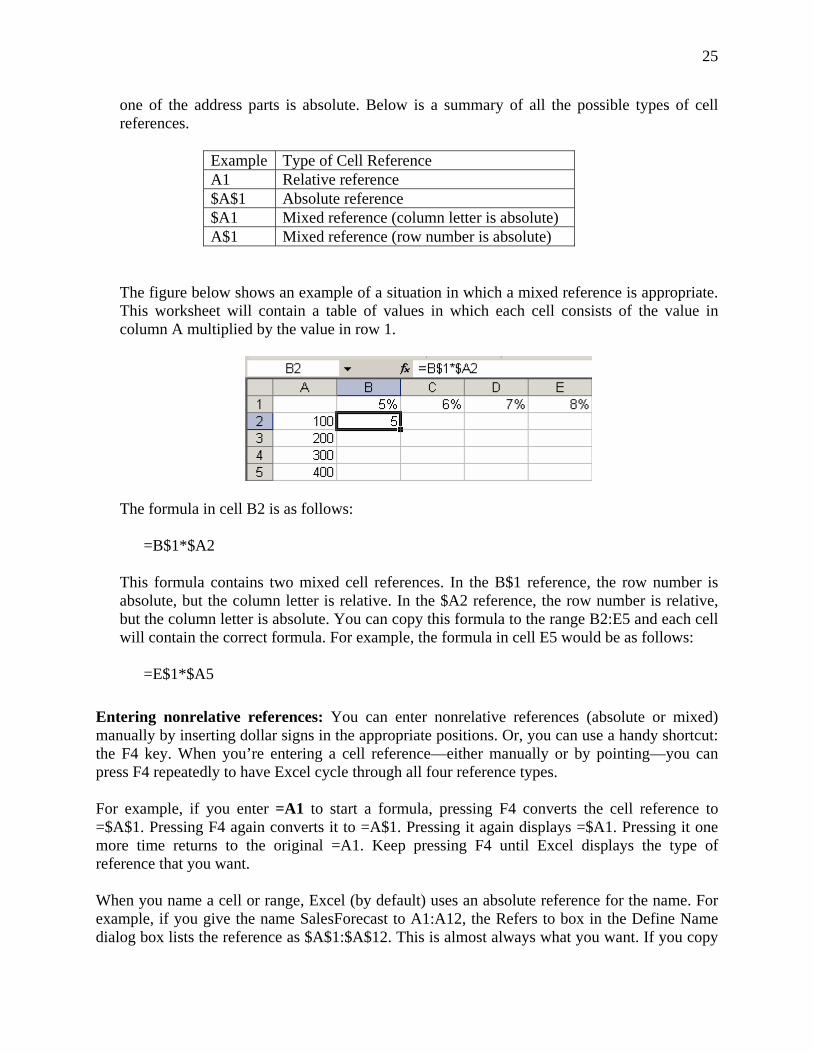
Cell D3: =B3*C3 • Absolute references – Sometimes you do want a cell reference to be copied verbatim. The

figure below shows an example of a formula that contains an absolute reference.

Formula in cell D2 with absolute references

In this example, cell B5 contains a sales tax rate. The formula in cell D2 is as follows:

=(B2*C2)*$B$5 Notice that the reference to cell B5 has dollar signs preceding the column letter and the row number. These dollar signs indicate to Excel that you want to use an absolute cell reference. When you copy this formula to the next cell below, Excel generates the following formula:

Cell D3: =(B3*C3)*$B$6

In this case, the relative cell references were changed, but the reference to cell B5 wasn’t changed, because it’s an absolute reference.

• Mixed References -- An absolute reference uses two dollar signs in its address: one for the

column letter and one for the row number. Excel also allows mixed references in which only

25

one of the address parts is absolute. Below is a summary of all the possible types of cell references.

Example Type of Cell Reference A1 Relative reference $A$1 Absolute reference $A1 Mixed reference (column letter is absolute) A$1 Mixed reference (row number is absolute)

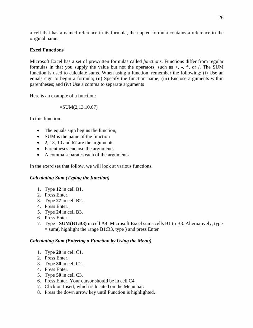
The figure below shows an example of a situation in which a mixed reference is appropriate. This worksheet will contain a table of values in which each cell consists of the value in column A multiplied by the value in row 1.

The formula in cell B2 is as follows:

=B$1*$A2

This formula contains two mixed cell references. In the B$1 reference, the row number is absolute, but the column letter is relative. In the $A2 reference, the row number is relative, but the column letter is absolute. You can copy this formula to the range B2:E5 and each cell will contain the correct formula. For example, the formula in cell E5 would be as follows:

=E$1*$A5 Entering nonrelative references: You can enter nonrelative references (absolute or mixed) manually by inserting dollar signs in the appropriate positions. Or, you can use a handy shortcut: the F4 key. When you’re entering a cell reference—either manually or by pointing—you can press F4 repeatedly to have Excel cycle through all four reference types. For example, if you enter =A1 to start a formula, pressing F4 converts the cell reference to =$A$1. Pressing F4 again converts it to =A$1. Pressing it again displays =$A1. Pressing it one more time returns to the original =A1. Keep pressing F4 until Excel displays the type of reference that you want. When you name a cell or range, Excel (by default) uses an absolute reference for the name. For example, if you give the name SalesForecast to A1:A12, the Refers to box in the Define Name dialog box lists the reference as $A$1:$A$12. This is almost always what you want. If you copy

26

a cell that has a named reference in its formula, the copied formula contains a reference to the original name. Excel Functions

Microsoft Excel has a set of prewritten formulas called functions. Functions differ from regular formulas in that you supply the value but not the operators, such as +, -, *, or /. The SUM function is used to calculate sums. When using a function, remember the following: (i) Use an equals sign to begin a formula; (ii) Specify the function name; (iii) Enclose arguments within parentheses; and (iv) Use a comma to separate arguments

Here is an example of a function:

=SUM(2,13,10,67) In this function:

• The equals sign begins the function, • SUM is the name of the function • 2, 13, 10 and 67 are the arguments • Parentheses enclose the arguments • A comma separates each of the arguments

In the exercises that follow, we will look at various functions.

Calculating Sum (Typing the function)

1. Type 12 in cell B1. 2. Press Enter. 3. Type 27 in cell B2. 4. Press Enter. 5. Type 24 in cell B3. 6. Press Enter. 7. Type =SUM(B1:B3) in cell A4. Microsoft Excel sums cells B1 to B3. Alternatively, type

= sum(, highlight the range B1:B3, type ) and press Enter

Calculating Sum (Entering a Function by Using the Menu)

1. Type 20 in cell C1. 2. Press Enter. 3. Type 30 in cell C2. 4. Press Enter. 5. Type 50 in cell C3. 6. Press Enter. Your cursor should be in cell C4. 7. Click on Insert, which is located on the Menu bar. 8. Press the down arrow key until Function is highlighted.

27

9. Press Enter. 10. Click on Math & Trig in the Function Category box. 11. Click on Sum in the Function Name box. 12. Click on OK. 13. Type C1:C3 in the Number1 entry field, if it does not automatically appear. 14. Click on OK. 15. Move to cell A4. 16. Type the word Sum. 17. Press Enter.

Calculating an Average

You can use the AVERAGE function to calculate an average from a series of numbers. Using the series of numbers used in calculating sum, do the following:

1. Move the cursor to cell A5. 2. Type Average. 3. Press the right arrow key. 4. Type =AVERAGE(B1:B3). 5. Press Enter. The average should appear.

Calculating Min

You can use the MIN function to find the lowest number in a series of numbers.

1. Move the cursor the cell A6. 2. Type Min. 3. Press the right arrow key. 4. Type = MIN(B1:B3). 5. Press Enter. The lowest number in the series, which is 12, should appear.

Calculating Max

You can use the MAX function to find the highest number in a series of numbers.

1. Move the cursor the cell A7. 2. Type Max. 3. Press the right arrow key. 4. Type = MAX(B1:B3). 5. Press Enter. The highest number in the series, which is 27, should appear.

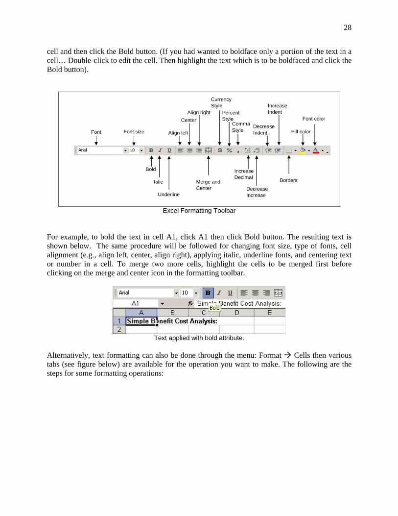
• Formatting Text and Numbers in Excel

Format text and individual characters: To make text stand out, you can format all of the text in a cell or selected characters. Select the characters you want to format, and then click a button on the Formatting toolbar (see figure below). Thus, to boldface all text in a cell click the desired

28

cell and then click the Bold button. (If you had wanted to boldface only a portion of the text in a cell… Double-click to edit the cell. Then highlight the text which is to be boldfaced and click the Bold button).

Font Font size

Bold

Italic

Underline

Align left

CenterAlign right

Merge and Center

CurrencyStyle

PercentStyle

CommaStyle

IncreaseDecimal

DecreaseIncrease

Borders

DecreaseIndent

IncreaseIndent

Fill color

Font color

Excel Formatting Toolbar

For example, to bold the text in cell A1, click A1 then click Bold button. The resulting text is shown below. The same procedure will be followed for changing font size, type of fonts, cell alignment (e.g., align left, center, align right), applying italic, underline fonts, and centering text or number in a cell. To merge two more cells, highlight the cells to be merged first before clicking on the merge and center icon in the formatting toolbar.

Text applied with bold attribute.

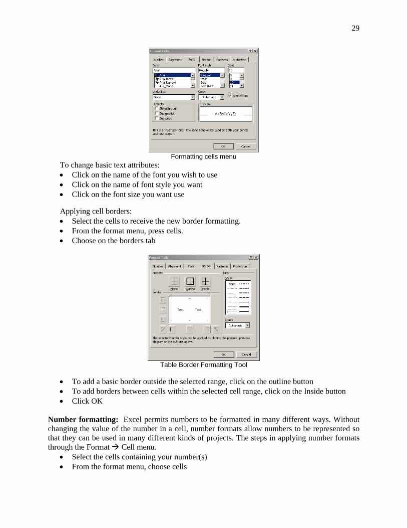
Alternatively, text formatting can also be done through the menu: Format Cells then various tabs (see figure below) are available for the operation you want to make. The following are the steps for some formatting operations:

29

Formatting cells menu

To change basic text attributes: • Click on the name of the font you wish to use • Click on the name of font style you want • Click on the font size you want use

Applying cell borders: • Select the cells to receive the new border formatting. • From the format menu, press cells. • Choose on the borders tab

Table Border Formatting Tool

• To add a basic border outside the selected range, click on the outline button • To add borders between cells within the selected cell range, click on the Inside button • Click OK

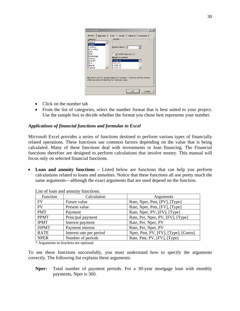
Number formatting: Excel permits numbers to be formatted in many different ways. Without changing the value of the number in a cell, number formats allow numbers to be represented so that they can be used in many different kinds of projects. The steps in applying number formats through the Format Cell menu.

• Select the cells containing your number(s) • From the format menu, choose cells

30

• Click on the number tab • From the list of categories, select the number format that is best suited to your project.

Use the sample box to decide whether the format you chose best represents your number. Applications of financial functions and formulae in Excel Microsoft Excel provides a series of functions destined to perform various types of financially related operations. These functions use common factors depending on the value that is being calculated. Many of these functions deal with investments or loan financing. The Financial functions therefore are designed to perform calculations that involve money. This manual will focus only on selected financial functions. • Loan and annuity functions – Listed below are functions that can help you perform

calculations related to loans and annuities. Notice that these functions all use pretty much the same arguments—although the exact arguments that are used depend on the function. List of loan and annuity functions.

Function Calculation Arguments FV Future value Rate, Nper, Pmt, [PV], [Type] PV Present value Rate, Nper, Pmt, [FV], [Type] PMT Payment Rate, Nper, PV, [FV], [Type] PPMT Principal payment Rate, Per, Nper, PV, [FV], [Type] IPMT Interest payment Rate, Per, Nper, PV ISPMT Payment interest Rate, Per, Nper, PV RATE Interest rate per period Nper, Pmt, PV, [FV], [Type], [Guess] NPER Number of periods Rate, Pmt, PV, [FV], [Type]

* Arguments in brackets are optional To use these functions successfully, you must understand how to specify the arguments correctly. The following list explains these arguments:

Nper: Total number of payment periods. For a 30-year mortgage loan with monthly payments, Nper is 360.

31

Per: Period in the loan for which the calculation is being made; it must be a number between 1 and Nper.

Pmt: Fixed payment made each period for an annuity or a loan. This usually includes

principal and interest (but not fees or taxes). FV: Future value (or a cash balance) after the last payment is made. The future value for

a loan is 0. If FV is omitted, Excel uses 0. Type: Either 0 or 1, and indicates when payments are due. Use 0 if the payments are due

at the end of the period, and 1 if they are due at the beginning of the period. Guess: Used only for the RATE function. It’s your best guess of the internal rate of return.

The closer your guess, the faster Excel can calculate the exact result. The Future Value of an Investment (FV): FV returns the future value of an investment based on periodic, constant payments and a constant interest rate. To calculate FV, you can use the FV() function. The syntax of this function is:

FV(rate,nper,pmt,pv,type)

where: Rate = is the interest rate per period. Pv = is the present value, or the lump-sum amount that a series of future payments is worth

right now. If pv is omitted, it is assumed to be 0 (zero), and you must include the pmt argument.

Nper, Pmt = are similarly defined above. Remarks

• Make sure that you are consistent about the units you use for specifying rate and nper. If you make monthly payments on a four-year loan at 12 percent annual interest, use 12%/12 for rate and 4*12 for nper. If you make annual payments on the same loan, use 12% for rate and 4 for nper.

• For all the arguments, cash you pay out, such as deposits to savings, is represented by negative numbers; cash you receive, such as dividend checks, is represented by positive numbers.

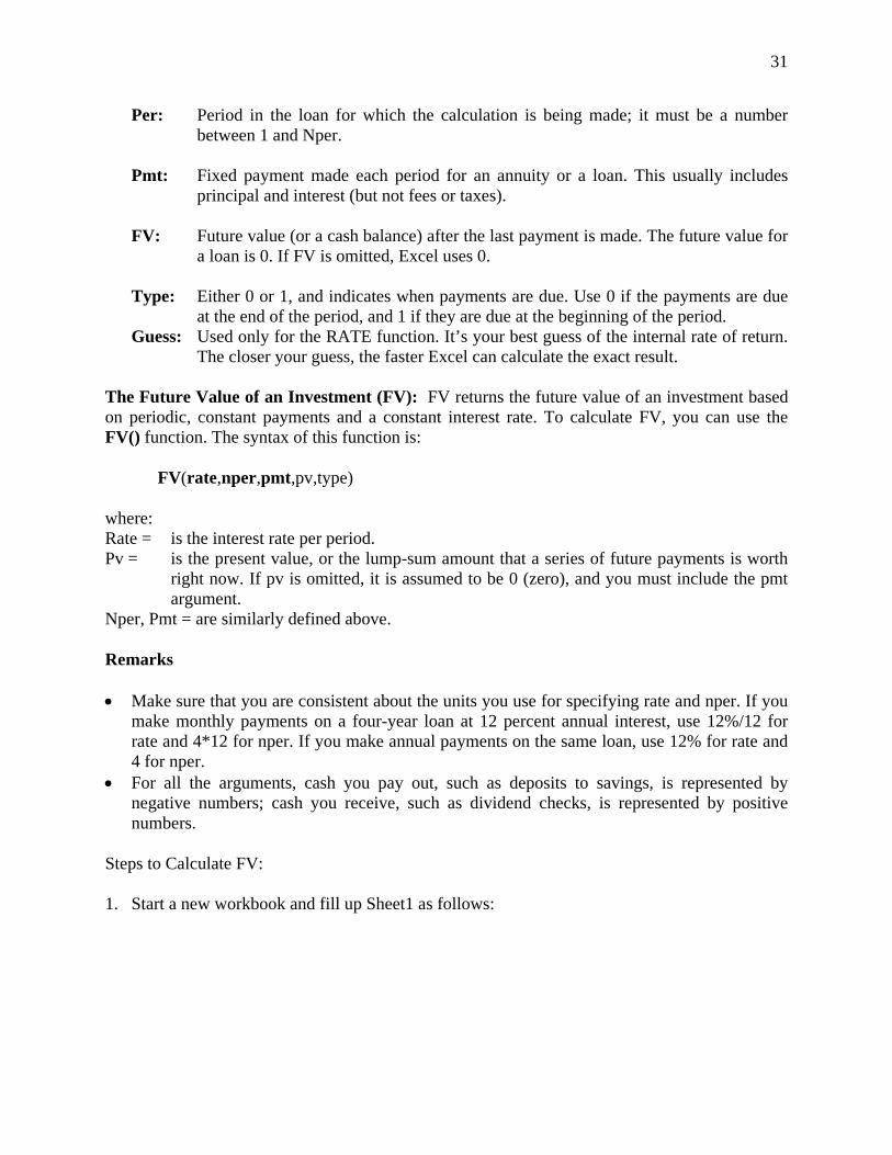
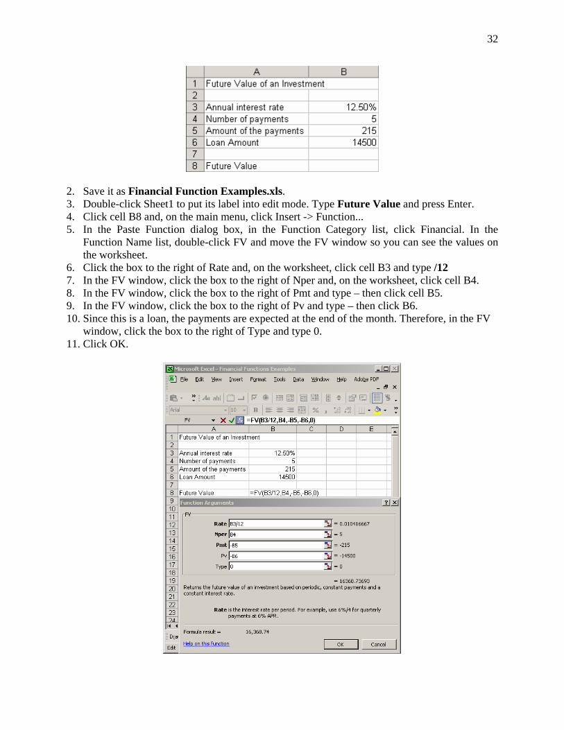
Steps to Calculate FV: 1. Start a new workbook and fill up Sheet1 as follows:

32

2. Save it as Financial Function Examples.xls. 3. Double-click Sheet1 to put its label into edit mode. Type Future Value and press Enter. 4. Click cell B8 and, on the main menu, click Insert -> Function... 5. In the Paste Function dialog box, in the Function Category list, click Financial. In the

Function Name list, double-click FV and move the FV window so you can see the values on the worksheet.

6. Click the box to the right of Rate and, on the worksheet, click cell B3 and type /12 7. In the FV window, click the box to the right of Nper and, on the worksheet, click cell B4. 8. In the FV window, click the box to the right of Pmt and type – then click cell B5. 9. In the FV window, click the box to the right of Pv and type – then click B6. 10. Since this is a loan, the payments are expected at the end of the month. Therefore, in the FV

window, click the box to the right of Type and type 0. 11. Click OK.

33

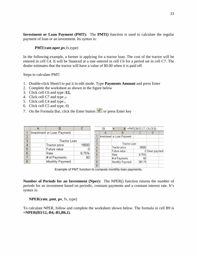
Investment or Loan Payment (PMT): The PMT() function is used to calculate the regular payment of loan or an investment. Its syntax is:

PMT(rate,nper,pv,fv,type) In the following example, a farmer is applying for a tractor loan. The cost of the tractor will be entered in cell C4. It will be financed at a rate entered in cell C6 for a period set in cell C7. The dealer estimates that the tractor will have a value of $0.00 when it is paid off. Steps to calculate PMT: 1. Double-click Sheet3 to put it in edit mode. Type Payments Amount and press Enter 2. Complete the worksheet as shown in the figure below 3. Click cell C6 and type /12, 4. Click cell C7 and type ,- 5. Click cell C4 and type , 6. Click cell C5 and type, 0) 7. On the Formula Bar, click the Enter button or press Enter key

Example of PMT function to compute monthly loan payments.

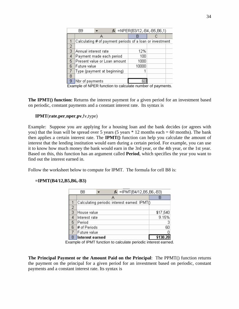
Number of Periods for an Investment (Nper): The NPER() function returns the number of periods for an investment based on periodic, constant payments and a constant interest rate. It’s syntax is:

NPER(rate, pmt, pv, fv, type)

To calculate NPER, follow and complete the worksheet shown below. The formula in cell B9 is =NPER(B3/12,-B4,-B5,B6,1).

34

Example of NPER function to calculate number of payments.

The IPMT() function: Returns the interest payment for a given period for an investment based on periodic, constant payments and a constant interest rate. Its syntax is

IPMT(rate,per,nper,pv,fv,type) Example: Suppose you are applying for a housing loan and the bank decides (or agrees with you) that the loan will be spread over 5 years (5 years * 12 months each = 60 months). The bank then applies a certain interest rate. The IPMT() function can help you calculate the amount of interest that the lending institution would earn during a certain period. For example, you can use it to know how much money the bank would earn in the 3rd year, or the 4th year, or the 1st year. Based on this, this function has an argument called Period, which specifies the year you want to find out the interest earned in. Follow the worksheet below to compute for IPMT. The formula for cell B8 is:

=IPMT(B4/12,B5,B6,-B3)

Example of IPMT function to calculate periodic interest earned.

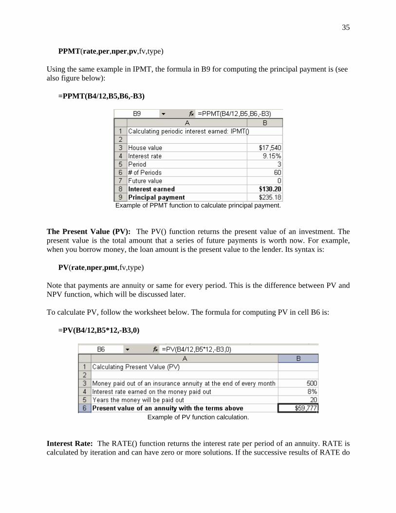
The Principal Payment or the Amount Paid on the Principal: The PPMT() function returns the payment on the principal for a given period for an investment based on periodic, constant payments and a constant interest rate. Its syntax is

35

PPMT(rate,per,nper,pv,fv,type)

Using the same example in IPMT, the formula in B9 for computing the principal payment is (see also figure below):

=PPMT(B4/12,B5,B6,-B3)

Example of PPMT function to calculate principal payment.

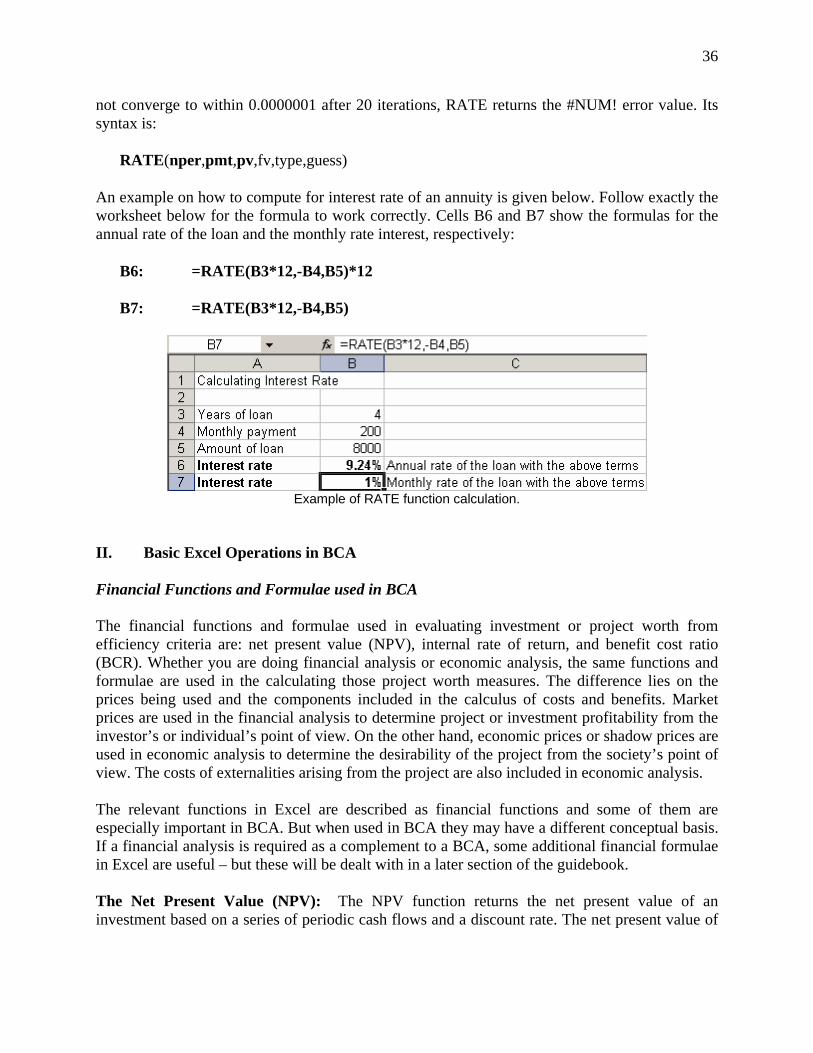
The Present Value (PV): The PV() function returns the present value of an investment. The present value is the total amount that a series of future payments is worth now. For example, when you borrow money, the loan amount is the present value to the lender. Its syntax is:

PV(rate,nper,pmt,fv,type)

Note that payments are annuity or same for every period. This is the difference between PV and NPV function, which will be discussed later. To calculate PV, follow the worksheet below. The formula for computing PV in cell B6 is:

=PV(B4/12,B5*12,-B3,0)

Example of PV function calculation.

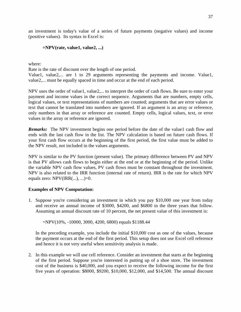
Interest Rate: The RATE() function returns the interest rate per period of an annuity. RATE is calculated by iteration and can have zero or more solutions. If the successive results of RATE do

36

not converge to within 0.0000001 after 20 iterations, RATE returns the #NUM! error value. Its syntax is:

RATE(nper,pmt,pv,fv,type,guess)

An example on how to compute for interest rate of an annuity is given below. Follow exactly the worksheet below for the formula to work correctly. Cells B6 and B7 show the formulas for the annual rate of the loan and the monthly rate interest, respectively:

B6: =RATE(B3*12,-B4,B5)*12

B7: =RATE(B3*12,-B4,B5)

Example of RATE function calculation.

II. Basic Excel Operations in BCA Financial Functions and Formulae used in BCA The financial functions and formulae used in evaluating investment or project worth from efficiency criteria are: net present value (NPV), internal rate of return, and benefit cost ratio (BCR). Whether you are doing financial analysis or economic analysis, the same functions and formulae are used in the calculating those project worth measures. The difference lies on the prices being used and the components included in the calculus of costs and benefits. Market prices are used in the financial analysis to determine project or investment profitability from the investor’s or individual’s point of view. On the other hand, economic prices or shadow prices are used in economic analysis to determine the desirability of the project from the society’s point of view. The costs of externalities arising from the project are also included in economic analysis. The relevant functions in Excel are described as financial functions and some of them are especially important in BCA. But when used in BCA they may have a different conceptual basis. If a financial analysis is required as a complement to a BCA, some additional financial formulae in Excel are useful – but these will be dealt with in a later section of the guidebook. The Net Present Value (NPV): The NPV function returns the net present value of an investment based on a series of periodic cash flows and a discount rate. The net present value of

37

an investment is today's value of a series of future payments (negative values) and income (positive values). Its syntax in Excel is:

=NPV(rate, value1, value2, ...)

where: Rate is the rate of discount over the length of one period. Value1, value2,... are 1 to 29 arguments representing the payments and income. Value1, value2,... must be equally spaced in time and occur at the end of each period.

NPV uses the order of value1, value2,... to interpret the order of cash flows. Be sure to enter your payment and income values in the correct sequence. Arguments that are numbers, empty cells, logical values, or text representations of numbers are counted; arguments that are error values or text that cannot be translated into numbers are ignored. If an argument is an array or reference, only numbers in that array or reference are counted. Empty cells, logical values, text, or error values in the array or reference are ignored.

Remarks: The NPV investment begins one period before the date of the value1 cash flow and ends with the last cash flow in the list. The NPV calculation is based on future cash flows. If your first cash flow occurs at the beginning of the first period, the first value must be added to the NPV result, not included in the values arguments.

NPV is similar to the PV function (present value). The primary difference between PV and NPV is that PV allows cash flows to begin either at the end or at the beginning of the period. Unlike the variable NPV cash flow values, PV cash flows must be constant throughout the investment. NPV is also related to the IRR function (internal rate of return). IRR is the rate for which NPV equals zero: NPV(IRR(...), ...)=0.

Examples of NPV Computation:

1. Suppose you're considering an investment in which you pay $10,000 one year from today and receive an annual income of $3000, $4200, and $6800 in the three years that follow. Assuming an annual discount rate of 10 percent, the net present value of this investment is:

=NPV(10%, -10000, 3000, 4200, 6800) equals $1188.44

In the preceding example, you include the initial $10,000 cost as one of the values, because the payment occurs at the end of the first period. This setup does not use Excel cell reference and hence it is not very useful when sensitivity analysis is made.

2. In this example we will use cell reference. Consider an investment that starts at the beginning of the first period. Suppose you're interested in putting up of a shoe store. The investment cost of the business is $40,000, and you expect to receive the following income for the first five years of operation: $8000, $9200, $10,000, $12,000, and $14,500. The annual discount

38

rate is 8%. This might represent the rate of inflation or the interest rate of a competing investment.

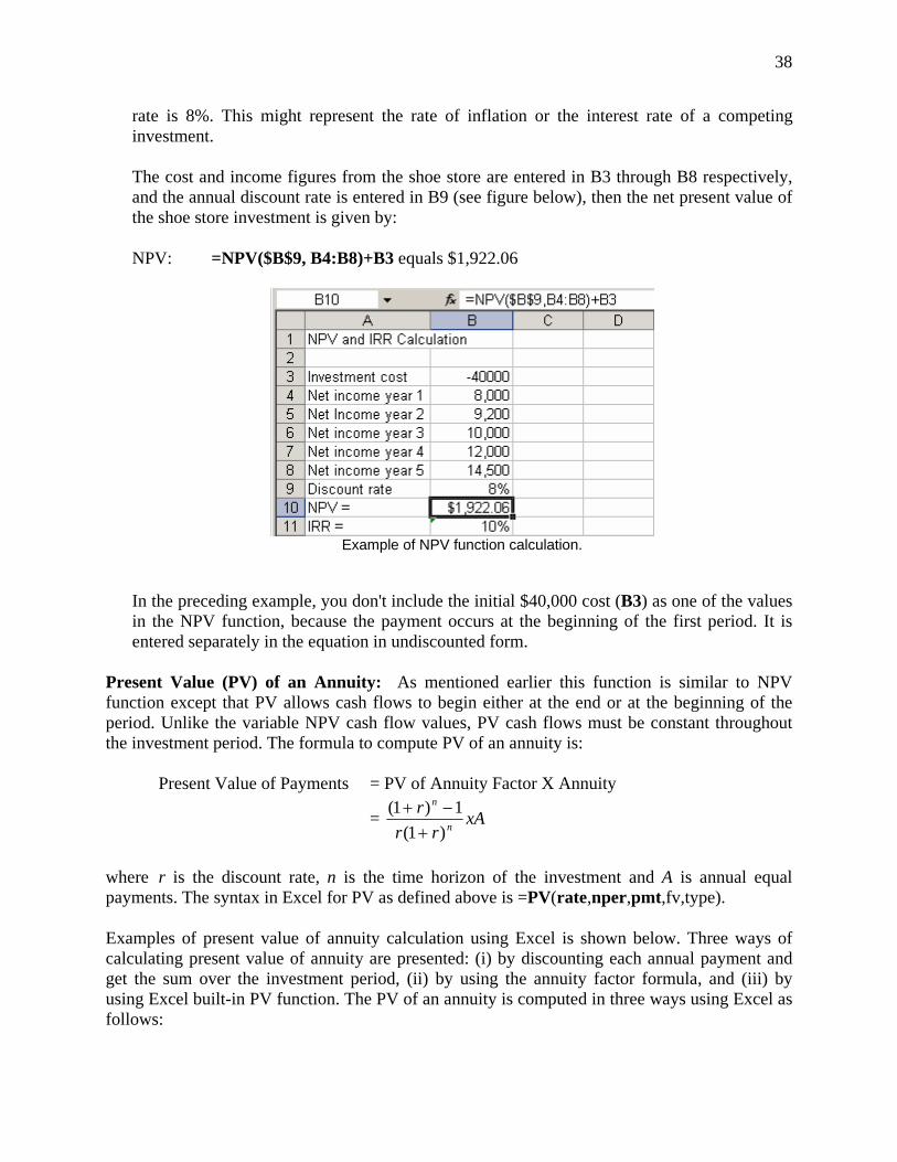
The cost and income figures from the shoe store are entered in B3 through B8 respectively, and the annual discount rate is entered in B9 (see figure below), then the net present value of the shoe store investment is given by:

NPV: =NPV($B$9, B4:B8)+B3 equals $1,922.06

Example of NPV function calculation.

In the preceding example, you don't include the initial $40,000 cost (B3) as one of the values in the NPV function, because the payment occurs at the beginning of the first period. It is entered separately in the equation in undiscounted form.

Present Value (PV) of an Annuity: As mentioned earlier this function is similar to NPV function except that PV allows cash flows to begin either at the end or at the beginning of the period. Unlike the variable NPV cash flow values, PV cash flows must be constant throughout the investment period. The formula to compute PV of an annuity is:

Present Value of Payments = PV of Annuity Factor X Annuity

= xArr

rn

n

)1(1)1(

+−+

where r is the discount rate, n is the time horizon of the investment and A is annual equal payments. The syntax in Excel for PV as defined above is =PV(rate,nper,pmt,fv,type).

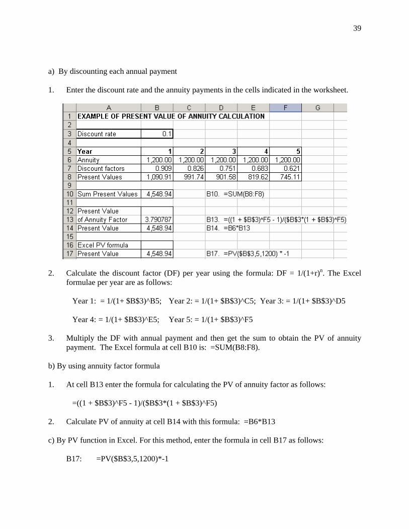
Examples of present value of annuity calculation using Excel is shown below. Three ways of calculating present value of annuity are presented: (i) by discounting each annual payment and get the sum over the investment period, (ii) by using the annuity factor formula, and (iii) by using Excel built-in PV function. The PV of an annuity is computed in three ways using Excel as follows:

39

a) By discounting each annual payment

1. Enter the discount rate and the annuity payments in the cells indicated in the worksheet.

2. Calculate the discount factor (DF) per year using the formula: DF = 1/(1+r)n. The Excel formulae per year are as follows:

Year 1: = 1/(1+ $B$3)^B5; Year 2: = 1/(1+ $B$3)^C5; Year 3: = 1/(1+ $B$3)^D5

Year 4: = 1/(1+ $B$3)^E5; Year 5: = 1/(1+ $B$3)^F5

3. Multiply the DF with annual payment and then get the sum to obtain the PV of annuity payment. The Excel formula at cell B10 is: =SUM(B8:F8).

b) By using annuity factor formula

1. At cell B13 enter the formula for calculating the PV of annuity factor as follows:

=((1 + $B$3)^F5 - 1)/($B$3*(1 + $B$3)^F5)

2. Calculate PV of annuity at cell B14 with this formula: =B6*B13

c) By PV function in Excel. For this method, enter the formula in cell B17 as follows:

B17: =PV($B$3,5,1200)*-1

40

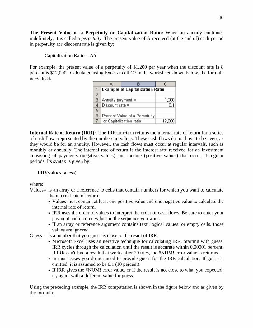
The Present Value of a Perpetuity or Capitalization Ratio: When an annuity continues indefinitely, it is called a perpetuity. The present value of A received (at the end of) each period in perpetuity at r discount rate is given by:

Capitalization Ratio = A/r For example, the present value of a perpetuity of $1,200 per year when the discount rate is 8 percent is $12,000. Calculated using Excel at cell C7 in the worksheet shown below, the formula is =C3/C4.

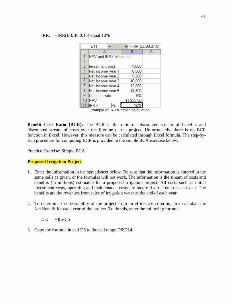
Internal Rate of Return (IRR): The IRR function returns the internal rate of return for a series of cash flows represented by the numbers in values. These cash flows do not have to be even, as they would be for an annuity. However, the cash flows must occur at regular intervals, such as monthly or annually. The internal rate of return is the interest rate received for an investment consisting of payments (negative values) and income (positive values) that occur at regular periods. Its syntax is given by:

IRR(values, guess)

where: Values= is an array or a reference to cells that contain numbers for which you want to calculate

the internal rate of return. • Values must contain at least one positive value and one negative value to calculate the

internal rate of return. • IRR uses the order of values to interpret the order of cash flows. Be sure to enter your

payment and income values in the sequence you want. • If an array or reference argument contains text, logical values, or empty cells, those

values are ignored. Guess= is a number that you guess is close to the result of IRR.

• Microsoft Excel uses an iterative technique for calculating IRR. Starting with guess, IRR cycles through the calculation until the result is accurate within 0.00001 percent. If IRR can't find a result that works after 20 tries, the #NUM! error value is returned.

• In most cases you do not need to provide guess for the IRR calculation. If guess is omitted, it is assumed to be 0.1 (10 percent).

• If IRR gives the #NUM! error value, or if the result is not close to what you expected, try again with a different value for guess.

Using the preceding example, the IRR computation is shown in the figure below and as given by the formula:

41

IRR: =IRR(B3:B8,0.15) equal 10%

Example of IRR function calculation.

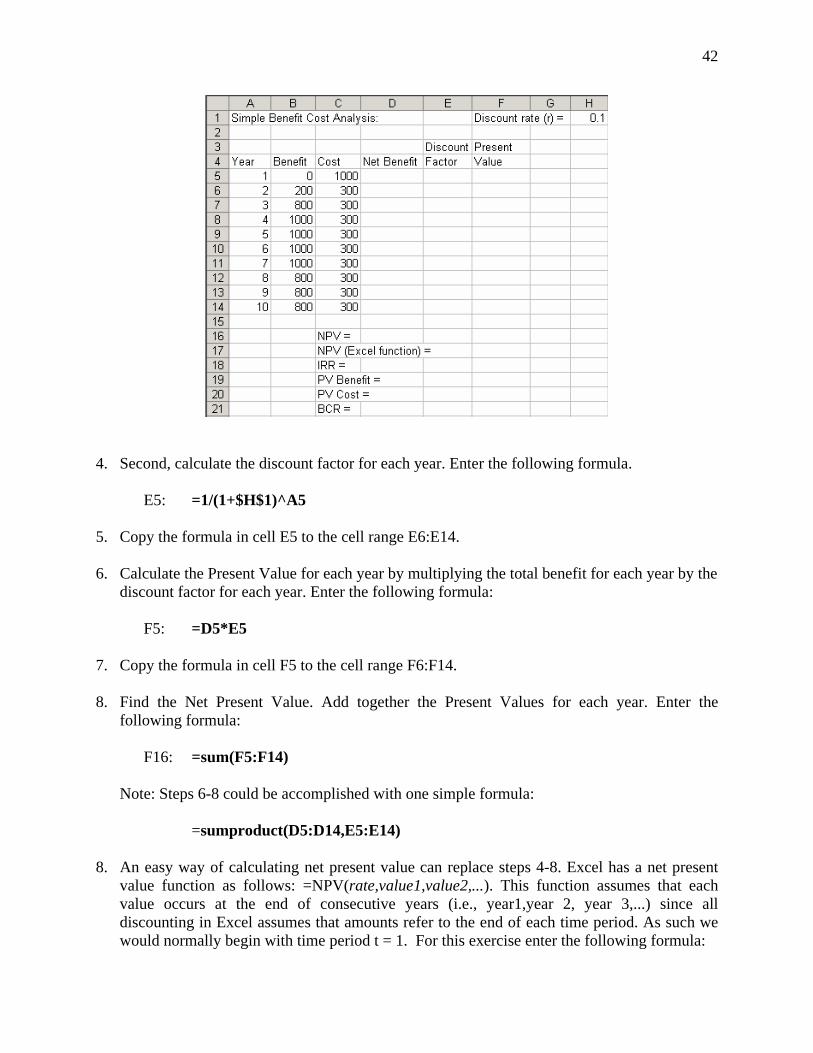
Benefit Cost Ratio (BCR): The BCR is the ratio of discounted stream of benefits and discounted stream of costs over the lifetime of the project. Unfortunately, there is no BCR function in Excel. However, this measure can be calculated through Excel formula. The step-by-step procedure for computing BCR is provided in the simple BCA exercise below. Practice Exercise: Simple BCA Proposed Irrigation Project 1. Enter the information in the spreadsheet below. Be sure that the information is entered in the

same cells as given, or the formulas will not work. The information is the stream of costs and benefits (in millions) estimated for a proposed irrigation project. All costs such as initial investment costs, operating and maintenance costs are incurred at the end of each year. The benefits are the revenues from sales of irrigation water at the end of each year.

2. To determine the desirability of the project from an efficiency criterion, first calculate the

Net Benefit for each year of the project. To do this, enter the following formula.

D5: =B5-C5

3. Copy the formula in cell D5 to the cell range D6:D14.

42

4. Second, calculate the discount factor for each year. Enter the following formula.

E5: =1/(1+$H$1)^A5

5. Copy the formula in cell E5 to the cell range E6:E14. 6. Calculate the Present Value for each year by multiplying the total benefit for each year by the

discount factor for each year. Enter the following formula:

F5: =D5*E5

7. Copy the formula in cell F5 to the cell range F6:F14. 8. Find the Net Present Value. Add together the Present Values for each year. Enter the

following formula:

F16: =sum(F5:F14) Note: Steps 6-8 could be accomplished with one simple formula:

=sumproduct(D5:D14,E5:E14) 8. An easy way of calculating net present value can replace steps 4-8. Excel has a net present

value function as follows: =NPV(rate,value1,value2,...). This function assumes that each value occurs at the end of consecutive years (i.e., year1,year 2, year 3,...) since all discounting in Excel assumes that amounts refer to the end of each time period. As such we would normally begin with time period t = 1. For this exercise enter the following formula:

43

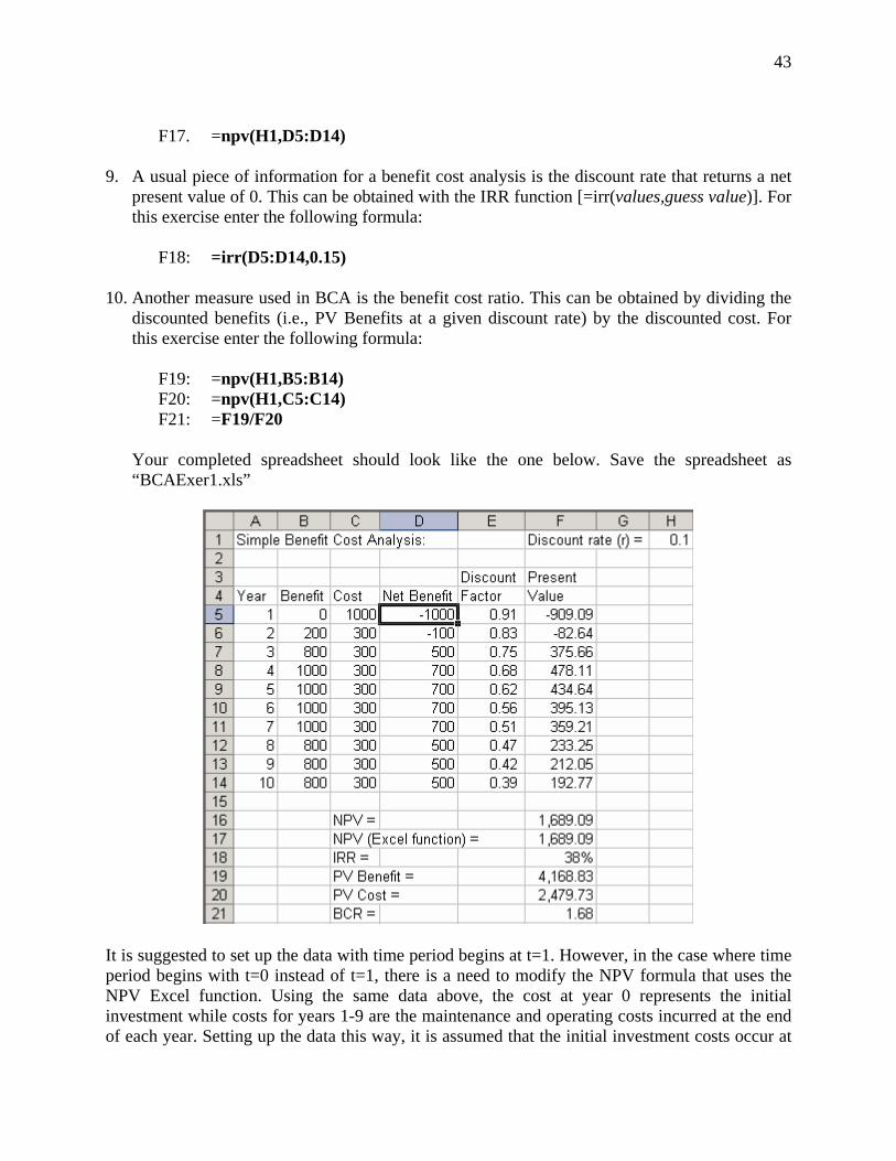
F17. =npv(H1,D5:D14)

9. A usual piece of information for a benefit cost analysis is the discount rate that returns a net

present value of 0. This can be obtained with the IRR function [=irr(values,guess value)]. For this exercise enter the following formula:

F18: =irr(D5:D14,0.15)

10. Another measure used in BCA is the benefit cost ratio. This can be obtained by dividing the

discounted benefits (i.e., PV Benefits at a given discount rate) by the discounted cost. For this exercise enter the following formula:

F19: =npv(H1,B5:B14) F20: =npv(H1,C5:C14) F21: =F19/F20

Your completed spreadsheet should look like the one below. Save the spreadsheet as “BCAExer1.xls”

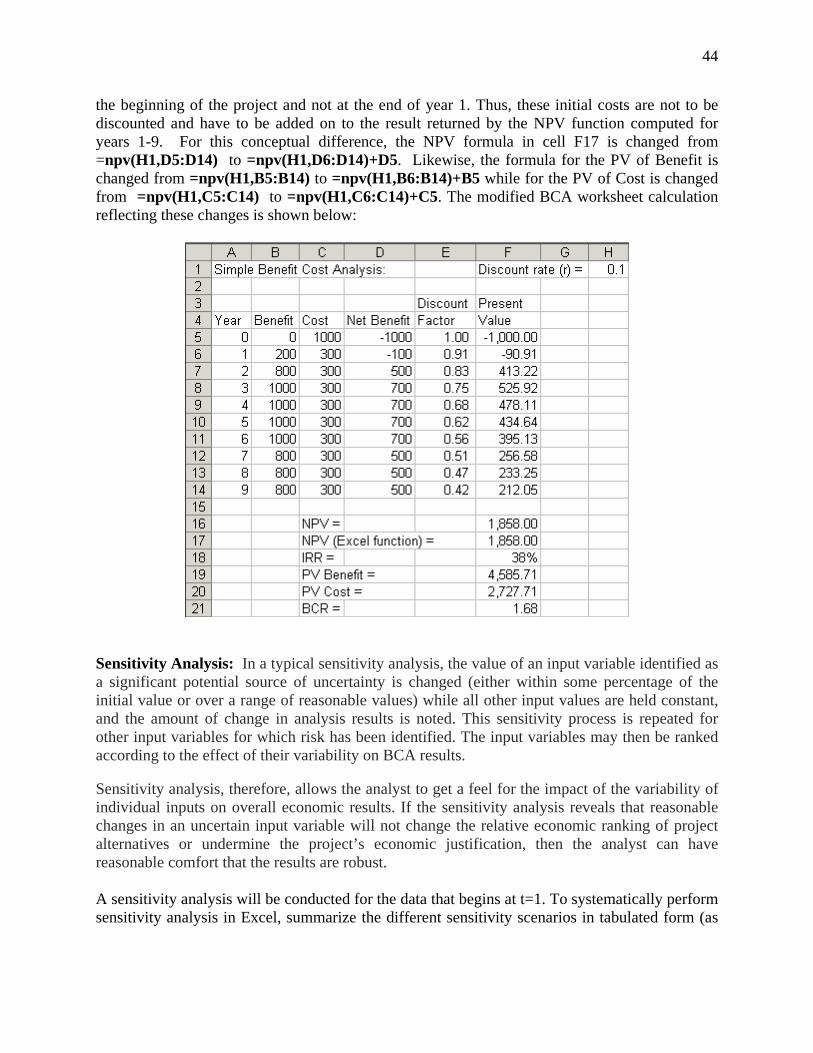
It is suggested to set up the data with time period begins at t=1. However, in the case where time period begins with t=0 instead of t=1, there is a need to modify the NPV formula that uses the NPV Excel function. Using the same data above, the cost at year 0 represents the initial investment while costs for years 1-9 are the maintenance and operating costs incurred at the end of each year. Setting up the data this way, it is assumed that the initial investment costs occur at

44

the beginning of the project and not at the end of year 1. Thus, these initial costs are not to be discounted and have to be added on to the result returned by the NPV function computed for years 1-9. For this conceptual difference, the NPV formula in cell F17 is changed from =npv(H1,D5:D14) to =npv(H1,D6:D14)+D5. Likewise, the formula for the PV of Benefit is changed from =npv(H1,B5:B14) to =npv(H1,B6:B14)+B5 while for the PV of Cost is changed from =npv(H1,C5:C14) to =npv(H1,C6:C14)+C5. The modified BCA worksheet calculation reflecting these changes is shown below:

Sensitivity Analysis: In a typical sensitivity analysis, the value of an input variable identified as a significant potential source of uncertainty is changed (either within some percentage of the initial value or over a range of reasonable values) while all other input values are held constant, and the amount of change in analysis results is noted. This sensitivity process is repeated for other input variables for which risk has been identified. The input variables may then be ranked according to the effect of their variability on BCA results. Sensitivity analysis, therefore, allows the analyst to get a feel for the impact of the variability of individual inputs on overall economic results. If the sensitivity analysis reveals that reasonable changes in an uncertain input variable will not change the relative economic ranking of project alternatives or undermine the project’s economic justification, then the analyst can have reasonable comfort that the results are robust.

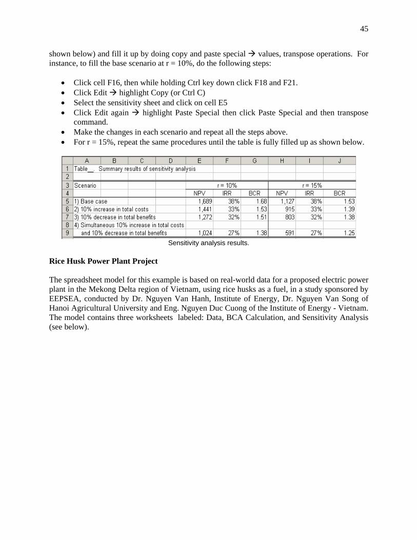
A sensitivity analysis will be conducted for the data that begins at t=1. To systematically perform sensitivity analysis in Excel, summarize the different sensitivity scenarios in tabulated form (as

45

shown below) and fill it up by doing copy and paste special values, transpose operations. For instance, to fill the base scenario at r = 10%, do the following steps:

• Click cell F16, then while holding Ctrl key down click F18 and F21. • Click Edit highlight Copy (or Ctrl C) • Select the sensitivity sheet and click on cell E5 • Click Edit again highlight Paste Special then click Paste Special and then transpose

command. • Make the changes in each scenario and repeat all the steps above. • For r = 15%, repeat the same procedures until the table is fully filled up as shown below.

Sensitivity analysis results.

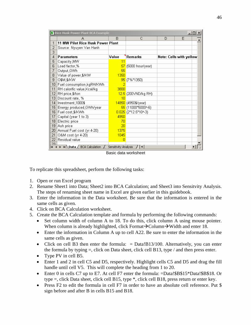
Rice Husk Power Plant Project The spreadsheet model for this example is based on real-world data for a proposed electric power plant in the Mekong Delta region of Vietnam, using rice husks as a fuel, in a study sponsored by EEPSEA, conducted by Dr. Nguyen Van Hanh, Institute of Energy, Dr. Nguyen Van Song of Hanoi Agricultural University and Eng. Nguyen Duc Cuong of the Institute of Energy - Vietnam. The model contains three worksheets labeled: Data, BCA Calculation, and Sensitivity Analysis (see below).

46

Basic data worksheet

To replicate this spreadsheet, perform the following tasks: 1. Open or run Excel program 2. Rename Sheet1 into Data; Sheet2 into BCA Calculation; and Sheet3 into Sensitvity Analysis.

The steps of renaming sheet name in Excel are given earlier in this guidebook. 3. Enter the information in the Data worksheet. Be sure that the information is entered in the

same cells as given. 4. Click on BCA Calculation worksheet. 5. Create the BCA Calculation template and formula by performing the following commands:

• Set column width of column A to 18. To do this, click column A using mouse pointer. When column is already highlighted, click Format Column Width and enter 18.

• Enter the information in Column A up to cell A22. Be sure to enter the information in the same cells as given.

• Click on cell B3 then enter the formula: = Data!B13/100. Alternatively, you can enter the formula by typing =, click on Data sheet, click cell B13, type / and then press enter.

• Type PV in cell B5. • Enter 1 and 2 in cell C5 and D5, respectively. Highlight cells C5 and D5 and drag the fill

handle until cell V5. This will complete the heading from 1 to 20. • Enter 0 in cells C7 up to E7. At cell F7 enter the formula: =Data!$B$15*Data!$B$18. Or

type =, click Data sheet, click cell B15, type *, click cell B18, press return or enter key. • Press F2 to edit the formula in cell F7 in order to have an absolute cell reference. Put $

sign before and after B in cells B15 and B18.

47

• Copy formula from cell F7 to G7 until V7. Or highlight cell F7 then drag the fill handle up to V7.

• Enter 0 in cells C8 up to U8. At cell V8 enter the formula: = Data!B22. • Enter 0 in cells C9 up to E9. At cell F9 enter the formula: =Data!$B15*Data!$B19. Copy

cell F9 to cell range G9:V9. • Sum total benefits in cells C10 up to V10. For cell C10, type =sum( then highlight

C7:C9, type ) and then press Enter. Copy cell C10 to range D10:V10. • Enter capital cost in cell C13 with the formula: =Data!$B17. Copy C13 to cell range

D13:E13. Then 0 to cell range F13:V13. • For fuel costs, enter 0 in cell range C14:E14. At cell F14, type the formula: =Data!$B20

or type = then click Data sheet, click B20 and press Enter. Click cell F14 and press F2 to edit formula. Put $ before B in the formula. Copy cell F14 to cell range G14:V14

• Copy cell F14 to cell range G14:V14 • Enter 0 for O&M costs in cell range C15:E15. At cell F15 enter the formula:

=Data!$B21. Copy cell F15 to cell range G15:V15. • Enter the formula: =sum(C13:C15) in cell C16. Copy cell C16 to cell range D16:V16 • Compute for Net Benefits in row 18. At cell C18 enter the formula: =C10-C16. Then

copy cell C18 to cell range D18:V18 • Enter the following commands for Present Value computation of each item in the cost

and benefit streams: B7. =NPV($B$3,C7:V7) B8. =NPV($B$3,C8:V8) B9. =NPV($B$3,C9:V9) B10. =NPV($B$3,C10:V10) B13. =NPV($B$3,C13:V13) B14. =NPV($B$3,C14:V14) B15. =NPV($B$3,C15:V15) B16. =NPV($B$3,C16:V16) B18. =NPV($B$3,C18:V18)

• Enter the formula for NPV, BCR and IRR:

B20. =NPV($B$3,C18:V18) for NPV B21. =B10/B16 for BCR B22. =IRR(C18:V18,10%) for IRR

• Draw borders in rows 5 and 18. At row 5 border, highlight cell range A5:V5 click border icon and select top and bottom border. For row 18, highlight cell range A18:V18

click border icon and select bottom border.

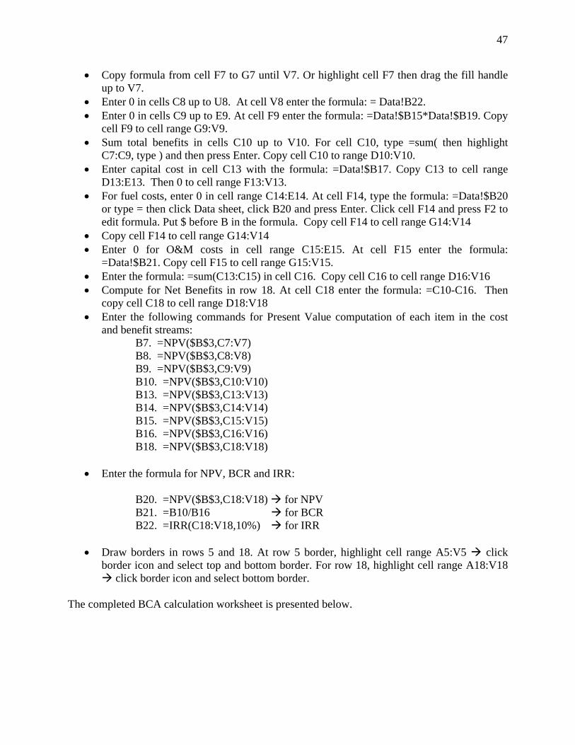
The completed BCA calculation worksheet is presented below.

48

BCA calculation worksheet

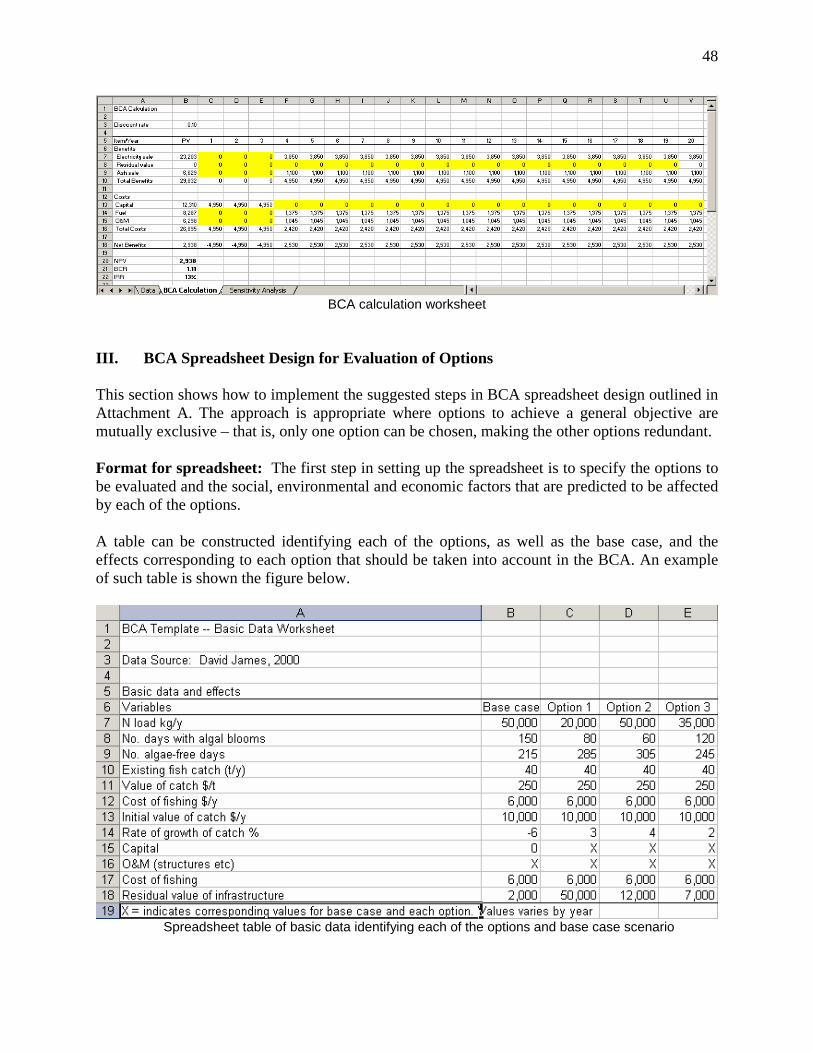
III. BCA Spreadsheet Design for Evaluation of Options This section shows how to implement the suggested steps in BCA spreadsheet design outlined in Attachment A. The approach is appropriate where options to achieve a general objective are mutually exclusive – that is, only one option can be chosen, making the other options redundant. Format for spreadsheet: The first step in setting up the spreadsheet is to specify the options to be evaluated and the social, environmental and economic factors that are predicted to be affected by each of the options. A table can be constructed identifying each of the options, as well as the base case, and the effects corresponding to each option that should be taken into account in the BCA. An example of such table is shown the figure below.

Spreadsheet table of basic data identifying each of the options and base case scenario

49

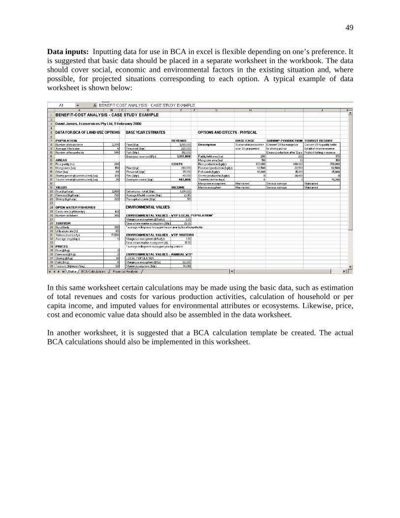
Data inputs: Inputting data for use in BCA in excel is flexible depending on one’s preference. It is suggested that basic data should be placed in a separate worksheet in the workbook. The data should cover social, economic and environmental factors in the existing situation and, where possible, for projected situations corresponding to each option. A typical example of data worksheet is shown below:

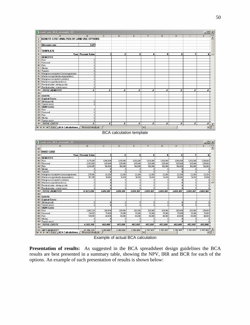
In this same worksheet certain calculations may be made using the basic data, such as estimation of total revenues and costs for various production activities, calculation of household or per capita income, and imputed values for environmental attributes or ecosystems. Likewise, price, cost and economic value data should also be assembled in the data worksheet. In another worksheet, it is suggested that a BCA calculation template be created. The actual BCA calculations should also be implemented in this worksheet.

50

BCA calculation template

Example of actual BCA calculation

Presentation of results: As suggested in the BCA spreadsheet design guidelines the BCA results are best presented in a summary table, showing the NPV, IRR and BCR for each of the options. An example of such presentation of results is shown below:

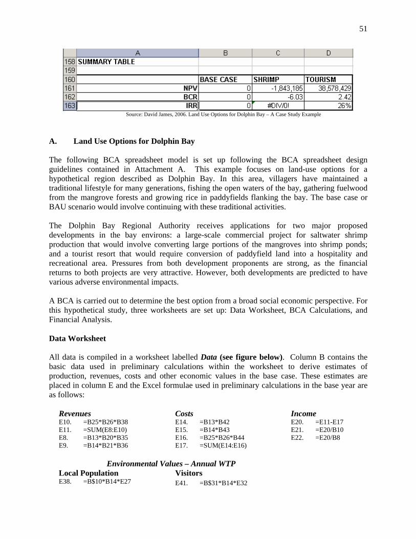
51

Source: David James, 2006. Land Use Options for Dolphin Bay – A Case Study Example

A. Land Use Options for Dolphin Bay The following BCA spreadsheet model is set up following the BCA spreadsheet design guidelines contained in Attachment A. This example focuses on land-use options for a hypothetical region described as Dolphin Bay. In this area, villagers have maintained a traditional lifestyle for many generations, fishing the open waters of the bay, gathering fuelwood from the mangrove forests and growing rice in paddyfields flanking the bay. The base case or BAU scenario would involve continuing with these traditional activities. The Dolphin Bay Regional Authority receives applications for two major proposed developments in the bay environs: a large-scale commercial project for saltwater shrimp production that would involve converting large portions of the mangroves into shrimp ponds; and a tourist resort that would require conversion of paddyfield land into a hospitality and recreational area. Pressures from both development proponents are strong, as the financial returns to both projects are very attractive. However, both developments are predicted to have various adverse environmental impacts. A BCA is carried out to determine the best option from a broad social economic perspective. For this hypothetical study, three worksheets are set up: Data Worksheet, BCA Calculations, and Financial Analysis. Data Worksheet All data is compiled in a worksheet labelled Data (see figure below). Column B contains the basic data used in preliminary calculations within the worksheet to derive estimates of production, revenues, costs and other economic values in the base case. These estimates are placed in column E and the Excel formulae used in preliminary calculations in the base year are as follows:

Revenues Costs Income E10. =B25*B26*B38 E14. =B13*B42 E20. =E11-E17 E11. =SUM(E8:E10) E15. =B14*B43 E21. =E20/B10 E8. =B13*B20*B35 E16. =B25*B26*B44 E22. =E20/B8 E9. =B14*B21*B36 E17. =SUM(E14:E16)

Environmental Values – Annual WTP Local Population Visitors E38. =B$10*B14*E27 E41. =B$31*B14*E32

52

E39. =B$10*E28 E42. =B$31*E33

Environmental Values – Capitalized Local Population Visitors E46. =E38/'BCA Calculations'!B$3 E49. =E41/'BCA Calculations'!B$3 E47. =E39/'BCA Calculations'!B$3 E50. =E42/'BCA Calculations'!B$3

Data Worksheet (Land Use Options for Dolphin Bay – A Case Study Example)

Options and Effects – Physical Base Case Shrimp Production Tourist Resort H11. =B13 I11. =B13 J11. =B13-B17 H12. =B14 I12. =B14-B16 J12. =B14 H13. =B13*B20 I13. =B13*B20 J13. =(B13-B17)*B20 H14. =B14*B21 I14. =(B14-B16)*B21 J14. =B14*B21 H15. =B25*B26 I16. =B16*B22 J17. =B31*B32

Worksheet for BCA Calculations Calculations for the BCA are carried out in a separate, linked worksheet labelled BCA Calculations. First, a template is constructed, containing all potential effects of the two proposed developments. A planning horizon of 20 years is assumed. The discount rate could be altered interactively and applied to all options in the BCA.

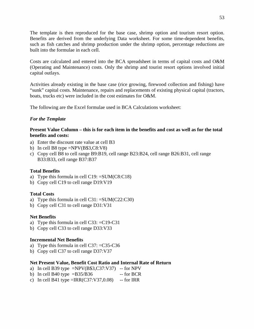
53

The template is then reproduced for the base case, shrimp option and tourism resort option. Benefits are derived from the underlying Data worksheet. For some time-dependent benefits, such as fish catches and shrimp production under the shrimp option, percentage reductions are built into the formulae in each cell. Costs are calculated and entered into the BCA spreadsheet in terms of capital costs and O&M (Operating and Maintenance) costs. Only the shrimp and tourist resort options involved initial capital outlays. Activities already existing in the base case (rice growing, firewood collection and fishing) have “sunk” capital costs. Maintenance, repairs and replacements of existing physical capital (tractors, boats, trucks etc) were included in the cost estimates for O&M. The following are the Excel formulae used in BCA Calculations worksheet: For the Template

Present Value Column – this is for each item in the benefits and cost as well as for the total benefits and costs: a) Enter the discount rate value at cell B3 b) In cell B8 type =NPV(B$3,C8:V8) c) Copy cell B8 to cell range B9:B19, cell range B23:B24, cell range B26:B31, cell range

B33:B33, cell range B37:B37 Total Benefits a) Type this formula in cell C19: =SUM(C8:C18) b) Copy cell C19 to cell range D19:V19 Total Costs a) Type this formula in cell C31: =SUM(C22:C30) b) Copy cell C31 to cell range D31:V31 Net Benefits a) Type this formula in cell C33: =C19-C31 b) Copy cell C33 to cell range D33:V33 Incremental Net Benefits a) Type this formula in cell C37: =C35-C36 b) Copy cell C37 to cell range D37:V37 Net Present Value, Benefit Cost Ratio and Internal Rate of Return a) In cell B39 type =NPV(B$3,C37:V37) -- for NPV b) In cell B40 type =B35/B36 -- for BCR c) In cell B41 type =IRR(C37:V37,0.08) -- for IRR

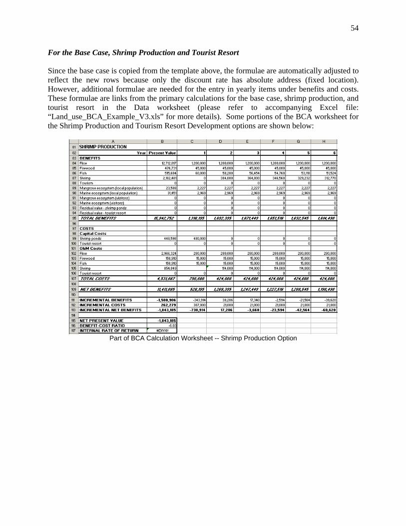
54

For the Base Case, Shrimp Production and Tourist Resort Since the base case is copied from the template above, the formulae are automatically adjusted to reflect the new rows because only the discount rate has absolute address (fixed location). However, additional formulae are needed for the entry in yearly items under benefits and costs. These formulae are links from the primary calculations for the base case, shrimp production, and tourist resort in the Data worksheet (please refer to accompanying Excel file: “Land_use_BCA_Example_V3.xls” for more details). Some portions of the BCA worksheet for the Shrimp Production and Tourism Resort Development options are shown below:

Part of BCA Calculation Worksheet -- Shrimp Production Option

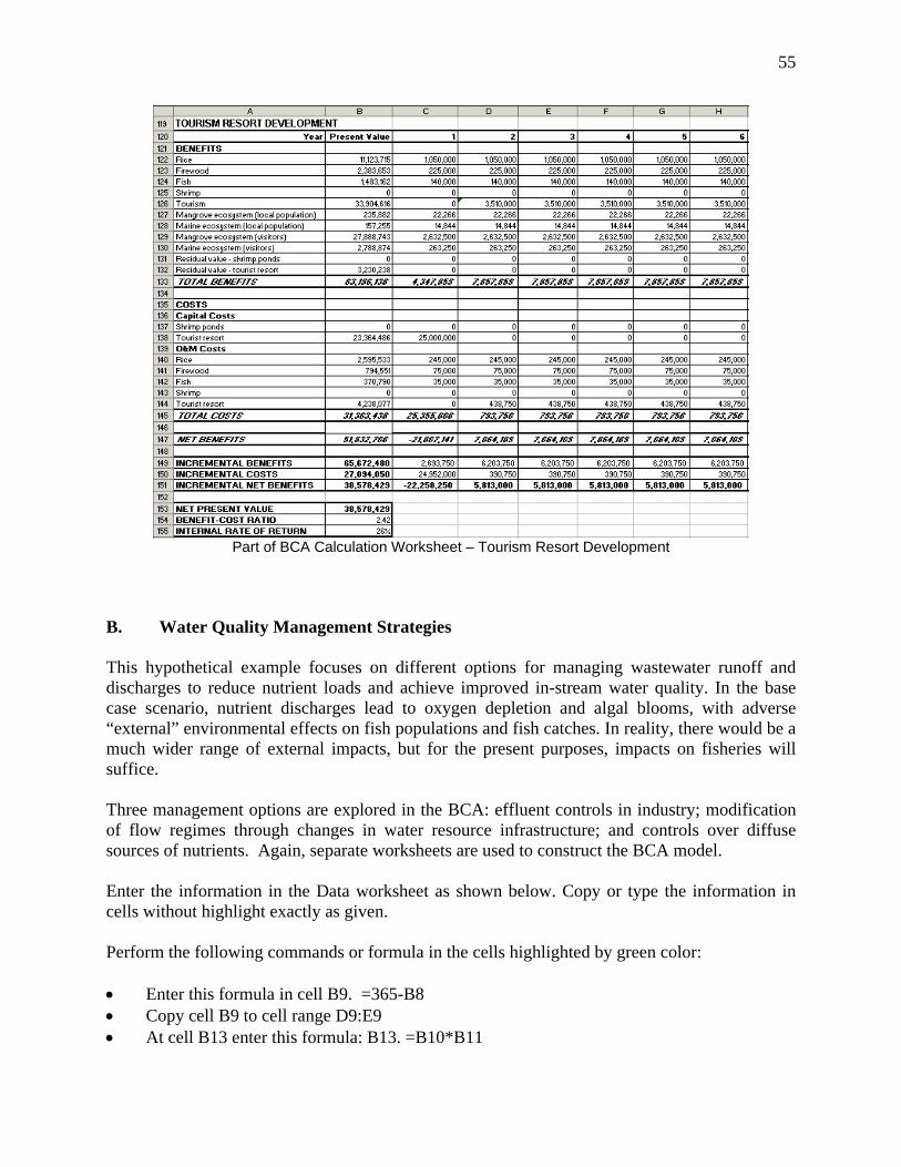
55

Part of BCA Calculation Worksheet – Tourism Resort Development

B. Water Quality Management Strategies This hypothetical example focuses on different options for managing wastewater runoff and discharges to reduce nutrient loads and achieve improved in-stream water quality. In the base case scenario, nutrient discharges lead to oxygen depletion and algal blooms, with adverse “external” environmental effects on fish populations and fish catches. In reality, there would be a much wider range of external impacts, but for the present purposes, impacts on fisheries will suffice. Three management options are explored in the BCA: effluent controls in industry; modification of flow regimes through changes in water resource infrastructure; and controls over diffuse sources of nutrients. Again, separate worksheets are used to construct the BCA model. Enter the information in the Data worksheet as shown below. Copy or type the information in cells without highlight exactly as given. Perform the following commands or formula in the cells highlighted by green color: • Enter this formula in cell B9. =365-B8 • Copy cell B9 to cell range D9:E9 • At cell B13 enter this formula: B13. =B10*B11

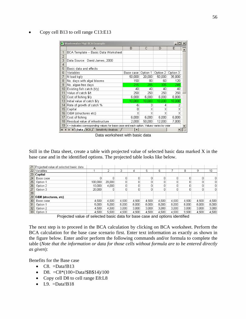
56

• Copy cell B13 to cell range C13:E13

Data worksheet with basic data

Still in the Data sheet, create a table with projected value of selected basic data marked X in the base case and in the identified options. The projected table looks like below.

Projected value of selected basic data for base case and options identified

The next step is to proceed in the BCA calculation by clicking on BCA worksheet. Perform the BCA calculation for the base case scenario first. Enter text information as exactly as shown in the figure below. Enter and/or perform the following commands and/or formula to complete the table (Note that the information or data for those cells without formula are to be entered directly as given): Benefits for the Base case

• C8. =Data!B13 • D8. =C8*(100+Data!$B$14)/100 • Copy cell D8 to cell range E8:L8 • L9. =Data!B18

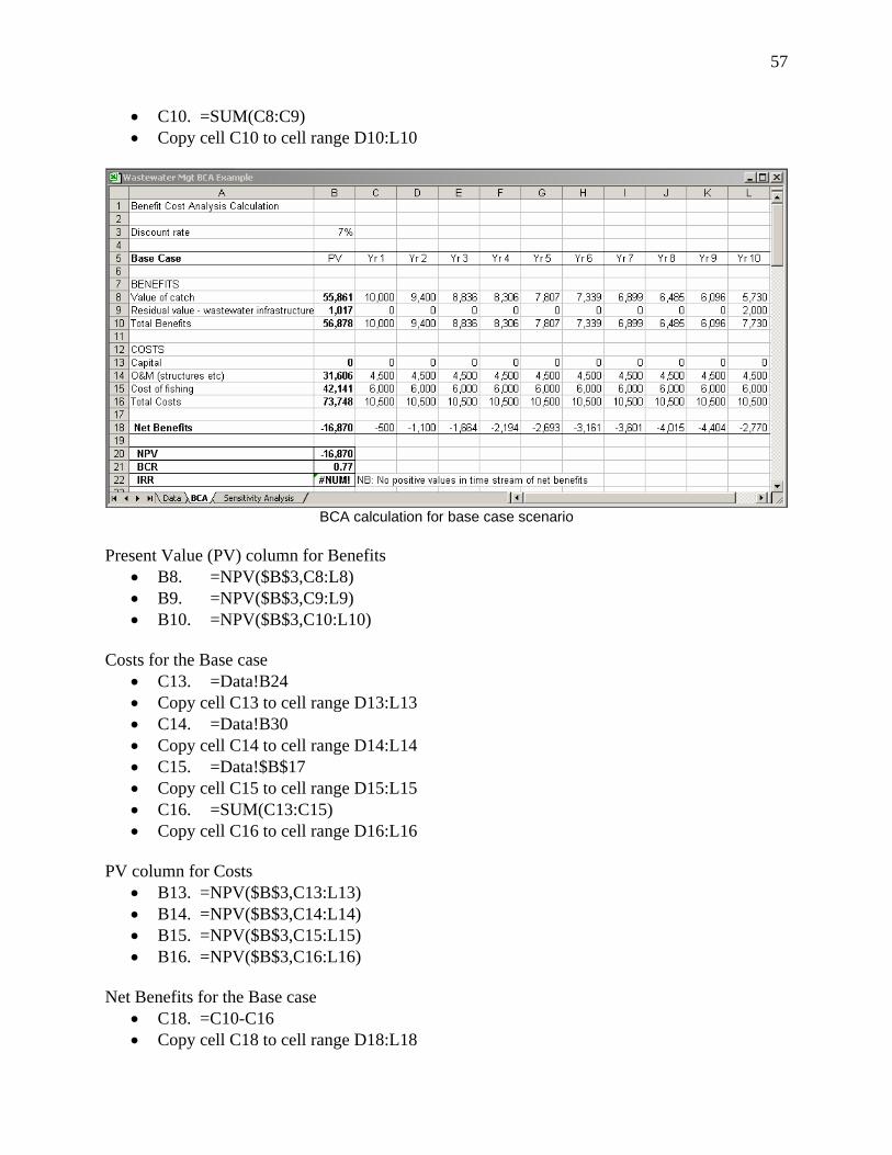
57

• C10. =SUM(C8:C9) • Copy cell C10 to cell range D10:L10

BCA calculation for base case scenario

Present Value (PV) column for Benefits

• B8. =NPV($B$3,C8:L8) • B9. =NPV($B$3,C9:L9) • B10. =NPV($B$3,C10:L10)

Costs for the Base case

• C13. =Data!B24 • Copy cell C13 to cell range D13:L13 • C14. =Data!B30 • Copy cell C14 to cell range D14:L14 • C15. =Data!$B$17 • Copy cell C15 to cell range D15:L15 • C16. =SUM(C13:C15) • Copy cell C16 to cell range D16:L16

PV column for Costs

• B13. =NPV($B$3,C13:L13) • B14. =NPV($B$3,C14:L14) • B15. =NPV($B$3,C15:L15) • B16. =NPV($B$3,C16:L16)

Net Benefits for the Base case

• C18. =C10-C16 • Copy cell C18 to cell range D18:L18

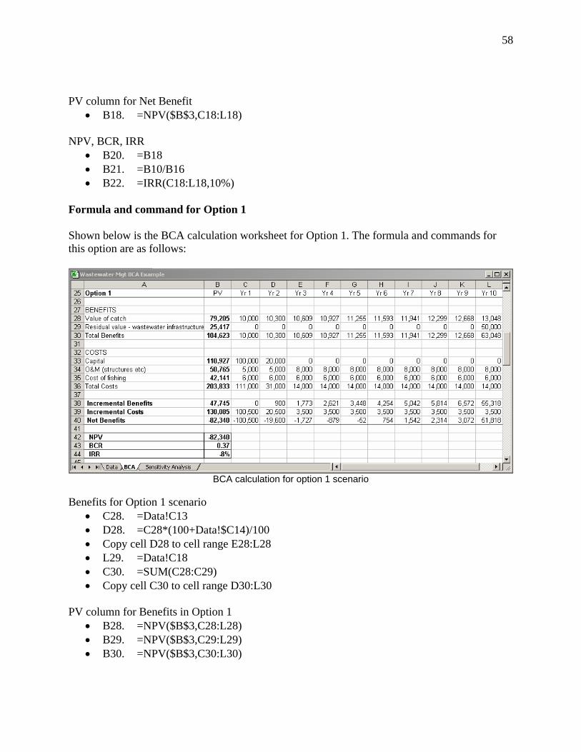
58

PV column for Net Benefit

• B18. =NPV($B$3,C18:L18) NPV, BCR, IRR

• B20. =B18 • B21. =B10/B16 • B22. =IRR(C18:L18,10%)

Formula and command for Option 1 Shown below is the BCA calculation worksheet for Option 1. The formula and commands for this option are as follows:

BCA calculation for option 1 scenario

Benefits for Option 1 scenario

• C28. =Data!C13 • D28. =C28*(100+Data!$C14)/100 • Copy cell D28 to cell range E28:L28 • L29. =Data!C18 • C30. =SUM(C28:C29) • Copy cell C30 to cell range D30:L30

PV column for Benefits in Option 1

• B28. =NPV($B$3,C28:L28) • B29. =NPV($B$3,C29:L29) • B30. =NPV($B$3,C30:L30)

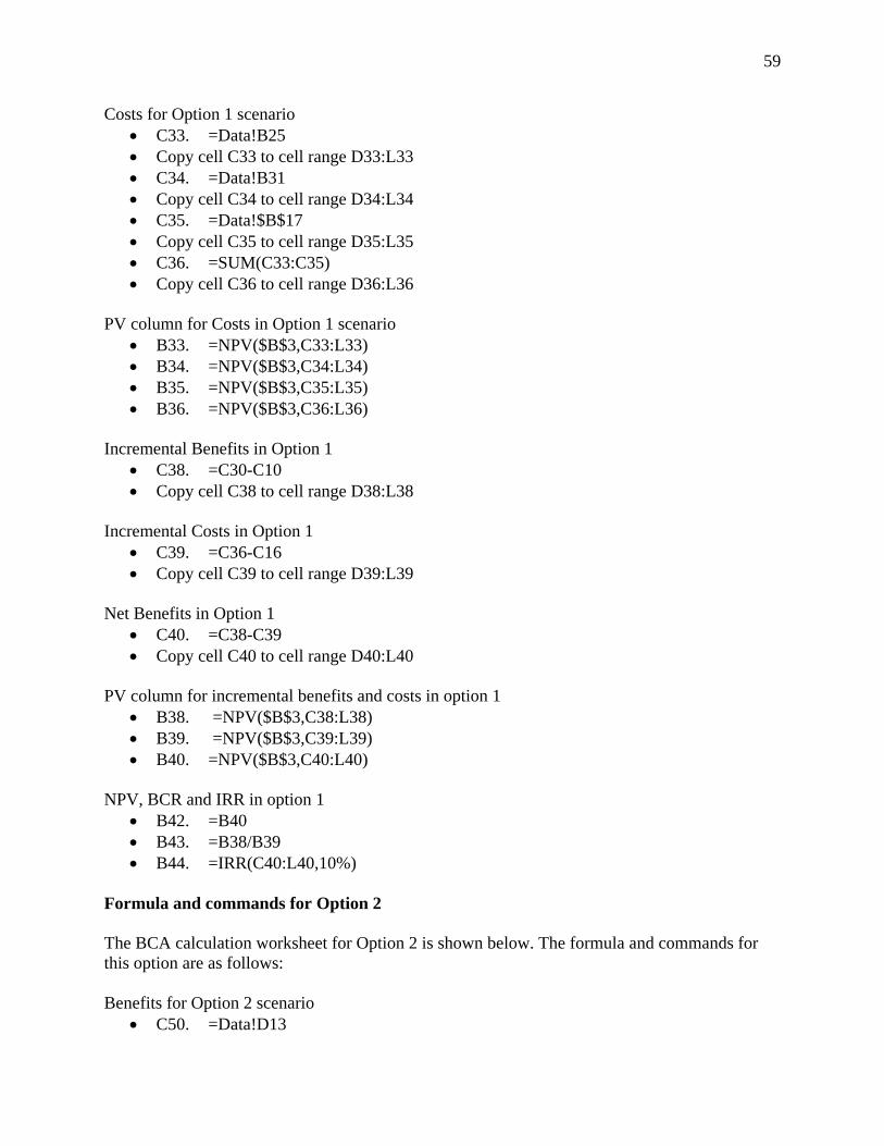
59

Costs for Option 1 scenario • C33. =Data!B25 • Copy cell C33 to cell range D33:L33 • C34. =Data!B31 • Copy cell C34 to cell range D34:L34 • C35. =Data!$B$17 • Copy cell C35 to cell range D35:L35 • C36. =SUM(C33:C35) • Copy cell C36 to cell range D36:L36

PV column for Costs in Option 1 scenario

• B33. =NPV($B$3,C33:L33) • B34. =NPV($B$3,C34:L34) • B35. =NPV($B$3,C35:L35) • B36. =NPV($B$3,C36:L36)

Incremental Benefits in Option 1

• C38. =C30-C10 • Copy cell C38 to cell range D38:L38

Incremental Costs in Option 1

• C39. =C36-C16 • Copy cell C39 to cell range D39:L39

Net Benefits in Option 1

• C40. =C38-C39 • Copy cell C40 to cell range D40:L40

PV column for incremental benefits and costs in option 1

• B38. =NPV($B$3,C38:L38) • B39. =NPV($B$3,C39:L39) • B40. =NPV($B$3,C40:L40)

NPV, BCR and IRR in option 1

• B42. =B40 • B43. =B38/B39 • B44. =IRR(C40:L40,10%)

Formula and commands for Option 2 The BCA calculation worksheet for Option 2 is shown below. The formula and commands for this option are as follows: Benefits for Option 2 scenario

• C50. =Data!D13

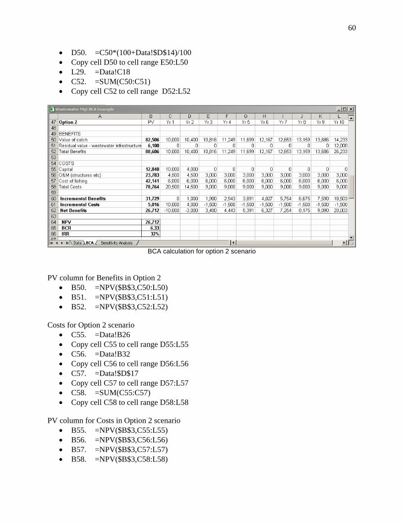
60

• D50. =C50*(100+Data!$D$14)/100 • Copy cell D50 to cell range E50:L50 • L29. =Data!C18 • C52. =SUM(C50:C51) • Copy cell C52 to cell range D52:L52

BCA calculation for option 2 scenario

PV column for Benefits in Option 2

• B50. =NPV($B$3,C50:L50) • B51. =NPV($B$3,C51:L51) • B52. =NPV($B$3,C52:L52)

Costs for Option 2 scenario • C55. =Data!B26 • Copy cell C55 to cell range D55:L55 • C56. =Data!B32 • Copy cell C56 to cell range D56:L56 • C57. =Data!$D$17 • Copy cell C57 to cell range D57:L57 • C58. =SUM(C55:C57) • Copy cell C58 to cell range D58:L58

PV column for Costs in Option 2 scenario

• B55. =NPV($B$3,C55:L55) • B56. =NPV($B$3,C56:L56) • B57. =NPV($B$3,C57:L57) • B58. =NPV($B$3,C58:L58)

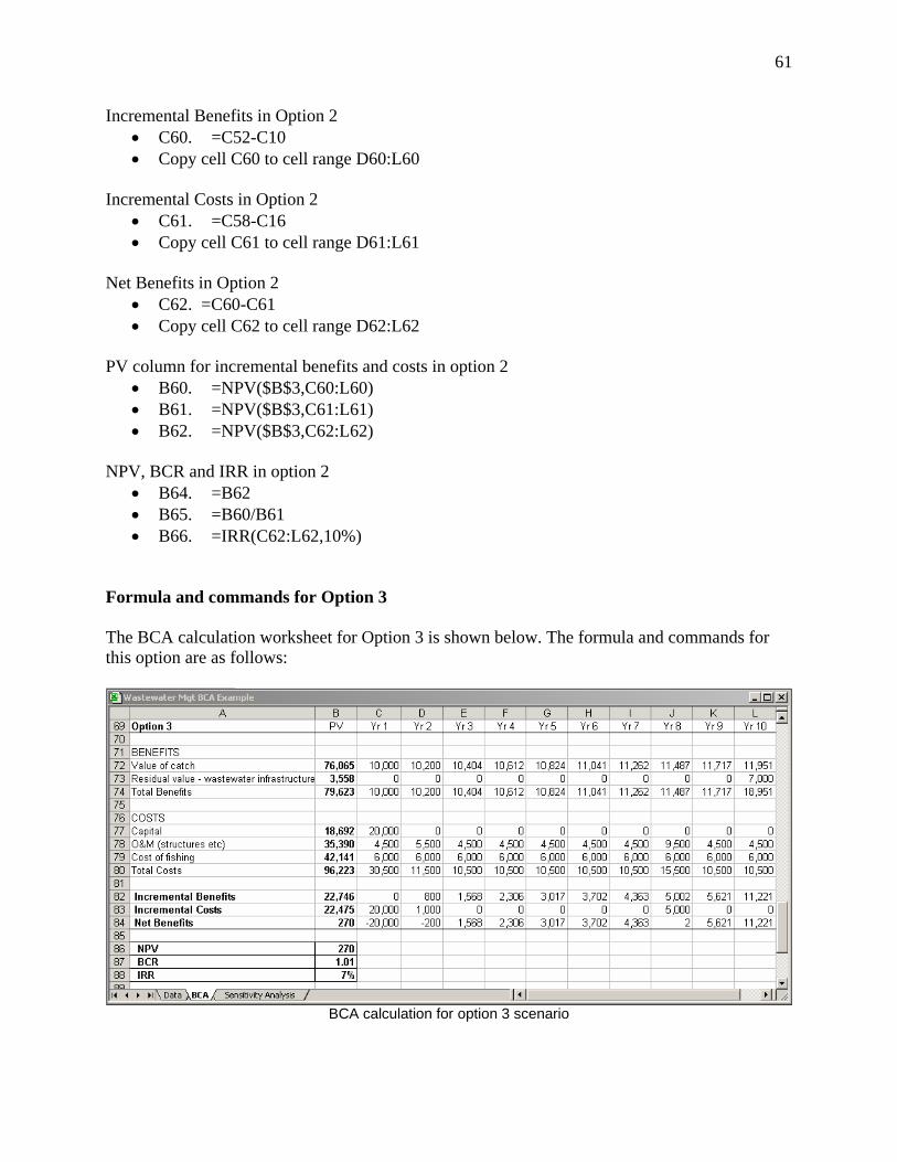
61

Incremental Benefits in Option 2 • C60. =C52-C10 • Copy cell C60 to cell range D60:L60

Incremental Costs in Option 2

• C61. =C58-C16 • Copy cell C61 to cell range D61:L61

Net Benefits in Option 2

• C62. =C60-C61 • Copy cell C62 to cell range D62:L62

PV column for incremental benefits and costs in option 2

• B60. =NPV($B$3,C60:L60) • B61. =NPV($B$3,C61:L61) • B62. =NPV($B$3,C62:L62)

NPV, BCR and IRR in option 2

• B64. =B62 • B65. =B60/B61 • B66. =IRR(C62:L62,10%)

Formula and commands for Option 3 The BCA calculation worksheet for Option 3 is shown below. The formula and commands for this option are as follows:

BCA calculation for option 3 scenario

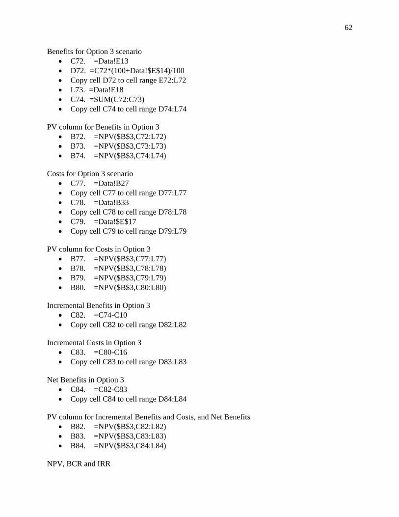
62

Benefits for Option 3 scenario • C72. =Data!E13 • D72. =C72*(100+Data!$E$14)/100 • Copy cell D72 to cell range E72:L72 • L73. =Data!E18 • C74. =SUM(C72:C73) • Copy cell C74 to cell range D74:L74

PV column for Benefits in Option 3

• B72. =NPV($B$3,C72:L72) • B73. =NPV($B$3,C73:L73) • B74. =NPV($B$3,C74:L74)

Costs for Option 3 scenario

• C77. =Data!B27 • Copy cell C77 to cell range D77:L77 • C78. =Data!B33 • Copy cell C78 to cell range D78:L78 • C79. =Data!$E$17 • Copy cell C79 to cell range D79:L79

PV column for Costs in Option 3

• B77. =NPV($B$3,C77:L77) • B78. =NPV($B$3,C78:L78) • B79. =NPV($B$3,C79:L79) • B80. =NPV($B$3,C80:L80)

Incremental Benefits in Option 3

• C82. =C74-C10 • Copy cell C82 to cell range D82:L82

Incremental Costs in Option 3

• C83. =C80-C16 • Copy cell C83 to cell range D83:L83

Net Benefits in Option 3

• C84. =C82-C83 • Copy cell C84 to cell range D84:L84

PV column for Incremental Benefits and Costs, and Net Benefits

• B82. =NPV($B$3,C82:L82) • B83. =NPV($B$3,C83:L83) • B84. =NPV($B$3,C84:L84)

NPV, BCR and IRR

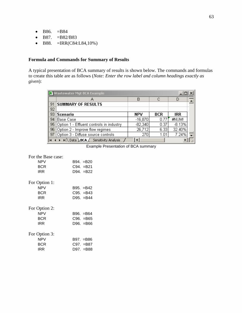
63

• B86. =B84 • B87. =B82/B83 • B88. =IRR(C84:L84,10%)

Formula and Commands for Summary of Results A typical presentation of BCA summary of results is shown below. The commands and formulas to create this table are as follows (Note: Enter the row label and column headings exactly as given):

Example Presentation of BCA summary

For the Base case:

NPV B94. =B20 BCR C94. =B21 IRR D94. =B22

For Option 1:

NPV B95. =B42 BCR C95. =B43 IRR D95. =B44

For Option 2:

NPV B96. =B64 BCR C96. =B65 IRR D96. =B66

For Option 3:

NPV B97. =B86 BCR C97. =B87 IRR D97. =B88

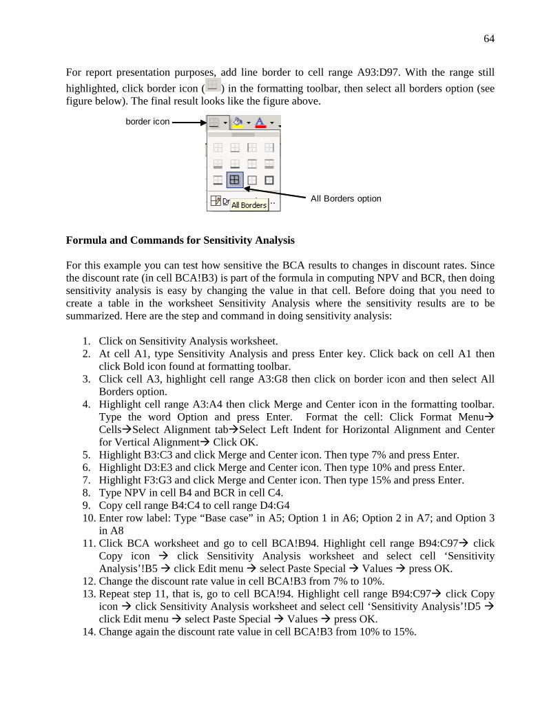
64

For report presentation purposes, add line border to cell range A93:D97. With the range still highlighted, click border icon ( ) in the formatting toolbar, then select all borders option (see figure below). The final result looks like the figure above. Formula and Commands for Sensitivity Analysis For this example you can test how sensitive the BCA results to changes in discount rates. Since the discount rate (in cell BCA!B3) is part of the formula in computing NPV and BCR, then doing sensitivity analysis is easy by changing the value in that cell. Before doing that you need to create a table in the worksheet Sensitivity Analysis where the sensitivity results are to be summarized. Here are the step and command in doing sensitivity analysis:

1. Click on Sensitivity Analysis worksheet. 2. At cell A1, type Sensitivity Analysis and press Enter key. Click back on cell A1 then

click Bold icon found at formatting toolbar. 3. Click cell A3, highlight cell range A3:G8 then click on border icon and then select All

Borders option. 4. Highlight cell range A3:A4 then click Merge and Center icon in the formatting toolbar.

Type the word Option and press Enter. Format the cell: Click Format Menu Cells Select Alignment tab Select Left Indent for Horizontal Alignment and Center for Vertical Alignment Click OK.

5. Highlight B3:C3 and click Merge and Center icon. Then type 7% and press Enter. 6. Highlight D3:E3 and click Merge and Center icon. Then type 10% and press Enter. 7. Highlight F3:G3 and click Merge and Center icon. Then type 15% and press Enter. 8. Type NPV in cell B4 and BCR in cell C4. 9. Copy cell range B4:C4 to cell range D4:G4 10. Enter row label: Type “Base case” in A5; Option 1 in A6; Option 2 in A7; and Option 3

in A8 11. Click BCA worksheet and go to cell BCA!B94. Highlight cell range B94:C97 click

Copy icon click Sensitivity Analysis worksheet and select cell ‘Sensitivity Analysis’!B5 click Edit menu select Paste Special Values press OK.

12. Change the discount rate value in cell BCA!B3 from 7% to 10%. 13. Repeat step 11, that is, go to cell BCA!94. Highlight cell range B94:C97 click Copy

icon click Sensitivity Analysis worksheet and select cell ‘Sensitivity Analysis’!D5 click Edit menu select Paste Special Values press OK.

14. Change again the discount rate value in cell BCA!B3 from 10% to 15%.

border icon

All Borders option

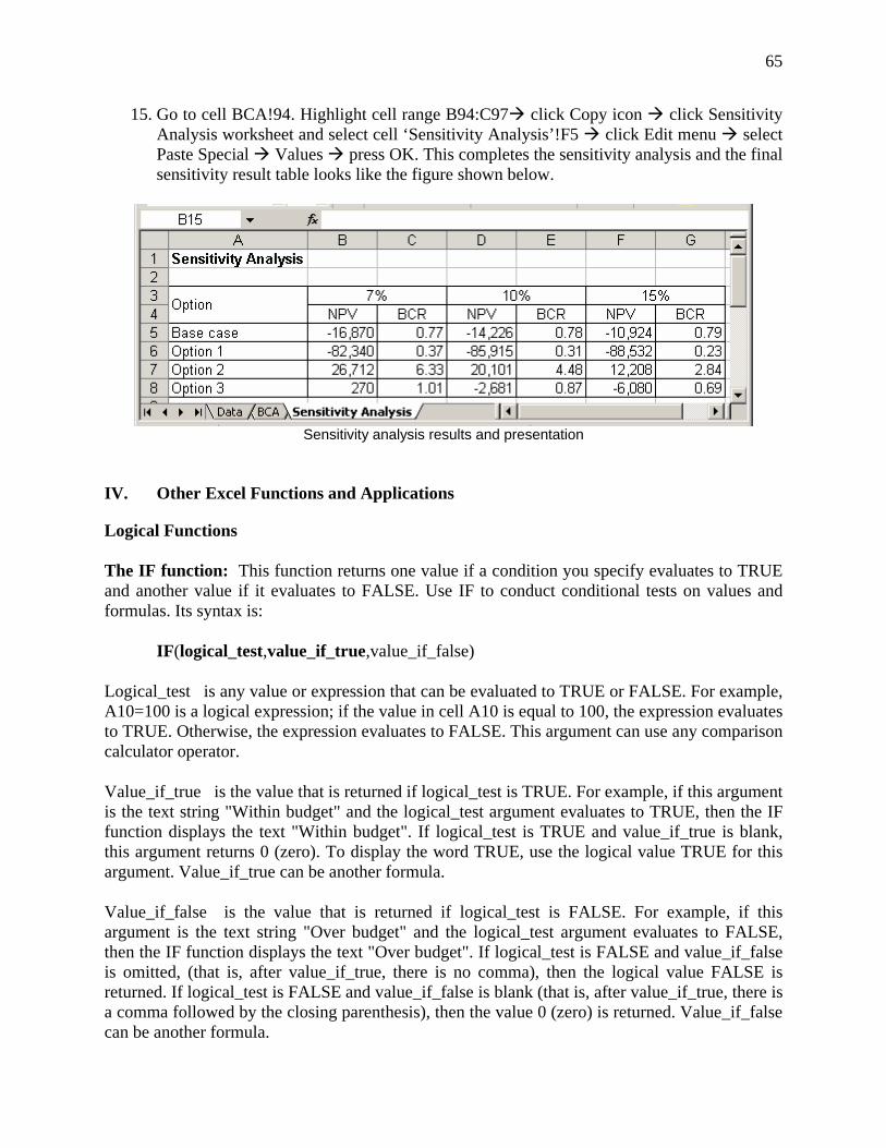
65

15. Go to cell BCA!94. Highlight cell range B94:C97 click Copy icon click Sensitivity Analysis worksheet and select cell ‘Sensitivity Analysis’!F5 click Edit menu select Paste Special Values press OK. This completes the sensitivity analysis and the final sensitivity result table looks like the figure shown below.

Sensitivity analysis results and presentation

IV. Other Excel Functions and Applications

Logical Functions

The IF function: This function returns one value if a condition you specify evaluates to TRUE and another value if it evaluates to FALSE. Use IF to conduct conditional tests on values and formulas. Its syntax is:

IF(logical_test,value_if_true,value_if_false)

Logical_test is any value or expression that can be evaluated to TRUE or FALSE. For example, A10=100 is a logical expression; if the value in cell A10 is equal to 100, the expression evaluates to TRUE. Otherwise, the expression evaluates to FALSE. This argument can use any comparison calculator operator.

Value_if_true is the value that is returned if logical_test is TRUE. For example, if this argument is the text string "Within budget" and the logical_test argument evaluates to TRUE, then the IF function displays the text "Within budget". If logical_test is TRUE and value_if_true is blank, this argument returns 0 (zero). To display the word TRUE, use the logical value TRUE for this argument. Value_if_true can be another formula.

Value_if_false is the value that is returned if logical_test is FALSE. For example, if this argument is the text string "Over budget" and the logical_test argument evaluates to FALSE, then the IF function displays the text "Over budget". If logical_test is FALSE and value_if_false is omitted, (that is, after value_if_true, there is no comma), then the logical value FALSE is returned. If logical_test is FALSE and value_if_false is blank (that is, after value_if_true, there is a comma followed by the closing parenthesis), then the value 0 (zero) is returned. Value_if_false can be another formula.

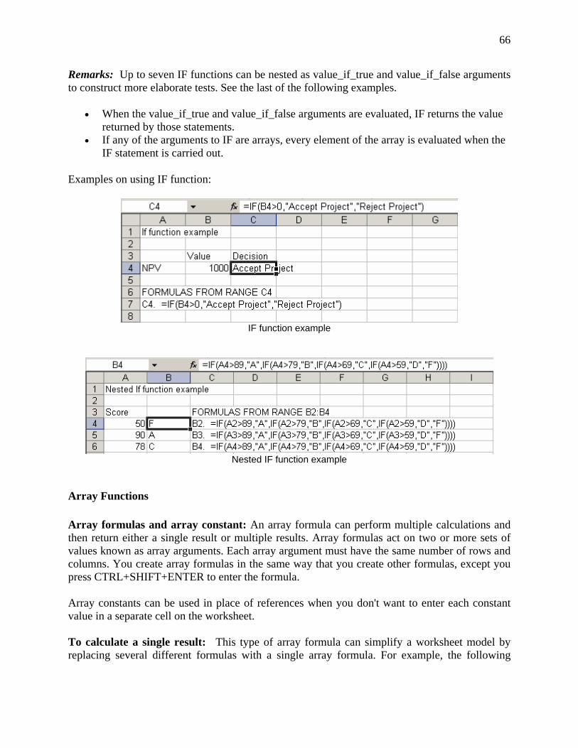
66

Remarks: Up to seven IF functions can be nested as value_if_true and value_if_false arguments to construct more elaborate tests. See the last of the following examples.

• When the value_if_true and value_if_false arguments are evaluated, IF returns the value returned by those statements.

• If any of the arguments to IF are arrays, every element of the array is evaluated when the IF statement is carried out.

Examples on using IF function:

IF function example

Nested IF function example

Array Functions Array formulas and array constant: An array formula can perform multiple calculations and then return either a single result or multiple results. Array formulas act on two or more sets of values known as array arguments. Each array argument must have the same number of rows and columns. You create array formulas in the same way that you create other formulas, except you press CTRL+SHIFT+ENTER to enter the formula. Array constants can be used in place of references when you don't want to enter each constant value in a separate cell on the worksheet. To calculate a single result: This type of array formula can simplify a worksheet model by replacing several different formulas with a single array formula. For example, the following

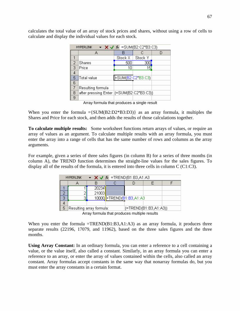
67

calculates the total value of an array of stock prices and shares, without using a row of cells to calculate and display the individual values for each stock.

Array formula that produces a single result

When you enter the formula ={SUM(B2:D2*B3:D3)} as an array formula, it multiples the Shares and Price for each stock, and then adds the results of those calculations together. To calculate multiple results: Some worksheet functions return arrays of values, or require an array of values as an argument. To calculate multiple results with an array formula, you must enter the array into a range of cells that has the same number of rows and columns as the array arguments. For example, given a series of three sales figures (in column B) for a series of three months (in column A), the TREND function determines the straight-line values for the sales figures. To display all of the results of the formula, it is entered into three cells in column C (C1:C3).

Array formula that produces multiple results

When you enter the formula =TREND(B1:B3,A1:A3) as an array formula, it produces three separate results (22196, 17079, and 11962), based on the three sales figures and the three months. Using Array Constant: In an ordinary formula, you can enter a reference to a cell containing a value, or the value itself, also called a constant. Similarly, in an array formula you can enter a reference to an array, or enter the array of values contained within the cells, also called an array constant. Array formulas accept constants in the same way that nonarray formulas do, but you must enter the array constants in a certain format.

68

Array constants can contain numbers, text, logical values such as TRUE or FALSE, or error values such as #N/A. Different types of values can be in the same array constant — for example, {1,3,4;TRUE,FALSE,TRUE}. Numbers in array constants can be in integer, decimal, or scientific format. Text must be enclosed in double quotation marks — for example, "Tuesday". Array constants cannot contain cell references, columns or rows of unequal length, formulas, or the special characters $ (dollar sign), parentheses, or % (percent sign). The format of array constants -- Array constants are enclosed in braces ({ }). Separate values in different columns with commas (,). For example, to represent the values 10, 20, 30, and 40, enter {10,20,30,40}. This array constant is known as a 1-by-4 array and is equivalent to a 1-row-by-4-column reference. Separate values in different rows with semicolons (;). For example, to represent the values 10, 20, 30, and 40 in one row and 50, 60, 70, and 80 in the row immediately below, you would enter a 2-by-4 array constant: {10,20,30,40;50,60,70,80}.

Algebraic Functions – Matrix Operations Elementary concepts of matrix operations are provided here for those users without a background in matrix algebra. Matrix operations are often used to derive information to support a BCA. As well as explaining the basic mathematical properties of matrices, this part of the manual describes matrix functions that are available in Excel and how to apply them. A matrix is defined as a rectangular array of numbers, parameters, or variables (Chiang 1984). The members of the array, referred to as elements of the matrix, are usually enclosed in brackets or sometimes in parentheses or with double vertical lines. The dimension of the matrix is defined by both the number of rows and the number of columns in a matrix. For example, if matrix A below contains m rows and n columns, then it is said to be of dimension m x n (read: “m by n”).

⎥⎥⎥⎥

⎦

⎤

⎢⎢⎢⎢

⎣

⎡

=

mnmm

n

n

aaa

aaaaaa

A

2 1

22221

11211

It is important to remember that the row number always precedes the column number; this is in line with the way the two subscripts in aij are ordered. In the special case where m = n, the matrix is called a square matrix. Some matrices may contain only one column. Such matrices are called column vectors. The dimension of a column vector is n x 1. Similarly, the matrices that contain only one row is called row vectors and the dimension of a row vector is 1 x n.

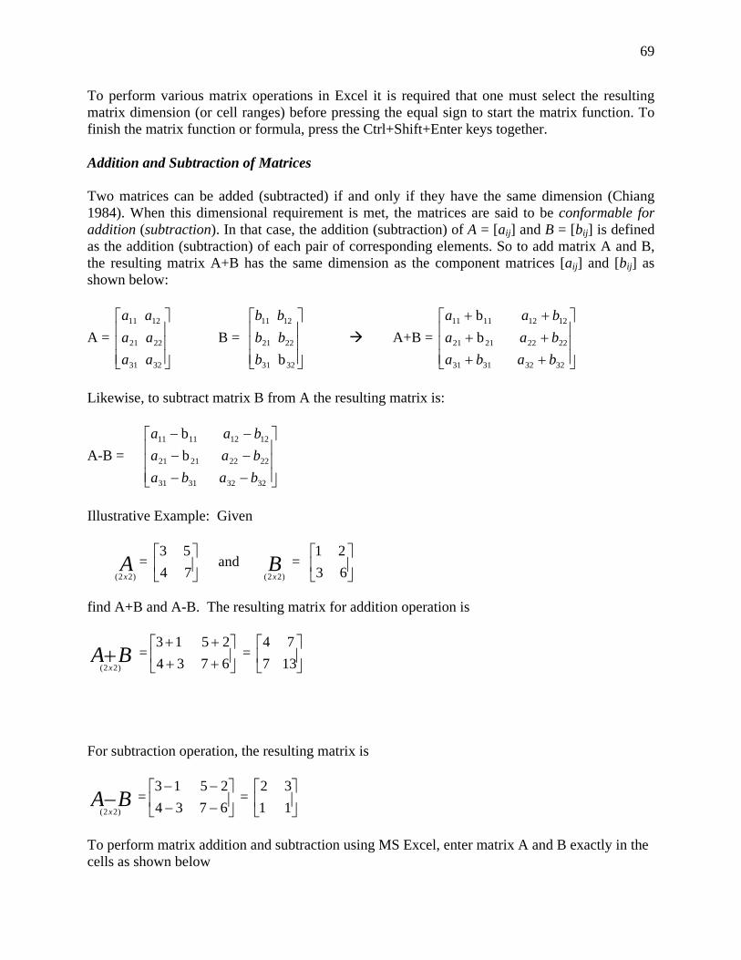
69

To perform various matrix operations in Excel it is required that one must select the resulting matrix dimension (or cell ranges) before pressing the equal sign to start the matrix function. To finish the matrix function or formula, press the Ctrl+Shift+Enter keys together. Addition and Subtraction of Matrices Two matrices can be added (subtracted) if and only if they have the same dimension (Chiang 1984). When this dimensional requirement is met, the matrices are said to be conformable for addition (subtraction). In that case, the addition (subtraction) of A = [aij] and B = [bij] is defined as the addition (subtraction) of each pair of corresponding elements. So to add matrix A and B, the resulting matrix A+B has the same dimension as the component matrices [aij] and [bij] as shown below:

A = ⎥⎥⎥

⎦

⎤

⎢⎢⎢

⎣

⎡

3231

2221

1211

aaaaaa

B = ⎥⎥⎥

⎦

⎤

⎢⎢⎢

⎣

⎡

3231

2221

1211

b

bbbbb

A+B = ⎥⎥⎥

⎦

⎤

⎢⎢⎢

⎣

⎡

++++++

32323131

22222121

12121111

b b

bababaabaa

Likewise, to subtract matrix B from A the resulting matrix is:

A-B = ⎥⎥⎥

⎦

⎤

⎢⎢⎢

⎣

⎡

−−−−−−

32323131

22222121

12121111

b b

bababaabaa

Illustrative Example: Given

Ax )22(

= ⎥⎦

⎤⎢⎣

⎡7 45 3

and Bx )22(

= ⎥⎦

⎤⎢⎣

⎡6 32 1

find A+B and A-B. The resulting matrix for addition operation is

BAx+

)22( = ⎥

⎦

⎤⎢⎣

⎡++++

67 3425 13

= ⎥⎦

⎤⎢⎣

⎡13 77 4

For subtraction operation, the resulting matrix is

BAx−

)22( = ⎥

⎦

⎤⎢⎣

⎡−−−−

67 3425 13

= ⎥⎦

⎤⎢⎣

⎡1 13 2

To perform matrix addition and subtraction using MS Excel, enter matrix A and B exactly in the cells as shown below

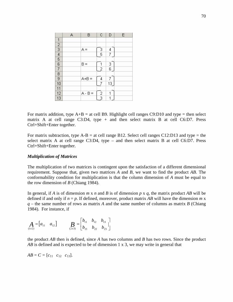
70

For matrix addition, type A+B = at cell B9. Highlight cell ranges C9:D10 and type = then select matrix A at cell range C3:D4, type + and then select matrix B at cell C6:D7. Press Ctrl+Shift+Enter together. For matrix subtraction, type A-B = at cell range B12. Select cell ranges C12:D13 and type = the select matrix A at cell range C3:D4, type – and then select matrix B at cell C6:D7. Press Ctrl+Shift+Enter together. Multiplication of Matrices The multiplication of two matrices is contingent upon the satisfaction of a different dimensional requirement. Suppose that, given two matrices A and B, we want to find the product AB. The conformability condition for multiplication is that the column dimension of A must be equal to the row dimension of B (Chiang 1984). In general, if A is of dimension m x n and B is of dimension p x q, the matrix product AB will be defined if and only if n = p. If defined, moreover, product matrix AB will have the dimension m x q – the same number of rows as matrix A and the same number of columns as matrix B (Chiang 1984). For instance, if

[ ]1211)21(

aaAx

= ⎥⎦

⎤⎢⎣

⎡=

232221

131211

)32( bbbbbb

Bx

the product AB then is defined, since A has two columns and B has two rows. Since the product AB is defined and is expected to be of dimension 1 x 3, we may write in general that AB = C = [c11 c12 c13].

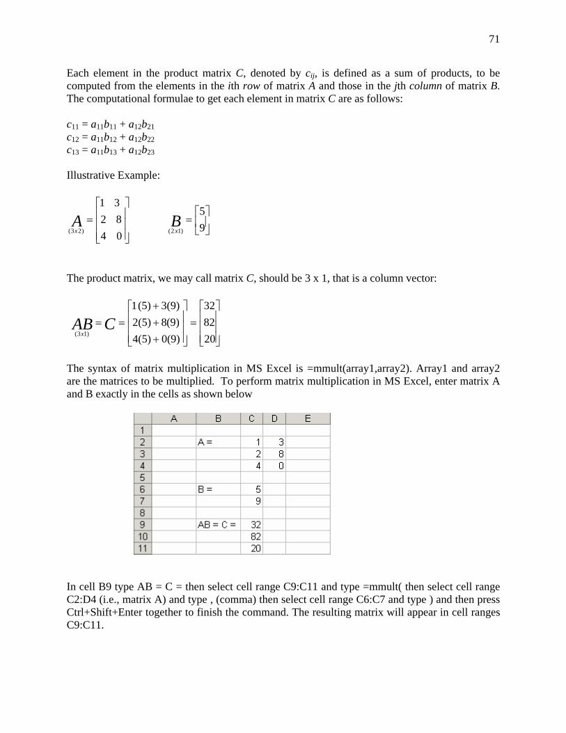
71

Each element in the product matrix C, denoted by cij, is defined as a sum of products, to be computed from the elements in the ith row of matrix A and those in the jth column of matrix B. The computational formulae to get each element in matrix C are as follows: c11 = a11b11 + a12b21 c12 = a11b12 + a12b22 c13 = a11b13 + a12b23 Illustrative Example:

⎥⎥⎥

⎦

⎤

⎢⎢⎢

⎣

⎡=

0 48 23 1

)23(Ax

⎥⎦

⎤⎢⎣

⎡=

95

)12(B

x

The product matrix, we may call matrix C, should be 3 x 1, that is a column vector:

⎥⎥⎥

⎦

⎤

⎢⎢⎢

⎣

⎡=

⎥⎥⎥

⎦

⎤

⎢⎢⎢

⎣

⎡

+++

==208232

)9(04(5))9(82(5)

3(9) (5) 1

)13(CAB

x

The syntax of matrix multiplication in MS Excel is =mmult(array1,array2). Array1 and array2 are the matrices to be multiplied. To perform matrix multiplication in MS Excel, enter matrix A and B exactly in the cells as shown below

In cell B9 type AB = C = then select cell range C9:C11 and type =mmult( then select cell range C2:D4 (i.e., matrix A) and type , (comma) then select cell range C6:C7 and type ) and then press Ctrl+Shift+Enter together to finish the command. The resulting matrix will appear in cell ranges C9:C11.

72

Determinant of a Matrix

Determinants play an important role in finding the inverse of a matrix and also in solving systems of linear equations. In the following we assume we have a square matrix (m=n). The determinant of a matrix A will be denoted by det(A) or |A|. Firstly the determinant of a 2x2 and 3x3 matrix will be introduced then the n x n case will be shown.

Determinant of a 2x2 matrix Assuming A is an arbitrary 2x2 matrix A, where the elements are given by:

The determinant of this matrix is as follows:

Determinant of a 3x3 matrix The determinant of a 3x3 matrix is a little more tricky and is found as follows ( for this case assume A is an arbitrary 3x3 matrix A, where the elements are given below)

The determinant of this matrix is as follows:

Determinant of a nxn matrix For the general case, where A is an n x n matrix the determinant is given by:

Where the coefficients are given by the relation

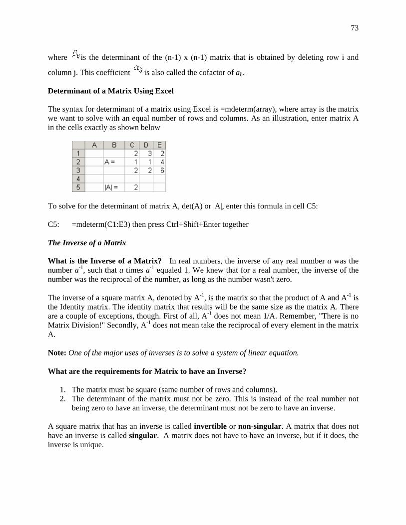
73

where is the determinant of the (n-1) x (n-1) matrix that is obtained by deleting row i and

column j. This coefficient is also called the cofactor of aij. Determinant of a Matrix Using Excel The syntax for determinant of a matrix using Excel is =mdeterm(array), where array is the matrix we want to solve with an equal number of rows and columns. As an illustration, enter matrix A in the cells exactly as shown below

To solve for the determinant of matrix A, det(A) or |A|, enter this formula in cell C5: C5: =mdeterm(C1:E3) then press Ctrl+Shift+Enter together The Inverse of a Matrix What is the Inverse of a Matrix? In real numbers, the inverse of any real number a was the number a-1, such that a times a-1 equaled 1. We knew that for a real number, the inverse of the number was the reciprocal of the number, as long as the number wasn't zero.

The inverse of a square matrix A, denoted by A-1, is the matrix so that the product of A and A-1 is the Identity matrix. The identity matrix that results will be the same size as the matrix A. There are a couple of exceptions, though. First of all, A-1 does not mean 1/A. Remember, "There is no Matrix Division!" Secondly, A-1 does not mean take the reciprocal of every element in the matrix A.

Note: One of the major uses of inverses is to solve a system of linear equation.

What are the requirements for Matrix to have an Inverse?

1. The matrix must be square (same number of rows and columns). 2. The determinant of the matrix must not be zero. This is instead of the real number not

being zero to have an inverse, the determinant must not be zero to have an inverse.

A square matrix that has an inverse is called invertible or non-singular. A matrix that does not have an inverse is called singular. A matrix does not have to have an inverse, but if it does, the inverse is unique.

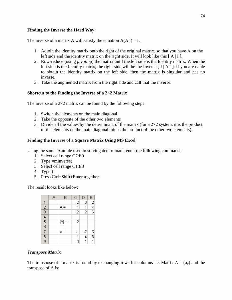
74

Finding the Inverse the Hard Way

The inverse of a matrix A will satisfy the equation A(A-1) = I.

1. Adjoin the identity matrix onto the right of the original matrix, so that you have A on the left side and the identity matrix on the right side. It will look like this [ A | I ].

2. Row-reduce (using pivoting) the matrix until the left side is the Identity matrix. When the left side is the Identity matrix, the right side will be the Inverse [ I | A-1 ]. If you are nable to obtain the identity matrix on the left side, then the matrix is singular and has no inverse.

3. Take the augmented matrix from the right side and call that the inverse.

Shortcut to the Finding the Inverse of a 2×2 Matrix

The inverse of a 2×2 matrix can be found by the following steps

1. Switch the elements on the main diagonal 2. Take the opposite of the other two elements 3. Divide all the values by the determinant of the matrix (for a 2×2 system, it is the product

of the elements on the main diagonal minus the product of the other two elements).

Finding the Inverse of a Square Matrix Using MS Excel Using the same example used in solving determinant, enter the following commands:

1. Select cell range C7:E9 2. Type =minverse( 3. Select cell range C1:E3 4. Type ) 5. Press Ctrl+Shift+Enter together

The result looks like below:

Transpose Matrix

The transpose of a matrix is found by exchanging rows for columns i.e. Matrix A = (aij) and the transpose of A is:

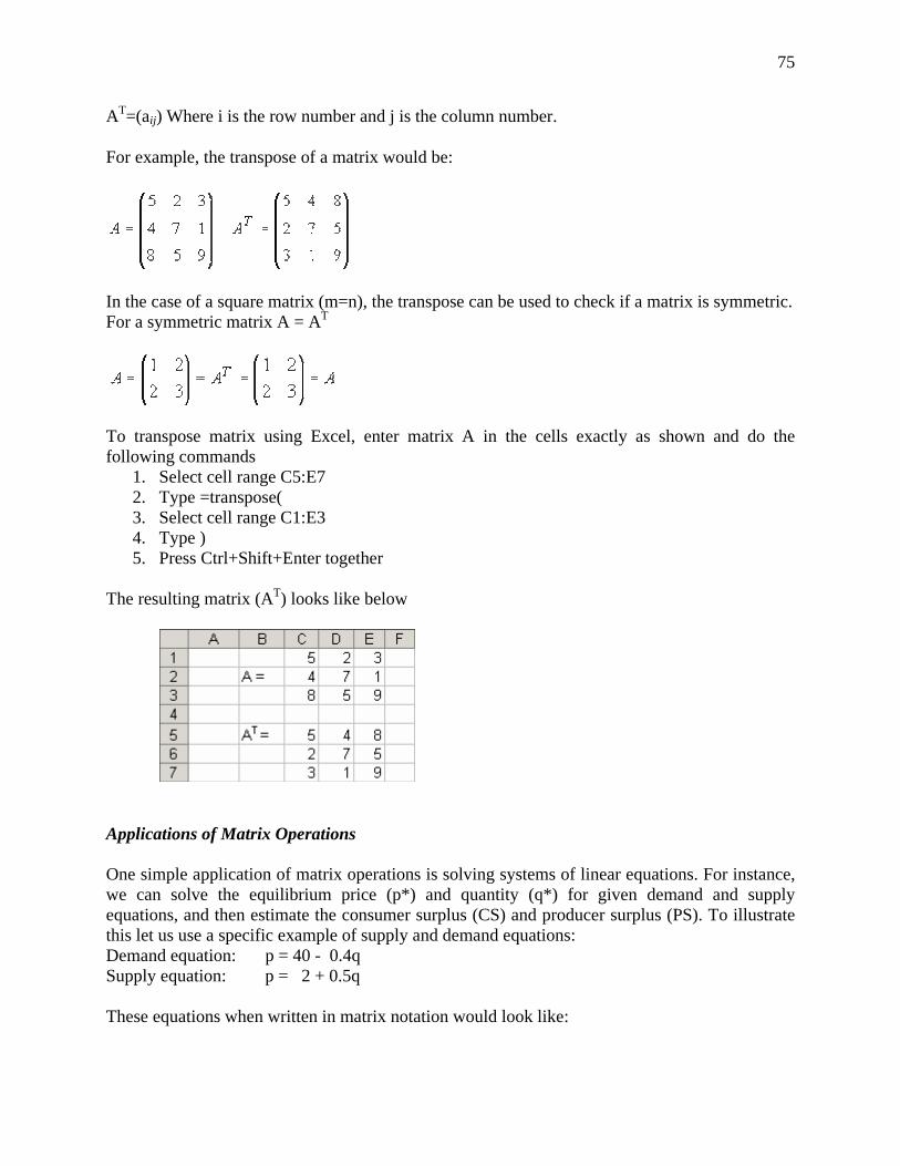
75

AT=(aij) Where i is the row number and j is the column number.

For example, the transpose of a matrix would be:

In the case of a square matrix (m=n), the transpose can be used to check if a matrix is symmetric. For a symmetric matrix A = AT

To transpose matrix using Excel, enter matrix A in the cells exactly as shown and do the following commands

1. Select cell range C5:E7 2. Type =transpose( 3. Select cell range C1:E3 4. Type ) 5. Press Ctrl+Shift+Enter together

The resulting matrix (AT) looks like below

Applications of Matrix Operations One simple application of matrix operations is solving systems of linear equations. For instance, we can solve the equilibrium price (p*) and quantity (q*) for given demand and supply equations, and then estimate the consumer surplus (CS) and producer surplus (PS). To illustrate this let us use a specific example of supply and demand equations: Demand equation: p = 40 - 0.4q Supply equation: p = 2 + 0.5q These equations when written in matrix notation would look like:

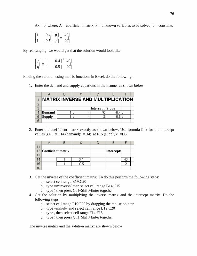
76

Ax = b, where: A = coefficient matrix, x = unknown variables to be solved, b = constants

⎥⎦

⎤⎢⎣

⎡=⎥

⎦

⎤⎢⎣

⎡⎥⎦

⎤⎢⎣

⎡2040

0.5- 10.4 1

qp

By rearranging, we would get that the solution would look like

⎥⎦

⎤⎢⎣

⎡⎥⎦

⎤⎢⎣

⎡=⎥

⎦

⎤⎢⎣

⎡2040

0.5- 10.4 1

-1

qp

Finding the solution using matrix functions in Excel, do the following:

1. Enter the demand and supply equations in the manner as shown below

2. Enter the coefficient matrix exactly as shown below. Use formula link for the intercept values (i.e., at F14 (demand): =D4; at F15 (supply): =D5

3. Get the inverse of the coefficient matrix. To do this perform the following steps: a. select cell range B19:C20 b. type =minverse( then select cell range B14:C15 c. type ) then press Ctrl+Shift+Enter together

4. Get the solution by multiplying the inverse matrix and the intercept matrix. Do the following steps:

a. select cell range F19:F20 by dragging the mouse pointer b. type =mmult( and select cell range B19:C20 c. type , then select cell range F14:F15 d. type ) then press Ctrl+Shift+Enter together

The inverse matrix and the solution matrix are shown below

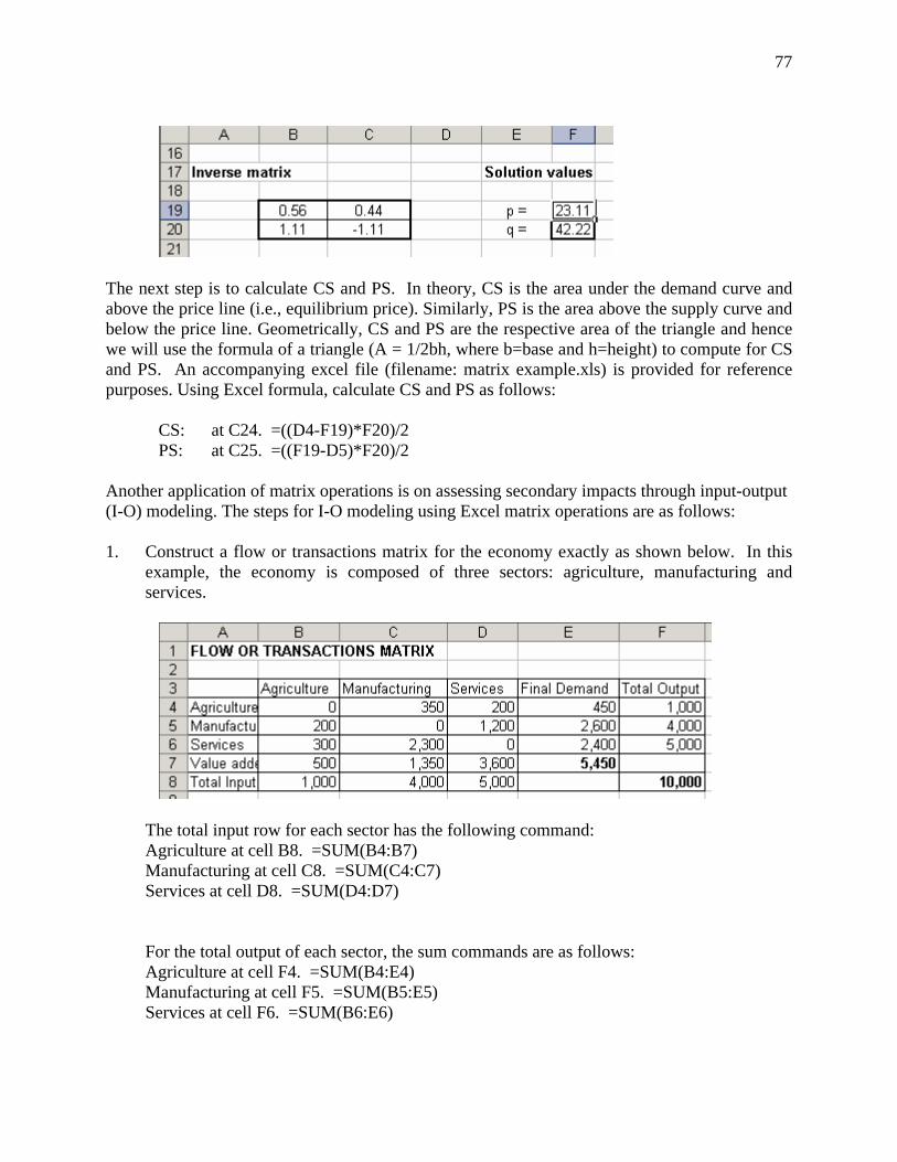
77

The next step is to calculate CS and PS. In theory, CS is the area under the demand curve and above the price line (i.e., equilibrium price). Similarly, PS is the area above the supply curve and below the price line. Geometrically, CS and PS are the respective area of the triangle and hence we will use the formula of a triangle (A = 1/2bh, where b=base and h=height) to compute for CS and PS. An accompanying excel file (filename: matrix example.xls) is provided for reference purposes. Using Excel formula, calculate CS and PS as follows: CS: at C24. =((D4-F19)*F20)/2

PS: at C25. =((F19-D5)*F20)/2 Another application of matrix operations is on assessing secondary impacts through input-output (I-O) modeling. The steps for I-O modeling using Excel matrix operations are as follows: 1. Construct a flow or transactions matrix for the economy exactly as shown below. In this

example, the economy is composed of three sectors: agriculture, manufacturing and services.

The total input row for each sector has the following command: Agriculture at cell B8. =SUM(B4:B7) Manufacturing at cell C8. =SUM(C4:C7) Services at cell D8. =SUM(D4:D7)

For the total output of each sector, the sum commands are as follows: Agriculture at cell F4. =SUM(B4:E4) Manufacturing at cell F5. =SUM(B5:E5) Services at cell F6. =SUM(B6:E6)

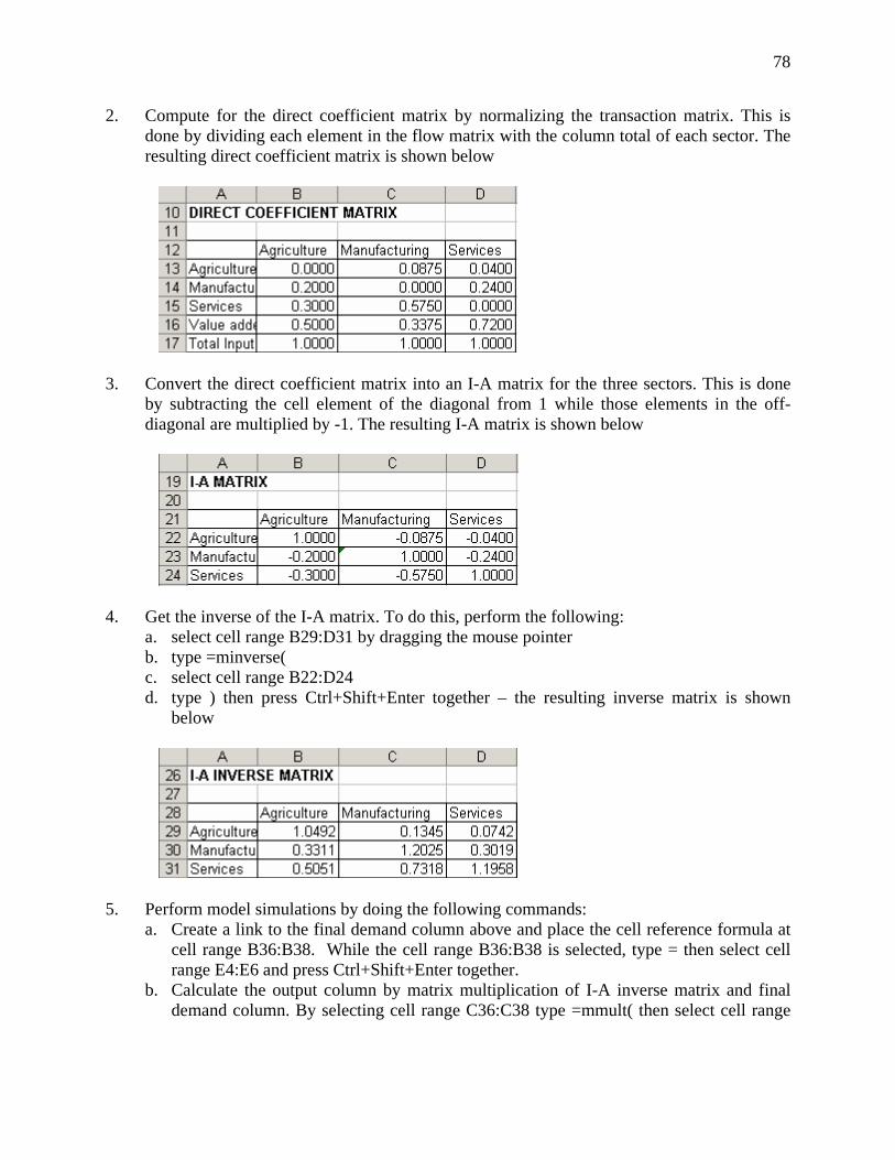
78

2. Compute for the direct coefficient matrix by normalizing the transaction matrix. This is done by dividing each element in the flow matrix with the column total of each sector. The resulting direct coefficient matrix is shown below

3. Convert the direct coefficient matrix into an I-A matrix for the three sectors. This is done

by subtracting the cell element of the diagonal from 1 while those elements in the off-diagonal are multiplied by -1. The resulting I-A matrix is shown below

4. Get the inverse of the I-A matrix. To do this, perform the following:

a. select cell range B29:D31 by dragging the mouse pointer b. type =minverse( c. select cell range B22:D24 d. type ) then press Ctrl+Shift+Enter together – the resulting inverse matrix is shown

below

5. Perform model simulations by doing the following commands:

a. Create a link to the final demand column above and place the cell reference formula at cell range B36:B38. While the cell range B36:B38 is selected, type = then select cell range E4:E6 and press Ctrl+Shift+Enter together.

b. Calculate the output column by matrix multiplication of I-A inverse matrix and final demand column. By selecting cell range C36:C38 type =mmult( then select cell range

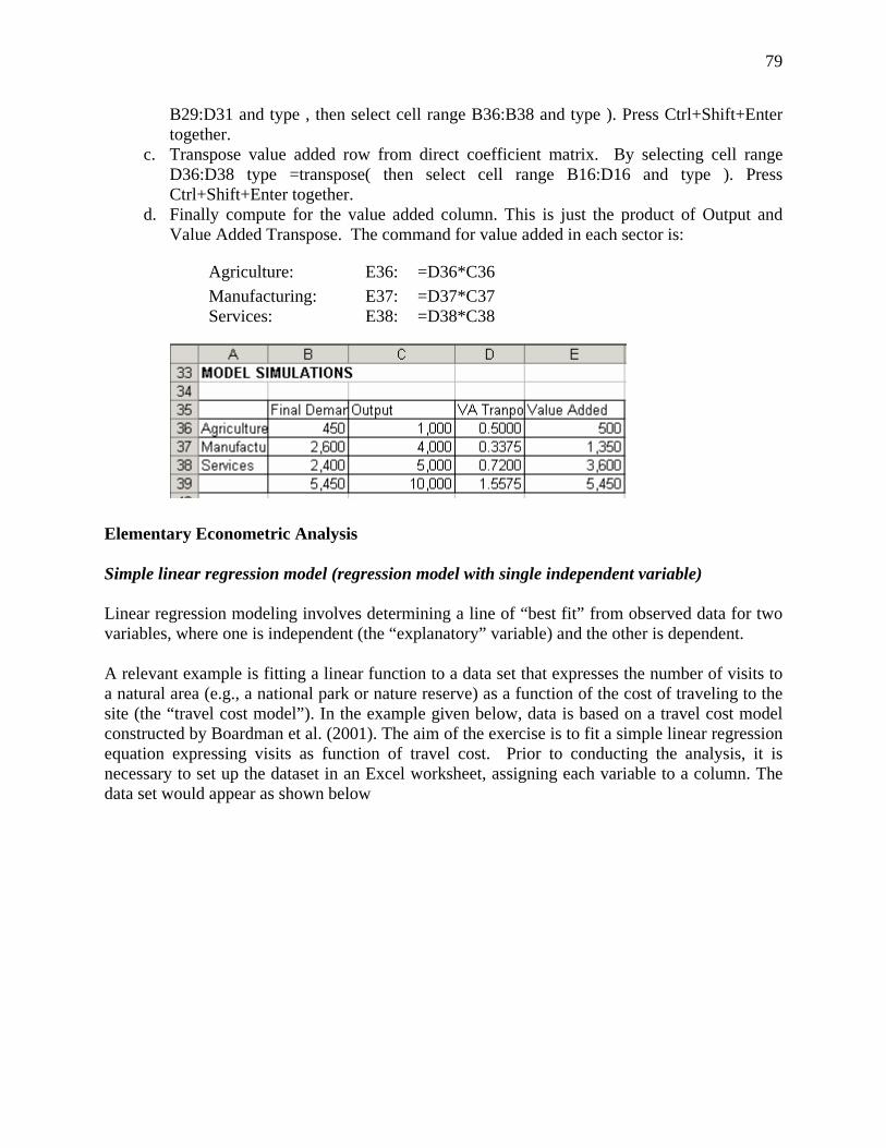
79

B29:D31 and type , then select cell range B36:B38 and type ). Press Ctrl+Shift+Enter together.

c. Transpose value added row from direct coefficient matrix. By selecting cell range D36:D38 type =transpose( then select cell range B16:D16 and type ). Press Ctrl+Shift+Enter together.

d. Finally compute for the value added column. This is just the product of Output and Value Added Transpose. The command for value added in each sector is:

Agriculture: E36: =D36*C36 Manufacturing: E37: =D37*C37 Services: E38: =D38*C38

Elementary Econometric Analysis Simple linear regression model (regression model with single independent variable) Linear regression modeling involves determining a line of “best fit” from observed data for two variables, where one is independent (the “explanatory” variable) and the other is dependent. A relevant example is fitting a linear function to a data set that expresses the number of visits to a natural area (e.g., a national park or nature reserve) as a function of the cost of traveling to the site (the “travel cost model”). In the example given below, data is based on a travel cost model constructed by Boardman et al. (2001). The aim of the exercise is to fit a simple linear regression equation expressing visits as function of travel cost. Prior to conducting the analysis, it is necessary to set up the dataset in an Excel worksheet, assigning each variable to a column. The data set would appear as shown below

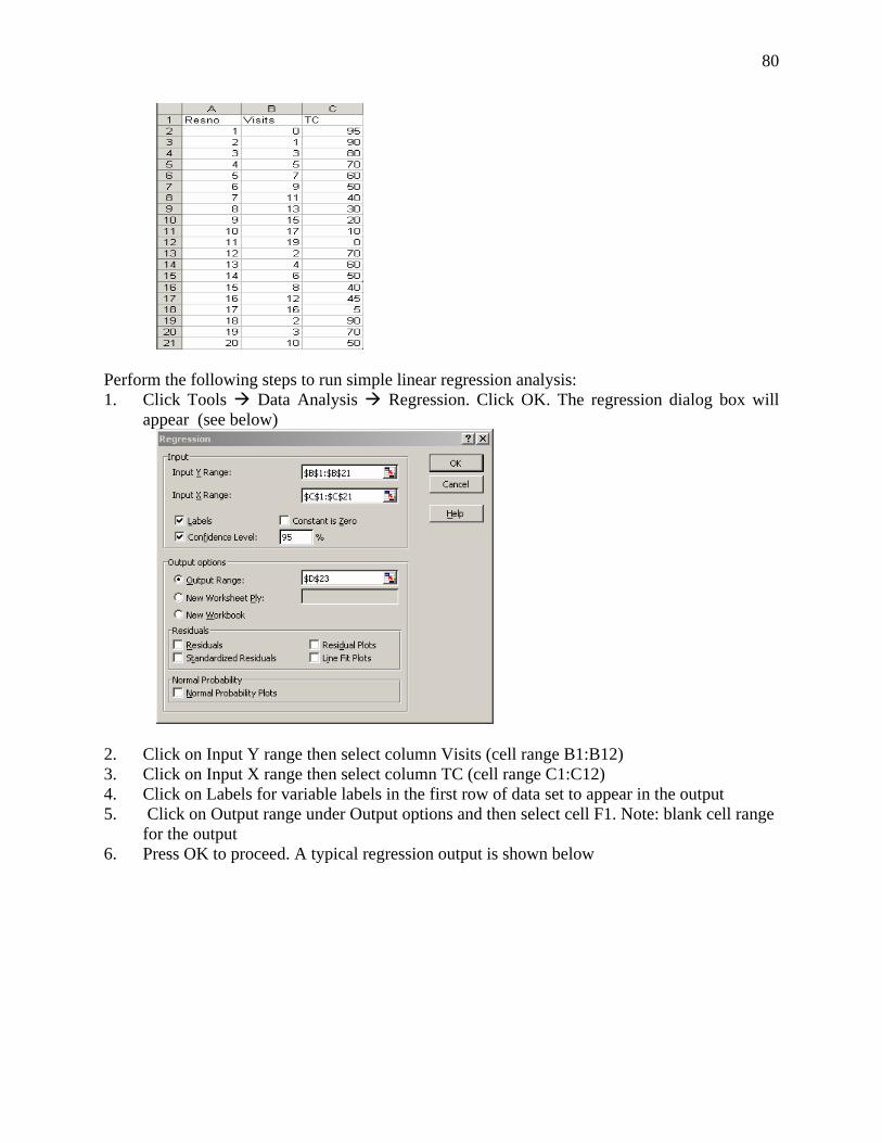
80

Perform the following steps to run simple linear regression analysis: 1. Click Tools Data Analysis Regression. Click OK. The regression dialog box will

appear (see below)

2. Click on Input Y range then select column Visits (cell range B1:B12) 3. Click on Input X range then select column TC (cell range C1:C12) 4. Click on Labels for variable labels in the first row of data set to appear in the output 5. Click on Output range under Output options and then select cell F1. Note: blank cell range

for the output 6. Press OK to proceed. A typical regression output is shown below

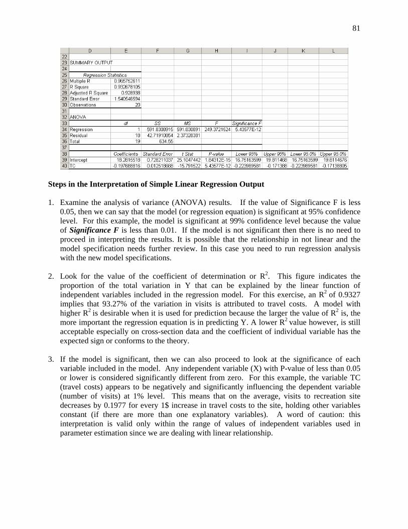
81

Steps in the Interpretation of Simple Linear Regression Output 1. Examine the analysis of variance (ANOVA) results. If the value of Significance F is less

0.05, then we can say that the model (or regression equation) is significant at 95% confidence level. For this example, the model is significant at 99% confidence level because the value of Significance F is less than 0.01. If the model is not significant then there is no need to proceed in interpreting the results. It is possible that the relationship in not linear and the model specification needs further review. In this case you need to run regression analysis with the new model specifications.

2. Look for the value of the coefficient of determination or R2. This figure indicates the

proportion of the total variation in Y that can be explained by the linear function of independent variables included in the regression model. For this exercise, an R2 of 0.9327 implies that 93.27% of the variation in visits is attributed to travel costs. A model with higher R2 is desirable when it is used for prediction because the larger the value of R2 is, the more important the regression equation is in predicting Y. A lower R2 value however, is still acceptable especially on cross-section data and the coefficient of individual variable has the expected sign or conforms to the theory.

3. If the model is significant, then we can also proceed to look at the significance of each

variable included in the model. Any independent variable (X) with P-value of less than 0.05 or lower is considered significantly different from zero. For this example, the variable TC (travel costs) appears to be negatively and significantly influencing the dependent variable (number of visits) at 1% level. This means that on the average, visits to recreation site decreases by 0.1977 for every 1$ increase in travel costs to the site, holding other variables constant (if there are more than one explanatory variables). A word of caution: this interpretation is valid only within the range of values of independent variables used in parameter estimation since we are dealing with linear relationship.

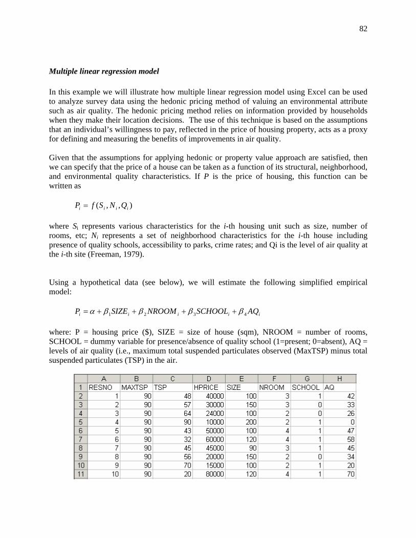
82

Multiple linear regression model In this example we will illustrate how multiple linear regression model using Excel can be used to analyze survey data using the hedonic pricing method of valuing an environmental attribute such as air quality. The hedonic pricing method relies on information provided by households when they make their location decisions. The use of this technique is based on the assumptions that an individual’s willingness to pay, reflected in the price of housing property, acts as a proxy for defining and measuring the benefits of improvements in air quality. Given that the assumptions for applying hedonic or property value approach are satisfied, then we can specify that the price of a house can be taken as a function of its structural, neighborhood, and environmental quality characteristics. If P is the price of housing, this function can be written as

),,( iiii QNSfP =

where Si represents various characteristics for the i-th housing unit such as size, number of rooms, etc; Ni represents a set of neighborhood characteristics for the i-th house including presence of quality schools, accessibility to parks, crime rates; and Qi is the level of air quality at the i-th site (Freeman, 1979). Using a hypothetical data (see below), we will estimate the following simplified empirical model:

iiiii AQSCHOOLNROOMSIZEP 4321 ββββα ++++= where: P = housing price ($), SIZE = size of house (sqm), NROOM = number of rooms, SCHOOL = dummy variable for presence/absence of quality school (1=present; 0=absent), AQ = levels of air quality (i.e., maximum total suspended particulates observed (MaxTSP) minus total suspended particulates (TSP) in the air.

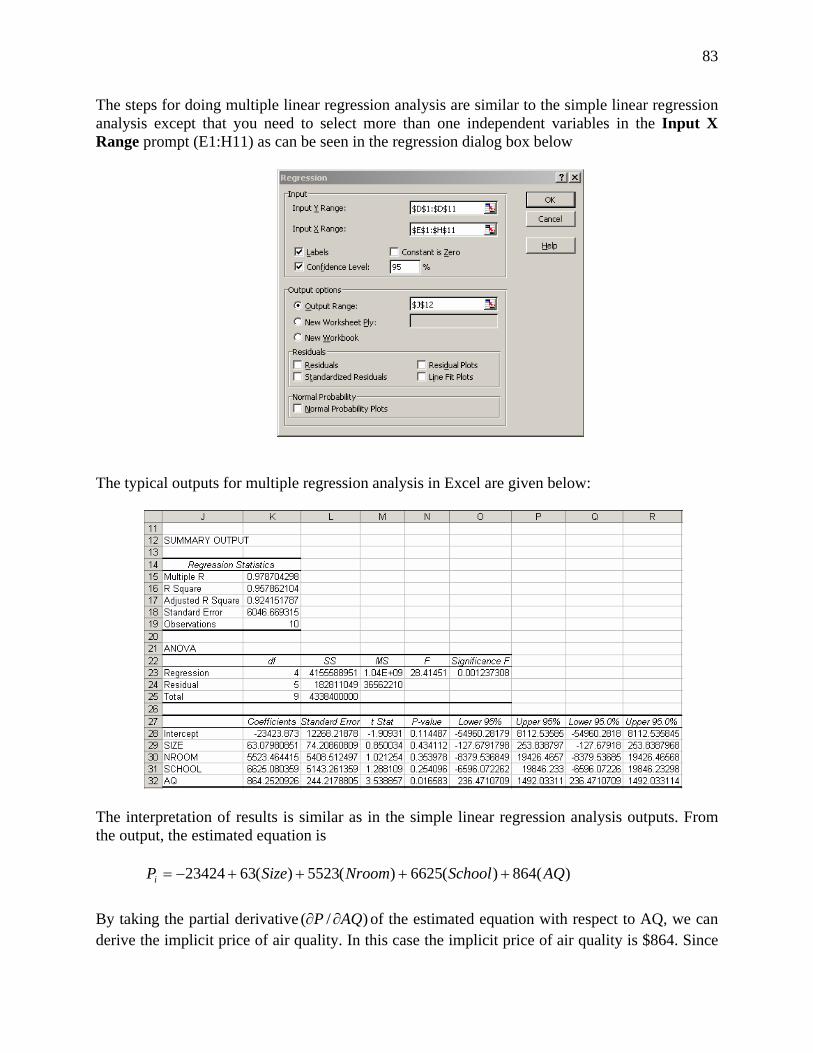
83

The steps for doing multiple linear regression analysis are similar to the simple linear regression analysis except that you need to select more than one independent variables in the Input X Range prompt (E1:H11) as can be seen in the regression dialog box below

The typical outputs for multiple regression analysis in Excel are given below:

The interpretation of results is similar as in the simple linear regression analysis outputs. From the output, the estimated equation is

)(864)(6625)(5523)(6323424 AQSchoolNroomSizePi ++++−=

By taking the partial derivative )/( AQP ∂∂ of the estimated equation with respect to AQ, we can derive the implicit price of air quality. In this case the implicit price of air quality is $864. Since

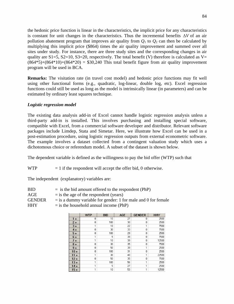
84

the hedonic price function is linear in the characteristics, the implicit price for any characteristics is constant for unit changes in the characteristics. Thus the incremental benefits V∆ of an air pollution abatement program that improves air quality from Q1 to Q2 can then be calculated by multiplying this implicit price ($864) times the air quality improvement and summed over all sites under study. For instance, there are three study sites and the corresponding changes in air quality are S1=5, S2=10, S3=20, respectively. The total benefit (V) therefore is calculated as V= (864*5)+(864*10)+(864*20) = $30,240 This total benefit figure from air quality improvement program will be used in BCA. Remarks: The visitation rate (in travel cost model) and hedonic price functions may fit well using other functional forms (e.g., quadratic, log-linear, double log, etc). Excel regression functions could still be used as long as the model is intrinsically linear (in parameters) and can be estimated by ordinary least squares technique. Logistic regression model The existing data analysis add-in of Excel cannot handle logistic regression analysis unless a third-party add-in is installed. This involves purchasing and installing special software, compatible with Excel, from a commercial software developer and distributor. Relevant software packages include Limdep, Stata and Simetar. Here, we illustrate how Excel can be used in a post-estimation procedure, using logistic regression outputs from external econometric software. The example involves a dataset collected from a contingent valuation study which uses a dichotomous choice or referendum model. A subset of the dataset is shown below. The dependent variable is defined as the willingness to pay the bid offer (WTP) such that WTP = 1 if the respondent will accept the offer bid, 0 otherwise. The independent (explanatory) variables are: BID = is the bid amount offered to the respondent (PhP) AGE = is the age of the respondent (years) GENDER = is a dummy variable for gender: 1 for male and 0 for female HHY = is the household annual income (PhP)

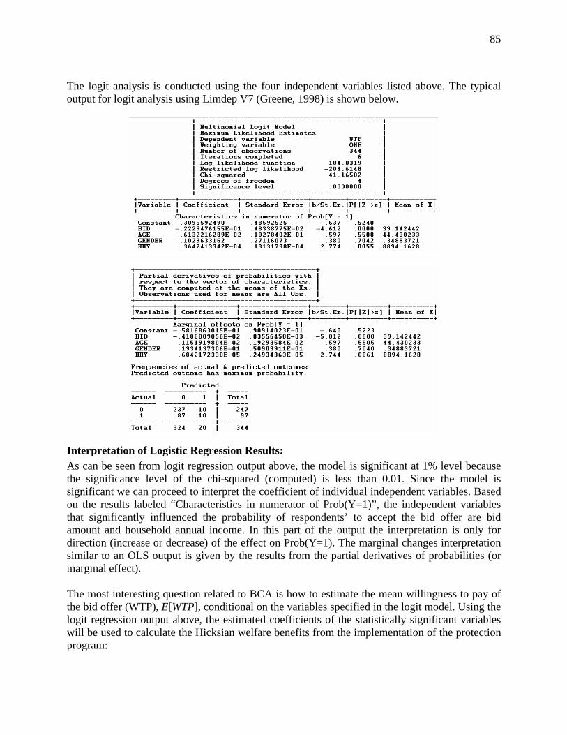
85

The logit analysis is conducted using the four independent variables listed above. The typical output for logit analysis using Limdep V7 (Greene, 1998) is shown below.

Interpretation of Logistic Regression Results: As can be seen from logit regression output above, the model is significant at 1% level because the significance level of the chi-squared (computed) is less than 0.01. Since the model is significant we can proceed to interpret the coefficient of individual independent variables. Based on the results labeled “Characteristics in numerator of Prob(Y=1)”, the independent variables that significantly influenced the probability of respondents’ to accept the bid offer are bid amount and household annual income. In this part of the output the interpretation is only for direction (increase or decrease) of the effect on Prob(Y=1). The marginal changes interpretation similar to an OLS output is given by the results from the partial derivatives of probabilities (or marginal effect). The most interesting question related to BCA is how to estimate the mean willingness to pay of the bid offer (WTP), E[WTP], conditional on the variables specified in the logit model. Using the logit regression output above, the estimated coefficients of the statistically significant variables will be used to calculate the Hicksian welfare benefits from the implementation of the protection program:

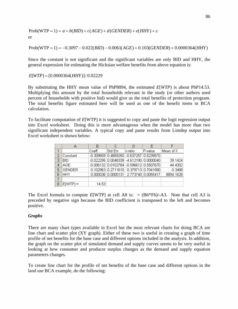
86

ε+++++== )()()()(1)Prob(WTP HHYeGENDERdAGEcBIDba or

)(0000364.0)(103.0)(0061.0)(022.03097.01)Prob(WTP HHYGENDERAGEBID ++−−−==

Since the constant is not significant and the significant variables are only BID and HHY, the general expression for estimating the Hicksian welfare benefits from above equation is:

02229.0/)](0000364.0[][ HHYWTPE = By substituting the HHY mean value of PhP8894, the estimated E[WTP) is about PhP14.53. Multiplying this amount by the total households relevant in the study (or other authors used percent of households with positive bid) would give us the total benefits of protection program. The total benefits figure estimated here will be used as one of the benefit items in BCA calculation. To facilitate computation of E[WTP) it is suggested to copy and paste the logit regression output into Excel worksheet. Doing this is more advantageous when the model has more than two significant independent variables. A typical copy and paste results from Limdep output into Excel worksheet is shown below:

The Excel formula to compute E[WTP] at cell A8 is: = (B6*F6)/-A3. Note that cell A3 is preceded by negative sign because the BID coefficient is transposed to the left and becomes positive.

Graphs There are many chart types available in Excel but the most relevant charts for doing BCA are line chart and scatter plot (XY graph). Either of these two is useful in creating a graph of time profile of net benefits for the base case and different options included in the analysis. In addition, the graph on the scatter plot of simulated demand and supply curves seems to be very useful in looking at how consumer and producer surplus changes as the demand and supply equation parameters changes. To create line chart for the profile of net benefits of the base case and different options in the land use BCA example, do the following:

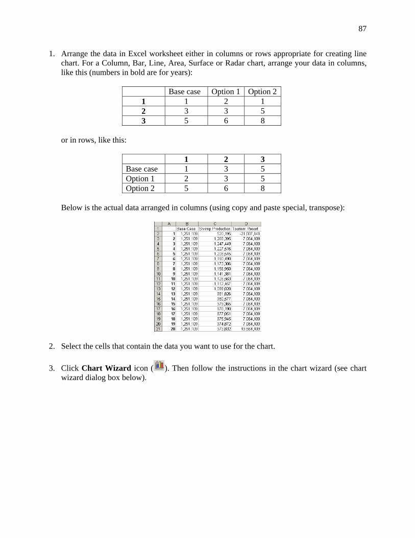
87

1. Arrange the data in Excel worksheet either in columns or rows appropriate for creating line chart. For a Column, Bar, Line, Area, Surface or Radar chart, arrange your data in columns, like this (numbers in bold are for years):

Base case Option 1 Option 2 1 1 2 1 2 3 3 5 3 5 6 8

or in rows, like this:

1 2 3 Base case 1 3 5 Option 1 2 3 5 Option 2 5 6 8

Below is the actual data arranged in columns (using copy and paste special, transpose):

2. Select the cells that contain the data you want to use for the chart.

3. Click Chart Wizard icon ( ). Then follow the instructions in the chart wizard (see chart wizard dialog box below).

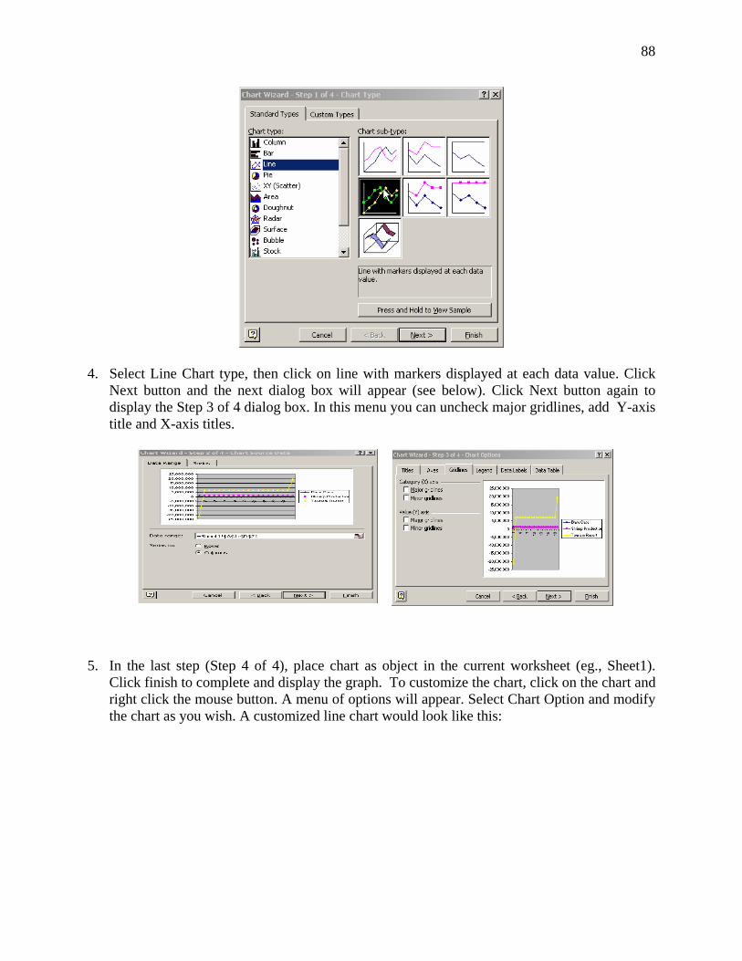
88

4. Select Line Chart type, then click on line with markers displayed at each data value. Click Next button and the next dialog box will appear (see below). Click Next button again to display the Step 3 of 4 dialog box. In this menu you can uncheck major gridlines, add Y-axis title and X-axis titles.

5. In the last step (Step 4 of 4), place chart as object in the current worksheet (eg., Sheet1). Click finish to complete and display the graph. To customize the chart, click on the chart and right click the mouse button. A menu of options will appear. Select Chart Option and modify the chart as you wish. A customized line chart would look like this:

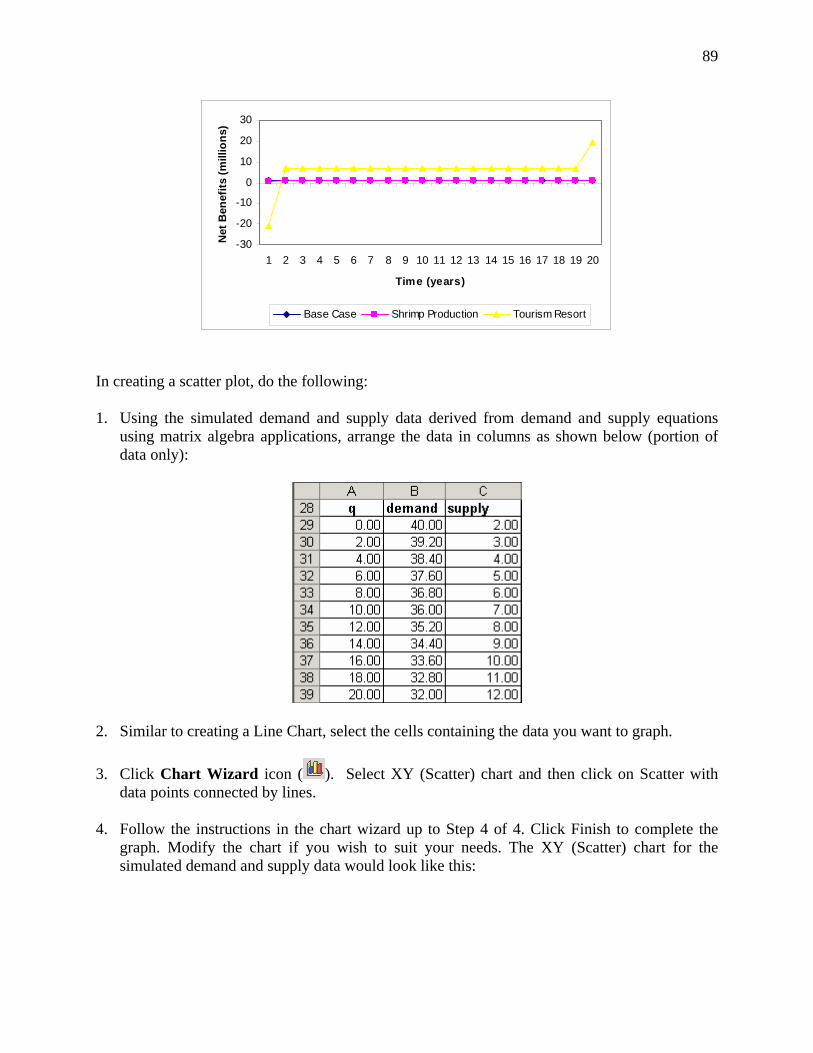
89

-30

-20

-10

0

10

20

30

1 2 3 4 5 6 7 8 9 10 11 12 13 14 15 16 17 18 19 20

Time (years)

Net

Ben

efits

(mill

ions

)

Base Case Shrimp Production Tourism Resort

In creating a scatter plot, do the following: 1. Using the simulated demand and supply data derived from demand and supply equations

using matrix algebra applications, arrange the data in columns as shown below (portion of data only):

2. Similar to creating a Line Chart, select the cells containing the data you want to graph. 3. Click Chart Wizard icon ( ). Select XY (Scatter) chart and then click on Scatter with

data points connected by lines. 4. Follow the instructions in the chart wizard up to Step 4 of 4. Click Finish to complete the

graph. Modify the chart if you wish to suit your needs. The XY (Scatter) chart for the simulated demand and supply data would look like this:

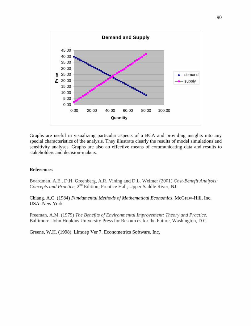
90

Demand and Supply

0.005.00

10.0015.0020.0025.0030.0035.0040.0045.00

0.00 20.00 40.00 60.00 80.00 100.00

Quantity

Pric

e demandsupply

Graphs are useful in visualizing particular aspects of a BCA and providing insights into any special characteristics of the analysis. They illustrate clearly the results of model simulations and sensitivity analyses. Graphs are also an effective means of communicating data and results to stakeholders and decision-makers. References Boardman, A.E., D.H. Greenberg, A.R. Vining and D.L. Weimer (2001) Cost-Benefit Analysis: Concepts and Practice, 2nd Edition, Prentice Hall, Upper Saddle River, NJ. Chiang. A.C. (1984) Fundamental Methods of Mathematical Economics. McGraw-Hill, Inc. USA: New York Freeman, A.M. (1979) The Benefits of Environmental Improvement: Theory and Practice. Baltimore: John Hopkins University Press for Resources for the Future, Washington, D.C. Greene, W.H. (1998). Limdep Ver 7. Econometrics Software, Inc.

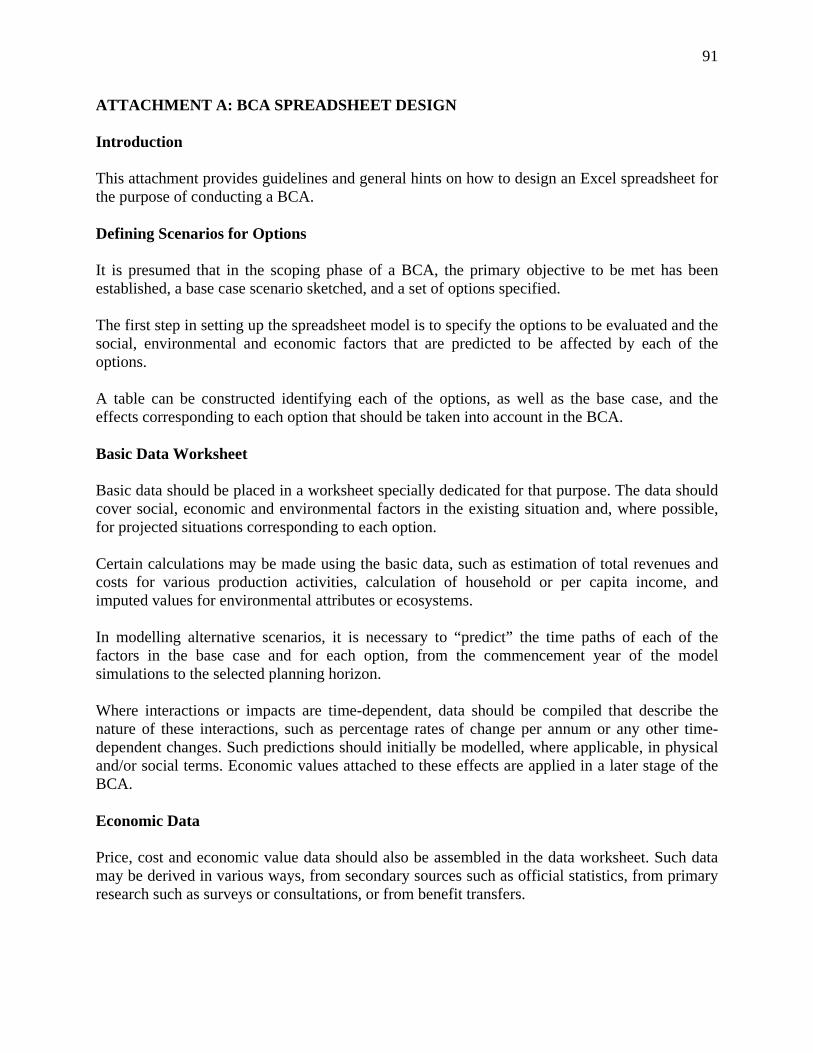
91

ATTACHMENT A: BCA SPREADSHEET DESIGN Introduction This attachment provides guidelines and general hints on how to design an Excel spreadsheet for the purpose of conducting a BCA. Defining Scenarios for Options It is presumed that in the scoping phase of a BCA, the primary objective to be met has been established, a base case scenario sketched, and a set of options specified. The first step in setting up the spreadsheet model is to specify the options to be evaluated and the social, environmental and economic factors that are predicted to be affected by each of the options. A table can be constructed identifying each of the options, as well as the base case, and the effects corresponding to each option that should be taken into account in the BCA. Basic Data Worksheet Basic data should be placed in a worksheet specially dedicated for that purpose. The data should cover social, economic and environmental factors in the existing situation and, where possible, for projected situations corresponding to each option. Certain calculations may be made using the basic data, such as estimation of total revenues and costs for various production activities, calculation of household or per capita income, and imputed values for environmental attributes or ecosystems. In modelling alternative scenarios, it is necessary to “predict” the time paths of each of the factors in the base case and for each option, from the commencement year of the model simulations to the selected planning horizon. Where interactions or impacts are time-dependent, data should be compiled that describe the nature of these interactions, such as percentage rates of change per annum or any other time-dependent changes. Such predictions should initially be modelled, where applicable, in physical and/or social terms. Economic values attached to these effects are applied in a later stage of the BCA. Economic Data Price, cost and economic value data should also be assembled in the data worksheet. Such data may be derived in various ways, from secondary sources such as official statistics, from primary research such as surveys or consultations, or from benefit transfers.

92

BCA Spreadsheet The spreadsheet model for the BCA should be constructed using a separate Excel worksheet. The worksheet should include a blank “master” template that can be applied to all options; provision for setting the discount rate interactively at any desired value; and a table that summarises all results of the analysis. Other cells may be earmarked that allow the analyst to alter model values or parameters interactively to explore the effects of different assumptions in the BCA. Setting up the Template The blank template acts as a common platform through which to calculate economic benefits and costs for each of the options. All factors or variables potentially affected by all options should be identified and listed in the template. The template is best constructed using columns to represent years and rows to represent the factors affected by options. Factors affected can be classified as follows (more detailed entries can be included within each item depending on the specific factors or effects incorporated in the analysis): Benefits Consumers surplus Revenues from production Residual values of remaining capital “External” environmental benefits Costs Capital costs Replacement/repair costs Other operating costs (labour, materials, maintenance) Environmental protection costs “External” environmental costs Interest payments and depreciation estimates should not be included in the estimates of economic costs. The template should contain Excel formulae that will be used in model simulations and the BCA calculations for each of the options. Such formulae will include summation of entries and the calculation of NPV, BCR and IRR. The main advantage of including the formulae in the template is that they do not have to be re-written when applying the template to each of the options.

93

Specifying the Base Case The base case should represent what can be expected in the absence of any of the proposed “new” options. It should indicate the time paths of all factors or variables potentially affected, valued in monetary terms, without any proposed new options or interventions in the system. The initial year of the base case should be the existing situation, or the situation corresponding to the first year of model simulations. In a “steady state” scenario the magnitudes of all variables will remain constant over time. However, the base case does not necessarily mean a repetition of the existing situation. Where base case variables do change over time, this must be represented in the base case scenario. In these circumstances, it is customary to refer to a “shifting” baseline. Assessing the Effects of Options The same blank template, described above, should be used for each option. The predicted time paths of monetary values associated with each of the factors affected by each option should be entered into the blank template. In many cases, an option will affect only some of the variables listed in the template. All other effects will be irrelevant and can be represented by zeros in the spreadsheet. If the template has been correctly constructed, it will automatically produce results for total benefits and total costs in the base case and for each of the options. Incremental Benefits and Costs The template, after being applied to the base case and to the options under consideration, will also produce results for incremental benefits and costs of options relative to the base case. Incremental benefits for each option are calculated by subtracting the values calculated for each option from the corresponding values in the base case. Incremental benefits in the base case itself will be zero, even with a shifting baseline. The reason is that base case values will be subtracted from the same base case values. The result will always be zero. Incremental costs for each option are calculated in a similar way. It follows that incremental costs in the base case will be zero.

94

Calculation of NPV, BCR and IRR The accepted evaluation criteria through which to evaluate options are Net Present Value (NPV); the Benefit-Cost Ratio (BCR); and the Internal Rate of Return (IRR). These can most easily be calculated using financial formulae contained in Excel. Incremental net benefits provide the information from which NPV, BCR and IRR are calculated for each option. Incremental net benefits are found by subtracting the incremental costs from incremental benefits for each option, in each year, from the initial year of analysis up to the planning horizon. All calculated results for NPV, BCR and IRR should be placed in a summary table. Options should then be ranked according to the calculated NPVs. For any “new” option to be acceptable on economic grounds, its NPV must be positive. A positive NPV means that the option produces higher net economic benefits, measured in present value terms, in comparison with those for the base case scenario. The “best” option from an economic perspective is the one with the highest NPV. In some appraisals, the “best” option is the base case itself. All “new” options should be rejected. The base case will have a value of zero for its NPV. The “new” options must all have negative NPVs. In these circumstances, even though the base case has a zero value for NPV, it will still represent the highest value and will constitute the “best” option on economic grounds. An alternative criterion for any option to be acceptable on economic grounds is that its BCR should be greater than 1. However, options should not be ranked according to their BCRs. Ranking should be conducted on the basis of NPVs. The IRR provides additional information on the internal economic productivity of any option. It is often compared to the discount rate. However, the IRR should not be used to rank options, as this may produce a ranking that is inconsistent with a ranking based on NPVs. For some options, it may not be possible to calculate an IRR. This occurs when the time path for net benefits for the option fails to change sign (-ve to +ve or vice versa). In such cases, Excel will produce a result such as #DIV/0! instead of a value for IRR. Sensitivity Analysis Sensitivity analysis is usually carried out for different discount rates. It is recommended that absolute referencing be used for the cell that contains the discount rate, and incorporate this cell in all Excel financial formulae applying the discount rate. This allows the analyst to vary the discount rate and automatically apply it in all calculations of present values. It is thus possible to see whether rankings of options are sensitive to the discount rate.

95

An alternative means of assessing the importance of the discount rate is to include, say, three different rates when setting up the spreadsheet. This will produce three sets of results for NPV and BCR. Note that when varying the discount rate, results can be computed for the NPV and BCR but not the IRR. The reason for not attempting sensitivity analysis for the IRR is that the IRR is itself the discount rate that reduces NPV to zero. In most cases, there is only one IRR for each option. However, in some cases there may be several possible values for IRR and it is not certain whether the value produced by Excel is the most relevant. Sensitivity analysis can also be carried out for costs as a whole and for benefits as a whole – for example, by assuming a 20% (or some other arbitrary variation) up or down and documenting the results. If this approach is taken, it is recommended that the variations should be incorporated as scaling factors in the formulae for benefits and costs, and accessed via cells with absolute references, to determine the effects on NPV, BCR and IRR. Another important form of sensitivity analysis occurs when it there is a need to alter individual variables for any particular option. For example, there may be considerable uncertainty about the effects of an option on some environmental quality indicator such as the dissolved oxygen level in a river. In this case, it is recommended that a scaling factor be incorporated in the spreadsheet, using cells with absolute referencing that can be altered interactively to assess whether effects characterised by uncertainty might critically influence the calculated NPV, BCR and IRR. Yet another application of sensitivity analysis, extending from the case just described, is where it might be desirable to determine the threshold value that would have to be attached to environmental benefits or costs, to change significantly the calculated NPV, BCR and IRR. Again, cells with absolute referencing can be incorporated in the formulae to facilitate model simulations and sensitivity analyses. Presentation of Results Results are best presented in a summary table, showing the NPV, BCR and IRR for each of the options. The ranking of options, from best to worst, can be determined from such a table. Where sensitivity analysis has been carried out, separate tables of results should be presented for each set of assumptions adopted.