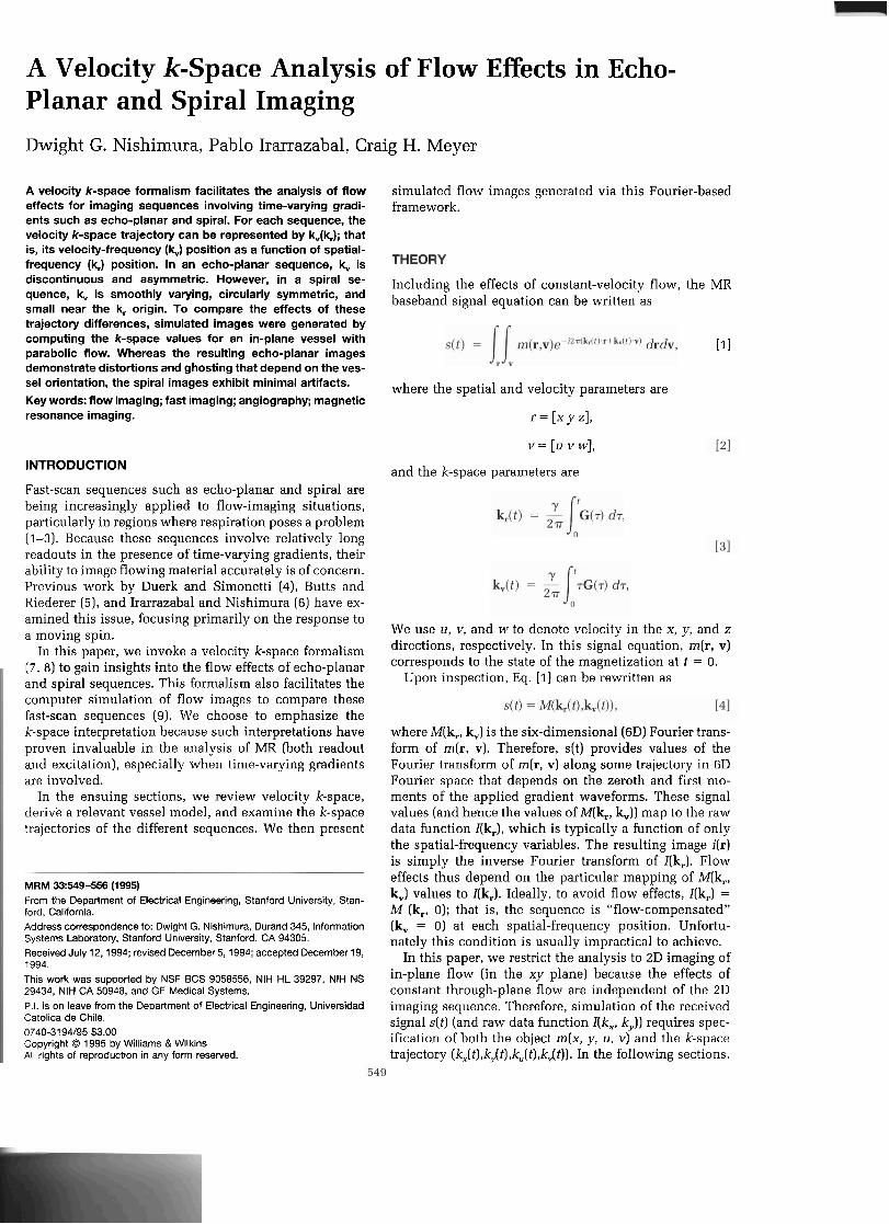
A Velocity k-Space Analysis of Flow Effects in Echo- Planar and Spiral Imaging

Dwight G. Nishimura, Pablo Irarrazabal, Craig H. Meyer

A velocity k-space formalism facilitates the analysis of flow simulated flow images generated via this Fourier-based effects for imaging sequences involving time-varying gradi- framework. ents such as echo-planar and spiral. For each sequence, the velocity k-space trajectory can be represented by k,(k,); that is, its velocity-frequency (kJ position as a function of spatial- frequency (k,) position. In an echo-planar sequence, k, is discontinuous and asymmetric. However, in a spiral se- ~ ~ ~ l ~ d i ~ ~ the effects of constant-ve~oc~ty flow, the MR quence, k, is smoothly varying, circularly symmetric, and baseband signal equation can be written as small near the k, origin. To compare the effects of these trajectory differences, simulated images were generated by computing the k-space values for an in-plane vessel with parabolic flow. Whereas the resulting echo-planar images [I1

demonstrate distortions and ghosting that depend on the ves- sel orientation, the spiral images exhibit minimal artifacts. where the spatial and velocity parameters are Key words: flow imaging; fast imaging; angiography; magnetic resonance imaging. r = [xyzl,

INTRODUCTION

Fast-scan sequences such as echo-planar and spiral are being increasingly applied to flow-imaging situations, particularly in regions where respiration poses a problem (1-3). Because these sequences involve relatively long readouts in the presence of time-varying gradients, their ability to image flowing material accurately is of concern. Previous work by Duerk and Simonetti (4), Butts and Riederer (5), and Irarrazabal and Nishimura (6) have ex- amined this issue, focusing primarily on the response to a moving spin.

In this paper, we invoke a velocity k-space formalism ( 7 , 8) to gain insights into the flow effects of echo-planar and spiral sequences. This formalism also facilitates the computer simulation of flow images to compare these fast-scan sequences (9). We choose to emphasize the k-space interpretation because such interpretations have proven invaluable in the analysis of MR (both readout and excitation), especially when time-varying gradients are involved.

In the ensuing sections, we review velocity k-space, derive a relevant vessel model, and examine the k-space trajectories of the different sequences. We then present

MRM 33:549-556 (1995) From the Department of Electrical Engineering, Stanford University, Stan- ford, California. Address correspondence to: Dwight G. Nishimura, Durand 345, Information Systems Laboratory. Stanford University, Stanford, CA 94305. Received July 12,1994; revised December 5, 1994; accepted December 19, 1994. This work was supported by NSF BCS 9058556, NIH HL 39297. NIH NS 29434, NIH CA 50948, and GE Medical Systems. P.I. is on leave from the Department of Electrical Engineering, Universidad Catolica de Chile. 0740-3194195 $3.00 Copyright O 1995 by Williams & Wilkins All rights of reproduction in any form resewed.

v = [u v w],

and the k-space parameters are

We use u, v, and w to denote velocity in the x, y, and z directions, respectively. In this signal equation, m(r, v) corresponds to the state of the magnetization at t = 0.

Upon inspection, Eq. [I] can be rewritten as

where M(k,, k,) is the six-dimensional (6D) Fourier trans- form of m(r, v). Therefore, s(t) provides values of the Fourier transform of m(r, v) along some trajectory in 6D Fourier space that depends on the zeroth and first mo- ments of the applied gradient waveforms. These signal values (and hence the values of M(h, k,)) map to the raw data function I(k,), which is typically a function of only the spatial-frequency variables. The resulting image i(r) is simply the inverse Fourier transform of I(k,). Flow effects thus depend on the particular mapping of M(k,, k,,) values to I(k,). Ideally, to avoid flow effects, I(k,) = M (k,, 0); that is, the sequence is "flow-compensated" (k, = 0) at each spatial-frequency position. Unfortu- nately this condition is usually impractical to achieve.

In this paper, we restrict the analysis to 2D imaging of in-plane flow (in the xy plane) because the effects of constant through-plane flow are independent of the 2D imaging sequence. Therefore, simulation of the received signal s(t) (and raw data function I(k,, k,)) requires spec- ification of both the object m(x, y, u, v) and the k-space trajectory (kx(t),k,,(t),k,(t),kv(t)). In the following sections.

550 Nishimura et al.

we elaborate on (1) the object model and (2) the k-space positions along each chord map to a particular velocity u. trajectories for the echo-planar and spiral sequences. Hence,

Object Model

We first consider a simple illustrative situation where an object m,(x, y) (at t = 0) moves at a constant speed with velocity components (u,, v,). In this case,

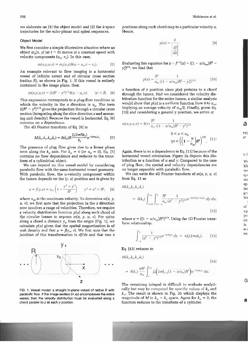
An example relevant to flow imaging is a horizontal vessel of infinite extent and of circular cross section (radius R), as shown in Fig. 1. If this vessel is entirely contained in the image plane, then

This expression corresponds to a plug-flow condition in which the velocity in the x direction is u,. The term 2(RZ - f ) ' I 2 gives the projection through a circular cross section (integrating along the slice direction z and assum- ing unit density). Because the vessel is horizontal, Eq. [6] contains no x dependence.

The 4D Fourier transform of Eq. [6] is

Evaluating this equation for z = f '(u) = ((1 - u/um)RZ - y,Z)'I2, we find that

a function of y position since p(u) pertains to a chord through the lumen. Had we considered the velocity dis- tribution function for the entire lumen, a similar analysis would show that p(u) is a uniform function from 0 to u,,, implying an average velocity of u,/2. Finally, given Eq. [ lo] and considering a general y position, we arrive at

J I ( ~ ~ ~ ~ ~ ) -i2m,k, O < u < u ,

M(kx,ky,ku,kv) = 6(kx)R e PI kY yl < ((I - ~ ) R Z ) ' I z .

urn The presence of plug flow gives rise to a linear phase term along the k, axis. For k, = 0 (or u, = O), Eq. [7 ] Again, there is no x dependence in Eq. [Ill because of the contains no flow dependence and reduces to the trans- horizontal vessel orientation. Figure 2a depicts this dis- form of a cylindricaf object. tribution as a function of u and i. cornpared to the case

We can expand on this vessel model by considering of plug flow, the spatial and velocity dependencies are parabolic flow with the same horizontal vessel geometry. no longer separable with parabolic flow. With parabolic flow, the u-velocity component within We can write the 4D Fourier transform of m(x, y, u, v) the lumen depends on the (y, z) position and is given by from Eq. 11 as

where urn is the maximum velocity. To determine m(x, y, u, v), we first note that the projection in the z direction now involves a range of velocities. Therefore, we require a velocity distribution function p(u) along each chord of the circular lumen to express m(x, y, u, v). For spins along a chord a distance yo from the origin (Fig. I), we calculate p(u) given that the spatial magnetization is of unit density and that u = fly,, z). We first note that the Jacobian of this transformation is df/dz and that two z

where a = ((1 - u/u,)R~)"~. Using the 1D Fourier trans- form relationship:

Eq. [12] reduces to

FIG of

Wl bli Kt

q L ' rnt SP' l e ~ gr: tin

I of

UP

Pe CO'

is acc en

z The remaining integral is difficult to evaluate analyti-

G

FIG. 1. Vessel model: a straight in-plane vessel of radius R with c a l l ~ but may be for k~ and parabolic flow. If the image section (in xy) encompasses the entire ku, The result is shown in Fig. 2b which displays the vessel, then the velocity distribution must be evaluated along a magnitude of M in k, - k, space. Again for k,, = 0, the chord parallel to z at each y position. function reduces to the transform of a cylinder. a

Velocity k-Space Analysis of Flow Effects 5 5 1

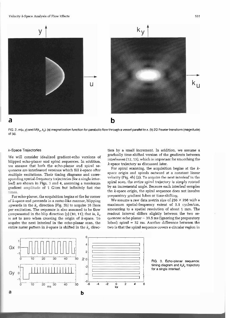
I a b FIG. 2. m(u, y) and M(k,, k,,): (a) magnetization function for parabolic flow through a vessel parallel tox. (b) 2D Fourier transform (magnitude) of (a).

k-Space Trajectories tion by a small increment. In addition, we assume a gradually time-shifted version of the gradients between

We will consider idealized gradient-echo versions of interleaves (12,13), which is important for smoothing the blipped echo-planar and spiral sequences. In addition, k-space trajectory as discussed later. we assume that both the echo-planar and spiral se-

quences are interleaved versions which fill k-space after For spiral scanning, the acquisition begins at the k-

multiple excitations. Their timing diagrams and corre- space origin and spirals outward at a constant linear

spending spatial-frequency trajectories (for a single inter- velocity (Fig. 4b) (2). To acquire the next interleaf in the

leaf) are shown in ~ i ~ ~ . and 4, assuming a maximum spiral scan, the entire spiral trajectory is simply rotated

gradient of 1 (ycm but infinitely fast rise by an incremental angle. Because each interleaf samples the k-space origin, the spiral sequence does not involve

For echo-planar, the acquisition begins at the far corner Preparatory gradient lobes or time-shifting.

of k-space and proceeds in a raster-like manner, blipping We assume a raw data matrix size of 256 X 256 with a

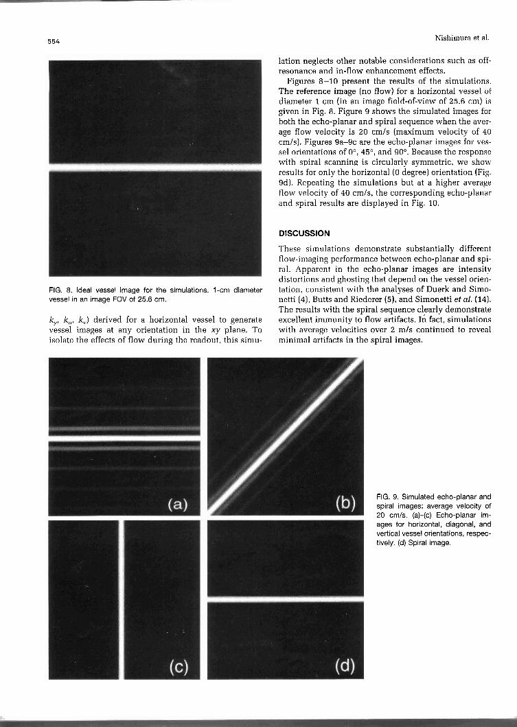
upwards in the k, direction (Fig. 3b) to acquire 16 lines maximum spatial-frequency extent of 5.1 cycles/cm, per excitation. The sequence is also assumed to be flow amounting to a spatial resolution of about 1 mm. The compensated in the blip direction (y) (10, 11); that is, k, readout interval differs slightly between the two se- is set to zero when crossing the origin of k-space. To quences: echo planar = 39.5 ms (ignoring the preparatory acquire the next interleaf in the echo-planar scan, the lobes); spiral = 32 ms. Another difference between the entire raster pattern in k-space is shifted in the k, direc- two is that the spiral sequence covers a circular region in

I . I

I - I . I

FIG. 3. Echo-planar sequence: timing diagram and k&, trajectory

I . for a single interleaf. I I

0 -6 -4 -2 0 2 4 6 kx

b

I 552 Nishimura et al.

k&, space while the echo-planar sequence covers a square region.

One display of the velocity k-space trajectory depicts k,(k,, k,) and (k,(k,, k,)) as gray levels in a 2D "image" of the spatial-frequency plane. Such depictions are pre- sented in Figs. 5 and 6 for the echo planar and spiral sequences respectively (intermediate gray corresponds to zero amplitude). An alternative display is given in Fig. 7 which shows a portion of the central area of kJcY space. At each (k,, k,) position, the arrow represents the vector [k, k,]; hence both the amplitude and direction of the first moment are apparent.

For the echo-planar sequence (Figs. 5 and 7a), there exists discontinuities in the behavior of [k, k,] due to the interleaving and the square-wave readout (G,) gradient. For example, along the k, axis, k, is a square-wave func- tion that jumps between some value k,, and zero (Fig. 5a). This oscillation corresponds to G, being flow com-

pensated on alternate gradient echoes during the readout (an even-echo rephasing phenomenon). The behavior of k, (Fig. 5b) is smooth due to the time-shifting of the interleaves that was mentioned earlier; without the time- shifting, k, would also exhibit discontinuous behavior. For k,,, there exists both a linear and quadratic variation with k,,. The linear variation corresponds to material flowing along y being displaced in y by an amount de- pendent on the non-zero TE. From a k-space perspective, this displacement occurs because the linear variation in k, with k, position gives rise to linear phase in the raw data for constant-velocity material. For k,, there exists mainly a linear variation with k, but the slope of this variation increases from one readout line to the next. Given the train of readout lines after excitation, this steady increase in slope corresponds to increasing dis- placements in x because the readout lines occur at pro- gressively later times.

FIG. 4. Spiral sequence: timing di- agram and k&, trajectory for a sin- gle interleaf.

FIG. 5. Echo-planar velocity k-space trajectory: (a) k,(kx, k,), displayed as a gray level (neutral gray corresponds to zero). (b) k,(kx, k,).

Velocity k-Space Analysis of Flow Effects

ky t

ku kv b a

FIG. 6. Spiral velocity k-space trajectory: (a) k,(kx, k,), displayed as a gray level (neutral gray corresponds to zero). (b) k,(k,, k,).

The spiral trajectory (Figs. 6 and 7b) exhibits signifi- cantly different behavior than the echo-planar trajectory. One salient property of the spiral trajectory is its circular symmetry (apparent in Fig. 7b). Also the length and direction of the vector [k, k,] change smoothly, growing with radial distance from the origin, and largely pointing away from the origin.

SIMULATION RESULTS

Given an object model and a timing diagram for a given sequence, the general procedure to generate a flow image using the velocity k-space framework is summarized be- low.

1. Determine M(kx, k,,, k,, k,) for the object.

FIG. 7. Velocity k-space trajecto- ries: (a) echo-planar-the vector [k, k,] is displayed as a function of (k,, k,) position. The center portion of k-space is shown. (b) Spiral.

2. Compute k;qn(kx,ky) and k",'qn(kx,ky) for the imaging sequence.

3. Let the raw data I(k,, k,) = M(kx,k,,k~qn(kx,k,),k","qn (kX,kJ).

4. Take the inverse Fourier transform of I(kx, k,,) to reconstruct the image i(x, y).

For our simulations, we consider the k, and k, maps for echo-planar and spiral scanning as shown in Figs. 5 and 6, while for the object, we use the infinitely long in-plane vessel with a circular lumen and parabolic flow. Because the vessel is assumed to be of infinite extent, generation of the raw data is conveniently constrained to reside along a line in k&,, space. For the horizontal vessel, this line is along the k,, axis. Using the rotation property of Fourier transforms, we can rotate the M(k,,

554 Nishimura et al.

lation neglects other notable considerations such as off- resonance and in-flow enhancement effects.

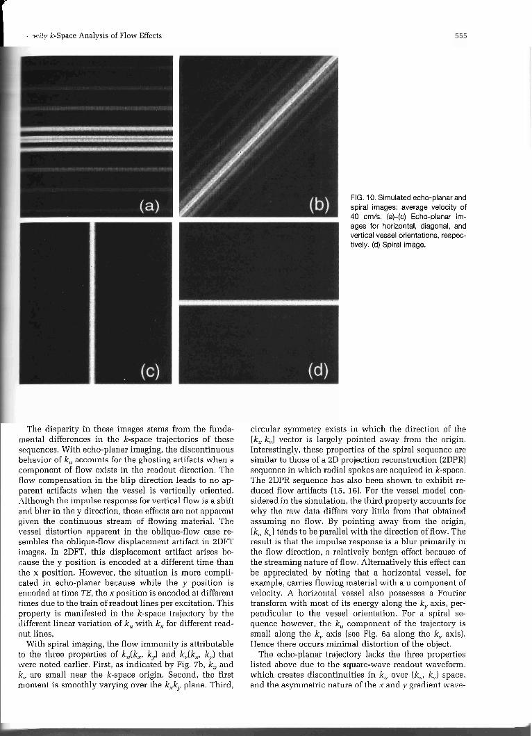
Figures 8-10 present the results of the simulations. The reference image (no flow) for a horizontal vessel of diameter 1 cm (in an image field-of-view of 25.6 cm) is given in Fig. 8. Figure 9 shows the simulated images for both the echo-planar and spiral sequence when the aver- age flow velocity is 20 cm/s (maximum velocity of 40 cmts). Figures 9a-9c are the echo-planar images for ves- sel orientations of 0°, Go, and 90". Because the response with spiral scanning is circularly symmetric, we show . "

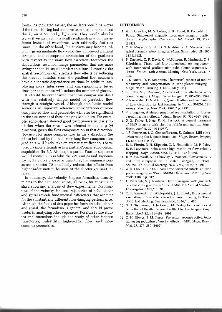
results for only the horizontal (0 degree) orientation (Fig. 9d). Repeating the simulations but at a higher average flow velocity of 40 cmts, the corresponding echo-planar and spiral results are displayed in Fig. 10.

DISCUSSION

These simulations demonstrate substantially different flow-irnaging performance between echo-planar and spi- ral. Apparent in the echo-planar images are intensitv distortions and ghosting that depend on the vessel orien-

FIG. 8. Ideal vessel image for the simulations. 1-crn diameter tation, consistent with ;he anaGses of Duerk and Simo- vessel in an image FOV of 25.6 cm. netti (4), Butts and Riederer (5), and Simonetti et al. (14). 1

The results with the spiral sequence clearly demonstrate k,, k,, k,) derived for a horizontal vessel to generate excellent immunity to flow artifacts. 1n fact, simulations vessel images at any orientation in the xy plane. To with average velocities over 2 m/s continued to reveal isolate the effects of flow during the readout, this simu- minimal artifacts in the spiral images. i

FIG. 9. Simulated echo-planar and spiral images: average velocity of 20 cm/s. (a)-(c) Echo-planar im- ages for horizontal, diagonal, and vertical vessel orientations, respec- tively. (d) Spiral image.

I

n: S t '

bc c r fl c

P ' :I a r p 1

VF

S C'

in ca th ca en t i r

P' di OU

to IVC

k , m c

R - ?city k-Space Analysis of Flow Effects

FIG. 10. Simulated echo-planar and spiral images: average velocity of 40 cm/s. (a)-fcl Echo-olanar im-

\ , \ , - , ages for horizontal, diagonal, and vertical vessel orlentatlons, respec- tively. (d) Spiral image.

The disparity in these images stems from the funda- mental differences in the k-space trajectories of these sequences. With echo-planar imaging, the discontinuous behavior of k, accounts for the ghosting artifacts when a component of flow exists in the readout direction. The flow compensation in the blip direction leads to no ap- parent artifacts when the vessel is vertically oriented. .ilthough the impulse response for vertical flow is a shift and blur in the y direction, these effects are not apparent given the continuous stream of flowing material. The vessel distortion apparent in the oblique-flow case re- sembles the oblique-flow displacement artifact in 2DFT images. In ZDFT, this displacement artifact arises be- cause the y position is encoded at a different time than the x position. However, the situation is more compli- cated in echo-planar because while the y position is encoded at time TE, the x position is encoded at different times due to the train of readout lines per excitation. This property is manifested in the k-space trajectory by the different linear variation of k, with k, for different read- out lines.

With spiral imaging, the flow immunity is attributable to the three properties of k,(k,, k,,) and kv(k,, k,,) that were noted earlier. First, as indicated by Fig. 7b, k, and k, are small near the k-space origin. Second, the first moment is smoothly varying over the k&, plane. Third,

circular symmetry exists in which the direction of the [k, kv] vector is largely pointed away from the origin. Interestingly, these properties of the spiral sequence are similar to those of a 2D projection reconstruction (BDPR) sequence in which radial spokes are acquired in k-space. The 2DPR sequence has also been shown to exhibit re- duced flow artifacts (15, 16). For the vessel model con- sidered in the simulation, the third property accounts for why the raw data differs very little from that obtained assuming no flow. By pointing away from the origin, [k, kv] tends to be parallel with the direction of flow. The result is that the impulse response is a blur primarily in the flow direction, a relatively benign effect because of the streaming nature of flow. Alternatively this effect can be appreciated by <oting that a horizontal vessel, for example, carries flowing material with a u component of velocity. A horizontal vessel also possesses a Fourier transform with most of its energy along the k,, axis, per- pendicular to the vessel orientation. For a spiral se- quence however, the k,, component of the trajectory is small along the k, axis (see Fig. 6a along the k,, axis). Hence there occurs minimal distortion of the object.

The echo-planar trajectory lacks the three properties listed above due to the square-wave readout waveform, which creates discontinuities in k,, over (k,, k,,) space. and the asymmetric nature of the x and y gradient wave-

Nishimura e:

forms. A s indicated earlier, the artifacts would be worse if the t ime shifting h a d not been assumed to smooth out the k, variation in (k,, k,) space. They would also be worse if w e assumed physically realizable gradient wave- forms instead of waveforms with arbitrarily fast rise times. O n the other hand, the artifacts may become tol- erable given moderate flow velocities, improved gradient strength, and appropriate orientation of the gradients wi th respect to the main flow direction. Moreover the simulations assumed image parameters that are more stringent than in usual implementations. Lowering the spatial resolution wil l alleviate flow effects by reducing the readout duration since t h e gradient first moments have a quadratic dependence o n time. In addition, em- ploying more interleaves a n d correspondingly fewer lines per acquisition wil l reduce the number of ghosts.

It should be emphasized that this comparison dealt wi th the relatively simple model of parabolic flow through a straight vessel. Although this basic model serves as a n important reference, consideration of more complicated flow a n d geometries will also be significant i n the assessment of these imaging sequences. For exam- ple, echo-planar showed good performance i n this sim- ulation w h e n the vessel was oriented i n the bl ip (y) direction, given the flow compensation i n that direction. However, for more complex flow i n the y direction, the phase induced by the relatively long flow-compensation gradients will likely take o n greater significance. There- fore, a viable alternative is a partial-Fourier echo-planar acquisition (in k,). Although a partial-Fourier sequence would continue to exhibit discontinuities and asymme- try in its velocity k-space trajectory, the sequence pos- sesses a shorter TE a n d likely reduces the effects from higher-order motion because of the shorter gradient in- terval.

In summary, the velocity k-space formalism directly relates to the data acquisition, allowing for convenient simulation a n d analysis of flow experiments. Examina- t ion of the velocity k-space trajectories of echo-planar a n d spiral reveals fundamental differences that account for the substantially different flow-imaging performance. Although the focus of this paper has been o n echo-planar a n d spiral, the formalism is general and should prove useful i n analyzing other sequences. Possible future stud- ies a n d extensions include the s tudy of other k-space trajectories, pulsatility, higher-order flow, and more complex geometries.

REFERENCES

1. A. P. Crawley, M. S. Cohen, E. K. Yucel, B. Poncelet. T Brady, Single-shot magnetic resonance imaging: appli;: tions to angiography. Cardiovasc. Int. Radiol. 15, 32-:. (1992).

2. C. H. Meyer, B. S. Hu, D. G. Nishimura, A. Macovski. FZG- spiral coronary artery imaging. Magn. Reson. Med. 28, 20:- 213 (1992).

3. S. Duewell, C. P. Davis, G. McKinnon, B. Marincek, G I. Schulthess, Three- and four-dimensional mr angiograp5- with interleaved gradient-echo echo-planar sequences. .- "Pro~. , SMRM, 12th Annual Meeting, New York, 1993." r 385.

4. J. L. Duerk, 0 . P. Simonetti, Theoretical aspects of motior sensitivity and compensation in echo-planar imaging. '

Magn. Reson. Imaging. 1, 643-650 (1991). 5. K. Butts, S. J. Riederer, Analysis of flow effects in echc-

planar imaging. J. Magn. Reson. Imaging. 2, 285-293 (1992 6. P. Irarrazabal, D. Nishimura, Quantification and cornparisor

of flow distortion for fast imaging, i n "Proc., SMRM, 12th Annual Meeting, New York, 1993," p. 1257.

7. S. Ljunggren, A simple graphical representation of fourier- based imaging methods. J. Magn. Reson. 54,338-343 (1983).

8. D. B. Twieg, J. Katz, R. M. Peshock, A general treatment of NMR imaging with chemical shifts and motion. Magn. Reson. Med. 5, 32-46 (1987).

9. J. S. Petersson, J.-0. Christoffersson, K. Golman, MRI sirnu- lation using the k-space formalism. M&. Reson. Imaging 11, 557-568 (1993).

10. D. N. Firmin, R. H. Klipstein, G. L. Hounsfield, M. P. Pale?. D. B. Longmore, Echo-planar high-resolution flow velocit!. mapping. Magn. Reson. Med. 12, 316-327 (1989).

11. R. M. Weisskoff, A. P. Chawley, V. Wedeen, Flow sensitivity and flow compensation in instant imaging, i n "Proc.. SMRM, 9th Annual Meeting, New York, 1992," p. 398.

12. Z. H. Cho, C. B. Ahn, Phase error corrected interlaced echo planar imaging, i n "Proc., SMRM, 6th Annual Meeting, New York, 1987," p. 912.

13. F. Farzaneh, S. J. Riederer, Hybrid imaging with gradient- recalled sliding echos, i n "Proc., SMRI, 7th Annual Meeting, Los Angeles, 1989," p. 70.

14. 0. P. Simonetti, P. Wielopolski, J. L. Duerk, Experimental evaluation of flow effects in echo-planar imaging, i n "Proc., SMR, 2nd Meeting, San Francisco, 1994," p. 460.

15. D. G. Nishimura, J. I. Jackson, J. M. Pauly, On the nature and reduction of the displacement artifact in flow images. Magn. Reson. Med. 22, 481-492 (1991).

16. C. H. Glover, J. M. Pauly, Projection reconstruction tech- niques for reduction of motion effects in MRI. Magn. Reson. Med. 28, 275-289 (1992).

MI 1 Frc

I Cc

Ad Ph Tn 6J Re be Th Tn 07 Cc All