Embed Size (px)
Citation preview
A Viscosity Adaptive Lattice BoltzmannMethod
Vom Fachbereich Maschinenbau und Verfahrenstechnikder Technischen Universität Kaiserslauternzur Verleihung des akademischen Grades
Doktor-Ingenieur (Dr.-Ing.)genehmigte
Dissertation
von
Herrn
Dipl.-Ing. Daniel Conradaus Kaiserslautern
2015
Tag der mündlichen Prüfung: 23. März 2015Dekan: Prof. Dr.-Ing. Christian SchindlerVorsitzender: Prof. Dr.-Ing. Sergiy AntonyukBerichterstatter: Prof. Dr.-Ing. Martin Böhle
Prof. Dr.-Ing. habil. Uwe Janoske
D 386


In Gedenken an meinen Bruder
Christopher Conrad(14.04.1992 - 08.07.1996)

Danksagung
Die vorliegende Dissertation entstand während meiner Tätigkeit als wissenschaftlicher Mit-arbeiter am Lehrstuhl für Strömungsmechanik und Strömungsmaschinen der TechnischenUniversität Kaiserslautern.
Zuerst möchte ich mich bei meinem Doktorvater Prof. Dr.-Ing. Martin Böhle dafürbedanken, dass er uns die größt mögliche Freiheit zum Erreichen unserer Ziele eingeräumthat. Mit seinem Vertrauen in unser Lattice Boltzmann Team hat er mir gezeigt wasForschung bedeutet.
Ferner danke ich Herrn Prof. Dr.-Ing. habil. Uwe Janoske für die Übernahme der Zweitkor-rektur sowie Herrn Prof. Dr.-Ing. Sergiy Antonyuk für den Vorsitz der Prüfungskommission.
Den gesamten Mitarbeitern des SAM Lehrstuhls danke ich für die gute Zusammenarbeitund die Kollegialität sowohl innerhalb als auch außerhalb des Institutes.
Mein Dank gilt auch dem Regionalen Hochschulrechenzentrum Kaiserslautern für dieinfrastrukturelle und fachliche Unterstützung. Namentlich möchte ich hier speziell HerrnDr.-Ing. Markus Hillenbrand und Herrn PD Dr. habil. Josef Schüle erwähnen.
Tiefer Dank gilt meiner Oma Erna und meiner Mutter Angelika, die nie an mir gezweifeltund mich in jeder Situation unterstützt haben. Insbesondere möchte ich mich bei meinerMutter dafür bedanken, dass sie mich schon immer moralisch auf meinem Weg begleitethat.
Bei meinem SAM-Lattice Mitentwickler, Kollegen und Freund Andreas Schneider möchteich mich für die gemeinsamen Jahre herzlich bedanken. Ich hätte mir keinen besserenMitstreiter wünschen können.
Letztlich danke ich meiner Frau Lena von ganzen Herzen für die vielen Entbehrungen,ihre uneingeschränkte Unterstützung und Liebe. Auch möchte ich mich bei unserem SohnJohann bedanken, der mein Leben so sehr bereichert.
Kaiserslautern, im April 2015. Daniel Conrad


Contents
Abstract xi
Kurzfassung auf Deutsch xv
1 Introduction 1
2 Route to the Lattice Boltzmann Equation 32.1 Preliminaries . . . . . . . . . . . . . . . . . . . . . . . . . . . . . . . . . . 3
2.1.1 Tensor Notation and Calculus . . . . . . . . . . . . . . . . . . . . . 32.1.2 Landau Notation . . . . . . . . . . . . . . . . . . . . . . . . . . . . 3
2.2 The Boltzmann Equation . . . . . . . . . . . . . . . . . . . . . . . . . . . . 52.2.1 Equilibrium Distribution . . . . . . . . . . . . . . . . . . . . . . . . 52.2.2 Moments of the Continuous Distribution . . . . . . . . . . . . . . . 6
2.3 The Discrete Boltzmann Equation . . . . . . . . . . . . . . . . . . . . . . . 72.3.1 Discrete Equilibrium Distribution . . . . . . . . . . . . . . . . . . . 82.3.2 DnQm Lattices . . . . . . . . . . . . . . . . . . . . . . . . . . . . . 92.3.3 Moments of the Discrete Distribution . . . . . . . . . . . . . . . . . 112.3.4 Derivation of the Navier-Stokes Equations . . . . . . . . . . . . . . 13
2.4 The Lattice Boltzmann Equation . . . . . . . . . . . . . . . . . . . . . . . 192.4.1 Accuracy . . . . . . . . . . . . . . . . . . . . . . . . . . . . . . . . . 222.4.2 Diffusive Scaling vs. Acoustic Scaling . . . . . . . . . . . . . . . . . 252.4.3 Stability . . . . . . . . . . . . . . . . . . . . . . . . . . . . . . . . . 25
2.5 Extensions to LBM . . . . . . . . . . . . . . . . . . . . . . . . . . . . . . . 262.5.1 Multiple Relaxation Time . . . . . . . . . . . . . . . . . . . . . . . 262.5.2 Grid Refinement . . . . . . . . . . . . . . . . . . . . . . . . . . . . 292.5.3 Generalized Newtonian Flow . . . . . . . . . . . . . . . . . . . . . . 322.5.4 External Force . . . . . . . . . . . . . . . . . . . . . . . . . . . . . 34
vii
viii CONTENTS
3 Implementation 353.1 Lattice Generation . . . . . . . . . . . . . . . . . . . . . . . . . . . . . . . 35
3.1.1 Generation Algorithms . . . . . . . . . . . . . . . . . . . . . . . . . 383.1.2 Grid Refinement and Lattice Smoothing . . . . . . . . . . . . . . . 393.1.3 Higher Order Schemes . . . . . . . . . . . . . . . . . . . . . . . . . 41
3.2 Solver Implementation . . . . . . . . . . . . . . . . . . . . . . . . . . . . . 443.2.1 Multi-Level Treatment . . . . . . . . . . . . . . . . . . . . . . . . . 463.2.2 Boundary Conditions . . . . . . . . . . . . . . . . . . . . . . . . . . 483.2.3 Force and Reference Frames . . . . . . . . . . . . . . . . . . . . . . 55
4 Solver Verification 574.1 Newtonian . . . . . . . . . . . . . . . . . . . . . . . . . . . . . . . . . . . . 58
4.1.1 Stokes’s First Problem: The Suddenly Accelerated Plate . . . . . . 584.1.2 Stokes’s Second Problem: The Oscillating Plate . . . . . . . . . . . 59
4.2 Generalized Newtonian . . . . . . . . . . . . . . . . . . . . . . . . . . . . . 624.2.1 Hagen-Poiseuille Channel Flow . . . . . . . . . . . . . . . . . . . . 624.2.2 Hagen-Poiseuille Pipe Flow . . . . . . . . . . . . . . . . . . . . . . 69
5 Viscosity Adaption Method 735.1 Theoretical Considerations . . . . . . . . . . . . . . . . . . . . . . . . . . . 745.2 Choice of Time Step Size . . . . . . . . . . . . . . . . . . . . . . . . . . . . 755.3 Mach Number Limitation . . . . . . . . . . . . . . . . . . . . . . . . . . . 765.4 Multi-Level Approach . . . . . . . . . . . . . . . . . . . . . . . . . . . . . . 765.5 Algorithm Overview . . . . . . . . . . . . . . . . . . . . . . . . . . . . . . 77
6 Verification and Validation of the Viscosity Adaptive LBM 796.1 Simple Case: Hagen-Poiseuille . . . . . . . . . . . . . . . . . . . . . . . . . 79
6.1.1 Steady-State . . . . . . . . . . . . . . . . . . . . . . . . . . . . . . . 796.1.2 Transient . . . . . . . . . . . . . . . . . . . . . . . . . . . . . . . . 82
6.2 Complex Case: Propeller Viscosimeter . . . . . . . . . . . . . . . . . . . . 866.2.1 Experimental and Virtual Setup . . . . . . . . . . . . . . . . . . . . 866.2.2 Discretization . . . . . . . . . . . . . . . . . . . . . . . . . . . . . . 896.2.3 Simulation . . . . . . . . . . . . . . . . . . . . . . . . . . . . . . . . 91
7 Sensitivity Analysis of the VAM 1037.1 Influence of the Adaption Interval . . . . . . . . . . . . . . . . . . . . . . . 1037.2 Influence of the Relaxation Parameter λ . . . . . . . . . . . . . . . . . . . 1077.3 Influence of the Mach Number Threshold δ . . . . . . . . . . . . . . . . . . 1107.4 Accuracy of Non-Newtonian Simulations . . . . . . . . . . . . . . . . . . . 114
7.4.1 SRT . . . . . . . . . . . . . . . . . . . . . . . . . . . . . . . . . . . 1167.4.2 MRT . . . . . . . . . . . . . . . . . . . . . . . . . . . . . . . . . . . 122
CONTENTS ix
8 Conclusions and Perspective 1258.1 Conclusions . . . . . . . . . . . . . . . . . . . . . . . . . . . . . . . . . . . 1258.2 Directions for Further Work . . . . . . . . . . . . . . . . . . . . . . . . . . 127
A MRT matrix 129
Nomenclature 131
Bibliography 135
Curriculum Vitae 141

Abstract
The present thesis describes the development and validation of a viscosity adaption methodfor the numerical simulation of non-Newtonian fluids on the basis of the Lattice BoltzmannMethod (LBM), as well as the development and verification of the related software bundleSAM-Lattice.
By now, Lattice Boltzmann Methods are established as an alternative approachto classical computational fluid dynamics methods. The LBM has been shown to bean accurate and efficient tool for the numerical simulation of weakly compressible orincompressible fluids. Fields of application reach from turbulent simulations throughthermal problems to acoustic calculations among others. The transient nature of themethod and the need for a regular grid based, non body conformal discretization makesthe LBM ideally suitable for simulations involving complex solids. Such geometries arecommon, for instance, in the food processing industry, where fluids are mixed by staticmixers or agitators. Those fluid flows are often laminar and non-Newtonian.
This work is motivated by the immense practical use of the Lattice Boltzmann Method,which is limited due to stability issues. The stability of the method is mainly influencedby the discretization and the viscosity of the fluid. Thus, simulations of non-Newtonianfluids, whose kinematic viscosity depend on the shear rate, are problematic. Severalauthors have shown that the LBM is capable of simulating those fluids. However, thevast majority of the simulations in the literature are carried out for simple geometriesand/or moderate shear rates, where the LBM is still stable. Special care has to be takenfor practical non-Newtonian Lattice Boltzmann simulations in order to keep them stable.A straightforward way is to truncate the modeled viscosity range by numerical stabilitycriteria. This is an effective approach, but from the physical point of view the viscositybounds are chosen arbitrarily. Moreover, these bounds depend on and vary with the gridand time step size and, therefore, with the simulation Mach number, which is freely chosenat the start of the simulation. Consequently, the modeled viscosity range may not fit tothe actual range of the physical problem, because the correct simulation Mach numberis unknown a priori. A way around is, to perform precursor simulations on a fixed gridto determine a possible time step size and simulation Mach number, respectively. Theseprecursor simulations can be time consuming and expensive, especially for complex cases
xi
xii
and a number of operating points. This makes the LBM unattractive for use in practicalsimulations of non-Newtonian fluids.
The essential novelty of the method, developed in the course of this thesis, is thatthe numerically modeled viscosity range is consistently adapted to the actual physicallyexhibited viscosity range through change of the simulation time step and the simulationMach number, respectively, while the simulation is running. The algorithm is robust,independent of the Mach number the simulation was started with, and applicable forstationary flows as well as transient flows. The method for the viscosity adaption will bereferred to as the "’viscosity adaption method (VAM)"’ and the combination with LBMleads to the "’viscosity adaptive LBM (VALBM)"’.
Besides the introduction of the VALBM, a goal of this thesis is to offer assistance inthe spirit of a theory guide to students and assistant researchers concerning the theory ofthe Lattice Boltzmann Method and its implementation in SAM-Lattice. In Chapter 2, themathematical foundation of the LBM is given and the route from the BGK approximationof the Boltzmann equation to the Lattice Boltzmann (BGK) equation is delineated in detail.The derivation is restricted to isothermal flows only. Restrictions of the method, such aslow Mach number flows are highlighted and the accuracy of the method is discussed.
SAM-Lattice is a C++ software bundle developed by the author and his colleagueDipl.-Ing. Andreas Schneider. It is a highly automated package for the simulation ofisothermal flows of incompressible or weakly compressible fluids in 3D on the basis ofthe Lattice Boltzmann Method. By the time of writing of this thesis, SAM-Latticecomprises 5 components. The main components are the highly automated lattice generatorSamGenerator and the Lattice Boltzmann solver SamSolver. Postprocessing is done withParaSam, which is our extension of the open source visualization software ParaView.Additionally, domain decomposition for MPI parallelism is done by SamDecomposer, whichmakes use of the graph partitioning library MeTiS. Finally, all mentioned components canbe controlled through a user friendly GUI (SamLattice) implemented by the author usingQT, including features to visually track output data. In Chapter 3, some fundamentalaspects on the implementation of the main components, including the correspondingflow charts will be discussed. Actual details on the implementation are given in thecomprehensive programmers guides to SamGenerator and SamSolver.
In order to ensure the functionality of the implementation of SamSolver, the solver isverified in Chapter 4 for Stokes’s First Problem, the suddenly accelerated plate, and forStokes’s Second Problem, the oscillating plate, both for Newtonian fluids. Non-Newtonianfluids are modeled in SamSolver with the power-law model according to Ostwald de Waele.The implementation for non-Newtonian fluids is verified for the Hagen-Poiseuille channelflow in conjunction with a convergence analysis of the method. At the same time, the localgrid refinement as it is implemented in SamSolver, is verified. Finally, the verification ofhigher order boundary conditions is done for the 3D Hagen-Poiseuille pipe flow for bothNewtonian and non-Newtonian fluids.
Abstract xiii
In Chapter 5, the theory of the viscosity adaption method is introduced. For theadaption process, a target collision frequency or target simulation Mach number must bechosen and the distributions must be rescaled according to the modified time step size. Aconvenient choice is one of the stability bounds. The time step size for the adaption step isdeduced from the target collision frequency Ωt and the currently minimal or maximal shearrate in the system, while obeying auxiliary conditions for the simulation Mach number.The adaption is done in the collision step of the Lattice Boltzmann algorithm. We use thetransformation matrices of the MRT model to map from distribution space to momentspace and vice versa. The actual scaling of the distributions is conducted on the backmapping, because we use the transformation matrix on the basis of the new adaption timestep size. It follows an additional rescaling of the non-equilibrium part of the distributions,because of the form of the definition for the discrete stress tensor in the LBM context.For that reason it is clear, that the VAM is applicable for the SRT model as well as theMRT model, where there is virtually no extra cost in the latter case. Also, in Chapter 5,the multi level treatment will be discussed.
Depending on the target collision frequency and the target Mach number, the VAM canbe used to optimally use the viscosity range that can be modeled within the stability boundsor it can be used to drastically accelerate the simulation. This is shown in Chapter 6.The viscosity adaptive LBM is verified in the stationary case for the Hagen-Poiseuillechannel flow and in the transient case for the Wormersley flow, i.e., the pulsatile 3DHagen-Poiseuille pipe flow. Although, the VAM is used here for fluids that can be modeledwith the power-law approach, the implementation of the VALBM is straightforward forother non-Newtonian models, e.g., the Carreau-Yasuda or Cross model. In the samechapter, the VALBM is validated for the case of a propeller viscosimeter developed at thechair SAM. To this end, the experimental data of the torque on the impeller of three shearthinning non-Newtonian liquids serve for the validation. The VALBM shows excellentagreement with experimental data for all of the investigated fluids and in every operatingpoint. For reasons of comparison, a series of standard LBM simulations is carried out withdifferent simulation Mach numbers, which partly show errors of several hundred percent.Moreover, in Chapter 7, a sensitivity analysis on the parameters used within the VAM isconducted for the simulation of the propeller viscosimeter.
Finally, the accuracy of non-Newtonian Lattice Boltzmann simulations with the SRTand the MRT model is analyzed in detail. Previous work for Newtonian fluids indicatethat depending on the numerical value of the collision frequency Ω, additional artificialviscosity is introduced due to the finite difference scheme, which negatively influencesthe accuracy. For the non-Newtonian case, an error estimate in the form of a functionalis derived on the basis of a series expansion of the Lattice Boltzmann equation. Thisfunctional can be solved analytically for the case of the Hagen-Poiseuille channel flow ofnon-Newtonian fluids. The estimation of the error minimum is excellent in regions wherethe Ω error is the dominant source of error as opposed to the compressibility error.
xiv
Result of this dissertation is a verified and validated software bundle on the basis of theviscosity adaptive Lattice Boltzmann Method. The work restricts itself on the simulationof isothermal, laminar flows with small Mach numbers. As further research goals, thetesting of the VALBM with minimal error estimate and the investigation of the VALBMin the case of turbulent flows is suggested.
Kurzfassung auf Deutsch
Die vorliegende Dissertation beschreibt die Entwicklung und Validierung eines Viskosi-tätsadaptierungsverfahrens zur numerischen Strömungssimulation von nicht-NewtonschenFluiden auf Basis der Lattice Boltzmann Methode (LBM), sowie die Entwicklung undVerifizierung des dazugehörigen Softwarepaketes SAM-Lattice. Die Lattice BoltzmannMethode hat sich als Alternative zu klassischen Methoden der numerischen Strömungsme-chanik zur Simulation von schwach kompressiblen und inkompressiblen Fluiden etabliert.Sie wird bereits in vielen technischen Bereichen eingesetzt. Diese reichen unter anderemvon turbulenten Strömungen, über thermischen Problemstellungen, bis hin zur Berechnungakustischer Wellen. Insbesondere die transiente Natur des Verfahrens und die bei der LBMnotwendige, nicht randkonforme Diskretisierung mit strukturierten Gittern eignet sichhervorragend zur Simulation von Strömungen in komplexen Geometrien. Solche Geome-trien sind beispielsweise in der Nahrungsmittelindustrie vorzufinden, wo Flüssigkeitenmit statischen Mischern oder Rührern bearbeitet werden. Solche Strömungen sind häufiglaminar und die Flüssigkeiten weisen nicht-Newtonsches Verhalten auf.
Diese Arbeit ist durch den großen praktischen Nutzen dieser Vorteile der Lattice Boltz-mann Methode motiviert, deren Einschränkung jedoch die numerische Stabilität darstellt.Diese hängt im Wesentlichen von der Diskretisierung und der Viskosität des Fluides abund ist daher für Simulationen nicht-Newtonscher Fluide, deren kinematische Viskositätvon der Scherrate abhängt, problematisch. Mehrere Autoren haben bereits gezeigt, dass dieSimulation von nicht-Newtonschen Fluiden mit der Lattice Boltzmann Methode möglichist. Die überwiegende Mehrheit der in der Literatur vorzufindenden nicht-NewtonschenLBM Simulationen finden jedoch in einfachen Geometrien und/oder in einem modera-ten Scherratenbereich statt so, dass die Lattice Boltzmann Methode stabil bleibt. Fürpraktische nicht-Newtonsche LBM Simulation ist es zwingend notwendig den modelliertenViskositätsbereich des simulierten Fluides nach Stabilitätskriterien einzuschränken, umdie numerische Stabilität zu gewährleisten. Dies ist ein effektiver Ansatz, jedoch werdendie Viskositätsgrenzen aus physikalischer Sicht willkürlich gewählt. Außerdem ändernsich diese Grenzen mit der Gitterweite ∆x und der Zeitschrittweite ∆t und damit mit
xv
xvi
der Simulations-Machzahl, welche vor der Simulation frei gewählt wird. Die Konsequenzdaraus ist, dass der simulierte Viskositätsbereich nicht mit dem tatsächlich physikalischauftretenden Viskositätsbereich zusammenfällt, da eine angepasste Simulations-Machzahl apriori unbekannt ist. Eine geeignete Simulations-Machzahl kann durch eine Reihe von Vor-laufsimulationen bei fester Gitterweite abgeschätzt werden. Dies ist aber mithin sehr zeit-und kostenintensiv, insbesondere für komplexe Geometrien und mehreren Betriebspunkten.Dieser Umstand macht die Lattice Boltzmann Methode unattraktiv für Simulationenpraktischer Problemstellungen.
Wesentliche Neuheit des in dieser Dissertation entwickelten Verfahrens ist, dass dernumerisch modellierte Viskositätsbereich konsistent durch Änderung des Zeitschrittesbzw. der globalen Simulations-Machzahl während der Simulation an den physikalischauftretenden Viskositätsbereich adaptiert wird. Der Algorithmus ist robust, unabhängigvon der Ausgangs-Machzahl beim Start der Simulation und sowohl für stationäre als auchfür transiente Strömungen einsetzbar. Die Methode zur Viskositätsanpassung wird als„viscosity adaption method (VAM)“ bezeichnet und die Kombination mit LBM führt aufdie „viscosity adaptive Lattice Boltzmann Method (VALBM)“.
Neben der Einführung der VALBM, ist es die Aufgabe der vorliegenden Arbeit, Stu-denten und wissenschaftlichen Mitarbeitern eine Hilfestellung zur Theorie der LatticeBoltzmann Methode und deren Implementierung in SAM-Lattice zu bieten. In Kapitel 2 wer-den die mathematischen Grundlagen der LBM und der Weg von der BGK-Approximationder Boltzmann Gleichung zur Lattice Boltzmann (BGK) Gleichung ausführlich beschrieben.Die Herleitung beschränkt sich auf isotherme Strömungen. Einschränkungen der Methode,wie die Voraussetzung kleiner Machzahlen werden aufgezeigt und die Genauigkeit derMethode diskutiert.
SAM-Lattice ist ein C++ Softwarepaket, dass von dem Autor und seinem KollegenDipl.-Ing Andreas Schneider entwickelt wurde. Zum Zeitpunkt des Verfassens dieser Arbeitumfasst SAM-Lattice 5 Komponenten. Die Hauptkomponenten sind der stark automati-sierte Gittergenerator SamGenerator und der Lattice Boltzmann Löser SamSolver. DieVerarbeitung der Simulationsergebnisse geschieht in ParaSam, unserer Erweiterung deropen-source Software ParaView. Zusätzlich steht das Programm SamDecomposer zurVerfügung, welches mit Hilfe der Graph-Partitionierungsbibliothek MeTiS, die Gebietszer-legung für eine MPI Parallelisierung durchführt. Schließlich können die zuvor genanntenKomponenten mit einer benutzerfreundlichen GUI (SamLattice) gesteuert werden, welchevon dem Autor mittels QT implementiert wurde und die visuelle Verfolgung der Simu-lationsergebnisse gestattet. In Kapitel 3 werden neben den Ablaufdiagrammen beiderHauptkomponenten fundamentale Aspekte der Implementierung des Gittergenerators unddes Lösers aufgezeigt. Die eigentlichen Implementierungsdetails sind den umfangreichenProgrammierdokumentationen zu SamGenerator und SamSolver zu entnehmen.
Um die Funktionalität der Implementierung von SamSolver sicher zu stellen, wirdder Löser in Kapitel 4 anhand des Ersten Stokes’schen Problems, der plötzlich in Gang
Kurzfassung auf Deutsch xvii
gesetzten Platte und des Zweiten Stokes’schen Problems, der oszillierenden Platte, fürNewtonsche Fluide verifiziert. Nicht-Newtonsche Fluide werden in SamSolver mit dem Po-tenzansatz nach Ostwald de Waele modelliert. Die Implementierung für nicht-NewtonscheFluide wird am Beispiel der Hagen-Poiseuille Kanalströmung in Verbindung mit einerKonvergenzstudie des Verfahrens verifiziert. Gleichzeitig wird die in SamSolver imple-mentierte lokale Gitterverfeinerung verifiziert. Es folgt schließlich eine Verifizierung vonRandbedingungen höherer Ordnung am Beispiel der 3D Hagen-Poiseuille Rohrströmung,sowohl für Newtonsche als auch für nicht-Newtonsche Fluide.
In Kapitel 5 wird die Theorie zur viscosity adaption method vorgestellt. Zur Adaptierungmuss eine Ziel-Kollisionsfrequenz bzw. Ziel-Machzahl gewählt und die Verteilungsfunktionengemäß der veränderten Zeitschrittweite skaliert werden. Zweckmäßig ist die Wahl einerder Stabilitätsgrenzen. Die Zeitschrittweite für einen Adaptierungsschritt wird aus derZielkollisionsfrequenz Ωt und der aktuellen maximalen bzw. minimalen Scherrate im Systemunter Einhaltung von Nebenbedingungen an die Simulations-Machzahl bestimmt. DieAdaptierung geschieht im Kollisionsschritt des Lattice Boltzmann Algorithmus. Dabeibedienen wir uns der Abbildungsmatrizen des MRT Modells für die Transformation ausdem Verteilungsraum in den Momentenraum und umgekehrt. Die eigentliche Skalierungder Verteilungen geschieht bei der Rücktransformation aus dem Momentenraum zurückin den Verteilungsraum, da hierfür die Transformationsmatrix auf der Grundlage desneuen Adaptionszeitschrittes benutzt wird. Es schließt sich eine zusätzliche Skalierungdes Nichtgleichgewichtsanteils der Verteilungen aufgrund der Definition des diskretenSpannungstensors im LBM Kontext an. Aus diesem Grund ist es klar, dass die VAMsowohl für das SRT, also auch für das MRT Model anwendbar ist, wobei für letzteresnahezu kein Mehraufwand besteht. Es wird in Kapitel 5 auch auf die Vorgehensweise beilokaler Gitterverfeinerung eingegangen.
Abhängig von der Zielkollisionsfrequenz bzw. der Ziel-Machzahl kann die VAM dazugenutzt werden, den in den Stabilitätsgrenzen modellierbaren Viskositätsbereich optimalauszunutzen oder die Simulation drastisch zu beschleunigen. Dies wird in Kapitel 6gezeigt. Die viscosity adaptive LBM wird für den stationären Fall mit der Hagen-PoiseuilleKanalströmung verifiziert. Zur Verifizierung im transienten Fall dient eine WomersleyStrömung, d.h. eine pulsierende 3D Hagen-Poiseuille Rohrströmung. Obwohl die VAM hierfür Fluide eingesetzt wird, die mit dem Potenzansatz beschrieben werden können, ist dieÜbertragung auf andere nicht-Newtonsche Modelle, wie dem Carreau-Yasuda oder demCross Modell, unkompliziert. Im selben Kapitel wird die VALBM für den komplexen Falleines am SAM entwickelten Propellerviskosimeters validiert. Hierzu dienen Messdaten desDrehmomentverlaufes für 3 verschiedene scherverdünnende nicht-Newtonsche Flüssigkeiten.Die VALBM zeigt für alle Simulationen der untersuchten Fluide in allen Betriebspunktenexzellente Übereinstimmungen mit den Messdaten.
Zum Vergleich werden eine Reihe von Standard LBM Simulationen mit verschiedenenMachzahlen vorgenommen, welche teilweise Fehler von mehreren hundert Prozent aufweisen.
xviii
Weiter wird in Kapitel 7 eine Sensitivitätsanalyse der in der VAM verwendeten Parameterfür den Fall des Propellerviskosimeters durchgeführt.
Schließlich wird die Genauigkeit von nicht-Newonschen Lattice Boltzmann Simula-tionen sowohl für das SRT Modell also auch für das MRT Modell detailliert analysiert.Vorarbeiten für Newtonsche Fluide zeigen, dass abhängig von dem numerischen Wert derKollisionsfrequenz Ω zusätzliche künstliche Viskosität aufgrund des Finite DifferenzenSchemas eingeführt wird, was negativen Einfluss auf die Genauigkeit des Verfahrens hat.Für den nicht-Newtonschen Fall wird hier auf Basis einer Reihenentwicklung der LatticeBoltzmann Gleichung eine Abschätzung für diesen Fehler in Form eines Funktionaleshergeleitet. Für die Hagen-Poiseuille Kanalströmung nicht-Newtonscher Fluide kann dasFunktional analytisch gelöst werden. Die Vorhersage des Fehlerminimums ist exzellent inBereichen bei denen der Ω Fehler gegenüber dem Kompressibilitätsfehler dominiert.
Ergebnis der Dissertation ist ein verifiziertes und validiertes Softwarepaket auf Basisder viscosity adaptive Lattice Boltzmann Method. Dabei beschränkt sich die Arbeit aufisotherme, laminare Strömungen kleiner Machzahlen. Als weiterführende Forschungszielewerden die Erprobung der VALBM mit minimalen Fehlerschätzer und die Untersuchungder VALBM für turbulente Strömungen vorgeschlagen.

CHAPTER 1
Introduction
At the Institute of Fluid Mechanics and Fluid Machinery (SAM) at TU Kaiserslautern,the wish emerged to start research in the field of computational fluid dynamics on thebasis of the Lattice Boltzmann Method. To put this into practice, it was necessary tocreate a software framework from scratch. In the course of this thesis, such a frameworkwith the name SAM-Lattice accrued.
SAM-Lattice
SAM-Lattice is a C++ software bundle developed by the author and his colleague Dipl.-Ing.Andreas Schneider. It is a highly automated package for the simulation of isothermalflows of incompressible or weakly compressible fluids in 3D on the basis of the LatticeBoltzmann Method. By the time of writing of this thesis, SAM-Lattice comprises fivecomponents. The main components are the lattice generator SamGenerator and theLattice Boltzmann solver SamSolver. Some details on the implementation of these aregiven in Chapter 3. Postprocessing is done with ParaSam, which is an extension of theopen source visualization software ParaView. Additionally, domain decomposition for MPIparallelism is done by SamDecomposer, which makes use of the MeTiS library. Finally,all mentioned components can be controlled through a user friendly GUI (SamLattice)implemented by the author using QT, including features to visually track output data.
1
2
Scope of this WorkAlthough capabilities for the computation of turbulent fluid flows are implemented inSAM-Lattice, this thesis restricts itself to the investigation of laminar flows. Central resultof this thesis is an algorithm termed Viscosity Adaption Method (VAM) for generalizedNewtonian flows. It enables the simulation to automatically and consistently adjust themodeled viscosity range to the physical range of the system, which will be shown inChapter 5. This ultimately results in a Viscosity Adaptive Lattice Boltzmann Method(VALBM).
In the spirit of a theory guide, a goal of this thesis is to offer assistance to studentsand assistant researchers working on SAM-Lattice. Unlike most implementations of theLBM, we do not rely on a dimensionless representation of the internal variables. Therefore,results from the literature are often not directly applicable. Although this approach mayseem unconventional at heart, it has didactic benefits. Internal variables can directly beinterpreted with their physical meaning and, therefore, be checked for validity already inthe debugging process. Formulas can be checked more intuitively through dimensionalanalysis. Especially time step sizes and grid sizes are chosen to be unity in a dimensionlessformulation. It is common practice in the literature to replace such quantities with theirscalar value. Once this is done, the information that this scalar has a physical meaningis lost in the plain formula. Hence, it is important to understand the derivation of theindividual correlations frequently used in the Lattice Boltzmann community.
OutlineChapter 2 is intended to delineate the route from the BGK approximation of the Boltzmannequation to the Lattice Boltzmann (BGK) equation. The derivation is restricted toisothermal flows only. Restrictions of the method such as low Mach number flows arehighlighted and the accuracy of the method is discussed. There exists a comprehensiveprogrammers documentation for SamGenerator and SamSolver. Therefore, in Chapter 3,some fundamental aspects of the corresponding algorithms used for the implementationof the lattice generator and LBM solver are outlined. Verification of the code is done inChapter 4 for both Newtonian and non-Newtonian fluids. In Chapter 5, the ViscosityAdaption Method, the basis of the VALBM, is presented. The proposed method is verifiedin Chapter 6 for simple steady state and transient cases as well as validated with acomplex application example: A Propeller viscosimeter operating in a shear thinning fluid.Chapter 7 focuses on the accuracy of non-Newtonian LBM simulations with the aim tofurther improve simulation results through an ideal choice of VAM parameters. The thesisis summarized in Chapter 8 and some perspectives are discussed.
CHAPTER 2
Route to the Lattice Boltzmann Equation
2.1 Preliminaries
2.1.1 Tensor Notation and Calculus
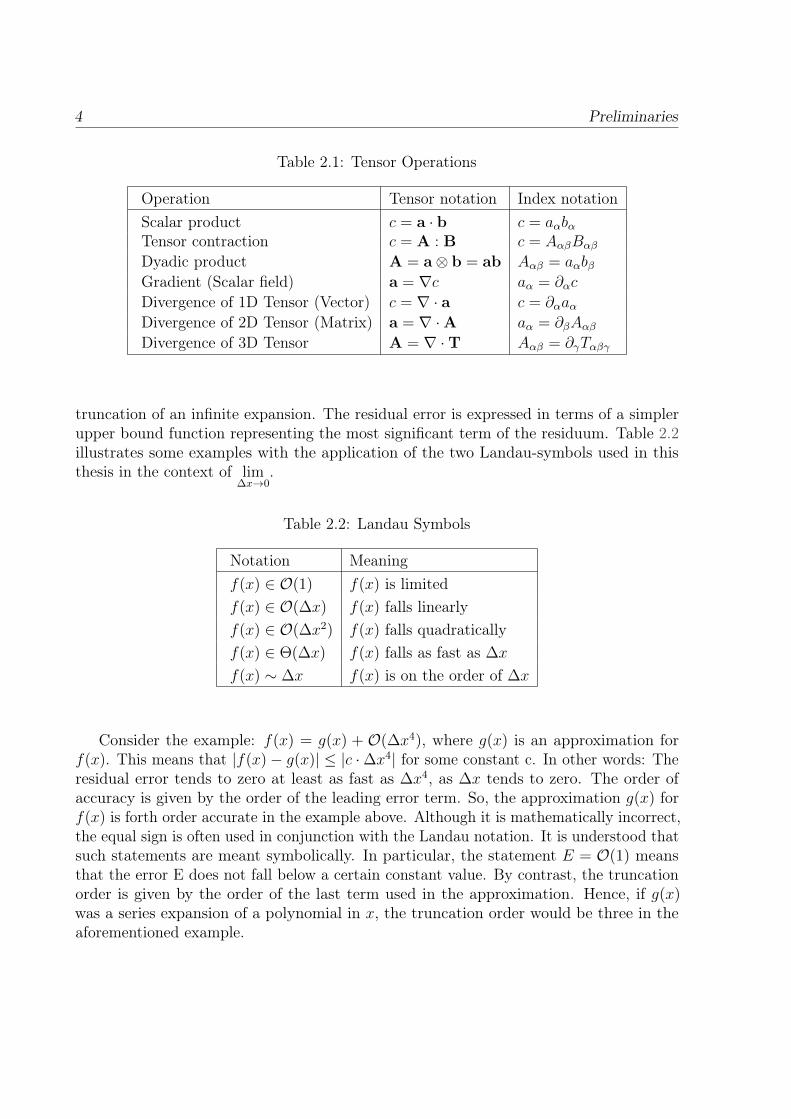
In the style of [40], it is useful to define some frequently used tensor operations along withtheir notation used throughout this thesis. Vectors will be denoted by bold lower caseletters a and higher order Tensors by bold capital letters A. The corresponding indexnotation will appear in normal type with indices in lower case Greek letters. Accordingly,a plain scalar quantity is written in normal type lower case letters. Preferably, the tensornotation is used, but to achieve lucidity, we will switch to index notation where appropriate.In conjunction with index notation, the Einstein summation convention is employed. Thismeans if a single term contains the same index repeatedly the sum over that index is impliedwithout explicitly writing a summation sign. To distinguish operations involving the ∇operator, the divergence operation is denoted by a dot product in contrast to the gradientoperation. Furthermore, it is common practice in the Lattice Boltzmann community todenote partial derivatives by an index such that spatial derivatives become ∂/∂xα = ∂αand temporal derivatives become ∂/∂t = ∂t. The following Table 2.1 illustrates somecommon operations.
2.1.2 Landau Notation
For the sake of formality, a brief description of the Landau notation is given. Landausymbols are used here to express asymptotic behavior of a function when their argumenttends to zero. This is commonly used to describe the residual error due to discretization or
3
4 Preliminaries
Table 2.1: Tensor Operations
Operation Tensor notation Index notationScalar product c = a · b c = aαbαTensor contraction c = A : B c = AαβBαβ
Dyadic product A = a⊗ b = ab Aαβ = aαbβGradient (Scalar field) a = ∇c aα = ∂αc
Divergence of 1D Tensor (Vector) c = ∇ · a c = ∂αaαDivergence of 2D Tensor (Matrix) a = ∇ ·A aα = ∂βAαβDivergence of 3D Tensor A = ∇ ·T Aαβ = ∂γTαβγ
truncation of an infinite expansion. The residual error is expressed in terms of a simplerupper bound function representing the most significant term of the residuum. Table 2.2illustrates some examples with the application of the two Landau-symbols used in thisthesis in the context of lim
∆x→0.
Table 2.2: Landau Symbols
Notation Meaningf(x) ∈ O(1) f(x) is limitedf(x) ∈ O(∆x) f(x) falls linearlyf(x) ∈ O(∆x2) f(x) falls quadraticallyf(x) ∈ Θ(∆x) f(x) falls as fast as ∆x
f(x) ∼ ∆x f(x) is on the order of ∆x
Consider the example: f(x) = g(x) + O(∆x4), where g(x) is an approximation forf(x). This means that |f(x)− g(x)| ≤ |c ·∆x4| for some constant c. In other words: Theresidual error tends to zero at least as fast as ∆x4, as ∆x tends to zero. The order ofaccuracy is given by the order of the leading error term. So, the approximation g(x) forf(x) is forth order accurate in the example above. Although it is mathematically incorrect,the equal sign is often used in conjunction with the Landau notation. It is understood thatsuch statements are meant symbolically. In particular, the statement E = O(1) meansthat the error E does not fall below a certain constant value. By contrast, the truncationorder is given by the order of the last term used in the approximation. Hence, if g(x)was a series expansion of a polynomial in x, the truncation order would be three in theaforementioned example.
Route to the Lattice Boltzmann Equation 5
2.2 The Boltzmann EquationThe Boltzmann equation expresses the balance of molecules with respect to an infinitesimalvolume in phase space. The 6-dimensional phase space is the union of the physical spaceexpressed by space vector x and the space of absolute molecular velocities expressed by thevelocity vector ξ . In this context, the molecules are mathematically captured through aprobability density function f(x, ξ, t). At a fixed time t, this function gives the probabilityto find a molecule moving with velocity ξ+dξ at a place x+dx. Hereafter, the probabilitydensity function will synonymously be called probability distribution or simply distributionand its arguments will be dropped unless it is useful for comprehensibility.
Our starting point of the route to the Lattice Boltzmann equation is the BGK approxi-mation of the Boltzmann equation without external forces [28, 59, 61]:
∂tf + ξ · ∇f =1
τ(f eq − f). (2.1)
As already stated, the Boltzmann equation balances molecules in an infinitesimal volumein phase space. The left hand side is the material derivative of f describing the rate ofchange of the probability distribution through transport (advection) of the molecules.Molecules may also change their velocity as a consequence of inter-molecular collisionand, therefore, drop out of or enter the infinitesimal volume in phase space. Thus, theright hand side of the equation expresses the rate of change of f through collision of themolecules.
In the above equation (2.1), the original mathematically complex operator describinginter-molecular collisions is already replaced by a much simpler collision operator. Froman engineer’s point of view, collisions between particular molecules are of no importance.What matters is their long term effect on the macroscopic quantities. By experience,we know that a gas in non-equilibrium state relaxes towards its equilibrium state aftera fair amount of collisions took place. So, we substitute the original collision operatorwith the relaxation of the distribution towards its equilibrium expressed by f eq with acharacteristic collision time τ where 1/τ is called collision frequency. The time neededto reach equilibrium is different for different kinds of gases. As it will turn out, thecollision time must be connected with the viscosity of the gas. This model is known asthe BGK approximation of the collision operator due to the originators Bhatnagar, Gross,and Kroog [3] and is the basis of the majority of LBM models used. The BGK collisionoperator conserves mass, momentum, and energy. As stated in the introduction we willrestrict ourselves to isothermal and weakly compressible flows for which the temperatureis constant and the energy conservation will not be considered in the sequel.
2.2.1 Equilibrium Distribution
The equilibrium state is characterized by vanishing gradients of macroscopic quantities.Transferred to the microscopic view of a gas in the continuum limit, the equilibrium
6 The Boltzmann Equation
state is given if the collision integral vanishes. That is, if for every molecule leavingthe infinitesimal volume in phase space, an inverse collision can be found for which another molecule enters it. When gradients vanish, it is perspicuous that the probabilitydistribution should be spherically symmetric. The equilibrium distribution is given by thewell known Maxwell-Boltzmann distribution [24, 28],
f eq =ρ
(2πRT )3/2· exp
(−(ξ − u)2
2RT
), (2.2)
where R is the specific gas constant, T the Temperature, u the macroscopic flow velocity,and ρ the density.
2.2.2 Moments of the Continuous Distribution
The link between the microscopic state and the macroscopic variables is established throughthe calculation of the moments m of the distribution function. A moment is generallydefined as the integral of the product of a function a(ξ)k with the probability distributionf over ξ
m =
∫ξ
a(ξ)k · f dξ. (2.3)
We will define moments up to order k by which the order is determined through the orderof the tensor product in the function a(ξ)k. From this definition, an arbitrary numberof moments can be defined at which only low order moments can be assigned a physicalmeaning. For the purpose of the simulation of isothermal and weakly compressible fluidflow, we define moments up to order three. Moments in equilibrium state meq are buildfrom the equilibrium distribution eq. (2.2) for which the integrals give [11, 28, 59]
ρ =
∫f eq dξ (2.4)
ρu =
∫ξf eq dξ (2.5)
Πeq =
∫ξξf eq dξ = pI + ρuu (2.6)
Qeq =
∫ξαξβξγf
eq dξ = ρuαuβuγ + p(uαδβγ + uβδαγ + uγδαβ), (2.7)
where p is the thermodynamic pressure . The quantities mass and momentum do notcontain non-equilibrium contributions fneq = f − f eq and are, thus, conserved duringcollision in eq. (2.1), ∫
f − f eq dξ =
∫fneq dξ = 0 (2.8)∫
ξ(f − f eq) dξ =
∫ξfneq dξ = 0.
Route to the Lattice Boltzmann Equation 7
We will call this the conservation condition or, more generally, solvability conditionfollowing the terminology in the literature. Thus, with eq. (2.8) we get the followingmoments up to the second order from the complete distribution,
ρ =
∫f dξ
ρu =
∫ξf dξ
Π =
∫ξξf dξ = pI + ρuu− σ. (2.9)
Here, the stress tensor σ arises from the non-equilibrium part of the distribution.
2.3 The Discrete Boltzmann Equation
In order to end up with a method that can be implemented in a computer code, the phasespace has to be discretized. For reasons of structuring, the result of this step will be givenin advance. The discrete Boltzmann equation in contrast to its continuous counterpartreads
∂tfi + ξi · ∇fi =1
τ(f eqi − fi). (2.10)
This section is intended to present the basis for the discretization of the continuousBoltzmann equation. To this end, we need to introduce a few correlations and definitions.It is well known that the speed of sound cs of a gas is temperature dependent and can becalculated using the specific gas constant and the isotropic exponent κ,
cs =√κRT . (2.11)
In the context of LBM, κ is simply chosen to be unity. Furthermore, the Mach numberMa is introduced, which is the ratio of a characteristic flow speed U to the speed of sound,
Ma =U
cs. (2.12)
Throughout this thesis, we will assume that the macroscopic flow velocity is of the orderof the characteristic flow speed,
|u| ∼ U. (2.13)
Finally, because we simulate isothermal, weakly compressible flows, the equation of statefor an ideal gas simplifies to
p = c2sρ. (2.14)
8 The Discrete Boltzmann Equation
2.3.1 Discrete Equilibrium Distribution
For the following investigation, the equilibrium function eq. (2.2) is subdivided into termsinvolving u and terms not involving u:
f eq =ρ
(2πRT )3/2· exp
(− ξ2
2RT+
ξ · uRT− u2
2RT
)(2.15)
=ρ
(2πRT )3/2· exp
(− ξ2
2RT
)· exp
(ξ · uRT− u2
2RT
).
The exponential functions may be expanded in a Taylor series around zero up to secondorder,
exp(x) = 1 + x+x2
2!+O(x3) |x| 1. (2.16)
It can be easily shown through generalized ratio test that this series converges everywhere.However, this truncated series at second order will only yield reasonable results forarguments close enough to zero. Expanding the macroscopic velocity dependent exponentialfunction and using eq. (2.11) together with eq. (2.13) yields
f eq = w(ξ)ρ ·
1 +ξ · uc2s︸ ︷︷ ︸
O(Ma)
− u · u2c2s︸ ︷︷ ︸
O(Ma2)
+(ξ · u)2
2c4s︸ ︷︷ ︸
O(Ma2)
− ξ · u · u · u2c4s︸ ︷︷ ︸
O(Ma3)
+(u · u)2
8c4s︸ ︷︷ ︸
O(Ma4)
, (2.17)
where the remaining terms are summarized in a weighting factor w(ξ) . Truncating atsecond order in Mach gives the equilibrium function, which is only valid for small Machnumbers because of the second order Taylor expansion as shown above,
f eq = w(ξ)ρ ·(
1 +ξ · uc2s
+ξ · u · ξ · u
2c4s
− u · u2c2s
)(2.18)
= w(ξ)ρ ·(
1 +ξαuαc2s
+ξαuαξβuβ
2c4s
− uαuαc2s
2c4s
)= w(ξ)ρ ·
(1 +
ξαuαc2s
+(ξαξβ − c2
sδαβ)uαuβ2c4s
)= w(ξ)ρ ·
(1 +
ξ · uc2s
+1
2c4s
(ξξ − c2sI) : uu
).
Discretization of phase space means that, in addition to the domain discretization, thevelocity space needs to be discretized as well. From the microscopic point of view, werestrict the possible direction of motions of the molecules to a finite set of molecular
Route to the Lattice Boltzmann Equation 9
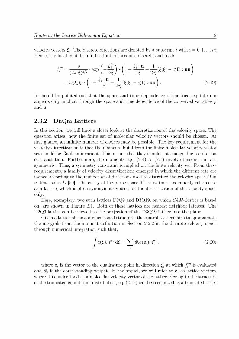
velocity vectors ξi .The discrete directions are denoted by a subscript i with i = 0, 1, ...,m.Hence, the local equilibrium distribution becomes discrete and reads
f eqi =ρ
(2πc2s)
3/2· exp
(− ξ2
i
2c2s
)·(
1 +ξi · uc2s
+1
2c4s
(ξiξi − c2sI) : uu
)= w(ξi)ρ ·
(1 +
ξi · uc2s
+1
2c4s
(ξiξi − c2sI) : uu
). (2.19)
It should be pointed out that the space and time dependence of the local equilibriumappears only implicit through the space and time dependence of the conserved variables ρand u.
2.3.2 DnQm Lattices
In this section, we will have a closer look at the discretization of the velocity space. Thequestion arises, how the finite set of molecular velocity vectors should be chosen. Atfirst glance, an infinite number of choices may be possible. The key requirement for thevelocity discretization is that the moments build from the finite molecular velocity vectorset should be Galilean invariant. This means that they should not change due to rotationor translation. Furthermore, the moments eqs. (2.4) to (2.7) involve tensors that aresymmetric. Thus, a symmetry constraint is implied on the finite velocity set. From theserequirements, a family of velocity discretizations emerged in which the different sets arenamed according to the number m of directions used to discretize the velocity space Q inn dimensions D [50]. The entity of the phase space discretization is commonly referred toas a lattice, which is often synonymously used for the discretization of the velocity spaceonly.
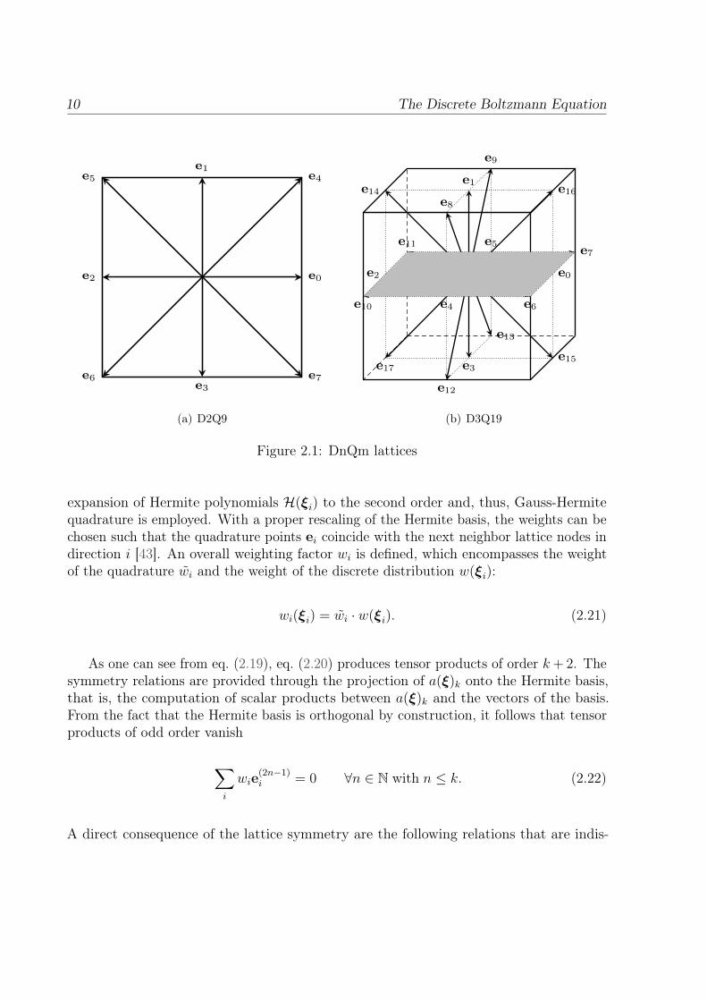
Here, exemplary, two such lattices D2Q9 and D3Q19, on which SAM-Lattice is basedon, are shown in Figure 2.1. Both of these lattices are nearest neighbor lattices. TheD2Q9 lattice can be viewed as the projection of the D3Q19 lattice into the plane.
Given a lattice of the aforementioned structure, the central task remains to approximatethe integrals from the moment definition in Section 2.2.2 in the discrete velocity spacethrough numerical integration such that,∫
a(ξ)kfeq dξ =
∑i
wia(ei)kfeqi , (2.20)
where ei is the vector to the quadrature point in direction ξi at which feqi is evaluated
and wi is the corresponding weight. In the sequel, we will refer to ei as lattice vectors,where it is understood as a molecular velocity vector of the lattice. Owing to the structureof the truncated equilibrium distribution, eq. (2.19) can be recognized as a truncated series
10 The Discrete Boltzmann Equation
e0
e1
e2
e3
e5
e7
e4
e6
(a) D2Q9
e0
e1
e2
e3
e4
e5
e6
e7
e8
e9
e10
e11
e12
e13
e14
e15
e16
e17
(b) D3Q19
Figure 2.1: DnQm lattices
expansion of Hermite polynomials H(ξi) to the second order and, thus, Gauss-Hermitequadrature is employed. With a proper rescaling of the Hermite basis, the weights can bechosen such that the quadrature points ei coincide with the next neighbor lattice nodes indirection i [43]. An overall weighting factor wi is defined, which encompasses the weightof the quadrature wi and the weight of the discrete distribution w(ξi):
wi(ξi) = wi · w(ξi). (2.21)
As one can see from eq. (2.19), eq. (2.20) produces tensor products of order k + 2. Thesymmetry relations are provided through the projection of a(ξ)k onto the Hermite basis,that is, the computation of scalar products between a(ξ)k and the vectors of the basis.From the fact that the Hermite basis is orthogonal by construction, it follows that tensorproducts of odd order vanish
∑i
wie(2n−1)i = 0 ∀n ∈ N with n ≤ k. (2.22)
A direct consequence of the lattice symmetry are the following relations that are indis-
Route to the Lattice Boltzmann Equation 11
pensable lattice properties for the goal to simulate fluid dynamics [28, 40]:
∑i
wi = 1 (2.23)∑i
wieiαeiβ = c2sδαβ (2.24)∑
i
wieiαeiβeiγeiδ = c4s(δαβδγδ + δαγδβδ + δαδδβγ). (2.25)
Therefore, with this order of truncation of the equilibrium function, the lattice must bechosen so that it is able to recover symmetric 4th rank tensors because we have k ≤ 3.
The lattices in Figure 2.1 are also known under the name of multi-speed latticesbecause of the different length of the ei vectors. In fact, these lattices possess threedifferent normalized magnitudes of lattice speeds:
√2 for the cross links, 1 for the
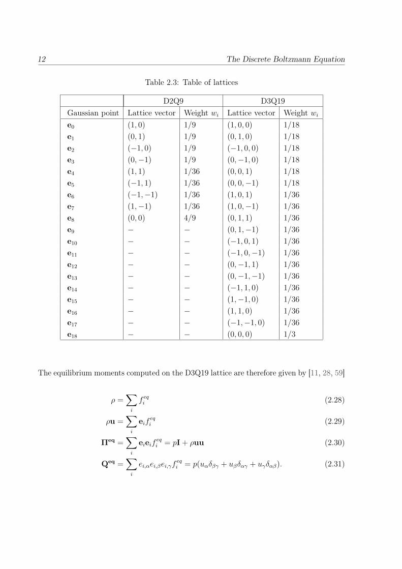
principle axis links, and 0 for the zero direction representing particles at rest. Table 2.3summarizes the Gaussian quadrature points, which coincide with the neighbor nodes andtheir corresponding weights.
An important result of the discretization of the velocity space is the constant (andlattice specific) relation between the components ξ of the molecular velocity vector ξ andthe speed of sound
ξ =√
3cs, (2.26)
which states that ξ ∼ cs. With eq. (2.26), the weighting factor w(ξi) becomes constantand so does the overall weighting factor wi for which the values are given in Table 2.3.
For the derivation of the integral approximations using Gauss-Hermite quadrature, thereader is referred to [57]. An extensive discussion on different lattice structures may befound in [61].
2.3.3 Moments of the Discrete Distribution
With the findings in Section 2.3.2, we can calculate the macroscopic moments from thediscrete probability distribution function by applying the integration formulas. Thus, thediscrete and truncated equilibrium eq. (2.19) takes its final lattice form:
f eqi = wiρ ·(
1 +ei · uc2s
+1
2c4s
(eiei − c2sI) : uu
). (2.27)
12 The Discrete Boltzmann Equation
Table 2.3: Table of lattices
D2Q9 D3Q19Gaussian point Lattice vector Weight wi Lattice vector Weight wie0 (1, 0) 1/9 (1, 0, 0) 1/18
e1 (0, 1) 1/9 (0, 1, 0) 1/18
e2 (−1, 0) 1/9 (−1, 0, 0) 1/18
e3 (0,−1) 1/9 (0,−1, 0) 1/18
e4 (1, 1) 1/36 (0, 0, 1) 1/18
e5 (−1, 1) 1/36 (0, 0,−1) 1/18
e6 (−1,−1) 1/36 (1, 0, 1) 1/36
e7 (1,−1) 1/36 (1, 0,−1) 1/36
e8 (0, 0) 4/9 (0, 1, 1) 1/36
e9 − − (0, 1,−1) 1/36
e10 − − (−1, 0, 1) 1/36
e11 − − (−1, 0,−1) 1/36
e12 − − (0,−1, 1) 1/36
e13 − − (0,−1,−1) 1/36
e14 − − (−1, 1, 0) 1/36
e15 − − (1,−1, 0) 1/36
e16 − − (1, 1, 0) 1/36
e17 − − (−1,−1, 0) 1/36
e18 − − (0, 0, 0) 1/3
The equilibrium moments computed on the D3Q19 lattice are therefore given by [11, 28, 59]
ρ =∑i
f eqi (2.28)
ρu =∑i
eifeqi (2.29)
Πeq =∑i
eieifeqi = pI + ρuu (2.30)
Qeq =∑i
ei,αei,βei,γfeqi = p(uαδβγ + uβδαγ + uγδαβ). (2.31)
Route to the Lattice Boltzmann Equation 13
It should be noted that the only moment that differs from its continuous counterpart isthe third order moment Qeq. The discrete version lacks the ρuuu term. This is due tothe fact that next neighbor lattices do not provide enough discrete directions to computethe third order moment correctly. Strictly speaking, this breaks the Galilean invariance[14], but it is often argued that the deviation is small, due to this term being O(Ma3) [51].A corresponding evaluation for the moments of the complete distribution yields:
ρ =∑i
fi
ρu =∑i
eifi
Π =∑i
eieifi = pI + ρuu− σ. (2.32)
With these definitions, the transition from the continuous LBE to the discrete LBE interms of phase space and the probability distribution is complete. Before we proceed tothe Lattice Boltzmann equation, we will show that a solution to the restricted (low Mach,isothermal) mesoscopic dynamics of the Boltzmann equation is in fact a solution to themacroscopic Navier-Stokes equations.
2.3.4 Derivation of the Navier-Stokes Equations
The basis of the derivation of the Navier-Stokes equations from the continuous Boltzmannequation is the Chapman-Enskog expansion. It is a pertubation method in which a smallparameter ε 1 is introduced to separate physical phenomena that happen on differentscales. Physically, the parameter ε can be interpreted as the Knudsen number Kn, which isthe ratio of the mean free path and a characteristic length scale L or a time scale equivalentT . We denote this by the infinitesimal space scale δx and time scale δt, respectively,
Kn =δx
L=δt
T= ε. (2.33)
In the Chapman-Enskog expansion, the distributions are expanded around equilibriumin powers of ε. Therefore, the distributions with a superscript represent corrections tothe non-equilibrium state, which get less important with increasing order of ε. As theKnudsen number is small, only small perturbations from equilibrium are allowed, whichrenders this method only valid for near continuum flows,
f = f eq + εf (1) + ε2f (2) +O(ε3). (2.34)
Additionally, the time scales and the corresponding differential operators are separated
∂t = ∂t0 + ε∂t1 +O(ε2). (2.35)
14 The Discrete Boltzmann Equation
Short term physics happens on order t1, whereas long term physics such as diffusionhappens on t0. Since the derivatives of the scales t0 and t1 may be of the same order, theparameter ε ensures appropriate hierarchy of scales. In the classical approach, the spacescales are also expanded and the relations eq. (2.34) and eq. (2.35) are inserted into asecond order Taylor expansion of eq. (2.1). Taking moments of these resulting equationsfor the different orders of ε leads to the Euler and Navier-Stokes equations, respectively.
An alternative formulation of the Chapman-Enskog procedure is highlighted by Dellarin [14], which we follow here in a more elaborated manner. In contrast to the classicalapproach, we take moments of eq. (2.1) first and expand the moments in ε. The resultingequations describe the evolution of the moments with contributions from different physicalscales. In that sense, the macroscopic equations are solutions to the moment equations onthe long term scale. We will use this fact by truncating the expansions at appropriateorders as shown below. The following moment expansion together with eq. (2.35) isintroduced:
Π = Πeq + εΠ(1) + ε2Π(2) +O(ε3)
Q = Qeq + εQ(1) + ε2Q(2) +O(ε3). (2.36)
Since the collision process happens locally, the space scales are left unexpanded. Theconserved moments eq. (2.4) and eq. (2.5) are also unexpanded because of the conservationcondition eq. (2.8).
We start the derivation by extracting the smallness parameter ε from the collision timethrough τ = ετ ∗. This formal rescaling ensures that both sides of the equation are oforder O(1). For simplicity and without loss of generality, the derivation is done using thecontinuous variables
∂tf + ξ · ∇f =1
ετ ∗(f eq − f). (2.37)
Next, we take moments of eq. (2.37) up to second order, starting with zero order moments∫∂tf dξ +
∫ξ · ∇f dξ =
1
ετ ∗
(∫f eq dξ −
∫f dξ
). (2.38)
The right hand side becomes zero by virtue of the conservation condition eq. (2.8). Applyingthe product rule backwards on the second term on the left hand side yields:
∂t
∫f dξ +
∫∇ · (fξ) dξ −
∫f∇ · ξ dξ = 0. (2.39)
By definition, the space derivative of the molecular velocity is zero. Inserting the time
Route to the Lattice Boltzmann Equation 15
expansion eq. (2.35), the equation further becomes
∂t0
∫f dξ + ε∂t1
∫f dξ +∇ ·
∫(fξ) dξ = 0 +O(ε2)
⇔ ∂t0ρ+ ε∂t1ρ+∇ · (ρu) = 0 +O(ε2). (2.40)
Now, we take first order moments. Again, the right hand side vanishes because of theconservation condition.
∂t0
∫ξf dξ + ε∂t1
∫ξf dξ +∇ ·
∫ξ(fξ) dξ = 0 +O(ε2) (2.41)
Inserting the moment expansion eq. (2.36) leads to:
∂t0ρu + ε∂t1ρu +∇ · (Πeq + εΠ(1)) = 0 +O(ε2) (2.42)
Accordingly, taking second order moments yields:
∂t0
∫ξξf dξ + ε∂t1
∫ξξf dξ +∇ ·
∫ξξ(fξ) dξ =
1
ετ ∗
(∫ξξf eq dξ −
∫ξξf dξ
)+O(ε2)
(2.43)Inserting the expansions eq. (2.36) gives a non-zero right hand side:
∂t0(Πeq+εΠ(1))+ε∂t1(Π
eq+εΠ(1))+∇·(Qeq+εQ(1)) =1
ετ ∗(Πeq − (Πeq + εΠ(1))
)+O(ε2)
(2.44)
Zeroth Order Truncation
Taking moments up to second order resulted in the equations (2.40), (2.42), and (2.44),which is enough to recover the Navier-Stokes equations. As one can see, each momentequation contains contributions for which higher order moments need to be determined.The moment equation of the next order in turn depends on subsequent moments. Therefore,one ends up with an infinite series of moment equations. The particular higher ordermoments can be viewed as corrections to the evolution of non-equilibrium moments. Totruncate this infinite series lies at the heart of the Chapman-Enskog expansion. Thus,truncating the derived moment equations at O(1) yields the compressible Euler equations:
∂t0ρ+∇ · (ρu) = 0 (2.45)∂t0ρu +∇ · (Πeq) = 0. (2.46)
With the definition of Πeq in eq. (2.6) we get
∂t0ρu +∇ · (pI + ρuu) = 0
⇔ ∂t0ρu + I · ∇p+ p∇ · I +∇ · (ρu⊗ u) = 0.
(2.47)
16 The Discrete Boltzmann Equation
For the evaluation of the divergence in the last term, we switch to index notation
∂t0ρuα + ∂αp+ ∂β(ρuαuβ) = 0
⇔ ∂t0ρuα + ∂αp+ uαuβ∂βρ+ ρuβ∂βuα + ρuα∂βuβ = 0. (2.48)
Factoring out uα and applying the product rule backwards yields
∂t0ρuα + ∂αp+ ρuβ∂βuα + uα(uβ∂βρ+ ρ∂βuβ) = 0
⇔ ∂t0ρu +∇p+ ρu · ∇u + u(∇ · (ρu)) = 0. (2.49)
Taking the time derivative and rearranging the resulting terms gives
u∂t0ρ+ ρ∂t0u +∇p+ ρu · ∇u + u(∇ · (ρu)) = 0
⇔ ρ(∂t0u + u · ∇u) + u(∂t0ρ+∇ · (ρu)) = −∇p. (2.50)
The last term in parenthesis on the left hand side represents the continuity equation (2.45)and is, therefore, equal to zero. What remains is the total derivative of u. This is themomentum equation of the Euler equations
ρDu
Dt0= −∇p
⇔ ∂t0u + u · ∇u = −1
ρ∇p. (2.51)
There is no external force and especially no friction present. Fluid motion is merelygoverned by pressure gradients. The incorporation of viscous forces leads to the Navier-Stokes equations.
First Order Truncation
In the context of our derivation, we truncate the moment expansion at order O(ε) andcompute the first order correction to the momentum flux εΠ(1) apparent in eq. (2.42).Truncating eq. (2.40), eq. (2.42), and eq. (2.44) at O(ε) gives,
∂t0ρ+ ε∂t1ρ+∇ · (ρu) = 0 (2.52)
∂t0ρu + ε∂t1ρu +∇ · (Πeq + εΠ(1)) = 0 (2.53)
∂t0(Πeq + εΠ(1)) + ε∂t1(Π
eq + εΠ(1)) +∇ · (Qeq + εQ(1)) = − 1
τ ∗Π(1). (2.54)
Because mass and momentum are conserved during collisions, terms of the scale t1 haveno impact on those quantities. Therefore, eq. (2.52) and eq. (2.53) simplify to:
∂t0ρ+∇ · (ρu) = 0 (2.55)
∂t0ρu +∇ · (Πeq + εΠ(1)) = 0. (2.56)
Route to the Lattice Boltzmann Equation 17
The second order moment equation (2.54) gives the evolution of the first non-equilibriumcontribution of the momentum flux Π(1). In order to compute the first correction εΠ(1) ineq. (2.56), we multiply eq. (2.54) with ε,
∂t0(εΠeq + ε2Π(1)) + ε2∂t1(Π
eq + εΠ(1)) +∇ · (εQeq + ε2Q(1)) = − 1
τ ∗εΠ(1). (2.57)
On the current truncation order, terms of order O(ε2) are neglected. Thus the firstcorrection term depends on the equilibrium part of the second and third order momentsonly,
∂t0εΠeq +∇ · εQeq = − 1
τ ∗εΠ(1)
⇔ −ετ ∗(∂t0Πeq +∇ ·Qeq) = εΠ(1). (2.58)
Obviously, Π(1) consists of the two contributions in parentheses, which we will examineseparately to attain their meaning in the macroscopic equation. Inserting the definition ofΠeq from eq. (2.6) gives
∂t0Πeq = ∂t0(c
2sρI + ρuu)
= c2sI∂t0ρ+ ∂t0(ρu)⊗ u + ρu⊗ ∂t0u
= c2sI∂t0ρ+ ∂t0(ρu)u + ρu∂t0u. (2.59)
Because Πeq is an equilibrium quantity, we can use the O(1) approximation of eq. (2.46)to obtain
∂t0Πeq = c2
sI∂t0ρ+ (−∇ ·Πeq)u + ρu∂t0u. (2.60)
Applying the product rule backwards on the last term and subsequent insertion of eq. (2.46)gives
∂t0Πeq = c2
sI∂t0ρ+ (−∇ ·Πeq)u + u(∂t0ρu− u∂t0ρ)
= c2sI∂t0ρ+ (−∇ ·Πeq)u + u(−∇ ·Πeq)− uu∂t0ρ. (2.61)
Using the definition of Πeq and eliminating the last time derivative through the continuityequation eq. (2.45) leads to
∂t0Πeq = c2
sI∂t0ρ− (∇ · (c2sρI + ρuu))u− u(∇ · (c2
sρI + ρuu))− uu∂t0ρ
= −c2sI∇ · (ρu)− (c2
s∇ · (ρI) +∇ · (ρuu))u− u((c2s∇ · (ρI) (2.62)
+∇ · (ρuu)) + uu∇ · (ρu)
= −c2sδαβ∂γρuγ − c2
suα∂βρ− uα∂γρuβuγ − c2suβ∂αρ− uβ∂γρuαuγ + uαuβ∂γρuγ,
18 The Discrete Boltzmann Equation
where the last two terms partly cancel to give the expression
∂t0Πeq = −c2
sδαβ∂γρuγ − c2suα∂βρ− c2
suβ∂αρ− uα∂γρuβuγ − uβρuγ∂γuα. (2.63)
The dyadic product in the last term is commutative, because the resulting tensor issymmetric. Thus, the last two terms can be collapsed in a single divergence term of athird rank tensor:
∂t0Πeq = −c2
sδαβ∂γρuγ − c2suα∂βρ− c2
suβ∂αρ− ∂γρuαuβuγ. (2.64)
Equation (2.64) gives an expression for the time derivative of the equilibrium part of themomentum flux tensor ∂t0Π
eqαβ. Next, the second part of the parentheses in eq. (2.58) is
examined. The divergence for the definition of the third order moment tensor eq. (2.7)gives
∂γQeqαβγ = ∂γρuαuβuγ + ∂γc
2sρuαδβγ + ∂γc
2sρuβδαγ + ∂γc
2sρuγδαβ. (2.65)
Applying the product rule and using the identity ∇I = 0 we get
∂γQeqαβγ = ∂γρuαuβuγ + c2
sδβγ∂γρuα + c2sδαγ∂γρuβ + c2
sδαβ∂γρuγ
= ∂γρuαuβuγ + c2s∂βρuα + c2
s∂αρuβ + c2sδαβ∂γρuγ
= ∂γρuαuβuγ + c2suα∂βρ+ c2
sρ∂βuα + c2sρ∂αuβ + c2
suβ∂αρ+ c2sδαβ∂γρuγ.
(2.66)
Rearranging the last equation finally gives an expression for the divergence of Qeq:
∂γQeqαβγ = c2
sδαβ∂γρuγ + c2suα∂βρ+ c2
suβ∂αρ+ ∂γρuαuβuγ + c2sρ(∂βuα + ∂αuβ). (2.67)
At this point, eq. (2.58) can be evaluated by adding the two expressions ∂t0Πeq and ∇·Qeq
that were just derived in detail. One can see that all terms except the last parenthesis ineq. (2.67) cancel on adding. Therefore, the first order correction term to the momentumflux is given by:
εΠ(1)αβ = −ετ ∗c2
sρ(∂βuα + ∂αuβ). (2.68)
Finally, the formal rescaling of eq. (2.37) is revoked by absorbing ε into the collisiontime τ ∗. Hence, the viscous contribution εΠ(1) takes the form:
εΠ(1)αβ = −τc2
sρ(∂βuα + ∂αuβ). (2.69)
Obviously, the expression in parenthesis is twice the macroscopic strain rate tensor ε.Thus, the dynamic viscosity µ is related to the collision time according to
µ = τc2sρ (2.70)
⇔ ν = τc2s, (2.71)
Route to the Lattice Boltzmann Equation 19
where ν is the kinematic viscosity and −εΠ(1)αβ is identified with the macroscopic stress
tensor σ,− εΠ(1) = σ. (2.72)
This finding explains the minus sign in the moment definition eq. (2.9). Note that thestress tensor encompasses the parameter ε, which will be illuminated in the next chapter.Now we can assemble the first order truncation, which incorporates viscous forces. Thezeroth order moment equation remains unchanged and the first order moment equationcontains the first correction term to the momentum flux εΠ(1). Therefore, we have
∂t0ρ+∇ · ρu = 0
ρ (∂t0uα + uβ∂βuα) = −∂αp+ ∂β (µ(∂βuα + ∂αuβ))
⇔ ∂t0u + u · ∇u = −1
ρ∇p+∇ ·
(ν(∇u + (∇u)T
)), (2.73)
where the same transformations were applied as for the Euler equations. Equation (2.73)is the isothermal compressible Navier-Stokes equation without external force. It should benoted, that through the isothermal assumption, the bulk viscosity is fixed to µ′ = µ(2/3)[11, 51].
2.4 The Lattice Boltzmann Equation
In the preceding sections, eq. (2.1) was discretized in phase space. Therefore, the continuousBoltzmann equation became discrete because the probability distribution function andthe molecular velocity in eq. (2.10) appear in their discretized form. Moreover, it wasshown that if the probability density function f is known at any time, the macroscopicsolutions of the Navier-Stokes equations are known through the moments of f . Thequestion remains, how fi is determined from the discrete Boltzmann equation. In order togain an equation for determining the probability distribution, eq. (2.10) has to be renderedfully discrete by additional discretization in time. Due to the second order accuracy in ε,the solutions to the Navier-Stokes equation are formally second order accurate in spaceand time because of eq. (2.33). A straightforward way to realize a second order timeaccuracy is the Cranck-Nicolson method where the time integration is done locally usingthe trapezoidal rule. The time step size will be denoted by ∆t. As already stated, the lefthand side of the Boltzmann equation describes the transport of the molecules, whereasthe right hand side is associated with the collision of molecules. Because the collisiontime is much smaller than the macroscopic time step size τ ∆t, the two operations canbe treated separately. However, it can be shown that such a time discretization resultsin first order accuracy only because of the operator splitting (transport and collision)in conjunction with local time integration [13]. A remedy is the integration along a
20 The Lattice Boltzmann Equation
characteristic, that is, a space-time integration, where the space step ∆x is replaced withξi∆t. Hence, integration of eq. (2.10) in space-time gives∫ ∆t
0
d fi(x + ξi · s, t+ s)
dsds =
1
τ
∫ ∆t
0
(f eqi (x + ξi · s, t+ s)− fi(x + ξi · s, t+ s)) ds,
(2.74)where the total derivative formulation on the left hand side integrates directly and yieldsthe difference between end and start point. In addition, the time step size is set so thatthe integration interval ends with the Gaussian quadrature point in direction i. Therefore,we have
ei = ∆x/∆t. (2.75)
More pictorially, ∆t is chosen so that the molecules with velocity ξi fly to the correspondingnearest neighbor node within one time step. The right hand side of the equation can beapproximated using the trapezoidal rule,
fi(x + ei∆t, t+ ∆t)− fi(x, t) =1
2τ∆t (f eqi (x + ei∆t, t+ ∆t)− fi(x + ei∆t, t+ ∆t)
+f eqi (x, t)− f(x, t)) +O(∆t2).
(2.76)
This equation is implicit because terms involving t + ∆t appear on the right hand sideof the equation. He et al. [30] introduced a change of variables to render the equationexplicit:
fi(x, t) = fi(x, t) +∆t
2τ(fi(x, t)− f eqi (x, t)) . (2.77)
The resulting equation is now solved for fi instead of fi and reads
fi(x + ei∆t, t+ ∆t)− fi(x, t) =∆t
τ + 0.5∆t
(f eqi (x, t)− fi(x, t)
). (2.78)
Furthermore, the fraction in eq. (2.78) is recognized as the dimensionless collision frequencyand is denoted by Ω. Mathematically, it is a relaxation parameter that controls therelaxation of fi towards the local equilibrium state. Here, the natural assumption thatthe relaxation parameter has to be connected with the viscosity of the gas is confirmedbecause the collision time appears in the denominator. With the relation eq. (2.71) thedimensionless collision time Ω can be written
Ω =∆t
τ + 0.5∆t=
c2s∆t
ν + 0.5c2s∆t
Ω ∈ [0, 2]. (2.79)
In contrast to the (time) continuous version of the discrete Boltzmann equation (2.10), thecollision time in the denominator contains an additional contribution, which steams from
Route to the Lattice Boltzmann Equation 21
discretization. It can be viewed as the lattice viscosity, which is absorbed in the collisiontime to yield the correct transport coefficient. The left side of eq. (2.10) represents thetransport step, which does not even contain any round off errors when implemented in acomputer code. Subsequent collision results in values for fi for the proximate time step,
fi(x + ei∆t, t+ ∆t) = fi(x, t) + Ω ·(f eqi (x, t)− fi(x, t)
). (2.80)
The macroscopic values needed to compute the local equilibrium prior to the collision stepare computed from the distributions fi(x, t) after the transport step. Equation (2.80) isthe well known Lattice Boltzmann equation (LBE), where we drop the overline of thechange of variables in the sequel. Fortunately, the change of variables does not affectthe conserved quantities because of the solvability condition eq. (2.8). Yet, higher ordermoments get affected, especially the macroscopic stress tensor εΠ(1). However, a problemis its correct computation because the direct computation of εΠ(1) from the distributionsrequires the knowledge of f (1) and ε. Thus, the term εΠ(1) is approximated with thenon-equilibrium part of the momentum flux tensor and the moment expansion eq. (2.36):
εΠ(1) ≈ Πneq = Π−Πeq
= εΠ(1) +O(ε2). (2.81)
The expression in eq. (2.81) reveals that the approximation of the stress tensor is formallysecond order accurate within the Lattice Boltzmann framework. This statement is sup-ported with numerical results from SamLattice in [56] and the literature, e.g., [37].Now, with the change of variables, the computation of the non-equilibrium part of thesecond order moment from the distributions fi yields
Π−Πeq
= Π +∆t
2τ(Π−Πeq)−Πeq
=
(1 +
∆t
2τ
)(Π−Πeq)
⇔ Πneq =
(1 +
∆t
2τ
)−1 (Π−Π
eq)
(2.82)
⇔ εΠ(1) ≈(
1 +∆t
2τ
)−1
Πneq
. (2.83)
The overlines of the momentum flux tensor will be dropped for simplicity in the sequelas well. Finally, the generalized Hook’s law for isotropic materials gives the stress-strainrelation [11, 35], which was already implicitly used in eq. (2.69), eq. (2.70), and eq. (2.72),
σ = 2µε + µ′Tr (ε) I. (2.84)
22 The Lattice Boltzmann Equation
Here, Tr (ε) = 0 in the incompressible limit. This relates the second order moment tensorto the macroscopic stress tensor using eq. (2.72) in the following way
σ = −(
1 +∆t
2τ
)−1
Πneq
= −(
1 +c2s∆t
2ν
)−1
Πneq
= −(
2ν + c2s∆t
2c2s∆t
· c2s∆t
ν
)−1
Πneq
= − Ων
c2s∆t
Πneq, (2.85)
where the relations eq. (2.69), eq. (2.70), and eq. (2.79) were used.
2.4.1 Accuracy
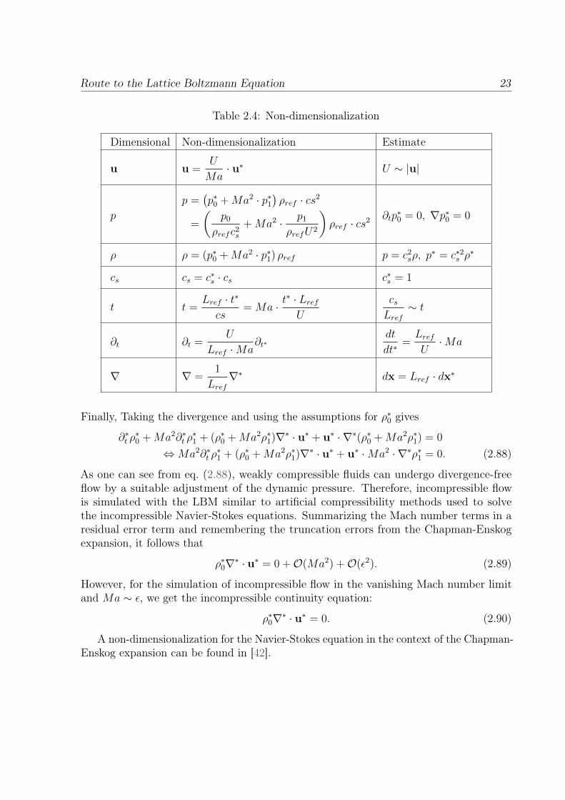
This section deals with the accuracy of the LBM for the simulation of weakly compressibleand incompressible fluids. For this purpose, we investigate the continuity equation andhave a look at the various error terms present in a simulation. In order to providean order of magnitude estimate, the continuity equation is non-dimensionalized. Wewill denote dimensionless values by an asterisk. To this end, the non-dimensionalizedquantities are introduced together with their estimation in Table 2.4. Most definitions arestraightforward, except the pressure transformation. The pressure is split into two parts,where p0 is the thermodynamic pressure and p1 is the dynamic pressure. It is assumed thatthe thermodynamic pressure is spatially and temporally constant and scales with the speedof sound. By contrast, p1 scales proportional to the dynamic reference pressure ρrefU2.Because U is on the macroscopic scale and cs on the molecular scale, the dimensionlessdynamic pressure has to be rescaled with Ma2. Accordingly, things are similar for thedensity transformation because of the isothermal equation of state. With these definitions,the continuity equation can be rewritten:
∂tρ+∇ · (ρu) = 0
⇔ (∂tp∗0 +Ma2∂tp
∗1) · ρref +∇ · ((p∗0 +Ma2p∗1) · ρref · u) = 0
⇔ (∂tρ∗0 +Ma2∂tρ
∗1) · ρref +
1
Lref∇∗ · ((ρ∗0 +Ma2ρ∗1) · ρref ·
U
Mau∗) = 0 (2.86)
Introducing the dimensionless time derivative and simplifying the equation yields
(∂∗t ρ∗0 +Ma2∂∗t ρ
∗1) · ρref ·
U
Lref ·Ma+
1
Lref∇∗ · ((ρ∗0 +Ma2ρ∗1) · ρref ·
U
Mau∗) = 0
⇔ ∂∗t ρ∗0 +Ma2∂∗t ρ
∗1 +∇∗ · ((ρ∗0 +Ma2ρ∗1) · u∗) = 0.
(2.87)
Route to the Lattice Boltzmann Equation 23
Table 2.4: Non-dimensionalization
Dimensional Non-dimensionalization Estimate
u u =U
Ma· u∗ U ∼ |u|
p
p =(p∗0 +Ma2 · p∗1
)ρref · cs2
=
(p0
ρrefc2s
+Ma2 · p1
ρrefU2
)ρref · cs2 ∂tp
∗0 = 0, ∇p∗0 = 0
ρ ρ = (p∗0 +Ma2 · p∗1) ρref p = c2sρ, p
∗ = c∗2s ρ∗
cs cs = c∗s · cs c∗s = 1
t t =Lref · t∗cs
= Ma · t∗ · LrefU
csLref
∼ t
∂t ∂t =U
Lref ·Ma∂t∗
dt
dt∗=LrefU·Ma
∇ ∇ =1
Lref∇∗ dx = Lref · dx∗
Finally, Taking the divergence and using the assumptions for ρ∗0 gives
∂∗t ρ∗0 +Ma2∂∗t ρ
∗1 + (ρ∗0 +Ma2ρ∗1)∇∗ · u∗ + u∗ · ∇∗(ρ∗0 +Ma2ρ∗1) = 0
⇔Ma2∂∗t ρ∗1 + (ρ∗0 +Ma2ρ∗1)∇∗ · u∗ + u∗ ·Ma2 · ∇∗ρ∗1 = 0. (2.88)
As one can see from eq. (2.88), weakly compressible fluids can undergo divergence-freeflow by a suitable adjustment of the dynamic pressure. Therefore, incompressible flowis simulated with the LBM similar to artificial compressibility methods used to solvethe incompressible Navier-Stokes equations. Summarizing the Mach number terms in aresidual error term and remembering the truncation errors from the Chapman-Enskogexpansion, it follows that
ρ∗0∇∗ · u∗ = 0 +O(Ma2) +O(ε2). (2.89)
However, for the simulation of incompressible flow in the vanishing Mach number limitand Ma ∼ ε, we get the incompressible continuity equation:
ρ∗0∇∗ · u∗ = 0. (2.90)
A non-dimensionalization for the Navier-Stokes equation in the context of the Chapman-Enskog expansion can be found in [42].
24 The Lattice Boltzmann Equation
Given that the LBM is a numerical scheme, different sources of errors are present ina simulation. First, there are typical discretization errors that scale like the square ofthe step sizes used, because of the second order accuracy in ε. Namely, the space errorEx = O(∆x2) and the time error Et = O(∆t2). Moreover, the equations in this sectionshow that there is a compressibility error present that scales like Ma2 when incompressiblefluids are simulated with the LBM approach. Thus, the compressibility error can beexpressed as EMa = O(∆t2/∆x2). As stated in [40], the overall error is composed of thesethree contributions:
E = Ex + Et + EMa = O(∆x2) +O(∆t2) +O(∆t2/∆x2). (2.91)
However, this statement does not account for truncation errors of the numerical scheme.As it was proposed by Junk [33], the LBM can be viewed as a finite difference scheme.A comprehensive study based on a truncation error analysis of the Boltzmann equation[32] indicates that the relaxation parameter Ω is used as a weight to create an effectivefinite difference stencil out of the nearest neighbors finite different stencil. Both stencilscoincide at Ω = 1.0. A result of the truncation error analysis is that the value of therelaxation time can be used to minimize numerical diffusion errors. Therefore, there areadditional errors due to an improper choice of the value of the dimensionless collision time.For details of these investigations the reader is referred to [32]. The findings of [32] arenumerically confirmed in, e.g., [36]. Because Ω cannot be chosen independently, eq. (2.91)may be valid for simulations with a fixed Reynolds number where the viscosity is constant.However, for the simulation of non-Newtonian fluids, the dimensionless collision time canvary as will be shown in Section 2.5.3. Thus, an additional error term EΩ is introduced.The influence of this error source will be investigated in Chapter 7. Moreover, the finiterepresentation of the simulation geometry introduces an error Eg to the overall error. Thistrite source of error is often forgotten in practical simulations. The simulation domainis approximated with a discretization of the domain boundaries, which is independentof the lattice discretization. We denote the geometry discretization step size by ∆g. InSection 4.2.2 we will have a look at the geometry discretization in conjunction with wallboundary conditions. As a result, one can state that the geometry discretization has tobe chosen such that ∆x ∼ ∆g and ∆g = Θ(∆x). Finally, there are additional errors dueto imperfect boundary conditions that we denote by EBC . Sometimes, these are fairlyhard to quantify. For wall boundary conditions there exists schemes with EBC = O(∆x2).Therefore, the overall error is extended to
E = Ex + Et + EMa + EΩ + Eg + EBC . (2.92)
This definition only summarizes the main sources of error, which crucially determine themethod’s convergence.
Route to the Lattice Boltzmann Equation 25
2.4.2 Diffusive Scaling vs. Acoustic Scaling
In order to improve the accuracy of a LBM simulation, one has the possibility to increasethe spatial resolution to capture gradients more precisely. But this cannot be doneindependently of the time step size since both are coupled through the simulation Mach-number Ma ∝ ∆t/∆x. Therefore, for weakly compressible flow where the physicalMach-number has to be met, the time step size has to be rescaled like ∆t ∝ ∆x in orderto keep the simulation Mach-number constant. This scaling is known as the acousticscaling. The name is inspired from the fact that the speed of sound is held constant.Also this scaling is used for grid refinement to keep the macroscopic variables continuousacross grid scales. However, for incompressible fluids, the acoustic scaling creates a racecondition between decreasing spatial and temporal errors and increasing compressibilityerrors when increasing the resolution. This actually results in divergence behavior whenthe compressibility errors begin to dominate [40]. This can also be seen in the definitionabove. One can state that the acoustic scaling results in a O(1) behavior of the overallerror:
E = Ex + Et + EMa = O(∆x2) +O(∆x2) +O(∆x2/∆x2) (2.93)E = O(1). (2.94)
The divergence behavior was already found by Reider and Sterling [52] who state that allerror terms must be reduced consistently. Thus, the diffusive scaling is introduced, whichscales ∆t ∝ ∆x2 [34]. That way, if the spacing is halved, the Mach number is halved aswell, which consequently reduces compressibility effects. This scaling results in secondorder convergence behavior:
E = Ex + Et + EMa = O(∆x2) +O(∆x4) +O(∆x4/∆x2) (2.95)E = O(∆x2). (2.96)
An important remark is that the diffusive scaling reduces the time accuracy effectively tofirst order because reducing the error by a factor ∆x2 results in a 1/∆x2 factor increase inthe number of time steps needed.
2.4.3 Stability
For the sake of completeness, a short discussion on the stability of the LBM should begiven.
It is well known that the Lattice Boltzmann algorithm becomes unstable when theviscosity is low and the collision frequency Ω approaches 2. The equilibrium distribution iscrucial in the theoretical framework of the LBM. By definition, the Maxwell distributionsatisfies the Second Law of thermodynamics [28]. Unfortunately, the compliance with the
26 Extensions to LBM
H-theorem is lost in the course of the discretization. In fact, one can prove, that it isimpossible to construct polynominal equilibria with this property [63].
Incipient instability manifests itself in spurious oscillations of the solution variables.Actual divergence occurs, when one of the distributions becomes negative. Several ap-proaches to prevent the instability were developed in the past. A group of LBM modelsemerged, which restore the compliance with the H-theorem. They use a different form ofthe equilibrium and solve an entropic estimate equation during collision and are, therefore,known under the name Entropic Lattice Boltzmann Methods (ELBM). One simple andyet robust way to ensure stability is the positivity rule or also known as "fix-up" or "hyperviscosity" model. This rule states, that if a distribution becomes negative after the collision,the collision is rerun with just enough artificial viscosity to ensure that the minimum valueof the distribution is zero. A comparison of the positivity rule and the ELBM can befound in [60].
Introduction of artificial viscosity is a major obstacle to the simulation of, e.g., acousticwaves. An attempt to overcome this problem was developed by Ricot et al. [54], who usefiltering on the LBE to damp out unwanted modes of the oscillating variables.
Details on the implementation of stability measures in SamSolver can be found in thePhD thesis of Schneider [56]. For an extensive discussion on stabilization of the LatticeBoltzmann Method, the reader is referred to [7].
2.5 Extensions to LBM
In this section, some extensions to the LBM are introduced, which are used in the courseof this thesis.
2.5.1 Multiple Relaxation Time
It is well known that the Lattice Boltzmann algorithm is not unconditionally stable. Itsuffers from numerical instability when the viscosity gets very low or the simulation isunder-resolved. Both cases have the effect that the relaxation parameter Ω approachestwo, as can be seen from eq. (2.79). Because Ω is the only free parameter in eq. (2.80),this model is known as the single relaxation time (SRT) model. An improvement in termsof numerical stability is the multiple relaxation time (MRT) model. In this model, thecollision operation is reformulated to take place in the moment space [15],
M−1 · S · (Mf eqi −Mfi). (2.97)
Here, the matrix M has maximum rank and defines a linear transformation from distribu-tion space to moment space. For the D3Q19 lattice, M is a 19× 19 matrix, which mapsthe 19 distributions to 19 linear independent moments. The definition of M is given in
Route to the Lattice Boltzmann Equation 27
appendix A. In eq. (2.80), the relaxation parameter is extended to the relaxation MatrixS with the non-zero entries representing independent collision rates sa−e ∈ [0, 2]:
S = diag(0, sa, sb, 0, sc, 0, sc, 0, sc,Ω, sd,Ω, sd,Ω,Ω,Ω, se, se, se). (2.98)
Among the moments are the second order moments defined in Section 2.3.3 which getrelaxed with Ω to yield the correct transport coefficient. Moments representing mass andmomentum do not get relaxed since these are conserved moments and, thus, their entry inS is zero. The remaining moments are non-hydrodynamic moments, which are sometimescalled "ghost variables" in the literature. They are relaxed with the independent relaxationparameters sa−e, which are often set to 1.0. This means that the non-hydrodynamicmoments are simply set to their equilibrium value. A listing of the 19 moments usedin this model along with their corresponding definition and relaxation time is given inTable 2.5. The parameters sa−e are problem specific and can be used to tune the accuracyand stability. Hints on how to choose these parameters may be found in [23].
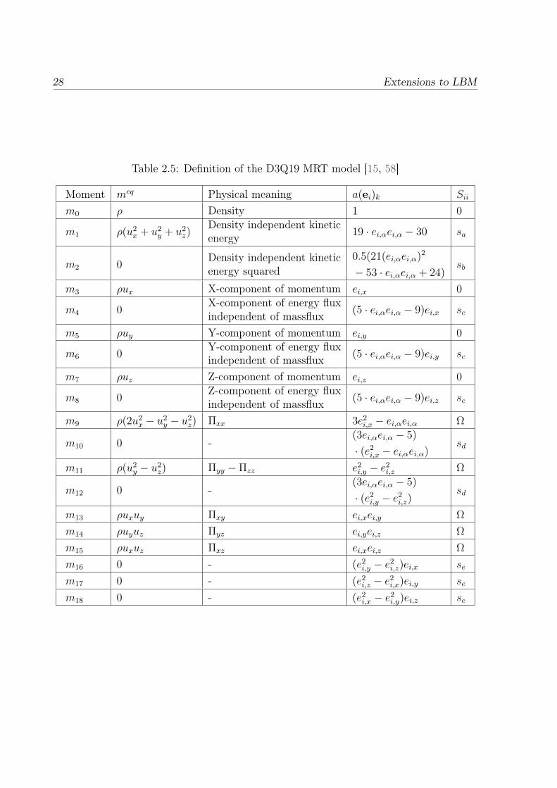
28 Extensions to LBM
Table 2.5: Definition of the D3Q19 MRT model [15, 58]
Moment meq Physical meaning a(ei)k Sii
m0 ρ Density 1 0
m1 ρ(u2x + u2
y + u2z)
Density independent kineticenergy 19 · ei,αei,α − 30 sa
m2 0Density independent kineticenergy squared
0.5(21(ei,αei,α)2
− 53 · ei,αei,α + 24)sb
m3 ρux X-component of momentum ei,x 0
m4 0X-component of energy fluxindependent of massflux (5 · ei,αei,α − 9)ei,x sc
m5 ρuy Y-component of momentum ei,y 0
m6 0Y-component of energy fluxindependent of massflux (5 · ei,αei,α − 9)ei,y sc
m7 ρuz Z-component of momentum ei,z 0
m8 0Z-component of energy fluxindependent of massflux (5 · ei,αei,α − 9)ei,z sc
m9 ρ(2u2x − u2
y − u2z) Πxx 3e2
i,x − ei,αei,α Ω
m10 0 -(3ei,αei,α − 5)
· (e2i,x − ei,αei,α)
sd
m11 ρ(u2y − u2
z) Πyy − Πzz e2i,y − e2
i,z Ω
m12 0 -(3ei,αei,α − 5)
· (e2i,y − e2
i,z)sd
m13 ρuxuy Πxy ei,xei,y Ω
m14 ρuyuz Πyz ei,yei,z Ω
m15 ρuxuz Πxz ei,xei,z Ω
m16 0 - (e2i,y − e2
i,z)ei,x se
m17 0 - (e2i,z − e2
i,x)ei,y se
m18 0 - (e2i,x − e2
i,y)ei,z se
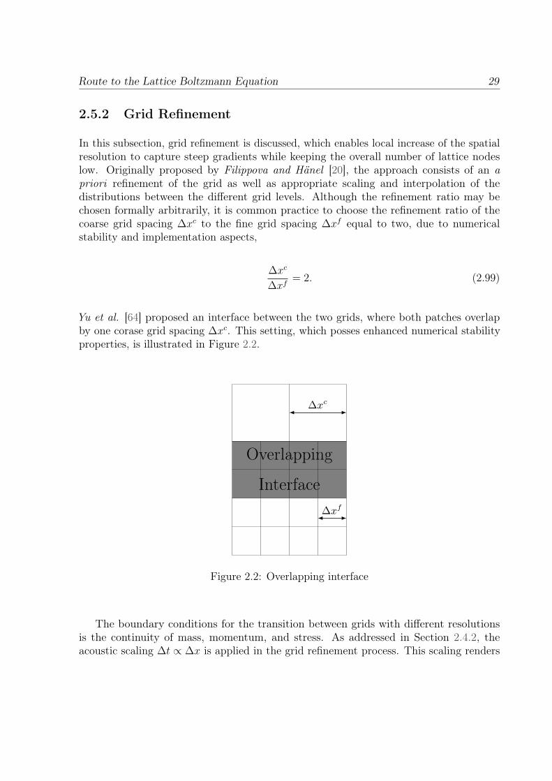
Route to the Lattice Boltzmann Equation 29
2.5.2 Grid Refinement
In this subsection, grid refinement is discussed, which enables local increase of the spatialresolution to capture steep gradients while keeping the overall number of lattice nodeslow. Originally proposed by Filippova and Hänel [20], the approach consists of an apriori refinement of the grid as well as appropriate scaling and interpolation of thedistributions between the different grid levels. Although the refinement ratio may bechosen formally arbitrarily, it is common practice to choose the refinement ratio of thecoarse grid spacing ∆xc to the fine grid spacing ∆xf equal to two, due to numericalstability and implementation aspects,
∆xc
∆xf= 2. (2.99)
Yu et al. [64] proposed an interface between the two grids, where both patches overlapby one corase grid spacing ∆xc. This setting, which posses enhanced numerical stabilityproperties, is illustrated in Figure 2.2.
Overlapping
Interface
∆xc
∆xf
Figure 2.2: Overlapping interface
The boundary conditions for the transition between grids with different resolutionsis the continuity of mass, momentum, and stress. As addressed in Section 2.4.2, theacoustic scaling ∆t ∝ ∆x is applied in the grid refinement process. This scaling renders
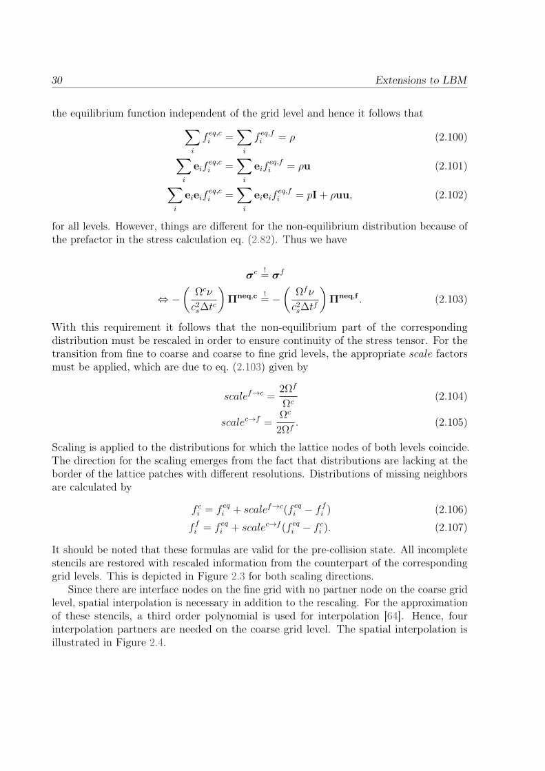
30 Extensions to LBM
the equilibrium function independent of the grid level and hence it follows that∑i
f eq,ci =∑i
f eq,fi = ρ (2.100)∑i
eifeq,ci =
∑i
eifeq,fi = ρu (2.101)∑
i
eieifeq,ci =
∑i
eieifeq,fi = pI + ρuu, (2.102)
for all levels. However, things are different for the non-equilibrium distribution because ofthe prefactor in the stress calculation eq. (2.82). Thus we have
σc != σf
⇔ −(
Ωcν
c2s∆t
c
)Πneq,c !
= −(
Ωfν
c2s∆t
f
)Πneq,f . (2.103)
With this requirement it follows that the non-equilibrium part of the correspondingdistribution must be rescaled in order to ensure continuity of the stress tensor. For thetransition from fine to coarse and coarse to fine grid levels, the appropriate scale factorsmust be applied, which are due to eq. (2.103) given by
scalef→c =2Ωf
Ωc(2.104)
scalec→f =Ωc
2Ωf. (2.105)
Scaling is applied to the distributions for which the lattice nodes of both levels coincide.The direction for the scaling emerges from the fact that distributions are lacking at theborder of the lattice patches with different resolutions. Distributions of missing neighborsare calculated by
f ci = f eqi + scalef→c(f eqi − f fi ) (2.106)
f fi = f eqi + scalec→f (f eqi − f ci ). (2.107)
It should be noted that these formulas are valid for the pre-collision state. All incompletestencils are restored with rescaled information from the counterpart of the correspondinggrid levels. This is depicted in Figure 2.3 for both scaling directions.
Since there are interface nodes on the fine grid with no partner node on the coarse gridlevel, spatial interpolation is necessary in addition to the rescaling. For the approximationof these stencils, a third order polynomial is used for interpolation [64]. Hence, fourinterpolation partners are needed on the coarse grid level. The spatial interpolation isillustrated in Figure 2.4.
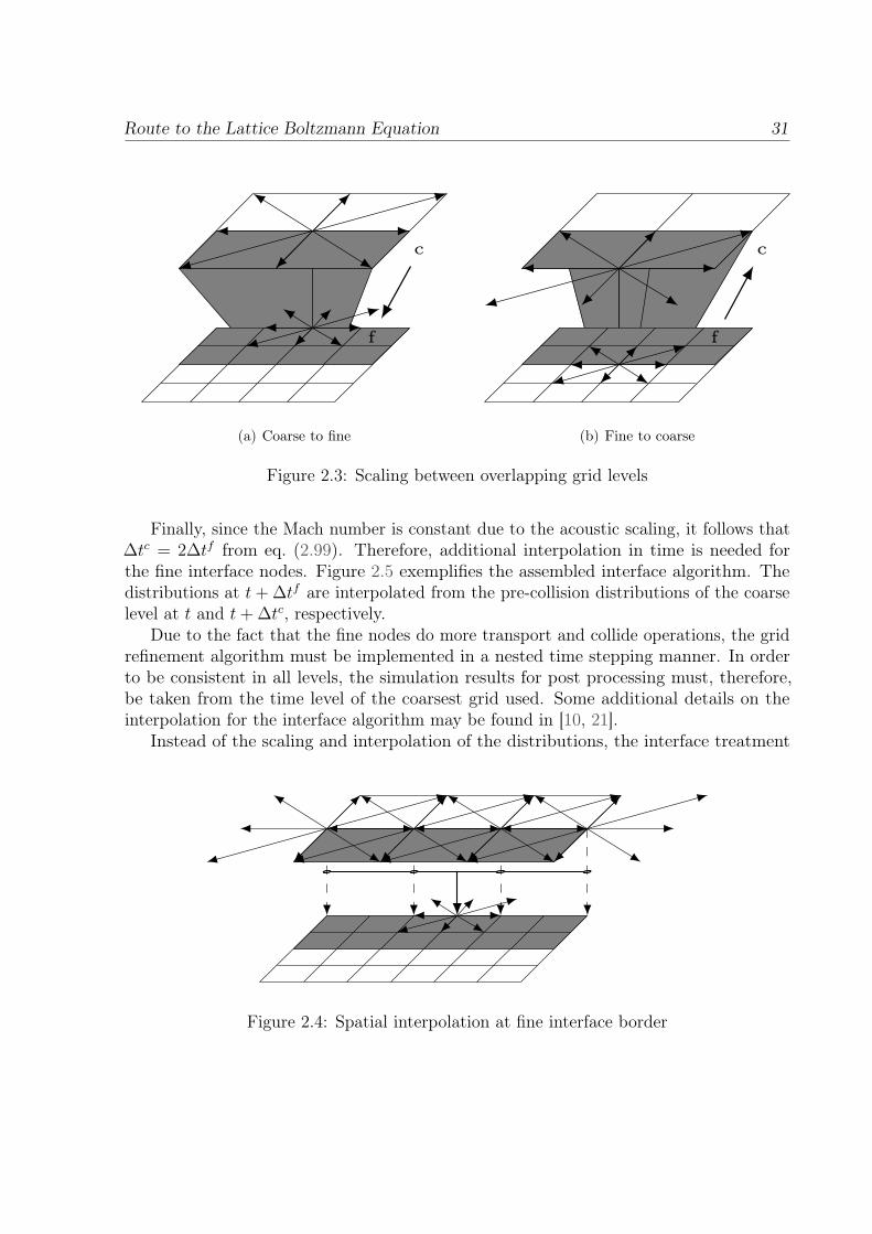
Route to the Lattice Boltzmann Equation 31
f
c
(a) Coarse to fine
f
c
(b) Fine to coarse
Figure 2.3: Scaling between overlapping grid levels
Finally, since the Mach number is constant due to the acoustic scaling, it follows that∆tc = 2∆tf from eq. (2.99). Therefore, additional interpolation in time is needed forthe fine interface nodes. Figure 2.5 exemplifies the assembled interface algorithm. Thedistributions at t+ ∆tf are interpolated from the pre-collision distributions of the coarselevel at t and t+ ∆tc, respectively.
Due to the fact that the fine nodes do more transport and collide operations, the gridrefinement algorithm must be implemented in a nested time stepping manner. In orderto be consistent in all levels, the simulation results for post processing must, therefore,be taken from the time level of the coarsest grid used. Some additional details on theinterpolation for the interface algorithm may be found in [10, 21].
Instead of the scaling and interpolation of the distributions, the interface treatment
Figure 2.4: Spatial interpolation at fine interface border
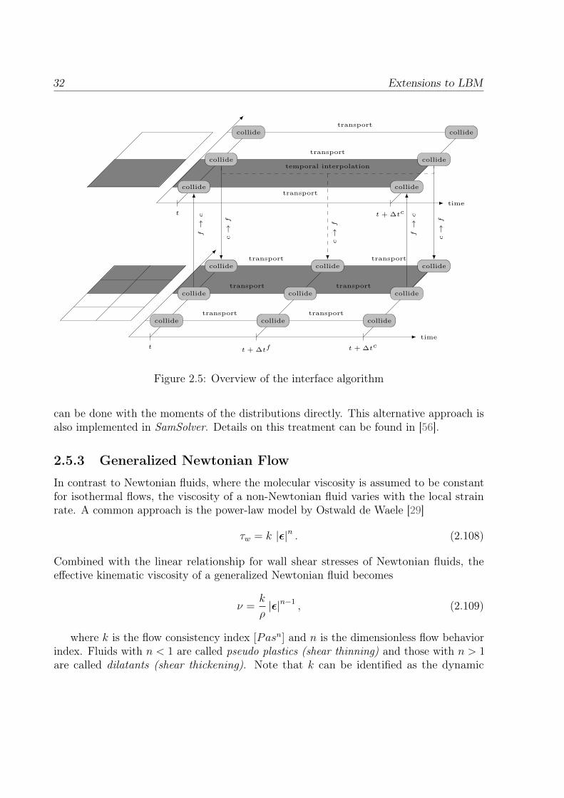
32 Extensions to LBM
time
time
t t + ∆tf t + ∆tc
t t + ∆tc
collide
temporal interpolation
c→
f
collidetransport
collide
collidetransport
collide
collidetransport
collide
collidetransport transport
collide
collidetransport
collidetransport
collide
collidetransport
collidetransport
collide
c→
f
c→
f
f→
c
f→
c
Figure 2.5: Overview of the interface algorithm
can be done with the moments of the distributions directly. This alternative approach isalso implemented in SamSolver. Details on this treatment can be found in [56].
2.5.3 Generalized Newtonian Flow
In contrast to Newtonian fluids, where the molecular viscosity is assumed to be constantfor isothermal flows, the viscosity of a non-Newtonian fluid varies with the local strainrate. A common approach is the power-law model by Ostwald de Waele [29]
τw = k |ε|n . (2.108)
Combined with the linear relationship for wall shear stresses of Newtonian fluids, theeffective kinematic viscosity of a generalized Newtonian fluid becomes
ν =k
ρ|ε|n−1 , (2.109)
where k is the flow consistency index [Pasn] and n is the dimensionless flow behaviorindex. Fluids with n < 1 are called pseudo plastics (shear thinning) and those with n > 1are called dilatants (shear thickening). Note that k can be identified as the dynamic
Route to the Lattice Boltzmann Equation 33
viscosity for Newtonian fluids, where n = 1. These parameters are fluid dependent andmust be determined through curve fitting of experimental data. Incorporation of non-Newtonian behavior can be done by substitution of the kinematic viscosity in eq. (2.79)with the effective viscosity related to the magnitude of the strain rate tensor according tothe constitutive law used. One of the major advantages of the lattice Boltzmann methodis the ability to evaluate the stress and strain tensors locally with second order accuracy[37]. The magnitude of the strain rate tensor is calculated through the second invariant,
|ε| = Ω
∆t · ρ · c2s
∑αβ
√1
2· Πneq
αβ Πneqαβ ∀α 6= β. (2.110)
The kinematic viscosity is then computed from eq. (2.109). Technically speaking, thisexpression cannot be evaluated directly because the kinematic viscosity itself appears inthe collision frequency eq. (2.79). For an exact solution, the root of this implicit equationhas to be computed. However, to keep the algorithm simple, the viscosity from the previoustime step is used to compute the collision frequency in eq. (2.110), which has proved to bea good approximation.
As already stated in the beginning of this chapter, the LBM suffers from instabilitieswhen the viscosity gets low. Hence, for the case of shear thinning fluids, the viscosityobtained through eq. (2.109) must be limited with a lower bound in regions with vanishingmagnitude of the strain rate tensor. Similarly, it is necessary to introduce an upper boundon ν [22]. The upper bound was introduced in [22] with the very general rationale toensure hydrodynamic behavior. As will be discussed in Chapter 7, the upper bound isneeded to limit the error EΩ introduced in Section 2.4.1. In the case of the power-lawmodel, the effective viscosity becomes
ν =
νmax ε > εmaxkρ|ε|n−1 εmin ≤ ε ≤ εmax
νmin ε < εmin
. (2.111)
This effectively results in a lower bound Ωmin and an upper bound Ωmax of the dimensionlesscollision frequency. Therefore, the stability criteria are given by:
Ω =
Ωmax =
c2s∆t
νmin + 0.5c2s∆t
Ω
Ωmin =c2s∆t
νmax + 0.5c2s∆t
(2.112)
In our simulations, we use an upper bound of Ωmax = 1.965 for the SRT model andΩmax = 1.985 for the MRT model. The choice of Ωmin is addressed in Chapter 7. Whennot stated otherwise, the value of Ωmin is set to 1.0.
34 Extensions to LBM
2.5.4 External Force
There exists an extensive overview on the different force implementations by Guo et al.[25], who analyzed the proper way to implement spatially and temporally varying forcesthat include discretization effects by a posteriori matching of the forcing term to themacroscopic equations. The incorporation of external forces fF = ρa is achieved by addingan additional forcing term to the LBE,
fi(x + ei∆t, t+ ∆t) = fi(x, t) + Ω · (f eqi (x, t)− fi(x, t)) + ∆tfFi . (2.113)
The discretized forcing term fFi is expressed similar to the series expansion of the equilib-rium distribution eq. (2.27) and reads
fFi = wi
(Ων
c2s∆t
)·(
ei · fFc2s
+1
2c4s
(eiei − c2sI) : (ufF + fFu)
). (2.114)
The same result can be obtained a priori through hermite series expansion of the forcingterm. Since forces must not increase mass, the zeroth moment of fFi is zero. It should benoted that due to the presence of external forces, the first moment is altered. As can beseen from eq. (2.78), eq. (2.76), and eq. (2.22), the change of variables causes [43]:
wi∑i
eifi = ρu− ∆tfF
2. (2.115)
Since the equilibrium function is given in terms of the physical velocity u, the computationof f eq must be done with
u =1
ρwi∑i
eifi +∆tfF
2. (2.116)
With this scheme, additional non-physical terms involving space and time derivativesof the forcing term in the macroscopic equations get canceled. Hence, in the case of aspatially constant body forces for which the time derivative is small or zero, the forcingterm is often simplified to
fFi = wi ·(
ei · fFc2s
). (2.117)
This applies to the SRT model. The same simplified forcing term is easily incorporated inthe MRT model by addition of the corresponding momentum due to the body force onthe macroscopic moments for the momentum in Table 2.5 after the collision step.
mpost3 = mpre
3 + ∆tfFx (2.118)
mpost5 = mpre
5 + ∆tfFy
mpost7 = mpre
7 + ∆tfFz
For the implementation details of the fully discrete forcing scheme in the case of the MRTmodel, the reader is referred to [26].
CHAPTER 3
Implementation
This chapter is concerned with some theoretical aspects of the implementation of SAM-Lattice. Details on the actual programming may be found in the programmers documenta-tion to SamGenerator and SamSolver, respectively.
3.1 Lattice Generation
One part of any form of computational fluid dynamics is the spatial discretization of thegeometry that will be subject to the simulation. This is the task of the program Sam-Generator. The concept of Lattice Boltzmann calls for an equidistant lattice that can berepresented by a joint set of hexahedra cells. Such an representation is known in computergraphics as a voxel (neologism of volumetric and pixel) representation. Starting point ofthe discretization, i.e, the input file for SamGenerator is a triangulated representationof the boundaries of the geometry. Each triangle in the triangulation is defined by threepoints and a normal vector. By definition, the normals point out of the fluid domain.The requirements for a valid SamGenerator input file is met by either a modified stl(stereolithography) format or a boundary mesh, e.g, in msh format, consisting of triangleelements only. Note, that the standard stl format does not offer possibilities to assigntriangles to surfaces of the geometry.
SamGenerator is octree based, which allows for local grid refinement, where a coarsecell is decomposed in eight child cells. In that sense, each octree level is assigned anumber, for which the coarsest discretization is on level 0. Figure 3.1 shows a flowchartof SamGenerator with the most significant program routines. They are grouped by theirfunctional affiliation.
35
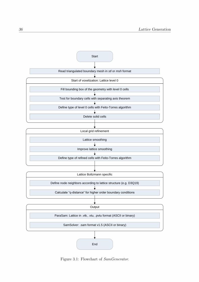
36 Lattice Generation
Output
Lattice Boltzmann specific
Start of voxelization: Lattice level 0
Local grid refinement
Fill bounding box of the geometry with level 0 cells
Test for boundary cells with separating axis theorem
Define type of level 0 cells with Feito-Torres algorithm
Delete solid cellsDelete solid cells
Lattice smoothing
Improve lattice smoothing
Define type of refined cells with Feito-Torres algorithm
Define node neighbors according to lattice structure (e.g. D3Q19)
Calculate “q-distance“ for higher order boundary conditions
SamSolver: .sam format v1.5 (ASCII or binary)
ParaSam: Lattice in .vtk, .vtu, .pvtu format (ASCII or binary)
Read triangulated boundary mesh in stl or msh format
End
Start
Figure 3.1: Flowchart of SamGenerator.
Implementation 37
Upon the start of SamGenerator, the input file is read and stored internally in containersprovided by the C++ standard template library. Discretization begins by filling thebounding box of the fluid domain with hexaedra with edge length according to the desiredlattice spacing in level 0. In the next step, we have to decide, which cells are inside thefluid domain. To this end, we use a combination of the separating axis theorem and apoint inclusion test algorithm by Feito and Torres, which will be discussed in Section 3.1.1.The separating axis theorem is used to filter those cells intersecting the boundary of thegeometry, that is, we test if the boundary triangle and the lattice cell overlap. Sincethe LBM is node based, we then need to test if the nodes, which the boundary cells arecomposed of, lie inside or outside of the fluid domain, i.e., if a node is a fluid node or awall/boundary node. This is done with the Feito-Torres algorithm. Based on the nodetypes in the tested boundary cells, we use a flood fill procedure to separate cells thatcompletely lie in the fluid domain from those cells located completely inside an obstacle oroutside the fluid domain (solid cells). The latter can be deleted to save valuable memory.
If desired, the level 0 lattice can be locally refined. Objectives of the refinement can beeither refinement of the boundary discretization or local refinement of an area inside ofthe fluid domain. Local domain refinement is implemented in SamGenerator in two ways.On one side, a box, defined by an origin and its extension in three dimensions, can beused and on the other hand, areas of refinement can be arbitrarily shaped through usageof an auxiliary geometry in .stl or .msh format. Both approaches need to be suppliedwith the desired refinement depth, i.e., the number of the octree level for the local gridrefinement. Due to stability issues at the interface, neighboring lattice levels must not differby more than one lattice level [10]. Therefore, the lattice is smoothed in regions, wherethis condition is violated. In some cases, the result of the smoothing can be improved. Amore detailed discussion on lattice smoothing is done in the sequel. Especially in the caseof boundary refinement, the resulting higher level cells and corresponding new nodes needto be tested for their type. This is again done with the Feito-Torres algorithm.
So far, the previously described discretization gives a three dimensional lattice with anstaggered boundary representation. Therefore, an additional tool was written, which makesit possible to export the lattice in the CGNS format in order to use it in a classical Navier-Stokes solver. An additional step is needed to make the lattice boundary conform. For usewith the Lattice Boltzmann method, the appropriate neighbor relationships must be setaccording to the velocity discretization model used, e.g, D3Q19. In order to incorporatethe actual geometry into the simulation, as opposed to its staggered representation, theintersections of the lattice links and the geometry is calculated. A dimensionless distancefrom the fluid nodes to the geometry, known as "q-distance", is introduced, which will bediscussed in Section 3.1.3.
Result of the whole discretization process is the voxelized geometry in one of the VTK(Virtual Tool Kit) formats, readable by ParaSam, and/or the .sam file, which serves as
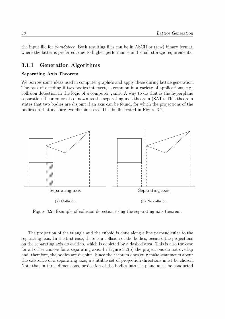
38 Lattice Generation
the input file for SamSolver. Both resulting files can be in ASCII or (raw) binary format,where the latter is preferred, due to higher performance and small storage requirements.
3.1.1 Generation Algorithms
Separating Axis Theorem
We borrow some ideas used in computer graphics and apply these during lattice generation.The task of deciding if two bodies intersect, is common in a variety of applications, e.g.,collision detection in the logic of a computer game. A way to do that is the hyperplaneseparation theorem or also known as the separating axis theorem (SAT). This theoremstates that two bodies are disjoint if an axis can be found, for which the projections of thebodies on that axis are two disjoint sets. This is illustrated in Figure 3.2.
Separating axis
(a) Collision
Separating axis
(b) No collision
Figure 3.2: Example of collision detection using the separating axis theorem.
The projection of the triangle and the cuboid is done along a line perpendicular to theseparating axis. In the first case, there is a collision of the bodies, because the projectionson the separating axis do overlap, which is depicted by a dashed area. This is also the casefor all other choices for a separating axis. In Figure 3.2(b) the projections do not overlapand, therefore, the bodies are disjoint. Since the theorem does only make statements aboutthe existence of a separating axis, a suitable set of projection directions must be chosen.Note that in three dimensions, projection of the bodies into the plane must be conducted
Implementation 39
prior to the projection on a separating axis. In its basic form, the separating axis theoremis only valid for convex bodies. Fortunately, this is enough in our case, since we exclusivelydeal with hexahedra and triangles. In our work, we rely on a fast box-triangle algorithmderived in [1]. The algorithm consists of 3 overlapping tests for the bounding boxes, oneoverlapping test for the triangle normal, and 9 overlapping tests for the triangle edges.
For reasons of simplicity, the hexahedron is transformed into the origin, such that it isaxis aligned with the global coordinate system and the triangle is transformed accordingly.On the first 3 tests, a axis aligned bounding box around the triangle is tested against thecuboid, while projecting on the principal axes. Next, a plane-bounding box overlap testfrom [27] is used with the normal vector of the triangle. Finally, each of the three edges ofthe triangles are used to project the triangle and the box on each of the principal axes,which gives 9 tests in total. The algorithm is terminated, if a separating axis could befound in one of the projections. This is the reason why the SAT algorithm is very fast,since it is possible to find a separating axis early within the few first tests.
The algorithm is used in the course of the discretization to check if a cell and thetriangulated geometry intersect. In that sense, we want to determine if a cell is a boundarycell, e.g., inlet or wall boundary, for which boundary conditions must be provided.
In order to save computational work, we loop over STL triangles and only test thosehexahedra that lie in the bounding box of the triangle. That way, a large part of thecells can be left out of the SAT test for the particular triangle. Those cells can easily becalculated based on their index in the lattice.
Feito-Torres Algorithm
Feito and Torres presented a planar point inclusion algorithm in [16], which does notresort to solving equation systems or use of trigonometric functions. Hence, the test doesnot suffer from stability problems. The idea of the inclusion test, is to decompose the testpolygon into sub-polygons involving the test point I. The orientation of the sub-polygonsis used to decide, whether the test point lies inside or outside of the polygon. In the case ofa triangle with the nodes ABC, which are arranged to give a positive orientation, the testpoint I is checked for inclusion by decomposing the triangle into three sub-triangles IAB,IBC, and ICA. The orientation of the triangles can be computed via the correspondingdeterminants. The point I lies inside the triangle if, and only if, all three sub triangles havethe same orientation as the geometry triangle ABC, i.e., if all determinants are positive.
The same authors presented a generalization of their algorithm to 3 dimensions in [17],where we have to compute determinants of tetrahedra.
3.1.2 Grid Refinement and Lattice Smoothing
As already mentioned, SamGenerator is octree based, which allows for local grid refinement,where a coarse cell is decomposed in eight child cells. Each octree level is assigned a
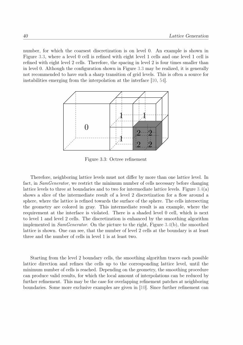
40 Lattice Generation
number, for which the coarsest discretization is on level 0. An example is shown inFigure 3.3, where a level 0 cell is refined with eight level 1 cells and one level 1 cell isrefined with eight level 2 cells. Therefore, the spacing in level 2 is four times smaller thanin level 0. Although the configuration shown in Figure 3.3 may be realized, it is generallynot recommended to have such a sharp transition of grid levels. This is often a source forinstabilities emerging from the interpolation at the interface [10, 54].
1
1 1
0
22
2 2
Figure 3.3: Octree refinement
Therefore, neighboring lattice levels must not differ by more than one lattice level. Infact, in SamGenerator, we restrict the minimum number of cells necessary before changinglattice levels to three at boundaries and to two for intermediate lattice levels. Figure 3.4(a)shows a slice of the intermediate result of a level 2 discretization for a flow around asphere, where the lattice is refined towards the surface of the sphere. The cells intersectingthe geometry are colored in gray. This intermediate result is an example, where therequirement at the interface is violated. There is a shaded level 0 cell, which is nextto level 1 and level 2 cells. The discretization is enhanced by the smoothing algorithmimplemented in SamGenerator. On the picture to the right, Figure 3.4(b), the smoothedlattice is shown. One can see, that the number of level 2 cells at the boundary is at leastthree and the number of cells in level 1 is at least two.
Starting from the level 2 boundary cells, the smoothing algorithm traces each possiblelattice direction and refines the cells up to the corresponding lattice level, until theminimum number of cells is reached. Depending on the geometry, the smoothing procedurecan produce valid results, for which the local amount of interpolations can be reduced byfurther refinement. This may be the case for overlapping refinement patches at neighboringboundaries. Some more exclusive examples are given in [10]. Since further refinement can
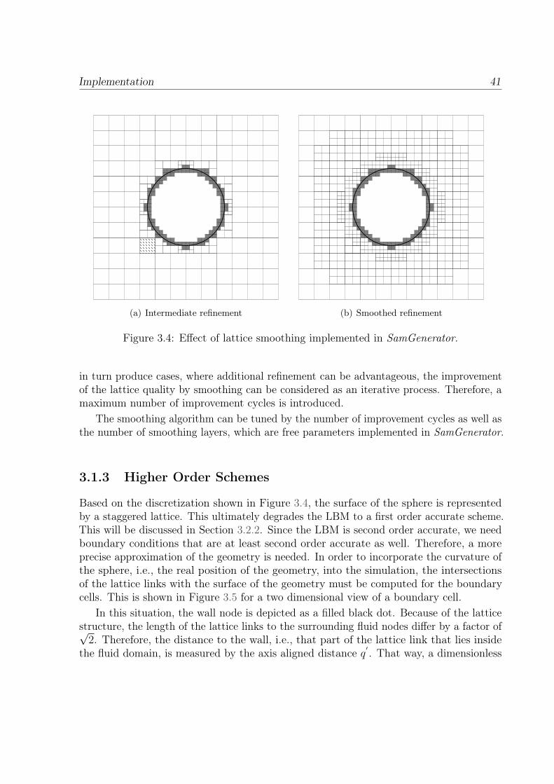
Implementation 41
(a) Intermediate refinement (b) Smoothed refinement
Figure 3.4: Effect of lattice smoothing implemented in SamGenerator.
in turn produce cases, where additional refinement can be advantageous, the improvementof the lattice quality by smoothing can be considered as an iterative process. Therefore, amaximum number of improvement cycles is introduced.
The smoothing algorithm can be tuned by the number of improvement cycles as well asthe number of smoothing layers, which are free parameters implemented in SamGenerator.
3.1.3 Higher Order Schemes
Based on the discretization shown in Figure 3.4, the surface of the sphere is representedby a staggered lattice. This ultimately degrades the LBM to a first order accurate scheme.This will be discussed in Section 3.2.2. Since the LBM is second order accurate, we needboundary conditions that are at least second order accurate as well. Therefore, a moreprecise approximation of the geometry is needed. In order to incorporate the curvature ofthe sphere, i.e., the real position of the geometry, into the simulation, the intersectionsof the lattice links with the surface of the geometry must be computed for the boundarycells. This is shown in Figure 3.5 for a two dimensional view of a boundary cell.
In this situation, the wall node is depicted as a filled black dot. Because of the latticestructure, the length of the lattice links to the surrounding fluid nodes differ by a factor of√
2. Therefore, the distance to the wall, i.e., that part of the lattice link that lies insidethe fluid domain, is measured by the axis aligned distance q′ . That way, a dimensionless
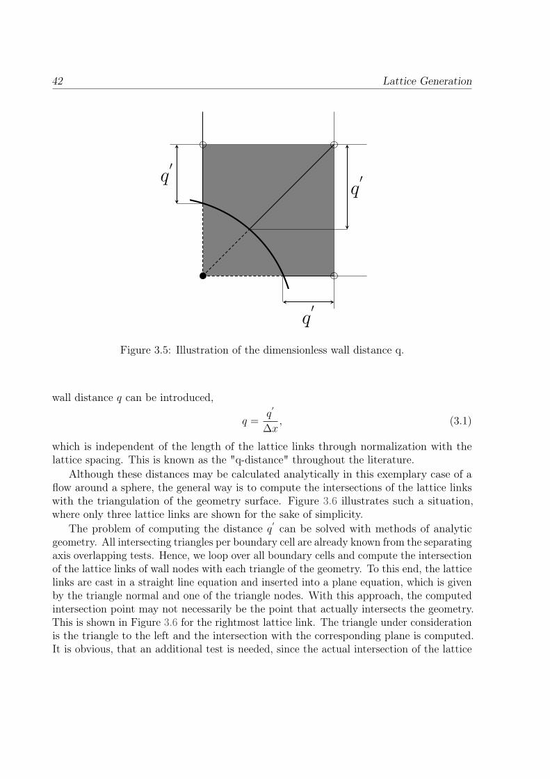
42 Lattice Generation
q′q
′
q′
Figure 3.5: Illustration of the dimensionless wall distance q.
wall distance q can be introduced,
q =q′
∆x, (3.1)
which is independent of the length of the lattice links through normalization with thelattice spacing. This is known as the "q-distance" throughout the literature.
Although these distances may be calculated analytically in this exemplary case of aflow around a sphere, the general way is to compute the intersections of the lattice linkswith the triangulation of the geometry surface. Figure 3.6 illustrates such a situation,where only three lattice links are shown for the sake of simplicity.
The problem of computing the distance q′ can be solved with methods of analyticgeometry. All intersecting triangles per boundary cell are already known from the separatingaxis overlapping tests. Hence, we loop over all boundary cells and compute the intersectionof the lattice links of wall nodes with each triangle of the geometry. To this end, the latticelinks are cast in a straight line equation and inserted into a plane equation, which is givenby the triangle normal and one of the triangle nodes. With this approach, the computedintersection point may not necessarily be the point that actually intersects the geometry.This is shown in Figure 3.6 for the rightmost lattice link. The triangle under considerationis the triangle to the left and the intersection with the corresponding plane is computed.It is obvious, that an additional test is needed, since the actual intersection of the lattice
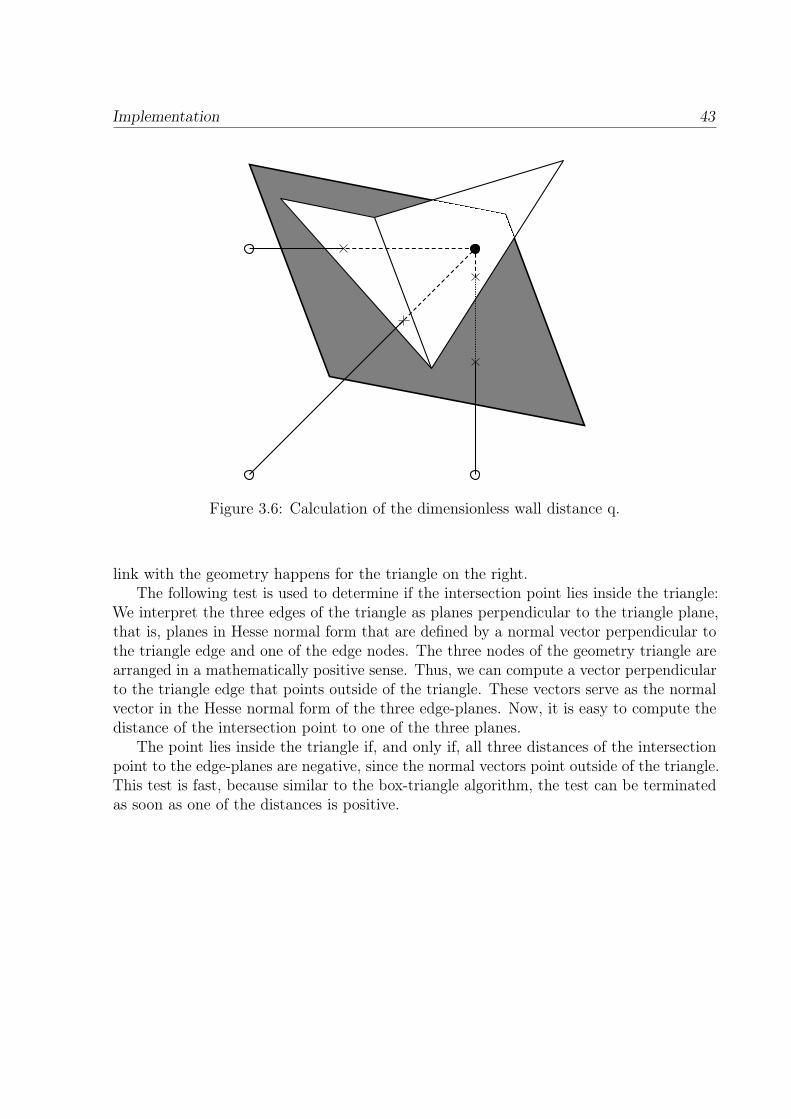
Implementation 43
Figure 3.6: Calculation of the dimensionless wall distance q.
link with the geometry happens for the triangle on the right.The following test is used to determine if the intersection point lies inside the triangle:
We interpret the three edges of the triangle as planes perpendicular to the triangle plane,that is, planes in Hesse normal form that are defined by a normal vector perpendicular tothe triangle edge and one of the edge nodes. The three nodes of the geometry triangle arearranged in a mathematically positive sense. Thus, we can compute a vector perpendicularto the triangle edge that points outside of the triangle. These vectors serve as the normalvector in the Hesse normal form of the three edge-planes. Now, it is easy to compute thedistance of the intersection point to one of the three planes.
The point lies inside the triangle if, and only if, all three distances of the intersectionpoint to the edge-planes are negative, since the normal vectors point outside of the triangle.This test is fast, because similar to the box-triangle algorithm, the test can be terminatedas soon as one of the distances is positive.
44 Solver Implementation
3.2 Solver Implementation
The modular structure of the program package SAM-Lattice manifests itself in the variousoutput files generated by the individual modules. The advantage of this concept is agreat flexibility, because different modules can act on the input/output file of an other.SamGenerator generates the .sam file, which can either be used directly as the inputfile for SamSolver or as the input file for SamDecomposer. A slight disadvantage of thisapproach is the I/O overhead and the associated space requirements. Although this willnot be discussed in detail, the application SamDecomposer can be used to decomposethe lattice on the basis of the graph partition library MeTiS. Therefore, the .sam fileserves as the input for SamDecomposer, which results in a series of .samd files, containingthe decomposed parts of the lattice and numbered according to their processor affiliation.Moreover, SamSolver is parallelized in shared memory (SMP) architectures through usageof the OpenMP library [8, 31].
Figure 3.7 shows a flowchart for SamSolver with the most important program routines.In addition to the lattice information in the .sam file, there is a solver control file. Thisis a text file, which contains information of the various boundary conditions associatedwith the corresponding boundary in the lattice. Most boundary conditions implementedin SamSolver will be discussed in Section 3.2.2. Moreover, general settings, e.g., theduration of the simulation, write interval, etc., are stored in the control file. Upon thestart of SamSolver, the .sam file and the control file are read and the data is storedinternally in the various variables and C++ containers. The .sam file contains informationon the interface connectivity for lattices with local grid refinement. A setup routine isimplemented, which sets the corresponding relationships at the interface for the spatial andtemporal interpolation. In the preprocessing for MPI runs, the corresponding send/receiverrelationships for the inter-processor communication is set up. Before the start of asimulation, the distributions must be initialized. This is done by calculating the equilibriumdistributions according to a prescribed global value for the velocity and the density,respectively. Additionally, an advanced initialization procedure, proposed in [44], isimplemented in SamSolver to generate a pressure field that is consistent with the velocityfield.
After the preprocessing, the solver is started with different configurations dependingon whether the lattice is refined or not. Moreover, there is a different treatment in thecollide routine. The simulation can be carried out with the SRT or the MRT collisionmodel as well as it can be laminar or turbulent and non-Newtonian. We use a Large EddySimulation (LES) approach for modeling of turbulent flows. An intensive investigation andapplication of this feature of SamSolver can be found in the PhD thesis of Schneider [56].
This flexibility in terms of the different solvers and models is internally realized throughusage of C++ functors. In the single level case, the solver enters a time loop which controlsthe duration of the simulation. According to the Lattice Boltzmann algorithm, the collideand transport step are conducted for each individual time step.
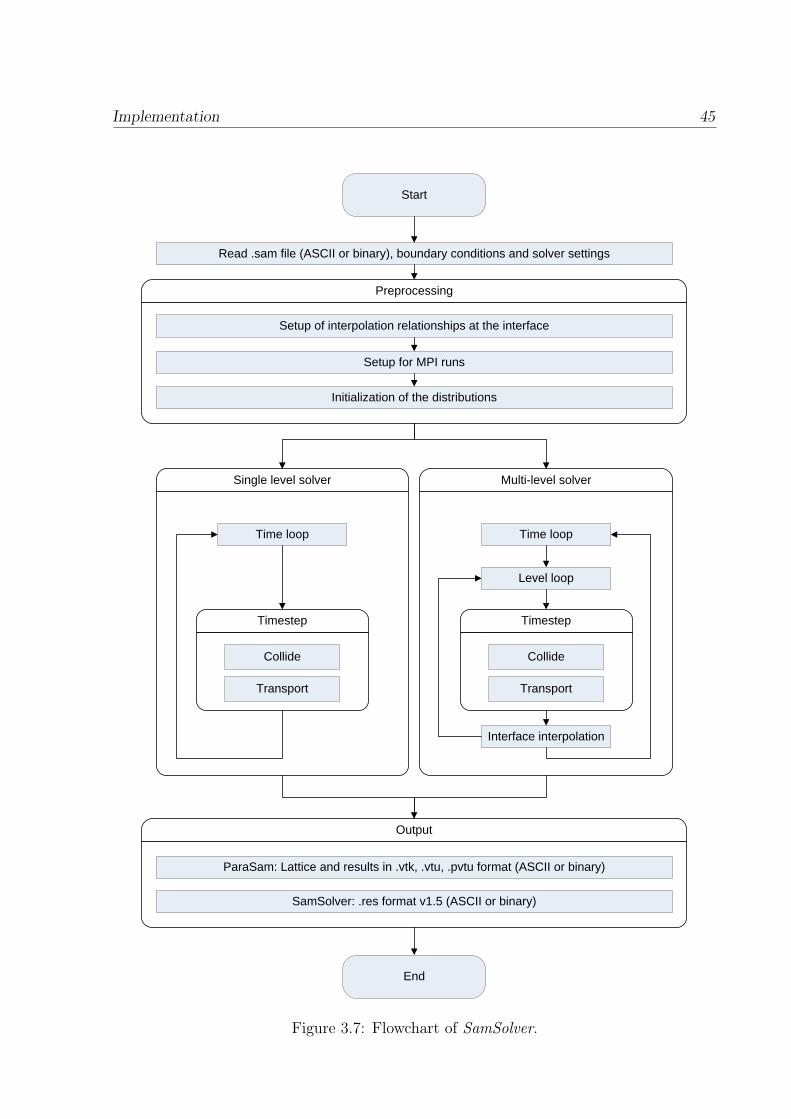
Implementation 45
Output
Preprocessing
Setup of interpolation relationships at the interface
Setup for MPI runs
Initialization of the distributions
SamSolver: .res format v1.5 (ASCII or binary)
ParaSam: Lattice and results in .vtk, .vtu, .pvtu format (ASCII or binary)
Read .sam file (ASCII or binary), boundary conditions and solver settings
End
Start
Single level solver Multi-level solver
Interface interpolation
Timestep
Collide
Transport
Timestep
Collide
Transport
Time loopTime loop
Level loop
Figure 3.7: Flowchart of SamSolver.
46 Solver Implementation
Additionally, there is a command interpreter implemented in the class SamCommand-Interpreter, which is nested in the outer time loop. This makes it possible to control thesolver through editing of the .sam_cmd file, while the simulation is running. Actions rangefrom a simple change of the simulation duration over modification of boundary conditions,to change of the number of processor threads in shared memory parallelized runs. Thevarious commands can be found in the programmers documentation.
For the multi-level treatment, there is an additional loop for the different octree levels,which will be discussed in Section 3.2.1. This level loop is nested inside the time loop.
At prescribed write intervals or at the end of the simulation, SamSolver producesvarious output files depending on the settings. Simulation results such as velocity, pressure,viscosity, etc., are written in the partitioned vtu format .pvtu, which is the master filefor assembling of different part files in the .vtu format. That way, it is possible to realizeparallel output in SMP runs or each MPI process outputs its part file. In both cases, theresults can be in ASCII or (raw) binary. There is also the possibility to directly output thedistributions of each lattice node in the .psam file and calculate the macroscopic momentswith our extension to ParaView : ParaSAM.
Finally, there is a .res file, which freezes the current distributions and settings toresume the simulation at a later point in time.
3.2.1 Multi-Level Treatment
In this subsection, the implementation of the multi-level treatment is discussed. Basis ofthe implementation is the need for a nested time stepping. Our grid refinement algorithmrelies on the acoustic scaling ∆t ∝ ∆x. Owing to the octree structure, the spacing ∆x isalways halved on the transition to a finer resolution. Hence, the time step on an octreelevel n is twice the time step on a level n+ 1.
Listing 3.1 shows the C++ style pseudo code for the multi-level solver. In lines 1-4some control variables are defined, where maxLevel gives the maximum number of octreelevel as shown in Figure 3.3.
Depending on the number of octree levels, a series determining the sequence in whichthe nodes on the corresponding levels perform a collide and transport step can be de-rived. Therefore, the array levels of length maxLevel stores the series of the form2maxLevel−octreeLevel. It is computed in line 6. There are two member functions in thelisting. The member function timeStep, implements the collide and transport step forthe corresponding level passed to it in parenthesis. Furthermore, the member functioninterpolateInterface implements the interpolation in space and time for the interface nodesof the corresponding levels. Besides the rescaling to the fine level, the distributions have tobe interpolated in space for nodes, where there is no colocated node on the correspondingcoarse grid. For odd times, the values have to be interpolated in time as well. For even
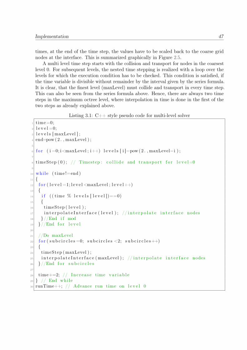
Implementation 47
times, at the end of the time step, the values have to be scaled back to the coarse gridnodes at the interface. This is summarized graphically in Figure 2.5.
A multi level time step starts with the collision and transport for nodes in the coarsestlevel 0. For subsequent levels, the nested time stepping is realized with a loop over thelevels for which the execution condition has to be checked. This condition is satisfied, ifthe time variable is divisible without remainder by the interval given by the series formula.It is clear, that the finest level (maxLevel) must collide and transport in every time step.This can also be seen from the series formula above. Hence, there are always two timesteps in the maximum octree level, where interpolation in time is done in the first of thetwo steps as already explained above.
Listing 3.1: C++ style pseudo code for multi-level solver1 time=0;2 l e v e l =0;3 l e v e l s [ maxLevel ] ;4 end=pow ( 2 . , maxLevel ) ;5
6 f o r ( i =0; i<maxLevel ; i++) l e v e l s [ i ]=pow ( 2 . , maxLevel−i ) ;7
8 t imeStep ( 0 ) ; // Timestep : c o l l i d e and t ranspo r t f o r l e v e l=09
10 whi le ( time !=end )11 12 f o r ( l e v e l =1; l e v e l <maxLevel ; l e v e l++)13 14 i f ( ( time % l e v e l s [ l e v e l ])==0)15 16 t imeStep ( l e v e l ) ;17 i n t e r p o l a t e I n t e r f a c e ( l e v e l ) ; // i n t e r p o l a t e i n t e r f a c e nodes18 //End i f mod19 //End f o r l e v e l20
21 //Do maxLevel22 f o r ( s u b c i r c l e s =0; s ub c i r c l e s <2; s u b c i r c l e s++)23 24 t imeStep (maxLevel ) ;25 i n t e r p o l a t e I n t e r f a c e (maxLevel ) ; // i n t e r p o l a t e i n t e r f a c e nodes26 //End f o r s u b c i r c l e s27
28 time+=2; // Inc r e a s e time va r i ab l e29 // End whi l e30 runTime++; // Advance run time on l e v e l 0
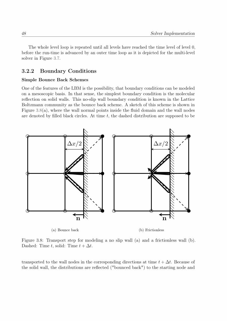
48 Solver Implementation
The whole level loop is repeated until all levels have reached the time level of level 0,before the run-time is advanced by an outer time loop as it is depicted for the multi-levelsolver in Figure 3.7.
3.2.2 Boundary Conditions
Simple Bounce Back Schemes
One of the features of the LBM is the possibility, that boundary conditions can be modeledon a mesoscopic basis. In that sense, the simplest boundary condition is the molecularreflection on solid walls. This no-slip wall boundary condition is known in the LatticeBoltzmann community as the bounce back scheme. A sketch of this scheme is shown inFigure 3.8(a), where the wall normal points inside the fluid domain and the wall nodesare denoted by filled black circles. At time t, the dashed distribution are supposed to be
n
∆x/2
(a) Bounce back
n
∆x/2
(b) Frictionless
Figure 3.8: Transport step for modeling a no slip wall (a) and a frictionless wall (b).Dashed: Time t, solid: Time t+ ∆t.
transported to the wall nodes in the corresponding directions at time t+ ∆t. Because ofthe solid wall, the distributions are reflected ("bounced back") to the starting node and
Implementation 49
point to the corresponding counter direction of the wall nodes at time t + ∆t. This isillustrated with black arrows. Formally this scheme is given by
fi−(x, t+ ∆t) = fi(x, t) with ei− = −ei. (3.2)
A direct consequence of this treatment is the positioning of the wall at ∆x/2, since thespace-time integration is bound to the values for the step sizes ∆t and ∆x. More pictorially,the molecules with their corresponding molecular velocities must travel the distance ∆x inone time step with size ∆t. It should be noted, that this form of the bounce back schemeis known as the "half way bounce back". In this case, the velocity vanishes exactly midwaybetween the fluid and wall node at ∆x/2. Therefore, an error of O(∆x) is introduced forwalls positioned off-center, which reduces the accuracy of the LBM to first order in thesecases [28]. It is also possible to model moving walls with this approach. An additionalterm is introduced by Ladd and Verberg [39], where the velocity of the wall uw is used tocompute the first order term of the equilibrium distribution. The form of this term emergesfrom the balance of momentum, which will be discussed in more detail in Section 3.2.3.The bounce back scheme for a wall moving with velocity uw reads
fi−(x, t+ ∆t) = fi(x, t)− 2 · wiρ ·ei · uwc2s
with ei− = −ei. (3.3)
In a similar manner, frictionless walls can be modeled with the simple bounce back scheme.To this end, the normal component of the velocity is reflected and the tangential componentof the velocity is conserved. This is shown in Figure 3.8(b) with solid black lines andmathematically expressed in the following equation:
fi−(x, t+ ∆t) = fi(x, t) with ei−,n = −ei,n and ei−,t = ei,t. (3.4)
As in the no-slip case, the modeled wall is placed at ∆x/2, because the normal velocityvanishes at this point.
Higher Order Bounce Back Schemes
Since the Lattice Boltzmann Method is second order accurate, several authors extendedthe wall treatment to incorporate the exact position of the wall into the simulation. Threeof these approaches are discussed in the sequel. Common to all, is the usage of thedimensionless wall distance, as it was discussed in Section 3.1.3 with the difference thatwe do not restrict ourselves to flat walls anymore. Hence, the dimensionless wall distancebecomes discrete in each lattice direction i as shown in Figure 3.5.
50 Solver Implementation
Bounce Back Filippova
Historically, the first wall boundary treatment for curved boundaries was presented byFilippova and Hänel in [19]. The idea of this approach is to compute a fictitious equilibriumat the surface of the wall with values for u from the fluid node xf or extrapolated valuesfor u on the wall node xw depending on the dimensionless wall distance qi. Values for ρare always taken from the fluid nodes. The resulting equilibrium is then combined throughlinear interpolation with the distributions from the simple bounce back rule. Accordingto the Chapman-Enskog analysis in [20], this scheme provides results with second orderaccuracy. As a result of a stability analysis, a case distinction in terms of the dimensionlesswall distance qi is made. The computation of the "bounced back" distributions can besummarized as follows [19, 28]:
Case: qi < 0.5
− Compute f eqi (x, t) with u = u(xf , t) and ρ = ρ(xf , t).
− Compute weighting factor χ =Ω
1− Ω· (2qi − 1).
− Combine bounce back (ei− = −ei) with f eqi according to:
fi−(xf , t+ ∆t) = (1− χ) · fi(xf , t) + χ · f eqi − 2 · wiρ ·ei · uwc2s
Case: qi ≥ 0.5
− Compute f eqi (x, t) with u = u(xf , t) ·(
1− 1
qi
)+
1
qi· uw.
and ρ = ρ(xf , t).
− Compute weighting factor χ = Ω · (2qi − 1).
− Combine bounce back (ei− = −ei) with f eqi according to:
fi−(xf , t+ ∆t) = (1− χ) · fi(xf , t) + χ · f eqi − 2 · wiρ ·ei · uwc2s
Bounce Back Mei
This bounce back descendant is a further improvement of the scheme proposed by Filippova.According to the authors, it is more stable, that is, it allows for higher values of Ω.This scheme was developed in 2D by Mei et al. [45]. An extension to 3D with furtherimprovements was presented by the same authors in [46]. Based on the fictitious equilibriumapproach, the linear interpolation is the same as for the Filippova scheme,
fi−(xf , t+ ∆t) = (1− χ) · fi(xf , t) + χ · f eqi − 2 · wiρ ·ei · uwc2s
with ei− = −ei. (3.5)

Implementation 51
A no-slip wall at rest is modeled by setting the wall velocity uw equal to zero. Theequilibrium function in eq. (3.5) is defined with separate velocities for the first and secondorder terms of the equilibrium [46]:
f eqi = wi · ρ(xf , t) ·(
1 +ei · ubc2s
+1
2c4s
(eiei − c2sI) : u(xf , t)u(xf , t)
). (3.6)
Again, as in the previous scheme, the velocity at the boundary surface ub and theinterpolation parameter χ are a function of the dimensionless wall distance q. Moreover, acase distinction is used for the computation of these values, due to stability issues. Thus,the values for ub and χ are chosen according to
ub =
u(xf + ei−∆t, t) qi < 0.5(
1− 32qi
)· u(xf , t) + 3
2qi· uw qi ≥ 0.5
(3.7)
χ =
2qi−1Ω−2
qi < 0.52qi−1Ω+0.5
qi ≥ 0.5(3.8)
in the Mei scheme. It can be shown through a Chapman-Enskog expansion, that thisscheme also provides results that are second order accurate [45, 46]. Furthermore, it shouldbe noted, that the schemes of Filippova and Mei only use information from the nearestneighbors to model curved walls and can therefore be considered as local schemes.
Bounce Back Bouzidi
In contrast to the higher order wall treatments presented above, the wall boundary conditiondeveloped by Bouzidi et al. [5] is an interpolation supplemented scheme. The idea of thisboundary condition is to exploit the stability and simplicity of the simple bounce backrule, while remaining time consistency, which results in the need for spatial extrapolationor interpolation of distributions, respectively. It is well known, that extrapolation ofdistributions renders the LBM vulnerable for instability. For that reason, a case distinctionis needed in order to be able to interpolate, independent of the wall position. Two casesmust be distinguished: The wall is closer to the fluid node (q < 0.5) or closer to thewall node (q ≥ 0.5). These are the same cases as in the fictitious equilibrium schemes,but derived from a different point of view, as will be discussed now. In both cases, theresult of the boundary treatment must be the values for the unknown distributions in wallopposite direction at the wall adjacent fluid nodes. Figure 3.9(a) shows the situation forthe distribution pointing in direction normal to the wall, which is q∆x < 0.5∆x away fromthe fluid node at xf1 and at time t.
An interpolation or extrapolation in time can be avoided by keeping the space-timeintegration consistent with all other nodes, that is, integrating from t to t + ∆t. Theintegration can be split in two parts: Integrating along direction i over the interval
52 Solver Implementation
s = ei∆t(1− q) and integration along the counter direction i− over ei−∆t · q. Since thetarget end point of the integration is xf1 in this case, the start point is located at xs asshown in Figure 3.9(a). Linear interpolation involving xf1 and xf2 is used to compute thedistributions at xs and at time t.
In the second case for q ≥ 0.5, the spatial interpolation is done at time t+ ∆t. Startpoint of the space-time integration is xf1 at time t as it is depicted in Figure 3.9(b). Theintegration is done over ei∆t · q along direction i and over s = ei−∆t(1− q) along directioni−, which results in values for the distributions in direction i− at xs and at time t+ ∆t.Missing distributions for the node at xf1 and for time t+ ∆t can be computed throughlinear interpolation between the corresponding distributions of xf2 and xs in direction i−.
The Bouzidi scheme including the terms for moving walls is given by [5]
fi−(xf1, t+ ∆t) =
2qifi(xf1, t) + (1− 2qi)fi(xf2, t)− 2wiρ(xf1, t)
eiuwc2s
qi < 0.5
1
2qifi(xf1, t) +
2qi − 1
2qifi−(xf2, t+ ∆t)− 1
qiwiρ(xf1, t)
eiuwc2s
qi ≥ 0.5,
(3.9)
where it can easily be seen, that the wall boundary condition according to Bouzidi reducesto the simple bounce back rule for q = 0.5. Owing to the interpolation, this scheme mustbe considered non local, since next-to-neighbor information is needed.
Strictly speaking, since this scheme acts on the distributions through interpolation inspace, it breaks the conservation of mass. The departure from mass conservation directlydepends on the accuracy of the interpolation scheme employed. In practical simulations,this error source can be neglected, especially because the density variation scales like thesquare of the Mach number.
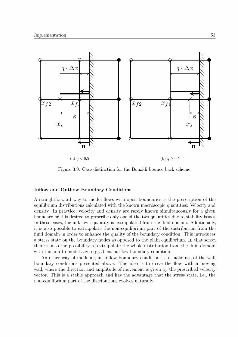
Implementation 53
n
xs
xf1xf2
s
q ·∆x
(a) q < 0.5
n
xs
xf1xf2
s
q ·∆x
(b) q ≥ 0.5
Figure 3.9: Case distinction for the Bouzidi bounce back scheme.
Inflow and Outflow Boundary Conditions
A straightforward way to model flows with open boundaries is the prescription of theequilibrium distributions calculated with the known macroscopic quantities: Velocity anddensity. In practice, velocity and density are rarely known simultaneously for a givenboundary or it is desired to prescribe only one of the two quantities due to stability issues.In these cases, the unknown quantity is extrapolated from the fluid domain. Additionally,it is also possible to extrapolate the non-equilibrium part of the distribution from thefluid domain in order to enhance the quality of the boundary condition. This introducesa stress state on the boundary nodes as opposed to the plain equilibrium. In that sense,there is also the possibility to extrapolate the whole distribution from the fluid domainwith the aim to model a zero gradient outflow boundary condition.
An other way of modeling an inflow boundary condition is to make use of the wallboundary conditions presented above. The idea is to drive the flow with a movingwall, where the direction and amplitude of movement is given by the prescribed velocityvector. This is a stable approach and has the advantage that the stress state, i.e., thenon-equilibrium part of the distributions evolves naturally.
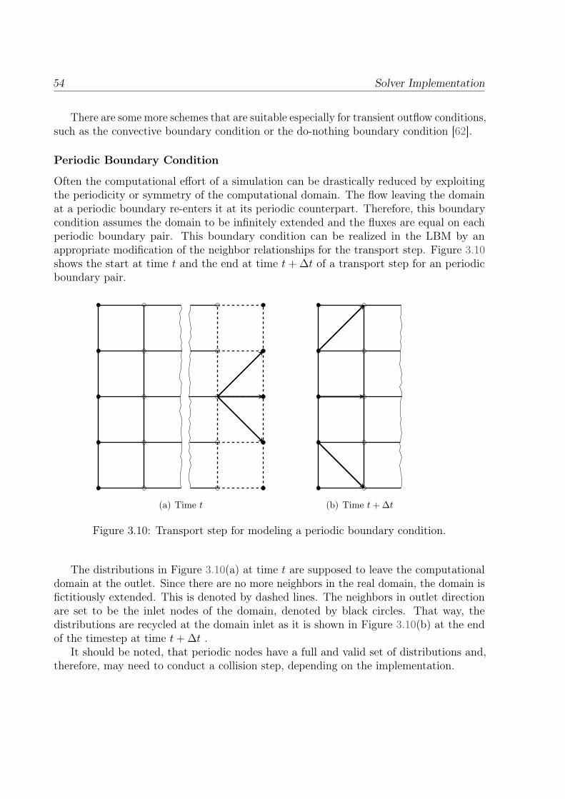
54 Solver Implementation
There are some more schemes that are suitable especially for transient outflow conditions,such as the convective boundary condition or the do-nothing boundary condition [62].
Periodic Boundary Condition
Often the computational effort of a simulation can be drastically reduced by exploitingthe periodicity or symmetry of the computational domain. The flow leaving the domainat a periodic boundary re-enters it at its periodic counterpart. Therefore, this boundarycondition assumes the domain to be infinitely extended and the fluxes are equal on eachperiodic boundary pair. This boundary condition can be realized in the LBM by anappropriate modification of the neighbor relationships for the transport step. Figure 3.10shows the start at time t and the end at time t+ ∆t of a transport step for an periodicboundary pair.
(a) Time t (b) Time t+ ∆t
Figure 3.10: Transport step for modeling a periodic boundary condition.
The distributions in Figure 3.10(a) at time t are supposed to leave the computationaldomain at the outlet. Since there are no more neighbors in the real domain, the domain isfictitiously extended. This is denoted by dashed lines. The neighbors in outlet directionare set to be the inlet nodes of the domain, denoted by black circles. That way, thedistributions are recycled at the domain inlet as it is shown in Figure 3.10(b) at the endof the timestep at time t+ ∆t .
It should be noted, that periodic nodes have a full and valid set of distributions and,therefore, may need to conduct a collision step, depending on the implementation.
Implementation 55
3.2.3 Force and Reference Frames
The question arises, how forces acting on surfaces can be computed within the LatticeBoltzmann Method. Since the force on a surface is an integral quantity, it can be computed,by integration of the surface stress. The stress may in turn be computed from the strainrate tensor using the generalized Hook’s law as well as the pressure acting on the surface.
An elegant alternative to the integration of the surface stress was proposed by Ladd andVerberg [38], which is known as the momentum exchange method in the LBM community.The fact, that force equals the derivative of momentum with respect to time is used tocompute surface forces. This method is used throughout the thesis for the evaluation offorces. It is implemented in SamSolver as the force acting on the wall evaluated at thewall nodes xw
fF =∆x3
∆t
∑xw
∑i
ei · (fi(xf , t) + fi(xf , t+ ∆t)− 2wiρ), (3.10)
where direction i denotes the incoming distributions from the fluid nods xf along theavailable lattice links. In contrast to the original momentum exchange method, we extendedthe expression with an ambient pressure term 2wiρ built from the zero velocity equilibriumdistribution. This is necessary for the correct evaluation of forces on bodies that are notcompletely immersed in the fluid, e.g., a wall mounted cube. Since there is no surface onthe opposite of the lid surface, the momentum exchange method gives wrong results insuch cases. For bodies completely immersed in the fluid, the ambient pressure term cancels,when summing over all wall nodes and therefore our scheme reduces to the original one. Itshould be noted, that the space and time steps have to be taken from the correspondingoctree levels for simulations with grid refinement.
In this scheme, the time interval is simply chosen to be ∆t, evaluated at the wallnode and the adjacent fluid node. Thus, the momentum exchange method is a first ordermethod, since the same argumentation for the simple bounce back scheme holds. However,the momentum exchange method gives reliable results even for curved boundaries [47].
The same approach can be used to compute moment forces. In addition to the forcevector fF , one has to compute the radius rw, that is, the shortest distance between thewall node and the moment axis, e.g., the axis of rotation of an impeller. Given is a momentaxis defined by the direction vector d and the origin point a. The radius of a wall node tothe axis is computed, by projection of
s = (xw − a) · d, (3.11)
onto the moment axis. It is then given by
rw = xw − (a + s · d) (3.12)
56 Solver Implementation
and the torque vector mT is computed with the momentum exchange method according to
mT =∆x3
∆t
∑xw
rw ×∑i
ei · (fi(xf , t) + fi(xf , t+ ∆t)− 2wiρ). (3.13)
This approach is used throughout the thesis to compute moment forces and in particularthe torque on the impeller in Section 6.2, where the spinning impeller is modeled with awall moving with circumferential velocity. The velocity is computed with the same radiusderived above. For the sake of completeness it should be mentioned, that a moving wallapproach is equivalent to the frozen rotor approach in a system with relative velocityformulation. This is also implemented in SamSolver. If a moving reference frame approachis taken, one has to consider additional forces, such as the Coriolis force. For a discussionon moving reference frames and the corresponding forces, the reader is referred to [65].
CHAPTER 4
Solver Verification
This chapter is dedicated to the verification of SAM-Lattice. Before we start, the conceptof verification and validation should be addressed in accordance to [2]. The concern ofverification is to make sure, that the code is free of mistakes and accurately solves theimplemented mathematical models. Therefore, the solutions of SAM-Lattice are comparedto solutions where the mathematical description can be solved analytically. By contrast,the task of validation is to check how good a model matches real world processes forwhich the model was designed. In that sense, there is no validation without experimentaldata. Thus, the solutions of the computer code are compared with data from real worldexperiments and the accuracy is investigated with the auxiliary condition of experimentaluncertainty. A sophisticated code development process relies on verification prior tovalidation. Hence, verification is done in this chapter, whereas validation will be conductedin Chapter 6 with experimental data of a propeller viscosimeter.
Verification is split into two parts. The Newtonian cases ensure the correctness of themain LBM implementation, whereas the generalized Newtonian case focuses more on theverification of the non-Newtonian model. The results of the Newtonian cases are presentedhere only qualitatively. The accuracy and convergence behavior is investigated in moredetail in the generalized Newtonian case for both Newtonian and non-Newtonian fluids.
57
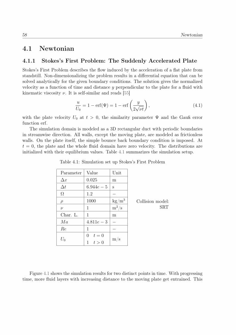
58 Newtonian
4.1 Newtonian
4.1.1 Stokes’s First Problem: The Suddenly Accelerated Plate
Stokes’s First Problem describes the flow induced by the acceleration of a flat plate fromstandstill. Non-dimensionalizing the problem results in a differential equation that can besolved analytically for the given boundary conditions. The solution gives the normalizedvelocity as a function of time and distance y perpendicular to the plate for a fluid withkinematic viscosity ν. It is self-similar and reads [55]
u
U0
= 1− erf(Ψ) = 1− erf
(y
2√νt
), (4.1)
with the plate velocity U0 at t > 0, the similarity parameter Ψ and the Gauß errorfunction erf.
The simulation domain is modeled as a 3D rectangular duct with periodic boundariesin streamwise direction. All walls, except the moving plate, are modeled as frictionlesswalls. On the plate itself, the simple bounce back boundary condition is imposed. Att = 0, the plate and the whole fluid domain have zero velocity. The distributions areinitialized with their equilibrium values. Table 4.1 summarizes the simulation setup.
Table 4.1: Simulation set up Stokes’s First Problem
Parameter Value Unit∆x 0.025 m∆t 6.944e− 5 sΩ 1.2 −ρ 1000 kg/m3
ν 1 m2/sChar. L. 1 mMa 4.811e− 3 −Re 1 −
U0
0 t = 0
1 t > 0m/s
Collision model:SRT
Figure 4.1 shows the simulation results for two distinct points in time. With progressingtime, more fluid layers with increasing distance to the moving plate get entrained. This
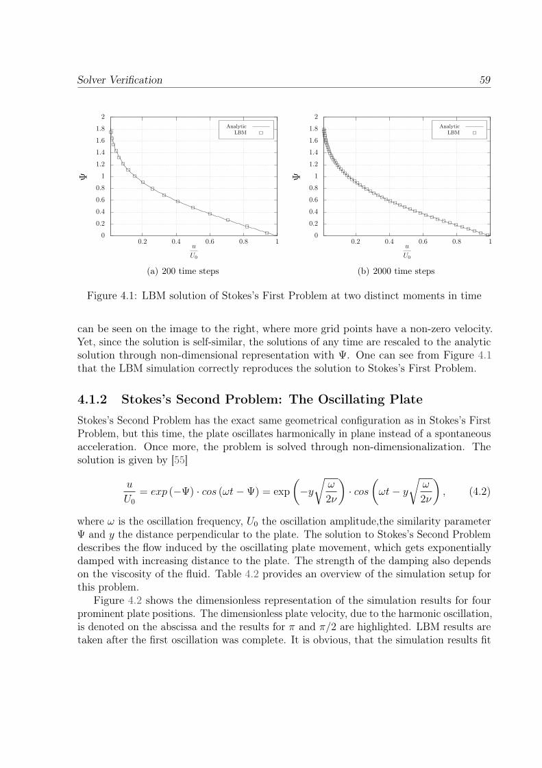
Solver Verification 59
0
0.2
0.4
0.6
0.8
1
1.2
1.4
1.6
1.8
2
0.2 0.4 0.6 0.8 1
Ψ
u
U0
AnalyticLBM
(a) 200 time steps
0
0.2
0.4
0.6
0.8
1
1.2
1.4
1.6
1.8
2
0.2 0.4 0.6 0.8 1
Ψ
u
U0
AnalyticLBM
(b) 2000 time steps
Figure 4.1: LBM solution of Stokes’s First Problem at two distinct moments in time
can be seen on the image to the right, where more grid points have a non-zero velocity.Yet, since the solution is self-similar, the solutions of any time are rescaled to the analyticsolution through non-dimensional representation with Ψ. One can see from Figure 4.1that the LBM simulation correctly reproduces the solution to Stokes’s First Problem.
4.1.2 Stokes’s Second Problem: The Oscillating Plate
Stokes’s Second Problem has the exact same geometrical configuration as in Stokes’s FirstProblem, but this time, the plate oscillates harmonically in plane instead of a spontaneousacceleration. Once more, the problem is solved through non-dimensionalization. Thesolution is given by [55]
u
U0
= exp (−Ψ) · cos (ωt−Ψ) = exp
(−y√
ω
2ν
)· cos
(ωt− y
√ω
2ν
), (4.2)
where ω is the oscillation frequency, U0 the oscillation amplitude,the similarity parameterΨ and y the distance perpendicular to the plate. The solution to Stokes’s Second Problemdescribes the flow induced by the oscillating plate movement, which gets exponentiallydamped with increasing distance to the plate. The strength of the damping also dependson the viscosity of the fluid. Table 4.2 provides an overview of the simulation setup forthis problem.
Figure 4.2 shows the dimensionless representation of the simulation results for fourprominent plate positions. The dimensionless plate velocity, due to the harmonic oscillation,is denoted on the abscissa and the results for π and π/2 are highlighted. LBM results aretaken after the first oscillation was complete. It is obvious, that the simulation results fit
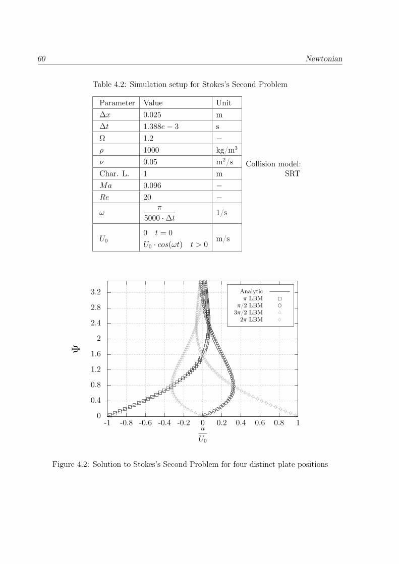
60 Newtonian
Table 4.2: Simulation setup for Stokes’s Second Problem
Parameter Value Unit∆x 0.025 m∆t 1.388e− 3 sΩ 1.2 −ρ 1000 kg/m3
ν 0.05 m2/sChar. L. 1 mMa 0.096 −Re 20 −ω
π
5000 ·∆t 1/s
U0
0 t = 0
U0 · cos(ωt) t > 0m/s
Collision model:SRT
0
0.4
0.8
1.2
1.6
2
2.4
2.8
3.2
-1 -0.8 -0.6 -0.4 -0.2 0 0.2 0.4 0.6 0.8 1
Ψ
u
U0
Analyticπ LBM
π/2 LBM3π/2 LBM
2π LBM
Figure 4.2: Solution to Stokes’s Second Problem for four distinct plate positions
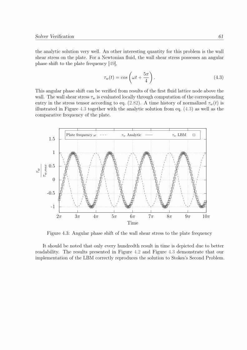
Solver Verification 61
the analytic solution very well. An other interesting quantity for this problem is the wallshear stress on the plate. For a Newtonian fluid, the wall shear stress possesses an angularphase shift to the plate frequency [49],
τw(t) = cos
(ωt+
5π
4
). (4.3)
This angular phase shift can be verified from results of the first fluid lattice node above thewall. The wall shear stress τw is evaluated locally through computation of the correspondingentry in the stress tensor according to eq. (2.82). A time history of normalized τw(t) isillustrated in Figure 4.3 together with the analytic solution from eq. (4.3) as well as thecomparative frequency of the plate.
-1
-0.5
0
0.5
1
1.5
2π 3π 4π 5π 6π 7π 8π 9π 10π
τ wτ w
,max
Time
Plate frequency ω τw Analytic τw LBM
Figure 4.3: Angular phase shift of the wall shear stress to the plate frequency
It should be noted that only every hundredth result in time is depicted due to betterreadability. The results presented in Figure 4.2 and Figure 4.3 demonstrate that ourimplementation of the LBM correctly reproduces the solution to Stokes’s Second Problem.
62 Generalized Newtonian
4.2 Generalized NewtonianThis section deals with the verification of the generalized Newtonian power-law modelas it was discussed in Section 2.5.3. The simulation domains are modeled with periodicboundaries in streamwise direction and the pressure gradient is substituted for a spatiallyconstant body force according to eq. (2.117). To quantify the quality of the simulation,we measure its accuracy with respect to the analytic solution over all lattice sites N ,
E =
√1
N·∑x
(u(x)− ua(x))2. (4.4)
This is the general definition of the global absolute error for the velocity distribution usedthroughout this thesis. Since the investigation in this chapter deals with steady stateproblems, the simulations are run until the following convergence criterion is reached:
|E(t)− E(t−∆t)| < 10−12. (4.5)
4.2.1 Hagen-Poiseuille Channel Flow
Since the correctness of the core implementation was already demonstrated in the previousSection 4.1, we will have a closer look at the spatial convergence behavior of the method.In order to investigate this with minimal influence of the wall boundary conditions, theflow through two parallel plates is considered. The simulation domain is modeled as asquare channel, where one pair of opposite walls are treated as frictionless walls and onthe other pair, the simple bounce back wall boundary condition is imposed. Therefore,the plane Hagen-Poiseuille equation can be used. Usually, the equation is given for aNewtonian fluid, but can be extended to generalized Newtonian power-law fluids. Thevelocity distribution for this case is given by [4]
ua(y) =n
n+ 1· (dpdx
1
k)
1n · (hn+1
n − y n+1n ), (4.6)
where y ∈ [−h, h] is perpendicular to the flow direction. Again, the pressure gradientis substituted for the body force dp/dx = ρ · a. It should be noted, that the lattice isgenerated as to exactly retain the channel width and height. The height of the channel His set to one and is measured from the center line of the channel. Moreover, the channelis axis aligned. Therefore, the simple bounce back scheme becomes a second order wallboundary condition. The simulation setup is summarized in Table 4.3 for the coarsestlattice investigated. All simulations are initialized with zero velocity equilibrium values.
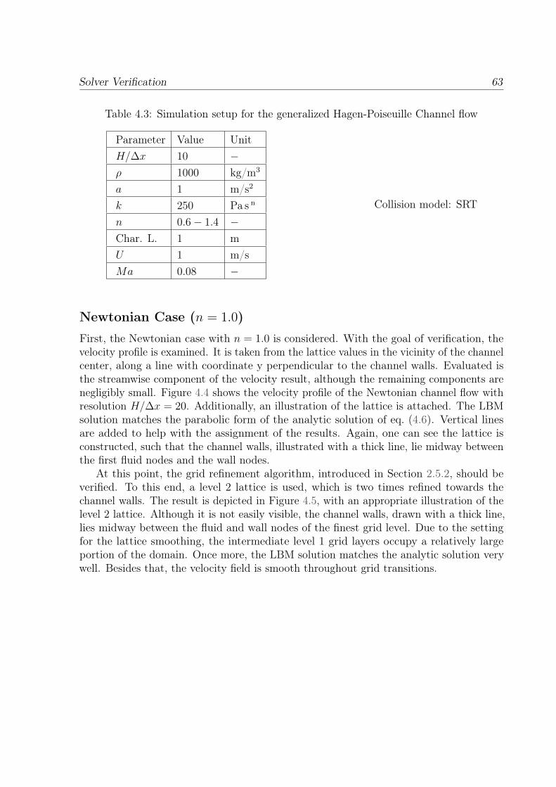
Solver Verification 63
Table 4.3: Simulation setup for the generalized Hagen-Poiseuille Channel flow
Parameter Value UnitH/∆x 10 −ρ 1000 kg/m3
a 1 m/s2
k 250 Pa s n
n 0.6− 1.4 −Char. L. 1 mU 1 m/sMa 0.08 −
Collision model: SRT
Newtonian Case (n = 1.0)
First, the Newtonian case with n = 1.0 is considered. With the goal of verification, thevelocity profile is examined. It is taken from the lattice values in the vicinity of the channelcenter, along a line with coordinate y perpendicular to the channel walls. Evaluated isthe streamwise component of the velocity result, although the remaining components arenegligibly small. Figure 4.4 shows the velocity profile of the Newtonian channel flow withresolution H/∆x = 20. Additionally, an illustration of the lattice is attached. The LBMsolution matches the parabolic form of the analytic solution of eq. (4.6). Vertical linesare added to help with the assignment of the results. Again, one can see the lattice isconstructed, such that the channel walls, illustrated with a thick line, lie midway betweenthe first fluid nodes and the wall nodes.
At this point, the grid refinement algorithm, introduced in Section 2.5.2, should beverified. To this end, a level 2 lattice is used, which is two times refined towards thechannel walls. The result is depicted in Figure 4.5, with an appropriate illustration of thelevel 2 lattice. Although it is not easily visible, the channel walls, drawn with a thick line,lies midway between the fluid and wall nodes of the finest grid level. Due to the settingfor the lattice smoothing, the intermediate level 1 grid layers occupy a relatively largeportion of the domain. Once more, the LBM solution matches the analytic solution verywell. Besides that, the velocity field is smooth throughout grid transitions.
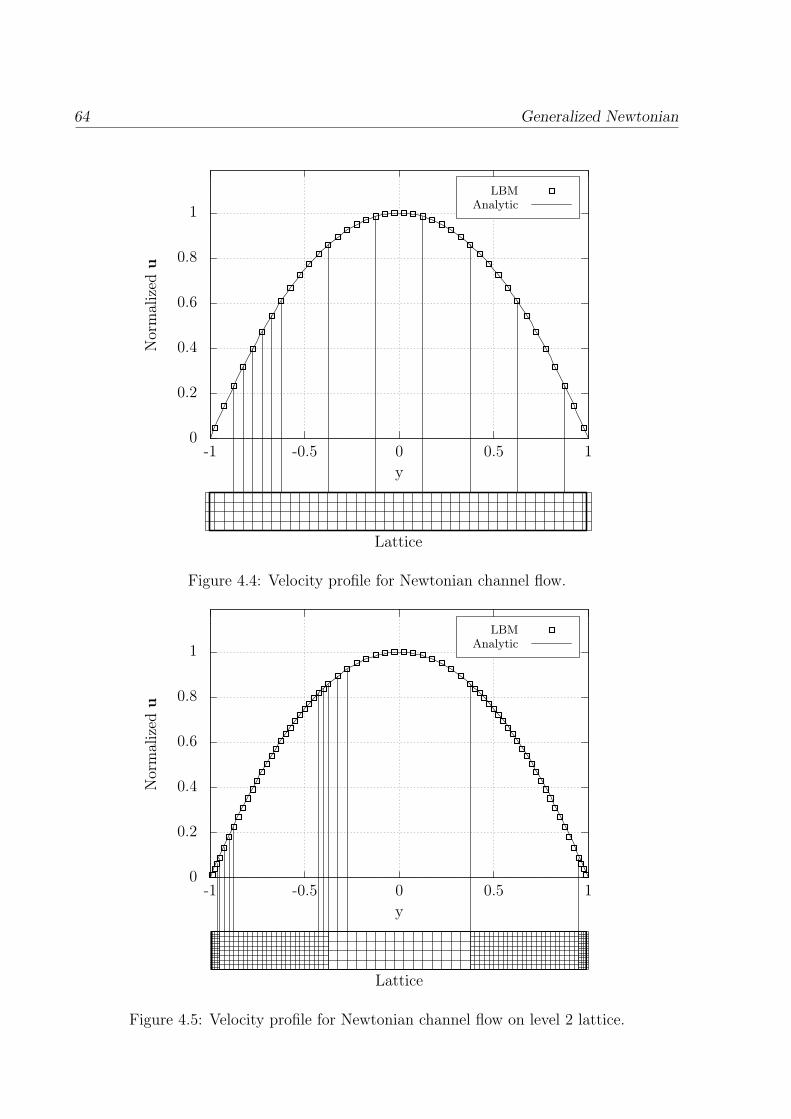
64 Generalized Newtonian
0
0.2
0.4
0.6
0.8
1
-1 -0.5 0 0.5 1
Nor
mal
ized
u
y
LBMAnalytic
Lattice
Figure 4.4: Velocity profile for Newtonian channel flow.
0
0.2
0.4
0.6
0.8
1
-1 -0.5 0 0.5 1
Nor
mal
ized
u
y
LBMAnalytic
Lattice
Figure 4.5: Velocity profile for Newtonian channel flow on level 2 lattice.
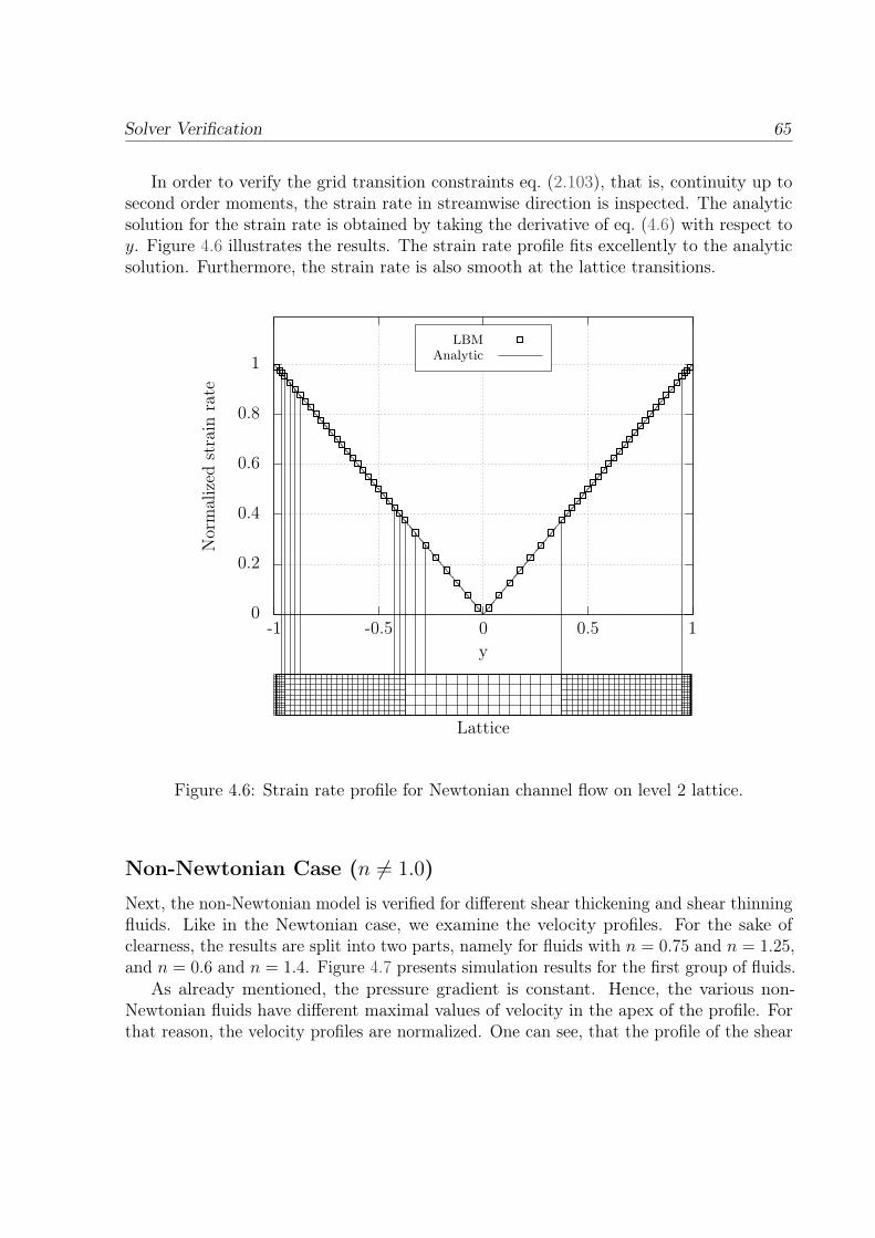
Solver Verification 65
In order to verify the grid transition constraints eq. (2.103), that is, continuity up tosecond order moments, the strain rate in streamwise direction is inspected. The analyticsolution for the strain rate is obtained by taking the derivative of eq. (4.6) with respect toy. Figure 4.6 illustrates the results. The strain rate profile fits excellently to the analyticsolution. Furthermore, the strain rate is also smooth at the lattice transitions.
0
0.2
0.4
0.6
0.8
1
-1 -0.5 0 0.5 1
Nor
mal
ized
stra
inra
te
y
LBMAnalytic
Lattice
Figure 4.6: Strain rate profile for Newtonian channel flow on level 2 lattice.
Non-Newtonian Case (n 6= 1.0)
Next, the non-Newtonian model is verified for different shear thickening and shear thinningfluids. Like in the Newtonian case, we examine the velocity profiles. For the sake ofclearness, the results are split into two parts, namely for fluids with n = 0.75 and n = 1.25,and n = 0.6 and n = 1.4. Figure 4.7 presents simulation results for the first group of fluids.
As already mentioned, the pressure gradient is constant. Hence, the various non-Newtonian fluids have different maximal values of velocity in the apex of the profile. Forthat reason, the velocity profiles are normalized. One can see, that the profile of the shear
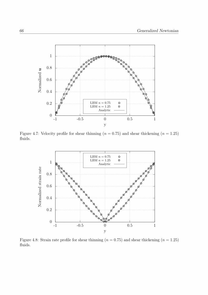
66 Generalized Newtonian
0
0.2
0.4
0.6
0.8
1
-1 -0.5 0 0.5 1
Nor
mal
ized
u
y
LBM n = 0.75LBM n = 1.25
Analytic
Figure 4.7: Velocity profile for shear thinning (n = 0.75) and shear thickening (n = 1.25)fluids.
0
0.2
0.4
0.6
0.8
1
-1 -0.5 0 0.5 1
Nor
mal
ized
stra
inra
te
y
LBM n = 0.75LBM n = 1.25
Analytic
Figure 4.8: Strain rate profile for shear thinning (n = 0.75) and shear thickening (n = 1.25)fluids.
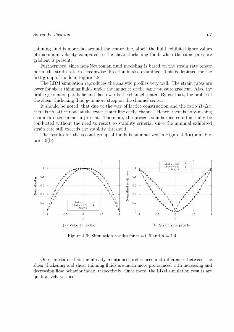
Solver Verification 67
thinning fluid is more flat around the center line, albeit the fluid exhibits higher valuesof maximum velocity compared to the shear thickening fluid, when the same pressuregradient is present.
Furthermore, since non-Newtonian fluid modeling is based on the strain rate tensornorm, the strain rate in streamwise direction is also examined. This is depicted for thefirst group of fluids in Figure 4.8.
The LBM simulation reproduces the analytic profiles very well. The strain rates arelower for shear thinning fluids under the influence of the same pressure gradient. Also, theprofile gets more parabolic and flat towards the channel center. By contrast, the profile ofthe shear thickening fluid gets more steep on the channel center.
It should be noted, that due to the way of lattice construction and the ratio H/∆x,there is no lattice node at the exact center line of the channel. Hence, there is no vanishingstrain rate tensor norm present. Therefore, the present simulations could actually beconducted without the need to resort to stability criteria, since the minimal exhibitedstrain rate still exceeds the stability threshold.
The results for the second group of fluids is summarized in Figure 4.9(a) and Fig-ure 4.9(b).
0
0.2
0.4
0.6
0.8
1
-1 -0.5 0 0.5 1
Nor
mal
ized
u
y
LBM n = 1.4LBM n = 0.60
Analytic
(a) Velocity profile
0
0.2
0.4
0.6
0.8
1
-1 -0.5 0 0.5 1
Nor
mal
ized
stra
inra
te
y
LBM n = 0.60LBM n = 1.40
Analytic
(b) Strain rate profile
Figure 4.9: Simulation results for n = 0.6 and n = 1.4.
One can state, that the already mentioned preferences and differences between theshear thickening and shear thinning fluids are much more pronounced with increasing anddecreasing flow behavior index, respectively. Once more, the LBM simulation results arequalitatively verified.
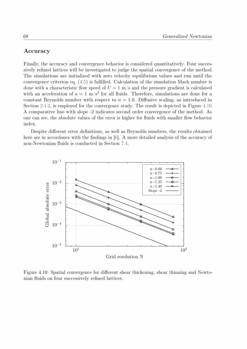
68 Generalized Newtonian
Accuracy
Finally, the accuracy and convergence behavior is considered quantitatively. Four succes-sively refined lattices will be investigated to judge the spatial convergence of the method.The simulations are initialized with zero velocity equilibrium values and run until theconvergence criterion eq. (4.5) is fulfilled. Calculation of the simulation Mach number isdone with a characteristic flow speed of U = 1 m/s and the pressure gradient is calculatedwith an acceleration of a = 1 m/s2 for all fluids. Therefore, simulations are done for aconstant Reynolds number with respect to n = 1.0. Diffusive scaling, as introduced inSection 2.4.2, is employed for the convergence study. The result is depicted in Figure 4.10.A comparative line with slope -2 indicates second order convergence of the method. Asone can see, the absolute values of the error is higher for fluids with smaller flow behaviorindex.
Despite different error definitions, as well as Reynolds numbers, the results obtainedhere are in accordance with the findings in [6]. A more detailed analysis of the accuracy ofnon-Newtonian fluids is conducted in Section 7.4.
10−5
10−4
10−3
10−2
10−1
101 102
Glo
bala
bsol
ute
erro
r
Grid resolution N
n=0.60n=0.75n=1.00n=1.25n=1.40
Slope -2
Figure 4.10: Spatial convergence for different shear thickening, shear thinning and Newto-nian fluids on four successively refined lattices.
Solver Verification 69
4.2.2 Hagen-Poiseuille Pipe Flow
The Hagen-Poiseuille equation gives the pressure drop in a fluid, flowing with a given massflow rate through a cylindrical pipe with radius R. Because of the no-slip condition at thepipe walls, the velocity profile of a pipe flow takes paraboloidal form. In this case, thegeneralized analytic velocity distribution is given in radial coordinates [4]
ua(r) =n
n+ 1·(dp
dx
1
2k
) 1n
·(R
n+1n − r n+1
n
), (4.7)
where r ∈ [−R,R], the flow consistency index k and the flow behavior index n, respectively.
Newtonian Case (n = 1.0)
For the purpose of verification, we will first investigate a Newtonian fluid for n = 1.0. Thespatial convergence was already demonstrated in the previous subsection. Hence, we willhave a closer look at the implementation of the wall boundary conditions. Since the wallspossess curvature, it is necessary to make use of higher order bounce back schemes for whichthe proposed O(∆x2) behavior of EBC can be inspected. In this context, the influenceof the error Eg due to the geometry discretization, as introduced in Equation (2.92), ishighlighted.
In order to ensure spatial convergence, the diffusive scaling is employed. This effectivelymeans that the relaxation parameter Ω is constant throughout the different resolvedlattices. Table 4.4 shows the simulation set up for the Newtonian pipe flow with thecoarsest lattice resolution used. The pipe geometry is discretized with a medium resolutionfor the additional investigation of Eg. All second order wall boundary conditions introducedin Section 3.2.2 are tested.
Table 4.4: Simulation set up for the Newtonian pipe flow case n = 1.0
Parameter Value Unit∆x 0.2 m∆g 0.05 m∆t 1.777e− 2 sΩ 1.2 −ρ 1000 kg/m3
k 250 Pa sR 1 mMa 0.15396 −
Collision model: SRT
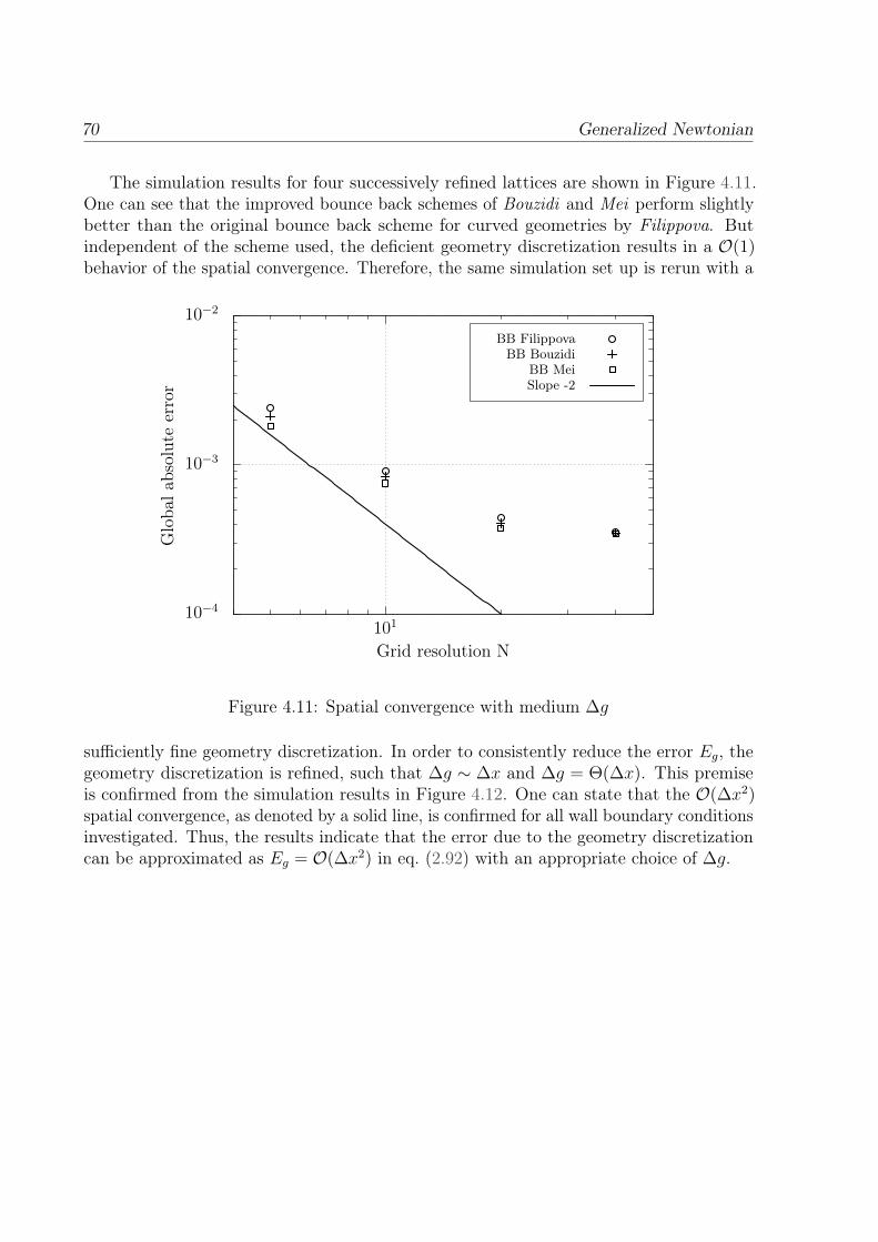
70 Generalized Newtonian
The simulation results for four successively refined lattices are shown in Figure 4.11.One can see that the improved bounce back schemes of Bouzidi and Mei perform slightlybetter than the original bounce back scheme for curved geometries by Filippova. Butindependent of the scheme used, the deficient geometry discretization results in a O(1)behavior of the spatial convergence. Therefore, the same simulation set up is rerun with a
10−4
10−3
10−2
101
Glo
bala
bsol
ute
erro
r
Grid resolution N
BB FilippovaBB Bouzidi
BB MeiSlope -2
Figure 4.11: Spatial convergence with medium ∆g
sufficiently fine geometry discretization. In order to consistently reduce the error Eg, thegeometry discretization is refined, such that ∆g ∼ ∆x and ∆g = Θ(∆x). This premiseis confirmed from the simulation results in Figure 4.12. One can state that the O(∆x2)spatial convergence, as denoted by a solid line, is confirmed for all wall boundary conditionsinvestigated. Thus, the results indicate that the error due to the geometry discretizationcan be approximated as Eg = O(∆x2) in eq. (2.92) with an appropriate choice of ∆g.
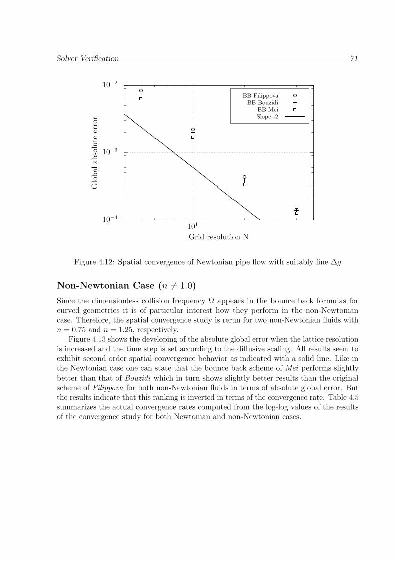
Solver Verification 71
10−4
10−3
10−2
101
Glo
bala
bsol
ute
erro
r
Grid resolution N
BB FilippovaBB Bouzidi
BB MeiSlope -2
Figure 4.12: Spatial convergence of Newtonian pipe flow with suitably fine ∆g
Non-Newtonian Case (n 6= 1.0)
Since the dimensionless collision frequency Ω appears in the bounce back formulas forcurved geometries it is of particular interest how they perform in the non-Newtoniancase. Therefore, the spatial convergence study is rerun for two non-Newtonian fluids withn = 0.75 and n = 1.25, respectively.
Figure 4.13 shows the developing of the absolute global error when the lattice resolutionis increased and the time step is set according to the diffusive scaling. All results seem toexhibit second order spatial convergence behavior as indicated with a solid line. Like inthe Newtonian case one can state that the bounce back scheme of Mei performs slightlybetter than that of Bouzidi which in turn shows slightly better results than the originalscheme of Filippova for both non-Newtonian fluids in terms of absolute global error. Butthe results indicate that this ranking is inverted in terms of the convergence rate. Table 4.5summarizes the actual convergence rates computed from the log-log values of the resultsof the convergence study for both Newtonian and non-Newtonian cases.
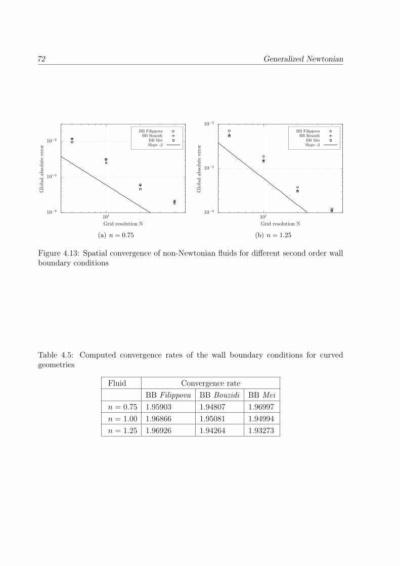
72 Generalized Newtonian
10−4
10−3
10−2
101
Glo
bala
bsol
ute
erro
r
Grid resolution N
BB FilippovaBB Bouzidi
BB MeiSlope -2
(a) n = 0.75
10−4
10−3
10−2
101
Glo
bala
bsol
ute
erro
r
Grid resolution N
BB FilippovaBB Bouzidi
BB MeiSlope -2
(b) n = 1.25
Figure 4.13: Spatial convergence of non-Newtonian fluids for different second order wallboundary conditions
Table 4.5: Computed convergence rates of the wall boundary conditions for curvedgeometries
Fluid Convergence rateBB Filippova BB Bouzidi BB Mei
n = 0.75 1.95903 1.94807 1.96997
n = 1.00 1.96866 1.95081 1.94994
n = 1.25 1.96926 1.94264 1.93273
CHAPTER 5
Viscosity Adaption Method
The Lattice Boltzmann Method can be extended to non-Newtonian fluid flows as wasshown in Section 2.5.3. Several authors have demonstrated its applicability, e.g., in [6].The regular grid based scheme makes the LBM ideally suitable for simulations involvingcomplex solids. Such geometries are common in the food processing industry, where fluidsare mixed by static mixers or agitators. Those fluid flows are often laminar and non-Newtonian. Special care has to be taken for non-Newtonian Lattice Boltzmann simulationsin order to keep them stable. A straightforward way is to truncate the modeled viscosityrange by numerical stability criteria eq. (2.112). This is an effective approach, but fromthe physical point of view the viscosity bounds are chosen arbitrarily. Moreover, thesebounds depend on and vary with the grid and time step size and, therefore, with thesimulation Mach number. However, the simulation Mach number is problem dependentand must be set by the user a priori. Thus, the modeled viscosity range may not fit to theactual physical problem, which yields corrupted simulation results. A way around is todetermine a suitable simulation Mach number by longsome precursor simulations [9, 48].This renders the standard LBM unattractive for practical use, especially for complex cases.Moreover, in the standard LBM the simulation Mach number is constant throughout thesimulation and, thus, the LBM cannot account for changing transient viscosity ranges.
In this chapter, we derive the viscosity adaption method (VAM) to consistently andconstantly adapt the modeled viscosity range to the actual physical problem. This isthe basis of the viscosity adaptive Lattice Boltzmann Method (VALBM). We verify theVALBM in Chapter 6 for steady state channel flow and transient pulsatile pipe flow ofnon-Newtonian fluids. Additionally, validation is done with experimental data from apropeller viscosimeter.
73
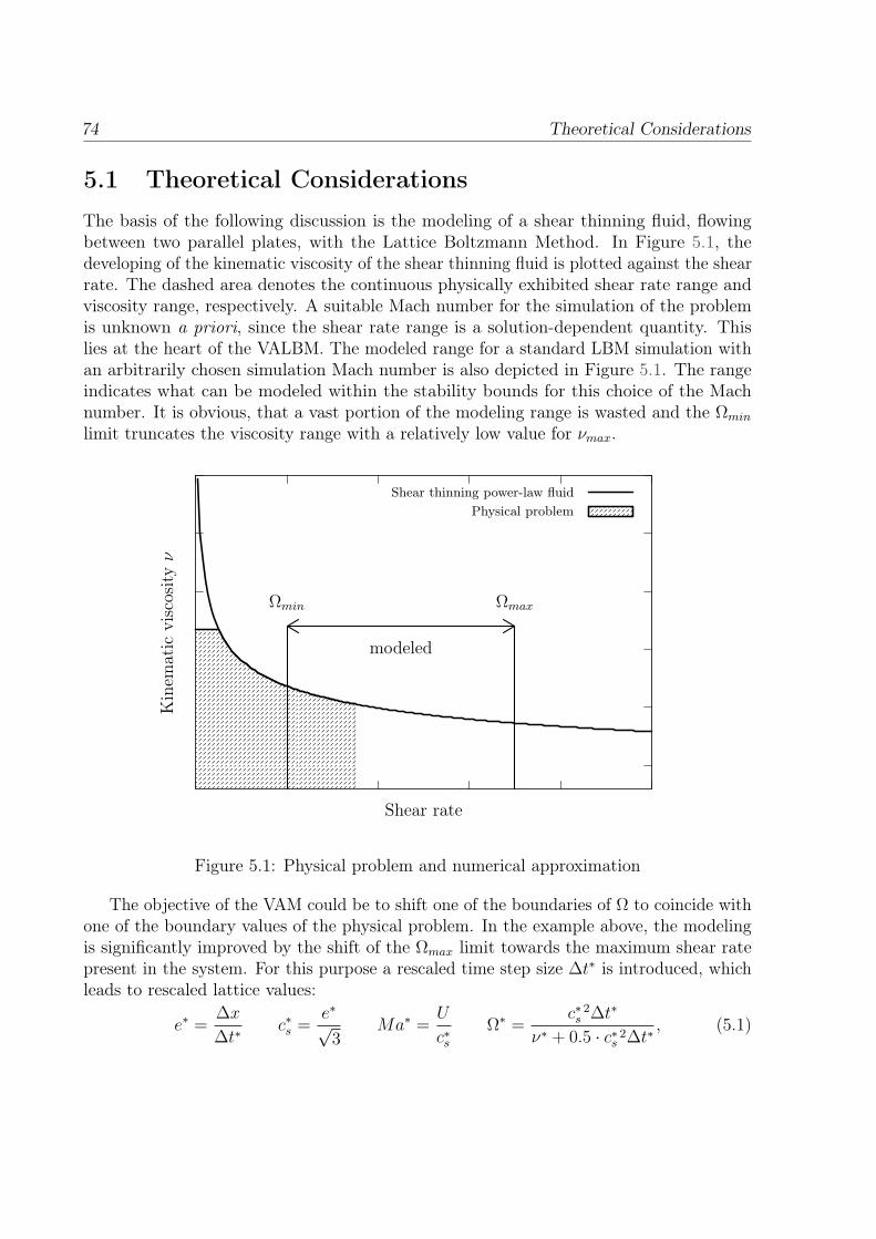
74 Theoretical Considerations
5.1 Theoretical ConsiderationsThe basis of the following discussion is the modeling of a shear thinning fluid, flowingbetween two parallel plates, with the Lattice Boltzmann Method. In Figure 5.1, thedeveloping of the kinematic viscosity of the shear thinning fluid is plotted against the shearrate. The dashed area denotes the continuous physically exhibited shear rate range andviscosity range, respectively. A suitable Mach number for the simulation of the problemis unknown a priori, since the shear rate range is a solution-dependent quantity. Thislies at the heart of the VALBM. The modeled range for a standard LBM simulation withan arbitrarily chosen simulation Mach number is also depicted in Figure 5.1. The rangeindicates what can be modeled within the stability bounds for this choice of the Machnumber. It is obvious, that a vast portion of the modeling range is wasted and the Ωmin
limit truncates the viscosity range with a relatively low value for νmax.
Kin
emat
icvi
scos
ityν
Shear rate
modeled
Ωmin Ωmax
Shear thinning power-law fluidPhysical problem
Figure 5.1: Physical problem and numerical approximation
The objective of the VAM could be to shift one of the boundaries of Ω to coincide withone of the boundary values of the physical problem. In the example above, the modelingis significantly improved by the shift of the Ωmax limit towards the maximum shear ratepresent in the system. For this purpose a rescaled time step size ∆t∗ is introduced, whichleads to rescaled lattice values:
e∗ =∆x
∆t∗c∗s =
e∗√3
Ma∗ =U
c∗sΩ∗ =
c∗ 2s ∆t∗
ν∗ + 0.5 · c∗ 2s ∆t∗
, (5.1)
Viscosity Adaption Method 75
where Ω∗ must be rescaled at each lattice site. In order to yield the same macroscopicmoments in the new system, the distributions fi must be rescaled. This is done with thelinear transformation matrices M in the old system and M∗ in the new system accordingto
f ∗i = M∗−1Mfi . (5.2)
By definition, the moments and especially the second order moment tensor Παβ is unchangedby this operation. However, the macroscopic shear rate eq. (2.110) changes because ofthe pre-factor. Consequently, the kinematic viscosity changes through the constitutivelaw used in the simulation. It is desired that the rescale operation (5.2) leaves the shearrate and, therefore, the viscosity unaffected. We achieve this through rescaling of f ∗neqi ineq. (2.110) to give the same shear rate, hence ν∗ = ν,
f ∗∗i = f ∗ eqi +ν + ∆x2
6·∆t∗
ν + ∆x2
6·∆t· (f ∗i − f ∗ eqi ), (5.3)
where f ∗ eqi is computed from eq. (2.27) in the new system.
5.2 Choice of Time Step Size
In order to adapt to the physical problem, the time step size ∆t∗ is determined from theminimal or maximal shear rate in the modeled system, which is a solution-dependentquantity. Following the example situation in Figure 5.1, the numerical approximation ofthe physical problem is improved if we shift the maximal collision frequency towards themaximal shear rate of the system. Therefore, the target collision frequency Ωt should takethe value of Ωmax, built with the kinematic viscosity νm obtained from the maximum shearrate. Thus, we choose the new time step size ∆t∗ according to
∆t∗ =( 1
Ωt− 1
2) ·∆x2
3 · νm. (5.4)
Since the value of νm is solution-dependent, it can be expected to converge to the physicalvalue of the system if the time step size is recursively adapted. From eq. (5.1) it followsthat an increase in Ω causes a decreased time step size and, therefore, a decrease in Machbecause Ma ∝ ∆t
∆x. Hence, we can expect a prolonged simulation time with an enhanced
time resolution. Another possibility is to set the target relaxation parameter by Ωmin.This is possible in cases where the lowest shear rate still exceeds a valid threshold likein the non-Newtonian Hagen-Poiseuille channel flow (see Figure 4.8). In this discretephysical problem, we can opt for the Ωmin bound without triggering the upper Machnumber limitation. If ∆t∗ is determined by eq. (5.4) with Ωt = Ωmin and νm from theminimal shear rate, the time step size as well as the Mach number is increased. Therefore,
76 Mach Number Limitation
the simulation is accelerated. Note, that in a general flow situation it may then be possibleto cut off viscosities from high shear rates due to the Ωmax limit with this approach. Theoptimal choice for Ωmin will be part of the investigations in Chapter 7.
5.3 Mach Number LimitationAs described in Section 5.2, the viscosity adaptive LBM makes use of a variable time stepsize on a fixed grid. Given that the Mach number is coupled with the time step size, wehave to make sure the lattice values remain valid throughout the simulation. To this end,we limit the possible choice of the time step size through physically meaningful Machnumber limits.
Ma∗∗ =
Mamax Ma∗ > Mamax
Ma+ λ · (Ma∗ −Ma) λ ∈ [0, 1]
Mamin Ma∗ < Mamin(5.5)
It is common practice to consider flows with Mach numbers Mamax below 0.3 tobe weakly compressible [18]. Additionally, we set Mamin = 10−4 to stay in the weaklycompressible regime because the hydrodynamic limit does not exist for uncorrected BGKdynamics [12, 40]. In practice, this also prevents the time step size to get uneconomicallysmall. For enhanced stability properties of the viscosity adaptive LBM, we computethe simulation Mach number for the next time step Ma∗∗, through under-relaxation ofthe Mach number Ma∗ obtained from eq. (5.1) and eq. (5.4). The final lattice valuesincluding the time step size have to be recomputed from Ma∗∗. For stationary flows, thesimulation Mach number can be expected to converge as the target shear rate convergesto the physical problem. Hence, we are able to introduce a convergence criterion for thesimulation Mach number,
|Ma∗∗ −Ma|Ma
< δ. (5.6)
If the expected Mach number change is small, the adaption process can be abandoned. Inorder to keep the Mach number threshold δ independent of the actual value of the Machnumbers and, therefore, meaningful for all simulations, the relative Mach number changeis considered.
5.4 Multi-Level ApproachSo far, the presented considerations are valid for single level simulations. The questionarises, how the VAM can be extended to simulations with local grid refinement. In orderto ensure continuity of the Re number, a redefinition of the stability criteria eq. (2.112)and eq. (2.111) is necessary, since the relationship Ωc > Ωf holds at the interface. As
Viscosity Adaption Method 77
the maximal value for Ωmax must not be exceeded in the whole simulation domain, theminimal value of the viscosity used for the dimensionless collision frequency in each level isdetermined by νmin = νcmin computed from Ωmax on the coarsest level. On the other hand,Ωmin must not be exceeded globally. Hence, the global maximal value for the viscosityνmax = νfmax is computed from Ωmin on the finest level. The stability criteria for the coarseand fine level can, thus, be expressed as:
Ωc =
Ωmax =
c2s∆t
c
νcmin + 0.5c2s∆t
c
Ω
Ωcmin =
c2s∆t
c
νfmax + 0.5c2s∆t
c
(5.7)
Ωf =
Ωfmax =
c2s∆t
f
νcmin + 0.5c2s∆t
f
Ω
Ωmin =c2s∆t
f
νfmax + 0.5c2s∆t
f.
(5.8)
It should be noted, that this multi-level approach narrows the overall modeled viscosityrange as opposed to what would be possible with the increased resolution, since it is theintersecting set of the viscosity ranges of the coarsest and finest level. This is the priceto pay for stability of simulations with grid refinement. Thus, another possibility, whichpresumes some knowledge about the flow of interest, is to refine the grid such that thevalues of Ωc and Ωf of the interface region are far enough from the stability borders. Thatway, the single level approach can be used for each grid level separately. An investigationand discussion on the different approaches in a simulation with local grid refinement isdone in Section 6.2.
5.5 Algorithm OverviewFinally, we will summarize the proposed algorithm. To precis the procedure, we considera stationary flow of a shear thinning fluid (Figure 5.1) with the aim to accelerate thesimulation. Starting the algorithm for the viscosity adaption method at an arbitrary timestep t0 with an arbitrary simulation Mach number it can be summarized as follows:
- Save the minimal shear rate |εm| present in the system.
- Compute νm with |εm| according to the constitutive law, e.g., eq. (2.109).
- Compute new time step size ∆t∗ with the target collision frequency Ωt and νm fromeq. (5.4).
78 Algorithm Overview
- Compute new lattice values from eq. (5.1).
- Relax Ma with under-relaxation factor λ or truncate it eq. (5.5).
- Recompute final adapted lattice values eq. (5.1) with the time step size obtainedfrom Mach number Ma∗∗ and the new viscosity bounds for eq. (2.112).
- Finally rescale distributions through eq. (5.2) and eq. (5.3).
The algorithm must be repeated in the subsequent time steps until the Mach numberMa∗∗ converges and the desired target collision frequency is reached. This can also berealized in adaption intervals, allowing the solution to develop in between VAM steps.
In order to maximize the modeled viscosity range in the aforementioned exampleof Figure 5.1, an other possibility is to shift Ωmax to the maximal physical shear rate.Hence, νm should be computed with the maximal shear rate |εm| in the system and Ωt isset to Ωmax. The remaining steps in the algorithm are identical to the ones in the list above.
Actual physical boundaries, if known, can easily be implemented in the VALBM bysetting the appropriate values in eq. (2.112). For example, the real upper bound on theviscosity for a shear thinning material corresponds to the horizontal line of the shadedarea (physical problem) in Figure 5.1. In practical simulations, the collision frequencybuilt with the real upper viscosity bound of the material (if known) may lead to valuesΩmin 1, which in turn leads to instability of the LBM. Thus, a smaller viscosity boundmust be chosen, such that, e.g., Ωmin = 1.0. If the real upper bound results in a collisionfrequency of Ωmin ≥ 1.0, that value must be chosen for the limits in eq. (2.112). Hence,the implementation of the VALBM is straightforward for other non-Newtonian models,e.g., the Carreau-Yasuda or Cross model.
CHAPTER 6
Verification and Validation of the Viscosity Adaptive LBM
In this chapter, we consider the verification and validation of the viscosity adaptive LBMapproach. First, the method is verified for the Hagen-Poiseuille flow for both the steadystate and the transient case. Afterwards, the method is validated with experimental datafrom a propeller viscosimeter that was developed at the chair SAM.
6.1 Simple Case: Hagen-Poiseuille
6.1.1 Steady-State
For the verification of the proposed algorithm we investigate the flow through a 3D duct.We impose periodic boundary conditions in streamwise direction and the flow is driventhrough a body force similar to the simulations in Chapter 4. The lattice is constructedas to exactly retain the channel width and height, while using the simple bounce backboundary condition. For the sake of simplicity, we model the side walls of the duct tobe frictionless. Therefore we can use the plane Hagen-Poiseuille solution for power-lawfluids eq. (4.6). Again, the quality of the simulation is measured through the absoluteglobal error eq. (4.4) and the simulations are run until the convergence criterion eq. (4.5)is fulfilled.
Mach Number Investigation
In a first approach, we want to investigate the convergence properties of the viscosityadaption method and its robustness to the starting Mach number, which is unknown userinput. A series of simulations with starting Mach numbers from 0.1 to 10−4 are conducted
79
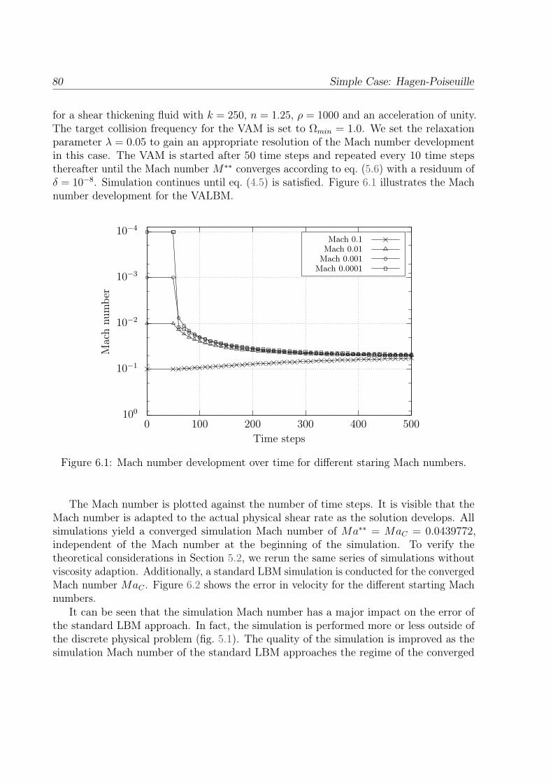
80 Simple Case: Hagen-Poiseuille
for a shear thickening fluid with k = 250, n = 1.25, ρ = 1000 and an acceleration of unity.The target collision frequency for the VAM is set to Ωmin = 1.0. We set the relaxationparameter λ = 0.05 to gain an appropriate resolution of the Mach number developmentin this case. The VAM is started after 50 time steps and repeated every 10 time stepsthereafter until the Mach number M∗∗ converges according to eq. (5.6) with a residuum ofδ = 10−8. Simulation continues until eq. (4.5) is satisfied. Figure 6.1 illustrates the Machnumber development for the VALBM.
10−4
10−3
10−2
10−1
1000 100 200 300 400 500
Mac
hnu
mbe
r
Time steps
Mach 0.1Mach 0.01
Mach 0.001Mach 0.0001
Figure 6.1: Mach number development over time for different staring Mach numbers.
The Mach number is plotted against the number of time steps. It is visible that theMach number is adapted to the actual physical shear rate as the solution develops. Allsimulations yield a converged simulation Mach number of Ma∗∗ = MaC = 0.0439772,independent of the Mach number at the beginning of the simulation. To verify thetheoretical considerations in Section 5.2, we rerun the same series of simulations withoutviscosity adaption. Additionally, a standard LBM simulation is conducted for the convergedMach number MaC . Figure 6.2 shows the error in velocity for the different starting Machnumbers.
It can be seen that the simulation Mach number has a major impact on the error ofthe standard LBM approach. In fact, the simulation is performed more or less outside ofthe discrete physical problem (fig. 5.1). The quality of the simulation is improved as thesimulation Mach number of the standard LBM approaches the regime of the converged
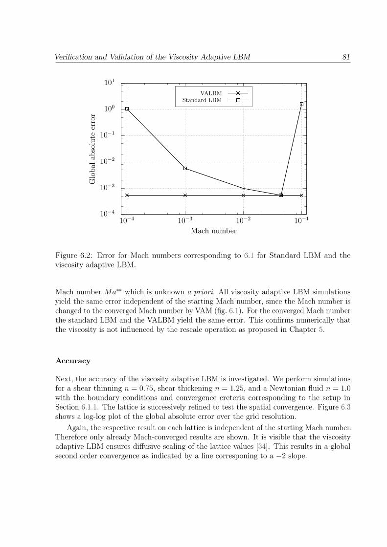
Verification and Validation of the Viscosity Adaptive LBM 81
10−4
10−3
10−2
10−1
100
101
10−4 10−3 10−2 10−1
Glo
bala
bsol
ute
erro
r
Mach number
VALBMStandard LBM
Figure 6.2: Error for Mach numbers corresponding to 6.1 for Standard LBM and theviscosity adaptive LBM.
Mach number Ma∗∗ which is unknown a priori. All viscosity adaptive LBM simulationsyield the same error independent of the starting Mach number, since the Mach number ischanged to the converged Mach number by VAM (fig. 6.1). For the converged Mach numberthe standard LBM and the VALBM yield the same error. This confirms numerically thatthe viscosity is not influenced by the rescale operation as proposed in Chapter 5.
Accuracy
Next, the accuracy of the viscosity adaptive LBM is investigated. We perform simulationsfor a shear thinning n = 0.75, shear thickening n = 1.25, and a Newtonian fluid n = 1.0with the boundary conditions and convergence creteria corresponding to the setup inSection 6.1.1. The lattice is successively refined to test the spatial convergence. Figure 6.3shows a log-log plot of the global absolute error over the grid resolution.
Again, the respective result on each lattice is independent of the starting Mach number.Therefore only already Mach-converged results are shown. It is visible that the viscosityadaptive LBM ensures diffusive scaling of the lattice values [34]. This results in a globalsecond order convergence as indicated by a line corresponing to a −2 slope.
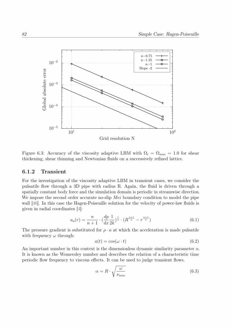
82 Simple Case: Hagen-Poiseuille
10−5
10−4
10−3
10−2
101 102
Glo
bala
bsol
ute
erro
r
Grid resolution N
n=0.75n=1.25
n=1Slope -2
Figure 6.3: Accuracy of the viscosity adaptive LBM with Ωt = Ωmin = 1.0 for shearthickening, shear thinning and Newtonian fluids on a successively refined lattice.
6.1.2 Transient
For the investigation of the viscosity adaptive LBM in transient cases, we consider thepulsatile flow through a 3D pipe with radius R. Again, the fluid is driven through aspatially constant body force and the simulation domain is periodic in streamwise direction.We impose the second order accurate no-slip Mei boundary condition to model the pipewall [46]. In this case the Hagen-Poiseuille solution for the velocity of power-law fluids isgiven in radial coordinates [4]:
ua(r) =n
n+ 1· (dpdx
1
2k)
1n · (Rn+1
n − r n+1n ) (6.1)
The pressure gradient is substituted for ρ · a at which the acceleration is made pulsatilewith frequency ω through:
a(t) = cos(ω · t) (6.2)
An important number in this context is the dimensionless dynamic similarity parameter α.It is known as the Womersley number and describes the relation of a characteristic timeperiodic flow frequency to viscous effects. It can be used to judge transient flows.
α = R ·√
ω
νmin(6.3)
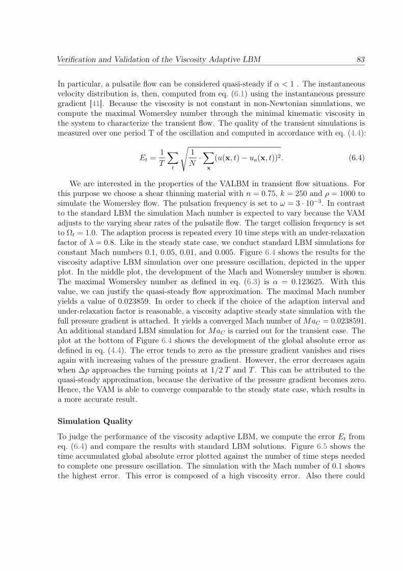
Verification and Validation of the Viscosity Adaptive LBM 83
In particular, a pulsatile flow can be considered quasi-steady if α < 1 . The instantaneousvelocity distribution is, then, computed from eq. (6.1) using the instantaneous pressuregradient [41]. Because the viscosity is not constant in non-Newtonian simulations, wecompute the maximal Womersley number through the minimal kinematic viscosity inthe system to characterize the transient flow. The quality of the transient simulations ismeasured over one period T of the oscillation and computed in accordance with eq. (4.4):
Et =1
T
∑t
√1
N·∑x
(u(x, t)− ua(x, t))2. (6.4)
We are interested in the properties of the VALBM in transient flow situations. Forthis purpose we choose a shear thinning material with n = 0.75, k = 250 and ρ = 1000 tosimulate the Womersley flow. The pulsation frequency is set to ω = 3 · 10−3. In contrastto the standard LBM the simulation Mach number is expected to vary because the VAMadjusts to the varying shear rates of the pulsatile flow. The target collision frequency is setto Ωt = 1.0. The adaption process is repeated every 10 time steps with an under-relaxationfactor of λ = 0.8. Like in the steady state case, we conduct standard LBM simulations forconstant Mach numbers 0.1, 0.05, 0.01, and 0.005. Figure 6.4 shows the results for theviscosity adaptive LBM simulation over one pressure oscillation, depicted in the upperplot. In the middle plot, the development of the Mach and Womersley number is shown.The maximal Womersley number as defined in eq. (6.3) is α = 0.123625. With thisvalue, we can justify the quasi-steady flow approximation. The maximal Mach numberyields a value of 0.023859. In order to check if the choice of the adaption interval andunder-relaxation factor is reasonable, a viscosity adaptive steady state simulation with thefull pressure gradient is attached. It yields a converged Mach number of MaC = 0.0238591.An additional standard LBM simulation for MaC is carried out for the transient case. Theplot at the bottom of Figure 6.4 shows the development of the global absolute error asdefined in eq. (4.4). The error tends to zero as the pressure gradient vanishes and risesagain with increasing values of the pressure gradient. However, the error decreases againwhen ∆p approaches the turning points at 1/2 T and T . This can be attributed to thequasi-steady approximation, because the derivative of the pressure gradient becomes zero.Hence, the VAM is able to converge comparable to the steady state case, which results ina more accurate result.
Simulation Quality
To judge the performance of the viscosity adaptive LBM, we compute the error Et fromeq. (6.4) and compare the results with standard LBM solutions. Figure 6.5 shows thetime accumulated global absolute error plotted against the number of time steps neededto complete one pressure oscillation. The simulation with the Mach number of 0.1 showsthe highest error. This error is composed of a high viscosity error. Also there could
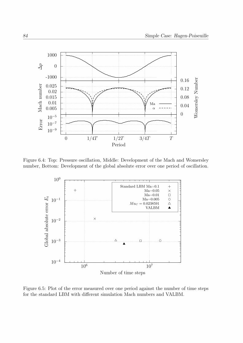
84 Simple Case: Hagen-Poiseuille
-1000
0
1000
∆p
0.0050.01
0.0150.02
0.025
0
0.04
0.08
0.12
0.16
Mac
hnu
mbe
r
Wom
ersl
eyN
umbe
r
Maα
10−9
10−7
10−5
0 1/4T 1/2T 3/4T T
Err
or
Period
Figure 6.4: Top: Pressure oscillation, Middle: Development of the Mach and Womersleynumber, Bottom: Development of the global absolute error over one period of oscillation.
10−4
10−3
10−2
10−1
100
106 107
Glo
bala
bsol
ute
erro
rE
t
Number of time steps
Standard LBM Ma=0.1Ma=0.05Ma=0.01
Ma=0.005MaC = 0.0238591
VALBM
Figure 6.5: Plot of the error measured over one period against the number of time stepsfor the standard LBM with different simulation Mach numbers and VALBM.
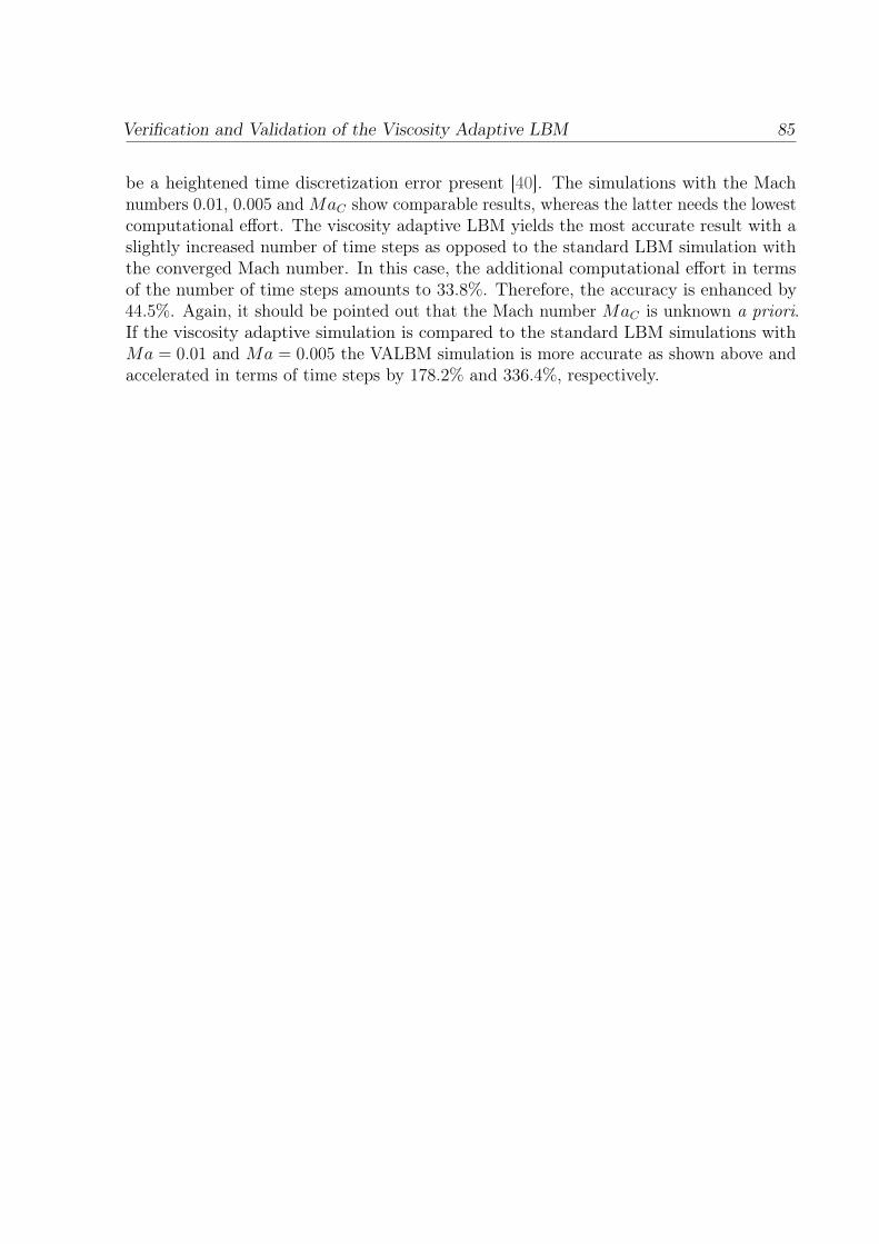
Verification and Validation of the Viscosity Adaptive LBM 85
be a heightened time discretization error present [40]. The simulations with the Machnumbers 0.01, 0.005 andMaC show comparable results, whereas the latter needs the lowestcomputational effort. The viscosity adaptive LBM yields the most accurate result with aslightly increased number of time steps as opposed to the standard LBM simulation withthe converged Mach number. In this case, the additional computational effort in termsof the number of time steps amounts to 33.8%. Therefore, the accuracy is enhanced by44.5%. Again, it should be pointed out that the Mach number MaC is unknown a priori.If the viscosity adaptive simulation is compared to the standard LBM simulations withMa = 0.01 and Ma = 0.005 the VALBM simulation is more accurate as shown above andaccelerated in terms of time steps by 178.2% and 336.4%, respectively.
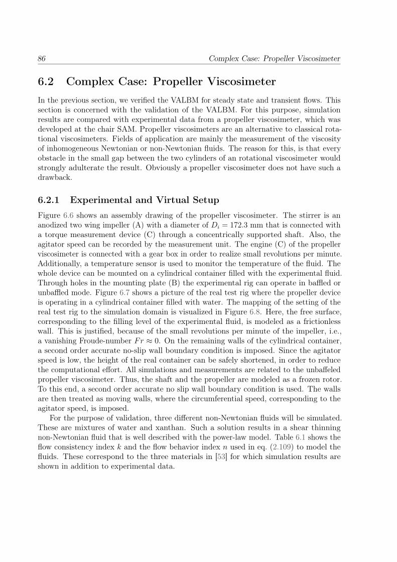
86 Complex Case: Propeller Viscosimeter
6.2 Complex Case: Propeller ViscosimeterIn the previous section, we verified the VALBM for steady state and transient flows. Thissection is concerned with the validation of the VALBM. For this purpose, simulationresults are compared with experimental data from a propeller viscosimeter, which wasdeveloped at the chair SAM. Propeller viscosimeters are an alternative to classical rota-tional viscosimeters. Fields of application are mainly the measurement of the viscosityof inhomogeneous Newtonian or non-Newtonian fluids. The reason for this, is that everyobstacle in the small gap between the two cylinders of an rotational viscosimeter wouldstrongly adulterate the result. Obviously a propeller viscosimeter does not have such adrawback.
6.2.1 Experimental and Virtual Setup
Figure 6.6 shows an assembly drawing of the propeller viscosimeter. The stirrer is ananodized two wing impeller (A) with a diameter of Di = 172.3 mm that is connected witha torque measurement device (C) through a concentrically supported shaft. Also, theagitator speed can be recorded by the measurement unit. The engine (C) of the propellerviscosimeter is connected with a gear box in order to realize small revolutions per minute.Additionally, a temperature sensor is used to monitor the temperature of the fluid. Thewhole device can be mounted on a cylindrical container filled with the experimental fluid.Through holes in the mounting plate (B) the experimental rig can operate in baffled orunbaffled mode. Figure 6.7 shows a picture of the real test rig where the propeller deviceis operating in a cylindrical container filled with water. The mapping of the setting of thereal test rig to the simulation domain is visualized in Figure 6.8. Here, the free surface,corresponding to the filling level of the experimental fluid, is modeled as a frictionlesswall. This is justified, because of the small revolutions per minute of the impeller, i.e.,a vanishing Froude-number Fr ≈ 0. On the remaining walls of the cylindrical container,a second order accurate no-slip wall boundary condition is imposed. Since the agitatorspeed is low, the height of the real container can be safely shortened, in order to reducethe computational effort. All simulations and measurements are related to the unbaffeledpropeller viscosimeter. Thus, the shaft and the propeller are modeled as a frozen rotor.To this end, a second order accurate no slip wall boundary condition is used. The wallsare then treated as moving walls, where the circumferential speed, corresponding to theagitator speed, is imposed.
For the purpose of validation, three different non-Newtonian fluids will be simulated.These are mixtures of water and xanthan. Such a solution results in a shear thinningnon-Newtonian fluid that is well described with the power-law model. Table 6.1 shows theflow consistency index k and the flow behavior index n used in eq. (2.109) to model thefluids. These correspond to the three materials in [53] for which simulation results areshown in addition to experimental data.
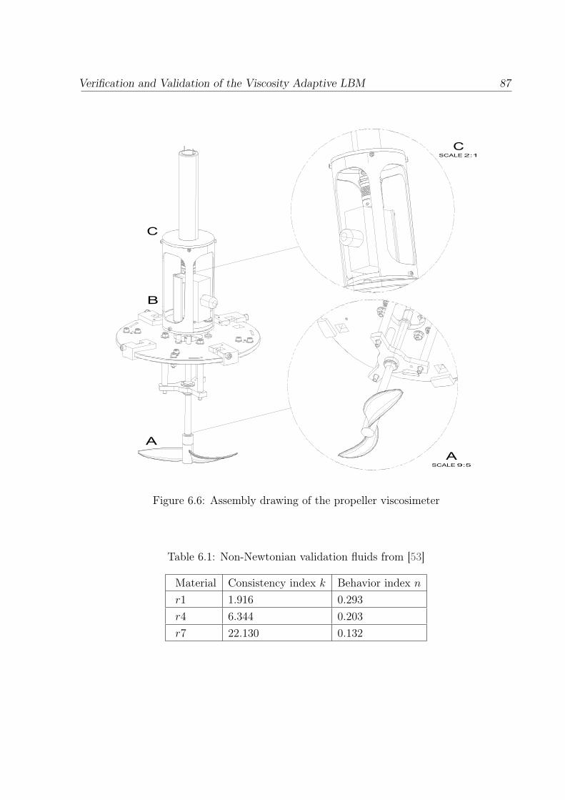
Verification and Validation of the Viscosity Adaptive LBM 87
ASCALE 9:5
CSCALE 2:1
C
A
B
Figure 6.6: Assembly drawing of the propeller viscosimeter
Table 6.1: Non-Newtonian validation fluids from [53]
Material Consistency index k Behavior index nr1 1.916 0.293
r4 6.344 0.203
r7 22.130 0.132
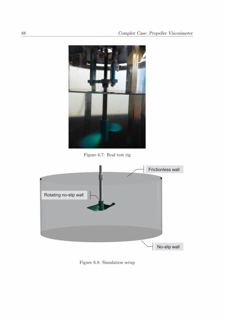
88 Complex Case: Propeller Viscosimeter
Figure 6.7: Real test rig
Frictionless wall
No-slip wall
Rotating no-slip wall
Figure 6.8: Simulation setup

Verification and Validation of the Viscosity Adaptive LBM 89
6.2.2 Discretization
In this geometrically complex case, the full capabilities of SamGenerator, which has beendeveloped in the course of this thesis, can be exploited. The lattice is generated automati-cally with minimal user input. SamGenerator expects a triangulated representation of thegeometry. A straightforward way is to create the input geometry in the stereolithography(stl) format. Unfortunately, the common CAD programs do not provide enough freedom tocreate a high quality triangulation. Those CAD stl representations may be unhesitatinglyused for visualization purposes, but do not necessarily fit for the purpose of simulation.Hence, a boundary mesh in the msh format consisting of triangle elements is used torepresent the geometry of Figure 6.8 in order to minimize Eg of eq. (2.92). Additionally,SamGenerator offers the possibility to refine parts of the computational domain with thehelp of boxes or arbitrarily shaped auxiliary geometries in the stl format. This capabilityis used to refine the region around the propeller in order to locally enhance the spatialresolution. As it was shown in Section 2.5.2, a nested time stepping algorithm is used, whenworking with local grid refinement. Therefore, the number of stream and collide operationsneeded to complete one time step, depends on the refinement level chosen. A level twolattice is used for the simulations, as a trade-off between resolution and computationaleffort. This means, the computational domain is discretized with a base resolution andthe region around the propeller is discretized with a resolution that is four times finerthan the base resolution. The transition between the regions of different resolution issmoothed. Figure 6.9 shows a slice of the lattice, viewed from the side of the propellerviscosimeter. One can see the domain refinement around the impeller and the shaft. It ischosen sufficiently large, such that the multi-level approach from section 5.4 of the VAMcan be used or each refinement level can be treated individually. The frictionless wall onthe top is also refined to ensure a consistent height of the cylinder. This is necessary sincethe frictionless approximation is realized through the simple bounce back scheme.
Figure 6.10 shows a top view of the lattice. Illustrated is a slice through the lattice atthe height level of the impeller. In particular, the differently resolved patches are shown bytheir 3D cell representation to highlight the refinement ratio. As one can see, a cylindricalauxiliary geometry was used for the domain refinement, for which the sides of the cylinderare cropped to avoid an unnecessary amount of level two nodes. The axis aligned regularlattice leads to an apparently staggered approximation of the impeller. Second orderaccurate wall boundary conditions incorporate the real position of the impeller geometryinto the simulation. A comparison of the two differently resolved lattices in Figure 6.11shows the effect of the resolution on the approximation of the impeller geometry. Theresolution is expressed through the ratio Di/∆x, which gives the number of lattice nodesin terms of the base resolution along the impeller diameter.
For the sake of completeness, the computational performance of SamGenerator for thisvalidation case should be mentioned. With a resolution of Di/∆x = 60, a total amount of17.812.591 cells were created during construction. For the simulation, the lattice contains a
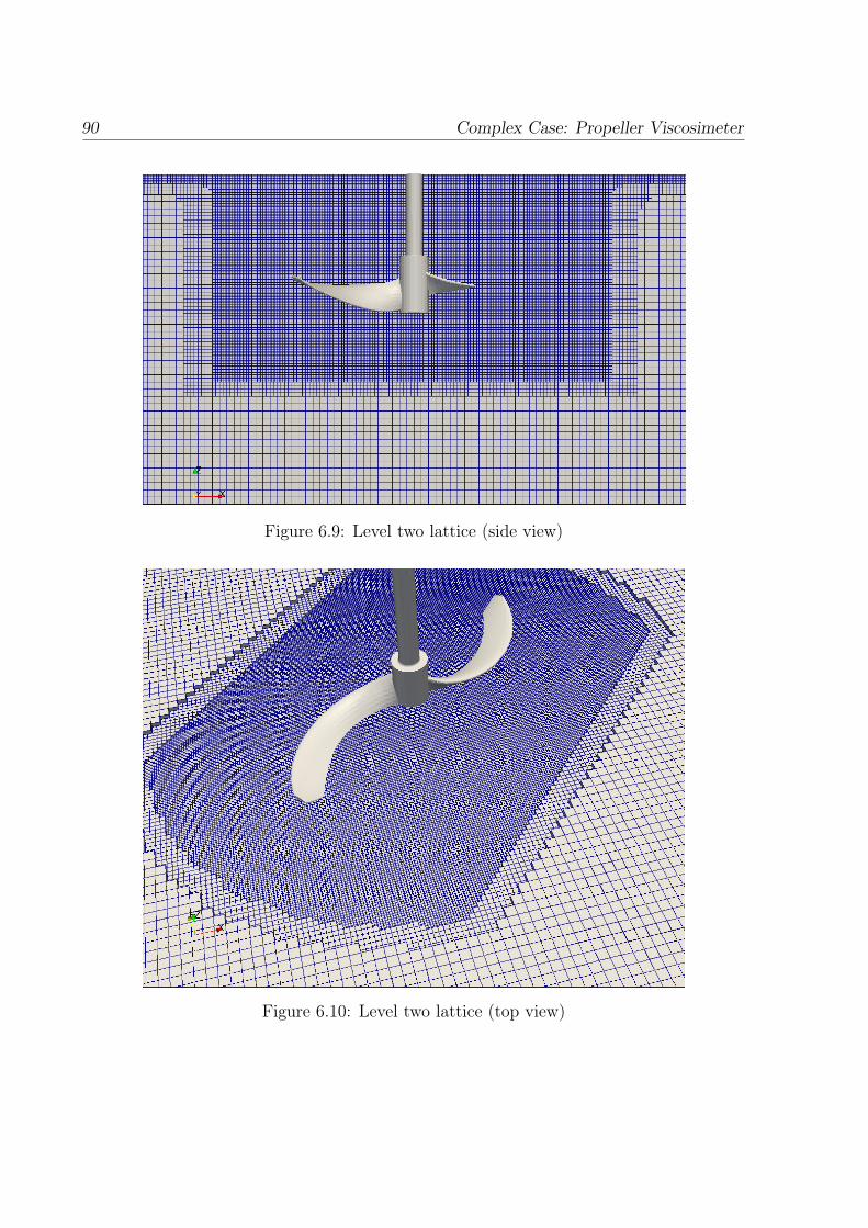
90 Complex Case: Propeller Viscosimeter
Figure 6.9: Level two lattice (side view)
Figure 6.10: Level two lattice (top view)
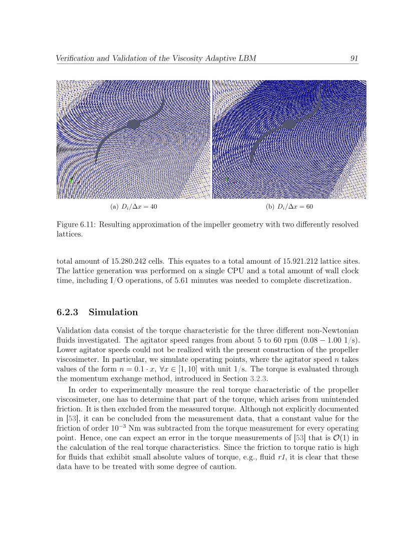
Verification and Validation of the Viscosity Adaptive LBM 91
(a) Di/∆x = 40 (b) Di/∆x = 60
Figure 6.11: Resulting approximation of the impeller geometry with two differently resolvedlattices.
total amount of 15.280.242 cells. This equates to a total amount of 15.921.212 lattice sites.The lattice generation was performed on a single CPU and a total amount of wall clocktime, including I/O operations, of 5.61 minutes was needed to complete discretization.
6.2.3 Simulation
Validation data consist of the torque characteristic for the three different non-Newtonianfluids investigated. The agitator speed ranges from about 5 to 60 rpm (0.08− 1.00 1/s).Lower agitator speeds could not be realized with the present construction of the propellerviscosimeter. In particular, we simulate operating points, where the agitator speed n takesvalues of the form n = 0.1 · x, ∀x ∈ [1, 10] with unit 1/s. The torque is evaluated throughthe momentum exchange method, introduced in Section 3.2.3.
In order to experimentally measure the real torque characteristic of the propellerviscosimeter, one has to determine that part of the torque, which arises from unintendedfriction. It is then excluded from the measured torque. Although not explicitly documentedin [53], it can be concluded from the measurement data, that a constant value for thefriction of order 10−3 Nm was subtracted from the torque measurement for every operatingpoint. Hence, one can expect an error in the torque measurements of [53] that is O(1) inthe calculation of the real torque characteristics. Since the friction to torque ratio is highfor fluids that exhibit small absolute values of torque, e.g., fluid r1, it is clear that thesedata have to be treated with some degree of caution.
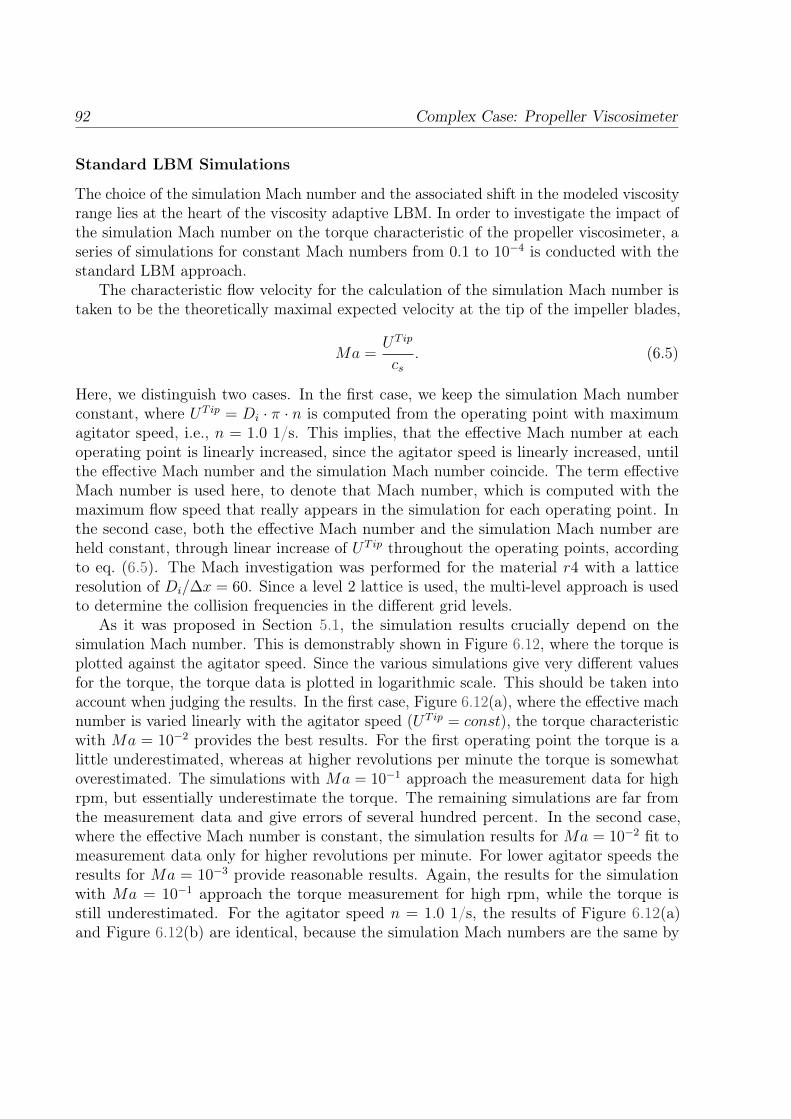
92 Complex Case: Propeller Viscosimeter
Standard LBM Simulations
The choice of the simulation Mach number and the associated shift in the modeled viscosityrange lies at the heart of the viscosity adaptive LBM. In order to investigate the impact ofthe simulation Mach number on the torque characteristic of the propeller viscosimeter, aseries of simulations for constant Mach numbers from 0.1 to 10−4 is conducted with thestandard LBM approach.
The characteristic flow velocity for the calculation of the simulation Mach number istaken to be the theoretically maximal expected velocity at the tip of the impeller blades,
Ma =UT ip
cs. (6.5)
Here, we distinguish two cases. In the first case, we keep the simulation Mach numberconstant, where UT ip = Di · π · n is computed from the operating point with maximumagitator speed, i.e., n = 1.0 1/s. This implies, that the effective Mach number at eachoperating point is linearly increased, since the agitator speed is linearly increased, untilthe effective Mach number and the simulation Mach number coincide. The term effectiveMach number is used here, to denote that Mach number, which is computed with themaximum flow speed that really appears in the simulation for each operating point. Inthe second case, both the effective Mach number and the simulation Mach number areheld constant, through linear increase of UT ip throughout the operating points, accordingto eq. (6.5). The Mach investigation was performed for the material r4 with a latticeresolution of Di/∆x = 60. Since a level 2 lattice is used, the multi-level approach is usedto determine the collision frequencies in the different grid levels.
As it was proposed in Section 5.1, the simulation results crucially depend on thesimulation Mach number. This is demonstrably shown in Figure 6.12, where the torque isplotted against the agitator speed. Since the various simulations give very different valuesfor the torque, the torque data is plotted in logarithmic scale. This should be taken intoaccount when judging the results. In the first case, Figure 6.12(a), where the effective machnumber is varied linearly with the agitator speed (UT ip = const), the torque characteristicwith Ma = 10−2 provides the best results. For the first operating point the torque is alittle underestimated, whereas at higher revolutions per minute the torque is somewhatoverestimated. The simulations with Ma = 10−1 approach the measurement data for highrpm, but essentially underestimate the torque. The remaining simulations are far fromthe measurement data and give errors of several hundred percent. In the second case,where the effective Mach number is constant, the simulation results for Ma = 10−2 fit tomeasurement data only for higher revolutions per minute. For lower agitator speeds theresults for Ma = 10−3 provide reasonable results. Again, the results for the simulationwith Ma = 10−1 approach the torque measurement for high rpm, while the torque isstill underestimated. For the agitator speed n = 1.0 1/s, the results of Figure 6.12(a)and Figure 6.12(b) are identical, because the simulation Mach numbers are the same by
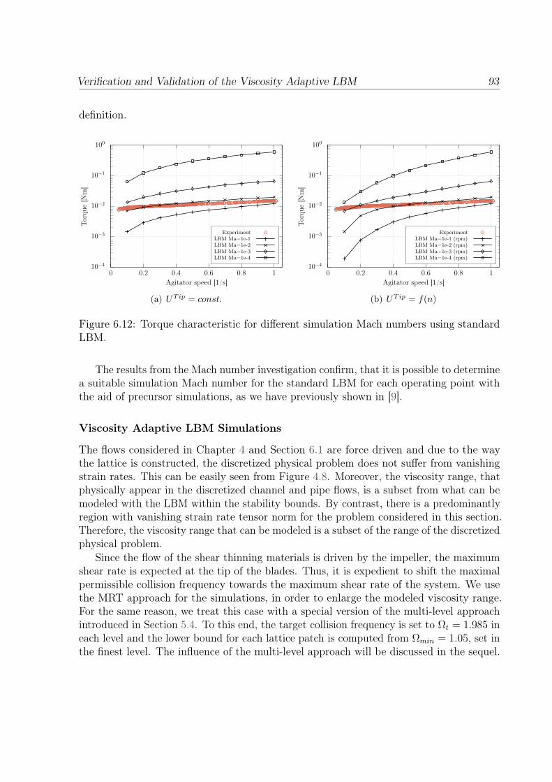
Verification and Validation of the Viscosity Adaptive LBM 93
definition.
10−4
10−3
10−2
10−1
100
0 0.2 0.4 0.6 0.8 1
Torq
ue[N
m]
Agitator speed [1/s]
ExperimentLBM Ma=1e-1LBM Ma=1e-2LBM Ma=1e-3LBM Ma=1e-4
(a) UTip = const.
10−4
10−3
10−2
10−1
100
0 0.2 0.4 0.6 0.8 1
Torq
ue[N
m]
Agitator speed [1/s]
ExperimentLBM Ma=1e-1 (rpm)LBM Ma=1e-2 (rpm)LBM Ma=1e-3 (rpm)LBM Ma=1e-4 (rpm)
(b) UTip = f(n)
Figure 6.12: Torque characteristic for different simulation Mach numbers using standardLBM.
The results from the Mach number investigation confirm, that it is possible to determinea suitable simulation Mach number for the standard LBM for each operating point withthe aid of precursor simulations, as we have previously shown in [9].
Viscosity Adaptive LBM Simulations
The flows considered in Chapter 4 and Section 6.1 are force driven and due to the waythe lattice is constructed, the discretized physical problem does not suffer from vanishingstrain rates. This can be easily seen from Figure 4.8. Moreover, the viscosity range, thatphysically appear in the discretized channel and pipe flows, is a subset from what can bemodeled with the LBM within the stability bounds. By contrast, there is a predominantlyregion with vanishing strain rate tensor norm for the problem considered in this section.Therefore, the viscosity range that can be modeled is a subset of the range of the discretizedphysical problem.
Since the flow of the shear thinning materials is driven by the impeller, the maximumshear rate is expected at the tip of the blades. Thus, it is expedient to shift the maximalpermissible collision frequency towards the maximum shear rate of the system. We usethe MRT approach for the simulations, in order to enlarge the modeled viscosity range.For the same reason, we treat this case with a special version of the multi-level approachintroduced in Section 5.4. To this end, the target collision frequency is set to Ωt = 1.985 ineach level and the lower bound for each lattice patch is computed from Ωmin = 1.05, set inthe finest level. The influence of the multi-level approach will be discussed in the sequel.
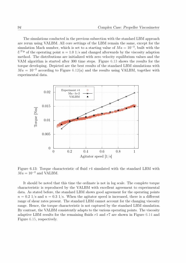
94 Complex Case: Propeller Viscosimeter
The simulations conducted in the previous subsection with the standard LBM approachare rerun using VALBM. All core settings of the LBM remain the same, except for thesimulation Mach number, which is set to a starting value of Ma = 10−3, built with theUT ip of the operating point n = 1.0 1/s and changed afterwards by the viscosity adaptionmethod. The distributions are initialized with zero velocity equilibrium values and theVAM algorithm is started after 300 time steps. Figure 6.13 shows the results for thetorque developing. Depicted are the best results of the standard LBM simulations withMa = 10−2 according to Figure 6.12(a) and the results using VALBM, together withexperimental data.
0
0.005
0.01
0.015
0.02
0 0.2 0.4 0.6 0.8 1
Torq
ue[N
m]
Agitator speed [1/s]
Experiment r4Ma=1e-2VALBM
Figure 6.13: Torque characteristic of fluid r4 simulated with the standard LBM withMa = 10−2 and VALBM.
It should be noted that this time the ordinate is not in log scale. The complete torquecharacteristic is reproduced by the VALBM with excellent agreement to experimentaldata. As stated before, the standard LBM shows good agreement for the operating pointsn = 0.2 1/s and n = 0.3 1/s. When the agitator speed is increased, there is a differentrange of shear rates present. The standard LBM cannot account for the changing viscosityrange. Hence, the torque characteristic is not captured by the standard LBM simulation.By contrast, the VALBM consistently adapts to the various operating points. The viscosityadaptive LBM results for the remaining fluids r1 and r7 are shown in Figure 6.14 andFigure 6.15, respectively.
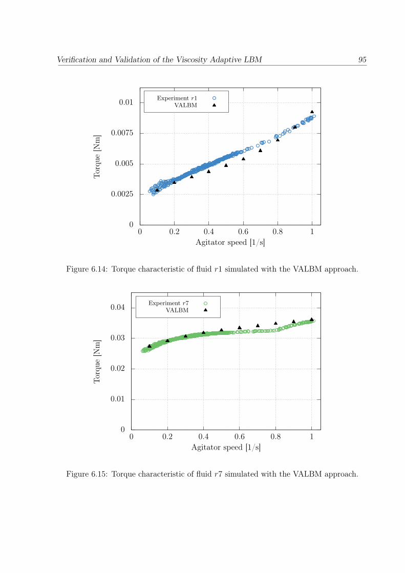
Verification and Validation of the Viscosity Adaptive LBM 95
0
0.0025
0.005
0.0075
0.01
0 0.2 0.4 0.6 0.8 1
Torq
ue[N
m]
Agitator speed [1/s]
Experiment r1VALBM
Figure 6.14: Torque characteristic of fluid r1 simulated with the VALBM approach.
0
0.01
0.02
0.03
0.04
0 0.2 0.4 0.6 0.8 1
Torq
ue[N
m]
Agitator speed [1/s]
Experiment r7VALBM
Figure 6.15: Torque characteristic of fluid r7 simulated with the VALBM approach.
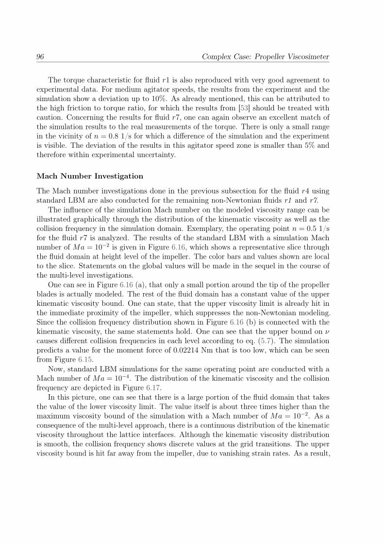
96 Complex Case: Propeller Viscosimeter
The torque characteristic for fluid r1 is also reproduced with very good agreement toexperimental data. For medium agitator speeds, the results from the experiment and thesimulation show a deviation up to 10%. As already mentioned, this can be attributed tothe high friction to torque ratio, for which the results from [53] should be treated withcaution. Concerning the results for fluid r7, one can again observe an excellent match ofthe simulation results to the real measurements of the torque. There is only a small rangein the vicinity of n = 0.8 1/s for which a difference of the simulation and the experimentis visible. The deviation of the results in this agitator speed zone is smaller than 5% andtherefore within experimental uncertainty.
Mach Number Investigation
The Mach number investigations done in the previous subsection for the fluid r4 usingstandard LBM are also conducted for the remaining non-Newtonian fluids r1 and r7.
The influence of the simulation Mach number on the modeled viscosity range can beillustrated graphically through the distribution of the kinematic viscosity as well as thecollision frequency in the simulation domain. Exemplary, the operating point n = 0.5 1/sfor the fluid r7 is analyzed. The results of the standard LBM with a simulation Machnumber of Ma = 10−2 is given in Figure 6.16, which shows a representative slice throughthe fluid domain at height level of the impeller. The color bars and values shown are localto the slice. Statements on the global values will be made in the sequel in the course ofthe multi-level investigations.
One can see in Figure 6.16 (a), that only a small portion around the tip of the propellerblades is actually modeled. The rest of the fluid domain has a constant value of the upperkinematic viscosity bound. One can state, that the upper viscosity limit is already hit inthe immediate proximity of the impeller, which suppresses the non-Newtonian modeling.Since the collision frequency distribution shown in Figure 6.16 (b) is connected with thekinematic viscosity, the same statements hold. One can see that the upper bound on νcauses different collision frequencies in each level according to eq. (5.7). The simulationpredicts a value for the moment force of 0.02214 Nm that is too low, which can be seenfrom Figure 6.15.
Now, standard LBM simulations for the same operating point are conducted with aMach number of Ma = 10−4. The distribution of the kinematic viscosity and the collisionfrequency are depicted in Figure 6.17.
In this picture, one can see that there is a large portion of the fluid domain that takesthe value of the lower viscosity limit. The value itself is about three times higher than themaximum viscosity bound of the simulation with a Mach number of Ma = 10−2. As aconsequence of the multi-level approach, there is a continuous distribution of the kinematicviscosity throughout the lattice interfaces. Although the kinematic viscosity distributionis smooth, the collision frequency shows discrete values at the grid transitions. The upperviscosity bound is hit far away from the impeller, due to vanishing strain rates. As a result,
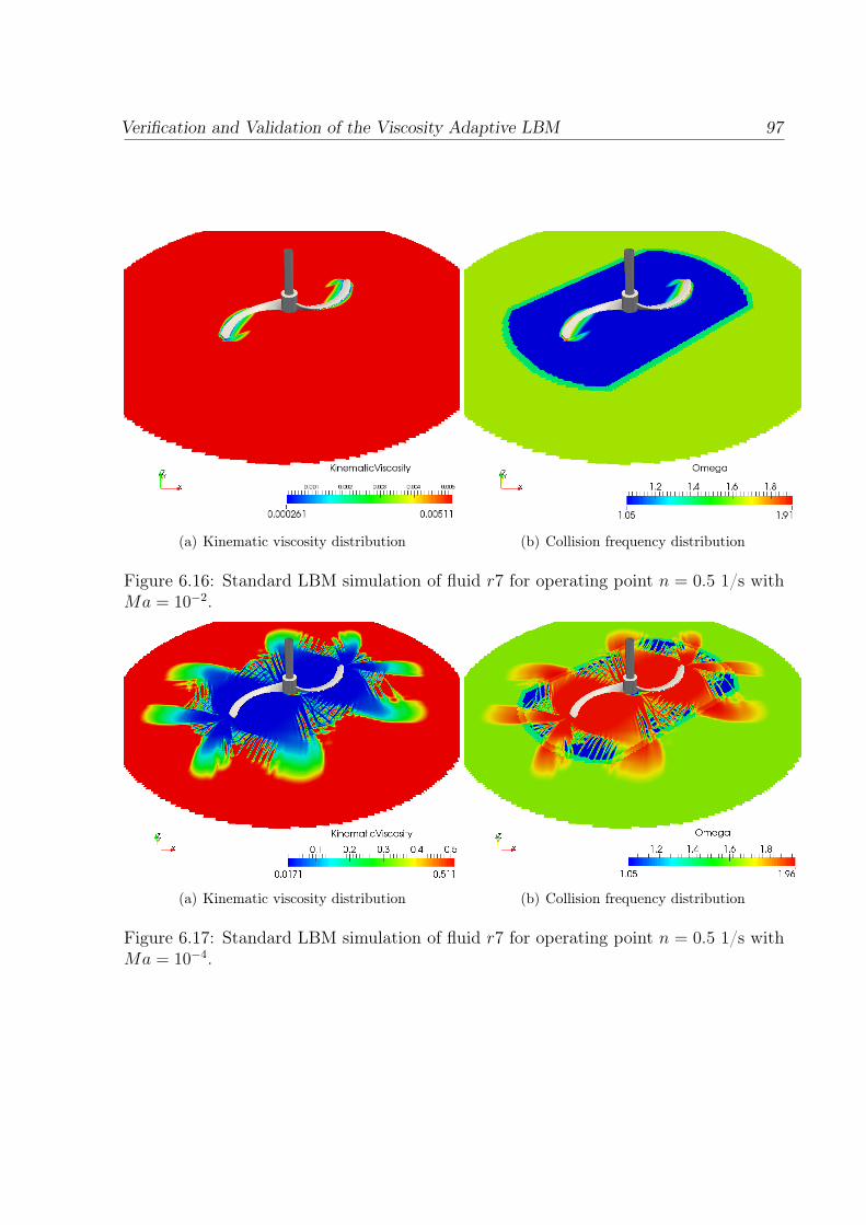
Verification and Validation of the Viscosity Adaptive LBM 97
(a) Kinematic viscosity distribution (b) Collision frequency distribution
Figure 6.16: Standard LBM simulation of fluid r7 for operating point n = 0.5 1/s withMa = 10−2.
(a) Kinematic viscosity distribution (b) Collision frequency distribution
Figure 6.17: Standard LBM simulation of fluid r7 for operating point n = 0.5 1/s withMa = 10−4.
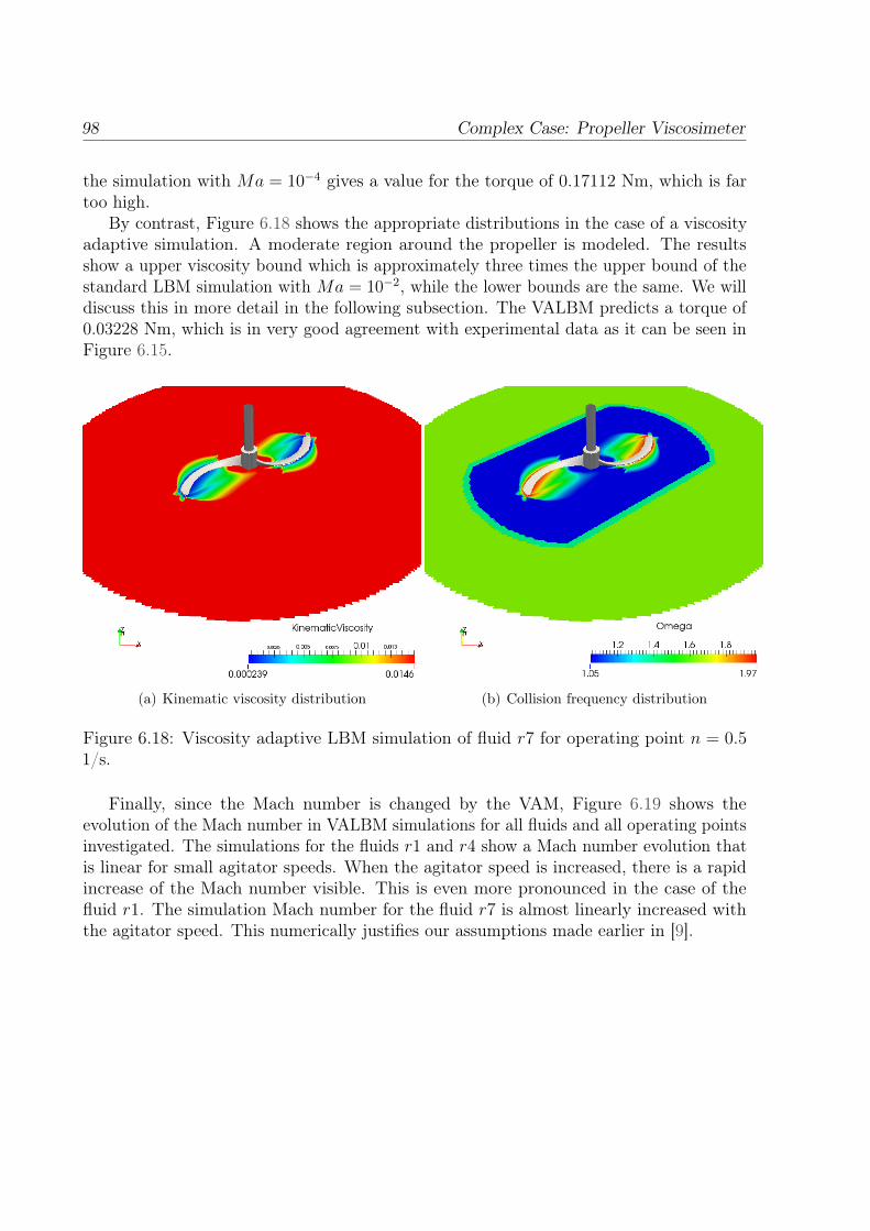
98 Complex Case: Propeller Viscosimeter
the simulation with Ma = 10−4 gives a value for the torque of 0.17112 Nm, which is fartoo high.
By contrast, Figure 6.18 shows the appropriate distributions in the case of a viscosityadaptive simulation. A moderate region around the propeller is modeled. The resultsshow a upper viscosity bound which is approximately three times the upper bound of thestandard LBM simulation with Ma = 10−2, while the lower bounds are the same. We willdiscuss this in more detail in the following subsection. The VALBM predicts a torque of0.03228 Nm, which is in very good agreement with experimental data as it can be seen inFigure 6.15.
(a) Kinematic viscosity distribution (b) Collision frequency distribution
Figure 6.18: Viscosity adaptive LBM simulation of fluid r7 for operating point n = 0.51/s.
Finally, since the Mach number is changed by the VAM, Figure 6.19 shows theevolution of the Mach number in VALBM simulations for all fluids and all operating pointsinvestigated. The simulations for the fluids r1 and r4 show a Mach number evolution thatis linear for small agitator speeds. When the agitator speed is increased, there is a rapidincrease of the Mach number visible. This is even more pronounced in the case of thefluid r1. The simulation Mach number for the fluid r7 is almost linearly increased withthe agitator speed. This numerically justifies our assumptions made earlier in [9].
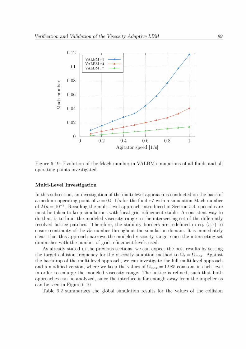
Verification and Validation of the Viscosity Adaptive LBM 99
0
0.02
0.04
0.06
0.08
0.1
0.12
0 0.2 0.4 0.6 0.8 1
Mac
hnu
mbe
r
Agitator speed [1/s]
VALBM r1VALBM r4VALBM r7
Figure 6.19: Evolution of the Mach number in VALBM simulations of all fluids and alloperating points investigated.
Multi-Level Investigation
In this subsection, an investigation of the multi-level approach is conducted on the basis ofa medium operating point of n = 0.5 1/s for the fluid r7 with a simulation Mach numberof Ma = 10−2. Recalling the multi-level approach introduced in Section 5.4, special caremust be taken to keep simulations with local grid refinement stable. A consistent way todo that, is to limit the modeled viscosity range to the intersecting set of the differentlyresolved lattice patches. Therefore, the stability borders are redefined in eq. (5.7) toensure continuity of the Re number throughout the simulation domain. It is immediatelyclear, that this approach narrows the modeled viscosity range, since the intersecting setdiminishes with the number of grid refinement levels used.
As already stated in the previous sections, we can expect the best results by settingthe target collision frequency for the viscosity adaption method to Ωt = Ωmax. Againstthe backdrop of the multi-level approach, we can investigate the full multi-level approachand a modified version, where we keep the values of Ωmax = 1.985 constant in each levelin order to enlarge the modeled viscosity range. The lattice is refined, such that bothapproaches can be analyzed, since the interface is far enough away from the impeller ascan be seen in Figure 6.10.
Table 6.2 summarizes the global simulation results for the values of the collision
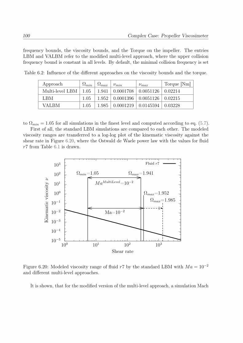
100 Complex Case: Propeller Viscosimeter
frequency bounds, the viscosity bounds, and the Torque on the impeller. The entriesLBM and VALBM refer to the modified multi-level approach, where the upper collisionfrequency bound is constant in all levels. By default, the minimal collision frequency is set
Table 6.2: Influence of the different approaches on the viscosity bounds and the torque.
Approach Ωmin Ωmax νmin νmax Torque [Nm]Multi-level LBM 1.05 1.941 0.0001708 0.0051126 0.02214
LBM 1.05 1.952 0.0001396 0.0051126 0.02215
VALBM 1.05 1.985 0.0001219 0.0145594 0.03228
to Ωmin = 1.05 for all simulations in the finest level and computed according to eq. (5.7).First of all, the standard LBM simulations are compared to each other. The modeled
viscosity ranges are transferred to a log-log plot of the kinematic viscosity against theshear rate in Figure 6.20, where the Ostwald de Waele power law with the values for fluidr7 from Table 6.1 is drawn.
10−5
10−4
10−3
10−2
10−1
100
101
102
103
100 101 102 103
Kin
emat
icvi
scos
ityν
Shear rate
Ma=10−2
Ωmin=1.05
Ωmax=1.985
MaMultiLevel=10−2
Fluid r7
Ωmax=1.952
Ωmax=1.941
Figure 6.20: Modeled viscosity range of fluid r7 by the standard LBM with Ma = 10−2
and different multi-level approaches.
It is shown, that for the modified version of the multi-level approach, a simulation Mach
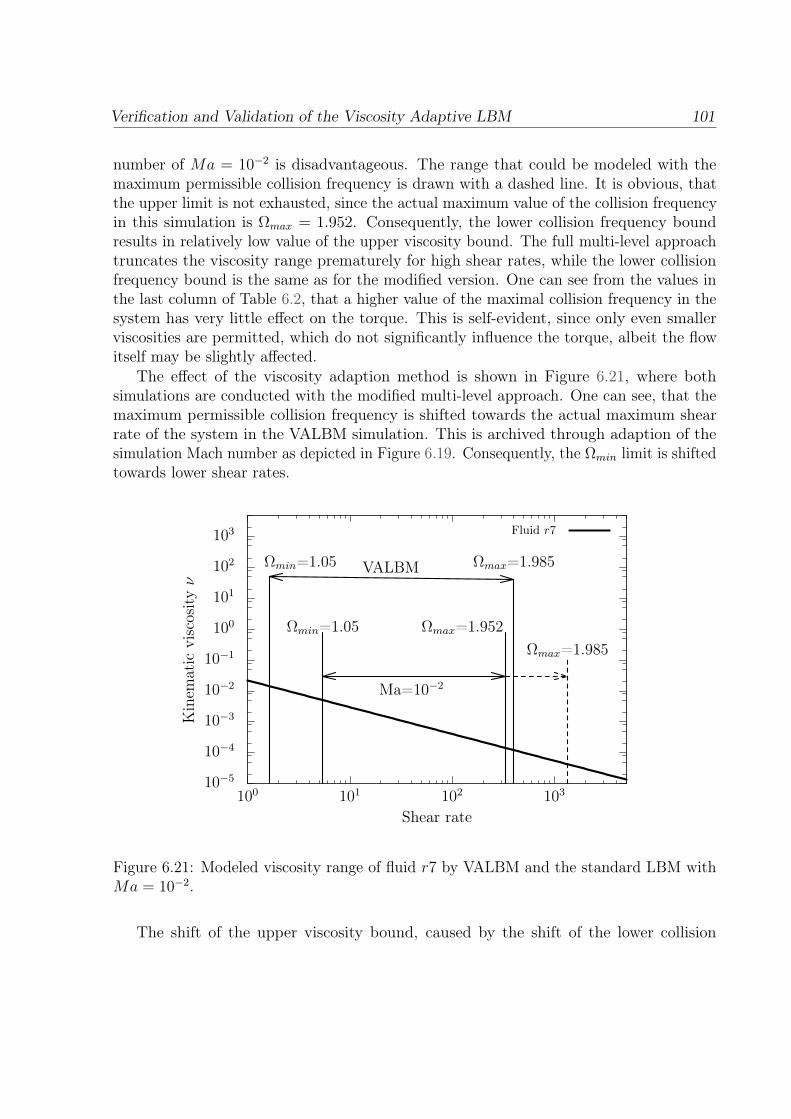
Verification and Validation of the Viscosity Adaptive LBM 101
number of Ma = 10−2 is disadvantageous. The range that could be modeled with themaximum permissible collision frequency is drawn with a dashed line. It is obvious, thatthe upper limit is not exhausted, since the actual maximum value of the collision frequencyin this simulation is Ωmax = 1.952. Consequently, the lower collision frequency boundresults in relatively low value of the upper viscosity bound. The full multi-level approachtruncates the viscosity range prematurely for high shear rates, while the lower collisionfrequency bound is the same as for the modified version. One can see from the values inthe last column of Table 6.2, that a higher value of the maximal collision frequency in thesystem has very little effect on the torque. This is self-evident, since only even smallerviscosities are permitted, which do not significantly influence the torque, albeit the flowitself may be slightly affected.
The effect of the viscosity adaption method is shown in Figure 6.21, where bothsimulations are conducted with the modified multi-level approach. One can see, that themaximum permissible collision frequency is shifted towards the actual maximum shearrate of the system in the VALBM simulation. This is archived through adaption of thesimulation Mach number as depicted in Figure 6.19. Consequently, the Ωmin limit is shiftedtowards lower shear rates.
10−5
10−4
10−3
10−2
10−1
100
101
102
103
100 101 102 103
Kin
emat
icvi
scos
ityν
Shear rate
Ma=10−2
Ωmin=1.05
Ωmax=1.985
VALBMΩmin=1.05
Fluid r7
Ωmax=1.952
Ωmax=1.985
Figure 6.21: Modeled viscosity range of fluid r7 by VALBM and the standard LBM withMa = 10−2.
The shift of the upper viscosity bound, caused by the shift of the lower collision
102 Complex Case: Propeller Viscosimeter
frequency bound Ωmin, has major impact on the torque. In low strain rate regions aroundthe impeller, e.g., near the axis of rotation, the fluid is more viscous, which resultsin a higher overall value of the moment force. Figure 6.21 exemplifies, that the VAMconsistently adapts the modeled viscosity range to the actual range of the physical problem,while preserving the stability of Lattice Boltzmann simulations even in cases with localgrid refinement.
Concluding Remarks
The results in this section demonstrate the validity of the viscosity adaptive LBM. TheMach number for the simulations of the propeller viscosimeter operating at differentrevolutions per minute was automatically and consistently adjusted by the VAM algorithm.The results are independent of the Mach number the simulation was started with. Allmoment forces at each operating point fit excellently to experimental data.
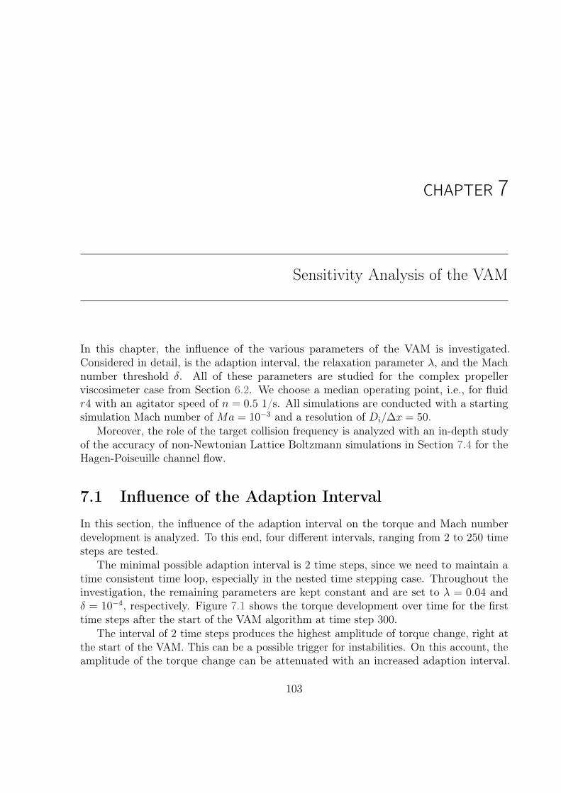
CHAPTER 7
Sensitivity Analysis of the VAM
In this chapter, the influence of the various parameters of the VAM is investigated.Considered in detail, is the adaption interval, the relaxation parameter λ, and the Machnumber threshold δ. All of these parameters are studied for the complex propellerviscosimeter case from Section 6.2. We choose a median operating point, i.e., for fluidr4 with an agitator speed of n = 0.5 1/s. All simulations are conducted with a startingsimulation Mach number of Ma = 10−3 and a resolution of Di/∆x = 50.
Moreover, the role of the target collision frequency is analyzed with an in-depth studyof the accuracy of non-Newtonian Lattice Boltzmann simulations in Section 7.4 for theHagen-Poiseuille channel flow.
7.1 Influence of the Adaption Interval
In this section, the influence of the adaption interval on the torque and Mach numberdevelopment is analyzed. To this end, four different intervals, ranging from 2 to 250 timesteps are tested.
The minimal possible adaption interval is 2 time steps, since we need to maintain atime consistent time loop, especially in the nested time stepping case. Throughout theinvestigation, the remaining parameters are kept constant and are set to λ = 0.04 andδ = 10−4, respectively. Figure 7.1 shows the torque development over time for the firsttime steps after the start of the VAM algorithm at time step 300.
The interval of 2 time steps produces the highest amplitude of torque change, right atthe start of the VAM. This can be a possible trigger for instabilities. On this account, theamplitude of the torque change can be attenuated with an increased adaption interval.
103
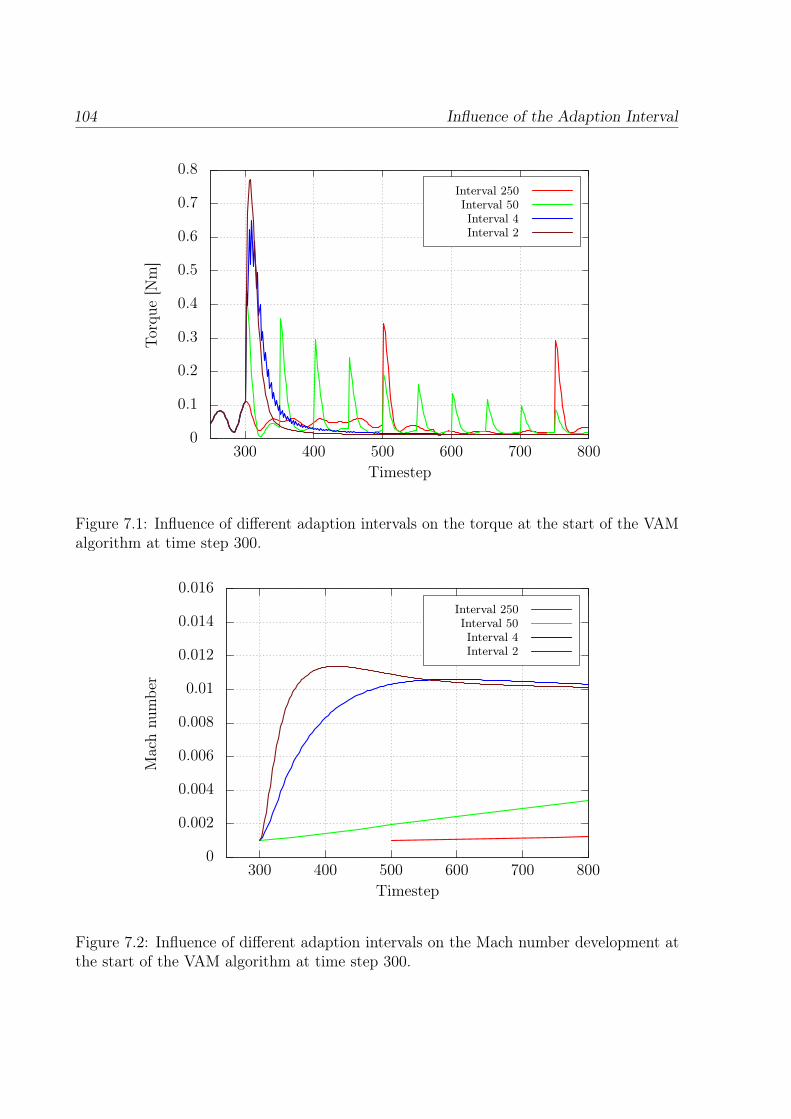
104 Influence of the Adaption Interval
0
0.1
0.2
0.3
0.4
0.5
0.6
0.7
0.8
300 400 500 600 700 800
Torq
ue[N
m]
Timestep
Interval 250Interval 50Interval 4Interval 2
Figure 7.1: Influence of different adaption intervals on the torque at the start of the VAMalgorithm at time step 300.
0
0.002
0.004
0.006
0.008
0.01
0.012
0.014
0.016
300 400 500 600 700 800
Mac
hnu
mbe
r
Timestep
Interval 250Interval 50Interval 4Interval 2
Figure 7.2: Influence of different adaption intervals on the Mach number development atthe start of the VAM algorithm at time step 300.
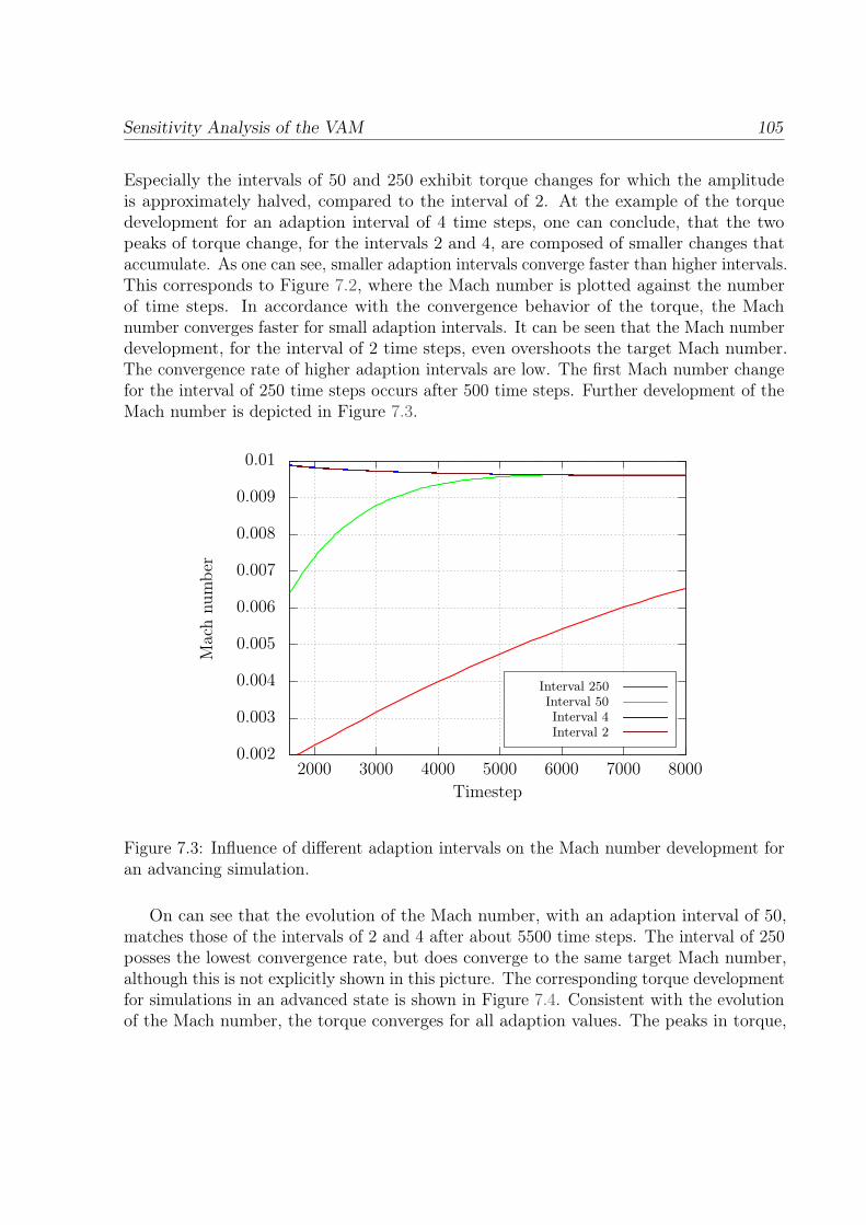
Sensitivity Analysis of the VAM 105
Especially the intervals of 50 and 250 exhibit torque changes for which the amplitudeis approximately halved, compared to the interval of 2. At the example of the torquedevelopment for an adaption interval of 4 time steps, one can conclude, that the twopeaks of torque change, for the intervals 2 and 4, are composed of smaller changes thataccumulate. As one can see, smaller adaption intervals converge faster than higher intervals.This corresponds to Figure 7.2, where the Mach number is plotted against the numberof time steps. In accordance with the convergence behavior of the torque, the Machnumber converges faster for small adaption intervals. It can be seen that the Mach numberdevelopment, for the interval of 2 time steps, even overshoots the target Mach number.The convergence rate of higher adaption intervals are low. The first Mach number changefor the interval of 250 time steps occurs after 500 time steps. Further development of theMach number is depicted in Figure 7.3.
0.002
0.003
0.004
0.005
0.006
0.007
0.008
0.009
0.01
2000 3000 4000 5000 6000 7000 8000
Mac
hnu
mbe
r
Timestep
Interval 250Interval 50Interval 4Interval 2
Figure 7.3: Influence of different adaption intervals on the Mach number development foran advancing simulation.
On can see that the evolution of the Mach number, with an adaption interval of 50,matches those of the intervals of 2 and 4 after about 5500 time steps. The interval of 250posses the lowest convergence rate, but does converge to the same target Mach number,although this is not explicitly shown in this picture. The corresponding torque developmentfor simulations in an advanced state is shown in Figure 7.4. Consistent with the evolutionof the Mach number, the torque converges for all adaption values. The peaks in torque,
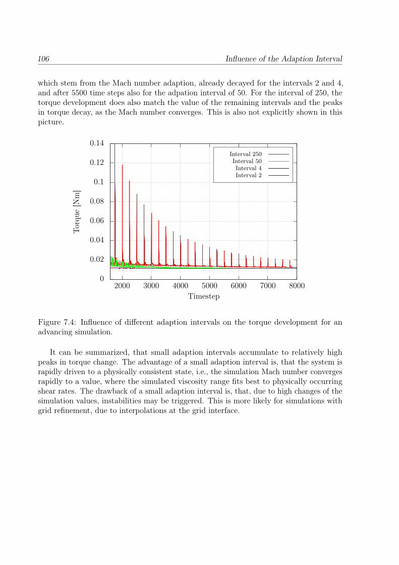
106 Influence of the Adaption Interval
which stem from the Mach number adaption, already decayed for the intervals 2 and 4,and after 5500 time steps also for the adpation interval of 50. For the interval of 250, thetorque development does also match the value of the remaining intervals and the peaksin torque decay, as the Mach number converges. This is also not explicitly shown in thispicture.
0
0.02
0.04
0.06
0.08
0.1
0.12
0.14
2000 3000 4000 5000 6000 7000 8000
Torq
ue[N
m]
Timestep
Interval 250Interval 50Interval 4Interval 2
Figure 7.4: Influence of different adaption intervals on the torque development for anadvancing simulation.
It can be summarized, that small adaption intervals accumulate to relatively highpeaks in torque change. The advantage of a small adaption interval is, that the system israpidly driven to a physically consistent state, i.e., the simulation Mach number convergesrapidly to a value, where the simulated viscosity range fits best to physically occurringshear rates. The drawback of a small adaption interval is, that, due to high changes of thesimulation values, instabilities may be triggered. This is more likely for simulations withgrid refinement, due to interpolations at the grid interface.
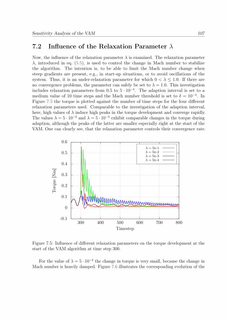
Sensitivity Analysis of the VAM 107
7.2 Influence of the Relaxation Parameter λ
Now, the influence of the relaxation parameter λ is examined. The relaxation parameterλ, introduced in eq. (5.5), is used to control the change in Mach number to stabilizethe algorithm. The intention is, to be able to limit the Mach number change whensteep gradients are present, e.g., in start-up situations, or to avoid oscillations of thesystem. Thus, it is an under-relaxation parameter for which 0 < λ ≤ 1.0. If there areno convergence problems, the parameter can safely be set to λ = 1.0. This investigationincludes relaxation parameters from 0.5 to 5 · 10−4. The adaption interval is set to amedium value of 10 time steps and the Mach number threshold is set to δ = 10−4. InFigure 7.5 the torque is plotted against the number of time steps for the four differentrelaxation parameters used. Comparable to the investigation of the adaption interval,here, high values of λ induce high peaks in the torque development and converge rapidly.The values λ = 5 · 10−2 and λ = 5 · 10−3 exhibit comparable changes in the torque duringadaption, although the peaks of the latter are smaller especially right at the start of theVAM. One can clearly see, that the relaxation parameter controls their convergence rate.
-0.1
0
0.1
0.2
0.3
0.4
0.5
0.6
300 400 500 600 700 800
Torq
ue[N
m]
Timestep
λ = 5e-1λ = 5e-2λ = 5e-3λ = 5e-4
Figure 7.5: Influence of different relaxation parameters on the torque development at thestart of the VAM algorithm at time step 300.
For the value of λ = 5 · 10−4 the change in torque is very small, because the change inMach number is heavily damped. Figure 7.6 illustrates the corresponding evolution of the
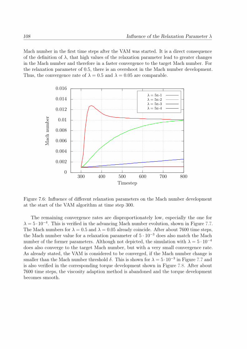
108 Influence of the Relaxation Parameter λ
Mach number in the first time steps after the VAM was started. It is a direct consequenceof the definition of λ, that high values of the relaxation parameter lead to greater changesin the Mach number and therefore in a faster convergence to the target Mach number. Forthe relaxation parameter of 0.5, there is an overshoot in the Mach number development.Thus, the convergence rate of λ = 0.5 and λ = 0.05 are comparable.
0
0.002
0.004
0.006
0.008
0.01
0.012
0.014
0.016
300 400 500 600 700 800
Mac
hnu
mbe
r
Timestep
λ = 5e-1λ = 5e-2λ = 5e-3λ = 5e-4
Figure 7.6: Influence of different relaxation parameters on the Mach number developmentat the start of the VAM algorithm at time step 300.
The remaining convergence rates are disproportionately low, especially the one forλ = 5 · 10−4. This is verified in the advancing Mach number evolution, shown in Figure 7.7.The Mach numbers for λ = 0.5 and λ = 0.05 already coincide. After about 7600 time steps,the Mach number value for a relaxation parameter of 5 · 10−3 does also match the Machnumber of the former parameters. Although not depicted, the simulation with λ = 5 · 10−4
does also converge to the target Mach number, but with a very small convergence rate.As already stated, the VAM is considered to be converged, if the Mach number change issmaller than the Mach number threshold δ. This is shown for λ = 5 ·10−3 in Figure 7.7 andis also verified in the corresponding torque development shown in Figure 7.8. After about7600 time steps, the viscosity adaption method is abandoned and the torque developmentbecomes smooth.
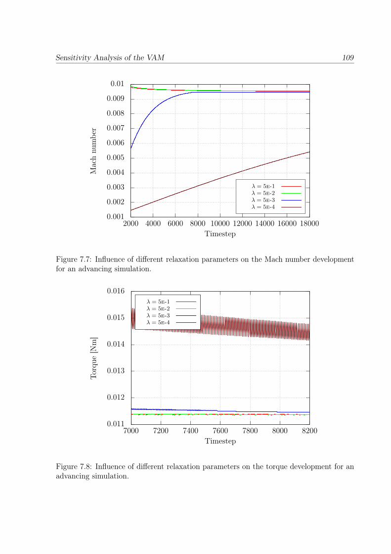
Sensitivity Analysis of the VAM 109
0.001
0.002
0.003
0.004
0.005
0.006
0.007
0.008
0.009
0.01
2000 4000 6000 8000 10000 12000 14000 16000 18000
Mac
hnu
mbe
r
Timestep
λ = 5e-1λ = 5e-2λ = 5e-3λ = 5e-4
Figure 7.7: Influence of different relaxation parameters on the Mach number developmentfor an advancing simulation.
0.011
0.012
0.013
0.014
0.015
0.016
7000 7200 7400 7600 7800 8000 8200
Torq
ue[N
m]
Timestep
λ = 5e-1λ = 5e-2λ = 5e-3λ = 5e-4
Figure 7.8: Influence of different relaxation parameters on the torque development for anadvancing simulation.
110 Influence of the Mach Number Threshold δ
The VAM is still active for the simulation with λ = 5 · 10−4. Since the Mach numberchange is still relatively high, but gets damped by the relaxation parameter, there arestill pronounced peaks visible. These will decay, as the mach number converges in theprogressing simulation. One can conclude, small values of λ lead to small peaks in thetorque development and therefore may increase stability. By contrast, higher values ofλ lead to higher convergence rates. Moderate values are preferable, due to unnecessaryovershoots of the Mach number change.
7.3 Influence of the Mach Number Threshold δ
Finally, the impact of the Mach number threshold δ is investigated. It was introduced ineq. (5.6). Its purpose is to reduce the amount of computational effort, since very smallchanges in Mach number do not significantly improve the result. Thus, the threshold δis introduced to be able to abandon the adaption process and save computational effort.The question arises, what can be considered to be a good trade off between accuracy andcomputational work. For this investigation, three different values for the threshold arechosen, ranging from δ = 0.01, that is, one percent in relative Mach number change, toδ = 10−4. Again, the remaining parameters are kept constant and are set to λ = 0.04 witha medium value for the adaption interval of 10 time steps. The influence of the Machnumber threshold on the torque evolution is shown in Figure 7.9, where the torque isplotted against the number of time steps.
One can see, that the adaption process is stopped after different amounts of time steps.After about 700 time steps, the torque development for δ = 10−2 becomes smooth. Thesame can be stated for the torque evolution with a Mach number threshold of 10−3 afterabout 1000 time steps. At time step 1200 also the simulation with δ = 10−4 converges,but the VAM becomes activated again after about time step 1300. More informationabout the convergence behavior of the VAM for the different thresholds can be taken fromFigure 7.10. Indeed, the VAM converges prematurely after about 700 time steps for thesimulation with a relatively high Mach number threshold of 1%.
As it was seen from the torque development for δ = 10−4, the Mach number is constantfrom about time step 1200 to 1300. Thereafter, the flow seems to change, such that theMach number is further adjusted by the VAM. By contrast, this flow induced change ofshear rates is not high enough to exceed the threshold of δ = 10−3 for which the Machnumber is constant from about time step 1000 on. Further evolution of the Mach numberis illustrated in Figure 7.11. One can see, that the Mach number for the simulation withmedium threshold is sporadically adapted. Mach number adaption is deferred, until thethreshold is exceeded and the simulation Mach number changes.
The simulation with δ = 10−4 converges to a value of about Ma = 0.0096 and evolvesbelow the Mach number development with medium threshold. Since the simulation withthe smallest Mach number threshold is supposed to be the most accurate, relative errors
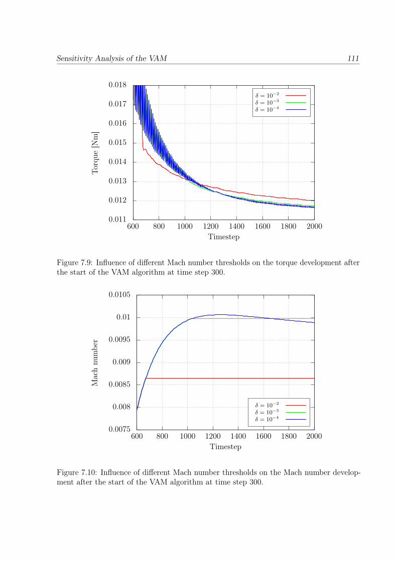
Sensitivity Analysis of the VAM 111
0.011
0.012
0.013
0.014
0.015
0.016
0.017
0.018
600 800 1000 1200 1400 1600 1800 2000
Torq
ue[N
m]
Timestep
δ = 10−2
δ = 10−3
δ = 10−4
Figure 7.9: Influence of different Mach number thresholds on the torque development afterthe start of the VAM algorithm at time step 300.
0.0075
0.008
0.0085
0.009
0.0095
0.01
0.0105
600 800 1000 1200 1400 1600 1800 2000
Mac
hnu
mbe
r
Timestep
δ = 10−2
δ = 10−3
δ = 10−4
Figure 7.10: Influence of different Mach number thresholds on the Mach number develop-ment after the start of the VAM algorithm at time step 300.
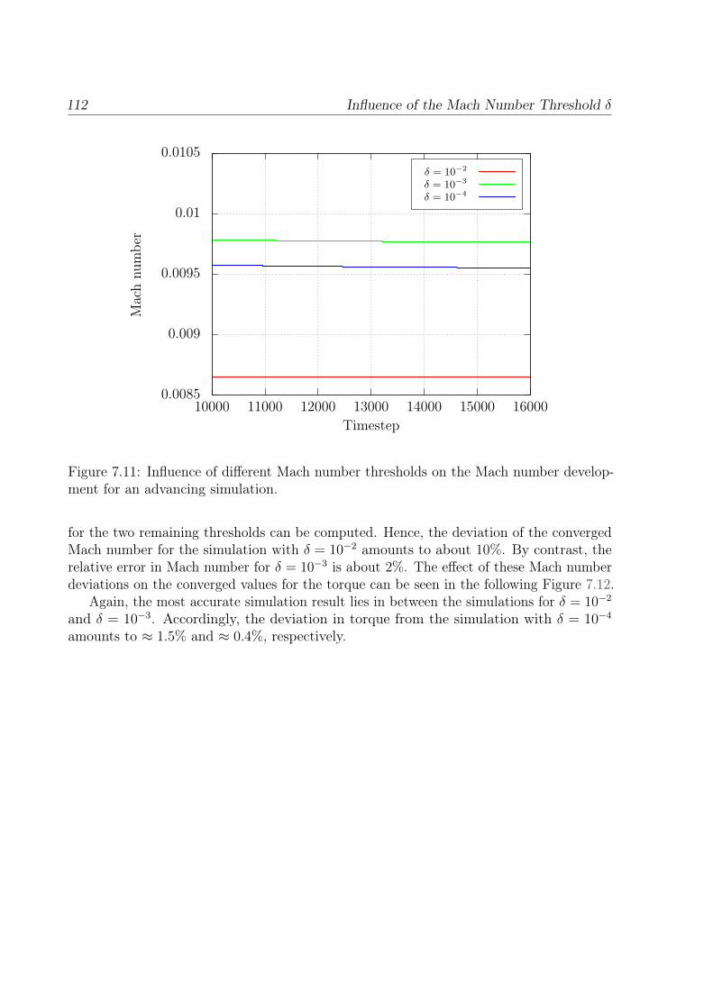
112 Influence of the Mach Number Threshold δ
0.0085
0.009
0.0095
0.01
0.0105
10000 11000 12000 13000 14000 15000 16000
Mac
hnu
mbe
r
Timestep
δ = 10−2
δ = 10−3
δ = 10−4
Figure 7.11: Influence of different Mach number thresholds on the Mach number develop-ment for an advancing simulation.
for the two remaining thresholds can be computed. Hence, the deviation of the convergedMach number for the simulation with δ = 10−2 amounts to about 10%. By contrast, therelative error in Mach number for δ = 10−3 is about 2%. The effect of these Mach numberdeviations on the converged values for the torque can be seen in the following Figure 7.12.
Again, the most accurate simulation result lies in between the simulations for δ = 10−2
and δ = 10−3. Accordingly, the deviation in torque from the simulation with δ = 10−4
amounts to ≈ 1.5% and ≈ 0.4%, respectively.
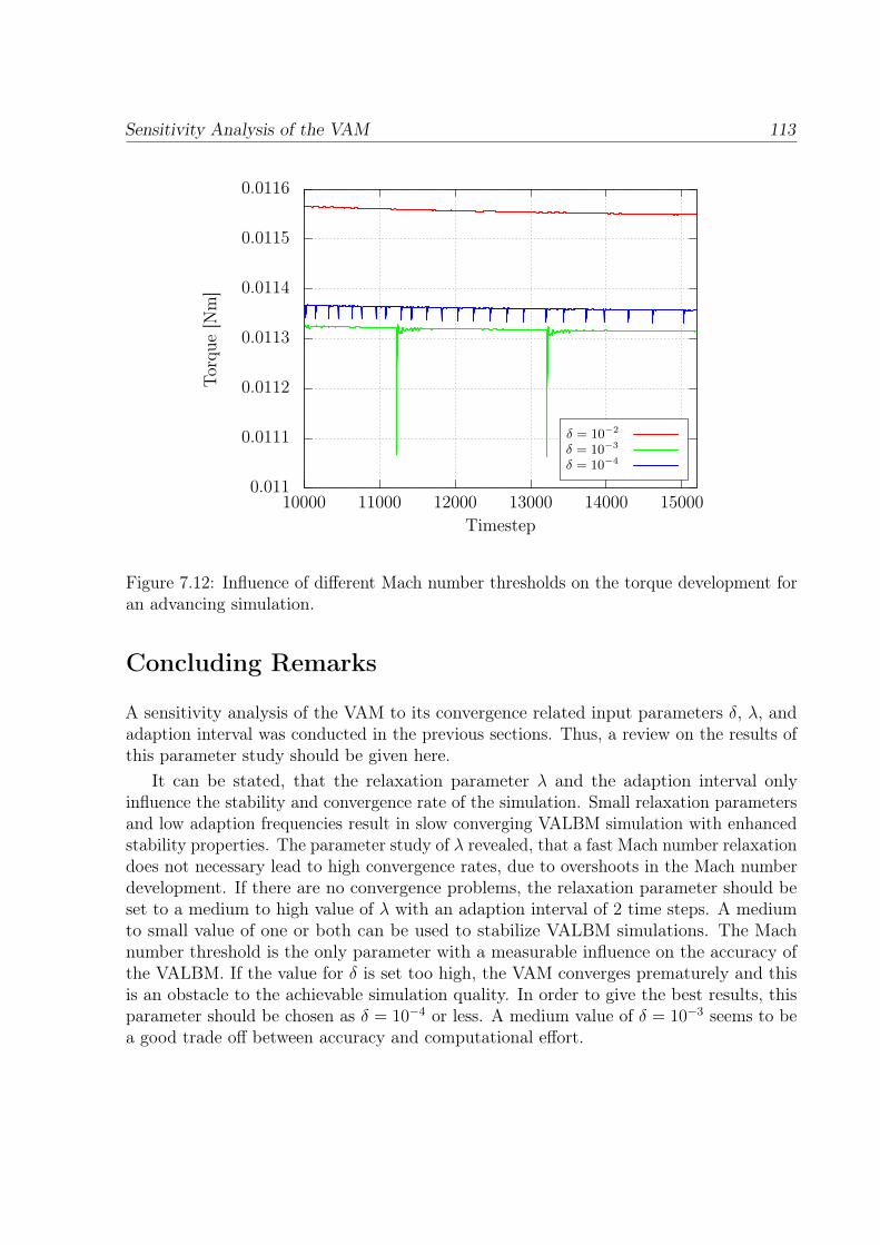
Sensitivity Analysis of the VAM 113
0.011
0.0111
0.0112
0.0113
0.0114
0.0115
0.0116
10000 11000 12000 13000 14000 15000
Torq
ue[N
m]
Timestep
δ = 10−2
δ = 10−3
δ = 10−4
Figure 7.12: Influence of different Mach number thresholds on the torque development foran advancing simulation.
Concluding Remarks
A sensitivity analysis of the VAM to its convergence related input parameters δ, λ, andadaption interval was conducted in the previous sections. Thus, a review on the results ofthis parameter study should be given here.
It can be stated, that the relaxation parameter λ and the adaption interval onlyinfluence the stability and convergence rate of the simulation. Small relaxation parametersand low adaption frequencies result in slow converging VALBM simulation with enhancedstability properties. The parameter study of λ revealed, that a fast Mach number relaxationdoes not necessary lead to high convergence rates, due to overshoots in the Mach numberdevelopment. If there are no convergence problems, the relaxation parameter should beset to a medium to high value of λ with an adaption interval of 2 time steps. A mediumto small value of one or both can be used to stabilize VALBM simulations. The Machnumber threshold is the only parameter with a measurable influence on the accuracy ofthe VALBM. If the value for δ is set too high, the VAM converges prematurely and thisis an obstacle to the achievable simulation quality. In order to give the best results, thisparameter should be chosen as δ = 10−4 or less. A medium value of δ = 10−3 seems to bea good trade off between accuracy and computational effort.
114 Accuracy of Non-Newtonian Simulations
Each parameter was varied, while the remaining ones were kept constant. Interplay ofthe parameters could, thus, not be taken into account. Moreover, the simulations wereperformed for a constant starting Mach number of Ma = 10−3 and the VAM was startedafter 300 time steps. Especially the influence of the starting point of the VAM algorithm isnot analyzed, since it was shown in Section 6.2 and Section 6.1.1 that the converged Machnumber is independent from the starting Mach number. Yet, the impact of the qualityof the flow field initialization on the overall duration of the simulation is not studied indetail. From all the simulations conducted in this thesis, regarding the computationaleffort, it can be stated that a zero velocity initialization can be a better initial guess than astandard LBM simulation with a poor choice of the simulation Mach number. An educatedguess of the simulation Mach number can speed up VALBM simulations.
7.4 Accuracy of Non-Newtonian Simulations
This section deals with the accuracy of non-Newtonian Lattice Boltzmann simulations.The basis of the simulations in this section is the generalized Newtonian Hagen-Poiseuillechannel flow with the analytic solution, error definitions, material data, and simulationsetup of Section 4.2.1. A goal of this accuracy analysis is to derive a recommendation forthe best choice of the target collision frequency Ωt, i.e., target simulation Mach numberfor the VALBM. In particular, the influence of the error contribution EΩ, introduced ineq. (2.92) is investigated. The Lattice Boltzmann equation can be expressed in terms ofthe equilibrium distribution only [32]. Therefore, a series expansion is conducted throughrecursive application of the LBE to express the distribution function in terms of theequilibrium distributions from neighboring nodes at different times in the past. Recallingthe LBE, we have,
fi(x + ei∆t, t+ ∆t) = fi(x, t) + Ω · (f eqi (x, t)− fi(x, t))= (1− Ω) · fi(x, t) + Ω · f eqi (x, t). (7.1)
Now, substitution of the fi(x, t) on the right hand side through the LBE for x− ei∆t andt−∆t leads to
fi(x + ei∆t, t+ ∆t) = (1− Ω)2 · fi(x− ei∆t, t−∆t) + Ω · (1− Ω) · f eqi (x− ei∆t, t−∆t)
+ Ω · f eqi (x, t), (7.2)
which is the first order term in the series expansion. Considering the f eq terms, one canderive a series formula
fi(x + ei∆t, t+ ∆t) = Ω∞∑k=1
(1− Ω)k−1f eqi (x− kei∆t, t− k∆t) (7.3)
Sensitivity Analysis of the VAM 115
with the number of neighbors k. This is the effective computational stencil that reducesto a nearest neighbor stencil for k = 1. The terms (1 − Ω)k−1 represent the weights ofthe contributions from the neighboring nodes. Thus, for Ω = 1, the stencil only containsnearest neighbor distributions. For Ω < 1 the weights have the same sign for all neighbors.They increase in value with increasing Ω and decrease with increasing k. The weightsalternate in sign for even and odd neighbors k when Ω > 1. Hence, it is possible to cancelerror terms stemming from numerical diffusion. For all kinds of flows it is therefore wiseto stay in the over-relaxation regime Ω > 1 and this is why we choose Ωmin = 1.05 inthe simulations of the propeller viscosimeter. While the optimum choice of Ω is problemdependent, the form of the weights and the polynominals derived in [32] suggest that aminimum of the error occurs in the vicinity of Ω = 1. According to [32], the choice ofΩ 6= 1 introduces additional artificial viscosity that has influence on the viscous and errorterms. A more rigorous analysis of the impact of the finite centered difference stencil onthe macroscopic equations may be found in [33, 34].
As already observed in Section 4.2.1 and throughout the literature,e.g., [6, 22], shearthinning non-Newtonian power-law fluids with n < 1 exhibit higher error values for theHagen-Poiseuille channel flow than fluids with n > 1 on the same grid. Thus, it is anopen question if the aforementioned numerical diffusion errors are responsible for thisphenomenon, since the collision frequency changes within a non-Newtonian simulationdue to strain rate dependent effective viscosities. Numerical diffusion errors are expectedto have a minimum in the vicinity Ω = 1, that is, if the distribution is close to equilibrium.We believe the following definition of EΩ is a good measure to describe the influence ofthe error stemming from the Ω deviation in a well-defined simulation,
EΩ =1
N·∑x
|Ω · (1− Ω)| . (7.4)
The view on this term can be twofold. At first, it should be interpreted as a weightedsum of the collision frequencies in the domain with N lattice sites, where the weights(1− Ω) consider the departure from equilibrium. On the other hand, it is the weight ofthe first next-to-neighbor contributions from the series expression eq. (7.3) of the effectivecomputational stencil. In order to minimize the global absolute error in, e.g., the velocityfield, the error EΩ should be minimized. For non-Newtonian simulations the collisionfrequency is reformulated to incorporate the Mach number. It reads
Ω =
U ·∆x√3 ·Ma(
kρ|ε|n−1 + 0.5
U ·∆x√3 ·Ma
) , (7.5)
where the kinematic viscosity depends on the shear rate tensor through the constitutivelaw used, e.g., the power-law. Hence, Ω also depends implicitly on space and time via
116 Accuracy of Non-Newtonian Simulations
the values u and ρ in the computation of the strain rate tensor eq. (2.110) and ν. Anexpression for the error source EΩ is obtained analytically through
EΩ(Ma) =
∫x
|Ω · (1− Ω)| dx, (7.6)
where the integral is computed over the whole domain. The evolution of the strain ratecan be computed through the derivative of the velocity distribution eq. (4.6). Since theexpression eq. (7.6) still depends on the simulation Mach number, a possible best choiceof Ma may be obtained by minimizing the functional EΩ(Ma), which gives
Maopt = minMa
∫x
|Ω · (1− Ω)| dx. (7.7)
The analytic solution for the optimal Mach numberMaopt is computed using the commercialsoftware Mathematica.
7.4.1 SRT
In order to determine the influence of the simulation Mach number on the absolute globalerror in velocity, a series of simulations with Mach numbers Ma = 0.01 · x, ∀x ∈ [1, 20]and additionally the upper limit Ma = 0.3 are conducted for different values of the flowbehavior index n. For each non-Newtonian fluid, four successively refined lattices areinvestigated, where the scaling ∆t ∝ ∆x2 is employed. Thus, the largest value for the Machnumber on the finest grid is Ma = 0.0375 corresponding to Ma = 0.3 on the coarsest grid.The characteristic velocity is set to U = 1 throughout this investigation. We are interestedin the evolution of the global absolute error in velocity. Since the Hagen-Poiseuille flow isstationary, the simulations are run until eq. (4.5) is fulfilled. For the sake of structuring, allsimulation results are presented for the coarsest grid. The evolution of the global absoluteerror remains the same for all grids, albeit the value of the error itself changes. Hence,conclusion drawn are valid for all lattice resolutions. A grid convergence study is attached,where the convergence rates are investigated for the different Mach numbers. In a firstrun, we simulate a Newtonian fluid with n = 1.0. Figure 7.13 shows a plot of the globalabsolute error in velocity against the simulation Mach number. In the Newtonian case,we are able to additionally plot against the collision parameter Ω, which is applied onthe top abscissa of the figure. The evolution of the error clearly shows a minimum atMa ≈ 0.13, which is about one order more accurate than the majority of the simulationresults, e.g., Ma = 0.05. In terms of the collision frequency, the error minimum is aboutΩ ≈ 0.95. This confirms the statements made above, that a minimum of EΩ is expected inthe vicinity of Ω = 1. However, the global absolute error is always an interplay of differenterror sources and especially the compressibility error shows its influence for increasingMach numbers. If the Mach number is increased past the minimum value, the error rises
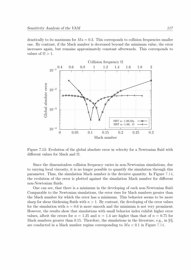
Sensitivity Analysis of the VAM 117
drastically to its maximum for Ma = 0.3. This corresponds to collision frequencies smallerone. By contrast, if the Mach number is decreased beyond the minimum value, the errorincreases again, but remains approximately constant afterwards. This corresponds tovalues of Ω > 1.
10−4
10−3
10−2
10−1
0 0.05 0.1 0.15 0.2 0.25 0.3
0.4 0.6 0.8 1 1.2 1.4 1.6 1.8 2
Glo
bala
bsol
ute
erro
r
Mach number
Collision frequency Ω
SRT n=1.00,MaSRT n=1.00, Ω
Figure 7.13: Evolution of the global absolute error in velocity for a Newtonian fluid withdifferent values for Mach and Ω.
Since the dimensionless collision frequency varies in non-Newtonian simulations, dueto varying local viscosity, it is no longer possible to quantify the simulation through thisparameter. Thus, the simulation Mach number is the decisive quantity. In Figure 7.14,the evolution of the error is plotted against the simulation Mach number for differentnon-Newtonian fluids.
One can see, that there is a minimum in the developing of each non-Newtonian fluid.Comparable to the Newtonian simulations, the error rises for Mach numbers greater thanthe Mach number for which the error has a minimum. This behavior seems to be moresharp for shear thickening fluids with n > 1. By contrast, the developing of the error valuesfor the simulation with n = 0.6 is more smooth and the minimum is not very prominent.However, the results show that simulations with small behavior index exhibit higher errorvalues, albeit the errors for n = 1.25 and n = 1.4 are higher than that of n = 0.75 forMach numbers greater than 0.15. Therefore, the simulations in the literature, e.g., in [6],are conducted in a Mach number regime corresponding to Ma < 0.1 in Figure 7.14.
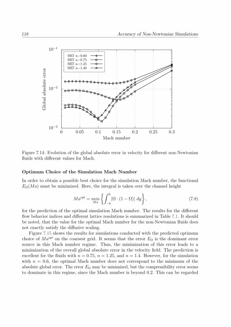
118 Accuracy of Non-Newtonian Simulations
10−3
10−2
10−1
0 0.05 0.1 0.15 0.2 0.25 0.3
Glo
bala
bsol
ute
erro
r
Mach number
SRT n=0.60SRT n=0.75SRT n=1.25SRT n=1.40
Figure 7.14: Evolution of the global absolute error in velocity for different non-Newtonianfluids with different values for Mach.
Optimum Choice of the Simulation Mach Number
In order to obtain a possible best choice for the simulation Mach number, the functionalEΩ(Ma) must be minimized. Here, the integral is taken over the channel height
Maopt = minMa
∫ h
−h|Ω · (1− Ω)| dy
, (7.8)
for the prediction of the optimal simulation Mach number. The results for the differentflow behavior indices and different lattice resolutions is summarized in Table 7.1. It shouldbe noted, that the value for the optimal Mach number for the non-Newtonian fluids doesnot exactly satisfy the diffusive scaling.
Figure 7.15 shows the results for simulations conducted with the predicted optimumchoice of Maopt on the coarsest grid. It seems that the error EΩ is the dominant errorsource in this Mach number regime. Thus, the minimization of this error leads to aminimization of the overall global absolute error in the velocity field. The prediction isexcellent for the fluids with n = 0.75, n = 1.25, and n = 1.4. However, for the simulationwith n = 0.6, the optimal Mach number does not correspond to the minimum of theabsolute global error. The error EΩ may be minimized, but the compressibility error seemsto dominate in this regime, since the Mach number is beyond 0.2. This can be regarded
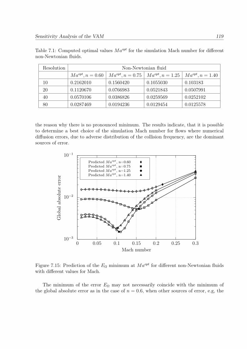
Sensitivity Analysis of the VAM 119
Table 7.1: Computed optimal values Maopt for the simulation Mach number for differentnon-Newtonian fluids.
Resolution Non-Newtonian fluidMaopt, n = 0.60 Maopt, n = 0.75 Maopt, n = 1.25 Maopt, n = 1.40
10 0.2162010 0.1560420 0.1055030 0.103183
20 0.1120670 0.0766983 0.0521843 0.0507991
40 0.0570106 0.0386826 0.0259569 0.0252102
80 0.0287469 0.0194236 0.0129454 0.0125578
the reason why there is no pronounced minimum. The results indicate, that it is possibleto determine a best choice of the simulation Mach number for flows where numericaldiffusion errors, due to adverse distribution of the collision frequency, are the dominantsources of error.
10−3
10−2
10−1
0 0.05 0.1 0.15 0.2 0.25 0.3
Glo
bala
bsol
ute
erro
r
Mach number
Predicted Maopt, n=0.60Predicted Maopt, n=0.75Predicted Maopt, n=1.25Predicted Maopt, n=1.40
Figure 7.15: Prediction of the EΩ minimum at Maopt for different non-Newtonian fluidswith different values for Mach.
The minimum of the error EΩ may not necessarily coincide with the minimum ofthe global absolute error as in the case of n = 0.6, when other sources of error, e.g, the
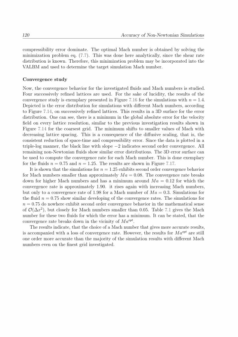
120 Accuracy of Non-Newtonian Simulations
compressibility error dominate. The optimal Mach number is obtained by solving theminimization problem eq. (7.7). This was done here analytically, since the shear ratedistribution is known. Therefore, this minimization problem may be incorporated into theVALBM and used to determine the target simulation Mach number.
Convergence study
Now, the convergence behavior for the investigated fluids and Mach numbers is studied.Four successively refined lattices are used. For the sake of lucidity, the results of theconvergence study is exemplary presented in Figure 7.16 for the simulations with n = 1.4.Depicted is the error distribution for simulations with different Mach numbers, accordingto Figure 7.14, on successively refined lattices. This results in a 3D surface for the errordistribution. One can see, there is a minimum in the global absolute error for the velocityfield on every lattice resolution, similar to the previous investigation results shown inFigure 7.14 for the coarsest grid. The minimum shifts to smaller values of Mach withdecreasing lattice spacing. This is a consequence of the diffusive scaling, that is, theconsistent reduction of space-time and compressibility error. Since the data is plotted in atriple-log manner, the black line with slope −2 indicates second order convergence. Allremaining non-Newtonian fluids show similar error distributions. The 3D error surface canbe used to compute the convergence rate for each Mach number. This is done exemplaryfor the fluids n = 0.75 and n = 1.25. The results are shown in Figure 7.17.
It is shown that the simulations for n = 1.25 exhibits second order convergence behaviorfor Mach numbers smaller than approximately Ma = 0.08. The convergence rate breaksdown for higher Mach numbers and has a minimum around Ma = 0.12 for which theconvergence rate is approximately 1.90. it rises again with increasing Mach numbers,but only to a convergence rate of 1.98 for a Mach number of Ma = 0.3. Simulations forthe fluid n = 0.75 show similar developing of the convergence rates. The simulations forn = 0.75 do nowhere exhibit second order convergence behavior in the mathematical senseof O(∆x2), but closely for Mach numbers smaller than 0.05. Table 7.1 gives the Machnumber for these two fluids for which the error has a minimum. It can be stated, that theconvergence rate breaks down in the vicinity of Maopt.
The results indicate, that the choice of a Mach number that gives more accurate results,is accompanied with a loss of convergence rate. However, the results for Maopt are stillone order more accurate than the majority of the simulation results with different Machnumbers even on the finest grid investigated.
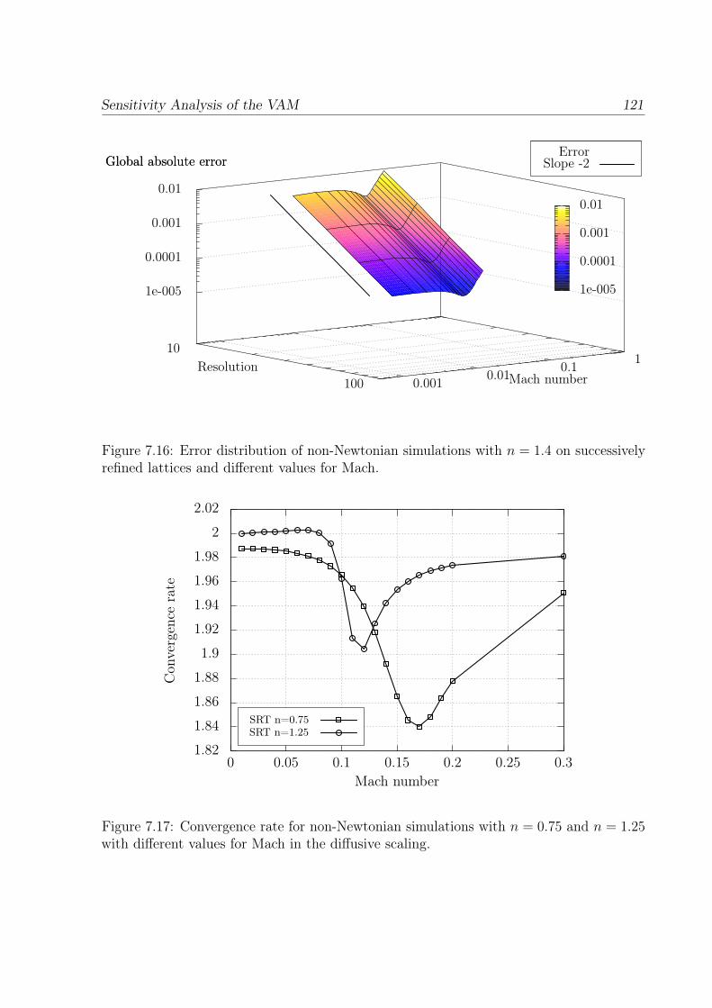
Sensitivity Analysis of the VAM 121
10
100 0.001 0.01 0.1 1
1e-005
0.0001
0.001
0.01
Global absolute errorError
Slope -2
ResolutionMach number
Global absolute error
1e-005
0.0001
0.001
0.01
Figure 7.16: Error distribution of non-Newtonian simulations with n = 1.4 on successivelyrefined lattices and different values for Mach.
1.82
1.84
1.86
1.88
1.9
1.92
1.94
1.96
1.98
2
2.02
0 0.05 0.1 0.15 0.2 0.25 0.3
Con
verg
ence
rate
Mach number
SRT n=0.75SRT n=1.25
Figure 7.17: Convergence rate for non-Newtonian simulations with n = 0.75 and n = 1.25with different values for Mach in the diffusive scaling.
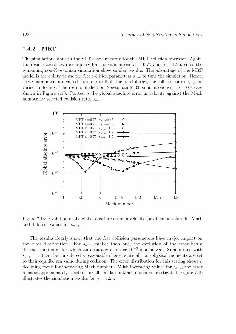
122 Accuracy of Non-Newtonian Simulations
7.4.2 MRT
The simulations done in the SRT case are rerun for the MRT collision operator. Again,the results are shown exemplary for the simulations n = 0.75 and n = 1.25, since theremaining non-Newtonian simulation show similar results. The advantage of the MRTmodel is the ability to use the free collision parameters sa−e to tune the simulation. Hence,these parameters are varied. In order to limit the possibilities, the collision rates sa−e arevaried uniformly. The results of the non-Newtonian MRT simulations with n = 0.75 areshown in Figure 7.18. Plotted is the global absolute error in velocity against the Machnumber for selected collision rates sa−e.
10−4
10−3
10−2
10−1
100
0 0.05 0.1 0.15 0.2 0.25 0.3
Glo
bala
bsol
ute
erro
r
Mach number
MRT n=0.75, sa−e=0.5MRT n=0.75, sa−e=0.8MRT n=0.75, sa−e=1.0MRT n=0.75, sa−e=1.2MRT n=0.75, sa−e=1.5
Figure 7.18: Evolution of the global absolute error in velocity for different values for Machand different values for sa−e.
The results clearly show, that the free collision parameters have major impact onthe error distribution. For sa−e smaller than one, the evolution of the error has adistinct minimum for which an accuracy of order 10−3 is achieved. Simulations withsa−e = 1.0 can be considered a reasonable choice, since all non-physical moments are setto their equilibrium value during collision. The error distribution for this setting shows adeclining trend for increasing Mach numbers. With increasing values for sa−e, the errorremains approximately constant for all simulation Mach numbers investigated. Figure 7.19illustrates the simulation results for n = 1.25.
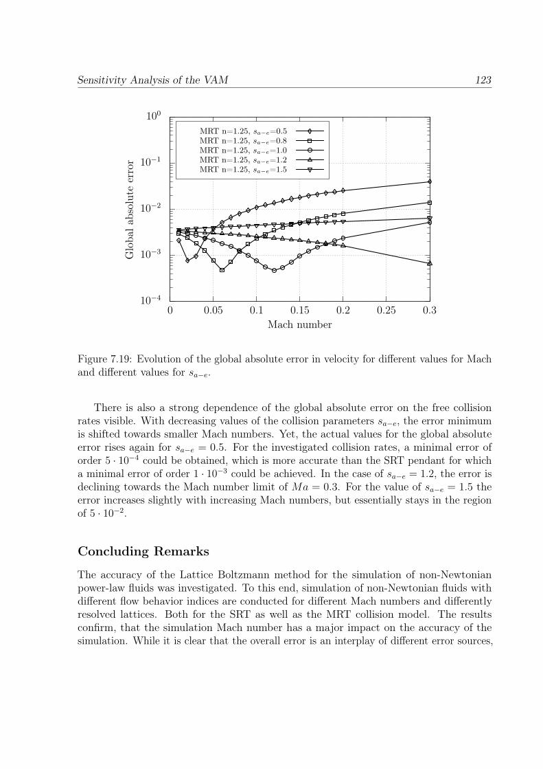
Sensitivity Analysis of the VAM 123
10−4
10−3
10−2
10−1
100
0 0.05 0.1 0.15 0.2 0.25 0.3
Glo
bala
bsol
ute
erro
r
Mach number
MRT n=1.25, sa−e=0.5MRT n=1.25, sa−e=0.8MRT n=1.25, sa−e=1.0MRT n=1.25, sa−e=1.2MRT n=1.25, sa−e=1.5
Figure 7.19: Evolution of the global absolute error in velocity for different values for Machand different values for sa−e.
There is also a strong dependence of the global absolute error on the free collisionrates visible. With decreasing values of the collision parameters sa−e, the error minimumis shifted towards smaller Mach numbers. Yet, the actual values for the global absoluteerror rises again for sa−e = 0.5. For the investigated collision rates, a minimal error oforder 5 · 10−4 could be obtained, which is more accurate than the SRT pendant for whicha minimal error of order 1 · 10−3 could be achieved. In the case of sa−e = 1.2, the error isdeclining towards the Mach number limit of Ma = 0.3. For the value of sa−e = 1.5 theerror increases slightly with increasing Mach numbers, but essentially stays in the regionof 5 · 10−2.
Concluding Remarks
The accuracy of the Lattice Boltzmann method for the simulation of non-Newtonianpower-law fluids was investigated. To this end, simulation of non-Newtonian fluids withdifferent flow behavior indices are conducted for different Mach numbers and differentlyresolved lattices. Both for the SRT as well as the MRT collision model. The resultsconfirm, that the simulation Mach number has a major impact on the accuracy of thesimulation. While it is clear that the overall error is an interplay of different error sources,
124 Accuracy of Non-Newtonian Simulations
numerical diffusion error and compressibility errors seem to be the dominant sources oferror. One goal of this investigation was to deduce a best choice for the simulation Machnumber in order to incorporate these recommendations into the viscosity adaptive LBM.Therefore, the expression eq. (7.4) was derived, to quantify additional numerical diffusionerrors EΩ, introduced by the effective computational stencil. This was done analyticallyfor the Hagen-Poiseuille flow by minimization of the functional EΩ(Ma), which gives theoptimal Mach number Maopt, eq. (7.7).
Excellent agreement of the results from the simulations with Maopt and the predictedminimum global error could be obtained in regions where the numerical diffusion erroris the dominant source of error. The expressions derived for the prediction refer to theSRT model as can be seen from eq. (7.3), since the collision frequency is not expanded ina collision matrix. Indeed, the results clearly show, that the free relaxation parameters ofthe MRT model drastically influence the error in velocity and the value of the optimalMach number for which that error is minimal. Generally, the MRT model shows a smallervalue of the overall global absolute error for selected values of the free collision parameters.However, due to the influence of the parameters sa−e, which can be chosen arbitrarily,eq. (7.7) is no longer suitable for the prediction of the optimal choice for the simulationMach number in the MRT case.
CHAPTER 8
Conclusions and Perspective
8.1 Conclusions
This dissertation described the development, verification, and validation of a viscosityadaptive Lattice Boltzmann Method (VALBM) for the numerical simulation of non-Newtonian fluids, as well as the development and verification of the related software bundleSAM-Lattice.
Besides the introduction of the VALBM, a goal of this thesis is to offer assistance inthe spirit of a theory guide to students and assistant researchers concerning the theory ofthe Lattice Boltzmann Method and its implementation in SAM-Lattice. In Chapter 2, themathematical foundation of the LBM was given and the route from the BGK approximationof the Boltzmann equation to the Lattice Boltzmann (BGK) equation was delineated indetail. The derivation is restricted to isothermal flows only. Restrictions of the method,such as low Mach number flows were highlighted and the accuracy of the method wasdiscussed.
In Chapter 3, some fundamental aspects on the implementation of the main com-ponents, including the corresponding flow charts were discussed. Actual details to theimplementation are given in the comprehensive programmers guides to SamGenerator andSamSolver. In order to ensure the functionality of the implementation of SamSolver, thesolver was verified in Chapter 4 for both Newtonian and non-Newtonian fluids, including aconvergence study of the method and an investigation on higher order boundary conditions.
The essential novelty of the method, developed in the course of this thesis, is thatthe numerically modeled viscosity range is consistently adapted to the actual physicallyexhibited viscosity range through change of the simulation time step and the simulation
125
126 Conclusions
Mach number, respectively, while the simulation is running. The algorithm is robust,independent of the Mach number the simulation was started with, and applicable forstationary flows as well as transient flows. The theory of the viscosity adaption method wasintroduced in Chapter 5. Although the VAM was used here for fluids that can be modeledwith the power-law approach, the implementation of the VALBM is straightforward forother non-Newtonian models, e.g., the Carreau-Yasuda or Cross model.
In Chapter 6 the VALBM was verified in the stationary case for the Hagen-Poiseuillechannel flow and in the transient case for the Wormersley flow. Moreover, the VALBMwas validated for the case of a propeller viscosimeter developed at the chair SAM. Tothis end, the experimental data of the torque on the impeller of 3 shear thinning non-Newtonian liquids served for the validation. The VALBM showed excellent agreementwith experimental data for all of the investigated fluids and in every operating point. Forreasons of comparison, a series of standard LBM simulations was carried out with differentsimulation Mach numbers, which partly showed errors of several hundred percent.
In Chapter 7 the sensitivity to the parameters used in the VAM was analyzed. Theresult of this study was that the relaxation parameter λ and the adaption interval onlyinfluence the convergence and stability of the simulation. If there are no stability problems,a medium to high value of λ and an interval of 2 are suggested for the VAM. By contrast,the Mach number threshold δ saves computational work but limits the possible accuracy.A value of δ = 10−3 seems to be a good trade off between accuracy and computationaleffort.
Finally, the accuracy of non-Newtonian Lattice Boltzmann simulations with SRT andthe MRT model was analyzed in detail. For the non-Newtonian case, an error estimatein the form of a functional was derived on the basis of a series expansion of the LatticeBoltzmann equation. This functional can be solved analytically for the case of the Hagen-Poiseuille channel flow of non-Newtonian fluids. The estimation of the error minimum isexcellent in regions where the Ω error is the dominant source of error as opposed to thecompressibility error for the SRT collision operator.
Conclusions and Perspective 127
8.2 Directions for Further WorkResult of this dissertation is a verified and validated software bundle on the basis of theviscosity adaptive Lattice Boltzmann Method. The work restricts itself on the simulation ofisothermal, laminar flows with small Mach numbers. As further research goals concerningthe VALBM, the following suggestions are made:
- TurbulenceSince we only dealt with laminar flows, the capabilities of the Lattice BoltzmannMethod and in particular of the VALBM for the simulation of turbulent non-Newtonian flows should be investigated. There is already a LES model with thestandard Smagorinsky SGS model implemented.
- Application of the Error EstimateAn error estimate for the error contribution EΩ was derived for the SRT collisionmodel. A possible target simulation Mach number for the VAM can be deduced byminimizing the Ω error estimate, while the simulation is running. This should beimplemented in SamSolver and the VALBM should be tested with this objective.
- Derivation for the MRT modelThe series expansion of the Lattice Boltzmann equation for the derivation of theerror estimate was done for the SRT model. The results in Chapter 7 have shown,that this form of the estimate is not suitable for the MRT model, because of theinfluence of the free collision parameters sa−e. A corresponding derivation could beconducted for the MRT case.
- Further TestingThe VALBM has been shown to provide excellent results for the simulation of realworld experiments as in the case of the propeller viscosimeter. However, furthertesting is needed to explore the cababilities of this new method.
Generally, SamGenerator and SamSolver should be extended to higher lattices, such asthe D3Q39 or D3Q121 velocity discretization, in order to incorporate heat transfer anddeal with compressible fluids.

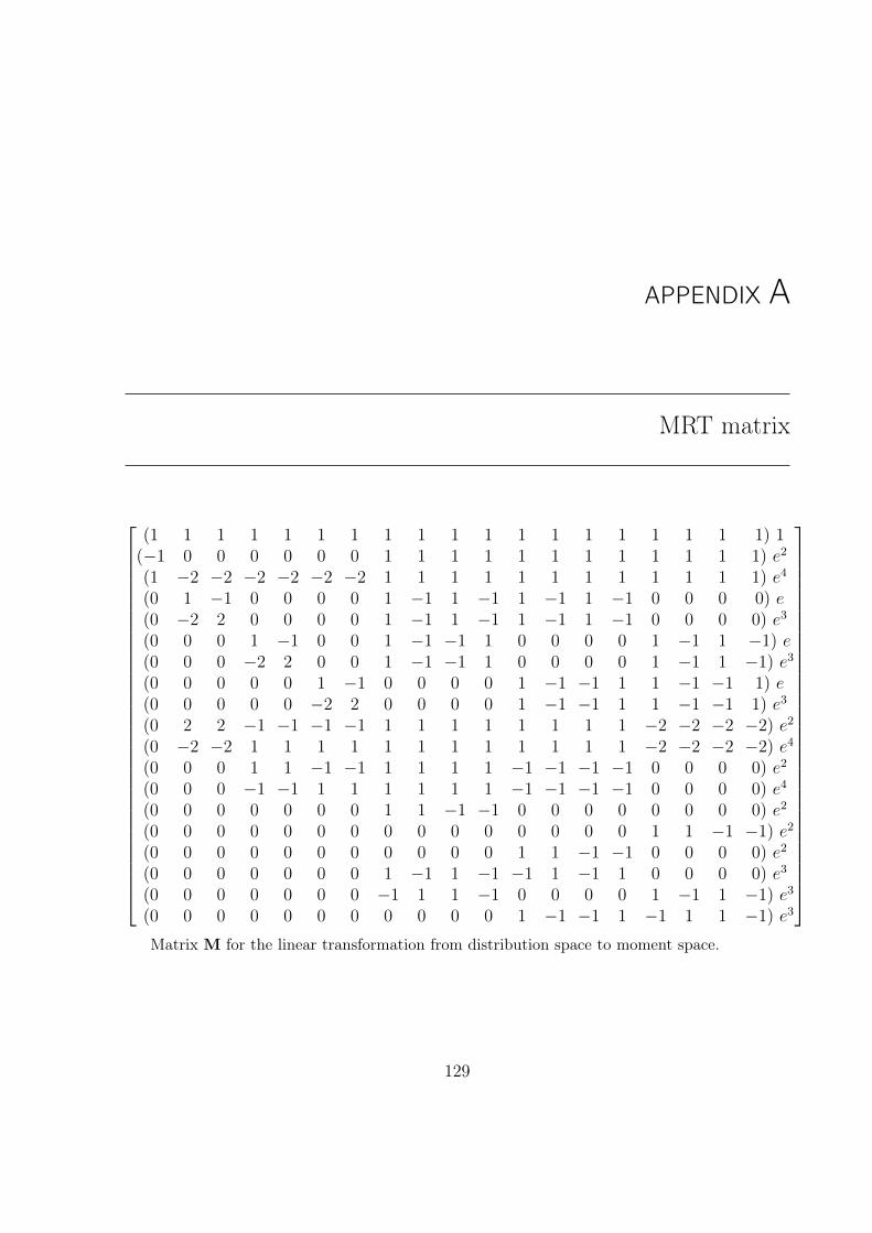
APPENDIX A
MRT matrix
(1 1 1 1 1 1 1 1 1 1 1 1 1 1 1 1 1 1 1) 1(−1 0 0 0 0 0 0 1 1 1 1 1 1 1 1 1 1 1 1) e2
(1 −2 −2 −2 −2 −2 −2 1 1 1 1 1 1 1 1 1 1 1 1) e4
(0 1 −1 0 0 0 0 1 −1 1 −1 1 −1 1 −1 0 0 0 0) e(0 −2 2 0 0 0 0 1 −1 1 −1 1 −1 1 −1 0 0 0 0) e3
(0 0 0 1 −1 0 0 1 −1 −1 1 0 0 0 0 1 −1 1 −1) e(0 0 0 −2 2 0 0 1 −1 −1 1 0 0 0 0 1 −1 1 −1) e3
(0 0 0 0 0 1 −1 0 0 0 0 1 −1 −1 1 1 −1 −1 1) e(0 0 0 0 0 −2 2 0 0 0 0 1 −1 −1 1 1 −1 −1 1) e3
(0 2 2 −1 −1 −1 −1 1 1 1 1 1 1 1 1 −2 −2 −2 −2) e2
(0 −2 −2 1 1 1 1 1 1 1 1 1 1 1 1 −2 −2 −2 −2) e4
(0 0 0 1 1 −1 −1 1 1 1 1 −1 −1 −1 −1 0 0 0 0) e2
(0 0 0 −1 −1 1 1 1 1 1 1 −1 −1 −1 −1 0 0 0 0) e4
(0 0 0 0 0 0 0 1 1 −1 −1 0 0 0 0 0 0 0 0) e2
(0 0 0 0 0 0 0 0 0 0 0 0 0 0 0 1 1 −1 −1) e2
(0 0 0 0 0 0 0 0 0 0 0 1 1 −1 −1 0 0 0 0) e2
(0 0 0 0 0 0 0 1 −1 1 −1 −1 1 −1 1 0 0 0 0) e3
(0 0 0 0 0 0 0 −1 1 1 −1 0 0 0 0 1 −1 1 −1) e3
(0 0 0 0 0 0 0 0 0 0 0 1 −1 −1 1 −1 1 1 −1) e3
Matrix M for the linear transformation from distribution space to moment space.
129

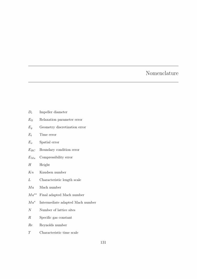
Nomenclature
Di Impeller diameter
EΩ Relaxation parameter error
Eg Geometry discretization error
Et Time error
Ex Spatial error
EBC Boundary condition error
EMa Compressibility error
H Height
Kn Knudsen number
L Characteristic length scale
Ma Mach number
Ma∗∗ Final adapted Mach number
Ma∗ Intermediate adapted Mach number
N Number of lattice sites
R Specific gas constant
Re Reynolds number
T Characteristic time scale
131
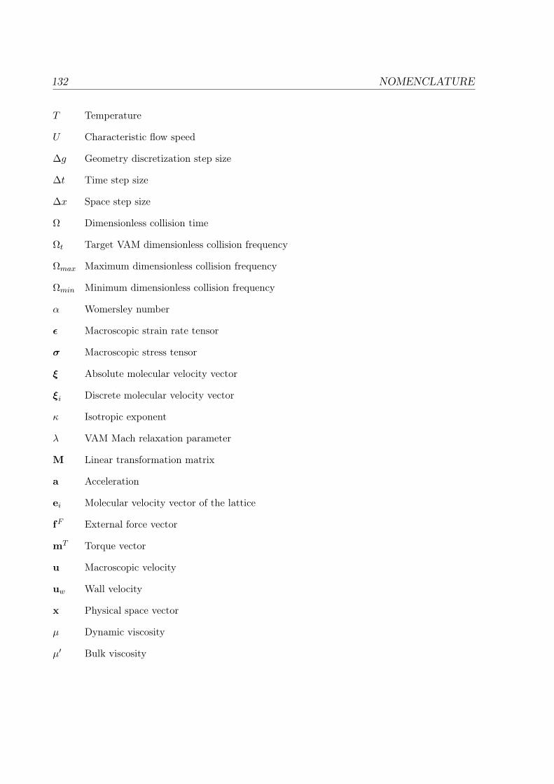
132 NOMENCLATURE
T Temperature
U Characteristic flow speed
∆g Geometry discretization step size
∆t Time step size
∆x Space step size
Ω Dimensionless collision time
Ωt Target VAM dimensionless collision frequency
Ωmax Maximum dimensionless collision frequency
Ωmin Minimum dimensionless collision frequency
α Womersley number
ε Macroscopic strain rate tensor
σ Macroscopic stress tensor
ξ Absolute molecular velocity vector
ξi Discrete molecular velocity vector
κ Isotropic exponent
λ VAM Mach relaxation parameter
M Linear transformation matrix
a Acceleration
ei Molecular velocity vector of the lattice
fF External force vector
mT Torque vector
u Macroscopic velocity
uw Wall velocity
x Physical space vector
µ Dynamic viscosity
µ′ Bulk viscosity
NOMENCLATURE 133
ν Kinematic viscosity
νmax Maximum kinematic viscosity
νmin Minimum kinematic viscosity
ρ Density
τ Dimensional collision time
τw Wall shear stress
ξ Component of the molecular velocity vector ξ
cs Speed of sound
f(x, ξ, t) density probability function
feq Equilibrium probability distribution function
fneq Non-equilibrium part of the distribution f
k Flow consistency index
m Macroscospic moment of the probability distribution function
n Agitator speed
n Flow behavior index
p Thermodynamic pressure
sa−e Relaxation parameters for non-hydrodynamic moments
scale Scale factors of grid refinement
w weighting factor
E Error
R Radius
t Time

Bibliography
[1] T. Akenine-Möller. Fast 3D Triangle-Box Overlap Testing. In ACM SIGGRAPH 2005Courses, page 8. ACM, 2005.
[2] ASME-V&V-20-Committee. Standard for Verification and Validation in ComputationalFluid Dynamics and Heat Transfer. American Society of Mechanical Engineers, New York,November 2009.
[3] P. L. Bhatnagar, E. P. Gross, and M. Krook. A Model For Collison Processes in Gases.Phys. Rev., 94:511, 1954.
[4] R. B. Bird, W. E. Stewart, and E. N. Lightfoot. Transport Phenomena. John Wiley & Sons,2007.
[5] M. Bouzidi, M. Firdaouss, and P. Lallemand. Momentum Transfer of a Boltzmann-LatticeFluid with Boundaries. Physics of Fluids (1994-present), 13(11):3452–3459, 2001.
[6] J. Boyd, J. Buick, and S. Green. A Second-Order Accurate Lattice Boltzmann non-NewtonianFlow Model. Journal of physics A: Mathematical and General, 39(46):14241, 2006.
[7] R. Brownlee, A. N. Gorban, and J. Levesley. Stability and Stabilization of the LatticeBoltzmann Method. Physical Review E, 75(3):036711, 2007.
[8] R. Chandra. Parallel Programming in OpenMP. Morgan Kaufmann, 2001.
[9] D. Conrad, A. Schneider, and M. Böhle. Numerical Investigation of an Extended PropellerViscosimeter by Means of Lattice Boltzmann Methods. In ASME 2013 Fluids Engineer-ing Division Summer Meeting, pages V01AT03A015–V01AT03A015. American Society ofMechanical Engineers, 2013.
[10] B. Crouse. Lattice-Boltzmann Strömungssimulationen auf Baumdatenstrukturen. PhD thesis,TU Braunschweig, 2003.
135
136 BIBLIOGRAPHY
[11] P. J. Dellar. Bulk and Shear Viscosities in Lattice Boltzmann Equations. Physical Review E,64(3):031203, 2001.
[12] P. J. Dellar. Incompressible Limits of Lattice Boltzmann Equations using Multiple RelaxationTimes. Journal of Computational Physics, 190(2):351–370, 2003.
[13] P. J. Dellar. An Interpretation and Derivation of the Lattice Boltzmann Method usingStrang Splitting. Computers & Mathematics with Applications, 65(2):129–141, 2013.
[14] P. J. Dellar. Lattice Boltzmann Algorithms without Cubic Defects in Galilean Invariance onStandard Lattices. Journal of Computational Physics, 259:270–283, 2013.
[15] D. d’Humières, I. Ginzburg, M. Krafczyk, P. Lallemand, and L.-S. Luo. Multiple–Relaxation–Time Lattice Boltzmann Models in Three Dimensions. Philosophical Transactions of the RoyalSociety of London. Series A: Mathematical, Physical and Engineering Sciences, 360(1792):437–451, 2002.
[16] F. R. Feito, C. J. Torres, and A. Ureña. Orientation, Simplicity and Inclusion Test forPlanar Polygons. Comput. & Graphics, 19(4):595–600, 1995.
[17] F. R. Feito and J. C. Torres. Inclusion Test for General Polyhedra. Comput. & Graphics,21(1):23–30, 1997.
[18] J. H. Ferziger and M. Perić. Computational Methods for Fluid Dynamics, volume 3. SpringerBerlin, 1996.
[19] O. Filippova and D. Hänel. Boundary-Fitting and Local Grid Refinement for Lattice-BGKModels. International Journal of Modern Physics C, 9(08):1271–1279, 1998.
[20] O. Filippova and D. Hänel. Grid Refinement for Lattice-BGK Models. Journal of Computa-tional Physics, 147(1):219–228, 1998.
[21] S. Freudiger. Entwcklung eines Parallelen, Adaptiven, Komponentenbasieren Strömungskernsfür Hierarische Gitter auf Basis der Lattice Boltzmann Methode. PhD thesis, TU Braun-schweig, 2009.
[22] S. Gabbanelli, G. Drazer, and J. Koplik. Lattice Boltzmann Method for non-Newtonian(Power-law) Fluids. Phys. Rev. E, 72:046312, Oct 2005.
[23] I. Ginzburg, F. Verhaeghe, and D. d’Humieres. Two-Relaxation-Time Lattice BoltzmannScheme: About Parametrization, Velocity, Pressure and Mixed Boundary Conditions. Com-munications in computational physics, 3(2):427–478, 2008.
[24] Z. Guo and C. Shu. Lattice Boltzmann Method and Its Application in Engineering. WorldScientific Pub Co, 2013.
[25] Z. Guo, C. Zheng, and S. Baochang. Discrete Lattice Effects on the Forcing Term in theLattice Boltzmann Method. Phys Rev E, 65:046308, 2002.
BIBLIOGRAPHY 137
[26] Z. Guo, C. Zheng, and B. Shi. Lattice Boltzmann Equation with Multiple Effective RelaxationTimes for Gaseous Microscale Flow. Physical Review E, 77(3):036707, 2008.
[27] E. A. Haines and J. R. Wallace. Shaft Culling for Efficient Ray-Cast Radiosity. In Photore-alistic rendering in computer graphics, pages 122–138. Springer, 1994.
[28] D. Hänel. Molekulare Gasdynamik. Springer, 2006.
[29] J. Harris. Rheology and non-Newtonian Flow. Longman London, 1977.
[30] X. He, S. Chen, and G. D. Doolen. A Novel Thermal Model for the Lattice BoltzmannMethod in Incompressible Limit. Journal of Computational Physics, 146(1):282–300, 1998.
[31] S. Hoffmann and R. Lienhart. OpenMP: Eine Einführung in die Parallele Programmierungmit C/C++. Informatik im Fokus. Springer, 2009.
[32] D. J. Holdych, D. R. Noble, J. G. Georgiadis, and R. O. Buckius. Truncation Error Analysisof Lattice Boltzmann Methods. Journal of Computational Physics, 193(2):595–619, 2004.
[33] M. Junk. A Finite Difference Interpretation of the Lattice Boltzmann Method. NumericalMethods for Partial Differential Equations, 17(4):383–402, 2001.
[34] M. Junk, A. Klar, and L.-S. Luo. Asymptotic Analysis of the Lattice Boltzmann Equation.Journal of Computational Physics, 210(2):676–704, 2005.
[35] M. Krafczyk. Gitter-Boltzmann-Methoden: Von der Theorie zur Anwendung. Habilitationss-chrift,Lehrstuhl für Bauinformatik, TU-München, 2001.
[36] T. Krüger, F. Varnik, and D. Raabe. Shear Stress in Lattice Boltzmann Simulations. PhysicalReview E, 79(4):046704, 2009.
[37] T. Krüger, F. Varnik, and D. Raabe. Second-Order Convergence of the Deviatoric StressTensor in the Standard Bhatnagar-Gross-Krook Lattice Boltzmann Method. Physical ReviewE, 82(2):025701, 2010.
[38] A. J. C. Ladd. Numerical Simulation of Particulate Suspensions via a Discrete BoltzmannEquation. Part 1. Theoretical Foundation. J. Fluid. Mech., 271:285–309, 1994.
[39] A. J. C. Ladd and R. Verberg. Lattice-Boltzmann Simulations of Particle-Fluid Suspensions.Journal of Statistical Physics, 104(5-6):1191–1251, 2001.
[40] J. Latt. Hydrodynamic Limit of Lattice Boltzmann Equations. PhD thesis, Université deGenéve, 03/09 2007.
[41] C. Loudon and A. Tordesillas. The Use of the Dimensionless Womersley Number toCharacterize the Unsteady Nature of Internal Flow. Journal of theoretical biology, 191(1):63–78, 1998.
138 BIBLIOGRAPHY
[42] L.-S. Luo. Lattice-Gas Automata and Lattice Boltzmann Equations for Two-DimensionalHydrodynamics. PhD thesis, Georgia Institute of Technology, Atlanta, 1993.
[43] O. Malaspinas. Lattice Boltzmann Method for the Simulation of Viscoelastic Fluid Flows.PhD thesis, École Polytechnique Fédérale De Lausanne, 2009.
[44] R. Mei, L.-S. Luo, P. Lallemand, and D. d’Humières. Consistent Initial Conditions forLattice Boltzmann Simulations. Computers & Fluids, 35(8):855–862, 2006.
[45] R. Mei, L.-S. Luo, and W. Shyy. An Accurate Curved Boundary Treatment in the LatticeBoltzmann Method. Journal of Computational Physics, 155(2):307–330, 1999.
[46] R. Mei, W. Shyy, D. Yu, and L.-S. Luo. Lattice Boltzmann Method for 3-D Flows withCurved Boundary. Journal of Computational Physics, 161(2):680–699, 2000.
[47] R. Mei, D. Yu, W. Shyy, and L.-S. Luo. Force Evaluation in the Lattice Boltzmann MethodInvolving Curved Geometry. Physical Review E, 65(4):041203, 2002.
[48] R. Ouared and B. Chopard. Lattice Boltzmann Simulations of Blood Flow: Non-NewtonianRheology and Clotting Processes. Journal of Statistical Physics, 121:209–221, Oct. 2005.
[49] D. Pritchard, C. R. McArdle, and S. K. Wilson. The Stokes Boundary Layer for a Power-lawFluid. Journal of Non-Newtonian Fluid Mechanics, 166(12):745–753, 2011.
[50] Y. Qian, D. d’Humières, and P. Lallemand. Lattice BGK Models for Navier-Stokes Equation.EPL (Europhysics Letters), 17(6):479–484, 1992.
[51] Y. Qian and S. Orzag. Lattice BGK Models for the Navier-Stokes Equation – NonlinearDeviation in the Compressible Regimes. EPL (Europhysics Letters), 21(3):255–259, 1993.
[52] M. B. Reider and J. D. Sterling. Accuracy of Discrete-Velocity BGKModels for the Simulationof the Incompressible Navier-Stokes Equations. Computers & fluids, 24(4):459–467, 1995.
[53] T. Reviol. Experimentelle und Numerische Untersuchungen eines Modifizierten Propeller-Viskosimeters zur Bestimmung der Fließeigenschaften nicht-Newtonscher Medien mit Inho-mogenem Charakter. PhD thesis, TU Kaiserslautern, 2010.
[54] D. Ricot, S. Marié, P. Sagaut, and C. Bailly. Lattice Boltzmann Method with SelectiveViscosity Filter. Journal of Computational Physics, 228(12):4478–4490, 2009.
[55] H. Schlichting and K. Gersten. Boundary-Layer Theory. Springer, 2000.
[56] A. Schneider. A Consistent Large Eddy Approach for Lattice Boltzmann Methods and itsApplication to Complex Flows. PhD thesis, TU Kaiserslautern, 2015.
[57] X. Shan, X.-F. Yuan, and H. Chen. Kinetic Theory Representation of Hydrodynamics: AWay Beyond the Navier–Stokes Equation. Journal of Fluid Mechanics, 550:413–441, 2006.
BIBLIOGRAPHY 139
[58] M. Stiebler, M. Krafczyk, S. Freudiger, and M. Geier. Lattice Boltzmann Large EddySimulation of Subcritical Flows Around a Sphere on non-Uniform Grids. Computers &Mathematics with Applications, 61(12):3475–3484, 2011.
[59] S. Succi. The Lattice Boltzmann Equation: For Fluid Dynamics and Beyond. Oxforduniversity press, 2001.
[60] F. Tosi, S. Ubertini, S. Succi, H. Chen, and I. V. Karlin. Numerical Stability of EntropicVersus Positivity-Enforcing Lattice Boltzmann Schemes. Mathematics and Computers inSimulation, 72(2):227–231, 2006.
[61] D. A. Wolf-Gladrow. Lattice-Gas Cellular Automata and Lattice Boltzmann Models: AnIntroduction. Springer, 2000.
[62] Z. Yang. Analysis of Lattice Boltzmann Boundary Conditions. PhD thesis, UniversitätKonstanz, 2007.
[63] W.-A. Yong and L.-S. Luo. Nonexistence of H-Theorems for the Athermal Lattice BoltzmannModels with Polynomial Equilibria. Physical Review E, 67(5):051105, 2003.
[64] D. Yu, R. Mei, and W. Shyy. A Multi-Block Lattice Boltzmann Method for Viscous FluidFlows. International Journal for Numerical Methods in Fluids, 39(2):99–120, 2002.
[65] R. Zhang, C. Sun, Y. Li, R. Satti, R. Shock, J. Hoch, and H. Chen. Lattice BoltzmannApproach for Local Reference Frames. Communications in Computational Physics, 9(5):1193,2011.

Curriculum Vitae
Daniel Conrad
Education
Since 10/2009 PhD in Mechanical EngineeringUniversity of Kaiserslautern, GermanyDepartment of Mechanical and Process Engineering- Institute of Fluid Mechanics and Turbo Machinery (SAM)
09/2009 Diplom in Mechanical EngineeringUniversity of Kaiserslautern, GermanyDiploma Thesis: Implementation of a 2D Lattice Boltzmann(BGK) Algorithm with Turbulence Modeling
10/2008–03/2009 Internship abroad at Sulzer, Winterthur, Switzerland.
10/2004–09/2009 Studies in Mechanical Engineering (9 semesters)Major: Fundamentals of Mechanical EngineeringMinors: Energy TechnologiesUniversity of Kaiserslautern, Germany
04/2003–09/2004 Military service, paratroopers battalion Zweibrücken
03/2003 Graduation (Abitur) at BurggymnasiumKaiserslautern, Germany
Wissenschaftlicher undberuflicher Werdegang
Daniel Conrad
Ausbildung
Seit 10/2009 Promotion in MaschinenbauTechnische Universität KaiserslauternFachbereich Maschinenbau und Verfahrenstechnik- Lehrstuhl Strömungmechanik und Strömungsmaschinen (SAM)
09/2009 Diplom in MaschinenbauTechnische Universität KaiserslauternThema der Diplomarbeit: Implementierung eines 2D Lattice Boltzmann(BGK) Algorithmus mit Turbulenzmodellierung
10/2008–03/2009 Auslandspraktikum bei Sulzer, Winterthur, Schweiz.
10/2004–09/2009 Studium des Maschinenbaus (9 Semester)Hauptfach: Grundlagen des MaschinenbausNebenfach: EnergietechnikTechnische Universität Kaiserslautern
04/2003–09/2004 Wehrdienst, Fallschirmjägerbataillon Zweibrücken
03/2003 Abitur am Burggymnasium Kaiserslautern


![From Lattice Boltzmann Method to Lattice Boltzmann Flux … · From Lattice Boltzmann Method to Lattice Boltzmann Flux Solver Yan Wang 1, ... flows [8,13–15], compressible flows](https://img.pdfslide.net/doc/110x75/5cadf91b88c9938f4d8c0cd6/from-lattice-boltzmann-method-to-lattice-boltzmann-flux-from-lattice-boltzmann.jpg)