A Vlsi architecture for lifting-based wavelet packet

UNLV Retrospective Theses & Dissertations

1-1-2003

A Vlsi architecture for lifting-based wavelet packet transform in A Vlsi architecture for lifting-based wavelet packet transform in

fingerprint image compression fingerprint image compression

Tao Zhu University of Nevada, Las Vegas

Follow this and additional works at: https://digitalscholarship.unlv.edu/rtds

Repository Citation Repository Citation Zhu, Tao, "A Vlsi architecture for lifting-based wavelet packet transform in fingerprint image compression" (2003). UNLV Retrospective Theses & Dissertations. 1574. http://dx.doi.org/10.25669/rssr-i4i0

This Thesis is protected by copyright and/or related rights. It has been brought to you by Digital Scholarship@UNLV with permission from the rights-holder(s). You are free to use this Thesis in any way that is permitted by the copyright and related rights legislation that applies to your use. For other uses you need to obtain permission from the rights-holder(s) directly, unless additional rights are indicated by a Creative Commons license in the record and/or on the work itself. This Thesis has been accepted for inclusion in UNLV Retrospective Theses & Dissertations by an authorized administrator of Digital Scholarship@UNLV. For more information, please contact [email protected].

http://library.unlv.edu/

http://library.unlv.edu/

https://digitalscholarship.unlv.edu/rtds

https://digitalscholarship.unlv.edu/rtds?utm_source=digitalscholarship.unlv.edu%2Frtds%2F1574&utm_medium=PDF&utm_campaign=PDFCoverPages

http://dx.doi.org/10.25669/rssr-i4i0

mailto:[email protected]

A VLSI ARCHITECTURE FOR LIFTING-BASED WAVELET PACKET

TRANSFORM IN FINGERPRINT IMAGE COMPRESSION

by

Tao Zhu

Bachelor of Science Shanghai Jiaotong University, Shanghai, P. R. China

1997

A thesis submitted in fulfillment of the requirements for the

Master of Science Degree in Engineering Department of Electrical and Computer Engineering

Howard R Hughes College of Engineering

Graduate College University of Nevada, Las Vegas

December, 2003

Reproduced with permission of the copyright owner. Further reproduction prohibited without permission.

UMI Number: 1417747

INFORMATION TO USERS

The quality of this reproduction is dependent upon the quality of the copy

submitted. Broken or indistinct print, colored or poor quality illustrations and

photographs, print bleed-through, substandard margins, and improper

alignment can adversely affect reproduction.

In the unlikely event that the author did not send a complete manuscript

and there are missing pages, these will be noted. Also, if unauthorized

copyright material had to be removed, a note will indicate the deletion.

UMIUMI Microform 1417747

Copyright 2004 by ProQuest Information and Learning Company.

All rights reserved. This microform edition is protected against

unauthorized copying under Title 17, United States Code.

ProQuest Information and Learning Company 300 North Zeeb Road

P.O. Box 1346 Ann Arbor, Ml 48106-1346

Reproduced witfi permission of tfie copyrigfit owner. Furtfier reproduction profiibited witfiout permission.

ITNTV Thesis ApprovalThe Graduate College University of Nevada, Las Vegas

The Thesis prepared by

The Zhu

November 7 20Qj

Entitled

"A VLSI A r c h ite c tu r e fo r L if t in g -B a s e d W avelet Transform In

F in g e r p r in t Image Com pression"

is approved in partial fulfillment of the requirements for the degree of

______ M aster o f S c ie n c e in E le c t r i c a l E n g in eer in g

xam im tion G tm m ittee M em ber

E xam inatim Com m ittee M em ber

Graduate Cmlege Faculty Rejjresentative

(J \ W -Exam ination C om m ittee Chcttf

Dean o f the G raduate College

PR/1017-53/1-00 11


ABSTRACT

A VLSI Architecture for Lifting-Based Wavelet Packet Transform In Fingerprint Image Compression

by

Tao Zhu

Dr. Shahram Latifi, Examination Committee Chair Professor of Electrical and Computer Engineering

University of Nevada, Las Vegas

FBI uses a technique called Wavelet Scalar Quantization (WSQ), a wavelet packet

transform (WPT) based method, to compress its fingerprint images. Though many VLSI

architectures have heen proposed for wavelet transform in the literature, it is not the case

for the WPT. In this thesis, a VLSI architecture capable of computing the WPT is

presented for application of WSQ. In the proposed architecture. Lifting Scheme (LS) is

used to generate wavelets instead of the traditional convolution filter-bank (FB) specified

in original standard. A comparative study between LS and FB shows that quality of

images transformed by LS is completely acceptable (with 30dB ~ 40dB PSNR at a target

bit rate of 0.75dpp) while fewer operations required. In particular, to compare with FB,

the hardware consumption, for our WSQ application, is reduced to half due to the LS.

Moreover, this architecture can be easily configured to compute any required WPT

application.

m


TABLE OF CONTENTS

ABSTRACT.............................................................................................................................iii

TABLE OF CONTENTS........................................................................................................iv

LIST OF TABLES .................................................................................................................vii

LIST OF FIGURES ..............................................................................................................viii

ACKNOWLEDGMENTS .......................................................................................................x

CHAPTER 1 INTRODUCTION ....................................................................................... 11.1 Statement of Problem and Obj ectives........................................................................... 21.2 Thesis Overview.............................................................................................................6

CHAPTER 2 WAVELET TRANSFORM AND WAVELET PACKETS .................... 72.1 Fourier Transform..........................................................................................................82.2 Wavelet Transform .................................................................................................... 112.3 Wavelet Transform and Filer bank ............................................................................ 13

Two-Channel Filter Bank ...................................................................................... 13Multiresolution Analysis........................................................................................ 15Dilation and Wavelet Equations with Filter Banks.............................................. 17

2.4 Wavelet Packets...........................................................................................................192.5 Sum m ary...................................................................................................................... 21

CHAPTER 3 WAVELET TRANSFORM WITH LIFTING SCHEME...................... 233.1 A General Lifting Scheme ..........................................................................................23

Split Stage ...............................................................................................................24Predict Stage ...........................................................................................................25Update S tag e ...........................................................................................................26The Inverse Transform...........................................................................................27

3.2 Boundary Treatment ................................................................................................... 283.3 Advantages of Lifting Scheme................................................................................... 293.4 Summary...................................................................................................................... 30

CHAPTER 4 FINGERPRINT AND ITS FBI COMPRESSIONSPECIFICATION......................................................................................31

4.1 Types of Fingerprints and Their Interpretation.........................................................334.2 A Model of the Human Visual System ......................................................................35

IV


4.3 FBI Gray-scale Fingerprint Compression Specification............................................36The 64-subbands Discrete Wavelet Packet Transform....................................... 38An Adaptive Scalar Quantization .........................................................................40A Two-pass Huffman Coding............................................................................... 40

4.4 Sum m ary........................................................................................................................42

CHAPTERS SOFTWARE IMPLEMENTATION ........................................................ 435.1 Transformation Algorithms ......................................................................................... 44

One-dimensional Wavelet Transform.................................................................. 45Standard Convolution Filter Banks (Bior9-7)................................................45LS-based algorithm (LS9-7) ...........................................................................49Integer LS-based algorithm (LS9-7I)............................................................. 51

Two-dimensional Transform................................................................................. 52Decomposition Scheme..........................................................................................54

5.2 Experimental Results and Performanee A nalysis.......................................................56Image Quality Measures and Test Image.............................................................. 56

Distortion Measure............................................................................................56Fingerprint Matching........................................................................................57Test Fingerprint Images................................................................................... 58

Experiments and Results........................................................................................58First Experiment................................................................................................ 58Second Experiment...........................................................................................63

5.3 Computational Complexity.......................................................................................... 705.4 Summary........................................................................................................................ 73

CHAPTER 6 HARDWARE IMPLEMENTATION........................................................746.1 Proposed Arehitecture...................................................................................................74

Data Flow Design .................................................................................................. 75Transform Computation Style and O rder............................................................. 76Processing Bloek and Module D esign..................................................................77Integer-to-integer Transform D esign....................................................................78

Lifting Coefficients..........................................................................................79Signal Values ................................................................................................... 80Data P a th ...........................................................................................................81

Scheduling...............................................................................................................81Memory Organizations and S ize ........................................................................... 86

MEMl M odule................................................................................................. 86MEM2 M odule................................................................................................. 88

Control ....................................................................................................................89Tim ing.....................................................................................................................90

6.2 Implementations and Analysis..................................................................................... 91Design F lo w ........................................................................................................... 91Design Units and Their Implementations ............................................................ 93

Design U nits..................................................................................................... 93Implementation Results .................................................................................. 94

6.3 Summary........................................................................................................................97


CHAPTER 7 CONCLUSIONS AND FUTUE W O RK .................................................987.1 Conclusions................................................................................................................... 987.2 Future W ork .................................................................................................................100

BIBLIOGRAPHY.................................................................................................................101

V IT A ......................................................................................................................................105

VI


LIST OF TABLES

Table 4-1 Types of fingerprint .......................................................................................... 33Table 4-2 Analysis Wavelet Filter Coefficients for WSQ ..............................................38Table 4-3 Huffman Coding Input Symbols....................................................................... 41Table 5-1 Test Fingerprint Images and Their Sizes......................................................... 58Table 5-2 PSNRs of Reconstructed Fingerprint Images from 64 Subbands.................59Table 5-3 PSNRs of Reconstructed Fingerprint Images fiom Subbands 0 to 5 9 ..........60Table 5-4 PSNRs of Compressed Fingerprint Images Using Bior9-7 .......................... 64Table 5-5 PSNRs of Compressed Fingerprint Images Using LS9-7I............................ 65Table 5-6 Minutiae Detection and Fingerprint Identification .........................................67Table 5-7 Computational complexities of standard algorithm and Lifting-based

algorithm ...........................................................................................................71Table 5-8 Execution times (second).................................................................................. 72Table 6-1 Constant Coefficients for Forward Transform................................................ 79Table 6-2 Constant Coefficients for Inverse Transform.................................................. 79Table 6-3 Part of the schedule for PMl and PM2 applied on an even-element (8x8)

block.................................................................................................................. 84Table 6-4 Part of the schedule for PMl and PM2 applied on an odd-element (9x9)

block.................................................................................................................. 85Table 6-5 Accessing Order of MEMl (Example in Section 6 .1 .5).................................87Table 6-6 Preliminary Gate Count Estimates of Basic Components.............................. 96Table 6-7 Preliminary Gate Count Estimates and Number of Components Used in the

Proposed Architecture and the Convolution Filter-bank Architecture.........96

Vll


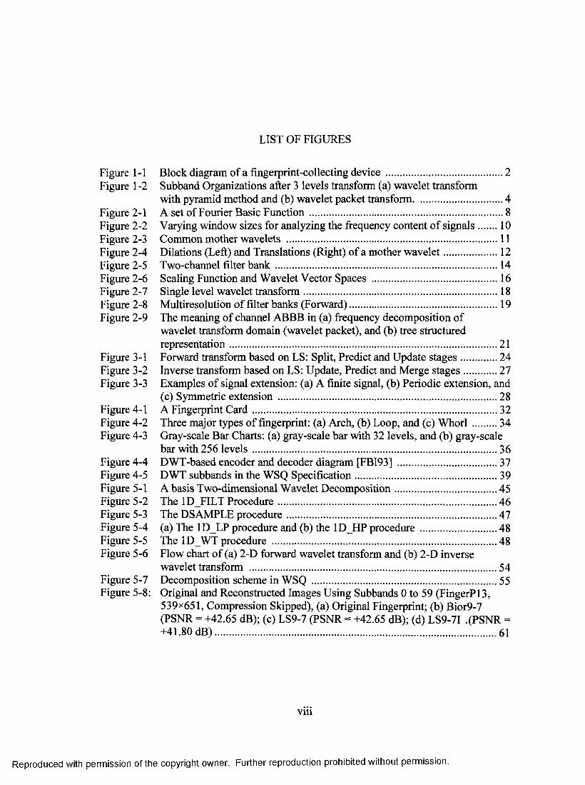
LIST OF FIGURES

Figure 1-1 Block diagram of a fingerprint-collecting device .............................................2Figure 1-2 Subband Organizations after 3 levels transform (a) wavelet transform

with pyramid method and (b) wavelet packet transform..................................4Figure 2-1 A set of Fourier Basic Function......................................................................... 8Figure 2-2 Varying window sizes for analyzing the ft-equency content of signals.........10Figure 2-3 Common mother wavelets ................................................................................11Figure 2-4 Dilations (Left) and Translations (Right) of a mother w avelet......................12Figure 2-5 Two-channel filter b an k .................................................................................... 14Figure 2-6 Sealing Function and Wavelet Vector Spaces ................................................ 16Figure 2-7 Single level wavelet transform .......................................................................18Figure 2-8 Multiresolution of filter banks (Forward).........................................................19Figure 2-9 The meaning of channel ABBB in (a) frequency decomposition of

wavelet transform domain (wavelet packet), and (b) tree structuredrepresentation................................................................................................... 21

Figure 3-1 Forward transform based on LS: Split, Predict and Update stages............... 24Figure 3-2 Inverse transform based on LS: Update, Predict and Merge stages..............27Figure 3-3 Examples of signal extension: (a) A finite signal, (b) Periodie extension, and

(c) Symmetrie extension................................................................................. 28Figure 4-1 A Fingerprint C ard ............................................................................................ 32Figure 4-2 Three major types of fingerprint: (a) Arch, (b) Loop, and (c) W horl...........34Figure 4-3 Gray-scale Bar Charts: (a) gray-scale bar with 32 levels, and (b) gray-scale

bar with 256 levels........................................................................................... 36Figure 4-4 DWT-based encoder and decoder diagram [FBI93].......................................37Figure 4-5 DWT subbands in the WSQ Specification...................................................... 39Figure 5-1 A basis Two-dimensional Wavelet Decomposition........................................45Figure 5-2 The ID FILT Procedure...................................................................................46Figure 5-3 The DSAMPLE procedure................................................................................47Figure 5-4 (a) The ID LP procedure and (b) the 1D_HP procedure .............................. 48Figure 5-5 The ID WT procedure .....................................................................................48Figure 5-6 Flow chart of (a) 2-D forward wavelet transform and (b) 2-D inverse

wavelet transform ............................................................................................54Figure 5-7 Decomposition scheme in WSQ ...................................................................... 55Figure 5-8: Original and Reconstructed Images Using Subbands 0 to 59 (FingerPl3,

539x651, Compression Skipped), (a) Original Fingerprint; (b) Bior9-7 (PSNR = +42.65 dB); (e) LS9-7 (PSNR = +42.65 dB); (d) LS9-7I .(PSNR = +41.80 dB ).........................................................................................................61

vm


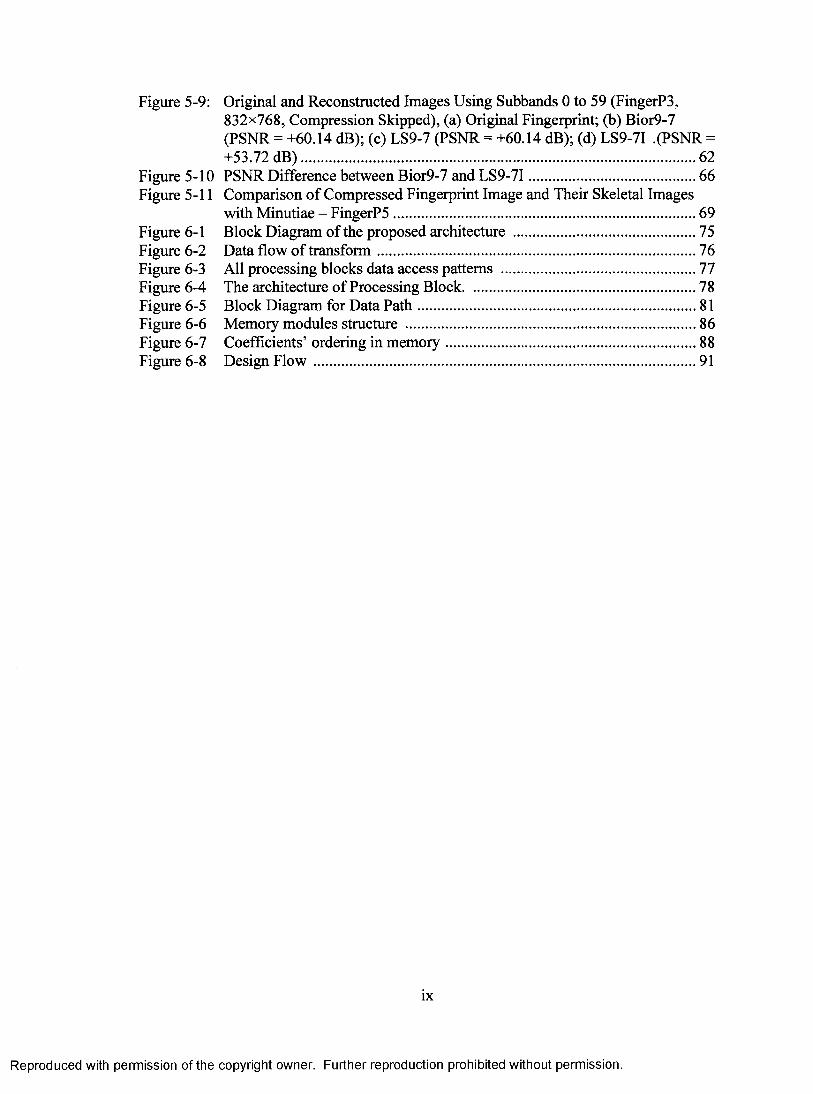
Figure 5-9: Original and Reconstructed Images Using Subbands 0 to 59 (FingerP3, 832x768, Compression Skipped), (a) Original Fingerprint; (b) Bior9-7 (PSNR = +60.14 dB); (c) LS9-7 (PSNR - +60.14 dB); (d) LS9-7I .(PSNR =+53.72 dB ).........................................................................................................62

Figure 5-10 PSNR Difference between Bior9-7 and LS9-7I............................................. 66Figure 5-11 Comparison of Compressed Fingerprint Image and Their Skeletal Images

with Minutiae - FingerP5................................................................................ 69Figure 6-1 Bloek Diagram of the proposed architecture ..................................................75Figure 6-2 Data flow of transform......................................................................................76Figure 6-3 All processing blocks data access patterns .....................................................77Figure 6-4 The architecture of Processing Block............................................................... 78Figure 6-5 Bloek Diagram for Data P a th ........................................................................... 81Figure 6-6 Memory modules strueture .............................................................................. 86Figure 6-7 Coefficients’ ordering in m em ory....................................................................88Figure 6-8 Design F lo w .......................................................................................................91

IX


ACKNOWLEDGMENTS

I would like to take this opportunity to express my sincere gratitude to the following

people for their invaluable contribution to my research:

My committee chair. Dr. Shahram Latifi, who initially inspired my interests in the

image processing field, and who guided me through the entire research process of this

thesis. He helped me learn and grow, and for his meticulously correcting my writing and,

more importantly, for his continuous encouragement and believing in me.

My committee members. Dr. Emma Regentova, Dr. Henry Selvaraj, and Dr.

Wolfgang Bein, who assisted me in improving this thesis.

My wife, Xiaojun. She offers full support to me all the time.

I would like to extend my thanks to all the professors and graduates in the Electrical

and Computer Engineering Department, and the Computer Science Department.


CHAPTER 1

INTRODUCTION

Fingerprints have been used as unique identifiers of individuals for a very long time.

FBI’s fingerprints collection effort is one of the notable examples. FBI had already

maintained about 200 million criminal records with fingerprints in the form of inked

impressions on paper cards in 1995 [Bris95]. FBI expected this fingerprint database to be

digitized at 500 dots per inch with 8 bits of grayscale resolution. This resulted in some

10 megabytes per card, making the entire database about 2,000 terabytes in size. It would

eost a significant storage spaee. So, FBI adopted an approaeh to eompress the database,

which is a discrete wavelet transform-based approach referred to as Wavelet/Scalar

Quantization (WSQ). Following this approach, FBI produced archival quality images at

compression ratios of up to 15:1 [BrBH93].

Fingerprint data collected by FBI continues to aecumulate at a rate of 30000 to

50000 new cards per day. In addition, fingerprints are still collected in the form of inked

impressions on paper cards. Those cards are digitized and compressed later. The current

situation introduces a crucial problem in transmission, storage, and automatic analysis -

the fingerprints will not be analyzed or identified on time. One of the feasible solutions

is to collect fingerprints in digital form directly by a portable fingerprint-collecting device

with a fingerprint sensor, an image processor, and a storage module (as shown in Figure

1-1). The image processor consists of a wavelet transform module, a quantization

1


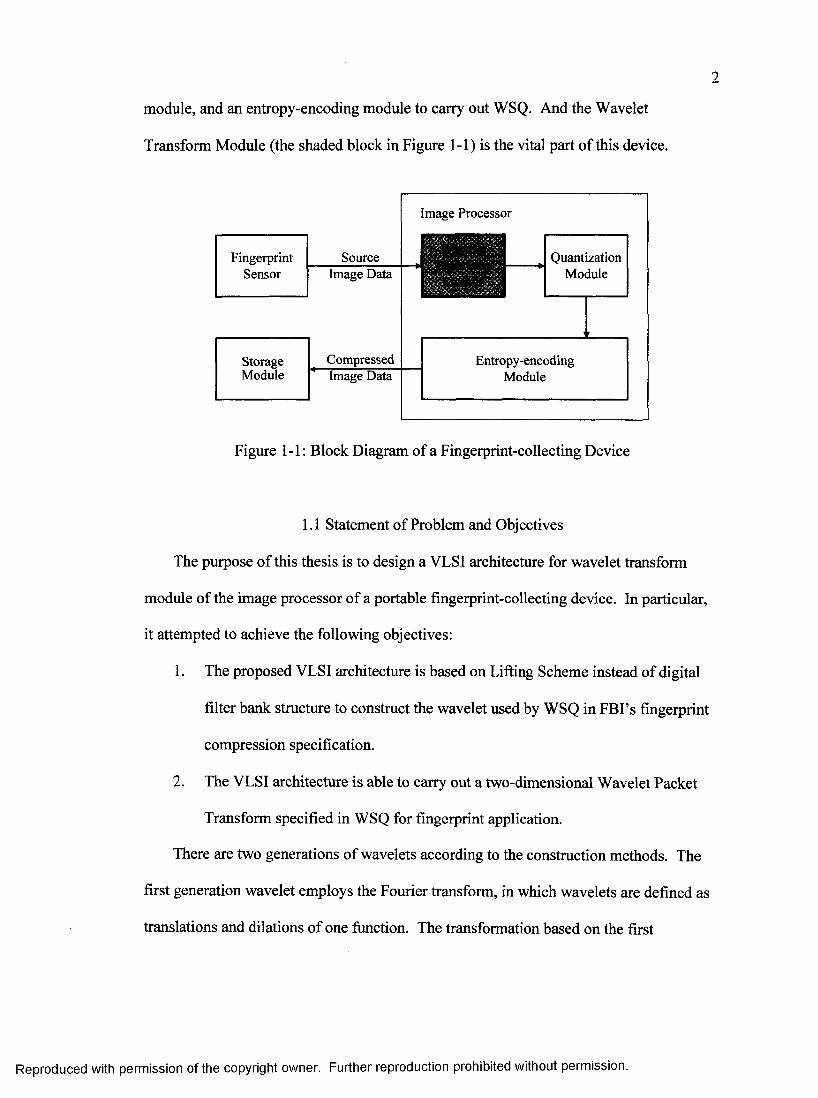
module, and an entropy-encoding module to carry out WSQ. And the Wavelet

Transform Module (the shaded block in Figure 1-1) is the vital part of this device.

Image Processor

FingerprintSensor

SourceImage Data

QuantizationModule

ModuleCompressedImage Data

Entropy-encodingModule

Figure 1-1 : Block Diagram of a Fingerprint-collecting Device

1.1 Statement of Problem and Objectives

The purpose of this thesis is to design a VLSI architecture for wavelet transform

module of the image processor of a portable fingerprint-collecting device. In particular,

it attempted to achieve the following objectives;

1. The proposed VLSI architecture is based on Lifting Scheme instead of digital

filter bank structure to construct the wavelet used by WSQ in FBI’s fingerprint

compression specification.

2. The VLSI architecture is able to carry out a two-dimensional Wavelet Packet

Transform specified in WSQ for fingerprint application.

There are two generations of wavelets according to the construction methods. The

first generation wavelet employs the Fourier transform, in which wavelets are defined as

translations and dilations of one function. The transformation based on the first


3

generation wavelets can be generated from digital filter banks, such as the filter banks

used by WSQ, in which a 9-tap lowpass filter and a 7-tap highpass filter are used. It has

been implemented by convolution traditionally. Such an implementation demands both a

large number of computations and a large storage - features that are not desirable for

high-speed or low-power applications.

The second generation wavelets are based on Lifting Scheme (LS), which was

introduced in 1995 by W. Sweldens [Swel95]. The main feature of this scheme is to

break up the highpass and lowpass filters into a sequence of upper and lower triangular

matrices and converts the filter implementation into banded matrix multiplications

[DaSw98]. It requires far fewer computations than the previous type.

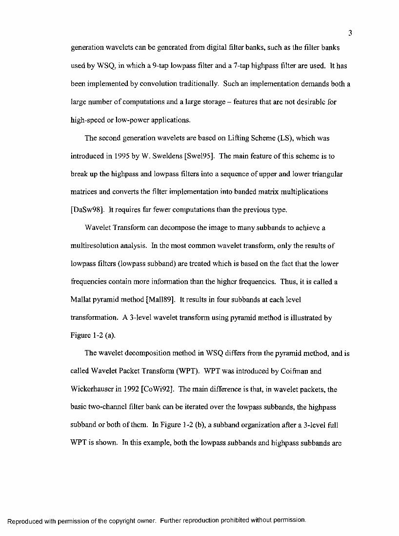
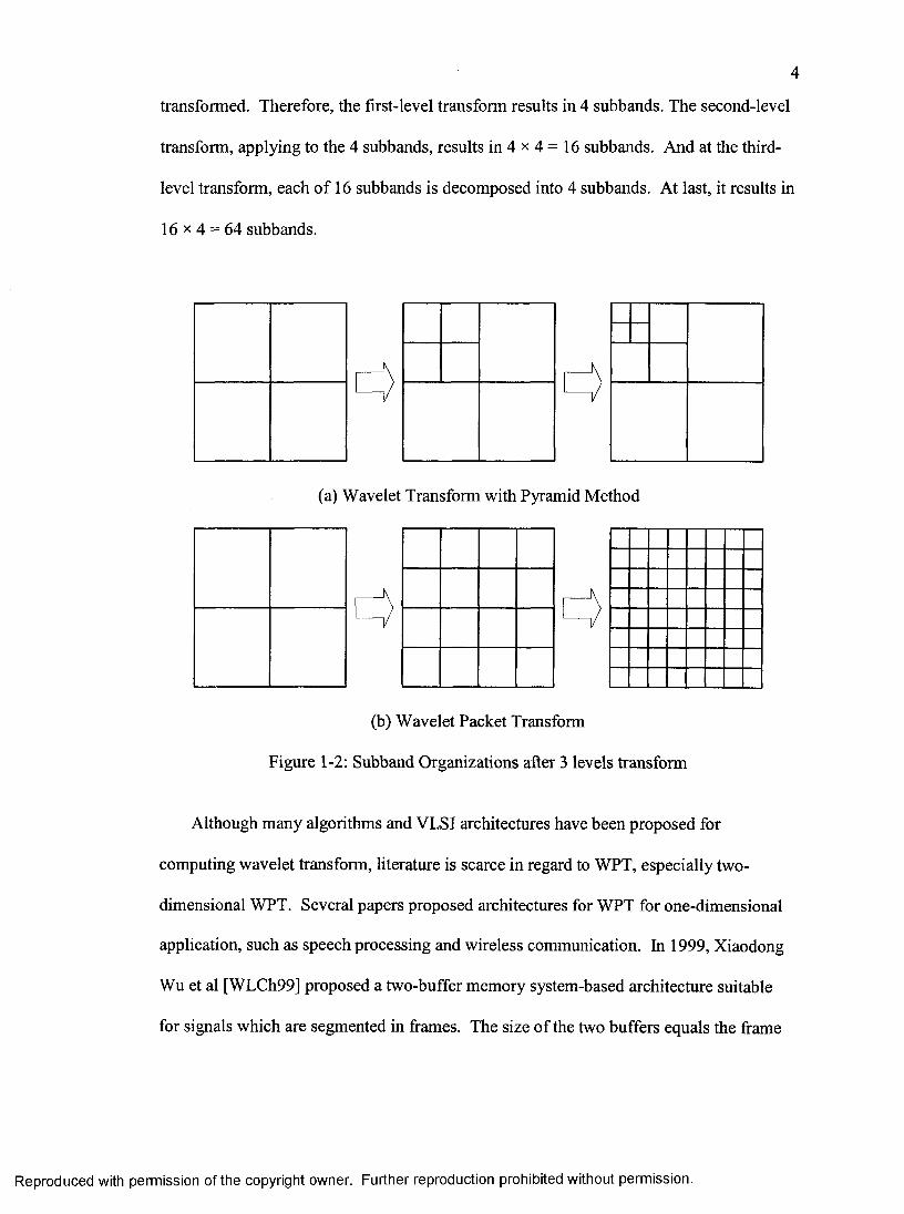
Wavelet Transform can decompose the image to many subbands to achieve a

multiresolution analysis. In the most common wavelet transform, only the results of

lowpass filters (lowpass subband) are treated which is based on the fact that the lower

frequencies contain more information than the higher frequencies. Thus, it is called a

Mallat pyramid method [Mall89]. It results in four subbands at each level

transformation. A 3-level wavelet transform using pyramid method is illustrated by

Figure 1-2 (a).

The wavelet decomposition method in WSQ differs from the pyramid method, and is

called Wavelet Packet Transform (WPT). WPT was introduced by Coifman and

Wickerhauser in 1992 [CoWi92]. The main difference is that, in wavelet packets, the

basic two-channel filter bank can be iterated over the lowpass subbands, the highpass

subband or both of them. In Figure 1-2 (b), a subband organization after a 3-level full

WPT is shown. In this example, both the lowpass subbands and highpass subbands are


4

transformed. Therefore, the first-level transform results in 4 subbands. The second-level

transform, applying to the 4 subbands, results in 4 x 4 = 16 subbands. And at the third-

level transform, each of 16 subbands is decomposed into 4 subbands. At last, it results in

16 X 4 = 64 subbands.

(a) Wavelet Transform with Pyramid Method

(b) Wavelet Packet Transform

Figure 1-2; Subband Organizations after 3 levels transform

Although many algorithms and VLSI architectures have been proposed for

computing wavelet transform, literature is scarce in regard to WPT, especially two-

dimensional WPT. Several papers proposed architectures for WPT for one-dimensional

application, such as speech processing and wireless communication. In 1999, Xiaodong

Wu et al [WLCh99] proposed a two-buffer memory system-based architecture suitable

for signals which are segmented in frames. The size of the two buffers equals the frame


5

length. In 2000, [TLZaOO] proposed a configurable architecture for WPT which was

based on [WLCh99] and made some improvements. It is a word-serial architecture

where the inputs are supplied to the filters in a serial manner. Corresponding to a J-level

WPT, J identical process units and / memory modules are cascaded. This architecture

owns a smaller memory module and smaller latency than [WLCh99]. In 2002, [TLZa02]

and [JaMa02] proposed two similar word-parallel architectures. These two architectures,

both came from [TLZaOO], achieve a higher transform speed by feeding the inputs into

the filters in a parallel manner. Since the above four architectures were all designed for

one dimensional WPT applications, it will be very difficult to extend them to fit to two

dimensional applications. The extensions will either require massive memory or cause

worse hardware utilization.

We propose a VLSI architecture for two dimensional WPT, which is capable of

executing the filters mentioned in WSQ using the LS. In designing this architecture, our

goal is the same as in design of any VLSI system, i.e. to achieve high hardware

utilization and to reduce chip area. The chip area can be reduced by minimizing the

number of processing elements, registers and interconnection wires. And better hardware

utilization can be achieved by better scheduling of pipeline and computation. The

prototype consists of four processing blocks, which can perform integer-to-integer

transforms and generate a pair of wavelet coefficients at a time. The data path is

pipelined. The output is written back to memory in-place. Furthermore, this architecture

can perform both forward transform and inverse transform by just swapping the lifting

coefficients. The proposed architecture is area efficient, and provides parallel executions.


6

It is suitable for on-chip or single-chip implementation. It can be used not only in

fingerprint image processing but also as a WPT engine in other real-time systems.

1.2 Thesis Overview

The thesis is organized as follows:

• Chapter 2 covers a survey on the theoretical background, briefly introducing the

Wavelet Transform, Packets and their relations with filter bank structure.

• Chapter 3 explains the Lifting Scheme implementation of the Discrete Wavelet

Transform, by highlighting its different phases, properties and advantages.

• Chapter 4 introduces the FBI fingerprint compression standard.

• Chapter 5 describes the performance comparison between filter-bank based DWT

algorithm used by FBI WSQ standard and alternative Lifting Scheme based

integer-to-integer transform algorithm. This chapter is essential for understanding

the hardware design as explained in the chapter 6.

• Chapter 6 proposes the VLSI architecture for wavelet decomposition framework

of FBI standard. The organization of the design is a bottom-up fashion and

architecture is optimized for WPT.

• Chapter 7 presents a short description of what was achieved in this thesis,

discusses the potential of the design and gives some tips for future improvement.


CHAPTER 2

WAVELET TRANSFORM AND WAVELET PACKETS

A wavelet transform is similar to a Fourier transform. With a Fourier transform, a

function (or a signal) is decomposed into a weighted sum of sinusoids and cosines. With

a wavelet transform, a function (or a signal) is decomposed into a weighted sum of

wavelet function.

Why should we use wavelets instead of the traditional Fourier methods? There are

some important differences between Fourier analysis and wavelets. First, Fourier basis

functions are localized in frequencies but not in time. Small frequency changes in

Fourier transform will produce changes everywhere in the time domain. Wavelets are

local in both frequency/scale (via dilations) and in time (via translations). This

localization is an advantage in many cases. In particular, the wavelet transform (WT) is

of interest for the analysis of non-stationary signals, because it provides an alternative to

classical short-time Fourier transform (STFT). The basic difference is as follows: in

contrast to STFT, which uses a single analysis window, the WT uses short windows at

high frequencies and long windows at low frequencies.

Second, many classes of functions can be represented by wavelets in a more compact

way. For example, functions with discontinuities and functions with sharp spikes usually

take substantially fewer wavelet basis functions than sine-cosine basis functions to

achieve a comparable approximation. This sparse coding makes wavelets excellent tools

7


8

in data compression, like FBI fingerprint compression we focus on in this thesis. The

compression ratios are up to 15:1, and the difference between the original image and the

decompressed one can be perceived only by an expert [BrBH93].

2.1 Fourier Transform

A survey on Fourier Transform (FT) is first presented prior to going further to the

Wavelet Transform because the Fourier Transform is widely used in analyzing and

interpreting signals and images.

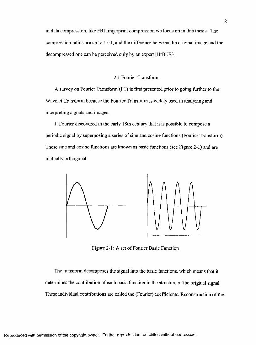
J. Fourier discovered in the early 18th century that it is possible to compose a

periodic signal by superposing a series of sine and cosine functions (Fourier Transform).

These sine and cosine functions are known as basic functions (see Figure 2-1) and are

mutually orthogonal.

Figure 2-1 : A set of Fourier Basic Function

The transform decomposes the signal into the basic functions, which means that it

determines the contribution of each basis function in the structure o f the original signal.

These individual contributions are called the (Fourier) coefficients. Reconstruction of the


9

original signal from its Fourier coefficients is accomplished by multiplying each basic

function with its corresponding coefficient and adding them up together. The standard

forward and inverse Fourier transform can be expressed as:

(2.1)

(2 .2)

Discrete Fourier Transform (DPT) is an estimation of the Fourier Transform, which

uses a finite number of sample points of the original signal to estimate the Fourier

Transform of it. The order o f computation cost for the DFT is in order of where n is

the length of the signal. Fast Fourier Transform (FFT) is an efficient implementation of

the Discrete Fourier Transform, which can be applied to the signal if the samples are

uniformly spaced. FFT reduces the computation complexity to the order of 0(n log n) by

taking advantage of self similarity properties of the DFT [Daub92].

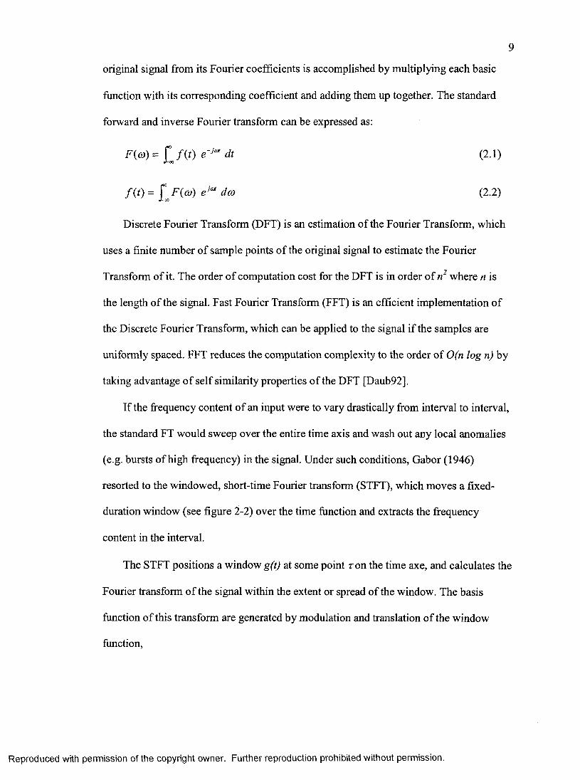
If the frequency content of an input were to vary drastically from interval to interval,

the standard FT would sweep over the entire time axis and wash out any local anomalies

(e.g. bursts of high frequency) in the signal. Under such conditions, Gabor (1946)

resorted to the windowed, short-time Fourier transform (STFT), which moves a fixed-

duration window (see figure 2-2) over the time function and extracts the frequency

content in the interval.

The STFT positions a window at some point ron the time axe, and calculates the

Fourier transform of the signal within the extent or spread of the window. The basis

function of this transform are generated by modulation and translation of the window

function.


10

F {co, t) = £ f i t ) g ( t - r) e''®' dt (2.3)

where w and t are modulation and translation factors, respectively.

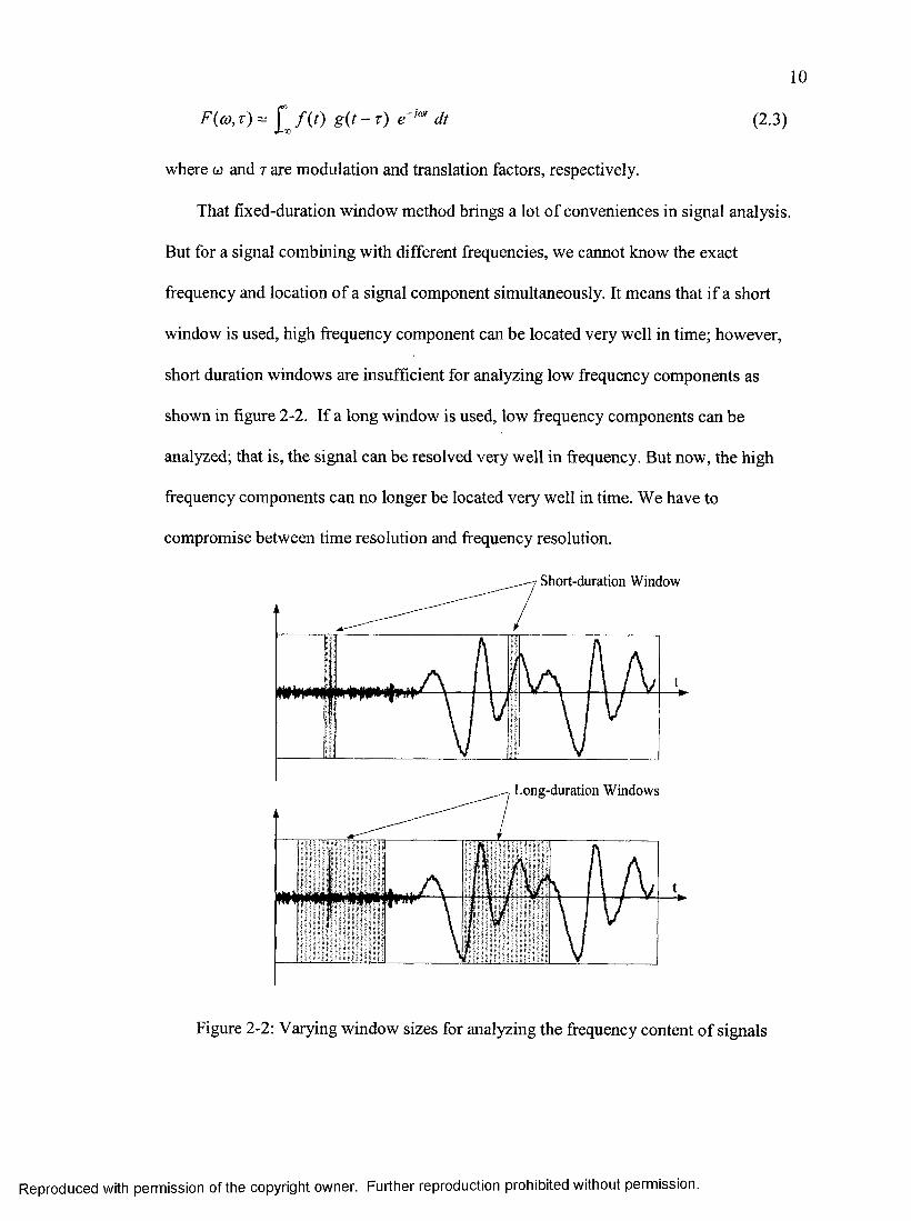
That fixed-duration window method brings a lot of conveniences in signal analysis.

But for a signal combining with different frequencies, we cannot know the exact

frequency and location of a signal component simultaneously. It means that if a short

window is used, high frequency component can be located very well in time; however,

short duration windows are insufficient for analyzing low frequency components as

shown in figure 2-2. If a long window is used, low frequency components can be

analyzed; that is, the signal can be resolved very well in frequency. But now, the high

frequency components can no longer be located very well in time. We have to

compromise between time resolution and frequency resolution.

Short-duration Window

Long-duration Windows

Figure 2-2: Varying window sizes for analyzing the frequency content of signals


11

2.2 Wavelet Transform

Unlike the FT and STFT, the wavelet transform is founded on basis functions formed

by dilation and translation of a prototype function. These basis functions are shot-

duration, high-frequency and long-duration, low-frequency functions. So, the varying of

the time interval, or window length, is exactly what the wavelet transform accomplishes.

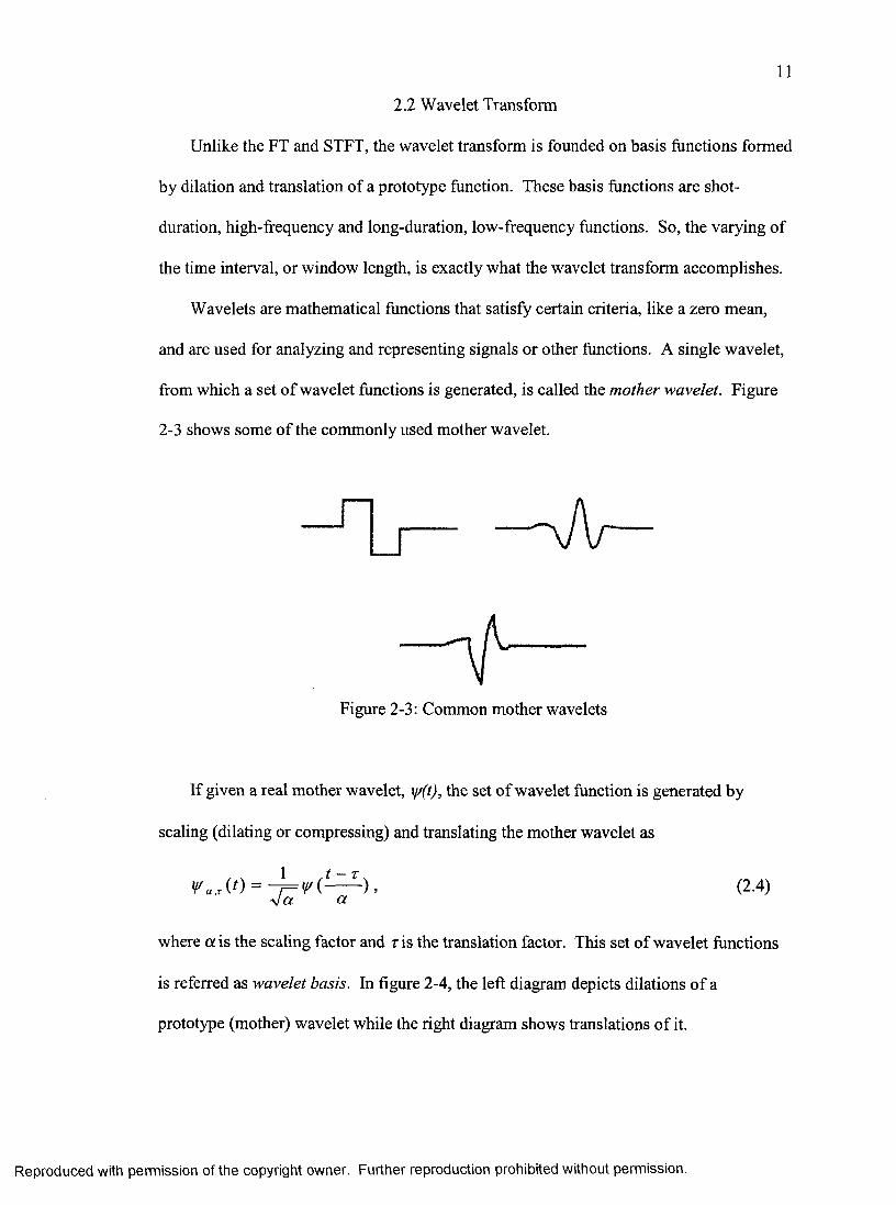
Wavelets are mathematical functions that satisfy certain criteria, like a zero mean,

and are used for analyzing and representing signals or other functions. A single wavelet,

from which a set of wavelet functions is generated, is called the mother wavelet. Figure

2-3 shows some of the commonly used mother wavelet.

Figure 2-3: Common mother wavelets

If given a real mother wavelet, \g(t), the set of wavelet function is generated by

scaling (dilating or compressing) and translating the mother wavelet as

= (2.4)ct

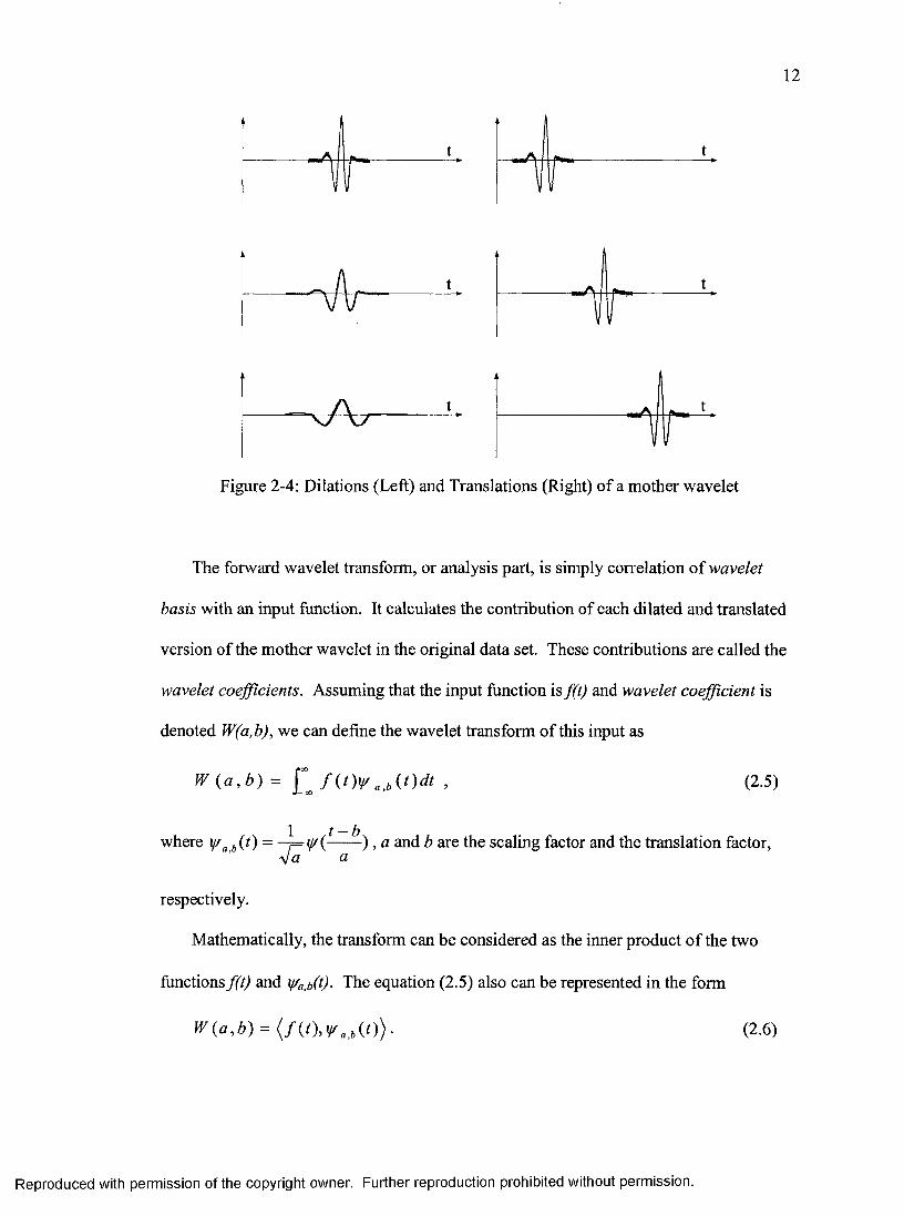
where a is the scaling factor and r is the translation factor. This set of wavelet functions

is referred as wavelet basis. In figure 2-4, the left diagram depicts dilations of a

prototype (mother) wavelet while the right diagram shows translations of it.


12

Figure 2-4: Dilations (Left) and Translations (Right) of a mother wavelet

The forward wavelet transform, or analysis part, is simply correlation of wavelet

basis with an input function. It calculates the contribution of each dilated and translated

version of the mother wavelet in the original data set. These contributions are called the

wavelet coefficients. Assuming that the input function is f(t) and wavelet coefficient is

denoted W(a,b), we can define the wavelet transform of this input as

W ( a , b ) = f ( t ) i g ^ ^ ( t ) d t , (2.5)

where = —Lry/(-—- ) , a and b are the scaling factor and the translation factor,f a a

respectively.

Mathematically, the transform can be considered as the inner product of the two

functions f(t) and y/a,b(t)- The equation (2.5) also can be represented in the form

W{a, b) = [ f i t \ \ j / ^ ^ { t ) ) . (2.6)


13

Since wavelets are used to transform a function, the inverse transform is needed and

defined by

/ ( ' ) = ^ r f f (2-7)( J~ CO QO ^

where the quantity C is defined by means of which is the Fourier transform of

2.3 Wavelet Transform and Filer bank

In many applications, one never has to deal directly with the scaling functions or

wavelets for wavelet transform. Only the scaling function coefficients, wavelet

coefficients and the output coefficients after transforms need be considered, and they can

be view as digital filters coefficients and digital signals respectively. Therefore, It is

possible to develop most of the results of wavelet theory using only filter banks. In this

section, we will connect the wavelet transform (DWT) and filter banks.

2.3.1 Two-Channel Filter Bank

A filter is a linear operator defined in terms of its filter coefficients A(0), A(l), ....

Since the number of filter coefficients h(f) is finite, the filter is a finite impulse response

or FIR and the operator is represented as

y(n) = ^ h { k ) x ( n - k) = h* X (2.8)k

where x(n) andy(n) are the input and output signals, respectively, and the symbol *

indicates a convolution.


14

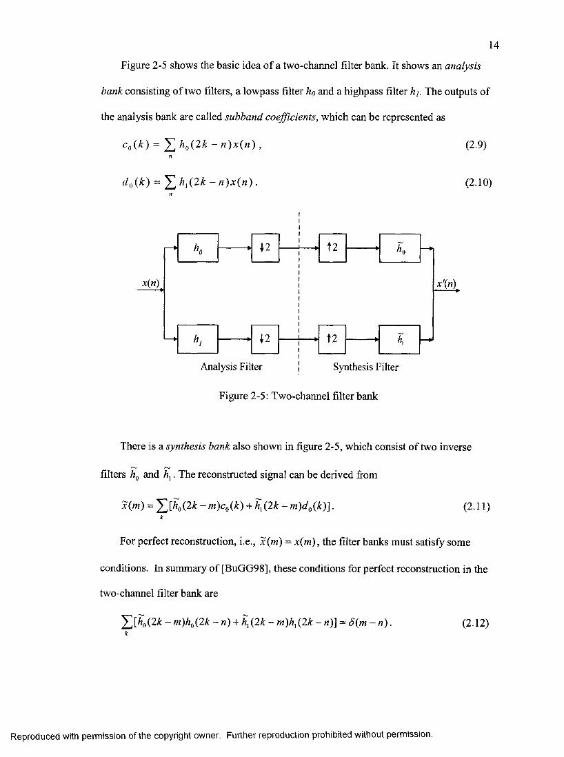
Figure 2-5 shows the basic idea of a two-channel filter bank. It shows an analysis

bank consisting of two filters, a lowpass filter ho and a highpass filter h j . The outputs of

the analysis bank are called subband coefficients, which can be represented as

Coik) = Y ^ h ^ { l k - n ) x { n ) , (2.9)

^ o (^ ) = X h f l k - n ) x { n ) . (2 10)

An).

Analysis Filter Synthesis Filter

Figure 2-5: Two-channel filter bank

There is a synthesis bank also shown in figure 2-5, which consist of two inverse

filters Ag and A,. The reconstructed signal can be derived from

^(m) = ^[Àg(2A: - w)Co(A:) + h f l k - w)Jo(^)] • (2.11)k

For perfect reconstruction, i.e., x(m) = x (m ) , the filter banks must satisfy some

conditions. In summary of [BuGG98], these conditions for perfect reconstruction in the

two-channel filter bank are

^[hf^{2k - m)hQ(2k - n) + h f 2 k - m) h f 2 k - n)] = S ( m - n ) . (2.12)


15

In order for it to hold, the four filters have to be related as

( 1 ) In the orthogonal case,

= (2.13)

*!)(«) = A (,(7 /-l-M ), (2.14)

A,(») = (-l)"Ao(M); (2.15)

(2) In the biorthogonal case,

Â;(M) = (-1)"A ,(1-»), (2.16)

A,(M) = (-1)"À,(1-M). (2.17)

2.3.2 Multiresolution Analysis

A decomposition of the whole function space into individual subspaces following a

multiple scales is known as multiresolution. In multiresolution, there are two families of

subspaces, F, and fV,-, - oo < / < oo , which are called as the Scaling Function space

Wavelet Vector space in wavelet transform system, respectively. The spaces F, are

increasing as i increases. The space W/ are the differences between the V/. In summary of

[ErHJ96], the family of subspaces F,- must satisfy the following four requirements.

(1) F. c F,„ and n F;. = {0} and U = r

(2) / ( f ) e F ;C > /(2 f ) e F , , ,

(3) /(O e Fo <=> f ( t - /c)eFo

(4) Fo has an orthonormal basis {^(t - k ) } .

Where -oo < t < oo and A: = 0, 1, 2, ... is the shift time. A functiony(^) in the whole space

has a projection in each subspace. Those projections contain more and more of the full

information inXO- The projection in F/ is calledyj(0.


16

w

Figure 2-6; Scaling Function and Wavelet Vector Spaces

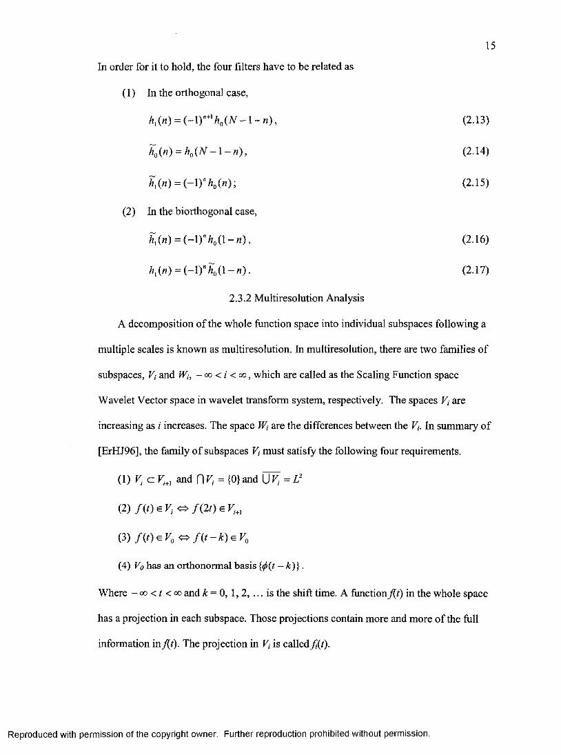
Now, we identify the second family of subspaces. JV, contains the new information

A/i (0 = /+! (0 - f i (0 • This is the detail at level i. From the viewpoint of individual

functions,

(f) 4/i/;. (f) = (2.113)

and from the viewpoint of the subspaces they lie in, these are

r, (D Mr, = p".i+i (2.19)

where © denoted the direct sum. As shown in figure 2-6, Wi is the orthogonal

complement of P}, within the large space P +/. Each function in F,+j is the sum of two

orthogonal parts, yj in P, and A/i in Wi. When we start from Fo, and add up details

(subspaces), then we have

Fo©iFo©ip, ©ip2 © ...® if;. = (2.20)

For the functions in these subspaces, this equation is simply

fo (0 + A/o(0 + A/i (t) + A /,(t) + ... + Af.(0 = {t) . (2.21)


17

2.3.3 Dilation and Wavelet Equations with Filter Banks

In a wavelet system, the dilation equation can be defined as [BuGG98]

,p(t) = y f l Y , h(k)</>i2t - k ) , (2.22)k

which is a direct consequence of Vg c E ,. There will be a finite set of coefficients

h { 0 ) , h ( N ) , when the function ^ (t) is supported on [0, N].

The scaling functions <f>{2' f - A:) are orthogonal at each scale separately. They are

not orthogonal across scales. For example, the function ((>{t) in Vo is also in Vi. So 0{t) is

not orthogonal to the basis function 0(2t-k) in Vj. Orthogonality across scales comes

from wavelet subspaces W, and their basis function % (0-

The translations of \|t(0 span Wo- The translations of \|/(2V) span W,. Those spaces

are orthogonal because Wq c V, and _L as shown in figure 2-6. The wavelet

equation produces the wavelet directly from the scaling function:

(P (f) == ar(;k)f>(:2f - *:). (2!J!3)

The wavelet coefficient, g(k), are required by orthogonality to be related to the

scaling function coefficients (orthogonal wavelet system) by

g(k) = i - l f h ( N - l - k ) , (2.24)

or the dual scaling function coefficients (biorthogonal wavelet system) by

g (t) = (-l)*Â '(l-& ). (2.25)

According to equation (2.21), any function/(t) in the whole space could be written

= (0 + YÆ uSii^k)¥ j,k (0 (2.26)k j k

as a series expansion in terms of the scaling function and wavelets.


18

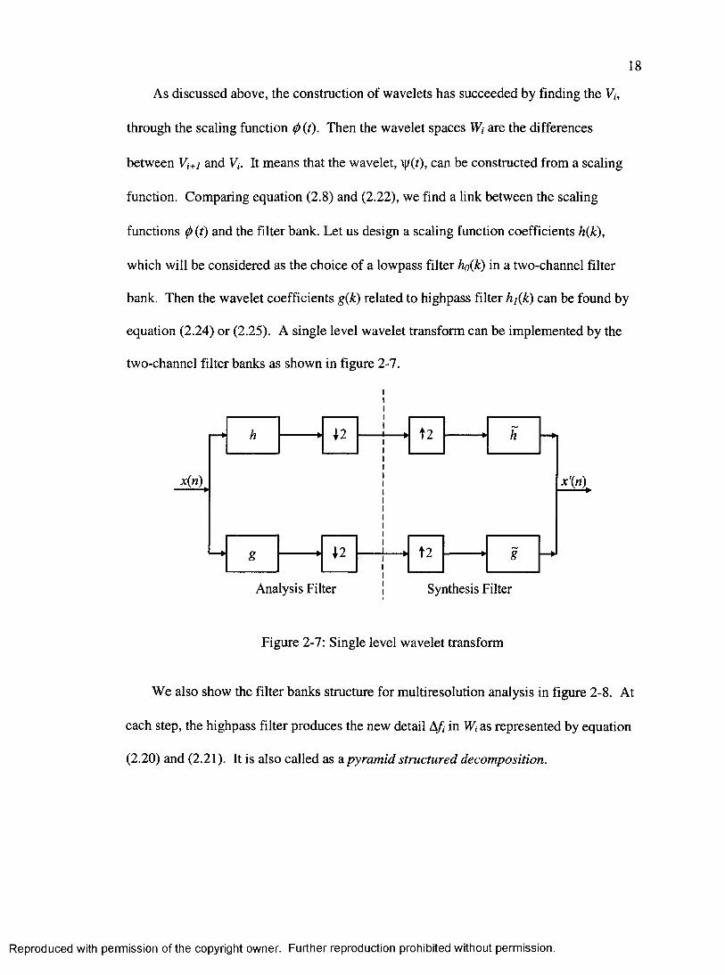
As discussed above, the construction of wavelets has succeeded by finding the Vi,

through the scaling function ^(t). Then the wavelet spaces Wi are the differences

between Vi+j and V,. It means that the wavelet, can be constructed from a scaling

function. Comparing equation (2.8) and (2.22), we find a link between the scaling

functions <j) (t) and the filter bank. Let us design a scaling function coefficients h{k),

which will be considered as the choice of a lowpass filter ho{k) in a two-channel filter

bank. Then the wavelet coefficients g{k) related to highpass filter hi{k) can be found by

equation (2.24) or (2.25). A single level wavelet transform can be implemented by the

two-channel filter banks as shown in figure 2-7.

x{n) x'{n\

Analysis Filter Synthesis Filter

Figure 2-7: Single level wavelet transform

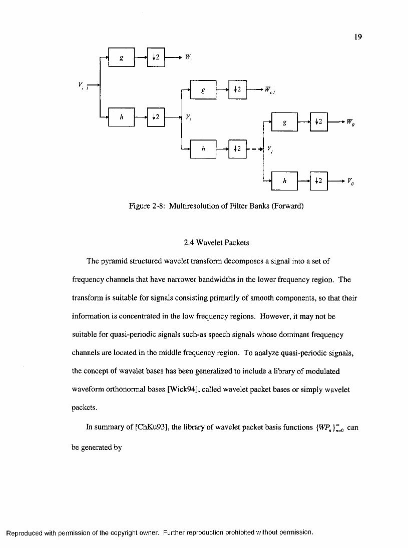
We also show the filter banks structure for multiresolution analysis in figure 2-8. At

each step, the highpass filter produces the new detail A/i in W, as represented by equation

(2.20) and (2.21). It is also called as a pyramid structured decomposition.


19

'j'2 - — <*

Figure 2-8: Multiresolution of Filter Banks (Forward)

2.4 Wavelet Packets

The pyramid structured wavelet transform decomposes a signal into a set of

frequency channels that have narrower bandwidths in the lower frequency region. The

transform is suitable for signals consisting primarily of smooth components, so that their

information is concentrated in the low frequency regions. However, it may not be

suitable for quasi-periodic signals such-as speech signals whose dominant frequency

channels are located in the middle frequency region. To analyze quasi-periodic signals,

the concept of wavelet bases has been generalized to include a library of modulated

waveform orthonormal bases [Wick94], called wavelet packet bases or simply wavelet

packets.

In summary of [ChKu93], the library of wavelet packet basis functions {WP„ }~ o can

be generated by


20

(0 = V2 g )1WP (2f - 1) (2.27)k

t*7!b+i(f) = g(&)t14P:(:k--;k) (2J!8)k

where the function WPo(t) can be identified with the scaling function <]) and WPi(t) with

the mother board wavelet y/. Then, the library of wavelet packet bases can be defined to

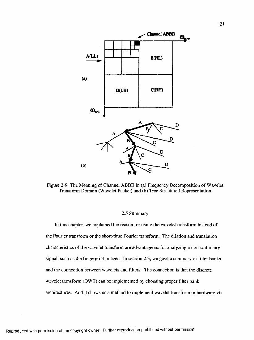
be the collection of orthonormal bases, composed of functions of the form WPn(2^t-k),

where l , k e Z ,n e N . Each element of the library is determined by a subset of the

indices: a scaling parameter I, a localization parameter k, and an oscillation parameter n.

The tree-structured wavelet transform as shown in Figure 2-9, provides an algorithmic

approach to represent a function in terms of a certain wavelet packet basic.

The 2-D wavelet (or wavelet packet) basis functions can be expressed by the tensor

product of 1-D wavelet (or wavelet packet) basis functions along the horizontal and

vertical directions. The corresponding 2-D filter coefficients can be expressed as

Au_(t,Z) = A (t)W ),

hui (k,l) = h (k)g(l) ,

hnL{k,l) = g{k)h{l),

huH(k,l) = g(k)g(l) (2.29)

where the first and second subscripts denote the lowpass and highpass filter

characteristics in x and y directions, respectively.


21

Channel ABBB

A(LL)

(a)

'col

D(LH)

B(HL)

C(HH)

(b)

Figure 2-9: The Meaning of Channel ABBB in (a) Frequency Decomposition of Wavelet Transform Domain (Wavelet Packet) and (b) Tree Structured Representation

2.5 Summary

In this chapter, we explained the reason for using the wavelet transform instead of

the Fourier transform or the short-time Fourier transform. The dilation and translation

characteristics of the wavelet transform are advantageous for analyzing a non-stationary

signal, such as the fingerprint images. In section 2.3, we gave a summary of filter banks

and the connection between wavelets and filters. The connection is that the discrete

wavelet transform (DWT) can be implemented by choosing proper filter bank

architectures. And it shows us a method to implement wavelet transform in hardware via


22

the mature filter bank technique. A summary of a wavelet packet was given in section

2.4. The wavelet packet transform provides a different decomposition structure with a

traditional pyramid algorithm. Since it is adopted by FBI in fingerprint image processing,

which will be introduced in chapter 4, we will propose a VLSI architecture for it in

chapter 6.


CHAPTER 3

WAVELET TRANSFORM WITH LIFTING SCHEME

Wavelets based on dilations and translations of a mother wavelet are referred to as

first generation wavelets or classical wavelets. The Lifting Scheme (LS) provides a much

more flexible method for constructing wavelets. These wavelets are named as second

generation wavelets. Unlike the classical wavelet, wavelets based on LS are not

necessarily translations and dilations of one function. Therefore, they can be used

conveniently to define wavelet bases for bound intervals, irregular sample grids or even

for solving equations or analyzing data on curves or surfaces. In addition, those existing

classical wavelets can be implemented with LS by factoring them into Lifting steps

[DaSw98].

3.1 A General Lifting Scheme

The basic idea behind the lifting scheme is very simple that the redundancy will be

removed by using the correlation in the data. To reach this goal, the data are first split

into two subsets, odd subset with the odd-indexed samples and even subset with the even-

indexed samples. It is called split stage. And then, we predict the odd subset from the

even subset. It is called the predict stage. At last, the prediction error, which is the

difference between odd-indexed sample and its prediction, is used to update the even-

23


24

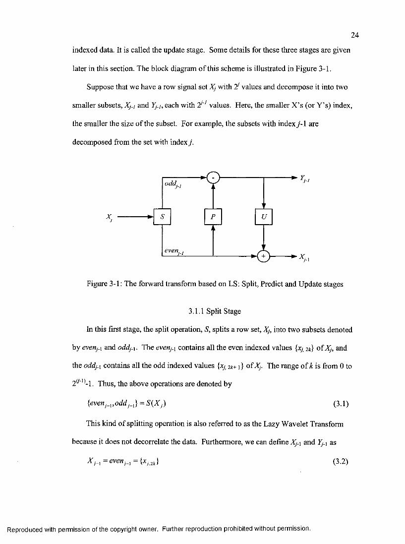
indexed data. It is called the update stage. Some details for these three stages are given

later in this section. The block diagram of this scheme is illustrated in Figure 3-1.

Suppose that we have a row signal set Xj with 7! values and decompose it into two

smaller subsets, Xj-i and Yj,i, each with T!'' values. Here, the smaller X’s (or Y’s) index,

the smaller the size of the subset. For example, the subsets with index j - \ are

decomposed from the set with index j.

%

► T.odd,

even

Figure 3-1 : The forward transform based on LS: Split, Predict and Update stages

3.1.1 Split Stage

In this first stage, the split operation, S, splits a row set, Xj, into two subsets denoted

by evenj-x and oddj.\. The evenj.x contains all the even indexed values {x 2k} ofXj, and

the oddj.x contains all the odd indexed values {xy, 2k+1} of Xj. The range of k is from 0 to

2(/'-')-i the above operations are denoted by

{evenJ_ , oddj_ } = 5'(%y) (3.1)

This kind of splitting operation is also referred to as the Lazy Wavelet Transform

because it does not decorrelate the data. Furthermore, we can define Xj.\ and Yj.\ as

(3.2)


25

Y = odd — {x (3.3)

3.1.2 Predict Stage

Because each value in odd subset is adjacent to the corresponding value in the even

subset, the values in two subsets are correlated and either can be used to predict the other.

Here, in the second stage — the predict stage, the even subset everij.\ is used to predict the

odd subset oddj.\ by a prediction function P, which is independent of the data. The

prediction is denoted by

f (evgMy_,) = f (%y_,) . (3.4)

Then it seems that evenj.\ can be used to replace the original data set, since we can predict

the missing part to reassemble Xj.

But in practice, it is impossible to predict oddj,\ from evenj.x exactly. Since YPj.x is

very close to oddj.x (or Yj.x), we can replace Yj.x with the difference between itself and its

predicted value YPj.x and denote it by

-? (% ,_ ,). (3.5)

If the prediction is reasonable, Yj.x, the difference from equation 3.5, will contain much

less information than the original oddj.x (or l^.i).

We can now iterate the split stage and the predict stage so that Xj.x is split into two

subsets Xj.2 and Yj.2 and then replace Yj.2 with the difference between Yj.2 and P{Xj.2). By

iterating the scheme m times, we can replace the original data set Xj with the wavelet

representation {Xj.„, Yj.^, ... , Yj.i). Given that the wavelet sets encode the difference

with some predicted values based on a correlation model, this gives a more compact

representation.


26

3.1.3 Update Stage

However, the split and predict stages are not sufficient in some case. The reason is

that we want some global properties of the original data set to be maintained in the

smaller set Xj.m- For example, in an image, we would like the smaller images Xj.m to have

the same overall brightness, i.e. the same average pixel value, as Xj. If the splitting stage

is simply subsampling and we iterate the scheme till Xj.^ is only 1 pixel, that pixel will be

an arbitrary pixel from the original image. We would rather have the last value to be the

average of all the pixel values in the original image instead of that arbitrary pixel value.

To achieve this purpose, the third stage - update stage, is introduced in lifting

scheme. The idea is to find a better _i, so that a certain scalar quantity Q, e.g. the mean,

is preserved, or

G (^y_,)=6(^y). (3.6)

Then, a new operator U is constructed to ensure the preservation of the quality.

Therefore, we use the already computed wavelet set Yj.j to update Xj.i. In other words,

we construct an operator U and update Xj.\ as

+U(y,_,). (3.7)

In summary, the lifting scheme consisting of three stages leads to the following

forward wavelet transform algorithm:

for j - n downto 1

:=yy_,-f(% y_,);:=%y_,+U(y,_,);

end for.


27

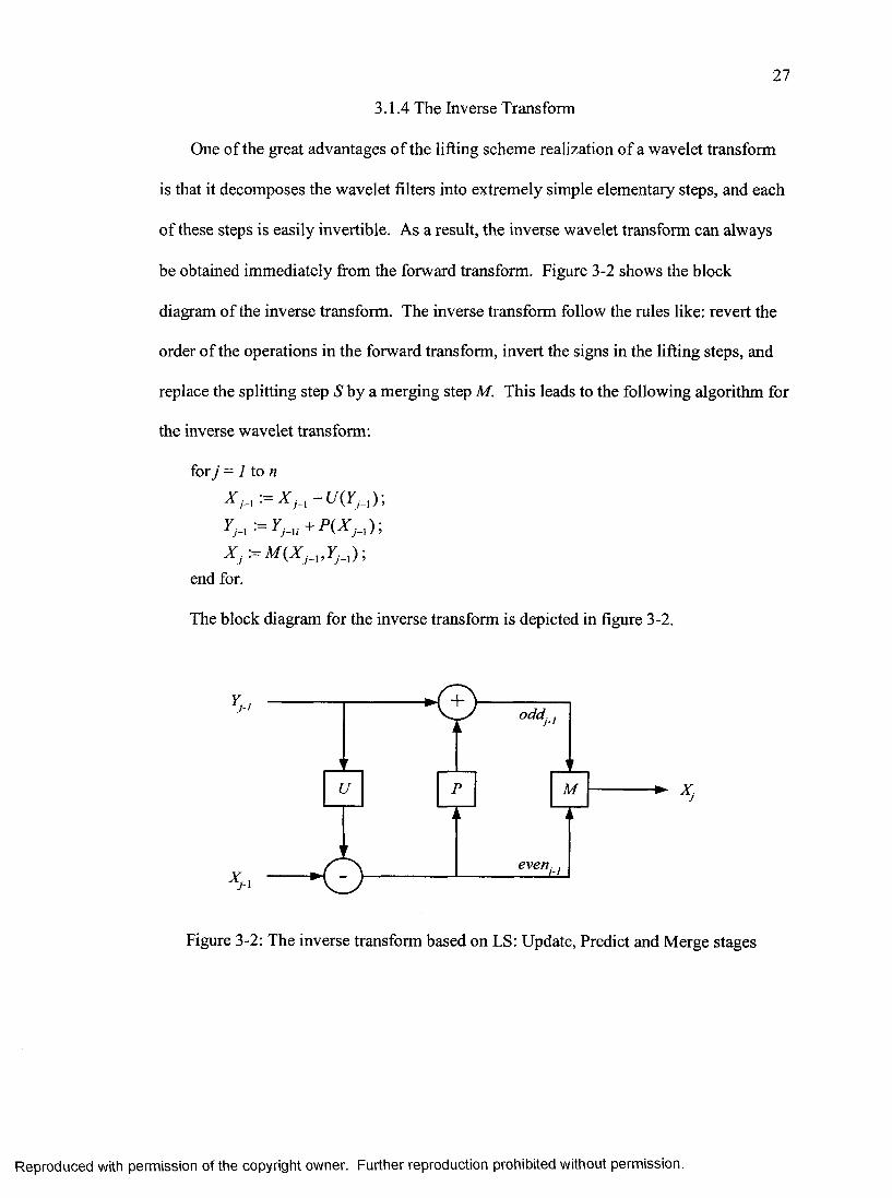
3.1.4 The Inverse Transform

One of the great advantages of the lifting scheme realization of a wavelet transform

is that it decomposes the wavelet filters into extremely simple elementary steps, and each

of these steps is easily invertible. As a result, the inverse wavelet transform can always

be obtained immediately from the forward transform. Figure 3-2 shows the block

diagram of the inverse transform. The inverse transform follow the rules like: revert the

order of the operations in the forward transform, invert the signs in the lifting steps, and

replace the splitting step S by a merging step M. This leads to the following algorithm for

the inverse wavelet transform:

for y = 7 to M

y,-i := y ,-i;+ p{^ j- \ ) j

end for.

The block diagram for the inverse transform is depicted in figure 3-2.

odd,

even

M

Figure 3-2: The inverse transform based on LS: Update, Predict and Merge stages


28

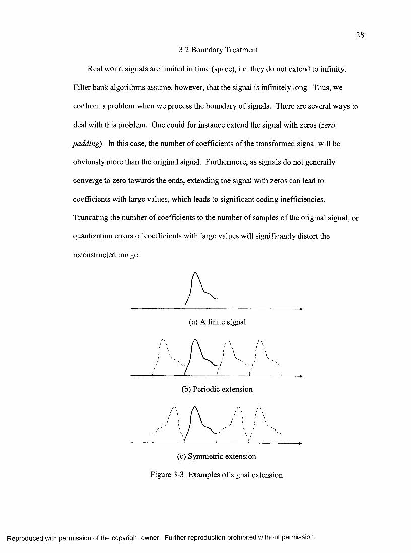
3.2 Boundary Treatment

Real world signals are limited in time (space), i.e. they do not extend to infinity.

Filter bank algorithms assume, however, that the signal is infinitely long. Thus, we

confront a problem when we process the boundary of signals. There are several ways to

deal with this problem. One could for instance extend the signal with zeros {zero

padding). In this case, the number of coefficients of the transformed signal will be

obviously more than the original signal. Furthermore, as signals do not generally

converge to zero towards the ends, extending the signal with zeros can lead to

coefficients with large values, which leads to significant coding inefficiencies.

Truncating the number of coefficients to the number of samples of the original signal, or

quantization errors of coefficients with large values will significantly distort the

reconstructed image.

(a) A finite signal

(b) Periodic extension

/ \* t ! t S \

\ I \ /

(c) Symmetric extension

Figure 3-3: Examples of signal extension


29

Another option is to make the signal periodic, i.e. to repeat the signal at its ends

(Figure 3-5-b). As the values at the left and right ends of the signal are not necessarily

the same, discontinuity will appear at signal ends and as a result, a similar problem can

arise as mentioned with zero padding.

For symmetric wavelets, an effective strategy for handling boundaries is to extend

the image via reflection. Such an extension preserves continuity at the boundaries and

usually leads to much smaller wavelet coefficients than if discontinuities were present at

the boundaries (Figure 3-5-c).

3.3 Advantages of Lifting Scheme

Summarized, the lifting scheme has the following immediate advantages, when

compared to the classical filter bank algorithm:

• Lifting leads to a speedup when compared to the classic implementation.

Classical wavelet transform has a complexity of order n, where n is the number

of samples. For long filters. Lifting Scheme speeds up the transform with a

factor of two [Swel95]. Hence it is also referred to as fast lifting wavelet

transform (FLWT).

• All operations within lifting scheme can be done entirely in parallel while the

only sequential part is the order of lifting operations.

• Lifting scheme allows a fully in-place calculation of the wavelet transform. An

auxiliary memory is not needed since it does not need other samples than the

output of the previous lifting step. The value in original signal can be replaced

with its transform.


30

• The inverse wavelet transform based on LS can always be obtained

immediately from the forward transform. The only thing to do is to reverse the

operations and toggle + and - .

3.4 Summary

In this chapter, the Lifting Scheme implementation of the Wavelet Transform is

described briefly. We saw that the Lifting scheme uses three simple steps to calculate the

wavelet coefficients, namely the Split, Predict and Update phase. We discussed these

three steps and explained how the inverse transform can easily be calculated in a similar

way. Furthermore, we discussed how boundary issues, rising in finite length signals, can

be treated by using adaptive filters in the Lifting scheme. A summary of the nice

properties of the Lifting Scheme was given in section 3.3. Conclusively, when we

implement wavelet transform in hardware, the LS provides a simpler and more efficient

method than the traditional filter bank. In the following chapters, we will use the LS to

fulfill the wavelet transform for the fingerprint image processing which once was

processed by filter banks.


CHAPTER 4

FINGERPRINT AND ITS FBI COMPRESSION SPECIFICATION

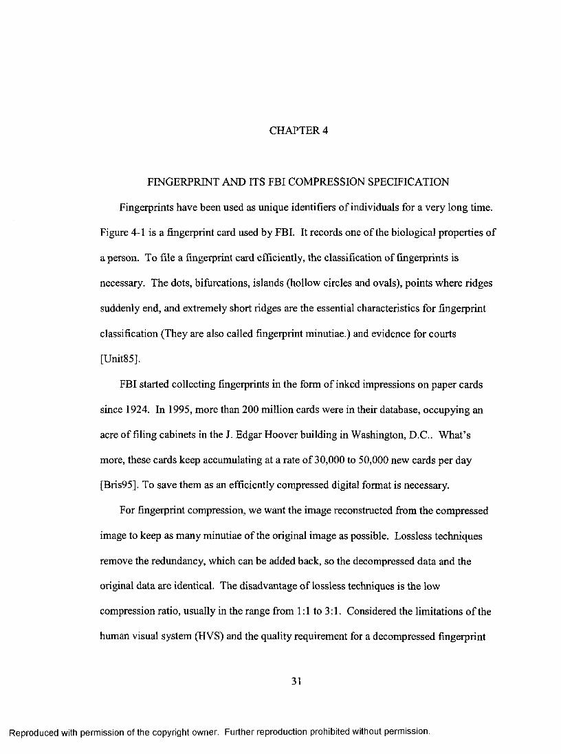
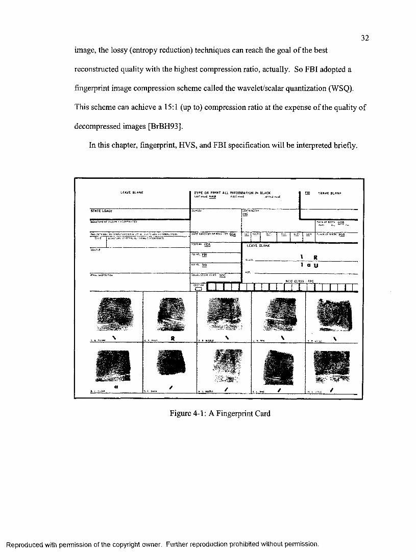
Fingerprints have been used as unique identifiers of individuals for a very long time.

Figure 4-1 is a fingerprint card used by FBI. It records one of the biological properties of

a person. To file a fingerprint card efficiently, the classification of fingerprints is

necessary. The dots, bifurcations, islands (hollow circles and ovals), points where ridges

suddenly end, and extremely short ridges are the essential characteristics for fingerprint

classification (They are also called fingerprint minutiae.) and evidence for courts

[Unit85].

FBI started collecting fingerprints in the form of inked impressions on paper cards

since 1924. In 1995, more than 200 million cards were in their database, occupying an

acre of filing cabinets in the J. Edgar Hoover building in Washington, D.C.. What’s

more, these cards keep accumulating at a rate of 30,000 to 50,000 new cards per day

[Bris95]. To save them as an efficiently compressed digital format is necessary.

For fingerprint compression, we want the image reconstructed from the compressed

image to keep as many minutiae of the original image as possible. Lossless techniques

remove the redundancy, which can be added back, so the decompressed data and the

original data are identical. The disadvantage of lossless techniques is the low

compression ratio, usually in the range from 1:1 to 3:1. Considered the limitations o f the

human visual system (HVS) and the quality requirement for a decompressed fingerprint

31


32image, the lossy (entropy reduction) techniques can reach the goal of the best

reconstructed quality with the highest compression ratio, actually. So FBI adopted a

fingerprint image compression scheme called the wavelet/scalar quantization (WSQ).

This scheme can achieve a 15:1 (up to) compression ratio at the expense of the quality of

decompressed images [BrBH93].

In this chapter, fingerprint, HVS, and FBI specification will be interpreted briefly.

lE A Y E B U N K

MM PfcTi «*r M fati

TYPE OR P R IN T A L L iN FO R M A TtO N IN BLACKUJT»*(we NAM W&ÜLiNÂrft

Sücui. i s c m ry ho. ^.QC

d

ES! lE A K E BLANK

K.ÎE # SAT, ooB

i:on-poa

LEAVE BLANK

1I a u

NCIC CLASS • FPC

». * «ct« R a. ». wioptr ^# no /

# C- MMMX* / , . _ /

Figure 4-1 : A Fingerprint Card


334.1 Types of Fingerprints and Their Interpretation

A fingerprint is the mark that the ridges of skin on fingers and thumbs leave on

objects touched. Our fingerprints are perfectly formed seven months before we are bom.

The fingerprint is unique. In this world of approximately 6.3 billion humans, each with

ten fingerprints, there is not one fingerprint exactly like another. Even twins who look

exactly alike have different fingerprints.

Fingerprints may be resolved into the following three large general groups of types:

loop, arch and whorl [Unit85]. Each group bears the same general characteristics or

family resemblance. The types may be further divided into subgroups by means of the

smaller differences existing between the types in the same general group. Table 4-1 lists

the groups and subgroups. Statistical data show that loops occur in about 65 percent of

all fingerprints, whorls in about 30 percent, and arches in the remaining 5 percent

[Coll85].

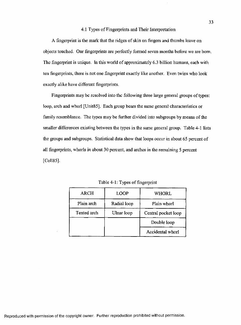
Table 4-1 : Types of fingerprint

ARCH LOOP WHORL

Plain arch Radial loop Plain whorl

Tented arch Ulnar loop Central pocket loop

Double loop

Accidental whorl


34

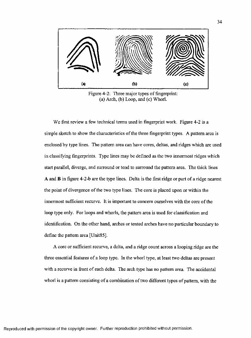
Figure 4-2; Three major types of fingerprint: (a) Arch, (b) Loop, and (c) Whorl.

We first review a few technical terms used in fingerprint work. Figure 4-2 is a

simple sketch to show the characteristics of the three fingerprint types. A pattern area is

enclosed by type lines. The pattern area can have cores, deltas, and ridges which are used

in classifying fingerprints. Type lines may be defined as the two innermost ridges which

start parallel, diverge, and surround or tend to surround the pattern area. The thick lines

A and B in figure 4-2-b are the type lines. Delta is the first ridge or part of a ridge nearest

the point of divergence of the two type lines. The core is placed upon or within the

innermost sufficient recurve. It is important to concern ourselves with the core of the

loop type only. For loops and whorls, the pattern area is used for classification and

identification. On the other hand, arches or tented arches have no particular boundary to

define the pattern area [Unit85].

A core or sufficient recurve, a delta, and a ridge count across a looping ridge are the

three essential features of a loop type. In the whorl type, at least two deltas are present

with a recurve in front of each delta. The arch type has no pattern area. The accidental

whorl is a pattern consisting of a combination of two different types of pattern, with the


35exception of the plain arch, which has two or more deltas, or a pattern which possesses

some of the requirements for two or more different types, or a pattern which conforms to

none of the above definitions [Unit85].

4.2 A Model of the Human Visual System

The physical properties of the optical transmission pathway through the iris to the

retina produce a lowpass spectral response which, when combined with the highpass

characteristic due to interconnection of the receptors gives an overall band-pass response.

Associated with this spatial response is a logarithmic amplitude non-linearity due to

adaptation to background luminance necessary for the eye to function over a wide range

of average scene intensities. The fact that the eye has preferred regions of spatial

frequency response and a non-linear amplitude response mechanism can be utilized to

develop better coding algorithms [Clar96].

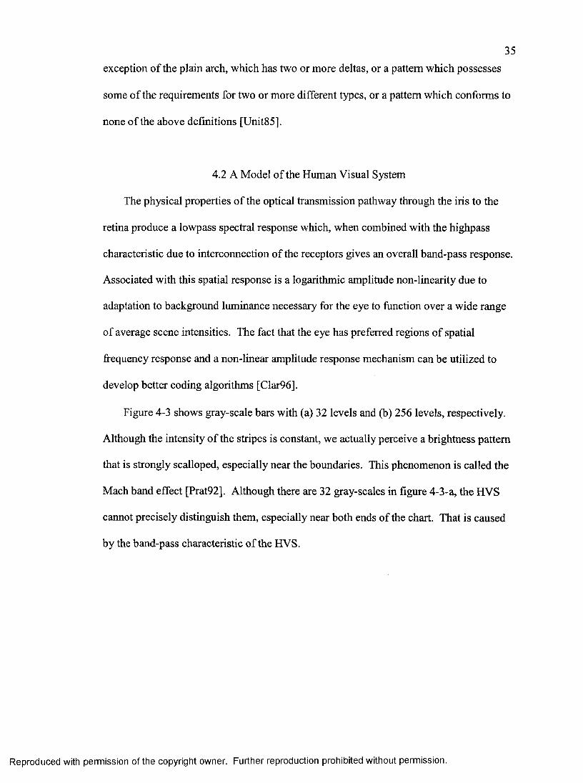
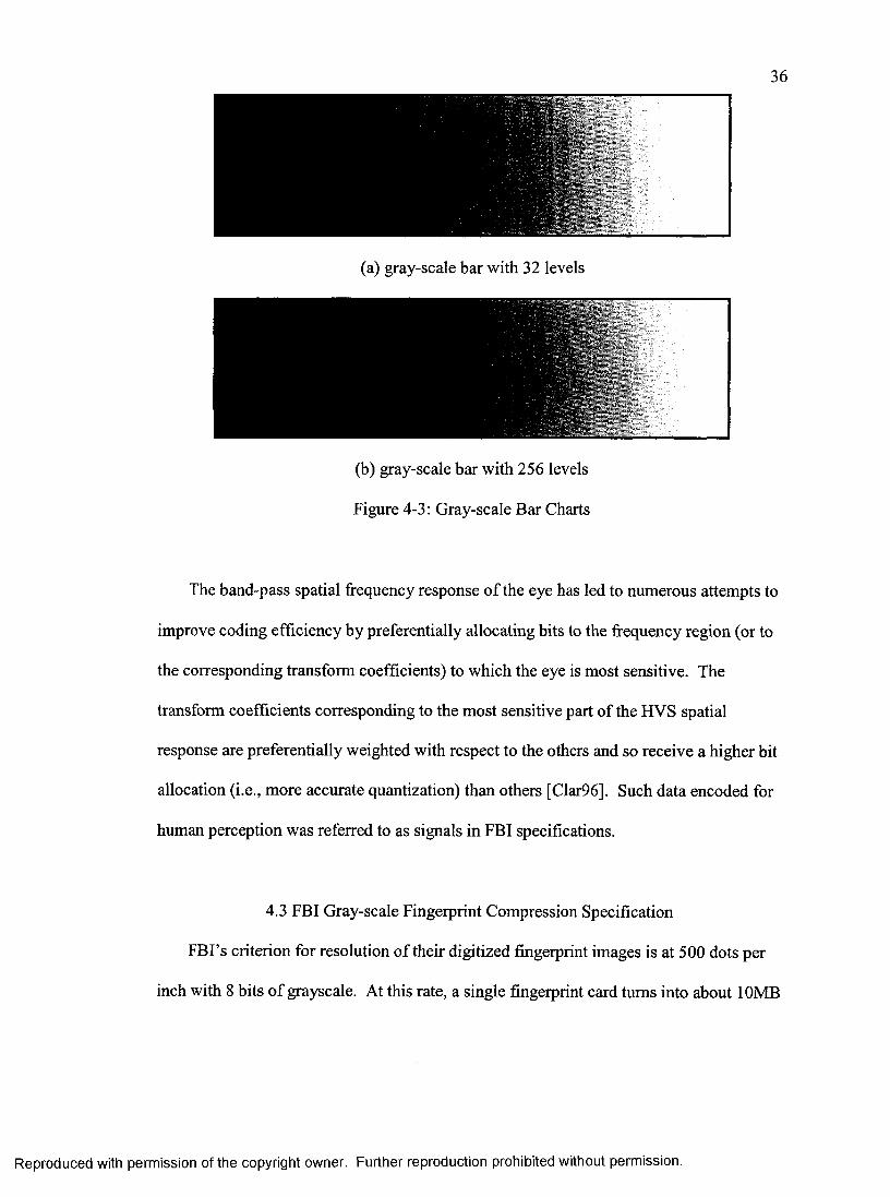
Figure 4-3 shows gray-scale bars with (a) 32 levels and (b) 256 levels, respectively.

Although the intensity o f the stripes is constant, we actually perceive a brightness pattern

that is strongly scalloped, especially near the boundaries. This phenomenon is called the

Mach band effect [Prat92]. Although there are 32 gray-scales in figure 4-3-a, the HVS

cannot precisely distinguish them, especially near both ends of the chart. That is caused

by the band-pass characteristic of the HVS.


36

(a) gray-scale bar with 32 levels

(b) gray-scale bar with 256 levels

Figure 4-3: Gray-scale Bar Charts

The band-pass spatial frequency response of the eye has led to numerous attempts to

improve coding efficiency by preferentially allocating bits to the frequency region (or to

the corresponding transform coefficients) to which the eye is most sensitive. The

transform coefficients corresponding to the most sensitive part of the HVS spatial

response are preferentially weighted with respect to the others and so receive a higher bit

allocation (i.e., more accurate quantization) than others [Clar96]. Such data encoded for

human perception was referred to as signals in FBI specifications.

4.3 FBI Gray-scale Fingerprint Compression Specification

FBI’s criterion for resolution of their digitized fingerprint images is at 500 dots per

inch with 8 bits of grayscale. At this rate, a single fingerprint card turns into about 10MB


37of data. Thus, the total size of the digitized collection would be more than 2000 terabytes

(a terabyte is 2^ bytes).

Compression is, therefore, a must. After carefully research. The FBI’s Criminal

Justice Information Services Division and researchers at Los Alamos National Laboratory

and the National Institute of Standards and Technology have developed the national

standards for digitization [ANSt93] and lossy image compression [HBBr93]. The

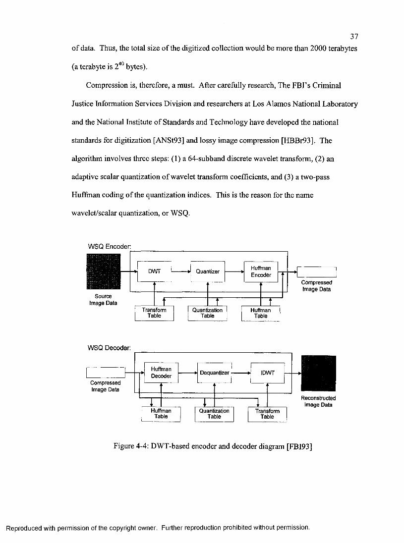
algorithm involves three steps; (1) a 64-subband discrete wavelet transform, (2) an

adaptive scalar quantization of wavelet transform coefficients, and (3) a two-pass

Huffman coding of the quantization indices. This is the reason for the name

wavelet/scalar quantization, or WSQ.

WSQ Encoder:

HuffmanEncoder

Quantizer

Source Image Data

Transform Quantization HuffmanTable Table Table

Compressed Image Data

WSQ Decoder;

HuffmanDecoder Dequantizer IDWr

Compressed Image Data

Huffman Quantization TransformTable Table Table

Reconstructed Image Data

Figure 4-4: DWT-based encoder and decoder diagram [FBI93]


38Figure 4-4 shows the main procedures for WSQ encoding and decoding. The same

tables specified for an encoder to use to compress a particular image must be provided to

a decoder to reconstruct that image.

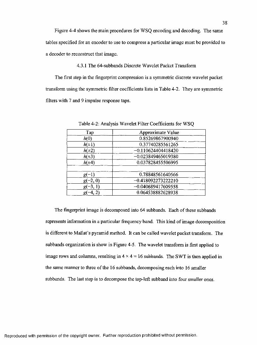
4.3.1 The 64-subbands Discrete Wavelet Packet Transform

The first step in the fingerprint compression is a symmetric discrete wavelet packet

transform using the symmetric filter coefficients lists in Table 4-2. They are symmetric

filters with 7 and 9 impulse response taps.

Table 4-2; Analysis Wavelet Filter Coefficients for WSQ

Tap Approximate ValueA(0) 0.85269867900940h{±\) 0.37740285561265A(±2) -0.110624404418420h(±3) -0.023849465019380h(±4) 0.037828455506995

g (- l) 0.78848561640566g(-2 ,0) -0.418092273222210g ( -3 ,1) -0.040689417609558g(-4 ,2) 0.064538882628938

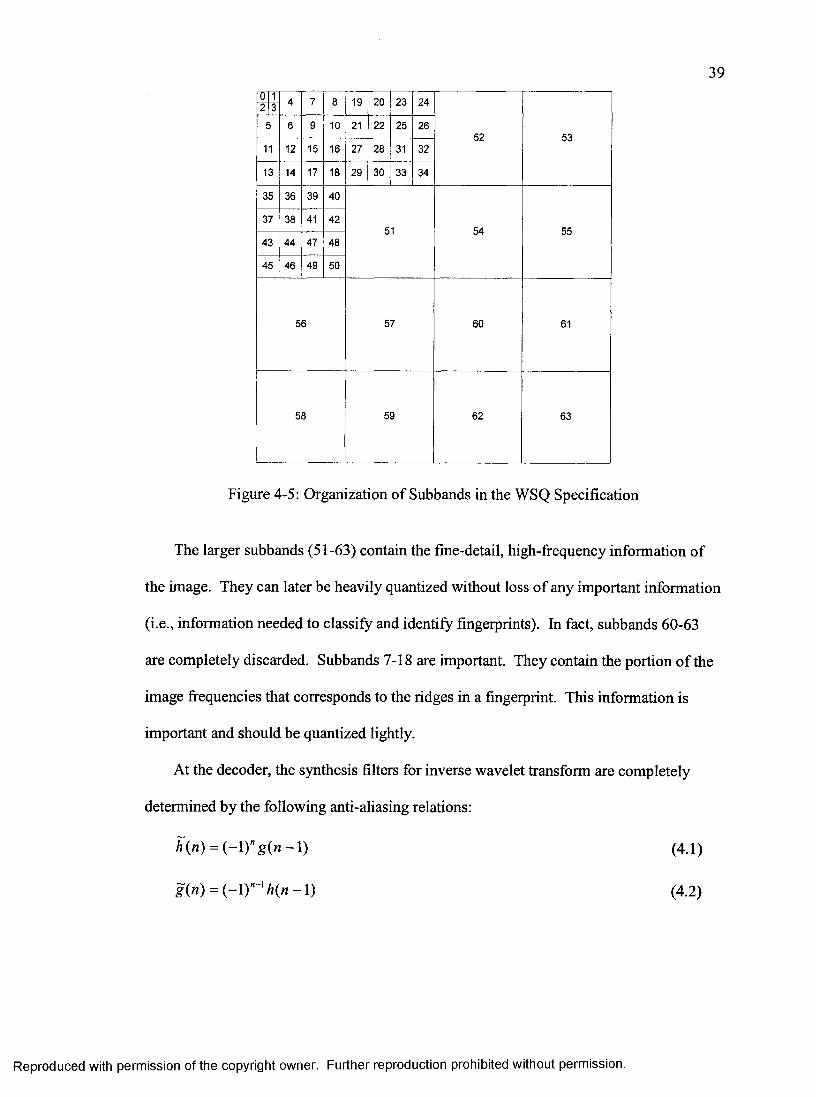
The fingerprint image is decomposed into 64 subbands. Each of these subbands

represents information in a particular fi-equency band. This kind of image decomposition

is different to Mallat’s pyramid method. It can be called wavelet packet transform. The

subbands organization is show in Figure 4-5. The wavelet transform is first applied to

image rows and columns, resulting in 4 x 4 = 16 subbands. The SWT is then applied in

the same manner to three of the 16 subbands, decomposing each into 16 smaller

subbands. The last step is to decompose the top-left subband into four smaller ones.


390 1 4 7 8 19 20 23 24

52 53

2 3

5 6 9 10 21 22 25 26

11 12 15 16 27 28 31 32

13 14 17 18 29 30 33 34

35 36 39 40

51 54 5537 38 41 42

43 44 47 48

45 46 49 50

56 57 60 61

58 59 62 63

Figure 4-5: Organization of Subbands in the WSQ Specification

The larger subbands (51-63) contain the fme-detail, high-frequency information of

the image. They can later be heavily quantized without loss of any important information

(i.e., information needed to classify and identify fingerprints). In fact, subbands 60-63

are completely discarded. Subbands 7-18 are important. They contain the portion of the

image frequencies that corresponds to the ridges in a fingerprint. This information is

important and should be quantized lightly.

At the decoder, the synthesis filters for inverse wavelet transform are completely

determined by the following anti-aliasing relations:

h(n) = { - i y g { n - \ ) (4.1)

g(») = (-l)"-'A (M -l) (4.2)


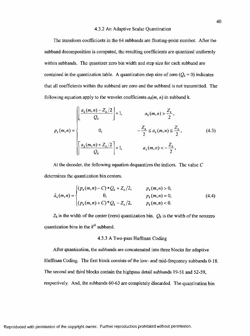
404.3.2 An Adaptive Scalar Quantization

The transform coefficients in the 64 subbands are floating-point number. After the

subband decomposition is computed, the resulting coefficients are quantized uniformly

within subbands. The quantizer zero bin width and step size for each subband are

contained in the quantization table. A quantization step size of zero (Qk - 0) indicates

that all coefficients within the subband are zero and the subband is not transmitted. The

following equation apply to the wavelet coefficients aiSm, n) in subband k.

a ^ ( m ,n ) - Z j 2

a+1,

0,

a^{m,n) + Z j 2

a+1,

04 3)

At the decoder, the following equation dequantizes the indices. The value C

determines the quantization bin centers.

\p ^ { m ,n ) - C ) * Q ^ + Z j2 ,

0,{p^{m,n) + C ) * Q ^ - Z j 2 ,

p^(m,n)>0, p ^(m ,n )^0 , p^(m,n) < 0.

(4.4)

Zk is the width of the center (zero) quantization bin. is the width of the nonzero

quantization bins in the subband.

4.3.3 A Two-pass Huffman Coding

After quantization, the subbands are concatenated into three blocks for adaptive

Huffman Coding. The first block consists of the low- and mid-frequency subbands 0-18.

The second and third blocks contain the highpass detail subbands 19-51 and 52-59,

respectively. And, the subbands 60-63 are completely discarded. The quantization bin


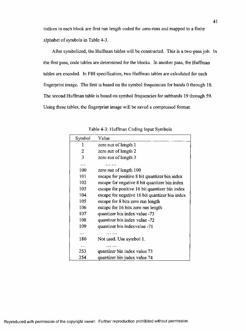
41indices in each block are first run length coded for zero-runs and mapped to a finite

alphabet of symbols in Table 4-3.

After symbolized, the Huffman tables will be constmcted. This is a two-pass job. In

the first pass, code tables are determined for the blocks. In another pass, the Huffman

tables are encoded. In FBI specification, two Huffman tables are calculated for each

fingerprint image. The first is based on the symbol frequencies for bands 0 through 18.

The second Huffman table is based on symbol frequencies for subbands 19 through 59.

Using these tables, the fingerprint image will be saved a compressed format.

Table 4-3: Huffman Coding Input Symbols

Symbol Value1 zero run of length 12 zero run of length 23 zero run of length 3

100 zero run of length 100101 escape for positive 8 bit quantizer bin index102 escape for negative 8 bit quantizer bin index103 escape for positive 16 bit quantizer bin index104 escape for negative 16 bit quantizer bin index105 escape for 8 bits zero run length106 escape for 16 bits zero run length107 quantizer bin index value -73108 quantizer bin index value -72109 quantizer bin indexvalue -71

180 Not used. Use symbol 1.

253 quantizer bin index value 73254 quantizer bin index value 74


424.4 Summary

This chapter presented the WSQ gray-scale fingerprint image compression

specification adopted by FBI. It is a lossy compression specification. FBI wants to

impose more strict criteria on compressing a fingerprint image than other normal images

because the decompressed fingerprint images may be used in court as evidence.

However, it does not mean that a lossless eompression is required. FBI still chooses this

lossy compression technique for two reasons: First, to achieve a higher compression

ratio; Second, to keep the acceptable quality by considering the limitations of the human

visual system (HVS). In the next chapter, we focus on the wavelet transforms as the

basis for fingerprint compression. The filter-banks-based transform scheme is compared

with a fast lifting wavelet transform, as a basis for the hardware design.


CHAPTER 5

SOFTWARE IMPLEMENTATION

As discussed in Chapter 3, the lifting scheme provides a new approach to generate

wavelets for transform. The integer-to-integer transform, one of the advanced features of

lifting scheme, could make the transform more efficient and inverse transform easier. In

this chapter, we will further discuss the feasibility of VLSI architecture for WPT using

lifting scheme to transform data integer to integer. We will show that although integer-

to-integer lifting scheme based transform causes some more loss of minutiae o f the

fingerprint images than standard convolution filter banks transform does, the

reconstructed image quality is still acceptable. PSNR values are only slightly lower. The

changes are undetectable by HVS. And, most important, it will not influence matching of

the fingerprints.

A software package written in Matlab is developed to simulate three different

transform algorithms.

The first one applies the current FBI standard. In this case, WPT is implemented by

a 9-tap lowpass filter and a 7-tap highpass filter, which are convolved with the image

rows and columns. We call it Bior9-7 in this thesis. A fingerprint image is convolved

with this filter pair. The odd samples of the filtered outputs are discarded resulting in

43


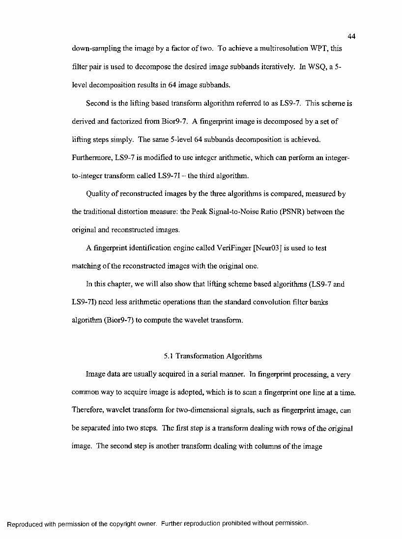
44down-sampling the image by a factor of two. To achieve a multiresolution WPT, this

filter pair is used to decompose the desired image subbands iteratively. In WSQ, a 5-

level decomposition results in 64 image subbands.

Second is the lifting based transform algorithm referred to as LS9-7. This scheme is

derived and factorized from Bior9-7. A fingerprint image is decomposed by a set of

lifting steps simply. The same 5-level 64 subbands decomposition is achieved.

Furthermore, LS9-7 is modified to use integer arithmetic, which can perform an integer-

to-integer transform called LS9-7I - the third algorithm.

Quality of reconstructed images by the three algorithms is compared, measured by

the traditional distortion measure: the Peak Signal-to-Noise Ratio (PSNR) between the

original and reconstructed images.

A fingerprint identification engine called VeriFinger [Neur03] is used to test

matching of the reconstructed images with the original one.

In this chapter, we will also show that lifting scheme based algorithms (LS9-7 and

LS9-7I) need less arithmetic operations than the standard convolution filter banks

algorithm (Bior9-7) to compute the wavelet transform.

5.1 Transformation Algorithms

Image data are usually acquired in a serial manner. In fingerprint processing, a very

common way to acquire image is adopted, which is to scan a fingerprint one line at a time.

Therefore, wavelet transform for two-dimensional signals, such as fingerprint image, can

be separated into two steps. The first step is a transform dealing with rows of the original

image. The second step is another transform dealing with colunms of the image


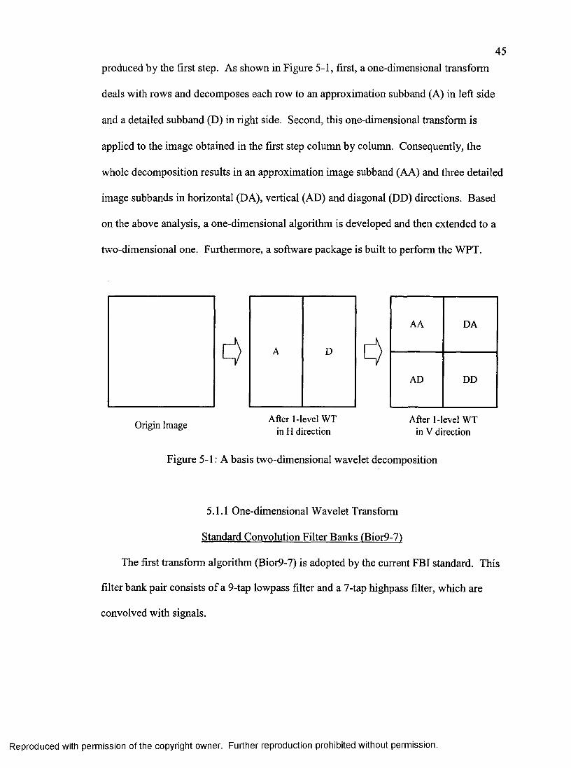
45produced by the first step. As shown in Figure 5-1, first, a one-dimensional transform

deals with rows and decomposes each row to an approximation suhhand (A) in left side

and a detailed suhhand (D) in right side. Second, this one-dimensional transform is

applied to the image obtained in the first step column by column. Consequently, the

whole decomposition results in an approximation image suhhand (AA) and three detailed

image suhhands in horizontal (DA), vertical (AD) and diagonal (DD) directions. Based

on the above analysis, a one-dimensional algorithm is developed and then extended to a

two-dimensional one. Furthermore, a software package is built to perform the WPT.

After 1 -level WT in H direction

AA DA

AD DD

Origin Image

Figure 5-1: A basis two-dimensional wavelet decomposition

After 1-level WT in V direction

5.1.1 One-dimensional Wavelet Transform

Standard Convolution Filter Banks (Bior9-71

The first transform algorithm (Bior9-7) is adopted by the current FBI standard. This

filter bank pair consists of a 9-tap lowpass filter and a 7-tap highpass filter, which are

convolved with signals.


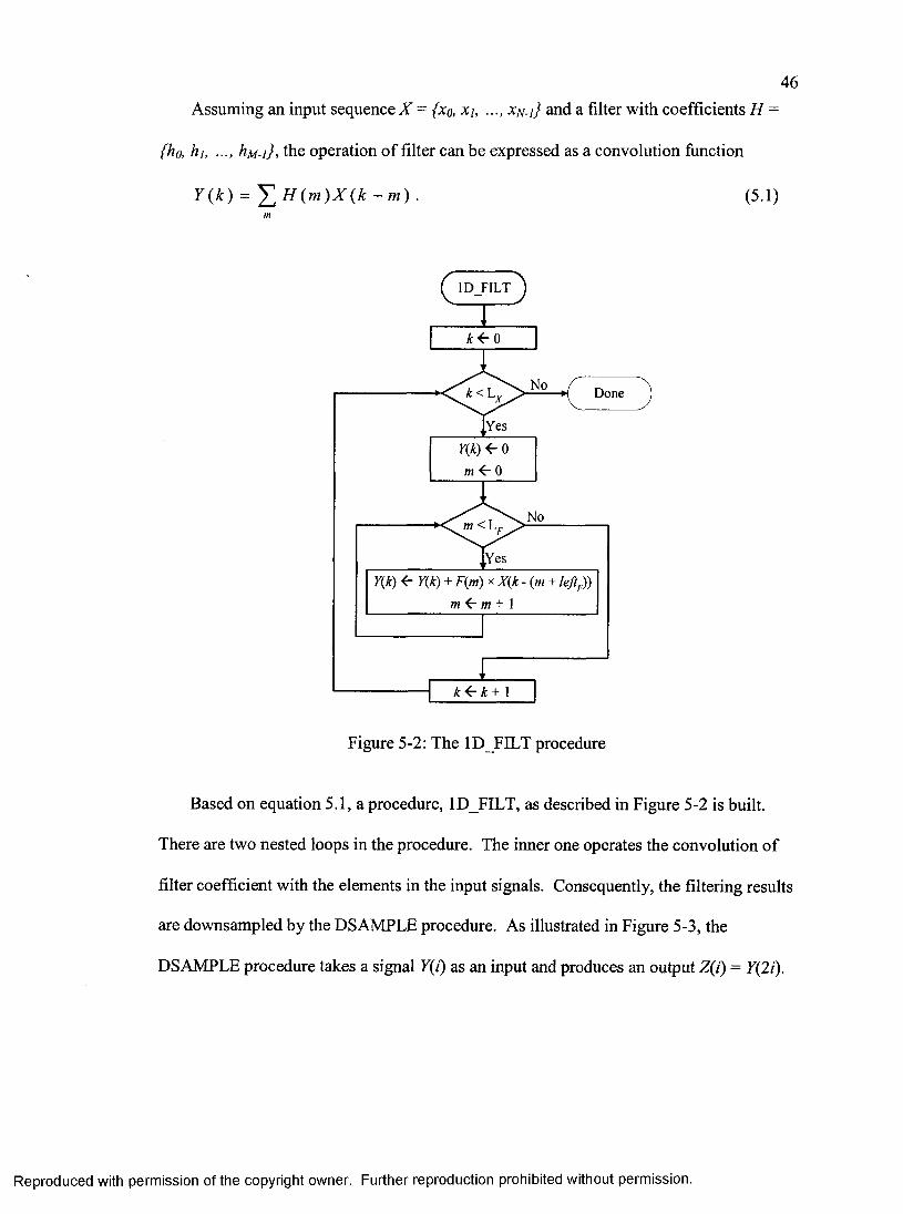
46Assuming an input sequence X = (xq, xi, xn-i} and a filter with coefficients H -

{ho, hi, ..., hM-j}, the operation of filter can be expressed as a convolution function

7(Æ) = . (5.1)

^ 1D_FILT ^

Y(k) e 0

y(jt) <- y(A) + fXm) X - (m +m ^ m + \

k + I

Figure 5-2: The ID FILT procedure

Based on equation 5.1, a procedure, ID FILT, as described in Figure 5-2 is built.

There are two nested loops in the procedure. The inner one operates the convolution of

filter coefficient with the elements in the input signals. Consequently, the filtering results

are downsampled by the DSAMPLE procedure. As illustrated in Figure 5-3, the

DSAMPLE procedure takes a signal 7(0 as an input and produces an output Z(i) = 7(20-


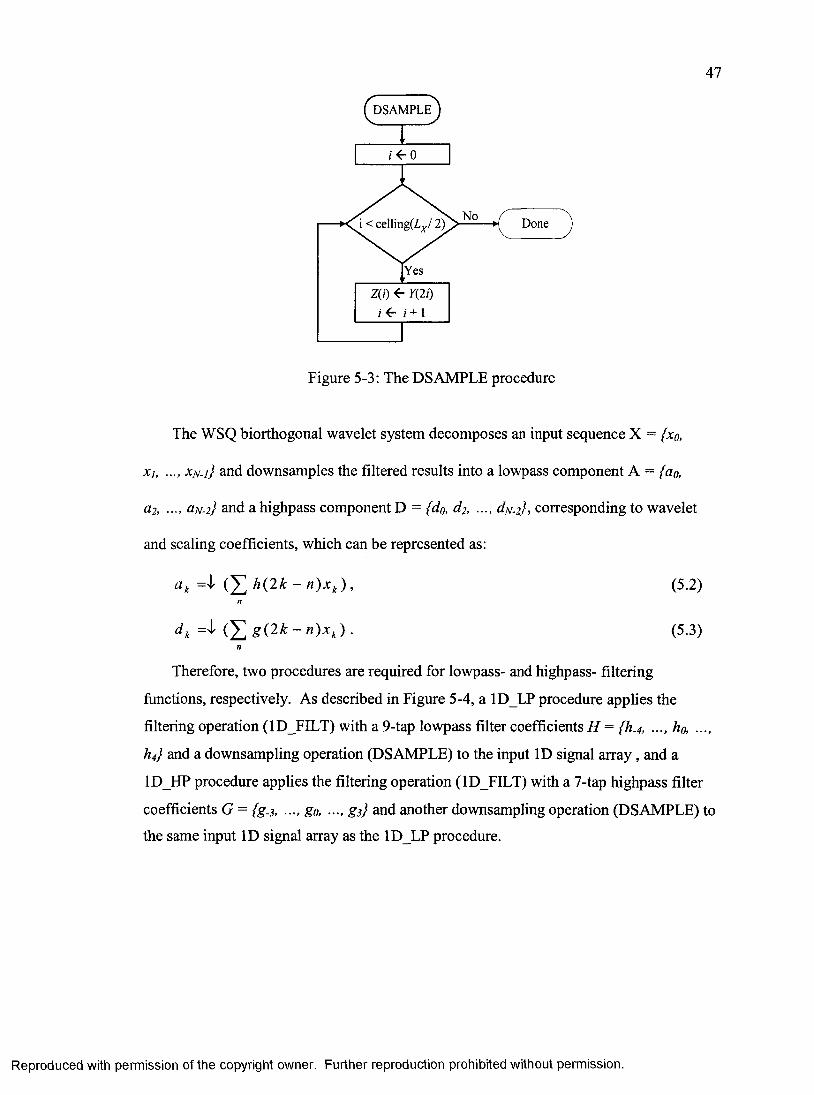
47

No Done

Yes

f 4-0

Figure 5-3: The DSAMPLE procedure

The WSQ biorthogonal wavelet system decomposes an input sequence X = {x q ,

xi, ...,xn.i} and downsamples the filtered results into a lowpass component A = {ao,

Ü 2 , ü N . z } and a highpass component D = { d o , d 2 , d N - 2} , corresponding to wavelet

and scaling coefficients, which can be represented as:

{ Y ^ h { l k - n ) x ^ ) , (5.2)

dk ■ (5.3)

Therefore, two procedures are required for lowpass- and highpass- filtering

functions, respectively. As described in Figure 5-4, a ID LP procedure applies the

filtering operation (ID FILT) with a 9-tap lowpass filter coefficients H = { h . 4, h o , . . . ,

h4} and a downsampling operation (DSAMPLE) to the input ID signal array, and a

ID HP procedure applies the filtering operation (ID FILT) with a 7-tap highpass filter

coefficients G = (g.j, ..., go, ..., gs} and another downsampling operation (DSAMPLE) to

the same input ID signal array as the ID LP procedure.


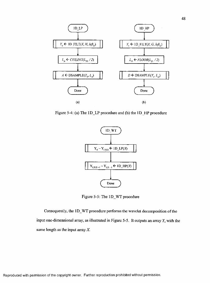
48

ID LP ID HP

Done Done

<r CElLING(Ly^ / 2) e FLOOR(Ly / 2)

D e D SA M PLE(r,, ig )A <r DSAMPLE(Po, L^)

y, e 1D_FILT(A', G, l e f gEg <- lD_FILT(Jf, H, left^)

(a) (b)

Figure 5-4: (a) The ID LP procedure and (b) the ID HP procedure

^ 1D_WT ^

1D_LPW

Y Lx/2+.-Y ^_,<-lD _H P(A )

^ Done ^

Figure 5-5: The ID WT procedure

Consequently, the I D W T procedure performs the wavelet decomposition of the

input one-dimensional array, as illustrated in Figure 5-5. It outputs an array Y, with the

same length as the input array W.


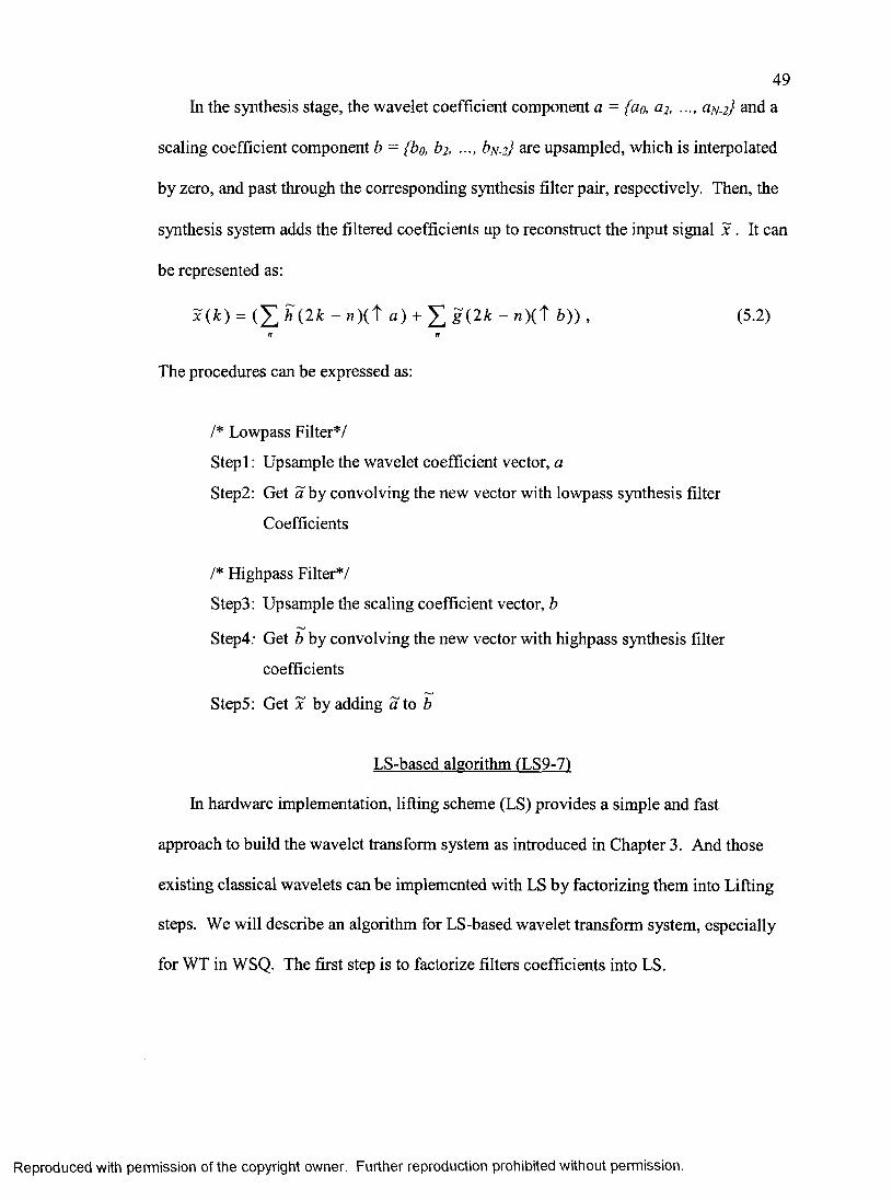
49In the synthesis stage, the wavelet coefficient component a = {ao, ü2, 0 ^.2} and a

scaling coefficient component b = (bo, b2, bN-2} are upsampled, which is interpolated

by zero, and past through the corresponding synthesis filter pair, respectively. Then, the

synthesis system adds the filtered coefficients up to reconstruct the input signal x . It can

be represented as:

= ( E ^(2 * - »)(T a) + E g(2 t - »)(T 6 )) , (5.2)n n

The procedures can be expressed as:

/* Lowpass Filter*/

Step I : Upsample the wavelet coefficient vector, a

Step2: Get a by convolving the new vector with lowpass synthesis filter

Coefficients

/* Highpass Filter*/

Step3: Upsample the scaling coefficient vector, b

Step4.- Get b by convolving the new vector with highpass synthesis filter

coefficients

StepS: Get x by adding a to 6

LS-based algorithm (LS9-7I

In hardware implementation, lifting scheme (LS) provides a simple and fast

approach to build the wavelet transform system as introduced in Chapter 3. And those

existing classical wavelets can be implemented with LS by factorizing them into Lifting

steps. We will describe an algorithm for LS-based wavelet transform system, especially

for WT in WSQ. The first step is to factorize filters coefficients into LS.


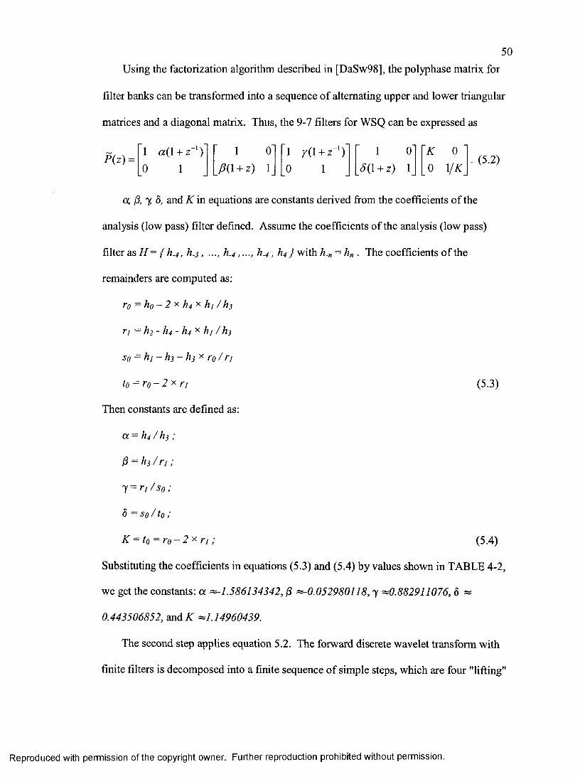
50Using the factorization algorithm described in [DaSw98], the polyphase matrix for

filter banks can be transformed into a sequence of alternating upper and lower triangular

matrices and a diagonal matrix. Thus, the 9-7 filters for WSQ can be expressed as

f (z ) =1 a(lH-z ') 0 1

1 0 A I + z) 1

1 r ( i + z -‘) 0 1

1 00(1 + z) 1

A: 00 1/A

(5.2)

a, 13, y, Ô, and K in equations are constants derived from the coefficients of the

analysis (low pass) filter defined. Assume the coefficients of the analysis (low pass)

filter as { h.4 , h- 3 , h.4 h. 4 , h4 } with h.„ = h„ . The coefficients of the

remainders are computed as:

ro - ho - 2 X h4 X hj / hs

ri = h2 - h4 - h4 X hi / hs

s o ^ h i - h s - h j x ro/ri

to = r o - 2 X n

Then constants are defined as:

(5.3)

a = h4 / hs ;

0 = h s / n ;

y = r i / s o ;

b =so/to;

K = to = r o - 2 x r i ; (5.4)

Substituting the coefficients in equations (5.3) and (5.4) by values shown in TABLE 4-2,

we get the constants: o: ^1.586134342, 0 =^-0.052980118, y ^0.882911076, b »

0.443506852, and A ^1.14960439.

The second step applies equation 5.2. The forward discrete wavelet transform with

finite filters is decomposed into a finite sequence of simple steps, which are four "lifting"


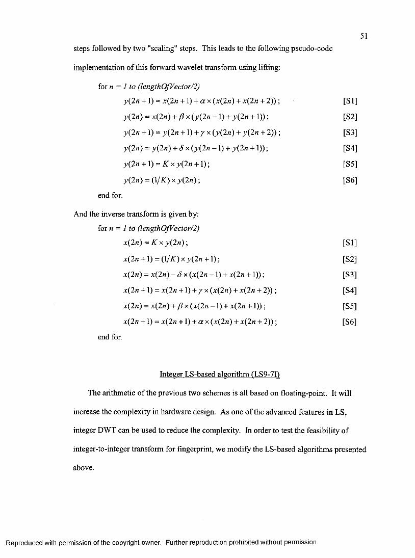
51steps followed by two "scaling" steps. This leads to the following pseudo-code

implementation of this forward wavelet transform using lifting:

îoxn = 1 to (lengthOjVector/2)

y{2n +1) = x{2n 4-1) -I- a x (x(2n) + x(2n + 2)); [SI]

y{2n) = x(2n) + J3x (y(2n -1 ) + y{2n + 1)) ; [S2]

y{2n + 1) = y{2n + V) + y x (y(2n) + y(2n + 2)) ; [S3]

y(2n) = y(2n) + S x (y{2n -1 ) + y(2n + 1)) ; [S4]

y{2n + l) = K x y (2 n + \); [S5]

X2») = (l/A)xX2«); [S6]end for.

And the inverse transform is given by:

for n = i to (lengthOfVector/2)

x{2n) = K X y{2n) ■, [SI]

x(2« + l) = (l/A)x>;(2n + l); [S2]

x(2n) = x { 2 n ) - 5 x {x{2n -1 ) + x{2n +1)); [S3]

x{2n 4 -1 ) = x{2n 4 -1 ) 4- y x {x{2n) 4- x(2n 4- 2)) ; [S4]

x{2n) - x{2n) + f i x (x(2n - 1 ) 4 - x(2n 4 -1 ) ) ; [S5]

x{2n 4 -1 ) = x(2n 4 -1 ) 4- or x (x(2n) + x(2n 4- 2)) ; [S6]

end for.

Integer LS-based algorithm (LS9-7I)

The arithmetic of the previous two schemes is all based on floating-point. It will

increase the complexity in hardware design. As one of the advanced features in LS,

integer DWT can be used to reduce the complexity. In order to test the feasibility of

integer-to-integer transform for fingerprint, we modify the LS-based algorithms presented

above.


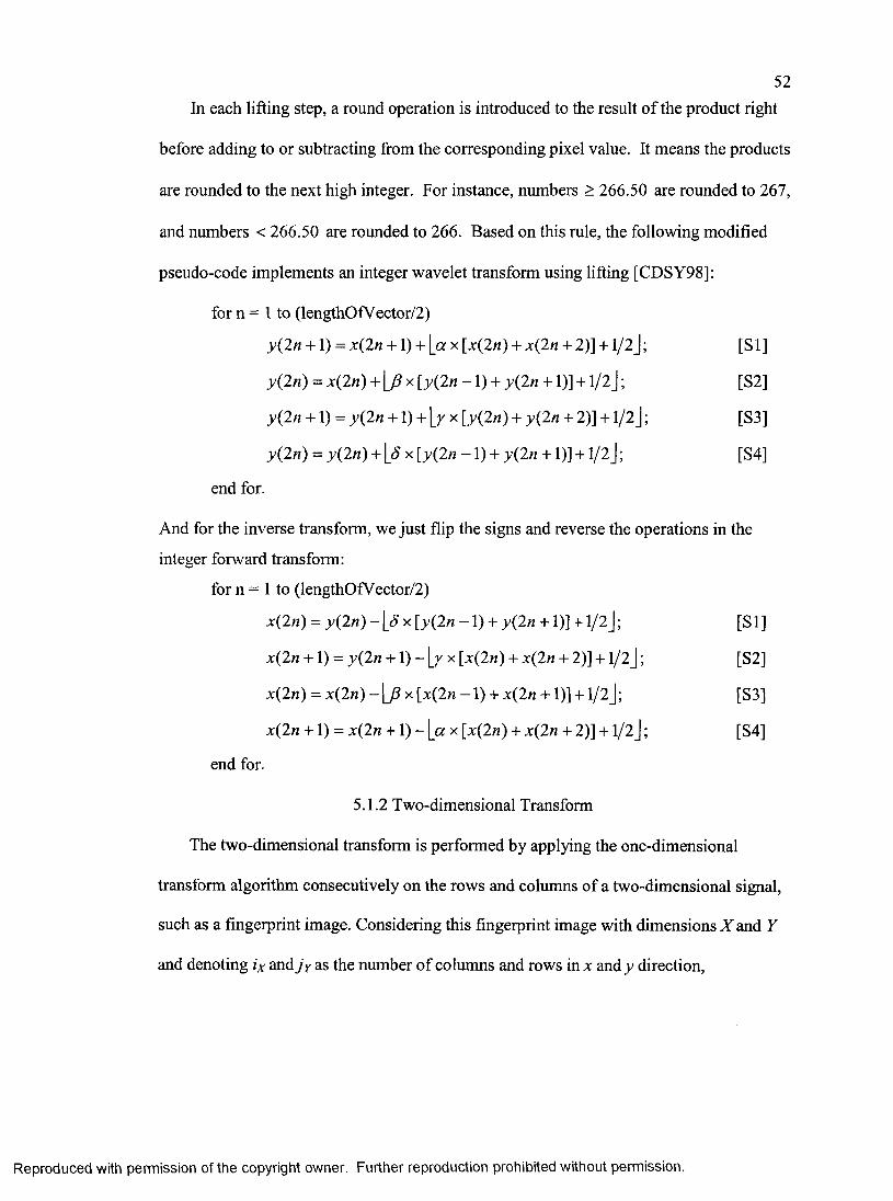
52In each lifting step, a round operation is introduced to the result of the product right

before adding to or subtracting from the corresponding pixel value. It means the products

are rounded to the next high integer. For instance, numbers > 266.50 are rounded to 267,

and numbers < 266.50 are rounded to 266. Based on this rule, the following modified

pseudo-code implements an integer wavelet transform using lifting [CDSY98];

for n = 1 to (lengthOfVector/2)

y(2n + 1) = x(2« + 1) + 1_« X [x{2n) + x{2n + 2)] 1/2 J ; [SI]

y{2n) = x{2n) + \_Px [y{2n -1 ) -F y{2n -f 1)] -f 1/2J ; [S2]

y{2n -F1) = y{2n -F1) -F |_y x [y{2n) -F y{2n -F 2)] -F l/2 j ; [S3]

y{2n) = y{2n)+ \p x[y(2«-1)-Fy(2n-Fl)] + l/2 j; [S4]

end for.

And for the inverse transform, we just flip the signs and reverse the operations in the

integer forward transform:

for n = 1 to (lengthOfVector/2)

x(2n) = y { 2 n ) - \ô x [y(2« -1 ) + y(2« +1)] + l/2 j; [SI]

x{2n +1) = y{2n + 1) - [y x [x{2n) -F x{2n + 2)] + l/2 j ; [S2]

x{2n) = x{2n) - \ j 3 x [x{2n -1 ) + x{2n + 1)] +1/2 J ; [S3]

x(2n -FI) = x(2n -F1) - [« x [x(2n) + x(2n + 2)]+ 1/2J; [S4]

end for.

5.1.2 Two-dimensional Transform

The two-dimensional transform is performed by applying the one-dimensional

transform algorithm consecutively on the rows and columns of a two-dimensional signal,

such as a fingerprint image. Considering this fingerprint image with dimensions X and Y

and denoting z> and Jy as the number of columns and rows in x and y direction.


53respectively, the forward two-dimensional transform algorithm for one level WT is as

follows:

For the forward two-dimensional wavelet transform, we begin with iteration level 0

as current level. The one-dimensional forward transform is first applied to all the rows,

and then to all the columns. Subsequently, we move to the next iteration level and repeat

the two steps above, and so on, until all the iteration levels are accomplished. In this

thesis, five-level decompositions are required.

For the inverse transform, the inverse one-dimensional transform is applied exactly

in the opposite order. Flowcharts below illustrate the two-dimensional forward transform

and inverse algorithm.

The flowchart in Figure 5-6a shows the 2D FDWT procedure which decomposes an

image or low-level subband into four next-level subbands. As shown in Figure 5-6b, the

2D IDWT synthesizes an image or low-level subband from four high-level subbands.

Notes that ID WT procedure and ID IWT procedure use three different algorithms

corresponding to three testing schemes as discussed in section 5.2.


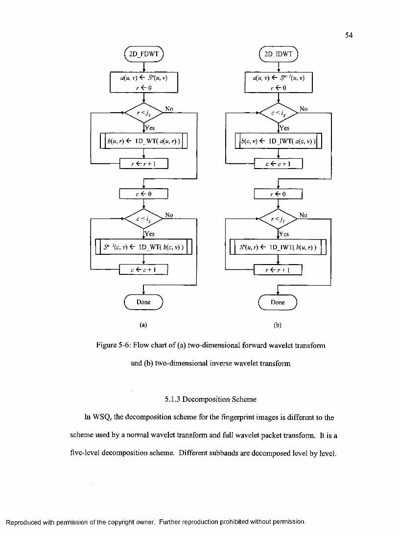
54

^2D_FDWT^

a{u, v) 5"(m, v)

r < -0

No

I Yes

b{u, r) f - 1D_WT( a{u, r) )

r 4- r + 1

No

[Yes

lD _W T (è(c,v ))

c ^ c + 1

(a)

a(u, v) 4r S""'{u, v)

r 0

No

[Yes

i(c ,v )< - lD _IW T (a(c,v))

C <- c + 1

No

[Yes

y (« , r) <- lD_lW T(è(M ,r))

r ^ r + \

(b)

Figure 5-6: Flow chart of (a) two-dimensional forward wavelet transform

and (b) two-dimensional inverse wavelet transform

5.1.3 Decomposition Scheme

In WSQ, the decomposition scheme for the fingerprint images is different to the

scheme used by a normal wavelet transform and full wavelet packet transform. It is a

five-level decomposition scheme. Different subbands are decomposed level by level.


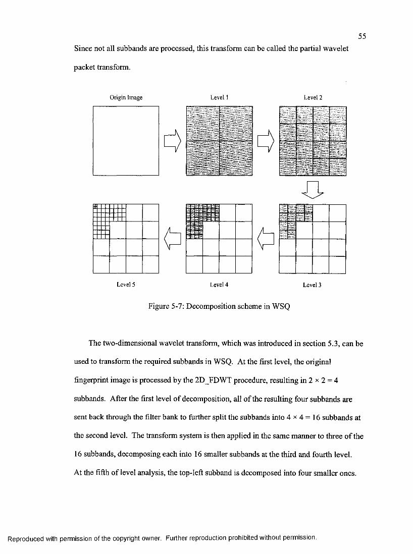
55Since not all subbands are processed, this transform can be called the partial wavelet

packet transform.

Origin Image Level 1 Level 2

Level 5 Level 4 Level 3

Figure 5-7: Decomposition scheme in WSQ

The two-dimensional wavelet transform, which was introduced in section 5.3, can he

used to transform the required subbands in WSQ. At the first level, the original

fingerprint image is processed by the 2D FDWT procedure, resulting in 2 x 2 = 4

subbands. After the first level of decomposition, all of the resulting four subbands are

sent back through the filter bank to further split the subbands into 4 x 4 = 1 6 subbands at

the second level. The transform system is then applied in the same manner to three of the

16 subbands, decomposing each into 16 smaller suhhands at the third and fourth level.

At the fifth of level analysis, the top-left subband is decomposed into four smaller ones.


56The desired subband structure is obtained, which consists of 64-suhands. Figure 5-7

shows these procedures.

5.2 Experimental Results and Performance Analysis

Two experiments are done. In the first experiment, we want to find out the loss

caused hy transform only. So, the compression and decoding steps are skipped. We

reconstruct the images from wavelet coefficients obtained from transform. In the second

experiment, we want to find out the total loss caused by both transform and compression.

We apply a compression step to the wavelet coefficients and then reconstruct the images

from the compressed data.

5.2.1 Image Quality Measures and Test Image

Distortion Measure

A standard objective measure of distortion of the reconstructed images is Peak

Signal-to-Noise Ratio (PSNR). Here, for a 256 gray scale fingerprint image, the PSNR is

defined as

PSNR = lOlog 10

^ 255^^MSE

[in dB], (5.5)

MSE is the mean square error, which is the average of the energy of the difference

between the original image and the reconstructed image:

N M

where A x M is the total number of pixels in the image, x{i,j) is an original pixel, and

x(x, j ) is a reconstructed pixel. PSNR values range from infinity, for identical images.


57to 0, for images with no commonality. Typical PSNR values for images range from 20 to

40. A PSNR value of 30 or greater is considered to be acceptable for subject recognition

[GeKi96]. PSNR drops as the compression ratio increases on an image. Though PSNR

is not a direct measure of the perceptual visual quality, it is widely used an indicator of

the image quality.

Fingerprints Matching

There are many interruptions of ridge across the impression of fingerprints. These

inteiTuptions - ridge endings and bifurcations are known as minutiae. The definitive

information used to determine that one fingerprint matches another is in the fine detail of

these minutiae and their relationships. There are three steps for fingerprint images

matching generally.

First step, a fingerprint image is processed through a series of image processing

algorithms to obtain a clear unambiguous skeletal image of the original gray tone

impression, clarifying smudged areas, removing extraneous artifacts and healing most

scars, cuts and breaks.

Second step, minutiae within the skeletal image are identified and encoded,

providing critical placement, orientation and linkage information for the matcher.

Third step, the matcher compares data of the input search image against all records in

the database to determine if a probable match exits. If yes, it indicates matching and

gives file name(s) of the matched image(s). If no, it indicates matching fails.

The fingerprint identification engine that we use to test matching of the reconstructed

fingerprint images with the original one is called VeriFinger, offered hy

Neurotechnologija, Ltd. [Neur03].


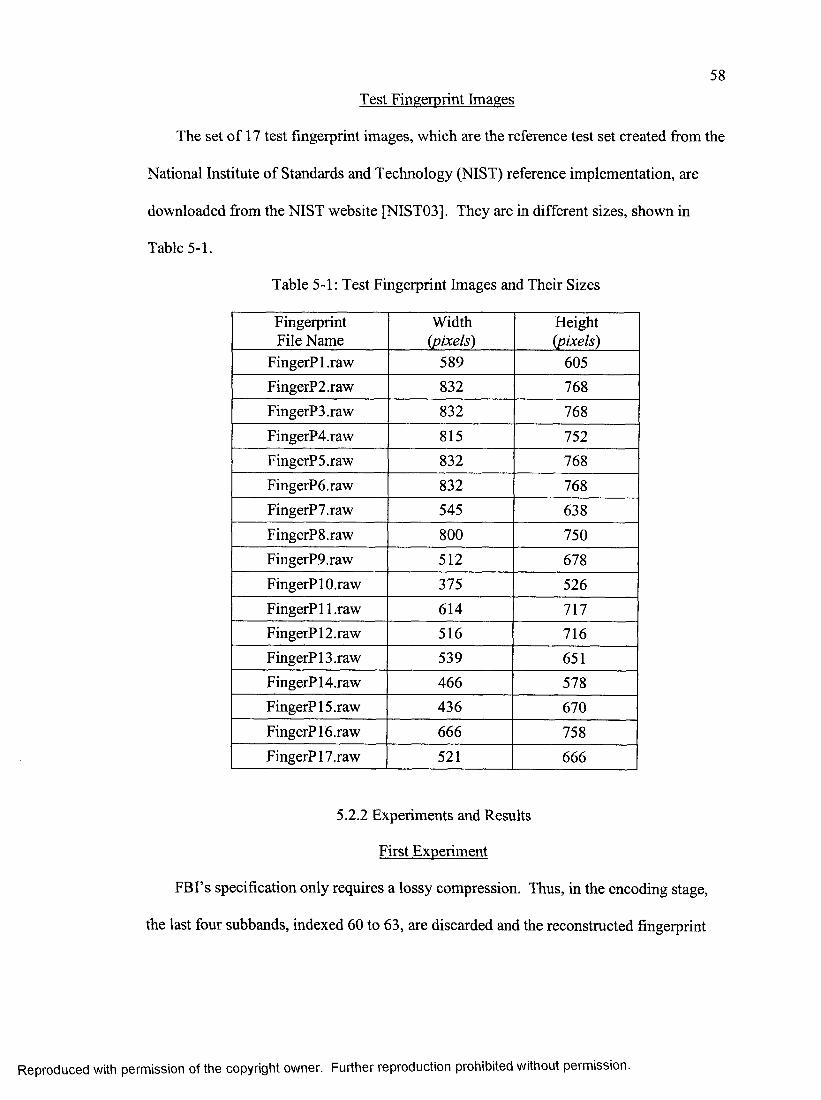
58Test Fingerprint Images

The set of 17 test fingerprint images, which are the reference test set created from the

National Institute of Standards and Technology (NIST) reference implementation, are

downloaded from the NIST website [NIST03]. They are in different sizes, shown in

Table 5-1.

Table 5-1; Test Fingerprint Images and Their Sizes

Fingerprint File Name

Width(pixels)

Height(pixels)

FingerPl.raw 589 605FingerP2.raw 832 768FingerP3.raw 832 768FingerP4.raw 815 752FingerP5.raw 832 768FingerP6.raw 832 768FingerP7.raw 545 638FingerPS.raw 800 750FingerP9.raw 512 678FingerPlO.raw 375 526FingerPll.raw 614 717FingerP12.raw 516 716FingerP13.raw 539 651FingerP14.raw 466 578FingerP15.raw 436 670FingerP16.raw 666 758FingerP17.raw 521 666

5.2.2 Experiments and Results

First Experiment

FBI’s specification only requires a lossy compression. Thus, in the encoding stage,

the last four subbands, indexed 60 to 63, are discarded and the reconstructed fingerprint


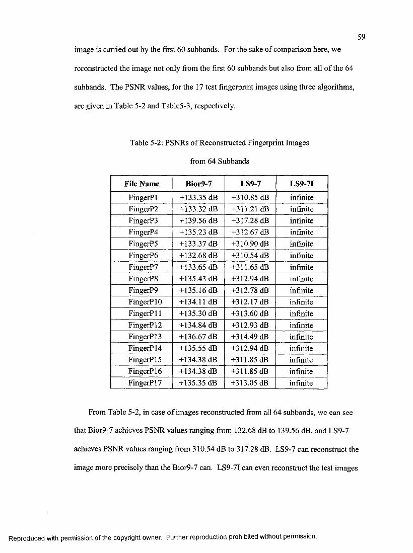
59image is carried out by the first 60 subbands. For the sake of comparison here, we

reconstructed the image not only from the first 60 suhhands but also from all of the 64

suhhands. The PSNR values, for the 17 test fingerprint images using three algorithms,

are given in Table 5-2 and Table5-3, respectively.

Table 5-2: PSNRs of Reconstructed Fingerprint Images

from 64 Subbands

File Name Bior9-7 LS9-7 LS9-7I

FingerPl +133.35 dB +310.85 dB infiniteFingerP2 +133.32 dB +311.21 dB infiniteFingerP3 +139.56 dB +317.28 dB infiniteFingerP4 +135.23 dB +312.67 dB infiniteFingerP5 +133.37 dB +310.90 dB infiniteFingerP6 +132.68 dB +310.54 dB infiniteFingerP7 +133.65 dB +311.65 dB infiniteFingerP8 +135.43 dB +312.94 dB infiniteFingerP9 +135.16 dB +312.78 dB infiniteFingerPlO +134.11 dB +312.17 dB infiniteFingerPll +135.30 dB +313.60 dB infiniteFingerPl 2 +134.84 dB +312.93 dB infiniteFingerPl 3 +136.67 dB +314.49 dB infiniteFingerPl 4 +135.55 dB +312.94 dB infiniteFingerPl 5 +134.38 dB +311.85 dB infiniteFingerPl 6 +134.38 dB +311.85 dB infiniteFingerPl 7 +135.35 dB +313.05 dB infinite

From Table 5-2, in case of images reconstructed from all 64 subbands, we can see

that Bior9-7 achieves PSNR values ranging from 132.68 dB to 139.56 dB, and LS9-7

achieves PSNR values ranging from 310.54 dB to 317.28 dB. LS9-7 can reconstruct the

image more precisely than the Bior9-7 can. LS9-7I can even reconstruct the test images


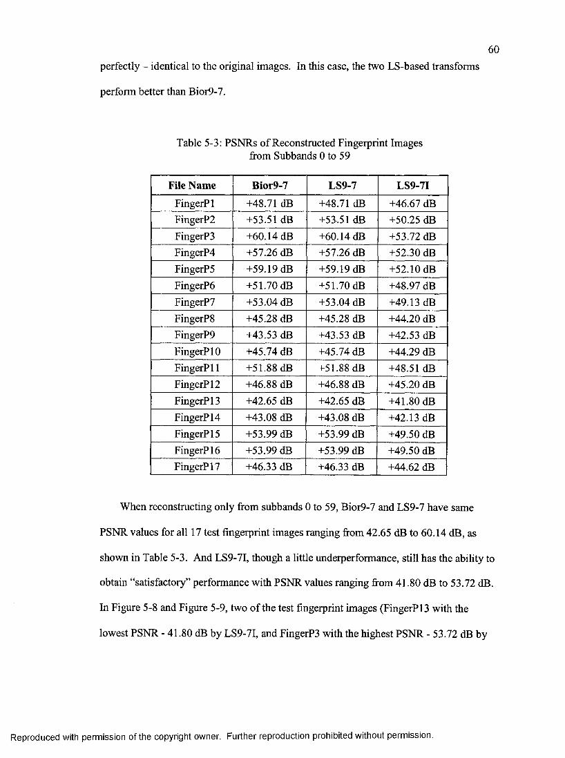
60perfectly - identical to the original images. In this case, the two LS-based transforms

perform better than Bior9-7.

Table 5-3: PSNRs of Reconstructed Fingerprint Images from Subbands 0 to 59

File Name Bior9-7 LS9-7 LS9-7I

FingerPl +48.71 dB +48.71 dB +46.67 dBFingerP2 +53.51 dB +53.51 dB +50.25 dBFingerP3 +60.14 dB +60.14 dB +53.72 dBFingerP4 +57.26 dB +57.26 dB +52.30 dBFingerP5 +59.19 dB +59.19 dB +52.10 dBFingerP6 +51.70 dB +51.70 dB +48.97 dBFingerP7 +53.04 dB +53.04 dB +49.13 dBFingerP8 +45.28 dB +45.28 dB +44.20 dBFingerP9 +43.53 dB +43.53 dB +42.53 dBFingerPlO +45.74 dB +45.74 dB +44.29 dBFingerPll +51.88 dB +51.88 dB +48.51 dBFingerPl 2 +46.88 dB +46.88 dB +45.20 dBFingerPl 3 +42.65 dB +42.65 dB +41.80 dBFingerPl 4 +43.08 dB +43.08 dB +42.13 dBFingerPl 5 +53.99 dB +53.99 dB +49.50 dBFingerPl 6 +53.99 dB +53.99 dB +49.50 dBFingerPl 7 +46.33 dB +46.33 dB +44.62 dB

When reconstructing only from subhands 0 to 59, Bior9-7 and LS9-7 have same

PSNR values for all 17 test fingerprint images ranging from 42.65 dB to 60.14 dB, as

shown in Table 5-3. And LS9-7I, though a little underperformance, still has the ability to

obtain “satisfactory” performance with PSNR values ranging from 41.80 dB to 53.72 dB.

In Figure 5-8 and Figure 5-9, two of the test fingerprint images (FingerPl 3 with the

lowest PSNR - 41.80 dB hy LS9-7I, and FingerP3 with the highest PSNR - 53.72 dB by


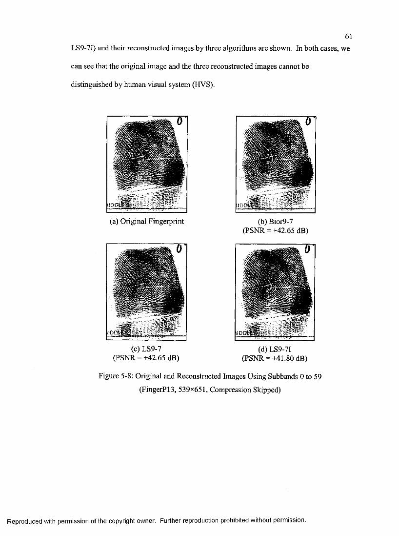
61LS9-7I) and their reconstructed images by three algorithms are shown. In both cases, we

can see that the original image and the three reconstructed images cannot be

distinguished by human visual system (HVS).

(a) Original Fingerprint

(c) LS9-7 (PSNR = +42.65 dB)

'i t ^

(b) Bior9-7 (PSNR - +42.65 dB)

(d) LS9-7I (PSNR-+41.80 dB)

Figure 5-8: Original and Reconstructed Images Using Subbands 0 to 59

(FingerPl3, 539x651, Compression Skipped)


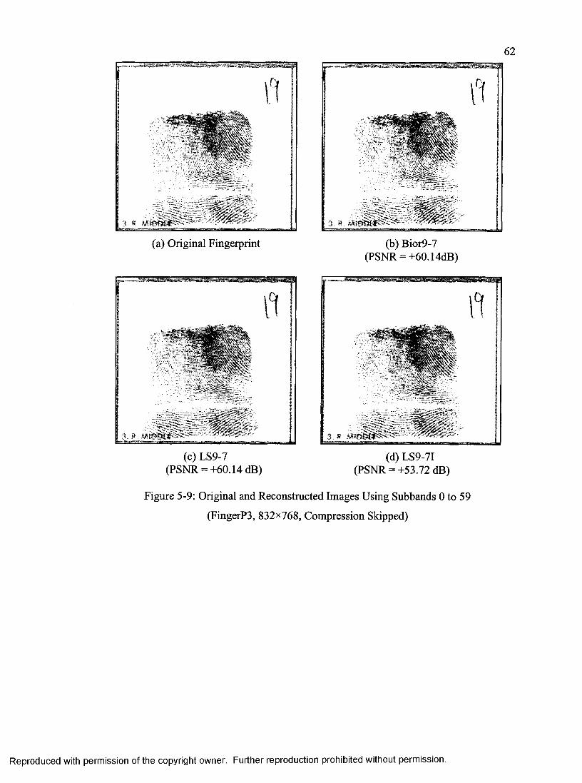
Il

3 R

(a) Original Fingerprint

(c) LS9-7 (P S N R -+60.14 dB)

(b) Bior9-7 (PSNR-+60.14dB)

(d) LS9-7I (PSNR - +53.72 dB)

Figure 5-9: Original and Reconstructed Images Using Subbands 0 to 59

(FingerP3, 832x768, Compression Skipped)

62

AU U

3 R


63Second Experiment

In the second experiment, we attach an entropy coder to both Bior9-7 and LS9-7I.

The entropy coder is adopted from FBI WSQ standard for gray-scale fingerprint image

compression [BrBH93]. So in this experiment, the 17 test fingerprint images are

compressed following the WSQ standard - the compression steps (quantization step and

Huffman coding) just deal with the first 60 suhhands (0 to 59) of 64 subbands obtained in

the decomposition step and the target bit rates range from l.OObpp to O.lObpp with

interval of 0.05bpp. The compressed images are reconstructed and PSNRs to the original

image are calculated. PSNR values of Bior9-7 are shown in Tahle 5-4. PSNR values of

LS9-7I are shown in Table 5-5. The difference of PSNR values between Bior9-7 and

LS9-7I (PSNR Diff) corresponding to different hit rates are shown in Figure 5-9. While

PSNR of Bior9-7 is higher than that of LS9-7I, PSNR Diff is positive, otherwise,

negative.


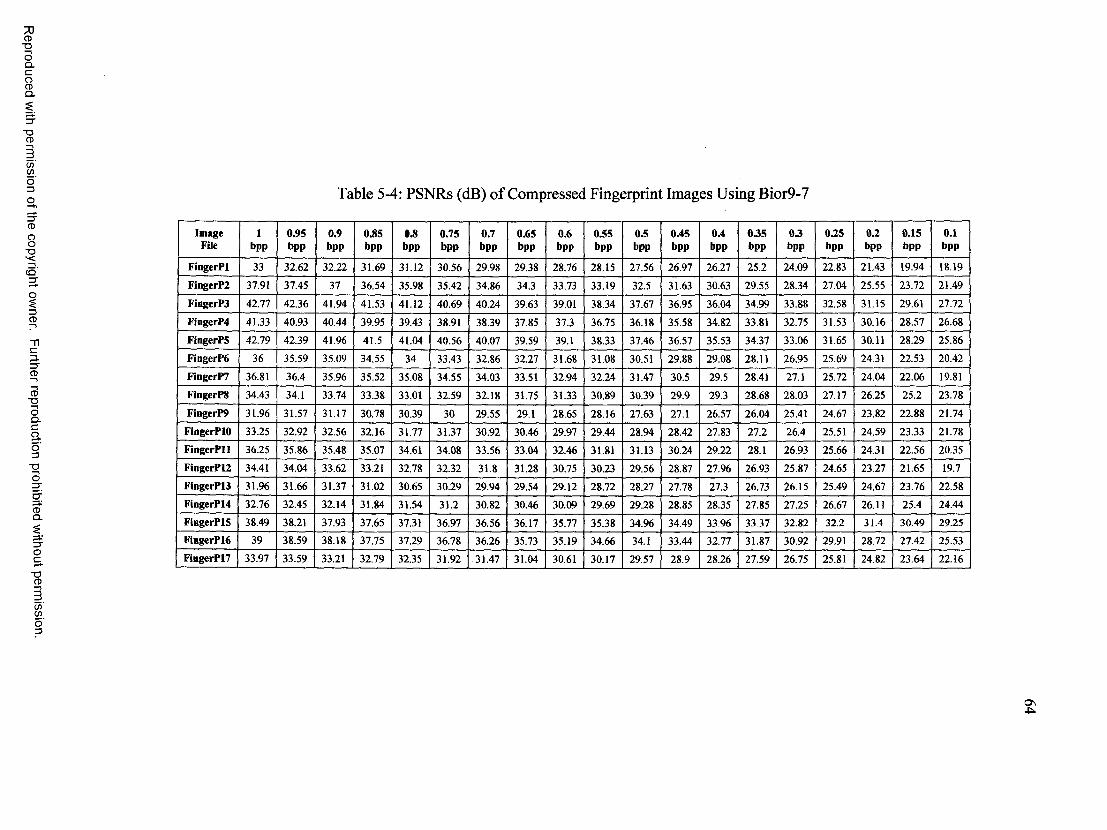
7]CD"DOQ.C

gQ.

■OCD

C/)

o '3 Table 5-4: PSNRs (dB) of Compressed Fingerprint Images Using Bior9-7

8ci-

3-3"CD

CD■OOClCg.o3

■OO

CDQ.

OC

C/)eno '3

ImageFile

1bpp

0.95bpp

0.9bpp

0.85bpp

0.8bpp

0.75bpp

0.7bpp

0.65bpp

0.6bpp

0.55bpp

0.5bpp

0.45bpp

0.4bpp

035bpp

03bpp

035bpp

03bpp

0.15bpp

0.1bpp

FingerPl 33 32.62 32.22 31.69 31.12 30.56 29.98 29.38 28.76 28.15 27.56 26.97 26.27 25.2 24.09 22.83 21.43 19.94 18.19

FingerP2 37.91 37.45 37 36.54 35.98 35.42 34.86 34.3 33.73 33.19 32.5 31.63 30.63 29.55 28.34 27.04 25.55 23.72 21.49

FingerP3 42.77 42.36 41.94 41.53 41.12 40.69 40.24 39.63 39.01 38.34 37.67 36.95 36.04 34.99 33.88 32.58 31.15 29.61 27.72

FingerP4 41.33 40.93 40.44 39.95 39.43 38.91 38.39 37.85 37.3 36.75 36.18 35.58 34.82 33.81 32.75 31.53 30.16 28.57 26.68

FingerPS 42.79 42.39 41.96 41.5 41.04 40.56 40.07 39.59 39.1 38.33 37.46 36.57 35.53 34.37 33.06 31.65 30.11 28.29 25.86

FingerPô 36 35.59 35.09 34.55 34 33.43 32.86 32.27 31.68 1 31.08 30.51 29.88 29.08 28.11 26.95 25.69 24.31 22.53 20.42

FingerP? 36.81 36.4 35.96 35.52 35.08 34.55 34.03 33.51 32.94 32.24 31.47 30.5 29.5 28.41 27.1 25.72 24.04 22.06 19.81

FingerPS 34.43 34,1 33.74 33.38 33.01 32.59 32.18 31.75 31.33 30.89 30.39 29.9 29.3 28.68 28.03 27.17 26.25 25.2 23.78

FingerP9 31.96 31.57 31.17 30.78 30.39 30 29.55 29.1 28.65 28.16 27.63 27.1 26.57 26.04 25.41 24.67 23.82 22.88 21.74

FingerPlO 33.25 32.92 32.56 32.16 31.77 31.37 30.92 30.46 29.97 29.44 28.94 28.42 27.83 27.2 26.4 25.51 24.59 23.33 21.78

FingerPll 36.25 35.86 35.48 35.07 34.61 34.08 33.56 33.04 32.46 31.81 31.13 30.24 29.22 28.1 26.93 25.66 24.31 22.56 20.35

FingerPU 34.41 34.04 33.62 33.21 32.78 32.32 31.8 31.28 30.75 30.23 29.56 28.87 27.96 26.93 25.87 24.65 23.27 21.65 19.7

FingerP13 31.96 31.66 31.37 31.02 30.65 30.29 29.94 29.54 29.12 28.72 28.27 27.78 27.3 26.73 26.15 25.49 24.67 23.76 22.58

FingerPM 32.76 32.45 32.14 31.84 31.54 31.2 30.82 30.46 30.09 29.69 29.28 28.85 28.35 27.85 27.25 26.67 26.11 25.4 24.44

FingerPlS 38.49 38.21 37.93 37.65 37.31 36.97 36.56 36.17 35.77 35.38 34.96 34.49 33.96 33.37 32.82 32.2 31.4 30.49 29.25FingerPlO 39 38.59 38.18 37.75 37.29 36.78 36.26 35.73 35.19 34.66 34.1 33.44 32.77 31.87 30.92 29.91 28.72 27.42 25.53FingerPl? 33.97 33.59 33.21 32.79 32.35 31.92 31.47 31.04 30.61 30.17 29.57 28.9 28.26 27.59 26.75 25.81 24.82 23.64 22.16

S

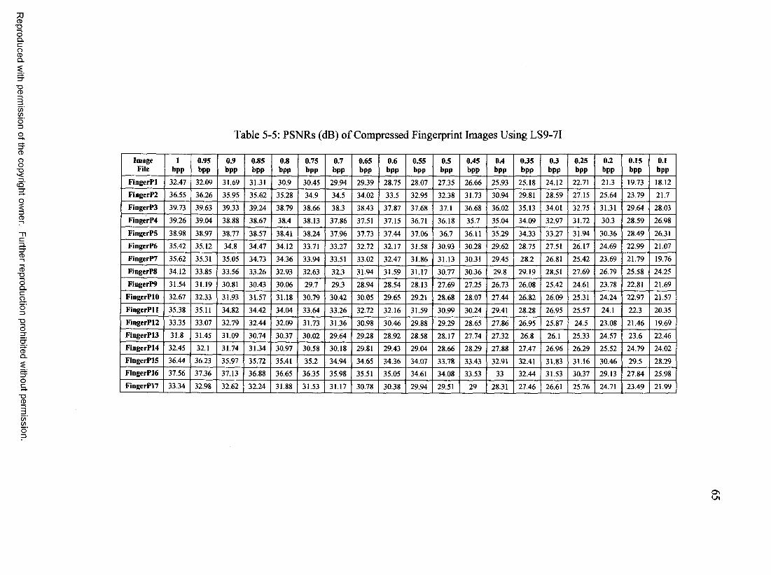
73CD"OOQ.cgQ.

"OCD

C/)Wo '3O Table 5-5: PSNRs (dB) of Compressed Fingerprint Images Using LS9-7I

8( O '

3.3"CD

CD■DOQ.Cg.o3

"Oo

CDQ.

■DCD

ImageFile

1bpp

0.95bpp

0.9bpp

0.85bpp

0.8bpp

0.75bpp

0.7bpp

0.65bpp

0.6bpp

0.55bpp

0.5bpp

0.45bpp

0.4bpp

0 J5bpp

0 3bpp

035bpp

0.2bpp

0.15bpp

0.1bpp

FlngerPl 32.47 32.09 31.69 31.31 30.9 30.45 29.94 29.39 28.75 28.07 27.35 26.66 25.93 25.18 24.12 22.71 21.3 19.73 18.12

FingerP2 36.55 36.26 35.95 35.62 35.28 34.9 34.5 34.02 33.5 32.95 32.38 31.73 30.94 29.81 28.59 27.15 25.64 23.79 21.7

FingerP3 39.73 39.63 39.33 39.24 38.79 38.66 38.3 38.43 37.87 37.68 37.1 36.68 36.02 35.13 34.01 32.75 31.31 29.64 28.03

FingerP4 39.26 39.04 38.88 38.67 38.4 38.13 37.86 37.51 37.15 36.71 36.18 35.7 35.04 34.09 32.97 31.72 30.3 28.59 26.98

FingerPS 38.98 38.97 38.77 38.57 38.41 38.24 37.96 37.73 37.44 37.06 36.7 36.11 35.29 34.33 33.27 31.94 30.36 28.49 26.31

FingerP6 35.42 35.12 34.8 34.47 34.12 33.71 33.27 32.72 32.17 31.58 30.93 30.28 29.62 28.75 27.51 26.17 24.69 22.99 21.07

FingerP? 35.62 35.31 35.05 34.73 34.36 33.94 33.51 33.02 32.47 31.86 31.13 30.31 29.45 28.2 26.81 25.42 23.69 21.79 19.76

FingerPS 34.12 33.85 33.56 33.26 32.93 32.63 32.3 31.94 31.59 31.17 30.77 30.36 29.8 29.19 28.51 27.69 26.79 25.58 24.25

FingerP9 31.54 31.19 30.81 30.43 30.06 29.7 29.3 28.94 28.54 28.13 27.69 27.25 26.73 26.08 25.42 24.61 23.78 22.81 21.69

FingerPlO 32.67 32.33 31.93 31.57 31.18 30.79 30.42 30.05 29.65 29.21 28.68 28.07 27.44 26.82 26.09 25.31 24.24 22.97 21.57

FingerPIl 35.38 35.11 34.82 34.42 34.04 33.64 33.26 32.72 32.16 31.59 30.99 30.24 29.41 28.28 26.95 25.57 24.1 22.3 20.35

FingerP12 33.35 33.07 32.79 32.44 32.09 31.73 31.36 30.98 30.46 29.88 29.29 28.65 27.86 26.95 25.87 24.5 23.08 21.46 19.69

FingerP13 31.8 31.45 31.09 30.74 30.37 30.02 29.64 29.28 28.92 28.58 28.17 27.74 27.32 26.8 26.1 25.33 24.57 23.6 22.46FingerP14 32.45 32.1 31.74 31.34 30.97 30.58 30.18 29.81 29.43 29.04 28.66 28.29 27.88 27.47 26.96 26.29 25.52 24.79 24.02FingerPlS 36.44 36.23 35.97 35.72 35.41 35.2 34.94 34.65 34.36 34.07 33.78 33.43 32.91 32.41 31.83 31.16 30.46 29.5 28.29FingerP16 37.56 37.36 37.13 36.88 36.65 36.35 35.98 35.51 35.05 34.61 34.08 33.53 33 32.44 31.53 30.37 29.13 27.84 25.98FingerP17 33.34 32.98 32.62 32.24 31.88 31.53 31.17 30.78 30.38 29.94 29.51 29 28.31 27.46 26.61 25.76 24.71 23.49 21.99

C / )C / )

LA

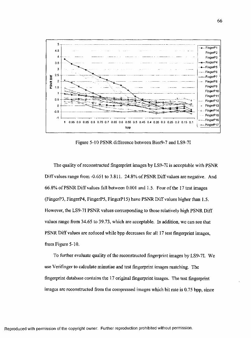
66

1 0,95 0.9 0.85 0.8 0.75 0.7 0.65 0.6 0.55 0.5 0.45 0.4 0.35 0.3 0.25 0.2 0.15 0.1

bpp

FingerPI FingerP2 FingerP3

-*-F ingerP4 FingerP5

-)— FingerP6 FingerP7- FingerP8

FingerPg FingerPlO FingerPIl FingerP12 F figerP13 F ngerP14 FingerPIS

— FingerPlO— FingerP 17

Figure 5-10 PSNR difference between Bior9-7 and LS9-7I

The quality o f reconstructed fingerprint images by LS9-7I is acceptable with PSNR

Diff values range from -0.651 to 3.811. 24.8% of PSNR Diff values are negative. And

66.8% of PSNR Diff values fall between 0.001 and 1.5. Four of the 17 test images

(FingerPS, FingerP4, FingerP5, FingerP 15) have PSNR Diff values higher than 1.5.

However, the LS9-7I PSNR values corresponding to those relatively high PSNR Diff

values range from 34.65 to 39.73, which are acceptable. In addition, we can see that

PSNR Diff values are reduced while bpp decreases for all 17 test fingerprint images,

from Figure 5-10.

To further evaluate quality of the reconstructed fingerprint images by LS9-7I. We

use Verifinger to calculate minutiae and test fingerprint images matching. The

fingerprint database contains the 17 original fingerprint images. The test fingerprint

images are reconstructed fi-om the compressed images which bit rate is 0.75 bpp, since


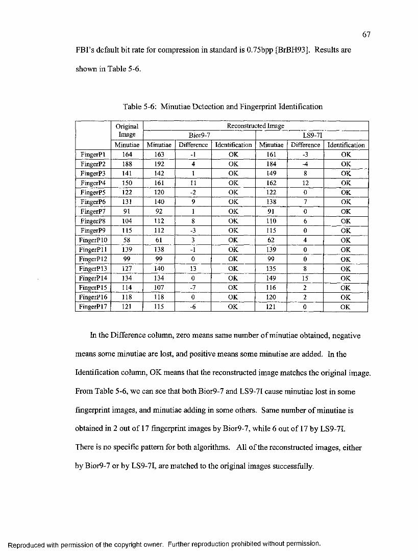
67

FBI’s default bit rate for compression in standard is 0.75bpp [BrBH93]. Results are

shown in Table 5-6.

Table 5-6; Minutiae Detection and Fingerprint Identification

OriginalImage

Reconstructed ImageBior9-7 LS9-7I

Minutiae Minutiae Difference Identification Minutiae Difference IdentificationFingerP 1 164 16S -1 OK 161 -S OKFingerP2 188 192 4 OK 184 -4 OKFingerPS 141 142 1 OK 149 8 OKFingerP4 ISO 161 11 OK 162 12 OKFingerPS 122 120 -2 OK 122 0 OKFingerP6 ISl 140 9 OK 1S8 7 OKFingerP? 91 92 1 OK 91 0 OKFingerPS 104 112 8 OK 110 6 OKFingerP9 l i s 112 -S OK 115 0 OK

FingerPlO 58 61 S OK 62 4 OKFingerPIl 1S9 1S8 -1 OK 1S9 0 OKFingerP 12 99 99 0 OK 99 0 OKFingerPIS 127 140 IS OK ISS 8 OKFingerP 14 1S4 1S4 0 OK 149 IS OKFingerPIS 114 107 -7 OK 116 2 OKFingerP 16 118 118 0 OK 120 2 OKFingerP 17 121 115 -6 OK 121 0 OK

In the Difference column, zero means same number of minutiae obtained, negative

means some minutiae are lost, and positive means some minutiae are added. In the

Identifieation column, OK means that the reconstructed image matches the original image.

From Table 5-6, we can see that both Bior9-7 and LS9-7I cause minutiae lost in some

fingerprint images, and minutiae adding in some others. Same number of minutiae is

obtained in 2 out of 17 fingerprint images by Bior9-7, while 6 out of 17 by LS9-7I.

There is no specific pattern for both algorithms. All of the reconstructed images, either

by Bior9-7 or by LS9-7I, are matched to the original images successfully.


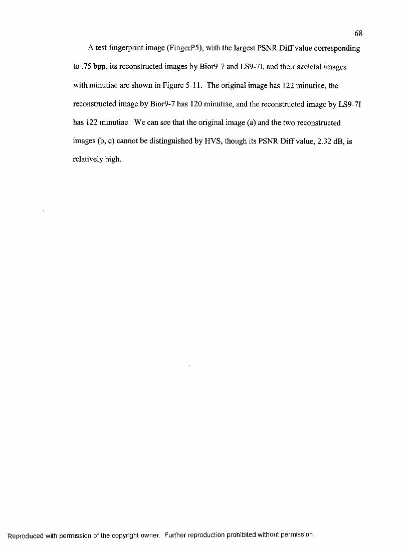
68

A test fingerprint image (FingerPS), with the largest PSNR Diff value corresponding

to .75 bpp, its reconstructed images by Bior9-7 and LS9-7I, and their skeletal images

with minutiae are shown in Figure 5-11. The original image has 122 minutiae, the

reconstructed image by Bior9-7 has 120 minutiae, and the reconstructed image by LS9-7I

has 122 minutiae. We can see that the original image (a) and the two reconstructed

images (b, c) cannot be distinguished by HVS, though its PSNR Diff value, 2.32 dB, is

relatively high.

Reproduced with permission ot the copyright owner. Further reproduction prohibited without permission.

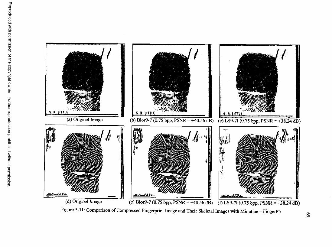
CD■DOQ .C

gQ .

■DCD

C/)

o '3O

8

CQ'

33"CD

CD■DOQ .CaO3

■DO

CDQ .

■DCD

C / )C / )

5 R UTTIE 5. R. UTTIE S.R.UTTIE(a) Original Image (b) Bior9-7 (0.75 bpp, PSNR - +40.56 dB) (c) LS9-7I (0.75 bpp, PSNR = +38.24 dB)

IL:.

0

: ■i'

1 *5 1 [

(d) Original Image (e) Bior9-7 (0.75 bpp, PSNR - +40.56 dB) (f) LS9-7I (0.75 bpp, PSNR = +38.24 dB)

Figure 5-11 : Comparison of Compressed Fingerprint Image and Their Skeletal Images with Minutiae - FingerPSO nNO

70

5.3 Computational Complexity

In this section, we compare the computational complexities of the wavelet transform

computed using standard algorithm (Bior9-7) with that computed using lifting-based

algorithm (LS9-7I). Bior9-7 is used as a comparison base. The unit we use is the cost,

measured in number of multiplications and additions, of computing one sample pair

In general, the cost of applying a «-tap filter h isn multiplications and (« - 1)

additions. The cost of the standard algorithm thus is (2« - 1). If the filter coefficients are

symmetric and the length of filter is odd, the cost is (3« - l)/2 with ((n - l) /2 + 1)

multiplications and (n - 1) additions. Therefore, for (9, 7) filters in WSQ, the total cost

of the standard algorithm is (13 + 10) - 23, in which the cost of applying 9-tap filter is 13

with 5 multiplications and 8 additions, and the cost of applying 7-tap filter is 10 with 4

multiplications and 6 additions.

Let us consider the lifting-based algorithm now. The cost of two scale steps (S5, S6)

is 1 multiplication each. The cost of four lifting steps (SI, S2, S3 and S4) is 1

multiplication and 2 additions each. Thus, the total cost of the lifting algorithm is (4 x (1

+ 2) + 2 X 1) = 14. Roughly, the cost of the lifting algorithm for (9, 7) filter is 60 percent

of the cost of the standard algorithm. Table5-1 gives the cost S of standard algorithm, the

cost L of the lifting-based algorithm, and the relative speedup {S/L - 1) for the (9, 7)

filters using in WSQ.


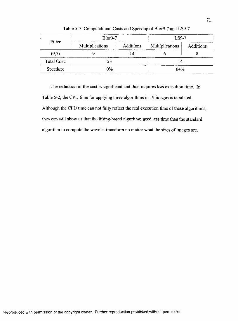
71

Table 5-7: Computational Costs and Speedup of Bior9-7 and LS9-7

FilterBior9-7 LS9-7

Multiplications Additions Multiplications Additions

(9 /0 9 14 6 8

Total Cost: 23 14

Speedup: 0% 64%

The reduction of the cost is significant and then requires less execution time. In

Table 5-2, the CPU time for applying three algorithms in 19 images is tabulated.

Although the CPU time can not fully reflect the real execution time of these algorithms,

they can still show us that the lifting-based algorithm need less time than the standard

algorithm to compute the wavelet transform no matter what the sizes of images are.


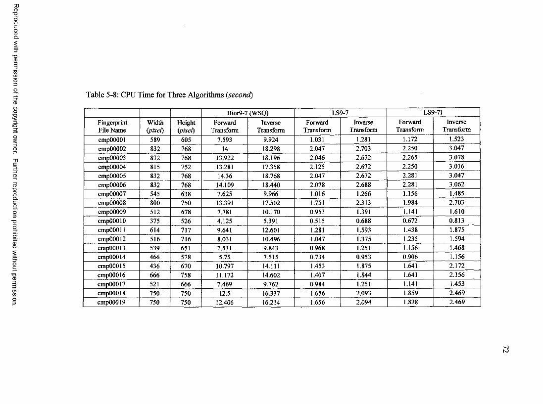
CD■DOQ .C

8Q .

■DCD

C/)C/)

Table 5-8: CPU Time for Three Algorithms (second)

8

CD

3.3"CD

3"OOQ .CaO3

■DO

CDQ .

■DCD

C / )C / )

Bior9-7 (WSQ) LS9-7 LS9-71

Fingerprint Width Height Forward Inverse Forward Inverse Forward InverseFile Name (pixel) (pixel) Transform Transform Transform Transform Transform Transform

cmpOOOOl SS9 605 7.593 9.924 1.031 1.281 1.172 1.523cmp00002 S32 76S 14 18.298 2.047 2.703 2.250 3.047cmpOOOOS S32 768 13.922 18.196 2.046 2.672 2.265 3.078cmp00004 SIS 752 13.281 17.358 2.125 2.672 2.250 3.016cmpOOOOS S32 76S 14.36 18.768 2.047 2.672 2.281 3.047cmpOOOOô S32 768 14.109 18.440 2.078 2.688 2.281 3.062cmpOOOO? 54S 638 7.625 9.966 1.016 1.266 1.156 1.485cmpOOOOS soo 750 13.391 17.502 1.751 2.313 1.984 2.703cmp00009 512 678 7.781 10.170 0.953 1.391 1.141 1.610cmpOOOlO 375 526 4.125 5.391 0.515 0.688 0.672 0.813cmpOOOll 614 717 9.641 12.601 1.281 1.593 1.438 1.875cmp00012 516 716 8.031 10.496 1.047 1.375 1.235 1.594cmpOOOlS 539 651 7.531 9.843 0.968 1.251 1.156 1.468cmp00014 466 578 5.75 7.515 0.734 0.953 0.906 1.156cmpOOOlS 436 670 10.797 14.111 1.453 1.875 1.641 2.172cmp00016 666 758 11.172 14.602 1.407 1.844 1.641 2.156cmpOOOl? 521 666 7.469 9.762 0.984 1.251 1.141 1.453cmpOOOlS 750 750 12.5 16.337 1.656 2.093 1.859 2.469cmp00019 750 750 12.406 16.214 1.656 2.094 1.828 2.469

K)

73

5.4 Summary

In this chapter, we first described the algorithm for traditional wavelet transform.

After that, we factorized this wavelet transform into a scheme based on lifting.

Furthermore, we modified the lifting-based algorithm to perform an integer-to-integer

transform. Consequently, a comparative study of these three algorithms was performed

considering Peak Signal-Noise-Ratio of the original and reconstructed fingerprint images

and cost of computation. The experimental results indicate the following:

• The quality of image reconstructed by lifting-based wavelet packet transform is

not significantly worse than that by the standard wavelet packet transform. The

lifting-based algorithm can be used to substitute the standard algorithm in WSQ.

• The computational cost of the lifting algorithm for (9, 7) filter is 60 percent of the

cost of the standard algorithm. In hardware implementation, the reduction of the

cost for computation makes lifting-based schemes a great choice for both high

throughput and low-power applications.

Based on above study, the conclusion is that the lifting-based integer wavelet

transform is an excellent alternative to the standard wavelet transform on fingerprint

processing, other than those wavelet transforms based on filter bank structure. We will

propose a VLSI architecture for WPT using lifting scheme to transform data integer to

integer in the following chapter.


CHAPTER 6

HARDWARE IMPLEMENTATION

In this chapter, a novel FPGA architecture for Wavelet Packet Transform (WPT) is

proposed which is optimized for special decomposition procedure based on WSQ

specification. We follow a bottom-up approach to describe the design — starting from the

lowest level and building up the structure of the design gradually.

6.1 Proposed Architecture

The proposed architecture calculates the forward transform and inverse transform

(IWPT) in row-column fashion on a block of data of size M^N. To perform the WPT, the

architecture reads in the block data, carries out the transform, and outputs the LL, LH,

HE, and HH data at each level of decomposition. To perform the IWPT, first all the sub

bands from the lowest level are read in. At the end, the LL, HL, LH and HH values of

the next higher level are obtained. Then, the transform values of all the four subbands

(LL, LH, HL, and HH) are read in, and IWPT is carried out in the new data set.

The architecture, as shown in Figure 6-1, consists of two processing modules (PMl

and PM2), and two memory modules (MEMl, MEM2). Each processing module

consists of two processing blocks (PB) along with a register file (REG). We have PBl,

PB2, and REGI for PMl, and have PB3, PB4, and REG2 for PM2. As mentioned in

Chapter 3, the forward transform and inverse transform of each subband are symmetrical

74


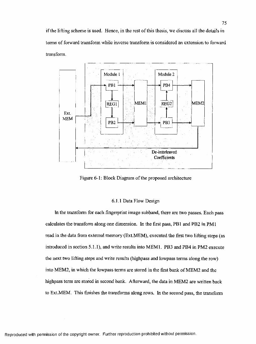
75if the lifting scheme is used. Hence, in the rest of this thesis, we discuss all the details in

terms of forward transform while inverse transform is considered an extension to forward

transform.

Ext.MEM

Module 1

PBl

REGI

PB2

MEMl

Module 2

PB4

REG2|

PB3

MEM2

De-interleavedCoefficients

Figure 6-1 : Block Diagram of the proposed architecture

6.1.1 Data Flow Design

In the transform for each fingerprint image subband, there are two passes. Each pass

calculates the transform along one dimension. In the first pass, PBl and PB2 in PMl

read in the data firom external memory (Ext.MEM), executed the first two lifting steps (as

introduced in section 5.1.1), and write results into MEMl. PB3 and PB4 in PM2 execute

the next two lifting steps and write results (highpass and lowpass terms along the row)

into MEM2, in which the lowpass terms are stored in the first bank of MEM2 and the

highpass term are stored in second bank. Afterward, the data in MEM2 are written back

to Ext.MEM. This finishes the transforms along rows. In the second pass, the transform


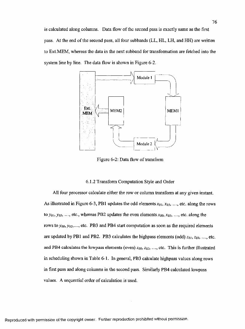
76is calculated along columns. Data flow of the second pass is exactly same as the first

pass. At the end of the second pass, all four subbands (LL, HL, LH, and HH) are written

to Ext.MEM, whereas the data in the next subband for transformation are fetched into the

system line by line. The data flow is shown in Figure 6-2.

Module 2

Module 1

MEM2 MEMlExt.

MEM

Figure 6-2: Data flow of transform

6.1.2 Transform Computation Style and Order

All four processor calculate either the row or column transform at any given instant.

As illustrated in Figure 6-3, PBl updates the odd elements xqi, xqs, ..., etc. along the rows

to yoi, yo3 , •.., etc., whereas PB2 updates the even elements xoo, xq2 , ■■■, etc. along the

rows to y 0 0 , y 0 2 ,. ., etc. PB3 and PB4 start computation as soon as the required elements

are updated by PBl and PB2. PB3 calculates the highpass elements (odd) zoi, zos, ..., etc.

and PB4 calculates the lowpass elements (even) zoo, Z02, ■■■, etc. This is further illustrated

in scheduling shown in Table 6-1. In general, PB3 calculate highpass values along rows

in first pass and along columns in the second pass. Similarly PB4 calculated lowpass

values. A sequential order of calculation is used.


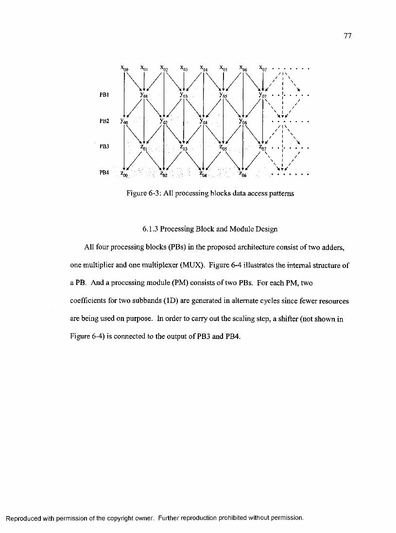
77

'00 '01 '0 2 '0 3 '0 4 '05 '0 6 '0 7

PBl

PB2

PB3

PB4

Figure 6-3: All processing blocks data access patterns

6.1.3 Processing Block and Module Design

All four processing blocks (PBs) in the proposed architecture consist of two adders,

one multiplier and one multiplexer (MUX). Figure 6-4 illustrates the internal structure of

a PB. And a processing module (PM) consists of two PBs. For each PM, two

coefficients for two subbands (ID) are generated in alternate cycles since fewer resources

are being used on purpose. In order to carry out the scaling step, a shifter (not shown in

Figure 6-4) is connected to the output of PB3 and PB4.


78

PB

select0: Forward > operation 1: Inverse C peration

— : Mode Select Signal

— ► : Data Stream

□ B : Lifting Coefficient

© : Adder

© : Multiplier

Figure 6-4: The architecture of Processing Block.

Note that in this lifting-based architecture, PBs are not only designed for forward

transform but also for inverse transform because DWT and IDWT of each subhand are

symmetrical. A multiplexer built in processing block achieves the coefficient-choosing

mechanism for both transforms. Thus, there are two working modes for system, mode 0

and mode 1. Selecting mode 0 will make the PBs working on forward operation, that the

coefficients of forward transform are input to multipliers. Selecting mode 1 will make

system working on inverse operation, and the coefficients of forward transform are input.

6.1.4 Integer-to-integer Transform Design

As discussed in Chapter 5, the lifting scheme makes the transform possible from

integer to integer without loss of the image quality. And in the hardware implementation,

the integer arithmetic will be executed more efficiently and the hardware complexity will

be reduced dramatically. So, an integer-to-integer transform is adopted here.


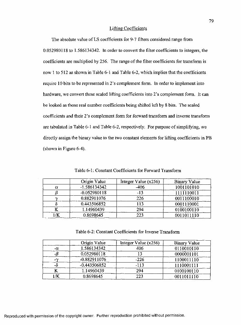
79Lifting Coefficients

The absolute value of LS coefficients for 9-7 filters considered range from

0.052980118 to 1.586134342. In order to convert the filter coefficients to integers, the

coefficients are multiplied by 256. The range of the filter coefficients for transform is

now 1 to 512 as shown in Table 6-1 and Table 6-2, which implies that the coefficients

require 10 bits to be represented in 2’s complement form. In order to implement into

hardware, we convert these scaled lifting coefficients into 2’s complement form. It can

be looked as those real number coefficients being shifted left by 8 bits. The scaled

coefficients and their 2’s complement form for forward transform and inverse transform

are tabulated in Table 6-1 and Table 6-2, respectively. For purpose of simplifying, we

directly assign the binary value to the two constant elements for lifting coefficients in PB

(shown in Figure 6-4).

Table 6-1; Constant Coefficients for Forward Transform

Origin Value Integer Value (x256) Binary Valuea -1.586134342 -406 1001101010/3 -0.052980118 -13 11111100117 0.882911076 226 001I 100010Ô 0.443506852 113 0001110001K 1.14960439 294 0100100110

1/K 0.8698645 223 0011011110

Table 6-2: Constant Coefficients for Inverse Transform

Origin Value Integer Value (x256) Binary Value-a 1.586134342 406 0110010110-13 0.052980118 13 0000001101-7 -0.882911076 -226 1100011110-Ô -0.443506852 -113 lllO O O lIllK 1.14960439 294 0100100110

1/K 0.8698645 223 0011011110


80

At the end of the multiplication, the product is shifted right by 8 to get the required

result. This is implemented in hardware by rounding the eight least significant hits. The

products are rounded to the next highest integer. And rounding operation is applied to

the individual product terms instead of applying rounding to the results of the filter

operation in order to avoid building a bigger accumulator.

Signal Values

The signal values have to be shifted left 2 hits as well in order to increase the

precision. This shift operation occurs at the input signal. After accumulating all factors,

the PB will shift the result right by 2 bits. An example is given below to illustrate this

integer-to-integer transform scheme.

Consider the general structure in a lifting-based scheme

y = %, + nx(Xo (6-1)

where a is the lifting coefficient, xs are the signal samples , y is the transform value and

with a = 0.2345, xq = 156, xj = 10, X2 = 56. The floating-point implementation result is y

- 59.714. Let’s assume that the lifting coefficient is shifted left by 8 bits (and round to

nearest integer) and the signal samples are shifted left by 2 hits. Then, a = 60, xo = 624,

xi = 40, X2 = 224. The product is 60 (624 + 224) = 50880. Shifting the product right by 8

hits and rounding will yield 199. Therefore, y = 40+ 199 = 239. This should be

interpreted as round [239/4 + decimal equivalent of two LSBs of 239] = round [59 + 0.75]

= 60.


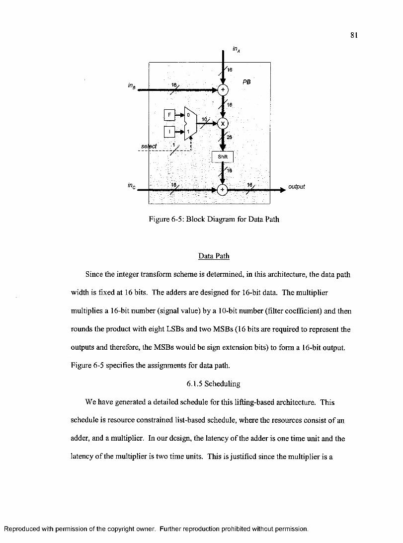
81

PB

Shift

output

Figure 6-5: Block Diagram for Data Path

Data Path

Since the integer transform scheme is determined, in this architecture, the data path

width is fixed at 16 bits. The adders are designed for 16-bit data. The multiplier

multiplies a 16-bit number (signal value) by a 10-bit number (filter coefficient) and then

rounds the product with eight LSBs and two MSBs (16 bits are required to represent the

outputs and therefore, the MSBs would be sign extension bits) to form a 16-bit output.

Figure 6-5 specifies the assignments for data path.

6.1.5 Scheduling

We have generated a detailed schedule for this lifting-hased architecture. This

schedule is resource constrained list-based schedule, where the resources consist of an

adder, and a multiplier. In our design, the latency of the adder is one time unit and the

latency of the multiplier is two time units. This is justified since the multiplier is a


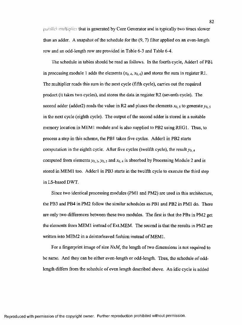
82

p ara lle l multiplier that is generated by Core Generator and is typically two times slower

than an adder. A snapshot of the schedule for the (9, 7) filter applied on an even-length

row and an odd-length row are provided in Table 6-3 and Table 6-4.

The schedule in tables should be read as follows. In the fourth cycle, Adder 1 of PBl

in processing module 1 adds the elements (xq, 4, %o, e) and stores the sum in register R 1.

The multiplier reads this sum in the next cycle (fifth cycle), carries out the required

product (it takes two cycles), and stores the data in register R2 (seventh cycle). The

second adder (adder2) reads the value in R2 and pluses the elements xq, 5 to generate yo, 5

in the next cycle (eighth cycle). The output of the second adder is stored in a suitable

memory location in MEMl module and is also supplied to PB2 using REGl. Thus, to

process a step in this scheme, the PBl takes five cycles. Adder 1 in PB2 starts

computation in the eighth cycle. After five cycles (twelfth cycle), the result yo, 4

computed from elements yo, 3, yo, 5 and jco, 4 is absorbed by Processing Module 2 and is

stored in MEMl too. Adder 1 in PB3 starts in the twelfth cycle to execute the third step

in LS-based DWT.

Since two identical processing modules (PMl and PM2) are used in this architecture,

the PB3 and PB4 in PM2 follow the similar schedules as PBl and PB2 in PMl do. There

are only two differences between these two modules. The first is that the PBs in PM2 get

the elements from MEMl instead of Ext.MEM. The second is that the results in PM2 are

written into MEM2 in a deinterleaved fashion instead of MEMl.

For a fingerprint image of size NxM, the length of two dimensions is not required to

be same. And they can be either even-length or odd-length. Thus, the schedule of odd-

length differs from the schedule of even length described above. An idle cycle is added


83right after PBl and PB3 complete the computation of a row or column. This is illustrated

in Table 6-4 as marked a symbol


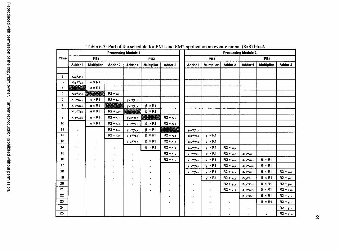
CD■ D

OQ .C

gQ .

■ DCD

C/)Wo"303CD

8

ci'3"

13CD

"nc3.3 "CD

CD■ D

OQ .CaO3■DO

CDQ .

■ DCD

C/)C/)

Table 6-3: Part of the schedule for PMl and PM2 applied on an even-element (8x8) block

TimeProcessing Module 1 Processing Moduie 2

PBl PB2 PB3 PB4

Adder 1 Muttipiier Adder 2 Adder 1 Muitipiier Adder 2 Adder 1 Muitipiier Adder 2 Adder 1 Multiplier Adder 2

12 Xo.O+Xo,23 Xo,2+Xo,4 a X Ri

4 a X R15 Xo.6+Xo,8 R2 + X0.1

6 Xl.0+Xl,2 a X R1 R2 + Xo,3 y o ,i+ y o ,i

7 Xl,2+Xl,4 a X Ri yo ,i+ y o ,3 P xR1

8 Xl.4+X,,6 a X Ri R2 + Xo,7 3 xR1

9 Xl,6+Xl,6 a X R1 R2 + X i,i yo,5+yo,7 R2 + Xo.o

10 a X RI R2 + Xi,3 y i , i + y i , i 3 xR1 R2 + Xo,211 R2 + Xi,5 y i . i+ y i .3 3 xR1 yo.o+yo.2

12 R2 + Xi,7 y i ,3 + y i,5 3 xR1 R2 + Xo,6 yo,2+yo,4 y x R i

13 y i.5 + y o ,7 3 xR1 R2 + Xi,o yo,4+yo,6 V X RI

14 3 xR1 R2 + Xi,2 yo,6+yo,8 Y xR I R2 + yo,i

15 R2 + Xi 4 y i ,o + y i,2 Y X RI R2 + yo,3 Zo,1+ Z o,116 R2 + Xi,6 y i.2 + y i .4 Y X RI R2 + Yo.s Zo.l+Zo.3 6 X RI

17 y i .4 + y i.8 Y xR1 R 2 + yo,7 Zo.3+Zo,5 6 X R1

18 y i,8 + y i,8 Y xR1 R2 + Y i,i Zo,6+Zo,7 5 X RI R 2 + Yo.o

19 Y X RI R2 + Yi ,3 Z l,1 + Z l,l 6 X RI R 2 + yo,2

20 R 2 + y i,5 Z l,1 + Z i,3 5 X R1 R 2 + yo,4

21 R2 + y i,7 Z l,3 + Z i,5 5 X R1 R 2 + yo.8

22 Z l.5 + Z l,7 5 X R1 R 2 + y i ,o

23 5 X R1 R 2 + y i ,2

24 R 2 + Yi .4

25 R 2 + y i.6OO4:

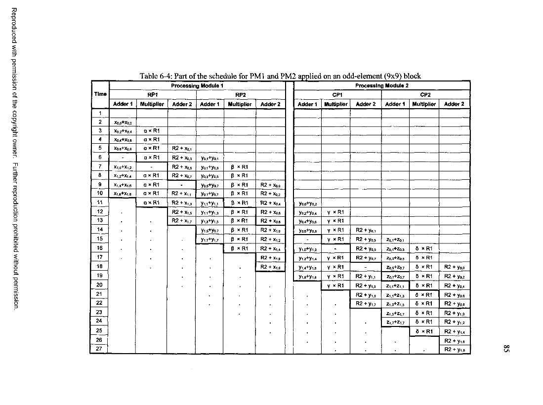
CD■DOQ .C

8Q .

"DCD

(/)Wo"303CD

8ci'3 "

13CD

"nc3.3 "CD

CD■DOQ .CaO3"OO

CDQ .

■DCD

C/)(/)

Table 6-4: Part of the schedule for PMl and PM2 applied on an odd-element (9x9) block

TimeProcessing Module 1 Processing Moduie 2

RP1 RP2 CPI CP2

Adder 1 Multiplier Adder 2 Adder 1 Multiplier Adder 2 Adder 1 Multiplier Adder 2 Adder 1 Multiplier Adder 21

2 Xo,0+Xo,23 Xo,2+Xo,4 a X R I

4 Xo,4+Xo,6 a X R I

5 Xo,S+Xo,8 a X R I R 2 + X0.16 - a X R 1 R 2 + Xo,3 yo,i+yo,i7 Xl,0+Xl,2 - R 2 + X0.5 yo ,i+ yo .3 P x R 1

8 X l,2+X l,4 a X R I R 2 + Xo,7 yo,3+yo,5 P X R 1

9 X l,4+X l,8 a X R I - yo .s+yo,7 P x R 1 R 2 + Xo.o

10 Xl,8"*"Xl,8 a X R I R 2 + x i , i yo,7+yo,7 P X R 1 R 2 + Xo,2

1 1 a X R I R 2 + X i ,3 y i , i + y i . i P * R 1 R 2 + X o ,4 y o .o + y o ,21 2 R 2 + x ,.5 y i , i+ y i .3 P X R I R 2 + Xo,6 yo.2+yo,4 V X R I

13 R2 + x i,7 y i .3 + y i,5 P X R 1 R 2 + Xo.8 yo,4+yo,8 V X R 1

14 y i,5 + y o ,7 P x R 1 R 2 + Xi,o yo,6+yo.8 V X R I R 2 + yo ,i

15 y i,7 + y i,7 P X R 1 R 2 + Xi,2 - V x R 1 R 2 + yo,3 Z o .l+ Z o .116 P x R 1 R 2 + Xi,4 yi,o+yi.2 - R 2 + yo.5 Zo.1+Zo,3 5 X R I

17 R2 + x,,6 y i.2 + y i .4 Y X R 1 R 2 + yo.7 Zo,3+Zo,5 6 x R 1

18 R 2 + Xi.8 y i ,4 + y i .8 Y X R I - Z d,5+Z o,7 5 x R 1 R 2 + Yo.o

19 y i,8 + y i.8 Y X R I R 2 + y i , i Zo.7+Zo,7 6 X R 1 R 2 + Yo,220 Y X R1 R 2 + y i ,3 Z l,1 + Z i,i 5 X R I R 2 + Yo,42 1 R 2 + y , .5 Z l.1 + Z i,3 5 X R 1 R 2 + Yo,622 R 2 + y ,,7 Z l,3 + Z i,5 6 X R 1 R 2 + yo.8

23 Z i ,5+ Z i ,7 5 X R I R 2 + y i .o

24 Z i ,7 + Z i ,7 5 X R1 R 2 + y i ,2

25 5 X R I R 2 + y 1.4

26 R 2 + y i .8

27 R 2 + y 1,8 00LA

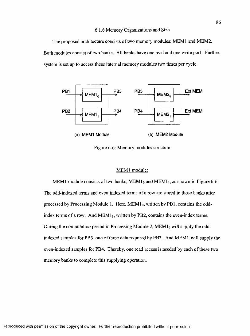
866.1.6 Memory Organizations and Size

The proposed architecture consists of two memory modules: MEMl and MEM2.

Both modules consist of two banks. All banks have one read and one write port. Further,

system is set up to access these internal memory modules two times per cycle.

Ext.MEMPB3PB3PB1

PB4 Ext.MEMPB4PB2MEM2

MEM2,MEM1

MEM1

(a) MEM1 Module (b) MEM2 Module

Figure 6-6: Memory modules structure

MEMl module:

MEMl module consists of two banks, MEMlo and MEMl,, as shown in Figure 6-6.

The odd-indexed terms and even-indexed terms of a row are stored in these banks after

processed by Processing Module 1. Here, MEMlo, written by PBl, contains the odd-

index terms of a row. And MEM l,, written by PB2, contains the even-index terms.

During the computation period in Processing Module 2, MEMlo will supply the odd-

indexed samples for PB3, one of three data required by PB3. And M EM l, will supply the

even-indexed samples for PB4. Thereby, one read access is needed by each of these two

memory banks to complete this supplying operation.


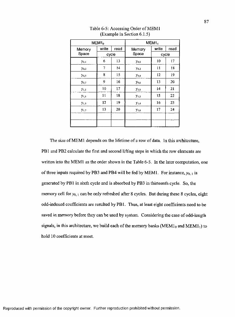
87Table 6-5: Accessing Order of MEMl

(Example in Section 6.1.5)

M E M lo M E M I1

M em oryS p a c e

w rite read M em oryS p a c e

w rite read

c y c le c y c le

yo.i 6 13 yo,o 10 17

yo,3 7 14 yo,2 11 18

yo,5 8 15 yo,4 12 19

yo,7 9 16 yo,6 13 20

yi.i 10 17 yi.o 14 21

yi,3 11 18 yi,2 15 22

yi,5 12 19 yi,4 16 23

yi,7 13 20 yi.6 17 24

The size of MEMl depends on the lifetime of a row of data. In this architecture,

PBl and PB2 calculate the first and second lifting steps in which the row elements are

written into the MEMl as the order shown in the Table 6-5. In the later computation, one

of three inputs required by PB3 and PB4 will be fed by M EM l. For instance, yo, i is

generated by PBl in sixth cycle and is absorbed by PB3 in thirteenth cycle. So, the

memory cell foryo, i can be only refreshed after 8 cycles. But during these 8 cycles, eight

odd-indexed coefficients are resulted by PBl. Thus, at least eight coefficients need to be

saved in memory before they can be used by system. Considering the case of odd-length

signals, in this architecture, we build each of the memory banks (MEMlo and MEMl i) to

hold 10 coefficients at most.


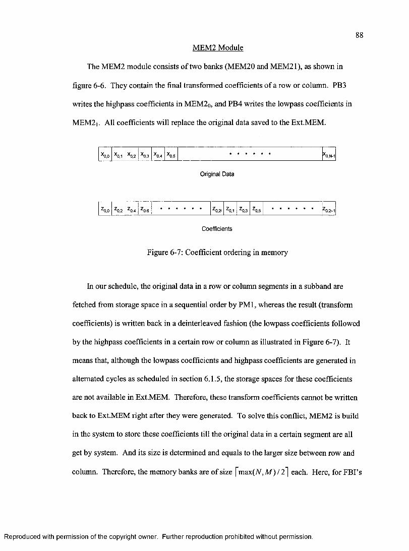
88MEM2 Module

The MEM2 module consists of two banks (MEM20 and MEM21), as shown in

figure 6-6. They contain the final transformed coefficients of a row or column. PB3

writes the highpass coefficients in MEM2q, and PB4 writes the lowpass coefficients in

MEM2,. All coefficients will replace the original data saved to the Ext.MEM.

^0,0 ^0,1 \ , 2 ^0,3 * 0 4 *0,5 *0,N-1

Original Data

Coefficients

Figure 6-7: Coefficient ordering in memory

In our schedule, the original data in a row or column segments in a subband are

fetched from storage space in a sequential order by PMl, whereas the result (transform

coefficients) is written back in a deinterleaved fashion (the lowpass coefficients followed

by the highpass coefficients in a certain row or column as illustrated in Figure 6-7). It

means that, although the lowpass coefficients and highpass coefficients are generated in

alternated cycles as scheduled in section 6.1.5, the storage spaces for these coefficients

are not available in Ext.MEM. Therefore, these transform coefficients cannot be written

back to Ext.MEM right after they were generated. To solve this conflict, MEM2 is build

in the system to store these coefficients till the original data in a certain segment are all

get by system. And its size is determined and equals to the larger size between row and

column. Therefore, the memory banks are of size fmax(A, M ) / 1 \ each. Here, for FBI’s


89application here, up to 850x850 pixels per fingerprint, the quantity to contain 500 pixel

values each bank is sufficient.

6.1.7 Control

Control signals are needed primarily to maintain the steady flow o f data to and from

the processors. Our design consists of two PM controllers and one WPT controller. The

PM controllers locate in each of the processing modules. And the WPT controller is a

top-level controller of the whole architecture. All controllers communicate with each

other by handshaking signals. WPT controller generates the addresses needed to get the

correct input subband. And the PM controllers command the processing modules to do

the actual transform works. Each controller consists of three components: Counter,

Memory Read and Write Signals Generation Unit (MSGU), and Address Generation Unit

(AGU).

In the WPT controller. Counter records the number of the wavelet transform level

and the number of the subbands being processed. MSGU generates the read and write

logic to direct the system to access subbands in the Ext.MEM. According to output of

counter and logic signals, AGU generates the addresses of the start point and end point of

subbands. These signals are passed to processing module and drive the PM to complete

the wavelet transform for each subband. WPT controller is programmable to suit for

different wavelet transform schemes by changing the read and write logic. Here, a five-

level transform with 64 subbands is designed. And it is easy to expand system to execute

a fully WPT.

PM controllers start working after getting commands fi-om WPT controller. In this

controller. Counters keep track of the number of rows and the number o f elements in each


90row that have been processed, which are primarily used to generate the memory read and

write signals. All the counters are capable of counting up to a maximum of N. MSGU,

which is driven by counter output, generates the signals required for memory reads and

writes (i.e., row, element values). One of the inputs to the second adder (in all the

processing blocks) has to be read from memory, and the memory write signals are

generated based on this signal. And the exactly element address is generated by AGU

with an “in place” addressing scheme.

6.1.8 Timing

The latency of this system depends on latency of the processing blocks and the start

time of PB3. We assume the latency of the adder is t^, and the delay of the multiplier is

Tm- For each processing block, the latency is

latencyPB = 2 t„ + . ( 6 -2 )

And in our architecture, PB3 can start the transform right after two required elements of

the first adder are ready. As shown in Table 6-1, it takes one cycle. Thereby, to get the

first output of transformed coefficient, the latency is

latency = 4 x latencyps + 1

= STo + 4 7}» + 1. (6-3)

Therefore, the total time required for one level of decomposition of an A x M subband is

calculated as following

tiynepQidi timecQi f fi 4* titnerow

= {latency + |”A / 2 ] x M ) + {latency + |”m / 2 ] x A )

= 2 X latency + { \n I 1 \x M + \ M N ) (6-4)

Substituted equation 6-3 in equation 6-4, the time required for this architecture is


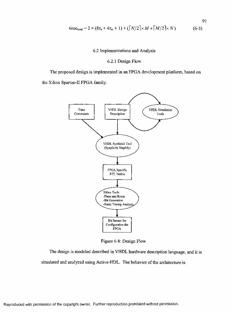
91

timctotai = 2 X ( 8 t« + 4t„ + 1) + { \ N / 2 ] x M + [M/2"1x7V^)

6.2 Implementations and Analysis

6.2.1 Design Flow

The proposed design is implemented in an FPGA development platform, based on

the Xilinx Spartan-II FPGA family.

ConstraintsVHDL Design

Description

1'

VHDL Synthesis Tool (Synplicity Sinplify)

FPGA Specific RTL Netlist

Xilinx Tools -Place and Route -Bit Generation -Static Timing Analysis

Bit Stream for Configuration the

FPGA

VHDL Simulation Tools

Figure 6-8: Design Flow

The design is modeled described in VHDL hardware description language, and it is

simulated and analyzed using Active-HDL. The behavior of the architecture is


92synthesized using Synplify Pro synthesis package. Then, the implementation tool, Xilinx

ISE, is used to map the logic to componets, place the logic cells, route the signals, and

generate a bitstream file to do the final configuration in the FPGA device.

The technology libraries and symbol libraries that were used in Active-HDL,

Synplify and Xilinx ISE for synthesis and simulation were all based on the standard

library for Xilinx FPGA. This guarantees that synthesized design has the nearest

simulation results as the final implementation.

Transferring the design from Synplify Pro to Xilinx ISE is accomplished by

generating a VHDL netlist as a logical design file format, which creates symbol and

schematic views for all levels of the design hierarchy. In our design, an EDIF file (one

format of netlist) is created for the following usages.

By implementing to a specific Xilinx architecture, the logical design file format, like

the EDIF just achieved, is converted into a physical file format. The physical information

for FPGAs is contained in the Native Circuit Description (NCD) file.

Many verification simulation steps are involved in the design flow. The first one is

named Register Transfer Level (RTL) simulation which uses VHDL simulation tools to

verify the functional correctness of the architecture’s behavior. The second is a post

synthesis functional simulation which is applied to confirm the functionality of the

extracted gate-level circuit. The third, post-implementation simulation ensures that the

gate-level schematic, which has been imported and edited in Xilinx ISE, is equivalent to

the proposed architecture. These are followed by the DRC (design rule checking), which

evaluate the NCD file for problems that could prevent the design fi-om functioning


93properly and is done with Xilinx BitGen. Once DRC is done, it is assumed that the

design is functional correct.

At last, the final bitstream is generated from the NCD file. It can be used to program

the Xilinx device with Xilinx iMPACT software package.

6.2.2 Design Units and Their Implementations

Design Units

Here is a short description of the VHDL design units:

Adder/Subtracter: This is a component created by Core Generator. It operates on

signed data. The data inputs are provided on the A and B input buses,

which is a 16-bit bus each. It is used in the design unit — Processing

Block.

Multiplier: This component was generated with the Core Generator, too. This

multiplier functions a 16-bit data by 10-bit data multiplying operation.

The output bus width is 20-bit. It is used in the Processing Block for

multiplying the lifting coefficients with the corresponding data which is a

sum of two pixels.

Processing Block: This unit consists of three components which are one

multiplier, one 2-to-l multiplex, and two adders. It executes one of four

lifting steps. Processing block is used as a component in the architecture

of entity — Processing Modules. The output of multiplier in this unit is

rounded from 26 bits to 16 bits as illustrated in section 6.1.4.


94Processing Module: Each processing module consists of two processing block.

They are controlled by a state machine to read/write data. This entity-

architecture pair implements the schedule as specified in section 6.1.5.

DWT_97_Core: This entity-architecture pair includes two components which are

PMl and PM2. The function of this unit is to execute a one-dimension

transform for elements based on line. Under command of a state machine,

it also reads data from MEM modules and writes the results back.

MEMl Module, MEM2 Module: These components were generated with Core

Generator. They function as storage elements for the results of two

Processing Modules in this system as described in section 6.1.6.

WPT Controller: This entity-architecture pair implements the control functions

for Wavelet Packet Transform. It generates signals and data required by

transformation, such as the size of subband, and the location of data in

storage space.

Transform (top-level entity): This entity-architecture pair instantiates all

necessary components and describes the interconnections to compose the

organization described in section 6.1. In this design unit, a number of

state machines implement this 2-D wavelet packet transform algorithms.

Implementation Results

The logic resources of the FPGA are divided in different categories as Look-Up-

Tables (LUT), Input/Output Blocks (lOB), Flip-flops, Multiplex, RAM Blocksetc. A

specific group of a number of these resources is called Configurable Logic Block (CLB)


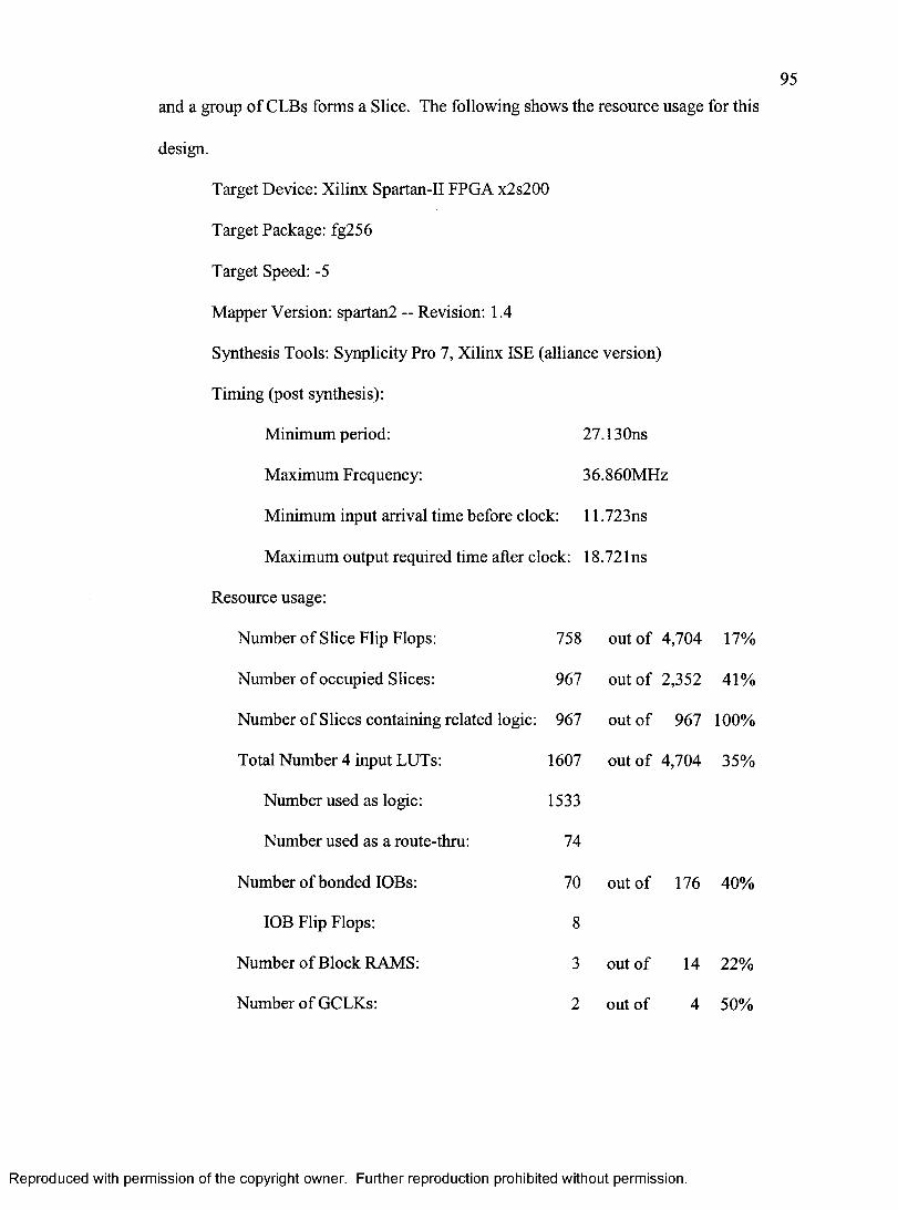
95and a group of CLBs forms a Slice. The following shows the resource usage for this

design.

Target Device; Xilinx Spartan-II FPGA x2s200

Target Package: fg256

Target Speed: -5

Mapper Version: spartan2 — Revision: 1.4

Synthesis Tools: Synplicity Pro 7, Xilinx ISE (alliance version)

Timing (post synthesis):

Minimum period: 27.130ns

Maximum Frequency: 36.860MHz

Minimum input arrival time before clock: 11.723ns

Maximum output required time after clock: 18.721ns

Resource usage:

Number of Slice Flip Flops: 758 out of 4,704 17%

Number of occupied Slices: 967 out of 2J52 41%

Number of Slices containing related logic: 967 out of 967 100%

Total Number 4 input LUTs: 1607 out of 4,704 35%

Number used as logic: 1533

Number used as a route-thru: 74

Number of bonded lOBs: 70 out of 176 40%

lOB Flip Flops: 8

Number of Block RAMS: 3 out of 14 22%

Number of GCLKs: 2 out of 4 50%


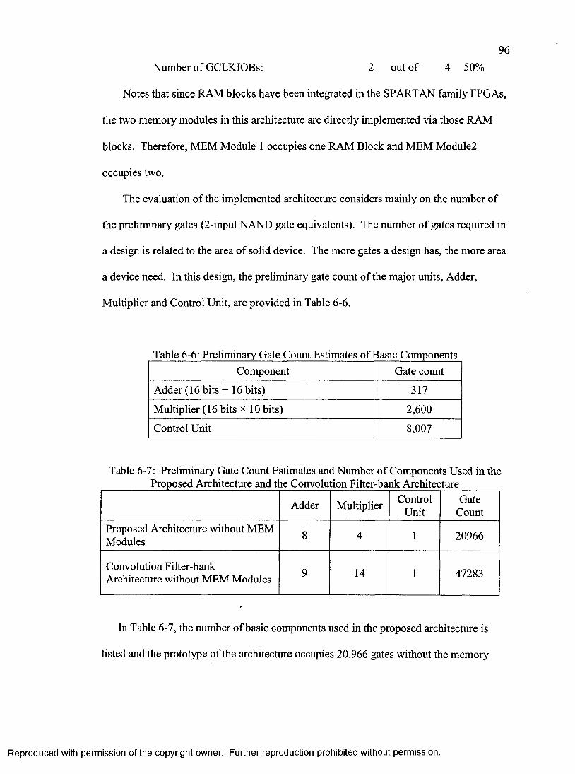
96Number of GCLKIOBs: 2 out of 4 50%

Notes that since RAM blocks have been integrated in the SPARTAN family FPGAs,

the two memory modules in this architecture are directly implemented via those RAM

blocks. Therefore, MEM Module 1 occupies one RAM Block and MEM Module2

occupies two.

The evaluation of the implemented architecture considers mainly on the number of

the preliminary gates (2-input NAND gate equivalents). The number of gates required in

a design is related to the area of solid device. The more gates a design has, the more area

a device need. In this design, the preliminary gate count of the major units. Adder,

Multiplier and Control Unit, are provided in Table 6-6.

Table 6-6: Preliminary Gate Count Estimates o f f lasic ComponentsComponent Gate count

Adder (16 bits +16 bits) 317

Multiplier (16 bits x 10 bits) 2,600

Control Unit 8,007

Table 6-7: Preliminary Gate Count Estimates and Number of Components Used in theProposed Architecture and t le Convolution Filter-bank Architecture

Adder Multiplier ControlUnit

GateCount

Proposed Architecture without MEM Modules 8 4 1 20966

Convolution Filter-bank Architecture without MEM Modules 9 14 1 47283

In Table 6-7, the number of basic components used in the proposed architecture is

listed and the prototype of the architecture occupies 20,966 gates without the memory


97modules. For the sake of comparison, the preliminary gate counts for the convolution

filter-bank architecture are also tabulated in Table 6-7. Because of the hierarchy in the

design, the same basic components like adder unit and multiplier unit, and the same top-

level controller are used. Only the DWT 97 Core is implemented with convolution-

based algorithm instead of LS based one. Comparing first row and second row in table 6-

7, we can notice that the number of Adder unit decreases from 14 in convolution based

scheme down to 8 in the proposed architecture. In the meantime, the number of multiplier

unit decreases from 9 down to 4. The reductions cause the total gates required by

proposed architecture based on integer LS scheme decreasing dramatically, which is from

47283 down to 20966. The ratio of reduction on gates reaches to 56 percentages.

6.3 Summary of Chapter 6

In this chapter, a hardware architecture for WPT algorithm in fingerprint image

processing was proposed and explored in details. First, the framework was explained as a

combination of several functional modules - processing module, memory module, etc.

Subsequently, the data flow among the modules was discussed and an integer transform

was designed. Furthermore, the schedules of computation were analyzed. Based on

these schedules, the processing modules and memory modules were designed and

arranged well. At last, this architecture was implemented into a hardware platform,

which is a Xilinx Spartan-II family FPGA. The result of implementation shows us that

the usage of hardware by lifting architecture is only half of the usage of convolution filter

structure. The goal of reducing hardware requirement was achieved.


CHAPTER 7

CONCLUSIONS AND FUTURE WORK

7.1 Conclusions

In this thesis, a VLSI architecture implementing a wavelet packet transform

algorithm for fingerprint image compression was proposed. The wavelet packet

transform algorithm is based on lifting scheme (LS9-7I) instead of the traditional

convolution method (Bior9-7) used by FBI. And it can transform the image pixel values

in the integer format. This architecture was implemented on reprogrammable hardware -

FPGA. We compared the quality of the reconstructed images processed by LS9-7I and

Bior9-7 by means of image quality measure - Peak Signal-to-Noise Ration (PSNR) and

the application of identification - fingerprint matching. We also compared the hardware

usages after synthesis of both architectures. Comparison results show that our proposed

architecture can reduce the size of processor to half and the loss of image quality is

insignificant and acceptable.

The proposed hardware can fulfill the wavelet packet transform on fingerprint image

efficiently. The quality o f the reconstructed image is acceptable. To compare it to one

by Bior9-7, the difference cannot be distinguished by human visual system, though the

fingerprint images reconstructed by LS9-7I have slightly lower peak signal-to-noise ratio

values than those by Bior9-7. Furthermore, the reconstructed image still can be matched

with the original image successfully, by calculating the minutiae.

98


99Lifting scheme leads to a speedup when compared to the traditional (convolution

filter-banks) implementation. At the meantime, the hardware usage of lifting-based

architecture is significantly less than that of the traditional architecture.

In the processor hardware, integer arithmetic is generally much faster than floating

point arithmetic. Integer numbers are more efficient to transform and take less space to

store. Hence, the feature of the integer-to-integer transformation of lifting scheme makes

the processor computationally efficient as well as permits lossless representation of the

image pixels.

Computation intensive problems often require a hardware intensive solution. Unlike

a general purpose microprocessor with fixed number o f Arithmetic and Logic Unit

(ALU), a hardware implementation on FPGAs can achieve greater parallelism, and hence

higher throughput.

7.2 Future Work

The lessons learned from this experience will help us enhance similar

implementations in the future. Few of the improvements that we now foresee are listed

below:

The controller unit is reconfigurable so that, if necessary, this architecture is not only

able to process WPT for fingerprint images, but also provides a method to process any

type of two-dimensional WPT.

The design has the potential of further performance improvement. The hardware

unit is designed to be hierarchical and scalable. This means that, when enough hardware


100resources are available, the multiple units can be cascaded to achieve the requirement of

higher speed processing.

A corresponding coder-codec can be built on the FPGA to process the obtained

wavelet coefficients. Furthermore, it is worth to implement FBI fingerprint image

processing on a single processor completely.

Data movement from processor to out-chip image storage and back to processor

takes a significant amount of the processing time. Data movement could have been

minimized. A suggestion with respect to embedded memory architecture is to increase

the size of embedded memory modules, so that the subband that will be processed in next

iteration can be stored and fetched by processor more quickly.

When FPGAs are utilized more than 40%, the timing performance drops sharply.

This is because the FPGA runs out of routing resources. Consequently many long and

circuitous routes are resulted. Hence the overall system clock drops. One possible

solution to this problem is to compromise between FPGA utilization and timing

performance to achieve more optimized results. Another possible solution is to improve

the timing performance by applying the FPGA decomposition method to optimize the

route scheme in the synthesis step.


BBLIOGRAPHY

[ANSt93] American National Standard, Data format for interchange offingerprint

information, NatT. Inst. Standards Tech., June 1993. {ANSI/NISTCSL, 1-

1993}

[Bris95] C. M. Brislawn, “Fingerprints Go Digital”, Notices o f the American

Mathematical Society, vol. 42, no. 11, pp. 1278-1283, November 1995.

[BrBH93] J. N. Bradley, C. M. Brislavyn, and T. Hopper, “The FBI wavelet/scalar

quantization standard for gray-scale fingerprint image compression,” Visual

Info. Process. II, volume 1961 o f Proc. SPIE, pp. 293-304, Orlando, FL,

April 1993.

[BuGG98] C. S. Burrs, R. A. Gopinath, and Haitao Guo, Introduction to wavelet and

wavelet transforms, Prentice Hall, 1998

[CDSY98] A. R. Calderbank, I. Daubechies, W. Sweldens, and B. YEO, “Wavele

Transforms that Map Integers to Integers,” Applied and Computational

Harmonic Analysis, no.3, pp. 332-370,1998

[ChKu93] T. Chang and C. C. Kuo, “Texture analysis and Classification with Tree-

structured Wavelet Transform,” IEEE Trans. On Image Processing, vol.2,

no.4, ppl429-441, Oct. 1993.

101


102[Clar96] R J. Clarke, Digital Compression o f Still Images and Video, New York, NY,

Academic Press, 1996.

[Coll85] C. G. Collins, Fingerprint Science: How to Roll, Classify, File and Use

Fingerprints, Custom Publishing Company, 1985.

[CoWi92] R. R. Coifman and M. V. Wickerhauser, “Entropy-based Algorithms for

Best Basis Selection,” ÆE'Æ' Trans. Inform. Theory, vol. 38, no. 2, March

1992.

[DaSw98’] I. Daubechies and W. Sweldens, “Factoring wavelet transforms into lifting

schemes,” /. Fourier Anal. Appl, vol. 4, pp. 247-269, 1998.

[Daub92] 1. Daubechies, Ten Lectures on Wavelets, Society for Industrial and Applied

Mathematics, Philadelphia, PA, 1992

[ErHJ96] G. Erlebacher, M. Y. Hussaini, and L. M. Jameson, Wavelet: Theory and

Application, New York, NY, Oxford University Press, pp. 520, 1996.

[GeKi96] D. B. Gerhard and W. Kinsner, “Lossy Compression of Flead and Shoulder

Images Using Zerotrees of Wavelet Coefficients”, IEEE Canadian

Conference on Electrical and Computer Engineering, 1996, Calgary,

Alberta, pp. 433-437, 1996.

[HBBr93] T. Hopper, C. Brislawn, and J. Bradley, WSQ gray-scale fingerprint image

compression specification. Federal Bureau of Investigation, Feb. 1993.

{IAFIS-IC-0110v2}


103[JaMa02] A. Jamin and P Mahonen, “FPGA Implementation of the Wavelet Packet

Transform for High Speed Communicaitons,” Lecture Notes in Computer

Science, no.2438, pp. 212-221, 2002

[Mall89] S. Mallat, “A Theory for Multiresolution Signal Decomposition: The

Wavelet Representation,” IEEE Trans. On Pattern Analysis and Machine

Intelligence, vol. 11, no.7, pp. 674-693, July 1989.

[NeurOS] http:/Avww.neurotechnolosiia. com. VeriFinger v 4.1, Neurotechnologija

Ltd. in Vilnius, Lithuania

[NIST03] ftp://sequovah.nist.gov/pub/cmp imgs/cmp imgs/. Reference Test Fingprint

Images Set, National Institute of Standards and Technology (NIST) in USA

[Swel95] W. Sweldens, “The lifting scheme: A new philosophy in biorthogonal

wavelet constructions,” in Proc. SPIE, vol. 2569, 1995, pp. 68-79.

[TLZaOO] M.A.Trenas, J.Lopez, and E.L. Zapata, “Architecture for Wavelet Packet

Transform with Best Tree Searching,” in IEEE In t’l Conf. on Application-

Specific Systems, Architectures and Processors (ASAP’2000), pp. 244-251,

2000 .

[TLZa02] M. A. Trenas, J. Lopez and E. L. Zapata, “A Configurable Architecture for

the Wavelet Packet Transform,” Journal o f VLSI Signal Processing, vol. 32,

pp. 255-273, 2002


ftp://sequovah.nist.gov/pub/cmp

104[Unit85] United States Department of Justice, Federal Bureau of Investigation, The

science o f Fingerprints: Classification and Uses. Washington, DC: U.S.

Government Printing Office, 1985, 211pp. {Stock No. 027-001-00033-5}

[WLCh99] X. Wu, Y. Li, and H. Chen, “Programmable Wavelet Packet Transform

Processor,” IEEE Electronics Letters, vol. 35, no. 6, pp. 449-450, March

1999

[Wick94] M. V. Wickerhauser, Adapted Wavelet Analysis from Theory to Software,

Wellesley. MA. AK Peters, pp.473, 1994.


VITA

Graduate College University of Nevada, Las Vegas

Zhu, Tao

Local Address:4250 S Arville St, Apt 204 Las Vegas, Nevada 89103

Home Address:118 Tianhe Road, Room 706 Guangzhou, Guangdong, P.R.China 510620

Degree:Bachelor of Science, Telecommunication Engineering, 1997 Shanghai Jiaotong University

Thesis Title: A VLSI Architecture for Lifting-Based Wavelet Packet Transform In Fingerprint Image Compression

Thesis Examination Committee:Chair, Dr. Shahram Latifi, Ph. D.Committee Member: Dr. Emma Regentova, Ph. D. Committee Member: Dr. Henry Selvaraj, Ph. D.Graduate Faculty Representative: Dr. Wolfgang Bein, Ph. D.

105


Documents

A Vlsi architecture for lifting-based wavelet packet