Embed Size (px)
Citation preview

[\23> I c\

ANALYSES AND TRADE OFFS
SUPPORTING THE SDI SYSTEM ARCHITECTURE
(PHASE 2C PROGRAM)
FINAL REPORT
15 JANUARY 1988
Approved By:
lymond J. Leoppld Program Manager/Project Leader
Primary Authors: Ray Leopold George Muncaster Ken Peterson John Shepard
*"■ ■ ■-■ ■■■'■! i i)..;-..:. ...)..•...■ ju>i j. Jn.
Lx-j::-fV(j:j k.r ~*j.hlir, release; Distribution Unlimited
m
® MOTOROLA INC. Strategie Electronics Division 2501 S. Price Rd. Chandler, AZ 85248-2899

Accession Number: 2319
Publication Date: Jan 15, 1988
Title: Analyses and Trade Offs Supporting The SDI System Architecture (Phase 2C Program)
Personal Author: Leopold, R.; Muncaster, G.; Peterson, K.; Shepard, J.
Corporate Author Or Publisher: Motorola Inc., 2501 S. Price Road, Chandler, AZ 85248-2899
Descriptors, Keywords: Architecture System Tradeoff Threat Jamming Communication Network Rad/Hard Microelectronics Security Survivability EHF Laser
Pages: 246
Cataloged Date: Dec 05, 1990
Contract Number: MDA903-85-C-0064
Document Type: HC
Number of Copies In Library: 000001
Record ID: 21256

FORWARD
This report summarizes, and in certain areas extends, the
analyses and- key tradeoff studies the Strategic Electronics
Division of the Government Electronics Group of Motorola,
Incorporated has performed for SPARTA, Incorporated, from March
1987 to January 1988 on Subcontract No.87-094 in support of
SPARTA's Systems Security tasking on their Phase lie contract
(MDA 903-85-C-0064) for the SDI Systems Security and Key
Technologies Program.
The areas covered during this period included the following
preliminary reports generated by Motorola for SPARTA: l) a
jamming estimate (Secret report, entitled "Threat Technology,"
dated July 20, 1987); 2) a preliminary assessment of transmission
and antenna technology; anti-jam and coding techniques; system
security, processors, COMSEC/TRANSEC, authentication, and ic
device technologies (report, entitled »Technology Preliminary
Assessment Report," dated 19 May 1987); and, 3) three white
papers, "Trends in Radiation Hardened Micro-Electronics for SDI,"
"Embedded Comsec for SDI," and "Impact of Compusec on Fault
Tolerant Computers» (report, entitled »SDI Technology Assessment
Report," dated 21 May 1987). Though portions of this final
report are drawn from these previously submitted reports and some
reference is made to them, they are not extended here, per se,
and therefore stand alone in their original form. Appendices C,
D, and E are exact reproductions of the three white papers.
Nevertheless, another jamming scenario is incorporated here that
follows specifically from the more current October 1987 World
Situation Set, Appendix A, rather than the earlier Secret work.
Appendix B contains information on the propagation of EHF waves
through a nuclearly-perturbed environment that was informally
presented during discussions with SPARTA at Motorola on November
9-10, 1987.
A series of charts, curves, and block diagrams, with an ap-
propriate amount of supporting text (report, entitled "Anti-Jam
Communication System Design," undated—hand delivered to SPARTA
on August 26, 1987) depicts a general communications system
design for SDI satellites. Spread-spectrum techniques are
inherent in that work and in the work presented here. We
conclude that pseudo-noise (PN) spreading should be employed to
the extent where nuclear scintillations have a relatively
limited adverse effect (further discussion in Section II) . The
remainder of the available bandwidth should then be used for
frequency hopping. The geometry itself will counter any poten-
tial follower-jamming threat provided that pulse widths are kept
reasonably short—a microsecond is recommended, but it can be
wider (see Section II). The state-of-the-art does not need to be
improved in any of these areas. Section II provides additional
jamming information which is then used in the margin analysis of
Section VI.

A collection of charts and a presentation entitled "SDI Laser/EHF
Communications Link Comparison" was presented at SPARTA in both
August and October 1987 as an interim look at the subject and as
a departure point to elicit feedback. A Technology Preliminary
Assessment Report (entitled "Communications Architecture
Consideration," dated 3 December 1987) developed the topic
further and expanded the analysis into a more global context.
While the early work focused more on key technical areas," the
later work gave more emphasis to an overall architectural
concept.
This final report is structured more globally, similar to the
latter report, folding in or referring to the earlier work as
appropriate and completing the analyses alluded to in the 3
December report. Continued analysis, beyond the scope and
resources of this effort, is needed to hone the details of the
concept developed; nevertheless, this provides, at least in part,
a sound and systematic technological basis for policy decisions
and a general systems baseline.
In both content and emphasis, EHF communications links will
appear to overshadow lasercom links in this report. Though
originally unanticipated, the evolution toward EHF communications
occurred quite logically. Considerable emphasis has been given
to lasercom by various advocacy groups and a "systematized"
conceptual laser approach for several of the links was described
in earlier work done for the SDIO, some through RADC. In this

comparison of EHF with laser technology for the SDI links, no
comparable systemization of EHF (choosing architectural tradeoffs
better supporting EHF) for SDI links could be found. Therefore,
one was developed here for comparison purposes.
On the other hand, when seeking information to characterize and
to size both EHF and lasercom systems, we found the EHF
information readily available from people building space-
qualified hardware, whereas lasercom information was largely
conjectural—space-qualified laser hardware was of a different
type and not easily transferrable into the SDI context, and that
hardware of relevance is still primarily in the laboratory, not
yet developed into a space-based configuration. This represents
a case in point for what is one of the primary differences
between lasers and EHF: technical maturity. The EHF
architecture proposed here requires some limited further
development, primarily in the area of electronically steerable
antennas, but this development is relatively low risk as known
steps are taken to completed the design. Lasers, on the other
hand, require technical breakthroughs in several largely
undefined areas that may or may not be completed in time for SDI.
Perhaps one of the more succinct observations is that lasers
offer considerable promise in AJ, prime power, bandwidth, etc.
and EHF should be thought of as the SDI baseline position;
nevertheless, if laser research is well supported and EHF
research is not, and if laser research fails to develop or

develops too slowly, when it comes time to launch the SDS, no
communications may be available. Both technologies must continue
to be supported.

TABLE OF CONTENTS
PAGE
I. Introduction 7
II. Threat ' 12
III. Representative Geometry .- 20
IV.. Data Rates and Numbers of Links 70
V. Antenna System Considerations 78
VI. Margin Analysis 83
VII. Diverse Geometry/Parallel Link Analysis 108
VIII. COMSEC/TRANSEC, KEYING, AUTHENTICATION 134
IX. Size, Weight, and Power. ............ 148
X. EHF/Laser Comparison 165
XI. Summary 188
Appendix A - World Situation Set 19 3
B - Propagation Through a Nuclearly- Perturbed Environment 2 04
C - Trends in Radiation Hardened Micro- Electronics for SDI 219
D - Embedded COMSEC for SDI 236
E - Impact of COMPUSEC on Fault Tolerant Computers 242

I. INTRODUCTION

INTRODUCTION
The overall security architecture for the Space Defense
Initiative (SDI) has as its fundamental backbone the
communications architecture for the Space Defense System (SDS).
Communications among the various space segments, airborne nodes
and ground nodes (as currently postulated for SDS) must be
designed to maintain connectivity in the presence of hostile
interference from electromagnetic (EM) jammers, in the case where
EM communications links are used, or electro optic (EO) or
infrared (IR) jammers, in the case where laser communications
links are used, as well as from nuclear scintillations generated
by localized (probably exoatmospheric) events purposefully
focused on SDS communications links. Furthermore, Communications
Security (COMSEC), Transmission Security (TRANSEC), and Computer
Security (COMPUSEC) must be maintained at appropriate levels to
guarantee that military operating concepts, strategies, and
tactics are not compromised during the normal peacetime
functioning of the SDS and during military exercises. It is
expected that SDS will reguire layers of security and
compartmenting of information. Specific security topics are
addressed in Section VIII and in the Appendices.
The focus of the analysis in this report is narrowed in two ways:
1) Connectivity of the SDS is the primary topic, and 2)
Connectivity among and within the SDS satellite constellations is
treated most heavily.

Though the SDI/SDS Baseline Concept Definition (BCD) was used as
a departure point, it was treated as advisory, not as directive,
in nature. As such, an architecture for a very robust SDS
netting of nodes is proposed here which can carry data at rates
ranging from a few kilohertz (KHz) to hundreds of megahertz
(MHz). Such a network will degrade very gracefully whether
jamming or scintillation degrades links or whether nodes are
actually lost.
The postulation of the communications system described in the
pages that follow actually evolved heuristically rather than by
design. In searching, for the relative merits of using lasercom
links versus extremely high freguency (EHF) links (30 to 3 00
gigahertz (GHz)) it appeared that many BCD parameters did not
allow for exploiting some of the EHF option's greatest advantage,
most notably the ability to support many narrow beam links by
employing electronically-agile, multi-beam antennas. When
parallel links and the relay of information among the satellites
are reconsidered, a very robust architecture is possible. Now
it appears that lasers may also, at some point in time, be able
to slew over a wide range very guickly, so robustness may not
totally be dependent on EHF; although for now, the steps needed
to support a very robust EHF architecture are understood and
achievable, whereas a comparably robust laser architecture
involves risky unknowns. A comparison of lasers versus EHF is
included in Section X, while the. size, weight, and prime power

requirements for EHF are treated in precise detail in Section IX
and the comparable laser information is still subject to much
conjecture and thus treated more generally in that same section.
Jamming threats can be of several types and one of the
fundamental postulates to consider is that one does not get into
a power against power situation with the adversary enjoying
static ground resources while trying to counter him from a mobile
(especially airborne or spaceborne) platform. As such, virtually
all space-to-space EHF links are focusing in the atmospheric
absorption regions near 60 GHz. (While there are similar regions
at 118 GHz and 180 GHz, current technology more readily supports
a 60 GHz baseline.) Jamming techniques and a postulated threat
from the World Situation Set (Appendix A) are discussed in
Section II, and these numbers, together with the nuclear
scintillation numbers from Appendix B, are used in an overall
margin analysis described in Section VI.
The robust architecture presented herein is derived from the SDS
geometry depicted in Section III, and the numbers of parallel
links and data rates are described in Section IV. A discussion
of antenna systems to support this architecture is contained in
Section V, and a numerical analysis, as well as a qualitative
analysis, of the value of these parallel connectivity links is
shown in Section VII.
10
In total this report describes a secure communications
architecture for SDI/SDS with a discussion of relative
advantages/disadvantages of laser versus EHF communications
systems. EHF communications currently enjoys the major advantage
of being more technically mature and, with the exception of one
major technical thrust, in the area of electronically-agile
antennas, the current state-of-the-art is not pushed beyond known,
developmental steps. On the other hand, any of the several laser
sources, and each of their unique wavelengths, requires
significant development, not the least of which is the packaging
for sustained operations in space.
11

II. THREAT
12

THREAT
A summary of potential jamming threats is shown in Table II-l.
Each of the generic threats will be discussed here briefly.
Follower Jammer. The usual design requirements to negate the
potential effects of a frequency follower can be relaxed even
further for the SDI/SDS. The geometry itself will counter such a
threat since the distances between satellites are so great and
any orientation that takes a potential jammer off the straight
line between satellites adds to the permissible dwell time.
Consider the simple case where two CV/SBIs are 1000 Km apart. If
a follower jammer is off as little as 500 Km from the mid-point
between the two satellites the added distance adds more than a
millisecond delay to the Transmitter-Receiver routing (See Figure
II-l) and the jamming signal misses the receiver if the dwell
time is a millisecond or less!
13

Table II-l. SUMMARY JAMMING THREATS
JAM THREAT
Follower Jammer
USUAL DESIGN REQUIREMENTS
100ns Dwell Time
STATE OF ART
10nS Dwell Time 32 Freq Cells
Tone Jammer Direct Sequence PN 1 GHz/S
High Power Broad Band Jamming
Spread Bandwidth
Null Steering
4 GHz
20 dB Null
Pulse Jammer Data Interleaving Long Memory Error Correct- ing Coding
Figure II-l
CV/SBI (Transmit)
llrn II
1,000 Km
500 Km
CV/SBI (Receive)
"R"
Jammer iijii
Distance from T-J-R equals 1404 Km. Time from T - R 3.3 mS Time from T-J-R 4.7 mS
Difference 1.4 mS
14

Generally it is assumed that. half of the signal dwell must be
overwhelmed by ä follower's power to deny connectivity;
therefore, a dwell time as wide as 1 uS would require a transmit-
jammer-receiver routing to stay within 150 m of the transmit-
receive line-of-sight (LOS) to be effective! Given the distance
involved, the fact that all satellites are always moving, and the
fact that satellites at different radii move at different rates,
it is inconceivable that a sufficient number of follower
constellations can- be launched against the SDS unless one jammer
is devoted to each SDS satellite (positioned in the same orbit of
each SDS satellite, going in the same direction, within 150 m
LOS). The SDS postulates a 500 Km minimum spacing (kill
distance), so effective follower jammers are simply not a threat.
A nominal l uS dwell time is therefore assumed as a baseline
parameter for the EHF system presented here.
Tone Jammer. Direct sequence PN spreading up to 1 GHz is within
the state-of-the-art to protect against enemy tone jammers. For
the SDS, however,, a stricter limit on PN spreading (between 10
MHz and 100 MHz) occurs due to the propagation limitations
associated with exoatmospheric nuclear events (See Appendix B) .
Depending upon the link, the PN spreading is selected to be
between 10 MHz and 100 MHz.
15

High Power Broad-Band Jammer. Spread Spectrum is a key element
negating the effect of high power. It is assumed here that the
full advantage of the available bandwidth (10%) will be used. As
a baseline, once the PN-spreading is selected, the total
available bandwidth is divided into hopping frequencies, and a 1
uS dwell time (from above) will employ a 100% duty-factor
yielding a 1 MHz hopping rate.
Null steering should be considered on a link to link basis and as
many as two nulls should be available per beam; 20 dB of added
margin is within current technology.
Route diversity and parallel links, coupled with the previous and
following methods, can pretty much guarantee connectivity against
any jamming threat. The geometry of a very robust system is
described in the next section.
Pulse Jammer. Long-memory error detecting and correcting codes
(EDACs) are within current capabilities. As a baseline, data
interleaving, and even synchronization-bit interleaving, is a
preferred approach.
Summary. Given an architecture employing the parameters
described above and coupled with the geometry and parallel links
defined in the next sections, even a perfunctory jamming threat
deployed by an adversary would be an obviously poor use of their
resources. Their threat to deploy, however, does have great
16

value since it forces us to add significant complexity, and
expense, to our system. The threat to SDS would then have to
come from sources other than jamming. Nevertheless, the WSS
postulates 36 jammers and they are positioned here for apparently
maximum effectiveness.
The threats of concern to the design of the communication links
are the EW and nuclear threats. The EW threat is based on the
use of airborne and space jammers whose nominal characteristics
are given in Table II-2 and II-3. It is assumed that each
receiver is equipped with error correcting codes, interleaving,
and a hybrid frequency hopping/direct sequence spread spectrum
system so that the optimum jammer strategy is to resort to
broadband noise jamming. Hence the importance of the bandwidth
parameter shown in the tables below.
Per the WSS, the airborne jammer is assumed capable of
transmitting 200 KW of power and utilizes a 3 meter antenna at
50% efficiency. The airborne jammer parameters are summarized in
Table II-2.
The space-based jammers are capable of 5.2 KW of output power and
are assumed to be equipped with monolithic array antennas capable
of producing multiple independently steerable beams. The
parameters of the space based jammers are summarized in Table II-
4.
17

TABUE II-2 AIRBORNE JAMMERS
Frequency GHz Power dBm
Antenna Gain (dB) EIRP dBm
Bandwidth GHz
20 83 53 •136 2
TABLE II-3 SPACE BASED JAMMERS
Frequency GHz
Max Power dBm
Antenna Gain (dB)
Max EIRP (dBm)
Bandwidth GHz
20 67.2 60 127.2 2
44 67.2 55 122.2 4.4
60 67.2 50 117.2 6.0
TABLE II-4 DNA MULTIPLE BURST ENVIRONMENT
30 GHz 60 GHz
To .04 msec. .08 msec.
fo 2.6 MHz 41 MHz
Scattering Loss 21.2 dB 15.1 dB
Absorption 4.8 dB 1.1 dB
Ant. Temperature 8900° K 4000° K _

The space-based jammers are divided into 2 constellations. One
constellation consists of 6 jammers in the same orbit as the BSTS
satellites and spaced a distance of 1,000 Km from each of the
BSTS satellites. The remaining 30 jammers are uniformally
distributed in the SSTS planes, at an altitude midway between the
SSTS and CV/SBI constellations. These jammers are assumed to be
equipped with multiple-beam phased-array antennas so that a
single jammer can jam 2 SSTS satellites and 10 CV/SBI satellites
simultaneously. Assuming 5.2 KW of available power, 1,737 W have
been allocated per SSTS satellite and 173.6 W per CV/SBI all at
60 GHz.
The nuclear threat is based on 60 bursts uniformly distributed
over a 2,000 Km x 3,000 Km region at an altitude of 250 Km.
Table II-4 shows the resulting significant parameters to be used
in the Rayleigh fading model proposed by DNA at 3 0 GHz and 60
GHz. These nominal parameters are used in computing the various
link margins discussed in Section VI. A further discussion of
the nuclear fading model can be found in Appendix B.
19

III. REPRESENTATIVE GEOMETRY
20
REPRESENTATIVE GEOMETRY
INTRODUCTION
With the most current information available, nominal
constellations for the BSTS, SSTS, and CV/SBI satellites are
formed to depict the robustness in angular diversity of the
communications links. All LOS links at least 100 Km above the
earth's surface are considered. A primary thesis is that the
robustness of the geometry provides an inherent degree of
protection against both electronic countermeasures (ECM) and
natural phenomena. To disregard the advantages inherent in such
a robust geometry is tantamount to giving adversaries
constellations of jammers which render these potential links
useless. The depictions shown here of the angular diversity also
aid in determining antenna system designs that should be
considered for each type of satellite.
Angular diversity coupled with parallel links provide advantages
to the overall SDS beyond that associated with possible ECM and
natural phenomena. First, regardless of how/why a link or a mode
breaks down, degradation of the entire system is considerably
more graceful than one in which a relatively static architecture
is employed. Secondly, whenever a nuclear event occurs,
disruption of communications for any particular satellite can be
expected in that general radial region from the satellite toward
the event, whereas links in other directions may very well
(depending upon the proximity of the event) maintain their
21
Connectivity. Thirdly, the overall . link margin and bit-error
rate (BER) is improved.
The geometric diversity is primarily explained here in a
pictorial form. The data rates, number of links, margin
analysis, etc. follow in later sections.
All plots are static determinations of available lines of sight.
No attempt is made to calculate links at all points in all
orbits, but rather to calculate links available for
representative geometries. Constellations are generated for each
satellite type: BSTS, SSTS, and CV/SBI.
Several simplifying assumptions are made. The BSTS satellites
are all put in the equatorial plane. From orbit to orbit the
CV/SBI satellites are not offset from one another; however, the
SSTS satellites are equally offset in phase from orbit to orbit.
Orbital planes are uniformly distributed within constellations.
And, all satellites within a constellation are in circular orbits
with identical radii, and the radii are representative of the
current expectation of orbital parameters.
Nevertheless, the enclosed analysis is most representative of the
robustness of the geometry available for communications.
22

CV/SBI - CV/SBI LINKS
Figure III-l represents the number of CV/SBI satellites that can
be seen from any one CV/SBI satellite. At the higher latitudes
(both north and south) more than 60 are visible, whereas at the
equator, just under 25 can be seen.
Though the current philosophy precludes these satellites from
performing communications relay functions, maintaining a nominal
number of (10) links per CV/SBI adds significantly to both the
BER and to the relative immunity to jamming. Further study on
the value of multiple links is included in Section VII.
23

FIGURE III-l
Variation in CV/SBIs Seen
75
50
Number of CV/SBIs Seen
25
Equator
1 I r
Other Pole
1—I—I—|—I—r
Equator Pole
One CV/SBI through one orbit
24

Figures III-2, 3, and 4 depict the look angle diversity available
among the CV/SBI-to-CV/SBI links from a CV/SBI satellite
positioned at a very high latitude (near the North Pole).
Figure III-2 shows the angular diversity as seen from, a point
along a line from the- center of the earth through the CV/SBI
satellite at a very large distance. The satellites are
distributed unequally, but not bunched, around 360°. This view
will be referred to as the back view. Note that for all back,
side, and top views, the abscissa and ordinate have equal scales;
therefore, all angles are true. In some cases a dot or X can
represent more than one satellite.
Figure III-3 shows the same geometry as viewed from the side.
(Assume side means "at a great distance on the right normal line
from the CV/SBI parallel to a plane of latitude.") In this case,
many of the dots represent two satellites. In this case, the
satellites are unequally distributed around approximately 180°
and some angular bunching is apparent.
Figure III-4 shows the same geometry as the previous two but
viewed from the top. (Assume top means "at a great distance on
the top normal line from the CV/SBI parallel to a plan of
longitude including the center of the earth and the CV/SBI
satellite.") Here, again, the satellites are equally distributed
around approximately 180° with some angular bunching.
25

FIGURE III-2
Back View (CV/SBI to CV/SBIs)
;5
1.-3 —
»♦ ♦ •
•
1.0 —
•
•
« «
« •
t 1
t *
» ♦
« f-*-
• *
«
.8 —
• ♦
* t
♦ *
•
* » » *
•
*5 —
4 «
1 1 1 1 1 1 1 1 1 1 II. 1 1 1 1 1 1 1 1 1 1 1 1 r— .8 1.0 1.3 1.5 1.8 2.0
Viewer at 1.0, 1.0 Units = 10,000 KM
26

FIGURE III-3
Side View (CV/SBI to CV/SBIs)
.1;5
4.3
•1.0
.8
•
-
.
'
J
♦
*
4 « 4 • *
-
t ♦
1 1 1 1 1 1 1 1 1 1 1 1 1 1 1 1 1 1 1 1 1 1 1 1 1 1 ^5 8 2.0
Viewer at 1.0, 1.0 Units = 10,000 KM
27

FIGURE III-4
Top View (CV/SBI to CV/SBIs)
1.5-
1.3-
1.0
.-B
J5 .8
, -
•
t
«
l\ ♦
• — ♦
♦ f ►
» •
» « *
I
*
«
— t
— •
-
1 1 I 1 1 1 1 1 1 1 . i i 1 1 1 1 1 1 1 1 1 1 1 1 1 1.0 1.3 1.5 1.8 2.0
Viewer at 1.0, 1.0
Units = 10,000 KM
28

Figures III-5, 6, and 7 depict the angular diversity available
among the CV/SBI-to-CV/SBI links from a CV/SBI satellite
positioned at a point above the equator (the point where the
fewest are visible). The same three views (back, side, and top)
as the previous three charts are shown and some doubling-up of
satellites occurs in the side and top views. The angular
diversity is similar to the previous three charts-, but the total
number of available LOS links is about one-third as many.
29

FIGURE III-5
Back View (CV/SBI to CV/SBIs)
t.**3 —
♦ • » *
1.3 — ♦ .
♦ * « ♦ *
— * 1.0 — $ ^ •
« » 4 * ♦
.8 — «
"" « • •
.5 — 1 1 f 1 1 1 I 1 1 1 1 1 lilt 1 1 1 1 1 1 1 1 *■*" .8 1.0 1.3 1.5 1.8 2.--0
Viewer at 1.0, 1.0
Units = 10,000 KM
30

FIGURE III-6
Side View (CV/SBI to CV/SBIs)
0*3
1.3
1.0
8
_ • »•
... •• #
* _. »■- *
.-5 •S 1.0 1.3 1.3 1.8 2.0
Viewer at 1.0, 1.0
Units = 10,000 KM
31

FIGURE II1-7
Top View (CV/SBI to CV/SBIs)
.
*
1 - 3 — •
4
••* ♦
•
1.0 — > t
4 «
— •
•
* ♦
.8 —
.'
^^ *
— «
.5 — 1 t 1 | 1 1 1 1 III! 1 1 1 1 1 1 1 1 1 1 1 1 1.0 1.3 2.0
Viewer at 1.0, 1.0 Units = 10,000 KM
f 32

In summary, more than twenty and as many as sixty LOS CV/SBI-to-
CV/SBI links are available from the orbital geometry and back-
view links exists around 360°. Side-view and top-view links
exist around nearly 180°, and some bunching of satellites at
certain radial positions occurs. This configuration allows for
an extremely robust angular diversity of links and it also
supports a large number of links. To insure a robust
architecture, ten of the many available links are arbitrarily
chosen as sufficient to provide significant angular and parallel
diversity. Analysis later will show this choice is probably
higher than required for robustness, link margin, and bit-error
rate (BER); nevertheless, generating architectural implications
(data rates, size, weight, power, etc.).of ten links will provide,
a surplus margin that can easily support fewer links.
The question which will remain beyond the scope of this report is
just how far relaying should go. For example, in Phase l should
BSTS-to-CV/SBI-to-CV/SBI relay links be sufficient to negate
potential jammers and potential nuclear events or should BSTS
through several CV/SBIs to CV/SBI be adopted? Before that
question can be answered, analysis must be performed to determine
how the relaying should take place: The shortest CV/SBI to
CV/SBI links? The longest? some pseudo-random selection
process of ten from all those within LOS? An educated guess from
those studying this geometry is that single or double relays
pseudo-randomly selected from among those links at a medium
33

distance (eliminate the nearest since a nuclear event is most
likely to affect several in close proximity, and eliminate the
furthest as not providing as much jam resistance because of
range). Should the SDI/SDS baseline evolve to where partitioning
of data is deemed favorable due to battle-management
considerations, the partitioning would have to be taken into
account and the level of robustness used to alleviate nuclear
interference would be degraded somewhat.
34

CV/SBI-SSTS Links
Figure III-8 and 9 represent the number of SSTS satellites that
can be seen from a single CV/SBI satellite as it traverses an
orbit. The differences between the charts occur because of
differences in the relative phases from orbit to orbit. The main
point is that generally a CV/SBI can see four to six
(occasionally seven) SSTS satellites, and for the purpose of
describing a robust architecture here, the fact that a minimum of
four (each at a significantly different angle) are visible is
satisfactory.
Two sets of back., side, and top views of the CV/SBI-to-SSTS
geometries follow in Figure Ill-io through 15, and these charts
show the representative angular diversity.
35

FIGURE III-8
Variation in SSTSs Seen
Number of SSTSs Seen
Pole
i—i y ® I—I—r Equator Other Pole Equator Pole
One CV/SBI through one orbit
36
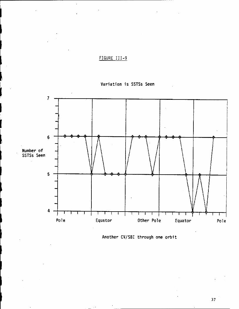
FIGURE III-9
Variation is SSTSs Seen
Number of SSTSs Seen
i—i—r
Other Pole Equator
Another CV/SBI through one orbit
37
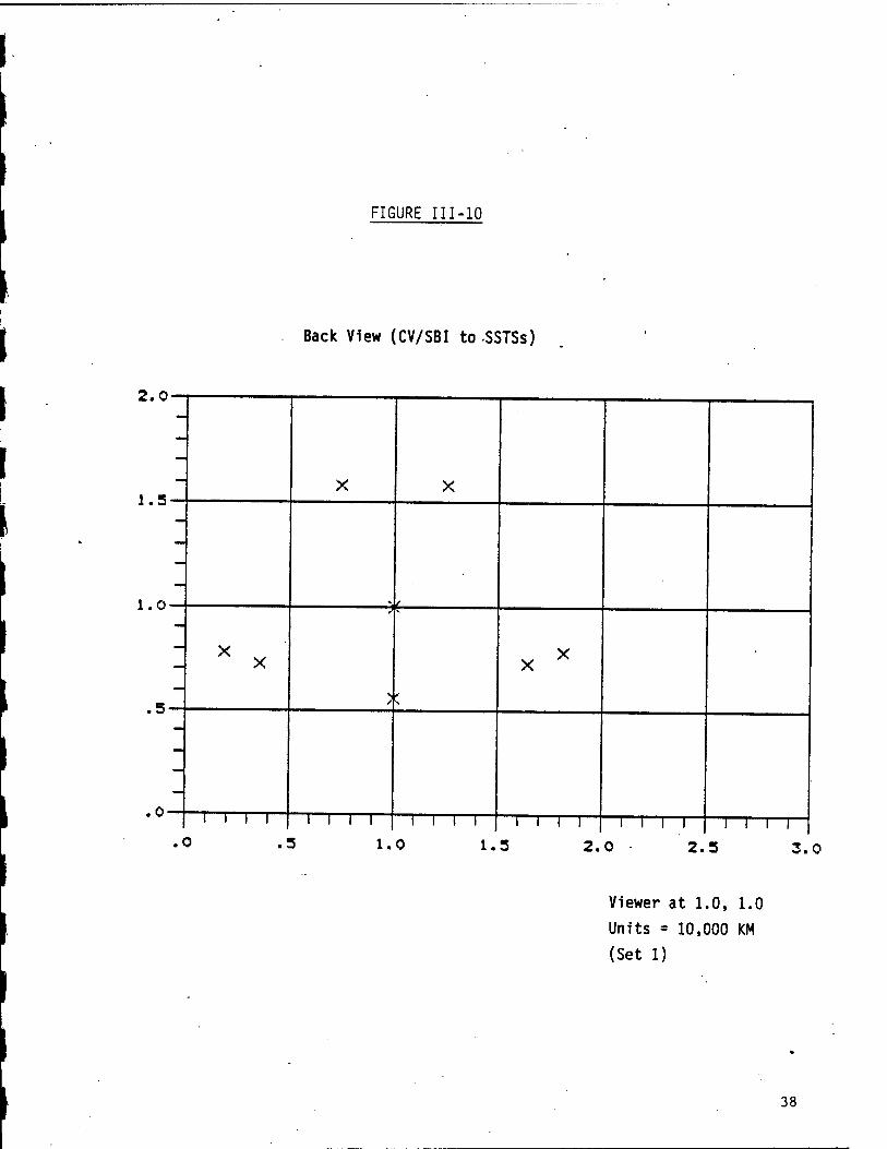
FIGURE III-10
Back View (CV/SBI to SSTSs)
2.0
1.5
1.0
X X
'
x X
;
x x
-
1 1 1 1 till 1 1 1 1 1 1 1 1 1 1 1 1 1 till .0 .3 1.0 1.3 3.0
Viewer at 1.0, 1.0
Units = 10,000 KM
(Set 1)
38

FIGURE III-ll
Side View (CV/SBI to SSTSs)
2.0
l.S
1.0
X
f S ———^^—^-^^^^mmmm— ^^^^^MMBH^^^MHH^B. -MMMi^^^^wMMM^aH^^
: x x
~ ><
.0 3 1.0 l.S. 2.0 2.5 3.0
.Viewer at 1.0, 1.0
Units = 10,000 KM
(Set 1)
39
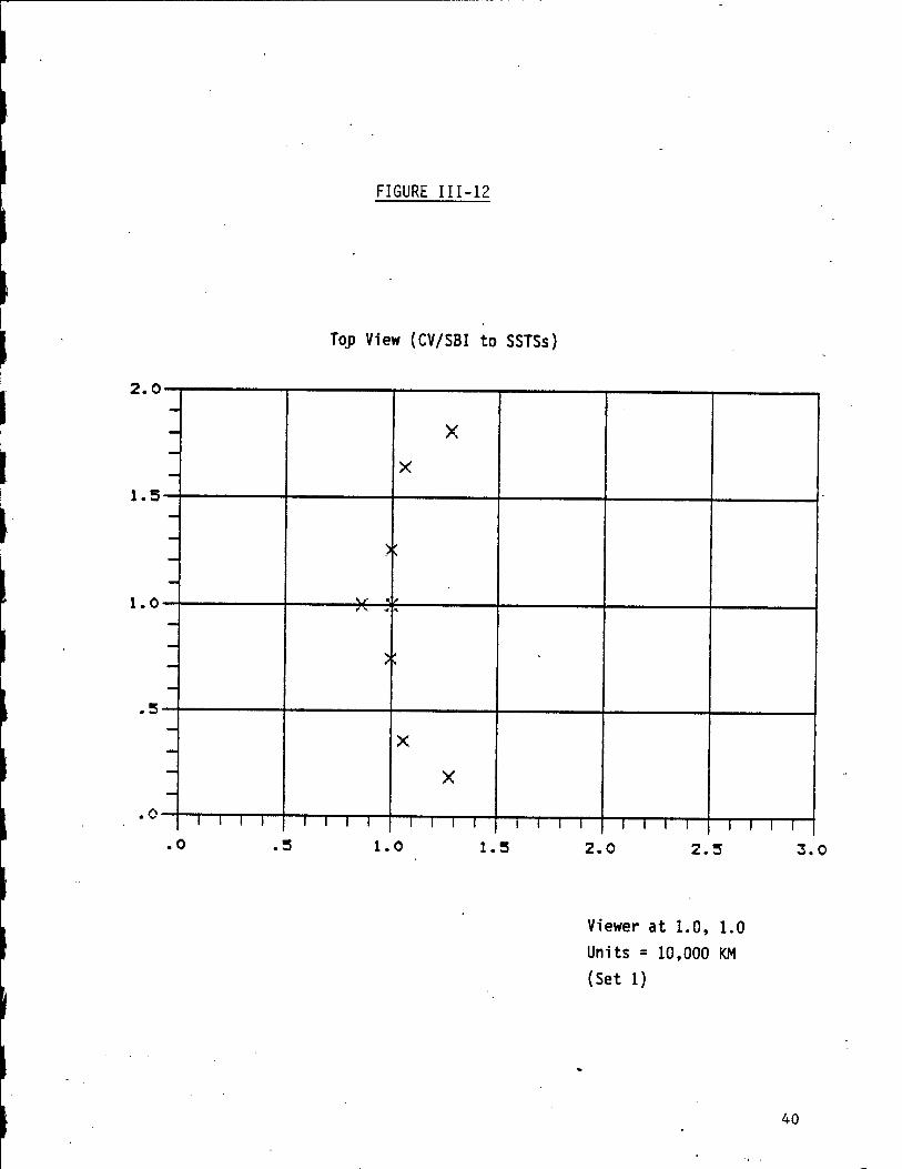
FIGURE 111-12
Top View (CV/SBI to SSTSs)
2.0
1.5
1.0
0
X
X
>
V 1
- > *
— X
X
1 1 1 1 1 1 1 1 1 1 1 1 1 1 1 1 1 1 1 1 1 1 i 1 1 .0 .3 1-0 1.3 2.0 2.3 3.0
Viewer at 1.0, 1.0
Units = 10,000 KM
(Set 1)
40

FIGURE 111-13
Back View (CV/SBI to SSTSs)
K
1.5 — X
X
1.0 — *'■
X
.5 — X
- X
.0 — I l 1 1 1 1 1 1 III! i 1 1 1 1 1 1 1 1 1 1
.0 1.0 1.5 2.0 2.3 3.0
Viewer at 1.0, 1.0
Units = 10,000 KM
(Set 2)
41

FIGURE 111-14
Side View (CV/SBI to SSTSs)
2.0
1.5
1.0
— V > >
X
X
■i X »
>
X
1 1 1 1 1 1 1 1 1 1 1 1 1 1 1 1 1 1 1 1 1 1 1 1
.0 .5 1.0 1.5 2.0 2.5 3.0
Viewer at 1.0, 2.0
Units = 10,000 KM
(Set 2)

FIGURE 111-15
Top View (CV/SBI to SSTSs)
2.0
1-.5
1.0
.5
X
X
c
— X
X
—
III! 1 1 1 1 I I 1 1 1 1 1 1 1 1 1 1 1 1 1 1 1 .0 • 5 1.0 l.S 2.0 2.3 3.0
Viewer at 1.0, 1.0
Units = 10,000 KM
(Set 2)
43

In summary.., at least four SSTS satellites are always visible, and
the back view supports 360° of angular diversity. The side and
top views tend to be in a broad line to both "sides" of the
CV/SBI satellite. In actuality, this angular configuration lends
itself to a robust amount of angular diversity (back view) while
not over complicating the demands (side, top views) put upon an
antenna system. A relatively small, yet marginally very
significant (as is shown later), number of links can be
supported. For purposes here, two of the four links are selected
for robustness. This link primarily provides for health and
status information—not of the highest priority. And, as before,
analyses to determine that exactly two of the four available
links are best (if they are) and which two to use are beyond the
scope of this report.
44

CV/SBI-BSTS Links
Figures 111-16 and 17 depict two representative variations of the
BSTS satellites from the CV/SBIs. Depending upon the relative
phase of the CV/SBI satellite, either three or four BSTSs will
generally be seen, except when near the poles where six are
visible.
Again, "Health and Status" is the primary linkage and the
relative priority of the information is low. It is not clear
that multiplying the connectivity of any of these links is
necessary.
45

Number of BSTSs Seen
FIGURE 111-16
Variation in BSTSs Seen
~i—i—i—r
Pole
$—i> MM
"1—TH—T
Equator
$ ft $ $ O $
■*■
~i—r~i—i—i—i—r
Other Pole Equator
i—i—r
Pole
One CV/SBI Through One Orbit
46
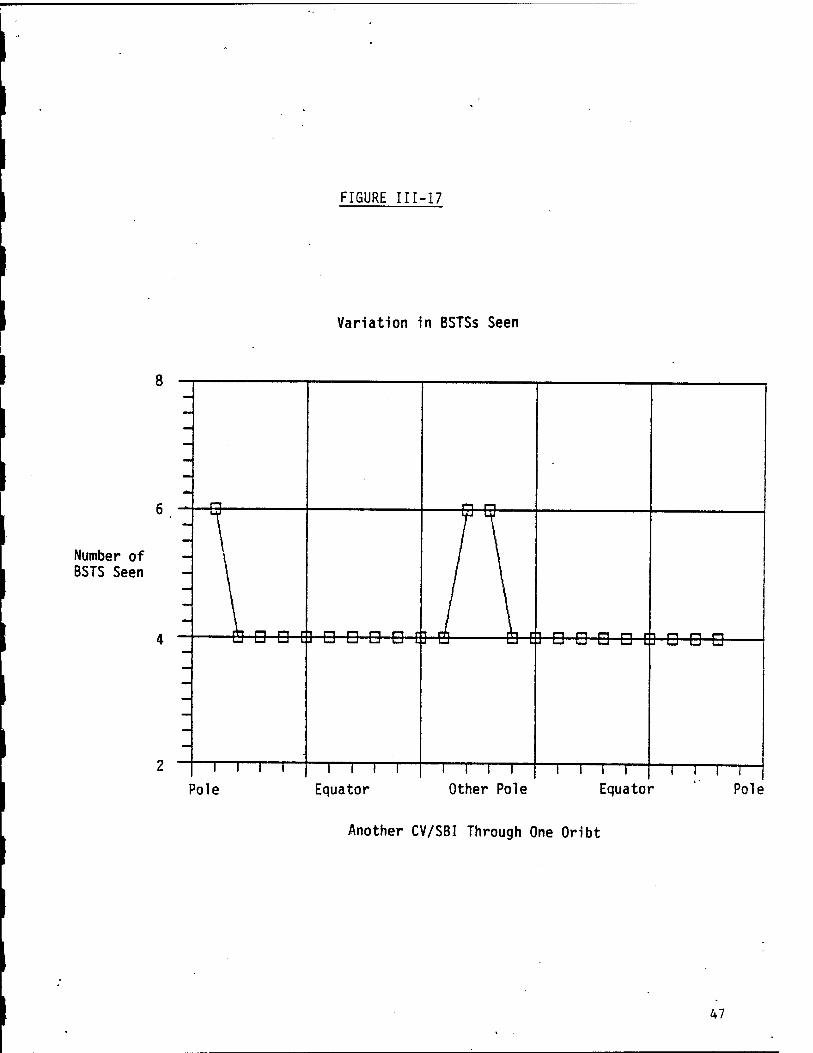
FIGURE 111-17
Variation in BSTSs Seen
Number of BSTS Seen
D D [3 D D D D »
Pole
~i—i—i—r Equator
I 1 I Other Pole
E3 0DDDÜODD
Equator i—r
Pole
Another CV/SBI Through One Oribt
47

SSTS-CV/SBI Links
From 60 to 110 CV/SBIs are visible from an SSTS at any point in
time. Figures 111-18 and 19 show two representative orbits with
six samples per orbit. (The two views represent two SSTSs that
are phased differently, but representively within two separate
SSTS orbital planes.)
Figures 111-20, 21, and 22 show the back, side, and top views
which demonstrate the angular diversity of the CV/SBIs within LOS
from an SSTS positioned high (toward the North Pole) in it's
orbit. Whereas Figures 111-23, 24, and 25 show the same views of
angular diversity from an SSTS that is positioned above a point
close to the equator.
In summary, the back view shows some small amount of bunching
around a full 360° of diversity, with top and side views showing
nominal bunching through about 180°. Up to 60 links can be
maintained LOS from the geometry. In Phase 2 this is a critical
data link and parallel., lines of connectivity are expected to be
of value. The high data rate works against supporting too many
links. For purposes here, as a strawman, 34 distinct links from
each SSTS is selected. Therefore, some redundancy in each link
is maintained.
48

FIGURE 111-18
Variation in CV/SBIs Seen
125
c (U
. v «♦- in o
«/» QJ CO
100
75
50
Pole Equator Equator
One SSTS through one orbit
49
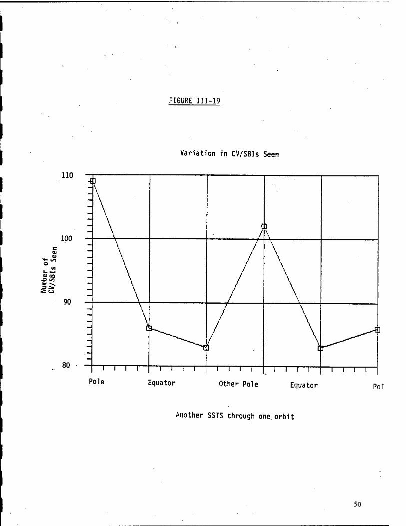
FIGURE 111-19
Variation in CV/SBIs Seen
110
100
<U 0)
<«- (/> o t. 1—1 0) 00
■S ">
90
80 T—i—r
Pole
i—|—i—i—i—r
Equator
L
T—I—I—|—
Other Pole
\
i—i—i—r~
Equator Pol
Another SSTS through one orbit
50

FIGURE 111-20
Back View (SSTS to CV/SBIs)
2.0
1.5
1.0
.5
-
4*
-
•
. '-'■■ •»
• ♦
*
*
•
♦ * ♦ ♦
* 4
4
« « ft
.♦
* 4
♦ *
«
*
1
4 » 4 »
till 1 1 1 1 1 1 1 1 1 1 1 1 1 1 1 1 1 1 1 1
.0 .5 1.0 1.5 2.0 2.5 3.0
Viewer at 1.0, 1.0
Units = 10,000 KM
(Set 1)
51

FIGURE 111-21
Side View (SSTS to CV/SBIs)
2.0
1.5
1.0
.5
.0
—
— • 4
f. • « *
t « 1
*
.' . ♦
* • '
♦
• * * »
* 4
— 4
- -
—
1 1 1 1 1 1 1 1 1 1 1 1 1 1 1 1 1 1 1 1 1 1 1 1 1 .0 .3 1.0 1.3 2.0 2.5 3.0
Viewer at 1.0, 1.0
Units - 10,000 KM
(Set 1)
52

FIGURE 111-22
Top View (SSTS to CV/SBIs)
2.0
1.3
1.0
.5
.0
•
— ♦ »
t *♦
»♦ 0 *
t
♦ *
• t
_ 4*
- ♦ * *
• — » «
1 1 1 1 1 1 1 1 1 1 1 1 1 1 1 1 1 1 1 1 1 1 1 1 .0 1.0 1.5 2.0 2.3 3.0
Viewer at 1.0, 1.0
Units = 10,000 KM
(Set 1)
53

FIGURE 111-23
Back View (SSTS to CV/SBIs)
2.0-
1.3-
1.0-
.3-
-.0-
.0 I I I I I I
1.0 1.5
I I I 1 I I I I I I I I
2.0 2.3 3.0
Viewer at 1.0, 1.0
Units = 10,000 KM
(Set 2)
54

FIGURE 111-24
Side View (SSTS to CV/SBIs)
, ^^^m
.
1.5 — > «"•
* •< . •
_
0, *« ♦ -
1.0 — ....•• . »
...«• • . •
• •♦• • ♦ •♦
.3 — • ♦ . •
< ••
-
—
.0 — 1 1 1 1 1 1 1 1 1 | 1 1 1 1 1 1 1 1 1 1 1 1 1 1 1 I 1
.0 1.0 1.3 2.0 2.3 3.0
Viewer at 1.0, 1.0
Units - 10,000 KM
(Set 2)
55

FIGURE 111-25
Top View (SSTS to CV/SBIs)
2.0
1.5
1.0
.5
«
*
«
* »
1
» 1
-
* *
» ••
1
t
«
—
1 1 1 1 1 1 1 1 1 1 1 1 1 1 1 1 1 1 1 1 1 1 1 1 1 1 .0 • S 1.0 1.3 2.0 2.3 3.0
Viewer at 1.0, 1.0
Units = 10,000 KM
(Set 2)
56

SSTS-SSTS Links
No chart showing the number of SSTSs visible from an SSTS is
included since, for all orientations, the number is exactly
eight. Two sets of back, side, and top views are shown in
Figures 111-26 through 31 to depict the angular diversity. The
two views represent different phases of the satellite's orbits-
together, the views are representative.
These links support a very high data rate and eight parallel
links are probably too many. The strawman here is four angularly
diverse links. Again, the back view shows 360° of angular
diversity whereas the top and side views show roughly 180°. It
is not clear whether the closest, furthest, or middle links
should be chosen or whether they should be pseudo-randomly
selected. Inter-orbit, rather than intra-orbit, links provide
more angular diversity and more tracking complexity. Where a
laser link may be chosen over an EHF link, assuming EHF phased
arrays are available and laser antenna agility is much more
difficult, laser links may need to stay with the less diverse
intra-orbit netting. EHF, on the other hand, may just as easily
take advantage of the more diverse inter-orbit netting.
57

FIGURE 111-26
Back View (SSTS to SSTSs)
2.0-
1.5-
1.0'
.0
;<
fr
i i i | i i
1.0 1.5 I I I I
2.0 I I I I
2.5 3.0
Viewer at 1.0, 1.0
Units = 10,000 KM
(Set 1)
58

FIGURE 111-27
Side View (SSTS to SSTSs)
2.0
1.5
1.0
x x X
X
A X — L'
v —
- X
- X
i i i r I I I 1 1 1 1 1 1 1 1 1 1 1 1 1 1 1 III! ■
.0 •5 1.0 1.3 2.0 2.5 3.0
Viewer at 1.0, 1.0
Units = 10,000 KM
(Set 1)
59

FIGURE 111-28
Top View (SSTS to SSTSs)
2.0 1 1.5-
1.0-
.0-
X
>:
£c ü.
X
.0 I I I I I I I I 1
• 3 1.0 TT I I I 1 I I I
i-3 2.0 2.5 3.0
Viewer at 1.0, 1.0
Units = 10,000 KM
(Set 1)
60

FIGURE 111-29
Back View (SSTS to SSTSs)
1.5 —
X X
1.0 — ■ x x a I x w
.5 —
* 0 \
.0 —
X X
1 1 1 1 1 1 1 1 1 1 1 1 1 1 1 1 1 1 1 1 'TT-f MM" .0 1.0 1.5 2.0 2.5 3.0
Viewer at 1.0, 1.0
Units = 10,000 DM
(Set 2)
61

FIGURE 111-30
Side View (SSTS to SSTSs)
X <
1.5 —
1.0 — ». , x v -
r.
.5 —
.0 —
X
1 1 1 1 | I l 1 1 1 1 1 1 1 1 1 1 1 1 1 1 1 1 1 1 1
.0 .3 1.0 1.3 2.0 2.S 3.0
Viewer at 1.0, 1.0
Units = 10,000 DM
(Set 2)
62

FIGURE 111-31
Top View (SSTS to SSTSs)
X
X 1.5 —
X
X
1.0 — A f
X
X .5 —
— X
— X
.0 — I l 1 1 l 1 1 1 | 1 1 1 1 1 1 1 1 1 1 ■ I—1—f- 1 1 1 r""j
.0 .3 l-° l.S 2.0 2.S ' 3.0
Viewer at 1.0, 1.0 Units = 10,000 KM (Set 2)
63

SSTS-BSTS Links
The SSTS-BSTS angular diversity is obvious. Two or three links
can easily be maintained while an additional one is being
acquired. This link is not of the highest priority, and while
the angular differences are reasonably wide, they track rather
routinely, not adding significantly to any sort of covertness.
With the small number of BSTS satellites expecting narrow-beam
signals from known angles jamming is still a difficult, and
probably prohibitively expensive task. More so than most of the
other links lasers may tradeoff favorably for this link, but as
discussed in Section X, a hybrid EHF/laser communication system
for the SDS is very undesirable.
64

BSTS-CV/SBI Links
Depending upon orientation, each BSTS satellite can see 190-200
CV/SBI satellites. One representative orbit with six data points
is shown in Figure 111-32. All the satellites are within a field
of view of approximately 19°. A "wide" beam broadcast to all
satellites is possible, but well over" 30 dB added gain is
available by pointing to the individual satellites. Some of the
advantage can be gained by narrowing the beam partially and
broadcasting to clusters of satellites. Tradeoffs of all
potential configurations are beyond the resources of this study.
In a very robust architecture, each BSTS can generate ten beams
of TDMA information (fifteen satellites per beam). TDMA must be
synchronized to the TOA at each CV/SBI. CDMA orthogonal codes
superimposed upon TDMA can be employed to improve separation, if
necessary.
For purposes here, this latter approach which supports multiple,
high-gain (narrow beam) links is adopted to most effectively
guarantee connectivity of this most important link (especially in
Phase 1) where both jamming and nuclear interference may pose
problems.
65

FIGURE 111-32
Variation in CV/SBIs Seen
200
c 0)
<*- to o t- 1-4
0) CO
3 > z o
195
One BSTS through one orbit
66

t
BSTS-SSTS Links
Again, depending upon orientation, each BSTS can see 14-16 SSTS
satellites. One representative orbit with six points is shown in
Figure 111-33. The arguments made for the BSTS-CV/SBI links
apply with two minor changes: the field of view widens to
roughly 21° and the number of links is a little more than an
order of magnitude different (190 vs. 15). For purposes here,
and using the same antenna system supporting the BSTS-CV/SBI
links, nine BSTS-SSTS links will be supported per BSTS satellite.
This is an important Phase 2 link and robustness is merited. How
nine of the 14-16 are selected depends upon the same concerns
expressed in earlier discussions—if nothing else they can be
pseudo-randomly selected. Again, all antenna aiming is assumed
to be aided with ephemeris information, and all antenna fine
calibration is done in space using the SDS constellations which
will allow the maximum capability possible. If considered in
isolation, lasers could tradeoff reasonably well for this link;
however, EHF is probably preferred for the multi-directional,
multi-beam BSTS-CV/SBI link, and it would be best to take
advantage of the same hardware for these links.
67
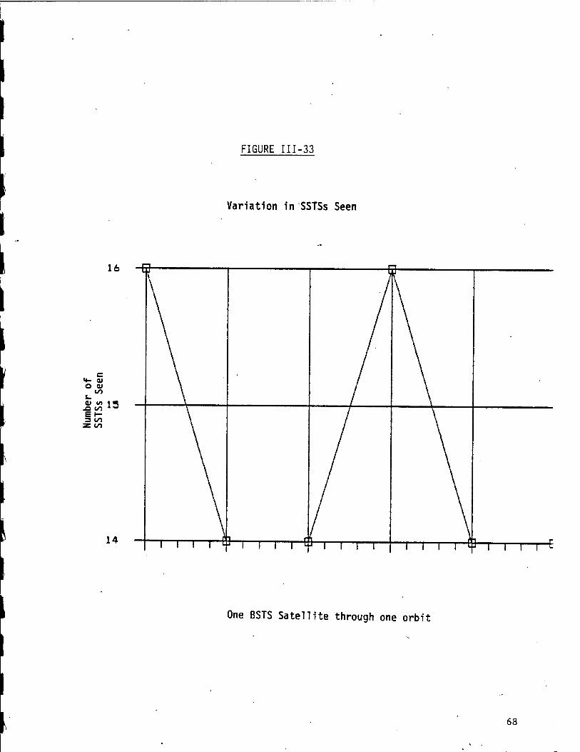
FIGURE 111-33
Variation in SSTSs Seen
i6 -e
c «4- <U O 0)
$-
-o oo iJ Et- 3 00 Z OO
14
One BSTS Satellite through one orbit
68

BSTS-BSTS Links
The geometry is obvious, and in a robust architecture, anticipate
four BSTS-BSTS links per satellite. This added robustness adds a
significant advantage to AJ and BER as shown in Section VII. The
data rates are not terribly high and the update rates provide
time for parallel connectivity. If the number of BSTS satellites
increases beyond the nominal baseline, additional parallel links
should- be considered. Finally, as with the SSTS<—>SSTS and
BSTS<—>SSTS links, in isolation, lasers could tradeoff
favorably. But, again, it is probably best to avoid EHF/laser
hybrid communication systems (see Section X for further
discussion).
69

IV. DATA RATES AND NUMBERS OF LINKS
70

DATA RATES AND NUMBERS OF LINKS
From the World Situation Set (Appendix A) it is assumed that the
number of objects tracked in the post-boost phase is 3,500 while
during midcourse the number could possibly balloon to over
400,000. For purposes here 3,500 and 475,000 will be used.
During the SDI Communications Workshop in September 1987, TRW
presented analysis supporting a maximum of 235-bit-per-packet
data package (the maximum allowable in their link budget) which
in actuality contains 193 bits of information including 8 bits
for synchronization. In this analysis it is assumed that a 235-
bit packet is employed and that as many as 50 bits can be used
for synchronization. It is further assumed that the sync bits
are distributed throughout the packet so that sync verification
is a very high quality estimate of message verification. Further
analysis of connectivity probabilities and message quality is
covered in Section VII.
The data rate associated with each of the links is dependent on
the number of links over which any one satellite is receiving
identical information. This is the route diversity concept
alluded to earlier. The particular number chosen for any given
link is dependent upon the number of different satellites that
are in the line of sight of any one satellite as well as on the
improvement factor obtainable as discussed in Section VII. The
link margins discussed in Section VI have been chosen based on a
bit error probability of 10"5. This probability of error is a
good compromise as can be seen upon examining the link margins
presented in Section VI.
71

The link redundancy numbers shown in Tables IV-1 thru 5, while
not based on an exhaustive analysis, serves as a reasonable
initial estimate to examine the advantages of a robust
architecture. The redundancy numbers shown range from one to ten
depending upon the particular link. Certain links transmit only
health and status information which is not as crucial as other
links transmitting sensor data, hence redundancy tends to be
higher on the latter type of link. Link redundancy is the
parameter important to computing the advantage enjoyed by the
parallel links described in Section VII.
Now, given the packet size, update rates, number of sensors, and
number of objects tracked,.we can determine the rates associated
with each link. For the BSTS carousel we have, (without TDMA)
data rate = 3500 objects x (3 sensors) x 235 bits/sensor/2 second
updata rate
=1.25 MBPS
TDMA data rate =1.25 MBPS x 4 = 5 MBPS.
Similarly for the SSTS carousel we obtain, (without TDMA) data
rate = 475,000 objects x (3 sensors) x 235 bits/sensor x (1.7
growth factor)/10 updata rate =59.5 MBPS
TDMA data rate =59.5 Mbs x 4 = 238 MBPS.
72

Data rates associated with tracking, telemetry, and command
(TT&C) links or health and status links utilize the Satellite
Data Link Standard (SDLS) rates, nominally 5 KBPS. The remaining
data rates shown in Table IV-1 thru 5 are based on results
presented at the various Phase 2C architecture conferences and
are not derived herein.
73

Table IV-1
BSTS Transmits TO Burst RATE fMBPS'
BSTS 5
SSTS 1.8
CV/SBI(10 beams) 7.5
GEP(S) 1.25
GEP(TTC) .0048
# of Links
4
9
15 per beam
1
1
Redundancy
N/A
N/A
N/A
. N/A
N/A
BSTS Receives FROM
BSTS 5
SSTS .015
CV/SBI .005
GEP(S) N/A
GEP(TTC) .0048
4
9
150
N/A
1
4
3
3
N/A
1*
* Redundancy not critical
74

Table IV-2
SSTS Transmits TO Burst Rate fMBPS^ # of Links
BSTS .015
SSTS 238
CV/SBI(2 beams) 14
GEP(S) 238
GEP(TTC) .0048
Redundancy
3 N/A
4 N/A
17 per beam N/A
1 N/A
1 N/A
SSTS Receives FROM
BSTS 1.8
SSTS 238
CV/SBI 4
GEP(S) 20
GEP(TTC) .0048
3
4
34
1
1
3
4
2
1*
1*
♦Redundancy Not Critical
75

Table IV-3
CV/SBI Transmits TO Burst Rate fMBPS^ # of Links Redundancy
BSTS .005 1 N/A
SSTS 4 2 N/A
CV/SBI(2 beams) 4 10 N/A
KKV .003 10 N/A
CV/SBI Receives FROM
BSTS 7.5 3 3
SSTS 14 2 2
CV/SBI 4 10 10*
KKV N/A N/A N/A
♦Redundancy beyond parallel point-to-point links and the
determination of how much relaying should be supported in the
architecture is beyond the analysis here. It is possible that
when considering BSTS to CV/SBI information (direct, relayed
through SSTSs, and relayed through CV/SBIs), the numbers here may
provide more redundancy that is needed to insure connectivity.
Analysis in this report does show that this much redundancy is
probably beyond the point where the marginal utility of
additional links is optimized. Therefore, read the number of
links and redundancy numbers as containing some margin which can
be traded off as necessary to produce a more cost-effective
system.
76

Table IV-4
GSTS Transmits TO Burst Rate fMBPS^ # of Links
GEP .0048 1
CV/SBI .6 1
Redundancy
N/A
N/A
GSTS Receives FROM
GEP
CV/SBI
.0048
.6
1
1
1
1
Table IV-5
ERIS Transmits TO Burst Rate fMBPS^ # of Links
GEP .0048 1
CV/SBI .003 1
Redundancy
N/A
N/A
ERIS Receives FROM
GEP
CV/SBI
.0048
.003
1
1
1
1
77

V . ANTENNA SYSTEM CONSIDERATIONS
78

ANTENNA SYSTEM CONSIDERATIONS
As discussed in Section X, for the near term EHF, links are
preferred primarily due to their technical maturity. Each link
will require, some type of antenna of which there are currently
three choices:
1) Steerable parabolic dish with or without multiple
feeds.
2) Waveguide-steerable multiple-beam phased array.
3) Monolithic-steerable multiple-beam phased array.
The communication system architecture described here requires
that certain satellites have antenna structures within which
multiple independently steerable beams can be formed (e.g., the
BSTS to CV/SBI links). If the first approach is selected, for
the BSTS satellite, as many as 10 dish antennas (each with a
diameter of .7 meters or more) would be mounted on the satellite.
Gimbals are required to steer these antennas giving rise to
excessive, probably unacceptable, weight (on the order of 350
pounds per antenna). Also, reflector surface smoothness for dish
antennas operating at millimeter wave frequencies is an area of
concern. For such antennas the gain is reduced as given by:
G/GQ ~ exp {-a2/ A2)
79

Where G0 is the ideal gain and G is the actual gain due to an rms
surface irregularity of magnitude a meters.
And, finally, on any satellite system employing sensors, it is
certainly preferable to avoid, moving masses which will generate
perturbations that must be damped out before reaching the
sensors.
If this type of antenna system would ever be required, the
tradeoff between beamwidth (i.e. number of CV/SBIs illuminated)
and total number of beams would have to be revisited. For the
architecture described in this report, a better, though riskier
in the near term, approach is available, and it is probably
preferred.
The second alternative is unrealistic, with the possible
exception where one is dealing with a very small number of units,
because the requirement for excessively thin waveguide elements,
as dictated by the antenna geometry at this frequency, as well as
the large number of precisionally-oriented elements, would be
labor intensive and extremely expensive. The weight of a
reasonably sized array (3500 elements) would also be a concern.
The BSTS constellation itself, because of the relatively few
satellites, may consider this approach only if no other
alternative can be found. Because of the numbers alone, the
other satellites cannot possibly employ this technique. And,
since the other satellites will require some other antenna system
80

at this frequency, unless the constellation must be launched
early, it is inconceivable that the BSTS could not use the same
type of antenna system.
The third alternative is the most viable method, especially for
the BSTS to CV/SBI link. Obviously, if this approach is used on
any one type of satellite, it may as well be developed for all of
them. The primary disadvantage of the monolithic phased array is
that the technology is relatively immature. (But, unlike
lasercom systems, EHF has only this one area of relatively
immature technology, and it is an area where we know how to
proceed to gain maturity.) For 60 GHz links, monolithic array
antennas (though being built in the laboratory for 20 GHz and 44
GHz antenna systems) are five to ten years away from being
incorporated into a space-qualified hardware system.
Nonetheless, this is the most promising approach, development is
being funded, and hence it has been selected for the architecture
described herein. (A better funded development program could
make the technology available sooner, and consideration should be
given to put more emphasis in this area.)
Finally, a few words need to be written on null-steering
possibilities. For any properly-designed, phased-array antenna
system, one or more nulls can be steered with the addition of
another receiver and more processing.* Where jammers are
*See Coherent Sidelobe Cancelling by Peterson and Weiss, J. Appl Phys., 1 August 1984.
81

employed on satellites, their ephemeris information can be used
to help steer the nulls. The inclusion of a single null on any
SDS satellite makes an already "near impossible" jamming problem
at least twice as hard. However, there is another advantage
gained from nulling: The processing link budgets (inherent in
the data and bandwidth numbers) of Section VI can be relaxed, or
the advantage offered by nulling can be used to offset any of the
other parameters comprising of the total link margin. Note that
this is another situation where a "good guy/bad guy" dB tradeoff
has meaning well beyond the number of decibels—here an
additional receiver and some processing would have to be negated
with "jamming geometry," that is, more satellites at different
angles. It is inconceivable that an adversary would waste so
much in resources for so little gain. Nulling should be
considered to enhance link margins beyond what is shown in
Section VI.
82

VI. MARGIN ANALYSIS
83

MARGIN ANALYSIS
The EW threat consists of airborne, ship, and spacebome jammers.
The spacebome jammers have been set at 36 by the WSS, with 6
allocated by us here to the same orbit as the BSTS satellites
while the remaining 30 have been placed in the same orbital
planes as the SSTS satellites but at an altitude midway between
the SSTS and CV/SBI constellations. The spacebome jammers have
been restricted to a 5-2 KW output power level while the ground-
based jammers are capable of 200 KW. Each of the jammers in the
SSTS orbital plane is assumed to be equipped with 2 phased array
antennas capable of multi-beam propagation. Thus, any one jammer
can simultaneously jam 10 CV/SBI and 2 SSTS satellites.
Table VI-1 shows the required Eß/No ratios for the various types
of links imposed by the threat environment and the system
architecture. Table VI-2 identifies which channel type each of
the SDS links are associated with while Table VI-3 summarizes the
required data rates. The nuclear effect parameters are
itemized in Table VI-4. These parameters are based on a multiple
burst DNA model which is discussed in Appendix B.
84
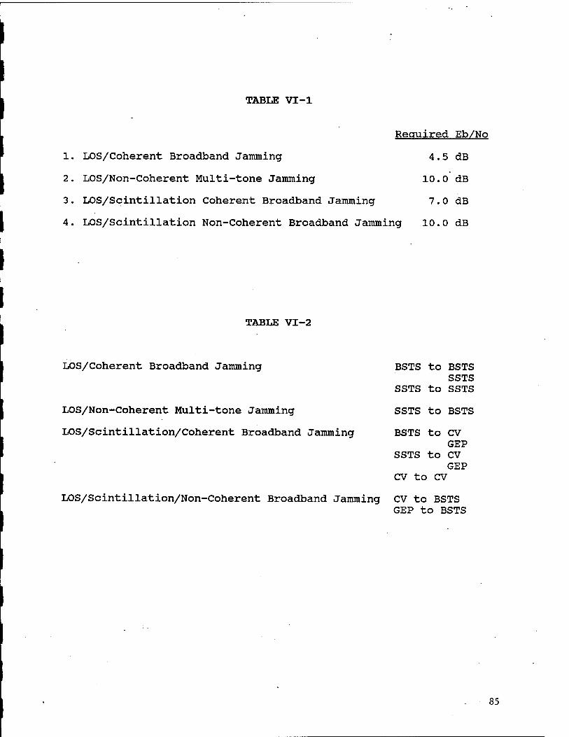
TABLE VI-1
Required Eb/No
1. LOS/Coherent Broadband Jamming 4.5 dB
2. LOS/Non-Coherent Multi-tone Jamming 10.0 dB
3. LOS/Scintillation Coherent Broadband Jamming 7.0 dB
4. LOS/Scintillation Non-Coherent Broadband Jamming 10.0 dB
TABLE VI-2
LOS/Coherent Broadband Jamming
LOS/Non-Coherent Multi-tone Jamming
LOS/Scintillation/Coherent Broadband Jamming
BSTS to BSTS SSTS
SSTS to SSTS
SSTS to BSTS
BSTS to CV GEP
SSTS to CV GEP
CV to CV
LOS/Scintillation/Non-Coherent Broadband Jamming CV to BSTS GEP to BSTS
85

Transmitter
BSTS
SSTS
CV
GEP
TABLE VI-3 DATA RATES IN MB/S
RECEIVER BSTS SSTS CV GEP
5 1.8 7.5 1.25
0.015 238 14 20
0.005 4 4 0.005
0.005 20 0.005 —
TABLE VI-4 SCINTILLATION PARAMETERS
To
Ground-to-Space Links
0.04 mS
Space to Space Links
0.08 mS
fo 2.6 MHz 41 MHz
2 d rms 122 nS 7.8 nS
Antenna Loss 21.1 dB 15.1 dB
Absorption
Temp
4.8 dB
8900° K
1.1 dB
4000° K
86

The following tables show the various link margins for the
following cases:
1) No jamming, no nuclear burst.
2) No nuclear burst.
3) Margins without multiple links.
4) Margins with five parallel links.
The transmitter power levels and antenna gains have been selected
to be commensurate with monolithic array technology as well as to
provide slightly positive link margins for the third case above
(there is only one exception to the positive margin result).
Tables VI-5 through VI-8 contain the link margins where there is
no jamming present, no nuclear threat, and only one link, i.e.
case (1) above. As noted, all links have positive margins,
several of them substantial.
The results in each table presented herein are based on a bit
error probability of 10~5 as discussed in Appendix B. Also per
the Appendix, a processing gain produced by a spread bandwidth
equivalent to 10% of the carrier frequency has been assumed for
all links.
87

TABLE VI-5 TRANSMITTER B
Receiver
Distance (Km)
Data Rate (KBPS)
Frequency (GHz)
Power (dBm)
X/Ant Gain (dB)
Xmit Loss (dB)
R/Ant Gain (dB)
RCV Loss (dB)
Scatter Loss (dB)
Absorption (dB)
T (°K)
EB/NO (dB)
EB/NJ (dB)
EB/NT (dB)
Req'd EB/NT (dB)
Margin (dB)
B
73000(Max) 48000(Max) 44000(Max) 34000(Min)
5000 1800 7500 1250
60 60 60 20
50 40 40 50
50 45 50 50
2 2 2 2
50 45 50 60
2 2 2 2
0 0 0 0
0 0 0 0
1000 1000 1000 1000
22.3 30.4 14.9 54.9
N/A N/A N/A N/A
22.3 30.4 14.9 54.9
4.5 4.5 7 7
17.8 25.9 7.9 47.9
88

TABUE VI-6 TRANSMITTER S
Receiver B S C G
Distance (Km) 48000(Max) 12900(Max) 9100(Max) 3000(Min)
Data Rate (KBPS) 15 238000 14000 238000
Frequency (GHz) 60 60 60 20
Power (dBm) 40 50 47 50
X/Ant Gain (dB) 40 50 50 50
Xmit Loss (dB) 2 2 2 2
R/Ant Gain (dB) 40 50 50 50
RCV Loss (dB) 2 2 2 2
Scatter Loss (dB) 0 0 0 0
Absorption (dB) 0 0 0 0
T (°K) 1000 1000 1000 1000
EB/NO (dB) 21.2 20.6 29.9 53.6
EB/NJ (dB) N/A N/A N/A N/A
EB/NT (dB) 21.2 20.6 29.9 53.6
Req'd EB/NT (dB) 4.5 4.5 7 7
Margin (dB) 16.7 16.1 22.9 46.8
89

TABLE YI-7 TRANSMITTER C
Receiver B S C G
Distance (Km) 44000 (Max) 9100 (Max) 4600 (Max) 500 (Min)
Data Rate (KBPS) 5 4000 4000 5
Frequency (GHz) 60 60 60 20
Power (dBm) 45 45 45 25
X/Ant Gain (dB) 40 47.5 45 35
Xmit Loss (dB) 2 2 2 2
R/Ant Gain (dB) 40 47.5 45 35
RCV Loss (dB) 2 2 2 2
Scatter Loss (dB) 0 0 0 0
Absorption (dB) 0 0 0 0
T (°K) 1000 1000 1000 1000
EB/NO (dB) 31.7 31.4 32.3 50.2
EB/NJ (dB) N/A N/A N/A N/A
EB/NT (dB) 31.7 31.4 32.3 50.2
Req'd EB/NT (dB) 4.5 4.5 7 7
Margin (dB) 27.2 26.9 25.3 43.2
90

TABIiE VI-8 TRANSMITTER G
Receiver B S C
Distance (Km) 34000 (Min) 3000 (Min) 500 (Min)
Data Rate (KBPS) 5 20000 5
Frequency (GHz) 44 44 44
Power (dBm) 38 43 27 .
X/Ant Gain (dB) 38.8 43.8 27.8
Xmit Loss (dB) 2 2 2
R/Ant Gain (dB) 43 48 32
RCV Loss (dB) 2 2 2
Scatter Loss (dB) 0 0 0
Absorption (dB) 0 0 0
T (°K) 1000 1000 1000
EB/NO (dB) 31.4 31.9 35.1
EB/NJ (dB) N/A N/A N/A
EB/NT (dB) 31.4 31.9 35.1
Req'd EB/NT (dB) 4.5 4.5 7
Margin (dB) 26.9 27.4 28.1

Tables VI-9 through VI-12 show link margins when jamming is
present with no nuclear threat, i.e. case (2) above. Note all
links have positive margins except the BSTS to GEP link where
there is zero margin. With the nuclear environment added, this
particular link is actually better due to the attenuation
experienced by the jammer.
92

TABLE VI-9 TRANSMITTER B
Receiver B S C G
Distance (Km) 73000 (Max) 48000 (Max) 44000 (Max) 34000 (Min) Data Rate (KBPS) 5000 1800 7500 1250 Frequency (GHz) 60 60 60 20 Power (dBm) 50 40 40 50 X/Ant Gain (dB) 50 45 50 5- Xmit Loss (dB) 2 2 2 2 R/Ant Gain (dB) 50 45 50 60 RCV Loss (dB) 2 2 2 2 Scatter Loss (dB) 0 0 0 0 Absorption (dB) 0 0 0 0 T (°K) 1000 1000 1000 1000 EB/NO (dB) 22.3 30.4 14.9 44.5 EB/NJ (dB) 11.3 30.2 12.7 7.0 EB/NT (dB) 11.0 27.3 10.7 2.0 Req'd EB/NT (dB) 4.5 4.5 7 7 Margin (dB) 6.5 2.8 3.7 0
JAMMER
Receiver B S C G
Distance (Km) 1000 2000 500 1000 Bandwidth (GHz) 6 6 6 2 Frequency (GHz) 60 60 60 20 Power (dBm) 67.2 62.4 52.4 83 X/Ant Gain (dB) 50 50 50 46.4 Xmit Loss (dB) 2 2 2 2 Scatter Loss (dB) 0 0 0 0 Absorption (dB) 0 0 0 0 Sidelobe (dB) -35 -35 -35 -35 Null Depth (dB) 0 0 0 0 J Density(dBm/Hz) -157.6 -168.4 -166.4 -121.1
93

TABLE VI-10 TRANSMITTER S
Receiver B S C G
Distance (Km) 48000 (Max) 12900 (Max) 9100 (Max) 3000 (Min) Data Rate (KBPS) 15 238000 14000 238000 Frequency (GHz) 60 60 60 20 Power (dBm) 40 50 47 50 X/Ant Gain (dB) 40 50 50 50 Xmit Loss (dB) 2 2 2 2 R/Ant Gain (dB) 40 50 50 50 RCV Loss (dB) 2 2 2 2 Scatter Loss (dB) 0 0 0 0 Absorption (dB) 0 0 0 0 T (°K) 1000 1000 1000 1000 EB/NO (dB) 21.2 20.6 29.9 53.6 EB/NJ (dB) 10.2 20.4 27.8 21.7 EB/NT (dB) 9.9 17.5 29.9 21.7 Req'd EB/NT (dB) 4.5 4.5 7 7 Margin (dB) 5.4 13.0 22.7 21.7
JAMMER
Receiver B S C G
Distance (Km) 1000 2000 500 1000 Bandwidth (GHz) 6 6 6 2 Frequency (GHz) 60 60 60 20 Power (dBm) 67.2 62.4 52.4 83 X/Ant Gain (dB) 50 50 50 46.4 Xmit Loss (dB) 2 2 2 2 Scatter Loss (dB) 0 0 0 0 Absorption (dB) 0 0 0 0 Sidelobe (dB) -35 -35 -35 -35 Null Depth (dB) 0 0 0 0 J Density(dBm/Hz) -157.6 -168.4 -166.4 -121.1
94

TABLE VI-11 TRANSMITTER C
Receiver B S C G
Distance (Km) 44000 (Max) 9100 (Max) 4600 (Max) 500 Data Rate (KBPS) 5 4000 4000 5 Frequency (GHz) 60 60 60 20 Power (dBm) 45 45 45 25 X/Ant Gain (dB) 40 47.5 45 35 Xmit Loss (dB) 2 2 2 2 R/Ant Gain (dB) 40 47.5 45 35 RCV Loss (dB) 2 2 2 2 Scatter Loss (dB) 0 0 0 0 Absorption (dB) 0 0 0 0 T (°K) 1000 1000 1000 1000 EB/NO (dB) 31.7 38.4 32.3 50.2 EB/NJ (dB) 20.7 31.2 30.1 39.1 EB/NT (dB) 20.4 28.3 28.1 38.8 Req'd EB/NT (dB) 4.5 4.5 7 7 Margin (dB) 15.9 23.8 21.1 31.8
(Min)
JAMMER
Receiver B S C G
Distance (Km) 1000 2000 500 1000 Bandwidth (GHz) 6 6 6 2 Frequency (GHz) 60 60 60 20 Power (dBm) 67.2 62.4 52.4 83 X/Ant Gain (dB) 50 50 50 46.4 Xmit Loss (dB) 2 2 2 2 Scatter Loss (dB) 0 0 0 0 Absorption (dB) 0 0 0 0 Sidelobe (dB) -35 -35 -35 -35 Null Depth (dB) 0 0 0 0 J Density(dBm/Hz) -157.6 -168.4 166.4 -121.1
95

TABLE VI-12 TRANSMITTER G
Receiver B S C
Distance (Km) 34000 (Min) 3000 (Min) 500 (Min) Data Rate (KBPS) 5 20000 5 Frequency (GHz) 44 44 44 Power (dBm) 38 43 27 X/Ant Gain (dB) 38.8 43.8 27.8 Xmit Loss (dB) 2 2 2 R/Ant Gain (dB) 43 48 32 RCV Loss (dB) 2 2 2 Scatter Loss (dB) 0 0 0 Absorption (dB) 0 0 0 T (°K) 1000 1000 1000 EB/NO (dB) 31.4 31.5 35.1 EB/NJ (dB) 1000 17.2 1000 EB/NT (dB) 31.4 17.0 35.1 Req'd EB/NT (dB) 4.5 4.5 7 Margin (dB) 26.9 12.5 28.1
Receiver
Distance (Km) Bandwidth (GHz) Frequency (GHz) Power (dBm) X/Ant Gain (dB) Xmit Loss (dB) Scatter Loss (dB) Absorption (dB) Sidelobe (dB) Null Depth (dB) J Density (dBm/Hz)
JAMMER
S
2000 4.4 44
62.4 55 2 0 0
-35 0
154.4
96

Tables VT-13 through VT-16 show link margins for the case where
both jamming as well as nuclear scintillations are present,
however, only a single link margin is calculated here; i.e. case
(3) above. As noted, all links have positive margin with the
exception of the BSTS to CV link. The nuclear environment is the
cause of this difficulty and may be circumvented by relaying the
information through a less-perturbed link (use the robustness),
by increasing the transmitted power or the size of the antenna by
narrowing the antenna beamwidth further, and/or utilizing more
processing on the BSTS satellite to lower the data rate.
Multiple parallel links are built into the discussion of this
report, so any one link breaking connectivity does not prohibit
the information from being communicated as long as care is taken
to judiciously choose the multiple CV/SBI-CV/SBI relay links to
insure that the same nuclear event cannot break all linkages
among several CV/SBI satellites. Increasing power is purely a
function of cost as is antenna sizing—3 to 5 dB advantage for
each is possible. Antenna beamwidth can be reduced for another 4
dB improvement, but again the cost increases. In each of these
cases the RF section and/or antenna system cost will increase
(roughly) linearly with the improvement. The additional BSTS
processing can yield up to about 7 dB margin, while the cost
should not increase too dramatically, since margin is already
built into its assumed capability. But, none of these possible
improvements in link margin is either recommended or deemed
necessary. An appropriate selection of multiple routes or
multiple routing schemes, in the case of pseudo-random
97

selections, is considered capable of closing the link. The
underlying concept needs to be that if any BSTS-CV/SBI or SSTS-
CV/SBI link is connected then, except for those CV/SBIs extremely
close to a nuclear event (where survivability of the CV/SBI may
be questioned) , the information will permeate the CV/SBI
constellation.
98

TABLE VI-13 TRANSMITTER B
Receiver B S C G
Distance (Km) 73000 (Max) 48000 (Max) 44000 (Max) 34000 (Min) Data Rate (KBPS) 5000 1800 7500 1250 Frequency (GHz) 60 60 60 20 Power (dBm) 50 40 40 50 - X/Ant Gain (dB) 50 45 50 50 Xmit Loss (dB) 2 2 2 2 R/Ant Gain (dB) . 50 45 50 60 RCV Loss (dB) 2 2 2 2 Scatter Loss (dB) 0 0 15.1 21.1 Absorption (dB) 0 0 1.1 4.8 T (°K) 1000 1000 4000 8900 EB/NO (dB) 22.3 30.4 -7.3 19.1 EB/NJ (dB) 11.3 30.2 28.9 32.9 EB/NT (dB) 11.0 27.3 -7.3 18.9 Req'd EB/NT (dB) 4.5 4.5 7 7 Margin (dB) 6.5 2.8 -14.3* 11.9
JAMMER
Receiver B S C G
Distance (Km) 1000 2000 500 1000 Bandwidth (GHz) 6 6 6 2 Frequency (GHz) 60 60 60 20 Power (dBm) 67.2 62.4 52.4 83 X/Ant Gain (dB) 50 50 50 46.4 Xmit Loss (dB) 2 2 2 2 Scatter Loss (dB) 0 0 15.1 21.1 Absorption (dB) 0 0 1.1 4.8 Sidelobe (dB) -35 -35 -35 -35 Null Depth (dB) 0 0 0 0 J Density(dBm/Hz) -157.6 -168.4 -182.6 -147.0
*Read discussion on how this link can be closed.
99

TABLE VI-14 TRANSMITTER S
Receiver B S C G
Distance (Km) 48000 (Max) 12900 (Max) 9100 (Max) 3000 (Min) Data Rate (KBPS) 15 238000 14000 238000 Frequency (GHz) 60 60 60 20 Power (dBm) 40 50 47 50 X/Ant Gain (dB) 40 50 50 50 Xmit Loss (dB) 2 2 2 2 R/Ant Gain (dB) 40 50 50 50 RCV Loss (dB) 2 2 2 2 Scatter Loss (dB) 0 0 15.1 21.1 Absorption (dB) 0 0 1.1 4.8 T (°K) 1000 1000 4000 8900 EB/NO (dB) 21.2 20.6 7.7 18.2 EB/NJ (dB) 10.2 20.4 43.9 21.7 EB/NT (dB) 9.9 17.5 7.7 16.6 Req'd EB/NT (dB) 4.5 4.5 7 7 Margin (dB) 5.4 13.0 .7 9.6
JAMMER
Receiver B S C G
Distance (Km) 1000 2000 500 1000 Bandwidth (GHz) 6 6 6 2 Frequency (GHz) 60 60 60 20 Power (dBm) 67.2 62.4 52.4 83 X/Ant Gain (dB) 50 50 50 46.4 Xmit Loss (dB) 2 2 2 2 Scatter Loss (dB) 0 0 15.1 21.1 Absorption (dB) 0 0 1.1 4.8 Sidelobe (dB) -35 -35 -35 -35 Null Depth (dB) 0 0 0 0 J Density(dBm/Hz) -157.6 -168.4 -182.6 -147.0
100

TABLE VI-15 TRANSMITTER C
Receiver B
Distance (Km) 44000 (Max) 9100 (Max) 4600 (Max) 500 (Min) Data Rate (KBPS) 5 4000 4000 5 Frequency (GHz) 60 60 60 20 Power (dBm) 45 45 45 25 X/Ant Gain (dB) 40 47.5 45 35 Xmit Loss (dB) 2 2 2 2 R/Ant Gain (dB) 40 47.5 45 35 RCV Loss (dB) 2 2 2 2 Scatter Loss (dB) 15.1 15.1 15.1 21.1 Absorption (dB) 1.1 1.1 1.1 4.8 T (°K) 4000 4000 4000 8900 EB/NO (dB) 9.5 9.2 10.1 14.8 EB/NJ (dB) 36.9 47.4 46.3 65.0 EB/NT (dB) 9.5 9.2 10.1 14.8 Req'd EB/NT (dB) 5.0 4.7 3.1 6.8 Margin (dB) 30.0 14.7 18.1 81.8
JAMMER
Receiver B S C G
Distance (Km) 1000 2000 500 1000 Bandwidth (GHz) 6 6 6 2 Frequency (GHz) 60 60 60 20 Power (dBm) 67.2 62.4 52.4 83 X/Ant Gain (dB) 50 50 50 46.4 Xmit Loss (dB) 2 2 2 2 Scatter Loss (dB) 15.1 15.1 15.1 21.1 Absorption (dB) 1.1 1.1 1.1 4.8 Sidelobe (dB) -35 -35 -35 -35 Null Depth (dB) 0 0 0 0 J Density(dBm/Hz) -173.8 -184.6 82.6 -147.0
101

TABLE VI-16 TRANSMITTER G
Receiver B
Distance (Km) 34000 (Min) 3000 (Min) 500 (Min) Data Rate (KBPS) 5 20000 5 Frequency (GHz) 44 44 44 Power (dBm) 38 43 27 X/Ant Gain (dB) 38.8 43.8 27.8 Xmit Loss (dB) 2 2 2 R/Ant Gain (dB) 43 48 32 RCV Loss (dB) 2 2 2 Scatter Loss (dB) 15.1 15.1 15.1 Absorption (dB) 1.1 1.1 1.1 T (°K) 4000 4000 4000 EB/NO (dB) 9.2 9.3 12.9 EB/NJ (dB) 1000 33.4 1000 EB/NT (dB) 9.2 9.3 12.9 Req'd EB/NT (dB) 4.5 4.5 7 Margin (dB) 4.7 4.8 5.9
Receiver
JAMMER
Distance (KM) Bandwidth (GHz) Frequency (GHz) Power (dBM) X/Ant Gain (dB) Xmit Loss (dB) Scatter Loss (dB) Absorption (dB) Sidelobe (dB) Null Depth (dB) J Density (dBm/Hz)
2000 4.4
44 62.4
55 2
15.1 1.1 -35
0 ■170.6
102
Tables VI-17 through VI-20 contain link margins for the case when
jamming is present as well as the nuclear threat but assumes five
parallel links are present in each case (case 4 above). Five
parallel links result in a 4-5 dB reduction in the required Eb/Nrp
ratio thus improving all link margins by 4.6 dB. But, again,
bear in mind, this improvement is a spatial improvement and
though it can be numerically expressed, in reality in most
instances when the favorable geometry can be and is selected, the
effect can be tantamount to eliminating the jammer and the
nuclear interference. Where the geometry is unfavorable or not
exploited, it may add no margin. The geometry here is so vast
and so robust, the only question is determining how best to
exploit it.
103

TABUE VI-17 TRANSMITTER B
Receiver B S C G
Distance (Km) 73000 (Max) 48000 (Max) 44000 (Max) 34000 Data Rate (KBPS) 5000 1800 7500 1250 Frequency (GHz) 60 60 60 20 Power (dBm) 50 40 40 50 X/Ant Gain (dB) 50 45 50 50 Xmit Loss (dB) 2 2 2 2 R/Ant Gain (dB) 50 45 50 60 RCV Loss (dB) 2 2 2 2 Scatter Loss (dB) 0 0 15.1 21.1 Absorption (dB) 0 0 1.1 4.8 T (°K) 1000 1000 4000 8900 EB/NO (dB) 22.3 30.4 -7.3 9.1 EB/NJ (dB) 11.3 30.2 28.9 22.9 EB/NT (dB) 11.0 27.3 -7.3 8.9 Req'd EB/NT (dB) -.1 -.1 2.4 2.4 Margin (dB) 11.1 27.4 -9.7* 6.5
(Min)
JAMMER
Receiver B S C G
Distance (Km) 1000 2000 500 1000 Bandwidth (GHz) 6 6 6 2 Frequency (GHz) 60 60 60 20 Power (dBm) 67.2 62.4 52.4 83 X/Ant Gain (dB) 50 50 50 46.4 Xmit Loss (dB) 2 2 2 2 Scatter Loss (dB) 0 0 15.1 21.1 Absorption (dB) 0 0 1.1 4.8 Sidelobe (dB) -35 -35 -35 -35 Null Depth (dB) 0 0 0 0 J Density(dBm/Hz) -157.6 -168.4 -182.6 -147.0
*Read discussion on how this link can be closed.
104

TABLE VI-18 TRANSMITTER S
Receiver B S C G
Distance (Km) 48000 (Max) 12900 (Max) 9100 (Max) 3000 (Min) Data Rate (KBPS) 15 238000 14000 238000 Frequency (GHz) 60 60 60 20 Power (dBm) 40 50 47 50 X/Ant Gain (dB) 40 50 50 50 Xmit Loss (dB) 2 2 2 2 R/Ant Gain (dB) 40 50 50 50 RCV Loss (dB) 2 2 2 2 Scatter Loss (dB) 0 0 15.1 21.1 Absorption (dB) 0 0 1.1 4.8 T (°K) 1000 1000 4000 8900 EB/NO (dB) 21.2 20.6 7.7 18.2 EB/NJ (dB) 10.2 20.4 43.9 21.7 EB/NT (dB) 9.9 17.5 7.7 16.6 Req'd EB/NT (dB) -.1 -.1 2.4 2.4 Margin (dB) 10.0 17.6 5.3 14.2
JAMMER
Receiver B " S C G
Distance (Km) 1000 2000 500 1000 Bandwidth (GHz) 6 6 6 2 Frequency (GHz) 60 60 60 20 Power (dBm) 67.2 62.4 52.4 83 X/Ant Gain (dB) 50 50 50 46.4 Xmit Loss (dB) 2 2 2 2 Scatter Loss (dB) 0 0 15.1 21.1 Absorption (dB) 0 0 1.1 4.8 Sidelobe (dB) -35 -35 -35 -35 Null Depth (dB) 0 0 0 0 J Density(dBm/Hz) -157.6 -168.4 -182.6 -147.0
105

TABLE VI-19 TRANSMITTER C
Receiver B S C G
Distance (Km) 44000 (Max) 9100 (Max) 4600 (Max) 500 (Min) Data Rate (KBPS) 5 4000 4000 5 Frequency (GHz) 60 60 60 20 Power (dBm) 45 45 45 25 X/Ant Gain (dB) 40 47.5 45 35 Xmit Loss (dB) 2 2 2 2 R/Ant Gain (dB) 40 47.5 45 35 RCV Loss (dB) 2 2 2 2 Scatter Loss (dB) 15.1 15.1 15.1 21.1 Absorption (dB) 1.1 1.1 1.1 4.8 T (°K) 4000 4000 4000 8900 EB/NO (dB) 9.5 9.2 10.1 14.8 EB/NJ (dB) 36.9 47.4 46.3 65.0 EB/NT (dB) 9.5 9.2 10.1 14.8 Req'd EB/NT (dB) -.1 -.1 2.4 2.4 Margin (dB) 9.6 9.3 7.7 12.4
Receiver B S C G
Distance (Km) 1000 2000 500 1000 Bandwidth (GHz) 6 6 6 2 Frequency (GHz) 60 60 60 20 Power (dBm) 67.2 62.4 52.4 83 X/Ant Gain (dB) 50 50 50 46.4 Xmit Loss (dB) 2 2 2 2 Scatter Loss (dB) 15.1 15.1 15.1 21.1 Absorption (dB) 1.1 1.1 1.1 4.8 Sidelobe (dB) -35 -35 -35 -35 Null Depth (dB) 0 0 0 0 J Density(dBm/Hz) -173.8 -184.6 82.6 -147.0
106

TABLE VI-20 TRANSMITTER G
Receiver B
Distance (Km) 34000 (Min) 3000 (Min) 500 (Min) Data Rate (KBPS) 5 20000 5 Frequency (GHz) 44 44 44 Power (dBm) 38 43 27 X/Ant Gain (dB) 38.8 43.8 27.8 Xmit Loss (dB) 2 2* 2 R/Ant Gain (dB) 43 48 32 RCV Loss (dB) 2 2 2 Scatter Loss (dB) 15.1 15.1 15.1 Absorption (dB) 1.1 1.1 1.1 T (°K) 4000 4000 4000 EB/NO (dB) 9.2 9.3 12.9 EB/NJ (dB) 1000 33.4 1000 EB/NT (dB) 9.2 33.4 12.9 Req'd EB/NT (dB) -.1 -.1 2.4 Margin (dB) 9.3 9.4 10.5
JAMMER
Receiver
Distance (Km) Bandwidth (GHz) Frequency (GHz) Power (dBm) X/Ant Gain (dB) Xmit Loss (dB) Scatter Loss (dB) Absorption (dB) Sidelobe (dB) Null Depth (dB) J Density (dBm/Hz)
2000 4.4 44
62.4 55 2
15.1 1.1 -35
0 ■170.6
107

VII. DIVERSE GEOMETRY/PARALLEL LINK ANALYSIS
108

DIVERSE GEOMETRY, PARALLEL LINK ANALYSIS
The questions naturally arise: Can the real advantage of
geometrically-robust, parallel-link architecture be explained and
can the advantage be specified numerically? The answer to both
questions is yes. Of course analysis to support the answer can
be made very complex; however, in this instance, it can also be
made considerably less complex by thinking it through with a firm
grip on the angular diversity shown in Section III and with an
appreciation for the vast distances involved in the SDS
constellations. If any node-to-node link can be closed where
there is no jamming and no nuclear scintillations and spatially
diverse alternate, parallel links are available, then
connectivity is maintained in the presence of
jamming/scintillations except when all the available routings are
disrupted. All routings, jamming interference, and nuclear
interference are spatial in nature and to equate the sum total to
a simplified "dB link margin" analysis is both all that can be
completed within the scope and resources of this particular
effort and, through nominally correct, somewhat misleading in its
numerical simplicity. For example, an additional 3 dB of margin
can mean twice as much power, a narrower beamwidth, closer nodes,
or . . . in a spatial sense, could mean an adversary would need
twice as many angular orientations (i.e. twice a many
constellations of jammers) for equal effectiveness. This spatial
angular diversity is the key exploitable link for maintaining
connectivity for a system as spatially robust as SDS. Jamming
109

and/or scintillations would have to be intense to the degree
where the node's survival would be in jeopardy to effectively
deprive it of all available angular connectivity.
An analysis to numerically calculate the specific link margin
advantage of a truly robust geometry with many parallel links as
described in Section III should be taken well beyond the
numerical analysis presented in the remainder of this section.
It would have to make alternative proposals as to which of the
available parallel links would be used. Jamming and nuclear
scintillation scenarios would need to be modeled, and an
heuristic, iterative process would yield a valid baseline scheme.
The specific multiple-link analysis could then determine the
specific link margin for each parallel link for each of several
typical hostile scenarios and the overall link margin can then
be calculated. Even without the investment in such an analysis,
a simple reference to the benign, then the jammed, then the
scintillated, then the combined jammed/scintillated margin
analysis while remembering the geometry easily allows one to leap
to the conclusion that with a moderate amount of parallelism,
connectivity is assured.
Now a first order numerical analysis is shown beginning with an
understanding from the geometries presented in Section III.
In every instance there is sufficient geometric diversity to
support the contention that for the number of links chosen
between any two nodes, spatial independence can be maintained
110

(e.g. When selecting which CV/SBIs talk to one another, a choice
can be made which assures that only one will be within a single
beamwidth for any one transmission burst.). Furthermore, if any
question of spatial independence remains, the temporal diversity
from the multiplexing adds another layer of independence.
Therefore, the autocorrelation propagation noise between any two
links is essentially zero.
Prior to discussing specific techniques to process data bits to
obtain the benefits inherent in route diversity, we will discuss
majority logic decision processing and show how this in effect
improves bit error probabilities. Majority logic decision
processing is utilized in each of two different data bit process-
ing approaches which will be discussed subsequently.
Figure VTI-1 illustrates the majority logic decision process for
N routes, i.e. N different bit streams each supposedly carrying
identical data. Suppose that each of the N-bit streams have
identical bit error probabilities Pe (this assumption may not be
met in practice but serves to illustrate the improvement route
diversity provides), then the probability that one of the output
data bits of Figure VII-1 is in error, Pe, is simply the
probability that [N/2] + 1 of that input data streams have bits
in error at the clock sampling instant. Since each data stream
is independent,
111

DATA STREAM #1
DATA STREAM #N
CLOCK
COMPARATOR -DATA
THRESHOLD SET AT [N/2] + 1 FOR DATA € {0,1}
NOTE: [ ] DENOTES THE GREATEST INTEGER FUNCTION.
FIGURE VII-1
112
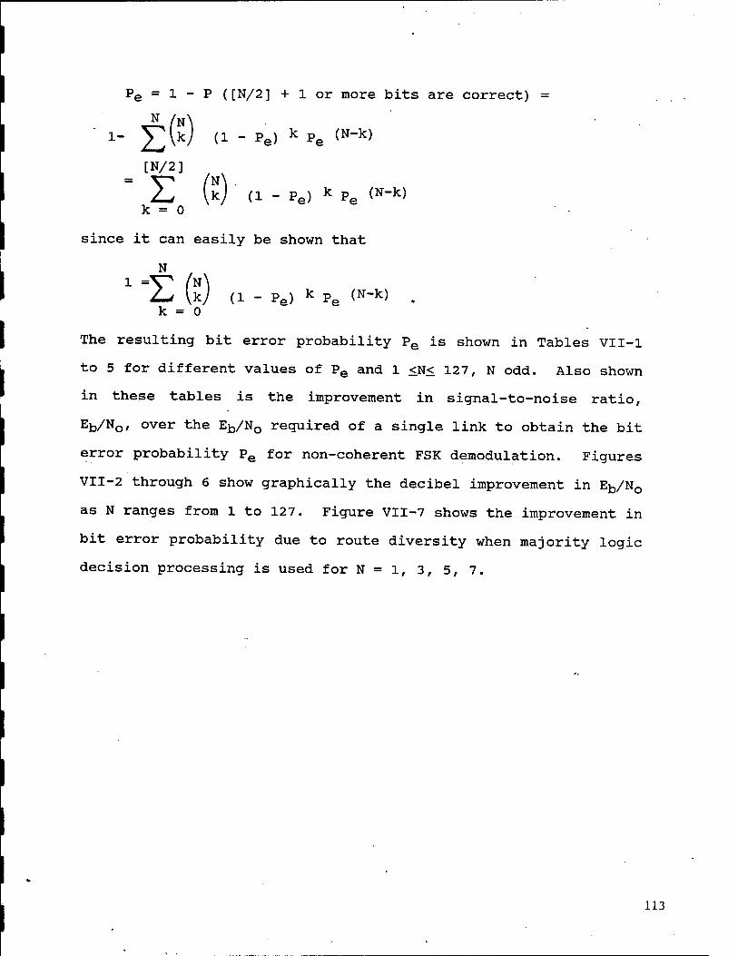
= 1 - P ([N/2] + 1 or more bits are correct) =
(1 - Pe) k Pe (N-k) - £© [N/2]
I] (k) (1 - Pe) k pe (N-k) k = 0
since it can easily be shown that
N
1 ~£J (k) (1 - Pe) * pe (N-k) . k = o
The resulting bit error probability Pe is shown in Tables VII-1
to 5 for different values of Pe and 1 <N< 127, N odd. Also shown
in these tables is the improvement in signal-to-noise ratio,
Eb/Nc over the Eb/N0 required of a single link to obtain the bit
error probability Pe for non-coherent FSK demodulation. Figures
VII-2 through 6 show graphically the decibel improvement in Eb/N0
as N ranges from 1 to 127. Figure VII-7 shows the improvement in
bit error probability due to route diversity when majority logic
decision processing is used for N = l, 3, 5, 7.
113

N
1 3 5 7 9
ii 13 15 17 1? 21
C"7
29 3-1
37 39 41 43 45 47 49 51 5 3 55 57 59 61 63 65 67 69 71 73 75 77 79 31 S3 85 87 89 91 93 95 97 99 101 103 105
TABLE VII-1
Pe
.1000000000ÖOOOD
.28000000000000D
.8560000Ö0Ö0000D
.27280000000000D ,890920000000000 .295706080000000- .992854864000000- .33624887968000D- .114644359972000- .392988232712800- „ 13530649719634D- .467576826279530- . 16208341601861D- .56335697082132D- .196261317941350- „68512030739788D- .23959466828070D- .S3922763495056D- .29437603570079D- .103391194437450- .363555151540170- . 12J97262148697D- .45090404095519D- .159014492750530- .56123427003392D" .198234590145640- „700677800751270- .247821738502120- .877047736354520- .310564957205560- .110030053336830- .390013342278030- .138312767820800- .490715232404900- .17417123839357D- .61843403832975D- .21967011583964D- .78055018650104D- .277443919992150- „986476929712980- .350356342653850- .124823460719160- .444203355738250- .15811781743041D- .562973735690360-
+00 -01 02 02
-03 -03 -04 -04 -04 -05 -05 -06 -06 -07 -07 -08 -08 ■09 •09 -09 ■ 10 -10 -11 -11 -12 -12 -13 ■13 -14 -14 -14 •15 •15 •16 •16 •17 •17 ■18 •18 •19 •19 ■19 ■20 •20
Eb/NQ = 5.08 dB
dB Improvement
.00OÖ0000O0Ö000 2.53080546855927 4.02654141187668 5.10250151157379 5.94736933708191
64489686489105 23987758159638 75917887687683 22023630142212 63502323627472 01213467121124 35795187950134 67734694480896 97412919998169 25133132934570 51140904426575 75638294219971 98793029785156 20746374130249 41618013381958 61510825157166 80513381958008
-21 .200492955543860-21 .714182777438640-22 .254457222891430-22 .906799940839820-23 .323218223497380-23 . 11522969943653D-23 .410879079183660-24 .146535076347750-24
6. 7. 7. 8. 8. 9. 9. 9. 9.
10. 10. 10. 10. 11. 11. 11. 11. 11. 12. 12. 1 *y
12. 12. 12. 13. 13. 13. 13. 13. 13. 13. 13. 14. 14. 14. 14. 14. 14. 14. 14. 14. 14. 15. 15. 15. 15. 15. 15.
0"=;cr-5;l=:
16146111488342 32903003692627 49025821685791 64561176300049 79550790786743 94031977653503 08038234710693 21600079536438 34745168685913 47498178482056 59832354736328 71918320655823 33625383145447 95021080970764 06121730804443 16942238307678 27496433258057 37797307968140 '47356783866882 57685947418213 67295050621033 7669398 7846375 85391699790955 94896650314331 03716945648193 12359733349915 20832300186157 29141306877136 37292718837329 45292615390503
114

TABLE VII-1 (Contd.)
107 109 ill 113 115 117 119 121 123 125 127
,52269007411926D-25 , 18647442824815D-25 ,6653713784831SD-26 , 23745226023519D-26 ,84752701197219D-27 30254755126772B-27 ,10801759461626D-27 38570400091689D-28 13774336210621D-28 491974178599430-29 ,17573866343420D-29
15.53146481513977 15.60859680175781 15.68436980247498 15.75883388519287 15.83203077316284 15.90400457382202 15.97479581832886 16.04444265365601 16.11298084259033 16.'18044734001160 16.24687194824219
115

N
TABLE VII-2
Pe
1 .1OOOOOOOOOOOOOD-01 3 .29S0O0000O00O0D-03 5 .98506000000000D-05 4 7 .341669800000000-06 5. 9 .121853685700000-07 6.
11 .44254343383480D-09 7. 13 .16278881392003D-10 7. 15 .604524S4932097D-12 8. 17 .22614362673891D-13 8. 19 .85091047329055D-15 9. 21 .32169401503951D-16 9. 23 .12209889904170D-17 10. 25 .46496735528439D-19 10. 27 .17756842846041D-20 10. 29 .67978999250222D-22 11. 31 .26080409268757D-23 11. ^5-S .100247538196360-24 11. 35 .38597617161819D-26 11. 37 .148832321694830-27 12. 39 .57466967263472D-29 12. 41 .222160746314090-30 12. 43 .85979697145185D-32 12. 45 .33309026011526D-33 12. 47 .129160169033790-34 13. 49 .50126062283819D-36 13. 51 .19468761102962D-37 13. 53 .75670641141438D-39 13. 55 .29431219069577D-40 13. 57 .11454089101670D-41 13. 59 .44603208583829D-43 14. 61 .17373345641816D-44 14. 63 .67744282216084D-46 14. 65 .26420754122169D-47 14. 67 .10308934686610D-4S 14. 69 .40240846809747D-50 14. 71 .15714293247932D-51 14. 73 .613885720109230-53 14. 75 . 23990340628497D--54 15. 77 , 937850140394850--56 15. 79 . 36675089679497D--57 15. 31 .143463930172070-58 15. 83 .56136025723641B-60 15. 85 .219716182427230-61 15. 87 860197790946 710-63 15. 89 .336856802596750-64 15. 91 .1319466005171OD-65 15. 93 .51695465089167D-67 15. 95 202583375923600-68 16. 97 794050814943420-70 16. 99 311302193371640-71 16.
101 122068030701650-72 16. 103 47374500104933D-74 16. 105 187795S5162298D-75 16.
Eb/N0 = 8.93 dB
dB Improvement
00000000000000 78310865163803 .42420750856400 59772968292236 .51377618312836 .26607501506805 90479838848114 .46001505851746 95119369029999 39167916774750 79102075099945 15629291534424 49288392066956 80499172210693 09595417976379 36846780776978 62474274635315 86661243438721 09561705589294 31306076049805 52005934715271 71757364273071 90643692016602 08737754821777 26103568077087 .42797756195068 58870267868042 74366044998169 89325141906738 03783440589905 17773604393005 31324958801270 44464445114136 57216262317333 69602584838867 31644034385631 93359327316284 04765510559082 15878677368164 26713490486145 37283539772034 47601530619812 57679176330566 67527413368225 77156662940979 86576223373413 95795154571533 04821920394897 13664269447327 22329592704773 30824923515320 39156699180603 47331237792969
116
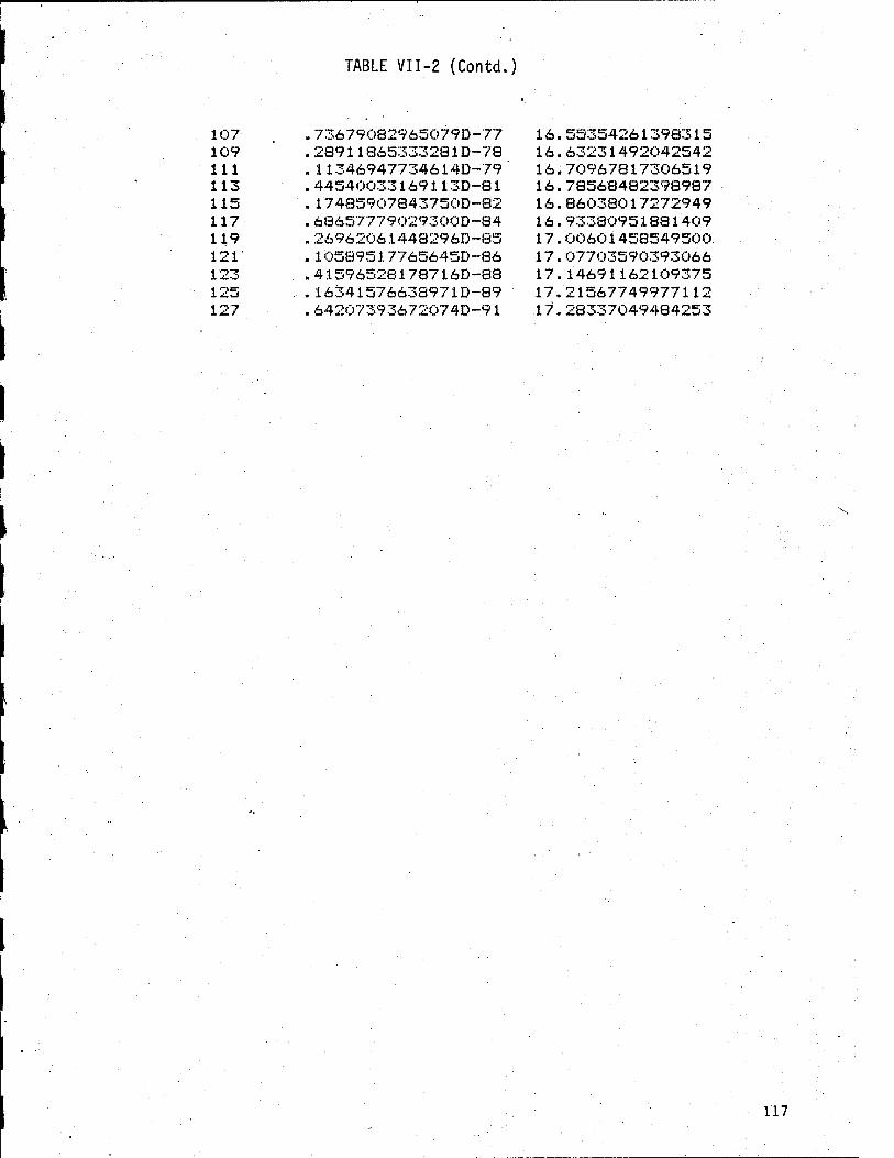
TABLE VII-2 (Contd.)
107 109 111 113 115 117 119 121' 123 125 127
, 73679082965079D-77 28911865333281D-78 11346947734614D-79 44540033169113D-81 17485907843750D-82 68657779029300D-S4 26962061448296D-85 10589517765645D-86 41596528178716D-88 16341576638971D-89 64207393672074D-91
16.55354261398315 16.63231492042542 16.70967817306519 16.78568482398987 16.86033017272949 16.93330951881409
,00601458549500 , 07703590393066 , 14691162109375 21567749977112
17. 17. 17. 17. 17.2833704948425:
117

N
5 7 9
11 13 15 17 19 21
27 29 31
37 39 41. 43 45 47 49 51 53 55 57 59 61 63 65 67 69 71 73 75 "7 "7 t .'
79 81 S3 85 87 89 91 93 95 97 99
101 103 105
TABLE VII-3
Pe
.1OÖÖOÖO0OÖOOOOD-Ö2
.2998Ö000000000D-05
.99850060000000D-08
.34916069980000D-10
.12558053968507D-12
.46002346192139D-15
.17070109959924D-17
.639506 79443501D-20
.24135523900157D-22
.91624945379266D-25 „3494961671-3818D-27 .13384127706799D-29 .51426503295719D-32 .19816290225791D-34 .7654700532221BD-37 .29632521019136D-39 ,. 11492961426S45D-41 .44650416912406D-44 .17372863881865D-46 .67686738111581D-49 .26403744180160D-5i .10311183031761D-53 „40307905S32263D-56
'. 1577152S564250D--53 .61762758120557D-61 .24205844249103D-63 ,. 94935572966301D-66 .37258913849320D-68 .14631994632779D-70 .57495083638707D-73 .22604516051140D-75 .88916445528822D-78
.. 34992725517642D-80 ■. 13777482613197D-82 .54268409462464D-85 . 2.1334498945674D-87 . 84297815085328D--90 .. 33242222S54855D-92 .. 131 13306646420D-94 .51745826971555D-97 .20425489997170D-99 .80648677850522-102 . 31852510414182-104 .12583636553611-106 .49725546383535-109 . 19654364737682-111 .. 77703390980556-114 .30726860872517-116 .. 12153173210605-118 .. 480 784 77162854-121 .19023819356842-123 .75288283265538-126 i29801396254758-128
Eb/N0= 10.94 dB dB Improvement
.00000000000000 2.8665032982S262 4.55271333456039 5.75522243976593 6.69174134731293 7.45939731597900 8.11013633973236 8.67504954338074 9.17424380779266 9.62148189544678 10.02660155296326 10.39688229560852 10.73736139488220 11.05334945869446 11.34827256202698 11.62389273411365 11.88297390937805 12.12739467620850 12.35872745513916 12.57830619312012 12.78727173805237 12.98660278320312 13.17715167999268 13.35965991020203 13.53477954864502 13.70308876037598 13.86509656906128 14.02125954627991 14.17198419570923 14.31763768196106 14.45855140686035 14.59502220153809 14.72732543945312 14.85570549964905 14.98039007186890 15.10158658027649 15.21948456764221 15.33425807952881 15.44607043266296 15.55506944656372 15.66139340400696 15.76517224311829 15.866522 78900146 15.96555709838867 16.06238007545471 16.15708589553833 16.24976754188538 16.34 0 50 346O9 9354 16.42938852310181 16.51648402214050 16.60186290740967 16.68559312320435 16.767736673355iO
118

TABLE VI'I-3 (Contd.)
107 109 in 113 115 117 119 121 123 125 127
.11798330744773-130
.46717756883183-133
.18501744993365-135
.73284482602725-138
.29032043856824-140
.11502895948197-142
.45582550753317-145
.18065495326560-147
.71607580939063-150
.28387305136317-152
.11254950940738-154
16.84835433959961 16.92749357902527 17.00522422790527 17.08158135414124 17.15661764144897 17.23037600517273 17.30290293693542 17.37423419952393 17.44441390037537 17.51347422599792 17.!
119

N
TABLE VII-4
Pe
10000000000000D-03 3 .29993000000000D-07 2 5 .99985000600000D-11 4 7 .34991600699980D-14 5 9 .12595800539969D-17 6
11 .46180203464692D-21 . 7 13 .17150993001760D-24 8 15 .64309970809162D-28 8 17 .24292502368179D-31 9 19 .92302445707432D-35 9 21 .35239281127015D-33 10 23 .13507057580298D-41 10 25 .51945083536422D-45 10 27 .200339762310670-48 11 ^O .77457026379102D-52 11 31 .30011618334906D-55 11 y,y< .11650411930789D-58 12 35 .45302653292289D-62 12 37 .176424361509730-65 12 39 .687986532033140-69 12 41 .268615612224430-72 12 43 .10499382586044D-75 13 45 .41030446988125D-79 13 47 .160882381169920-82 ;13 49 .630596062373330-86 13 51 „ 24736301773134D-89 13 53 .97103202849533D-93 13 55 .381438814626150-96 14 57 .14992995332036D-99 14 59 .58966563745569-103 14 61 .23203880114567-106 14 63 .91356158730300-110 14 65 .35985197340082-113 14 67 „14180985448498-116 14 69 .559080172851.00-120 15 71 .22050404869108-123 15 73 .87001017108231-127 15 75 .34339077138002-130 15 77 .13558178809129-133 15 79 .53549457347657-137 15 SI .21156452675221-140 15 83 .83610007999140-144 15 85 .33051817424397-147 15 87 .13069135707355-150 16 89 .51690725537969-154 16 91 .20449504667696-157 16 93 ... 80919741375843-161 16 95 .32027530612367-164 16 97 . 1.2679020636752-167 16. 99 .50203904768033-171 16. 101 .19882696880786-174 16. 103 ,.78758197522510-178 16, 105 .31202959836925-181 16.
Eb/N0 =12.31 dB dB Improvement
.00000000000000
.90569335222244
.61263835430145
.82829236984253
.77400887012482
.54851693875427
.20458769798279
.77378463745117
.27650749683380
.72670972347260
. 13435840606689
.50632663917542
.84971666336060
.16739392280579
.46332025527954
.74023873443604
.00058579444835
.24610924720764
.47844815254211
.69894957542419
.90876269340515
.10887313568115
.30015132495117
.48333477973933
.65903384323120
.82798075675964
.99053931236267
.14721846580505
.29843068122864
.44454312324524
.58588957786560
.72277164459229
.85546350479126
.93421311378479
.10924935340881
.23077345573425
.34899592399597
.46407341957092
.57617664337158
.68545341491699
.79204440116882
.89607715606639
.99767327308655
.09694361686707
.19399189949036
.28891537257335
.38180732727051
.47275090217590
.56182527542114
.64910793304443
.73466920852661 „81357466697693 .90088868141174
120

TABLE VII-4 (Contd.)
107 ■ .12364381687967- -184 109 .49003015263932- -188 111 .19424253934642- -191 113 .77007766082621- -195 115 .30534510440939- -198 117 .12109087015909- -201 119 .43027911183809- -205 121 .19051791550459- -208 123 .75585036892927- .C X .&
125 .29991064340948- -215 127 .11901513962299- -218
16.98166847229004 17.06097245216370 17.13885307312012 17.21535921096802 17.29053974151611 17.36443877220154 17.43710041046143 17.50856637954712 17.57887244224548 17.64805793762207 17.71615743637085
121

TABLE VII-5
N
1
5 7 9
11 13 15 17 19 21
31
35 37 39 41 43 45 47 49
59 61 63 65 6 7 69 71
77 79 81' 83 85 87 89 91 93 95 97 99 101 103 105
Pe
.100000000000000-04
.29999800000000D-09
.99998500006000D-14
.34999160007000D-18
.12599580005400D-22
.461980200346500-27
.17159099120020D-31
.64345996108106D-36
.24308249735691D-40
.92370442077123D-45
.352683669043000-49
.13519407184539D-53
.51997205677448D-58
.200558663964930-62
.. 775485810354780-67
.30049776860093D-71
.116662680561280-75
.453683691832620-80
.17669610124572D-84
.689107936525380-39
.269077562727790-93
.105183817738870-97
.41158475104603-102
.1612024208263 i-106
.63190718994804-111
.24789957948349-115 ,97322567951392-120 .33233484583981-124 ,15029564677935-128 ,59115697841673-133 .23264655357874-137 ,91603666160787-142 ,36085932510340-146 , 14221960830902-150 ,56074599986054-155 , 22118093587912-159 ,87275930198769-164 ,34450681033145-168 ,13603466392499-172 ,53733155568750-177 , 21230937208605-181 83911913626251-186 33174146036059-190 13118735805153-194 51891369873434-199 20530728180324-203 31248452941283-208 32160524620947-212 12732815175466-216 50421444270840-221 19970646996479-225 79113695607635-230 31346622745178-234
6 7 8
.3 9 9 10 10 10 11 11 11 12 12 12 12 12 13 13 13
13 14 14 14 14 14 14 14 15 15 15 15 15 15 15 15 15 16 16 16 16 16 16 16 16 16 16, 16
Eb/N0 = 13.35 dB
dB Improvement
.00000000000000 3.92815476655960 ^.64685440063477 .86991488933563 .82079136371613 .59913206100464 .25817823410034 .82976174354553 .33444738388062 .78629589080811 .19534826278687 .56902335437012 .91297984123230 .23159170150757 .52834892272949 .80606126735273 .06703066825867 .31316447257996 .54606008529663 .76706933975220 .97735095024109 .17739673805237 .36957216262817 .55312705039973 .72922301292419 .89344298362732 .06130433082581 .21826958656311 .36974883079529 .51611399650574 .65769886970520 .79480743403203 .92771267890930 .05666613578796 .. 13139549446106 .30360937113530 „42200088500977 .53724527359009 .64950823783875 .75893378936768 .86567521095276 .96984982490540 „07157945632935 .17097854614258 .26815199851990 „36319637298584 „45620226860046 .54725551605225 .63643836975098 .72332473945618 .80948495864368 „8934369*7662354 .97589397430420 122

TABLE VII-5 (Contd.
107 109 111 113 115 117 119 121 123 125 127
,12422426353461- 49237488759099- 19518952260329- 77390160082270- 30688394699288- 12171406081682- 48279428255393- 19153286661271- 75994539124407- 30156261676784- 11967897510415-
238 17 243 17 247 17 252 17 256 17 260 17 265 17 269 17 274 17 278 17 282 17
,05676436424255 13615536689758 21411943435669 29070782661438 36596703529358 43994474411011 51268148422241 58421897838184 65459656715393 72385001132556 79201626777649
123

FIGURE VII-2
Re IMPROVEMENT VS. NUMBER OF LINKS. (Pel=.l)
D 15.0- B
I M P R 0 V E M E N
■10.0-
5.0-
0-
/
0
I- I I I I t I 1 I I 1 ' I I I I I I I ' I
20.0 40.0 60.0 80.0 100.0 120.0 140.0
NUMBER QF LINKS
124
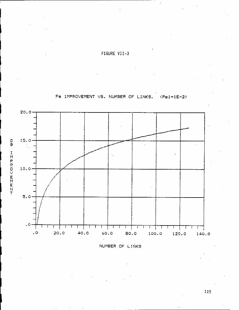
FIGURE VII-3
Pe IMPROVEMENT VS. NUMBER OF LINKS. CPel=lE-2)
D B
I M P R 0 V E M E N T
20.0-
15.0-
10.
5.0-
Al
/
0-
.0
y_ s
20.0 T~T 1—T
40.0 60.0 eO.O 100.0 120.0 140.0
NUMBER OF LINKS
125

FIGURE VII-4
Pa IMPROVEMENT VS. NUMBER OF LINKS. (Pel=lE-3>
D B
I M P R Q V E M E N T
20.0-
15.0-
10. 0- /
/
5.0- i +
.0-
.0
X z_
20
i i r . 0 40.0 60.0 80.0 100.0 120.0 140.0
NUMBER OF LINKS
126

FIGURE VII-5
Pe IMPROVEMENT VS. NUMBER OF LINKS. <Pel=lE-4)
20.0
D B
T
M P R 0 v E M E N
15.0
5.0
-^-^^^
^^
v"* -
^
-
/' J /
/ / i
1
/
—
/ 1
1
1 I I
J
! 1 1 1 1 1 1 1 1 1 I 1 1 1 1 1 1 1 1 I
.0 20.0 40. 0 60.0 80.0 100.0 120.0 140.0
NUMBER OF LINKS
127

FIGURE VII-6
Pe IMPROVEMENT VS. NUMBER OF LINKS. <Pei=lE-5>
D B
I M P R 0
E M E N T
20.0-
15.0'
10.0-
5.0
dL /
i~\—r T
20.0 40.0 60.0 SO.O 100.0 120.0 140.0
NUMBER OF LINKS
128

FIGURE VII-7
1 *° 9 8 7 S
s
10_11
U z <
10"2i
■5 in J-U
5 S < >
■J a
m m u -i ü >- u
■3, 9 s 7 S
S
10-4,
IQ"5
g=j===j=g5=j=^============================^^===================== :===^===
s^==sssssss^sEssg^gggggggsgspgp^^^l^^^^^^^^^^^^^^^^^^^^=^^^^^==M§jS~gj
BBIIBBBB^IBBBBBB »^nfflnm!i!siiissiiiii!S!!!BBBBBB _IE U1L- —iSliiLiin:
I I 1 1 ''-III 1) 1 1 1 ' 1 1 1 1 "1 1 1 1 1 1 | 1 '
=jjgijlj!S!j!=j^'=H^I!:!gpgg=g
_=t ¥- |\ -^||r-^ r1" — 'j— ■- ■ ■ ■■■ ■ ■■ ■ ■ ■ ■" ■ " \ ' 1 ""V'j" — " j—1——'—
\ \ 1 ] ■ \ ' I 1
■||llllllj||jjlllB| 1
_3E _ ^__i_^±^_L|^3:_-_ 1 | Mi
' i ' 1
Wi|ijiHliW|ll|llll|IBBIHBgWM — =(=: = = =j= = = = = = = — — — — = = = = = = =!== = = = == = = = = — = -zz:=:= = = =r= = = = = = = = = = = = z j' j j = 1 E j j j =£= — zzhri^ — j—— ^H 1 | ~ M [ 1— ^SS^^^^^^^^S^SESSS^^^-^-^^LL^5^ | ==Iil^II^== = ^ = s j '^^~^^^
BIlBlIII|||IliIIIIj!lH*liIiiIH|jI|^HH pliiiiiHll|lSJlllllllllllllliiiiiiiBii||ij|ÄÄ^ "± ~-- P ^ h*^T^—
ill —4— 1
l|ll^lgilillIIlJlljlllllMl|MIIMIII||g^^ E(EE5EiEEEEEEE5E55EEEEEE5EEiEHi5B55SEEEEEEEESEE^EE^^E — _„___„ 1 .——j—1— .—,—1—.—
j^pjjjpgjjjjjjjjjjgjpjaj^jj^M itiig^^^ — ^r=Lr=4rz — -ri—~ — — — — = "^ — — ~=: = = = =r|^: = ~ ~ = — — — — ^ =z — — — — — — — —=zfc= = = == = = j !_ j = =—1 1— ! ==: = = =_J — = ^= = = = = = = = = = = = = —= = = =^^ = = = —= — — = — —= —=— — — — —— = = — — — —— = —=^ — = = = r=^=T|=r_-|—l_j-J=:=^==;=|=; -^i-""" -" 1 — ~^~^=^-^p— ^= ...-_■—--. , g- -—._-■■.,■--- - _._--^ _■_______- _^-_ -|- -- \^== Ijjlll lllllllllllllllllllllllljlllljljljlll jllll^_ll -±-= -—- = jp-llpl—^ §=—=]=-*—
1 1 , 1 [ 1 ; 1 ' ' ' J I j I '
129
-14 •10 -2 0 Eb/N0 (dB)
10 14

Now, if we use the full 50 distributed synchronization bits
available in any packet (Section IV) and establish processing
rules, an analysis of bit error rates (BERs) and link margin
gains (+dB) can be determined. Two separate decision rules are
depicted in Figures VII-8a and VII-8b.
MAJORITY GATE
VI1-8a Method 1
Majority Logic on N links Then Sync Checked
N
SYNC CHECK
SYNC CHECK
SYNC CHECK
VII-8b Method 2
N Links Each Sync Checked Then Use Majority Logic on "Good" Links
The task at hand is really twofold: 1) maintain link connec-
tivity, and 2) maintain a sufficient level of link quality. If
we concentrate on two potent comm-link threats, active jamming
and nuclear event interference to propagation, in a parallel-link
architecture with angular robustness, we would expect the
following:
1) Any single jammer in a dynamic space-borne environ-
ment to possibly disrupt one of the links; and
130

2) Any nuclear event to be localized so as to disrupt a
region no larger than a hemisphere, and more
probably a half-hemisphere, angularly from any mode.
For Method 1, a jammer of a single link where N>3 would expect
little problem with connectivity but BER would suffer some,
whereas for Method 2 the connectivity probability should be
roughly the same (very slightly better) but the BER should be
better since signals propagated through a very noisy channel
would be eliminated earlier.
For Method 1, a nuclear event may disrupt several links and
connectivity would have a higher probability of being lost,
whereas for Method 2, if any one link maintains a sufficient
signal-to-noise ratio, connectivity should be maintained.
In each of the cases, the numerical analysis bears out the
arguments.
For both methods, assume that 50 of 50 synchronization bits must
be correct for connectivity to be considered acceptable (though
not analyzed here, less than 50 of 50 can be acceptable or be
acceptable in certain instances).
Method 1
P (not connected) = 1 - P (all L sync bits correct)
= 1 - (1 - Pe)L ~ LPe for Pe « 1
131

where Pe is the individual bit error probability induced by the
majority logic decision. Note Pe « Pe.
Method 2
P (not connected) = P (all N links have at least one error in L
sync bits)
= [1 - (1 - Pe)L] N c=r (LPe)
N for Pe « l
where Pe is the individual bit error probability. Note this
expression assumes the N links are all statistically independent
which is justified by the discussion at the beginning of this
section.
Suppose now that Pe = lo-5, N = 5, L = 50. Then for Method 2 we
obtain,
P (not connected) 2? (50 X 10"5)5 = 3.125 X 10""17
For Method 1 we note that from Table VII-5 Pe ~ 10"14
so P (no connected)^ 50 X 10*"14 = 5 X 10~13.
In conclusion, decision rules corresponding to Method 2 are more
favorable. Furthermore, since the numerical results show such a
great advantage in both BER and link margin gains, a packet with
50 distributed synchronization pulses could support a robust
architecture where no more than 5 to 9 (where the marginal
improvement tends to fall off) parallel links need be used.
Given that the final tradeoffs are not yet being made and that in
some earlier cases we chose other than 5 to 9 parallel links, we
132

will proceed with the understanding that extra margin is built
into some of the numbers. It is also noted that in the case of
choosing 50 synchronization pulses in a 235-bit packet, no margin
remained in the packet architecture. Also, some lower priority
links can probably do without as much redundancy. Obviously,
tradeoffs will continue, but for here the number of links listed
in Section IV are, at least, a reasonable point of departure for
continued tradeoff analyses...
133

VIII. COMSEC/TRANSEC, KEYING, AUTHENTICATION
134

COMSEC/TRANSEC, KEYING, AUTHENTICATION
COMSEC/TRANSEC
In the area of COMSEC/TRANSEC, the. major hurdle for SDI will be
in meeting Level 2 radiation requirements. The present equipment
and architectures will support SDI needs in all other areas
(assuming that no new encryption/decryption algorithms need to be
developed) , but device technologies in use at this time do not
approach the required hardness levels. Indeed, the Level 1
requirements at this time are difficult to meet, but attainable.
The current state-of-the-art in COMSEC/TRANSEC includes digital
encryptors ranging from one bit per second to hundreds of
megabits per second, using any of several different algorithms
and either of two modes of operation, with keying via resident
variables or via remote electronic interface, and with the
capability to change keys. One feature of these encryptors is
their "fault intolerance"—i.e., their guarantee of shutdown in
case of any internal failures that might compromise the security
of the data.
One recent trend that seems likely to continue for SDI is the
integration, or embedment, of COMSEC and TRANSEC functions
directly into associated communications equipment instead of the
use of separate COMSEC or TRANSEC boxes. VLSI efforts have
reduced the COMSEC or TRANSEC function to a few integrated
circuits, thus decreasing the size, weight, and power of the
135

overall function. As a result, the overhead penalties have
increased in terms of mechanical packaging of a separate box and
the risks involved for the embedder have decreased to the point
that it makes more sense to include the COMSEC/TRANSEC function
within other parts of the communications system.
The development of COMSEC/TRANSEC algorithms and their use in any-
particular application has in the past been determined by the
government. Algorithms that have been used for space systems in
the recent past include KG-28, KG-29, BAYLESS, KEESEE, and
others, all of which entail serial digital data encryption and
decryption. For SDI communication systems, any of these could
potentially be used. Alternatively, the government might elect
to develop entirely new algorithms for SDI, since it seems to be
a "standalone" system that will not require interoperability with
existing systems.
Three basic encryption operating modes have been considered for
the communication system design. Each of these types of
encryptors have applications in which they are best suited and
those in which they are poorly suited. Table VIII-1 provides a
direct comparison of these types. Encryptor Type 1 needs to be
synchronized before data can be transmitted whereas Encryptor
Type 2 does not require a specific synchronizing sequence.
Operating data rates for Encryptor Type 1 or 2 are not an issue.
136

Encryptor Type 3, the block mode encryptor, is the most suitable
for the SDI communication systems. The major drawback to this
design is the timing of the block gate that must identify the
first bit of encrypted data.
The code table required for the block encryptor can be generated
by a variety of techniques, one of which is to operate Encryptor
Type 1 in a burst mode by using the block gate to start and stop
the clock to the encryptor shift register.
137

TABLE VIII-1 ENCRYPTOR COMPARISONS
ENCRYPTOR DATA TYPE
BIT TIMES TO
SYNCHRONIZE ERROR
MULTIPLICATION
IMMUNITY TO JAMMING
DURING SYNCHR
AFTER SYNCHR
1 CONTINUOUS 500 TO 1000 NO POOR GOOD
2 CONTINUOUS NONE YES N/A POOR
3 BURST 100 NO GOOD GOOD
138

KEYING
Depending upon the type of security device employed, a set of
input variables (keys) are required. To maintain the determined
security requirement any or all of the inputs will be treated as
variables, whereas some may be fixed.
On board the satellites, keys for the security devices are
derived from three sources: time of day, fixed parameters preset
in PROMSs, and other variables communicated to the satellites
(over-the-air parameters). Any or all of these sources can be
employed for a given situation. Different layers of security can
employ different sets and different mixtures of the same types of
parameters.
1) Time of Dav - It is assumed that time of day (TOD)
information of sufficient accuracy is available on
board the satellite and it will naturally be
employed as part of the key of COMSEC and
especially for TRANSEC. (Generally the TOD is
augmented with a command sequence
counter/authenticator and for purposes here this
will all be considered as TOD.) Only one issue
must be highlighted: The satellites are so far
apart that time will appear to be different from
satellite to satellite. Knowing ephemeris
variables and managing the network to synchronize
the arrival time of a signal with its
139

correspondingly correct COMSEC/TRANSEC keys will
protect TOD as a useful (and preferred) piece of
the key.
2) Fixed Parameters - A series of 100-200 unique
codes can be pre-programmed prior to satellite
launch and be managed by either a predetermined
process or by signals from the ground. Such a
configuration and management scheme is within
current capabilities. The notion of visiting or
refurbishing a satellite to change a PROM or re-
initialize a tape is considered not feasible for
SDI. If security tradeoff analyses eliminate
consideration of over-the-air parameters, a scheme
of fixed parameters (coupled with the TOD) should
be employed.
3) Over-the-Air Rekevina (OTAR) - OTAR has one
tremendously advantageous characteristic: immense
flexibility—keys can be changed whenever the
network manager chooses and any code can be used.
It also has one major disadvantage: the fear that
the OTAR link can be intercepted and exploited or
be spoofed rendering the links useless. The
state-of-the-art is such that OTAR information can
be distributed/interlevered, coded, etc. to be
accomplished with extremely low, acceptable risk.
.. 140

Spoofing can be dealt with in an equally
acceptable fashion.
Conclusion - TOD, presets, and OTAR can all be employed on
SDI without significantly pushing the state-of-the-art for
keying or key management. Some OTAR parameters will allow
for more flexibility in growing and evolving the SDS as time
goes on and would therefore be a very favorable technique.
The probability of exploitation and spoofing can be made
acceptable with design tradeoffs coupled to the actual
security requirement. And, of course, different levels of
security should be treated with separate analyses and the
preferred mix of TOD, fixed, and OTAR parameters will most
probably differ among the various security levels.
Current methods of keying encryption/decryption systems allow the
addressing of individual satellites or ground stations as well as
addressing of sub-nets or entire networks simultaneously. If a
particular satellite is suspected of being compromised, it can be
excluded from the ongoing communications through the use of a
different key. Most newer systems allow rekeying, either from
internally stored key variables or via encrypted variables sent
over the link. The NSA has developed rekeying algorithms
implementable in hardware for strategic systems that could also
be applied to SDI COMSEC.
Most current cryptographic systems have resident processors to
141

ensure security and provide needed control sequences. These
processors accept external control inputs and provide status
outputs. In response to the control inputs, the processor
conducts internal self-test, security checks, and alarm checks,
as well as configuring the key generator for the selected mode of
operation. Unique firmware-secured COMSEC/TRANSEC architectures
can provide greater than 90% fault grade on internal nodes via
system firmware. These processors help- to meet the Security
Fault Analysis (SFA) requirements of COMSEC equipment.
142

AUTHENTICATION
There are currently three authenticate methods that have been
used in conjunction with the decrypt/command uplink. They are as
follows:
1. KIR-23
2. KGR-29
3. KGX-60
The KIR-23, currently being upgraded on the KEYWAY program as the
KIR-123, is block decryptor followed by an authenticator. The
block decryptor, decrypts and gives the entire word to the
authenticate logic. The word is made up of four segments: a
command data portion, a fill bit, and actual authenticate word.
The authenticate word, which is an internally stored count of
valid authenticated commands, is incremented (+1) with every
valid authenticate and can be reloaded with the command data
filed. During normal operation the command data is only output
if the authenticate was valid. The command rate is:
KIR-23 6 Commands Per Second
KIR-123 (KEYWAY) 280 Commands Per Second
The KGR-29 is a serial machine which passes variable length
command data, although authenticate dictates a minimum and a
maximum length. This authenticate algorithm, unlike the KIR-123,
143

passes "unauthenticated" data as well as authenticated data. The
authenticate output is an "Accept" or "Reject" pulse at the end
of the authenticate cycle. The authenticate cycle begins upon
receipt of the correct coded data. The KGR-29 is a ternary data
box with three valid decoded commands, as follows:
1. Authenticate
2. Fill
3. Increment
The serial bit stream is composed of two parts, the command data
and the authenticate data. The first four bits on the
authenticate are decoded to determine which command is present.
The authenticate word contains three segments, the fixed data
portion, the vehicle (V-word) word segment and the time word
section (T-word). The V word is incremented (+1) for each valid
authenticate. Both T and V words can be altered by use of the
fill or increment commands. The increment commands will add one
to the T-word and set the V-word to 1. The fill command puts the
immediately following command data bits into the T-word and again
sets the V-word to 1. Neither command will be executed unless
the command was authenticated. The KGR-29 can also be used to
transmit serial data in a continuous manner when authentication
is not necessary, such as a long data transfer. The maximum bit
rate is 128 Kbps for this unit.
The third type of authentication that has been used is that used
144

in the KGX-60. The output of the KG (plain text) is in a quasi-
telemetry format. A 2 4-bit sync word is used in order to
synchronize the authenticate. After the sync word is detected
three consecutive times in the serial bit stream from the KG (KG-
29/59), the authenticate proceeds. Until sync is found all data
is passed unmodified through the unit. After sync, the 4 bytes
of command data are temporarily stored and replaced with
previously authenticated data. The assembled command data is
exclusively "OR"ed with on-board IRIG "B" time and checked for
correctness using a BCH error-checking algorithm. When the BCH
checks okay, authenticate, the entire command block, command data
plus BCH extension is transmitted during the next format. When
the authenticate is not valid the command data block is inhibited
and zeros are transmitted followed by the actual BCH remainder.
The current bit rates for the KGX-60 is 96K BPS or 196K BPS.
Each of the three methods of authentication has a specific use.
The KIR-23 method works well for low data rates when only command
data is required and security is paramount, since the KIR-23 does
not output unless authentication is valid. Increasing the
command rate to above 1,000 command per second would be easily
obtainable using current technology. The KG-29/KG-57 family is
useful for transmitting long data streams, such as those used in
reloading or updating memory banks. This system is not as
secure, however, since it depends on the processor to act on the
accept-reject pulse after receipt of the actual command data.
The KGX-6 0 method has the advantage of passing either
145

authenticated data or ordinary traffic, that does not require
authentication.
Additional security can be added to any of the above systems by
adding security checks within the receiving processor. The KGX-
60 function, for instance, uses a Row-Column check on several
commands for further verification.
In essence, the optimum method of authentication depends on the
data rate as well as the overall system capabilities.
146

SUMMARY
Barring any new special security requirements, the technology for
COMS EC/TRANS EC, KEYING .(to include key management), and
AUTHENTICATION now exists and is available for SDI/SDS. The
specific design needs to be determined using the channel
requirements which must be validated for the entire system.
147

IX. SIZE, WEIGHT, AND POWER
148

SIZE, WEIGHT, AND POWER
EHF and laser communication terminal size, weight, and power
estimates have been generated for each of the spaceborne SDS
elements. The results for EHF technology is presented in Tables
IX-4 through IX-8 while the lasercom results are discussed at the
end of this section. The EHF technology will be discussed first.
EHF Estimates
EHF terminal estimates are based on the use of monolithic phased
arrays, as described in Section V. This technology utilizes
solid state power amplifiers embedded in the transmitters1
arrays. It is expected that this technology will be available
within five to ten years or perhaps sooner if sufficient research
funds are directed to this effort.
The receiver and transmitter electronics assume use of current
LSI technology and are based on systems of like complexity
currently being produced. Each communication system's size,
weight, and power estimate incorporates allowances for the use of
error correction, interleaving, spread spectrum, and encryption.
Tables IX-1 through IX-3 provide the basis for the estimates of
each of the SDS elements shown in Tables IX-4 through IX-8.
Payload estimates have been separated from antenna estimates
since the antenna structure would be external or near conformed
to the spacecraft.
149

TABLE IX-1 60 GHZ
Transmitter Exciter
Size Weight Input Power
186 Cubic Inches 14.7 Pounds 26 Watts
Transmit Antenna & Power Amplifier flOOW^
Size Weight Input Power Efficiency
216 Cubic Inches 6 Pounds 667 Watts 15%
Receiver
Size Weight Input Power
186 Cubic Inches 14.7 Pounds 26 Watts
Receiver Antenna
Size Weight
216 Cubic Inches 5 Pounds
150

Transmitter Exciter
TABLE IX-2 44 GHZ
Size Weight Input Power
186 Cubic Inches 14.7 Pounds 26 Watts
Transmit Antenna & Power Amplifier flOOW^
Size Weight Input Power Efficiency
402 Cubic Inches 11 Pounds 500 Watts 20%
Receiver
Size Weight Input Power
186 Cubic Inches 14.7 Pounds 26 Watts
Receiver Antenna
Size Weight
402 Cubic Inches 10 Pounds
151

Transmitter Exciter
TABLE IX-3 20 GHZ
Size Weight Input Power
186 Cubic Inches 14.7 Pounds 26 Watts
Transmit Antenna & Power Amplifier flOOWl
Size Weight Input Power Efficiency
1944 Cubic Inches 46 Pounds 400 Watts 25%
Receiver
Size Weight Input Power
186 Cubic Inches 14.7 Pounds 26 Watts
Receiver Antenna
Size Weight
1944 Cubic Inches 45 Pounds
152

BSTS
The BSTS estimate is based on the use of three 60 GHz
transmit/receive units so that each of the 60 GHz links can
operate concurrently. The BSTS-to-BSTS links utilize two
transmit as well as two receive arrays to obtain the required
angular coverage. The remaining 60 GHz links (to the SSTSs and
CV/SBIs) only require one of these units. The 44 GHz and 20 GHz
payloads are receive-only and transmit-only, respectively, with
angular requirements such that each system requires only one
antenna array.
TABLE IX-4 BSTS
60 GHz Communication Package
Pavload (3 Tx/Rx Units) Size Weight Power
1116 Cubic Inches 88.2 Pounds 156 Watts
Transmit Antennas & Power Amplifiers (4 Units) Size 864 Cubic Inches Weight 24 Pounds Power 2000 Watts
Receiver Antennas IA Units) Size Weight
864 Cubic Inches 20 Pounds
44 GHz Communication Package
Pavload fl Rx) Size Weight Power
Receiver Antenna (1 Unit) Size Weight
186 Cubic Inches 14.7 Pounds 26 Watts
402 Cubic Inches 10 Pounds
153

TABLE IX-4 (Contd.)
20 GHz Communication Package
Payload (1 Tx) Size Weight Power
186 Cubic Inches 14.7 Pounds 26 Watts
Transmit Antenna & Power Amplifier Size Weight Power
1944 Cubic Inches 46 Pounds 400 Watts
Power Converter Size Weight Efficiency
1771 Cubic Inches 125 Pounds 70%
Summary
Payload Size Weight Power
3259 Cubic Inches 243 Pounds 3726 Watts
Antennas Size Weight Power
4074 Cubic Inches 100 Pounds 2400 Watts
154

SSTS
The SSTS estimate is based on the use of three 60 GHz
transmit/receive units to enable simultaneous operation of each
60 GHz link. The SSTS to SSTS and SSTS to CV/SBI links utilize
two transmit and two receive arrays each to obtain the correct
angular coverage. The SSTS to BSTS link requires only one array
each for transmit and receive. The 44 GHz and 20 GHz payloads
are receive and transmit only respectively and require only one
array each of the appropriate type.
TABLE IX-5 SSTS-
60 GHz Communications Package
Pavload (3 Tx/Rx Units) Size Weight Power
1116 Cubic Inches 88.2 Pounds 156 Watts
Transmit Antennas & Power Amplifiers (5 Units) Size 1080 Cubic Inches Weight 30 Pounds Power 2000 Watts
Receiver Antennas (5 Units) Size Weight
1080 Cubic Inches 25 Pounds
155

TABLE IX-5 (Contd.)
44 GHz Communication Packacre
Pavload (1 Rx) Size Weight Power
Receiver Antenna (1 Unit) Size Weight
186 Cubic Inches 14.7 Pounds 26 Watts
402 Cubic Inches 10 Pounds
20 GHz Communication Package
Pavload (1 Tx) Size Weight Power
186 Cubic Inches 14.7 Pounds 26 Watts
Transmit Antenna & Power Amplifier (1 Unit) Size 1944 cubic Inches Weight 46 Pounds Power 400 Watts
Power Converter
Size Weight Efficiency
1771 Cubic Inches 125 Pounds 70%
Summary
Payload
Antennas
Size Weight Power
Size Weight Power
3259 Cubic Inches 243 Pounds 372 6 Watts
4506 Cubic Inches 111 Pounds 2400 Watts
156

CV/SBI
The CV/SBI estimate is based on the use of five 60 GHz
transmit/receive units to accommodate the CV to BSTS, SSTS, CV,
ERIS, and GSTS links. The CV to SSTS and CV to CV links require
two transmit and two receive arrays each to obtain sufficient
angular coverage. The remaining 60 GHz links can be accommodated
with a single array of each type.
157

TABUS IX-6 SBI-CV
60 GHz Communication Package
Pavload (5 Tx/Rx Units) Size Weight Power
1860 Cubic Inches 147 Pounds 260 Watts
Transmit Antennas & Power Amplifiers (7 Units) Size 1512 Cubic Inches Weight 42 Pounds Power 2668 Watts
Receiver Antennas (7 Units) Size Weight
1512 Cubic Inches 35 Pounds
Power Converter Size Weight Efficiency
1943 Cubic Inches 137 Pounds 70%
Summary
Pavload
Antennas
Size Weight Power
Size Weight Power
3803 Cubic Inches 284 Pounds 4183 Watts
3024 Cubic Inches 77 Pounds 2668 Watts
158

GSTS
The GSTS estimate is based on one 60 GHz transmit/receive unit to
accommodate the link to the CV/SBI as well as a single 20 GHz
transmitter to communicate to the GEP. It is expected that the
angular coverage can be met with single transmit and receive
arrays.
TABLE IX-7 GSTS
60 GHz Communication Package
Pavload (1 Tx/Rx Unit^ Size Weight Power
372 Cubic Inches 30 Pounds 52 Watts
Transmit Antenna & Power Amplifier (1 Unit) Size 216 Cubic Inches Weight 6 Pounds Power 667 Watts
Receiver Antenna (1 Unit^ Size Weight
216 Cubic Inches 5 Pounds
20 GHz Communication Package
Pavload (1 Tx) Size Weight Power
186 Cubic Inches 14.7 Pounds 26 Watts
159
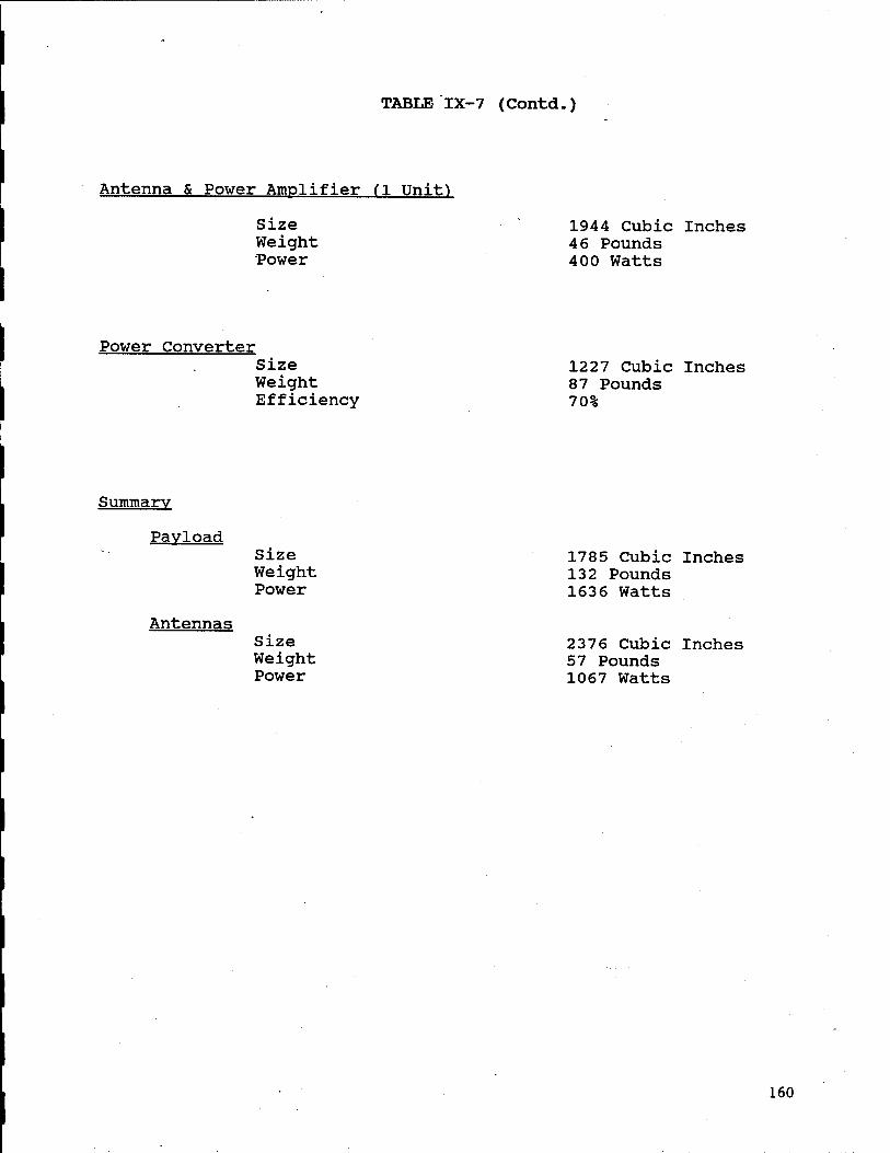
TABLE IX-7 (Contd.)
Antenna & Power Amplifier (1 Unit)
Size Weight Power
1944 Cubic Inches 46 Pounds 400 Watts
Power Converter Size Weight Efficiency
1227 Cubic Inches 87 Pounds 70%
Summary
Pavload
Antennas
Size Weight Power
Size Weight Power
1785 Cubic Inches 132 Pounds 1636 Watts
2376 Cubic Inches 57 Pounds 1067 Watts
160
ERIS
The ERIS estimate is based on one 60 GHz transmit/receive unit to
accommodate the link to the CV/SBI as well as a single 44 GHz
receiver to communicate with the ERIS farm battle manager. It is
estimated that two transmit and receive arrays will be required
at 60 GHz to provide the needed angular coverage. At 44 GHz a
single array will suffice.
161

TABLE IX-8 ERIS
60 Ghz Communication Package
Pavload fl Tx/Rx Unit) Size Weight Power
Transmit Antenna (2 Units) Size Weight Power
Receiver Antenna (2 Units) Size Weight
372 Cubic Inches 30 Pounds 52 Watts
432 Cubic Inches 12 Pounds 667 Watts
432 Cubic Inches 10 Pounds
44 GHz Communication Package
Payload fl Tx) Size Weight Power
Receive Antenna (1 Unit) Size Weight
Power Converter Size Weight Efficiency
Summary
Payload Size Weight Power
Antennas
IASERCOM
Size Weight Power
186 Cubic Inches 14.7 Pounds 26 Watts
402 Cubic Inches 10 Pounds
750 Cubic Inches 53 Pounds 70%
1308 Cubic Inches 98 Pounds 1064 Watts
1266 Cubic Inches 32 Pounds 667 Watts
162

LASERCOM
Due to an insufficient applicable analytical baseline, size,
weight and power projections for free-space SDS communications
applications cannot be included with confidence in this report.
Few lasercom studies and developments have aimed at operational
uses, and these have been for quite unique single-string
applications. Alternatively, highly publicized lasercom
experiments have focused primarily on feasibility
demonstrations. These did not incorporate sufficiently robust
design philosophies to permit direct extension to an operational
SDS environment. Hardware designs have in all cases, however,
been constrained significantly, either by the need to displace
existing alternative capabilities or by size/weight/power budgets
dictated by a potential host vehicle or program sponsor. Of
necessity, thus, wide confidence intervals in size, weight, and
power trades have persisted. Alternatively, lasercom
reliability/lifetime analyses have shown divergent results and
conclusions when performed by independent and/or competing study
teams.
For these reasons, we recommend that hardware definition studies
be undertaken immediately to definitize and refine the currently
disparate estimates of lasercom terminal impact on SDS host
spacecraft. Such studies should be commissioned by the SDIO,
funded through the spacecraft hardware prime contractors, and
163

should proceed in concert with the SDS architecture
participants, from a common technical requirements baseline to
generate a valid development planning perspective for lasercom
hardware.
In any case, it is important to contrast the size, weight, and
power projections developed in this section for . EHF
communications link hardware with the corresponding numbers
profferred by laser systems contractors to which we have been
afforded access. Whereas virtually no relevant productized
lasercom size, weight, and power budgets are at hand, EHF budgets
developed herein are based on experience with existing
manufacturing-oriented hardware production programs.
164

X. EHF/LASER COMPARISON
165

EHF/LASER COMPARISON
Introduction
Inspection of technical and popular literature sources shows a
burgeoning number of research and application developments in EHF
and lightwave communications. Such readily available sources,
however, do not usually address those current military
developments which are most relevant to free-space communications
applications. For the most part, industrial and fiber optic
laser applications as well as short-range, transmit-power-
intensive EHF applications are spotlighted. This report,
however, considers existing results and projected capabilities of
EHF and free-space laser communications systems applications
including fiber-optic communications (FOC) and reported military
developments.
The foremost application driving low power laser system develop-
ment is now commercial FOC. Close behind are all-solid-state
reprographics uses (printing, copying, scanning, facsimile
transmission, etc.). The military use of low power laser
systems has already begun, since this technology offers promising
advantages. Ground-based FOC systems are inherently EMP-hard and
reguire no emanations shielding (TEMPEST) while offering large
weight and power advantages over wire and cable-based alterna-
tives. Ultra-wideband signaling (2-20 gigabits per second
[GBPS]) is today being demonstrated in the laboratory with solid-
state lasers. Solid-state copy and facsimile machines are
166

expected to be available within 5 years. These should be more
reliable than today's electrostatic machines and will probably
offer workers a "single-station office" with computer interface,
printing and high quality graphics—nearly comparable to that of
photographic images (150Ö-3000 dots per inch).
Of all laser types investigated to date, only those based on III-
V materials [combinations of one or more of gallium (Ga) ,
Aluminum (Al),and Indium (In) with arsenic (As) and/or phosphorus
(P)] satisfy commercial FOC and reprographics requirements.
Space Communications
Free-space laser communications investigations began almost
simultaneously with the discovery of the He-Ne laser in the early
1960s. These have continued at steady but subdued interest
levels for applications ever since. Although He-Ne is no longer
a serious contender for communications, investigations into the
potential of gaseous C02, solid-state neodymium-doped, alexand-
rite and III-V material diode lasers have continued. Since
facilities for such work require the investment of considerable
capital and research, it is not surprising that work on each type
of laser (and its unique frequency) has been undertaken primarily
by a single organization. For example, infrared C02 laser
communications, originally pursued by Hughes Aircraft Co., now
appears of interest only to the European Space Agency (ESA).
167

Neodymium-doped substances (such as yttrium-aluminum-garnet
[Nd+:YAG], yttrium-aluminum oxide [Nd+:YA10] and various glasses
[Nd+:glass] appear to be the province of McDonnell-Douglas
Astronautics Company (MDAC). Alexandrite is championed by
Allied-Signal Corporation. However, III-V materials are, as
previously noted, the most widely investigated and used at
present. In the United States RCA, TRW, and ATT are highly
visible, while Hitachi, Nippon Telephone and Telegraph and
Thomson-CSF are prominent overseas in high data rate (hundreds of
MBPS) FOC applications. Until this time, however, the
established, evolving history of RF space communications, along
with the technical difficulties inherent in space-ground
transmission through the atmosphere, has effectively limited
consideration of free-space laser communications only to those
potential applications which may not be able to sustain an RF
alternative.
Those free-space applications suited to lasers are largely also
suited to EHF/millimeter-wave signaling. The product state-of-
the-art at EHF reflects a history of sustained research,
development and product funding. Significant United States
government involvement in support of C3/EW projects is quite
apparent, along with corollary developments in Europe and Japan.
Military or'quasi-military programs have often paved the way for
commercial satellite and space station exploitation, and
millimeter-wave frequencies are no exception. A great deal of
"applications-pull" investment is now reflected in the strong
168

competitive position of several firms in the EHF communications
marketplace.
Phenomenology
Alternating regimes of semi-transparency and opacity characterize
the EHF/millimeter-wave band. "Windows" (Figure X-l) at 30-55
GHz, 62-115 GHz, 125-175 GHz, and 190-300 GHz become progres-
sively less transparent due to even denser absorption features at
frequencies beyond 300 GHz. Between these window regions there
exist radio opaque absorption "curtains" due to 02 and H20
centered at 60, 118, and 180 GHz. At these latter frequencies,
RF energy cannot readily penetrate the earth's atmosphere. These
"curtain frequencies" are thus appropriate for exoatmospheric
communications (space crosslinks), while the "windows" are best
suited for space-to-ground up/down links.
For technological reasons, the EHF band has been utilized most
heavily near its low frequency end with progressively less use
evident in the upper regions. Certain tactical ground and
airborne radars, along with the FLAGE/LEDI missile, operate at
frequencies near 35 GHz. A commercially successful European
marine/harbor radar system operates between 36 and 40 GHz. EHF
space communications developments have proceeded chiefly at 30
GHz (ACTS) and 44 GHz (MILSTAR uplinks). LPI applications for
space crosslinks, tactical communications and radar altimetry
have been the focus of 60 GHz R&D thrusts. Radar and C3
169

FIGURE X-l
FREQUENCY (GHZ)
100. 200. 300. 400. 50,0. 60,0. 700. 800. SOO. 1000.1100.1200. —r 1 1 1 1 1 1 1 I + 4 r-HO*
2 * * 8 10 12 14 16 18 20 z'z 24 26 28 30 32 34 36 38 id
MflVENUttBER ICM-l)
Zenith Attenuation (Nepers, Decibels) Through the Entire Atmosphere (U.S. Standard)
170-

requirements have again driven efforts in the 85-110 GHz
frequency window. Very limited use of frequencies beyond 110 GHz
is in evidence, although some R&D has been supported. (Some
missile radar and fuze development efforts are underway at 140
GHz.) United States military technological thrusts are focused
on: 1) developing reliable, solid-state EHF sources (fund-
amental and harmonic frequency Gunn diodes); 2) low noise
receivers operating between 60-140 GHz; and 3) electronically
agile solid-state antenna arrays (simplex, and, with more
complexity, duplex) templated on the RADC 20 GHz effort which
will be extensible throughout the band.
Current Technical Issues
General
There are significant technical communications issues which will
require hardware demonstrations in the near term to increase
confidence in SDI systems capabilities. These include:
accurate, precise, low-jitter antenna positioning; transmission
power sufficient to close all required links at system end-of-
life (EOL) ; and, transient and total-dose nuclear hardening of
associated components and subsystems. Derivative pointing and
tracking requirements encompass rapid, accurate antenna/beam
slewing over large solid angles in response to spacecraft
dynamics and line-of-sight constraints. The achievement of
electronically-agile antennas at the frequencies of interest is a
171

central technical concern. To maintain both jam-resistant links
and the robust-geometry network presented in earlier sections,
the ability of such antennas to direct a transmit or receive beam
toward any one of a number of alternative internetted SDS
platforms is a critical and essential requirement.
EHF/Millimeter Waves
At EHF, a predominant concern is the selection of one or more
baseline communications frequencies appropriate to the range of
SDI missions in the time frame of interest. Considerable
experience has been gained with traveling-wave tube amplifier
(TWTA) and IMPATT sources below 100 GHz. However, serious design
manufacturing and reliability issues persist with TWTAs, and
IMPATT diodes are inherently noisy devices. These concerns now
appear to preclude consideration of tube sources above 50 GHz for
space communications use. Nevertheless, significant progress has
been demonstrated in the development of Gunn devices, and hybrid
and space-fed power combining techniques now make solid-state
sources competitive, up to 60 GHz. To satisfy robustness
requirements for multiple, simultaneous links, employ high-gain,
electronically-steered (vice mechanically repositioned) transmit
and receive antenna arrays.
Ultimately an EHF space communications system for SDS would
feature electronically-agile, beam-steered, transmit and receive
antenna arrays. Building upon the successful RF electronics
172

development history at S, C, X, and K band, these agile arrays
would embody: multiple-link availability/target tracking over
large solid angles; system robustness through platform
internetting; significant anti-jam capability, including
steerable nulls; and, graceful performance degradation with the
loss of individual module elements. Each individual array should
be able to communicate with all other mission platforms in its
field of view (between +45° and + 60°) . SDS constellation
geometry, not total numbers of platforms, would then dictate the
number and placement of spare terminals for the SDS. Overall
communications system size, weight, and power requirements would
not necessarily increase on future spacecraft, as more SDS
nodes are added to space segment constellations.
Laser
The proposed coherent near-IR SDI laser communications systems
would required operation through a variety of disturbed, high-
background environments and still demonstrate effective residual
anti-jam capability. In addition to an approximate 10 dB signal-
to-noise ratio improvement over equivalent direct detection
schemes, coherent laser communications systems would only be
threatened by on-axis jammers or by direct attack. With their
extremely narrow effective beamdwidths, coherent laser systems
would also permit continued link operations even when a receiver
platform infrequently transits the solar disk. Our discussion
here will focus on a coherent lasercom system as the preferred
(more link margin, better AJ, and no sun problem compared to
173

noncoherent systems) long-term laser candidate for SDS. This
assumption is consistent with the general consensus* of the
community regarding laser communications.
It does not appear that current III-V materials technologies will
be able to produce individual, long-life diode lasers with output
power sufficient to close all required SDI links. Hybrid power
combining techniques require mechanical positioning (or external
cavity stability) to within 0.1 micrometers. Thus, although
feasible for potential benign environment uses, mechanical power
combining does not appear promising for space system
applications. Monolithic power combining of several injection-
locked diode lasers fabricated side-by-side on the same
substrate, however, appear quite capable of ultimately satisfying
power, beam quality and beam steering requirements.
Nevertheless, the developmental history of such devices has
consistently demonstrated the necessity of performing device
design model (as well as acceptance, power output, stability and
life) testing under conditions which simulate actual flight
configuration as nearly as possible.
*See the following: 1) "Space Coherent Optical Communications System-An Introduction," by V.W.S. Chan, in the IEEE Journal of Lightwave Technology. April 1987; 2) "Coherent Optical Space Communications System Architecture and Technology Issues," by V.W.S. Chan in the Proceedings SPIE (San Diego), September 1981; 3) "Space Data Relay Networks," by F.W. Floyd, in the M.I.T. Lincoln Laboratory TR-572, December 3, 1981; 4) "Heterodyne and Coherent Optical Fiber Communications," by T. Okoshi, in the IEEE Transactions on Microwave Theory Technology, August 1982; and 5) "Laser Communications Experiment I, by T.R. Bristow and S.D. Simmons, in RADC-TR-86-156 (Vol. 1), November 1986.
174

A separate concern is the amplitude, frequency, and phase
stability of diode lasers suitable for local oscillator
applications. For coherent space communications precise
frequency tunability will also be required to compensate for
relative doppler shifts between platforms. Doppler frequency
shifts induced by relative platform motion are likely to exceed
coherent local oscillator laser line widths.
Only a handful of laser types practical for free-space
communications links have been discovered/developed to date.
Corporate and organizational investments in laser systems
development have, not surprisingly, been justified on
comparatively narrow grounds—the level of required investment in
ä single technology precludes a single firm from mounting
competitive internal efforts. Individual program selections of
laser types (and thus wavelength) have largely been driven by the
potential of exploiting theoretical or novel laser attributes.
Since free-space laser communications engineering state of the
art a priori trails that of RF systems, this translates into a
relatively weaker competitive position, one based upon expediency
or advocacy rather than competition-motivated market
optimization. This narrower laser system investment, development
and product baseline should be reflected in inherently higher
technical, schedule and cost risk elements for a near-term system
development.
175

Two basic types of laser systems (externally modulated "physical"
lasers, such as Nd+:YAG, and monolithic III-V diode lasers, e.g.
GaAlAs) have been proposed. Each shows tremendous promise, but a
considerable expenditure of both time and resources will be
required to determine if either can be systematized effectively
for SDS. Significant technical drivers for both laser types have
been the development of stable long-life sources and transmitter
packaging (size/weight/prime power needs optimized for the
operational environment).
Beam-steering requirements for SDI laser links may be
accomplished either mechanically or electronically. Mechanical
beam redirection involves a two-stage process: Antenna slew
between platforms not in the same telescopic FOV (angles greater
than 1-2 degrees) will be required for most SDI communications
links. Gimballed mirror repositioning between targets offset by
angles greater than a few milliradians but less than the FOV will
probably also be required. Electronic (electro optic, magneto
optic, etc.) steering is the alternative approach here. Whereas
mechanical repositioning schemes may be satisfactory for
occasional link repositioning (e.g., BSTS - BSTS), electronic
beam steering with large slew angles, is probably required for
those links involving SSTS and CV assets.
Diode lasers lend themselves to coherent power combining and beam
sharpening through monolithic integration. Injection locking of
several production-quality lasers on one monolithic substrate is
176

one part of the solution. Recent progress has been reported with
coherent CW diode laser arrays yielding in excess of 1 watt of
optical power output. However, taking such research devices to
the point where they are space-qualified products is not a
straightforward issue. The second . solution component is
electronic beam-steering circuitry. Later, monolithic
integration will probably result in the all-solid-state laser
transmitter. In summary, laser system state-of-the-art will
continue to progress in response to advances in solid-state
materials, process and fabrication technologies.
Current approaches to laser communications for space require the
use of physical antenna telescopes. Monolithic laser transmitter
systems (described above), functionally similar to their RF
counterparts, should be demonstrated within the next three or
four years. However, a monolithic ("fly's eye") receiver antenna
at optical frequencies is now (and should remain for the
foreseeable future) beyond the technical state-of-the-art. It is
therefore not possible for us to baseline the use of all-
monolithic receivers in an SDS communications hardware
implementation plan. (Today, development forecasts are barely
conjectural for such antennas.)
Therefore, the projected number of laser communications receiver
telescopes on each SDS platform even for simplex laser links
(e.g. BSTS-to-CV/SBI), will be driven by the total number of
platforms to be simultaneously (rapid TDMA) internetted. The
177

number of monolithic laser transmitter arrays, however, would
ultimately be driven by the overall SDS geometry and dynamics.
(This would be similar to the EHF transmitter case.)
Nevertheless, the ultimate requirement for multiple laser
receiver terminals on each receiver platform would remain. Such
an "open hardware architecture" feature places lasercom at a
severe, probably disqualifying, disadvantage with respect to EHF.
Comparison Summary
Table X-l summarizes the results of comparing the attributes and
technical parameters of EHF and laser links. Comparisons are
listed both for a "near-term" communications system (one
developed using the current technical baseline) and a "mid-term"
system (which allows four additional years of technology).
We judge that the technical maturity of EHF systems will today
better support SDS near-term communications requirements than
will laser links. EHF is still less risky for a mid-term system,
although a laser technical baseline should then accommodate all
but the robustness attributes. A separate receiver will be
required on each platform for each simultaneous/rapid TDMA link
supported. Both technologies will eventually support all SDS
data rates, jam resistance, and lifetime requirements but these
links would much more readily be built today at EHF.
178

TABLE X-l
COMPARISON SUMMARY
1988 Cutoff 1992 Cutoff
Technical Maturity EHF (Favored) EHF Laser Should Meet Non-Robust Requirements
Data Rate EHF Both
Jam Resistance Overall EHF EHF Power Required Laser Laser Max Power EHF EHF Divergence Laser Laser Geometry EHF EHF PAT EHF EHF
Lasers Should Accommodate All But Fast, Large Slews
Physical Size & Weight Laser* Both*** Prime Power Laser* Laser***
Robustness EHF EHF
System Expansion EHF EHF
Nuclear Effects Both** Both**
Reliability EHF (Better Both (?) Understood)
Competition EHF EHF
Cost EHF (Probably) EHF
♦Assumes defenses against passive counter-measures are not required. **Depends upon laser system configuration. ***Laser RX technical breakthroughs required to
support system expansion.
179
Lasers at much higher frequencies than EHF, would feature
extremely narrow link beamwidths with sidelobes essentially
confined to the vicinity of the receive platform. (For
equivalent telescope/antenna quality, beamwidth scales with
carrier wavelength. EHF, with wavelengths approximately 3000
times longer than diode lasers, would yield correspondingly
larger beamdwidths.) Consequently, both system prime power and
radiated power requirements are less for lasers than EHF (with
reasonable power conversion efficiencies). However, EHF links
are judged capable of higher (potentially exceeding an order of
magnitude) output power—SDS constellation geometries and
dynamics significantly frustrate threat jammers so that with
reasonably designed anti-jamming techniques enemy jamming will be
ineffective. Realization of electronically agile EHF transmit
and receive antenna arrays with null-steering, frequency hopping
and spread spectrum capabilities would render EHF the ultimate
anti-jam technology choice for the foreseeable future. Due to
its wider inherent beamwidth, the electronically agile EHF
transmit array will require less beam steering precision and
accuracy for pointing and tracking (PAT). Since such an advanced
array cannot be projected for a laser receiver, in-band jamming
(chiefly from aperture illumination scattering to reduce SNR or
attempt command takeover C2 functions) will remain a concern for
laser links.
Lasercom hardware, some of which has been manufactured to date
for experiments and demonstration programs, ought to require less
180

volume, weight, and power for SDI C3 applications if a 1988
technology cutoff date were established. The inherently smaller
beamwidths of lasers afford a significant prime power advantage
over EHF for a single, otherwise equivalent link. The active
transmit aperture at EHF is judged to require less development.
When the EHF receiver is considered, vis a vis the need for
several separate laser receivers, EHF communications systems are
ultimately projected to assume a commanding advantage for
operational SDS applications.
Nuclear effects are expected to be neutralized operationally by
employing appropriate hardware and by a carefully designed
operational concept, system design, development and test effort,
both for EHF and laser links. Either type of link must be
designed specifically to operate in stressed and disturbed
environments for such technology (i.e., laboratory) developments
to translate into actual military space communications
capabilities. Chief areas of concern here include transient and
total dose, optical and RF detector/mixer materials and
circuitry, receiver amplifiers, antenna surfaces, focal
plane/feed thermal effects, and performance drift of filters and
phase shifter components.
Overall, there is a vigorous competitive environment for state-
of-the-art EHF systems. This situation is currently fueled by a
variety of military uses whose targeted applications and nuclear
hardening requirements should continue the relative disparity
181

between EHF and lasers. Since EHF programs are proceeding apace
from a broader baseline, both reliability and cost factors will
continue to favor EHF developments and products for tactical and
free-space communications applications.
Conclusions
In principle, EHF and laser communications systems appear
potentially capable of satisfying the gross SDS communications
requirements (i.e., single-link data rates over required platform
separation distances) . Significant concerns arise as a
consequence of the large numbers of simultaneous links which may
be required for robustness, the effects of inherent platform
dynamics, and communications susceptibility in stressed (nuclear
and jamming) environments. Overall, we judge that EHF
communications systems today are more mature than lasers with
respect to providing an initial capability which can evolve to
satisfy ultimate SDI system requirements. Laser systems will
continue to improve rapidly, thanks to microelectronic materials,
processing and fabrication advances. However, solid-state EHF
advances based on these same technologies will benefit at least
as much as lasers from a maturing common technical baseline. We
judge that EHF will thus retain a strong comparative advantage
for the foreseeable future. Such lower EHF communications
technical risk translates, in sequence, into lower overall
schedule and cost risk elements, or alternatively, better
technical performance for equal risk exposure for the overall SDS
network. 182

The communications design philosophy which has been established
for other major military and civil space projects should also be
applied to the SDS communications network: It is then most
efficient and cost effective, with less risk, to baseline the
adoption of a single communications framework (frequencies,
protocols, operational disciplines, hardware baseline, test and
evaluation, activation plans, etc.) for all crosslink
applications. Thus, hybrid (laser and RF) approaches do not
appear advisable. The need to implement an integrated
communications and battle management (BM) capability in the short
term also calls into question a hybrid, joint development risk,
communication architecture. Let us therefore focus our
assessment on the current status and suitability of laser
developments with respect to total SDS communications system
requirements.
The technical baseline and competitive posture of the contractor
community is more mature for EHF hardware. This translates into
higher expected ability to meet technical performance, schedule
and cost milestones in a development/production program. The
relative robustness and growth/flexibility attributes of.. EHF
links must also weigh heavily in a binary selection process. We
also find that EHF links are likely to be present on SDS
platforms to satisfy ultimate operational internetting
requirements involving CV/SBI (and probable SSTS) crosslinks and
space-ground up/down links. In contrast to these factors, we
have the promise for lasers of lower prime power needs, enhanced
183

anti-jam capability (very questionable in a robust architecture)
and larger available bandwidth.
Bandwidth does not appear to be at issue for the data rates
envisioned in an operational SDS environment. Available EHF
bandwidth allocations and hardware capabilities are sufficient.
In the earlier "Comparison Summary," we concluded that EHF links
can deliver the required level of anti-jam* performance. Although
an individual laser link will require less spacecraft prime power
than an equivalent individual EHF link incorporating active
arrays, this is a misleading comparison: single link pairs do
not an SDS make! EHF crosslink packages, based upon
electronically active array technology, have been identified and
defined in this report to accommodate an open-ended expansion of
the number of platforms in the overall SDS space segment.
In response to the concern that lasercom should not be so readily
dismissed, we cannot in this report aim to predict the future.
When projecting operational SDS communications technical postures
we do not foreclose the possibility that lasercom could play a
significant role. Nevertheless, we cannot identify a single SDS
application for which lasercom is expected to be clearly
superior. It is true that some SDS links may well be satisfied
by either lasercom or EHF signalling. For example, where few
links with little geometric/dynamic diversity are required (such
as BSTS - BSTS), perhaps either alternative could be made to
work. It is progressively much less advisable, however, to
184

consider laser iinks involving, in turn, SSTS, CV/SBI platforms
and space-ground up/down links.
Lasercom should be developed not necessarily for SDS use, but in
anticipation of future needs for extremely high free-space data
rate (>20 GBPS) links and/or for links at extreme ranges
(>120,000 NM) . (For example, NASA deep-space probes outside the
solar system may be forced to adopt optical links for data relay
back to the Earth.) We conclude, however, on balance that EHF
communications links are preferred over laser links for all SDS
communications applications.
Recommendations
We recognize the critical role of C3BM/C3 counter-measures (CM) as
a fundamental SDS system acquisition driver. Recommended here
are capable and survivable system mission links ensuring mission
accomplishment through robust performance. It is most critical
to immediately implement a strong C3BM/C3CM program thrust. An
integrated, highly visible SDS C3 development office, managed
both to aggressively exploit the evolving technical state of the
art and to enforce communications architecture discipline will
contribute significantly to near and far term SDS viability.
185
Achievement of such communications system hardware will require a
focused EHF development program. Hardware design and development
programs for each link should begin immediately build upon near
term system performance simulations. Critical supporting
technical demonstrations of efficient low-loss power combining
and electronically agile transmit and receive arrays are needed
early in the program. These should exploit recently demonstrated
successes with like efforts at Ku-band and the applications
state-of-the-art in advanced MMIC/MIMIC III-V technologies.
So that efficient system upgrade planning is incorporated a
priori, we recommend vigorous C3 program office sponsorship of
appropriate relevant advanced technologies. Applications-
oriented research and development of mid-upper EHF and high-
payoff lasercom technologies will provide the basis for efficient
and cost-effective system block changes. Once operational, the
SDS C3 network size and complexity could effectively deter
attempts to upgrade it. In this context, a modest amount of
margin ought to be designed into, and reserved for, the pre-
planned product improvement (P3I) of communications on board all
SDS spacecraft. More advanced capabilities, once proven in the
laboratory, could then be configured for and experimentally
demonstrated in the operational SDS environment prior to
commitment to any C3 system upgrade. FOV and external viewing
placement are critical components of such reserved margin.
186

EHF is the frequency band recommended for all SDS links. Space-
to-space communications operation in the 02 band at 58-62 GHz
should be baselined for critical mission link protection from
ground and airborne jamming threats. Lower millimeter wave (MMW)
frequencies are most appropriate for up/down links at this time.
To fully realize the weight, prime power advantage, and narrow
beamwidth advantages of higher MMW frequencies, we recommend
planning to move to mid-EHF ( 100 GHz) at least for up/down links
as the technical base and platform internetting requirements
become more firmly established. Careful upgrade planning with
associated technical/investment emphasis is essential to
survivable SDS mission links as both domestic and threat
capabilities evolve.
187

XI. SUMMARY
188

SUMMARY
A robust communications architecture was described to provide the
background for the overall security of the SDI/SDS Program. The
angular diversity provided by this satellite-to-satellite
communications architecture, coupled with the dynamic nature of
each node, assures system connectivity and renders jamming to be
virtually useless. The robust angularity of the parallel
linkages also helps alleviate disruption from nuclear events.
Electronically-agile antennas are at the heart of this
architecture and, in the EHF band, remain the only significant
technology that requires heavy emphasis—these devices are in the
laboratory at 20 GHz and 44 GHz, and development at 60 GHz has
begun. Resources to space-qualify the systematization of these
devices also exist, but more emphasis is required to guarantee
their timely availability for SDI/SDS.
The BER and link-margin advantages associated with multiple
independent links are clearly demonstrated, even accepting just
the simple analysis here, but hard, numerical descriptions of the
actual SDS geometry are both 1) expected to be better than the
numbers shown here, and 2) in need of considerably more analysis
than available in this study.
The penalties associated with guaranteeing connectivity as
described in this architecture are higher data rates (generally
189

more bursts, not necessarily more data per burst) and more
capable antenna systems. The data rates are currently
achievable, and the antenna systems for EHF are in development,
as described earlier. The comparable laser antenna systems with
fast, large slews are not available in the near future; and
regarding lasercom receivers, may not be available for SDS at any
time in the foreseeable future. For some links, most notably
BSTS-BSTS, robustness cannot be increased dramatically and lasers
are more feasible than they are for other links; however, a
laser/EHF hybrid communications system would pay severe size and
weight penalties and it is recommended that as long as one
technology can support all the links, that SDS stay with one
technology. Other links gain significantly from the multiple
routing of information.
In the long term lasers may have unique advantages that can be
effectively exploited: very narrow beamwidths (though in some
cases, may be too narrow), the physical capacity to handle
extremely large data rates, and possible size/weight/prime-power
advantages. Laser reliability involves many unknowns and trade
offs associated with systematizing the laboratory technology need
much more development. Also, certain potential vulnerabilities,
especially relatively inexpensive passive countermeasures,
require further analysis—a laser communications system that
would have to address such vulnerabilities could suffer very
significant size/weight/power penalties.
190

An EHF/laser comparison was treated with considerable depth, and
at this point it is recommended that both technologies be
supported. However, in the near term, plan for EHF links. In
any case, do not underestimate the value of robustness or
overestimate the penalties associated with its implementation.
Further analysis is required to determine how best to exploit
SDS's robust geometry and the advantages of satellite-to-
satellite relaying of information. If .sensor information
penetrates to any satellite .within the CV/SBI constellation
(clearly a certainty), then a properly constructed inter-orbit
netting of links will guarantee connectivity in the most severe
jamming and nuclear environment. Some educated guesses as to
more desirable choices of robust netting schemes were included
here, but more study is required.
Finally, with the multitude of SDI/SDS thrusts currently in
being, a government or government-sponsored focal point for
communications architecture is essential to the successful
integration of all information nodes. The robust advantages
inherent in the SDS geometry can only be exploited with an
harmonious architecture supported within each element.
191

APPENDICES
192

A. WORLD SITUATION SET
(Developed by the SDI Phase 2 Architects and the AF Architects During Phase 2 Project Convergence)
193
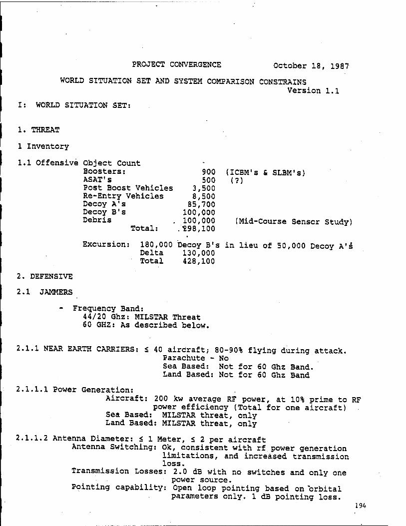
PROJECT CONVERGENCE October 18, 1987
WORLD SITUATION SET AND SYSTEM COMPARISON CONSTRAINS Version 1,1
I: WORLD SITUATION SET:
1. THREAT
1 Inventory
1.1 Offensive Object Count Boosters: 900 ASAT's 500 Post Boost Vehicles 3,500 Re-Entry Vehicles 8,500 Decoy A's 85,700 Decoy B's 100,000 Debris . 100,000
Total: ."298,100
ilCBM's & SLBM'S) (?)
[Mid-Course Sensor Study)
Excursion: 180,000 Decoy B's in lieu of 50,000 Decoy A's Delta 130,000 Total 428,100
2. DEFENSIVE
2.1 JAMMERS
- Frequency Band: 44/20 Ghz: MILSTAR Threat 60 GHZ: As described below.
2.1.1 NEAR EARTH CARRIERS: < 40 aircraft; 80-90% flying during attack. Parachute - No Sea Based: Not for 60 Ghz Band. Land Based: Not for 60 Ghz Band
2.1.1.1 Power Generation: Aircraft: 200 kw average RF power, at 10% prime to RF
power efficiency (Total for one aircraft) Sea Based: MILSTAR threat, only Land Based: MILSTAR threat, only
2.1.1.2 Antenna Diameter: £ 1 Meter, < 2 per aircraft Antenna Switching: Ok, consistent with rf power generation
limitations, and increased transmission loss.
Transmission Losses: 2.0 dB with no switches and only one power source.
Pointing capability: Open loop pointing based on orbital parameters only. 1 dB pointing loss.
194
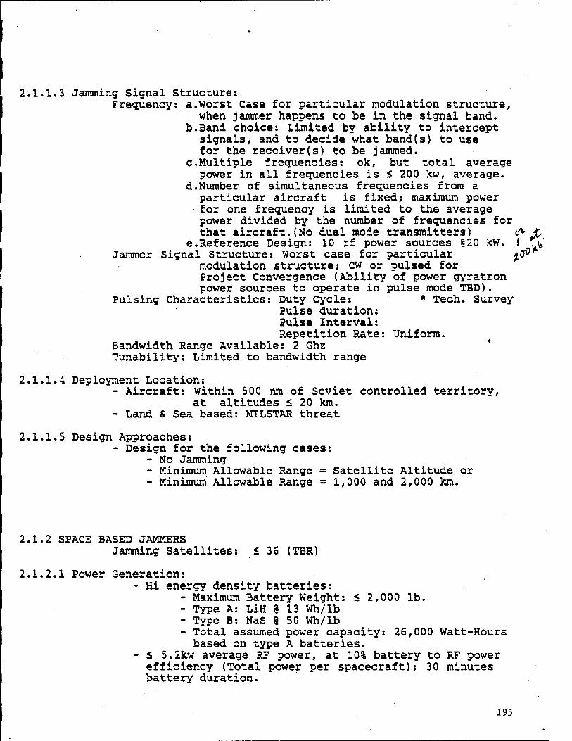
2.1.1.3 Jamming Signal Structure: Frequency: a.Worst Case for particular modulation structure,
when jammer happens to be in the signal band. b.Band choice: Limited by ability to intercept
signals, and to decide what band(s) to use for the receiver(s) to be jammed,
c.Multiple frequencies: ok, but total average power in all frequencies is < 200 kw, average,
d.Number of simultaneous frequencies from a particular aircraft is fixed; maximum power
- for one frequency is limited to the average power divided by the number of frequencies for that aircraft.(No dual mode transmitters) «A- £
e.Reference Design: 10 rf power sources @20 kW. i ^> Jammer Signal Structure: Worst case for particular ttfi
modulation structure; CW or pulsed for Project Convergence (Ability of power gyratron power sources to operate in pulse mode TBD).
Pulsing Characteristics: Duty Cycle: * Tech. Survey Pulse duration: Pulse Interval: Repetition Rate: Uniform.
Bandwidth Range Available: 2 Ghz Tunability: Limited to bandwidth range
2.1.1.4 Deployment Location: - Aircraft: Within 500 nm of Soviet controlled territory,
at altitudes < 20 km. - Land & Sea based: MILSTAR threat
2.1.1.5 Design Approaches: - Design for the following cases:
- No Jamming - Minimum Allowable Range = Satellite Altitude or - Minimum Allowable Range = 1,000 and 2,000 km.
2.1.2 SPACE BASED JAMMERS Jamming Satellites: < 36 (TBR)
2.1.2.1 Power Generation: - Hi energy density batteries:
- Maximum Battery Weight: < 2,000 lb. - Type A: LiH @ 13 Wh/lb - Type B: NaS @ 50 Wh/lb - Total assumed power capacity: 26,000 Watt-Hours based on type A batteries.
- < 5.2kw average RF power, at 10% battery to RF power efficiency (Total power per spacecraft); 30 minutes battery duration.
195

2.1.2.2 Antennas Diameterr: a. < 3 Meter, < 3 per jamming spacecraft or
b. < 1 Meter, <10 per jamming spacecraft or • c. < .1 Meter, < 64 per jamming spacecraft
Switching: Ok, consistent with rf power generation limitations, and increased transmission loss.
Transmission Losses: 2.0 dB with no switches and only one power source.
Pointing capability: Open loop pointing based on orbital parameters only; 1.0 dB pointing loss.
2.1.2.3 Jamming Signal Structure: Frequency: a.Worst Case for particular modulation structure,
when jammer happens to be in signal band. b.Band choice: Limited by ability to intercept
signals, and to decide what band(s) to use for the receiver(s) to be jammed,
c.Multiple frequencies: ok, but total average power in all frequencies is < 5.2 kw, average,
d.Number of simultaneous frequencies from a particular spacecraft is fixed; maximum power for one frequency is limited to the average power divided by the number of frequencies for that spacecraft.
e. Reference design: 10 power sources @ 520 watts Jammer Signal Structure: Worst case for particular
modulation structure; cw or pulsed for Project Convergence
Pulsing Characteristics: Duty Cycle: *Tech survey Pulse duration: Pulse Interval: Repetition Rate: Uniform.
Bandwidth Range Available: 2 Ghz Tunability: Limited to bandwidth range.
2.1.2.4 Deployment Location: - Any altitude < 2,000 km above SSTS for above power levels. - Any altitude > 2,000 km above SSTS for power levels not to exceed 30% of the above power levels.
- Worst case for satellite whose receivers are to be jammed.
2.1.2.5 Design Approaches - Design three cases, as follows:
- Reference: No jammers - With Jammers; Minimum Allowable Range = 1,000 km - With Jammers; Minimum Allowable Range = 500 km.
196

2.1.3 ROCKET BASED JAMMERS Number of Rockets: None; considered to be impractical.
2.1.3.1 Power Generation: 1 lkw average RP power, at 10% prime to RF power efficiency
2.1.3.2 Antennas Diameter: a. < 1 Meter, <2 per rocket or
b. < .1 Meter, < 10 per rocket Switching: Ok, consistent with rf power generation
limitations, and increased transmission loss. Transmission Losses: 2i-0 dB with no switches and only one\_
power source. Pointing capability: Open loop pointing based on orbital
parameters only; 1.0 dB pointing loss.
2.1.3.3 Jamming Signal Structure: Frequency: a.Worst Case for particular modulation structure,
when jammer happens to be in signal band. b.Band choice: Limited by ability to intercept
signals, and to decide what band(s) to use for the receiver(s) to be jammed. *
c.Multiple frequencies: ok, but total average power in all frequencies is < 1 kw, average,
d.Number of simultaneous frequencies from a particular spacecraft is fixed; maximum power for one frequency is limited to the average power divided by the number of frequencies for that spacecraft.
Jammer Signal Structure: Worst case for particular modulation structure; cw or pulsed for Project Convergence
Pulsing Characteristics: Duty Cycle: *Tech survey Pulse duration: Pulse Interval: Repetition Rate: Uniform.
Amplifier Bandwidth Available: 2 Ghz Tunability: Limited to amplifier bandwidth
2.1.3.4 Deployment: Launch Site: Any ship or submarine further than 100 nm from
CONUS. Trajectory: Similar to ERIS, GSTS etc, but with parachute
type descent during reentry.
2.1.3.5 Tactics: Deployment of this type of jammer in lieu of an equivalent number of ballistic missiles is questionable.
197

2.2. NUCLEAR EFFECTS
2.2.1 COMMUNICATIONS SUPPRESSION
2.2.1.1 Type A: SPACE TO CONUS COMMUNICATIONS DISRUPTION
Depressed trajectory SLBM launches simultaneously with ICBM launch, in order to introduce defense suppression and high altitude nuclear bursts for communications disruption.
2.2.1.1.1 Number of launches:12 per Submarine; 2 submarines
2.2.1.1.2 Launch locations: one off of the east coast, one off of the west coast.
2.2.1.1.3 Intended burst locations: a. CONUS fixed SDS Control Centers b. 200 km bursts distributed over CONUS as illustrated in the attached CONUS figure.
2.2.1.2 Type B: Boost Battle Space: Communications suppression nuclear bursts over the Soviet Uni6n concurrent with other booster launches.
2.2.1.2.1 Burst Locations: - Distributed equally over a 2,000 x 3,000 directly over the Soviet Union per attached figure.
- Altitude: Most Effective; nominally 250 kM.
2.2.1.2.2 Number of Bursts: 60 in each of two waves separated by two minutes, with the first launch concurrent with first ICBM booster launch.
2.2.1.3 Type C - Midcourse Battle Space Communications suppression nuclear bursts over the polar region.
2.2.1.3.1 Burst Locations: - Distributed equally over a 2,000 x 3,000 directly over the Soviet Union per attached figure.
- Altitude: Most Effective; nominally 250 kM.
2.2.1.3.2 Number of Bursts: 60 in each of two waves separated by two minutes, with the first launch concurrent with arrival of first ICBM booster.
2.2.2 ASAT*s
2.2.2.1 General: Directly ascent missiles attacking CV's and SSTS satellites launched from Soviet landmass.
198
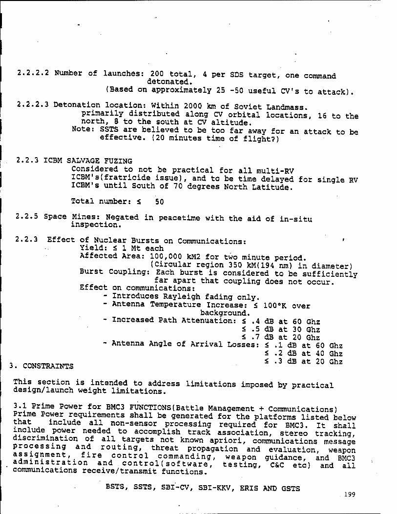
2.2.2.2 Number of launches: 200 total, 4 per SDS target, one command detonated.
(Based on approximately 25 -50 useful CV's to attack).
2.2.2.3 Detonation location: Within 2000 km of Soviet Landmass. primarily distributed along CV orbital locations, 16 to the north, 8 to the south at CV altitude.
Note: SSTS are believed to be too far away for an attack to be effective. (20 minutes time of flight?)
2.2.3 ICBM SALVAGE FUZING Considered to not be practical for all multi-RV ICBM's(fratricide issue), and to be time delayed for single RV ICBM's until South of 70 degrees North Latitude.
Total number: < 50
2.2.5 Space Mines: Negated in peacetime with the aid of in-situ inspection.
2.2.3 Effect of Nuclear Bursts on Communications: * Yield: < 1 Mt each Affected Area: 100,000 kM2 for two minute period.
(Circular region 350 kM(194 nm) in diameter) Burst Coupling: Each burst is considered to be sufficiently
far apart that coupling does not occur. Effect on communications:
- Introduces Rayleigh fading only. - Antenna Temperature Increase: < 100°K over
background. - Increased Path Attenuation: < .4 dB at 60 Ghz
< .5 dB at 30 Ghz < .7 dB at 20 Ghz
- Antenna Angle of Arrival Losses: < .1 dB at 60 Ghz
3. CONSTRAINTS
< .2 dB at 40 Ghz < .3 dB at 20 Ghz
This section is intended to address limitations imposed by practical design/launch weight limitations.
3.1 Prime Power for BMC3 FUNCTIONS(Battle Management + Communications) Prime Power requirements shall be generated for the platforms listed below that include all non-sensor processing required for BMC3. It shall include_ power needed to accomplish track association, stereo tracking, discrimination of all targets not known apriori, communications message processing and routing, threat propagation and evaluation, weapon assignment^ fire control commanding, weapon guidance, and BMC3 administration and control (software, testing, C&C etc) and all communications receive/transmit functions.
BSTS, SSTS, SBI-CV, SBI-KKV, ERIS AND GSTS 199

I Fault-tolerance and non-volatile memory for critical functions (egRiming, tracking filter covariances, critical programs and data base parameters)
I shall be provided.
I Traceability shall be provided to support/justify the values used to generate the totals. Analysis and supporting rationale shall be generated
j to support the values used for items not yet in existence.
These estimates shall not include additional power required for (environmental control when not operating. However, if dual systems are
provided, both shall be powered up 25 minutes prior to expected use.
3.2 Weight for BMC3 FUNCTIONS(Battle Management + Communications) Weight estimate shall be generated for the platforms listed- below that include all non-sensor processing required for BMC3. It shall include weight of the processors needed to accomplish track association, stereo tracking, discrimination of all targets not known apriori, communications message processing and routing, threat propagation and evaluation, weapon assignment, fire control commanding, weapon guidance, and BMC3 administration and control (software, testing, CSC etc) and all communications receive/transmit functions including TT&C, GPS and time reference/base oscillators and clocks. .*
BSTS; SSTS, SBI-CV, SBI-KKV, ERIS AND GSTS
Fault-tolerance and non-volatile memory for critical functions (eg,timing, tracking filter covariances, critical programs and data base parameters) shall be provided.
Traceability shall be provided to support/justify the values used to generate the totals. Analysis and supporting rationale shall be generated to support the values used for items not yet in existence.
These estimates shall not include additional weight required for environmental control, or power generation; ie, equipment shall be assumed to be mounted within the host spacecraft except for transmitters that must be mounted above antenna gimbals (between the gimbals and the ..antennas).
200

/^^TI^'A'!,'-!'-'"""!,." . ",H'!Mi''l"f!|.W*■
'.v .'
Tl1 ' '.JT~"—
;^:
.I;V(. VV 5
;.'■' •-' /«■*•i^•■-'^^i;v^■.^^?>:l^^v*,^^^{».:;;•:^:^••^'^;.;;:>•vl<.V^•.•••:•.
' ifiterr'.'•■• :i''NL!-!:/>'--"-i^'f'"'tft'iSJ>i;'».';^^';:'•<■'?';."::v."»^'i;'>'■':-Yv '. ^y- ' - • ■ ■'.- ' .■:'.' il.?li.r"l '• '■■■.:-•'■''■•:'.'■'•■'■;.".. ■ ...'"'•..■
B'.',*!•.■ ■'■'!'".■■.■•'•.iV'i'V'<•■<' T.: '••'■••. ■•'V;-;.'-.*''^-'^;.-'.;'«.;';.'• F.:^^~^.•l• ~:-*^;>^>.iv^^i!>;' ... »■/.••.•••«•.:.'■•. -.V.f ' r .'. *'.vr'.";:".'. 1.5 •• *■ •■• :.-: '.'■».•;■.'' .•-\ir - '■ L
;'•■'';»•'; •'.■"•'i'."'."-' '■'■.'S'Ä'i.'a ! !',i?. "••" •*■*•'' . ■•■'?.'•'.■''.; '•'. .;.
&2ß ■*■■"'.>• ■>-V.'.-:• .■*...■-;. o'-V'^-■'-'•; • • ••' '••■: :•"'
:':?"'fe^.:;:5'->'•;•■'•>•*:v^;;■I,,ää
,-''.'7.,.
;I.,J'>' .:■ ''
o ci> o m'.i.
C>^c*-<N:M-■•-■-.»!'•£ «•■';•,■ .'•'■. .^„■••JMt ,-»•; ,\;;;.. -,;Vl'^... .'. '<-. :
■ui .■•■:;.>-•
T-
■S" »
üö oo - S ' • ( i t- i i X :
.2.2 2. 2 2 i .LI
KÜS
...'>,.'•■,;-rr-j..'.-1^-. 'M.
1. pjMtf S;; ' /.■**.'"::/.''
m rs.
?si?
i^l^'-.'
..:;£,;.. •r-£'-:>■ »~ • CO' f> • 00". 3>V
•>:-^:>:'!
.-, ' " '■•.•■.•■.. ' • - ■ •'■ ■; ■"■•; ±^m tA.Wth'eA Oi .1 ... '.••■1 ,•"••.' •'■• ' ■ ••■■■'^'-.;v i .^^^ U WM:UH .: . '
■: v&)i i-&- ^^<^&3-*VY;X\:K-: 201 a»>i-W ^^■'in4i>iW>i1>iM
^gjpg^ni mg^valdiröi jmijC^I ^

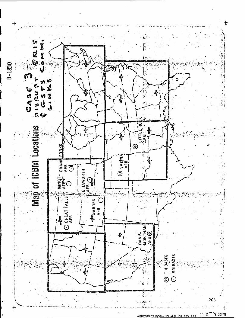
+ ».•X -ft ••"-**\1 "
*» *
*;,,.■•
:sv O t: m : oo ■ f—•
I CO
O
Co
r -■■■■. ■;---|->3'-"--r:'.'«o;" . !::-;:^T^ ■■
*-, j ***************u\mrrrmmMmu7tt
\ +
...f CO. -«5 ..■ •
' vr.- ...ik-'..
•':•' 4
AEPOSPACEFQPM NO 4651 ■100 REV 7 79
203
■ - ■■ - - +
5-1 0 'S 35V9

B. PROPAGATION THROUGH A NUCLEAR-PERTURBED ENVIRONMENT
204

PROPAGATION THROUGH A NUCLEAR-PERTURBED ENVIRONMENT
(NOTE: The majority of this appendix is excerpted from private communications with Dr. Peter Monsen, a consultant" in this study, as well as two published works: A Trans- Ionspheric Signal Specification for Satellite C^ Applications, by Dr. Leon Wittwer (DNA Report #5662D, dated 31 December 1980) and Fading Channel Communications. by Dr. Monsen (IEEE Communications Magazine, dated January 1980).
The SDS architecture consists of the following terminals:
1) BSTS 2) SSTS 3) CV/SBI 4) GEP 5) ERIS 6) GSTS
Communication between these terminals is to be maintained when
exposed to the EW and nuclear environment outlined in the WSS
(Appendix A). To accomplish this, a hybrid direct
sequence/frequency hopping (DS/FH) form of modulation operating
in a burst mode is assumed with all of the 10% available emission
bandwidth used for spreading. It is recognized that it may in
some instances be impractical to obtain all of the processing
gain via spreading and that a combination of spreading and
sidelobe cancelling may have to be employed. Further, to operate
near optimally in the fading environment imposed by the nuclear
threat, it will be assumed that coherent demodulation will be
used for data rates greater than 500Kb/s and noncoherent
techniques utilized for data rates less than 500 Kb/s.
The following frequency bands are presumed for the various links:
1) Satellite-to-Satellite 60 GHz
205

2) Uplink* 44 GHz
3) Downlink 20 GHz
It will be assumed that an optimized jammer is employed which,
due to the countermeasures utilized, is a broadband noise jammer.
The scintillation channel will be presumed to be endowed with the
following types of disturbances:
1) Fading
2) Multipath
3) Scattering
4) Absorbtion
5) Antenna Temperature Increase
The communication channel perturbed by nuclear bursts is modeled
as a linear channel possessing a time varying impulse response.
Thus,
R(t) = J dT h(t,T) S(t-T) (1) 0
Where,
S(t) » transmitted signal
R(t) = received signal (complex number representation)
h(t,f) » channel impulse response function
The specification channel impulse response functions:
0»
" 2wf r(t) er N(t)l f h(t,x) = A(t)exp i £ i—^ jd(Af) iis(t,Af)
exp cr N(t)Af2
■i ^ i2irAf r c ^■m (2)
206

Where,
c
c
carrier frequency (hz)
,8 light speed (3x10 m/sec)
z(t) = propagation path length (m)
15 r = classical electron radius (2.82x10 m) o
N(t) = total electron content ("> )
(2)
For other than circular polarization, Equation 1 should be
applied to each polarization state and N(t) used to calculate the
Faraday rotation effects.
A(t) = exp(-0.11SKA)
• H m
1 L.Cf9)9 , 02._ 2. G(öTJdj^r-exp(-e /2V (3)
^A
G(6)
2
= absorption (dB)
= antenna gain function 2
= energy angle of arrival variance (rad )
V1
as a
,Af) =JdTJc df hs(f,T)exp(i2irAfT+i2irft) (4)
Equation 3 assumes that the transmitter is on the antenna axis
and that the antenna pattern is cylindrically symmetric about
that axis. If the threat has amplitude fluctuations (always
assumed Rayleigh), then hs(f,r ) is a zero mean normally
distributed random variable with an autocovariance defined by
h!(f,T)h (f\T') » «(f-f,V'(T-T')r2(f,T) (5a)
hs(f,T)hs(f\T') = 0 (5b)
207
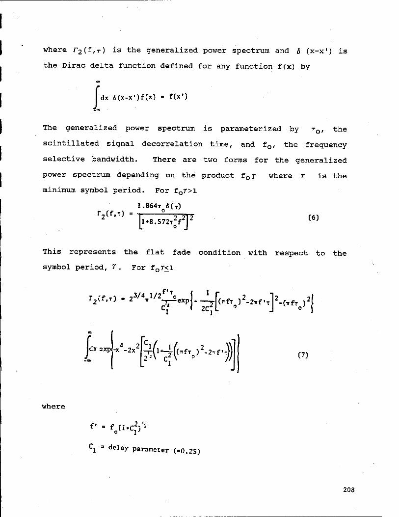
where r2(f,T) is the generalized power spectrum and ö (x-x1) is
the Dirac delta function defined for any function f(x) by
as
i dx 5(x-x')f(x) = f(x')
The generalized power spectrum is parameterized by rQl the
scintillated signal decorrelation time, and f0, the frequency
selective bandwidth. There are two forms for the generalized
power spectrum depending on the product f 0 r where T is the
minimum symbol period. For f0r>l
r2(f,T) = 1.864T 6(T)
|l+8.S72T2f2] (6)
This represents the flat fade condition with respect to the
symbol period, T. For fQT<l
r2(f.r) . 2^,'^„pj ' fct.y.z.r'ry.^y
dx exp{-x4-2x2 thh^4 (7)
where
2 '«
Cj = delay parameter (=0.2S)
208
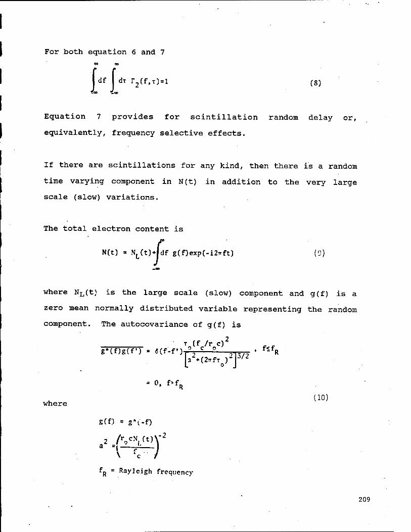
For both equation 6 and 7
r2(f.T)«l (8)
» es
Idf di
T» »00
Equation 7 provides for scintillation random delay or,
equivalently, frequency selective effects.
If there are scintillations for any kind, then there is a random
time varying component in N(t) in addition to the very large
scale (slow) variations.
The total electron content is
N(t) - N.(t)*|df g(f)exp(-i2»ft) (3) - NL(t)+ldf
where NL(t) is the large scale (slow) component and g(f) is a
zero mean normally distributed variable representing the random
component. The autocovariance of g(f) is
• T (f IT C)2
g*(f)g(f) - g(f-f')r°2 C ° 5-P77 ' R
- 0, f>fR
where ;io)
ecn = s\-f) ,-2
2 a =, I r . I
fR = Rayleigh frequency
209
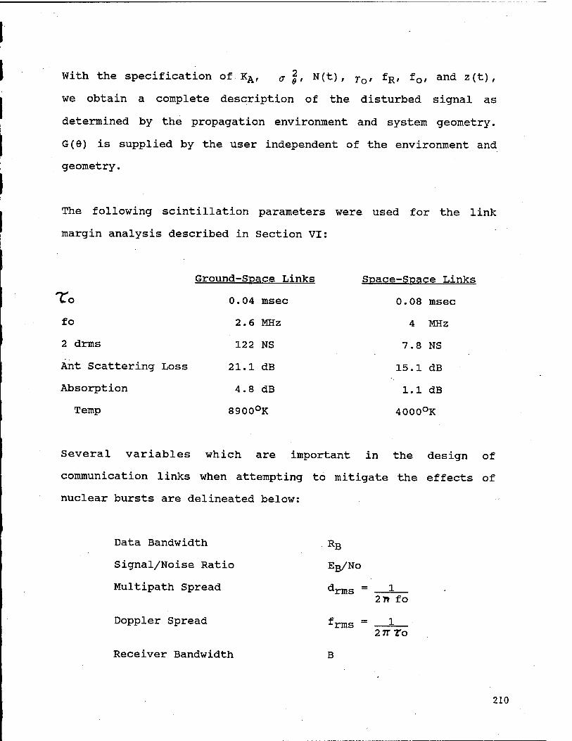
With the specification of KA, a |, N(t) , To, fR, fQ/ and z(t),
we obtain a complete description of the disturbed signal as
determined by the propagation environment and system geometry.
G(9) is supplied by the user independent of the environment and
geometry.
The following scintillation parameters were used for the link
margin analysis described in Section VI:
To fo
2 drms
Ant Scattering Loss
Absorption
Temp
Ground-Space Links
0.04 msec
2.6 MHz
122 NS
21.1 dB
4.8 dB
8900°K
Space-Space Links
0.08 msec
4 MHz
7.8 NS
15.1 dB
1.1 dB
4000°K
Several variables which are important in the design of
communication links when attempting to mitigate the effects of
nuclear bursts are delineated below:
Data Bandwidth
Signal/Noise Ratio
Multipath Spread
Doppler Spread
Receiver Bandwidth
RB
Eß/No
^rms =
frms =
B
2n fo
2 IT To
210

Small Data Bandwidth RB « l/drms (NO Intersymbol Interference [ISI])
Large Data Bandwidth (ISI) RB ~» l/drms
To mitigate fading a combination of frequency spreading, Forward
Error Correction (FEC), and interleaving is typically used. The
effect of direct sequence modulation on fading is easily
summarized. Suppose a pseudo noise (PN) sequence is used with
chip time Tc seconds. Then, time selective fading occurs when
the channel changes in less than Tc seconds.
Frequency selective fading occurs when received frequencies in
signal band have decorrelated fading and are separated by less
than BHz. To mitigate both effects use DS modulation with Tc «
Frequency selective fading also gives rise to the following two
cases:
Case 1
B > Bc > RB
Implicit Diversity
NO ISI
Case 2
B > RB > Bc
Implicit Diversity
ISI
211

To mitigate any resulting ISI, equalization techniques are
employed. Adaptive equalizers have been demonstrated which are
efficiently able to detect digital signals perturbed by a fading
channel medium while tracking the fading variations. If
adaptation requires significantly less signal-to-noise ratio per
bit than conventional detection of the digital signal, the
decisions can be effectively used as the estimate of the
transmitted signal to achieve what is referred to as decision-
directed adaptation. Such systems can be operated without
transmission of special pilot or reference signals for channel
tracking. In troposcatter communication, adaptive techniques
have increased the digital rate capability by at least an order
of magnitude.
A linear equalizer (LE) is defined as an equalizer which linearly
filters each of the N explicit diversity inputs. An improvement
to the LE is realized when an additional filtering is performed
upon the detected data decisions. Because it uses decisions in a
feedback scheme, this equalizer is known as a decision-feedback
equalizer (DFE).
The operation of a matched filter receiver, an LE, and a DFE can
be compared from examination of the received pulse train example
of Figure 1. The binary modulated. pulses have been smeared by
the channel medium producing pulse distortion and interference
from adjacent pulses. Conventional detection without multi-path
protection would integrate the process over a symbol period and
212

decide a +1 was transmitted if the integrated voltage is positive
and -1 if the voltage is negative. The pulse distortion reduces
the margin again in that integration process. A matched filter
correlates the received waveform with the received pulse replica
thus increasing the noise margin. The intersymbol interference
arises from both future and past pulses in these radio systems
since the multipath contributors near the mean path delay
normally have the greatest strength. This ISI can be compensated
for in a linear equalizer by using properly weighted time shifted
versions of the received signal to cancel future and past
interferers. The DFE uses time shifted versions of the received
signal only to reduce the future ISI. The past ISI is cancelled
by filtering past detected symbols to produce the correct ISI
voltage from these interferers. The matched filtering property
in both the LE and DFE is realized by spacing the taps on the
TDLE at intervals smaller than the symbol period.
Figure 1. Received Pulse Sequence After Channel Filtering
Desired pulse
Future pulse
213
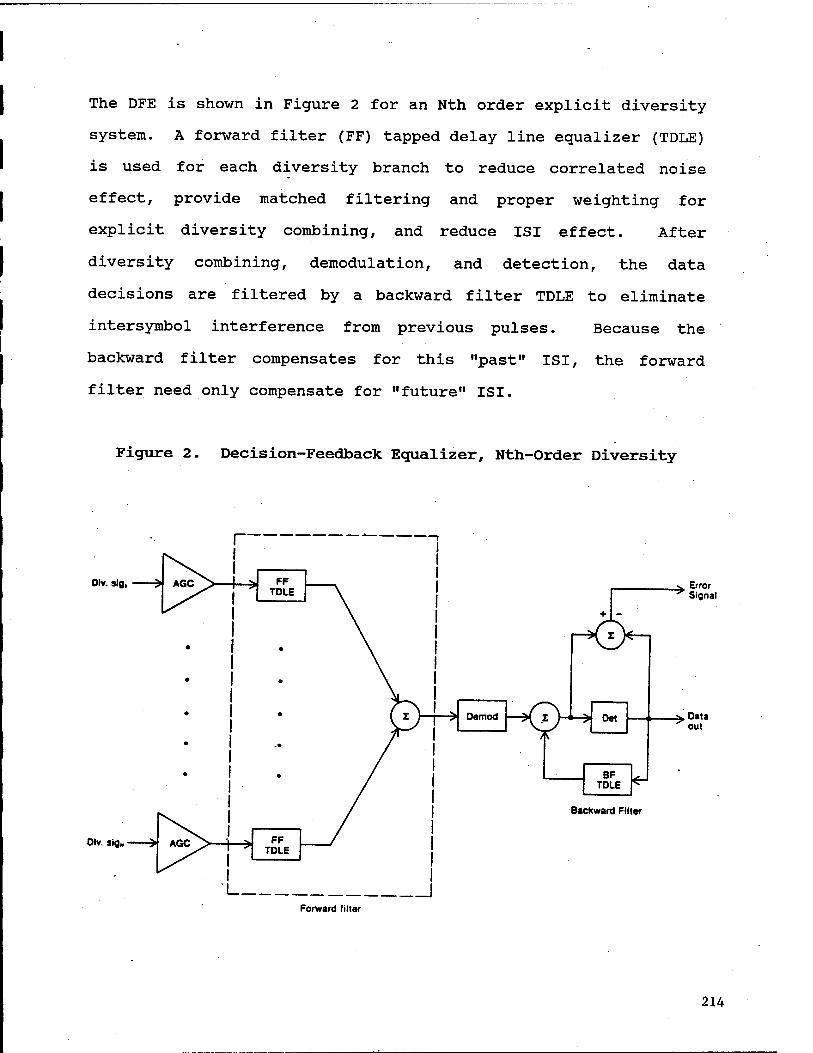
The DFE is shown in Figure 2 for an Nth order explicit diversity
system. A forward filter (FF) tapped delay line equalizer (TDLE)
is used for each diversity branch to reduce correlated noise
effect, provide matched filtering and proper weighting for
explicit diversity combining, and reduce ISI effect. After
diversity combining, demodulation, and detection, the data
decisions are filtered by a backward filter TDLE to eliminate
intersymbol interference from previous pulses. Because the
backward filter compensates for this "past" ISI, the forward
filter need only compensate for "future" ISI.
Figure 2. Decision-Feedback Equalizer, Nth-Order Diversity
Olv. sig,
Oiv. sig»
Error Signal
.Data out
Backward Filter
Forward filter
214

An automatic gain "control (AGC) amplifier is shown for each
diversity branch in order to bring the fading signal into the
dynamic range of the TDLE. A decision-directed error signal for
adaptation of the DFE is shown as the difference between the
detector input and output. Qualitatively one can see that if the
DFE . is well adapted this error signal should be small.
Reference-directed adaptation can be accomplished by multiplexing
a known bit pattern into the message stream for periodic
adaptation.
When error propagation due to detector errors is ignored, the DFE
has the same or smaller mean-square error that the LE for all
channels. The error propagation mechanism has been examined by
a Markov chain analysis and shown to be negligible in practical
fading channel applications. Also in an Nth order diversity
application, the total number of TDLE taps is generally less for
the DFE than for the LE. This follows because the former uses
only one backward filter after combining of the diversity
channels in the forward filter.
The performance of a DFE on a fading channel can be predicted
using a transformation technique which converts implicit
diversity into explicit diversity and which treats the ISI
effects as a Gaussian interferer. As an example, the average
probability of error versus the total received bit energy (Ej-,)
relative to the noise spectral density (N0) is shown in Figure 3
for a quadruple diversity system. The dashed line represents the
215

zero multipath spread (cy =0) performance and the solid lines
show performance for different DFE configurations (N - number of
forward filter taps and A = normalized tap spacing) and ISI
conditions when the ratio of multipath spread to symbol period T
is 0.25. The no-ISI conditions are performance bounds
determining by setting the ISI components to zero. When aJT =
0.25, performance would be to the right of the dashed line if
adaptive signal processing were not employed. The equalizer is
seen to remove this degradation and also provide an implicit
diversity gain which is measured by the difference between the
solid line N = 3, A = 0.5 curve and the dashed line. The
difference between the N = 3, A = 0.5 curve and the next curve
labeled "No ISI" is the intersymbol interference penalty. With
the filter parameters N = 3, A = 0.5, no technique for removing
ISI can do better than this curve. The small-ISI penalty in this
typical example is a strong argument for the use of the DFE
versus more powerful ISI techniques. Finally the leftmost solid
line approximates the very best that can be done as results show
negligible improvement as the number of taps is increased
further. The small difference exhibited shows that a DFE with
only a modest number of forward filter taps performs to an ideal
DFE with an infinite number of taps.
216

Figure 3. DFE Performance, Quad Diversity
10"
10-
10"
io-4
10"
10-
10"
No fading
Quad diversity
O//T-0.25
N-11 A-0.125 NolSI
N-Number of FF taps
a _ tan spacing ~ symbol period
10 15
Total £.N (dB)
25
Error correcting may be utilized to mitigate the effects of
fading as well as pulsed jamming. Assuming the use of a
convolutional code with constraint length 7 and rate 1/2, the
following shows the minimum required energy per bit to noise
density ratios (Eb/NO) that can be tolerated to give a bit error
probability of 10~5 for the various types of links encountered in
the SDS architecture:
217

Req'd Eg/No for 10~5 BER
1) LOS/Coherent Broadband Jamming 4.5 dB
2) LOS/Non-Coherent Multitone Jamming 10.0 dB
3) LOS/Seintillation Coherent Broadband Jamming
No ISI Modes Diversity B > Bc > RB 7.0 dB ISI Large Diversity B » RB ^ Bc 7.0 dB
4) LOS/Scintillation Non-Coherent Broadband Jamming .. 10.0 dB
These ratios were used to determine link margins presented in
Section VI.
218

C. TRENDS IN RADIATION HARDENED MICROELECTRONICS FOR SDI
219

TRENDS IN RADIATION HARDENED MICRO-ELECTRONICS
SUMMARY
The SDI program has defined two levels of radiation requirements, level 1 and level 2. Table A-l presents the quantitative device parameters for these two levels.
The less severe application, level 1, is attainable with current technology and processing capabilities. Although there are not a lot of devices obtainable today meeting the level 1 requirements, the reason is market demand, not technology. With proper.market demand, it is anticipated that the VLSI devices required to support SDI equipments could be obtained in CMOS, bi-polar, and GaAs, as needed by the specific application.
Level 2, on the other hand, has little chance of being implemented with presently manufacturable process technologies. An extension to existing technology and process cababilities will be needed. Two technologies appear promising for level 2 applications. These are:
Gallium Arsenide (GaAs)- This technology is needed for applications requiring high speeds and medium gate densities. Processing has been demonstrated, producing low density devices with good total dose radiation hardness. The technology extension is needed to increase the gate densities, improve the transient radiation hardness, and address high volume production issues.
CMOS-Silicon On Insulator (CMOS-SOI)- This technology is needed for high density, medium speed, and low power applications. Although MSI devices have been produced in a laboratory environment, technology work is needed to refine the process and to validate the anticipated inherent radiation hardness.
In summary, CMOS whether bulk or SOI will be the choice for level 1 complex processing applications, LSI, VLSI or greater. GaAs and bi-polar are applicable to level 1 equipments requiring very high speed, but possibly at the expense of power and density. The more stringent level 2 environments will necessitate the use of CMOS.-SOI or GaAs. GaAs will be chosen in high speed applications and CMOS-SOI in medium speed, low power applications.
REQUIRED RADIATION TOLERANCE
The SDI Survivability, Acquisition and Tracking Program and the Radiation Hardened LSI Technology Program (SAT-8.1) have defined two survivability requirements, Levels 1 and 2, for SDI\ Level 1 is applicable to ground based systems and space based demonstration models, while the more demanding Level 2 is applicable to space based systems. The requirements for the two levels are summarized in Table A-l.
220

Table A-l Survivability Requirement Levels
Level
Total Dose (Rad(Si))
Dose Rate (Rad(Si)/sec) Upset Survival
Neutron (lMeV n/cm2)
1
1.0 E
1.0E l.OE]
1.0E
2
3.0E
1.0E l.OE"
1.0E
Single Event Upset (Bit Errors/Bit-Day)
Directed Energy Weapons Upset to Protons (Bit Errors/Bit-Day)
Thermomechanical (cal/gm)
1.0.E l.OE
INTEGRATED CIRCUIT DEVICE TECHNOLOGY
The choice of process technologies to implement custom SDI integrated circuit requirements will be determined by two major considerations. The first is the general speed-power performance common to all spaceborne systems. The second is the severe radiation requirements under which SDI systems, in particular, will be required to function. The electronics of SDI systems are required to survive the prompt and delayed radiation from nuclear detonations, natural and nuclear-detonation-pumped charged particle belts, cosmic rays and directed energy weapons. Technologies which are currently in use or under consideration include:
Silicon CMOS or Bipolar Devices Gallium Arsenide FET or Bipolar Devices Josephson Junction Devices Silicon on Insulator Systems (SOI) Silicon on Sapphire Devices (SOS)
Of the 5 technologies cited above, Silicon On Saphire and Josephson Junction are not believed to be viable candidates for the following reasons.
SOS is considered an obsolete process. Technical problems associated with the heteroepitaxial structure, while partially overcome, have continued to plague the technology.
221

In addition, the parasitic edge devices and back plane leakage path have severely compromised its radiation resistance, even for Level 1. Although heroic efforts have been mounted by some suppliers to overcome these inherent disadvantages, SOS appears to be a technology that has missed its window.
Josephson junctions, based upon superconducting materials, have lagged behind the Silicon and GaAs devices because of problems of implementing circuits at liquid helium temperatures. Although recent advances have produced working signal processing systems, currently this is not a mainstream technology, even for ground applications. This is, however, a rapidly changing area, which should be closely monitored for quantum breakthroughs.
The remaining semiconductor technologies merit further consideration. Figure A-l is a comparison of speed-power results for several advanced Si based and GaAs based IC technologies. The curves marked CML (1.25 microns) and CML (0.5 microns) represent results for VHSIC technology. All the results shown are for ring oscillators, thus giving a direct comparison on intrinsic gate speeds.
CURRENT CAPABILITIES
Recent process development efforts have increased the hardness of both Si and GaAs (Table A-2). Gallium arsenide MESFETS have been shown to be only minimally sensitive to a total dose of 250 Mrads (GaAs) and a neutron fluence of 1E14 neutrons/sq.cm. GaAs MOSFET circuits have shown no upset to dose rates of 1E10 rad/sec. Such radiation hardness levels are also representative of recently demonstrated Si capabilities. Radiation hardened CMOS (RHCMOS) circuits have been fabricated with demonstrated total dose hardness in excess of 1E7 rad, and latch-up and burn-out immunity to dose rates in excess of 1E12 Rad(Si)/sec. While current upset levels are of the order of 1-3E8 Rad/sec, current developmental goals in excess of 5E10 Rad(Si)/sec. are considered attainable.
It is not possible to say whether GaAs or Silicon is generically superior for Level 1 requirements. Applications must be examined on a case by case basis to determine which technology is most appropriate to a particular portion of a system. In general, when the highest possible speed is required, or when the lowest possible noise at high frequencies is required, gallium arsenide (even at higher cost/gate) will be the preferred choice. For large scale integration involving command and control functions, data processing, or low to intermediate frequency communication, where minimum power consumption is essential, silicon would be the optimum material.
222

Figure A-l Comparison of Speed/Power For Various Technologies
a
a p
10ns
1ns
100ps -
10ps -
1ps
U/GaAs UODFET
-L 1jiW 10pW 100|iW 1mW 10mW 100mW
Power Dissipation/gate
Total Dose Dose Rate HESUBSH Upset Survival
Technology fRadrsin fR,ad(Sj)/sec) fRaflfSj)/sec) _LD/25?) Comment
RHCMOS(2> >1E7 1E11<4> >1E12 >1E14 Projected dose rate capabilities. May satisfy both levels.
CMOS >1E4 (Commercial)
CMOS SOS(3) >1E6
>1E8 >1E9 >1E14 Falls short in total dose.
>1E10(5) >1E12 >1E14 Total dose problem. Not scalable below 3 micron.
1E12 1E12 TBD Hot mature, labora- tory SEU/upset inune.
lBllt1' >1E12 >1E14 High speed and dose rate, low power uses. Limited by high cost/, gate, processing difficulties.
Consents: (1) SElo demonstrated. (2) Projected SEO capability of 1X10"10 errors/bit-day. RHCMOS is Radiation Hard CMOS. (3) 2X10⁻⁹ errors/bit-day. (4) 3E8 demonstrated. (5) Only if hardened by design.
CMOS (SOI)
GaAs
TBD
>7E7
TABLE A-2 IC TECHNOLOGY HARDNESS
223

DISCUSSION OF HARDENING TO LEVEL 2 REQUIREMENTS-
, The radiation requirements of Level 2 will only be attained through the implementation of a new technology base. The most likely silicon candidate at this time is the one that is known generically as Silicon on Insulator (SOI). (GaAs is a non-silicon candidate, and will be discussed later in this report.) While SOI systems lack sufficient maturity to consider implementation at this time, most of the component techniques required to assemble the process have been developed. In fact, some SSI/MSI implementations have been demonstrated. However, issues of manufacturability, sourceability, yield, and reliability have yet to be addressed. There remains a concern that SOI may have the same low total dose susceptibility as SOS. However, it is generally felt that an aggressive developmental effort in this area will most likely be successful.
To accelerate the development of RHCMOS and SOI technologies, radiation effects test structures and circuits will have to be developed and evaluated in the total dose, dose rate, neutron, and single event upset environments. GFE simulation facilities will have to be used for the evaluation of the susceptibility of the technologies to DEW SEU. All this presupposes the availability of a viable SOI process capability.
A comparison of radiation tolerance of Silicon Bipolar and GaAs circuits shows each can withstand total integrated dose and that both have difficulty withstanding transient radiation. Silicon Bipolar is hardenable to greater than 10 MegaRads by relatively common process modifications. GaAs circuits are inherently hard to total integrated dose. The semi-insulting GaAs substrate does not require the use of dielectric isolation such as Silicon Dioxide used in most silicon circuits. The omission of the dielectric removed the threshold variations and field inversion problems associated with charge storage in the oxides and the interface state generation problems encountered at the silicon- silicondioxide boundary. The resulting dielectric free devices suffer only minor performance degradation after greater than 100 MegaRads.
Transient upset manifests itself differently in Silicon and GaAs. The primary reasons for transient upset in silicon have to due with photocurrent generation and the effects the photocurrents have on power distribution (Rail Span Collapse) and circuits or individual transistors with gain (Secondary Photocurrent generation). Photocurrents are free charge formed by the radiation pulse that are collected in the depletion regions of junctions. Hardening of Silicon CMOS has been accomplished by replacing junctions used for horizontal device isolation with dielectric boundaries and vertical isolation to the substrate junction by SOI, a buried dielectric layer. Silicon Bipolar transistors are inherently PNP or NPN junctions and cannot be removed from the device structure. Transient hardening of Silicon Bipolar is therefore limited to minimization of photocurent
224

effects and will never achieve the exceedingly high transient radiation levels of Silicon CMOS and GaAs.
GaAs also has difficulty with transient upset. GaAs E/D circuits lack sufficient noise margin to tolerate the transient noise environment. Noise in the power distribution and a reduction in the insulating nature of the GaAs substrate, causing device to device condition combine to exceed the noise margin of the gates and result in upset. Current GaAs II E/D upset levels are Figure A-l Comparison Of Speed/Power For Various Technologies
similar to Silicon Bipolar (1E8 to 1E9 rads/sec), though improvement is rapid since the same efforts to improve circuit complexity are directly benefiting transient radiation tolerance. Heterojunction GaAs III FETs have noise margins many times better than E/D MESFETs and have demonstrated superior transient upset tolerance. Upset free work-through has been demonstrated at 5E10 Rads/sec.
COMPARISON OF SILICON AND GALLIUM ARSENIDE-
Silicon is an ideal material for the fabrication of VLSI circuits. Silicon can be easily purified; grows fused quartz as its native oxide to serve as a dielectric layer and diffusion barrier; is easily etched and mechanically strong; can withstand high processing temperatures; forms ohmic contacts to metallic conductors easily; and supports the formation of a wide range of active and passive devices such as NPN and PNP bipolar devices, N and P channel mosfets, JFETS, resistors, capacitors, etc. It is the ease of fabrication that causes silicon to be the dominant semiconductor technology in spite of its subordinate electrical characteristics.
Gallium Arsenide (GaAs), on the other hand, has nearly ideal dielectric properties at microwave communication frequencies. It has very high electron mobility so that extremely fast active devices can be fabricated. It has the flexibility of bandgap modification through the addition of ternary compounds to produce materials such as AlGaAs. Being a direct bandgap material, optically active devices such as LEDs and lasers can be integrated directly into custom configuration. Only the difficulties of circuit processing limit the utilization of GaAs for LSI fabrication.
Silicon Bulk CMOS will provide the high density radiation hardened process technology for all but Level 2 requirements where CMOS/SOI will be required. The high speed technology applications will utilize silicon bipolar in the near-term except for power critical and high transient dose rate environments. In the longer term both GaAs MESFET and GaAs heterojunction technologies will exceed both the performance and complexity achievable with silicon bipolar.. Level 2 requirements will be met by GaAs Heterojunction technology.
CMOS technologies excel in complex processing and data storage
225

applications. CMOS's virtual lack of static power consumption makes if ideal for memories and complex digital processors where most internal nodes are static. Bulk CMOS also offers continued promise in radiation hardened applications. Total dose hardening efforts have resulted in hardened bulk CMOS devices that can withstand a MegaRad, with advanced processed offering 10 to 100 MegaRads of total integrated dose hardness, adequate in all applications. Transient hardening efforts have made progress by simply improving power supply distribution, enabling bulk CMOS devices to achieve in excess of 1E10 Rads/sec (Si). This level will improve still further without employing more difficult and exotic techniques such as Silicon On Insulator (SOI) technology.
SOI techniques are as yet unproven, having only been demonstrated at the MSI level in laboratory environments, but are expected to become producible in the next 5 years. Performance and hardening advantages may make SOI acceptance broad once manufacturable. The inclusion of the buried Si02 layer reduces device capacitance, increasing speed or reducing power, while simultaneously eliminating the under - channel junction's charge collection volume. These improvements may result in both commercial and military application. CMOS/SOI is expected to tolerate 1E12 Rads/sec (Si) without transient upset. The buried isolation layer is also expected to provide Single Event Upset (SEU) hardness by interrupting the ionized charge funnel formed under the device along the particle track.
CMOS device speeds are improving with smaller geometries, though not sufficiently to offer an alternative to high speed Silicon Bipolar or GaAs. High speed applications will require the use of Silicon Bipolar or GaAs technologies. The choice of GaAs or Bipolar must be based on specific system requirements. Both are capable of speeds greater than 1 GigaHertz, with GaAs circuits operating as high as several GigaHertz.
Circuit complexity achievable currently with Silicon bipolar is approaching 10,000 equivalent gates (45,000 transistors). Silicon bipolar has made significant density strides in recent years utilizing self alignment techniques, buried contacts and more highly concentric device structures. Continued density improvement will continue tracking photolithography progress. Bipolar speeds have progressed due to the much smaller geometries, pushing device Ft above 10 GHz as high as 17 GHz. Gate delays of less than 100 picoseconds have been demonstrated at gate powers of 4 to 8 milliwatts. Current Silicon Bipolar devices may be limited by total power dissipation in applications where such exotic cooling techniques such as liquid cooling are impractical. Flight applications will be required .to limit total device complexity to remain when the bounds of conduction and radiated cooling capacities. Ground based applications are more flexible, currently accepting chip power dissipations a-s high as 30 watts.
Gallium Arsenide digital circuits have developed more slowly than Silicon. Original all depletion mode (GaAs 1) circuits met with
226

limited acceptance due to high power and low levels of integration. SSI to MSI level device complexity limitations, due to high power dissipation, resulted in minimal system speed improvement, utilized only in strategic circuit bottlenecks.
The introduction of Enhancement/Depletion (E/D GaAs II) mode circuits allowed significantly higher levels of integration due to reduced power consumption. GaAs II E/D circuit processing is today offering a relatively mature.technology. Circuit densities in the LSI level, greater than 3000 gates, are currently achievable. Maximum integration level's are still limited by processing difficulties, primarily a lack of adequate noise margin to absorb process and parametric variations. GaAs II E/D does offer a speed-power product 3 to 5 times better than Silicon Bipolar. A current comparison of "achievable density gives Silicon Bipolar a 3X to 4X greater complexity, but if each technology is allowed to mature to where total power dissipation again becomes the limiting factor in device complexity, GaAs circuits will achieve a higher level of complexity due to lower speed-power product.
Heterojuntion GaAs III circuits are currently progressing from laboratory to a manufacturable technology. GaAs Heterojunction Bipolar Junction Transistors (HBT) and heterojunction FETs are being developed. Similar to silicon, the HBTs are expected to find application in linear, analog and high speed applications. The FETs will operate at the lower power levels amenable to high density applications. Heterojunction GaAs FETs gates operating at 50 to 70 picoseconds have been demonstrated at the 2000 gate level. This technology lags GaAs II MESFETs by several years but offers a speed-power product low enough to carry multi-GigaHertz GaAs ICs into the VLSI integration levels (10,000 to 100,000 gates) before being power dissipation limited.
In summary, CMOS whether bulk or SOI will be the choice for complex processing applications, LSI, VLSI or greater. Bulk CMOS will meet most radiation hardening requirements through 5E10 Rads/sec. More stringent environments will necessitate the use x>f CMOS/SOI. High speed applications will require Silicon Bipolar or Gallium Arsenide. Ultimately GaAs will exceed the density and performance of Silicon Bipolar but not for 3 to 5 years. In the interim, GaAs will only be chosen in power critical applications or due to high transient dose rate requirements. Level 2 environments will required the utilization of GaAs III Heterojunction technology. The maturity, manufacturability/cost, and recent advancements of Silicon Bipolar will preserve its holed on the high speed technology market share.
DISCUSSION OF VHSIC PROGRAM
The present effort of military IC technology is the VHSIC program, which has developed 38 very high speed integrated circuits using a 1.25 micron feature. This program also involves inserting these chips into nine brassboards. Currently all the chips have reached the testing phase and many have or are being
227

employed in the VHSIC brassboards. Furthermore, the yield improv-ement phase has been in progress for a year or more. Efforts are now being concentrated on the development and generation of the submicron (0.5 micron) chip technology.
Also, the current maturity of the gallium arsenide technology was evaluated. Presently this technology appears to be a viable option to silicon technology for high speed and radiation hardened applications.
VHSIC LITHOGRAPHY
The present high level of chip integration has resulted from the generation of micropatterns produced by the refinement of conventional optical lithography. The sophistication, reliability, and economic feasibility of electronic systems have increased in direct proportion to the increase in circuit densities of integrated circuit chips. Much of the performance enhancement of integrated circuits can be attributed to the increased circuit density and speed obtained by reductions in the feature size of circuit patterns. Figure A-2 is a forecast of pattern application line widths which must be supported by lithography tools, if the goals of the VHSIC program are to be met.
1995
1990
< 1985 >
1980
1975
_ FIGURE A-2 LITHOGRAPHY TOOL REQUIREMENTS
MIBL S&R X-RAY S&R
E-BEAM
10:1 AND 5:1 OPTICAL STEP & REPEAT (S&R)
1:1 SCAN PROJECTION
0.5 1.0 1.5 2.0 2.5 3.0 3.5 FEATURE SIZE (MICRONS)
4.0 4.5
228

The VHSIi. hase I chip prototyping and yield enhancement efforts establ-isV i that optical stepper lithography can be employed as a 1.25 mic. •;... baseline technology. It also demonstrated that a hybrid "m :.x and match" patterning approach using both optical and E-beam lithography can be employed for the alignment of chips with 0.5 micron feature. The use of commercial projection aligners and optical steppers have proven to be feasible for the task of patterning super chips.
The fabrication of the VHSIC Phase II chip is a difficult task, since the complexities of this chip are anticipated to range from 1E5 to 2E6 gates per sq cm and chip sizes ranging from 0.7 cm to 5.0 cm on a side. Not only is prototyping an issue, but also future chip production line availability and operating costs are critical and unavoidable issues. Hence it can be concluded that micropattern generation of the submicron feature chips will require employment of E-beam, X-ray and Masked Ion Beam (MIB) technologies as well as optical lithography.
Basically, the VHSIC EBL prototype throughput requirements specify at least 20 (100 mm dia.) wafers per hour at a resist sensitivity of 20 uC/sq cm and a pattern complexity described as 1E6 geometries per sq cm, or a 30% wafer coverage.
Due to current business conditions and program withdrawals, the only VHSIC supported development that remains available for VHSIC Phase II chip prototyping and early chip production is the PE AEBLE-150. This machine offers a quick turnaround and customization of chips even below 0.5 micron in small quantities (less than 10,000) in a cost effective manner.
Due to its serial mode of information processing, EBL patterning will be expensive and impractical for large volume production. Because certain wavelength X-rays are inherently capable of being used for submicron patterning and parallel data transfer, the VHSIC program includes the development of an X-ray step and repeat system (XSR). The VHSIC XSR development is well along in development (Perkin-Elmar).
ADDITIONAL DEVICE SPEED-POWER INFORMATION
The gate power-delay product is the most used figure of merit when evaluating the performance of an integrated circuit gate. By definition it is:
Ug - p*tg (1)
where Ug - energy in joules. p - gate dissipation in watts, tg - gate delay time in seconds.
Equation 1 represents the minimum energy dissipated in a switching circuit when it changes from one binary state to the
229
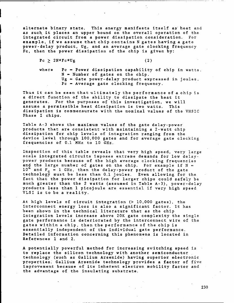
alternate binary state. This energy manifests itself as heat and as such it places an upper bound on the overall operation of the integrated circuit from a power dissipation consideration. For example, if we assume that chip contains N gates having a gate power-delay product, Ug, and an average gate clocking frequency Fc, then the power dissipation of the chip is given by:
Pc > 2N*Fc*Ug (2)
where Pc - Power dissipation capability of chip in watts. N - Number of gates on the chip. Ug - Gate power-delay product expressed in joules. Fc - Average gate clocking frequency.
Thus it can be seen that ultimately the performance of a chip is a direct function of the ability to dissipate the heat it generates. For the purposes of this investigation, we will assume a permissible heat dissipation is two watts. This dissipation is commensurate with the nominal values of the VHSIC Phase I chips.
Table A-3 shows the maximum values of the gate delay-power products that are consistent with maintaining a 2-watt chip dissipation for chip levels of integration ranging from the device level through 100,000 gates and for average gate clocking frequencies of 0.1 MHz to 10 GHz.
Inspection of this table reveals that very high speed, very large scale integrated circuits imposes extreme demands for low delay- power products because of the high average clocking frequencies and the large number of gates on the chip. For example if N = 10 and Fc - 1 GHz, then the delay-power product of the gate technology must be less than 0.1 joules. Even allowing for the fact that the power dissipation for larger chips could safely be much greater than the 2 watts (assumed in Table A-3), power-delay products less than 1 picojoule are essential if very high speed VLSI is to be a reality.
At high levels of circuit integration (> 10,000 gates), the interconnect energy loss is also a significant factor. It has been shown in the technical literature that as the chip integration levels increase above 20K gate complexity the single gate performance is deteriorated by the interconnect wire of the gates within a chip, then the performance of the chip is essentially independent of the individual gate performance. Detailed information concerning this phenomena is located in References 1 and 2.
A potentially powerful method for increasing switching speed is to replace the silicon technology with another semiconductor technology (such as Gallium Arsenide) having superior e-lectronic properties. Gallium Arsenide technology provides a factor of five improvement because of its inherent electron mobility factor and the advantage of the insulating substrate.
230

Figure A-3 is a graph of the power-delay product as functions of the gate delay and gate power dissipations for most of the silicon circuit technologies and also that anticipated with the gallium arsenide technology.
For any given point on the graph, the ordinates axis defines the gate delay in nanoseconds, the x axis defines the respective gate dissipation in milliwatts, and the intersecting diagonal line provides the magnitude of the power-delay product in picojoules.
Hence, it can be noted that the diagonal lines of the graph toward the lower left-hand corner of the graph represent smaller power-delay products. The solid triangles represent lower power- delay products achieved by the VHSIC Phase I circuit technologies (all implemented with the silicon technology) and, as such, provide a benchmark of the current military integrated circuit technology.
Referring to Figure A-4, it can be observed that CMOS/SOS circuit technology and gallium arsenide technology exhibit the lower power-delay products, and it is somewhat less than 0.1 picojoule. CMOS/SOS possesses the minimum gate power, while gallium arsenide technology has a small gate delay, about 40 times less than CMOS/SOS. However, the gate power dissipation of the gallium arsenide gate is approximately 60 times that of CMOS/SOS. Therefore, in applications where very large scale integration is required and speed is not a limiting factor then the CMOS/SOS is an optimum choice. Applications where speed is the prime requirement, gallium arsenide technology is the most optimum selection and as such, the chip level is limited by its gate dissipation. See References 1, 4 and 5 for additional details.
VHSIC DENSITIES-
A valuable benchmark for accessing the military silicon integrated technology is the results obtained on the VHSIC Phase I effort. The contractors of the VHSIC Phase I utilized five circuit technologies, NMOS, ISL, CMOS, STL and 3D Bipolar. These chips were developed using a 1.0 to 1.25 micron feature size. Table A-4 provides a summarized tabulation of the chip parameters, the chip size, gates per chip, device count per chip, gate dissipation, gate delay and the power-delay product.
In summary it can be seen that the current nominal chips are 0.119 inches (0.34 x 0.35), and the gate densities for this chip size range from 131,000 to 364,000 gates per inch with the largest densities achieved by the NMOS technology. The power- delay product ranges from .1 picojoules (CMOS) to 3 picojoules (3D bipolar).
During the past five years, considerable attention and effort has been devoted by the IC industry to the development of digital integrated circuit area using the gallium arsenide technology. Table A-4 b summarizes the chip performance that is achievable in the laboratory today and a projection of what should be
231

achievable in five years.
It can be observed from this table that the key features of this technology are the power-delay product, the very short gate delay, and its excellent radiation performance. The level of chip integration is somewhat less than that achievable with silicon technology. One of the key issues that remains to be resolved is the degradation of the chip performance when the chip level of integration attains a 10,000 gate (and greater) complexity. At these.levels the chip performance is more dependent upon the interconnect effects rather than the individual gate performance.
Gates/Chip
Clock Frequency
0.1 MHz 1.0 MHz 10 MHz 100 MHz 1 GHz 10 GHz
ULSI 1E5
VLSI 1E4
LSI 1E3
MSI 1E2
100 pj 10 pj
10J pj 100 pj
104 pj
10D pj
IQ"3 pj
104 pj
1 pj
10 pj
100 pj
io- PJ
0.1 pj
1 pj
10 pj
100 pj
0.01 pj
o.i Pj
1 pj
10 pj
0.001 pj
0.01 pj
o.i Pj
1 pj
Table A-3 Maximum Gate Dynamic Switching Energies for Various Average Clock Frequencies (2-Watt Chip Dissipation)
When the GaAs technology is implemented into logic chips, there are several key issues which must be considered. The GaAs circuitry requires interface circuitry when the internal chip functions are connected to circuits in another chip. Therefore, the logic output signals are implemented with driver circuits. Each driver circuit consumes 15 to 30 milliwatts, so that the total driver power consumption is approximately 100 to 250 times that of a single Ga As logic element. One can conclude that the chip interface circuitry is not a trivial concern. Furthermore, the real estate occupied by this driver circuit is large in comparison to the GaAs logic cell real estate. One approach being considered is the application of optical coupling for chip to chip signal interconnects.
232

TABLE A-4a VHSIC Phase I Chip Parameters
Circuit Chip Size Technology (sq. in.)
Gate K Gates Gate Count Per Sq. Oiss (K) In. (mW)
Gate Delay Power (nanosec) Delay
Product (pO)
3D
STL
ISL
NMOS
CMOS (Hughes)
0.314 x 0.272
0.35 x 0.35
0.3 x 0.3
0.32 x 0.32
0.368 x 0.315
CMOS 0.34 x 0.35 (West.)
11.8
16
27.3
37.3
18
23
138
131
303
364
154
192
0.38
0.15
0.07
0.089
0.04
0.016
7.9
7.4
10.0
8.0
5.0
6.0
3
1.1
0.72
0.7
0.2
0.11
Table A-4 b Gallium Arsenide Chip Parameters
Parameter
Feature size (uM)
Gate Power (mW)
Gate Delay (ps)
Power-Delay (p«3)
Integration Level (number of gates)
Radiation
Total Dose Rad(SI)
1986
1.0
.5
100
.05
4000
107 - 108
1991
0.5 to 0.7
.5
70
.035
15000 to 20000
10 8
Transient Rad(S1)/sec 109 - 1010 1011 - 1012
233

g 100
w o 10
< Ü < 1.0 Q_ o a. LU
0.1
0.01 1uw 10uw 0.1 mw 1.0mw 10mw
POWER DISSIPATION / GATE 100mw
FIGURE A-3 SILICON AND GALLIUM ARSENIDE GATE CHARACTERISTICS
234

REFERENCES
1. Solid State Technology Trends Motorola Report, BMD Program M. B.. Aufderheide, 12/20/85.
2. IEEE Nuclear and Space Radiation Conference Monterey, California, July 21, 1985.
3a. A VHSIC Overview Solid State Technology, March 1986.
3b. Masked Ion Beam Lithography: An emerging Technology Solid State Technology, March 1986.
4. HEMT: A Super Fast Transistor IEEE-Spectrum. February 1984.
235

D. EMBEDDED COMSEC FOR SDI
236

SUMMARY-
COMSEC imbedment is a loosely defined term. The basic concept is to "imbed" the COMSEC function into the system as an integral part of the system. How this is accomplished is still subject to debate. Depending on the source of information, COMSEC imbedment ranges from a chip or chip set which is added to the system components, to an intelligent standalone data processing equipment which requires minimum inputs and provides few outputs. The compromise of these two extremes is a medium size module which has a small amount of "intelligence", thus requiring less external control than a chip set but more than a standalone equipment.
This white paper discusses COMSEC Embedment at each of the three levels, chip(s), module, and a standalone unit. In principle, the advantages of embedded COMSEC is a reduction in overall system size, weight, power, and complexity resulting from sharing resources (such as housings, power converters, system controllers, etc.) between the COMSEC function and host equipment function. In summary:
Chip embedment usually results in the simplest system, but may cause undue administrative problems, and a considerable increase in non-recurring cost and program risk.
.. Module embedment may result in a slight increase in host equipment complexity (over chip embedment), but provides a tremendous reduction in the administrative costs and risks.
The standalone COMSEC approach is perhaps the highest recurring cost approach, but presents a lesser non-recurring cost and risk situation.
Many factors must be considered when determining the level of COMSEC embedment. The following discusses some of these factors.
SECURITY AND ADMINISTRATIVE FACTORS -
For the chip and module embedment case, the host equipment supplier is obligated to implement many security features (such as the alarm test, red-black separation, SFA analysis, etc) which are perhaps totally foreign to him. Some host equipment suppliers may not even have a secure facility and personal clearances.
For the chip case, the host equipment would be responsible for the TEMPEST design, analysis, and subsequent verification testing. For the module case, some of the TEMPEST design would be included in the module, but the host equipment developer is still responsible for the physical isolation and power supply aspects of TEMPEST, and for performing the system TEMPEST testing .Again. this may be a totally new discipline for him.
For the chip and module embebment cases, the host system is responsible for implementing the local agent portion of the
237

network re-key protocols. The whole concept of rekeying may be foreign to the host equipment supplier.
The procuring agency would be obligated to provide "applications information" as part of the host equipment specifications. In addition to the normal KG requirements specifications (including such things as the communications protocols, variable processing, chip interfaces, randomization, alarm test, etc.), additional tutorial and philosophy/doctrine information would probably be needed. The degree of support from government security agencies (monitoring the design, attending design reviews, etc.) would probably be increased, so that problems could be detected and corrected before the design is frozen.
Most likely, chips and modules would be procured from one or more traditional COMSEC equipment suppliers, so the procuring agency would probably do the vendor control and monitoring in the normal manner. There are probably numerous different suppliers of host equipment into which the COMSEC function is embedded. The COMSEC procuring agency must monitor each one of them, including providing security guidelines, monitoring the design, reviewing and approving the analyses, attending design reviews, etc.
Although the chip embeddment may result in the minimum hardware system implementation, the approach imposes an administrative burden on the host equipment supplier and the procuring agency. This approach may be practical in situations where the host- system supplier is also cognizent of cryptographic issues, has a cleared facility, is up to speed on security issues, understands protocol issues, with key management, and understands TEMPEST design and testing. It does not seem practical, however, in situations where the host equipment supplier has never been exposed to COMSEC issues.
The standalone COMSEC approach is the simplest from an administrative standpoint, and probably results in the lowest non-recurring cost, least program risk, highest security, but the highest recurring cost.
Chip embedment appears to be the least desireable, since it places the maximum security responsibility on the largest number (and possibly least experienced) equipment designers, and distributes the security responsibility widely.
The embedded module case appears to be a reasonable compromise between non-recurring cost and administrative risks. The COMSEC design, security analyses, etc. are confined to one vendor (the module supplier). Although the host equipment supplier still must maintain some security responsibility (TEMPEST, and some functional control) his involvement is considerably less than in the chip case.
The extreme case is the standalone COMSEC case, where security responsibility is clearly maintained with a single vendor, the COMSEC equipment supplier. The COMSEC is largely transparent to
238

the host equipment being protected.
CONTROL COMPLEXITY-
The next factor to consider is the embedment impact on system complexity and processing capabilities. If a chip set is to be integrated into a system assembly, the processing power to maintain that chip set and to perform general housekeeping functions must be added to the system.
The next higher level of embedment would involve a module which would handle the general housekeeping functions of the chip set and require a lesser degree of control from the host processor during traffic operations. The module approach decreases the amount of processing which must be dedicated to the COMSEC function, when compared to the chip approach.
System processing power requirements are reduced even further if the stand alone data processing approach is taken. This approach requires only rudimentary control functions from the host system processor. The COMSEC system would perform its own checks and control all COMSEC housekeeping functions. It could be designed to perform self diagnostics and provide status indications.
The most important thing to keep in mind is the complexity of the function which the COMSEC equipment must perform. This complexity will directly affect the next factor, the system interconnections.
SYSTEM INTERCONNECTIONS-
The chip or chip set would require a large number of interconnections. All diagnostic signals, SFA critical signals, and traffic processing signals must be accessed. Most likely, the chip would be designed to mount directly on a printed circuit board or in a socket. Hopefully, the chip packaging would be compatible with the host equipment supplier's board assembly procedures, so special handling would not be required during board assembly.
The module approach would probably require a cable harness or back plane connection to connect it into the host system. It would also require area or a platform for mechanical mounting into the host system. The number of physical interconnects required would vary depending upon the extent of the module local intelligence. The more intelligence the module contains, the fewer the number of interconnects which would be required.
The standalone equipment would require minimal interconnection between the system and the COMSEC equipment. However, this approach would require the largest area on the platform".
POWER CONSIDERATIONS-
A tradeoff of power is also an important factor to consider
239
nstween the three approaches. The chip set is the most efficient, because it would operate from power on the host system printed circuit board. Assuming chip voltage levels were compatible with the host system, no extra power converter or regulators would be needed (except possibly for TEMPEST). Additionally, sharing resources with the host system (such as using the host controller for the KG function) probably requires less power than adding an additional control function.
The module could be designed to operate from the prime power, or from a regelated or semi-regulated power bus. The better regulated the power bus, the more efficient the module could be by eliminating the need for internal regulators.
The standalone equipment could also be powered by a regulated or semi-regulated power bus. The total power required by this approach is probably greater than the other two approaches, since it requires the most circuitry.
SPECIFICATION AND INTEGRATION ISSUES-
Before beginning a discussion of the specification, integration, and testing of COMSEC embedment approaches some other considerations should be presented. When considering which embedment approach to use great care must be exercised not to apply one method indiscriminatly. It is not appropriate to assume that one approach is best for all application. In a low speed, simple application the chip approach may be the best. However, the chip approach could be very cumbersome when applied to a high speed or complex function. Simply put, all aspects of an embedment approach should be considered when trying to choose the one best suited.
COMSEC embedment tends to work best if standardization could be achieved. Simple requirements such as power supply voltages and regulation specifications, standard packages and mountings, standardized connectors, standard signal voltage levels and timing characteristics. This standardization may lead to inherent inefficiency in an embedment system. The amount of inefficiency is completely dependent on the versatility of the COMSEC embedment component. This versatility will be a direct result of the design specifications of the embedment component.
When a COMSEC element has been identified for embedment, the next task is to determine which embedment approach will be choosen. After the approach is choosen the task of determining the specifications can begin.
If a chip implementation has been choosen, a large amount of specifications will be required. The mechanical outline, heat sinking techniques available, temperature design limits-, input and output data and clock timing relationships and amplitudes, leakage currents, frequency of operation, power supply voltages and functional task. The best scenerio for the specification of any approach is a dialogue between the system integrator and the
240

COMSEC supplier. The greater the level of interconnect complexity the more critical the definition of the COMSEC equipment task becomes.
The earlier the specification can be given to the host the better the chance for a useful piece of equipment. The ideal time to provide the detailed information on actual device operation is after the part has been fully tested. Because this is usually too late in the program a compromise must be struck. The best place to compromise seems to be about the time the part has been pronounced 'operational but before it has been fully qualified. This would yield preliminary data which can be used by the system designer to firm up system design contigent of some risk.
Module specifications should contain much the same information as chip specifications. The module specification will probably -contain fewer input and output specifications because of the greater integration within the module. The specification should still-contain information on temperature limits, power supply characteristics, operational frequency and the functional task.
The stand alone COMSEC equipment would probably have even fewer input and outputs than either the module or the chip. The type of information necessary for the stand alone specification would be the same as the information required for the module approach.
The specification of the TEMPEST requirements for the chip and the module approach would be different. Traditionally TEMPEST has been a consideration for the COMSEC equipment supplier. The chip and module approach move some of this responsibility to the system integrator. These two approaches also complicate the system integrator security fault analysis task. The integrator must now consider the consquences of compromise via more interfaces.
Theoretically the test of COMSEC embedable elements would not be difficult if all components of the system met original specifications. Practically it would be safe to assume that problems will be encountered and a supplier representative may need to be accessible during system integration if not present to assist. Problems worked through a resident liason intimately familiar with the comsec equipment could reduce problems and save time.
The testing of the chip, module or stand alone equipment would be performed by the COMSEC supplier to assure that the piece meets all specifications. The piece would then be. delivered for integration into the system.
COMSEC embedment is a comlex issue with merits and drawbacks. Some system components will lend themselves easily to embedment and others will not. Forcing embedment on all parts of the system would not be wise without considering all of the aspects involved. The nature of embedment also leads to a need for increased dialogue between system and COMSEC companies.
241

E. IMPACT OF COMPUSEC ON FAULT TOLERANT COMPUTERS
242

A. Introduction And Summary
Trusted application software is still perceived to be a major SDI risk area, requiring quantum improvement in software generation and validation techniques, including tools. In general, the concern extends well beyond multilevel data security protection. Security compromises due to software errors are disasterous, but blowing up Philadelphia due to a software error is generally considered to be a no-no.
Many of the concepts called out in the orange book (in the context of MLS) are applicable to provably correct software in other applications. This includes such things as a formal (mathmatically rigorous) policy statement, partitioning the software into a trusted set and untrusted set, formal specifications, formal analysis and verification, configuration control, etc.
This paper is a first cut at identifying areas of interaction between fault tolerant processors and COMPUSEC. For the sake of this discussion, COMPUSEC is not confined to a strict MLS context, and is considered to include all trusted applications software.
In summary, there seems to be compatibility between the fault tolerant processor architecture and COMPUSEC. One possible problem is in the area of run-time testing, where test features would be required to tamper with the security mechanisms. The real divergence is between the applications software and COMPUSEC, primarily from a performance penalty. Details are presented in the following sections of this white paper.
B. Current Situation With Traditional MLS COMPUSEC-
1. Orange Book is well established and widely distributed.
2. Al certification has been obtained for at least the SCOMP. It can be done!
3. The Trusted Network Interpretation of the orange book is still in formulative stage, and is apparently controversial. It is this adaptation that is probably applicable to the BM/C3 processing.
4. NSA certification still appears to be very Ad Hoc and open ended. It is not clear how to scope and propose a program requiring COMPUSEC, nor how to maintain schedules during the conduct of the program.
o open ended- impossible to budget and schedule. You're done when NSA says you're done. Hardware and software fixes may be demanded at any point in the program.
o Lots of extra meetings, reports, travel, etc.
243

o Hard to find qualified people to do it- Its a rotten job, and new enough that there are not a lot of people who have done it before.
5. Some tools available, lots more needed. Many of the existing tools need upgrading.
6. No■known tool to go from problem specification to object code
C. Areas Of Compatibility Between COMPUSEC And Fault Tolerance.
1. Fault Tolerance, particularly where hardware fault masking is needed, provides good assurance that the processor hardware contains no undetected failures. This assurance is provided essentially continuously, without the overhead of real time test and diagnostic routines. Although the Orange book pre-supposes that the hardware is perfect, the fault tolerance via fault masking provides high assurance that the hardware actually meets these constraints.
2. Fault tolerance and robust software design needs the support of strong memory management, privileged instructions affecting system state and/or configuration, memory integrity (no undetected random errors), addresrs bounds checking, run-time error trapping (such as overflow and underflow, data tag violations, capability violations, etc) and task partitioning. These attributes are also important to COMPUSEC.
Data abstraction is also beneficial to both. If a process references data by a logical rather than a physical name,the hardware can more easily substitute a new physical storage element to hold the object in case the original storage element fails. Error correcting codes may be used to protect the data integrity during the storage failure.
A processor chosen to support a fault tolerant application must have these inherent attributes as a starting point. COMPUSEC requires them as a starting point, also.
). Areas Of Conflict With Respect To Processor Architecture.
1. Fault tolerance requires thorough built in testing, probably including special hardware which might defeat some of the security mechanisms. (Examples: Control logic to provide direct access to "hidden" registers, provisions to dump the contents of the cache, provisions for forcing violations to occur, maintaining memory access restrictions while testing the memory management hardware, etc.). This is a significant conflict.
2. Addition of alarm test circuits for COMSEC processors could be a problem. This feature requires providing both hardware and code
244

to deliberately force security viola ons (presumably, under a controlled and benign environment) ti insure that the logic can detect them. This circuitry provide; a attack point for denial of service, and increases the system failure rate, both due to extra program memory and extra hardware logic. This is a significant conflict.
3. Fault tolerance starts with maximizing inherent equipment reliability. Adding hardware features to support COMPUSEC (such as hardware security label enforcement, tagged registers, tagged memory, capability-based addressing, etc.) decreases reliability. Additional memory required (separate instantiations of the software, extra code for added features, buffers for audit data collection, etc.) increases the memory unreliability. A significant factor in the memory area, but probably not as significant in the remaining hardware areas.
E. Areas of Conflict With Respect to the Application.
1. In general, COMPUSEC, through its formal isolation between functions, strict control of information flow, etc. reduces throughput significantly. In a situation where performance is already critically taxing the hardware state of the art, this is a major problem.
2. Audit Data collection eats up memory, processing time, and communications bandwidth. All of these are precious resources.
3. The application will probably require multiple processors, and some form of distributed operating system. This could be a critical design problem in a COMPUSEC environment. COMPUSEC wants everything to be very deterministic and analyzable at the design phase. It discourages run-time decisions, task repartitioning based on current processor loads, run-time hardware or software reconfigurationing, etc.
F. Policy Questions-
1. Use of Cache Memory.
Cache memory is frequently used in high performance processors to minimize bus contention and to provide fast access to data and instructions. From a COMPUSEC standpoint, an issue to consider is the requirement for object reuse.
It is possible that the data Cache could contain sensitive information after a context switch from a trusted process to an untrusted process. In addition, it is probably impractical to predict, model, and/or analyze what information might be in the Cache at any instant of time.
For maximum performance, it is undesirable to flush the Cache whenever a context switch is made, or when control is passed from a trusted process to an untrusted process. Since the Cache data -
245

is not directly accessible by normal software means, it seems reasonable to assume that the Cache need not be subjected to object reuse restrictions.
2. Audit Data Collection and Archiving.
Another policy point to consider is the importance of collecting and maintaining auditing data during the periods of high peak loading (such as the start of battle). It may be desireable to back off on the data collection, so that memory can be preserved for more important functions (such as track files), so that link overhead to distribute the information can be preserved, and to reduce the processor loading.
Also', it may be desireable to flush the collected audit trail when re-configuring in response to a hard failure. The savings are in a smaller data base which must be preserved in response to a fault'.
3. Mass Storage And RAM-Based Software.
In all likelihood, the majority of the applications software will be executed from RAM, with only a small subset (probably not even all of the TCB) contained in RAM. Reasons for this are:
o To support fault recovery, resources must be obtained from a "spares pool". It is unlikely that a spare could contain enough ROMs to cover all possible assignments.
o The two mission concept, the tasks changing as a function of orbit, and the hierarchical node functional redundancy probably require that very different software be executed as a function of time. Minimizing hardware complexity will preclude having all software resident, with overlaying occuring to configure the program for the current mission phase.
o With the long life expectancy, concurrent ground simulation and testing, and complexity of the overall software, changes and fixes are inevitable.
Again, it is possible that security software and trusted software will be involved in the remote loading operations. The fault tolerance must be adequate to mask the effect of RAM bit errors, so that should not be an issue. The real issues involve a trusted path between the ground station and the mass storage device, and a method for authenticating and validating the program loading, and guaranteeing a secure initial state. Has the security center dealt with this issue before?
246