n̂θ

A

I

αzf

Surface Radiance and Image Irradiance

α

22 )cos/(

cos

)cos/(

cos

αα

αθ

fI

zA

=2

cos

cos⎟⎟⎠

⎞⎜⎜⎝

⎛=

fz

IA

θα

Same solid angle

Pinhole Camera Model

n̂A

I

αzf

d

Surface Radiance and Image Irradiance

α

απααπ 3

2

2

2

cos4)cos/(

cos

4⎟⎠

⎞⎜⎝

⎛==Ω

z

d

z

d

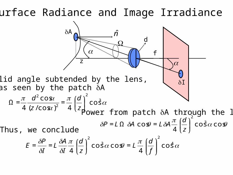
Solid angle subtended by the lens, as seen by the patch A

θαπθ coscos4

cos 32

⎟⎠

⎞⎜⎝

⎛=Ω=

z

dALALP

Power from patch A through the lens

Ω

απθαπ

4

2

32

cos4

coscos4 ⎟⎟

⎠

⎞⎜⎜⎝

⎛=⎟

⎠

⎞⎜⎝

⎛==

f

dL

z

d

I

AL

I

PE

Thus, we conclude

n̂A

I

αzf

d

Surface Radiance and Image Irradiance

αΩ

απθαπ

4

2

32

cos4

coscos4 ⎟⎟

⎠

⎞⎜⎜⎝

⎛=⎟

⎠

⎞⎜⎝

⎛==

f

dL

z

d

I

AL

I

PE

€

E ∝ LeImage intensity isproportional to ExidentRadiance

Radiance emitted by point sources• small, distant sphere radius

and uniform radiance E, which is far away and subtends a solid angle of about

€

Ω=π d

⎛

⎝ ⎜

⎞

⎠ ⎟2

€

Le = ρ d x( ) Li x,ω( )cosθ idωΩ

∫= ρ d x( ) Lidω cosθ i

Ω

∫

≈ ρ d x( )ε

r(x)

⎛

⎝ ⎜

⎞

⎠ ⎟2

E cosθ i

= kρ d x( )cosθ i

r x( )2

Standard nearby point source model

• N is the surface normal

• rho is diffuse albedo

• S is source vector - a vector from x to the source, whose length is the intensity term– works because a dot-product is

basically a cosine

€

ρd x( )N x( )•S x( )

r x( )2

⎛

⎝ ⎜

⎞

⎠ ⎟

Standard distant point source model

• Issue: nearby point source gets bigger if one gets closer– the sun doesn’t for any

reasonable binding of closer

• Assume that all points in the model are close to each other with respect to the distance to the source. Then the source vector doesn’t vary much, and the distance doesn’t vary much either, and we can roll the constants together to get:

€

ρd x( ) N x( )•Sd x( )( )

Line sources

radiosity due to line source varies with inverse distance, if the source is long enough

Area sources

• Examples: diffuser boxes, white walls.

• The radiosity at a point due to an area source is obtained by adding up the contribution over the section of view hemisphere subtended by the source – change variables and add up

over the source

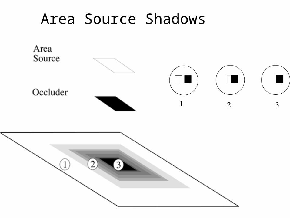
Area Source Shadows

Shading models

• Local shading model– Surface has radiosity due only

to sources visible at each point

– Advantages:

• often easy to manipulate, expressions easy

• supports quite simple theories of how shape information can be extracted from shading

• Global shading model– surface radiosity is due to

radiance reflected from other surfaces as well as from surfaces

– Advantages:

• usually very accurate

– Disadvantage:

• extremely difficult to infer anything from shading values

Photometric stereo

• Assume:– a local shading model

– a set of point sources that are infinitely distant

– a set of pictures of an object, obtained in exactly the same camera/object configuration but using different sources

– A Lambertian object (or the specular component has been identified and removed)

Projection model for surface recovery - usually calleda Monge patch

€

z = f (x, y)

r n =

∂z /∂x

∂z /∂y

1

⎡

⎣

⎢ ⎢ ⎢

⎤

⎦

⎥ ⎥ ⎥

ˆ n =r n /

r n

€

ˆ n

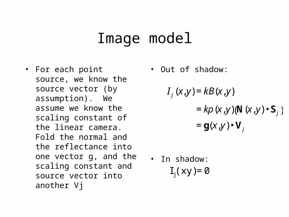
Image model

• For each point source, we know the source vector (by assumption). We assume we know the scaling constant of the linear camera. Fold the normal and the reflectance into one vector g, and the scaling constant and source vector into another Vj

• Out of shadow:

• In shadow:

€

I j(x,y) = 0

€

I j (x, y) = kB(x, y)

= kρ (x, y) N(x, y) • S j( )

= g(x,y)• Vj

Dealing with shadows

€

I12(x, y)

I22(x, y)

..

In2(x, y)

⎛

⎝

⎜ ⎜ ⎜ ⎜

⎞

⎠

⎟ ⎟ ⎟ ⎟

=

I1(x, y) 0 .. 0

0 I2(x, y) .. ..

.. .. .. 0

0 .. 0 In(x,y)

⎛

⎝

⎜ ⎜ ⎜ ⎜

⎞

⎠

⎟ ⎟ ⎟ ⎟

V1

T

V2

T

..

Vn

T

⎛

⎝

⎜ ⎜ ⎜ ⎜

⎞

⎠

⎟ ⎟ ⎟ ⎟

g(x, y)

Known Known Known Unknown

€

rb = A

r x General form:

n x 3n x 1

For each x,y point

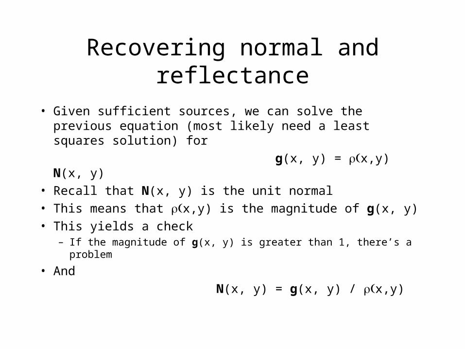
Recovering normal and reflectance

• Given sufficient sources, we can solve the previous equation (most likely need a least squares solution) for

g(x, y) = x,y) N(x, y)

• Recall that N(x, y) is the unit normal

• This means that x,y) is the magnitude of g(x, y)

• This yields a check– If the magnitude of g(x, y) is greater than 1, there’s a problem

• And

N(x, y) = g(x, y) / x,y)

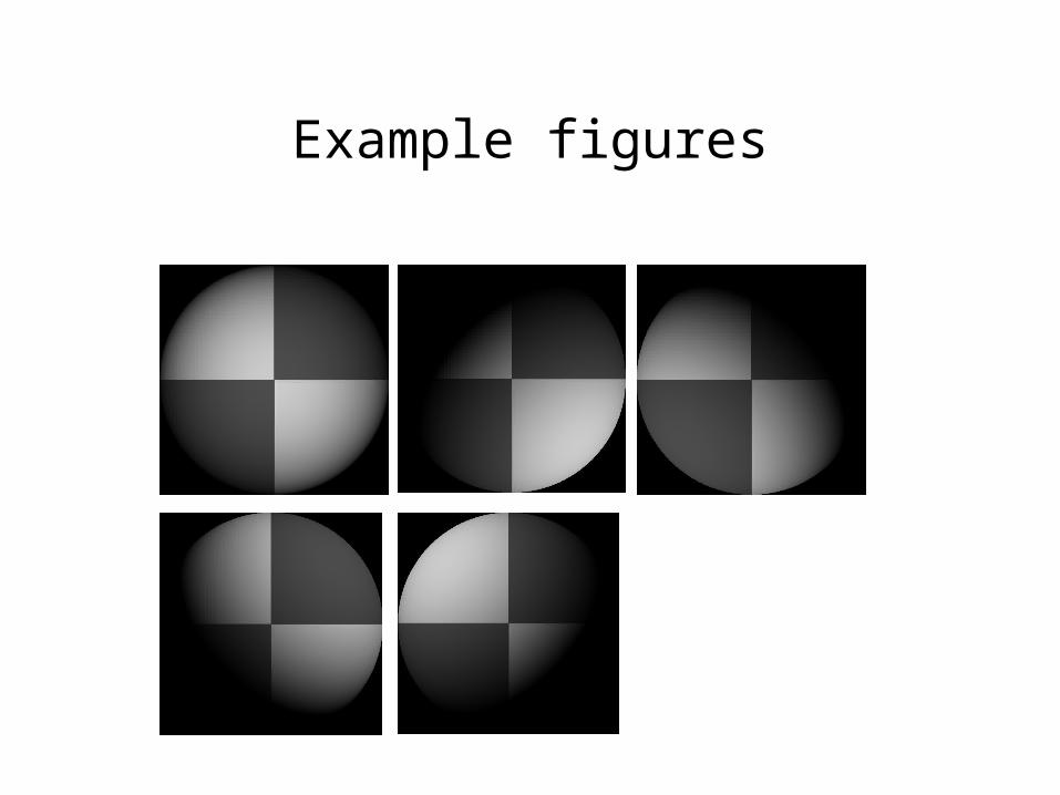
Example figures

Recovered reflectance

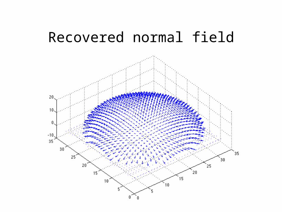
Recovered normal field

Recovering a surface from normals - 1

• Recall the surface is written as

• This means the normal has the form:

• If we write the known vector g as

• Then we obtain values for the partial derivatives of the surface:

€

(x,y, f (x, y))

€

g(x, y) =

g1(x, y)

g2 (x, y)

g3(x, y)

⎛

⎝

⎜ ⎜

⎞

⎠

⎟ ⎟

€

fx (x,y) = g1(x, y) g3(x, y)( )

€

fy(x, y) = g2(x,y) g3(x,y)( )

€

N(x,y) =1

fx2 + fy

2 +1

⎛

⎝ ⎜

⎞

⎠ ⎟

− fx

− fy

1

⎛

⎝

⎜ ⎜

⎞

⎠

⎟ ⎟

Recovering a surface from normals - 2

• Recall that mixed second partials are equal --- this gives us a check. We must have:

(or they should be similar, at least)

• We can now recover the surface height at any point by integration along some path, e.g.

€

∂ g1(x, y) g3(x, y)( )∂y

=

∂ g2(x, y) g3(x, y)( )∂x

€

f (x, y) = fx (s, y)ds0

x

∫ +

fy (x, t)dt0

y

∫ + c

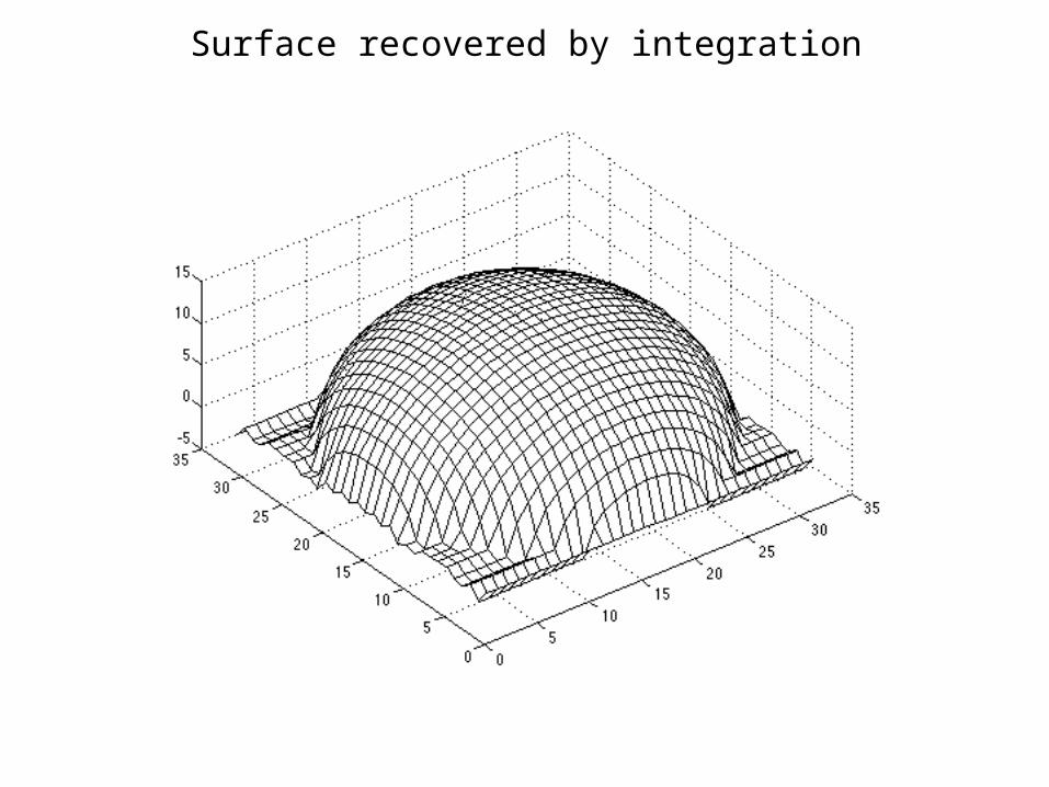
Surface recovered by integration

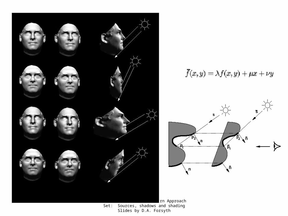
Shape from Shading with ambiguity

What to do if light source unknown?

Only one image?

Ans: Use prior knowledge in the form of constraints (e.g. regularization methods, Bayesian methods), take advantage of the habits (regularities) of images.

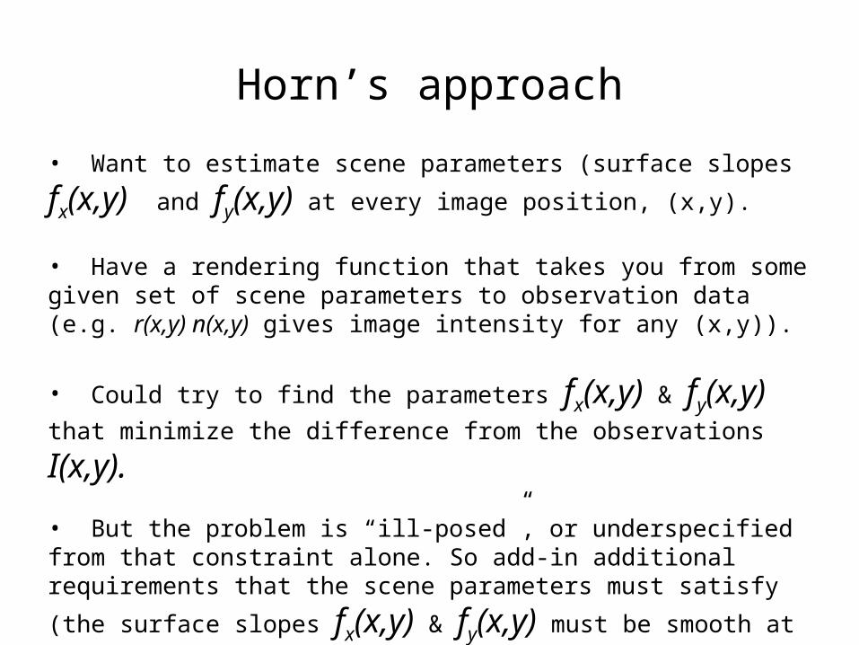
Horn’s approach

• Want to estimate scene parameters (surface slopes fx(x,y) and fy(x,y) at

every image position, (x,y).

• Have a rendering function that takes you from some given set of scene parameters to observation data (e.g. r(x,y) n(x,y) gives image intensity for any (x,y)).

• Could try to find the parameters fx(x,y) & fy(x,y) that minimize the

difference from the observations I(x,y).

• But the problem is “ill-posed”, or underspecified from that constraint alone. So add-in additional requirements that the scene parameters must satisfy (the

surface slopes fx(x,y) & fy(x,y) must be smooth at every point).

RegularizationFor each normal, compute the distance from the normal to its neighbors:

€

Prior/regularizer

s(i, j) =r n i + k, j + l( ) −

r n (i, j)( )

2

k={−1,1}∑

l={−1,1}∑

Intensity Error

r(i, j) = I i, j( ) − Ipred (i, j)( )2

Err = r(i, j) + λs(i, j)i, j

∑

Computer Vision - A Modern ApproachSet: Sources, shadows and shading

Slides by D.A. Forsyth

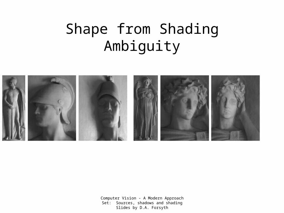
Shape from Shading Ambiguity

Computer Vision - A Modern ApproachSet: Sources, shadows and shading

Slides by D.A. Forsyth

Curious Experimental Fact

• Prepare two rooms, one with white walls and white objects, one with black walls and black objects

• Illuminate the black room with bright light, the white room with dim light

• People can tell which is which (due to Gilchrist)

• Why? (a local shading model predicts they can’t).

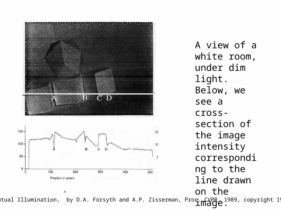
Figure from “Mutual Illumination,” by D.A. Forsyth and A.P. Zisserman, Proc. CVPR, 1989, copyright 1989 IEEE

A view of a white room, under dim light.Below, we see a cross-section of the image intensity corresponding to the line drawn on the image.

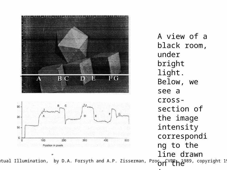
Figure from “Mutual Illumination,” by D.A. Forsyth and A.P. Zisserman, Proc. CVPR, 1989, copyright 1989 IEEE

A view of a black room, under bright light.Below, we see a cross-section of the image intensity corresponding to the line drawn on the image.

What’s going on here?

• local shading model is a poor description of physical processes that give rise to images– because surfaces reflect light onto one another

• This is a major nuisance; the distribution of light (in principle) depends on the configuration of every radiator; big distant ones are as important as small nearby ones (solid angle)

• The effects are easy to model

• It appears to be hard to extract information from these models

Interreflections - a global shading model

• Other surfaces are now area sources - this yields:

• Vis(x, u) is 1 if they can see each other, 0 if they can’t

€

Radiosity at surface = Exitance + Radiosity due to other surfaces

B x( ) = E x( ) + ρ d x( ) B u( )cosθ i cosθ s

πr(x,u)2 Vis x,u( )dAu

all othersurfaces

∫

What do we do about this?

• Attempt to build approximations– Ambient illumination

• Study qualitative effects– reflexes

– decreased dynamic range

– smoothing

• Try to use other information to control errors

Shadows cast by a point source

• A point that can’t see the source is in shadow

• For point sources, the geometry is simple

Ambient Illumination

• Two forms– Add a constant to the radiosity at every point in the scene to

account for brighter shadows than predicted by point source model• Advantages: simple, easily managed (e.g. how would you

change photometric stereo?)• Disadvantages: poor approximation (compare black and white

rooms– Add a term at each point that depends on the size of the clear

viewing hemisphere at each point (see next slide)• Advantages: appears to be quite a good approximation, but

jury is out• Disadvantages: difficult to work with

At a point inside a cube or room, the surface sees light in all directions, so add a large term. At a point on the base of a groove, the surface sees relatively little light, so add a smaller term.

Reflexes

• A characteristic feature of interreflections is little bright patches in concave regions– Examples in following slides

– Perhaps one should detect and reason about reflexes?

– Known that artists reproduce reflexes, but often too big and in the wrong place

Figure from “Mutual Illumination,” by D.A. Forsyth and A.P. Zisserman, Proc. CVPR, 1989, copyright 1989 IEEE

At the top, geometry of a semi-circular bump on a plane; below, predicted radiosity solutions, scaled to lie on top of each other, for different albedos of the geometry. When albedo is close to zero, shading follows a local model; when it is close to one, there are substantial reflexes.

Radiosity observed in an image of this geometry; note the reflexes, which are circled.

Figure from “Mutual Illumination,” by D.A. Forsyth and A.P. Zisserman, Proc. CVPR, 1989, copyright 1989 IEEE

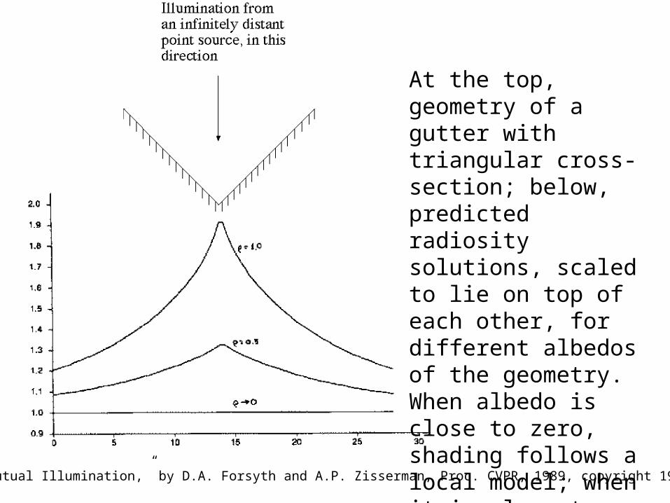
Figure from “Mutual Illumination,” by D.A. Forsyth and A.P. Zisserman, Proc. CVPR, 1989, copyright 1989 IEEE

At the top, geometry of a gutter with triangular cross-section; below, predicted radiosity solutions, scaled to lie on top of each other, for different albedos of the geometry. When albedo is close to zero, shading follows a local model; when it is close to one, there are substantial reflexes.

Radiosity observed in an image of this geometry; above, for a black gutter and below for a white one

Figure from “Mutual Illumination,” by D.A. Forsyth and A.P. Zisserman, Proc. CVPR, 1989, copyright 1989 IEEE

Figure from “Mutual Illumination,” by D.A. Forsyth and A.P. Zisserman, Proc. CVPR, 1989, copyright 1989 IEEE

At the top, geometry of a gutter with triangular cross-section; below, predicted radiosity solutions, scaled to lie on top of each other, for different albedos of the geometry. When albedo is close to zero, shading follows a local model; when it is close to one, there are substantial reflexes.

Radiosity observed in an image of this geometry for a white gutter.

Figure from “Mutual Illumination,” by D.A. Forsyth and A.P. Zisserman, Proc. CVPR, 1989, copyright 1989 IEEE

Smoothing

• Interreflections smooth detail– E.g. you can’t see the pattern of a stained glass window by looking

at the floor at the base of the window; at best, you’ll see coloured blobs.

– This is because, as I move from point to point on a surface, the pattern that I see in my incoming hemisphere doesn’t change all that much

– Implies that fast changes in the radiosity are local phenomena.

Fix a small patch near a large radiator carrying a periodic radiosity signal; the radiosity on the surface is periodic, and its amplitude falls very fast with the frequency of the signal. The geometry is illustrated above. Below, we show a graph of amplitude as a function of spatial frequency, for different inclinations of the small patch. This means that if you observe a high frequency signal, it didn’t come from a distant source.