Embed Size (px)
Citation preview

Aalborg Universitet
Dynamic Study on the 400 kV 60 km Kyndbyværket – Asnæsværket Line
Ohno, Teruo
Publication date:2012
Document VersionEarly version, also known as pre-print
Link to publication from Aalborg University
Citation for published version (APA):Ohno, T. (2012). Dynamic Study on the 400 kV 60 km Kyndbyværket – Asnæsværket Line. Department ofEnergy Technology, Aalborg University.
General rightsCopyright and moral rights for the publications made accessible in the public portal are retained by the authors and/or other copyright ownersand it is a condition of accessing publications that users recognise and abide by the legal requirements associated with these rights.
? Users may download and print one copy of any publication from the public portal for the purpose of private study or research. ? You may not further distribute the material or use it for any profit-making activity or commercial gain ? You may freely distribute the URL identifying the publication in the public portal ?
Take down policyIf you believe that this document breaches copyright please contact us at [email protected] providing details, and we will remove access tothe work immediately and investigate your claim.
Downloaded from vbn.aau.dk on: maj 04, 2018

PhD Thesis
Dynamic Study on the 400 kV 60 km Kyndbyværket –
Asnæsværket Line
PhD student Teruo Ohno
Supervisor: Claus Leth Bak
Co-supervisors: Thomas Kjærsgaard Sørensen, Wojciech Tomasz Wiechowski and Akihiro Ametani
Period: December 1st 2009 - December 1st 2012

Preface
This thesis is submitted to the Faculty of Engineering, Science and Medicine at Aalborg University
in the partial fulfilment of the requirements for the PhD degree in Electrical Engineering. The
research was conducted at the Department of Energy Technology for Energinet.dk.
The research has been followed full time by Professor Claus Leth Bak (Department of Energy
Technology), Professor Akihiro Ametani (Doshisha University), Dr. Thomas Kjærsgaard Sørensen
(Energinet.dk), and Dr. Wojciech Wiechowski (RWE Innogy).
Energinet.dk has fully funded the research leading to this thesis "Dynamic Study on the 400 kV 60
km Kyndbyværket – Asnæsværket Line". The funding, which has covered course fees to attend
project-related and more general study-oriented courses and travel expenses to participate in
international conferences, has been crucial to the research.
The research has been conducted while the PhD student is working full-time for Tokyo Electric
Power Company (TEPCO), one of major users of EHV cables. The work in TEPCO, including
international consultancy projects on EHV cables, has contributed to the research.
This thesis is divided into seven chapters. A list of all authored and co-authored publications written
by the author is presented in Section 7.2. Literature references are shown as [j], where j is the
number of the literature in the reference list. References to figures, tables, and equations are shown
as Fig. C.F, Table C.F, or Eqn. C.F, where C is the chapter number and F indicates the figure, table
or equation number.

Acknowledgments
I owe gratitude to many people that have helped me in various ways. In particular, I would like to
thank:
My supervisors, Claus Leth Bak, Akihiro Ametani, Thomas Kjærsgaard Sørensen, and
Wojciech Wiechowski for all their kind support, especially their comments to papers, during
the project period.
Claus Leth Bak, Akihiro Ametani, Thomas Kjærsgaard Sørensen, Per Balle Holst, Unnur
Stella Guðmundsdóttir, Thomas Kvarts, and Wojciech Wiechowski for their contribution
during status meetings.
Per Balle Holst and Thomas Kjærsgaard Sørensen for their help in interfacing me with
Energinet.dk, especially in providing necessary information of Energinet.dk, providing
feedbacks from Energinet.dk, and in granting funding for courses and conferences.
Wojciech Wiechowski and Energinet.dk for giving me a chance to pursue the PhD degree and
work together.
All members of the CIGRE WG C4.502 for valuable discussions during the WG meetings and
teleconferences.
Finally, my wife Sachiko and two children Yuta and Tomoharu for their support and
understanding.
Teruo Ohno, December 2012, Aalborg

Abstract
Until recently, the use of HVAC underground cable systems has been mainly limited to densely
populated area. As such, HVAC underground cable systems are limited both in length and numbers
to date. This tendency has been changing over the past ten years as the service experience of HVAC,
cable systems have shown to be satisfactory. The applications of HVAC cable systems are proposed
more often for transmission projects, and recently proposed HVAC underground cable systems are
longer compared to existing cable systems. Due to this historical background, HVAC underground
cable systems have been studied and tested primarily with short cable lengths. Some knowledge
from short cable lines can be directly applied to long cable lines, but there are several phenomena
which are peculiar to long cable lines.
The main objectives of the PhD project are to shed light on the phenomena peculiar to long cable
lines. The PhD project focuses on the 400 kV 60 km Kyndbyværket – Asnæsværket line, which will
feed power to Copenhagen, the Danish capital. The PhD project addresses major problems and
potential countermeasures related to the installation and operation of a long cable line, through:
(1) Insulation coordination study
(2) Derivation of theoretical formulas of sequence currents
(3) Identification of dominant frequency components contained in the overvoltage
(4) Analysis on the statistical distribution of energization overvoltages
(5) Protection study
First, the insulation coordination study have found that it is feasible to build and operate the 400 kV
60 km Kyndbyværket – Asnæsværket line and have identified necessary considerations in the
equipment specification and required countermeasures against possible problems. Especially,
severe temporary overvoltages caused by parallel resonance and system islanding are observed,
which requires a consideration in the selection of surge arresters.
Second, the PhD project has derived theoretical formulas of sequence currents of a cross-bonded
cable and a solidly-bonded cable. These formulas are obtained by solving equations which are
derived from the setups for measuring sequence currents of cross-bonded and solidly-bonded cables.
For a cross-bonded cable, the equations are solved utilizing the known impedance matrix reduction
technique. The derived formulas consider the cable as a cable system; they can thus consider sheath
bonding and sheath grounding resistance. An accuracy of proposed formulas is verified through a

comparison with EMTP simulation results. The verified accuracy of the proposed formulas shows
sequence impedance / current can be obtained before the installation without making measurements
for a majority of cables. This gives an important advantage in setting up transient overvoltage
studies as well as planning studies.
Third, as the switching of EHV cables can trigger temporary overvoltages, it is important to find
the dominant frequency component contained in the switching overvoltages of these cables. Since
there are no theoretical formulas to find the dominant frequency, it is generally found by means of
time domain simulations or frequency scans. The derivation of theoretical formulas has been
desired as the formulas would be useful in verifying the results of time domain simulations or
frequency scans. Additionally, the formulas could eliminate the necessity of building simulation
models of some network components.
The PhD project has derived the simple theoretical formulas for estimating the propagation velocity
and dominant frequency from impedance and admittance calculations. The comparison between the
proposed formulas and the simulation results is performed using the Kyndbyværket – Asnæsværket
line. From the comparison, the derived formulas are found to be sufficiently accurate to be used for
efficient analysis of resonance overvoltages. In addition, the accuracy of the formulas derived
demonstrates that the propagation velocity and the dominant frequency are determined by two
inter-phase modes for long cables.
Forth, the statistical distribution of energization overvoltages of EHV cables is derived in the PhD
project from a number of simulations. Through the comparison with the statistical distributions of
energization overvoltages of overhead lines, the main characteristics of the statistical distribution
for cables are identified. In particular, it has been found that line energization overvoltages of
cables are lower than those of overhead lines with respect to maximum, 2 %, and mean values. The
standard deviation has been found to be smaller for cables.
The main characteristics of the statistical distribution are found to be caused not by random
switching by accident, rather there are contributing factors and physical meanings behind the
characteristics. These contributing factors and physical meanings are identified from the theoretical
analysis of voltage waveforms of energization overvoltages. These findings are useful not only for
the determination of insulation levels of cable systems, but also for insulation coordination studies
of cable systems.

Finally, through the calculation of the ground loop impedance for cable lines, it has been found that,
for long EHV cable lines, the reliable operation of the ground distance relay is possible with a
typical relay setting. It is known that the ground loop impedance of EHV cable lines does not have
a linear relationship to the distance. There is a discontinuity in the ground loop impedance at
cross-bonding points, which may have an ill effect on the reliable operation of the ground distance
relay. However, the discontinuity of the ground loop reactance of the long EHV cable lines is small
enough for the ground distance relay to operate satisfactory with a typical relay setting. Effects of
parameters, such as substation grounding, cable layouts and transposition, are also found through
the analysis.

Table of contents
©2012 Aalborg University. All Rights Reserved.
Table of contents
INTRODUCTION _________________________________________________ 1-1 CHAPTER 1
Background ___________________________________________________________ 1-1 1.1
Problem Formulation ___________________________________________________ 1-4 1.2
Thesis Outline _________________________________________________________ 1-6 1.3
REACTIVE POWER COMPENSATION _____________________________ 2-1 CHAPTER 2
Kyndbyværket – Asnæsværket Line ________________________________________ 2-1 2.1
Considerations in Reactive Power Compensation _____________________________ 2-2 2.2
Impedance and Admittance Calculations ____________________________________ 2-3 2.3
2.3.1 Impedance Calculation in IEC 60909-2 _________________________________ 2-3
2.3.2 Derivation of Theoretical Formulas of Sequence Currents ___________________ 2-5
2.3.3 Comparison with EMTP Simulations __________________________________ 2-14
2.3.4 Application to the Kyndbyværket – Asnæsværket Line ____________________ 2-18
2.3.5 Impedance and Admittance of the Kyndbyværket – Asnæsværket Line ________ 2-18
Maximum Unit Size of 400 kV Shunt Reactors ______________________________ 2-20 2.4
Compensation Patterns _________________________________________________ 2-22 2.5
Voltage Profile under Normal Operating Conditions __________________________ 2-24 2.6
2.6.1 No Load Condition ________________________________________________ 2-25
2.6.2 Maximum Power Flow Condition _____________________________________ 2-26
Active Power Loss ____________________________________________________ 2-28 2.7
Effect on the Transmission Capacity _______________________________________ 2-29 2.8
Ferranti Phenomenon __________________________________________________ 2-31 2.9
Conclusion __________________________________________________________ 2-35 2.10
MODEL SETUP __________________________________________________ 3-1 CHAPTER 3
Power Flow Data _______________________________________________________ 3-1 3.1
Modeled Area _________________________________________________________ 3-3 3.2
Underground Cables ____________________________________________________ 3-6 3.3
3.3.1 Physical and Electrical Information ____________________________________ 3-6
3.3.2 Cable Layout _____________________________________________________ 3-14
3.3.3 Cable Route ______________________________________________________ 3-15
3.3.4 Modeling of Auxiliary Components ___________________________________ 3-17
3.3.5 Effects of Cable Models ____________________________________________ 3-18

Table of contents
©2012 Aalborg University. All Rights Reserved.
3.3.6 Effects of Cross-bonding____________________________________________ 3-23
3.3.7 Effects of Span Length _____________________________________________ 3-24
3.3.8 Effects of Armour _________________________________________________ 3-28
Overhead Transmission Lines ____________________________________________ 3-30 3.4
3.4.1 Conductor and Tower Configuration ___________________________________ 3-30
3.4.2 Phase Configuration _______________________________________________ 3-32
3.4.3 Comparison between PSCAD and ATP-EMTP __________________________ 3-32
Transformers _________________________________________________________ 3-34 3.5
Shunt Reactors _______________________________________________________ 3-39 3.6
Surge arresters ________________________________________________________ 3-41 3.7
Generators ___________________________________________________________ 3-43 3.8
Loads _______________________________________________________________ 3-45 3.9
TEMPORARY OVERVOLTAGE ANALYSIS __________________________ 4-1 CHAPTER 4
Series Resonance Overvoltage ____________________________________________ 4-3 4.1
4.1.1 Overview _________________________________________________________ 4-3
4.1.2 Most Severe Scenarios ______________________________________________ 4-4
4.1.3 Dominant Frequency in Energization Overvoltage _________________________ 4-6
4.1.4 Natural Frequency of Series Resonance Circuit __________________________ 4-35
4.1.5 Simulation Results of Series Resonance Overvoltage _____________________ 4-42
Parallel Resonance Overvoltage __________________________________________ 4-48 4.2
4.2.1 Overview ________________________________________________________ 4-48
4.2.2 Most Severe Scenarios _____________________________________________ 4-50
4.2.3 Natural Frequency of Parallel Resonance Circuit _________________________ 4-52
4.2.4 Simulation Results of Parallel Resonance Overvoltage ____________________ 4-59
Overvoltage Caused by the System Islanding ________________________________ 4-66 4.3
4.3.1 Overview ________________________________________________________ 4-66
4.3.2 Study Conditions __________________________________________________ 4-67
4.3.3 ASV 400 kV Bus Fault _____________________________________________ 4-71
4.3.4 KYV 400 kV Bus Fault _____________________________________________ 4-83
4.3.5 TOR 400 kV Bus Fault _____________________________________________ 4-84
Conclusion __________________________________________________________ 4-88 4.4

Table of contents
©2012 Aalborg University. All Rights Reserved.
SLOW-FRONT OVERVOLTAGE ANALYSIS _________________________ 5-1 CHAPTER 5
Overvoltage Caused by Line Energization from Lumped Source _________________ 5-1 5.1
5.1.1 Overview _________________________________________________________ 5-1
5.1.2 Past Studies by CIGRE WGs _________________________________________ 5-2
5.1.3 Study Conditions and Parameters ______________________________________ 5-8
5.1.4 Simulation Results and Statistical Distributions __________________________ 5-12
5.1.5 Summary ________________________________________________________ 5-22
Overvoltage Caused by Line Energization from Complex Source ________________ 5-24 5.2
5.2.1 Study Conditions __________________________________________________ 5-24
5.2.2 Energization from ASV _____________________________________________ 5-24
5.2.3 Energization from KYV ____________________________________________ 5-27
5.2.4 Effects of Synchronized Switching ____________________________________ 5-29
Analysis of Statistical Distribution of Energization Overvoltages ________________ 5-32 5.3
5.3.1 Analysis on the Highest Overvoltages _________________________________ 5-32
5.3.2 Analysis on the Effects of Line Length _________________________________ 5-36
5.3.3 Analysis on the Effects of Feeding Network ____________________________ 5-40
5.3.4 Summary ________________________________________________________ 5-42
Ground Fault and Fault Clearing Overvoltage _______________________________ 5-44 5.4
5.4.1 Study Conditions and Parameters _____________________________________ 5-44
5.4.2 Results of the Analysis _____________________________________________ 5-45
5.4.3 Results with the Sequential Switching _________________________________ 5-47
Conclusion __________________________________________________________ 5-52 5.5
OTHER STUDIES ________________________________________________ 6-1 CHAPTER 6
Protection of the EHV Cable System _______________________________________ 6-1 6.1
6.1.1 Main Protection ____________________________________________________ 6-1
6.1.2 Backup Protection – Ground Loop Impedance ____________________________ 6-2
6.1.3 Cross-bonded Cable with One Major Section _____________________________ 6-6
6.1.4 ASV – TOR Cable Line _____________________________________________ 6-9
6.1.5 Summary ________________________________________________________ 6-26
Leading Current Interruption ____________________________________________ 6-27 6.2
Zero-missing Phenomenon ______________________________________________ 6-29 6.3
6.3.1 Sequential Switching_______________________________________________ 6-31
6.3.2 Summary ________________________________________________________ 6-36
Cable Discharge ______________________________________________________ 6-37 6.4
Overvoltage Caused by Restrike __________________________________________ 6-38 6.5

Table of contents
©2012 Aalborg University. All Rights Reserved.
CONCLUSION ___________________________________________________ 7-1 CHAPTER 7
Summary _____________________________________________________________ 7-1 7.1
7.1.1 Insulation Coordination Study ________________________________________ 7-1
7.1.2 Required Specifications for the Related Equipment ________________________ 7-3
New Contributions _____________________________________________________ 7-4 7.2
Future Work __________________________________________________________ 7-6 7.3

Chapter 1 Introduction
1-1 ©2012 Aalborg University. All Rights Reserved.
Introduction Chapter 1
Background 1.1
In order to mitigate climate change, many countries have set a target to reduce their greenhouse
gasses. Due to its abundant natural resources (wind) and green minded people, Denmark is one of
the leading countries in this effort of the world to tackle global warming. As of the year 2011, the
wind energy accounted for 29.1 % in generation capacity and 28.1 % of the electrical production
[1].
This change of the generation profile has led to and will continue to lead to the necessity of major
upgrades in the Danish transmission grid. Especially, the expansion of Horns Rev, the world largest
offshore wind farm, will require the ability of the Danish transmission grid to transmit increased
power from west to east where the electricity is consumed.
As in Denmark, transmission system operators (TSOs) in the world have been seeing growing
numbers of transmission line projects in the recent years, due to different reasons, which include
the increase of cross-border trades, renewable energy sources, smart grid projects, the replacement
of aging facilities, and in some countries due to growing demand.
Until recently, TSOs in the world have responded to these necessary transmission upgrades mostly
by the introduction of overhead lines (OHLs). HVAC underground cable systems have been used,
but their applications have been mainly limited to densely populated area. As such, HVAC
underground cable systems are limited both in length and numbers to date.
This tendency has been changing over the past ten years as the service experience of HVAC,
especially EHV AC, cable systems have become satisfactory [2]. The applications of HVAC cable
systems are proposed more often in order to protect the beautiful landscape and also public health,
e.g. EMF.
In Denmark, receiving public and political pressures to underground its OHLs, Energinet.dk
published a report on the future expansion and undergrounding of its transmission grid on the 3rd of
April 2008 [3]. The report proposed and compared five principles (A – E in Fig. 1.1). From the five
principles, the Danish government has selected Principle C in which all new 400 kV lines will
basically be undergrounded.

Chapter 1 Introduction
1-2 ©2012 Aalborg University. All Rights Reserved.
Fig. 1.1 Five principles for the future grid expansion (from [3]).
Fig. 1.2 Grid expansion plan based on Principle C (from [3]).
Undergrounding of existing 132 kV and 150 kV gridsin accordance with separate cable action plan
AComplete
undergrounding
AComplete
undergrounding
BNew power
lines inunderground
cables
BNew power
lines inunderground
cables
CNew power
lines in under-ground cables
and new towersin an existing
line route
CNew power
lines in under-ground cables
and new towersin an existing
line route
DNew overheadlines in areas
where overheadlines have
already beenconstructed
DNew overheadlines in areas
where overheadlines have
already beenconstructed
ENew overhead
lines
ENew overhead
lines
FNo grid
expansion
FNo grid
expansion
Improvement of the visual appearance of the existing 400 kV gridusing lower towers in a new design
and undergrounding of specifically chosen sections
Improvement of the visual appearance of the existing 400 kV gridusing lower towers in a new design
and undergrounding of specifically chosen sections
132 kV and
150 kV
400 kV

Chapter 1 Introduction
1-3 ©2012 Aalborg University. All Rights Reserved.
Due to the historical background, HVAC underground cable systems have been studied and tested
primarily with short cable lengths. Because of this shift in trend, however, the recently proposed
HVAC underground cable systems are longer compared with existing cable systems. As a result,
when TSOs face increased number of recent transmission projects with HVAC underground cables,
there is a lack of knowledge and expertise in long underground cables. Some knowledge and
expertise from short cable lines can be directly applied to long cable lines. However, there are
several phenomena which are peculiar to long cable lines [4] – [10].
The objectives of this PhD thesis are to shed light on the phenomena peculiar to long cable lines.
The PhD thesis will focus on the 400 kV 60 km Kyndbyværket – Asnæsværket line, which is the
longest 400 kV line in the grid expansion plan based on Principle C and will help to ensure the
supply to Copenhagen. The thesis will address major problems and potential countermeasures
related to the installation of this long cable line.

Chapter 1 Introduction
1-4 ©2012 Aalborg University. All Rights Reserved.
Problem Formulation 1.2
One of the biggest problems in the EMT (electromagnetic transient) analysis of long cable lines is a
lack of understanding in frequency components contained in the overvoltages. Although an
extensive study was performed upon the installation of the 500 kV Shin-Toyosu line, there was a
lack of understanding in frequency components contained in the overvoltages associated with long
cable lines. More importantly, the significance of the frequency components was not well
understood.
Thanks to the recent progress in the modelling technique and computational limitations [11] – [22],
the EMT analysis with EHV cables is considered to have a reasonable accuracy whose typical error
can be less than 10% in magnitude. However, the typical error is expected to increase to around
30% when the waveform of the overvoltage is considered. This implies that some frequency
components are not accurately reproduced in the EMT analysis for some reason.
It has to be noted that one of the most worrying problems for long cable lines is the resonance
overvoltage, which shows significant nonlinearity around the resonance frequencies. From this
point of view, frequency components in the overvoltages have to be found with greater accuracy,
compared with other EMT analyses. Reasonable accuracy may not be good enough for the analysis
of long cable lines.
Objectives of the PhD project include the following items:
(1) Insulation coordination study for the 400 kV Kyndbyværket – Asnæsværket line
The PhD project intends to address major problems and potential countermeasures related to
the installation of the 400 kV Kyndbyværket – Asnæsværket line.
(2) Identification of dominant frequency components contained in the overvoltage
In relation to the study of the 400 kV Kyndbyværket – Asnæsværket line, the PhD project
intends to explore ways to find dominant frequency components contained in the overvoltage.
As discussed above, it is crucial especially in the resonance overvoltage study.
(3) Finding probabilistic distribution of the overvoltage
Probabilistic distribution of the overvoltages [23][24] is another research interest of the PhD
project. Because of the low frequency components in the overvoltages, the probabilistic
distribution of the overvoltages can be very different from the one assumed for OHLs. An
effect of the frequency components on the probabilistic distribution will be explored in order to

Chapter 1 Introduction
1-5 ©2012 Aalborg University. All Rights Reserved.
find the meaning of well-known 2 % overvoltage and the conversion factor for long cable lines.
(4) Protection studies for the long EHV cable
The PhD project also covers protection studies. Especially, effects of cable layouts and
transposition on the ground loop impedance of cross-bonded cables are studied.

Chapter 1 Introduction
1-6 ©2012 Aalborg University. All Rights Reserved.
Thesis Outline 1.3
This thesis is composed of seven chapters. This section gives the short descriptions of these
chapters:
Chapter 1 Introduction
This chapter first presents background of this PhD project. It explains the current situation in
which more and more long cable lines are planned and installed. Problems and challenges the
PhD project tackles are then described in this chapter.
Chapter 2 Reactive Power Compensation
The charging capacity of a long EHV AC cable line needs to be compensated in order to
suppress the steady-state overvoltage of the network around the cable line or at the cable open
terminal and to mitigate the reduction of the effective transmission capacity due to the charging
current. This chapter finds the optimal reactive power compensation for the Kyndbyværket –
Asnæsværket line.
Chapter 3 Model Setup
This chapter describes how transient simulation models were created. The derivation of input
data is explained for each type of equipment. Considerations in the cable model setup are
discussed in detail.
Chapter 4 Temporary Overvoltage Analysis
Temporary overvoltages are the highest concerns when studying long EHV AC cable lines. This
chapter analyses the temporary overvoltages – the resonance overvoltage and the overvoltage
caused by the system islanding.
Chapter 5 Slow-front Overvoltage Analysis
The slow-front overvoltages caused by line energization, ground fault and fault clearing are
studied in this chapter in order to compare those in cables and in overhead lines. The statistical
distributions of the slow-front overvoltages are also derived and compared between cables and
overhead lines.

Chapter 1 Introduction
1-7 ©2012 Aalborg University. All Rights Reserved.
Chapter 6 Other Studies
This chapter discusses other studies related to the installation of long EHV AC cable lines, such
as protection studies, leading current interruption and zero-missing phenomenon.
Countermeasures are proposed to these problems.
Chapter 7 Conclusion
The final chapter summarizes the results of the insulation coordination study of the
Kyndbyværket – Asnæsværket line and new contributions of the PhD project to the future cable
studies.

Chapter 1 Introduction
1-8 ©2012 Aalborg University. All Rights Reserved.
References
[1] Danish Annual Energy Statistics 2011, (available on the web) Danish Energy Authority,
October 2008,
http://www.ens.dk/en-US/Info/FactsAndFigures/Energy_statistics_and_indicators/Annual%20
Statistics/Documents/Energy%20in%20Denmark%202010.pdf.
[2] Update of Service Experience of HV Underground and Cable Systems, CIGRE Technical
Brochure 379, April 2009
[3] Technical report on the future expansion and undergrounding of the electricity transmission
grid, (available on the web) Energinet.dk, April 2008,
https://selvbetjening.preprod.energinet.dk/NR/rdonlyres/CC966C3A-FE78-41D8-9DC7-6B45
5210B502/0/TechnicalReportSummary.pdf.
[4] Joint Feasibility Study on the 400kV Cable Line Endrup-Idomlund: Final Report, Tokyo
Electric Power Company, April 2008,
[5] Assessment of the Technical Issues relating to Significant Amounts of EHV Underground
Cable in the All-island Electricity Transmission System, (available on the web) Tokyo Electric
Power Company, November 2009, http://www.eirgrid.com/media/Tepco%20Report.pdf.
[6] V. Akhmatov. “Excessive over-voltage in long cables of large offshore windfarms,” Wind
Engineering, vol. 30, no. 5, pp. 375-383, 2006
[7] N. Momose, H. Suzuki, S. Tsuchiya, T. Watanabe, "Planning and Development of 500 kV
Underground Transmission System in Tokyo Metropolitan Area," CIGRE Session 1998,
37-202
[8] T. Kawamura, T. Kouno, S. Sasaki, E. Zaima, T. Ueda, Y. Kato, "Principles and Recent
Practices of Insulation Coordination in Japan," CIGRE Session 2000, 33-109
[9] L. Colla, S. Lauria, F. M. Gatta, “Temporary Overvoltages due to Harmonic Resonance in
Long EHV Cables,” IPST 2007,
http://www.ipst.org/techpapers/2007/ipst_2007/papers_IPST2007/Session16/233. pdf.
[10] M. Rebolini, L. Colla, F. Iliceto, “400 kV AC new submarine cable links between Sicily and
the Italian mainland. Outline of project and special electrical studies,” CIGRE Session 2008,
C4-116
[11] Atef Morched, Bjørn Gustavsen, Manoocher TartibiA, “Universal Model for Accurate
Calculation of Electromagnetic Transients on Overhead Lines and Underground Cables,”
IEEE Trans. on Power Delivery, vol. 14, no.3, July 1999
[12] Bjørn Gustavsen, Adam Semlyen, “Simulation of Transmission Line Transients Using Vector
Fitting and Modal Decomposition,” IEEE Trans. on Power Delivery, vol. 13, no. 2, April 1998

Chapter 1 Introduction
1-9 ©2012 Aalborg University. All Rights Reserved.
[13] B. Gustavsen, J. Sletbak, T. Henriksen, “Calculation of Electromagnetic Transients in
Transmission Cables and Lines Taking Frequency Dependent Effects Accurately into Account,”
IEEE Trans. on Power Delivery, vol. 10, no. 2, April 2005
[14] T.Noda, N.Nagaoka, A.Ametani, “Phase Domain Modeling of Frequency-Dependent
Transmission Lines by Means of an ARMA Model,” IEEE Trans. on Power Delivery, vol. 11,
no. 1, January 1996
[15] T.Noda, N.Nagaoka, A.Ametani, “Further Improvements to a Phase-Domain ARMA Line
Model in Terms of Convolution, Steady-State Initialization, and Stability,” IEEE Trans. on
Power Delivery, vol. 12, no. 3, July 1997
[16] N. Amekawa, N. Nagaoka, V. Baba and A. Ametani, “Derivation of a semiconducting layer
impedance and its effect on wave propagation characteristics on a cable,” IEE Proceedings,
Generation, Transmission and Distribution, vol. 150, issue 4, page(s): 434 – 440, July 2003
[17] A. Ametani, Y. Miyamoto, N. Nagaoka, “Semiconducting Layer Impedance and its Effect on
Cable Wave-Propagation and Transient Characteristics,” IEEE Trans. on Power Delivery, vol.
19, no. 4, October 2004
[18] N. Amekawa, N. Nagaoka and A. Ametani, “Impedance Derivation and Wave Propagation
Characteristics of Pipe-Enclosed and Tunnel-Installed Cables,” IEEE Trans. on Power
Delivery, vol. 19, no. 1, January 2004
[19] H. V. Nguyen, H. W. Dommel, J. R. Marti, “Direct Phase-Domain Modelling of
Frequency-Dependent Overhead Transmission Lines,” IEEE Trans. on Power Delivery, vol.
12, no. 3, July 1997
[20] F. Castellanos, J. R. Marti, “Full Frequency-dependent Phase-domain Transmission Line
Model,” IEEE Trans on Power Systems, vol. 12, no. 3, August 1997
[21] Ting-Chung Yu, J. R. Marti, “A Robust Phase-Coordinates Frequency-Dependent
Underground Cable Model (zCable) for the EMTP,” IEEE Trans. on Power Delivery, vol. 18,
no. 1, January 2003
[22] Abner Ramirez, J. Luis Naredo, Pablo Moreno, “Full Frequency-Dependent Line Model for
Electromagnetic Transient Simulation Including Lumped and Distributed Sources,” IEEE
Trans. on Power Delivery, vol. 20, no. 1, January 2005
[23] Insulation Coordination for Power Systems, Andrew R. Hileman, published by Marcel Dekker
Inc., June 1999
[24] CIGRE WG 13.02, “Switching Overvoltages in EHV and UHV Systems with Special
Reference to Closing and Reclosing Transmission Lines,” ELECTRA, Oct. 1973, pp. 70-122

Chapter 2 Reactive Power Compensation
2-1 ©2012 Aalborg University. All Rights Reserved.
Reactive Power Compensation Chapter 2
Kyndbyværket – Asnæsværket Line 2.1
This section briefly introduces the Kyndbyværket – Asnæsværket line, which is being planned by
Energinet.dk.
The 400 kV network in Zealand is shown by red lines in Fig. 2.1. Solid lines are overhead lines,
and dotted lines are cable lines. The Kyndbyværket – Asnæsværket line will complete the loop
configuration of the 400 kV network, which will improve the overall reliability of the Danish
power system.
Fig. 2.1 Danish power system and Kyndbyværket – Asnæsværket line.
As the length of the Kyndbyværket – Asnæsværket line is expected to be 60 km, the cable line will
definitely require reactive power compensation as discussed in this chapter. It has not been
determined yet if a switching station or a substation will be built at Torslunde, but it will not change
the necessity of the reactive power compensation.
ASV
TOR
KYV

Chapter 2 Reactive Power Compensation
2-2 ©2012 Aalborg University. All Rights Reserved.
Considerations in Reactive Power Compensation 2.2
Cable lines become sources of reactive power like shunt capacitors. Especially, long EHV cable
lines produce large reactive power and usually require reactive power compensation for the
following reasons:
Cable lines become sources of reactive power like shunt capacitors. Especially, long EHV cable
lines produce large reactive power and usually require reactive power compensation for the
following reasons:
Suppress the steady-state overvoltage around the cable line
Suppress the steady-state overvoltage at the cable open terminal
Prevent the reduction of the active power transmission capacity due to the large charging
current
Reduce the leading current that flows through the line breaker so that it becomes lower
than the leading current interruption capability of the line breaker
When the compensation rate 100 % is adopted, the installation of the cable line does not affect the
reactive power balance around the cable line. Because of this, the compensation rate of 100 % is
usually preferred in the planning of the cable line.
However, the compensation rate near 100 % cannot be achieved in some cases due to the unit size
of shunt reactors for the compensation. For example, when a cable line has a charging capacity
250 MVar, two units of 100 MVar shunt reactors may be installed for the compensation, which
results in the compensation rate of 80 %. In order to raise the compensation rate, the unit size needs
to be increased to, for example, 120 MVar, but it is sometimes not a cost effective selection
depending on manufacturers.
When the compensation rate, as a result, becomes low, it leads to steady-state overvoltage on the
cable line. In addition, the compensation rate becomes low when the cable line needs to be operated
even if one unit of the shunt reactor is out of service. It is not a focus of this PhD project, but it
requires a careful consideration in the planning process.
The low compensation rate also leads to higher temporary overvoltages. It is highly recommended
to study the temporary overvoltage in the feasibility study or at an earlier stage as it may affect the
decision on the reactive power compensation in the planning process.

Chapter 2 Reactive Power Compensation
2-3 ©2012 Aalborg University. All Rights Reserved.
Impedance and Admittance Calculations 2.3
In order to perform the reactive power compensation analysis, the impedance and admittance of the
400 kV Kyndbyværket – Asnæsværket line are calculated in this section. The cable type assumed
for the Kyndbyværket – Asnæsværket line is Al 1600 mm2 XLPE cable (Al sheath). Physical and
electrical parameters of the cable are given in Section 3.3.1.
2.3.1 Impedance Calculation in IEC 60909-2
The impedance of a cable is often measured after the installation by a cable supplier. Before the
cable is installed, it has to be calculated by theoretical formulas.
In IEC/TR 60909-2 ed2.0 (2008) “Short-circuit currents in three-phase a.c. systems - Part 2: Data
of electrical equipment for short-circuit current calculations”, impedance formulas are given as
follows [2]:
SmS
Sm
LL
r
djR
r
d
r
djRZ
ln2
ln2
ln4
1
2 0
20
01
Eqn. 2.1
3 2
00
2
3 2
00
3 2
000
ln2
38
3
ln2
38
3
ln34
1
283
drjR
drj
drjRZ
Sm
S
Sm
L
L
Eqn. 2.2
Here, 1Z : positive sequence impedance
0Z : zero sequence impedance
LR : conductor resistance
SR : metallic sheath resistance
d : geometric mean distance between phases
Lr : core radius
Smr : cable outer radius
0
85.1 : equivalent penetration depth

Chapter 2 Reactive Power Compensation
2-4 ©2012 Aalborg University. All Rights Reserved.
: soil resistivity
We now show how the positive sequence impedance is derived in IEC 60909-2. Only the positive
sequence impedance is necessary for the reactive compensation analysis.
The voltage drop caused by the current in the conductor can be calculated by
smcc IZIZV Eqn. 2.3
where cI and sI are conductor and sheath currents, and cZ and mZ are conductor self and
mutual impedances between the core and the metallic sheath.
Assuming the sheath is solidly-bonded and earthed at both ends, the following equation is satisfied:
sscm IZIZ 0 Eqn. 2.4
Here, mSmSs jXRZRZ is the sheath self impedance.
Eliminating sI from Eqn. 2.3 using Eqn. 2.4,
cmS
mc
cs
mc
cs
mcc
IjXR
XZ
IZ
ZZ
IZ
ZIZV
2
2
2
Eqn. 2.5
Therefore,
SmS
Sm
LL
mS
mc
r
djR
r
d
r
djR
jXR
XZZ
ln2
ln2
ln4
1
2 0
20
0
2
1
Eqn. 2.6
It is verified that the impedance formulas in IEC 60909-2 are derived assuming solidly-bonded
cables and ignoring a grounding resistance of the sheath at substations.

Chapter 2 Reactive Power Compensation
2-5 ©2012 Aalborg University. All Rights Reserved.
2.3.2 Derivation of Theoretical Formulas of Sequence Currents
The sequence impedance / current calculation of overhead lines is well known and introduced in
textbooks [1]. For underground cables, theoretical formulas are proposed for the cable itself [2]-[5]
as described in the previous section. In order to derive accurate theoretical formulas, however, it is
necessary to consider the whole cable system, including sheath bonding, since the return current of
an underground cable flows through both metallic sheath and ground. Until now, there has existed
no formula of the sequence impedances / currents which can consider sheath bonding and sheath
grounding resistance at substations and normal joints. As a result, it has been a common practice
that those sequence impedances or currents are measured after the installation, and it is considered
difficult to predict those values beforehand.
For underground cable systems which are longer than about 2 km, it is a common practice to
cross-bond the metallic sheaths of three phase cables to reduce sheath currents and to suppress
sheath voltages at the same time [6]. Submarine cables, which are generally solidly-bonded, are
now becoming a popular type of cable due to the increase of off-shore wind farms and cross-border
transactions.
Therefore, this section derives theoretical formulas of the sequence currents for a majority of
underground cable systems, that is, a cross-bonded cable which has more than a couple of major
sections. It also derives theoretical formulas for a solidly-bonded cable, considering the increased
use of submarine cables.
2.3.2.1 Cross-bonded Cable
(a) 6 6 impedance matrix
One cable system corresponds to 6 conductor system composed of 3 cores and 3 metallic sheaths.
The 6 6 impedance matrix of the cable system is given by the following equation [1].
ZsZm
ZmZc
ZsZm
ZmZcZ t Eqn. 2.7
c
ZccZabZac
ZabZbbZab
ZacZabZaa
Zc
,
sZccZabZac
ZabZbbZab
ZacZabZaa
Zs

Chapter 2 Reactive Power Compensation
2-6 ©2012 Aalborg University. All Rights Reserved.
m
ZccZabZac
ZabZbbZab
ZacZabZaa
Zm
where c: core,s: sheath,m: mutual coupling between core and sheath, t: transpose
In Eqn. 2.7, cable phase a is assumed to be laid symmetrical to phase c against phase b. The flat
configuration and the trefoil configuration, which are typically adopted, satisfy this assumption.
(b) 4 4 reduced impedance matrix [7][8]
The lengths of minor sections can have imbalances due to the constraint on the location of joints.
The imbalances are designed to be as small as possible since they increases sheath currents and
raises sheath voltages. When a cable system has multiple major sections, the overall balance is
considered to minimize sheath currents. As a result, when a cable system has more than a couple of
major sections, sheath currents are generally balanced among 3 conductors, which allows us to
reduce 3 metallic sheaths to one conductor.
Reducing the sheath conductors, the 6 conductor system is reduced to the 4 conductor system
composed of 3 cores and 1 equivalent metallic sheath as shown in Fig. 2.2. The 4 4 reduced
impedance matrix can be expressed as
ZssZsaZsbZsa
ZsaZaaZabZac
ZsbZabZbbZab
ZsaZacZabZaa
Z Eqn. 2.8
Here, )4,(),4( jZjZ can be calculated from the 6 6 impedance matrix Z as
6
4
41);,(3
1),4(
i
jjiZjZ Eqn. 2.9

Chapter 2 Reactive Power Compensation
2-7 ©2012 Aalborg University. All Rights Reserved.
(a) Cross-bonded cable system with m-major sections
(b) Equivalent 4 conductor system
Fig. 2.2 Cross-bonded cable and its equivalent model.
(c) Zero sequence current
The following equations are derived from Fig. 2.3. Here, sheath grounding at normal joints is
ignored, but sheath grounding at substations can be considered through Vs.
11 IZV Eqn. 2.10
where
t
t
IsIcIbIaI
VsEEEV
1
1
Fig. 2.3(a) shows the setup for measuring the zero-sequence current for a cross-bonded cable
Z
Z
Rg 1Rg RgRgn
Rg Rg

Chapter 2 Reactive Power Compensation
2-8 ©2012 Aalborg University. All Rights Reserved.
(a) Zero-sequence current
(b) Positive-sequence current
Fig. 2.3 Setup for measuring sequence currents for a cross-bonded cable.
Z
Z

Chapter 2 Reactive Power Compensation
2-9 ©2012 Aalborg University. All Rights Reserved.
Assuming the grounding resistance at substations Rg, the sheath voltage Vs can be found by
RgIsVs 2 Eqn. 2.11
Since Zsa = Zsc stands in the flat configuration and the trefoil configuration, the following
equations can be obtained by solving Eqn. 2.10 and Eqn. 2.11.
02111
01222
/)(
/)(
EZZIb
EZZIcIa Eqn. 2.12
where
RgZssssZ
ZZssZZsbZsaZabZ
ssZZsbZbbZ
ssZZsaZacZaaZ
ZZZZ
2
2,/
/
/2
122112
222
211
211222110
The zero-sequence current can be found from Eqn. 2.12 in the following equation.
)22(3
3/)2(
211222110
0
ZZZZE
IbIaI
Eqn. 2.13
When three phase cables are laid symmetrical to each other, the following equations are satisfied.
ZnZsbZsaZmZacZabZsZbbZaaZcZbbZaa
cc
sscc
,,
Eqn. 2.14
Using symmetrical impedances Zc, Zm, and Zn in Eqn. 2.14, Z11, Z22, and Z12 can be expressed as
ssZZnZmZ
ssZZnZcZ
ssZZnZmZcZ
/
/
/2
212
222
211
Eqn. 2.15
Substituting Z11, Z22, and Z12 in Eqn. 2.12 and Eqn. 2.13 by the symmetrical impedances,

Chapter 2 Reactive Power Compensation
2-10 ©2012 Aalborg University. All Rights Reserved.
10
11
/
/3,/
EI
ssZZnEIsEIcIbIa Eqn. 2.16
where ssZZnZmZc /32 21
(d) Positive sequence current
In Fig. 2.3(b), the equation Isa + Isb + Isc = 0 is satisfied at the end of the cable line. The following
equations are obtained since Vs = 0.
t
t
IsIcIbIaI
EEEV
1
21 0
Eqn. 2.17
where 3/2exp j
Solving Eqn. 2.17 for Ia, Ib, and Ic yields Eqn. 2.18.
Ic
Ib
Ia
ZZZ
ZZZ
ZZZ
E
E
E
111213
122212
1312112
E
E
E
ZZZZZZZZZ
ZZZZZZZZ
ZZZZZZZZZ
E
E
E
ZZZ
ZZZ
ZZZ
Ic
Ib
Ia
2
21222111113122213
212
111312213
211111312
2213212111312
2122211
2
1
111213
122212
131211
)(
)()(
)(1
Eqn. 2.18
Here,
ZssZscZsaZabZ
ZssZsbZsaZabZ
ZssZsbZbbZ
ZssZsaZaaZ
/
/
/
/
13
12
222
211

Chapter 2 Reactive Power Compensation
2-11 ©2012 Aalborg University. All Rights Reserved.
The positive sequence current is derived from Eqn. 2.18.
3)2(
)2)((3
)(3
1
212131122
12131113112
21
ZZZZ
ZZZZZE
IcIbIaI
Eqn. 2.19
where 21213112213112 2)()( ZZZZZZ
When three phase cables are laid symmetrical to each other, Eqn. 2.19 can be further simplified
using Eqn. 2.14.
ZmZc
EI
1 Eqn. 2.20
2.3.2.2 Solidly-bonded Cable
(a) 6 6 impedance matrix
Fig. 2.4 shows a sequence current measurement circuit for a solidly-bonded cable. The following
equations are given from the 6 6 impedance matrix in Eqn. 2.7 and Fig. 2.4.
IsZmIZcE Eqn. 2.21
IsRgIsZsIZmVs 2 Eqn. 2.22
Here, tIaIbIaI : core current
tIsaIsbIsaIs : sheath current
111
111
111
RgRg
From Eqn. 2.22, sheath current Is is found by
IZmRgZsIs 12 Eqn. 2.23

Chapter 2 Reactive Power Compensation
2-12 ©2012 Aalborg University. All Rights Reserved.
Eliminating sheath current Is in Eqn. 2.21, core current I can be derived as
EZmRgZsZmZcI112 Eqn. 2.24
(a) Zero-sequence current
(b) Positive-sequence current
Fig. 2.4 Setup for measuring sequence currents for a solidly-bonded cable.
(b) Zero sequence current
From Fig. 2.4(a), E and I are expressed as
tt IaIbIaIEEEE , Eqn. 2.25
Core current I is obtained from Eqn. 2.24 and Eqn. 2.25, and then the zero sequence current is
calculated as 3/0 IcIbIaI .
Z
Z
Chapter 2 Reactive Power Compensation
2-13 ©2012 Aalborg University. All Rights Reserved.
Since the relationship ZsZm generally stands, Eqn. 2.21 and Eqn. 2.22 can be simplified to
Eqn. 2.26 using Eqn. 2.14.
IUZsZc
IZsZcVsE
Eqn. 2.26
where U : 3 × 3 unit (identity) matrix
Hence,
VsEZsZc
IcIbIaI
1
0
Eqn. 2.27
Using Eqn. 2.27, core current I in Eqn. 2.22 can be eliminated, which yields Eqn. 2.28.
IsZmVsEZmZsZc
Vs
1
Eqn. 2.28
Adding all three rows in Eqn. 2.28,
VsRg
ZmZsVsE
ZsZc
ZmZsVs
2
2233
Eqn. 2.29
Solving Eqn. 2.29 for Vs and eliminating Vs from Eqn. 2.27, the zero sequence current is found as
EZmZsZsZcZmZcRg
ZmZsRgI
226
260
Eqn. 2.30
(c) Positive sequence current
From Fig. 2.4(b), E and I are expressed as
ttIaIbIaIEEEE ,2 Eqn. 2.31
Core current I is obtained from Eqn. 2.24 and Eqn. 2.31. Once the core current is found, the

Chapter 2 Reactive Power Compensation
2-14 ©2012 Aalborg University. All Rights Reserved.
positive sequence current can be calculated as 3/)( 21 IcIbIaI .
The theoretical formula of the positive sequence current can also be simplified using Eqn. 2.26.
VsEVsEVsEZsZc
I
221 3
1
ZsZc
E
Eqn. 2.32
Eqn. 2.32 shows that the positive sequence current can be approximated by the coaxial mode
current. It also shows that, similarly to a cross-bonded cable, the positive sequence current is not
affected by substation grounding resistance Rg.
2.3.3 Comparison with EMTP Simulations
A comparison with EMTP simulations are conducted in order to verify the accuracy of theoretical
formulas derived in the previous chapter.
Fig. 2.5 shows physical and electrical data of the 400 kV cable used for the comparison. An
existence of semi-conducting layers introduces an error in the charging capacity of the cable.
Relative permittivity of the insulation (XLPE) is converted from 2.4 to 2.729 according to Eqn.
2.33 in order to correct the error and have a reasonable cable model [9].
Core inner radius: 0.0 cm, R2 = 3.26 cm, R3 = 6.14 cm, R4 = 6.26 cm, R5 = 6.73 cm
Core resistivity: 1.724×10⁻⁸ Ωm, Metallic sheath resistivity: 2.840×10⁻⁸ Ωm,
Relative permittivity (XLPE, PE): 2.4
Fig. 2.5 Physical and electrical data of the cable.

Chapter 2 Reactive Power Compensation
2-15 ©2012 Aalborg University. All Rights Reserved.
729.24.2)10.34/50.59ln(
2.60)ln(61.40/3ε
Rso/Rsi)ln(
ln(R3/R2)'ε rr Eqn. 2.33
where Rsi: inner radius of the insulation, Rso: outer radius of the insulation
Fig. 2.6 shows the layout of the cables. It is assumed that the cables are directly buried at the depth
of 1.3 m with the separation of 0.5 m between phases.
Fig. 2.6 Layout of the cable.
The lengths of a minor section and a major section are respectively set to 400 m and 1200 m. The
total length of the cable is set as 12 km with 10 major sections.
Calculation process in case of a cross-bonded cable using proposed formulas is shown below. The 6
× 6 impedance matrix Z is found by CABLE CONSTANTS [10]-[12]:
[Z’] (unit: Ω)
634853.6834382.0635667.6591371.0809874.6591371.0635667.6591371.0
635667.6591371.0449867.8716463.0285238.6591366.0762618.5591366.0
809874.6591371.0285238.6591366.0449867.8716463.0285238.6591366.0
635667.6591371.0762618.5591366.0285238.6591366.0449867.8716463.0
jjjj
jjjj
jjjj
jjjj
1.3 m
0.5 m 0.5 m

Chapter 2 Reactive Power Compensation
2-16 ©2012 Aalborg University. All Rights Reserved.
Zero Sequence Current
j31.778479-81.814700(rms)
0.2745275 j+4.0386840
0.1372637 j+2.0193420
2.1450759 j+2.1959039
2.2224336 j+4.0641578
j12.489448+-3.9605900
0
21
12
22
11
0
I
Z
Z
Z
Z
Positive Sequence Current
j251.86277-14.118637(rms)
j0.8650940-0.2419636
j0.5159115-0.2482475
1.4707768 j+0.3801952
j1.8221556+0.3670612
j1.8394591--4.8574998
1
13
12
22
11
2
I
Z
Z
Z
Z
Table 2-1 shows zero and positive sequence currents derived by proposed formulas and EMTP
simulations. In the calculations, the applied voltage is set to E = 1 kV / 3 (angle: 0 degree) and
the source impedance is not considered. In this thesis, sequence currents are derived in accordance
with the setups for measuring sequence currents in Fig. 2.3 and Fig. 2.4. The assumptions on the
applied voltage and the source impedance match a condition in actual setups for measuring
sequence currents since testing sets are generally used in the measurements. Grounding resistances
at substations and normal joints are set to 1Ω and 10Ω, respectively
Table 2-1 Comparison of Proposed Formulas with EMTP Simulations
(a) Cross-bonded cable
Zero Sequence Positive Sequence
Amplitude [A] Angle [deg] Amplitude [A] Angle [deg]
EMTP Simulation 133.8 -21.42 356.4 -86.35
Proposed formulas,
eq. (8)/(14) 124.1 -21.23 356.7 -86.79

Chapter 2 Reactive Power Compensation
2-17 ©2012 Aalborg University. All Rights Reserved.
(b) Solidly-bonded cable
Zero Sequence Positive Sequence
Amplitude [A] Angle [deg] Amplitude [A] Angle [deg]
EMTP Simulation 121.6 -21.80 694.9 -50.40
Proposed formulas,
eq. (19), (20)/(26) 124.8 -22.50 722.7 -49.08
From the results in Table 2-1, it is confirmed that the proposed formulas have satisfactory accuracy
for planning and implementation studies, compared to the results of EMTP simulations. An error of
7 % is observed in the zero sequence current of a cross-bonded cable. It is caused by the impedance
matrix reduction discussed in Section 2.3.2. Due to the matrix reduction, unbalanced sheath
currents that flow into earth at normal joints are not considered in proposed formulas.
Table 2-1 shows that the positive sequence impedance is smaller for a solidly-bonded cable than for
a cross-bonded cable as the positive sequence current is larger for a solidly-bonded cable. This is
because the return current flows only through the metallic sheath of the same cable and earth in the
solidly-bonded cable whereas the return current flows through the metallic sheath of all the three
phase cables in a cross-bonded cable (Zc – Zm > Zc – Zs).
The impedance calculation in IEC 60909-2 assumes solidly-bonding as discussed in Section 2.3.1.
As a result, if the positive sequence impedance of a cross-bonded cable is derived based on IEC
60909-2, it might be smaller than the actual positive sequence impedance.
The phase angle of the zero sequence current in Table 2-1 demonstrates that the zero sequence
current is significantly affected by a grounding resistance at substations in both cross-bonded and
solidly-bonded cables. As a result, there is little difference in the zero sequence impedance between
the cross-bonded cable and the solidly-bonded cable. The result has indicated an importance of
obtaining an accurate grounding resistance at substations to derive an accurate zero sequence
impedances of cable systems.

Chapter 2 Reactive Power Compensation
2-18 ©2012 Aalborg University. All Rights Reserved.
2.3.4 Application to the Kyndbyværket – Asnæsværket Line
According to the proposed formulas, when E = Ea = 1 kV (rms) is applied, the sequence current in
the Asnæsværket – Torslunde line can be calculated as:
Table 2-2 Sequence Current in the Asnæsværket – Torslunde Line
Zero Sequence Positive Sequence
Amplitude [A] Angle [deg] Amplitude [A] Angle [deg]
EMTP Simulation 99.6 -21.0 164.1 -83.2
Proposed formulas 95.7 -18.5 164.3 -84.1
The Torslunde – Kyndbyværket line is composed of a land part (22 km) and a submarine part (10
km). The sequence current in the line is calculated as:
Table 2-3 Sequence Current in the Torslunde – Kyndbyværket Line
Zero Sequence Positive Sequence
Amplitude [A] Angle [deg] Amplitude [A] Angle [deg]
EMTP Simulation 57.9 -22.8 165.1 -77.7
Proposed formulas 57.3 -22.3 166.1 -77.5
Table 2-2 and Table 2-3 show sequence currents in the Asnæsværket – Torslunde – Kyndbyværket
line is calculated accurately by the proposed formulas.
2.3.5 Impedance and Admittance of the Kyndbyværket – Asnæsværket Line
Table 2-2 and Table 2-3 give us the impedances of the Asnæsværket – Torslunde line and the
Torslunde – Kyndbyværket as shown in Table 2-4. In the table, the admittance of the line was
calculated using Eqn. 2.34. Per unit values were calculated on a system base 100 MVA.
[mho/km]10213.6
10
0.28
0.55ln
008854.04.22502
ln
2
5
6
0
Rsi
RsoB r
p
Eqn. 2.34
where 0 is permittivity of free space (0.008854 μF/km).

Chapter 2 Reactive Power Compensation
2-19 ©2012 Aalborg University. All Rights Reserved.
Table 2-4 Impedances and Admittances of the Kyndbyværket – Asnæsværket Line
R X Y
Asnæsværket –
Torslunde
0.515 ohm
0.000322 pu
4.943 ohm
0.00309 pu
0.001740 mho
2.783 pu
Torslunde –
Kyndbyværket
1.066 ohm
0.000666 pu
4.800 ohm
0.00300 pu
0.001988 mho
3.181 pu
Table 2-4 shows the impedance and admittance of the Torslunde – Kyndbyværket line including
both the land part (cross-bonded) and the submarine part (solidly-bonded). Table 2-5 calculates
them separately.
Table 2-5 Impedance and Admittance of the Torslunde – Kyndbyværket Line
R X Y
Land part
(22 km)
0.405 ohm
0.000253 pu
3.884 ohm
0.00243 pu
0.001367 mho
2.187 pu
Submarine part
(10 km)
0.661 ohm
0.000413 pu
0.916 ohm
0.000573 pu
0.0006213 mho
0.994 pu
Chapter 2 Reactive Power Compensation
2-20 ©2012 Aalborg University. All Rights Reserved.
Maximum Unit Size of 400 kV Shunt Reactors 2.4
Maximum unit size can be determined from the allowable voltage variation in switching operations.
The Danish Grid Code specifies the following allowable voltage variations [13]:
In the normal operating condition: 4 %
Generally, shunt reactors connected to the 400 kV buses are switched in the normal operating
condition for the voltage control. In this case, the switching of the shunt reactor should not cause
the voltage variation exceeding 4 %. In contrast, shunt reactors connected directly to the cable line
are generally not switched for the voltage control since they are installed to meet leading current
interruption or to suppress temporary overvoltage.
The following severe assumptions were applied in the analysis:
The switching can be performed in the off-peak condition.
There can be a shunt reactor station at Torslunde, but it is not a switching station or a
substation.
All generators at Asnæsværket and Kyndbyværket are out of operation.
Fig. 2.7, Fig. 2.8, and Fig. 2.9 respectively show the voltage variation caused by the shunt reactor
switching at the Asnæsværket, Torslunde, and Kyndbyværket 400 kV buses. The figures show that
the maximum unit size of the shunt reactor can be much higher than 300 MVar, even though 300
MVar is much larger than existing shunt reactors. Considering the charging capacity of the
Kyndbyværket – Asnæsværket line, it is enough to confirm that 300 MVar shunt reactor can be
adopted.

Chapter 2 Reactive Power Compensation
2-21 ©2012 Aalborg University. All Rights Reserved.
Fig. 2.7 Voltage variation caused by the shunt reactor switching at ASV 400 kV.
Fig. 2.8 Voltage variation caused by the shunt reactor switching at TOR 400 kV.
Fig. 2.9 Voltage variation caused by the shunt reactor switching at KYV 400 kV.
0
0.5
1
1.5
2
2.5
0 100 200 300
Shunt Reactor Size [MVar]
Vol
tage
Var
iati
on [
%]
73 ASV
74 ASV
387 HKS
391 TOR
0
0.5
1
1.5
2
2.5
0 100 200 300
Shunt Reactor Size [MVar]
Vol
tage
Var
iati
on [
%]
73 ASV
74 ASV
390 KYV
391 TOR
0
0.5
1
1.5
2
2.5
0 100 200 300
Shunt Reactor Size [MVar]
Vol
tage
Var
iati
on [
%]
73 ASV
180 HVE
390 KYV
391 TOR

Chapter 2 Reactive Power Compensation
2-22 ©2012 Aalborg University. All Rights Reserved.
Compensation Patterns 2.5
In addition to the unit size limitation in the previous section, the switching of the cable with the
shunt reactors should not cause the voltage variation exceeding 4 %. This requirement can set the
restriction on the compensation rate. However, it is not an issue for most 400 / 500 kV cables. As
their charging capacity is generally compensated line by line, the compensation rate near 100 % is
often selected.
An area compensation is often adopted for 275 / 220 kV or lower voltages. In that case, shunt
reactors are connected to the bus, not to the line, in many cases, and compensation rates range
widely depending on the system requirements for the voltage control. Then, the voltage variation
caused by the cable line switching becomes an important issue.
The following items are considered to determine compensation patterns and they suggest the
compensation rate near 100 % is preferred:
Voltage variation when switching the cable with shunt reactors
Leading current interruption
Ferranti phenomenon (sustained temporary overvoltage)
Considering the zero-miss phenomenon, lower compensation rates are preferred since the DC
component of zero-miss current is smaller for lower compensation rates. However, it is not
considered here as there are countermeasures that can be taken against the zero-miss phenomenon
as discussed in Section 6.3.
The following items are not considered since they are not the scope of the PhD project:
Voltage and reactive power control
Transmission capacity
Charging capacity of the Kyndbyværket – Asnæsværket line is:
Asnæsværket – Torslunde: 278.3 MVar at 400 kV
Torslunde – Kyndbyværket: 318.1 MVar at 400 kV

Chapter 2 Reactive Power Compensation
2-23 ©2012 Aalborg University. All Rights Reserved.
The following compensation patterns are considered to compensate the charging capacity. It is
assumed that these shunt reactors are connected directly to the line.
Table 2-6 Studied Compensation Patterns of the Kyndbyværket – Asnæsværket Line
Pattern 1 Pattern 2 Pattern 3 Pattern 4
Asnæsværket 300 MVar 250 MVar 150 MVar 150 MVar
Torslunde – – 300 MVar 250 MVar
Kyndbyværket 300 MVar 300 MVar 150 MVar 150 MVar
Compensation Rate 100.7 % 92.2 % 100.7 % 92.2 %
Unit size will be considered after the voltage profile under the normal operating condition and
active power loss are studied.
Chapter 2 Reactive Power Compensation
2-24 ©2012 Aalborg University. All Rights Reserved.
Voltage Profile under Normal Operating Conditions 2.6
The Kyndbyværket – Asnæsværket line was split into twelve sections:
Asnæsværket – Torslunde Line: 4.67 (= 28 / 6) km × 6 sections
Torslunde – Kyndbyværket Line: 5.5 (= 22 / 4) km × 4 sections (land section)
5 (= 10 / 2) km × 2 sections (submarine section)
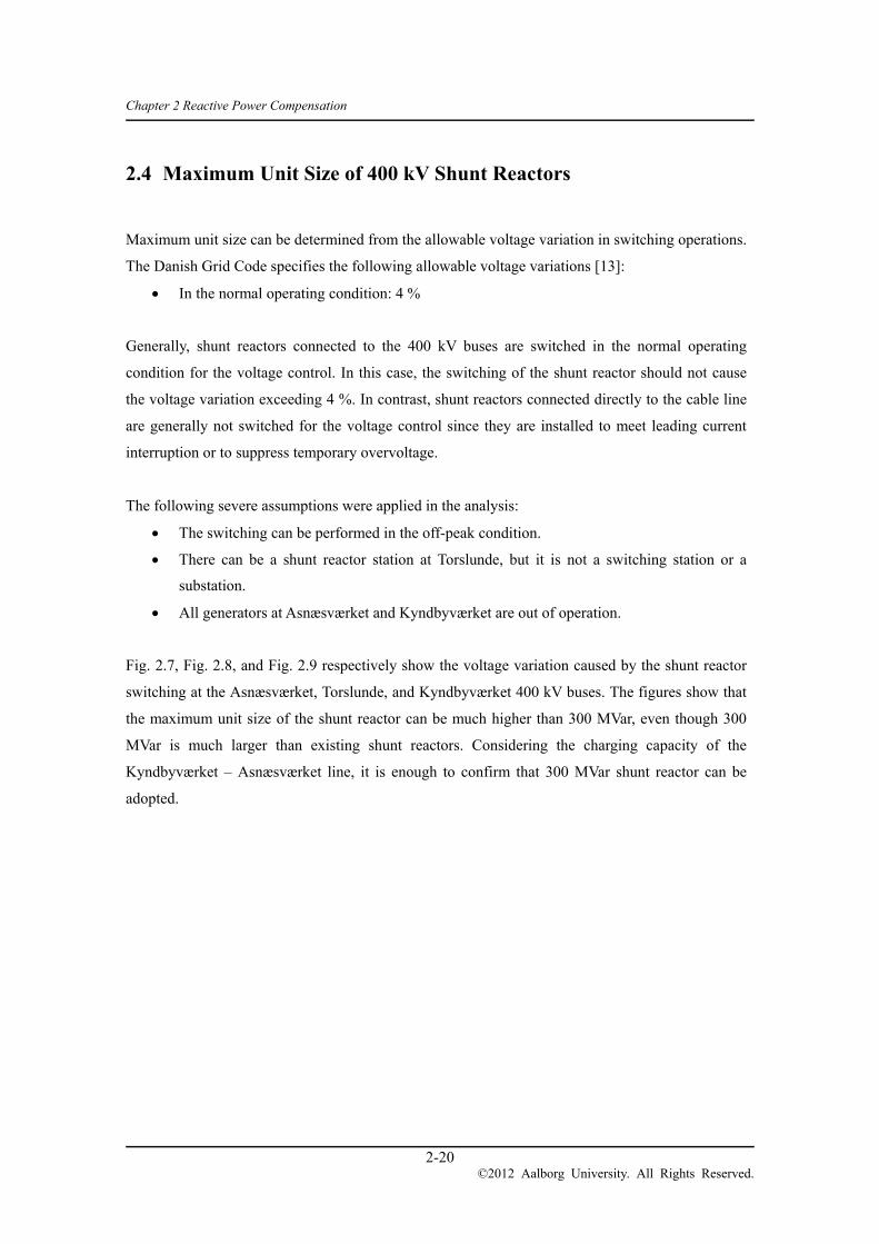
Table 2-7 shows the impedance and admittance of these sections set to PSS/E data, and Fig. 2.10
shows the power flow in the Kyndbyværket – Asnæsværket line in the no load condition with the
compensation Pattern 3.
The voltages at the Asnæsværket and Kyndbyværket 400 kV buses are fixed at 410 kV as a severe
assumption.
Table 2-7 Impedances and Admittances of the Kyndbyværket – Asnæsværket Line
R X Y
ASV – TOR (4.67 km) 0.0000537 pu 0.000515 pu 0.464 pu
TOR – KYV (5.5 km, land) 0.0000633 pu 0.000608 pu 0.547 pu
TOR – KYV (5.0 km, submarine) 0.000207 pu 0.000287 pu 0.497 pu
Fig. 2.10 Power flow in the Kyndbyværket – Asnæsværket line in the no load condition.
1ASV
1.025410.0
0.1
22.1R
1
2AT1
1.026410.2
0.1
-135.5
-0.1
86.8
3AT2
1.026410.3
0.1
-86.8
-0.1
38.0
4AT3
1.026410.4
0.1
-38.0
-0.1
-10.8
5AT4
1.026410.3
0.1
10.8
-0.1
-59.6
6AT5
1.025410.1
0.1
59.6
-0.1
-108.4
7TOR
1.025409.9
0.1
108.4
-0.1
-157.0
8TK1
1.025410.2
0.1
-158.0
-0.1
100.6
9TK2
1.026410.3
0.1
-100.6
-0.1
43.1
10TK3
1.026410.4
0.1
-43.1
-0.1
-14.4
11TK4
1.026410.3
0.1
14.4
-0.1
-72.0
12TK5
1.025410.2
0.1
72.0
-0.0
-124.2
13KYV
1.025410.0
0.0
-18.8R0.0
124.2
-0.0
-176.4
1
1 0.0
157.61
0.0
157.6
1 0.0
315.0

Chapter 2 Reactive Power Compensation
2-25 ©2012 Aalborg University. All Rights Reserved.
2.6.1 No Load Condition
Fig. 2.11 shows the voltage variation in the Kyndbyværket – Asnæsværket line in the no load
condition. For the analysis, the active power output from the generator model at the Asnæsværket
and Kyndbyværket 400 kV buses are set to nearly zero. Since the Asnæsværket 400 kV bus is the
swing bus, there is small active power output 0.1 MW from the generator model.
From the result of the above analysis, the highest voltage along the Kyndbyværket – Asnæsværket
line becomes greater than the both ends by 1.8 kV with the compensation Patterns 1 and 2. These
two compensation patterns yield the same voltage profile as their difference is only the shunt
reactor size at the Asnæsværket 400 kV bus where the bus voltage is fixed at 410 kV.
The compensation Patterns 3 and 4 yield even flatter voltage profile because of the shunt reactor at
Torslunde. Most power systems do not require the flatness at this level; voltage profiles of all
patterns are acceptable.
In Fig. 2.11, there is a discontinuity in the slope of the voltage profiles at the connection between
land part and submarine part. It is caused by the difference of reactance per length between the
cross-bonded cable and the solidly-bonded cable.
Fig. 2.11 Voltage variation in the Kyndbyværket – Asnæsværket line in the no load condition.
Table 2-8 shows the reactive power supplied into the Kyndbyværket – Asnæsværket line. Since
Patterns 1 and 3 are over-compensation by 0.7 %, small reactive power 2 – 4 MVar has to be
supplied from the outside. Patterns 2 and 4 are under-compensation by 7.8 %. It is reasonable that
reactive power approximately 50 MVar flows out from the cable line to the outside.
408.5
409
409.5
410
410.5
411
411.5
412
ASV AT2 AT4 TOR TK2 TK4 KYV
Vol
tage
[kV
]
Pattern 1, 2
Pattern 3
Pattern 4

Chapter 2 Reactive Power Compensation
2-26 ©2012 Aalborg University. All Rights Reserved.
This imbalance will not have a noticeable impact on the overall voltage and reactive power control
of the network. The reactive power loss in the cable line is negligible because of the assumed no
load condition.
Table 2-8 Reactive Power Supplied to the Kyndbyværket – Asnæsværket Line in the No Load
Condition
Asnæsværket
[MVar]
Kyndbyværket
[MVar]
Imbalance
[MVar]
Pattern 1 23.8 -21.7 2.1
Pattern 2 -28.8 -21.7 -50.5
Pattern 3 22.1 -18.8 3.3
Pattern 4 -3.8 -45.4 -49.2
2.6.2 Maximum Power Flow Condition
The voltage profile can change in the maximum power flow condition. Al 1600 mm2 XLPE cable is
assumed for the Kyndbyværket – Asnæsværket line, and typical transmission capacity for this type
of cable is around 800 – 900 MVA.
Fig. 2.12 shows the voltage variation with 800 MW power flow. The active power output from the
generator model at Kyndbyværket is changed from 0 MW to – 800 MW. The negative sign means
the power flow from Asnæsværket to Kyndbyværket.
The voltage variation becomes larger with 800 MW power flow, but it is still small enough. All
compensation patterns are considered satisfactory.

Chapter 2 Reactive Power Compensation
2-27 ©2012 Aalborg University. All Rights Reserved.
Fig. 2.12 Voltage variation in the Kyndbyværket – Asnæsværket line with 800 MW power flow.
Table 2-9 shows the reactive power supplied to the Kyndbyværket – Asnæsværket line in the
maximum power flow condition. In Patterns 1 and 3, larger reactive power is supplied to the cable
line, compared to the results in the no load condition. Comparing these two results, reactive power
35 – 40 MVar is lost in the line due to the large power flow in the line.
Due to the same reason, the reactive power supplied from the cable line to the outside is reduced by
35 – 40 MVar in Patterns 2 and 4. The amount of imbalance and reactive power loss should be
acceptable in the Danish network.
Table 2-9 Reactive Power Supplied to the Kyndbyværket – Asnæsværket Line in the
Maximum Power Flow Condition
Asnæsværket
[MVar]
Kyndbyværket
[MVar]
Imbalance
[MVar]
Pattern 1 -87.3 126.1 38.8
Pattern 2 -139.8 126.1 -13.7
Pattern 3 -89.1 130.1 41.0
Pattern 4 -114.9 103.3 -11.6
408.5
409
409.5
410
410.5
411
411.5
412
412.5
ASV AT2 AT4 TOR TK2 TK4 KYV
Vol
tage
[kV
]
Pattern 1, 2
Pattern 3
Pattern 4

Chapter 2 Reactive Power Compensation
2-28 ©2012 Aalborg University. All Rights Reserved.
Active Power Loss 2.7
Active power loss in the cable line under the maximum power flow condition is found as below. It
is confirmed that the reactive power compensation does not have meaningful impact on the active
power loss.
Patterns 1, 2 6.4 MW
Patterns 3, 4 6.2 MW

Chapter 2 Reactive Power Compensation
2-29 ©2012 Aalborg University. All Rights Reserved.
Effect on the Transmission Capacity 2.8
Large reactive power flow can affect the active power transmission capacity of the cable line.
Reactive power flow changes along the cable line, and Table 2-10 shows the largest reactive power
flow in the Kyndbyværket – Asnæsværket line.
Table 2-10 Reactive Power Flow in the Kyndbyværket – Asnæsværket Line
No load condition
[MVar]
800 MW active
power flow [MVar]
Pattern 1, 2 336.8 402.5
Pattern 3 176.4 288.9
Pattern 4 203.0 272.5
Fig. 2.13 Transmission Capacity of the Kyndbyværket – Asnæsværket line.
Fig. 2.13 illustrates the effect of this reactive power flow on the transmission capacity. Since the
PhD project does not include the transmission capacity calculation, it assumes the transmission
capacity 900 MVA.
According to the figure, Patterns 1 and 2 have lower active power transmission capacity by
approximately 50 MW, compared to Patterns 3 and 4. Thus, it should be considered how much
transmission capacity is necessary for the cable line. In addition, actual reactive power flow might
0
200
400
600
800
1000
0 200 400 600 800 1000
P [MW]
Q [
MV
ar]
Patttern 1,2
Pattern 3
Pattern 4

Chapter 2 Reactive Power Compensation
2-30 ©2012 Aalborg University. All Rights Reserved.
be affected by the network outside the cable line. As such, the analysis acts only as a relative
comparison between the four compensation patterns.
For example, when the reactive power flow injection of 200 MVar is assumed from the network
outside the cable line, Fig. 2.13 changes to Fig. 2.14. The effect of the compensation patterns on the
transmission capacity increases for larger reactive power injection. In Fig. 2.14, the difference of
transmission capacity with Pattern 1 and Pattern 4 increases to 90 MW.
Fig. 2.14 Transmission Capacity of the Kyndbyværket – Asnæsværket line.
0
200
400
600
800
1000
0 200 400 600 800 1000
P [MW]
Q [
MV
ar] Pattern 1
Pattern 2
Pattern 3
Pattern 4

Chapter 2 Reactive Power Compensation
2-31 ©2012 Aalborg University. All Rights Reserved.
Ferranti Phenomenon 2.9
The voltage profile under the normal operating condition was studied in previous sections. In the
normal operating condition, there is no technical reason to choose one proposed pattern over the
others.
In the selection of the reactive power compensation, however, the following condition should
additionally be considered:
One shunt reactor out of service
One end of the cable line is opened
Adopting large shunt reactors is a cheaper solution, but an effect of the shunt reactor outage
becomes significant. Table 2-11 shows the compensation rate and leading current interruption
capability when the largest shunt reactor is out of service.
Table 2-11 Leading Current Interruption with One Shunt Reactor out of Service
Pattern 1 Pattern 2 Pattern 3 Pattern 4
Asnæsværket 300 MVar 250 MVar 150 MVar 150 MVar
Torslunde – – 300 MVar 250 MVar
Kyndbyværket 300 MVar 300 MVar 150 MVar 150 MVar
Compensation Rate 50.3 % 41.9 % 50.3 % 50.3 %
Leading Current 427.8 A 500.0 A 427.8 A 427.8 A
In the calculation of the required leading current interruption capability, it is assumed that both ends
of the cable line are not opened at the same timing. As is sometimes the case in reality, one side is
assumed to be opened earlier than the other, and the latter circuit breaker needs to open the
charging (leading) current of the whole cable line.
The required leading current interruption capability is higher than the rated capacitive switching
current specified in IEC 622271-100, which is 400 A for 420 kV equipment. The rated capacitive
switching current is specified at the voltage factor 1.4 pu, and actual capability of circuit breakers
are higher than the IEC rating for the lower voltage factor. If the expected voltage in the leading
current interruption is lower than this, leading current interruption in Table 2-11 can be acceptable.
However, actual capability of the circuit breaker has to be tested and verified in a factory for the
cable line.

Chapter 2 Reactive Power Compensation
2-32 ©2012 Aalborg University. All Rights Reserved.
Additional discussions with regard to the leading current interruption are given in Sections 6.2 and
6.3.
Considering the required leading current interruption capability, it is recommended to adopt smaller
unit size if the cable line has to be in-service even when the shunt reactor is out of service. Table
2-12 shows the proposed compensation pattern with smaller unit sizes. With the proposed
compensation pattern in Table 2-12, there will be no problem in the leading current interruption
capability even when one shunt reactor is out of service.
Table 2-12 Proposed Compensation Patterns with Smaller Unit Sizes
Pattern 1’ Pattern 2’ Pattern 3’ Pattern 4’
Asnæsværket 150 MVar × 2 100 MVar × 1
150 MVar × 1 150 MVar × 1 150 MVar × 1
Torslunde – – 150 MVar × 2 100 MVar × 1
150 MVar × 1
Kyndbyværket 150 MVar × 2 150 MVar × 2 150 MVar × 1 150 MVar × 1
Compensation Rate 100.6 % 92.2 % 100.6 % 92.2 %
Now, we consider the voltage profile when one end of the cable line is opened. One end of the
cable line is opened when:
the cable line is energized from one end, or
a bus fault is cleared by opening one end of the cable line.
In both occasions, system operators cannot monitor the voltage at the opened terminal. It is
therefore recommended to limit the voltage at the open terminal to the critical maximum voltage
420 kV.
Fig. 2.15 shows the voltage profile in the Kyndbyværket – Asnæsværket line when the
Kyndbyværket side is opened. The figure shows that there will be no problem in the voltage profile
even when one side of the cable line is opened.

Chapter 2 Reactive Power Compensation
2-33 ©2012 Aalborg University. All Rights Reserved.
Fig. 2.15 Voltage variation in the Kyndbyværket – Asnæsværket line when the KYV side is opened.
When smaller shunt reactor sizes are adopted, the voltage profile will become severest when one
shunt reactor is out of service and one end of the cable line is opened. Table 2-13 shows the
severest condition.
Table 2-13 Severest Condition for the Voltage Profile with Smaller Unit Sizes
Pattern 1’ Pattern 2’ Pattern 3’ Pattern 4’
Asnæsværket 150 MVar × 2 100 MVar × 1
150 MVar × 1 150 MVar × 1 150 MVar × 1
Torslunde – – 150 MVar × 2 100 MVar × 1
150 MVar × 1
Kyndbyværket
(Open Terminal)
150 MVar × 1
150 MVar × 1
150 MVar × 1
150 MVar × 1 150 MVar × 1 150 MVar × 1
Compensation Rate 75.5 % 67.1 % 75.5 % 67.1 %
Fig. 2.16 shows the voltage profile in the severest condition. In the severest case, there will be
about 5 kV voltage rise at the opened terminal. The result tells us that the Asnæsværket or
Kyndbyværket 400 kV bus voltage has to be kept lower than 415 kV, when one (small) shunt
reactor is out of service.
409
409.5
410
410.5
411
411.5
412
412.5
ASV AT2 AT4 TOR TK2 TK4 KYV
Vol
tage
[kV
]
Pattern 1, 2
Pattern 3
Pattern 4

Chapter 2 Reactive Power Compensation
2-34 ©2012 Aalborg University. All Rights Reserved.
Fig. 2.16 Voltage variation in the Kyndbyværket – Asnæsværket line when one small shunt reactor is out of service and KYV side is opened.
407
408
409
410
411
412
413
414
415
416
ASV AT2 AT4 TOR TK2 TK4 KYV
Vol
tage
[kV
]
Pattern 1, 2
Pattern 3
Pattern 4

Chapter 2 Reactive Power Compensation
2-35 ©2012 Aalborg University. All Rights Reserved.
Conclusion 2.10
The reactive power compensation analysis has been performed for the compensation patterns in
Table 2-6 (reproduced below as Table 2-14). The analysis includes:
Voltage profile in the cable line
Active power loss
Effect on the transmission capacity
Leading current interruption capability
Table 2-14 Studied Compensation Patterns of the Kyndbyværket – Asnæsværket Line
(Reproduced)
Pattern 1 Pattern 2 Pattern 3 Pattern 4
Asnæsværket 300 MVar 250 MVar 150 MVar 150 MVar
Torslunde – – 300 MVar 250 MVar
Kyndbyværket 300 MVar 300 MVar 150 MVar 150 MVar
Compensation Rate 100.7 % 92.2 % 100.7 % 92.2 %
The analysis does not reveal a reason to choose one pattern over the others. Thus, it is
recommended to choose Pattern 1 for the following reasons:
It will be the cheapest solution because of the small number of shunt reactor units.
As it uses only 300 MVar unit, it has an advantage in keeping spare reactors in stock.
Pattern 1 is assumed in this PhD project.
If the cable line has to be in-service even when the shunt reactor is out of service, it is
recommended to adopt smaller unit size as in Table 2-12 (reproduced below as Table 2-15). Among
these patterns, Patterns 1’ and 3’ are preferred as they use only 150 MVar unit. When one shunt
reactor is out of service and the cable line is in-service, the Asnæsværket or Kyndbyværket 400 kV
bus voltage has to be kept lower than 415 kV.

Chapter 2 Reactive Power Compensation
2-36 ©2012 Aalborg University. All Rights Reserved.
Table 2-15 Proposed Compensation Patterns with Smaller Unit Sizes
Pattern 1’ Pattern 2’ Pattern 3’ Pattern 4’
Asnæsværket 150 MVar × 2 100 MVar × 1
150 MVar × 1 150 MVar × 1 150 MVar × 1
Torslunde – – 150 MVar × 2 100 MVar × 1
150 MVar × 1
Kyndbyværket 150 MVar × 2 150 MVar × 2 150 MVar × 1 150 MVar × 1
Compensation Rate 100.6 % 92.2 % 100.6 % 92.2 %

Chapter 2 Reactive Power Compensation
2-37 ©2012 Aalborg University. All Rights Reserved.
References
[1] A. Ametani, Distributed-Parameter Circuit Theory, Corona Pub. Co., 1990 (in Japanese).
[2] IEC/TR 60909-2 ed. 2.0, “Short-circuit currents in three-phase a.c. systems - Part 2: Data of
electrical equipment for short-circuit current calculations,” (2008)
[3] Central Station Engineers, Electrical Transmission and Distribution Reference Book, 4th
Edition, Westinghouse Electric Corporation, 1964.
[4] J. Lewis Blackburn, Symmetrical Components for Power Systems Engineering, CRC Press,
1993.
[5] Jesus Vargas, Armando Guzman, Jorge Robles, ”Underground/submarine cable protection
using a negative-sequence directional comparison scheme,” 26th Annual Western Protective
Relay Conference, Spokane, Washington, October 25-28, 1999
[6] CIGRE WG B1.19, “General Guidelines for the Integration of a New Underground Cable
System in the Network,” CIGRE Technical Brochure 250, 2004.
[7] N. Nagaoka and A. Ametani, “Transient Calculations on Crossbonded Cables,” IEEE Trans.
on Power Apparatus and Systems, vol. PAS-102, no. 4, 1983.
[8] A. Ametani, Y. Miyamoto, and N. Nagaoka, “An Investigation of a Wave Propagation
Characteristic on a Crossbonded Cable,” IEEJ Trans. PE, vol. 123, no. 3, pp. 395-401, 2003
(in Japanese).
[9] Bjørn Gustavsen “Panel Session on Data for Modeling System Transients. Insulated Cables”,
Proc. IEEE. Power Engineering Society Winter Meeting , 2001
[10] A. Ametani, “A GENERAL FORMULATION OF IMPEDANCE AND ADMITTANCE OF
CABLES,” IEEE Transactions on Power Apparatus and Systems, vol. PAS-99, no. 3
May/June 1980.
[11] A. Ametani, “On the Impedance and the Admittance in the EMTP Cable Constants /
Parameters,” European EMTP-ATP Users Group Meeting, Delft, the Netherlands, October
26-28, 2009.
[12] W. Scott-Meyer, ATP Rule Book, Can / Am EMTP User Group, 1982.
[13] Energinet.dk, “Technical Regulation 2.1.1 – Grid Dimensioning Rules”, available in Danish at:
http://energinet.dk/SiteCollectionDocuments/Danske%20dokumenter/El/TF%202.1.1%20Net
dimensioneringsreglergældende.pdf.

Chapter 3 Model Setup
3-1 ©2012 Aalborg University. All Rights Reserved.
Model Setup Chapter 3
Power Flow Data 3.1
The power flow data in the year 2015 was provided from Energinet.dk. The impedance and
admittance of the 400 kV Kyndbyværket – Asnæsværket line are modified according to the values
found in the previous chapter.
The power flow data provided from Energinet.dk include the peak load condition (south transit) and
the off-peak load condition (north transit). A comparison of the total load in Zealand is shown in
Table 3-1. As the severe temporary overvoltage can often be caused in the off-peak load condition,
the north transit power flow data is used as the base of the model setup.
Table 3-1 Comparison of Total Demand in Zealand
North Transit South Transit North / South
1719 MW 2773 MW 62 %
Fig. 3.1 shows the power flow diagram in the off-peak load condition after the addition of the
Kyndbyværket – Asnæsværket line.

Chapter 3 Model Setup
3-2 ©2012 Aalborg University. All Rights Reserved.
Fig. 3.1 Power flow diagram in the off-peak load condition after the installation of the Kyndbyværket – Asnæsværket line.
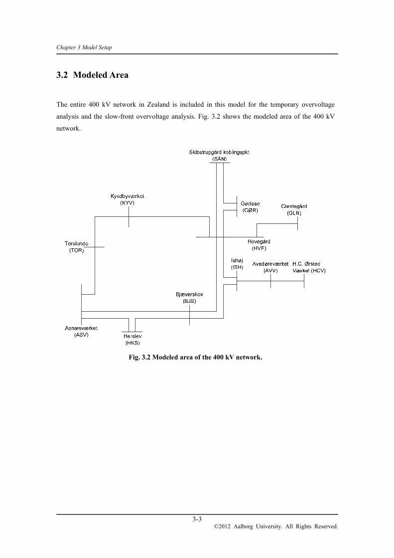
Chapter 3 Model Setup
3-3 ©2012 Aalborg University. All Rights Reserved.
Modeled Area 3.2
The entire 400 kV network in Zealand is included in this model for the temporary overvoltage
analysis and the slow-front overvoltage analysis. Fig. 3.2 shows the modeled area of the 400 kV
network.
Fig. 3.2 Modeled area of the 400 kV network.

Chapter 3 Model Setup
3-4 ©2012 Aalborg University. All Rights Reserved.
Fig. 3.3 shows an example of the simulation model created in ATP-Draw. Each component in the
figure is explained in this section.
Fig. 3.3 Simulation model for the temporary overvoltage and slow-front overvoltage analysis in ATP-Draw.
LCC
22. km
LCC
46.73 km
AB
C
ASV40
SA
T
YY
HKS40
SA
T
YY
Y
LCC
26.2
5 k
m
LCC
11.1
4 k
m
ISH40LCC
5.675 km
LCC
6.89 km
V
LCC
20.6
8 k
m
LCC
35.8
5 k
m GOR40
SAT
Y Y
LC
C
27.
2 k
mV
12km
AVV40GROUPish_avv
9km
HCV40GROUPavv_hcv
12km
GLN40GROUPhve_gln
8.43km
GR
OU
Pgo
r_sa
n
9.47km
GR
OU
Phv
e_sa
n
BJS40
SA
T
YY
SA
T
YY
SA
T
YY
SA
T
YY
HVE40
SA
T
YY
SA
T
YY
SA
T
YY
SA
T
YY
SAT
Y Y
SA
T
Y
SA
T
Y
SAN40
SA
T
YY
LCC
18.15 km
LCC
4.76 km132kV
KYV40 LCC
1.99 kmLCC
1.99 km
KYV13
VABC
TOR40
GR
OU
PA
SV
-TO
R
V
KYV40
GR
OU
PT
OR
-KY
V
V
370MVar
126MVar
100MVar
LUP13
Ignore feeder 0.15km
HVE-OLS 7.3kmOLS-LUP (11.0-0.15)km
Hovegård – Kyndbyværket line
(upgraded to 400 kV operation)
Kyndbyværket – Asnæsværket line
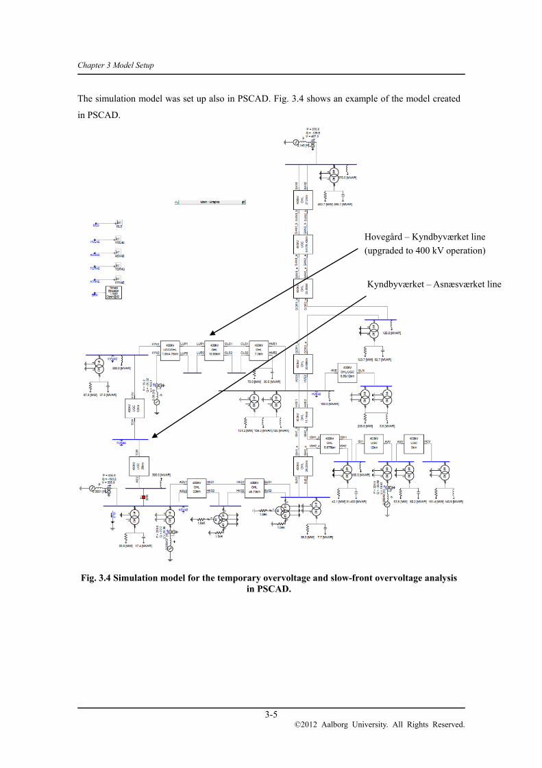
Chapter 3 Model Setup
3-5 ©2012 Aalborg University. All Rights Reserved.
The simulation model was set up also in PSCAD. Fig. 3.4 shows an example of the model created
in PSCAD.
Fig. 3.4 Simulation model for the temporary overvoltage and slow-front overvoltage analysis in PSCAD.
Hovegård – Kyndbyværket line
(upgraded to 400 kV operation)
Kyndbyværket – Asnæsværket line

Chapter 3 Model Setup
3-6 ©2012 Aalborg University. All Rights Reserved.
Underground Cables 3.3
3.3.1 Physical and Electrical Information
The simulation model includes the following four 400 kV cables:
Al 1600 mm2 XLPE cable (Al sheath)
Al 400 mm2 + Cu 1600 mm2 XLPE cable (Pb sheath)
Cu 1000 mm2 LPFF cable (Pb sheath + Al armour)
Cu 1000 mm2 LPFF cable (Pb sheath)
Fig. 3.5 shows the locations of these 400 kV cables in the network. The first cable type is for the
Kyndbyværket – Asnæsværket line. Additionally, this type was applied to the short section of the
Hovegård – Kyndbyværket line near the Kyndbyværket substation, where the overhead line is
designed as 132 kV. This short section (1.99 km) has to be replaced by 400 kV cables when the
Hovegård – Kyndbyværket line is operated at 400 kV.
Since the other types of the cable are located far from the point of the interest of this PhD project,
these cable models will not have a significant effect on the simulation results. These models have
been developed mainly for the future use at Energinet.dk.

Chapter 3 Model Setup
3-7 ©2012 Aalborg University. All Rights Reserved.
Fig. 3.5 Four types of cables in the simulation model.
(1) Al 1600 mm2 XLPE cable (Al sheath): Kyndbyværket – Asnæsværket line
Physical and electrical information of this type of the 400 kV cable is shown in Table 3-2. As the
Kyndbyværket – Asnæsværket line has not been constructed yet, it is not possible to obtain exact
parameters. Instead, the standard data was assumed based on ABB XLPE Underground Cable
Systems – User’s Guide (rev. 3) [1].
Asnæsværket(ASV)
Herslev(HKS)
22.00 km
68.73 km
46.73 km
Bjæverskov(BJS)
Ishøj(ISH)
31.92 km
37.39 km
16.82 km
Hovegård(HVE)
Gørløse(GØR)
Skibstrupgård koblingspkt(SÅN)
20.68 km
71.48 km
93.20 kmKyndbyværket
(KYV)22.91 km
Glentegård(GLN)
18.89 km
H.C. ØrstedVærket (HCV)
Avedøreværket(AVV)
12.09 km 8.99 km
(1)
(5)
(3)(4)(3)
(2)
(2) (2)
(1) Al 1600 mm2 XLPE cable (Al sheath)(2) Al 400 + Cu 1600 mm2 XLPE cable (Pb sheath)(3) Cu 1000 mm2 LPFF cable (Pb sheath + Al armour)(4) Cu 1000 mm2 LPFF cable (Pb sheath)(5) Al 2000 mm2 XLPE cable (Cu sheath, no data, ignored)
1.99 km(1)
Lyngerup(LUP)
18.30 km6.90 km
132 kV

Chapter 3 Model Setup
3-8 ©2012 Aalborg University. All Rights Reserved.
Table 3-2 Physical and Electrical Information for the 400 kV Cable used at ASV – KYV (1)
Conductor R1 Inner radius of the tubular core mm 0
R2 Outer radius of the tubular core mm 26.0
ρc Resistivity Ωm 2.84E-08
μc Relative permeability 1
Conductor Screen Rsi Outer radius of conductor screen mm 28.0
Insulation μI1 Relative permeability 1
εI1 Relative permittivity 2.852
Rso Outer radius of the insulation mm 55.0
Metallic Sheath R3 Inner radius of metallic sheath mm 58.0
R4 Outer radius of metallic sheath mm 59.2
ρs1 Resistivity 2.84E-08
μs1 Relative permeability 1
Outer Covering μI2 Relative permeability 1
εI2 Relative permittivity 2.4
Completed Cable R5 Average outer radius of cover mm 63.5
It is not possible to model semiconductive layers inside and outside the insulation in the subroutine
CABLE CONSTANTS. Hence, semiconductive layers inside and outside the insulation were
modeled as a part of the insulation since their resistivity is large enough in comparison to the
conductor or metallic sheath.
Because of this modification, the insulation appears thicker in the ATP-Draw model than the actual
thickness, and the charging capacity of the cable appears smaller than its actual value. In order to
compensate for this error, relative permittivity of the insulation was converted using the following
equation [2]:
852.24.2)0.28/0.55ln(
.0)ln(58.0/26εI0
Rso/Rsi)ln(
ln(R3/R2)εI1 Eqn. 3.1
Relative permittivity of the insulation was converted in the same manner for other 400 kV cables.
The Kyndbyværket – Asnæsværket line has both a land part and a submarine part. The submarine
part has an armour conductor outside of the metallic sheath. However, the armour was not included
in the model mainly because the armour causes only a minor effect on the transient overvoltage,
which will be discussed in Section 3.3.8.

Chapter 3 Model Setup
3-9 ©2012 Aalborg University. All Rights Reserved.
(2) Al 400 mm2 + Cu 1600 mm2 XLPE cable (Pb sheath)
Physical and electrical information of this type of the 400 kV cable is shown in Table 3-3.
Table 3-3 Physical and Electrical Information for the 400 kV Cable
used at ISH – AVV – HCV and HVE – GLN (2)
Conductor R1 Inner radius of the tubular core mm 0
R2 Outer radius of the tubular core mm 25.50
ρc Resistivity Ωm 1.724E-08
μc Relative permeability 1
Conductor Screen Rsi Outer radius of conductor screen mm 28.80
Insulation μI1 Relative permeability 1
εI1 Relative permittivity 2.96
Rso Outer radius of the insulation mm 57.80
Metallic Sheath R3 Inner radius of metallic sheath mm 60.25
R4 Outer radius of metallic sheath mm 63.85
ρs1 Resistivity 2.20E-08
μs1 Relative permeability 1
Outer Covering μI2 Relative permeability 1
εI2 Relative permittivity 2.4
Completed Cable R5 Average outer radius of cover mm 69.60
The core of this cable has a copper in the center and the aluminum around it. Since CABLE
CONSTANTS subroutine and PSCAD cannot deal with two different conductors without insulation
between them, the core is assumed to be composed only of the copper. The copper has lower
resistance than the aluminum, and thus this is a conservative assumption.
Physical and electrical information of the cable has been provided from NKT Cables through
Energinet.dk. The provided data sheet is shown in Fig. 3.6.

Chapter 3 Model Setup
3-10 ©2012 Aalborg University. All Rights Reserved.
Fig. 3.6 Provided data on Cable (2).

Chapter 3 Model Setup
3-11 ©2012 Aalborg University. All Rights Reserved.
(3) Cu 1000 mm2 LPFF cable (Pb sheath + Al armour)
Physical and electrical information of this type of the 400 kV cable is shown in Table 3-4.
Table 3-4 Physical and Electrical Information for the 400 kV Cable
used at HVE – SÅN and GØR – SÅN (3)
Conductor R1 Inner radius of the tubular core mm 8.65
R2 Outer radius of the tubular core mm 20.65
ρc Resistivity Ωm 1.724E-08
μc Relative permeability 1
Conductor Screen Rsi Outer radius of conductor screen mm 21.25
Insulation μI1 Relative permeability 1
εI1 Relative permittivity 2.56
Rso Outer radius of the insulation mm 45.25
Metallic Sheath R3 Inner radius of metallic sheath mm 46.20
R4 Outer radius of metallic sheath mm 49.40
ρs1 Resistivity 2.20E-07
μs1 Relative permeability 1
Insulation μI2 Relative permeability 1
εI2 Relative permittivity 2.4
Armour R5 Inner radius of metallic sheath mm 53.90
R6 Outer radius of metallic sheath mm 61.90
ρs1 Resistivity 2.84E-08
μs1 Relative permeability 1
Outer Covering μI2 Relative permeability 1
εI2 Relative permittivity 2.4
Completed Cable R7 Average outer radius of cover mm 66.30
Physical and electrical information of the cable has been provided from Energinet.dk. The provided
data sheet is shown in Fig. 3.7.

Chapter 3 Model Setup
3-12 ©2012 Aalborg University. All Rights Reserved.
Fig. 3.7 Provided data on Cable (3).

Chapter 3 Model Setup
3-13 ©2012 Aalborg University. All Rights Reserved.
(4) Cu 1000 mm2 LPFF cable (Pb sheath)
Physical and electrical information of this type of the 400 kV cable is shown in Table 3-5.
Table 3-5 Physical and Electrical Information for the 400 kV Cable
used at HVE – SÅN and GØR – SÅN (4)
Conductor R1 Inner radius of the tubular core mm 8.65
R2 Outer radius of the tubular core mm 20.65
ρc Resistivity Ωm 1.724E-08
μc Relative permeability 1
Conductor Screen Rsi Outer radius of conductor screen mm 21.05
Insulation μI1 Relative permeability 1
εI1 Relative permittivity 2.532
Rso Outer radius of the insulation mm 45.25
Metallic Sheath R3 Inner radius of metallic sheath mm 46.20
R4 Outer radius of metallic sheath mm 50.60
ρs1 Resistivity 2.20E-08
μs1 Relative permeability 1
Outer Covering μI2 Relative permeability 1
εI2 Relative permittivity 2.4
Completed Cable R5 Average outer radius of cover mm 55.75
Physical and electrical information of the cable has been provided from Energinet.dk. The provided
data sheet is shown in Fig. 3.8.

Chapter 3 Model Setup
3-14 ©2012 Aalborg University. All Rights Reserved.
Fig. 3.8 Provided data on Cable (4).
3.3.2 Cable Layout
All 400 kV cables were assumed to be buried in a flat formation as shown in Fig. 3.9. The buried
depth of 1.3 m and the phase spacing 0.3 m are assumed to be common for all the four cable
models.
Fig. 3.9 Cable layout.
1.3 m
0.3 m 0.3 m

Chapter 3 Model Setup
3-15 ©2012 Aalborg University. All Rights Reserved.
3.3.3 Cable Route
The assumed route of the Kyndbyværket – Asnæsværket line is illustrated in Fig. 3.10 by a red
dotted line. The cable line is assumed to be composed of land and submarine sections. The length
of each section is:
Asnæsværket to Torslunde: 28 km (only land section)
Torslunde to Kyndbyværket
o Land section: 22 km
o Submarine section: 10 km
Fig. 3.10 Cable route.
The cable model in the land section is cross-bonded, whereas the cable model in the submarine
section is solidly-bonded. The length of the minor section and the number of major / minor sections
are shown in Table 3-6.
Table 3-6 Cross-bonding of the Kyndbyværket – Asnæsværket line
Asnæsværket – Torslunde Torslunde – Kyndbyværket
Length of minor section 1867 m 1833 m
Number of minor sections 15 12
Number of major sections 5 4

Chapter 3 Model Setup
3-16 ©2012 Aalborg University. All Rights Reserved.
Finally, sheath bonding is modeled as shown in Fig. 3.11 and Fig. 3.12. Each node between minor
sections is named as AT1, AT2, …, AT15 for the Asnæsværket – Torslunde section and KT1, KT2,
…, KT14 for the Torslunde – Kyndbyværket section. These node names are later used to specify
fault locations or monitoring points for the overvoltage.
Fig. 3.11 Modeling of cross-bonding (Asnæsværket – Torslunde).
Fig. 3.12 Modeling of cross-bonding (Torslunde – Kyndbyværket).

Chapter 3 Model Setup
3-17 ©2012 Aalborg University. All Rights Reserved.
3.3.4 Modeling of Auxiliary Components
The setup of cable models requires the modeling of cross-bonding wires, grounding wires, and
other grounding conditions. The following settings are commonly applied for all 400 kV cables:
(a) Impedance of cross-bonding wires: 20 μH
Typical length of the cross-bonding wire from joint to link box is about 10 m. The impedance was
assumed to be 1μH/m.
(b) Impedance of grounding wires: 10 μH
Typical length of the grounding wire is about 10 m. The impedance was assumed to be 1μH/m.
(c) Grounding resistance
Substation: 1 ohm
Normal Joint: 5 ohm
(d) Ground resistivity: 100 ohm-m
Chapter 3 Model Setup
3-18 ©2012 Aalborg University. All Rights Reserved.
3.3.5 Effects of Cable Models
The PhD project set up the simulation model both in ATP-EMTP and PSCAD. Different cable
models are adopted in ATP-EMTP and PSCAD. The comparison of the cable models are given in
Table 3-7.
Table 3-7 Comparison of cable models in ATP-EMTP and PSCAD
ATP-EMTP PSCAD
Model name Bergeron Frequency dependent (phase)
Frequency dependent Non-frequency dependent Frequency dependent
Model domain Modal domain Phase domain
The resonance overvoltage analysis in Chapter 4 used the Bergeron model in ATP-EMTP since the
analysis was done before the release of PSCAD X4.4. When the PhD project was on the half-way,
however, the Manitoba HVDC Research Centre released PSCAD X4.4, which had an option to
calculate the earth-return impedance by the numerical integration of Pollaczek’s equation. The
numerical integration of Pollaczek’s equation helped to resolve the numerical instability
encountered in many cases. All transient analyses, except for the resonance overvoltage analysis,
were conducted after the release of PSCAD X4.4, and the frequency dependent (phase) model in
PSCAD was used for the analyses. Note that steady-state analyses used the steady-state
(power-frequency) calculation function in ATP-EMTP.
It is important for the setup of the Bergeron model to appropriately select the target frequency, at
which the cable impedance and admittance are calculated. It is a common practice, especially for
the temporary overvoltage analysis, to set the target frequency at 50 Hz as a severe assumption. The
lower target frequency leads to a smaller resistance, which normally causes a higher overvoltage. In
the PhD project, the target frequency was first set at 50 Hz. After the dominant frequency in the
overvoltage is known, however, the target frequency was changed to the dominant frequency in
order to obtain more reasonable results.
Since different cable models are adopted, frequency responses of the cable impedances are obtained
from both cable models in order to find the difference of these models. Fig. 3.13 and Fig. 3.14 show
the comparison of frequency responses of positive and zero sequence impedances of the
Kyndbyværket – Asnæsværket line. The target frequency of the Bergeron model is set to 50 Hz.
Considering the main focus of the PhD project, frequency responses are obtained in the range 0 –
2000 Hz at 10 Hz step.

Chapter 3 Model Setup
3-19 ©2012 Aalborg University. All Rights Reserved.
For both positive and zero sequence impedances, natural frequencies of the cable match between
two different models. The results indicate that natural frequencies of the network with the cable,
approximately 450 Hz and 1330 Hz, can be found by both cable models with an equal accuracy.
Fig. 3.13 Frequency response of positive sequence impedance of the KYV – ASV line.
Fig. 3.14 Frequency response of zero sequence impedance of the KYV – ASV line.
The differences can be more clearly seen in Fig. 3.15 and Fig. 3.16 where positive sequence
resistance and reactance are separately derived. Both resistance and reactance have peaks and zeros
at the same frequencies, but the magnitudes of the resistance and reactance at their peaks are
approximately two times higher than in the Bergeron model in ATP-EMTP.
0
200
400
600
800
1000
1200
0 500 1000 1500 2000
Frequency [Hz]
Impe
danc
e [o
hm]
PSCAD
ATP
0
40
80
120
160
200
0 500 1000 1500 2000
Frequency [Hz]
Impe
danc
e [o
hm]
PSCAD
ATP

Chapter 3 Model Setup
3-20 ©2012 Aalborg University. All Rights Reserved.
Fig. 3.15 Frequency response of positive sequence resistance of the KYV – ASV line.
Fig. 3.16 Frequency response of positive sequence reactance of the KYV – ASV line.
As a comparison in the time domain simulation, the Kyndbyværket – Asnæsværket line is energized
from the 400 kV voltage source behind the source impedance of 147 mH, which corresponds to the
fault current 5 kA. It is expected that the line energization overvoltages with the two cable models
become similar because the discrepancies of impedances between the two cable models are
observed only around the natural frequencies in Fig. 3.13 to Fig. 3.16. Considering the length of the
Kyndbyværket – Asnæsværket line, the dominant frequency in the overvoltages will be much lower
than the natural frequencies 450 Hz and 1330 Hz.
0
200
400
600
800
1000
1200
0 500 1000 1500 2000
Frequency [Hz]
Res
ista
nce
[ohm
]
PSCAD
ATP
-600
-400
-200
0
200
400
600
0 500 1000 1500 2000
Frequency [Hz]
Rea
ctan
ce [
ohm
]
PSCAD
ATP

Chapter 3 Model Setup
3-21 ©2012 Aalborg University. All Rights Reserved.
Fig. 3.17 and Fig. 3.18 respectively show the comparison of the line energization overvoltages at
the sending end and the receiving end. The waveforms of the overvoltages are similar in these cases,
but the magnitudes of the overvoltages include 5.9 % deviation at the sending end and 7.9 %
deviation at the receiving end. It is estimated that the deviation is caused by the small difference in
resistance.
Fig. 3.17 Overvoltage caused by the energization of the KYV – ASV line (sending end).
Fig. 3.18 Overvoltage caused by the energization of the KYV – ASV line (receiving end).
Fig. 3.19 shows frequency components contained in the line energization overvoltage. The
frequency components are obtained by the Fourier transform of the line energization overvoltages
-750
-500
-250
0
250
500
750
0 0.02 0.04 0.06 0.08 0.1
Time [s]
Vol
tage
[kV
]
PSCAD
ATP
PSCAD: 608.3kVATP: 572.3kV(5.9% deviation)
-750
-500
-250
0
250
500
750
0 0.02 0.04 0.06 0.08 0.1
Time [s]
Vol
tage
[kV
]
PSCAD
ATP
PSCAD: 650.2kVATP: 598.6kV(7.9% deviation)
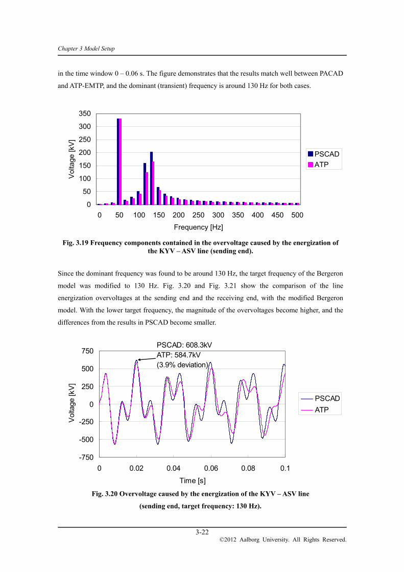
Chapter 3 Model Setup
3-22 ©2012 Aalborg University. All Rights Reserved.
in the time window 0 – 0.06 s. The figure demonstrates that the results match well between PACAD
and ATP-EMTP, and the dominant (transient) frequency is around 130 Hz for both cases.
Fig. 3.19 Frequency components contained in the overvoltage caused by the energization of the KYV – ASV line (sending end).
Since the dominant frequency was found to be around 130 Hz, the target frequency of the Bergeron
model was modified to 130 Hz. Fig. 3.20 and Fig. 3.21 show the comparison of the line
energization overvoltages at the sending end and the receiving end, with the modified Bergeron
model. With the lower target frequency, the magnitude of the overvoltages become higher, and the
differences from the results in PSCAD become smaller.
Fig. 3.20 Overvoltage caused by the energization of the KYV – ASV line
(sending end, target frequency: 130 Hz).
0
50
100
150
200
250
300
350
0 50 100 150 200 250 300 350 400 450 500
Frequency [Hz]
Vol
tage
[kV
]
PSCAD
ATP
-750
-500
-250
0
250
500
750
0 0.02 0.04 0.06 0.08 0.1
Time [s]
Vol
tage
[kV
]
PSCAD
ATP
PSCAD: 608.3kVATP: 584.7kV(3.9% deviation)

Chapter 3 Model Setup
3-23 ©2012 Aalborg University. All Rights Reserved.
Fig. 3.21 Overvoltage caused by the energization of the KYV – ASV line
(receiving end, target frequency: 130 Hz).
From the results, the Bergeron model produces a similar overvoltage to the frequency dependent
(phase) model during the first 20 ms after the energization. In finding the maximum overvoltage,
the choice of cable models between the Bergeron model and the frequency dependent (phase)
model does not have a noticeable impact. On the other hand, the overvoltages after the first 20 ms
following energization have notable differences. It may require the use of frequency dependent
(phase) model when matching simulation results to field measurements, although it is not included
in the scope of the PhD project.
3.3.6 Effects of Cross-bonding
The sheath cross-bonding has to be modelled as it changes the cable impedances as discussed in
Section 2.3.2. The analytical formulas and calculated results in the section show that the cable
inductances become larger due to the cross-bonding.
Furthermore, Eqn. 4.14 in Section 4.1.3 shows how the cable impedances and admittances affect
the propagation velocity of the overvoltages. Because of the larger cable inductance, the
propagation velocity is slower for cross-bonded cables.
Fig. 3.22 shows the energization overvoltage when the Kyndbyværket – Asnæsværket line is
energized from the Asnæsværket side. The black and red lines respectively show the overvoltage
-750
-500
-250
0
250
500
750
0 0.02 0.04 0.06 0.08 0.1
Time [s]
Vol
tage
[kV
]
PSCAD
ATP
PSCAD: 650.2kVATP: 611.6kV(5.9% deviation)

Chapter 3 Model Setup
3-24 ©2012 Aalborg University. All Rights Reserved.
when the cable line is cross-bonded and solidly-bonded. The figure demonstrates that the
propagation velocity is slower in the cross-bonded cable case.
Fig. 3.22 Effect of cross-bonding.
3.3.7 Effects of Span Length
It is a common practice to reduce the number of cable joints as much as possible in order to reduce
the cost and to shorten the construction duration. However, the cable span length (minor length) is
normally limited by restrictions in the transportation or by the sheath voltage. The restrictions in the
transportation mainly include:
Number of turns cables can be wound around a drum
Weight and height restrictions when a drum car has to go by road or cross bridges
The restriction in the sheath voltage differs from country to country and utility to utility. If the
restriction comes from a utility’s own safety codes, it may be possible to relax the restriction by
applying more strict work codes, for example, to wear specific gloves.
Table 3-6 explains that the PhD project assumes the cable span length to be around 1800 – 1900 m,
but this may be a difficult goal to achieve depending on the above mentioned restrictions. However,
when numerous numbers of simulations are performed for statistical switching studies, it is
convenient to have larger cable span lengths in order to reduce the computational burden.
-600
-400
-200
0
200
400
600
800
0 0.005 0.01 0.015 0.02 0.025 0.03 0.035 0.04
Time [s]
Vol
tage
[kV
]
Cross-bond
Two-point-bond

Chapter 3 Model Setup
3-25 ©2012 Aalborg University. All Rights Reserved.
This section studies the effects of assuming longer cable span length. The study was conducted
with the Kyndbyværket – Asnæsværket line, but the submarine part was removed from the line. The
sensitivity analysis considers the following parameters:
Cable span length: 2, 4, 6, 8, and 16 km
Total cable length: 24, 48, 72, 96 km
For Fig. 3.23 to Fig. 3.27, the highest overvoltages are compared for cable energization with
different cable span lengths. When the cable span length is increased to 4, 6 and 8 km, the errors
are below 5 %. When the cable span length is further increased to 16 km as in Fig. 3.27, the error
goes up to 9 %.
From the results of this study, the statistical switching studies in Section 5.1 increases the cable
span length to 6 km for 72 km cable line and to 8 km for 96 km cable line.
Fig. 3.23 Effect of cable span length for 24 km cable line (2 km → 4 km).
-600
-400
-200
0
200
400
600
0 0.02 0.04 0.06 0.08 0.1 0.12
Time [s]
Vol
tage
[kV
]
2km
4km
2km: 461.6kV4km: 448.3kV(3% error)

Chapter 3 Model Setup
3-26 ©2012 Aalborg University. All Rights Reserved.
Fig. 3.24 Effect of cable span length for 48 km cable line (2 km → 4 km).
Fig. 3.25 Effect of cable span length for 72 km cable line (2 km → 6 km).
-800
-600
-400
-200
0
200
400
600
800
0 0.02 0.04 0.06 0.08 0.1 0.12
Time [s]
Vol
tage
[kV
]
2km
4km
2km: 580.3kV4km: 566.2kV(2.4% error)
-500
-400
-300
-200
-100
0
100
200
300
400
500
0 0.02 0.04 0.06 0.08 0.1 0.12
Time [s]
Vol
tage
[kV
]
2km
4km
6km
2km: -419.9kV6km: -421.9kV(0.5% error)

Chapter 3 Model Setup
3-27 ©2012 Aalborg University. All Rights Reserved.
Fig. 3.26 Effect of cable span length for 96 km cable line (2 km → 8 km).
Fig. 3.27 Effect of cable span length for 24 km cable line (2 km → 16 km).
-800
-600
-400
-200
0
200
400
600
800
0 0.02 0.04 0.06 0.08 0.1 0.12
Time [s]
Vol
tage
[kV
]
2km
8km
2km: 566.3kV8km: 594.2kV(4.9% error)
-600
-400
-200
0
200
400
600
0 0.02 0.04 0.06 0.08 0.1 0.12
Time [s]
Vol
tage
[kV
]
2km
16km
2km: 430.5kV16km: 443.1kV(3% error)
2km: -496.7kV16km: -449.9kV(9% error)
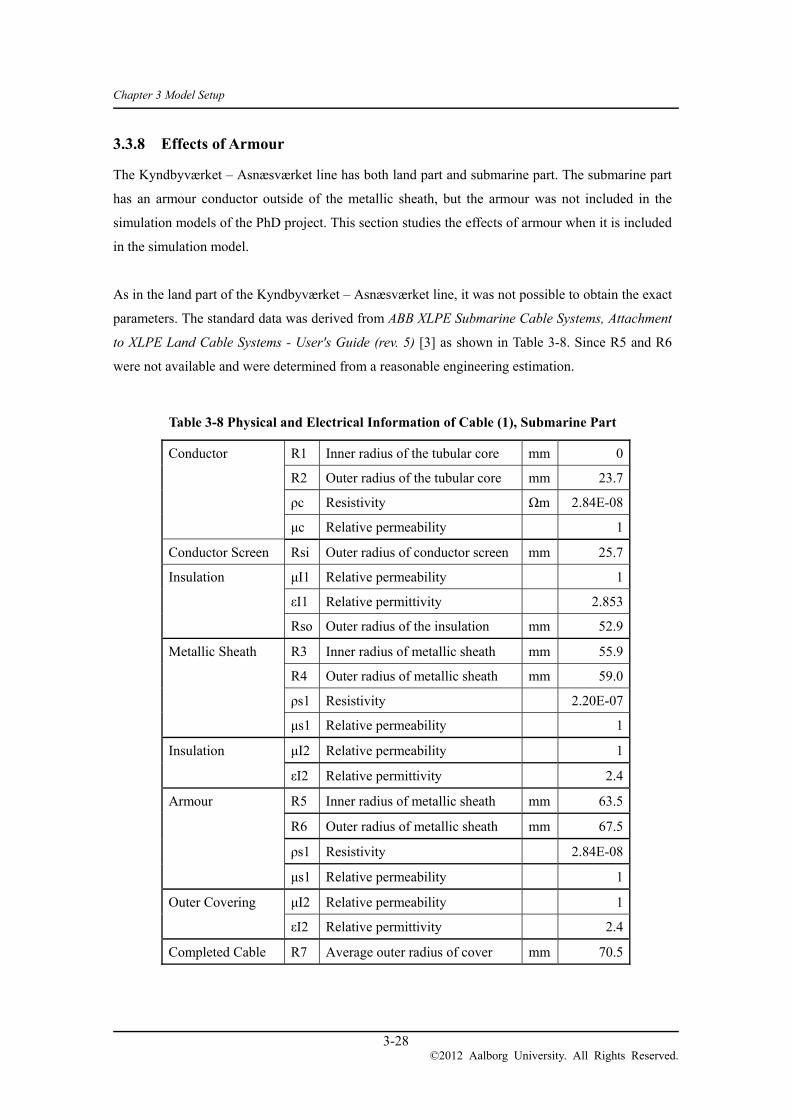
Chapter 3 Model Setup
3-28 ©2012 Aalborg University. All Rights Reserved.
3.3.8 Effects of Armour
The Kyndbyværket – Asnæsværket line has both land part and submarine part. The submarine part
has an armour conductor outside of the metallic sheath, but the armour was not included in the
simulation models of the PhD project. This section studies the effects of armour when it is included
in the simulation model.
As in the land part of the Kyndbyværket – Asnæsværket line, it was not possible to obtain the exact
parameters. The standard data was derived from ABB XLPE Submarine Cable Systems, Attachment
to XLPE Land Cable Systems - User's Guide (rev. 5) [3] as shown in Table 3-8. Since R5 and R6
were not available and were determined from a reasonable engineering estimation.
Table 3-8 Physical and Electrical Information of Cable (1), Submarine Part
Conductor R1 Inner radius of the tubular core mm 0
R2 Outer radius of the tubular core mm 23.7
ρc Resistivity Ωm 2.84E-08
μc Relative permeability 1
Conductor Screen Rsi Outer radius of conductor screen mm 25.7
Insulation μI1 Relative permeability 1
εI1 Relative permittivity 2.853
Rso Outer radius of the insulation mm 52.9
Metallic Sheath R3 Inner radius of metallic sheath mm 55.9
R4 Outer radius of metallic sheath mm 59.0
ρs1 Resistivity 2.20E-07
μs1 Relative permeability 1
Insulation μI2 Relative permeability 1
εI2 Relative permittivity 2.4
Armour R5 Inner radius of metallic sheath mm 63.5
R6 Outer radius of metallic sheath mm 67.5
ρs1 Resistivity 2.84E-08
μs1 Relative permeability 1
Outer Covering μI2 Relative permeability 1
εI2 Relative permittivity 2.4
Completed Cable R7 Average outer radius of cover mm 70.5

Chapter 3 Model Setup
3-29 ©2012 Aalborg University. All Rights Reserved.
In order to find the effects of armour on the energization overvoltages, the Kyndbyværket –
Asnæsværket line was energized from the 400 kV voltage source behind the source impedance of
147 mH, which corresponds to the fault current 5 kA. Fig. 3.28 and Fig. 3.29 respectively show the
comparison of the energization overvoltages at the sending end and the receiving end. The
waveforms demonstrate that the armour does not have noticeable effects on the energization
overvoltages.
Fig. 3.28 Effects of armour on the energization overvoltage (sending end).
Fig. 3.29 Effects of armour on the energization overvoltage (receiving end).
-750
-500
-250
0
250
500
750
0 0.02 0.04 0.06 0.08 0.1
Time [s]
Vol
tage
[kV
]
w/o Armour
with Armour
w/o Armour: 584.7kVwith Armour: 583.7kV(0.17% error)
-750
-500
-250
0
250
500
750
0 0.02 0.04 0.06 0.08 0.1
Time [s]
Vol
tage
[kV
]
w/o Armour
with Aumour
w/o Armour: 611.6kVwith Armour: 611.2kV(0.065% error)

Chapter 3 Model Setup
3-30 ©2012 Aalborg University. All Rights Reserved.
Overhead Transmission Lines 3.4
3.4.1 Conductor and Tower Configuration
400 kV overhead lines were modelled using a frequency dependent model (J. Marti model). Input
data for ATP-EMTP are shown in Table 3-9, and a cross-section diagram of transmission lines and
ground wires are shown in Fig. 3.30.
Table 3-9 Overhead Line Data
Types Inner
Radius [mm]
Outer Radius [mm]
Resistance per conductor [ohm/km]
Number of conductors in
a bundle
Separation between
conductors [cm]Transmission Line
(Martin) 6.025 18.085 0.04259 2 40
Ground Wire 4.65 8.10 0.208 – –
Fig. 3.30 Cross-section diagram of transmission line (left) and ground wire (right).
Fig. 3.31 shows the typical tower configuration for the 400 kV overhead lines. The layout of
transmission lines and ground wires were derived from the typical tower configuration as shown in
Table 3-10. This standard layout was applied to all 400 kV overhead lines.
Table 3-10 Layout of Standard 400 kV OHLs
Types Horizontal position [m] Vertical position [m]
Transmission Lines
±6.65 34.0
±8.60 26.0
±7.10 20.0
Ground wires ±3.00 41.0

Chapter 3 Model Setup
3-31 ©2012 Aalborg University. All Rights Reserved.
Fig. 3.31 Tower configuration of standard 400 kV OHLs.

Chapter 3 Model Setup
3-32 ©2012 Aalborg University. All Rights Reserved.
3.4.2 Phase Configuration
The phase configuration of 400 kV overhead lines is also provided from Energinet.dk. Fig. 3.32
shows the phase configuration of the existing 400 kV overhead lines.
Fig. 3.32 Phase configuration of the existing 400 kV OHLs.
As for the Hovegård – Kyndbyværket line, it was assumed that the line has the same phase
configuration after the line is upgraded to the 400 kV operation.
3.4.3 Comparison between PSCAD and ATP-EMTP
In PSCAD, it is not possible to model a hollow ground wire as shown in Table 3-9 since the inner
radius is always considered to be zero. To keep a satisfactory accuracy of the PSCAD model for an
overhead line, the sequence impedance of the double circuit tower line between Asnæsværket and
Herslev is calculated in PSCAD and ATP-EMTP. It is assumed that the Asnæsværket – Bjæverskov
line is cut at Herslev for the convenience in measurement.
Fig. 3.33 and Fig. 3.34 show a comparison of sequence impedances. A frequency dependent phase
model is used in PSCAD. The comparison shows the error in the model by PSCAD is negligible as

Chapter 3 Model Setup
3-33 ©2012 Aalborg University. All Rights Reserved.
the PhD project is focused on the frequency component less than 1 kHz.
Fig. 3.33 Comparison of the positive sequence impedance of 400 kV overhead line.
Fig. 3.34 Comparison of the zero sequence impedance of 400 kV overhead line.
0
50
100
150
200
0 500 1000 1500 2000
Frequency [Hz]
Impe
danc
e [o
hm]
PSCAD
ATP
0
200
400
600
800
0 500 1000 1500 2000
Frequency [Hz]
Impe
danc
e [o
hm]
PSCAD
ATP

Chapter 3 Model Setup
3-34 ©2012 Aalborg University. All Rights Reserved.
Transformers 3.5
(1) 400/132 kV transformers
Model parameters of all 400/132 kV transformers were derived from the PSS/E data provided by
Energinet.dk. Since all the 400/132 kV transformers except the one in GLN are modelled as two
winding transformers in the PSS/E data, only the impedance between the primary and secondary
windings is available. In the EMTP data, the impedance was split half and half in pu to the primary
and to the secondary. The parameters are given in Table 3-11.
Table 3-11 Model Parameters of 400 kV Transformers
R1 (ohm) R2 (ohm) X1 (mH) X2 (mH)
BJS 0.968 0.1054 191.9 20.90
ISH 0.528 0.0575 138.1 15.04
AVV 0.560 0.0610 122.9 13.39
HCV 0.416 0.0453 94.7 10.32
HVE 0.904 0.0984 165.5 18.02
0.512 0.0558 130.2 14.18
GLN 0.432 0.0470 98.4 10.72
0.432 0.0470 98.4 10.72
GØR 0.312 0.0340 77.6 8.45
SÅN 0.296 0.0322 65.6 7.14
The saturation characteristic of 400/132 kV transformers was not available from Energinet.dk.
Instead, a severe saturation characteristic within a reasonable extent, which is shown in Table 3-12
and Fig. 3.35, has been assumed for the analysis. Here, Phi is the flux linkage. The saturation
characteristic was set only in transformer inrush simulations.
Table 3-12 Applied Saturation Characteristic of 400 kV Transformers
I (A, peak) Phi (Wb-T, peak)
0 0
0.05 600.00
1.01 1200.00
150.00 1350.00
400.00 1450.00
650.00 1530.00
1250.00 1700.00

Chapter 3 Model Setup
3-35 ©2012 Aalborg University. All Rights Reserved.
Fig. 3.35 Applied saturation characteristic of 400 kV transformers.
In the simulations of transformer energizations, it is necessary to include the hysteresis
characteristic of a transformer. In ATP-EMTP, the hysteresis characteristic is obtained using the
subroutine HYSDAT. Assuming the positive saturation point at 1.4 pu, the hysteresis characteristic
in Table 3-13 is obtained. The positive saturation point is, in definition, the point in the first
quadrant where the hysteresis loop changes from being multi-valued to being single-valued.
Table 3-13 Hysteresis Characteristic of 400 kV Transformers (Positive Saturation at 1.4 pu)
I (A, peak) Phi (Wb-T, peak)
-100.000 -1407.353
-12.500 -1333.147
7.500 -1228.235
17.500 -955.294
33.750 827.353
52.500 1091.765
90.000 1253.824
166.250 1364.706
400.000 1450.000
550.000 1458.529
0
200
400
600
800
1000
1200
1400
1600
1800
0 200 400 600 800 1000 1200 1400
I (A, peak)
Phi (
Wb-
T, p
eak )

Chapter 3 Model Setup
3-36 ©2012 Aalborg University. All Rights Reserved.
The positive saturation point at 1.4 pu could be too severe. In order to perform a sensitivity analysis,
another hysteresis characteristic is derived assuming the positive saturation point at 1.3 pu as
shown in Table 3-14. The inrush current will be reduced when this characteristic is adopted instead
of the characteristic in Table 3-13.
Table 3-14 Hysteresis Characteristic of 400 kV Transformers (Positive Saturation at 1.3 pu)
I (A, peak) Phi (Wb-T, peak)
-37.500 -1310.294
-4.688 -1241.206
2.813 -1143.529
6.563 -889.412
12.656 770.294
19.688 1016.471
33.750 1167.353
62.344 1270.588
150.000 1350.000
206.250 1357.941
(2) Generator step-up transformers
Model parameters of all the generator step-up transformers were also derived from the PSS/E data
provided by Energinet.dk. Table 3-15 summarizes the model parameters of the generator step-up
transformers.
Table 3-15 Model Parameters of Generator Step-up Transformers
HV Side LV Side R1 (ohm) R2 (ohm) X1 (mH) X2 (mH)
ASV 400 kV 21.0 kV 0.160 0.00044 47.2 0.130
AVV
400 kV 19.5 kV 0.172 0.00041 58.4 0.139
400 kV 11.5 kV 1.511 0.00125 396.1 0.327
1.511 0.00125 396.1 0.327
HV Side LV Side R1 (ohm) R2 (ohm) X1 (mH) X2 (mH)
ASV 132 kV 12.0 kV 0.091 0.0008 25.6 0.211
KYV
132 kV 10.0 kV 2.108 0.0121 134.2 0.770
132 kV 18.0 kV 0.068 0.0013 13.1 0.244
0.061 0.0011 12.3 0.229

Chapter 3 Model Setup
3-37 ©2012 Aalborg University. All Rights Reserved.
(3) Phase shifting transformer
Model parameters of a phase shifting transformer in Asnæsværket were obtained from
Energinet.dk’s document Modelling of tap changers of the ASNÆSVÆRKETS 400/132 kV
TRANSFORMER using the DIgSILENT PowerFactory software [4]. The document contains the
following two tables for the phase shifter and the voltage amplitude tap changer.
Table 3-16 Data of Phase Shifter Given at Each Tap Position
Trin Nr. UHv
[kV]
Rt at 500
[%]
Xt at 500
[%]
Loading
[%]
Vinkel
[deg]
1 399,97 0,000 0,000 100 0,00
2 395,73 0,004 0,013 100 1,07
3 391,36 0,009 0,027 100 2,12
4 387,11 0,013 0,040 100 3,15
5 381,91 0,017 0,053 100 4,15
6 378,19 0,022 0,067 100 5,13
7 371,99 0,026 0,080 100 6,08
8 367,70 0,031 0,095 100 7,02
9 371,38 0,031 0,095 100 8,09
10 374,39 0,031 0,095 100 9,18
11 376,53 0,031 0,095 100 10,28
12 378,49 0,031 0,095 100 11,40
13 381,44 0,031 0,095 100 12,53
14 384,12 0,031 0,095 100 13,68
15 386,22 0,031 0,095 100 14,84
16 388,25 0,031 0,095 100 16,02
17 390,05 0,031 0,095 100 17,20
18 391,54 0,031 0,095 100 18,40
19 392,70 0,031 0,095 100 19,61
20 395,34 0,031 0,095 100 20,83
21 396,50 0,031 0,095 100 22,05

Chapter 3 Model Setup
3-38 ©2012 Aalborg University. All Rights Reserved.
Table 3-17 Data of Voltage Amplitude Tap Changer Given at Each Tap Position
Trin Nr. UHv
[kV]
Rt at 500
[%]
Xt at 500
[%]
Loading
[%]
Vinkel
[deg]
1 447,23 0,197 15,399 100 0
2 443,62 0,197 15,329 100 0
3 440,01 0,196 15,259 100 0
4 436,40 0,196 15,189 100 0
5 432,79 0,196 15,119 100 0
6 429,18 0,195 15,049 100 0
7 425,57 0,195 14,979 100 0
8 421,96 0,194 14,919 100 0
9 418,35 0,194 14,849 100 0
10 414,74 0,194 14,779 100 0
11 411,13 0,193 14,709 100 0
12 407,52 0,193 14,639 100 0
13 403,91 0,193 14,569 100 0
14 399,97 0,192 14,499 100 0
15 396,69 0,193 14,449 100 0
16 393,08 0,194 14,389 100 0
17 389,47 0,195 14,339 100 0
18 385,86 0,196 14,279 100 0
19 382,25 0,197 14,229 100 0
20 378,64 0,198 14,179 100 0
21 375,03 0,199 14,119 100 0
22 371,42 0,200 14,069 100 0
23 367,81 0,201 14,019 100 0
24 364,20 0,202 13,959 100 0
25 360,59 0,203 13,909 100 0
26 356,98 0,204 13,849 100 0
27 353,37 0,205 13,798 100 0
The tap positions were selected according to the PSS/E power flow data. The tap positions were set
at Tap No. 2 for the phase shifter and at Tap No. 15 for the voltage amplitude tap changer,
respectively.

Chapter 3 Model Setup
3-39 ©2012 Aalborg University. All Rights Reserved.
Shunt Reactors 3.6
Chapter 2 concluded that one unit of a 400 kV 300 MVar shunt reactor should be installed at
Kyndbyværket and Asnæsværket, respectively. These shunt reactors should be directly connected to
the Kyndbyværket – Asnæsværket line, but not to the buses.
In most analyses, the shunt reactors were modelled as a linear inductance as it yields higher
overvoltages. When it is necessary, the shunt reactors are modelled with their saturation
characteristics. These saturation characteristics were provided by Energinet.dk, but their capacities
were 70 and 140 MVar. Assuming that the saturation characteristic of a 300 MVar shunt reactor was
equal to that of a 140 MVar shunt reactor, the saturation characteristic was derived as shown in
Table 3-18 and Fig. 3.36.
Mutual inductances between phases were not considered since 300 MVar shunt reactors would have
to be a single phase shunt reactor.
Table 3-18 Saturation Characteristic of 400 kV 300 MVar Shunt Reactors
I (A, peak) Phi (Wb-T, peak)
0 0
116.64 218.32
233.28 436.63
349.93 654.95
466.57 873.26
583.21 1091.58
699.85 1298.97
816.50 1506.37
933.14 1702.86
1049.78 1877.51
1166.42 2052.16
1283.07 2161.32
1399.71 2292.31
1516.35 2412.38

Chapter 3 Model Setup
3-40 ©2012 Aalborg University. All Rights Reserved.
Fig. 3.36 Saturation characteristic of 400 kV 300 MVar shunt reactors.
0
500
1000
1500
2000
2500
0 200 400 600 800 1000 1200 1400 1600
Ipeak (A, peak)
Phi
(W
b-T
, pe
ak)

Chapter 3 Model Setup
3-41 ©2012 Aalborg University. All Rights Reserved.
Surge arresters 3.7
The V-I characteristic of existing 400 kV surge arresters was provided by Energinet.dk as shown in
Table 3-19 and Fig. 3.37. The surge arrester model was built by a nonlinear branch (Type 92 in
ATP-EMTP).
Table 3-19 V-I characteristic of Surge Arresters
I (A) V (V)
1.0E-03 4.81E+05
1.0E-02 5.09E+05
1.0E-01 5.44E+05
1.0E+00 5.78E+05
1.0E+01 6.13E+05
1.0E+02 6.47E+05
5.0E+02 6.84E+05
1.0E+03 7.04E+05
2.0E+03 7.32E+05
5.0E+03 7.75E+05
Line discharge class 3 was assumed for the existing surge arresters. The energy absorption
capability of these surge arresters are given as:
2.6 MJ (= 7.8 kJ/kV × 336 kV) for impulse
4.4 MJ (= 13 kJ/kV × 336 kV) for thermal stress
For the new surge arresters installed for the Kyndbyværket – Asnæsværket line, the line discharge
class can be upgraded to Class 5 when necessary. Since the energy absorption capability of Class 5
surge arresters is not available for the thermal stress, it was derived by linear approximation.
5.7 MJ ( = 17 kJ/kV × 336 kV) for impulse
kV 336
impulse)for (Class3, kJ/kV 7.8
stress) lfor therma (Class3, kJ/kV 13 kJ/kV 17 MJ 5.9 for thermal stress

Chapter 3 Model Setup
3-42 ©2012 Aalborg University. All Rights Reserved.
Fig. 3.37 V-I characteristic of surge arresters.
It is the normal practice in the insulation coordination to ensure that surge arresters are the weakest
equipment against overvoltages. They protect other important equipment in a substation, but they
themselves are considered sacrificable in unforeseeable events. Since a failure of a surge arrester
can lead to the unavailability of equipment which has been protected by it, they should not fail in
foreseeable events.
The withstand voltages of surge arresters can be an issue for the temporary overvoltage with low
damping. Temporary overvoltages found in Chapter 4 were evaluated against surge arrester ratings,
i.e. energy absorption capability and withstand voltages. Table 3-20 shows the withstand voltages
(phase to ground, rms) of surge arresters assumed in the analysis.
Table 3-20 Withstand Voltages of Surge Arresters
Maximum continuous operating voltage 269 kV (1.16 pu)
Power frequency withstand voltage (1 min) 364 kV (1.58 pu)
Temporary overvoltage 10 sec 370 kV (1.60 pu)
1 sec 390 kV (1.69 pu)
For efficient overvoltage analysis, most of the simulations were performed without the surge
arrester model. When a high overvoltage occurs compared with the withstand voltages, the
simulation was repeated with the surge arrester model in order to evaluate the effectiveness and
energy absorption of the surge arrester.
0
200
400
600
800
1000
0.001 0.1 10 1000 100000
Current [A]
Vol
tage
[kV
]
Slow-front
Temporary

Chapter 3 Model Setup
3-43 ©2012 Aalborg University. All Rights Reserved.
Generators 3.8
In EMTP simulations, generators are often modeled as an ideal voltage sources without the
generator impedance. The generator impedance jX”d (subtransient direct-axis impedance) of a
generator has to be considered outside of the voltage source.
In contrast, in power flow calculations, generators models normally include jX”d inside themselves.
Results of power flow calculations, as a result, do not give us the magnitude and the phase angle of
the voltage source behind jX”d.
In Fig. 3.38, the magnitude Vb and phase angle θb of the generator terminal voltage is know from
the results of the power flow calculation. In order to set up the generator models in EMTP
simulations, it is necessary to find the magnitude Vg and phase angle θg of the ideal voltage source
from the generator terminal voltage and the output of the generator P+jQ.
Generator terminal Ideal voltage source
Fig. 3.38 Setup of generator models.
bjbb eVV : generator terminal voltage (phase-to-phase)
''dXX : subtransient direct-axis reactance
: voltage source behind the subtransient reactance
''djX
bV
gV
I
jQP
gθjgg eVV

Chapter 3 Model Setup
3-44 ©2012 Aalborg University. All Rights Reserved.
jX
VVVIVjQP
bgbb
)(3
***
X
VeVVj
X
VVVj
bθθj
gb
bgb
gb 2)(
** )(
X
VθθVVQ
X
θθVVP
bbggb
bggb
2)cos(
)sin(
Modifying the above equations, gV and g are found by the following equations:
)sin(
tan2
1
bgbg
bb
g
V
XPV
X
VQ
P
In the off-peak load condition, only two large generators are in-service at Asnæsværket (ASV) and
Avedøreværket (AVV). Distributed generations operating in the HV network are not included in the
simulation model. It is a common practice since their effects on the EHV network can be ignored
and their operating conditions cannot be monitored in the real-time operation.
Table 3-21 shows the input data for generator models obtained from power flow calculation results.
Since line parameters in power flow calculations are different from those in EMTP simulations, it is
sometimes necessary to slightly adjust the values in in Table 3-21 in order to have an appropriate
initial power flow conditions for the transient overvoltage analysis. Also, in some analyses, network
conditions were modified in order to consider severer conditions. In such cases, it is necessary to
adjust the generator model setting in order to produce appropriate initial conditions.
Table 3-21 Calculated Data for Generators
Rated Voltage P (MW) Q (MVar) X (mH) Vg (kV) θg (deg)
ASV 21.0 kV 384 -116.3 0.407 19.24 -109.8
AVV 19.5 kV 331.2 83.8 0.480 20.06 68.4

Chapter 3 Model Setup
3-45 ©2012 Aalborg University. All Rights Reserved.
Loads 3.9
Load models were connected to 132 kV buses of 400 kV substations. First, the power flows in the
400/132 kV transformers were obtained from the power flow calculation results. These power
flows were then converted to equivalent RL or RC circuits. The equivalent circuits were connected
to 132 kV buses as constant impedance load models. When the reactive power was fed from the
400 kV buses, a RL equivalent circuit is adopted. Otherwise, when the reactive power was fed from
the 132 kV buses, a RC equivalent circuit is adopted.
The conversion to the equivalent circuits is necessary only in ATP-EMTP. In PSCAD, active and
reactive power loads obtained from the power flows in the 400/132 kV transformers can be
connected to the 132 kV buses without the conversion. The conversion is then automatically
performed inside PSCAD.
Table 3-22 shows the active and reactive loads and the constant impedance load models assumed in
the off-peak load condition.
Table 3-22 Load Models in Off-peak Load Condition
Bus # P [MW] Q [MVar] R [ohm] L [mH] R [ohm] C [uF]
ASV Total 80.5 23.2 - - 216.4 4.238
BJS 92 38.8 -5.0 - - 449.1 0.913
ISH 187 42.1 69.7 - - 413.9 12.733
AVV 82 50.5 -68.6 - - 345.0 12.532
HCV 156 172.0 167.1 12497 38647 - -
HVE 179 149.9 266.6 8540 48344 - -
KYV 224 77.2 -35.9 - - 225.7 6.558
GLN 133 265.4 17.0 17388 3545 - -
GOR 144 125.3 -73.0 - - 139.1 13.336
SAN 52 400.8 -319.0 - - 43.5 58.276
Chapter 3 Model Setup
3-46 ©2012 Aalborg University. All Rights Reserved.
References
[1] XLPE Underground Cable Systems – User’s Guide (rev. 3), ABB.
[2] Bjørn Gustavsen “Panel Session on Data for Modeling System Transients. Insulated Cables”,
Proc. IEEE. Power Engineering Society Winter Meeting, 2001.
[3] XLPE Submarine Cable Systems, Attachment to XLPE Land Cable Systems - User's Guide (rev.
5), ABB.
[4] Modelling of tap changers of the ASNÆSVÆRKETS 400/132 kV TRANSFORMER using the
DIgSILENT PowerFactory software, Energinet.dk (company internal document of
Energinet.dk).

Chapter 4 Temporary Overvoltage Analysis
4-1 ©2012 Aalborg University. All Rights Reserved.
Temporary Overvoltage Analysis Chapter 4
Temporary overvoltages are the greatest concerns when studying long EHV AC cables. Because of
the large charging capacity and large shunt reactors for the compensation, the natural frequencies of
a network with the long EHV AC cables tend to be much lower than those of a conventional
network without the EHV cables. As such, in conventional networks, switching operations such as
cable energization and fault clearance are considered as causes of slow-front overvoltages, but they
need to be considered as causes of temporary overvoltages in a network with long EHV AC cables.
Even though several studies on temporary overvoltages of long EHV AC cables have been
published, there is no widely accepted guideline on the temporary overvoltage analysis with the
long EHV AC cables [1]-[4]. When we standardize the temporary overvoltage analysis on long
EHV AC cables, there are the following technical difficulties:
Simulation models need to include a wide area away from the point of interest.
A severe overvoltage occurs only in particular operating conditions.
As for the first point, it is necessary to model a very wide area away from the point of interest in
order to accurately reproduce low frequency components of a temporary overvoltage. However, it
is not always possible to obtain precise information of all equipment. The availability largely
depends on a utility’s practice. A compromise to some extent is often necessary. In addition, large
models can slow down a simulation depending on the adopted models and simulation software,
which almost prohibits a daily analysis.
Model reduction is discussed to deal with this problem, but in order to obtain a reduced model, a
full model has to be built first. It is not recommended to obtain a reduced model from power flow
data, since it can match only the fundamental frequency response of the network. As such, the
model reduction can contribute to speed up the simulation, but modeling of a very wide area is still
necessary.
As for the second point, temporary overvoltages such as the resonance overvoltages and the
overvoltages caused by load shedding are low probability phenomena. Only certain and particular
network conditions can yield a severe overvoltage that can lead to an equipment failure. Major
difficulties exist in finding these certain and particular network conditions. Evaluating a
low-probability high-consequence risk is also difficult but must be done when and after the cables
are installed. The risks may be avoided via carefully prepared operational countermeasures, but not
all utilities can take operational countermeasures as it can be a major burden for system analysts.

Chapter 4 Temporary Overvoltage Analysis
4-2 ©2012 Aalborg University. All Rights Reserved.
Considering these difficulties, the PhD project takes the following steps:
Start from the full model created in the previous chapter
Confirm the full model runs within a reasonable duration which enables analyses of the
model on a daily rush basis. Otherwise, consider the reduction of the model.
Consider the most severe scenario to characterize problems
Perform sensitivity analysis on source impedances, load levels, and 132 kV networks

Chapter 4 Temporary Overvoltage Analysis
4-3 ©2012 Aalborg University. All Rights Reserved.
Series Resonance Overvoltage 4.1
4.1.1 Overview
When inductance L and capacitance C are connected in series, the total impedance or series
impedance becomes zero at the frequency LC
f n2
1 . When a voltage source of this frequency
is connected to the series circuit as shown in Fig. 4.1, an infinitely large current flows into the
series circuit in theory. Because of this large current, the voltages across the inductance VL and the
capacitance VC become infinite if the resistance of the circuit is neglected. This is called series
resonance, and VL and VC are the resonance overvoltage.
Fig. 4.1 Simple series resonance circuit.
The series resonance overvoltage can occur in an actual power system. Fig. 4.2 shows an example
of series resonance circuits. When one transmission line is energized, a part of the energization
overvoltage travels into the series resonance circuit which is composed of transformer inductance L
and cable capacitance C, as shown by the red arrow in the figure. If the energization overvoltage
contains the natural frequency fn of the series resonance circuit, the series resonance overvoltage
can be caused at the secondary side of the transformer. Therefore, when studying the series
resonance overvoltage, we need to know both the dominant frequency contained in the energization
overvoltage and the natural frequency of the series resonance circuit.
L
C
V = V0sin(2πfnt+θ0)VL
VC

Chapter 4 Temporary Overvoltage Analysis
4-4 ©2012 Aalborg University. All Rights Reserved.
Fig. 4.2 Example of series resonance circuits in actual power systems.
In addition, when the transmission line energized in Fig. 4.2 is a long EHV cable line, the dominant
frequency contained in the energization overvoltage could be very low, depending on the source
impedance. The low-frequency overvoltage is weakly damped, which can lead to a severe
resonance overvoltage at a far location.
In this PhD project, the series resonance overvoltage is studied in the following procedure:
Find the most severe switching scenarios
Simulate the most severe switching scenarios to find the dominant frequency contained in
the energization overvoltage
Find the natural frequency of the series resonance circuit composed of transformer
inductance and cable capacitance
Check the match of two frequencies – dominant frequency and natural frequency
Simulate the most severe switching scenarios when the two frequencies are matched
4.1.2 Most Severe Scenarios
According to the study procedure, we start from identifying the most severe switching scenarios
related to the Kyndbyværket – Asnæsværket line.
Fig. 4.3 shows the assumed most severe scenario for the Kyndbyværket 132 kV network. The series
resonance overvoltage is caused by the energization of the Kyndbyværket – Asnæsværket line from
the Kyndbyværket side. The energization overvoltage first travels to the Asnæsværket side (open
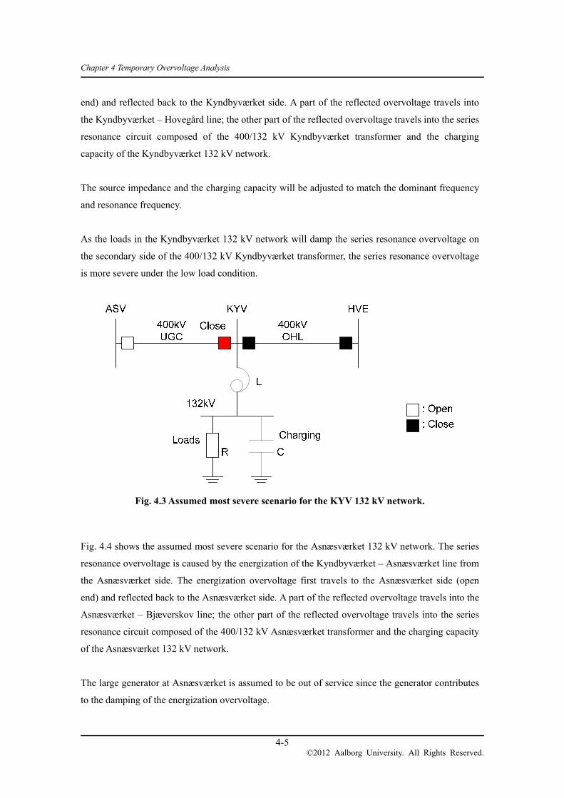
Chapter 4 Temporary Overvoltage Analysis
4-5 ©2012 Aalborg University. All Rights Reserved.
end) and reflected back to the Kyndbyværket side. A part of the reflected overvoltage travels into
the Kyndbyværket – Hovegård line; the other part of the reflected overvoltage travels into the series
resonance circuit composed of the 400/132 kV Kyndbyværket transformer and the charging
capacity of the Kyndbyværket 132 kV network.
The source impedance and the charging capacity will be adjusted to match the dominant frequency
and resonance frequency.
As the loads in the Kyndbyværket 132 kV network will damp the series resonance overvoltage on
the secondary side of the 400/132 kV Kyndbyværket transformer, the series resonance overvoltage
is more severe under the low load condition.
Fig. 4.3 Assumed most severe scenario for the KYV 132 kV network.
Fig. 4.4 shows the assumed most severe scenario for the Asnæsværket 132 kV network. The series
resonance overvoltage is caused by the energization of the Kyndbyværket – Asnæsværket line from
the Asnæsværket side. The energization overvoltage first travels to the Asnæsværket side (open
end) and reflected back to the Asnæsværket side. A part of the reflected overvoltage travels into the
Asnæsværket – Bjæverskov line; the other part of the reflected overvoltage travels into the series
resonance circuit composed of the 400/132 kV Asnæsværket transformer and the charging capacity
of the Asnæsværket 132 kV network.
The large generator at Asnæsværket is assumed to be out of service since the generator contributes
to the damping of the energization overvoltage.

Chapter 4 Temporary Overvoltage Analysis
4-6 ©2012 Aalborg University. All Rights Reserved.
Fig. 4.4 Assumed most severe scenario for the ASV 132 kV network.
Here, the Kyndbyværket – Asnæsværket line is energized from Bjæverskov since the generator at
Asnæsværket does not have a black start capability. If the generator has the black start capability,
the energization from the generator at Asnæsværket can be the most severe scenario which needs to
be studied.
4.1.3 Dominant Frequency in Energization Overvoltage
4.1.3.1 Derivations of Theoretical Formulas of Dominant Frequency
As discussed previously, severe temporary overvoltages, such as resonance overvoltages, only
occur in particular network conditions, and considerable efforts are made in system studies to find
these severe conditions. As the modeling of a broader area is necessary for the temporary
overvoltage analysis, it is time consuming to set up cable line models and to perform time domain
simulations and / or frequency scans in EMT-type programs.
As more long cables are installed, a simple estimation of the propagation velocity and the dominant
frequency component without carrying out time domain simulations or frequency scans is desired
for an efficient planning or operational planning of the network. For example, we can do without
the resonance overvoltage analysis caused by the switching of a particular cable if we know the
dominant frequency component caused by the switching of the cable does not match the natural

Chapter 4 Temporary Overvoltage Analysis
4-7 ©2012 Aalborg University. All Rights Reserved.
frequency of the network. With the knowledge on the estimated dominant frequency, therefore, the
efforts to find severe conditions can be greatly reduced. Based on the impedance and admittance
calculation in [5][6], this section addresses the estimation of the propagation velocity and the
dominant frequency component contained in the switching overvoltage of long cables.
(a) Average Impedance and Admittance
The metallic sheaths of a long cable are generally cross-bonded in order to reduce both the sheath
induced current and the sheath voltage. It has been found that the cross-bonding affect the
impedance and the admittance of the cable and their derivation is given in [5][6].
Assuming each minor section of a cable has an equal length, the average impedance of the
cross-bonded cable for one minor section is given in the following equation.
3/)( 11 RzRRzRzZ Eqn. 4.1
Here, z is the impedance of the cable per unit length for one minor section and R is a rotation
matrix.
ShShCoSh
CoShCoCo
zz
zzz Eqn. 4.2
010000
001000
100000
000100
000010
000001
R Eqn. 4.3
where CoCoz : impedance between conductors
CoShz : impedance between conductors and sheaths
ShShz : impedance between sheaths

Chapter 4 Temporary Overvoltage Analysis
4-8 ©2012 Aalborg University. All Rights Reserved.
Fig. 4.5 Cross-bonding Diagram.
The calculation of the average impedance yields the following equations.
ShShT
CoSh
CoShCoCo
ZZ
ZZZ Eqn. 4.4
CoCoCoCo zZ Eqn. 4.5
CSCSCS
BSBSBS
ASASAS
CoSh
ZZZ
ZZZ
ZZZ
Z Eqn. 4.6
SSSMSM
SMSSSM
SMSMSS
ShSh
ZZZ
ZZZ
ZZZ
Z Eqn. 4.7
Impedances in Eqn. 4.6 and Eqn. 4.7 are given by
3/)(
3/)(
3/)(
3/)(
3/)(
cabcabSM
ccbbaaSS
CcCbCaCS
BcBbBaBS
AcAbAaAS
zzzZ
zzzZ
zzzZ
zzzZ
zzzZ
Eqn. 4.8
In the subscripts of the impedances, capital letters show the phase of the conductor and lower
letters show the phase of the metallic sheath.

Chapter 4 Temporary Overvoltage Analysis
4-9 ©2012 Aalborg University. All Rights Reserved.
Similarly, the average admittance of the cross-bonded cable for one minor section can be calculated
as follows:
ShShCoSh
CoShCoCo
YY
YY
RyRRyRyY 3/)( 11
Eqn. 4.9
IyY AACoCo Eqn. 4.10
111
111
111
3AA
CoShy
Y Eqn. 4.11
IyY SSShSh Eqn. 4.12
In Eqn. 4.10 and Eqn. 4.12, I is an identity matrix.
Since the metallic sheath of the cross-bonded cable is earthed at the both ends of a major section,
Z and Y can be reduced to 4 × 4 matrices. The reduction is, however, not performed as the
dominant frequency can be found in a simpler form without the matrix reduction.
(b) Derivation of Theoretical Formulas
The main focus of the PhD project is to find the dominant frequency from Z and Y in simple
theoretical formulas. For a given length of a line, one propagation velocity is linked to one
dominant frequency by Eqn. 4.13.
length) (line44
1
i
if
Eqn. 4.13
Thus, we need to find the propagation velocity of the dominant frequency component in simple
theoretical formulas.
It is known that the propagation velocity of each mode is found by Eqn. 4.14 [7].
iii
yz
f02 Eqn. 4.14
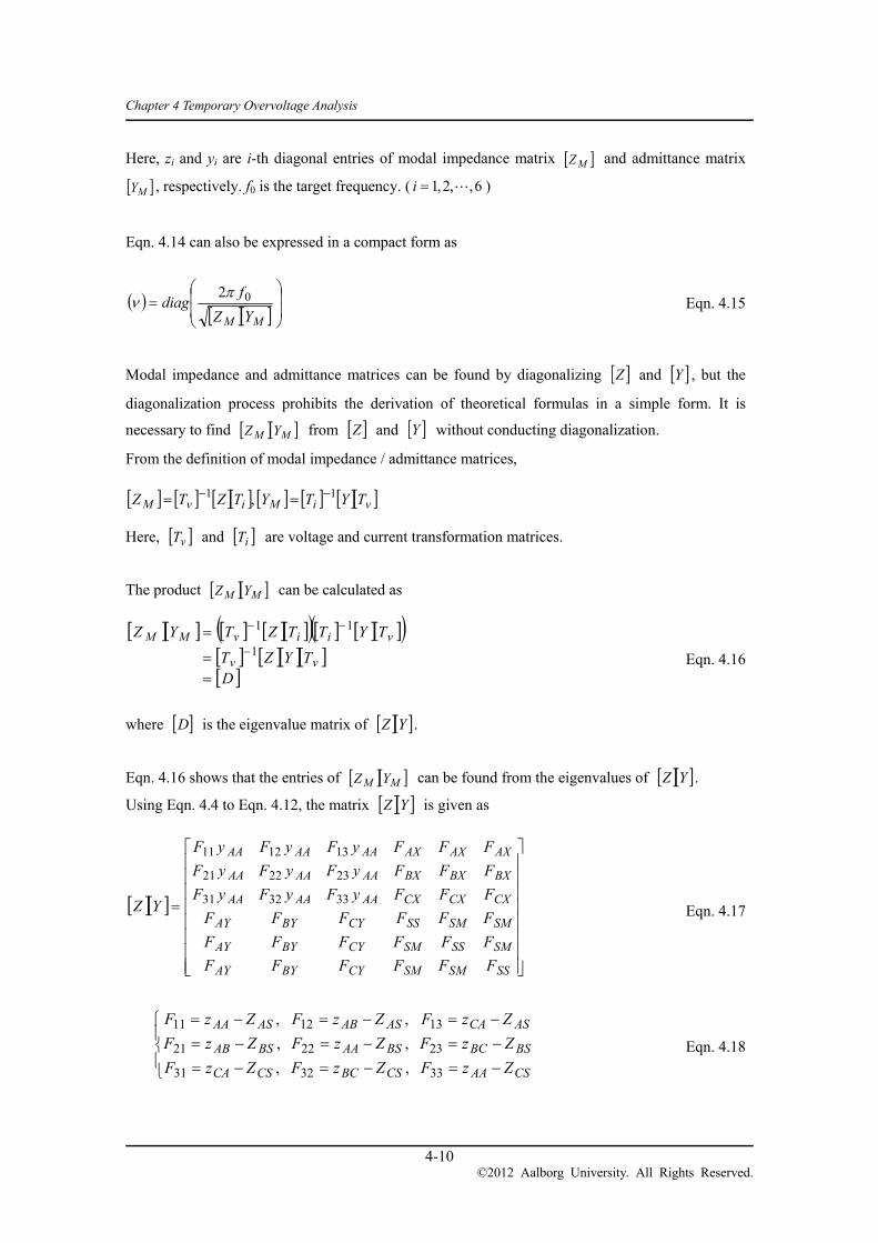
Chapter 4 Temporary Overvoltage Analysis
4-10 ©2012 Aalborg University. All Rights Reserved.
Here, zi and yi are i-th diagonal entries of modal impedance matrix MZ and admittance matrix
MY , respectively. f0 is the target frequency. ( 6,,2,1 i )
Eqn. 4.14 can also be expressed in a compact form as
MM YZ
fdiag 02
Eqn. 4.15
Modal impedance and admittance matrices can be found by diagonalizing Z and Y , but the
diagonalization process prohibits the derivation of theoretical formulas in a simple form. It is
necessary to find MM YZ from Z and Y without conducting diagonalization.
From the definition of modal impedance / admittance matrices,
viMivM TYTYTZTZ 11 ,
Here, vT and iT are voltage and current transformation matrices.
The product MM YZ can be calculated as
D
TYZT
TYTTZTYZ
vv
viivMM
1
11
Eqn. 4.16
where D is the eigenvalue matrix of YZ .
Eqn. 4.16 shows that the entries of MM YZ can be found from the eigenvalues of YZ .
Using Eqn. 4.4 to Eqn. 4.12, the matrix YZ is given as
SSSMSMCYBYAY
SMSSSMCYBYAY
SMSMSSCYBYAY
CXCXCXAAAAAA
BXBXBXAAAAAA
AXAXAXAAAAAA
FFFFFF
FFFFFF
FFFFFF
FFFyFyFyF
FFFyFyFyF
FFFyFyFyF
YZ 333231
232221
131211
Eqn. 4.17
CSAACSBCCSCA
BSBCBSAABSAB
ASCAASABASAA
ZzFZzFZzF
ZzFZzFZzF
ZzFZzFZzF
333231
232221
131211
,,
,,
,,
Eqn. 4.18

Chapter 4 Temporary Overvoltage Analysis
4-11 ©2012 Aalborg University. All Rights Reserved.
SSASAACAABAAAX yZyzzzF 3/)( Eqn. 4.19
BXF and CXF can be found similarly.
3/)2( AASMSSAAASAY yZZyZF Eqn. 4.20
BYF and CYF can be found similarly.
SSSSAACSBSASSS yZyZZZF 3/)( Eqn. 4.21
SSSMAACSBSASSM yZyZZZF 3/)( Eqn. 4.22
Instead of diagonalizing YZ , we propose to assume that the overvoltage caused by the
energization of a cross-bonded cable is dominated by inter-phase modes and the eigenvectors of
inter-phase modes are found in an ideal form in order to find the theoretical formulas in a simple
form. This assumption is reasonable since the overvoltage caused by the cable energization is
dominated by the coaxial mode when the dominant frequency found by Eqn. 4.13 is higher than
approximately 1000 – 1500 Hz, depending on the physical and electrical construction of a cable.
For a long cable, the dominant frequency is much lower than this and the overvoltage is dominated
by inter-phase modes.
Since the ideal eigenvector of the first inter-phase mode is known as
TVT )0003/13/23/1(1 , the eigenvalue corresponds to this inter-phase mode can be
estimated as
2/)2(
or)2(1
AABCABAA
AAACAAAB
yzzz
yzzzD
Eqn. 4.23
The eigenvalue corresponds to the second inter-phase mode TVT )0002/102/1(2 is
estimated as
AAACAA yzzD )(2 Eqn. 4.24
Once the eigenvalues are found by Eqn. 4.23 and Eqn. 4.24, the propagation velocities are found by
ii Df /2 0 Eqn. 4.25

Chapter 4 Temporary Overvoltage Analysis
4-12 ©2012 Aalborg University. All Rights Reserved.
(f0: target frequency, i = 1, 2)
Eqn. 4.23 to Eqn. 4.25 indicate that simple and readily available data give the estimation of
dominant frequency.
(c) Effect of Source Impedance
Theoretical formulas are, so far, derived assuming there is no source impedance. It can be justified
in the slow-front overvoltage analysis as the source impedance changes depending on the network
condition and no source impedance is supposedly the most severe assumption.
We consider below the effect of the source impedance since it affects the dominant frequency. The
amplitude of the overvoltage caused by the cable line energization will be mitigated by the
introduction of the source impedance, but also the lowered dominant frequency may excite
resonance and lead to higher resonance overvoltages.
First, when source impedance is given as lumped parameter impedance Z0, it has to be converted to
distributed parameter source impedance z0 by Eqn. 4.26. Fig. 4.6 illustrates the reason why the
conversion is necessary. By the conversion, the lumped parameter source impedance can be
considered as a part of distributed parameter cable line. The dominant frequency for the distributed
parameter model can be derived from Eqn. 4.13 and Eqn. 4.14.
2
00 4
2
Zz Eqn. 4.26
LCf
LCf
4
1
2
1
Fig. 4.6 Comparison of dominant frequency.
Assuming the source impedance is a part of the cable line, the eigenvalues correspond to the two
inter-phase modes are estimated as:

Chapter 4 Temporary Overvoltage Analysis
4-13 ©2012 Aalborg University. All Rights Reserved.
2/)2(
or)2(
0
01
AABCABAA
AAACAAAByzzzz
yzzzzD
Eqn. 4.27
AAACAA yzzzD )( 02 Eqn. 4.28
When the eigenvalues are found, the propagation velocity is calculated by Eqn. 4.25.
(d) Example
In order to verify the derived theoretical formulas, the dominant frequency calculated by the
theoretical formulas is compared with that found by EMTP simulations.
The dominant frequency contained in the overvoltage caused by the energization of the
Kyndbyværket – Asnæsværket line is very low because of the following two reasons:
The Kyndbyværket – Asnæsværket line is very long (60 km)
The fault current level around the Kyndbyværket – Asnæsværket line is very low
As only very low frequency components are contained, the Kyndbyværket – Asnæsværket line does
not suit for the verification. In addition, the Kyndbyværket – Asnæsværket line has the submarine
section near Kyndbyværket. Since the submarine cable is solidly-bonded, the dominant frequency
is determined by the coaxial mode, whose frequency is much simpler to find. As the dominant
frequency is not determined by the inter-phase mode, the derived theoretical formulas cannot be
applied.
Considering these problems, the verification was performed by the following conditions:
Assuming a switching station exists at Torslunde, the Asnæsværket – Torslunde line is
energized from Asnæsværket
The fault current level is adjusted by adding a dummy generator at Asnæsværket.
The source impedance of the dummy generator is changed from almost zero to infinite in order to
cover a broad range of the fault current level. The theoretical dominant frequency is found for each
source impedance as shown in Table 4-1. Since there are two inter-phase modes, an average of two
modes is adopted as the theoretical propagation velocity and the dominant frequency, assuming
equal contribution from the two modes.
Table 4-1 Source Impedance and Theoretical Dominant Frequency
Source Impedance
(Dummy Generator) 0.1 mH 50 mH 100 mH 200 mH Infinite

Chapter 4 Temporary Overvoltage Analysis
4-14 ©2012 Aalborg University. All Rights Reserved.
Network Source Impedance 0.1 mH 24.5 mH 37.5 mH 51.0 mH 71.4 mH
Propagation Velocity (mode 1) 97.6 m/μs 44.5 m/μs 37.0 m/μs 32.2 m/μs 27.5 m/μs
Propagation Velocity (mode 2) 86.9 m/μs 42.3 m/μs 35.7 m/μs 31.3 m/μs 27.0 m/μs
Propagation Velocity (average) 92.3 m/μs 43.4 m/μs 36.3 m/μs 31.7 m/μs 27.2 m/μs
Dominant Frequency 823.7 Hz 387.5 Hz 324.4 Hz 283.3 Hz 243.1 Hz
The EMTP simulations are performed with PSCAD in order to find dominant frequencies. Fig. 4.7
shows the simulation model set up for the analysis.
Fig. 4.7 PSCAD simulation model for finding the dominant frequency.

Chapter 4 Temporary Overvoltage Analysis
4-15 ©2012 Aalborg University. All Rights Reserved.
Fig. 4.8 to Fig. 4.12 show energization overvoltages at the open terminal Torslunde for different
fault current levels. The dominant frequency in each case is found by performing Fourier transform
to the voltage waveform.
Fig. 4.8 Energization overvoltage at open terminal (dummy source 0.1 mH).
Fig. 4.9 Energization overvoltage at open terminal (dummy source 50 mH).
(file Source0mH0.1s.adf; x-var Time) TOR40A TOR40B TOR40C 0.00 0.02 0.04 0.06 0.08 0.10 0.12
-500
-240
20
280
540
800
(file Source25mH0.1s.adf; x-var Time) TOR40A TOR40B TOR40C 0.00 0.02 0.04 0.06 0.08 0.10 0.12
-500
-280
-60
160
380
600

Chapter 4 Temporary Overvoltage Analysis
4-16 ©2012 Aalborg University. All Rights Reserved.
Fig. 4.10 Energization overvoltage at open terminal (dummy source 100 mH).
Fig. 4.11 Energization overvoltage at open terminal (dummy source 200 mH).
(file Source38mH0.1s.adf; x-var Time) TOR40A TOR40B TOR40C 0.00 0.02 0.04 0.06 0.08 0.10 0.12
-500
-280
-60
160
380
600
(file Source47mH0.1s.adf; x-var Time) TOR40A TOR40B TOR40C 0.00 0.02 0.04 0.06 0.08 0.10 0.12
-500
-280
-60
160
380
600

Chapter 4 Temporary Overvoltage Analysis
4-17 ©2012 Aalborg University. All Rights Reserved.
Fig. 4.12 Energization overvoltage at open terminal (no dummy source).
Fig. 4.13 illustrates the comparison of dominant frequencies derived by theoretical formulas and
those found by EMTP simulations. The comparison shows that the derived theoretical formulas
have very high accuracy.
Fig. 4.13 Comparison of dominant frequencies found by theoretical formulas and EMTP
simulations.
(file Source71mH0.1s.adf; x-var Time) TOR40A TOR40B TOR40C 0.00 0.02 0.04 0.06 0.08 0.10 0.12
-500
-280
-60
160
380
600
100
300
500
700
900
0 25 50 75
Network Source Impedance (mH)
Dom
inan
t Fr
eque
ncy
(Hz)
Theoretical Formulas
Simulation result

Chapter 4 Temporary Overvoltage Analysis
4-18 ©2012 Aalborg University. All Rights Reserved.
In addition to the Asnæsværket – Torslunde line, the energization of the Kyndbyværket – Torslunde
line is studied for the verification. In the same way as in the Asnæsværket – Torslunde line, the
fault current level is adjusted by adding a dummy generator at Kyndbyværket.
The Kyndbyværket – Torslunde line has a 10 km submarine section on the Kyndbyværket side. As
the submarine cable is solidly-bonded, the propagation velocity in this section is faster compared
with that in the cross-bonded section. Only for the verification, the 10 km submarine cable is
replaced by the underground cable (cross-bonded) so that the theoretical formula can be applied.
The source impedance of the dummy generator is changed from almost zero to infinite in order to
cover broad range of the fault current level. The theoretical dominant frequency is found for each
source impedance as shown in Table 4-2. Since there are two inter-phase modes, an average of two
modes is adopted as the theoretical propagation velocity and dominant frequency, assuming equal
contribution from the two modes.
Table 4-2 Source Impedance and Theoretical Dominant Frequency
Source Impedance
(Dummy Generator) 0.1 mH 50 mH 100 mH 200 mH Infinite
Network Source Impedance 0.1 mH 24.5 mH 37.5 mH 51.0 mH 71.4 mH
Propagation Velocity (mode 1) 97.6 m/μs 58.7 m/μs 50.9 m/μs 45.5 m/μs 37.5 m/μs
Propagation Velocity (mode 2) 86.9 m/μs 44.6 m/μs 38.0 m/μs 33.5 m/μs 27.3 m/μs
Propagation Velocity (average) 92.3 m/μs 51.6 m/μs 44.5 m/μs 39.5 m/μs 32.4 m/μs
Dominant Frequency 720.7 Hz 403.5 Hz 347.3 Hz 308.5 Hz 252.9 Hz
The EMTP simulations are performed with PSCAD in order to find dominant frequencies. Fig. 4.20
to Fig. 4.24 show energization overvoltages at the open terminal Torslunde for different fault
current levels. The dominant frequency in each case is found by performing Fourier transform to
the voltage waveform.

Chapter 4 Temporary Overvoltage Analysis
4-19 ©2012 Aalborg University. All Rights Reserved.
Fig. 4.14 Energization overvoltage at open terminal (dummy source 0.1 mH).
Fig. 4.15 Energization overvoltage at open terminal (dummy source 50 mH).
(file Source0mH0.1s.adf; x-var Time) TOR40A TOR40B TOR40C 0.00 0.02 0.04 0.06 0.08 0.10 0.12
-600
-340
-80
180
440
700
(file Source24mH0.1s.adf; x-var Time) TOR40A TOR40B TOR40C 0.00 0.02 0.04 0.06 0.08 0.10 0.12
-500
-280
-60
160
380
600

Chapter 4 Temporary Overvoltage Analysis
4-20 ©2012 Aalborg University. All Rights Reserved.
Fig. 4.16 Energization overvoltage at open terminal (dummy source 100 mH).
Fig. 4.17 Energization overvoltage at open terminal (dummy source 200 mH).
(file Source37mH0.1s.adf; x-var Time) TOR40A TOR40B TOR40C 0.00 0.02 0.04 0.06 0.08 0.10 0.12
-400
-200
0
200
400
600
(file Source50mH0.1s.adf; x-var Time) TOR40A TOR40B TOR40C 0.00 0.02 0.04 0.06 0.08 0.10 0.12
-400
-250
-100
50
200
350
500

Chapter 4 Temporary Overvoltage Analysis
4-21 ©2012 Aalborg University. All Rights Reserved.
Fig. 4.18 Energization overvoltage at open terminal (no dummy source).
Fig. 4.19 illustrates the comparison of dominant frequencies evaluated by theoretical formulas and
those found by EMTP simulations. The comparison shows that the derived theoretical formulas
agree satisfactory with the simulation results with the largest error of 50 Hz.
Fig. 4.19 Comparison of dominant frequencies found by theoretical formulas and EMTP
simulations.
(file Source80mH0.1s.adf; x-var Time) TOR40A TOR40B TOR40C 0.00 0.02 0.04 0.06 0.08 0.10 0.12
-500
-375
-250
-125
0
125
250
375
500
0.0
200.0
400.0
600.0
800.0
0 20 40 60 80
Source Impedance (mH)
Dom
inan
t Fre
quen
cy (
Hz)
Theoretical Formulas
Simulation result

Chapter 4 Temporary Overvoltage Analysis
4-22 ©2012 Aalborg University. All Rights Reserved.
The following observations / evaluations can be made to the error of theoretical formulas:
The error 50 Hz does not affect the practical usefulness of the theoretical formulas since
the natural frequency of a series resonance circuit as described in Sections 4.1.1 and 4.1.2
can range much broader than 50 Hz due to different load conditions.
From the comparison for source impedance 0.1 mH, the inter-phase modes are estimated
accurately. The error was introduced by the effect of the source impedance
The effect of the source impedance or a surrounding network is actually a difficult problem,
and a clear solution to this problem has not been found yet. In the energization of the
Asnæsværket – Torslunde line, the surrounding network is closer to the ideal condition
since the Asnæsværket – Herslev line (22 km) and the Herslev – Bjæverskov line (47 km)
is long and the distance to the neighboring voltage source is longer than 100 km. In
contrast, in the energization of the Kyndbyværket – Torslunde line, the Kyndbyværket –
Lyngerup line (7 km) and the Lyngerup – Hovegård line (18 km) is short for typical 400
kV lines and the distance to the neighboring voltage source is shorter. The energization
overvoltage of the Kyndbyværket – Torslunde line is, therefore, more affected by the
reflection at nearby substations (Lyngerup and Hovegård), which is not considered in the
theoretical formulas.
4.1.3.2 Off-peak Load Condition
First, the dominant frequency in an energization overvoltage is studied in the off-peak load
condition. When a transmission line, either an overhead line or a cable, is energized from a weaker
source, which has a larger source impedance (off-peak load condition), the magnitude of the
energization overvoltage becomes lower and the dominant frequency becomes lower. In general,
the off-peak load condition is a more severe assumption because of the following reasons:
Damping from the loads (more important)
The loads in the Asnæsværket or Kyndbyværket 132 kV network will damp the series
resonance overvoltage on the secondary side of the 400/132 kV transformer. The load level
has to be low in order to have a severe resonance.
Damping from the network (transformers, lines, and etc.)
The lower dominant frequency means an extended duration of the overvoltage. The high
frequency components, which raise the magnitude of the overvoltage in a stiff source case,
typically dies out quickly due to the large damping (losses).
However, this general notion may not be true in the energization of the Kyndbyværket –
Asnæsværket line. In Section 3.3, the Kyndbyværket – Asnæsværket line was energized from the

Chapter 4 Temporary Overvoltage Analysis
4-23 ©2012 Aalborg University. All Rights Reserved.
400 kV voltage source behind source impedance 147 mH, which corresponds to the fault current 5
kA. In that case, the dominant frequency was already low (100 – 150 Hz) in the energization, due to
the large charging capacity of the cable. If we make the source impedance larger, the dominant
frequency goes down towards 50 Hz, and it is hard to observe the energization overvoltage as the
magnitude becomes lower. The dominant frequency in the peak load condition is, therefore, studied
in the next section.
Here, in the off-peak load condition, the Kyndbyværket – Asnæsværket line is energized from the
Kyndbyværket side according to Fig. 4.3. Only one large generator in AVV and the equivalent
generator in SAN are assumed to be in-service in the simulation. The cable line is energized at the
phase b voltage peak.
The energization overvoltage is shown in Fig. 4.20 and Fig. 4.21. Fig. 4.20 is the voltage waveform
at the sending end (Kyndbyværket side), and Fig. 4.21 is the voltage waveform at the receiving end
(Asnæsværket side cable open terminal). As can be seen from the figure, the waveforms look not
like typical energization overvoltages due to the length of the cable and the large charging capacity.
High frequency components are contained in the waveforms with very small proportions.
Fig. 4.20 Energization overvoltage of the KYV – ASV line from the KYV side (sending end).
(file SeriesResonance_KYV.pl4; x-var t) v:KYV40A v:KYV40B v:KYV40C 0 10 20 30 40 50 60 70 80[ms]
-500
-350
-200
-50
100
250
400
[kV]

Chapter 4 Temporary Overvoltage Analysis
4-24 ©2012 Aalborg University. All Rights Reserved.
Fig. 4.21 Energization overvoltage of the KYV – ASV line from the KYV side (receiving end).
(file SeriesResonance_KYV.pl4; x-var t) v:ASV4RA v:ASV4RB v:ASV4RC 0 10 20 30 40 50 60 70 80[ms]
-500
-350
-200
-50
100
250
400
[kV]
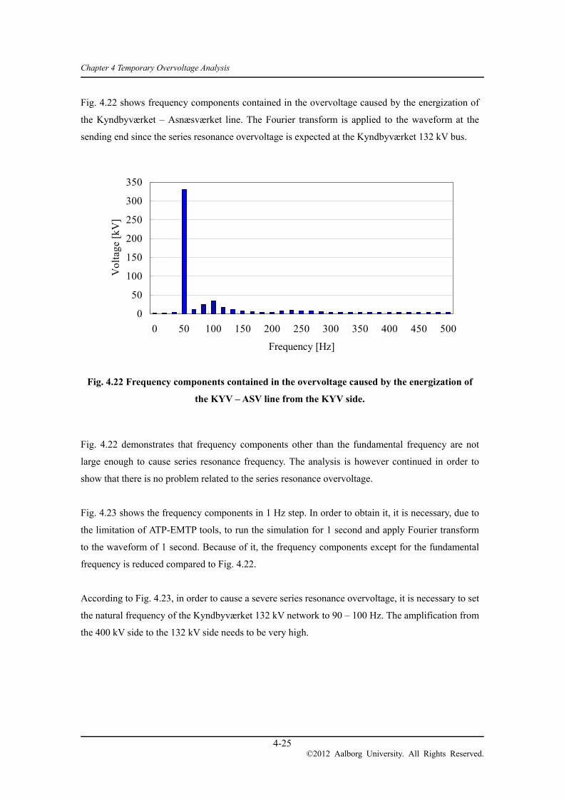
Chapter 4 Temporary Overvoltage Analysis
4-25 ©2012 Aalborg University. All Rights Reserved.
Fig. 4.22 shows frequency components contained in the overvoltage caused by the energization of
the Kyndbyværket – Asnæsværket line. The Fourier transform is applied to the waveform at the
sending end since the series resonance overvoltage is expected at the Kyndbyværket 132 kV bus.
Fig. 4.22 Frequency components contained in the overvoltage caused by the energization of
the KYV – ASV line from the KYV side.
Fig. 4.22 demonstrates that frequency components other than the fundamental frequency are not
large enough to cause series resonance frequency. The analysis is however continued in order to
show that there is no problem related to the series resonance overvoltage.
Fig. 4.23 shows the frequency components in 1 Hz step. In order to obtain it, it is necessary, due to
the limitation of ATP-EMTP tools, to run the simulation for 1 second and apply Fourier transform
to the waveform of 1 second. Because of it, the frequency components except for the fundamental
frequency is reduced compared to Fig. 4.22.
According to Fig. 4.23, in order to cause a severe series resonance overvoltage, it is necessary to set
the natural frequency of the Kyndbyværket 132 kV network to 90 – 100 Hz. The amplification from
the 400 kV side to the 132 kV side needs to be very high.
0
50
100
150
200
250
300
350
0 50 100 150 200 250 300 350 400 450 500
Frequency [Hz]
Vol
tage
[kV
]

Chapter 4 Temporary Overvoltage Analysis
4-26 ©2012 Aalborg University. All Rights Reserved.
Fig. 4.23 Frequency components contained in the overvoltage caused by the energization of
the KYV – ASV line from the KYV side (1Hz step).
Second, the Kyndbyværket – Asnæsværket line is energized from the Asnæsværket side according
to Fig. 4.4. The cable line is energized at the phase b voltage peak.
The energization overvoltage is shown in Fig. 4.24 and Fig. 4.25. Fig. 4.24 is the voltage waveform
at the sending end (Asnæsværket side), and Fig. 4.25 is the voltage waveform at the receiving end
(Kyndbyværket side cable open terminal). As in the energization overvoltage from the
Kyndbyværket side, high frequency components are contained in the waveforms with very small
proportions.
0
0.5
1
1.5
2
2.5
0 50 100 150 200 250 300
Frequency [Hz]
Vol
tage
[kV
]

Chapter 4 Temporary Overvoltage Analysis
4-27 ©2012 Aalborg University. All Rights Reserved.
Fig. 4.24 Energization overvoltage of the KYV – ASV line from the ASV side (sending end).
Fig. 4.25 Energization overvoltage of the KYV – ASV line from the ASV side (receiving end).
(file SeriesResonance_ASV.pl4; x-var t) v:ASV40A v:ASV40B v:ASV40C 0 10 20 30 40 50 60 70 80[ms]
-500
-350
-200
-50
100
250
400
[kV]
(file SeriesResonance_ASV.pl4; x-var t) v:KYV4RA v:KYV4RB v:KYV4RC 0 10 20 30 40 50 60 70 80[ms]
-500
-350
-200
-50
100
250
400
[kV]

Chapter 4 Temporary Overvoltage Analysis
4-28 ©2012 Aalborg University. All Rights Reserved.
Fig. 4.26 and Fig. 4.27 show frequency components contained in the overvoltage caused by the
energization of the Kyndbyværket – Asnæsværket line from the Asnæsværket side. The Fourier
transform is applied to the waveform at the sending end since the series resonance overvoltage is
expected at the Asnæsværket 132 kV bus.
Fig. 4.26 Frequency components contained in the overvoltage caused by the energization of
the KYV – ASV line from the ASV side.
Fig. 4.27 Frequency components contained in the overvoltage caused by the energization of
the KYV – ASV line from the ASV side (1Hz step).
0
50
100
150
200
250
300
350
0 50 100 150 200 250 300 350 400 450 500
Frequency [Hz]
Vol
tage
[kV
]
0
0.5
1
1.5
2
2.5
3
0 50 100 150 200 250 300
Frequency [Hz]
Vol
tage
[kV
]

Chapter 4 Temporary Overvoltage Analysis
4-29 ©2012 Aalborg University. All Rights Reserved.
As in the energization from the Kyndbyværket side, the natural frequency of the Asnæsværket 132
kV has to be set to 85 – 100 Hz in order to cause a severe series resonance overvoltage. The
amplification from the 400 kV side to the 132 kV side needs to be very high.
4.1.3.3 Peak Load Condition
In order to have a larger magnitude of the energization overvoltage, energizations from the stiffer
voltage source, namely in the peak load condition, is additionally studied. To make the voltage
source stiffer, the large generator at Asnæsværket is assumed to be in-service. In addition,
equivalent generators are modeled near the line, that is, at the HVE and BJS 132 kV buses. Adding
equivalent generators at the ASV and KYV 132 kV buses would be more efficient to make the
voltage source stiffer, but it is not considered since these voltage sources will suppress the series
resonance overvoltage at the ASV and KYV 132 kV buses.
The source impedances for these equivalent generators are derived from the results of the short
circuit current calculation in the peak load condition as shown in Table 4-3. Only the short circuit
current from the 132 kV network is considered
Table 4-3 Source Impedances of 132 kV Equivalent Generators
132 kV Buses Short Circuit Current Source Impedance
Hovegård 19.6 kA 12.4 mH
Bjæverskov 13.3 kA 18.2 mH
Fig. 4.28 shows these additions of generators in the simulation model in the peak load condition.

Chapter 4 Temporary Overvoltage Analysis
4-30 ©2012 Aalborg University. All Rights Reserved.
Fig. 4.28 Addition of generators to set up the peak load condition.
Fig. 4.29 and Fig. 4.30 show energization overvoltages of the Kyndbyværket – Asnæsværket line
when the line is energized from the Kyndbyværket side. In overall, the waveforms of the
overvoltages are similar to the ones observed in the off-peak load condition. The change of the
loading condition does not have a significant difference on the energization overvoltage. It is
mainly because the fault current level at the Kyndbyværket 400 kV bus is very small, only 11.4 kA,
even in the peak load condition.
Only one notable difference is that the energization overvoltages in the peak load condition have
more damping. In the off-peak load condition, non-fundamental components can be observed in the
LCC
22. km
LCC
46.73 km
AB
C
ASV40S
AT
YY
HKS40
SA
T
YY
Y
LC
C
26.
25
km
LC
C
11.
14
km
ISH40LCC
5.675 km
LCC
6.89 km
V
LC
C
20.
68 k
m
LCC
35.8
5 k
m GOR40
SAT
Y Y
LCC
27.
2 k
m
V
12km
AVV40GROUPish_avv
9km
HCV40GROUPavv_hcv
12km
GLN40GROUPhve_gln
8.43km
GR
OU
Pgo
r_sa
n
9.47km
GR
OU
Phv
e_sa
n
BJS40
SA
T
YY
SA
T
YY
SA
T
YY
SA
T
YY
HVE40S
AT
YY
SA
T
YY
SA
T
YY
SA
T
YY
SAT
Y Y
SA
T
Y
X0133
SA
T
Y
SAN40
SA
T
YY
LCC
18.15 km
LCC
4.76 km132kV
KYV40 LCC
1.99 kmLCC
1.99 km
KYV13
VABC
ASV4R
TOR40
GR
OU
PA
SV
-TO
R
V
KYV4S
GR
OU
PT
OR
-KY
V
V
370MVar
126MVar
100MVar
V
LUP13
Ignore feeder 0.15km
HVE-OLS 7.3kmOLS-LUP (11.0-0.15)km
Large generator at ASV
Equivalent source
at BJS 132 kV
Equivalent source
at HVE 132 kV

Chapter 4 Temporary Overvoltage Analysis
4-31 ©2012 Aalborg University. All Rights Reserved.
waveform even at 80 ms. In contrast, in the peak load condition, we can observe only a
fundamental frequency component after 40 ms.
Fig. 4.29 Energization overvoltage of the KYV – ASV line from the KYV side (peak load,
sending end).
Fig. 4.30 Energization overvoltage of the KYV – ASV line from the KYV side (peak load,
receiving end).
(file SeriesResonance_KYV_Peak.pl4; x-var t) v:KYV40A v:KYV40B v:KYV40C 0 10 20 30 40 50 60 70 80[ms]
-500
-350
-200
-50
100
250
400
[kV]
(file SeriesResonance_KYV_Peak.pl4; x-var t) v:ASV4RA v:ASV4RB v:ASV4RC 0 10 20 30 40 50 60 70 80[ms]
-500
-350
-200
-50
100
250
400
[kV]

Chapter 4 Temporary Overvoltage Analysis
4-32 ©2012 Aalborg University. All Rights Reserved.
Fig. 4.31 and Fig. 4.32 show frequency components contained in the overvoltage caused by the
energization of the Kyndbyværket – Asnæsværket line. The dominant frequency goes up to 120 –
125 Hz, which explains the more damping observed in the voltage waveforms. Compared to the
off-peak load condition, the distribution of frequency components becomes flatter. It is clear that
the off-peak load condition is more severe in terms of the overvoltage which propagates into the
Kyndbyværket 132 kV bus.
Fig. 4.31 Frequency components contained in the overvoltage caused by the energization of
the KYV – ASV line from the KYV side (peak load).
Fig. 4.32 Frequency components contained in the overvoltage caused by the energization of
the KYV – ASV line from the KYV side (peak load, 1Hz step).
0
50
100
150
200
250
300
350
0 50 100 150 200 250 300 350 400 450 500
Frequency [Hz]
Vol
tage
[kV
]
0
0.5
1
1.5
2
2.5
0 50 100 150 200 250 300
Frequency [Hz]
Vol
tage
[kV
]
flatter
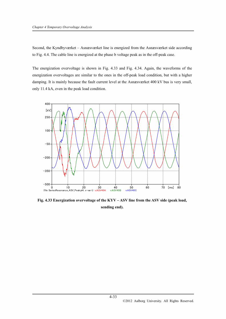
Chapter 4 Temporary Overvoltage Analysis
4-33 ©2012 Aalborg University. All Rights Reserved.
Second, the Kyndbyværket – Asnæsværket line is energized from the Asnæsværket side according
to Fig. 4.4. The cable line is energized at the phase b voltage peak as in the off-peak case.
The energization overvoltage is shown in Fig. 4.33 and Fig. 4.34. Again, the waveforms of the
energization overvoltages are similar to the ones in the off-peak load condition, but with a higher
damping. It is mainly because the fault current level at the Asnæsværket 400 kV bus is very small,
only 11.4 kA, even in the peak load condition.
Fig. 4.33 Energization overvoltage of the KYV – ASV line from the ASV side (peak load,
sending end).
(file SeriesResonance_ASV_Peak.pl4; x-var t) v:ASV40A v:ASV40B v:ASV40C 0 10 20 30 40 50 60 70 80[ms]
-500
-350
-200
-50
100
250
400
[kV]

Chapter 4 Temporary Overvoltage Analysis
4-34 ©2012 Aalborg University. All Rights Reserved.
Fig. 4.34 Energization overvoltage of the KYV – ASV line from the ASV side (peak load,
receiving end).
Fig. 4.35 and Fig. 4.36 show frequency components contained in the overvoltage caused by the
energization of the Kyndbyværket – Asnæsværket line from the Asnæsværket side in the peak load
condition. As in the energization from the Kyndbyværket side, the dominant frequency goes up to
120 – 125 Hz, which explains the better damping observed in the voltage waveforms. Compared to
the off-peak load condition, the distribution of frequency components becomes flatter. It is clear
that the off-peak load condition is more severe in terms of the overvoltage which propagates into
the Kyndbyværket 132 kV bus.
(file SeriesResonance_ASV_Peak.pl4; x-var t) v:KYV4RA v:KYV4RB v:KYV4RC 0 10 20 30 40 50 60 70 80[ms]
-500
-350
-200
-50
100
250
400
[kV]
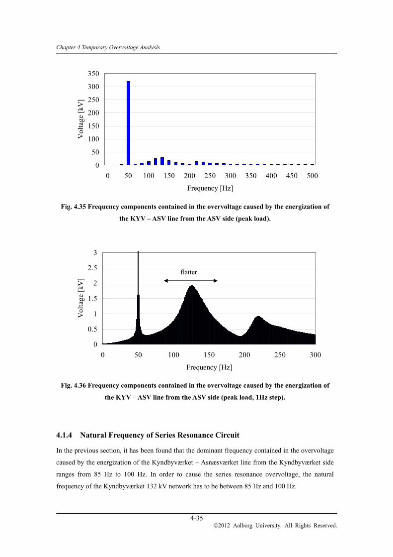
Chapter 4 Temporary Overvoltage Analysis
4-35 ©2012 Aalborg University. All Rights Reserved.
Fig. 4.35 Frequency components contained in the overvoltage caused by the energization of
the KYV – ASV line from the ASV side (peak load).
Fig. 4.36 Frequency components contained in the overvoltage caused by the energization of
the KYV – ASV line from the ASV side (peak load, 1Hz step).
4.1.4 Natural Frequency of Series Resonance Circuit
In the previous section, it has been found that the dominant frequency contained in the overvoltage
caused by the energization of the Kyndbyværket – Asnæsværket line from the Kyndbyværket side
ranges from 85 Hz to 100 Hz. In order to cause the series resonance overvoltage, the natural
frequency of the Kyndbyværket 132 kV network has to be between 85 Hz and 100 Hz.
0
50
100
150
200
250
300
350
0 50 100 150 200 250 300 350 400 450 500
Frequency [Hz]
Vol
tage
[kV
]
0
0.5
1
1.5
2
2.5
3
0 50 100 150 200 250 300
Frequency [Hz]
Vol
tage
[kV
]
flatter

Chapter 4 Temporary Overvoltage Analysis
4-36 ©2012 Aalborg University. All Rights Reserved.
As discussed in Section 4.1.1, the natural frequency of the Kyndbyværket 132 kV network can be
found as LC
fn2
1 using 400/132 kV transformer inductance L and 132 kV cable capacitance
C. In order to set the natural frequency to 90 Hz, Eqn. 4.29 has to be satisfied.
9002088.02
1
C Eqn. 4.29
C = 149.8 [μF]
Cable capacitance 149.8 μF corresponds to 819.8 MVar in the 132 kV network. This amount of
cable capacitance is too large to assume in the 132 kV network. In terms of the cable length,
assuming the typical cable capacitance per length 0.2 μF/km, cable capacitance 149.8 μF
corresponds to 132 kV cable of about 750 km in circuit length. From the above, it is reasonable to
conclude that the series resonance overvoltage will not occur in the Kyndbyværket 132 kV network
due to the installation of the Kyndbyværket – Asnæsværket line.
The series resonance overvoltage is, however, studied from an academic interest. When 132 kV
cable capacitance 149.8 μF is connected to the Kyndbyværket 132 kV bus, it results in the natural
frequency of the Kyndbyværket 132 kV network to 90 Hz and, at the same time, will raise the
steady-state system voltage around the Kyndbyværket substation. A shunt reactor has to be assumed
at the Kyndbyværket 132 kV bus, so as to prevent the steady-state overvoltage.
In order to 100 % compensate for the large reactive power produced from the cable capacitance
149.8 μF, the shunt reactor L = 67.65 mH has to be connected to the Kyndbyværket 132 kV bus.
However, this shunt reactor shifts the natural frequency of the Kyndbyværket 132 kV network to
100 Hz, which is not ideal to cause a severe series resonance. In order to shift the natural frequency
lower, the cable capacitance is increased to 170.0 μF. It is confirmed that this increase does not
cause the steady-state overvoltage.
In the above mentioned condition, the frequency scan is performed to find the natural frequency of
the Kyndbyværket 132 kV network. Fig. 4.37 shows the result of the frequency scan. As can be
seen from the figure, the natural frequency of the Kyndbyværket 132 kV network is successfully set
to 95 Hz.

Chapter 4 Temporary Overvoltage Analysis
4-37 ©2012 Aalborg University. All Rights Reserved.
Fig. 4.37 Series resonance frequency of the KYV network.
In order to have severe series resonance, it is necessary to have a high voltage amplification ratio
from the Kyndbyværket 400 kV bus to the 132 kV bus. The amplification ratio is shown in Fig.
4.38. It is observed in the figure that the amplification ratio is approximately 6 at 88 Hz, which is
not very high.
(file FreqScan_KYV_AddC.pl4; x-var t) v:KYV40A v:KYV40B v:KYV40C 0 100 200 300 400 500[Hz]
0.0
0.3
0.6
0.9
1.2
1.5
[MΩ]
(file FreqScan_KYV_AddC.pl4; x-var t) v:KYV40A v:KYV40B v:KYV40C 0 100 200 300 400 500[Hz]
0
20
40
60
80
100
120
140
160
[kΩ]
Zoom
95Hz 219Hz

Chapter 4 Temporary Overvoltage Analysis
4-38 ©2012 Aalborg University. All Rights Reserved.
Fig. 4.38 Voltage amplification ratio from the KYV 400 kV bus to the 132 kV bus.
The amplification ratio is highly affected by the loading condition. In terms of the amplification
ratio, the assumed condition is already severe since it is derived in the off-peak load condition. If it
is necessary to assume the no load condition in the Kyndbyværket 132 kV network, it significantly
increases the amplification ratio. Fig. 4.39 shows that the amplification ratio increases to around 25
in the no load condition.
Fig. 4.39 Voltage amplification ratio from the KYV 400 kV bus to the 132 kV bus in the no
load condition.
0
1
2
3
4
5
6
7
0 100 200 300 400 500 600
Frequency [Hz]
Am
plif
icat
ion
Rat
io (
V13
2/V
400)
0
5
10
15
20
25
30
0 100 200 300 400 500 600
Frequency [Hz]
Am
plif
icat
ion
Rat
io (
V13
2/V
400)

Chapter 4 Temporary Overvoltage Analysis
4-39 ©2012 Aalborg University. All Rights Reserved.
The same analysis is performed for the Asnæsværket 132 kV network. According to Eqn. 4.30, 132
kV cable capacitance 77.7 μF is assumed in the Asnæsværket 132 kV network. Again, this cable
capacitance corresponds to 425.4 MVar or 388.6 km in circuit length in the Asnæsværket 132 kV
network. It is thus concluded that the series resonance overvoltage will not occur in the
Asnæsværket 132 kV network due to the installation of the Kyndbyværket – Asnæsværket line.
90
0402.00000362.02
1
C Eqn. 4.30
C = 77.7 [μF]
Fig. 4.40 shows the result of the frequency scan. As can be seen from the figure, the natural
frequency of the Asnæsværket 132 kV network is successfully set to 100 Hz. The natural frequency
is shifted from 90 Hz to 100 Hz by the inductance L = 130.4 mH, which represents the shunt
reactor to compensate for the large reactive power from the 132 kV cable. It is not possible in this
case to lower the natural frequency by increasing 132 kV cable capacitance as it causes steady-state
overvoltage.
In order to have severe series resonance, it is necessary to have a high voltage amplification ratio
from the Asnæsværket 400 kV bus to the 132 kV bus. The amplification ratio is shown in Fig. 4.41.
It is clear in the figure that the amplification ratio is approximately 3.5 at 100 Hz, which is not very
high.
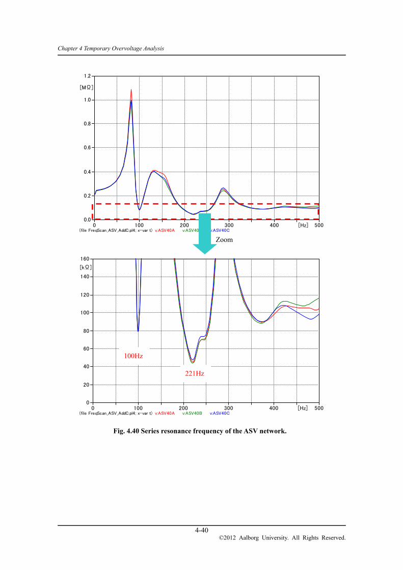
Chapter 4 Temporary Overvoltage Analysis
4-40 ©2012 Aalborg University. All Rights Reserved.
Fig. 4.40 Series resonance frequency of the ASV network.
(file FreqScan_ASV_AddC.pl4; x-var t) v:ASV40A v:ASV40B v:ASV40C 0 100 200 300 400 500[Hz]
0.0
0.2
0.4
0.6
0.8
1.0
1.2
[MΩ]
(file FreqScan_ASV_AddC.pl4; x-var t) v:ASV40A v:ASV40B v:ASV40C 0 100 200 300 400 500[Hz]
0
20
40
60
80
100
120
140
160
[kΩ]
Zoom
100Hz
221Hz

Chapter 4 Temporary Overvoltage Analysis
4-41 ©2012 Aalborg University. All Rights Reserved.
Fig. 4.41 Voltage amplification ratio from the ASV 400 kV bus to the 132 kV bus.
In the no load condition, the amplification ratio is increased to around 43 as shown in Fig. 4.42.
Fig. 4.42 Voltage amplification ratio from the ASV 400 kV bus to the 132 kV bus in the no
load condition.
0
0.5
1
1.5
2
2.5
3
3.5
4
0 100 200 300 400 500 600
Frequency [Hz]
Am
plif
icat
ion
Rat
io (
V13
2/V
400)
0
10
20
30
40
50
0 100 200 300 400 500 600
Frequency [Hz]
Am
plif
icat
ion
Rat
io (
V13
2/V
400)

Chapter 4 Temporary Overvoltage Analysis
4-42 ©2012 Aalborg University. All Rights Reserved.
4.1.5 Simulation Results of Series Resonance Overvoltage
The time domain simulations are performed to find the series resonance overvoltage in the assumed
most severe condition. First, the Kyndbyværket – Asnæsværket line is energized from the
Kyndbyværket side and the overvoltage in the Kyndbyværket 132 kV bus is monitored as shown in
Fig. 4.43.
Fig. 4.43 Simulation model to find the series resonance overvoltage in the Kyndbyværket 132
kV bus.
Results of the time domain simulations are shown in Fig. 4.44. In the figure, the upper graph shows
the phase to ground overvoltage, and the lower graph shows the phase to phase overvoltage.
According to IEC 60071, the standard short-duration power-frequency withstand voltage for the
132 kV equipment is (185), 230 or 275 kV (rms). The same withstand voltages are applied to both
the phase to ground overvoltage and the phase to phase overvoltage. Here, the application to the
LCC
22. km
LCC
46.73 km
AB
C
ASV40
SA
T
YY
HKS40
SA
T
YY
Y
LC
C
26
.25
km
LC
C
11.1
4 k
m
ISH40LCC
5.675 km
LCC
6.89 km
V
LC
C
20.
68
km
LC
C
35.
85
km GOR40
SAT
Y Y
LCC
27
.2 k
m
V
12km
AVV40GROUPish_avv
9km
HCV40GROUPavv_hcv
12km
GLN40GROUPhve_gln
8.43kmG
RO
UP
gor_
san
9.47km
GR
OU
Phv
e_sa
n
BJS40
SA
T
YY
SA
T
YY
SA
T
YY
SA
T
YY
HVE40
SA
T
YY
SA
T
YY
SA
T
YY
KYV13
SA
T
YY
SAT
Y Y
SA
T
Y
SA
T
Y
SAN40
SA
T
YY
LCC
18.15 km
LCC
4.76 km132kV
KYV40 LCC
1.99 kmLCC
1.99 km
KY132
VABC
ASV4R
TOR40
GR
OU
PA
SV
-TO
R
V
KYV4S
GR
OU
PT
OR
-KY
V
V
370MVar
126MVar
100MVarClose at 5ms
VV
ShR
LUP13
Ignore feeder 0.15km
HVE-OLS 7.3kmOLS-LUP (11.0-0.15)km
For Resonance
Close breaker to
energize the cable line
Monitor the series
resonance overvoltage
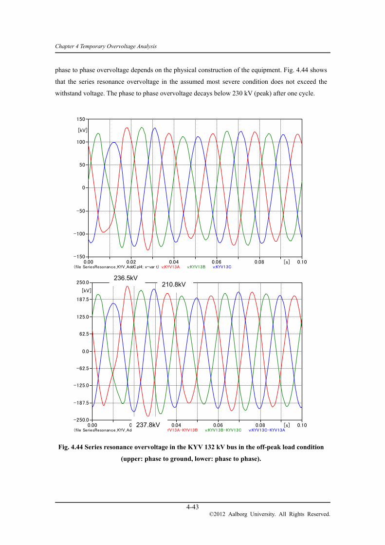
Chapter 4 Temporary Overvoltage Analysis
4-43 ©2012 Aalborg University. All Rights Reserved.
phase to phase overvoltage depends on the physical construction of the equipment. Fig. 4.44 shows
that the series resonance overvoltage in the assumed most severe condition does not exceed the
withstand voltage. The phase to phase overvoltage decays below 230 kV (peak) after one cycle.
Fig. 4.44 Series resonance overvoltage in the KYV 132 kV bus in the off-peak load condition
(upper: phase to ground, lower: phase to phase).
(file SeriesResonance_KYV_AddC.pl4; x-var t) v:KYV13A v:KYV13B v:KYV13C 0.00 0.02 0.04 0.06 0.08 0.10[s]
-150
-100
-50
0
50
100
150
[kV]
(file SeriesResonance_KYV_AddC.pl4; x-var t) v:KYV13A-KYV13B v:KYV13B-KYV13C v:KYV13C-KYV13A 0.00 0.02 0.04 0.06 0.08 0.10[s]
-250.0
-187.5
-125.0
-62.5
0.0
62.5
125.0
187.5
250.0
[kV]
236.5kV
237.8kV
210.8kV

Chapter 4 Temporary Overvoltage Analysis
4-44 ©2012 Aalborg University. All Rights Reserved.
The same simulations are repeated with the no load condition. Fig. 4.45 shows the results of the
simulations. Only minor difference is observed compared with the results in the off-peak load
condition.
Fig. 4.45 Series resonance overvoltage in the KYV 132 kV bus in the no load condition
(upper: phase to ground, lower: phase to phase).
(file SeriesResonance_KYV_AddC.pl4; x-var t) v:KYV13A v:KYV13B v:KYV13C 0.00 0.02 0.04 0.06 0.08 0.10[s]
-150
-100
-50
0
50
100
150
[kV]
(file SeriesResonance_KYV_AddC.pl4; x-var t) v:KYV13A-KYV13B v:KYV13B-KYV13C v:KYV13C-KYV13A 0.00 0.02 0.04 0.06 0.08 0.10[s]
-250.0
-187.5
-125.0
-62.5
0.0
62.5
125.0
187.5
250.0
[kV]
236.7kV
239.3kV
204.1kV

Chapter 4 Temporary Overvoltage Analysis
4-45 ©2012 Aalborg University. All Rights Reserved.
Second, the Kyndbyværket – Asnæsværket line is energized from the Asnæsværket side and the
overvoltage in the Asnæsværket 132 kV bus is monitored. Fig. 4.46 and Fig. 4.47 show the series
resonance overvoltage found with the off-peak load condition and the no load condition,
respectively.
The overvoltage level is higher compared with the overvoltage in the Kyndbyværket 132 kV bus,
but it is still much lower than the withstand voltage as long as the withstand voltage 230 or 275 kV
is selected. The phase to phase overvoltage decays below 230 kV after one cycle. As in the
overvoltage in the Kyndbyværket 132 kV bus, the load level has only minor impact on the
overvoltage level. It is because the load level is already low in the off-peak load condition.

Chapter 4 Temporary Overvoltage Analysis
4-46 ©2012 Aalborg University. All Rights Reserved.
Fig. 4.46 Series resonance overvoltage in the ASV 132 kV bus in the off-peak load condition
(upper: phase to ground, lower: phase to phase).
(file SeriesResonance_ASV_AddC.pl4; x-var t) v:ASV13A v:ASV13B v:ASV13C 0.00 0.02 0.04 0.06 0.08 0.10[s]
-160
-120
-80
-40
0
40
80
120
160
[kV]
(file SeriesResonance_ASV_AddC.pl4; x-var t) v:ASV13A-ASV13B v:ASV13B-ASV13C v:ASV13C-ASV13A 0.00 0.02 0.04 0.06 0.08 0.10[s]
-300
-200
-100
0
100
200
300
[kV]
274.0kV
213.0kV
215.1kV

Chapter 4 Temporary Overvoltage Analysis
4-47 ©2012 Aalborg University. All Rights Reserved.
Fig. 4.47 Series resonance overvoltage in the ASV 132 kV bus in the no load condition
(upper: phase to ground, lower: phase to phase).
(file SeriesResonance_ASV_AddC.pl4; x-var t) v:ASV13A v:ASV13B v:ASV13C 0.00 0.02 0.04 0.06 0.08 0.10[s]
-160
-120
-80
-40
0
40
80
120
160
[kV]
(file SeriesResonance_ASV_AddC.pl4; x-var t) v:ASV13A-ASV13B v:ASV13B-ASV13C v:ASV13C-ASV13A 0.00 0.02 0.04 0.06 0.08 0.10[s]
-300
-200
-100
0
100
200
300
[kV]
285.5kV
215.4kV
228.7kV
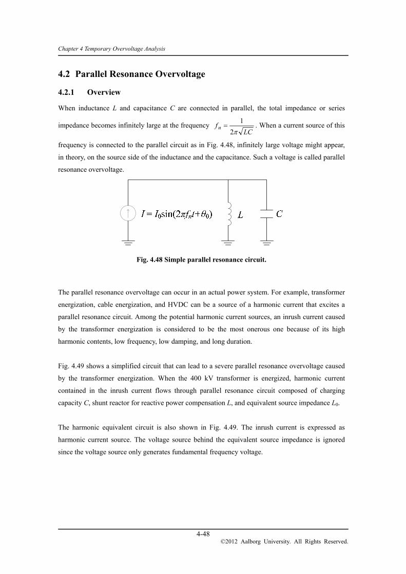
Chapter 4 Temporary Overvoltage Analysis
4-48 ©2012 Aalborg University. All Rights Reserved.
Parallel Resonance Overvoltage 4.2
4.2.1 Overview
When inductance L and capacitance C are connected in parallel, the total impedance or series
impedance becomes infinitely large at the frequency LC
f n2
1 . When a current source of this
frequency is connected to the parallel circuit as in Fig. 4.48, infinitely large voltage might appear,
in theory, on the source side of the inductance and the capacitance. Such a voltage is called parallel
resonance overvoltage.
Fig. 4.48 Simple parallel resonance circuit.
The parallel resonance overvoltage can occur in an actual power system. For example, transformer
energization, cable energization, and HVDC can be a source of a harmonic current that excites a
parallel resonance circuit. Among the potential harmonic current sources, an inrush current caused
by the transformer energization is considered to be the most onerous one because of its high
harmonic contents, low frequency, low damping, and long duration.
Fig. 4.49 shows a simplified circuit that can lead to a severe parallel resonance overvoltage caused
by the transformer energization. When the 400 kV transformer is energized, harmonic current
contained in the inrush current flows through parallel resonance circuit composed of charging
capacity C, shunt reactor for reactive power compensation L, and equivalent source impedance L0.
The harmonic equivalent circuit is also shown in Fig. 4.49. The inrush current is expressed as
harmonic current source. The voltage source behind the equivalent source impedance is ignored
since the voltage source only generates fundamental frequency voltage.

Chapter 4 Temporary Overvoltage Analysis
4-49 ©2012 Aalborg University. All Rights Reserved.
Fig. 4.49 Equivalent circuit of parallel resonance caused by transformer inrush.
The condition for the parallel resonance is:
0
11
LLC
nnn
0
11
2
1
CLCLf n
Eqn. 4.31
Here, nf is the natural frequency of the parallel resonance circuit.
Since the second harmonic current is contained in the inrush current with a higher proportion
compared to the other harmonic components, a parallel resonance overvoltage is most severe when
the natural frequency of the parallel circuit is 100 Hz, that is:
10011
2
1
0
CLCLfn
Eqn. 4.32

Chapter 4 Temporary Overvoltage Analysis
4-50 ©2012 Aalborg University. All Rights Reserved.
When the compensation rate of the cable is 100 %, the natural frequency ignoring the source
impedance is 50 Hz, that is:
501
2
1
CLfn
Eqn. 4.33
The source impedance will raise the natural frequency, and it becomes 100 Hz when L0 = L / 3 as
shown in Eqn. 4.34.
100
21
2
1
31
2
1
11
2
1
0
CL
CLCL
CLCLfn
Eqn. 4.34
However, the source impedance is usually much smaller than L / 3 in most networks in typical
operating conditions. The natural frequency, therefore, becomes 100 Hz in weak networks such as
in the black start operations. The load level is generally low in weak networks, and it highly
contributes to a severe parallel resonance overvoltage.
In this PhD project, the parallel resonance overvoltage is studied in the following procedure:
Find the natural frequency of the parallel resonance circuit
Set the natural frequency to 100 Hz by adjusting source impedance
Simulate the most severe switching scenarios (transformer energization) with the natural
frequency 100 Hz
4.2.2 Most Severe Scenarios
As discussed in the previous section, the transformer energization will be studied in the PhD project
as the most severe switching scenarios. In order to cause parallel resonance, a transformer needs to
be energized through a cable whose charging current is compensated by shunt reactors.
Fig. 4.50 shows the assumed most severe scenario for the energization of the 400 / 132 kV
Kyndbyværket transformer. The transformer is energized through the Kyndbyværket –
Asnæsværket line. The voltage source for the energization is assumed on the Bjæverskov side, and

Chapter 4 Temporary Overvoltage Analysis
4-51 ©2012 Aalborg University. All Rights Reserved.
the source impedance is adjusted so that the natural frequency of the parallel resonance circuit
becomes 100 Hz. The Kyndbyværket – Hovegård line is assumed to be opened in order to have a
large source impedance (weak network) and to limit the propagation path of the inrush current.
If the generator at Asnæsværket has black start capability, the Kyndbyværket – Hovegård line can
be opened assuming the black start operation from Asnæsværket. It, in theory, causes more severe
overvoltages because of limited propagation paths of the inrush current and lower load level.
Fig. 4.50 Assumed most severe scenario for the energization of KYV transformer.
Fig. 4.51 shows the assumed most severe scenario for the energization of the 400 / 132 kV
Asnæsværket transformer and phase shifting transformer. The transformers are energized through
the Kyndbyværket – Asnæsværket line.
As the generator at Kyndbyværket has the black start capability, the most severe scenario assumes
the black start operation from Kyndbyværket. As such, the following three lines are assumed not to
be in service.
Asnæsværket – Herslev line
Asnæsværket – Bjæverskov line
Kyndbyværket – Hovegård line
It may not be possible to adjust the natural frequency of the parallel resonance frequency exactly at

Chapter 4 Temporary Overvoltage Analysis
4-52 ©2012 Aalborg University. All Rights Reserved.
100 Hz because of the limited number of available generators at Kyndbyværket. Even with that
condition, severe overvoltages are often caused due to limited propagation paths of the inrush
current and lower load level.
Fig. 4.51 Assumed most severe scenario for the energization of ASV transformers.
4.2.3 Natural Frequency of Parallel Resonance Circuit
First, the energization of the 400 / 132 kV Kyndbyværket transformer is studied. The natural
frequencies of the network are found by frequency scan using the simulation model illustrated in
Fig. 4.52. The operating condition of the network is modified according to the most severe scenario
in Fig. 4.50.
Since it is expected to have the natural frequency at 100 Hz, the target frequency of all the
Bergeron models is set to 100 Hz.

Chapter 4 Temporary Overvoltage Analysis
4-53 ©2012 Aalborg University. All Rights Reserved.
Fig. 4.52 Simulation model for frequency scan for the energization of KYV transformer.
Results of the frequency scan are shown in Fig. 4.53. Natural frequencies are found at 92 Hz and
324 Hz in the figure. The magnitude of the impedance is 1306 ohm at 92 Hz and goes down to 878
ohm at 100 Hz.
To have a natural frequency at 92 Hz means that the network is already too weak in the off-peak
condition. In order to have a peak at 100 Hz, it is necessary to have a smaller source impedance
according to Eqn. 4.31. In order for it, the dummy source impedance 450 mH is added to the
Bjæverskov 400 kV bus as illustrated in Fig. 4.52.
Results of the frequency scan after the adjustment is shown in Fig. 4.54. The figure shows that the
LCC
22. km
LCC
46.73 km
AB
C
ASV40S
AT
YY
HKS40
SA
T
YY
Y
LC
C
26.
25
km
LCC
11.1
4 k
m
ISH40LCC
5.675 km
LCC
6.89 km
V
LCC
20.6
8 k
m
LC
C
35.
85
km GOR40
SAT
Y Y
LCC
27.
2 k
m
V
12km
AVV40GROUPish_avv
9km
HCV40GROUPavv_hcv
12km
GLN40GROUPhve_gln
8.43km
GR
OU
Pgo
r_sa
n
9.47km
GR
OU
Phv
e_sa
n
BJS40
SA
T
YY
SA
T
YY
SA
T
YY
SA
T
YY
HVE40S
AT
YY
SA
T
YY
SA
T
YY
KYV40
KYV13
SA
T
YY
SAT
Y Y
SA
T
Y
SA
T
Y
SAN40
SA
T
YY
LCC
18.15 km
LCC
4.76 km132kV
LCC
1.99 kmLCC
1.99 km
KY132
VABC
TOR40
GR
OU
PA
SV
-TO
R
Dummy
GR
OU
PT
OR
-KY
V
V
370MVar
126MVar
100MVar
V
1A
LUP13
Ignore feeder 0.15km
HVE-OLS 7.3kmOLS-LUP (11.0-0.15)km
Current source
KYV transformer
Kyndbyværket – Asnæsværket line
Opened for severe condition
Opened for severe condition
Dummy source to adjust natural frequency
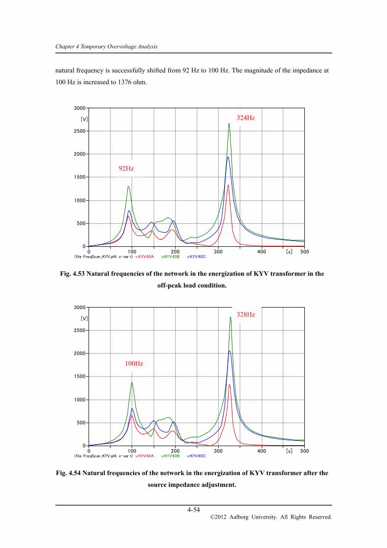
Chapter 4 Temporary Overvoltage Analysis
4-54 ©2012 Aalborg University. All Rights Reserved.
natural frequency is successfully shifted from 92 Hz to 100 Hz. The magnitude of the impedance at
100 Hz is increased to 1376 ohm.
Fig. 4.53 Natural frequencies of the network in the energization of KYV transformer in the
off-peak load condition.
Fig. 4.54 Natural frequencies of the network in the energization of KYV transformer after the
source impedance adjustment.
(file FreqScan_KYV.pl4; x-var t) v:KYV40A v:KYV40B v:KYV40C 0 100 200 300 400 500[s]
0
500
1000
1500
2000
2500
3000
[V]
(file FreqScan_KYV.pl4; x-var t) v:KYV40A v:KYV40B v:KYV40C 0 100 200 300 400 500[s]
0
500
1000
1500
2000
2500
3000
[V]
100Hz
328Hz
92Hz
324Hz

Chapter 4 Temporary Overvoltage Analysis
4-55 ©2012 Aalborg University. All Rights Reserved.
Second, the energization of the 400 / 132 kV Asnæsværket transformer and phase shifting
transformer is studied. Assuming the black start restoration from the KYV generator, the operating
condition of the network is modified according to the most severe scenario in Fig. 4.51.
In the black start restoration scenario, the following steps are assumed:
(1) Black start Kyndbyværket 132 kV generator
(2) Restore the Kyndbyværket 132 kV load 20 MW
(3) Energize the Kyndbyværket 400 / 132 kV transformer from the secondary side
(4) Energize the Kyndbyværket – Asnæsværket line from the Kyndbyværket side
(5) Energize the 400 / 132 kV Asnæsværket transformer or phase shifting transformer
The parallel resonance overvoltage is studied in Step (5).
Fig. 4.55 shows the results of the frequency scan. Initially, only one Kyndbyværket 132 kV
generator, Machine 224 in the provided PSS/E data, is assumed to be in-service. The source
impedance 578.5 mH which corresponds to this generator is connected to the Kyndbyværket 132
kV bus. The figure shows that the network has a very sharp peak at 52 Hz. The magnitude of the
impedance is 6773 ohm, but it goes down to 168 ohm at 100 Hz.
Fig. 4.55 Natural frequencies of the network in the energization of ASV transformer in the
black start restoration.
(file FreqScan_ASV.pl4; x-var t) v:ASV40A v:ASV40B v:ASV40C 0 100 200 300 400 500[Hz]
0
1000
2000
3000
4000
5000
6000
7000
[Ω]

Chapter 4 Temporary Overvoltage Analysis
4-56 ©2012 Aalborg University. All Rights Reserved.
As discussed in the previous section, the natural frequency of the network is located at 50 Hz
without a source impedance and loads. The results show that the source impedance and the loads
increase the natural frequency only by 2 Hz because of the following reasons:
The source impedance is very large since the capacity of the assumed black start generator
is small (28.57 MVA).
The source impedance is large since there is only one 400 / 132 kV Kyndbyværket
transformer.
The load level is very low (20 MW) due to the assumed black start restoration scenario.
In order to shift the natural frequency to 100 Hz, it is necessary to assume a smaller source
impedance. Assuming many other generators in the Kyndbyværket 132 kV network are in-service,
the source impedance is decreased from 578.5 mH to 8 mH. The source impedance 8 mH
corresponds to the fault current level 30.3 kA at the Kyndbyværket 132 kV bus. As shown in Fig.
4.56, the natural frequency is successfully shifted to 100 Hz. The magnitude of the impedance is
9439 ohm at 100 Hz.
Fig. 4.56 Natural frequencies of the network in the energization of ASV transformer after the
source impedance adjustment.
As it is assumed that many other generators are in-service, it is not realistic to assume that only 20
(file FreqScan_ASV.pl4; x-var t) v:ASV40A v:ASV40B v:ASV40C 0 100 200 300 400 500[Hz]
0
2
4
6
8
10
[kΩ]

Chapter 4 Temporary Overvoltage Analysis
4-57 ©2012 Aalborg University. All Rights Reserved.
MW load is restored at the Kyndbyværket 132 kV. In Fig. 4.57, the Kyndbyværket 132 kV load is
increased from 20 MW to the off-peak load 67.8 MW. The load increase does not shift the natural
frequency, but lowered the magnitude of the impedance to 7364 ohm.
Fig. 4.57 Natural frequencies of the network in the energization of ASV transformer after the
source impedance adjustment with increased load.
Even though, the natural frequency is successfully shifted to 100 Hz, it may not be realistic to
assume the fault current level 30.3 kA at Kyndbyværket 132 kV bus. In order to make it more
realistic the following modified restoration scenario is considered:
(1) Black start Kyndbyværket 132 kV generators
(2) Restore the Kyndbyværket 132 kV load 67.8 MW (off-peak)
(3) Energize the Kyndbyværket 400 / 132 kV transformer from the secondary side
(4) Energize the Kyndbyværket – Hovegård line from the Kyndbyværket side
(5) Energize the two Hovegård 400 / 132 kV transformers
(6) Start up generators connected to the Hovegård 132 kV network
(7) Restore the Hovegård 132 kV load 151.2 MW (off-peak)
(8) Energize the Kyndbyværket – Asnæsværket line from the Kyndbyværket side
(9) Energize the 400 / 132 kV Asnæsværket transformer or phase shifting transformer
The parallel resonance overvoltage is studied in Step (9).
(file FreqScan_ASV_Large.pl4; x-var t) v:ASV40A v:ASV40B v:ASV40C 0 100 200 300 400 500[Hz]
0
1000
2000
3000
4000
5000
6000
7000
8000
[Ω]

Chapter 4 Temporary Overvoltage Analysis
4-58 ©2012 Aalborg University. All Rights Reserved.
In the modified scenario, Hovegård is restored before Kyndbyværket in Steps (4) – (7). Since
Hovegård has two 400 / 132 kV transformers, it is easier to have a small source impedance. The
simulation model for the modified restoration scenario is illustrated in Fig. 4.58
Fig. 4.58 Simulation model for frequency scan for the energization of ASV transformer after
HVE is restored.
In the modified restoration scenario, it is possible to have a source impedance at the Hovegård 132
kV bus as well as the Kyndbyværket 132 kV bus. First, the source impedance at the Kyndbyværket
132 kV bus is increased from 8 mH to 20 mH. The source impedance 20 mH corresponds to the
fault current level 12.1 kA. This is more realistic assumption compared with the original scenario.
The source impedance at the Hovegård 132 kV bus is set to 80 mH in order to have the natural
frequency at 100 Hz. The source impedance 80 mH corresponds to the fault current level 3.0 kA.
Fig. 4.59 shows the results of the frequency scan. It is observed in the figure that the natural
frequency is successfully set at 100 Hz. The magnitude of the impedance at 100 Hz is 18846 ohm,
which is extremely high.
LCC
22. km
LCC
46.73 km
AB
C
ASV40
SA
T
YY
SA
T
YY
Y
LC
C
26
.25
km
LC
C
11
.14
km
LCC
5.675 km
LCC
6.89 km
V
LCC
20.6
8 k
m
LCC
35.8
5 k
m
SAT
Y Y
V
GROUPish_avv
GROUPavv_hcv
GROUPhve_gln
SA
T
YY
SA
T
YY
SA
T
YY
SA
T
YY
HVE40
SA
T
YY
SA
T
YY
SA
T
YY
KYV40
KYV13
SA
T
YY
SA
T
Y
SA
T
Y
SA
T
YY
LCC
18.15 km
LCC
4.76 km132kV
LCC
1.99 kmLCC
1.99 km
KY132
VABC
TOR40
GR
OU
PA
SV
-TO
RG
RO
UP
TO
R-K
YV
V
126MVar
100MVar
V
1A
20mH
80mH
LUP13
Ignore feeder 0.15km
HVE-OLS 7.3kmOLS-LUP (11.0-0.15)km

Chapter 4 Temporary Overvoltage Analysis
4-59 ©2012 Aalborg University. All Rights Reserved.
Fig. 4.59 Natural frequencies of the network in the energization of ASV transformer after
HVE is restored and the source impedance is adjusted.
4.2.4 Simulation Results of Parallel Resonance Overvoltage
First, the energization of the Kyndbyværket 400 / 132 kV transformer is studied. The natural
frequency of the network is set to 100 Hz as adjusted in Fig. 4.54. The hysteresis characteristic of
the transformer is set as Table 3-13, assuming the positive saturation point at 1.4 pu. The remanent
flux is assumed in phase a (85 %) and phase b (-85 %).
Results of the time domain simulation are shown in Table 4-4. Since the inrush current highly
depends on the switch timing, the switch timing is changed from 0 ms to 19 ms by 1 ms step. The
highest overvoltage 469.5 kV is observed when the switch timing is 11 ms. The waveforms of the
parallel resonance overvoltage and inrush current with the switch timing 11 ms are shown in Fig.
4.60 and Fig. 4.61.
The parallel resonance overvoltage in Fig. 4.60 is not very high. Even if the highest overvoltage
level is continued for 10 seconds, the overvoltage is within withstand voltages of related equipment
(1.60 pu for the assumed arrester). The magnitude of the inrush current in Fig. 4.61 is reasonable as
the highest inrush current 4008 A is eight times larger than the rated current of the transformer (350
MVA, 505 A).
(file FreqScan_ASV_Large.pl4; x-var t) v:ASV40A v:ASV40B v:ASV40C 0 100 200 300 400 500[Hz]
0
4
8
12
16
20
[kΩ]

Chapter 4 Temporary Overvoltage Analysis
4-60 ©2012 Aalborg University. All Rights Reserved.
Table 4-4 Parallel Resonance Overvoltage Caused by the KYV Transformer Energization
Switch Time Overvoltage [kV]
Phase a Phase b Phase c
0 ms 360.4 411.7 395.0
1 ms 377.9 405.5 398.1
2 ms 394.6 391.1 397.1
3 ms 409.6 393.2 374.2
4 ms 443.8 387.0 385.2
5 ms 435.8 422.5 392.8
6 ms 420.8 427.7 400.4
7 ms 402.7 406.7 410.2
8 ms 436.8 408.4 430.1
9 ms 448.6 409.6 434.7
10 ms 438.8 423.4 459.0
11 ms 433.8 430.5 469.5
12 ms 433.1 422.0 465.8
13 ms 411.5 407.8 435.3
14 ms 401.1 424.5 421.6
15 ms 413.6 428.0 420.2
16 ms 430.9 433.7 398.8
17 ms 424.5 392.9 378.0
18 ms 418.5 400.3 373.6
19 ms 400.6 397.3 381.4
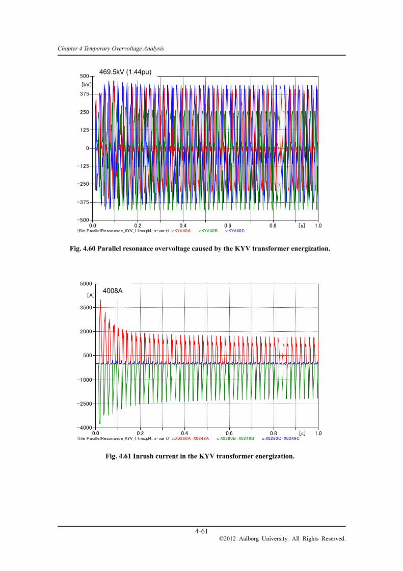
Chapter 4 Temporary Overvoltage Analysis
4-61 ©2012 Aalborg University. All Rights Reserved.
Fig. 4.60 Parallel resonance overvoltage caused by the KYV transformer energization.
Fig. 4.61 Inrush current in the KYV transformer energization.
(file ParallelResonance_KYV_11ms.pl4; x-var t) v:KYV40A v:KYV40B v:KYV40C 0.0 0.2 0.4 0.6 0.8 1.0[s]
-500
-375
-250
-125
0
125
250
375
500
[kV]
(file ParallelResonance_KYV_11ms.pl4; x-var t) c:X0280A-X0249A c:X0280B-X0249B c:X0280C-X0249C 0.0 0.2 0.4 0.6 0.8 1.0[s]
-4000
-2500
-1000
500
2000
3500
5000
[A]
469.5kV (1.44pu)
4008A
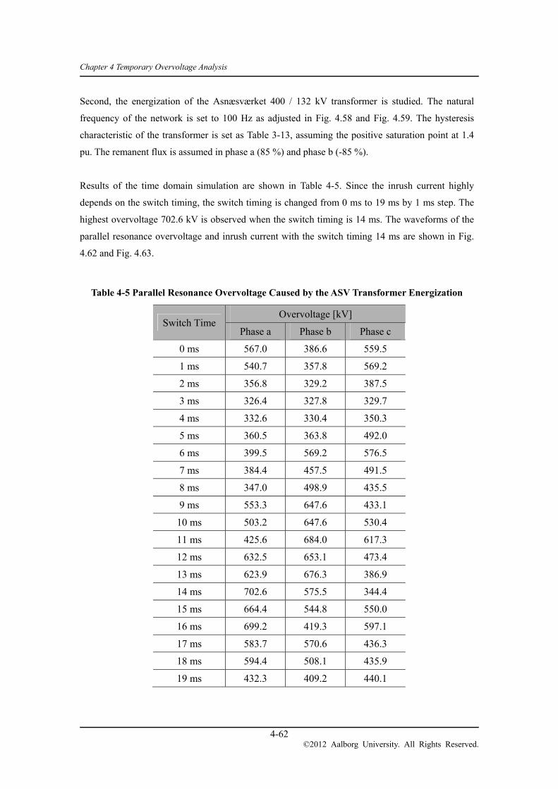
Chapter 4 Temporary Overvoltage Analysis
4-62 ©2012 Aalborg University. All Rights Reserved.
Second, the energization of the Asnæsværket 400 / 132 kV transformer is studied. The natural
frequency of the network is set to 100 Hz as adjusted in Fig. 4.58 and Fig. 4.59. The hysteresis
characteristic of the transformer is set as Table 3-13, assuming the positive saturation point at 1.4
pu. The remanent flux is assumed in phase a (85 %) and phase b (-85 %).
Results of the time domain simulation are shown in Table 4-5. Since the inrush current highly
depends on the switch timing, the switch timing is changed from 0 ms to 19 ms by 1 ms step. The
highest overvoltage 702.6 kV is observed when the switch timing is 14 ms. The waveforms of the
parallel resonance overvoltage and inrush current with the switch timing 14 ms are shown in Fig.
4.62 and Fig. 4.63.
Table 4-5 Parallel Resonance Overvoltage Caused by the ASV Transformer Energization
Switch Time Overvoltage [kV]
Phase a Phase b Phase c
0 ms 567.0 386.6 559.5
1 ms 540.7 357.8 569.2
2 ms 356.8 329.2 387.5
3 ms 326.4 327.8 329.7
4 ms 332.6 330.4 350.3
5 ms 360.5 363.8 492.0
6 ms 399.5 569.2 576.5
7 ms 384.4 457.5 491.5
8 ms 347.0 498.9 435.5
9 ms 553.3 647.6 433.1
10 ms 503.2 647.6 530.4
11 ms 425.6 684.0 617.3
12 ms 632.5 653.1 473.4
13 ms 623.9 676.3 386.9
14 ms 702.6 575.5 344.4
15 ms 664.4 544.8 550.0
16 ms 699.2 419.3 597.1
17 ms 583.7 570.6 436.3
18 ms 594.4 508.1 435.9
19 ms 432.3 409.2 440.1

Chapter 4 Temporary Overvoltage Analysis
4-63 ©2012 Aalborg University. All Rights Reserved.
Fig. 4.62 Parallel resonance overvoltage caused by the ASV transformer energization.
Fig. 4.63 Inrush current in the ASV transformer energization.
(file ParallelResonance_ASV_Large_14ms.pl4; x-var t) v:ASV40A v:ASV40B v:ASV40C 0.0 0.2 0.4 0.6 0.8 1.0[s]
-600
-400
-200
0
200
400
600
800
[kV]
(file ParallelResonance_ASV_Large_14ms.pl4; x-var t) c:X0127A-X0001A c:X0127B-X0001B c:X0127C-X0001C 0.0 0.2 0.4 0.6 0.8 1.0[s]
-8000
-4600
-1200
2200
5600
9000
[A]
702.6kV (2.15pu)
517.8kV (1.59pu)
8483A

Chapter 4 Temporary Overvoltage Analysis
4-64 ©2012 Aalborg University. All Rights Reserved.
Even though the observed highest overvoltage 702.6 kV is very high as a temporary overvoltage, it
is clear from the waveform that the overvoltage exceeding 700 kV lasts only for one impulse. It is
thus reasonable to evaluate the overvoltage against the switching impulse withstand overvoltage
1050 kV and conclude the observed overvoltage is within the equipment standards. The highest
overvoltage after half cycle is 518.7 kV, which is also within withstand voltages of related
equipment (1.60 pu – 10 sec for the assumed arrester).
The highest inrush current 8483 A in Fig. 4.63 is too large, compared with the typical inrush current,
as it is 12 times larger than the rated current of the transformer (500 MVA, 722 A).
As discussed in Section 3.5, the positive saturation point 1.4 pu is a severe assumption, which
caused the large inrush current 8483 A. When the positive saturation point 1.3 pu is assumed, the
highest overvoltage is lowered to 506.9 kV. The waveforms of the parallel resonance overvoltage
and inrush current under this moderate assumption are shown in Fig. 4.64 and Fig. 4.65. The
observed overvoltages are within withstand voltages of related equipment. The highest inrush
current 5163 A is reasonable as it is seven times larger than the rated current of the transformer.
Fig. 4.64 Parallel resonance overvoltage caused by the ASV transformer energization
(positive saturation point 1.3 pu).
(file ParallelResonance_ASV_Large_14ms_1.3pu.pl4; x-var t) v:ASV40A v:ASV40B v:ASV40C 0.0 0.2 0.4 0.6 0.8 1.0[s]
-500
-280
-60
160
380
600
[kV]
506.9kV (1.55pu)

Chapter 4 Temporary Overvoltage Analysis
4-65 ©2012 Aalborg University. All Rights Reserved.
Fig. 4.65 Inrush current in the ASV transformer energization
(positive saturation point 1.3 pu).
(file ParallelResonance_ASV_Large_14ms_1.3pu.pl4; x-var t) c:X0127A-X0001A c:X0127B-X0001B c:X0127C-X0001C
0.0 0.2 0.4 0.6 0.8 1.0[s]-5000
-2800
-600
1600
3800
6000
[A]
5163A

Chapter 4 Temporary Overvoltage Analysis
4-66 ©2012 Aalborg University. All Rights Reserved.
Overvoltage Caused by the System Islanding 4.3
4.3.1 Overview
When one end of a long cable is opened, a part of a network can be separated from the main grid
together with the long cable. The equivalent circuit expressing the situation is illustrated in Fig.
4.66. Here, the assumed fault is a bus fault since a cable line fault will result in the removal of the
cable line from the equivalent circuit.
Fig. 4.66 Equivalent circuit of the system islanding.
From the above equivalent circuit, the overvoltage caused by the system islanding can be expressed
by the following equations [8]:
tVtVtv mm 00
sinsin)( Eqn. 4.35
CLCLLCLL
LEV m
m11
,)1( 0
020
Eqn. 4.36
where L0 is source impedance of the weaker islanded system and Em is the source voltage behind L0.
Charging capacity of the long cable and inductance of the shunt reactors directly connected to the
cable are expressed by C and L, respectively.
Eqn. 4.35 shows that the overvoltage contains two frequency components, the nominal frequency ω
and the resonance frequency ω0. Since the overvoltage is caused by the superposition of two
frequency components, the resulting overvoltage is oscillatory, and its level is often difficult to
estimate before the simulation. The result of a simulation performed for the 500 kV Shin-Toyosu
line is shown in Fig. 4.67 [1].

Chapter 4 Temporary Overvoltage Analysis
4-67 ©2012 Aalborg University. All Rights Reserved.
Without Surge Arresters
With Surge Arresters
Fig. 4.67 Example of the overvoltage caused by the system islanding.
The overvoltage level is sensitive to L0, which expresses the short circuit level in the islanded
system. In order to find the most severe overvoltage, it is necessary to study different fault current
levels or network conditions.
4.3.2 Study Conditions
This system islanding can easily occur when the long cable is installed in a radial network. As the
Kyndbyværket – Asnæsværket line is installed as a part of the loop network, the system islanding
can only occur in specific conditions. Among these specific conditions, an outage of the Hovegård
– Kyndbyværket line (under 400 kV operation) is the most likely precondition in which an
Asnæsværket 400 kV bus fault can lead to the system islanding. Fig. 4.68 illustrates the network
1.0s
1.0s
2.23 pu
1.69 pu

Chapter 4 Temporary Overvoltage Analysis
4-68 ©2012 Aalborg University. All Rights Reserved.
condition that leads to the system islanding. The islanded system is actually connected to the main
grid through the 132 kV system, but the connection to the main grid is weak enough to cause the
oscillatory overvoltage. The system islanding actually occurs in simulations as the simulation
model in PSCAD does not include the connection in the 132 kV system. In this point, the study
condition is more severe than the actual system.
Fig. 4.68 ASV 400 kV bus fault and the system islanding.
Generators in the Kyndbyværket 132 kV network need to be modeled in order for the islanded
system to experience the oscillatory overvoltage. A dummy generator was connected to the
Kyndbyværket 132 kV bus through the source impedance whose value L0 was considered as a
parameter in order to study different fault current levels. Table 4-6 shows the fault current levels
and their associated values of the source impedance considered in the analysis. Since there are no
other generators in the islanded system, the calculation of the source impedance is straightforward.
The maximum fault current level was set to 40 kA since the typical breaking capability of the 132
kV breakers in the Danish network was 40 kA.

Chapter 4 Temporary Overvoltage Analysis
4-69 ©2012 Aalborg University. All Rights Reserved.
Table 4-6 Source Impedances of the KYV 132 kV Dummy Generator
Fault current level at the
KYV 132 kV bus [kA] 5 10 20 30 40
Source impedance of the
dummy generator [mH] 48.5 24.3 12.1 8.09 6.06
Now, we consider study conditions where the Kyndbyværket 400 kV bus fault results in the system
islanding. As the 400 kV transmission lines from Asnæsværket to Hovegård via Bjæverskov are all
double circuit lines, the Kyndbyværket 400 kV bus fault will not lead to the system islanding in
normal or N-1 preconditions. When we consider an outage of the Asnæsværket – Herslev line,
however, the Kyndbyværket – Asnæsværket line is only weakly connected to the main grid via
Bjæverskov in case of the Kyndbyværket 400 kV bus fault. As the Asnæsværket 400 kV bus is
approximately 69 km away from Bjæverskov, the oscillatory overvoltage may occur depending on
the fault current level at Asnæsværket. Fig. 4.69 shows the network condition which may lead to
the oscillatory overvoltage.
Fig. 4.69 KYV 400 kV bus fault and the system islanding.
Asnæsværket(ASV)
Herslev(HKS)
22.00 km
68.73 km
46.73 km
Bjæverskov(BJS)
Ishøj(ISH)
31.92 km
37.39 km
16.82 km
Hovegård(HVE)
Gørløse(GØR)
Skibstrupgård koblingspkt(SÅN)
20.68 km
71.48 km
93.20 km
Lyngerup(LUP)
Kyndbyværket(KYV)
24.90 kmGlentegård
(GLN)
18.89 km
H.C. ØrstedVærket (HCV)
Avedøreværket(AVV)
12.09 km 8.99 km
18.30 km6.90 km
(1) Out of service
132 kV
(2) Bus fault
(3) Islanded System

Chapter 4 Temporary Overvoltage Analysis
4-70 ©2012 Aalborg University. All Rights Reserved.
Different fault current levels were considered also for the Kyndbyværket 400 kV bus fault. Based
on the off-peak load condition, the fault current level at the Asnæsværket 132 kV bus was adjusted
to 10, 20, 30, and 40 kA by adding a dummy generator to the Asnæsværket 132 kV bus. As the fault
current level at the Asnæsværket 132 kV bus is 8.70 kA in the off-peak load condition, the
remaining fault current has to be fed from the dummy generator.
Table 4-7 Source Impedances of the ASV 132 kV Dummy Generator
Fault current level at the
ASV 132 kV bus [kA] 10 20 30 40
Fault current fed from the
dummy generator [kA] 1.30 11.3 21.3 31.3
Source impedance of the
dummy generator [mH] 186 21.5 11.4 7.75
Table 4-8 summarizes the study conditions for the overvoltage caused by the system islanding. The
fault in the Torslunde 400 kV bus was additionally studied assuming there is a switching station at
Torslunde. As for the fault type, only the three phase fault was considered as it was the most severe
fault with respect to the overvoltage caused by the system islanding.
We can see which conditions can theoretically affect the overvoltage from Eqn. 4.35. While the
charging capacity of the Kyndbyværket – Asnæsværket line cannot be changed, two other
conditions, the source impedance L0 and the shunt reactors L can be changed as the study condition.
According to the conclusion of Chapter 2, one unit of 300 MVar shunt reactor needs to be
connected to both sides of the Kyndbyværket – Asnæsværket line in Pattern 1. In this case, L takes
a fixed value. When two units of 150 MVar shunt reactors are connected to both sides as in Pattern
1’, one of the four shunt reactors can be taken out of service, which lowers the compensation rate to
75.5 %. This condition was studied as a more severe assumption.
Table 4-8 Study Conditions for the Overvoltage Caused by the System Islanding
Fault location ASV, KYV, TOR 400 kV buses
Fault type Three phase fault (no fault resistance)
Fault current level (5,) 10, 20, 30, 40 kA at the ASV or KYV 132 kV bus
Shunt compensation All shunt reactors in service (100.7 %)
One 150 MVar shunt reactor out of service (75.5 %)

Chapter 4 Temporary Overvoltage Analysis
4-71 ©2012 Aalborg University. All Rights Reserved.
4.3.3 ASV 400 kV Bus Fault
4.3.3.1 All Shunt Reactors in Service
First, the simulations were performed with all reactors in service. Fig. 4.70 shows the overvoltage
caused by the system islanding with the fault current level of 5 kA at the Kyndbyværket 132 kV bus.
The highest overvoltage 744.6 kV was observed at the open-end of the cable in phase c.
Fig. 4.70 Overvoltage caused by the ASV bus fault leading to the system islanding (all shunt
reactors in service, fault current level: 5kA).
From the waveform of the overvoltage, it is clear that the resonant frequency is superimposed on
the nominal frequency. The resonant frequency can be found by the Fourier transform of the
waveform. Fig. 4.71 shows frequency components contained in the overvoltage. The resonant
frequency of 75 Hz was found from the Fourier transform of the waveform of the overvoltage.
Fig. 4.71 Frequency components contained in the overvoltage caused by the ASV bus fault
leading to the system islanding (all shunt reactors in service, fault current level: 5kA).
-600
-400
-200
0
200
400
600
800
0 0.1 0.2 0.3 0.4 0.5
Time [s]
Vo
ltage
[kV
]
phase a
phase b
phase c
0
40
80
120
160
200
0 20 40 60 80 100 120 140
Frequency [Hz]
Am
plitu
de [
kV]
744.6kV (2.28pu)
340.3kV

Chapter 4 Temporary Overvoltage Analysis
4-72 ©2012 Aalborg University. All Rights Reserved.
Here the resonant frequency can also be derived theoretically from Eqn. 4.35. The theoretical
derivation gives the resonant frequency 76.6 Hz, which is close enough to the one derived from
simulation results.
The overvoltage when the fault current level is increased to 10, 20, 30, and 40 kA is shown in Fig.
4.72 to Fig. 4.75.
Fig. 4.72 Overvoltage caused by the ASV bus fault leading to the system islanding (all shunt
reactors in service, fault current level: 10kA).
Fig. 4.73 Overvoltage caused by the ASV bus fault leading to the system islanding (all shunt
reactors in service, fault current level: 20kA).
-600
-400
-200
0
200
400
600
800
0 0.1 0.2 0.3 0.4 0.5
Time [s]
Vo
ltage
[kV
]
phase a
phase b
phase c
-800
-600
-400
-200
0
200
400
600
800
0 0.1 0.2 0.3 0.4 0.5
Time [s]
Vo
ltage
[kV
]
phase a
phase b
phase c
613.4kV (1.88pu)
727.5kV (2.23pu)

Chapter 4 Temporary Overvoltage Analysis
4-73 ©2012 Aalborg University. All Rights Reserved.
Fig. 4.74 Overvoltage caused by the ASV bus fault leading to the system islanding (all shunt
reactors in service, fault current level: 30kA).
Fig. 4.75 Overvoltage caused by the ASV bus fault leading to the system islanding (all shunt
reactors in service, fault current level: 40kA).
Fig. 4.76 shows the comparison of resonant frequencies derived from the theoretical formula and
simulation results. The resonant frequencies derived from simulation results match closely to those
derived from the theoretical formula. The deviation of 2.5 Hz can be considered as a round-off error
as the Fourier transform identifies the resonant frequency with a 2.5 Hz step. This demonstrates that
overvoltages as expected from Eqn. 4.35 are produced in the simulations.
-800
-600
-400
-200
0
200
400
600
800
0 0.1 0.2 0.3 0.4 0.5
Time [s]
Vo
ltage
[kV
]
phase a
phase b
phase c
-800
-600
-400
-200
0
200
400
600
800
0 0.1 0.2 0.3 0.4 0.5
Time [s]
Vo
ltage
[kV
]
phase a
phase b
phase c
627.3kV (1.92pu)
607.4kV (1.86pu)

Chapter 4 Temporary Overvoltage Analysis
4-74 ©2012 Aalborg University. All Rights Reserved.
Fig. 4.76 Resonant frequencies derived from theoretical formula and simulation results.
Comparing the waveforms of the overvoltages, the most severe overvoltage was caused when the
fault current level was set to 5 kA or 20 kA. The initial overvoltage level is slightly higher with the
fault current level of 5 kA, but the sustained overvoltage with the frequency around 1 Hz can be
observed with the fault current level of 20 kA.
The simulations were, so far, performed without surge arrester. Here, the overvoltage with the fault
current level of 20 kA was evaluated against the ratings of the modeled surge arrester.
Fig. 4.77 shows the overvoltage with one surge arrester connected to the open-end of the cable
when the fault current level was set to 20 kA. The highest overvoltage was lowered by the surge
arrester. The low frequency oscillation (1 Hz) is not damped within 1 s, but the overvoltage level is
lowered to 400 kV (1.22 pu) within 0.4 s. Considering the power frequency withstand voltage (1
min) 1.58 pu of the modelled surge arrester, it can endure the overvoltage shown in Fig. 4.77.
60
70
80
90
100
110
0 10 20 30 40
Fault current level [kA]
Res
onan
t fr
eque
ncy
[Hz]
Theoretical formula
Simulation results

Chapter 4 Temporary Overvoltage Analysis
4-75 ©2012 Aalborg University. All Rights Reserved.
Fig. 4.77 Overvoltage caused by the ASV bus fault leading to the system islanding with an
arrester (all shunt reactors in service, fault current level: 20kA).
Fig. 4.78 shows the energy absorbed by the surge arrester in the overvoltage. The energy absorbed
by the surge arrester is within the energy absorption capability 9.5 MJ of the modeled surge
arrester.
Fig. 4.78 Energy absorption by an arrester in the islanding overvoltage (all shunt reactors in
service, fault current level: 20kA).
-800
-600
-400
-200
0
200
400
600
800
0 0.2 0.4 0.6 0.8 1
Time [s]
Vo
ltage
[kV
]
phase a
phase b
phase c
0
100
200
300
400
500
600
700
800
0 0.2 0.4 0.6 0.8 1
Time [s]
En
erg
y ab
sorp
tion
[kJ]
phase a
phase b
phase c
684.2kV (2.09pu)

Chapter 4 Temporary Overvoltage Analysis
4-76 ©2012 Aalborg University. All Rights Reserved.
4.3.3.2 Effects of One Shunt Reactor out of Service
This section discusses the overvoltage with one 150 MVar shunt reactor out of service. As the
overvoltage is highest at the open-end of the cable, it is most severe to take one shunt reactor at
Asnæsværket out of service.
Fig. 4.79 to Fig. 4.83 show the overvoltages caused by the system islanding with the fault current
levels of 5 to 40 kA. The overvoltage level becomes higher due to the lower compensation rate. The
sustained overvoltage is observed due to the surplus reactive power supply in the islanded system.
Fig. 4.79 Overvoltage caused by the ASV bus fault leading to the system islanding (one shunt
reactors out of service, fault current level: 5kA).
Fig. 4.80 Overvoltage caused by the ASV bus fault leading to the system islanding (one shunt
reactors out of service, fault current level: 10kA).
-800
-600
-400
-200
0
200
400
600
800
0 0.1 0.2 0.3 0.4 0.5
Time [s]
Vo
ltage
[kV
]
phase a
phase b
phase c
-800
-600
-400
-200
0
200
400
600
800
0 0.1 0.2 0.3 0.4 0.5
Time [s]
Vo
ltage
[kV
]
phase a
phase b
phase c
805.0kV (2.46pu)
674.9kV (2.07pu)

Chapter 4 Temporary Overvoltage Analysis
4-77 ©2012 Aalborg University. All Rights Reserved.
Fig. 4.81 Overvoltage caused by the ASV bus fault leading to the system islanding (one shunt
reactors out of service, fault current level: 20kA).
Fig. 4.82 Overvoltage caused by the ASV bus fault leading to the system islanding (one shunt
reactors out of service, fault current level: 30kA).
-800
-600
-400
-200
0
200
400
600
800
0 0.1 0.2 0.3 0.4 0.5
Time [s]
Vo
ltage
[kV
]
phase a
phase b
phase c
-800
-600
-400
-200
0
200
400
600
800
0 0.1 0.2 0.3 0.4 0.5
Time [s]
Vo
ltage
[kV
]
phase a
phase b
phase c
771.9kV (2.36pu)
782.0kV (2.36pu)

Chapter 4 Temporary Overvoltage Analysis
4-78 ©2012 Aalborg University. All Rights Reserved.
Fig. 4.83 Overvoltage caused by the ASV bus fault leading to the system islanding (one shunt
reactors out of service, fault current level: 40kA).
Fig. 4.84 shows the comparison of resonant frequencies derived from the theoretical formula and
simulation results. The resonant frequencies derived from simulation results match closely to those
derived from the theoretical formula, as in the cases with all shunt reactors in service.
Fig. 4.84 Resonant frequencies derived from theoretical formula and simulation results (one
shunt reactor out of service).
-800
-600
-400
-200
0
200
400
600
800
0 0.1 0.2 0.3 0.4 0.5
Time [s]
Vo
ltage
[kV
]
phase a
phase b
phase c
60
70
80
90
100
110
0 10 20 30 40
Fault current level [kA]
Res
onan
t fr
eque
ncy
[Hz]
Theoretical formula
Simulation results
659.6kV (2.02pu)

Chapter 4 Temporary Overvoltage Analysis
4-79 ©2012 Aalborg University. All Rights Reserved.
Comparing the waveforms of the overvoltages, the most severe overvoltage was caused when the
fault current level was set to 5 kA or 40 kA. The initial overvoltage level is significantly higher
with the fault current level of 5 kA, but the sustained overvoltage with the frequency around 1 Hz
can be observed with the fault current level of 40 kA.
Here, the overvoltage with the fault current level of 5 kA was evaluated against the ratings of a
surge arrester. Fig. 4.85 shows the overvoltage with one surge arrester connected to the open-end of
the cable. The overvoltage level is lowered to 400 kV (1.22 pu) within 0.4 s. Considering the power
frequency withstand voltage (1 min) 1.58 pu of the modelled surge arrester, it can endure the
overvoltage shown in Fig. 4.85.
Fig. 4.85 Overvoltage caused by the ASV bus fault leading to the system islanding with an
arrester (one shunt reactor out of service, fault current level: 5kA).
Fig. 4.86 shows the energy absorbed by the surge arrester in the overvoltage. The energy absorbed
by the surge arrester is within the energy absorption capability 9.5 MJ of the modeled surge
arrester.
-800
-600
-400
-200
0
200
400
600
800
0 0.2 0.4 0.6 0.8 1
Time [s]
Vo
ltage
[kV
]
phase a
phase b
phase c
-680.0kV (-2.08pu)

Chapter 4 Temporary Overvoltage Analysis
4-80 ©2012 Aalborg University. All Rights Reserved.
Fig. 4.86 Energy absorption by an arrester in the islanding overvoltage (one shunt reactor out
of service, fault current level: 5kA).
Finally, the highest overvoltages caused by the system islanding due to the Asnæsværket 400 kV
bus fault is summarized in Table 4-9. Values in red ink show the results with one surge arrester
modeled at the open-end of the cable.
Table 4-9 Highest Overvoltages Caused by the System Islanding due to the ASV 400 kV Bus
Fault
Fault current level All shunt reactors in service One shunt reactor out of service
5kA 744.6 kV (2.28 pu) 805.0 kV (2.46 pu)
680.0 kV (2.08 pu)
10kA 613.4 kV (1.88 pu) 674.9 kV (2.07 pu)
20kA 727.5 kV (2.23 pu)
684.2 kV (2.09 pu) 771.9 kV (2.36 pu)
30kA 627.3 kV (1.92 pu) 782.0 kV (2.36 pu)
40kA 607.4 kV (1.86 pu) 659.6 kV (2.02 pu)
4.3.3.3 Effects of Timing for Fault Clearing
This section studies the effects of the timing for the fault clearing. The fault clearing always occurs
at current zero, but by changing the timing, it is possible to change the order of three phases.
In this analysis, it was assumed that all shunt reactors were in service. The fault current level at the
Kyndbyværket 132 kV bus was set to 20 kA since the most severe overvoltage was observed with
0
100
200
300
400
500
600
0 0.2 0.4 0.6 0.8 1
Time [s]
En
erg
y a
bso
rptio
n [k
J]
phase a
phase b
phase c

Chapter 4 Temporary Overvoltage Analysis
4-81 ©2012 Aalborg University. All Rights Reserved.
this condition.
When the fault current level was 20 kA, the fault clearing occurs in the order of phase a, c, and b in
Section 4.3.3.1. By delaying the fault clearing timing, the order can be changed to phase c, b, and a.
Further delay can result in the order of phase b, a, and c. The magnitude of the highest overvoltages
is highly affected by the phase angle of the voltage source when the fault is cleared. It is expected
that the highest overvoltages are observed in different phases by changing the fault clearing timing.
Table 4-10 summarizes the highest overvoltages and the phases in which the highest overvoltages
are observed. As expected, they are affected by the fault clearing timing. The highest overvoltages
are observed in the last phase in the order of the fault clearing. The magnitude of the highest
overvoltages becomes low for the last order of the fault clearing.
Table 4-10 Highest Overvoltages Caused by the System Islanding with Different Fault
Clearing Timings
Order of the fault clearing Highest overvoltages Phase in which highest
overvoltages are observed
Phase a→c→b 727.5 kV (2.23 pu) Phase b
Phase c→b→a 726.3 kV (2.22 pu) Phase a
Phase b→a→c 670.7 kV (2.05 pu) Phase c
Fig. 4.87 shows the waveforms of the overvoltages with different fault clearing timings. The
similarity of the waveforms suggests that the frequency components contained in the overvoltages
do not change with the fault clearing timing. In addition, it is clear that the fault clearing timing
does not have a noticeable effect on the damping characteristic of the overvoltages. These
characteristics of the overvoltages are mainly determined by the fault current level, charging
capacity, and the compensation rate of the cable line, and are not affected by the fault clearing
timing.

Chapter 4 Temporary Overvoltage Analysis
4-82 ©2012 Aalborg University. All Rights Reserved.
Fig. 4.87 Overvoltage caused by the system islanding with different fault clearing timings
(top: phase c→b→a, middle: phase b→a→c, bottom: phase a→c→b).
-800
-600
-400
-200
0
200
400
600
800
0 0.1 0.2 0.3 0.4 0.5
Time [s]
Vo
ltage
[kV
]
phase a
phase b
phase c
-800
-600
-400
-200
0
200
400
600
800
0 0.1 0.2 0.3 0.4 0.5
Time [s]
Vo
ltage
[kV
]
phase a
phase b
phase c
-800
-600
-400
-200
0
200
400
600
800
0 0.1 0.2 0.3 0.4 0.5
Time [s]
Vo
ltage
[kV
]
phase a
phase b
phase c
Zoom
Zoom
Zoom
727.5kV (2.23pu)
-726.3kV (-2.22pu)
670.7kV (2.05pu)

Chapter 4 Temporary Overvoltage Analysis
4-83 ©2012 Aalborg University. All Rights Reserved.
4.3.4 KYV 400 kV Bus Fault
As mentioned in Section 4.3.2, an outage of the Asnæsværket – Herslev line is considered as the
precondition. When the Kyndbyværket 400 kV bus fault occurs, the Asnæsværket 400 kV bus is
weakly connected to the main grid via Bjæverskov, which may lead to the oscillatory overvoltage.
Fig. 4.88 shows the overvoltages caused by the system islanding with the fault current level of 10
kA. It has been confirmed that the oscillatory overvoltage does not occur with the fault current
levels of 10, 20, 30, 40 kA. The Asnæsværket 400 kV bus is weakly connected to the main grid, but
it is enough to damp the oscillatory overvoltage to a harmless level.
Fig. 4.88 Overvoltage caused by the KYV bus fault leading to the system islanding (all shunt
reactors in service, fault current level: 10kA).
-500
-400
-300
-200
-100
0
100
200
300
400
500
0 0.05 0.1 0.15 0.2 0.25 0.3
Time [s]
Vo
ltage
[kV
]
phase a
phase b
phase c

Chapter 4 Temporary Overvoltage Analysis
4-84 ©2012 Aalborg University. All Rights Reserved.
4.3.5 TOR 400 kV Bus Fault
The fault in the Torslunde 400 kV bus was additionally studied assuming there is a switching
station at Torslunde. Compared with the Asnæsværket 400 kV bus fault without the switching
station, the shunt reactors L in Eqn. 4.35 becomes twice larger and the charging capacity C
becomes half, which affects the overvoltage.
Fig. 4.89 TOR 400 kV bus fault and the system islanding.
Fig. 4.90 to Fig. 4.94 show the overvoltages caused by the system islanding with the fault current
levels of 5 to 40 kA. The overvoltage becomes lower compared with the Asnæsværket 400 kV bus
fault without the Torslunde switching station.
Asnæsværket(ASV)
Herslev(HKS)
22.00 km
68.73 km
46.73 km
Bjæverskov(BJS)
Ishøj(ISH)
31.92 km
37.39 km
16.82 km
Hovegård(HVE)
Gørløse(GØR)
Skibstrupgård koblingspkt(SÅN)
20.68 km
71.48 km
93.20 km
Lyngerup(LUP)
Kyndbyværket(KYV)
24.90 kmGlentegård
(GLN)
18.89 km
H.C. ØrstedVærket (HCV)
Avedøreværket(AVV)
12.09 km 8.99 km
18.30 km6.90 km
(1) Out of service
132 kV
(2) Bus fault
(3) Islanded System
Torslunde(TOR)

Chapter 4 Temporary Overvoltage Analysis
4-85 ©2012 Aalborg University. All Rights Reserved.
Fig. 4.90 Overvoltage caused by the TOR bus fault leading to the system islanding (fault
current level: 5kA).
Fig. 4.91 Overvoltage caused by the TOR bus fault leading to the system islanding (fault
current level: 10kA).
-800
-600
-400
-200
0
200
400
600
800
0 0.1 0.2 0.3 0.4 0.5
Time [s]
Vo
ltage
[kV
]
phase a
phase b
phase c
-800
-600
-400
-200
0
200
400
600
800
0 0.1 0.2 0.3 0.4 0.5
Time [s]
Vo
ltage
[kV
]
phase a
phase b
phase c
-602.4kV (-1.84pu)
650.8kV (1.99pu)

Chapter 4 Temporary Overvoltage Analysis
4-86 ©2012 Aalborg University. All Rights Reserved.
Fig. 4.92 Overvoltage caused by the TOR bus fault leading to the system islanding (fault
current level: 20kA).
Fig. 4.93 Overvoltage caused by the TOR bus fault leading to the system islanding (fault
current level: 30kA).
-800
-600
-400
-200
0
200
400
600
800
0 0.1 0.2 0.3 0.4 0.5
Time [s]
Vo
ltage
[kV
]
phase a
phase b
phase c
-800
-600
-400
-200
0
200
400
600
800
0 0.1 0.2 0.3 0.4 0.5
Time [s]
Vo
ltage
[kV
]
phase a
phase b
phase c
651.7kV (2.00pu)
-608.9kV (-1.86pu)

Chapter 4 Temporary Overvoltage Analysis
4-87 ©2012 Aalborg University. All Rights Reserved.
Fig. 4.94 Overvoltage caused by the TOR bus fault leading to the system islanding (fault
current level: 40kA).
-800
-600
-400
-200
0
200
400
600
800
0 0.1 0.2 0.3 0.4 0.5
Time [s]
Vo
ltage
[kV
]
phase a
phase b
phase c
-613.7kV (-1.88pu)

Chapter 4 Temporary Overvoltage Analysis
4-88 ©2012 Aalborg University. All Rights Reserved.
Conclusion 4.4
This chapter studied temporary overvoltages on the Kyndbyværket – Asnæsværket line. In Section
4.1, the series resonance overvoltage caused by the cable energization was studied. The most severe
switching scenarios were first identified. The simulations were performed with the most severe
assumptions of the Kyndbyværket 132 kV network and the Asnæsværket 132 kV network. The
simulations found that the series resonance overvoltages in the assumed most severe conditions
were much lower than the withstand voltages as long as the withstand voltage 230 or 275 kV was
selected. The phase to phase overvoltage decayed below 230 kV (peak) after one cycle.
A simple estimation of the dominant frequency component without carrying out time domain
simulations or frequency scans is useful for an efficient planning or operational planning of the
network. Section 4.1.3.1 derived theoretical formulas of the dominant frequency. The comparison
of dominant frequencies derived by theoretical formulas and those found by EMTP simulations
shows that the derived theoretical formulas have the satisfactory accuracy.
Section 4.2 studied the parallel resonance caused by transformer inrush currents as the most severe
scenarios. Among the potential harmonic current sources, an inrush current caused by the
transformer energization is considered to be the most onerous one because of its high harmonic
contents, low frequency, low damping, and long duration. Severe overvoltages were observed with
the most severe scenarios, but they were within withstand voltages of related equipment.
Section 4.3 studied the overvoltage caused by the system islanding. A fault on the Kyndbyværket,
Asnæsværket, and Torslunde 400 kV buses were studied with different fault current levels, different
shunt compensation degrees, and different timings for the fault clearing. The study showed that the
overvoltages were most severe when a fault occurs on the Asnæsværket 400 kV bus, but they were
within withstand voltages of related equipment.

Chapter 4 Temporary Overvoltage Analysis
4-89 ©2012 Aalborg University. All Rights Reserved.
References
[1] N. Momose, H. Suzuki, S. Tsuchiya, T. Watanabe, "Planning and Development of 500 kV
Underground Transmission System in Tokyo Metropolitan Area," CIGRE Session 1998,
37-202.
[2] Assessment of the Technical Issues relating to Significant Amounts of EHV Underground
Cable in the All-island Electricity Transmission System, (available on the web) Tokyo Electric
Power Company, November 2009, http://www.eirgrid.com/media/Tepco%20Report.pdf.
[3] M. Rebolini, L. Colla, F. Iliceto, “400 kV AC new submarine cable links between Sicily and
the Italian mainland. Outline of project and special electrical studies,” CIGRE Session 2008,
C4-116.
[4] L. Colla, S. Lauria, F. M. Gatta, “Temporary Overvoltages due to Harmonic Resonance in
Long EHV Cables,” IPST 2007,
http://www.ipst.org/techpapers/2007/ipst_2007/papers_IPST2007/Session16/233.pdf
[5] N. Nagaoka, A. Ametani, “Transient Calculations on Crossbonded Cables,” IEEE Trans. on
Power Apparatus and Systems, vol. PAS-102, no. 4, April 1983.
[6] A. Ametani, Y. Miyamoto, N. Nagaoka, “An Investigation on a Wave Propagation
Characteristic on a Crossbonded Cable,” IEEJ Trans. PE , vol. 123-B, no.3, pp. 395-401,
March 2003
[7] Stephen H. Hall, Howard L. Heck, Advanced Signal Integrity for High-Speed Digital Designs,
Wiley-IEEE Press, March 2009
[8] T. Karasaki, T. Goto, A. Ametani, ”An Abnormal Overvoltage due to Load Rejection on EHV
Underground Transmission Lines”, International Conference on Power System Transients
(IPST), September 1995.

Chapter 5 Slow-front Overvoltage Analysis
5-1 ©2012 Aalborg University. All Rights Reserved.
Slow-front Overvoltage Analysis Chapter 5
It has never been reported that the slow-front overvoltage exceeds insulation strengths of
equipment in cable systems. Until now, SIWV (switching impulse withstand voltage) determined
with power systems predominantly composed of overhead lines showed no problem with the power
systems that contain the cable systems.
Presently, the slow-front overvoltage analysis is not conducted any more in the implementation
study of overhead lines in most cases. It is known from past studies that the slow-front overvoltage
does not exceed SIWV as long as the typical one (generally, 1050 kV for 420 kV equipment) is
selected. In contrast, it is a typical practice to study the slow-front overvoltages for the installation
of EHV cables, mainly due to the lack of past studies or experiences.
In the PhD project, slow-front overvoltages caused by line energization, ground fault, and fault
clearing were studied in order to compare those in cables and overhead lines. The main interest of
the study is to find the statistical distributions of the slow-front overvoltages.
Overvoltage Caused by Line Energization from Lumped Source 5.1
5.1.1 Overview
Statistical distributions of slow-front overvoltages have played an important role in determining
insulation levels and considering insulation coordination of EHV systems. Especially, key values in
the statistical distributions, such as 2 %, maximum, and mean values, have been considered as
indicators when assessing the insulation performance of the EHV systems [1].
CIGRE Working Groups 13.02 and 13.05 studied the statistical distributions of line energization
and reclosing overvoltages, gathering the simulation results by TNAs and digital computers from
all over the world [2] – [5]. The results of the study have formed the basis of today’s insulation
coordination.
When the study by CIGRE WGs 13.02 and 13.05 was conducted in 1970s, the WGs focused on the
overvoltages in EHV overhead lines. EHV cable lines were not included in the study since their
installed amount was limited, though some EHV cables were already in service [6] – [10].
Therefore, statistical distribution of switching overvoltages of EHV cables is not available to date.
Most of the insulation levels determined with overhead lines have been applied to cable systems.

Chapter 5 Slow-front Overvoltage Analysis
5-2 ©2012 Aalborg University. All Rights Reserved.
Since the study by CIGRE WGs 13.02 and 13.05, the installed amount of EHV cables has grown to
a level at which statistical evaluations are possible. CIGRE WG B1.07 reported that 5,555 circuit
km and 1,586 circuit km of underground cables were installed respectively at 220 – 314 kV and
315 – 500 kV in 2007 [11][12]. Thanks to this increase of cable installations, it is now possible to
obtain various data which contain physical and electrical parameters of installed cables as well as
cable layouts.
Based on the obtained cable data, the PhD project derives the statistical distribution of energization
overvoltages of EHV cables. Characteristics of the statistical distribution are found through a
comparison between the statistical distributions of EHV cables and overhead lines.
5.1.2 Past Studies by CIGRE WGs
In the survey by CIGRE WG 13.02, energization overvoltages were decomposed into the power
frequency (pf) component and the transient component. It discusses the effects of the following
parameters:
Line length
Feeding network
Shunt compensation
Closing resistors
Trapped charge
Additionally, the effects of the following parameters are briefly discussed, but with no simulation
results or examples:
Closing angle, pole span
Line parameters
Corona
Saturation
Among these parameters, line length, feeding network, and shunt compensation are parameters
relevant to the cable energization. Closing resistors are not used with cable lines since slow-front
overvoltages associated with cable lines are known to be lower than those associated with overhead
lines. Also, trapped charge is not relevant since autoreclose is not applied to cable lines.
For example for line length, CIGRE WG 13.02 found the effect of line length on energization
overvoltages as illustrated in Fig. 5.1. The figure shows that the transient component becomes

Chapter 5 Slow-front Overvoltage Analysis
5-3 ©2012 Aalborg University. All Rights Reserved.
lower for longer lines, but the pf component becomes higher for longer lines. As a result, the line
length does not influence the overall overvoltage level as long as the line charging capacity is
compensated at 70 %.
Fig. 5.1 Effects of line length on energization overvoltages (from [2]).
Fig. 5.2 Effects of feeding network on energization overvoltages (from [2]).

Chapter 5 Slow-front Overvoltage Analysis
5-4 ©2012 Aalborg University. All Rights Reserved.
The effects of the feeding network are illustrated in Fig. 5.2. As the overvoltage curves are flat over
the typical source impedance level, the feeding network (source impedance) causes a minor effect
on the overvoltage level.
One of the purposes in this section is to find the characteristic of a cable energization overvoltage in
comparison with an overhead line energization overvoltage as shown in Fig. 5.3. In the figure,
effects of line length on overhead line energization overvoltages are found by CIGRE WG 13.02
and are expressed by black lines and dots. The red line shows effects of line length on cable
energization overvoltages, which will later be found in this chapter. The red line is just an arbitrary
line and is not based on simulation results at this moment.
Fig. 5.3 Effect of line length on cable energization overvoltages (from [2]).
CIGRE WG 13.05 published the following three papers on the calculation of switching surges in
Electra.
I. Comparison of transient network analyser results [3]
II. Network representation for energization and re-energization studies on lines fed by an
inductive source [4]
III. Transmission line representation for energization and re-energization studies with
complex feeding sources [5]
The red line is arbitrary.

Chapter 5 Slow-front Overvoltage Analysis
5-5 ©2012 Aalborg University. All Rights Reserved.
CIGRE WG 13.05 conducted more systematic studies with model networks with different TNAs,
while the report by CIGRE WG 13.02 is a compilation of energization studies which different
utilities carried out for their networks with TNAs and digital computers.
Reference [4] discusses the model setup for the energization studies. The studies were performed
40 years ago, but the modeling practice is basically the same as the today’s practice.
Generators
Variation of subtransient inductance with time and AVR & governors are disregarded.
Transformers
Ignored: Frequency dependence of leakage inductance, magnetizing impedance
Considered: Frequency dependence of resistance
Lines
Continuously transposed
Corona effects are ignored.
Breakers
Prestrike is introduced in the statistical model.
Pre-insertion resistor is considered.

Chapter 5 Slow-front Overvoltage Analysis
5-6 ©2012 Aalborg University. All Rights Reserved.
Cumulative distributions of energization overvoltages are shown in [4] as in Fig. 5.4. The length of
the line and the (inductive) feeding network were fixed in the analysis.
Fig. 5.4 Comparison of cumulative distribution of receiving end peaks obtained by digital and
TNA methods with no pre-insertion breakers – 202.8 km line, 630 MVA source (from [4]).

Chapter 5 Slow-front Overvoltage Analysis
5-7 ©2012 Aalborg University. All Rights Reserved.
Reference [5] studies energization from complex sources in order to find the effect of rapid initial
rise of overvoltages. Fig. 5.5 shows the model network for the energization from the complex
feeding sources. The line length was set to 265 km, which was close to the length 202.8 km in Fig.
5.4. The 450 km double-circuit transmission line realizes the rapid initial rise of overvoltages.
Fig. 5.5 Model network for the energization from complex sources (from [5]).
Fig. 5.6 shows the cumulative distribution of the energization overvoltages. Compared with Fig. 5.4,
the overvoltage becomes significantly lower in case of the energization from complex feeding
sources. With complex feeding sources, the overvoltages are not contained in the energized line,
which leads to the lower overvoltage levels. The overvoltages can propagate into the complex
feeding sources (from Bus B to Bus A in Fig. 5.5) and are damped in the complex feeding sources.
With the inductive feeding sources, in contrast, the overvoltages are contained in the energized line
since the surge impedance of the feeding source is much larger than that of the energized line. If the
feeding source is inductive (lumped source), the total reflection occurs at Bus B in Fig. 5.5, and the
reflected overvoltage goes back to the open end.

Chapter 5 Slow-front Overvoltage Analysis
5-8 ©2012 Aalborg University. All Rights Reserved.
Fig. 5.6 Cumulative distribution of the overvoltage peak values: envelope of all available TNA results (from [5]).
5.1.3 Study Conditions and Parameters
The PhD project derives the statistical distributions of energization overvoltages of both EHV
cables and overhead lines for comparison. The distribution of overhead lines had been already
studied by CIGRE WGs 13.02 and 13.05 [2] – [5]. However, it was studied again in order to find
the distributions with the same conditions and parameters as much as possible for cables and
overhead lines, which would make it easier to compare the distributions.
5.1.3.1 Common Conditions and Parameters
First, we discuss the common conditions and parameters for cables and overhead lines. In this
thesis, the statistical distributions of energization overvoltages were derived from the results of 200
line energization cases with the statistical (random) switching. CIGRE Working Group 13.05
conducted 100 line energizations to obtain the distribution. The number of energizations can be
increased due to the higher computer capability for higher accuracy in finding key values in the
statistical distributions. With the 200 line energization cases, 2 % value is the fourth highest value
in the repeated simulations.

Chapter 5 Slow-front Overvoltage Analysis
5-9 ©2012 Aalborg University. All Rights Reserved.
In the statistical switching, two kinds of randomness were considered. The first randomness is the
phase angle (point-of-wave) when the line circuit breakers receive the command to close
themselves. A uniform distribution from 0 to 360 degrees was assumed for this randomness. The
second randomness is the difference of close timings between three phases. A normal distribution
with standard deviation of 1 ms was assumed for the randomness.
CIGRE WG 13.02 considered parameters such as line length, feeding network, shunt compensation,
existence of closing resistors, trapped charge, and so on [2]. Among them, this thesis focuses on
two parameters: line length and feeding network.
Table 5-1 shows the variation of the two parameters. The line length is increased up to 96 km,
considering the fact that the cable line as long as this level was studied [13]. The variation of the
feeding network covers a weak source to a strong source within a reasonable range. Only the
lumped parameter inductive source is considered as in the study by CIGRE WG 13.05. However,
the source impedance 1 mH is also included in order to realize a steep initial voltage rise, which is
expected in the line energization from a distributed parameter source [5].
Table 5-1 Study Conditions and Parameters for the Cable Energization Overvoltage
Line length 24, 48, 72, and 96 km
Feeding network
1, 15, 30, and 100 mH
(corresponds to fault current of 735, 49,
25, and 7 kA at 400 kV)
In all the energization cases, the charging capacity of EHV cables is compensated by shunt reactors
directly connected to the cables. The compensation rate is set to 100 % so that only a transient
component of the overvoltage can be observed. The steady-state component of the overvoltage is
not the focus here and can be calculated theoretically.
The shunt reactors are directly connected to the line at both line ends when the line length is 24, 48,
or 72 km. When the line length is 96 km, the shunt reactors are additionally connected to the center
of the line. Necessary capacity of shunt reactors for 100 % compensation is shared by shunt
reactors at both line ends and at the center with the proportions of 1/4, 1/4, and 1/2. Saturation
characteristics of shunt reactors were not modeled due to unavailability of the characteristics for
different capacity of shunt reactors.

Chapter 5 Slow-front Overvoltage Analysis
5-10 ©2012 Aalborg University. All Rights Reserved.
The charging capacity of overhead lines is also compensated to 100 % in order to find the statistical
distributions of overvoltages in the same condition as cables. However, the distributions are studied
also without shunt compensation since it is not common to compensate the charging capacity of the
overhead lines of this length.
5.1.3.2 Cables
In order to derive the statistical distributions, 3,200 line energization simulations (4 line lengths × 4
feeding networks × 200 random switchings) were performed with 10 types of EHV cables. Cable
types, physical and electrical parameters, and burial layouts were selected based on actual
installations. Table 5-2 shows key parameters of 10 types of EHV cables.
All the 10 types of EHV cables are represented using the frequency-dependent model in the phase
domain. It was assumed that their metallic sheaths are cross-bonded, which is the typical practice
for a cable of this length. Fig. 5.7 illustrates the simulation model for line energizations. The
highest overvoltages were observed at the open end of the line.
In order to assure a reasonable computational speed and numerical stability, the number of minor
sections was reduced to 12. This means that the length of the minor section was increased to 8 km.
This minor section length has not been achievable in underground cables, but it has been confirmed
by test simulations that the errors introduced by this modification were below 5 %.

Chapter 5 Slow-front Overvoltage Analysis
5-11 ©2012 Aalborg University. All Rights Reserved.
Fig. 5.7 Simulation model for cable line energizations.
Table 5-2 Key Parameters of 10 Types of Cables
UGC1 UGC2 UGC3 UGC4 UGC5 UGC6 UGC7 UGC8 UGC9 UGC
10
Voltage [kV]
400 400 400 500 275 275 275 230 230 230
Core Al Cu Cu Cu Al Cu Cu Cu Al Cu
Size [mm2]
1600 1000 2500 2500 1600 2500 1400 630 1000 2000
Insulation XLPE SCFF XLPE XLPE XLPE XLPE SCFF SCFF SCFF XLPE
Sheath Al Pb Al Al Al Al Al Al Al Al
Layout Flat Flat Flat Tre-
foil Flat
Tre-
foil
Tre-
foil Flat Flat
Tre-
foil
Phase separation [m]
0.3 0.3 0.5 0.17 0.5 0.17 0.5 0.3 0.3 0.14
(SCFF: Self contained fluid filled)

Chapter 5 Slow-front Overvoltage Analysis
5-12 ©2012 Aalborg University. All Rights Reserved.
5.1.3.3 Overhead Lines
The statistical distributions of overhead lines are derived from energization simulations with 10
types of overhead lines. Physical and electrical parameters of the overhead lines and tower
configurations were determined from actual installations. Table 5-3 shows key parameters of 10
types of overhead lines.
Table 5-3 Key Parameters of 10 Types of Overhead Lines
OHL1 OHL2 OHL3 OHL4 OHL5 OHL6 OHL7 OHL8 OHL9 OHL
10
Voltage [kV]
400 400 400 500 275 275 275 500 400 400
Phase conductor
Mar-
tin Finch
Cur-
lew
TACS
R 810
TACS
R 610Zebra
LGJ
240
LGJ
400 Dove
Card-
inal
# of conductors in a bundle
2 2 2 4 4 2 6 4 4 4
Conductor separation [cm]
40 40 45 50 50 40 37.5 45 40 40
# of ground wires
2 2 2 2 2 2 2 2 2 2
Tower type Barrel Barrel Single Pine Pine Single Two Two Danu-
be
Danu-
be
Height of lower conductor [m]
20 20 22 46 43.5 20 30.8 30.8 31.75 31.75
(TACSR: ASCR with higher allowable temperature, Single: Single level delta tower, Two: Two level
delta tower)
5.1.4 Simulation Results and Statistical Distributions
This section discusses simulation results of the line energizations and obtained statistical
distributions. The effects of studied parameters, i.e., line length and feeding network, are also
discussed.
The observed overvoltages are expressed in per unit, where 1 pu stands for the peak value of a
phase-to-ground normal operating voltage.

Chapter 5 Slow-front Overvoltage Analysis
5-13 ©2012 Aalborg University. All Rights Reserved.
5.1.4.1 Probability Distributions
Fig. 5.8 shows cumulative probabilities by which the maximum overvoltage can exceed each
overvoltage level (horizontal axis). First, each probability distribution was found from the results of
32,000 line energization cases. Comparing cumulative probabilities of cables and overhead lines,
the overhead lines clearly generate higher overvoltages. The maximum overvoltage observed with
cables and overhead lines were respectively 2.54 pu and 2.91 pu.
In contrast, on the lower side, the differences are very small. For the overvoltage below 1.7 pu, the
probabilities are virtually equal for the cables and the overhead lines. It leads to the small difference
in the mean values shown in Table 5-4. The standard deviation for the cables is therefore smaller
than that for the overhead lines.
Fig. 5.8 Cumulative probability distributions.
Table 5-4 Means and Standard Deviations of Probability Distributions
Mean [pu] σ [pu]
Cable 1.93 0.14
OHL (100 % compensation) 2.05 0.23
OHL (no compensation) 2.08 0.23
(σ: standard deviation)
0
0.2
0.4
0.6
0.8
1
1 1.5 2 2.5 3
Overvoltages [pu]
Pro
babi
lity
Cables
OHLs (100%compensation)
OHLs (Nocompensation)

Chapter 5 Slow-front Overvoltage Analysis
5-14 ©2012 Aalborg University. All Rights Reserved.
As the charging capacity of the overhead lines is relatively small, there exist only minor differences
between the overhead lines with 100 % compensation and those without compensation.
Second, probability distributions are found from each 200 random energization case. With 32,000
line energization cases, 160 probability distributions are obtained respectively for cables and
overhead lines.
Probability distributions of random energization cases are often compared to the normal
distribution [1]. For the parametric test, the skewness and kurtosis are obtained from 160
probability distributions. Table 5-5 shows average values of 160 skewness and kurtosis. The
skewness (S) and kurtosis (K) are calculated as
3200
1200
1
i
i xxS
Eqn. 5.1
4200
1200
1
i
i xxK
Eqn. 5.2
where xi is sample values, and x is the mean value.
Table 5-5 Average Skewness and Kurtosis of Probability Distributions
Skewness Kurtosis
Cable -0.65 4.22
OHL (100 % compensation) -0.52 3.62
Examples of probability distributions of cables and overhead lines are respectively shown in Fig.
5.9 and Fig. 5.10 with fitted normal distribution curves. The skewness and kurtosis of the overhead
lines without compensation are not shown as the difference between with and without
compensation is found to be negligible.
For both cables and overhead lines, the average skewness takes negative values, which means that
their probability distributions have longer tail to the left side than to the right side. As the average
skewness of the cables is smaller than that of the overhead lines, such a characteristic is more

Chapter 5 Slow-front Overvoltage Analysis
5-15 ©2012 Aalborg University. All Rights Reserved.
noticeable in the probability distributions of the cables. The characteristic can also be observed in
Fig. 5.9 and Fig. 5.10.
Table 5-5 also shows the average kurtosis for both cables and overhead lines. The kurtosis becomes
equal to three when a probability distribution follows the normal distribution. The larger values of
kurtosis mean probability distributions have more acute peaks than the normal distribution. The
peaks of the probability distributions of the cables are more acute than those of the overhead lines.
The characteristic can also be observed in Fig. 5.9 and Fig. 5.10. In conclusion, both skewness and
kurtosis shows that the probability distributions of the overhead lines are closer to the normal
distribution than those of the cables.
Mean: 1.98 pu, Standard dev.: 0.10 pu, Skewness: -0.68, Kurtosis: 4.44
Fig. 5.9 Example of probability distributions (UGC1, line length: 48 km, source impedance:
30mH).
1.0 1.5 2.0 2.5 3.0
01
02
03
04
05
0
Overvoltage [pu]
Fre
qu
en
cy

Chapter 5 Slow-front Overvoltage Analysis
5-16 ©2012 Aalborg University. All Rights Reserved.
Mean: 2.21 pu, Standard dev.: 0.23 pu, Skewness: -0.54, Kurtosis: 3.35
Fig. 5.10 Example of probability distributions (OHL1 with 100 % compensation, line length:
48 km, source impedance: 30mH).
In addition to the parametric test, a Kolmogorov-Smirnov test was performed to the probability
distributions obtained [17]. In Fig. 5.11, the horizontal axis is the significance level at which the
hypothesis that the probability distributions follow the normal distribution is evaluated. The figure
illustrates cumulative probabilities by which the probability distributions pass the
Kolmogorov-Smirnov test at different significance levels. For example for cables, 16 probability
distributions out of 160 (10 %) pass the Kolmogorov-Smirnov test at the 20 % significance level.
The Kolmogorov-Smirnov test, as well as the parametric test, demonstrates that probability
distributions of the overhead lines are closer to the normal distribution than those of the cables.
1.0 1.5 2.0 2.5 3.0
05
10
15
20
25
Overvoltage [pu]
Fre
qu
en
cy

Chapter 5 Slow-front Overvoltage Analysis
5-17 ©2012 Aalborg University. All Rights Reserved.
Fig. 5.11 Cumulative probabilities by which probability distributions pass the
Kolmogorov-Smirnov test.
5.1.4.2 2 % Value
The 2 % values can be found as the fourth largest overvoltage in 200 random energization cases.
With 32,000 line energization cases, one hundred sixty (160) 2 % values were obtained. Fig. 5.12
shows cumulative probabilities by which the 2 % value can exceed each overvoltage level.
Fig. 5.12 Cumulative probability distributions of 2 % values.
0.0
0.2
0.4
0.6
0.8
1.0
0.0 0.2 0.4 0.6 0.8 1.0
Significance level
Pro
babi
lity
Cables
OHLs (100%compensation)
0
0.2
0.4
0.6
0.8
1
1.8 2 2.2 2.4 2.6 2.8
2% Value [pu]
Pro
babi
lity
Cables
OHLs (100%compensation)

Chapter 5 Slow-front Overvoltage Analysis
5-18 ©2012 Aalborg University. All Rights Reserved.
The characteristics and differences of the probability distributions observed in Fig. 5.8 can also be
observed in Fig. 5.12. However, as shown in Table 5-6, the difference of the mean value between
cables and overhead lines becomes larger. On the contrary, the difference of the standard deviations
becomes smaller.
Table 5-6 Means and Standard Deviations of Probability Distributions of 2 % Values
Mean [pu] σ [pu]
Cable 2.16 0.12
OHL (100 % compensation) 2.42 0.16
5.1.4.3 Comparison of Maximum Overvoltages with 2 % Values
CIGRE WG 13.02 reported for overhead lines that in 90 % of all line energization cases, maximum
overvoltages were not more than 6.5 % higher than 2 % values. In addition, in 50 % of all the cases,
maximum overvoltages were not more than 2.5 % higher than 2 % values.
The probabilities were also found from our simulation results for comparison. Table 5-7
summarizes the probabilities. The table shows that the differences between maximum overvoltages
and 2 % values are larger in cables, compared with overhead lines, but the deviation between the
cables and the overhead lines is minor. In the table, r2m is defined as
100 value% 2
value% 2 OVMaximum2
mr Eqn. 5.3
Table 5-7 Comparison of Maximum Overvoltages with 2 % Values
WG 13.02 Cables OHLs
P(r2m ≤ 6.5) 90 % 90 % 96 %
P(r2m ≤ 2.5) 50 % 45 % 59 %
(P: probability)
5.1.4.4 Effects of Line Length
Fig. 5.13 and Fig. 5.14 respectively show the effect of line length on the maximum overvoltages

Chapter 5 Slow-front Overvoltage Analysis
5-19 ©2012 Aalborg University. All Rights Reserved.
and 2 % values in 200 line energizations. Different colors in the figures show different types of the
line and different feeding networks (10 × 4 colors).
The overvoltages in the overhead lines have clear dependence on the line length. Regardless of line
types or feeding networks, the highest overvoltages are observed when the line length is 72 km.
The overvoltage level is raised with the increase of line length for short lines but is lowered after it
reaches the highest with the line length 72 km.
In contrast, it is difficult to find any dependence of the overvoltages in cables on line length. The
maximum overvoltages range around 2.0 – 2.6 pu regardless of line length and line types.
Fig. 5.13 Effects of line length – maximum overvoltages (top: cables, bottom: overhead lines
with 100 % compensation).
1.8
2
2.2
2.4
2.6
0 20 40 60 80 100 120
Line Length [km]
Max
imum
Ove
rvo
ltage
[pu]
1mH
15mH
30mH
100mH
2
2.2
2.4
2.6
2.8
3
0 20 40 60 80 100 120
Line Length [km]
Ma
xim
um
Ove
rvo
ltag
e [p
u]
1mH
15mH
30mH
100mH

Chapter 5 Slow-front Overvoltage Analysis
5-20 ©2012 Aalborg University. All Rights Reserved.
Fig. 5.14 Effects of line length – 2 % values (top: cables, bottom: overhead lines with 100 %
compensation).
5.1.4.5 Effects of Feeding Network
Fig. 5.15 and Fig. 5.16 respectively show the effect of a feeding network on the maximum
overvoltages and 2 % values in 200 line energizations. Different colors in the figures indicate
different types of the line and different line lengths (10 × 4 colors).
It is observed in the figures that the overvoltages in the cables are dependent on a feeding network.
1.8
2
2.2
2.4
2.6
0 20 40 60 80 100 120
Line Length [km]
2% V
alu
e [p
u]
1mH
15mH
30mH
100mH
2
2.2
2.4
2.6
2.8
3
0 20 40 60 80 100 120
Line Length [km]
2% V
alue
[pu
]
1mH
15mH
30mH
100mH

Chapter 5 Slow-front Overvoltage Analysis
5-21 ©2012 Aalborg University. All Rights Reserved.
The overvoltage level becomes lower for a larger source impedance (weaker feeding network)
regardless of line types. The dependence is opposite in the overhead lines when the source
impedance is small. For the source impedance 1 to 30 mH, the overvoltages in the overhead lines
become higher for a larger source impedance.
Fig. 5.15 Effects of feeding network – maximum overvoltages (top: cables, bottom: overhead
lines with 100 % compensation).
1.8
2
2.2
2.4
2.6
0 20 40 60 80 100 120
Source Impedance [mH]
Ma
xim
um O
verv
olta
ge
[pu]
24km
48km
72km
96km
2
2.2
2.4
2.6
2.8
3
0 20 40 60 80 100 120
Source Impedance [mH]
Max
imum
Ove
rvo
ltage
[pu
]
24km
48km
72km
96km

Chapter 5 Slow-front Overvoltage Analysis
5-22 ©2012 Aalborg University. All Rights Reserved.
Fig. 5.16 Effects of feeding network – 2 % values (top: cables, bottom: overhead lines with
100 % compensation).
5.1.5 Summary
The statistical distributions of energization overvoltages of EHV cables have been derived from
repeated simulations. Based on a comparison with the statistical distributions of overhead lines, it
has been found out that line energization overvoltages in cables are lower than those in OHLs with
respect to maximum, 2 %, and mean values. In addition, standard deviations are smaller for cables.
From the statistical distributions introduced in this thesis, a power system with cables receives
1.8
2
2.2
2.4
2.6
0 20 40 60 80 100 120
Source Impedance [mH]
2% V
alue
[pu
]
24km
48km
72km
96km
2
2.2
2.4
2.6
2.8
3
0 20 40 60 80 100 120
Source Impedance [mH]
2%
Va
lue
[pu
]
24km
48km
72km
96km
Chapter 5 Slow-front Overvoltage Analysis
5-23 ©2012 Aalborg University. All Rights Reserved.
lower stress on its equipment compared with one with overhead lines. As a result, if only
energization overvoltages are considered, it is possible to apply lower withstand voltages to the
power system with the cables. However, careful examinations are necessary as possibility of a
severe temporary overvoltage related to the cable systems has recently been reported [13] – [16].
The effects of line length and a feeding network have also been studied. The energization
overvoltages of cables become lower for a weaker feeding network regardless of line types. In
contrast, it is difficult to find any dependence of the overvoltages in cables on line length.

Chapter 5 Slow-front Overvoltage Analysis
5-24 ©2012 Aalborg University. All Rights Reserved.
Overvoltage Caused by Line Energization from Complex Source 5.2
The previous section studied the cable / overhead line energization from an inductive source. In this
section, the energization from a complex source is studied with the Kyndbyværket – Asnæsværket
line.
According to the results of the past studies by CIGRE WG 13.02 and 13.05, it is obvious that the
overvoltage level is lower when a line is energized from a complex source. It is estimated due to the
fact that the overvoltage can propagate into adjacent lines when these lines are modeled in the
simulations. In the previous section, the observed overvoltages were lower than SIWV. It is
therefore expected that overvoltages observed in this section will be even lower than those in the
previous section.
5.2.1 Study Conditions
As in the previous section, two kinds of randomness were considered in the statistical switching.
The first randomness is the phase angle (point-of-wave) when the line circuit breakers receive the
command to close themselves. A uniform distribution from 0 to 360 degrees was assumed for this
randomness. The second randomness is the difference of close timings between three phases. A
normal distribution with standard deviation 1 ms was assumed for the randomness.
Two different feeding networks were considered. One is the off-peak load condition (weak source)
which is discussed in Section 3.1. In the other feeding network, a peak load condition (strong
source) was considered by adding a dummy source to the Kyndbyværket or Asnæsværket 400 kV
bus. The source impedance of the dummy source was set to 1 mH (extremely strong) so that the
contrast with the off-peak load condition became clear.
Finally, the overvoltages were observed at the open end terminal. The profile of overvoltage along
with the line length was studied for the most severe case.
5.2.2 Energization from ASV
This section studies the energization from the Asnæsværket side. The energization overvoltages on
the Kyndbyværket side (open end terminal) were monitored.
Fig. 5.17 and Table 5-8 show the cumulative probability distributions and their characteristics. As
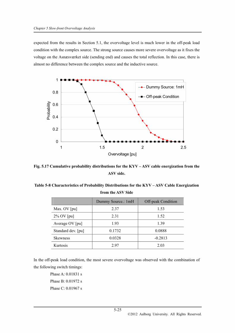
Chapter 5 Slow-front Overvoltage Analysis
5-25 ©2012 Aalborg University. All Rights Reserved.
expected from the results in Section 5.1, the overvoltage level is much lower in the off-peak load
condition with the complex source. The strong source causes more severe overvoltage as it fixes the
voltage on the Asnæsværket side (sending end) and causes the total reflection. In this case, there is
almost no difference between the complex source and the inductive source.
Fig. 5.17 Cumulative probability distributions for the KYV – ASV cable energization from the
ASV side.
Table 5-8 Characteristics of Probability Distributions for the KYV – ASV Cable Energization
from the ASV Side
Dummy Source.: 1mH Off-peak Condition
Max. OV [pu] 2.37 1.53
2% OV [pu] 2.31 1.52
Average OV [pu] 1.93 1.39
Standard dev. [pu] 0.1732 0.0888
Skewness 0.0328 -0.2813
Kurtosis 2.97 2.03
In the off-peak load condition, the most severe overvoltage was observed with the combination of
the following switch timings:
Phase A: 0.01831 s
Phase B: 0.01972 s
Phase C: 0.01967 s
0
0.2
0.4
0.6
0.8
1
1 1.5 2 2.5
Overvoltage [pu]
Pro
babi
lity
Dummy Source: 1mH
Off-peak Condition
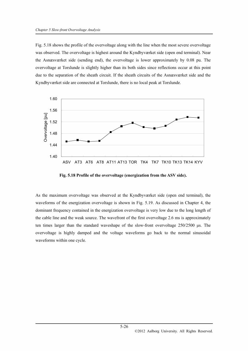
Chapter 5 Slow-front Overvoltage Analysis
5-26 ©2012 Aalborg University. All Rights Reserved.
Fig. 5.18 shows the profile of the overvoltage along with the line when the most severe overvoltage
was observed. The overvoltage is highest around the Kyndbyværket side (open end terminal). Near
the Asnæsværket side (sending end), the overvoltage is lower approximately by 0.08 pu. The
overvoltage at Torslunde is slightly higher than its both sides since reflections occur at this point
due to the separation of the sheath circuit. If the sheath circuits of the Asnæsværket side and the
Kyndbyværket side are connected at Torslunde, there is no local peak at Torslunde.
Fig. 5.18 Profile of the overvoltage (energization from the ASV side).
As the maximum overvoltage was observed at the Kyndbyværket side (open end terminal), the
waveforms of the energization overvoltage is shown in Fig. 5.19. As discussed in Chapter 4, the
dominant frequency contained in the energization overvoltage is very low due to the long length of
the cable line and the weak source. The wavefront of the first overvoltage 2.6 ms is approximately
ten times larger than the standard waveshape of the slow-front overvoltage 250/2500 μs. The
overvoltage is highly damped and the voltage waveforms go back to the normal sinusoidal
waveforms within one cycle.
1.40
1.44
1.48
1.52
1.56
1.60
ASV AT3 AT6 AT8 AT11 AT13 TOR TK4 TK7 TK10 TK13 TK14 KYV
Ove
rvol
tage
[pu
]

Chapter 5 Slow-front Overvoltage Analysis
5-27 ©2012 Aalborg University. All Rights Reserved.
Fig. 5.19 Voltage waveform of the energization overvoltage at the KYV side (open terminal).
5.2.3 Energization from KYV
This section studies the energization from the Kyndbyværket side. The energization overvoltages
on the Asnæsværket side (open end terminal) were monitored.
Fig. 5.20 and Table 5-9 show the cumulative probability distributions and their characteristics. The
overvoltage level is even lower compared with the energization from the Kyndbyværket side.
Besides that, the distributions and characteristics are very similar to those in case of the
energization from the Asnæsværket side.
Fig. 5.20 Cumulative probability distributions for the KYV – ASV cable energization from the KYV side.
-600
-400
-200
0
200
400
600
0 0.01 0.02 0.03 0.04 0.05 0.06
Time [s]
Vol
tage
[kV
]
Phase a
Phase b
Phase c
0
0.2
0.4
0.6
0.8
1
1 1.5 2 2.5
Overvoltage [pu]
Pro
babi
lity
Dummy Source: 1mH
Off-peak Condition
2.6 ms

Chapter 5 Slow-front Overvoltage Analysis
5-28 ©2012 Aalborg University. All Rights Reserved.
Table 5-9 Characteristics of Probability Distributions for the KYV – ASV Cable Energization
from the KYV Side
Dummy Source: 1mH No Additional Source
Max. OV [pu] 2.33 1.31
2% OV [pu] 2.30 1.29
Average OV [pu] 1.91 1.20
Standard dev. [pu] 0.192 0.0413
Skewness -0.352 0.141
Kurtosis 2.84 2.69
In the off-peak load condition, the most severe overvoltage was observed with the combination of
the following switch timings:
Phase A: 0.02370 s
Phase B: 0.02337 s
Phase C: 0.02260 s
Fig. 5.21 shows the profile of the overvoltage along with the line when the most severe overvoltage
was observed. Similarly to the energization from the Kyndbyværket side, the overvoltage is highest
around the Asnæsværket side (open end terminal). Near the Kyndbyværket side (sending end), the
overvoltage is lower approximately by 0.17 pu. The local peak at Torslunde cannot be observed in
this case.
Fig. 5.21 Profile of the overvoltage (energization from the KYV side).
1.10
1.15
1.20
1.25
1.30
1.35
1.40
ASV AT3 AT6 AT8 AT11 AT13 TOR TK4 TK7 TK10 TK13 TK14 KYV
Ove
rvol
tage
[pu
]

Chapter 5 Slow-front Overvoltage Analysis
5-29 ©2012 Aalborg University. All Rights Reserved.
As the maximum overvoltage was observed at the Asnæsværket side (open end terminal), the
waveforms of the energization overvoltage is shown in Fig. 5.22. As in the energization from the
Asnæsværket side, the dominant frequency contained in the energization overvoltage is very low,
and the overvoltage is highly damped.
Fig. 5.22 Voltage waveform of the energization overvoltage at the ASV side (open terminal).
5.2.4 Effects of Synchronized Switching
As a countermeasure to the zero-missing phenomenon discussed in Section 6.3, the synchronized
switching (point-on-wave switching) may be applied to the Kyndbyværket – Asnæsværket line.
When each phase of the cable line is energized at its voltage peak by the synchronized switching,
the DC component in the energization current can be minimized, resulting in the prevention of the
zero-missing phenomenon.
The energization overvoltage analysis in this section, so far, considered two kinds of randomness in
the statistical switching. However, due to the synchronized switching, the phase angle
(point-of-wave) when the line circuit breakers receive the command to close themselves is no
longer random. The randomness of the deviation from the voltage peak is modeled by the normal
distribution with standard deviation 1 ms.
As the synchronized switching controls to energize the line at the voltage peak, it can lead to the
higher energization overvoltages. It is therefore useful to find how the synchronized switching
affects the probability distributions of the energization overvoltages.
-500
-400
-300
-200
-100
0
100
200
300
400
500
0 0.01 0.02 0.03 0.04 0.05 0.06
Time [s]
Vo
ltage
[kV
]
Phase a
Phase b
Phase c

Chapter 5 Slow-front Overvoltage Analysis
5-30 ©2012 Aalborg University. All Rights Reserved.
Fig. 5.23 and Fig. 5.24 compare the cumulative probability distributions for the energization of the
Kyndbyværket – Asnæsværket line with and without synchronized switching. The cable line was
energized from the Asnæsværket side, and two feeding networks, off-peak load condition and peak
load condition with a dummy source, were considered.
These figures show that the maximum overvoltages become lower with the synchronized switching.
Standard deviations of the probability distributions become significantly lower by the synchronized
switching, which helps to lower the maximum overvoltages. The average overvoltages can be lower
or higher with the synchronized switching, depending on the feeding network.
Fig. 5.23 Effect of synchronized switching on cumulative probability distributions (off-peak
load condition).
0
0.2
0.4
0.6
0.8
1
1 1.5 2
Overvoltage [pu]
Pro
babi
lity
w SynchronizedSwitchingw/o SynchronizedSwitching

Chapter 5 Slow-front Overvoltage Analysis
5-31 ©2012 Aalborg University. All Rights Reserved.
Fig. 5.24 Effect of synchronized switching on cumulative probability distributions (dummy
source: 1 mH).
0
0.2
0.4
0.6
0.8
1
1 1.5 2 2.5
Overvoltage [pu]
Pro
babi
lity
w SynchronizedSwitchingw/o SynchronizedSwitching

Chapter 5 Slow-front Overvoltage Analysis
5-32 ©2012 Aalborg University. All Rights Reserved.
Analysis of Statistical Distribution of Energization Overvoltages 5.3
Sections 5.1 and 5.2 have identified characteristics of statistical distributions of energization
overvoltages of EHV cables, compared with those of OHLs. They discussed possible causes that
can lead to the characteristics, but the discussions are limited to qualitative analyses. Consequently,
it is not clear which possible cause has the most dominant effect. This section identifies causes and
physical meanings of the characteristics so that it becomes possible to use the obtained statistical
distributions for the determination of insulation levels of cable systems.
Sections 5.1 and 5.2 studied 10 planned and existing EHV OHLs and cables, respectively. Four line
lengths and four feeding networks (source impedances) were considered as parameters. The
simulations were performed 200 times with random switches under each study condition. As a
result, the study has found the following main characteristics of statistical distributions:
Energization overvoltages for cables are lower than those for OHLs with respect to maximum,
2 %, and mean values. (Section 5.3.1)
Energization overvoltages for cables do not show any dependence on the line length while
those for OHLs peak with the line length 72 km. (Section 5.3.2)
Energization overvoltages for cables become lower for a larger source impedance while those
for OHLs peak with the source impedance 30 mH. (Section 5.3.3)
This section focuses on these three main characteristics in the identification of causes and physical
meanings. The analysis in this section shows only one type of OHLs and cables because the same
characteristics and contributing factors were found in all OHL and cable types.
5.3.1 Analysis on the Highest Overvoltages
First, we study why energization overvoltages for cables are lower than those for OHLs with
respect to maximum, 2 %, and mean values. It is done by analysing voltage waveforms of
energization overvoltages. Here, we define the maximum overvoltage as the largest overvoltage
found in 200 random simulations, and the highest overvoltage as the largest overvoltage in one
figure, or in other words, in one to four voltage waveforms.
Fig. 5.25 shows initial voltage waveforms of the energization overvoltage at the receiving end (Vr)
and at the sending end (Vs) for one type of OHLs. The OHL was energized at the voltage peak of
phase a (5 ms), and the voltage waveforms of phase a are shown in Fig. 5.25. The line length and
the source impedance were fixed to 48 km and 30 mH, respectively.

Chapter 5 Slow-front Overvoltage Analysis
5-33 ©2012 Aalborg University. All Rights Reserved.
Fig. 5.25 Initial voltage waveforms of the energization overvoltage for an OHL
(line length: 48 km, source impedance: 30 mH).
For the OHL, the overvoltage of the inter-phase mode travels at the speed of light. It arrives at the
receiving end 0.16 ms after it departs from the sending end (1st wave).
48km 300m μs⁄ 0.16ms
The inter-phase mode is reflected back to the sending end, but Vr rises towards around 2 pu as the
overvoltage of the earth-return mode arrives. The propagation time of the earth-return mode can be
obtained by performing frequency scan to the energized system or by performing Fourier transform
to the voltage waveform. The result of the frequency scan shows the dominant frequency 980 Hz,
which corresponds to the cycle time 1.02 ms. The result is reasonable as Fig. 5.25 shows the
voltage peak of the earth-return mode with an interval of 1.02 ms.
The initial voltage rise time at the receiving end is difficult to find theoretically. The receiving end
voltage starts to rise at 5.16 ms. Looking at the voltage amplitude of the earth-return mode, the
voltage starts to rise from near the minimum. It suggests that it takes about 0.51 (= 1.02 / 2) ms to
reach the maximum of the earth-return mode, but Fig. 5.25 shows the earth-return mode reaches its
maximum in approximately 0.32 ms after it starts to rise.
-400
-200
0
200
400
600
800
0.004 0.005 0.006 0.007 0.008
Time [s]
Vol
tage
[kV
]
Vr
Vs
0.16ms
0.32ms 0.32ms0.32ms
1.02ms 1.02ms

Chapter 5 Slow-front Overvoltage Analysis
5-34 ©2012 Aalborg University. All Rights Reserved.
This can be explained by the rate of voltage rise. When the voltage starts from the minimum, the
rate of the voltage rise should increase in the first (1.02 / 4) ms and should decrease in the
remaining (1.02 / 4) ms, assuming the receiving voltage follows the sinusoidal wave. However, in
Fig. 5.25, the rate of voltage rise is largest when the receiving voltage starts to rise. This makes the
voltage rise time to 2 pu shorter, and the earth-return mode reaches its maximum in approximately
5.48 (= 5.16 + 0.32) ms.
This reduction of the voltage rise time affects the magnitude of the highest overvoltage since 5.48
ms is exactly when the inter-phase mode comes back to the receiving end (2nd wave). As shown in
Fig. 5.25, the inter-phase mode comes back to the receiving end with an interval of 0.32 ms as it
travels at the speed of light. Since the peak of the earth-return mode (1st wave) and the peak of the
inter-phase mode (2nd wave) reach their maximum almost at the same time around 5.48 ms, Vr
goes above 2 pu and reaches to 2.3 pu.
The same analysis on the initial voltage waveforms is performed for one type of underground
cables. Fig. 5.26 shows initial voltage waveforms of the energization overvoltage at the receiving
end (Vr) and at the sending end (Vs). Study conditions, such as the switch timing (5 ms), line length
(48 km), and source impedance (30 mH), are kept equal to the study on the OHL.
Fig. 5.26 Initial voltage waveforms of the energization overvoltage for a cable
(line length: 48 km, source impedance: 30 mH).
-400
-200
0
200
400
600
800
0.004 0.006 0.008 0.01 0.012
Time [s]
Vol
tage
[kV
]
Vr
Vs
0.28ms
1.62ms 3.85ms

Chapter 5 Slow-front Overvoltage Analysis
5-35 ©2012 Aalborg University. All Rights Reserved.
In case of the underground cable, the overvoltage of the coaxial mode first arrives at the receiving
end (1st wave). When a cable is not cross-bonded, the coaxial mode travels at
300
√ 1
300
√2.852178m μs⁄ Eqn. 5.4
Here, ɛI1 is the relative permittivity of the insulation in Table 3-2, which is corrected to account for
semiconductive layers.
For a cross-bonded cable, it is known that the propagation velocity is reduced further, but it is not
known how to analytically derive the reduced velocity. The propagation velocity is therefore
derived from the propagation time. Fig. 5.26 shows the coaxial mode (1st wave) arrives at the
receiving end 0.28 ms after it leaves the sending end. The propagation velocity is calculated as 171
m/μs (= 48 km / 0.28 ms). The reduction of 7 m/μs or 3.5 % is a typical value.
Similarly to the OHL, the coaxial mode is reflected back to the sending end, but Vr rises towards
around 2 pu as the overvoltage of the inter-phase mode arrives. The propagation time of the
inter-phase mode can be obtained by performing frequency scan to the energized system or by
performing Fourier transform to the voltage waveform. The result of the frequency scan shows the
dominant frequency 260 Hz, which corresponds to the cycle time 3.85 ms. The result is reasonable
as Fig. 5.26 shows the voltage peak of the inter-phase mode with an interval of 3.85 ms.
The modes found in the energization overvoltage of the OHL and the cable are summarized in
Table 5-10.
Table 5-10 Dominant Mode and Superimposed Mode of the Energization Overvoltage
OHL Underground cable
Dominant mode
(cycle time)
Earth-return mode
(1.02 ms)
Inter-phase mode
(3.85 ms)
Superimposed mode
(propagation time)
Inter-phase mode
(0.16 ms)
Coaxial mode
(0.28 ms)
Now, comparing the initial voltage waveforms of the OHL and the cable, the superimposition of
two different modes found in the OHL cannot be observed clearly in the cable. There are some
distortions of voltage waveforms on the inter-phase mode caused by the coaxial mode, but the
distortions only have a small contribution on the highest overvoltage. This is because the
overvoltage of the coaxial mode is smaller and more obtuse, compared with the inter-phase mode in
the OHL.

Chapter 5 Slow-front Overvoltage Analysis
5-36 ©2012 Aalborg University. All Rights Reserved.
Another factor affecting the difference in the highest overvoltage is the long cycle time of the
inter-phase mode in the cable. About the time when the inter-phase mode reaches its maximum (1st
wave), the 4th wave of the coaxial mode arrives at the receiving end. At this time, the coaxial mode
is highly damped and is difficult to observe. Even in the OHL, the inter-phase mode can have an
impact on the highest overvoltage only until its 2nd wave. It is highly damped and is difficult to
observe after the 3rd wave.
5.3.2 Analysis on the Effects of Line Length
Second, we study why energization overvoltages for cables do not show any dependence on the line
length while those for OHLs peak with the line length 72 km.
Fig. 5.37 shows initial voltage waveforms of energization overvoltages of the OHL at the receiving
end (Vr). The switch timing is set to 5 ms as in the last section. The source impedance is set to
30 mH since the maximum overvoltage was observed with the source impedance 30 mH.
Fig. 5.27 Initial voltage waveforms of the energization overvoltage for the OHL
(source impedance: 30 mH).
Fig. 5.27 demonstrates that highest overvoltages are caused by the superimposition of the
earth-return mode (1st wave) and the inter-phase mode (2nd wave), regardless of the line length.
-400
-200
0
200
400
600
800
0.004 0.005 0.006 0.007 0.008
Time [s]
Vo
ltage
(V
r) [
kV]
24km
48km
72km
96km
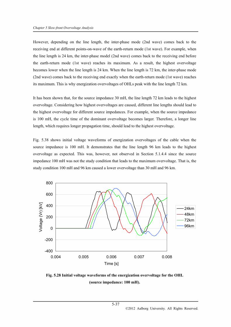
Chapter 5 Slow-front Overvoltage Analysis
5-37 ©2012 Aalborg University. All Rights Reserved.
However, depending on the line length, the inter-phase mode (2nd wave) comes back to the
receiving end at different points-on-wave of the earth-return mode (1st wave). For example, when
the line length is 24 km, the inter-phase model (2nd wave) comes back to the receiving end before
the earth-return mode (1st wave) reaches its maximum. As a result, the highest overvoltage
becomes lower when the line length is 24 km. When the line length is 72 km, the inter-phase mode
(2nd wave) comes back to the receiving end exactly when the earth-return mode (1st wave) reaches
its maximum. This is why energization overvoltages of OHLs peak with the line length 72 km.
It has been shown that, for the source impedance 30 mH, the line length 72 km leads to the highest
overvoltage. Considering how highest overvoltages are caused, different line lengths should lead to
the highest overvoltage for different source impedances. For example, when the source impedance
is 100 mH, the cycle time of the dominant overvoltage becomes larger. Therefore, a longer line
length, which requires longer propagation time, should lead to the highest overvoltage.
Fig. 5.38 shows initial voltage waveforms of energization overvoltages of the cable when the
source impedance is 100 mH. It demonstrates that the line length 96 km leads to the highest
overvoltage as expected. This was, however, not observed in Section 5.1.4.4 since the source
impedance 100 mH was not the study condition that leads to the maximum overvoltage. That is, the
study condition 100 mH and 96 km caused a lower overvoltage than 30 mH and 96 km.
Fig. 5.28 Initial voltage waveforms of the energization overvoltage for the OHL
(source impedance: 100 mH).
-400
-200
0
200
400
600
800
0.004 0.005 0.006 0.007 0.008
Time [s]
Vol
tage
(V
r) [
kV]
24km
48km
72km
96km

Chapter 5 Slow-front Overvoltage Analysis
5-38 ©2012 Aalborg University. All Rights Reserved.
Fig. 5.29 shows initial voltage waveforms of energization overvoltages of the cable at the receiving
end (Vr). The source impedance is set to 1 mH since the maximum overvoltage was observed with
the source impedance 1 mH. As the source impedance is set so small, not only the rate of voltage
rise but also the magnitude of the overvoltage becomes larger, compared with other source
impedance values.
Another significant difference from other source impedance values is how the coaxial mode is
reflected at the sending end. With the source impedance 1 mH, the reflection at the sending end is
negative reflection, whereas the reflection at the sending end is positive reflection with other source
impedance values. It is because the voltage level at the sending end is fixed to the source voltage
when the source impedance is 1 mH.
The difference of the reflection can clearly observed in Fig. 5.29. So far, the superimposition of the
two modes raised the highest overvoltage. On the contrary, in Fig. 5.29, the negative coaxial mode
(2nd wave) makes dents on the peaks of the inter-phase mode (1st wave). The inter-phase mode
(1st wave) is larger for shorter line lengths, but the negative coaxial mode (2nd wave) is also larger
for shorter line lengths. As a result, the highest overvoltage is observed in case of the line length
48 km, and the effect of the line length on the highest overvoltage is reduced.
Fig. 5.29 Initial voltage waveforms of the energization overvoltage for the cable
(source impedance: 1 mH).
-400
-200
0
200
400
600
800
0.004 0.005 0.006 0.007 0.008
Time [s]
Vo
ltag
e (V
r) [
kV]
24km
48km
72km
96km
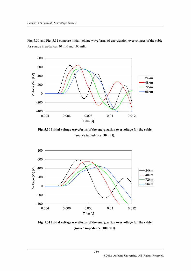
Chapter 5 Slow-front Overvoltage Analysis
5-39 ©2012 Aalborg University. All Rights Reserved.
Fig. 5.30 and Fig. 5.31 compare initial voltage waveforms of energization overvoltages of the cable
for source impedances 30 mH and 100 mH.
Fig. 5.30 Initial voltage waveforms of the energization overvoltage for the cable
(source impedance: 30 mH).
Fig. 5.31 Initial voltage waveforms of the energization overvoltage for the cable
(source impedance: 100 mH).
-400
-200
0
200
400
600
800
0.004 0.006 0.008 0.01 0.012
Time [s]
Vo
ltage
(V
r) [k
V]
24km
48km
72km
96km
-400
-200
0
200
400
600
800
0.004 0.006 0.008 0.01 0.012
Time [s]
Vol
tage
(V
r) [
kV]
24km
48km
72km
96km
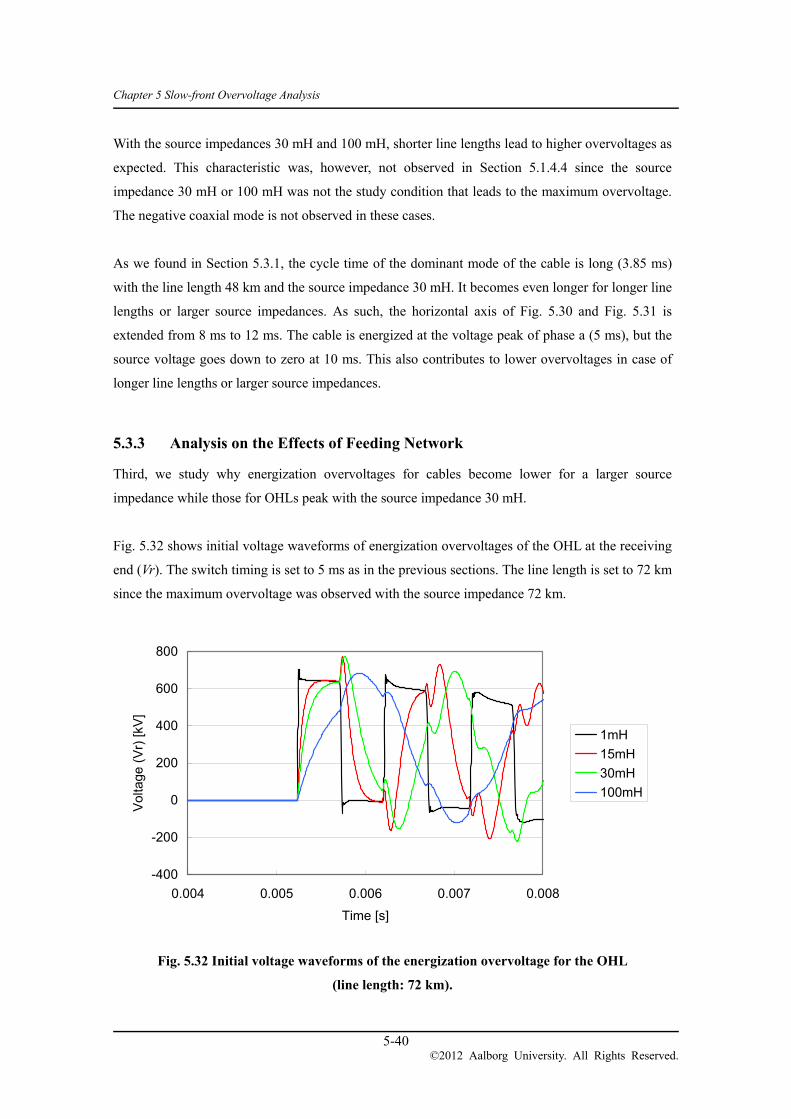
Chapter 5 Slow-front Overvoltage Analysis
5-40 ©2012 Aalborg University. All Rights Reserved.
With the source impedances 30 mH and 100 mH, shorter line lengths lead to higher overvoltages as
expected. This characteristic was, however, not observed in Section 5.1.4.4 since the source
impedance 30 mH or 100 mH was not the study condition that leads to the maximum overvoltage.
The negative coaxial mode is not observed in these cases.
As we found in Section 5.3.1, the cycle time of the dominant mode of the cable is long (3.85 ms)
with the line length 48 km and the source impedance 30 mH. It becomes even longer for longer line
lengths or larger source impedances. As such, the horizontal axis of Fig. 5.30 and Fig. 5.31 is
extended from 8 ms to 12 ms. The cable is energized at the voltage peak of phase a (5 ms), but the
source voltage goes down to zero at 10 ms. This also contributes to lower overvoltages in case of
longer line lengths or larger source impedances.
5.3.3 Analysis on the Effects of Feeding Network
Third, we study why energization overvoltages for cables become lower for a larger source
impedance while those for OHLs peak with the source impedance 30 mH.
Fig. 5.32 shows initial voltage waveforms of energization overvoltages of the OHL at the receiving
end (Vr). The switch timing is set to 5 ms as in the previous sections. The line length is set to 72 km
since the maximum overvoltage was observed with the source impedance 72 km.
Fig. 5.32 Initial voltage waveforms of the energization overvoltage for the OHL
(line length: 72 km).
-400
-200
0
200
400
600
800
0.004 0.005 0.006 0.007 0.008
Time [s]
Vol
tage
(V
r) [k
V]
1mH
15mH
30mH
100mH

Chapter 5 Slow-front Overvoltage Analysis
5-41 ©2012 Aalborg University. All Rights Reserved.
As discussed in Section 5.3.2, the highest overvoltage of the OHL is determined by the timing
when the earth-return mode reaches its maximum and the inter-phase mode arrives at the receiving
end. Fig. 5.32 shows that source impedances 15 mH and 30 mH have the timing to cause high
overvoltages. When the source impedance is 1 mH, the overvoltage of the inter-phase mode is
smaller, which results in the lower overvoltage.
Fig. 5.33 and Fig. 5.34 show initial voltage waveforms of energization overvoltages of the cable for
line lengths 24 km and 48 km. These two lengths were selected as we learned, in Section 5.3.2, that
shorter line lengths lead to higher overvoltages except when the source impedance is 1 mH.
Fig. 5.33 demonstrates that smaller source impedances lead to larger overvoltages as we found in
Section 5.1.4.5. This is not true only when the source impedance is 1 mH.
Fig. 5.33 Initial voltage waveforms of the energization overvoltage for the cable
(line length: 24 km).
When the source impedance is 1 mH, the highest overvoltage is caused when the line length is
48 km as we learned in the last section. Looking at the source impedance 1 mH in Fig. 5.34 and
other source impedances in Fig. 5.33, it is clear that smaller source impedances lead to larger
overvoltages.
-400
-200
0
200
400
600
800
0.004 0.005 0.006 0.007 0.008 0.009 0.01
Time [s]
Vol
tage
(V
r) [
kV]
1mH
15mH
30mH
100mH

Chapter 5 Slow-front Overvoltage Analysis
5-42 ©2012 Aalborg University. All Rights Reserved.
Fig. 5.34 Initial voltage waveforms of the energization overvoltage for the cable
(line length: 48 km).
It is reasonable to have larger overvoltages with smaller source impedances as the rate of voltage
rise becomes larger for smaller source impedances. The larger rate of voltage rise is apparent as the
smaller source impedances lead to a higher dominant frequency contained in the energization
overvoltage. For larger source impedances, due to their slow rates of voltage rise, the fundamental
component already starts to decrease from the voltage peak by the time when the inter-phase mode
reaches its maximum.
5.3.4 Summary
This section analyzed the characteristics of the energization overvoltage found in Sections 5.1 and
5.2. The analysis has found that these characteristics are not caused by random switching by
accident, rather there are contributing factors and physical meanings behind the characteristics.
In summary, the analysis has identified contributing factors and has explained their physical
meanings as follows:
Energization overvoltages for cables are lower than those for OHLs because the overvoltage
of the coaxial mode in cables is smaller and more obtuse, compared with the inter-phase mode
in OHLs. The long cycle time of the inter-phase mode in cables also affects this characteristic.
Energization overvoltages for cables do not show any dependence on the line length because
-400
-200
0
200
400
600
800
0.004 0.005 0.006 0.007 0.008 0.009 0.01
Time [s]
Vo
ltage
(V
r) [k
V]
1mH
15mH
30mH
100mH

Chapter 5 Slow-front Overvoltage Analysis
5-43 ©2012 Aalborg University. All Rights Reserved.
the maximum overvoltages are observed with the source impedance 1 mH. The negative
coaxial mode makes dents on the peaks of the maximum overvoltage when the source
impedance is 1 mH. With the other source impedances, shorter line lengths lead to higher
overvoltages.
Energization overvoltages for cables become lower for larger source impedances, which is
reasonable from the theoretical analysis.
Highest energization overvoltages for OHLs are caused by the superimposition of the
inter-phase mode on the earth-return mode. The timing of the superimposition determines the
magnitude of the highest overvoltage, and the line length and the source impedance affect this
timing. The energization overvoltage for OHLs peak with the line length 72 km and the source
impedance 30 mH because the combination provided the best timing for the superimposition
within the studied conditions.
Since the contributing factors and physical meanings of the characteristics have been identified, it
is now possible to use the obtained statistical distribution for the determination of insulation levels
of cable systems. Especially, the obtained statistical distribution suggests a possible application of
lower insulation levels to cable systems compared with OHLs. However, it may present a future
challenge to define insulation levels for temporary overvoltages since a possibility of severe
temporary overvoltages are reported in relation to cable systems [13][14][18][19].

Chapter 5 Slow-front Overvoltage Analysis
5-44 ©2012 Aalborg University. All Rights Reserved.
Ground Fault and Fault Clearing Overvoltage 5.4
5.4.1 Study Conditions and Parameters
The idea of the statistical evaluation is also applied to the evaluation of the ground fault and fault
clearing overvoltages since the fault location and the fault timing vary and cannot be controlled.
Instead of considering them as random phenomena, it is a common practice to cover different fault
locations and fault timings with fixed (pre-defined) steps.
Table 5-11 summarizes the study conditions and parameters for the ground fault and fault clearing
overvoltages. The 10 fault locations were selected so that the separation between each fault location
is limited to 3 – 6 km. In order to cover 10 fault locations and 19 fault timings, 190 simulations
were performed. The 2 % value is the 3rd highest overvoltage in these simulations.
Table 5-11 Study Conditions and Parameters for the Ground Fault and Fault Clearing
Overvoltage
Fault type Single line to ground fault (core to sheath)
Fault location Five points between ASV – TOR and TOR – KYV
ASV – TOR: AT3, AT6, AT8, AT11 and AT13
TOR – KYV: TK4, TK7, TK10, TK13 and TK14
Fault timing 0° – 180° (10° step)
Fault clearing time First current zero at least 40 ms after the fault occurrence
Fault clearing sequence Line-CBs of all three phases are opened at the above fault
clearing time.
Sequential switching
Feeding source Off-peak load condition + dummy source: 15 mH (strong
source) and 100 mH (weak source)
As in the energization overvoltage analysis, two feeding networks were considered. One is the
strong source case and the other one is the weak source case. Both feeding networks were modeled
based on the off-peak load condition and by adding a dummy source to the Asnæsværket 400 kV
bus. The source impedance of the dummy source impedance was set to 15 mH and 100 mH in the
weak source and strong source case, respectively.
Since the ground fault and fault clearing overvoltages depend on the fault current, the fault current
level needs to be set within a reasonable range. In a cable energization overvoltage analysis, the
dummy source impedance was set to 1 mH in order to find the effect of a steep rise of an initial

Chapter 5 Slow-front Overvoltage Analysis
5-45 ©2012 Aalborg University. All Rights Reserved.
overvoltage. However, this setting should be avoided in the ground fault and fault clearing
overvoltage analysis as unreasonably large fault current will flow in the simulation with this setting.
The dummy source impedance was therefore set to 15 mH in the strong source case.
The dummy source was also added to the off-peak load condition even in the weak source case, but
the dummy source impedance was set to a large value (100 mH). Without the dummy source,
ground fault and fault clearing overvoltages were almost unnoticeable since the fault current was
too small.
In the ground fault and fault clearing overvoltage analysis, the highest overvoltage is not always
observed at the open terminal. In addition, there is no open terminal for the ground fault
overvoltage. As such, the overvoltages were monitored at AT3, AT6, AT8, AT11, AT13, TK4, TK7,
TK10, TK13 and TK14 as well as at Asnæsværket, Torslunde and Kyndbyværket.
5.4.2 Results of the Analysis
Fig. 5.35 and Table 5-12 show the cumulative probability distributions of the ground fault and fault
clearing overvoltages and their characteristics. The overvoltage level is as low as the energization
overvoltage of the Kyndbyværket – Asnæsværket line in the off-peak load condition. The
probability distributions are affected by the dummy source impedance, but the overvoltage level is
low in both cases.
Fig. 5.35 Cumulative probability distributions for the ground fault and fault current
overvoltage.
0
0.2
0.4
0.6
0.8
1
1 1.2 1.4 1.6
Overvoltage [pu]
Cum
ulat
ive
Pro
bab
ility
Dummy Source: 15mH
Dummy Source: 100mH

Chapter 5 Slow-front Overvoltage Analysis
5-46 ©2012 Aalborg University. All Rights Reserved.
Table 5-12 Characteristics of Probability Distributions for the Ground Fault and Fault
Clearing Overvoltage
Dummy Source: 15mH Dummy Source: 100mH
Max. OV [pu] 1.33 1.37
2% OV [pu] 1.30 1.36
Average OV [pu] 1.17 1.14
Standard dev. [pu] 0.0482 0.0647
Skewness 0.430 1.79
Kurtosis 3.52 5.76
With the dummy source impedance 15 mH and 100 mH, the maximum overvoltage was observed
when the fault occurs at AT3 and at the phase angle 60° and 70°, respectively. In both cases, the
maximum overvoltage was the ground fault overvoltages and was not the fault clearing
overvoltages. Fig. 5.36 shows the profile of the maximum ground fault overvoltages along the
length of the Kyndbyværket – Asnæsværket line. The figure shows that the maximum overvoltages
were observed at the Asnæsværket 400 kV bus.
Fig. 5.36 Profile of the maximum ground fault overvoltages.
As the maximum overvoltage was observed at the Asnæsværket 400 kV bus, the voltage waveforms
at the Asnæsværket 400 kV bus are given in Fig. 5.37 and Fig. 5.38. The figures show that both
ground fault overvoltages and fault clearing overvoltages are highly damped.
1.10
1.15
1.20
1.25
1.30
1.35
1.40
ASV AT3 AT6 AT8 AT11 AT13 TOR TK4 TK7 TK10 TK13 TK14 KYV
Ove
rvo
ltage
[pu
]
Dummy Source: 15mH
Dummy Source: 100mH

Chapter 5 Slow-front Overvoltage Analysis
5-47 ©2012 Aalborg University. All Rights Reserved.
Fig. 5.37 Voltage waveforms of the maximum ground fault overvoltage at the ASV 400 kV bus
(dummy source: 15 mH).
Fig. 5.38 Voltage waveforms of the maximum ground fault overvoltage at the ASV 400 kV bus
(dummy source: 100 mH).
5.4.3 Results with the Sequential Switching
The sequential switching has been adopted as a countermeasure to the zero-missing phenomenon.
With the sequential switching, the sequence for the fault clearing is different from the ordinal
sequence simulated in the previous section. Detailed explanations on the sequential switching are
given in Section 6.3.1.
-500
-400
-300
-200
-100
0
100
200
300
400
500
0 0.02 0.04 0.06 0.08 0.1
Time [s]
Vol
tage
[kV
]
Phase a
Phase b
Phase c
-500
-400
-300
-200
-100
0
100
200
300
400
500
0 0.02 0.04 0.06 0.08 0.1
Time [s]
Vol
tage
[kV
]
Phase a
Phase b
Phase c
Fault occurrence (60°) Fault clearance
Fault occurrence (70°) Fault clearance

Chapter 5 Slow-front Overvoltage Analysis
5-48 ©2012 Aalborg University. All Rights Reserved.
According to the fault clearing sequence with the sequential switching, the ground fault and fault
clearing overvoltage was analyzed with the following sequence:
Fault occurrence (phase a): 0.0 – 0.1 s
Fault clearing (phase a): 0.05 s
Shunt reactor tripping (phases b and c): 0.11 s (only on the Kyndbyværket side)
Line breaker tripping (phases b and c): 0.17 s
The time separations between above steps were set shorter than the actual setting. As long as the
overvoltage caused by the previous step is well damped, the shorter time separations have no effect
on the overvoltage caused by the next step.
In the previous section with the normal fault clearing sequence, ground faults in different phases
were simulated. In this section with the sequential switching, ground faults occurs only in phase a.
Since three phases are well balanced in the Kyndbyværket – Asnæsværket cable model, it is not
expected that this has a major impact on the simulation results.
Fig. 5.39 and Table 5-13 show the cumulative probability distributions of the ground fault and fault
clearing overvoltage and their characteristics. The maximum overvoltage level is lower than the
overvoltage with the normal fault clearing sequence approximately by 0.1 pu. The average
overvoltage is not affected by the sequential switching. The probability distributions are affected by
the dummy source impedance, but the overvoltage level is low in both cases.
Fig. 5.39 Cumulative probability distributions for the ground fault and fault current
overvoltage with the sequential switching.
0
0.2
0.4
0.6
0.8
1
1 1.2 1.4
Overvoltage [pu]
Cum
ulat
ive
Pro
babi
lity
Dummy Source: 15mH
Dummy Source: 100mH

Chapter 5 Slow-front Overvoltage Analysis
5-49 ©2012 Aalborg University. All Rights Reserved.
Table 5-13 Characteristics of Probability Distributions for the Ground Fault and Fault
Clearing Overvoltage with the Sequential Switching
Dummy Source: 15mH Dummy Source: 100mH
Max. OV [pu] 1.21 1.16
2% OV [pu] 1.21 1.15
Average OV [pu] 1.14 1.11
Standard dev. [pu] 0.0410 0.0145
Skewness 0.167 1.59
Kurtosis 1.42 4.47
With the dummy source impedance 15 mH and 100 mH, the maximum overvoltage was observed
when the fault occurs at TK13 and TK17 respectively, and at the phase angle 130°. In both cases,
the maximum overvoltages were the ground fault overvoltages and were not the fault clearing
overvoltages. This means that the difference of the maximum overvoltage, compared to the one
with the normal fault clearing, was not caused by the difference of the fault clearing sequence. The
difference was caused by the faulted phase.
Fig. 5.40 shows the profile of the maximum ground fault overvoltages along the length of the
Kyndbyværket – Asnæsværket line. The figure shows that the maximum overvoltages were
observed at TK13 with the dummy source impedance 15 mH and at the Asnæsværket 400 kV bus
with the dummy source impedance 100 mH.
Fig. 5.40 Profile of the maximum ground fault overvoltages with the sequential switching.
1.00
1.05
1.10
1.15
1.20
1.25
1.30
ASV AT3 AT6 AT8 AT11 AT13 TOR TK4 TK7 TK10 TK13 TK14 KYV
Ove
rvol
tage
[pu]
Dummy Source: 15mH
Dummy Source: 100mH

Chapter 5 Slow-front Overvoltage Analysis
5-50 ©2012 Aalborg University. All Rights Reserved.
As the maximum overvoltage was observed at TK13 with the dummy source impedance 15 mH,
the voltage waveforms at TK13 are shown in Fig. 5.41. The line current at the Asnæsværket side is
also shown in the figure for the better understanding of the sequential switching. The figures show
that both ground fault overvoltages and fault clearing overvoltages are highly damped.
Fig. 5.41 Voltage and current waveforms of the maximum ground fault overvoltage at the
ASV 400 kV bus with the sequential switching (dummy source: 15 mH).
-500
-400
-300
-200
-100
0
100
200
300
400
500
0 0.05 0.1 0.15 0.2
Time [s]
Vol
tage
[kV
]
Phase a
Phase b
Phase c
-3
-2
-1
0
1
2
3
0 0.05 0.1 0.15 0.2
Time [s]
Cur
rent
[kA
]
Phase a
Phase b
Phase c
Fault occurrence (130°)
Fault clearance Reactor tripping
Line tripping (phase b,c)

Chapter 5 Slow-front Overvoltage Analysis
5-51 ©2012 Aalborg University. All Rights Reserved.
As the maximum overvoltage was observed at Kyndbyværket 400 kV bus with the dummy source
impedance 100 mH, the voltage waveforms at the bus are shown in Fig. 5.42
Fig. 5.42 Voltage and current waveforms of the maximum ground fault overvoltage at the
ASV 400 kV bus with the sequential switching (dummy source: 100 mH).
-500
-400
-300
-200
-100
0
100
200
300
400
500
0 0.05 0.1 0.15 0.2
Time [s]
Vo
ltage
[kV
]
Phase a
Phase b
Phase c
-3
-2
-1
0
1
2
3
0 0.05 0.1 0.15 0.2
Time [s]
Cur
rent
[kA
]
Phase a
Phase b
Phase c
Fault occurrence (130°)
Fault clearance Reactor tripping
Line tripping (phase b,c)

Chapter 5 Slow-front Overvoltage Analysis
5-52 ©2012 Aalborg University. All Rights Reserved.
Conclusion 5.5
This chapter studied the slow-front overvoltages of cable systems. In Section 5.1, the statistical
distributions of line energization overvoltages were compared between overhead lines and cables.
Through the comparison, it has been found that line energization overvoltages in cables are lower
than those in overhead lines. More precisely, the maximum and mean values are lower, but the
minimum values are almost equal. As a result, standard deviations are smaller for cables, and the
statistical distributions of overhead lines are closer to the normal distribution than those of cables.
The statistical distributions show that, if one considers only line energization overvoltages, it is
possible to apply lower withstand voltages for cable systems. However, there are issues related to
temporary overvoltages in cable systems as discussed in the previous chapter. As such, careful
examinations are necessary.
Section 5.2 studied the statistical distributions of energization overvoltages of the Kyndbyværket –
Asnæsværket line. Even with an extremely severe condition, the maximum overvoltage found in
the analysis was 2.37 pu, which was much lower than SIWV 1050 kV (3.2 pu).
The study has found that a strong source yields more severe results, which is in line with the
simulation results with an inductive source. In addition, standard deviations were larger with the
strong source. Additionally, it has been found that the maximum overvoltage becomes lower by the
synchronized switching.
In all energizations, waveforms of the overvoltages looked very different from the ones typically
observed with overhead lines. The observed wavefront was 2.6 ms, which is approximately ten
times larger than the standard waveshape of the slow-front overvoltage 250/2500 μs. The difference
was caused by the low dominant frequency contained in the energization overvoltages as discussed
in Section 4.1.3.
Section 5.3 analyzed the characteristics of the energization overvoltage found in Sections 5.1 and
5.2. The section identified the contributing factors and physical meanings of the characteristics as
summarized in Section 5.4.3 so that it would become possible to use the obtained statistical
distributions for the determination of insulation levels of cable systems.
Section 5.4 studied the statistical distributions of ground fault and fault clearing overvoltages of the

Chapter 5 Slow-front Overvoltage Analysis
5-53 ©2012 Aalborg University. All Rights Reserved.
Kyndbyværket – Asnæsværket line. The maximum overvoltage found in the analysis was 1.37 pu,
which was much lower than SIWV 1050 kV (3.2 pu). The study has found that ground fault
overvoltages are larger than fault clearing overvoltages. Effects of dummy source impedances were
not significant.
The sequential switching may be applied to the Kyndbyværket – Asnæsværket line as a
countermeasure of the zero-missing phenomenon. Since ground fault overvoltages were larger than
fault clearing overvoltages, the sequential switching did not affect the severity of the overvoltages.

Chapter 5 Slow-front Overvoltage Analysis
5-54 ©2012 Aalborg University. All Rights Reserved.
References
[1] Insulation Coordination for Power Systems, Andrew R. Hileman, published by Marcel Dekker
Inc., June 1999
[2] CIGRE Working Group 13.02, “Switching Overvoltages in EHV and UHV Systems with
Special Reference to Closing and Reclosing Transmission Lines,” Electra N°30, pp. 70-122,
1973.
[3] CIGRE Working Group 13.05, “The Calculation of Switching Surges,” Electra N°19, pp.
67-78, 1971.
[4] CIGRE Working Group 13.05, “The Calculation of Switching Surges – II. Network
Representation for Energization and Re-energization Studies on Lines Fed by an Inductive
Source,” Electra N°32, pp. 17-42, 1974.
[5] CIGRE Working Group 13.05, “The Calculation of Switching Surges – III. Transmission Line
Representation for Energization and Re-energization Studies with Complex Feeding
Networks,” Electra N°62, pp. 45-78, 1979.
[6] J. Sato, Y. Tsuchiya, A. Arai, N. Hotta, J. Shinavawa, N. Matsumoto, “Technical Development
and View of Underground and Overhead Transmission Line,” SWCC Showa Review, vol. 51,
No. 1, 2001 (in Japanese)
[7] L. Elgh, C.T. Jacobsen, B. Bjurstrom, G. Hjalmarsson, S.O. Olsson, “The 420 kV AC
Submarine Cable Connection Denmark-Sweden,” CIGRE Session 1974, 21-02.
[8] I.A. Gubinsky, M.G. Khanukov, L.A. Kusnetsov, V.I. Masold, I.B. Peshkov, N.K. Sorochkin,
“500 kV cable lines for hydro power stations,” CIGRE Session 1976, 21-03.
[9] W. Hahn, U. Muller, E.F. Peschke, ” The first 380 kV bulk power transmission in Germany,”
CIGRE Session 1976, 21-08
[10] G. Gualtieri, G.M. Lanfranconi, W. Cavalli, “330-kV Oil-Filled Cables Laid in 1600-FT
Vertical Shaft at Kafue Gorge Hydroelectric Plant,” IEEE Trans. on Power Apparatus and
Systems, vol. PAS-92, no. 6, Nov. 1973.
[11] Statistics of AC Underground Cables in Power Networks, CIGRE Technical Brochure 338,
December 2007.
[12] Update of Service Experience of HV Underground and Cable Systems, CIGRE Technical
Brochure 379, April 2009.
[13] Assessment of the Technical Issues relating to Significant Amounts of EHV Underground
Cable in the All-island Electricity Transmission System, (available on the web) Tokyo Electric
Power Company, November 2009, http://www.eirgrid.com/media/Tepco%20Report.pdf.

Chapter 5 Slow-front Overvoltage Analysis
5-55 ©2012 Aalborg University. All Rights Reserved.
[14] N. Momose, H. Suzuki, S. Tsuchiya, T. Watanabe, "Planning and Development of 500 kV
Underground Transmission System in Tokyo Metropolitan Area," CIGRE Session 1998,
37-202.
[15] M. Rebolini, L. Colla, F. Iliceto, “400 kV AC new submarine cable links between Sicily and
the Italian mainland. Outline of project and special electrical studies,” CIGRE Session 2008,
C4-116.
[16] L. Colla, S. Lauria, F. M. Gatta, “Temporary Overvoltages due to Harmonic Resonance in
Long EHV Cables,” IPST 2007,
http://www.ipst.org/techpapers/2007/ipst_2007/papers_IPST2007/Session16/233.pdf.
[17] Massey, F. J. “The Kolmogorov-Smirnov Test for Goodness of Fit,” Journal of the American
Statistical Association, vol. 46, no. 253, 1951, pp. 68–78.
[18] T. Karasaki, T. Goto, A. Ametani, ”An Abnormal Overvoltage due to Load Rejection on EHV
Underground Transmission Lines”, International Conference on Power System Transients
(IPST), September 1995.
[19] L. Colla, M. Rebolini, F. Iliceto, “400 kV AC new submarine cable links between Sicily and
the Italian mainland. Outline of project and special electrical studies”, CIGRE Session C4-116,
2008.
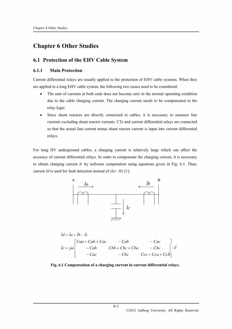
Chapter 6 Other Studies
6-1 ©2012 Aalborg University. All Rights Reserved.
Other Studies Chapter 6
Protection of the EHV Cable System 6.1
6.1.1 Main Protection
Current differential relays are usually applied to the protection of EHV cable systems. When they
are applied to a long EHV cable system, the following two issues need to be considered:
The sum of currents at both ends does not become zero in the normal operating condition
due to the cable charging current. The charging current needs to be compensated in the
relay logic.
Since shunt reactors are directly connected to cables, it is necessary to measure line
currents excluding shunt reactor currents. CTs and current differential relays are connected
so that the actual line current minus shunt reactor current is input into current differential
relays.
For long HV underground cables, a charging current is relatively large which can affect the
accuracy of current differential relays. In order to compensate the charging current, it is necessary
to obtain charging current Ic by software computation using equations given in Fig. 6.1. Then,
current Id is used for fault detection instead of (Ia+ Ib) [1].
cIbIaIdI
V
CcbCcaCccCbcCac
CbcCbaCbcCbbCab
CacCabCacCabCaa
jcI
Fig. 6.1 Compensation of a charging current in current differential relays.
aI bI
cI
A B

Chapter 6 Other Studies
6-2 ©2012 Aalborg University. All Rights Reserved.
6.1.2 Backup Protection – Ground Loop Impedance
Backup protection of EHV cable systems normally adopts a distance protection. The following
items are often discussed with respect to the distance protection of long EHV cable systems:
It is required to know accurate impedances of cable systems.
Negative sequence distance protection is effective since it is not affected by the load
current.
Low order harmonics are contained in voltages and currents under disturbances, such as
contingencies and network operations. Careful considerations are necessary to extract
fundamental components from them.
Cable faults are normally single line to ground (SLG) faults. Short circuits are mostly man-caused
and occur in very limited occasions. In a SLG fault, a cable core is short-circuited to the cable
sheath, which is grounded at cable heads and normal joints. The return circuit for a SLG fault is
later explained with Fig. 6.5.
Fig. 6.2 shows a circuit that expresses a SLG fault in a cable line. Zl is the cable impedance
between the location of the impedance relay and the fault location.
Fig. 6.2 SLG fault in a cable line.
The SLG fault in Fig. 6.2 can be expressed using symmetrical components as in Fig. 6.3.

Chapter 6 Other Studies
6-3 ©2012 Aalborg University. All Rights Reserved.
Fig. 6.3 Loop impedance in a single line to ground fault.
In Fig. 6.3,
1 2 0
1 1 1 2 2 2 0 0 0
1 1 2 2 0 0 1 2 0
1 1 1 2 0 0
1 1 2 0 0 1 0
10 13 1
3 0
Eqn. 6.1
The ground loop impedance (positive sequence impedance) calculated by the ground impedance
relay is
1 0 13 1 3 0
0 3 0
Eqn. 6.2
Here, the zero-sequence compensation 0 0 1 3 1⁄ .
Therefore, by considering the zero-sequence compensation, the ground impedance relay can
accurately calculate the positive sequence impedance to the fault location. In a typical practice, the
zero-sequence compensation k0 is calculated with the positive-sequence impedance Zl1 and
zero-sequence impedance Zl0 for the total length of the line, assuming that both Zl1 and Zl0 have a
linear relationship to the distance to the fault location.

Chapter 6 Other Studies
6-4 ©2012 Aalborg University. All Rights Reserved.
Ground Loop Impedance of Cross-Bonded Cables
The ground loop impedance Zl1 of an overhead line is almost linear to the distance to the fault
location as long as the line type and the tower configuration do not change too much. Using this
characteristic, it is possible for the impedance relay to find the distance to the fault location.
For cross-bonded cables, it has been known that the ground loop impedance does not exhibit a
linear relationship to the distance to the fault location [2], [3]. Fig. 6.4 shows the compensated loop
impedance of a cable line. The ground loop impedance shows discontinuity at the cross-bonding
points. This leads to the nonlinear relationship to the distance to the fault location and may result in
unwanted operations or mis-operations of impedance relays.
Fig. 6.4 Compensated loop impedance for cross-bonded cables. (Source: Protection of
High-Voltage AC Cables [3]).

Chapter 6 Other Studies
6-5 ©2012 Aalborg University. All Rights Reserved.
It has been found in the PhD project that an imbalance of impedances between phases caused the
discontinuity of the ground loop impedance. Let us focus on one cross-bonding point. Because of
the cross-bonding, a SLG fault before the cross-bonding point has a different return circuit (sheath)
from a SLG fault on the same phase but after the cross-bonding point, as shown in Fig. 6.5.
Therefore, if there is an imbalance of impedance between phases, the change of the return circuit
can cause the discontinuity of the ground loop impedance.
Fig. 6.5 Return circuit for a SLG fault before and after a cross-bonding point.
Cable Head IJ IJOpen end
Earth
Cable Head IJ IJOpen end
Earth

Chapter 6 Other Studies
6-6 ©2012 Aalborg University. All Rights Reserved.
6.1.3 Cross-bonded Cable with One Major Section
In order to confirm the validity of the statement, the ground loop impedances were calculated for
the following types of cross-bonded cables:
Directly buried in a flat formation without transposition
Directly buried in a flat formation with transposition
Directly buried in a trefoil formation without transposition
Directly buried in a trefoil formation with transposition
Laid in a tunnel in a trefoil formation with transposition
Here, transposition means the transposition of the whole cable, which is different from
cross-bonding.
As in the previous section, it was assumed that the cross-bonded cable had only one major section.
The physical and electrical parameters of the Asnæsværket – Torslunde cable were used for the
calculation. Assumed cable layouts are illustrated in Fig. 6.6.
Fig. 6.6 Cable layouts.
1.3m
(a) Directly buried in a flat formation
0.3m
1.3m
0.3m
1.69m 0.17m
(c) Laid in a trefoil formation in a tunnel
(b) Directly buried in a trefoil formation

Chapter 6 Other Studies
6-7 ©2012 Aalborg University. All Rights Reserved.
The ground loop impedances were calculated using the steady-state calculation function of the
ATP-EMTP. The cable parameters were thus calculated by the subroutine CABLE CONSTANTS
with the target frequency 50 Hz within ATP-EMTP.
Fig. 6.7 shows the compensated ground loop impedances for different cable layouts and
with/without transposition. It has been found that the transposition does not have any impact on the
ground loop impedance when the cable is laid in a trefoil formation. Comparing the ground loop
impedance, the discontinuity at the cross-bonding points is larger in the following order as shown
in Table 6-1:
(1) Directly buried in a flat formation without transposition (Flat w/o Transp.)
(2) Directly buried in a flat formation with transposition (Flat w Transp.)
(3) Directly buried in a trefoil formation (Trefoil)
(4) Laid in a tunnel in a trefoil formation with transposition (Tunnel)
This order is reasonable considering the impedance balance between phases.
Table 6-1 Largest Discontinuity of Ground Loop Reactance at Cross-bonding Points
Cable layouts (1) Flat w/o Transp. (2) Flat w Transp. (3) Trefoil (4) Tunnel
Largest
discontinuity 17.0 % 14.5 % 13.8 % 11.7 %
The difference of the discontinuity is significant especially at the second cross-bonding point where
only minor discontinuity is observed for the cable laid in a trefoil formation in a tunnel. This is
because the cable laid in a trefoil formation in a tunnel has the best impedance balance between
phases due to the existence of the perfect ground (tunnel) close to the cable.
The calculated loop impedance shows the difficulty in protecting a short cross-bonded cable by the
impedance relay without communication. When it is necessary, the rectangular characteristic is
more suited than the mho characteristic.

Chapter 6 Other Studies
6-8 ©2012 Aalborg University. All Rights Reserved.
Fig. 6.7 Compensated ground loop impedance for cross-bonded cables with one major section.
0
0.1
0.2
0.3
0.4
0 2 4 6
Distance [km]
Rl [Ω
]
Flat w Transposition
Flat w/o Transposition
Trefoil
Trefoil in Tunnel
0
0.2
0.4
0.6
0.8
0 2 4 6
Distance [km]
Xl [Ω
]
Flat w Transposition
Flat w/o Transposition
Trefoil
Trefoil in Tunnel
0
0.2
0.4
0.6
0.8
0 0.1 0.2 0.3 0.4
Rl [Ω]
Zl [Ω
]
Flat w Transposition
Flat w/o Transposition
Trefoil
Trefoil in Tunnel

Chapter 6 Other Studies
6-9 ©2012 Aalborg University. All Rights Reserved.
6.1.4 ASV – TOR Cable Line
The ground loop impedance of a cross-bonded cable with one major section was previously
discussed in literature even though its relationship with cable layouts or transposition has never
been investigated [2], [3]. The ground loop impedance of a long cable has not been discussed, but
the effect of the discontinuity is expected to become relatively small since the impedance of the
total length becomes large.
This section studies the ground loop impedance calculated for the 400 kV 28 km Asnæsværket –
Torslunde cable line. Effects of substation grounding resistance, cross-bonding, cable layouts and
transposition are discussed.
6.1.4.1 Effects of Substation Grounding Resistance
As discussed in Section 6.1.2, the ground impedance relay calculates the ground loop impedance
(positive-sequence impedance) using the zero-sequence compensation 0 0 1 3 0⁄ .
Here, the zero-sequence compensation k0 is calculated with the positive-sequence impedance Zl1
and zero-sequence impedance Zl0 for the total length of the line. It is important to obtain Zl1 and
Zl0 accurately in order to calculate k0 and the ground loop impedance with accuracy.
Fig. 6.8 illustrates the setup to obtain the zero-sequence impedance Zl0 of the Asnæsværket –
Torslunde cable line. This section focuses on the grounding of phase conductors, enclosed by the
dotted square in Fig. 6.8. From the theoretical formulas of sequence currents derived in Section 2.3,
it is known that, whereas Zl1 is not affected by the substation grounding resistance, Zl0 is affected
by the substation grounding resistance. The grounding of phase conductors therefore affects the
accuracy of Zl0.
The upper figures of Fig. 6.9 describe the grounding of phase conductors in the setups for the field
measurements in detail. Depending on the setups, the grounding of phase conductors can be close
to or far from the grounding of cable heads.
The grounding of phase conductors is close to the grounding of cable heads in Phase conductor
grounding (1). As shown in the lower left figure of Fig. 6.9, the sheath return current can go back to
the source without going through the substation grounding resistance in this case. The
cross-bonding is not shown in the figure for simplicity.

Chapter 6 Other Studies
6-10 ©2012 Aalborg University. All Rights Reserved.
In contrast, the grounding of phase conductors is far from the grounding of cable heads in Phase
conductor Grounding (2). As shown in the lower right figure of Fig. 6.9, the sheath/earth return
current needs to go through the substation grounding resistance in this case.
Fig. 6.8 Setup to obtain the zero-sequence impedance of the ASV-TOR cable line.
Normal Joint (NJ)
Cable Head
Insulated Joint (IJ)
Legend

Chapter 6 Other Studies
6-11 ©2012 Aalborg University. All Rights Reserved.
Phase conductor grounding (1) Phase conductor grounding (2)
Fig. 6.9 Comparison of phase conductor groundings.
It is therefore expected that Zl0 obtained by the setup with Phase conductor grounding (1) has a
smaller real part. Table 6-2 compares Zl0 and k0 with the substation grounding resistance 1 ohm. It
is known that Zl1 is not affected by the phase conductor grounding or substation grounding
resistances, but it is also shown in the table just to confirm it. The calculation results show that the
phase conductor grounding has a significant effect on both Zl0 and k0. Since this difference will
affect the calculated ground loop impedance, it is necessary to know which phase conductor
grounding was selected for the field measurements of Zl0.
Table 6-2 Effects of Phase Conductor Grounding (1 ohm)
Phase conductor grounding (1) (2)
Zl1 [Ω] 0.487 + j5.07
Zl0 [Ω] 4.82 + j 2.78 7.50 + j 3.42
k0 –0.122 – j 0.296 –0.0639 – j 0.467

Chapter 6 Other Studies
6-12 ©2012 Aalborg University. All Rights Reserved.
Fig. 6.10 shows the sheath/earth return current in the SLG fault in a cable line. It is clear from the
figure that the sheath return current can go back to the source without going through the substation
grounding resistance. This means that Phase conductor grounding (1) is more appropriate for the
field measurements of Zl0, considering that the value is used for the impedance relay setting. If the
field measurements are conducted with Phase conductor grounding (2), the results need to be
modified using EMTP simulations.
Fig. 6.10 considers the SLG fault in a cable line, for example, the Asnæsværket – Torslunde cable
line. When a SLG fault occurs in another feeder from Asnæsværket, it will be arrested by the
second zone or the third zone of the impedance relay located at the Torslunde side. In this case, the
transformers at the Asnæsværket will provide the path for the return current. Therefore, the
selection of the phase conductor grounding is not important in this case.
Fig. 6.10 Sheath/earth return current in the single line to ground fault.
One thing we need to keep in mind is that Zl0 calculated with Phase conductor grounding (2) may
be preferred for other studies such as transient stability studies. Since Phase conductor grounding
(2) leads to larger Zl0, it will result in a conservative assessment. We need to know which phase
conductor grounding was selected when the field measurements of Zl0 are performed before we
apply the value for the calculation of the ground loop impedance.
The discussion of this section, so far, assumed the substation grounding resistance 1 ohm. This
value is an upper limit in a practice of many utilities. The choice of this value normally leads to a
conservative evaluation in most studies. However, in reality, the substation grounding resistance of
0.1 ohm is often achieved.

Chapter 6 Other Studies
6-13 ©2012 Aalborg University. All Rights Reserved.
Table 6-3 shows Zl0 and k0 calculated with Phase conductor grounding (1) and (2) with the
substation grounding resistance 0.1 ohm. The calculation results show that the phase conductor
grounding does not have a meaningful effect on Zl0 and k0 in terms of the impedance relay setting.
Table 6-3 Effects of Phase Conductor Grounding (0.1 ohm)
Phase conductor grounding (1) (2)
Zl1 [Ω] 0.487 + j5.07
Zl0 [Ω] 2.57 + j 2.22 2.86 + j 2.25
k0 –0.173 – j 0.153 –0.169 – j 0.172

Chapter 6 Other Studies
6-14 ©2012 Aalborg University. All Rights Reserved.
6.1.4.2 Effects of Cross-Bonding
In a typical practice, the zero-sequence compensation k0 is calculated with the positive-sequence
impedance Zl1 and zero-sequence impedance Zl0 for the total length of the line. Assuming that both
Zl1 and Zl0 have a linear relationship to the distance to the fault location, k0 takes a constant value
regardless of the fault location.
However, for cross-bonded cables, Zl0 does not have a linear relationship to the distance to the fault
location as shown in Section 6.1.3. As a result, the actual value of 0 0 1 3 0⁄
changes depending on the fault location. Since k0 is normally input as a constant value for each
zone setting, it causes an error in the calculation of the ground loop impedance.
This section studies how Zl0 and k0 changes according to the fault location with substation
grounding resistances 1 ohm and 0.1 ohm. The actual values of Zl0 and k0 are calculated with the
steady-state calculation function of ATP-EMTP. A SLG fault is placed at each joint in phase a, then
Va / Ia gives (2Zl1 + Zl0) / 3 from the relay location to the fault location. As we know that Zl1 has a
linear relationship to the distance to the fault location, Zl1 can be theoretically calculated from Zl1
of the total length in Table 6-2 and Table 6-3. This means that the actual values of Zl0 can be
calculated as
0 3 2 1 Eqn. 6.3
Here, Zl1 and Zl0 are the positive-sequence and zero-sequence impedances from the relay location
to the fault location. Note that they are not the sequence impedances for the total length.
Fig. 6.11 shows the comparison of the actual Zl0 calculated from Eqn. 6.3 and Zl0 obtained from
the field measurements for the total length. When deriving Zl0 from the field measurements, it was
assumed that Zl0 had the linear relationship to the distance to the fault location. Measurements (1)
and (2) respectively mean the field measurements performed with Phase conductor groundings (1)
and (2). Substation grounding resistance was set as 1 ohm.
From the figure, it is obvious that Zl0 does not have the linear relationship to the distance to the
fault location. The discontinuities of Zl0 at cross-bonding points can be observed. As discussed in
Section 6.1.4.1, Measurement (1) is closer to the actual Zl0. Measurements (1) and (2) are derived
from the field measurements performed with the total length, there is no noticeable difference
between the actual Zl0 and Measurement (1) at the end of the line.

Chapter 6 Other Studies
6-15 ©2012 Aalborg University. All Rights Reserved.
Fig. 6.11 Comparison of actual Zl0 and Zl0 obtained from field measurements (1 ohm).
0
2
4
6
8
0 10 20 30
Distance [km]
Rea
l [oh
m]
Actual (Va/Ia)
Measurement (1)
Measurement (2)
0
2
4
6
8
0 10 20 30
Distance [km]
Imag
inar
y [o
hm]
Actual (Va/Ia)
Measurement (1)
Measurement (2)
0
2
4
6
8
0 2 4 6 8
Real [ohm]
Imag
inar
y [o
hm]
Actual (Va/Ia)
Measurement (1)
Measurement (2)

Chapter 6 Other Studies
6-16 ©2012 Aalborg University. All Rights Reserved.
Fig. 6.12 shows the comparison of the actual k0 calculated using EMTP simulations and k0
obtained from the field measurements for the total length. Since Measurements (1) and (2) assume
the linear relationship between Zl0 and the distance to the fault location, k0 obtained from the field
measurements becomes constant regardless of the fault location. It is clear from the results that k0
has a relatively large error when the fault occurs near the relay location.
Fig. 6.13 and Fig. 6.14 show the comparison of the actual Zl0 and k0 calculated using EMTP
simulations and Zl0 and k0 obtained from the field measurements for the total length. The
difference from Fig. 6.11 and Fig. 6.12 is the assumed substation grounding resistance, which was
reduced from 1 ohm to 0.1 ohm. The discontinuities at cross-bonding points are observed in a
similar fashion, but the error of Zl0 and k0 obtained from the field measurements become much
smaller. Only the results with Measurement (1) are shown since Measurements (1) and (2) do not
have a meaningful difference.

Chapter 6 Other Studies
6-17 ©2012 Aalborg University. All Rights Reserved.
Fig. 6.12 Comparison of actual k0 and k0 obtained from field measurements (1 ohm).
-0.2
0
0.2
0.4
0.6
0.8
1
0 10 20 30
Distance [km]
Rea
l Actual (Va/Ia)
Measurement (1)
Measurement (2)
-3
-2
-1
0
0 10 20 30
Distance [km]
Imag
inar
y
Actual (Va/Ia)
Measurement (1)
Measurement (2)
-3
-2
-1
0
-0.5 0 0.5 1
Real
Imag
inar
y
Actual (Va/Ia)
Measurement (1)
Measurement (2)

Chapter 6 Other Studies
6-18 ©2012 Aalborg University. All Rights Reserved.
Fig. 6.13 Comparison of actual Zl0 and Zl0 obtained from field measurements (0.1 ohm).
0
0.5
1
1.5
2
2.5
3
0 10 20 30
Distance [km]
Rea
l [oh
m]
Actual (Va/Ia)
Measurement
-0.5
0
0.5
1
1.5
2
2.5
3
0 10 20 30
Distance [km]
Imag
inar
y [o
hm]
Actual (Va/Ia)
Measurement
-1
0
1
2
3
0 1 2 3 4
Real [ohm]
Imag
inar
y [o
hm]
Actual (Va/Ia)
Measurement

Chapter 6 Other Studies
6-19 ©2012 Aalborg University. All Rights Reserved.
Fig. 6.14 Comparison of actual k0 and k0 obtained from field measurements (0.1 ohm).
-0.6
-0.4
-0.2
0
0.2
0.4
0 10 20 30
Distance [km]
Rea
l Actual (Va/Ia)
Measurement
-0.8
-0.6
-0.4
-0.2
0
0 10 20 30
Distance [km]
Imag
inar
y
Actual (Va/Ia)
Measurement
-1
-0.8
-0.6
-0.4
-0.2
0
-0.6 -0.4 -0.2 0 0.2 0.4
Real
Imag
ina
ry
Actual (Va/Ia)
Measurement

Chapter 6 Other Studies
6-20 ©2012 Aalborg University. All Rights Reserved.
6.1.4.3 Calculation of Ground Loop Impedance
In previous sections, we have found the effects of the substation grounding resistance and the
cross-bonding. This section studies the impact of these effects on the ground loop impedance.
Fig. 6.15 illustrates the ground loop impedance calculated for the 400 kV 28 km Asnæsværket –
Torslunde cable line. In the figure, ZRy is the actual uncompensated (k = 0) and compensated (k =
k0) ground loop impedance calculated by the impedance relay, and Zpos is the positive sequence
impedance obtained by field measurements for the total length. The substation grounding
resistances were first assumed to be 1 ohm.
In Fig. 6.15, the ground loop impedance exhibits the discontinuity at cross-bonding points. The
Asnæsværket – Torslunde cable line is assumed to be directly laid in a flat formation with
transposition. The largest discontinuity of the compensated ground loop reactance at cross-bonding
points is approximately 5.6 % of the reactance of the total length. The discontinuity at each
cross-bonding point became much smaller, as expected, compared with the cross-bonded cable with
one major section. The discontinuity is not observed at normal joints, which is reasonable.
Comparing the actual uncompensated (k = 0) and compensated (k = k0) ground loop impedance in
the figure, an error in k0 has a larger impact on the ground loop impedance when the fault location
is away from the relay location. It is because k0 has a larger impact when I0 becomes larger
compared with Ia as can be seen from Eqn. 6.2. As a result, the large error of k0 found in the last
section when the fault occurs near the relay location will not lead to the unwanted operation or
mis-operation of impedance relays.
If the first zone of the impedance relay covers 90 % of the total length, it may overreach to the bus
on the other end and also to the next feeders due to the discontinuity of 5.6 %. The overreach is not
favourable as it can result in an unwanted tripping of the Asnæsværket – Torslunde cable line in
case of a fault in the bus on the other end or in the next feeders. It is more common to cover 80 %
of the total length by the first zone. With this setting, the first zone will not overreach to the bus on
the other end, even with the discontinuity of 5.6 % and a typical error around 5 % in the total
impedance.

Chapter 6 Other Studies
6-21 ©2012 Aalborg University. All Rights Reserved.
Fig. 6.15 Ground loop impedance for the ASV – TOR cable line (1 ohm).
0
1
2
3
0 5 10 15 20 25 30
Distance [km]
Rl [Ω
] ZRy (k=0)
ZRy (k=k0)
Zpos
0
1
2
3
4
5
6
0 5 10 15 20 25 30
Distance [km]
Xl [Ω
] ZRy (k=0)
ZRy (k=k0)
Zpos
0
1
2
3
4
5
6
0 0.5 1 1.5 2 2.5
Rl [Ω]
Xl [Ω
] ZRy (k=0)
ZRy (k=k0)
Zpos

Chapter 6 Other Studies
6-22 ©2012 Aalborg University. All Rights Reserved.
Fig. 6.16 shows the ground loop impedance with the reduced substation grounding resistance (1 Ω
to 0.1 Ω). It can be seen that ZRy becomes much closer to Zpos, especially for the resistance part Rl,
which means that a better impedance relay setting is possible.
In contrast, with regard to the discontinuity, the largest discontinuity of the compensated ground
loop reactance is increased to approximately 6.4 % of the reactance of the total length, by the
reduction of the substation grounding resistance. This increase is reasonable since the substation
grounding resistance is a balanced component for three phases. As a proportion of the balanced
component in the total ground loop impedance is decreased, the imbalance of impedances between
phases is increased. However, the first zone will not overreach to the bus on the other end with the
discontinuity of 6.4 %, as long as it covers 80 % of the total length.
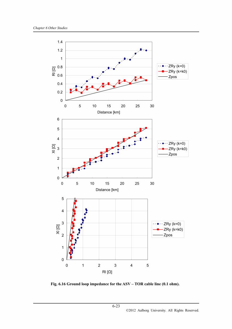
Chapter 6 Other Studies
6-23 ©2012 Aalborg University. All Rights Reserved.
Fig. 6.16 Ground loop impedance for the ASV – TOR cable line (0.1 ohm).
0
0.2
0.4
0.6
0.8
1
1.2
1.4
0 5 10 15 20 25 30
Distance [km]
Rl [Ω
] ZRy (k=0)
ZRy (k=k0)
Zpos
0
1
2
3
4
5
6
0 5 10 15 20 25 30
Distance [km]
Xl [Ω
] ZRy (k=0)
ZRy (k=k0)
Zpos
0
1
2
3
4
5
0 1 2 3 4 5
Rl [Ω]
Xl [Ω
] ZRy (k=0)
ZRy (k=k0)
Zpos

Chapter 6 Other Studies
6-24 ©2012 Aalborg University. All Rights Reserved.
6.1.4.4 Effects of Cable Layouts and Transposition
Section 6.1.3 shows the effects of cable layouts and transposition with a cross-bonded cable with
one major section. This section studies how the effects are changed with a long cable. In Section
6.1.4.3, the Kyndbyværket – Asnæsværket cable line was assumed to be directly buried in a flat
formation with transposition. In this section, the ground loop impedances are compared with the
following cable layouts as in Section 6.1.3:
(1) Directly buried in a flat formation without transposition (Flat w/o Transp.)
(2) Directly buried in a flat formation with transposition (Flat w Transp.)
(3) Directly buried in a trefoil formation (Trefoil)
(4) Laid in a tunnel in a trefoil formation with transposition (Tunnel)
Fig. 6.17 shows the comparison of the compensated ground loop impedance for different cable
layouts. Substation grounding resistance was set to 0.1 Ω, and Phase conductor grounding (1) is
assumed for the calculation of k0.
Table 6-4 shows proportions of the largest discontinuities of the compensated ground loop
reactances against the reactances for the total length. The cross-bonded cable laid in a tunnel has a
lower discontinuity compared with the other three cable layouts. As the discontinuities became
smaller compared with the cross-bonded cable with one major section, the difference of the other
three cable layouts became negligible.
Table 6-4 Largest Discontinuity of Ground Loop Reactance at Cross-bonding Points
Cable layouts (1) Flat w/o Transp. (2) Flat w Transp. (3) Trefoil (4) Tunnel
Largest
discontinuity 6.0 % 6.4 % 6.4 % 4.6 %
The first zone will not overreach to the bus on the other end with this level of discontinuities, as
long as it covers 80 % of the total length. The discontinuities are larger for the resistance part of the
ground loop impedance compared with the reactance part. However, the discontinuities of the
resistance part are not very important for the impedance relay setting as it is necessary to consider a
fault resistance.

Chapter 6 Other Studies
6-25 ©2012 Aalborg University. All Rights Reserved.
Fig. 6.17 Ground loop impedance for the ASV – TOR cable line with different cable layouts.
0
0.1
0.2
0.3
0.4
0.5
0.6
0.7
0 5 10 15 20 25 30
Distance [km]
Rl [Ω
]
(1) Flat w/o Transp.
(2) Flat w Transp.
(3) Trefoil
(4) Tunnel
0
1
2
3
4
5
0 5 10 15 20 25 30
Distance [km]
Xl [Ω
]
(1) Flat w/o Transp.
(2) Flat w Transp.
(3) Trefoil
(4) Tunnel
0
1
2
3
4
5
0 1 2 3 4 5
Rl [Ω]
Xl [Ω
] (1) Flat w/o Transp.
(2) Flat w Transp.
(3) Trefoil
(4) Tunnel

Chapter 6 Other Studies
6-26 ©2012 Aalborg University. All Rights Reserved.
6.1.5 Summary
In conclusion, the analysis of the ground loop impedance has found the following items:
It is difficult to protect a short cross-bonded cable by the impedance relay without
communication as the discontinuities at cross-bonding points can go up to 17 % of the total
reactance.
It is possible to protect the Asnæsværket – Torslunde cable line (long cross-bonded cables) by
the impedance relay without communication. The first zone will not overreach to the bus on
the other end with the typical setting with the level of discontinuities found in the analysis.
The substation grounding resistance affects the zero-sequence compensation k0. It is necessary
to know the setup when the field measurements are performed.
Since a constant value is assumed for the zero-sequence compensation k0, there is a large error
in k0 when a SLG fault occurs near the relay location. However, it will not lead to the
mis-operation or the unwanted operation of impedance relays since k0 has a smaller impact on
the ground loop impedance near the relay location.
Cable layouts and transposition affect the nonlinear characteristic of the ground loop
impedance as the discontinuity is caused by an imbalance of impedances between phases.
A cable laid in a flat formation has a larger discontinuity than a cable laid in a trefoil formation.
However, it is difficult to see the difference in a long cross-bonded cable as the difference
becomes small due to their homogenous nature [4][5].

Chapter 6 Other Studies
6-27 ©2012 Aalborg University. All Rights Reserved.
Leading Current Interruption 6.2
When the leading current is interrupted at current zero, it occurs at a voltage peak assuming that the
current waveform is leading the voltage waveform by 90 degrees. After the interruption, the voltage
on the source side of the circuit breaker changes according to the system voltage, whereas the
voltage on the other side is fixed at the peak voltage E as shown in Fig. 6.18. The most severe
overvoltage occurs when a restrike occurs after half cycle when the voltage on the source side
becomes -E. As the voltage difference between the source side and the other side is 2E, the
overvoltage can go as high as -3E. The restrike can be repeated to cause a very severe overvoltage.
Fig. 6.18 Overvoltage caused by leading current interruption and restrike.
Considering the severe overvoltage that can be caused by the leading current interruption, the
leading current interruption capability of circuit breakers is specified in IEC 62271-100. Table 6-5
shows the leading current interruption capability according to IEC 62271-100. It is necessary to
make sure that leading currents interrupted by line breakers are below 400 A for the Kyndbyværket
– Asnæsværket line.

Chapter 6 Other Studies
6-28 ©2012 Aalborg University. All Rights Reserved.
Table 6-5 Leading Current Interruption Capability according to IEC 62271-100
Rated Voltage Rated Capacitive Switching
Currents* (Cable)
420 kV 400 A
550 kV 500 A
*: Preferred values, voltage factor: 1.4 pu
When the charging capacity of a long EHV cable line is not compensated by shunt reactors directly
connected to the line, the leading current interruption capability requires a careful attention [1].
Considering typical capacitance 0.2 μF/km, the maximum line length for 400 kV cable line is
limited approximately below 26 km. Here, it is assumed that the leading current is interrupted by
one end, and the other end is open before the interruption.
Usually, a long EHV cable line, including the Kyndbyværket – Asnæsværket line, is compensated
by shunt reactors directly connected to the line. When the compensation rate is high enough, the
leading current interruption capability is not a concern. If the sequential switching is applied to a
cable line as a countermeasure to the zero-missing phenomenon, however, the tripping of shunt
reactors makes the compensation rate lower, sometimes even to 0 %. This is the only occasion that
requires a careful attention and is discussed more in detail in Section 6.3.

Chapter 6 Other Studies
6-29 ©2012 Aalborg University. All Rights Reserved.
Zero-missing Phenomenon 6.3
A DC offset current (Zero-missing current) appears when an EHV underground cable is energized
with its shunt reactors [1][2][6][7][8][9]. In this condition, an AC component of a charging current
has the opposite phase angle to the AC component of a current flowing into the shunt reactors. If
the compensation rate of the cable is 100 %, the summation of these AC components becomes zero,
and only the DC component remains. Since the DC component decays slowly with time, it can take
more than 1 second, depending on the compensation rate, before a current that flows through the
circuit breaker crosses the zero point. When the circuit breaker is to be operated to interrupt this
current without the zero crossing, it may lead to a failure of this circuit breaker.
Fig. 6.19 shows an example of current waveforms when an EHV underground cable is energized
with its shunt reactors. It can be seen that the AC component of the energization current is very
small since the compensation rate is close to 100%. The simulation was run for 0.2 seconds, but the
energization current did not cross the zero point during this duration.
Since the Zero-missing phenomenon is caused by a DC component of an energization current, it is
severest when the cable is energized when the maximum DC component is contained in the current.
In order to realize this condition in phase A, the cable was energized at the voltage zero point of
phase a.
Fig. 6.19 Zero-missing current in the underground cable energization.
0.00 0.04 0.08 0.12 0.16 0.20[s]-5000
-3750
-2500
-1250
0
1250
2500
3750
5000
[A]
Phase A

Chapter 6 Other Studies
6-30 ©2012 Aalborg University. All Rights Reserved.
Table 6-6 summarizes countermeasures of the zero-missing phenomenon. All of these
countermeasures, except for Countermeasure (4), have already been applied to the cable line in
operation. Countermeasure (1), which in particular has a number of application records to long
EHV cable lines, is discussed in detail later in this section.
Countermeasure (2) is also a proven technology. It is more often applied to the transformer
energization in order to minimize inrush current. The effects of point-on-wave switching
(synchronized switching) on the cable energization overvoltage are discussed in Section 5.2.4.
Countermeasure (3) can be implemented rather easier as long as a cable line is installed together
with single phase circuit breakers and current differential relays. For this reason, this
countermeasure is more suited to EHV cable lines than HV cable lines.
In this countermeasure, the faulted phase is opened instantly, but healthy phases are opened about
10 seconds later when the DC component is decayed enough. When this countermeasure is applied
near a generator and especially when the cable line offers radial path to the generator, it is
necessary to evaluate the negative-sequence current capability of the generator as this
countermeasure causes an unbalanced operation for a prolonged duration.
Countermeasure (4) is applicable in theory [10][11], but the cost of the breaker will prohibit its
application depending on the required size of pre-insertion resisters. Line breakers with
pre-insertion resisters were, in the first place, proposed for overhead lines in order to lower the
switching overvoltage. However, it could not become mainstream mainly due to its cost. A
breakthrough, especially on heat dissipation, would be necessary to be applied as a countermeasure.
In Countermeasure (5), a resistance is connected in series to shunt reactors when a cable line is
energized. The resistance needs to be sized so that the DC component decays fast enough. After the
cable line is energized, the resistance is bypassed in order to reduce losses. Considering the
additional cost for the resistance, this countermeasure is more suited to HV cable lines than EHV
cable lines.
Countermeasure (6) cannot always be applied; especially, it is difficult to apply (6) to long EHV
cables due to the steady-state overvoltage.
Table 6-6 Countermeasures of Zero-missing Phenomenon

Chapter 6 Other Studies
6-31 ©2012 Aalborg University. All Rights Reserved.
Countermeasures Notes
(1) Sequential switching
requires higher leading current interruption capability
requires single phase circuit breaker and current differential
relay
(2) Point-on-wave switching
(synchronized switching)
may cause higher switching overvoltage
requires single-phase circuit breaker
(3) Delayed opening of
healthy phases
requires single phase circuit breaker and current differential
relay
may not be possible to apply near generators
(4) Breaker with pre-insertion
resistor
may be necessary to develop a new circuit breaker
(expensive)
(5)
Additional series
resistance in shunt reactor
for energization
requires special control to bypass series resistance after
energization
(6) Energize shunt reactor
after the cable causes higher steady-state overvoltage and voltage step
6.3.1 Sequential Switching
When a single line to ground fault occurs before the zero-missing current phenomenon disappears,
the line breaker cannot interrupt the current, and it may result in the failure of the line breaker.
Fig. 6.20 shows zero-missing current with a single line to ground fault in phase b.
In Fig. 6.20, a single line to ground fault is applied in phase b of an EHV underground cable before
energization. The figure shows that the current in the faulted phase contains a large AC component
due to the fault current. The line breaker of the faulted phase can interrupt this current since this
fault current superimposed on the cable energization current crosses the zero point due to its large
AC component.

Chapter 6 Other Studies
6-32 ©2012 Aalborg University. All Rights Reserved.
Fig. 6.20 Zero-missing phenomenon with a single line to ground fault.
Fig. 6.21 shows the time sequence of sequential switching when the cable line is energized from
Substation A. The line breaker of phase b is opened, in Step 1, 60 ms after the fault, and the fault is
cleared by this CB tripping. Since the fault is already cleared by the opening of phase b line breaker,
there is no problem to take some time before opening line breakers of other healthy phases.
In Step 2, shunt reactors are tripped before the line breakers of healthy phases. It is necessary to trip
shunt reactors of only healthy phases. At this time, it is not necessary and not recommended to trip
shunt reactors of the faulted phase since the current through shunt-reactor breakers of the faulted
phase does not cross the zero point.
It is now possible to open the line breakers of the healthy phases in Step 3. Fig. 6.22 shows that the
current in healthy phases contains the AC component and crosses the zero point after tripping the
shunt reactors.
Since shunt reactors are tripped before line breakers of healthy phases, it is required to confirm that
the leading current in the line breakers does not exceed its breaking capability in Table 6-5. For a
very long cable, as the Kyndbyværket – Asnæsværket line, it is highly recommended to trip half of
the shunt reactors before the line breakers of healthy phases in order to reduce the leading current
in the line breakers of healthy phases.
0.00 0.04 0.08 0.12 0.16 0.20[s]-15
-10
-5
0
5
10
15
[kA] Phase b

Chapter 6 Other Studies
6-33 ©2012 Aalborg University. All Rights Reserved.
Step1: Fault clearance
Step2: Shunt reactor-CB open
Step3: Line-CB open (Load side)
Fig. 6.21 Time Sequence of sequential switching.
Sub
stat
ion
A
Sub
stat
ion
B
Sub
stat
ion
A
Sub
stat
ion
B
Sub
stat
ion
A
Sub
stat
ion
B
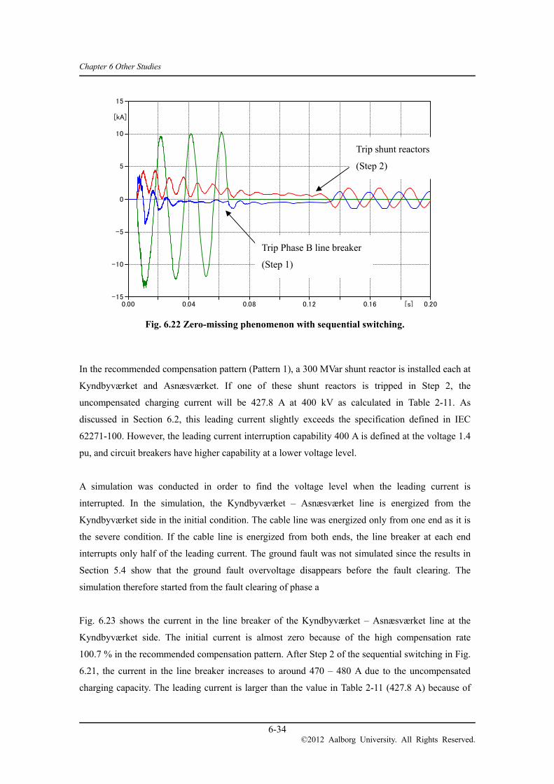
Chapter 6 Other Studies
6-34 ©2012 Aalborg University. All Rights Reserved.
Fig. 6.22 Zero-missing phenomenon with sequential switching.
In the recommended compensation pattern (Pattern 1), a 300 MVar shunt reactor is installed each at
Kyndbyværket and Asnæsværket. If one of these shunt reactors is tripped in Step 2, the
uncompensated charging current will be 427.8 A at 400 kV as calculated in Table 2-11. As
discussed in Section 6.2, this leading current slightly exceeds the specification defined in IEC
62271-100. However, the leading current interruption capability 400 A is defined at the voltage 1.4
pu, and circuit breakers have higher capability at a lower voltage level.
A simulation was conducted in order to find the voltage level when the leading current is
interrupted. In the simulation, the Kyndbyværket – Asnæsværket line is energized from the
Kyndbyværket side in the initial condition. The cable line was energized only from one end as it is
the severe condition. If the cable line is energized from both ends, the line breaker at each end
interrupts only half of the leading current. The ground fault was not simulated since the results in
Section 5.4 show that the ground fault overvoltage disappears before the fault clearing. The
simulation therefore started from the fault clearing of phase a
Fig. 6.23 shows the current in the line breaker of the Kyndbyværket – Asnæsværket line at the
Kyndbyværket side. The initial current is almost zero because of the high compensation rate
100.7 % in the recommended compensation pattern. After Step 2 of the sequential switching in Fig.
6.21, the current in the line breaker increases to around 470 – 480 A due to the uncompensated
charging capacity. The leading current is larger than the value in Table 2-11 (427.8 A) because of
0.00 0.04 0.08 0.12 0.16 0.20[s]-15
-10
-5
0
5
10
15
[kA]
Trip Phase B line breaker
(Step 1)
Trip shunt reactors
(Step 2)

Chapter 6 Other Studies
6-35 ©2012 Aalborg University. All Rights Reserved.
the voltage rise caused by the shunt reactor tripping (Step 2).
Fig. 6.23 Leading current interruption with sequential switching.
Fig. 6.24 shows the overvoltage caused by the shunt reactor tripping. The overvoltage goes up to
around 1.1 pu after the shunt reactor tripping. As the overvoltage is much lower than 1.4 pu, it is
highly likely that the line breaker can interrupt the leading current around 470 – 480 A without a
problem. It is recommended to test the leading current interruption capability at the voltage 1.15 pu
or 1.2 pu in order to confirm it.
Fig. 6.24 Overvoltage with sequential switching.
-0.8
-0.6
-0.4
-0.2
0
0.2
0.4
0.6
0.8
0 0.04 0.08 0.12 0.16
Time [s]
Cur
rent
[kA
]
Ia
Ib
Ic
-400
-300
-200
-100
0
100
200
300
400
0 0.04 0.08 0.12 0.16
Time [s]
Vol
tag
e [k
V]
Va
Vb
Vc
Shunt reactor tripping
Leading current interruption
Chapter 6 Other Studies
6-36 ©2012 Aalborg University. All Rights Reserved.
6.3.2 Summary
This PhD project recommends to apply Countermeasure (1) (sequential switching) to the
Kyndbyværket – Asnæsværket line after confirming the leading current interruption capability of
line breakers.
Countermeasure (1) has a lot of application records for EHV cable lines and is also the most
reliable countermeasure in terms of the duplication. Since the failure of the scheme may lead to the
failure of a line breaker, it is necessary to ensure that a single failure will not lead to the failure of
the scheme. The followings describe how the duplication is ensured in Countermeasure (1):
Considering the failure of the main relay (current differential), both Main 1 and Main 2
protection trigger the sequential switching.
In case of the breaker failure of a shunt reactor, the sequential switching trips the shunt reactor
on the other end.
The duplication can be achieved as the Kyndbyværket – Asnæsværket line has shunt reactors on the
both ends. For shorter cable lines which have only one shunt reactor, the duplication is not achieved.
In order to standardize the countermeasure for the zero-missing phenomenon including these
shorter cable lines, it is effective to apply both Countermeasures (1) and (2).

Chapter 6 Other Studies
6-37 ©2012 Aalborg University. All Rights Reserved.
Cable Discharge 6.4
If a shunt reactor is directly connected to a cable line, the cable line is discharged through the shunt
reactor when disconnected from the network. In this case, the time constant of the discharge
process is determined by Q factor of the shunt reactor. Since Q factor ranges around 500 for EHV
shunt reactors, the time constant of the discharge process is around 8 minutes.
If a cable line is disconnected from the network and energized again within a couple of minutes,
there remains a residual charge in the cable line, and the residual charge can be highly dependent on
the time separation between the disconnection and the re-energization. Under this condition, the
re-energization overvoltage can exceed SIWV when the residual voltage has an opposite sign to the
source voltage at the time of re-energization.
This is usually an issue for overhead lines since auto-reclose is applied to overhead lines. For cable
lines, it is not common to apply auto-reclose. If it is applied to the cable lines, they may experience
higher overvoltages because of their higher residual voltage. System operators are required to know
that they need to wait for about 10 minutes (maybe more to be conservative) before re-energizing a
cable line though it would not be a typical operation to re-energize a cable line.
If a shunt reactor is not directly connected to the cable line, the cable line is discharged through
inductive VTs. In this case, the discharge process will be completed within several milliseconds.
The inductive VTs need to have enough discharge capability if a cable line can be operated without
a shunt reactor or all the shunt reactors are tripped by sequential switching. It takes several hours
for the inductive VTs to dissipate heat after dissipating the cable charge. If the inductive VTs are
required to dissipate the cable charge twice within several hours, the required discharge capability
will be doubled.

Chapter 6 Other Studies
6-38 ©2012 Aalborg University. All Rights Reserved.
Overvoltage Caused by Restrike 6.5
When a circuit breaker of a shunt reactor is opened, it can interrupt a current into the shunt reactor
[1][9]. The interrupted current is usually very small, but it can cause a high slow-front overvoltage
expressed by dt
diL . Due to this high slow-front overvoltage, a restrike can occur between the
contacts of the opening circuit breaker, generally with a higher probability compared with circuit
breakers used for other equipment.
In addition, this slow-front overvoltage imposes a severe initial condition for the overvoltage
caused by the restrike. An example of the initial condition is shown in Fig. 6.25. In this example,
the shunt reactor CB was opened when a current through the CB was 10 A, which was a very
severe assumption contingent on the unit size of the shunt reactor.
Fig. 6.25 Results of the current chopping analysis.
After opening the circuit breaker, it can be seen that the voltage on the shunt reactor side (red line)
becomes very high as explained above. The voltage on the system side (green line) is kept at 1pu.
0 4 8 12 16 20[ms]-700
-525
-350
-175
0
175
350
525
700
[kV]
-609.0kV
317.2kV
open shunt reactor CB

Chapter 6 Other Studies
6-39 ©2012 Aalborg University. All Rights Reserved.
Fig. 6.26 shows an example of the analysis of the overvoltage caused by the restrike. For the
simulation, arc impedance is modeled by a series circuit of resistance 2Ω and inductance 0.5μH
[12]. The overvoltage is higher than LIWV without surge arresters for shunt reactors.
Fig. 6.26 Overvoltage caused by the restrike.
It is highly recommended to apply point-of-wave switching to the circuit breakers of shunt reactors.
The point-of-wave switching should adjust the CB open command timing so that the distance
between the contacts of the CB is at the maximum when shunt reactor current reaches the zero
point. Since the zero-crossing point of shunt reactor current is different for each phase, this control
requires a separate control for the CBs of different phases.
Even if the overvoltage level is lower than the withstand voltage, the restrike itself is an
unfavorable phenomenon as it can damage the CB contacts and nozzles. By applying the
point-of-wave switching, the restrike phenomenon itself can be avoided. A comparison between the
two countermeasures, the surge arrester and point-of-wave switching, is compared in Table 6-7.
Table 6-7 Comparisons of Countermeasures for the Overvoltage Caused by the Restrike
Advantage Disadvantage
Surge arrester No worry about malfunction Damage to CB contacts and
nozzles cannot be avoided.
Point-of-wave switching Restrike itself can be avoided. Malfunction of the controller
may lead to equipment failures.

Chapter 6 Other Studies
6-40 ©2012 Aalborg University. All Rights Reserved.
References
[1] T. Ohno, “Operation and Protection of HV Cable Systems in TEPCO”, Global Facts, Trends
and Visions in Power Industry, Swiss Chapter of IEEE PES, April 2010.
Presentation available on the web:
http://www.ieee.ch/assets/Uploads/pes/downloads/1004/10042ohnoexperiencetepco.pdf.
[2] V. Leitloff, X. Bourgeat, and G. Duboc, “Setting Constraints for Distance Protection on
Underground Cables”, in Proc. 2001 7th IEE International Conference on Developments in
Power System Protection.
[3] D. A. Tziouvaras, “Protection of High-Voltage AC Cables”, available on the web:
http://www2.selinc.com/techpprs/6221_ProtectionACCables_DT_20060131.pdf.
[4] N. Nagaoka and A. Ametani, “Transient Calculations on Crossbonded Cables,” IEEE Trans.
on Power Apparatus and Systems, vol. PAS-102, no. 4, 1983.
[5] A. Ametani, Y. Miyamoto, and N. Nagaoka, “An Investigation of a Wave Propagation
Characteristic on a Crossbonded Cable,” IEEJ Trans. PE, vol. 123, no. 3, pp. 395-401, 2003
(in Japanese).
[6] B. Kulicke, H. H. Schramm, “Clearance of Short-circuits with Delayed Current Zeros in the
Itaipu 550 kV-Substation”, IEEE Trans. on Power Apparatus and Systems, vol. PAS-99, no. 4,
July/Aug 1980.
[7] T. Michigami, S. Imai, O. Takahashi, “Theoretical Background for Zero-miss Phenomenon in
the Cable Network and Field Measurements”, IEEJ General Meeting 1459, 1997 (in
Japanese).
[8] H. Hamada, Y. Nakata, T. Maekawa, “Measurement of Delayed Current Zeros Phenomena in
500 kV Cable System”, IEEJ General Meeting 2001 (in Japanese).
[9] “Joint Feasibility Study on the 400 kV Cable Line Endrup-Idomlund”, Final Report, Tokyo
Electric Power Company, April 2008.
[10] F. Faria da Silva, C. L. Bak, U. S. Gudmundsdottir, W. Wiechowski, M.R.Knardrupgard, “Use
of a preinsertion resistor to minimize zero-missing phenomenon and switching overvoltages”,
IEEE-PES General Meeting 2009.
[11] F. Faria da Silva, "Analysis and simulation of electromagnetic transients in HVAC cable
transmission grids", PhD Thesis, Aalborg University, 2011.
[12] S. Ogawa, E. Haginomori, S. Nishiwaki, T. Yoshida, K. Terasaka, “Estimation of Restriking
Transient Overvoltage on Disconnecting Switch for GIS,” IEEE Trans. on Power Systems, vol.
PWRD-1, no. 2, April 1986.

Chapter 7 Conclusion
7-1 ©2012 Aalborg University. All Rights Reserved.
Conclusion Chapter 7
The objectives of this PhD project have been to shed light on the phenomena peculiar to long cable
lines. Through the studies on the 400 kV 60 km Kyndbyværket – Asnæsværket line, the thesis has
addressed major problems and potential countermeasures related to the installation of long cable
lines. The PhD project has tackled all the problems formulated in Chapter 1 and has yielded
important findings which will be useful for studies on future cable lines.
Summary 7.1
7.1.1 Insulation Coordination Study
First of all, the PhD project performed the insulation coordination study for the 400 kV 60 km
Kyndbyværket – Asnæsværket line in order to address the technical feasibility of the cable line and
identify major problems and possible countermeasures.
The reactive power compensation analysis in Chapter 2 found the best compensation pattern, which
requires installing one 300 MVar shunt reactor each at Kyndbyværket and Asnæsværket. The
compensation rate becomes 100.7 % in this compensation pattern. It is confirmed that the
steady-state overvoltage will not be a problem even considering a Ferranti phenomenon. However,
if the cable line has to be in-service even when one shunt reactor is out of service, it is
recommended to install two 150 MVar shunt reactors each at Kyndbyværket and Asnæsværket.
The temporary overvoltage analysis in Chapter 4 covered the resonance overvoltage and the
overvoltage caused by the system islanding. Table 7-1 summarizes the results of the analysis. With
respect to the initial overvoltage (first impulse), the highest overvoltage 805.0 kV was caused by
the overvoltage caused by the system islanding, but it is much lower than the SIWV (1050 kV)
defined in IEC 60071-1. The high overvoltage 517.8 kV was observed after the first peak in the
parallel resonance overvoltage. It is highly recommended that the applied surge arresters have a
withstand voltage higher than or equal to 1.60 pu for 1 second.

Chapter 7 Conclusion
7-2 ©2012 Aalborg University. All Rights Reserved.
Table 7-1 Summary of the Temporary Overvoltage Analysis
Highest Overvoltage
(peak)
Withstand Voltage
(peak)
Series Resonance 1st peak 285.5 kV
230 or 275 kV × √2 *1 3rd peak 228.7 kV
Parallel Resonance 1st peak 702.6 kV (2.15 pu) 1050 kV (3.21 pu, SIWV)
1 sec 517.8 kV (1.59 pu) 551.5 kV (1.69 pu, Arrester)
Overvoltage Caused by
the System Islanding
1st peak 805.0 kV (2.46 pu) 1050 kV (3.21 pu, SIWV)
10 sec 400.0 kV (1.22 pu) 523.3 kV (1.60 pu, Arrester)
*1: Standard short-duration power-frequency withstand voltage defined in IEC 60071-1
The slow-front overvoltage analysis in Chapter 5 covered the line energization overvoltage and the
ground fault and fault clearing overvoltage. The line energization overvoltage is much higher than
the ground fault and fault clearing overvoltage. Both overvoltages are lower than the SIWV (1050
kV) defined in IEC 60071-1 and will not be a problem in the operation of the Kyndbyværket –
Asnæsværket line.
Table 7-2 Summary of the Slow-front Overvoltage Analysis
Highest Overvoltage
(peak)
Withstand Voltage
(peak)
Line Energization 775.2 kV (2.37 pu) 1050 kV (3.21 pu, SIWV)
Ground Fault and Fault Clearing 448.4 kV (1.37 pu) 1050 kV (3.21 pu, SIWV)

Chapter 7 Conclusion
7-3 ©2012 Aalborg University. All Rights Reserved.
7.1.2 Required Specifications for the Related Equipment
The insulation coordination study and other studies have identified required or recommended
specifications for the related equipment. Table 7-3 summarizes these required or recommended
specifications.
Table 7-3 Required / Recommended Specifications for the Related Equipment
Required / Recommended Specifications
Cable
(IEC 62067)
Required: Power frequency withstand voltage 440 kV – 15 min,
SIWV 1050 kV, LIWV 1425 kV
Surge Arrester
(IEC 60099)
Required: Withstand voltage 1.60 pu – 1 sec
Recommended: Line discharge class 3
Line Breaker
(IEC 62271-100)
Required: Leading current interruption capability
400 A – 1.4 pu, 480 A – 1.15 pu (voltage)
Shunt Reactor Breaker
(IEC 62271-100)
Required: Point-on-wave switching for opening if ASV or KYV
400 kV bus is GIS.
Protection Relay
Required: Current differential relay (main)
Distance relay (backup)
Sequential switching for the fault clearance
Recommended: Distance relay that can apply different
zero-sequence compensation k0 for different zones
VT (Line) Discharge capability is not necessary as shunt reactors are
always directly connected to the ASV – KYV line.

Chapter 7 Conclusion
7-4 ©2012 Aalborg University. All Rights Reserved.
New Contributions 7.2
The PhD project produced the five papers listed in Table 7-4. The findings and contributions of
these papers were used for the study on the Kyndbyværket – Asnæsværket line and will be useful
for studies on future cable lines.
Table 7-4 Papers Produced by the PhD Project
Title Co-authors Outlet Status
Derivation of Theoretical Formulas
of Sequence Currents on
Underground Cable System
Teruo Ohno, Akihiro
Ametani, Claus Leth Bak IPST 2011 Published
Derivation of Theoretical Formulas
of the Frequency Component
Contained in the Overvoltage
related to Long EHV Cables
Teruo Ohno, Claus Leth
Bak, Wojciech Wiechowski,
Thomas Sørensen,
Akihiro Ametani
IEEE
Transactions on
Power Delivery
Published
Statistical Distribution of
Energization Overvoltages of EHV
Cables
Teruo Ohno, Claus Leth
Bak, Wojciech Wiechowski,
Thomas Sørensen,
Akihiro Ametani
IEEE
Transactions on
Power Delivery
Under
2nd
review
Ground Loop Impedance of Long
EHV Cable Lines
Teruo Ohno, Claus Leth
Bak, Thomas Sørensen
Western
Protective Relay
Conference
Published
Analysis of the Statistical
Distribution of Energization
Overvoltages of EHV Cables and
OHLs
Teruo Ohno, Claus Leth
Bak, Wojciech Wiechowski,
Thomas Sørensen,
Akihiro Ametani
IPST 2013 Abstract
submitted
Although the findings and contributions of these papers have already been discussed in detail in
this thesis, the important points are summarized here for convenience:
(1) Derivation of theoretical formulas of sequence currents on underground cable system (Section
2.3.2)
The PhD project derived theoretical formulas of sequence currents of a cross-bonded cable and
a solidly-bonded cable. The derived formulas consider the cable as a cable system; they can
thus consider sheath bonding and sheath grounding resistance. The verified accuracy of the
proposed formulas shows sequence impedance / current can now be obtained before the

Chapter 7 Conclusion
7-5 ©2012 Aalborg University. All Rights Reserved.
installation without making measurements for a majority of cables. This gives an important
advantage in setting up transient overvoltage studies as well as planning studies.
(2) Derivation of theoretical formulas of the frequency component contained in the overvoltage
related to long EHV cables (Section 4.1.3.1)
The PhD project derived the simple theoretical formulas for estimating the propagation
velocity and dominant frequency from impedance and admittance calculations. The comparison
between the proposed formulas and the simulation results was performed using the
Kyndbyværket – Asnæsværket line. From the comparison, the derived formulas were found to
be sufficiently accurate to be used for the efficient analysis of resonance overvoltages.
(3) Statistical distribution of energization overvoltages of EHV cables (Sections 5.1 and 5.2)
The PhD project derived the statistical distributions of energization overvoltages of EHV
cables from a number of simulations. Through the comparison with the statistical distributions
of energization overvoltages of overhead lines, it has been found that line energization
overvoltages on the cables are lower than those on the overhead lines with respect to maximum,
2 %, and mean values. In addition, standard deviations are smaller for the cables.
(4) Ground loop impedance of long EHV cable lines (Section 6.1)
Through the calculation of the ground loop impedance for cable lines, The PhD project has
found that, for long EHV cable lines, the reliable operation of the ground distance relay is
possible with a typical relay setting, despite the discontinuity at cross-bonding points. Effects
of parameters, such as substation grounding, cable layouts and transposition, are also found
through the analysis.
(5) Analysis of the statistical distribution of energization overvoltages of EHV cables and OHLs
(Section 5.3)
The PhD project has identified the causes and physical meanings of the characteristics of the
statistical distribution of energization overvoltages of EHV cables. From the theoretical
analysis of voltage waveforms, the main characteristics of the statistical distribution are found
to be caused not by random switching by accident, rather there are contributing factors and
physical meanings behind the characteristics.

Chapter 7 Conclusion
7-6 ©2012 Aalborg University. All Rights Reserved.
Future Work 7.3
This section lists future works related to the installation and operation of long EHV cables. These
items may require serious considerations even though they are not studied in the PhD project:
Evaluation of high-impact low-probability (HILP) events
Since a severe temporary overvoltage occurs only in specific conditions, it can be considered as
a low-probability event. When it occurs, however, it can cause a major damage to related
equipment, which poses a high-impact on the safe operation of the power system.
It will be helpful for future construction and operation of EHV cable lines to establish a
procedure to evaluate risks associated with HILP events.
Burden that can be placed on the system operation
Severe temporary overvoltages are similar to extreme contingencies, such as N-2 contingencies,
as they both are HILP events. One difference is that severe temporary overvoltages can be
avoided not only by equipment specifications but also by applying operational constraints since
they occur only in specific conditions. However, if operational constraints are too strict or too
complicated, it will place a burden on the system operation. The decisions should be made also
based on the skills of system operators.
Should cable test voltages be re-considered?
In order to test the insulation performance of cables, lightning impulse voltages, switching
impulse voltages and power frequency test voltages are applied to cables according to
international and national standards. IEC 62067 defines the test methods and requirements for
XLPE cables and accessories for rated voltages above 150 kV up to 500 kV. According to IEC
62067, the test voltage 440 kV is applied to 400 kV cables for 15 minutes, as power frequency
voltage test, after the lightning impulse voltage test.
Considering the level of temporary overvoltages found in the PhD project, the level of applied
power frequency voltage in IEC 62067 appears to be low, and the duration is long. However, it
requires discussions to decide if cable test voltages in IEC 62067 should be re-considered, since
it is a common practice to test the insulation performance of equipment at lower voltages with
longer duration. In addition, the mismatch is not an immediate issue as the overvoltage is
normally evaluated against the insulation performance and the energy absorption capability of
surge arresters.

Chapter 7 Conclusion
7-7 ©2012 Aalborg University. All Rights Reserved.
Effects on harmonics
As we have seen in the parallel resonance overvoltage analysis, the introduction of long cable
lines with shunt reactors significantly lower parallel resonance frequencies of power systems.
The system total impedances at 5th and 7th harmonic frequencies are often increased by this
shift of resonance frequencies. Since the increase of impedances will results in the increase of
the total voltage harmonic distortion, it should be evaluated in the areas where harmonics are of
concern.