Embed Size (px)
Citation preview
Aalborg Universitet
Techniques for Efficient Spectrum Usage for Next Generation Mobile CommunicationNetworks. An LTE and LTE-A Case StudyKumar, Sanjay
Publication date:2009
Document VersionPublisher's PDF, also known as Version of record
Link to publication from Aalborg University
Citation for published version (APA):Kumar, S. (2009). Techniques for Efficient Spectrum Usage for Next Generation Mobile CommunicationNetworks. An LTE and LTE-A Case Study. Institut for Elektroniske Systemer, Aalborg Universitet.
General rightsCopyright and moral rights for the publications made accessible in the public portal are retained by the authors and/or other copyright ownersand it is a condition of accessing publications that users recognise and abide by the legal requirements associated with these rights.
? Users may download and print one copy of any publication from the public portal for the purpose of private study or research. ? You may not further distribute the material or use it for any profit-making activity or commercial gain ? You may freely distribute the URL identifying the publication in the public portal ?
Take down policyIf you believe that this document breaches copyright please contact us at [email protected] providing details, and we will remove access tothe work immediately and investigate your claim.
Downloaded from vbn.aau.dk on: juli 25, 2018
Techniques for Efficient Spectrum Usagefor Next Generation MobileCommunication Networks
An LTE and LTE-A Case Study
PhD Thesisby
Sanjay Kumar
A Dissertation submitted tothe Faculty of Engineering, Science and Medicine of Aalborg University
in partial fulfillment for the degree ofDoctor of Philosophy.
Aalborg, DenmarkJune 2009
Supervisors:Ramjee Prasad, PhD,Professor, Director, CTIF, Aalborg University, Denmark.Preben Elgaard Mogensen, PhD,Professor, Aalborg University, Denmark.
Assessment Committee:Uma S. Jha, PhD,Director, Product Management, Qualcomm Inc., USA.Markku Juntti, PhD,Professor, University of Oulu, Finland.Troels B. Sorensen, PhD,Associate Professor, Aalborg University, Denmark.
Moderator:Flemming B Frederiksen,Associate Professor, Aalborg University, Denmark.
ISBN 978-87-92328-29-8
Copyright c©2009, Sanjay Kumar.All rights reserved. The work may not be reposted without the explicit permission of the copyrightholder.

ToMy Parents,
My wife Babita,My daughter Shraddha, son Nitin,
andto the respectful memories of
My Grandparents.

Abstract
This PhD study aims to investigate techniques for efficient usage of spectrum for nextgeneration mobile communication networks. The Long Term Evolution (LTE) and LTE-Advanced (LTE-A) systems are taken as case studies. The LTE is under developmentwithin 3rd Generation Partnership Project (3GPP) and heading towards its final phaseof standardization. The LTE aims for reduced latency, higher user data rates, improvedsystem capacity and coverage, and reduced cost for the operators. Currently the Inter-national Telecommunications Union (ITU) is working on specifying the system require-ments towards next generation mobile communication systems called International Mo-bile Telecommunications-Advanced (IMT-A). The 3GPP aims to further evolve LTE to-wards LTE-A in order to meet or exceed the IMT-A requirements as well as its ownrequirements for advancing LTE for long term competitiveness.
The first half of the PhD study is mainly concerned with LTE, with the main fo-cus on higher order sectorization and inter-cell interference avoidance to improve systemcapacity and coverage. Typically three antennas are considered rendering 3 sector sitedeployments for LTE. A migration to 6 sector site deployment has been investigated. Amixed network topology composed of a combination of 3 and 6 sectors site deploymentis also proposed. The mixed network topology is found to provide significantly high per-formance gains in terms of cell throughput and user outage throughput performance, andtherefore recommended as a potential solution to meet high traffic demands in localizedareas such as hot spots.
LTE uses Orthogonal Frequency Division Multiple Access (OFDMA) in the downlinkwith universal frequency reuse. Due to the characteristics of OFDMA, the intra-cell in-terference is ideally avoided , but the environment still remains interference limited dueto the presence of inter-cell interference. Our focus in this study is on development ofschemes for inter-cell interference avoidance under fractional load conditions. The frac-tional load conditions arise when all the resources are not required to be used due to lackof traffic in the cell. We propose several autonomous inter-cell interference avoidanceschemes, which do not require inter-cell signaling and provide significant improvementsin cell throughput and user outage throughput performance.
The second half of the study is concerned with LTE-A, which aims to provide peakdata rates in the order of 1 Gbps in downlink and 500 Mbps in uplink for the nomadiclocal area/indoor deployment scenarios. Such high data rates may require high spectralefficiency and a wide bandwidth spectrum allocation in the order of 100 MHz. Suchhigh bandwidth allocation may require sharing of spectrum among operators in a flexiblemanner. Currently, Home e-nodeB (HeNB) is emerging as a potential solution to providehigh data rate high quality indoor coverage.
Potentially large scale uncoordinated deployment of HeNBs, sharing over the same
v
vi Abstract
radio spectrum is expected, giving rise to severe radio interference problems. A newmechanism is required to ensure coexistence of HeNBs in the given area. The conceptof Flexible Spectrum Usage (FSU) is considered a key enabler, which allows spectrumallocation from a common pool and ensures coexistence. The Spectrum Load Balanc-ing (SLB) and Resource Chunk Selection (RCS) algorithms are proposed for FSU amongHeNBs, which ensure coexistence by partially or completely preventing mutual interfer-ence on the shared spectrum and also provide self configurable solutions towards unco-ordinated HeNBs deployment. The framework of the FSU study is further extended toautonomous component carrier selection schemes that also allow uncoordinated HeNBdeployment without prior radio network planning.
Further, a policy assisted light cognitive radio enabled FSU has been proposed forefficient and flexible spectrum allocation in multi operator domain. The concept is basedon cognitive radio cycle, where the decision making is assisted by a policy, where thepolicy refers to a set of rules agreed among operators to facilitate FSU. The FSU study hasbeen primarily focused within the same radio access technology in the licensed frequencyband.
Dansk Resumé
Dette ph.d.-studium sigter mod at udforske teknikker til effektiv udnyttelse af frekvensspek-teret ifm. den næste generation af mobilkommunikationsnetværk. "Long Term Evolution"(LTE) og "LTE-Advanced" (LTE-A) systemer anvendes som eksempler. LTE er underudvikling ifm. "The 3rd Generation Partnership Project" (3GPP) og nærmer sig sin en-delige standardiseringsfase. LTE sigter mod reduceret latens, større bruger datahastighed,forøget systemkapacitet og -dækning samt reducerede omkostninger for operatørerne. Forøjeblikket arbejder den internationale telekommunikationsunion (ITU) på at specificeresystemkravene for næste generation af mobilkommunikationssystemer benævnt "Interna-tional Mobile Telecommunications-Advanced" (IMT-A). 3GPP sigter mod at videreud-vikle LTE mod LTE-A med henblik på at opfylde eller overstige IMT-A kravene og somet led i sine egne bestræbelser mod at sikre LTE lang tids konkurrencedygtighed
Den første halvdel af ph.d.-studiet er hovedsageligt rettet mod LTE med særligt fokuspå høj ordens sektorisation og hindring af inter-cell interferens til forbedring af systemetskapacitet og dækning. Tre antenner forventes typisk at skulle varetage tre sektorer ifm.LTE-afvikling. En udvikling til LTE-afvikling i seks sektorer er undersøgt. En blandetnetværkstopologi - sammensat ved en kombination af afviklingerne i 3 og 6 sektorer -er også foreslået. Den blandede netværkstopologi har vist sig at præstere særligt højeydelsesforbedringer m.h.t. cell-throughput og user-outage-throughput-performance, ogden er derfor anbefalet som en potentiel løsning til imødekommelse af store datatrafikkravi afgrænsede områder såsom hot spots.
LTE anvender Orthogonal-Frequency-Division-Multiple-Access (OFDMA) ifm. down-link med universal-frequency-reuse. Grundet OFDMA’s særlige egenskaber tilføres derikke intra-cell interferens, men omgivelserne indeholder fortsat interferens, der dog aleneskyldes tilstedeværelsen af inter-cell interferens. Vores fokus i dette studium er at ud-vikle systemer til hindring af inter-cell interferens under små belastningsforhold. Småbelastningsforhold optræder når alle ressourcerne ikke behøves på grund af begrænsetcelletrafik. Vi foreslår forskellige uafhængige systemer til hindring af inter-cell inter-ferens, og som ikke kræver signalering mellem cellerne men tilvejebringer signifikanteforbedringer i cellegennemgangen samt i bruger outage-throughput præstationerne.
Den anden halvdel af studiet er rettet mod LTE-A, som sigter mod at tilvejebringe top-datahastigheder af størrelsesordenen 1 Gbps i downlink og 500 Mbps i uplink for de no-madiske lokal-area/indendørs afviklinger. Sådanne høje datahastigheder kræver eventuelthøj spektral effektivitet og en stor båndbreddetildeling af størrelsesordenen 100 MHz.Store båndbreddetildelinger forudsætter eventuelt fleksibel spektrumsfordeling mellemoperatørerne. For tiden fremstår Home e-nodeB (HeNB) som en potentiel løsning fortilvejebringelse af høje datahastigheder ifm. indendørs dækning med høj kvalitet. Po-tentielt forventes der I stor skala og ukoordineret en spektral fordeling af det fælles ra-
vii
viii Dansk Resumé
diospektrum mellem HeNB’s, hvilket vil udløse alvorlige radio interferensproblemer. Derbehøves en ny mekanisme til at sikre sameksistensen mellem HeNB’s indenfor det givneområde. Konceptet: "Flexible Spectrum Usage" (FSU), der betragtes som en nøgle her-til, tillader spektrumstildeling fra en fælles pulje og sikrer en sameksistens. "SpectrumLoad Balancing" (SLB) og "Resource Chunk Selection" (RCS) algoritmerne er foreslåetaf FSU blandt diverse HeNB’s og sikrer sameksistens ved delvist eller helt at afværge in-dbyrdes interferens i det fælles spektrum, og det tilfører samt selvkonfigurerer endvidereløsninger til brug for en ukoordineret HeNB-afvikling. Rammen for FSU-studiet udvidesendvidere med et uafhængigt component-carrier-selection system, der endvidere tilladerukoordineret HeNB-udnyttelse uden en forudgående radio-netværksplanlægning. End-videre foreslås der et strategisk light-cognitive radio styret FSU til effektiv og fleksibelallokering af spektrum i et multioperator domæne. Konceptet baseres på en cognitiveradio cyclus, hvor beslutningsforløbet støttes af en strategi med reference til et regelsæt,som operatørerne har vedtaget med sigte på at lette FSU. FSU-studiet har primært væretrettet mod en og samme radio access technologi i det licensbehæftede frekvensbånd.
Preface and Acknowledgments
This dissertation is the result of a three years research project carried out at the Radio Ac-cess Technology (RATE) section, Center for TeleInFrastruktur (CTIF), Institute of Elec-tronic Systems, Aalborg University, Denmark, under the supervision and guidance ofProfessor Ramjee Prasad (Director, CTIF, Aalborg University, Denmark) and ProfessorPreben E. Mogensen (Aalborg University, Denmark). The dissertation has been com-pleted in parallel with the mandatory course work, teaching, and project work obligationsin order to obtain the PhD degree. This research project has been co-financed by BirlaInstitute of Technology, Ranchi, India and Radio Access Technology (RATE) section,Center for TeleInFrastruktur (CTIF), Aalborg University, Aalborg.
First of all, I express my sincere gratitude to my supervisors Professor Ramjee Prasadand Professor Preben E. Mogensen for their constant encouragement and support. Theirextremely rich technical experience and clear understanding about the research directionhave always made me confident towards my research work. More importantly, their hu-man understanding on personal issues always made me optimistic and comfortable evenin times of difficult situations. They have always given me courage to continue and com-plete the work. It has been a privilege for me to work with such supervisors. I am highlyindebted for their guidance, support and co-operation. I shall always remain grateful tothem.
I would like to thank Professor S.C. Goel of Birla Institute of Technology, Ranchi,India for giving me this opportunity to come to Aalborg University for research work.I thank Professor Nisha Gupta for her initiative in this project and constant support. Iwould like to thank Professor R. Sukesh Kumar for giving me encouragement and advice.I thank Professor PK Barhai, Vice Chancellor, Birla Institute of Technology for providingme all the needed support to complete the work. I also thank Professor H. C. Pande,Vice Chancellor Emeritus, Birla Institute of Technology for being a constant source ofinspiration. I would like to thank all my colleagues and all the members of the Departmentof Electronics and Communications Engineering, Birla Institute of Technology, RanchiIndia.
I worked in close association with Klaus I. Pedersen and Istvan Z. Kocavs of NokiaSiemens Networks, Aalborg for a considerable part of my research work. Their clear vi-sion and expertise in the area of research gave me an invaluable learning experience. I amextremely thankful for their understanding and cooperation. I thank Troels Kolding, MadsBrix and Frank Frederiksen of Nokia Siemens Networks, Aalborg for all the administra-tive and technical support. I also thank all the colleagues at Nokia Siemens Networks,Aalborg for their cooperation and friendly support.
I am extremely thankful to Troels B. Sorensen, who introduced to me about the re-search activities at RATE section and also for his willingness to help whenever needed. I
ix
x Chapter 0
am grateful to Flemming B. Frederiksen for his sincere concern for me and also for trans-lating the abstract into Danish. I would be extremely pleased to thank Nicola Marchettifor his constant support, feedback and cooperation during a considerable part of the PhDwork.
I very well appreciate and extend my thanks to the caring and sincere secretaries Lis-beth Schiønning Larsenand, Inga Hauge, Sussan Norrevang and Jytte Larsen for makingmy stay free from administrative worries. I thank Jytte Larsen also for providing feedbackon the language of the thesis.
During the PhD study I was fortunate to work in close cooperation with my fellowresearchers Guillaume Monghal, Yuanye Wang, Luis Garcia and Gustavo Costa. I thankthem for their sincere collaboration. I would like to thank Andrea Fabio Cattoni, Mohm-mad Anas, Francesco D. Calabrese, Naizheng Zheng, Oumer M. Teyeb, Gilberto Berar-dinelli and Carles N. Manchon for making my stay pleasant in Aalborg. I would liketo thank former RATE colleagues Suvra Shekar Das, Mohammad Imadur Rahman, andAkhilesh Pokhariyal for inspiration and fruitful discussion at the early stage of my PhDwork. I would also like to express my gratitude to all the colleagues at Radio AccessTechnology section and CTIF, Aalborg University for their friendly support.
I will never forget to thank Professor H.K. Grewal, my master thesis supervisor forher trust in me and introducing me into the noble world of teaching and research after myretirement from the defense services. I also thank my master project students for theirinterest and involvement in the project and their hard work.
It is the boundless blessings of my parents, endless sacrifice of my wife Babita, mydaughter Shraddha and son Nitin, which gave me enough strength to complete the work.They have shown extreme patience and supported me in every possible way. Words alonecan never express my gratitude to them. I express my thanks to my uncle and aunts, allthe relatives and friends for their blessings and encouragement for my academic pursuit.
Finally, I thank the ultimate source of energy of every particle in the universe, theAlmighty, for giving me enough energy to complete the work.
Sanjay Kumar, June, 2009.
Abbreviations
AMC Adaptive Modulation and Coding
ARQ Automatic Repeat ReQuest
AVI Actual Value Interface
BLER BLock Error Rate
CP Cyclic Prefix
CQI Channel Quality Information
DL Downlink
DL-SCH Downlink Shared Channel
eNode-B Evolved Node B
EPC Evolved Packet Core
EPS Evolved Packet System
E-UTRAN Evolved Universal Terrestrial Radio Access Network
FD Frequency-Domain
FDD Frequency Division Duplex
FDM Frequency Domain Multiplexing
FDPS Frequency-Domain Packet Scheduling
FEC Forward Error Correction
HARQ Hybrid Automatic Repeat reQuest
ISI Inter-Symbol Interference
LA Link Adaptation
LTE Long Term Evolution
MAC Medium Access Control
MCS Modulation and Coding Scheme
MIMO Multiple Input Multiple Output
xi
xii Abbreviations
MRC Maximal Ratio Combining
OFDM Orthogonal Frequency Division Multiplexing
OFDMA Orthogonal Frequency Division Multiple Access
OLLA Outer Loop Link Adaptation
PAPR Peak-to-Average Power Ratio
PDCP Packet Data Convergence Protocol
PDP Power Delay Profile
PF Proportional Fair
PF Proportional Fair
PHY Physical Layer
PRBs Physical Resource Blocks
QAM Quadrature Amplitude Modulation
QPSK Quadrature Phase Shift Keying
RLC Radio Link Control
RR Round Robin
RRC Radio Resource Control
RRM Radio Resource Management
SC-FDMA Single-Carrier Frequency Division Multiple Access
SINR Signal-to-Interference-plus-Noise Ratio
SISO Single Input Single Output
TDD Time Division Duplex
TD Time-Domain
TDPS Time-Domain Packet Scheduling
TTI Transmission Time Interval
UL Uplink
UTRAN Universal Terrestrial Radio Access Network
CN Core Network
DwPTS Downlink Pilot Time Slot
EPC Evolved Packet Core
EPS Evolved Packet System
Abbreviations xiii
GP Guard Period
HeNB Home eNode-B
HeNBs Home eNode-Bs
IRC Interference Ratio Combining
LA Link Adaptation
LTE Long Term Evolution
LTE-A LTE-Advanced
MME Mobility Management Entity
MUD Multi User Diversity
PRB Physical Resource Block
PCC Primary Component Carrier
P-GW PDN Gateway
RAN Radio Access Network
SINR Signal to Interference plus Noise Ratio
SCC Secondary Component Carrier
S-GW Serving Gateway
UpPTS Uplink Pilot Time Slot
WINNER Wireless World Initiative New Radio

Contents
Abstract v
Dansk Resumé vii
Preface and Acknowledgments ix
Abbreviations xi
1 Thesis Introduction 11.1 Introduction . . . . . . . . . . . . . . . . . . . . . . . . . . . . . . . . . 11.2 Evolution of 3GPP Standards . . . . . . . . . . . . . . . . . . . . . . . . 21.3 Thesis Motivation and Objectives . . . . . . . . . . . . . . . . . . . . . . 41.4 Scientific Methodology Employed . . . . . . . . . . . . . . . . . . . . . 61.5 Novelty and Contributions . . . . . . . . . . . . . . . . . . . . . . . . . 71.6 Thesis Outline . . . . . . . . . . . . . . . . . . . . . . . . . . . . . . . . 10
2 System Description 132.1 Introduction . . . . . . . . . . . . . . . . . . . . . . . . . . . . . . . . . 132.2 LTE Architecture . . . . . . . . . . . . . . . . . . . . . . . . . . . . . . 13
2.2.1 Orthogonal Frequency Division Multiplexing . . . . . . . . . . . 142.2.2 Orthogonal Frequency Division Multiple Access . . . . . . . . . 152.2.3 Single-Carrier Frequency Division Multiple Access . . . . . . . . 16
2.3 RRM Functionality . . . . . . . . . . . . . . . . . . . . . . . . . . . . . 172.3.1 Packet Scheduling . . . . . . . . . . . . . . . . . . . . . . . . . 182.3.2 Link Adaptation . . . . . . . . . . . . . . . . . . . . . . . . . . 192.3.3 Hybrid ARQ . . . . . . . . . . . . . . . . . . . . . . . . . . . . 202.3.4 Channel Quality Indicator . . . . . . . . . . . . . . . . . . . . . 20
2.4 Duplexing Scheme and LTE Frame Structure . . . . . . . . . . . . . . . 212.5 LTE System Model . . . . . . . . . . . . . . . . . . . . . . . . . . . . . 222.6 LTE-A System Model . . . . . . . . . . . . . . . . . . . . . . . . . . . . 24
2.6.1 Deployment Scenario . . . . . . . . . . . . . . . . . . . . . . . . 252.6.2 Multiple Access Scheme . . . . . . . . . . . . . . . . . . . . . . 25
xv
xvi CONTENTS
2.6.3 Duplexing Schemes . . . . . . . . . . . . . . . . . . . . . . . . 272.6.4 Physical Resource Block . . . . . . . . . . . . . . . . . . . . . . 272.6.5 Propagation model . . . . . . . . . . . . . . . . . . . . . . . . . 272.6.6 System Bandwidth and Traffic Models Used . . . . . . . . . . . . 28
3 Higher Order Sectorization for UTRAN LTE 313.1 Introduction . . . . . . . . . . . . . . . . . . . . . . . . . . . . . . . . . 313.2 Higher Order Sectorization . . . . . . . . . . . . . . . . . . . . . . . . . 313.3 The Antenna Pattern and Network Topologies . . . . . . . . . . . . . . . 333.4 Modeling Assumptions . . . . . . . . . . . . . . . . . . . . . . . . . . . 35
3.4.1 Simulation Parameters . . . . . . . . . . . . . . . . . . . . . . . 353.4.2 Key Performance Indicators (KPIs) . . . . . . . . . . . . . . . . 36
3.5 Simulation Results . . . . . . . . . . . . . . . . . . . . . . . . . . . . . 383.5.1 Comparison with 3 Sector Site Cellular Deployment . . . . . . . 383.5.2 Deployment under Different HPBWs . . . . . . . . . . . . . . . 403.5.3 Comparison under Macro Cell Case #1 and Case #3 . . . . . . 423.5.4 Performance under Finite and Infinite Buffer Traffic Models . . . 423.5.5 Performance with Ideal and non Ideal Serving Cell Selections . . 453.5.6 Performance under Mixed Network Topologies . . . . . . . . . . 47
3.6 Conclusions . . . . . . . . . . . . . . . . . . . . . . . . . . . . . . . . . 49
4 Inter-Cell Interference Avoidance in Fractional Load for LTE DL 514.1 Introduction . . . . . . . . . . . . . . . . . . . . . . . . . . . . . . . . . 514.2 Inter-Cell Interference Coordination in LTE DL . . . . . . . . . . . . . . 514.3 Inter-cell Interference Avoidance in Fractional Load . . . . . . . . . . . . 524.4 The Proposed Schemes . . . . . . . . . . . . . . . . . . . . . . . . . . . 53
4.4.1 Resource Overlapping Avoidance (ROA) Scheme . . . . . . . . . 534.4.2 Random Selection with Correlation (RSC) Scheme . . . . . . . . 544.4.3 Correlation with Weighting Coefficient (CWC) Scheme . . . . . 554.4.4 Quality Estimation based Selection (QES) . . . . . . . . . . . . . 564.4.5 Integration of Proposed ICIA Schemes with Packet Scheduler . . 57
4.5 Modeling Assumptions . . . . . . . . . . . . . . . . . . . . . . . . . . . 574.6 Performance Evaluations . . . . . . . . . . . . . . . . . . . . . . . . . . 61
4.6.1 Performance in Best Effort Traffic with Low Load Factor . . . . . 614.6.2 Performance in Best Effort Traffic with Medium Load Factor . . . 654.6.3 Performance in Constant Bit Rate Traffic . . . . . . . . . . . . . 67
4.7 Conclusions . . . . . . . . . . . . . . . . . . . . . . . . . . . . . . . . . 71
5 Flexible Spectrum Usage for Local Area Deployment 735.1 Introduction . . . . . . . . . . . . . . . . . . . . . . . . . . . . . . . . . 73
CONTENTS xvii
5.1.1 Home eNode-B . . . . . . . . . . . . . . . . . . . . . . . . . . . 735.1.2 Key Issues for HeNB Deployment in Local Area . . . . . . . . . 735.1.3 Flexible Spectrum Usage (FSU) . . . . . . . . . . . . . . . . . . 745.1.4 Aim of this Chapter . . . . . . . . . . . . . . . . . . . . . . . . . 75
5.2 SLB Algorithm for Flexible Spectrum Usage . . . . . . . . . . . . . . . 765.3 System Modeling . . . . . . . . . . . . . . . . . . . . . . . . . . . . . . 81
5.3.1 Assumptions and Main Parameters . . . . . . . . . . . . . . . . . 815.3.2 Key Performance Indicators (KPIs) . . . . . . . . . . . . . . . . 815.3.3 Reference Schemes . . . . . . . . . . . . . . . . . . . . . . . . . 82
5.4 Performance Evaluation . . . . . . . . . . . . . . . . . . . . . . . . . . . 825.4.1 Comparison in DL and UL with Reuse 1 Scheme . . . . . . . . . 835.4.2 Comparison with Reuse 1, 2 and 4 schemes in DL . . . . . . . . 905.4.3 Limitations of SLB Algorithm . . . . . . . . . . . . . . . . . . . 92
5.5 Resource Chunk Selection (RCS) Algorithm . . . . . . . . . . . . . . . 935.5.1 Motivation and Aim for the Algorithm . . . . . . . . . . . . . . . 935.5.2 Description of RCS Algorithm . . . . . . . . . . . . . . . . . . . 945.5.3 Performance Evaluation . . . . . . . . . . . . . . . . . . . . . . 96
5.6 Conclusions . . . . . . . . . . . . . . . . . . . . . . . . . . . . . . . . . 100
6 Autonomous Component Carrier Selection for Local Area Deployment 1016.1 Introduction . . . . . . . . . . . . . . . . . . . . . . . . . . . . . . . . . 101
6.1.1 Carrier Aggregation . . . . . . . . . . . . . . . . . . . . . . . . 1016.1.2 Concept of Primary and Secondary Component Carriers . . . . . 1026.1.3 HeNB Deployment in Local Area . . . . . . . . . . . . . . . . . 1026.1.4 Aim of this Chapter . . . . . . . . . . . . . . . . . . . . . . . . . 103
6.2 The Proposed Concept . . . . . . . . . . . . . . . . . . . . . . . . . . . 1036.2.1 Description of Overall Primary States . . . . . . . . . . . . . . . 1036.2.2 Proposed Measurements Required at Different Primary States . . 1046.2.3 Algorithm for Initial Selection of Primary Component Carrier . . 1066.2.4 Quality Monitoring of Primary Component Carrier . . . . . . . . 1096.2.5 Recovery Actions to Improve Primary Quality . . . . . . . . . . 110
6.3 Modeling Assumptions . . . . . . . . . . . . . . . . . . . . . . . . . . . 1136.4 Performance Evaluation . . . . . . . . . . . . . . . . . . . . . . . . . . . 1156.5 Conclusions . . . . . . . . . . . . . . . . . . . . . . . . . . . . . . . . . 122
7 Policy Assisted Light Cognitive Radio for FSU 1237.1 Introduction . . . . . . . . . . . . . . . . . . . . . . . . . . . . . . . . . 123
7.1.1 Multi-Operator FSU . . . . . . . . . . . . . . . . . . . . . . . . 1237.1.2 State of the Art . . . . . . . . . . . . . . . . . . . . . . . . . . . 124
xviii CONTENTS
7.1.3 Aim of This Chapter . . . . . . . . . . . . . . . . . . . . . . . . 1257.2 Proposed Concept . . . . . . . . . . . . . . . . . . . . . . . . . . . . . . 125
7.2.1 Policy Assisted Light Cognitive Radio . . . . . . . . . . . . . . . 1257.2.2 Utility Function . . . . . . . . . . . . . . . . . . . . . . . . . . . 126
7.3 Proposed Algorithm . . . . . . . . . . . . . . . . . . . . . . . . . . . . . 1277.4 Modeling Assumptions . . . . . . . . . . . . . . . . . . . . . . . . . . . 1307.5 Performance Evaluation . . . . . . . . . . . . . . . . . . . . . . . . . . . 1317.6 Conclusions . . . . . . . . . . . . . . . . . . . . . . . . . . . . . . . . . 136
8 Overall Conclusions and Recommendations 1378.1 Higher Order Sectorization for LTE DL . . . . . . . . . . . . . . . . . . 1378.2 Inter-Cell Interference Avoidance under Fractional Load . . . . . . . . . 1388.3 Flexible Spectrum Usage in Local Area Deployment . . . . . . . . . . . 1398.4 Autonomous Component Carrier Selection . . . . . . . . . . . . . . . . . 1408.5 Policy Assisted Light Cognitive Radio Enabled FSU . . . . . . . . . . . 1408.6 Topics for Future Research . . . . . . . . . . . . . . . . . . . . . . . . . 141
A Link Level Performance and Propagation Conditions 143
Bibliography 147
Chapter 1
Thesis Introduction
1.1 Introduction
In the world of telecommunications, people today are more connected and more mobilethan ever. We have more devices and more ways of staying in touch with one another[1]. In recent years the cellular operators across the world have seen a rapid growth inthe number of mobile broadband subscribers as well as a constant increase in the trafficvolume per subscriber. The users are demanding huge amount of data while on move. Anincrease of 6-14 times mobile data usage was reported in 2007 and 30-50 times in 2008compared with 2006 [1]. The increasing demand for mobile data access to multimedia andinternet applications and services presents a challenge for the mobile network operatorsas their existing network becomes capacity constrained. Operators need to upgrade theirnetwork to offer more compelling user experience. Users expect the network to originate,terminate and maintain a session while the user is moving and roaming. The serviceshave to be delivered to the users based on their preferences. The requirements on theradio technology include improved performance as well as reduced system and devicecomplexity. Over the last few years this has created new interest among existing andemerging operators to explore new technologies and network architecture to offer suchservices at low cost [2]. What is needed is a solution that offers a lower cost per bit,higher capacity and higher data rates.
This chapter is organized as follows. The evolution of 3GPP standards is presentedin section 1.2, with the purpose of highlighting the recent historical development lead-ing up to Long Term Evolution (LTE) and LTE-Advanced (LTE-A) systems, where thetechnological requirements and the main considerations for the future mobile commu-nication systems are also discussed briefly. Section 1.3 outlines the main motivationsbehind this PhD study, and the key issues identified for study and investigation. The sci-entific methodologies for system level investigations are discussed in section 1.4, whereassection 1.5 brings into light the novelty of this research work and the main contributionsmade towards the scientific community. Finally section 1.6 presents the organization ofthis PhD thesis.
1
2 Thesis Introduction
1.2 Evolution of 3GPP Standards
The wireless industry has rapidly grown through the development of multiple standardsand technologies. Each wireless standard has evolved with its specialized service suchas voice, video streaming, wireless internet access, or email services. Presently we areaiming for the 4th generation of mobile communication systems.
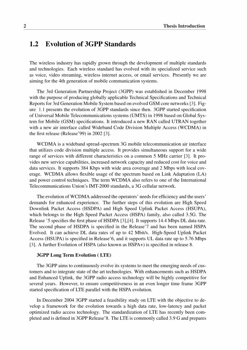
The 3rd Generation Partnership Project (3GPP) was established in December 1998with the purpose of producing globally applicable Technical Specifications and TechnicalReports for 3rd Generation Mobile System based on evolved GSM core networks [3]. Fig-ure 1.1 presents the evolution of 3GPP standards since then. 3GPP started specificationof Universal Mobile Telecommunications systems (UMTS) in 1998 based on Global Sys-tem for Mobile (GSM) specifications. It introduced a new RAN called UTRAN togetherwith a new air interface called Wideband Code Division Multiple Access (WCDMA) inthe first release (Release’99) in 2002 [3].
WCDMA is a wideband spread-spectrum 3G mobile telecommunication air interfacethat utilizes code division multiple access. It provides simultaneous support for a widerange of services with different characteristics on a common 5 MHz carrier [3]. It pro-vides new service capabilities, increased network capacity and reduced cost for voice anddata services. It supports 384 Kbps with wide area coverage and 2 Mbps with local cov-erage. WCDMA allows flexible usage of the spectrum based on Link Adaptation (LA)and power control techniques. The term WCDMA also refers to one of the InternationalTelecommunications Union’s IMT-2000 standards, a 3G cellular network.
The evolution of WCDMA addressed the operators’ needs for efficiency and the users’demands for enhanced experience. The further steps of this evolution are High SpeedDownlink Packet Access (HSDPA) and High Speed Uplink Packet Access (HSUPA),which belongs to the High Speed Packet Access (HSPA) family, also called 3.5G. TheRelease ’5 specifies the first phase of HSDPA [3],[4]. It supports 14.4 Mbps DL data rate.The second phase of HSDPA is specified in the Release’7 and has been named HSPAEvolved. It can achieve DL data rates of up to 42 Mbit/s. High-Speed Uplink PacketAccess (HSUPA) is specified in Release’6, and it supports UL data rate up to 5.76 Mbps[3]. A further Evolution of HSPA (also known as HSPA+) is specified in release 8.
3GPP Long Term Evolution ( LTE)
The 3GPP aims to continuously evolve its systems to meet the emerging needs of cus-tomers and to integrate state of the art technologies. With enhancements such as HSDPAand Enhanced Uplink, the 3GPP radio access technology will be highly competitive forseveral years. However, to ensure competitiveness in an even longer time frame 3GPPstarted specification of LTE parallel with the HSPA evolution.
In December 2004 3GPP started a feasibility study on LTE with the objective to de-velop a framework for the evolution towards a high data rate, low-latency and packetoptimized radio access technology. The standardization of LTE has recently been com-pleted and is defined in 3GPP Release’8. The LTE is commonly called 3.9 G and prepares
Thesis Introduction 3
Figure 1.1: Evolution of 3GPP standards
the way forward towards 4G systems with a new simplified core network and radio accessnetwork (RAN) architecture, to reduce latency for a packet based network. LTE aimsfor reduced latency, higher user data rates, improved system capacity and coverage, andreduced cost for the operators. The first LTE product is expected to be available in 2010[1].
The new LTE RAN is called E-UTRAN, which is composed of only one node, calledEvolved Node-B (eNode-B) [5]. The radio interface of LTE uses Orthogonal FrequencyDivision Multiple Access (OFDMA) in the DL and Single-Carrier Frequency DivisionMultiple Access (SC-FDMA) in the UL. LTE standards have been defined with as muchflexibility as possible so that the operators can deploy them in all current and existingfrequencies as well as new spectrum. The physical layer of the LTE is defined in abandwidth-agnostic way and supports various system bandwidth (1.4 to 20 MHz) in bothFDD and TDD modes [3]. OFDMA multiplexes different users in time and frequencydomain. The time and frequency domain adaptation of OFDMA is a key feature for in-creasing cellular capacity. The radio resource is subdivided into PRBs consisting of 12subcarriers with 15 KHz spacing and a time duration of 1 ms [3]. PRBs are dynamicallyallocated to users in order to realize multi-user diversity gain in both time and frequencydomains, leveraging adaptive modulation and coding with hybrid automatic repeat request(HARQ). To meet the performance requirements, the LTE Release’8 relies on MIMOtransmission and reception techniques, with 2x2 MIMO as the baseline for DL and 1X2MIMO for UL. However, higher order antenna configurations are also supported [5].
LTE is an all IP technology and supports full mobility and global roaming. LTE alsofacilitates gradual deployment ensuring smooth migration from the existing networks andoffers deployment in existing and new FDD spectrum bands. LTE will be the technology
4 Thesis Introduction
of choice for most of the existing 3GPP networks. The research forecasts more than 32million LTE subscribers by 2013 despite the fact that LTE network will not be commercialuntil 2010 [1].
3GPP Long Term Evolution-Advanced ( LTE-A)
The International Telecommunications Union (ITU) is currently working on speci-fying the system requirements towards next generation mobile communication systemscalled International Mobile Telecommunications-Advanced (IMT-A). The deployment ofIMT-A systems is believed to take place around year 2015 at mass market level. IMT-Asystems are expected to provide peak data-rates in the order of 1 Gbps in downlink and500 Mbps in uplink [6], [7]. The 3GPP aims to further evolve the LTE towards LTE-Asystems in order to meet or exceed the IMT-A requirements as well as its own require-ments for advancing LTE for long term competitiveness [6]. The following performancetargets are set for LTE-A to meet the IMT-A requirements, while maintaining the back-ward compatibility with LTE release’8 [6], [8].
LTE- A Performance Targets
• Average spectral efficiencies of up to 3.7 b/s/Hz/cell in the DL (with 4× 4 antennaconfiguration) and 2.0 b/s/Hz/cell in UL (2× 4).
• Cell edge spectral efficiencies of 0.12 b/s/Hz in the DL (4 × 4) and 0.07 b/s/Hz inthe UL (2× 4).
• Peak data rates of up to 1Gb/s in the DL and 500 Mb/s in the UL.
• Peak spectrum efficiencies of 30 b/s/Hz in the DL and 15 b/s/Hz in the UL usingantenna configurations of 8× 8 in DL and 4× 4 in the UL.
• Low cost of infrastructure deployments and terminals and power efficiency in thenetwork and terminals.
1.3 Thesis Motivation and Objectives
The network operators need to maximize the utilization of spectral resources in orderto meet the ambitious data rate targets of the next generation communication systems.Hence, there is a need to develop solutions allowing for a more efficient utilization of theavailable spectrum. The aim of the PhD study is to investigate the potential techniques forefficient usage of the spectrum keeping in view the requirements of the next generationmobile communication systems. The overall objective of this PhD study is identified toanswer the question, "How to enhance the efficiency of spectrum usage for the next gen-eration mobile communication systems?" The LTE and LTE-A are taken as the examplecases for next generation systems. Our focus is on Wide Area (WA) outdoor and LocalArea (LA) indoor cellular deployment scenarios. For WA outdoor deployment the studyis focused on LTE, whereas for LA indoor deployment scenario the study is focused on
Thesis Introduction 5
LTE-A system. Our focus is on developing system level solutions and their performanceevaluation.
The spectrum efficiency (amount of information bits per unit of spectrum per unit ofarea) is often used as figure of merit. The spectrum efficiency determines the requiredamount of spectrum to meet the service requirements. It directly relates to the operators’economies, cost of service delivery, and users’ experience [9].
Two main approaches could be used to improve spectral utilization. The first approachrelies on squeezing a larger number of bits/second/Hz in the allocated spectrum. This canbe accomplished by using higher order modulation and MIMO techniques at the physicallayer. The second approach relies on aggressive spatial reuse of assigned spectrum. Thisinvolves breaking large cells into smaller cells and deploying more base stations usinglower peak power [9].
This PhD study is motivated by the second approach for the following reasons:
• The growth in wireless capacity is exemplified by following observation of MartinCooper: "The wireless capacity has doubled every 30 months over the last 104years". This translates into an approximately million fold capacity increase since1957. Breaking down these gains shows a 25x improvement from wider spectrum, a5 x improvement by dividing the spectrum into smaller slices, a 5x improvement bydesigning a better modulation scheme, and a 1600x gain through reduced cell sizesand transmit distance. The enormous gains reaped from smaller cell sizes arisefrom efficient spatial reuse of the spectrum or, alternatively, higher area spectralefficiency [10].
• So far plenty of efforts have been dedicated for improving the spectral efficiencyusing physical layer techniques. The research studies show that the physical layertechniques have nearly reached their capacity limits, and the improvements in spec-trum usage could be only marginally improved at reasonable cost, whereas thesystem level approaches have not been fully exploited towards improving systemcapacity.
We identified the following open issues for investigation:
The first issue we need to address is the higher order sectorization (HOS). In order toincrease the spectrum utilization, HOS is considered in the DL of LTE system. Typicallythree sectors per site deployment are considered for the LTE systems. A migration to sixsectors per site deployment is considered in this study. The scope of study also includes amixed network topology consisting of a combination of three and six sectors per site. TheHOS provides a means to improve the coverage and capacity per unit area and thereforeimproves the efficiency of spectrum utilization.
The second critical issue is Inter-cell Interference Avoidance (ICIA)for LTE, which isan important aspect for improving system capacity and coverage. Inter-cell interferencecoordination (ICIC) has been extensively considered in LTE for controlling the interfer-ence between cells in order to further improve the so-called cell-edge user performance.
6 Thesis Introduction
The ICIC schemes primarily rely on frequency domain sharing between cells and adjust-ment of transmission power. This PhD study aims to develop mechanisms for ICIA underfractional load conditions. The fractional load conditions arise when there is no enoughtraffic in the cell and all the resources are not required to be used. Under this conditionthe mechanisms can be developed to efficiently use the required amount of spectrum toimprove the experienced SINR condition and in turn to improve the coverage and capacityover the given amount of spectrum.
Another research topic is concerning LTE-A, which is expected to provide 1Gbps inDL. Such high data rate requires high bandwidth as well as high efficiency of spectrumusage. The surest way to increase capacity of a wireless link is by getting the transmitterand receiver closer to each other, which create the dual benefits of higher quality link andmore spatial reuse. In a network with nomadic users, this inevitably involves deployingmore infrastructures, typically in the form of micro cells, hot spots, distributed antennasor relays. A less expensive alternative is the recent concept of home base stations, whichare data access points installed by home users to get better indoor voice and data coverage[10]. Due to their short transmit -receive distance, home base stations can greatly lowertransmit power and achieve a higher SINR. This translates into improved reception andhigher capacity, and therefore improved spectrum utilization.
When several operators will deploy home base stations in the given geographical area,sharing over the same spectrum pool, then policies become mandatory to ensure fair andefficient usage of the spectrum. Moreover, the Home base stations are expected to beuser deployed, self configurable and self adjustable according to the radio environment,therefore a degree of cognitivity is also assumed. Keeping these perspectives in view thisPhD study also investigates the concept of policy and the cognitive aspects of the devices.
In summary the detailed objectives explained above can be boiled down into the fol-lowing fundamental task: "Improvement in system capacity and coverage over the givenspectrum with minimum increase in system complexity and signaling requirements".
1.4 Scientific Methodology Employed
The main objective of this PhD study is to provide an understanding at the system levelperformance, hence a system level approach is used. In fact the system level performancecan be analyzed by various means such as analytical approach based on system model,computer aided simulation and field trial in operational network. Analytical approachmay provide a viable approach when the system model is simple, but it becomes infea-sible for modern cellular systems which are complex and involve numerous assumptionsand constraints. The system level performance of modern cellular systems depends ona large number of parameters whose behavior cannot be predicted beforehand, makingit tedious to formulate a theoretical framework. Consequently, a closed form analyticalexpression characterizing system performance is seldom possible. On the other hand fieldtrial requires the availability of the network, which may not always be feasible (e.g. theLTE and LTE-A operational networks are not yet available). Under such circumstances
Thesis Introduction 7
the computer aided simulation approach presents a suitable option. If the metrics aremeaningful and the methodology reflects realistic networks, computer aided simulation isa good way to compare different concepts and predict the network performance [8]. Forthis reason a computer aided system level simulation has been used in this PhD study asthe main performance assessment methodology, sometimes supported by the theoreticalanalysis to understand the simulation results more accurately.
The work in this thesis is divided in two phases. The first phase provides the perfor-mance results for LTE system in the DL. A quasi-dynamic system level simulator built inC++ is employed, which uses the 3GPP LTE system model as described in [11]. The sys-tem model includes detailed implementation of Link Adaptation (LA) based on AdaptiveModulation and Coding (AMC), explicit scheduling of Hybrid Automatic Repeat reQuest(HARQ) processes including retransmissions, link-to-system mapping techniques suitablefor OFDMA. The study included development of the system level simulator for six sectorimplementation and performance evaluation in typical urban macro cellular environment.
The second part of the study involves LTE-A indoor deployment, which is based ona quasi dynamic system level simulator built in Matlab. The system model uses mostof the features for IMT-A system recommended for local area scenario. The simula-tor is still in the development phase. The simulator provides features for fully con-figurable room/apartment/ wall/corridor/floor for indoor layout. It supports randomizedusers generation and distribution, different synchronization cases, i.e. fully, loose, non-synchronized, and several other features to support the LTE-A system requirements. Thesimulator is further developed to support the features of the proposed algorithms.
1.5 Novelty and Contributions
This PhD study mainly contributes towards providing a system level understanding ofvarious mechanisms for improving the efficiency of spectrum utilization. The LTE andLTE-A systems are mainly considered for such study. The considered mechanisms in thisstudy involved conceptual design, system modeling, software development, implementa-tion and performance evaluation.
The first topic of research is related to Higher Order Sectorization, where we consider6 sector site deployment for LTE DL. My main contribution in this regard is implemen-tation and performance evaluation of 6 sector site network deployment. In addition tothis my contribution also lies in proposal, implementation, and performance evaluationof mixed network topology. A mixed network topology consists of a combination of 3and 6 sector site deployment. A significant system capacity gain is realized by 6 sectorover the typically assumed 3 sector deployment. The realized gain is further improved bymixed network topology. The main contribution and novelty of this PhD study lies in thefact that no such performance study was available in the open literature for LTE; thereforethis study fills the gap in the literature in this regard. The results of this study have beenpublished in the following article:
8 Thesis Introduction
• " Sanjay Kumar, I. Z. Kovacs, G Monghal, K. I. Pedersen, P. E. Mogensen "Perfor-mance Evaluation of 6 Sector Cell Lay Out For 3GPP Long Term Evolution", IEEEVTC, Calgary, Canada, 21-24 Sep, 2008.
The second topic of research is related to the Inter-Cell Interference Avoidance (ICIA)under Fraction Load (FL) conditions for LTE DL. Numerous studies are available onInter-Cell Interference Coordination (ICIC) at full load conditions, but only few studiesare available on FL. In this study we propose several algorithms for ICIA and recommendthat the ICIA algorithm needs to be integrated with the packet scheduler functionalitiesin order to improve the average experienced SINR, leading to improved coverage and ca-pacity. Part of the discussion and the results presented in this study is an outcome of acollaborative work with a fellow researcher and joint supervision of master thesis at Aal-borg University in collaboration with Nokia Siemens Networks, Aalborg. My contributionis in jointly developing the algorithm, planning simulation methodology and adaptation tothe system level simulator. The results of this contribution are published in the followingarticle:
• " Sanjay Kumar, G. Monghal, Jaume Nin, Ivan Ordas, K. I. Pedersen, P. E. Mo-gensen, "Autonomous Inter Cell Interference Avoidance under Fractional Load forDownlink Long Term Evolution", IEEE Vehicular Technology Conference, Barcelona,Apr 26-29, 2009.
In addition, the following article in this area of study is also co- authored:
• " Guillaume Monghal, Sanjay Kumar, K. I. Pedersen and P. E. Mogensen, " Inte-grated Fractional Load and Packet Scheduling for OFDMA Systems ", (Submittedto ICC for International Workshop on LTE Evolution,June 2009, Dresden, Ger-many.
The third topic of research presented in this study is related to Flexible SpectrumUsage (FSU) in local area indoor deployment for LTE-A. The work was undertaken to-gether with the fellow researchers at Aalborg University as part of the Spectrum Sharingproject. In this regard our effort was directed to develop an autonomous, self-configurableand scalable solution for such deployment scenario. My personal contribution in this re-gards was proposal, development and performance evaluation of a novel Spectrum LoadBalancing (SLB) algorithm. The SLB algorithm ensures coexistence in the given geo-graphical area by partially or completely preventing mutual interference over the sharedspectrum. Further, an Resource Chunk Selection (RCS) algorithm was developed in col-laboration with a fellow researcher, where my personal contribution lies in jointly devel-oping the concept of the algorithm and evaluation of the performance in the given sce-nario. Presently, the research in this area is in the evolving phase, therefore the proposedconcepts and algorithms can be regarded as significant contributions in this emerging areaof research. The results of this study are published in the following article:
Thesis Introduction 9
• " Sanjay Kumar, Y. Wang, N. Marchetti, I. Z. Kovács and P. E. Mogensen, "Spec-trum Load Balancing for Flexible Spectrum Usage in Local Area Deployment Sce-nario" IEEE Symposium on Dynamic Spectrum Access 2008 (DySPAN 2008),Chicago, USA, Oct 14-17, 2008
In addition, the following article has been also published, which is an outcome of jointwork with fellow researchers during the initial phase of study on flexible spectrum usage.
• " Sanjay Kumar, G. Costa, S. Kant, Flemming B. Frederiksen, N. Marchetti andP. E. Mogensen, "Spectrum Sharing for Next Generation Wireless CommunicationNetworks", First International Workshop on Cognitive Radio and Advanced Spec-trum Management (CogART’08), Aalborg, Feb. 14, 2008.
Also, the following article has been co-authored during the study on local area deploymentand flexible spectrum usage.
• " Yuanye Wang, Sanjay Kumar, Luis Garcia, K. I. Pedersen, I. Z. Kovács, SimoneFrattasi, Nicola Marchetti, P. E. Mogensen and T. B. Sørensen "Fixed FrequencyReuse for LTE-Advanced Systems in Different Scenarios", IEEE Vehicular Tech-nology Conference, Barcelona, Apr 26-29, 2009.
The fourth topic presented in this thesis is on Autonomous Component Carrier Selectionin uncoordinated deployment for local area of LTE-A. This is a joint work with fellowresearcher at Aalborg University and Nokia Siemens Networks colleagues in Aalborg.My main contribution in this study is related to jointly developing primary componentcarrier selection scheme, quality monitoring of primary component carrier and recoveryaction. The concept and the outcome of the results of this study are presented in thefollowing 3GPP contributions:
• " 3GPP, R1-090735, "Primary Component Carrier Selection, Monitoring, and Recovery–Nokia Siemens Networks, Nokia", TSG RAN WG1 Meeting , Athens, Greece,February 9-13, 2009.
• " 3GPP, R1-084321, "Algorithms and Results for Autonomous Component CarrierSelection for LTE-Advanced- Nokia Siemens Networks, Nokia", TSG RAN WG1Meeting Prague, Czech Republic, November 10-14, 2008.
• " 3GPP, R1-083103, "Autonomous Component Carrier Selection for LTE-Advanced–Nokia Siemens Networks, Nokia", TSG RAN WG1 Meeting, Jeju Island, Korea,August 18-22, 2008
The fifth and the last topic of study presented in this thesis is related to multi operatorFSU, where the deployment by several operators in the given geographical area is consid-ered. In this regard a novel concept ’Policy Assisted Light Cognitive Radio enabled FSU’
10 Thesis Introduction
is presented in the thesis. The work and my contribution in this chapter includes proposalof the concept, algorithm development and implementation, and performance evaluationfor the given scenario. However, during the implementation phase the support by masterstudents at Aalborg university, whom I co-supervised, is also recognized.
• " Sanjay Kumar, V. Palma, E. Borgat, N. Marchetti, and P. E. Mogensen "LightCognitive Radio for Flexible Spectrum Usage in Local Area Deployment" IEEEVehicular Technology Conference 2009 (VTC 2009), Barcelona, Apr 26-29, 2009.
In addition the following article has been published, which provides an overview of theexisting state of the art concerning the technical requirements and technological solutionsfor IMT-A systems.
• " Sanjay Kumar and Nicola Marchetti, "IMT-Advanced : Technological Require-ments and Solution Components", International Conference on Wireless VITAE,Aalborg, 17-20 May 2009
Apart from the above contributions, the following articles have also been published duringthe PhD study. These are the outcome of the preliminary directions at the outset of thePhD study, and are not included in the PhD thesis.
• " Sanjay Kumar, S. S. Das and Ramjee Prasad, "Proportional Fair Scheduling WithQoS Constraints in the Downlink of OFDMA Systems," Symposium on WirelessPersonal Multimedia Communications (WPMC), Jaipur, India, Dec 3-6, 2007.
• " Nicola Marchetti, Muhammad Imadur Rahman, Sanjay Kumar and Ramjee Prasad,"OFDM: principles and challenges", chapter in the book ’New Directions in Wire-less Communications Research’, Springer Publications, in press.
1.6 Thesis Outline
The PhD thesis is organized as follows:
Chapter 2: System Description.This chapter provides a general description of LTE and LTE-A systems. The Architec-ture, Radio Resource Management (RRM) functionalities, Multiplexing and Duplexingschemes of LTE are discussed. A general system model of LTE under consideration isoutlined. Also, a general system model of LTE-A and various assumptions for local areaindoor deployment scenario are presented in this chapter.
Chapter 3: Higher Order Sectorization for LTE DL.This chapter introduces briefly the concept and benefits of higher order sectorization. It
Thesis Introduction 11
includes the antenna pattern and different network topologies used for performance eval-uation of 6 sector site deployment for LTE DL. The proposed mixed network topologiesand their performance evaluation are also presented in this chapter.
Chapter 4: Inter-cell Interference Avoidance under Fractional Load for LTE DL.This chapter provides a brief account of the Inter-Cell Interference Coordination (ICIC)for LTE DL and afterwards provides a discussion on the concept of Inter-Cell Interfer-ence Avoidance (ICIA) under fractional load conditions. The description of the variousschemes proposed for ICIA are given, and their performance results are presented in thischapter.
Chapter 5: Flexible Spectrum Usage for LTE-Advanced.This chapter discusses the relevance of Flexible Spectrum Usage in the context LTE-Alocal area deployment scenario. The proposed Spectrum Load Balancing (SLB) and Re-source Chunk Selection (RCS) algorithms for FSU are described in this chapter. Theperformance analysis of the proposed schemes are presented, and a self-configurable so-lution for local area indoor deployment scenario is suggested in this chapter.
Chapter 6: Autonomous Component Carrier Selection for IMT-A.This chapter presents the concept of carrier aggregation as a means to achieve wider band-width for the LTE-A system. A concept of primary and secondary component carriers isprovided. A description of the overall primary states, quality monitoring and recoveryaction are discussed in this chapter. A self-adjustable solution for LTE-A uncoordinatedlocal area deployment is suggested by means of autonomous component carrier selectionmechanism.
Chapter 7: Policy Assisted Light Cognitive Radio for FSU.This chapter describes the concept of FSU in multi operators’ domain and highlights theimportance of policy and the concept of cognitive radio for fair, flexible and efficientspectrum allocation among the operators deployed in the given geographical area. In thisrespect a concept of Policy Assisted Light Cognitive Radio for FSU is presented.
Chapter 8: Conclusions and Recommendations.This chapter provides the summary of overall study and discusses future research issues.

Chapter 2
System Description
2.1 Introduction
This chapter provides a description of the systems under consideration. Different as-sumptions are outlined and their relevance to the study is discussed. The Long TermEvolution (LTE) and LTE-Advanced (LTE-A) are considered as the case study, thereforethe descriptions provided in this chapter are mostly relevant to these systems.
The chapter is organized as follows: Section 2.2 provides an overview of the LTEarchitecture and a discussion on its main components. Section 2.3 gives a description ofthe Radio Resource Management (RRM) functionality in LTE. The duplexing scheme andLTE frame structures are illustrated in section 2.4. The LTE and LTE-A system modelsunder consideration are outlined in section 2.5 and 2.6 respectively.
2.2 LTE Architecture
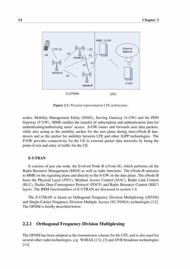
The LTE architecture has two distinct components: Core Network (CN) and Radio Ac-cess Network (RAN). The CN is called Evolved Packet Core (EPC) and the RAN iscalled Evolved Universal Terrestrial Radio Access Network (E-UTRAN). The EPC andE-UTRAN together constitute the Evolved Packet System (EPS). Figure 2.1 gives a pic-torial representation of the LTE architecture.
Evolved Packet Core (EPC)
The EPC is based on the internet protocol and provides one common packet corenetwork for 3GPP radio access (LTE, 2G and 3G), non 3GPP radio access (WLAN andWiMAX), and fixed access (Ethernet, DSL, cable and fiber). The main characteristicof EPC is its simplified architecture. The network latency and complexity are reducedin EPC as there are fewer hopes in both the control and data planes. It has three main
13
14 Chapter 2
Figure 2.1: Pictorial representation LTE architecture.
nodes; Mobility Management Entity (MME), Serving Gateway (S-GW) and the PDNGateway (P-GW). MME enables the transfer of subscription and authentication data forauthenticating/authorizing users’ access. S-GW routes and forwards user data packets,while also acting as the mobility anchor for the user plane during inter-eNode-B han-dovers and as the anchor for mobility between LTE and other 3GPP technologies. TheP-GW provides connectivity for the UE to external packet data networks by being thepoint of exit and entry of traffic for the UE.
E-UTRAN
It consists of just one node, the Evolved Node B (eNode-B), which performs all theRadio Resource Management (RRM) as well as radio functions. The eNode-B interactsto MME on the signaling plane and directly to the S-GW on the data plane. The eNode-Bhosts the Physical Layer (PHY), Medium Access Control (MAC), Radio Link Control(RLC), Packet Data Convergence Protocol (PDCP) and Radio Resource Control (RRC)layers. The RRM functionalities of E-UTRAN are discussed in section 1.4.
The E-UTRAN is based on Orthogonal Frequency Division Multiplexing (OFDM)and Single-Carrier Frequency Division Multiple Access (SC-FDMA) technologies [12].The OFDM is briefly described below.
2.2.1 Orthogonal Frequency Division Multiplexing
The OFDM has been adopted as the transmission scheme for the LTE, and is also used forseveral other radio technologies, e.g. WiMAX [13], [3] and DVB broadcast technologies[14].
System Description 15
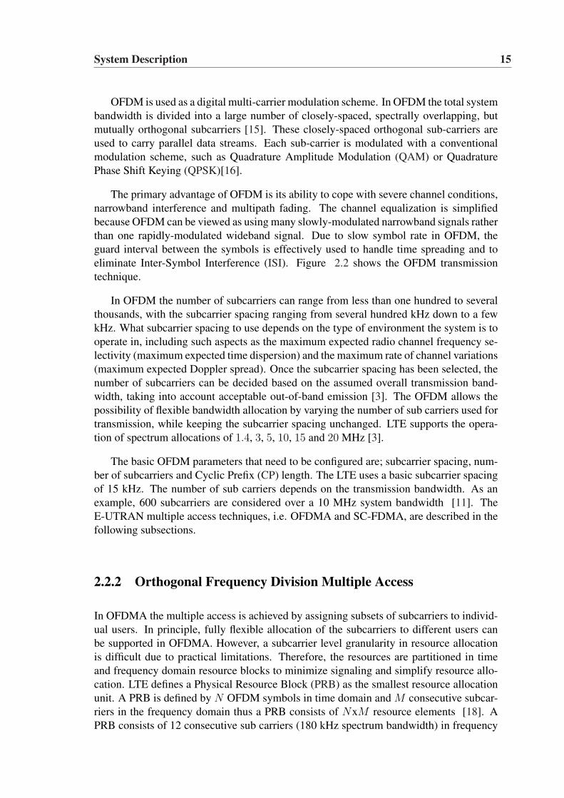
OFDM is used as a digital multi-carrier modulation scheme. In OFDM the total systembandwidth is divided into a large number of closely-spaced, spectrally overlapping, butmutually orthogonal subcarriers [15]. These closely-spaced orthogonal sub-carriers areused to carry parallel data streams. Each sub-carrier is modulated with a conventionalmodulation scheme, such as Quadrature Amplitude Modulation (QAM) or QuadraturePhase Shift Keying (QPSK)[16].
The primary advantage of OFDM is its ability to cope with severe channel conditions,narrowband interference and multipath fading. The channel equalization is simplifiedbecause OFDM can be viewed as using many slowly-modulated narrowband signals ratherthan one rapidly-modulated wideband signal. Due to slow symbol rate in OFDM, theguard interval between the symbols is effectively used to handle time spreading and toeliminate Inter-Symbol Interference (ISI). Figure 2.2 shows the OFDM transmissiontechnique.
In OFDM the number of subcarriers can range from less than one hundred to severalthousands, with the subcarrier spacing ranging from several hundred kHz down to a fewkHz. What subcarrier spacing to use depends on the type of environment the system is tooperate in, including such aspects as the maximum expected radio channel frequency se-lectivity (maximum expected time dispersion) and the maximum rate of channel variations(maximum expected Doppler spread). Once the subcarrier spacing has been selected, thenumber of subcarriers can be decided based on the assumed overall transmission band-width, taking into account acceptable out-of-band emission [3]. The OFDM allows thepossibility of flexible bandwidth allocation by varying the number of sub carriers used fortransmission, while keeping the subcarrier spacing unchanged. LTE supports the opera-tion of spectrum allocations of 1.4, 3, 5, 10, 15 and 20 MHz [3].
The basic OFDM parameters that need to be configured are; subcarrier spacing, num-ber of subcarriers and Cyclic Prefix (CP) length. The LTE uses a basic subcarrier spacingof 15 kHz. The number of sub carriers depends on the transmission bandwidth. As anexample, 600 subcarriers are considered over a 10 MHz system bandwidth [11]. TheE-UTRAN multiple access techniques, i.e. OFDMA and SC-FDMA, are described in thefollowing subsections.
2.2.2 Orthogonal Frequency Division Multiple Access
In OFDMA the multiple access is achieved by assigning subsets of subcarriers to individ-ual users. In principle, fully flexible allocation of the subcarriers to different users canbe supported in OFDMA. However, a subcarrier level granularity in resource allocationis difficult due to practical limitations. Therefore, the resources are partitioned in timeand frequency domain resource blocks to minimize signaling and simplify resource allo-cation. LTE defines a Physical Resource Block (PRB) as the smallest resource allocationunit. A PRB is defined by N OFDM symbols in time domain and M consecutive subcar-riers in the frequency domain thus a PRB consists of NxM resource elements [18]. APRB consists of 12 consecutive sub carriers (180 kHz spectrum bandwidth) in frequency
16 Chapter 2
Figure 2.2: Illustration of the OFDM transmission technique [17].
domain and 14 adjacent OFDM symbols (1 ms duration) in time domain for short cyclicprefix configuration. The time domain allocation unit is also called Transmission TimeInterval (TTI) in LTE.
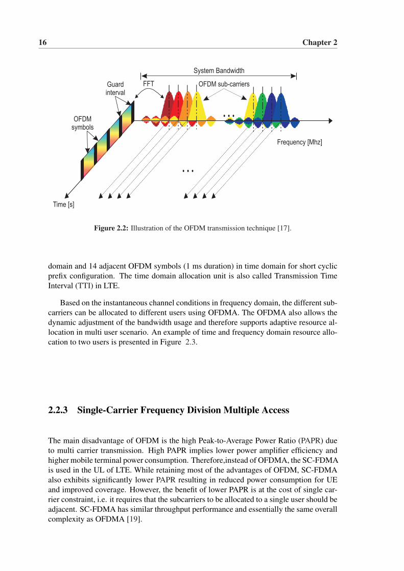
Based on the instantaneous channel conditions in frequency domain, the different sub-carriers can be allocated to different users using OFDMA. The OFDMA also allows thedynamic adjustment of the bandwidth usage and therefore supports adaptive resource al-location in multi user scenario. An example of time and frequency domain resource allo-cation to two users is presented in Figure 2.3.
2.2.3 Single-Carrier Frequency Division Multiple Access
The main disadvantage of OFDM is the high Peak-to-Average Power Ratio (PAPR) dueto multi carrier transmission. High PAPR implies lower power amplifier efficiency andhigher mobile terminal power consumption. Therefore,instead of OFDMA, the SC-FDMAis used in the UL of LTE. While retaining most of the advantages of OFDM, SC-FDMAalso exhibits significantly lower PAPR resulting in reduced power consumption for UEand improved coverage. However, the benefit of lower PAPR is at the cost of single car-rier constraint, i.e. it requires that the subcarriers to be allocated to a single user should beadjacent. SC-FDMA has similar throughput performance and essentially the same overallcomplexity as OFDMA [19].
System Description 17
Figure 2.3: Example of time and frequency domain resource allocation using OFDMA [5].
2.3 RRM Functionality
RRM involves strategies and algorithms for controlling interference, transmit power, mod-ulation schemes etc., in order to utilize the radio resources as efficiently as possible. Thewireless channel experiences variations due to frequency selective fading, shadow fad-ing, distance dependent path loss and interference. These variations could be exploitedfavorably to improve system performance by means of channel dependent scheduling.The channel dependent scheduling takes the channel variations into account to achieveefficient resource allocation. The Link Adaptation (LA) is closely related to the channeldependent scheduling. The LA deals with setting the transmission parameters of a ra-dio link to handle variation of the radio link quality. The channel dependent schedulingtogether with LA aim to adapt the channel variations prior to transmission. However, aperfect adaptation to instantaneous radio link quality is not realized, due to the randomchannel variations. The data may be received in error. Therefore, a Hybrid Automatic Re-peat reQuest (HARQ) scheme is employed, which requests retransmission of erroneouslyreceived data. In this way HARQ complements channel dependent scheduling and LAafter transmission.
18 Chapter 2
2.3.1 Packet Scheduling
The packet scheduler is basically responsible for selection of users to be scheduled, andalso scheduling of HARQ retransmissions. During the decision making, the packet sched-uler interacts closely with the LA unit. The information about the Downlink (DL) chan-nel conditions, necessary for channel dependent scheduling, is fed back from users to theeNode-B via channel quality reports. The channel quality reports, also known as ChannelQuality Information (CQI), include information about the instantaneous channel qualityin the frequency domain. The PS in LTE dynamically determines, in each 1 ms interval,which users are supposed to receive Downlink Shared Channel (DL-SCH) transmissionsand on what resources. The one millisecond basis for PS in LTE is used in order to adaptto fast channel variations and therefore take advantage of the Multi User Diversity (MUD)gain, where the gain obtained by transmitting to users with favorable channel conditionsis called MUD gain.
In addition to the CQI, the packet scheduler also takes into account the buffer status,QoS parameters of different users and priorities, HARQ status and ACK/NAK reports inthe scheduling decisions. Interference coordination, which tries to control the interfer-ence, is also part of the packet scheduler functionality. In our study we used decoupledtime and frequency Domain Packet Scheduler [20], briefly explained below.
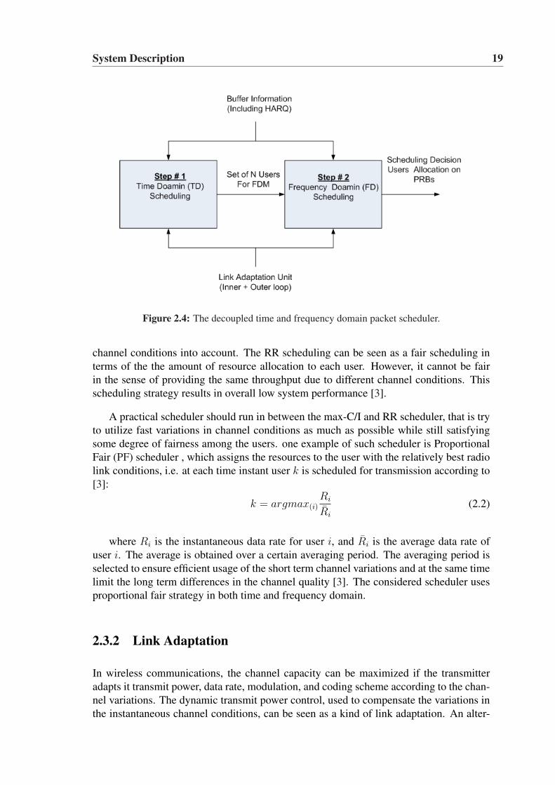
Decoupled Time and Frequency Domain Packet Scheduler
Figure 2.4 presents the basic architecture of the decoupled time and frequency Do-main PS. It consists of two main entities : Time-Domain Packet Scheduling (TDPS) andFrequency-Domain Packet Scheduling (FDPS). The Time-Domain (TD) scheduling isfirst performed followed by Frequency-Domain (FD) scheduling. For each TTI the TDPSselects N users for Frequency Domain Multiplexing (FDM). The FDPS then decides howto multiplex those users on the available Physical Resource Blocks (PRBs). This PS of-fers simple, flexible and low complexity framework for time and frequency domain packetscheduling. Both the TDPS and FDPS entities take input from the LA unit in order to takethe radio channel conditions into account in the scheduling decision.
Packet Scheduling Strategies
Different strategies could be used for packet scheduling. The scheduling of the userswith the best channel condition is referred to as max-C/I (maximum rate scheduling),which can be expressed as scheduling user k given by:
k = argmax(i)Ri (2.1)
where Ri is the instantaneous data rate for user i. This leads to high multiuser diversitygain and hence high system capacity. The high MUD gain is realized when the numberof users is large and the channel variations are high. However, a pure max-C/I schedul-ing may starve the users in bad channel conditions, and therefore this scheduling doesnot provide a fair strategy. An alternative to max-C/I is Round Robin (RR) scheduling,which allows the users to take turns in using the resource, without taking the instantaneous
System Description 19
Figure 2.4: The decoupled time and frequency domain packet scheduler.
channel conditions into account. The RR scheduling can be seen as a fair scheduling interms of the the amount of resource allocation to each user. However, it cannot be fairin the sense of providing the same throughput due to different channel conditions. Thisscheduling strategy results in overall low system performance [3].
A practical scheduler should run in between the max-C/I and RR scheduler, that is tryto utilize fast variations in channel conditions as much as possible while still satisfyingsome degree of fairness among the users. one example of such scheduler is ProportionalFair (PF) scheduler , which assigns the resources to the user with the relatively best radiolink conditions, i.e. at each time instant user k is scheduled for transmission according to[3]:
k = argmax(i)Ri
Ri
(2.2)
where Ri is the instantaneous data rate for user i, and Ri is the average data rate ofuser i. The average is obtained over a certain averaging period. The averaging period isselected to ensure efficient usage of the short term channel variations and at the same timelimit the long term differences in the channel quality [3]. The considered scheduler usesproportional fair strategy in both time and frequency domain.
2.3.2 Link Adaptation
In wireless communications, the channel capacity can be maximized if the transmitteradapts it transmit power, data rate, modulation, and coding scheme according to the chan-nel variations. The dynamic transmit power control, used to compensate the variations inthe instantaneous channel conditions, can be seen as a kind of link adaptation. An alter-
20 Chapter 2
native to dynamic transmit power control is dynamic rate control, where the data rate isdynamically adjusted to compensate for the varying channel conditions. The data rate iscontrolled by adjusting the modulation scheme and/or channel coding rate, and therefore,sometimes referred to as Adaptive Modulation and Coding (AMC)[3].
LTE supports fast adaptive LA, performed on millisecond basis. The LA is basedon the CQI reports and aims to ensure that the most suitable Modulation and CodingScheme (MCS) is always used. The PS interacts with LA unit in order to make schedulingdecisions. The LA unit consists of an inner loop algorithm and an outer loop algorithm.The inner loop algorithm is the primary unit, which estimates the transport block size andmodulation scheme based on the CQIs reports. Whereas the Outer Loop Link Adaptation(OLLA) helps to maintain the desired BLock Error Rate (BLER) target.
2.3.3 Hybrid ARQ
In LTE HARQ, a combination of Forward Error Correction (FEC) and Automatic RepeatReQuest (ARQ) is used to provide a robustness against transmission errors. HARQ usesFEC to correct a subset of all errors and relies on error detection to detect uncorrectableerrors. Erroneously received packets are discarded, and the receiver requests retransmis-sions. In HARQ with soft combining, the erroneously received packet is stored in a buffermemory and later combined with the retransmission to obtain a single, combined packetwhich is more reliable than its constituents. The HARQ with soft combining is usuallycategorized with the chase combining and incremental redundancy. In chase combiningthe retransmissions consist of the same set of coded bits as the original transmission. Inincremental redundancy, each retransmission need not to be identical with the originaltransmission.
LTE employs HARQ with soft combining. The HARQ protocol is part of the MAClayer, while the soft combining is handled at physical layer. In LTE the HARQ protocoluses multiple parallel stop and wait processes. The current assumption in LTE is asyn-chronous and adaptive HARQ for the DL. This implies that the PS has the freedom tofreely schedule pending HARQ retransmissions in both the frequency and time domain.
2.3.4 Channel Quality Indicator
The information about the DL channel conditions, necessary for link adaptation and chan-nel dependent scheduling, is fed back from users to the eNode-B via channel quality re-ports. The channel quality reports also known as CQI, include information about theinstantaneous channel quality in the frequency domain. The basis of CQI report is mea-surement on the DL reference signals.
The PS and LA entities employ CQI feedback. The inner loop LA unit determinesthe modulation scheme for the different users based on CQI feedback. The CQI consistsof a set of values corresponding to an estimate of the Signal to Interference plus Noise
System Description 21
Figure 2.5: The LTE type 1 frame structure, applicable for both full and half duplex FDD [18]
Ratio (SINR) on each CQI block. A CQI block consisting of 2 PRBs is considered in ourLTE study. The receiver imperfections are modeled by adding a zero mean Gaussian errorof 1 dB standard deviation to the ideal CQI as in [21]. The CQI is further quantified witha 1dB step. A processing delay equivalent to 2 TTI is considered.
2.4 Duplexing Scheme and LTE Frame Structure
LTE supports both Frequency Division Duplex (FDD) and Time Division Duplex (TDD)schemes. DL and UL transmissions are organized in radio frames with 10 ms duration.Two frame structures are supported. Type 1 applicable to FDD and Type 2 applicable toTDD [18].
Frame Structure Type 1
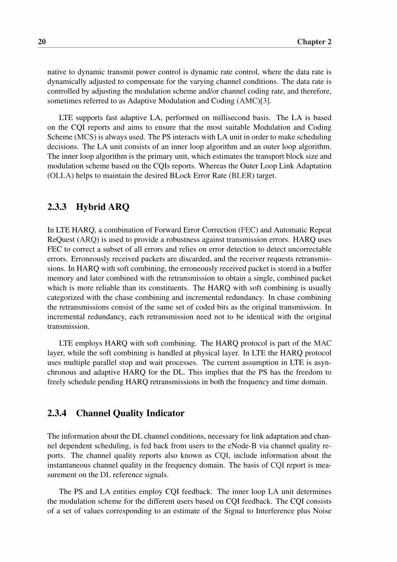
This is applicable to both full duplex and half duplex FDD. Each LTE frame consistsof 10 ms duration. They are divided into 10 subframes, each subframe is further dividedinto two slots, each of 0.5 ms duration. A slot consists of either 6 or 7 OFDM symbols,depending on whether a short or long cyclic prefix is used. Subframe is defined as twoconsecutive slots where subframe i consists of slots 2i, and 2i + 1. Figure 2.5 shows theframe structure.
Frame Structure Type 2
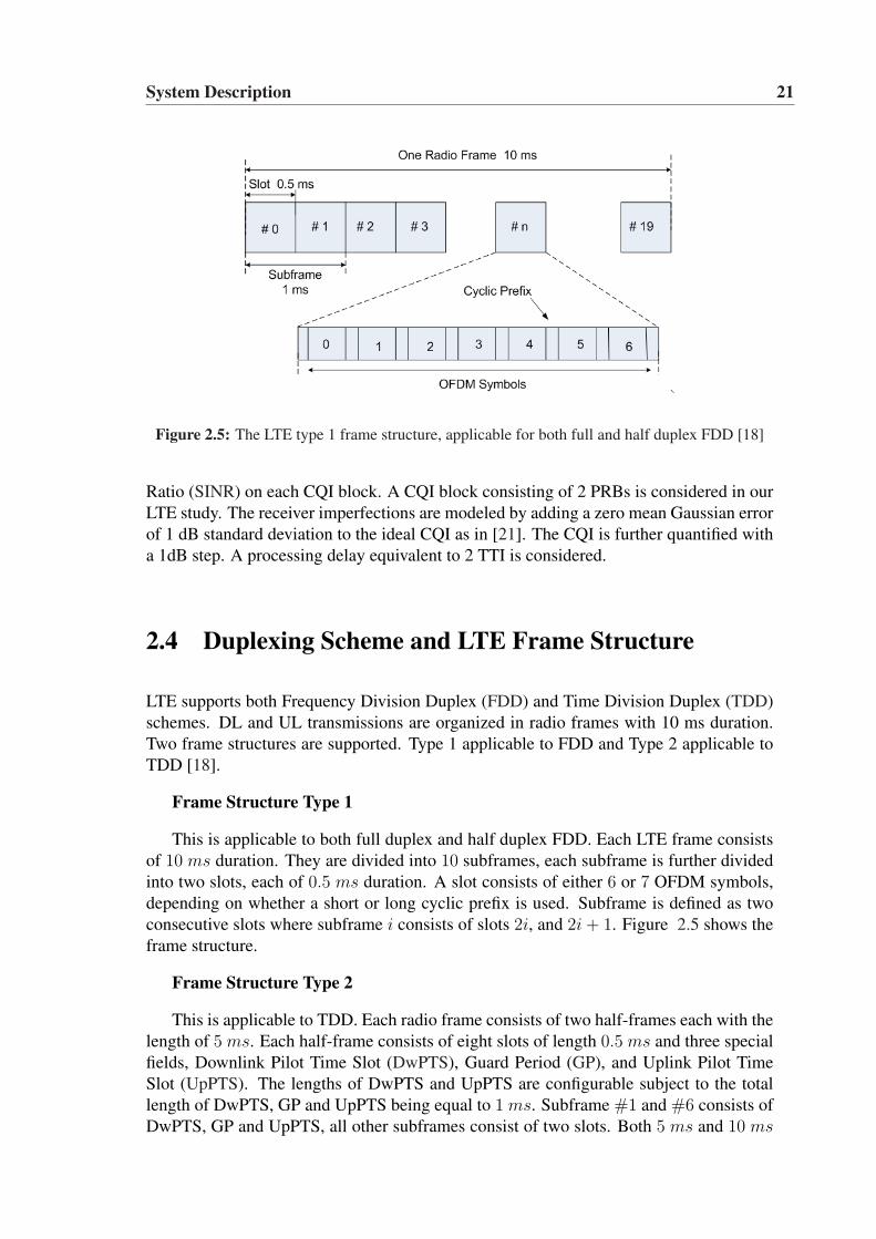
This is applicable to TDD. Each radio frame consists of two half-frames each with thelength of 5 ms. Each half-frame consists of eight slots of length 0.5 ms and three specialfields, Downlink Pilot Time Slot (DwPTS), Guard Period (GP), and Uplink Pilot TimeSlot (UpPTS). The lengths of DwPTS and UpPTS are configurable subject to the totallength of DwPTS, GP and UpPTS being equal to 1 ms. Subframe #1 and #6 consists ofDwPTS, GP and UpPTS, all other subframes consist of two slots. Both 5 ms and 10 ms
22 Chapter 2
Figure 2.6: The LTE type 2 frame structure, applicable for TDD [18]
switch-point periodicity are supported. Figure 2.6 shows the structure of frame type 2.
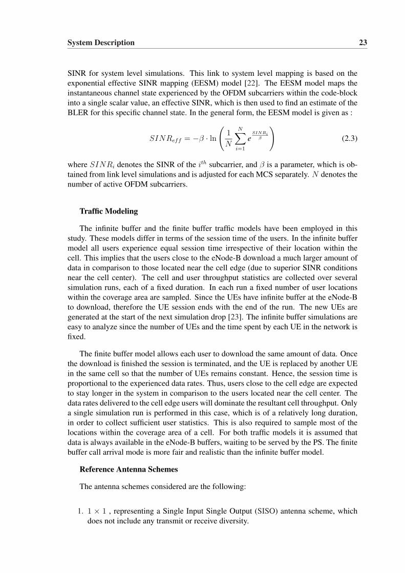
2.5 LTE System Model
Figure 2.7 represents a general system model under consideration. The system modelused for performance evaluation follows the 3GPP LTE recommendations [11]. A cellularlayout of 19 hexagonal sites is considered. Each site typically consists of 3 sectors. Eachsector is covered by a sectorized antenna. Only the centre site has been simulated withactive User Equipments (UEs), where the locations of UEs are randomly assigned with auniform probability distribution. All other sites in the assumed network are considered asinterfering sites. Once a UE is dropped, the links are created with all the sectors. Each linkis associated with shadow fading, antenna gain and path gain. A quasi-dynamic simulationapproach is used, where a UE remains in the same location until the end of the session,implying that the shadow fading, antenna gains and path gains remain unchanged. Butthe fast fading variations are taken into account. For this, the users are assumed to movewith a certain speed and the corresponding variations in fast fading due to movement isconsidered. It is assumed that the users move around the same approximate locations. Themultipath model used is ITU Typical Urban (TU) 20 paths (explained in appendix A).
2 GHz carrier frequency and 10 MHz operating system bandwidth is considered.Frequency Division Duplex (FDD) is employed. Shadowing is fully correlated betweenthe cells of the same site, whereas the correlation is assumed to be 0.5 between sites.
Link-To-System Performance Mapping Function
In OFDMA each subcarrier may experience a different SINR. An effective SINR met-ric is needed to compress a set of SINR values at the link level to represent an effective
System Description 23
SINR for system level simulations. This link to system level mapping is based on theexponential effective SINR mapping (EESM) model [22]. The EESM model maps theinstantaneous channel state experienced by the OFDM subcarriers within the code-blockinto a single scalar value, an effective SINR, which is then used to find an estimate of theBLER for this specific channel state. In the general form, the EESM model is given as :
SINReff = −β · ln(
1
N
N∑i=1
eSINRi
β
)(2.3)
where SINRi denotes the SINR of the ith subcarrier, and β is a parameter, which is ob-tained from link level simulations and is adjusted for each MCS separately. N denotes thenumber of active OFDM subcarriers.
Traffic Modeling
The infinite buffer and the finite buffer traffic models have been employed in thisstudy. These models differ in terms of the session time of the users. In the infinite buffermodel all users experience equal session time irrespective of their location within thecell. This implies that the users close to the eNode-B download a much larger amount ofdata in comparison to those located near the cell edge (due to superior SINR conditionsnear the cell center). The cell and user throughput statistics are collected over severalsimulation runs, each of a fixed duration. In each run a fixed number of user locationswithin the coverage area are sampled. Since the UEs have infinite buffer at the eNode-Bto download, therefore the UE session ends with the end of the run. The new UEs aregenerated at the start of the next simulation drop [23]. The infinite buffer simulations areeasy to analyze since the number of UEs and the time spent by each UE in the network isfixed.
The finite buffer model allows each user to download the same amount of data. Oncethe download is finished the session is terminated, and the UE is replaced by another UEin the same cell so that the number of UEs remains constant. Hence, the session time isproportional to the experienced data rates. Thus, users close to the cell edge are expectedto stay longer in the system in comparison to the users located near the cell center. Thedata rates delivered to the cell edge users will dominate the resultant cell throughput. Onlya single simulation run is performed in this case, which is of a relatively long duration,in order to collect sufficient user statistics. This is also required to sample most of thelocations within the coverage area of a cell. For both traffic models it is assumed thatdata is always available in the eNode-B buffers, waiting to be served by the PS. The finitebuffer call arrival mode is more fair and realistic than the infinite buffer model.
Reference Antenna Schemes
The antenna schemes considered are the following:
1. 1 × 1 , representing a Single Input Single Output (SISO) antenna scheme, whichdoes not include any transmit or receive diversity.
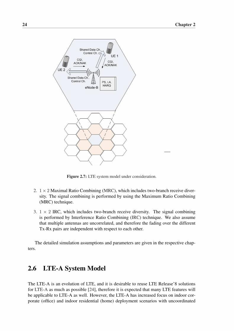
24 Chapter 2
Figure 2.7: LTE system model under consideration.
2. 1× 2 Maximal Ratio Combining (MRC), which includes two-branch receive diver-sity. The signal combining is performed by using the Maximum Ratio Combining(MRC) technique.
3. 1 × 2 IRC, which includes two-branch receive diversity. The signal combiningis performed by Interference Ratio Combining (IRC) technique. We also assumethat multiple antennas are uncorrelated, and therefore the fading over the differentTx-Rx pairs are independent with respect to each other.
The detailed simulation assumptions and parameters are given in the respective chap-ters.
2.6 LTE-A System Model
The LTE-A is an evolution of LTE, and it is desirable to reuse LTE Release’8 solutionsfor LTE-A as much as possible [24], therefore it is expected that many LTE features willbe applicable to LTE-A as well. However, the LTE-A has increased focus on indoor cor-porate (office) and indoor residential (home) deployment scenarios with uncoordinated
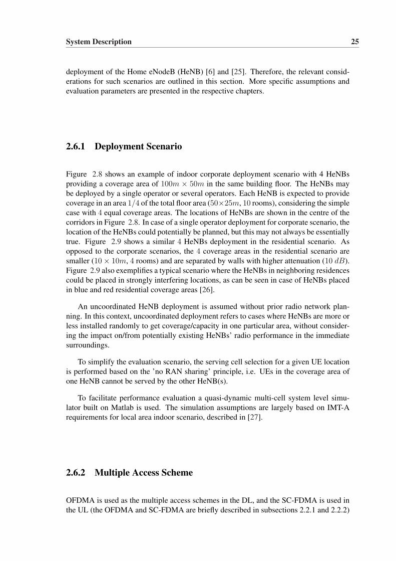
System Description 25
deployment of the Home eNodeB (HeNB) [6] and [25]. Therefore, the relevant consid-erations for such scenarios are outlined in this section. More specific assumptions andevaluation parameters are presented in the respective chapters.
2.6.1 Deployment Scenario
Figure 2.8 shows an example of indoor corporate deployment scenario with 4 HeNBsproviding a coverage area of 100m × 50m in the same building floor. The HeNBs maybe deployed by a single operator or several operators. Each HeNB is expected to providecoverage in an area 1/4 of the total floor area (50×25m, 10 rooms), considering the simplecase with 4 equal coverage areas. The locations of HeNBs are shown in the centre of thecorridors in Figure 2.8. In case of a single operator deployment for corporate scenario, thelocation of the HeNBs could potentially be planned, but this may not always be essentiallytrue. Figure 2.9 shows a similar 4 HeNBs deployment in the residential scenario. Asopposed to the corporate scenarios, the 4 coverage areas in the residential scenario aresmaller (10× 10m, 4 rooms) and are separated by walls with higher attenuation (10 dB).Figure 2.9 also exemplifies a typical scenario where the HeNBs in neighboring residencescould be placed in strongly interfering locations, as can be seen in case of HeNBs placedin blue and red residential coverage areas [26].
An uncoordinated HeNB deployment is assumed without prior radio network plan-ning. In this context, uncoordinated deployment refers to cases where HeNBs are more orless installed randomly to get coverage/capacity in one particular area, without consider-ing the impact on/from potentially existing HeNBs’ radio performance in the immediatesurroundings.
To simplify the evaluation scenario, the serving cell selection for a given UE locationis performed based on the ’no RAN sharing’ principle, i.e. UEs in the coverage area ofone HeNB cannot be served by the other HeNB(s).
To facilitate performance evaluation a quasi-dynamic multi-cell system level simu-lator built on Matlab is used. The simulation assumptions are largely based on IMT-Arequirements for local area indoor scenario, described in [27].
2.6.2 Multiple Access Scheme
OFDMA is used as the multiple access schemes in the DL, and the SC-FDMA is used inthe UL (the OFDMA and SC-FDMA are briefly described in subsections 2.2.1 and 2.2.2)
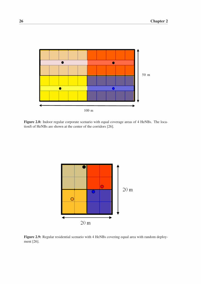
26 Chapter 2
Figure 2.8: Indoor regular corporate scenario with equal coverage areas of 4 HeNBs. The loca-tionS of HeNBs are shown at the center of the corridors [26].
Figure 2.9: Regular residential scenario with 4 HeNBs covering equal area with random deploy-ment [26].
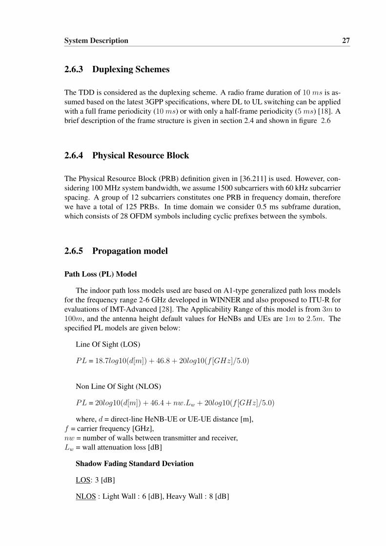
System Description 27
2.6.3 Duplexing Schemes
The TDD is considered as the duplexing scheme. A radio frame duration of 10 ms is as-sumed based on the latest 3GPP specifications, where DL to UL switching can be appliedwith a full frame periodicity (10 ms) or with only a half-frame periodicity (5 ms) [18]. Abrief description of the frame structure is given in section 2.4 and shown in figure 2.6
2.6.4 Physical Resource Block
The Physical Resource Block (PRB) definition given in [36.211] is used. However, con-sidering 100 MHz system bandwidth, we assume 1500 subcarriers with 60 kHz subcarrierspacing. A group of 12 subcarriers constitutes one PRB in frequency domain, thereforewe have a total of 125 PRBs. In time domain we consider 0.5 ms subframe duration,which consists of 28 OFDM symbols including cyclic prefixes between the symbols.
2.6.5 Propagation model
Path Loss (PL) Model
The indoor path loss models used are based on A1-type generalized path loss modelsfor the frequency range 2-6 GHz developed in WINNER and also proposed to ITU-R forevaluations of IMT-Advanced [28]. The Applicability Range of this model is from 3m to100m, and the antenna height default values for HeNBs and UEs are 1m to 2.5m. Thespecified PL models are given below:
Line Of Sight (LOS)
PL = 18.7log10(d[m]) + 46.8 + 20log10(f [GHz]/5.0)
Non Line Of Sight (NLOS)
PL = 20log10(d[m]) + 46.4 + nw.Lw + 20log10(f [GHz]/5.0)
where, d = direct-line HeNB-UE or UE-UE distance [m],f = carrier frequency [GHz],nw = number of walls between transmitter and receiver,Lw = wall attenuation loss [dB]
Shadow Fading Standard Deviation
LOS: 3 [dB]
NLOS : Light Wall : 6 [dB], Heavy Wall : 8 [dB]
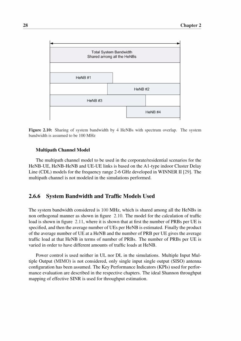
28 Chapter 2
Figure 2.10: Sharing of system bandwidth by 4 HeNBs with spectrum overlap. The systembandwidth is assumed to be 100 MHz
Multipath Channel Model
The multipath channel model to be used in the corporate/residential scenarios for theHeNB-UE, HeNB-HeNB and UE-UE links is based on the A1-type indoor Cluster DelayLine (CDL) models for the frequency range 2-6 GHz developed in WINNER II [29]. Themultipath channel is not modeled in the simulations performed.
2.6.6 System Bandwidth and Traffic Models Used
The system bandwidth considered is 100 MHz, which is shared among all the HeNBs innon orthogonal manner as shown in figure 2.10. The model for the calculation of trafficload is shown in figure 2.11, where it is shown that at first the number of PRBs per UE isspecified, and then the average number of UEs per HeNB is estimated. Finally the productof the average number of UE at a HeNB and the number of PRB per UE gives the averagetraffic load at that HeNB in terms of number of PRBs. The number of PRBs per UE isvaried in order to have different amounts of traffic loads at HeNB.
Power control is used neither in UL nor DL in the simulations. Multiple Input Mul-tiple Output (MIMO) is not considered, only single input single output (SISO) antennaconfiguration has been assumed. The Key Performance Indicators (KPIs) used for perfor-mance evaluation are described in the respective chapters. The ideal Shannon throughputmapping of effective SINR is used for throughput estimation.
System Description 29
Figure 2.11: Scheme for the calculation of traffic load for different HeNBs.

Chapter 3
Higher Order Sectorization for UTRANLTE
3.1 Introduction
The Universal Terrestrial Radio Access Network (UTRAN) LTE typically employs threeantennas per site to render 3 sector deployment. A migration to Higher Order Sectoriza-tion (HOS), such as 6 sectors per site is considered a potential option to increase systemcapacity. This chapter provides investigations on 6 sector deployment and its performanceevaluation for UTRAN LTE in the downlink.
The chapter is organized as follows. Section 3.2 provides a brief description of HOS.Section 3.3 presents the antenna pattern and different cell topologies under considerationfor our study. Section 3.4 gives an account of the simulation environment and various pa-rameters assumed to test the underlying concepts. Section 3.5 presents simulation resultsand their interpretations. Finally section 3.6 provides a summary of the conclusions.
3.2 Higher Order Sectorization
A key parameter for the performance evaluation of a cellular system is the capacity itoffers. The capacity of a cellular system is expected to increase by exploiting the spatialdimension. There are several approaches to exploit the spatial dimension. Main conceptssuggested are HOS, fixed beam switching concept and adaptive beam forming [30].
Our focus in this study will be on HOS. The network operators may need to installnew sites to provide the necessary capacity. One way to increase the capacity withoutinstalling new sites is to migrate the existing sites with HOS antenna systems [31][32].
HOS provides a promising technique to increase system capacity by increasing thenumber of UEs supported in the system, because each antenna can serve almost the same
31
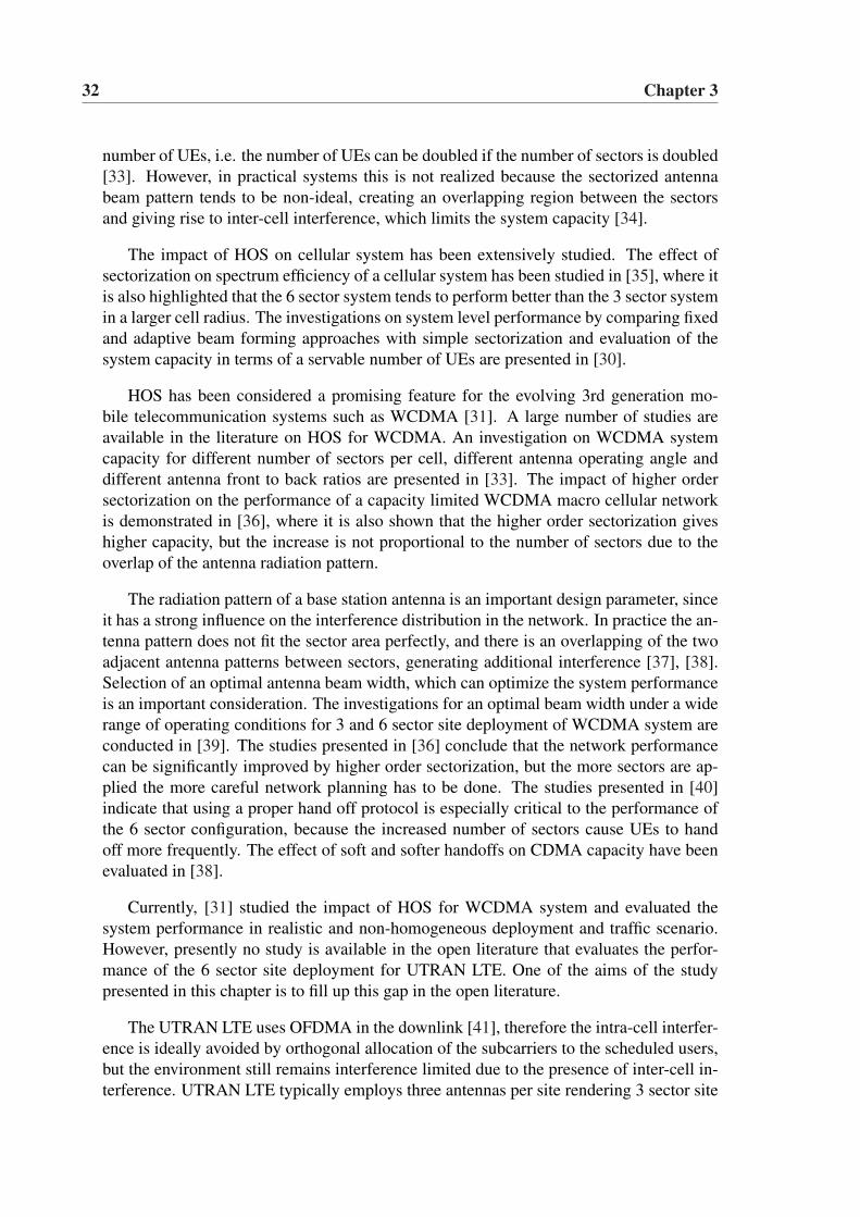
32 Chapter 3
number of UEs, i.e. the number of UEs can be doubled if the number of sectors is doubled[33]. However, in practical systems this is not realized because the sectorized antennabeam pattern tends to be non-ideal, creating an overlapping region between the sectorsand giving rise to inter-cell interference, which limits the system capacity [34].
The impact of HOS on cellular system has been extensively studied. The effect ofsectorization on spectrum efficiency of a cellular system has been studied in [35], where itis also highlighted that the 6 sector system tends to perform better than the 3 sector systemin a larger cell radius. The investigations on system level performance by comparing fixedand adaptive beam forming approaches with simple sectorization and evaluation of thesystem capacity in terms of a servable number of UEs are presented in [30].
HOS has been considered a promising feature for the evolving 3rd generation mo-bile telecommunication systems such as WCDMA [31]. A large number of studies areavailable in the literature on HOS for WCDMA. An investigation on WCDMA systemcapacity for different number of sectors per cell, different antenna operating angle anddifferent antenna front to back ratios are presented in [33]. The impact of higher ordersectorization on the performance of a capacity limited WCDMA macro cellular networkis demonstrated in [36], where it is also shown that the higher order sectorization giveshigher capacity, but the increase is not proportional to the number of sectors due to theoverlap of the antenna radiation pattern.
The radiation pattern of a base station antenna is an important design parameter, sinceit has a strong influence on the interference distribution in the network. In practice the an-tenna pattern does not fit the sector area perfectly, and there is an overlapping of the twoadjacent antenna patterns between sectors, generating additional interference [37], [38].Selection of an optimal antenna beam width, which can optimize the system performanceis an important consideration. The investigations for an optimal beam width under a widerange of operating conditions for 3 and 6 sector site deployment of WCDMA system areconducted in [39]. The studies presented in [36] conclude that the network performancecan be significantly improved by higher order sectorization, but the more sectors are ap-plied the more careful network planning has to be done. The studies presented in [40]indicate that using a proper hand off protocol is especially critical to the performance ofthe 6 sector configuration, because the increased number of sectors cause UEs to handoff more frequently. The effect of soft and softer handoffs on CDMA capacity have beenevaluated in [38].
Currently, [31] studied the impact of HOS for WCDMA system and evaluated thesystem performance in realistic and non-homogeneous deployment and traffic scenario.However, presently no study is available in the open literature that evaluates the perfor-mance of the 6 sector site deployment for UTRAN LTE. One of the aims of the studypresented in this chapter is to fill up this gap in the open literature.
The UTRAN LTE uses OFDMA in the downlink [41], therefore the intra-cell interfer-ence is ideally avoided by orthogonal allocation of the subcarriers to the scheduled users,but the environment still remains interference limited due to the presence of inter-cell in-terference. UTRAN LTE typically employs three antennas per site rendering 3 sector site
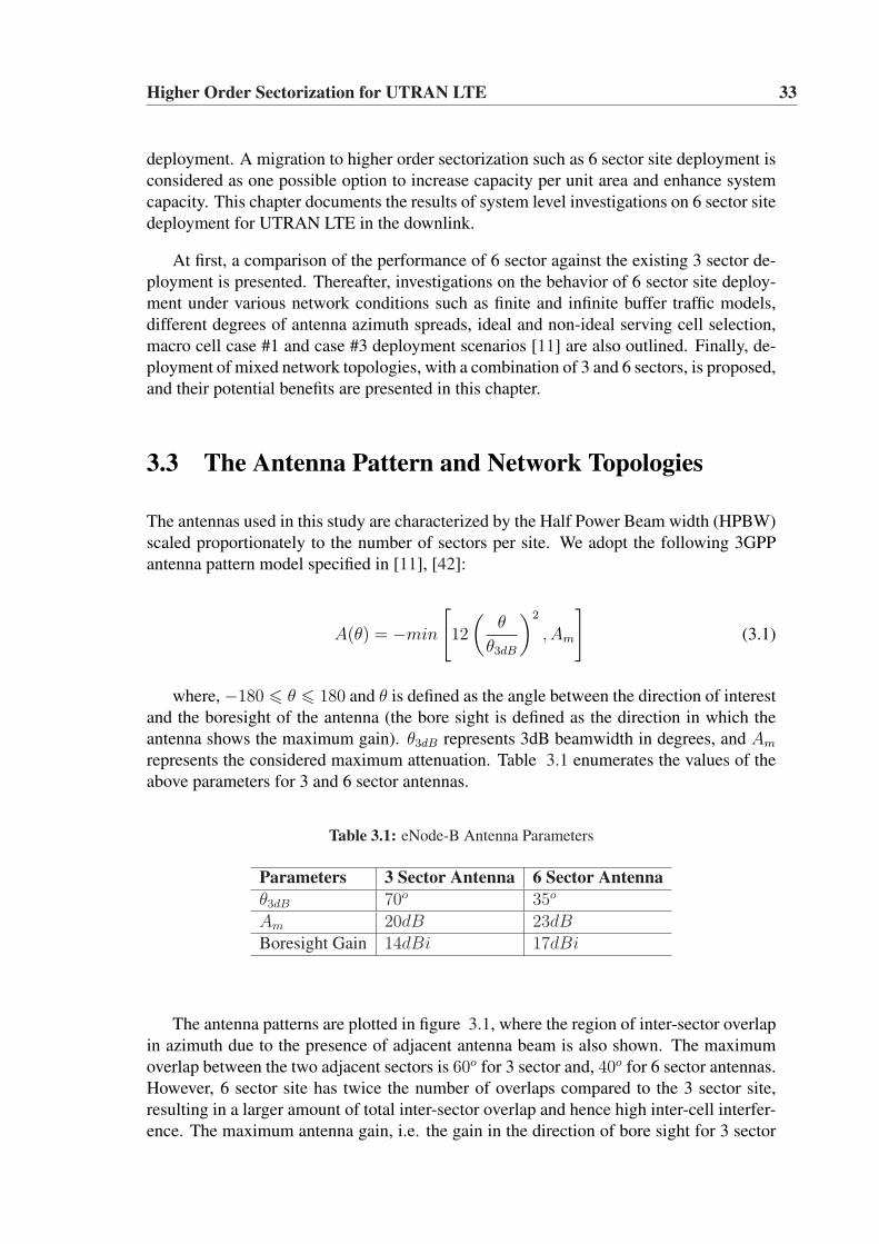
Higher Order Sectorization for UTRAN LTE 33
deployment. A migration to higher order sectorization such as 6 sector site deployment isconsidered as one possible option to increase capacity per unit area and enhance systemcapacity. This chapter documents the results of system level investigations on 6 sector sitedeployment for UTRAN LTE in the downlink.
At first, a comparison of the performance of 6 sector against the existing 3 sector de-ployment is presented. Thereafter, investigations on the behavior of 6 sector site deploy-ment under various network conditions such as finite and infinite buffer traffic models,different degrees of antenna azimuth spreads, ideal and non-ideal serving cell selection,macro cell case #1 and case #3 deployment scenarios [11] are also outlined. Finally, de-ployment of mixed network topologies, with a combination of 3 and 6 sectors, is proposed,and their potential benefits are presented in this chapter.
3.3 The Antenna Pattern and Network Topologies
The antennas used in this study are characterized by the Half Power Beam width (HPBW)scaled proportionately to the number of sectors per site. We adopt the following 3GPPantenna pattern model specified in [11], [42]:
A(θ) = −min
[12
(θ
θ3dB
)2
, Am
](3.1)
where,−180 6 θ 6 180 and θ is defined as the angle between the direction of interestand the boresight of the antenna (the bore sight is defined as the direction in which theantenna shows the maximum gain). θ3dB represents 3dB beamwidth in degrees, and Am
represents the considered maximum attenuation. Table 3.1 enumerates the values of theabove parameters for 3 and 6 sector antennas.
Table 3.1: eNode-B Antenna Parameters
Parameters 3 Sector Antenna 6 Sector Antennaθ3dB 70o 35o
Am 20dB 23dBBoresight Gain 14dBi 17dBi
The antenna patterns are plotted in figure 3.1, where the region of inter-sector overlapin azimuth due to the presence of adjacent antenna beam is also shown. The maximumoverlap between the two adjacent sectors is 60o for 3 sector and, 40o for 6 sector antennas.However, 6 sector site has twice the number of overlaps compared to the 3 sector site,resulting in a larger amount of total inter-sector overlap and hence high inter-cell interfer-ence. The maximum antenna gain, i.e. the gain in the direction of bore sight for 3 sector
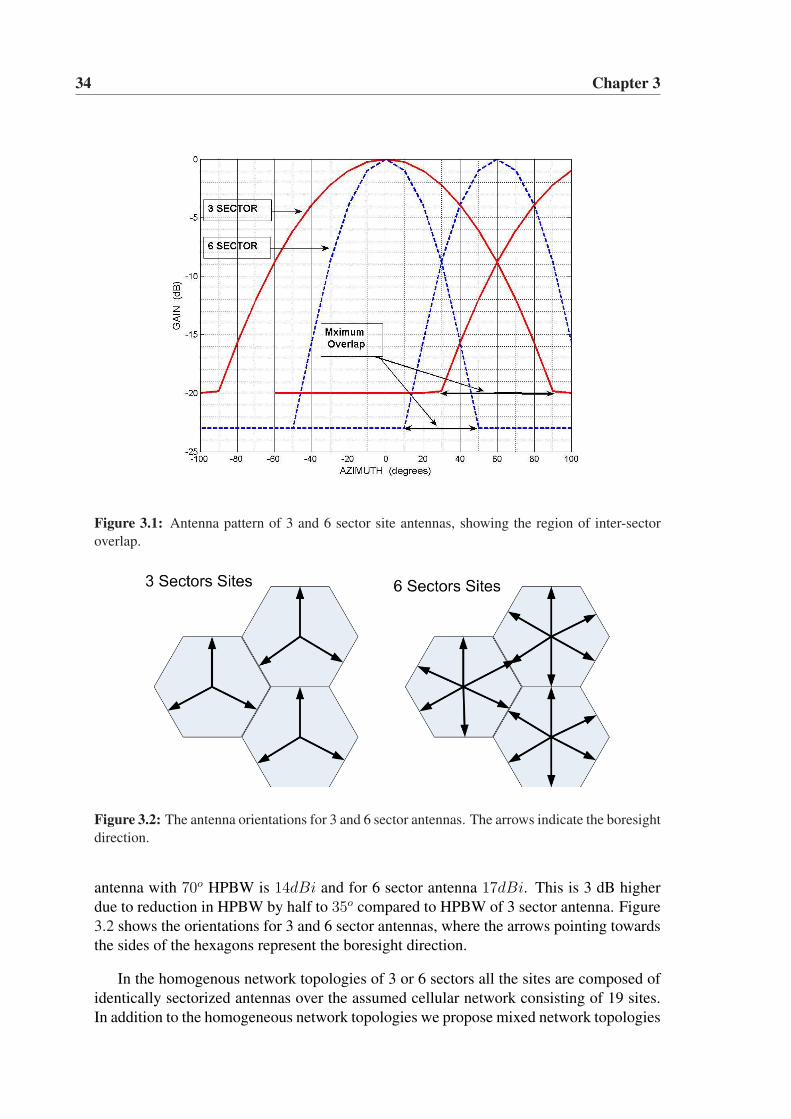
34 Chapter 3
Figure 3.1: Antenna pattern of 3 and 6 sector site antennas, showing the region of inter-sectoroverlap.
Figure 3.2: The antenna orientations for 3 and 6 sector antennas. The arrows indicate the boresightdirection.
antenna with 70o HPBW is 14dBi and for 6 sector antenna 17dBi. This is 3 dB higherdue to reduction in HPBW by half to 35o compared to HPBW of 3 sector antenna. Figure3.2 shows the orientations for 3 and 6 sector antennas, where the arrows pointing towardsthe sides of the hexagons represent the boresight direction.
In the homogenous network topologies of 3 or 6 sectors all the sites are composed ofidentically sectorized antennas over the assumed cellular network consisting of 19 sites.In addition to the homogeneous network topologies we propose mixed network topologies
Higher Order Sectorization for UTRAN LTE 35
Figure 3.3: Proposed mixed network topologies
with the combinations of 3 and 6 sector sites within the network. Two different combina-tions, namely mode1 and mode2 are proposed. In mode1 the centre site is composed of 6sectors, and all the other 18 sites are composed of 3 sectors. In mode2, the centre site andthe sites within the first ring are composed of 6 sectors, and the remaining 12 sites of theouter ring are composed of 3 sectors. Figure 3.3 provides the pictorial representation ofthe proposed mixed network topologies.
3.4 Modeling Assumptions
3.4.1 Simulation Parameters
To facilitate the performance evaluation a quasi-dynamic multicell system level simula-tor has been used. The simulation assumptions are largely based on the 3GPP UTRANLTE specifications [41]. The system model employed is as per the discussion in chapter2 (section 2.5). Here more specific parameters and assumptions used for the performanceevaluation are presented. The macro cell case #1 (inter-site distance of 500 meters) andcase #3 (inter-site distance of 1732 meters) are employed [11]. In the considered hexago-nal cellular layout of 19 sites, each site is composed of either 3 or 6 sectors per site basedon the simulation requirements. The site refers to the area covered by a eNode-B, and thesector refers to the area covered by one of the sectorial antennas in that eNode-B.
The finite and infinite full buffer traffic models are considered. 2Mbit packet size ischosen as the buffer information for the finite buffer model. In infinite buffer model UEs
36 Chapter 3
always have data to transmit. A total of 120 UEs per site is simulated, which is scaledper sector according to the number of sectors. This amounts to 40 UEs per sector for 3sector and 20 UEs per sector for 6 sector sites. Link to system level mapping is based onexponential effective SINR model [43]. A decoupled time and frequency domain packetscheduler is considered. The maximum scheduling of N = 12 UEs per TTI is considered.
For 6 sector antennas the azimuth angle spread of 5o and 10o are considered, resultingin an increased effective HPBWs of 40o and 45o. For 40o HPBW the maximum inter-celloverlap amounts to 60o, and for 45o HPBW this amounts to 80o, resulting in increasedadditional inter-cell interference.
The ideal and non ideal serving cell selections are assumed. In ideal cell selection a UEis always connected to the cell with the minimum total path loss. In this context, the totalpath loss includes the effect of the distance dependent path loss, shadowing, minimumcoupling loss, and antenna gains. A more realistic serving cell selection could be a non-ideal serving cell selection, assuming that sometimes UEs are not connected to the optimalcell, i.e. the cell with the minimum total path loss. In non-ideal serving cell selection theUE randomly selects one of the cells to be the serving cell with equal selection probability,out of the virtual active set of cells with a total path loss within the given handover windowoffset margin. The handover window offset margin explicitly includes effects from havingUE measurement imperfections for serving cell selection. This assumption is taken toaccount for imperfections from the serving cell selection algorithm. Table 3.2 provides asummary of the main parameters and simulation assumptions.
3.4.2 Key Performance Indicators (KPIs)
Geometry Factor, Average User Goodput, Average Cell Throughput and Average SiteThroughput are taken as KPI.
• Geometry Factor is defined as the ratio between the desired received signal powerthat a UE receives and the total amount of inter-cell interference plus white noiseaveraged over the fast fading, which is expressed as:
Geometry Factor =PRx
Pint + Pnoise
(3.2)
where, PRx, Pint, Pnoise represent signal power, total amount of interference andnoise received respectively.
• The Average Cell Throughput is described as :
TP cell =Total bits correctly delivered
Simulation time, (3.3)
where the numerator is an aggregate of the correctly delivered bits over all the activesessions in the system [44]. The Average Site Throughput is defined as the productof Average cell throughput and the number of cells within the site.
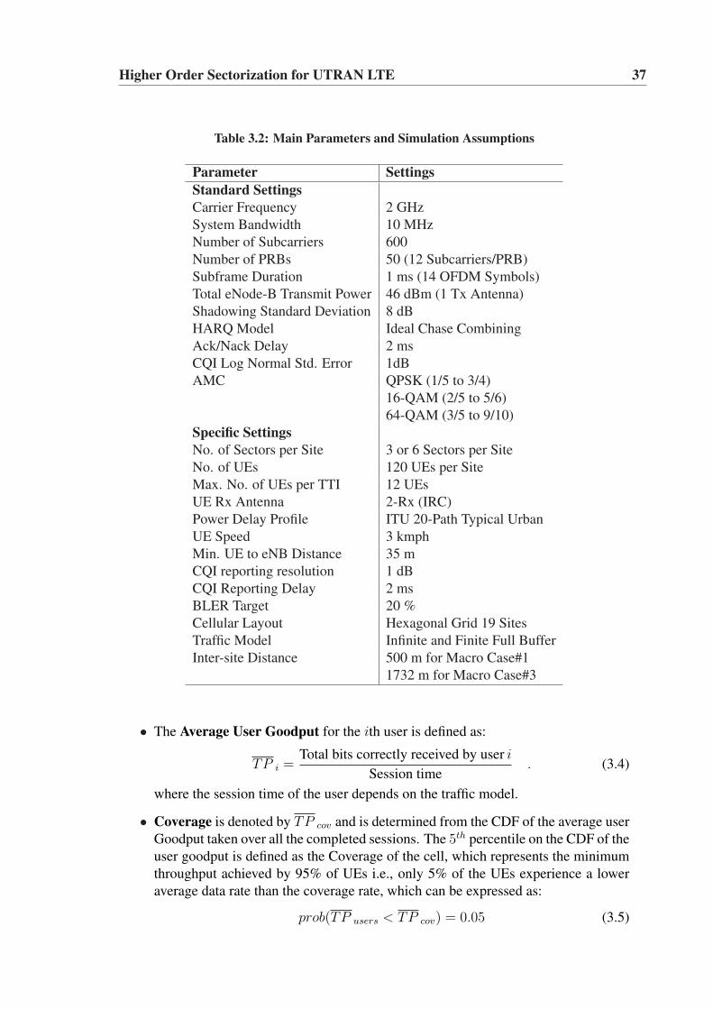
Higher Order Sectorization for UTRAN LTE 37
Table 3.2: Main Parameters and Simulation Assumptions
Parameter SettingsStandard SettingsCarrier Frequency 2 GHzSystem Bandwidth 10 MHzNumber of Subcarriers 600Number of PRBs 50 (12 Subcarriers/PRB)Subframe Duration 1 ms (14 OFDM Symbols)Total eNode-B Transmit Power 46 dBm (1 Tx Antenna)Shadowing Standard Deviation 8 dBHARQ Model Ideal Chase CombiningAck/Nack Delay 2 msCQI Log Normal Std. Error 1dBAMC QPSK (1/5 to 3/4)
16-QAM (2/5 to 5/6)64-QAM (3/5 to 9/10)
Specific SettingsNo. of Sectors per Site 3 or 6 Sectors per SiteNo. of UEs 120 UEs per SiteMax. No. of UEs per TTI 12 UEsUE Rx Antenna 2-Rx (IRC)Power Delay Profile ITU 20-Path Typical UrbanUE Speed 3 kmphMin. UE to eNB Distance 35 mCQI reporting resolution 1 dBCQI Reporting Delay 2 msBLER Target 20 %Cellular Layout Hexagonal Grid 19 SitesTraffic Model Infinite and Finite Full BufferInter-site Distance 500 m for Macro Case#1
1732 m for Macro Case#3
• The Average User Goodput for the ith user is defined as:
TP i =Total bits correctly received by user i
Session time. (3.4)
where the session time of the user depends on the traffic model.
• Coverage is denoted by TP cov and is determined from the CDF of the average userGoodput taken over all the completed sessions. The 5th percentile on the CDF of theuser goodput is defined as the Coverage of the cell, which represents the minimumthroughput achieved by 95% of UEs i.e., only 5% of the UEs experience a loweraverage data rate than the coverage rate, which can be expressed as:
prob(TP users < TP cov) = 0.05 (3.5)
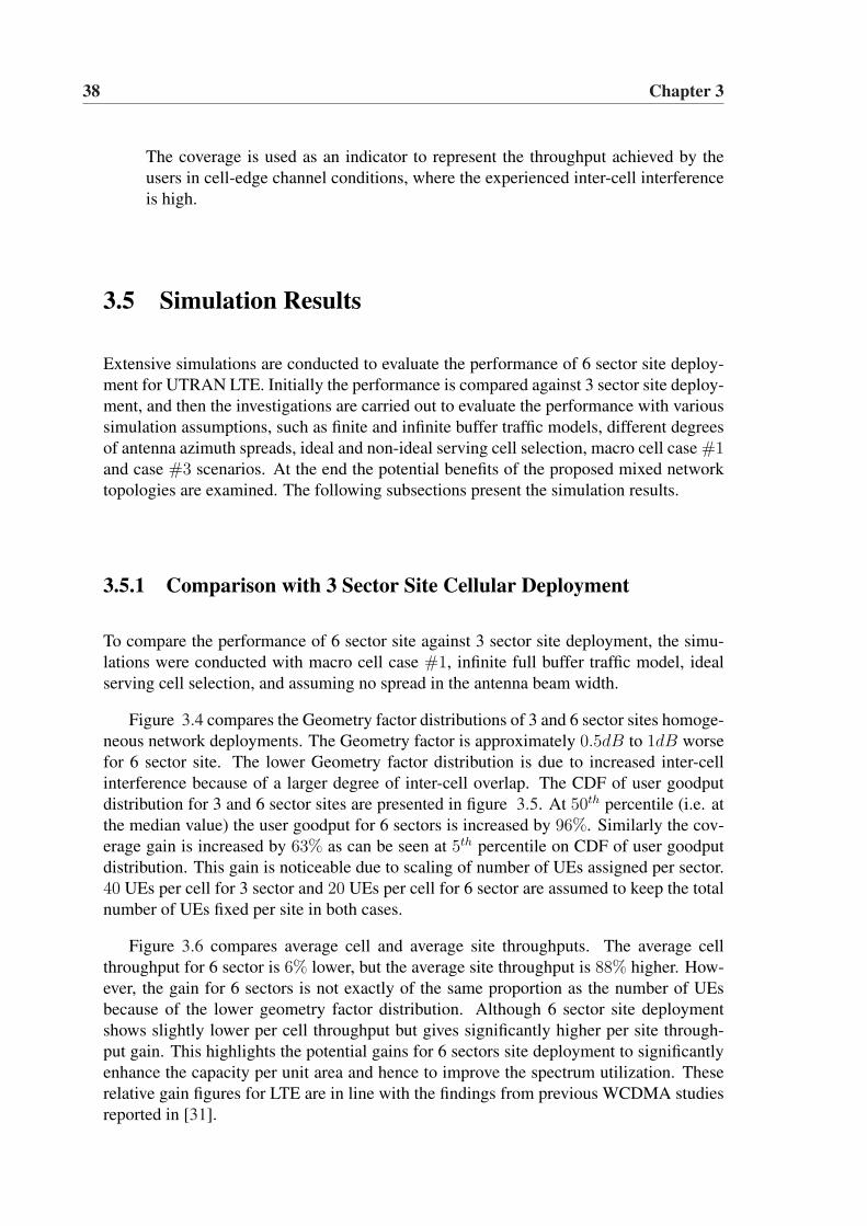
38 Chapter 3
The coverage is used as an indicator to represent the throughput achieved by theusers in cell-edge channel conditions, where the experienced inter-cell interferenceis high.
3.5 Simulation Results
Extensive simulations are conducted to evaluate the performance of 6 sector site deploy-ment for UTRAN LTE. Initially the performance is compared against 3 sector site deploy-ment, and then the investigations are carried out to evaluate the performance with varioussimulation assumptions, such as finite and infinite buffer traffic models, different degreesof antenna azimuth spreads, ideal and non-ideal serving cell selection, macro cell case #1and case #3 scenarios. At the end the potential benefits of the proposed mixed networktopologies are examined. The following subsections present the simulation results.
3.5.1 Comparison with 3 Sector Site Cellular Deployment
To compare the performance of 6 sector site against 3 sector site deployment, the simu-lations were conducted with macro cell case #1, infinite full buffer traffic model, idealserving cell selection, and assuming no spread in the antenna beam width.
Figure 3.4 compares the Geometry factor distributions of 3 and 6 sector sites homoge-neous network deployments. The Geometry factor is approximately 0.5dB to 1dB worsefor 6 sector site. The lower Geometry factor distribution is due to increased inter-cellinterference because of a larger degree of inter-cell overlap. The CDF of user goodputdistribution for 3 and 6 sector sites are presented in figure 3.5. At 50th percentile (i.e. atthe median value) the user goodput for 6 sectors is increased by 96%. Similarly the cov-erage gain is increased by 63% as can be seen at 5th percentile on CDF of user goodputdistribution. This gain is noticeable due to scaling of number of UEs assigned per sector.40 UEs per cell for 3 sector and 20 UEs per cell for 6 sector are assumed to keep the totalnumber of UEs fixed per site in both cases.
Figure 3.6 compares average cell and average site throughputs. The average cellthroughput for 6 sector is 6% lower, but the average site throughput is 88% higher. How-ever, the gain for 6 sectors is not exactly of the same proportion as the number of UEsbecause of the lower geometry factor distribution. Although 6 sector site deploymentshows slightly lower per cell throughput but gives significantly higher per site through-put gain. This highlights the potential gains for 6 sectors site deployment to significantlyenhance the capacity per unit area and hence to improve the spectrum utilization. Theserelative gain figures for LTE are in line with the findings from previous WCDMA studiesreported in [31].
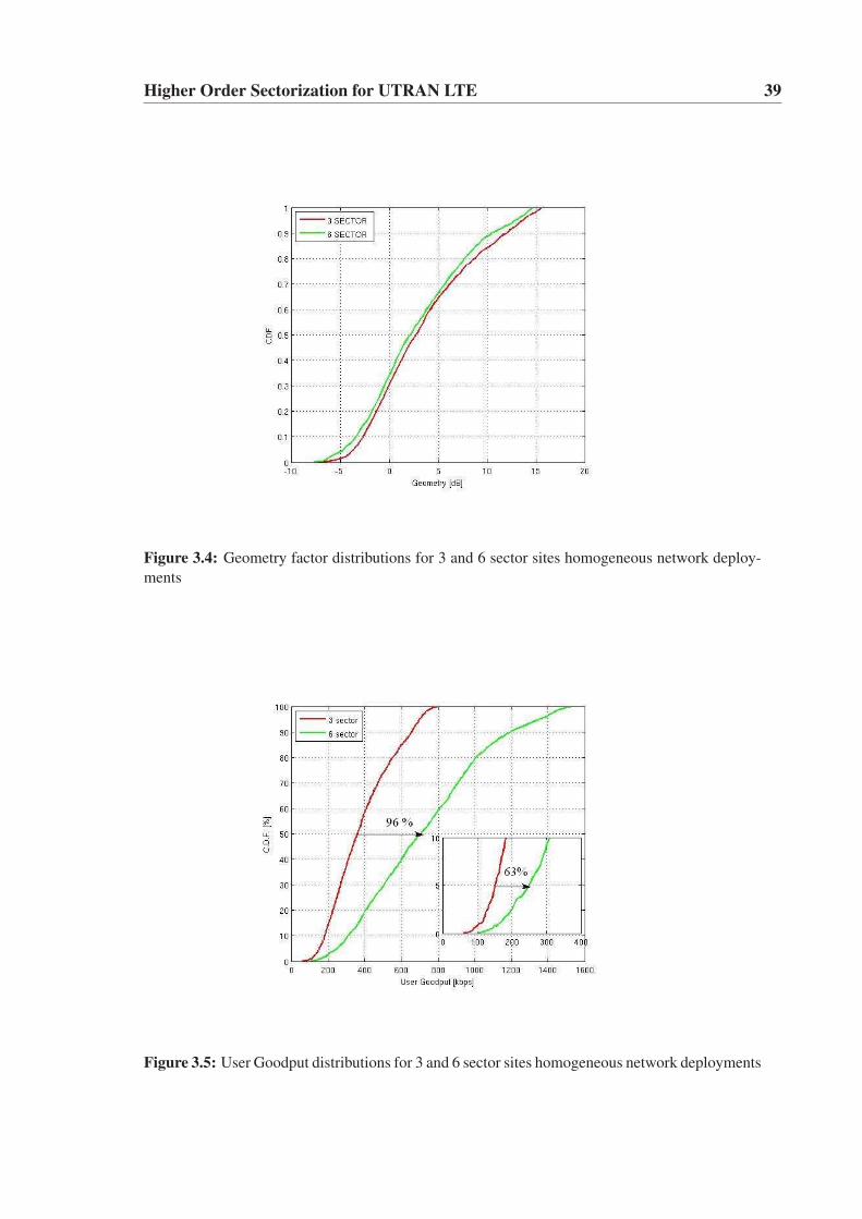
Higher Order Sectorization for UTRAN LTE 39
Figure 3.4: Geometry factor distributions for 3 and 6 sector sites homogeneous network deploy-ments
Figure 3.5: User Goodput distributions for 3 and 6 sector sites homogeneous network deployments
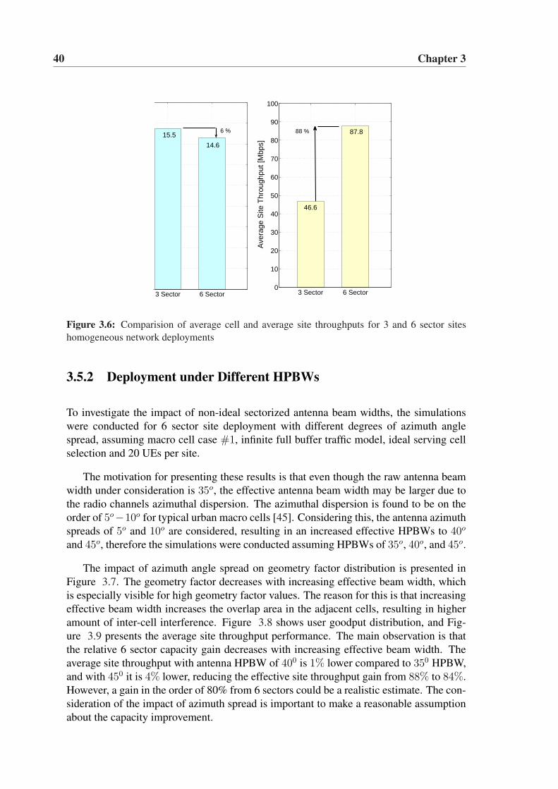
40 Chapter 3
3 Sector 6 Sector0
10
20
30
40
50
60
70
80
90
100
Ave
rage
Site
Thr
ough
put [
Mbp
s]
3 Sector 6 Sector
6 % 88 % 87.8
46.6
14.6
15.5
Figure 3.6: Comparision of average cell and average site throughputs for 3 and 6 sector siteshomogeneous network deployments
3.5.2 Deployment under Different HPBWs
To investigate the impact of non-ideal sectorized antenna beam widths, the simulationswere conducted for 6 sector site deployment with different degrees of azimuth anglespread, assuming macro cell case #1, infinite full buffer traffic model, ideal serving cellselection and 20 UEs per site.
The motivation for presenting these results is that even though the raw antenna beamwidth under consideration is 35o, the effective antenna beam width may be larger due tothe radio channels azimuthal dispersion. The azimuthal dispersion is found to be on theorder of 5o−10o for typical urban macro cells [45]. Considering this, the antenna azimuthspreads of 5o and 10o are considered, resulting in an increased effective HPBWs to 40o
and 45o, therefore the simulations were conducted assuming HPBWs of 35o, 40o, and 45o.
The impact of azimuth angle spread on geometry factor distribution is presented inFigure 3.7. The geometry factor decreases with increasing effective beam width, whichis especially visible for high geometry factor values. The reason for this is that increasingeffective beam width increases the overlap area in the adjacent cells, resulting in higheramount of inter-cell interference. Figure 3.8 shows user goodput distribution, and Fig-ure 3.9 presents the average site throughput performance. The main observation is thatthe relative 6 sector capacity gain decreases with increasing effective beam width. Theaverage site throughput with antenna HPBW of 400 is 1% lower compared to 350 HPBW,and with 450 it is 4% lower, reducing the effective site throughput gain from 88% to 84%.However, a gain in the order of 80% from 6 sectors could be a realistic estimate. The con-sideration of the impact of azimuth spread is important to make a reasonable assumptionabout the capacity improvement.
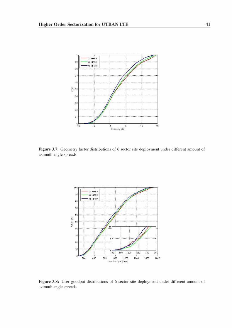
Higher Order Sectorization for UTRAN LTE 41
Figure 3.7: Geometry factor distributions of 6 sector site deployment under different amount ofazimuth angle spreads
Figure 3.8: User goodput distributions of 6 sector site deployment under different amount ofazimuth angle spreads
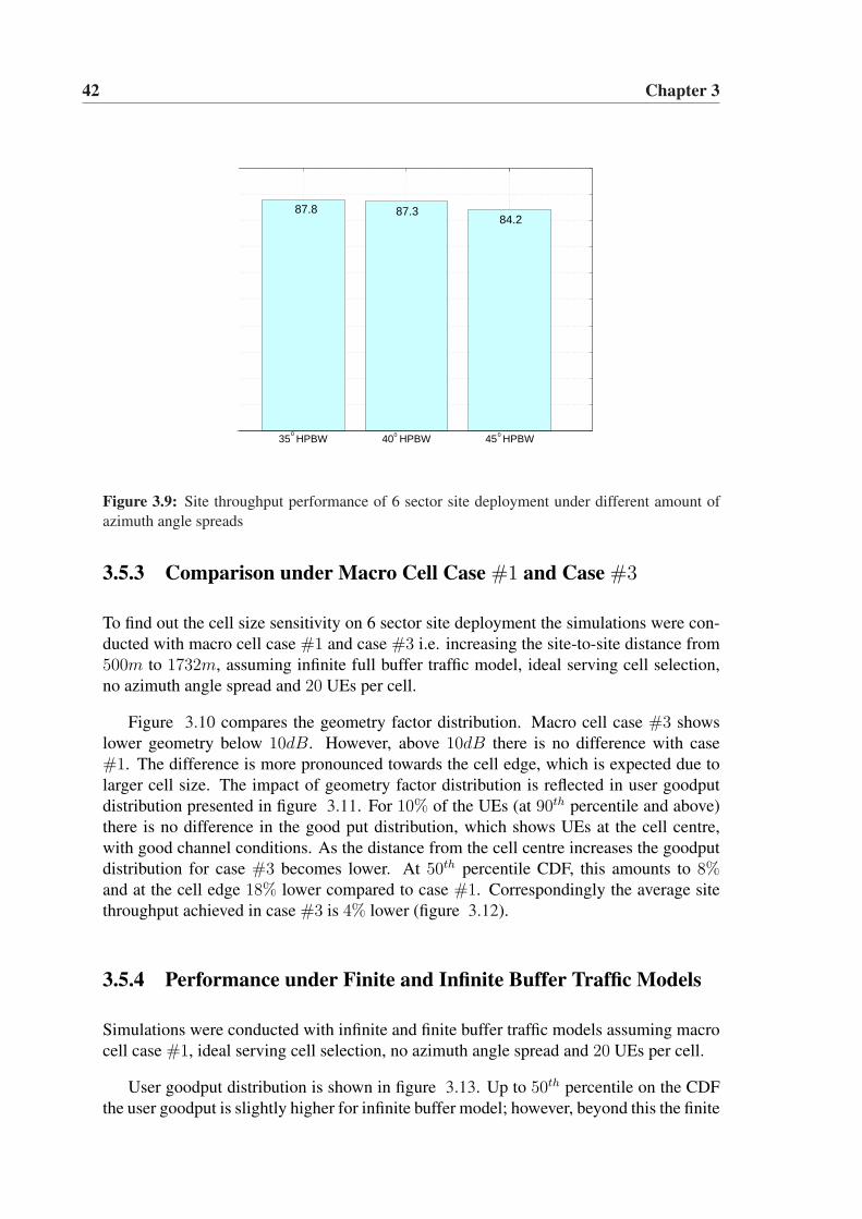
42 Chapter 3
35 HPBW 40 HPBW 45 HPBW00 0
84.287.387.8
Figure 3.9: Site throughput performance of 6 sector site deployment under different amount ofazimuth angle spreads
3.5.3 Comparison under Macro Cell Case #1 and Case #3
To find out the cell size sensitivity on 6 sector site deployment the simulations were con-ducted with macro cell case #1 and case #3 i.e. increasing the site-to-site distance from500m to 1732m, assuming infinite full buffer traffic model, ideal serving cell selection,no azimuth angle spread and 20 UEs per cell.
Figure 3.10 compares the geometry factor distribution. Macro cell case #3 showslower geometry below 10dB. However, above 10dB there is no difference with case#1. The difference is more pronounced towards the cell edge, which is expected due tolarger cell size. The impact of geometry factor distribution is reflected in user goodputdistribution presented in figure 3.11. For 10% of the UEs (at 90th percentile and above)there is no difference in the good put distribution, which shows UEs at the cell centre,with good channel conditions. As the distance from the cell centre increases the goodputdistribution for case #3 becomes lower. At 50th percentile CDF, this amounts to 8%and at the cell edge 18% lower compared to case #1. Correspondingly the average sitethroughput achieved in case #3 is 4% lower (figure 3.12).
3.5.4 Performance under Finite and Infinite Buffer Traffic Models
Simulations were conducted with infinite and finite buffer traffic models assuming macrocell case #1, ideal serving cell selection, no azimuth angle spread and 20 UEs per cell.
User goodput distribution is shown in figure 3.13. Up to 50th percentile on the CDFthe user goodput is slightly higher for infinite buffer model; however, beyond this the finite
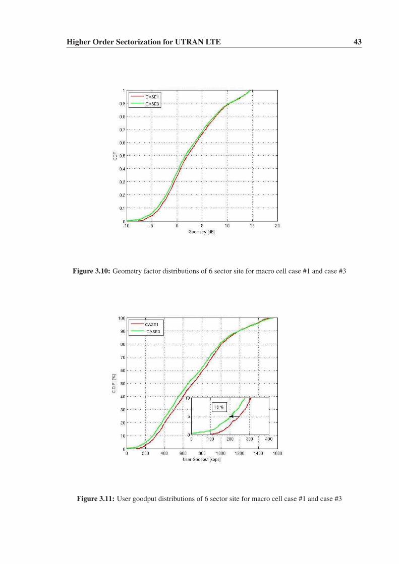
Higher Order Sectorization for UTRAN LTE 43
Figure 3.10: Geometry factor distributions of 6 sector site for macro cell case #1 and case #3
Figure 3.11: User goodput distributions of 6 sector site for macro cell case #1 and case #3
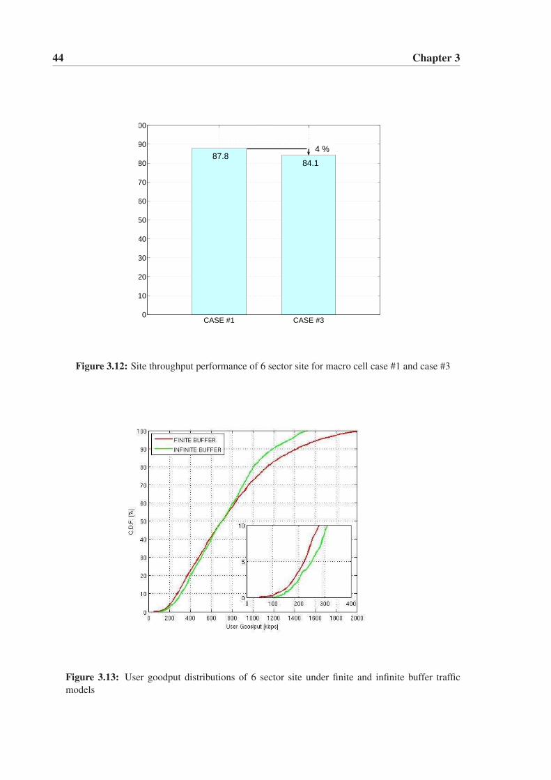
44 Chapter 3
CASE #1 CASE #30
10
20
30
40
50
60
70
80
90
100
87.884.1
4 %
Figure 3.12: Site throughput performance of 6 sector site for macro cell case #1 and case #3
Figure 3.13: User goodput distributions of 6 sector site under finite and infinite buffer trafficmodels
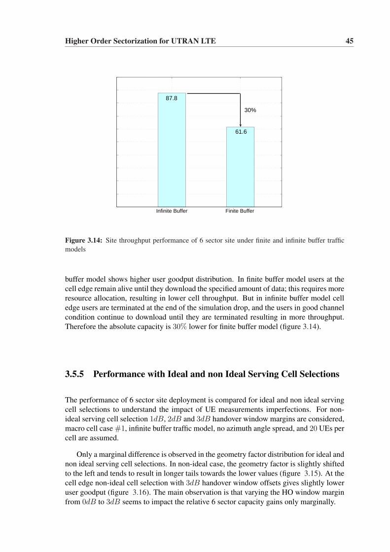
Higher Order Sectorization for UTRAN LTE 45
Infinite Buffer Finite Buffer 0
10
20
30
40
50
60
70
80
90
100
87.8
61.6
30%
Figure 3.14: Site throughput performance of 6 sector site under finite and infinite buffer trafficmodels
buffer model shows higher user goodput distribution. In finite buffer model users at thecell edge remain alive until they download the specified amount of data; this requires moreresource allocation, resulting in lower cell throughput. But in infinite buffer model celledge users are terminated at the end of the simulation drop, and the users in good channelcondition continue to download until they are terminated resulting in more throughput.Therefore the absolute capacity is 30% lower for finite buffer model (figure 3.14).
3.5.5 Performance with Ideal and non Ideal Serving Cell Selections
The performance of 6 sector site deployment is compared for ideal and non ideal servingcell selections to understand the impact of UE measurements imperfections. For non-ideal serving cell selection 1dB, 2dB and 3dB handover window margins are considered,macro cell case #1, infinite buffer traffic model, no azimuth angle spread, and 20 UEs percell are assumed.
Only a marginal difference is observed in the geometry factor distribution for ideal andnon ideal serving cell selections. In non-ideal case, the geometry factor is slightly shiftedto the left and tends to result in longer tails towards the lower values (figure 3.15). At thecell edge non-ideal cell selection with 3dB handover window offsets gives slightly loweruser goodput (figure 3.16). The main observation is that varying the HO window marginfrom 0dB to 3dB seems to impact the relative 6 sector capacity gains only marginally.
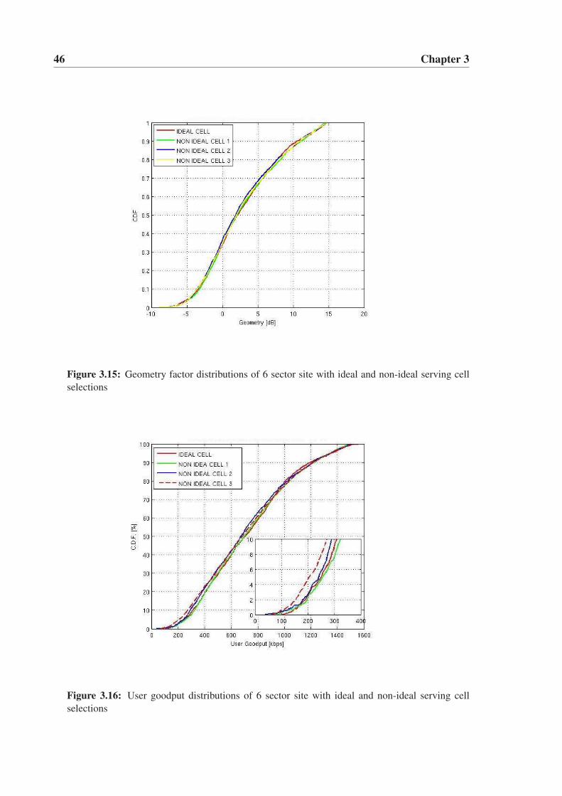
46 Chapter 3
Figure 3.15: Geometry factor distributions of 6 sector site with ideal and non-ideal serving cellselections
Figure 3.16: User goodput distributions of 6 sector site with ideal and non-ideal serving cellselections
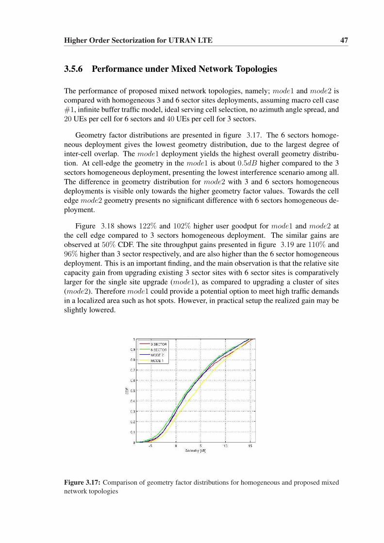
Higher Order Sectorization for UTRAN LTE 47
3.5.6 Performance under Mixed Network Topologies
The performance of proposed mixed network topologies, namely; mode1 and mode2 iscompared with homogeneous 3 and 6 sector sites deployments, assuming macro cell case#1, infinite buffer traffic model, ideal serving cell selection, no azimuth angle spread, and20 UEs per cell for 6 sectors and 40 UEs per cell for 3 sectors.
Geometry factor distributions are presented in figure 3.17. The 6 sectors homoge-neous deployment gives the lowest geometry distribution, due to the largest degree ofinter-cell overlap. The mode1 deployment yields the highest overall geometry distribu-tion. At cell-edge the geometry in the mode1 is about 0.5dB higher compared to the 3sectors homogeneous deployment, presenting the lowest interference scenario among all.The difference in geometry distribution for mode2 with 3 and 6 sectors homogeneousdeployments is visible only towards the higher geometry factor values. Towards the celledge mode2 geometry presents no significant difference with 6 sectors homogeneous de-ployment.
Figure 3.18 shows 122% and 102% higher user goodput for mode1 and mode2 atthe cell edge compared to 3 sectors homogeneous deployment. The similar gains areobserved at 50% CDF. The site throughput gains presented in figure 3.19 are 110% and96% higher than 3 sector respectively, and are also higher than the 6 sector homogeneousdeployment. This is an important finding, and the main observation is that the relative sitecapacity gain from upgrading existing 3 sector sites with 6 sector sites is comparativelylarger for the single site upgrade (mode1), as compared to upgrading a cluster of sites(mode2). Therefore mode1 could provide a potential option to meet high traffic demandsin a localized area such as hot spots. However, in practical setup the realized gain may beslightly lowered.
Figure 3.17: Comparison of geometry factor distributions for homogeneous and proposed mixednetwork topologies
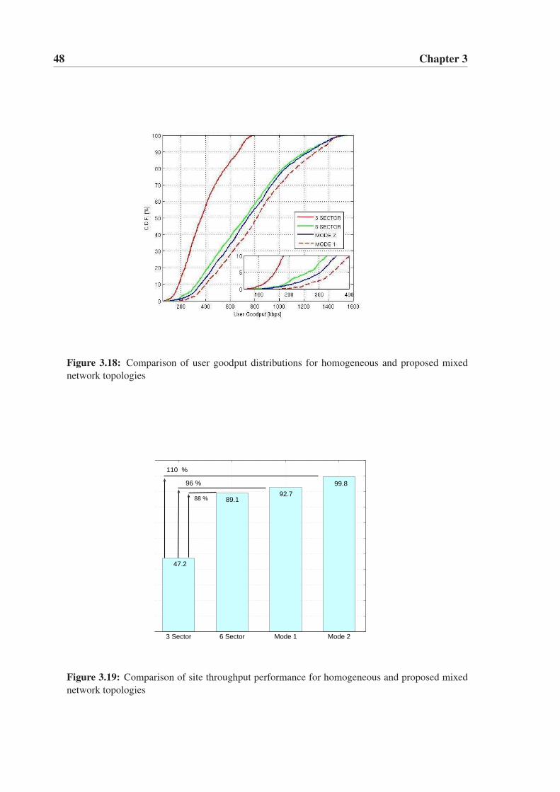
48 Chapter 3
Figure 3.18: Comparison of user goodput distributions for homogeneous and proposed mixednetwork topologies
3 Sector 6 Sector Mode 1 Mode 2
47.2
110 %
96 %
89.192.7
99.8
88 %
Figure 3.19: Comparison of site throughput performance for homogeneous and proposed mixednetwork topologies
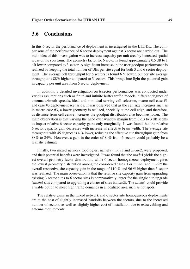
Higher Order Sectorization for UTRAN LTE 49
3.6 Conclusions
In this 6 sector the performance of deployment is investigated in the LTE DL. The com-parisons of the performance of 6 sector deployment against 3 sector are carried out. Themain idea of this investigation was to increase capacity per unit area by increased spatialreuse of the spectrum. The geometry factor for 6 sector is found approximately 0.5 dB to 1dB lower compared to 3 sector. A significant increase in the user goodput performance isrealized by keeping the total number of UEs per site equal for both 3 and 6 sector deploy-ment. The average cell throughput for 6 sectors is found 6 % lower, but per site averagethroughput is 88% higher compared to 3 sectors. This brings into light the potential gainin capacity per unit area from 6 sector deployment.
In addition, a detailed investigation on 6 sector performances was conducted undervarious assumptions such as finite and infinite buffer traffic models, different degrees ofantenna azimuth spreads, ideal and non-ideal serving cell selection, macro cell case #1and case #3 deployment scenarios. It was observed that as the cell size increases such asin macro case #3, a lower geometry is realized, specially at the cell edge, and therefore,as distance from cell centre increases the goodput distribution also becomes lower. Themain observation is that varying the hand over window margin from 0 dB to 3 dB seemsto impact relative 6 sector capacity gains only marginally. It was found that the relative6 sector capacity gain decreases with increase in effective beam width. The average sitethroughput with 45 degrees is 4 % lower, reducing the effective site throughput gain from88% to 84%. However, a gain in the order of 80% from 6 sectors could probably be arealistic estimate.
Finally, two mixed network topologies, namely mode1 and mode2, were proposed,and their potential benefits were investigated. It was found that the mode1 yields the high-est overall geometry factor distribution, while 6 sector homogeneous deployment givesthe lowest geometry distribution among the considered cases. For mode1 and mode2 theoverall respective site capacity gain in the range of 110 % and 96 % higher than 3 sectorwas realized. The main observation is that the relative site capacity gain from upgradingexisting 3 sector sites to 6 sector sites is comparatively larger for the single site upgrade(mode1), as compared to upgrading a cluster of sites (mode2). The mode1 could providea viable option to meet high traffic demands in a localized area such as hot spots.
The relative gains in the mixed network and 6 sector site homogeneous deploymentsare at the cost of slightly increased handoffs between the sectors, due to the increasednumber of sectors, as well as slightly higher cost of installation due to extra cabling andantenna requirements.

Chapter 4
Inter-Cell Interference Avoidance inFractional Load for LTE DL
4.1 Introduction
LTE employs OFDMA in downlink. Due to the property of OFDMA, the intra-cell inter-ference is ideally avoided, but the cellular environment still remains interference limiteddue to the presence of inter-cell interference (ICI), which limits the system performance.An investigation on inter-cell interference avoidance (ICIA) techniques for LTE downlinkunder fractional load conditions are presented in this chapter.
The chapter is organized as follows. Section 4.2 briefly discusses the Inter-Cell Inter-ference Coordination (ICIC) techniques for LTE downlink, whereas section 4.3 presentsa concept of inter-cell interference avoidance under Fractional Load (FL)conditions. Sec-tion 4.4 describes the proposed inter-cell interference avoidance schemes. The modelingassumptions and related results are presented in sections 4.5 and 4.6. Finally, the conclu-sions are outlined in section 4.7.
4.2 Inter-Cell Interference Coordination in LTE DL
The ICIC techniques have been considered to control ICI in order to improve the systemperformance, especially the cell edge performance. The ICIC techniques primarily rely onfrequency domain sharing and/or adjustment of transmission power in order to ensure ef-fective sharing of the spectral resources between the adjacent eNode-Bs. The reactive andproactive ICIC schemes are discussed for LTE [46]. In reactive scheme the performance ismonitored based on the measurements. If the performance drops below the desired leveldue to excessive interference, then appropriate actions are taken to reduce the interfer-ence. Whereas, in proactive scheme, an eNode-B informs its neighbors in advance aboutits scheduling plan so that the neighboring eNode-Bs can plan their own scheduling, min-
51
52 Chapter 4
imizing the intercell interference. The proactive scheme in LTE downlink is facilitated bystandardized Relative Narrow Band Transmit Power (RNTP) indicator, signaled over X2interface. The RNTP provides an indication on downlink power restriction per PRB toneighboring eNode-Bs for interference aware scheduling [47].
A considerable amount of studies are available on ICIC for LTE downlink under fullload conditions [48], [49], [50], [51], [52] and [53]. The main conclusion from thesestudies is that under full load conditions the ICIC techniques do not bring significantperformance gains. The signaling involved for ICIC consumes a considerable amount oftransmission bandwidth, but the achieved SINR improvement is not high enough to realizeeffective gain. As Shannon’s capacity expression, C = Wlog2(1 + SINR) requiresthat the SINR improvement should be high enough to compensate for the reduced usefultransmission bandwidth W .
A dynamic eNode-B packet scheduler using CQI information for packet schedulingcan effectively control the trade-off between coverage and capacity at full load [49]. How-ever, a mechanism to control ICI under FL is still a potential research area. We aim in thischapter to present our investigations on mechanisms to control ICI under FL conditionsfor LTE downlink.
4.3 Inter-cell Interference Avoidance in Fractional Load
The fractional load conditions arise when only a portion of the system bandwidth is re-quired to be used due to lack of traffic in the cell. Therefore, a packet scheduler needs toemploy only a subset of PRBs for transmission. This leads to a situation where a certainPRB in a cell becomes active if employed, otherwise remains dormant. This results ina PRB activity state in the cell. Under fractional load conditions, the PRB activity statewill be different at each cell as well as it can vary from frame to frame, resulting in largerinter-cell interference dynamics compared to the full load conditions. In this situation apacket scheduler can play an important role to control the ICI by proper selection of PRBactivity state at each enode-B. Under low fractional load conditions it could be possibleto employ non-overlapping sets of active PRBs at a eNode-B with respect to neighboringenode-Bs. In fact, the inter-cell interference reduction under fractional load will largelydepend on allocation of the non-overlapping set of active PRBs with respect to the neigh-boring eNode-Bs.
Therefore, under low fractional load conditions the ICI may automatically be mini-mized by use of CQI aware frequency domain packet scheduling, without any need ofdedicated signaling [54]. A detailed study on the performance of Frequency DomainPacket Scheduler (FDPS) under fractional load can be found in [55], where the packetscheduler aims to optimize the throughput performance under given load conditions intime and frequency domain by avoiding transmissions on PRBs that are experiencingsevere interference. This assumes no coordination between eNode-Bs to avoid ICI. How-ever, the performance of such a packet scheduler is very sensitive to the inaccuracy anddelay in CQI reporting [55].
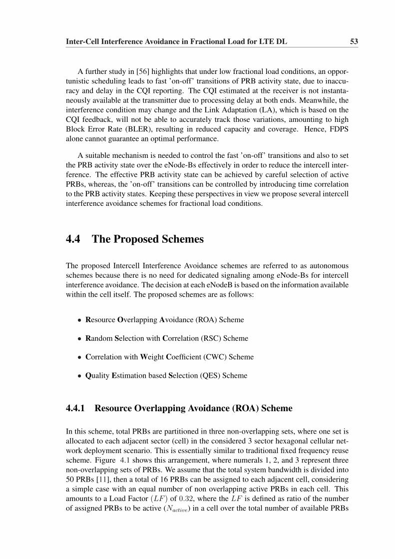
Inter-Cell Interference Avoidance in Fractional Load for LTE DL 53
A further study in [56] highlights that under low fractional load conditions, an oppor-tunistic scheduling leads to fast ’on-off’ transitions of PRB activity state, due to inaccu-racy and delay in the CQI reporting. The CQI estimated at the receiver is not instanta-neously available at the transmitter due to processing delay at both ends. Meanwhile, theinterference condition may change and the Link Adaptation (LA), which is based on theCQI feedback, will not be able to accurately track those variations, amounting to highBlock Error Rate (BLER), resulting in reduced capacity and coverage. Hence, FDPSalone cannot guarantee an optimal performance.
A suitable mechanism is needed to control the fast ’on-off’ transitions and also to setthe PRB activity state over the eNode-Bs effectively in order to reduce the intercell inter-ference. The effective PRB activity state can be achieved by careful selection of activePRBs, whereas, the ’on-off’ transitions can be controlled by introducing time correlationto the PRB activity states. Keeping these perspectives in view we propose several intercellinterference avoidance schemes for fractional load conditions.
4.4 The Proposed Schemes
The proposed Intercell Interference Avoidance schemes are referred to as autonomousschemes because there is no need for dedicated signaling among eNode-Bs for intercellinterference avoidance. The decision at each eNodeB is based on the information availablewithin the cell itself. The proposed schemes are as follows:
• Resource Overlapping Avoidance (ROA) Scheme
• Random Selection with Correlation (RSC) Scheme
• Correlation with Weight Coefficient (CWC) Scheme
• Quality Estimation based Selection (QES) Scheme
4.4.1 Resource Overlapping Avoidance (ROA) Scheme
In this scheme, total PRBs are partitioned in three non-overlapping sets, where one set isallocated to each adjacent sector (cell) in the considered 3 sector hexagonal cellular net-work deployment scenario. This is essentially similar to traditional fixed frequency reusescheme. Figure 4.1 shows this arrangement, where numerals 1, 2, and 3 represent threenon-overlapping sets of PRBs. We assume that the total system bandwidth is divided into50 PRBs [11], then a total of 16 PRBs can be assigned to each adjacent cell, consideringa simple case with an equal number of non overlapping active PRBs in each cell. Thisamounts to a Load Factor (LF ) of 0.32, where the LF is defined as ratio of the numberof assigned PRBs to be active (Nactive) in a cell over the total number of available PRBs
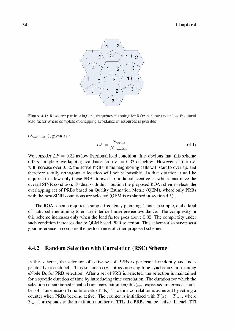
54 Chapter 4
Figure 4.1: Resource partitioning and frequency planning for ROA scheme under low fractionalload factor where complete overlapping avoidance of resources is possible
(Navailable ), given as :
LF =Nactive
Navailable
(4.1)
We consider LF = 0.32 as low fractional load condition. It is obvious that, this schemeoffers complete overlapping avoidance for LF = 0.32 or below. However, as the LFwill increase over 0.32, the active PRBs in the neighboring cells will start to overlap, andtherefore a fully orthogonal allocation will not be possible. In that situation it will berequired to allow only those PRBs to overlap in the adjacent cells, which maximize theoverall SINR condition. To deal with this situation the proposed ROA scheme selects theoverlapping set of PRBs based on Quality Estimation Metric (QEM), where only PRBswith the best SINR conditions are selected (QEM is explained in section 4.5).
The ROA scheme requires a simple frequency planning. This is a simple, and a kindof static scheme aiming to ensure inter-cell interference avoidance. The complexity inthis scheme increases only when the load factor goes above 0.32. The complexity undersuch condition increases due to QEM based PRB selection. This scheme also serves as agood reference to compare the performance of other proposed schemes.
4.4.2 Random Selection with Correlation (RSC) Scheme
In this scheme, the selection of active set of PRBs is performed randomly and inde-pendently in each cell. This scheme does not assume any time synchronization amongeNode-Bs for PRB selection. After a set of PRB is selected, the selection is maintainedfor a specific duration of time by introducing time correlation. The duration for which theselection is maintained is called time correlation length Tcorr, expressed in terms of num-ber of Transmission Time Intervals (TTIs). The time correlation is achieved by setting acounter when PRBs become active. The counter is initialized with T (k) = Tcorr, whereTcorr corresponds to the maximum number of TTIs the PRBs can be active. In each TTI
Inter-Cell Interference Avoidance in Fractional Load for LTE DL 55
the counter steps down by one unit step and when T (k) = 0, a new set of PRBs is selected.The required number of active PRBs for a particular LF is calculated as:
NLF = Navailable × LF (4.2)
Since the number of active PRBs may be time variant therefore it may be required tobe increased or decreased.
• The Nactive PRBs in a cell should be equal to NLF .
• In case Nactive > NLF , then randomly Nactive − NLF PRBs are set to dormant statefrom the set of Nactive PRBs.
• In case, Nactive < NLF , then randomly NLF − Nactive PRBs are set to active statefrom the set of Ndormant PRBs.
The steadiness in PRB activity state is achieved by introducing time correlation. Thetime correlation should be kept long enough to control frequent ’on-off’ transitions, andat the same time short enough to provide frequency diversity and interference averaging.This scheme does not ensure allocation of non overlapping set of PRBs with respect toadjacent eNode-Bs even under low fractional load conditions. It is a simple scheme dueto random PRB allocation. It requires no frequency planing.
4.4.3 Correlation with Weighting Coefficient (CWC) Scheme
CWC is a channel aware scheme in contrast to RSC. The CWC selects PRBs based onthe packet scheduler metric. A concept of weighting coefficient WTP is introduced in thisalgorithm. The WTP is determined by using the results of proportional fair (PF) packetscheduler metric [57]. We define WTP as ratio between the PF metric of the dormant andthe active PRBs, expressed in ( 4.3) and ( 4.4), WTP is given in ( 4.5). If the instantaneousthroughput of a dormant PRB is at least WTP times higher than the one of an activePRB then the currently dormant PRB will be prioritized for scheduling. otherwise thepreviously scheduled PRB will be rescheduled.
Mdormant =TPi(CQIdormant)
TP i
(4.3)
Mactive =TPi(CQIactive)
TP i
(4.4)
WTP =Mdormant
Mactive
=TPi(CQIdormant)
TPi(CQIactive)(4.5)
56 Chapter 4
In ( 4.3) and ( 4.4) TP i represents the average delivered throughput to user i. Theinstantaneous supported throughputs of user i over the dormant and active PRBs are rep-resented by TPi(CQIdormant) and TPi(CQIactive) respectively. The difference in thesupported throughput is realized due to the difference in the number of data bits carriedby employing different modulation and coding schemes (MCS), expressed as:
TPi = log2Nsymbols · k
n(4.6)
where Nsymbols represents the number of symbols in the constellation and kn
representsthe coding rate. Table 2 shows the relative throughput gain for a range of commonly usedMCS as an example [58].
Table 4.1: Relative Throughput Gain for a Range of Commonly used MCS
64QAM 45
64QAM 23
64QAM 12
16QAM 45
16QAM 23
16QAM 12
QPSK 23
QPSK 12
64QAM 45
1.00 1.20 1.60 1.50 1.80 2.40 3.60 4.8064QAM 2
31.00 1.33 1.25 1.50 2.00 3.00 4.00
64QAM 12
1.00 0.94 1.12 1.50 2.25 3.0016QAM 4
51.00 1.20 1.60 2.41 3.20
16QAM 23
1.00 1.33 2.00 2.6716QAM 1
21.00 1.50 2.00
QPSK 23
1.00 1.33QPSK 1
2
A dormant PRB will be prioritized over an active PRB as long as a throughput upgrad-ing equivalent to at least WTP is realized, otherwise the previously scheduled PRB willbe rescheduled. However, in order to limit the number of times a PRB being scheduleda concept of time correlation Tcorr function, similar to RCS is also introduced. The timecorrelation function depends on the number of consecutive schedules which determinesthe maximum number of times the same PRB can be scheduled.
4.4.4 Quality Estimation based Selection (QES)
QES scheme selects the set of active PRBs based on Quality Estimation Metric (QEM).The QEM is generated based on the estimated quality over the PRBs. The estimatedquality over the PRBs in downlink is based on the SINR estimates over the PRBs reportedby the users, whereas, in uplink this is based on the e-NodeB’s own estimates over thePRBs towards the users.
The Quality of the PRBs is estimated in the following steps.
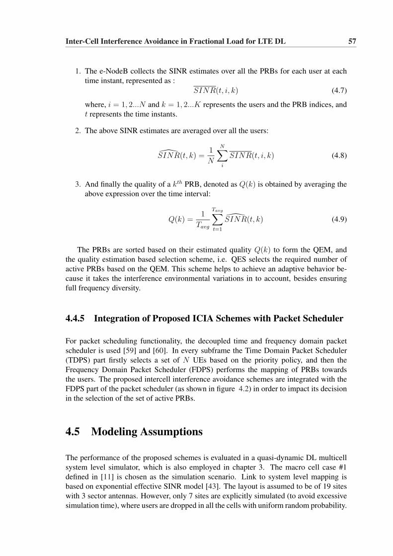
Inter-Cell Interference Avoidance in Fractional Load for LTE DL 57
1. The e-NodeB collects the SINR estimates over all the PRBs for each user at eachtime instant, represented as :
SINR(t, i, k) (4.7)
where, i = 1, 2...N and k = 1, 2...K represents the users and the PRB indices, andt represents the time instants.
2. The above SINR estimates are averaged over all the users:
SINR(t, k) =1
N
N∑i
SINR(t, i, k) (4.8)
3. And finally the quality of a kth PRB, denoted as Q(k) is obtained by averaging theabove expression over the time interval:
Q(k) =1
Tavg
Tavg∑t=1
SINR(t, k) (4.9)
The PRBs are sorted based on their estimated quality Q(k) to form the QEM, andthe quality estimation based selection scheme, i.e. QES selects the required number ofactive PRBs based on the QEM. This scheme helps to achieve an adaptive behavior be-cause it takes the interference environmental variations in to account, besides ensuringfull frequency diversity.
4.4.5 Integration of Proposed ICIA Schemes with Packet Scheduler
For packet scheduling functionality, the decoupled time and frequency domain packetscheduler is used [59] and [60]. In every subframe the Time Domain Packet Scheduler(TDPS) part firstly selects a set of N UEs based on the priority policy, and then theFrequency Domain Packet Scheduler (FDPS) performs the mapping of PRBs towardsthe users. The proposed intercell interference avoidance schemes are integrated with theFDPS part of the packet scheduler (as shown in figure 4.2) in order to impact its decisionin the selection of the set of active PRBs.
4.5 Modeling Assumptions
The performance of the proposed schemes is evaluated in a quasi-dynamic DL multicellsystem level simulator, which is also employed in chapter 3. The macro cell case #1defined in [11] is chosen as the simulation scenario. Link to system level mapping isbased on exponential effective SINR model [43]. The layout is assumed to be of 19 siteswith 3 sector antennas. However, only 7 sites are explicitly simulated (to avoid excessivesimulation time), where users are dropped in all the cells with uniform random probability.
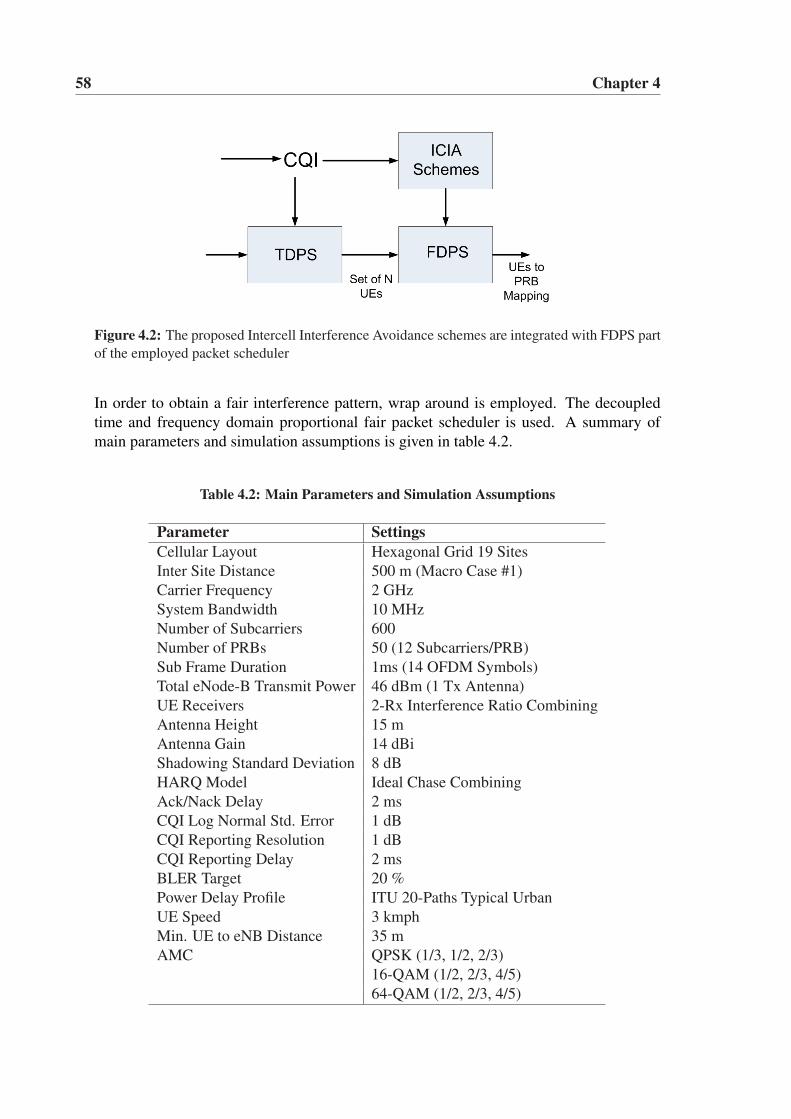
58 Chapter 4
Figure 4.2: The proposed Intercell Interference Avoidance schemes are integrated with FDPS partof the employed packet scheduler
In order to obtain a fair interference pattern, wrap around is employed. The decoupledtime and frequency domain proportional fair packet scheduler is used. A summary ofmain parameters and simulation assumptions is given in table 4.2.
Table 4.2: Main Parameters and Simulation Assumptions
Parameter SettingsCellular Layout Hexagonal Grid 19 SitesInter Site Distance 500 m (Macro Case #1)Carrier Frequency 2 GHzSystem Bandwidth 10 MHzNumber of Subcarriers 600Number of PRBs 50 (12 Subcarriers/PRB)Sub Frame Duration 1ms (14 OFDM Symbols)Total eNode-B Transmit Power 46 dBm (1 Tx Antenna)UE Receivers 2-Rx Interference Ratio CombiningAntenna Height 15 mAntenna Gain 14 dBiShadowing Standard Deviation 8 dBHARQ Model Ideal Chase CombiningAck/Nack Delay 2 msCQI Log Normal Std. Error 1 dBCQI Reporting Resolution 1 dBCQI Reporting Delay 2 msBLER Target 20 %Power Delay Profile ITU 20-Paths Typical UrbanUE Speed 3 kmphMin. UE to eNB Distance 35 mAMC QPSK (1/3, 1/2, 2/3)
16-QAM (1/2, 2/3, 4/5)64-QAM (1/2, 2/3, 4/5)
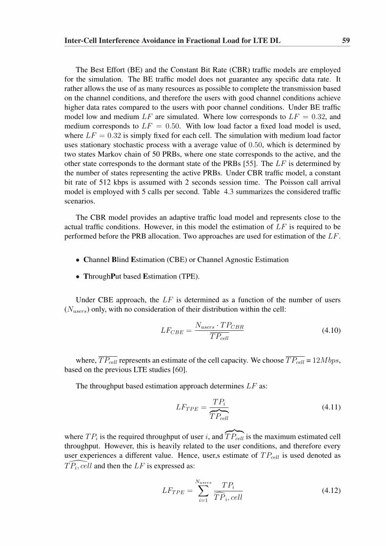
Inter-Cell Interference Avoidance in Fractional Load for LTE DL 59
The Best Effort (BE) and the Constant Bit Rate (CBR) traffic models are employedfor the simulation. The BE traffic model does not guarantee any specific data rate. Itrather allows the use of as many resources as possible to complete the transmission basedon the channel conditions, and therefore the users with good channel conditions achievehigher data rates compared to the users with poor channel conditions. Under BE trafficmodel low and medium LF are simulated. Where low corresponds to LF = 0.32, andmedium corresponds to LF = 0.50. With low load factor a fixed load model is used,where LF = 0.32 is simply fixed for each cell. The simulation with medium load factoruses stationary stochastic process with a average value of 0.50, which is determined bytwo states Markov chain of 50 PRBs, where one state corresponds to the active, and theother state corresponds to the dormant state of the PRBs [55]. The LF is determined bythe number of states representing the active PRBs. Under CBR traffic model, a constantbit rate of 512 kbps is assumed with 2 seconds session time. The Poisson call arrivalmodel is employed with 5 calls per second. Table 4.3 summarizes the considered trafficscenarios.
The CBR model provides an adaptive traffic load model and represents close to theactual traffic conditions. However, in this model the estimation of LF is required to beperformed before the PRB allocation. Two approaches are used for estimation of the LF .
• Channel Blind Estimation (CBE) or Channel Agnostic Estimation
• ThroughPut based Estimation (TPE).
Under CBE approach, the LF is determined as a function of the number of users(Nusers) only, with no consideration of their distribution within the cell:
LFCBE =Nusers · TPCBR
TPcell
(4.10)
where, TPcell represents an estimate of the cell capacity. We choose TPcell = 12Mbps,based on the previous LTE studies [60].
The throughput based estimation approach determines LF as:
LFTPE =TPi︷ ︸︸ ︷
TPcell
(4.11)
where TPi is the required throughput of user i, and︷ ︸︸ ︷TPcell is the maximum estimated cell
throughput. However, this is heavily related to the user conditions, and therefore everyuser experiences a different value. Hence, user,s estimate of TPcell is used denoted asTPi, cell and then the LF is expressed as:
LFTPE =Nusers∑
i=1
TPi
TP i, cell(4.12)
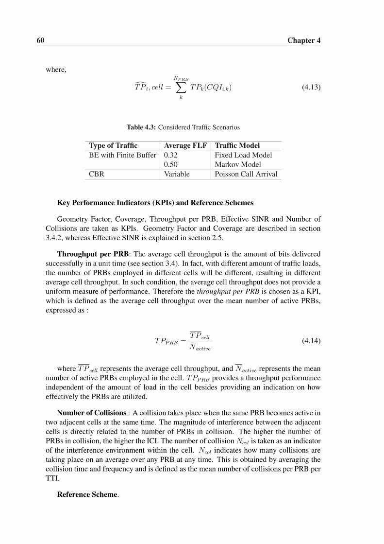
60 Chapter 4
where,
TP i, cell =
NPRB∑
k
TPk(CQIi,k) (4.13)
Table 4.3: Considered Traffic Scenarios
Type of Traffic Average FLF Traffic ModelBE with Finite Buffer 0.32 Fixed Load Model
0.50 Markov ModelCBR Variable Poisson Call Arrival
Key Performance Indicators (KPIs) and Reference Schemes
Geometry Factor, Coverage, Throughput per PRB, Effective SINR and Number ofCollisions are taken as KPIs. Geometry Factor and Coverage are described in section3.4.2, whereas Effective SINR is explained in section 2.5.
Throughput per PRB: The average cell throughput is the amount of bits deliveredsuccessfully in a unit time (see section 3.4). In fact, with different amount of traffic loads,the number of PRBs employed in different cells will be different, resulting in differentaverage cell throughput. In such condition, the average cell throughput does not provide auniform measure of performance. Therefore the throughput per PRB is chosen as a KPI,which is defined as the average cell throughput over the mean number of active PRBs,expressed as :
TPPRB =TP cell
Nactive
(4.14)
where TP cell represents the average cell throughput, and Nactive represents the meannumber of active PRBs employed in the cell. TPPRB provides a throughput performanceindependent of the amount of load in the cell besides providing an indication on howeffectively the PRBs are utilized.
Number of Collisions : A collision takes place when the same PRB becomes active intwo adjacent cells at the same time. The magnitude of interference between the adjacentcells is directly related to the number of PRBs in collision. The higher the number ofPRBs in collision, the higher the ICI. The number of collision Ncol is taken as an indicatorof the interference environment within the cell. Ncol indicates how many collisions aretaking place on an average over any PRB at any time. This is obtained by averaging thecollision time and frequency and is defined as the mean number of collisions per PRB perTTI.
Reference Scheme.
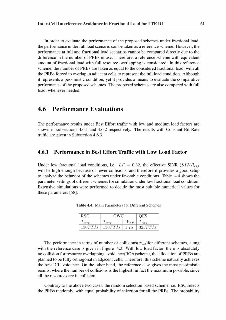
Inter-Cell Interference Avoidance in Fractional Load for LTE DL 61
In order to evaluate the performance of the proposed schemes under fractional load,the performance under full load scenario can be taken as a reference scheme. However, theperformance at full and fractional load scenarios cannot be compared directly due to thedifference in the number of PRBs in use. Therefore, a reference scheme with equivalentamount of fractional load with full resource overlapping is considered. In this referencescheme, the number of PRBs are taken as equal to the considered fractional load, with allthe PRBs forced to overlap in adjacent cells to represent the full load condition. Althoughit represents a pessimistic condition, yet it provides a means to evaluate the comparativeperformance of the proposed schemes. The proposed schemes are also compared with fullload, whenever needed.
4.6 Performance Evaluations
The performance results under Best Effort traffic with low and medium load factors areshown in subsections 4.6.1 and 4.6.2 respectively. The results with Constant Bit Ratetraffic are given in Subsection 4.6.3.
4.6.1 Performance in Best Effort Traffic with Low Load Factor
Under low fractional load conditions, i.e. LF = 0.32, the effective SINR (SINReff
will be high enough because of fewer collisions, and therefore it provides a good setupto analyze the behavior of the schemes under favorable conditions. Table 4.4 shows theparameter settings of different schemes for simulation under low fractional load condition.Extensive simulations were performed to decide the most suitable numerical values forthese parameters [58].
Table 4.4: Main Parameters for Different Schemes
RSC CWC QESTcorr Tcorr WTP TAvg
130TTIs 130TTIs 1.75 325TTIs
The performance in terms of number of collisions(Ncol)for different schemes, alongwith the reference case is given in Figure 4.3. With low load factor, there is absolutelyno collision for resource overlapping avoidance(ROA)scheme, the allocation of PRBs areplanned to be fully orthogonal in adjacent cells. Therefore, this scheme naturally achievesthe best ICI avoidance. On the other hand, the reference case gives the most pessimisticresults, where the number of collisions is the highest; in fact the maximum possible, sinceall the resources are in collision.
Contrary to the above two cases, the random selection based scheme, i.e. RSC selectsthe PRBs randomly, with equal probability of selection for all the PRBs. The probability
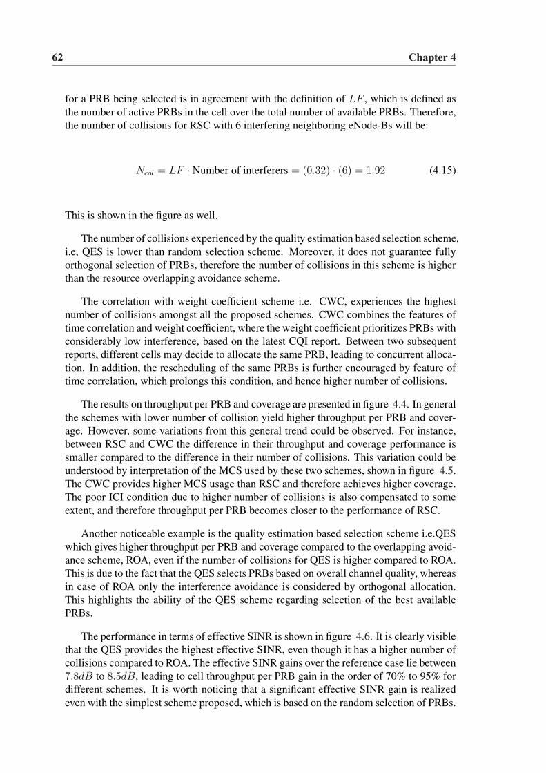
62 Chapter 4
for a PRB being selected is in agreement with the definition of LF , which is defined asthe number of active PRBs in the cell over the total number of available PRBs. Therefore,the number of collisions for RSC with 6 interfering neighboring eNode-Bs will be:
Ncol = LF · Number of interferers = (0.32) · (6) = 1.92 (4.15)
This is shown in the figure as well.
The number of collisions experienced by the quality estimation based selection scheme,i.e, QES is lower than random selection scheme. Moreover, it does not guarantee fullyorthogonal selection of PRBs, therefore the number of collisions in this scheme is higherthan the resource overlapping avoidance scheme.
The correlation with weight coefficient scheme i.e. CWC, experiences the highestnumber of collisions amongst all the proposed schemes. CWC combines the features oftime correlation and weight coefficient, where the weight coefficient prioritizes PRBs withconsiderably low interference, based on the latest CQI report. Between two subsequentreports, different cells may decide to allocate the same PRB, leading to concurrent alloca-tion. In addition, the rescheduling of the same PRBs is further encouraged by feature oftime correlation, which prolongs this condition, and hence higher number of collisions.
The results on throughput per PRB and coverage are presented in figure 4.4. In generalthe schemes with lower number of collision yield higher throughput per PRB and cover-age. However, some variations from this general trend could be observed. For instance,between RSC and CWC the difference in their throughput and coverage performance issmaller compared to the difference in their number of collisions. This variation could beunderstood by interpretation of the MCS used by these two schemes, shown in figure 4.5.The CWC provides higher MCS usage than RSC and therefore achieves higher coverage.The poor ICI condition due to higher number of collisions is also compensated to someextent, and therefore throughput per PRB becomes closer to the performance of RSC.
Another noticeable example is the quality estimation based selection scheme i.e.QESwhich gives higher throughput per PRB and coverage compared to the overlapping avoid-ance scheme, ROA, even if the number of collisions for QES is higher compared to ROA.This is due to the fact that the QES selects PRBs based on overall channel quality, whereasin case of ROA only the interference avoidance is considered by orthogonal allocation.This highlights the ability of the QES scheme regarding selection of the best availablePRBs.
The performance in terms of effective SINR is shown in figure 4.6. It is clearly visiblethat the QES provides the highest effective SINR, even though it has a higher number ofcollisions compared to ROA. The effective SINR gains over the reference case lie between7.8dB to 8.5dB, leading to cell throughput per PRB gain in the order of 70% to 95% fordifferent schemes. It is worth noticing that a significant effective SINR gain is realizedeven with the simplest scheme proposed, which is based on the random selection of PRBs.
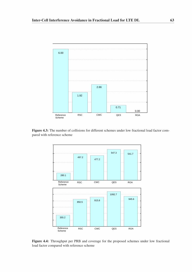
Inter-Cell Interference Avoidance in Fractional Load for LTE DL 63
6.00
1.92
2.66
0.710.00
Reference Scheme
RSC CWC QES ROA
Figure 4.3: The number of collisions for different schemes under low fractional load factor com-pared with reference scheme
200
300
400
500
600
280.1
497.2477.2
547.3 541.7
ReferenceScheme
RSC CWC QES ROA
0
200
400
600
800
1000
1200
355.2
850.5915.8
1092.7
945.6
Reference Scheme
RSC CWC QES ROA
Figure 4.4: Throughput per PRB and coverage for the proposed schemes under low fractionalload factor compared with reference scheme
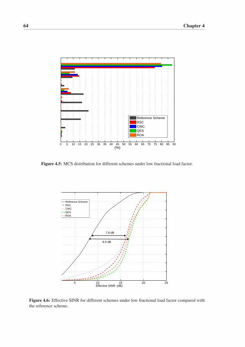
64 Chapter 4
0 5 10 15 20 25 30 35 40 45 50 55 60 65 70 75 80 85 90(%)
Reference SchemeRSCCWCQESROA
Figure 4.5: MCS distribution for different schemes under low fractional load factor.
5 10 15 20 25Effective SINR (dB)
Reference SchemeRSCCWCQESROA
8.5 dB
7.8 dB
Figure 4.6: Effective SINR for different schemes under low fractional load factor compared withthe reference scheme.
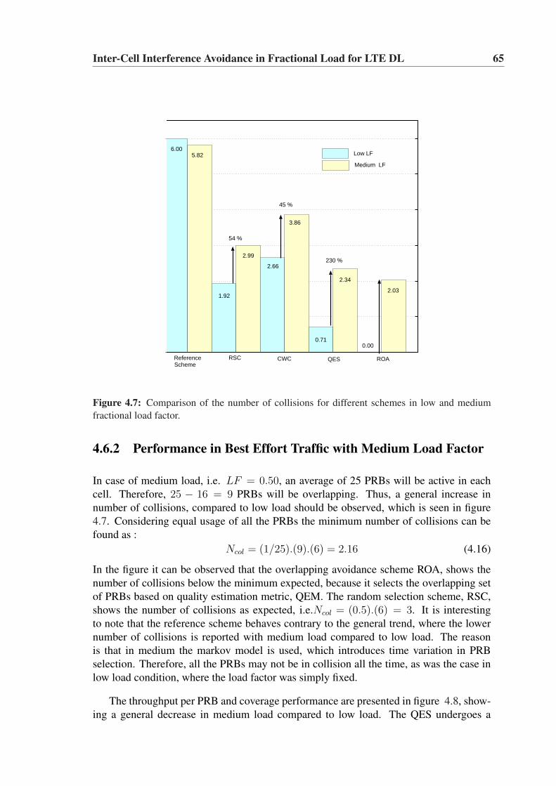
Inter-Cell Interference Avoidance in Fractional Load for LTE DL 65
6.005.82
1.92
2.99
2.66
3.86
0.71
2.34
0.00
2.03
54 %
45 %
230 %
Reference Scheme
RSC CWC QES ROA
Low LF
Medium LF
Figure 4.7: Comparison of the number of collisions for different schemes in low and mediumfractional load factor.
4.6.2 Performance in Best Effort Traffic with Medium Load Factor
In case of medium load, i.e. LF = 0.50, an average of 25 PRBs will be active in eachcell. Therefore, 25 − 16 = 9 PRBs will be overlapping. Thus, a general increase innumber of collisions, compared to low load should be observed, which is seen in figure4.7. Considering equal usage of all the PRBs the minimum number of collisions can befound as :
Ncol = (1/25).(9).(6) = 2.16 (4.16)
In the figure it can be observed that the overlapping avoidance scheme ROA, shows thenumber of collisions below the minimum expected, because it selects the overlapping setof PRBs based on quality estimation metric, QEM. The random selection scheme, RSC,shows the number of collisions as expected, i.e.Ncol = (0.5).(6) = 3. It is interestingto note that the reference scheme behaves contrary to the general trend, where the lowernumber of collisions is reported with medium load compared to low load. The reasonis that in medium the markov model is used, which introduces time variation in PRBselection. Therefore, all the PRBs may not be in collision all the time, as was the case inlow load condition, where the load factor was simply fixed.
The throughput per PRB and coverage performance are presented in figure 4.8, show-ing a general decrease in medium load compared to low load. The QES undergoes a
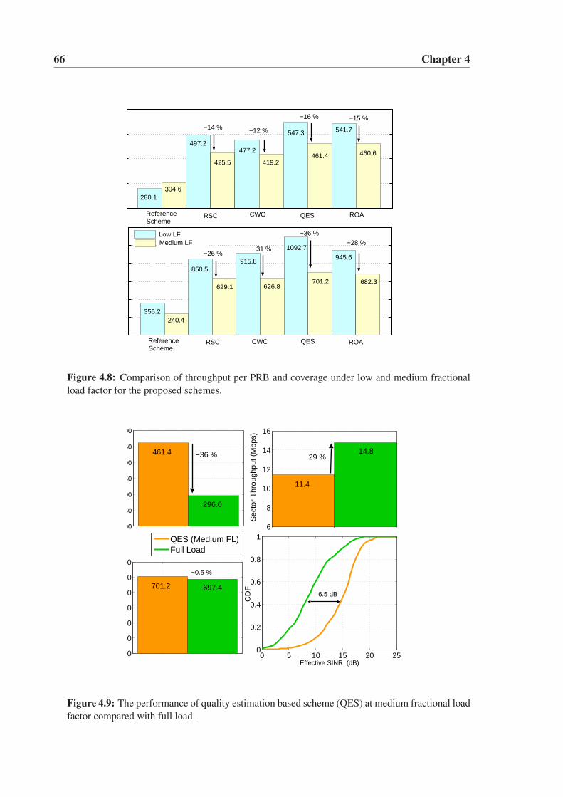
66 Chapter 4
280.1304.6
497.2
425.5
477.2
419.2
547.3
461.4
541.7
460.6
−14 % −12 %
−16 % −15 %
Reference Scheme
RSC CWC QES ROA
0
200
400
600
800
1000
1200
355.2240.4
850.5
629.1
915.8
626.8
1092.7
701.2
945.6
682.3
−26 %−31 %
−36 %
−28 %
Reference Scheme
RSC CWC QES ROA
Medium LFLow LF
Figure 4.8: Comparison of throughput per PRB and coverage under low and medium fractionalload factor for the proposed schemes.
200
250
300
350
400
450
500
461.4
296.0
−36 %
6
8
10
12
14
16
11.4
14.829 %
Sec
tor
Thr
ough
put (
Mbp
s)
600
620
640
660
680
700
720
701.2 697.4
−0.5 %
0 5 10 15 20 250
0.2
0.4
0.6
0.8
1
Effective SINR (dB)
CD
F
QES (Medium FL)Full Load
6.5 dB
Figure 4.9: The performance of quality estimation based scheme (QES) at medium fractional loadfactor compared with full load.
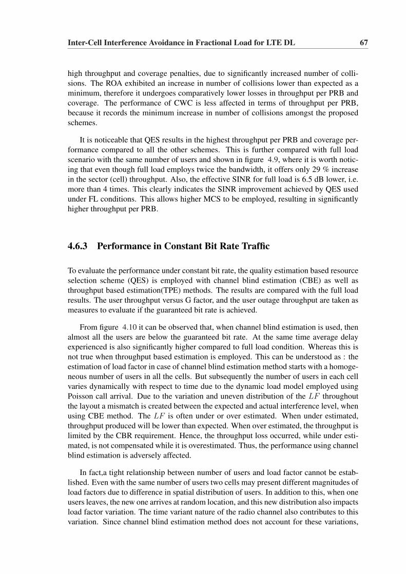
Inter-Cell Interference Avoidance in Fractional Load for LTE DL 67
high throughput and coverage penalties, due to significantly increased number of colli-sions. The ROA exhibited an increase in number of collisions lower than expected as aminimum, therefore it undergoes comparatively lower losses in throughput per PRB andcoverage. The performance of CWC is less affected in terms of throughput per PRB,because it records the minimum increase in number of collisions amongst the proposedschemes.
It is noticeable that QES results in the highest throughput per PRB and coverage per-formance compared to all the other schemes. This is further compared with full loadscenario with the same number of users and shown in figure 4.9, where it is worth notic-ing that even though full load employs twice the bandwidth, it offers only 29 % increasein the sector (cell) throughput. Also, the effective SINR for full load is 6.5 dB lower, i.e.more than 4 times. This clearly indicates the SINR improvement achieved by QES usedunder FL conditions. This allows higher MCS to be employed, resulting in significantlyhigher throughput per PRB.
4.6.3 Performance in Constant Bit Rate Traffic
To evaluate the performance under constant bit rate, the quality estimation based resourceselection scheme (QES) is employed with channel blind estimation (CBE) as well asthroughput based estimation(TPE) methods. The results are compared with the full loadresults. The user throughput versus G factor, and the user outage throughput are taken asmeasures to evaluate if the guaranteed bit rate is achieved.
From figure 4.10 it can be observed that, when channel blind estimation is used, thenalmost all the users are below the guaranteed bit rate. At the same time average delayexperienced is also significantly higher compared to full load condition. Whereas this isnot true when throughput based estimation is employed. This can be understood as : theestimation of load factor in case of channel blind estimation method starts with a homoge-neous number of users in all the cells. But subsequently the number of users in each cellvaries dynamically with respect to time due to the dynamic load model employed usingPoisson call arrival. Due to the variation and uneven distribution of the LF throughoutthe layout a mismatch is created between the expected and actual interference level, whenusing CBE method. The LF is often under or over estimated. When under estimated,throughput produced will be lower than expected. When over estimated, the throughput islimited by the CBR requirement. Hence, the throughput loss occurred, while under esti-mated, is not compensated while it is overestimated. Thus, the performance using channelblind estimation is adversely affected.
In fact,a tight relationship between number of users and load factor cannot be estab-lished. Even with the same number of users two cells may present different magnitudes ofload factors due to difference in spatial distribution of users. In addition to this, when oneusers leaves, the new one arrives at random location, and this new distribution also impactsload factor variation. The time variant nature of the radio channel also contributes to thisvariation. Since channel blind estimation method does not account for these variations,
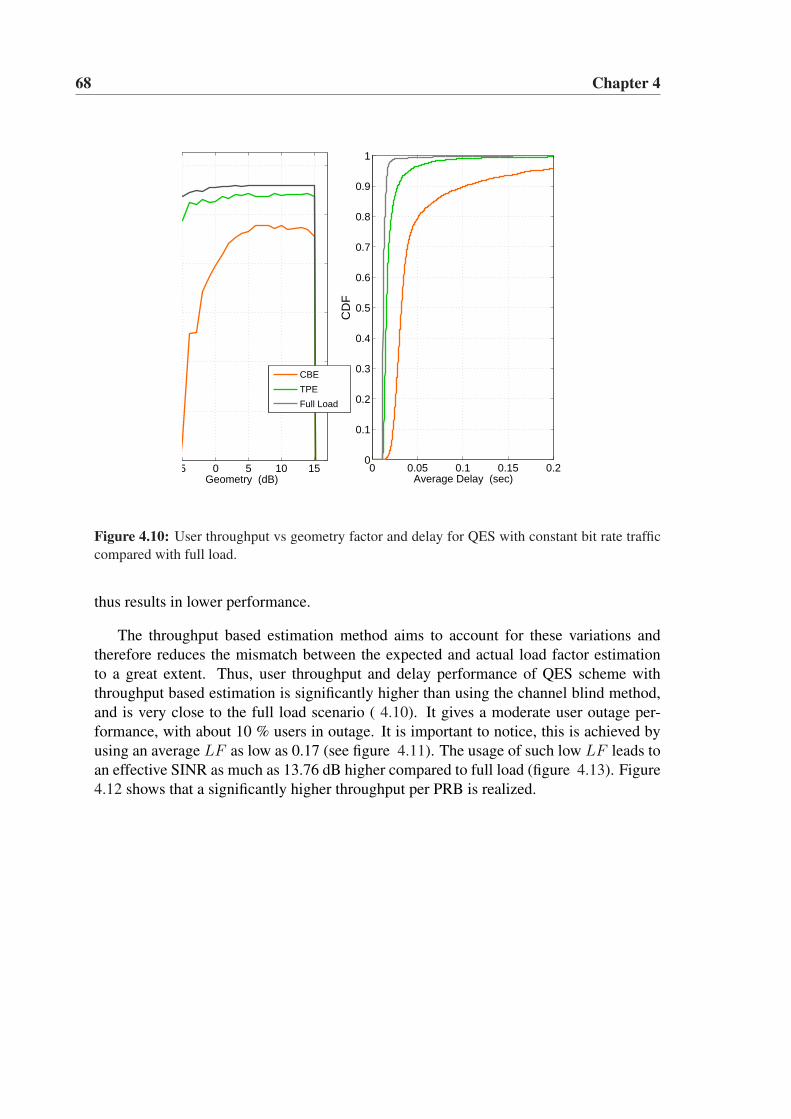
68 Chapter 4
−5 0 5 10 15Geometry (dB)
0 0.05 0.1 0.15 0.20
0.1
0.2
0.3
0.4
0.5
0.6
0.7
0.8
0.9
1
Average Delay (sec)
CD
F
CBE
TPE
Full Load
Figure 4.10: User throughput vs geometry factor and delay for QES with constant bit rate trafficcompared with full load.
thus results in lower performance.
The throughput based estimation method aims to account for these variations andtherefore reduces the mismatch between the expected and actual load factor estimationto a great extent. Thus, user throughput and delay performance of QES scheme withthroughput based estimation is significantly higher than using the channel blind method,and is very close to the full load scenario ( 4.10). It gives a moderate user outage per-formance, with about 10 % users in outage. It is important to notice, this is achieved byusing an average LF as low as 0.17 (see figure 4.11). The usage of such low LF leads toan effective SINR as much as 13.76 dB higher compared to full load (figure 4.13). Figure4.12 shows that a significantly higher throughput per PRB is realized.
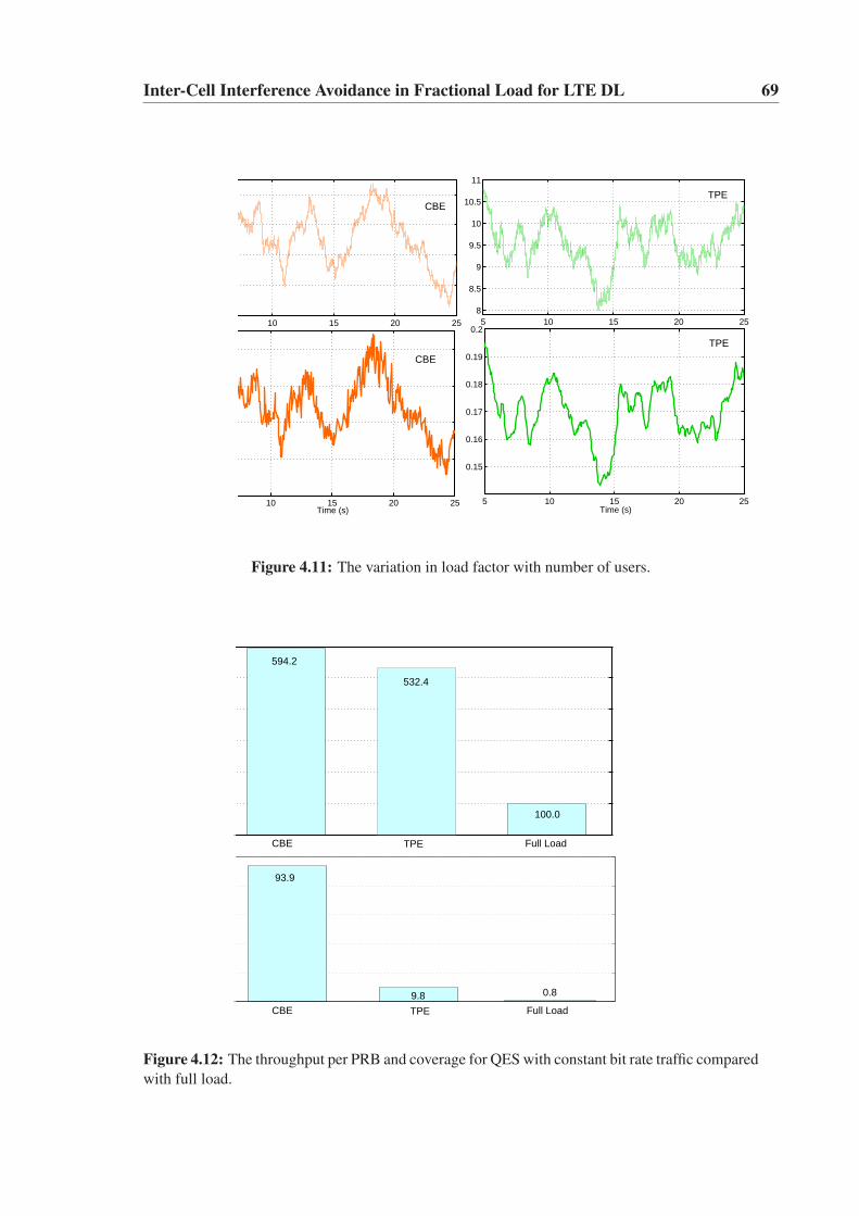
Inter-Cell Interference Avoidance in Fractional Load for LTE DL 69
10 15 20 25 5 10 15 20 258
8.5
9
9.5
10
10.5
11
10 15 20 25Time (s)
5 10 15 20 25
0.15
0.16
0.17
0.18
0.19
0.2
Time (s)
TPE
TPE
CBE
CBE
Figure 4.11: The variation in load factor with number of users.
594.2
532.4
100.0
CBE TPE Full Load
93.9
9.8 0.8
CBE TPE Full Load
Figure 4.12: The throughput per PRB and coverage for QES with constant bit rate traffic comparedwith full load.
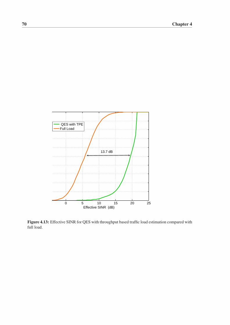
70 Chapter 4
0 5 10 15 20 25Effective SINR (dB)
QES with TPEFull Load
13.7 dB
Figure 4.13: Effective SINR for QES with throughput based traffic load estimation compared withfull load.
Inter-Cell Interference Avoidance in Fractional Load for LTE DL 71
4.7 Conclusions
This chapter investigates schemes to avoid inter-cell interference in fractional load condi-tions. It was discussed that under fractional load condition, a CQI aware frequency do-main packet scheduling can avoid inter-cell interference by avoiding scheduling of PRBswith high interference. But the performance of such scheduling is highly sensitive to inac-curacy and delay in CQI reports, leading to fast on-off transition of PRBs and high BLER.Therefore, the need for a mechanism was realized for : i) proper selection of PRBs withrespect to adjacent cells in order to avoid/minimize ICI and ii) controlling the fast on-offtransitions to control the high BLER.
Several autonomous intercell interference avoidance schemes are proposed for frac-tional load conditions in this chapter. The proposed schemes require no dedicated inter-cell signaling for controlling the ICI. The simplest proposed scheme that is based onrandom selection of PRBs combined with time correlation, also gives significant SINRimprovement, resulting in throughput per PRB and coverage enhancements over the ref-erence scheme. Moreover, the proposed Quality Estimation based PRB selection Scheme(QES) further improves the performance.
When QES with medium load factor (i.e. 50% fractional load) is compared with fullload under best effort traffic, it was found that QES gives 6.5 dB higher effective SINR.Besides, even though full load employs twice the bandwidth, it offers only 29% increasein the sector (cell) throughput. The QES achieves significantly higher throughput perPRB compared to full load. However, the coverage gain is only slightly higher in QEScompared to full load.
Further, the comparison of QES was performed with full load under constant bit rate(CBR) traffic with throughput based traffic load estimation method. A much higher ef-fective SINR (in the order of 13 dB) compared to full load is realized, resulting in signifi-cantly higher throughput per PRB ( in the order of 5 times). This performance is achievedwith only about 10 % users in outage.

Chapter 5
Flexible Spectrum Usage for Local AreaDeployment
5.1 Introduction
IMT-A has increased focus on nomadic / local area network solution [24], [7], whichis envisioned to be the only way to significantly boost the increasing demand for highnetwork capacity and high user data rates. 80 to 90% of traffic volume is estimated to begenerated in the indoor and hot spot nomadic scenarios [61]. Currently, Home eNode-B (HeNB) is emerging as a potential solution for high data rate and high quality servicesin indoor local area [62]. It is considered as an alternative way of delivering the benefitsof fixed-mobile convergence [62].
5.1.1 Home eNode-B
A HeNB is a small cellular base station, typically designed to be used in indoor environ-ment. It incorporates the functionality of a typical base station and uses a simple plug andplay device. HeNB will likely be deployed by the subscribers to support an individualcoverage in a small area. A large scale deployment of HeNBs is expected, potentially inan uncoordinated manner, and therefore a rigorous planning is not necessarily feasible,which gives rise to several deployment issues.
5.1.2 Key Issues for HeNB Deployment in Local Area
• A conventional cellular network is designed to support a relatively small number ofbase stations in a given area, whereas HeNBs will be deployed in large numbers.As a consequence, a different architectural approach will be required [62].
• Due to the fact that the HeNBs are likely to be deployed by the subscribers, it
73
74 Chapter 5
seems difficult for the operator to pre-configure and coordinate the deployment inorder to minimize mutual interference. Under such deployment conditions it willbe difficult to estimate the level of interference beforehand, that one HeNB couldpractically cause towards the coverage area of the other HeNBs. Hence, a key issuewill be to address the question, how the HeNBs will coexist in the given area withdesired performance?
• The HeNB should provide reasonable performance whether it is deployed in iso-lation or in the vicinity of multiple HeNBs. In the later case, the level of interfer-ence could be very high, and therefore, requires an effective interference manage-ment mechanism to provide reasonable performance. The interference managementmechanism may pose challenges to HeNBs in managing their radio resources. Themaximum power output of a HeNB should be able to provide adequate coverage,while not exceeding the HeNB interference limits [62].
• Therefore, an efficient technique will be essential to support HeNBs to self-configure,use spectrum in a flexible manner, minimize interference and to ensure coexistencewith other HeNBs in the given area [9],[63].
The above mentioned issues are important to be considered in order to provide anefficient local area solution. The concept of Flexible Spectrum Usage (FSU) is widelyseen as an important component to facilitate such solution.
5.1.3 Flexible Spectrum Usage (FSU)
The increasing demand of spectrum for wireless applications makes it necessary to im-prove efficiency of spectrum utilization by spectrum sharing techniques [64]. A largenumber of wireless systems and services under development will make it difficult to iden-tify exclusive spectrum for all wireless systems and services [65]. In face of the abovescenario, the Federal Communication Commission (FCC)’s Spectrum Policy Task Force(SPTF) has made recommendations to develop a spectrum policy that maximizes the flex-ibility of spectrum use [9]. Therefore, the framework of radio spectrum regulation isundergoing a vital change towards flexible and open access to the spectrum[63].
The commercial success of flexible and open access to spectrum for wireless appli-cations such as WLAN in the unlicensed bands is one example, to believe that it will beuseful to move towards a more flexible spectrum access [66].
Recently, the flexible sharing of spectrum is extensively addressed by the researchcommunity. The underlying concept considers two mechanisms in order to share thespectrum: (i) Spectrum Sharing (SS) and (ii) Flexible Spectrum Usage (FSU) [65]. Thespectrum sharing is the notion that considers sharing of spectrum between different radioaccess technologies (RATs). This can be regarded as a form of inter-system spectrumsharing. Whereas, sharing of spectrum between different radio access networks (RANs)using the same RAT is defined as FSU. Wireless World Initiative New Radio (WINNER)
Flexible Spectrum Usage for Local Area Deployment 75
has developed a flexible and scalable radio interface, which covers different domains (lo-cal area, metropolitan area, and wide area) with the same radio interface [67].
The FSU is mainly viewed in the context of multi-operator scenario providing ser-vices over the same RAT. It is based on the concept that, when one network operator is indemand of additional spectrum, the other operator might have an excess of it. If a meanscan be provided to dynamically access spectrum on spatio-temporal basis in the situa-tion described above, rapid traffic fluctuations can be met efficiently, and the capacity-on-demand capabilities can be achieved [9]. FSU can inherently enable such dynamicaccess and help to expand network capacity at peak traffic times. However, FSU is notlimited to the multi-operator domain only. It can be employed within a single operator’snetwork as well. While the multi-operator FSU allows different operators to access thecommon spectrum pool in a flexible manner based on their individual requirements, thesingle operator FSU aims to achieve high performance in uncoordinated and random net-work deployment. In this chapter we focus on a single operator FSU in local area indoordeployment.
A somewhat similar scenario is introduced in [68], [63] and [69], where an algo-rithm is provided to smooth out the allocation of the available transmission time amongthe devices in a WLAN scenario. The algorithm uses the concept of water filling. Thewater filling in time domain enables a decentralized, coordinated and opportunistic useof spectrum [66]. The algorithm is referred to as spectrum load smoothing (SLS). WithSLS the competing radio systems aim simultaneously at an equal utilization of the spec-trum. Based on the observation of the past usage of the radio resource, the radio systemsinteract and redistribute their allocations of the spectrum under the consideration of theQoS requirements. In these references, only time domain and fully orthogonal redistri-bution of the spectrum is shown. However, we aim to provide a mechanism for sharingin frequency domain with some degree of spectrum overlap, with an objective to enhancespectrum usage.
5.1.4 Aim of this Chapter
We aim to provide non-contention based algorithms to enable FSU among HeNBs, andensure their co-existence in local area deployment by partially or completely preventingmutual interference on the shared spectrum. We assume an uncoordinated deployment ofHeNBs by a single operator. The proposed algorithms work on the principle of self as-sessment of surrounding radio environment and aim to provide self-configurable, decen-tralized and scalable solution. The following two algorithms are proposed in this chapter:
1. Fixed SINR threshold based Spectrum Load Balancing (SLB) algorithm.
2. Comparative interference threshold based Resource Chunk Selection (RCS) algo-rithm.
76 Chapter 5
This chapter is organized as follows. Section 5.2 presents the description of the spec-trum load balancing algorithm proposed for flexible spectrum usage. Section 5.3 givesan account of the simulation environment. The main parameter settings and simulationassumptions, key performance indicators and the reference schemes are described in thissection. In section 5.4 main results on the performance of the SLB algorithm are pre-sented, and their pros and cons are discussed. Section 5.5 describes comparative interfer-ence threshold based RCS algorithm, which has been proposed as an improvement overthe SLB algorithm, and the performance results of this algorithm are also presented in thissection. Finally in section 5.6 the main findings are summarized.
5.2 SLB Algorithm for Flexible Spectrum Usage
Our assumption is that several HeNBs access the common pool of spectrum in order tomeet individual traffic requirements. These HeNBs potentially interfere with each otherdue to their vicinity in the given geographical area. We assume that there is no dedi-cated communication link between HeNBs. However, a limited information exchange isassumed via over-the-air-communication [70].
The SLB algorithm aims to ensure co-existence of mutually interfering HeNBs byspectrum allocation based on SINR threshold (SINRth). The spectral resources withSINR below the SINRth are not selected by HeNBs. The SINR threshold plays an im-portant role in setting the level of tolerable mutual interference as well as it ensures adesirable throughput performance. The degree of spectrum overlap is controlled by thelevel of SINR threshold. The higher the SINR threshold the lower the spectrum overlapand vice-versa. Therefore the selection of SINRth depends on the trade-off between theallowed mutual interference and spectrum utilization. The underlaying concept of SLBalgorithm is explained below.
The cell capacity in terms of SINR for an individual HeNB in the network can berepresented by using Shannon’s expression as:
C = ρ ·B log2
(1 +
S
I + N
)(5.1)
where, B,S, I and N represent respectively the system bandwidth, signal power,amount of interference and noise power over the system bandwidth respectively, and ρrepresents the fraction of the bandwidth utilization. The total system capacity C for amulticellular network can be expressed as:
C =
Ncells∑i=1
K∑
k=1
Cki (5.2)
where,
Flexible Spectrum Usage for Local Area Deployment 77
Cki = ρk
i
B
K· log2
1 +
P∑Kk=1 ρk
i
gkii
∑Ncells
j 6=i,j=1P∑K
k=1 ρkj
gkijρ
kj + N0
BK
(5.3)
where, i = 1, 2, ...., Ncells and k = 1, 2, ..., K represent the number of consideredcells in the network and total number of available Resource Blocks (RBs) over the totalsystem bandwidth, where a RB is defined as a unit of spectrum allocation in time andfrequency domain. P represents the total transmit power, and Ck
i represents capacity ofcell i over the kth RB. The channel gain between the cell i and its own user within the cellis represented by gk
ii whereas, gkij is channel gain from the interferers over RB k from cell
j. N0 represents noise spectral density.
The consideration of ρki in the expression ( 5.3) is crucial for FSU algorithms, which
significantly impacts SINR conditions and therefore the overall network performance in amulticellular environment. The FSU algorithm at HeNB aims to suitably determine ρk
i byselecting a subset of resource blocks such that it avoids the mutual interference as much aspossible. If the kth RB is selected for the ith HeNB then ρk
i = 1, otherwise ρki = 0. Where,
the expression∑K
k=1 ρki gives the fraction of total spectrum allocated by ith HeNB.
In the proposed SLB algorithm the SINR threshold (SINRth) is used as a decisioncriterion to select ρk
i = 0 or ρki = 1 for a HeNB over set of all the resource blocks. The
detailed explanation of the algorithm is given below.
Description of SLB AlgorithmThe SLB algorithm is performed in two phases, A) initialization phase and B) spectrumallocation phase.
A. Initialization PhaseThe initialization phase starts as soon as the HeNB is powered on. At this moment thereis no information on which PRBs to use, therefore the HeNB allocates PRBs randomly inorder to start carrying traffic. In this phase, ρk
i = 1 , if k ∈ N loadi , otherwise ρk
i = 0, whereN load
i is the set of PRBs selected randomly to meet the requirements of the traffic load byith HeNB. Once the communication is established between UE (s) and HeNB, the SINRestimates over the PRBs become available. The SINR estimates are used for allocation ofthe PRBs in the next phase of the algorithm.
B. Spectrum Allocation PhaseThis is performed in two steps, i) Allocation of free PRBs using Water Filling (WF) andii) Allocation of PRBs based on SINR threshold.
Step 1: Allocation of Free Spectrum using WF
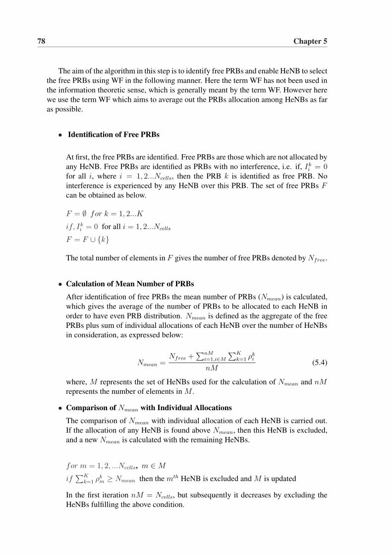
78 Chapter 5
The aim of the algorithm in this step is to identify free PRBs and enable HeNB to selectthe free PRBs using WF in the following manner. Here the term WF has not been used inthe information theoretic sense, which is generally meant by the term WF. However herewe use the term WF which aims to average out the PRBs allocation among HeNBs as faras possible.
• Identification of Free PRBs
At first, the free PRBs are identified. Free PRBs are those which are not allocated byany HeNB. Free PRBs are identified as PRBs with no interference, i.e. if, Ik
i = 0for all i, where i = 1, 2...Ncells, then the PRB k is identified as free PRB. Nointerference is experienced by any HeNB over this PRB. The set of free PRBs Fcan be obtained as below.
F = ∅ for k = 1, 2...K
if, Iki = 0 for all i = 1, 2...Ncells
F = F ∪ {k}
The total number of elements in F gives the number of free PRBs denoted by Nfree.
• Calculation of Mean Number of PRBs
After identification of free PRBs the mean number of PRBs (Nmean) is calculated,which gives the average of the number of PRBs to be allocated to each HeNB inorder to have even PRB distribution. Nmean is defined as the aggregate of the freePRBs plus sum of individual allocations of each HeNB over the number of HeNBsin consideration, as expressed below:
Nmean =Nfree +
∑nMi=1,i∈M
∑Kk=1 ρk
i
nM(5.4)
where, M represents the set of HeNBs used for the calculation of Nmean and nMrepresents the number of elements in M .
• Comparison of Nmean with Individual Allocations
The comparison of Nmean with individual allocation of each HeNB is carried out.If the allocation of any HeNB is found above Nmean, then this HeNB is excluded,and a new Nmean is calculated with the remaining HeNBs.
for m = 1, 2, ...Ncells, m ∈ M
if∑K
k=1 ρkm ≥ Nmean then the mth HeNB is excluded and M is updated
In the first iteration nM = Ncells, but subsequently it decreases by excluding theHeNBs fulfilling the above condition.
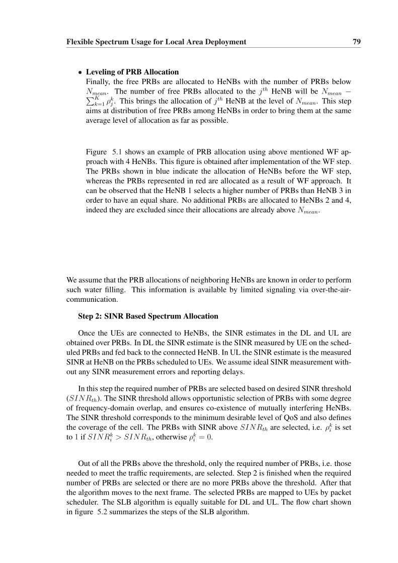
Flexible Spectrum Usage for Local Area Deployment 79
• Leveling of PRB AllocationFinally, the free PRBs are allocated to HeNBs with the number of PRBs belowNmean. The number of free PRBs allocated to the jth HeNB will be Nmean −∑K
k=1 ρkj . This brings the allocation of jth HeNB at the level of Nmean. This step
aims at distribution of free PRBs among HeNBs in order to bring them at the sameaverage level of allocation as far as possible.
Figure 5.1 shows an example of PRB allocation using above mentioned WF ap-proach with 4 HeNBs. This figure is obtained after implementation of the WF step.The PRBs shown in blue indicate the allocation of HeNBs before the WF step,whereas the PRBs represented in red are allocated as a result of WF approach. Itcan be observed that the HeNB 1 selects a higher number of PRBs than HeNB 3 inorder to have an equal share. No additional PRBs are allocated to HeNBs 2 and 4,indeed they are excluded since their allocations are already above Nmean.
We assume that the PRB allocations of neighboring HeNBs are known in order to performsuch water filling. This information is available by limited signaling via over-the-air-communication.
Step 2: SINR Based Spectrum Allocation
Once the UEs are connected to HeNBs, the SINR estimates in the DL and UL areobtained over PRBs. In DL the SINR estimate is the SINR measured by UE on the sched-uled PRBs and fed back to the connected HeNB. In UL the SINR estimate is the measuredSINR at HeNB on the PRBs scheduled to UEs. We assume ideal SINR measurement with-out any SINR measurement errors and reporting delays.
In this step the required number of PRBs are selected based on desired SINR threshold(SINRth). The SINR threshold allows opportunistic selection of PRBs with some degreeof frequency-domain overlap, and ensures co-existence of mutually interfering HeNBs.The SINR threshold corresponds to the minimum desirable level of QoS and also definesthe coverage of the cell. The PRBs with SINR above SINRth are selected, i.e. ρk
i is setto 1 if SINRk
i > SINRth, otherwise ρki = 0.
Out of all the PRBs above the threshold, only the required number of PRBs, i.e. thoseneeded to meet the traffic requirements, are selected. Step 2 is finished when the requirednumber of PRBs are selected or there are no more PRBs above the threshold. After thatthe algorithm moves to the next frame. The selected PRBs are mapped to UEs by packetscheduler. The SLB algorithm is equally suitable for DL and UL. The flow chart shownin figure 5.2 summarizes the steps of the SLB algorithm.
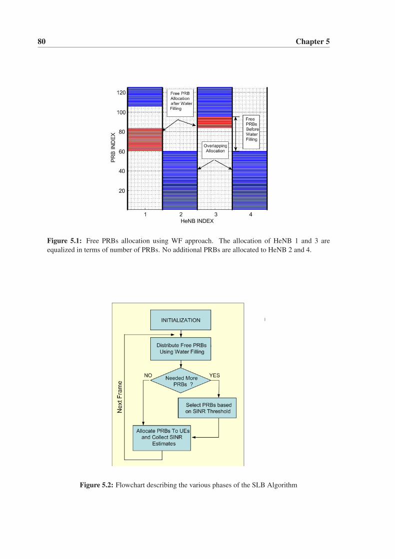
80 Chapter 5
Figure 5.1: Free PRBs allocation using WF approach. The allocation of HeNB 1 and 3 areequalized in terms of number of PRBs. No additional PRBs are allocated to HeNB 2 and 4.
Figure 5.2: Flowchart describing the various phases of the SLB Algorithm
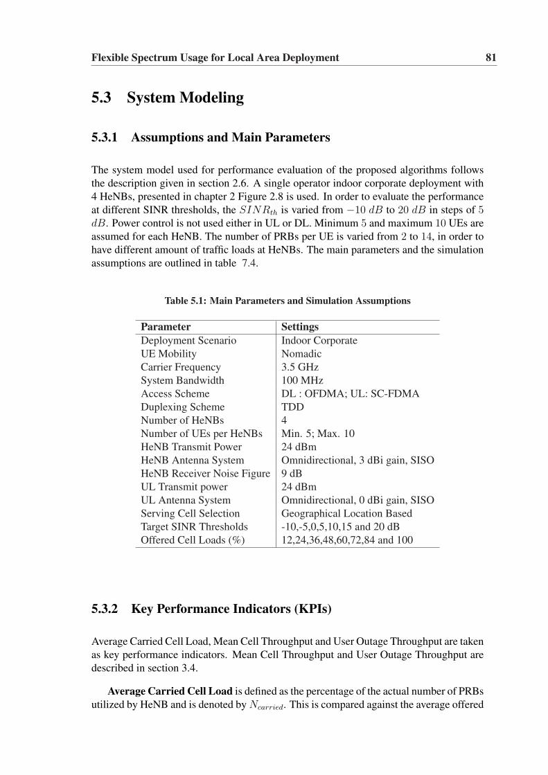
Flexible Spectrum Usage for Local Area Deployment 81
5.3 System Modeling
5.3.1 Assumptions and Main Parameters
The system model used for performance evaluation of the proposed algorithms followsthe description given in section 2.6. A single operator indoor corporate deployment with4 HeNBs, presented in chapter 2 Figure 2.8 is used. In order to evaluate the performanceat different SINR thresholds, the SINRth is varied from −10 dB to 20 dB in steps of 5dB. Power control is not used either in UL or DL. Minimum 5 and maximum 10 UEs areassumed for each HeNB. The number of PRBs per UE is varied from 2 to 14, in order tohave different amount of traffic loads at HeNBs. The main parameters and the simulationassumptions are outlined in table 7.4.
Table 5.1: Main Parameters and Simulation Assumptions
Parameter SettingsDeployment Scenario Indoor CorporateUE Mobility NomadicCarrier Frequency 3.5 GHzSystem Bandwidth 100 MHzAccess Scheme DL : OFDMA; UL: SC-FDMADuplexing Scheme TDDNumber of HeNBs 4Number of UEs per HeNBs Min. 5; Max. 10HeNB Transmit Power 24 dBmHeNB Antenna System Omnidirectional, 3 dBi gain, SISOHeNB Receiver Noise Figure 9 dBUL Transmit power 24 dBmUL Antenna System Omnidirectional, 0 dBi gain, SISOServing Cell Selection Geographical Location BasedTarget SINR Thresholds -10,-5,0,5,10,15 and 20 dBOffered Cell Loads (%) 12,24,36,48,60,72,84 and 100
5.3.2 Key Performance Indicators (KPIs)
Average Carried Cell Load, Mean Cell Throughput and User Outage Throughput are takenas key performance indicators. Mean Cell Throughput and User Outage Throughput aredescribed in section 3.4.
Average Carried Cell Load is defined as the percentage of the actual number of PRBsutilized by HeNB and is denoted by Ncarried. This is compared against the average offered
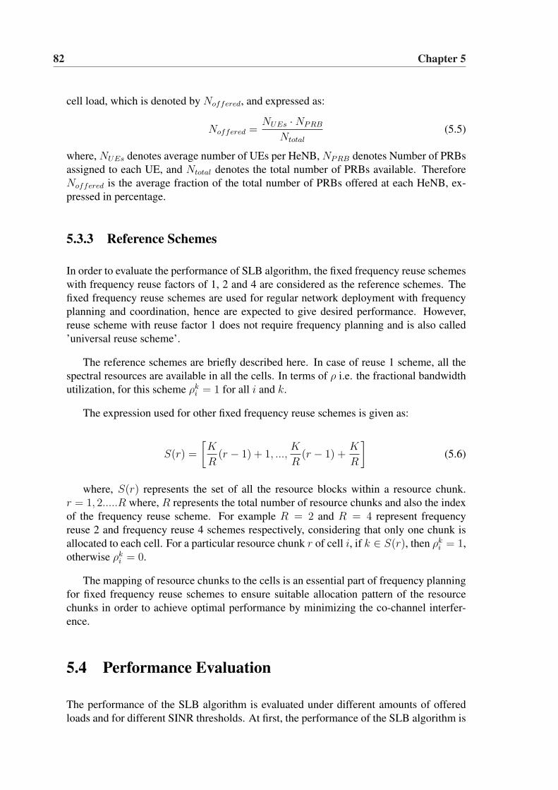
82 Chapter 5
cell load, which is denoted by Noffered, and expressed as:
Noffered =NUEs ·NPRB
Ntotal
(5.5)
where, NUEs denotes average number of UEs per HeNB, NPRB denotes Number of PRBsassigned to each UE, and Ntotal denotes the total number of PRBs available. ThereforeNoffered is the average fraction of the total number of PRBs offered at each HeNB, ex-pressed in percentage.
5.3.3 Reference Schemes
In order to evaluate the performance of SLB algorithm, the fixed frequency reuse schemeswith frequency reuse factors of 1, 2 and 4 are considered as the reference schemes. Thefixed frequency reuse schemes are used for regular network deployment with frequencyplanning and coordination, hence are expected to give desired performance. However,reuse scheme with reuse factor 1 does not require frequency planning and is also called’universal reuse scheme’.
The reference schemes are briefly described here. In case of reuse 1 scheme, all thespectral resources are available in all the cells. In terms of ρ i.e. the fractional bandwidthutilization, for this scheme ρk
i = 1 for all i and k.
The expression used for other fixed frequency reuse schemes is given as:
S(r) =
[K
R(r − 1) + 1, ...,
K
R(r − 1) +
K
R
](5.6)
where, S(r) represents the set of all the resource blocks within a resource chunk.r = 1, 2.....R where, R represents the total number of resource chunks and also the indexof the frequency reuse scheme. For example R = 2 and R = 4 represent frequencyreuse 2 and frequency reuse 4 schemes respectively, considering that only one chunk isallocated to each cell. For a particular resource chunk r of cell i, if k ∈ S(r), then ρk
i = 1,otherwise ρk
i = 0.
The mapping of resource chunks to the cells is an essential part of frequency planningfor fixed frequency reuse schemes to ensure suitable allocation pattern of the resourcechunks in order to achieve optimal performance by minimizing the co-channel interfer-ence.
5.4 Performance Evaluation
The performance of the SLB algorithm is evaluated under different amounts of offeredloads and for different SINR thresholds. At first, the performance of the SLB algorithm is
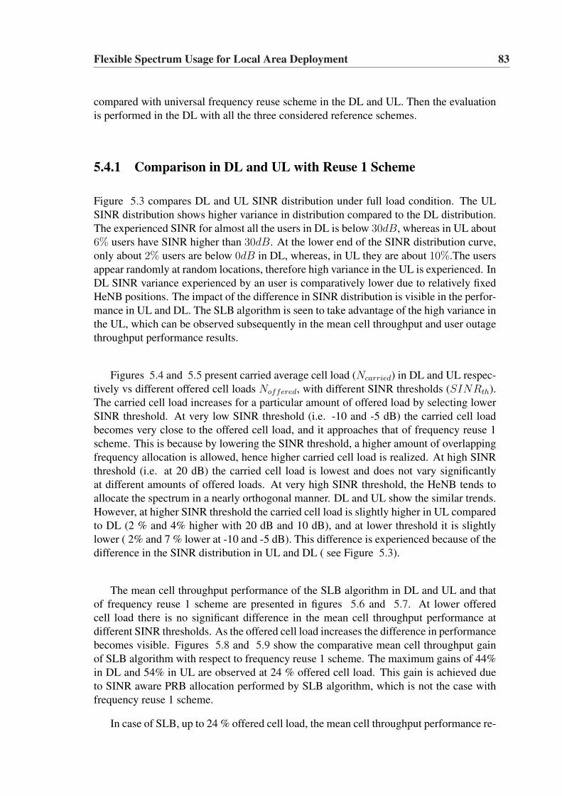
Flexible Spectrum Usage for Local Area Deployment 83
compared with universal frequency reuse scheme in the DL and UL. Then the evaluationis performed in the DL with all the three considered reference schemes.
5.4.1 Comparison in DL and UL with Reuse 1 Scheme
Figure 5.3 compares DL and UL SINR distribution under full load condition. The ULSINR distribution shows higher variance in distribution compared to the DL distribution.The experienced SINR for almost all the users in DL is below 30dB, whereas in UL about6% users have SINR higher than 30dB. At the lower end of the SINR distribution curve,only about 2% users are below 0dB in DL, whereas, in UL they are about 10%.The usersappear randomly at random locations, therefore high variance in the UL is experienced. InDL SINR variance experienced by an user is comparatively lower due to relatively fixedHeNB positions. The impact of the difference in SINR distribution is visible in the perfor-mance in UL and DL. The SLB algorithm is seen to take advantage of the high variance inthe UL, which can be observed subsequently in the mean cell throughput and user outagethroughput performance results.
Figures 5.4 and 5.5 present carried average cell load (Ncarried) in DL and UL respec-tively vs different offered cell loads Noffered, with different SINR thresholds (SINRth).The carried cell load increases for a particular amount of offered load by selecting lowerSINR threshold. At very low SINR threshold (i.e. -10 and -5 dB) the carried cell loadbecomes very close to the offered cell load, and it approaches that of frequency reuse 1scheme. This is because by lowering the SINR threshold, a higher amount of overlappingfrequency allocation is allowed, hence higher carried cell load is realized. At high SINRthreshold (i.e. at 20 dB) the carried cell load is lowest and does not vary significantlyat different amounts of offered loads. At very high SINR threshold, the HeNB tends toallocate the spectrum in a nearly orthogonal manner. DL and UL show the similar trends.However, at higher SINR threshold the carried cell load is slightly higher in UL comparedto DL (2 % and 4% higher with 20 dB and 10 dB), and at lower threshold it is slightlylower ( 2% and 7 % lower at -10 and -5 dB). This difference is experienced because of thedifference in the SINR distribution in UL and DL ( see Figure 5.3).
The mean cell throughput performance of the SLB algorithm in DL and UL and thatof frequency reuse 1 scheme are presented in figures 5.6 and 5.7. At lower offeredcell load there is no significant difference in the mean cell throughput performance atdifferent SINR thresholds. As the offered cell load increases the difference in performancebecomes visible. Figures 5.8 and 5.9 show the comparative mean cell throughput gainof SLB algorithm with respect to frequency reuse 1 scheme. The maximum gains of 44%in DL and 54% in UL are observed at 24 % offered cell load. This gain is achieved dueto SINR aware PRB allocation performed by SLB algorithm, which is not the case withfrequency reuse 1 scheme.
In case of SLB, up to 24 % offered cell load, the mean cell throughput performance re-
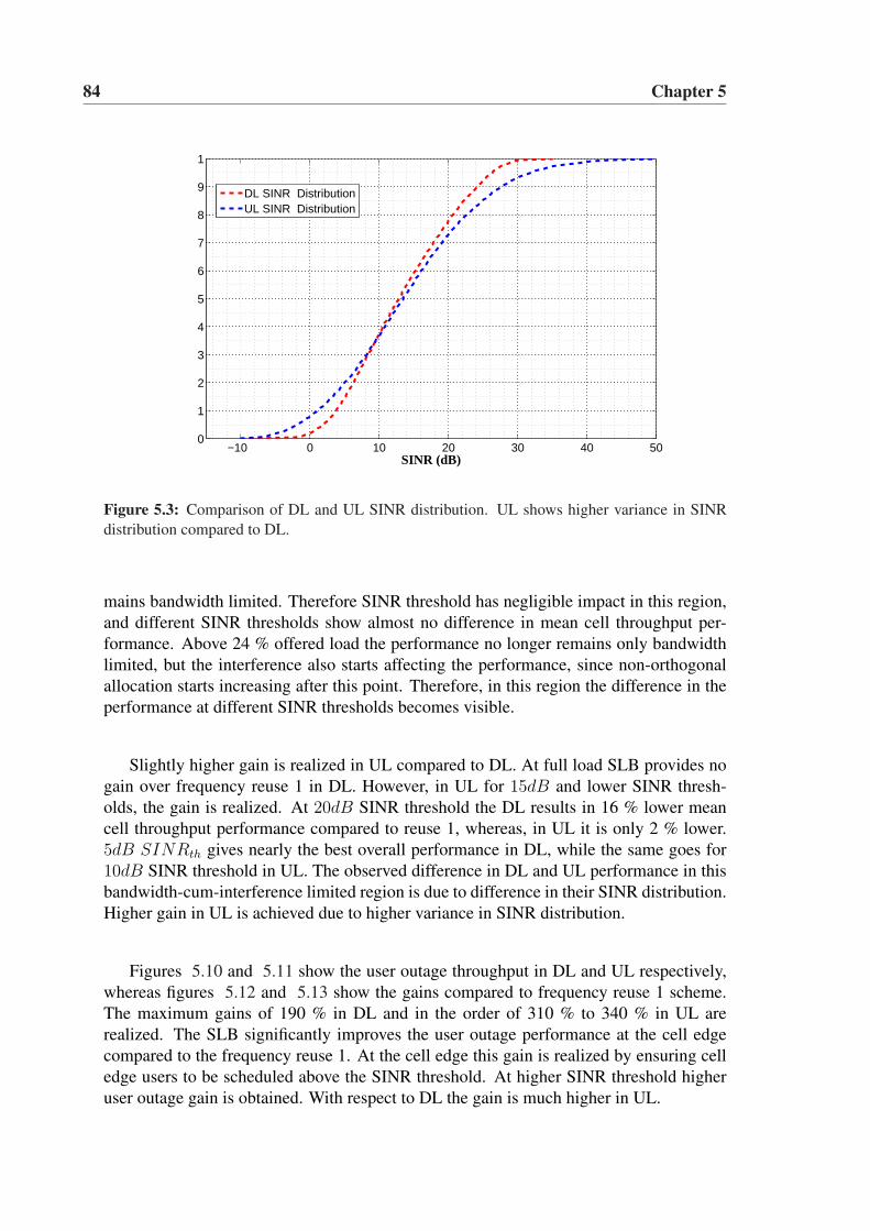
84 Chapter 5
−10 0 10 20 30 40 500
0.1
0.2
0.3
0.4
0.5
0.6
0.7
0.8
0.9
1
SINR (dB)
DL SINR DistributionUL SINR Distribution
Figure 5.3: Comparison of DL and UL SINR distribution. UL shows higher variance in SINRdistribution compared to DL.
mains bandwidth limited. Therefore SINR threshold has negligible impact in this region,and different SINR thresholds show almost no difference in mean cell throughput per-formance. Above 24 % offered load the performance no longer remains only bandwidthlimited, but the interference also starts affecting the performance, since non-orthogonalallocation starts increasing after this point. Therefore, in this region the difference in theperformance at different SINR thresholds becomes visible.
Slightly higher gain is realized in UL compared to DL. At full load SLB provides nogain over frequency reuse 1 in DL. However, in UL for 15dB and lower SINR thresh-olds, the gain is realized. At 20dB SINR threshold the DL results in 16 % lower meancell throughput performance compared to reuse 1, whereas, in UL it is only 2 % lower.5dB SINRth gives nearly the best overall performance in DL, while the same goes for10dB SINR threshold in UL. The observed difference in DL and UL performance in thisbandwidth-cum-interference limited region is due to difference in their SINR distribution.Higher gain in UL is achieved due to higher variance in SINR distribution.
Figures 5.10 and 5.11 show the user outage throughput in DL and UL respectively,whereas figures 5.12 and 5.13 show the gains compared to frequency reuse 1 scheme.The maximum gains of 190 % in DL and in the order of 310 % to 340 % in UL arerealized. The SLB significantly improves the user outage performance at the cell edgecompared to the frequency reuse 1. At the cell edge this gain is realized by ensuring celledge users to be scheduled above the SINR threshold. At higher SINR threshold higheruser outage gain is obtained. With respect to DL the gain is much higher in UL.
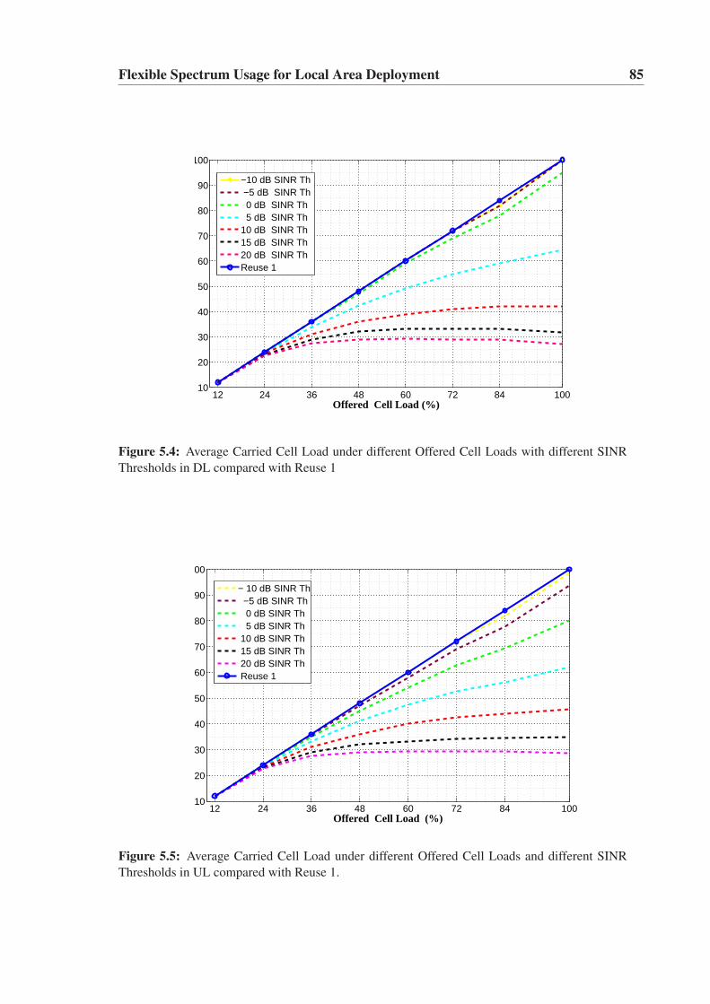
Flexible Spectrum Usage for Local Area Deployment 85
12 24 36 48 60 72 84 10010
20
30
40
50
60
70
80
90
100
Offered Cell Load (%)
−10 dB SINR Th −5 dB SINR Th 0 dB SINR Th 5 dB SINR Th10 dB SINR Th15 dB SINR Th20 dB SINR ThReuse 1
Figure 5.4: Average Carried Cell Load under different Offered Cell Loads with different SINRThresholds in DL compared with Reuse 1
12 24 36 48 60 72 84 10010
20
30
40
50
60
70
80
90
100
Offered Cell Load (%)
− 10 dB SINR Th −5 dB SINR Th 0 dB SINR Th 5 dB SINR Th 10 dB SINR Th 15 dB SINR Th 20 dB SINR Th Reuse 1
Figure 5.5: Average Carried Cell Load under different Offered Cell Loads and different SINRThresholds in UL compared with Reuse 1.
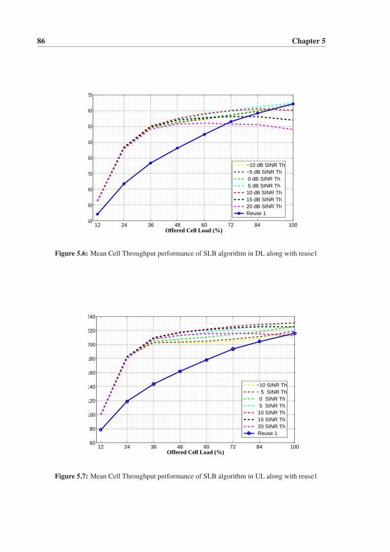
86 Chapter 5
12 24 36 48 60 72 84 10060
80
100
120
140
160
180
200
220
Offered Cell Load (%)
−10 dB SINR Th −5 dB SINR Th 0 dB SINR Th 5 dB SINR Th 10 dB SINR Th 15 dB SINR Th 20 dB SINR Th Reuse 1
Figure 5.6: Mean Cell Throughput performance of SLB algorithm in DL along with reuse1
12 24 36 48 60 72 84 10060
80
100
120
140
160
180
200
220
240
Offered Cell Load (%)
−10 SINR Th − 5 SINR Th 0 SINR Th 5 SINR Th 10 SINR Th 15 SINR Th 20 SINR Th Reuse 1
Figure 5.7: Mean Cell Throughput performance of SLB algorithm in UL along with reuse1
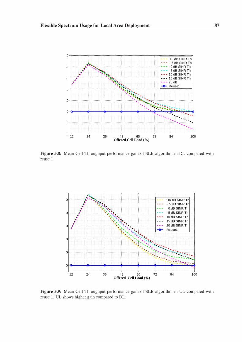
Flexible Spectrum Usage for Local Area Deployment 87
12 24 36 48 60 72 84 100−20
−10
0
10
20
30
40
50
Offered Cell Load (%)
−10 dB SINR Th −5 dB SINR Th 0 dB SINR Th 5 dB SINR Th 10 dB SINR Th 15 dB SINR Th 20 dB Reuse1
Figure 5.8: Mean Cell Throughput performance gain of SLB algorithm in DL compared withreuse 1
12 24 36 48 60 72 84 100
0
10
20
30
40
50
Offered Cell Load (%)
−10 dB SINR Th − 5 dB SINR Th 0 dB SINR Th 5 dB SINR Th 10 dB SINR Th 15 dB SINR Th 20 dB SINR Th Reuse1
Figure 5.9: Mean Cell Throughput performance gain of SLB algorithm in UL compared withreuse 1. UL shows higher gain compared to DL.
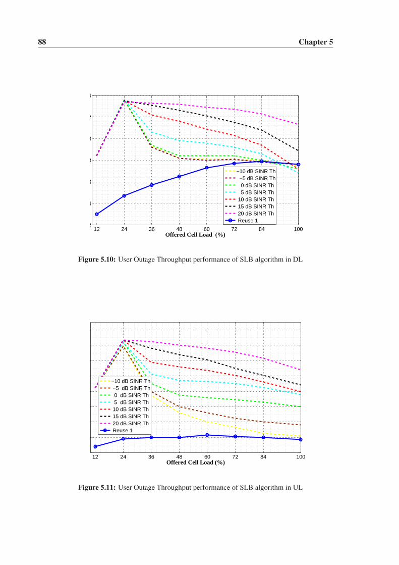
88 Chapter 5
12 24 36 48 60 72 84 1002
4
6
8
10
12
14
Offered Cell Load (%)
−10 dB SINR Th −5 dB SINR Th 0 dB SINR Th 5 dB SINR Th 10 dB SINR Th 15 dB SINR Th 20 dB SINR Th Reuse 1
Figure 5.10: User Outage Throughput performance of SLB algorithm in DL
12 24 36 48 60 72 84 1002
4
6
8
10
12
14
16
18
Offered Cell Load (%)
−10 dB SINR Th −5 dB SINR Th 0 dB SINR Th 5 dB SINR Th 10 dB SINR Th 15 dB SINR Th 20 dB SINR Th Reuse 1
Figure 5.11: User Outage Throughput performance of SLB algorithm in UL
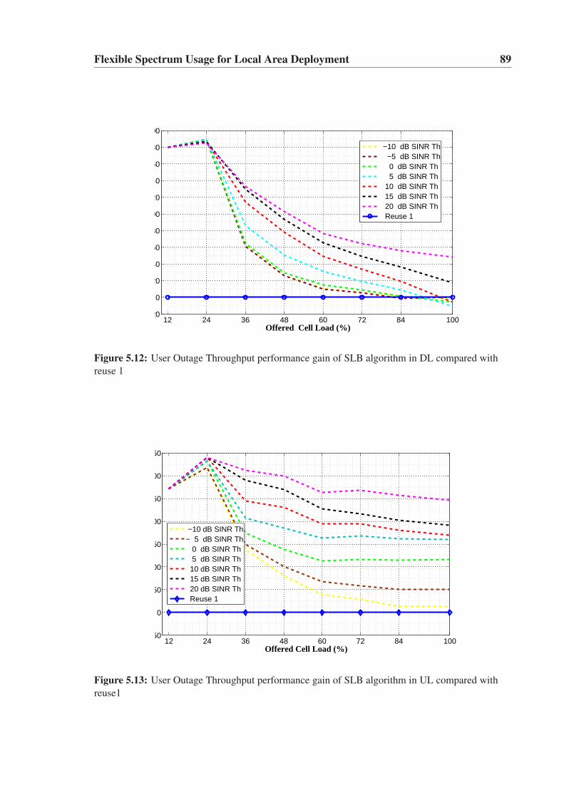
Flexible Spectrum Usage for Local Area Deployment 89
12 24 36 48 60 72 84 100−20
0
20
40
60
80
100
120
140
160
180
200
Offered Cell Load (%)
−10 dB SINR Th −5 dB SINR Th 0 dB SINR Th 5 dB SINR Th 10 dB SINR Th 15 dB SINR Th 20 dB SINR Th Reuse 1
Figure 5.12: User Outage Throughput performance gain of SLB algorithm in DL compared withreuse 1
12 24 36 48 60 72 84 100−50
0
50
100
150
200
250
300
350
Offered Cell Load (%)
−10 dB SINR Th− 5 dB SINR Th 0 dB SINR Th 5 dB SINR Th 10 dB SINR Th 15 dB SINR Th 20 dB SINR Th Reuse 1
Figure 5.13: User Outage Throughput performance gain of SLB algorithm in UL compared withreuse1
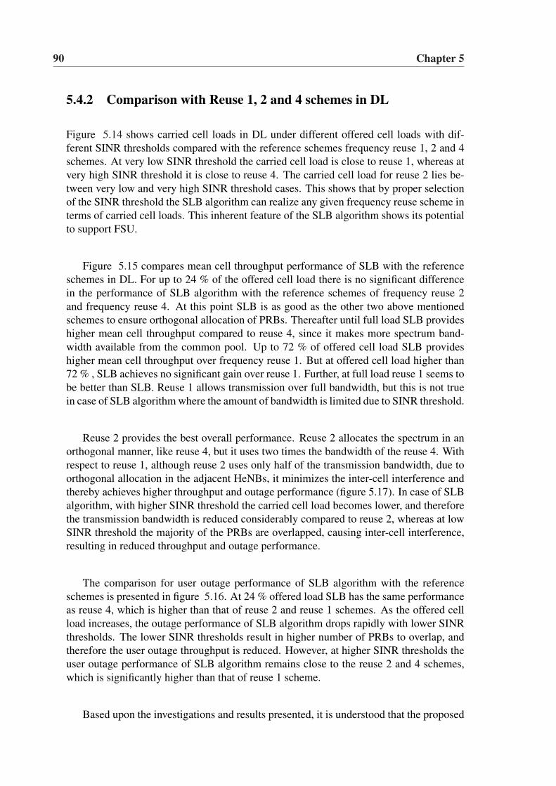
90 Chapter 5
5.4.2 Comparison with Reuse 1, 2 and 4 schemes in DL
Figure 5.14 shows carried cell loads in DL under different offered cell loads with dif-ferent SINR thresholds compared with the reference schemes frequency reuse 1, 2 and 4schemes. At very low SINR threshold the carried cell load is close to reuse 1, whereas atvery high SINR threshold it is close to reuse 4. The carried cell load for reuse 2 lies be-tween very low and very high SINR threshold cases. This shows that by proper selectionof the SINR threshold the SLB algorithm can realize any given frequency reuse scheme interms of carried cell loads. This inherent feature of the SLB algorithm shows its potentialto support FSU.
Figure 5.15 compares mean cell throughput performance of SLB with the referenceschemes in DL. For up to 24 % of the offered cell load there is no significant differencein the performance of SLB algorithm with the reference schemes of frequency reuse 2and frequency reuse 4. At this point SLB is as good as the other two above mentionedschemes to ensure orthogonal allocation of PRBs. Thereafter until full load SLB provideshigher mean cell throughput compared to reuse 4, since it makes more spectrum band-width available from the common pool. Up to 72 % of offered cell load SLB provideshigher mean cell throughput over frequency reuse 1. But at offered cell load higher than72 % , SLB achieves no significant gain over reuse 1. Further, at full load reuse 1 seems tobe better than SLB. Reuse 1 allows transmission over full bandwidth, but this is not truein case of SLB algorithm where the amount of bandwidth is limited due to SINR threshold.
Reuse 2 provides the best overall performance. Reuse 2 allocates the spectrum in anorthogonal manner, like reuse 4, but it uses two times the bandwidth of the reuse 4. Withrespect to reuse 1, although reuse 2 uses only half of the transmission bandwidth, due toorthogonal allocation in the adjacent HeNBs, it minimizes the inter-cell interference andthereby achieves higher throughput and outage performance (figure 5.17). In case of SLBalgorithm, with higher SINR threshold the carried cell load becomes lower, and thereforethe transmission bandwidth is reduced considerably compared to reuse 2, whereas at lowSINR threshold the majority of the PRBs are overlapped, causing inter-cell interference,resulting in reduced throughput and outage performance.
The comparison for user outage performance of SLB algorithm with the referenceschemes is presented in figure 5.16. At 24 % offered load SLB has the same performanceas reuse 4, which is higher than that of reuse 2 and reuse 1 schemes. As the offered cellload increases, the outage performance of SLB algorithm drops rapidly with lower SINRthresholds. The lower SINR thresholds result in higher number of PRBs to overlap, andtherefore the user outage throughput is reduced. However, at higher SINR thresholds theuser outage performance of SLB algorithm remains close to the reuse 2 and 4 schemes,which is significantly higher than that of reuse 1 scheme.
Based upon the investigations and results presented, it is understood that the proposed
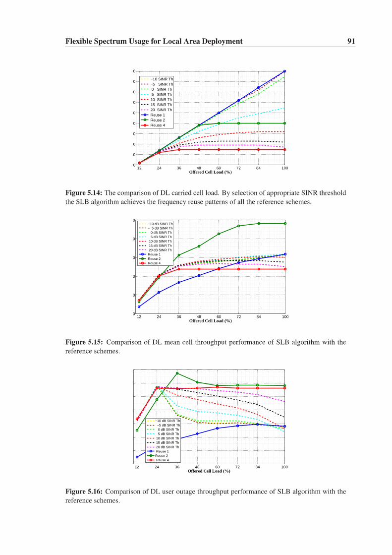
Flexible Spectrum Usage for Local Area Deployment 91
12 24 36 48 60 72 84 10010
20
30
40
50
60
70
80
90
100
Offered Cell Load (%)
−10 SINR Th −5 SINR Th 0 SINR Th 5 SINR Th 10 SINR Th 15 SINR Th 20 SINR Th Reuse 1 Reuse 2 Reuse 4
Figure 5.14: The comparison of DL carried cell load. By selection of appropriate SINR thresholdthe SLB algorithm achieves the frequency reuse patterns of all the reference schemes.
12 24 36 48 60 72 84 10050
100
150
200
250
300
Offered Cell Load (%)
−10 dB SINR Th − 5 dB SINR Th 0 dB SINR Th 5 dB SINR Th 10 dB SINR Th 15 dB SINR Th 20 dB SINR Th Reuse 1 Reuse 2 Reuse 4
Figure 5.15: Comparison of DL mean cell throughput performance of SLB algorithm with thereference schemes.
12 24 36 48 60 72 84 1002
4
6
8
10
12
14
16
Offered Cell Load (%)
−10 dB SINR Th −5 dB SINR Th 0 dB SINR Th 5 dB SINR Th 10 dB SINR Th 15 dB SINR Th 20 dB SINR Th Reuse 1Reuse 2 Reuse 4
Figure 5.16: Comparison of DL user outage throughput performance of SLB algorithm with thereference schemes.
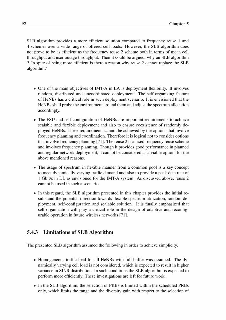
92 Chapter 5
SLB algorithm provides a more efficient solution compared to frequency reuse 1 and4 schemes over a wide range of offered cell loads. However, the SLB algorithm doesnot prove to be as efficient as the frequency reuse 2 scheme both in terms of mean cellthroughput and user outage throughput. Then it could be argued, why an SLB algorithm? In spite of being more efficient is there a reason why reuse 2 cannot replace the SLBalgorithm?
• One of the main objectives of IMT-A in LA is deployment flexibility. It involvesrandom, distributed and uncoordinated deployment. The self-organizing featureof HeNBs has a critical role in such deployment scenario. It is envisioned that theHeNBs shall probe the environment around them and adjust the spectrum allocationaccordingly.
• The FSU and self-configuration of HeNBs are important requirements to achievescalable and flexible deployment and also to ensure coexistence of randomly de-ployed HeNBs. These requirements cannot be achieved by the options that involvefrequency planning and coordination. Therefore it is logical not to consider optionsthat involve frequency planning [71]. The reuse 2 is a fixed frequency reuse schemeand involves frequency planning. Though it provides good performance in plannedand regular network deployment, it cannot be considered as a viable option, for theabove mentioned reasons.
• The usage of spectrum in flexible manner from a common pool is a key conceptto meet dynamically varying traffic demand and also to provide a peak data rate of1 Gbit/s in DL as envisioned for the IMT-A system. As discussed above, reuse 2cannot be used in such a scenario.
• In this regard, the SLB algorithm presented in this chapter provides the initial re-sults and the potential direction towards flexible spectrum utilization, random de-ployment, self-configuration and scalable solution. It is finally emphasized thatself-organization will play a critical role in the design of adaptive and reconfig-urable operation in future wireless networks [71].
5.4.3 Limitations of SLB Algorithm
The presented SLB algorithm assumed the following in order to achieve simplicity.
• Homogeneous traffic load for all HeNBs with full buffer was assumed. The dy-namically varying cell load is not considered, which is expected to result in highervariance in SINR distribution. In such conditions the SLB algorithm is expected toperform more efficiently. These investigations are left for future work.
• In the SLB algorithm, the selection of PRBs is limited within the scheduled PRBsonly, which limits the range and the diversity gain with respect to the selection of
Flexible Spectrum Usage for Local Area Deployment 93
PRBs from the full range of PRBs. This assumption was made in order to avoidthe complexity in SINR estimation over the full range of PRBs, and also to save thebattery life of UEs. Estimation of pilots over the whole spectrum involves powerconsumption at the UE. It Also increases the signaling overhead. Therefore weconsider that the UEs sense the pilots over the scheduled PRBs only.
5.5 Resource Chunk Selection (RCS) Algorithm
5.5.1 Motivation and Aim for the Algorithm
During the performance evaluation of the SLB algorithm it was found that the fixedfrequency reuse 2 scheme achieves the highest mean cell throughput and user outagethroughput performance compared to all the other schemes in consideration. Fixed fre-quency reuse 2 scheme requires that the assignment of spectrum chunks to the HeNBsmust be pre-planned so that the strongest interference can be avoided for optimized per-formance. In a regular network deployment this configuration can easily be achieved,however, in the assumed LA scenarios no such planning is feasible, where the deploy-ment is assumed to be random and uncoordinated. Therefore a mechanism is needed toresult in frequency reuse 2-like configuration in a self-organized manner in the absence ofany coordination and network planning.
Keeping the above mentioned points in view, a comparative interference thresholdbased Resource Chunk Selection (RCS) algorithm is proposed. The chunk refers to thepart of the system bandwidth allocated to one HeNB. In case of frequency reuse 2 thewhole system bandwidth is divided in two equal size chunks; one chunk is allocated toeach HeNB keeping in view to avoid the allocation of the same chunk to adjacent HeNBs.Since we aim to achieve a comparable performance with frequency reuse 2 configuration,therefore, as a starting point we consider that the RCS algorithm also divides the total sys-tem bandwidth in two equal size chunks. However, the RCS algorithm is not limited to thefrequency reuse 2 like configuration. This algorithm can easily be adopted to approach theconfiguration of any other frequency reuse scheme. The proposed RCS algorithm startswith random selection of a chunk at each HeNB and aims to achieve frequency reuse 2like configuration in self organized manner. The main motivation for this algorithm isto provide a self-configurable and scalable solution for random and uncoordinated LAdeployment scenario with improved performance over SLB algorithm and close to fre-quency reuse 2 scheme.
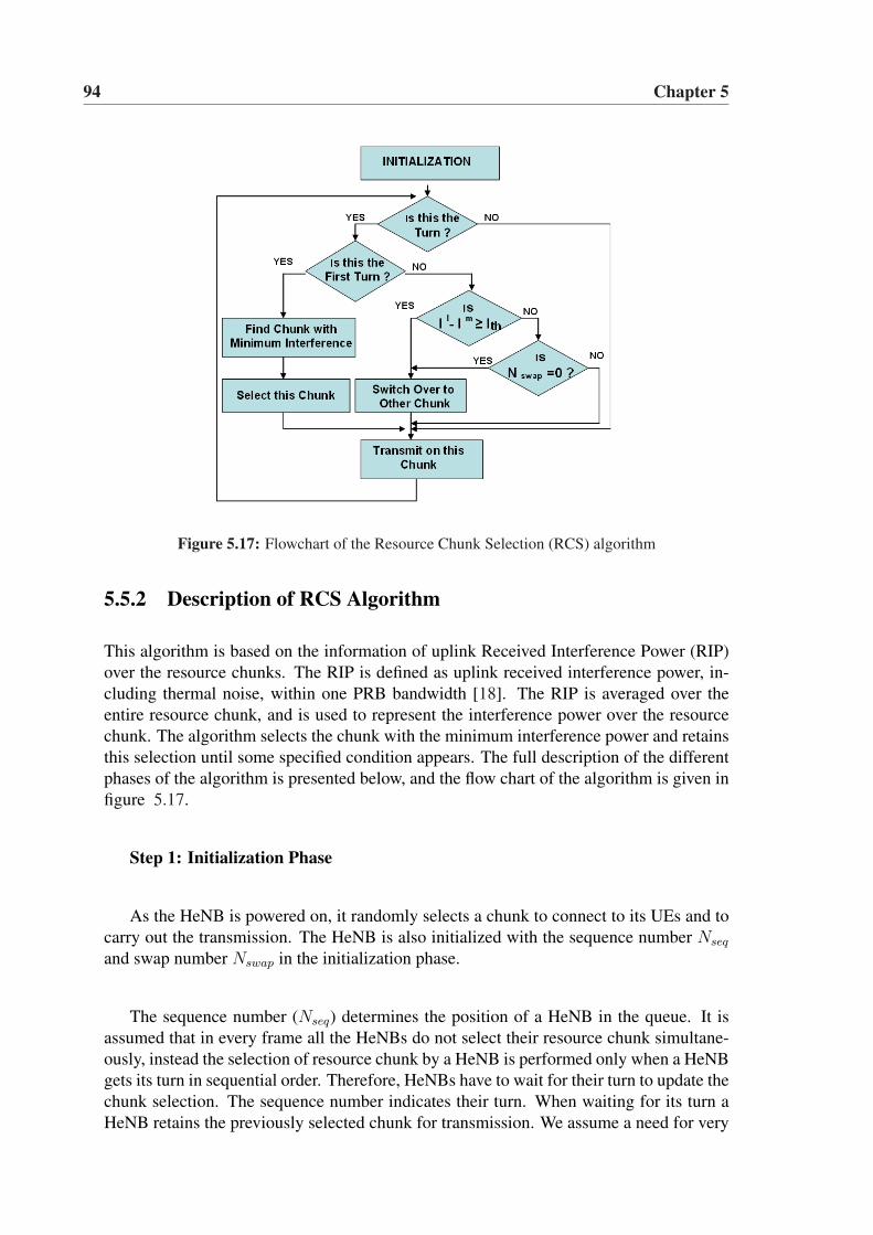
94 Chapter 5
Figure 5.17: Flowchart of the Resource Chunk Selection (RCS) algorithm
5.5.2 Description of RCS Algorithm
This algorithm is based on the information of uplink Received Interference Power (RIP)over the resource chunks. The RIP is defined as uplink received interference power, in-cluding thermal noise, within one PRB bandwidth [18]. The RIP is averaged over theentire resource chunk, and is used to represent the interference power over the resourcechunk. The algorithm selects the chunk with the minimum interference power and retainsthis selection until some specified condition appears. The full description of the differentphases of the algorithm is presented below, and the flow chart of the algorithm is given infigure 5.17.
Step 1: Initialization Phase
As the HeNB is powered on, it randomly selects a chunk to connect to its UEs and tocarry out the transmission. The HeNB is also initialized with the sequence number Nseq
and swap number Nswap in the initialization phase.
The sequence number (Nseq) determines the position of a HeNB in the queue. It isassumed that in every frame all the HeNBs do not select their resource chunk simultane-ously, instead the selection of resource chunk by a HeNB is performed only when a HeNBgets its turn in sequential order. Therefore, HeNBs have to wait for their turn to update thechunk selection. The sequence number indicates their turn. When waiting for its turn aHeNB retains the previously selected chunk for transmission. We assume a need for very
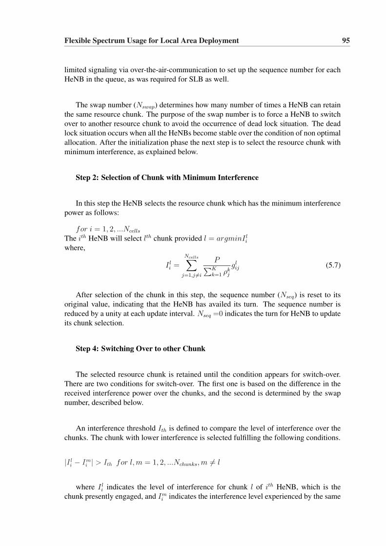
Flexible Spectrum Usage for Local Area Deployment 95
limited signaling via over-the-air-communication to set up the sequence number for eachHeNB in the queue, as was required for SLB as well.
The swap number (Nswap) determines how many number of times a HeNB can retainthe same resource chunk. The purpose of the swap number is to force a HeNB to switchover to another resource chunk to avoid the occurrence of dead lock situation. The deadlock situation occurs when all the HeNBs become stable over the condition of non optimalallocation. After the initialization phase the next step is to select the resource chunk withminimum interference, as explained below.
Step 2: Selection of Chunk with Minimum Interference
In this step the HeNB selects the resource chunk which has the minimum interferencepower as follows:
for i = 1, 2, ...Ncells
The ith HeNB will select lth chunk provided l = argminI li
where,
I li =
Ncells∑
j=1,j 6=i
P∑Kk=1 ρk
j
glij (5.7)
After selection of the chunk in this step, the sequence number (Nseq) is reset to itsoriginal value, indicating that the HeNB has availed its turn. The sequence number isreduced by a unity at each update interval. Nseq =0 indicates the turn for HeNB to updateits chunk selection.
Step 4: Switching Over to other Chunk
The selected resource chunk is retained until the condition appears for switch-over.There are two conditions for switch-over. The first one is based on the difference in thereceived interference power over the chunks, and the second is determined by the swapnumber, described below.
An interference threshold Ith is defined to compare the level of interference over thechunks. The chunk with lower interference is selected fulfilling the following conditions.
|I li − Im
i | > Ith for l, m = 1, 2, ...Nchunks, m 6= l
where I li indicates the level of interference for chunk l of ith HeNB, which is the
chunk presently engaged, and Imi indicates the interference level experienced by the same
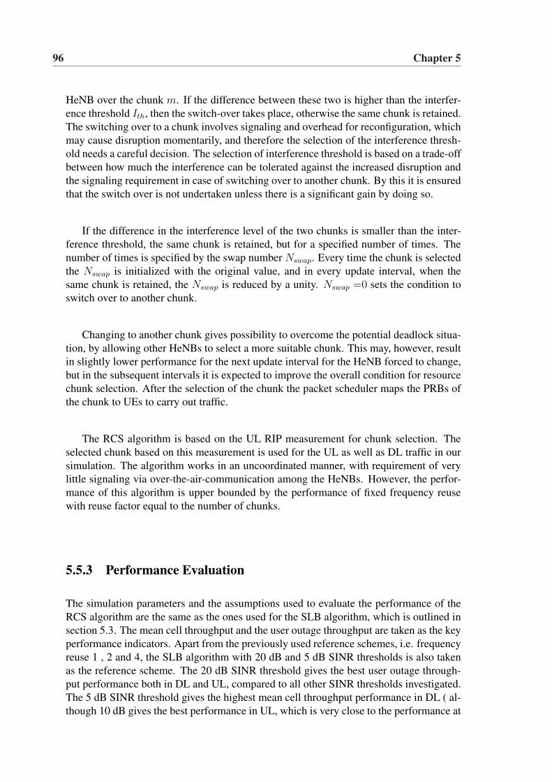
96 Chapter 5
HeNB over the chunk m. If the difference between these two is higher than the interfer-ence threshold Ith, then the switch-over takes place, otherwise the same chunk is retained.The switching over to a chunk involves signaling and overhead for reconfiguration, whichmay cause disruption momentarily, and therefore the selection of the interference thresh-old needs a careful decision. The selection of interference threshold is based on a trade-offbetween how much the interference can be tolerated against the increased disruption andthe signaling requirement in case of switching over to another chunk. By this it is ensuredthat the switch over is not undertaken unless there is a significant gain by doing so.
If the difference in the interference level of the two chunks is smaller than the inter-ference threshold, the same chunk is retained, but for a specified number of times. Thenumber of times is specified by the swap number Nswap. Every time the chunk is selectedthe Nswap is initialized with the original value, and in every update interval, when thesame chunk is retained, the Nswap is reduced by a unity. Nswap =0 sets the condition toswitch over to another chunk.
Changing to another chunk gives possibility to overcome the potential deadlock situa-tion, by allowing other HeNBs to select a more suitable chunk. This may, however, resultin slightly lower performance for the next update interval for the HeNB forced to change,but in the subsequent intervals it is expected to improve the overall condition for resourcechunk selection. After the selection of the chunk the packet scheduler maps the PRBs ofthe chunk to UEs to carry out traffic.
The RCS algorithm is based on the UL RIP measurement for chunk selection. Theselected chunk based on this measurement is used for the UL as well as DL traffic in oursimulation. The algorithm works in an uncoordinated manner, with requirement of verylittle signaling via over-the-air-communication among the HeNBs. However, the perfor-mance of this algorithm is upper bounded by the performance of fixed frequency reusewith reuse factor equal to the number of chunks.
5.5.3 Performance Evaluation
The simulation parameters and the assumptions used to evaluate the performance of theRCS algorithm are the same as the ones used for the SLB algorithm, which is outlined insection 5.3. The mean cell throughput and the user outage throughput are taken as the keyperformance indicators. Apart from the previously used reference schemes, i.e. frequencyreuse 1 , 2 and 4, the SLB algorithm with 20 dB and 5 dB SINR thresholds is also takenas the reference scheme. The 20 dB SINR threshold gives the best user outage through-put performance both in DL and UL, compared to all other SINR thresholds investigated.The 5 dB SINR threshold gives the highest mean cell throughput performance in DL ( al-though 10 dB gives the best performance in UL, which is very close to the performance at
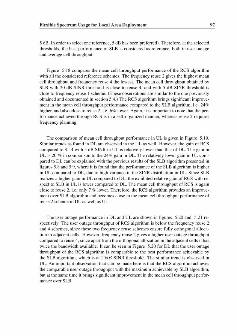
Flexible Spectrum Usage for Local Area Deployment 97
5 dB. In order to select one reference, 5 dB has been preferred). Therefore, at the selectedthresholds, the best performance of SLB is considered as reference, both in user outageand average cell throughput.
Figure 5.18 compares the mean cell throughput performance of the RCS algorithmwith all the considered reference schemes. The frequency reuse 2 gives the highest meancell throughput and frequency reuse 4 the lowest. The mean cell throughput obtained bySLB with 20 dB SINR threshold is close to reuse 4, and with 5 dB SINR threshold isclose to frequency reuse 1 scheme. (These observations are similar to the one previouslyobtained and documented in section 5.4.) The RCS algorithm brings significant improve-ment in the mean cell throughput performance compared to the SLB algorithm, i.e. 24%higher, and also close to reuse 2, i.e. 6% lower. Again, it is important to note that the per-formance achieved through RCS is in a self-organized manner, whereas reuse 2 requiresfrequency planning.
The comparison of mean cell throughput performance in UL is given in Figure 5.19.Similar trends as found in DL are observed in the UL as well. However, the gain of RCScompared to SLB with 5 dB SINR in UL is relatively lower than that of DL. The gain inUL is 20 % in comparison to the 24% gain in DL. The relatively lower gain in UL com-pared to DL can be explained with the previous results of the SLB algorithm presented infigures 5.8 and 5.9, where it is found that the performance of the SLB algorithm is higherin UL compared to DL, due to high variance in the SINR distribution in UL. Since SLBrealizes a higher gain in UL compared to DL, the exhibited relative gain of RCS with re-spect to SLB in UL is lower compared to DL. The mean cell throughput of RCS is againclose to reuse 2, i.e. only 7 % lower. Therefore, the RCS algorithm provides an improve-ment over SLB algorithm and becomes close to the mean cell throughput performance ofreuse 2 scheme in DL as well as UL.
The user outage performance in DL and UL are shown in figures 5.20 and 5.21 re-spectively. The user outage throughput of RCS algorithm is below the frequency reuse 2and 4 schemes, since these two frequency reuse schemes ensure fully orthogonal alloca-tion in adjacent cells. However, frequency reuse 2 gives a higher user outage throughputcompared to reuse 4, since apart from the orthogonal allocation in the adjacent cells it hastwice the bandwidth available. It can be seen in Figure 5.20 for DL that the user outagethroughput of the RCS algorithm is comparable to the best performance achievable bythe SLB algorithm, which is at 20dB SINR threshold. The similar trend is observed inUL. An important observation that can be made here is that the RCS algorithm achievesthe comparable user outage throughput with the maximum achievable by SLB algorithm,but at the same time it brings significant improvement in the mean cell throughput perfor-mance over SLB.
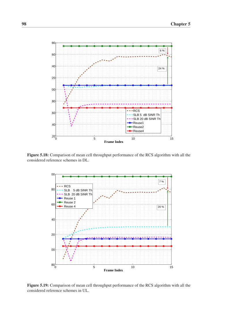
98 Chapter 5
0 5 10 15120
140
160
180
200
220
240
260
280
Frame Index
RCS SLB 5 dB SINR ThSLB 20 dB SINR ThReuse1 Reuse2Reuse4
24 %
6 %
Figure 5.18: Comparison of mean cell throughput performance of the RCS algorithm with all theconsidered reference schemes in DL.
0 5 10 15180
200
220
240
260
280
300
Frame Index
RCS SLB 5 dB SINR Th SLB 20 dB SINR Th Reuse 1 Reuse 2 Reuse 4 20 %
7 %
Figure 5.19: Comparison of mean cell throughput performance of the RCS algorithm with all theconsidered reference schemes in UL.
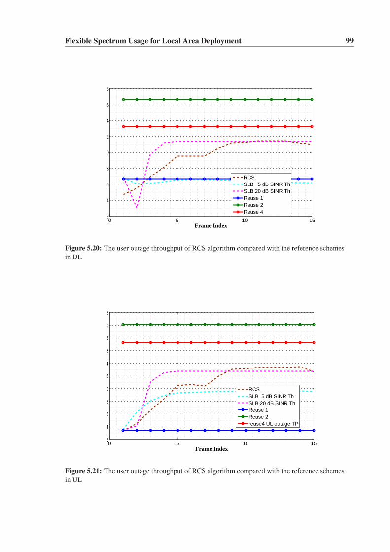
Flexible Spectrum Usage for Local Area Deployment 99
0 5 10 152
4
6
8
10
12
14
16
18
Frame Index
RCSSLB 5 dB SINR ThSLB 20 dB SINR ThReuse 1Reuse 2 Reuse 4
Figure 5.20: The user outage throughput of RCS algorithm compared with the reference schemesin DL
0 5 10 152
4
6
8
10
12
14
16
18
20
22
Frame Index
RCSSLB 5 dB SINR ThSLB 20 dB SINR ThReuse 1 Reuse 2 reuse4 UL outage TP
Figure 5.21: The user outage throughput of RCS algorithm compared with the reference schemesin UL
5.6 Conclusions
Currently HeNB is emerging as a potential solution for high quality and high data rateservices in local area indoor environment. A large scale, random and uncoordinated de-ployment of HeNBs is envisioned in near future. This will require a mechanism to supportself-configurable and scalable deployment. The Flexible Spectrum usage (FSU) is con-sidered as key enabler for such deployment scenario.
This chapter proposes Spectrum Load Balancing (SLB) and Resource Chunk Selec-tion (RCS) algorithms for FSU. The SLB is SINR threshold-based, whereas RCS is acomparative interference threshold-based algorithm. Both algorithms work on the princi-ple of self assessment of surrounding radio environment and ensure coexistence of HeNBsby partially or completely preventing mutual interference on the shared spectrum. The al-gorithms support self configurable deployment of HeNBs.
The proposed algorithms are compared with fixed frequency reuse 1, 2 and 4 schemes.The SLB algorithm is found to provide higher average cell throughput and user outagethroughput performance compared to reuse 1 and 4 schemes over a wide range of offeredcell loads. However, the SLB is outperformed by reuse2 scheme. One important charac-teristic of SLB is that, it can resemble any given fixed frequency reuse pattern by properselection of SINR threshold, therefore it supports FSU.
The RCS algorithm has been proposed to further improve the performance over SLB.The mean cell throughput and user outage throughput achieved by RCS is significantlyhigher compared to SLB. The throughput provided by RCS is close to reuse 2 scheme.However, in terms of outage, the reuse 2 still gives higher performance in the given sce-nario. The significance of the RCS algorithm is, it achieves the performance in self-organized manner in the uncoordinated and random deployment scenario. Whereas reuse2 performs in regular deployment with frequency planning, which is potentially not feasi-ble in the envisioned scenario.
The proposed algorithms support flexible spectrum usage, self configuration, flexibleand scalable deployment. Therefore, the algorithms are suitable for implementation in thelocal area solution envisioned for IMT-A systems.
Chapter 6
Autonomous Component CarrierSelection for Local Area Deployment
6.1 Introduction
The LTE Release’8 standardization is coming to its completion and the focus is nowgradually shifting towards its further evolution, referred to as LTE-A. One of the goals ofthis evolution is to reach and even surpass the requirements of IMT-A in terms of data ratesand low cost deployment. This includes the possibility for peak data rates up to 1 Gbpsin Downlink (DL) and 500 Mbps in Uplink (UL) [72],[7] and [6]. Such high data ratetargets can only be fulfilled in a reasonable way with a further increase of the transmissionbandwidth. A transmission bandwidth up to 100 MHz has been considered in the contextof LTE-A [6]. Such a bandwidth extension should be done while preserving the backwardspectrum compatibility, since LTE-A will be an evolution of LTE. A direct consequence ofthis requirement is that an LTE-A network should appear as an LTE network for a legacyterminal. Such compatibility is of critical importance for a smooth transition to LTE-Acapabilities.
6.1.1 Carrier Aggregation
The bandwidth extension for LTE-A can be achieved by carrier aggregation [73] and [74].The carrier aggregation can also fulfill the requirement of backward compatibility, wheremultiple LTE component carriers are aggregated to provide the desired LTE-A systembandwidth [72], [75] and [76]. Further, it is expressed that operation of LTE and LTE-Ashould be possible over the same radio spectrum [6]. In this context, a LTE terminal canreceive one of these component carriers while an an LTE-A terminal can simultaneouslyaccess multiple component carriers.
In principle, the aggregation of component carriers could be either contiguous or non
101
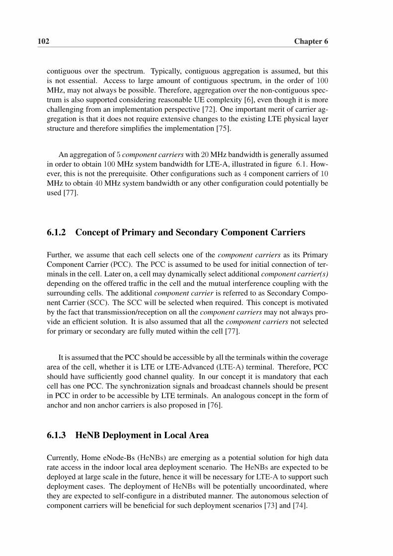
102 Chapter 6
contiguous over the spectrum. Typically, contiguous aggregation is assumed, but thisis not essential. Access to large amount of contiguous spectrum, in the order of 100MHz, may not always be possible. Therefore, aggregation over the non-contiguous spec-trum is also supported considering reasonable UE complexity [6], even though it is morechallenging from an implementation perspective [72]. One important merit of carrier ag-gregation is that it does not require extensive changes to the existing LTE physical layerstructure and therefore simplifies the implementation [75].
An aggregation of 5 component carriers with 20 MHz bandwidth is generally assumedin order to obtain 100 MHz system bandwidth for LTE-A, illustrated in figure 6.1. How-ever, this is not the prerequisite. Other configurations such as 4 component carriers of 10MHz to obtain 40 MHz system bandwidth or any other configuration could potentially beused [77].
6.1.2 Concept of Primary and Secondary Component Carriers
Further, we assume that each cell selects one of the component carriers as its PrimaryComponent Carrier (PCC). The PCC is assumed to be used for initial connection of ter-minals in the cell. Later on, a cell may dynamically select additional component carrier(s)depending on the offered traffic in the cell and the mutual interference coupling with thesurrounding cells. The additional component carrier is referred to as Secondary Compo-nent Carrier (SCC). The SCC will be selected when required. This concept is motivatedby the fact that transmission/reception on all the component carriers may not always pro-vide an efficient solution. It is also assumed that all the component carriers not selectedfor primary or secondary are fully muted within the cell [77].
It is assumed that the PCC should be accessible by all the terminals within the coveragearea of the cell, whether it is LTE or LTE-Advanced (LTE-A) terminal. Therefore, PCCshould have sufficiently good channel quality. In our concept it is mandatory that eachcell has one PCC. The synchronization signals and broadcast channels should be presentin PCC in order to be accessible by LTE terminals. An analogous concept in the form ofanchor and non anchor carriers is also proposed in [76].
6.1.3 HeNB Deployment in Local Area
Currently, Home eNode-Bs (HeNBs) are emerging as a potential solution for high datarate access in the indoor local area deployment scenario. The HeNBs are expected to bedeployed at large scale in the future, hence it will be necessary for LTE-A to support suchdeployment cases. The deployment of HeNBs will be potentially uncoordinated, wherethey are expected to self-configure in a distributed manner. The autonomous selection ofcomponent carriers will be beneficial for such deployment scenarios [73] and [74].
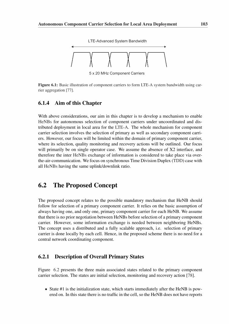
Autonomous Component Carrier Selection for Local Area Deployment 103
Figure 6.1: Basic illustration of component carriers to form LTE-A system bandwidth using car-rier aggregation [77].
6.1.4 Aim of this Chapter
With above considerations, our aim in this chapter is to develop a mechanism to enableHeNBs for autonomous selection of component carriers under uncoordinated and dis-tributed deployment in local area for the LTE-A. The whole mechanism for componentcarrier selection involves the selection of primary as well as secondary component carri-ers. However, our focus will be limited within the domain of primary component carrier,where its selection, quality monitoring and recovery actions will be outlined. Our focuswill primarily be on single operator case. We assume the absence of X2 interface, andtherefore the inter HeNBs exchange of information is considered to take place via over-the-air-communication. We focus on synchronous Time Division Duplex (TDD) case withall HeNBs having the same uplink/downlink ratio.
6.2 The Proposed Concept
The proposed concept relates to the possible mandatory mechanism that HeNB shouldfollow for selection of a primary component carrier. It relies on the basic assumption ofalways having one, and only one, primary component carrier for each HeNB. We assumethat there is no prior negotiation between HeNBs before selection of a primary componentcarrier. However, some information exchange is needed between neighboring HeNBs.The concept uses a distributed and a fully scalable approach, i.e. selection of primarycarrier is done locally by each cell. Hence, in the proposed scheme there is no need for acentral network coordinating component.
6.2.1 Description of Overall Primary States
Figure 6.2 presents the three main associated states related to the primary componentcarrier selection. The states are initial selection, monitoring and recovery action [78].
• State #1 is the initialization state, which starts immediately after the HeNB is pow-ered on. In this state there is no traffic in the cell, so the HeNB does not have reports
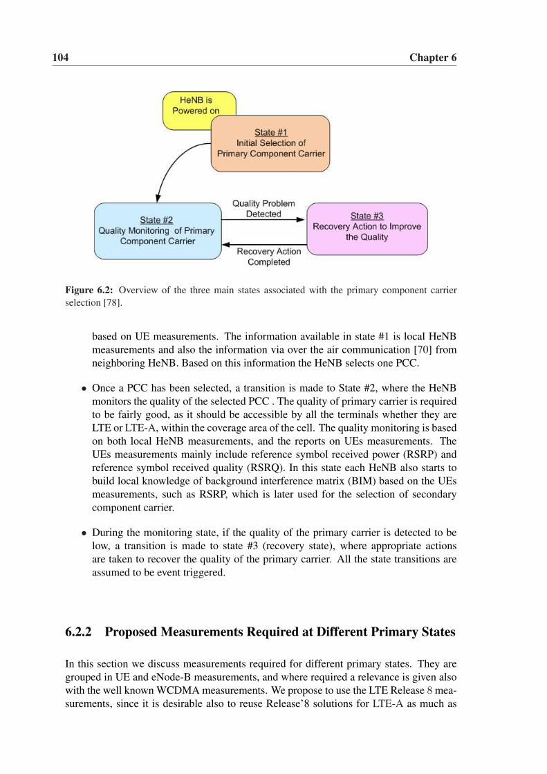
104 Chapter 6
Figure 6.2: Overview of the three main states associated with the primary component carrierselection [78].
based on UE measurements. The information available in state #1 is local HeNBmeasurements and also the information via over the air communication [70] fromneighboring HeNB. Based on this information the HeNB selects one PCC.
• Once a PCC has been selected, a transition is made to State #2, where the HeNBmonitors the quality of the selected PCC . The quality of primary carrier is requiredto be fairly good, as it should be accessible by all the terminals whether they areLTE or LTE-A, within the coverage area of the cell. The quality monitoring is basedon both local HeNB measurements, and the reports on UEs measurements. TheUEs measurements mainly include reference symbol received power (RSRP) andreference symbol received quality (RSRQ). In this state each HeNB also starts tobuild local knowledge of background interference matrix (BIM) based on the UEsmeasurements, such as RSRP, which is later used for the selection of secondarycomponent carrier.
• During the monitoring state, if the quality of the primary carrier is detected to below, a transition is made to state #3 (recovery state), where appropriate actionsare taken to recover the quality of the primary carrier. All the state transitions areassumed to be event triggered.
6.2.2 Proposed Measurements Required at Different Primary States
In this section we discuss measurements required for different primary states. They aregrouped in UE and eNode-B measurements, and where required a relevance is given alsowith the well known WCDMA measurements. We propose to use the LTE Release 8 mea-surements, since it is desirable also to reuse Release’8 solutions for LTE-A as much as
Autonomous Component Carrier Selection for Local Area Deployment 105
possible [24].
UE Measurements
Reference signal received power (RSRP), is determined for a considered cell as thelinear average over the power contributions (in[W])of the resource elements that carrycell-specific reference signals within the considered measurement frequency bandwidth[79]. This provides measurement on DL signal strength and is reported by UEs to theserving eNode-B.
Received Signal Strength Indicator (RSSI), is comprised of the total received wide-band power observed by the UE from all sources, including co-channel serving and nonserving cells, adjacent channel interference and thermal noise etc. The measurement isperformed over the bandwidth defined by the receiver pulse shaping filter [79].
Reference Signal Received Quality (RSRQ) is defined as the ratio N ∗ RSRPRSSI
, whereN is the number of resource blocks of the RSSI measurement bandwidth. The measure-ments in the numerator and denominator shall be made over the same set of resourceblocks [79].
HeNB Measurements
Downlink Reference Signal Transmit (DL RS TX) power is determined for a con-sidered cell as the linear average over the power contributions (in [W])of the resourceelements that carry cell-specific reference signals which are transmitted by the eNode-Bwithin its operating system bandwidth. This represents the measurement of eNode-B DLtransmit power over reference symbols. Our assumption is that this measurement can beexchanged between HeNBs via over-the-air-communication, so one HeNB knows the DLRS Tx power of the neighboring HeNBs.
The Uplink Received Interference Power (RIP)is defined as uplink received inter-ference power, including thermal noise, within one PRB bandwidth. The RIP measure-ment is in a certain manner similar to WCDMA RTWP (Received Total Wideband Power)measurement. Where it can be understood as RTWP = RIP + wanted signal.
Path Loss Estimates towards Neighboring HeNBs: The eNode-B to eNode-B pathloss measurements could in principle be measured by the RSRP from other eNode-Bs dur-ing time periods where those are transmitting in the DL. Such measurements, combinedwith knowledge of the corresponding DL RS Tx power, can be used to get the knowledgeof path loss towards the neighboring eNode-Bs. A eNode-B measuring the RSRP from
106 Chapter 6
another eNode-B will have to be completely muted with no transmission, in this regardsimilar to the UE RSRP measurement. We assume that the HeNB measures the RSRP onPCC of the surrounding cells.
UL SINR is defined as the ratio of the received power of the reference signal trans-mitted by the UE to the total interference and noise power received by the eNode-B overthe UE occupied bandwidth.
6.2.3 Algorithm for Initial Selection of Primary Component Carrier
The proposed algorithm provides a simple and fully distributed approach for the initial se-lection of PCC after the HeNB is powered on. The initial selection of PCC is mainly basedon the local HeNB measurements and the information from neighboring HeNBs about thecarriers they use as their primary and secondary. At this moment no UE measurementsare available since there are no UEs attached to the HeNB. The proposed algorithm givesstrong emphasis on assuring the quality of a primary carrier as it attempts to avoid itsreuse by nearby HeNBs as much as possible. The goal is to make reconfiguration of thesecomponent carriers as slow as possible as opposed to secondary component carrier whichcan be reselected on a somewhat faster basis.
The process of initial selection of primary carrier involves three stages, shown in figure6.3 [78], where information is gathered, aggregated and processed leading to the selec-tion of the PCC. During the sensing and decoding step the newly entered HeNB gathersknowledge about surrounding cells. We assume that the limited inter-HeNB informationexchange takes place via over-the-air-communication [70]. From this the neighbors’ in-formation on selection of primary and secondary carrier is obtained. In this stage thepath loss to the neighboring HeNBs is estimated, and the uplink received interferencepower is measured. After the sensing and decoding stage, we assume that the followinginformation becomes locally available [78]:
1. Neighboring cell indexes (cell IDs).
2. Component carrier occupancy of each detectable neighbor as well as informationon whether a component carrier is used as either primary or secondary.
3. Path loss estimates towards each neighboring HeNBs.
4. Uplink RIP for each component carrier.
The first three pieces of information are then used to create a N x M matrix similar tothe one depicted in figure 6.4, where N corresponds to the number of component carriers
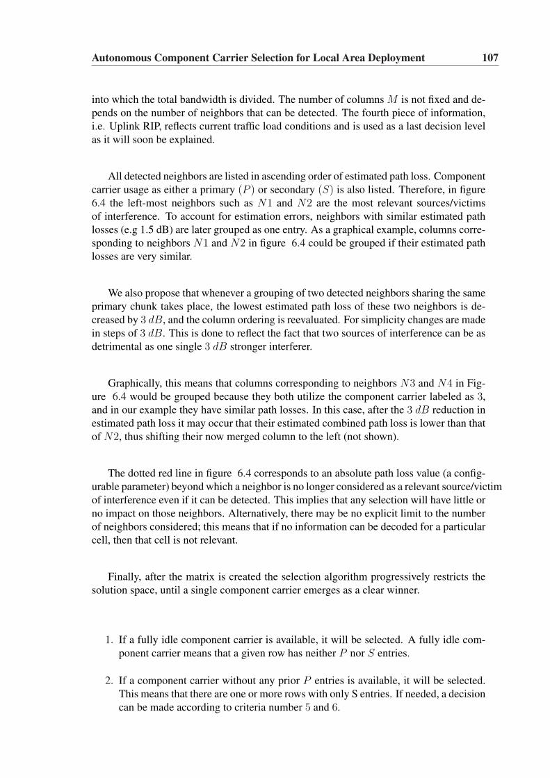
Autonomous Component Carrier Selection for Local Area Deployment 107
into which the total bandwidth is divided. The number of columns M is not fixed and de-pends on the number of neighbors that can be detected. The fourth piece of information,i.e. Uplink RIP, reflects current traffic load conditions and is used as a last decision levelas it will soon be explained.
All detected neighbors are listed in ascending order of estimated path loss. Componentcarrier usage as either a primary (P ) or secondary (S) is also listed. Therefore, in figure6.4 the left-most neighbors such as N1 and N2 are the most relevant sources/victimsof interference. To account for estimation errors, neighbors with similar estimated pathlosses (e.g 1.5 dB) are later grouped as one entry. As a graphical example, columns corre-sponding to neighbors N1 and N2 in figure 6.4 could be grouped if their estimated pathlosses are very similar.
We also propose that whenever a grouping of two detected neighbors sharing the sameprimary chunk takes place, the lowest estimated path loss of these two neighbors is de-creased by 3 dB, and the column ordering is reevaluated. For simplicity changes are madein steps of 3 dB. This is done to reflect the fact that two sources of interference can be asdetrimental as one single 3 dB stronger interferer.
Graphically, this means that columns corresponding to neighbors N3 and N4 in Fig-ure 6.4 would be grouped because they both utilize the component carrier labeled as 3,and in our example they have similar path losses. In this case, after the 3 dB reduction inestimated path loss it may occur that their estimated combined path loss is lower than thatof N2, thus shifting their now merged column to the left (not shown).
The dotted red line in figure 6.4 corresponds to an absolute path loss value (a config-urable parameter) beyond which a neighbor is no longer considered as a relevant source/victimof interference even if it can be detected. This implies that any selection will have little orno impact on those neighbors. Alternatively, there may be no explicit limit to the numberof neighbors considered; this means that if no information can be decoded for a particularcell, then that cell is not relevant.
Finally, after the matrix is created the selection algorithm progressively restricts thesolution space, until a single component carrier emerges as a clear winner.
1. If a fully idle component carrier is available, it will be selected. A fully idle com-ponent carrier means that a given row has neither P nor S entries.
2. If a component carrier without any prior P entries is available, it will be selected.This means that there are one or more rows with only S entries. If needed, a decisioncan be made according to criteria number 5 and 6.
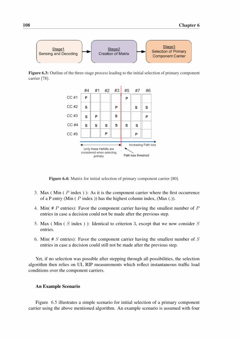
108 Chapter 6
Figure 6.3: Outline of the three-stage process leading to the initial selection of primary componentcarrier [78].
Figure 6.4: Matrix for initial selection of primary component carrier [80].
3. Max ( Min ( P index ) ): As it is the component carrier where the first occurrenceof a P entry (Min ( P index )) has the highest column index, (Max (.)).
4. Min( # P entries): Favor the component carrier having the smallest number of Pentries in case a decision could not be made after the previous step.
5. Max ( Min ( S index ) ): Identical to criterion 3, except that we now consider Sentries.
6. Min( # S entries): Favor the component carrier having the smallest number of Sentries in case a decision could still not be made after the previous step.
Yet, if no selection was possible after stepping through all possibilities, the selectionalgorithm then relies on UL RIP measurements which reflect instantaneous traffic loadconditions over the component carriers.
An Example Scenario
Figure 6.5 illustrates a simple scenario for initial selection of a primary componentcarrier using the above mentioned algorithm. An example scenario is assumed with four
Autonomous Component Carrier Selection for Local Area Deployment 109
Figure 6.5: Sketch of a scenario with 4 existing HeNBs with selected primary (P) and secondary(S) component carriers. Subsequently the HeNB # 5 is switched on and therefore does not haveany component carrier at this moment [80].
existing HeNBs (HeNB #1 to #4), where a new HeNB (eNB #5) is switched on. Thefirst task of the new HeNB is to select one component carrier as its primary. We assumea configuration with 5 component carriers. Here, P and S denote the primary and sec-ondary component carriers currently selected by the existing HeNBs. This information isavailable to the new HeNB from the surrounding HeNBs via over-the-air-communication.In addition to having this information the new HeNB performs path loss measurements ofthe surrounding cells locally. For this purpose inter HeNB RSRP measurements are used,where it is proposed that an HeNB measures the RSRP from its neighboring HeNBs.These measurements, combined with knowledge of the corresponding DL RS Tx power,are used to estimate the path loss towards the neighboring HeNBs. Using this informationthe new HeNB will select a primary component carrier. In this example the new HeNBwill most likely select the #4 CC as its primary.
6.2.4 Quality Monitoring of Primary Component Carrier
After the HeNB selects a primary component carrier, it may start to carry traffic and alsoto monitor the quality of the PCC. Now the UEs gets connected, hence, apart from ini-tial HeNB measurements, the other measurements such as UL SINR, throughput, RSRP,RSRQ etc. also become available. Some of these measurements are used for quality mon-itoring.
Our proposal is to individually monitor the quality in UL and DL, as different actions
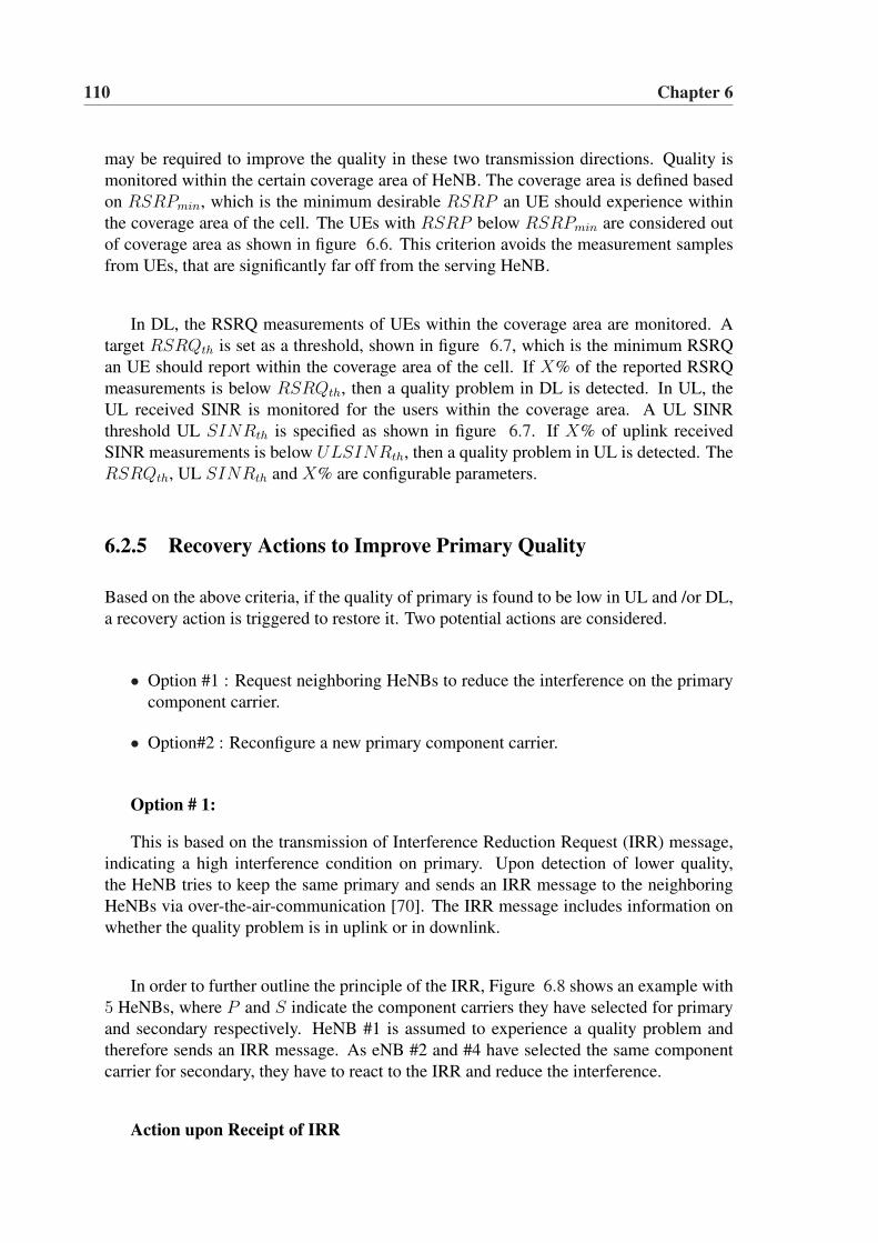
110 Chapter 6
may be required to improve the quality in these two transmission directions. Quality ismonitored within the certain coverage area of HeNB. The coverage area is defined basedon RSRPmin, which is the minimum desirable RSRP an UE should experience withinthe coverage area of the cell. The UEs with RSRP below RSRPmin are considered outof coverage area as shown in figure 6.6. This criterion avoids the measurement samplesfrom UEs, that are significantly far off from the serving HeNB.
In DL, the RSRQ measurements of UEs within the coverage area are monitored. Atarget RSRQth is set as a threshold, shown in figure 6.7, which is the minimum RSRQan UE should report within the coverage area of the cell. If X% of the reported RSRQmeasurements is below RSRQth, then a quality problem in DL is detected. In UL, theUL received SINR is monitored for the users within the coverage area. A UL SINRthreshold UL SINRth is specified as shown in figure 6.7. If X% of uplink receivedSINR measurements is below ULSINRth, then a quality problem in UL is detected. TheRSRQth, UL SINRth and X% are configurable parameters.
6.2.5 Recovery Actions to Improve Primary Quality
Based on the above criteria, if the quality of primary is found to be low in UL and /or DL,a recovery action is triggered to restore it. Two potential actions are considered.
• Option #1 : Request neighboring HeNBs to reduce the interference on the primarycomponent carrier.
• Option#2 : Reconfigure a new primary component carrier.
Option # 1:
This is based on the transmission of Interference Reduction Request (IRR) message,indicating a high interference condition on primary. Upon detection of lower quality,the HeNB tries to keep the same primary and sends an IRR message to the neighboringHeNBs via over-the-air-communication [70]. The IRR message includes information onwhether the quality problem is in uplink or in downlink.
In order to further outline the principle of the IRR, Figure 6.8 shows an example with5 HeNBs, where P and S indicate the component carriers they have selected for primaryand secondary respectively. HeNB #1 is assumed to experience a quality problem andtherefore sends an IRR message. As eNB #2 and #4 have selected the same componentcarrier for secondary, they have to react to the IRR and reduce the interference.
Action upon Receipt of IRR
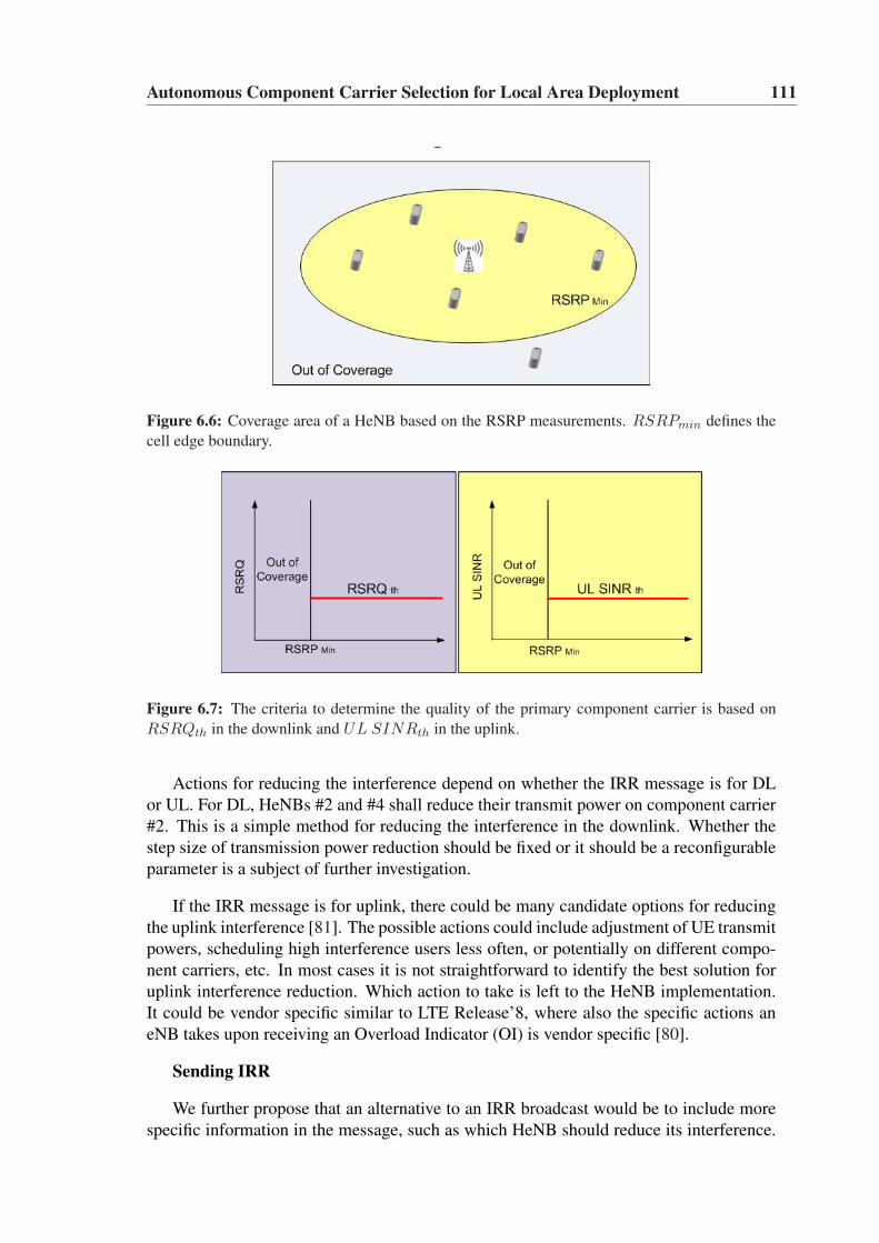
Autonomous Component Carrier Selection for Local Area Deployment 111
Figure 6.6: Coverage area of a HeNB based on the RSRP measurements. RSRPmin defines thecell edge boundary.
Figure 6.7: The criteria to determine the quality of the primary component carrier is based onRSRQth in the downlink and UL SINRth in the uplink.
Actions for reducing the interference depend on whether the IRR message is for DLor UL. For DL, HeNBs #2 and #4 shall reduce their transmit power on component carrier#2. This is a simple method for reducing the interference in the downlink. Whether thestep size of transmission power reduction should be fixed or it should be a reconfigurableparameter is a subject of further investigation.
If the IRR message is for uplink, there could be many candidate options for reducingthe uplink interference [81]. The possible actions could include adjustment of UE transmitpowers, scheduling high interference users less often, or potentially on different compo-nent carriers, etc. In most cases it is not straightforward to identify the best solution foruplink interference reduction. Which action to take is left to the HeNB implementation.It could be vendor specific similar to LTE Release’8, where also the specific actions aneNB takes upon receiving an Overload Indicator (OI) is vendor specific [80].
Sending IRR
We further propose that an alternative to an IRR broadcast would be to include morespecific information in the message, such as which HeNB should reduce its interference.
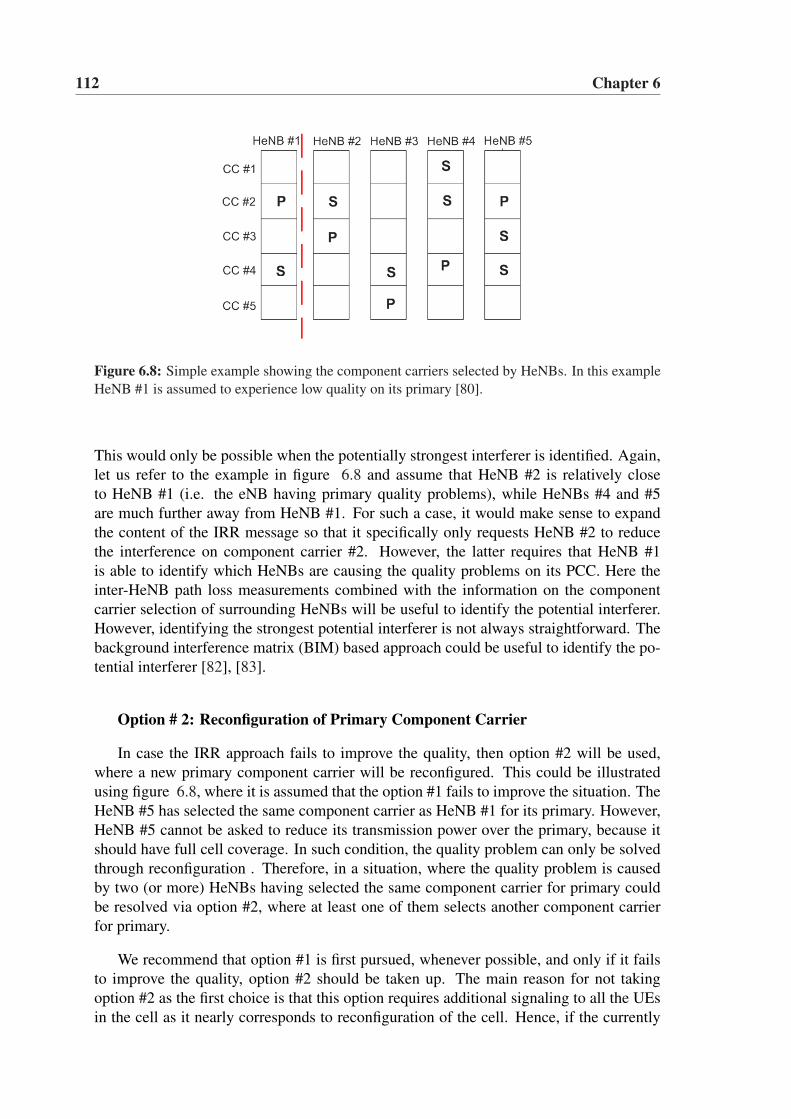
112 Chapter 6
Figure 6.8: Simple example showing the component carriers selected by HeNBs. In this exampleHeNB #1 is assumed to experience low quality on its primary [80].
This would only be possible when the potentially strongest interferer is identified. Again,let us refer to the example in figure 6.8 and assume that HeNB #2 is relatively closeto HeNB #1 (i.e. the eNB having primary quality problems), while HeNBs #4 and #5are much further away from HeNB #1. For such a case, it would make sense to expandthe content of the IRR message so that it specifically only requests HeNB #2 to reducethe interference on component carrier #2. However, the latter requires that HeNB #1is able to identify which HeNBs are causing the quality problems on its PCC. Here theinter-HeNB path loss measurements combined with the information on the componentcarrier selection of surrounding HeNBs will be useful to identify the potential interferer.However, identifying the strongest potential interferer is not always straightforward. Thebackground interference matrix (BIM) based approach could be useful to identify the po-tential interferer [82], [83].
Option # 2: Reconfiguration of Primary Component Carrier
In case the IRR approach fails to improve the quality, then option #2 will be used,where a new primary component carrier will be reconfigured. This could be illustratedusing figure 6.8, where it is assumed that the option #1 fails to improve the situation. TheHeNB #5 has selected the same component carrier as HeNB #1 for its primary. However,HeNB #5 cannot be asked to reduce its transmission power over the primary, because itshould have full cell coverage. In such condition, the quality problem can only be solvedthrough reconfiguration . Therefore, in a situation, where the quality problem is causedby two (or more) HeNBs having selected the same component carrier for primary couldbe resolved via option #2, where at least one of them selects another component carrierfor primary.
We recommend that option #1 is first pursued, whenever possible, and only if it failsto improve the quality, option #2 should be taken up. The main reason for not takingoption #2 as the first choice is that this option requires additional signaling to all the UEsin the cell as it nearly corresponds to reconfiguration of the cell. Hence, if the currently
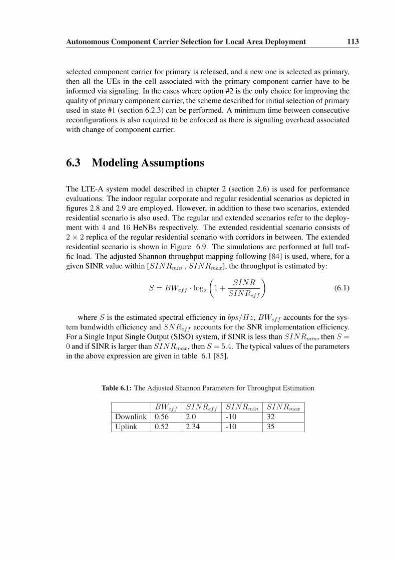
Autonomous Component Carrier Selection for Local Area Deployment 113
selected component carrier for primary is released, and a new one is selected as primary,then all the UEs in the cell associated with the primary component carrier have to beinformed via signaling. In the cases where option #2 is the only choice for improving thequality of primary component carrier, the scheme described for initial selection of primaryused in state #1 (section 6.2.3) can be performed. A minimum time between consecutivereconfigurations is also required to be enforced as there is signaling overhead associatedwith change of component carrier.
6.3 Modeling Assumptions
The LTE-A system model described in chapter 2 (section 2.6) is used for performanceevaluations. The indoor regular corporate and regular residential scenarios as depicted infigures 2.8 and 2.9 are employed. However, in addition to these two scenarios, extendedresidential scenario is also used. The regular and extended scenarios refer to the deploy-ment with 4 and 16 HeNBs respectively. The extended residential scenario consists of2 × 2 replica of the regular residential scenario with corridors in between. The extendedresidential scenario is shown in Figure 6.9. The simulations are performed at full traf-fic load. The adjusted Shannon throughput mapping following [84] is used, where, for agiven SINR value within [SINRmin , SINRmax], the throughput is estimated by:
S = BWeff · log2
(1 +
SINR
SINReff
)(6.1)
where S is the estimated spectral efficiency in bps/Hz, BWeff accounts for the sys-tem bandwidth efficiency and SNReff accounts for the SNR implementation efficiency.For a Single Input Single Output (SISO) system, if SINR is less than SINRmin, then S =0 and if SINR is larger than SINRmax, then S = 5.4. The typical values of the parametersin the above expression are given in table 6.1 [85].
Table 6.1: The Adjusted Shannon Parameters for Throughput Estimation
BWeff SINReff SINRmin SINRmax
Downlink 0.56 2.0 -10 32Uplink 0.52 2.34 -10 35
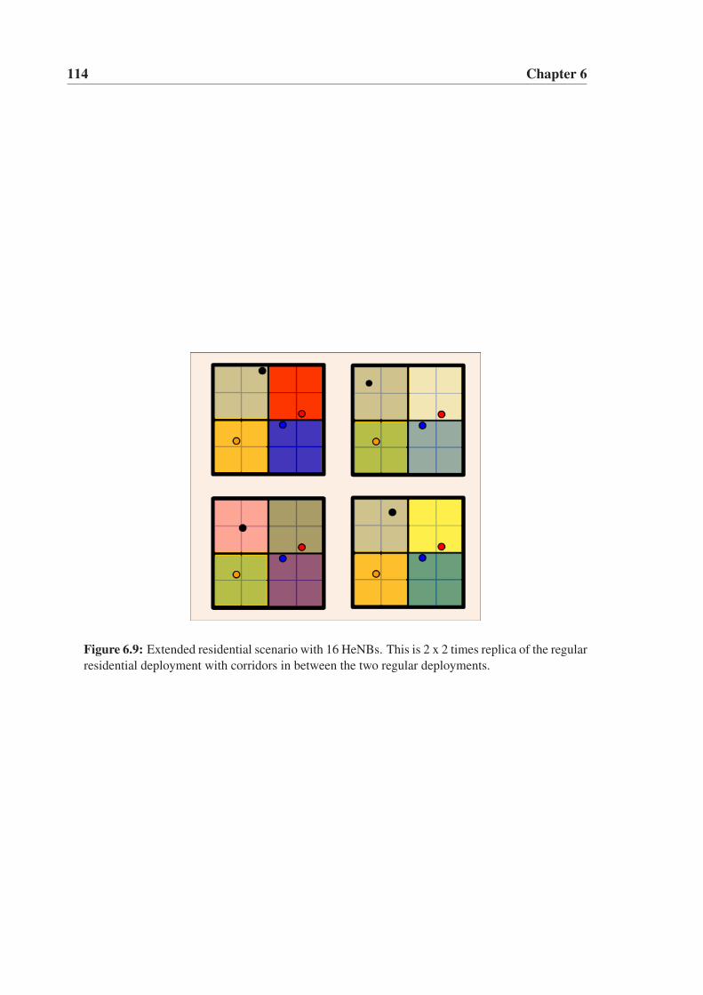
114 Chapter 6
Figure 6.9: Extended residential scenario with 16 HeNBs. This is 2 x 2 times replica of the regularresidential deployment with corridors in between the two regular deployments.
Autonomous Component Carrier Selection for Local Area Deployment 115
6.4 Performance Evaluation
The performance results are presented in two phases. In the first phase, HeNBs are as-sumed to switch on in a sequence, whereas in the second phase, HeNBs are assumed toswitch on in a random order. The latter represents a more realistic situation. After switch-ing on, each HeNB selects a PCC. No simultaneous selection is assumed. The simulationcontinues until all the HeNBs have acquired one and only one PCC. The results are col-lected from the last simulation step. The results do not include the effect of any recoveryaction, i.e. the HeNBs will not change their primary after initial selection.
The primary focus is to evaluate the sensitivity of the proposed algorithm in selectionof PCC in comparison with the corresponding fixed frequency reuse schemes. The fixedfrequency reuse schemes are planned and are expected to provide optimal frequency al-location over the network. The PCC selection by proposed algorithm should converge tothe fixed frequency reuse schemes.
In order to evaluate the performance with a different number of component carriers,the assumed system bandwidth of 100 MHz is divided into 2, 4, 8 and 16 component car-riers. The performance in each case is compared with the corresponding fixed frequencyreuse schemes, i.e. with reuse factors 2, 4, 8 and 16. The comparison is performed interms of average cell throughput and 5% outage user throughput, normalized against theresults of fixed frequency reuse 1 (universal frequency reuse) scheme.
Sequential HeNB Switching
With sequential switching, 2 and 4 component carriers are considered for regular cor-porate, and 2, 4, 8 and 16 component carriers are considered for extended residentialscenario. For regular corporate 5-10 UEs are simulated within each HeNB, whereas, forextended residential 2-4 UEs are simulated.Figure 6.10 shows SINR distribution in DL and UL for regular corporate scenario. TheSINR distribution of reuse 1 is also included in the figure. The SINR distribution ofthe PCC algorithm is essentially the same as its corresponding reuse schemes. Figure6.11 compares the distribution of average cell throughput and average user throughputin DL, which is also essentially the same. Further, figures 6.12 and 6.13 compare thenormalized average cell throughput and 5% outage user throughput in DL and UL respec-tively. The proposed PCC algorithm provides nearly the same performance compared tothe corresponding fixed frequency reuse schemes. This implies that the selection of thecomponent carriers by PCC at HeNBs resembles the optimally planned fixed frequencyreuse schemes.The normalized cell throughput and user outage throughput in DL of extended residentialscenario is presented in figure 6.14. The PCC algorithm with more than 2 componentcarriers gives nearly the same performance as it corresponding reuse schemes. A lowerperformance is realized with 2 component carriers, especially in the user outage through-
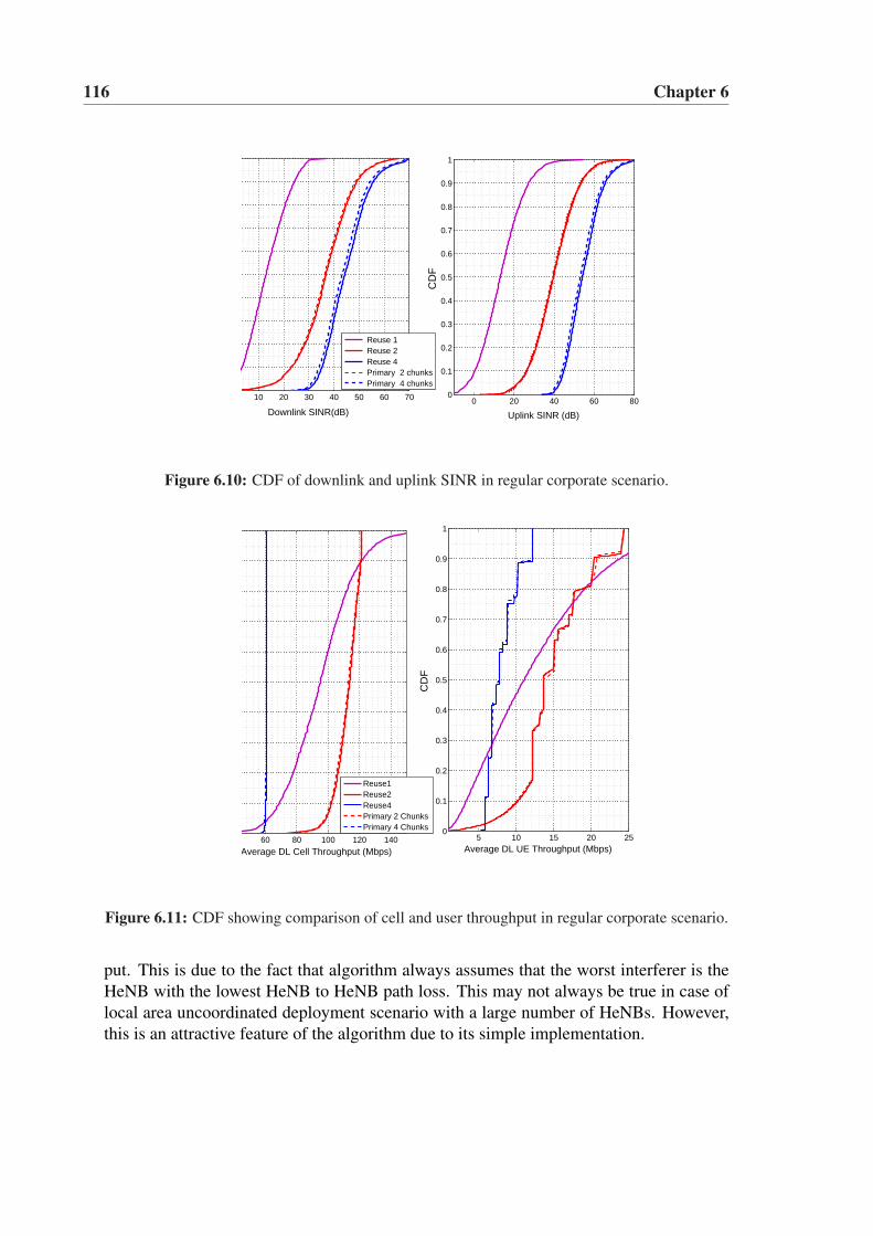
116 Chapter 6
10 20 30 40 50 60 70
Downlink SINR(dB)
0 20 40 60 800
0.1
0.2
0.3
0.4
0.5
0.6
0.7
0.8
0.9
1
Uplink SINR (dB)
CD
F
Reuse 1 Reuse 2 Reuse 4 Primary 2 chunks Primary 4 chunks
Figure 6.10: CDF of downlink and uplink SINR in regular corporate scenario.
40 60 80 100 120 140
Average DL Cell Throughput (Mbps)
5 10 15 20 250
0.1
0.2
0.3
0.4
0.5
0.6
0.7
0.8
0.9
1
Average DL UE Throughput (Mbps)
CD
F
Reuse1Reuse2 Reuse4Primary 2 ChunksPrimary 4 Chunks
Figure 6.11: CDF showing comparison of cell and user throughput in regular corporate scenario.
put. This is due to the fact that algorithm always assumes that the worst interferer is theHeNB with the lowest HeNB to HeNB path loss. This may not always be true in case oflocal area uncoordinated deployment scenario with a large number of HeNBs. However,this is an attractive feature of the algorithm due to its simple implementation.
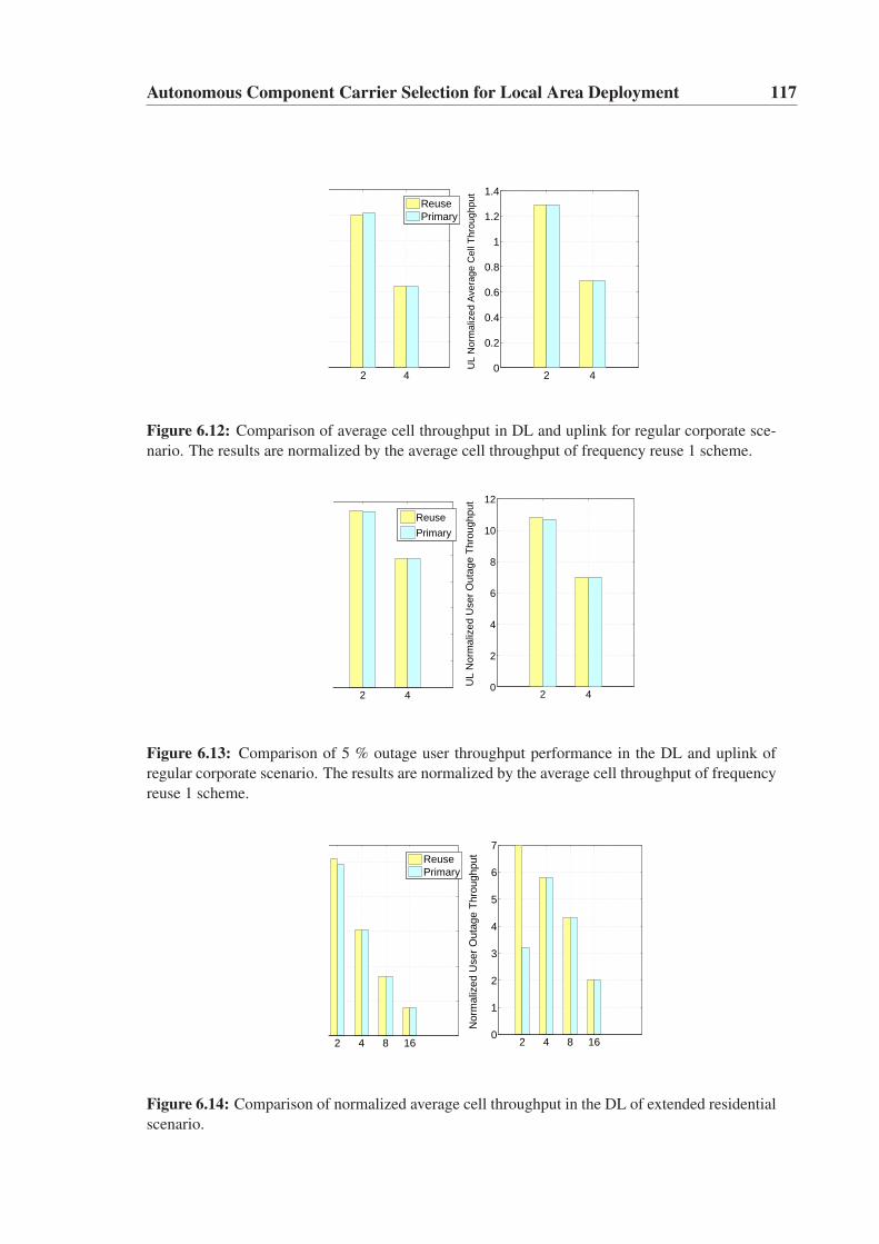
Autonomous Component Carrier Selection for Local Area Deployment 117
2 4
ReusePrimary
2 40
0.2
0.4
0.6
0.8
1
1.2
1.4
UL
Nor
mal
ized
Ave
rage
Cel
l Thr
ough
put
Figure 6.12: Comparison of average cell throughput in DL and uplink for regular corporate sce-nario. The results are normalized by the average cell throughput of frequency reuse 1 scheme.
2 40
2
4
6
8
10
12
UL
Nor
mal
ized
Use
r O
utag
e T
hrou
ghpu
t
2 4
Reuse
Primary
Figure 6.13: Comparison of 5 % outage user throughput performance in the DL and uplink ofregular corporate scenario. The results are normalized by the average cell throughput of frequencyreuse 1 scheme.
2 4 8 16
2 4 8 160
1
2
3
4
5
6
7
Nor
mal
ized
Use
r O
utag
e T
hrou
ghpu
t
ReusePrimary
Figure 6.14: Comparison of normalized average cell throughput in the DL of extended residentialscenario.
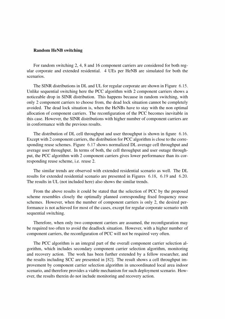
Random HeNB switching
For random switching 2, 4, 8 and 16 component carriers are considered for both reg-ular corporate and extended residential. 4 UEs per HeNB are simulated for both thescenarios.
The SINR distributions in DL and UL for regular corporate are shown in Figure 6.15.Unlike sequential switching here the PCC algorithm with 2 component carriers shows anoticeable drop in SINR distribution. This happens because in random switching, withonly 2 component carriers to choose from, the dead lock situation cannot be completelyavoided. The dead lock situation is, when the HeNBs have to stay with the non optimalallocation of component carriers. The reconfiguration of the PCC becomes inevitable inthis case. However, the SINR distributions with higher number of component carriers arein conformance with the previous results.
The distribution of DL cell throughput and user throughput is shown in figure 6.16.Except with 2 component carriers, the distribution for PCC algorithm is close to the corre-sponding reuse schemes. Figure 6.17 shows normalized DL average cell throughput andaverage user throughput. In terms of both, the cell throughput and user outage through-put, the PCC algorithm with 2 component carriers gives lower performance than its cor-responding reuse scheme, i.e. reuse 2.
The similar trends are observed with extended residential scenario as well. The DLresults for extended residential scenario are presented in Figures 6.18, 6.19 and 6.20.The results in UL (not included here) also shows the similar trends.
From the above results it could be stated that the selection of PCC by the proposedscheme resembles closely the optimally planned corresponding fixed frequency reuseschemes. However, when the number of component carriers is only 2, the desired per-formance is not achieved for most of the cases, except for regular corporate scenario withsequential switching.
Therefore, when only two component carriers are assumed, the reconfiguration maybe required too often to avoid the deadlock situation. However, with a higher number ofcomponent carriers, the reconfiguration of PCC will not be required very often.
The PCC algorithm is an integral part of the overall component carrier selection al-gorithm, which includes secondary component carrier selection algorithm, monitoringand recovery action. The work has been further extended by a fellow researcher, andthe results including SCC are presented in [82]. The result shows a cell throughput im-provement by component carrier selection algorithm in uncoordinated local area indoorscenario, and therefore provides a viable mechanism for such deployment scenario. How-ever, the results therein do not include monitoring and recovery action.
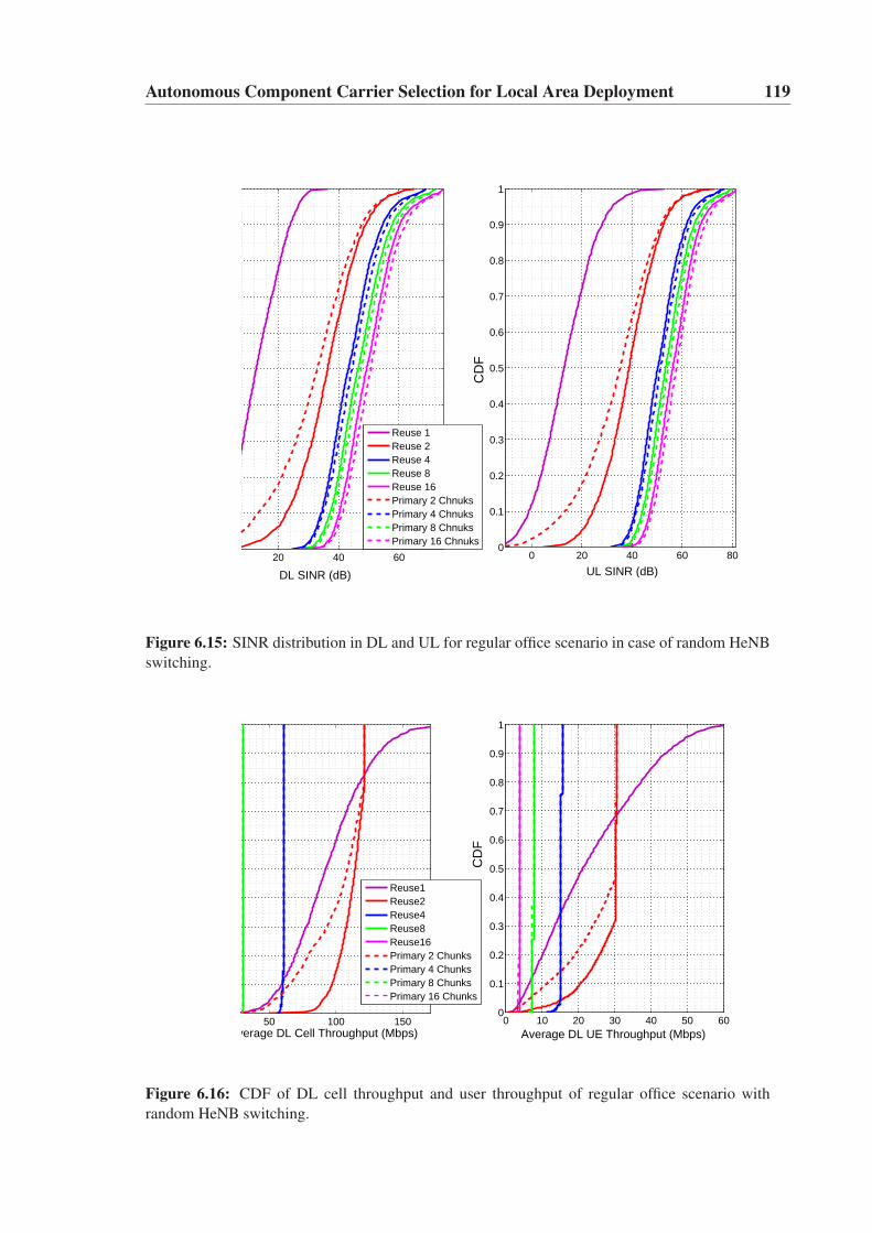
Autonomous Component Carrier Selection for Local Area Deployment 119
0 20 40 60 800
0.1
0.2
0.3
0.4
0.5
0.6
0.7
0.8
0.9
1
UL SINR (dB)
CD
F
20 40 60
DL SINR (dB)
Reuse 1Reuse 2Reuse 4Reuse 8Reuse 16Primary 2 ChnuksPrimary 4 ChnuksPrimary 8 ChnuksPrimary 16 Chnuks
Figure 6.15: SINR distribution in DL and UL for regular office scenario in case of random HeNBswitching.
50 100 150Average DL Cell Throughput (Mbps)
0 10 20 30 40 50 600
0.1
0.2
0.3
0.4
0.5
0.6
0.7
0.8
0.9
1
Average DL UE Throughput (Mbps)
CD
F
Reuse1Reuse2Reuse4Reuse8Reuse16Primary 2 ChunksPrimary 4 ChunksPrimary 8 ChunksPrimary 16 Chunks
Figure 6.16: CDF of DL cell throughput and user throughput of regular office scenario withrandom HeNB switching.
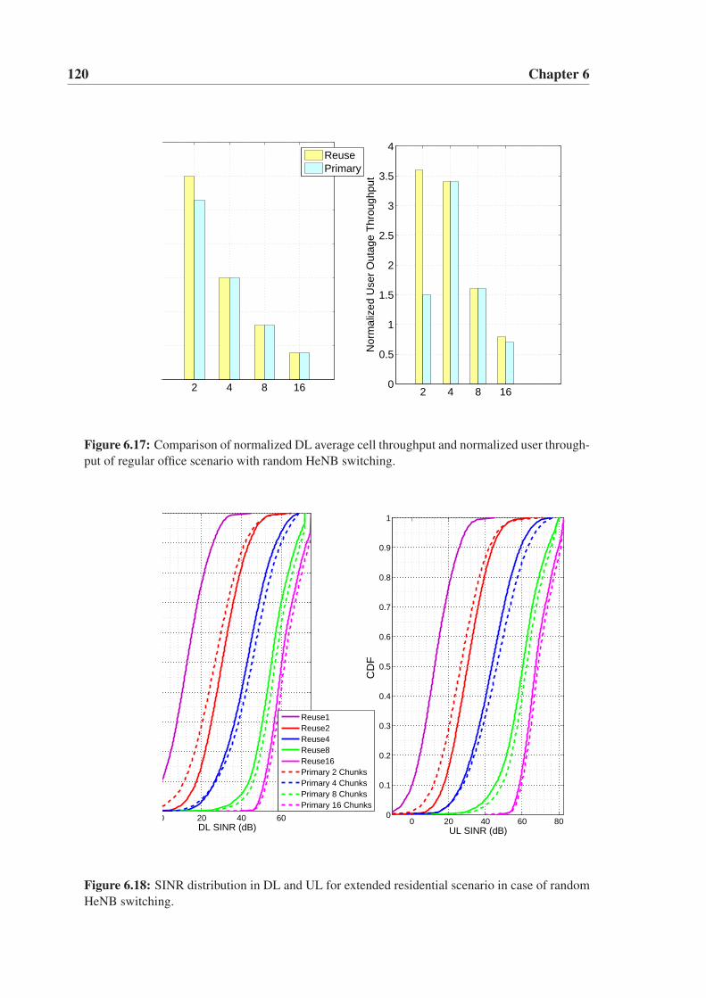
120 Chapter 6
2 4 8 16
ReusePrimary
2 4 8 160
0.5
1
1.5
2
2.5
3
3.5
4
Nor
mal
ized
Use
r O
utag
e T
hrou
ghpu
t
Figure 6.17: Comparison of normalized DL average cell throughput and normalized user through-put of regular office scenario with random HeNB switching.
0 20 40 60 DL SINR (dB)
0 20 40 60 800
0.1
0.2
0.3
0.4
0.5
0.6
0.7
0.8
0.9
1
UL SINR (dB)
CD
F
Reuse1Reuse2Reuse4Reuse8Reuse16Primary 2 ChunksPrimary 4 ChunksPrimary 8 ChunksPrimary 16 Chunks
Figure 6.18: SINR distribution in DL and UL for extended residential scenario in case of randomHeNB switching.
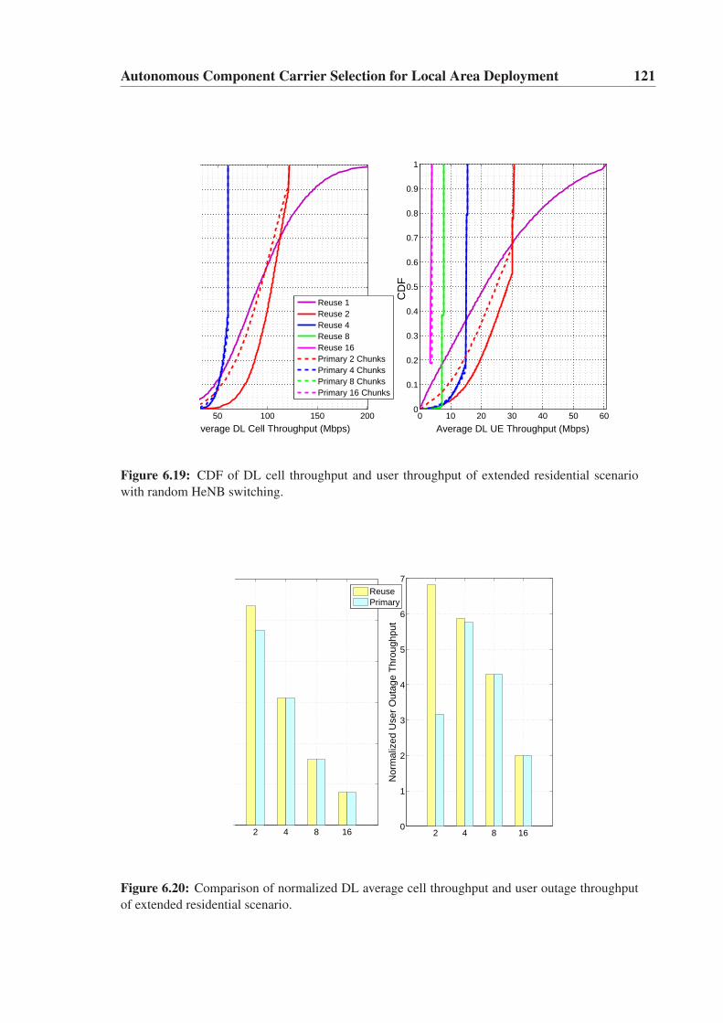
Autonomous Component Carrier Selection for Local Area Deployment 121
0 10 20 30 40 50 600
0.1
0.2
0.3
0.4
0.5
0.6
0.7
0.8
0.9
1
Average DL UE Throughput (Mbps)
CD
F
50 100 150 200
Average DL Cell Throughput (Mbps)
Reuse 1Reuse 2Reuse 4Reuse 8Reuse 16Primary 2 ChunksPrimary 4 ChunksPrimary 8 ChunksPrimary 16 Chunks
Figure 6.19: CDF of DL cell throughput and user throughput of extended residential scenariowith random HeNB switching.
2 4 8 16
ReusePrimary
2 4 8 160
1
2
3
4
5
6
7
Nor
mal
ized
Use
r O
utag
e T
hrou
ghpu
t
Figure 6.20: Comparison of normalized DL average cell throughput and user outage throughputof extended residential scenario.
6.5 Conclusions
In this chapter the carrier aggregation as a possible method to obtain LTE-A system band-width is discussed. The concept of primary and secondary component carriers is illus-trated. A basic concept for the distributed autonomous component carrier selection isoutlined. The concept is motivated by the fact that each HeNB does not always needthe full LTE-Advanced system bandwidth; in many cases one only needs a sub-set of theavailable component carriers.
We proposed an algorithm for the initial selection of the primary component carrier. Amechanism is also proposed for monitoring and protection of the quality of primary com-ponent carrier. In case the quality of primary is found to be low, the HeNB can initiate therecovery action to restore the quality of primary component carrier. It is also proposedthat the Interference Reduction Request (IRR) message based recovery action should bepreferred as a first step over the reconfiguration of the primary component carriers.
The proposed concept for selection of primary component carrier is fully distributedand does not involve any centralized network components; the selection is rather per-formed locally and independently by each HeNB, where each HeNB always selects one,and only one, primary component carrier.
The simulation results presented in this chapter indicate that the presented concepthelps to achieve an autonomous scalable and self-adjusting frequency reuse mechanism,which allows uncoordinated HeNB deployment without prior network planning.
Adaptation of the proposed concept for LTE-Advanced is simple since it entails min-imal changes to the standard as it mostly relies on existing release 8 UE and HeNB mea-surements.
Chapter 7
Policy Assisted Light Cognitive Radiofor FSU
7.1 Introduction
It is discussed in chapter 5 that currently HeNB is emerging as a potential solution for highdata rate and high quality services in indoor local area deployment scenario. The FSU hasbeen considered to allow coexistence of HeNBs in the given geographical area. FSU canbe performed in single-operator as well as multi-operators’ domain. Single operator FSUaims to facilitate high performance in uncoordinated and random deployments, whereasmulti-operator FSU facilitates different operators to access the common spectrum poolin flexible manner, based on their individual traffic requirements. The FSU in multi op-erators’ domain becomes necessary if the HeNBs are deployed by several operators in agiven geographical area, sharing over the common spectrum pool.
7.1.1 Multi-Operator FSU
The multi-operator FSU is based on the concept that when one network operator is in de-mand of the extra spectrum, the other network operators might have the spectrum availablein excess. In this situation the sharing of spectrum helps to exploit the unused spectrum,which leads to a higher degree of spectrum utilization. In order to facilitate FSU amongthe operators it is assumed that the operators access the spectrum in a flexible mannerfrom a common pool of spectrum.
In a multi operator FSU scenario a certain number of different operators are consideredto deploy HeNBs in the given geographical area and to have access to the same licensedfrequency band using the same radio access technology. An operator is allowed to installHeNBs without prior coordination with the other operators having access to the samefrequency band. Spectrum regulators decide how many operators have access to the givenlicensed spectrum bands in the given area. This implies that it is known a-priori by each
123
124 Chapter 7
operator, how many other operators are operating in the same band.
When several network operators are deployed in the local area scenario and make useof the same radio spectrum, a major concern is the interference. In traditional macrocell and micro cell deployment scenario this has been handled by a proper network plan-ning, including frequency re-use plans, base station location, transmit power levels, andantenna radiation characteristics. In contrast to these scenarios, in the case of local areadeployments the installation of the HeNBs cannot be planned by operators. The HeNBsare user employable, resulting in a random deployment. It is also natural to envision thelack of coordination between operators providing LA services in the same geographicalarea. Therefore, in the LA deployment scenarios the radio interference problem becomesmuch more severe compared to the traditional cellular deployment cases, and new mitiga-tion solutions need to be found. Another important aspect is high traffic load variabilityamong different operators operating in the given geographical area over the same radiospectrum, requiring a mechanism to exploit the traffic load variations by utilizing spec-trum in a flexible manner.
So far most of the deployment scenarios in either macro cells or micro cells con-sider coordinated deployment among operators. In this context, coordinated deploymentmeans that the BS /access point installations are planned to have good coverage and lowinterference between adjacent cells, which typically implies radio network planning priorto installation of new BS/access point. However, in the considered scenario an unco-ordinated HeNB deployment without prior radio network planning is envisioned. In thiscontext, uncoordinated deployment refers to cases where HeNBs are more or less installedrandomly to get coverage/capacity in one particular area, without considering the impacton/from potentially existing HeNBs radio performance in the immediate surroundings.
The FSU concept allows uncoordinated HeNB deployment without prior radio net-work planning exercises, therefore, the support for uncoordinated deployment is espe-cially considered to be attractive for LA areas in case of multi operator deployment sce-nario. However, the uncoordinated deployment with multi operators represents new chal-lenges for FSU. Moreover, the requirements of high spectral efficiency and fairness amongoperators demand a mechanism for FSU to enable overall radio resource utilization andsharing in a flexible manner.
7.1.2 State of the Art
Many studies have recently focused on inter-operator FSU [86], [87], [88], [89], [64]. In awide area broadband network assuming all the operators using same radio access technol-ogy, an increase in overall spectrum efficiency is realized by spectrum sharing among theoperators [86]. Taking into account the operational revenue and the QoS requirements,different criteria and optimization methods are outlined to improve the spectral efficiencyby coordinated spectrum usage for flexible spectrum allocation in [64]. The performanceof spectrum sharing for UMTS FDD DL for competing network operators is investigatedin [88], wherein an algorithm is proposed using total transmitted energy thresholds in the
Policy Assisted Light Cognitive Radio for FSU 125
shared band, allowing multiple operators to coexist. The concept of FSU is outlined in theperspectives of private commons in [9]. The private commons enable multiple parties toaccess the spectrum in existing licensed band based on the discretion of license holders,where the ultimate ownership of the licensed spectrum is retained with them. The respon-sibility for setting rules and the enforcement of these rules lies entirely with the licensedholders. It seems that for licensed band the solution is easier to imagine, though may notbe straightforward to implement [90], even though it is believed that in the long run theprivate-common will be the viable market option [9].
7.1.3 Aim of This Chapter
This chapter is focused on multi operator FSU, and therefore aims to provide a mechanismto enable FSU in LA indoor deployment with several operators, allowing them to coexistin the same geographical area with partially or completely preventing mutual interferenceon the shared spectrum while meeting individual traffic requirements. A random anduncoordinated deployment is considered. A very limited signaling exchange via over theair communication is assumed.
The proposed mechanism is based on the concept of policy assisted light CognitiveRadio (CR) enabled FSU. It follows the CR cycle and considers policy as an importantelement to assist FSU among the operators. The proposed concept is illustrated in thefollowing section.
This chapter is organized as follows: in section 2 the proposed concept is described,whereas the proposed algorithm is described in section 3. Section 4 outlines the mod-eling assumptions and section 5 the performance results. Finally, section 6 outlines theconclusions.
7.2 Proposed Concept
7.2.1 Policy Assisted Light Cognitive Radio
We consider that each HeNB makes independent decision for spectrum allocation basedon the interference conditions present over the spectrum with the support of Light Cogni-tive Radio and Policy, referred to as Policy-Assisted-Light-Cognitive-Radio(PA-LCR) forFSU.
Policy
It is considered that a policy based approach is needed to allow fair, efficient andflexible spectrum sharing among the operators from the common pool. In general, the termpolicy has been defined in several references. In [91] various Channel Access Mechanisms(CAMs) are discussed to handle the traffic generated in 802.11e WLAN, where a policy
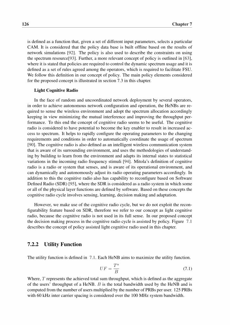
126 Chapter 7
is defined as a function that, given a set of different input parameters, selects a particularCAM. It is considered that the policy data base is built offline based on the results ofnetwork simulations [92]. The policy is also used to describe the constraints on usingthe spectrum resource[93]. Further, a more relevant concept of policy is outlined in [63],where it is stated that policies are required to control the dynamic spectrum usage and it isdefined as a set of rules agreed among the operators, which is required to facilitate FSU.We follow this definition in our concept of policy. The main policy elements consideredfor the proposed concept is illustrated in section 7.3 in this chapter.
Light Cognitive Radio
In the face of random and uncoordinated network deployment by several operators,in order to achieve autonomous network configuration and operation, the HeNBs are re-quired to sense the wireless environment and adopt the spectrum allocation accordinglykeeping in view minimizing the mutual interference and improving the throughput per-formance. To this end the concept of cognitive radio seems to be useful. The cognitiveradio is considered to have potential to become the key enabler to result in increased ac-cess to spectrum. It helps to rapidly configure the operating parameters to the changingrequirements and conditions in order to automatically coordinate the usage of spectrum[90]. The cognitive radio is also defined as an intelligent wireless communication systemthat is aware of its surrounding environment, and uses the methodologies of understand-ing by building to learn from the environment and adapts its internal states to statisticalvariations in the incoming radio frequency stimuli [94]. Mitola’s definition of cognitiveradio is a radio or system that senses, and is aware of its operational environment, andcan dynamically and autonomously adjust its radio operating parameters accordingly. Inaddition to this the cognitive radio also has capability to reconfigure based on SoftwareDefined Radio (SDR) [95], where the SDR is considered as a radio system in which someor all of the physical layer functions are defined by software. Based on these concepts thecognitive radio cycle involves sensing, learning, decision making and adaptation.
However, we make use of the cognitive radio cycle, but we do not exploit the recon-figurability feature based on SDR, therefore we refer to our concept as light cognitiveradio, because the cognitive radio is not used in its full sense. In our proposed conceptthe decision making process in the cognitive radio cycle is assisted by policy. Figure 7.1describes the concept of policy assisted light cognitive radio used in this chapter.
7.2.2 Utility Function
The utility function is defined in 7.1. Each HeNB aims to maximize the utility function.
UF =T α
B(7.1)
Where, T represents the achieved total sum throughput, which is defined as the aggregateof the users’ throughput of a HeNB. B is the total bandwidth used by the HeNB and iscomputed from the number of users multiplied by the number of PRBs per user. 125 PRBswith 60 kHz inter carrier spacing is considered over the 100 MHz system bandwidth.
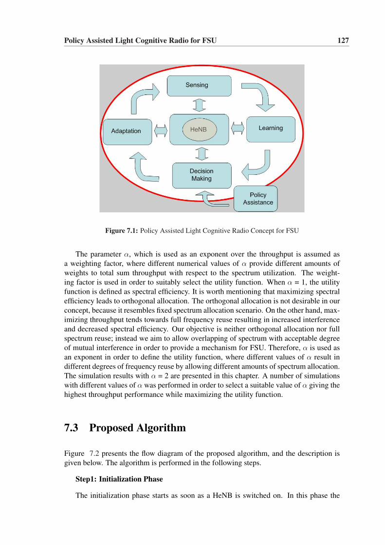
Policy Assisted Light Cognitive Radio for FSU 127
Figure 7.1: Policy Assisted Light Cognitive Radio Concept for FSU
The parameter α, which is used as an exponent over the throughput is assumed asa weighting factor, where different numerical values of α provide different amounts ofweights to total sum throughput with respect to the spectrum utilization. The weight-ing factor is used in order to suitably select the utility function. When α = 1, the utilityfunction is defined as spectral efficiency. It is worth mentioning that maximizing spectralefficiency leads to orthogonal allocation. The orthogonal allocation is not desirable in ourconcept, because it resembles fixed spectrum allocation scenario. On the other hand, max-imizing throughput tends towards full frequency reuse resulting in increased interferenceand decreased spectral efficiency. Our objective is neither orthogonal allocation nor fullspectrum reuse; instead we aim to allow overlapping of spectrum with acceptable degreeof mutual interference in order to provide a mechanism for FSU. Therefore, α is used asan exponent in order to define the utility function, where different values of α result indifferent degrees of frequency reuse by allowing different amounts of spectrum allocation.The simulation results with α = 2 are presented in this chapter. A number of simulationswith different values of α was performed in order to select a suitable value of α giving thehighest throughput performance while maximizing the utility function.
7.3 Proposed Algorithm
Figure 7.2 presents the flow diagram of the proposed algorithm, and the description isgiven below. The algorithm is performed in the following steps.
Step1: Initialization Phase
The initialization phase starts as soon as a HeNB is switched on. In this phase the
128 Chapter 7
HeNB randomly allocates PRBs to establish communication with its UEs and to meet thetraffic requirements. In addition to this, the HeNB requires to establish its own positionin the queue for updating spectrum allocation in the subsequent frames. This step is re-quired because it is assumed that the HeNBs update their spectrum allocation in sequence,at their own turns. In order to establish its position in the sequence the new HeNB com-municates with other potentially existing HeNBs using over-the-air-communication [70].This process requires a limited amount of signaling exchange, because the setting of se-quence is needed only when a HeNB leaves or enters the network. Once the sequence isset, it remains unchanged for the given set of active HeNBs.
The algorithm assumes, that HeNBs update their spectrum allocation in sequence ontheir own turns. This implies that when one HeNB updates, all other HeNBs follow theirprevious allocation. This assumption is made to ensure that while updating the spectrumallocation, the interference condition remains predictable for the HeNB. It also helps toavoid the yo-yo like situation which may happen if two or more HeNBs are allowed toupdate their spectrum allocation at the same time. If HeNBs are allowed to update atthe same time, it is possible that they sense low interference over the same PRBs anddecide to allocate, which will result in very high interference over those PRBs in the nextframe. In the next frame those PRBs will not be allocated by any HeNB,resulting in lowerinterference in the subsequent frame. This process will be repeated, creating an yo-yo likeunstable situation.
Therefore, during initialization phase two important tasks are accomplished: 1) estab-lishing communication with UEs and 2) setting up sequence.
Step 2: Interference Sensing and PRB Sorting
Once the communication is established between UE(s) and HeNB during the initial-ization phase, it becomes possible for HeNB to sense interference over the spectrum. Inthis phase the HeNB senses interference over all the PRBs. A similar to UL ReceivedInterference Power (RIP) measurement is assumed in the sensing phase. The UL RIP isdefined as uplink received interference power, including thermal noise, measured at eNBwithin one PRB bandwidth [18]. The UL RIP has been standardized as a measurementthat LTE physical layer should report to higher layer [79]. Once the interference, i.e. theUL RIP is measured over all the PRBs, the PRBs are sorted in an ascending order basedon the amount of interference present over them. This implies that the sorted list startswith the best PRB.i.e. the PRBs with the lowest interference. When the PRBs are requiredto be selected, the selection starts with the best PRBs consecutively from the sorted list.
Step 3: Interference Threshold Based PRB Allocation
In this phase the HeNBs select PRBs from the sorted list based on interference thresh-old (Ith). The set of PRBs with interference level below Ith are considered as availablePRBs (Navailable)for allocation by a HeNB. The HeNB is allowed to allocate PRBs onlyfrom the Navailable set of PRBs. The Ith allows opportunistic allocation of PRBs withsome degree of frequency domain overlap and ensures co-existence of mutually interfer-ing HeNBs. The Ith corresponds to the minimum desirable level of QoS and also definesthe coverage of the cell. The Ith is agreed among the operators as part of a policy, which
Policy Assisted Light Cognitive Radio for FSU 129
may be decided depending on the knowledge of the observed traffic conditions. Duringthis phase the allocation of PRBs follows further policy constraints, described below.
• Only the required number of PRBs to meet the traffic requirement from the availablePRBs will be selected with a constraint that the selected number of PRBs shouldnot exceed Nmax. where Nmax is defined as the maximum number of PRBs that anyHeNB is allowed to select and is defined as X % of total PRBs. The constraint onNmax aims to prevent one HeNB from allocating all the PRBs. The value of Nmax
is required to be carefully chosen in order to achieve the desired performance. Theselection Nmax depends on the knowledge of observed average interference condi-tions. A high value of Nmax can be selected if the observed interference conditionis very low otherwise, a low value is preferred.
• The proposed algorithm does not assume the QoS differentiation among the users.Therefore an equal number of PRBs to all the users will be allocated by a HeNB.Another policy constraint determines minimum (Nmin/UE) and maximum (Nmax/UE)number of PRBs per user. The Nmin/UE is used to ensure a certain minimum ser-vice quality to the users, whereas Nmax/UE is employed to impose restriction on thenumber of maximum PRBs one HeNB is allowed to allocate.
• If the number of available PRBs (Navailable, number of PRBs below the interferencethreshold) is not enough to meet the Nmin/UE criteria, then some users will bedropped and the number of PRBs per user will be determined by the expression( 7.2), subject to the Nmin/UE , which is a policy constraint that determines theminimum number of PRBs to be allocated to each user.
Number of PRBs per UE =Number of Available PRBs
Number of UEs(7.2)
• The policy also determines the initial number of PRBs to be allocated to each userdenoted as Ninitial. It is not necessary that the Ninitial should be equal to Nmin/UE .
Step 4: Successive PRB Increment
In the subsequent frames the number of PRBs per user is increased in steps by provid-ing a certain number of additional PRBs called Nadd. Besides avoiding greedy allocation,it ensures that the HeNB with a higher number of users has the opportunity to allocatemore PRBs in subsequent frames. In case due to lower number of Navailable, if it is notpossible to allocate Nadd then the possibility for Nadd−1 will be examined. If this is notpossible either, then the allocation will take place meeting Nmin/UE criteria. The pro-cess of successive increment in PRB per UE takes place for a definite number of framescalled Nframe, after which this phase ends. During this phase the pay-off is computedusing utility function for each allocation. The computed pay-offs are stored for futurereference. This part of the algorithm constitutes the learning phase of the cognitive radiocycle, which assists the decision making process.
Step 5: Revision Process
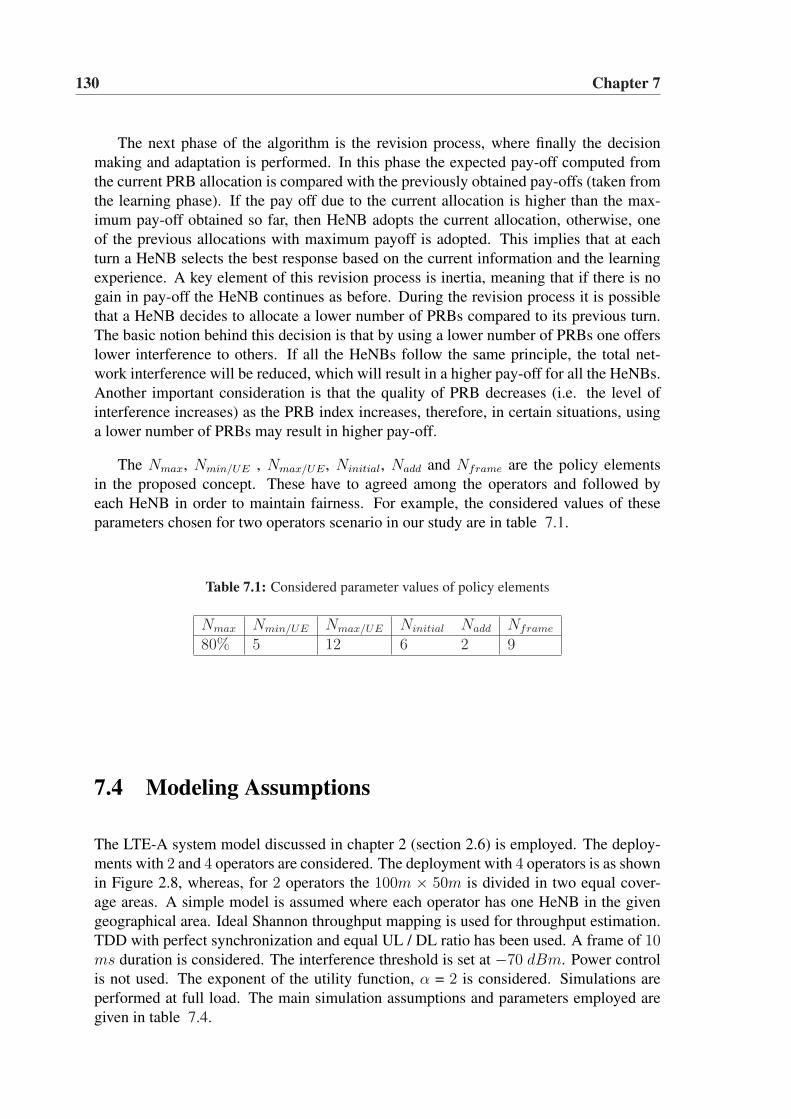
130 Chapter 7
The next phase of the algorithm is the revision process, where finally the decisionmaking and adaptation is performed. In this phase the expected pay-off computed fromthe current PRB allocation is compared with the previously obtained pay-offs (taken fromthe learning phase). If the pay off due to the current allocation is higher than the max-imum pay-off obtained so far, then HeNB adopts the current allocation, otherwise, oneof the previous allocations with maximum payoff is adopted. This implies that at eachturn a HeNB selects the best response based on the current information and the learningexperience. A key element of this revision process is inertia, meaning that if there is nogain in pay-off the HeNB continues as before. During the revision process it is possiblethat a HeNB decides to allocate a lower number of PRBs compared to its previous turn.The basic notion behind this decision is that by using a lower number of PRBs one offerslower interference to others. If all the HeNBs follow the same principle, the total net-work interference will be reduced, which will result in a higher pay-off for all the HeNBs.Another important consideration is that the quality of PRB decreases (i.e. the level ofinterference increases) as the PRB index increases, therefore, in certain situations, usinga lower number of PRBs may result in higher pay-off.
The Nmax, Nmin/UE , Nmax/UE , Ninitial, Nadd and Nframe are the policy elementsin the proposed concept. These have to agreed among the operators and followed byeach HeNB in order to maintain fairness. For example, the considered values of theseparameters chosen for two operators scenario in our study are in table 7.1.
Table 7.1: Considered parameter values of policy elements
Nmax Nmin/UE Nmax/UE Ninitial Nadd Nframe
80% 5 12 6 2 9
7.4 Modeling Assumptions
The LTE-A system model discussed in chapter 2 (section 2.6) is employed. The deploy-ments with 2 and 4 operators are considered. The deployment with 4 operators is as shownin Figure 2.8, whereas, for 2 operators the 100m × 50m is divided in two equal cover-age areas. A simple model is assumed where each operator has one HeNB in the givengeographical area. Ideal Shannon throughput mapping is used for throughput estimation.TDD with perfect synchronization and equal UL / DL ratio has been used. A frame of 10ms duration is considered. The interference threshold is set at −70 dBm. Power controlis not used. The exponent of the utility function, α = 2 is considered. Simulations areperformed at full load. The main simulation assumptions and parameters employed aregiven in table 7.4.
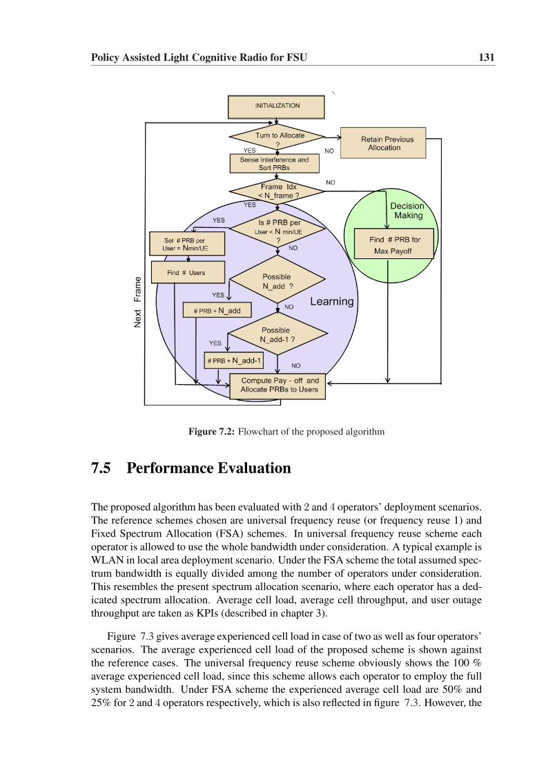
Policy Assisted Light Cognitive Radio for FSU 131
Figure 7.2: Flowchart of the proposed algorithm
7.5 Performance Evaluation
The proposed algorithm has been evaluated with 2 and 4 operators’ deployment scenarios.The reference schemes chosen are universal frequency reuse (or frequency reuse 1) andFixed Spectrum Allocation (FSA) schemes. In universal frequency reuse scheme eachoperator is allowed to use the whole bandwidth under consideration. A typical example isWLAN in local area deployment scenario. Under the FSA scheme the total assumed spec-trum bandwidth is equally divided among the number of operators under consideration.This resembles the present spectrum allocation scenario, where each operator has a ded-icated spectrum allocation. Average cell load, average cell throughput, and user outagethroughput are taken as KPIs (described in chapter 3).
Figure 7.3 gives average experienced cell load in case of two as well as four operators’scenarios. The average experienced cell load of the proposed scheme is shown againstthe reference cases. The universal frequency reuse scheme obviously shows the 100 %average experienced cell load, since this scheme allows each operator to employ the fullsystem bandwidth. Under FSA scheme the experienced average cell load are 50% and25% for 2 and 4 operators respectively, which is also reflected in figure 7.3. However, the
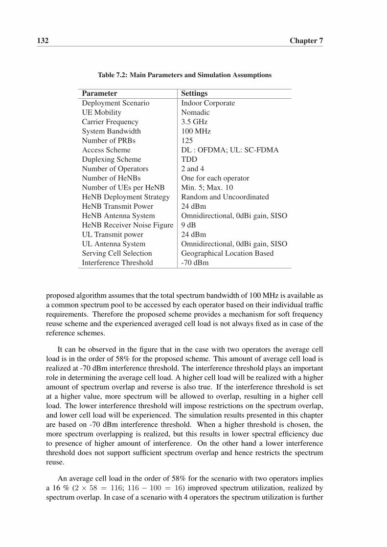
132 Chapter 7
Table 7.2: Main Parameters and Simulation Assumptions
Parameter SettingsDeployment Scenario Indoor CorporateUE Mobility NomadicCarrier Frequency 3.5 GHzSystem Bandwidth 100 MHzNumber of PRBs 125Access Scheme DL : OFDMA; UL: SC-FDMADuplexing Scheme TDDNumber of Operators 2 and 4Number of HeNBs One for each operatorNumber of UEs per HeNB Min. 5; Max. 10HeNB Deployment Strategy Random and UncoordinatedHeNB Transmit Power 24 dBmHeNB Antenna System Omnidirectional, 0dBi gain, SISOHeNB Receiver Noise Figure 9 dBUL Transmit power 24 dBmUL Antenna System Omnidirectional, 0dBi gain, SISOServing Cell Selection Geographical Location BasedInterference Threshold -70 dBm
proposed algorithm assumes that the total spectrum bandwidth of 100 MHz is available asa common spectrum pool to be accessed by each operator based on their individual trafficrequirements. Therefore the proposed scheme provides a mechanism for soft frequencyreuse scheme and the experienced averaged cell load is not always fixed as in case of thereference schemes.
It can be observed in the figure that in the case with two operators the average cellload is in the order of 58% for the proposed scheme. This amount of average cell load isrealized at -70 dBm interference threshold. The interference threshold plays an importantrole in determining the average cell load. A higher cell load will be realized with a higheramount of spectrum overlap and reverse is also true. If the interference threshold is setat a higher value, more spectrum will be allowed to overlap, resulting in a higher cellload. The lower interference threshold will impose restrictions on the spectrum overlap,and lower cell load will be experienced. The simulation results presented in this chapterare based on -70 dBm interference threshold. When a higher threshold is chosen, themore spectrum overlapping is realized, but this results in lower spectral efficiency dueto presence of higher amount of interference. On the other hand a lower interferencethreshold does not support sufficient spectrum overlap and hence restricts the spectrumreuse.
An average cell load in the order of 58% for the scenario with two operators impliesa 16 % (2 × 58 = 116; 116 − 100 = 16) improved spectrum utilization, realized byspectrum overlap. In case of a scenario with 4 operators the spectrum utilization is further
Policy Assisted Light Cognitive Radio for FSU 133
enhanced. The average cell load for each operator is in the order of 40%, which implies60% (4 × 40 = 160; 160 − 100 = 60) improved spectrum utilization. These observa-tions highlight the characteristic feature of the proposed algorithm in improving spectrumutilization compared to the FSA scheme.
Figure 7.4 presents the cdf of cell and user throughput for two operators. The FSAscheme shows a nearly uniform distribution, which is not true for proposed and universalfrequency reuse schemes, because there is no in-band interference in the FSA scheme,where the spectrum is allocated among operators in orthogonal manner. However, theproposed and universal reuse schemes exhibit spectrum overlap causing in band interfer-ence, which results in high variance in the distribution curve. Further, when a comparisonis made between the proposed scheme and the universal reuse scheme, it is clearly visiblethat the proposed scheme results in higher cell throughput performance.
Noticeably, this performance is achieved with only 58% spectrum use compared touniversal reuse scheme (fig. 7.3). This results in improved spectrum efficiency. In case ofuniversal reuse scheme the whole system bandwidth is used without interference consid-erations, whereas proposed scheme allocates spectrum to operators based on interferenceconsideration. Further, when the proposed scheme is compared with FSA, it gives com-parable average cell throughput, but uses 10 % extra spectrum resource (fig. 7.3). In FSAscheme the spectrum is orthogonally allocated to the operators therefore, there is no inband interference, resulting in higher SINR over the spectrum and hence there is higherthroughput and spectral efficiency.
In terms of user outage throughput, the proposed scheme gives improved performanceover the universal frequency reuse scheme. The higher spectrum overlap in universal reusescheme results in poor SINR conditions at the cell edge, and hence lower user outagethroughput performance is realized. When the proposed scheme is compared with FSA,its performance is comparatively lower. The orthogonal spectrum allocation in FSA helpsto keep the cell edge conditions favorable, resulting in higher user outage throughput.
From the above discussion it becomes obvious that when two operators are consid-ered over a 100 MHz system bandwidth, the FSA gives better performance comparedto the proposed scheme. However, the proposed scheme is preferable over the univer-sal frequency reuse scheme since it provides higher cell throughput and the user outagethroughput performance using significantly lower spectrum resource.
Figure 7.5 presents the cdf of cell and user throughput performance. It is observedthat the proposed scheme presents an overall higher cell throughput and user throughputdistribution compared to the FSA and universal frequency reuse schemes. The FSA givesthe lowest cell throughput performance, because it has significantly lower amount of thespectrum allocation, i.e. only one fourth of the total considered system bandwidth. Theproposed scheme gives an average cell throughput higher than both the reference schemes,because it makes more amount of spectrum available to each operator from the commonpool compared to the FSA scheme. Also, it improves performance compared to universalreuse scheme due to its interference aware spectrum allocation. When compared in termsof user outage throughput the performance of the proposed scheme is significantly higher
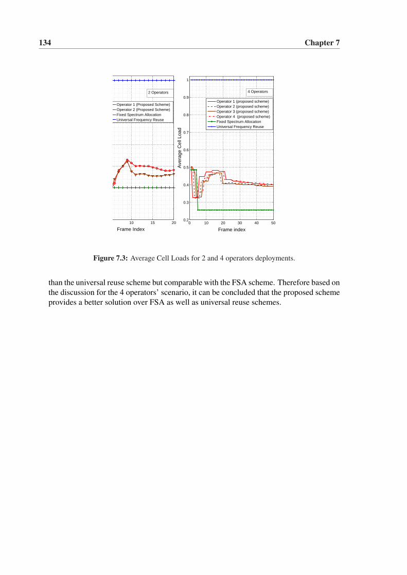
134 Chapter 7
5 10 15 20
Frame Index
Operator 1 (Proposed Scheme)Operator 2 (Proposed Scheme)Fixed Spectrum AllocationUniversal Frequency Reuse
0 10 20 30 40 500.2
0.3
0.4
0.5
0.6
0.7
0.8
0.9
1
Frame index
Ave
rage
Cel
l Loa
d
Operator 1 (proposed scheme)Operator 2 (proposed scheme)Operator 3 (proposed scheme)Operator 4 (proposed scheme)Fixed Spectrum AllocationUniversal Frequency Reuse
4 Operators2 Operators
Figure 7.3: Average Cell Loads for 2 and 4 operators deployments.
than the universal reuse scheme but comparable with the FSA scheme. Therefore based onthe discussion for the 4 operators’ scenario, it can be concluded that the proposed schemeprovides a better solution over FSA as well as universal reuse schemes.
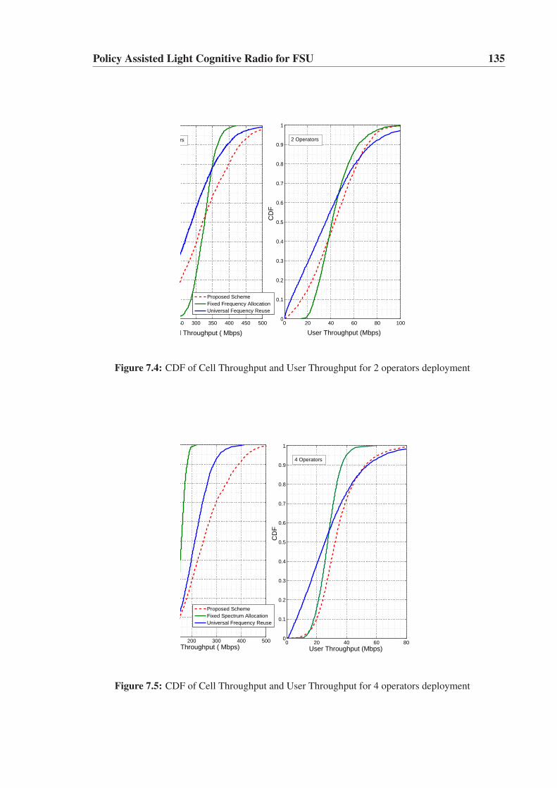
Policy Assisted Light Cognitive Radio for FSU 135
250 300 350 400 450 500
Cell Throughput ( Mbps)
0 20 40 60 80 1000
0.1
0.2
0.3
0.4
0.5
0.6
0.7
0.8
0.9
1
User Throughput (Mbps)
CD
F
Proposed SchemeFixed Frequency Allocation Universal Fequency Reuse
2 Operators 2 Operators
Figure 7.4: CDF of Cell Throughput and User Throughput for 2 operators deployment
0 20 40 60 800
0.1
0.2
0.3
0.4
0.5
0.6
0.7
0.8
0.9
1
User Throughput (Mbps)
CD
F
200 300 400 500Cell Throughput ( Mbps)
Proposed SchemeFixed Spectrum AllocationUniversal Frequency Reuse
4 Operators
Figure 7.5: CDF of Cell Throughput and User Throughput for 4 operators deployment
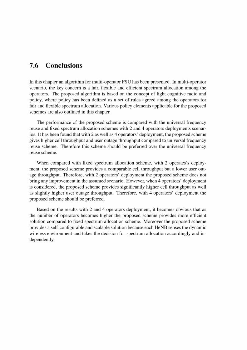
7.6 Conclusions
In this chapter an algorithm for multi-operator FSU has been presented. In multi-operatorscenario, the key concern is a fair, flexible and efficient spectrum allocation among theoperators. The proposed algorithm is based on the concept of light cognitive radio andpolicy, where policy has been defined as a set of rules agreed among the operators forfair and flexible spectrum allocation. Various policy elements applicable for the proposedschemes are also outlined in this chapter.
The performance of the proposed scheme is compared with the universal frequencyreuse and fixed spectrum allocation schemes with 2 and 4 operators deployments scenar-ios. It has been found that with 2 as well as 4 operators’ deployment, the proposed schemegives higher cell throughput and user outage throughput compared to universal frequencyreuse scheme. Therefore this scheme should be preferred over the universal frequencyreuse scheme.
When compared with fixed spectrum allocation scheme, with 2 operates’s deploy-ment, the proposed scheme provides a comparable cell throughput but a lower user out-age throughput. Therefore, with 2 operators’ deployment the proposed scheme does notbring any improvement in the assumed scenario. However, when 4 operators’ deploymentis considered, the proposed scheme provides significantly higher cell throughput as wellas slightly higher user outage throughput. Therefore, with 4 operators’ deployment theproposed scheme should be preferred.
Based on the results with 2 and 4 operators deployment, it becomes obvious that asthe number of operators becomes higher the proposed scheme provides more efficientsolution compared to fixed spectrum allocation scheme. Moreover the proposed schemeprovides a self-configurable and scalable solution because each HeNB senses the dynamicwireless environment and takes the decision for spectrum allocation accordingly and in-dependently.
Chapter 8
Overall Conclusions andRecommendations
The overall objective of this PhD study has been to investigate the potential techniquesto enhance efficiency of the spectrum usage for the next generation mobile communica-tion systems. The LTE and LTE-A systems were considered as example cases. In thefirst phase the study was focused on LTE, where Higher Order Sectorization (HOS) andInter-Cell Interference Avoidance (ICIA) were considered. In the second phase the studywas focused on LTE-A in local area indoor deployment scenario, where mechanisms forFlexible Spectrum Usages (FSU) were investigated. The techniques for improving theefficiency of spectrum usage mainly relied on the concept of aggressive spatial reuse ofthe given spectrum.
8.1 Higher Order Sectorization for LTE DL
The first topic investigated in the thesis was HOS. The main idea behind HOS has been toincrease the usage of spectrum per unit area. In this respect, 6 sectors per site deploymenthas been considered against typically assumed 3 sectors per site deployment. When theperformance is compared, it is found that the geometry factor for 6 sector deployment isapproximately 0.5 dB to 1 dB lower compared to 3 sector deployment. This is due toincreased inter sector antenna overlapping in 6 sector case because of increased numberof sectors. Therefore, the average sector throughput for 6 sector is 6 % lower. However,average site throughput is 88% higher compared to 3 sectors, realizing a significantlyenhanced system capacity gain. This increases spectrum utilization by increasing capacityper unit area.
Further, a mixed network topology has been proposed. A mixed network topologyconsists of a combination of 3 and 6 sectors site deployment. Two different mixed topolo-gies, namely mode1 and mode2, are proposed, where mode1 consists of 6 sectors in thecentre site and 3 sectors in the remaining 18 sites, and mode2 consists of centre site and
137
138 Chapter 8
the sites in the first ring with 6 sectors surrounded by the remaining 12 sites with 3 sec-tors. The main idea behind this proposal was to investigate the performance of mixeddeployment compared to 3 or 6 sectors homogeneous deployments. The mode1 is foundto provide the highest overall geometry factor distribution. At cell edge the geometry ofthe mode1 is about 0.5 dB higher compared to the 3 sectors homogeneous deployment,presenting the lowest interference scenario, whereas 6 sector homogeneous deploymentgives the lowest geometry factor distribution. High average site throughput gains withmixed topology are realized, which are 110 % and 96% higher for mode1 and mode2respectively, over 3 sectors deployment.
These results were obtained by keeping the number of users per site the same in both6 and 3 sector deployments. These relative gains in the mixed network and 6 sectorsite homogeneous deployments are at the cost of slightly increased hand-offs between thesectors, due to the increased number of sectors as well as slightly higher cost of installationdue to extra cabling and antenna requirements.
One of the important observations was that the relative site capacity gain from up-grading existing 3 sector sites with 6 sector sites is comparatively larger for the singlesite upgrade (mode1), as compared to upgrading a cluster of sites (mode2). The mode1could provide a viable option to meet high traffic demands in a localized area such as hotspots. Therefore, this is recommended to be used in order to provide high capacity in hotspot area. Moreover, a migration to 6 sector deployment is recommended to increase thesystem capacity and coverage.
8.2 Inter-Cell Interference Avoidance under FractionalLoad
Further, the mechanisms were investigated to control Inter-Cell Interference (ICI) underfractional load conditions for LTE DL. Under fractional load it can be possible to em-ploy a set of non-overlapping PRBs in the adjacent cells, which reduces the ICI. In factunder fractional load the CQI aware frequency domain packet scheduling can effectivelyminimize ICI. However, the performance of such packet scheduler is very sensitive to in-accuracy and delay in CQI reporting. The inaccuracy and delay in CQI reporting result infast on-off transitions of PRBs and high BLER.
Therefore, several autonomous inter-cell interference avoidance schemes are proposedto allocate non-overlapping sets of PRBs in the adjacent cells as far as possible and also toprovide time correlation to the allocated set of PRBs to avoid on-off transitions. Amongall the proposed schemes, it was found that the Quality Estimation Based PRB selectionScheme (QES) gives the best performance. However, the simplest scheme, which ran-domly selects PRBs and then provides time correlation to the selected set of PRBs, alsohelps to improve effective SINR gain significantly. When QES with 50% fractional loadis compared with full load under best effort traffic, it is found to improve the effectiveSINR by 6.5 dB over full load, which is more than 4 times higher. Moreover, even though
Overall Conclusions and Recommendations 139
the full load employs twice the bandwidth, it offers only 29% increase in the sector (cell)throughput. Therefore, QES achieves a significantly higher throughput per PRB comparedto full load.
Further, QES was compared to full load under Constant Bit Rate (CBR) traffic withChannel Blind traffic load Estimation (CBE) and ThroughPut based traffic load Estimation(TPE) methods. With CBE, most of the users result in throughput below the guaranteedbit rate and also experience delay much higher than the full load. This happens becauseCBE does not account for channel variations and spatial distribution of the users in thecell. However, TPE takes into account the channel variations and spatial distributions ofthe users in the cell, hence, estimates the traffic load more accurately. This significantlyimproves the performance over CBE, and the realized user throughput and delay becomeclose to full load case. However, an important observation is that this performance isachieved at very low fractional load factor, as low as 0.17 only. Therefore a significantlyhigher throughput per PRB, in the order of 5 times compared to full load, is realized.
From the performance evaluation it is found that the proposed schemes significantlyimprove the effective SINR condition leading to improved efficiency of the spectrum uti-lization. Moreover, the schemes are autonomous, requiring no signaling exchange forICIA. It is recommended to integrate the proposed scheme with the packet schedulerfunctionality.
8.3 Flexible Spectrum Usage in Local Area Deployment
In the second phase, the issues related to the local area indoor deployment of HeNBsfor LTE-A were addressed. Considering the expected large scale, random and uncoor-dinated deployments of HeNBs, the main challenges considered are controlling mutualinterference and allowing coexistence of HeNBs in the given area. The Flexible SpectrumUsage (FSU) is considered a key enabler, and therefore to realize the FSU the SpectrumLoad Balancing (SLB) and Resource Chunk Selection (RCS) algorithms are proposed.The SLB is SINR threshold-based, whereas RCS is a comparative interference threshold-based algorithm. Both algorithms work on the principle of self-assessment of surroundingradio environment and ensure coexistence of HeNBs by partially or completely prevent-ing mutual interference on the shared spectrum. The algorithms support self-configurable,decentralized and scalable deployment of HeNBs. The SLB provides granularity for spec-trum allocation at the PRB level, whereas RCS has a granularity of a chunk, where onechunk is considered to have half of the system bandwidth in the considered case. A verylimited signaling exchange via over-the-air-communications is assumed to perform FSU.The proposed algorithms support flexible spectrum usage, self-configuration, flexible andscalable deployment. Therefore, the algorithms are suitable for implementation in the un-coordinated and random deployment in local area solution envisioned for IMT-A systems.
140 Chapter 8
8.4 Autonomous Component Carrier Selection
Since LTE-A will be an evolution of LTE, it is desirable to have backward compatibility.It is considered that the desired bandwidth for LTE-A can be achieved by carrier aggre-gation. Several component carriers are assumed for LTE-A. Further, it is assumed thateach HeNB will not require all of the component carriers at all times, hence a conceptof primary and secondary component carrier has been proposed. The primary componentcarrier is assumed to be used for initial connections of the terminals in the cell, and lateron a cell may additionally select secondary component carrier(s) depending on offeredtraffic in the cell and on mutual interference coupling.
An algorithm for the selection of the primary component carrier has been proposed,which is fully distributed and does not involve any centralized network component; theselection is rather performed locally and independently by each HeNB. The simulationresults presented in this chapter provide an indication that the presented concept helpsto achieve an autonomous scalable and self-adjusting frequency re-use mechanism, whichallows uncoordinated HeNB deployment without prior network planning. Further, mecha-nisms are also proposed for monitoring and recovery of the quality of primary componentcarrier. It is recommended that Interference Reduction Request (IRR) message based re-covery action should be preferred as a first step over the reconfiguration of the primarycomponent carriers.Adaptation of the proposed concept for LTE-Advanced is simple since it entails minimalchanges to the standard as it mostly relies on existing Release’8 UE and HeNB measure-ments.
8.5 Policy Assisted Light Cognitive Radio Enabled FSU
Further, the multi-operators domain FSU was considered, where it was assumed that sev-eral operators may deploy HeNBs in the given geographical area and share the spectrumfrom a common pool. The multi-operator uncoordinated deployment scenario presentsnew challenges, such as fair, efficient and flexible spectrum usage among operators. There-fore the need for policy and the concept of light cognitive radio is envisaged. The schemeproposed is referred to as policy assisted light cognitive radio enabled FSU, where thedecision making process during the cognitive radio cycle is assisted by policy.
The proposed scheme is compared with universal frequency reuse and Fixed SpectrumAllocation (FSA) schemes with 2 and 4 operators’ deployments scenarios. For both thedeployment scenarios, the proposed scheme gives higher cell throughput and user out-age throughput over the universal reuse scheme. However, when compared with FSA,in the scenario with two operators, the proposed scheme is found to give comparablecell throughput, but lower user outage throughput. Instead, with 4 operators’ scenariothe proposed scheme outperforms FSA in both average cell throughput and user outagethroughput.
Overall Conclusions and Recommendations 141
The proposed scheme provides a self-configurable solution, because each HeNB sensesthe dynamic wireless environment and takes the decision for spectrum allocation inde-pendently. The implementation of the proposed scheme requires only a small amount ofsignaling exchange. The proposed scheme provides a viable solution for multi-operatorsFSU and is therefore recommended for the LTE-A local area indoor deployment withmulti operators.
8.6 Topics for Future Research
With respect to higher order sectorization, the performance of 6 sector deployment wasonly evaluated in Downlink. As a next step the performance can be evaluated in uplink aswell. Further, the impact of antenna tilting in vertical domain can be investigated alongwith the 6 sector deployment, in order to evaluate the impact on the system capacityand coverage. The study on Inter-Cell Interference Avoidance under fractional load wasconducted with 3 sector deployment, the study can be further carried out in the 6 sectordeployment scenario.
In the performance results of the SLB algorithm, a homogeneous traffic load for allHeNBs was assumed with full buffer. A dynamically varying cell load was not considered.The SLB is expected to perform more efficiently under such conditions. It will be useful toinvestigate the performance of SLB algorithm under such conditions. The SLB algorithmpresently assumes the selection of PRBs to be limited within the scheduled PRBs only,which limits the diversity gain and range of the PRBs for selection. This assumption wasused to avoid the complexity in SINR estimation over full range of PRBs and also to limitthe power consumption of the user equipment. Further, development of the SLB algorithmwith full range of PRBs selection will be a useful step. The performance of the SLB andRCS algorithms are evaluated only in the regular corporate scenario. A deeper insight canbe gained if the performance is evaluated in residential as well as extended deploymentscenarios. Presently RCS works on the uplink RIP measurement only; a DL measurementbased approach will be more accurate for DL spectrum allocation.
In Autonomous component carrier selection algorithm the implementation of the qual-ity monitoring and recovery action is not yet implemented, it is considered for the futurework. With regard to policy assisted light cognitive radio enabled FSU, only a simplecase with one HeNB per operator has been evaluated. Performance with higher numberof HeNBs per operator will be useful to gain further insight on the proposed concept.

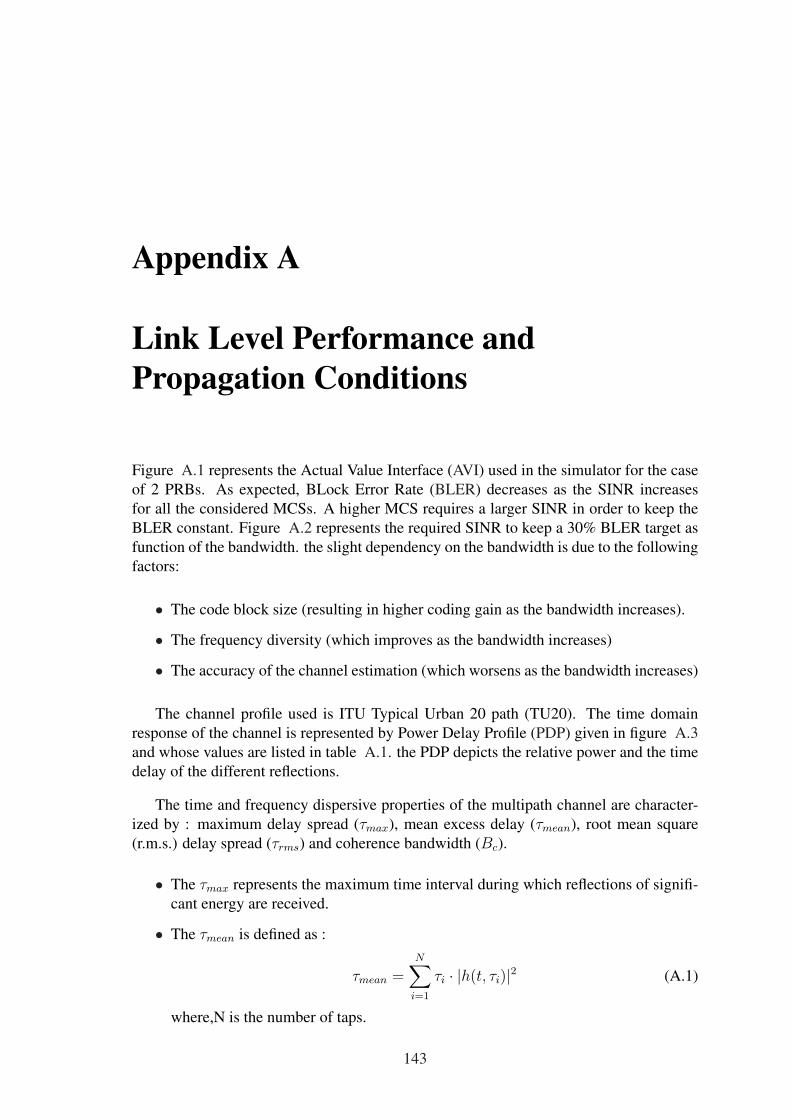
Appendix A
Link Level Performance andPropagation Conditions
Figure A.1 represents the Actual Value Interface (AVI) used in the simulator for the caseof 2 PRBs. As expected, BLock Error Rate (BLER) decreases as the SINR increasesfor all the considered MCSs. A higher MCS requires a larger SINR in order to keep theBLER constant. Figure A.2 represents the required SINR to keep a 30% BLER target asfunction of the bandwidth. the slight dependency on the bandwidth is due to the followingfactors:
• The code block size (resulting in higher coding gain as the bandwidth increases).
• The frequency diversity (which improves as the bandwidth increases)
• The accuracy of the channel estimation (which worsens as the bandwidth increases)
The channel profile used is ITU Typical Urban 20 path (TU20). The time domainresponse of the channel is represented by Power Delay Profile (PDP) given in figure A.3and whose values are listed in table A.1. the PDP depicts the relative power and the timedelay of the different reflections.
The time and frequency dispersive properties of the multipath channel are character-ized by : maximum delay spread (τmax), mean excess delay (τmean), root mean square(r.m.s.) delay spread (τrms) and coherence bandwidth (Bc).
• The τmax represents the maximum time interval during which reflections of signifi-cant energy are received.
• The τmean is defined as :
τmean =N∑
i=1
τi · |h(t, τi)|2 (A.1)
where,N is the number of taps.
143
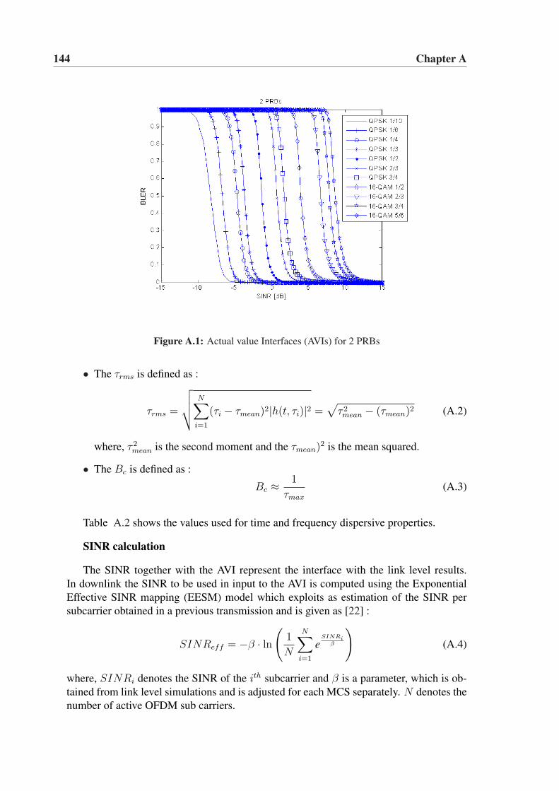
144 Chapter A
Figure A.1: Actual value Interfaces (AVIs) for 2 PRBs
• The τrms is defined as :
τrms =
√√√√N∑
i=1
(τi − τmean)2|h(t, τi)|2 =√
τ 2mean − (τmean)2 (A.2)
where, τ 2mean is the second moment and the τmean)2 is the mean squared.
• The Bc is defined as :
Bc ≈ 1
τmax
(A.3)
Table A.2 shows the values used for time and frequency dispersive properties.
SINR calculation
The SINR together with the AVI represent the interface with the link level results.In downlink the SINR to be used in input to the AVI is computed using the ExponentialEffective SINR mapping (EESM) model which exploits as estimation of the SINR persubcarrier obtained in a previous transmission and is given as [22] :
SINReff = −β · ln(
1
N
N∑i=1
eSINRi
β
)(A.4)
where, SINRi denotes the SINR of the ith subcarrier and β is a parameter, which is ob-tained from link level simulations and is adjusted for each MCS separately. N denotes thenumber of active OFDM sub carriers.
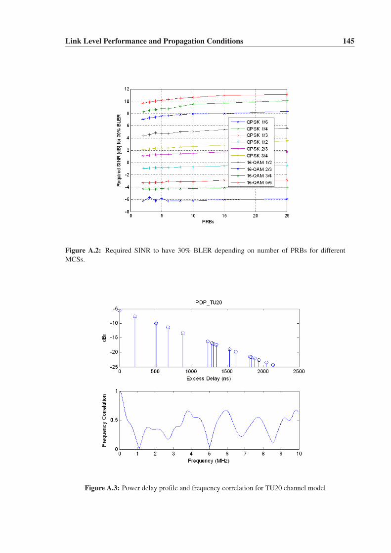
Link Level Performance and Propagation Conditions 145
Figure A.2: Required SINR to have 30% BLER depending on number of PRBs for differentMCSs.
Figure A.3: Power delay profile and frequency correlation for TU20 channel model
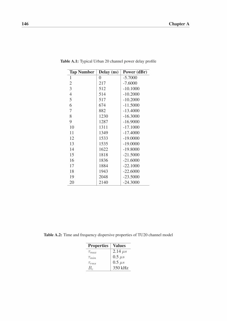
146 Chapter A
Table A.1: Typical Urban 20 channel power delay profile
Tap Number Delay (ns) Power (dBr)1 0 -5.70002 217 -7.60003 512 -10.10004 514 -10.20005 517 -10.20006 674 -11.50007 882 -13.40008 1230 -16.30009 1287 -16.900010 1311 -17.100011 1349 -17.400012 1533 -19.000013 1535 -19.000014 1622 -19.800015 1818 -21.500016 1836 -21.600017 1884 -22.100018 1943 -22.600019 2048 -23.500020 2140 -24.3000
Table A.2: Time and frequency dispersive properties of TU20 channel model
Properties Valuesτmax 2.14 µsτmin 0.5 µsτrms 0.5 µsBc 350 kHz
Bibliography
[1] D. McQueen, “The Momentum Behind LTE Adoption,” IEEE Communiations Magazine, vol. 47,no. 02, pp. 44–45, February 2009.
[2] K. Etemad, “Overview of Mobile WiMAX Technology and Evolution,” IEEE Communiations Maga-zine, vol. 46, no. 10, pp. 31–40, October 2008.
[3] E. Dahlman, S. Parkvall, J. Skold, and P. Beming, Eds., 3G Evolution : HSPA and LTE for MobileBroadband. Academic Press, 2007.
[4] H. Holma, T. Kolding, K. Pedersen, and J. Wigard, HSDPA/HSUPA for UMTS – High Speed RadioAccess for Mobile Communications. ISBN 0-470-01884-4: John Wiley & Sons Ltd, 2006, ch. RadioResource Management, pp. 95–122.
[5] D.Astely, E. Dalhman, A. Furuskar, Y. Jading, M. Lindstorm, and S. parkvall, “LTE: The Evolutionof mobile Broadband,” IEEE Communications Magazine, vol. 47, no. 04, pp. 44–51, April 2009.
[6] 3GPP Technical Report 36.913, version 8.0.0, Requirement for Further Advancements for E-UTRA(LTE-Advance) (Release 8), 2008.
[7] ITU-R, “Framework and Overall Objectives of the Future Deployment of IMT-2000 and Systemsbeyond IMT-2000,” Recommendations ITU-R M-16452, 2003.
[8] R. Irmer, H. Mayer, A. Weber, V. Braun, M. Schmidt, M. Ohm, N. Ahr, A. Zoch, P. Marsch, andG. Fettweis, “Multisite Field Trial for LTE and Advanced Concepts,” IEEE Communiations Magazine,vol. 47, no. 02, pp. 92–98, February 2009.
[9] M. M. Buddhikot, “Understanding Dynamic Spectrum Access : Models Taxonomy and Challenges,”in Proceedings of the IEEE Symposium on Dynamic Spectrum Access (DySPAN), Dublin, Ireland,April 2007.
[10] V. Chandrasekhar and J. Andrews, “Femtocell Networks: A Survey,” IEEE Communiations Magazine,vol. 46, no. 9, pp. 59–67, September 2008.
[11] 3GPP Technical Report 25.814, version 7.1.0, Physical Layer Aspect for Evolved Universal TerrestrialRadio Access (UTRA), September 2006.
[12] 3GPP Technical Specification 36.201, version 0.2.0, LTE Physical Layer - General Description,November 2006.
[13] WiMAX Forum, “Mobile WiMAX - Part I: A Technical Overview and Performance Evaluation’,”White Paper, August 2006.
[14] ETSI, “Digital Video Broadcasting (DVB): Framing Structure, Channel Coding and Modulation forDigital Terrestrial Television,” ETSI, ETS EN 300 744 v 1.1.2, ??
[15] R. Prasad, OFDM for Wireless Communications Systems. Artech House Publishers, 2003.
[16] H. Yang, “A Road to Future Broadband Wireless Access: MIMO-OFDM-Based Air Interface,” IEEECommuniations Magazine, vol. 43, no. 1, pp. 53–60, January 2005.
[17] 3GPP Technical Report 25.892, version 6.0.0, feasibility study for OFDM for UTRAN Enhancement,June 2004.
147
148 Bibliography
[18] 3GPP Technical Specification 36.211, version 8.3.0, Evolved Universal Terrestrial Radio Access (E-UTRA); Physical Channels and Modulation, May 2008.
[19] H. G. Myung, J. Lim, and D. J. Goodman, “Single Carrier FDMA for Uplink Wireless Transmission,”IEEE Vehicular Technology Magazine, p. ??, September 2006.
[20] A. Pokhariyal, T. E. Kolding, and P. E. Mogensen, “Performance of Downlink Frequency DomainPacket Scheduling for the UTRAN Long Term Evolution,” in Proceedings of IEEE Personal Indoorand Mobile Radio Communications Conference (PIMRC), Helsinki, Finland, September 2006, pp.1–5.
[21] K. I. Pedersen, G. Monghal, I. Z. Kovacs, T. E. Kolding, A. Pokhariyal, F. Frederiksen, and P. E.Mogensen, “Frequency Domain Scheduling for OFDMA with Limited and Noisy Channel Feedback,”in Proceedings of IEEE Vehicular Technology Confreence (VTC), Baltimore, USA, October 2007.
[22] K. Brueninghaus, D. Astley, T. Salzer, S. Visuri, A. Alexiou, S. Karger, and G.-A. Seraji, “Link Per-formance Models for System Level Simulations of Broadband Radio Access Systems,” in Proceedingsof the IEEE Personal Indoor and Mobile Radio Communications Conference (PIMRC), vol. 4, Berlin,Germany, September 2005, pp. 2306–2311.
[23] A. Pokhariyal, K. I. Pedersen, G. Monghal, I. Z. Kovacs, C. Rosa, T. E. Kolding, and P. E. Mo-gensen, “HARQ Aware Frequency Domain Packet Scheduler with Different Degrees of Fairness forthe UTRAN Long Term Evolution,” in Proceedings of the IEEE Vehicular Technology Conference(VTC), Dublin, Ireland, April 2007, pp. 2761–2765.
[24] 3GPP Technical Report 36.913, version 4.0.0, Requirement for Further Advancements for E-UTRA(LTE-Advance) (Release 8), 2008.
[25] Nokia Siemens Network, Nokia, “LTE-Advanced Simulation Methodology and Assumptions,” 3GPPTSG-RAN1, R1-083102, August 2008.
[26] Internal Document Nokia Siemens Networks, Aalborg, “Rel’9 / LTE-A FSU Scenarios and LightSimulation Tool,” June 2008.
[27] TR 101 112 (UMTS 30.03 V3.2.0), ETSI Technical Report, Selection procedures for the choice ofradio transmission technologies of the UMTS , 2004.
[28] IST-4-027756 WINNER II, D1.1.2, WINNER II Channel Models part I, September 2007.
[29] “http://www.ist-winner.org.”
[30] M. Schacht, A. Dekorsy, and P. Jung, “System Capacity from UMTS Smart Antenna Concepts,” inProceedings of the IEEE Vehicular Technology Conference (VTC), vol. 5, Florida, USA, October 2003,pp. 3126–3130.
[31] B. Hagerman, D. Imbeni, J. Barta, A. Pollard, R. Wohlmuth, and P. Cosimini, “WCDMA 6 SectorDeployment-Case study of a real installed UMTS-FDD Network,” in Proceedings of the IEEE Vehic-ular Technology Conference (VTC), vol. 2, Melbourne, Australia, May 2006, pp. 703–707.
[32] W. C. Jakes, Ed., Microwave Mobile Communications. ISBN 0-7803-1069-1: IEEE Press, NewJersey, 1994.
[33] B.Christer, V. Johansson, and S. Stefansson, “Optimizing Antenna Parameters for SectorizedWCDMA Networks,” in Proceedings of the IEEE Vehicular Technology Conference (VTC), vol. 4,Rhodes, Greece, September 2000, pp. 1524–1531.
[34] T.I.Song, D.J.Kim, and C.H.Cheon, “Optimization of Sectorized Antenna Beam Pattern for CDMA2000 Systems,” in Proceedings of the IEE Conference Publication Number 489 on 3G Mobile Com-munications Technologies, May 2002, pp. 428–432.
[35] G. K. Chan, “Effects of Sectorization on the Spectrum Efficiency of Cellular Radio Systems,” IEEETransactions on vehicular Technology, vol. 41, no. 3, pp. 217–225, August 1992.
[36] A. Waker, J.L.steffens, K.Sipila, and K.Heiska, “The Impact of Base Station Sectorization onWCDMA Radio Network Performance,” in Proceedings of the IEEE Vehicular Technology Confer-ence (VTC), Houston, USA, April 1999, pp. 2611–2615.
Bibliography 149
[37] X. Yang, S. G. Niri, and R. Tafazolli, “Sectorization Gain in CDMA Cellular Systems,” in 3G MobileCommunication Technologies,Conf. Publ. No. 471, 2000, pp. 70–75.
[38] C.-C. Lee and R. Steele, “Effects of Soft and softer Handoffs on CDMA System Capacity,” IEEETransactions on vehicular Technology, vol. 47, no. 3, pp. 830–841, August 1998.
[39] F. Athley, “On Base Station Beamwidth for Sectorized WCDMA Systems,” in Proceedings of theIEEE Vehicular Technology Conference (VTC), Montreal, Canada, September 2006, pp. 1–5.
[40] W.-J. Wang, I.-T. Lu, and S.-C. Liu, “Soft Handoff Performance of 3-sector and 6-sector Multi-cell CDMA Systems,” in Proceedings of the IEEE Vehicular Technology Conference (VTC), vol. 4,Rhodes, Greece, May 2001, pp. 2338–2342.
[41] 3GPP Technical Specification 36.300, version 8.3.0, Evolved Universal Terrestrial Radio Access (E-UTRA) and Evolved Universal Terrestrial Radio Access (E-UTRAN); Overall Description; Stage 2,January 2008.
[42] 3GPP Technical Report 25.996, version 6.1.0, Spatial Channel Model for MIMO Simulations, Septem-ber 2003.
[43] K. Brueninghaus, D. Astley, T. Salzer, S. Visuri, A. Alexiou, S. Karger, and G.-A. Seraji, “Link Per-formance Models for System Level Simulations of Broadband Radio Access Systems,” in Proceedingsof the IEEE Personal Indoor and Mobile Radio Communications Conference (PIMRC), vol. 4, Berlin,Germany, September 2005, pp. 2306–2311.
[44] A. Pokhariyal, “Downlink Frequency-Domain Adaptation and Scheduling – A Case Study Based onthe UTRA Long Term Evolution,” Ph.D. dissertation, Radio Access Technology Section, Institute ofElectronic Systems, Aalborg University, Aalborg, Denmark, August 2007.
[45] K. I. Pedersen, P. Mogensen, and B. Fleury, “Spatial Channel Characteristics in Outdoor Environ-ments and Their Impact on BS Antenna System Performance,” in Proceedings of the IEEE VehicularTechnology Conference (VTC), Ottawa, Canada, May 1998, pp. 719–723.
[46] Ericsson, “Reactive and Pro-active use of Uplink Overload Indication in LTE,” 3GPP TSG-RAN1,R1-074379, October 2007.
[47] 3GPP Technical Specifications 36.423, version 8.3.0, Evolved Universal Terrestrial Radio AccessNetwork(E-UTRAN); X2 application protocol, (Release 8), May 2008.
[48] A. Simonsson, “Frequency Reuse and Intercell Interference Co-Ordination In E-UTRA,” in Proceed-ings of the IEEE Vehicular Technology Conference (VTC), Dublin, Ireland, April 2007, pp. 3091–3095.
[49] Nokia, Nokia Siemens Networks, “Downlink Interference Coordination,” 3GPP TSG-RAN1, R1-072974, June 2007.
[50] Ericsson, “On Inter-cell Interference Coordination Schemes without/with Traffic Load indication,”3GPP TSG-RAN1, R1-073039, June 2007.
[51] Alcatel-Lucent, “Semi-Static Interference Coordination Method,” 3GPP TSG-RAN1, R1-081873,May 2008.
[52] Siemens, “Interference Mitigation by Partial Frequency Reuse,” 3GPP TSG-RAN1, R1-060135, Jan-uary 2006.
[53] Ericsson, “Options for Inter-cell Interference Coordination (ICIC),” 3GPP TSG-RAN3, R3-061199,September 2006.
[54] Nokia, Nokia Siemens Networks, “Low load scenarios with CQI-based interference coordination,”3GPP TSG-RAN1, R1-073679, August 2007.
[55] A. Pokhariyal, G. Monghal, K. I. Pedersen, P. E. Mogensen, I. Z. Kovacs, C. Rosa, and T. E. Kolding,“Frequency Domain Packet Scheduling Under Fractional Load for the UTRAN LTE Downlink,” inProceedings of the IEEE Vehicular Technology Conference (VTC), Dublin, Ireland, April 2007, pp.699–703.
150 Bibliography
[56] S. Kumar, G. Monghal, J. Nin, I. Ordas, K. I. Pedersen, and P. E. Mogensen, “Autonomous Inter CellInterference Avoidance under Fractional Load for Downlink Long Term Evolution,” in Proceedingsof the 69th IEEE Vehicular Technology Conference (VTC), Barcelona, Spain, April 2009, pp. ??–??
[57] T. E. Kolding, F. Frederiksen, and A. Pokhariyal, “Low-Bandwidth Channel Quality Indication forOFDMA Frequency Domain Packet Scheduling,” in Proceedings of International Symposium on Wire-less Communication Systems (ISWCS), Valencia, Spain, September 2006.
[58] J. N. Guerrero and I. O. Villamandos, “Autonomous Physical Resource Block Selection in FractionalLoad Scenario for 3GPP Long Term Evolution Downlink,” Master’s thesis, Aalborg University, Aal-borg, Denmark, 2007.
[59] G. Monghal, S. Kumar, K. I. Pedersen, and P. E. Mogensen, “Integrated Fractional Load and PacketScheduling for OFDMA Systems,” in Proceedings of the IEEE International Conference on Commu-nications(ICC), Dresden, Germany, June 2009, pp. ??–??
[60] A. Pokhariyal, K. I. Pedersen, G. Monghal, I. Z. Kovacs, C. Rosa, T. E. Kolding, and P. E. Mo-gensen, “HARQ Aware Frequency Domain Packet Scheduler with Different Degrees of Fairness forthe UTRAN Long Term Evolution,” in Proceedings of the IEEE Vehicular Technology Conference(VTC), Dublin, Ireland, April 2007, pp. 2761–2765.
[61] 3GPP RAN, “Workshop on IMT-Advanced, Shenzhen, China,,” available atftp://ftp.3gpp.org/workshop/, April 2008.
[62] 3GPP Technical Report 25.820, version 8.2.0, 3G Home NodeB Study Item Technical Report(Release8), September 2008.
[63] L. B. et al, “Policy Based Reasoning for Spectrum Sharing in Cognitive Radio Networks,” in IEEEInternational Symposium on Spread Spectrum Techniques and Applications (ISSSTA), vol. 3, Sydney,Australia, September 2005, pp. 355–358.
[64] Y. Bai and L. Chen, “Flexible Spectrum Allocation Methods for Wireless Network Providers,” in IEEEInternational Symposium on Personal, Indoor and Mobile Radio Communications (PIMRC), Helsinki,Finland, September 2006, pp. 1–5.
[65] J. P. Kermoal, S. Pfletschinger, k. Hooli, S. Thilakawardana, J. Lara, and Y. Zhu, “Spectrum Shar-ing for WINNER Radio Access Networks,” in IEEE International Conference on Cognitive RadioOreiented Wireless Networks and Communications, Greece, june 2006, pp. 1–5.
[66] S. Mangold, L. Berlemann, and S. Nandagopalan, “Spectrum Sharing with Value Orientation forCognitive Radio,” European Transactions on Telecommunications, pp. 383–394, 2006.
[67] Wireless World Initiative New Radio+, “WINNER II Spectrum Sharing Studies,” IST-4-027756 WIN-NER D5.10.3 v1.0, website; http://www.ist-winner.org, November 2006.
[68] L. Berlemann and B. Walke, “Spectrum Load Smoothing for Optimized Spectrum Utilization-Rationale and Algorithm,” in Proceedings of the IEEE Wireless Communications and NetworkingConference(WCNC), vol. 3, New Orleans, USA, March 2005, pp. 1952–1956.
[69] L. Berlemann, S. Mangold, G. R. Hiertz, and B. H. Walke, “Spectrum Load Smoothing : dis-tributed quality od service Support for Cognitive Radios in Open Spectrum,” European Transactionson Telecommunications, pp. 395–406, 2006.
[70] Nokia Siemens Network, Nokia, “Inter eNB Over the Air Communication (OTAC)for LTE-Advanced,” 3GPP TSG-RAN1, R1-090236, January 2009.
[71] A. A. et. al., “Duplexing, Resource Allocation and Inter-cell Coordination : Design Recommendationsfor Next Generation Wireless Systems,” Wireless Communications and Mobile computing in WileyInterScience, vol. 5, pp. 77–93, January 2005.
[72] S. Parkvall, E. Dahlman, A. Furuskar, Y. Jading, M. Olsson, S. Wanstedt, and K. Zangi, “LTE-Advanced Evolving LTE towards IMT-Advanced,” in Proceedings of the IEEE Vehicular TechnologyConference (VTC), Calgary, Canada, September 2008, pp. 1–5.
Bibliography 151
[73] Huawei, “Consideration on Carrier Aggreagation for Home eNB,” 3GPP TSG-RAN 1, R1-090817,Feb 2009.
[74] Alcatel Shanghai Bell, Alcatel-Lucent, “Support of Wider Bandwidth for Home eNodeB in LTE-Advanced,” 3GPP TSG-RAN1, R1-084125, November 2008.
[75] Ericsson, “Carrier Aggregation in LTE-Advanced,” 3GPP TSG-RAN1, R1-082468, June 2008.
[76] Qualcomm Europe, “Notion of Anchor Carrier in LTE-A,” 3GPP TSG-RAN1, R1-080356, January2009.
[77] Nokia Siemens Network, Nokia, “Autonomous Component Carrier selction for LTE-Advanced,”3GPP TSG-RAN1, R1-083103, August 2008.
[78] Internal Document Nokia Siemens Networks, Aalborg, “Autonomous Component Carrier SelctionConcept,” December 2008.
[79] 3GPP Technical Specification 36.214, version 8.2.0, Evolved Universal Terrestrial Radio Access (E-UTRA); Physical Layer - Measurements (Release 8), May 2008.
[80] Nokia Siemens Network, Nokia, “Primary Component Carrier selction, Monitoring and RecoveryAction,” 3GPP TSG-RAN1, R1-090735, February 2009.
[81] Nokia Siemens Network, Nokia., “On Definition and Usage of the Uplink Overload Indicator,” 3GPPTSG-RAN1, R1-080332, January 2009.
[82] L. G. U. Garcia, K. I. Pedersen, and P. E. Mogensen, “Autonomous Component Carrier Selection forLocal Area Uncoordinated Deployment of LTE-Advanced.”
[83] Nokia Siemens Network, Nokia, “Use of Background Interference Matrix for Autonomous Compo-nent Carrier selction for LTE-Advanced,” 3GPP TSG-RAN1, R1-090235, January 2009.
[84] P. E. Mogensen, W. Na, I. Z. Kovacs, F. Frederiksen, A. Pokhariyal, K. I. Pedersen, T. Kolding,K. Hugl, and M. Kuusela, “LTE Capacity Compared to the Shanon Bound,” in Proceedings of the65th IEEE Vehicular Technology Conference (VTC), Dublin, Ireland, April 2007, pp. 1234–1238.
[85] Y. Wang, S. Kumar, L. Garcia, K. I. Pedersen, I. Z. Kovács, S. Frattasi, N. Marchetti, P. E. Mogensen,and T. B. Sørensen, “Fixed Frequency Reuse for LTE-Advanced Systems in Different Scenarios,” inProceedings of the 69th IEEE Vehicular Technology Conference (VTC).
[86] G. Middleton, K. Hooli, A. Tolli, and J. Lilleberg, “Inter Operator Spectrum Sharing in a Broad-band Cellular Network,” in Proceedings of the IEEE International Symposium on Spread SpectrumTechniques and Applications, Brazil, August 2008, pp. 376–380.
[87] M. Bennis and J. Lilleberg, “Inter Operator Resource Sharing for 3G Systems and Beyond,” in Pro-ceedings of the IEEE International Symposium on Spread Spectrum Techniques and Applications,Brazil, August 2006, pp. 401–405.
[88] J. L. M. D. M.K. Pereirasamy and C. Hartmann, “An Approach for Inter Operator Spectrum Sharingfor 3G Systems and Beyond,” in Proceedings of IEEE Personal Indoor and Mobile Radio Communi-cations Conference(PIMRC, vol. 3, Barcelona, Spain, September 2004, pp. 1952–1956.
[89] M. Pereirasamy, J. Luo, M. Dillinger, and C. Hartmann, “Dynamic Inter Operator Spectrum Sharingfor UMTS FDD with Displaced Cellular Network,” in Proceedings of the IEEE Wireless Communica-tions and Networking Conference(WCNC), New Orleans, USA, March 2005, pp. 1720–1725.
[90] A. Attar and A. H. Aghvami, “A framework for Unified Spectrum Management in heterogeneousWireless Networks,” IEEE Communications Magazine, vol. 45, pp. 44–51, September 2007.
[91] D. Gozalvez, J. Monserrat, and D. Calabuig, “Policy Based Channel Access Mechanism Selection forQoS Provision in IEEE 802.11e,” IEEE Vehicular Technology magazine, September 2007.
[92] S. Horrich, S.B.Jamaa, and P. Houze, “Policy Based RRM for Network Terminal Decision Sharing,”IEEE Vehicular Technology magazine, September 2007.
152 Bibliography
[93] D. Elenius, G. Denker, M. O. Stehr, R. senanayake, C. Talcott, and D. Wilkins, “CoRaL policy lan-guage and reasoning techniques for spectrum policies,” IEEE computer society, 2007.
[94] S. Haykin, “Cognitive Radio: Brain-Empowered Wireless Communication,” IEEE JSAC, February2005.
[95] J. M. III and G. Q. Marguire, “Cognitive Radio: Making Software Radio More Personal,” IEEEPersona Communications Mag., vol. 6, no. 4, pp. 13–18, August 1999.


![Effective Wide Spectrum Sharing Techniques Relying on CR ... · comprehensive survey on spectrum sharing toward 5G networks. Reference [29] presented a brief survey on advanced techniques](https://img.pdfslide.net/doc/110x75/5f08fdc37e708231d424b501/effective-wide-spectrum-sharing-techniques-relying-on-cr-comprehensive-survey.jpg)