An Introduction to tidymodelsAn Introduction to tidymodels

Max Kuhn topepo @topepos

R has always had a rich set of modeling tools that itinherited from S. For example, the formula interface hasmade it simple to specify potentially complex modelstructures.

R has cutting edge models. Many researchers in variousdomains use R as their primary computing environmentand their work o�en results in R packages.

It is easy to port or link to other applications. R doesn't tryto be everything to everyone. If you prefer modelsimplemented in C, C++, tensorflow, keras, python,stan, or Weka, you can access these applications withoutleaving R.

However, there is a huge consistency problem. Forexample:

There are two primary methods for specifying whatterms are in a model. Not all models have both.99% of model functions automatically generatedummy variables.Sparse matrices can be used (unless the can't).Many package developers don't know much aboutthe language and omit OOP and other core Rcomponents.

Two examples follow...

Modeling in R

2 / 39

Between-Package InconsistencySyntax for computing predicted class probabilities:

Function Package Code

lda MASS predict(obj)

glm stats predict(obj, type = "response")

gbm gbm predict(obj, type = "response", n.trees)

mda mda predict(obj, type = "posterior")

rpart rpart predict(obj, type = "prob")

Weka RWeka predict(obj, type = "probability")

logitboost LogitBoost predict(obj, type = "raw", nIter)

pamr.train pamr pamr.predict(obj, type = "posterior")

3 / 39

Within-Package Inconsistency: glmnet PredictionsThe glmnet model can be used to fit regularized generalized linear models with a mixture of L1 and L2 penalties.

We'll look at what happens when we get predictions for a regression model (i.e. numeric Y) as well as classificationmodels where Y has two or three categorical values.

The models shown below contain solutions for three regularization values ( ).

The predict method gives the results for all three at once (👍).

λ

4 / 39

Numeric glmnet PredictionsPredicting a numeric outcome for two new data points:

new_x

## x1 x2 x3 x4## sample_1 1.649 -0.483 -0.294 -0.815## sample_2 0.656 -0.420 0.880 0.109

predict(reg_mod, newx = new_x)

## s0 s1 s2## sample_1 9.95 9.95 10## sample_2 9.95 9.95 10

A matrix result and we will assume that the values are in the same order as what we gave to the model fit function.λ

5 / 39

glmnet Class PredictionsPredicting an outcome with two classes:

predict(two_class_mod, newx = new_x, type = "class")

## s0 s1 s2 ## sample_1 "a" "b" "b"## sample_2 "a" "b" "b"

Not factors! That's di�erent from what is required for the y argument. From ?glmnet:

For family="binomial" [y] should be either a factor with two levels, or a two-column matrix of counts orproportions

I'm guessing that this is because they want to keep the result a matrix (to be consistent).

6 / 39

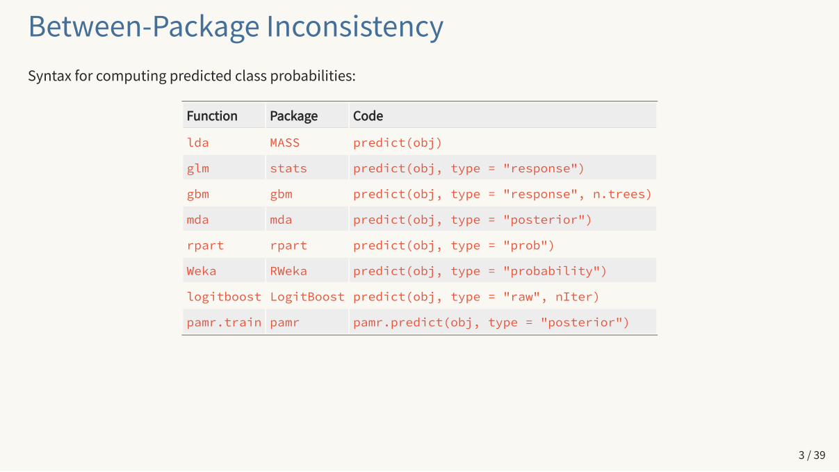
glmnet Class Probabilities (Two Classes)predict(two_class_mod, newx = new_x, type = "response")

## s0 s1 s2## sample_1 0.5 0.5 0.506## sample_2 0.5 0.5 0.526

Okay, we get a matrix of the probability for the second level of the outcome factor.

To make this fit into most code, we can manually calculate the other probability. No biggie!

7 / 39

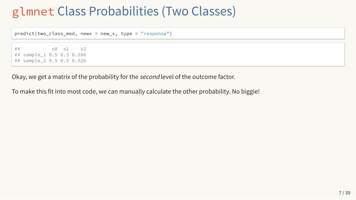
predict(three_class_mod, newx = new_x, type = "response")

## , , s0## ## a b c## sample_1 0.333 0.333 0.333## sample_2 0.333 0.333 0.333## ## , , s1## ## a b c## sample_1 0.333 0.333 0.333## sample_2 0.333 0.333 0.333## ## , , s2## ## a b c## sample_1 0.373 0.244 0.383## sample_2 0.327 0.339 0.334

😳

No more matrix results. 3D array and we get all of theprobabilities back this time.

Am I working for glmnet or is it is working for me?

Maybe a structure like this would work better:

## # A tibble: 6 x 4## a b c lambda## <dbl> <dbl> <dbl> <dbl>## 1 0.333 0.333 0.333 1 ## 2 0.333 0.333 0.333 1 ## 3 0.333 0.333 0.333 0.1 ## 4 0.333 0.333 0.333 0.1 ## 5 0.373 0.244 0.383 0.01## 6 0.327 0.339 0.334 0.01

glmnet Class Probabilities (Three Classes)

8 / 39

What We NeedUnless you are doing a simple one-o� data analysis, the lack of consistency between, and sometimes within, R packagescan be very frustrating.

If we could agree on a set of common conventions for interfaces, return values, and other components, everyone's lifewould be easier.

Once we agree on conventions, two challenges are:

As of October 2020, there are over 16K R packages on CRAN. How do we "harmonize" these without breakingeverything?

How can we guide new R users (or people unfamiliar with R) in making good choices in their modeling packages?

These prospective and retrospective problems will be addressed in a minute.

9 / 39

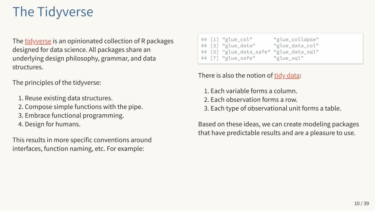
The tidyverse is an opinionated collection of R packagesdesigned for data science. All packages share anunderlying design philosophy, grammar, and datastructures.

The principles of the tidyverse:

1. Reuse existing data structures.2. Compose simple functions with the pipe.3. Embrace functional programming.4. Design for humans.

This results in more specific conventions aroundinterfaces, function naming, etc. For example:

## [1] "glue_col" "glue_collapse" ## [3] "glue_data" "glue_data_col" ## [5] "glue_data_safe" "glue_data_sql" ## [7] "glue_safe" "glue_sql"

There is also the notion of tidy data:

1. Each variable forms a column.2. Each observation forms a row.3. Each type of observational unit forms a table.

Based on these ideas, we can create modeling packagesthat have predictable results and are a pleasure to use.

The Tidyverse

10 / 39

Tidymodelstidymodels is a collection of modeling packages that live in the tidyverse and are designed in the same way.

My goals for tidymodels are:

1. Encourage empirical validation and good methodology.

2. Smooth out diverse interfaces.

3. Build highly reusable infrastructure.

4. Enable a wider variety of methodologies.

The tidymodels packages address the retrospective and prospective issues. We are also developing a set of principlesand templates to make prospective (new R packages) easy to create.

11 / 39

12 / 39

tidymodels.org

Tidy Modeling with R (tmwr.org)

13 / 39

Selected Modeling Packagesbroom takes the messy output of built-in functions in R, such as lm, nls, or t.test, and turns them into tidy dataframes.

recipes is a general data preprocessor with a modern interface. It can create model matrices that incorporatefeature engineering, imputation, and other tools.

rsample has infrastructure for resampling data so that models can be assessed and empirically validated.

parsnip gives us a unified modeling interface.

tune has functions for grid search and sequential optimization of model parameters.

14 / 39

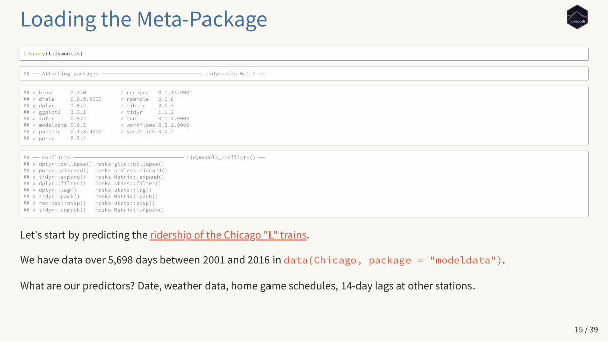
Loading the Meta-Packagelibrary(tidymodels)

## ── Attaching packages ──────────────────────────────── tidymodels 0.1.1 ──

## ✓ broom 0.7.0 ✓ recipes 0.1.13.9001## ✓ dials 0.0.9.9000 ✓ rsample 0.0.8 ## ✓ dplyr 1.0.2 ✓ tibble 3.0.3 ## ✓ ggplot2 3.3.2 ✓ tidyr 1.1.2 ## ✓ infer 0.5.2 ✓ tune 0.1.1.9000 ## ✓ modeldata 0.0.2 ✓ workflows 0.2.1.9000 ## ✓ parsnip 0.1.3.9000 ✓ yardstick 0.0.7 ## ✓ purrr 0.3.4

## ── Conflicts ─────────────────────────────────── tidymodels_conflicts() ──## x dplyr::collapse() masks glue::collapse()## x purrr::discard() masks scales::discard()## x tidyr::expand() masks Matrix::expand()## x dplyr::filter() masks stats::filter()## x dplyr::lag() masks stats::lag()## x tidyr::pack() masks Matrix::pack()## x recipes::step() masks stats::step()## x tidyr::unpack() masks Matrix::unpack()

Let's start by predicting the ridership of the Chicago "L" trains.

We have data over 5,698 days between 2001 and 2016 in data(Chicago, package = "modeldata").

What are our predictors? Date, weather data, home game schedules, 14-day lags at other stations.

15 / 39

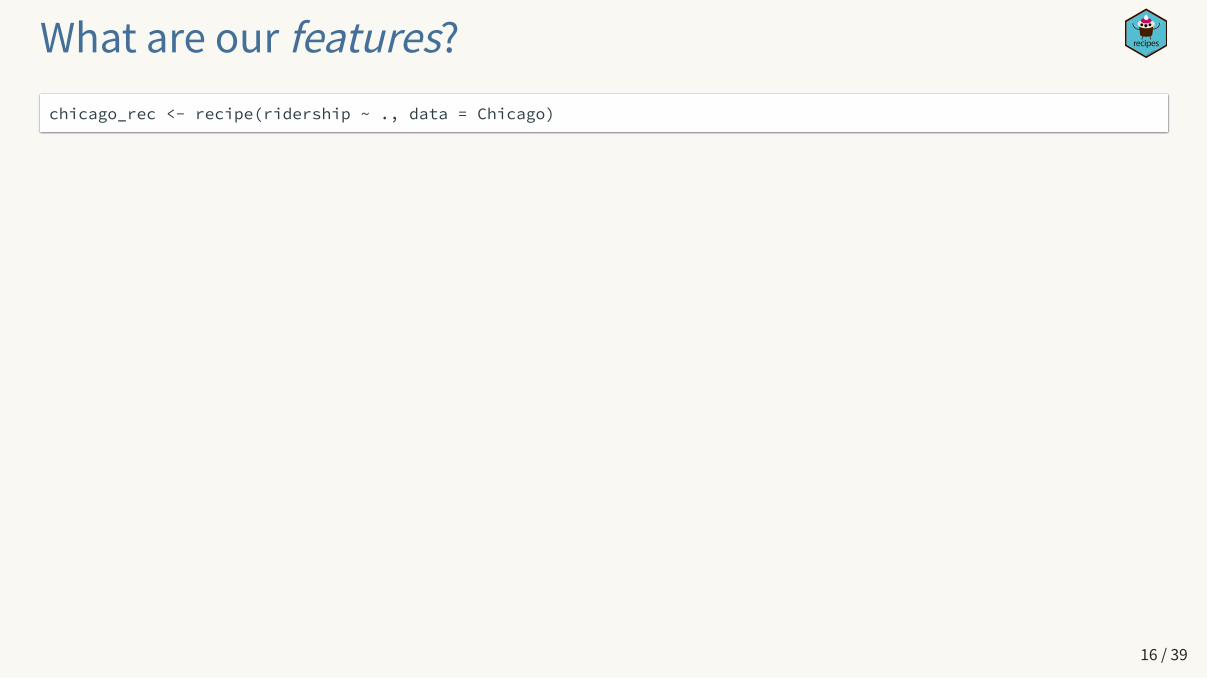
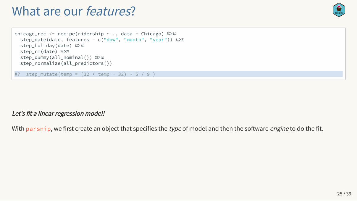
What are our features?chicago_rec <- recipe(ridership ~ ., data = Chicago)

16 / 39

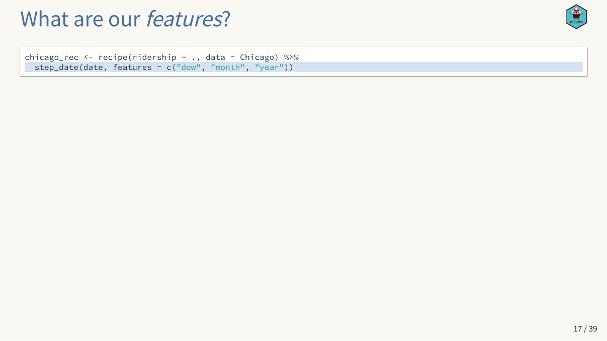
What are our features?chicago_rec <- recipe(ridership ~ ., data = Chicago) %>% step_date(date, features = c("dow", "month", "year"))

17 / 39

What are our features?chicago_rec <- recipe(ridership ~ ., data = Chicago) %>% step_date(date, features = c("dow", "month", "year")) %>% step_holiday(date)

18 / 39

What are our features?chicago_rec <- recipe(ridership ~ ., data = Chicago) %>% step_date(date, features = c("dow", "month", "year")) %>% step_holiday(date) %>% step_rm(date)

19 / 39

What are our features?chicago_rec <- recipe(ridership ~ ., data = Chicago) %>% step_date(date, features = c("dow", "month", "year")) %>% step_holiday(date) %>% step_rm(date) %>% step_dummy(all_nominal())

20 / 39

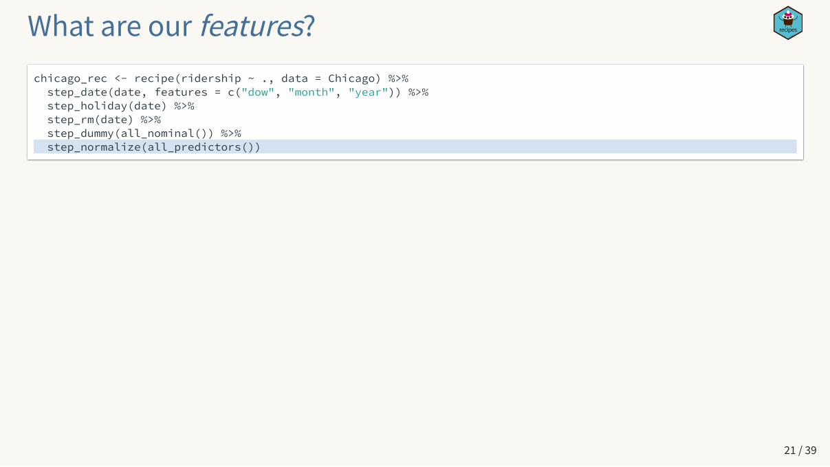
What are our features?chicago_rec <- recipe(ridership ~ ., data = Chicago) %>% step_date(date, features = c("dow", "month", "year")) %>% step_holiday(date) %>% step_rm(date) %>% step_dummy(all_nominal()) %>% step_normalize(all_predictors())

21 / 39

What are our features?chicago_rec <- recipe(ridership ~ ., data = Chicago) %>% step_date(date, features = c("dow", "month", "year")) %>% step_holiday(date) %>% step_rm(date) %>% step_dummy(all_nominal()) %>% step_normalize(all_predictors())

#? step_pca(one_of(stations), num_comp = 10)

22 / 39

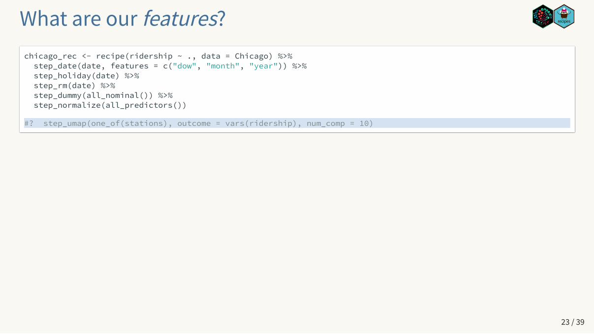
What are our features?chicago_rec <- recipe(ridership ~ ., data = Chicago) %>% step_date(date, features = c("dow", "month", "year")) %>% step_holiday(date) %>% step_rm(date) %>% step_dummy(all_nominal()) %>% step_normalize(all_predictors())

#? step_umap(one_of(stations), outcome = vars(ridership), num_comp = 10)

23 / 39

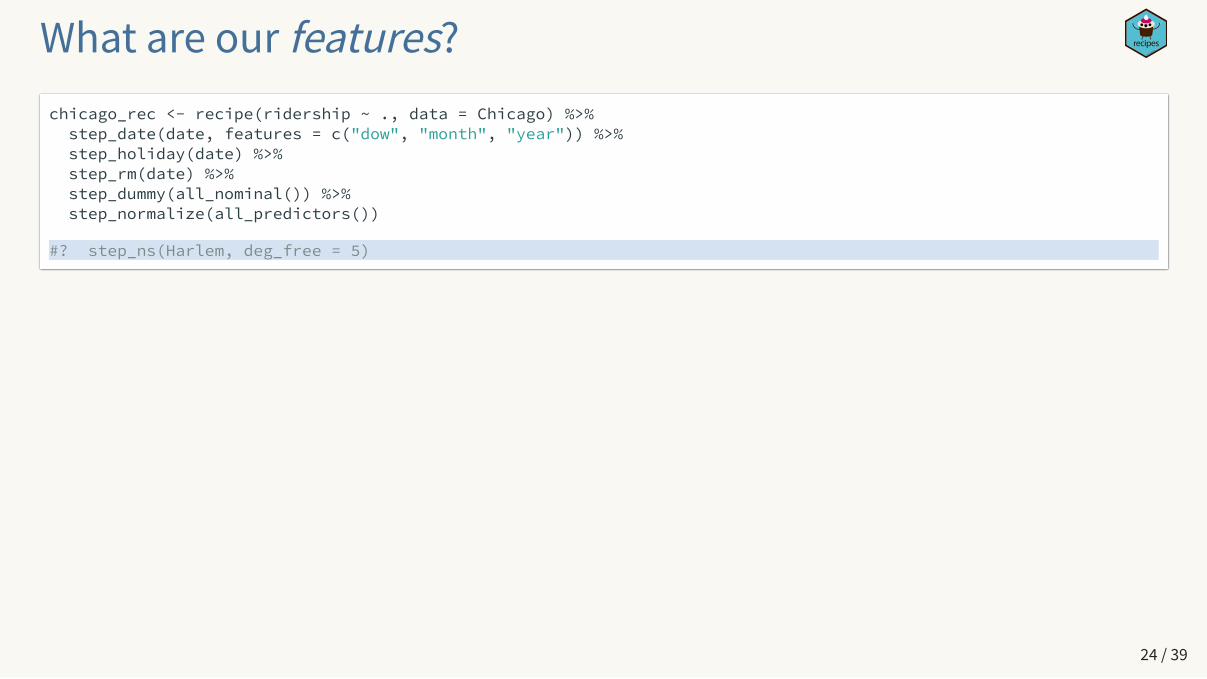
What are our features?chicago_rec <- recipe(ridership ~ ., data = Chicago) %>% step_date(date, features = c("dow", "month", "year")) %>% step_holiday(date) %>% step_rm(date) %>% step_dummy(all_nominal()) %>% step_normalize(all_predictors())

#? step_ns(Harlem, deg_free = 5)

24 / 39

What are our features?chicago_rec <- recipe(ridership ~ ., data = Chicago) %>% step_date(date, features = c("dow", "month", "year")) %>% step_holiday(date) %>% step_rm(date) %>% step_dummy(all_nominal()) %>% step_normalize(all_predictors())

#? step_mutate(temp = (32 * temp − 32) * 5 / 9 )

Let's fit a linear regression model!

With parsnip, we first create an object that specifies the type of model and then the so�ware engine to do the fit.

25 / 39

linear_mod <- linear_reg()

This says "Let's fit a model with a numeric outcome, and intercept, andslopes for each predictor."

Other model types include nearest_neighbors(),decision_tree(), rand_forest(), arima_reg(), and so on.

The set_engine() function gives the details on how it should be fit.

Linear regression specification

26 / 39

linear_mod <- linear_reg() %>% set_engine("lm")

Let's fit it with...

27 / 39

linear_mod <- linear_reg() %>% set_engine("keras")

Let's fit it with...

28 / 39

linear_mod <- linear_reg() %>% set_engine("spark")

Let's fit it with...

29 / 39

linear_mod <- linear_reg() %>% set_engine("stan")

Let's fit it with...

30 / 39

linear_mod <- linear_reg() %>% set_engine("glmnet")

Let's fit it with...

31 / 39

linear_mod <- linear_reg(penalty = 0.1, mixture = 0.5) %>% set_engine("glmnet")

Let's fit it with...

32 / 39

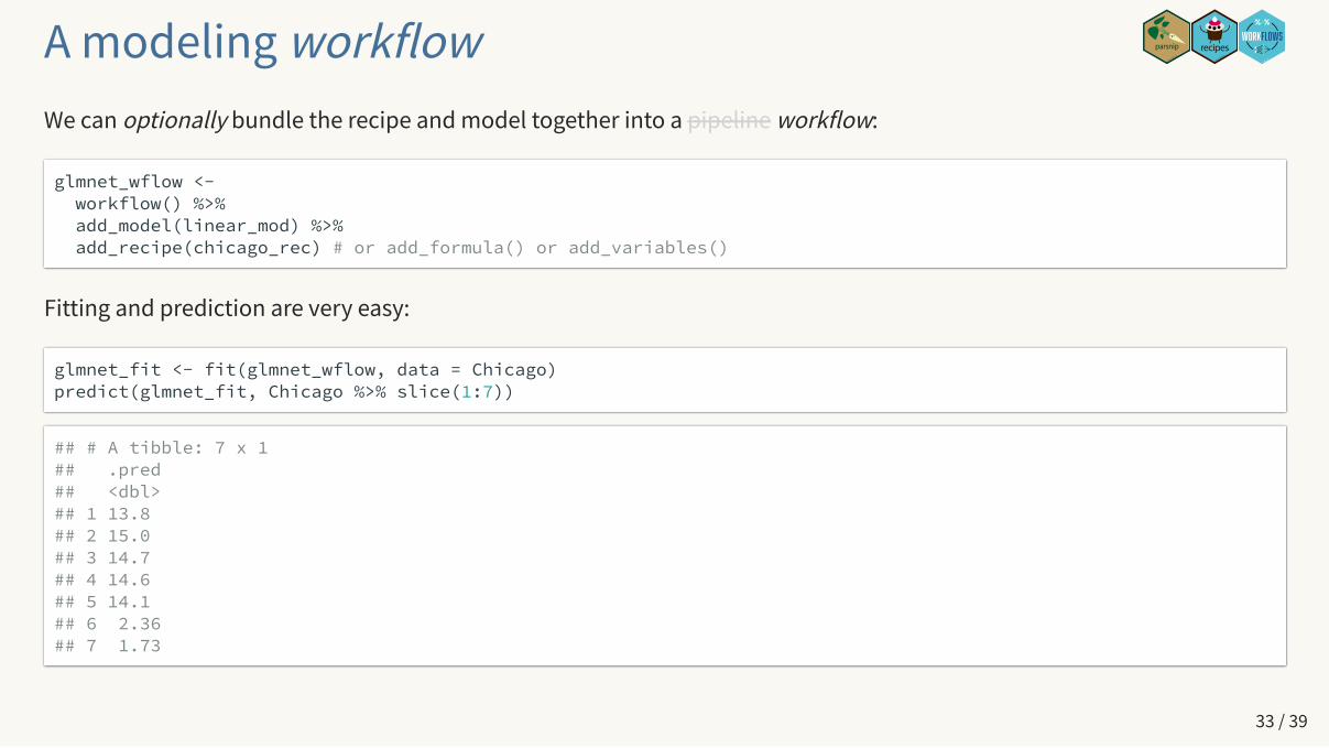
A modeling workflowWe can optionally bundle the recipe and model together into a pipeline workflow:

glmnet_wflow <- workflow() %>% add_model(linear_mod) %>% add_recipe(chicago_rec) # or add_formula() or add_variables()

Fitting and prediction are very easy:

glmnet_fit <- fit(glmnet_wflow, data = Chicago)predict(glmnet_fit, Chicago %>% slice(1:7))

## # A tibble: 7 x 1## .pred## <dbl>## 1 13.8 ## 2 15.0 ## 3 14.7 ## 4 14.6 ## 5 14.1 ## 6 2.36## 7 1.73

33 / 39

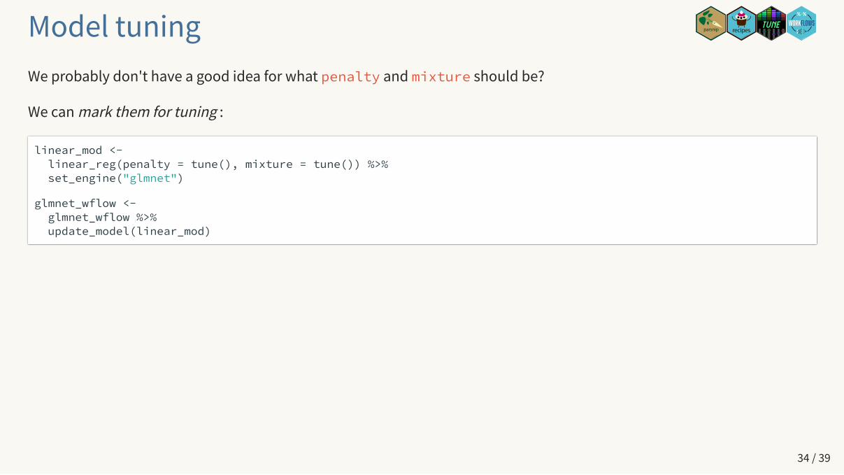
Model tuningWe probably don't have a good idea for what penalty and mixture should be?

We can mark them for tuning :

linear_mod <- linear_reg(penalty = tune(), mixture = tune()) %>% set_engine("glmnet")

glmnet_wflow <- glmnet_wflow %>% update_model(linear_mod)

34 / 39

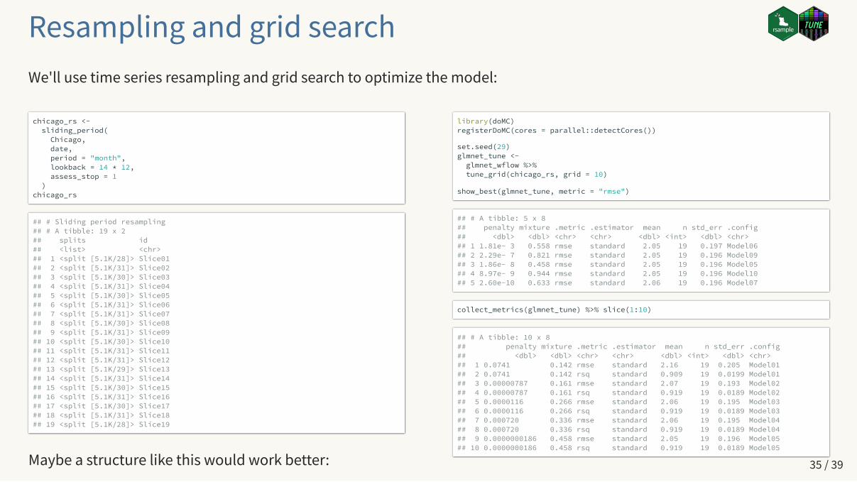
chicago_rs <- sliding_period( Chicago, date, period = "month", lookback = 14 * 12, assess_stop = 1 )chicago_rs

## # Sliding period resampling ## # A tibble: 19 x 2## splits id ## <list> <chr> ## 1 <split [5.1K/28]> Slice01## 2 <split [5.1K/31]> Slice02## 3 <split [5.1K/30]> Slice03## 4 <split [5.1K/31]> Slice04## 5 <split [5.1K/30]> Slice05## 6 <split [5.1K/31]> Slice06## 7 <split [5.1K/31]> Slice07## 8 <split [5.1K/30]> Slice08## 9 <split [5.1K/31]> Slice09## 10 <split [5.1K/30]> Slice10## 11 <split [5.1K/31]> Slice11## 12 <split [5.1K/31]> Slice12## 13 <split [5.1K/29]> Slice13## 14 <split [5.1K/31]> Slice14## 15 <split [5.1K/30]> Slice15## 16 <split [5.1K/31]> Slice16## 17 <split [5.1K/30]> Slice17## 18 <split [5.1K/31]> Slice18## 19 <split [5.1K/28]> Slice19

Maybe a structure like this would work better:

library(doMC)registerDoMC(cores = parallel::detectCores())

set.seed(29)glmnet_tune <- glmnet_wflow %>% tune_grid(chicago_rs, grid = 10)

show_best(glmnet_tune, metric = "rmse")

## # A tibble: 5 x 8## penalty mixture .metric .estimator mean n std_err .config## <dbl> <dbl> <chr> <chr> <dbl> <int> <dbl> <chr> ## 1 1.81e- 3 0.558 rmse standard 2.05 19 0.197 Model06## 2 2.29e- 7 0.821 rmse standard 2.05 19 0.196 Model09## 3 1.86e- 8 0.458 rmse standard 2.05 19 0.196 Model05## 4 8.97e- 9 0.944 rmse standard 2.05 19 0.196 Model10## 5 2.60e-10 0.633 rmse standard 2.06 19 0.196 Model07

collect_metrics(glmnet_tune) %>% slice(1:10)

## # A tibble: 10 x 8## penalty mixture .metric .estimator mean n std_err .config## <dbl> <dbl> <chr> <chr> <dbl> <int> <dbl> <chr> ## 1 0.0741 0.142 rmse standard 2.16 19 0.205 Model01## 2 0.0741 0.142 rsq standard 0.909 19 0.0199 Model01## 3 0.00000787 0.161 rmse standard 2.07 19 0.193 Model02## 4 0.00000787 0.161 rsq standard 0.919 19 0.0189 Model02## 5 0.0000116 0.266 rmse standard 2.06 19 0.195 Model03## 6 0.0000116 0.266 rsq standard 0.919 19 0.0189 Model03## 7 0.000720 0.336 rmse standard 2.06 19 0.195 Model04## 8 0.000720 0.336 rsq standard 0.919 19 0.0189 Model04## 9 0.0000000186 0.458 rmse standard 2.05 19 0.196 Model05## 10 0.0000000186 0.458 rsq standard 0.919 19 0.0189 Model05

Resampling and grid searchWe'll use time series resampling and grid search to optimize the model:

35 / 39

Next stepsThere are functions to plot the results, substitute the best parameters for the tune() placeholders, fit the final model,measure the test set performance, etc etc.

These API's focus on harmonizing Existing packages.

(If we still have time) Let's talk about designing better packages.

36 / 39

Principles of Modeling PackagesWe have a set of guidelines for making good modeling packages. For example:

Separate the interface that the modeler uses from the code to do the computations. They serve two very di�erent purposes.

Have multiple interfaces (e.g. formula, x/y, etc).

The user-facing interface should use the most appropriate data structures for the data (as opposed to the computations). Forexample, factor outcomes versus 0/1 indicators and data frames versus matrices.

type = "prob" for class probabilities 😄 .

Use S3 methods.

The predict method should give standardized, predictable results.

Rather than try to make methodologists into so�ware developers, have tools to help them create high quality modeling packages.

37 / 39

Making better packagesWe have methods for creating all of the S3 sca�olding for modeling packages.

You have some functions for creating a model fit; hardhat provides a package directory using best practices:

library(hardhat)

create_modeling_package("~/tmp/lantern", model = "torch_mlp")

There is a video demo that shows how to create a package in 9 steps.

38 / 39

ThanksThanks for the invitation to speak today!

Special thanks for the RStudio folks who contributed so much to tidymodels: Davis Vaughan, Julia Silge, Alison Hill, andDesirée De Leon.

39 / 39