Embed Size (px)
Citation preview
Ab-initio Electronic Structure Simulations
Comp session of
1

2
Formation energy evaluations of AlN with QE
About this course
- Advanced
Band gap evaluation of AlN with CASINO
- Basic

3
Quantum Espresso
- Open source electronic-structure simulation code Density Functional Theory (DFT) Plane wave basis set & Pseudo potentials
http://www.quantum-espresso.org
- Features: Single-point energy, geometry optimization, Phonon simulations, etc.

4
CASINO
- Open source QMC simulation code
PWSCF/CASTEP/GAUSSIAN/GAMESS...
http://vallico.net/casinoqmc/
- Post-processing simulations for
5
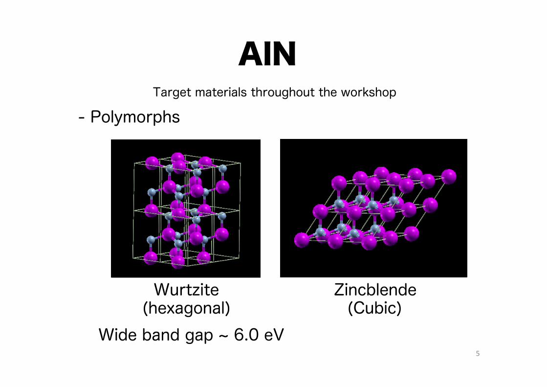
Wide band gap ~ 6.0 eV
AlN
- Polymorphs
Wurtzite (hexagonal)
Target materials throughout the workshop
Zincblende (Cubic)

6
Phase diagram - DFT simulations/QE & Phonopy
à Gibbs free energies
Formation energies
- CALPHAD
Specific heats at constant pressure
Wurtzite and Zincblende structure Inputs:
Outputs:
Inputs: Gibbs free energies Outputs: Phase diagram

Formation energies
7
ΔEf = EAlN − EAl/FCC +1 2EN2 /gass( )Al FCC( )+1 2N2 gass( ) + ΔEf WZ/ZB( ) = AlN WZ/ZB( )
Wurtzite(kJ/mol):
Zincblende(kJ/mol):
Difference(kJ/mol):
-289.207 -274.056 -370.692 -301.998
PW91/US PBE/US PZ/NC Exp.
-285.602 -270.643 -366.281
-3.605 -3.413 -4.411

Is DFT enough?
8
- Band gap problem
Standard DFT always underestimates...
- Wurtzite
Experimental values: 6.0 eV
3.9 ‒ 4.7 eV DFT values:
More reliable methods needed!
Quantum Monte Carlo

9
Numerous keywords to be specified?
For beginners difficult to get started from scratch
- Practical obstacles
Crystal structures?
Methods?
This tutorial will answer you.

10
QE inputs http://www.quantum-espresso.org/wp-content/uploads/Doc/INPUT_PW.html
11
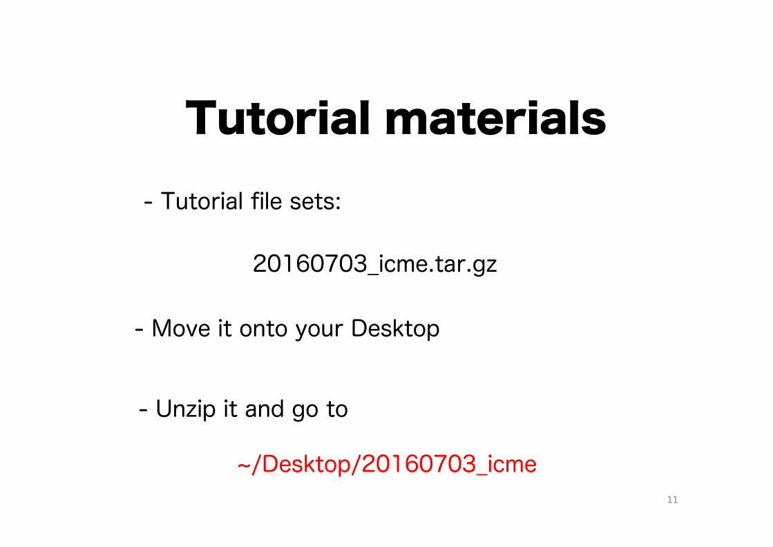
20160703_icme.tar.gz
Tutorial materials
- Move it onto your Desktop
- Unzip it and go to
~/Desktop/20160703_icme
- Tutorial file sets:
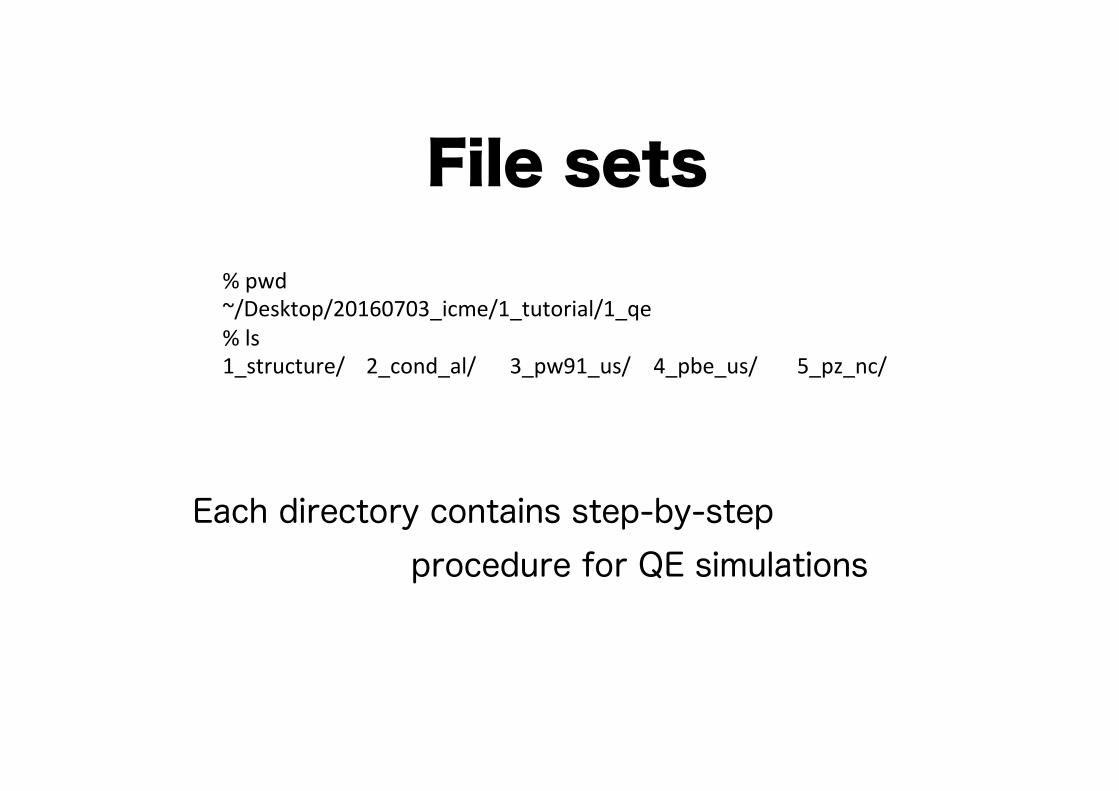
File sets %pwd~/Desktop/20160703_icme/1_tutorial/1_qe%ls1_structure/ 2_cond_al/ 3_pw91_us/ 4_pbe_us/ 5_pz_nc/
Each directory contains step-by-step procedure for QE simulations

Procedure for QE overview
1/Crystal structures for QE inputs 1_structure
2/Computational conditions for Al(FCC) 2_cond_al
3/Formation energy with GGA-PW91/US-PPs 3_pw91_us
4/Formation energy with GGA-PBE/US-PPs 4_pbe_us
5/Formation energy with LDA-PZ/NC-PPs 5_pz_nc
pw.xwith “vc-relax/relax”
pw.xwith “scf”
cif2cell: convert cif files to QE inputs xcrysden: visualize structures from QE inputs

for good and bad parameter setups
Importance of proper setting of computational parameters
Convergence
Wurtzite(kJ/mol):
Zincblende(kJ/mol):
Difference(kJ/mol):
-202.652 -370.692
Poor Good
-203.869 -366.281
30 80 Ecut [Ry]:
1.217 -4.411
- PZ/NC results
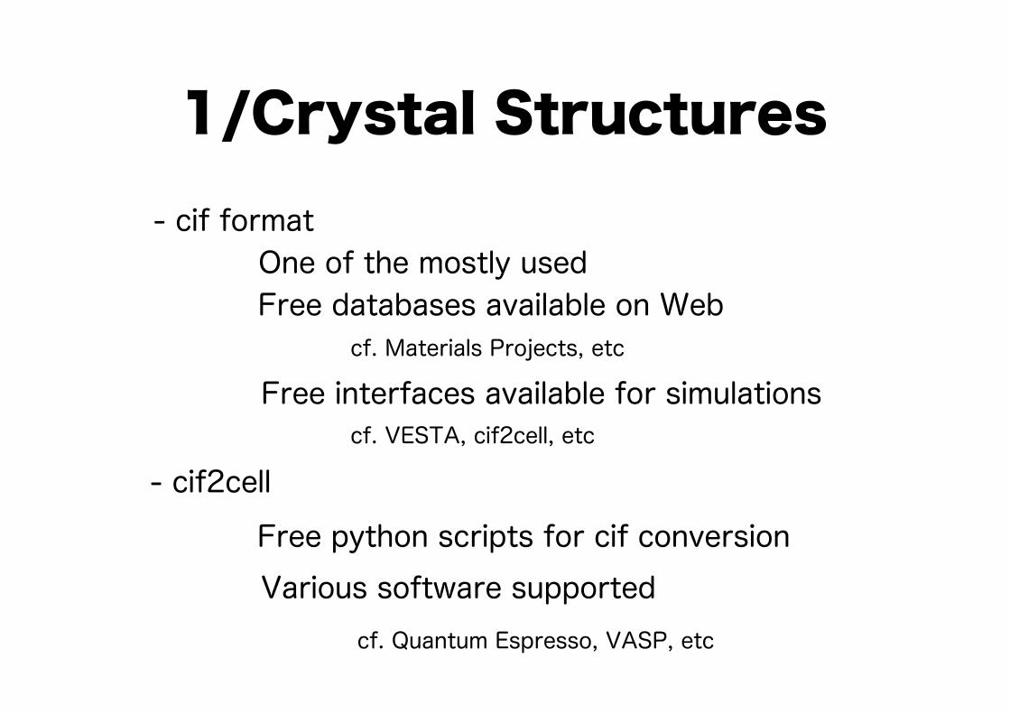
One of the mostly used
- cif2cell
1/Crystal Structures
Free databases available on Web cf. Materials Projects, etc
- cif format
Free interfaces available for simulations
Free python scripts for cif conversion Various software supported
cf. VESTA, cif2cell, etc
cf. Quantum Espresso, VASP, etc

16
1) Go to ‘1_structure/1_wurtzite’
cif2celll
cif2cell ‒p pwscf wurtzite.cif
Covert cif files to QE inputs
2) Execute:
3) Output: wurtzite.in

17
Xcrysden
Xcrysden --pwi wurtzite.in
Visualize QE input geoetries
1) Execute:
2) Follow instructions by Lecturers
N.B. Not single “-”, but double “--”

18
Exercise 1 Visualize QE input geoetries
1) Go to ‘../2_zincblende’
2) Generate QE geometry and view it

19
Homework
1) Find a cif file for your favorite crystal on Web
2) Get the cif file and convert it to a QE input
3) Visualize your crystal using Xcrysden

QE simulations - PWSCF DFT energy engine (executable: pw.x)
- Inputs: Crystal structure DFT functional & Pseudo potential Computational parameters
- Outputs: Optimized Crystal structure (only for geom. Opt.) DFT total energy KS orbitals and energies
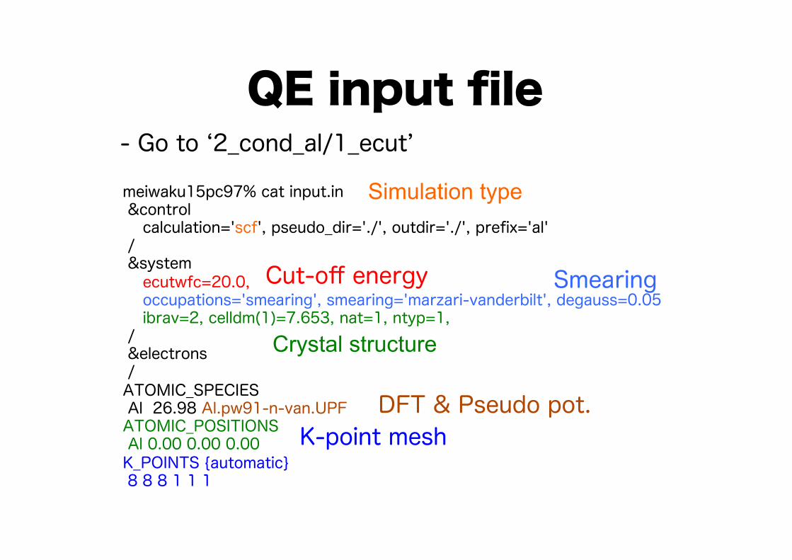
QE input file - Go to ‘2_cond_al/1_ecut’
meiwaku15pc97% cat input.in &control calculation='scf', pseudo_dir='./', outdir='./', prefix='al' / &system ecutwfc=20.0, occupations='smearing', smearing='marzari-vanderbilt', degauss=0.05 ibrav=2, celldm(1)=7.653, nat=1, ntyp=1, / &electrons / ATOMIC_SPECIES Al 26.98 Al.pw91-n-van.UPF ATOMIC_POSITIONS Al 0.00 0.00 0.00 K_POINTS {automatic} 8 8 8 1 1 1
K-point mesh
Cut-off energy Smearing
DFT & Pseudo pot.
Crystal structure
Simulation type

Tips for input - All the parameters can be seen at:
hEp://www.quantum-espresso.org/wp-content/uploads/Doc/INPUT_PW.html
But there exists numerous paramaeters...
- In most cases, the default values work well
- Is there any useful example?
Look into the following QE directory:
espresso-5.4.0/PW/examples
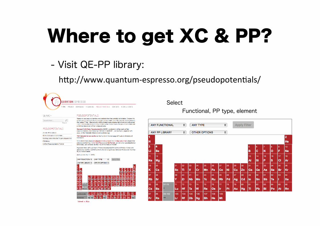
Where to get XC & PP? - Visit QE-PP library: hEp://www.quantum-espresso.org/pseudopotenPals/
Functional, PP type, element Select
24
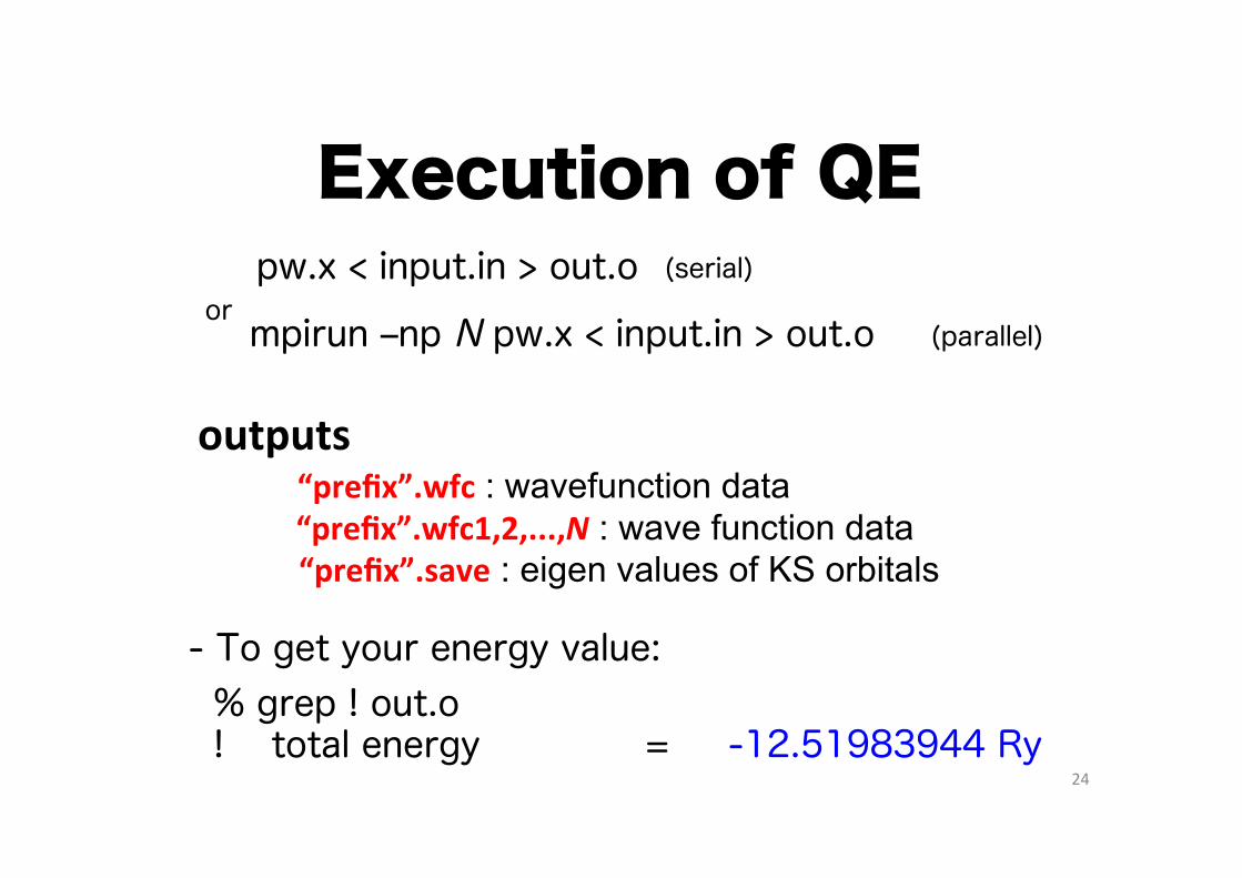
Execution of QE
“prefix”.wfc : wavefunction data outputs
“prefix”.save : eigen values of KS orbitals “prefix”.wfc1,2,...,N : wave function data
or pw.x < input.in > out.o (serial)
mpirun ‒np N pw.x < input.in > out.o (parallel)
% grep ! out.o ! total energy = -12.51983944 Ry
- To get your energy value:

Resoluton of KS orbital expansion
- K-point mesh
2/Comp. Cond. for Al
- Cut-off energy
How large periodicity is considered?
Discontinuity of occupation at Fermi surface
- Smearing (only for metallic systems)
to get converged single-point energies
N×N×N mesh corresponds to N×N×N supercell simulation
Ecut = 1 2 Gmax2
φKS r( ) = cG ⋅exp −iG ⋅r( )G <Gmax∑
causes ‘sloshing’ at SCF procedure
“Smear” out the discontinuity
26
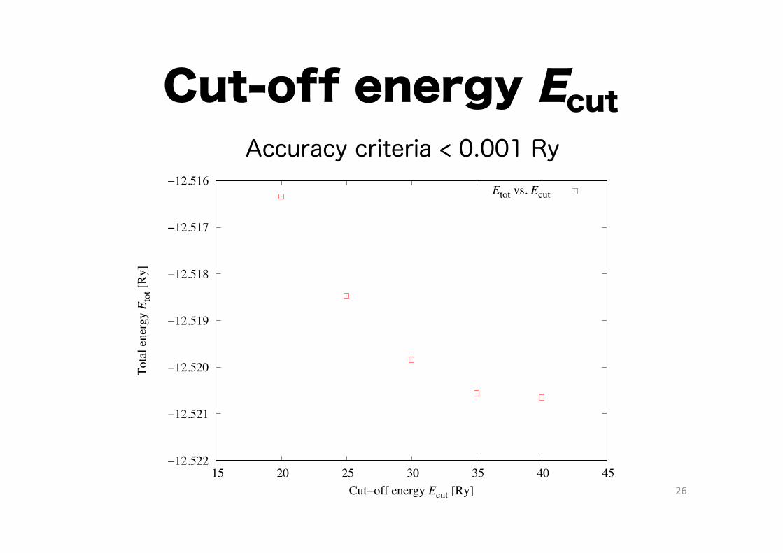
Cut-off energy Ecut
−12.522
−12.521
−12.520
−12.519
−12.518
−12.517
−12.516
15 20 25 30 35 40 45
Tota
l ene
rgy E t
ot [R
y]
Cut−off energy Ecut [Ry]
Etot vs. Ecut
Accuracy criteria < 0.001 Ry
27
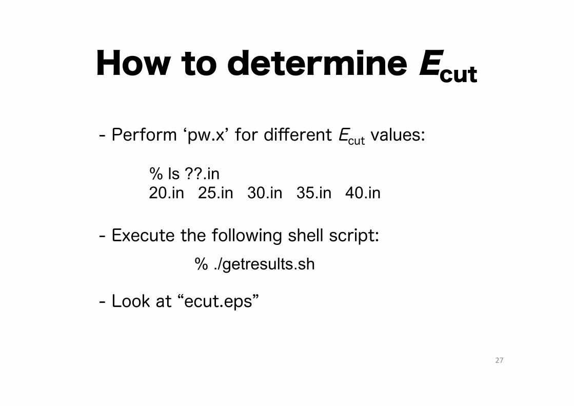
How to determine Ecut
- Perform ‘pw.x’ for different Ecut values:
% ls ??.in 20.in 25.in 30.in 35.in 40.in
- Execute the following shell script: % ./getresults.sh
- Look at “ecut.eps”

28
K-point & smearing Accuracy criteria < 0.001 Ry
−12.522
−12.521
−12.520
−12.519
−12.518
−12.517
−12.516
0 0.02 0.04 0.06
Tota
l ene
rgy E t
ot [R
y]
degauss [Ry]
4x4x46x6x68x8x8
10x10x10
29
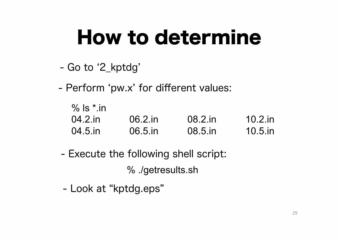
How to determine
- Perform ‘pw.x’ for different values:
% ls *.in 04.2.in 06.2.in 08.2.in 10.2.in 04.5.in 06.5.in 08.5.in 10.5.in
- Execute the following shell script: % ./getresults.sh
- Look at “kptdg.eps”
- Go to ‘2_kptdg’

30
Routine works
- Execute: ./all.sh
- Execution of all the jobs by hands is annoying...
- Go to ‘3_routine’
- Look at the shell script “all.sh”

31
Homework
- Execute it
- Referring to all.sh, make a script for Ecut

3/FE with GGA-PW91/US - Formation energy of Al
ΔEf = EAlN − EAl/FCC +1 2EN2 /gass( )
- Go to ‘3_pw91_us’
Four DFT total energy simulations needed for
AlN (Wurtzite structure); 3_aln/1_wurtzite AlN (Zincblende structure); 3_aln/2_zincblende
Al (FCC structure); 1_al/N2 molecule (gas phase); 2_n2/

Our choice of XC & PP
GGA: Generalized Gradient Approximation PW91: Perdew/Wang 1991 implementation
- DFT XC functional
Known to work well for cohesive energies compared to LDA
- Pseudopotential US: Ultrasoft pseudopotential (w. Vernderbilt implementation)
Less computational demand in cut-off energy compared to norm-conserving ones
3_pw91_us/3_aln/1_wurtzite/Al.pw91-n-van.UPF 3_pw91_us/3_aln/1_wurtzite/N.pw91-van_ak.UPF
downloaded from QE PP library

QE inputs
- Molecules
calculation='vc-relax'
- Crystals the same conditions as ‘2_cond_al’ except for “calculation”
Lattice parameters Atomic positions in unit cell
Optimize:
a molecule in a large simulation box (10Å)
Only atomic positions in unit cell Optimize:
calculation = 'relax' celldm(1) = 10.0,

QE execution - At each directory, execute ‘pw.x’
- Execute the following:
automatically evaluate your FE
./formationenergy.sh
from your PW91/US simulations
Q. What is your AlN formation energy?

36
Exercise 2
GGA-PBE simulations
- Go to ‘4_pbe_us’
with Vanderbilt ultrasoft pseudopotentials
- Follow the same procedure as ‘3_pw91_us’
- Compare results between PW91/US and PBE/US
37
Exercise 3
LDA-PZ simulations
- Go to ‘5_pz_nc’
with VonBorth-Car norm conserving pps.
- Follow the same procedure as ‘3_pw91_us’
- Q. Your result looks good?
38
Cont’d
- Q. What causes this failure?
- Q. How do you correct this?

fin