AB INITIO TREATMENTS OF THE ISING MODEL IN A …

International Journal of Modern Physics B, Vol. 14, No. 15 (2000) 1517-1536© World Scientific Publishing Company

AB INITIO TREATMENTS OF THE ISING MODEL IN ATRANSVERSE FIELD

R. F. BISHOP', D. J. J. FARNELL* and M. L. RISTIGt• Department of Physics, University of Manchester Institute of Science

and Technology (UM/ST), P.O. Box 88, Manchester M60 lQD, United Kingdomt Institut fur Theoretische Physik, Universitiit zu Koln;

Ziiipicher Str., 50931 Koln, Germany

Received 7 February 2000

In this article new results are presented for the zero-temperature ground-state propertiesof the spin-half transverse Ising model on various lattices using three different approxi-mate techniques. These are, respectively, the coupled cluster method, the correlated basisfunction method, and the variational quantum Monte Carlo method. The methods, atdifferent levels of approximation, are used to study the ground-state properties of thesesystems, and the results are found to be in excellent agreement both with each otherand with results of exact calculations for the linear chain and results of exact cumulantseries expansions for lattices of higher spatial dimension. The different techniques usedare compared and contrasted in the light of these results, and the constructions of theapproximate ground-state wave functions are especially discussed.

PACS number(s): 75.1O.Jm, 75.30.Gw, 75.50.Ee, 75.40.Cx

1. Introduction

Two of the most versatile and most accurate semi-analytical formalisms of micro-scopic quantum many-body theory (QMBT) are the coupled cluster method'<"and the correlated basis function (CBF) method.9-19 In recent years such QMBTmethods, together with various quantum Monte Carlo (QMC) techniques, have beenapplied with a great deal of success to lattice quantum spin systems at zero temper-ature. Some typical recent examples of such applications include Refs. 20-27 for theCCM, Refs. 29-32 for the CBF method, and Refs. 33-40 for the various QMC tech-niques. Current state of the art is such that these methods are sufficiently accurateto describe the various quantum phase transitions between the states of differentquantum order that exist in such abundance for spin-lattice systems. However, eachof the above methods is characterised by its own strengths and weaknesses. Hence,a fuller and more complete understanding of such strongly interacting systems asthe lattice quantum spin systems is expected to be given by the application of arange of such techniques rather than by the single application of anyone of them.In this article we wish to apply the CCM, the CBF method, and the variational

1517

1518 R. F. Bishop, D. J. J. Farnell f1 M. L. Ristig

quantum Monte Carlo (VQMC) method to the spin-half transverse Ising model(for reviews of this model see, for example, Refs. 41-46). The Hamiltonian for thismodel on a lattice of N sites, each of which has z nearest neighbours, is given by

H = (~ + A) N - L at aJ - AL at',(i,j) i

(1)

where the a-operators are the usual Pauli spin operators and (i, j) indicates thateach of the zN /2 nearest-neighbour bonds on the lattice is counted once only. Wework in the thermodynamic limit where N -t 00. We note that this model has anexact solution in one dimensionr'" and approximate techniques, such as the randomphase approximation (RPA)47 and exact cumulant series expansions,48,49 have alsobeen applied to it for lattices of higher spatial dimensionality. For A :::> 0, we notefurthermore that the model contains two distinct phases, with a critical couplingstrength Ac depending on lattice type and dimensionality. For A < Ac there isnonzero spin ordering in the z-direction, and hence this regime will be referred tohere as the ferromagnetic regime. By contrast, for A > Ac, all of the ferromagneticordering is destroyed, and the classical behaviour oi chese systems is that the spinslie along the positive x-axis. Hence, the A > Ac regime will be referred to here asthe paramagnetic regime. In Sec. 2 the technical aspects of applyin« the CCM, theCBF, and the VQMC methods to the spin-half transverse Ising model are presented,and in Sec. 3 the results of these calculations are discussed. Finally, the conclusionsare given in Sec. 4.

2. Quantum Many-Body Techniques

2.1. The coupled cluster method (GGM)

In this section, we firstly describe the general CCM formalism.l+" and then proceedto apply it to the specific case of the spin-half transverse Ising model. The exactket and bra ground-state energy eigenvectors, 1'lJ) and (~I, of a many-body systemdescribed by a Hamiltonian H,

(2)

are parametrised within the single-reference CCM as follows:

s= ~SICt,NO

s= 1+ ~SICi.1,#0

(3)

The single model or reference state I<]?) is required to have the property of beinga cyclic vector with respect to two well-defined Abelian subalgebras of multi-configurational creation operators {ct} and their Hermitian-adjoint destructioncounterparts {Ci == (Cnt}. Thus, I<]?) plays the role of a vacuum state with

Ab Initio Treatments of the Ising Model 1519

respect to a suitable set of (mutually commuting) many-body creation operators{ct},

Crl<I» = 0, I i= 0, (4)

with Co == 1, the identity operator. These operators are complete in the many-bodyHilbert (or Fock) space,

1= I<I»(I+L ctl<I»(ICr .foIO

Also, the correlation operator S is decomposed entirely in terms of these creationoperators {ct}, which, when acting on the model state ({ct I<I»}), create excita-tions from it. We note that although the manifest Hermiticity, (Wit = Iw)/(wlw)),is lost, the intermediate normalisation condition (Wlw) = (lw)= (I<I»== 1 isexplicitly imposed. The correlation coefficients {Sf, Sf} are regarded as being in-dependent variables, even though formally we have the relation,

(5)

_ (lest eS

(IS = (lesteSI<I» .

The full set {S1,S1} thus provides a complete description of the ground state. Forinstance, an arbitrary operator A will have a ground-state expectation value given

(6)

as,

(7)

We note that the exponentiated form of the ground-state CCM parametrisationof Eq. (3) ensures the correct counting of the independent and excited correlatedmany-body clusters with respect to I<I»which are present in the exact ground stateIW). It also ensures the exact incorporation of the Goldstone linked-cluster theo-rem, which itself guarantees the size-extensivity of all relevant extensive physicalquantities.

The determination of the correlation coefficients {S I ,Sf} is achieved by takingappropriate projections onto the ground-state Schrodinger equations of Eq. (2).Equivalently, they may be determined variationally by requiring the ground-stateenergy expectation functional H( {S1, SJ}), defined as in Eq. (7), to be stationarywith respect to variations in each of the (independent) variables of the full set. Wethereby easily derive the following coupled set of equations,

off loS1 = 0 => (ICre-s HeSI<I» = 0, I i= 0;

oH IJS1 = 0 => (ISe-S[H, CtJesl<I» = 0, I i= o.

(8)

(9)

Equation (8) also shows that the ground-state energy at the stationary point hasthe simple form

(10)


It is important to realize that this (bi- )variational formulation does not lead to anupper bound for Eg when the summations for Sand S in Eq. (3) are truncated,due to the lack of exact Hermiticity when such approximations are made. However,it is clear that the important Hellmann-Feynman theorem is preserved in all suchapproximations.

We also note that Eq. (8) represents a coupled set of nonlinear multinomialequations for the c-number correlation coefficients {S [ }. The nested commutatorexpansion of the similarity-transformed Hamiltonian,

A -8 S 1H == e He = H + [H,S] + ,[[H,S],S] + ... , (11)2.together with the fact that all of the individual components of S in the sum inEq. (3) commute with one another, imply that each element of S in Eq. (3) islinked directly to the Hamiltonian in each of the terms in Eq, (11). Thus, each of thecoupled equation (8) is of linked cluster type. Furthermore, each of these equationsis of finite length when expanded, since the otherwise infinite series of Eq. (11) willalways terminate at a finite order, provided (as is usually the case) that each termin the second-quantised form of the Hamiltonian H contains a finite number ofsingle-body destruction operators, defined with respect to the reference (vacuum)state liP). Therefore, the CCM parametrisation naturally leads to a workable schemewhich can be efficiently implemented computationally. It is also important to notethat at the heart of the CCM lies a similarity transformation, in contrast with theunitary transformation in a standard variational formulation in which the bra state(~I is simply taken as the explicit Hermitian adjoint of 1111).

The CCM formalism is exact in the limit of inclusion of all possible multi-spincluster correlations for Sand S, although in any real application this is usuallyimpossible to achieve. It is therefore necessary to utilise various approximationschemes within Sand S. The three most commonly employed schemes previouslyutilised have been: (1) the SUBn scheme, in which all correlations involving only n orfewer spins are retained, but no further restriction is made concerning their spatialseparation on the lattice; (2) the SUBn-m sub-approximation, in which all SUBncorrelations spanning a range of no more than m adjacent lattice sites are retained;and (3) the localised LSUBm scheme, in which all multi-spin correlations overdistinct locales on the lattice defined by m or fewer contiguous sites are retained.The specific application of the CCM to the spin-half transverse Ising model in theparamagnetic and ferromagnetic regimes is now described.

2.1.1. The paramagnetic regime

In the paramagnetic regime, a model state is utilised in which all spins point alongthe x-axis, although it is found to be useful to rotate the local spin coordinates ofthese spins such that all spins in the model state point in the "downwards" direction(i.e., along the negative z-axis). This (canonical) transformation is given by,

(12)


such that the transverse Ising Hamiltonian of Eq. (1) is now given in the (rotated)spin-coordinate frame by,

H = (~+ A)N - L [o-{o-t + 0-;0-; + o-;o-t + o-{o-;] + A Lo-i, (13)(i,j) i

where o-t == Ho-k ± io-n· In these local coordinates the model state is thus the"ferromagnetic" state I\II) = I-W. ... -l.- ... ) in which all spins point in the downwardsdirection. In order to reflect the symmetries of this Hamiltonian, the cluster cor-relations within S are explicitly restricted to those for which sf = Li sf (in therotated coordinate frame) is an even number. Hence, the LSUB2 approximation isdefined by

(14)

where p covers all nearest-neighbour lattice vectors. The ground-state energy is nowgiven in terms of b1 by,

E z- = -(1- bt).N 2

(15)

It is found that this expression is valid for any level of approximation for S. UsingEq. (7) it is found that,

5bi + 4Ab1 - 1 = 0 , (16)

and hence an approximate solution for the ground-state energy at the LSUB2 ap-proximation level purely in terms of A may be obtained. The SUB2 approximationcontains all possible two-body correlations, for a given lattice, and is defined by

(17)

where the index r indicates a lattice vector. Equation (7) may once again beutilised to determine the SUB2 ket-state equations. Hence the CCM SUB2 ket-state equation corresponding to a two-body correlation characterised by index s isgiven by,

T

We note that this equation is meaningful only for s =I- 0 as we may only everhave one Pauli raising operator per lattice site. This equation may be solved byperforming a Fourier transformation. (Details of how this is achieved in practiceare not given here and the interested reader is referred to Refs. 20 and 23.) Analternative approach, however, is to use Eq. (18) in order to fully define the SUB2-m equations. This is achieved by truncating the range of the two-body correlations(i.e., by setting [s] ~ m), and the corresponding SUB2-m equations may be solvednumerically via the Newton-Raphson technique (or other such techniques). We note

1522 R. F. Bishop, D. J. J. Farnell 8 M. L. Ristig

that coupled sets of high-order LSUBm equations may be derived using computer-algebraic techniques, as discussed in Ref. 24. The technicalities of these calculationsare not considered here, but the interested reader is referred to Ref. 24. A fulldiscussion of the CCM results based on the paramagnetic model state is deferreduntil Sec. 3.

2.1.2. The ferromagnetic regime

In the ferromagnetic regime, a model state is chosen in which all spins point "down-wards" (along the negative z-axis), and so the Hamiltonian of Eq. (1) may thereforebe utilised directly within the CCM calculations. The lowest order approximationis now the SUB1 approximation (in which case, S = a Liof) and the ground-stateenergy is given in terms of a by,

EN=A(1-a). (19)

It is again noted that this expression is valid for any level of approximation inS. In this case, it is found that the solution of the SUB2 approximation collapsesonto the LSUB2 solution due to the simple nature of the Hamiltonian and modelstate, although it is again possible to perform high-order LSUBm calculations.Furthermore, the lattice magnetisation (i.e., the magnetisation in the z-direction),M, is defined within the CCM framework by,

1 N _

M = - N L('l1latl'l1),i=l

(20)

which may be determined once both the ket- and bra-state equations have beensolved at a given level of approximation. Again, the discussion of the results forthis model state is deferred until Sec. 3.

2.2. The CBF formalism

The treatment of the transverse Ising model by the CBF method is begun bydefining the lattice magnetisation (i.e., again the magnetisation in the z-direction),given by

M = ('If; Iat I1/!)(1/!I1/!) , (21)

for a ground-state trial wave function, I'lf;). Furthermore, the "transverse" magnet i-sation is given by,

A = (1/!laf I1/!)(1jJI1jJ) . (22)

It is also found to be useful to define a spatial distribution function (which plays acrucial part in any CBF calculation) in the following manner,

( ) _ (1/!Iat a} I1/!) (23)g n - (1/!I1/!) ,


where n = ri - rj. The corresponding approximation to the ground-state energyper spin is given by

E (1PIHI1P) z 1N = N(1PI1P) = 2 - 2L~(n)g(n) + oX(1- A),

n

(24)

where the function ~(n) is equal to unity when n is a nearest-neighbour latticevector and is zero elsewhere. It is noted that the distribution function g(n) may bedecomposed according to g(n) = 8n,o+(1-8n,o)M2+(1-M2)G(n) such that G(n)now contains the short-range part of the spatial distribution function and vanishesin the limit [n] --+ 00. The magnetisation, M, and the transverse magnetisation, A,may now be expressed in a factorised form in terms of a "spin-exchange strength" ,n12, such that,

A = (1- M2)!n12.

The energy functional is now expressed in terms of G(n) and n12 as,

(25)

E 2){z 1" } { 2!}N = (1 - M 2 - 2 L..- .6.(n)G(n) + oX 1 - (1 - M ) 2 n12 .

n

(26)

Note that in the mean-field approximation G(n) in Eq. (26) is set to zero (for alln) and n12 is set to unity.

In order to determine the ground-state energy and other such ground-stateexpectation values, a Hartree-Jastrow Ansatz is now introduced, given by

11P) = exp{MUM + U}IO). (27)

The reference state 10) is a tensor product of spin states which have eigenvalues of+1 with respect to a", The correlation operators U and UM are written in termsof pseudopotentials, u(rij), ul(ri), and uM(rij), where

N

U = ~Lu(rij)ataj,i<j

(28)

andN N

UM = Lul(ri)ai + ~LUM(rij) (ai + aJ).i i<j

(29)

The pseudopotential Ul (ri) "" Ul is independent of the lattice position by transla-tional invariance, and the pseudopotentials, u(rij) and uM(rij), similarly dependonly on the relative distance, [n] = [r, - rjl "" Irijl. The" Jastrow correlations aredetermined via a cluster expansion of the various quantities in the Hamiltonian, asexplained in Refs. 29-32. A common approximation yields the hypernetted chain(HNCjO) equations, which one may solve iteratively in order to determine theHartree-Jastrow pseudopotentials. One then wishes to determine the expectationvalues such as the ground-state energy, and in the paramagnetic regime an explicit

1524 R. F. Bishop, D. J. J. Farnell C3 M. L. Ristig

assumption is made that M = O. However, in the ferromagnetic regime M is takento be a variational parameter with respect to the ground-state energy of Eq. (26).

There are now two ways of determining the pseudopotentials from the HNCequations. The first such approach is to assume that the pseudopotential has thesimple parametrised form,

u(n) = a.6.(n) , (30)

where .6.(n) is unity if n is a nearest-neighbour lattice vector and is zero otherwise.This approach is henceforth denoted as the parametrised HNC-CBF method. Thec-number a is taken to be a variational parameter with respect to which the ground-state energy is minimized. In the paramagnetic regime, the minimum of the energysurface as a function of ex is sought, at a given value of A. This is easily performedcomputationally, and the solution is readily tracked iteratively, starting from thetrivial limit A -t 00 and then moving to smaller values of A. In the ferromagneticregime, one again searches for a minimum of the energy surface, but this timewith respect to both a and M, at a given value of A. In this case, one tracksfrom the trivial limit of A = 0 to higher values of A. In previous articles,29-32this was achieved by analytically determining the derivative of the energy withrespect to M, although in this article a computational minimisation of the energyis performed with respect to both variables. The second such approach allows one tofind the optimal pseudopotential within the CBF /HNC framework from a functionalminimisation,

6E6u(n) = O. (31)

Within the context of this article, this is henceforth denoted as the paired phononapproximation (PPA) (or, more precisely, the paired magnon approximation), andthe corresponding equations are the PPA equations. Note that in this article thePPA calculation is only performed in the paramagnetic regime, although PPA re-sults in the ferromagnetic regime have also been performed previously.30,31 (In-deed, results for the phase transition points predicted by the PPA-CBF approachof Refs. 30 and 31 are quoted in the Table 1 in sec. 3.) A full discussion of theresults of the CBF calculations presented in this section, in comparison to thecorresponding results of the CCM and the VQMC method, is given in Sec. 3.

2.3. The VQMC formalism

Although the specific variational calculations presented in this article concentrateon the spin-half transverse Ising model, we note that the formalism presented in thissection is given in a generalised form and that the treatment of other spin modelswould follow a similar pattern. We shall specifically consider here the transverseIsing model in the ferromagnetic regime where the relevant Hamiltonian is definedby Eq, (1). An Ansatz for the expansion coefficients, {CI}, of a ground-state wave


function defined by

17J!) = L cIII) ,I

is chosen. Note that {II)} denotes a complete set of Ising basis states, defined as allpossible tensor products of states on all sites having eigenvalues ±1 with respect toa", An expression for the ground-state energy is thus given by,

(32)

E = "L:h,I2 ctcI,(hIHlh)"L:II ICll1

2 .

Specifically for the spin-half transverse Ising model, a Hartree-Jastrow Ansatz50

(for A > 0) is now defined with respect to the {cr} expansion coefficients, where

Cl = (II rr(1+ akPI) II( 1+ Aj [P/Pf + P/P]])iI). (34)k t<J

(33)

The pt and P~ are the usual projection operators of the spin-half "up" and "down"states respectively. The simplest form of the variational Ansatz of Eq. (34) is givenby,

];'j= {ho

if i and j are nearest neighbours,(35)

otherwise.

The symmetry-breaking term ad= a) is also independent of k by translationalinvariance. The expectation value of Eq. (33) may now be evaluated directly andthe variational ground-state energy minimised with respect to both a and h at eachvalue of A. However, such a calculation is soon limited by the rapidly increasingset of Ising states and the amount of computational power available. Indeed, forthe spin-half transverse Ising model the number of states that one must sum overis 2N, where N is the number of lattice sites. For the linear chain it is possible tosolve for chains of length N :S ,...,12with relatively little computational difficulty,although the calculations with N > 12 grow rapidly in computational difficulty.

Hence, as an alternative for lattices of larger size, we may simulate the summa-tion over all the states h in Eq. (33). In order to to do this we define the probabilitydistribution for the set of states {II)}, given by

icll2P(l) := ~ I 12' (36)

I' Cl'

and the local energy of these states, given by

Ed!) == L Cll (IIHlh).11 ci

(37)

The expression of Eq. (33) may thus be equivalently written as,

E = 2:P(I)EL(I) .I

(38)

1526 R. F. Bishop, D. J. J. Farnell fj M. L. Ristig

We now wish to perform a random walk based on the probability distributionof Eq. (36). However, a few more useful quantities should be defined before a de-tailed description of the VQMC algorithm is actually given. Firstly, the acceptanceprobability, A(I ----+ I'), of the Monte Carlo "move" from state II) to state II') isgiven by

A(I -+ I') = minjl , q(I -+ I')J , (39)

where

(I -+ I') = P(I')T(I' -+ I)q - P(I)T(I ----+ I') . (40)

Here, T(I ----+ I') is the sampling distribution function. For spin lattice problems, ifstate II) can connect to K(I) possible Ising states via the off-diagonal elements ofthe Hamiltonian then T(I ----+ 1') = 1/K(I). Hence, q(I --t I') is written as

(I ----+ I') = P(J')K(I)q P(I)K(J') . (41)

For the spin-half transverse Ising model, we note that K(I) is equal to N for anystate II) and so the common factor of N in Eq. (41) cancels. The simplest VQMCprocedure is now defined by the following algorithm:

(1) Select an initial Ising state II) for which (II1lI) i= 0, where 11Ji) is the "true"ground-state wave function of the system.

(2) Choose a particular state II') out of the K(I) possible states accessible to II)via the off-diagonal elements in H.

(3) Define a random number r in the range [O,IJ and accept this move from stateII) to state II') if and only if

A(I -+ I') > r . (42)

(4) If the move is accepted then let 1----+1' and c[ --t Cj»:

(5) Obtain the local energy E(I) of Eq. (37) for state II).(6) Repeat from stage (2) NMC times.(7) The average ground-state energy (and the error therein) may be determined

from the number N MC of local energies during the simulation.

The minimal VQMC ground-state energy is now obtained by searching overthe variational parameter space for either the lowest ground-state energy or lowestvariance in the ground-state energy (here for a given value of .Ain H). In order todetermine the lattice magnetisation, we note that

M = I (~I Li O'fI~)IN('ljJI'ljJ)

= I~P(I)ML(I)I, (43)


where P(I) is the probability density function given above, and

ML(I) '= L ::~ (IILailh) = ~(IILaiII).[1. .

1 t •

(44)

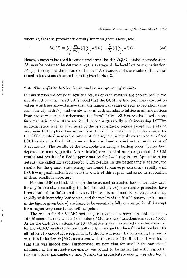
Hence, a mean value (and its associated error) for the VQMC lattice magnetisation,M, may be obtained by determining the average of the local lattice magnetisation,ML(I) , throughout the lifetime of the run. A discussion of the results of the varia-tional calculations discussed here is given in Sec. 3.

\l

2.4. The infinite lattice limit and convergence of results

In this section we consider how the results of each method are determined in theinfinite lattice limit. Firstly, it is noted that the CCM method produces expectationvalues which are size-extensive (i.e., the numerical values of each expectation valuescale linearly with N), and we always deal with an infinite lattice in all calculationsfrom the very outset. Furthermore, the "raw" CCM LSUBm results based on theferromagnetic model state are found to converge rapidly with increasing LSUBmapproximation level m over most of the ferromagnetic regime except for a regionvery near to the phase transition point. In order to obtain even better results forthe CCM method across the whole of this regime, a simple extrapolation of theLSUBm data in the limit m --+ 00 has also been carried out at each value ofA separately. The results of the extrapolation using a leading-order "power-law"dependence (see Appendix A for details) are denoted as Extrapolated(l) CCMresults and results of a Pade approximation for l = 0 (again, see Appendix A fordetails) are called Extrapolated(2) CCM results. In the paramagnetic regime, theresults for the ground-state energy are found to converge extremely rapidly withLSUBm approximation level over the whole of this regime and so no extrapolationof these results is necessary.

For the CBF method, although the treatment presented here is formally validfor any lattice size (including the infinite lattice case), the results presented havebeen obtained for finite-sized lattices. The results are found to converge extremelyrapidly with increasing lattice size, and the results of the 20 x 20 square lattice (usedin the figures given below) are found to be essentially fully converged for all A exceptfor a region very near to the critical point.

The results for the VQMC method presented below have been obtained for a16x 16 square lattice, where the number of Monte Carlo iterations was set to 50000.As for the CBF calculations, the 16x16 lattice is again expected to be large enoughfor the VQMC results to be essentially fully converged to the infinite lattice limit forall values of A except for a region near to the critical point. By comparing the resultsof a 10x 10 lattice VQMC calculation with those of a 16x 16 lattice it was foundthat this was indeed true. Furthermore, we note that for small A the variationalminimum of the ground-state energy was found to be rather flat with respect tothe variational parameters a and II, and the ground-state energy was also highly

1528 R. F. Bishop, D. J. J. Farnell fj M. L. Ristig

1.80 l~~1 ~'''''''--'1.60

1.40

1.20 rI

1.00 f

0.80 r0.60 l0.40

0.20

0.000.0

- Extrapolated(l) CCM- - - Extrapolated(2) CCM

+VQMC0--0 Parametrised HNC CBF

0.5 1.0 3.01.5 2.0A

2.5

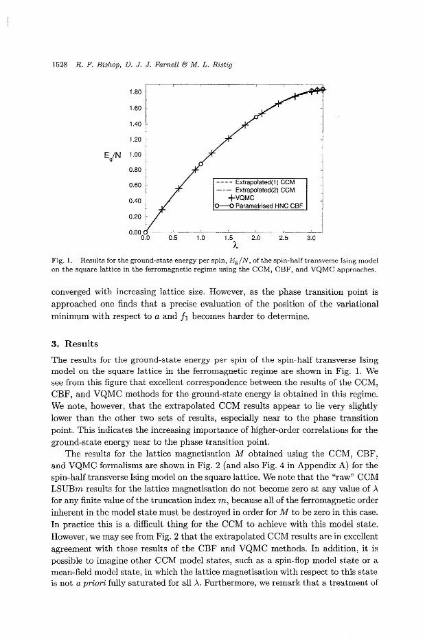
Fig. 1. R.esults for the ground-state energy per spin, Eg/N, of the spin-half transverse Ising modelon the square lattice in the ferromagnetic regime using the CCM, CBF, and VQMC approaches.

converged with increasing lattice size. However, as the phase transition point isapproached one finds that a precise evaluation of the position of the variationalminimum with respect to a and II becomes harder to determine.

3. Results

The results for the ground-state energy per spin of the spin-half transverse Isingmodel on the square lattice in the ferromagnetic regime are shown in Fig. 1. Wesee from this figure that excellent correspondence between the results of the CCM,CBF, and VQMC methods for the ground-state energy is obtained in this regime.We note, however, that the extrapolated CCM results appear to lie very slightlylower than the other two sets of results, especially near to the phase transitionpoint. This indicates the increasing importance of higher-order correlations for theground-state energy near to the phase transition point.

The results for the lattice magnetisation M obtained using the CCM, CBF,and VQMC formalisms are shown in Fig. 2 (and also Fig. 4 in Appendix A) for thespin-half transverse Ising model on the square lattice. We note that the "raw" CCMLSUBm results for the lattice magnetisation do not become zero at any value of A.for any finite value of the truncation index m, because all of the ferromagnetic orderinherent in the model state must be destroyed in order for M to be zero in this case.In practice this is a difficult thing for the CCM to achieve with this model state.However, we may see from Fig. 2 that the extrapolated CCM results are in excellentagreement with those results of the CBF and VQMC methods. In addition, it ispossible to imagine other CCM model states, such as a spin-flop model state or amean-field model state, in which the lattice magnetisation with respect to this stateis not a priori fully saturated for all A.. Furthermore, we remark that a treatment of

Ab Initio Treatments oj the Ising Model 1529

1.0

0.8

1.........'. i

0.6 ........- LSUB2 1M ---- LSUB7--- Extrapolated(1) CCM ", j

0.4 -- Extrapolated(2) CCM ,I0--0 Parametrised HNC CBF

1+VQMC

0.2 r

f 1I

0.0 i0.0 1.0 2.0 3.0

A

,i"

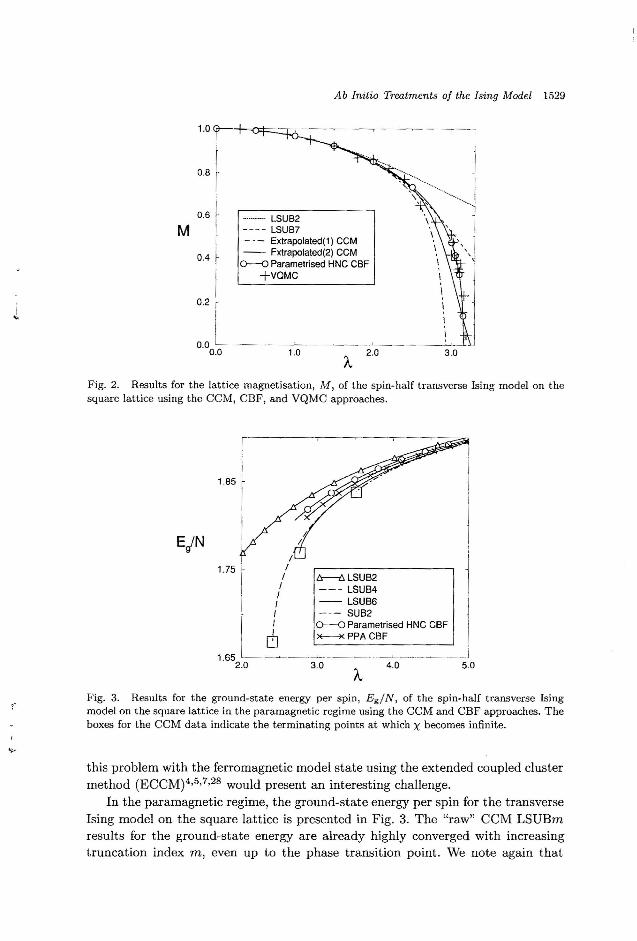
Fig. 2. Results for the lattice magnetisation, M, of the spin-half transverse Ising model on thesquare lattice using the CCM, CBF, and VQMC approaches.

/

1.751~ III 1:r--f::,. LSUB2

--- LSUB4

I "-- LSUB6

, --- SUB2

I· I ~ Parametnsed HNC CBF IdJ ~PPACBF !

1.65 --_._-'-.---._- ---L-. I

~O 3.0 ~O ~oA

1.85

Eg'N

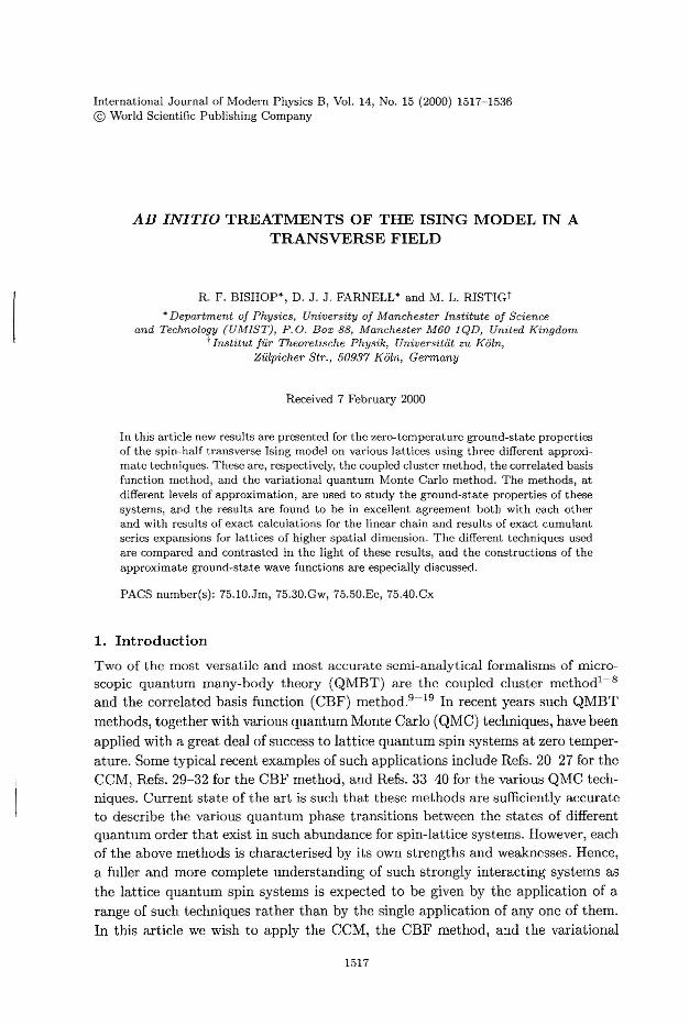
Fig. 3. Results for the ground-state energy per spin, Eg/N, of the spin-half transverse Isingmodel on the square lattice in the paramagnetic regime using the CCM and CBF approaches. Theboxes for the CCM data indicate the terminating points at which X becomes infinite.

this problem with the ferromagnetic model state using the extended coupled clustermethod (ECCM)4,5,7,28 would present an interesting challenge.

In the paramagnetic regime, the ground-state energy per spin for the transverseIsing model on the square lattice is presented in Fig. 3. The "raw" CCM LSUBmresults for the ground-state energy are already highly converged with increasingtruncation index m, even up to the phase transition point. We note again that

1530 R. F. Bishop, D. J. J. Farnell & M. L. Ristig

an extrapolation in the limit m ~ 00 is therefore not necessary. Indeed, goodcorrespondence between the results of the different methods is seen although it isnoted that CCM LSUB4 and LSUB6 ground-state energies lie lower than thosepredicted by the CBF method. This indicates that high-order order correlationsbecome increasingly important the nearer one gets to the phase transition point.However, this could be rectified, in principle, for the CBF method by the inclusion ofhigher-order (than pairwise Jastrow) correlations in the ground-state wave function.We note that in practice, however, the inclusion of such higher-order correlationsin the ground-state wave function in the CBF and VQMC methods is a difficultand unresolved question.

It is also possible to determine the second-derivative of the ground-state energyper spin with respect to A for the CCM calculations based on the paramagneticmodel state, defined by

182EX- g

= - N 8A2 .

It is found that X diverges at some critical value Ac for the SUB2 approximationin any dimension, and for SUB2-m and LSUBm (with m ~ 4) approximations forspatial dimensionality greater than one. Again, this behaviour is associated with aphase trarisition in the real system and the point at which this occurs is denoted Ac.Correspondingly, CCM results for A < Ac based on the paramagnetic model statedo no exist, and hence Ac acts as a terminating point for the calculation in theparamagnetic regime. Also, it is found that the SUB2-m results for Ac as a functionof m scale with m-2 for large m, and a simple linear extrapolation gives the fullSUB2 result for the critical point to within 2% accuracy. By analogy, this rule hasalso been used for the LSUBm results to extrapolate to the limit m ~ 00, and theresults thus determined are shown in Table 1. The values thus obtained are also ingood agreement with the points at which M ~ 0 from the extrapolations in theferromagnetic regime discussed above (and see Fig. 2 for the square lattice case).

For the CBF and VQMC methods the point, in terms of A, at which M becomeszero is taken to indicate a quantum phase transition and is again denoted, Ac, andthese results are presented in Table 1. The phase transition point predicted by theVQMC method on the square lattice case is estimated to be at Ac = 3.15 ± 0.05.For the linear chain, the expression for ground-state energy of Eq. (33) has beenobtained directly for chains with N ::; 12. These results are found to be in goodagreement with a previous calculation-" using the Ansatz of Eq. (34) for the linearchain transverse Ising model which predicted a value for the phase transition pointof .xc = 1.206.

(45)

4. Conclusions

In this article, results of the CCM, CBF, and VQMC approaches for the ground-state energy, the lattice magnetisation, and the position of the critical point ofthe spin-half transverse Ising model on various lattices have been presented. These


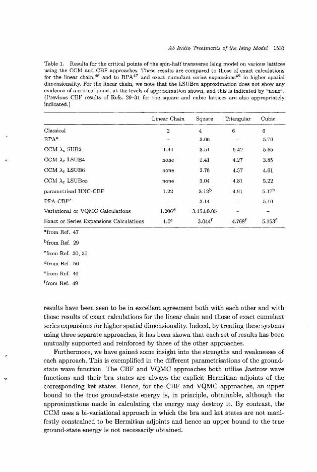
Table 1. Results for the critical points of the spin-half transverse Ising model on various latticesusing the CCM and CBF approaches. These results are compared to those of exact calculationsfor the linear chain,46 and to RPA47 and exact cumulant series expansions=? in higher spatialdimensionality. For the linear chain, we note that the LSUBm approximation does not show anyevidence of a critical point, at the levels of approximation shown, and this is indicated by "none".(Previous CBF results of Refs. 29-31 for the square and cubic lattices are also appropriatelyindicated. )

Linear Chain Square Triangular Cubic

Classical 2 4 6 6RPAa 3.66 5.76

CCM,\c SUB2 1.44 3.51 5.42 5.55

CCM '\C LSUB4 none 2.41 4.27 3.85

CCM '\C LSUB6 none 2.76 4.57 4.61

CeM '\c LSUBoo none 3.04 4.81 5.22

parametrised HNC-CBF 1.22 3.12b 4.91 5.17b

PPA·CBFc 3.14 5.10

Variational or VQMC Calculations 1.206d 3.15±0.05

Exact or Series Expansions Calculations 1.0e 3.044f 4.768f 5.153f

afrom Ref. 47

bfrom Ref. 29

cfrom Ref. 30, 31

d from Ref. 50

efrom Ref. 46

ffrom Ref. 49

results have been seen to be in excellent agreement both with each other and withthose results of exact calculations for the linear chain and those of exact cumulantseries expansions for higher spatial dimensionality. Indeed, by treating these systemsusing three separate approaches, it has been shown that each set of results has beenmutually supported and reinforced by those of the other approaches.

Furthermore, we have gained some insight into the strengths and weaknesses ofeach approach. This is exemplified in the different parametrisations of the ground-state wave function. The CBF and VQMC approaches both utilise Jastrow wavefunctions and their bra states are always the explicit Hermitian adjoints of thecorresponding ket states. Hence, for the CBF and VQMC approaches, an upperbound to the true ground-state energy is, in principle, obtainable, although theapproximations made in calculating the energy may destroy it. By contrast, theCCM uses a bi-variational approach in which the bra and ket states are not mani-festly constrained to be Hermitian adjoints and hence an upper bound to the trueground-state energy is not necessarily obtained.


Also, the CCM uses creation operators with respect to some suitably normalisedmodel state in order to span the complete set of (here) Ising states. The other ap-proaches, in essence, use projection operators to form the Hartree and the Jastrowcorrelations. For the CBF case, this is with respect to a reference state, whereasfor the VQMC case, the Hartree--Jastrow Ansatz is encoded within the expansioncoefficients of the ground-state wave function with respect to a complete set of Isingstates. In some sense, the CCM is found to contain less correlations than the oth-ers at "equivalent" levels of approximation (e.g., the CCM LSUB2 approximationversus Hartree and nearest-neighbour Jastrow correlations). A fuller account of thedifferent parametrisations of the ground-state wave function within the CCM andCBF methods has been given in Ref. 32. However, in practice the other methods aredifficult to extend to approximations which contain more than two-body or three-body correlations. By contrast, the CCM is well-suited to treat such higher-ordercorrelations via computational techniques, as has been demonstrated here.

Furthermore, the CCM requires no information other than the approximationin Sand S in order to determine an approximate ground state of a given system.The CBF method, however, may require that only a certain subset of all possiblediagrams are summed over (e.g., the HNC/O approximation). The VQMC approachalso often requires an intimate knowledge of the manner in which the two-bodycorrelations behave with increasing lattice separation if all two-body correlationsare to be included. This information may be approximated, for example, by useof the results of spin-wave theory. In any case, it is often necessary to reduce theminimisation of the variational ground-state energy with respect to N parametersto much fewer parameters. Another potential application of all of the methodspresented here is the use of their ground-state wave functions as trial or guidingwave functions in (Green function or similar) quantum Monte Carlo calculations.

Finally, encouraged by these results for the transverse Ising model, we intendto extend them to other models of interest, such as systems with higher quantumspin number or those with complex crystallographic lattices. A further goal is toextend the treatment of this and other spin models, via these methods, to nonzerotemperatures.

Acknow ledgrnents

We thank Dr. N. E. Ligterink for his useful and enlightening discussions. One of us(RFB) gratefully acknowledges a research grant from the Engineering and PhysicalSciences Research Council (EPSRC) of Great Britain. This work has also been sup-ported in part by the Deutsche Forschungsgemeinschaft (GRK 14, Graduiertenkol-leg on "Classification of Phase Transitions in Crystalline Materials"). One of us(RFB) also acknowledges the support of the Isaac Newton Institute for Mathemat-ical Sciences, University of Cambridge, during a stay at which the final version ofthis paper was written.


Appendix A. Extrapolation of CCM Results

In this Appendix, we explain how we extrapolate a set of LSUBm data points,{Xi, yd, in the limit i -t oo at each value of some parameter (>.) within the Hamil-tonian separately. Note that the number of data elements to be extrapolated isgiven by the index p. The value of Xi is now set to be 11m and Yi is set to be thecorresponding value of an expectation value (for example, the lattice magnetisa-tion) determined using the CCM at this level of approximation at a given value ofA. Note that the value of m must increase with increasing index i, although m andi do not have to be equal.

Before the extrapolation procedures are given in detail, we define some usefulquantities. Firstly, the mean value of a set {Ci} is denoted by c and of a set {dd isdenoted by d. Secondly, the linear correlation, R, of a set of two-dimensional points,{ci,di}, is defined by

p

2)Ci - c)(di - d)

R == r==t='==l==--;===== (A.1)P

2)di - d)2i=l

We are now in a position to outline the the first extrapolation procedure. Thisprocedure firstly assumes that the data scales with a leading-order "power-law"dependence, given by

Yi = a + bxr· (A.2)

We set Ci= log(xi) and di = log(Yi - a), where {xi,yd is the LSUBm data set atsome fixed value of a parameter within the Hamiltonian. Hence the best fit of thedata set, {Xi, Yi}, to the power-law dependence of Eq. (A.2) is obtained when theabsolute value of R is maximised with respect to the variable a. Indeed, we makethe assumption that this value of a is then taken to be the extrapolated value ofthe Yi in the limit i -t 00 (in which case, Xi -t 0).

The second extrapolation procedure of the LSUBm data uses Pade approxi-mants. This is achieved by firstly assuming that the set of data can be modeled bythe ratio of two polynomials, given by

k 'Lj=D ajxi

Yi = I ' •1+ Lj=l bjx;

(A.3)

Note that when limplies that,

0, this is a simple integral power series. This furthermore

We now wish to determine the coefficients aj and bj in order to find the polynomials


0.6

4.0

M0---0 LSUB2___ LSUB3

0.4 fL ~~~:+---<I LSUB6"l---4l LSUB7- Pad6 Approximation (1=0)

0.2 - - - Pad'; Approximant (1=3)- - Pad'; Approximant (1=5)

[ I - - - Leading-Order 'Power-Law' Scaling

O~ !.!

0.0 1.0 2~

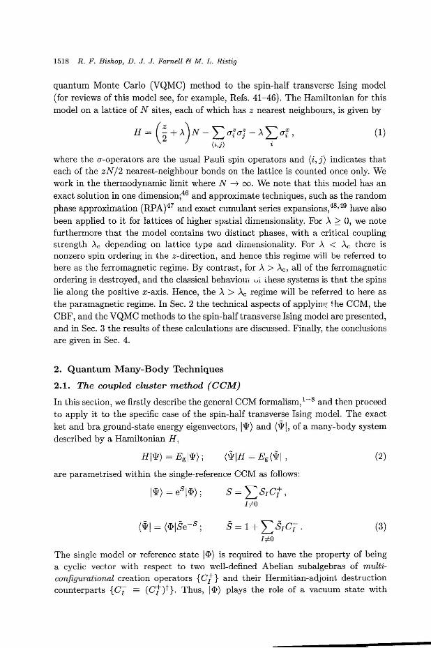
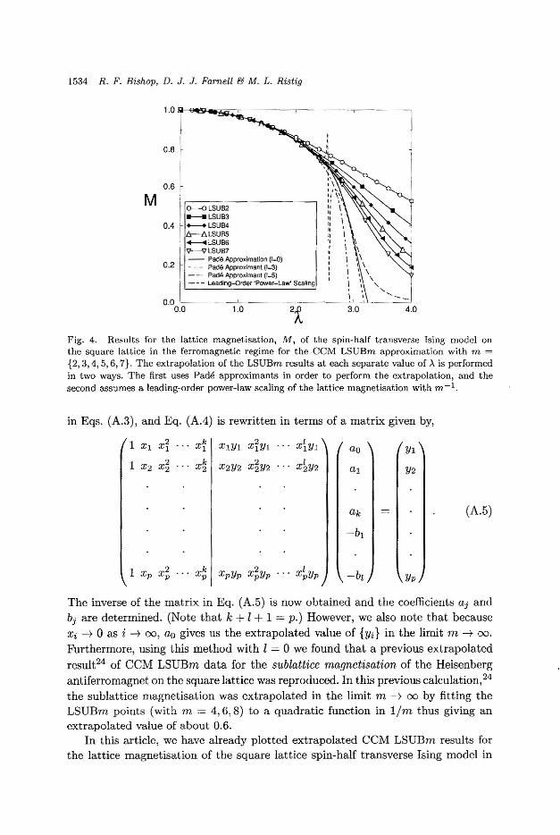
Fig. 4. Results for the lattice magnetisation, M, of the spin-half transverse Ising model onthe square lattice in the ferromagnetic regime for the eeM LSUBm approximation with m ={2,3, 4, 5, 6, 7}. The extrapolation of the LSUBm results at each separate value of,\ is performedin two ways. The first uses Pade approximants in order to perform the extrapolation, and thesecond assumes a leading-order power-law scaling of the lattice magnetisation with m -1.

in Eqs. (A.3), and Eq. (A.4) is rewritten in terms of a matrix given by,

1 Xl xi xk XIYI xiYI xiYI ao YII1 X2 x~

kX2Y2 X~Y2 X~Y2x2 al Y2

ak (A.5)

-b:

1 xp X2 xk xPYP2 I -i,P P xpYP xpYP YP

The inverse of the matrix in Eq. (A.5) is now obtained and the coefficients aj andbj are determined. (Note that k + I + 1 = p.) However, we also note that becauseXi -t 0 as i -t 00, ao gives us the extrapolated value of {Vi} in the limit m -t 00.

Furthermore, using this method with I = 0 we found that a previous extrapolatedresult24 of CCM LSUBm data for the sublattice magnetisation of the Heisenbergantiferromagnet on the square lattice was reproduced. In this previous calculation, 24

the sublattice magnetisation was extrapolated in the limit m -t 00 by fitting theLSUBm points (with m = 4,6,8) to a quadratic function in 11m thus giving anextrapolated value of about 0.6.

In this article, we have already plotted extrapolated CCM LSUBm results forthe lattice magnetisation of the square lattice spin-half transverse Ising model in


Fig. 2, and these results were seen to be in excellent agreement with those resultsof CBF and VQMC calculations. However, a further discussion of the extrapolatedCCM results presented here is also useful in order to illustrate the strengths andweaknesses of the extrapolation procedures outlined in this appendix. We can seefrom Fig. 4 below that the results for the Pade approximant extrapolation withl = 3 contains a zero in the denominator of Eq, (A.3) at about A ~ 2.6 such thatthe results show a divergence for IvI in Fig. 4 which is simply an artifact of theextrapolation procedure. This is because an assumption is made as to the scaling ofthe LSUBm data with 11m to some functional form. The validity of this assumptionis unknown as no exact scaling laws are known, as yet, for the behaviour of CCMLSUBm results as functions of m. However, the empirical evidence in Fig. 4 suggeststhat this is a reasonable assumption over much of the ferromagnetic phase, except,of course, for those points at which the Pade approximant results demonstrate this"artificial" divergence.

References

1. F. Coester, Nucl. Phys. 7,421 (1958); F. Co ester and H. Kiimmel, ibid. 17,477 (1960).2. H. Kiimmel, K. H. Liihrmann and J. G. Zabolitzky, Phys. Rep. 36C, 1 (1978).3. R. F. Bishop and K. H. Liihrmann, Phys. Rev. B17, 3757 (1978).4. J. S. Arponen, Ann. Phys. (N. Y) 151, 311 (1983).5. J. S. Arponen, R. F. Bishop and E. Pajanne, Phys. Rev. A36, 2519 (1987); ibid. 36,

2539 (1987); J. S. Arponen, R. F. Bishop, E. Pajanne and N. 1. Robinson ibid. 37,1065 (1988).

6. R. F. Bishop, Theor. Chim. Acta 80, 95 (1991).7. J. S. Arponen and R. F. Bishop, Ann. Phys. (N. Y) 207, 171 (1991); ibid. 227, 275

(1993); ibid. 227, 2334 (1993).8. R. F. Bishop, in Microscopic Quantum-Many-Body Theories and Their Applications,

ed. J. Navarro and A. Polls, Lecture Notes in Physics, Vol. 510 (Springer-Verlag,Berlin, 1998), p. 1.

9. J. W. Clark and E. Feenberg, Phys. Rev. 113, 388 (1959).10. H. W. Jackson and E. Feenberg, Rev. Mod. Phys. 34,686 (1962).11. E. Feenberg, Theory of Quantum Fluids, (Academic Press, New York, 1969).12. J. W. Clark, in Progress in Particle and Nuclear Physics, ed. D. H. Wilkinson, Vol.

2 (Pergamon, Oxford, 1979), p. 89.13. V. R. Pandharipande and R. B. Wiringa, Rev. Mod. Phys. 51, 821 (1979).14. E. Krotscheck and J. W. Clark, Nucl. Phys. A333, 77 (1980).15. J. W. Clark, in The Many-Body Problem: Jastrow Correlations Versus Brueckner

Theory, eds. R. Guardiola and J. Ros, Lecture Notes in Physics, Vol. 138 (Springer-Verlag, Berlin, 1981), p. 184.

16. S. Rosati, in International School of Physics Enrico Fermi, Course LXXIX, ed. A.Molinari (North-Holland, Amsterdam, 1981), p. 73.

17. A. Fabrocini and S. Fantoni, in First International Course on Condensed Matter,ACIF Series, eds. D. Prosperi, S. Rosati and S. Violini, Vol. 8 (World Scientific,Singapore, 1987), p. 87.

18. S. Fantoni and V.R. Pandharipande, Phys. Rev. C37, 1687 (1988).19. S. Fantoni and A. Fabrocini, in Microscopic Quantum Many-Body Theories and

Their Applications, eds. J. Navarro and A. Polls, Lecture Notes in Physics, Vol. 510


(Springer- Verlag, Berlin, 1998), p. 119.20. R. F. Bishop, J. B. Parkinson and Y. Xian, Phys. Rev. B44, 9425 (1991).21. R. F. Bishop, R. G. Hale and Y. Xian, Phys. Rev. Lett. 73, 3157 (1994).22. C. Zeng and R. F. Bishop, in Coherent Approaches to Fluctuations, eds. M. Suzuki

and N. Kawashima (World Scientific, Singapore, 1996), p. 296.23. D. J. J. Farnell, S. A. Kriiger and J. B. Parkinson, J. Phys.: Condens. Matter 9,7601

(1997).24. C. Zeng, D. J. J. Farnell and R. F. Bishop, J. Stat. Phys. 90, 327 (1998).25. R. F. Bishop, D. J. J. Farnell and J. B. Parkinson, Phys. Rev. B58, 6394 (1998).26. R. F. Bishop and D. J. J. Farnell, Mol. Phys. 94, No.1, 73 (1998).27. R. F. Bishop, D. J. J. Farnell and Zeng Chen, Phys. Rev. B59, 1000 (1999).28. J. Rosenfeld, N. E. Ligterink and R. F. Bishop, Phys. Rev. B60, 4030 (1999).29. M. L. Ristig and J. W. Kim, Phys. Rev. B53, 6665 (1996).30. M. L. Ristig, J. W. Kim and J. W. Clark, in Theory of Spin Lattices and Lattice

Gauge Models, eds. J. W. Clark and M. L. Ristig, Lecture Notes in Physics, Vol. 494(Springer-Verlag, Berlin, 1997), p. 62.

31. M. L. Ristig, J. W. Kim and J. W. Clark, Phys. Rev. B57, 56 (1998).32. R. F. Bishop, D. J. J. Farnell and M. L. Ristig, in Condensed Matter Theories, Vol. 14

(1999) - in press.33. J. Carlson, Phys. Rev. B40, 846 (1989).34. T. Barnes, D. Kotchan and E. S. Swanson, Phys. Rev. B39, 4357 (1989).35. N. Trivedi and D. M. Ceperley, Phys. Rev. B41, 4552 (1990).36. K. J. Runge, Phys. Rev. B45, 12292 (1992); ibid. B45, 7229 (1992).37. M. Boninsegni, Phys. Rev. B52, 15304 (1995).38. B. B. Beard and U. J. Wiese, Phys. Rev. Lett. 77, 5130 (1996).39. A. W. Sandvik, Phys. Rev. B56, 11678 (1997).40. M. C. Buonaura and S. Sorella, Phys. Rev. B57, 11445 (1998).41. P. G. de Gennes, Solid State Comm. 1, 132 (1963).42. R. Blinc, J. Phys. Chem. Solids 13, 204 (1960).43. S. Katsura, Phys. Rev. 127, 1508 (1962).44. M. Suzuki, Prog. Theor. Phys. 46, 1337 (1971); ibid. 56, 1454 (1976).45. B. K. Chakrabarti, A. Dutta and P. Sen, in Quantum Ising Phases and Transitions

in Transverse Ising Models, Lecture Notes in Physics, Vol. m 41 (Springer-Verlag,Berlin 1996).

46. D. C. Mattis, in The Theory of Magnetism II: Thermodynamics and Statistical Me-chanics, Springer Series in Solid-State Sciences, VoL 55 (Springer-Verlag, Berlin, Hei-delberg, New York, Tokyo 1985), p. 109.

47. Y.-L. Wang and B. R. Cooper, Phys. Rev. 172, 539 (1968); ibid. 185, 696 (1969).48. P. Pfeuty and R. J. Elliot, J. Phys. C4, 2370 (1971).49. Weihong Zheng, J. Oitmaa and C. J. Hamer, J. Phys. A23, 1775 (1990); ibid. A27,

5425 (1994).50. R. B. Pearson, Phys. Rev. A18, 2655 (1978).

Documents

AB INITIO TREATMENTS OF THE ISING MODEL IN A …