Embed Size (px)
Citation preview

©2016 Navigant Consulting, Inc.
AB802 Technical Analysis Potential Savings Analysis
Prepared for:
California Public Utilities Commission
Submitted by: Navigant Consulting, Inc. 1 Market Street Spear Tower, Suite 1200 San Francisco, CA 94105 415-356-7100 navigant.com Reference No.: 174655 March 31, 2016

AB802 Technical Analysis
Page i ©2016 Navigant Consulting, Inc.
This study was conducted by Navigant Consulting, Inc. under contract to the California Public Utilities Commission. Principal authors include:
• Greg Wikler • Amul Sathe • Surya Swamy • Karen Ehrhardt-Martinez • Aayush Daftari • Semih Oztreves • Julie Pierce • Carishma Menon • Jack Cullen
Navigant was supported by:
• Tierra Resource Consultants LLC • DNV GL
Special thanks are due to the staff of California Public Utilities Commission and the many stakeholders for providing direction, guidance, insight, and input throughout the conduct of this study.

AB802 Technical Analysis
Page ii ©2016 Navigant Consulting, Inc.
TABLE OF CONTENTS
Disclaimer .................................................................................................................... vii Executive Summary ...................................................................................................... 1
Background and Scope 1 Methodology 3
Stranded Potential Methodology ............................................................................................... 3 Operational Efficiency Methodology .......................................................................................... 4 Double Counted Savings Methodology ..................................................................................... 5
Preliminary Results 6 Impacts on the CEC Demand Forecast ..................................................................................... 6 Impacts on Utility Program Budgets .......................................................................................... 9
Limitations and Caveats 10 Recommendations 12
1. Introduction ............................................................................................................. 13
1.1 Policy Background 13 1.2 Scope of Technical Analysis 13 1.3 Existing vs. Code Baseline for Equipment 15 1.4 Types of Measure Installations 16 1.5 Below-Code Savings and “Stranded Potential” 17
1.5.1 Stranded Potential in Repair Eligible Equipment ........................................................... 17 1.5.2 Stranded Potential in Retrofit Replacement Measures .................................................. 18 1.5.3 Below-Code Savings in Replace on Burnout Measures ................................................ 18
1.6 Stranded Potential in the Context of Demand Forecasting 19
2. Methodology ............................................................................................................ 21
2.1 Equipment Upgrade Savings Methodology 21 2.1.1 Unit Energy Savings ....................................................................................................... 21 2.1.2 Consumer Adoption Modeling ........................................................................................ 23 2.1.3 Equipment Stock Accounting ......................................................................................... 25 2.1.4 Incentives and Program Costs ....................................................................................... 26 2.1.5 Cost Effectiveness .......................................................................................................... 28
2.2 Data Collection - Equipment Upgrades 29 2.2.1 Measure Type Selection ................................................................................................. 30 2.2.2 Existing Conditions Baseline .......................................................................................... 32 2.2.3 Repair Eligible Measure Data/Assumptions ................................................................... 36
2.3 Equipment Savings Uncertainty Analysis 38 2.3.1 Uncertainty Range of Individual Variables ..................................................................... 38 2.3.2 Low and High Case for Stranded Potential .................................................................... 39
2.4 Double Counted Savings 39 2.4.1 Methodology ................................................................................................................... 40 2.4.2 Data Collection and Assumptions .................................................................................. 41
2.5 Operational Efficiency 42 2.5.1 Defining Behavior and Operational Efficiency ................................................................ 42 2.5.2 Representative Programs Modeled ................................................................................ 45
3. Preliminary Results ................................................................................................. 50

AB802 Technical Analysis
Page iii ©2016 Navigant Consulting, Inc.
3.1 Impact on CEC Demand Forecast 50 3.1.1 Incrementally New AB802 Savings ................................................................................ 51 3.1.2 Double Counted Savings ................................................................................................ 52
3.2 Impact on Incremental Program Savings Forecast 52 3.2.1 Overall Portfolio Savings ................................................................................................ 53 3.2.2 Stranded Potential Details .............................................................................................. 55 3.2.3 Operational Efficiency Details ........................................................................................ 57 3.2.4 Double Counted Savings Details .................................................................................... 59
3.3 Impact on Program Budgets 61 3.4 Scenario Analysis 62
3.4.1 Stranded Potential .......................................................................................................... 63 3.4.2 Double Counted Savings ................................................................................................ 65 3.4.3 Operational Efficiency Potential ..................................................................................... 67
4. Caveats, Limitations and Recommendations ....................................................... 69
4.1 Caveats and Limitations 69 4.2 Recommendations 70
Summary of Stakeholder Comments on Program Budgets ............ A-1
Codes and Standards Data ................................................................. B-1
B.1 Savings in Existing Buildings B-1 B.2 C&S Included in the Best Estimate of Double Counted Savings B-7
Equipment Data collection ................................................................. C-1
C.1 Sources Reviewed C-1 C.2 Existing Baseline Efficiency C-2
Behavior and Operational efficiency Data collection ....................... D-1
D.1 Lighting Controls D-4 D.2 Building Information & Energy Management Systems (BIEMS) D-22 D.3 Tenant Engagement D-5
Stranded Potential Sensitivity Analysis .............................................E-1

AB802 Technical Analysis
Page iv ©2016 Navigant Consulting, Inc.
FIGURES AND TABLES
Figure 1: Savings Considered in the CEC Demand Forecast ..................................................................... 7 Figure 2: Incrementally New Savings from AB802 ...................................................................................... 8 Figure 3: Annual Energy Efficiency Program Budget by Savings Category .............................................. 10 Figure 4: Illustration of Age of Equipment in the Building Stock ................................................................ 18 Figure 5: Illustration of Energy Efficiency Savings in the Demand Forecast – Historic Approach ............ 20 Figure 6: Illustration of Energy Efficiency Savings in the Demand Forecast – AB802 Impacts ................ 20 Figure 7: Defining Average Existing Baseline ............................................................................................ 22 Figure 8: Code Impacts on UES of a Measure .......................................................................................... 23 Figure 9: Nested Consumer Choice Illustration ......................................................................................... 24 Figure 10: Illustrative Replace on Burnout Equipment Saturation over Time ............................................ 26 Figure 11: Illustrative Repair Eligible Equipment Saturation over Time .................................................... 26 Figure 12: Comparative Energy Savings from Three Hypothetical Customers ......................................... 27 Figure 13: Change in Load Profile from Efficient Equipment Replacement .............................................. 43 Figure 14: Examples of Load Profiles from Changes in Equipment Operation ......................................... 44 Figure 15: Comparison of Equipment Efficiency and Operational Efficiency ........................................... 44 Figure 16: Savings Considered in the CEC Demand Forecast ................................................................. 51 Figure 17. Incrementally New Savings from AB802 .................................................................................. 52 Figure 18: Effects of AB802 on the Incremental Program Savings Forecast (GWh)................................. 53 Figure 19: Effects of AB802 on the Incremental Program Savings Forecast (MW) .................................. 54 Figure 20: Effects of AB802 on the Incremental Program Savings Forecast (MM Therms) ..................... 55 Figure 21: PA Stranded Potential by End-Use (GWh) ............................................................................... 56 Figure 22: PA Stranded Potential by End-Use (MW) ................................................................................. 56 Figure 23: PA Stranded Potential by End-Use (MM Therms) .................................................................... 57 Figure 24: PA Operational Efficiency by Intervention (GWh) ..................................................................... 58 Figure 25: PA Operational Efficiency by Intervention (MW) ...................................................................... 58 Figure 26: PA Operational Efficiency by Intervention (MM Therms).......................................................... 59 Figure 27: Double Counted Savings (Best Estimate) by End-Use (GWh) ................................................. 60 Figure 28: Double Counted Savings (Best Estimate) by End-Use (MW) .................................................. 60 Figure 29: Double Counted Savings (Best Estimate) by End-Use (MM Therms) ...................................... 61 Figure 30: Effects of AB802 on the Annual Program Budget Forecast ..................................................... 62 Figure 31: Low/Mid/High Case - Cumulative PA Stranded Potential in 2026 (GWh) ................................ 63 Figure 32: Low/Mid/High Case - Cumulative PA Stranded Potential in 2026 (MW) .................................. 64 Figure 33: Low/Mid/High Case - Cumulative PA Stranded Potential in 2026 (MM Therms) ..................... 64 Figure 34: Cumulative Double Counted Savings in 2026 (GWh) .............................................................. 65 Figure 35: Cumulative Double Counted Savings in 2026 (MW) ................................................................ 66 Figure 36: Cumulative Double Counted Savings in 2026 (MM Therms) ................................................... 66 Figure 37: Low/Mid/High PA Operational Efficiency Savings in 2026 (GWh) ........................................... 67 Figure 38: Low/Mid/High PA Operational Efficiency Savings in 2026 (MW) ............................................. 67 Figure 39: Low/Mid/High PA Operational Efficiency Savings in 2026 (MM Therms) ................................. 68 Figure 40: Change in Load Profile from Efficient Equipment Replacement ............................................ D-1 Figure 41: Examples of Load Profiles from Changes in Equipment Operation ....................................... D-2 Figure 42: Comparison of Equipment Efficiency and Operational Efficiency ......................................... D-3 Figure 43: 2009 CBSA Commercial Market Lighting Control Saturations ............................................... D-8 Figure 44: Average savings (%) by Control Type .................................................................................. D-12 Figure 45: Data Sources for the Commercial Municipal Behavior Wedge Model .................................... D-9 Figure 46: Sensitivity of Program Savings to Uncertain Variables (GWh) ............................................... E-1 Figure 47: Sensitivity of Program Savings to Uncertain Variables (MW) ................................................ E-2

AB802 Technical Analysis
Page v ©2016 Navigant Consulting, Inc.
Figure 48: Sensitivity of Program Savings to Uncertain Variables (MM Therms) .................................... E-3 Figure 49: Sensitivity of Program Budget to Uncertain Variables ............................................................ E-4 Table 1: Increases in Program Costs and Savings Relative to the 2015 PG Study .................................. 10 Table 2: Definitions of Baseline Terminology ............................................................................................. 15 Table 3: Hypothetical Measure Energy Consumption ............................................................................... 15 Table 4: Measure Incentive Assumptions .................................................................................................. 28 Table 5: Cost Benefit Test Considerations ................................................................................................ 29 Table 6: Residential Measure Classifications ............................................................................................ 31 Table 7: Commercial Measure Classifications ........................................................................................... 32 Table 8: Preferred Data Sources for Existing Condition Baseline Update ................................................ 33 Table 9: Stranded Equipment Saturation for Repair Eligible Measures .................................................... 37 Table 10: Repair Life Assumptions ............................................................................................................ 37 Table 11: Repair Cost Eligible for Repair Eligible Measures ..................................................................... 38 Table 12: Low and High Case of Stranded Potential Analysis Parameters ............................................... 39 Table 13: Increases in Program Costs and Savings Relative to the 2015 PG Study ................................ 62 Table 14: Low and High Case of Stranded Potential Analysis Parameters ............................................... 63 Table 15: Residential Measure Existing Baseline Conditions Summary ................................................. C-4 Table 16: Commercial Measure Existing Baseline Conditions Summary ................................................ C-8 Table 17: CSS Study Distribution of Lamps by Control Type .................................................................. D-6 Table 18: Distribution of Lamps by Control Type and Business Size – Indoor Lighting .......................... D-7 Table 19: 2014 CBSA Indoor Lighting Power by Control Type and Building Type ................................ D-8 Table 20: Compliance Rates for 2008 Title 24 Standards ..................................................................... D-10 Table 21: Title 24 Codes – Potential Savings ........................................................................................ D-10 Table 22: Energy savings by building type ............................................................................................ D-11 Table 23: Comparison of savings for reviewed and non-reviewed papers ............................................ D-11 Table 24: NREL Lighting Control Savings Factors ................................................................................ D-13 Table 25: Title 25-2016 Lighting Control Power Factors ....................................................................... D-13 Table 26: Change in Operating Associated with Occupancy Sensors .................................................. D-14 Table 27: Modelled Savings Associated with Switching Technologies ................................................. D-14 Table 28: Potential actions and actors for optimized daylighting office retrofit ...................................... D-15 Table 29: PIER Report Daylight Harvesting Savings Potential by IOU ................................................ D-16 Table 30: 2009 CEUS Baseline Electricity Usage, Lighting ................................................................... D-18 Table 31. Lighting Control Saturation Forecast ..................................................................................... D-19 Table 32: Lighting Control Application and Energy Savings Assumptions ............................................ D-20 Table 33: IOU Costs for 2015 Lighting Programs .................................................................................. D-20 Table 34: Lighting Control Gross Measure Costs - SCE ....................................................................... D-21 Table 35: Lighting Control Gross Measure Costs – PG&E .................................................................... D-22 Table 36: Share of Energy Management Systems by Business Type .................................................. D-24 Table 37: Share of Energy Management Systems by Utility, Site Weighted ......................................... D-24 Table 38: Share of Energy Management Systems by Business Size, Site Weighted ........................... D-25 Table 39: Share of Energy Management Systems by End-Use Controls .............................................. D-25 Table 40: Distribution Controls: EMS Percent of Regional Conditioned Floor Area .............................. D-26 Table 41: Comparison of the Market Saturation of EMS Systems by Building Type ............................. D-26 Table 42: Maintenance Summary by Business Size ............................................................................. D-27 Table 43: HVAC Maintenance Summary by IOU ................................................................................... D-27 Table 44: Energy and Cost Savings of BIEMS Applications .................................................................. D-29 Table 45: HVAC Systems Savings Estimates by Building Type ............................................................ D-29 Table 46: Summary Characteristics of BIEMS-Enabled Buildings ........................................................ D-31 Table 47. Starting Technology Saturation by Building Type .................................................................... D-1
AB802 Technical Analysis
Page vi ©2016 Navigant Consulting, Inc.
Table 48. Enabling Technology Saturation Forecast ............................................................................... D-2 Table 49. BIEMS Saturation Forecast ..................................................................................................... D-2 Table 50: 2015 Monitoring Based Commissioning Program Costs ......................................................... D-3 Table 51: 2015 MBCx Program Cost Allocation ...................................................................................... D-4 Table 52: 2015 MBCx Program Cost Allocation per Unit Saved by Fuel Type ....................................... D-4 Table 53: Categories of Commercial Savings Estimates by Building Type and Energy End Use .......... D-8 Table 54: Building Types ........................................................................................................................ D-10 Table 55: Ownership Status of Commercial Buildings by Building Activity ........................................... D-11 Table 56: Percent of Measures Applicable to Tenant Engagement ...................................................... D-12 Table 57: Energy Consumption by End Use .......................................................................................... D-12 Table 58: Energy Savings by Building Type .......................................................................................... D-12 Table 59: Facility Level Savings by Building Type ................................................................................. D-14 Table 60. Market Penetration Scenarios ................................................................................................ D-14

AB802 Technical Analysis
Page vii ©2016 Navigant Consulting, Inc.
DISCLAIMER
This report was prepared by Navigant Consulting, Inc. (Navigant) for the California Public Utilities Commission. The work presented in this report represents Navigant’s professional judgment based on the information available at the time this report was prepared. Navigant is not responsible for the reader’s use of, or reliance upon, the report, nor any decisions based on the report. NAVIGANT MAKES NO REPRESENTATIONS OR WARRANTIES, EXPRESSED OR IMPLIED. Readers of the report are advised that they assume all liabilities incurred by them, or third parties, as a result of their reliance on the report, or the data, information, findings and opinions contained in the report. The views and opinions of authors expressed herein do not necessarily state or reflect those of the California Public Utilities Commission.

AB802 Technical Analysis
Page 1 ©2016 Navigant Consulting, Inc.
EXECUTIVE SUMMARY
Background and Scope
California Assembly Bill 802 (AB802) has the potential to significantly shift the way California energy efficiency Program Administrators (PAs) rebate and claim energy savings from energy efficiency programs. Historically Investor Owned Utilities (IOU) programs have been limited to seeking, rebating, and claiming energy efficiency savings for equipment that exceeds current code or standard. Furthermore, the only energy savings that could be claimed was the difference between code or standard and the high efficiency installation; this is referred to as “above-code savings”.1 However, AB802 will shift away from this paradigm to allow and incentivize all energy savings (including those that are “below-code”).2 Furthermore, AB802 instructs energy efficiency be achieved not only though equipment installations but also through behavior and operational efficiency interventions. The bill states:
the commission… shall, by September 1, 2016, authorize electrical corporations or gas corporations to provide financial incentives, rebates, technical assistance, and support to their customers to increase the energy efficiency of existing buildings based on all estimated energy savings and energy usage reductions, taking into consideration the overall reduction in normalized metered energy consumption as a measure of energy savings. Those programs shall include energy usage reductions resulting from the adoption of a measure or installation of equipment required for modifications to existing buildings to bring them into conformity with, or exceed, the requirements of Title 24 of the California Code of Regulations, as well as operational, behavioral, and retrocommissioning activities reasonably expected to produce multiyear savings.
Historically, the California Public Utilities Commission (CPUC) developed goals for IOU rebate programs focusing on above-code savings. Navigant has been supporting the CPUC in this goal setting process since 2011 by forecasting energy efficiency (EE) potential in California using the California Potential and Goals Model (PG model). The passage of AB802 has led the CPUC to consider multiple changes to program policy and planning among which include a technical assessment of the impact of AB802 on EE potential and IOU goals. AB802 opens the door to a new source of savings that can be counted towards EE programs. As part of its role in the PG study, Navigant developed a methodology, collected supporting data, and conducted a preliminary analysis of the savings potential related to the below-code, operational efficiency and behavioral initiatives targeted in AB802. This technical analysis focuses on two sources of savings:
1. Equipment Upgrade Savings in the residential and commercial sectors
2. Operational Efficiency (OE) and Behavior Savings in the commercial sector
1 “Above code savings” also refers to savings from energy efficiency equipment that exceeded the minimum efficiency appliance standards. “Above code” thus means “above building code or appliance standard” 2 “Below code” is synonymous with “to code” throughout this document. They can be used interchangeably.

AB802 Technical Analysis
Page 2 ©2016 Navigant Consulting, Inc.
This study reflects the first technical analysis of AB802 and the first significant analysis of below-code savings in a California potential study.3 The CPUC and Navigant anticipated many challenges at the outset of the study, thus the scope was set with the following objectives:
• Develop a set of nomenclature required to categorize and define below-code savings. • Consider different classes of measures and develop metrics to help understand where the
additional potential lies and where it doesn’t. • Consider if all below-code savings is truly additional potential or if a portion of it is already
counted elsewhere. • Develop a robust modeling methodology that serves as an initial basis to simulate the savings
that lies below code. • Collect as much reliable secondary data as is available that can inform a preliminary forecast. • Continue to forecast savings based on the list of measures used in the 2015 PG study. • Test the updated methodology in the PG model by developing a preliminary forecast of the
amount of additional EE potential that could be captured due to AB802. • Identify levels of uncertainty in the forecast. • Identify data gaps that require further research and understanding.
The result of this analysis includes the following sources of savings:
• Above-code savings from all sectors and measures considered in the 2015 PG study. • Below-code savings from measures in the following end uses and sectors:
o Residential and Commercial HVAC equipment o Commercial Lighting o Residential and Commercial Water heating equipment
• Behavioral and Operational Efficiency savings from select programs: o Home Energy Reports and Building Operator Certification and Training (both included in
the 2015 PG Study) o Three new commercial sector programs (Lighting Controls, Building Energy
Management, and Tenant Engagement) The CPUC and Navigant recognize that this analysis is not all encompassing of the below-code savings opportunities. The scope, availability of data and timeline limited what could be considered in this analysis. Additional measures and sectors should be considered in future updates. Possible sources of savings not considered in this analysis include (but may not be limited to):
• Below-code savings from Industrial and Agriculture measures • Below-code savings from Commercial and Residential building shell measures • Below-code savings from Commercial refrigeration equipment • Impacts of code compliance enhancement programs resulting from AB802
3 The modeling methodology used for this analysis was selected because of its ability to adapt the existing PG 2015 model and leverage available data. Modeling methodology may change in the future depending on the following factors: 1) further definition of the policy framework for implementing AB802 programs, 2) further definition of how normalized metered energy savings are to be calculated and utilized in PA reporting savings, 3) additional types of market data previously unavailable, 4) further insight and understanding of how below code savings can be integrated into the CEC’s demand forecast.

AB802 Technical Analysis
Page 3 ©2016 Navigant Consulting, Inc.
This analysis continues to leverage the CPUC PG model developed by Navigant; the modeling methodology was modified to accommodate this analysis. The PG model is primarily a “bottom up” measure-based analyses that relies on deemed savings estimates to forecast EE potential. Future CPUC program policies may not follow a completely deemed approach (i.e. use of metered consumption data); however, the PG model’s aggregate results still produces valid results for planning purposes.
Methodology
The impacts of AB802 can manifest itself in multiple ways. AB802 can generate savings that fall into three buckets:
• Stranded Potential - Stranded Potential is defined as the opportunities for EE that are not currently captured by either EE program administrator (PA) rebate programs or codes and standards. Stranded Potential is below-code savings that is not materializing in the market because there is no incentive for the customer to upgrade their existing equipment given current program rebate policy. Under AB802, PAs could start offering rebates for bringing existing equipment up to code thus motivating a whole new subset of customers to install EE measures and thus capture the Stranded Potential.
• Operational Efficiency - Operational efficiency (OE) saves energy by changing how equipment is operated. Operational efficiency reduces energy use by doing less work and generally involves changing the load shape throughout a machine or system’s operating cycle. AB802 encourages the industry to seek out additional OE savings.
• Double Counted Savings – These are the below-code savings generated from rebated equipment that would be realized even in the absence of PA rebate programs. These savings would occur as equipment naturally turns over and is replaced with code-compliant equipment. These savings are already embedded and accounted for in the California Energy Commission (CEC) Demand Forecast, thus further decrementing the forecast with these savings would be double counting.
Stranded Potential Methodology
Stranded potential exists because a subset of customers maintains certain types of equipment well beyond the equipment’s expected useful life. Long lived measures exist for two reasons:
1. The equipment is repairable and customers have been repairing the equipment rather than replacing the equipment when it fails (examples include boilers and chillers). Navigant refers to these measure types as “Repair Eligible”.
2. There is no catastrophic system failure that triggers the customer to repair or replace the entire system (examples include insulation and commercial lighting fixtures). Navigant refers to these measure types as “Retrofit Replacement”.
Influencing customers to replace long-lived equipment rather than keeping them in place results in real, below-code savings. This intervention has not previously been modeled in the PG study. For analysis of the stranded potential, Navigant modified the PG model to simulate the possibility of long lived measures and the decisions these customers are faced with in the real world. Modifications to the modeling methodology include:
• Classifying select measures as Repair Eligible or Retrofit Replacement

AB802 Technical Analysis
Page 4 ©2016 Navigant Consulting, Inc.
• Allowing for additional data on Repair Eligible and Retrofit Replacement measures including:
o Fraction of the equipment in the market beyond its expected useful life
o Average efficiency level of equipment that exceeds is useful life
o Cost of repairing (rather than replacing) equipment as well as how long the repair lasts
• Modifying the consumer decision algorithm allowing the possibility that customers have the option to repair rather than replace equipment
• Modifying how the model allocates rebates for measures including offering rebates for below code savings and use of a tiered rebate structure offering high rebates to customers that exceed code.
With these methodology changes, the PG model is now capable of forecasting below-code savings for the purposes of estimating the stranded potential. Navigant used the modified model and applied it to the measures considered in the 2015 PG study. Data was collected from a variety of sources including California saturation studies, U.S. Department of Energy analyses, and stakeholder submitted data. It’s important to note that the 2015 PG study has a set list of measures that were initially selected based on their ability to produce cost effective, above-code savings. Thus, our preliminary results for the stranded potential have a limited scope. Future updates to the PG study can consider new measures as new sources of below-code savings.
Operational Efficiency Methodology
The 2015 PG study included behavioral efficiency savings from Home Energy Reports (HER) in the residential sector and building operator certification and training (BOC) programs in the commercial sector across the four investor owned utilities (IOUs) in California. This analysis expands upon savings in the commercial sector by considering further Operational Efficiency (OE) savings sources and their costs. In the commercial sector, the OE continuum is broken into the three categories of actions that generate energy savings: Enhancement of Equipment Functionality, Optimization of Equipment Operations, and Shifting of Individual and Organizational Actions. OE savings typically result from the choices and actions of building operators, energy managers, and/or building tenants (whether owners or renters) and their employees. Ultimately energy savings are achieved as a result of shifts in HOW MUCH and HOW OFTEN equipment is used and HOW WELL it is optimized (functionality) and maintained.
The types of programs that would be representative of the activities included in the OE continuum are closely associated with the concept of Building Performance Optimization (BPO). BPO aligns with the intent of current legislation, including AB758 and potential initiatives post AB1109, and has the goal of achieving optimal design and operation of the holistic performance of buildings and their energy systems. Examples of programs that might make up a BPO initiative include:
1. Building Operator Certification
2. Lighting Controls
3. Building Information and Energy Management Systems (BIEMS)
4. Tenant Engagement Building Operator Certification was included in the 2015 PG Study. This analysis focuses on the other three initiatives listed above. Savings from these initiatives were estimated using a multi-step process:

AB802 Technical Analysis
Page 5 ©2016 Navigant Consulting, Inc.
1. Understand the current market baseline. Understand what customers are currently doing with regards to the modeled interventions.
2. Consider any code requirements. Code does not all of these interventions though may affect some.
3. Document savings per participant. Savings vary by building type and targeted applications within the building type.
4. Estimate annual program savings. Using understanding of the current market, existing forecasts for growth in the market, and professional judgement, Navigant estimated reasonable low/mid/high participation rates into the future.
5. Estimate annual program costs. A high level estimate of program cost was developed leveraging information from existing programs as a proxy.
Double Counted Savings Methodology
Double counted savings are those savings that could be counted two places:
1. These savings are already counted within the CEC’s baseline demand forecast
2. PAs could claim these savings in their energy efficiency rebate programs. These double counted savings would happen due to C&S even in the absence of PA programs. The savings are only double counted if the customer receives a rebate or incentive for the equipment and the PAs claim the measure towards their program accomplishments.4 This is to say that programs could be designed to minimize double counted savings. Navigant estimated the double counted savings; it is not currently possible to forecast the actual amount that will occur in the real world. The estimate produces two views of double counted savings. An upper limit to the amount of double counted savings and a “best estimate” of the double counted savings. The estimate of the upper limit includes all possible double counted savings from all sectors, end uses, measures, and all possible market activity. By capturing all sectors, end uses, and market activity this assumes that any customer taking on any action to reduce their building’s energy consumption will apply for a PA rebate and the PA will grant that rebate. For example, a customer purchasing a new standard-compliant television to replace their old broken television could show a reduction in their billed energy use and apply for a rebate. As written, AB802 could allow this type of claimed savings even though it would have occurred in the absence of the program (due to the standard). This illustrates that in the extreme case and under the broadest interpretation of AB802, almost any replacement of equipment in a building could be claimed as energy efficiency towards PA programs. However, this is not the likely outcome in the real world. Our best estimate of double counted savings makes several downward adjustments to constrain the scope to what is most likely to occur in the real world. Double counted savings are most likely to occur at times when the “reduction in normalized metered energy consumption” method is used (as opposed to a deemed approach) for quantifying energy savings. This method is most likely to be employed during whole building renovations (rather than “one-off” purchases like the previous television example).
• Whole building renovations trigger installations of certain types of measures more often than “one-off” installations. We assume HVAC, Building Envelope, Lighting and Water Heating
4 Double counted savings could occur regardless of the program delivery mechanism.

AB802 Technical Analysis
Page 6 ©2016 Navigant Consulting, Inc.
upgrades are more often made during a major renovation than an individual installation. This is not to say that appliances and electronics are not upgraded during major renovations but rather that a significant number of appliances and electronics upgrades happen as individual upgrades. Thus, our best estimate of double counted savings only considers HVAC, Building Envelope, Lighting, and Water Heating measures.
• Not all measures within the HVAC, Building Envelope, Lighting and Water Heating end uses are necessarily prone to happen during a major renovation. Navigant reviewed individual measures to further eliminate those technologies that are more likely to be upgraded outside of a major renovation. This includes savings from residential lighting, water fixtures, and residential HVAC air filter replacements. The remainder of C&S are those most likely to be double counted.
Even after the above adjustments, our resulting estimate could still be an overestimate. Our best estimate still assumes all buildings and measures that meet the above criteria will apply for a PA rebated during any sort of energy reducing renovation. In reality, a subset of customers are not likely to apply for rebates.
Preliminary Results
Results are presented for the combined IOU service territories under a mid-case scenario. Results are considered preliminary for many reasons which are documented in our Limitations and Caveats section.
Impacts on the CEC Demand Forecast
The CEC develops the California Energy Demand Forecast, a 10-year forecast for electricity consumption, retail sales, and peak demand for each of five major electricity planning areas and for the state.5 The demand forecast includes the effects of multiple sources of EE including building codes, appliance standards, and voluntary EE programs. Embedded in the baseline forecast are historic codes and standards and utility programs implemented in 2015 and prior. Incremental to the baseline forecast, the Additional Achievable Energy Efficiency (AAEE) is accounted to develop a revised forecast. The AAEE consists of planned programs and codes and standards starting in 2016 and going into the future. The 2015 AAEE savings forecast was derived from the 2015 PG study (prior to any consideration of AB802). This section presents the estimated impacts of AB802 on the demand forecast. Figure 1 illustrates the various impacts of AB802 on the CEC peak demand forecast and focuses on the mid-case results. The solid black line in Figure 1 shows the CEC’s 2015 Baseline Demand Forecast. All components above the solid black line represent savings that are already embedded in the Baseline Forecast. All components below the solid black line are incremental savings to the Baseline Forecast. The dashed black line shows the CEC’s 2015 Adjusted Demand Forecast, calculated by subtracting the 2015 AAEE forecast from the 2015 Baseline Forecast. All components that fall below the dashed black line represent incrementally new savings within the scope of our analysis that are attributed to AB802. The “hashed” wedges illustrating double counted savings are also attributed to AB802 but do not act to reduce California’s peak demand. Further discussion of the incrementally new AB802 savings and the double counted savings results follows Figure 1.
5 Kavalec, Chris, Nick Fugate, Cary Garcia, and Asish Gautam. 2016. California Energy Demand 2016-2026, Revised Electricity Forecast. California Energy Commission. Publication Number: CEC-200-2016-001-V1

AB802 Technical Analysis
Page 7 ©2016 Navigant Consulting, Inc.
Figure 1: Savings Considered in the CEC Demand Forecast
Source: Navigant Analysis
Incrementally new savings due to AB802 are reflected by the purple wedge that falls below the dashed black line in Figure 1. These new savings come from three sources as illustrated in Figure 2. In total the combined incremental potential from these three sources is forecasted to add 1,192 MW of savings in 2026.6
• Additional Above-Code Savings – The measures that make up this savings wedge are measures for which PAs have been historically7 rebating and claiming savings. The availability of incentives based on an existing conditions baseline framework are expected to drive more participation in above code measures (as even these measures would see larger rebates). These savings are reflected in Figure 2, which represents the additional market activity and amounts to 507 MW of savings in 2026.
• PA Stranded Potential – This wedge consists of below code savings from repair eligible and retrofit measures. These savings would not have happened in the absence of AB802 and are thus new, incremental savings. This wedge is constrained to only consider the potential from measures that were included in the 2015 PG study. We recognize that there are other possible actions that can be taken to capture below code savings that are not included in our analysis such as building envelope and commercial refrigeration measures. Therefore, the stranded potential could be larger than the scope of our analysis allows it to be. The stranded potential modeled in this study is forecasted to add 535 MW of savings in 2026.
• PA Operational Efficiency Potential – This wedge consists of new savings from three representative commercial operational efficiency programs (Lighting Controls, Tenant Engagement, and Building Information & Energy Management Systems). These are newly modeled programs that produce incrementally new savings. We recognize that there are other
6 We present peak demand savings only as it is the primary driver of procurement and generation planning decisions in California. 7 Prior to the passage of AB802

AB802 Technical Analysis
Page 8 ©2016 Navigant Consulting, Inc.
possible actions that can be taken beyond the three representative programs modeled. Thus, operational efficiency potential could be larger but we lack data on the feasibility and scope at this time. The operational efficiency potential modeled in this study is forecasted to add 150 MW of savings in 2026.
Figure 2: Incrementally New Savings from AB802
Navigant further investigated if the stranded equipment potential is truly incremental savings and is not already embedded in the Baseline Forecast (and therefore part of the Double Counted savings). If the CEC’s demand forecast model assumes a higher turnover rate of equipment resulting in very few pieces of equipment surviving beyond their useful life, then it would imply that a portion of the stranded potential is already embedded in the forecast. Navigant held a discussion with CEC’s staff to understand the stock turnover assumptions used in the demand forecast. The CEC model does allow for long lived equipment and has similar assumptions about the mean life of equipment compared to the deemed EULs used by the CPUC. At this time Navigant sees no need to decrement the stranded potential, however the relationship of modeled assumptions and real market conditions should be further investigated. Double Counted savings are presented in two wedges in Figure 1: the Best Estimate and the Upper Bound. The actual amount of double counted savings in the real world depends on the number of customers that apply for PA rebates and the types of measures included in their building renovation. Our Best Estimate of double counted savings amounts to 1,680 MW in 2026 while the Upper Bound amounts to 5,040 MW in 2026. While both of these values eclipse the forecasted 1,192 MW of incrementally new potential, it’s important to note that the double counted savings in this preliminary analysis is likely overestimated8 while the incrementally new savings from AB802 is likely underestimated9. As this analysis shows, there is great uncertainty in the results.
8 Our estimate of Double Counted savings assumes that all customers will apply for a rebate during any sort of energy reducing renovation or measure installation. It could be interpreted as a “worst case scenario”. It reality, a subset of customers is not likely to apply for rebates. Data is unavailable to estimate the true amount of customers that would fall in this category.. 9 Stranded Potential is underestimated because it may not capture the universe of stranded equipment and buildings in the market, as further discussed in Section 4.

AB802 Technical Analysis
Page 9 ©2016 Navigant Consulting, Inc.
Lighting and HVAC end uses account for the majority of Stranded Potential analyzed in this study; however they also account for the majority of double counted savings. For this reason, lighting and HVAC projects must be closely examined to reduce the amount of double counted savings and maximize the amount of stranded potential captured. Stranded Potential is defined as capturing the savings from old equipment beyond its useful life. However, Double Counted savings reflects the expected regular turnover of equipment in the market (based on sales and shipment data). Thus, program administrators and policy makers should be careful to truly target functional equipment beyond its useful life. If such targeting is not implemented, there is higher risk of double counted savings and the possibility that no new stranded potential will actually be captured. Furthermore, a non-targeted approach could lead to significant amounts of spending on savings that would have happened anyway (leading to low net-to-gross ratios) reducing the amount of funding available for projects that would have produced real new savings. On the other hand, our analysis of the Stranded Potential did not include many building envelope measures due to the scope of our study. Furthermore there is relatively little double counted savings from building envelope measures as natural turnover is infrequent. This further solidifies our hypothesis that there is additional stranded potential from building envelope measures. Additional analysis including measure characterization (savings, cost, market conditions, and measure life) are needed to test this hypothesis and to better understand this additional Stranded Potential.
Impacts on Utility Program Budgets
Utility program budgets are typically planned on an annual basis. Program costs include the sum of incentives paid to customers as well as non-incentive costs required to run the program. Program costs modeled in this analysis exclude non-resource programs and budget for IOU C&S advocacy efforts. The budget forecast consists of the required budget to achieve all electric, demand, and gas savings. Figure 3 shows the annual budget forecast for all IOUs to run their programs under AB802. The budget is broken down into four components (which have each been previously described): PA Savings (Pre-AB802 framework), PA Stranded Potential, PA Operational Efficiency Potential, and Double Counted Savings (Best Estimate). The black dotted line reflects the budget that would be needed to achieve the savings that the 2015 PG study forecasted.

AB802 Technical Analysis
Page 10 ©2016 Navigant Consulting, Inc.
Figure 3: Annual Energy Efficiency Program Budget by Savings Category
Source: Navigant Analysis
Table 1 illustrates program costs along with program savings considering incrementally new impacts of AB802 (excluding double counted savings) in comparison to the 2015 PG study results. . In 2016, program spending could increase 25% and result in an additional 22.5% electric savings, 16.1% demand savings, and 5% gas savings. In 2024, program spending could increase 24.4% and result in an additional 41.6% electric savings, 51% demand savings, and 20% gas savings. This is due to expected Operational Efficiency cost reductions driven from Tenant Engagement.
Table 1: Increases in Program Costs and Savings Relative to the 2015 PG Study
Percent Increase Relative to 2015 PG study
Program Year 2016 Program Year 2024
Electric Savings 22.5% 41.6%
Demand Savings 16.7% 51.0%
Gas Savings 5.0% 20.0%
Program Budget 23.8% 24.4% Note: Excludes Double Counted Savings
That said, the pattern filled purple shaded area called as “Double Counted Savings (Below Code)” demonstrates the amount of budget that the PAs could spend on the savings that would happen due to C&S even in the absence of PA programs. This potential risk is estimated to be $4 billion cumulative from 2016 to 2026. This is to say, if programs are not properly designed and targeted at the true stranded potential, PAs could spend up to $4 billion on savings that would have materialized even without the rebate.
Limitations and Caveats
As previously mentioned, the scope of this study was primarily to develop an updated methodology that allows for the analysis of the impacts of AB802. Navigant then used the updated modeling methodology to develop a primary estimate of the impacts of AB802 based on readily available market data.

AB802 Technical Analysis
Page 11 ©2016 Navigant Consulting, Inc.
1. There is likely more stranded potential than what this preliminary forecast captures. This preliminary forecast is limited in scope to the same measures considered in the 2015 and 2013 PG study. The previous PG studies selected measures to analyze based on their ability to produce above-code savings. Thus very few to-code measures were considered. We believe additional stranded potential lies in building envelope measures and commercial refrigeration measures. Furthermore, the scope of this study was to only consider the residential and commercial sector. We recognize additional stranded potential likely resides in the industrial and agriculture sectors.
2. There may be more operational efficiency potential than what this preliminary forecast captures, albeit uncertain. This preliminary forecast considers three representative commercial sector operational efficiency programs. The analysis is based on limited available data and professional judgement by Navigant; still, some savings estimates from these activities can be uncertain and the persistence of savings for some of the measures is unclear. The scope and timeline of this analysis did not allow for stakeholder vetting. Our operational efficiency forecasts should be considered an initial framework for continued research in this area. We recognize additional operational efficiency potential likely resides in the industrial sector.
3. Double Counted Savings is highly uncertain. Double counted savings can only occur when a customer receives a rebate or incentive for equipment. Even then, in theory programs can be designed in such a way to minimize double counted savings (by purposely targeting old equipment and buildings that are still functional). We are uncertain about the level of double counted savings at this time as there is no overall program guidance around customer eligibility. Furthermore, double counted savings is based on an estimate of renovation activity that occurs in existing buildings; there was limited data to inform this estimate.
4. Assumptions about program incentive structures are those of Navigant’s given limited input from Program Administrators. It is unclear what PA rebate programs will ultimately look like under AB802. Will some measures continue to have deemed savings and deemed rebates? Will all measures and projects necessarily use a “pay for performance” approach? Rebate amounts are a key driver in the forecast of customer adoption. Without known rebate policies and program budgets to calibrate to, the forecast may not be an accurate representation of modified programs under AB802. Navigant sought input from PAs on this topic during a public workshop. While the responses were useful, they were broad statements rather than specific plans. Additional discussion with policy makers and PAs is needed.
5. Data informing the estimate of the stranded potential is uncertain. This analysis initially developed a short list of commercial and residential measures that were hypothesized to have uncaptured stranded potential. After collecting and reviewing available market data it became apparent there are data gaps. Small sample sizes prevent a robust determination of the true amount of equipment that is “very old”. Limited data were available on the cost to repair and the added lifetime a repair offers.
6. Consumer adoption parameters are based on data sets in which consumers did not have an option to repair equipment. The new paradigm of seeking out below-code stranded potential involves influencing an inherently different decision process. Historically the PG study only modeled the consumer’s decision between a standard and high efficiency replacement (i.e. “what do I replace my old equipment with?”). Forecasting stranded potential introduces another decision: “Do I even replace the old equipment in the first place given I have the option to repair it and extend its life?” This analysis applies the same economic decision framework and assumptions as used in the PG study to this question of repairing. However, it’s possible the decision to repair rather than replace is a fundamentally different decision than the decision “what

AB802 Technical Analysis
Page 12 ©2016 Navigant Consulting, Inc.
do I replace it with?” and thus our decision algorithms may not accurately reflect what real consumer do when faced with this situation.
Recommendations
To better inform future updates to the potential study, Navigant identified a list areas for further research and consideration. Some of the data gaps identified could be filled through existing or future EM&V or market studies. These recommendations are described in further detail in Section 4.2.
1. Further Updates to the Modeling Methodology may be required. Modeling methodology may change in the future depending on multiple factors including further definition of the policy framework for utility funded below code programs.
2. Characterize Additional Residential and Commercial Equipment. We recommend further research and measure characterization for building envelope (insulation, roofing, windows, air sealing, etc.) and commercial refrigeration equipment.
3. Characterize Below Code Savings Opportunities in the Agriculture and Industrial Sectors. Below-code savings exists in the industrial and agriculture sectors, however they were not quantified through this study. Additional clarity is needed regarding CPUC baseline policy these sectors.
4. Expand Saturation Studies to Consider a Broader List of Technologies and End Uses. A dataset on distribution of age of all commercial equipment would more easily allow us to identify where the stranded potential truly lies.
5. Further Research to Inform the Double Counted Savings. Additional data collection and analysis will be needed to develop a more refined estimate of double counted savings. The most useful data would be a better understanding of the number of building alterations that occur in California and the amount of to-code activities that naturally occurs through these alterations.
6. Comparison and Alignment to CEC Demand Forecast. A more robust comparison and alignment of assumptions between used by this study and the CEC demand forecast is needed before the AAEE can be updated.
7. Further Research to Inform Operational Efficiency Savings. Consider further research in multiple areas including additional interventions, persistence, and industrial sector opportunities.
8. Collect Data on Equipment Removed by Program Participants. As new programs seeking below-code savings are implemented, program administrators should carefully document the age, type, and condition of equipment that is being replaced by program participants. These data could inform future studies.
9. Research Measure Repair Characteristics. The counterfactual to replacing old, below-code equipment in this study is the continued maintenance and use of old equipment. More robust data on the repair and maintenance characteristics of repair eligible equipment will lead to a more informed forecast.

AB802 Technical Analysis
Page 13 ©2016 Navigant Consulting, Inc.
1. INTRODUCTION
1.1 Policy Background California Assembly Bill 802 (AB802) has the potential to significantly shift the way California energy efficiency Program Administrators (PAs)10 rebate and claim energy savings from energy efficiency programs. Historically Investor Owned Utilities (IOU) programs have been limited to seeking, rebating, and claiming energy efficiency savings for equipment that exceeds current code or standard. Furthermore, the only energy savings that could be claimed was the difference between code or standard and the high efficiency installation; this is referred to as “above-code savings”.11 However, AB802 could shift away from this paradigm to allow and incentivize all energy savings (including those that are “below-code”).12 Furthermore, AB802 instructs energy efficiency be achieved not only though equipment installations but also through behavior and operational efficiency interventions. The bill states:
the commission… shall, by September 1, 2016, authorize electrical corporations or gas corporations to provide financial incentives, rebates, technical assistance, and support to their customers to increase the energy efficiency of existing buildings based on all estimated energy savings and energy usage reductions, taking into consideration the overall reduction in normalized metered energy consumption as a measure of energy savings. Those programs shall include energy usage reductions resulting from the adoption of a measure or installation of equipment required for modifications to existing buildings to bring them into conformity with, or exceed, the requirements of Title 24 of the California Code of Regulations, as well as operational, behavioral, and retrocommissioning activities reasonably expected to produce multiyear savings.
Historically, the California Public Utilities Commission (CPUC) developed goals for IOU rebate programs focusing on above-code savings. Navigant has been supporting the CPUC in this goal setting process since 2011 by forecasting energy efficiency (EE) potential in California using the California Potential and Goals Model (PG model). The passage of AB802 has led the CPUC to consider multiple changes to program policy and planning among which include a technical assessment of the impact of AB802 on EE potential and IOU goals. AB802 opens the door to a new source of savings that can be counted towards EE programs.
1.2 Scope of Technical Analysis As part of its role in the PG study, Navigant developed a methodology, collected supporting data, and conducted a preliminary analysis on the savings potential related to the below-code, operational efficiency and behavioral initiatives targeted in AB802. This technical analysis focuses on two sources of savings:
1. Equipment Upgrade Savings in the residential and commercial sectors
2. Operational Efficiency (OE) and Behavior Savings in the commercial sector This analysis continues to leverage the CPUC PG model developed by Navigant; the model was modified to accommodate this analysis. The PG model is primarily a “bottom up” measure-based analyses that relies on deemed savings estimates to forecast EE potential. Future CPUC program policies may not
10 As this analysis is not setting utility goals, we will refer to Program Administrators as opposed to Investor Owned Utilities 11 “Above code savings” also refers to savings from energy efficiency equipment that exceeded the minimum efficiency appliance standards. “Above code” thus means “above building code or appliance standard” 12 “Below code” is synonymous with “to code” throughout this document. They can be used interchangeably.

AB802 Technical Analysis
Page 14 ©2016 Navigant Consulting, Inc.
follow a completely deemed approach (i.e. use of metered consumption data); however, the PG model’s aggregate results still produces valid results for planning purposes. This study reflects the first technical analysis of AB802 and the first significant analysis of below-code savings in a California potential study. The CPUC and Navigant anticipated many challenges at the outset of the study, thus the scope was set with the following objectives:
• Develop a set of nomenclature required to categorize and define below-code savings. • Consider different classes of measures and develop metrics to help understand where the
additional potential lies and where it doesn’t. • Consider if all below-code savings is truly additional potential or if a portion of it is already
counted elsewhere. • Develop a robust modeling methodology to simulate the savings that lies below code. • Collect as much reliable secondary data as is available that can inform a preliminary forecast. • Continue to forecast savings based on the list of measures used in the 2015 PG study. • Test the updated methodology in the PG model by developing a preliminary forecast of the
amount of additional EE potential that could be captured due to AB 802. • Identify levels of uncertainty in the forecast. • Identify data gaps that require further research and understanding.
The result of this analysis includes the following sources of savings:
• Above code savings from all sectors and measures considered in the 2015 PG study • Below code savings from measures in the following end uses and sectors:
o Residential and Commercial HVAC equipment o Commercial Lighting o Residential and Commercial Water heating equipment
• Behavioral and Operational Efficiency savings from select programs: o Home Energy Reports and Building Operator Certification and Training (both included in
the 2015 PG Study) o Three new commercial sector programs (Lighting Controls, Building Energy
Management, and Tenant Engagement) The CPUC and Navigant recognize that this analysis is not all encompassing of the below-code savings opportunities. The scope, availability of data and timeline limited what could be considered in this analysis. Additional measures and sectors should be considered in future updates. Possible sources of savings not considered in this analysis include (but may not be limited to):
• Below-code savings from Industrial and Agriculture measures • Below-code savings from Commercial and Residential building shell measures • Below-code savings from Commercial refrigeration equipment • Impacts of code compliance enhancement programs resulting from AB802
Historically, the PG study considered technical, economic and market potential for equipment rebate programs. These types of EE potential are described as follows:
1. Technical Potential: The amount of energy savings that would be possible if all technically applicable opportunities to improve energy efficiency are taken immediately.

AB802 Technical Analysis
Page 15 ©2016 Navigant Consulting, Inc.
2. Economic Potential: The subset of the technical potential when limited to only cost effective opportunities (based on the Total Resource Cost test).
3. Market Potential: The energy efficiency savings that could be expected in response to specific levels of incentives and assumptions about policies, market influences, and barriers. Some studies also refer to this as “achievable potential.”
IOU goals are informed by the market potential. Therefore, this analysis focuses on updating the market potential results. This report does not contain any revised estimates of the technical or economic potential.
1.3 Existing vs. Code Baseline for Equipment Table 2 provides the definitions of the baseline terms considered in this analysis.
Table 2: Definitions of Baseline Terminology
Term Definition Precedent
Code Baseline Minimum level of efficiency
required for new units that go into service
Set by the governing regulatory body or other
industry standards
Existing Conditions Baseline
Level of efficiency of units going out of service (being
replaced by new units)
A range set by historical markets and is generally a mix of technologies below
current code. Over the past several years, the EE potential studies in California have used code baseline as the baseline assumption. Code baseline refers to the energy efficiency required by codes & standards (such as Title 24, Title 20, or Federal appliance standards) in place at the time of measure installation. Code baseline is most readily applicable to New Construction as well as Replace on Burnout (ROB) retrofits in which a measure failure triggers a code or standard minimum efficiency for the replacement measure. Existing conditions baseline refers to the actual efficiency level of the equipment that is being replaced. Equipment being replaced are generally near, at, or beyond their effective useful life. To further illustrate this issue, Navigant presents a hypothetical EE measure savings calculation based on the code vs. existing baseline methodology in Table 3. Under historic practice, a program administrator could claim 500 kWh of UES for the hypothetical measure (3,000 – 2,500 = 500), referred to as “above-code” savings. However, the customer’s billed energy usage would decrease on average by 700 kWh (3,200 – 2,500 = 700); 700 kWh is the sum of “above-code” savings and “below-code” saving. Following the “letter of the law” of AB802, program administrators would essentially be able to claim savings based on the customer’s billed energy reduction (including below-code energy savings).
Table 3: Hypothetical Measure Energy Consumption
Equipment Efficiency Annual Energy Use (KWh)
Existing Conditions Baseline 3,200
Code Baseline 3,000
Efficient Technology 2,500

AB802 Technical Analysis
Page 16 ©2016 Navigant Consulting, Inc.
1.4 Types of Measure Installations The PG study forecasts the adoption of more than 150 energy efficiency measures in the residential and commercial sector. Each measure can be classified into one of several broad measure types. Each measure type is treated differently in terms of calculating cost effectiveness, calculating energy savings, and modeling consumer decisions and market adoption. These differences are further discussed throughout the report. The types of measure installations are:
• New Construction – Equipment that is installed in a newly constructed building. In this situation, energy savings calculations are always relative to code. Installation of energy efficiency in new construction buildings is not covered in this analysis.
• Installation in Existing Buildings
o Equipment
Replace on Burnout (ROB) – New equipment needs to be installed to replace equipment that has reached the end of its useful life, has failed, and is no longer functional. Upon failure ROB equipment is generally not repaired by the customer and instead replaced with a new piece of equipment. Appliance standards are applicable to some types of ROB equipment and apply to all new purchases. An example of an ROB measure is the light bulb.
Repair Eligible – Equipment reaches the end of its Effective Useful Life (EUL) and fails but is “repairable”. The customer is faced with a choice of repairing the existing equipment or purchasing new equipment. The repair extends the life of the existing equipment (the duration of which is the “repair life”). Appliance standards are applicable to some types of Repair Eligible equipment but only apply to new purchases (not the repair). Examples include measures such as boilers and chillers.
o Retrofit
Retrofit Add-on – New equipment being installed onto an existing system, either as an additional, integrated component or to replace a component of the existing system. In either case, the primary purpose of the add-on measure is to improve overall efficiency of the system. These measures are not able to operate on their own as stand-alone equipment and are not required for the operation of the existing equipment or building. Codes or standards may be applicable to some types of Retrofit Add-on measures by setting minimum efficiency levels of newly installed equipment; but the codes or standards do not require the measure to be installed. Examples include measures such as boiler controls, VFDs, and window film.
Retrofit Replacement – Measures that will be replaced not due to equipment failure but rather triggered by building renovation. These measures are those that are installed to replace previously existing equipment that has either not failed or is past the end of its EUL but is not compromising use of the building (such as insulation and water fixtures). Many of these installations are subject to building code but upgrades are not always required by code until a major building renovation (and even then some may not be required).
Several stakeholders have commented on using the nomenclature and assumptions used by the California Technical Forum (CalTF) on “Repair Indefinitely” (RI) measures. Upon initial review of CalTFs comments and discussion with CalTF representatives, Navigant sees RI measures are similar to the treatment of “Repair Eligible“ and “Retrofit Replacement” as defined above. Thus our analysis is not at odds with CalTF’s research.

AB802 Technical Analysis
Page 17 ©2016 Navigant Consulting, Inc.
1.5 Below-Code Savings and “Stranded Potential” This section discusses the below-code savings from three measure types:
• Repair Eligible Equipment
• Retrofit Replacement Measures
• Replace on Burnout Equipment A portion of below-code savings contains the “Stranded Potential”. Stranded Potential is defined as the opportunities for energy efficiency that are not currently captured by either PA rebate programs or codes and standards. Stranded Potential is savings that is not materializing in the market because there is no incentive for the customer to upgrade their existing equipment given current program rebate policy. Under AB802, PAs could start offering rebates for bringing existing equipment up to code thus motivating a whole new subset of customers to install energy efficiency and capturing the Stranded Potential.
1.5.1 Stranded Potential in Repair Eligible Equipment Data shows there are certain types of equipment in the market for which a subset of customers have units well beyond their deemed useful life. For example, the deemed effective useful life (EUL) for energy efficient boilers is 20 years13 yet anecdotal observations have found +60 year old boilers currently functioning in the market. This leads us to conclude the following:
• For Repair Eligible equipment, the EUL used for efficiency planning purposes is not a reasonable limiting cap on the age of existing equipment currently in the market
• Very old equipment exists in the market because customers have been repairing the equipment rather than replacing the entire piece of equipment when it fails.
o The cost to repair equipment (likely a single failed component) is considerably less than replacing the entire piece of equipment.
o The repair extends the life of the below-code equipment and keeps old, inefficient units in the market.
A portion of the Stranded Potential in equipment lies in these Repair Eligible equipment types. A 60-year-old boiler has a much lower efficiency than a new boiler that would meet current minimum efficiency requirements. Thus replacing the old boiler even with a standard minimum efficient boiler could result in significant energy savings to the customer. Stranded Potential from this type of activity can be captured if the energy efficiency industry:
• Focuses on identifying these Repair Eligible technologies where significant below-code equipment exists
• Incentivizes customers to replace very old equipment rather than continuing to repair the equipment when it fails
• Recognizes that customers incentivized to replace very old equipment with standard minimum efficiency equipment lead to new energy efficiency savings
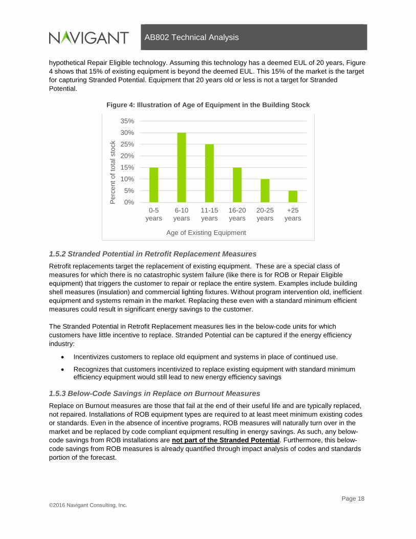
It is important to note that Stranded Potential from equipment lies in those very old pieces of equipment. This is further illustrated below in Figure 4 which shows the distribution of the age of equipment of a 13 Based on DEER
AB802 Technical Analysis
Page 18 ©2016 Navigant Consulting, Inc.
hypothetical Repair Eligible technology. Assuming this technology has a deemed EUL of 20 years, Figure 4 shows that 15% of existing equipment is beyond the deemed EUL. This 15% of the market is the target for capturing Stranded Potential. Equipment that 20 years old or less is not a target for Stranded Potential.
Figure 4: Illustration of Age of Equipment in the Building Stock
1.5.2 Stranded Potential in Retrofit Replacement Measures Retrofit replacements target the replacement of existing equipment. These are a special class of measures for which there is no catastrophic system failure (like there is for ROB or Repair Eligible equipment) that triggers the customer to repair or replace the entire system. Examples include building shell measures (insulation) and commercial lighting fixtures. Without program intervention old, inefficient equipment and systems remain in the market. Replacing these even with a standard minimum efficient measures could result in significant energy savings to the customer. The Stranded Potential in Retrofit Replacement measures lies in the below-code units for which customers have little incentive to replace. Stranded Potential can be captured if the energy efficiency industry:
• Incentivizes customers to replace old equipment and systems in place of continued use.
• Recognizes that customers incentivized to replace existing equipment with standard minimum efficiency equipment would still lead to new energy efficiency savings
1.5.3 Below-Code Savings in Replace on Burnout Measures Replace on Burnout measures are those that fail at the end of their useful life and are typically replaced, not repaired. Installations of ROB equipment types are required to at least meet minimum existing codes or standards. Even in the absence of incentive programs, ROB measures will naturally turn over in the market and be replaced by code compliant equipment resulting in energy savings. As such, any below-code savings from ROB installations are not part of the Stranded Potential. Furthermore, this below-code savings from ROB measures is already quantified through impact analysis of codes and standards portion of the forecast.
0%
5%
10%
15%
20%
25%
30%
35%
0-5years
6-10years
11-15years
16-20years
20-25years
+25years
Perc
ent o
f tot
al s
tock
Age of Existing Equipment

AB802 Technical Analysis
Page 19 ©2016 Navigant Consulting, Inc.
1.6 Stranded Potential in the Context of Demand Forecasting Although all forms of below-code equipment savings could be claimed by PAs under AB802, it is only the Stranded Potential that is truly new savings. This is better illustrated in the following figures which depict how energy efficiency is incorporated into California’s energy demand forecasts. Figure 5 illustrates how energy efficiency potential has historically been incorporated into energy demand forecasting. Various sources of energy savings are subtracted from a baseline demand forecast to result in an adjusted demand forecast. Historic practice has included the following:
• Naturally Occurring Savings – energy efficiency resulting from customers responding to technological change, market conditions and economic conditions. This occurs absent of codes and standards (C&S) and PA programs.
• Savings from Codes and Standards (Below-Code) – the below-code savings generated from the natural turnover of ROB equipment that is replaced at the end of its life as well as savings from routine building renovations that bring a building up to code. Historically, a portion of savings from C&S have been attributable to the IOUs (not illustrated in Figure 5 for simplicity).
• PA Savings (Pre-AB802 Framework) – the savings that PAs were allowed to claim for their rebate programs prior to the passing of AB802. This includes all above-code savings as well as some below code savings (from early retirement and retrofit programs that were previously allowable). These savings have been the primary subject of the 2015 PG study and all prior California potential studies.
Figure 6 illustrates how the accounting of savings would be updated with the implementation of AB802. Figure 6 is similar to Figure 5 with several noted differences:
• Double Counted Savings (Below-Code) – the below-code savings generated from rebated ROB measures. Under AB802 these would be classified as energy efficiency savings. However, this below-code savings would be realized even in the absence of PA rebate programs as equipment would naturally turn over and be replaced with code compliant equipment. Thus, in Figure 6 this savings is illustrated to “cannibalize” a portion of Savings from Codes and Standards. Decrementing this savings from the demand forecast would be double counting.
• PA Stranded Potential – Incrementally new equipment savings resulting from AB802 policy. This category includes new sources of savings that would not have happened in the absence of AB802-enabled rebate programs. This includes below-code savings from repair eligible measures, additional savings from retrofit measures, and additional above-code market activity resulting from AB802. These savings are attributable to PA rebate programs and further reduce the adjusted demand forecast.
• PA Operational Efficiency Potential – Additional savings from operational efficiency programs targeted at the commercial sector. AB802 encourages the commission to consider these savings in its policies. These savings further reduce the adjusted demand forecast

AB802 Technical Analysis
Page 20 ©2016 Navigant Consulting, Inc.
Figure 5: Illustration of Energy Efficiency Savings in the Demand Forecast – Historic Approach
Note: Figure not to scale.
Figure 6: Illustration of Energy Efficiency Savings in the Demand Forecast – AB802 Impacts
Note: Figure not to scale.
This report focuses on the methodology and data required to quantify PA Stranded Potential, PA Operational Efficiency Potential, and Double Counted Savings. This report also discussed these saving in the context of the demand forecast.

AB802 Technical Analysis
Page 21 ©2016 Navigant Consulting, Inc.
2. METHODOLOGY
This analysis largely uses the same analysis methodology as the 2013 PG Study14 and 2015 PG Study15. This section discusses the modifications made to the PG study and model methodology to accommodate analysis of AB802.
• Section 2.1 discusses the modeling approach for equipment upgrade savings analysis.
• Section 2.2 discusses the approach to quantifying double counted savings.
• Section 2.2 discusses data collection to support equipment upgrade analysis.
• Section 2.3 discusses the approach for operational efficiency savings.
• Section 2.4 discusses uncertainty analysis. Throughout the development and refinement of the methodology and data collection, Navigant reviewed and considered the comments from multiple stakeholders. Comments were provided verbally at two workshops as well as in writing following these workshops.16 The first workshop was held April 28, 2015 the second on November 6, 2015.
2.1 Equipment Upgrade Savings Methodology The PG Model uses a bottom-up approach to estimate the number of installations of high efficiency equipment based on the influence of PA programs and C&S. This analysis continues to use the same residential and commercial measures at the existing PG Model.
2.1.1 Unit Energy Savings Unit energy savings (UES) is defined as the difference in energy consumption between the baseline measure and the efficient technology replacement. In the case of above-code savings, UES is defined relative to the code baseline. However, when considering AB802, UES can be calculated relative to the existing baseline. Thus, to accommodate analysis of AB802, Navigant modified the PG model to be able to track UES relative to both code and existing conditions baseline. While the true assessment of existing conditions baseline can result in a unique baseline condition for every piece of equipment or building, average existing conditions baseline must be used for forecasting and planning purposes. We recognize that each situation in the real world will have a different existing conditions baseline; however, each unique case cannot be modeled for planning purposes. Figure 7 illustrates this concept. In Figure 7, eight customers are found to have old, operational equipment near, at, or beyond its useful life. Each has its own unique efficiency level that falls below current code minimum efficiency; an average across these customers can be used to define the average existing baseline.
14 Navigant. 2013 California Energy Efficiency Potential and Goals Study. February 2014 15 Navigant. Energy Efficiency Potential and Goals Study for 2015 and Beyond. September 2015. 16 Written comments were provided by the following organizations: Alternative Energy Systems Consulting, Association of Bay Area Governments, California Energy Efficiency Industry Council, California Technical Forum (Cal TF), Ecology Action, EnerNOC, FirstFuel, Heating, Air-conditioning & Refrigeration Distributors International, Home Energy Analytics, kW Engineering, Local Government Sustainable Energy Coalition, Marin Clean Energy, Natural Resources Defense Council, Office of Ratepayer Advocates, Pacific Gas and Electric (PG&E), San Diego Gas & Electric Company (SDG&E), Southern California Edison (SCE), Southern California Gas Company (SCG), Southern California Regional Energy Network, The Utility Reform Network, and the University of California.

AB802 Technical Analysis
Page 22 ©2016 Navigant Consulting, Inc.
Figure 7: Defining Average Existing Baseline
As C&S become more stringent over time it affects UES. Figure 8 illustrates how above-code and below-code UES changes over time for a specific measure as a result of code changes. The UES of a new installation decreases as the code or standard becomes more stringent while the below-code savings increases.17 Figure 8 illustrates that the existing baseline efficiency is expected to remain constant over time. This is in specific reference to the subset of old, inefficient equipment which remains in service in the absence of intervention. That population of equipment is expected to shrink over time (discussed further in section 2.1.3).
17 This illustration is for a set high efficiency measure that has a defined efficiency level (i.e. a SEER 18 air conditioner). We recognize that other higher efficiency measures may become more readily available in the market in the future. Those measures would also experience what is illustrated in Figure 7.

AB802 Technical Analysis
Page 23 ©2016 Navigant Consulting, Inc.
Figure 8: Code Impacts on UES of a Measure
2.1.2 Consumer Adoption Modeling The previous PG model was designed to focus on tracking installations of measures that result in above-code savings; the model was agnostic between customers that remain at their existing baseline and those that replace the existing baseline with a code compliant equipment. The previous PG model used a consumer decision algorithm in which customers are presented with two options when equipment needs to be upgraded:
1) install a standard compliant piece of equipment (for which no savings are claimed or tracked)
2) install an above standard compliant piece of equipment (for which savings are claimed and tracked)
Complete details on the methodology employed PG model can be found in section 3.3 Market Potential Analysis of the 2013 PG Study.18 To accommodate the assessment of stranded potential from AB802, the consumer decision algorithm in the PG model has been updated. Decisions are processed differently based on the type of measure being analyzed. The previous PG model considered only two broad types of measures (Replace on Burnout and Retrofit). The PG model was updated to accommodate four measure types (introduced earlier in section 1.4). The approach to consumer adoption modeling for each measure type is described further below. Equipment – Replace on Burnout In these situations, the existing consumer decision algorithm in the PG model is applied. Consumers have the choice of installing a code compliant piece of equipment or a high efficiency piece of equipment.
18 Navigant. 2013 California Energy Efficiency Potential and Goals Study. February 2014. Page 61-67

AB802 Technical Analysis
Page 24 ©2016 Navigant Consulting, Inc.
Equipment – Repair Eligible In these situations, the customer is faced with three options when it comes time to upgrade equipment:
1) Repair the existing equipment at some cost (lower than purchasing code compliant equipment) and extend its life.
2) Install a code compliant piece of equipment
3) Install an above-code compliant piece of equipment Navigant uses a nested approach within the model to account for the customer’s decision to repair, as shown below. Upon failure of repair eligible equipment, consumers face a first decision (Decision 1) to choose between repairing and replacing the existing equipment. If the first-level decision is to repair, then the life of the existing equipment is extended (known as the “repair life”, similar to modeling RUL). If instead the customer chooses to replace, then at the second-level (Decision 2) the customer chooses whether to install a code compliant or above-code compliant piece of equipment (sometimes having multiple options of above-code equipment to choose from).
Figure 9: Nested Consumer Choice Illustration
Modeling the consumer’s decision to repair equipment requires additional data and assumptions beyond what the PG study has historically tracked and collected. Additional data needs include:
1) Stranded Equipment Saturation – The fraction of repair eligible equipment currently in the market that is beyond its EUL.
2) Repair Cost – Navigant expects this cost to be a fraction of the cost of purchasing new, code compliant equipment
3) Repair Life – the added equipment lifetime that results from repairing failed equipment. Navigant expects this will be a fraction of the deemed EUL for the equipment.
These data items are further discussed in section 2.2.3. Retrofit Add-on

AB802 Technical Analysis
Page 25 ©2016 Navigant Consulting, Inc.
In these situations, the existing consumer decision algorithm in the PG model is applied. Consumers have the choice of doing nothing or installing the new equipment. The PG model has historically modeled such decisions. Retrofit Replacement In these situations, the customer is faced with three options:
1) Do nothing with no cost incurred and continue to use existing equipment
2) Replace existing equipment with a code compliant piece of equipment
3) Replace existing equipment with an above-code compliant piece of equipment In these situations, the existing consumer decision algorithm in the PG model is applied. The PG model has historically modeled such decisions.
2.1.3 Equipment Stock Accounting Old, inefficient equipment is expected to naturally turn over and be replaced with new equipment in the future. The rate of turnover varies by measure type and is thus modeled differently for each type:
• Replace on Burnout Equipment turnover is strongly correlated with equipment EUL. As old inefficient equipment reaches the end of its useful life it is replaced with new equipment that is at least code compliant or better. At a certain time in the future, all currently below-code equipment is expected to have naturally turned over in the market (without PA influence) and will be at or better than code. This concept is illustrated below in Figure 10. Figure 10 illustrates a market in which 30% of equipment is currently below-code. As time passes, the below-code stock decays to 0% saturation due to the natural replacement of below-code equipment. Historically, program administrators sought to influence customers to install above-code units (as opposed to at-code units) when it came time to replace equipment. Furthermore, for some technologies, program administrators sought to accelerate the conversion of below-code equipment to above-code equipment through “early retirement” programs. The PG model is already capable of modeling above code adoptions as well as early retirement measures, thus no model modifications were necessary for ROB equipment.
• Repair Eligible Equipment turnover is less correlated with equipment EUL. As old inefficient equipment reaches the end of its useful life it can be repaired extending its life and delaying its upgrade to code. It’s possible that in the absence of program intervention, the below-code stock of equipment decreases only slightly over time. This concept is illustrated below in Figure 11. Figure 11 illustrates a market in which 30% of equipment is currently below-code. As time passes, the below-code stock minimally decays as some equipment is replaced while most is repaired and kept in service. Under AB802, program administrators could seek to influence customers to replace (rather than repair) below-code equipment with at-code or above-code equipment and claim savings relative to the existing baseline. The PG model was modified to track the below code population separately from the at-code population and to further track the number of customer who choose to repair (and remain in the existing stock) verses replace and enter the at-code or above-code stock.

AB802 Technical Analysis
Page 26 ©2016 Navigant Consulting, Inc.
Figure 10: Illustrative Replace on Burnout Equipment Saturation over Time
Figure 11: Illustrative Repair Eligible Equipment Saturation over Time
2.1.4 Incentives and Program Costs Incentives (i.e. rebates) are an important driver of customer adoption within the PG model since they reduce the purchase cost of the efficient equipment, which helps overcome one key barrier (among several) to adoption of EE technologies – the upfront cost of the technology. Incentive amounts are a key driver in estimating the total cost of energy efficiency programs. Program costs also consider non-incentive costs (such as administration, marketing, education, and outreach). The analysis for existing baseline updates assumptions about program incentives (described further in this section) but does not change assumptions about program non-incentive costs (fully documented in the 2015 PG study).

AB802 Technical Analysis
Page 27 ©2016 Navigant Consulting, Inc.
The traditional modeling approach sets incentives as a fixed percent of incremental above-code costs for all replace on burnout measures. The traditional approach is simple to implement and communicate, but its assumptions are less appropriate to change the behavior (real and modeled) of customers that maintain and repair existing below-code equipment rather than replace it upon failure. The introduction of the existing baseline paradigm presents an opportunity to align the rebate structure to better capture savings for this below-code customer segment. Figure 12 helps to further illustrate the traditional modeling approach to the existing baseline paradigm. Figure 12 illustrates three customers replacing the same piece of old, inefficient equipment with new equipment of differing efficiency (noted by the differing energy consumption amounts on the Y-axis). Customer 1 installs equipment significantly above-code, Customer 2 installs equipment marginally above-code, and Customer 3 installs equipment that just meets code. Under historic program design, Customer 3 was not eligible for a rebate while Customer 1 could receive a substantially larger rebate than Customer 2 (given the relative difference in their above-code savings). Under AB802, program administrators may start to value to-code savings allowing Customer 3 to receive a rebate. Furthermore, these rebates could be more equitable across the three customers given the total savings (to + above-code) are more equitable.
Figure 12: Comparative Energy Savings from Three Hypothetical Customers
Navigant’s preliminary consideration of incentives given AB802 policy revealed several important questions that were posed to PAs (as well as other stakeholders) during a public workshop in November 2015:
1. Will program administrators (PAs) increase incentives under the new paradigm?
2. Will PAs reallocate incentives levels (e.g. provide higher incentives for lower hanging fruit)?
3. Will PA program budgets increase? PA’s submitted informal comments in response to these questions. Most PAs recognize there are multiple possibilities and suggested considering a tiered incentive system among those possibilities. A tiered

AB802 Technical Analysis
Page 28 ©2016 Navigant Consulting, Inc.
system is that in which above-code savings are assigned a premium compared to below-code savings in setting incentives. Comments were mixed on whether or not program budgets would increase. SCE suggested budgets may not need to increase if budgets are re-optimized to better target below-code savings. SoCalREN meanwhile suggested budgets should “significantly increase”. A summary of relevant PA comments are provided in Appendix A. Table 4 contains a summary of the incentives assumptions made in this preliminary analysis. Navigant modeled a tiered incentive approach in which incentives are set based on estimated first year savings (kWh and therms). Furthermore, higher incentives are offered per unit of above-code savings compared to below-code savings. A cap is also set such that incentives do not exceed 50% of the equipment’s incremental cost. Using this approach does not necessarily suggest a “pay for performance” approach. Rather, this implies that incentive levels are set by primarily considering the amount of savings measure produces rather than primarily considering the equipment cost. As was assumed in past modeling efforts, the incentive is paid in full to the customer in the year of the equipment purchase. The above code incentive levels were initially set based on the results of the 2015 PG study. The 2015 PG study applied a rebate equal to 50% of the incremental cost of equipment. Navigant divided the total incentive budget from the 2015 PG model by the total above code program savings. This sets an initial $/First Year Savings value to use in this analysis. We recognize actual rebate amounts per unit energy savings may be lower; we use these values to ensure consistency with the previous PG study incentive levels. Table 4 summarizes the incentive levels used in this analysis. Above-code Rebates are informed by the 2015 PG study while To-Code Rebates are assumed to be half the value of Above-code Rebates (thus simulating a tiered incentive structure).
Table 4: Measure Incentive Assumptions
Source: Navigant analysis.
2.1.5 Cost Effectiveness The 2015 PG study used a cost effectiveness screen to determine those measures that are to be included in the economic and market potential. Calculation of cost effectiveness in the PG model will continue to follow CPUC guidelines. Table 5 summarizes the benefits and measure costs that will be considered for each measure type under the AB802 analysis. The noted difference compared to the 2015 PG model is the treatment of repair eligible measures.
Residential To-Code Rebate Above-Code Rebate
Electric Savings $0.36/kWh $0.73/kWh
Gas Savings $6.07/Therm $12.14/Therm
Commercial To-Code Rebate Above-Code Rebate Electric Savings $0.35/kWh $0.70/kWh
Gas Savings $3.37/Therm $6.73/Therm
Incentive Cap
Percent of Incremental Cost 50%

AB802 Technical Analysis
Page 29 ©2016 Navigant Consulting, Inc.
Table 5: Cost Benefit Test Considerations
Measure Type Benefits Duration of Benefits Measure Costs
Equipment – Replace on Burnout
Above-code energy savings only EUL of replacement Code to efficient
incremental cost
Equipment – Repair Eligible
Dual baseline - savings relative to
existing baseline for Repair Life, and then relative to code for remainder of the
replacement’s EUL
EUL of efficient replacement
Full cost of efficient equipment minus repair
cost (minus deferred replacement credit)
Retrofit Add-on Savings relative to existing baseline RUL of baseline Full cost of efficient
equipment
Retrofit Replacement Savings relative to existing baseline EUL of replacement Full cost of efficient
equipment
2.2 Data Collection - Equipment Upgrades
This analysis continues to use the same measures at the existing PG Model. For the 2013 and 2015 Study, Navigant compiled an extensive set of measure-level data for the Residential and Commercial sectors into a database. Navigant combined information from multiple versions of the Database for Energy Efficient Resources (DEER), the Frozen Ex Ante (FEA) database, various IOU workpapers, and saturation studies. This data was combined into Navigant’s Measure Input Characterization System (MICS). The MICS database houses approximately 65,000 unique rows of Residential and Commercial measure characteristics that allow the calculation of technical, economic, and market potential for each measure by climate zone, building type, and service territory. Each of the 65,000 rows of data consists of up to 87 data parameters that define the measure. To accommodate the analysis of AB802, MICS and the PG model was updated with several key pieces of new data:
• Measure Type Selection – The 2015 PG model included two installation classifications for measures applied to existing buildings: Replace on Burnout and Retrofit. To support this analysis, Navigant expanded the installation types available to existing residential and commercial stocks, assigning each existing PG measure one of the updated installation types below (described earlier in section 1.4)
o Equipment – Replace on Burnout
o Equipment – Repair Eligible
o Retrofit Add-on
o Retrofit Replacement
• Existing Conditions Baseline – utilizing the most recent market data in 2015, Navigant researched and updated the existing conditions baseline for the selected measures, explained in section 2.2.2.2. Existing conditions baseline informs the unit energy consumption of the baseline equipment and ultimately informs the UES.

AB802 Technical Analysis
Page 30 ©2016 Navigant Consulting, Inc.
• Repair Eligible Measure Data/Assumptions – for those measures that were assigned the Equipment - Repair Eligible classification, several additional data points, detailed in section 2.2.3, needed to be collected for the updated methodology.
2.2.1 Measure Type Selection Navigant worked closely with CPUC staff to determine measure classifications for the different measures in the PG study. First, measure type determinations were made by End Use Sub-Categories as shown in Table 6 and Table 7. Each measure in the potential study maps to one of these sub categories. Appendix C presents the installation type classification by measure for the residential and commercial sectors. A draft of Table 6 and Table 7 were presented to stakeholders during a workshop in November 2015. Feedback was incorporated as appropriate. One stakeholder commented that the existence of repair services for home appliances such as laundry and dishwasher equipment indicated that these measures should be classified as repair eligible. However, upon further discussion with CPUC and review of market data it was determined these do not meet the criteria. Market data shows very few home appliance units are kept in the market beyond their deemed EUL. This implies two things: 1) repair services are used to fix broken appliances that has not reached its EUL, 2) when appliances nears the end of its EUL it is replaced with new a new appliance rather than repaired. Other stakeholder comments (including those from Heating, Air-conditioning & Refrigeration Distributors International and the University of California) confirmed that HVAC equipment falls under the Repair Eligible category. Comments indicated commercial and public sector building HVAC equipment tends to be left in the field far past the deemed useful life due to various financial reasons (tax codes and limited capital improvement budgets).

AB802 Technical Analysis
Page 31 ©2016 Navigant Consulting, Inc.
Table 6: Residential Measure Classifications
Measure Classification End Use Category End Use Sub-Category
Equipment – Replace on Burnout
Plug Loads & Appliances
Dishwasher Laundry
Refrigeration PC/Monitors
Indoor/Outdoor Lighting Lamps
Recreation Pool Pumps
Equipment – Repair Eligible
HVAC Space Heating Space Cooling
Service Hot Water Water Heaters/Boilers
Retrofit Add-On
Building Envelope Window Film
HVAC Ventilation
Service Hot Water Boiler Controls
Retrofit Replacement
Plug Loads & Appliances Smart Strips
Appliance Recycling
Building Envelope Insulation
HVAC Duct Sealing/Repair
Indoor/Outdoor Lighting Fixtures/Ballast
Controls Source: Navigant and CPUC staff.
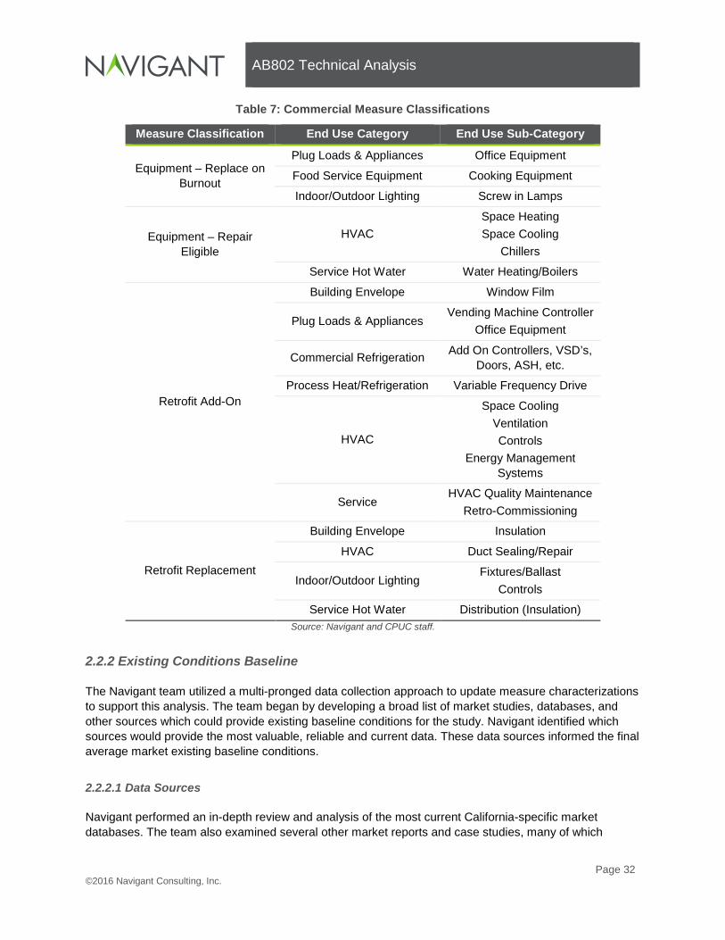
AB802 Technical Analysis
Page 32 ©2016 Navigant Consulting, Inc.
Table 7: Commercial Measure Classifications
Measure Classification End Use Category End Use Sub-Category
Equipment – Replace on Burnout
Plug Loads & Appliances Office Equipment
Food Service Equipment Cooking Equipment
Indoor/Outdoor Lighting Screw in Lamps
Equipment – Repair Eligible
HVAC Space Heating Space Cooling
Chillers
Service Hot Water Water Heating/Boilers
Retrofit Add-On
Building Envelope Window Film
Plug Loads & Appliances Vending Machine Controller
Office Equipment
Commercial Refrigeration Add On Controllers, VSD’s, Doors, ASH, etc.
Process Heat/Refrigeration Variable Frequency Drive
HVAC
Space Cooling Ventilation Controls
Energy Management Systems
Service HVAC Quality Maintenance
Retro-Commissioning
Retrofit Replacement
Building Envelope Insulation
HVAC Duct Sealing/Repair
Indoor/Outdoor Lighting Fixtures/Ballast
Controls
Service Hot Water Distribution (Insulation) Source: Navigant and CPUC staff.
2.2.2 Existing Conditions Baseline
The Navigant team utilized a multi-pronged data collection approach to update measure characterizations to support this analysis. The team began by developing a broad list of market studies, databases, and other sources which could provide existing baseline conditions for the study. Navigant identified which sources would provide the most valuable, reliable and current data. These data sources informed the final average market existing baseline conditions.
2.2.2.1 Data Sources
Navigant performed an in-depth review and analysis of the most current California-specific market databases. The team also examined several other market reports and case studies, many of which

AB802 Technical Analysis
Page 33 ©2016 Navigant Consulting, Inc.
stakeholders had identified after the April, 2015 Stakeholder Workshop on existing baseline.19 Another critical source that informs existing baseline conditions are Federal Codes and Standards, Title 20 and Title 24. The team leveraged these Codes and Standards sources for applicable measures where there were extensive data gaps in the existing market databases and reports. Certain data sources received higher priority than others, due to the source vintage and quality. The priority of sources is as follows, with the highest priority sources at the top and descending to the lowest priority sources:
1. Current California Market Databases (CLASS and CSS)
2. Current Market Reports and Case Studies
3. Codes and Standards
4. DEER Database
5. IOU Workpapers Though Navigant reviewed many databases, reports and case studies, only a limited number of sources provided the detailed and quality data necessary for this study. Table 8 details the sources ultimately relied upon for this effort, providing the source name, author, the affected sector (residential, commercial, or both), the data provided by the source, and a description and link to the source. A full list of data sources considered and reviewed is provided in Appendix C.
Table 8: Preferred Data Sources for Existing Condition Baseline Update
Source Name Author Sector Data Provided Description and Source Link
California Lighting and Appliance Saturation
Study (CLASS)
DNV-GL Residential
Baseline Efficiencies
& Equipment
Age
A residential onsite study on a sample of single-family, multi-family and mobile home residences in CA. Provided detailed information on residential lighting, appliances, HVAC, water heating equipment and construction types. https://webtools.dnvgl.com/projects62/Default.aspx?tabid=190
19 Written comments were provided by the following organizations: Alternative Energy Systems Consulting, Association of Bay Area Governments, California Energy Efficiency Industry Council, California Technical Forum (Cal TF), Ecology Action, EnerNOC, FirstFuel, Heating, Air-conditioning & Refrigeration Distributors International, Home Energy Analytics, kW Engineering, Local Government Sustainable Energy Coalition, Marin Clean Energy, Natural Resources Defense Council, Office of Ratepayer Advocates, Pacific Gas and Electric (PG&E), San Diego Gas & Electric Company (SDG&E), Southern California Edison (SCE), Southern California Gas Company (SCG), Southern California Regional Energy Network, The Utility Reform Network, and the University of California.

AB802 Technical Analysis
Page 34 ©2016 Navigant Consulting, Inc.
Source Name Author Sector Data Provided Description and Source Link
California Commercial Saturation
Study (CSS)
Itron Commercial
Baseline Efficiencies
& Equipment
Age
A commercial onsite and phone study on a sample of commercial buildings in CA. Provided detailed information on commercial lighting, some HVAC, and office equipment only. http://www.calmac.org/publications/California_Commercial_Saturation_Study_Report_Finalv2ES.pdf
HVAC Service Life and
Maintenance Cost
Database
ASHRAE Commercial Equipment Age
ASHRAE provides a database that focuses on commercial HVAC and water heat equipment service life and maintenance costs. http://xp20.ashrae.org/publicdatabase/summary.asp
Database for Energy Efficient
Resources (DEER)
J.J. Hirsch &
Associates Residential
Baseline Efficiencies
& Equipment
Age
Ex-Ante EE measure savings and cost Database. Existing baseline data was extracted from DEER during measures characterization in the 2015 Potential and Goals study but never directly used for that study. http://www.deeresources.com/
Codes and Standards
Federal & CA Title 20/24
Residential and
Commercial
Baseline Efficiency
The average age of equipment and/or effective useful life (EUL) of the equipment was used to determine the code efficiency requirements at the time of that average age year. Research included Federal C&S, CA Title 20 and 24.
2.2.2.2 Data Collection and Analysis
The purpose of this analysis is to determine the average efficiency level of equipment coming out of service. To inform this value Navigant sought measure level data for the following two data points in the residential and commercial sectors:
• Average Efficiency Level of Equipment, and
• Average Age of Equipment Based on the availability of these two data points, Navigant developed two different methods of analysis to determine the average existing conditions baseline. The average age of equipment was generally available within the reviewed data sources and is critical to determining the average efficiency level of equipment, regardless of the method utilized below. However, the reviewed market studies and databases only provided limited data on average efficiency level of equipment. CLASS and CSS both

AB802 Technical Analysis
Page 35 ©2016 Navigant Consulting, Inc.
collected data on the efficiency level of equipment, but not necessarily on all of the equipment the potential study examined. If the efficiency data was available in these data sources, the team also analyzed the robustness of that data based on both the total number of equipment observed in the market study and the percentage of that equipment with known efficiency levels. If the market studies provided robust data on the efficiency of equipment, the team utilized the preferred market data method. The team used the secondary codes and standards analysis method, if market research yielded unreliable equipment efficiency data or if equipment efficiency data was not available for a measure. Market Data Method Navigant utilized the market data method to analyze the average efficiency of equipment coming out of service only if market research provided robust data on both the efficiency of equipment and the age of equipment. In this method, the team analyzed the average existing efficiency of equipment in several buckets, based on the age of equipment in the market data. This analysis resulted in the average efficiency level of equipment in the total market, equipment greater than 5 years old, greater than 10 years old, greater than 15 years old, and greater than 20 years old. The team looked at both the EUL and average age of equipment to determine which bucket was most appropriate to utilize for the purposes of updating the existing baseline in the PG model. For example, if a measure’s EUL was 15 years and the average age of equipment from the market data was 11 years, the team utilized the average baseline efficiency of equipment greater than 10 years old. Using the average efficiency from this bucket excludes the newer equipment that utility programs will not target and allows for a more accurate measure level savings calculation. Codes and Standards Method For the equipment types where research did not provide the average efficiency, historic codes and standards were used to define the existing baseline. Navigant looked back into history a certain number of years to assess what the code or standard was at the time and used that as a proxy for existing baseline efficiency. Navigant took one of two approaches to determine how far back in history to look. The first (preferred approach) was to use market data to obtain the average age of equipment for the subset of equipment that exceeded the measure EUL. The second approach (only used when the first approach wasn’t possible) was to use the EUL of equipment. California Title 20 and 24 were first consulted for historic efficiency levels. If Title 20 and 24 did not exist at the time, federal standards were consulted.
2.2.2.3 Integrating Findings into MICS
MICS was updated to reflect the new existing conditions baseline data that had been collected. MICS contains six key data points leveraged in this analysis:
• Baseline condition description
• Baseline unit energy consumption (UEC)
• Code measure description
• Code UEC
• Efficient measure description

AB802 Technical Analysis
Page 36 ©2016 Navigant Consulting, Inc.
• Efficient UEC
This analysis updated the baseline condition description and estimated the baseline UEC. The code and efficient descriptions and UECs were previously determined during the 2015 PG study using a variety of data sources (see the 2015 PG study for details). Baseline UEC was estimated using two options:
1. DEER or workpaper data was used if these data sources were able to provide UECs for the researched existing condition.
2. When option 1 was not possible, a linear extrapolation process was used leveraging efficiency levels and UECs of the code and efficient measures.
The three UEC values (baseline, code, efficient) could then be used to calculate above and below code savings.
2.2.3 Repair Eligible Measure Data/Assumptions
Three new types of information needed to be collected to appropriately model Repair Eligible measures:
• Stranded Equipment Saturation
• Repair Life
• Repair Cost
2.2.3.1 Stranded Equipment Saturation
The stranded equipment saturation is defined as the saturation of equipment in the market that is performing beyond its effective useful life (i.e. has likely been repaired). This saturation is only applicable to measures classified as Equipment - Repair Eligible and is not directly available in current market studies. Navigant developed a methodology to estimate the stranded equipment saturation by analyzing the percentage of equipment in the market which are past their deemed effective useful life (EUL). The team leveraged earlier research from CLASS and CSS, deriving two key data points: the total number of observations of a measure and the total number of observations past the EUL of the measure. The team calculated the stranded equipment saturation by dividing the total past EUL observations of a measure by the total number of observations in the market study. CSS did not contain commercial water heating measures, which Navigant assumed to be at 25% saturation in lieu of other data sources. CSS has very limited data on boilers and chillers, Navigant leveraged information from CalTF. Table 9 presents the stranded equipment saturation by measure type, sector and source. Table 9 shows that several measures initially postulated to be repair eligible and to have significant stranded potential may not actually fit this category (based on the available data collected). Residential water heaters (which have a 20-year deemed EUL) show very few units in the market that are actually past their EUL (3-5%). Similarly, residential furnaces have an EUL of 20 years but show only 10% of the equipment in the market is older than 20 years. This implies that residential water heaters and furnaces tend to be replaced on burnout rather than repaired and kept in the market. On the other hand, HVAC equipment tends to have a larger portion of the population beyond its EUL. Our analysis continues to model all of these measures as repair eligible; however, our results will ultimately show very little (if any) stranded potential from residential water heaters and furnaces.

AB802 Technical Analysis
Page 37 ©2016 Navigant Consulting, Inc.
Table 9: Stranded Equipment Saturation for Repair Eligible Measures
Measure Type Sector Stranded Equipment Saturation Source
Split AC Residential* 17% CLASS
Split HP Residential* 14% CLASS
Furnace Residential* 10% CLASS
Electric Water Heating Residential* 3% CLASS
Gas Water Heating Residential* 5% CLASS
Split AC Commercial 25% CSS
Split HP Commercial 17% CSS
Package AC Commercial 33% CSS
Package HP Commercial 41% CSS
Boilers Commercial 77% CalTF**
Chillers Commercial 77% Navigant Assumption (Same as Boilers)
Furnace Commercial 24% CSS
Electric Water Heating Commercial 25% Navigant Assumption
Gas Water Heating Commercial 25% Navigant Assumption * Based on data from the Single Family subsector.
** CalTF data only included boilers from the large multifamily subsector in a limited geography.
2.2.3.2 Repair Life
Data on repair life is unavailable. Navigant assumed repair life varies by sector and estimates a range for scenario analysis purposes. Repair life is assumed to be some fraction of the deemed EUL of the equipment that is being repaired. The range of assumed Repair Life can be found in Table 10.
Table 10: Repair Life Assumptions
Sector Repair Life (Low) Repair Life (Mid) Repair Life (High)
Commercial 1/2 EUL 3/4 EUL 1 EUL
Residential 1/3 EUL 1/2 EUL 2/3 EUL Source: Navigant assumptions.
2.2.3.3 Repair Cost
Repair Cost is the associated cost to the customer to repair equipment and extend the life of the equipment (the Repair Life). Repair costs are reflected as a fraction of the costs to purchase new, minimum efficiency compliant equipment obtained from DEER. These costs vary by measure type. The repair costs were based on equipment material costs or part replacement costs as stated in DOE Standards and Rulemaking Technical Support Documents. Other sources, such as CalTF reports, were
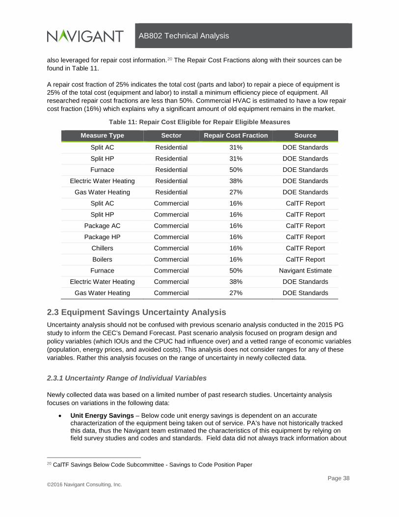
AB802 Technical Analysis
Page 38 ©2016 Navigant Consulting, Inc.
also leveraged for repair cost information.20 The Repair Cost Fractions along with their sources can be found in Table 11. A repair cost fraction of 25% indicates the total cost (parts and labor) to repair a piece of equipment is 25% of the total cost (equipment and labor) to install a minimum efficiency piece of equipment. All researched repair cost fractions are less than 50%. Commercial HVAC is estimated to have a low repair cost fraction (16%) which explains why a significant amount of old equipment remains in the market.
Table 11: Repair Cost Eligible for Repair Eligible Measures
Measure Type Sector Repair Cost Fraction Source
Split AC Residential 31% DOE Standards
Split HP Residential 31% DOE Standards
Furnace Residential 50% DOE Standards
Electric Water Heating Residential 38% DOE Standards
Gas Water Heating Residential 27% DOE Standards
Split AC Commercial 16% CalTF Report
Split HP Commercial 16% CalTF Report
Package AC Commercial 16% CalTF Report
Package HP Commercial 16% CalTF Report
Chillers Commercial 16% CalTF Report
Boilers Commercial 16% CalTF Report
Furnace Commercial 50% Navigant Estimate
Electric Water Heating Commercial 38% DOE Standards
Gas Water Heating Commercial 27% DOE Standards
2.3 Equipment Savings Uncertainty Analysis Uncertainty analysis should not be confused with previous scenario analysis conducted in the 2015 PG study to inform the CEC’s Demand Forecast. Past scenario analysis focused on program design and policy variables (which IOUs and the CPUC had influence over) and a vetted range of economic variables (population, energy prices, and avoided costs). This analysis does not consider ranges for any of these variables. Rather this analysis focuses on the range of uncertainty in newly collected data.
2.3.1 Uncertainty Range of Individual Variables
Newly collected data was based on a limited number of past research studies. Uncertainty analysis focuses on variations in the following data:
• Unit Energy Savings – Below code unit energy savings is dependent on an accurate characterization of the equipment being taken out of service. PA’s have not historically tracked this data, thus the Navigant team estimated the characteristics of this equipment by relying on field survey studies and codes and standards. Field data did not always track information about
20 CalTF Savings Below Code Subcommittee - Savings to Code Position Paper

AB802 Technical Analysis
Page 39 ©2016 Navigant Consulting, Inc.
the efficiency of equipment (sometimes just the age of equipment). Based on professional judgment, we believe below code unit energy savings has a range of ±10%.
• Repair Cost Fraction – Navigant found very few studies that provided reliable data on the cost of equipment repairs. Based on a review of the limited available data and Navigant professional judgment, we believe our repair cost fraction estimates could vary by ±50%.
• Repair Life – Navigant found no studies that provided reliable data on the number of years equipment repairs last. Based on Navigant professional judgment alone, we believe our repair life estimates have a range as presented earlier in section 2.2.3.2.
• Stranded Equipment Saturation – Stranded equipment saturation was estimated based on field survey studies. Navigant estimated saturation by quantifying the percent of equipment that is older than its deemed EUL. However, we note that actual measure life forms a distribution around the deemed EUL. Thus based on Navigant professional judgment, we believe our stranded equipment saturation values could vary by ±50%.
2.3.2 Low and High Case for Stranded Potential
Navigant developed a Low and High forecast based on the uncertainty of variables stated above. The Low and High case were developed by compounding the lower and upper range for each uncertain variable. The low and high ranges for each variable are applied such that they produce the lowest and highest savings potential respectively. Table 12 summarizes the multipliers and values used in the Low and High case used in the analysis.
Table 12: Low and High Case of Stranded Potential Analysis Parameters
Uncertain Parameter Low Case High Case
Unit Energy Savings (UES) Best Estimate Minus 10% Best Estimate Plus 10%
Repair Cost Fraction Best Estimate Minus 50% Best Estimate Plus 50%
Repair Life 2/3 EUL (Residential) 1 EUL (Commercial)
1/3 EUL (Residential) 1/2 EUL (Commercial)
Stranded Equipment Saturation Best Estimate Minus 50% Best Estimate Plus 50% Source: Navigant professional judgement.
2.4 Double Counted Savings
Double counted savings are those savings that could be counted two places:
3. These savings are already counted within the CEC’s baseline demand forecast
4. PAs could claim these savings in their energy efficiency rebate programs. Through the process of updating the demand forecast, the CEC accounts for additional energy efficiency from PA rebate programs. Counting these savings within the baseline forecast and further accounting for them in the Additional Achievable Energy Efficiency would be double counting the savings. These double counted savings would happen due to C&S even in the absence of PA programs. The savings are only double counted if the PAs provide a rebate to the customer and claim it towards their program accomplishments.

AB802 Technical Analysis
Page 40 ©2016 Navigant Consulting, Inc.
Navigant provides an estimate of the double counted savings; it is not currently possible to forecast the actual amount that will occur in the real world. The actual amount of double counted savings depends on the programs and measures offered by the PAs. This is to say that programs could be designed to minimize double counted savings.
2.4.1 Methodology
The PG model contains a set list of utility rebated measures (determined at the beginning of the 2013 PG study). These measures were originally selected based on their ability to produce above-code savings for IOU programs; very few measures that only produce below-code savings were characterized. AB802 could allow PAs to claim savings from rebated measures Navigant has not historically examined in the IOU rebate program forecast, such as:
• Savings from measures not included in the voluntary program forecast (i.e. efficient windows)
• Savings from buildings that come up to code through normal renovation activities
• To-standard adoptions for all equipment in the market (the PG model has historically focused on the voluntarily adoptions of measures that exceed minimum standards)
Limiting the analysis of double counted savings only to rebated measures in the PG study would understate the possibility of double counting. Savings from C&S captures the majority of below-code savings in the market from expected turnover of equipment and building renovation. These savings are expected to happen even in the absence of PA programs and captures the activity of the entire market. Below code savings is strictly an issue related to existing buildings (not new construction); thus, we focus our analysis of double counted savings on the C&S savings that occurs in existing buildings. Our estimate produces two views of double counted savings. An upper limit to the amount of double counted savings and a “best estimate” of the double counted savings.
2.4.1.1 Upper Limit
The estimate of the upper limit includes all possible double counted savings from all sectors, end uses, measures, and all possible market activity. By capturing all sectors, end uses, and market activity this assumes that any customer taking on any action to reduce their building’s energy consumption will apply for a PA rebate and the PA will grant that rebate. For example, a customer purchasing a new standard-compliant television to replace their old broken television could show a reduction in their billed energy use and apply for a rebate. As written, AB802 could allow this type of claimed savings even though it would have occurred in the absence of the program (due to the standard). This illustrates that in the extreme case and under the broadest interpretation of AB802, almost any replacement of equipment in a building could be claimed as energy efficiency towards PA programs. However, this is not the likely outcome in the real world. Thus, we also present a “best estimate” of the double counted savings.
2.4.1.2 Best Estimate
Our best estimate of double counted savings makes several downward adjustments to constrain the scope to what is most likely to occur in the real world. Double counted savings are most likely to happen when Replace on Burnout Measures are upgraded during a whole building renovation.

AB802 Technical Analysis
Page 41 ©2016 Navigant Consulting, Inc.
To further elaborate on this, double counted savings are most likely to occur at times when the “reduction in normalized metered energy consumption” method is used (as opposed to a deemed approach) for quantifying energy savings. This method is most likely to be employed during whole building renovations (rather than “one-off” purchases like the previous television example).
• Whole building renovations trigger installations of certain types of measures more often than “one-off” installations. We assume HVAC, Building Envelope, Lighting and Water Heating upgrades are more often made during a major renovation than an individual installation. This is not to say that appliances and electronics are not upgraded during major renovations but rather that a significant number of appliances and electronics upgrades happen as individual upgrades. Thus, our best estimate of double counted savings only considers HVAC, Building Envelope (such as insulation, cool roofs, and windows), Lighting, and Water Heating measures.
• Not all measures within the HVAC, Building Envelope, Lighting and Water Heating end uses are necessarily prone to happen during a major renovation. Navigant reviewed individual C&S measures to further eliminate those technologies that are more likely to be upgraded outside of a major renovation. This includes savings from residential lighting, water fixtures, and residential HVAC air filter replacements. The remainder of C&S are those most likely to be double counted.
Even after the above adjustments, our resulting estimate could still be an overestimate. Our best estimate still assumes all buildings and measures that meet the above criteria will apply for a PA rebated during any sort of energy reducing renovation. In reality, a subset of customers is not likely to apply for rebates.
2.4.2 Data Collection and Assumptions
The methodology and data sources to forecast savings from C&S is described in the 2013 and 2015 PG study reports. Navigant collected additional data to accommodate this analysis. Two additional data sets were necessary:
• A factor that splits C&S savings into those that occur in existing buildings (EB) and those that occur in new construction (NC).
• A short list of C&S most likely to be double counted. Navigant developed the EB/NC splits using three different approaches described below. Appendix B.1 provides all the splits for each code or standard.
• EUL Method: For appliance standards (T-20 and Fed Appliances), data does not exist to describe the installations in existing vs. new buildings; thus Navigant estimated the split. Navigant estimated the stock turnover rate for equipment in existing buildings and compared it to estimates of installations in new construction relying on EUL of the equipment and IEPR21 new construction rates. This method is best explained with an example. If a residential measure has a EUL equal to 10 years, then the annual turnover of the equipment stock in existing buildings is 10% (calculated as 1/EUL). This means every year, 10% of the existing equipment will burn out be replaced by standard compliant equipment. On the other hand, new construction is equal to 1% of the total building stock for residential sector based on IEPR forecast. This means annual installations in existing buildings is 10 times more than installations in new construction for this measure (10%/1%). Navigant used this approach to estimate the portion of savings from each standard that comes from installations in existing buildings. Appendix B shows the EUL, new
21 CEC. 2014 Integrated Energy Policy Report (IEPR) Update and Demand Forecast Forms. Adopted Feb. 2015.

AB802 Technical Analysis
Page 42 ©2016 Navigant Consulting, Inc.
construction rates, and resulting ratios for all T-20 and Federal standards. This method produces an estimate of the ratio of savings between existing buildings and new construction. Total market activity (installations) of standard minimum efficiency equipment is unchanged.
• Evaluation Report Data: For evaluated 2008 T-24 building codes, Navigant used the distribution of savings between new construction and alterations from the statewide codes and standards impact evaluation report.22 The report examined individual components of T-24 (but not every single one). Where data on individual components did not exist, Navigant used a 55% and 45% split for new construction versus existing buildings, respectively, based on the statement below from the evaluation report.
“In the estimated potential for this evaluation, the IOUs identified 55% of the electric energy and demand savings with new construction and the remaining 45% with alteration projects.”
• Navigant Assumptions: For future unevaluated T-24 building codes, Navigant applied assumptions based on the scope of the forecasted savings. The majority of future T-24 savings forecasts comes from new construction buildings. The PG study forecasted limited future T-24 savings in existing buildings due to lack of data. For 2005 T-24 building codes, Navigant applied the knowledge gained from the evaluation report (mentioned on the method above) to make assumptions about each 2005 T-24 component.
Appendix B.2 lists the C&S that are included in our best estimate of double counted savings.
2.5 Operational Efficiency The PG study considers savings from multiple market interventions. Although the majority of potential comes from equipment rebate programs and codes and standards, the PG study included behavioral efficiency savings from multiple (yet a limited set) of interventions. The 2015 PG study included savings from Home Energy Reports (HER) in the residential sector and building operator certification and training (BOC) programs in the commercial sector across the four investor owned utilities (IOUs) in California. This analysis expands upon savings in the commercial sector by considering further operational efficiency (OE) savings sources and their costs.
As previously mentioned, the 2015 PG study considered technical, economic and market potential for equipment rebate programs. However, when considering savings from behavior and codes and standards, only market potential was forecasted. The focus of this effort is on forecasting the market potential for new OE savings sources beyond BOC, including revising forecasts for measure included in the previous PG forecast iterations, and also new measures not considered in those reports. Throughout the conduct of this analysis the Navigant team reviewed and considered stakeholder written comments including information submitted by the California Energy Efficiency Industry Council.
2.5.1 Defining Behavior and Operational Efficiency Almost all energy savings result from either replacing less efficient equipment with more efficient equipment, or by changing how a piece of equipment is operated. When equipment is replaced it does not change how equipment is operated, it simply requires less power for the machine to do the same work. This reduction in power requirement is sometimes referred to as the ‘delta watt’, and the load
22 Cadmus and DNV GL. Statewide Codes and Standards Program Appendices to Impact Evaluation Report for Program Years 2010-2012. August, 2014. http://www.calmac.org/publications/CS_Evaluation_Report_Appendices_FINAL_10052014.pdf

AB802 Technical Analysis
Page 43 ©2016 Navigant Consulting, Inc.
shape that results from equipment replacement is generally the same as the baseline equipment load shape, but requires lower power. For example, a lighting retrofit will typically reduce the wattage (i.e. the delta watt) required to operate the lamps and ballasts, but the new lights will stay on for the same period of time as the old lights.
Figure 13 provides an illustration of how the installation of efficient equipment saves energy when there is no change in operating characteristics of the replacement equipment when compared to the baseline equipment. In this example, the replacement equipment uses only 60% of the power required by the baseline equipment, but operates for the same time duration, has the same general load profile, and does the same work. Energy savings result from the 40% power saved (i.e., the ‘delta watt’) throughout the operating cycle.
Figure 13: Change in Load Profile from Efficient Equipment Replacement
From a behavioral perspective, equipment replacement involves influencing the purchasing decision that results in a more efficient piece of equipment being installed. Programs targeting equipment efficiency include marketing strategies, education, incentives, and other strategies intended to shift equipment selection toward more energy efficient options and/or to accelerate equipment replacement. In contrast to the equipment replacement, operational efficiency (OE) saves energy by changing how equipment is operated. Operational efficiency reduces energy use by doing less work and generally involves changing the load shape throughout a machine’s operating cycle. In the lighting retrofit example discussed above, an operational efficiency component would include adding daylight harvesting capability to the lighting retrofit so that some portion of the lights can be turned off or dimmed in areas where windows allow adequate sunlight. This control aspect changes the static on/off load shape of a simple lamp and ballast replacement into a more dynamic load shape that adjusts power level to match the work needed to supplement available sunlight. Equipment and operational savings can occur within the same project, such as a lighting retrofit that includes a daylight harvesting design, however operational efficiency does not always require equipment replacement, and so has an added dimension of market potential. For example, operational efficiency can involve teaching occupants of a commercial building to turn off lights and save resources in areas where natural light is sufficient. This OE action reduces the amount of work done by a baseline lighting system and does not involve any equipment replacement. Figure 14 provides several illustrations of how operating efficiency saves energy compared to the baseline equipment operation. In these examples, energy is saved by reducing the amount of work performed by converting constant loads to variable loads, reducing operating times, reducing the total number of load cycles, or completely eliminating the load. Figure 15 provide a more expansive comparison of the various aspect and attributes of equipment efficiency and operational efficiency.
Baseline equipment load profile
Replacement equipment load profile
Savings(Green shaded area)
100% Power
0% PowerTime
60% Power relative to baseline
0% PowerTime Time

AB802 Technical Analysis
Page 44 ©2016 Navigant Consulting, Inc.
Figure 14: Examples of Load Profiles from Changes in Equipment Operation
Figure 15: Comparison of Equipment Efficiency and Operational Efficiency
In the commercial sector, the OE continuum is broken into the three categories of actions that generate energy savings: Enhancement of Equipment Functionality, Optimization of Equipment Operations, and Shifting of Individual and Organizational Actions. OE savings typically result from the choices and actions of building operators, energy managers, and/or building tenants (whether owners or renters) and their
Time
x
Convert constant load to variable load. Power required varies during a load cycle and may equal base case power requirement at some point.
Reduce time duration of load cycle. Total number of load cycles and maximum power for each cycle remains the same between the base and efficient case
Reduce total number of load cycles. Time duration of the load cycles remaining in the efficient case is the same as the base
Eliminate load and load cycle. Different process is used to accomplish the same work
100% Power
0% Power
Baseline equipment load profile
Operational efficiency load profile
Savings(Green shaded area)
DSM Potential
Equipment Efficiency
Saves energy by doing the same work for less energy.
Savings based on a delta watt achieved by replacing low efficiency equipment with high efficiency equipment and running new equipment the same way.
Keeps load shape, but shifts it ‘down’ through reduced demand.
Organizational decisions are generally purchasing decisions.
Requires information about the base and efficient machines.
Potential is estimated primarily through stock turnover and assuming consistent operation.
Subject to revision as codes and standards prescribe more efficient equipment.
All project required investment in equipment purchase. High percentage of projects require capital budget.
More closely aligned with the term ‘efficiency’.
Saves energy by doing less work.
Savings based on controlling the device output to match the necessary work.
Changes load shape but generally keeps peak demand the same.
Organizational decisions center on ability to influence behavior, and developing information and management infrastructure needed to maintain and verify.
Requires information about the operation, operator, and work being done.
Potential is estimated primarily by forecasting changes load profile that result from changes in operating behavior.
Not generally subject to code, but can be achieved as event based (e.g. Spare the Air).
Most projects are expense items or do not require any money for purchase.
More closely aligned with the term ‘conservation’.
Operational Efficiency

AB802 Technical Analysis
Page 45 ©2016 Navigant Consulting, Inc.
employees. Ultimately energy savings are achieved as a result of shifts in HOW MUCH and HOW OFTEN equipment used and HOW WELL it is optimized (functionality) and maintained. The types of activities that comprise the OE continuum include:
1. Operator behavior. This includes optimization of equipment operation and maintenance that requires occasional and repeat operator attention. For example, re-commissioning activities such as adjusting set points fall into this category, as do maintenance actions like replacing filters. Energy information systems, such as those used to continuously monitor and adjust facility operation, are another example.
2. Information and machine control. This includes optimization of equipment operation using automated controls or energy management systems that do not require continuous operator monitoring to save energy. For example, this would include installing daylight harvesting systems that automatically dim lights when natural lighting is adequate, or converting a constant volume air handling systems to a variable air volume system.
3. Tenant engagement. These are operational savings that result from how occupants interact with the building and how they use appliances and work related equipment. These savings are achieved by helping tenants adopt efficiency oriented policies and practices.
The PG study already includes savings from equipment change-outs (i.e. light fixtures, HVAC equipment, etc.) and retrofits (adding insulation, etc.). Thus, this analysis focuses purely on changes in the actions of utility customers that enhance equipment functionality and building operations and engage building tenants and their employees in ways that reduce energy consumption.
2.5.2 Representative Programs Modeled
The types of programs that would be representative of the activities included in the OE continuum are closely associated with the concept of Building Performance Optimization (BPO). BPO aligns with the intent of current legislation, including AB758 and potential initiatives post AB1109, and has the goal of achieving optimal design and operation of the holistic performance of buildings and their energy systems. Example of programs that might make up a BPO initiative includes;
1. Building Operator Certification
2. Lighting Controls
3. Building Information and Energy Management Systems (BIEMS)
4. Tenant Engagement Building Operator Certification was included in the 2015 PG. This analysis focuses on the other three initiatives listed above.
2.5.2.1 Lighting Controls
Many baseline studies indicate that the penetration of lighting controls is low compared to potential applications. Favorable trends in technology and costs suggest penetration of lighting control could be much higher, though various barriers remain. This analysis forecasts the savings from two types of control technologies, switching and dimming, including an assessment of current market and code baseline conditions. The market for lighting controls in commercial buildings is expanding due to improvements in control technology, an increasing range of technology options and vendors, and favorable price trends in

AB802 Technical Analysis
Page 46 ©2016 Navigant Consulting, Inc.
information and controls technology. For the purpose of this analysis, we combined all forms of lighting controls into two broad categories;
1. Switching Systems. Some of the most common switching control strategies for commercial building include:
a. Scheduling, a change in lighting based on a schedule.
i. EMS and timeclocks
b. Occupancy, a change in lighting based on the presence or absence of people.
i. Manual Switching
ii. Motion Sensor
The typical operating mode for switching controls is binary, such that a light is either on, operating at 100% of full power, or it is off and so uses no energy.
2. Dimming Systems.
a. Photocell, a change in lighting at a point in response to the amount of available natural light.
b. Daylight harvesting, a change in lighting over a zone in response to the amount of available natural light.
c. Personal controls, a change in light levels by an individual according to personal preference.
Typical operating parameters for dimming system are that a lighting system dimmed to a minimum level of 20% of light output consumes roughly 35.1% of full power. At 50% light output, the power consumption is 59.6% of full power.23
A Navigant Research report24 forecasts a compound annual growth rate (CAGR) of revenue for the worldwide market for intelligent lighting controls in commercial buildings of 17.2% between 2013 and 2020. The Navigant Research forecast assumes that achieving these growth rates will require some form of market intervention to address the following barriers;
• Financial Barriers. Although many of the components of networking lighting systems are falling in price, the total upfront cost of such a system is still a primary barrier to broader adoption. Cost can have an impact in the following ways;
o Initial cost;
o Capital not available or competition for capital exists;
o Strict return on investment (ROI) thresholds, and
o Split incentive problem in leased buildings.
• Complexity. Buildings under 100,000 SF make up approximately 98% of all commercial buildings by number in the United States, and a similarly high percentage globally. Owners of these small and medium sized buildings are often unable or unwilling to install highly complex networked lighting control systems. Smaller buildings are less likely to have dedicated building managers who could learn and manage such systems, and decision makers worry that complicated systems would go underutilized or, worse, could cause unnecessary problems.
23 Office Daylighting Potential. Task 3 of the PIER Daylighting Plus Research Program. Public Interest Energy Research (PIER) Program. FINAL PROJECT REPORT. Heschong Mahone Group, Inc. 24 Intelligent Lighting Controls for Commercial Buildings. Navigant Research, Published 3Q 2013.

AB802 Technical Analysis
Page 47 ©2016 Navigant Consulting, Inc.
• Lack of Standardization. Until the last decade or two, most dimming ballasts were part of fully integrated proprietary systems, many of them for the specialized theatrical lighting industry. For example, Lutron developed its commercial-oriented systems over time to optimize the capabilities of dimming ballasts at the system level. Other vendors have similarly developed systems that can only communicate with their own equipment.
• Insufficient Knowledge and Experience. Many of the key parties in the building industry do not generally understand building controls. Owners and property managers, for example, are not necessarily aware of the capabilities of modern lighting systems. Thus, despite opportunities to include higher efficiency lighting and lighting controls, these items are seldom placed high on the list of priorities. In addition, designers who have not yet worked with some of the sophisticated control systems may be reluctant to suggest adding them to projects; they will expect the learning curve to be steep, and may feel their reputations are at risk if something does not work as planned.
Savings from lighting controls were estimated as follows:
1. Understand the current market baseline. Various studies were reviewed to establish the current saturation of lighting control technologies. The California Commercial Saturation Study (CSS) indicates that buildings that had been retrofit through some form of PA program had higher rates of lighting control installation than did non-program participants. Control technologies also vary by size of building.
2. Consider any code requirements. From the 2013 Nonresidential Compliance Manual, all non-residential lighting systems must have switching or control capabilities to allow lights to be turned off when they are not needed. Additionally, “it is desirable to reduce light output and power consumption when full light output is not needed. These mandatory requirements apply to all nonresidential, high-rise residential and hotel/motel buildings for both conditioned and unconditioned interior spaces”.
3. Document savings per participant. Energy savings from lighting controls in commercial buildings varies by control strategy and building type. The average savings from various control strategies range between 20% and 30% depending on the control and building type.
4. Estimate annual program penetration. Using understanding of the current market, existing forecasts for growth in the market, and professional judgement, Navigant estimated reasonable low/mid/high penetration rates into the future.
5. Estimate annual program costs. A high level estimate of program cost was developed leveraging information from existing California commercial lighting programs as a proxy.
Additional details and documentation can be found in Appendix D.
2.5.2.2 Building Information & Energy Management Systems (BIEMS)
Building Energy Information and Continuous Commissioning System Baseline studies indicate that the penetration of controls system is low compared to potential applications, and new ways to extract value from these systems are also emerging. Favorable trends in information systems and control technology and costs suggest penetration of these technologies could be much higher, though various barriers remain. This analysis forecasts the savings from leveraging the combined use of Building Information & Energy Management Systems (BIEMS) to better understand and optimize energy-consuming processes, including an assessment of current market and code baseline conditions.

AB802 Technical Analysis
Page 48 ©2016 Navigant Consulting, Inc.
A Navigant Research report25 defines building energy management systems as IT-based monitoring and control systems that provide information on the performance of some or all of the components of a building’s infrastructure, including its envelope, heating and ventilation, lighting, plug load, water use, occupancy, and other critical resources. A building energy management system (BEMS) primarily consists of software, but is often supported by hardware (such as dedicated controllers, sensors, and submeters), as well as value-added services (including outsourced software management, building maintenance contracts, and others). At present the market for BEMSs is crowded, with hundreds of active vendors around the world. The capabilities of these vendors’ offerings range considerably, from basic energy dashboards to sophisticated monitoring and analytics platforms that tie into building management systems (BMSs) and building automation systems (BASs). These state-of-the-art monitoring systems afford visibility into and control of energy and operations at the device, building, campus, or enterprise level. Market-leading solutions can reduce energy consumption by as much as 30% through the intelligent application of BEMS technology. In the long term, BEMSs will help facilitate broader interactions between buildings, the grid, and electric vehicle (EV) infrastructure. As discussed in the Navigant Research report, several key applications that form the core of the BEMSs are:
• Energy visualization. Energy Visualization. Energy visualization represents the most minimal version of a BEMS. It uses basic utility, submeter, and other sensor data to provide a basic visualization of energy consumption, sometimes in real time depending on data availability. Although basic energy dashboards have no control capability, energy savings can be achieved through awareness and behavior impact. For example, many energy dashboards are used on university campuses to help students comprehend their energy consumption in campus energy efficiency efforts. Moreover, energy dashboards can serve as the front end for deeper energy management systems.
• Energy analytics. Energy analytics go beyond energy dashboards to take energy-related data (from a range of sources, including BAS/BMSs, utility meters, and energy bills) to analyze building-related energy data. Such analytics engines can perform a wide variety of functions depending on the vendor. Most compare energy data with external data sources such as weather and temperature data, average building performance data for specific facility types, and building occupancy and space utilization data, while others uncover opportunities to improve efficiency. Some software systems can provide predictive analytics to anticipate future conditions based on past performance and avoid unforeseen facility management issues.
• Operations and Facility Management. Operations and facility management represents a separate application, often managed by separate groups from energy-related teams within large firms. However, IT is increasingly being built into facility management services processes and is being integrated into broader corporate energy management platforms.
• Continuous Commissioning and Self-Healing Buildings. Continuous commissioning is a specialized application that several market-leading BEMS vendors offer. This requires the application of fault detection and diagnostics-based algorithms that track individual control and equipment performance on an ongoing basis to detect anomalies in system performance as compared to ideal parameters and reports faults to the facility manager. In contrast with the traditional commissioning process, which is rarely repeated more than once every 3 to 5 years in buildings today, BEMSs can serve as the foundation for continuous commissioning services in which buildings are continually tuned and optimized. Certain continuous commissioning offerings allow buildings to “self-heal” – in other words, the system can both detect faults and recalibrate the control system to meet ideal parameters.
25 Building Energy Management Systems Landscape. Navigant Research, Q1 2013

AB802 Technical Analysis
Page 49 ©2016 Navigant Consulting, Inc.
Savings from BIEMS were estimated as follows:
1. Understand the current market baseline. Because BIEMS are hybrids that combine energy information, analytics, facilities management, and continuous commissioning there is no single baseline estimate for this market. A baseline can be estimated using the current market saturation for the key enabling technology, energy management systems (EMS) and also a profile of current maintenance practices.
2. Consider any code requirements. There is no current requirement for whole building information-enabled continuous monitoring activities.
3. Document savings per participant. Savings vary by building type and targeted applications within the building type.
4. Estimate annual program savings. Using understanding of the current market, existing forecasts for growth in the market, and professional judgement, Navigant estimated reasonable low/mid/high penetration rates into the future.
5. Estimate annual program costs. A high level estimate of program cost was developed leveraging information from existing California commercial sector programs as a proxy.
Additional details and documentation can be found in Appendix D.
2.5.2.3 Tenant Engagement
The everyday practices of commercial building tenants play a large role in shaping commercial building energy consumption. Energy consumption is shaped by everything from decisions regarding thermostat set points, to the use of lighting controls, to decisions about the amount of plug load equipment to install and how it is operated and whether it is ever turned off. Savings can come from a variety of types of interventions including everything from community-wide energy saving competitions, to changes in company policies and procedures, to green leases and employee engagement programs.
Savings from Tenant Engagement heavily leveraged the Commercial Municipal Behavior Wedge Model (CMBWM)26 and was estimated as follows:
1. Identify Savings Opportunities. Savings vary by building type and end uses. Furthermore, savings can come from both building operator actions and tenant actions. This analysis focused on tenant actions in a subset of six building types: small and large offices, restaurants, schools and colleges, and hotels.
2. Estimate Savings per Participant. Tenant-based savings opportunities were found to vary from 2% to 9% depending on the building type.
3. Define eligible population and forecast penetration. California building stock data was used to define the target population for tenant engagement. Using examples from other jurisdictions and professional judgement, Navigant estimated reasonable low/mid/high penetration rates into the future.
4. Estimate program costs. Program costs were estimated using data from similar programs in Charlotte, North Carolina.
Additional details and documentation can be found in Appendix D.
26 Ehrhardt-Martinez, Karen. 2015. “Municipal Behavior Wedge Project: Methodology Report.” Garrison Institute.

AB802 Technical Analysis
Page 50 ©2016 Navigant Consulting, Inc.
3. PRELIMINARY RESULTS
This chapter presents preliminary results for all IOU territories combined.
3.1 Impact on CEC Demand Forecast The CEC develops the California Energy Demand Forecast, a 10-year forecast for electricity consumption, retail sales, and peak demand for each of five major electricity planning areas and for the state.27 The demand forecast includes the effects of multiple sources of energy efficiency including building codes, appliance standards, and voluntary energy efficiency programs. Embedded in the baseline forecast are historic codes and standards and utility programs implemented in 2015 and prior. Incremental to the baseline forecast, the Additional Achievable Energy Efficiency (AAEE) is accounted to develop a revised forecast. The AAEE consists of planned programs and codes and standards starting in 2016 and going into the future. The 2015 AAEE savings forecast was derived from the 2015 PG study (prior to any consideration of AB802). This section presents the estimated impacts of AB802 on the demand forecast. AAEE savings is expressed as net cumulative savings. Historically utility program goals have been set using gross incremental savings. Net savings applies net-to-gross ratios to forecasted rebate program savings. Cumulative savings in a given year represent the total savings from energy efficiency program efforts from measures installed since 2016 and are still active in the current year. It includes the decay of savings as measures reach the end of their useful lives. Figure 16 illustrates the various impacts of AB802 on the CEC peak demand forecast and focuses on the mid-case results. The solid black line in Figure 16 shows the CEC’s 2015 Baseline Demand Forecast. All components above the solid black line represent savings that are already embedded in the Baseline Forecast. All components below the solid black line are incremental savings to the Baseline Forecast. The dotted black line shows the CEC’s 2015 Adjusted Demand Forecast, the 2015 Adjusted Forecast is calculated by subtracting the 2015 AAEE forecast from the 2015 Baseline Forecast. Everything below the dotted black line represent incrementally new savings within the scope of our analysis that are attributed to AB802. The “hashed” wedges illustrating double counted savings are also attributed to AB802 but do not act to reduce California’s peak demand. Further discussion of the incrementally new AB802 saving and the double counted savings results follows Figure 16.
27 Kavalec, Chris, Nick Fugate, Cary Garcia, and Asish Gautam. 2016. California Energy Demand 2016-2026, Revised Electricity Forecast. California Energy Commission. Publication Number: CEC-200-2016-001-V1

AB802 Technical Analysis
Page 51 ©2016 Navigant Consulting, Inc.
Figure 16: Savings Considered in the CEC Demand Forecast
Source: Navigant Analysis
3.1.1 Incrementally New AB802 Savings
Incrementally new savings due to AB802 come from three sources. In total the combined incremental potential from these three sources is forecasted to add approximately 1,192 MW of savings in 2026, as illustrated in Figure 17.
• Additional Above-Code Savings – The measures that make up this savings wedge are measures for which PAs have been historically28 rebating and claiming savings. The availability of incentives based on an existing conditions baseline framework are expected to drive more participation in above code measures (as even these measures would see larger rebates). These savings are reflected in Figure 17, which represents the additional market activity and amounts to 507 MW of savings in 2026.
• PA Stranded Potential – This wedge consists of below code savings from repair eligible and retrofit measures. These savings would not have happened in the absence of AB802 and are thus new, incremental savings. This wedge is constrained to only consider the potential from measures that were included in the 2015 PG study. We recognize that there are other possible actions that can be taken to capture below code savings that are not included in our analysis. Thus, the stranded potential is likely larger than the scope of our analysis allows it to be. The stranded potential modeled in this study is forecasted to add 535 MW of savings in 2026.
• PA Operational Efficiency Potential – This wedge consists of new savings from three representative operational efficiency programs. These are newly modeled programs that produce incrementally new savings. We recognize that there are other possible actions that can be taken beyond the three representative programs modeled. Thus, operational efficiency potential could be larger. The operational efficiency potential modeled in this study is forecasted to add 150 MW of savings in 2026.
28 Prior to the passage of AB802

AB802 Technical Analysis
Page 52 ©2016 Navigant Consulting, Inc.
Figure 17. Incrementally New Savings from AB802
Navigant further investigated if the stranded equipment potential is truly incremental savings and is not already embedded in the Baseline Forecast (and therefore part of the Double Counted savings). If the CEC’s demand forecast model assumes a higher turnover rate of equipment resulting in very few pieces of equipment surviving beyond their useful life, then it would imply that a portion of the stranded potential is already embedded in the forecast. Navigant held a discussion with CEC’s staff to understand the stock turnover assumptions used in the demand forecast. The CEC model does allow for long lived equipment and has similar assumptions about the mean life of equipment compared to the deemed EULs used by the CPUC. At this time Navigant sees no need to decrement the stranded potential.
3.1.2 Double Counted Savings
Double Counted savings are presented in two wedges in Figure 16: Best Estimate and Upper Bound. As previously discussed in section 2.4, the actual amount of double counted savings in the real world depends on the number of customers that apply for PA rebates and the types of measures included in their building renovation. Our Best Estimate of double counted savings amounts to 1,680 MW in 2026 while the Upper Bound amounts to 5,040 MW in 2026. While both of these values eclipse the forecasted 1,192 MW of incrementally new potential, it’s important to note that the double counted savings is likely overestimated (as discussed in section 2.4) while the incrementally new savings from AB802 is likely underestimated.
3.2 Impact on Incremental Program Savings Forecast Historically, the CPUC has set utility program goals based on gross incremental (sometimes referred to as “first-year”) savings. During program years 2013 – 2015, program goals have been expressed on an annual basis each year (as opposed to a cumulative goal for the entire period). This section presents the

AB802 Technical Analysis
Page 53 ©2016 Navigant Consulting, Inc.
estimated impact of AB802 policies on the gross incremental program savings. This is not a restatement of program goals nor a recommendation to update program goals.
3.2.1 Overall Portfolio Savings
Figure 18 through Figure 20 illustrate the estimated impact of AB802 policies on the gross incremental program savings for electric, demand, and gas savings. The black dotted line on the graphs shows the previous estimates for the incremental program savings from the 2015 PG Study (which were used to inform the IOU goals). The dark grey shaded area that is labeled as “PA Savings (Pre-AB802 Framework)” shows the new estimates for the types of savings and measures that PA programs could historically rebate (includes above code and some below code savings from early retirement and retrofit measures). The pink shaded area that is labeled as “PA Stranded Potential” shows the below-code savings that make up the stranded potential. The purple shaded area that is labeled as “PA Operational Efficiency Potential” shows potential from operational improvements in commercial buildings. As previously mentioned in section 3.1.1, the PA Stranded Potential is likely underestimated and there could be other forms of Operational Efficiency we have not captured. The pattern filled purple shaded area that is labeled as “Double Counted Savings (Below Code)” shows the Best Estimate of savings that PA programs might claim under AB802 policies but are in fact already accounted for the CEC baseline forecast. The double counted savings are included in these graphs to illustrate the risk of funding and claiming savings that would occur even in the absence of PA programs. Figure 18 illustrates that incremental gross electricity savings could increase with AB802 policies. PA Savings (Pre-AB802 Framework) are higher than those estimated in the 2015 PG study; these savings still experience a drop in 2018 when new lighting standards come into effect. Additional details on trends in the PA Stranded Potential, PA Operational Efficiency Potential, and Double Counted Savings can be found in sections 3.2.2, 3.2.3, and 3.2.4 respectively.
Figure 18: Effects of AB802 on the Incremental Program Savings Forecast (GWh)
Note: Double counted savings represents the Best Estimate.
Source: Navigant analysis

AB802 Technical Analysis
Page 54 ©2016 Navigant Consulting, Inc.
Figure 19 illustrates that incremental gross peak demand saving could increase with AB802 policies. PA Savings (Pre-AB802 Framework) are actually lower than those estimated in the 2015 PG study (in contrast to electricity savings illustrated in Figure 18. This is due to the updated modeling methodology and rebate structure. The model forecasts a shift in participation trends leading to more HVAC measures being installed as to-code and less being installed as above-code. However, the overall impact is still an increase in peak demand savings due to increased participation.
Figure 19: Effects of AB802 on the Incremental Program Savings Forecast (MW)
Note: Double counted savings represents the Best Estimate.
Source: Navigant analysis

AB802 Technical Analysis
Page 55 ©2016 Navigant Consulting, Inc.
Figure 20 illustrates gas savings could increase minimally (not nearly as much as electric and demand savings could). This is due to the negative interactive effects from lighting measures. Stranded Potential and Operational Efficiency Potential contain a significant amount of lighting savings.
Figure 20: Effects of AB802 on the Incremental Program Savings Forecast (MM Therms)
Note: Double counted savings represents the Best Estimate.
Source: Navigant analysis
3.2.2 Stranded Potential Details
Figure 21 through Figure 23 show the breakdown of the PA Stranded Potential wedge by end-use for electric, demand, and gas savings. Most of the electric and demand PA Stranded Potential is made up of lighting and HVAC savings, while the majority of the gas savings are from Storage Hot Water (SHW) end-use. Savings from the lighting end use increase in 2018 as new lighting standards are passed. As the standard becoming more stringent it increases the amount of savings that are below the standard.

AB802 Technical Analysis
Page 56 ©2016 Navigant Consulting, Inc.
Figure 21: PA Stranded Potential by End-Use (GWh)
Source: Navigant analysis
Figure 22: PA Stranded Potential by End-Use (MW)
Source: Navigant analysis

AB802 Technical Analysis
Page 57 ©2016 Navigant Consulting, Inc.
Figure 23: PA Stranded Potential by End-Use (MM Therms)
Source: Navigant analysis
3.2.3 Operational Efficiency Details
Figure 24 through Figure 26 show PA Operational Efficiency savings by measure for electric, demand, and gas savings. The increasing nature of the forecast is reflective of our assumptions that more and more customers are enrolled in these programs as time progresses. Assumptions about program penetration and participation can be found in Appendix D. Tenant Engagement represents the highest incremental savings of the three Operational Efficiency interventions modeled. Lighting controls produced negative gas savings (as expected) due to interactive effects.

AB802 Technical Analysis
Page 58 ©2016 Navigant Consulting, Inc.
Figure 24: PA Operational Efficiency by Intervention (GWh)
Source: Navigant analysis
Figure 25: PA Operational Efficiency by Intervention (MW)
Source: Navigant analysis

AB802 Technical Analysis
Page 59 ©2016 Navigant Consulting, Inc.
Figure 26: PA Operational Efficiency by Intervention (MM Therms)
Source: Navigant analysis
3.2.4 Double Counted Savings Details
Figure 27 through Figure 29 show best estimate double counted savings by end-use for electric, demand, gas savings (see Section 2.4.1 for details on how best estimate double counted savings are calculated). Lighting accounts for most of the electric double counted savings while HVAC accounts for most the double counted demand savings. The spike in 2018 is due to the upcoming Title 20 Small Diameter Directional Lamp Standard. For gas savings, water heating (SHW) dominates the savings followed by building envelope (BldgEnv). Lighting and HVAC also account for the majority of Stranded Potential analyzed in this study. While there is significant stranded potential in these end uses there is also significant danger of double counted savings. For this reason, lighting and HVAC projects must be closely examined. Stranded Potential is defined as capturing the savings from old equipment beyond its useful life. However, Double Counted savings reflects the expected regular turnover of equipment in the market (based on sales and shipment data). Thus, program administrators and policy makers should be careful to truly target old equipment. If such targeting is not implemented, the risk of double counted savings will be high. On the other hand, there is relatively little double counted electric savings from building envelope measures (insulation, roofing, windows, etc.); there is noteworthy (albeit relatively small) gas savings from building envelope measures. As previously discussed, our analysis of the Stranded Potential did not include building envelope measures due to the scope of our study. The relatively small amount of double counted building envelope savings leads us to believe there are limited savings from such measures that are regularly occurring during normal bundling renovation. This further solidifies our hypothesis that there is additional stranded potential from building envelope measures. Additional analysis including measure characterization (savings, cost, market conditions, and measure life) are needed to test this hypotheses and better understand the magnitude of the additional Stranded Potential.

AB802 Technical Analysis
Page 60 ©2016 Navigant Consulting, Inc.
Figure 27: Double Counted Savings (Best Estimate) by End-Use (GWh)
Source: Navigant analysis
Figure 28: Double Counted Savings (Best Estimate) by End-Use (MW)
Source: Navigant analysis

AB802 Technical Analysis
Page 61 ©2016 Navigant Consulting, Inc.
Figure 29: Double Counted Savings (Best Estimate) by End-Use (MM Therms)
Source: Navigant analysis
3.3 Impact on Program Budgets Similar to program goals, program budgets and expenditure are typically reported on an annual basis. This section presents the estimated impact of AB802 policies on annual program costs. Program costs include the sum of incentives paid to customers as well as non-incentive costs required to run the program. Program costs exclude non-resource programs and budget for IOU C&S advocacy efforts. Figure 30 shows the annual budget forecast for all IOUs to run their programs under AB802. The budget forecast consists of the required budget to achieve all electric, demand, and gas savings. Color coding and labeling is similar to those explained in section 3.2.1. Navigant added new functionality to the 2015 PG Model to estimate program budgets; the black dotted line reflects the budget required to achieve the savings that the 2015 PG study forecasted.
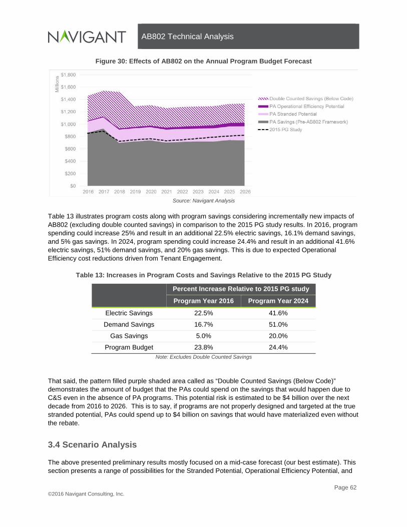
AB802 Technical Analysis
Page 62 ©2016 Navigant Consulting, Inc.
Figure 30: Effects of AB802 on the Annual Program Budget Forecast
Source: Navigant Analysis
Table 13 illustrates program costs along with program savings considering incrementally new impacts of AB802 (excluding double counted savings) in comparison to the 2015 PG study results. In 2016, program spending could increase 25% and result in an additional 22.5% electric savings, 16.1% demand savings, and 5% gas savings. In 2024, program spending could increase 24.4% and result in an additional 41.6% electric savings, 51% demand savings, and 20% gas savings. This is due to expected Operational Efficiency cost reductions driven from Tenant Engagement.
Table 13: Increases in Program Costs and Savings Relative to the 2015 PG Study
Percent Increase Relative to 2015 PG study
Program Year 2016 Program Year 2024
Electric Savings 22.5% 41.6%
Demand Savings 16.7% 51.0%
Gas Savings 5.0% 20.0%
Program Budget 23.8% 24.4% Note: Excludes Double Counted Savings
That said, the pattern filled purple shaded area called as “Double Counted Savings (Below Code)” demonstrates the amount of budget that the PAs could spend on the savings that would happen due to C&S even in the absence of PA programs. This potential risk is estimated to be $4 billion over the next decade from 2016 to 2026. This is to say, if programs are not properly designed and targeted at the true stranded potential, PAs could spend up to $4 billion on savings that would have materialized even without the rebate.
3.4 Scenario Analysis
The above presented preliminary results mostly focused on a mid-case forecast (our best estimate). This section presents a range of possibilities for the Stranded Potential, Operational Efficiency Potential, and

AB802 Technical Analysis
Page 63 ©2016 Navigant Consulting, Inc.
Double Counted savings. The low and high ranges here are still bound by our scope of analysis. These low and high ranges represent an uncertainty range in the variables researched.
3.4.1 Stranded Potential
The low and high case for the Stranded Potential were developed by compounding the lower and upper range for each uncertain variable. Table 14 summarizes the multipliers and values used in the low and high case used in the analysis.
Table 14: Low and High Case of Stranded Potential Analysis Parameters
Uncertain Parameter Low Case High Case
Unit Energy Savings (UES) Best Estimate Minus 10% Best Estimate Plus 10%
Repair Cost Fraction Best Estimate Minus 50% Best Estimate Plus 50%
Repair Life 2/3 EUL (Residential) 1 EUL (Commercial)
1/3 EUL (Residential) 1/2 EUL (Commercial)
Stranded Equipment Saturation Best Estimate Minus 50% Best Estimate Plus 50% Source: Navigant professional judgement.
Figure 31 through Figure 33 show the sensitivity in the estimated cumulative PA Stranded Potential in 2026 for electric, demand, and gas savings. The low and high case of the estimated cumulative PA Stranded Potential in 2026 for electric savings are equal to -13% and +20% of the mid case. The low and high case of the estimated cumulative PA Stranded Potential in 2026 for demand savings are equal to -13% and +23% of the mid case. The low and high case of the estimated cumulative PA Stranded Potential in 2026 for gas savings are equal to -12% and +1% of the mid case.
Figure 31: Low/Mid/High Case - Cumulative PA Stranded Potential in 2026 (GWh)
Source: Navigant analysis

AB802 Technical Analysis
Page 64 ©2016 Navigant Consulting, Inc.
Figure 32: Low/Mid/High Case - Cumulative PA Stranded Potential in 2026 (MW)
Source: Navigant analysis
Figure 33: Low/Mid/High Case - Cumulative PA Stranded Potential in 2026 (MM Therms)
Source: Navigant analysis
Navigant tested the sensitivity of the Stranded Potential savings and total program budget results to the four uncertain parameters listed in Table 12. Tornado charts showing the impact of each variable on the results can be found in Appendix E.

AB802 Technical Analysis
Page 65 ©2016 Navigant Consulting, Inc.
3.4.2 Double Counted Savings
Figure 34 through Figure 36 show two estimates of the cumulative Double Counted Savings in 2026 for electricity, demand, and gas savings. See section 2.4.1 for details on the assumptions for the Best Estimate and Upper Bound. The Upper Bound of the cumulative Double Counted Savings in 2026 for electricity savings is equal to approximately four times the Best Estimate. The Upper Bound of the cumulative Double Counted Savings in 2026 for demand savings is equal to approximately three times the best estimate. The upper boundary of the cumulative Double Counted Savings (Below Code) in 2026 for gas savings is equal to 20% more than the best estimate. The smaller sensitivity in gas savings is due to interactive effects of different end uses in the total savings.
Figure 34: Cumulative Double Counted Savings in 2026 (GWh)
Source: Navigant analysis

AB802 Technical Analysis
Page 66 ©2016 Navigant Consulting, Inc.
Figure 35: Cumulative Double Counted Savings in 2026 (MW)
Source: Navigant analysis
Figure 36: Cumulative Double Counted Savings in 2026 (MM Therms)
Source: Navigant analysis

AB802 Technical Analysis
Page 67 ©2016 Navigant Consulting, Inc.
3.4.3 Operational Efficiency Potential
Figure 37 through Figure 39 show the sensitivity in the estimated cumulative PA Operational Efficiency in 2026 for electric, demand, and gas savings. The low and high case of the estimated cumulative PA Operational Efficiency in 2026 for electric, demand, and gas savings are equal to -25% and +25% of the mid case. This is the result of our approach to low/mid/high penetration forecasts for each intervention in which low and high scenarios were assumed to have participation -25% and +25% respectively relative to the mid case.
Figure 37: Low/Mid/High PA Operational Efficiency Savings in 2026 (GWh)
Source: Navigant analysis
Figure 38: Low/Mid/High PA Operational Efficiency Savings in 2026 (MW)

AB802 Technical Analysis
Page 68 ©2016 Navigant Consulting, Inc.
Source: Navigant analysis
Figure 39: Low/Mid/High PA Operational Efficiency Savings in 2026 (MM Therms)
Source: Navigant analysis

AB802 Technical Analysis
Page 69 ©2016 Navigant Consulting, Inc.
4. CAVEATS, LIMITATIONS AND RECOMMENDATIONS
4.1 Caveats and Limitations
As previously mentioned, the scope of this study was primarily to develop an updated methodology that allows for the analysis of the impacts of AB802. Navigant then used the updated modeling methodology to develop a primary estimate of the impacts of AB802 based on readily available market data.
1. There is likely more stranded potential than what this preliminary forecast captures. This preliminary forecast is limited in scope to the same measures considered in the 2015 and 2013 PG study. The previous PG studies selected measures to analyze based on their ability to produce above-code savings. Thus very few to-code measures were considered. We believe additional stranded potential lies in building envelope measures and commercial refrigeration measures. Furthermore, the scope of this study was to only consider the residential and commercial sector. We recognize there may be additional stranded potential in the industrial and agriculture sectors.
2. There may be more operational efficiency potential than what this preliminary forecast captures, albeit uncertain. This preliminary forecast considers three representative commercial sector operational efficiency programs. The analysis is based on limited available data and professional judgement by Navigant; still, some savings estimates from these activities can be uncertain and the persistence of savings for some of the measures is unclear. The scope and timeline of this analysis did not allow for stakeholder vetting. Our operational efficiency forecasts should be considered an initial framework for continued research in this area. We recognize additional operational efficiency potential likely resides in the industrial sector.
3. Double Counted Savings is highly uncertain. Double counted savings can only occur when a customer applies for a rebate from a PA. Even then, in theory programs can be designed in such a way to minimize double counted savings (by purposely targeting old equipment and buildings that are still functional). We are uncertain about the level of double counted savings at this time as there is no overall program guidance around customer eligibility. Furthermore, double counted savings is based on an estimate of renovation activity that occurs in existing buildings; there was limited data to inform this estimate.
4. Assumptions about program incentive structures are those of Navigant’s given limited input from Program Administrators. It is unclear what PA rebate programs will ultimately look like under AB802. Will some measures continue to have deemed savings and deemed rebates? Will all measures and projects necessarily use a “pay for performance” approach? Rebate amounts are a key driver in the forecast of customer adoption. Without known rebate policies and program budgets to calibrate to, the forecast may not be an accurate representation of modified programs under AB802. Navigant sought input from PAs on this topic during a public workshop. While the responses were useful, they were broad statements rather than specific plans. Additional discussion with policy makers and program administrators is needed.
5. Data informing the estimate of the stranded potential is uncertain. This analysis initially developed a short list of commercial and residential measures that were hypothesized to have uncaptured stranded potential. After collecting and reviewing available market data it became apparent there are data gaps. Small sample sizes prevent a robust determination of the true amount of equipment that is “very old”. Limited data were available on the cost to repair and the added lifetime a repair offers.

AB802 Technical Analysis
Page 70 ©2016 Navigant Consulting, Inc.
6. Consumer adoption algorithms are based on data sets in which consumers did not have an option to repair equipment. The new paradigm of seeking out below-code stranded potential involves influencing an inherently different decision process. Historically the PG study only modeled the consumer’s decision between a standard and high efficiency replacement (i.e. “what do I replace my old equipment with?”). Forecasting stranded potential introduces another decision: “Do I even replace the old equipment in the first place given I have the option to repair it and extend its life?” This analysis applies the same economic decision framework and assumptions as used in the PG study to this question of repairing. However, it’s possible the decision to repair rather than replace is a fundamentally different decision than the decision “what do I replace it with?” and thus our decision algorithms may not accurately reflect what real consumer do when faced with this situation.
4.2 Recommendations
This study reflects the first technical analysis of AB802 and the first significant analysis of below-code savings in a California potential study. The CPUC and Navigant anticipated many challenges at the outset of the study and also encountered many, the most of which were related to data. To better inform future updates to the potential study, Navigant identified a list areas for further research and consideration. Some of the data gap identified could be filled through existing or future EM&V or market studies.
1. Further Updates to the Modeling Methodology may be required. The modeling methodology used for this analysis was selected because of its ability to adapt the existing PG 2015 model and leverage available data. Modeling methodology may change in the future depending on the following factors:
a. Further definition of the policy framework for implementing AB802 programs
b. Further definition of how normalized metered energy savings are to be calculated and utilized in PA reporting savings
c. Additional types of market data previously unavailable
d. Further insight and understanding of how below code savings can be integrated into the CEC’s demand forecast.
Further investigation into these three areas are recommended. Additional data collection is discussed in the following recommendations.
2. Characterize Additional Residential and Commercial Equipment. This study continued to use the same measures listed in the 2015 PG study. The 2015 PG study initially selected measures based on their ability to deliver above-code savings. Given historic program policies, much of the recent measure research through utility workpapers and DEER focused on characterizing measures that fit within the existing program policies. Thus, there has been little historic characterization of the cost, efficiency level, savings, and remaining useful life of old, below-code equipment. We recommend further research and measure characterization for building envelope (insulation, roofing, windows, air sealing, etc.) and commercial refrigeration equipment. DEER contains limited measure for both of these end uses.
3. Characterize Below Code Savings Opportunities in the Agriculture and Industrial Sectors. Below-code savings exists in the industrial and agriculture sectors, however they were not quantified through this study. Most efficiency projects in these sectors are routed through the utility “custom” or “calculated savings” programs. Rather than relying on deemed savings, these projects rely on engineering calculations or other site-specific methods to quantify savings. Furthermore, projects in these sectors are compared against Industry Standard Practice (ISP) as a baseline. ISP can be considered a substitution for “code baseline” and is often a higher efficiency level than equipment being replaced; it was factored into the 2015 PG study. Additional

AB802 Technical Analysis
Page 71 ©2016 Navigant Consulting, Inc.
clarity is needed in the role that ISP plays in the context of AB802 before a technical analysis of this sector can be completed.
4. Expand Saturation Studies to Consider a Broader List of Technologies and End Uses. Understanding the characteristics of the population of buildings and installed technologies in California is key to quantifying the savings potential that lies below code. Specifically we need to information on the distribution of age of installed technologies. This study relied upon CSS to quantify the amount of existing commercial equipment that is beyond its EUL. Although CSS (and is predecessor, CEUS) was a robust data set for its originally intended scope, it is limited in its ability to provide insight to this study. CSS was a minor update to CEUS and only contained a few end uses and select measures within those end uses. CSS did not contain robust inform on boilers and chillers, it was also lacking in building envelope data. These are essential measures to consider in future updates as they hold promise for below-code savings. A dataset on distribution of age of all commercial equipment would more easily allow us to identify where the stranded potential truly lies. Residential data found in CLASS was relatively more robust for the purposes of this study compared to available commercial sector data.
5. Further Research to Inform the Double Counted Savings. Additional data collection and analysis will be needed to develop a more refined estimate of double counted savings. The most useful data would be a better understanding of the number of building alterations that occur in California and the amount of to-code activities that naturally occurs through these alterations. Significant data is available on new construction activity though limited data is available for alterations.
6. Comparison and Alignment to CEC Demand Forecast. The CEC demand forecast simulates the continued use of a subset of equipment past its EUL (or “mean life” as used by the CEC). However, a more robust comparison and alignment of assumptions between used by this study and the CEC demand forecast is needed before the AAEE can be updated. This requires further discussions and collaboration between Navigant, the CPUC and CEC. Such collaboration could reveal if there additional stranded potential not captured in this study or it a portion of the stranded potential is already embedded in the forecast.
7. Further Research to Inform Operational Efficiency Savings. The scope and timeline for the analysis conducted on operational efficiency did not allow for stakeholder vetting. These estimate could be improved upon by:
a. Further researching persistence b. Reviewing assumptions with program administrators to vet the reasonableness of
participation rates c. Considering additional operational efficiency potential programs and sectors (including
the industrial sector). 8. Collect Data on Equipment Removed by Program Participants. Since the AB802 legislation
requires programs to be authorized as soon as September 2016, limited new data can be collected before September to inform these programs. As new programs seeking below-code savings are implemented, program administrators should carefully document the age, type, and condition of equipment that is being replaced by program participants. These data could inform future field data collection efforts to obtain statistically representative data of the existing population. They could also serve as an initial “litmus test” to see if programs are indeed capturing stranded potential (replacing equipment beyond its EUL) vs. capturing double counted savings.
9. Research Measure Repair Characteristics. The counterfactual to replacing old, below-code equipment in this study is the continued maintenance and use of old equipment. This continued maintenance presumably comes as a cost (albeit minimal compare to the purchase of new equipment) and may be required on a regular basis. This analysis considers these two factors as the Repair Cost and the Repair Lifetime. Both factors are important to understanding the decision that customer face to repair vs. replace equipment. Limited data was available for both of these
AB802 Technical Analysis
Page 72 ©2016 Navigant Consulting, Inc.
parameters and they were often estimated by Navigant. More robust data on the repair and maintenance characteristics of repair eligible equipment will lead to a more informed forecast. Sensitivity analysis shows peak demand savings can vary ± 10% when repair related data is modeled across a range (see Figure 47 in Appendix E.)
10. Research Consumer Preferences in Repairing vs. Replacing Equipment. Consumer adoption parameters used in this study are based on data sets in which consumers did not have an option to repair equipment. Given our scope and timeline, we were unable to confirm if consumers apply the same implied discount rate to the decision to maintain existing equipment as that used in the decision to purchase high efficiency equipment over standard efficiency equipment. We note the previously researched consumer preference parameters is the best available data at this time. This could be an area for further research.

AB802 Technical Analysis
Page A-1 ©2016 Navigant Consulting, Inc.
SUMMARY OF STAKEHOLDER COMMENTS ON PROGRAM BUDGETS
• PG&E: o Multiple incentive scenarios are possible. o Custom program incentives could be revised to a lower cents per kWh amount and
spread over the full amount of savings, not just the savings above-code. o A tiered system could be considered in which below-code savings receives a smaller
$/kwh incentive and above-code savings receives a larger one.
• Southern California Gas o Anticipates incentive could increase to motivate customers to not only get to code, but
more importantly go above-code. o More stringent codes in the future increase the cost for customer to come to or exceed
code, which theoretically will entice them to repair rather than replace. Utility program incentives would need to be increased to offset the effect of escalating costs.
o PAs will need to consider the effect of the incentive changes on a portfolio-wide basis to determine changes to budgets, which will continue to be linked with cost-effectiveness considerations.
• Southern California Edison:
o Maximizing cost-effective savings based is the key driver to program budgets. SCE does not foresee requesting program budgets to increase, but rather would consider re-optimizing the portfolio to target below-code opportunities in the market.
o Does not foresee future changes to incentive levels until program savings and design changes are better understood.
o Consider a tiered incentive approach: expect to pay less per kWh saved for below-code but more per kWh for above-code.
o Recommends extending a 50% of incremental measure cost cap for existing baseline activity in order to match current program activity requirements.
o SCE is considering using following guiding principles in helping to in establish rebate framework: Consideration of the existing financial and other barriers that prevent customers
from installing code-based equipment to design incentives that help customer overcome those barriers.
Optimization of the level of below-code incentives by assessing the cost-effectiveness of the lifecycle incentive costs and other program admin costs against the lifecycle benefits that SCE customers receive utilizing the PAC test framework.
• SDG&E
o Overall, it is difficult to provide specific responses to questions about future budgets and incentives. “SDG&E will make these determinations based on the additional energy savings potential that will become eligible towards meeting its energy efficiency goals.”
o “Currently, SDG&E has incentive caps on the amount of incentives that are based on $/KWH or therm savings, e.g., not to exceed 50 percent of installation costs. It is reasonable to expect that incentive caps will still be in place to manage the incentive budget and allow for greater participation.”

AB802 Technical Analysis
Page A-2 ©2016 Navigant Consulting, Inc.
o Suggest considering tiered rebates in which above-code savings are valued at a premium. In past programs, SDG&E has offered premium incentives for higher energy efficiency levels (based on above-code savings only).
• SoCalREN
o “The SoCalREN is confident that studies currently in process will conclude that the “to code” savings potential of existing buildings is very significant. Given this assumption, the energy efficiency portfolio budgets for Program Administrators will need to be significantly increased.” The following table provides the breakdown of savings from each code or standard that is expected in existing buildings verses new construction buildings.

AB802 Technical Analysis
Page B-1 ©2016 Navigant Consulting, Inc.
CODES AND STANDARDS DATA
B.1 Savings in Existing Buildings
Codes and Standards Measures EUL Sector Existing Building Turnover
Rate
New Construction
Turnover Rate
Existing Building
%
New Construction
% Estimation Method
2005 T-20: Commercial Refrigeration Equipment, Solid Door 9.0 Commercial 11.1% 2.2% 83.5% 16.5% EUL Method
2005 T-20: Commercial Refrigeration Equipment, Transparent Door 9.0 Commercial 11.1% 2.2% 83.5% 16.5% EUL Method
2005 T-20: Commercial Ice Maker Equipment 9.0 Commercial 11.1% 2.2% 83.5% 16.5% EUL Method
2005 T-20: Walk-In Refrigerators / Freezers 10.0 Commercial 10.0% 2.2% 82.0% 18.0% EUL Method
2005 T-20: Refrigerated Beverage Vending Machines 10.0 Commercial 10.0% 2.2% 82.0% 18.0% EUL Method
2005 T-20: Large Packaged Commercial Air-Conditioners, Tier 1 15.0 Commercial 6.7% 2.2% 75.2% 24.8% EUL Method
2005 T-20: Large Packaged Commercial Air-Conditioners, Tier 2 15.0 Commercial 6.7% 2.2% 75.2% 24.8% EUL Method
2005 T-20: Residential Pool Pumps, High Eff Motor, Tier 1 10.0 Residential 10.0% 1.0% 90.9% 9.1% EUL Method
2005 T-20: Portable Electric Spas 10.0 Residential 10.0% 1.0% 90.9% 9.1% EUL Method
2005 T-20: General Service Incandescent Lamps, Tier 1 1.0 Residential 100.0% 1.0% 99.0% 1.0% EUL Method
2005 T-20: Pulse Start Metal Halide HID Luminaires, Tier 1(Vertical Lamps) 13.0 Commercial 7.7% 2.2% 77.8% 22.2% EUL Method
2005 T-20: Pulse Start Metal Halide HID Luminaires, Tier 2(All other MH 13.0 Commercial 7.7% 2.2% 77.8% 22.2% EUL Method
2005 T-20: Modular Furniture Task Lighting Fixtures 15.0 Commercial 6.7% 2.2% 75.2% 24.8% EUL Method
2005 T-20: Hot Food Holding Cabinets 15.0 Commercial 6.7% 2.2% 75.2% 24.8% EUL Method
2005 T-20: External Power Supplies, Tier 1 7.0 Res/Com 14.3% 1.6% 89.9% 10.1% EUL Method
2005 T-20: External Power Supplies, Tier 2 7.0 Res/Com 14.3% 1.6% 89.9% 10.1% EUL Method
2005 T-20: Consumer Electronics - Audio Players 5.0 Residential 20.0% 1.0% 95.2% 4.8% EUL Method

AB802 Technical Analysis
Page B-2 ©2016 Navigant Consulting, Inc.
Codes and Standards Measures EUL Sector Existing Building Turnover
Rate
New Construction
Turnover Rate
Existing Building
%
New Construction
% Estimation Method
2005 T-20: Consumer Electronics - TVs 7.0 Residential 14.3% 1.0% 93.5% 6.5% EUL Method
2005 T-20: Consumer Electronics - DVDs 5.0 Residential 20.0% 1.0% 95.2% 4.8% EUL Method
2005 T-20: Water Dispensers 8.0 Commercial 12.5% 2.2% 85.0% 15.0% EUL Method
2005 T-20: Unit Heaters and Duct Furnaces 15.0 Commercial 6.7% 2.2% 75.2% 24.8% EUL Method
2005 T-20: Commercial Dishwasher Pre-Rinse Spray Valves 5.0 Commercial 20.0% 2.2% 90.1% 9.9% EUL Method
2006 T-20: Residential Pool Pumps, 2-speed Motors, Tier 2 10.0 Residential 10.0% 1.0% 90.9% 9.1% EUL Method
2006 T-20: General Service Incandescent Lamps, Tier 2 1.0 Residential 100.0% 1.0% 99.0% 1.0% EUL Method
2006 T-20: General Service Incandescent Lamps, Tier 2 1.0 Residential 100.0% 1.0% 99.0% 1.0% EUL Method
2006 T-20: General Service Incandescent Lamps, Tier 2 1.0 Residential 100.0% 1.0% 99.0% 1.0% EUL Method
2006 T-20: BR, ER and R20 Incandescent Reflector Lamps: Residential 4.0 Residential 25.0% 1.0% 96.2% 3.8% EUL Method
2006 T-20: BR, ER and R20 Incandescent Reflector Lamps: Commercial 1.0 Commercial 100.0% 2.2% 97.8% 2.2% EUL Method
2008 T-20: Metal Halide Fixtures 14.0 Commercial 7.1% 2.2% 76.5% 23.5% EUL Method
2008 T-20: Portable Lighting Fixtures 12.0 Residential 8.3% 1.0% 89.3% 10.7% EUL Method
2008 T-20: General Purpose Lighting -- 100 watt 2.0 Residential 50.0% 1.0% 98.0% 2.0% EUL Method
2008 T-20: General Purpose Lighting -- 75 watt 2.0 Residential 50.0% 1.0% 98.0% 2.0% EUL Method
2008 T-20: General Purpose Lighting -- 60 and 40 watt 2.0 Residential 50.0% 1.0% 98.0% 2.0% EUL Method
2009 T-20: Televisions - Tier 1 10.0 Residential 10.0% 1.0% 90.9% 9.1% EUL Method
2009 T-20: Televisions - Tier 2 10.0 Residential 10.0% 1.0% 90.9% 9.1% EUL Method
2011 T-20: Battery charger - consumer - Tier 1 3.3 Res/Com 30.1% 1.6% 94.9% 5.1% EUL Method
2011 T-20: Battery charger - large - Tier 1 10.0 Commercial 10.0% 2.2% 81.9% 18.1% EUL Method
2011 T-20: Battery charger - large - Tier 2 incremental 10.0 Commercial 10.0% 2.2% 81.9% 18.1% EUL Method
Future T-20: Air Filter Labeling 1.0 Residential 100.0% 1.0% 99.0% 1.0% EUL Method
Future T-20: Commercial Clothes Dryers 14.0 Commercial 7.1% 2.2% 76.5% 23.5% EUL Method
Future T-20: Computers - Tier 1 | Desktops, Notebooks 4.0 Res/Com 25.0% 1.6% 94.0% 6.0% EUL Method

AB802 Technical Analysis
Page B-3 ©2016 Navigant Consulting, Inc.
Codes and Standards Measures EUL Sector Existing Building Turnover
Rate
New Construction
Turnover Rate
Existing Building
%
New Construction
% Estimation Method
Future T-20: Dimming Ballasts 13.0 Commercial 7.7% 2.2% 77.8% 22.2% EUL Method
Future T-20: Electronic Displays 5.0 Commercial 20.0% 2.2% 90.1% 9.9% EUL Method
Future T-20: Faucets (Residential)- Gas Water Heaters 10.0 Residential 10.0% 1.0% 90.9% 9.1% EUL Method
Future T-20: Faucets (Residential)- Electric Water Heaters 10.0 Residential 10.0% 1.0% 90.9% 9.1% EUL Method
Future T-20: Game Consoles (Tier 1) 6.0 Residential 16.7% 1.0% 94.3% 5.7% EUL Method
Future T-20: Game Consoles (Tier 2) 6.0 Residential 16.7% 1.0% 94.3% 5.7% EUL Method
Future T-20: Pool Pumps & Spas 10.0 Res/Com 10.0% 1.6% 86.2% 13.8% EUL Method
Future T-20: Set Top Boxes (Tier 1) 6.7 Residential 14.9% 1.0% 93.7% 6.3% EUL Method
Future T-20: Small Diameter Directional Lamps (Tier 1) 1.0 Res/Com 100.0% 1.6% 98.4% 1.6% EUL Method
Future T-20: Small Diameter Directional Lamps (Tier 2) 2.0 Res/Com 50.0% 1.6% 96.9% 3.1% EUL Method
Future T-20: Small Network Equipment 5.0 Residential 20.0% 1.0% 95.2% 4.8% EUL Method
Future T-20: Toilets (Commercial) 12.0 Commercial 8.3% 2.2% 79.1% 20.9% EUL Method
Future T-20: Toilets (Residential) 25.0 Commercial 4.0% 2.2% 64.5% 35.5% EUL Method
Future T-20: Urinals 12.0 Commercial 8.3% 2.2% 79.1% 20.9% EUL Method
Future T-20: Water Meters 15.0 Res/Com 6.7% 1.6% 80.6% 19.4% EUL Method
Fed Appliance: Electric Motors 1-200HP 7.0 Commercial 14.3% 2.2% 86.7% 13.3% EUL Method
Fed Appliance: Refrigerated Beverage Vending Machines 10.0 Commercial 10.0% 2.2% 82.0% 18.0% EUL Method
Fed Appliance: Commercial Refrigeration 10.0 Commercial 10.0% 2.2% 82.0% 18.0% EUL Method
Fed Appliance: Residential Electric & Gas Ranges 19.0 Residential 5.3% 1.0% 84.0% 16.0% EUL Method
Fed Appliance: General Service Fluorescent Lamps 6.0 Res/Com 16.7% 1.6% 91.2% 8.8% EUL Method
Fed Appliance: Incandescent Reflector Lamps 1.0 Residential 100.0% 1.0% 99.0% 1.0% EUL Method
Fed Appliance: Commercial Clothes Washers 11.0 Commercial 9.1% 2.2% 80.5% 19.5% EUL Method
Fed Appliance: Residential Pool Heaters 10.0 Residential 10.0% 1.0% 90.9% 9.1% EUL Method
Fed Appliance: Residential Direct Heating Equipment 15.0 Residential 6.7% 1.0% 87.0% 13.0% EUL Method
Fed Appliance: Residential Refrigerators & Freezers 15.0 Residential 6.7% 1.0% 87.0% 13.0% EUL Method
Fed Appliance: Residential Room AC 11.0 Residential 9.1% 1.0% 90.1% 9.9% EUL Method

AB802 Technical Analysis
Page B-4 ©2016 Navigant Consulting, Inc.
Codes and Standards Measures EUL Sector Existing Building Turnover
Rate
New Construction
Turnover Rate
Existing Building
%
New Construction
% Estimation Method
Fed Appliance: Fluorescent Ballasts 13.0 Res/Com 7.7% 1.6% 82.8% 17.2% EUL Method
Fed Appliance: Residential Clothes Dryers 16.0 Residential 6.3% 1.0% 86.2% 13.8% EUL Method
Fed Appliance: Residential Gas Fired Water Heaters 13.0 Residential 7.7% 1.0% 88.5% 11.5% EUL Method
Fed Appliance: Residential Electric Storage Water Heaters 13.0 Residential 7.7% 1.0% 88.5% 11.5% EUL Method
Fed Appliance: Residential Gas Instant Water Heaters 20.0 Residential 5.0% 1.0% 83.3% 16.7% EUL Method
Fed Appliance: Residential Oil Fired Water Heaters 13.0 Residential 7.7% 1.0% 88.5% 11.5% EUL Method
Fed Appliance: Small Electric Motors 7.0 Commercial 14.3% 2.2% 86.7% 13.3% EUL Method
Fed Appliance: Residential Clothes Washers (Front Loading) 14.0 Residential 7.1% 1.0% 87.7% 12.3% EUL Method
Fed Appliance: Residential Clothes Washers (Top Loading) Tier I 14.2 Residential 7.1% 1.0% 87.6% 12.4% EUL Method
Fed Appliance: Residential Clothes Washers (Top Loading) Tier II 14.2 Residential 7.1% 1.0% 87.6% 12.4% EUL Method
Fed Appliance: Residential Central AC and Heat Pumps 18.2 Residential 5.5% 1.0% 84.6% 15.4% EUL Method
Fed Appliance: External Power Supplies 4.7 Res/Com 21.4% 1.6% 93.0% 7.0% EUL Method
Fed Appliance: Battery Chargers 3.9 Res/Com 26.0% 1.6% 94.2% 5.8% EUL Method
Fed Appliance: Walk-in Coolers & Freezers 10.0 Commercial 10.0% 2.2% 82.0% 18.0% EUL Method
Fed Appliance: Commercial Refrigeration (Cycle 2) 10.0 Commercial 10.0% 2.2% 82.0% 18.0% EUL Method
Fed Appliance: Metal Halide Lamp Fixtures 23.0 Commercial 4.3% 2.2% 66.4% 33.6% EUL Method
Fed Appliance: High-Intensity Discharge Lamps 3.0 Commercial 33.3% 2.2% 93.8% 6.2% EUL Method
Fed Appliance: General Service Fluorescent Lamps 6.0 Res/Com 16.7% 1.6% 91.2% 8.8% EUL Method
Fed Appliance: ASHRAE Products (Commercial boilers) 30.0 Commercial 3.3% 2.2% 60.2% 39.8% EUL Method
2005 T-24: Time dependent valuation, Residential 45% 55% Navigant Assumption
2005 T-24: Time dependent valuation, Nonresidential 45% 55% Navigant Assumption
2005 T-24: Res. Hardwired lighting 0.0% 100.0% Navigant Assumption
2005 T-24: Duct improvement 100.0% 0.0% Navigant Assumption
2005 T-24: Window replacement 100.0% 0.0% Navigant Assumption

AB802 Technical Analysis
Page B-5 ©2016 Navigant Consulting, Inc.
Codes and Standards Measures EUL Sector Existing Building Turnover
Rate
New Construction
Turnover Rate
Existing Building
%
New Construction
% Estimation Method
2005 T-24: Lighting controls under skylights 0.0% 100.0% Navigant Assumption
2005 T-24: Ducts in existing commercial buildings 100.0% 0.0% Navigant Assumption
2005 T-24: Cool roofs 80% 20% Navigant Assumption
2005 T-24: Relocatable classrooms 0% 100% Navigant Assumption
2005 T-24: Bi-level lighting control credits 95% 5% Navigant Assumption
2005 T-24: Duct testing/sealing in new commercial buildings 0.0% 100.0% Navigant Assumption
2005 T-24: Cooling tower applications 45% 55% Navigant Assumption
2005 T-24: Multifamily Water Heating 45% 55% Navigant Assumption
2005 T-24: Composite for Remainder - Res 45% 55% Navigant Assumption
2005 T-24: Composite for Remainder - Non-Res 45% 55% Navigant Assumption
2005 T-24: Whole Building - Res New Construction (Electric) 0.0% 100.0% Navigant Assumption
2005 T-24: Whole Building - Non-Res New Construction (Electric) 0.0% 100.0% Navigant Assumption
2005 T-24: Whole Building - Res New Construction (Gas) 0.0% 100.0% Navigant Assumption
2005 T-24: Whole Building - Non-Res New Construction (Gas) 0.0% 100.0% Navigant Assumption
2008 T-24: Envelope insulation 90% 10% Evaluation Report Data
2008 T-24: Overall Envelope Tradeoff 0% 100% Evaluation Report Data
2008 T-24: Skylighting 0% 100% Evaluation Report Data
2008 T-24: Sidelighting 0% 100% Evaluation Report Data
2008 T-24: Tailored Indoor lighting 95% 5% Evaluation Report Data
2008 T-24: TDV Lighting Controls 45% 55% Evaluation Report Data
2008 T-24: DR Indoor Lighting 45% 55% Evaluation Report Data
2008 T-24: Outdoor Lighting 45% 55% Evaluation Report Data
2008 T-24: Outdoor Signs 0% 100% Evaluation Report Data
2008 T-24: Refrigerated warehouses 0% 100% Evaluation Report Data

AB802 Technical Analysis
Page B-6 ©2016 Navigant Consulting, Inc.
Codes and Standards Measures EUL Sector Existing Building Turnover
Rate
New Construction
Turnover Rate
Existing Building
%
New Construction
% Estimation Method
2008 T-24: DDC to Zone 0% 100% Evaluation Report Data
2008 T-24: Residential Swimming pool 0% 100% Evaluation Report Data
2008 T-24: Site Built Fenestration 0% 100% Evaluation Report Data
2008 T-24: Residential Fenestration 15% 85% Evaluation Report Data
2008 T-24: Cool Roof Expansion 80% 20% Evaluation Report Data
2008 T-24: MF Water heating control 45% 55% Evaluation Report Data
2008 T-24: CfR IL Complete Building Method 95% 5% Evaluation Report Data
2008 T-24: CfR IL Area Category Method 95% 5% Evaluation Report Data
2008 T-24: CfR IL Egress Control 0% 100% Evaluation Report Data
2008 T-24: CfR HVAC Efficiency 0% 100% Evaluation Report Data
2008 T-24: CfR Res Cool Roofs 0% 100% Evaluation Report Data
2008 T-24: CfR Res Central Fan WL 0% 100% Evaluation Report Data
2013 T-24 - Single family NC 0.0% 100.0% Navigant Assumption
2013 T-24 - Multi-family NC 0.0% 100.0% Navigant Assumption
2013 T-24 - Nonres NC 0.0% 100.0% Navigant Assumption
2013 T-24 - others 100.0% 0.0% Navigant Assumption
2016 T-24 - Single family NC 0.0% 100.0% Navigant Assumption
2016 T-24 - Multi-family NC 0.0% 100.0% Navigant Assumption
2016 T-24 - Nonres NC 0.0% 100.0% Navigant Assumption
2019 T-24 - Single family NC 0.0% 100.0% Navigant Assumption
2019 T-24 - Multi-family NC 0.0% 100.0% Navigant Assumption
2019 T-24 - Nonres NC 0.0% 100.0% Navigant Assumption
2022 T-24 - Single family NC 0.0% 100.0% Navigant Assumption
2022 T-24 - Multi-family NC 0.0% 100.0% Navigant Assumption
2022 T-24 - Nonres NC 0.0% 100.0% Navigant Assumption

AB802 Technical Analysis
Page B-7 ©2016 Navigant Consulting, Inc.
B.2 C&S Included in the Best Estimate of Double Counted Savings
Code or Standard Included Sector End Use
2005 T-20: Modular Furniture Task Lighting Fixtures Commercial Lighting
2005 T-20: Pulse Start Metal Halide HID Luminaires, Tier 1 (Vertical Lamps) Commercial Lighting
2005 T-20: Pulse Start Metal Halide HID Luminaires, Tier 2 (All other MH) Commercial Lighting
2005 T-20: Unit Heaters and Duct Furnaces Commercial HVAC
2005 T-24: Cool roofs Commercial BldgEnv
2005 T-24: Cooling tower applications Commercial HVAC
2005 T-24: Duct improvement Residential HVAC
2005 T-24: Ducts in existing commercial buildings Commercial HVAC
2005 T-24: Multifamily Water Heating Residential SHW
2005 T-24: Window replacement Residential BldgEnv
2006 T-20: General Service Incandescent Lamps, Tier 2 Commercial Lighting
2008 T-20: General Purpose Lighting -- 60 and 40 watt Commercial Lighting
2008 T-20: Metal Halide Fixtures Commercial Lighting
2008 T-24: Cool Roof Expansion Commercial BldgEnv
2008 T-24: Envelope insulation Commercial BldgEnv
2008 T-24: Outdoor Lighting Commercial Lighting
2008 T-24: Residential Fenestration Residential BldgEnv
2008 T-24: Tailored Indoor lighting Commercial Lighting
Fed Appliance: ASHRAE Products (Commercial boilers) Commercial HVAC
Fed Appliance: Fluorescent Ballasts Commercial Lighting
Fed Appliance: General Service Fluorescent Lamps Commercial Lighting
Fed Appliance: Incandescent Reflector Lamps Commercial Lighting
Fed Appliance: Metal Halide Lamp Fixtures Commercial Lighting
Fed Appliance: Residential Central AC and Heat Pumps Residential HVAC
Fed Appliance: Residential Direct Heating Equipment Residential HVAC
Fed Appliance: Residential Electric Storage Water Heaters Residential SHW

AB802 Technical Analysis
Page B-8 ©2016 Navigant Consulting, Inc.
Fed Appliance: Residential Gas Fired Water Heaters Residential SHW
Fed Appliance: Residential Gas Instant Water Heaters Residential SHW
Fed Appliance: Residential Oil Fired Water Heaters Residential SHW
Future T-20: Dimming Ballasts Commercial Lighting
Future T-20: Small Diameter Directional Lamps Commercial Lighting Source: Navigant analysis.

AB802 Technical Analysis
Page C-1 ©2016 Navigant Consulting, Inc.
EQUIPMENT DATA COLLECTION
C.1 Sources Reviewed
Source Name Source Author Year Description
Codes and Standards US DOE, CEC Multiple Federal, CA Title 20 and Title 20 – Year is dependent on measure and average age of equipment
CLASS Database DNV-GL 2012
California Lighting and Appliance Saturation Survey. Utilized for nearly all residential measures. https://webtools.dnvgl.com/projects62/Default.aspx?tabid=190
CSS Database Itron 2014
California Commercial Saturation Study. Utilized for commercial lighting, HVAC, and plug loads existing baseline. http://www.calmac.org/publications/California_Commercial_Saturation_Study_Report_Finalv2ES.pdf
CUES Database Itron 2006
California Commercial End Use Survey. This survey was reviewed, but was not considered a top source due to the age of the study. http://capabilities.itron.com/ceusweb/
CBECS Database US DOE 2012
Commercial Buildings Energy Consumption Survey. Data did not include baseline efficiency levels. http://www.eia.gov/consumption/commercial/data/2012/index.cfm?view=microdata
DEER Database
J.J. Hirsch & Associates 2015
Database for Energy Efficient Resources. Existing baseline data was derived from DEER during the 2015 release of the Potential and Goals - this data was only updated if research found a different baseline efficiency than utilized from DEER. http://www.deeresources.com/
HVAC Permitting: A Study to Inform IOU HVAC Programs
DNV-GL 2014
Did not contain baseline efficiency or repair data. http://www.calmac.org/startDownload.asp?Name=FINAL_REPORT_PGE_HVAC_Permitting_for_IOU_Programs_Study_v20141010ES.pdf&Size=258KB
SMUD Residential HVAC Program Evaluation
RLW Analytics and the Benningfield Group
2008 Did not contain baseline efficiency or repair data. http://www.performancealliance.org/Portals/4/Documents/Committees/EMV/SMUD - RLW Mar 08.pdf
CalTF Savings Below Code Subcommittee- Savings to Code Position Paper
California Technical Forum
2015
Describes the sources identified by Cal TF staff as most likely to yield evidence concerning particular "Repair Indefinitely" measures. Provides data on stranded equipment saturation and HVAC repair costs www.caltf.org/s/TPP1_Savings-To-Code-Subcommittee_v6.docx
Local Government Sustainable Energy Coalition Website (LGSEC)
LGSEC 2015 Did not contain baseline efficiency or repair data. http://www.lgsec.org/
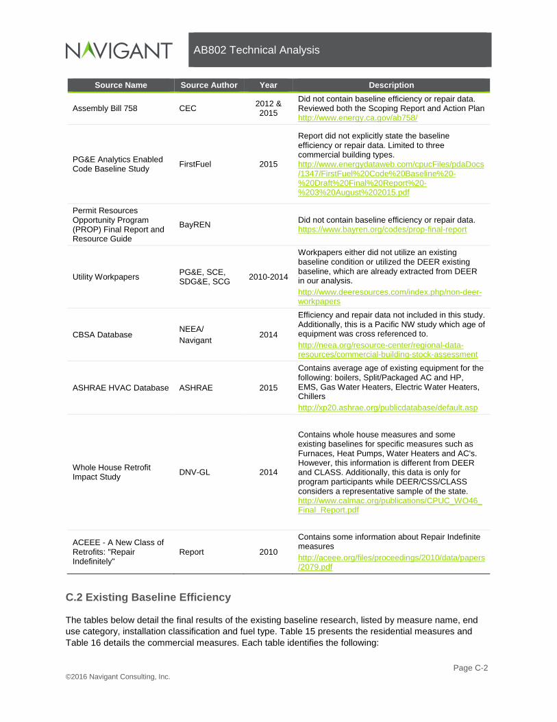
AB802 Technical Analysis
Page C-2 ©2016 Navigant Consulting, Inc.
Source Name Source Author Year Description
Assembly Bill 758 CEC 2012 & 2015
Did not contain baseline efficiency or repair data. Reviewed both the Scoping Report and Action Plan http://www.energy.ca.gov/ab758/
PG&E Analytics Enabled Code Baseline Study FirstFuel 2015
Report did not explicitly state the baseline efficiency or repair data. Limited to three commercial building types. http://www.energydataweb.com/cpucFiles/pdaDocs/1347/FirstFuel%20Code%20Baseline%20-%20Draft%20Final%20Report%20-%203%20August%202015.pdf
Permit Resources Opportunity Program (PROP) Final Report and Resource Guide
BayREN Did not contain baseline efficiency or repair data. https://www.bayren.org/codes/prop-final-report
Utility Workpapers
PG&E, SCE, SDG&E, SCG 2010-2014
Workpapers either did not utilize an existing baseline condition or utilized the DEER existing baseline, which are already extracted from DEER in our analysis. http://www.deeresources.com/index.php/non-deer-workpapers
CBSA Database
NEEA/ Navigant
2014
Efficiency and repair data not included in this study. Additionally, this is a Pacific NW study which age of equipment was cross referenced to. http://neea.org/resource-center/regional-data-resources/commercial-building-stock-assessment
ASHRAE HVAC Database ASHRAE 2015
Contains average age of existing equipment for the following: boilers, Split/Packaged AC and HP, EMS, Gas Water Heaters, Electric Water Heaters, Chillers http://xp20.ashrae.org/publicdatabase/default.asp
Whole House Retrofit Impact Study DNV-GL 2014
Contains whole house measures and some existing baselines for specific measures such as Furnaces, Heat Pumps, Water Heaters and AC's. However, this information is different from DEER and CLASS. Additionally, this data is only for program participants while DEER/CSS/CLASS considers a representative sample of the state. http://www.calmac.org/publications/CPUC_WO46_Final_Report.pdf
ACEEE - A New Class of Retrofits: "Repair Indefinitely"
Report 2010
Contains some information about Repair Indefinite measures http://aceee.org/files/proceedings/2010/data/papers/2079.pdf
C.2 Existing Baseline Efficiency
The tables below detail the final results of the existing baseline research, listed by measure name, end use category, installation classification and fuel type. Table 15 presents the residential measures and Table 16 details the commercial measures. Each table identifies the following:

AB802 Technical Analysis
Page C-3 ©2016 Navigant Consulting, Inc.
• Efficiency Metric: Measure specific efficiency metrics that differ depending on equipment (e.g. SEER levels for HVAC equipment)
• Efficiency Levels for Existing Baseline, Code and EE Measure: The Existing Baseline Efficiency column details the existing baseline results from the research done in this study. The Code and EE Measure Efficiency columns detail the code and EE measure efficiency measures already utilized in the 2015 PG model release
• Existing Baseline Source: This column provides the source(s) of the existing baseline efficiency level. If the team utilized the Codes and Standards method, the table describes the source of the average age of equipment in addition to C&S.
The analysis team did not analyze or research the existing baseline for Retrofit Add On measures. This is because the EE measure is not a more efficient version of the base measure, rather it makes the existing equipment more efficient by adding a new component. The tables include these measures for reference, but include NA for all columns. Some measures that utilize the same baseline because of their inclusion in a competition group are grouped together in the tables below.

AB802 Technical Analysis
Page C-4 ©2016 Navigant Consulting, Inc.
Table 15: Residential Measure Existing Baseline Conditions Summary
Measure Name End Use Category Installation Classification Fuel Type
Efficiency Metric
Existing Baseline
Efficiency
Code Efficiency
EE Measure
Efficiency
Existing Baseline Source
Attic Batt Insulation Building Envelope Retrofit Replacement Elec/Gas R < R-11 >= R-30 >= R-30 CLASS
Wall Spray On Insulation Building Envelope Retrofit Replacement Elec/Gas R R0 R-13 R-13 CLASS
Window Film Building Envelope Retrofit Add On Elec NA NA NA NA NA
Gas Furnace HVAC Equipment - Repair Eligible Gas AFUE 77.5 80 93 CLASS
Direct Evaporative Cooler HVAC Equipment - Repair Eligible Elec SEER 10 14 NA CLASS
SEER Rated Split System AC HVAC Equipment - Repair Eligible Elec SEER 10 14 15/18/22 CLASS
SEER Rated Split System Heat Pump HVAC Equipment - Repair Eligible Elec SEER 10 14 15/18/22 CLASS
Whole House Fan HVAC Retrofit Add On Elec NA NA NA NA NA
Repair Duct System HVAC Retrofit Replacement Elec % 32% 14% 14% DEER
Compact Fluorescent Lamp (Basic High - Indoor) Indoor/Outdoor Lighting Equipment - ROB Elec Wattage 81.5 59 22.5 CLASS
Compact Fluorescent Lamp (Basic High - Outdoor) Indoor/Outdoor Lighting Equipment - ROB Elec Wattage 87 62.5 22.5 CLASS
Compact Fluorescent Lamp (Basic Low - Indoor) Indoor/Outdoor Lighting Equipment - ROB Elec Wattage 46 38 12.5 CLASS
Compact Fluorescent Lamp (Basic Low - Outdoor) Indoor/Outdoor Lighting Equipment - ROB Elec Wattage 57 41 13 CLASS
Compact Fluorescent Lamp (Reflector - Indoor) Indoor/Outdoor Lighting Equipment - ROB Elec Wattage 71.5 51.5 16 CLASS
Compact Fluorescent Lamp (Reflector - Outdoor) Indoor/Outdoor Lighting Equipment - ROB Elec Wattage 76 54.5 19 CLASS
Compact Fluorescent Lamp (Specialty - Indoor) Indoor/Outdoor Lighting Equipment - ROB Elec Wattage 42 30 13 CLASS
Compact Fluorescent Lamp (Specialty - Outdoor) Indoor/Outdoor Lighting Equipment - ROB Elec Wattage 38 27 14.5 CLASS
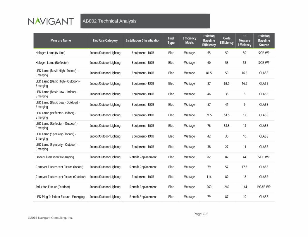
AB802 Technical Analysis
Page C-5 ©2016 Navigant Consulting, Inc.
Measure Name End Use Category Installation Classification Fuel Type
Efficiency Metric
Existing Baseline
Efficiency
Code Efficiency
EE Measure
Efficiency
Existing Baseline Source
Halogen Lamp (A-Line) Indoor/Outdoor Lighting Equipment - ROB Elec Wattage 65 50 50 SCE WP
Halogen Lamp (Reflector) Indoor/Outdoor Lighting Equipment - ROB Elec Wattage 60 53 53 SCE WP
LED Lamp (Basic High - Indoor) - Emerging Indoor/Outdoor Lighting Equipment - ROB Elec Wattage 81.5 59 16.5 CLASS
LED Lamp (Basic High - Outdoor) - Emerging Indoor/Outdoor Lighting Equipment - ROB Elec Wattage 87 62.5 16.5 CLASS
LED Lamp (Basic Low - Indoor) - Emerging Indoor/Outdoor Lighting Equipment - ROB Elec Wattage 46 38 8 CLASS
LED Lamp (Basic Low - Outdoor) - Emerging Indoor/Outdoor Lighting Equipment - ROB Elec Wattage 57 41 9 CLASS
LED Lamp (Reflector - Indoor) - Emerging Indoor/Outdoor Lighting Equipment - ROB Elec Wattage 71.5 51.5 12 CLASS
LED Lamp (Reflector - Outdoor) - Emerging Indoor/Outdoor Lighting Equipment - ROB Elec Wattage 76 54.5 14 CLASS
LED Lamp (Specialty - Indoor) - Emerging Indoor/Outdoor Lighting Equipment - ROB Elec Wattage 42 30 10 CLASS
LED Lamp (Specialty - Outdoor) - Emerging Indoor/Outdoor Lighting Equipment - ROB Elec Wattage 38 27 11 CLASS
Linear Fluorescent Delamping Indoor/Outdoor Lighting Retrofit Replacement Elec Wattage 82 82 44 SCE WP
Compact Fluorescent Fixture (Indoor) Indoor/Outdoor Lighting Retrofit Replacement Elec Wattage 79 57 17.5 CLASS
Compact Fluorescent Fixture (Outdoor) Indoor/Outdoor Lighting Equipment - ROB Elec Wattage 114 82 18 CLASS
Induction Fixture (Outdoor) Indoor/Outdoor Lighting Retrofit Replacement Elec Wattage 260 260 144 PG&E WP
LED Plug-In Indoor Fixture - Emerging Indoor/Outdoor Lighting Retrofit Replacement Elec Wattage 79 87 10 CLASS

AB802 Technical Analysis
Page C-6 ©2016 Navigant Consulting, Inc.
Measure Name End Use Category Installation Classification Fuel Type
Efficiency Metric
Existing Baseline
Efficiency
Code Efficiency
EE Measure
Efficiency
Existing Baseline Source
LED Plug-In Outdoor Fixture - Emerging Indoor/Outdoor Lighting Equipment - ROB Elec Wattage 114 82 10 CLASS
Night Light Fixture (LED) Indoor/Outdoor Lighting Equipment - ROB Elec Wattage 13 13 0.65 PG&E WP
Seasonal Lighting Indoor/Outdoor Lighting Equipment - ROB Elec Wattage 110 110 12 SCE WP
Plug-In Fixture (Exterior) Indoor/Outdoor Lighting Retrofit Replacement Elec Wattage 137 137 39 CLASS
Plug-In Fixture (Linear Fluorescent) Indoor/Outdoor Lighting Retrofit Replacement Elec Wattage 72 72 45 CLASS
Occupancy Sensor Indoor/Outdoor Lighting Retrofit Replacement Elec Presence No Yes Yes CLASS
Dishwasher (Electric) Plug Loads & Appliances Equipment - ROB Elec EF 0.45 0.45 0.665 CLASS/C&S
Dishwasher (Gas) Plug Loads & Appliances Equipment - ROB Gas EF 0.45 0.45 0.665 CLASS/C&S
Clothes Washer (Electric) Plug Loads & Appliances Equipment - ROB Elec MEF 1.04 1.26 2.1 CLASS/C&S
Clothes Washer (Gas) Plug Loads & Appliances Equipment - ROB Gas MEF 1.04 1.26 2.1 CLASS/C&S
Heat Pump Clothes Dryer Plug Loads & Appliances Equipment - ROB Elec CEF 3.01 3.11 6.22 CLASS
Self-Contained Refrigerator Plug Loads & Appliances Equipment - ROB Elec Consumption
(kWh) 727 613 562 CLASS/C&S
Computer Monitor Plug Loads & Appliances Equipment - ROB Elec Type CRT CRT LCD CLASS
Desktop Computer Plug Loads & Appliances Equipment - ROB Elec Energy Star Non-ES Non-ES ES 5.0 CLASS
Smart Strips Plug Loads & Appliances Retrofit Replacement Elec Type Std Std Smart CLASS

AB802 Technical Analysis
Page C-7 ©2016 Navigant Consulting, Inc.
Measure Name End Use Category Installation Classification Fuel Type
Efficiency Metric
Existing Baseline
Efficiency
Code Efficiency
EE Measure
Efficiency
Existing Baseline Source
Variable Speed Pool Pump Recreation Equipment - ROB Elec Type Single Speed
Two Speed VSD C&S
EF Rated Heat Pump Water Heater Service Hot Water Equipment - Repair Eligible Elec EF 0.86 0.86 2.0 CLASS/C&S
EF Rated Instantaneous Water Heater (Electric) Service Hot Water Equipment - Repair Eligible Elec EF 0.86 0.86 0.94 CLASS/C&S
EF Rated Instantaneous Water Heater (Gas) Service Hot Water Equipment - Repair Eligible Gas EF 0.58 0.69 0.87 CLASS
EF Rated Storage Water Heater (Electric) Service Hot Water Equipment - Repair Eligible Elec EF 0.86 0.86 0.93 CLASS/C&S
EF Rated Storage Water Heater (Gas) Service Hot Water Equipment - Repair Eligible Gas EF 0.58 0.69 0.82 CLASS
Boiler Controls Service Hot Water Retrofit Add On Gas NA NA NA NA NA

AB802 Technical Analysis
Page C-8 ©2016 Navigant Consulting, Inc.
Table 16: Commercial Measure Existing Baseline Conditions Summary
Measure Name End Use Category Installation Classification Fuel Type
Efficiency Metric
Existing Baseline
Efficiency
Code Efficiency
EE Measure
Efficiency
Existing Baseline Source
Attic Batt Insulation Building Envelope Retrofit Replacement Elec/Gas R < R-11 >= R-30 >= R-30 CSS
Wall Spray On Insulation Building Envelope Retrofit Replacement Elec/Gas R R0 R-13 R-13 CSS
Window Film Building Envelope Retrofit Add On Elec NA NA NA NA NA
Strip Curtain for Walk In Refrigerator Commercial Refrigeration Retrofit Add On Elec NA NA NA NA NA
Refrigerated Case Night Cover (Med Temp) Commercial Refrigeration Retrofit Add On Elec NA NA NA NA NA
Refrigerated Case Night Cover (Low Temp) Commercial Refrigeration Retrofit Add On Elec NA NA NA NA NA
Door Gasket (Reach-In Refrigerator) Commercial Refrigeration Retrofit Add On Elec NA NA NA NA NA
Door Gasket (Walk-In Refrigerator) Commercial Refrigeration Retrofit Add On Elec NA NA NA NA NA
Electric Steamer Food Service Equipment Equipment - ROB Elec ES vs Non ES Std Std ES PG&E WP/
Energy Star
Oven (Electric) Food Service Equipment Equipment - ROB Elec ES vs Non ES Std Std ES PG&E WP/
Energy Star
Electric Griddle Food Service Equipment Equipment - ROB Elec ES vs Non ES Std Std ES PG&E WP/
Energy Star
Grill to Order Cabinet Food Service Equipment Equipment - ROB Elec ES vs Non ES Std Std ES PG&E WP/
Energy Star
Fryer (Electric) Food Service Equipment Equipment - ROB Elec ES vs Non ES Std Std ES PG&E WP/
Energy Star
Fryer (Gas) Food Service Equipment Equipment - ROB Gas ES vs Non ES Std Std ES PG&E WP/
Energy Star
Oven (Gas) Food Service Equipment Equipment - ROB Gas ES vs Non ES Std Std ES PG&E WP/
Energy Star
AFUE Rated Boiler, All Sizes HVAC Equipment - Repair Eligible Gas AFUE 80.00 81 94 CSS

AB802 Technical Analysis
Page C-9 ©2016 Navigant Consulting, Inc.
Measure Name End Use Category Installation Classification Fuel Type
Efficiency Metric
Existing Baseline
Efficiency
Code Efficiency
EE Measure
Efficiency
Existing Baseline Source
AFUE Rated Boiler, All Sizes HVAC Equipment - Repair Eligible Gas AFUE 80.00 81 83 CSS
ET Rated Boiler, All Sizes HVAC Equipment - Repair Eligible Gas ET 75.00 80 94 DEER
Gas Furnace HVAC Equipment - Repair Eligible Gas AFUE 80.00 81 92 CSS
Direct Evaporative Cooler HVAC Equipment - Repair Eligible Elec EER 9.38 10.1 NA CSS/C&S
EER Rated Package Rooftop AC HVAC Equipment - Repair Eligible Elec EER 9.38 10.51 11.41 CSS
EER Rated Package Rooftop HP HVAC Equipment - Repair Eligible Elec EER 9.28 10.32 11.2 CSS
SEER Rated Package Rooftop AC (Recharge) HVAC Retrofit Add On Elec NA NA NA NA NA
SEER Rated Package Rooftop AC HVAC Equipment - Repair Eligible Elec SEER 10.81 13/14 14/15 CSS
SEER Rated Package Rooftop HP HVAC Equipment - Repair Eligible Elec SEER 10.05 13/14 14/15 CSS
SEER Rated Split System AC HVAC Equipment - Repair Eligible Elec SEER 10.69 13/14 14/15 CSS
SEER Rated Split System HP HVAC Equipment - Repair Eligible Elec SEER 10.22 13/14 14/15 CSS
Chiller (Centrifugal) HVAC Equipment - Repair Eligible Elec kw/Ton > 0.65 0.65 0.56 DEER Mrk Avg
Chiller (Reciprocating) HVAC Equipment - Repair Eligible Elec kw/Ton > 1.05 1.05 0.84 DEER Mrk Avg
Chiller (Screw) HVAC Equipment - Repair Eligible Elec kw/Ton > 0.85 0.85 0.68 DEER Mrk Avg
Demand Controlled Ventilation HVAC Retrofit Add On Elec NA NA NA NA NA
Energy Recovery Ventilation HVAC Retrofit Add On Elec NA NA NA NA NA
Repair Duct System HVAC Retrofit Replacement Elec % 32% 14% 14% DEER
Thermostat HVAC Retrofit Add On Elec/Gas NA NA NA NA NA
HVAC - Energy Management System HVAC Retrofit Add On Elec/Gas NA NA NA NA NA
Cold Cathode Lamp Indoor/Outdoor Lighting Equipment - ROB Elec Wattage 15 15 3 SCE WP

AB802 Technical Analysis
Page C-10 ©2016 Navigant Consulting, Inc.
Measure Name End Use Category Installation Classification Fuel Type
Efficiency Metric
Existing Baseline
Efficiency
Code Efficiency
EE Measure
Efficiency
Existing Baseline Source
Compact Fluorescent Lamp (Basic High - Indoor) Indoor/Outdoor Lighting Equipment - ROB Elec Wattage 132 132 37 CSS/DEER
Compact Fluorescent Lamp (Basic Low - Indoor) Indoor/Outdoor Lighting Equipment - ROB Elec Wattage 58 58 16 CSS/DEER
Halogen Lamp (A-Line) Indoor/Outdoor Lighting Equipment - ROB Elec Wattage 65 50 50 SCE WP
Halogen Lamp (Reflector) Indoor/Outdoor Lighting Equipment - ROB Elec Wattage 60 53 53 SCE WP
LED Lamp (Basic High - Indoor) - Emerging Indoor/Outdoor Lighting Equipment - ROB Elec Wattage 132 132 24 CSS/DEER
LED Lamp (Basic Low - Indoor) - Emerging Indoor/Outdoor Lighting Equipment - ROB Elec Wattage 58 58 11 CSS/DEER
Linear Fluorescent Delamping Indoor/Outdoor Lighting Retrofit Replacement Elec Wattage 40 40 0 PG&E WP
High Bay HID to T5 Indoor/Outdoor Lighting Retrofit Replacement Elec Wattage 351 351 254 CSS/DEER
Low Bay HID to T5 Indoor/Outdoor Lighting Retrofit Replacement Elec Wattage 285 285 247 CSS/DEER
Compact Fluorescent Fixture (Indoor) Indoor/Outdoor Lighting Retrofit Replacement Elec Wattage 104 104 37 CSS/DEER
Exit Fixture (LED) Indoor/Outdoor Lighting Retrofit Replacement Elec Wattage 24 7.5 3 CSS/DEER
Induction Fixture (Indoor) Indoor/Outdoor Lighting Retrofit Replacement Elec Wattage 175 175 100 PG&E WP
Induction Fixture (Outdoor) Indoor/Outdoor Lighting Retrofit Replacement Elec Wattage 175 175 100 PG&E WP
LED Fixture (Replacing T8) - Emerging Indoor/Outdoor Lighting Retrofit Replacement Elec Wattage 90 90 33 CSS/DEER
LED Plug-In Indoor Fixture - Emerging Indoor/Outdoor Lighting Retrofit Replacement Elec Wattage 100 100 14 CSS/DEER
Linear Fluorescent Fixture (Low Wattage T8) Indoor/Outdoor Lighting Retrofit Replacement Elec Wattage 90 90 71 CSS/DEER
Linear Fluorescent Fixture (T8) Indoor/Outdoor Lighting Retrofit Replacement Elec Wattage 111 90 90 CSS/DEER
Plug-In Fixture (Compact Fluorescent) Indoor/Outdoor Lighting Retrofit Replacement Elec Wattage 100 100 28 PG&E WP
Plug-In Fixture (Exterior) Indoor/Outdoor Lighting Retrofit Replacement Elec Wattage 152 152 86 PG&E WP
Plug-In Fixture (Induction) Indoor/Outdoor Lighting Retrofit Replacement Elec Wattage 313 313 196 PG&E WP
Plug-In Fixture (Linear Fluorescent) Indoor/Outdoor Lighting Retrofit Replacement Elec Wattage 400 400 234 PG&E WP
Plug-In Fixture (MH Directional) Indoor/Outdoor Lighting Retrofit Replacement Elec Wattage 70 70 34 PG&E WP

AB802 Technical Analysis
Page C-11 ©2016 Navigant Consulting, Inc.
Measure Name End Use Category Installation Classification Fuel Type
Efficiency Metric
Existing Baseline
Efficiency
Code Efficiency
EE Measure
Efficiency
Existing Baseline Source
Plug-In Fixture (PSMH with Electronic Ballast) Indoor/Outdoor Lighting Retrofit Replacement Elec Wattage 545 545 352 PG&E WP
Plug-In Fixture (PSMH) Indoor/Outdoor Lighting Retrofit Replacement Elec Wattage 555 555 365 PG&E WP
Light Sensor Indoor/Outdoor Lighting Retrofit Replacement Elec Presence No No Yes NA
Occupancy Sensor Indoor/Outdoor Lighting Retrofit Replacement Elec Presence No Yes Yes NA
Vending Machine Controls Plug Loads & Appliances Retrofit Add On Elec NA NA NA NA NA
Desktop Computer Power Management Plug Loads & Appliances Retrofit Add On Elec NA NA NA NA NA
Occupancy Sensor Plug Strip Plug Loads & Appliances Retrofit Replacement Elec Presence No No Yes NA
Computer Monitor Plug Loads & Appliances Equipment - ROB Elec Type CRT CRT LCD CSS
Boiler Draft Fan Process Heat/Refrigeration Retrofit Add On Elec NA NA NA NA NA
Comprehensive Rooftop Unit Quality Maintenance Service Retrofit Add On Elec NA NA NA NA NA
Retro-Commissioning Service Retrofit Add On Elec/Gas NA NA NA NA NA
HVAC Fault Detection & Diagnostics Service Retrofit Add On Elec NA NA NA NA NA
EF Rated Instantaneous Water Heater (Electric) Service Hot Water Equipment - Repair Eligible Elec EF 0.86 0.86 0.94 ASHRAE/
C&S
EF Rated Instantaneous Water Heater (Gas) Service Hot Water Equipment - Repair Eligible Gas EF 0.54 0.57 0.68 ASHRAE/
C&S
EF Rated Storage Water Heater (Electric) Service Hot Water Equipment - Repair Eligible Elec EF 0.86 0.86 0.93 ASHRAE/
C&S
EF Rated Storage Water Heater (Gas) Service Hot Water Equipment - Repair Eligible Gas EF 0.54 0.57 0.66 ASHRAE/ C&S
ET Rated Instantaneous Water Heater Service Hot Water Equipment - Repair Eligible Gas ET 0.78 0.8 0.85 ASHRAE/ C&S
ET Rated Storage Water Heater Service Hot Water Equipment - Repair Eligible Gas ET 0.78 0.8 0.86 ASHRAE/ C&S

AB802 Technical Analysis
Page C-12 ©2016 Navigant Consulting, Inc.
Measure Name End Use Category Installation Classification Fuel Type
Efficiency Metric
Existing Baseline
Efficiency
Code Efficiency
EE Measure
Efficiency
Existing Baseline Source
Pipe and Tank Insulation Service Hot Water Retrofit Add on Gas NA NA NA NA NA

AB802 Technical Analysis
Page D-1 ©2016 Navigant Consulting, Inc.
BEHAVIOR AND OPERATIONAL EFFICIENCY DATA COLLECTION
The PG study considers savings from multiple market interventions. Although the majority of potential comes from equipment rebate programs and codes and standards, the PG study included behavioral efficiency savings from multiple (yet a limited set) of interventions. Three previous iterations of the potential study (2011, 2013, and 2015) included savings from Home Energy Reports (HER) in the residential sector and building operator certification and training (BOC) programs in the commercial sector across the four investor owned utilities (IOUs) in California. This analysis will expand upon savings in the commercial sector by considering further operational efficiency (OE) savings sources and their costs. As previously mentioned, the 2015 PG study considered technical, economic and market potential for equipment rebate programs. However, when considering savings from behavior and codes and standards, only market potential was forecasted. The focus of this effort will be on forecasting the market potential for new OE savings sources beyond BOC, including revising forecasts for measure included in the previous PG forecast iterations, and also new measures not considered in those reports. Defining Behavior and Operational Efficiency Almost all energy savings result from either replacing less efficient equipment with more efficient equipment, or by changing how a piece of equipment is operated. The most common approach to energy efficiency typically involves equipment replacement that involves replacing one piece of equipment with a more efficient piece of equipment that does the same work using less energy. This replacement does not change how equipment is operated, it simply requires less power for the machine to do the same work. This reduction in power requirement is sometimes referred to as the ‘delta watt’, and the load shape that results from equipment replacement is generally the same as the baseline equipment load shape, but requires lower power. For example, a lighting retrofit will typically reduce the wattage (i.e. the delate watt) required to operate the lamps and ballasts, but the new lights will stay on for the same period of time as the old lights. In this example the amount of work is the same (i.e. the amount of light provided), it is just accomplished more efficiently. Figure 40 provides an illustration of how the installation of efficient equipment saves energy when there is no change in operating characteristics of the replacement equipment when compared to the baseline equipment. In this example, the replacement equipment uses only 60% of the power required by the baseline equipment, but operates for the same time duration, has the same general load profile, and does the same work. Energy savings results from the 40% power saved (i.e., the ‘delta watt’) during throughout the operating cycle.
Figure 40: Change in Load Profile from Efficient Equipment Replacement
Baseline equipment load profile
Replacement equipment load profile
Savings(Green shaded area)
100% Power
0% PowerTime
60% Power relative to baseline
0% PowerTime Time

AB802 Technical Analysis
Page D-2 ©2016 Navigant Consulting, Inc.
From a behavioral perspective, equipment replacement involves influencing the purchasing decision that results in a more efficient piece of equipment being installed. Programs targeting equipment efficiency include marketing strategies, education, incentives, and other strategies intended to shift equipment selection toward more energy efficient options and/or to accelerate equipment replacement. In contrast to the equipment replacement, operational efficiency (OE) saves energy by changing how equipment is operated. Operational efficiency reduces energy use by doing less work and generally involves changing the load shape throughout a machine’s operating cycle. In the lighting retrofit example discussed above, an operational efficiency component would include adding daylight harvesting capability to the lighting retrofit so that some portion of the lights can be turned off or dimmed in areas where windows allow adequate sunlight. This control aspect changes the static on/off load shape of a simple lamp and ballast replacement into a more dynamic load shape that adjusts power level to match the work needed to supplement available sunlight. Equipment and operational savings can occur within the same project, such as a lighting retrofit that includes a daylight harvesting design, however operational efficiency does not always require equipment replacement, and so has an added dimension of market potential. For example, operational efficiency can involve teaching occupants of a commercial building to turn off lights and save resources in areas where natural light is sufficient. This OE action reduces the amount of work done by a baseline lighting system and does not involve any equipment replacement. Figure 41 provides several illustrations of how operating efficiency saves energy compared to the baseline equipment operation. In these examples, energy is saved by reducing the amount of work performed by converting constant loads to variable loads, reducing operating times, reducing the total number of load cycles, or completely eliminating the load. Figure 42 provide a more expansive comparison of the various aspect and attributes of equipment efficiency and operational efficiency.
Figure 41: Examples of Load Profiles from Changes in Equipment Operation
Time
x
Convert constant load to variable load. Power required varies during a load cycle and may equal base case power requirement at some point.
Reduce time duration of load cycle. Total number of load cycles and maximum power for each cycle remains the same between the base and efficient case
Reduce total number of load cycles. Time duration of the load cycles remaining in the efficient case is the same as the base
Eliminate load and load cycle. Different process is used to accomplish the same work
100% Power
0% Power
Baseline equipment load profile
Operational efficiency load profile
Savings(Green shaded area)

AB802 Technical Analysis
Page D-3 ©2016 Navigant Consulting, Inc.
Figure 42: Comparison of Equipment Efficiency and Operational Efficiency
In the commercial sector, the OE continuum is broken into the three categories of actions that generate energy savings: Enhancement of Equipment Functionality, Optimization of Equipment Operations, and Shifting of Individual and Organizational Actions. OE savings typically result from the choices and actions of building operators, energy managers, and/or building tenants (whether owners or renters) and their employees. Ultimately energy savings are achieved as a result of shifts in HOW MUCH and HOW OFTEN equipment used and HOW WELL it is optimized (functionality) and maintained. The types of activities that comprise the OE continuum include:
1. Operator behavior. This includes optimization of equipment operation and maintenance that requires occasional and repeat operator attention. For example, re-commissioning activities such as adjusting set points fall into this category, as do maintenance actions like replacing filters. Energy information systems, such as those used to continuously monitor and adjust facility operation, are another example.
2. Information and machine control. This includes optimization of equipment operation using automated controls or energy management systems that do not require continuous operator monitoring to save energy. For example, this would include installing a daylight harvesting systems that automatically dims light when natural lighting is adequate, or implementing energy information systems that allow operators to understand and manage energy use, or advanced controls on HVAC systems.
3. Tenant engagement. These as operational savings that results from how occupants interact with the building and how they use appliances and work related equipment. These savings are achieved by helping tenant adopt efficiency oriented policies and practices.
DSM Potential
Equipment Efficiency
Saves energy by doing the same work for less energy.
Savings based on a delta watt achieved by replacing low efficiency equipment with high efficiency equipment and running new equipment the same way.
Keeps load shape, but shifts it ‘down’ through reduced demand.
Organizational decisions are generally purchasing decisions.
Requires information about the base and efficient machines.
Potential is estimated primarily through stock turnover and assuming consistent operation.
Subject to revision as codes and standards prescribe more efficient equipment.
All project required investment in equipment purchase. High percentage of projects require capital budget.
More closely aligned with the term ‘efficiency’.
Saves energy by doing less work.
Savings based on controlling the device output to match the necessary work.
Changes load shape but generally keeps peak demand the same.
Organizational decisions center on ability to influence behavior, and developing information and management infrastructure needed to maintain and verify.
Requires information about the operation, operator, and work being done.
Potential is estimated primarily by forecasting changes load profile that result from changes in operating behavior.
Not generally subject to code, but can be achieved as event based (e.g. Spare the Air).
Most projects are expense items or do not require any money for purchase.
More closely aligned with the term ‘conservation’.
Operational Efficiency

AB802 Technical Analysis
Page D-4 ©2016 Navigant Consulting, Inc.
The PG study already includes savings from equipment change-outs (i.e. light fixtures, HVAC equipment, etc.) and retrofits (adding insulation, etc.). Thus, this analysis focuses purely on changes in the actions of utility customers that enhance equipment functionality and building operations and engage building tenants and their employees in ways that reduce energy consumption. Representative Programs The types of programs that would be representative of the activities included in the OE continuum are closely associated with the concept of Building Performance Optimization (BPO). BPO aligns with the intent of current legislation, including AB758 and potential initiatives post AB1109, and has the goal of achieving optimal design and operation of the holistic performance of buildings and their energy systems. Examples of programs that represent a BPO environment include;
1. Lighting Controls
2. Building Information and Energy Management Systems (BIEMS)
3. Tenant Engagement
4. Building Operator Certification The following sections define the market potential for the lighting controls, BIEMS, and tenant engagement. Estimates for the potential associated with building operator certification are already present in the PG model and are not addressed in this analysis. Each sections includes a discussion on programs market premise, current market and code baselines, a discussion on savings estimates, and a summary of PG model inputs.
D.1 Lighting Controls
Lighting Control Market Premise Many baseline studies indicate that the penetration of lighting controls is low compared to potential applications. Favorable trends in technology and costs suggest penetration of lighting control could be much higher, though various barriers remain. This analysis forecasts the savings from two types of control technologies, switching and dimming, including an assessment of current market and code baseline conditions. Lighting Control Technologies The market for lighting controls in commercial buildings is expanding due to improvements in control technology, an increasing range of technology options and vendors, and favorable prices trends in information and controls technology. For the purpose of this analysis, we combined all forms of lighting controls into two broad categories;
1. Switching Systems. Some of the most common switching control strategies for commercial building includes:
a. Scheduling, a change in lighting based on a schedule.
i. EMS and timeclocks
b. Occupancy, a change in lighting based on the presence or lack of people.
i. Manual Switching

AB802 Technical Analysis
Page D-5 ©2016 Navigant Consulting, Inc.
ii. Motion Sensor
The typical operating mode for a switching controls is binary, such that a light is either on, operating at 100% of full power, or it is off and so uses no energy.
2. Dimming Systems.
a. Photocell, a change in lighting at a point in response to the amount of available natural light.
b. Daylight harvesting, a change in lighting over a zone in response to the amount of available natural light.
c. Personal controls, a change in light levels by an individual according to personal preference.
Typical operating parameters for dimming system are that a lighting system dimmed to a minimum level of 20% of light output consumes roughly 35.1% of full power. At 50% light output, the power consumption is 59.6% of full power.29
Various market reports forecasts compound annual growth rates (CAGR) for lighting controls in commercial buildings with an average forecast of 17% between 2013 and 2020. Occupancy sensors are forecast to grow at a CAGR of 13%, and revenue from photo sensors is forecast to grow with a CAGR of 15%. Dimming ballasts and drivers used for daylight harvesting and other dimming applications are expected to experience a CAGR of 30% from 2013 to 2020 as more end-use applications begin to incorporate continuous dimming, and the capability for dimming begins to be built into LED drivers almost by default. A Navigant Research report30 forecast assumes that achieving growth in the lighting control market will require some form of market intervention to address the following barriers;
• Financial Barriers. Although many of the components of networking lighting systems are falling in price, the total upfront cost of such a system is still a primary barrier to broader adoption. Cost can have an impact in the following ways;
o Initial cost;
o Capital not available or competition for capital exists;
o Strict return on investment (ROI) thresholds, and
o Split incentive problem in leased buildings.
• Complexity. Buildings under 100,000 SF make up approximately 98% of all commercial buildings by number in the United States, and a similarly high percentage globally. Owners of these small and medium sized buildings are often unable or unwilling to install highly complex networked lighting control systems. Smaller buildings are less likely to have dedicated building managers who could learn and manage such systems, and decision makers worry that complicated systems would go underutilized or, worse, could cause unnecessary problems.
• Lack of Standardization. Until the last decade or two, most dimming ballasts were part of fully integrated proprietary systems, many of them for the specialized theatrical lighting industry. Many vendors have developed systems that can only communicate with their own equipment.
• Insufficient Knowledge and Experience. Many of the key parties in the building industry do not generally understand building controls. Owners and property managers, for example, are not necessarily aware of the capabilities of modern lighting systems. Thus, despite opportunities to include higher efficiency lighting and lighting controls, these items are seldom placed high on the list of priorities. In addition, designers who have not yet worked with some of the sophisticated control
29 Office Daylighting Potential. Task 3 of the PIER Daylighting Plus Research Program. Public Interest Energy Research (PIER) Program. FINAL PROJECT REPORT. Heschong Mahone Group, Inc.

AB802 Technical Analysis
Page D-6 ©2016 Navigant Consulting, Inc.
systems may be reluctant to suggest adding them to projects; they will expect the learning curve to be steep, and may feel their reputations are at risk if something does not work as planned.
Because saturations of lighting controls in California remains a relatively low 33%, as discussed later in this analysis, the forecast potential uses an average CAGR of 14.7% from lighting controls on the assumption that these same global revenue growth rates and barriers apply to the California market. Current Lighting Control Market Baseline Various studies were reviewed to establish the current saturation of lighting control technologies. Table 17 is an excerpt from the 2015 Commercial Saturation Study (CSS) that indicates that buildings that had been retrofit through some form of utility program had higher rates of lighting control installation than did non-program participants.31 For example, 69% of CSS respondents who had also participated in a DSM lighting programs used manual switching to control lights, versus 82% of the CSS respondents who had not participated in a program. The estimated average (unweighted) saturation of lighting controls is 67% manual and 33% of lights operated through some form of non-manual control mechanism. Table 18 shows the distribution of control technologies by size of building indicating that very small to medium sized building primarily use manual switching to control lighting.32 This study implies that the smaller the building, the more prevalent the use of manual controls.
Table 17: CSS Study Distribution of Lamps by Control Type
Control Type EE Lighting
Non-Participant
EE Lighting Participant
Control Participant
DR Participant
Manual 82.0% 69.0% 65.0% 53.0%
Manual w/ Occ. Sensor 0.7% 1.4% 1.1% 2.3%
EMS 6.0% 13.0% 11.0% 20.0%
Photocell & Motion Sensor 1.9% 0.8% 1.4% 1.5%
Motion Sensor 8.0% 11.0% 14.0% 15.0%
Continuous On 0.4% 1.0% 1.7% 0.9%
Photocell and/or Timeclock 1.4% 3.0% 3.0% 4.7%
Daylighting & Other 0.1% 1.4% 2.9% 2.1%
Total 100.0% 100.0% 100.0% 100.0%
31 California Commercial Saturation Survey. Itron Inc., August 2014 Table 5-82 32 California Commercial Saturation Survey. Itron Inc., August 2014 Table 5-84

AB802 Technical Analysis
Page D-7 ©2016 Navigant Consulting, Inc.
Table 18: Distribution of Lamps by Control Type and Business Size – Indoor Lighting
Control Type Large Medium Small Very Small
Manual 39% 76% 86% 96%
Manual w/ Occ. Sensor 0.7% 1.4% 0.5% 0.3%
EMS 29% 9% 3.6% 0%
Photocell & Motion Sensor 2.9% 0.4% 3.7% 0.1%
Motion Sensor 20% 11% 5% 2.7%
Continuous On 1.7% 0.5% 0.4% 0.2%
Photocell and/or Timeclock 4.0% 2.7% 0.9% 0.1%
Daylighting & Other 1.8% 0.2% <0.1% 0.1%
Total 100% 100% 100% 100%
The 2009 and 2014 Commercial Building Stock Assessment (CBSA) conducted in the Northwest33,34 were also reviewed and show similar saturations of lighting controls in that region. Table 19 shows the current saturation estimates based on the 2014 CBSA study and Figure 43 shows the changes in lighting control technology saturations that occurred between the 2003 and 2009 CBSA studies, confirming a trend that lighting controls are replacing manual switching. The 2014 CBSA saturations align well with the 2015 CSS study and indicate that the remaining market for lighting controls is quite large. This analysis uses the average 2015 CSS saturation of lighting controls for the commercial market where 67% of lights are controlled manually and 33% are operated with various other types of controls.
33 Commercial Building Stock Assessment. NEEA, 2009. 34 Commercial Building Stock Assessment. NEEA, 2014.

AB802 Technical Analysis
Page D-8 ©2016 Navigant Consulting, Inc.
Table 19: 2014 CBSA Indoor Lighting Power by Control Type and Building Type35
Control Type Manual Occupancy
Sensor EMS
System Dimming Timeclock Photocell Other None (Continuous)
All 0.74 0.08 0.08 0.01 0.02 0 0.05 0.02
Assembly 0.77 0.07 0.09 0.03 0.02 0 0.02 0.01
Food Service 0.87 0 0.03 0.06 0 0 0.01 0.02
Grocery 0.71 0.01 0.12 0 0.01 0 0.08 0.07
Lodging 0.86 0.01 0 0.03 0.01 0 0 0.08
Office 0.75 0.09 0.05 0 0.01 0 0.08 0.01
Residential Care 0.91 0.02 0.01 0 0.01 0 0 0.05
Retail 0.64 0.02 0.2 0 0.05 0.01 0.07 0.02
School 0.6 0.21 0.09 0 0.01 0 0.08 0
Warehouse 0.81 0.18 0 0 0.01 0 0 0
Other 0.8 0.11 0.04 0.01 0.01 0 0.02 0.02
Figure 43: 2009 CBSA Commercial Market Lighting Control Saturations
35 Figure AAA.4.28

AB802 Technical Analysis
Page D-9 ©2016 Navigant Consulting, Inc.
Current Lighting Control Code Baseline From the 2013 Nonresidential Compliance Manual, all non-residential lighting systems must have switching or control capabilities to allow lights to be turned off when they are not needed. Additionally, “it is desirable to reduce light output and power consumption when full light output is not needed. These mandatory requirements apply to all nonresidential, high-rise residential and hotel/motel buildings for both conditioned and unconditioned interior spaces”. A partial list of the Title 24 non-residential mandatory lighting control requirements can be summarized as follows;36
1. Area Lighting Controls. All luminaires in each area enclosed by ceiling-height partitions shall be independently controlled from luminaires in other areas, with fully functional manual ON and OFF lighting controls.
2. Multi-level control (dimming capability) for lighting systems > 0.5 W/ft² in rooms > than 100 ft2. This requirement applies to enclosed spaces larger than 100 square feet and with a connected general lighting load greater than 0.5 W/ square foot. General lighting does not include task lights, display, or ornamental lighting.
3. Automatic daylighting controls in daylit areas >100 ft2 except when the total installed general lighting is less than 120 watts or the glazing area is less than 24 ft2. In addition to lighting controls installed to comply with §130.1(a)(manual ON and OFF switches located in each room); §130.1(b)(multi-level lighting controls); §130.1(d)(daylighting controls); and 130.1(e) (demand responsive controls).
4. Automatic Shut-OFF Controls. In addition to lighting controls installed to comply with §130.1(a)(manual ON and OFF switches located in each room); §130.1(b)(multi-level lighting controls); §130.1(d)(daylighting controls); and §130.1(e)(demand responsive controls).
5. Mandatory Automatic Daylighting Controls. Daylighting can be used as an effective strategy to reduce electric lighting energy use by reducing electric lighting power in response to available daylight. §130.1(d) address mandatory requirements for daylighting. Additional lighting controls are required in daylit zones to automatically shut off lighting when sufficient daylight is available.
6. Demand responsive controls in buildings larger than 10,000 ft2 capable of being automatically reducing lighting power by a minimum of 15% in response to a demand response signal.
a. Lighting power in buildings larger than 10,000 square feet shall be capable of being automatically reduced in response to a Demand Responsive Signal; so that the building’s total lighting power can be lowered by a minimum of 15 percent below the total installed lighting power. Lighting shall be reduced in a manner consistent with uniform level of illumination requirements in TABLE 5-2 of this manual (Table 130.1-A in the Standards).
b. Spaces that are non-habitable shall not be used to comply with this requirement, and spaces with a sum total lighting power density of less than 0.5 watts per square foot shall not be counted toward the building’s total lighting power. Non-habitable spaces are those that are rarely used such as storage closets, unconditioned sheds, etc, Spaces with very low lighting power densities are less likely to have spare lighting capacity to shed during peak demand times.
Table 20 provides compliance rates for each 2008 Title 24 code from the Cadmus Statewide Codes and Standards Program Impact Evaluation for program years 2010 through 2012. Table 21 shows potential savings “If all savings from a standard were from nonresidential new construction, such as for standards B18, B19, and B27, then we applied the nonresidential new construction rate. However, if some of the potential
36 2013 Nonresidential Compliance Manual January 2014

AB802 Technical Analysis
Page D-10 ©2016 Navigant Consulting, Inc.
savings were from new construction and the rest were from alteration projects, we calculated a weighted average of the compliance rates”.37 The impact evaluation report did not clearly delineate between new construction (NC) and existing buildings (EB) for either compliance rates. The impact evaluation did report associated savings in NC vs. EB for select standards, but does not break down by compliance rates for the NC and EB markets. This analysis considers that the high code compliance rates presented in Table 20 apply to new construction projects, and the code compliance rates of lighting controls in retrofit projects is largely unknown.
Table 20: Compliance Rates for 2008 Title 24 Standards
REF 2008 Title 24 GWh MW MTherms
Std B19 Skylighting 115% 117% 101%
Std B20 Sidelighting 115% 117% 101%
Std B21 Tailored Indoor lighting 108% 107% 107%
Std B22a TDV Lighting Controls NA NA NA
Std B22b DR Indoor Lighting 115% 117% NA
Std B23 Outdoor Lighting 83% 83% NA
Std B24 Outdoor Signs 83% 83% 83%
Std B33a CfR IL Complete Bldg Method 108% 107% 107%
Table 21: Title 24 Codes – Potential Savings38
Standard IOU-Estimated Savings* Evaluated Savings
GWh MW Mtherms GWh MW Mtherms
Std B19 Skylighting 3.7 0.2 - 3.3 0.2 -
Std B20 Sidelighting 1.2 0.5 - 1.3 0.6 -
Std B21 Tailored Indoor Lighting 30.9 6.8 -0.4 27.6 6.1 -0.1
Std B22a TDV lighting Controls - - - - - -
Std B22b DR Indoor Lighting - - - - - -
Std B23 Outdoor Lighting 7.8 - - 7.8 - -
Std B24 Outdoor Signs 1.2 - - 1.2 - -
Std B33a CfR IL Complete Building Method 149.6 33.3 - 124.6 27.7 -0.5
Std B33b CfR IL Area Category Method 82.5 18.5 - 68.6 15.4 -0.3
Savings Estimates Various studies and documents were reviewed to determine the saving potential for lighting controls. A meta-analysis of energy savings from lighting controls in commercial buildings completed by Lawrence
37 Statewide Codes and Standards Program Impact Evaluation Report For Program Years 2010-2012 Cadmus, Energy Services Division and DNV GL. August 2014, Table 46. 38 Statewide Codes and Standards Program Impact Evaluation Report For Program Years 2010-2012 Cadmus, Energy Services Division and DNV GL. August 2014, Table 44.

AB802 Technical Analysis
Page D-11 ©2016 Navigant Consulting, Inc.
Berkeley National Laboratory (LBNL)39 provides an estimate of savings by control strategy by building type, shown in Table 22.40 Table 23 provides a comparison of savings for reviewed and non-reviewed papers included by the LBNL study41, while Figure 44 shows the average savings from various control strategies ranging between 30% and 45%.
Table 22: Energy savings by building type
Building Type (Alone) Occupancy Daylighting Personal Tuning
Institutional Tuning
Multiple Types
Office 22% 27% 35% 36% 40% Warehouse 31% 28% - - -
Lodging 45% - - - - Education 18% 29% 6% - 34%
Retail (other than Mall) - 29% - 60% - Healthcare Inpatient - - - - 35%
Public Assembly 36% 36% - - - Healthcare Outpatient 23% - - - -
Other 7% 18% - - -
Table 23: Comparison of savings for reviewed and non-reviewed papers
Control Type Reviewed Not Reviewed Occupancy 24% 23% Daylighting 29% 26% Personal Tuning 33% 24% Institutional Tuning 42% 26% Multiple Types 43% 30%
39 A Meta-Analysis of Energy Savings from Lighting Controls in Commercial Buildings. Energy Analysis Department, Lawrence Berkeley National Laboratory. Erik Page & Associates, Inc. September 2011, Fig. 2. 40 A Meta-Analysis of Energy Savings from Lighting Controls in Commercial Buildings. Energy Analysis Department, Lawrence Berkeley National Laboratory. Erik Page & Associates, Inc. September 2011, Table 7 41 A Meta-Analysis of Energy Savings from Lighting Controls in Commercial Buildings. Energy Analysis Department, Lawrence Berkeley National Laboratory. Erik Page & Associates, Inc. September 2011, Table 6.

AB802 Technical Analysis
Page D-12 ©2016 Navigant Consulting, Inc.
Figure 44: Average savings (%) by Control Type
Estimates of the potential savings from lighting controls from the National Renewable Energy Laboratory (NREL) Uniform Methods Project42 were also reviewed. This resources defines a control savings factor (CSF), shown in Table 24, which estimates the annual savings for specific lighting control measure as follows;
CSF = 1 - (EFLHpost/ EFLHpre) Where
CSF = Control savings factor is the annualized reduction factor calculated across the equivalent full load hours (EFLH) EFLHpre = Annual equivalent full load hours prior to application of controls EFLHpost = Annual equivalent full load hours after application of controls citation
42 The Uniform Methods Project: Methods for Determining Energy Efficiency Savings for Specific Measures. Chapter 3: Commercial and Industrial Lighting Controls Evaluation Protocol. NREL/SR-7A30-53827. April 2013

AB802 Technical Analysis
Page D-13 ©2016 Navigant Consulting, Inc.
Table 24: NREL Lighting Control Savings Factors
Lighting Control Type CSF
Light switch 0%
No controls 0%
Daylight controls (DC)—continuous dimming 30%
DC—multiple-step dimming 20%
Occupancy Sensor (OS) 30%
OS w/DC—continuous dimming 40%
OS w/DC—multiple-step dimming 35%
OS w/DC—ON/OFF 35% The Codes and Standards Enhancement Initiatives (CASE) report43 represented in California Title 24-2016 identify advanced control options that can be installed in exchange for a higher interior lighting power allowance calculated using a power adjustment factor. These factors, presented in Table 24. are suggestive of energy savings for the given strategy over its controlled lighting load. For example, if occupancy sensing is installed in a large open plan office, and each sensor’s controlled area is 125 sq.ft. or smaller, the power adjustment factor if 0.40, which is suggestive of 40 percent estimated energy savings based on the following equation;
Lighting Energy Savings [kWh] = {Pre Lighting Demand [kW] – Post Lighting Demand [kW] *Power Adjustment Factor [%]}*Stipulated Annual Hours of Operation [hrs]
Table 25: Title 25-2016 Lighting Control Power Factors
Type of Control Type of Area Factor
Daylight Dimming plus OFF Control Luminaires in skylit daylit zone or primary sidelit daylit zone. 0.10
Occupant Sensing Controls in Large Open Plan Offices
In open plan offices >250 sq.ft.,: One sensor controlling an area that is:
< 125 sq.ft. 0.40
126 to 250 sq.ft. 0.30
251 to 500 sq.ft. 0.20
Manual Dimming Controls with High End Trim Tuning
Luminaires in non-daylit areas. PAF is additive with other control PAFs. 0.10
A review of the impact on operating hours (weighted average of all building types) from the ESPI Public Stakeholder Workshop44 was also reviewed and indicate that Occupancy sensors reduce operating hours by approximately 26%, as shown in Table 26.
43 Nonresidential Lighting Controls: Clarification and Control Credits Measure Number: 2016-NR-LTG-5-F Nonresidential Indoor Lighting Controls. California Utilities Statewide Codes and Standards Team October 2014. 44 ESPI Public Stakeholder Workshop PY2014 Nonresidential ESPI Impact Evaluations, March 10, 2016

AB802 Technical Analysis
Page D-14 ©2016 Navigant Consulting, Inc.
Table 26: Change in Operating Associated with Occupancy Sensors
ESPI Measure Sites Operating Hours
Pre-Retrofit Post-Retrofit
Occupancy Sensors 255 2,463 1,827
Based on these references, Table 27 presented the savings associated with various switching technologies.
Table 27: Modelled Savings Associated with Switching Technologies
Building Type %
Baseline Savings,
Switching Switching Savings Definition
Small Office 30% Occupant sensing controls in large open plan. One sensor controlling an area that is 125 to 250 sq. ft.
Large Office 30% Occupant sensing controls in large open plan. One sensor controlling an area that is 125 to 250 sq. ft.
Restaurant 20% Partial-ON occupant sensing control, any area <250 sq. ft. enclosed by floor-to-ceiling partitions; any size classroom, conference or waiting room
Retail Store 20% Partial-ON occupant sensing control, any area <250 sq. ft. enclosed by floor-to-ceiling partitions; any size classroom, conference or waiting room
Food/Liquor 20% Partial-ON occupant sensing control, any area <250 sq. ft. enclosed by floor-to-ceiling partitions; any size classroom, conference or waiting room
Unref Warehouse 30% Occupant sensing controls in large open plan. One sensor controlling an area that is 125 to 250 sq. ft.
School 20% Partial-ON occupant sensing control, any area <250 sq. ft. enclosed by floor-to-ceiling partitions; any size classroom, conference or waiting room
College 20% Partial-ON occupant sensing control, any area <250 sq. ft. enclosed by floor-to-ceiling partitions; any size classroom, conference or waiting room
Health Care 20% Partial-ON occupant sensing control, any area <250 sq. ft. enclosed by floor-to-ceiling partitions; any size classroom, conference or waiting room
Hotel 20% Partial-ON occupant sensing control, any area <250 sq. ft. enclosed by floor-to-ceiling partitions; any size classroom, conference or waiting room
Misc 20% Occupant sensing controls in large open plan. One sensor controlling an area that greater than 250 sq. ft.
Ref. Warehouse 30% Occupant sensing controls in large open plan. One sensor controlling an area that is 125 to 250 sq. ft.
Studies were also reviewed to assess the savings associated with various dimming systems. A study completed by TRC Energy Services45 indicates that 31% of all existing office square footage had cost effective daylight savings available. Additionally, 76% of savings was immediately adjacent to windows, typically within eight to ten feet of the window, and that there is an additional 24% of lighting energy savings to be had deeper into the space in the secondary and tertiary daylit zones. Barriers to installation include “current daylighting systems also do not fit in well with our cultural preference for simple, plug and play, out- 45 What’s the Hold Up? Are Existing Office Buildings Ready for Daylight Retrofits? Lisa Heschong, TRC Energy Services

AB802 Technical Analysis
Page D-15 ©2016 Navigant Consulting, Inc.
of-the box, one-size-fits-all, branded products, with a singular IP (intellectual property) owner who has clear profit motives driven to optimize the marketing message and delivery channels. Instead, daylighting retrofit systems tend to swim in the realm of multiple disconnected market actors, victim to the difficulty of maintaining coordination across time, multiple professions and budget sources”. The TRC report also describes how “a comprehensive office daylighting retrofit might involve quite a number of independent decision makers and budgetary sources” as shown in Table 28.46 Many of the interventions in Table 28 would result from engaged tenants.
Table 28: Potential actions and actors for optimized daylighting office retrofit
Step System Actions Actors Budgets
1 window remove or add films, and/or exterior shading, to improve daylight availability, thermal comfort
architect or facility manager
owner's maintenance
2 ceiling raise ceiling when possible, paint ductwork, address acoustic concerns
architect or facility manager
owner's maintenance
3 partitions relocate to improve daylight penetration, add glass for transparency and view
architect or facility manager
tenant improvements
4 room surfaces
select higher brightness ceiling tiles, carpets, and/or wall paint interior designer no cost
5 window blinds
change and/or automate blinds or shades to optimize daylight availability, manage glare interior designer tenant
improvements
6 furniture select and layout furniture to take advantage of daylight and to improve daylight penetration interior designer tenant's capital
budget
7 lighting system
select new fixtures to improve efficiency, and compatibility with daylight distribution and color
lighting designer or electrical
engineer
tenant improvements
8 lighting controls
add photo controls, zoned to optimize daylight savings and minimize distraction
electrical engineer and/or contractor
tenant improvements
9 lighting controls
commission lighting controls, once all other decisions are implemented, and space occupied
electrical contractor and/or
Cx agent
tenant improvements
10 furniture add task lighting as supplement to ambient daylight, on as needed basis for occupants
tenant's purchasing department
tenant's operations
Min /max 1 to 7 2 to 10 1 to 6 1 to 4
A study of the relationship between light output and power consumption for 16 different dimming systems completed by NEEA in 201647 indicates that a 28% reduction in power results in an average lighting level reduction of 33%. A PIER report48 indicates that statewide annual energy savings potential from daylighting was approximately 458.5 GWh and 184.2 MW of demand savings at the time of publication. This estimate
46 What’s the Hold Up? Are Existing Office Buildings Ready for Daylight Retrofits? Lisa Heschong, TRC Energy Services, Table 1. 47 Dimming Systems Characteristics. Prepared for NEEA by Cascade Engineering Services. REPORT #E16-297. March 9, 2016 48 Office Daylighting Potential. Task 3 of the PIER Daylighting Plus Research Program. Public Interest Energy Research (PIER) Program. FINAL PROJECT REPORT. Heschong Mahone Group, Inc. Contract Number: 500-06-039

AB802 Technical Analysis
Page D-16 ©2016 Navigant Consulting, Inc.
represents technical potential and indicates that an initial statewide retrofit program that incentivizes the cost and installation of photo controls, may achieve a 10% market penetration in five years, and thus provide 45.9 GWh of energy savings and 18.4 MW of peak demand savings annually. The report also provides statewide savings estimates from daylighting by utility territory, shown in Table 29, based on the following definitions;
• Energy Savings (GWh): Total energy savings for all office buildings in the defined category in Gigawatt-hours.
• Demand Savings (MW): Total demand savings for all office buildings in the defined category in Megawatt-hours. Demand period defined in Section 5.2 of the PIER report.
Table 29: PIER Report Daylight Harvesting Savings Potential by IOU
Type
PG&E SCE SDG&E
Energy Savings (GWh)
Demand Savings
(MW)
Energy Savings (GWh)
Demand Savings
(MW)
Energy Savings (GWh)
Demand Savings
(MW)
All Office Bldgs 176.43 61.93 153.84 52.65 55.22 19.95
Small 59.85 22.61 82.76 29.75 35.64 13.74
Large 116.58 39.32 71.08 22.9 19.58 6.21
Lighting Controls Model Inputs The equation used to define savings for switching systems for each building type is comprised of two equations;
1. Savings from Switching (GWh) = % of Lighting Consumption Available for Switching x Total
Annual Consumption x % Switching Savings
2. % of Lighting Consumption Available for Switching = (% Lighting Consumption Applicable for Control - % Lighting Consumption with Lighting Controls - % of Lighting Consumption Available for Dimming) x (% Total Lighting End-Use Consumption)
Similarly, the two equations used to define savings for dimming systems are;
1. Savings from Dimming (GWh) = % of Lighting Consumption Available for Dimming x Total
Annual Consumption x % Dimming Savings
2. % of Lighting Consumption Available for Dimming = (% Lighting Consumption Applicable for Control - % Lighting Consumption with Lighting Controls - % of Lighting Consumption Available for Switching) x (% Total Lighting End-Use Consumption)
The variables in these equations are described as follows. Based on the review of technologies, current code and market baseline data, and savings estimates for various type of control applications, Table 32 provides the inputs used to inform the savings potential forecast for lighting controls.
1. % Lighting Consumption Applicable for Control. Total percentage of lighting consumption
applicable to lighting control, based on professional judgment.

AB802 Technical Analysis
Page D-17 ©2016 Navigant Consulting, Inc.
2. % Lighting Consumption with Lighting Controls. Current lighting controls baseline saturation based on market studies for the saturation of non-manual switching controls.
3. % Lighting Consumption Available for Dimming. Percentage of consumptions applicable for dimming for select building types based on HMG study of potential for daylighting systems.49
4. % Lighting Consumption Available for Switching. Percentage of consumptions applicable for switching controls.
5. % Total Lighting End-Use Consumption. Energy use for lighting in various types of buildings is based on 2009 CEUS50 estimates as presented in Table 30.
49 What’s the Hold Up? Are Existing Office Buildings Ready for Daylight Retrofits? Lisa Heschong, TRC Energy Services 50 California Commercial Saturation Survey. Itron Inc., August 2014

AB802 Technical Analysis
Page D-18 ©2016 Navigant Consulting, Inc.
Table 30: 2009 CEUS Baseline Electricity Usage, Lighting
Building Type PGE SCE SDGE
Small Office 28% 29% 32%
Large Office 25% 26% 23%
Restaurant 17% 15% 16%
Retail Store 44% 43% 43%
Food/Liquor 20% 22% 20%
Unref Warehouse 51% 49% 44%
School 40% 38% 40%
College 32% 33% 29%
Health Care 25% 24% 26%
Hotel 29% 27% 32%
Misc 30% 25% 27%
6. Total Annual Consumption. Baseline whole building energy consumption by building type from
2009 CEUS 7. % Dimming Savings. Percentage of baseline interior lighting usage (GWh) that can be saved from
dimming for applicable building types. 8. % Switching Savings. Percentage of baseline interior lighting usage (GWh) that can be saved from
switching controls by building type. 9. EUL. All dimming and switching controls have an EUL of 10 years. 10. Cost estimates. This analysis uses program costs of $0.31 per KWh saved through lighting controls
based total kWh savings divided by total program costs for select programs in the 2015 portfolio that comprise the majority of lighting savings for SCE and PG&E as shown in Table 33. This tables also shows average incentives of $0.19 per kWh saved. Based on the 2015 SCE and PG&E filings shown in Table 34 and Table 35, gross measure costs for lighting control is approximately $0.42 per kWh saved, indicating the incentives of $0.19 offset roughly 43% of gross measure costs.
11. Lighting Control Saturation Forecast. The starting saturation for lighting controls is consistent with the 2014 CSS survey summarized in Table 17 indicating that, on average, 67% of commercial lighting is controlled with manual switching.51 The mid case model scenario assumes that program interventions will add 1% additional control coverage (as a % of eligible sq.ft.) in the first year, with a CAGR of 14.7% per year such that 3.4% of additional incremental coverage is achieved in year 10, as shown in Table 31. Cumulative additional saturation by year 10 is 20% above current market baseline. Per the current baseline lighting control saturation of 33% discussed at Table 17, this implies that after year ten, 53% of commercial lighting could be operated through some type non-manual control technology. The high and low case scenarios presented in Table 31 use this same 14.7% CAGR throughout the forecast horizon, but assumes that program interventions beginning in year 1 will add 1.25% (high) and 0.75% (low), respectively.
51 This is the average of the EE Lighting Non-Participant, EE Lighting Participants, Control Participants, and DR Participant survey categories.

AB802 Technical Analysis
Page D-19 ©2016 Navigant Consulting, Inc.
Table 31. Lighting Control Saturation Forecast
Lighting Control
Saturation Forecast
Program Year
1 2 3 4 5 6 7 8 9 10
Annual Incremental Additional Coverage (% of Sq. Ft)
Low 0.75% 0.86% 0.99% 1.13% 1.30% 1.49% 1.71% 1.96% 2.25% 2.58%
Mid 1.00% 1.15% 1.32% 1.51% 1.73% 1.99% 2.28% 2.61% 3.00% 3.44%
High 1.25% 1.43% 1.64% 1.89% 2.16% 2.48% 2.85% 3.26% 3.74% 4.30%
Cumulative Coverage (% of Sq. Ft)
Low 0.75% 1.61% 2.60% 3.73% 5.03% 6.52% 8.22% 10.18% 12.43% 15.01%
Mid 1.00% 2.15% 3.46% 4.97% 6.70% 8.69% 10.96% 13.58% 16.57% 20.01%
High 1.25% 2.68% 4.33% 6.21% 8.38% 10.86% 13.71% 16.97% 20.72% 25.01%

AB802 Technical Analysis
Page D-20 ©2016 Navigant Consulting, Inc.
Table 32: Lighting Control Application and Energy Savings Assumptions
Building Type
% Lighting Consumption Applicable for
Control
% Lighting Consumption with Lighting
Controls
% Lighting Consumption Available for
Dimming
% Lighting Consumption Available for
Switching
% Switching Savings
% Dimming Savings
Small Office 90% 33% 0% 47% 30% N/A
Large Office 90% 33% 27% 20% 30% 28%
Restaurant 50% 33% 0% 17% 20% N/A
Retail Store 50% 33% 0% 17% 20% N/A
Food/Liquor 50% 33% 0% 17% 20% N/A
Unref Warehouse 80% 33% 27% 20% 30% 28%
School 80% 33% 27% 20% 20% 28%
College 80% 33% 27% 20% 20% 28%
Health Care 50% 33% 0% 17% 20% N/A
Hotel 75% 33% 0% 42% 20% N/A
Misc 75% 33% 0% 42% 20% N/A
Refr Warehouse 80% 33% 0% 47% 30% N/A
Table 33: IOU Costs for 2015 Lighting Programs
Utility Program
Sum of Budget
Marketing Outreach
Sum of Budget Admin
Sum of Budget Activity
Sum of Total
Incentive
Sum of Total
Budget
PGE RightLights $0.02 $0.07 $0.19 $0.24 $0.52
Primary Lighting $0.02 $0.02 $0.06 $0.17 $0.27
SCE Primary Lighting Program $0.00 $0.00 $0.01 $0.14 $0.15
Average ($/kWh) $0.01 $0.03 $0.08 $0.19 $0.31

AB802 Technical Analysis
Page D-21 ©2016 Navigant Consulting, Inc.
Table 34: Lighting Control Gross Measure Costs - SCE
Lighting Controls - SCE Sum of Gross
kWh /yr
Sum of Gross Measures
Cost
Ltg - Ctrls 8,245,526 $3,799,209 Lighting controls -occupancy sensors 2,753,894 $943,693 New Construction - Above Code Design - Daylighting Controls 2,400,000 $1,008,000 Lighting controls - energy management system (EMS) 1,108,399 $703,189 New Construction - Above Code Systems Design - Daylighting Controls 1,016,603 $249,673 EE/DR: Dimming Ballasts - 20% Tuning + Occupancy Sensor + Daylt Harvesting w/ Side Ltg Photo Cntrls 300,000 $297,929
Day lighting controls 200,032 $175,821 Dimming Ballasts - 20% Tuning + Occupancy Sensor + Daylight Harvesting with Side Lighting Photo Cont 150,000 $148,964
EE/DR: Dimming Ballasts - 20% Tuning + Daylight Harvesting + Auto Demand Response 130,100 $129,202
Day lighting systems with dimmable ballast 122,030 $85,119 EE/DR: Dimming Ballasts - 20% Tuning + Auto Demand Response 50,100 $49,754 Dimming Ballasts - 20% Tuning 5,706 $4,108 New Construction - Above Code Systems Design - Lighting Controls 3,384 $744 Lighting Controls - timeclock 2,659 $1,277 Exterior lighting controls - occupancy sensors 1,519 $644 EE/DR: Dimming Ballasts - 20% Tuning + Occupancy Sensor + Auto Demand Response 900 $894

AB802 Technical Analysis
Page D-22 ©2016 Navigant Consulting, Inc.
Table 35: Lighting Control Gross Measure Costs – PG&E
Lighting Controls – PG&E Sum of Gross
kWh /yr
Sum of Gross
Measures Cost
Ltg - Ctrls 2,954,092 $1,124,180 Lighting retrofit/new-int-controls-other 408,823 $377,337 Lighting retrofit/new-int-controls-occupancy sensors 938,214 $476,853 Lighting retrofit/new-int-controls-timeclock/scheduling 1,757 $1,916 Lighting retrofit/new-int-controls-install lighting ems 1,469,038 $207,760 Lighting retrofit/new-ext-controls-occupancy sensors 3,583 $1,196 Lighting retrofit/new-ext-controls-photocell 5,034 $5,485 Lighting retrofit/new-ext-controls-timeclock/scheduling 127,644 $53,634 Ltg - ctrls 124,803 $11,304 Time clock: refrigeration case lighting 124,803 $11,304
D.2 Building Information & Energy Management Systems (BIEMS)
BIEMS Market Premise Various studies indicate that the penetration of energy information systems (EIS) and energy management systems (EMS) is low compared to potential applications, and new ways to combine and extract value from these systems are also emerging. Additionally, the past five years has seen the growth of many new companies and applications involving energy information. Favorable trends in information systems, controls technologies, and related costs suggest penetration of these technologies could be much higher, though various barriers remain. This analysis forecasts the potential to leverage the combined use of these EIS and EMS technologies (referred to in this document as ‘Building Information & Energy Management Systems’, or BIEMS) to better understand building energy consuming and energy management opportunities, including an assessment of enabling technologies, current market and code baseline conditions, and savings potential. BIEMS Technologies This research defines building energy management systems (BIEMS) as IT-based monitoring and control systems that provide information on the performance of some or all of the components of a building’s infrastructure, including its envelope, heating and ventilation, lighting, plug load, water use, occupancy, and other critical resources. A BIEMS primarily consists of software, hardware (such as dedicated controllers, sensors, and submeters), as well as value-added services (including outsourced software management, building maintenance contracts, and others).
At present the market for BIEMS is growing, with hundreds of active vendors around the world. The capabilities of these vendors’ offerings range considerably, from basic energy dashboards to sophisticated monitoring and analytics platforms that tie into building management systems (BMSs) and building automation systems (BASs). These state-of-the-art monitoring systems afford visibility into and control of energy and operations at the device, building, campus, or enterprise level. Some vendors offer remote services such the energy use in portfolios of buildings can be actively managed from a centralized service.

AB802 Technical Analysis
Page D-23 ©2016 Navigant Consulting, Inc.
Market-leading solutions can reduce energy consumption by as much as 30% through the intelligent application of BIEMS technologies. In the long term, BIEMS will help facilitate broader interactions between buildings, the grid, and electric vehicle (EV) infrastructure. As discussed in the Navigant Research report, several key applications that form the core of the BIEMS are:
• Energy visualization. Energy visualization represents the most minimal version of a BIEMS. It uses basic utility, submeter, and other sensor data to provide a basic visualization of energy consumption, sometimes in real time depending on data availability. Although basic energy dashboards have no control capability, energy savings can be achieved through awareness and behavior impact. For example, many energy dashboards are used to help tenant comprehend their energy consumption and promote energy efficiency efforts, including the impacts on carbon emissions.
• Energy analytics. Energy analytics go beyond energy dashboards to take energy-related data (from a range of sources, including building management systems (BMS) and building automation systems (BAS), utility meters, and energy bills) to analyze building-related energy data. Such analytics engines can perform a wide variety of functions depending on the vendor. Most compare energy data with external data sources such as weather and temperature data, average building performance data for specific facility types, and building occupancy and space utilization data, while others uncover opportunities to improve efficiency. This component of BIEMS is critical for building benchmarking efforts.
• Operations and Facility Management. Operations and facility management represents a separate application, often managed by separate groups from energy-related teams within large firms. However, IT is increasingly being built into facility management services processes and is being integrated into broader corporate energy management platforms. Many platforms offer fault detection and diagnostics that identify performance anomalies and equipment faults due to erratic performance (related to ongoing commissioning). These services help automate and track maintenance and repair action items, including automation of a building’s maintenance schedule, reconciling with changes in equipment/control set points. Some platforms also assist in managing capital expenditures related to equipment and asset management, or helping customers evaluate any available energy supply options, including analysis of demand response opportunities.
• Continuous Commissioning and Self-Healing Buildings. Continuous commissioning is a specialized application that several BIEMS vendors currently offer. This is closely related to operations management and typically requires the application of fault detection and diagnostics-based algorithms that track individual control and equipment performance on an ongoing basis to detect anomalies in system performance as compared to ideal parameters and reports any performance variance. In contrast with the traditional commissioning processes, which are rarely repeated more than once every 3 to 5 years in buildings today, BIEMS can serve as the foundation for continuous commissioning services in which buildings are continually tuned and optimized. Certain continuous commissioning offerings allow buildings to “self-heal” – in other words, the system can both detect faults and recalibrate the control system to meet ideal parameters.
There are many firms that have been implementing building controls for decades and most of these systems have begun to incorporate a more robust set of energy visualization, energy analytics, and enhanced operations and facility management capabilities features. In addition, as of 2014, approximately 22 new companies have entered the market through venture capital funding to provide services relevant to the BIEMS market.52
52 Source: CrunchBase

AB802 Technical Analysis
Page D-24 ©2016 Navigant Consulting, Inc.
Current BIEMS Market Baseline
Because BIEMS are hybrids that combine energy information, analytics, facilities management, and continuous commissioning there is no single baseline estimate for this market. A baseline can be estimated using the current market saturation for the key enabling technology, energy management systems (EMS) and also a profile of equipment managements and maintenance practices. Similar to the approach for lighting controls, various studies were reviewed to establish the current saturation of EMS technologies. Table 36 from the 2015 CSS53 presents the share of sites by business type with Energy Management Systems in the commercial frame, indicating low EMS penetration for all building types, while Table 37 indicates low EMS saturations across all utilities. Table 38 indicates a high saturation in large business, with penetration dropping off significantly in medium and small buildings.54 There appears to be some discrepancy in the CSS report between the overall saturation by building type and saturation by size. The CSS saturation estimates based on building size would indicate a higher overall penetration of EMS systems than is presented in Table 36. Table 39 shows that most EMS systems control HVAC, followed by lighting as the second most common end-use controlled.55
Table 36: Share of Energy Management Systems by Business Type
Business Type Share of sites with EMS
Food/Liquor 4% Health/Medical - Clinic 4%
Miscellaneous 2% Office 3%
Restaurant 1% Retail 2% School 15%
Warehouse 1% n 202
Table 37: Share of Energy Management Systems by Utility, Site Weighted
Utility CSS On-sites Completed
Share of Sites with EMS
PG&E 573 3%
SCE 642 2%
SDG&E 224 4%
n 1,439 202
53 California Commercial Saturation Survey. Itron Inc., August 2014 Table 10-1 54 California Commercial Saturation Survey. Itron Inc., August 2014 Table 10-3 55 California Commercial Saturation Survey. Itron Inc., August 2014 Table 10-7

AB802 Technical Analysis
Page D-25 ©2016 Navigant Consulting, Inc.
Table 38: Share of Energy Management Systems by Business Size, Site Weighted
Business Size Share of Sites with EMS
Large 60%
Medium 22%
Small 2%
Very Small 0.2%
Table 39: Share of Energy Management Systems by End-Use Controls
End Use Controls Share of End Use
HVAC Units 78%
Inside Lighting 59%
Outside Lighting 34%
HVAC Auxiliary 17%
Central Plant (chiller, boiler) 8%
The 2009 Commercial Building Stock Assessment (CBSA) conducted in the Northwest56 was also reviewed and shows significant variance in the saturation of EMS systems when compared to the 2015 CSS. The CBSA report indicates that, overall, saturation of EMS systems in the Northwest is 37% across all commercial building types, as shown in Table 40. Table 41 provides a comparison between the 2015 CSS and 2009 CBSA estimates for the saturation of EMS systems.57 The BIEMS analysis presented here uses the EMS saturation estimates in the 2009 CBSA report because the definition of EMS systems used in the CBSA is consistent with the type of system used on BIEMS systems, and because of the inconsistences in the CSS estimates of EMS saturations noted previously.
56 Commercial Building Stock Assessment. NEEA, 2009. Table C-DC1 57 The model incorporates scenario analysis between the 2015 Itron Commercial Saturation Study (CSS) and the 2009 Commercial Building Stock Assessment (CBSA) study. The 2015 Itron CSS found an average saturation for EMS systems of ~3% across IOU service territory commercial building stocks while the 2009 CBSA study found an average saturation for EMS system of ~37% across Pacific Northwest commercial building stocks. The 2009 CBSA study findings were used as the CSS commercial EMS saturation figures looked conservative from engineering reviews of the datasets.

AB802 Technical Analysis
Page D-26 ©2016 Navigant Consulting, Inc.
Table 40: Distribution Controls: EMS Percent of Regional Conditioned Floor Area
Building Type Use of EMS
Yes No
Dry Goods Retail 24% 76%
Groc 32% 68%
Office 50% 50%
Rest <1% 99%
Ware - house 11% 89%
Hospital 56% 44%
Hotel / Motel 25% 75%
Other Health 41% 59%
Other 35% 65%
School 59% 41%
University 80% 20%
Total 37% 63%
Table 41: Comparison of the Market Saturation of EMS Systems by Building Type
Business Type CSS On-sites Completed
CSS Share of Sites with EMS
2009 CBSA On-sites Completed
2009 CBSA Share of Sites with EMS
Food/Liquor 127 4% 127 32%
Health/Medical - Clinic 128 4% 120 56%
Miscellaneous 246 2% 289 35%
Office 246 3% 329 50%
Restaurant 170 1% 108 1%
Retail 233 2% 284 25%
School 161 15% 223 70%
Warehouse 128 1% 128 11%
n 1,439 202 1,608 595
The second component of establishing a BIEMS baseline is based on a profile of current systems management and maintenance practices. Table 42 indicates that 84% of the large sites perform maintenance on their HVAC systems periodically while medium and smaller firms are less frequent. For smaller firms, there is no maintenance or only when a problem is known to exist58. Table 43 provides a summary view of maintenance practices by IOU which indicates that between 65 and 72% of those surveyed are either unaware of their maintenance practices, never perform maintenance, or only engage when a problem is known to exist.59
58 California Commercial Saturation Survey. Itron Inc., August 2014. Table 9-25 59 California Commercial Saturation Survey. Itron Inc., August 2014. Table 9-24

AB802 Technical Analysis
Page D-27 ©2016 Navigant Consulting, Inc.
Table 42: Maintenance Summary by Business Size
Maintenance Schedule Large Medium Small Very Small
Maintenance Periodically 84% 71% 43% 21% Only when Problem 10% 20% 24% 25%
Never 0% 2% 20% 46% Don’t Know 6% 6% 13% 8%
Total 100% 100% 100% 100% N 96 451 417 292
Table 43: HVAC Maintenance Summary by IOU
Maintenance Schedule PG&E SCE SDG&E
Maintenance Periodically 35% 28% 30%
Only when Problem 25% 23% 24%
Never 33% 41% 26%
Don’t Know 7% 8% 20%
Total 100% 100% 100%
In summary, the low penetration of EMS that enable BIEMS, and the maintenance practices and protocols necessary to yield the benefits of a BIEMS approach at a market level are nascent. Current BIEMS Code Baseline From review of the 2013 Nonresidential Compliance manual, there is no current requirement for whole building information-enabled continuous monitoring activities. There do however exist requirements for Energy Management Control System (EMCS) enabled buildings to report metrics to operators for monitoring for certain configurations such as buildings with cooling towers or CO2-demand controlled ventilation (DCV) based zonal controls. The following is a summary list of the Title 24 non-residential mandatory EMCS control requirements; 60
1. Open and Closed Circuit Cooling Towers. The makeup water line must be equipped with an analog flow meter that is either wired or wireless and an overflow alarm to prevent overflow of the sump in the event of water valve failure. The alarm system may send an audible signal or an alert through an EMCS.
2. CO2-DCV based system performance. For systems that are equipped with DDC to the zone level, the CO2 sensor(s) reading for each zone must be displayed continuously, and recorded. The energy management control system (EMCS) may be used to display and record the sensors’ readings. The display(s) must be readily available to maintenance staff so they can monitor the systems performance.
3. Automatic Demand Shed Controls; a. The controls shall have a capability to remotely setup the operating cooling temperature set
points by four degrees or more in all non-critical zones on signal from a centralized contact or software point within an EMCS.
60 2013 Nonresidential Compliance Manual January 2014
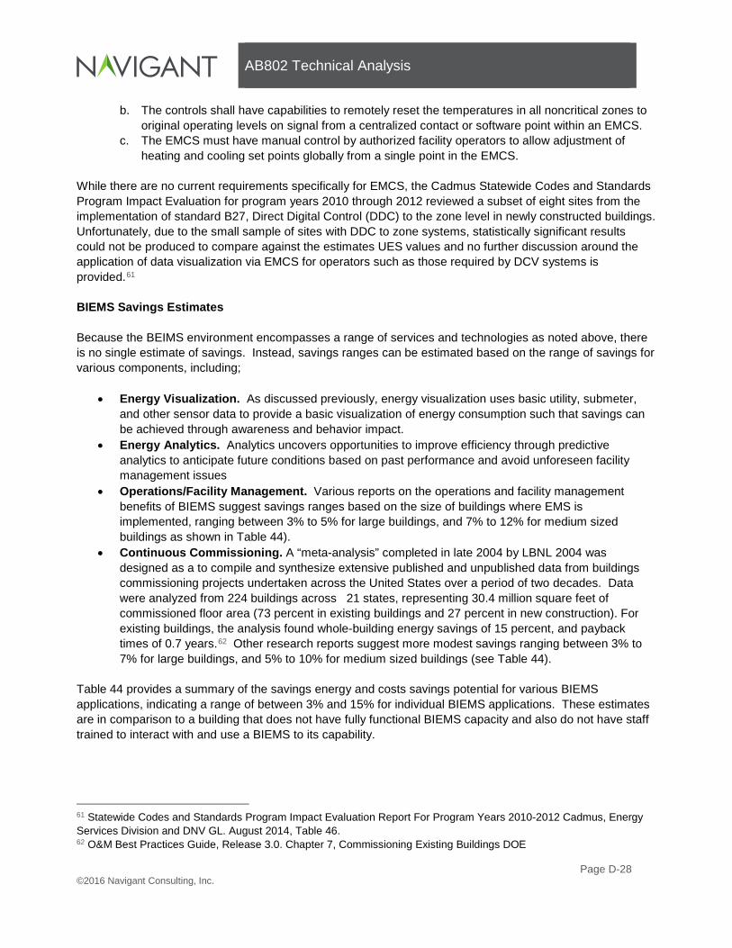
AB802 Technical Analysis
Page D-28 ©2016 Navigant Consulting, Inc.
b. The controls shall have capabilities to remotely reset the temperatures in all noncritical zones to original operating levels on signal from a centralized contact or software point within an EMCS.
c. The EMCS must have manual control by authorized facility operators to allow adjustment of heating and cooling set points globally from a single point in the EMCS.
While there are no current requirements specifically for EMCS, the Cadmus Statewide Codes and Standards Program Impact Evaluation for program years 2010 through 2012 reviewed a subset of eight sites from the implementation of standard B27, Direct Digital Control (DDC) to the zone level in newly constructed buildings. Unfortunately, due to the small sample of sites with DDC to zone systems, statistically significant results could not be produced to compare against the estimates UES values and no further discussion around the application of data visualization via EMCS for operators such as those required by DCV systems is provided.61 BIEMS Savings Estimates Because the BEIMS environment encompasses a range of services and technologies as noted above, there is no single estimate of savings. Instead, savings ranges can be estimated based on the range of savings for various components, including;
• Energy Visualization. As discussed previously, energy visualization uses basic utility, submeter, and other sensor data to provide a basic visualization of energy consumption such that savings can be achieved through awareness and behavior impact.
• Energy Analytics. Analytics uncovers opportunities to improve efficiency through predictive analytics to anticipate future conditions based on past performance and avoid unforeseen facility management issues
• Operations/Facility Management. Various reports on the operations and facility management benefits of BIEMS suggest savings ranges based on the size of buildings where EMS is implemented, ranging between 3% to 5% for large buildings, and 7% to 12% for medium sized buildings as shown in Table 44).
• Continuous Commissioning. A “meta-analysis” completed in late 2004 by LBNL 2004 was designed as a to compile and synthesize extensive published and unpublished data from buildings commissioning projects undertaken across the United States over a period of two decades. Data were analyzed from 224 buildings across 21 states, representing 30.4 million square feet of commissioned floor area (73 percent in existing buildings and 27 percent in new construction). For existing buildings, the analysis found whole-building energy savings of 15 percent, and payback times of 0.7 years.62 Other research reports suggest more modest savings ranging between 3% to 7% for large buildings, and 5% to 10% for medium sized buildings (see Table 44).
Table 44 provides a summary of the savings energy and costs savings potential for various BIEMS applications, indicating a range of between 3% and 15% for individual BIEMS applications. These estimates are in comparison to a building that does not have fully functional BIEMS capacity and also do not have staff trained to interact with and use a BIEMS to its capability.
61 Statewide Codes and Standards Program Impact Evaluation Report For Program Years 2010-2012 Cadmus, Energy Services Division and DNV GL. August 2014, Table 46. 62 O&M Best Practices Guide, Release 3.0. Chapter 7, Commissioning Existing Buildings DOE

AB802 Technical Analysis
Page D-29 ©2016 Navigant Consulting, Inc.
Table 44: Energy and Cost Savings of BIEMS Applications
Maintenance Schedule Large Medium
Energy Visualization 5-15% 5-15%
Energy Analytics 5-10% 5-10%
Operations/Facility Management 3-5% 7-12%
Continuous Commissioning 3-7% 5-10%
The extent to various BIEMS applications apply to buildings will vary depending on the size of the building, and the nature of the underlying management and maintenance skills. Small buildings are generally not well maintained and energy management is typically not a focus of owners and operators. For these facilities BIEMS will provide a pathway to address both issues. Larger buildings have a greater focus on energy management, and also greater staff capacity. Here, BIEMS will provide the tools to maximize these advantages. Table 45 provides the BIEMS savings estimates used in the analysis. These savings estimates are applied only to energy used for building HVAC systems because savings lighting controls are considered separately in the analysis on the potential for lighting controls.
Table 45: HVAC Systems Savings Estimates by Building Type
Total HVAC Systems
Savings by Building Type
Small Office 10%
Large Office 5%
Restaurant 10%
Retail Store 10%
Food/Liquor 10%
Unref Warehouse 0%
School 10%
College 5%
Health Care 5%
Hotel 10%
Misc 10%
Refr Warehouse 0%
BIEMS Model Inputs Based on the review of technologies, current market and code baseline data, and savings estimates for various energy control and information applications, the following definitions summarize the inputs used to model BIEMS impacts, as presented in Table 46. The equation used to estimate BIEMS savings is;

AB802 Technical Analysis
Page D-30 ©2016 Navigant Consulting, Inc.
Energy Savings, BIEMS = Starting Saturation of EMS by Building Type x Total Annual Consumption x % End Use Consumption for Heat, Cool, Vent x % End Use Savings by Building Type.
Table 46 columns and contents are described as follows:
1. Building Type. This definition also includes and Large and medium buildings will use EMS and small to very small will use improved maintenance resulting from EIS and energy use visualization tools and services. This definition is consistent across all IOUs.
2. Starting Saturation of EMS by Building Type. HVAC EMS control used as a proxy for current market baselines are derived from the 2009 Commercial Building Stock Assessment (CBSA) Study as shown in Table 46.63 This definition is consistent across all IOUs.
3. Total Annual Consumption. Baseline whole building energy consumption by building type from 2009 CEUS for Electric and Gas respectively.
4. % End Use Consumption for Heat, Cool, Vent. Building stock consumption by building type are derived for both electric and gas fuel types from the 2009 California Commercial End-Use Survey (CEUS) for HVAC Heating, Cooling, and Ventilation energy end-use intensities (EUI’s) applied to respective CEC IEPR stocks by building type and IOU. Table 46 presents an average across all IOUs, weighted by CEUS consumption estimates for each IOU.
5. % End Use Savings by Building Type. Estimates will range from 10% for small building to 5% for large buildings. The rationale is that 84% of large and medium operators perform periodic maintenance while only 20% of small and very small operators perform any maintenance. Table 46 presents an average across all IOUs, weighted by CEUS consumption estimates for each IOU.
63 The model incorporates scenario analysis between the 2015 Itron Commercial Saturation Study (CSS) and the 2009 Commercial Building Stock Assessment (CBSA) study. The 2015 Itron CSS found an average saturation for EMS systems of ~3% across IOU service territory commercial building stocks while the 2009 CBSA study found an average saturation for EMS system of ~37% across Pacific Northwest commercial building stocks. The 2009 CBSA study findings were used as the CSS commercial EMS saturation figures looked conservative from engineering reviews of the datasets.

AB802 Technical Analysis
Page D-31 ©2016 Navigant Consulting, Inc.
Table 46: Summary Characteristics of BIEMS-Enabled Buildings64
Building Type
Starting Saturation of
EMS by Building Type
% End Use Consumption for Heat, Cool, Vent (Electric)
% End Use Consumption for Heat, Cool,
Vent (Gas)
% End Use Savings by
Building Type
Small Office 50% 31% 72% 10%
Large Office 50% 40% 79% 5%
Restaurant 1% 22% 3% 10%
Retail Store 24% 29% 53% 10%
Food/Liquor 32% 13% 31% 10%
Unref Warehouse 11% 14% 87% 0%
School 59% 30% 60% 10%
College 80% 39% 66% 5%
Health Care 56% 44% 43% 5%
Hotel 25% 38% 16% 10%
Misc 35% 21% 31% 10%
Refr Warehouse 11% 3% 11% 0%
Total 36% 28% 37% 7%
6. Staring Technology Saturation by Building Type. The saturation of BIEMS depends on the
installation of EMS and EIS systems and related services. The starting saturations for enabling technology as a % of eligible building stocks is presented in Table 47. This estimate shows a current market average saturation of 36% and represents a weighted average of outyear saturation rates that vary depending on current EMS saturation estimate for various building types. The second column in the table reflects the annual EMS saturation growth scalar that is applied to the base saturation to model the year-over-year growth of EMS over time.
7. Enabling Technology Saturation Forecast. An average compound annual growth rate (CAGR) of 16.8% year-over-year per market research has been applied to estimate the market growth rate of the software, services, and hardware installations that enable BIEMS applications, as shown in Table 48.65 This average CAGR of 16.8% over the forecast horizon is based on a curve that assumes that growth will be higher in early years at 18%, as higher value installations are targeted and completed, while harder to reach or lower value installations will occur later resulting in a lower CAGR in outyears. This growth rate implies that the number of buildings with BIEMS enabled technologies will reach 50% after 10 years.
8. BIEMS Saturation Forecast. The mid case model scenario assumes that program interventions will add 1% additional BIEMS coverage in the first year, with a CAGR of 16.8% per year such that 4.41% of additional incremental coverage is achieved in year 10, as shown in Table 49. Cumulative additional saturation by year 10 is 18.6% above current market baseline. Per the starting saturation of 36% for enabling technologies presented in Table 48, this implies that after year ten, 54% of commercial facilities could participate in a BIEMS initiative. The high and low case scenarios presented in Table 49 use the same 16.8% CAGR throughout the forecast horizon but assume that
64 Results are presented as a weighted average by commercial building stocks across all IOUs. 65 Building Energy Management Systems. Navigant research, Q1 2015.

AB802 Technical Analysis
Page D-32 ©2016 Navigant Consulting, Inc.
the initial program interventions beginning in year 1 will add 1.25% (high) and 0.75% (low) additional coverage, respectively.
9. EUL. The cumulative program participation reflects a 5 year measure life of BIEMS based on the assumption that while the hardware and software that enable BIEMS has a long measures66, the savings that results are subject to having trained operators who are knowledge and capable to capturing all of the benefits from these systems. Literature from building operator training programs indicate that the effects of training persist for 5 years based on a number of factors, such as knowledge retention or staff turnover.
10. Building Stocks by IOU. Derived from the California Energy Commission (CEC) forecasts developed for the 2015 Integrated Energy Policy Report (IEPR) for the period from 2016 through 2025 which includes new construction and demolitions.
11. Costs. Costs for BIEMS are estimated based on the cost of Monitoring Based Commissioning (MBCx) programs in the 2015 PG&E portfolio. This program was selected as the prototype cost model because these programs combine the hardware, software, and service elements required in a BIEMS environment. Table 50 provides details on the four MBCx programs included PG&E portfolio, while Table 51 provides guidance on how the allocation of costs in these programs compare to the PG&E portfolio. Table 52 defines the cost for first year savings from MBCx programs as $0.38/kWh and $11.22/Therm. Gross electric measure costs are $0.33/kWh, with incentives of $0.25 offsetting roughly 74% of costs. Gross natural gas measure costs are $13.55/Therm, with incentives of $1.99 offsetting roughly 15% of costs.
66 EMS systems typically have an EUL exceeding 13 years

AB802 Technical Analysis
Page D-1 ©2016 Navigant Consulting, Inc.
Table 47. Starting Technology Saturation by Building Type
BIEMS Building Type 2009 CBSA
EMS Saturation
Annual EMS Saturation
Growth Scalar
Average 36% 4.0%
Retail Store 24% 4.2%
Food/Liquor 32% 4.2%
Small Office 50% 4.2%
Large Office 50% 4.2%
Restaurant 1% 8.4%
Unref Warehouse 11% 8.4%
Refr Warehouse 11% 0.0%
Health Care 56% 2.1%
Hotel 25% 4.2%
Residential Care 41% 4.2%
Misc 35% 4.2%
Assembly 35% 4.2%
School 59% 2.1%
College 80% 1.5%

AB802 Technical Analysis
©2016 Navigant Consulting, Inc. Page D-2
Table 48. Enabling Technology Saturation Forecast
Year 1 2 3 4 5 6 7 8 9 10
Compound Average Growth Rate (CAGR) 18% 18% 18% 18% 18% 18% 18% 18% 17% 16%
Enabling Technology Saturation as a % of Eligible Building Stock 36% 38% 39% 40% 42% 43% 45% 47% 48% 50%
Table 49. BIEMS Saturation Forecast
BIEMS Saturation Forecast
Program Year
1 2 3 4 5 6 7 8 9 10
Annual Incremental Additional Coverage (% of Sq. Ft)
Low 0.75% 1.04% 1.23% 1.45% 1.72% 2.02% 2.39% 2.82% 3.08% 3.31%
Mid 1.00% 1.39% 1.64% 1.94% 2.29% 2.70% 3.19% 3.76% 4.11% 4.41%
High 1.25% 1.74% 2.05% 2.42% 2.86% 3.37% 3.98% 4.70% 5.14% 5.51%
Cumulative Coverage (% of Sq. Ft)
Low 0.75% 1.79% 3.03% 4.48% 6.20% 7.47% 8.82% 10.40% 12.03% 13.62%
Mid 1.00% 2.39% 4.04% 5.97% 8.26% 9.96% 11.75% 13.87% 16.04% 18.16%
High 1.25% 2.99% 5.04% 7.47% 10.33% 12.45% 14.69% 17.34% 20.05% 22.70%
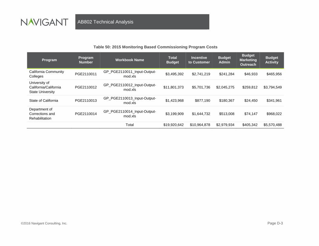
AB802 Technical Analysis
©2016 Navigant Consulting, Inc. Page D-3
Table 50: 2015 Monitoring Based Commissioning Program Costs
Program Program Number Workbook Name Total
Budget Incentive
to Customer Budget Admin
Budget Marketing Outreach
Budget Activity
California Community Colleges PGE2110011 GP_PGE2110011_Input-Output-
mod.xls $3,495,392 $2,741,219 $241,284 $46,933 $465,956
University of California/California State University
PGE2110012 GP_PGE2110012_Input-Output-mod.xls $11,801,373 $5,701,736 $2,045,275 $259,812 $3,794,549
State of California PGE2110013 GP_PGE2110013_Input-Output-mod.xls $1,423,968 $877,190 $180,367 $24,450 $341,961
Department of Corrections and Rehabilitation
PGE2110014 GP_PGE2110014_Input-Output-mod.xls $3,199,909 $1,644,732 $513,008 $74,147 $968,022
Total $19,920,642 $10,964,878 $2,979,934 $405,342 $5,570,488

AB802 Technical Analysis
Page D-4 ©2016 Navigant Consulting, Inc.
Table 51: 2015 MBCx Program Cost Allocation
Total Budget
Incentive to
Customer Budget Admin
Budget Marketing Outreach
Budget Activity
MBCx 55% 15% 2% 28%
PG&E 2015 Portfolio 47% 10% 6% 36%
Table 52: 2015 MBCx Program Cost Allocation per Unit Saved by Fuel Type
Fuel kWh Therm
Fuel savings 26,131,200 883,897
Btu 89,159,653,195 88,389,713,343
% Savings 50.2% 49.8%
Allocated costs $10,003,514 $9,917,128
Costs / unit saved $0.38 $11.22

AB802 Technical Analysis
Page D-5 ©2016 Navigant Consulting, Inc.
D.3 Tenant Engagement
Tenant Engagement Market Premise Tenant engagement programs in commercial buildings have only recently begun to gain attention and traction among utilities. They may be best exemplified by programs like the Smart Energy Now (SEN) component of the Envision Charlotte program which was launched in 2011 and evaluated in 2014. Given the positive results of the SEN program (6.2% net savings67), a growing number of utilities have begun to develop similar programs for some or all commercial buildings in their territories during the past 12 to 18 months. In addition to such broad sweeping types of programs, a variety of other tenant-based energy saving opportunities are provided more targeted or discrete efforts including those provided through the use of smart leases and more ad hoc company led efforts. To date, these more targeted efforts have typically been promoted on a much smaller scale. Given the relative novelty of all types of tenant engagement programs, the market penetration of such programs is considered to be very low, while the low cost of behavioral programs suggests that penetration could be much higher. The realization of these opportunities will depend, in part, on evolving regulatory signals and the degree to which utilities are able to claim behavior-related energy savings. This analysis forecasts the savings from tenant engagement associated with a variety of different end uses including HVAC, lighting, hot water, refrigeration, cooking, and plugload. Tenant Behavior Technologies and Initiatives The market for tenant engagement in commercial buildings is expanding due to improvements in metering and submetering technologies, a growing recognition of the importance of tenant behavior in determining energy consumption, the expanding application of social science insights in utility programs, and recent shifts in regulatory acceptance of behavioral programs. As noted above, we consider tenant engagement as it is associated with six particular end use categories: HVAC, lighting, hot water, refrigeration, cooking, and plug loads.
1. HVAC. Tenant engagement for HVAC is restricted to small buildings in which tenants (rather than building operators) are most likely to be responsible for temperature settings and equipment maintenance. HVAC-related engagement includes initiatives that are focused on: a. Energy efficient temperature settings and schedules.
i. Reducing temperature settings in the winter and increasing in the summer ii. Minimizing HVAC use during unoccupied periods (i.e. evenings and weekends) iii. Managing solar heat gain
b. HVAC equipment maintenance. i. Keeping equipment clean and in good repair. Most small businesses report either that
they never perform maintenance or only perform maintenance when there is a problem. 2. Lighting. Applies to all buildings.
a. Management of manual lighting controls. Reduce unnecessary lighting by turning off lighting when daylighting is adequate or when space is unoccupied whether during work hours, after hours, weekends, etc. These lighting measures are independent of those associated with automated lighting controls described in section D.1 of this report.
b. Delamping to minimize over-lighting. Reduce the amount of lighting in overlit spaces through selective delamping.
67 Hall, Nick and Johna Roth. 2014. “Impact Evaluation of the Smart Energy Now Program (NC) (Pilot).” Prepared for Duke Energy.

AB802 Technical Analysis
Page D-6 ©2016 Navigant Consulting, Inc.
3. Hot Water. Applies to all buildings as noted below. a. Reducing hot water use in hotels/motels, schools, colleges, and restaurants through changes
in water use behaviors. b. Change water heater settings and maintain tank water heaters to maximize efficiency in small
buildings.
4. Refrigeration. Applies to all buildings as noted below. a. Adjust commercial refrigeration controls and maintain equipment to maximize energy
efficiency in restaurants, hotels, schools and colleges. b. Limit the number of household refrigerators (consolidate) in office buildings, schools,
colleges, hotels/motels. c. Adjust settings on household refrigerators and maintain equipment to maximize energy
efficiency in all types of buildings with household refrigerators. 5. Cooking. Applies to restaurants, hotels/motels, schools and colleges.
a. Manage the use of cooking and ventilation equipment to minimize energy waste. b. Maintain cooking equipment to maximize energy efficiency.
6. Plugload. This applies to all building types and sizes. a. Consolidate the amount of plugload equipment by eliminating unnecessary/duplicative
equipment. b. Use energy efficient equipment settings c. Establish energy efficient equipment leasing and procurement policies. d. Use smart strips, timers and other devices to control operation and power draw of plugload
devices. An evaluation of the Smart Energy Now component of the Envision Charlotte program estimated behavior-based electricity savings of 6.2 percent in large office buildings. Roughly 43 percent of the savings were estimated to have been generated by turning off workspace lights while 37 percent were generated by turning off computers. These findings suggest that a large proportion (roughly 80%) of the program savings came from lighting and plug load management strategies. While this was true for the SEN program, this savings pattern may not be the same for other commercial building types and/or sizes since the SEN program exclusively targeted large commercial office buildings.68 Current Tenant Engagement Market Baseline The market baseline for tenant engagement programs is shaped by a variety of factors including the proportion of building tenants already engaged in such programs, the ability of non-participating tenants to take action, and the motivational parameters that shape the likelihood that eligible tenants will take action. These considerations are explored in more depth below. While little information exists concerning the proportion of commercial building space that already actively employs the types tenant engagement savings initiatives reviewed for this report, evidence suggests that these types of initiatives are in their infancy and that current initiatives are relatively limited in scope. Among the notable exceptions is PG&E’s recent launch of its Step Up & Power Down Initiative (SUPD). The SUPD Initiative is designed using the Smart Energy Now approach but is applied to a broader set of
68 Hall, Nick and Johna Roth. 2014. “Impact Evaluation of the Smart Energy Now Program (NC) (Pilot).” Prepared for Duke Energy.

AB802 Technical Analysis
Page D-7 ©2016 Navigant Consulting, Inc.
building types (office, retail, hotels, restaurants) within specifically defined geographical sections in the cities of San Francisco and San Jose. Given the nascent nature of the baseline, opportunity estimates can be derived from a variety of market characterization measures such as those provided by the Commercial Building Energy Consumption Survey (CBECS)69, the California Commercial Building End Use Survey (CEUS) and other resources that provide relevant information about technology saturation, occupant reliance on manual controls, and technology use patterns. For example, data from the 2015 Commercial Saturation Study (CSS) indicates that 74 percent of all commercial buildings rely on manual lighting controls. The percentage is even higher for small businesses (86% of small businesses and 96% of very small businesses relying on manual lighting controls). Similarly, data on HVAC maintenance schedules also provides eligibility insights for tenant engagement programs, showing that 44 percent of small businesses and 71% of very small businesses currently fail to maintain their HVAC system unless there is a problem. These and other measures are used to assess the opportunity structure associated with each of the end-use specific tenant behaviors outlined above. Baseline eligibility may also be shaped by the effect of split incentives on the likelihood of program participation. It is reasonable to hypothesize that since owner occupants are more likely to receive direct benefits in the form of cost savings from program participation, they may be more likely to participate in such programs compared to non-owner occupants. However, the relevance of split incentive issues is much less clear when applied to programs focused on tenant behavior as opposed to those that are focused on investment in building technologies. This distinction is important because the principal investment in the case of tenant engagement programs is generally limited to time rather than a large outlay of financial resources in building infrastructure. This consideration is further complicated by the recognition that in certain types of buildings, ownership may not be a good indicator of whether or not tenants are likely to pay for energy directly. Relevant examples include restaurants, schools and hotels. For these reasons, we assume that building ownership does not limit participation in tenant engagement programs for those types of buildings included in this assessment with the exception of small office buildings. In the case of small office space, we recognize that tenant are highly likely to be leasing their space and highly unlikely to be submetered or to pay for their energy directly. In addition, given their small size, their participation in tenant engagement programs is likely to be more difficult to coordinate and motivate. Current Tenant Engagement Code Baseline There are no California building codes or equipment standards that require tenant engagement as a source of energy efficiency in commercial buildings. LEED certification for existing buildings does allow credits for “occupant engagement” though it is not a required action. Tenant Engagement Savings Estimates The most comprehensive set of behavior-based savings estimates is provided by the Commercial Municipal Behavior Wedge Model (CMBWM). The CMBWM is a potential model developed by Dr. Karen Ehrhardt-Martinez and the Garrison Institute with funding from the Kresge Foundation and the Innovation Fund of the Urban Sustainability Director’s Network and serves as the primary source of existing energy
69 EIA. [Energy Information Administration] 2012. Commercial Buildings Energy Consumption Survey.

AB802 Technical Analysis
Page D-8 ©2016 Navigant Consulting, Inc.
savings estimates provided here70. The CMBWM estimates the achievable municipal-level energy savings that can be attained through programs and projects that address the energy-related routines, actions, and decisions of building operators and building tenants in the commercial buildings sector. The CMBWM provides city-level estimates of savings potential for each of 9 building types across a range of energy end uses as illustrated in Table 53.
Table 53: Categories of Commercial Savings Estimates by Building Type and Energy End Use
Energy End Uses No. of Behaviors Space Heating 15 Space Cooling 10
Ventilation 5 Water Heating 8
Lighting 12 Cooking 3
Refrigeration 11 Office Equipment 8
Computers 7 Other 12 Total 91
The CMBW model uses relevant literature to identify a subset of occupant and operator behaviors that encompass the most significant savings opportunities across the 9 types of commercial buildings included in the model. The CMBWM therefore contains a strategically selected subset of behavior-based savings opportunities. The identification of the most relevant behavioral opportunities was informed by previous research, including a 2010 report on “Commercial Miscellaneous Electric Loads”71 and a variety of other reports on commercial building plug loads by the National Renewable Energy Lab (NREL)72 73and the Pacific Northwest National Lab (PNNL)74. While the commercial sector model includes a longer list of behaviors, the list is not comprehensive and the estimates that are derived from it will necessarily undercount the full range of energy savings opportunities. Figure 45 below provides a graphic summary of the variety of data sources that are used in the Commercial Behavior Wedge estimation model, including data from the Commercial Buildings Energy Consumption Survey (CBECS), the U.S. Census Bureau, and insights from industry experts and related literature. CBECS data provide the core set of data for the Commercial Behavior Wedge estimates. The CBECS data set includes detailed information about energy use by building type and by end use as well as building counts by building type for each census division. They also provide critical information about
70 Ehrhardt-Martinez, Karen. 2015. “Municipal Behavior Wedge Project: Methodology Report.” Garrison Institute. 71 McKenney, Kurtis; Guernsey, Matthew; Ponoum, Ratcharit; and Jeff Rosenfeld. 2010. “Commercial Miscellaneous Electric Loads: Energy Consumption Characterization and Savings Potential in 2008 by Building Type.” TIAX LLC. 72 [NREL] National Renewable Energy Laboratory. 2013. “Assessing and Reducing Plug and Process Loads in Office Buildings.” Golden, Colorado: National Renewable Energy Lab. 73 [NREL] National Renewable Energy Laboratory. 2011. “Assessing and Reducing Plug and Process Loads in Retail Buildings.” Golden, Colorado: National Renewable Energy Lab. 74 [PNNL] Pacific Northwest National Laboratory. 2011. “Assessing and Reducing Miscellaneous Electric Loads (MELs) in Lodging.” Richland, Washington: Pacific Northwest National Lab.

AB802 Technical Analysis
Page D-9 ©2016 Navigant Consulting, Inc.
the square footage and energy intensity of various types of buildings. These data play an important role is establishing estimates of baseline energy use. The U.S. Census provides population and workforce information for both cities and census districts. These data are important for understanding the local context and adjusting CBECS data to reflect city characteristics. Relevant literature and expert insights are used to assess eligibility and the likely range of savings associated with particular behaviors. Taken together, these three types of data provide the means for estimating both existing patterns of energy consumption and potential energy savings opportunities.
Figure 45: Data Sources for the Commercial Municipal Behavior Wedge Model
Tenant Engagement Model Inputs Estimates of the market potential for commercial sector tenant engagement programs are built around three core data sources and a variety of supplemental data sources. The core data include estimates from the Commercial Municipal Behavior Wedge Model (CMBWM), data from the Smart Energy in Offices Program (the energy “pillar” of Envision Charlotte), and specific building metrics (building type and square footage) for the pertinent utility territories. This information is supplemented with information from CBECS (EIA 2012) and information for a select set of behavior-related experiments, pilots and programs. The following discussion defines the range of savings associated with tenant behaviors as shown in Table 58. The equation used to estimate tenant engagement savings for each building type is;
Tennant Engagement Savings = % CMBWM Achievable Savings x % Tenant Savings Contribution x Ownership Factor (i.e. % Leased) x Total Annual Consumption.
1. Building Type (Row 1). Savings from tenant engagement are estimated by building type for the
following 2009 CEUS facility types shown in Table 54 and represent those types of buildings for which estimates are considered more reliable. No estimates of savings for other buildings types were forecast due to limited of data or a lack of understanding of how tenants might participate.

AB802 Technical Analysis
Page D-10 ©2016 Navigant Consulting, Inc.
Table 54: Building Types
Building Type Code Description
EPR / ESE Primary / Secondary Education
HTL Hotel
OFL Large Office
RFF Fast Food Restaurant
ECC / EUN Community College / Universities
MTL Motel
OFS Small Office
RSD Sit Down Restaurant
2. Building Size Category (Row 2). These represent building size assignments consistent with
2009 CEUS. Facility size tends to define who has influence over energy use. For smaller facilities the tenant and the operator who manages energy use are the same. This is generally the case with smaller facilities, such as sit down restaurants, small offices or primary schools. For larger facilities, tenants have control over some energy uses, such as manual switches on lights or select plug loads, but less control over some building level energy use, such as central plants or large area lighting controlled through an energy management system. This is typically the case with large offices or universities that generally have a dedicated facilities management staff.
3. % CMBWM Achievable Savings (Row 3). The Commercial Municipal Behavior Wedge Model (CMBWM) provides city-specific estimates of energy savings opportunities for 9 different types of commercial buildings by end use.75 76 CMBWM estimates of achievable energy savings associated with both tenant and operator behaviors. These savings represent a participation rate of 50% of high value measures.
4. % Tenant Savings Contribution (Row 4). In order to apply the CMBWM model to forecast tenant OE savings it was necessary to clearly define what measures can be controlled by tenants, and which are controlled by operators. Row 4 shows the percent of CMBWM savings associated for measures that can be influenced by tenants based on the tenant versus operator assignments for various measures shown in rows 5 through 31. This represents the sum of savings estimate for each measure end-use category. Once tenant-specific behaviors have been identified for each end use and building type, they are multiplied by the corresponding measure of building energy use associated with the same end use and building type as indicated by the California Commercial End Use Survey (2006), shown in Table 57. The products of each end-use-specific calculation are then added up and the sum is multiplied by the estimate of the combined (operator and tenant) savings opportunity for the specified building type (as shown in Table 58, row 3). The resulting estimate of the savings opportunity associated with tenant behaviors is shown in row 4 of Table 58 as the % Tenant Savings Contribution. Behaviors
75 Ehrhardt-Martinez, Karen. 2015. “Municipal Behavior Wedge Project: Methodology Report.” Garrison, NY: Garrison Institute. 76 Ehrhardt-Martinez, Karen. 2016. “Behavior-based Energy Savings Opportunities in Commercial Buildings: Estimates for 4 U.S. Cities.” Proceedings of the 2016 ACEEE Summer Study on Energy Efficiency in Buildings.

AB802 Technical Analysis
Page D-11 ©2016 Navigant Consulting, Inc.
highlighted in light greeen represent those that were identified in the CMBWM as providing the majority of building-specific saving opportunities.
5. Total Annual Consumption. Baseline whole building energy consumption by building type from 2009 CEUS.
6. Ownership Factor. Savings for each building type are further reduced to reflect ownership status. We assume that office tenants are less likely to be motivated to take action to save energy given that utility expenses are frequently not paid directly by tenants and because tenant engagement based on non-economic incentives is likely to be more difficult to achieve across a more widely disbursed and heterogeneous set of companies. For all other building types included in the model, we assume that tenants are eligible and equally likely to participate in tenant engagement programs whether they own or lease the space that they occupy. In the case of food service, lodging, and education we do not make the same assumptions since these types of businesses typically operate in standalone buildings even when the building space is leased and because they are considerably more likely to pay their own energy bill. We use the 2012 Commercial Building Energy Consumption Survey (CBECS) to assess ownership status as shown in Table 55.
Table 55: Ownership Status of Commercial Buildings by Building Activity
Ownership and Occupancy
All Buildings Office Education
Food service Lodging
Nongovernment owned 67,499 12,815 3,082 1,702 5,360
Owner occupied 30,601 3,169 2,469 1,008 3,656
Leased to tenant(s) 26,100 7,118 327 656 1,130 Owner occupied and leased 8,873 2,528 Q Q 574
Unoccupied 1,925 N N N N
Government owned 19,543 3,136 9,154 Q 466
Federal 1,573 600 Q N N
State 5,539 1,203 2,408 Q Q
Local 12,431 1,333 6,689 Q Q
% Leased 45.2% 65.4% 10.6% 38.5% 26.4%
7. Tenant / Operator assignment (Rows 5 through 31). In order to arrive at estimates of savings from tenant behaviors only, we review each of the 27 behaviors listed in rows 5 through 31 for each building type shown in Table 58 to assess whether the savings measure is more likely to be under the control of building tenants or guests (designated by ‘T’ or ‘G’ in Table 58) or the building operator (designated by ‘O’ in Table 58). Estimates of savings opportunities associated with tenant (and guest) behaviors are then derived by calculating the proportion of savings measures under tenant (and guest) control for each of the energy end use categories. Table 56 shows the percentage of savings within each measure category that can be controlled by tenants for each building type considered. For example, tenants can control 100% of HVAC savings potential in a small office, but have less control in large offices where facilities management staff typically control HVAC functions. In this example, tenants have control of 17% of HVAC measures in large office.
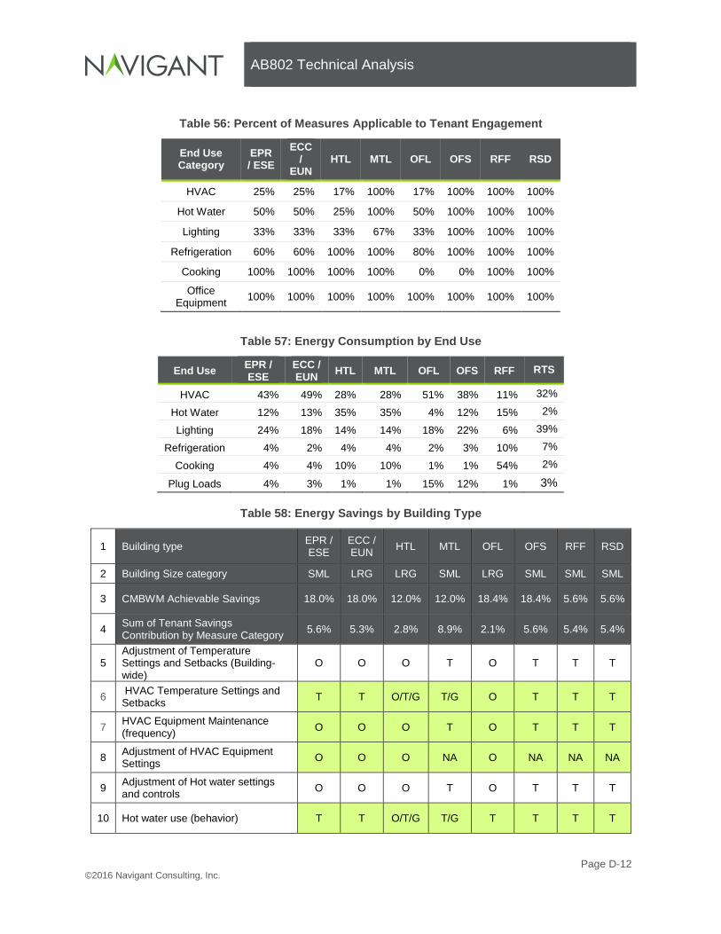
AB802 Technical Analysis
Page D-12 ©2016 Navigant Consulting, Inc.
Table 56: Percent of Measures Applicable to Tenant Engagement
End Use Category
EPR / ESE
ECC /
EUN HTL MTL OFL OFS RFF RSD
HVAC 25% 25% 17% 100% 17% 100% 100% 100%
Hot Water 50% 50% 25% 100% 50% 100% 100% 100%
Lighting 33% 33% 33% 67% 33% 100% 100% 100%
Refrigeration 60% 60% 100% 100% 80% 100% 100% 100%
Cooking 100% 100% 100% 100% 0% 0% 100% 100%
Office Equipment 100% 100% 100% 100% 100% 100% 100% 100%
Table 57: Energy Consumption by End Use
End Use EPR / ESE
ECC / EUN HTL MTL OFL OFS RFF RTS
HVAC 43% 49% 28% 28% 51% 38% 11% 32%
Hot Water 12% 13% 35% 35% 4% 12% 15% 2%
Lighting 24% 18% 14% 14% 18% 22% 6% 39%
Refrigeration 4% 2% 4% 4% 2% 3% 10% 7%
Cooking 4% 4% 10% 10% 1% 1% 54% 2%
Plug Loads 4% 3% 1% 1% 15% 12% 1% 3%
Table 58: Energy Savings by Building Type
1 Building type EPR / ESE
ECC / EUN HTL MTL OFL OFS RFF RSD
2 Building Size category SML LRG LRG SML LRG SML SML SML
3 CMBWM Achievable Savings 18.0% 18.0% 12.0% 12.0% 18.4% 18.4% 5.6% 5.6%
4 Sum of Tenant Savings Contribution by Measure Category 5.6% 5.3% 2.8% 8.9% 2.1% 5.6% 5.4% 5.4%
5 Adjustment of Temperature Settings and Setbacks (Building-wide)
O O O T O T T T
6 HVAC Temperature Settings and Setbacks T T O/T/G T/G O T T T
7 HVAC Equipment Maintenance (frequency) O O O T O T T T
8 Adjustment of HVAC Equipment Settings O O O NA O NA NA NA
9 Adjustment of Hot water settings and controls O O O T O T T T
10 Hot water use (behavior) T T O/T/G T/G T T T T

AB802 Technical Analysis
Page D-13 ©2016 Navigant Consulting, Inc.
11 Adjustment of Interior Lighting controls (% sensor, occupancy vs vacancy)
O O O O O NA NA NA
12 Interior Lighting use management T T/O T T T T T T
13 Interior Delamping O O O T O T T T
14 Adjustment of HH Refrigerator controls T T T T T T T T
15 HH Refrigerator maintenance (defrost, seals, cleaning) T T T T T T NA NA
16 HH Refrigerator - limit the number T T T/G T/G T T NA NA
17 Comm Refrigerator controls O O T T T NA T T
18 Comm Refrigerator maintenance O O T T T NA T T
19 Cooking equipment management of use T T T T NA NA T T
20 Cooking equipment maintenance T T T T NA NA T T
21 Office equipment consolidation (printers, copiers, etc) T T T T T T T T
22 Office equipment settings T T T T T T T T
23 Office equipment leasing policies (EE) T T T T T T T T
24 Computer equipment inventory (consolidate monitors, use laptops) T T T T T T T T
25 Computer equipment settings (power off, screen savers, etc) T T T T T T T T
26
Computers; common area equipment inventory management (computers, screens, projectors, etc)
T T T T T T T T
27 Computer equipment procurement policies (EE) T T T T T T T T
28 Computer networks, servers, and remote access systems T T T T T T T T
29 Vending machines & misc plug load inventory mgmt T T T T T T T T
30 Vending machines and misc plug load settings T T T T T T T T
31 Other Plugload Hours of Operation (ie water cooler, space heaters, TVs, kiosks, etc
T T T T T T T T
Table 59 provides the final facility level savings by building type as applied to both electric and gas consumption.

AB802 Technical Analysis
Page D-14 ©2016 Navigant Consulting, Inc.
Table 59: Facility Level Savings by Building Type
Building Type % Tenant potential Average 2.2%
Small Office 5.6% Large Office 2.1%
RFF 5.4% RSD 5.4%
EPR / ESE 5.6% ECC / EUN 5.3%
HTL 2.8% MTL 8.9%
8. Economic Useful Life. It is assumed that the EUL for tenant engagement is 1 year. 9. Cost Calculations. Annual program costs are estimated by using the program costs reported by
Envision Charlotte. Total utility costs per kWh for years 1 through 5 of the program were reported as $.062, $.038, $.035, $.036, and $.036 (K&L Gates 2014). Because the tenant engagement is assumed to have a 1 year EUL, program costs increase each year to add new tenants, and also to re-engaged tenants from each preceding year.
10. Saturation for Tenant Engagement Programs. Starting saturation for tenant engagement programs is assumed to be zero. The first year of program operations it is assumed that 2.0% of the market can be impacted through tenant engagement programs. This penetration grows at 2% per year through the first 5 year as high value facilities are targeted, then reduces to 1% per year thereafter. Because the tenant engagement is assumed to have a 1 year EUL, tenants from previous years must be re-engaged each year in order to reach a saturation of 15% of the market by the 10th year of program operation, as shown in Table 60. The low scenarios assume a saturation rate that is 25% lower than the mid, while the high scenario assumes a saturation rate that is 125% of mid.
Table 60. Market Penetration Scenarios
Tenant Engagement Saturation Forecast
Program Year
1 2 3 4 5 6 7 8 9 10
Low Scenario 1.50% 3.00% 4.50% 6.00% 7.50% 8.30% 9.00% 9.80% 10.50% 11.30%
Mid Scenario 2.00% 4.00% 6.00% 8.00% 10.00% 11.00% 12.00% 13.00% 14.00% 15.00%
High Scenario 2.50% 5.00% 7.50% 10.00% 12.50% 13.80% 15.00% 16.30% 17.50% 18.80%

AB802 Technical Analysis
Page E-1 ©2016 Navigant Consulting, Inc.
STRANDED POTENTIAL SENSITIVITY ANALYSIS
Navigant tested the sensitivity of the Stranded Potential savings and total program budget results to four uncertain parameters (discussed earlier in section 2.3.1). Figure 46 through Figure 48 show the percent impact of changing each of these parameters on the electric, demand, and gas savings respectively. Figure 46 shows UES has the highest impact on the electric savings; the low to high range on UES can have a total swing of 15% on electric savings. The other variables have less than 4% total impact on the savings. For three of the four variables, the low range results in lower savings and the high range results in higher savings. The only exception is “Repair Life” variable, where it is reversed and shows higher savings for the low range and lower savings for the high range. This is because a lower Repair Life means that repairs do not last as long and are less financially attractive compared to replacing equipment. Thus, customers are more likely to adopt higher efficiency equipment earlier. Whereas a high Repair Life means repairs last longer and equipment stays in the field longer, which postpones the higher efficiency equipment adoption and makes repairs more financially attractive to customers. Figure 47 shows similar to trends in the electric savings for the demand savings. UES has the highest impact on demand savings, the low to high range on UES can have a total 21% on demand savings. Also the other variables have less swing range, but they are higher than those for the electric savings, especially the “Repair Life” variable. This is because demand savings are comprised of higher percentage of HVAC savings compared to electric savings, and HVAC savings inherently have more uncertainty associated with them.
Figure 46: Sensitivity of Program Savings to Uncertain Variables (GWh)
Note: includes PA Savings and PA Stranded Potential
Source: Navigant analysis.

AB802 Technical Analysis
Page E-2 ©2016 Navigant Consulting, Inc.
Figure 47: Sensitivity of Program Savings to Uncertain Variables (MW)
Note: includes PA Savings and PA Stranded Potential
Source: Navigant analysis.
Figure 48 shows similar trends to the two charts above. UES has the highest impact on the gas savings with approximately 18% total swing, while all the other scenarios have less than 6% swing. The only difference in the trends for gas savings is in the “Saturation of Stranded Equipment” variable. The low scenario option shows higher savings whereas the high scenario option does not show any sensitivity. This is driven by interactive effects.

AB802 Technical Analysis
Page E-3 ©2016 Navigant Consulting, Inc.
Figure 48: Sensitivity of Program Savings to Uncertain Variables (MM Therms)
Note: includes PA Savings and PA Stranded Potential
Source: Navigant analysis.

AB802 Technical Analysis
Page E-4 ©2016 Navigant Consulting, Inc.
Figure 49 similarly shows that UES has the biggest impact on program budgets while all the other variables have a much smaller impact.
Figure 49: Sensitivity of Program Budget to Uncertain Variables
Note: includes PA Savings and PA Stranded Potential
Source: Navigant analysis.