P a g e | 1

Abandoned Object Detection in Video

A BACHELOR’S THESIS

submitted in partial fulfillment

of the requirements for the award of the degree

of

BACHELOR OF TECHNOLOGY

in

INFORMATION TECHNOLOGY

(B.Tech in IT)

Submitted by

Abhineet Kumar Singh (IIT2009148)

Under the Guidance of:

Dr. Anupam Agrawal

Professor

IIIT-Allahabad

INDIAN INSTITUTE OF INFORMATION TECHNOLOGY

ALLAHABAD – 211 012 (INDIA)

July, 2013

P a g e | 2

CANDIDATE’S DECLARATION

I hereby declare that the work presented in this thesis entitled ―Abandoned object detection in

video‖, submitted in the partial fulfillment of the degree of Bachelor of Technology (B.Tech), in

Information Technology at Indian Institute of Information Technology, Allahabad, is an

authentic record of my original work carried out under the guidance of Dr. Anupam Agrawal.

Due acknowledgements have been made in the text of the thesis to all other material used. This

thesis work was done in full compliance with the requirements and constraints of the prescribed

curriculum.

Place: Allahabad Abhineet Kumar Singh

Date: R. No. IIT2009148

CERTIFICATE FROM SUPERVISOR

I do hereby recommend that the thesis work prepared under my supervision by Abhineet Kumar

Singh titled ―Abandoned object detection in video‖ be accepted in the partial fulfillment of the

requirements of the degree of Bachelor of Technology in Information Technology for

Examination.

Date: Dr. Anupam Agrawal

Place: Allahabad Professor, IIITA

Committee for Evaluation of the Thesis

_______________________ _______________________

_______________________ _______________________

P a g e | 3

ACKNOWLEDGEMENTS

The author would like to express his sincere gratitude to his project supervisor Dr. Anupam

Agrawal for his support and guidance that have been crucial to the successful completion of this

project.

Place: Allahabad Abhineet Kumar Singh

Date: B Tech Final Year, IIITA

P a g e | 4

ABSTRACT

Abandoned object detection is one of the most practically useful areas of computer vision due to

its application in automated video surveillance systems for the detection of suspicious activities

that might endanger public safety, especially in crowded places like airports, railway stations,

shopping malls, movie theatres and the like. An abandoned object is defined as one that has been

lying stationary at a certain place with no apparent human attendance for an extended period of

time. Such objects are usually inconspicuous commonplace objects that people often carry

around including backpacks, suitcases and boxes. Detection of abandoned objects is of prime

importance in uncovering and forestalling terrorist activities since it is a reasonable supposition

that an abandoned object, if left behind on purpose, may be hiding dangerous items like

explosives.

The present work is an attempt to create a flexible and modular framework that can be used to

experiment with several different methods for each stage of the overall task of detecting

abandoned and removed objects in a video stream. Several existing methods have been

implemented for each of these stages and integrated into the system in a way that makes it

possible to switch between them in real time. This enables the user to observe and compare the

performance of different methods of solving the same problem and choose the one most suited to

any given scenario. The system has also been designed to allow new methods to be added for any

stage of the system with minimum programming effort.

P a g e | 5

Table of Contents

1. Introduction………………………………………………………………………………1

1.1 Currently existing technologies…………………………………………………..1

1.2 Analysis of previous research in this area………………………………………....3

1.3 Problem definition and scope.………………………………………………….….4

1.4 Formulation of the present problem…………………………………………….…5

1.5 Organization of the thesis…………………………………………………..……..6

2. Description of Hardware and Software Used…………………………………………..6

2.1 Hardware…………………………………………………………………………..6

2.2 Software…………………………………………………………………………...6

3. Theoretical Tools – Analysis and Development………………………………………..7

3.1 Pre-processing……………………………………………………………………..8

3.2 Background Modeling and Subtraction…….........................................................11

3.3 Foreground analysis….…………………………………………………………..14

3.4 Blob extraction……………………………………………………….…………..18

3.5 Blob tracking……………………………………………………………………..18

3.6 Abandonment analysis.…………………………………………………………..20

3.7 Blob filtering.…...………………………………………………………………..22

4. Development of Software ………………………………………..................................22

4.1 User interface module…...……………………………………………………….25

4.2 Pre-processing module……..…………………………………………………….25

4.3 BGS module………………..…………………………………………………….26

4.4 Foreground analysis module.………………….....................................................27

4.5 Blob extraction module ……………………….....................................................27

4.6 Blob tracking module............………………….....................................................27

4.7 Abandonment analysis module.……………….....................................................29

4.8 Blob filtering module...……….……………….....................................................29

5. Testing and Analysis…………………………………………………………………..31

5.1 Setup……………..…………...………………………………………………….31

5.2 Datasets………………………...………………………………………………...31

5.3 Result summary………………..………………………………………………...34

5.4 Result analysis…………………………………………………………………...36

5.5 Comparison with existing systems….…….……………………………………...37

6. Conclusions and Future Work………………………………………………………..38

Appendix - Explanation of the Source Code………………………….……………....39

References……………………………………………………………………………....48

P a g e | 1

1. Introduction

An automatic abandoned object detection system typically uses a combination of background

subtraction and object tracking to look for certain pre defined patterns of activity that occur when

an object is left behind by its owner. Though humans are much better at this task than even state

of the art systems, it is often practically unfeasible to employ enough manpower to continuously

monitor each one of the very large number of cameras that are required in a large scale

surveillance scenario. An automatic detection system therefore helps to complement the

available manpower by serving as both a standalone monitoring system for less critical areas and

also integrated into manually monitored cameras so that it can detect any drops that the human

may have missed.

1.1 Currently existing technologies: Most existing techniques of abandoned (and removed)

object detection employ a modular approach with several independent steps where the output of

each step serves as the input for the next one. Many efficient algorithms exist for carrying out

each of these steps and any single complete AOD system has to address the problem of finding a

suitable combination of algorithms to suit a specific scenario. Following is a brief description of

these steps and related methods, in the order they are carried out:

1.1.1 Background Modeling and Subtraction (BGS): This stage creates a dynamic model of the

scene background and subtracts it from each incoming frame to detect the current foreground

regions. The output of this stage is usually a mask depicting pixels in the current frame that do

not match the current background model. Some popular background modeling techniques

include adaptive medians [1], running averages [2], mixture of Gaussians [3, 4], kernel density

estimators [5, 6], Eigen-backgrounds [7] and mean-shift based estimation [8]. There also exist

methods that employ dual backgrounds [9] or dual foregrounds [10] for this purpose. The BGS

step often utilizes feedback from the object tracking stage to improve its performance.

1.1.2 Foreground Analysis: The BGS step is often unable to adapt to sudden changes in the scene

(of lighting, etc.) since the background model is typically updated slowly. It might also confuse

parts of a foreground object as background if their appearance happens to be similar to the

corresponding background, thus causing a single object to be split into multiple foreground

blobs. In addition, certain foreground areas, while being detected correctly, are not of interest for

P a g e | 2

further processing. The above factors necessitate an additional refinement stage to remove both

false foreground regions, caused by factors like background state changes and lighting variations,

as well as correct but uninteresting foreground areas like shadows.

Several methods exist for detecting sudden lighting changes, ranging from simple gradient and

texture based approaches [11, 12] to those that utilize complex lighting invariant features

combined with binary classifiers like support vector machines [13]. Shadow detection is usually

carried out by performing a pixel-by-pixel comparison between the current frame and the

background image to evaluate some measure of similarity between them. These measures

include normalized cross correlation [11, 14], edge-width information and illumination ratio

[15]. There are many other shadow detection methods as enumerated in [16].

1.1.3 Blob Extraction: This stage applies a connected component algorithm to the foreground

mask to detect the foreground blobs while optionally discarding too small blobs created due to

noise. Most existing methods use an efficient linear time algorithm that was developed in [17].

The popularity of this method is owing to the fact that it requires only a single pass over the

image to identify and label all the connected components therein, as opposed to most other

methods that require two passes [18, 19, 20].

1.1.4 Blob Tracking: This is often the most critical step in the AOD process and is concerned

with finding a correspondence between the current foreground blobs and the existing tracked

blobs from the previous frame (if any). The results of this step are sometimes used as feedback to

improve the results of background modeling. Many methods exist for carrying out this task,

including finite state machines [13], color histogram ratios [21], Markov chain Monte Carlo

model [22, 23], Bayesian inference [24, 25], Hidden Markov models [26] and Kalman filters

[27].

1.1.5 Abandonment Analysis: This step classifies a static blob detected by the tracking step as

either abandoned or removed object or even a very still person. An alarm is raised if a detected

abandoned/removed object remains in the scene for a certain amount of time, as specified by the

user. The task of distinguishing between removed and abandoned objects is generally carried out

by calculating the degree of agreement between the current frame and the background frame

around the object‘s edges, under the assumption that the image without any object would show

P a g e | 3

better agreement with the immediate surroundings. There exist several ways to calculate this

degree of agreement; two of the popular methods are based on edge energy [28, 11] and region

growing [29]. There also exist methods [13] that use human tracking to look for the object‘s

owner and evaluate the owner‘s activities around the dropping point to decide whether the object

is abandoned or removed.

1.2 Analysis of previous research in this area: A great deal of research has been carried out in

the area of AOD owing to its significance in anti-terrorism measures. Most methods developed

recently can be classified into two major groups: those that employ background modeling and

those that rely on tracking based detection. Some of the methods in the first group have been

presented in [9, 10, 29-35] Most of these use Gaussian Mixture Model (GMM) [3] for

background subtraction. In this model, the intensity at each pixel is modeled as the weighted sum

of multiple Gaussian probability distributions, with separate distributions representing the

background and the foreground. The method used in [30] first detects blobs from the foreground

using pixel variance thresholds and then calculates several features for these blobs to decrease

false positives. The approach in [10] maintains two separate backgrounds- one each for long and

short term durations- and modifies them using Bayesian learning. These are then compared with

each frame to estimate dual foregrounds. The method detailed in [31] mainly focuses on tracking

an object and its owner in an indoor environment with the aim of informing the owner if

someone else takes that object. The method proposed in [29] applies GMM with three

distributions for background modeling and uses these to categorize the foreground into moving,

abandoned and removed objects. A similar background modeling method has been used in [34]

along with crowd filtering to isolate the moving pedestrians in the foreground from the crowd by

the use of vertical line scanning. There are also some approaches to background modeling that do

not employ GMM such as the method in [9] that uses approximate median model for this

purpose. Just like in [10], this one too maintains two separate backgrounds, one of which is

updated more frequently than the other.

Some of the approaches based on the other class of methods, based on tracking, can be found in

[21, 22, 36-39]. The tracking based approach used in [36] comprises three levels of processing-

starting with background modeling in the lowest level using feedback from higher levels,

followed by person and object tracking in the middle level and finally the person-object split in

P a g e | 4

the highest level to classify an object as abandoned. The system proposed in [37] considers the

abandonment of an object to comprise of four sub-events, from the arrival of the owner with the

object to his departure without it. Whenever the system detects any unattended object, it traces

back in time to identify the person who brought it into the scene and thus identifies the owner.

Tracking and detection of carried objects is performed using histograms in [21] where the

missing colors in ratio histogram between the frames with and without the object are used to

identify the abandoned object. The method used in [22] performs tracking through a trans-

dimensional Markov Chain Monte Carlo model suitable for tracking generic blobs and thus

incapable of distinguishing between humans and other objects as the subject of tracking. The

output of this tracking system therefore needs to be subjected to further processing before

luggage can be identified and labeled as abandoned.

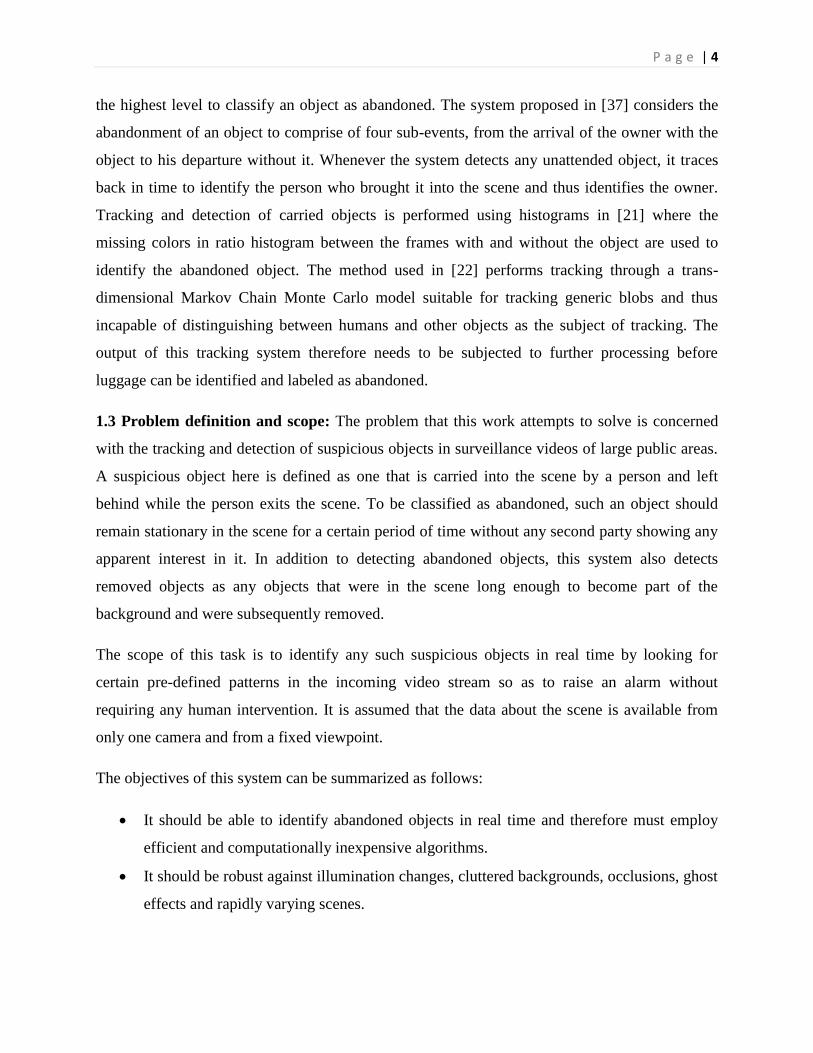
1.3 Problem definition and scope: The problem that this work attempts to solve is concerned

with the tracking and detection of suspicious objects in surveillance videos of large public areas.

A suspicious object here is defined as one that is carried into the scene by a person and left

behind while the person exits the scene. To be classified as abandoned, such an object should

remain stationary in the scene for a certain period of time without any second party showing any

apparent interest in it. In addition to detecting abandoned objects, this system also detects

removed objects as any objects that were in the scene long enough to become part of the

background and were subsequently removed.

The scope of this task is to identify any such suspicious objects in real time by looking for

certain pre-defined patterns in the incoming video stream so as to raise an alarm without

requiring any human intervention. It is assumed that the data about the scene is available from

only one camera and from a fixed viewpoint.

The objectives of this system can be summarized as follows:

It should be able to identify abandoned objects in real time and therefore must employ

efficient and computationally inexpensive algorithms.

It should be robust against illumination changes, cluttered backgrounds, occlusions, ghost

effects and rapidly varying scenes.

P a g e | 5

It should try to maximize the detection rate while at the same time minimizing false

positives.

1.4 Formulation of the present problem: The overall problem of AOD can be broken down

into a set of smaller, independent problems each of which is solved by a separate stage in the

automatic AOD system. These stages are typically executed one after another with each stage

using the output of the last stage as its input. There are five main stages in this process:

1.4.1 Background Modeling and Subtraction: This stage creates a dynamic model of the scene

background and subtracts it from each incoming frame to detect the current foreground regions.

The output of this stage is usually a mask depicting pixels in the current frame that do not match

the current background model.

1.4.2 Foreground Analysis: The BGS step is often unable to adapt to sudden changes in the scene

(of lighting, etc.) since the background model is typically updated slowly. It might also confuse

parts of a foreground object as background if their appearance happens to be similar to the

corresponding background, thus causing a single object to be split into multiple foreground

blobs. In addition, certain foreground areas, while being detected correctly, are not of interest for

further processing. The above factors necessitate an additional refinement stage to remove both

false foreground regions, caused by factors like background state changes and lighting variations,

as well as correct but uninteresting foreground areas like shadows.

1.4.3 Blob Extraction: This stage applies a connected component algorithm to the foreground

mask to detect the foreground blobs while optionally discarding too small blobs created due to

noise.

1.4.4 Blob Tracking: This is often the most critical step in the AOD process and is concerned

with finding a correspondence between the current foreground blobs and the existing tracked

blobs from the previous frame (if any).The results of this step are sometimes used as feedback to

improve the results of background modeling.

1.4.5 Abandonment Analysis: This step classifies a static blob detected by the tracking step as

either abandoned or removed object or even a very still person. An alarm is raised if a detected

abandoned object remains in the scene for a certain amount of time, as defined by the user.

P a g e | 6

1.5 Organization of the thesis: Rest of this thesis is organized as follows: section 2 presents a

brief description of the hardware and software used for developing and testing this application;

section 3 describes the system methodology; section 4 describes the different modules in the

system and their user interface; section 5 presents the details of testing methodology and the

obtained results; finally, section 6 presents the conclusions and scope for future work.

2. Description of Hardware and Software Used

2.1 Hardware

Like most computer vision and image processing tasks, AOD is an extremely computationally

intensive process and requires powerful hardware to run in real time. The present system has

been tested on a fairly modern and moderately powerful laptop computer whose configuration is

given below:

CPU: Intel Core i5 3210M with 2 cores/4 threads running at 3.10 GHz

RAM: 4GB DDR3 running at 1600MHz

GPU: Nvidia Gefore GT635M with 96 CUDA cores clocked at 660MHz and having 1

GB of GDDR3 video memory clocked at 1800MHz

HDD: 1 TB SATA-3 HDD with 5400 rpm

Testing has been done on both online and offline video streams. The online streams have been

captured using both the integrated laptop camera and a dedicated Microsoft web-camera with

respective resolutions of 1280x720 and 640x480 The offline test set includes videos from 3

publicly available benchmark datasets: PETS2006 [48], PETS2007 [49] and AVSS-iLiDS [50].

It also includes a custom dataset consisting of 18 videos shot using a Sony DSC-W35 digital

camera. The video resolutions are 720x576 for public benchmark datasets and 640x480 for the

custom prepared dataset.

2.2 Software

The application has been coded entirely in C++ and makes use of OpenCV library version 2.4.4.

Coding has been done using Microsoft Visual Studio 2008 integrated development environment

and tested on both Windows XP 32-bit and Windows 7 64-bit operating systems.

P a g e | 7

3. Theoretical Tools – Analysis and Development

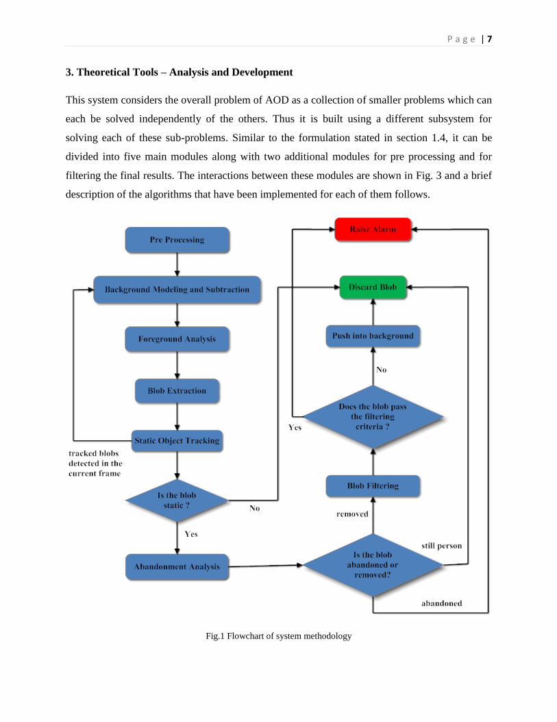
This system considers the overall problem of AOD as a collection of smaller problems which can

each be solved independently of the others. Thus it is built using a different subsystem for

solving each of these sub-problems. Similar to the formulation stated in section 1.4, it can be

divided into five main modules along with two additional modules for pre processing and for

filtering the final results. The interactions between these modules are shown in Fig. 3 and a brief

description of the algorithms that have been implemented for each of them follows.

Fig.1 Flowchart of system methodology

P a g e | 8

3.1 Pre-processing: This module performs the following two functions:

3.1.1 Contrast enhancement: This step helps to improve the quality of low light videos like

those taken at night (Fig. 1) by normalizing the difference between maximum and minimum

intensities in the image which in turn helps to increase visibility in darker areas of the scene.

Following three methods have been implemented for carrying it out:

3.1.1.1 Histogram equalization: This method involves the following steps:

i. Split the input RGB image into 3 grayscale images, one corresponding to each channel.

ii. Compute the histogram for each of these grayscale images and normalize it so that the

sum of histogram bins becomes 255.

iii. Compute the image corresponding to the transformed histograms using their integral.

iv. Join the 3 transformed grayscale images to get the output RGB image.

Fig. 2 shows the input and processed images together with their respective histograms.

3.1.1.2 Linear contrast stretching: This method involves the following steps:

i. Split the input RGB image into 3 grayscale images, one corresponding to each channel.

ii. For each of these images, calculate the maximum and minimum cutoff intensities based

on a user specified cutoff percentile and the image intensity distribution.

iii. Set the intensity values of all pixels above the maximum and below the minimum cutoff

as maximum and minimum intensity respectively.

iv. Normalize (or stretch) the intensity distribution so that the minimum and maximum

intensities become 0 and 255 respectively.

v. Combine the transformed grayscale images to get the output RGB image.

Fig. 3 shows the result of applying this method.

3.1.1.3 Image filtering: This method involves the following steps:

i. Split the input RGB image into 3 grayscale images, one corresponding to each channel

ii. Apply the following formula to each pixel in each of these images:

𝐼𝑛𝑒𝑤 𝑖, 𝑗 = 5 ∗ 𝐼𝑜𝑙𝑑 𝑖, 𝑗 − 𝐼𝑜𝑙𝑑 𝑖 − 1, 𝑗 + 𝐼𝑜𝑙𝑑 𝑖 + 1, 𝑗 + 𝐼𝑜𝑙𝑑 𝑖, 𝑗 − 1 + 𝐼𝑜𝑙𝑑 𝑖, 𝑗 + 1 (1)

iii. Combine the transformed grayscale images to get the output RGB image.

Fig. 3 shows the result of applying this method.

P a g e | 9

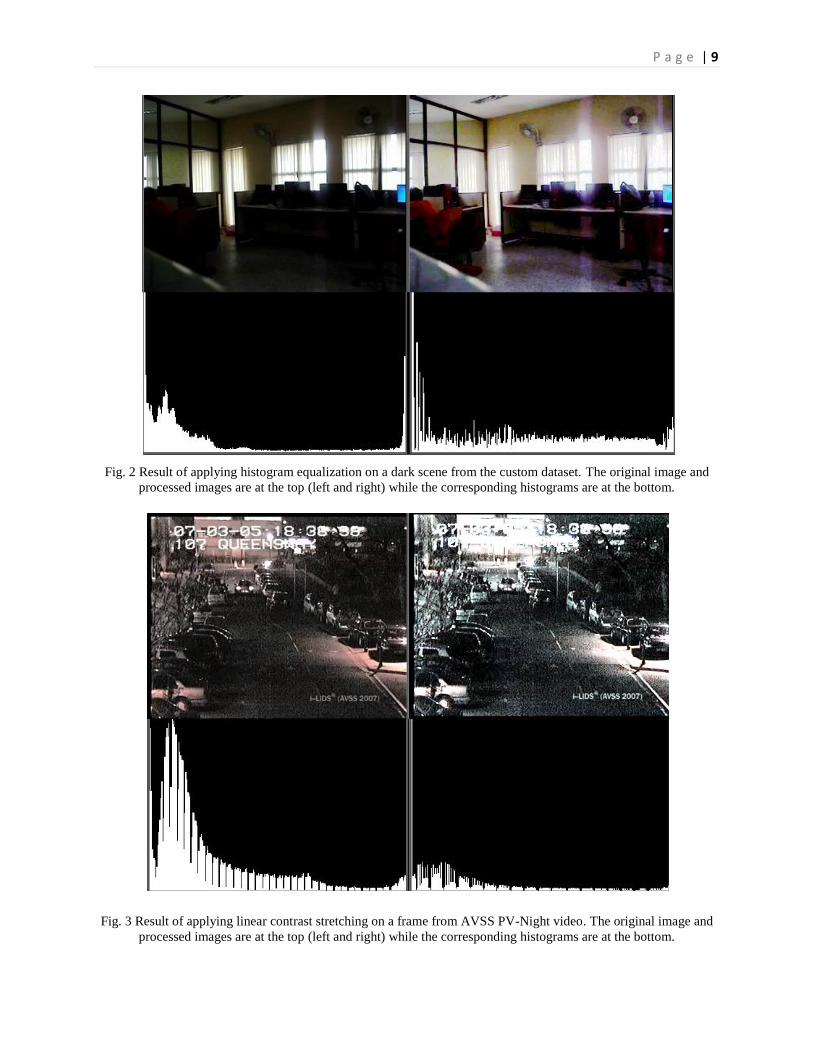
Fig. 2 Result of applying histogram equalization on a dark scene from the custom dataset. The original image and

processed images are at the top (left and right) while the corresponding histograms are at the bottom.

Fig. 3 Result of applying linear contrast stretching on a frame from AVSS PV-Night video. The original image and

processed images are at the top (left and right) while the corresponding histograms are at the bottom.

P a g e | 10

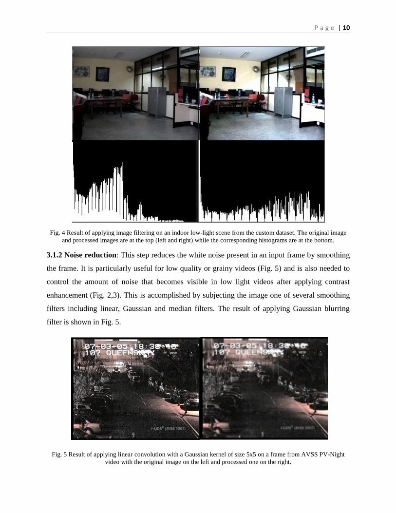
Fig. 4 Result of applying image filtering on an indoor low-light scene from the custom dataset. The original image

and processed images are at the top (left and right) while the corresponding histograms are at the bottom.

3.1.2 Noise reduction: This step reduces the white noise present in an input frame by smoothing

the frame. It is particularly useful for low quality or grainy videos (Fig. 5) and is also needed to

control the amount of noise that becomes visible in low light videos after applying contrast

enhancement (Fig. 2,3). This is accomplished by subjecting the image one of several smoothing

filters including linear, Gaussian and median filters. The result of applying Gaussian blurring

filter is shown in Fig. 5.

Fig. 5 Result of applying linear convolution with a Gaussian kernel of size 5x5 on a frame from AVSS PV-Night

video with the original image on the left and processed one on the right.

P a g e | 11

3.2 Background modeling and subtraction (BGS): The system currently includes three

different BGS algorithms which are modified to perform object level background updating rather

than the typical pixel level one. This is accomplished through a mask of currently tracked objects

that is fed back from the blob tracking module (section 3.5) and is used to disable background

updating at the corresponding pixels This is needed to prevent static foreground objects from

being learned into the background before they can be classified as abandoned or removed by the

abandonment analysis module (section 3.6). A brief description of the three algorithms is

presented below:

3.2.1 Gaussian mixture model (GMM): This method, first introduced in [3] and improved

significantly in [4], models the distribution of pixel intensity values over time as a weighted sum

of three Gaussian distributions. It assumes that the overall intensity at any pixel at each instant is

produced by a combination of background and foreground processes, and each such process can

be modeled by a single Gaussian probability distribution function. For each pixel in the current

frame, the probability of observing the current intensity is given by:

𝑃 𝑋𝑡 = 𝜔𝑖 ,𝑡 ∗ 𝜂 𝑋𝑡 ,𝜇𝑖 ,𝑡 ,Σi,t 𝐾𝑖=1 (2)

Here, K is the no. of distributions (K=3 here); 𝜔𝑖 ,𝑡 is the weight associated with the 𝑖𝑡𝑕

distribution at time t while 𝜇𝑖 ,𝑡 is the mean and Σi,t is the co-variance matrix of this distribution,

𝜂 is the exponential Gaussian probability density function given by:

𝜂 𝑋𝑡 ,𝜇𝑡 ,Σt =1

(2𝜋)𝑛2 Σt

12

𝑒−1

2 𝑋𝑡 − 𝜇𝑡 𝑇Σt

−1 𝑋𝑡 − 𝜇𝑡 (3)

Here, n is the dimensionality of each pixel‘s intensity value (e.g. n=1 for grayscale image and

n=3 for RGB image). In order to avoid a costly matrix inversion and decrease computation cost,

it is also assumed that the red, green and blue channels in the input images are not only

independent but also have the same variance 𝜍𝑘 ,𝑡2 so that the covariance matrix becomes:

Σk,t = 𝜍𝑘 ,𝑡2 𝐈 (4)

The K Gaussian distributions are always ordered in the decreasing order of their contribution to

the current background model. This contribution is measured by the ratio 𝜔/𝜍 under the

assumption that higher is the weight and lower is the variance of a distribution, more is the

P a g e | 12

likelihood that it represents the background process. This assumption stems from the reasonable

supposition that the background process not only has the maximum influence over a pixel‘s

observed intensities but also shows very little variations over time (since the background is by

definition static and unchanging). In the faster version of this method, presented in [4], the

distributions are ordered simply by their weights, thus getting rid of the task of calculating 𝜔/𝜍

and also simplifying the sorting procedure without any significant impact on performance. Both

of the above variants of GMM have been implemented in this system.

For each pixel in an incoming frame, its intensity value is compared with the means of the

existing distributions starting from the first one and a match is said to be obtained if its Euclidean

distance from the mean is less than m standard deviations (m=3 is used here), i.e. it satisfies the

following condition:

𝐼𝑡 − 𝜇𝑘 ,𝑡 < 𝑚 ∗ 𝜍𝑘 ,𝑡 (5)

Here, 𝐼𝑡 is the pixel intensity while 𝜇𝑘 ,𝑡 and 𝜍𝑘 ,𝑡 are the mean and standard deviation of the 𝑘𝑡𝑕

distribution at time t.

Since the background model is dynamic, it needs to be updated with each frame. While the

weights are updated for all distributions, the mean and variance are updated only for the matched

distributions. Following are the standard update equations used for this purpose:

𝜇𝑡 = 1 − 𝜌 𝜇𝑡−1 + 𝜌𝑋𝑡 (6)

𝜍𝑡2 = 1 − 𝜌 𝜍𝑡−1

2 + 𝜌 𝑋𝑡 − 𝜇𝑡 𝑇 𝑋𝑡 − 𝜇𝑡 (7)

𝜔𝑘 ,𝑡 = 1 − 𝛼 𝜔𝑘 ,𝑡−1 + 𝛼 𝑀𝑘 ,𝑡 (8)

Here 𝑋𝑡 is the pixel intensity while 𝑀𝑘 ,𝑡=1 for matched distributions and 0 for unmatched ones

while 𝜌 and 𝛼 are learning rates. In the current work 𝜌 and 𝛼 are related as:

𝜌𝑘 ,𝑡 =𝛼

𝜔𝑘 ,𝑡 (9)

Thus, while 𝛼 is fixed for all distributions (𝛼 = 0.001 used here), 𝜌 is smaller for higher

weighted distributions. If none of the existing distributions match the current intensity, the least

P a g e | 13

probable distribution (i.e. with the smallest value of 𝜔/𝜍) is replaced by a new distribution with

a high initial variance, low prior weight and the new intensity value as its mean.

3.2.2 Adaptive median: This BGS method, described in [1], works under the assumption that

the background is more likely to appear at any given pixel over a period of time than foreground

objects, i.e. the past history of pixel intensity values is likely to contain maximum occurrences of

the background intensity at the pixel location. This leads to the reasonable supposition that the

pixel stays in the background for more than half the values in its history. The median of previous

𝑛 frames can therefore be used as the background model.

Though this BGS method is relatively easy to perform from a computational standpoint, it has

fairly high memory requirements since the previous 𝑛 frames must be stored in a buffer at any

given time and 𝑛 must be quite large to get a good estimate of the actual background. This is

why a simpler recursive version of this algorithm is more practically feasible. In this approach,

the running estimate of the median is incremented by one if the current intensity is larger than

the existing estimate and decremented by one if it is smaller. The estimate is left unchanged if it

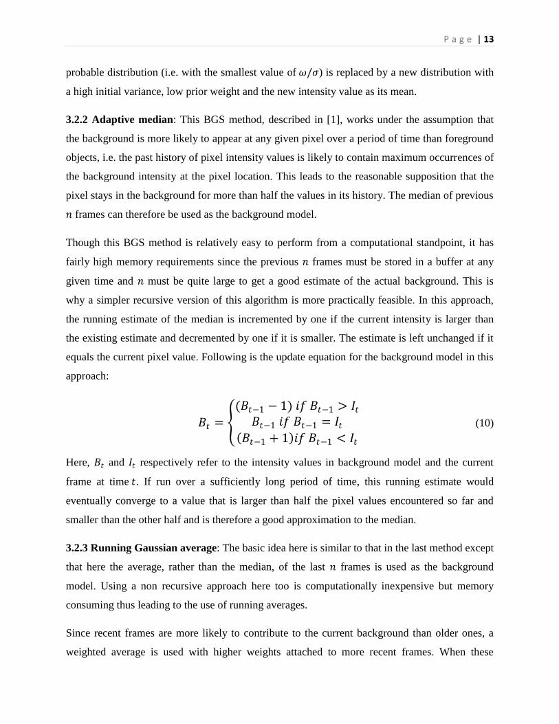
equals the current pixel value. Following is the update equation for the background model in this

approach:

𝐵𝑡 =

(𝐵𝑡−1 − 1) 𝑖𝑓 𝐵𝑡−1 > 𝐼𝑡𝐵𝑡−1 𝑖𝑓 𝐵𝑡−1 = 𝐼𝑡

𝐵𝑡−1 + 1 𝑖𝑓 𝐵𝑡−1 < 𝐼𝑡

(10)

Here, 𝐵𝑡 and 𝐼𝑡 respectively refer to the intensity values in background model and the current

frame at time 𝑡. If run over a sufficiently long period of time, this running estimate would

eventually converge to a value that is larger than half the pixel values encountered so far and

smaller than the other half and is therefore a good approximation to the median.

3.2.3 Running Gaussian average: The basic idea here is similar to that in the last method except

that here the average, rather than the median, of the last 𝑛 frames is used as the background

model. Using a non recursive approach here too is computationally inexpensive but memory

consuming thus leading to the use of running averages.

Since recent frames are more likely to contribute to the current background than older ones, a

weighted average is used with higher weights attached to more recent frames. When these

P a g e | 14

weights vary according to the Gaussian distribution, the running Gaussian average is obtained.

This process can alternatively be interpreted as the fitting of a single Gaussian distribution over

the pixel intensity histogram.

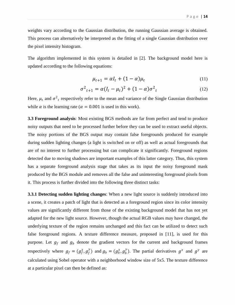
The algorithm implemented in this system is detailed in [2]. The background model here is

updated according to the following equations:

𝜇𝑡+1 = 𝛼𝐼𝑡 + 1 − 𝛼 𝜇𝑡 (11)

𝜍2𝑡+1 = 𝛼(𝐼𝑡 − 𝜇𝑡)

2 + 1 − 𝛼 𝜍2𝑡 (12)

Here, 𝜇𝑡 and 𝜍2𝑡 respectively refer to the mean and variance of the Single Gaussian distribution

while 𝛼 is the learning rate (𝛼 = 0.001 is used in this work).

3.3 Foreground analysis: Most existing BGS methods are far from perfect and tend to produce

noisy outputs that need to be processed further before they can be used to extract useful objects.

The noisy portions of the BGS output may contain false foregrounds produced for example

during sudden lighting changes (a light is switched on or off) as well as actual foregrounds that

are of no interest to further processing but can complicate it significantly. Foreground regions

detected due to moving shadows are important examples of this latter category. Thus, this system

has a separate foreground analysis stage that takes as its input the noisy foreground mask

produced by the BGS module and removes all the false and uninteresting foreground pixels from

it. This process is further divided into the following three distinct tasks:

3.3.1 Detecting sudden lighting changes: When a new light source is suddenly introduced into

a scene, it creates a patch of light that is detected as a foreground region since its color intensity

values are significantly different from those of the existing background model that has not yet

adapted for the new light source. However, though the actual RGB values may have changed, the

underlying texture of the region remains unchanged and this fact can be utilized to detect such

false foreground regions. A texture difference measure, proposed in [11], is used for this

purpose. Let 𝑔𝑓 and 𝑔𝑏 denote the gradient vectors for the current and background frames

respectively where 𝑔𝑓 = (𝑔𝑓𝑥 ,𝑔𝑓

𝑦) and 𝑔𝑏 = (𝑔𝑏

𝑥 ,𝑔𝑏𝑦

). The partial derivatives 𝑔𝑥 and 𝑔𝑦 are

calculated using Sobel operator with a neighborhood window size of 5x5. The texture difference

at a particular pixel can then be defined as:

P a g e | 15

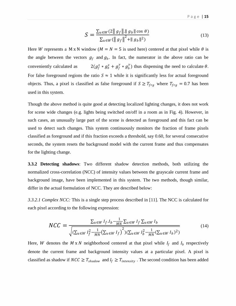
𝑆 = (2 𝑔𝑓 . 𝑔𝑏 cos 𝜃)𝑢∈𝑊

( 𝑔𝑓 2

+ 𝑔𝑏 2

𝑢∈𝑊 ) (13)

Here 𝑊 represents a M x N window (𝑀 = 𝑁 = 5 is used here) centered at that pixel while 𝜃 is

the angle between the vectors 𝑔𝑓 and 𝑔𝑏 . In fact, the numerator in the above ratio can be

conveniently calculated as 2(𝑔𝑓𝑥 ∗ 𝑔𝑏

𝑥 + 𝑔𝑓𝑦∗ 𝑔𝑏

𝑦) thus dispensing the need to calculate 𝜃.

For false foreground regions the ratio 𝑆 ≈ 1 while it is significantly less for actual foreground

objects. Thus, a pixel is classified as false foreground if 𝑆 ≥ 𝑇𝑓𝑟𝑔 where 𝑇𝑓𝑟𝑔 = 0.7 has been

used in this system.

Though the above method is quite good at detecting localized lighting changes, it does not work

for scene wide changes (e.g. lights being switched on/off in a room as in Fig. 4). However, in

such cases, an unusually large part of the scene is detected as foreground and this fact can be

used to detect such changes. This system continuously monitors the fraction of frame pixels

classified as foreground and if this fraction exceeds a threshold, say 0.60, for several consecutive

seconds, the system resets the background model with the current frame and thus compensates

for the lighting change.

3.3.2 Detecting shadows: Two different shadow detection methods, both utilizing the

normalized cross-correlation (NCC) of intensity values between the grayscale current frame and

background image, have been implemented in this system. The two methods, though similar,

differ in the actual formulation of NCC. They are described below:

3.3.2.1 Complex NCC: This is a single step process described in [11]. The NCC is calculated for

each pixel according to the following expression:

𝑁𝐶𝐶 = 𝐼𝑓 .𝐼𝑏𝑢∈𝑊 −

1

𝑀𝑁 𝐼𝑓𝑢∈𝑊 𝐼𝑏𝑢∈𝑊

( 𝐼𝑓2

𝑢∈𝑊 −1

𝑀𝑁 𝐼𝑓𝑢∈𝑊

2)( 𝐼𝑏

2𝑢∈𝑊 −

1

𝑀𝑁 𝐼𝑏𝑢∈𝑊 2)

(14)

Here, 𝑊 denotes the 𝑀 x 𝑁 neighborhood centered at that pixel while 𝐼𝑓 and 𝐼𝑏 respectively

denote the current frame and background intensity values at a particular pixel. A pixel is

classified as shadow if 𝑁𝐶𝐶 ≥ 𝑇𝑠𝑕𝑎𝑑𝑜𝑤 and 𝐼𝑓 ≥ 𝑇𝑖𝑛𝑡𝑒𝑛𝑠𝑖𝑡𝑦 . The second condition has been added

P a g e | 16

to avoid misclassification of very dark areas as shadows. 𝑇𝑠𝑕𝑎𝑑𝑜𝑤 = 0.60 and 𝑇𝑖𝑛𝑡𝑒𝑛𝑠𝑖𝑡𝑦 = 5 have

been used in this work.

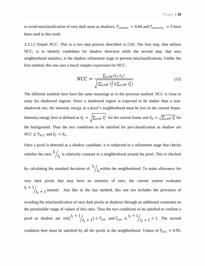
3.3.2.2 Simple NCC: This is a two step process described in [14]. The first step, that utilizes

NCC, is to identify candidates for shadow detection while the second step, that uses

neighborhood statistics, is the shadow refinement stage to prevent misclassifications. Unlike the

first method, this one uses a much simpler expression for NCC:

𝑁𝐶𝐶 = (𝐼𝑓 .𝐼𝑏𝑢∈𝑊 )

( 𝐼𝑓2

𝑢∈𝑊 )( 𝐼𝑏2

𝑢∈𝑊 ) (15)

The different symbols here have the same meanings as in the previous method. NCC is close to

unity for shadowed regions. Since a shadowed region is expected to be darker than a non-

shadowed one, the intensity energy in a pixel‘s neighborhood must be less in the current frame.

Intensity energy here is defined as 𝐸𝑓 = 𝐼𝑓2

𝑢∈𝑊 for the current frame and 𝐸𝑏 = 𝐼𝑏2

𝑢∈𝑊 for

the background. Thus the two conditions to be satisfied for pre-classification as shadow are

𝑁𝐶𝐶 ≥ 𝑇𝑁𝐶𝐶 and 𝐸𝑓 < 𝐸𝑏 .

Once a pixel is detected as a shadow candidate, it is subjected to a refinement stage that checks

whether the ratio 𝐼𝑓𝐼𝑏

is relatively constant in a neighborhood around the pixel. This is checked

by calculating the standard deviation of 𝐼𝑓𝐼𝑏

within the neighborhood. To make allowance for

very dark pixels that may have an intensity of zero, the current system evaluates

𝐼𝑓 + 1𝐼𝑏 + 1 instead. Just like in the last method, this one too includes the provision of

avoiding the misclassification of very dark pixels as shadows through an additional constraint on

the permissible range of values of this ratio. Thus the two conditions to be satisfied to confirm a

pixel as shadow are 𝑠𝑡𝑑(𝐼𝑓 + 1

𝐼𝑏 + 1 ) < 𝑇𝑠𝑡𝑑 and 𝑇𝑚𝑖𝑛 ≤𝐼𝑓 + 1

𝐼𝑏 + 1 < 1. The second

condition here must be satisfied by all the pixels in the neighborhood. Values of 𝑇𝑁𝐶𝐶 = 0.95,

P a g e | 17

𝑇𝑠𝑡𝑑 = 0.05 and 𝑇𝑚𝑖𝑛 = 0.5 have been used in this system. Neighborhood size of 3x3 has been

used for both shadow detection methods.

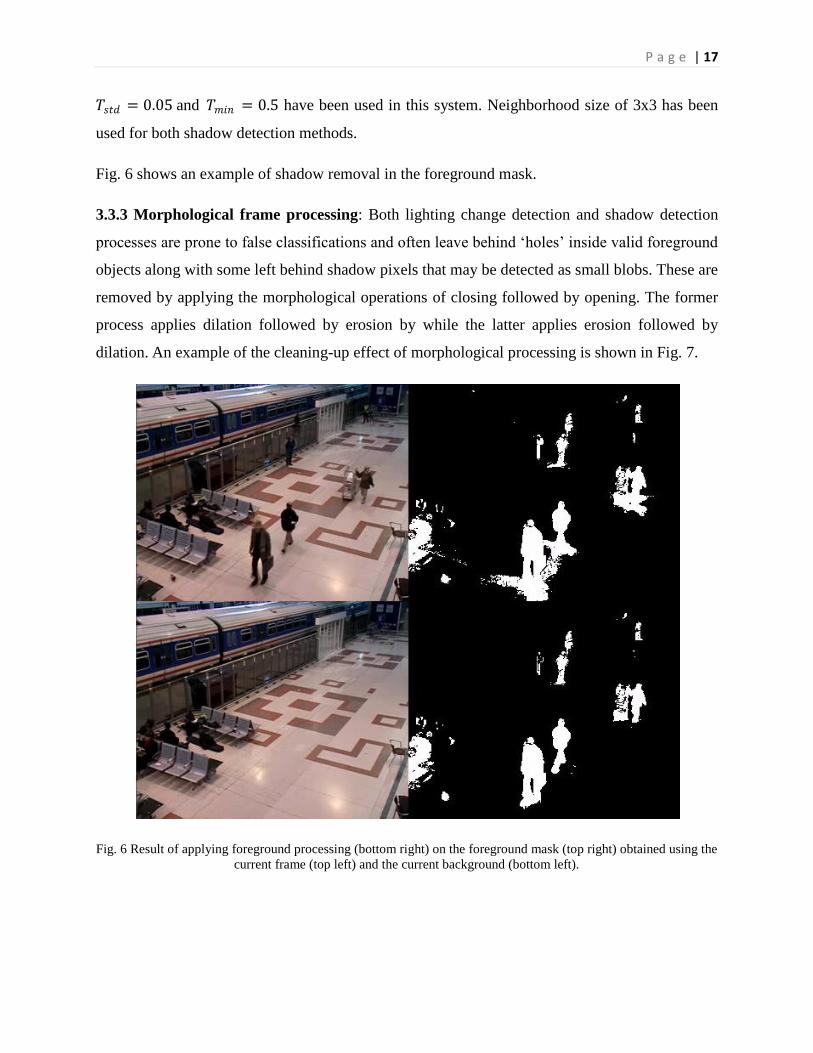
Fig. 6 shows an example of shadow removal in the foreground mask.

3.3.3 Morphological frame processing: Both lighting change detection and shadow detection

processes are prone to false classifications and often leave behind ‗holes‘ inside valid foreground

objects along with some left behind shadow pixels that may be detected as small blobs. These are

removed by applying the morphological operations of closing followed by opening. The former

process applies dilation followed by erosion by while the latter applies erosion followed by

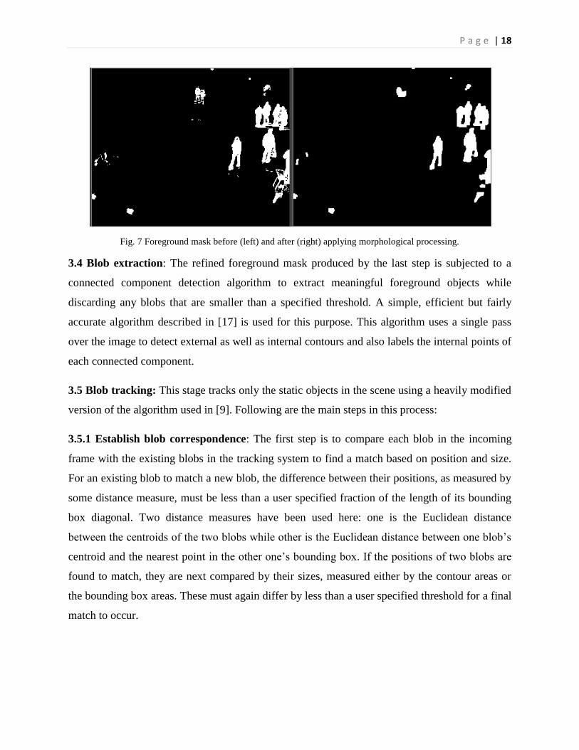
dilation. An example of the cleaning-up effect of morphological processing is shown in Fig. 7.

Fig. 6 Result of applying foreground processing (bottom right) on the foreground mask (top right) obtained using the

current frame (top left) and the current background (bottom left).

P a g e | 18

Fig. 7 Foreground mask before (left) and after (right) applying morphological processing.

3.4 Blob extraction: The refined foreground mask produced by the last step is subjected to a

connected component detection algorithm to extract meaningful foreground objects while

discarding any blobs that are smaller than a specified threshold. A simple, efficient but fairly

accurate algorithm described in [17] is used for this purpose. This algorithm uses a single pass

over the image to detect external as well as internal contours and also labels the internal points of

each connected component.

3.5 Blob tracking: This stage tracks only the static objects in the scene using a heavily modified

version of the algorithm used in [9]. Following are the main steps in this process:

3.5.1 Establish blob correspondence: The first step is to compare each blob in the incoming

frame with the existing blobs in the tracking system to find a match based on position and size.

For an existing blob to match a new blob, the difference between their positions, as measured by

some distance measure, must be less than a user specified fraction of the length of its bounding

box diagonal. Two distance measures have been used here: one is the Euclidean distance

between the centroids of the two blobs while other is the Euclidean distance between one blob‘s

centroid and the nearest point in the other one‘s bounding box. If the positions of two blobs are

found to match, they are next compared by their sizes, measured either by the contour areas or

the bounding box areas. These must again differ by less than a user specified threshold for a final

match to occur.

P a g e | 19

An additional constraint is imposed on the matching process that each existing blob may match

at most one new blob and vice versa All new blobs that do not match any existing blob are added

to the tracking system with their hit counts initialized to one.

3.5.2 Update state variables for existing blobs: Three state variables are maintained for tacked

blobs hit count, miss count and occluded count. When a match is found for an existing blob, its

hit count is incremented by one while its miss and occluded counts are set to zero.

An existing blob that does not match any of the new blobs is checked for occlusion by assuming

that if more than a certain fraction (say 0.8) of the blob‘s pixels has been detected as foreground

in the current frame, then it is occluded by one or more foreground objects. In this case, both its

hit count and occluded count are incremented by one. If the object is not detected as occluded, it

is considered as missing in the current frame and its miss count is incremented by one.

3.5.3 Remove non-static objects: An object is discarded from the tracking system if one of the

following conditions is satisfied:

Not detected/matched for several consecutive frames: This occurs when its miss count

exceeds either a user specified threshold or the current hit count.

Occluded for too long: This occurs when the occluded count exceeds a threshold.

Appearance changes significantly.

A blob‘s appearance information is maintained by storing the incoming frame (or its gradient)

when the blob is first added to the tracking system. If the object is indeed static, its appearance

would not change significantly in subsequent frames as long as it remains visible (i.e. not

occluded). This change in appearance is measured by the mean difference in pixel intensity

between the stored image and the current frame averaged over all the pixels in the blob‘s

bounding box. If this difference exceeds a threshold, the object is immediately discarded. An

exponential moving average of these mean differences is also maintained for use by the

abandonment analysis module for distinguishing between actual static objects and very still

persons.

3.5.4 Change object label: If the hit count of an object exceeds a user defined threshold, it is

labeled as static and its maximum permissible occluded and miss counts are multiplied by

P a g e | 20

respective constant factors to make greater allowance for accidental misses and prolonged

occlusions. If it exceeds a second higher threshold, this object is passed to the abandonment

analysis module to be classified as abandoned or removed.

3.5.5 Provide feedback to the BGS module: To prevent static objects from being learnt into the

background, all the tracked objects that are detected in the current frame fed back to the BGS

module so that the background model is not updated for pixels contained in their bounding

boxes. An object as a whole is pushed into the background if one of the following conditions

hold true:

i. It is detected as a state change in the abandonment analysis module.

ii. It is detected as abandoned or removed and the alarm timeout has been reached.

This feedback enables the BGS algorithm to perform object-level (as opposed to pixel-level)

background updating and thus helps to avoid foreground fragmentation in addition to maintain

the objects of interest in the foreground.

3.6 Abandonment analysis: This is the final stage whose purpose is to prevent false detections

of abandoned objects due to the ‗ghost effect‘ created when an object in the background is

removed, leaving behind a false foreground object. It also checks the blob‘s internal variation

during the period it has been tracked to ensure that it is not a very still person. This module

therefore can be divided into two sub-modules:

3.6.1 Removed object detection: When a background object is removed from the scene, it is

reasonable to assume that the area thus vacated will now exhibit a higher degree of agreement

with its immediate surroundings than before since that object was presumably hiding a part of

the relatively uniform backdrop that was visible in its neighborhood. Conversely, when a new

object is added to the scene, the region where it lies is likely to show a decreased level of

conformity with its surroundings. This assumption can be used to classify an object as

abandoned or removed by evaluating, in both the background image and the current frame, a

measure of agreement of the object‘s edge (and nearby interior) pixels with their immediate

neighborhood pixels (outside the object). Provided that the two images exhibit a significant

difference in conformity levels, the object is likely to be an abandoned object if the background

image shows greater agreement and a removed object otherwise. If the two images exhibit fairly

P a g e | 21

similar degrees of conformity, the object is likely to represent a state change (like a door

closing). Following two methods have been implemented to measure this degree of agreement in

this system:

3.6.1.1 Region Growing: This method was introduced in [29] and consists of a two step process.

In the first step, the blob‘s boundary is eroded to obtain a set of pixels that lie near the boundary

but are completely inside the object. These pixels are then used as seed points in a standard

region growing algorithm to add all the surrounding pixels that are similar to these. This process

is repeated for both the background and the current frame. The image not containing the object is

likely to exhibit a significantly greater number of added pixels than the other one where the

region growing process would stop around the object‘s actual boundaries. Thus, the object is

considered removed if the region growth is significantly more in the current frame and

abandoned otherwise.

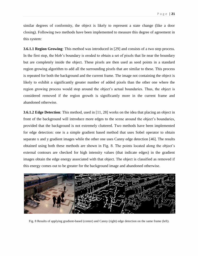
3.6.1.2 Edge Detection: This method, used in [11, 28] works on the idea that placing an object in

front of the background will introduce more edges to the scene around the object‘s boundaries,

provided that the background is not extremely cluttered. Two methods have been implemented

for edge detection: one is a simple gradient based method that uses Sobel operator to obtain

separate x and y gradient images while the other one uses Canny edge detection [46]. The results

obtained using both these methods are shown in Fig. 8. The points located along the object‘s

external contours are checked for high intensity values (that indicate edges) in the gradient

images obtain the edge energy associated with that object. The object is classified as removed if

this energy comes out to be greater for the background image and abandoned otherwise.

Fig. 8 Results of applying gradient-based (center) and Canny (right) edge detection on the same frame (left).

P a g e | 22

3.6.2 Still person detection: As mentioned in section 5, an exponential running average of mean

pixel differences between the current frame and the stored image is maintained for each object in

the tracking system. The basic idea here, introduced in [45] is that while the appearance of a true

static object remains completely unchanged (provided that it is not occluded) frame after frame

while a false static object detected due to a very still person will show some variations in the

pixel values within the constant bounding box (unless the person is standing perfectly and

unnaturally still). These internal blob variations are captured by the running average of mean

differences and if this value exceeds a certain threshold, the object is classified as a still person.

In order to make this process immune to lighting changes, gradient images, instead of the actual

images, can be used to calculate these mean differences.

3.7 Blob filtering: The abandonment module classifies a static blob into one of four categories:

abandoned, removed, state change or still person. A blob detected as a state change or a still

person is removed from the tracking system. If a state change, it is also pushed into the

background. An object detected as abandoned causes an alarm to be raised immediately while

one detected as removed is first passed through a filtering process where it is compared to each

of the user-specified regions in the scene (provided that any have been added to the filtering

module). An alarm is raised only if it matches one of them. This matching can be done on the

basis of the blob‘s position, size, appearance or any combination of these, as specified by the

user.

4. Development of Software

The present system has been built using a modular approach with several distinct sub-systems,

each of which solves a particular aspect of the AOD problem. Since this system is meant to be

more of a flexible framework than a stand-alone system, multiple methods have been

implemented for each of these sub-systems with the possibility of adding more in the future

without too much re-programming effort. All of these methods have been integrated into the

system in such a way that the user has the option to not only tweak the parameters of any one

method but to switch between different methods in real time while observing its impact in terms

of both accuracy and speed. It is also possible to switch between the online and offline input

sources without having to restart the system run.

P a g e | 23

The application‘s user interface has been designed to allow the user to interact with the system in

the following ways:

Adjust each of the system parameters and switch between the different methods

implemented in each module in real time. This can help to quickly find the optimal values

of various parameters and determine the combination of methods that provide the best

performance in any given scenario.

Switch between different input sources (camera or video file) as well as different datasets

(or different videos in the same dataset) in real time without having to restart the system

run. This can be useful for gauging the performance of a particular combination of

methods and parameters under different scenarios.

Selectively modify the BGS process by selecting some or all of the blobs in the current

frame to be pushed into the background. This can help the system to take advantage of

the vastly superior human visual processing ability to improve its performance in very

difficult scenarios while still being completely autonomous most of the time.

This feature is particularly useful at the beginning of the video stream processing (or after

a scene wide appearance change) when the background model differs significantly from

the true background, thus leading to several false foreground blobs. These can not only

slow down the processing speed but can also occlude actual foreground objects of

interest. The user, in such cases, can conveniently push all unwanted blobs into the

background at the press of a key.

Specify particular locations in the scene which are to be monitored for removed objects

(refer section 3.7). For example, the user may want an alarm to be raised only for some

valuable items in the scene (e.g. a CPU or monitor in a computer lab) but not for non-

important items (e.g. chairs).

Alter the input video stream either by pausing or by fast-forwarding it to a particular

frame. The former can be used to test the results of applying different processing methods

(e.g. detecting edges using either Sobel gradient operator or Canny edge detection) on the

P a g e | 24

same frame while the latter can be useful for quickly getting to the point of interest (e.g.

the actual drop or removal event).

Adjust the processing resolution in real time and observe its impact on both performance

and accuracy.

This application has been written entirely in C++ using OpenCV library that allows track bars

and mouse/keyboard events as the only options for user interactions. Therefore parameter

adjusting and switching between different methods, input sources or datasets are all

accomplished using track bars. Each module in the system displays one or more windows where

that module‘s output is displayed along with all the relevant track bars. A couple of sample

windows are shown in Fig. 8. Keyboard events are used for modifying the BGS process while

mouse events are used for selecting objects to remove (push into the background) or add (for

filtering).

The system can take its input from a video file as well as from a camera attached to the system.

The video files must have their filenames formatted in the certain manner that specifies their set,

camera angle and size. The shows the output images of all the stages in different windows and

also saves the important ones into separate video files so that they can be run later at the original

frame rates.

An important aspect of this system is the large number of user-adjustable parameters that it

offers. Each of the five main modules has its own parameters and in all there are currently more

than 50 parameters, all of them adjustable in real time. The system reads the initial values of

these parameters from an ASCII text file that can be formatted in a user friendly way with

comments describing the purpose and possible values of each of these parameters. During the

program execution, each parameter is assigned its own sliding track bar in the appropriate

window and can be conveniently adjusted by moving the slider. Each of the subsystems creates

one or more windows to display its output and place the track bars. Since OpenCV places a very

strict limit on the length of track bar labels, the user is also provided a detailed description of

each track bar along with its possible values whenever a mouse click is received anywhere inside

the concerned window (Fig. 10,11,15).

P a g e | 25

Following are the main modules along with screenshots and descriptions of the interface they

provide to the user:

4.1 User interface module: This module is responsible for allowing the user to change the input

source in real time. It also allows the user to adjust the processing resolution in case it is desired

to be lower than the original input resolution so as to increase the processing speed. It creates

two windows: one shows the current input frame in its original resolution along with the input

source parameters while the other one shows a combined image with current frame, processed

and un-processed foreground masks, the background image and the results produced by the

abandonment module (either edge detection or region growing) for both current and background

images. Both of these windows also show the average and current frame rates obtained with the

present configuration. The images displayed in the second window are all at the processing

resolution. Examples of the two windows are shown in Fig. 9.

Fig. 9 Windows created by the User interface module showing the processing (left) and input source (right)

parameters

4.2 Pre-processing module: As stated in section 3.1, this module carries out two functions:

contrast enhancement and noise reduction. It creates one window that allows the user to enable

or disable these functions, choose one of the several methods for carrying each out and adjust the

parameters relevant to the chosen method. It also provides an option to display the histograms of

images computed before and after they are pre-processed. The image displayed in this window is

P a g e | 26

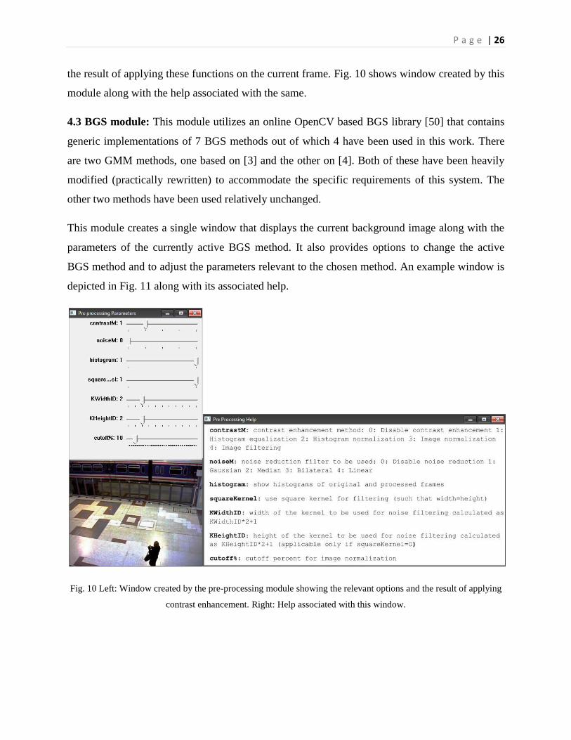
the result of applying these functions on the current frame. Fig. 10 shows window created by this

module along with the help associated with the same.

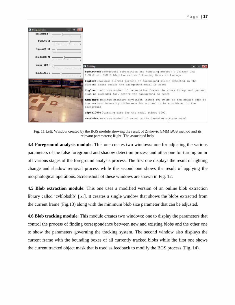
4.3 BGS module: This module utilizes an online OpenCV based BGS library [50] that contains

generic implementations of 7 BGS methods out of which 4 have been used in this work. There

are two GMM methods, one based on [3] and the other on [4]. Both of these have been heavily

modified (practically rewritten) to accommodate the specific requirements of this system. The

other two methods have been used relatively unchanged.

This module creates a single window that displays the current background image along with the

parameters of the currently active BGS method. It also provides options to change the active

BGS method and to adjust the parameters relevant to the chosen method. An example window is

depicted in Fig. 11 along with its associated help.

Fig. 10 Left: Window created by the pre-processing module showing the relevant options and the result of applying

contrast enhancement. Right: Help associated with this window.

P a g e | 27

Fig. 11 Left: Window created by the BGS module showing the result of Zivkovic GMM BGS method and its

relevant parameters; Right: The associated help.

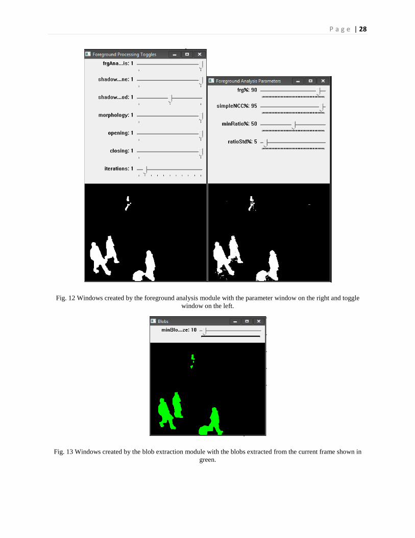
4.4 Foreground analysis module: This one creates two windows: one for adjusting the various

parameters of the false foreground and shadow detection process and other one for turning on or

off various stages of the foreground analysis process. The first one displays the result of lighting

change and shadow removal process while the second one shows the result of applying the

morphological operations. Screenshots of these windows are shown in Fig. 12.

4.5 Blob extraction module: This one uses a modified version of an online blob extraction

library called ‗cvblobslib‘ [51]. It creates a single window that shows the blobs extracted from

the current frame (Fig.13) along with the minimum blob size parameter that can be adjusted.

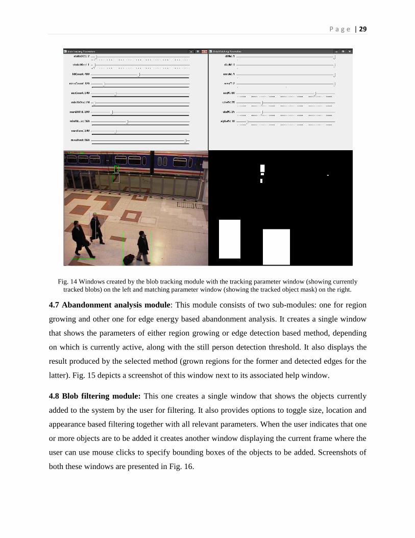
4.6 Blob tracking module: This module creates two windows: one to display the parameters that

control the process of finding correspondence between new and existing blobs and the other one

to show the parameters governing the tracking system. The second window also displays the

current frame with the bounding boxes of all currently tracked blobs while the first one shows

the current tracked object mask that is used as feedback to modify the BGS process (Fig. 14).

P a g e | 28

Fig. 12 Windows created by the foreground analysis module with the parameter window on the right and toggle

window on the left.

Fig. 13 Windows created by the blob extraction module with the blobs extracted from the current frame shown in

green.

P a g e | 29

Fig. 14 Windows created by the blob tracking module with the tracking parameter window (showing currently

tracked blobs) on the left and matching parameter window (showing the tracked object mask) on the right.

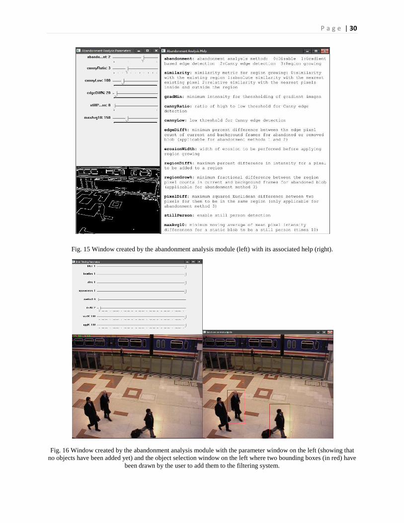
4.7 Abandonment analysis module: This module consists of two sub-modules: one for region

growing and other one for edge energy based abandonment analysis. It creates a single window

that shows the parameters of either region growing or edge detection based method, depending

on which is currently active, along with the still person detection threshold. It also displays the

result produced by the selected method (grown regions for the former and detected edges for the

latter). Fig. 15 depicts a screenshot of this window next to its associated help window.

4.8 Blob filtering module: This one creates a single window that shows the objects currently

added to the system by the user for filtering. It also provides options to toggle size, location and

appearance based filtering together with all relevant parameters. When the user indicates that one

or more objects are to be added it creates another window displaying the current frame where the

user can use mouse clicks to specify bounding boxes of the objects to be added. Screenshots of

both these windows are presented in Fig. 16.

P a g e | 30

Fig. 15 Window created by the abandonment analysis module (left) with its associated help (right).

Fig. 16 Window created by the abandonment analysis module with the parameter window on the left (showing that

no objects have been added yet) and the object selection window on the left where two bounding boxes (in red) have

been drawn by the user to add them to the filtering system.

P a g e | 31

5. Testing and Analysis

5.1 Setup: Since the system features multiple methods for several of its modules, it is not

possible to provide the results of every possible combination of these methods. Therefore, some

preliminary testing was done and the following combination of methods was found to give good

results in most cases:

Pre-processing: Both contrast enhancement and noise reduction were turned off except in a

few night/low light scenes.

BGS: modified GMM introduced in [4] (section 3.2.1).

Shadow detection: Simple NCC based method (section 3.3.2)

Morphological processing: Both closing and opening operations were enabled (section 3.3.3).

Abandonment analysis: Canny edge detection (sub-section 3.6.1.2).

The results presented here have been obtained using this configuration for all the tests with only

a few minor modifications for specific cases.

5.2 Datasets: This system has been tested on 4 different databases, 3 of which are publicly

available benchmark databases while one is a custom prepared dataset with videos of various

indoor and outdoor scenarios featuring both day and night time scenes. Following is a brief

description of these datasets:

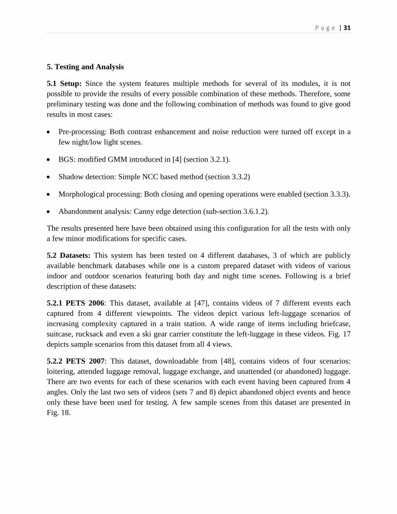
5.2.1 PETS 2006: This dataset, available at [47], contains videos of 7 different events each

captured from 4 different viewpoints. The videos depict various left-luggage scenarios of

increasing complexity captured in a train station. A wide range of items including briefcase,

suitcase, rucksack and even a ski gear carrier constitute the left-luggage in these videos. Fig. 17

depicts sample scenarios from this dataset from all 4 views.

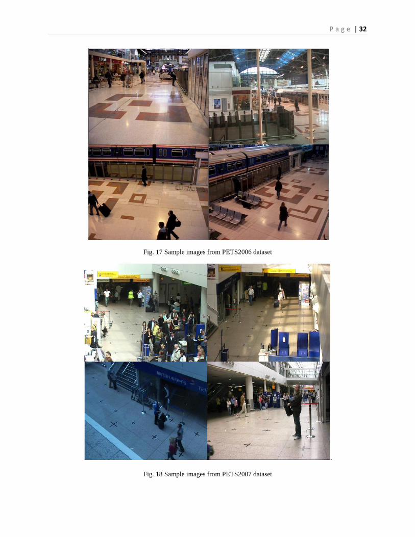
5.2.2 PETS 2007: This dataset, downloadable from [48], contains videos of four scenarios:

loitering, attended luggage removal, luggage exchange, and unattended (or abandoned) luggage.

There are two events for each of these scenarios with each event having been captured from 4

angles. Only the last two sets of videos (sets 7 and 8) depict abandoned object events and hence

only these have been used for testing. A few sample scenes from this dataset are presented in

Fig. 18.

P a g e | 32

Fig. 17 Sample images from PETS2006 dataset

.

Fig. 18 Sample images from PETS2007 dataset

P a g e | 33

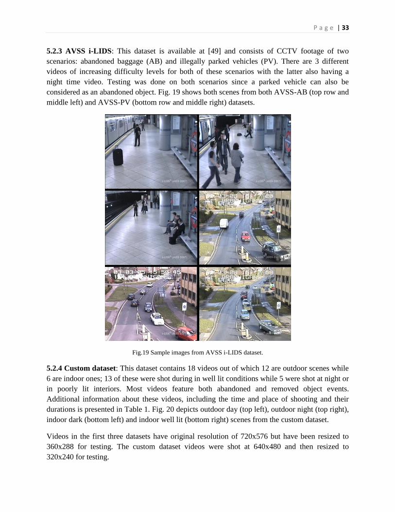
5.2.3 AVSS i-LIDS: This dataset is available at [49] and consists of CCTV footage of two

scenarios: abandoned baggage (AB) and illegally parked vehicles (PV). There are 3 different

videos of increasing difficulty levels for both of these scenarios with the latter also having a

night time video. Testing was done on both scenarios since a parked vehicle can also be

considered as an abandoned object. Fig. 19 shows both scenes from both AVSS-AB (top row and

middle left) and AVSS-PV (bottom row and middle right) datasets.

Fig.19 Sample images from AVSS i-LIDS dataset.

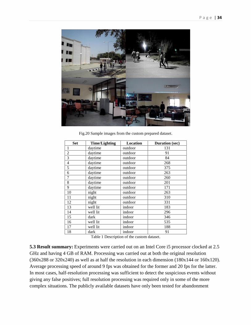
5.2.4 Custom dataset: This dataset contains 18 videos out of which 12 are outdoor scenes while

6 are indoor ones; 13 of these were shot during in well lit conditions while 5 were shot at night or

in poorly lit interiors. Most videos feature both abandoned and removed object events.

Additional information about these videos, including the time and place of shooting and their

durations is presented in Table 1. Fig. 20 depicts outdoor day (top left), outdoor night (top right),

indoor dark (bottom left) and indoor well lit (bottom right) scenes from the custom dataset.

Videos in the first three datasets have original resolution of 720x576 but have been resized to

360x288 for testing. The custom dataset videos were shot at 640x480 and then resized to

320x240 for testing.

P a g e | 34

Fig.20 Sample images from the custom prepared dataset.

Set Time/Lighting Location Duration (sec)

1 daytime outdoor 131

2 daytime outdoor 91

3 daytime outdoor 84

4 daytime outdoor 268

5 daytime outdoor 375

6 daytime outdoor 263

7 daytime outdoor 260

8 daytime outdoor 201

9 daytime outdoor 171

10 night outdoor 263

11 night outdoor 310

12 night outdoor 331

13 well lit indoor 183

14 well lit indoor 296

15 dark indoor 346

16 well lit indoor 535

17 well lit indoor 188

18 dark indoor 91

Table 1 Description of the custom dataset.

5.3 Result summary: Experiments were carried out on an Intel Core i5 processor clocked at 2.5

GHz and having 4 GB of RAM. Processing was carried out at both the original resolution

(360x288 or 320x240) as well as at half the resolution in each dimension (180x144 or 160x120).

Average processing speed of around 9 fps was obtained for the former and 20 fps for the latter.

In most cases, half-resolution processing was sufficient to detect the suspicious events without

giving any false positives; full resolution processing was required only in some of the more

complex situations. The publicly available datasets have only been tested for abandonment

P a g e | 35

events while the custom dataset has been tested for both abandonment and removal events. The

results have been summarized below in Tables 2 and 3.

Set Actual events True detections False detections

Still Persons Other objects

PETS2006

1 4 4 0 1

2 4 4 0 0

3 0 0 0 0

4 0 0 1 0

5 4 4 1 1

6 4 4 0 1

7 4 3 0 1

Total 20 19 2 4

PETS2007

7 4 3 0 0

8 4 3 0 0

Total 8 6 0 0

AVSS i-LIDS

AB Easy 1 1 0 0

Medium 1 1 0 0

Hard 1 1 1 1

Total 3 3 1 0

PV Easy 1 1 0 0

Medium 1 0 0 1

Hard 1 0 0 1

Night 1 1 0 0

Total 4 2 0 2

Total 7 5 1 3

Custom dataset

1 1 1 0 0

2 1 1 0 0

3 0 0 0 0

4 2 2 0 0

5 2 2 0 0

6 2 1 0 0

7 2 0 0 0

8 2 2 0 0

9 1 0 0 1

10 2 2 0 0

11 2 2 0 0

12 2 2 0 0

13 2 2 0 0

14 2 2 1 0

15 2 0 0 0

16 8 8 0 1

17 1 1 0 0

18 1 0 0 0

Total 35 28 1 2

Overall 70 58 4 9

Table 2 Result summary for all the datasets

P a g e | 36

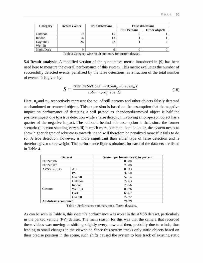
Category Actual events True detections False detections

Still Persons Other objects

Outdoor 19 15 0 1

Indoor 16 13 1 1

Daytime /

Well lit

26 22 1 2

Night/Dark 9 6 0 0

Table 3 Category wise result summary for custom dataset.

5.4 Result analysis: A modified version of the quantitative metric introduced in [9] has been

used here to measure the overall performance of this system. This metric evaluates the number of

successfully detected events, penalized by the false detections, as a fraction of the total number

of events. It is given by:

𝑆 =𝑡𝑟𝑢𝑒 𝑑𝑒𝑡𝑒𝑐𝑡𝑖𝑜𝑛𝑠 −(0.5∗𝑛𝑝+0.25∗𝑛𝑏 )

𝑡𝑜𝑡𝑎𝑙 𝑛𝑜 .𝑜𝑓 𝑒𝑣𝑒𝑛𝑡𝑠 (16)

Here, 𝑛𝑝and 𝑛𝑏 respectively represent the no. of still persons and other objects falsely detected

as abandoned or removed objects. This expression is based on the assumption that the negative

impact on performance of detecting a still person as abandoned/removed object is half the

positive impact due to a true detection while a false detection involving a non-person object has a

quarter of the negative impact. The rationale behind this assumption is that, since the former

scenario (a person standing very still) is much more common than the latter, the system needs to

show higher degree of robustness towards it and will therefore be penalized more if it fails to do

so. A true detection, however, is more significant than either type of false detection and is

therefore given more weight. The performance figures obtained for each of the datasets are listed

in Table 4.

Dataset System performance (S) in percent

PETS2006 85.00

PETS2007 75.00

AVSS i-LiDS AB 83.33

PV 37.50

Overall 57.14

Custom

Outdoor 77.63

Indoor 76.56

Well Lit 80.76

Dark 66.67

Overall 72.72

All datasets combined 76.79

Table 4 Performance summary for different datasets.

As can be seen in Table 4, this system‘s performance was worst in the AVSS dataset, particularly

in the parked vehicle (PV) dataset. The main reason for this was that the camera that recorded

these videos was moving or shifting slightly every now and then, probably due to winds, thus

leading to small changes in the viewpoint. Since this system tracks only static objects based on

their precise position in the scene, such shifts caused the system to lose track of existing static

P a g e | 37

objects and start tracking them all over again. In addition, the camera exposure appeared to be

changing frequently leading to several scene-wide lighting changes and this in turn caused the

background to be reset repeatedly. Performance in the abandoned object (AB) dataset was much

better with 100% detection rate though there were a couple of false detections in the AB-Hard

video sequence.

The system‘s performance in the remaining datasets was fairly good, being consistently above

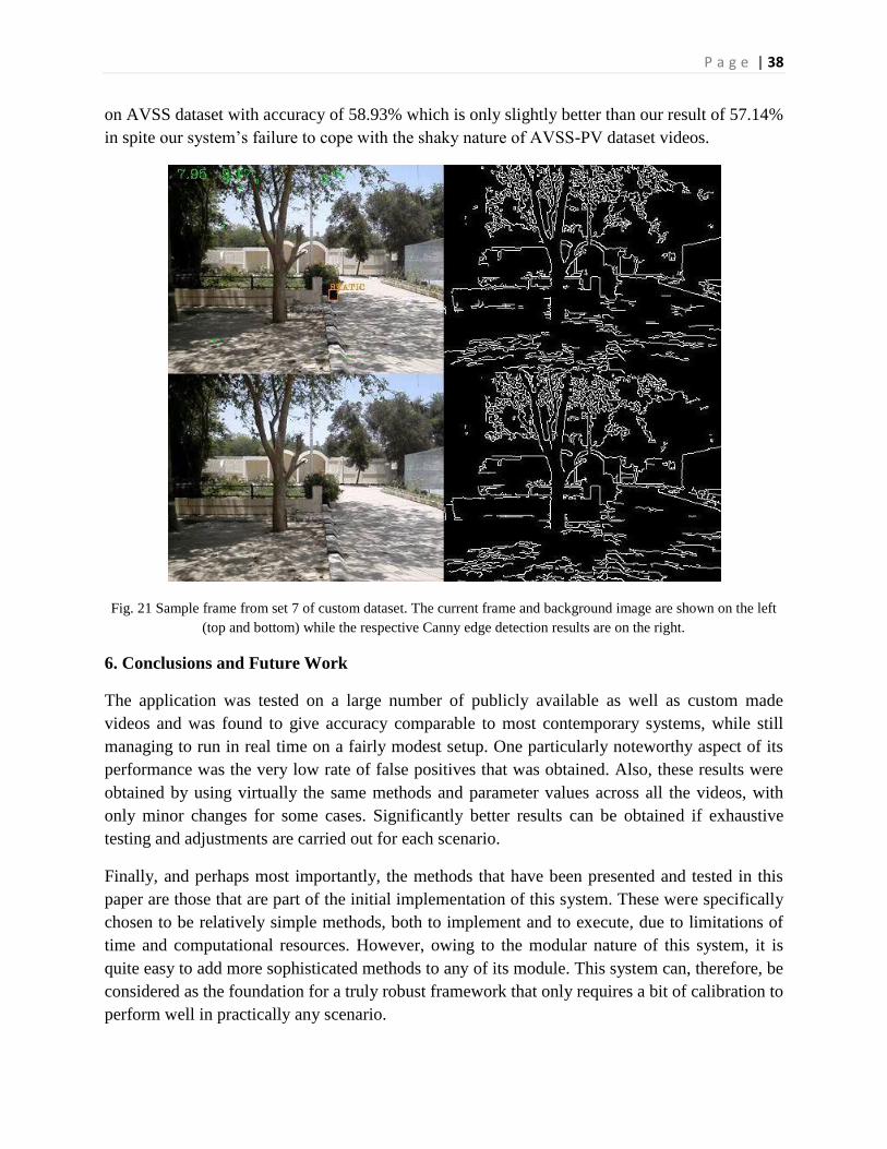
the 70% accuracy mark. The only major failures in the custom dataset were in sets 7, 9, 15 and

18. The first one occurred because of extremely cluttered background that always presents

problems for the edge detection based abandonment analysis employed here (Fig. 21). The

second one occurred because the black colored test object was placed in a shadowy region and

was invisible even to human eyes. A similar issue plagued the last two videos since they were

shot in very dark indoor conditions and the test object simply blended in with the background in

spite of applying contrast enhancement during pre processing.

Performance in the two PETS datasets was quite similar, with PETS2006 showing slightly better

results. This occurred mainly because one of the views in PETS2007 (view 1) featured a very

crowded queue that led to constant occlusions of the test object. In addition, the objects in this

dataset were left behind for too short periods of times for alarm to be successfully raised.

5.5 Comparison with existing systems: Though both PETS2006 and AVSS i-LiDS datasets

have been used for testing in many contemporary works in literature, very few of these report

sufficiently detailed results for direct comparison with our results. For example, even though

PETS2006 has been used in [9], [10], [21], [22], [24] and [29], the results for all 4 views have

not been reported in even one In addition, some, like [24] and [21], have provided no

information about false positives.

Combined results for PETS2006 and AVSS-AB datasets have been reported in [9]. Using a

similar but slightly more relaxed metric, the overall accuracy reported there is 85.20%. The

corresponding figure for our system is 84.78%.though it must be noted that this has been

obtained using a stricter metric. The results in [10] have been reported for AVSS-AB dataset

with accuracy of 66.67% which is significantly worse than our result of 83.33%. The results of

AVSS-PV and PETS2006 datasets have also been reported here but only partially and cannot be

compared with our results. The system presented in [21] has been tested on PETS2006 and

PETS2007 datasets but no information has been provided about false positives or individual

views, again rendering it unsuitable for comparison with our system.

Results in [22], [24] and [29] have been reported for only one view for each of the 7 scenarios in

PETS2006 dataset. In addition, the actual false positive count has not been reported in [22] and

[24]. The approximate accuracy figures are 80% for [22] and 91.67% for [24] and 90% for [29].

These are comparable to our accuracy of 85% obtained over all the 4 views; choosing only the

best result for each scenario would increase it to 100%. The system in [29] has also been tested

P a g e | 38

on AVSS dataset with accuracy of 58.93% which is only slightly better than our result of 57.14%

in spite our system‘s failure to cope with the shaky nature of AVSS-PV dataset videos.

Fig. 21 Sample frame from set 7 of custom dataset. The current frame and background image are shown on the left

(top and bottom) while the respective Canny edge detection results are on the right.

6. Conclusions and Future Work

The application was tested on a large number of publicly available as well as custom made

videos and was found to give accuracy comparable to most contemporary systems, while still

managing to run in real time on a fairly modest setup. One particularly noteworthy aspect of its

performance was the very low rate of false positives that was obtained. Also, these results were

obtained by using virtually the same methods and parameter values across all the videos, with

only minor changes for some cases. Significantly better results can be obtained if exhaustive

testing and adjustments are carried out for each scenario.

Finally, and perhaps most importantly, the methods that have been presented and tested in this

paper are those that are part of the initial implementation of this system. These were specifically

chosen to be relatively simple methods, both to implement and to execute, due to limitations of

time and computational resources. However, owing to the modular nature of this system, it is

quite easy to add more sophisticated methods to any of its module. This system can, therefore, be

considered as the foundation for a truly robust framework that only requires a bit of calibration to

perform well in practically any scenario.

P a g e | 39

Appendix A: Explanation of Source Code

The application has been coded entirely in C++ and makes use of OpenCV 2.4.4 library. The

coding was done using Microsoft Visual Studio 2008 IDE and the application therefore exists as

a Visual C++ solution.

A modular approach has been chosen to design this application with a view to facilitate easy

expandability in the future. The application source is divided into 8 main modules and 4 helper

modules, each consisting of one or more classes. A brief description of each of these modules

follows along with an explanation of the important functions and variables.

A.1. Main modules

A.1.1 User interface module

Purpose: Creates the input-output interface for the user and allow the adjustment of various

frame processing options (section 4.1).

Files: userInterface.hpp (header) and userInterface.cpp (function definitions)

Class Name: UserInterface

Core member functions:

i. initInputInterface: sets up the input video stream either from camera or from a

video file; also creates several windows with which the user interacts with the

application.

ii. initOutputInterface: sets up the video writers that save the outputs of arious

modules as a video file on disk; also sets up various images that display these outputs to

the user in real time.

iii. initProcInterface: sets up several images that are used for proccessing by other

modules; also provides the user the option to change the processing resolution in real

time.

iv. initInterface: wrapper function for the above three functions and called whenever

the user adjusts some input/processing parameters that require a system reset.

v. initIOParams/initProcParams: initialize the input-output and processing

parameters with values provided by the SystemParameters module.

Window related member functions:

i. initIOWindow/updateInputSource/updateIOParams: setup the window that

provides options for changing the input source in real time.

ii. initProcWindow/updateProcParams: setup the window that allows the user to

adjust the processing resolution in real time.

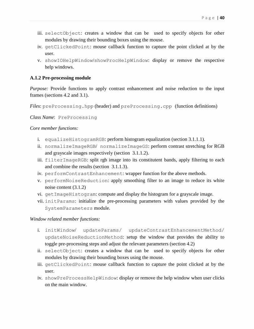
P a g e | 40

iii. selectObject: creates a window that can be used to specify objects for other

modules by drawing their bounding boxes using the mouse.

iv. getClickedPoint: mouse callback function to capture the point clicked at by the

user.

v. showIOHelpWindow/showProcHelpWindow: display or remove the respective

help windows.

A.1.2 Pre-processing module

Purpose: Provide functions to apply contrast enhancement and noise reduction to the input

frames (sections 4.2 and 3.1).

Files: preProcessing.hpp (header) and preProcessing.cpp (function definitions)

Class Name: PreProcessing

Core member functions:

i. equalizeHistogramRGB: perform histogram equalization (section 3.1.1.1).

ii. normalizeImageRGB/ normalizeImageGS: perform contrast stretching for RGB

and grayscale images respectively (section 3.1.1.2).

iii. filterImageRGB: split rgb image into its constitutent bands, apply filtering to each

and combine the results (section 3.1.1.3).

iv. performContrastEnhancement: wrapper function for the above methods.

v. performNoiseReduction: apply smoothing filter to an image to reduce its white

noise content (3.1.2)

vi. getImageHistogram: compute and display the histogram for a grayscale image.

vii. initParams: initialize the pre-processing parameters with values provided by the

SystemParameters module.

Window related member functions:

i. initWindow/ updateParams/ updateContrastEnhancementMethod/

updateNoiseReductionMethod: setup the window that provides the ability to

toggle pre-processing steps and adjust the relevant parameters (section 4.2)

ii. selectObject: creates a window that can be used to specify objects for other

modules by drawing their bounding boxes using the mouse.

iii. getClickedPoint: mouse callback function to capture the point clicked at by the

user.

iv. showPreProcessHelpWindow: display or remove the help window when user clicks

on the main window.

P a g e | 41

A.1.3 BGS module

Purpose: Provide functions to conveniently use and switch between the various BGS methods

adapted from the online OpenCV BGS library [50]. It therefore serves as a unifying

frontend/wrapper for the different classes used for the four BGS techniques.

Files: bgsModels.hpp (header) and bgsModels.cpp (function definitions)

Class Name: BgsModels

Core member functions:

i. initBGSModels: initializes the structures that hold parameters for each of the four

BGS methods.

ii. initBGSMethod: sets up the currently active BGS method.

iii. initBGSParams /initBGSToggleParams: initializes the parameters of the chosen

BGS method with values provided by the SystemParameters module.

Window related member functions:

i. initWindow/updateBGSMethod/updateBGSToggleParams: setup the window

that allows user to switch between BGS methods and adjust parameters of the chosen

BGS method.

ii. showBGSHelpWindow: display or remove the help window when user clicks on the

main window.

A.1.4 Foreground analysis module

Purpose: Refine the foreground mask produced by the BGS module by removing shadows and

regions of sudden lighting changes (section 3.3).

Files: foregroundProcessing.hpp (header) and foregroundProcessing.cpp

(function definitions)

Class Name: ForegroundProc

Core member functions:

i. detectLightingChange: detects and removes foreground regions created due to

sudden lighting changes (section 3.3.1)

ii. detectShadowUsingComplexNCC: detects shadows using the complex NCC

approach (section 3.3.2.1)

iii. detectShadowUsingSimpleNCC: detects shadows using the simple NCC approach

(section 3.3.2.2)

P a g e | 42

iv. isShadow: function pointer that can refer to either of the previous two functions.

v. removeFalseForeground: wrapper function for the lighting change and shadow

detection functions.

vi. isShadowCandidate: decides if a pixel is a shadow candidate in simple NCC

approach (section 3.3.2.2)

vii. detectFalseShadow: refines the shadow candidates detected by the previous method

(section 3.3.2.2).

viii. getWindowExtentForImage/getWindowExtentForPixel: calculate

the extents of the filtering window when it is centered at a particular pixel, over all pixels

in the image.

Window related member functions:

i. initWindow/updateParams: setup the window that allows the user to adjust the

parameters of the currently active foreground analysis techniques (section 4.4).

ii. initMorphWindow/updateShadowMethod: setup the window that allows the user

to enable or disable the various foreground analysis techniques (section 4.4).

iii. showForegroundProcHelpWindow/showForegroundToggleHelpWindow:

display or remove the foreground processing parameters and toggles help windows when

user clicks on the respective main window.

A.1.5 Blob extraction module

Purpose: Extract blobs (connected components) from the foreground mask (section 3.4). This

module serves as a frontend for the blob extraction and manipulation library ‗cvBlobsLib [51].

Files: blobDetection.hpp (header) and blobDetection.cpp (function definitions)

Class Name: ForegroundProc

Core member functions:

i. getBlobs: extracts blobs from the given binary image while discarding all that are

below the minimum specified size; also displays the bounding boxes of these blobs

overlayed on the current frame(section 3.3.1)

ii. initParams: initializes the minimum blob size parameter.

Window related member functions:

i. initWindow/updateParams: setup the window that can be used to adjust the

minimum blob size (section 4.5).

P a g e | 43

ii. showBlobDetectionHelpWindow: display or remove the help window for this

module.

A.1.6 Blob tracking module

Purpose: Establish correspondence between new and existing blobs and use it to track static

blobs in the scene (section 3.5).

Files: blobTracking.hpp (header) and blobTracking.cpp (function definitions)

Class Name: BlobTracking

Core member functions:

i. updateTrackedBlobs: compares each of the blobs extracted from the current frame

with the existing blobs to establish correspondence between them; also does occlusion

detection (section 3.5.1)

ii. processTrackedBlobs: updates the status/label of the tracked blobs on the basis of

the result of the previous function; also adds and removes blobs from the tracking

system(section 3.5.1-3.5.4).

iii. updateBlobImage: update the image displaying the currently tracked blobs.

iv. updateTrackedStaticMask: updates the mask showing all tracked objects visible

in the current frame that is used as feedback for BGS module (section 3.5.5)

v. updateMovingAverageOfDifference: updates a running average of pixel

intensit difference for each tracked blob (section 3.5.3).

vi. initParamsMatch/ initParamsTrack: initialize the matching and tracking

parameters (section 4.6).

Window related member functions:

i. initWindowTrack/updateParamsTrack/updateStaticFactor: setup the

window that allows the user to adjust the parameters that control the duration for which

blobs are to be tracked before changing their status or removing them from the system.

ii. initWindowMatch /updateParamsMatch/ updateDiffMethod/

updateDistanceMethod/ updateAreaMethod: setup the window that allows

the user to adjust the parameters that control the matching and correspondence of blobs

(section 4.6).

iii. showTrackHelpWindow/ showMatchHelpWindow: display or help window

associated with the respective main window.

P a g e | 44

A.1.7 Abandonment analysis module

Purpose: Classify static blobs into either abandoned/removed objects, state changes or still

persons (section 3.6)

Files: AbandonmentAnalysis.hpp (header) , abandonmentAnalysis.cpp

(important function definitions), regionGrowing.cpp (helper function for region growing

sub-module, mostly obsolete)

Class Name: ForegroundProc

Core member functions:

i. detectRemovedObjectsUsingRegionGrowing: detects removed objects using

the region growing technique (section 3.6.1.1).

ii. detectRemovedObjectsUsingGradientEdgeDetection: detects removed

objects using Sobel gradient based edge detection (section 3.6.1.2).

iii. detectRemovedObjectsUsingCannyEdgeDetection: detects removed objects

using Canny edge detection (section 3.6.1.2).

iv. evaluateRegionGrowingPixelCount/performRegionGrowing: calculates

the number of pixels added to a contour by applying region growing.

v. evaluateGradientEdgePixelCount/evaluateCannyEdgePixelCount:

calculates the number of pixels along an object‘s boundary that are edge pixels in the

given image.

vi. evaluatePixellSimilarity/comparePixellSimilarity/evaluateRe

gionSimilarity: implement the various metrics of evaluating a pixel‘s similarity to

a region.

vii. evaluateSimilarity : function pointer that can refer to any of the 3 previous

functions.

Window related member functions:

i. initWindow/updateParams/updateAbandonmentMethod/updateSimila

rityMethod: setup the window that allows the user to adjust parameters pertaining to

the currently active abandonment analysis method (section 4.7).

ii. showAbandonmentHelpWindow: display or remove the abandonment analysis help

window when user clicks on the main window.

A.1.8 Blob filtering module

Purpose: Allow the user to add objects and filter removed objects by comparing them to these

added objects (section 3.7).

P a g e | 45

Files: blobFilter.hpp (header) and blobFilter.cpp (function definitions)

Class Name: BlobFilter

Core member functions:

i. addCandidateRemovedObjects: create an interactive window where user can

specify bounding boxes of objects to be added to the filtering system (section 4.8)

ii. getObject: detect a single bounding box added by the user; also detect when existing

objects are to be removed.

iii. getClickedPoint: mouse callback function that detects mouse clicks and hover.

iv. refreshSelectionImage: update the selection image to reflect the objects added so

far.

v. matchObjectLocation/ matchObjectSize/matchObjectAppearance:

match two objects accoring to their location,size or appearance using user specified

thresholds for each.

vi. findMatchingeObject: compare a given object with all the objects added to the

filtering system to find a match.

vii. filterRemovedOjects: uses the previous function to eliminate removed objects that

do not match any existing filtering object.

Window related member functions:

i. initWindow/updateParams/updateMatch/updateFiltering: setup the

window that allows the user to adjust the blob filtering parameters (section 4.8).

ii. initMorphWindow/updateShadowMethod: setup the window that allows the user

to enable or disable the various foreground analysis techniques (section 4.4).

iii. showBlobFilteringHelpWindow: display or remove the help window associated

with this module.

A.2 Helper modules

A.2.1 System parameter initialization module

Purpose: Read the initial values of all the parameters for each of the main modules from a

formatted ASCII file (called ‗init_parameters.txt‘ by default) that makes it convenient for the

user to specify these values.

Files: systemParameters.hpp (header) and systemParameters.cpp (function

definitions)

Class Name: SystemParameters

Important member functions:

P a g e | 46

i. readInitialParams: acts as a wrapper function for the individual parameter

reading functions for each of the main modules.

ii. getParamString: reads a single parameter as a string from the file while ignoring

comments and blank spaces.

iii. getParamVal: uses the previous function to obtain a numeric parameter value.

A.2.2 Combine images module

Purpose: Combine two images into a single composite image by stacking them horizontally or

vertically; is used by the user interface module to combine several informative images into a

single one for the user‘s convenience.

Files: combineImages.hpp (header) and combineImages.cpp (function definitions)

Class Name: There is no class in this module; it is merely a collection of related functions

Important functions:

i. initializeCombinedImage: initializes an IplImage structure that can hold the

result of combining the specified images in the specified configuration.

ii. combineImages: combines two images into a single image.

iii. covertGrayscaleToRGB: converts a grayscale image to an equivalent RGB image

by using its single intensity value for all three channels. This is useful if grayscale and

RGB images are to be combined by the last function since it requires all its input images

to have the same number of channels.

A.2.3 Running statistics module

Purpose: Maintains the running mean and variance of a set of values whose members are added

one at a time; it is used by the tracking module to maintain running average of differences (3.5.3)

Files: runningStat.hpp (header and definitions)

Class Name: There are two classes: RunningStatVector (for multi dimensional data) and

RunningStatScalar (for single dimensional or scalar data)

Important functions:

i. addElement: add an element to the set of values and simultaneously update their

mean and variance.

A.2.4 BGS techniques modules

Purpose: These are four modules that implement the individual BGS techniques (section 3.2)

and are all adapted from an online BGS library [50]. All of these classes are derived from a

P a g e | 47

single (virtual) base class called Bgs defined in Bgs.hpp. They also make use of some

special data structures specified in the files Image.hpp and Image.cpp.

Files:

Original GMM [3] (section 3.2.1): GrimsonGMM.hpp (header) and

GrimsonGMM.hpp (function definitions)

Improved GMM [4] (section 3.2.1): ZivkovicAGMM.hpp (header) and

ZivkovicAGMM.hpp (function definitions)

Adaptive median (section 3.2.2): AdaptiveMedianBGS.hpp (header) and

AdaptiveMedianBGS.hpp (function definitions)

Running Gaussian average (section 3.2.3): WrenGA.hpp (header) and WrenGA.hpp

(function definitions)

Class Names:

Original GMM : GrimsonGMM

Improved GMM: ZivkovicAGMM

Adaptive median : AdaptiveMedianBGS

Running Gaussian average : WrenGA

Important functions: Following functions are common amongst all 4 classes:

i. Subtract: this is the original background subtraction function that produces the

foreground mask

ii. Subtract2: this is a modified version of the previous one (used only in the two GMM

methods) and uses a mask to selectively update background pixels.

iii. Update: this is used in adaptive median and running Gaussian modules to selectively

update the background model.

iv. pushIntoBackground: pushes an object, specified by its bounding box, into the

background by writing pixel values from the current frame into those locations.

v. resetBackground: copies the current frame onto the background model except at the

pixels specified through a mask.

vi. SubtractPixel/ SubtractPixel2: original and modified versions of the pixel

level background updating functions; the latter is defined only for the two GMM

methods.

P a g e | 48

REFERENCES

[1] N. McFarlane and C. Schofield, ―Segmentation and tracking of piglets in images,‖ Machine

Vision and Applications Vol. 8, Issue 3, pp. 187–193, 1995.

[2] C.Wren, A. Azarbayejani,T. Darrell, and A. Pentland, ―Pfinder: real-time tracking of the

human body,‖ IEEE Transactions on Pattern Analysis and Machine Intelligence, Vol. 19 Issue 7,

pp. 780-785, July 1997.

[3] C. Stauffer and W. E. L. Grimson, ―Adaptive background mixture models for real-time

tracking,‖ in Proc. IEEE Conference on Computer Vision and Pattern Recognition, Vol. 2, pp.

246–252, Feb. 1999.

[4] Z. Zivkovic, ―Improved adaptive Gausian mixture model for background subtraction,‖ in

Proc. International Conference on Pattern Recognition, Vol. 2, pp. 28–31, Aug. 2004.

[5] A. Elgammal., D. Harwood and L.S. Davis, ―Nonparametric background model for

background subtraction,‖ in Proc. 6th European Conference on Computer Vision, Vol. 2, pp.

751-767, 2000

[6] A. Elgammal, D. Harwood, R. Duraiswami and L.S. Davis, ―Background and Foreground

Modeling Using Nonparametric Kernel Density Estimation for Visual Surveillance,‖ in Proc.

The IEEE, Vol. 90, Issue 7, pp.1151-1163, Jul. 2002.

[7] N. M. Oliver, B. Rosario, and A. P. Pentland, ―A Bayesian Computer Vision System for

Modeling Human Interactions,‖ IEEE Transactions on Pattern Analysis and Machine

Intelligence, Vol. 22, Issue. 8, pp. 831-843, Aug. 2000

[8] B. Han, D. Comaniciu, and L.S. Davis, "Sequential kernel density approximation through

mode propagation: applications to background modeling,‖ in Proc. Asian Conference on

Computer Vision, Jan. 2004.

[9] A.Singh, S.Sawan, M.Hanmandlu, V.K.Madasu, B.C.Lovell ―An Abandoned Object

Detection System Based On Dual Background Segmentation,‖ in Proc. Sixth IEEE International

Conference on Advanced Video and Signal Based Surveillance, pp. 352-357, 2009.

[10] Fatih Porikli, Yuri Ivanov and Tetsuji Haga ―Robust Abandoned Object Detection Using

Dual Foregrounds,‖ EURASIP Journal on Advances in Signal Processing, 2008.

[11] Y. Tian, M. Lu and A. Hapapur, ―Robust and efficient foreground analysis for real-time

video surveillance,‖ in Proc. IEEE Conference on Computer Vision and Pattern Recognition,

vol. 1, pp. 1182-1187, June 2005.

[12] L. Li and M.K.H. Leung, ―Integrating intensity and texture differences for robust change

detection,‖ IEEE Transactions on Image Processing, Vol. 11, Issue 2, pp. 105-112, Aug. 2002.

P a g e | 49

[13] Q. Fan and S. Pankanti, ―Robust Foreground and Abandonment Analysis for Large-Scale

Abandoned Object Detection in Complex Surveillance Videos,‖ in Proc. Ninth IEEE

International Conference on Advanced Video and Signal-Based Surveillance, pp. 58-63, Sept.

2012.

[14] J.C.S. Jacques, C.R. Jung and S.R. Musse, ―Background Subtraction and Shadow Detection

in Grayscale Video Sequences,‖ in Proc 18th Brazilian Symposium on Computer Graphics and

Image Processing, pp. 189-196, Oct. 2005.

[15] J. Stander, R. Mech and J. Ostermann, ―Detection of moving cast shadows for object

segmentation,‖ IEEE Transactions on Multimedia, Vol. 1, Issue 1, pp. 65-76, Mar. 1999.

[16] N. Al-Najdawi, H. E. Bez, J. Singhai and E. A. Edirisinghe ―A survey of cast shadow

detection algorithms,‖ Pattern Recognition Letters, Vol. 33, Issue 6, pp. 752-764, April 2012.

[17] F. Chang, C. Chen and C. Lu, ―A linear-time component labeling algorithm using contour

tracing technique,‖ Computer Vision and Image Understanding, Vol. 93, Issue 2, pp. 206-220,

Feb. 2004.

[18] A. Rosenfeld and P. Pfaltz, ―Sequential operations in digital picture processing,‖ Journal of

the Association for Computing Machinery, Vol. 13, Issue 4, pp. 471-494, Oct. 1966.

[19] C. Fiorio and J. Gustedt, ―Two linear time Union-Find strategies for image processing,‖

Theoretical Computer Science, Vol. 152, Issue 2, pp. 165-181, Feb. 1996.

[20] R. Lumia, L. Shapiro and O. Zuniga, ―A new connected components algorithm for virtual

memory computers,‖ Computer Vision, Graphics, and Image Processing, Vol. 22, Issue 2, pp.

287-300, May 1983.

[21] Xuli Li, Chao Zhang, Duo Zhang ―Abandoned Objects Detection Using Double

Illumination Invariant Foreground Masks,‖ in Proc. 20th International Conference on Pattern

Recognition, pp. 436-439, Aug. 2010.

[22] Smith, K., Quelhas, P. and Gatica-Perez, D, ―Detecting Abandoned Luggage Items in a

Public Space,‖ in Proc. Ninth IEEE International Workshop on Performance Evaluation of

Tracking and Surveillance, pp. 75 – 82, June 2006.

[23] Z. Khan, T. Balch and F. Dellaert, ―MCMC-based particle filtering for tracking a variable

number of interacting targets,‖ IEEE Transactions on Pattern Analysis and Machine

Intelligence, Vol. 27, Issue 11, pp. 1805-1819, Nov. 2005.

[24] F. Lv, X. Song, X., B. Wu, V. Kumar and R. Singh, ―Left Luggage Detection using

Bayesian Inference,‖ in Proc 9th IEEE International Workshop on Performance Evaluation

of Tracking and Surveillance, pp. 83—90, June 2006.

P a g e | 50

[25] R. Singh, S. Vishwakarma, A. Agrawal and M. D. Tiwari, ―Unusual activity detection for

video surveillance,‖ in Proc. 1st International Conference on Intelligent Interactive

Technologies and Multimedia, pp. 297-305, Dec. 2010.

[26] D. W. Park, J. Kwon and K. M. Lee, ―Robust visual tracking using autoregressive hidden

Markov Model,‖ in Proc. IEEE Conference on Computer Vision and Pattern Recognition, pp.

1964-1971, June 2012.

[27] Z. Han, Q. Ye and J. Jiao, ―Online feature evaluation for object tracking using Kalman

Filter,‖ in Proc. 19th

International Conference on Pattern Recognition, pp. 1-4, Dec. 2008.

[28] J. Connell, A.W. Senior, A. Hampapur, Y.-L. Tian, L. Brown and S. Pankanti, ―Detection

and Tracking in the IBM PeopleVision System,‖ in Proc. IEEE Conference on Multimedia and

Expo, Vol. 2, pp. 1403-1406, June 2004.

[29] Y. Tian, R. Feris and A. Hampapur ―Real-time detection of abandoned and removed

objects in complex environments,‖ in Proc. IEEE International Workshop Visual Surveillance

(in conjunction with ECCV‘08), Marseille, France, 2008.

[30] Jianting,Wen,Haifeng Gong , Xia Zhang and Wenze Hu ―Generative model for abandoned

object detection.‖ IEEE International Conference on Image Processing, pp. 853-856, Nov. 2009.

[31] Silvia Ferrando, Gianluca Gera, Massimo Massa, Carlo Regazzoni ―A New Method for

Real Time Abandoned Object Detection and Owner Tracking.‖, IEEE International Conference

on Image Processing, pp. 3329-3332, Oct. 2006.

[32] Bhargava, M.; Chia-Chih Chen; Ryoo, M.S.; Aggarwal, J.K. ―Detection of Abandoned

Objects in Crowded Environments.‖ In Proc. IEEE Conference on Advanced Video and Signal

Based Surveillance, pp. 271-276, Sept. 2007.

[33] Chi-Hung Chuang, Jun-Wei Hsieh, Luo-Wei Tsai, Sin-Yu Chen, and Kuo-Chin Fan

―Carried Object Detection Using Ratio Histogram and its Application to Suspicious Event

Analysis.‖ IEEE Transactions on Circuits and Systems for Video Technology, pp. 911-916, June

2009.

[34] Chuan-Yu Cho, Wei-Hao Tung and Jia-Shung Wang ―A crowd-filter for detection of

abandoned objects in crowded area.‖ in Proc. 3rd International Conference on Sensing

Technology, pp. 581-584, Nov. 30 – Dec. 3, 2008, Tainan, Taiwan.

[35] Ying-li Tian, Rogerio Feris, Arun Hampapur ―Robust Detection of Abandoned and

Removed Objects in Complex Surveillance Videos.‖ IEEE Transactions on Systems, Man, and

Cybernetics, Part C: Applications and Reviews, Vol. 41, Issue 5, pp. 565-576, Sept. 2011.

P a g e | 51

[36] Chih-Yang Lin and Wen-Hao Wang ―An Abandoned Objects Management System

Based on the Gaussian Mixture Model.‖ International Conference on Convergence and Hybrid

Information Technology, 2008.

[37] Simon Denman, Sridha Sridharan, Vinod Chandran ―Abandoned object detection using

multi-layer motion detection.‖ in Proc. International Conference on Signal Processing and

Communication Systems, pp. 439-448, 2007.

[38] E Auvinet, E Grossmann, C Rougier, M Dahmane, J Meunier ―Left-luggage detection using

homographies and simple heuristics.‖ in PETS, pp. 51–58, 2006.

[39] Sadiye Guler, Jason A. Silverstein and Ian H. Pushee ―Stationary objects in multiple object

tracking.‖ in Proc. IEEE Conference on Advanced Video and Signal Based Surveillance, pp.

248-253, 2007.

[40] M. Spengler and B. Schiele ―Automatic detection and tracking of abandoned objects.‖ in

Proc. IEEE International Workshop VSPETS, 2003.

[41] Jiyan Pan, Quanfu Fan, Sharath Pankanti ―Robust abandoned object detection using region-

level analysis.‖ in Proc. 18th

IEEE International Conference on Image Processing, pp. 3597-

3600, Sept. 2011.

[42] Xiaoyang Tan and Bill Triggs ―Enhanced Local Texture Feature Sets for Face Recognition

Under Difficult Lighting Conditions.‖ IEEE Transactions on Image Processing, Vol. 19 Issue 6,

pp. 1635-1650, June 2010.

[43] Kurt Skifstad, Ramesh Jain ―Illumination independent change detection for real world

image sequence.‖ Computer Vision, Graphics, and Image Processing, Vol. 46, Issue 3, pp. 387-

399, June 1989.

[44] Ying-li Tian , Rogerio Feris , Arun Hampapur ―Modeling of temporarily static objects for

robust abandoned object detection in urban surveillance.‖ in Proc. Eight IEEE International

Conference on Advanced Video and Signal-Based Surveillance, pp. 36-41, Sept. 2011.

[45] N. Bird, S. Atev, N. Caramelli, R. Martin, O. Masoud and N. Papanikolopoulos, ―Real

Time, Online Detection of Abandoned Objects in Public Areas.‖ in Proc. IEEE

International Conference on Robotics and Automation, pp. 3775-3780, May 2006.

[46] J. Canny, ―A Computational Approach to Edge Detection,‖ IEEE Transactions on Pattern

Analysis and Machine Intelligence, Vol. 8, Issue 6, pp. 679-698, Nov. 1986.

[47] ―PETS 2006 Benchmark Data,‖ http://www.cvg.rdg.ac.uk/PETS2006/data.html, June 2013.

[48] ―PETS 2007 Benchmark Data,‖ http://www.cvg.rdg.ac.uk/PETS2007/data.html, June 2013.

P a g e | 52

[49] "2007 IEEE International Conference on Advanced Video and Signal based Surveillance

(AVSS 2007),‖ http://www.eecs.qmul.ac.uk/~andrea/avss2007_d.html, June 2013.

[50] OpenCV based BGS Library written by Donovan Parks and available at

http://dparks.wikidot.com/source-code.

[51] OpenCV based blob extraction library ―cvBlobsLib‖ available at

http://opencv.willowgarage.com/wiki/cvBlobsLib.