Embed Size (px)
Citation preview

8/15/2019 Abaqus Analysis Intro-book
http://slidepdf.com/reader/full/abaqus-analysis-intro-book 1/469
w w w . 3
d s . c o m |
©
D a s s a u l t S y s t è m e s
R
Introduction to Abaqus/Standard
and Abaqus/Explicit
6.12
w w w . 3
d s
. c o m |
©
D a s s a u l t S y s t è m e s
Course objectivesUpon completion of this course you will be able to:
Complete finite element models using Abaqus keywords.
Submit and monitor analysis jobs.
View and evaluate simulation results.
Solve structural analysis problems using Abaqus/Standard and Abaqus/Explicit, including the effects of
material nonlinearity, large deformation and contact.
Targeted audience
Simulation Analysts
PrerequisitesNone
About this Course
3 days
1

8/15/2019 Abaqus Analysis Intro-book
http://slidepdf.com/reader/full/abaqus-analysis-intro-book 2/469
w w w . 3
d s . c o m |
©
D a s s a u l t S y s t è m e s
Day 1
Lesson 1 Defining an Abaqus Model
Workshop 1 Basic Input and Output
Lesson 2 Linear Static Analysis
Workshop 2 Linear Static Analysis of a Cantilever Beam:
Multiple Load Cases
Lesson 3 Nonlinear Analysis in Abaqus/Standard
Workshop 3 Nonlinear Statics
w w w . 3
d s
. c o m |
©
D a s s a u l t S y s t è m e s
Day 2
Lesson 4 Multistep Analysis in Abaqus
Workshop 4 Unloading Analysis
Lesson 5 Constraints and Contact
Workshop 5 Seal Contact
Lesson 6 Introduction to Dynamics
Workshop 6 Dynamics
2

8/15/2019 Abaqus Analysis Intro-book
http://slidepdf.com/reader/full/abaqus-analysis-intro-book 3/469
w w w . 3
d s . c o m |
©
D a s s a u l t S y s t è m e s
Day 3
Lesson 7 Using Abaqus/Explicit
Workshop 7 Contact with Abaqus/Explicit
Lesson 8 Quasi-Static Analysis in Abaqus/Explicit
Workshop 8 Quasi-Static Analysis (Optional )
Lesson 9 Combining Abaqus/Standard and Abaqus/Explicit
Workshop 9 Import Analysis (Optional )
w w w . 3
d s
. c o m |
©
D a s s a u l t S y s t è m e s
Additional Material
Appendix 1 Element Selection Criteria
Appendix 2 Contact Issues Specific to Abaqus/Standard
Appendix 3 Contact Issues Specific to Abaqus/Explicit
3

8/15/2019 Abaqus Analysis Intro-book
http://slidepdf.com/reader/full/abaqus-analysis-intro-book 4/469
w w w . 3
d s . c o m |
©
D a s s a u l t S y s t è m e s
Legal Notices
The Abaqus Software described in this documentation is available only under license from Dassault
Systèmes and its subsidiary and may be used or reproduced only in accordance with the terms of such
license.
This documentation and the software described in this documentation are subject to change without
prior notice.
Dassault Systèmes and its subsidiaries shall not be responsible for the consequences of any errors oromissions that may appear in this documentation.
No part of this documentation may be reproduced or distributed in any form without prior written
permission of Dassault Systèmes or its subsidiary.
© Dassault Systèmes, 2012.
Printed in the United States of America
Abaqus, the 3DS logo, SIMULIA and CATIA are trademarks or registered trademarks of Dassault
Systèmes or its subsidiaries in the US and/or other countries.
Other company, product, and service names may be trademarks or service marks of their respective
owners. For additional information concerning trademarks, copyrights, and licenses, see the Legal
Notices in the Abaqus 6.12 Release Notes and the notices at:
http://www.3ds.com/products/simulia/portfolio/product-os-commercial-programs.
w w w . 3
d s
. c o m |
©
D a s s a u l t S y s t è m e s
Revision Status
Lecture 1 5/12 Updated for 6.12
Lecture 2 5/12 Updated for 6.12
Lecture 3 5/12 Updated for 6.12
Lecture 4 5/12 Updated for 6.12
Lecture 5 5/12 Updated for 6.12
Lecture 6 5/12 Updated for 6.12
Lecture 7 5/12 Updated for 6.12
Lecture 8 6/12 Minor edits
Lecture 9 5/12 Updated for 6.12
Appendix 1 5/12 Updated for 6.12Appendix 2 5/12 Updated for 6.12
Appendix 3 5/12 Updated for 6.12
Workshop 1 5/12 Updated for 6.12
Workshop 2 5/12 Updated for 6.12
Workshop 3 5/12 Updated for 6.12
Workshop 4 5/12 Updated for 6.12
Workshop 5 5/12 Updated for 6.12
Workshop 6 5/12 Updated for 6.12
Workshop 7 5/12 Updated for 6.12
Workshop 8 5/12 Updated for 6.12
Workshop 9 5/12 Updated for 6.12
4

8/15/2019 Abaqus Analysis Intro-book
http://slidepdf.com/reader/full/abaqus-analysis-intro-book 5/469
Notes
5

8/15/2019 Abaqus Analysis Intro-book
http://slidepdf.com/reader/full/abaqus-analysis-intro-book 6/469
Notes
6

8/15/2019 Abaqus Analysis Intro-book
http://slidepdf.com/reader/full/abaqus-analysis-intro-book 7/469
L1.1
w w w . 3
d s . c o m |
©
D a s s a u l t S y s t è m e s
Lesson content :
Introduction
Documentation
Components of an Abaqus Model
Details of an Abaqus Input File
Abaqus Input Conventions
Abaqus Output
Example: Cantilever Beam Model
Parts and Assemblies (optional)
Workshop Preliminaries
Workshop 1: Basic Input and Output (IA)
Workshop 1: Basic Input and Output (KW)
Lesson 1: Defining an Abaqus Model
2 hours
Both interactive (IA) and keywords (KW) versionsof the workshop are provided. Complete only one.
L1.2
w w w . 3
d s
. c o m |
©
D a s s a u l t S y s t è m e s
Introduction (1/14)
SIMULIA is the Dassault Systèmes brand that delivers a scalable portfolio of Realistic Simulation solutions
including
The Abaqus product suite for Unified FEA
Multiphysics solutions for insight into challenging engineering problems
Lifecycle management solutions for managing simulation data, processes, and intellectual property
Headquartered in Providence, RI, USA
R&D centers in Providence and in Velizy, France
7

8/15/2019 Abaqus Analysis Intro-book
http://slidepdf.com/reader/full/abaqus-analysis-intro-book 8/469
L1.3
w w w . 3
d s . c o m |
©
D a s s a u l t S y s t è m e s
Introduction (2/14)
Course preliminaries
This course introduces Abaqus/Standard and Abaqus/Explicit; basic knowledge of finite element
analysis is assumed.
This course introduces concepts in a manner that gives users a working knowledge of Abaqus asquickly as possible—the lecture notes do not attempt to cover all the details of Abaqus completely.
There are several sources for additional information on the topics presented in this course:
SIMULIA Home Page (available via the Internet athttp://www.3ds.com/products/simulia/overview ).
Abaqus documentation—all usage details are covered in the user’s manuals.
Extensive library of courses developed by SIMULIA on particular topics (course descriptionsavailable at http://www.3ds.com/products/simulia/overview ).
L1.4
w w w . 3
d s
. c o m |
©
D a s s a u l t S y s t è m e s
Introduction (3/14)
Abaqus FEA is a suite of finite element analysis modules
8

8/15/2019 Abaqus Analysis Intro-book
http://slidepdf.com/reader/full/abaqus-analysis-intro-book 9/469
L1.5
w w w . 3
d s . c o m |
©
D a s s a u l t S y s t è m e s
Introduction (4/14)
Abaqus/CAE
Complete Abaqus Environmentfor modeling, managing, and monitoring Abaqus analyses, as well as visualizingresults.
Intuitive and consistent user interfacethroughout the system.
Based on the concepts of partsand assemblies of part instances, which arecommon to many CAD systems.
Parts can be created within Abaqus/CAE orimported from other systems as geometry(to be meshed in Abaqus/CAE) or asmeshes.
Built-in feature-based parametric modelingsystem for creating parts. Abaqus/CAE main user interface
L1.6
w w w . 3
d s
. c o m |
©
D a s s a u l t S y s t è m e s
Introduction (5/14)
Analysis modules
Abaqus/Standard and Abaqus/Explicit provide
the user with two complementary analysis
tools.*
Abaqus/Standard’s capabilities:
General analyses
Static stress/displacement
analysis:
I. Rate-independent response
II. Rate-dependent
(viscoelastic/creep/viscoplastic)
response
Transient dynamic stress/displacement
analysis
Transient or steady-state heat transfer
analysis
Transient or steady-state mass diffusion
analysis
Steady-state transport analysis
Articulation of an automotive
boot seal
Abaqus/CFD is a computational fluid dynamics
analysis product; it is not discussed in this course.
9

8/15/2019 Abaqus Analysis Intro-book
http://slidepdf.com/reader/full/abaqus-analysis-intro-book 10/469
L1.7
w w w . 3
d s . c o m |
©
D a s s a u l t S y s t è m e s
Introduction (6/14)
Multiphysics:
Thermal-mechanical analysis
Structural-acoustic analysis
Linear piezoelectric analysis
Thermal-electrical (Joule heating)
analysis
Thermal-electrical-structural analysis
Fully or partially saturated
pore fluid flow-deformation
Fluid-structure interaction
Thermal stresses in an exhaust manifold
L1.8
w w w . 3
d s
. c o m |
©
D a s s a u l t S y s t è m e s
Introduction (7/14)
Linear perturbation analyses
Static stress/displacement analysis:
I. Linear static
stress/displacement analysis
II. Eigenvalue buckling
load prediction
Dynamic stress/displacement analysis:
I. Determination of natural modes and frequencies
II. Transient response via modal superposition
III. Steady-state response resulting from harmonic loading
» Includes alternative ―subspace projection‖ method for efficient analysis of large
models with frequency-dependent properties (like damping)
IV. Response spectrum analysis
V. Dynamic response resulting from random loading
Harmonic excitationof a tire
10

8/15/2019 Abaqus Analysis Intro-book
http://slidepdf.com/reader/full/abaqus-analysis-intro-book 11/469
L1.9
w w w . 3
d s . c o m |
©
D a s s a u l t S y s t è m e s
Introduction (8/14)
Abaqus/Explicit’s capabilities:
High-speed dynamics
Quasi-static analysis
Coupled Eulerian-Lagrangian (CEL)
Adaptive meshing using ALE
Multiphysics
Thermal-mechanical analysis
I. Fully coupled: Explicit algorithms
for both the mechanical and
thermal responses
II. Can include adiabatic heatingeffects
Structural-acoustic analysis
Fluid-structure interaction
Drop test of a cell phone
L1.10
w w w . 3
d s
. c o m |
©
D a s s a u l t S y s t è m e s
Introduction (9/14)
Comparing Abaqus/Standard and Abaqus/Explicit
Abaqus/Standard
A general-purpose finite element
program.
I. Nonlinear problems require
iterations.
Can solve for true static equilibrium in
structural simulations.
Provides a large number of capabilitiesfor analyzing many different types of
problems.
I. Nonstructural applications.
II. Coupled or uncoupled response.
Abaqus/Explicit
A general-purpose finite element
program for explicit dynamics.
I. Solution procedure does not
require iteration.
Solves highly discontinuous high-speed
dynamic problems efficiently.
Coupled-field analyses include:
I. Thermal-mechanical
II. Structural-acoustic
III. FSI
11

8/15/2019 Abaqus Analysis Intro-book
http://slidepdf.com/reader/full/abaqus-analysis-intro-book 12/469
L1.11
w w w . 3
d s . c o m |
©
D a s s a u l t S y s t è m e s
Introduction (10/14)
Interactive postprocessing
Abaqus/Viewer is the postprocessing module
of Abaqus/CAE.
Available with Abaqus/CAE or as astand-alone product
Can be used to visualize Abaqus results
whether or not the model was created in
Abaqus/CAE
Provides efficient visualization of large
models
Contour plot of an aluminum
wheel hitting a curb in
Abaqus/Viewer
L1.12
w w w . 3
d s
. c o m |
©
D a s s a u l t S y s t è m e s
Introduction (11/14)
What is covered in this course
Introduction to the analysis modules and
interactive postprocessing
Details of using Abaqus to solve a variety of
structural analysis problems:
Linear Static Analysis
Workshop 1: Basic Input and Output—analysis of forces on a connecting lug
Workshop 2: Linear Static Analysis of a
Cantilever Beam—multiple load cases
12

8/15/2019 Abaqus Analysis Intro-book
http://slidepdf.com/reader/full/abaqus-analysis-intro-book 13/469
L1.13
w w w . 3
d s . c o m |
©
D a s s a u l t S y s t è m e s
Introduction (12/14)
Nonlinear Finite Element Analysis
Workshop 3: Nonlinear Statics—large
deformation analysis of a skew plate
Simulations with Several Analysis Steps
Workshop 4:Unloading analysis—unloading
of a skew plate
Contact among Multiple Bodies
Workshop 5: Seal Contact—compression
analysis of a rubber seal.
L1.14
w w w . 3
d s
. c o m |
©
D a s s a u l t S y s t è m e s
Introduction (13/14)
Linear and Nonlinear Dynamic Analysis
Workshop 6: Dynamics—frequency analysis
and implicit and explicit free
vibration analysis of a cantilever beam
High-Speed Dynamics in Abaqus/Explicit
Workshop 7: Contact with Abaqus/Explicit—
pipe whip problem
13

8/15/2019 Abaqus Analysis Intro-book
http://slidepdf.com/reader/full/abaqus-analysis-intro-book 14/469
L1.15
w w w . 3
d s . c o m |
©
D a s s a u l t S y s t è m e s
Introduction (14/14)
Quasi-Static Combined Analysis inAbaqus/Standard and Abaqus/Explicit
Workshop 8 (Optional): Quasi-StaticAnalysis—deep drawing of a can bottom
Workshop 9 (Optional): Import Analysis—
springback analysis of formed can bottom
Nonstructural applications—such as heattransfer, soils consolidation, and acoustics—
are not discussed.
All Abaqus analysis techniques use the
same framework.
The knowledge gained in this course will
help in learning to use Abaqus for other
applications.
L1.16
w w w . 3
d s
. c o m |
©
D a s s a u l t S y s t è m e s
Documentation (1/7)
Primary reference materials
Abaqus Analysis User’s Manual
Abaqus/CAE User’s Manual
Abaqus Example Problems Manual
Abaqus Benchmarks Manual
Abaqus Verification Manual
Abaqus Keywords Reference Manual
Abaqus User Subroutines Reference Manual
Abaqus Theory Manual
All documentation is available in HTML and PDF format
The documentation is available through the Help menu on the main menu bar of Abaqus/CAE.
14
8/15/2019 Abaqus Analysis Intro-book
http://slidepdf.com/reader/full/abaqus-analysis-intro-book 15/469
L1.17
w w w . 3
d s . c o m |
©
D a s s a u l t S y s t è m e s
Documentation (2/7)
Additional reference materials
Abaqus Installation and Licensing Guide (print version available)
Installation instructions
Abaqus Release Notes
Explains changes since previous release
Advanced lecture notes on various topics
(print only)Tutorials
Getting Started with Abaqus: Interactive Edition
Getting Started with Abaqus: Keywords Edition
Programming
Scripting and GUI Toolkit manuals
SIMULIA home page
http://www.3ds.com/products/simulia/overview/
L1.18
w w w . 3
d s
. c o m |
©
D a s s a u l t S y s t è m e s
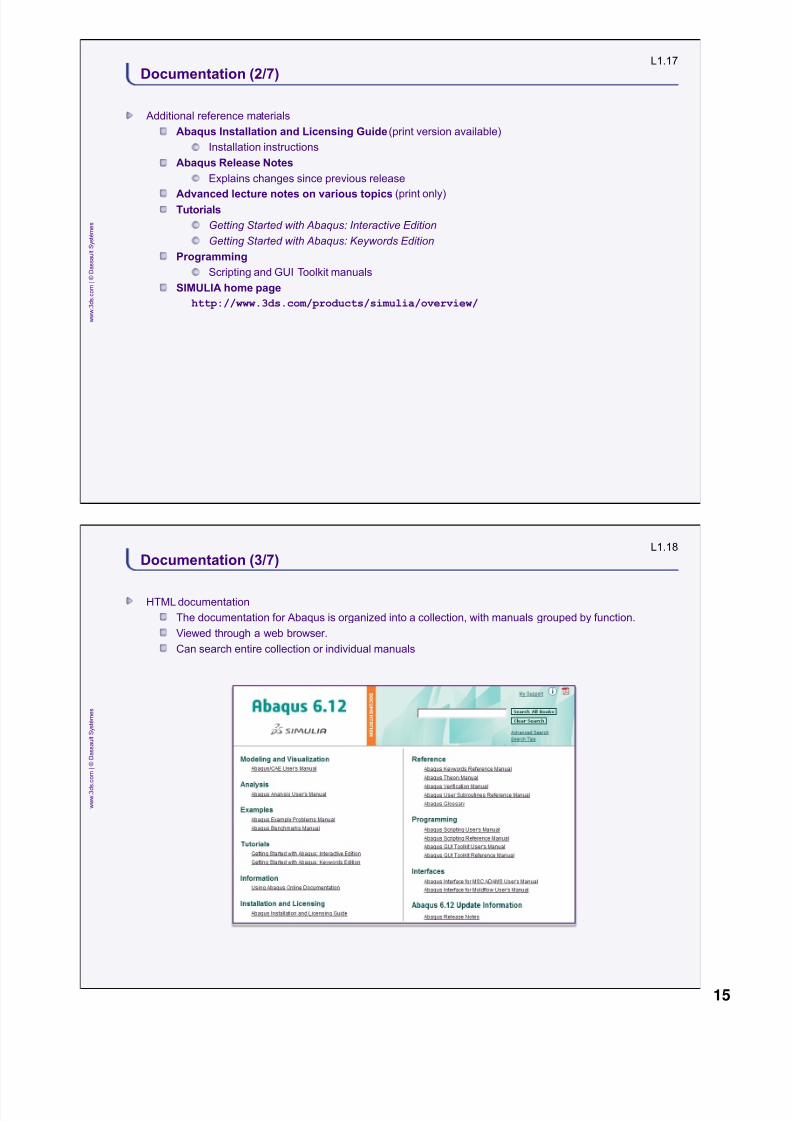
Documentation (3/7)
HTML documentation
The documentation for Abaqus is organized into a collection, with manuals grouped by function.
Viewed through a web browser.
Can search entire collection or individual manuals
15

8/15/2019 Abaqus Analysis Intro-book
http://slidepdf.com/reader/full/abaqus-analysis-intro-book 16/469
L1.19
w w w . 3
d s . c o m |
©
D a s s a u l t S y s t è m e s
Documentation (4/7)
Searching the documentation
Enter one or more search terms in the search field
The table of contents
entry is highlighted
The text frame displays the
corresponding section
Terms in the search field:
Appear in any order
May or may not be adjacent
Appear within the proximity criterion
(default is a single section)
L1.20
w w w . 3
d s
. c o m |
©
D a s s a u l t S y s t è m e s
Documentation (5/7)
Searching the documentation (cont’d)
Use quotes to search for exact strings
16

8/15/2019 Abaqus Analysis Intro-book
http://slidepdf.com/reader/full/abaqus-analysis-intro-book 17/469
L1.21
w w w . 3
d s . c o m |
©
D a s s a u l t S y s t è m e s
Documentation (6/7)
Advanced search
Advanced search allows you to control the proximity criterion
L1.22
w w w . 3
d s
. c o m |
©
D a s s a u l t S y s t è m e s
Documentation (7/7)
Advanced search (cont’d)
17
8/15/2019 Abaqus Analysis Intro-book
http://slidepdf.com/reader/full/abaqus-analysis-intro-book 18/469
L1.23
w w w . 3
d s . c o m |
©
D a s s a u l t S y s t è m e s
Components of an Abaqus Model (1/6)
The Abaqus analysis modules run as batch programs.
The primary input to the analysis modules is an input file, which contains options from element,
material, procedure, and loading libraries.
These options can be combined in any reasonable way, allowing a tremendous variety of problems to bemodeled.
The input file is divided into two parts: model data and history data.
Model data
Geometric options—nodes, elements
Material options
Other model options
History data Procedure options
Loading options
Output options
L1.24
w w w . 3
d s
. c o m |
©
D a s s a u l t S y s t è m e s
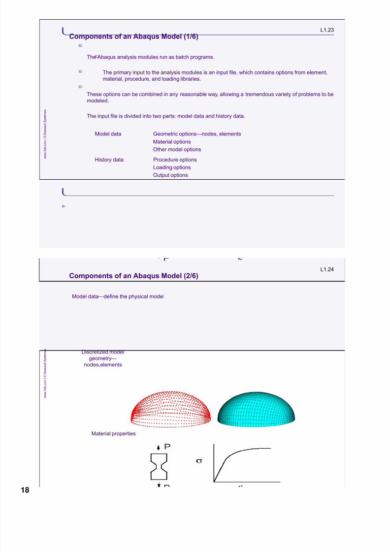
Model data—define the physical model
Discretized model
geometry—
nodes,elements
Material properties
Components of an Abaqus Model (2/6)
18

8/15/2019 Abaqus Analysis Intro-book
http://slidepdf.com/reader/full/abaqus-analysis-intro-book 19/469
L1.25
w w w . 3
d s . c o m |
©
D a s s a u l t S y s t è m e s
Model data
v0
Fixed constraints
Initial conditions
Components of an Abaqus Model (3/6)
pin dof 2 fixed
ENCASTRE
L1.26
w w w . 3
d s
. c o m |
©
D a s s a u l t S y s t è m e s
Components of an Abaqus Model (4/6)
History data—specify what happens to the model
Types of analysis procedures—static, dynamic, soil, heat transfer, etc.
Loadings
Prescribed constraints
Output requests— stresses, strains, reaction forces, contact pressure, etc.
ENCASTRE
X -symmetry
Y -symmetry
19

8/15/2019 Abaqus Analysis Intro-book
http://slidepdf.com/reader/full/abaqus-analysis-intro-book 20/469
L1.27
w w w . 3
d s . c o m |
©
D a s s a u l t S y s t è m e s
Components of an Abaqus Model (5/6)
History subdivided into analysis steps
Steps are convenient subdivisions in an analysis history.
Different steps can contain different analysis procedures—for example, static followed by dynamic.
Distinction between general and linear perturbation steps:
General steps define a sequence of events that follow one another.
I. The state of the model at the end of the previous general step provides the initial conditions
for the start of the next general step.
II. This is needed for any history-dependent analysis.
Linear perturbation steps provide the linear response about the base state, which is the state at
the end of the most recent general step.
L1.28
w w w . 3
d s
. c o m |
©
D a s s a u l t S y s t è m e s
Components of an Abaqus Model (6/6)
Example: Bow and arrow simulation
Step 1: String the bow
Step 2: Pull back on the bow string
Step 3: Linear perturbation step to extract the natural frequencies of the system—
has no effect on subsequent steps
Step 4: Release the arrow
Step 1 = pretension Step 2 = pull back Step 4 = dynamic release
Step 3 = natural
frequency extraction
20

8/15/2019 Abaqus Analysis Intro-book
http://slidepdf.com/reader/full/abaqus-analysis-intro-book 21/469
L1.29
w w w . 3
d s . c o m |
©
D a s s a u l t S y s t è m e s
Details of an Abaqus Input File (1/9)
Option blocks
All data are defined in ―option blocks‖ that describe specific aspects of the problem definition, such as an
element definition, etc. Together the option blocks build the model.
Node option block Property reference
option block
Material option
block
Element option
block
Boundary conditions
option block
Contact option
block
Initial conditions
option block
Analysis procedure
option blockLoading option block
Output request
option block
Model
data
History
data
L1.30
w w w . 3
d s
. c o m |
©
D a s s a u l t S y s t è m e s
Details of an Abaqus Input File (2/9)
Each option block begins with a keyword line (first character is *).
Data lines, if needed, follow the keyword line.
Comment lines, starting with **, can be included anywhere.
All input lines have a limit of 256 characters (including blanks).
Names can be up to 80 characters long and must begin with a letter. For example, the following would
be a permissible name:
nodes_at_the_top_of_the_block_next_to_the_gasket
Note: Regardless of whether you specify only a file name, a relative path name, or a full path
name, the complete name including the path can have a maximum of 80 characters .
21
8/15/2019 Abaqus Analysis Intro-book
http://slidepdf.com/reader/full/abaqus-analysis-intro-book 22/469
L1.31
w w w . 3
d s . c o m |
©
D a s s a u l t S y s t è m e s
Details of an Abaqus Input File (3/9)
Keyword lines
Begin with a single * followed directly by the name of the option.
May include a combination of required and optional parameters, along with their values, separated by
commas.
Example: A material option block defines a set of material properties.
keyword
*MATERIAL, NAME=material name
parameter parameter value
The first line in a material option block
L1.32
w w w . 3
d s
. c o m |
©
D a s s a u l t S y s t è m e s
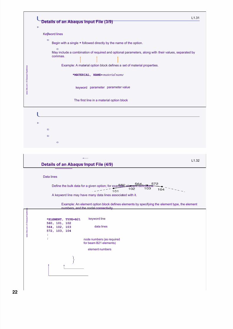
Details of an Abaqus Input File (4/9)
Data lines
Define the bulk data for a given option; for example, element definitions.
A keyword line may have many data lines associated with it.
Example: An element option block defines elements by specifying the element type, the element
numbers, and the nodal connectivity.
*ELEMENT, TYPE=B21560, 101, 102564, 102, 103
572, 103, 104::
keyword line
data lines
node numbers (as required
for beam B21 elements)
element numbers
22

8/15/2019 Abaqus Analysis Intro-book
http://slidepdf.com/reader/full/abaqus-analysis-intro-book 23/469
L1.33
w w w . 3
d s . c o m |
©
D a s s a u l t S y s t è m e s
Details of an Abaqus Input File (5/9)
Example: The elastic material option block defines the type of elasticity model as well as the elastic
material properties.
*ELASTIC, TYPE=ISOTROPIC200.0E4, 0.30, 20.0150.0E3, 0.35, 400.0
··
keyword line
data lines
temperature
Poisson’s ratio
modulus of
elasticity
L1.34
w w w . 3
d s
. c o m |
©
D a s s a u l t S y s t è m e s
Details of an Abaqus Input File (6/9)
Ordering of option blocks
Each option block belongs in either the model data or the history data—one or the other —as specified in
the user’s manual.
The ordering within the model data or history data is arbitrary, except for a few cases.
Examples:
*HEADING must be the first option in the input file.
*ELASTIC, *DENSITY, and *PLASTIC are suboptions of *MATERIAL. As such, they must
follow *MATERIAL directly. Suboptions have no name references of their own.
Procedure options (*STATIC, *DYNAMIC, and *FREQUENCY, etc.) must follow *STEP to
specify the analysis procedure for the step.
23

8/15/2019 Abaqus Analysis Intro-book
http://slidepdf.com/reader/full/abaqus-analysis-intro-book 24/469
L1.35
w w w . 3
d s . c o m |
©
D a s s a u l t S y s t è m e s
Details of an Abaqus Input File (7/9)
Node sets and element sets
Used for efficient cross-referencing.
Allow you to refer to a set all at once instead of each node or element individually.
Node setTOPNODES contains
nodes 101,102, ...
Boundary condition
applied to all nodes innode set TOPNODES
Example: Node sets*NODE, NSET=TOPNODES101, 0.345, 0.679, 0.223102, 0.331, 0.699, 0.234..*BOUNDARY, TYPE=DISPLACEMENTTOPNODES, YSYMM
L1.36
w w w . 3
d s
. c o m |
©
D a s s a u l t S y s t è m e s
Details of an Abaqus Input File (8/9)
Example: Element sets
*ELEMENT, TYPE=B21, ELSET=SEATPOST
560, 101, 102,
564, 102, 103
.
.
*BEAM SECTION, SECTION=PIPE, MATERIAL=STEEL,
ELSET=SEATPOST
0.12, 0.004
pipe radius
wall thickness
These beam cross-section
properties apply to all
elements in element set SEATPOST
Element set SEATPOST
contains elements 560,
564, ...
24

8/15/2019 Abaqus Analysis Intro-book
http://slidepdf.com/reader/full/abaqus-analysis-intro-book 25/469

8/15/2019 Abaqus Analysis Intro-book
http://slidepdf.com/reader/full/abaqus-analysis-intro-book 26/469
L1.39
w w w . 3
d s . c o m |
©
D a s s a u l t S y s t è m e s
Abaqus Input Conventions (2/8)
Example: Properties of mild steel at room temperature
Quantity
U.S. units
SI units
Conductivity 28.9 Btu/ft hr ºF 50 W/m ºC
2.4 Btu/in hr ºF
Density 15.13 slug/ft3 (lbf s2/ft4) 7800 kg/m3
0.730 × 10⁻³ lbf s2/in4
0.282 lbm/in3
Elastic modulus
30 × 106 psi
207 × 109 Pa
Specific heat 0.11 Btu/lbm ºF 460 J/kg ºC
Yield stress 30 × 103 psi 207 × 106 Pa
L1.40
w w w . 3
d s
. c o m |
©
D a s s a u l t S y s t è m e s
Abaqus Input Conventions (3/8)
Time measures
Abaqus keeps track of both total time in an analysis and step time for each analysis step.
Time is physically meaningful for some analysis procedures, such as transient dynamics.
Time is not physically meaningful for some procedures. In rate-independent, static procedures ―time‖ is
just a convenient, monotonically increasing measure for incrementing loads.
26
8/15/2019 Abaqus Analysis Intro-book
http://slidepdf.com/reader/full/abaqus-analysis-intro-book 27/469
8/15/2019 Abaqus Analysis Intro-book
http://slidepdf.com/reader/full/abaqus-analysis-intro-book 28/469
L1.43
w w w . 3
d s . c o m |
©
D a s s a u l t S y s t è m e s
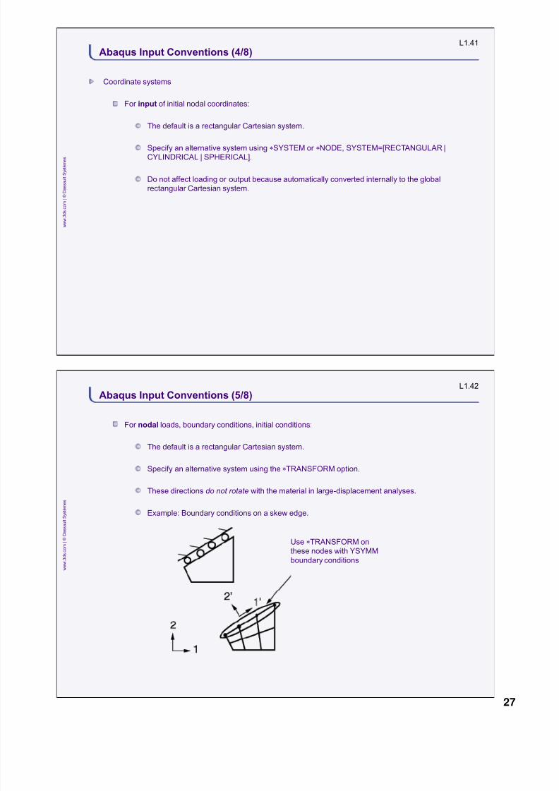
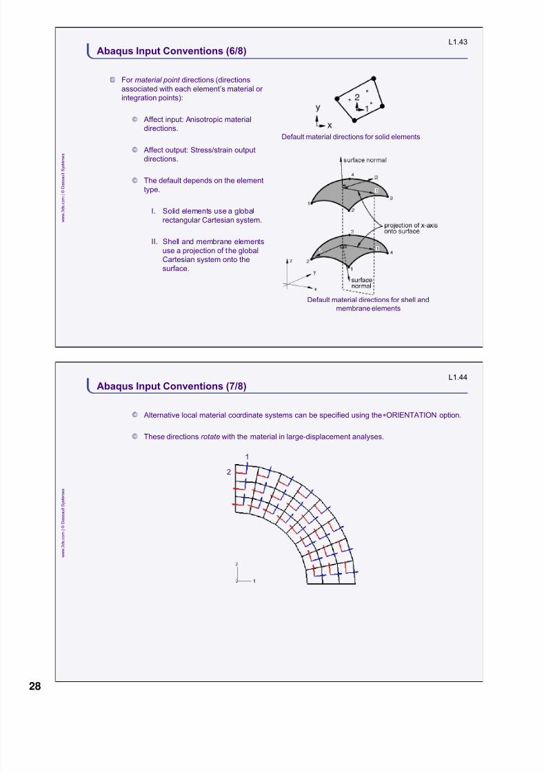
Abaqus Input Conventions (6/8)
For material point directions (directions
associated with each element’s material or
integration points):
Affect input: Anisotropic material
directions.
Affect output: Stress/strain output
directions.
The default depends on the element
type.
I. Solid elements use a global
rectangular Cartesian system.
II. Shell and membrane elements
use a projection of the global
Cartesian system onto the
surface.
Default material directions for shell and
membrane elements
Default material directions for solid elements
L1.44
w w w . 3
d s
. c o m |
©
D a s s a u l t S y s t è m e s
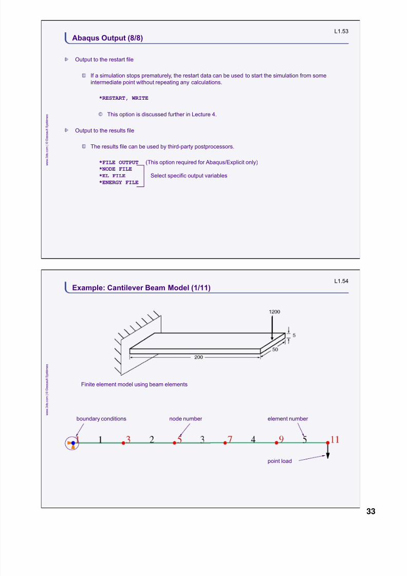
Abaqus Input Conventions (7/8)
Alternative local material coordinate systems can be specified using the *ORIENTATION option.
These directions rotate with the material in large-displacement analyses.
2
1
28

8/15/2019 Abaqus Analysis Intro-book
http://slidepdf.com/reader/full/abaqus-analysis-intro-book 29/469
L1.45
w w w . 3
d s . c o m |
©
D a s s a u l t S y s t è m e s
Abaqus Input Conventions (8/8)
Degrees of freedom
Primary solution variables at the nodes.
Available nodal degrees of freedom depend on the element type.
Each degree of freedom is labeled with a number: 1= x -displacement, 2=y -displacement,
11=temperature, etc.
L1.46
w w w . 3
d s
. c o m |
©
D a s s a u l t S y s t è m e s
Abaqus Output (1/8)
Output
Four types of output are available:
Neutral binary output can be written to the output database (.odb) file using the *OUTPUT option
and related suboptions.
Printed output can be written to the data (.dat) file.
I. This is available only for Abaqus/Standard.
Restart output can be written to the restart (.res) file using the *RESTART option for the
purpose of conducting restart analyses (discussed in Lecture 4).
Results (.fil) file output can be written for use with third-party postprocessors.
29

8/15/2019 Abaqus Analysis Intro-book
http://slidepdf.com/reader/full/abaqus-analysis-intro-book 30/469
L1.47
w w w . 3
d s . c o m |
©
D a s s a u l t S y s t è m e s
Abaqus Output (2/8)
Output to the output database file
The output database file is used by
Abaqus/Viewer.
An interface (API) is availablein Python and C++ to use for external
postprocessing (e.g.,
to add data to display in
Abaqus/Viewer).
Two types of output data: field and history
data.
Field data is used for model (deformed,
contour, etc.) and
X –Y plots:
*OUTPUT, FIELD
History data is used for X –
Y plots:*OUTPUT, HISTORY
L1.48
w w w . 3
d s
. c o m |
©
D a s s a u l t S y s t è m e s
Abaqus Output (3/8)
Frequency of output for either type can be controlled
Field output can be requested according to
Number of increments (Abaqus/Standard only)
*OUTPUT, FIELD, FREQUENCY=n
Number of intervals
*OUTPUT, FIELD, NUMBER INTERVAL=n
Time intervals
*OUTPUT, FIELD, TIME INTERVAL=x
Time points
*OUTPUT, FIELD, TIME POINTS=t_out
*TIME POINTS, name = t_out
Every n increments
At n evenly spaced time intervals
At user-specified time
points
Every x units of time
30

8/15/2019 Abaqus Analysis Intro-book
http://slidepdf.com/reader/full/abaqus-analysis-intro-book 31/469
L1.49
w w w . 3
d s . c o m |
©
D a s s a u l t S y s t è m e s
Abaqus Output (4/8)
History output can be requested according to:
Number of increments
*OUTPUT, HISTORY, FREQUENCY=n
Number of intervals (Abaqus/Standard only)*OUTPUT, HISTORY, NUMBER INTERVAL=n
Time intervals
*OUTPUT, HISTORY, TIME INTERVAL=x
Time points (Abaqus/Standard only)
*OUTPUT, HISTORY, TIME POINTS=t_out
*TIME POINTS, name=t_out
L1.50
w w w . 3
d s
. c o m |
©
D a s s a u l t S y s t è m e s
Abaqus Output (5/8)
Requesting output to the output database file
If you have no output requests in your model, behavior depends on environment file (abaqus_v6.env)
settings:
odb_output_by_default=ON: pre-selected output is written to the ODB
I. This is the default setting; output depends on the procedure type
odb_output_by_default=OFF : no ODB will be generated for your analysis
Default output can be overridden using any of the following suboptions of *OUTPUT :
*NODE OUTPUT
*ELEMENT OUTPUT
*ENERGY OUTPUT
*CONTACT OUTPUT
*INCREMENTATION OUTPUT (Abaqus/Explicit only)
31

8/15/2019 Abaqus Analysis Intro-book
http://slidepdf.com/reader/full/abaqus-analysis-intro-book 32/469
L1.51
w w w . 3
d s . c o m |
©
D a s s a u l t S y s t è m e s
Abaqus Output (6/8)
Pre-selected ODB output
Pre-selected output depends on the procedure type.
For example, for a general static procedure:
The default field output requests are for:
Stresses – S
Total Strains – E (or logarithmic strain LE if NLGEOM is active)
Plastic Strains – PE, PEEQ, and PEMAG
Displacements and Rotations – U
Reaction Forces and Moments – RF
Concentrated (applied) Forces and Moments – CF
Contact Stresses – CSTRESS
Contact Displacements – CDISP
The default history output request includes all model energies
For other procedures, see the Abaqus Analysis User’s Manual
L1.52
w w w . 3
d s
. c o m |
©
D a s s a u l t S y s t è m e s
Abaqus Output (7/8)
Output to the printed output file
These options allow tabular data to be written to an ASCII file that can be read with a text editor.
These options are available only for Abaqus/Standard.
Syntax:
*NODE PRINT*EL PRINT*ENERGY PRINT
32
8/15/2019 Abaqus Analysis Intro-book
http://slidepdf.com/reader/full/abaqus-analysis-intro-book 33/469

8/15/2019 Abaqus Analysis Intro-book
http://slidepdf.com/reader/full/abaqus-analysis-intro-book 34/469
L1.55
w w w . 3
d s . c o m |
©
D a s s a u l t S y s t è m e s
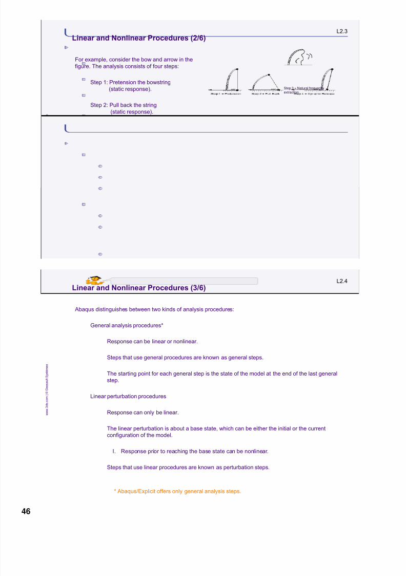
Example: Cantilever Beam Model (2/11)
Abaqus input file with some annotations
Model data*HEADINGCANTILEVER BEAM EXAMPLEUNITS IN MM, N, MPa*NODE
1, 0.0, 0.0:11, 200.0, 0.0*NSET, NSET=END11,*ELEMENT, TYPE=B21, ELSET=BEAMS1, 1, 3:5, 9, 11*BEAM SECTION, SECTION=RECT, ELSET=BEAMS, MATERIAL=MAT150.0, 5.0** Material from XXX testing lab*MATERIAL, NAME=MAT1*ELASTIC2.0E5, 0.3
*BOUNDARY1, ENCASTRE
comment line
property reference
option block
heading option block
node option block
node set definition
element option block
material option block
fixed boundary conditionoption block
This line will appear on each page of output.
elastic option block
L1.56
w w w . 3
d s
. c o m |
©
D a s s a u l t S y s t è m e s
Example: Cantilever Beam Model (3/11)
History data
*STEP APPLY POINT LOAD*STATIC*CLOAD11, 2, -1200.0*OUTPUT, FIELD, VARIABLE=PRESELECT, FREQUENCY=10*OUTPUT, HISTORY, FREQUENCY=1*NODE OUTPUT, NSET=ENDU,*EL PRINT, FREQUENCY=10S, E*NODE FILE, FREQUENCY=5
U,*END STEP
The history data begin withthe first *STEP option.
The history data end withthe last *END STEP option.
34

8/15/2019 Abaqus Analysis Intro-book
http://slidepdf.com/reader/full/abaqus-analysis-intro-book 35/469
L1.57
w w w . 3
d s . c o m |
©
D a s s a u l t S y s t è m e s
Example: Cantilever Beam Model (4/11)
Property references using set names
*ELEMENT, TYPE=B21, ELSET=BEAMS1, 1, 3*BEAM SECTION, SECTION=RECT, ELSET=BEAMS, MATERIAL=MAT150.0, 5.0*MATERIAL, NAME=MAT1*ELASTIC2.0E5, 0.3
The property reference *BEAM SECTION associates the element set BEAMS with the material definition
MAT1.
The option can also provide geometric information. In this case thecross-section type is rectangular (RECT); the width is 50.0, and the height is 5.0.
All elements in a model must have an appropriate property reference. Solid elements reference *SOLID
SECTION, shell elements reference *SHELL SECTION, etc.
L1.58
w w w . 3
d s
. c o m |
©
D a s s a u l t S y s t è m e s
Example: Cantilever Beam Model (5/11)
Material data
*MATERIAL, NAME=MAT1*ELASTIC2.0E5, 0.3
Definition for an isotropic linear elastic material
Abaqus interprets the options following a *MATERIAL option as part of the same material option block
until the next *MATERIAL option or the next nonmaterial property option, such as the *NODE option, is
encountered.
Options such as *ELASTIC are called suboptions and must be used in conjunction with the *MATERIAL
option.
Poisson’s ratio
elastic modulus
material name
35

8/15/2019 Abaqus Analysis Intro-book
http://slidepdf.com/reader/full/abaqus-analysis-intro-book 36/469

8/15/2019 Abaqus Analysis Intro-book
http://slidepdf.com/reader/full/abaqus-analysis-intro-book 37/469
L1.61
w w w . 3
d s . c o m |
©
D a s s a u l t S y s t è m e s
Example: Cantilever Beam Model (8/11)
Loading
Definition of a concentrated load in the global negative 2-direction:
*CLOAD11, 2, -1200.0
Many distributed loadings are also available, including surface pressure, body forces, centrifugal and
Coriolis loads, etc.
node or node set
degree of freedom
magnitude
L1.62
w w w . 3
d s
. c o m |
©
D a s s a u l t S y s t è m e s
Example: Cantilever Beam Model (9/11)
Output requests
*OUTPUT, FIELD, VARIABLE=PRESELECT, FREQUENCY=10*OUTPUT, HISTORY, FREQUENCY=1*NODE OUTPUT, NSET=ENDU,
In this case we have requested field output of a preselected set of the most commonly used output
variables.
We have also requested history output of displacements for the previously defined node set END.
Since history output is usually requested at relatively high frequencies, the sets should be as
small as possible.
Each output request includes a FREQUENCY parameter.
If the analysis requires many increments, the FREQUENCY parameter specifies how often
results will be written.
output to the output
database file
37

8/15/2019 Abaqus Analysis Intro-book
http://slidepdf.com/reader/full/abaqus-analysis-intro-book 38/469
L1.63
w w w . 3
d s . c o m |
©
D a s s a u l t S y s t è m e s
Example: Cantilever Beam Model (10/11)
*EL PRINT, FREQUENCY=10S, E*NODE FILE, FREQUENCY=5U,
Tabular output is printed to the data (.dat) file for visual inspection using the *EL PRINT option.
In this case we have requested output of the stress (S) and strain (E) components.
Binary output is written to the legacy Abaqus results (.fil) file using the *NODE FILE option; output is
used for postprocessing in other postprocessors.
In this case we have requested output of the displacement (U) components.
Printed output to the data file
Output to the results file
L1.64
w w w . 3
d s
. c o m |
©
D a s s a u l t S y s t è m e s
Example: Cantilever Beam Model (11/11)
End of step
*END STEP
Each analysis step ends with the *END STEP option.
The final option in the input file is the *END STEP option for the final analysis step.
ends the
analysis step
38

8/15/2019 Abaqus Analysis Intro-book
http://slidepdf.com/reader/full/abaqus-analysis-intro-book 39/469

8/15/2019 Abaqus Analysis Intro-book
http://slidepdf.com/reader/full/abaqus-analysis-intro-book 40/469

8/15/2019 Abaqus Analysis Intro-book
http://slidepdf.com/reader/full/abaqus-analysis-intro-book 41/469
L1.69
w w w . 3
d s . c o m |
©
D a s s a u l t S y s t è m e s
1. Objectives
a. When you complete this exercise you will be able to extract all the files necessary to complete the
demonstrations and workshops associated with this course
2. Workshop file setup (option 1: installation via plug-in)
a. From the main menu bar, selectPlug-ins→Tools →Install Courses.
b. In the Install Courses dialog box:
i. Specify the directory to which the files will be written.
ii. Chooses the course(s) for which the files will be
extracted.
iii. Click OK.
Workshop Preliminaries (1/2)
5 minutes
L1.70
w w w . 3
d s
. c o m |
©
D a s s a u l t S y s t è m e s
3. Workshop file setup (option 2: manual installation)
a. Find out where the Abaqus release is installed by typing
abq xxx whereami
where abq xxx is the name of the Abaqus execution procedure on your system. It can be defined to
have a different name. For example, the command for the 6.12 –1 release might be aliased to abq6121.
This command will give the full path to the directory where Abaqus is installed, referred to here asabaqus_dir .
b. Extract all the workshop files from the course tar file by typing
UNIX: abq xxx perl abaqus_dir /samples/course_setup.pl
Windows NT: abq xxx perl abaqus_dir \samples\course_setup.pl
c. The script will install the files into the current working directory. You will be asked to verify this and tochoose which files you wish to install. Choose y for the appropriate lecture series when prompted. Once
you have selected the lecture series, type q to skip the remaining lectures and to proceed with the
installation of the chosen workshops.
Workshop Preliminaries (2/2)
5 minutes
41

8/15/2019 Abaqus Analysis Intro-book
http://slidepdf.com/reader/full/abaqus-analysis-intro-book 42/469

8/15/2019 Abaqus Analysis Intro-book
http://slidepdf.com/reader/full/abaqus-analysis-intro-book 43/469

8/15/2019 Abaqus Analysis Intro-book
http://slidepdf.com/reader/full/abaqus-analysis-intro-book 44/469

8/15/2019 Abaqus Analysis Intro-book
http://slidepdf.com/reader/full/abaqus-analysis-intro-book 45/469
8/15/2019 Abaqus Analysis Intro-book
http://slidepdf.com/reader/full/abaqus-analysis-intro-book 46/469

8/15/2019 Abaqus Analysis Intro-book
http://slidepdf.com/reader/full/abaqus-analysis-intro-book 47/469
L2.5
w w w . 3
d s . c o m |
©
D a s s a u l t S y s t è m e s
Linear and Nonlinear Procedures (4/6)
General procedures
Static
Direct cyclic
Dynamic (transient)
Implicit
Explicit
Heat transfer
Mass diffusion
Coupled-field analysis
Thermal-mechanical
Thermal-electrical
Thermal-electrical-structural
Pore fluid diffusion/stress
Linear procedures
Static
Eigenvalue buckling
Linear dynamics
Natural frequency extraction
Transient modal dynamics
Steady-state dynamics
Response spectrum analysis
Random response analysis
L2.6
w w w . 3
d s
. c o m |
©
D a s s a u l t S y s t è m e s
Linear and Nonlinear Procedures (5/6)
Default amplitude references
Different defaults for different analysis procedures
AMPLITUDE=RAMP for procedures without natural time scales:
*STATIC
*HEAT TRANSFER, STEADY STATE
*COUPLED TEMPERATURE-DISPLACEMENT, STEADY STATE
*SOILS, STEADY STATE
*COUPLED THERMAL-ELECTRICAL, STEADY STATE
*STEADY STATE TRANSPORT
47

8/15/2019 Abaqus Analysis Intro-book
http://slidepdf.com/reader/full/abaqus-analysis-intro-book 48/469
L2.7
w w w . 3
d s . c o m |
©
D a s s a u l t S y s t è m e s
Linear and Nonlinear Procedures (6/6)
AMPLITUDE=STEP for procedures with natural time scales:
*DYNAMIC
*VISCO
*HEAT TRANSFER (transient)
*COUPLED TEMPERATURE-DISPLACEMENT (transient)
*DYNAMIC TEMPERATURE-DISPLACEMENT, EXPLICIT*COUPLED THERMAL-ELECTRICAL (transient)
*SOILS, CONSOLIDATION
*STEADY STATE DYNAMICS
*RANDOM RESPONSE
*MODAL DYNAMIC
A nonzero displacement boundary condition prescribed in an explicit dynamic procedure(*DYNAMIC, EXPLICIT) must refer to an amplitude option.
Note: Frequency domain procedures amplitude
references define load versus frequency.
L2.8
w w w . 3
d s
. c o m |
©
D a s s a u l t S y s t è m e s
Linear Static Analysis and Multiple Load Cases (1/5)
Static analysis is the only procedure that can be performed as either a general or perturbation step:
General step: response can be linear or nonlinear
*STEP
*STATIC
Perturbation step: linear response
*STEP, PERTURBATION
*STATIC
One advantage of static linear perturbation steps is that they can consider multiple load cases.
A load case defines a set of loads and boundary conditions and may contain the following:
Concentrated and distributed loads
Boundary conditions (may change from load case to load case)
Inertia relief
In addition to the static linear perturbation procedure, multiple load cases can also be used for steady-state dynamic (SSD) analysis (either direct or SIM-based modal analysis).
For SIM-based SSD analysis, base motion may also be definedas part of a load case.
48

8/15/2019 Abaqus Analysis Intro-book
http://slidepdf.com/reader/full/abaqus-analysis-intro-book 49/469

8/15/2019 Abaqus Analysis Intro-book
http://slidepdf.com/reader/full/abaqus-analysis-intro-book 50/469
L2.11
w w w . 3
d s . c o m |
©
D a s s a u l t S y s t è m e s
Linear Static Analysis and Multiple Load Cases (4/5)
Example: An agricultural implement
This is an agricultural implement attached to and towed behind a tractor through a 3-point hitch.
The purpose of the hitch is to transfer towing loads to the implement, but otherwise to allow the
implement to float and move more or less independently of the tractor.
L2.12
w w w . 3
d s
. c o m |
©
D a s s a u l t S y s t è m e s
Linear Static Analysis and Multiple Load Cases (5/5)
Three load cases
The connection is very flexible and the loads on the implement are not well defined, but are a
combination of many different types of loads.
Vertical Loads
Lateral Loads
Forward Loads
50

8/15/2019 Abaqus Analysis Intro-book
http://slidepdf.com/reader/full/abaqus-analysis-intro-book 51/469
L2.13
w w w . 3
d s . c o m |
©
D a s s a u l t S y s t è m e s
Multiple Load Case Usage (1/7)
*Step, perturbation
*Static
*Load Case, name="Bending A"
*Boundary
right, 1, 6*Cload
left, 3, 1.
*End Load Case
*Load Case, name="Bending B"
*Boundary
left, 1, 6
*Cload
right, 3, 1.
*End Load Case
*End Step
Node set left
Node set right
Bending A
Bending B
Example: Bending of a plate
L2.14
w w w . 3
d s
. c o m |
©
D a s s a u l t S y s t è m e s
Multiple Load Case Usage (2/7)
Basic rules
• Load case names ( Load Case, name=...) must be unique.
• Load options specified outside of load cases apply to all load cases.
• Base state boundary conditions propagate to all load cases.
• Rules for using OP=NEW :
• If used anywhere in a load case step, must be used everywhere in that step.
• If used on any BOUNDARY in a load case step, propagated boundary conditions will be
removed in all load cases.
•
LOAD CASE options do not propagate.
51

8/15/2019 Abaqus Analysis Intro-book
http://slidepdf.com/reader/full/abaqus-analysis-intro-book 52/469

8/15/2019 Abaqus Analysis Intro-book
http://slidepdf.com/reader/full/abaqus-analysis-intro-book 53/469
L2.17
w w w . 3
d s . c o m |
©
D a s s a u l t S y s t è m e s
Multiple Load Case Usage (5/7)
Output
Output requested per step (not per load case)
Available for the output database (.odb) and
data (.dat) files
For the output database file:
All output variables for a load case aremapped to a frame.
I. Similar to the way increments are
mapped to frames.
Frame contains load case name.
Field output only (no history output).
L2.18
w w w . 3
d s
. c o m |
©
D a s s a u l t S y s t è m e s
Multiple Load Case Usage (6/7)
Postprocessing with Abaqus/Viewer
Operations on entire frames supported
For selected frames, can create:
Linear combinations (e.g., linear
combination of load cases)
Min/Max envelope (e.g., find max
stresses over all load cases)
53

8/15/2019 Abaqus Analysis Intro-book
http://slidepdf.com/reader/full/abaqus-analysis-intro-book 54/469

8/15/2019 Abaqus Analysis Intro-book
http://slidepdf.com/reader/full/abaqus-analysis-intro-book 55/469

8/15/2019 Abaqus Analysis Intro-book
http://slidepdf.com/reader/full/abaqus-analysis-intro-book 56/469

8/15/2019 Abaqus Analysis Intro-book
http://slidepdf.com/reader/full/abaqus-analysis-intro-book 57/469

8/15/2019 Abaqus Analysis Intro-book
http://slidepdf.com/reader/full/abaqus-analysis-intro-book 58/469

8/15/2019 Abaqus Analysis Intro-book
http://slidepdf.com/reader/full/abaqus-analysis-intro-book 59/469

8/15/2019 Abaqus Analysis Intro-book
http://slidepdf.com/reader/full/abaqus-analysis-intro-book 60/469

8/15/2019 Abaqus Analysis Intro-book
http://slidepdf.com/reader/full/abaqus-analysis-intro-book 61/469
L3.1
w w w . 3
d s . c o m |
©
D a s s a u l t S y s t è m e s
Lesson content :
Nonlinearity in Structural Mechanics
Equations of Motion
Nonlinear Analysis Using Implicit Methods
Nonlinear Analysis Using Explicit Methods
Input File for Nonlinear Analysis
Status File
Message File
Output from Nonlinear Cantilever Beam Analysis
Workshop 3: Nonlinear Statics (IA)
Workshop 3: Nonlinear Statics (KW)
Lesson 3: Nonlinear Analysis in Abaqus
2 hours
Both interactive (IA) and keywords (KW) versionsof the workshop are provided. Complete only one.
L3.2
w w w . 3
d s
. c o m |
©
D a s s a u l t S y s t è m e s
Nonlinearity in Structural Mechanics (1/4)
Sources of nonlinearity
Material nonlinearities:
Nonlinear elasticity
Plasticity
Material damage
Failure mechanisms
Etc.
Note: material dependencies on temperature or field variables do not introduce nonlinearity if the
temperature or field variables are predefined.
Some examples of material nonlinearity
61

8/15/2019 Abaqus Analysis Intro-book
http://slidepdf.com/reader/full/abaqus-analysis-intro-book 62/469
L3.3
w w w . 3
d s . c o m |
©
D a s s a u l t S y s t è m e s
An example of self-contact: Example
Problem 1.1.17, Compression of a jounce
bumper
Nonlinearity in Structural Mechanics (2/4)
Boundary nonlinearities:
Contact problems
I. Boundary conditions change
during the analysis.
II. Extremely discontinuous form of
nonlinearity.
L3.4
w w w . 3
d s
. c o m |
©
D a s s a u l t S y s t è m e s
Nonlinearity in Structural Mechanics (3/4)
Geometric nonlinearities:
Large deflections and deformations
Large rotations
Structural instabilities (buckling)
Preloading effects
An example of geometric nonlinearity: elastomeric
keyboard dome
62

8/15/2019 Abaqus Analysis Intro-book
http://slidepdf.com/reader/full/abaqus-analysis-intro-book 63/469

8/15/2019 Abaqus Analysis Intro-book
http://slidepdf.com/reader/full/abaqus-analysis-intro-book 64/469
L3.7
w w w . 3
d s . c o m |
©
D a s s a u l t S y s t è m e s
Equations of Motion (2/3)
L3.8
w w w . 3
d s
. c o m |
©
D a s s a u l t S y s t è m e s
Equations of Motion (3/3)
Incremental solution schemes
Nonlinear problems are generally solved in an incremental fashion.
For a static problem a fraction of the total load is applied to the structure and the equilibrium
solution corresponding to the current load level is obtained.
I. The load level is then increased (i.e., incremented) and the process is repeated until the full
load level is applied.
For a dynamic problem, the equations of motion are numerically integrated in time using discrete
time increments.
There are two techniques available to solve the nonlinear equations:
Implicit method
Can solve for both static and dynamic equilibrium.
Requires direct solution of a set of matrix equations to obtain the state at the end of theincrement.
I. Iteration required.
This method is used by Abaqus/Standard and is the focus of this lecture.
Explicit method
Can only solve the dynamic equilibrium equations.
I. Can perform quasi-static simulations, however.
The state at the end of the increment depends solely on the state at the beginning of the
increment
I. No iteration required.
This method is used by Abaqus/Explicit and will be discussed in a later lecture.
64

8/15/2019 Abaqus Analysis Intro-book
http://slidepdf.com/reader/full/abaqus-analysis-intro-book 65/469

8/15/2019 Abaqus Analysis Intro-book
http://slidepdf.com/reader/full/abaqus-analysis-intro-book 66/469

8/15/2019 Abaqus Analysis Intro-book
http://slidepdf.com/reader/full/abaqus-analysis-intro-book 67/469
L3.13
w w w . 3
d s . c o m |
©
D a s s a u l t S y s t è m e s
Nonlinear Analysis Using Explicit Methods
Abaqus/Explicit solves for dynamic equilibrium using an explicit solution scheme:
Velocity and displacements at time t + Dt updated explicitly.
Solution is trivial:Diagonal mass matrix.
No iteration is required!
Conditionally stable.
The size of the time increment must be controlled.
Explicit methods generally require many, many more time increments than implicit methods for
the same problem.
Discontinuous forms of nonlinearity (e.g., contact) are handled more easily by explicit methods.
Explicit dynamics will be discussed further later.
1( ) ( )( )
t t
u M P I .
L3.14
w w w . 3
d s
. c o m |
©
D a s s a u l t S y s t è m e s
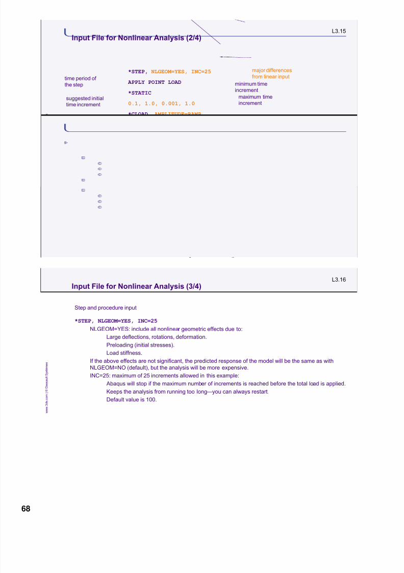
Input File for Nonlinear Analysis (1/4)
*HEADING
CANTILEVER BEAM EXAMPLE--LARGE DISPLACEMENT
*NODE
1, 0., 0.
11, 200., 0.
*NGEN
1, 11, 1
*ELEMENT, TYPE=B21
1, 1, 3
*ELGEN, ELSET=BEAMS
1, 5, 2, 1
*BEAM SECTION, SECTION=RECT, ELSET=BEAMS, MATERIAL=MAT1
50., 5.
*MATERIAL, NAME=MAT1
*ELASTIC2.E5, .3
*BOUNDARY
1, 1, 6
*AMPLITUDE, NAME=RAMP
0.0, 0.0, 0.5, 0.3, 1.0, 1.0
*RESTART, WRITE,FREQ=3
67
8/15/2019 Abaqus Analysis Intro-book
http://slidepdf.com/reader/full/abaqus-analysis-intro-book 68/469

8/15/2019 Abaqus Analysis Intro-book
http://slidepdf.com/reader/full/abaqus-analysis-intro-book 69/469

8/15/2019 Abaqus Analysis Intro-book
http://slidepdf.com/reader/full/abaqus-analysis-intro-book 70/469

8/15/2019 Abaqus Analysis Intro-book
http://slidepdf.com/reader/full/abaqus-analysis-intro-book 71/469
L3.21
w w w . 3
d s . c o m |
©
D a s s a u l t S y s t è m e s
CONVERGENCE TOLERANCE PARAMETERS FOR MOMENT
CRITERION FOR RESIDUAL MOMENT FOR A NONLINEAR PROBLEM 5.000E-03
CRITERION FOR ROTATION CORRECTION IN A NONLINEAR PROBLEM 1.000E-02
INITIAL VALUE OF TIME AVERAGE MOMENT 1.000E-02
AVERAGE MOMENT IS TIME AVERAGE MOMENT ALTERNATE CRIT. FOR RESIDUAL MOMENT FOR A NONLINEAR PROBLEM 2.000E-02
CRITERION FOR ZERO MOMENT RELATIVE TO TIME AVRG. MOMENT 1.000E-05
CRITERION FOR RESIDUAL MOMENT WHEN THERE IS ZERO FLUX 1.000E-05
CRITERION FOR ROTATION CORRECTION WHEN THERE IS ZERO FLUX 1.000E-03
CRITERION FOR RESIDUAL MOMENT FOR A LINEAR INCREMENT 1.000E-08
FIELD CONVERSION RATIO 1.00
CRITERION FOR ZERO MOMENT REL. TO TIME AVRG. MAX. MOMENT 1.000E-05
VOLUMETRIC STRAIN COMPATIBILITY TOLERANCE FOR HYBRID SOLIDS 1.000E-05
AXIAL STRAIN COMPATIBILITY TOLERANCE FOR HYBRID BEAMS 1.000E-05
TRANS. SHEAR STRAIN COMPATIBILITY TOLERANCE FOR HYBRID BEAMS 1.000E-05
SOFT CONTACT CONSTRAINT COMPATIBILITY TOLERANCE FOR P>P0 5.000E-03
SOFT CONTACT CONSTRAINT COMPATIBILITY TOLERANCE FOR P=0.0 0.100
CONTACT FORCE ERROR TOLERANCE FOR CONVERT SDI=YES 1.00
DISPLACEMENT COMPATIBILITY TOLERANCE FOR DCOUP ELEMENTS 1.000E-05ROTATION COMPATIBILITY TOLERANCE FOR DCOUP ELEMENTS 1.000E-05
EQUILIBRIUM WILL BE CHECKED FOR SEVERE DISCONTINUITY ITERATIONS
Output from Nonlinear Cantilever Beam Analysis (2/17)
L3.22
w w w . 3
d s
. c o m |
©
D a s s a u l t S y s t è m e s
Output from Nonlinear Cantilever Beam Analysis (3/17)
TIME INCREMENTATION CONTROL PARAMETERS:FIRST EQUILIBRIUM ITERATION FOR CONSECUTIVE DIVERGENCE CHECK 4EQUILIBRIUM ITERATION AT WHICH LOG. CONVERGENCE RATE CHECK BEGINS 8EQUILIBRIUM ITERATION AFTER WHICH ALTERNATE RESIDUAL IS USED 9 MAXIMUM EQUILIBRIUM ITERATIONS ALLOWED 16EQUILIBRIUM ITERATION COUNT FOR CUT-BACK IN NEXT INCREMENT 10 MAXIMUM EQUILIB. ITERS IN TWO INCREMENTS FOR TIME INCREMENT INCREASE 4 MAXIMUM ITERATIONS FOR SEVERE DISCONTINUITIES 50 MAXIMUM CUT-BACKS ALLOWED IN AN INCREMENT 5 MAXIMUM DISCON. ITERS IN TWO INCREMENTS FOR TIME INCREMENT INCREASE 50CUT-BACK FACTOR AFTER DIVERGENCE 0.2500CUT-BACK FACTOR FOR TOO SLOW CONVERGENCE 0.5000CUT-BACK FACTOR AFTER TOO MANY EQUILIBRIUM ITERATIONS 0.7500CUT-BACK FACTOR AFTER TOO MANY SEVERE DISCONTINUITY ITERATIONS 0.2500CUT-BACK FACTOR AFTER PROBLEMS IN ELEMENT ASSEMBLY 0.2500INCREASE FACTOR AFTER TWO INCREMENTS THAT CONVERGE QUICKLY 1.500 MAX. TIME INCREMENT INCREASE FACTOR ALLOWED 1.500
MAX. TIME INCREMENT INCREASE FACTOR ALLOWED (DYNAMICS) 1.250 MAX. TIME INCREMENT INCREASE FACTOR ALLOWED (DIFFUSION) 2.000 MINIMUM TIME INCREMENT RATIO FOR EXTRAPOLATION TO OCCUR 0.1000 MAX. RATIO OF TIME INCREMENT TO STABILITY LIMIT 1.000FRACTION OF STABILITY LIMIT FOR NEW TIME INCREMENT 0.9500TIME INCREMENT INCREASE FACTOR BEFORE A TIME POINT 1.000GLOBAL STABILIZATION CONTROL IS NOT USED
71

8/15/2019 Abaqus Analysis Intro-book
http://slidepdf.com/reader/full/abaqus-analysis-intro-book 72/469
L3.23
w w w . 3
d s . c o m |
©
D a s s a u l t S y s t è m e s
PRINT OF INCREMENT NUMBER, TIME, ETC., EVERY 1 INCREMENTS
RESTART FILE WILL BE WRITTEN EVERY 3 INCREMENTS
THE MAXIMUM NUMBER OF INCREMENTS IN THIS STEP IS 25
LARGE DISPLACEMENT THEORY WILL BE USED
LINEAR EXTRAPOLATION WILL BE USED
CHARACTERISTIC ELEMENT LENGTH 40.0
DETAILED OUTPUT OF DIAGNOSTICS TO DATABASE REQUESTED
PRINT OF INCREMENT NUMBER, TIME, ETC., TO THE MESSAGE FILE EVERY 1 INCREMENTS
EQUATIONS ARE BEING REORDERED TO MINIMIZE WAVEFRONT
COLLECTING MODEL CONSTRAINT INFORMATION FOR OVERCONSTRAINT CHECKS
COLLECTING STEP CONSTRAINT INFORMATION FOR OVERCONSTRAINT CHECKS
Output from Nonlinear Cantilever Beam Analysis (4/17)
L3.24
w w w . 3
d s
. c o m |
©
D a s s a u l t S y s t è m e s
INCREMENT 1 STARTS. ATTEMPT NUMBER 1, TIME INCREMENT 0.100
CONVERGENCE CHECKS FOR EQUILIBRIUM ITERATION 1
AVERAGE FORCE 1.251E+03 TIME AVG. FORCE 1.251E+03
LARGEST RESIDUAL FORCE -4.637E+03 AT NODE 11 DOF 1
LARGEST INCREMENT OF DISP. -1.84 AT NODE 11 DOF 2
LARGEST CORRECTION TO DISP. -1.84 AT NODE 11 DOF 2FORCE EQUILIBRIUM NOT ACHIEVED WITHIN TOLERANCE.
AVERAGE MOMENT 7.200E+03 TIME AVG. MOMENT 7.200E+03
LARGEST RESIDUAL MOMENT 28.8 AT NODE 9 DOF 6
LARGEST INCREMENT OF ROTATION -1.382E-02 AT NODE 11 DOF 6
LARGEST CORRECTION TO ROTATION -1.382E-02 AT NODE 11 DOF 6ROTATION CORRECTION TOO LARGE COMPARED TO ROTATION INCREMENT .
CONVERGENCE CHECKS FOR EQUILIBRIUM ITERATION 2
AVERAGE FORCE 37.8 TIME AVG. FORCE 37.8
LARGEST RESIDUAL FORCE 0.215 AT NODE 11 DOF 1
LARGEST INCREMENT OF DISP. -1.84 AT NODE 11 DOF 2
LARGEST CORRECTION TO DISP. -1.007E-02 AT NODE 11 DOF 1FORCE EQUILIBRIUM NOT ACHIEVED WITHIN TOLERANCE.
AVERAGE MOMENT 7.200E+03 TIME AVG. MOMENT 7.200E+03
LARGEST RESIDUAL MOMENT -0.346 AT NODE 5 DOF 6
LARGEST INCREMENT OF ROTATION -1.382E-02 AT NODE 11 DOF 6
LARGEST CORRECTION TO ROTATION 5.898E-07 AT NODE 11 DOF 6THE MOMENT EQUILIBRIUM EQUATIONS HAVE CONVERGED
× 0.005
6.25
× 0.005
0.2
× 0.005
36
× 0.005
36
Output from Nonlinear Cantilever Beam Analysis (5/17)
72

8/15/2019 Abaqus Analysis Intro-book
http://slidepdf.com/reader/full/abaqus-analysis-intro-book 73/469

8/15/2019 Abaqus Analysis Intro-book
http://slidepdf.com/reader/full/abaqus-analysis-intro-book 74/469
8/15/2019 Abaqus Analysis Intro-book
http://slidepdf.com/reader/full/abaqus-analysis-intro-book 75/469

8/15/2019 Abaqus Analysis Intro-book
http://slidepdf.com/reader/full/abaqus-analysis-intro-book 76/469

8/15/2019 Abaqus Analysis Intro-book
http://slidepdf.com/reader/full/abaqus-analysis-intro-book 77/469
L3.33
w w w . 3
d s . c o m |
©
D a s s a u l t S y s t è m e s
CONVERGENCE CHECKS FOR EQUILIBRIUM ITERATION 3
AVERAGE FORCE 559. TIME AVG. FORCE 255.LARGEST RESIDUAL FORCE -28.9 AT NODE 11 DOF 1LARGEST INCREMENT OF DISP. -14.1 AT NODE 11 DOF 2LARGEST CORRECTION TO DISP. 0.130 AT NODE 11 DOF 2
FORCE EQUILIBRIUM NOT ACHIEVED WITHIN TOLERANCE.
AVERAGE MOMENT 1.153E+05 TIME AVG. MOMENT 4.299E+04LARGEST RESIDUAL MOMENT 3.833E-02 AT NODE 5 DOF 6LARGEST INCREMENT OF ROTATION -0.106 AT NODE 11 DOF 6LARGEST CORRECTION TO ROTATION 1.112E-03 AT NODE 11 DOF 6ESTIMATE OF ROTATION CORRECTION -1.004E-06 MOMENT EQUILIB. ACCEPTED BASED ON SMALL RESIDUAL AND ESTIMATED CORRECTION
CONVERGENCE CHECKS FOR EQUILIBRIUM ITERATION 4
AVERAGE FORCE 1.053E+03 TIME AVG. FORCE 354.LARGEST RESIDUAL FORCE 1.092E-03 AT NODE 11 DOF 2LARGEST INCREMENT OF DISP. -14.1 AT NODE 11 DOF 2LARGEST CORRECTION TO DISP. -2.092E-04 AT NODE 11 DOF 2
THE FORCE EQUILIBRIUM EQUATIONS HAVE CONVERGED
AVERAGE MOMENT 1.153E+05 TIME AVG. MOMENT 4.299E+04LARGEST RESIDUAL MOMENT -2.910E-02 AT NODE 7 DOF 6LARGEST INCREMENT OF ROTATION -0.106 AT NODE 11 DOF 6LARGEST CORRECTION TO ROTATION -1.875E-06 AT NODE 11 DOF 6
THE MOMENT EQUILIBRIUM EQUATIONS HAVE CONVERGED
ITERATION SUMMARY FOR THE INCREMENT: 3 TOTAL ITERATIONS, OF WHICH
0 ARE SEVERE DISCONTINUITY ITERATIONS AND 3 ARE EQUILIBRIUM ITERATIONS.
TIME INCREMENT COMPLETED 0.338 , FRACTION OF STEP COMPLETED 0.913
STEP TIME COMPLETED 0.913 , TOTAL TIME COMPLETED 0.913
The residual is within tolerance, but the rotation
correction is too large. The estimate of the rotation
correction of the next iteration is acceptably small.
Output from Nonlinear Cantilever Beam Analysis (14/17)
L3.34
w w w . 3
d s
. c o m |
©
D a s s a u l t S y s t è m e s
INCREMENT 6 STARTS. ATTEMPT NUMBER 1, TIME INCREMENT 8.750E-02
CONVERGENCE CHECKS FOR EQUILIBRIUM ITERATION 1
AVERAGE FORCE 641. TIME AVG. FORCE 402.LARGEST RESIDUAL FORCE 74.0 AT NODE 11 DOF 1LARGEST INCREMENT OF DISP. -3.55 AT NODE 11 DOF 2LARGEST CORRECTION TO DISP. -0.180 AT NODE 11 DOF 1
FORCE EQUILIBRIUM NOT ACHIEVED WITHIN TOLERANCE.
AVERAGE MOMENT 1.179E+05 TIME AVG. MOMENT 5.547E+04LARGEST RESIDUAL MOMENT -99.4 AT NODE 5 DOF 6LARGEST INCREMENT OF ROTATION -2.702E-02 AT NODE 11 DOF 6LARGEST CORRECTION TO ROTATION 5.186E-04 AT NODE 11 DOF 6ESTIMATE OF ROTATION CORRECTION -1.594E-05
MOMENT EQUILIB. ACCEPTED BASED ON SMALL RESIDUAL AND ESTIMATED CORRECTION
CONVERGENCE CHECKS FOR EQUILIBRIUM ITERATION 2
AVERAGE FORCE 695. TIME AVG. FORCE 411.LARGEST RESIDUAL FORCE -0.505 AT NODE 11 DOF 1LARGEST INCREMENT OF DISP. -3.53 AT NODE 11 DOF 2LARGEST CORRECTION TO DISP. 1.386E-02 AT NODE 11 DOF 2
THE FORCE EQUILIBRIUM EQUATIONS HAVE CONVERGED
AVERAGE MOMENT 1.309E+05 TIME AVG. MOMENT 5.764E+04LARGEST RESIDUAL MOMENT 8.716E-02 AT NODE 7 DOF 6LARGEST INCREMENT OF ROTATION -2.687E-02 AT NODE 11 DOF 6LARGEST CORRECTION TO ROTATION 1.493E-04 AT NODE 11 DOF 6
THE MOMENT EQUILIBRIUM EQUATIONS HAVE CONVERGED
Output from Nonlinear Cantilever Beam Analysis (15/17)
77

8/15/2019 Abaqus Analysis Intro-book
http://slidepdf.com/reader/full/abaqus-analysis-intro-book 78/469

8/15/2019 Abaqus Analysis Intro-book
http://slidepdf.com/reader/full/abaqus-analysis-intro-book 79/469

8/15/2019 Abaqus Analysis Intro-book
http://slidepdf.com/reader/full/abaqus-analysis-intro-book 80/469

8/15/2019 Abaqus Analysis Intro-book
http://slidepdf.com/reader/full/abaqus-analysis-intro-book 81/469

8/15/2019 Abaqus Analysis Intro-book
http://slidepdf.com/reader/full/abaqus-analysis-intro-book 82/469

8/15/2019 Abaqus Analysis Intro-book
http://slidepdf.com/reader/full/abaqus-analysis-intro-book 83/469
L4.1
w w w . 3
d s . c o m |
©
D a s s a u l t S y s t è m e s
Lesson content :
Multistep Analyses
Restart Analysis in Abaqus
Workshop 4: Unloading Analysis (IA)
Workshop 4: Unloading Analysis (KW)
Lesson 4: Multistep Analysis in Abaqus
1 hour
Both interactive (IA) and keywords (KW) versionsof the workshop are provided. Complete only one.
L4.2
w w w . 3
d s
. c o m |
©
D a s s a u l t S y s t è m e s
Multistep Analyses (1/9)
It is often convenient to divide an Abaqus analysis into multiple steps
so that loads or boundary conditions can be applied in steps or output requests can be modified.
Usually there are several general analysis steps.
Response can be linear or nonlinear
General steps can be punctuated by perturbation steps.
Response is linear perturbation about a base state
What is the ―base state?‖
The base state is the current state of the model at the end of the last general analysis step (prior to the
linear perturbation step).
83

8/15/2019 Abaqus Analysis Intro-book
http://slidepdf.com/reader/full/abaqus-analysis-intro-book 84/469
L4.3
w w w . 3
d s . c o m |
©
D a s s a u l t S y s t è m e s
Multistep Analyses (2/9)
Possible step sequences
General step followed by another general step
General step continues from where previous general step ended
Loads are considered total loads
General step followed by perturbation step
Perturbation response about preceding general stepLoads are considered perturbation loads
Perturbation step followed by another perturbation step
These act as a series of independent steps in the analysis
Some ordering rules apply (e.g., frequency extraction before modal dynamics)
Perturbation step followed by a general step
General step continues from end of previous general step (if any)
The perturbation response is ignored in the general step that follows
L4.4
w w w . 3
d s
. c o m |
©
D a s s a u l t S y s t è m e s
Multistep Analyses (3/9)
Some comments on following a general step with a perturbation step
Perturbation step results are perturbations about the base state.
If geometric nonlinearity is included in the general analysis upon which a linear perturbation study
is based, stress stiffening or softening effects and load stiffness effects (from pressure and other
follower forces) are included in the linear perturbation analysis.
Eigenvalue buckling analyses are an exception:
I. The base state in a buckling analysis always includes the effects of stresses from previous
general steps even if geometric nonlinearity was not considered.
The contact state of the most recent general step is enforced in the perturbation step.
84

8/15/2019 Abaqus Analysis Intro-book
http://slidepdf.com/reader/full/abaqus-analysis-intro-book 85/469

8/15/2019 Abaqus Analysis Intro-book
http://slidepdf.com/reader/full/abaqus-analysis-intro-book 86/469

8/15/2019 Abaqus Analysis Intro-book
http://slidepdf.com/reader/full/abaqus-analysis-intro-book 87/469

8/15/2019 Abaqus Analysis Intro-book
http://slidepdf.com/reader/full/abaqus-analysis-intro-book 88/469

8/15/2019 Abaqus Analysis Intro-book
http://slidepdf.com/reader/full/abaqus-analysis-intro-book 89/469
L4.13
w w w . 3
d s . c o m |
©
D a s s a u l t S y s t è m e s
Restart Analysis in Abaqus (3/7)
Restart option syntax: Abaqus/Explicit
The Abaqus/Explicit restart files allow an analysis to be completed up to a certain point (an ―interval‖ of
restart output) in a particular run and restarted and continued in a subsequent run.
The package, state, and initial restart files are needed to restart an Abaqus/Explicit simulation.
The syntax for restarting an Abaqus/Explicit simulation is just slightly different from that used for
Abaqus/Standard:
*RESTART, READ, STEP= P , INTERVAL=Q
In this example the analysis is restarted just after the completion of interval Q of step P .
L4.14
w w w . 3
d s
. c o m |
©
D a s s a u l t S y s t è m e s
Restart Analysis in Abaqus (4/7)
Submission of a restart job:
abaqus job= job-name oldjob=oldjob-name
The following model data can be changed in a restart analysis:
Amplitude definitions
Node sets
Element sets
name of the
restart file
created by the
previous run
name of the
new input file
89

8/15/2019 Abaqus Analysis Intro-book
http://slidepdf.com/reader/full/abaqus-analysis-intro-book 90/469

8/15/2019 Abaqus Analysis Intro-book
http://slidepdf.com/reader/full/abaqus-analysis-intro-book 91/469

8/15/2019 Abaqus Analysis Intro-book
http://slidepdf.com/reader/full/abaqus-analysis-intro-book 92/469

8/15/2019 Abaqus Analysis Intro-book
http://slidepdf.com/reader/full/abaqus-analysis-intro-book 93/469
Notes
93

8/15/2019 Abaqus Analysis Intro-book
http://slidepdf.com/reader/full/abaqus-analysis-intro-book 94/469
Notes
94

8/15/2019 Abaqus Analysis Intro-book
http://slidepdf.com/reader/full/abaqus-analysis-intro-book 95/469
L5.1
w w w . 3
d s . c o m |
©
D a s s a u l t S y s t è m e s
Lesson content :
Constraints
Tie Constraints
Rigid Bodies
Shell-to-solid Coupling
Contact
Defining General Contact
Defining Contact Pairs
Contact Pair Surfaces
Local Surface Behavior
Relative Sliding of Points in Contact
Adjusting Initial Nodal Locations for Contact
Contact Output
Workshop 5: Seal Contact (IA)
Workshop 5: Seal Contact (KW)
Lesson 5: Constraints and Contact
2.5 hours
Both interactive (IA) and keywords (KW) versions
of the workshop are provided. Complete only one.
L5.2
w w w . 3
d s
. c o m |
©
D a s s a u l t S y s t è m e s
Constraints (1/4)
What are constraints?
Constraints allow you to model kinematic relationships between points.
These relationships are defined between degrees of freedom in the model.
Examples:
Tie constraints
Rigid body constraints
Shell-to-solid coupling
Multi-point constraints
95

8/15/2019 Abaqus Analysis Intro-book
http://slidepdf.com/reader/full/abaqus-analysis-intro-book 96/469
L5.3
w w w . 3
d s . c o m |
©
D a s s a u l t S y s t è m e s
Constraints (2/4)
Tie constraints
Allow you to fuse together two regions even though the meshes created on the surfaces of the
regions may be dissimilar.
Tie constraints used to join a mesh
containing hexahedral and
tetrahedral elements.
L5.4
w w w . 3
d s
. c o m |
©
D a s s a u l t S y s t è m e s
Constraints (3/4)
Rigid body constraints
Allow you to constrain the motion of
regions of the assembly to the motion of
a reference point.
Used to model parts which are massive
and stiff compared to other bodies in the
assembly (e.g., tools in a forming
analysis).
Shell-to-solid coupling
Couples the motion of a shell edge to
the motion of an adjacent solid face
Rolling of a symmetric I-section
Rollers are
modeled as rigid
96
8/15/2019 Abaqus Analysis Intro-book
http://slidepdf.com/reader/full/abaqus-analysis-intro-book 97/469
L5.5
w w w . 3
d s . c o m |
©
D a s s a u l t S y s t è m e s
Constraints (4/4)
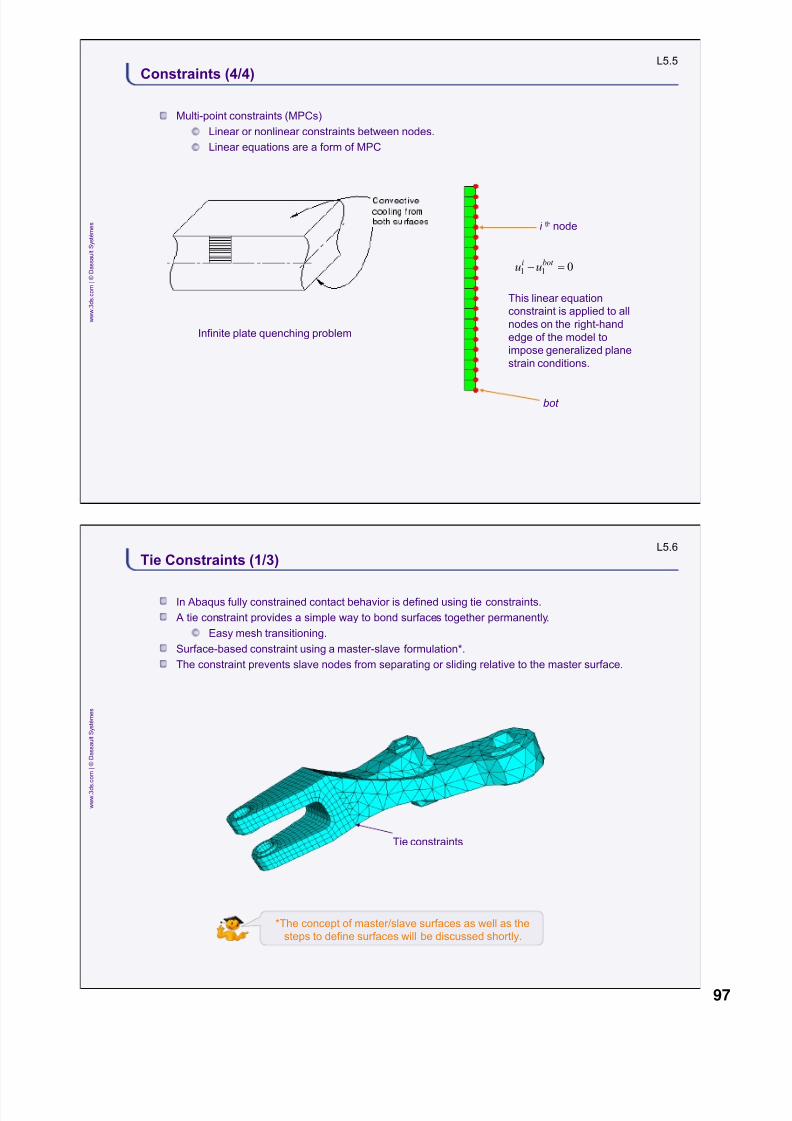
Multi-point constraints (MPCs)
Linear or nonlinear constraints between nodes.
Linear equations are a form of MPC
Infinite plate quenching problem
1 1 0i bot u u
bot
i th node
This linear equation
constraint is applied to all
nodes on the right-hand
edge of the model to
impose generalized plane
strain conditions.
L5.6
w w w . 3
d s
. c o m |
©
D a s s a u l t S y s t è m e s
Tie Constraints (1/3)
In Abaqus fully constrained contact behavior is defined using tie constraints.
A tie constraint provides a simple way to bond surfaces together permanently.
Easy mesh transitioning.
Surface-based constraint using a master-slave formulation*.
The constraint prevents slave nodes from separating or sliding relative to the master surface.
Tie constraints
*The concept of master/slave surfaces as well as the
steps to define surfaces will be discussed shortly.
97

8/15/2019 Abaqus Analysis Intro-book
http://slidepdf.com/reader/full/abaqus-analysis-intro-book 98/469

8/15/2019 Abaqus Analysis Intro-book
http://slidepdf.com/reader/full/abaqus-analysis-intro-book 99/469

8/15/2019 Abaqus Analysis Intro-book
http://slidepdf.com/reader/full/abaqus-analysis-intro-book 100/469

8/15/2019 Abaqus Analysis Intro-book
http://slidepdf.com/reader/full/abaqus-analysis-intro-book 101/469

8/15/2019 Abaqus Analysis Intro-book
http://slidepdf.com/reader/full/abaqus-analysis-intro-book 102/469
L5.15
w w w . 3
d s . c o m |
©
D a s s a u l t S y s t è m e s
Rigid Bodies (7/13)
The default “tie” classification takes precedence for nodes attached to more than one element type.
For example, if a node is attached to both CPE3 and B21 elements, the node will be a t ie node by
default.
Default node types can be overridden by including the same node in a pin or tie node set.
*RIGID BODY, REF NODE=node, ELSET=element set , PIN NSET=node set ,
TIE NSET=node set
thickness
L5.16
w w w . 3
d s
. c o m |
©
D a s s a u l t S y s t è m e s
Rigid Bodies (8/13)
Analytical rigid surfaces
Three types of analytical surfaces are available using the *SURFACE option:
Use TYPE=SEGMENTS to define a two-dimensional rigid surface.
Use TYPE=CYLINDER to define a three-dimensional rigid surface that is extruded infinitely in the
out-of-plane direction.
Use TYPE=REVOLUTION to define a three-dimensional surface of revolution.
Analytical rigid surfaces are not smoothed automatically. Contact calculations are easier with smoothed
surfaces, however.
Use the FILLET RADIUS parameter to provide the radius used to smooth segments of the
analytical rigid surface.
Use the *RIGID BODY option to assign the surface to a rigid body and assign the reference node.
102

8/15/2019 Abaqus Analysis Intro-book
http://slidepdf.com/reader/full/abaqus-analysis-intro-book 103/469

8/15/2019 Abaqus Analysis Intro-book
http://slidepdf.com/reader/full/abaqus-analysis-intro-book 104/469
L5.19
w w w . 3
d s . c o m |
©
D a s s a u l t S y s t è m e s
Rigid Bodies (11/13)
Location of the rigid body reference node
You can place the rigid body reference node anywhere in a model.
The location is important if the rigid body is to move freely under applied loads during the analysis; in
this case the node should be placed at the center of mass of the rigid body.
Abaqus can calculate the center of mass and relocate the reference node to this location automatically.
Abaqus will use the mass distribution from the elements making up the rigid body to determine the center
of mass.
If the reference node is relocated at the center of mass of the rigid body, the new coordinates of the
reference node are also printed out at the end of the printed output file.
Syntax:
*RIGID BODY, REF NODE=node, ELSET=element set ,POSITION=CENTER OF MASS
L5.20
w w w . 3
d s
. c o m |
©
D a s s a u l t S y s t è m e s
Rigid Bodies (12/13)
Inertial properties of rigid bodies
The mass and rotary inertia of a meshed rigid body can be calculated based on the contributions from
its elements, or they can be assigned specifically by using MASS and ROTARYI elements defined at the
slave nodes of a rigid body or the rigid body reference node.
The mass, the center of mass, and the moments of inertia about the center of mass of each rigid
body appear in the printed output f ile.
Using rigid bodies for model verification
It may be useful to specify parts of a model as rigid for model verification purposes.
For example, in complex models where all potential contact conditions cannot be anticipated,
elements far away from the region of interest could be included as part of a rigid body, resulting in
faster run times while developing a model.
When you are satisfied with the model and contact pair definitions, rigid body definitions can beremoved and an accurate deformable finite element representation can be incorporated
throughout.
104
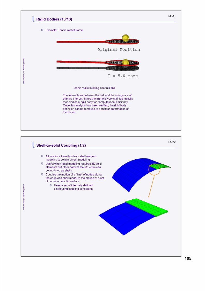
8/15/2019 Abaqus Analysis Intro-book
http://slidepdf.com/reader/full/abaqus-analysis-intro-book 105/469
L5.21
w w w . 3
d s . c o m |
©
D a s s a u l t S y s t è m e s
Rigid Bodies (13/13)
Example: Tennis racket frame
Tennis racket striking a tennis ball
The interactions between the ball and the strings are of
primary interest. Since the frame is very stiff, it is initially
modeled as a rigid body for computational efficiency.Once this analysis has been verified, the rigid body
definition can be removed to consider deformation of
the racket.
L5.22
w w w . 3
d s
. c o m |
©
D a s s a u l t S y s t è m e s
Shell-to-solid Coupling (1/2)
Allows for a transition from shell element
modeling to solid element modeling
Useful when local modeling requires 3D solid
elements but other parts of the structure can
be modeled as shells
Couples the motion of a “line” of nodes along
the edge of a shell model to the motion of a set
of nodes on a solid surface
Uses a set of internally defined
distributing coupling constraints
105

8/15/2019 Abaqus Analysis Intro-book
http://slidepdf.com/reader/full/abaqus-analysis-intro-book 106/469

8/15/2019 Abaqus Analysis Intro-book
http://slidepdf.com/reader/full/abaqus-analysis-intro-book 107/469

8/15/2019 Abaqus Analysis Intro-book
http://slidepdf.com/reader/full/abaqus-analysis-intro-book 108/469

8/15/2019 Abaqus Analysis Intro-book
http://slidepdf.com/reader/full/abaqus-analysis-intro-book 109/469
L5.29
w w w . 3
d s . c o m |
©
D a s s a u l t S y s t è m e s
Contact (6/12)
Deformable to rigid
body contact
Finite sliding between
the surfaces (large
displacements).
Finite strain of the
deforming components.
Typical examples:
I. Rubber seals
II. Tire on road
III. Pipeline on seabed
IV. Forming simulations
(rigid die/mold,
deformable component).
This example is taken from “Superplastic
forming of a rectangular box,” Section 1.3.2
in the Abaqus Example Problems Manual.
Example: metal forming simulation
L5.30
w w w . 3
d s
. c o m |
©
D a s s a u l t S y s t è m e s
Contact (7/12)
Abaqus provides two approaches for modeling
surface-based contact:
General contact allows you to define contact
between many or all regions of a model with a
single interaction.
The surfaces that can interact with one
another comprise the contact domain
and can span many disconnected
regions of a model.
Contact pairs describe contact between two
surfaces.
Requires more careful definition of
contact.
I. Every possible contact pairinteraction must be defined.
Has many restrictions on the types of
surfaces involved.
One contact domain in general contact
Multiple contact pairs required
109

8/15/2019 Abaqus Analysis Intro-book
http://slidepdf.com/reader/full/abaqus-analysis-intro-book 110/469
L5.31
w w w . 3
d s . c o m |
©
D a s s a u l t S y s t è m e s
Contact (8/12)
The general contact algorithm
The contact domain spans multiple bodies
(both rigid and deformable)
Default domain is defined automatically
via an
all-inclusive element-based surface
The method is geared toward models with
multiple components and complex topology
Greater ease in defining contact model
L5.32
w w w . 3
d s
. c o m |
©
D a s s a u l t S y s t è m e s
Contact (9/12)
The contact pair algorithm
Requires user-specified pairing of individual surfaces
Often results in more efficient analyses since contact surfaces are limited in scope
Slave surfaces for
contact pair analysis
110

8/15/2019 Abaqus Analysis Intro-book
http://slidepdf.com/reader/full/abaqus-analysis-intro-book 111/469
L5.33
w w w . 3
d s . c o m |
©
D a s s a u l t S y s t è m e s
Contact (10/12)
The choice between general contact and contact pairs is largely a trade-off between ease of defining contact
and analysis performance
Robustness and accuracy of both methods are similar
In some cases, the contact pair approach is required in order to access specific features not available with
general contact.
These include:
Analytical rigid surfaces (Abaqus/Standard)
Two-dimensional models (Abaqus/Explicit)
Node-based surfaces
Small sliding
Rough or Lagrange friction (Abaqus/Standard)
See the Abaqus Analysis User’s Manual for a complete list of general contact limitations
L5.34
w w w . 3
d s
. c o m |
©
D a s s a u l t S y s t è m e s
Contact (11/12)
Some additional details
Abaqus/Standard
Contact pairs: "Node-to-surface" contact
discretization is used by default:
I. Nodes on one surface
(the slave surface) contact the discretized
segments on the other surface (the master surface).
II. Also known as a strict master/slave formulation
General contact: “Surface-to-surface" contact discretization
I. Contact is enforced in an average sense.
II. This form of contact discretization may also be used with contact pairs
Abaqus/Explicit
A balanced master/slave formulation is used in most cases.I. The contact constraints are applied twice and averaged, reversing the master and slave
surfaces on the second application.
II. Decreases potential contact penetrations.
Shell thickness in contact
By default, Abaqus considers shell thickness in contact calculations with the exception of finite-
sliding, node-to-surface contact in Abaqus/Standard.
To ignore thickness effects, use the NO THICKNESS parameter on the *CONTACT PAIR option.
111

8/15/2019 Abaqus Analysis Intro-book
http://slidepdf.com/reader/full/abaqus-analysis-intro-book 112/469
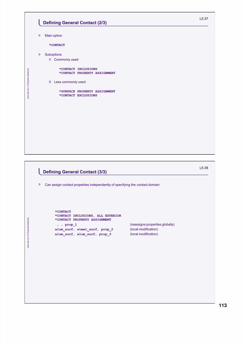
8/15/2019 Abaqus Analysis Intro-book
http://slidepdf.com/reader/full/abaqus-analysis-intro-book 113/469

8/15/2019 Abaqus Analysis Intro-book
http://slidepdf.com/reader/full/abaqus-analysis-intro-book 114/469

8/15/2019 Abaqus Analysis Intro-book
http://slidepdf.com/reader/full/abaqus-analysis-intro-book 115/469
L5.41
w w w . 3
d s . c o m |
©
D a s s a u l t S y s t è m e s
Defining Contact Pairs (3/5)
Defining surfaces
The surfaces are defined using the *SURFACE option.
The faces of each element set are specified using face label identifiers.
Either element set names or element numbers can be used to specify surfaces.
*SURFACE, NAME=ASURF
SLIDER, S1
*SURFACE, NAME=BSURF
BLOCK, S3
Contact occurs on bottom (S1) face of element set SLIDER
Contact occurs on top (S3) face of element set BLOCK
L5.42
w w w . 3
d s
. c o m |
©
D a s s a u l t S y s t è m e s
Defining Contact Pairs (4/5)
Defining pairs of surfaces that can interact
Once you have defined surfaces, you can define “contact pairs.”
Each contact pair specifies two surfaces that can contact each other during the analysis.
In Abaqus/Standard the first surface is the slave surface and the second surface is the master
surface.
In Abaqus/Explicit the order of the surfaces does not usually affect the contact calculations.
*CONTACT PAIR, INTERACTION=FRIC1
ASURF, BSURF
115

8/15/2019 Abaqus Analysis Intro-book
http://slidepdf.com/reader/full/abaqus-analysis-intro-book 116/469
L5.43
w w w . 3
d s . c o m |
©
D a s s a u l t S y s t è m e s
Defining Contact Pairs (5/5)
Defining surface interaction properties
The *SURFACE INTERACTION option block defines the surface interaction properties.
Defines surface behavior properties such as friction.
Defines contact interface out-of-plane thickness for two-dimensional cases.
This option is always necessary in Abaqus/Standard, even when additional properties are not
specified.I. It is optional in Abaqus/Explicit.
The *CONTACT PAIR option refers to a *SURFACE INTERACTION option by name.
*CONTACT PAIR, INTERACTION=FRIC1
ASURF, BSURF
*SURFACE INTERACTION, NAME=FRIC1
1.0,
*FRICTION
0.4,
Out-of-plane thickness
List surface constitutive
properties as suboptions of
*SURFACE INTERACTION
L5.44
w w w . 3
d s
. c o m |
©
D a s s a u l t S y s t è m e s
Contact Pair Surfaces (1/8)
Use the *SURFACE, TYPE=ELEMENT option to define surfaces on deformable bodies or meshed rigid
bodies.
Define surfaces by specifying element face identifier labels
or
Allow Abaqus to automatically determine the “free surfaces” of a body of continuum elements
Use the *SURFACE, TYPE=[SEGMENTS | CYLINDER | REVOLUTION] option with the *RIGID BODY
option to define analytical rigid surfaces.
Discussed earlier in the context of rigid bodies
Use the *SURFACE, TYPE=NODE option to specify individual nodes that may experience contact.
116
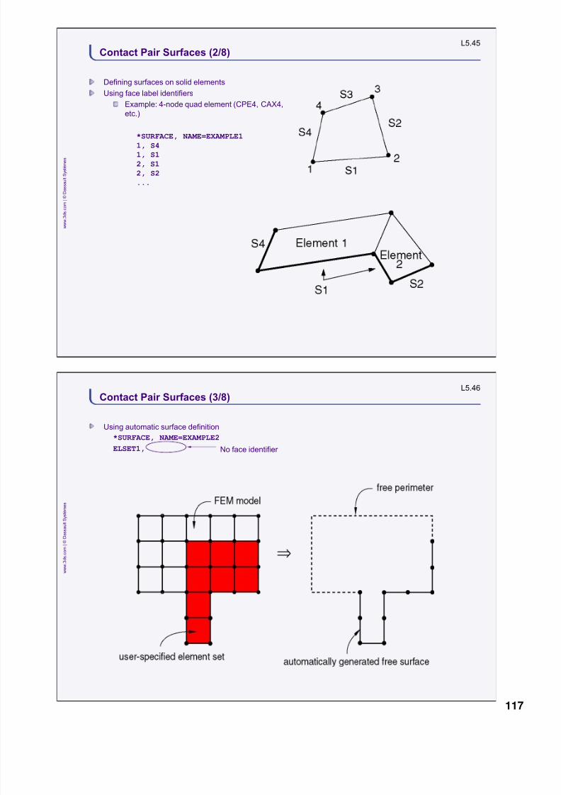
8/15/2019 Abaqus Analysis Intro-book
http://slidepdf.com/reader/full/abaqus-analysis-intro-book 117/469
L5.45
w w w . 3
d s . c o m |
©
D a s s a u l t S y s t è m e s
Contact Pair Surfaces (2/8)
Defining surfaces on solid elements
Using face label identifiers
Example: 4-node quad element (CPE4, CAX4,
etc.)
*SURFACE, NAME=EXAMPLE11, S4
1, S1
2, S12, S2
...
L5.46
w w w . 3
d s
. c o m |
©
D a s s a u l t S y s t è m e s
Contact Pair Surfaces (3/8)
Using automatic surface definition
*SURFACE, NAME=EXAMPLE2
ELSET1, No face identifier
117

8/15/2019 Abaqus Analysis Intro-book
http://slidepdf.com/reader/full/abaqus-analysis-intro-book 118/469

8/15/2019 Abaqus Analysis Intro-book
http://slidepdf.com/reader/full/abaqus-analysis-intro-book 119/469
L5.49
w w w . 3
d s . c o m |
©
D a s s a u l t S y s t è m e s
Contact Pair Surfaces (6/8)
Node-based surfaces
Alternative way to define points for contact.
Instead of specifying element faces as a contact surface, a node-based surface contains only
nodes.
Node-based surfaces are always considered slave surfaces.
Example: tennis racket strings
define surface containing
contact nodes
previously defined
surface
*SURFACE, TYPE=NODE, NAME=STRINGS
STRINGS,
*CONTACT PAIR, INTERACTION=SMOOTH
STRINGS, BALL
Strings: node-
based surface
Ball: element-
based surface
L5.50
w w w . 3
d s
. c o m |
©
D a s s a u l t S y s t è m e s
Contact Pair Surfaces (7/8)
General rules
All elements underlying a surface must be
compatible. They must be:
Of the same dimension (two- or three-
dimensional).
I. For two-dimensional surfaces: all
planar or all axisymmetric (but not
both).
Of the same order of interpolation (first-
or second-order).
All deformable or all rigid (but not both).
Additional restrictions
Surface normals
Master surface normals must be
consistent
Master surface normals should point
toward the slave surface.
I. Otherwise convergence difficulties
will occur.
Rigid surfaces
All surfaces defined on rigid bodies
must be specified as master surfaces.
119

8/15/2019 Abaqus Analysis Intro-book
http://slidepdf.com/reader/full/abaqus-analysis-intro-book 120/469
L5.51
w w w . 3
d s . c o m |
©
D a s s a u l t S y s t è m e s
Contact Pair Surfaces (8/8)
Master contact pair surfaces in Abaqus/Standard (when using the default node-to-surface algorithm) and
all contact pair surfaces in Abaqus/Explicit have an additional restriction:
It must be possible to traverse between any two points on the surface without leaving the surface,
passing through it, or passing through a single point.
valid master surfaces
Traversal requires
passing through or
leaving the surface.
invalid master surfaces
Traversal cannot take
place through a point.
L5.52
w w w . 3
d s
. c o m |
©
D a s s a u l t S y s t è m e s
Local Surface Behavior (1/7)
Contact modeling allows for interactions in the
normal and
tangential
contact directions.
Other contact interaction properties include contact damping and geometric properties such as out-of-
plane thickness.
120

8/15/2019 Abaqus Analysis Intro-book
http://slidepdf.com/reader/full/abaqus-analysis-intro-book 121/469
L5.53
w w w . 3
d s . c o m |
©
D a s s a u l t S y s t è m e s
Local Surface Behavior (2/7)
Behavior in the contact normal direction
Hard contact
“Hard” contact is the default local
behavior in all contact problems.
Contact constraints enforced via a:
Direct method (contact pairs only)
Penalty method (default for general
contact)
Augmented Lagrange method
Pressure-clearance relationship
*surface behavior, augmented lagrange (Abaqus/Standard only)
*surface interaction, name=...
*surface behavior, penalty
*contact pair, mechanical=penalty (Abaqus/Explicit)
(Abaqus/Standard)
Lagrange Multipliers for Abaqus/Standard
Precise kinematic compliance for Abaqus/Explicit
L5.54
w w w . 3
d s
. c o m |
©
D a s s a u l t S y s t è m e s
Local Surface Behavior (3/7)
Alternatives to hard contact
The *SURFACE BEHAVIOR
option is used as a suboption
of the *SURFACE
INTERACTION option to
specify:
Softened contact
(exponential or tabular
pressure-clearance
relationship)
Contact without separation
Other options:
Clearance-dependent viscous damping (*CONTACT DAMPING).
Contact with overclosure or tensile contact forces (*CONTACT CONTROLS; Abaqus/Standardonly).
121

8/15/2019 Abaqus Analysis Intro-book
http://slidepdf.com/reader/full/abaqus-analysis-intro-book 122/469
L5.55
w w w . 3
d s . c o m |
©
D a s s a u l t S y s t è m e s
Local Surface Behavior (4/7)
Behavior in the contact tangential direction
Frictional shear stresses, , may develop at the interface between contacting bodies.
If the magnitude reaches a critical value, the bodies will slip; otherwise they will stick .
L5.56
w w w . 3
d s
. c o m |
©
D a s s a u l t S y s t è m e s
Local Surface Behavior (5/7)
Friction is a highly nonlinear effect.
Solutions are more difficult to obtain.
Do not use unless physically important.
Friction is nonconservative.
In Abaqus/Standard friction causes the equation system to be unsymmetric. The *STEP,
UNSYMM=YES option is used automatically for high ( >0.2) .
Using UNSYMM=NO will give slower convergence, but the solution will be correct (if obtained). It
may also use less disk space.
This behavior is not an issue with Abaqus/Explicit, where there are no systems of equations to
solve.
122

8/15/2019 Abaqus Analysis Intro-book
http://slidepdf.com/reader/full/abaqus-analysis-intro-book 123/469

8/15/2019 Abaqus Analysis Intro-book
http://slidepdf.com/reader/full/abaqus-analysis-intro-book 124/469
L5.59
w w w . 3
d s . c o m |
©
D a s s a u l t S y s t è m e s
Relative Sliding of Points in Contact (1/3)
Two slide distance options:
Finite sliding Finite sliding is the most general—used by default. Arbitrarily large sliding
between surfaces and large rotations are allowed. Contact is governed by
evolving contact surfaces in current configuration.
Small-sliding Small relative sliding between surfaces. Allows large rotations of the
surfaces, as long as the surfaces do not move significantly relative to each
other.
Contact governed by the presence of local contact planes/lines defined in
the initial configuration.
Computationally less expensive than finite sliding since does not require the
generality of the finite-sliding algorithm.
Only available for contact pairs
*CONTACT PAIR,
SMALL SLIDING
*CONTACT PAIR
L5.60
w w w . 3
d s
. c o m |
©
D a s s a u l t S y s t è m e s
Relative Sliding of Points in Contact (2/3)
Some of the differences between finite and
small sliding will be illustrated by example.
Consider the model shown at right.
The rigid punch is displaced horizontally while
maintaining the clearance indicated in the
figure. Afterwards, it is pushed downward into
the deformable body.
With finite sliding, no contact occurs while the
clearance is maintained (as expected).
124

8/15/2019 Abaqus Analysis Intro-book
http://slidepdf.com/reader/full/abaqus-analysis-intro-book 125/469

8/15/2019 Abaqus Analysis Intro-book
http://slidepdf.com/reader/full/abaqus-analysis-intro-book 126/469

8/15/2019 Abaqus Analysis Intro-book
http://slidepdf.com/reader/full/abaqus-analysis-intro-book 127/469
L5.65
w w w . 3
d s . c o m |
©
D a s s a u l t S y s t è m e s
Adjusting Initial Nodal Locations for Contact (4/6)
Specifying a node set of slave nodes to adjust:
Overclosed slave nodes not in the node set will remain overclosed and will cause strains when
forced back onto the contact surface during the analysis.
Example of specifying an ADJUST node set:
*NSET, NSET=CONNODE, GENERATE
1, 8, 1*CONTACT PAIR, INTERACTION=RIG, ADJUST=CONNODE
L5.66
w w w . 3
d s
. c o m |
©
D a s s a u l t S y s t è m e s
Adjusting Initial Nodal Locations for Contact (5/6)
Visualizing strain-free adjustments
In Abaqus/Standard, output variable STRAINFREE is provided to visualize strain-free adjustments
This output variable is written by default if any initial strain-free adjustments are made
This variable is only available in the initial output frame at t = 0
Initial configuration
without contactSymbol plot of
STRAINFREE
127

8/15/2019 Abaqus Analysis Intro-book
http://slidepdf.com/reader/full/abaqus-analysis-intro-book 128/469

8/15/2019 Abaqus Analysis Intro-book
http://slidepdf.com/reader/full/abaqus-analysis-intro-book 129/469

8/15/2019 Abaqus Analysis Intro-book
http://slidepdf.com/reader/full/abaqus-analysis-intro-book 130/469
L5.71
w w w . 3
d s . c o m |
©
D a s s a u l t S y s t è m e s
Contact Output (4/4)
Two other options exist for generating printed output relevant to Abaqus/Standard contact analyses:
*PREPRINT, CONTACT=YES:
I. Controls output to the printed output file during preprocessing
II. Gives details of internally generated contact elements
III. Recommended for small-sliding contact problems to verify master-slave node interaction
IV. Use to check that surface definitions and interactions are correct*PRINT, CONTACT=YES:
I. Controls output to the message file during the analysis phase
II. Gives details of the iteration process
III. Use to understand where difficulties are occurring during contact
L5.72
w w w . 3
d s
. c o m |
©
D a s s a u l t S y s t è m e s
1. Workshop tasks
1. Evaluate a hyperelastic material model.
2. Define contact
1. Contact pairs
2. General contact
3. Apply boundary conditions
4. Perform large displacement analysis
5. Visualize the results.
Workshop 5: Seal Contact (IA)
1 hour
Interactive version. Choose either the interactiveor keywords version of this workshop.
130

8/15/2019 Abaqus Analysis Intro-book
http://slidepdf.com/reader/full/abaqus-analysis-intro-book 131/469
L5.73
w w w . 3
d s . c o m |
©
D a s s a u l t S y s t è m e s
1. Workshop tasks
1. Evaluate a hyperelastic material model.
2. Define contact
1. Contact pairs
2. General contact
3. Apply boundary conditions4. Perform large displacement analysis
5. Visualize the results.
Workshop 5: Seal Contact (KW)
1 hour
Keywords version. Choose either the interactive
or keywords version of this workshop.
131

8/15/2019 Abaqus Analysis Intro-book
http://slidepdf.com/reader/full/abaqus-analysis-intro-book 132/469132

8/15/2019 Abaqus Analysis Intro-book
http://slidepdf.com/reader/full/abaqus-analysis-intro-book 133/469

8/15/2019 Abaqus Analysis Intro-book
http://slidepdf.com/reader/full/abaqus-analysis-intro-book 134/469
Notes
134

8/15/2019 Abaqus Analysis Intro-book
http://slidepdf.com/reader/full/abaqus-analysis-intro-book 135/469
L6.1
w w w . 3
d s . c o m |
©
D a s s a u l t S y s t è m e s
Lesson content :
What Makes a Problem Dynamic?
Equations for Dynamic Problems
Linear Dynamics
Nonlinear Dynamics
Comparing Abaqus/Standard and Abaqus/Explicit
Nonlinear Dynamics Example
Workshop 6: Dynamics (IA)
Workshop 6: Dynamics (KW)
Lesson 6: Introduction to Dynamics
2 hours
Both interactive (IA) and keywords (KW) versionsof the workshop are provided. Complete only one.
L6.2
w w w . 3
d s
. c o m |
©
D a s s a u l t S y s t è m e s
What Makes a Problem Dynamic?
A problem is dynamic when the inertial forces (d’Alembert forces) are significant and vary rapidly in time.
Inertial forces are proportional to the acceleration of the mass in the structure.
Solving a dynamic problem may require the integration of the equations of motion in time.
I. Direct Integration (Expensive)
II. Modal Transient (Effective for Linear Problems)
Many dynamic vibration problems can be studied effectively in the frequency domain.
I. Frequency Response or Steady State Dynamics implies Harmonic Excitation and Responseand thus does not require integration
Sometimes we have large inertia loads but can do static analyses because the loads vary slowly
with time (constant acceleration, centrifugal loads)
I. However, centrifugal loads in flexible systems may lead to whirls (Complex Eigenvalues)
135

8/15/2019 Abaqus Analysis Intro-book
http://slidepdf.com/reader/full/abaqus-analysis-intro-book 136/469
L6.3
w w w . 3
d s . c o m |
©
D a s s a u l t S y s t è m e s
Equations for Dynamic Problems
Dynamic equilibrium
The dynamic equilibrium equations are written for convenience with the inertial forces isolated from the
other forces:
Assumptions:
M (the mass matrix) is constant in time.
I and P may depend on nodal displacements and velocities but not on any higher-order time
derivatives.
I. Thus, the system is second order in time, and damping/dissipation are included in I and P .
If where K (stiffness) and C (damping) are constant, the problem is linear .
These equilibrium equations are completely general.
They apply to the behavior of any mechanical system and contain all nonlinearities.
When the first term—the inertial or dynamic force—is small enough, the equations reduce to the
static form of equilibrium.
0M u I P
I Ku Cu
L6.4
w w w . 3
d s
. c o m |
©
D a s s a u l t S y s t è m e s
Linear Dynamics (1/12)
Linear dynamics problems require the use of an implicit solution scheme (i.e., Abaqus/Standard).
Several classes of linear dynamics problems can be solved with Abaqus:
Natural frequency extraction *
Modal superposition
Implicit (direct-integration) dynamics
Harmonic loading *
Response spectrum analysis *
Random loading *
In this section we focus on natural frequency extraction and give a brief overview of modal-superposition
methods.
*No integration required.
136

8/15/2019 Abaqus Analysis Intro-book
http://slidepdf.com/reader/full/abaqus-analysis-intro-book 137/469
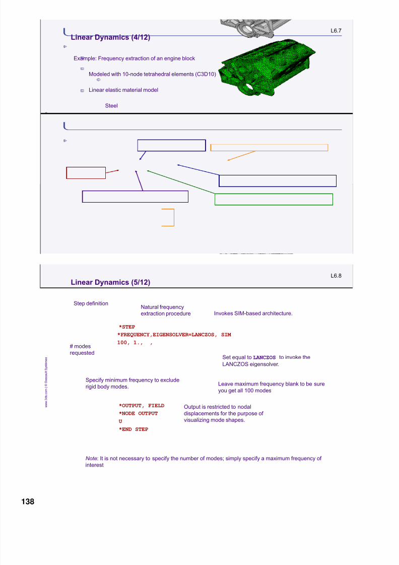
8/15/2019 Abaqus Analysis Intro-book
http://slidepdf.com/reader/full/abaqus-analysis-intro-book 138/469
L6.7
w w w . 3
d s . c o m |
©
D a s s a u l t S y s t è m e s
Linear Dynamics (4/12)
Example: Frequency extraction of an engine block
Modeled with 10-node tetrahedral elements (C3D10)
Linear elastic material model
Steel
The structure is unrestrained.
L6.8
w w w . 3
d s
. c o m |
©
D a s s a u l t S y s t è m e s
Linear Dynamics (5/12)
Step definition
*STEP
*FREQUENCY,EIGENSOLVER=LANCZOS, SIM
100, 1., ,
*OUTPUT, FIELD
*NODE OUTPUT
U
*END STEP
Set equal to LANCZOS to invoke the
LANCZOS eigensolver.
Specify minimum frequency to exclude
rigid body modes.Leave maximum frequency blank to be sure
you get all 100 modes
# modes
requested
Invokes SIM-based architecture.
Note: It is not necessary to specify the number of modes; simply specify a maximum frequency of
interest
Output is restricted to nodal
displacements for the purpose of
visualizing mode shapes.
Natural frequency
extraction procedure
138

8/15/2019 Abaqus Analysis Intro-book
http://slidepdf.com/reader/full/abaqus-analysis-intro-book 139/469
L6.9
w w w . 3
d s . c o m |
©
D a s s a u l t S y s t è m e s
Linear Dynamics (6/12)
The first 10 nonrigid body eigenmodes are shown below
Mode 1 Mode 2 Mode 3
Mode 4 Mode 5 Mode 6
Mode 7 Mode 8 Mode 9 Mode 10
L6.10
w w w . 3
d s
. c o m |
©
D a s s a u l t S y s t è m e s
Linear Dynamics (7/12)
Modal superposition
The eigenmodes of a structure can be used in several different mode-based procedures to study itslinear dynamic response:
Modal dynamics
I. Calculates linear dynamic response in time domain
II. Direct integration also available
Steady-state dynamics
I. Calculates dynamic response due to harmonic excitation
II. Direct solution or modal
Response spectrum
I. Estimates peak response to dynamic motion
Random response
I. Predicts response to random continuous excitation
139

8/15/2019 Abaqus Analysis Intro-book
http://slidepdf.com/reader/full/abaqus-analysis-intro-book 140/469
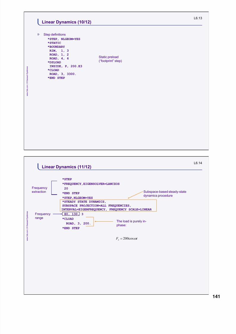
8/15/2019 Abaqus Analysis Intro-book
http://slidepdf.com/reader/full/abaqus-analysis-intro-book 141/469
L6.13
w w w . 3
d s . c o m |
©
D a s s a u l t S y s t è m e s
Linear Dynamics (10/12)
Step definitions
*STEP, NLGEOM=YES
*STATIC
*BOUNDARY
RIM, 1, 3
ROAD, 1, 2
ROAD, 4, 6*DSLOAD
INSIDE, P, 200.E3
*CLOAD
ROAD, 3, 3300.
*END STEP
Static preload(“footprint” step)
L6.14
w w w . 3
d s
. c o m |
©
D a s s a u l t S y s t è m e s
Linear Dynamics (11/12)
*STEP
*FREQUENCY,EIGENSOLVER=LANCZOS
20
*END STEP
*STEP,NLGEOM=YES
*STEADY STATE DYNAMICS,
SUBSPACE PROJECTION=ALL FREQUENCIES,
INTERVAL=EIGENFREQUENCY, FREQUENCY SCALE=LINEAR
80, 130, 3
*CLOAD
ROAD, 3, 200.
*END STEP
Frequency
range
Subspace-based steady-state
dynamics procedure
Frequency
extraction
The load is purely in-
phase:
200cos z
F t
141

8/15/2019 Abaqus Analysis Intro-book
http://slidepdf.com/reader/full/abaqus-analysis-intro-book 142/469
8/15/2019 Abaqus Analysis Intro-book
http://slidepdf.com/reader/full/abaqus-analysis-intro-book 143/469

8/15/2019 Abaqus Analysis Intro-book
http://slidepdf.com/reader/full/abaqus-analysis-intro-book 144/469
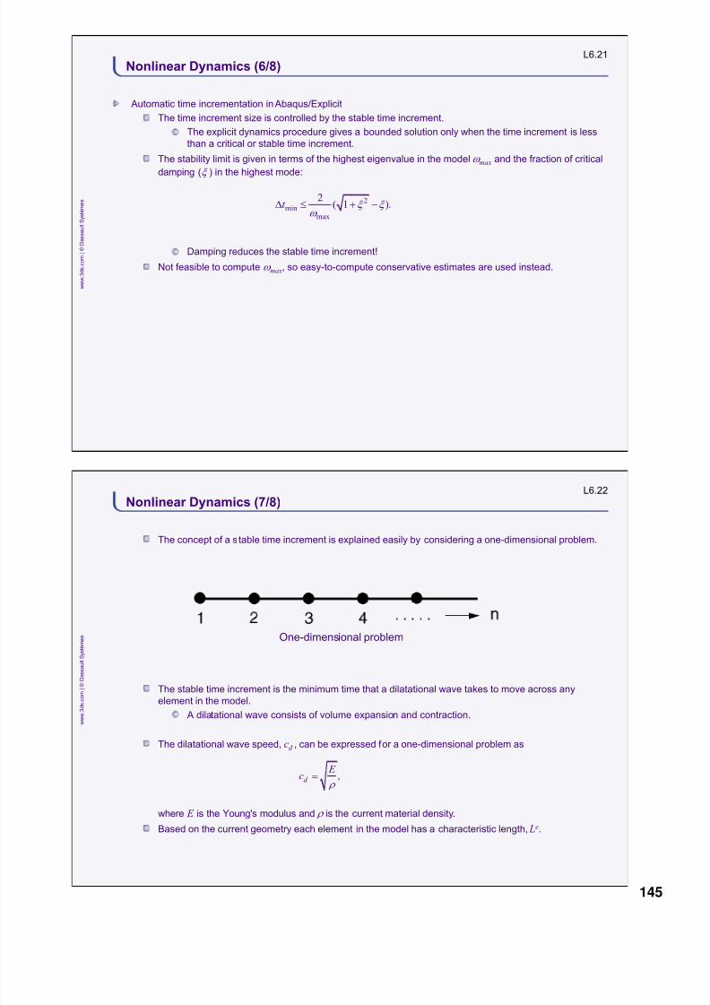
8/15/2019 Abaqus Analysis Intro-book
http://slidepdf.com/reader/full/abaqus-analysis-intro-book 145/469
L6.21
w w w . 3
d s . c o m |
©
D a s s a u l t S y s t è m e s
Nonlinear Dynamics (6/8)
Automatic time incrementation in Abaqus/Explicit
The time increment size is controlled by the stable time increment.
The explicit dynamics procedure gives a bounded solution only when the time increment is less
than a critical or stable time increment.
The stability limit is given in terms of the highest eigenvalue in the model max and the fraction of critical
damping ( ) in the highest mode:
Damping reduces the stable time increment!
Not feasible to compute max, so easy-to-compute conservative estimates are used instead.
2min
max
2( 1 )t
D .
L6.22
w w w . 3
d s
. c o m |
©
D a s s a u l t S y s t è m e s
Nonlinear Dynamics (7/8)
The concept of a stable time increment is explained easily by considering a one-dimensional problem.
The stable time increment is the minimum time that a dilatational wave takes to move across any
element in the model. A dilatational wave consists of volume expansion and contraction.
The dilatational wave speed, cd , can be expressed for a one-dimensional problem as
where E is the Young's modulus and is the current material density.
Based on the current geometry each element in the model has a characteristic length, Le.
One-dimensional problem
d
E c
,
145

8/15/2019 Abaqus Analysis Intro-book
http://slidepdf.com/reader/full/abaqus-analysis-intro-book 146/469
L6.23
w w w . 3
d s . c o m |
©
D a s s a u l t S y s t è m e s
Nonlinear Dynamics (8/8)
Thus, the stable time increment can be expressed as
Decreasing Le and/or increasing cd
will reduce the size of the stable time increment.
Decreasing element dimensions reduces Le.
Increasing material stiffness increases cd .
Decreasing material compressibility increases cd .
Decreasing material density increases cd .
Abaqus/Explicit monitors the finite element model throughout the analysis to determine a stable time
increment.
e
d
Lt
cD .
L6.24
w w w . 3
d s
. c o m |
©
D a s s a u l t S y s t è m e s
Comparing Abaqus/Standard and Abaqus/Explicit (1/3)
Abaqus/Standard
Time increment size is not limited: generally fewer
time increments required to complete a given
simulation.
Each time increment is relatively expensive since
the solution for a set of simultaneous equations is
required for each.
Abaqus/Explicit
Time increment size is limited: generally many more
time increments are required to complete a given
simulation.
Each time increment is relatively inexpensive
because the solution of a set of simultaneous
equations is not required.
Most of the computational expense is associated with
element calculations (forming and assembling I ).
146

8/15/2019 Abaqus Analysis Intro-book
http://slidepdf.com/reader/full/abaqus-analysis-intro-book 147/469
L6.25
w w w . 3
d s . c o m |
©
D a s s a u l t S y s t è m e s
Comparing Abaqus/Standard and Abaqus/Explicit (2/3)
Abaqus/Standard
Ideal for problems where the response period of
interest is long compared to the vibration frequency
of the model.
Difficult to use explicit dynamics effectively
because of the limit on the time increment
size.
Use for problems that are mildly nonlinear and where
the nonlinearities are smooth (e.g., plasticity).
With a smooth nonlinear response
Abaqus/Standard will need very few iterations
to find a converged solution.
Abaqus/Explicit
Ideal for high-speed dynamic simulations
Require very small time increments; implicit dynamics
inefficient.
Usually more reliable for problems involving
discontinuous nonlinearities.
Contact behavior is discontinuous and involves
impacts, both of which cause problems for implicit
time integration.
Other sources of discontinuous behavior include
buckling and material failure.
L6.26
w w w . 3
d s
. c o m |
©
D a s s a u l t S y s t è m e s
Comparing Abaqus/Standard and Abaqus/Explicit (3/3)
Example of a problem well suited for Abaqus/Explicit
Pipe whip
This example simulates
a pipe-on-pipe impact resulting from the
rupture of a high-pressure line in
a power plant.
A sudden release of fluid causes one
segment of the pipe to rotate about
its support and strike a neighboring
pipe.
147

8/15/2019 Abaqus Analysis Intro-book
http://slidepdf.com/reader/full/abaqus-analysis-intro-book 148/469
L6.27
w w w . 3
d s . c o m |
©
D a s s a u l t S y s t è m e s
Nonlinear Dynamics Example (1/3)
Reference: “Double cantilever elastic beam under point load,” Section 1.3.2 in the Abaqus Benchmarks
Manual.
L6.28
w w w . 3
d s
. c o m |
©
D a s s a u l t S y s t è m e s
Nonlinear Dynamics Example (2/3)
Abaqus/Standard input file
*HEADING
NONLINEAR ELASTIC BEAM
*NODE
1, 0.
6, 10.
*NGEN
1, 6
*NSET, NSET=NFIL
6,
*ELEMENT, TYPE=B23
1, 1, 2
*ELGEN, ELSET=BEAM
1, 5
*BEAM SECTION, ELSET=BEAM,
SECTION=RECT, MATERIAL=A11., .125
0., 0., -1.
3
*MATERIAL, NAME=A1
*ELASTIC
30.E6,
*DENSITY
2.5362E-4,
*RESTART, WRITE, FREQUENCY=10
*STEP, INC=400, NLGEOM=YES
*DYNAMIC
25.E-6, 5.E-3
*BOUNDARY
1, 1, 2
1, 6
6, 1
6, 6
*CLOAD
6, 2, 320.
*END STEP
148

8/15/2019 Abaqus Analysis Intro-book
http://slidepdf.com/reader/full/abaqus-analysis-intro-book 149/469
L6.29
w w w . 3
d s . c o m |
©
D a s s a u l t S y s t è m e s
Nonlinear Dynamics Example (3/3)
Comparing the Abaqus/Standard and Abaqus/Explicit results
The results obtained with the default incrementation schemes show excellent agreement.
Using a tighter half-increment residual tolerance for the implicit analysis further improves the
agreement.
In the non-default case shown here, the
half-increment scale factor was set to 0.05
(the default value is 1000)
*DYNAMIC, HALFINC SCALE FACTOR=0.05
L6.30
w w w . 3
d s
. c o m |
©
D a s s a u l t S y s t è m e s
1. Workshop tasks
1. Complete the model and
perform a frequency extraction analysis.
2. Examine the printed output for relevant frequency results.
3. View the eigenmodes in Abaqus/Viewer.
4. Evaluate the effects of mesh density and element dimension and order.
5. Perform a free-vibration analysis using the implicit dynamics method.
Workshop 6: Dynamics (IA)
1 hour
Interactive version. Choose either the interactiveor keywords version of this workshop.
149

8/15/2019 Abaqus Analysis Intro-book
http://slidepdf.com/reader/full/abaqus-analysis-intro-book 150/469

8/15/2019 Abaqus Analysis Intro-book
http://slidepdf.com/reader/full/abaqus-analysis-intro-book 151/469

8/15/2019 Abaqus Analysis Intro-book
http://slidepdf.com/reader/full/abaqus-analysis-intro-book 152/469
Notes
152

8/15/2019 Abaqus Analysis Intro-book
http://slidepdf.com/reader/full/abaqus-analysis-intro-book 153/469

8/15/2019 Abaqus Analysis Intro-book
http://slidepdf.com/reader/full/abaqus-analysis-intro-book 154/469
L7.3
w w w . 3
d s . c o m |
©
D a s s a u l t S y s t è m e s
Overview of the Explicit Dynamics Procedure (2/6)
Stress wave propagation
This stress wave propagation example illustrates how the explicit dynamics solution procedure works
without iterating or solving sets of linear equations.
We consider the propagation of a stress wave along a rod modeled with three elements. We study the
state of the rod as we increment through time.
Mass is lumped at the nodes.
Initial configuration of a rod with a
concentrated load, P, at the free end
L7.4
w w w . 3
d s
. c o m |
©
D a s s a u l t S y s t è m e s
Overview of the Explicit Dynamics Procedure (3/6)
Configuration at the end of Increment 1
11101
11
1
1111
1
el el el el
el el el
E d
dt d l
udt uu
M
P u
154
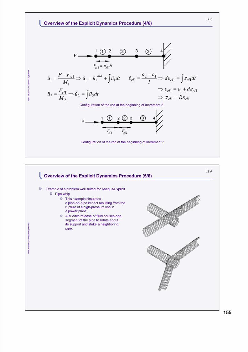
8/15/2019 Abaqus Analysis Intro-book
http://slidepdf.com/reader/full/abaqus-analysis-intro-book 155/469
L7.5
w w w . 3
d s . c o m |
©
D a s s a u l t S y s t è m e s
Overview of the Explicit Dynamics Procedure (4/6)
Configuration of the rod at the beginning of Increment 3
Configuration of the rod at the beginning of Increment 2
dt uu M
F u
dt uuu M
F P u
el
old el
22
2
1
2
111
1
1
1
11
111
el el
el el
E
d
dt d l
uuel el el 11
12
1
L7.6
w w w . 3
d s
. c o m |
©
D a s s a u l t S y s t è m e s
Overview of the Explicit Dynamics Procedure (5/6)
Example of a problem well suited for Abaqus/Explicit
Pipe whip
This example simulates
a pipe-on-pipe impact resulting from the
rupture of a high-pressure line in
a power plant.
A sudden release of fluid causes one
segment of the pipe to rotate about
its support and strike a neighboring
pipe.
155

8/15/2019 Abaqus Analysis Intro-book
http://slidepdf.com/reader/full/abaqus-analysis-intro-book 156/469
L7.7
w w w . 3
d s . c o m |
©
D a s s a u l t S y s t è m e s
Overview of the Explicit Dynamics Procedure (6/6)
Hydroforming
Uses fluid pressure to form a component.
Abaqus/Explicit captures the unstable
wrinkling of excess blank material.
A draw cap is
added to
decrease the
wrinkling effects.
L7.8
w w w . 3
d s
. c o m |
©
D a s s a u l t S y s t è m e s
Abaqus/Explicit Syntax (1/3)
The basic input structure and options for an Abaqus/Explicit model are the same as those for an
Abaqus/Standard model.
This allows users to leverage their knowledge of Abaqus/Standard toward learning Abaqus/Explicit.
An Abaqus/Explicit analysis is performed when the input file contains the *DYNAMIC, EXPLICIT procedure
option.
In the majority of Abaqus/Explicit analyses you provide just the total step time and the time increment size is
chosen automatically so that it always satisfies the stability limit.
*STEP
*DYNAMIC, EXPLICIT
, 70.E-3
Options for controlling the time increment size are available for special circumstances.
156

8/15/2019 Abaqus Analysis Intro-book
http://slidepdf.com/reader/full/abaqus-analysis-intro-book 157/469
L7.9
w w w . 3
d s . c o m |
©
D a s s a u l t S y s t è m e s
Abaqus/Explicit Syntax (2/3)
Unlike Abaqus/Standard, Abaqus/Explicit uses a finite-strain, large-displacement, large-rotation formulation by
default.
The NLGEOM parameter is not needed on the *STEP option.
Geometrically linear analysis (small-deformation analysis) can be obtained by setting NLGEOM=NO.
The numerics of the explicit dynamic procedure require that elements with lumped mass matrices be used.
Since solution efficiency is usually an important factor when using Abaqus/Explicit, only first-order reduced-
integration elements are generally available.
Exceptions:
Modified triangles and tetrahedrals (CPS6M, CPE6M, C3D10M),
second-order beam elements (B22 and B32),
fully-integrated membrane element (M3D4),
fully-integrated shell elements (S4, S4T), and
fully-integrated first-order hex elements (C3D8, C3D8I, C3D8T).
L7.10
w w w . 3
d s
. c o m |
©
D a s s a u l t S y s t è m e s
Abaqus/Explicit Syntax (3/4)
Some options unique to Abaqus/Explicit
The following model definition and history options are available only in Abaqus/Explicit (output and
control options are not listed):
Analysis *DYNAMIC, EXPLICIT: This procedure specifies an explicit dynamics step
procedures and that Abaqus/Explicit will be the solver program.
*DYNAMIC TEMPERATURE-DISPLACEMENT, EXPLICIT: This procedure
specifies a coupled thermal-mechanical step.
* ANNEAL: This procedure sets all nodal velocities to zero and sets all state
variables, such as stress and plastic strain, to zero.
Material *EOS: The equation of state material model can be used to model ahydrodynamic (explosive) material or a nearly incompressible fluid.
*EXTREME VALUE: This option specifies critical variables whose extremevalues will be monitored every increment.
*TRACER PARTICLE: This option defines tracer particles that track materialpoints in an adaptive mesh domain.
157

8/15/2019 Abaqus Analysis Intro-book
http://slidepdf.com/reader/full/abaqus-analysis-intro-book 158/469

8/15/2019 Abaqus Analysis Intro-book
http://slidepdf.com/reader/full/abaqus-analysis-intro-book 159/469

8/15/2019 Abaqus Analysis Intro-book
http://slidepdf.com/reader/full/abaqus-analysis-intro-book 160/469160

8/15/2019 Abaqus Analysis Intro-book
http://slidepdf.com/reader/full/abaqus-analysis-intro-book 161/469

8/15/2019 Abaqus Analysis Intro-book
http://slidepdf.com/reader/full/abaqus-analysis-intro-book 162/469

8/15/2019 Abaqus Analysis Intro-book
http://slidepdf.com/reader/full/abaqus-analysis-intro-book 163/469

8/15/2019 Abaqus Analysis Intro-book
http://slidepdf.com/reader/full/abaqus-analysis-intro-book 164/469

8/15/2019 Abaqus Analysis Intro-book
http://slidepdf.com/reader/full/abaqus-analysis-intro-book 165/469

8/15/2019 Abaqus Analysis Intro-book
http://slidepdf.com/reader/full/abaqus-analysis-intro-book 166/469
L8.7
w w w . 3
d s . c o m |
©
D a s s a u l t S y s t è m e s
Solution Strategies (3/3)
The final deformed configuration is shown at
right.
Near the end of the punch stroke, the
blank pulls through the blank holder and
begins to wrinkle.
The Abaqus/Standard job was about 20 times
more expensive (in terms of CPU cost) thanthe Abaqus/Explicit job.
Abaqus/Standard fails to converge at the point
where the blank begins to wrinkle.
L8.8
w w w . 3
d s
. c o m |
©
D a s s a u l t S y s t è m e s
Quasi-Static Simulations Using Explicit Dynamics (1/10)
Introduction
The explicit dynamics procedure is a true dynamic procedure. It was originally developed to model high-
speed impact events.
Explicit dynamics solves for the state of dynamic equilibrium where inertia can play a dominant
role in the solution.
Application of explicit dynamics to model quasi-static events, such as metal forming processes, requires
special consideration:
It is computationally impractical to model the process in its natural time period.
I. Recall that stability considerations limit the size of the allowable increment:
II. Literally millions of time increments would be required.
Artificially increasing the speed of the process in the simulation is necessary to obtain an
economical solution.
e
d
Lt
c .
166
8/15/2019 Abaqus Analysis Intro-book
http://slidepdf.com/reader/full/abaqus-analysis-intro-book 167/469
L8.9
w w w . 3
d s . c o m |
©
D a s s a u l t S y s t è m e s
Quasi-Static Simulations Using Explicit Dynamics (2/10)
Two approaches to obtaining economical quasi-static solutions with an explicit dynamics solver
Increased load rates
Artificially reduce the time scale of the process by increasing the loading rate.
Material strain rates calculated in the simulation are artificially high by the same factor applied to
increase the loading rate.
I. This is irrelevant if the material is rate insensitive.Mass scaling
If strain rate sensitivity is being modeled, erroneous solutions can result if the load rates are
increased. Mass scaling allows you to model processes in their natural time scale when
considering rate-sensitive materials.
I. Artificially increasing the material density by a factor of f 2 increases the stable time
increment by a factor of f .
L8.10
w w w . 3
d s
. c o m |
©
D a s s a u l t S y s t è m e s
Quasi-Static Simulations Using Explicit Dynamics (3/10)
How much can I increase the load rate or scale the mass?
Increased load rates and mass scaling achieve the same effect.
Increased load rates reduce the time scale of the simulation.
Mass scaling increases the size of the stable time increment.
With both approaches, fewer increments are needed to complete the job.
As the speed of the process is increased, a state of static equilibrium evolves into a state of dynamic
equilibrium.
Inertia forces become more dominant.
The goal is to model the process in the shortest time period (or with the most mass scaling) in which
inertia forces are still insignificant.
167

8/15/2019 Abaqus Analysis Intro-book
http://slidepdf.com/reader/full/abaqus-analysis-intro-book 168/469
L8.11
w w w . 3
d s . c o m |
©
D a s s a u l t S y s t è m e s
Quasi-Static Simulations Using Explicit Dynamics (4/10)
Suggested approach
Run a series of simulations in the order from the fastest load rate to the slowest (or largest mass scaling
to the smallest), since the analysis time is greater for slower load rates (or smaller mass scaling).
Examine the results (deformed shapes, stresses, strains, energies) to get an understanding for the
effects of varying the model.
For example, excessive tool speeds in explicit sheet metal forming simulations tend to suppress
wrinkling and to promote unrealistic localized stretching.
Excessive tool speeds in explicit bulk forming simulations cause ―jetting‖—hydrodynamic-type
response.
L8.12
w w w . 3
d s
. c o m |
©
D a s s a u l t S y s t è m e s
Quasi-Static Simulations Using Explicit Dynamics (5/10)
Jetting
Consider the following bulk forming process (180 section of an axisymmetric model).
When the tool speed is too large, highly localized deformation develops (jetting).
Effect of tool speed on deformed shape
jetting
tool speed = 500 m/stool speed = 10 m/s
168
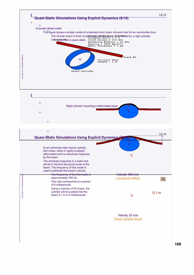
8/15/2019 Abaqus Analysis Intro-book
http://slidepdf.com/reader/full/abaqus-analysis-intro-book 169/469
L8.13
w w w . 3
d s . c o m |
©
D a s s a u l t S y s t è m e s
Quasi-Static Simulations Using Explicit Dynamics (6/10)
Example: sheet metal
This figure shows a simple model of a standard door beam intrusion test for an automobile door.
The circular beam is fixed at each end, and the beam is deformed by a rigid cylinder.
The actual test is quasi-static.
Rigid cylinder impacting a deformable beam
L8.14
w w w . 3
d s
. c o m |
©
D a s s a u l t S y s t è m e s
Velocity 25 m/s:
Good global result
0.1 mV
Velocity 400 m/s:
Localized effect
V
Quasi-Static Simulations Using Explicit Dynamics (7/10)
At an extremely high impact velocity,
400 m/sec, there is highly localized
deformation and no structural response
by the beam.
The dominant response in a static test
will be in the first structural mode of the
beam. The frequency of this mode is
used to estimate the impact velocity.
The frequency of the first mode is
approximately 250 Hz.
This rate corresponds to a period
of 4 milliseconds.
Using a velocity of 25 m/sec, the
cylinder will be pushed into thebeam 0.1 m in 4 milliseconds.
169

8/15/2019 Abaqus Analysis Intro-book
http://slidepdf.com/reader/full/abaqus-analysis-intro-book 170/469
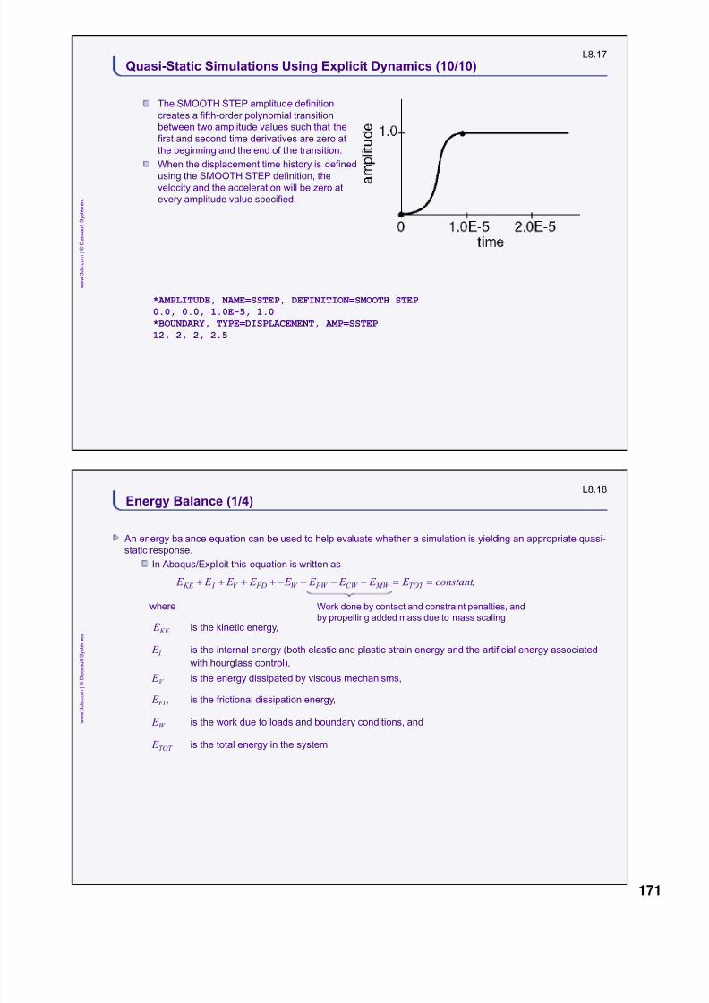
8/15/2019 Abaqus Analysis Intro-book
http://slidepdf.com/reader/full/abaqus-analysis-intro-book 171/469
L8.17
w w w . 3
d s . c o m |
©
D a s s a u l t S y s t è m e s
Quasi-Static Simulations Using Explicit Dynamics (10/10)
The SMOOTH STEP amplitude definition
creates a fifth-order polynomial transition
between two amplitude values such that the
first and second time derivatives are zero at
the beginning and the end of the transition.
When the displacement time history is defined
using the SMOOTH STEP definition, thevelocity and the acceleration will be zero at
every amplitude value specified.
*AMPLITUDE, NAME=SSTEP, DEFINITION=SMOOTH STEP
0.0, 0.0, 1.0E-5, 1.0
*BOUNDARY, TYPE=DISPLACEMENT, AMP=SSTEP
12, 2, 2, 2.5
L8.18
w w w . 3
d s
. c o m |
©
D a s s a u l t S y s t è m e s
Energy Balance (1/4)
An energy balance equation can be used to help evaluate whether a simulation is yielding an appropriate quasi-
static response.
In Abaqus/Explicit this equation is written as
where
E KE is the kinetic energy,
E I is the internal energy (both elastic and plastic strain energy and the artificial energy associated
with hourglass control),
E V is the energy dissipated by viscous mechanisms,
E FD is the frictional dissipation energy,
E W is the work due to loads and boundary conditions, and
E TOT is the total energy in the system.
KE I V FD W PW CW MW TOT E E E E E E E E E constant ,
Work done by contact and constraint penalties, and
by propelling added mass due to mass scaling
171

8/15/2019 Abaqus Analysis Intro-book
http://slidepdf.com/reader/full/abaqus-analysis-intro-book 172/469
L8.19
w w w . 3
d s . c o m |
©
D a s s a u l t S y s t è m e s
Energy Balance (2/4)
Consider a pull test applied to a uniaxial tensile
specimen.
If the physical test is quasi-static, the work
applied by the external forces in stretching the
specimen equals the internal energy in the
specimen.
Uniaxial pull test
L8.20
w w w . 3
d s
. c o m |
©
D a s s a u l t S y s t è m e s
Energy Balance (3/4)
The energy history for the quasi-static test would
appear as shown in the figure at right:
Inertia forces are negligible.
The velocity of material in the test specimen is
very small.
Kinetic energy is negligible.
As the speed of the test increases:
The response of the specimen becomes less
static, more dynamic.
Material velocities and, therefore, kinetic
energy become more significant.Energy history for quasi-static pull test
172
8/15/2019 Abaqus Analysis Intro-book
http://slidepdf.com/reader/full/abaqus-analysis-intro-book 173/469

8/15/2019 Abaqus Analysis Intro-book
http://slidepdf.com/reader/full/abaqus-analysis-intro-book 174/469
L8.23
w w w . 3
d s . c o m |
©
D a s s a u l t S y s t è m e s
Example: Load Rates (2/4)
We examine three different punch speeds:
3 m/s
30 m/s
150 m/s
The computation cost of each cylindrical cup deep drawing simulation is summarized in the following
table:
Punch speed
(m/s)
Time increments Normalized CPU time
3 (1X) 27929 1.0
30 (10X) 2704 0.097
150 (50X) 529 0.019
L8.24
w w w . 3
d s
. c o m |
©
D a s s a u l t S y s t è m e s
Vpunch = 3 m/s Vpunch = 30 m/s
Vpunch = 150 m/s
Example: Load Rates (3/4)
Contours of blank thickness in final
formed configuration
Excessive punch speeds lead
to results that do not
correspond to the physics. At
150 m/s unrealistic thinning
of the blank is predicted.
Results obtained at 30 m/s and
3 m/s are very similar, even
though the difference in
computation cost is a factor of
10.
174

8/15/2019 Abaqus Analysis Intro-book
http://slidepdf.com/reader/full/abaqus-analysis-intro-book 175/469
L8.25
w w w . 3
d s . c o m |
©
D a s s a u l t S y s t è m e s
Example: Load Rates (4/4)
Comparison of internal and kinetic energies
At a punch speed of 150 m/s the kinetic energy of the blank is a significant fraction of its internal energy.
At punch speeds of 3 m/s and 30 m/s the kinetic energy is only a small fraction of the internal energy
over the majority of the forming process history.
L8.26
w w w . 3
d s
. c o m |
©
D a s s a u l t S y s t è m e s
Example: Mass Scaling (1/2)
Uniaxial tension test
The figure shows the problem definition for a
tension test on a plane strain bar with the
material properties of a mild steel.
It is modeled with quarter symmetry.
Mass scaling is available through the *FIXED
MASS SCALING option.
Mass scaling applied at the beginning of
a step.
Syntax:
*FIXED MASS SCALING,
ELSET=name, FACTOR= f 2
The density of every element in the
specified element set is increased by f 2,thus increasing each element’s stable
time increment by f . Uniaxial tension test
175

8/15/2019 Abaqus Analysis Intro-book
http://slidepdf.com/reader/full/abaqus-analysis-intro-book 176/469
L8.27
w w w . 3
d s . c o m |
©
D a s s a u l t S y s t è m e s
Example: Mass Scaling (2/2)
25 Mass
scaling
factor
10000 1
Contours of PEEQ
This figure shows the results of three different
analyses.
The results on the left and in the center
are almost identical.
The solution for the results in the
center requires one-fifth the
computer time of the first solution.
The solution on the right gives an
essentially meaningless result compared
to the original static solution.
L8.28
w w w . 3
d s
. c o m |
©
D a s s a u l t S y s t è m e s
Adaptive Meshing (1/8)
Motivation
In many nonlinear simulations the material in the structure or process undergoes very large
deformations.
These deformations distort the finite element mesh, often to the point where the mesh is unable
to provide accurate results or the analysis terminates prematurely for numerical reasons.
In such simulations it is necessary to use adaptive meshing tools to minimize the distortion in the
mesh periodically.
Note: In this course we restrict our attention to the ALE adaptive meshing capability available in
Abaqus/Explicit.
The adaptive remeshing capability available in Abaqus/Standard and the Coupled Eulerian-Lagrangian
capability available in Abaqus/Explicit are not discussed here.
176

8/15/2019 Abaqus Analysis Intro-book
http://slidepdf.com/reader/full/abaqus-analysis-intro-book 177/469
L8.29
w w w . 3
d s . c o m |
©
D a s s a u l t S y s t è m e s
Adaptive Meshing (2/8)
Adaptive meshing is useful in a broad range of applications:
Can be used as a continuous adaptive meshing tool for transient analysis problems undergoing
large deformations, such as:
I. Dynamic impact
II. Penetration
III. SloshingIV. Forging
Can be used as a solution technique to model steady-state processes, such as:
I. Extrusion
II. Rolling
Can be used as a tool to analyze the transient phase in a steady-state process.
L8.30
w w w . 3
d s
. c o m |
©
D a s s a u l t S y s t è m e s
Adaptive Meshing (3/8)
Adaptive meshing basics
Adaptive meshing is performed in Abaqus/Explicit using the arbitrary Lagrangian-Eulerian (ALE)
method. The primary characteristics of the adaptive meshing capability are:
The mesh is smoothed at regular intervals to reduce element distortion and to maintain good
element aspect ratios.
The same mesh topology is maintained—the number of elements and nodes and their
connectivity do not change.
It can be used to analyze Lagrangian (transient) problems and Eulerian (steady-state) problems.
177

8/15/2019 Abaqus Analysis Intro-book
http://slidepdf.com/reader/full/abaqus-analysis-intro-book 178/469
L8.31
w w w . 3
d s . c o m |
©
D a s s a u l t S y s t è m e s
Adaptive Meshing (4/8)
Arbitrary Lagrangian-Eulerian (ALE) method
Lagrangian Nodes move exactly with material points.
description It is easy to track free surfaces and apply boundary conditions.
The mesh will become distorted with high strain gradients; default description in Abaqus.
Eulerian
Nodes stay fixed while material flows through the meshdescription It is more difficult to track free surfaces.
No mesh distortion because mesh is fixed.
Available using the Coupled Eulerian-Lagrangian (CEL) capability.
ALE Mesh motion is constrained to the material motion only where necessary (at free
boundaries), but otherwise material motion and mesh motion are independent.
L8.32
w w w . 3
d s
. c o m |
©
D a s s a u l t S y s t è m e s
Adaptive Meshing (5/8)
Motion of mesh and material with various methods
178

8/15/2019 Abaqus Analysis Intro-book
http://slidepdf.com/reader/full/abaqus-analysis-intro-book 179/469
L8.33
w w w . 3
d s . c o m |
©
D a s s a u l t S y s t è m e s
Undeformed model
Deformed meshes at 70% of die travel
Adaptive Meshing (6/8)
ALE simulation of an axisymmetric forging problem
L8.34
w w w . 3
d s
. c o m |
©
D a s s a u l t S y s t è m e s
Adaptive Meshing (7/8)
By using the adaptive meshing capability, a high-quality mesh can be maintained throughout the entire
forging process.
ALE simulation: deformed mesh at 100% of die travel
Interior nodes adaptively adjust in all directions
Nodes along the free boundary move
with the material in the direction normal
to the material’s surface. They are
allowed to adapt (adjust their position)
tangent to the free surface.
179
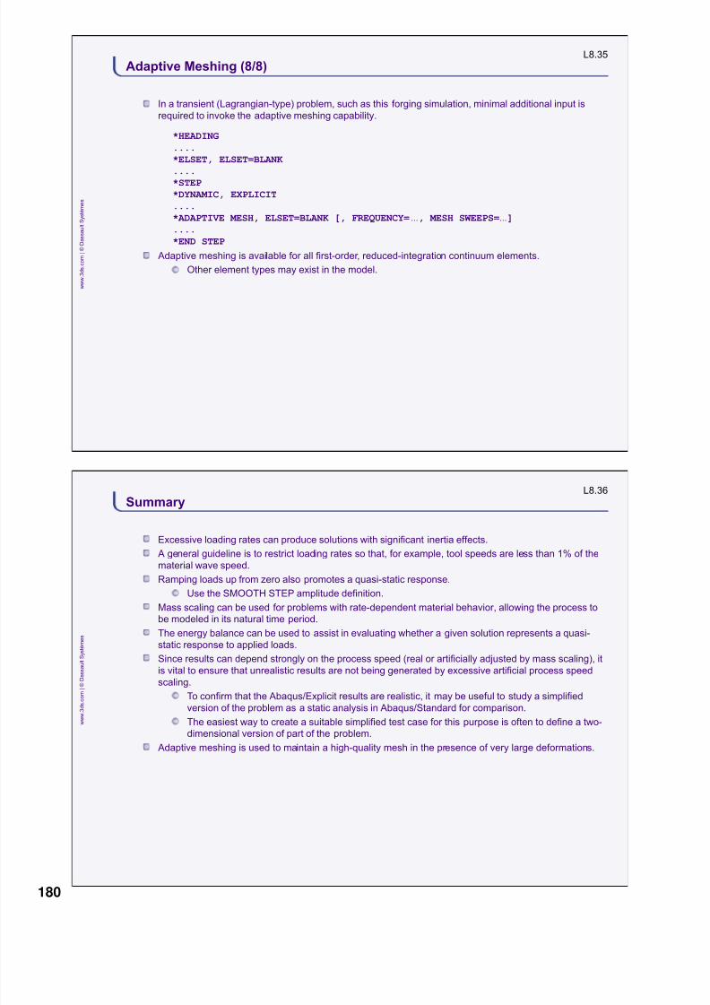
8/15/2019 Abaqus Analysis Intro-book
http://slidepdf.com/reader/full/abaqus-analysis-intro-book 180/469
L8.35
w w w . 3
d s . c o m |
©
D a s s a u l t S y s t è m e s
Adaptive Meshing (8/8)
In a transient (Lagrangian-type) problem, such as this forging simulation, minimal additional input is
required to invoke the adaptive meshing capability.
*HEADING
....
*ELSET, ELSET=BLANK
....
*STEP
*DYNAMIC, EXPLICIT
....
*ADAPTIVE MESH, ELSET=BLANK [, FREQUENCY=..., MESH SWEEPS=...]
....
*END STEP
Adaptive meshing is available for all first-order, reduced-integration continuum elements.
Other element types may exist in the model.
L8.36
w w w . 3
d s
. c o m |
©
D a s s a u l t S y s t è m e s
Summary
Excessive loading rates can produce solutions with significant inertia effects.
A general guideline is to restrict loading rates so that, for example, tool speeds are less than 1% of the
material wave speed.
Ramping loads up from zero also promotes a quasi-static response.
Use the SMOOTH STEP amplitude definition.
Mass scaling can be used for problems with rate-dependent material behavior, allowing the process to
be modeled in its natural time period.
The energy balance can be used to assist in evaluating whether a given solution represents a quasi-
static response to applied loads.
Since results can depend strongly on the process speed (real or artificially adjusted by mass scaling), it
is vital to ensure that unrealistic results are not being generated by excessive artificial process speed
scaling.
To confirm that the Abaqus/Explicit results are realistic, it may be useful to study a simplified
version of the problem as a static analysis in Abaqus/Standard for comparison.
The easiest way to create a suitable simplified test case for this purpose is often to define a two-
dimensional version of part of the problem.
Adaptive meshing is used to maintain a high-quality mesh in the presence of very large deformations.
180

8/15/2019 Abaqus Analysis Intro-book
http://slidepdf.com/reader/full/abaqus-analysis-intro-book 181/469
L8.37
w w w . 3
d s . c o m |
©
D a s s a u l t S y s t è m e s
1. Exercise simulates the deep drawing of a
can bottom
2. Workshop tasks include:
1. Perform a frequency extraction analysis to
determine an appropriate analysis time for this quasi-static process.
2. Complete the geometry definition of the rigid tools, and include contact and material definitions.
3. Include a SMOOTH STEP amplitude definition to improve quasi-static behavior.
4. Include mass scaling to reduce the analysis time without degrading the results.
5. Perform the analysis, and determine whether or not the results are acceptable.
Workshop 8: Quasi-Static Analysis (IA)
1 hour
This workshop is optional.
Interactive version. Choose either the interactive
or keywords version of this workshop.
L8.38
w w w . 3
d s
. c o m |
©
D a s s a u l t S y s t è m e s
1. Exercise simulates the deep drawing of a
can bottom
2. Workshop tasks include:
1. Perform a frequency extraction analysis to
determine an appropriate analysis time for this quasi-static process.
2. Complete the geometry definition of the rigid tools, and include contact and material definitions.
3. Include a SMOOTH STEP amplitude definition to improve quasi-static behavior.
4. Include mass scaling to reduce the analysis time without degrading the results.
5. Perform the analysis, and determine whether or not the results are acceptable.
Workshop 8: Quasi-Static Analysis (KW)
1 hour
This workshop is optional.
Keywords version. Choose either the interactiveor keywords version of this workshop.
181

8/15/2019 Abaqus Analysis Intro-book
http://slidepdf.com/reader/full/abaqus-analysis-intro-book 182/469182

8/15/2019 Abaqus Analysis Intro-book
http://slidepdf.com/reader/full/abaqus-analysis-intro-book 183/469
Notes
183

8/15/2019 Abaqus Analysis Intro-book
http://slidepdf.com/reader/full/abaqus-analysis-intro-book 184/469
Notes
184

8/15/2019 Abaqus Analysis Intro-book
http://slidepdf.com/reader/full/abaqus-analysis-intro-book 185/469
L9.1
w w w . 3
d s . c o m |
©
D a s s a u l t S y s t è m e s
Lesson content :
Introduction
Abaqus Usage
Springback Calculation Using Abaqus/Standard
Workshop 9: Import Analysis (IA)
Workshop 9: Import Analysis (KW)
Lesson 9: Combining Abaqus/Standard and Abaqus/Explicit
1 hour
Both interactive (IA) and keywords (KW) versionsof the workshop are provided. Complete only one.
L9.2
w w w . 3
d s
. c o m |
©
D a s s a u l t S y s t è m e s
Introduction (1/3)
Abaqus provides a capability to transfer a deformed mesh and an associated state between an
Abaqus/Explicit analysis and an Abaqus/Standard analysis.
This capability provides great flexibility, for example, in modeling springback in metal forming processes.
The deformed model can be transferred from Abaqus/Explicit to Abaqus/Standard to, for example:
Obtain the final static configuration after a dynamic event.
Simulate springback after a metal forming operation.
Perform eigenvalue or buckling simulations on a formed part.
Simulate the movement of rigid tools more efficiently.
The deformed model can be transferred from Abaqus/Standard to Abaqus/Explicit to, for example:
Simulate additional forming steps after an intermediary springback phase.Simulate forming processes that occur after a part cools down from a heat treatment phase (thermal
stresses are calculated in Abaqus/Standard).
Continue a simulation following a phase of the analysis that was done more efficiently in
Abaqus/Standard.
Follow the steady-state rolling of a tire in Abaqus/Standard with a transient rolling along a bumpy road in
Abaqus/Explicit.
185

8/15/2019 Abaqus Analysis Intro-book
http://slidepdf.com/reader/full/abaqus-analysis-intro-book 186/469
L9.3
w w w . 3
d s . c o m |
©
D a s s a u l t S y s t è m e s
Introduction (2/3)
Import summary
The ability to import the material state and the nodal positions is the main requirement of importing
results between the analysis modules.
The following table summarizes the import capabilities:
Can be imported Need to be respecified Cannot be imported
Material state * Boundary conditions Some materials *
Nodal positions Loads
Elements, element sets Contact definitions
Nodes, node sets Output requests
Temperatures Multi-point constraints
Nodal transformations
Amplitude definitions
L9.4
w w w . 3
d s
. c o m |
©
D a s s a u l t S y s t è m e s
Introduction (3/3)
Comments regarding material states
Only the material states for the some materials are imported correctly for further analysis. These
include:
Linear elastic
Hyperelastic
Mullins effect
Hyperfoam
Mises plasticity (including the kinematic hardening models)
Viscoelastic
User-defined materials (UMAT and VUMAT)
See Section 9.2.1 of the Abaqus Analysis User's Manual for a complete list of supported materials
186

8/15/2019 Abaqus Analysis Intro-book
http://slidepdf.com/reader/full/abaqus-analysis-intro-book 187/469

8/15/2019 Abaqus Analysis Intro-book
http://slidepdf.com/reader/full/abaqus-analysis-intro-book 188/469
L9.7
w w w . 3
d s . c o m |
©
D a s s a u l t S y s t è m e s
Abaqus Usage (3/4)
Elements and nodes
Specify the element sets that are to be imported on the data line of the *IMPORT option.
*IMPORT, STEP= step number , INTERVAL=interval number
elset_1, elset_2, elset_3
Each element set name specified on the data line of the *IMPORT option must have been used in
a section definition option (e.g., *SOLID SECTION) in the original analysis.
The current thickness of shell and membrane elements is imported automatically and becomes the initial
thickness for the element if UPDATE=YES.
All nodes attached to imported elements are imported.
Additional nodes and elements can be defined in the new analysis.
L9.8
w w w . 3
d s
. c o m |
©
D a s s a u l t S y s t è m e s
Abaqus Usage (4/4)
Material state and reference configuration
By default, the material state (for supported materials) is imported in an import analysis (STATE=YES on
the *IMPORT option).
For the analysis to continue without resetting the reference configuration, set UPDATE=NO on the
*IMPORT option:
*IMPORT, UPDATE=NO
In some cases it may be desirable to obtain springback displacements and strains relative to the
geometry at the start of the springback analysis (reset to zero at the start of the springback step). Set
UPDATE=YES on the *IMPORT option:
*IMPORT, UPDATE=YES
UPDATE=YES should not be used if additional forming stages will follow because the reference
configuration will not be consistent.
Other combinations of the STATE and UPDATE parameters are available but are not discussed here.
The setting of NLGEOM is imported and becomes the setting for the new analysis.
188

8/15/2019 Abaqus Analysis Intro-book
http://slidepdf.com/reader/full/abaqus-analysis-intro-book 189/469
L9.9
w w w . 3
d s . c o m |
©
D a s s a u l t S y s t è m e s
Springback Calculation Using Abaqus/Standard (1/7)
The blank shown in the figure at right undergoes
large deformations during the sheet metal forming
process.
Once the forming process is complete and the
confining tools are removed, the blank will
attempt to recover its elastic deformation.
This springback phenomenon may lead to
unacceptable warping of the formed product.
Forming tools must be designed to
compensate for springback effects.
L9.10
w w w . 3
d s
. c o m |
©
D a s s a u l t S y s t è m e s
Springback Calculation Using Abaqus/Standard (2/7)
For the calculation of springback associated with sheet metal forming processes:
Generally, the forming process is simulated using Abaqus/Explicit because it is more efficient for such
analyses.
The deformed mesh of the blank and its associated material state at the end of the forming process are
imported into an Abaqus/Standard model to analyze springback.
The springback calculation is performed more efficiently in Abaqus/Standard than in Abaqus/Explicit.
The displacements that Abaqus/Standard calculates are the totals from the forming and springback
stages if UPDATE=NO is used on the *IMPORT option.
189

8/15/2019 Abaqus Analysis Intro-book
http://slidepdf.com/reader/full/abaqus-analysis-intro-book 190/469
L9.11
w w w . 3
d s . c o m |
©
D a s s a u l t S y s t è m e s
Springback Calculation Using Abaqus/Standard (3/7)
Equilibrium
Upon importing the deformed blank and its current state into Abaqus/Standard, the model is not in static
equilibrium. Dynamic forces, contact forces, and boundary conditions that exist in Abaqus/Explicit but
not in Abaqus/Standard contribute to this condition:
Dynamic forces:
The forming process is simulated using a dynamic procedure, so the deformed blank is in a state
of dynamic equilibrium. Inertia and damping forces are present.
In a quasi-static forming simulation the state of dynamic equilibrium is relatively close to a state of
static equilibrium.
Boundary and contact conditions:
Contact forces are not imported.
Boundary conditions can be modified in the import analysis.
L9.12
w w w . 3
d s
. c o m |
©
D a s s a u l t S y s t è m e s
Springback Calculation Using Abaqus/Standard (4/7)
Achieving static equilibrium during springback analysis
When the deformed blank is imported with the material state into Abaqus/Standard, a set of artificial
internal stresses are automatically applied that equilibrate the imported stresses so that static
equilibrium is obtained at the start of the analysis.
These artificial stresses are ramped off during the springback calculation step.
As these stresses are removed, the blank deforms further (referred to as springback) as a result of
redistribution of internal forces.
The final configuration following springback is achieved after complete removal of the artificial stresses
or initial out-of-balance forces.
190

8/15/2019 Abaqus Analysis Intro-book
http://slidepdf.com/reader/full/abaqus-analysis-intro-book 191/469

8/15/2019 Abaqus Analysis Intro-book
http://slidepdf.com/reader/full/abaqus-analysis-intro-book 192/469
L9.15
w w w . 3
d s . c o m |
©
D a s s a u l t S y s t è m e s
Springback Calculation Using Abaqus/Standard (7/7)
The configuration after springback is shown in the figure. A magnification factor of 10 is applied to the
displacements for visualization purposes.
Deformed configuration after springback
L9.16
w w w . 3
d s
. c o m |
©
D a s s a u l t S y s t è m e s
1. This exercise simulates the springback of a
formed can bottom
2. Workshop tasks include:
1. Import the results into an Abaqus/Standard analysis to examine springback.
Workshop 9: Import Analysis (IA)
30 minutes
This workshop is optional.
Interactive version. Choose either the interactiveor keywords version of this workshop.
192

8/15/2019 Abaqus Analysis Intro-book
http://slidepdf.com/reader/full/abaqus-analysis-intro-book 193/469
L9.17
w w w . 3
d s . c o m |
©
D a s s a u l t S y s t è m e s
1. This exercise simulates the springback of a
formed can bottom
2. Workshop tasks include:
1. Import the results into an Abaqus/Standard analysis to examine springback.
Workshop 9: Import Analysis (KW)
30 minutes
This workshop is optional.
Keywords version. Choose either the interactive
or keywords version of this workshop.
193

8/15/2019 Abaqus Analysis Intro-book
http://slidepdf.com/reader/full/abaqus-analysis-intro-book 194/469

8/15/2019 Abaqus Analysis Intro-book
http://slidepdf.com/reader/full/abaqus-analysis-intro-book 195/469

8/15/2019 Abaqus Analysis Intro-book
http://slidepdf.com/reader/full/abaqus-analysis-intro-book 196/469

8/15/2019 Abaqus Analysis Intro-book
http://slidepdf.com/reader/full/abaqus-analysis-intro-book 197/469

8/15/2019 Abaqus Analysis Intro-book
http://slidepdf.com/reader/full/abaqus-analysis-intro-book 198/469

8/15/2019 Abaqus Analysis Intro-book
http://slidepdf.com/reader/full/abaqus-analysis-intro-book 199/469
A1.5
w w w . 3
d s . c o m |
©
D a s s a u l t S y s t è m e s
Elements in Abaqus (4/8)
Degrees of freedom
The primary variables that exist at the nodes of an element are the degrees of freedom in the finite
element analysis.
Examples of degrees of freedom are:
Displacements
RotationsTemperature
Electrical potential
Some elements have internal degrees of freedom that are not associated with the user-defined nodes.
A1.6
w w w . 3
d s
. c o m |
©
D a s s a u l t S y s t è m e s
Elements in Abaqus (5/8)
Formulation
The mathematical formulation used to describe the behavior of an element is another broad category
that is used to classify elements.
Examples of different element formulations:
IntegrationThe stiffness and mass of an element are calculated numerically at sampling points called ―integration
points‖ within the element.
The numerical algorithm used to integrate these variables influences how an element behaves.
Plane strain
Plane stress
Hybrid elements
Incompatible-mode elements
Small-strain shells
Finite-strain shells
Thick-only shells
Thin-only shells
199

8/15/2019 Abaqus Analysis Intro-book
http://slidepdf.com/reader/full/abaqus-analysis-intro-book 200/469
A1.7
w w w . 3
d s . c o m |
©
D a s s a u l t S y s t è m e s
Elements in Abaqus (6/8)
Abaqus includes elements with both ―full‖ and ―reduced‖ integration.
Full integration:
I. The minimum integration order required for exact integration of the strain energy for an
undistorted element with linear material properties.
Reduced integration:
I. The integration rule that is one order less than the full integration rule.
Second-order
interpolation
First-
order
interpolation
Full
integration
Reduced
integration
2 x 23 x 3
1 x 12 x 2
A1.8
w w w . 3
d s
. c o m |
©
D a s s a u l t S y s t è m e s
Elements in Abaqus (7/8)
Element naming conventions: examples
B21: Beam, 2-D,
1st-order interpolation
CAX8R: Continuum,
AXisymmetric, 8-node,
Reduced integration
DC3D4: Diffusion (heat transfer),
Continuum, 3-D, 4-node
S8RT: Shell, 8-node, Reduced
integration, Temperature
CPE8PH: Continuum, Plane strain,
8-node, Pore pressure, Hybrid
DC1D2E: Diffusion (heat transfer),
Continuum, 1-D, 2-node, Electrical
200

8/15/2019 Abaqus Analysis Intro-book
http://slidepdf.com/reader/full/abaqus-analysis-intro-book 201/469
A1.9
w w w . 3
d s . c o m |
©
D a s s a u l t S y s t è m e s
Elements in Abaqus (8/8)
Comparing Abaqus/Standard and Abaqus/Explicit element libraries
Both programs have essentially the same element families: continuum, shell, beam, etc.
Abaqus/Standard includes elements for many analysis types besides stress analysis: heat transfer, soils
consolidation, acoustics, etc.
Acoustic elements are also available in Abaqus/Explicit.
Abaqus/Standard includes many more variations within each element family.
Abaqus/Explicit includes mostly first-order reduced-integration elements.
Exceptions: second-order triangular and tetrahedral elements; second-order beam elements;
first-order fully-integrated brick (including incompatible mode version), shell, and membrane
elements.
Many of the same general element selection guidelines apply to both programs.
A1.10
w w w . 3
d s
. c o m |
©
D a s s a u l t S y s t è m e s
Structural (Shells and Beams) vs. Continuum Elements (1/3)
Continuum (solid) element models can be large and expensive, particularly in three-dimensional problems.
If appropriate, structural elements (shells and beams) should be used for a more economical solution.
A structural element model typically requires far fewer elements than a comparable continuum element
model.
For structural elements to produce acceptable results, the shell thickness or the beam cross-section
dimensions should be less than 1/10 of a typical global structural dimension, such as:
The distance between supports or point loads
The distance between gross changes in cross section
The wavelength of the highest vibration mode
201

8/15/2019 Abaqus Analysis Intro-book
http://slidepdf.com/reader/full/abaqus-analysis-intro-book 202/469
A1.11
w w w . 3
d s . c o m |
©
D a s s a u l t S y s t è m e s
Structural (Shells and Beams) vs. Continuum Elements (2/3)
Shell elements
Shell elements approximate a three-dimensional continuum with a surface model.
Model bending and in-plane
deformations efficiently.
If a detailed analysis of a region is needed, alocal three-dimensional continuum model canbe included using multi-point constraints orsubmodeling.
3-D continuum surface model
shell model of a hemispherical dome subjected
to a projectile impact
A1.12
w w w . 3
d s
. c o m |
©
D a s s a u l t S y s t è m e s
Structural (Shells and Beams) vs. Continuum Elements (3/3)
Beam elements
Beam elements approximate a three-
dimensional continuum with a line model.
Model bending, torsion, and axial forces
efficiently.
Many different cross-section shapes are
available.
Cross-section properties can also be
specified by providing engineering
constants.
line model
framed structure modeled using
beam elements
3-D continuum
202

8/15/2019 Abaqus Analysis Intro-book
http://slidepdf.com/reader/full/abaqus-analysis-intro-book 203/469
A1.13
w w w . 3
d s . c o m |
©
D a s s a u l t S y s t è m e s
Modeling Bending Using Continuum Elements (1/10)
Physical characteristics of pure bending
Plane cross-sections remain plane throughout the deformation.
The axial strain xx varies linearly through the thickness.
The strain in the thickness direction yy is zero if = 0.
No membrane shear strain.
Implies that lines parallel to the beam axis lie on a circular arc.
xx
A1.14
w w w . 3
d s
. c o m |
©
D a s s a u l t S y s t è m e s
Modeling Bending Using Continuum Elements (2/10)
Modeling bending using second-order solid elements (CPE8, C3D20R, …)
Second-order full- and reduced-integration solid elements model bending accurately:
The axial strain equals the change in length of the initially horizontal lines.
The thickness strain is zero.
The shear strain is zero.
lines that are initially vertical do not
change length (implies yy= 0).
Because the element edges can assume a curved
shape, the angle between the deformed isoparametric
lines remains equal to 90o (implies xy= 0).
203

8/15/2019 Abaqus Analysis Intro-book
http://slidepdf.com/reader/full/abaqus-analysis-intro-book 204/469

8/15/2019 Abaqus Analysis Intro-book
http://slidepdf.com/reader/full/abaqus-analysis-intro-book 205/469
A1.17
w w w . 3
d s . c o m |
©
D a s s a u l t S y s t è m e s
Modeling Bending Using Continuum Elements (5/10)
Hourglassing can propagate easily through a mesh of first-order reduced-integration elements, causing
unreliable results.
Hourglassing is not a problem if you use multiple elements—at least four through the thickness.
Each element captures either compressive or tensile axial strains but not both.
The axial strains are measured correctly.
The thickness and shear strains are zero.Cheap and effective elements.
A1.18
w w w . 3
d s
. c o m |
©
D a s s a u l t S y s t è m e s
Modeling Bending Using Continuum Elements (6/10)
Detecting and controlling hourglassing
Hourglassing can usually be seen in deformed shape plots.
Example: Coarse and medium meshes of a simply supported beam with a center point load.
Abaqus has built-in hourglass controls that limit the problems caused by hourglassing.
Verify that the artificial energy used to control hourglassing is small (<1%) relative to the internal
energy.
Same load and displacement magnification
(1000)
205

8/15/2019 Abaqus Analysis Intro-book
http://slidepdf.com/reader/full/abaqus-analysis-intro-book 206/469
A1.19
w w w . 3
d s . c o m |
©
D a s s a u l t S y s t è m e s
Modeling Bending Using Continuum Elements (7/10)
Use the X –Y plotting capability in Abaqus/CAE to compare the energies graphically.
internal energy
artificial energy artificial energy
internal energy
Two elements through the thickness:Ratio of artificial to internal energy is 2% Four elements through the thickness: Ratioof artificial to internal energy is 0.1%
A1.20
w w w . 3
d s
. c o m |
©
D a s s a u l t S y s t è m e s
Modeling Bending Using Continuum Elements (8/10)
Modeling bending using incompatible mode elements
(CPS4I, …)
Perhaps the most cost-effective solid continuum elements for bending-dominated problems.
Compromise in cost between the first- and second-order reduced-integration elements, with many of the
advantages of both.
Model shear behavior correctly—no shear strains in pure bending.
Model bending with only one element through the thickness.
No hourglass modes, and work well in plasticity and contact problems.
The advantages over reduced-integration first-order elements are reduced if the elements are severely
distorted; however, all elements perform less accurately if severely distorted.
206

8/15/2019 Abaqus Analysis Intro-book
http://slidepdf.com/reader/full/abaqus-analysis-intro-book 207/469
A1.21
w w w . 3
d s . c o m |
©
D a s s a u l t S y s t è m e s
Modeling Bending Using Continuum Elements (9/10)
Example: Cantilever beam with distorted elements
Parallel distortion Trapezoidal distortion
A1.22
w w w . 3
d s
. c o m |
©
D a s s a u l t S y s t è m e s
Modeling Bending Using Continuum Elements (10/10)
Summary
Element type xx
yy
xy Notes
Physical behavior 0 0 0
Second-order 0 0 0 OK
First-order, full integration 0 0 0 Shear locking
First-order, reduced
integration
0
0
0
0
0
0
Hourglassing if too few elements
through thickness
OK if enough elements through the
thickness
Incompatible mode 0 0 0 OK if not overly distorted
207
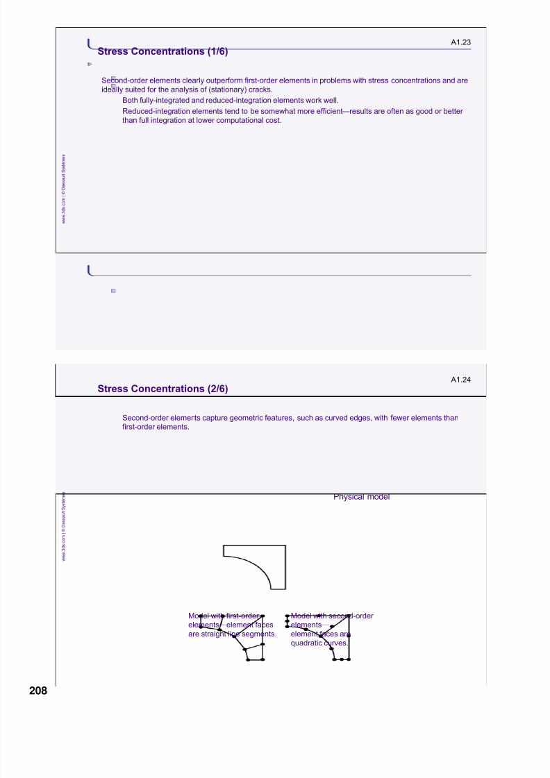
8/15/2019 Abaqus Analysis Intro-book
http://slidepdf.com/reader/full/abaqus-analysis-intro-book 208/469

8/15/2019 Abaqus Analysis Intro-book
http://slidepdf.com/reader/full/abaqus-analysis-intro-book 209/469
A1.25
w w w . 3
d s . c o m |
©
D a s s a u l t S y s t è m e s
Stress Concentrations (3/6)
Both first- and second-order quads and bricks become less accurate when their initial shape is distorted.
First-order elements are known to be less sensitive to distortion than second-order elements and,thus, are a better choice in problems where significant mesh distortion is expected.
Second-order triangles and tetrahedra are less sensitive to initial element shape than most otherelements; however, well-shaped elements provide better results.
ideal okay bad
distortedundistorted
A1.26
w w w . 3
d s
. c o m |
©
D a s s a u l t S y s t è m e s
Stress Concentrations (4/6)
A typical stress concentration problem, a NAFEMS benchmark problem, is shown at right. The analysis
results obtained with different element types follow.
elliptical shape
P
209

8/15/2019 Abaqus Analysis Intro-book
http://slidepdf.com/reader/full/abaqus-analysis-intro-book 210/469

8/15/2019 Abaqus Analysis Intro-book
http://slidepdf.com/reader/full/abaqus-analysis-intro-book 211/469
A1.29
w w w . 3
d s . c o m |
©
D a s s a u l t S y s t è m e s
Contact
If the surface-to-surface contact discretization is used:
No fundamental issues or element type restrictions
Abaqus/Standard always uses this formulation for general contact
If the node-to-surface contact discretization is used:
Best to avoid having second-order tetrahedral elements (C3D10, C3D10I) underlying the slave surface
with this contact discretizationSusceptible to poor convergence and extreme contact pressure noise
Use ―modified‖ versions of these elements (C3D10M) instead
Sometimes C3D10 or C3D10I elements work fine if penalty enforcement of contact is specified
Abaqus automatically activates supplementary constraints for this combination of features
But the extra (supplementary) constraints can be another source of convergence problems
A1.30
w w w . 3
d s
. c o m |
©
D a s s a u l t S y s t è m e s
Incompressible Materials (1/3)
Many nonlinear problems involve incompressible materials ( = 0.5) and nearly incompressible materials
( > 0.475).
Rubber
Metals at large plastic strains
Conventional finite element meshes often exhibit overly stiff behavior due to volumetric locking , which is
most severe when these materials are highly confined.
overly stiff behavior of an elastic-
plastic material with volumetric
locking
correct behavior of an
elastic-plastic material
Example of the effect of volumetric locking
211

8/15/2019 Abaqus Analysis Intro-book
http://slidepdf.com/reader/full/abaqus-analysis-intro-book 212/469
A1.31
w w w . 3
d s . c o m |
©
D a s s a u l t S y s t è m e s
Incompressible Materials (2/3)
For an incompressible material each integration point’s volume must remain almost constant. Thisoverconstrains the kinematically admissible displacement field and causes volumetric locking
For example, in a refined three-dimensional mesh of 8-node hexahedra, there is—on average—1node with 3 degrees of freedom per element.
The volume at each integration point must remain fixed.
Fully integrated hexahedra use 8 integration points per element; thus, in this example, we have
as many as 8 constraints per element, but only 3 degrees of freedom are available to satisfythese constraints.
The mesh is overconstrained—it ―locks.‖
Volumetric locking is most pronounced in fully integrated elements.
Reduced-integration elements have fewer volumetric constraints.
Reduced integration effectively eliminates volumetric locking in many problems with nearlyincompressible material.
A1.32
w w w . 3
d s
. c o m |
©
D a s s a u l t S y s t è m e s
Incompressible Materials (3/3)
Fully incompressible materials modeled with solid elements must use the ―hybrid‖ formulation (elements
whose names end with the letter ―H‖).
In this formulation the pressure stress is treated as an independently interpolated basic solution
variable, coupled to the displacement solution through the constitutive theory.
Hybrid elements introduce more variables into the problem to alleviate the volumetric locking
problem. The extra variables also make them more expensive.
The Abaqus element library includes hybrid versions of all continuum elements (except plane
stress elements, where this is not needed).
Hybrid elements are only necessary for:
All meshes with strictly incompressible materials, such as rubber.
Refined meshes of reduced-integration elements that still show volumetric locking problems.
Such problems are possible with elastic-plastic materials strained far into the plastic range.
Even with hybrid elements a mesh of first-order triangles and tetrahedra is overconstrained when
modeling fully incompressible materials.
Hence, these elements are recommended only for use as ―fillers‖ in quadrilateral or brick-type
meshes with such material.
212

8/15/2019 Abaqus Analysis Intro-book
http://slidepdf.com/reader/full/abaqus-analysis-intro-book 213/469
A1.33
w w w . 3
d s . c o m |
©
D a s s a u l t S y s t è m e s
Mesh Generation (1/5)
Meshes
Typical element shapes are shown at right.
Most elements in Abaqus are topologically
equivalent to these shapes.
For example, CPE4 (stress), DC2D4
(heat transfer), and AC2D4 (acoustics)
are topologically equivalent to a linear
quadrilateral.
A1.34
w w w . 3
d s
. c o m |
©
D a s s a u l t S y s t è m e s
Mesh Generation (2/5)
Quad/hex vs. tri/tet elements
Of particular importance when generating a mesh is the decision regarding whether to use quad/hex or
tri/tet elements.
Quad/hex elements should be used wherever possible.
They give the best results for the minimum cost.
When modeling complex geometries, however, the analyst often has little choice but to mesh with
triangular and tetrahedral elements.
Turbine blade with platform modeled with
tetrahedral elements
213
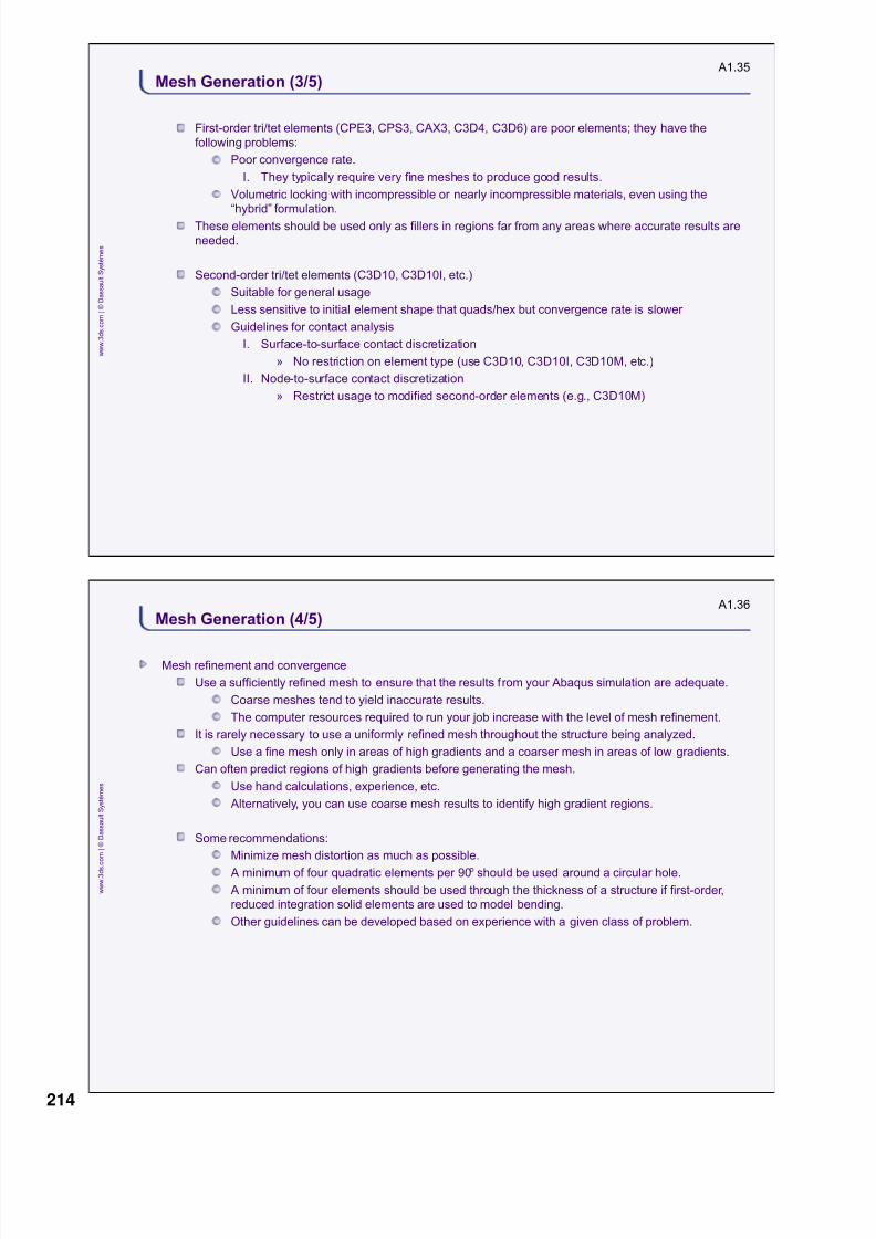
8/15/2019 Abaqus Analysis Intro-book
http://slidepdf.com/reader/full/abaqus-analysis-intro-book 214/469
A1.35
w w w . 3
d s . c o m |
©
D a s s a u l t S y s t è m e s
Mesh Generation (3/5)
First-order tri/tet elements (CPE3, CPS3, CAX3, C3D4, C3D6) are poor elements; they have the
following problems:
Poor convergence rate.
I. They typically require very fine meshes to produce good results.
Volumetric locking with incompressible or nearly incompressible materials, even using the
―hybrid‖ formulation.
These elements should be used only as fillers in regions far from any areas where accurate results are
needed.
Second-order tri/tet elements (C3D10, C3D10I, etc.)
Suitable for general usage
Less sensitive to initial element shape that quads/hex but convergence rate is slower
Guidelines for contact analysis
I. Surface-to-surface contact discretization
» No restriction on element type (use C3D10, C3D10I, C3D10M, etc.)
II. Node-to-surface contact discretization
» Restrict usage to modified second-order elements (e.g., C3D10M)
A1.36
w w w . 3
d s
. c o m |
©
D a s s a u l t S y s t è m e s
Mesh Generation (4/5)
Mesh refinement and convergence
Use a sufficiently refined mesh to ensure that the results from your Abaqus simulation are adequate.
Coarse meshes tend to yield inaccurate results.
The computer resources required to run your job increase with the level of mesh refinement.
It is rarely necessary to use a uniformly refined mesh throughout the structure being analyzed.
Use a fine mesh only in areas of high gradients and a coarser mesh in areas of low gradients.
Can often predict regions of high gradients before generating the mesh.
Use hand calculations, experience, etc.
Alternatively, you can use coarse mesh results to identify high gradient regions.
Some recommendations:
Minimize mesh distortion as much as possible.
A minimum of four quadratic elements per 90o should be used around a circular hole.
A minimum of four elements should be used through the thickness of a structure if first-order,
reduced integration solid elements are used to model bending.
Other guidelines can be developed based on experience with a given class of problem.
214

8/15/2019 Abaqus Analysis Intro-book
http://slidepdf.com/reader/full/abaqus-analysis-intro-book 215/469
A1.37
w w w . 3
d s . c o m |
©
D a s s a u l t S y s t è m e s
Mesh Generation (5/5)
It is good practice to perform a mesh convergence study.
Simulate the problem using progressively finer meshes, and compare the results.
I. The mesh density can be changed very easily using Abaqus/CAE since the definition of the
analysis model is based on the geometry of the structure.
When two meshes yield nearly identical results, the results are said to have ―converged.‖
I. This provides increased confidence in your results.
A1.38
w w w . 3
d s
. c o m |
©
D a s s a u l t S y s t è m e s
Solid Element Selection Summary (1/2)
Class of problem Best element choice Avoid using
General contact between
deformable bodies
First-order quad/hex Second-order elements with the node-to-
surface contact discretization
Contact with bending Incompatible mode First-order fully integrated quad/hex or
second-order elements with the node-to-
surface contact discretization
Bending (no contact) Second-order quad/hex First-order fully integrated quad/hex
Stress concentration Second-order First-order
Nearly incompressible
( >0.475 or large strain
plasticity pl >10%)
First-order elements or second-
order reduced integration
elements
Second-order fully integrated
215

8/15/2019 Abaqus Analysis Intro-book
http://slidepdf.com/reader/full/abaqus-analysis-intro-book 216/469
A1.39
w w w . 3
d s . c o m |
©
D a s s a u l t S y s t è m e s
Solid Element Selection Summary (2/2)
Class of problem Best element choice Avoid using
Completely incompressible
(rubber = 0.5)
Hybrid quad/hex, first-order if large deformations
are anticipated
Bulk metal forming(high mesh distortion)
First-order reduced integration quad/hex Second-orderquad/hex
Complicated model geometry
(linear material, no contact)
Second-order quad/hex if possible (if not overly
distorted) or second-order tet/tri (because of
meshing difficulties)
Complicated model geometry
(nonlinear problem or contact)
First-order quad/hex if possible (if not overly
distorted). If meshing requirements dictate,
use second-order tet/tri (modified form; use
regular form only with surface-to-surface
contact discretization)
Natural frequency
(linear dynamics)
Second-order
Nonlinear dynamic (impact) First-order Second-order
216

8/15/2019 Abaqus Analysis Intro-book
http://slidepdf.com/reader/full/abaqus-analysis-intro-book 217/469
Notes
217

8/15/2019 Abaqus Analysis Intro-book
http://slidepdf.com/reader/full/abaqus-analysis-intro-book 218/469
Notes
218

8/15/2019 Abaqus Analysis Intro-book
http://slidepdf.com/reader/full/abaqus-analysis-intro-book 219/469

8/15/2019 Abaqus Analysis Intro-book
http://slidepdf.com/reader/full/abaqus-analysis-intro-book 220/469

8/15/2019 Abaqus Analysis Intro-book
http://slidepdf.com/reader/full/abaqus-analysis-intro-book 221/469

8/15/2019 Abaqus Analysis Intro-book
http://slidepdf.com/reader/full/abaqus-analysis-intro-book 222/469

8/15/2019 Abaqus Analysis Intro-book
http://slidepdf.com/reader/full/abaqus-analysis-intro-book 223/469

8/15/2019 Abaqus Analysis Intro-book
http://slidepdf.com/reader/full/abaqus-analysis-intro-book 224/469

8/15/2019 Abaqus Analysis Intro-book
http://slidepdf.com/reader/full/abaqus-analysis-intro-book 225/469
A2.13
w w w . 3
d s . c o m |
©
D a s s a u l t S y s t è m e s
Contact Logic in Abaqus/Standard (9/10)
Increment summary:
ITERATION SUMMARY FOR THE INCREMENT: 5 TOTAL ITERATIONS, OF WHICH
4 ARE SEVERE DISCONTINUITY ITERATIONS AND 1 ARE EQUILIBRIUM ITERATIONS.
CURRENT VALUE OF MONITOR NODE 200 D.O.F. 2 IS -3.028E-03
TIME INCREMENT COMPLETED 1.266E-02, FRACTION OF STEP COMPLETED 5.047E-02
STEP TIME COMPLETED 5.047E-02, TOTAL TIME COMPLETED 2.05
A2.14
w w w . 3
d s
. c o m |
©
D a s s a u l t S y s t è m e s
Contact Logic in Abaqus/Standard (10/10)
Contact diagnostics in Abaqus/Viewer
Constrained nodes want to open:
incompatible contact state
Toggle on to see the locations in
the model where the contact state
is changing.
225

8/15/2019 Abaqus Analysis Intro-book
http://slidepdf.com/reader/full/abaqus-analysis-intro-book 226/469

8/15/2019 Abaqus Analysis Intro-book
http://slidepdf.com/reader/full/abaqus-analysis-intro-book 227/469
Notes
227

8/15/2019 Abaqus Analysis Intro-book
http://slidepdf.com/reader/full/abaqus-analysis-intro-book 228/469
Notes
228

8/15/2019 Abaqus Analysis Intro-book
http://slidepdf.com/reader/full/abaqus-analysis-intro-book 229/469
A3.1
w w w . 3
d s . c o m |
©
D a s s a u l t S y s t è m e s
Lesson content :
Contact Pairs as Part of the History Data
Enforcing the Contact Constraints
Double-Sided Contact
Initial Kinematic Compliance
Appendix 3: Contact Issues Specific to Abaqus/Explicit
30 minutes
A3.2
w w w . 3
d s
. c o m |
©
D a s s a u l t S y s t è m e s
Contact Pairs as Part of the History Data (1/2)
For Abaqus/Explicit the contact pair definition is part of the history data in the input file.
*HEADING
.
.
*STEP
*DYNAMIC, EXPLICIT
, 200E-3
*CONTACT PAIR
ASURF, BSURF
.
.
.
*STEP
*DYNAMIC, EXPLICIT
, 200E-3*CONTACT PAIR
ASURF, DSURF
Contact pairs are defined, or
removed, on a step-by-step basis as
needed.
229

8/15/2019 Abaqus Analysis Intro-book
http://slidepdf.com/reader/full/abaqus-analysis-intro-book 230/469
A3.3
w w w . 3
d s . c o m |
©
D a s s a u l t S y s t è m e s
Contact Pairs as Part of the History Data (2/2)
The *CONTACT PAIR option has the OP parameter, which can have the value ADD or DELETE.
Example:
*STEP
*DYNAMIC, EXPLICIT
.
.*CONTACT PAIR
ASURF, BSURF
*END STEP
*STEP
.
.
*CONTACT PAIR, OP=DELETE
ASURF, BSURF
*CONTACT PAIR, OP=ADD
BSURF, CSURF
*END STEP
Delete the contact pair involving surfaces ASURF and BSURF.
Add a contact pair involving surfacesBSURF and CSURF.
A3.4
w w w . 3
d s
. c o m |
©
D a s s a u l t S y s t è m e s
Enforcing the Contact Constraints (1/3)
Contact constraints can be enforced with one of the following algorithms:
Kinematic compliance (only available for contact pair algorithm)
Penalty
In most cases the kinematic and penalty algorithms will produce nearly the same results; however, in some
cases one method may be preferable to the other.
230

8/15/2019 Abaqus Analysis Intro-book
http://slidepdf.com/reader/full/abaqus-analysis-intro-book 231/469

8/15/2019 Abaqus Analysis Intro-book
http://slidepdf.com/reader/full/abaqus-analysis-intro-book 232/469
A3.7
w w w . 3
d s . c o m |
©
D a s s a u l t S y s t è m e s
Double-Sided Contact (1/3)
A single surface defined on shell, membrane, and rigid elements can include both the top (SPOS) and bottom
(SNEG) faces of these elements.
The general contact algorithm automatically uses double-sided surfaces.
For the contact pair algorithm:
Define a double-sided surface by omitting the face identifier from the *SURFACE option.
Consistent element normals are not required.
Contact can occur on either face of the elements forming the double-sided surface.
For example, a slave node can start out on one side of a double-sided surface and then pass around the
perimeter to the other side during the analysis.
Double-sided surfaces are often necessary in such situations.
The additional computational cost when performing an analysis with double-sided contact is minimal.
A3.8
w w w . 3
d s
. c o m |
©
D a s s a u l t S y s t è m e s
Double-Sided Contact (2/3)
Example: Compression of nested cylindrical shells
deformable cylinders
rigid box
Front view
rigid lid
Oblique view (front and
side of box removed)
232
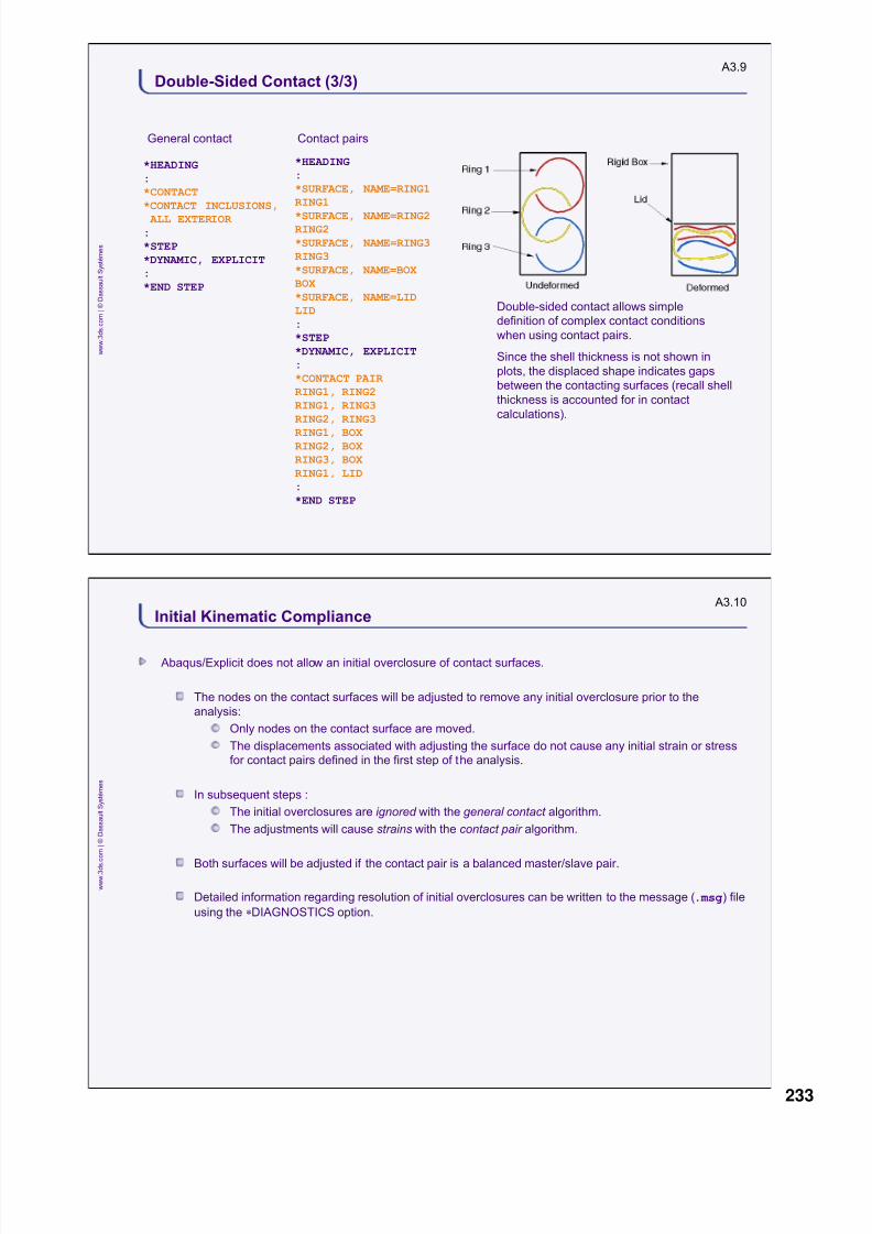
8/15/2019 Abaqus Analysis Intro-book
http://slidepdf.com/reader/full/abaqus-analysis-intro-book 233/469

8/15/2019 Abaqus Analysis Intro-book
http://slidepdf.com/reader/full/abaqus-analysis-intro-book 234/469234

8/15/2019 Abaqus Analysis Intro-book
http://slidepdf.com/reader/full/abaqus-analysis-intro-book 235/469

8/15/2019 Abaqus Analysis Intro-book
http://slidepdf.com/reader/full/abaqus-analysis-intro-book 236/469

8/15/2019 Abaqus Analysis Intro-book
http://slidepdf.com/reader/full/abaqus-analysis-intro-book 237/469
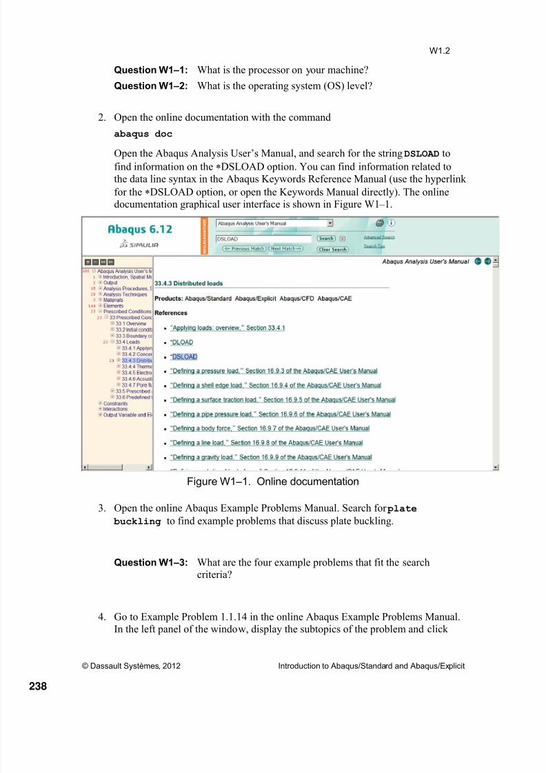
8/15/2019 Abaqus Analysis Intro-book
http://slidepdf.com/reader/full/abaqus-analysis-intro-book 238/469

8/15/2019 Abaqus Analysis Intro-book
http://slidepdf.com/reader/full/abaqus-analysis-intro-book 239/469
© Dassault Systèmes, 2012 Introduction to Abaqus/Standard and Abaqus/Explicit
W1.3
Input files. In the right panel of the window, the list of input files associated with
this problem appears. You can select any input filename from the list; a separate
window will open containing that file.
5. All example problem input files are included in the Abaqus release and can beobtained using the abaqus fetch utility. In your terminal window, enter
abaqus fetch job=damagefailcomplate_cps4
at the command line prompt.
6. Use the online documentation to determine the input syntax for some options.
followed directly by the keywordoption. Parameters and their associated values appear on the keyword line,separated by commas. Many options require data lines, which follow directly after
their associated keyword line and contain the data specified in the Abaqus
Keywords Reference Manual for each option. Data items are separated by
commas. Refer to the discussions of keyword line and data line syntax in Lecture1, as necessary.
Question W1 –4: How would you run a script from within the Abaqus/CAE
environment?
Hint: Search for “run script” in the Abaqus/CAE
User’s Manual
Question W1 –5: In the space provided, write which Category option youwould choose to define a displacement/rotation boundary
condition in Abaqus/CAE.
Hint: Search displacement/rotation boundary condition in
the Abaqus/CAE User’s Manual.
239

8/15/2019 Abaqus Analysis Intro-book
http://slidepdf.com/reader/full/abaqus-analysis-intro-book 240/469
© Dassault Systèmes, 2012 Introduction to Abaqus/Standard and Abaqus/Explicit
W1.4
Analyzing a connecting lug
Figure W1 –2. Sketch of the connecting lug
In this workshop you will model the connecting lug shown in Figure W1 – 2. The lug iswelded to a massive structure at one end, so we assume that this end is fixed. The other
end contains a hole through which a bolt is placed when the lug is in service. You have to
calculate the deflection of the lug when a load of 30 kN is applied to the bolt along the
negative 2-direction.
To model this problem, you will use three-dimensional continuum elements and perform
a linear analysis with elastic materials. You will model the load transmitted to the lug
through the bolt as a uniform pressure load applied to the bottom half of the hole, as
shown in Figure W1 – 2. In this workshop SI units (N, m, and s) will be used.
Preliminaries
1. Enter the working directory for this workshop:
../abaqus_solvers/interactive/lug2. Run the script ws_solver_lug.py using the following command:
abaqus cae startup=ws_solver_lug.py
The above command creates an Abaqus/CAE database named Lug.cae in the current
directory. The geometry, mesh, and step definitions for the lug are included in a model
named standard .
240

8/15/2019 Abaqus Analysis Intro-book
http://slidepdf.com/reader/full/abaqus-analysis-intro-book 241/469
© Dassault Systèmes, 2012 Introduction to Abaqus/Standard and Abaqus/Explicit
W1.5
Before completing the model, view the contents of the model using the Model Tree on
the left hand side of the main window.
Question W1 –6: How many steps are there in this analysis?
Use the Query information tool (or select Tools→Query from the main menu bar)
to query element information of the lug. Switch to the Mesh module and click . In theQuery dialog box, select Element in the General Queries field. Select one element ofthe lug in the viewport. Read the query results reported in the message area at the bottom
of the main window.
Question W1 –7: What element type is used to model the lug?
Completing the model
You will now add the material definition, and create the boundary conditions and the
pressure load to complete the lug model.1. Note that a dummy material named Steel has already been created and assigned
to the part Lug. Add the steel material properties to this material.
a. In the Model Tree, expand the Materials container and double-click Steel.
The material editor appears.
b. From the material editor’s menu bar , selectMechanical→Elasticity→Elastic. Enter the following elastic material
properties: Elastic modulus E = 200.E9 Pa and Poisson’s ratio = 0.3.
Question W1 –8: Do you need to define a density to complete the materialdefinition? Material density is necessary for what types of
analyses?
2. In the Model Tree, double-click the BCs container to create an ENCASTRE
boundary condition on the flat end as highlighted in Figure W1 – 3. TheENCASTRE boundary condition constrains all active structural degrees of
freedom.
a. In the Create Boundary Condition dialog box, name the boundary
condition Fix left end , choose the category Mechanical and the type
Symmetry/Antisymmetry/Encastre , and click Continue.
b. Select the flat end of the lug as shown in Figure W1 – 3. Use [Shift]+Click
to select both regions. Adjust your view, if necessary, to see the modelgeometry more clearly.
c. Click mouse button 2 in the viewport or click Done in the prompt area toconfirm the selections.
The boundary condition editor appears.
241

8/15/2019 Abaqus Analysis Intro-book
http://slidepdf.com/reader/full/abaqus-analysis-intro-book 242/469
© Dassault Systèmes, 2012 Introduction to Abaqus/Standard and Abaqus/Explicit
W1.6
d. The Edit Boundary Condition dialog box, choose ENCASTRE
(U1=U2=U3=UR1=UR2=UR3=0) and click OK to exit the boundary
condition editor.
The arrow symbols appear on the flat end indicating the constraineddegrees of freedom.
Question W1 –9: How else could you define a completely constrained boundary
condition?
Figure W1 –3. Region for fully constrained boundary condition
3. In the Model Tree, double-click the Loads container to create a distributed
pressure load with a magnitude of 50 MPa on the highlighted surfaces shown in
Figure W1 – 4.
a. In the Create Load dialog box, name the load Pressure Load , select
the step LugLoad, choose the category Mechanical and the type
Pressure, and click Continue.
b. Select the surfaces highlighted in Figure W1 – 4.
c. Click mouse button 2 in the viewport or click Done in the prompt area to
confirm the selections.
The load editor appears.
d. In the Edit Load dialog box, accept the Uniform distribution, enter a value
of 50E6 for the Magnitude, and click OK to exit the load editor.
Fully constrain this end
242

8/15/2019 Abaqus Analysis Intro-book
http://slidepdf.com/reader/full/abaqus-analysis-intro-book 243/469

8/15/2019 Abaqus Analysis Intro-book
http://slidepdf.com/reader/full/abaqus-analysis-intro-book 244/469
© Dassault Systèmes, 2012 Introduction to Abaqus/Standard and Abaqus/Explicit
W1.8
Running a full analysis
1. In the Model Tree, expand the Jobs container. Click mouse button 3 on the job
lug and select Continue from the menu that appears.
If Abaqus/CAE asks if you want to overwrite old job files, click OK. This means
that output files with the same job name that exist from a previous analysis will beoverwritten.
2. Monitor the job’s progress.
Postprocessing the results
When the analysis is complete, use the following procedure to view the analysis results in
the Visualization module:
1. In the Model Tree, click mouse button 3 on the job lug and select Results from
the menu that appears to open the file lug.odb in the Visualization module.
2. When the output database is opened in the Visualization module, the undeformedmodel shape is displayed by default. To change the plot mode, you can use either
the Plot menu or the toolbox icons displayed on the left side of the viewport (see
Figure W1 – 5). You can identify the function of each tool in the toolbox by positioning your cursor above the icon for that tool; a label for the icon pop-ups
describing its function.
1. To plot the deformed shape, click the Plot Deformed Shape tool in the
toolbox or select Plot→Deformed Shape from the main menu bar.
3. Open the Common Plot Options dialog box by clicking in the toolbox.Turn on the node and element numbers, and make the nodes visible.
4. Use the display option tools (see Figure W1 – 5) to switch to hidden line, filled, or
wireframe display.
244

8/15/2019 Abaqus Analysis Intro-book
http://slidepdf.com/reader/full/abaqus-analysis-intro-book 245/469
© Dassault Systèmes, 2012 Introduction to Abaqus/Standard and Abaqus/Explicit
W1.9
Figure W1 –5. Abaqus/Viewer main window
5. Note the displacement magnification factor shown in the bottom of the title. Bydefault, Abaqus/CAE automatically scales the displacement according to the
maximum model dimensions for a small-displacement analysis. Displacements
are scaled so that the deformed shape will be clear. For a large-displacement
analysis the scale factor is 1.0 by default.
Set the displacement magnification factor to 1.0 so that you can see the actual
displacement, and redraw the displaced shape plot.
Hint: You will have to use the Common Plot Options dialog box.
6. Create a contour plot of the Mises stress by clicking the Plot Contours on
Deformed Shape tool .
7. Frequently users want to remove all annotations that are written on the plots,especially when they are creating hard-copy images or animations. From the main
menu bar, select Viewport→Viewport Annotation Options to suppress the
annotations used in the plots.
View manipulation tools Display option tools
Toolbox
ResultsTree
245

8/15/2019 Abaqus Analysis Intro-book
http://slidepdf.com/reader/full/abaqus-analysis-intro-book 246/469
© Dassault Systèmes, 2012 Introduction to Abaqus/Standard and Abaqus/Explicit
W1.10
The annotations are divided into three categories: legend, title block, and state block. Each category can be controlled separately. The title block contains
information about which Abaqus version was used and when the analysis was performed. The state block contains the step title, the increment and step time of
the data being displayed, and information on the variable and magnification factor
used to calculate the shape of the model.8. Probe the displacement of the nodes around the hole in the lug.
a. Click the Query information tool . In the Query dialog box thatappears, select Probe values in the Visualization Module Queries field.
b. In the Probe Values dialog box that appears, click to change the
default field output variable to the displacement component U2.
c. In the Field Output dialog box that appears, select U as the outputvariable and U2 as the component and click OK to save the selection and
exit the Field Output dialog box.
d. In the Probe Values dialog box, select Nodes as the item to probe.
e. Select a node in viewport to obtain its displacement along the 2-direction.
Click on a node to query its displacement value along the 2 direction.
9. Use a similar procedure to probe the Mises stress in the elements around the holein the lug.
Modifying the model and understanding changes in the results
1. Switch to the Load module.
2. Reduce the amplitude of the distributed pressure load to 25 MPa.
3. Create a new job named lugmod and submit the analysis.
4. View the results in the Visualization module.
Question W1 –11: How have the displacement and stress results changed after
the load reduction? Do the results reflect the reduction in
loading?
Note: A script that creates the complete model described in theseinstructions is available for your convenience. Run this script if youencounter difficulties following the instructions or if you wish to check your
work. The script is named ws_solver_lug_answer.py and is available usingthe Abaqus fetch utility.
246

8/15/2019 Abaqus Analysis Intro-book
http://slidepdf.com/reader/full/abaqus-analysis-intro-book 247/469
© Dassault Systèmes, 2012 Introduction to Abaqus/Standard and Abaqus/Explicit
W1.11
Answers
Question W1 –1: What is the processor on your machine?
Answer: It depends on the system you are using.
Question W1 –2: What is the operating system (OS) level?
Answer: It depends on the system you are using.
Question W1 –3: What are the four example problems that fit the search
criteria?
Answer: Problem 1.1.14, ―Damage and failure of a laminatedcomposite plate‖
Problem 1.2.2, ―Laminated composite shells: buckling of a
cylindrical panel with a circular hole‖
Problem 1.2.5, ―Unstable static problem: reinforced plate
under compressive loads‖
Problem 9.1.8, ―Deformation of a sandwich plate underCONWEP blast loading‖
Question W1 –4: How would you run a script from within the Abaqus/CAE
environment?
Answer: From the main menu bar, select File→Run Script.
Question W1 –5: In the space provided, write which Category option youwould choose to define a displacement/rotation boundarycondition in Abaqus/CAE.
Answer: You would choose the Mechanical category option.
Question W1 –6: How many steps are there in this analysis?
Answer: Not including the initial step which is automatically created byAbaqus/CAE, there is only one step in this analysis.
Question W1 –7: What element type is used to model the lug?
Answer: C3D20R elements — i.e., 20-node brick elements (three-dimensional, quadratic, hexahedral continuum elements) with
reduced integration — are used to model the lug.
247
8/15/2019 Abaqus Analysis Intro-book
http://slidepdf.com/reader/full/abaqus-analysis-intro-book 248/469
© Dassault Systèmes, 2012 Introduction to Abaqus/Standard and Abaqus/Explicit
W1.12
Question W1 –8: Do you need to define a density to complete the material
definition? Material density is necessary for what types of
analyses?
Answer: No. The density is necessary for analysis procedures thatconsider inertia effects. In a static analysis inertia effects are
not considered.
Question W1 –9: How else could you define a completely constrained boundary
condition?
Answer: You could have chosen to fix all six degrees of freedom
separately by choosing the Displacement/Rotation type
boundary condition and specifying zero values for all degrees
of freedom from 1 through 6.
Question W1 –10:
How many elements are there in the model? How manyvariables are there?
Answer: The model has 288 elements. The total number of variables,
including degrees of freedom plus any Lagrange multiplier
variables, is 5211.
Question W1 –11: How have the displacement and stress results changed afterthe load reduction? Do the results reflect the reduction in
loading?
Answer: The displacements and stresses have decreased by a factor of
two, since this is a linear analysis and our load was decreased by a factor of two.
248

8/15/2019 Abaqus Analysis Intro-book
http://slidepdf.com/reader/full/abaqus-analysis-intro-book 249/469
Notes
249

8/15/2019 Abaqus Analysis Intro-book
http://slidepdf.com/reader/full/abaqus-analysis-intro-book 250/469
Notes
250

8/15/2019 Abaqus Analysis Intro-book
http://slidepdf.com/reader/full/abaqus-analysis-intro-book 251/469
Workshop 2
Linear Static Analysis of a Cantilever Beam:
Multiple Load Cases
Interactive Version
© Dassault Systèmes, 2012 Introduction to Abaqus/Standard and Abaqus/Explicit
Note: This workshop provides instructions in terms of the Abaqus GUIinterface. If you wish to use the Abaqus Keywords interface instead, pleasesee the “Keywords” version of these instructions.
Please complete either the Keywords or Interactive version of thisworkshop.
Introduction
In this workshop you will become familiar with using load cases in a linear staticanalysis. You will model a cantilever beam. The left end of the beam is encastred while aseries of loads are applied to the free end. Six load cases are considered: unit forces in the
global X-, Y-, and Z-directions as well as unit moments about the global X-, Y-, and Z-
directions. The model is shown in Figure W2 – 1. You will solve the problem using asingle perturbation step with six load cases and (optionally) using six perturbation stepswith a single load case in each step.
Figure W2 –1. Cantilever beam model
251

8/15/2019 Abaqus Analysis Intro-book
http://slidepdf.com/reader/full/abaqus-analysis-intro-book 252/469
© Dassault Systèmes, 2012 Introduction to Abaqus/Standard and Abaqus/Explicit
W2.2
Preliminaries
1. Enter the working directory for this workshop
../abaqus_solvers/interactive/load_cases
2. Run the script ws_solver_load_cases.py using the following command:
abaqus cae startup=ws_solver_load_cases.py.
The above command creates an Abaqus/CAE database named Beam.cae in the current
directory. The geometry, mesh and boundary condition definitions for the beam are
included in the model named LoadCases. You will add the step, load, and load case
definitions to complete the model.
Defining a linear perturbation static step
1. In the Model Tree, double-click the Steps container.
2. In the Create Step dialog box, name the step BeamLoadCases, choose the
Linear perturbation procedure type, and select Static, Linear perturbation from
the list of procedures, and click Continue.
The step editor appears.
3. In the Basic tabbed page of the step editor, type Six load cases applied
to right end of beam in the Description field.
4. Click OK to create the step and to exit the step editor.
Defining loads and load cases
As indicated in Figure W2 – 1, we wish to apply forces and moments to the right end ofthe beam. However, the beam is modeled with solid C3D8I elements which possess only
displacement degrees of freedom. Thus, only forces may be directly applied to the model.Rather than applying force couples to the model, we will apply concentrated moments tothe end of the beam. To this end, all loads will be transmitted to the beam through a rigid
body constraint. This approach is adopted to take advantage of the fact that the rigid body
reference node possesses six degrees of freedom in three-dimensions: 3 translations and 3rotations and thus allows direct application of concentrated moments. Rigid bodies and
constraints will be discussed further in Lecture 5.
Note that a rigid body constraint named Constraint-1 has been created to constrain
the free end of the beam with a predefined reference point named RP-1; therefore, the
forces and moments which you will specify on RP-1 will be transmitted to the beam
through this rigid body constraint (see Figure W2 – 2).
252

8/15/2019 Abaqus Analysis Intro-book
http://slidepdf.com/reader/full/abaqus-analysis-intro-book 253/469
© Dassault Systèmes, 2012 Introduction to Abaqus/Standard and Abaqus/Explicit
W2.3
Figure W2 –2. Rigid body reference point
To define loads:
1. In the Model Tree, double-click the Loads container.
2. In the Create Load dialog box, name the load Force-X, select the step
BeamLoadCases, choose the category Mechanical and the type Concentrated
force, and click Continue.
3. Select the reference point RP-1 as the point to which the load will be applied.
4.
Click mouse button 2 in the viewport or clickDone
in the prompt area to acceptthe selection.
5. In the Edit Load dialog box, enter a value of 1.0 for CF1.
6. Click OK to complete the load definition.
7. Using a similar procedure, create two additional Concentrated force loads
named Force-Y and Force-Z and three Moment loads named Moment-X,
Moment-Y, and Moment-Z, with the definitions as listed in Table W2 – 1.
Tip: To define the additional forces, simply copy Force-X into a new name andedit its definition; to define the moments, first create Moment-X and then
copy/edit it to define the additional loads.
Abaqus/CAE displays arrows at the reference point indicating the loads applied tothe model.
Apply all forces and
moments here.
253

8/15/2019 Abaqus Analysis Intro-book
http://slidepdf.com/reader/full/abaqus-analysis-intro-book 254/469
© Dassault Systèmes, 2012 Introduction to Abaqus/Standard and Abaqus/Explicit
W2.4
Table W2 –1. Load definitions
Load name Definition
Force-X CF1 = 1.0
Force-Y CF2 = 1.0
Force-Z CF3 = 1.0Moment-X CM1 = 1.0
Moment-Y CM2 = 1.0
Moment-Z CM3 = 1.0
To define load cases:
1. In the Model Tree, expand the branch of the step BeamLoadCases underneath
the Steps container and double-click Load Cases to create a load case in the
step.
2. In the Create Load Case dialog box, name the load case LC-Force-X, acceptBeamLoadCases as the step, and click Continue.
The load case editor appears.
3. Click at the bottom of the Edit Load Case dialog box.
4. In the Load Selection dialog box that appears, select Force-X and click OK toconfirm the selection and to return to the load case editor.
5. Click OK to exit the Edit Load Case dialog box.
6. Create five additional load cases: one for each of the remaining loads. Name the
load cases LC-Force-Y, LC-Force-Z, LC-Moment-X, LC-Moment-Y, and
LC-Moment-Z and add the corresponding load to each.
Tip: Copy/edit LC-Force-X to define the additional load cases.
Note that the fixed-end boundary conditions were defined in the initial step, and
as such, are active in each load case of the analysis step.
Creating and submitting the analysis job
To create and submit the analysis job:
1. Create a job named LoadCases for this linear static perturbation analysis.
Tip: To create a job, double-click
Jobs in the Model Tree.
2. Save your model database file and submit the job for analysis. In the Model Tree,
click mouse button 3 on the job name and select Submit from the menu thatappears. From the same menu, you can select Monitor to monitor the job’s
progress.
254

8/15/2019 Abaqus Analysis Intro-book
http://slidepdf.com/reader/full/abaqus-analysis-intro-book 255/469
© Dassault Systèmes, 2012 Introduction to Abaqus/Standard and Abaqus/Explicit
W2.5
Viewing the analysis results
When the job is complete, click mouse button 3 on the job LoadCases in the Model Tree
and select Results from the menu that appears.
Abaqus/CAE switches to the Visualization module and opens the output database
LoadCases.odb. Examine the results of the analysis. Note that load case output is
stored in separate frames in the output database. Use the Frame Selector (click in
the context bar) to choose which load case is displayed (alternatively, open the
Step/Frame dialog box by selecting Result→Step/Frame). Figure W2 – 3 shows contour
plots of the Mises stress for each of the load cases.
Figure W2 –3. Mises stress contours
Force-X Force-Y Force-Z
Moment-X Moment-Y Moment-Z
255

8/15/2019 Abaqus Analysis Intro-book
http://slidepdf.com/reader/full/abaqus-analysis-intro-book 256/469

8/15/2019 Abaqus Analysis Intro-book
http://slidepdf.com/reader/full/abaqus-analysis-intro-book 257/469
© Dassault Systèmes, 2012 Introduction to Abaqus/Standard and Abaqus/Explicit
W2.7
7. In the Step/Frame dialog box, select Session Step as the active step for output
and click OK.
8. Plot the Mises stress as shown in Figure W2 – 5. Note that this figure has beencustomized to overlay the undeformed model shape on the contour plot and a
deformation scale factor of 5e4 has been used.
Figure W2 –5 Mises stress due to combined loading.
9. Now create an envelope plot of the maximum stress in the beam:
a. From the main menu bar, select Tools→Create Field Output→From
Frames.
b. In the dialog box that appears, select Find the maximum value over all
frames as the operation.
c. In the Frames tabbed page, click . In the Add Frames dialog box
that appears, choose BeamLoadCases as the step from which to obtain
the data. Select all but the initial frame then click OK to close the dialog
box.
d. Switch to the Fields tabbed page. Unselect all output and then select onlyS and U.
e. Click OK to close the dialog box.
f. From the main menu bar, select Result→Step/Frame.
g. In the Step/Frame dialog box, select Session Step as the active step foroutput and The maxmum value over all selected frames as the frame,
as shown in Figure W2 – 6.
257

8/15/2019 Abaqus Analysis Intro-book
http://slidepdf.com/reader/full/abaqus-analysis-intro-book 258/469
© Dassault Systèmes, 2012 Introduction to Abaqus/Standard and Abaqus/Explicit
W2.8
Figure W2 –6 Frame selection for envelope plot.
h. In the Field Output dialog box (Result→Field Output), select S_max asthe primary variable and U_max as the deformed variable.
i. Plot the Mises stress as shown in Figure W2 – 7. Note that this figure has been customized to overlay the undeformed model shape on the contour
plot and a deformation scale factor of 5e4 has been used.
Figure W2 –7 Envelope plot of maximum Mises stress.
258

8/15/2019 Abaqus Analysis Intro-book
http://slidepdf.com/reader/full/abaqus-analysis-intro-book 259/469
© Dassault Systèmes, 2012 Introduction to Abaqus/Standard and Abaqus/Explicit
W2.9
Using Multiple Perturbation Steps (Optional)
Now perform the same analysis using multiple perturbation steps rather than multiple
load cases.
1. In the Model Tree, click mouse button 3 on the model LoadCases and select
Copy Model from the menu that appears. Name the new model MultiSteps.
2. For the model MultiSteps, delete the step BeamLoadCases.
Note that all of the loads and load cases will be deleted when you delete the step
BeamLoadCases.
3. Create six new linear perturbation static steps named Step-FX, Step-FY, Step-
FZ, Step-MX, Step-MY, and Step-MZ.
4. In the Model Tree, double-click the Loads container for the model MultiSteps
and define a concentrated force load called Force-X in the step Step-FX with
CF1=1.0 at the reference point.
5. Similarly, create loads named Force-Y, Force-Z, Moment-X, Moment-Y, and Moment-Z in steps Step-FY, Step-FZ, Step-MX, Step-MY, and Step-MZ,
respectively. Here CF2=1.0, CF3=1.0, CM1=1.0, CM2=1.0, and CM3=1.0 at
the reference point in the respective loads.
Note that the fixed-end boundary conditions were defined in the initial step, andtherefore, are active in each analysis step.
6. Create a new job named MultiSteps for the model MultiSteps and make sure to
select the new model for the source. Submit the new job for analysis and monitor
the job’s status.
7. When the job is complete, open the output database MultiSteps.odb in the
Visualization module and compare the results obtained using both modelingapproaches. You will find that the results are identical.
Comparing solution times
Next, open the message (.msg) file for each job in the job monitor. Scroll to the bottom
of the file and compare the solution times. You will notice that the multiple step analysis
required 2.5 times as much CPU time as the multiple load case analysis. For a small
model such as this one, the overall analysis time is small so speeding up the analysis by afactor of three may not appear significant. However, it is clear that for large jobs, the
speedup offered by multiple load cases will play a significant role in reducing the time
required to obtain a solution for a given problem.
259
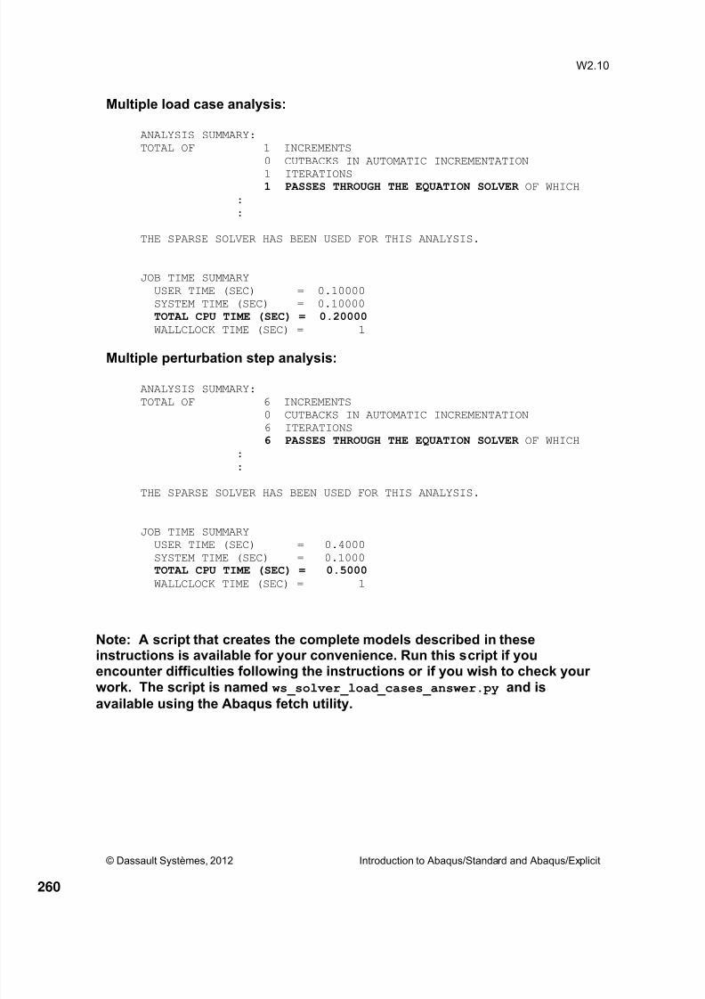
8/15/2019 Abaqus Analysis Intro-book
http://slidepdf.com/reader/full/abaqus-analysis-intro-book 260/469
© Dassault Systèmes, 2012 Introduction to Abaqus/Standard and Abaqus/Explicit
W2.10
Multiple load case analysis:
ANALYSIS SUMMARY:
TOTAL OF 1 INCREMENTS
0 CUTBACKS IN AUTOMATIC INCREMENTATION
1 ITERATIONS1 PASSES THROUGH THE EQUATION SOLVER OF WHICH
:
:
THE SPARSE SOLVER HAS BEEN USED FOR THIS ANALYSIS.
JOB TIME SUMMARY
USER TIME (SEC) = 0.10000
SYSTEM TIME (SEC) = 0.10000
TOTAL CPU TIME (SEC) = 0.20000WALLCLOCK TIME (SEC) = 1
Multiple perturbation step analysis:
ANALYSIS SUMMARY:
TOTAL OF 6 INCREMENTS
0 CUTBACKS IN AUTOMATIC INCREMENTATION
6 ITERATIONS
6 PASSES THROUGH THE EQUATION SOLVER OF WHICH :
:
THE SPARSE SOLVER HAS BEEN USED FOR THIS ANALYSIS.
JOB TIME SUMMARY
USER TIME (SEC) = 0.4000
SYSTEM TIME (SEC) = 0.1000
TOTAL CPU TIME (SEC) = 0.5000WALLCLOCK TIME (SEC) = 1
Note: A script that creates the complete models described in theseinstructions is available for your convenience. Run this script if youencounter difficulties following the instructions or if you wish to check yourwork. The script is named ws_solver_load_cases_answer.py and is
available using the Abaqus fetch utility.
260

8/15/2019 Abaqus Analysis Intro-book
http://slidepdf.com/reader/full/abaqus-analysis-intro-book 261/469
Notes
261

8/15/2019 Abaqus Analysis Intro-book
http://slidepdf.com/reader/full/abaqus-analysis-intro-book 262/469
Notes
262

8/15/2019 Abaqus Analysis Intro-book
http://slidepdf.com/reader/full/abaqus-analysis-intro-book 263/469
Workshop 3
Nonlinear Statics
Interactive Version
© Dassault Systèmes, 2012 Introduction to Abaqus/Standard and Abaqus/Explicit
Note: This workshop provides instructions in terms of the Abaqus GUIinterface. If you wish to use the Abaqus Keywords interface instead, pleasesee the “Keywords” version of these instructions.
Please complete either the Keywords or Interactive version of thisworkshop.
Goals
Define alternate nodal and material directions.
Include nonlinear geometric effects by adding the NLGEOM parameter.
Include nonlinear material effects by defining plastic material behavior.
Become familiar with the output for an incremental analysis.
Introduction
In this workshop you will model the plate shown in Figure W3 – 1. It is skewed at 30 tothe global X -axis, built-in at one end, and constrained to move on rails parallel to the
plate axis at the other end. You will determine the midspan deflection when the plate
carries a uniform pressure. You will modify the model to include alternate nodal and
material directions as well as nonlinear effects.
263

8/15/2019 Abaqus Analysis Intro-book
http://slidepdf.com/reader/full/abaqus-analysis-intro-book 264/469

8/15/2019 Abaqus Analysis Intro-book
http://slidepdf.com/reader/full/abaqus-analysis-intro-book 265/469
© Dassault Systèmes, 2012 Introduction to Abaqus/Standard and Abaqus/Explicit
W3.3
to the axis of the plate. It will be easier to interpret the results if the material directions
are aligned with the axis of the plate and the transverse direction. Therefore, a local
rectangular coordinate system is needed in which the local x-direction lies along the axisof the plate (i.e., at 30º to the global X -axis) and the local y-direction is also in the plane
of the plate.
You will define the datum coordinate system (CSYS) and then assign the materialorientation.
1. Switch to the Property module and define a rectangular datum coordinate system
as shown in Figure W3 – 2 using the Create Datum CSYS: 2 Lines tool .
a. Note the small black triangles at the base of the toolbox icons. Thesetriangles indicate the presence of hidden icons that can be revealed. Click
the Create Datum CSYS: 3 Points tool but do not release the mouse button. When additional icons appear, release the mouse button.
b. Select the Create Datum CSYS: 2 Lines tool . It appears in thetoolbox with a white background indicating that you selected it.
c. In the Create Datum CSYS dialog box, name the datum CSYS Skew,
select the Rectangular coordinate system type, and click Continue.Make the next two selections as indicated in Figure W3 – 2.
Figure W3 –2. Datum coordinate system used to define local directions
2. Assign the material orientations to the plate.
a. In the toolbox, click the Assign Material Orientation tool .
b. Select the entire part as the region to be assigned a local materialorientation.
Select this edge to be along the
local x-direction
Select this edgeto be in the
local x- y plane
265
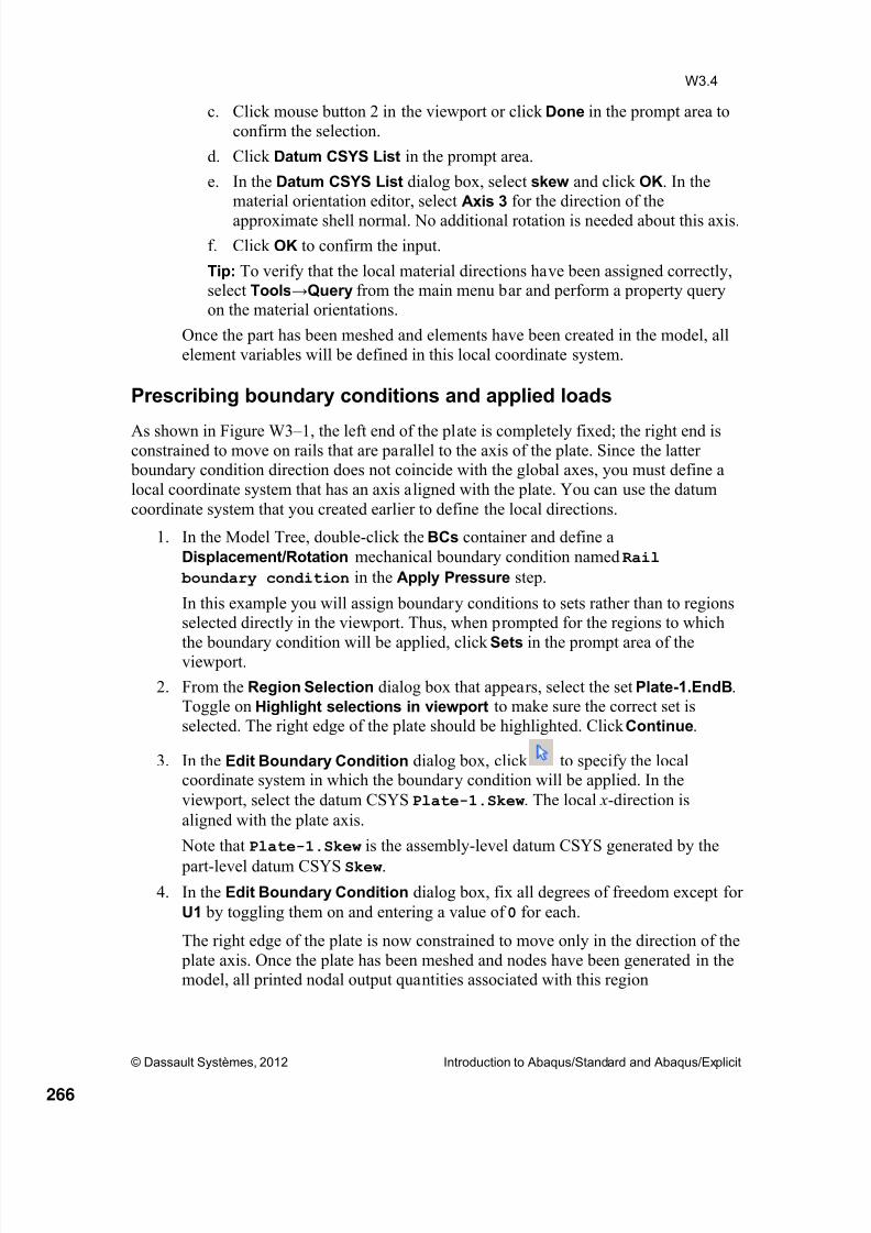
8/15/2019 Abaqus Analysis Intro-book
http://slidepdf.com/reader/full/abaqus-analysis-intro-book 266/469
© Dassault Systèmes, 2012 Introduction to Abaqus/Standard and Abaqus/Explicit
W3.4
c. Click mouse button 2 in the viewport or click Done in the prompt area to
confirm the selection.
d. Click Datum CSYS List in the prompt area.
e. In the Datum CSYS List dialog box, select skew and click OK. In thematerial orientation editor, select Axis 3 for the direction of the
approximate shell normal. No additional rotation is needed about this axis.
f. Click OK to confirm the input.
Tip: To verify that the local material directions have been assigned correctly,select Tools→Query from the main menu bar and perform a property queryon the material orientations.
Once the part has been meshed and elements have been created in the model, all
element variables will be defined in this local coordinate system.
Prescribing boundary conditions and applied loads
As shown in Figure W3 – 1, the left end of the plate is completely fixed; the right end isconstrained to move on rails that are parallel to the axis of the plate. Since the latter boundary condition direction does not coincide with the global axes, you must define a
local coordinate system that has an axis aligned with the plate. You can use the datum
coordinate system that you created earlier to define the local directions.
1. In the Model Tree, double-click the BCs container and define a
Displacement/Rotation mechanical boundary condition named Rail
boundary condition in the Apply Pressure step.
In this example you will assign boundary conditions to sets rather than to regionsselected directly in the viewport. Thus, when prompted for the regions to which
the boundary condition will be applied, click Sets in the prompt area of theviewport.
2. From the Region Selection dialog box that appears, select the set Plate-1.EndB.Toggle on Highlight selections in viewport to make sure the correct set is
selected. The right edge of the plate should be highlighted. Click Continue.
3. In the Edit Boundary Condition dialog box, click to specify the localcoordinate system in which the boundary condition will be applied. In the
viewport, select the datum CSYS Plate-1.Skew. The local x-direction is
aligned with the plate axis.
Note that Plate-1.Skew is the assembly-level datum CSYS generated by the
part-level datum CSYS Skew.
4. In the Edit Boundary Condition dialog box, fix all degrees of freedom except for
U1 by toggling them on and entering a value of 0 for each.
The right edge of the plate is now constrained to move only in the direction of the
plate axis. Once the plate has been meshed and nodes have been generated in themodel, all printed nodal output quantities associated with this region
266

8/15/2019 Abaqus Analysis Intro-book
http://slidepdf.com/reader/full/abaqus-analysis-intro-book 267/469
© Dassault Systèmes, 2012 Introduction to Abaqus/Standard and Abaqus/Explicit
W3.5
(displacements, velocities, reaction forces, etc.) will be written in this local
coordinate system.
5. Create another boundary condition named Fix left end to fix all degrees of
freedom at the left edge of the plate (set Plate-1.EndA). Use the default global
directions for this boundary condition.
6. Define a uniform pressure load named Pressure across the top of the shell in the
Apply Pressure step. Select both regions of the part using [Shift]+Click, andchoose the top side of the shell (Brown) as the surface to which the pressure load
will be applied. You may need to rotate the view to more clearly distinguish the
top side of the plate. Specify a load magnitude of 2.0E4 Pa.
Running the job and postprocessing the results
1. Create a job named SkewPlate with the following description: Linear
Elastic Skew Plate, 20 kPa Load .
2. Save your model database file.3. Submit the job for analysis and monitor the solution progress.
When the analysis is complete, use the following procedure to postprocess the
analysis results.
4. In the Model Tree, click mouse button 3 on the job SkewPlate and select Results
from the menu that appears to open the file SkewPlate.odb in the Visualization
module.
5. Click the Plot Deformed Shape tool to plot the deformed shape.
6. Use the the Query information tool to probe the value of the midspan
deformation.
a. In the Query dialog box, select Probe values in the Visualization
Module Queries field.
b. Change the displayed field variable to the displacement along the 3-
direction. In the Probe Values dialog box, click to change the defaultfield output variable to U3. In the Field Output dialog box that appears,
select U as the output variable and U3 as the component and click OK.
c. In the Probe Values dialog box, select Nodes as the item to probe.
d. Click on a node (as indicated in Figure W3 – 3) along the midespan to
probe its displacement along the 3-direction. Enter this value in the“Linear” column of Table W3– 1.
267

8/15/2019 Abaqus Analysis Intro-book
http://slidepdf.com/reader/full/abaqus-analysis-intro-book 268/469
© Dassault Systèmes, 2012 Introduction to Abaqus/Standard and Abaqus/Explicit
W3.6
Figure W3 –3. Midspan node
Adding geometric nonlinearity
Now perform the simulation considering geometrically nonlinear effects. Copy the model
named linear to a new model named nonlinear. You will add geometric nonlinearity
into the model nonlinear ; the changes required for this model are described next.
1. In the Model Tree, expand the Steps container and double-click Apply Pressure
to edit the step definition.
a. In the Basic tabbed page of the Edit Step dialog box, toggle on Nlgeom to include geometric nonlinearity effects and set the time period for the
step to 1.0.
b. In the Incrementation tabbed page, set the initial increment size to 0.1.
Note that the default maximum number of increments is 100; Abaqus may
use fewer increments than this upper limit, but it will stop the analysis if it
needs more.
You may wish to change the description of the step to reflect that it is now a
nonlinear analysis step.
2. Create a job named NlSkewPlate for the model nonlinear and give it the
description Nonlinear Elastic Skew Plate. Save your model database file.
3. Submit the job for analysis and monitor the solution progress.
The Job Monitor is particularly useful in nonlinear analyses. It gives a briefsummary of the automatic time incrementation used in the analysis for eachincrement. The information is written as soon as the increment is completed, so
you can monitor the analysis as it is running. This facility is useful in large,
complex problems. The information given in the Job Monitor is the same as that
given in the status file ( NlSkewPlate.sta).
4. When the job is complete, open the output database NlSkewPlate.odb in the
Visualization module and plot the deformed model shape.
268

8/15/2019 Abaqus Analysis Intro-book
http://slidepdf.com/reader/full/abaqus-analysis-intro-book 269/469
© Dassault Systèmes, 2012 Introduction to Abaqus/Standard and Abaqus/Explicit
W3.7
5. Query the vetical displacement (U3) of the same midspan node as discribed
earlier and enter the displacement result in the “Nlgeom” column of Table W3– 1.
Table W3 –1. Midspan displacements
Load (kPa) Linear (m) Nlgeom (m)20
60
6. Triple the pressure in both the linear and nonlinear analysis models. Create new jobs and run each of these analyses
7. Upon job completion, look at the results and enter the vertical displacement of thesame node in Table W3-1.
Question W3 –1: How does tripling the load affect the midspan displacement inthe linear analyses?
Question W3 –2: How do the results of the nonlinear analyses compare to eachother and to those from the linear analyses?
Adding Plasticity
You will now include another source of nonlinearity: plasticity. The material data areshown in Figure W3 – 4 (in terms of true stress vs. total log strain). Abaqus, however,
requires the plastic material data be defined in terms of true stress and plastic log strain.Thus, you will need to determine the plastic strains corresponding to each data point (see
the hint below). The changes described below are to be made to the nonlinear model.
1. In the Model Tree, expand the Materials container and double-click Steel.
2. In the Edit Material dialog box, add plasticity by choosingMechanical→Plasticity→ Plastic.
3. Enter the data lines corresponding to points A and B on the stress-strain curve as
shown in Figure W3 – 4.
The Young’s modulus for this material is 30E9 Pa.
Hint: The total strain tot at any point on the curve is equal to the sum of the
elastic strain el and plastic strain pl . The elastic strain at any point on the curve
can be evaluated from Young’s modulus and the true stress: el = / E . Use thefollowing relationship to determine the plastic strains to include on the plastic
option:
. E pl tot el tot
269

8/15/2019 Abaqus Analysis Intro-book
http://slidepdf.com/reader/full/abaqus-analysis-intro-book 270/469
© Dassault Systèmes, 2012 Introduction to Abaqus/Standard and Abaqus/Explicit
W3.8
You can use the command line interface (CLI) of Abaqus/CAE as a simplecalculator. For example, to compute the plastic strain at B, type
0.02-(3e7/3e10) in the command line interface and hit [Enter]. The value
of the plastic strain is printed (in this case the plastic strain at B is 0.019).
Note that the command line interface is hidden by default, but it uses the same
space that is occupied by the message area at the bottom of the main window.
To access the command line interface, click the yellow prompt button in
the bottom left corner of the main window.
Question W3 –3: Why is the second entry on the first data line of the plasticityoption equal to 0.0?
4. Change the pressure to 10 kPa.
a. In the Model Tree, double-click Pressure underneath the Loads container.
b. In the Edit Load dialog box that appears, enter a value of 10000 for
Magnitude.
5. Request restart output every increment in the step named Apply Pressure (switchto the Step module; select Output→Restart Requests).
Note that the step name is important for the restart analysis to be performed later.
6. Create a new job named PlSkewPlate and give it the description Nonlinear
Plastic Skew Plate.
7. Save your model database file.
8. Submit the job for analysis and monitor the solution progress.
Figure W3 –4. Stress versus strain curve
270

8/15/2019 Abaqus Analysis Intro-book
http://slidepdf.com/reader/full/abaqus-analysis-intro-book 271/469
© Dassault Systèmes, 2012 Introduction to Abaqus/Standard and Abaqus/Explicit
W3.9
Postprocessing an incremental analysis
When the job is complete, visualize the output database PlSkewPlate.odb in the
Visualization module.
1. By default, the last increment of the last step is selected. Use the Frame Selector
in the context bar to select other steps or increments; alternatively, use theStep/Frame dialog box (Result→Step/Frame).
2. Use the view manipulation tools to position the model as you wish. Turn
perspective on or off by clicking the Turn Perspective On tool or the Turn
Perspective Off tool in the toolbar.
3. Plot the deformed shape by clicking the Plot Deformed Shape tool .
A sample deformed shape plot is shown in Figure W3 – 5. Your plot may look
different if you have positioned your model differently
Figure W3 –5. Final deformed shape
4. Create a contour plot of variable S11 by following this procedure:
a. Click the Plot Contours tool in the toolbox.
b. Select Result→Field Output.
c. In the Field Output dialog box, select S11 as the stress component.
d. Click Section Points to select a section point.
e. In the Section Points dialog box that appears, select Top and bottom as
the active locations and click OK.Your contour plot should look similar to Figure W3 – 6. Abaqus plots thecontours of the Mises stress on both the top and bottom faces of each shell
element. To see this more clearly, rotate the model in the viewport.
271

8/15/2019 Abaqus Analysis Intro-book
http://slidepdf.com/reader/full/abaqus-analysis-intro-book 272/469
© Dassault Systèmes, 2012 Introduction to Abaqus/Standard and Abaqus/Explicit
W3.10
Figure W3 –6. Contour plot of S11: SPOS, top image; SNEG, bottom image
Question W3 –4: Where do the peak displacements and stresses occur in the
model?
5. Click the Animate: Time History tool to animate the results.
You can stop the animation and move between frames and steps by using the
arrow buttons in the context bar.
6. Render the shell thickness (View→ODB Display Options; toggle on Render
shell thickness).
The plot appears as shown in Figure W3 – 7. Note that for the purpose ofvisualization, a linear interpolation is used between the contours on the top and
bottom surfaces of the shell.
272
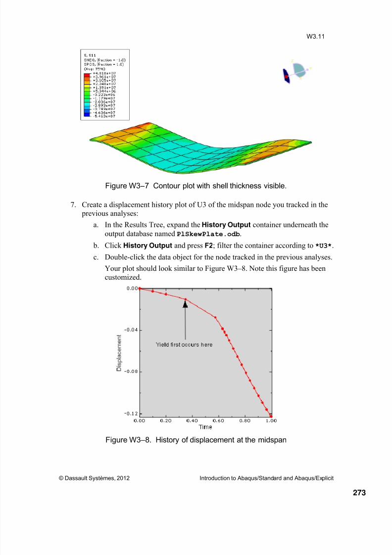
8/15/2019 Abaqus Analysis Intro-book
http://slidepdf.com/reader/full/abaqus-analysis-intro-book 273/469
© Dassault Systèmes, 2012 Introduction to Abaqus/Standard and Abaqus/Explicit
W3.11
Figure W3 –7 Contour plot with shell thickness visible.
7. Create a displacement history plot of U3 of the midspan node you tracked in the previous analyses:
a. In the Results Tree, expand the History Output container underneath the
output database named PlSkewPlate.odb.
b. Click History Output and press F2; filter the container according to *U3*.
c. Double-click the data object for the node tracked in the previous analyses.
Your plot should look similar to Figure W3 – 8. Note this figure has been
customized.
Figure W3 –8. History of displacement at the midspan
273

8/15/2019 Abaqus Analysis Intro-book
http://slidepdf.com/reader/full/abaqus-analysis-intro-book 274/469
© Dassault Systèmes, 2012 Introduction to Abaqus/Standard and Abaqus/Explicit
W3.12
Note: A script that creates the complete models described in theseinstructions is available for your convenience. Run this script if youencounter difficulties following the instructions or if you wish to check yourwork. The script is named
ws_solver_skew_plate_answer.py
and is available using the Abaqus fetch utility.
274

8/15/2019 Abaqus Analysis Intro-book
http://slidepdf.com/reader/full/abaqus-analysis-intro-book 275/469
© Dassault Systèmes, 2012 Introduction to Abaqus/Standard and Abaqus/Explicit
W3.13
Answers
Question W3 –1: How does tripling the load affect the midspan displacement in
the linear analyses?Answer: The midspan displacement is tripled in the linear analysis.
Question W3 –2: How do the results of the nonlinear analyses compare to each
other and to those from the linear analyses?
Answer: The midspan displacement is not tripled in the nonlinearanalysis when the load is tripled. At the higher load, the value
of the displacement predicted by the nonlinear analysis is less
than the value predicted by the linear analysis.
Question W3 –3: Why is the second entry on the first data line of the plasticoption equal to 0.0?
Answer: The first data line of the plastic option defines the initial yield
point. The plastic strain at this point is zero.
Question W3 –4: Where do the peak displacements and stresses occur in the
model?
Answer: The peak value of vertical displacement occurs at the midspan.
The supports of the plate are likely to be heavily stressed; this
is confirmed by contour plots of S11.
275

8/15/2019 Abaqus Analysis Intro-book
http://slidepdf.com/reader/full/abaqus-analysis-intro-book 276/469276

8/15/2019 Abaqus Analysis Intro-book
http://slidepdf.com/reader/full/abaqus-analysis-intro-book 277/469
Notes
277

8/15/2019 Abaqus Analysis Intro-book
http://slidepdf.com/reader/full/abaqus-analysis-intro-book 278/469
Notes
278

8/15/2019 Abaqus Analysis Intro-book
http://slidepdf.com/reader/full/abaqus-analysis-intro-book 279/469
Workshop 4
Unloading Analysis of a Skew Plate
Interactive Version
© Dassault Systèmes, 2012 Introduction to Abaqus/Standard and Abaqus/Explicit
Note: This workshop provides instructions in terms of the Abaqus GUIinterface. If you wish to use the Abaqus Keywords interface instead, pleasesee the “Keywords” version of these instructions.
Please complete either the Keywords or Interactive version of thisworkshop.
Introduction
You will now continue the analysis of the plate shown in Figure W4 – 1. Recall our
analysis includes geometric and material nonlinearity. We previously determined the
plate exceeded the material yield strength and therefore has some plastic deformation.Since we requested restart output, we can resume the analysis to determine the residual
stress state. In this workshop we will remove the load in order to recover the elastic
deformation; the plastic deformation will remain.
Figure W4 –1 Sketch of the skew plate.
All degrees of freedom at this end areconstrained except along the axis ofthe plate.
279

8/15/2019 Abaqus Analysis Intro-book
http://slidepdf.com/reader/full/abaqus-analysis-intro-book 280/469
© Dassault Systèmes, 2012 Introduction to Abaqus/Standard and Abaqus/Explicit
W4.2
Adding a restart model
Open the database ../abaqus_solvers/interactive/skew/SkewPlate.cae
created in the previous workshop and copy the model named nonlinear to a new model
named restart. The changes required for this model are described next.
Model Attributes
1. In the Model Tree, double-click the model restart to edit the attributes for therestart analysis model. (Alternatively, from the main menu bar, selectModel→Edit Attributes→restart .)
2. On the Restart tab of the Edit Model Attributes dialog box:
a. Click the checkbox to indicate the (previous) job where the restart data
was saved (recall this job was named PlSkewPlate). b. Indicate the step from which to restart the analysis (recall this step was
named Apply Pressure) and that the restart analysis will commence fromthe end of the step.
Step definition
1. In the Model Tree, double-click the Steps container to add a new general staticstep after the Apply Pressure step.
2. Name the step Unload .
3. In the Basic tabbed page of the Edit Step dialog box, Nlgeom should already be
on to include geometric nonlinearity effects.
4. Set the time period for the step to 1.0.
5. As before, in the Incrementation tabbed page, set the initial increment size to0.1.
Loads
1. Use the Load Manager to deactivate the pressure load in the step named Unload.Alternatively, you could simply edit the load magnitude (for example, to examine
the effect of a load reversal).
Job definition
1. Create a new job named PlSkewPlate-unload using the model restart and
enter the following job description: Unload Plastic Skew Plate. Note that the job type is set to Restart.
2. Save your model database file.
3. Submit the job for analysis, and monitor the solution progress.
4. Correct any modeling errors, and investigate the source of any warning messages.
280

8/15/2019 Abaqus Analysis Intro-book
http://slidepdf.com/reader/full/abaqus-analysis-intro-book 281/469
© Dassault Systèmes, 2012 Introduction to Abaqus/Standard and Abaqus/Explicit
W4.3
Postprocessing
In the Visualization module, contour the U3 displacement component in the plate:
1. Click the Plot Contours tool in the toolbox.
2. From the list of variable types on the left side of the Field Output toolbar, selectPrimary (if it is not already selected).
3. From the list of available output variables in the center of the toolbar, select
output variable U (spatial displacement at nodes).
4. From the list of available components and invariants on the right side of the Field
Output toolbar, select U3.
5. Compare to the results at the end of the Apply Pressure step.
Note that in this output database file, the results for frame 0 correspond to the
results at the end of the Apply Pressure step (use the Frame Selector to
switch to a different frame).The difference between the final state of the model and its initial state is due tothe elastic springback that has occurred. The deformation that remains is permanent and unrecoverable.
Note: A script that creates the complete models described in theseinstructions is available for your convenience. Run this script if youencounter difficulties following the instructions or if you wish to check yourwork. The script is named ws_solver_skew_plate_answer.py and is
available using the Abaqus fetch utility.
281

8/15/2019 Abaqus Analysis Intro-book
http://slidepdf.com/reader/full/abaqus-analysis-intro-book 282/469282

8/15/2019 Abaqus Analysis Intro-book
http://slidepdf.com/reader/full/abaqus-analysis-intro-book 283/469
Notes
283

8/15/2019 Abaqus Analysis Intro-book
http://slidepdf.com/reader/full/abaqus-analysis-intro-book 284/469
8/15/2019 Abaqus Analysis Intro-book
http://slidepdf.com/reader/full/abaqus-analysis-intro-book 285/469
Workshop 5
CLD Analysis of a Seal using Abaqus/Standard
Interactive Version
© Dassault Systèmes, 2012 Introduction to Abaqus/Standard and Abaqus/Explicit
Note: This workshop provides instructions in terms of the Abaqus GUIinterface. If you wish to use the Abaqus Keywords interface instead, pleasesee the “Keywords” version of these instructions.
Please complete either the Keywords or Interactive version of thisworkshop.
Goals
Evaluate a hyperelastic material.
Define contact interactions using contact pairs and general contact.
Perform a large displacement analysis with Abaqus/Standard.
Use the Visualization module to create a compression load-deflection curve.
Introduction
In this workshop, a compression analysis of a rubber seal is performed to determine theseal’s performance. The goal is to determine the seal’s compression load-deflection
(CLD) curve, deformation and stresses. The analysis will be performed usingAbaqus/Standard. Two analyses are performed: one using contact pairs and the other
using general contact.
As shown in Figure W5 – 1, the top outer surface of the seal is covered with a polymerlayer, and the seal is compressed between two rigid surfaces (the upper one is displacedalong the negative Y -direction; the lower one is fixed). During compression, the cover
contacts the top rigid surface; the outer surface of the seal is in contact with the cover andthe bottom rigid surface; in addition the inner surface of the seal may come into contact
with itself.
285

8/15/2019 Abaqus Analysis Intro-book
http://slidepdf.com/reader/full/abaqus-analysis-intro-book 286/469
© Dassault Systèmes, 2012 Introduction to Abaqus/Standard and Abaqus/Explicit
W5.2
Figure W5 –1. Seal model: meshed assembly
Preliminaries
1. Enter the working directory for this workshop
../abaqus_solvers/interactive/seal
2. Run the script ws_solver_seal.py using the following command:
abaqus cae startup=ws_solver_seal.py.
The above command creates an Abaqus/CAE database named seal.cae in the current
directory. The geometry, mesh, and material definitions are included in the model named
Seal. You will first perform a material evaluation to evaluate the stability of the
hyperelastic material model, add the necessary data to complete the model, run the job,
and finally postprocess the results.
Material Evaluation
It is important to determine whether the material model of the seal will be stable during
the analysis. Before completing the model, evaluate the material definition used for theseal.
1. Review the material definition. In the Model Tree, double-click Santoprene underneath the Materials container. It is a hyperelastic material with a first-order
polynomial strain energy potential. The coefficients are already chosen for theanalysis.
2. Evaluate the material definition. Abaqus/CAE provides a convenient Evaluate
option that allows you to view the behavior predicted by a hyperelastic material
by performing standard tests to choose a suitable material formulation. You willuse this option to view the behavior predicted by the material Santoprene.
Seal
Cover
Rigid
Surfaces
fixed
U2
286

8/15/2019 Abaqus Analysis Intro-book
http://slidepdf.com/reader/full/abaqus-analysis-intro-book 287/469
© Dassault Systèmes, 2012 Introduction to Abaqus/Standard and Abaqus/Explicit
W5.3
a. From the main menu bar in the Property module, choose
Material→Evaluate→Santoprene.
b. The Evaluate Material dialog box appears. Notice that you can chooseeither the Coefficients or Test data source for evaluating the material.Typically the test data are used to define a material model; you can use the
Evaluate option to view the predicted behavior and adjust the materialdefinition as necessary. In this workshop you will only evaluate thestability of the material model for the given coefficients.
c. In the Evaluate Material dialog box, accept all defaults and click OK.
Abaqus/CAE creates and submits a job to perform the standard tests using
the material Santoprene; at the same time, Abaqus/CAE switches to theVisualization module and displays the evaluation results when the job is
complete. Figure W5 – 2 shows the Material Parameters and Stability
Limit Information dialog box; Figure W5 – 3 shows three stress vs. strain
plots from uniaxial, biaxial, and planar tests.
Question W5 –1: What do the plots indicate about the stability of the material?
Based on these results, you can have confidence that your material will remainstable.
Figure W5 –2. Material parameters and stability limit information
287

8/15/2019 Abaqus Analysis Intro-book
http://slidepdf.com/reader/full/abaqus-analysis-intro-book 288/469

8/15/2019 Abaqus Analysis Intro-book
http://slidepdf.com/reader/full/abaqus-analysis-intro-book 289/469
© Dassault Systèmes, 2012 Introduction to Abaqus/Standard and Abaqus/Explicit
W5.5
Part 1: Analysis using contact pairs
Defining the step and the contact pairs
1. In the Model Tree, double-click the Steps container to create a static, general stepnamed PushDown.
a. In the Basic tabbed page of the step editor, set the time period to 1 and
turn on Nlgeom.
b. In the Incrementation tabbed page, enter a value of 0.005 for Initial
Increment size and 200 for Maximum number of increments.
c. In the Other tabbed page, select Unsymmetric as the matrix storagescheme (it is recommended when the surface-to-surface contactdiscretization method is used).
2. Define a contact pair between the seal and the bottom rigid surface.
a. In the Model Tree, double-click the Interactions container. In the CreateInteraction dialog box, name the interaction BotSeal and select the step
PushDown and Surface-to-surface contact (Standard). Click
Continue.
b. You will be prompted to select a master surface. In the prompt area, click
Surfaces. In the Region Selection dialog box that appears, select the
predefined surface Bottom and toggle on Highlight selections in
viewport to view this surface. Click Continue.
c. In the prompt area, select Surface as the slave surface type. In the Region
Selection dialog box that appears, select the predefined surface
SealOuter and visualize this surface. Click Continue.The interaction editor appears.
d. In the Edit Interaction dialog box accept all defaults and click OK.
Note that Abaqus/CAE automatically assigns the predefined (also the onlyavailable) interaction property frictionless to this interaction.
3. Using a similar procedure, define the following contact pairs as listed in Table
W5 – 1 with the interaction property frictionless.
Table W5 –1. Contact pairs
Interaction Name Master Surface Slave SurfaceTopCover Top Cover
SealCover Cover SealOuter
Question W5 –2: In the interaction SealCover, why do we choose SealOuter
as the slave surface?
289

8/15/2019 Abaqus Analysis Intro-book
http://slidepdf.com/reader/full/abaqus-analysis-intro-book 290/469
© Dassault Systèmes, 2012 Introduction to Abaqus/Standard and Abaqus/Explicit
W5.6
4. Create a self-contact interaction for the inner surface of the seal.
a. In the Model Tree, double-click the Interactions container. In the Create
Interaction dialog box, name the interaction SealSelf and select the
step PushDown and Self-contact (Standard). Click Continue.
b. In the Region Selection dialog box that appears, select the predefinedsurface SealInner and visualize this surface. Click Continue.
The interaction editor appears.
c. In the Edit Interaction dialog box accept all defaults and click OK.
Defining boundary conditions and output requests
Asymmetric lateral sliding of the model is prevented by constraining the seal and thecover along their vertical symmetry axes in the X -direction. The bottom rigid surface isfixed, and a displacement of – 6 units is applied to the top rigid surface along the Y -
direction to compress the seal between the two surfaces. To complete these boundary
conditions:1. In the Model Tree, double-click the BCs container to create a
Displacement/Rotation type boundary condition named Fix1 in the step
PushDown.
a. When prompted to select the region, click Sets in the prompt area (ifnecessary).
b. In the Region Selection dialog box, select the predefined set Fix1, toggleon Highlight selections in viewport to visualize the selection, and click
Continue.
c. In the Edit Boundary Condition dialog box, toggle on U1, accept the
default value of 0, and click OK.2. Create a Symmetry/Antisymmetric/Encastre type boundary condition named
FixBot to encastre the predefined set BotRP (the reference node of the bottom
rigid surface).
3. Create a Displacement/Rotation type boundary condition named PushDown in
the step PushDown to define the displacement of the top rigid surface.
a. Select the predefined set TopRP (the reference node of the top rigidsurface).
b. Specify a value of 0 for U1 and UR3, and -6 for U2.
4. Edit the field output request named F-Output-1 to include the nominal strain, NE.
5. Create a new history output request in the step PushDown for the set TopRP towrite the history of the variables Displacements: U and Forces: RF to the output
database file.
290

8/15/2019 Abaqus Analysis Intro-book
http://slidepdf.com/reader/full/abaqus-analysis-intro-book 291/469
© Dassault Systèmes, 2012 Introduction to Abaqus/Standard and Abaqus/Explicit
W5.7
Running the job and postprocessing the results
1. Create a job named seal for the model Seal.
2. Save your model database, submit the job for analysis, and monitor the job’s
process.
When the job is complete, open the output database file seal.odb in the
Visualization module and postprocess the results.
3. Plot the undeformed and the deformed model shapes. To distinguish between thedifferent instances, color code the model based on part instances.
Tip: From the toolbar, select Part instances from the color-coding pull down
menu, as shown in Figure W5 – 4 (or use the Color Code Dialog tool tocustomize the color for each part instance).
Figure W5 –4. Color-coding pull down menu
4. Use the Animate: Time History tool to animate the deformation history.
5. Display only the seal. In the Results Tree, expand the Instances container
underneath the output database file named seal.odb. Click mouse button 3 on
the instance SEAL-1 and select Replace from the menu that appears.
Abaqus/CAE now displays only this instance.
6. Contour the Mises stress of the seal on the deformed shape. If necessary, use the
frame selector in the context bar to select the final increment.
The contour plot is shown in Figure W5 – 5.
291

8/15/2019 Abaqus Analysis Intro-book
http://slidepdf.com/reader/full/abaqus-analysis-intro-book 292/469
© Dassault Systèmes, 2012 Introduction to Abaqus/Standard and Abaqus/Explicit
W5.8
Figure W5 –5. Mises contour plot
7. Contour the minimum and maximum principal nominal strains. Elastic strains can
be very high for hyperelastic materials. Because of this, the linear elastic materialmodel is not used because it is not appropriate for elastic strains greater than
approximately 5%.
8. Display the reaction force history at the reference node of the top rigid surface: In
the Results Tree, expand the History Output container underneath the output
database file named seal.odb and double-click Reaction force: RF2 PI: TOP-1
Node 3 in NSET TOPRP.
9. You will now create the CLD curve.
a. In the History Output container, click mouse button 3 on Reaction force:
RF2 PI: TOP-1 Node 3 in NSET TOPRP and select Save As from the
menu that appears. Save the data as Force. b. Click mouse button 3 on Spatial displacement: U2 PI: TOP-1 Node 3 in
NSET TOPRP and select Save As from the menu that appears. Save the
data as Disp.
c. In the Results Tree, double-click XYData. In the Create XY Data dialog
box that appears, select the Operate on XY data source and click
Continue.
The Operate on XY Data dialog box appears.
d. From the Operators listed in the Operate on XY Data dialog box, selectcombine(X, X) and then abs(A). Note that the abs(A) operator is used to
obtain the absolute values. In the XY Data field, double-click the curveDisp. The current expression reads combine(abs("Disp")). Move the
cursor before the far-right bracket, enter a comma, and then select theoperator abs(A). In the XY Data field, double-click the curve Force. The
final expression reads combine(abs("Disp"), abs("Force") ).
Click Plot Expression to plot this expression. Save this plot as CLD.
292

8/15/2019 Abaqus Analysis Intro-book
http://slidepdf.com/reader/full/abaqus-analysis-intro-book 293/469
© Dassault Systèmes, 2012 Introduction to Abaqus/Standard and Abaqus/Explicit
W5.9
10. Customize the plot as follows:
a. From the main menu bar, select Options→XY Options→Plot.
In the Plot Options dialog box, fill the plot background in white.
b. Double-click anywhere on the chart to open the Chart Options dialog
box. In the Grid Display tabbed page, toggle on the major X - and Y -
grid lines. Set the line color to blue and the line style to dashed.
Change the fill color using the following RGB values: red: 175;green: 250; blue: 185.
In the Grid Area tabbed page, select Square as the size and drag
the slider to 80. From the list of auto-alignments, choose the one
that places the chart in the center of the viewport
c. Double-click the legend to open the Chart Legend Options dialog box.
In the Contents tabbed page, click to increase the legend text
font size to 10.
In the Area tabbed page, toggle on Inset.
Toggle on Fill to flood the legend with a white background.
In the viewport, drag the legend over the chart.
d. Double-click either axis to open the Axis Options dialog box.
In the X Axis region of the dialog box, select the displacement
axis.
In the Scale tabbed page, place 4 major tick marks on the X -axis at
(use the By count method). In the Title tabbed page, change the X -axis title to Displacement
(inch).
In the Y Axis region of the dialog box, select the force axis.
In the Scale tabbed page, specify that the Y -axis should extend
from 0 (the Y -axis minimum) to 250 (the Y -axis maximum).
Increase the number of Y -axis minor tick marks per increment to 4.
In the Title tabbed page, change the Y -axis title to Force (lbf).
In the Axes tabbed page, change the font size for both axes to 10.
e. Expand the list of plot option icons in the toolbox:
293

8/15/2019 Abaqus Analysis Intro-book
http://slidepdf.com/reader/full/abaqus-analysis-intro-book 294/469
© Dassault Systèmes, 2012 Introduction to Abaqus/Standard and Abaqus/Explicit
W5.10
f. Examine the remaining options. Add the following plot title: CLD
Diagram . Double-click the plot title to open the Plot Title Options dialog
box.
In the Title tabbed page, click to change the legend text style to
bold.
In the Area tabbed page, toggle on Inset.
In the viewport, drag the plot title above the chart.
g. Click in the toolbox to open the Curve Options dialog box. Change
the legend text to Top Surface Ref Point and toggle on Show
symbol. Set the color for both the line and symbols to red. Use large filled
squares for the symbols. Reposition the legend as necessary.
The final plot appears as shown in Figure W5 – 6.
Figure W5 –6. Compression load deflection diagram
Question W5 –3: What does the inverted peak near 4 inches of deflectionrepresent?
294

8/15/2019 Abaqus Analysis Intro-book
http://slidepdf.com/reader/full/abaqus-analysis-intro-book 295/469
© Dassault Systèmes, 2012 Introduction to Abaqus/Standard and Abaqus/Explicit
W5.11
Part 2: Analysis using general contact
1. Copy the model named Seal to one named Seal_gc.
Make all subsequent modifications to the new model.
2. In the Model Tree, expand the Interactions container and select the 4 interactionsdefined earlier.
3. Click mouse button 3 and select Delete from the menu that appears, as shown in
Figure W5 – 7.
Figure W5 –7. Contact pairs to be deleted
4. In the Model Tree, double-click Interactions (or select Interaction→Create).
5. In the Create Interaction dialog box that appears, set the step to Initial andchoose General contact (Standard) as the type. Click Continue.
6. In the interaction editor, select frictionless from the list of available Global
property assignment options, as shown in Figure W5 – 8.
295
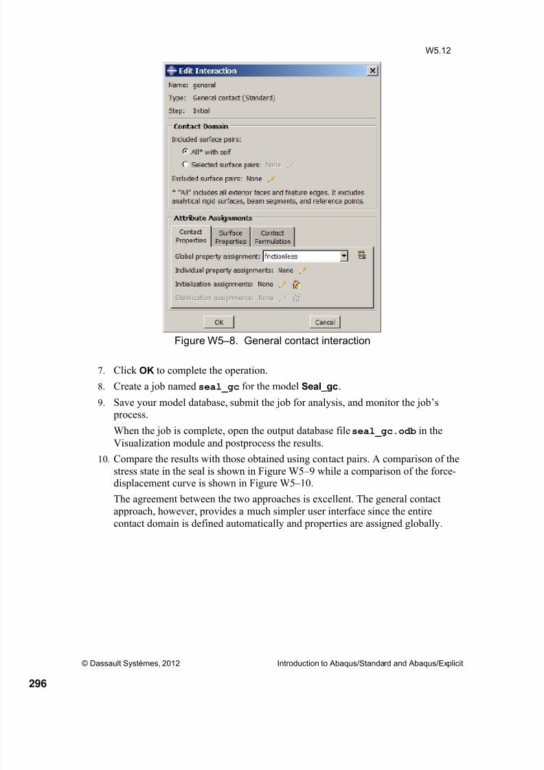
8/15/2019 Abaqus Analysis Intro-book
http://slidepdf.com/reader/full/abaqus-analysis-intro-book 296/469
© Dassault Systèmes, 2012 Introduction to Abaqus/Standard and Abaqus/Explicit
W5.12
Figure W5 –8. General contact interaction
7. Click OK to complete the operation.
8. Create a job named seal_gc for the model Seal_gc.
9. Save your model database, submit the job for analysis, and monitor the job’s process.
When the job is complete, open the output database file seal_gc.odb in the
Visualization module and postprocess the results.
10. Compare the results with those obtained using contact pairs. A comparison of the
stress state in the seal is shown in Figure W5 – 9 while a comparison of the force-displacement curve is shown in Figure W5 – 10.
The agreement between the two approaches is excellent. The general contact
approach, however, provides a much simpler user interface since the entire
contact domain is defined automatically and properties are assigned globally.
296

8/15/2019 Abaqus Analysis Intro-book
http://slidepdf.com/reader/full/abaqus-analysis-intro-book 297/469

8/15/2019 Abaqus Analysis Intro-book
http://slidepdf.com/reader/full/abaqus-analysis-intro-book 298/469
© Dassault Systèmes, 2012 Introduction to Abaqus/Standard and Abaqus/Explicit
W5.14
Note: A script that creates the complete seal model is available for yourconvenience. Run this script if you encounter difficulties following theinstructions or if you wish to check your work. The script is named
ws_solver_seal_answer.py
and is available using the Abaqus fetch utility.
298

8/15/2019 Abaqus Analysis Intro-book
http://slidepdf.com/reader/full/abaqus-analysis-intro-book 299/469
© Dassault Systèmes, 2012 Introduction to Abaqus/Standard and Abaqus/Explicit
W5.15
Answers
Question W5 –1: What do the plots indicate about the stability of the material?
Answer: The plots never have a negative slope, indicating that the
material is stable throughout the entire strain range.
Question W5 –2: In the interaction SealCover, why do we choose SealOuter
as the slave surface?
Answer: SealOuter has a more refined mesh and should therefore be
specified as the slave surface.
Question W5 –3: What does the inverted peak near 4 inches of deflectionrepresent?
Answer: This peak represents the inward buckling that occurs at the bottom corners of the seal during compression. If you look at
the deformed shape at the time corresponding to
approximately 3.7 inches of displacement, you will observethis phenomenon.
299

8/15/2019 Abaqus Analysis Intro-book
http://slidepdf.com/reader/full/abaqus-analysis-intro-book 300/469300

8/15/2019 Abaqus Analysis Intro-book
http://slidepdf.com/reader/full/abaqus-analysis-intro-book 301/469
Notes
301

8/15/2019 Abaqus Analysis Intro-book
http://slidepdf.com/reader/full/abaqus-analysis-intro-book 302/469
Notes
302

8/15/2019 Abaqus Analysis Intro-book
http://slidepdf.com/reader/full/abaqus-analysis-intro-book 303/469
Workshop 6
Dynamics
Interactive Version
© Dassault Systèmes, 2012 Introduction to Abaqus/Standard and Abaqus/Explicit
Note: This workshop provides instructions in terms of the Abaqus GUIinterface. If you wish to use the Abaqus Keywords interface instead, pleasesee the “Keywords” version of these instructions.
Please complete either the Keywords or Interactive version of thisworkshop.
Goals
Become familiar with the Abaqus/CAE procedures for frequency extraction andimplicit dynamic analyses.
Become more familiar with monitoring job status.
Learn how to plot eigenmodes and create history plots using Abaqus/CAE.
IntroductionIn this workshop the dynamic response of the cantilever beam shown in Figure W6 – 1 isinvestigated. A frequency extraction is performed to determine the 10 lowest vibration
modes of the beam. The effects of mesh refinement, element interpolation order, and
element dimension will be considered.
The problem is also solved by performing a direct integration dynamic analysis to
simulate the vibration of the beam upon removal of the tip load . The frequency of the
vibration predicted by the transient analysis will be compared with the natural frequency
results.
Figure W6 –1. Problem description
303

8/15/2019 Abaqus Analysis Intro-book
http://slidepdf.com/reader/full/abaqus-analysis-intro-book 304/469
© Dassault Systèmes, 2012 Introduction to Abaqus/Standard and Abaqus/Explicit
W6.2
Preliminaries
1. Enter the working directory for this workshop
../abaqus_solvers/interactive/dynamics
2. Run the script ws_solver_beam.py using the following command:
abaqus cae startup=ws_solver_beam.py.
The above command creates an Abaqus/CAE database named Beam.cae in the current
directory. The model named static includes the beam model for a static, general
analysis. Currently 5 B21 elements are used to discretize the beam. You will edit this
model further as described below.
Part 1: Frequency extraction analysis
Perform a frequency extraction analysis to determine the 10 lowest eigenmodes of the
structure. In the current model do the following.
1. Add a density of 2.3E6 unit to the beam material definition named MATEA .
In the Model Tree, expand the Materials container and double-click thematerial MATEA.
In the material editor, select General→Density from the menu bar.
Enter the value 2.3E-6 for Mass Density in the Density field.
2. The frequency analysis procedure will be used instead of the general static one.Thus, suppress the general static step named Displace (do not delete it since it
will be used later).
a. In the Model Tree, expand the Steps container and click mouse button 3
on the step Displace and select Suppress from the menu that appears. b. Create a new step named Frequency; select Linear perturbation as the
procedure type and Frequency from the list of available perturbation
steps.
c. Click Continue.
d. In the step editor, accept the default Lanczos eigensolver and enter a
value of 10 for Number of eigenvalues requested.
e. Click OK to save the change and exit the step editor.
3. Create a job named frequency.
4. Save your model database, submit the job for analysis, and monitor the job’s process.
304

8/15/2019 Abaqus Analysis Intro-book
http://slidepdf.com/reader/full/abaqus-analysis-intro-book 305/469
© Dassault Systèmes, 2012 Introduction to Abaqus/Standard and Abaqus/Explicit
W6.3
Visualizing results
When the analysis is complete, use the following procedure to view the eigenmodes andeigenvalues from the frequency analysis in the Visualization module:
1. In the Model Tree, click mouse button 3 on the job frequency and select Results
from the menu that appears to open the file frequency.odb in the Visualization
module.
2. Plot the first eigenmode (plot the deformed model shape and use the Frame
Selector or the Step/Frame dialog box to choose the frame corresponding toMode 1).
3. Using the arrow keys in the context bar, select different mode shapes.
4. The results for modes 1 and 4 are shown in Figure W6 – 2. These correspond to the
first and fourth transverse modes of the structure.
5.
Figure W6 –2. First and fourth transverse modes(coarse mesh; 2D linear beam elements)
Question W6 –1: Are there modes of the physical system that cannot be
captured by your model because of limitations in element typeor mesh? (Remember that the elements are planar and the
mesh is somewhat coarse.)
Question W6 –2: Do any of the mode shapes for your model look non-physical?
305

8/15/2019 Abaqus Analysis Intro-book
http://slidepdf.com/reader/full/abaqus-analysis-intro-book 306/469
© Dassault Systèmes, 2012 Introduction to Abaqus/Standard and Abaqus/Explicit
W6.4
Effect of mesh on extracted modes
From Figure W6 – 2 it is apparent that such a coarse mesh of linear-interpolation elementsis unable to adequately represent the mode shapes associated with the higher modes. In
fact the current mesh is unable to represent anything beyond the fifth mode.
To obtain accurate results for all extracted modes, a sufficiently refined mesh is required.Thus, increase the mesh refinement. Also, switch to quadratic interpolation elements
since these provide superior accuracy for frequency extraction analysis.
1. Remesh the part using a global seed size of 5.
2. Change the element type to B22.
3. Create a new job, run it, and compare the results with those obtained previously.
The results for modes 1 and 4 are shown in Figure W6 – 3.
Figure W6 –3. First and fourth transverse modes(fine mesh; 2D quadratic beam elements)
The results indicate that the refined mesh is able to represent all extracted modes.The natural frequency of the first mode predicted by the fine-mesh model is
within 2% of that predicted by the coarse mesh model. The difference in results
for the fourth mode is more significant: there is an 8% difference in the predicted
natural frequency for this mode.
Note that all modes with the exception of modes 6 and 10 are transverse modes.
Modes 6 and 10 are longitudinal modes. To see the longitudinal modes more
clearly, superimpose the undeformed model shape on the deformed model shape.
306

8/15/2019 Abaqus Analysis Intro-book
http://slidepdf.com/reader/full/abaqus-analysis-intro-book 307/469
© Dassault Systèmes, 2012 Introduction to Abaqus/Standard and Abaqus/Explicit
W6.5
Torsional and out-of-plane modes
The current model, given that it uses two-dimensional beam elements, is unable tocapture any torsional or out-of-plane modes. For this a three-dimensional model is
required (using either beam, solid, or shell elements). With three-dimensional beam
elements, however, it is not possible to visualize the modes. Thus, in what follows, shellelements are used to capture the out-of-plane modes.
A predefined model named shell is available that uses three-dimensional quadratic shellelements to represent the beam structure. The shell part is 200 units long by 50 units
wide. The part mesh consists of 40 S8R elements along the length of the structure and 10
along its width. Homogeneous shell section properties with the same material properties
used earlier and a thickness of 5 units are assigned to the part.
1. Create a job for the shell model, run it, and compare the results with those
obtained previously.
2. The results for the first and fourth transverse modes are shown in Figure W6 – 4.
The agreement in terms of both mode shape and natural frequency between the(refined) beam and shell models is excellent (compare with Figure W6 – 3).
Figure W6 –4. First and fourth transverse modes (3D shell model)
307

8/15/2019 Abaqus Analysis Intro-book
http://slidepdf.com/reader/full/abaqus-analysis-intro-book 308/469
© Dassault Systèmes, 2012 Introduction to Abaqus/Standard and Abaqus/Explicit
W6.6
3. The three-dimensional model captures the torsional and out-of-plane modes that
are suppressed by the two-dimensional model. The first three of these modes are
shown in Figure W6 – 5.
Figure W6 –5. Torsional and out-of-plane modes (3D shell model)
308

8/15/2019 Abaqus Analysis Intro-book
http://slidepdf.com/reader/full/abaqus-analysis-intro-book 309/469
© Dassault Systèmes, 2012 Introduction to Abaqus/Standard and Abaqus/Explicit
W6.7
Part 2: Transient dynamic analysis
You will now investigate the free vibration of the beam upon removal of the tip load,using an implicit dynamic procedure (Abaqus/Standard).
1. Copy the model named static to a model named dynamic. Make the followingchanges to the dynamic model.
2. Delete the frequency extraction step.
3. Resume the static, general step named Displace.
4. Create a dynamic, implicit step after the static, general step.
a. In the Model Tree, double-click the Steps container.
b. In the Create Step dialog box, name the step Release.
c. Select Dynamic, Implicit from the list of available General proceduretypes, and click Continue.
d. In the Edit Step dialog box, accept the default step time 1.e. In the Incrementation tabbed page, choose Automatic time
incrementation, enter a value of 200 for the maximum number of
increments, and 0.01 for the initial increment size.
f. Click OK to save the data and exit the step editor.
5. Deactivate the load in the step named Release.
a. In the Model Tree, expand the branch of the load DisplaceTip underneaththe Loads container, as shown in Figure W6 – 6a.
b. Click mouse button 3 on Release (propagated) under the States sub-container and select Deactivate from the menu that appears.
Note that Release (propagated) is changed into Release (Inactive), as
shown in Figure W6 – 6b, to indicate that the load is deactivated in this
step.
(a) (b)Figure W6 –6. Loads container in the Model Tree
309

8/15/2019 Abaqus Analysis Intro-book
http://slidepdf.com/reader/full/abaqus-analysis-intro-book 310/469
© Dassault Systèmes, 2012 Introduction to Abaqus/Standard and Abaqus/Explicit
W6.8
A part-level set named TIP has been predefined. This set will be used for writing
the displacement history of the tip node to the output database file and also to
monitor the solution progress. This set is indicated in Figure W6 – 3.
Figure W6 –3. Part-level node set
6. Add a history output request to write the displacement history every increment for
the set TIP to the output database file.
a. In the Model Tree, double-click the History Output Requests container.In the Create History dialog box, select the step Displace and click
Continue.
b. In the Edit History Output Request dialog box, select the domain Set
and the set Beam-1.TIP.
c. Expand the Displacement/Velocity/Acceleration branch in the Output
Variables field and toggle on U, Translations and rotations.
d. Click OK to exit the history output editor.
7. It is useful to be able to monitor the progress of an analysis by tracking the value
of one degree of freedom.
a. From the main menu bar of the Step module, select Output→DOFMonitor to open the DOF Monitor dialog box.
b. Activate the stippled entries by toggling on Monitor a degree of freedom
throughout the analysis.
c. Click to select the set Beam-1.TIP as the Region.
Tip: Click Points in the prompt area to select the set Beam-1.TIP from theRegion Selection dialog box.
d. Enter 2 as the Degree of freedom.
e. Click OK to exit the DOF Monitor dialog box.
8. Create a job named dynamic for the model dynamic.
9. Save your model database, submit the job for analysis, and monitor the job’s process.
TIP
310
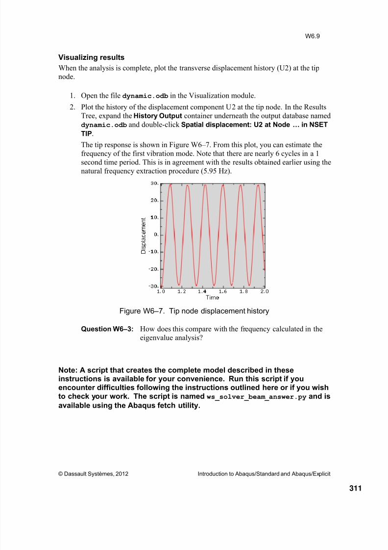
8/15/2019 Abaqus Analysis Intro-book
http://slidepdf.com/reader/full/abaqus-analysis-intro-book 311/469
© Dassault Systèmes, 2012 Introduction to Abaqus/Standard and Abaqus/Explicit
W6.9
Visualizing results
When the analysis is complete, plot the transverse displacement history (U2) at the tipnode.
1. Open the file dynamic.odb in the Visualization module.2. Plot the history of the displacement component U2 at the tip node. In the Results
Tree, expand the History Output container underneath the output database named
dynamic.odb and double-click Spatial displacement: U2 at Node … in NSET
TIP.
The tip response is shown in Figure W6 – 7. From this plot, you can estimate the
frequency of the first vibration mode. Note that there are nearly 6 cycles in a 1
second time period. This is in agreement with the results obtained earlier using the
natural frequency extraction procedure (5.95 Hz).
Figure W6 –7. Tip node displacement history
Question W6 –3: How does this compare with the frequency calculated in the
eigenvalue analysis?
Note: A script that creates the complete model described in theseinstructions is available for your convenience. Run this script if you
encounter difficulties following the instructions outlined here or if you wishto check your work. The script is named ws_solver_beam_answer.py and is
available using the Abaqus fetch utility.
311

8/15/2019 Abaqus Analysis Intro-book
http://slidepdf.com/reader/full/abaqus-analysis-intro-book 312/469
© Dassault Systèmes, 2012 Introduction to Abaqus/Standard and Abaqus/Explicit
W6.10
Answers
Question W6 –1: Are there modes of the physical system that cannot be
captured by your model because of limitations in element typeor mesh? (Remember that the elements are planar and the
mesh is somewhat coarse).
Answer: Because the model is two-dimensional, it cannot capture themodes that occur out of the plane of the model, including
torsional modes.
The mesh is too coarse to capture modes other than the firstfive. Use more elements to look at all 10 requested modes.
Question W6 –2: Do any of the mode shapes for your model look nonphysical?
Answer: No.
Question W6 –3: How does this compare with the frequency calculated in the
eigenvalue analysis?
Answer: The frequency calculated from the history plot of the tipdisplacement is approximately 5.9, which agrees very closelywith the frequency calculated in the eigenvalue analysis.
312

8/15/2019 Abaqus Analysis Intro-book
http://slidepdf.com/reader/full/abaqus-analysis-intro-book 313/469
Notes
313

8/15/2019 Abaqus Analysis Intro-book
http://slidepdf.com/reader/full/abaqus-analysis-intro-book 314/469
Notes
314

8/15/2019 Abaqus Analysis Intro-book
http://slidepdf.com/reader/full/abaqus-analysis-intro-book 315/469
Workshop 7
Contact with Abaqus/Explicit
Interactive Version
© Dassault Systèmes, 2012 Introduction to Abaqus/Standard and Abaqus/Explicit
Note: This workshop provides instructions in terms of the Abaqus GUIinterface. If you wish to use the Abaqus Keywords interface instead, pleasesee the “Keywords” version of these instructions.
Please complete either the Keywords or Interactive version of thisworkshop.
Goals
Define a rigid body constraint.
Define a general contact interaction.
Apply boundary and initial conditions.
Perform an impact analysis. Use Abaqus/Viewer to view results.
Introduction
This workshop involves the simulation of a pipe-on-pipe impact resulting from therupture of a high-pressure line in a power plant. It is assumed that a sudden release of
fluid could cause one segment of the pipe to rotate about its support and strike a
neighboring pipe. The goal of the analysis is to determine strain and stress conditions in both pipes and their deformed shapes. The simulation will be performed using
Abaqus/Explicit.
315

8/15/2019 Abaqus Analysis Intro-book
http://slidepdf.com/reader/full/abaqus-analysis-intro-book 316/469

8/15/2019 Abaqus Analysis Intro-book
http://slidepdf.com/reader/full/abaqus-analysis-intro-book 317/469
© Dassault Systèmes, 2012 Introduction to Abaqus/Standard and Abaqus/Explicit
W7.3
Question W7 –1: Why is density required in the material model definition? Can
you comment on the units of density used in this problem?
2. In the Model Tree, double-click Sections to create a homogeneous shell section
named PipeSection. In the Basic tabbed page of the Edit Section dialog box,
select During analysis for the section integration, specify a shell thickness of0.432 in, select the Gauss thickness integration rule, and view and accept all
other default settings. Click OK to exit the section editor.
3. In the Model Tree, expand the branch of each part underneath the Parts container
and double-click Section Assignments to assign this shell section to both parts.
Question W7 –2: Why are only three integration points used through the
thickness?
Defining rigid body constraint
You will define a rigid body constraint between the nodes at the pivot end of the
impacting pipe and the reference point, as shown in Figure W72.
1. In the Model Tree, double-click Constraints.
2. In the Create Constraint dialog box, select Rigid body as the constraint type andclick Continue.
3. In the Edit Constraint dialog box, select the region type Tie (nodes) and click
in the right side of the dialog box.
4. Select the edge(s) shown in Figure W7 – 2 as the tie region for the rigid body.5. Similarly, select the reference point RP-1 in the viewport as the rigid body
reference point.
6. In the Edit Constraint dialog box, click OK to apply the constraint.
Figure W7 –2. Rigid body constraint
tie region
317

8/15/2019 Abaqus Analysis Intro-book
http://slidepdf.com/reader/full/abaqus-analysis-intro-book 318/469
© Dassault Systèmes, 2012 Introduction to Abaqus/Standard and Abaqus/Explicit
W7.4
Question W7 –3: In order to drive both the translations and rotations of the pipe
edge nodes, what type of node set needs to be used in the rigid
body constraint?
Defining step and output requests
Because of the high-speed nature of the event, the simulation is performed using a singleexplicit dynamics step.
1. In the Model Tree, double-click Steps to create a Dynamic, Explicit step with a
time period of 0.015 seconds. Accept all defaults for the time incrementation and
other parameters.
2. In the Model Tree, expand the Field Output Requests container and double-click F-Output-1. In the Edit Field Output Requests dialog box, review the
preselected field output variables. Change the frequency at which the output is
written to 12 evenly spaced time intervals.
3. In the Model Tree, double-click History Output Requests to create a historyoutput request for reaction forces at the constrained end of the fixed pipe. In the
Edit History Output Request dialog box:
a. Select Set in the Domain field and select RefPt from the Set drop down
list. Note that the set RefPt contains the reference point.
b. Request history output at 100 evenly spaced time intervals during the
analysis.
c. From the list of available output variables, click the arrow next to
Forces/Reactions and toggle on RF, Reaction forces and moments
from the list that appears.
d. Click OK.
Defining contact interaction
1. In the Model Tree, double-click Interaction Properties.
2. In the Create Interaction Property dialog box, accept Contact as the interactiontype and click Continue.
3. In the Edit Contact Property dialog box, select Mechanical→Tangential
Behavior and choose the Penalty friction formulation. Specify a friction
coefficient of 0.2. Click OK to close the dialog box.
4. In the Model Tree, double-click Interactions.
5. In the Create Interaction dialog box, accept Step-1 as the step in which the
interaction will be created and General contact (Explicit) as the interaction type.Click Continue.
6. In the Edit Interaction dialog box, accept the All* with self contact domain.
7. Choose the contact property defined earlier and click OK to close the dialog box.
318

8/15/2019 Abaqus Analysis Intro-book
http://slidepdf.com/reader/full/abaqus-analysis-intro-book 319/469
© Dassault Systèmes, 2012 Introduction to Abaqus/Standard and Abaqus/Explicit
W7.5
Defining Initial conditions
The impacting pipe is given an initial angular velocity of 75 radians/sec about its
supported (pinned) end.
Question W7 –4: How can you use the coordinates of the reference point todefine the axis of rotation?
1. Perform a Point/Node query ( ) to determine the coordinates of two end points
on the axis of rotation at the pivot end of impacting pipe, as shown inFigure W7 – 3.
Figure W7 –3. Points on axis of rotation
The coordinates will be printed out to the message area as shown in Figure W7 – 4.
Figure W7 –4. Point coordinates
2. In the Model Tree, double-click Predefined Fields.
3. In the Create Predefined Field dialog box, select the Initial step, the Mechanical
category, and the Velocity type. Click Continue to proceed.4. Select the impacting pipe as the region to which the initial velocity will be
assigned, and click Done.
second point
first point
319

8/15/2019 Abaqus Analysis Intro-book
http://slidepdf.com/reader/full/abaqus-analysis-intro-book 320/469
© Dassault Systèmes, 2012 Introduction to Abaqus/Standard and Abaqus/Explicit
W7.6
5. In the Edit Predefined Field dialog box, change the field definition to Rotational
only. Enter a value of 75 for the Angular velocity. Use the coordinates of the
first point indicated in Figure W7 – 3 to define Axis point 1 and the coordinates of
the second point indicated in Figure W7 – 3 to define Axis point 2.
Tip: Copy and paste the coordinates from the message area into the dialog box.
Question W7 –5: What keyword was added to the input file when you created
the angular velocity field? Search the Abaqus Keywords
Reference Manual and read the documentation on this
keyword.
Hint: You can see how Abaqus/CAE creates the input file for
a given model by selecting Model→Edit Keywords from the
main menu bar and viewing its contents. In order to find what
keyword was added in a given step, check the keyword editor
before and after the step in Abaqus/CAE and note the changes.
Defining boundary conditions
The edges located on the symmetry plane must be given appropriate symmetry boundaryconditions. One end of the impacting pipe and both ends of the fixed pipe are fully
restrained.
1. In the Model Tree, double-click BCs.
2. In the Create Boundary Condition dialog box, accept Symmetry/
Antisymmetry/Encastre as the boundary condition type and click Continue tocreate the boundary conditions shown in Figure W7 – 5.
• Symmetry boundary conditions: Select the edges shown in Figure W7 – 5;and in the Edit Boundary Condition dialog box, choose the ZSYMM
(U3=UR1=UR2=0) boundary condition.
• Fully constrained boundary conditions: Select the edge shown inFigure W7 – 5; and in the Edit Boundary Condition dialog box, choose
the ENCASTRE (U1=U2=U3=UR1=UR2=UR3=0) boundary condition.
• Pinned Boundary condition: Select RP-1 in the viewport. In the Edit
Boundary Condition dialog box, choose the PINNED (U1=U2=U3=0)
boundary condition.
320

8/15/2019 Abaqus Analysis Intro-book
http://slidepdf.com/reader/full/abaqus-analysis-intro-book 321/469
© Dassault Systèmes, 2012 Introduction to Abaqus/Standard and Abaqus/Explicit
W7.7
Figure W7 –5. Boundary conditions
Question W7 –6: Would the results of this analysis differ if both halves of the pipe were modeled instead of using symmetry boundaryconditions?
Running the job and postprocessing the results
1. Save your model database file.
2. A job named pipe-whip has been already been created for you. Submit the job
for analysis, and monitor its progress.
3. When the analysis has completed, open the output database file pipe-whip.odb
in the Visualization module.
4. Plot the undeformed and the deformed model shapes. Use the Color Code Dialog
tool to customize the color for each instance, as shown in Figure W7 – 6.
Figure W7 –6. Deformed model shape
PINNED BC
fully constrained end:ENCASTRE BC
symmetry: ZSYMM BC(all edges on this plane)
321

8/15/2019 Abaqus Analysis Intro-book
http://slidepdf.com/reader/full/abaqus-analysis-intro-book 322/469
© Dassault Systèmes, 2012 Introduction to Abaqus/Standard and Abaqus/Explicit
W7.8
5. Use the Animate: Time History tool to animate the deformation history.
6. Contour the Mises stress and equivalent plastic strain (PEEQ) on the deformed
shape, as shown in Figure W7 – 7.
Figure W7 –7. Contour plots
7. Create X – Y plots of the model’s kinetic energy (ALLKE), internal energy
(ALLIE), and plastic dissipated energy (ALLPD). The energy plot is shown inFigure W7 – 8. Note this figure has been customized for clarity.
Tip: Expand the History Output container in the Results Tree and select the three
curves noted above. Click mouse button 3 and select Plot from the menu that
appears.
Figure W7 –8. Energy histories
Question W7 –7: What do the energy history plots indicate?
MISES PEEQ
322

8/15/2019 Abaqus Analysis Intro-book
http://slidepdf.com/reader/full/abaqus-analysis-intro-book 323/469
© Dassault Systèmes, 2012 Introduction to Abaqus/Standard and Abaqus/Explicit
W7.9
8. Select the pinned node reaction force components RF1, RF2, and RF3. The
reaction force plot is shown in Figure W7 – 9. Note this figure has been customized
for clarity.
Figure W7 –9. Reaction force histories
Note: A script that creates the complete pipe assembly model is availablefor your convenience. Run this script if you encounter difficulties followingthe instructions or if you wish to check your work. The script is named
ws_solver_pipe_whip_answer.py and is available using the Abaqus fetch
utility.
323

8/15/2019 Abaqus Analysis Intro-book
http://slidepdf.com/reader/full/abaqus-analysis-intro-book 324/469
© Dassault Systèmes, 2012 Introduction to Abaqus/Standard and Abaqus/Explicit
W7.10
Answers
Question W7 –1: Why is density required in the material model definition? Canyou comment on the units of density used in this problem?
Answer: All Abaqus/Explicit analyses require a density value becauseAbaqus/Explicit solves for dynamic equilibrium (i.e., inertiaeffects are considered). The units for all material parameters
must be consistent; in this problem, the English system is used
with pounds and inches as the units for force and length,
respectively. Thus, the consistent unit for density is lb-sec2/in
4.
Question W7 –2: Why are only three integration points used through thethickness?
Answer: Three section points are used to reduce the run time of the job.
Question W7 –3: In order to drive both the translations and rotations of the pipe
edge nodes, what type of node set needs to be used in the rigid
body constraint?
Answer: A tie node set needs to be used.
Question W7 –4: How can you use the coordinates of the reference point todefine the axis of rotation?
Answer: The axis passes through the reference point and is parallel to
the 3-direction. Thus, define the axis using two points. Each ofthe “axis” points must have the same 1- and 2-coordinates as
the reference point; the values of the 3-coordinates of the
“axis” points will dictate the sense of positive rotation.
Question W7 –5: What keyword was added to the input file when you createdthe angular velocity predefined field? Search the Abaqus
Keywords Manual and read the documentation on this
keyword.
Answer: Abaqus/CAE adds the keyword *INITIAL CONDITIONS,
TYPE=ROTATING VELOCITY, which imposes a rigid bodytype initial rotation on the chosen geometry about a defined
axis.
324

8/15/2019 Abaqus Analysis Intro-book
http://slidepdf.com/reader/full/abaqus-analysis-intro-book 325/469
© Dassault Systèmes, 2012 Introduction to Abaqus/Standard and Abaqus/Explicit
W7.11
Question W7 –6: Would the results of this analysis differ if both halves of the
pipe were modeled instead of using symmetry boundary
conditions?
Answer: As long as the model of the pipe whip (including loads, boundary conditions, and mesh) is symmetric about the
symmetry plane defined, the results from the full model andthe halved model will not differ.
Question W7 –7: What do the energy history plots indicate?
Answer: Near the end of the simulation, the impacting pipe is beginning to rebound, having dissipated the majority of its
kinetic energy by inelastic deformation in the crushed zone.
325

8/15/2019 Abaqus Analysis Intro-book
http://slidepdf.com/reader/full/abaqus-analysis-intro-book 326/469326

8/15/2019 Abaqus Analysis Intro-book
http://slidepdf.com/reader/full/abaqus-analysis-intro-book 327/469
Notes
327

8/15/2019 Abaqus Analysis Intro-book
http://slidepdf.com/reader/full/abaqus-analysis-intro-book 328/469

8/15/2019 Abaqus Analysis Intro-book
http://slidepdf.com/reader/full/abaqus-analysis-intro-book 329/469
Workshop 8
Quasi-Static Analysis
Interactive Version
© Dassault Systèmes, 2012 Introduction to Abaqus/Standard and Abaqus/Explicit
Note: This workshop provides instructions in terms of the Abaqus GUIinterface. If you wish to use the Abaqus Keywords interface instead, pleasesee the “Keywords” version of these instructions.
Please complete either the Keywords or Interactive version of thisworkshop.
Goals
Approximate a quasi-static solution using Abaqus/Explicit.
Understand the effects of mass scaling.
Introduction
In this workshop you will examine the deep drawing of a can bottom. A one-stageforming process is simulated in Abaqus/Explicit; the springback analysis is performed in
Abaqus/Standard. The final deformed shape of the can bottom is shown in Figure W8 – 1.In a subsequent workshop the import capability is used to transfer the results between
Abaqus/Explicit and Abaqus/Standard in order to perform a springback analysis.
One of the advantages of using Abaqus/Explicit for metal forming simulations is that, in
general, Abaqus/Explicit resolves complicated contact conditions more readily than
Abaqus/Standard.
329

8/15/2019 Abaqus Analysis Intro-book
http://slidepdf.com/reader/full/abaqus-analysis-intro-book 330/469
© Dassault Systèmes, 2012 Introduction to Abaqus/Standard and Abaqus/Explicit
W8.2
Figure W8 –1. Final deformed shape
Preliminaries1. Enter the working directory for this workshop:
../abaqus_solvers/interactive/forming
2. Run the script ws_solver_can_bottom.py using the following command:
abaqus cae startup=ws_solver_can_bottom.py
The above command creates an Abaqus/CAE database named canBottom.cae in the
current directory. It includes two models. The one named frequency will be used to
determine the first eigenmode of the blank to establish the step time for the subsequent
Abaqus/Explicit analysis. The one named stamp will initially be used to perform the
metal forming analysis and will later be edited for the springback analysis. Figure W8 – 2
shows the components of the model — the punch, the die, and the blank — in their initial
positions. The blank is modeled using axisymmetric shell elements (SAX1). The shell
reference surface lies at the shell midsurface.
330

8/15/2019 Abaqus Analysis Intro-book
http://slidepdf.com/reader/full/abaqus-analysis-intro-book 331/469
© Dassault Systèmes, 2012 Introduction to Abaqus/Standard and Abaqus/Explicit
W8.3
Figure W8 –2. Model geometry
Part 1: Establishing the Abaqus/Explicit analysis time
In this section you will determine the first eigenmode of the blank and use it to establishthe step time for the subsequent Abaqus/Explicit analysis.
1. Using the Model Tree, review the model definitions of the model frequency.
Question W8 –1: What analysis procedure is used in this model?
Question W8 –2: In Abaqus a distinction is made between linear perturbation
analysis steps and general analysis steps. What type of procedure is the analysis procedure in this model?
Question W8 –3: In an analysis with more than one step in the same model,
what influence does the result of a linear perturbation step
have on the base state of the model for the following analysisstep?
2. Create a job named frequency for the model frequency.
3. Save your model database file, submit the job for analysis, and monitor its
progress.
4. When the analysis is complete, open the output database file frequency.odb in
the Visualization module.
0.032, 0.03025
Origin
(0.0, 0.0)
(0.0, 0.00025)
331

8/15/2019 Abaqus Analysis Intro-book
http://slidepdf.com/reader/full/abaqus-analysis-intro-book 332/469
© Dassault Systèmes, 2012 Introduction to Abaqus/Standard and Abaqus/Explicit
W8.4
5. Plot the deformed model shape. The deformed shape for the first eigenmode will
be displayed in the viewport. The corresponding eigenvalue will be reported in
the state block.
The fundamental frequency, f , of the blank is 304 Hz, corresponding to a time
period of 0.0033 s ( 1/T f ). This time period provides a lower bound on the
step time for the first forming stage. Choosing the step time to be 10 times thetime period of the fundamental natural frequency, or 0.033 s, should ensure a
quality quasi-static solution. This time period corresponds to a constant punch
velocity of 0.45 m/s, which is typical for metal forming.
Part 2: Metal Forming Analysis
You will now complete the model stamp to perform the metal forming analysis using
ABAUS/Explicit. Make the following changes to the model stamp.
Completing the assembly
In this section you will complete the assembly definition of the can bottom forming
model (Figure W8 – 2) by instancing the part representing the punch (PUNCH1).
1. Make current the model stamp. If necessary, set this model to be the root of the
tree.
2. In the Model Tree, expand the Assembly container and double-click Instances
to create an instance of the analytical rigid part PUNCH1. In the Create Instance
dialog box, select part PUNCH1, accept all other default settings, and click OK.
Use the Translate Instance tool in the toolbox to offset the punch from the
blank by the half thickness of the blank (0.00025 m).
The viewport displays the assembly with the geometry as shown in Figure 8 – 2.
Defining displacement history output
In this section you will add a history output request to write the displacement history atthe reference point of the punch to the output database file.
1. Create a geometry-based set including the punch reference point.
a. In the Model Tree, expand the branch of the part PUNCH1 underneath the
Parts container and double-click Sets.
b. Name the set PunchRP.
c. From the viewport, select the reference point RP of the part PUNCH1.
2. In the Model Tree, double-click History Output Requests to create an additionalhistory output request to output the displacement (translation and rotation) history
for the set PUNCH1-1.PunchRP. Note that PUNCH1-1.PunchRP is an assembly-
level set generated from the previously-created part-level set PunchRP by
Abaqus/CAE.
332

8/15/2019 Abaqus Analysis Intro-book
http://slidepdf.com/reader/full/abaqus-analysis-intro-book 333/469
© Dassault Systèmes, 2012 Introduction to Abaqus/Standard and Abaqus/Explicit
W8.5
Defining contact
In this section you will define contact of the blank with the die and the punch.
1. Define a contact property.
a. In the Model Tree, double-click Interaction Properties. b. In the Create Interaction Property dialog box, select the type Contact
and click Continue.
c. From the menu bar of the contact property editor, selectMechanical→Tangential Behavior .
d. Select the Penalty friction formulation and enter 0.1 for the friction
coefficient.
e. Click OK to exit the contact property editor.
2. Define a contact pair between the blank and the die.
a. In the Model Tree, double-click the Interactions container. In the Create
Interaction dialog box, name the interaction blank_die, select Step-1 as
the step and the Surface-to-surface contact (Explicit) type, and click
Continue.
b. You will be prompted to select the first surface. In the viewport, select the
die.
c. Click mouse button 2 in the viewport or click Done in the prompt area to
confirm the selection.
d. You will be prompted to choose a side of the edge. Choose the side facingthe blank by selecting the corresponding color, Magenta or Yellow, in the
prompt area.
e. In the prompt area, select Surface as the second surface type. In the
viewport, select the blank.
f. Click mouse button 2 in the viewport or click Done in the prompt area to
confirm the selection.
g. Again, you will be prompted to choose a side of the edge. Choose the sidefacing the die.
The interaction editor appears.
h. In the Edit Interaction dialog box, view and accept the default setting.
Click OK to create the interaction and exit the interaction editor.
Note that Abaqus/CAE automatically assigns the previously-createdinteraction property to this interaction.
3. Using a similar procedure, define an additional surface-to-surface contact
interaction named blank_punch between the blank and punch.
Question W8 –4: What effect will an increase in friction have on the solution?
333
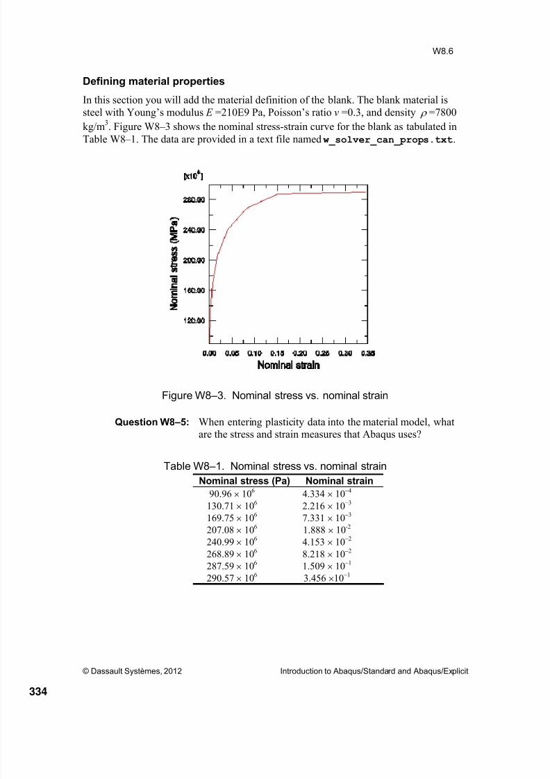
8/15/2019 Abaqus Analysis Intro-book
http://slidepdf.com/reader/full/abaqus-analysis-intro-book 334/469
© Dassault Systèmes, 2012 Introduction to Abaqus/Standard and Abaqus/Explicit
W8.6
Defining material properties
In this section you will add the material definition of the blank. The blank material is
steel with Young’s modulus E =210E9 Pa, Poisson’s ratio v =0.3, and density =7800
kg/m3. Figure W8 – 3 shows the nominal stress-strain curve for the blank as tabulated in
Table W8 – 1. The data are provided in a text file named w_solver_can_props.txt.
Figure W8 –3. Nominal stress vs. nominal strain
Question W8 –5: When entering plasticity data into the material model, whatare the stress and strain measures that Abaqus uses?
Table W8 –1. Nominal stress vs. nominal strain
Nominal stress (Pa) Nominal strain
90.96 106 4.334 104
130.71 106 2.216 103
169.75 106 7.331 103
207.08 106 1.888 10-2
240.99
10
6
4.153
10
2
268.89 106 8.218 102
287.59 106 1.509 101
290.57 106 3.456 101
334

8/15/2019 Abaqus Analysis Intro-book
http://slidepdf.com/reader/full/abaqus-analysis-intro-book 335/469
© Dassault Systèmes, 2012 Introduction to Abaqus/Standard and Abaqus/Explicit
W8.7
Note that a dummy material named Steel has been created and assigned to the part
BLANK. You will need to add the material properties.
Rather than convert the stress-strain data and define the material properties manually, you
will use the material calibration capability to define the material properties.
1. In the Model Tree, double-click Calibrations.
2. Name the calibration steel and click OK.
3. Expand the Calibrations container and then expand the steel item.
4. Double-click Data Sets.
a. In the Create Data Set dialog box, name the data set nominal and click
Import Data Set.
b. In the Read Data From Text File dialog box, click and choose the file
named w_solver_can_props.txt.
c. In the Properties region of this dialog box, specify that strain values will
be read from field 2 and stress values from field 1.
d. Select Nominal as the data set form.
e. Click OK to close the Read Data From Text File dialog box.
f. Click OK to close the Create Data Set dialog box.
Since the data is provided in nominal stress-strain format, it must be converted to
true stress-strain format.
5. Click mouse button 3 on nominal and select Process from the menu thatappears.
a. In the Data Set Processing dialog box, select Convert and click
Continue.
b. In the Change Data Set Form dialog box, select True Form and name
the new data set true. Click OK.
6. Double-click Behaviors.
a. Choose Elastic Plastic Isotropic as the type, and click Continue.
b. In the Edit Behavior dialog box, choose true as the data set for Elastic-
Plastic Data.
c. Click next to Yield point. In the viewport zoom in to select the yield point, as indicated in Figure W8 – 4.
335

8/15/2019 Abaqus Analysis Intro-book
http://slidepdf.com/reader/full/abaqus-analysis-intro-book 336/469
© Dassault Systèmes, 2012 Introduction to Abaqus/Standard and Abaqus/Explicit
W8.8
Alternative: Enter 0.00043, 91E+06 in the text field to define the yield
point precisely.
Figure W8 –4 Yield point.
d. Drag the Plastic points slider between Min and Max to generate plasticdata points.
The plastic data points appear as shown in Figure W8 – 5.
Figure W8 –5 Plastic data points.
e. Enter a Poisson's ratio of 0.3.
f. In the Edit Behavior dialog box, choose Steel from the Material drop-
down list, as shown in Figure W8 – 6.
336

8/15/2019 Abaqus Analysis Intro-book
http://slidepdf.com/reader/full/abaqus-analysis-intro-book 337/469
© Dassault Systèmes, 2012 Introduction to Abaqus/Standard and Abaqus/Explicit
W8.9
Figure W8 –6 Material behavior editor.
g. Click OK to add the properties to the material named steel.
7. In the Model Tree, expand the Materials container and examine the contents of
the material model. You will note that both elastic and plastic properties have
been defined (Young’s modulus should be approximately 2.1E11 Pa). If you wishto change the number of plastic points or need to modify the yield point, simply
return to the Edit Behavior dialog box, make the necessary changes, select the
name of the material to which the properties will be applied, and click OK. Thecontents of the material model are updated automatically.
8. To complete the material properties, define the density. From the menu bar of the
material editor, select General→Density and enter a value of 7800 for Mass
Density.
337

8/15/2019 Abaqus Analysis Intro-book
http://slidepdf.com/reader/full/abaqus-analysis-intro-book 338/469
© Dassault Systèmes, 2012 Introduction to Abaqus/Standard and Abaqus/Explicit
W8.10
9. To reduce high-frequency noise in the solution (caused primarily by the
oscillations of the blank’s free end) add stiffness proportional damping to the
material definition of the blank. It is best to use the smallest amount of damping possible to obtain the desired solution since increasing the stiffness damping
decreases the stable time increment and, thus, increases the computer time. To
avoid a dramatic drop in the stable time increment, the stiffness proportionaldamping factor R should be less than, or of the same order of magnitude as, theinitial stable time increment without damping. We choose a damping factor of
R=1107.
From the material editor’s menu bar , select Mechanical→ Damping and enter a
value of 1.e-7 in the Beta field.
10. Click OK to save the data and exit the material editor.
Question W8 –6: What effects would a higher damping coefficient have?
338

8/15/2019 Abaqus Analysis Intro-book
http://slidepdf.com/reader/full/abaqus-analysis-intro-book 339/469
© Dassault Systèmes, 2012 Introduction to Abaqus/Standard and Abaqus/Explicit
W8.11
Defining displacement boundary conditions
To form the can bottom, we will displace the punch by moving its rigid body reference
point 0.015 m in the negative 2-direction. The punch displacement will be applied in theform of a displacement boundary condition. Because Abaqus/Explicit does not permit
displacement discontinuities, prescribed displacements must refer to an amplitudedefinition. Figure W8 – 7 shows the desired displacement behavior for the punch. Notethat this curve is smooth in its first and second derivatives.
Question W8 –7: What is the slope of the curve at the beginning and end, and
why is this important?
1. In the Model Tree, double-click Amplitudes to define an amplitude curvecorresponding to Figure W8 – 7.
a. In the Create Amplitude dialog box, name the amplitude FORM1, choosethe Smooth step type, and click Continue.
b. In the Edit Amplitude dialog box, enter the data pair 0, 0 for the first
row and 0.033, 1 for the second row.
c. Click OK to exit the amplitude editor.
2. In the Model Tree, double-click BCs to create a Displacement/Rotation
boundary condition named PunchMove in Step-1 to move the punch reference
point in the 2-direction by – 0.015 m.
a. In the Edit Boundary Condition dialog box, toggle on U1, U2, and UR3.
b. Enter a value of -0.015 for U2 and 0 for U1 and UR3.
c. Choose the amplitude curve FORM1.
The amplitude values will be multiplied by the displacement you define in the boundary condition.
Question W8 –8: How would the results change if a linear amplitude definitionwas used instead?
339

8/15/2019 Abaqus Analysis Intro-book
http://slidepdf.com/reader/full/abaqus-analysis-intro-book 340/469
© Dassault Systèmes, 2012 Introduction to Abaqus/Standard and Abaqus/Explicit
W8.12
Figure W8 –7. Displacement curve of punch
Speeding up the analysis
In general, quasi-static processes cannot be modeled in their natural time scale inAbaqus/Explicit since a large number of time increments would be required (recall that
time increments in Abaqus/Explicit are generally very small). Thus, it is sometimesnecessary to increase the speed of the simulation artificially to reduce the computational
cost. One method to reduce the cost of the analysis is to use mass scaling.
While various forms of mass scaling are available in Abaqus/Explicit, we willconcentrate on fixed mass scaling in this workshop and will implement it using the fixed
mass scaling option available in the step editor. The reason for choosing fixed massscaling is that it provides a simple means to modify the mass properties of a quasi-static
model at the beginning of the analysis. It is also computationally less expensive than
variable mass scaling, because the mass is scaled only once at the beginning of the step.
1. In the Model Tree, expand the Steps container and double-click Step-1 to editthis step definition to include mass scaling.
2. In the Edit Step dialog box, click the Mass scaling tab.
3. In the Mass scaling tabbed page, choose Use scaling definitions below and
click Create.
4. In the Edit mass scaling dialog box that appears, accept all defaults and enter 10
in the Scale by factor field.
5. Click OK to save the data and exit the mass scaling editor.
6. Click OK to save the changes and exit the step editor.
340

8/15/2019 Abaqus Analysis Intro-book
http://slidepdf.com/reader/full/abaqus-analysis-intro-book 341/469
© Dassault Systèmes, 2012 Introduction to Abaqus/Standard and Abaqus/Explicit
W8.13
Question W8 –9: How do you determine if an analysis that includes mass
scaling produces acceptable results?
Question W8 –10: How does mass scaling affect the solution time?
Running job and postprocessing results
1. Create a job named draw_bot for the model Stamp.
2. Save your model database file, submit the job for analysis, and monitor its progress.
3. When the analysis is complete, open the output database file draw_bot.odb in
the Visualization module.
4. Display the curves of internal and kinetic energy (i.e., ALLIE and ALLKE) in the
same plot by selecting them from the Results Tree (underneath the History
Output container). Use the XY Curve Options tool in the toolbox to display
the curve symbols. You should see a plot similar to Figure W8 –
8. Note this figurehas been customized for clarity.
Tip: Use [Ctrl]+Click for multiple selections.
Figure W8 –
8. Internal and kinetic energy
5. Certain elements have hourglass modes that affect their behavior. Hourglassmodes are modes of deformation that do not cause any strains at the integration points. An indication of whether hourglassing has an effect on the solution is the
artificial energy, variable ALLAE. Plot the artificial energy and the internal
energy, variable ALLIE, on the same plot. The artificial energy should always bemuch less than the internal energy (say less than 0.5%).
341

8/15/2019 Abaqus Analysis Intro-book
http://slidepdf.com/reader/full/abaqus-analysis-intro-book 342/469
© Dassault Systèmes, 2012 Introduction to Abaqus/Standard and Abaqus/Explicit
W8.14
Question W8 –11: What elements are used to model the blank, and does this
element type have an hourglass deformation mode?
6. Display the deformed shape of the blank only. In the Results Tree, expand the
Instances container underneath the output database draw_bot.odb. Click
mouse button 3 on the instance BLANK-1 and select Replace from the menu that
appears.
7. Expand the displayed area to 180o by selecting View→ODB Display Options
from the main menu bar. In the Sweep/Extrude tabbed page in the ODB Display
Options dialog box, toggle on Sweep elements and accept the default settings.
You should see a shape similar to that in Figure W8 – 9.
Figure W8 –9. 180 expanded deformed shape
8. Contour the Mises stress distribution of the 180o model using the Plot Contours
on Deformed Shape tool in the toolbox. To select other variables forcontouring, use the Field Output toolbar.
9. Plot the punch displacement history (U2 for the node set PUNCHRP) shown in
Figure W8 – 7 by double-clicking Spatial displacement: U2 PI: PUNCH1-1
NODE xyz in NSET PUNCHRP under the History Output container in the
Results Tree.
Note: A scripts that creates the complete stamping model are available foryour convenience. Run this script if you encounter difficulties following theinstructions or if you wish to check your work. The script named
ws_solver_can_bottom_answer.py is available using the Abaqus fetch
utility.
342

8/15/2019 Abaqus Analysis Intro-book
http://slidepdf.com/reader/full/abaqus-analysis-intro-book 343/469

8/15/2019 Abaqus Analysis Intro-book
http://slidepdf.com/reader/full/abaqus-analysis-intro-book 344/469
© Dassault Systèmes, 2012 Introduction to Abaqus/Standard and Abaqus/Explicit
W8.16
Figure WA8 –1. Kinetic energy with and without damping
Question W8 –7: What is the slope of the curve at the beginning and end, andwhy is this important?
Answer: The slope of the amplitude curve at the beginning and end of
the step is zero. This is important because it prevents
discontinuities in the punch displacement, which lead to
oscillations in an Abaqus/Explicit analysis.
Question W8 –8: How would the results change if a linear amplitude definition
were used instead?
Answer: With a linear amplitude definition the displacement of the punch will be applied suddenly at the beginning of the step
and stopped suddenly at the end of the step, causingoscillations in the solution.
A linear amplitude definition results in large spikes in the
kinetic energy, especially at the beginning of the step. As aresult, the kinetic energy may be large compared to the
internal energy and the early solution may not be quasi-static.The preferred approach is to move the punch as smoothly as
possible. Figure WA8 – 2 compares the kinetic energy history
when a linear amplitude definition is used and when thesmooth step amplitude definition is used.
344
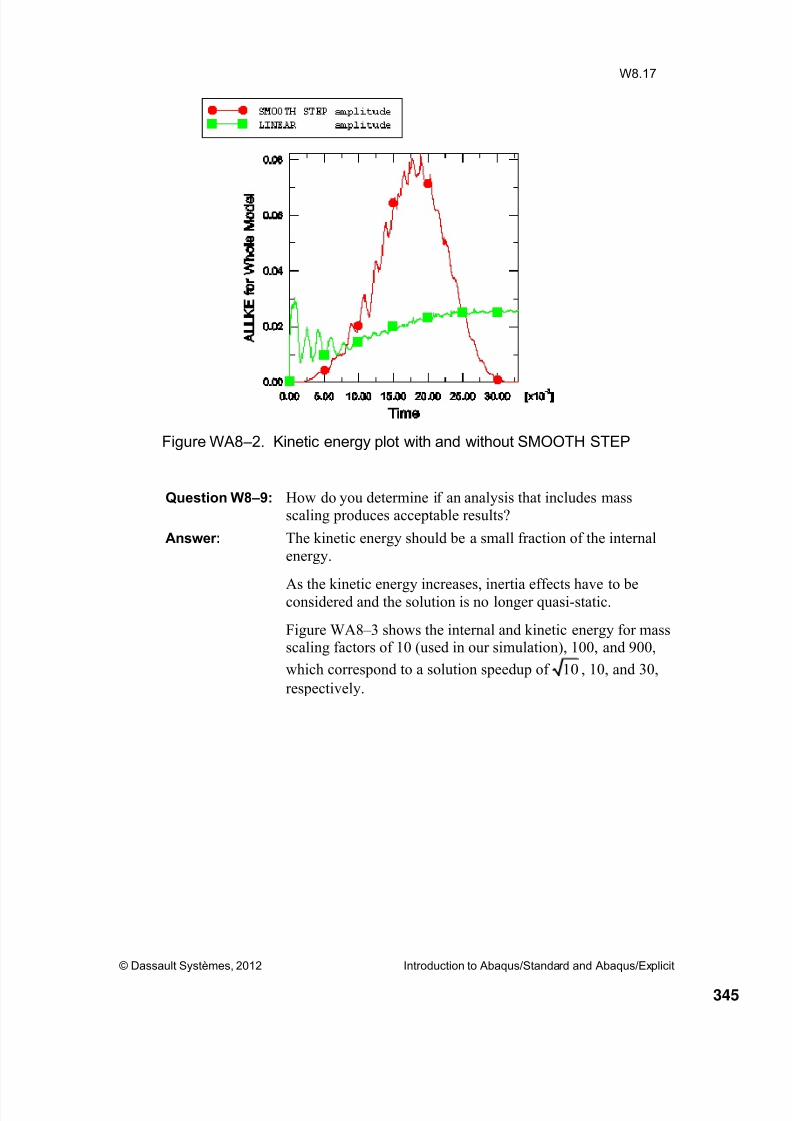
8/15/2019 Abaqus Analysis Intro-book
http://slidepdf.com/reader/full/abaqus-analysis-intro-book 345/469
© Dassault Systèmes, 2012 Introduction to Abaqus/Standard and Abaqus/Explicit
W8.17
Figure WA8 –2. Kinetic energy plot with and without SMOOTH STEP
Question W8 –9: How do you determine if an analysis that includes massscaling produces acceptable results?
Answer: The kinetic energy should be a small fraction of the internal
energy.
As the kinetic energy increases, inertia effects have to beconsidered and the solution is no longer quasi-static.
Figure WA8 – 3 shows the internal and kinetic energy for massscaling factors of 10 (used in our simulation), 100, and 900,
which correspond to a solution speedup of 10 , 10, and 30,
respectively.
345

8/15/2019 Abaqus Analysis Intro-book
http://slidepdf.com/reader/full/abaqus-analysis-intro-book 346/469
© Dassault Systèmes, 2012 Introduction to Abaqus/Standard and Abaqus/Explicit
W8.18
Figure WA8 –3. Energies with different mass scaling
Question W8 –10: How does mass scaling affect the solution time?
Answer: The stable time increment is calculated according to
min ,
e Lt stable c
d
where Le is a characteristic element length and cd is the
dilatational wave speed. An increase in density decreases cd ,
which in turn increases t stable.
Question W8 –11: What elements are used to model the blank, and does this
element type have an hourglass deformation mode?
Answer: The analysis uses SAX1 elements. These elements have no
hourglass modes. Consequently, hourglassing is not of
concern in the analysis.
346

8/15/2019 Abaqus Analysis Intro-book
http://slidepdf.com/reader/full/abaqus-analysis-intro-book 347/469
Notes
347

8/15/2019 Abaqus Analysis Intro-book
http://slidepdf.com/reader/full/abaqus-analysis-intro-book 348/469
Notes
348

8/15/2019 Abaqus Analysis Intro-book
http://slidepdf.com/reader/full/abaqus-analysis-intro-book 349/469
Workshop 9
Import Analysis
Interactive Version
© Dassault Systèmes, 2012 Introduction to Abaqus/Standard and Abaqus/Explicit
Note: This workshop provides instructions in terms of the Abaqus GUIinterface. If you wish to use the Abaqus Keywords interface instead, pleasesee the “Keywords” version of these instructions.
Please complete either the Keywords or Interactive version of thisworkshop.
Goals
Transfer results between Abaqus/Explicit and Abaqus/Standard.
Introduction
In this workshop you will use the import capability is used to transfer the results between
Abaqus/Explicit and Abaqus/Standard to examine the effects of springback in theanalysis of the deep drawing of a can bottom. The deformed shape of the can after the
forming stage is shown in Figure W9 – 1.
Figure W9 –1. Final deformed shape
349

8/15/2019 Abaqus Analysis Intro-book
http://slidepdf.com/reader/full/abaqus-analysis-intro-book 350/469
© Dassault Systèmes, 2012 Introduction to Abaqus/Standard and Abaqus/Explicit
W9.2
Preliminaries
1. Enter the working directory for this workshop:
../abaqus_solvers/interactive/forming
2. Open the model database file created in the previous workshop
(canBottom.cae):
Springback analysis
In the manufacturing process the part is removed after the forming has been completed
and the material is free to springback into an unconstrained state. To understand the finalshape after this physical effect, we perform a springback analysis in Abaqus/Standard.
1. Copy the model named stamp to a model named springback. Make all
subsequent model changes to the springback model.
2. Since only the blank needs to be imported, delete the following features from the
springback model:
a. Part instances DIE1-1 and PUNCH1-1.
b. All assembly-level sets and surfaces associated with the die and punch.
c. All contact interactions and properties.
d. Boundary conditions FixDie and PunchMove.
e. History output request for PunchRP.
3. Replace the dynamic, explicit step with a general, static step. Set the time period
to 1 and the initial increment to 0.1, and include the effects of geometric
nonlinearity. Rename the step springback.
4. Define an initial state.
a. In the Model Tree, double-click Predefined Fields.
b. In the Create Predefined Field dialog box, select Initial as the step,
Other as the category, and Initial state as the type.
c. Click Continue.
d. Select the blank as the instance to assign the initial state.
e. In the Edit Predefined Field dialog box that appears, enter the job namedraw_bot, accept all other default settings, and click OK.
This definition will allow the state of the model — stresses, strains, etc. — to be imported. By not updating the reference configuration, the springback
displacements will be referred to the original undeformed configuration.
350

8/15/2019 Abaqus Analysis Intro-book
http://slidepdf.com/reader/full/abaqus-analysis-intro-book 351/469
© Dassault Systèmes, 2012 Introduction to Abaqus/Standard and Abaqus/Explicit
W9.3
5. Note that the XSYMM boundary condition BlankSymm specified on the set
BSYM constrains rigid body motions in the U1 and UR3 directions of the blank.
Thus, you need an additional boundary condition to prevent rigid body motion
along U2. In what follows you will fix the node at its final position at the end ofthe forming stage.
a. In the Model Tree, double-click BCs to apply a Displacement/Rotation boundary condition to the set BSYM in Step-1.
b. In the Edit Boundary Condition dialog box, choose the Fixed at Current
Position method and fix U2.
6. Create a job named springback for the model springback.
7. Save your model database file, submit the job for analysis, and monitor its
progress.
Question W9 –1: Why is it advantageous to use Abaqus/Standard for the
springback analysis?
Postprocessing
1. When the analysis is complete, open the output database file springback.odb
in the Visualization module.
2. Contour the Mises stress distribution of the 180o model.
3. Plot the final deformed shape for the model springback.
4. Plot the springback and formed shapes together. (First toggle off the Sweep
elements option.)
By not updating the reference configuration, the formed shape is stored in frame 0of the output database. You must use overlay plots to superimpose the images:
a. From the main menu bar, select View→Overlay Plot.
b. Use the Frame Selector or the arrows in the context bar to selectframe 0.
c. In the Overlay Plot Layer Manager , click Create. Name the layer
formed .
d. Use the Frame Selector to select the last frame.
e. Use the Common Plot Options tool to change the fill color of theelements to blue.
f. In the Overlay Plot Layer Manager , click Create. Name the layer
springback.
In the Overlay Plot Layer Manager , click Plot Overlay.
Zoom in to examine the shape differences more closely.
351

8/15/2019 Abaqus Analysis Intro-book
http://slidepdf.com/reader/full/abaqus-analysis-intro-book 352/469
© Dassault Systèmes, 2012 Introduction to Abaqus/Standard and Abaqus/Explicit
W9.4
If you had updated the reference configuration, the formed shape is treated as the
undeformed shape of the import analysis model (recall that when the reference
configuration is updated, the end state of the previous analysis becomes the
reference configuration of the import analysis; the reference configuration isconsidered the undeformed shape):
a. In the toolbox, click the Allow Multiple Plot States tool .
b. In the toolbox, click both the Plot Undeformed Shape and Plot
Deformed Shape tools .
c. Use the Common Plot Options tool to increase the deformationscale factor so that the differences between the formed and springback
shapes are clearly visible.
Note: A scripts that creates the complete stamping model are available foryour convenience. Run this script if you encounter difficulties following theinstructions or if you wish to check your work. The script named
ws_solver_can_bottom_answer.py is available using the Abaqus fetch
utility.
352

8/15/2019 Abaqus Analysis Intro-book
http://slidepdf.com/reader/full/abaqus-analysis-intro-book 353/469
© Dassault Systèmes, 2012 Introduction to Abaqus/Standard and Abaqus/Explicit
W9.5
Answers
Question W9 –1: Why is it advantageous to choose Abaqus/Standard for thespringback analysis?
Answer: A true static procedure is the preferred approach for modelingspringback. The imported model will not be in static
equilibrium at the beginning of the step. Thus,Abaqus/Standard applies a set of artificial internal stresses to
the imported model state and then gradually removes these
stresses. This leads to the springback deformation. InAbaqus/Explicit the removal of the contact between the blank
and the tools represents a sudden load removal, which leads to
low frequency vibrations of the blank. While these vibrations
will eventually dissipate, this approach leads to lengthycomputation times.
353

8/15/2019 Abaqus Analysis Intro-book
http://slidepdf.com/reader/full/abaqus-analysis-intro-book 354/469354

8/15/2019 Abaqus Analysis Intro-book
http://slidepdf.com/reader/full/abaqus-analysis-intro-book 355/469
Notes
355

8/15/2019 Abaqus Analysis Intro-book
http://slidepdf.com/reader/full/abaqus-analysis-intro-book 356/469
Notes
356

8/15/2019 Abaqus Analysis Intro-book
http://slidepdf.com/reader/full/abaqus-analysis-intro-book 357/469
Workshop 1
Basic Input and Output
Keywords Version
© Dassault Systèmes, 2012 Introduction to Abaqus/Standard and Abaqus/Explicit
Note: This workshop provides instructions in terms of the AbaqusKeywords interface. If you wish to use the Abaqus GUI interface instead,please see the “Interactive” version of these instructions.
Please complete either the Keywords or Interactive version of thisworkshop.
Goals
Learn to use Abaqus utilities and documentation.
Understand the basic structure of an input file, and be able to make simplemodifications to it.
Learn how to perform a datacheck analysis and how to submit an analysis jobusing the Abaqus driver.
Gain familiarity with Abaqus/Viewer.
Explore the structure and contents of the data (.dat) and log (.log) files.
Abaqus utilities and documentation
Abaqus provides various utilities for obtaining information on usage, system
configuration, example problems, and environment settings for the analysis package.
1. At the prompt, enter the command
abaqus information=system
to obtain information on the system.
Note that abaqus
is a generic command that may have been renamed on your
system. For example, if more than one version is installed on the system, the
command might include the version number, as in abq6121. In the remainder of
this workshop as well as all subsequent workshops, use the appropriate command
for your system.
Question W1 –1: What is the processor on your machine?
Question W1 –2: What is the operating system (OS) level?
357

8/15/2019 Abaqus Analysis Intro-book
http://slidepdf.com/reader/full/abaqus-analysis-intro-book 358/469
© Dassault Systèmes, 2012 Introduction to Abaqus/Standard and Abaqus/Explicit
W1.2
2. Open the online documentation with the command
abaqus doc
Open the Abaqus Analysis User’s Manual, and search for the string DSLOAD to
find information on the DSLOAD option. You can find information related to
the data line syntax in the Abaqus Keywords Reference Manual (use the hyperlinkfor the DSLOAD option, or open the Keywords Manual directly). The online
documentation graphical user interface is shown in Figure W1 – 1.
Figure W1 –1. Online documentation
3. Open the online Abaqus Example Problems Manual. Search for plate buckling to find example problems that discuss plate buckling.
Question W1 –3: What are the four example problems that fit the searchcriteria?
4. Go to Example Problem 1.1.14 in the online Abaqus Example Problems Manual.In the left panel of the window, display the subtopics of the problem and click
Input files. In the right panel of the window, the list of input files associated with
this problem appears. You can select any input filename from the list; a separatewindow will open containing that file.
358

8/15/2019 Abaqus Analysis Intro-book
http://slidepdf.com/reader/full/abaqus-analysis-intro-book 359/469
© Dassault Systèmes, 2012 Introduction to Abaqus/Standard and Abaqus/Explicit
W1.3
5. All example problem input files are included in the Abaqus release and can be
obtained using the abaqus fetch utility. In your terminal window, enter
abaqus fetch job=damagefailcomplate_cps4
at the command line prompt.
6. Use the online documentation to determine the input syntax for some options.
A keyword line starts with an asterisk ( followed directly by the keyword
option. Parameters and their associated values appear on the keyword line,
separated by commas. Many options require data lines, which follow directly aftertheir associated keyword line and contain the data specified in the Abaqus
Keywords Reference Manual for each option. Data items are separated by
commas. Refer to the discussions of keyword line and data line syntax in
Lecture 1, as necessary.
Question W1 –4: In the space provided, write the input you would use to define
a node set called TOP_NODES that contains previously defined
nodes 21, 22, 23, and node set TOP_LEFT.
Hint: Use the information on the NSET option in the Abaqus
Keywords Reference Manual to determine the necessary
parameter and data line.
*NSET,
359

8/15/2019 Abaqus Analysis Intro-book
http://slidepdf.com/reader/full/abaqus-analysis-intro-book 360/469
© Dassault Systèmes, 2012 Introduction to Abaqus/Standard and Abaqus/Explicit
W1.4
Question W1 –5: In the space provided, write the input you would use to define
a velocity boundary condition on a node set named NALL
using the direct format. The velocity is 7.0 m/s in the
2-direction. Will this option appear in the model data or the
history data portion of the input file?
Hint: Use the information on the BOUNDARY option in theAbaqus Keywords Reference Manual, including the reference
to the ―Boundary Conditions‖ Section of the Abaqus Analysis
User’s Manual, to determine the appropriate syntax.
Question W1 –6: (Optional) In the space provided, write the input you would
use to define the BEAM SECTION option for beam elements
in element set ELBEAMS referring to a material named STEEL.
The beam has a rectangular cross-section with a height of 0.5
m and a width of 0.2 m.
Hint: This option requires one data line for the beam sectiongeometric data. Follow the hyperlink to the beam cross-section
library and the rectangular section to determine the
appropriate data line input.
*BEAM SECTION,
360

8/15/2019 Abaqus Analysis Intro-book
http://slidepdf.com/reader/full/abaqus-analysis-intro-book 361/469
© Dassault Systèmes, 2012 Introduction to Abaqus/Standard and Abaqus/Explicit
W1.5
Analyzing a connecting lug
Figure W1 –2. Sketch of the connecting lug
In this workshop you will model the connecting lug shown in Figure W1 – 2. The lug iswelded to a massive structure at one end, so we assume that this end is fixed. The other
end contains a hole through which a bolt is placed when the lug is in service. You have to
calculate the deflection of the lug when a load of 30kN is applied to the bolt in the 2direction.
To model this problem, you will use three-dimensional continuum elements and performa linear analysis with elastic materials. You will model the load transmitted to the lug
through the bolt as a uniform pressure load applied to the bottom half of the hole, as
shown in Figure W1 – 2. In this workshop SI units (N, m, and s) will be used.
Creating the input file
1. Change to the ../abaqus_solvers/keywords/lug directory.
2. View the contents of w_lug.inp. The model and history data are incomplete,and no mesh or loading is defined.
Question W1 –7: What is the first option in the model data? What is the last
option in the model data?
Question W1 –8: What is the first option in the history data?
Question W1 –9: How many steps are there in this analysis?
361

8/15/2019 Abaqus Analysis Intro-book
http://slidepdf.com/reader/full/abaqus-analysis-intro-book 362/469
© Dassault Systèmes, 2012 Introduction to Abaqus/Standard and Abaqus/Explicit
W1.6
3. View the files w_lug_nodes.inp and w_lug_elem.inp. Boundary conditions
and loads will be defined using the node and element sets defined in these files.
Question W1 –10: What type of elements are used to model the lug?
4. Edit the input file to set the INPUT parameter on the INCLUDE options to read
the appropriate node and element data files.5. Complete the MATERIAL option block by defining an elastic material with
elastic modulus E = 200 GPa and Poisson’s ratio = 0.3. The complete material block should appear as follows:
*MATERIAL, NAME=STEEL*ELASTIC200E9, 0.3
Question W1 –11: Do you need to define a density to complete the materialdefinition? Material density is necessary for what types of
analyses?
The boundary conditions and the loads cannot be defined without knowledge of the node
and element sets and surfaces. Figure W1 – 3 shows the various sets and surfaces.
Figure W1 –3. Useful sets and surfaces
Element setBUILTIN Node set LHEND
Surface PRESS
Node setHOLEBOT
362

8/15/2019 Abaqus Analysis Intro-book
http://slidepdf.com/reader/full/abaqus-analysis-intro-book 363/469
© Dassault Systèmes, 2012 Introduction to Abaqus/Standard and Abaqus/Explicit
W1.7
6. Boundary conditions are applied using the BOUNDARY option. Use the online
documentation to obtain a description of the option. The left end of the lug is
fixed. Thus, constrain degrees of freedom 1 through 6 of all nodes in node setLHEND by entering
*BOUNDARYLHEND, 1, 6
Question W1 –12: How else could you define a completely constrained boundarycondition?
7. Distributed loads are applied to surfaces using the *DSLOAD option. In this
problem, the load should be applied to the surface named PRESS (which covers
the bottom region of the hole). The option to specify the distributed (pressure)
load on this surface is
*DSLOADPRESS, P, 50.E6
The magnitude of the applied uniform pressure is 50 MPa. We determined the
load magnitude by dividing the total load by the projected horizontal area of the
hole, where30kN
50MPa2 0.015m 0.02m
.
8. Add printed output requests to the step using the NODE PRINT and EL PRINToptions. Abaqus includes a large amount of printed output by default. Requesting
printed output of specific variables allows you to limit the volume of output to the
data (.dat) file. Request printed data output of nodal displacements for node setHOLEBOT and reaction forces for node set LHEND (including the total force). In
addition, request output for stresses in element set BUILTIN.
You can do this by entering
*NODE PRINT, NSET=HOLEBOTU2*NODE PRINT, NSET=LHEND, TOTAL=YES, SUMMARY=NORF*EL PRINT, ELSET=BUILTINS, MISES
Default output requests for the output database are made automatically, and theywill be sufficient for this workshop.
Submitting a datacheck analysis
1. Submit the job for a datacheck analysis by entering the command
abaqus datacheck job=w_lug interactive
363

8/15/2019 Abaqus Analysis Intro-book
http://slidepdf.com/reader/full/abaqus-analysis-intro-book 364/469
© Dassault Systèmes, 2012 Introduction to Abaqus/Standard and Abaqus/Explicit
W1.8
at the prompt. The interactive parameter will cause all log file output to print
to the screen.
2. View the data file ( w_lug.dat) in a text editor.
Question W1 –13: What version of Abaqus are you using?
3. Search for the strings ―WARNING‖ and ―ERROR‖ to find any warning and errormessages. These messages will indicate whether anything unusual was
encountered during the datacheck analysis (keep in mind that your editor may be
case-sensitive for searching).
Question W1 –14: What warning messages did you get? Do they require changesto the input file, or can you ignore them?
4. Search for the string ―P R O B L E M‖ to see the summary of the problem size.Include spaces between the letters of the search string.
Question W1 –15: How many elements are there in the model? How many
variables are there?
Running a complete analysis
1. Submit w_lug.inp as an Abaqus job in interactive mode by typing
abaqus job=w_lug interactive
at the prompt.
If the driver asks if you want to overwrite old job files, type ―y.‖ This means that
output files with the same job name that exist from a previous analysis will be
overwritten.
2. Now resubmit the job in background mode by typing
abaqus job=w_lug
at the prompt.
The log file output will be saved in w_lug.log instead of printing to the screen.
You can open w_lug.log in a text editor and view its contents.
3. You can also let the Abaqus driver prompt you for the necessary job information by typing
abaqus
at the prompt.
Specify w_lug at the prompt for the job identifier, enter [RETURN] at the prompt
for user subroutines (since there are none for this job), and type ―y‖ to overwrite
the files from the last run with the same name. Doing so will submit the analysis
job in background mode.
4. List all files with w_lug as the root of the file name (using a ―long‖ format on
Unix systems):
364

8/15/2019 Abaqus Analysis Intro-book
http://slidepdf.com/reader/full/abaqus-analysis-intro-book 365/469
© Dassault Systèmes, 2012 Introduction to Abaqus/Standard and Abaqus/Explicit
W1.9
dir w_lug.* (NT)
ls -l w_lug.* (Unix)
Note the files that were created by Abaqus. We will take a closer look at the
printed output file ( w_lug.dat) later in this workshop.
Results visualization in Abaqus/Viewer
1. To run Abaqus/Viewer and load the output database for the lug analysis, type
abaqus viewer odb=w_lug
at the prompt.
Note: The file name extension (.odb) is not needed.
If an output database is not specified on the command line, you can selectFile→Open from the main menu bar in Abaqus/Viewer to access the Open
Database dialog box, as shown in Figure W1 – 4. Select the file w_lug.odb
from the output database list.
Figure W1 –4. Open Database dialog box
365

8/15/2019 Abaqus Analysis Intro-book
http://slidepdf.com/reader/full/abaqus-analysis-intro-book 366/469
© Dassault Systèmes, 2012 Introduction to Abaqus/Standard and Abaqus/Explicit
W1.10
2. When Abaqus/Viewer opens the output database, the undeformed model shape
will be displayed. To change the plot mode, you can use either the Plot menu or
the toolbox icons displayed on the left side of the viewport (see Figure W1 – 5).
You can identify the function of each tool in the toolbox by positioning yourcursor above the icon for that tool. A label for the icon will pop up describing its
function.
3. To plot the deformed shape, click the Plot Deformed Shape tool in the
toolbox or select Plot→Deformed Shape from the main menu bar.
4. Open the Common Plot Options dialog box by clicking in the toolbox.
Turn on the node and element numbers, and make the nodes visible.
5. Use the display option tools to switch to hidden line, filled, or wireframe display.
Figure W1 –
5. Abaqus/Viewer main window
View manipulation tools Display option tools
Toolbox
ResultsTree
366

8/15/2019 Abaqus Analysis Intro-book
http://slidepdf.com/reader/full/abaqus-analysis-intro-book 367/469
© Dassault Systèmes, 2012 Introduction to Abaqus/Standard and Abaqus/Explicit
W1.11
6. Note the displacement magnification factor shown in the bottom of the title.
By default, Abaqus/Viewer automatically scales the displacement according to the
maximum model dimensions for a small-displacement analysis. Displacements
are scaled so that the deformed shape will be clear. For a large-displacementanalysis the scale factor is 1.0 by default. Set the displacement magnification
factor to 1.0 so that you can see the actual displacement, and redraw the displacedshape plot.
Hint: You will have to use the Common Plot Options dialog box.
7. Create a contour plot of the Mises stress by clicking the Plot Contours on
Deformed Shape tool in the toolbox.
8. Frequently users want to remove all annotations that are written on the plots,especially when they are creating hard-copy images or animations. From the mainmenu bar, select Viewport→Viewport Annotation Options to suppress the
annotations used in the plots.
The annotations are divided into three categories: legend, title block, and state block. Each category can be controlled separately. The title block containsinformation about which Abaqus version was used and when the analysis was
performed. The state block contains the step title (which is the text provided on
the data line of the STEP option), the increment and step time of the data being
displayed, and information on the variable and magnification factor used to
calculate the shape of the model.
9. From the main menu bar, select File→Exit to exit from Abaqus/Viewer.
Viewing the printed output file
Open the printed output file w_lug.dat in the text editor of your choice.
1. Look at the input echo near the top of the file. Below this you will find the sectiontitled ―OPTIONS BEING PROCESSED.‖ This is the first place any warning or
error messages will appear.
2. A summary of model data follows. Here you can check that Abaqus has correctlyinterpreted your model definition.
Question W1 –16: Which elements are in element set HOLEIN?
3. Next you will find the summary of history data for each step. Search for the
strings ―B O U N D A R Y‖ and ―D I S T R I B U T E D‖ to verify that the
boundary conditions and distributed loads have been interpreted correctly. Includespaces between the letters of the search string. To start a search through the entire
file, go to the top of the file (some editors will wrap to the top of the file upon
reaching the end).
367

8/15/2019 Abaqus Analysis Intro-book
http://slidepdf.com/reader/full/abaqus-analysis-intro-book 368/469
© Dassault Systèmes, 2012 Introduction to Abaqus/Standard and Abaqus/Explicit
W1.12
4. The next section in the data file is the results section. The tables are printed
according to the various output requests.
Search for the strings ―N O D E‖ and ―E L E M E N T‖ to find the tables that
contain the output requested. The maximum deflection and peak stress are
reported at the ends of the respective tables.
Question W1 –17: What are the maximum direct stresses in the 1- and 2-
directions (i.e.,11
and22
)?
(Hint: The maximum direct stresses will occur in element set
BUILTIN.)
Question W1 –18: What is the deflection of node 20001 in node set HOLEBOT in
the 2-direction?
5. Search for the string ―TOTAL‖ to find the sum of the reaction forces in the 2-direction.
Question W1 –19: What is the net reaction force in the 2-direction at the nodes in
node set LHEND? Is this equal to the applied load?
Question W1 –20: Why is the sum of the reaction forces at the nodes in node set
LHEND in the horizontal direction (1-direction) zero?
Modifying the model and understanding changes in the results
1. Open the input file w_lug.inp in the text editor.
2. Reduce the distributed pressure load to 25 MPa.
3. Save the modified file to a new file named w_lugmod.inp.
4. Submit the new input file as an Abaqus job.
5. Look at the output database file in Abaqus/Viewer.
Question W1 –21: What is the deflection of node 20001 in node set HOLEBOT?
Do the results reflect the reduction in loading?
Note: A complete input file is available for your convenience. You mayconsult this file if you encounter difficulties following the instructionsoutlined here or if you wish to check your work. The input file is named
w_lug_complete.inp
and is available using the Abaqus fetch utility.
368

8/15/2019 Abaqus Analysis Intro-book
http://slidepdf.com/reader/full/abaqus-analysis-intro-book 369/469
© Dassault Systèmes, 2012 Introduction to Abaqus/Standard and Abaqus/Explicit
W1.13
Answers
Question W1 –1: What is the processor on your machine?
Answer: It depends on the system you are using.
Question W1 –2: What is the operating system (OS) level?
Answer: It depends on the system you are using.
Question W1 –3: What are the four example problems that fit the search
criteria?
Answer: Problem 1.1.14, ―Damage and failure of a laminatedcomposite plate‖
Problem 1.2.2, ―Laminated composite shells: buckling of a
cylindrical panel with a circular hole‖
Problem 1.2.5, ―Unstable static problem: reinforced plate
under compressive loads‖
Problem 9.1.8, ―Deformation of a sandwich plate underCONWEP blast loading‖
Question W1 –4: In the space provided, write the input you would use to define
a node set called TOP_NODES that contains previously definednodes 21, 22, 23, and node set TOP_LEFT.
Answer: *NSET, NSET=TOP_NODES21, 22, 23, TOP_LEFT
Question W1 –5: In the space provided, write the input you would use to define
a velocity boundary condition on a node set named NALL
using the direct format. The velocity is 7.0 m/s in the
2-direction. Will this option appear in the model data or thehistory data portion of the input file?
Answer: This option will appear in the history data section of the inputfile because it is a nonzero boundary condition.
*BOUNDARY, TYPE=VELOCITY NALL, 2, 2, 7.0
369
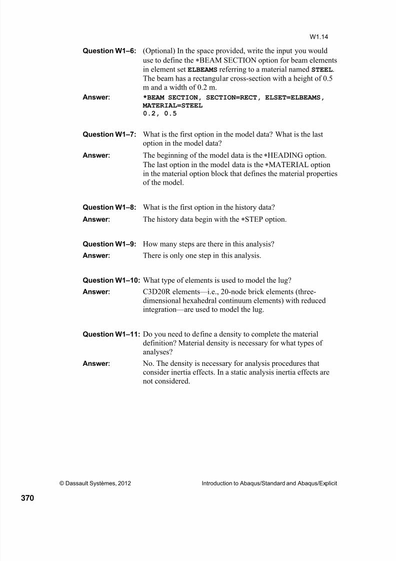
8/15/2019 Abaqus Analysis Intro-book
http://slidepdf.com/reader/full/abaqus-analysis-intro-book 370/469
© Dassault Systèmes, 2012 Introduction to Abaqus/Standard and Abaqus/Explicit
W1.14
Question W1 –6: (Optional) In the space provided, write the input you would
use to define the BEAM SECTION option for beam elements
in element set ELBEAMS referring to a material named STEEL.
The beam has a rectangular cross-section with a height of 0.5
m and a width of 0.2 m.
Answer: *BEAM SECTION, SECTION=RECT, ELSET=ELBEAMS, MATERIAL=STEEL0.2, 0.5
Question W1 –7: What is the first option in the model data? What is the last
option in the model data?
Answer: The beginning of the model data is the HEADING option.
The last option in the model data is the MATERIAL option
in the material option block that defines the material propertiesof the model.
Question W1 –8: What is the first option in the history data?
Answer: The history data begin with the STEP option.
Question W1 –9: How many steps are there in this analysis?
Answer: There is only one step in this analysis.
Question W1 –10: What type of elements is used to model the lug?
Answer: C3D20R elements — i.e., 20-node brick elements (three-dimensional hexahedral continuum elements) with reducedintegration — are used to model the lug.
Question W1 –11: Do you need to define a density to complete the material
definition? Material density is necessary for what types of
analyses?
Answer: No. The density is necessary for analysis procedures thatconsider inertia effects. In a static analysis inertia effects are
not considered.
370

8/15/2019 Abaqus Analysis Intro-book
http://slidepdf.com/reader/full/abaqus-analysis-intro-book 371/469
© Dassault Systèmes, 2012 Introduction to Abaqus/Standard and Abaqus/Explicit
W1.15
Question W1 –12: How else could you define a completely constrained boundary
condition?
Answer: ―Type‖ boundary condition labels (such as ENCASTRE) can
be also used to define fixed boundary conditions in the modeldata:
*BOUNDARYLHEND, ENCASTRE
Question W1 –13: What version of Abaqus are you using?
Answer: The version number appears at the top of the printed output
(.dat) file.
Question W1 –14: What warning messages did you get? Do they require changes
to the input file, or can you ignore them?
Answer: If you followed the instructions correctly to this point, thereshould be warning messages in the data (.dat) file indicating
that the rotational degrees of freedom — 4, 5, and 6 — are not
active in this model and cannot be restrained. Abaqus ignores boundary conditions on degrees of freedom that cannot be
restrained; therefore, you can safely ignore these warning
messages.
Question W1 –15: How many elements are there in the model? How manyvariables are there?
Answer: The model has 112 elements. The total number of variables,including degrees of freedom plus any Lagrange multipliervariables, is 2376.
Question W1 –16: Which elements are in element set HOLEIN?
Answer: Elements 1 and 16.
Question W1 –17: What are the maximum direct stresses in the 1- and 2-
directions (i.e., 11 and 22)?
Answer: The maximum direct stress in the 1-direction (S11) is3.4766E+08 Pa; the maximum direct stress in the 2-direction
(S22) is 8.7629E+07 Pa.
371

8/15/2019 Abaqus Analysis Intro-book
http://slidepdf.com/reader/full/abaqus-analysis-intro-book 372/469
© Dassault Systèmes, 2012 Introduction to Abaqus/Standard and Abaqus/Explicit
W1.16
Question W1 –18: What is the deflection of node 20001 in node set HOLEBOT in
the 2-direction?
Answer: The deflection is 3.1342 E04 m.
Question W1 –19:
What is the net reaction force in the 2-direction at the nodes innode set LHEND? Is this equal to the applied load?
Answer: The reaction forces in the node set LHEND sum to 30 kN,
which is equal to the applied load.
Question W1 –20: Why is the sum of the reaction forces at the nodes in node setLHEND in the horizontal direction (1-direction) zero?
Answer: At the section represented by node set LHEND, the reaction
forces in the horizontal direction simply couple to resist the
moment induced by the applied vertical load. Since there is noexternal load in the horizontal direction, the reaction forces
add up to zero in the horizontal direction.
Question W1 –21: What is the deflection of node 20001 in node set HOLEBOT?
Do the results reflect the reduction in loading?
Answer: The deflection of the nodes in node set HOLEBOT is now
reduced to 1.5671 E04 m. The deflections, reaction forces,and stresses decrease in proportion to the reduction in loading
since this is a linear analysis; in this case by a factor of 2.
372

8/15/2019 Abaqus Analysis Intro-book
http://slidepdf.com/reader/full/abaqus-analysis-intro-book 373/469
Notes
373

8/15/2019 Abaqus Analysis Intro-book
http://slidepdf.com/reader/full/abaqus-analysis-intro-book 374/469
Notes
374

8/15/2019 Abaqus Analysis Intro-book
http://slidepdf.com/reader/full/abaqus-analysis-intro-book 375/469
Workshop 2
Linear Static Analysis of a Cantilever Beam:
Multiple Load Cases
Keywords Version
© Dassault Systèmes, 2012 Introduction to Abaqus/Standard and Abaqus/Explicit
Note: This workshop provides instructions in terms of the AbaqusKeywords interface. If you wish to use the Abaqus GUI interface instead,please see the “Interactive” version of these instructions.
Please complete either the Keywords or Interactive version of thisworkshop.
Introduction
In this workshop you will become familiar with using load cases in a linear staticanalysis. You will model a cantilever beam. The left end of the beam is encastred while a
series of loads are applied to the free end. Six load cases are considered: unit forces in the
global X-, Y-, and Z-directions as well as unit moments about the global X-, Y-, and Z-
directions. The model is shown in Figure W2 – 1. You will solve the problem using a
single perturbation step with six load cases and (optionally) using six perturbation stepswith a single load case in each step.
Figure W2 –1. Cantilever beam model
375
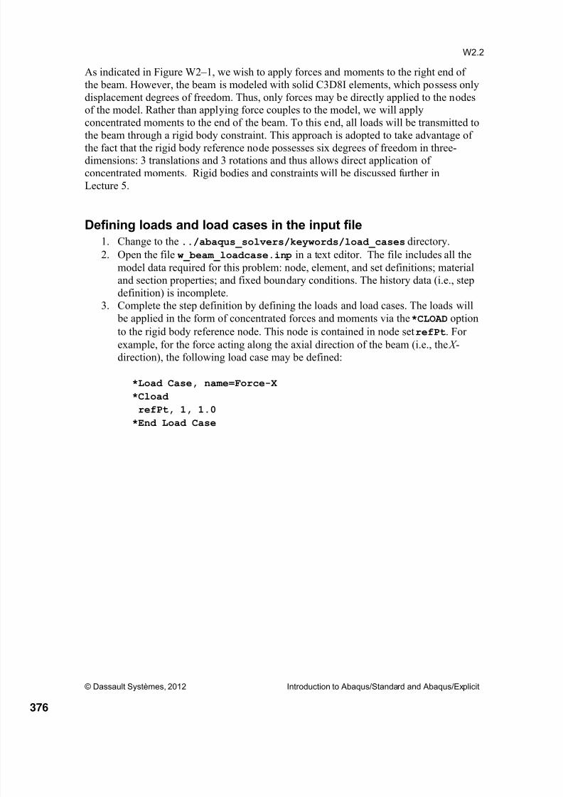
8/15/2019 Abaqus Analysis Intro-book
http://slidepdf.com/reader/full/abaqus-analysis-intro-book 376/469
© Dassault Systèmes, 2012 Introduction to Abaqus/Standard and Abaqus/Explicit
W2.2
As indicated in Figure W2 – 1, we wish to apply forces and moments to the right end of
the beam. However, the beam is modeled with solid C3D8I elements, which possess only
displacement degrees of freedom. Thus, only forces may be directly applied to the nodesof the model. Rather than applying force couples to the model, we will apply
concentrated moments to the end of the beam. To this end, all loads will be transmitted to
the beam through a rigid body constraint. This approach is adopted to take advantage ofthe fact that the rigid body reference node possesses six degrees of freedom in three-dimensions: 3 translations and 3 rotations and thus allows direct application of
concentrated moments. Rigid bodies and constraints will be discussed further in
Lecture 5.
Defining loads and load cases in the input file
1. Change to the ../abaqus_solvers/keywords/load_cases directory.
2. Open the file w_beam_loadcase.inp in a text editor. The file includes all the
model data required for this problem: node, element, and set definitions; material
and section properties; and fixed boundary conditions. The history data (i.e., stepdefinition) is incomplete.
3. Complete the step definition by defining the loads and load cases. The loads will
be applied in the form of concentrated forces and moments via the *CLOAD option
to the rigid body reference node. This node is contained in node set refPt. For
example, for the force acting along the axial direction of the beam (i.e., the X -
direction), the following load case may be defined:
*Load Case, name=Force-X
*Cload
refPt, 1, 1.0
*End Load Case
376

8/15/2019 Abaqus Analysis Intro-book
http://slidepdf.com/reader/full/abaqus-analysis-intro-book 377/469
© Dassault Systèmes, 2012 Introduction to Abaqus/Standard and Abaqus/Explicit
W2.3
4. The complete step definition should resemble the following:
*Step, name=BeamLoadCases, perturbation
*Static
**
*Load Case, name=Force-X*Cload
refPt, 1, 1.0
*End Load Case
**
*Load Case, name=Force-Y
*Cload
refPt, 2, 1.0
*End Load Case
**
*Load Case, name=Force-Z
*Cload
refPt, 3, 1.0
*End Load Case
**
*Load Case, name=Moment-X
*Cload
refPt, 4, 1.0
*End Load Case
**
*Load Case, name=Moment-Y
*CloadrefPt, 5, 1.0
*End Load Case
**
*Load Case, name=Moment-Z
*Cload
refPt, 6, 1.0
*End Load Case
**
*End Step
Note that the fixed-end boundary conditions have been defined as part of themodel data, and as such, are active in each load case.
5. Save the input file.
6. Submit the job for analysis by entering the following command at your system
prompt:
abaqus job=w_beam_loadcase
7. Monitor the status of the job by looking at the log (.log) or status (.sta) files.
377

8/15/2019 Abaqus Analysis Intro-book
http://slidepdf.com/reader/full/abaqus-analysis-intro-book 378/469
© Dassault Systèmes, 2012 Introduction to Abaqus/Standard and Abaqus/Explicit
W2.4
Viewing the analysis results
1. When the job has completed successfully, start a session of Abaqus/Viewer by
entering the following command at your system prompt:
abaqus viewer odb=w_beam_loadcase
Abaqus/Viewer opens the output database file w_beam_loadcase.odb created by the job and displays the undeformed model shape. Examine the results of the
analysis. Note that load case output is stored in separate frames in the output
database file. Use the Frame Selector (click in the context bar) to choose
which load case is displayed (alternatively, open the Step/Frame dialog box by
selecting Result→Step/Frame). Figure W2 – 2, for example, shows contour plots
of the Mises stress for each of the load cases.
Figure W2 –2. Mises stress contours
Force-X Force-Y Force-Z
Moment-X Moment-Y Moment-Z
378

8/15/2019 Abaqus Analysis Intro-book
http://slidepdf.com/reader/full/abaqus-analysis-intro-book 379/469
© Dassault Systèmes, 2012 Introduction to Abaqus/Standard and Abaqus/Explicit
W2.5
Combining results from the load cases and envelope plots
You will now linearly combine the results of each load case to plot the stress and
deformation in the beam under a given load combination. Recall that each load case is
based on a unit load; the results of each load case will be scaled relative to those obtained
for LC-Force-Y when combining the data.
1. From the main menu bar, select Tools→Create Field Output→From Frames.
2. In the dialog box that appears, accept Sum values over all frames as theoperation.
3. In the Frames tabbed page, click . In the Add Frames dialog box that
appears, choose Step-1 as the step from which to obtain the data. Click Select All
and then click OK to close the dialog box.
4. Remove the initial frame; for the remaining frames, enter the scale factors shownin Figure W2 – 3.
Figure W2 –3 Scale factors for linear combination of load cases.
5. Switch to the Fields tabbed page to examine the data that will be combined.Accept the default selection (all available field data) and click OK to close thedialog box.
6. From the main menu bar, select Result→Step/Frame.
379

8/15/2019 Abaqus Analysis Intro-book
http://slidepdf.com/reader/full/abaqus-analysis-intro-book 380/469
© Dassault Systèmes, 2012 Introduction to Abaqus/Standard and Abaqus/Explicit
W2.6
7. In the Step/Frame dialog box, select Session Step as the active step for output
and click OK.
8. Plot the Mises stress as shown in Figure W2 – 4. Note that this figure has beencustomized to overlay the undeformed model shape on the contour plot and a
deformation scale factor of 5e4 has been used.
Figure W2 –4 Mises stress due to combined loading.
9. Now create an envelope plot of the maximum stress in the beam:
a. From the main menu bar, select Tools→Create Field Output→From
Frames.
b. In the dialog box that appears, select Find the maximum value over all
frames as the operation.
c. In the Frames tabbed page, click . In the Add Frames dialog box
that appears, choose Step-1 as the step from which to obtain the data.
Select all but the initial frame then click OK to close the dialog box.
d. Switch to the Fields tabbed page. Unselect all output and then select onlyS and U.
e. Click OK to close the dialog box.
f. From the main menu bar, select Result→Step/Frame.
g. In the Step/Frame dialog box, select Session Step as the active step foroutput and The maxmum value over all selected frames as the frame,as shown in Figure W2 – 5.
380

8/15/2019 Abaqus Analysis Intro-book
http://slidepdf.com/reader/full/abaqus-analysis-intro-book 381/469
© Dassault Systèmes, 2012 Introduction to Abaqus/Standard and Abaqus/Explicit
W2.7
Figure W2 –5 Frame selection for envelope plot.
h. In the Field Output dialog box (Result→Field Output), select S_max asthe primary variable and U_max as the deformed variable.
i. Plot the Mises stress as shown in Figure W2 – 6. Note that this figure has been customized to overlay the undeformed model shape on the contour
plot and a deformation scale factor of 5e4 has been used.
Figure W2 –6 Envelope plot of maximum Mises stress.
Using Multiple Perturbation Steps (Optional)
Now perform the same analysis using multiple perturbation steps rather than multipleload cases.
1. Open the file w_beam_multstep.inp in a text editor. As before, the file
includes all the model data required for this problem: node, element, and set
definitions; material and section properties; and fixed boundary conditions. The
history data (i.e., step definition) is incomplete.
2. Complete the history data by defining the steps. As before, the loads will be
applied in the form of concentrated forces and moments via the *CLOAD option to
the rigid body reference node. This node is contained in node set refPt. For
381

8/15/2019 Abaqus Analysis Intro-book
http://slidepdf.com/reader/full/abaqus-analysis-intro-book 382/469
© Dassault Systèmes, 2012 Introduction to Abaqus/Standard and Abaqus/Explicit
W2.8
example, for the force acting along the axial direction of the beam (i.e., the X -
direction), the following step may be defined:
*Step, name=Force-X, perturbation
*Static
*Cload
refPt, 1, 1.*End Step
3. The complete set of step definitions should resemble the following:
*Step, name=Force-X, perturbation
*Static
*Cload
refPt, 1, 1.0
*End Step
**
*Step, name=Force-Y, perturbation*Static
*Cload
refPt, 2, 1.0
*End Step
**
*Step, name=Force-Z, perturbation
*Static
*Cload
refPt, 3, 1.0
*End Step
***Step, name=Moment-X, perturbation
*Static
*Cload
refPt, 4, 1.0
*End Step
**
*Step, name=Moment-Y, perturbation
*Static
*Cload
refPt, 5, 1.0*End Step
**
*Step, name=Moment-Z, perturbation
*Static
*Cload
refPt, 6, 1.0
*End Step
382

8/15/2019 Abaqus Analysis Intro-book
http://slidepdf.com/reader/full/abaqus-analysis-intro-book 383/469
© Dassault Systèmes, 2012 Introduction to Abaqus/Standard and Abaqus/Explicit
W2.9
Note that the fixed-end boundary conditions have been defined as part of the
model data, and as such, are active in each step.
4. Save the input file.
5. Submit the job for analysis by entering the following command at your system
prompt:abaqus job=w_beam_multstep
6. Monitor the status of the job by looking at the log (.log) or status (.sta) files.
7. When the job has completed successfully, open the output database
w_beam_multstep.odb created by the job in Abaqus/Viewer and compare the
results obtained using both modeling approaches. You will find that the results are
identical.
Comparing solution times
Next, open the message (.msg) file for each job in the job monitor. Scroll to the bottom
of the file and compare the solution times. You will notice that the multiple step analysisrequired 2.5 times as much CPU time as the multiple load case analysis. For a small
model such as this one, the overall analysis time is small so speeding up the analysis by afactor of three may not appear significant. However, it is clear that for large jobs, the
speedup offered by multiple load cases will play a significant role in reducing the timerequired to obtain a solution for a given problem.
383

8/15/2019 Abaqus Analysis Intro-book
http://slidepdf.com/reader/full/abaqus-analysis-intro-book 384/469
© Dassault Systèmes, 2012 Introduction to Abaqus/Standard and Abaqus/Explicit
W2.10
Multiple load case analysis:
ANALYSIS SUMMARY:
TOTAL OF 1 INCREMENTS
0 CUTBACKS IN AUTOMATIC INCREMENTATION
1 ITERATIONS1 PASSES THROUGH THE EQUATION SOLVER OF WHICH
:
:
THE SPARSE SOLVER HAS BEEN USED FOR THIS ANALYSIS.
JOB TIME SUMMARY
USER TIME (SEC) = 0.10000
SYSTEM TIME (SEC) = 0.10000
TOTAL CPU TIME (SEC) = 0.20000WALLCLOCK TIME (SEC) = 1
Multiple perturbation step analysis:
ANALYSIS SUMMARY:
TOTAL OF 6 INCREMENTS
0 CUTBACKS IN AUTOMATIC INCREMENTATION
6 ITERATIONS
6 PASSES THROUGH THE EQUATION SOLVER OF WHICH :
:
THE SPARSE SOLVER HAS BEEN USED FOR THIS ANALYSIS.
JOB TIME SUMMARY
USER TIME (SEC) = 0.4000
SYSTEM TIME (SEC) = 0.1000
TOTAL CPU TIME (SEC) = 0.5000WALLCLOCK TIME (SEC) = 1
Note: Complete input files are available for your convenience. You mayconsult these files if you encounter difficulties following the instructionsoutlined here or if you wish to check your work. The input files are named
w_beam_loadcase_complete.inp w_beam_multstep_complete.inp
and are available using the Abaqus fetch utility.
384

8/15/2019 Abaqus Analysis Intro-book
http://slidepdf.com/reader/full/abaqus-analysis-intro-book 385/469
Notes
385

8/15/2019 Abaqus Analysis Intro-book
http://slidepdf.com/reader/full/abaqus-analysis-intro-book 386/469
Notes
386

8/15/2019 Abaqus Analysis Intro-book
http://slidepdf.com/reader/full/abaqus-analysis-intro-book 387/469
Workshop 3
Nonlinear Statics
Keywords Version
© Dassault Systèmes, 2012 Introduction to Abaqus/Standard and Abaqus/Explicit
Note: This workshop provides instructions in terms of the AbaqusKeywords interface. If you wish to use the Abaqus GUI interface instead,please see the “Interactive” version of these instructions.
Please complete either the Keywords or Interactive version of thisworkshop.
Goals
Define alternate nodal and material directions.
Include nonlinear geometric effects by adding the NLGEOM parameter.
Include nonlinear material effects by defining plastic material behavior.
Become familiar with the output for an incremental analysis.
Introduction
In this workshop you will model the plate shown in Figure W3 – 1. It is skewed at 30 tothe global 1-axis, built-in at one end, and constrained to move on rails parallel to the plateaxis at the other end. You will determine the midspan deflection when the plate carries a
uniform pressure.
You will modify the input file that models this problem to include alternate nodal and
material directions as well as nonlinear effects.
You will first add the necessary data to complete the linear analysis model. You will later perform the simulation considering both geometrically and material nonlinear effects. In
a subsequent workshop a restart analysis will be performed to study the unloading of the plate.
387

8/15/2019 Abaqus Analysis Intro-book
http://slidepdf.com/reader/full/abaqus-analysis-intro-book 388/469
© Dassault Systèmes, 2012 Introduction to Abaqus/Standard and Abaqus/Explicit
W3.2
Alternate nodal and material directions
1. Change to the ../abaqus_solvers/keywords/skew directory, and open the
file w_skew_plate_linear.inp in an editor. You will need to specify local
nodal and material directions by following the steps given below.
2. The right end of the plate is constrained to move parallel to an axis that is skewed
relative to the global axes. Thus, the nodes at this end of the plate must be
transformed into a local coordinate system that is aligned with the plate. The
following TRANSFORM option block defines a local coordinate system, x ,
y , z , by specifying points a and b, as shown in Figure W3 – 2 (see the Abaqus
Analysis User’s Manual for a detailed explanation of the data line).
*TRANSFORM, NSET=ENDB, TYPE=R0.1, 0.0577, 0.0, -0.0577, 0.1, 0.0
x, y, z of point a x, y, z of point b
Figure W3 –1. Sketch of the skewed plate
All degrees of freedom at this end areconstrained except along the axis ofthe plate.
388

8/15/2019 Abaqus Analysis Intro-book
http://slidepdf.com/reader/full/abaqus-analysis-intro-book 389/469
© Dassault Systèmes, 2012 Introduction to Abaqus/Standard and Abaqus/Explicit
W3.3
Figure W3 –2. Rectangular Cartesian transformation
3. The default material directions in this model are aligned with the global axes. In
this default system the direct stress in the material 1-direction,11
, will contain
contributions from both the axial stress (produced by the bending of the plate) and
the stress transverse to the axis of the plate. The results will be easier to interpret
if the material directions are aligned with the axis of the plate and the transversedirection.
These local material directions can be defined with the following
ORIENTATION option. The first data line defines a local coordinate system byspecifying points a and b, as shown in Figure W3 – 2. The second data line defines
an additional rotation of 0.0 about the 3-axis (see the Abaqus Keywords
Reference Manual for detailed explanations of the data lines).
*ORIENTATION, NAME=SKEW, SYSTEM=RECTANGULAR
0.1, 0.0577, 0.0, -0.0577, 0.1, 0.0
3, 0.0
This option acts independently of the TRANSFORM option.
4. Run the analysis. To submit this job, you must enter
abaqus job=w_skew_plate_linear
at the prompt.
5. When the analysis is complete, open the data (.dat) file and find the value of the
vertical displacement (degree of freedom 3) at the midspan (node 357). Enter this
value in the “Linear” column of Table W3– 1.
389

8/15/2019 Abaqus Analysis Intro-book
http://slidepdf.com/reader/full/abaqus-analysis-intro-book 390/469
© Dassault Systèmes, 2012 Introduction to Abaqus/Standard and Abaqus/Explicit
W3.4
Geometric Nonlinearity
1. Copy the input file to a new file called w_skew_plate_nonlin.inp, and make
the following changes to account for geometric nonlinearity:
2. Set NLGEOM = YES on theSTEP option. This parameter indicates thatgeometric nonlinearity will be accounted for during the step.
3. Set the initial time increment to 0.1 and the total time to 1.0 on the data line
following the STATIC option.
“Time” in a static analysis is just a convenient way to measure the progress of anincremental solution unless rate-dependent behavior is involved. The beginning of
the step definition should look something like this:
*STEP, NLGEOM=YES
*STATIC
0.1, 1.0
Run the new analysis, and enter the vertical displacement (degree of freedom 3)of node 357 in the “NLGEOM” column of Table W3– 1.
Table W3 –1. Midspan displacements
Load (kPa) Linear (m) NLGEOM (m)
20
60
4. Triple the load in both the linear and nonlinear analysis input files, rerun each ofthese analyses, and enter the vertical displacement of node 357 from each analysisin Table W3 – 1. The pressure loading is applied normal to the shell surface with
the DLOAD option.
Question W3 –1: How does tripling the load affect the midspan displacement inthe linear analyses?
Question W3 –2: How do the results of the nonlinear analyses compare to each
other and to those from the linear analyses?
390

8/15/2019 Abaqus Analysis Intro-book
http://slidepdf.com/reader/full/abaqus-analysis-intro-book 391/469
© Dassault Systèmes, 2012 Introduction to Abaqus/Standard and Abaqus/Explicit
W3.5
Plasticity
You will now include another source of nonlinearity: plasticity. The material data areshown in Figure W3 – 3 (in terms of true stress vs. total log strain). Abaqus, however,
requires the plastic material data be defined in terms of true stress and plastic log
strain. Thus, you will need to determine the plastic strains corresponding to each data point (see the hint below).
1. In the material block of the input file w_skew_plate_nonlin.inp add the
PLASTIC option and enter the data lines corresponding to points A and B on the
stress-strain curve shown in Figure W3 – 3. The Young’s modulus for this materialis 30E9 Pa.
Hint: The total stain tot at any point on the curve is equal to the sum of the elastic
strain el and plastic strain pl . The elastic strain at any point on the curve can be
evaluated from Young’s modulus and the true stress: el = / E . Use the followingrelationship to determine the plastic strains:
. E pl tot el tot
Add the PLASTIC option underneath *MATERIAL to complete the material
block. The complete material option block is given below:
*MATERIAL, NAME=MAT1
*ELASTIC
3.0E10,0.3
*PLASTIC
2.E7, 0.0
3.E7, 0.019
Question W3 –3: Why is the second entry on the first data line of the
PLASTIC option equal to 0.0?
2. Change the pressure to 10 kPa.
391

8/15/2019 Abaqus Analysis Intro-book
http://slidepdf.com/reader/full/abaqus-analysis-intro-book 392/469
© Dassault Systèmes, 2012 Introduction to Abaqus/Standard and Abaqus/Explicit
W3.6
Figure W3 –3. Stress versus strain curve
3. Make the following additional changes:
a. Modify the RESTART option to write restart output every 10thincrement. Set the FREQUENCY parameter equal to 10.
b. You will use Abaqus/Viewer to postprocess the results. To create a more
readable printed output (.dat) file, set the output frequency to this file to
every 100 increments. Specifying a frequency larger than or equal to the
maximum number of increments ensures that output to the data file is
written only at the end of the last increment of the step.
c. It is useful to be able to check the progress of an analysis by monitoring
the value of one degree of freedom. To do so, add the MONITOR optionto the history section of the input file. Set the value of the NODE
parameter to 357, and set the value of the DOF parameter to 3.
4. Run the analysis. While the job is running, you can check on the progress of the
analysis by looking at the status (.sta) file. The “DOF MONITOR” column
should show the value of the midspan displacement.
392

8/15/2019 Abaqus Analysis Intro-book
http://slidepdf.com/reader/full/abaqus-analysis-intro-book 393/469
© Dassault Systèmes, 2012 Introduction to Abaqus/Standard and Abaqus/Explicit
W3.7
Postprocessing an Incremental Analysis in Abaqus/Viewer
1. Start Abaqus/Viewer by entering the following command at the prompt:
abaqus viewer
Open the appropriate output database by selecting File→Open from the mainmenu bar. Select the file w_skew_plate_nonlin.odb, and click OK.
2. By default, the last increment of the last step is selected. Use the Frame Selector
in the context bar to select other steps or increments; alternatively, use theStep/Frame dialog box (Result→Step/Frame).
3. Use the view manipulation tools to position the model as you wish. Turn
perspective on or off by clicking the Turn Perspective On tool or the Turn
Perspective Off tool in the toolbar.
4. Plot the deformed shape by clicking the Plot Deformed Shape tool .A sample deformed shape plot is shown in Figure W3 – 4. Your plot may look
different if you have positioned your model differently
Figure W3 –4. Final deformed shape
5. Create a contour plot of variable S11 by following this procedure:
a. Click the Plot Contours tool in the toolbox.
b. Select Result→Field Output.
c. In the Field Output dialog box, select S11 as the stress component.d. Click Section Points to select a section point.
e. In the Section Points dialog box that appears, select Top and bottom as
the active locations and click OK.
Your contour plot should look similar to Figure W3 – 5. Abaqus plots thecontours of the Mises stress on both the top and bottom faces of each shell
element. To see this more clearly, rotate the model in the viewport.
393

8/15/2019 Abaqus Analysis Intro-book
http://slidepdf.com/reader/full/abaqus-analysis-intro-book 394/469
© Dassault Systèmes, 2012 Introduction to Abaqus/Standard and Abaqus/Explicit
W3.8
Figure W3 –
5. Contour plot of S11: SPOS, top image; SNEG, bottom image
Question W3 –4: Where do the peak displacements and stresses occur in the
model?
6. Click the Animate: Time History tool to animate the results.
You can stop the animation and move between frames and steps by using thearrow buttons in the context bar.
7. Render the shell thickness (View→ODB Display Options; toggle on Render
shell thickness).
The plot appears as shown in Figure W3 – 6. Note that for the purpose ofvisualization, a linear interpolation is used between the contours on the top and
bottom surfaces of the shell.
394

8/15/2019 Abaqus Analysis Intro-book
http://slidepdf.com/reader/full/abaqus-analysis-intro-book 395/469
© Dassault Systèmes, 2012 Introduction to Abaqus/Standard and Abaqus/Explicit
W3.9
Figure W3 –6 Contour plot with shell thickness visible.
8. Use the following procedure to create a history plot of displacement U3 for node357:
a. In the Results Tree, expand the History Output container underneath the
output database named w_skew_plate_nonlin.odb.
b. Click History Output and press F2; filter the container according to *U3*.
c. Double-click the data object for node 357. Your plot should look similarto Figure W3 – 7. Note this figure has been customized.
Figure W3 –7. History of displacement at the midspan
395

8/15/2019 Abaqus Analysis Intro-book
http://slidepdf.com/reader/full/abaqus-analysis-intro-book 396/469
© Dassault Systèmes, 2012 Introduction to Abaqus/Standard and Abaqus/Explicit
W3.10
Note: Complete input files are available for your convenience. You mayconsult these files if you encounter difficulties following the instructionsoutlined here or if you wish to check your work. The input files are named
w_skew_plate_linear_complete.inp
w_skew_plate_nonlin_complete.inp
and are available using the Abaqus fetch utility.
396

8/15/2019 Abaqus Analysis Intro-book
http://slidepdf.com/reader/full/abaqus-analysis-intro-book 397/469
© Dassault Systèmes, 2012 Introduction to Abaqus/Standard and Abaqus/Explicit
W3.11
Answers
Question W3 –1: How does tripling the load affect the midspan displacement inthe linear analyses?
Answer: The midspan displacement is tripled in the linear analysis.
Question W3 –2: How do the results of the nonlinear analyses compare to each
other and to those from the linear analyses?
Answer: The midspan displacement is not tripled in the nonlinearanalysis when the load is tripled; at the higher load, the value
of the displacement predicted by the nonlinear analysis is lessthan the value predicted by the linear analysis.
Question W3 –3: Why is the second entry on the first data line of the
PLASTIC option equal to 0.0?
Answer: The first data line of the PLASTIC option defines the initialyield point. The plastic strain at this point is zero.
Question W3 –4: Where do the peak displacements and stresses occur in themodel?
Answer: The peak value of U3 occurs at the midspan. The supports ofthe plate are likely to be heavily stressed; this is confirmed by
contour plots of S11.
397

8/15/2019 Abaqus Analysis Intro-book
http://slidepdf.com/reader/full/abaqus-analysis-intro-book 398/469398

8/15/2019 Abaqus Analysis Intro-book
http://slidepdf.com/reader/full/abaqus-analysis-intro-book 399/469
Notes
399

8/15/2019 Abaqus Analysis Intro-book
http://slidepdf.com/reader/full/abaqus-analysis-intro-book 400/469
Notes
400

8/15/2019 Abaqus Analysis Intro-book
http://slidepdf.com/reader/full/abaqus-analysis-intro-book 401/469
Workshop 4
Unloading Analysis of a Skew Plate
Keywords Version
© Dassault Systèmes, 2012 Introduction to Abaqus/Standard and Abaqus/Explicit
Note: This workshop provides instructions in terms of the AbaqusKeywords interface. If you wish to use the Abaqus GUI interface instead,please see the “Interactive” version of these instructions.
Please complete either the Keywords or Interactive version of thisworkshop.
Introduction
You will now continue the analysis of the plate shown in Figure W4 – 1. Recall our
analysis includes geometric and material nonlinearity. We previously determined the plate exceeded the material yield strength and therefore has some plastic deformation.
Since we requested restart output, we can resume the analysis to determine the residual
stress state. In this workshop we will remove the load in order to recover the elastic
deformation; the plastic deformation will remain.
Figure W4 –1 Sketch of the skew plate.
All degrees of freedom at this end areconstrained except along the axis ofthe plate.
401

8/15/2019 Abaqus Analysis Intro-book
http://slidepdf.com/reader/full/abaqus-analysis-intro-book 402/469
© Dassault Systèmes, 2012 Introduction to Abaqus/Standard and Abaqus/Explicit
W4.2
Creating a restart analysis model
Change to the ../abaqus_solvers/keywords/skew directory.
Create a new input file named w_skew_plate_restart.inp. In this new input file, do
the following:
1. Add the HEADING option at the top of the file.
2. Add the RESTART option immediately after the HEADING option:
*RESTART, READ, STEP=1
This option specifies that the analysis will be continued from the end of the firststep of the previous job. The name of the previous job will be specified at the timeof job submission.
3. Define a step named UNLOAD within which to deactivate the applied pressure
load:
*STEP, NAME=UNLOAD, NLGEOM=YES
*STATIC
0.1, 1.
*DLOAD, OP=NEW
*END STEP
The OP=NEW parameter on the *DLOAD option removes the applied load in thecurrent step. The load will be ramped off according to the automatic time
incrementation in effect.
4. Use the following command to submit this job:
abaqus job=w_skew_plate_restart oldjob=w_skew_plate_nonlin
5. Monitor the solution progress.
6. Correct any modeling errors, and investigate the source of any warning messages.
402

8/15/2019 Abaqus Analysis Intro-book
http://slidepdf.com/reader/full/abaqus-analysis-intro-book 403/469
© Dassault Systèmes, 2012 Introduction to Abaqus/Standard and Abaqus/Explicit
W4.3
Postprocessing
In the Visualization module, contour the U3 displacement component in the plate:
1. Click the Plot Contours tool in the toolbox.
2. From the list of variable types on the left side of the Field Output toolbar, select
Primary (if it is not already selected).
3. From the list of available output variables in the center of the toolbar, select
output variable U (spatial displacement at nodes).
4. From the list of available components and invariants on the right side of the Field
Output toolbar, select U3.
5. Compare to the results at the end of the Apply Pressure step.
Note that in this output database file, the results for frame 0 correspond to the
results at the end of the Apply Pressure step (use the Frame Selector to
switch to a different frame).The difference between the final state of the model and its initial state is due tothe elastic springback that has occurred. The deformation that remains is permanent and unrecoverable.
Note: A complete input file is available for your convenience. You mayconsult this file if you encounter difficulties following the instructionsoutlined here or if you wish to check your work. The input file is named
w_skew_plate_restart_complete.inp
and is available using the Abaqus fetch utility.
403

8/15/2019 Abaqus Analysis Intro-book
http://slidepdf.com/reader/full/abaqus-analysis-intro-book 404/469404

8/15/2019 Abaqus Analysis Intro-book
http://slidepdf.com/reader/full/abaqus-analysis-intro-book 405/469
Notes
405

8/15/2019 Abaqus Analysis Intro-book
http://slidepdf.com/reader/full/abaqus-analysis-intro-book 406/469
Notes
406

8/15/2019 Abaqus Analysis Intro-book
http://slidepdf.com/reader/full/abaqus-analysis-intro-book 407/469
Workshop 5
CLD Analysis of a Seal using Abaqus/Standard
Keywords Version
© Dassault Systèmes, 2012 Introduction to Abaqus/Standard and Abaqus/Explicit
Note: This workshop provides instructions in terms of the AbaqusKeywords interface. If you wish to use the Abaqus GUI interface instead,please see the “Interactive” version of these instructions.
Please complete either the Keywords or Interactive version of thisworkshop.
Goals
Evaluate a hyperelastic material.
Define contact interactions using contact pairs and general contact.
Perform a large displacement analysis with Abaqus/Standard.
Use Abaqus/Viewer to create a compression load-deflection curve.
Introduction
In this workshop, a compression analysis of a rubber seal is performed to determine theseal’s performance. The goal is to determine the seal’s compression load-deflection(CLD) curve, deformation and stresses. The analysis will be performed using
Abaqus/Standard. Two analyses are performed: one using contact pairs and the other
using general contact.
As shown in Figure W5 – 1, the top outer surface of the seal is covered with a polymerlayer, and the seal is compressed between two rigid surfaces (the upper one is displaced
along the negative 2-direction; the lower one is fixed). During compression, the cover
contacts the top rigid surface; the outer surface of the seal is in contact with the cover andthe bottom rigid surface; in addition the inner surface of the seal may come into contact
with itself.
407

8/15/2019 Abaqus Analysis Intro-book
http://slidepdf.com/reader/full/abaqus-analysis-intro-book 408/469
© Dassault Systèmes, 2012 Introduction to Abaqus/Standard and Abaqus/Explicit
W5.2
Figure W5 –1. Seal model
Seal analysis
1. Change to the ../abaqus_solvers/keywords/seal directory.
2. Open the input file w_seal.inp, which already contains the nodes, elements,
and material model data for the analysis. You will first use Abaqus/CAEfunctionality to evaluate the stability of the hyperelastic material model and then
edit the input file to include the contact, step and boundary condition definitions.
Material Evaluation
It is important to determine whether the material model of the seal will be stable during
the analysis. Before completing the input file, evaluate the material definition that is usedfor the seal.
1. Use your text editor to review the supplied workshop model contained in the file
w_seal.inp.
2. The material named SANTOPRENE is used for the seal. Locate the *MATERIAL,
NAME=SANTOPRENE option. It is a hyperelastic material with a first order
polynomial strain energy potential. The coefficients are already specified for the
analysis.
3. Evaluate the material definition. Abaqus/CAE provides a convenient Evaluate option that allows you to view the behavior predicted by a hyperelastic material
by performing standard tests to choose a suitable material formulation. You willuse this option to view the behavior predicted by the material SANTOPRENE.
a. Start a session of AQUS/CAE using the following command at the
command prompt:
abaqus cae
In the Start Session dialog box, underneath Create Model Database,
click With Standard/Explicit Model.
Seal
Cover
Rigid
Surfaces
fixed
U2
408

8/15/2019 Abaqus Analysis Intro-book
http://slidepdf.com/reader/full/abaqus-analysis-intro-book 409/469
© Dassault Systèmes, 2012 Introduction to Abaqus/Standard and Abaqus/Explicit
W5.3
b. In the Model Tree, double-click the Materials container to create a
material definition as specified in the input file. In the Edit Material dialog
box, name the material Santoprene; from the menu bar, select
Mechanical→Elasticity→Hyperelastic; in the Hyperelastic field, selectthe Polynomial strain energy potential and the Coefficients input source,
accept a strain energy potential order of 1, and enter the values of thecoefficients (defined in the input file) as shown in Figure W5 – 2. Click OK
to save the material definition and exit the material editor.
Figure W5 –2. Material editor
c. From the main menu bar in the Property module, select
Material→Evaluate→Santoprene.
d. The Evaluate Material dialog box appears. Notice that you can chooseeither the Coefficients or Test data source for evaluating the material.
Typically the test data are used to define a material model; you can use the
Evaluate option to view the predicted behavior and adjust the material
definition as necessary. In this workshop you will only evaluate thestability of the material model for the given coefficients.
409

8/15/2019 Abaqus Analysis Intro-book
http://slidepdf.com/reader/full/abaqus-analysis-intro-book 410/469
© Dassault Systèmes, 2012 Introduction to Abaqus/Standard and Abaqus/Explicit
W5.4
e. In the Evaluate Material dialog box, accept all defaults and click OK.
Abaqus/CAE creates and submits a job to perform the standard tests using
the material Santoprene; at the same time, Abaqus/CAE switches to the
Visualization module and displays the evaluation results when the job iscomplete. Figure W5 – 3 shows the Material Parameters and Stability
Limit Information dialog box; Figure W5 – 4 shows three stress vs. strain plots from uniaxial, biaxial, and planar tests.
Question W5 –1: What do the plots indicate about the stability of the material?
Based on these results, you can have confidence that your material will remain
stable.
Figure W5 –3. Material parameters and stability limit information
410

8/15/2019 Abaqus Analysis Intro-book
http://slidepdf.com/reader/full/abaqus-analysis-intro-book 411/469
© Dassault Systèmes, 2012 Introduction to Abaqus/Standard and Abaqus/Explicit
W5.5
Figure W5 –4. Material evaluation results for uniaxial, biaxial, and planar tests
After evaluating the material, you can exit Abaqus/CAE and will now complete the
model definition.
411

8/15/2019 Abaqus Analysis Intro-book
http://slidepdf.com/reader/full/abaqus-analysis-intro-book 412/469
© Dassault Systèmes, 2012 Introduction to Abaqus/Standard and Abaqus/Explicit
W5.6
Part 1: Analysis using contact pairs
Contact interactions
1. Open the input file w_seal.inp in a text editor.2. Define contact pairs as listed in Table W5 – 1. The surfaces which will be used in
the contact pair definitions are shown in Figure W5 – 5. The required option is:
*CONTACT PAIR, INTERACTION=frictionless, TYPE=SURFACE TO SURFACEsealOuter, bottomsealOuter, covercover, top
Note that the interaction property named frictionless has already been
defined in the input file. Locate the *SURFACE INTERACTION,
NAME=frictionless option to review its definition.
Table W5 –1. Contact pairs
Slave Surface Master Surface
sealOuter bottom
sealOuter cover
cover top
Figure W5 –5. Contact surfaces
3. Define a self-contact definition for the inner surface of the seal:
*CONTACT PAIR, INTERACTION=frictionless, TYPE=SURFACE TO SURFACEsealInner,
Question W5 –2: In the interaction between the seal and the cover, why do we
choose SealOuter as the slave surface?
top
bottom
sealOuter
sealInner
cover
412

8/15/2019 Abaqus Analysis Intro-book
http://slidepdf.com/reader/full/abaqus-analysis-intro-book 413/469
© Dassault Systèmes, 2012 Introduction to Abaqus/Standard and Abaqus/Explicit
W5.7
Step definition
1. Define a general static step considering geometric nonlinearity. Set the initial time
increment size to 0.5% of the total time period. Invoke the unsymmetric solver
(the unsymmetric solver is generally recommended for the surface-to-surfacecontact discretization method). The following option defines the procedure:
*STEP, NLGEOM=YES, UNSYMM=YES*STATIC0.005, 1.
2. Use the following solution control parameter to improve the efficiency of theanalysis:
*CONTROLS, ANALYSIS=DISCONTINUOUS
Boundary conditions and history output requests
1. Asymmetric lateral sliding of the model is prevented by constraining the seal and
the cover along their vertical symmetry axes in the X -direction. The bottom rigidsurface is fixed, and a displacement of – 6 units is applied to the top rigid surface
along the Y -direction to compress the seal between the two surfaces. The node
sets on which the boundary conditions will be defined are shown in Figure W5 – 6.The following option completes these boundary conditions:
*BOUNDARYfix1, 1, 1
botRP, ENCASTREtopRP, 1, 1topRP, 2, 2, -6.topRP, 6, 6
Figure W5 –6. Node sets
topRP
botRP
fix1
413

8/15/2019 Abaqus Analysis Intro-book
http://slidepdf.com/reader/full/abaqus-analysis-intro-book 414/469

8/15/2019 Abaqus Analysis Intro-book
http://slidepdf.com/reader/full/abaqus-analysis-intro-book 415/469
© Dassault Systèmes, 2012 Introduction to Abaqus/Standard and Abaqus/Explicit
W5.9
Running the job and visualizing the results:
Run the analysis using the following command:
abaqus job=w_seal
When the job is complete, use the following procedure to visualize the results usingAbaqus/Viewer:
1. Start Abaqus/Viewer and open the file w_seal.odb:
abaqus viewer odb=w_seal.odb
2. Plot the undeformed and the deformed model shapes. To distinguish between the
different parts, color code the model based on section assignments.
Tip: From the toolbar, select Sections from the color-coding pull down menu, as
shown in Figure W5 – 7 (or use the Color Code Dialog tool to customize thecolor for each section).
Figure W5 –7. Color-coding pull down menu
3. Use the Animate: Time History tool to animate the deformation history.
4. Display only the seal. In the Results Tree, expand the Instances container
underneath the output database file named seal.odb. Click mouse button 3 on
the instance SEAL-1 and select Replace from the menu that appears.
Abaqus/CAE now displays only the elements associated with the seal.
5. Contour the Mises stress of the seal on the deformed shape. If necessary, use the
frame selector in the context bar to select the last increment.
The contour plot is shown in Figure W5 – 8.
415

8/15/2019 Abaqus Analysis Intro-book
http://slidepdf.com/reader/full/abaqus-analysis-intro-book 416/469
© Dassault Systèmes, 2012 Introduction to Abaqus/Standard and Abaqus/Explicit
W5.10
Figure W5 –8. Mises contour plot
6. Contour the minimum and maximum principal nominal strains. Elastic strains can
be very high for hyperelastic materials. Because of this, the linear elastic materialmodel is not used because it is not appropriate for elastic strains greater than
approximately 5%.
7. Display the reaction force history at the reference node of the top rigid surface: In
the Results Tree, expand the History Output container underneath the output
database file named w_seal.odb and double-click Reaction force: RF2 PI:
TOP-1 Node 3 in NSET TOPRP to display the reaction force history at the
reference node of the top rigid surface.
8. You will now create the CLD curve.
a. In the History Output container, click mouse button 3 on Reaction force:
RF2 PI: TOP-1 Node 3 in NSET TOPRP and select Save As from themenu that appears. Save the data as Force.
b. Click mouse button 3 on Spatial displacement: U2 PI: TOP-1 Node 3 in
NSET TOPRP and select Save As from the menu that appears. Save the
data as Disp.
c. In the Results Tree, double-click XYData. In the Create XY Data dialog
box, select Operate on XY data as the source and click Continue.
The Operate on XY Data dialog box appears.
d. From the Operators listed in the Operate on XY Data dialog box, selectcombine(X, X) and then abs(A). Note that the abs(A) operator is used to
obtain the absolute values. In the XY Data field, double-click the curveDisp. The current expression reads combine(abs("Disp")). Move the
cursor before the far-right bracket, enter a comma, and then select theoperator abs(A). In the XY Data field, double-click the curve Force. The
final expression reads combine(abs("Disp"), abs("Force") ).
Click Plot Expression to plot this expression. Save this plot as CLD.
416

8/15/2019 Abaqus Analysis Intro-book
http://slidepdf.com/reader/full/abaqus-analysis-intro-book 417/469
© Dassault Systèmes, 2012 Introduction to Abaqus/Standard and Abaqus/Explicit
W5.11
9. Customize the plot as follows:
a. From the main menu bar, select Options→XY Options→Plot.
In the Plot Options dialog box, fill the plot background in white.
b. Double-click anywhere on the chart to open the Chart Options dialog
box. In the Grid Display tabbed page, toggle on the major X - and Y -
grid lines. Set the line color to blue and the line style to dashed.
Change the fill color using the following RGB values: red: 175;green: 250; blue: 185.
In the Grid Area tabbed page, select Square as the size and drag
the slider to 80. From the list of auto-alignments, choose the one
that places the chart in the center of the viewport
c. Double-click the legend to open the Chart Legend Options dialog box.
In the Contents tabbed page, click to increase the legend text
font size to 10.
In the Area tabbed page, toggle on Inset.
Toggle on Fill to flood the legend with a white background.
In the viewport, drag the legend over the chart.
d. Double-click either axis to open the Axis Options dialog box.
In the X Axis region of the dialog box, select the displacement
axis.
In the Scale tabbed page, place 4 major tick marks on the X -axis at
(use the By count method). In the Title tabbed page, change the X -axis title to Displacement
(inch).
In the Y Axis region of the dialog box, select the force axis.
In the Scale tabbed page, specify that the Y -axis should extend
from 0 (the Y -axis minimum) to 250 (the Y -axis maximum).
Increase the number of Y -axis minor tick marks per increment to 4.
In the Title tabbed page, change the Y -axis title to Force (lbf).
In the Axes tabbed page, change the font size for both axes to 10.
e. Expand the list of plot option icons in the toolbox:
417

8/15/2019 Abaqus Analysis Intro-book
http://slidepdf.com/reader/full/abaqus-analysis-intro-book 418/469
© Dassault Systèmes, 2012 Introduction to Abaqus/Standard and Abaqus/Explicit
W5.12
f. Examine the remaining options. Add the following plot title: CLD
Diagram . Double-click the plot title to open the Plot Title Options dialog
box.
In the Title tabbed page, click to change the legend text style to
bold.
In the Area tabbed page, toggle on Inset.
In the viewport, drag the plot title above the chart.
g. Click in the toolbox to open the Curve Options dialog box. Change
the legend text to Top Surface Ref Point and toggle on Show
symbol. Set the color for both the line and symbols to red. Use large filled
circles for the symbols. Reposition the legend as necessary.
The final plot appears as shown in Figure W5 – 9.
Figure W5 –9. Compression load deflection diagram
Question W5 –3: What does the inverted peak near 4 inches of deflection
represent?
418
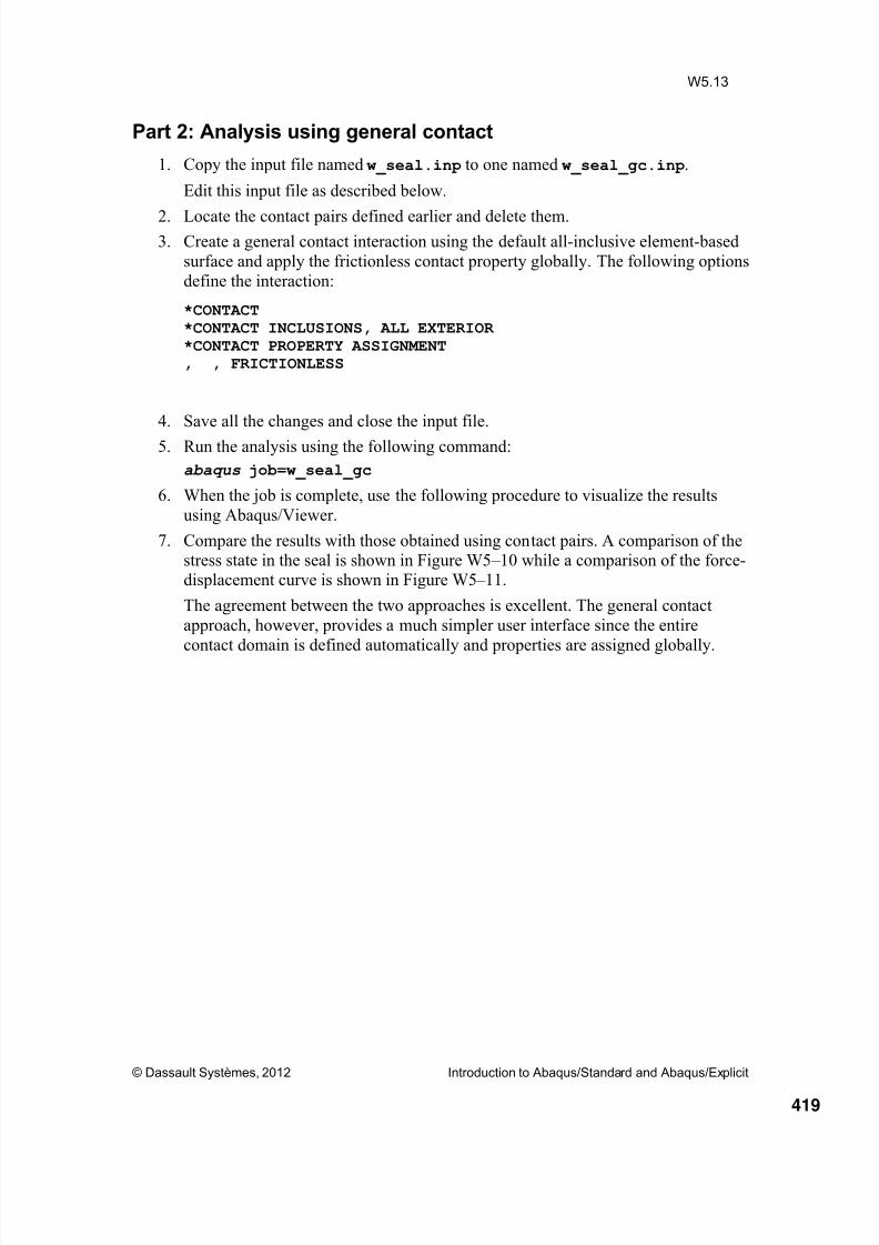
8/15/2019 Abaqus Analysis Intro-book
http://slidepdf.com/reader/full/abaqus-analysis-intro-book 419/469
© Dassault Systèmes, 2012 Introduction to Abaqus/Standard and Abaqus/Explicit
W5.13
Part 2: Analysis using general contact
1. Copy the input file named w_seal.inp to one named w_seal_gc.inp.
Edit this input file as described below.
2. Locate the contact pairs defined earlier and delete them.3. Create a general contact interaction using the default all-inclusive element-based
surface and apply the frictionless contact property globally. The following options
define the interaction:
*CONTACT*CONTACT INCLUSIONS, ALL EXTERIOR*CONTACT PROPERTY ASSIGNMENT, , FRICTIONLESS
4. Save all the changes and close the input file.
5. Run the analysis using the following command:
abaqus job=w_seal_gc
6. When the job is complete, use the following procedure to visualize the results
using Abaqus/Viewer.
7. Compare the results with those obtained using contact pairs. A comparison of thestress state in the seal is shown in Figure W5 – 10 while a comparison of the force-displacement curve is shown in Figure W5 – 11.
The agreement between the two approaches is excellent. The general contact
approach, however, provides a much simpler user interface since the entire
contact domain is defined automatically and properties are assigned globally.
419

8/15/2019 Abaqus Analysis Intro-book
http://slidepdf.com/reader/full/abaqus-analysis-intro-book 420/469
© Dassault Systèmes, 2012 Introduction to Abaqus/Standard and Abaqus/Explicit
W5.14
Figure W5 –10. Comparison of the stress state in the seal(general contact, top; contact pairs, bottom)
Figure W5 –11. Comparison of force-displacement curves
420

8/15/2019 Abaqus Analysis Intro-book
http://slidepdf.com/reader/full/abaqus-analysis-intro-book 421/469
© Dassault Systèmes, 2012 Introduction to Abaqus/Standard and Abaqus/Explicit
W5.15
Note: Complete input files are available for your convenience. You mayconsult these files if you encounter difficulties following the instructionsoutlined here or if you wish to check your work. The input files are named
w_seal_cp_complete.inp
w_seal_gc_complete.inp
and are available using the Abaqus fetch utility.
421

8/15/2019 Abaqus Analysis Intro-book
http://slidepdf.com/reader/full/abaqus-analysis-intro-book 422/469
© Dassault Systèmes, 2012 Introduction to Abaqus/Standard and Abaqus/Explicit
W5.16
Answers
Question W5 –1: What do the plots indicate about the stability of the material?
Answer: The plots never have a negative slope, indicating that thematerial is stable throughout the entire strain range.
Question W5 –2: In the interaction between the seal and the cover, why do we
choose SealOuter as the slave surface?
Answer: SealOuter has a more refined mesh and should therefore be
specified as the slave surface.
Question W5 –3: What does the inverted peak near 4 inches of deflectionrepresent?
Answer: This peak represents the inward bucking that occurs at the
bottom corners of the seal during compression. If you look at
the deformed shape at the time corresponding toapproximately 3.7 inches of displacement, you will observe
this phenomenon.
422

8/15/2019 Abaqus Analysis Intro-book
http://slidepdf.com/reader/full/abaqus-analysis-intro-book 423/469
Notes
423

8/15/2019 Abaqus Analysis Intro-book
http://slidepdf.com/reader/full/abaqus-analysis-intro-book 424/469
Notes
424

8/15/2019 Abaqus Analysis Intro-book
http://slidepdf.com/reader/full/abaqus-analysis-intro-book 425/469
Workshop 6
Dynamics
Keywords Version
© Dassault Systèmes, 2012 Introduction to Abaqus/Standard and Abaqus/Explicit
Note: This workshop provides instructions in terms of the AbaqusKeywords interface. If you wish to use the Abaqus GUI interface instead,please see the “Interactive” version of these instructions.
Please complete either the Keywords or Interactive version of thisworkshop.
Goals
Become familiar with the Abaqus/CAE procedures for frequency extraction andimplicit dynamic analyses.
Become more familiar with the status (.sta) and message (.msg) files.
Learn how to plot eigenmodes and create history plots using Abaqus/Viewer.
Introduction
In this workshop the dynamic response of the cantilever beam shown in Figure W6 – 1 isinvestigated. A frequency extraction is performed to determine the 10 lowest vibrationmodes of the beam. The effects of mesh refinement, element interpolation order, and
element dimension will be considered.
The problem is also solved by performing a direct integration dynamic analysis to
simulate the vibration of the beam upon removal of the tip load . The frequency of the
vibration predicted by the transient analysis will be compared with the natural frequency
results.
Figure W6 –1. Problem description
425
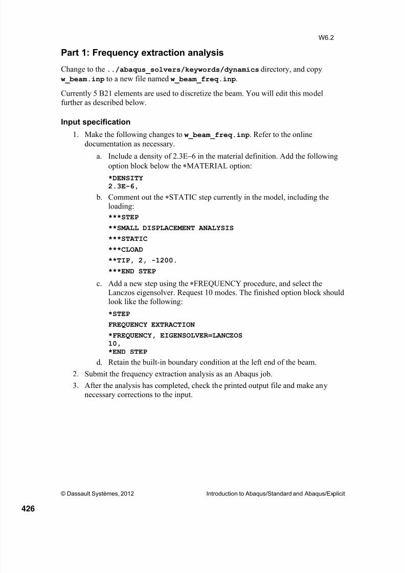
8/15/2019 Abaqus Analysis Intro-book
http://slidepdf.com/reader/full/abaqus-analysis-intro-book 426/469
© Dassault Systèmes, 2012 Introduction to Abaqus/Standard and Abaqus/Explicit
W6.2
Part 1: Frequency extraction analysis
Change to the ../abaqus_solvers/keywords/dynamics directory, and copy
w_beam.inp to a new file named w_beam_freq.inp.
Currently 5 B21 elements are used to discretize the beam. You will edit this model
further as described below.
Input specification
1. Make the following changes to w_beam_freq.inp. Refer to the online
documentation as necessary.
a. Include a density of 2.3E6 in the material definition. Add the following
option block below the MATERIAL option:
*DENSITY2.3E-6,
b. Comment out the
STATIC step currently in the model, including theloading:
***STEP
**SMALL DISPLACEMENT ANALYSIS
***STATIC
***CLOAD
**TIP, 2, -1200.
***END STEP
c. Add a new step using the FREQUENCY procedure, and select theLanczos eigensolver. Request 10 modes. The finished option block should
look like the following:
*STEP
FREQUENCY EXTRACTION
*FREQUENCY, EIGENSOLVER=LANCZOS10,*END STEP
d. Retain the built-in boundary condition at the left end of the beam.
2. Submit the frequency extraction analysis as an Abaqus job.
3. After the analysis has completed, check the printed output file and make any
necessary corrections to the input.
426

8/15/2019 Abaqus Analysis Intro-book
http://slidepdf.com/reader/full/abaqus-analysis-intro-book 427/469
© Dassault Systèmes, 2012 Introduction to Abaqus/Standard and Abaqus/Explicit
W6.3
Examining the eigenmodes and eigenvalues
1. Open the printed output file in the text editor of your choice.
2. Search for the second occurrence of “E I G E N” to find the beginning of theanalysis results. The first table gives the eigenvalue output. Find the frequency
(cycles/time) for the lowest mode.
3. Visualize results:
a. Start Abaqus/Viewer, and open the output database associated with thisanalysis.
b. Plot the first eigenmode (plot the deformed model shape and use the
Frame Selector or the Step/Frame dialog box to choose the framecorresponding to Mode 1).
c. Using the arrow keys in the context bar, select different mode shapes.
d. The results for modes 1 and 4 are shown in Figure W6 – 2. These
correspond to the first and fourth transverse modes of the structure.
Figure W6 –2. First and fourth transverse modes
(coarse mesh; 2D linear beam elements)
Question W6 –1: Are there modes of the physical system that cannot be
captured by your model because of limitations in element type
or mesh? (Remember that the elements are planar and themesh is somewhat coarse.)
Question W6 –2: Do any of the mode shapes for your model look nonphysical?
427

8/15/2019 Abaqus Analysis Intro-book
http://slidepdf.com/reader/full/abaqus-analysis-intro-book 428/469
© Dassault Systèmes, 2012 Introduction to Abaqus/Standard and Abaqus/Explicit
W6.4
Effect of mesh on extracted modes
From Figure W6 – 2 it is apparent that such a coarse mesh of linear-interpolation elementsis unable to adequately represent the mode shapes associated with the higher modes. In
fact the current mesh is unable to represent anything beyond the fifth mode.
To obtain accurate results for all extracted modes, a sufficiently refined mesh is required.Thus, you will increase the mesh refinement. Also, you will switch to quadratic
interpolation elements since these provide superior accuracy for frequency extraction
analysis.
1. Open the file w_beam_freq.inp.
Note the presence of the *PARAMETER option block near the top of the file. The
parameters defined in this block are used to control the mesh density. In
particular, the parameter nel defines the number of elements along the length of
the beam.
2. In the *PARAMETER option block, set nel to 40. The relevant portion of this
option block is shown below.
*PARAMETER
nel = 40
…
The model explicitly defines the first beam element and then uses the *ELGENoption to define the rest.
3. Locate the *ELEMENT option block. Change the element type to B22 andmodify the connectivity list of the first element so that nodes 1, 2, 3 are used to
define the element:
*ELEMENT, TYPE=B22, ELSET=BEAMS
1, 1, 2, 3
4. Run the job, and compare the results with those obtained previously.
The results for modes 1 and 4 are shown in Figure W6 – 3.
428

8/15/2019 Abaqus Analysis Intro-book
http://slidepdf.com/reader/full/abaqus-analysis-intro-book 429/469
© Dassault Systèmes, 2012 Introduction to Abaqus/Standard and Abaqus/Explicit
W6.5
Figure W6 –
3. First and fourth transverse modes(fine mesh; 2D quadratic beam elements)
The results indicate that the refined mesh is able to represent all extracted modes.
The natural frequency of the first mode predicted by the fine-mesh model iswithin 2% of that predicted by the coarse mesh model. The difference in results
for the fourth mode is more significant: there is an 8% difference in the predicted
natural frequency for this mode.
Note that all modes with the exception of modes 6 and 10 are transverse modes.
Modes 6 and 10 are longitudinal modes. To see the longitudinal modes moreclearly, superimpose the undeformed model shape on the deformed model shape.
429

8/15/2019 Abaqus Analysis Intro-book
http://slidepdf.com/reader/full/abaqus-analysis-intro-book 430/469

8/15/2019 Abaqus Analysis Intro-book
http://slidepdf.com/reader/full/abaqus-analysis-intro-book 431/469
© Dassault Systèmes, 2012 Introduction to Abaqus/Standard and Abaqus/Explicit
W6.7
3. The three-dimensional model captures the torsional and out-of-plane modes that
are suppressed by the two-dimensional model. The first three of these modes are
shown in Figure W6 – 5.
Figure W6 –5. Torsional and out-of-plane modes (3D shell model)
431

8/15/2019 Abaqus Analysis Intro-book
http://slidepdf.com/reader/full/abaqus-analysis-intro-book 432/469
© Dassault Systèmes, 2012 Introduction to Abaqus/Standard and Abaqus/Explicit
W6.8
Part 2: Transient dynamic analysis
We now investigate the free vibration of the beam upon removal of the tip load.
Input specification1. Copy w_beam_freq.inp to a new file named w_beam_dynam.inp.
Use the following steps to modify the file so that the tip of the model is loaded
and then released and allowed to vibrate freely:
a. Uncomment the static step.
b. Delete the frequency extraction step.
c. Add another step to the analysis history using the DYNAMIC procedure.Set the maximum number of time increments to 200 and specify an initial
time increment of 0.01 and a time period of 1.0.
d. Remove the tip load in the dynamic step by specifyingCLOAD,
OP=NEW. This option removes all existing concentrated loads.
e. Request predefined field output and that the tip displacement be written
every increment to the output database (.odb) file as history data. Use the
predefined node set named TIP for this purpose. This set contains the
node at the loaded end of the beam. Add the following output requests to
the input file:
*OUTPUT, FIELD, VARIABLE=PRESELECT
*OUTPUT, HISTORY, FREQUENCY=1*NODE OUTPUT, NSET=TIPU,
f. It is useful to be able to monitor the progress of an analysis by noting thevalue of one degree of freedom. To do so, add the following option to thefirst analysis step:
*MONITOR, NODE=TIP, DOF=2
2. Save the input file and run the Abaqus job.
While the job is running, you can check on the progress of the analysis by looking
at the status file.
432

8/15/2019 Abaqus Analysis Intro-book
http://slidepdf.com/reader/full/abaqus-analysis-intro-book 433/469
© Dassault Systèmes, 2012 Introduction to Abaqus/Standard and Abaqus/Explicit
W6.9
Visualizing results
1. Open the file w_beam_dynam.odb in the Visualization module.
2. Plot the history of the displacement component U2 at the tip node. In the Results
Tree, expand the History Output container underneath the output database named
dynamic.odb and double-click Spatial displacement: U2 at Node … in NSET
TIP.
The tip response is shown in Figure W6 – 7. From this plot, you can estimate the
frequency of the first vibration mode. Note that there are nearly 6 cycles in a 1second time period. This is in agreement with the results obtained earlier using the
natural frequency extraction procedure (5.95 Hz).
Figure W6 –7. Tip node displacement history
Question W6 –3: How does this compare with the frequency calculated in theeigenvalue analysis?
Note: Complete input files are available for your convenience. You mayconsult these files if you encounter difficulties following the instructionsoutlined here or if you wish to check your work. The input files are named
w_beam_freq_b21_complete.inp w_beam_freq_b22_complete.inp
w_beam_dynam_b22_complete.inp
and are available using the Abaqus fetch utility.
433

8/15/2019 Abaqus Analysis Intro-book
http://slidepdf.com/reader/full/abaqus-analysis-intro-book 434/469
© Dassault Systèmes, 2012 Introduction to Abaqus/Standard and Abaqus/Explicit
W6.10
Answers
Question W6 –1: Are there modes of the physical system that cannot becaptured by your model because of limitations in element type
or mesh? (Remember that the elements are planar and themesh is somewhat coarse).
Answer: Because the model is two-dimensional, it cannot capture the
modes that occur out of the plane of the model, including
torsional modes.The mesh is too coarse to capture modes other than the first
five. Use more elements to look at all 10 requested modes.
Question W6 –2: Do any of the mode shapes for your model look nonphysical?
Answer: No.
Question W6 –3: How does this compare with the frequency calculated in the
eigenvalue analysis?
Answer: The frequency calculated from the history plot of the tipdisplacement is approximately 5.9, which agrees very closely
with the frequency calculated in the eigenvalue analysis.
434

8/15/2019 Abaqus Analysis Intro-book
http://slidepdf.com/reader/full/abaqus-analysis-intro-book 435/469
Notes
435

8/15/2019 Abaqus Analysis Intro-book
http://slidepdf.com/reader/full/abaqus-analysis-intro-book 436/469
Notes
436

8/15/2019 Abaqus Analysis Intro-book
http://slidepdf.com/reader/full/abaqus-analysis-intro-book 437/469
Workshop 7
Contact with Abaqus/Explicit
Keywords Version
© Dassault Systèmes, 2012 Introduction to Abaqus/Standard and Abaqus/Explicit
Note: This workshop provides instructions in terms of the AbaqusKeywords interface. If you wish to use the Abaqus GUI interface instead,please see the “Interactive” version of these instructions.
Please complete either the Keywords or Interactive version of thisworkshop.
Goals
Define a rigid body constraint.
Define a general contact interaction.
Apply boundary and initial conditions.
Perform an impact analysis.
Use Abaqus/Viewer to view results.
Introduction
This workshop involves the simulation of a pipe-on-pipe impact resulting from therupture of a high-pressure line in a power plant. It is assumed that a sudden release of
fluid could cause one segment of the pipe to rotate about its support and strike a
neighboring pipe. The goal of the analysis is to determine strain and stress conditions in
both pipes and their deformed shapes. The simulation will be performed usingAbaqus/Explicit.
This workshop is based on “Pipe whip simulation,” Section 1.3.9 of the Abaqus
Benchmarks Manual.
437

8/15/2019 Abaqus Analysis Intro-book
http://slidepdf.com/reader/full/abaqus-analysis-intro-book 438/469
© Dassault Systèmes, 2012 Introduction to Abaqus/Standard and Abaqus/Explicit
W7.2
Figure W7 –1. Pipe whip model: finite element mesh
Both pipes have a mean diameter of 6.5 inches with a 0.432 inch wall thickness and aspan of 50 inches between supports. The fixed pipe is assumed to be fully restrained at both ends, while the impacting pipe is allowed to rotate about a fixed pivot located at one
of its ends, with the other end free. We exploit the symmetry of the structure and the
loading and, thus, model only the geometry on one side of the central symmetry plane, as
shown in Figure W7 – 1.
edge refPt fixed
zsymm
Figure W7 –2. Node sets
Impacting pipe
Fixed pipe
Pivot point
438

8/15/2019 Abaqus Analysis Intro-book
http://slidepdf.com/reader/full/abaqus-analysis-intro-book 439/469
© Dassault Systèmes, 2012 Introduction to Abaqus/Standard and Abaqus/Explicit
W7.3
Impact analysis
The model geometry, material properties, and loading history for the impact analysis arealready defined and can be found in
../abaqus_solvers/keywords/pipe_whip/w_pipe_whip.inp. You will have to
edit the input file to include the material properties, rigid body constraint, contactinteraction, initial conditions, boundary conditions, step definition, and output requests.
Predefined sets are included to ease your work. These are shown in Figure W7 – 2.
Material and section properties
1. Both pipes are made of steel. A von Mises elastic, perfectly plastic material model
is used. Create a material named Steel with the following properties:
Modulus of elasticity: 30E6 psi
Poisson's ratio: 0.3
Yield Stress: 45.0E3 psi
Density: 7.324E-4 lb-sec2/in
4
Question W7 –1: Why is density required in the material model definition? Canyou comment on the units of density used in this problem?
2. Assign shell section properties to each pipe. Each pipe is 0.432 inches thick. Use
Gauss integration with 3 points through the thickness for each section property.
The elements of the impacting pipe are contained in element set pipe-
impacting, while the elements of the fixed pipe are in element set pipe-
fixed .Question W7 –2: Why are only three integration points used through the
thickness?
Rigid body constraint
Define a rigid body constraint between the nodes at the pivot end of the impacting pipe
(node set edge) and the rigid body reference point (node set refPt). Both the
translations and rotations of the pipe nodes are controlled by the rigid body constraint.
Question W7 –3: In order to drive both the translations and rotations of the pipe
edge nodes, what type of node set needs to be used in the rigid
body constraint?
Contact interaction
Define general contact between the two pipes. Assume frictional contact with a
coefficient of friction equal to 0.2.
Question W7 –4: Are the contact constraints part of the model or history data?
439

8/15/2019 Abaqus Analysis Intro-book
http://slidepdf.com/reader/full/abaqus-analysis-intro-book 440/469
© Dassault Systèmes, 2012 Introduction to Abaqus/Standard and Abaqus/Explicit
W7.4
Initial conditions
The impacting pipe has an initial angular velocity of 75 radians/sec about its supported(pinned) end. Assign a rotating velocity initial condition to all the nodes in the impacting
pipe (node set pipe-impacting).
The rotation is about the positive Z -direction passing though the rigid body reference point. The coordinates of the reference point are 25.0, 6.932, 25.0.
Question W7 –5: How can you use the coordinates of the reference point todefine the axis of rotation?
Boundary conditions
The edges located on the symmetry plane (node set zsymm ) must be given appropriate
symmetry boundary conditions. One end of the fixed pipe is fully restrained (node set
fixed ). The rigid body reference point (node set refPt) is free to rotate about its
position.
Question W7 –6: Are the boundary conditions part of the model or history data
in an Abaqus/Explicit analysis?
Step definition and output requests
Because of the high-speed nature of the event, the simulation is performed using a single
explicit dynamics step.
1. Create an explicit dynamics step with a time period of 0.015 seconds.
2. Write preselected field output to the output database at 12 equally spacedintervals.
3. Request reaction force history output at the constrained end of the impacting pipe.Write the data to the output database at 100 evenly spaced time intervals during
the analysis.
4. Request preselected history output at the default number of intervals.
Save the input file, and run the impact analysis by entering the following command at the prompt:
abaqus job=w_pipe_whip
Visualization
1. Once the analysis completes successfully, open the output database file in
Abaqus/Viewer.
2. Plot the undeformed and the deformed model shapes. From the main menu bar,
select Tools→Color Code (or click in the toolbar) and assign different
440

8/15/2019 Abaqus Analysis Intro-book
http://slidepdf.com/reader/full/abaqus-analysis-intro-book 441/469
© Dassault Systèmes, 2012 Introduction to Abaqus/Standard and Abaqus/Explicit
W7.5
colors to the two pipes (you can distinguish between them using section
assignments), as shown in Figure W7 – 3.
Figure W7 –3. Deformed model shape
3. Use the Animate: Time History tool to animate the deformation history.
4. Contour the Mises stress and equivalent plastic strain (PEEQ) on the deformedshape, as shown in Figure W7 – 4.
Figure W7 –4. Contour plots
5. Create X – Y plots of the model’s kinetic energy (ALLKE), internal energy
(ALLIE), and dissipated energy (ALLPD). The energy plot is shown in FigureW7 – 5. Note this figure has been customized for clarity.
Tip: Expand the History Output container in the Results Tree and select the threecurves noted above. Click mouse button 3 and select Plot from the menu that
appears.
MISES PEEQ
441

8/15/2019 Abaqus Analysis Intro-book
http://slidepdf.com/reader/full/abaqus-analysis-intro-book 442/469
© Dassault Systèmes, 2012 Introduction to Abaqus/Standard and Abaqus/Explicit
W7.6
Figure W7 –
5. Energy histories
Question W7 –7: What do the energy history plots indicate?
442

8/15/2019 Abaqus Analysis Intro-book
http://slidepdf.com/reader/full/abaqus-analysis-intro-book 443/469
© Dassault Systèmes, 2012 Introduction to Abaqus/Standard and Abaqus/Explicit
W7.7
6. Select and plot the pinned node reaction force components RF1, RF2, and RF3. The curves appear in Figure W7 – 6. Note this figure has been customized for
clarity.
Figure W7 –6. Reaction force histories
Note: A complete input file is available for your convenience. You mayconsult this file if you encounter difficulties following the instructionsoutlined here or if you wish to check your work. The input file is named
w_pipe_whip_complete.inp
and is available using the Abaqus fetch utility.
443

8/15/2019 Abaqus Analysis Intro-book
http://slidepdf.com/reader/full/abaqus-analysis-intro-book 444/469
© Dassault Systèmes, 2012 Introduction to Abaqus/Standard and Abaqus/Explicit
W7.8
Answers
Question W7 –1: Why is density required in the material model definition? Can
you comment on the units of density used in this problem?
Answer: All Abaqus/Explicit analyses require a density value becauseAbaqus/Explicit solves for dynamic equilibrium (i.e., inertia
effects are considered). The units for all material parameters
must be consistent; in this problem the English system is usedwith pounds and inches as the units for force and length,
respectively. Thus, the consistent unit for density is lb-sec2/in
4.
The options required to complete the material model definition
are:
*material, name=steel*density7.324e-4,
*elastic3e+07, 0.3
*plastic45000.,0.
Question W7 –2: Why are only three integration points used through the
thickness?
Answer: Three section points are used to reduce the run time of the job.
The options required to complete the section definitions are:*shell section, elset=pipe-impacting,
material=steel, section integration=gauss0.432, 3*shell section, elset=pipe-fixed,
material=steel, section integration =gauss0.432, 3
Question W7 –3: In order to drive both the translations and rotations of the pipeedge nodes, what type of node set needs to be used in the rigid
body constraint?
Answer: A tie node set needs to be used.
The option required to define the rigid body constraint is:
*rigid body, ref node=refPt, tie nset=edge
444

8/15/2019 Abaqus Analysis Intro-book
http://slidepdf.com/reader/full/abaqus-analysis-intro-book 445/469
© Dassault Systèmes, 2012 Introduction to Abaqus/Standard and Abaqus/Explicit
W7.9
Question W7 –4: Should you add the contact definition to the model data or the
history data?
Answer: General contact definitions can be part of either the modeldata or the history data. The surface interaction properties aremodel data when used with general contact.
The (model data) options required to complete the contact
definition are:
*contact*contact inclusions, all exterior*contact property assignment, , fric
*surface interaction, name=fric*friction0.2,
Question W7 –5:
How can you use the coordinates of the reference point to
define the axis of rotation?
Answer: The axis passes through the reference point and is parallel tothe Z -direction. Thus, define the axis using two points. Each ofthe “axis” points must have the same X - and Y -coordinates as
the reference point; the values of the Z -coordinates of the
“axis” points will dictate the sense of positive rotation.
For example:
*initial conditions, type=rotating velocity
pipe-impacting, 75., 0., 0., 0.,25., 6.932, 0., 25., 6.932, 1.,
The second data line defines the axis of rotation.
445
8/15/2019 Abaqus Analysis Intro-book
http://slidepdf.com/reader/full/abaqus-analysis-intro-book 446/469
© Dassault Systèmes, 2012 Introduction to Abaqus/Standard and Abaqus/Explicit
W7.10
Question W7 –6: Are the boundary conditions part of the model data or the
history data in an Abaqus/Explicit analysis?
Answer: As with Abaqus/Standard, fixed boundary conditions can be
defined as either model or history data. Named boundaryconditions improve the readability of your input file and
provide a shortcut to defining commonly encountered supportconditions.
The options required to define the boundary conditions, step,and output are:
*dynamic, explicit, 0.015***boundaryzsymm, zsymmfixed, encastrerefPt, pinned*output, field, variable=preselect,number intervals=12*output, history, time interval=0.00015*node output, nset=refptrf1, rf2, rf3*output, history, variable=preselect
Question W7 –7: What do the energy history plots indicate?
Answer: Near the end of the simulation, the impacting pipe is
beginning to rebound, having dissipated the majority of its
kinetic energy by inelastic deformation in the crushed zone.
446

8/15/2019 Abaqus Analysis Intro-book
http://slidepdf.com/reader/full/abaqus-analysis-intro-book 447/469
Notes
447

8/15/2019 Abaqus Analysis Intro-book
http://slidepdf.com/reader/full/abaqus-analysis-intro-book 448/469
Notes
448

8/15/2019 Abaqus Analysis Intro-book
http://slidepdf.com/reader/full/abaqus-analysis-intro-book 449/469
Workshop 8
Quasi-Static Analysis
Keywords Version
© Dassault Systèmes, 2012 Introduction to Abaqus/Standard and Abaqus/Explicit
Note: This workshop provides instructions in terms of the AbaqusKeywords interface. If you wish to use the Abaqus GUI interface instead,please see the “Interactive” version of these instructions.
Please complete either the Keywords or Interactive version of thisworkshop.
Goals
Approximate a quasi-static solution using Abaqus/Explicit.
Understand the effects of mass scaling.
Introduction
In this workshop you will examine the deep drawing of a can bottom. A one-stageforming process is simulated in Abaqus/Explicit; the springback analysis is performed in
Abaqus/Standard. The final deformed shape of the can bottom is shown inFigure W8 – 1. In a subsequent workshop the import capability is used to transfer the
results between Abaqus/Explicit and Abaqus/Standard in order to perform a springback
analysis.
One of the advantages of using Abaqus/Explicit for metal forming simulations is that, ingeneral, Abaqus/Explicit resolves complicated contact conditions more readily than
Abaqus/Standard.
449
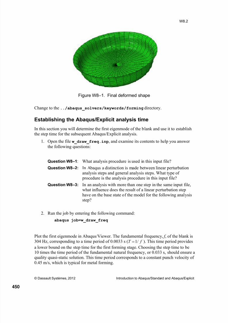
8/15/2019 Abaqus Analysis Intro-book
http://slidepdf.com/reader/full/abaqus-analysis-intro-book 450/469
© Dassault Systèmes, 2012 Introduction to Abaqus/Standard and Abaqus/Explicit
W8.2
Figure W8 –1. Final deformed shape
Change to the ../abaqus_solvers/keywords/forming directory.
Establishing the Abaqus/Explicit analysis time
In this section you will determine the first eigenmode of the blank and use it to establish
the step time for the subsequent Abaqus/Explicit analysis.
1. Open the file w_draw_freq.inp, and examine its contents to help you answer
the following questions:
Question W8 –1: What analysis procedure is used in this input file?
Question W8 –2: In Abaqus a distinction is made between linear perturbationanalysis steps and general analysis steps. What type of procedure is the analysis procedure in this input file?
Question W8 –3: In an analysis with more than one step in the same input file,what influence does the result of a linear perturbation step
have on the base state of the model for the following analysisstep?
2. Run the job by entering the following command:
abaqus job=w_draw_freq
Plot the first eigenmode in Abaqus/Viewer. The fundamental frequency, f , of the blank is
304 Hz, corresponding to a time period of 0.0033 s ( 1/T f ). This time period provides
a lower bound on the step time for the first forming stage. Choosing the step time to be10 times the time period of the fundamental natural frequency, or 0.033 s, should ensure a
quality quasi-static solution. This time period corresponds to a constant punch velocity of
0.45 m/s, which is typical for metal forming.
450

8/15/2019 Abaqus Analysis Intro-book
http://slidepdf.com/reader/full/abaqus-analysis-intro-book 451/469
© Dassault Systèmes, 2012 Introduction to Abaqus/Standard and Abaqus/Explicit
W8.3
Geometry definition
In this section you will complete the geometry definition of the can forming model by
defining the punch as an analytical rigid surface.
Figure W8 – 2 shows the components of the model — the punch, the die, and the blank — in
their initial positions. The blank is modeled using axisymmetric shell elements (SAX1).The shell reference surface lies at the shell midsurface.
Figure W8 –2. Model geometry
1. Open the file w_draw_bot.inp in an editor, and define punch 1 as an analytical
rigid surface (see Figure W8 – 2 for the relevant dimensions).
Use the definition of die 1 in the input file as an example of the input for ananalytical rigid surface. The end point for punch 1 lies on the symmetry axis, a
distance of half the blank thickness above the shell midsurface. Give the rigid
surface the name PUNCH1, and use node 1001 as the rigid body reference node.
The RIGID BODY option has been defined already.
Question W8 –4: How does the order of the line segments affect the ability ofAbaqus to resolve the contact condition?
0.032 0.03025
Origin
(0.0, 0.0)
(0.0, 0.00025)
451

8/15/2019 Abaqus Analysis Intro-book
http://slidepdf.com/reader/full/abaqus-analysis-intro-book 452/469
© Dassault Systèmes, 2012 Introduction to Abaqus/Standard and Abaqus/Explicit
W8.4
2. Define the surfaces, the contact pairs, and the surface interaction for the complete
model using the SURFACE, CONTACT PAIR, and SURFACE
INTERACTION options. The blank is defined such that the element normaldirection points toward the punch. The friction coefficient between the rigid toolsand the blank is 0.1.
Question W8 –5: What effect will an increase in friction have on the solution?
Question W8 –6: In Abaqus the input data are classified as either model or
history data. What type of data is the contact pair definition inAbaqus/Explicit? What type of data is the contact pair
definition in Abaqus/Standard?
Material definition
In this section you will add the entire material definition to the input file.
The material is steel with Young’s modulus E =210E9 Pa, Poisson’s ratio v =0.3, anddensity =7800 kg/m
3. Figure W8 – 3 shows the nominal plasticity material data for the
blank as tabulated in Table W8 – 1.
Figure W8 –3. Nominal stress vs. nominal strain
Question W8 –7: When entering plasticity data with the PLASTIC option,
what are the stress and strain measures that Abaqus uses?
452

8/15/2019 Abaqus Analysis Intro-book
http://slidepdf.com/reader/full/abaqus-analysis-intro-book 453/469
© Dassault Systèmes, 2012 Introduction to Abaqus/Standard and Abaqus/Explicit
W8.5
Table W8 –1
Nominal stress (Pa) Nominal strain
90.96 106 4.334 104
130.71 106 2.216 10
3
169.75 106 7.331 10
3
207.08 106
1.888 10-2
240.99 10
6 4.153 10
2
268.89 106 8.218 10
2
287.59 106 1.509 10
1
290.57 106 3.456 10
1
Table W8 –2
True stress (Pa) Log plastic strain
91 106 0.0
131 106
0.159 102
171 106 0.649 102
211 106 0.177 101
251 106 0.395 101
291 106 0.776 101
331 106 0.139
391 106 0.295
Table W8 – 2 lists the corresponding true stress and logarithmic strain values. These
values were obtained using the following relationships:
(1 )nom nom
1n(1 )nom
/ pl tot el tot E
These equations are valid for isotropic materials and establish the relationships betweenthe true stress and strain measures (used in Abaqus) and the nominal stress and strain
measures.
1. Complete the material definition, and name the material STEEL. Use the
ELASTIC option to enter Young’s modulus and Poisson’s ratio and the
PLASTIC option to enter the material data in Table W8 – 2.
Tip: Both of these options must be grouped under the *MATERIAL option.
2. To reduce high-frequency noise in the solution (caused primarily by the
oscillations of the blank’s free end), add stiffness proportional damping to thematerial definition of the blank. It is best to use the smallest amount of damping
possible to obtain the desired solution since increasing the stiffness damping
decreases the stable time increment and, thus, increases the computer time. Toavoid a dramatic drop in the stable time increment, the stiffness proportional
453

8/15/2019 Abaqus Analysis Intro-book
http://slidepdf.com/reader/full/abaqus-analysis-intro-book 454/469
© Dassault Systèmes, 2012 Introduction to Abaqus/Standard and Abaqus/Explicit
W8.6
damping factor R should be less than, or of the same order of magnitude as, theinitial stable time increment without damping. We choose a damping factor of
R = 1107, which is included by using the DAMPING, BETA=1.E7 material
option.
Question W8 –8: What effects would a higher damping coefficient have?
Amplitude definition
To form the can bottom, we will displace the punch by moving its rigid body reference node 0.015 m in the negative 2-direction. The punch displacement will be applied in the
form of a displacement boundary condition. Because Abaqus/Explicit does not permit
displacement discontinuities, prescribed displacements must refer to an amplitude
definition. In this section you will add the amplitude definition to the input file. FigureW8 – 4 shows the desired displacement behavior for the punch.
Question W8 –9: What is the slope of the curve at the beginning and end, andwhy is this important?
1. Define the amplitude curve corresponding to Figure W8 – 4. The curve shown in
Figure W8 – 4 is smooth in its first and second derivatives and is defined by using
the DEFINITION=SMOOTH STEP parameter with the AMPLITUDE option.
Define the punch displacement amplitude, and name the amplitude FORM1.
Question W8 –10: How would the results change if a linear amplitude definition
was used instead?
2. Note that in the input file there is a boundary condition that refers to the
amplitude definition (FORM1) just completed.
Speeding up the analysis
In general, quasi-static processes cannot be modeled in their natural time scale inAbaqus/Explicit since a large number of time increments would be required. (Recall that
time increments in Abaqus/Explicit are generally very small). Thus, it is sometimes
necessary to increase the speed of the simulation artificially to reduce the computational
cost. One method to reduce the cost of the analysis is to use mass scaling.
454
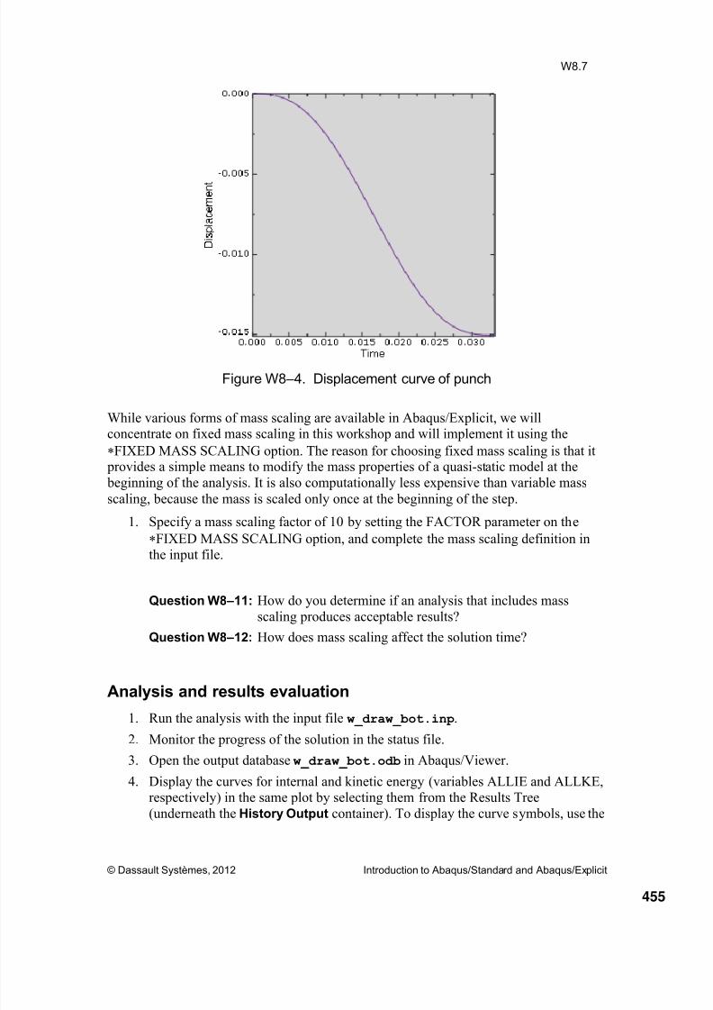
8/15/2019 Abaqus Analysis Intro-book
http://slidepdf.com/reader/full/abaqus-analysis-intro-book 455/469
© Dassault Systèmes, 2012 Introduction to Abaqus/Standard and Abaqus/Explicit
W8.7
Figure W8 –4. Displacement curve of punch
While various forms of mass scaling are available in Abaqus/Explicit, we willconcentrate on fixed mass scaling in this workshop and will implement it using the
FIXED MASS SCALING option. The reason for choosing fixed mass scaling is that it provides a simple means to modify the mass properties of a quasi-static model at the
beginning of the analysis. It is also computationally less expensive than variable mass
scaling, because the mass is scaled only once at the beginning of the step.
1. Specify a mass scaling factor of 10 by setting the FACTOR parameter on the
FIXED MASS SCALING option, and complete the mass scaling definition inthe input file.
Question W8 –11: How do you determine if an analysis that includes mass
scaling produces acceptable results?
Question W8 –12: How does mass scaling affect the solution time?
Analysis and results evaluation
1. Run the analysis with the input file w_draw_bot.inp.
2. Monitor the progress of the solution in the status file.
3. Open the output database w_draw_bot.odb in Abaqus/Viewer.
4. Display the curves for internal and kinetic energy (variables ALLIE and ALLKE,respectively) in the same plot by selecting them from the Results Tree
(underneath the History Output container). To display the curve symbols, use the
455

8/15/2019 Abaqus Analysis Intro-book
http://slidepdf.com/reader/full/abaqus-analysis-intro-book 456/469
© Dassault Systèmes, 2012 Introduction to Abaqus/Standard and Abaqus/Explicit
W8.8
XY Curve Options tool in the toolbox. You should see a plot similar toFigure W8 – 5. Note this figure has been customized for clarity.
Figure W8 –5. Internal and kinetic energy
5. Certain elements have hourglass modes that affect their behavior. Hourglass
modes are modes of deformation that do not cause any strains at the integration
points. An indication of whether hourglassing has an effect on the solution is the
artificial energy, variable ALLAE. Plot the artificial energy and the internalenergy, variable ALLIE, on the same plot. The artificial energy should always be
much less than the internal energy (say less than 0.5%).
Question W8 –13: What elements are used to model the blank, and does thiselement type have an hourglass deformation mode?
6. Display only the deformed shape of the blank:
a. Expand the Materials container in the Results Tree and click mouse button 3 on STEEL.
b. From the menu that appears, select Replace.
7. Expand the displayed area to 180o
:a. Select View ODB Display Options from the main menu.
b. In the Sweep/Extrude tabbed page of the ODB Display Options dialog
box, toggle on Sweep elements.
You should see a shape similar to that in Figure W8 – 6.
456

8/15/2019 Abaqus Analysis Intro-book
http://slidepdf.com/reader/full/abaqus-analysis-intro-book 457/469

8/15/2019 Abaqus Analysis Intro-book
http://slidepdf.com/reader/full/abaqus-analysis-intro-book 458/469
© Dassault Systèmes, 2012 Introduction to Abaqus/Standard and Abaqus/Explicit
W8.10
Answers
Question W8 –1: What analysis procedure is used in this input file?
Answer: The analysis procedure is a natural frequency extraction
(FREQUENCY). The procedure option must immediatelyfollow the STEP option.
Question W8 –2: In Abaqus a distinction is made between linear perturbation
analysis steps and general analysis steps. What type of procedure is the analysis procedure in this input file?
Answer: The FREQUENCY option is a linear perturbation procedure.
Question W8 –3: In an analysis with more than one step in the same input file,what influence does the result of a linear perturbation step
have on the base state of the model for the following analysis
step?
Answer: None. Only general analysis steps change the base state of themodel.
Question W8 –4: How does the order of the line segments affect the ability of
Abaqus to resolve the contact condition?
Answer: The order of the line segments determines the direction of the
outward normal vector of the rigid surface. If the outwardnormal points in the wrong direction, Abaqus cannot establish
the contact between the surfaces and, therefore, cannot find a
solution.
Question W8 –5: What effect will an increase in friction have on the solution?
Answer: An increased friction coefficient will increase the critical shear
stress crit at which sliding of the blank begins. Thus, thematerial will be stretched more, causing further thinning of the
material and increasing the stresses.
458

8/15/2019 Abaqus Analysis Intro-book
http://slidepdf.com/reader/full/abaqus-analysis-intro-book 459/469
© Dassault Systèmes, 2012 Introduction to Abaqus/Standard and Abaqus/Explicit
W8.11
Question W8 –6: In Abaqus the input data are classified as either model or
history data. What type of data is the contact pair definition in
Abaqus/Explicit? What type of data is the contact pair
definition in Abaqus/Standard?
Answer: The contact pair definition is history data in Abaqus/Explicit
and model data in Abaqus/Standard.
Question W8 –7: When entering plasticity data with the PLASTIC option,what are the stress and strain measures that Abaqus uses?
Answer: Abaqus uses true (Cauchy) stress and log strain.
Question W8 –8: What effects would a higher damping coefficient have?
Answer: A higher damping coefficient would reduce the stable time
increment. In general, damping should be chosen such thathigh frequency oscillations are smoothed or eliminated with
minimal effect on the stable time increment. Figure WA8 – 1
shows a plot of the kinetic energy with and without damping. Note the high frequency oscillations in the analysis without
damping.
Figure WA8 –1. Kinetic energy with and without damping
459
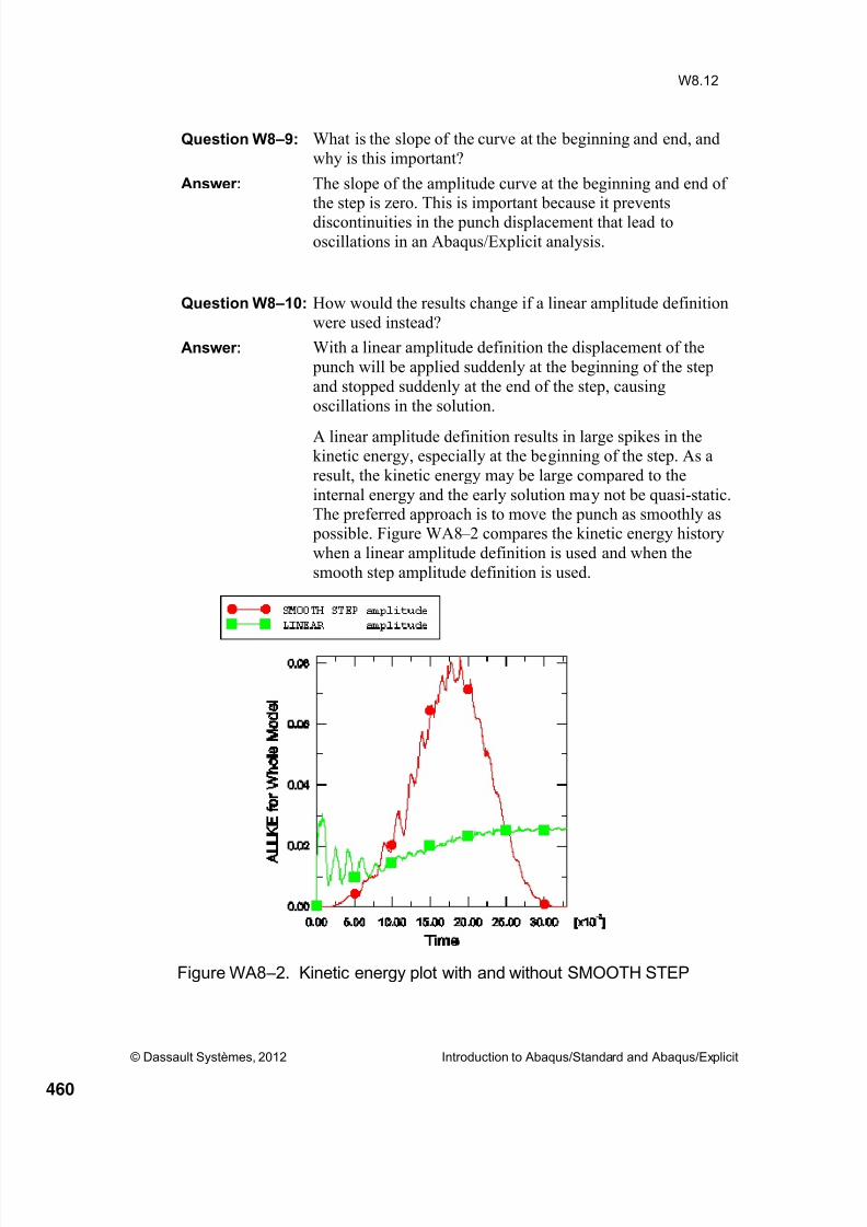
8/15/2019 Abaqus Analysis Intro-book
http://slidepdf.com/reader/full/abaqus-analysis-intro-book 460/469
© Dassault Systèmes, 2012 Introduction to Abaqus/Standard and Abaqus/Explicit
W8.12
Question W8 –9: What is the slope of the curve at the beginning and end, and
why is this important?
Answer: The slope of the amplitude curve at the beginning and end ofthe step is zero. This is important because it preventsdiscontinuities in the punch displacement that lead to
oscillations in an Abaqus/Explicit analysis.
Question W8 –10: How would the results change if a linear amplitude definition
were used instead?
Answer: With a linear amplitude definition the displacement of the
punch will be applied suddenly at the beginning of the step
and stopped suddenly at the end of the step, causing
oscillations in the solution.
A linear amplitude definition results in large spikes in thekinetic energy, especially at the beginning of the step. As a
result, the kinetic energy may be large compared to the
internal energy and the early solution may not be quasi-static.The preferred approach is to move the punch as smoothly as possible. Figure WA8 – 2 compares the kinetic energy history
when a linear amplitude definition is used and when the
smooth step amplitude definition is used.
Figure WA8 –2. Kinetic energy plot with and without SMOOTH STEP
460
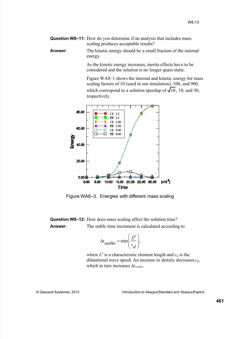
8/15/2019 Abaqus Analysis Intro-book
http://slidepdf.com/reader/full/abaqus-analysis-intro-book 461/469
© Dassault Systèmes, 2012 Introduction to Abaqus/Standard and Abaqus/Explicit
W8.13
Question W8 –11: How do you determine if an analysis that includes mass
scaling produces acceptable results?
Answer: The kinetic energy should be a small fraction of the internalenergy.
As the kinetic energy increases, inertia effects have to beconsidered and the solution is no longer quasi-static.
Figure WA8 – 1 shows the internal and kinetic energy for mass
scaling factors of 10 (used in our simulation), 100, and 900,
which correspond to a solution speedup of 10 , 10, and 30,
respectively.
Figure WA8 –3. Energies with different mass scaling
Question W8 –12: How does mass scaling affect the solution time?
Answer: The stable time increment is calculated according to
min ,e Lt stable c
d
where Le is a characteristic element length and cd is the
dilatational wave speed. An increase in density decreases cd ,
which in turn increases t stable.
461

8/15/2019 Abaqus Analysis Intro-book
http://slidepdf.com/reader/full/abaqus-analysis-intro-book 462/469
© Dassault Systèmes, 2012 Introduction to Abaqus/Standard and Abaqus/Explicit
W8.14
Question W8 –13: What elements are used to model the blank, and does this
element type have an hourglass deformation mode?
Answer: The analysis uses SAX1 elements. These elements have nohourglass modes. Consequently, hourglassing is not ofconcern in the analysis.
462

8/15/2019 Abaqus Analysis Intro-book
http://slidepdf.com/reader/full/abaqus-analysis-intro-book 463/469
Notes
463

8/15/2019 Abaqus Analysis Intro-book
http://slidepdf.com/reader/full/abaqus-analysis-intro-book 464/469

8/15/2019 Abaqus Analysis Intro-book
http://slidepdf.com/reader/full/abaqus-analysis-intro-book 465/469
Workshop 9
Import Analysis
Keywords Version
© Dassault Systèmes, 2012 Introduction to Abaqus/Standard and Abaqus/Explicit
Note: This workshop provides instructions in terms of the AbaqusKeywords interface. If you wish to use the Abaqus GUI interface instead,please see the “Interactive” version of these instructions.
Please complete either the Keywords or Interactive version of thisworkshop.
Goals
Transfer results between Abaqus/Explicit and Abaqus/Standard.
Introduction
In this workshop you will use the import capability is used to transfer the results between
Abaqus/Explicit and Abaqus/Standard to examine the effects of springback in the
analysis of the deep drawing of a can bottom. The deformed shape of the can after the
forming stage is shown in Figure W9 –
1.
Figure W9 –1. Final deformed shape
Before proceeding, change to the ../abaqus_solvers/keywords/forming
directory.
465

8/15/2019 Abaqus Analysis Intro-book
http://slidepdf.com/reader/full/abaqus-analysis-intro-book 466/469
© Dassault Systèmes, 2012 Introduction to Abaqus/Standard and Abaqus/Explicit
W9.2
Springback analysis
In the manufacturing process the part is removed after the forming has been completed
and the material is free to springback into an unconstrained state. To understand the final
shape after this physical effect, we perform a springback analysis in Abaqus/Standard.
1. Open the file w_draw_bot_spring.inp in an editor, and import the blank from
the end of the w_draw_bot analysis. Use the STATE=YES parameter on the
IMPORT option to import the material state of the elements.
Question W9 –1: To what value should the UPDATE parameter on the
IMPORT option be set if the total Mises stresses are to be
plotted at the end of the springback analysis?
Question W9 –2: Where do you find the information to define the STEP and
INTERVAL parameters on the IMPORT option?
2. The boundary conditions are not imported and must be respecified. In addition, itis necessary to fix a single point, such as node set BSYM , in the 2-direction to
prevent rigid body motion. It is important to use the FIXED parameter on the
*BOUNDARY option so that BSYM is fixed at its final position at the end of the
forming stage.
Question W9 –3: Why is it advantageous to choose Abaqus/Standard for thespringback analysis?
Analysis and postprocessing
1. Run the analysis by entering the following command:
abaqus job=w_draw_bot_spring oldjob=w_draw_bot
2. Open the output database w_draw_bot_spring.odb in Abaqus/Viewer.
3. Contour the Mises stress distribution of the 180o model.
4. Plot the final deformed model shape, as shown in Figure W9 – 1.
5. Plot the springback and formed shapes together. (First toggle off the Sweep
elements option.)
If you used UPDATE=NO, the formed shape is stored in frame 0 of the outputdatabase. You must use overlay plots to superimpose the images in this case:
a. Select View→Overlay Plot from the main menu bar.
b. Use the Frame Selector or the arrows in the context bar to select
frame 0.
c. In the Overlay Plot Layer Manager , click Create. Name the layer
formed .
466

8/15/2019 Abaqus Analysis Intro-book
http://slidepdf.com/reader/full/abaqus-analysis-intro-book 467/469
© Dassault Systèmes, 2012 Introduction to Abaqus/Standard and Abaqus/Explicit
W9.3
d. Use the Frame Selector or the arrows in the context bar to select
frame 1.
e. Use the Common Plot Options tool to change the fill color of the
elements to blue.
f. In the Overlay Plot Layer Manager , click Create. Name the layerspringback.
g. In the Overlay Plot Layer Manager , click Plot Overlay.
h. Zoom in to examine the shape differences more closely.
If you used UPDATE=YES, the formed shape is treated as the undeformed shape
of the import analysis model (recall that when UPDATE=YES, the end state of
the previous analysis becomes the reference configuration of the import analysis;
the reference configuration is considered the undeformed shape):
a. In the toolbox, click the Allow Multiple Plot States tool .
b. In the toolbox, click both the Plot Undeformed Shape and Plot
Deformed Shape tools .
c. Use the Common Plot Options tool to increase the deformation
scale factor so that the differences between the formed and springback
shapes are clearly visible.
Note: A complete input file is available for your convenience. You mayconsult this file if you encounter difficulties following the instructions
outlined here or if you wish to check your work. The input file is named w_draw_bot_spring_complete.inp
and is available using the Abaqus fetch utility.
467

8/15/2019 Abaqus Analysis Intro-book
http://slidepdf.com/reader/full/abaqus-analysis-intro-book 468/469
© Dassault Systèmes, 2012 Introduction to Abaqus/Standard and Abaqus/Explicit
W9.4
Answers
Question W9 –1: To what value should the UPDATE parameter on the
IMPORT option be set if the total Mises stresses are to be
plotted at the end of the springback analysis?
Answer: The UPDATE parameter should be set to NO. When the
UPDATE parameter is set to YES, the deformed configurationof the previous analysis is used as the reference configuration
for the import analysis. All stresses, strains, displacements,
etc. are reported relative to the updated referenceconfiguration and not as total values.
Question W9 –2: Where do you find the information to define the STEP and
INTERVAL parameters on the IMPORT option?
Answer: The status (.sta) file gives an overview of the progression onthe analysis. Information about the number of steps and the
number of increments completed in each step can be obtained
from this file.
In this analysis we wish to model the springback of the canafter the forming of the can bottom is complete: this is
STEP=1, INTERVAL=1.
Question W9 –3: Why is it advantageous to choose Abaqus/Standard for thespringback analysis?
Answer: A true static procedure is the preferred approach for modelingspringback. The imported model will not be in static
equilibrium at the beginning of the step. Thus,
Abaqus/Standard applies a set of artificial internal stresses tothe imported model state and then gradually removes thesestresses. This leads to the springback deformation. In
Abaqus/Explicit the removal of the contact between the blank
and the tools represents a sudden load removal, which leads tolow frequency vibrations of the blank. While these vibrations
will eventually dissipate, this approach leads to lengthy
computation times.
468

8/15/2019 Abaqus Analysis Intro-book
http://slidepdf.com/reader/full/abaqus-analysis-intro-book 469/469
Notes

![[PPT]Introduction - הפקולטה להנדסה ע"ש איבי ואלדר פליישמן ...harari/Courses/Intro/IABU-UNIT01-L01... · Web viewIntroduction to Abaqus Overview of Abaqus](https://img.pdfslide.net/doc/110x75/5ae80b5c7f8b9a08778f2743/pptintroduction-.jpg)