Abelian Gauge Theory, Knots and Odd Khovanov Homology

January 2, 2017

Abstract

A homological invariant of 3-manifolds is defined using abelian Yang-Mills gauge theory.It is shown that the construction, in an appropriate sense, is functorial with respect to thefamilies of 4-dimensional cobordisms. This construction and its functoriality are used to defineseveral link invariants. The strongest version of these invariants has the form of a filtered chaincomplex that can recover Khovanov homology of the mirror image as a bi-graded group.

Gauge theoretical methods are proven to be useful tools to study low dimensional manifolds. Asone of the first instances of this approach, Donaldson constructed a family of invariants, usuallyknown as Donaldson invariants, for smooth closed 4-manifolds that satisfy a mild topologicalassumption [4]. To construct these invariants, one fixes a Hermitian vector bundle of rank 2 on aRiemannian 4-manifold and considers the space of connections that satisfy a geometrical PDE (akaanti-self-duality equation) modulo the action of bundle automorphisms. Although the anti-self-duality equation depends on the Riemannian metric, a careful study of the moduli spaces of anti-self-dual connections leads to numerical invariants that depend only on the diffeomorphism typeof the 4-manifold. More recently, Kronheimer applied a modification of the original constructionto Hermitian vector bundles of rank n, with n ě 3, and defined similar 4-manifold invariants.In the case n “ 1, the relevant moduli spaces can be characterized by the classical topologicalinvariants (i.e.cohomology groups of the underlying 4-manifolds) and hence they do not give riseto any interesting numerical invariant that can be used to study the topology of 4-manifolds.

Let Y be a 3-manifold which has the same integral homology groups as the 3-dimensionalsphere. In [7], Floer used the moduli space of anti-self-dual connections on R ˆ Y to producetopological invariants of Y . In parallel to the case of 4-manifolds, one expects that anti-self-dualconnections on vector bundles of higher rank can be also utilized to define 3-manifold invariants.Kronheimer and Mrowka used this approach in a greater generality, and among other topologicalinvariants, they constructed invariants of 3-manifolds using higher rank bundles.

The purpose of this article is to show that the moduli space of anti-self-dual connections on aHermitian line bundle can be used to extract non-trivial data in 3-manifold topology. We will usea slight variation of these spaces to define an invariant that is called plane Floer homology. PlaneFloer homology of a 3-manifold Y is a graded vector space over a field Λ and is denoted by PFHpY q.As any other Floer homology theory, this vector space is the homology of a chain complex whichin this case is denoted by PFCpY q. An important feature of plane Floer homology is functoriality

1

with respect to cobordisms. That is to say, if W : Y0 Ñ Y1 is a 4-dimensional cobordism fromY0 to Y1, then there is a chain map PFCpW q : PFCpY0q Ñ PFCpY1q. This cobordism map isdefined with the aid of an appropriate metric on W . More generally, for a family of metrics on thecobordism W , we can define cobordism maps from PFCpY0q to PFCpY1q. The following theoremis the heart of this article:

Theorem 1. If L is a framed link with n connected components in a 3-manifold Y , then there isa chain complex PFCLpY q that has the same chain homotopy type as PFCpY q. The underlyingchain group of PFCLpY q is equal to:

à

mPt0,1un

PFCpYmq

For m “ pm1, . . . ,mnq P t0, 1un, the 3-manifold Ym is given by performing the mi-surgery along

the ith connected component of L for each i. The differential of this complex is also defined usingcobordism maps associated with certain families of metrics.

For a detailed version of this theorem see Theorem 2.9 and Corollary 2.10. To have a closerlook at Theorem 1, let L have one connected component and Yp1q (respectively, Yp0q) be the resultof 1-surgery (respectively, 0-surgery) along L. Let also W : Yp1q Ñ Yp0q be the standard cobordismthat is given by attaching a 2-handle to r0, 1s ˆ Yp1q along L. Therefore, there is a chain mapPFCpW q : PFCpYp1qq Ñ PFCpYp0qq. In this special case, PFCLpY q is the mapping cone of thechain map PFCpW q. As a consequence, there is an exact triangle of the following form:

PFHpY q

&&PFHpYp0qq

88

PFHpYp1qqoo

(1)

In the more general case that L has more than one connected component, there is again afiltration on the chain complex PFCLpY q. This filtration determines a spectral sequence thatabuts to PFHpY q. This spectral sequence should be thought as the counterpart of the surgeryspectral sequence of [16] for plane Floer homology. Similar spectral sequences for various otherFloer homologies are established in [11, 3, 17]. Note that in all these cases, the pages of thespectral sequence depend on the framed link L and are not 3-manifold invariants.

Let K be a link in S3 and ΣpKq be the branched double cover of S3 branched along K. Thechain complexes given by Theorem 1 can be used to construct additional structures on PFHpΣpKqqwhich are not otherwise apparent in the original chain complex. Let D be a link diagram for K.One can use this diagram to produce a framed link in ΣpKq (cf. section 3). Therefore, it can beused as an input for Theorem 1 to construct a chain complex that is denoted by PKCpDq. We shalldefine two gradings on PKCpDq which are called homological and δ-gradings. The differential of thechain complex PKCpDq does not decrease the homological grading and increases the δ-grading by1. We call a chain complex with a bi-grading that satisfies the above properties a filtered Z-gradedchain complex:

2

Theorem 2. The homotopy type of PKCpDq, as a filtered Z-graded chain complex, depends onlyon K and hence is a link invariant.

For the definition of the homotopy type of a filtered Z-graded chain complex see subsection 3.2.The homological filtration and the δ-grading of PKCpDq induces a spectral sequence tPKErpKquwhere PKErpKq is a bi-graded vector space. As an immediate corollary of Theorem 2, we have:

Corollary 1. For each r ě 2, there is a bi-graded vector space PKErpKq that is an invariant ofK.

Remark 1. The spectral sequence in Corollary 1 can be utilized to define a series of concordancehomomorphisms. In fact, an equivariant version of PKCpDq gives rise to other spectral sequencessimilar to that of Corollary 1. These spectral sequences are the starting point to define otherconcordance invariants. This circle of ideas will be explored in a forthcoming work.

Corollary 1 provides us with a series of homological link invariants which begs for further study.In the last part of this article, we take up the task of understanding the first invariant in this listand show that it is related to Khovanov homology. Khovanov homology is a categorification ofJones polynomial defined in [8]. In [15], an elaborate modification of the definition of Khovanovhomology was used to define another categorification of Jones polynomial that is known as oddKhovanov homology. Subsequently, Khovanov’s original link invariant is also known as even Kho-vanov homology. Even and odd Khovanov homology agree when one uses a characteristic two ringto define these homological link invariants. However, if a characteristic zero coefficient ring is used,then these invariants diverge significantly from each other.

Theorem 3. The invariant PKE2pKq is isomorphic to the Khovanov homology of the mirrorimage of K with coefficients in the field Λ.

The field Λ has characteristic two and is the quotient of a ring Λ with characteristic zero (cf.

subsection 1.4). The vector space PFHpY q can be lifted to an invariant ĆPFHpY q which is a Λ-module and is called the oriented plane Floer homology of Y . There is an analogue of the spectralsequence tPKErpKqu in the context of oriented plane Floer homology:

Theorem 4. There is a spectral sequence tĆPKErpKqu with coefficients in Λ that abuts to ĆPFHpΣpKqq.

The second page of this spectral sequence, ĆPKE2pKq, is isomorphic to odd Khovanov homology ofthe mirror image of K with coefficients in the ring Λ.

This article is organized as follows. In section 1, we focus on the definition of plane Floerhomology of 3-manifolds and the cobordism maps. Section 2 is devoted to providing the proof ofTheorem 1. In section 3, we use the results of section 2 in the special case of the branched doublecovers and upgrade plane Floer homology of branched double covers to a stronger invariant. Inparticular, Theorem 2 is proved in this section. In Section 4, we present a slight reformulation ofodd Khovanov homology and prove Theorems 3 and 4.

Acknowledgement. The author would like to thank his advisor, Peter Kronheimer, for manyilluminating discussions and support. This work was motivated by the thesis problem suggested to

3

the author by Peter Kronheimer. I am also grateful to Clifford Taubes, Tomasz Mrowka, SucharitSarkar, Robert Lipshitz, Steven Sivek, Katrin Wehrheim, and Jonathan Bloom for interestingconversations. I thank Steven Sivek for his helpful comments on an early draft of this paper.

1 Abelian Anti-Self-Dual Connections

Plane Floer homology is defined with the aid of the moduli spaces of spinc connections that satisfya version of anti-self-duality equation. The local behavior of these spaces is governed by the anti-self-duality operator. In subsection 1.1, we recall the definition of appropriate versions of thisoperator that serve better for our purposes. Then we review the basic properties of this operator.These are fairly standard facts whose proves are scattered in the literature. The moduli space ofanti-self-dual spinc connections are constructed in subsection 1.2. We use these spaces to definea primary version of plane Floer homology and cobordism maps in subsection 1.3. In the lastsubsection of this section, we discuss orientations of the moduli spaces and certain local coefficientsystems on these spaces. These structures are the main ingredients in the definition of cobordismmaps for oriented plane Floer homology in subsection 1.4.

1.1 Abelian ASD Operator

Suppose W ˝ : Y0 Ñ Y1 is a compact, connected cobordism between Riemannian 3-manifolds Y0 andY1. Although Y1 can have several (possibly zero) connected components, we require that Y0 to beconnected. We equip W ˝ with a Riemannian metric such that the metric in a collar neighborhoodof Y0 and Y1 is isometric to the product metric corresponding to the metrics on Y0 and Y1. One canglue cylindrical ends Rď0 ˆ Y0 and Rě0 ˆ Y1 with the product metric to W ˝ in order to producea non-compact and complete Riemannian manifold denoted by W . For a real number δ, let ψδbe a smooth positive function on W such that its value for pt, yq P Rď0 ˆ Y0

š

Rě0 ˆ Y1 is equalto eδ|t|. The weighted Sobolev space L2

k,δpW q is defined to be the space of functions f such that

ψδf P L2kpW q. Roughly speaking, if δ is positive, then the elements of this space have exponential

decay over the ends of W . Otherwise, they are allowed to have controlled exponential growth.This Banach spase is independent of the choice of ψδ. If different weights δ0 and δ1 are used on theends Rď0 ˆ Y0 and Rě0 ˆ Y1, then the resulting Banach space is denoted by L2

k,δ0,δ1pW q. Given a

vector bundle E with an inner product, the definition of L2k,δpW q can be extended to L2

k,δ sections

of E. The dual of the Banach space of L2k,δ sections of E is the space of L2

k,´δ sections of the same

vector bundle. The L2k-inner product defines the pairing between these Banach spaces.

The exterior derivative gives rise to a map d : L2k,δpW,Λ

lq Ñ L2k´1,δpW,Λ

l`1q. As usual the

formal adjoint of d is denoted by d˚ : L2k,δpW,Λ

l`1q Ñ L2k´1,δpW,Λ

lq. Since W is a Riemannian4-manifold, a 2-form on W decomposes as a summation of a self-dual form and an anti-self-dualform. Let d` : L2

k,δpW,Λ1q Ñ L2

k´1,δpW,Λ`q be the composition of d and the projection on the

space of self-dual 2-forms. Define the anti-self-duality operator (ASD operator) to be the differentialoperator ´d˚ ‘ d` : L2

k,δpW,Λ1q Ñ L2

k´1,δpW,Λ0 ‘ Λ`q.

4

In order to understand the ASD operator on a cobordism with cylindrical ends, we firstlyconsider the ASD operator on a cylinder pa, bq ˆ Y with the product metric. A 1-form A and ananti-self-dual form B on this cylinder can be decomposed in the following way:

A “ αptqdt` βptq B “1

2pdt^ γptq ` ˚3γptqq (2)

where for each t P pa, bq, αptq is a 0-form, and βptq, γptq are 1-forms on Y . Therefore, a 1-form onthe cylinder is given by a 1-parameter family of 0-forms and 1-forms, and an anti-self-dual 2-formis determined by a 1-parameter family of 1-forms. Given this, we can rewrite the ASD operator asddt ´Q where Q is equal to the following differential operator acting on Λ0pY q ‘ Λ1pY q:

Q :“

ˆ

0 d˚3d3 ´ ˚3 d3

˙

(3)

Here d3, d˚3 , and ˚3 are the exterior derivative, its adjoint, and the Hodge operator on Y . Theoperator Q is an unbounded and self-adjoint operator acting on L2pY,Λ0 ‘ Λ1q. There exists anorthonormal basis tφiu

8i“1 for L2pY,Λ0 ‘ Λ1q that consists of the eigenvectors of Q. If λi is the

eigenvalue corresponding to φi, then tλiu8i“1 is a discrete subset of R. Therefore the set of non-zero

eigenvalues has an element with the smallest magnitude. Fix δ to be a positive number smallerthan the magnitude of this element. The kernel of Q can be also identified as:

ˆ

αβ

˙

P kerpQq ðñ dα “ 0, dβ “ 0, d˚β “ 0 (4)

That is to say α is a constant function and β is a harmonic 1-form. Therefore, kerpQq has dimensionb1pY q ` 1.

In general, a 1-form a “ αptqdt ` βptq on a cylinder can be decomposed with respect to thespectrum of Q in the following way:

ˆ

αptqβptq

˙

“ÿ

i

fiptqφi (5)

Now assume that a is defined on Rě0 ˆ Y (respectively, on Rď0 ˆ Y ) and d˚paq “ 0, d`paq “ 0.Vanishing of a by the ASD operator implies that fiptq “ cie

λit. The 1-form a has a finite L2k,δ

norm if and only if a has a finite L2k-norm because if ||a||L2

kis finite, then ci “ 0 unless λi is

negative (respectively, positive). This in turn suffices to ensure that ||a||L2k,δ

is finite. For our

purposes, we need to work with slightly larger Banach spaces. The extended weighted Sobolevspace L2

k,extpY ˆ Rě0,Λ1q consists of the 1-forms a that can be written as a sum b ` h where b P

L2k,δpY ˆRě0,Λ1q and h is the pull-back of a harmonic 1-form on Y . Note that this decomposition

is unique and hence L2k,ext is a Banach bundle over the set of harmonic 1-forms with fiber L2

k,δ.

Going back to the case of a cobordism W : Y0 Ñ Y1, let δ be smaller than the smallest ofthe eigenvalues of the operator Q associated with the 3-manifold Y0

š

Y1. The Banach spaceL2k,extpW,Λ

1q for a cobordism W consists of the 1-forms that have finite L2k norm on the compact

subsets of W and their restrictions to the ends lie in L2k,extpY0ˆRď0,Λ1q and L2

k,extpY1ˆRě0,Λ1q.

5

Let C0 and C1 be the spaces of harmonic 1-forms on Y0 and Y1. Also, suppose ϕ : C0 ‘ C1 Ñ

L2k,extpW,Λ

1q is a linear map that sends an element h P C0 ‘ C1 to a smooth 1-form that isequal to the pull back of h on the ends. This map can be constructed for example by the aid ofappropriate cut-off functions on the ends. Each element of L2

k,extpW,Λ1q can be uniquely written

as the sum b`ϕphq where b P L2k,δpW,Λ

1q and h P C0‘C1. Therefore, L2k,extpW,Λ

1q is isomorphic

to L2k,δpW,Λ

1q ‘ C0 ‘ C1. This decomposition can be used to equip L2k,extpW,Λ

1q with an inner

product. The dual of this Banach space is L2k,´δpW,Λ

1q ‘C0 ‘C1. In the following, we will write

ιi for the projection of L2k,extpW,Λ

1q into Ci.

It is a standard fact that the ASD operator, acting on L2k,δpW,Λ

1q, (and hence on L2k,extpW,Λ

1q)is elliptic and Fredholm. In the following lemma we characterize the kernel and the cokernel ofthe ASD operator. Firstly we need to introduce the following notation: let Hi

comppW q be the ith

de Rham cohomology group with compact support. The intersection pairing Q : H2comppW q ˆ

H2pW q Ñ Z on W induces a non-degenerate bi-linear form on IpW q :“ imagepi : H2comppW q Ñ

H2pW qq. This space can be decomposed as I`pW q‘ I´pW q where I`pW q and I´pW q are choicesof a maximal positive definite and a maximal negative definite subspaces of IpW q. The dimensionof these spaces are denoted by b`pW q and b´pW q.

Lemma 1.1. The kernel and the cockerel of ´d˚ ‘ d` : L2k,extpW,Λ

1q Ñ L2k´1,δpW,Λ

0 ‘ Λ`q can

be identified with H1pW ;Rq and I`pW q ‘ R, respectively.

Proof. For α P L2k,extpW,Λ

1q in the kernel of ´d˚ ‘ d`, we have:

0 “

ż

W

dα^ dα “

ż

W

|d`α|2 ´ |d´α|2 “ ´

ż

W

|d´α|2 ùñ dα “ 0 (6)

where the first equality holds by Stokes’ theorem and the assumption k ě 1. Therefore, kerp´d˚‘d`q consists of L2

k,ext 1-forms that are annihilated by both d and d˚. There is a natural map from

this space, denoted by H1pW q, to H1pW q. We shall show that this map is an isomorphism (cf.also [2]).If α P H1pW q represents a zero cohomology class, then the restriction of α to t´tu ˆ Y0

š

ttu ˆ Y1

for any value of t is an exact 1-form. But this 1-form is exponentially asymptotic to a harmonic1-form on Y0

š

Y1. Therefore, the harmonic 1-form that α is asymptotic to on the ends of Wvanishes and α P L2

k,δpW,Λ1q. In particular, α is an L2 harmonic 1-form that represents the zero

cohomology class. In the proof of Proposition 4.9 of [2] it is shown that any such α has to bezero. To address surjectivity, fix a cohomology class ζ P H1pW q “ H1pW ˝q and let β be a closed1-form on W ˝ representing ζ. By subtracting an exact 1-form, we can assume that β in a collarneighborhood of W ˝ is the pull-back of a harmonic 1-form on Y0

š

Y1. Note that W ˝zBW ˝ isdiffeomorphic to W . We can use such a diffeomorphism to pull back the 1-form β to W to producethe closed 1-form γ that its restriction to the ends is pull back of harmonic 1-forms and it representsζ. Now the Fredholm alternative for the Fredholm operator d˚d : L2

k`1,δpW q Ñ L2k´1,δpW q implies

that there exists f P L2k`1,δpW q such that d˚df “ d˚γ. Thus df P L2

k,δpW,Λ1q and the harmonic

1-form γ ´ df P L2k,extpW,Λ

1q represents the cohomology class ζ.

Suppose pf, ωq P L2k,´δpW,Λ

0 ‘ Λ`q is in the co-kernel of ´d˚ ‘ d`. If α is a smooth 1-form

6

with compact support, then:

0 “

ż

W

xpd˚α, d`αq, pf, ωqy “

ż

W

xd˚α, fy `

ż

W

xdα, ωy “

ż

W

xα, df ` d˚ωy

Thus df ` d˚ω “ 0. In particular, pf, ωq on the cylindrical ends is asymptotic to an element inkerpQq. This in particular justifies the following identities:

||df ||2L2 “ ||d˚ω||2L2 “ ´xdf, d˚ωy “ 0 ùñ df “ 0, d˚ω “ 0, dω “ 0

Furthermore, if ω is asymptotic to h P C0 ‘ C1, then for an element h1 P C0 ‘ C1, we have:ż

W

xpd˚ϕph1q, d`ϕph1qq, pf, ωqy “

ż

W

xϕph1q, df ` d˚ωy`

ż

Y0š

Y1

xh1, hy “

ż

Y0š

Y1

xh1, hy ùñ h “ 0

Consequently, ω P L2k,δ. Therefore, cokernel of ´d˚ ‘ d` consists of the pairs pf, ωq where f is

a constant function and ω is an L2k,δ self-dual and harmonic 2-form. By [2] this space represents

I`pW q ‘ R.

Remark 1.2. Lemma 1.1 implies that the index of ´d˚‘d` : L2k,extpW,Λ

1q Ñ L2k´1,δpW,Λ

0‘Λ`q

is equal to b1pW q ´ b`pW q ´ 1. An examination of the long exact sequence of cohomology groupsfor the pair pW,Y0

š

Y1q shows that this number is equal to:

´χpW q ` σpW q

2`b1pY0q ` b1pY1q

2´b0pY0q ` b0pY1q

2.

There are two other operators that are of interest to us:

DW : L2k,extpW,Λ

1q Ñ L2k´1,δpW,Λ

0q0 ‘ L2k´1,δpW,Λ

`q ‘ C1 D1W : L2k,´δ,δpW,Λ

1q Ñ L2k,´δ,δpW,Λ

0 ‘ Λ`q

DW pαq :“ p´d˚pαq, d`pαq, ι1pαqq DW pαq :“ p´d˚pαq, d`pαqq

where L2k´1,δpW,Λ

0q0 is the subspace of L2k´1,δpW,Λ

0q that consists of the functions that theirintegrals over W vanish. An argument similar to the proof of Lemma 1.1 shows that:

kerpDW q “ kerpD1W q “ tα P L2k,exppW,Λ

1q | dα “ 0, d˚α “ 0, ι1pαq “ 0u (7)

cokerpDW q “ cokerpD1W q “ tω P L2k,´δ,δpW,Λ

`q | dω “ 0u (8)

A step in the proof of (7) involves showing that if α P L2k,´δ,δpW,Λ

1q is a closed and co-closed

1-form then α P L2k,extpW,Λ

1q with ι1pαq “ 0. Because α P L2k,´δ,δ, the 1-form α is asymptotic

to zero on the end Y1. On the other hand, the relations dα “ 0 and d˚α “ 0 assert that α isasymptotic to an element of kerpQq on the end Y0. Since Y0 is connected, an application of Stokestheorem for the closed 3-form ˚α shows that this element in kerpQq cannot have a component inΩ0pY q and hence α P L2

k,extpW,Λ1q. Lemma 1.1 shows that the index of the operator DW (and

hence D1W ) is equal to:

´χpW q ` σpW q

2`b1pY0q ´ b1pY1q

2´b0pY0q ` b0pY1q

2` 1 (9)

7

A family of metrics on a cobordism W ˝ parametrized by a manifold G is a fiber bundle W˝ withthe base G and the fiber W ˝ that is equipped with a partial metric. A partial metric on W˝ is a 2-tensor g P ΓpTW˝bTW˝q such that its restriction to each fiber is a metric. Furthermore, we assumethat in a collar neighborhood of the boundary the metric is the product metric corresponding to thefixed metrics on Y0 and Y1. That is to say, there exists a sub-bundle pr0, 1sˆY0

š

r´1, 0sˆY1qˆGof W˝ such that the restriction of the partial metric to this sub-bundle is the product metric forthe fixed metric metric on BW . Adding the cylindrical ends to the fibers of W˝ results in a fiberbundle over G such that each fiber is diffeomorphic to W . We will write W for this family ofmetrics with cylindrical ends.

The family of metrics W define a family of Fredholm operators parametrized by G. For eachelement g P G, the corresponding operator is DW g where W g is the fiber of W over g P G. Theindex of this family of Fredholm operators is an element of the real K-group of the base G (cf.[1]), and is denoted by indpW;Gq. We can equivalently use the operator D1W to define indpW;Gq.However, the operator DW is more suitable for the geometrical set up of this paper. There is onlyone point (Lemma 1.3) that it is more convenient for us to work with D1W .

Above discussion can be further generalized by working with broken Riemannian metrics [11]. Abroken Riemannian metric, strictly speaking, is not a metric on W . However, it can be consideredas the limit of a sequence of metrics on W . We firstly discuss model cases for such family of metrics.Let T be a compact orientable codimension 1 sub-manifold of W with i connected components T1,. . . , Ti . Also, define T0 :“ Y0, Ti`1 “ Y1. We call T a cut, if removing T decomposes W into aunion of i ` 1 cobordisms W0, . . . , Wi where Wk is a cobordism with exactly one incoming end,which is Tk, and several (possibly zero) outgoing ends. For each 1 ď k ď i ` 1, the connected3-manifold Tk appears as one of the outgoing ends of a cobordism that is denoted by Wopkq. Thesimplest arrangement is when Wk : Tk Ñ Tk`1 and W “ W0 ˝ ¨ ¨ ¨ ˝Wi. In this case opkq “ k ´ 1.For the most part, we are interested in such cuts. However, we need the more general cuts in theproof of exact triangles. It is worthwhile to point out that the formula (9) for such decompositionsof W is additive, i.e., indpDW q “ indpDW0q ` ¨ ¨ ¨ ` indpDWiq.

A broken metric on W with a cut along T is a metric g with cylindrical ends on the union of thecobordisms W0

š

. . .š

Wi such that the product metrics on Rě0ˆTk ĂWopkq and Rď0ˆTk ĂWk

are modeled on the same metric of Tk. Given g, we can construct a family of (possibly broken)metrics parametrized by r0,8si on W in the following way: for pt1, . . . , tiq P r0,8s

i, if tk ‰ 8,we remove the cylindrical ends Rě0 ˆ Tk Ă Wopkq, Rď0 ˆ Tk Ă Wk, and glue r´tk, tks ˆ Tk byidentifying t´tkuˆTk with t0uˆTk ĂWopkq and ttkuˆTk with t0uˆTk ĂWk. On the remainingpoints of W , we use the same metric as g. More generally, let Wk be a family of (non-broken)metrics on Wk parametrized with Gk such that for each k, the metrics on the ends Rď0 ˆ Tk andRě0ˆTk, induced by Wk and Wopkq, are modeled on the same metric of Tk. Then we can constructa family of (possibly broken) metrics on W parametrized by r0,8siˆG0ˆ¨ ¨ ¨ˆGi. From this pointon, we work with the following more general definition of family of metrics: a family of metrics Won the cobordisms W parametrized by the cornered manifold G is a bundle over G with a partialmetric such that for any codimension i face of G, the family over the interior of the face has theform W0 ˆ ¨ ¨ ¨ ˆWi. Furthermore, the family over a neighborhood of the interior of this face hasthe form of the above family parametrized by r0,8si ˆG0 ˆ ¨ ¨ ¨ ˆGi. For an organized review ofmanifolds with corners we refer the reader to [13]. Our treatment of cornered manifolds in this

8

paper, for the sake of simplicity of exposition, is rather informal.

Lemma 1.3. Suppose W is a family of metrics on W parametrized by G. Then there existsan element of KOpGq, called the index bundle of the family W and denoted by indpW;Gq, suchthat the following holds. Let G1 be a face of G corresponding to a cut T Ă W . Assume thatW zT “ W0

š

. . .š

Wi, G1 “ G0 ˆ ¨ ¨ ¨ ˆ Gi and the family of metrics over G1 has the form

W0 ˆ ¨ ¨ ¨ ˆWi where Wk is a family of (non-broken) metrics on Wk parametrized by Gk. Thenthe restriction of the index bundle to G1 is isomorphic to the following element of KOpG1q:

indpW0, G0q ‘ ¨ ¨ ¨ ‘ indpWi, Giq (10)

Note that Wk consists of non-broken metrics and hence indpWk, Gkq in (10) is already definedand we do not need to appeal to the lemma to define it. With a slight abuse of notation, indpWj , Gjqin (10) denotes an element of KOpG1q which is given by the pull-back of indpWj , Gjq P KOpGiqvia the projection map.

Proof. This lemma is a global manifestation of the additivity of the numerical index of the operatorDW . Firstly let W0 ˆ ¨ ¨ ¨ ˆWi be a family of broken metrics parametrized by G1 ˆ ¨ ¨ ¨ ˆ Gi onW corresponding to a decomposition of W to cobordisms W0, . . . , Wi. Here we assume that Gj isa compact space (not necessarily a manifold) that parametrizes the family of non-broken metricsWj . These families determine a family of metrics parametrized by r0,8si ˆG0 ˆ ¨ ¨ ¨ ˆGi on W .If T0 is large enough and one uses the operator D1W in the definition of the index bundles, thenthe arguments in [5, section 3.3] shows that the pull-back of the index bundle:

indpW0, G0q ‘ ¨ ¨ ¨ ‘ indpWi, Giq

to pT0,8si ˆG0 ˆ ¨ ¨ ¨ ˆGi gives an element of KOppT0,8s

i ˆG0 ˆ ¨ ¨ ¨ ˆGiq whose restriction toeach face is isomorphic to the index bundle of the corresponding family of metrics. In the generalcase, the parametrizing set G is a union of the sets of the above form. As it can be seen fromthe arguments of [5, section 3.3], the isomorphisms in the intersection of these sets can be madecompatible. Therefore, one can construct the desired determinant bundle over G.

The orientation bundle of indpW;Gq forms a Z2Z-bundle over G which is called the determi-nant bundle of the family of metrics W and is denoted by opWq. For each g P G the fiber opWq|gconsists of the set of orientations of the line ΛmaxpkerpDgqq b pΛmaxpcokerpDgqq˚.

As it is mentioned in the proof of Lemma 1.3, in the construction of the index bundles, weneed to identify the index bundles for broken metrics with the index of non-broken metrics thatare converging to the broken ones. These identifications (which are generalization of those of [5])involve choosing cut-off functions and hence are far from being unique. However, the set of choicesis contractible. Therefore, any two different choices in the construction of the index bundles giverise to isomorphic determinant bundles and the choice of the isomorphism is unique.

For a cobordism W and an arbitrary metric g on W , the determinant bundle for the one pointset tgu consists of two points. A homology orientation for W is a choice of one of these two points.Any other metric g1 can be connected to g by a path of metrics. This path produces an isomorphism

9

of the determinant bundles for g and g1. Furthermore, this isomorphism is independent of the choiceof the path. As a result, choice of the homology orientation for one metric determines a canonicalchoice of the homology orientation for any other metric. Therefore, it is legitimate to talk abouthomology orientations of W without any reference to a metric on W . We will write opW q for theset of homology orientations of W .

Suppose the cobordism W is the composition of cobordisms W0 : Y0 Ñ Y1 and W1 : Y1 Ñ Y2.Let also g0 and g1 be metrics on these two cobordisms. There is a 1-parameter family of metricsparametrized by p0,8s such that the metric over 8 is the broken one on W “W0 ˝W1 determinedby g0 and g1, and the metrics over the other points of p0,8s are non-broken. The index bundlefor this family over the point 8 has the form indpW g0

0 q ‘ indpW g1

1 q. Consequently, this family ofmetrics produces an isomorphism of opW1qbZ2Z opW2q and opW q. In particular, if W0 and W1 aregiven homology orientations, then W inherits a homology orientation that is called the compositionof the homology orientations of W0 and W1. As in the previous paragraph it is easy to see thatthe composition of homology orientations is independent of the choice of g0 and g1.

Suppose W0, . . . , Wi is a list of cobordisms with homology orientations. These homologyorientations can be used to define a homology orientation for W0

š

. . .š

Wi which is denoted byopW0, . . . ,Wiq. This homology orientation depends on the order of W0, . . . , Wi. For example:

opW0, . . . ,Wj`1,Wj , . . . ,Wiq “ p´1qindpDWj q¨indpDWj`1qopW0, . . . ,Wj ,Wj`1, . . . ,Wiq

Next, suppose that there is a cut T in a cobordism W such that W zT “ W0

š

. . .š

Wi. Lemma1.3 asserts that the homology orientations of W0, . . . , Wi define a homology orientation for W . If itdoes not make any confusion, we denote this homology orientation of W with opW0, . . . ,Wiq, too.This is a generalization of the composition of homology orientations in the previous paragraph.

1.2 Abelian ASD equation

Suppose Y is a (possibly disconnected) closed Riemannian 3-manifold. A spinc structure t on Yis a principal Spinp3q-bundle (or equivalently a principal Up2q-bundle) P such that the inducedSOp3q-bundle, determined by the adjoint action ad : Spincp3q – Up2q Ñ SOp3q, is identified withthe framed bundle of TY . We can also use the determinant map det : Up2q Ñ Up1q to constructa complex line bundle that is called the determinant bundle of t and is denoted by Lt. A smoothconnection B on t is spinc if the induced connection on adptq is the Levi-Civita connection. Thespinc connection B also determines a connection on Lt that is called the central part of B and isdenoted by B. Since the data of connections on t is equivalent to that of connections on TY andLt, a spinc connection B is uniquely determined by its central part. We will write Af pY, tq for thespace of all spinc connections on t with flat central parts. Note that Lt admits a flat connectionif and only if c1pLtq is a torsion element of H2pY ;Zq, and then any two flat connections on thisbundle differs by a closed 1-form on Y . Therefore, if c1pLtq is torsion, then Af pY, tq is an affinespace modeled on the space of closed 1-forms.

An automorphism of the spinc structure t is a smooth automorphism of t as a principal Up2q-bundle that acts trivially on the tangent bundle of Y . The gauge group of Y , denoted by GpY q,is the group of all such elements, and can be identified with the space of smooth maps from Y to

10

S1. The space GpY q acts on the space of spinc connections by pulling back the connections. Givenu : Y Ñ S1 and a spinc connection B on t, this action sends B to a connection with the centralpart B ´ 2u´1du. Therefore, this action changes the central part B by the twice of an integralclosed 1-form. The quotient of Af pY, tq with respect to the action of GpY q is denoted by RpY, tq.Let t be a torsion spinc structure, and fix a base point in Af pY, tq. Then RpY, tq can be identifiedwith JpY q :“ H1pY ;Rq2H1pY ;Zq which is a rescaling of the Jacobian torus of Y . We will writeRpY q for the union YtRpY, tq. Therefore, this space has a copy of JpY q for each torsion spinc

structure t.

Next consider a cobordism W ˝ : Y0 Ñ Y1 as in the previous section. In particular, we assumethat Y0 is a connected 3-manifold. As in the case of 3-manifolds, a spinc structure s on W ˝ (orequivalently W ) is a principal Spincp4q-bundle such that the induced SOp4q-bundle, induced by theadjoin action ad : Spincp4q Ñ SOp4q, is identified with the frame bundle of TW ˝. This principalbundle gives rise to a determinant bundle that is denoted by Ls. A spinc connection A on s is alsouniquely determined by the induced connection on Ls. Again, this induced connection is calledthe central part of A and is denoted by A. Here we are interested in spinc connections definedon W (rather than W ˝) and for analytical purposes we have to work with connections which arein an appropriate Sobolev space and behaves in a controlled way on the ends of W . To give theprecise definition of this space of connections, fix a connection A0 on s such that the restriction ofA0 to the ends Rď0 ˆ Y0

š

Rě0 ˆ Y1 is the pull-back of flat connections on Y0 and Y1. The spaceof weighted Sobolev spinc connections for the spinc structure s is defined as:

ApW, sq :“ tA | A “ A0 ` ia, a P L2k,extpW,Λ

1qu

where k is an integer number greater than 1.

The restriction of s to t0u ˆ Y0 and t0u ˆ Y1 gives rise to the spinc structures t0 and t1 onY0 and Y1, respectively. Furthermore, the limit of A|t´tuˆY0

and A|ttuˆY1as t goes to 8 induces

spinc connections on t0 and t1 with flat central parts. Therefore, there is a map R : ApW, sq ÑAf pY0, t0q ˆAf pY1, t1q. Note that if ti is non-torsion, then ApW, sq is empty, and from now on weassume that s|Yi is torsion.

A smooth map w : W Ñ S1 is harmonic on the ends if the restriction of w to Rď0ˆY0

š

Rě0ˆY1

is pull-back of a harmonic circle-valued map on Y0 and Y1. The weighted gauge group GpW q isdefined as follows:

GpW q :“ tu : W Ñ S1 | Dv, w : u “ vw, v P L2k`1,δpW,S

1q, w : W Ñ S1 is harmonic on the endsu

Here L2k`1,δpW,S

1q is the set of maps v : Y Ñ S1 such that v´1dv P L2k,δpW,Cq. Roughly speaking,

an element of GpW q is exponentially asymptotic to harmonic circle-valued maps on Y0 and Y1. Itis straightforward to see GpW q is an abelian Banach Lie group with the Lie algebra L2

k`1,δpW, iRq.The set of connected components of GpW q can be identified with H1pW,Zq – rW,S1s. The gaugegroup GpW q acts on ApW, sq by pulling-back the connections. If u : W Ñ S1 is an element ofGpW q and A is a spinc connection, then the action of u maps A to a spinc connection with thecentral part A ´ 2u´1du. The stabilizer of any point in ApW, sq consists of the constant maps inGpW q.

The quotient space BpW, sq :“ ApW, sqGpW q is a smooth Banach manifold and is called theconfiguration space of weighted Sobolev spinc connections on s. The tangent space at rAs P BpW, sq

11

is isomorphic to the kernel of d˚ : L2k,extpW, iΛ

1q Ñ L2k´1,δpW, iRq0. Moreover, the action of the

gauge group is compatible with R : ApW, sq Ñ Af pY0, t0q ˆ Af pY1, t1q. Thus R produces therestriction maps r0 : BpW, sq Ñ RpY0, t0q and r1 : BpW, sq Ñ RpY1, t1q. We will write BpW q forthe union

Ť

s BpW, sq. There are ressriction maps from BpW q to RpY0q and RpY1q which are alsodenoted by r0 and r1.

Remark 1.4. In fact, BpW, sq can be globally identified with the quotient of kerpd˚q with respectto the action of the discrete group H1pW,Zq.

By definition, the central part of a connection A P ApW, sq can be written as a sum of thesmooth connection A0 that is flat on the ends and an imaginary 1-form ia P L2

k,extpW, iΛ1q. Thus

FcpAq, the curvature of A, is an element of L2k´1,δpW, iΛ

2q. Consequently, F`c pAq, the self-dual

part of the curvature of A, is in L2k´1,δpW, iΛ

`q. The action of the gauge group does not change the

curvature and we have a well-defined map F`c : BpW, sq Ñ L2k´1,δpW, iΛ

`q. In local coordinates

around rAs, this map is equal to d` ` F`c pAq : kerpd˚q Ă L2k,extpW, iΛ

1q Ñ L2k´1,δpW, iΛ

`q where

d` is the self-dual part of the exterior derivative. For an arbitrary ν P L2k´1,δpW,Λ

2q, define thefollowing moduli spaces:

MνpW, sq :“ trAs P BpW, sq | F`c pAq “ iν`u

MνpW q :“ď

s

MνpW, sq

If there is a chance of confusion about the metric g on W which is used to define MνpW q,we denote this moduli space with MνpW

gq. With a slight abuse of notation, we will also writer0 : MνpW q Ñ RpY0q and r1 : MνpW q Ñ RpY1q for the restriction maps restricted to the modulispace MνpW q.

Lemma 1.5. The map F`c : BpW q Ñ L2k´1,δpW, iΛ

2q is smooth and Fredholm with dimpkerq “

b1pW q and dimpcokerq “ b`pW q.

Proof. Locally, the map F`c is affine and hence is smooth. The rest of the lemma follows easilyfrom Lemma 1.1.

This lemma implies that the index of F`c is equal to:

b1pW q ´ b`pW q “ ´χpW q ` σpW q

2`b1pY0q ` b1pY1q

2.

A global description of the moduli space MνpW q is given in the following lemma:

Lemma 1.6. The moduli space MνpW, sq is either empty or can be identified with JpW q :“H1pW ;Rq2H1pW ;Zq, and this identification is canonical up to a translation on JpW q. If b`pW q ą0, then ν can be chosen in such a way that MνpW, sq is empty, and in the case b`pW q “ 0, themoduli space, for any choice of ν, is isomorphic to JpW q.

12

Proof. Suppose MνpW, sq is not empty and rA0s PMνpW, sq. For rAs P BpW, sq:

F`c pAq “ F`c pA0 ` pA´A0qq “ F`c pA0q ` d`pA´A0q “ ν` ` d`pA´A0q

Thus rAs PMνpW, sq if and only if d`pA´ A0q “ 0, which in turn is equivalent to dpA´ A0q “ 0by (6). Two connections A and A1 give rise to the same element of MνpW, sq if A1 “ A´ 2u´1dufor u P GpW q, i.e., A1 and A differ by twice of an integral closed 1-form. In summary, after fixingA0, MνpW, sq can be identified with JpW q “ H1pW ;Rq2H1pW ;Zq.

In order to prove the second part, start with an arbitrary spinc connection A0 and try to modifythis element by a P L2

k,δpW,Λ1q:

F`pA0 ` iaq “ iν` ðñ d`ia “ iν` ´ F`pA0q (11)

Lemma 1.1 states that d` is surjective in the case b`pW q “ 0, and hence Equation (11) has solutionfor any choice of ν. If b`pW q ą 0, then d` is not surjective and ν can be picked such that Equation(11) does not have any solution.

Remark 1.7. By our previous discussions, JpY q and JpW q act on RpY, tq and MνpW, sq, respec-tively. These actions give isomorphisms of MνpW, sq, RpY, tq with JpW q, JpY q, in the case thatMνpW, sq, RpY, tq are non-empty. If these isomorphisms are chosen appropriately, then the restric-tion map r “ pr0, r1q : Mg

ν pW, sq Ñ RpY0, t0qˆRpY1, t1q can be identified with the restriction mapi “ pi0, i1q : JpW q Ñ JpY0q ˆ JpY1q, induced by the inclusion of Y0 and Y1 in W .

We can also define similar moduli spaces in the case that W is equipped with a broken metricg. Suppose g is a broken metric in correspondence with the cut T , and removing T decomposesW into the union of cobordisms W0, . . . , Wi. Let T1, . . . ,Ti be the connected components of Tsuch that Tj is the incoming end of the cobordism Wj and one of the outgoing ends of Wopjq. Letalso T0 “ Y0 and Ti`1 “ Y1. The metric g induces a metric gj on the cobordism Wj and hence wecan define the moduli spaces Mνj pW

gjj q for a perturbation term νj . Since Tj is the incoming end

of Wj , there is a restriction map r0j : Mνj pW

gjj q Ñ RpTjq. Furthermore, there is a restriction map

from MνopjqpWgopjqopjq q to RpTjq which will be denoted by r1

j . Define:

MνpWgq :“ tprA0s, . . . , rAisq PMν0pW

g0

0 q ˆ ¨ ¨ ¨ ˆMνipWgii q | r

j0prAjsq “ rj1prAopjqsq 1 ď j ď iu

One can still define the restriction maps r0 : MνpWgq Ñ RpY0q and r1 : MνpW

gq Ñ RpY1q withthe aid of the restriction maps on the moduli spaces Mν0pW

g0

0 q and Mνopi`1qpW

gopi`1q

opi`1q q.

The broken metric g determines a family of metrics parametrized with r0,8si on W . For eachelement g1 “ pt1, . . . , tiq P r1,8s

i of this family and prA0s, . . . , rAisq P MνpWgq, we can construct

a spinc connection on W . To that end, fix a function χ : R Ñ Rě0 such that fptq “ 1 for t ď 12

and fptq “ 0 for t ě 1. This function can be used to define a function χtj : Wj Ñ Rě0 for0 ď j ď i. The function χtj is defined to be equal to 1 on the compact part W ˝

j . For a point

pt, yq P Rď0 ˆ Yj in the incoming end, define χtj pt, yq :“ χp´ ttjq. Use a similar definition to

extend χtj to the outgoing ends. Now suppose A1j is the spinc connection on Wj which is equal

to Aj on W ˝j and is equal to χtjAj ` p1 ´ χtj qπ

˚2 pRkpAjqq for each end of the form Rď0 ˆ Tk or

13

Rě0 ˆ Tk where 1 ď k ď i. Here π2 : Rď0 ˆ Tkš

Rě0 ˆ Tk Ñ Tk is the projection to the secondfactor, and Rk : ApW q Ñ Af pTkq is the analogue of the map R, defined earlier. Therefore, A1j isa spinc connection whose restriction to the subset p´8,´tjs ˆ Tj is pull back of a connection onTj . A similar property holds for the outgoing ends. Because each cobordism Wj has one incomingend, there is a unique way to glue the connections A1j to define an element φg1pA0, . . . , Aiq of theconfiguration space of spinc connections on W with the (possibly broken) metric g1. Note thatthe construction of this element depends on the choice of the lift of rAjs P BpWjq to Aj P ApWjq.

However, for a non-broken metric g1 P r1,8qi, φg1pA0, . . . , Aiq determines a spinc connection onW that is independent of the choice of g1. We assign this spinc connection to prA0s, . . . , rAisq. Inparticular, the partition of the moduli space MνpW

gq with respect to the spinc structures is stillwell-defined in the case of broken metrics.

Let W be a family of metrics on W parametrized by a cornered manifold G. For each choice ofintegers l and k, we shall construct a space V lkpWq with a projection map π : V lkpWq Ñ G. The fiberof π over a non-broken metric g P G is equal to L2

k,δpWg,Λlq. These fibers together form a Banach

bundle on the interior of G. Let g P G be a broken metric determined by a Riemannian metricon the decomposition W0

š

. . .š

Wi of the complement of a cut T in W . We define the fiber ofV lkpWq over g to be equal to L2

k,δ,cpW0,Λlq‘L2

k,c,cpW1,Λlq‘¨ ¨ ¨‘L2

k,c,cpWi´1,Λlq‘L2

k,c,δpWi,Λlq.

The space L2k,δ,cpW0,Λ

lq is the subspace of elements of L2k,δpW0,Λ

lq that are supported in Rď0 ˆ

Z0 Y W ˝0 Y r0, 1s ˆ pB

outW0q where BoutW0 is the outgoing boundary of W0. The index c inthe other Banach spaces should be interpreted similarly. If we instead use the Banach spaceL2k,c,cpW0,Λ

lq ‘ L2k,c,cpW1,Λ

lq ‘ ¨ ¨ ¨ ‘ L2k,c,cpWi´1,Λ

lq ‘ L2k,c,cpWi,Λ

lq, the resulting space will be

dented by V lkpW˝q. Starting with such a metric, there is a family of metrics on W parametrized byr0,8si that forms part of G. The point of considering forms that vanish on the intermediate endsis that any element of L2

k,δ,cpW0,Λlq ‘ ¨ ¨ ¨ ‘ L2

k,c,δpWi,Λlq determines an element of L2

k,δpWg1 ,Λlq

where g1 P r0,8si. We can also define V`k pWq as a subspace of V2kpWq that consists of the self-dual

2-forms.

The definition of the moduli spaces can be extended to the family of metrics W. A perturbationterm for this family is a smooth section η : G Ñ V2

k´1pW˝q. Smoothness of η at the boundary

points of G should be interpreted in the following way. Fix a face G1 “ G0ˆ¨ ¨ ¨ˆGi of codimensioni in G. This face parametrizes a family of metrics broken along a cut T . Removing T decomposesW into the union of cobordisms W0

š

. . .š

Wi, and Gk parametrizes a family of metrics Wk onWk such that W|G1 “ W0 ˆ ¨ ¨ ¨ ˆWi. Smoothness of η over the face G1 implies that there areηk P V2

k´1pW˝kq and a neighborhood of G1 in G of the form r0,8si ˆG0 ˆ ¨ ¨ ¨ ˆGi such that:

ηpt1, . . . , ti, g0, . . . , giq|Wk“ ηkpgkq

The moduli space MηpWq is defined to be:

ď

gPG

MηpgqpWgq

Again, use π to denote the projection map from MηpWq to G. The definition of topology on thismoduli space is standard and we refer the reader to [9]. Given a face G1, we will write MηpW|G1qfor the part of the moduli space that is mapped to G1 by π.

14

The decomposition of the moduli spaces MηpWq with respect to spinc structures on W canbe recovered partly. Firstly let rAs P BpW, sq. Then the restriction of s to BW is a torsionspinc structure and hence self-intersection of c1psq, as a rational cohomology class, is well-defined.Therefore:

EprAsq :“ ´c1psq ¨ c1psq “ ´c1pLsq ¨ c1pLsq “1

4π2

ż

W

F pAq ^ F pAq

assigns a rational number to rAs that is called the energy of rAs. In fact, if m is the number oftorsion elements in H2pBW,Zq, then the restriction of mc1psq to BW , as an integer class, vanishes.Consequently, m2eprAsq is an integer number. In particular, the set of possible values for EprAsqis a discrete subset of the rational numbers. If g is a broken metric, inducing the decompositionW1

š

. . .š

Wi of W , and rAs PMνpWgq, then:

EprAsq :“iÿ

j“1

EprAjsq

where rAjs is the induced connection on Wj . If s is the spinc structure associated with the brokenspinc connection rAs, then it is still true that EprAsq “ ´c1psq ¨ c1psq. Therefore, the energy of anelement of the moduli space MνpW

gq again has the form km2 for an integer number k.

For a metric g (broken or non-broken), let MνpWg, eq be the set of elements of MνpW

gq withenergy e. More generally, if W is a family of metrics, then define:

MηpW; eq :“ trAs PMηpWq | EprAsq “ eu

Since the set of possible values for e is discrete, MηpW; eq is a union of the connected componentsof MηpWq.

Lemma 1.8. Suppose W is a family of metrics parametrized by a compact cornered manifold G.For any choice of a smooth perturbation η, the moduli space MηpW; eq is compact. Moreover, thereis a positive number ε such that if ||ηpgq||2 ă ε for any g P G, then MηpW; eq is empty for negativevalues of e.

Proof. Suppose rAs PMηpW; eq and g P G is the corresponding metric. Then:

EprAsq “ ´1

4π2p||F`pAq||22 ´ ||F

´pAq||22q ě ´1

4π2||ηpgq||22 (12)

This inequality verifies the second claim in the lemma, because the set of possible values for E isdiscrete.

Compactness of MηpW; eq can be proved by a standard argument. For the convenience ofthe reader, we sketch the main steps of the proof. Let tziuiPN Ă MηpW; eq and πprzisq “ gi.Compactness of G implies that, after passing to a subsequence, there is g0 P G such that thesequence converges to g0. By abuse of notation, we use the same notation tziuiPN each time thatwe pass to a subsequence. Firstly assume that g0 is in the interior of G and parametrizes a non-broken metric on W . Therefore, we can assume that gi is a non-broken metric. By trivializing W

15

in a neighborhood of g0, each element of the sequence tziu is represented by a spinc connection Aion a fixed cobordism W . As a consequence of (12):

||F pAiq||22 “ ||F

`ipAiq||22 ` ||F

´ipAiq||22 ď 4π2e` 2||ηpgiq||

22 (13)

where F`ipAiq and F´ipAiq are the self-dual and the anti-self-dual parts of F pAiq with respect tothe metric gi. The L2 norm in (13) is also computed with respect to gi. Because gi is convergent tog0 and η is a continuous section over G, the L2 norm of F pAiq is uniformly bounded. By Uhlenbeckcompactness theorem, there is a sequence ui P GpW q such that after passing to a subsequence,ui ¨Ai is L2

k convergent over a regular neighborhood of W ˝. Note that we are using the Uhlenbeckcompactness theorem for Up1q connections (which is essentially a result of the Hodge theory). Inparticular, the uniform bound on ||F pAiq||2 can be an arbitrary number (as oppose to the non-abelian case that the uniform bound has to be small enough.) Since the perturbations ηpgiq is zeroon the cylindrical ends, the restriction of the connection Ai to the ends is ASD and the techniqueof [5, Chapter 4] can be invoked to show that, after passing to a subsequence, the restriction of Aito the ends is L2

k,δ-convergent. (In fact k can be any arbitrary positive number.) Consequently, theconstructed subsequence is convergent over W by a standard patching argument [6]. It is worthnoting that because of the linear nature of our moduli spaces, the energy of a subsequence of theelements of MηpW; eq does not slide off the ends.

Next, let g0 be a broken metric and W0

š

. . .š

Wi be the corresponding decomposition ofW . A similar argument as before proves the convergence of a subsequence on the compact setW ˝

0

š

. . .š

W ˝i , the incoming end of W0 and the outgoing end of Wopi`1q. For the intermediate

ends, an analogue of [5, Proposition 4.4] can be applied to finish the proof of compactness.

We need to show that the moduli space MηpWq is a “nice” space for a “generic” choice of η. Westart with the case that W consists of only non-broken metrics. Define the family of configurationspaces BpWq to be the Banach bundle over G that its fiber over g P G is BpW gq. We denote anelement of BpWq by prAs, gq to emphasize that rAs is in the fiber over g. The space V`k´1pWq alsodefines a Banach bundle over G. For a perturbation η : GÑ V2

k´1, we can define:

F`G : BpWq Ñ V`k´1pWq

F`G prAs, gq “ F`g pAq ´ iηpgq`g

The moduli space MηpWq can be realized as the inverse image of the zero section of V`k´1pWq by

the map F`G . Lemma 1.5 implies that F`G is Fredholm and its index is equal to b1pW q ´ b`pW q.Therefore, if F`G is transverse to the zero section of V`k´1pWq, then MηpWq is a smooth manifoldof dimension b1pW q´ b`pW q`dimpGq. The following lemma states that for an appropriate choiceof η a stronger version of this transversality assumption holds:

Lemma 1.9. Let W be a family of non-broken metrics on the cobordism W parametrized by themanifold G. A smooth manifold X and a smooth map Φ : X Ñ RpY0q ˆ RpY1q are also given.Then there is a perturbation η such that F`G is transversal to the zero section of V`k´1pWq andr “ pr0, r1q : MηpWq Ñ RpY0q ˆRpY1q is transversal to Φ.

16

Proof. Firstly it will be shown that there is η such that the first required transversality holds.Choose two open covers tUiu and tViu of G such that:

G “nď

i“1

Ui “nď

i“1

Vi Vi Ă Ui

and W|Ui is a trivial bundle. We construct the perturbation η inductively onŤki“1 Ui such that

the transversality assumption holds onŤki“1 Vi. Suppose η is constructed on

Ťki“1 Ui and φ1 and

φ2 are two smooth functions on G with the following properties: φ1 is supported inŤki“1 Ui and

is non-zero onŤki“1 Vi. Similarly, φ2 is supported in Uk`1 and non-zero on Vk`1. Furthermore, we

assume that φ1 ` φ2|Ťk`1i“1 Vi

“ 1 . Define:

Ψ : Bpπ´1p

k`1ď

i“1

Uiqq ˆ L2k´1,cpW,Λ

2q Ñ V`k´1pWq

prAs, g, νq Ñ F`g pAq ´ iφ1η`g pgq ´ iφ2ν

`g

Note that the fibers of W over Uk`1 can be identified with W . In the definition of Ψ we fix onesuch identification and hence elements of L2

k´1,cpW,Λ2q can be considered as 2-forms on W g when

g P Uk`1. Because of our assumption on the supports of φ1 and φ2, it is clear that Ψ is well-defined.

For g PŤk`1i“1 Vi, if φ2pgq “ 0, then g P

Ťki“1 Vi and φ1pgq “ 1. Our assumption on η implies

that Ψ is transverse to the zero section in the fiber over g. If φ2pgq ą 0 and ΨprAs, g, νq “ 0, thenpost-composing the derivative of Ψ at f “ prAs, g, νq with the projection to the fiber of V`k´1pWqgives rise to a linear map:

DfΨ : kerpd˚q ‘ TgG‘ L2k´1,cpW,Λ

2q Ñ L2k´1,δpW,Λ

`g q

pa, 0, µq Ñ d`g paq ´ φ2µ`g

In order to construct the right inverse for DfΨ, observe that the set of harmonic g-self-dual forms,denoted by H`, does not have any non-zero element that is orthogonal to L2

k´1,cpW,Λ2q. Because

otherwise that element would be supported in the cylindrical ends and this is absurd according tothe discussion of the solutions of the equation d

dt ´Q in the previous subsection. Therefore, thereis a linear map T1 : H` Ñ L2

k´1,cpW,Λ`g q such that

ω ´ T1pωq P pH`qK Ă L2k´1,δpW,Λ

`g q.

where the orthogonal complement pH`qK of H` is defined with respect to the L2 norm defined byg. On the other hand, there is a linear operator T2 : pH`qK Ñ kerpd˚q such that d`g ˝ T2 “ id.Using these two operators, we can construct a right inverse for DfΨ:

L : L2k´1,δpW,Λ

`g q “ H` ‘ pH`qK Ñ kerpd˚q ‘ TgG‘ L2k´1,cpW,Λ

2q

Lpω, vq “ pT2pv ` ω ´ T1pωqq, 0,´T1pωqq

By the implicit function theorem for maps between Banach manifolds, the inverse image ofthe zero section, Ψ´1p0q Ă Bpπ´1p

Ťk`1i“1 Uiqq ˆ L2

k´1,cpW,Λ2q, is a regular Banach manifold. The

17

projection map from the Banach manifold Ψ´1p0q to L2k´1,cpW,Λ

2q is a Fredholm map whose index

is equal to dimpGq ` b1pW q ´ b`pW q. Thus by the Sard-Smale theorem there is a residual subsetof L2

k´1,cpW,Λ2q which are regular values of this projection map.

Next we want to show that η can be modified such that r is transverse to Φ. For the simplicity ofthe exposition we assume that G consists of one point g. Essentially the same argument treats thegeneral case. The key point is that replacing ηpgq with ηpgq`d`ga for an arbitrary a P L2

k,extpW,Λ1q

produces a moduli space that can be identified with MηpWgq. In fact, if F`g pAq “ iηpgq`g , then

F`g pA` iaq “ iηpgq`g ` d`ga. Moreover, regularity of MηpWgq at rAs implies the regularity of

Mη`d`apWgq at rA` ias. Consider the map:

Ψ1 : MηpWgq ˆ C0 ‘ C1 Ñ RpY0q ˆRpY1q

prAs, hq Ñ rprA` iϕphqsq

This map is clearly a submersion. Therefore again for a generic choice of h P C0‘C1 the restrictionmap of Mη`d`ϕphqpW

gq “MηpWgq ` ϕphq is transversal to Φ.

Remark 1.10. The proof of Lemma 1.9 shows that the following relative version is also valid.Suppose H Ă G is a compact sub-manifold and a perturbation η0, defined on an open neighborhoodof H, is given such that the transversality assumptions of Lemma 1.9 holds. Then there exists asmooth perturbation η defined on G such that η agrees with η0 in a probably smaller neighborhoodof H.

A perturbation η for a family of non-broken metrics W is called admissible if F`G is transverse tothe zero section of V`k´1pWq. In the presence of broken metrics, we need to require more in order tohave a well-behaved moduli spaces. In this case, if G1 is a face of G, then it parametrizes a familyof non-broken metrics on a cobordism W zT “ W0

š

. . .š

Wi for a cut T . By our assumptionG1 is equal to G0 ˆ ¨ ¨ ¨ ˆ Gi and for 0 ď k ď i, there is a family of (non-broken) metrics Wk

on Wk, parametrized with Gk, such that W|G1 “ W0 ˆ ¨ ¨ ¨ ˆWi. By definition, if η is a smoothperturbation for W, then there are perturbations ηk for the family of metrics Wk that determineη|G1 . We say η is admissible over G1, if it satisfies the following properties. Firstly we require ηkto be an admissible perturbation for Wk. Consider the restriction map:

rG1 : Mη0pW0q ˆ ¨ ¨ ¨ ˆMηipWiq Ñ RpY0q ˆRpY1q ˆ

iź

j“1

pRpZjq ˆRpZjqq (14)

that is defined by the restriction maps of the moduli spaces MηkpWkq. Also, consider:

Φ∆ :iź

k“1

RpZkq Ñiź

k“1

pRpZkq ˆRpZkqq

prB1s, . . . , rBisq Ñ prB1s, rB1s, . . . , rBis, rBisq (15)

As another assumption on the admissible perturbation η, we demand that rG1 is transverse to Φ∆.Let MηpWq|G1 be the subset of MηpWq that is mapped to G1 by the projection map π. The space

18

MηpWq|G1 is equal to the following fiber product:

MηpWq|G1

// RpY0q ˆRpY1q ˆś

iRpZiq

pid,id,Φ∆q

Mη0pW0q ˆ ¨ ¨ ¨ ˆMηipWiq

rG1 // RpY0q ˆRpY1q ˆśij“1pRpZjq ˆRpZjqq

(16)

Consequently, if η is an admissible perturbation, then MηpWq|G1 is a smooth manifold of dimension:

dimpG1q ´χpW q ` σpW q

2`b1pY0q ` b1pY1q

2

For a smooth admissible perturbation η the moduli space is a cornered manifold of the expecteddimension. The main step to show this claim is the following proposition:

Proposition 1.11. Suppose T is a cut in a cobordism W with connected components T1, . . . ,Ti. Suppose also W zT “ W0

š

. . .š

Wi, and Wi is a family of (non-broken) metrics on thecobordism Wk parametrized with Gk. These families define a family of metrics W1 on W zT thatis parametrized by G1 :“ G0 ˆ ¨ ¨ ¨ ˆGi. Assume that for each element of G1 the product metric onthe ends corresponding to Ti is induced by the same metric on Ti. Therefore, this family can beextended to a family of metrics W on the cobordism W parametrized with r0,8si ˆ G1. Let alsoηk be an admissible perturbation for Wk and η1 be the induced perturbation for W1. We can alsopull back η1 to produce a perturbation for the family W. We require that the restriction map rG1 in(14) is transverse to the map:

pidRpY0qˆRpY1q,Φ∆q : RpY0q ˆRpY1q ˆ

iź

k“1

RpZkq Ñ RpY0q ˆRpY1q

iź

k“1

pRpZkq ˆRpZkqq.

Then there exists τ ě 1 such that the followings hold:

i) η is an admissible perturbation for the non-broken metrics on W parametrized by pτ,8qiˆG1

and the corresponding moduli space is diffeomorphic to pτ,8qiˆMηpWq|G1 . More generally,η defines an admissible perturbation for the family of metrics that lie over H1ˆ¨ ¨ ¨ˆHiˆG

1

where Hj is either pτ,8q or t8u for each j. The corresponding moduli space is diffeomorphicto H1 ˆ ¨ ¨ ¨ ˆHi ˆMηpWq|G1 .

ii) The moduli space MηpWqpτ,8siˆG1 is homeomorphic to pτ,8si ˆMηpWq|G1 .

Moreover, if a map Φ : X Ñ RpY0q ˆRpY1q is given and rG1 is transverse to pΦ,Φ∆q, then τ canbe chosen large enough such that the map r : MηpWq Ñ RpY0q ˆ RpY1q restricted to the part ofthe moduli space that is parametrized by a set of the form H1 ˆ ¨ ¨ ¨ ˆHi ˆ G1 is transverse to Φ.The fiber products:

MηpWq|pτ,8siˆG1 ˆΦ X MηpWq|H1ˆ¨¨¨ˆHiˆG1 ˆΦ X

are respectively homeomorphic and diffeomorphic to:

pτ,8si ˆ pMηpWq|G1 ˆΦ Xq H1 ˆ ¨ ¨ ¨ ˆHi ˆ pMηpWq|G1 ˆΦ Xq

19

The techniques of [5, Chapter 4] can be used to prove this proposition and we leave the detailsof the proof for the reader.

Proposition 1.12. For a family of metrics W parametrized by a compact cornered manifold G,there is an admissible perturbation η such that the following holds. For a face G1 of G with co-dimension i, MηpWq|G1 is a smooth manifold of dimension:

dimpGq ´ i´χpW q ` σpW q

2`b1pY0q ` b1pY1q

2.

The total moduli space MηpWq is a cornered C0-manifold. Moreover, there is a continuous map ofcornered manifolds π : MηpWq Ñ G which maps a codimension i face of MηpWq to a codimensioni face of G by a smooth map. The perturbation η can be chosen such that for any face G1 of G,inducing the decomposition W0

š

. . .š

Wi, the restriction map rG1 is transverse to a given mapΦG1 : XG1 Ñ RpBW0q ˆ ¨ ¨ ¨ ˆRpBWiq.

Proof. Let G1 be a 0-dimensional face of G that defines a broken metric on W , and W0

š

. . .š

Wi

is the induced decomposition of W . Fix admissible perturbations η0, . . . , ηi on W0, . . . , Wi, andlet η be the induced perturbation for the 0-dimensional face G1. Then use the argument in thesecond part of Lemma 1.9 to insure that MηpWq|G1 is cut out transversally and rG1 is transverseto ΦG1 . Repeat this construction to extend η to all 0-dimensional faces of G. Use Lemma 1.9,Proposition 1.11, and Remark 1.10 to extend η, as an admissible perturbation, to the edges of Gsuch that the required transversality assumptions hold. The same argument can be used to extendη inductively to all faces of G. Proposition 1.11 implies that MηpWq is a cornered C0-manifold.This proposition also asserts the existence of the map π with the claimed properties.

The following example is extracted from [12]:

Example 1.13. The 4-manifold U “ D2 ˆ S2#CP 2satisfies b1pUq “ b`pUq “ 0 and can be

considered as a cobordism from Q “ S1ˆS2 to the empty set. There exists a disc D and a sphereS0 in the connected summand D2 ˆ S2 such that the following assumptions hold. The disc Dbounds S1 ˆ txu Ă Q for an arbitrary point x P S2, the sphere S0 intersects D in exactly one

point, and it has self-intersection 0. Pick also an embedded sphere S1 in the summand CP 2of U

that has self intersection -1 and is disjoint from D and S0. Let T1 be the boundary of a regularneighborhood of S1 that is diffeomorphic to S3. Consider a metric on W which is the standardproduct metric in a neighborhood of T1. We can construct a family of metrics parametrized withr0,8s by stretching this metric along T1. In particular, the metric corresponding to 8 is brokenalong the cut T1, i.e., it is a metric with cylindrical ends on UzT1 with connected components

U0 – D2 ˆ S2zD4 and U1 – CP 2zD4.

Next, consider the 2-sphere S11 “ S1#S0. This sphere also has self-intersection -1 and itsintersection with D is 1. By replacing S1 with S11, we can generate another family of metricsparametrized by r´8, 0s where ´8 corresponds to a broken metric with a cut along another copyof S3 that is denoted by T 11. The 4-manifold UzT 11 has connected components U 10 – D2 ˆ S2zD4

and U 11 – CP 2zD4. We can glue the two families to obtain a family of metrics U parametrized by

20

G “ r´8,8s. There is only one torsion spinc structure on Q which is the spin structure t0 on Q.Let s be a spinc structure on U such that s|Q “ t0. Any such spinc structure s on U is uniquelydetermined with an odd integer which is the pairing of c1psq and S1. Suppose s2k`1 be the choiceof the spinc structure such that the above number is 2k` 1. Then s2k`1, the complex conjugate ofs2k`1, has pairing ´2k ´ 1 with S1 and hence is equal to s´2k´1. The spinc structures s2k`1 ands´2k´1 have energy p2k ` 1q2. Because G is contractible, it makes sense to talk about the spinc

connection s2k`1 for the family U|p´8,8q.

Since b`pUq “ 0, any choice of the perturbation gives a regular moduli space (Lemma 1.6).We will write MpU, s2k`1q for the moduli space with zero perturbation and the spinc structures2k`1. For each g P G we have a unique connection Ag on s2k`1 such that F`g pAgq “ 0. Thusthe moduli space MpU, s2k`1q is an interval for each choice of k P Z. Self-duality of the curvatureof Ag implies that 1

2πiF pAgq is a g-harmonic form representing c1ps2k`1q. As g tends to 8, these

forms converge to a harmonic 2-form on UzT1 that vanishes on U0 and represents p2k` 1qPDpS1q

on U1. A similar discussion applies to g “ ´8.

Note that RpQq is a circle and is parametrized by the holonomy of its elements around BD0

which take the following values:

holpB, BD0q P R “"ˆ

e2πiθ 00 e2πiθ

˙

h0 | θ P r0, 1s

*

where B is a spinc connection on t0, and h0 P SUp2q is the holonomy of the spin connection aroundBD. By Gauss-Bonnet:

detpholpAg, BDqq “ exp

ˆż

D

F pAgq

˙

Thereforeş

DF pA8q “ 0 because D Ă U0 and A8 is flat on U0. Similarly,

ş

DF pA´8q “

2πip2k` 1q because S11 and D have intersection 1. As a result, detpholpAg, BDqq starts from 1 andtraverses the unit circle an odd number of times. Thus the image of rk : MpU|p´8,8q, skq Ñ RpQqis given by a path between h0 and ´h0 in R that consists of p2k` 1q half-circles. For the complexconjugate spinc structure, s´2k´1, this path is the complex conjugate of the above path. Union ofthese two paths form a loop inR with winding number 2k`1. In summary, image of MpU, p2k`1q2qin RpQq is a loop with winding number p2k ` 1q.

1.3 Cobordism maps

Plane Floer homology of a 3-manifold Y , denoted by PFHpY q, is defined to be the homology ofthe representation variety RpY q. In this subsection, we use the elements of the following Novikovring as the coefficient ring:

Λ0 :“ tÿ

qiPQaiu

qi |ai P Z2Z, ai ‰ 0, qi P Qě0, limiÑ8

qi “ 8u

where u is a formal variable. If we relax the condition that qi is non-negative, then the resultingfield is denoted by Λ. The space RpY q is a union of |TorpH1pY,Zqq| copies of JpY q. Therefore, we

21

have:PFHpY q – H˚pJpY q,Λ0q

‘|TorpH1pY,Zqq| – Λ2b1pY q¨|TorpH1pY,Zqq|0

Later we will need to work with the lift of PFHpY q to the level of chain complexes. To fix onesuch chain complex, let f be a Morse-Smale function on the compact manifold RpY q and definepPFCpY q, dpq to be the Morse complex for the homology of RpY q associated with f . Therefore,the generators of PFCpY q is equal to the set of the critical points of f and the differential dp mapsan index i critical point of f to a linear combination of index i´1 critical points. The definition ofdp involves counting unparameterized trajectories between critical points of f . Note that, however,because Λ0 has characteristic 2, we do not need to orient the moduli spaces of trajectories betweencritical points. This Morse complex is called the plane Floer complex of Y . Equip PFCpY q with agrading that its value on a critical point α of f is equal to:

degppαq :“ 2 ¨ indpαq ´ b1pY q

where indpαq stands for the Morse index of α.

For the remaining part of Section 1, we fix a family of metrics W on a cobordism W : Y0 Ñ Y1

which is parametrized by a compact cornered manifold G. As before, Y0 is required to be connected.A typical face of codimension i of G is denoted by G1. This face parametrizes a family of brokenmetrics with a cut along a sub-manifold T “ T1 Y T2 Y ¨ ¨ ¨ Y Ti. The restriction of W to this faceis given by the family of metrics W0ˆ ¨ ¨ ¨ ˆWi on W zT “W0

š

. . .š

Wi. Here Wj is a family of(non-broken) metrics on Wj , parametrized by a manifold Gj . In particular, G1 “ G0ˆ¨ ¨ ¨ˆGi. Inorder to set up the stage, fix Morse-Smale functions f0 on RpY0q, f1 on RpY1q, and hj on RpTjqfor each Tj as above. By the results of the last subsection, there is an admissible perturbation ηfor the family of metrics W such that the following hypothesis holds:

Hypothesis 1. Let α and β be critical points of f0 and f1, respectively. We will write Uα(respectively, Sβ) for the unstable (respectively, stable) manifold of α (respectively, β). Let Φpαq :Uα ãÝÑ RpY0q and Φpβq : Sβ ãÝÑ RpY1q be the inclusion maps. For a face G1 of G with codimension i,

suppose that the connected components of T “Ťij“1 Tj is divided to two disjoint sets tTi1 , Ti2 , . . . u

and tTj1 , Tj2 , . . . u. For each ik, consider critical points γik , γ1ik of hik and let Φik : Sγik ˆ Uγ1ikãÝÑ

RpTikq ˆRpTikq denote the inclusion map. For each jl, define Φjl : RpTjlq ˆ r0,8q Ñ RpTjlq ˆRpTjlq by Φjlpz, tq “ pϕtjlpzq, ϕ

´tjlpzqq where ϕtjl is the negative-gradient-flow of hjl on RpTjlq.

Given these maps, we introduce:

Φ : Uα ˆ Sβ ˆź

ik

pSγik ˆ Uγ1ikq ˆ

ź

jl

pRpTjlq ˆ r0,8qq Ñ

RpY0q ˆRpY1q ˆź

ik

pRpTikq ˆRpTikqq ˆź

jl

pRpTjlq ˆRpTjlqq

Φ :“ pΦpαq,Φpβq,Φi1 , . . . ,Φj1 , . . . q

The smooth admissible perturbation η is such that:

rG1 : Mη0pW0q ˆ ¨ ¨ ¨ ˆMηipWiq Ñ RpY0q ˆRpY1q ˆ

ź

ik

RpTikq ˆRpTikq ˆź

jl

RpTjlq ˆRpTjlq

22

is transverse to all such maps Φ. Also, η is chosen such that MηpW; eq is empty for negative valuesof e.

There are a few remarks about this hypothesis in order: firstly the domain of Φ is a corneredmanifold. The transversality assumption means that the restriction of Φ to each face is transverseto rG1 . Secondly, for each face G1 there are different but finitely many choices for Φ. This doesnot make any issue, as we can consider the union of the domains of all these different choices, anddefine a total map ΦG1 in order to use Proposition 1.12.

By Hypothesis 1 and Proposition 1.12, the following set:

MηpW, α, βq “ tz PMηpWq | pr0pzq, r1pzqq P Uα ˆ Sβu (17)

is a cornered manifold and the restriction of π maps the faces of MηpW, α, βq to the faces of G.We also have:

dimpMηpW, α, βqq “ dimpMηpWqq ` dimpUα ˆ Sβq ´ dimpRpY0q ˆRpY1qq

“1

2pdegppαq ´ degppβq ´ σpW q ´ χpW qq ` dimpGq (18)

LetMηpW, α, β; eq be the spaceMηpW, α, βqXMηpW; eq. This space is also a cornered manifold.Unlike MηpW; eq, the moduli space MηpW, α, β; eq is not necessarily a compact manifold. To seewhat might go wrong, consider a sequence tziuiPN P MηpW, α, β; eq. Since MηpW; eq is compact,this sequence is convergent to z0 P MηpW; eq after passing to a subsequence. The sequence r0pziqconverges to r0pz0q. However, the unstable manifold of α is not necessarily compact and r0pz0q

might not lie on this set. Nevertheless, z0 lives on the unstable manifold of a critical point α1

that degppα1q ď degppαq and equality holds if and only if α “ α1. (In fact, there exists a broken

trajectory from α to α1 [18].) Similarly, z0 is mapped by r1 to the stable manifold of a critical pointβ1 of f1 such that degppβ

1q ě degppβq and equality holds if and only if β “ β1. In summary, z0 P

MηpW, α1, β1; eq and the dimension of this moduli space is not greater than that of MηpW, α, β; eq.Furthermore, equality holds if and only if α1 “ α and β1 “ β.

Let α and β be chosen such that MηpW, α, βq is 0-dimensional, i.e.:

degppβq ´ degppαq “ 2 dimpGq ´ σpW q ´ χpW q (19)

The discussion of the previous paragraph implies that in this special case, MηpW, α, β; eq is com-pact. Furthermore, the transversality assumptions imply that the elements of MηpW, α, βq liveover the interior of G. The 0-dimensional space MηpW, α, βq is subset of a secondary moduli spaceĂMηpW, α, βq. The space ĂMηpW, α, βq is defined over an open fattening G of G, i.e., there is a map

π : ĂMηpW, α, βq Ñ G, and π´1pGq “MηpW, α, βq.

In order to construct G, firstly note that G is the union of all products p0,8si ˆG1 when i isan integer number and G1 is a codimension i face of G. The set:

t8u ˆ . . . t8u ˆ p0,8q

kth factor

ˆt8u ˆ ¨ ¨ ¨ ˆ t8u ˆG1 (20)

23

Figure 1: An open fattening of the white pentagon G is given by adding the shaded region.

can be regarded as an open subset of a codimension i ´ 1 face G2 in G. We can arrange thestandard neighborhoods p0,8si ˆG1 and p0,8si´1 ˆG2 of these two faces such that:

pt1, . . . , ti, gq P p0,8si ˆG1 pt1, . . . , tk´1, tk`1, . . . , ti, ptk, gqq P p0,8s

i´1 ˆG2 (21)

represent the same points in G, where tk P p0,8q and ptk, gq is considered as a point in (20).

Let p0,8q be the result of gluing the intervals p0,8s and r0.8q by identifying the 8 end of thefirst interval (the primary interval) with the 0 end of the second interval (the secondary interval).

The cornered manifold G is the union of all the products of the form p0,8qiˆG1 with the following

equivalence relation. For faces G1 and G2 we identify

p0,8qk´1

ˆ p0,8q ˆ p0,8qi´k

ˆG1

in which the kth factor is a primary interval, with an open subset of p0,8qi´1ˆG2 using (21). The

manifold G is non-compact and can be compactified to a cornered manifold that is homeomorphic toG. This compactification is given by a similar construction except that one replaces the secondaryinterval r0,8q Ă p0,8q with the closed interval r0,8s. If the product G1ˆG2 is a face of G, thenthe corresponding face of the compactification of G is the same as G1 ˆG2. A contraction map

ρ : G Ñ G can be defined in the following way. The subset p0,8qiˆG1 Ă G can be decomposed

to 2n sets of the following form:

H “ Al1 ˆ ¨ ¨ ¨ ˆAli ˆG1 (22)

where each lk is either 1 or 2 and determines whether the kth interval is primary or secondary, i.e.,A1 “ p0,8s and A2 “ r0,8q. Define:

ρ : H Ñ p0,8si ˆG1

pg, t1, t2, . . . , tiq Ñ pg, εl1pt1q, εl2pt2q, . . . , εliptiqq

where ε1 : A1 Ñ p0,8s is the identity map and ε2 : A2 Ñ p0,8s is the constant 8 map. Thesemaps together, for different involved choices, define the contraction map ρ : G Ñ G.

24

The moduli space ĂMηpW, α, βq will be produced by constructing moduli spaces over the subsetsH Ă G of the form of (22), and then putting them together. We denote the moduli space over

H by ĂMηpW, α, βq|H . This space can be defined without any assumption on the dimension ofMηpW, α, βq. Without loss of generality, assume that in the definition of H we have l1 “ ¨ ¨ ¨ “lk “ 1, lk`1 “ ¨ ¨ ¨ “ li “ 2. The subset I “ p0,8sk ˆ t8ui´k ˆ G1 of G parametrizes a family ofmetrics W1 on W 1 :“ W z

Ť

k`1ďjďi Tj with i´ k ` 1 connected components. The perturbation ηproduces a perturbation η1 for the family of metrics W1 and hence we can form the moduli spaceMη1pW

1, α, βq. Each 3-manifold Tj , k ` 1 ď j ď i, appears both as the incoming end of one of thecomponents of W 1, and also as an outgoing end of another component of W 1. Therefore, we havethe restriction maps rinj : Mη1pW

1, α, βq Ñ RpTjq and routj : Mη1pW1, α, βq Ñ RpTjq. The space

ĂMηpW, α, βq|H is defined to be the fiber-product of the following diagram:

ĂMηpW, α, βq|H

// śk`1ďjďiRpTjq ˆ r0,8q

Φ

Mη1pW

1, α, βq

ś

k`1ďjďi rinj ˆr

outj //ś

k`1ďjďiRpTjq ˆRpTjq

(23)

where Φ is defined as:

ΦpprBk`1s, tk`1q, . . . , prBis, tiqq Ñ pϕtk`1

k`1 prBk`1sq, ϕ´tk`1

k`1 prBk`1sq, . . . , ϕtii prBisq, ϕ

´tii prBisqqq

The map ϕtj is the negative-gradient-flow of the Morse-Smale functions hj . Hypothesis 1 implies

that ĂMηpW, α, βq|H is a smooth cornered manifold. This set consists of the following points:

ĂMηpW, α, βq|H “ tprAs, g, tk`1, . . . , tiq | prAs, gq PMη1pW1, α, βq, ϕ

tjj pr

outj prAsqq “ ϕ

´tjj prinj prAsqqu

(24)

We can also define π : ĂMηpW, α, βq|H Ñ H by:

πprAs, g, tk`1, . . . , tiq “ pg, tk`1, . . . , tiq

The dimension of ĂMηpW, α, βq|H is equal to that ofMηpW, α, βq. Thus in the case thatMηpW, α, βq

is zero dimensional, ĂMηpW, α, βq|H is 0-dimensional and π´1pBHq is empty. Therefore, we can put

together the moduli spaces ĂMηpW, α, βq|H , for different choices of H, to form a zero dimensional

moduli space ĂMηpW, α, βq and a map π : ĂMηpW, α, βq Ñ G. The energy functional can be extended

to ĂMηpW, α, βq and the spaces ĂMηpW, α, β; eq is defined to be the elements of ĂMηpW, α, βq withenergy equal to e.

Lemma 1.14. The moduli space ĂMηpW, α, β; eq is compact.

Proof. Suppose H “ Al1 ˆ ¨ ¨ ¨ ˆAli ˆG1 is as in (22), and H 1 Ď H is the set A1l1 ˆ ¨ ¨ ¨ ˆA

1liˆG1

such that A1lj “ r1,8s if Alj is a primary interval, and A1lj “ Alj if Alj is secondary. It suffices

to show that for each choice of H, ĂMηpW, α, β; eq|H1 :“ π´1pH 1q X ĂMηpW, α, β; eq is compact.For the simplicity of exposition, we assume that H has the above special form, i.e., the first k

25

intervals are primary and the remaining ones are secondary. Let tprAjs, gj , tjk`1, . . . , tji qujPN be

a sequence in ĂMηpW, α, β; eq|H1 . This sequence after passing to a subsequence is convergent toprA0

s, g0, t0k`1, . . . , t0i q with t0l P r1,8s, and prA0

s, g0q PMη1pW1, α1, β1; eq for critical points α1 of f0

and β1 of f1. Furthermore, degppα1q ď degppαq and degppβ

1q ě degppβq and the equalities hold if

and only if α1 “ α and β1 “ β. Suppose t0l “ 8 for some l. There is a trajectory γl : r0, tjl s Ñ RpTlqof the flow ϕtl that γlp0q “ routl prAjsq and γlp2t

jl q “ rinl prA

jsq. Since tjl tends to t0l “ 8, according

to [18] there is a broken trajectory that starts from routl prA0sq and terminates at rinl prA

0sq. In

particular, prinl prA0sq, routl prA0

sqq P Uαl ˆ Sβl wehre αl and βl are two critical points of hl, anddimpUαlq ` dimpSβlq ď dimpRpTlqq. The point prA0

s, g0, t0k`1, . . . , t0i q lives in the following fiber

product:

M

// śk`1ďlďiRl

Φ1

Mη1pW

1, α1, β1q

ś

k`1ďlďi rinl ˆr

outl // ś

k`1ďlďiRpTlq ˆRpTlq

(25)

If tl P r0,8q, Rl “ RpTlqˆ r0,8q , otherwise Rl “ Uαl ˆSβl is chosen as above. The smooth mapΦ is defined as in Hypothesis 1. Hypothesis 1 implies that,

ś

k`1ďlďi rinl ˆ r

outl is transverse to Φ.

The inequalities:

dimpRlq ď dimpRpTlq ˆ r0,8qq dimpMη1pW1, α1, β1qq ď dimpMη1pW

1, α, βqq (26)

imply that for a choice of η as above:

dimpMq ď dimpĂMηpW, α, βq|H1q

But the dimension of ĂMηpW, α, βq|H1 is zero. Therefore, M is non-empty only if the inequali-ties in (26) become equalities. That is to say, α1 “ α, β1 “ β, and all t0l are finite and hence

prA0s, g0, t0k`1, . . . , t

0i q P

ĂMηpW, α, β; eq|H1 . Therefore, ĂMηpW, α, β; eq|H1 is compact.

Now we are ready to define the map fηW : PFCpY0q Ñ PFCpY1q. Let α be a critical point of f0

and xαy be the corresponding generator of PFCpY0q:

fηWpxαyq “ÿ

βPCritpf1q

¨

˝

ÿ

pPĂMηpW,α,βq

ueppq

˛

‚xβy (27)

Here β ranges over all critical points of f1 that MηpW, α, βq is 0-dimensional. Lemma 1.14insures that the above sum is a well-defined element of Λ0. Note that this is the first place thatwe need to work with the Novikov ring Λ0 rather than, say, Z2Z. We call the coefficient of xβy inthe above expression, the matrix entry for the pair pα, βq and denote it by fηWpα, βq. As a resultof (19):

degppfηWq “ 2 dimpGq ´ σpW q ´ χpW q (28)

In order to study the homotopic properties of fηW, we construct secondary moduli spaces when

MηpW, α, βq is 1-dimensional. In this case, the space ĂMηpW, α, βq|H is a 1-manifold whose bound-ary lies over the codimension 1 faces of H via the projection map π. If H and H 1 are two sets

26

of the form (22) that share a face, then the moduli spaces over them match with each other. Inthe case that the common face has codimension at least 2, this is clear because the moduli spacesover the common face are empty and hence equal. To prove the case of codimension 1, let H beas above and H 1 be the following subset of G:

Al11 ˆ ¨ ¨ ¨ ˆAl1i ˆGb

where l11 “ l1 “ 1, . . . , l1k´1 “ lk´1 “ 1, l1k “ 2, l1k`1 “ lk`1 “ 2, . . . , l1i “ li “ 2. Then the modulispaces over the common face are equal to:

pĂMηpW, α, βq|Hq|HXH1 “ pĂMηpW, α, βq|H1q|HXH1 “ tprAs, g, tk`1, . . . , tiq | prAs, gq PMη1pW1, α, βq,

g P r0,8s ˆ ¨ ¨ ¨ ˆ r0,8slooooooooooomooooooooooon

k´1

ˆt8uˆGb, routk prAsq “ rink prAsq, ϕ

tjj pr

outj prAsqq “ ϕ

´tjj prinj prAsqqu

By gluing together these moduli spaces, form the 1-dimensional secondary moduli space ĂMηpW, α, βq.

As in the 0-dimensional case, the energy functional can be extended to ĂMηpW, α, βq, and the set

of elements of ĂMηpW, α, βq with energy e is denoted again by ĂMηpW, α, β; eq. The 1-dimensional

manifold ĂMηpW, α, βq is a union of open intervals and simple closed curves. An open interval canbe compactified by adding two endpoints, and a punctured neighborhood of these endpoints arecalled an open end of the interval.

Let G1, . . . , Gm be the codimension 1 faces of G such that each Gi parametrizes a familyof metrics with a cut along a connected 3-manifold Ti. There are two possibilities for each Ti.Removing Ti decomposes W to either cobordisms W i

1 : Y0 Ñ Ti and W i2 : Ti Ñ Y1 or cobordisms

W i1 : Y0 Ñ Ti

š

Y1 and W i2 : Ti ÑH. In each of these cases, there are families of metrics Wi

1, Wi2

over the cobordisms W i1, W i

2, parametrized by Gi1, Gi2, such that Gi “ Gi1ˆGi2 and the restriction

of W to the face Gi is given by Wi1 ˆWi

2.

Lemma 1.15. Let MηpW, α, βq be a 1-dimensional moduli space. Then the open ends of the moduli

space ĂMηpW, α, βq can be identified with the following set:

ď

i,γPCritphiq

ĂMηpWi1, α, γq ˆ

ĂMηpWi2, γ, βqY

ď

γPCritpf0q

indpαq´indpγq“1

Mpα, γq ˆ ĂMηpW, γ, βq Yď

γPCritpf1q

indpγq´indpβq“1

ĂMηpW, α, γq ˆMpγ, βq (29)

whereMpα, γq prespectively, Mpγ, βqq is the set of unparameterized Morse trajectories from α to γ

prespectively, from γ to βq. Furthermore, adding the endpoints of the moduli space ĂMηpW, α, β; eqmakes this moduli space compact.

Proof. The proof of this lemma is standard and consists of two parts. Firstly we need to show thatfor each point in (29) there is an open end of ĂMηpW, α, βq. In the second part, we need to show

that after adding the endpoints in (29) the moduli space ĂMηpW, α, β; eq is compact. The latter

27

can be proved in the similar way as in the proof of Lemma 1.14. In order to prove the first part,fix a codimension 1 face Gi of G and a critical point γ of the function hi. Define:

MpRpTiq,RpTiqq :“ tpz1, z2q P RpTiq ˆRpTiq | Dt P Rě0 φtipz1q “ φ´ti pz2qu. (30)

According to [18],MpRpTiq,RpTiqq can be compactified to a cornered manifold and the set UγˆSγis a codimension 1 face of this compactification. Roughly speaking, this face can be thought as thecase that t “ 8 and φtipz1q “ φ´ti pz2q “ γ. LetMγ be the union ofMpRpTiq,RpTiqq and UγˆSγ .This space as a manifold with boundary can be embedded in RpTiq ˆ RpTiq in a natural way.By Hypothesis 1, the restriction map r : MηpW

i1q ˆMηpW

i2q Ñ RpY0q ˆRpTiq ˆRpTiq ˆRpY1q

is transverse to the sub-manifolds RpY0q ˆMγ ˆ RpY1q. Note that r´1pMpRpTiq,RpTiqqq is an

open subset of ĂMηpW, α, βq. Therefore, r´1pMγq is a 1-dimensional manifold that its interior is

a subset of ĂMηpW, α, βq and its boundary is equal to ĂMηpWi1, α, γq ˆ

ĂMηpWi2, γ, βq. This verifies

that the first term in (30) parametrizes part of the open ends of ĂMηpW, α, βq. A similar argumentshows that the other two terms parametrize other open ends and these three sets of the open endsare mutually disjoint.

Lemma 1.16. For the family of metrics G as above, we have:

ÿ

i

fηWi

1ˆWi2“ d ˝ fηW ` fηW ˝ d (31)

If W zTi is the composition of the cobordisms W i1 : Y0 Ñ Ti and W i

2 : Ti Ñ Y1, then fηWi

1ˆWi2“

fηWi

1˝ fη

Wi2. If W zTi is the union of the cobordisms W i

1 : Y0 Ñ Tiš

Y1 and W i2 : Ti ÑH, then:

fηWi

1: PFCpY0q Ñ PFCpTi

ž

Y1q “ PFCpTiq b PFCpY1q fηWi

2: PFCpTiq Ñ Λ0

In this case, fηWi

1ˆWi2

is equal to pfηWi

2b idq ˝ fη

Wi1

Proof. By Lemma 1.15 elements of the set (29) form the boundary of a 1-dimensional manifold.In particular, they can be divided into pairs where elements of each pair consists of open ends ofan inerval. Elements of each pair have the same energy, because they are connected by a pathin MηpWq. Therefore, the weighted sum of the points is zero. Weighted number of the pointsin the first, second, and third sets of (29), respectively, correspond to the coefficients of xβy inřki“1 f

ηWi

1ˆWi2pxαyq, fηW ˝ dpxαyq, and d ˝ fηWpxαyq. Thus vanishing of the summation of these

numbers verifies the above relation.

In the case that G has only one metric g, Lemma 1.16 asserts that fηW is a chain map. We willwrite PFCpW q for fηW in this special case, and the resulting map at the level of homology will bedenoted by PFHpW q. Standard arguments show that:

Proposition 1.17. The map PFHpW q : PFHpY0q Ñ PFHpY1q is independent of the perturbationand the metric on W . If W “W0 ˝W1 then PFHpW q “ PFHpW1q ˝ PFHpW0q.

28

1.4 Oriented Moduli Spaces and a Local Coefficient System

In the previous subsections, plane Floer homology is defined as a functor from the category of 3-manifolds and cobordisms between them to the category of Z-graded Λ0-modules. In this section,this functor will be lifted to the category of of Z-graded modules over the following ring:

Λ0 :“ t8ÿ

i“1

aiuqi | ai P Z, qi P Qě0, lim

iÑ8qi “ 8u (32)

In the above definition, if we allow the exponents qi to be negative, then the resulting Novikov ringis denoted by Λ. To define such lift of plane Floer homology, it is necessary to change slightly thedefinition of morphisms in our topological category. In the new topological category, a morphismbetween two 3-manifolds is a cobordism with a choice of a homology orientation. Composition oftwo morphisms is also given by the composition of the underlying cobordisms equipped with thecomposition of homology orientations. As before, an important feature of the cobordism maps isthe possibility of extending their definition to the more general case of family of metrics.

Firstly we set our conventions for orienting the elements of the real K-group of a topologicalspace. For a topological space G, a line bundle can be associated with each element of KOpGqthat is called the orientation bundle. This line bundle for O “ rE1s ´ rE2s P KOpGq is definedas lO “ ΛmaxpE1q b pΛ

maxE2q˚. Different representations of this element of KOpGq gives rise to

naturally isomorphic line bundles (more precisely, Z2Z-bundles). As an example, the determinantbundle of a family of metrics is the orientation bundle of the index bundle. If O “ rE1s´ rE2s andP “ rF1s ´ rF2s are two elements of KOpGq then lO b lP and lO`P are isomorphic and we fix thisisomorphism to be:

pe1 ^ e˚2 q b pf1 ^ f

˚2 q P lO b lP Ñ p´1qdimpE2q¨dimpF1qpe1 ^ f1q ^ pe

˚2 ^ f

˚2 q P lO`P

where e1 P ΛmaxE1, and so on. In what follows, this convention is used to trivialize lO`P whenthe line bundles lO and lP are trivialized. Note that, the isomorphism depends on the order of Oand P , and reversing this order changes the isomorphism by p´1qrkpOq¨rkpP q.

For a 3-manifold Y , fix a Morse-Smale function f on RpY q and define pĆPFCpY q, dpq to be the

Morse complex of f with coefficients in Λ0(cf., for example, [9]). Because Λ0 is a characteristic zeroring, to define this chain complex, one needs to work with oriented moduli spaces of gradient flowlines between the critical points. For the convenience of the reader, we briefly recall the definitionof the Morse complex in this case. For a critical point α of the Morse function f , let K`α and K´αbe the tangent bundles of the stable and the unstable manifolds of α. Because these manifoldsare contractible, the tangent bundles are trivial. Define opαq to be the abelian group generatedby the two different orientations of K`α with the relation that these two generators are reverse ofeach other. Clearly, this group has rank 1. However, it does not have a distinguished generator.With this convention, ĆPFC “

À

αPCritpfq opαq bZ Λ0. In order to define the differential, we orientthe moduli spaces of flow lines in the following way. For two distinct critical points α and β,let Mpα, βq be the set of parametrized flow lines from α to β. By the aid of inclusion maps ofMpα, βq in the stable and the unstable manifolds, rK`β s ´ rK`α s can be regarded as an element

of KOpMpα, βqq, and is canonically isomorphic to rTMpα, βqs. The translation action of R on

29

Mpα, βq lets us to view this manifolds as a fiber bundle over Mpα, βq with the fiber R. Thus, asan identity in KOpMpα, βqq:

rRs ` rq˚pTMpα, βqqs “ rK`β s ´ rK`α s

where q : Mpα, βq ÑMpα, βq is the quotient map. Therefore, given elements of opαq and opβq,we can orient TMpα, βq. In the case that Mpα, βq is 0-dimensional, the orientation assigns asign to each gradient flow line and the signed count of the points of Mpα, βq is used to define

the differential of the Morse complex. The homology of the complex pĆPFCpY q, dP q, denoted byĆPFHpY q, is the oriented plane Floer homology of Y .

Remark 1.18. The standard convention to orient the moduli space Mpα, βq uses orientationsof K´α and K´β rather than K`α and K`β . In fact, the standard orientation gives rise to a Morsehomology group that is canonically isomorphic to singular homology groups. However, note that ifM is a compact manifold and f is a Morse-Smale function, then the stable manifolds (respectively,unstable manifolds) of f are the same as unstable manifolds (respectively, stable manifolds) of ´f .Therefore, the Morse complex for the homology of M , defined by f and the orientations of thestable manifolds of f , is the same as the Morse complex for the cohomology of M , defined by ´fand the orientations of the unstable manifolds of ´f . This is a manifestation of Poincare dualityat the level of Morse complexes. Thus ĆPFHpY q is in fact naturally isomorphic to the cohomologyof RpY q, and in order to identify it with the homology of RpY q, one needs to fix an orientation ofthe representation variety.

Let W be a family of metrics on a cobordism W : Y0 Ñ Y1 parametrized by a cornered manifoldG. Let also G1, . . . , Gm be the set of open faces of codimension 1 in G such that Gi “ Gi1ˆG

i2 and

the family of metrics W|Gi has the form Wi1ˆWi

2. Here Wij is a family of metrics parametrized by

Gij . We assume that for each i, j, an orientation of indpWij ;G

ijq and also an orientation of indpW;Gq

are fixed such that the following holds. The orientation of indpW;Gq induces an orientation ofindpW|Gi ;G

iq P KOpGiq which is required to be the same as the orientation given by the sumindpWi

1;Gi1q ` indpWi2;Gi2q. Furthermore, we assume that G and all Gij ’s are oriented. Thus Gi

can be either oriented as a codimension 1 face of G by the outward-normal-first convention or asthe product Gi1 ˆ Gi2 by the first-summand-first convention. We demand these two orientationsto be the same. We will write indpW ; Gq for the pull-back of the index bundle indpW ;Gq to thefattening G by the contraction map.

The following lemma explains how to orient ĂMηpW, α, βq:

Lemma 1.19. Suppose W is a family of metrics as above and η is an admissible perturbationfor this family that satisfies Hypothesis 1. Let also α, β be critical points of the Morse functionsf0, f1 such that MηpW, α, βq is either 0- or 1-dimensional. Then the orientation double cover ofĂMηpW, α, βq is canonically isomorphic to the pull-back of the orientation bundle of:

´rK`α s ` indpW; Gq ` rK`β s ` rTGs (33)

by the projection map π : ĂMηpW, α, βq Ñ G.

30

In (33), rK`α s and rK`β s are given by the pull-back of arbitrary constant maps from G to the

stable manifolds of α and β. These elements of KOpGq are well-defined because K`α and K`β arebundles over contractible spaces.

Proof. Firstly consider the case that MηpW, α, βq is 0-dimensional. Fix p P ĂMηpW, α, βq, and

without loss of generality assume that p P ĂMηpW, α, βq|H for the same choice of H that produces(24). Recall that this set is described as:

ĂMηpW, α, βq|H “ tprAs, g, tk`1, . . . , tiq | prAs, gq PMη1pW1, α, βq, ϕ

tjj pr

outj prAsqq “ ϕ

´tjj prinj prAsqqu

where the definitions of W 1, W1 and Mη1pW1, α, βq are given in the discussion before Diagram (23).

Schematically, the set ĂMηpW, α, βq|H is equal to F´1pCq for a Fredholm map of Banach manifoldsF : B1 Ñ B2 and a finite dimensional smooth sub-manifold C Ă B2. Hypothesis 1 asserts thatF is transversal to C and the tangent space of ĂMηpW, α, βq|H at p “ prAs, g, tk`1, . . . , tiq is givenby the kernel of the composition of DpF and the projection map to the the normal bundle of C

at the point F ppq. More explicitly, the tangent space TpĂMηpW, α, βq|H is given by the kernel of amap D that has the following form:

D : L2k,extpW

1, iΛ1q ‘ TgG1 ‘ Ri´k Ñ

Ñ L2k´1,δpW

1, iΛ0q0 ‘ L2k´1,δpW

1, iΛ`q ‘K`α ‘ CpTk`1q ‘ ¨ ¨ ¨ ‘ CpTiq ‘K´β

D “

¨

˚

˚

˚

˝

´d˚ ‘ d` ˚ ˚

˚ ˚ ˚

......

...˚ ˚ ˚

˛

‹

‹

‹

‚

Here CpTjq denotes the space of harmonic 1-forms on Tj . Although the terms which are representedby ˚ above can be spelled out in more detail, the only point that we need about them is that foreach of them either the domain or the codomain is finite dimensional. The direct sum D ‘ idK`βof D and the identity map of Kβ` has the same kernel as D, and there is a homotopy from thisoperator through the set of Fredholm operators to the following one:

D1 “ Aα ‘DW 1 ‘Bβ ‘ CG

where Aα : t0u Ñ K`α , Bβ : K`β Ñ t0u and CG : Tpg,tk`1,...,tiqG Ñ t0u. Orientation of

ĂMηpW, α, βq|H at p is determined by an orientation of the kernel (and hence the index) of D.The homotopy to D1 shows the set of orientations of the index of D is canonically isomorphic tothe set of orientations of the index of D1. The latter can be identified with the orientation of:

´rK`α s ` indpW; Gq ` rK`β s ` rTGs

at pg, tk`1, . . . , tiq. It is also easy to check that these identifications for different choices of H arecompatible.

In the case that MηpW, α, βq is 1-dimensional, the elements of ĂMηpW, α, βq that lie over theinterior of H can be oriented analogously, and this orientation can be extended to the boundary of

31

H in the obvious way. It is again straightforward to check that these orientations are compatibleand define an orientation of ĂMηpW, α, βq.

Remark 1.20. In the context of Lemma 1.19 consider the special case that G has only one elementg. Let L be a complex line bundle whose restriction to the ends of W : Y0 Ñ Y1 is trivialized.Let also A be a connection on L such that the induced connections on Y0 and Y1 are trivial andF`g pAq “ 0. Tensor product with the connection A, defines a map from ĂMηpW

g, α, βq to itself.The proof of Lemma 1.19 shows that this map is orientation preserving.

Suppose that MηpW, α, βq is 0-dimensional. In the previous subsection, the matrix entry

fηWpα, βq was defined by the weighted count of the points of the moduli space ĂMηpW, α, βq. To

lift this matrix entry element to a Λ0-module homomorphism fηWpα, βq : opαq b Λ0 Ñ opβq b Λ0,fix a generator for each of opαq and opβq (i.e. an orientation for each of K`α and K`β ). We canorient (33) using our convention to orient the direct sums. According to Lemma 1.19, this de-

termines an orientation of ĂMηpW, α, βq, i.e., a sign assignment to the points of ĂMηpW, α, βq. For

p P ĂMηpW, α, βq, define εp : opαq Ñ opβq to be the map that sends the generator of opαq to thegenerator of opβq if the sign of p is positive. Otherwise εp maps the generator of opαq to reverse ofthe generator of opβq. Define:

fηWpα, βq :“ÿ

pPĂMηpW,α,βq

εp b ueppq. (34)

Lemma 1.21. With our conventions as above:

ÿ

i

fηWi

1ˆWi2“ dp ˝ f

ηW ´ p´1qdimpGqfηW ˝ dp (35)

Proof. This lemma is the oriented version of Lemma 1.16 and the proof is very similar. Lemma1.19 explains how to orient ĂMηpW, α, βq when it is 1-dimensional. The terms in (35) are incorrespondence with the oriented boundary of such 1-dimensional manifolds. We leave it to thereader to check that our conventions produce the signs in (35).

Now let W : Y0 Ñ Y1 be a cobordism with a homology orientation, and g be a metric on W .By Lemma 1.21, a Λ0-module homomorphism ĆPFHpW q : ĆPFHpY0q Ñ ĆPFHpY1q can be defined by

fηW g . An analogue of Lemma 1.17 holds for ĆPFH, namely, ĆPFH defines a functor from the category

of 3-manifolds and cobordisms with homology orientations to the category of Λ0-modules.

To characterize the map ĆPFHpW q, we shall recall the definition of pull-up-push-down map. Inthe following diagram, suppose M , R0, R1 are smooth closed manifolds and r0, r1 are smoothmaps:

Mr0

~~

r1

R0 R1

(36)

32

The pull-up-push-down map from H˚pR0,Zq to H˚pR1,Zq is given by:

FM :“ PD´1R1˝ pr1q˚ ˝ PDM ˝ pr0q

˚

where PDX stands for the Poincare duality isomorphism from H˚pX,Zq to H˚pX,Zq. If f0, f1 arerespectively Morse functions on R0, R1, then the pull-up-push-down map can be lifted to the levelof Morse complexes by mapping a critical point α of f0 to:

ÿ

βPCirtpf1q

fM pα, βqβ

Here fM pα, βq is the signed count of the points of:

tz PM | pr0pzq, r1pzqq P Uα ˆ Sβu

where the signs of the points of this set are determined by an orientation of:

´rK`α s ` rTM s ´ rr˚1TR1s ` rK`β s

The involved moduli space in the definition of ĆPFHpW q is MνpW q for a generic choice of a 2-form

ν. Lemma 1.6 implies that ĆPFCpW q (and hence ĆPFHpW q) vanishes if b`pW q ą 0. On the otherhand, if b`pW q “ 0 and s is a spinc structure on W , with s|Yi “ ti, then the diagram:

MνpW, sq

r0

xx

r1

&&RpY0, t0q RpY1, t1q

(37)

can be identified with:JpW q

i0

i1

##JpY0q JpY1q

(38)

where i0 and i1 are induced by the inclusion maps of Y0 and Y1 in W (Remark 1.7). Although theidentification of RpYi, tiq with JpYiq is canonical only up to translation, the identification of thehomology groups of these spaces is canonical because the action of translation on the homology ofa torus is trivial. Therefore, the part of ĆPFHpW q, that is induced by the moduli space MνpW, sq,

maps the summand H˚pRpY0, t0q; Λ0q of ĆPFHpY0q by:

FJpW q b idΛ0: H˚pRpY0, t0q; Λ0q “ H˚pJpY0qq b Λ0 Ñ H˚pRpY1, t1q; Λ0q “ H˚pJpY1qq b Λ0

and maps the summands, corresponding to the other torsion spinc structures of Y0, to zero. Wewill write DpW ;Y0, Y1qpt0, t1q for this map. In summary we have:

Proposition 1.22. Suppose W : Y1 Ñ Y2 is a cobordism:

i) If b`pW q ą 0, then ĆPFHpW q “ 0.

33

ii) If b`pW q “ 0, then:

ĆPFHpW q “ÿ

s:t0Ñt1

u´c1psq.c1psqDpW ;Y0, Y1qpt0, t1q

where s : t0 Ñ t1 denotes a spinc structure s on W , with s|Y0“ t0 and s|Y1

“ t1 being torsion spinc

structures.

For the purpose of proving the existence of exact triangles in the next section, we need to extendthe definition of plane Floer homology again. Suppose Y is a connected and closed 3-manifold andζ is an embedded closed 1-manifold. We shall assign ĆPFHpY, ζq to this pair that is equal to ĆPFHpY qin the case that ζ is empty. This extension is defined with the aid of a local coefficient system Γζdefined on RpY q. For a cobordism of the pairs pW,Zq : pY0, ζ0q Ñ pY1, ζ1q, we also define a mapĆPFHpW ;Zq : ĆPFHpY0; ζ0q Ñ ĆPFHpY1, ζ1q. More generally, cobordism maps can be defined for thefamily of metrics over the pair pW,Zq (Definition 1.25).

Fix a pair pY, ζq and let α be the equivalence class of a spinc connection on Y under the actionof the gauge group. A triple pW,Z, rAsq fills pY, ζ, αq, if W is a compact oriented 4-manifold suchthat BW “ Y , Z is a compact, oriented and embedded surface in W with BZ “ ζ, and rAs is theequivalence class of a spinc connection A on W with rAs|BW “ α. For technical convenience, weassume that the restriction of A to a collar neighborhood of BW is given by the pull-back of arepresentative of α.

Lemma 1.23. Let pW,Z, rAsq fills pY, ζ, αq and fix a framing for the 1-manifold ζ. Use the framingto define:

ιpW,Z, rAsq :“1

2pZ ¨ Z ´

i

2π

ż

Z

F pAqq (39)

This function is constant under the homotopies of the connection rAs that fix rAs|Y . If pW 1, Z 1, rA1sqis another triple that fills pY, ζ, αq, then ιpW,Z, rAsq ´ ιpW 1, Z 1, rA1sq is an integer independent ofthe choice of the framing.

Proof. Glue the reverse of pW 1, Z 1, rA1sq to pW,Z, rAsq in order to form pW#W 1, Z#Z 1, rA#A1sq:

ιpW,Z, rAsq´ιpW 1, Z 1, rA1sq “1

2pZ#Z 1¨Z#Z 1´

i

2π

ż

Z

F pA#A1qq “1

2pZ#Z 1¨Z#Z 1´c1ps#s1qrZ#Z 1sq

where s#s1 is the spinc structure that carries rA#A1s. Since c1ps#s1q ” ω1pW#W 1q mod 2, Wu’sformula asserts that ιpW,Z, rAsq ´ ιpW 1, Z 1, rA1sq is an integer independent of the framing. Also,this topological interpretation implies that ι is constant under a homotopy that fixes the restrictionof rAs to the boundary.

Let Γζpαq be the abelian group generated by all the triples that fill pY, ζ, αq with the relationthat for any two triples pW,Z, rAsq, pW 1, Z 1, rA1sq we have pW,Z, rAsq “ ˘pW 1, Z 1, rA1sq where thesign is positive or negative depending on whether ιpW,Z, rAsq´ιpW 1, Z 1, rA1sq is even or odd. Takea cobordism of the pair pW,Zq : pY0, ζ0q Ñ pY1, ζ1q and let rAs be the equivalence class of a spinc

34

connection on W such that its restrictions to Y0, Y1 are equal to α0, α1, respectively. Then we candefine a map of the local coefficient systems:

ΓZprAsq : Γζ0pα0q Ñ Γζ1pα1q

ΓZprAsqprW0, Z0, rA0ssq “ p´1qιpW0#W#W1,Z0#Z#Z1,rA0#A#A1sqrW1, Z1, rA1ss

where pW0, Z0, rA0sq, pW1, Z1, rA1sq are fillings of pY0, ζ0, α0q, pY1, ζ1, α1q, respectively. Here, ιis defined as in (39). This definition is well-defined and does not depend on the choice of thegenerators of Γζ0pα0q and Γζ1pα1q.

Suppose tαtu is a path of spinc connections. This path determines a spinc connection (intemporal gauge) on I ˆ Y . Thus for any 1-manifold ζ Ă Y , we can define an isomorphismΓIˆζptαtuq : Γζpα0q Ñ Γζpα1q. This map depends only on the homotopy class of the path. ThusΓζ defines a local coefficient system on RpY q. The plane Floer homology of the pair pY, ζq, denoted

by ĆPFHpY, ζq, is the homology of RpY q with coefficients in Γζ . The Morse complex that realizes

this homology group is denoted by ĆPFCpY, ζq(cf. [9, Section 2]). In particular, for each criticalpoint α, this complex has a generator of the form Γζpαq b opαq b Λ0.

Lemma 1.24. If ζ and ζ 1 are 1-dimensional embedded sub-manifolds in a 3-manifold Y , inducingthe same elements of H1pY ;Z2Zq, then the local coefficient systems Γζ and Γζ1 are isomorphic.

In particular, ĆPFHpY, ζq – ĆPFHpY, ζ 1q.

Proof. Let γ be a closed loop in RpY q. This loop induces a spinc connection rAs on S1ˆY . SinceS1 ˆ ζ, S1 ˆ ζ have zero self-intersection and S1 ˆ Y is spin, the difference between the followingnumbers is even:

1

2ppS1 ˆ ζq ¨ pS1 ˆ ζq ´

i

2π

ż

S1ˆζ

F pAqq1

2ppS1 ˆ ζ 1q ¨ pS1 ˆ ζ 1q ´

i

2π

ż

S1ˆζ1F pAqq

Therefore, Γζ and Γζ1 are isomorphic local coefficient systems.

Definition 1.25. A family of non-broken metrics pW,Zq on the pair pW,Zq and parametrized byG consists of a family of non-broken metrics W over W and an embedded manifold Z Ă W suchthat Z is a fiber bundle over G with fiber Z.

Given a pair pW,Zq, let T be a cut in W transversal to Z and ξ be the embedded 1-manifold

ZXT . Let alsoŤij“1 Tj be the decomposition of T to the connected components, and ξj “ ξXTj .

Removing T decomposes W and Z to W0

š

. . .š

Wi and Z0

š

. . .š

Zi such that Zj Ă Wj . Fixthe labeling such that the pair pTj , ξjq is equal to the incoming end of pWj , Zjq and an outgoingend of pWopjq, Zopjqq:

Definition 1.26. A broken metric on pW,Zq with a cut along pT, ξq is given by a metric onWj for each j such that the following holds. After an appropriate identification of the incomingend of pWj , Zjq (respectively the outgoing end of pWopjq, Zopjqq in correspondence with pTj , ξjq)with Rď0 ˆ pTj , ξjq (respectively with Rě0 ˆ pTj , ξjq), the metric on Rď0 ˆ Tj ĂWj (respectivelyRě0 ˆ Tj ĂWopjq) is given by the product metric. Furthermore, we require that these metrics aregiven by the same metrics on Tj .

35

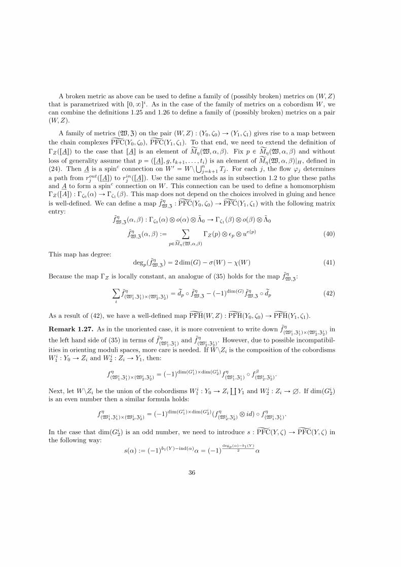
A broken metric as above can be used to define a family of (possibly broken) metrics on pW,Zqthat is parametrized with r0,8si. As in the case of the family of metrics on a cobordism W , wecan combine the definitions 1.25 and 1.26 to define a family of (possibly broken) metrics on a pairpW,Zq.

A family of metrics pW,Zq on the pair pW,Zq : pY0, ζ0q Ñ pY1, ζ1q gives rise to a map between

the chain complexes ĆPFCpY0, ζ0q, ĆPFCpY1, ζ1q. To that end, we need to extend the definition of

ΓZprAsq to the case that rAs is an element of ĂMηpW, α, βq. Fix p P ĂMηpW, α, βq and without

loss of generality assume that p “ prAs, g, tk`1, . . . , tiq is an element of ĂMηpW, α, βq|H , defined in(24). Then A is a spinc connection on W 1 “ W z

Ťnj“k`1 Tj . For each j, the flow ϕj determines

a path from routj prAsq to rinj prAsq. Use the same methods as in subsection 1.2 to glue these pathsand A to form a spinc connection on W . This connection can be used to define a homomorphismΓZprAsq : Γζ0pαq Ñ Γζ1pβq. This map does not depend on the choices involved in gluing and hence

is well-defined. We can define a map fηW,Z : ĆPFCpY0, ζ0q Ñ ĆPFCpY1, ζ1q with the following matrixentry:

fηW,Zpα, βq : Γζ0pαq b opαq b Λ0 Ñ Γζ1pβq b opβq b Λ0

fηW,Zpα, βq :“ÿ

pPĂMηpW,α,βq

ΓZppq b εp b ueppq (40)

This map has degree:degppf

ηW,Zq “ 2 dimpGq ´ σpW q ´ χpW q (41)

Because the map ΓZ is locally constant, an analogue of (35) holds for the map fηW,Z:

ÿ

i

fηpWi

1,Zi1qˆpW

i2,Z

i2q“ rdp ˝ f

ηW,Z ´ p´1qdimpGqfηW,Z ˝

rdp (42)

As a result of (42), we have a well-defined map ĆPFHpW,Zq : ĆPFHpY0, ζ0q Ñ ĆPFHpY1, ζ1q.

Remark 1.27. As in the unoriented case, it is more convenient to write down fηpWi

1,Zi1qˆpW

i2,Z

i2q

in

the left hand side of (35) in terms of fηpWi

1,Zi1q

and fηpWi

2,Zi2q

. However, due to possible incompatibil-

ities in orienting moduli spaces, more care is needed. If W zZi is the composition of the cobordismsW i

1 : Y0 Ñ Zi and W i2 : Zi Ñ Y1, then:

fηpWi

1,Zi1qˆpW

i2,Z

i2q“ p´1qdimpGi1qˆdimpGi2qfη

pWi1,Z

i1q˝ fβpWi

2,Zi2q.

Next, let W zZi be the union of the cobordisms W i1 : Y0 Ñ Zi

š

Y1 and W i2 : Zi ÑH. If dimpGi2q

is an even number then a similar formula holds:

fηpWi

1,Zi1qˆpW

i2,Z

i2q“ p´1qdimpGi1qˆdimpGi2qpfη

pWi2,Z

i2qb idq ˝ fη

pWi1,Z

i1q.

In the case that dimpGi2q is an odd number, we need to introduce s : ĆPFCpY, ζq Ñ ĆPFCpY, ζq inthe following way:

spαq :“ p´1qb1pY q´indpαqα “ p´1qdegppαq´b1pY q

2 α

36

where α is a generator of ĆPFCpY, ζq. The map s commutes with the cobordism maps up toa sign. For example, if pW,Zq is a family of metrics parametrized with G on the cobordismpW,Zq : pY0,Γ0q Ñ pY1,Γ1q, with Y0 and Y1 being connected, then:

s ˝ fηW,Z “ p´1qindpDW q`dimpGqfηW,Z ˝ s. (43)

For an odd dimensional family of metrics Gi2, we have:

fηpWi

1,Zi1qˆpW

i2,Z

i2q“ p´1qdimpGi1qˆdimpGi2qpfη

pWi2,Z

i2qb sq ˝ fη

pWi1,Z

i1q.

In the following, we study the cobordism map fηW,Z in two special cases. Suppose Z is an

embedded sphere in CP 2with self-intersection -1. Let D4 be a disc neighborhood of a point away

from Z and consider R :“ CP 2zD4. Equip the pair pR,Zq, as a cobordism from pS3,Hq to the

empty pair, with a metric that is cylindrical on the end. Let ĆPFCpR,Zq : ĆPFCpS3q Ñ Λ0 bethe cobordism map induced by an arbitrary homology orientation of R and the zero perturbation.The representation variety RpS3q consists of only one point α and b`pRq “ b1pRq “ 0. Therefore,the zero perturbation satisfies Hypothesis 1, and the moduli space MpRq consists of one spinc

connection for each choice of spinc structure. Any spinc structure s on R is uniquely determinedby the pairing of c1psq and Z which is an odd number. Let s2k`1 be the spinc structure that thispairing is equal to 2k` 1 and A2k`1 is the corresponding element of MpRq. The spinc connectionsA2k`1, A´2k´1 have the same energy and ΓZpA2k`1q “ ´ΓZpA´2k´1q. Furthermore, by Remark1.20 the orientation of the moduli space at these two points match with each other. Consequently,we have the following result, which is our main motivation to introduce plane Floer homology forcobordism pairs:

Lemma 1.28. The cobordism map ĆPFCpR,Zq is equal to zero.

Remark 1.29. Removing a ball neighborhood of a point in Z Ă CP 2produces a cobordism of

the pairs pR,ZzD2q from pS3, S1q to the empty pair. A similar argument as above shows thatĆPFCpR,ZzD2q “ 0.

Next, consider the cobordism U in Example 1.13 from Q to the empty 3-manifold. Extend Uto a cobordism of pairs pU,Zq : pQ,Hq Ñ pH,Hq by defining Z :“ S1. The family of metricsU in Example 1.13 determines a family of metrics pU,Zq on the pair pU,Zq. Fix a Morse-Smalefunction on RpQq with two critical points α of index 0 and α1 of index 1 such that neither of themis equal to h0 (defined in Example 1.13) or ´h0. Also fix a homology orientation for U and agenerator for opαq. By the characterization of moduli spaces in Example 1.13, the cobordism map

fU,Z : ĆPFCpQq Ñ Λ0, induced by the zero perturbation, sends the corresponding generator of opαqto:

c “8ÿ

i“0

˘p2k ` 1qup2k`1q2 P Λ0 (44)

for an appropriate choices of the signs. The ring element c can be regarded as an element of Λand independent of what the signs are it is invertible in Λ. On the other hand, fU,Z maps thesummand opα1q to zero.

37

Lemma 1.30. Consider pV :“ S1 ˆD3,Hq as a cobordism form pQ,Hq to the empty pair. Thenthere exists a homology orientation of V such that:

fU,Z “ c ¨ĆPFCpV q

Proof. Since MpV q “ RpQq and the outgoing end of V is empty, the cobordism map ĆPFCpV q, forappropriate choices of homology orientations of V and generators of opαq, maps the generator ofopαq to 1 P Λ0 and the summand opα1q to zero. This verifies the claim of the lemma.

Remark 1.31. Consider two 2-spheres S1 and S2. Then the cobordism U of Example 1.13 isdiffeomorphic to the plumbing of two disc bundles with Euler number -1 over these spheres. Thisdiffeomorphism can be chosen such that S1 is in correspondence with the previously defined S1,and S2 is sent to S11 with an orientation reversing map. Let pZ be the embedded surface in U thatis union of a fiber of the disc bundle over S1 and a fiber of the disc bundle over S2. The family ofmetrics U can be lifted to a family of metrics pU, pZq over the pair pU, pZq. The intersection qζ “ pZXQis equal to S1 ˆ tp, qu Ă Q – S1 ˆ S2 where p, q P S2 and the induced orientations on these twocircles are reverse of each other. Since the orientations of these two circles are different, there isan embedded annulus qZ in V such that its intersection with the boundary of V , identified with Q,is equal to qζ. Therefore, pV, qZq is another cobordism from pQ, qζq to the empty pair. The proof ofthe following relation is analogous to that of Lemma 1.30:

fU,pZ “ c ¨ĆPFCpV, qζq

2 Link Surgery Cube Complex

Suppose pC1, d1q and pC2, d2q are two (not necessarily Z-graded) chain complexes. A map f : C1 Ñ

C2 is an anti-chain map if:f ˝ d1 ` d2 ˝ f “ 0

Composition of two maps which are either chain map or anti-chain map is again either a chainmap or an anti-chain map. Two anti-chain maps f1, f2 : C1 Ñ C2 are chain homotopy equivalentif there is a map h : C1 Ñ C2 such that:

f2 ´ f1 “ h ˝ d1 ´ d2 ˝ h

A chain homotopy of chain maps is also defined in the standard way. Define CpRq to be thecategory whose objects are the collection of chain complexes over a fixed ring R. A morphismfrom pC1, d1q to pC2, d2q is represented by either a chain map or an anti-chain map and two suchmorphisms represent the same elements if they are chain homotopy equivalent.

Given a general category C, we can define the isomorphism equivalence relation on the objectsof C. That is to say, two objects are equivalent if there is an isomorphism between them. Theequivalence class of an object with respect to this relation is called the isomorphism class of thatobject. In the case of the category CpRq, the isomorphism class of an object is also called the chainhomotopy type of the corresponding chain complex.

38

Given a pair pY, ζq, the chain complex ĆPFCpY, ζq was associated with this pair in the previous

section. We use Λ as the coefficient ring in this section and hence ĆPFCpY, ζq is an object of CpΛq.We shall show that, for any framed link L in Y zζ, one can construct a new chain complex that

has the same chain homotopy type as ĆPFCpY, ζq. In subsection 2.1, starting with the pair pY, ζqand L, various families of metrics are introduced. These families of metrics are used in subsection2.2 to construct the new chain complex and to show that this chain complex has the same chainhomotopy type as ĆPFCpY, ζq.

2.1 Framed Links and Families of Metrics

Fix the lexicographical ordering on the lattice Zn which is induced by the standard ordering ofinteger numbers. For m “ pm1 . . . ,mnq P Zn, define:

|m|1 :“nÿ

i“1

mi |m|8 “ maxtm1, . . . ,mnu

Definition 2.1. A cube of dimension d in Zn consists of a pair pm,nq such that m ą n, |m ´

n|8 “ 1 and |m ´ n|1 “ d. A 1-dimensional (respectively, 2-dimensional) cube is called an edge(respectively, a face) of Zn. The set of edges and faces of Zn are denoted by Epnq and Fpnq .

Definition 2.2. A double-cube in Zn is a pair pm,nq such that m ą n, |m ´ n|8 “ 2, and theentries of m, n differ by 2 in exactly one instance. A triple-cube in Zn is a pair pm,nq such thatm ą n, |m ´ n|8 “ 3. Furthermore, we require that the entries of m, n differ by 3 in exactlyone instance and otherwise they differ by at most 1. Dimension of a double-cube (respectively,triple-cube) is equal to |m´ n|1 ´ 1 (respectively, |m´ n|1 ´ 2).

Suppose pY, ζq is a pair of a 3-manifold and an embedded closed 1-manifold. Let L “Ť

1ďiďnKi

be an oriented framed link with n connected components in Y zζ. The complement of a regularneighborhood of L in Y , denoted by Y L, is a 3-manifold with boundary

Ť

1ďiďn τi where τi isthe torus boundary of a neighborhood of Ki. The complement of a regular neighborhood of onlythe ith component is denoted by Y Ki . Since Ki is framed, τi has well-defined oriented longitudeand meridian and we will denote them by λi and µi. In particular, the orientation of τi “ BY

Ki

determined by the outward-normal-first convention agrees with the orientation determined by theordered pair tµi, λiu. Let γ0

i , γ1i , and γ2

i be oriented curves in τi in the homology class of λi,

´pλi ` µiq, and µi. We extend these curves to the family tγji ujPZ by requiring that this family is3-periodic in j. Given m “ pm1, . . . ,mnq P Zn, the closed 3-manifold Ym is defined to be the resultof the Dehn filling of Y L along the curves γmii . We will write Dm,i for the solid torus which isglued to Y L along τi. Note that γmi´1

i defines a framing of this solid torus. The 1-manifold ζm isequal to the union of ζ and

Ť

i ζm,i, where ζm,i is the core of Dm,,i if mi ” 0 mod 3, and is emptyotherwise. Fix a metric on Y L which is the standard product metric in the union

Ť

1ďiďn τi, andextend this to Ym by the standard metric on Dm,i.

For each pair pm,nq that m ě n, a cobordism of the pairs pWnm, Z

nmq : pYm, ζmq Ñ pYn, ζnq

can be defined as follows. Firstly let pm,nq be a 1-dimensional cube and the ith entry be the

39

Figure 2: A schematic picture of a 2-handle; the horizontal red line represents the core of the2-handle and the vertical red line is the representative of the co-core

only coordinate that m and n differs. In this case, define Wnm to be the elementary cobordism

from Ym to Yn given by attaching a 2-handle along Dm,i. More concretely, this cobordism can beconstructed as the union of r0, 1s ˆ Y Ki and the space:

H “ tpz1, z2q P C2 | |z1|, |z2| ď 1, |z1| ¨ |z2| ď1

2u

Boundary of H is the union of the following sets (Figure 2):

B0H “ tpz1, z2q P C2 | |z1| “ 1, |z2| ď1

2u B1H “ tpz1, z2q P C2 | |z1| ď

1

2, |z2| “ 1u

B2H “ tpz1, z2q P C2 | |z1|, |z2| ď 1, |z1| ¨ |z2| “1

2u

With the aid of the negative gradient flow of the Morse function |z1|2 ´ |z2|

2, the set B2H can beidentified with the product of the interval r0, 1s and the 2-dimensional torus. The space r0, 1sˆBY Ki

can be identified with the same space using the closed curves γmii and γmi´1i in BY Ki . The

cobordism Wnm is given by gluing r0, 1s ˆ Y Ki to H along these parts of their boundaries and

then adding the cylindrical ends. Thus Wnm is equal to the union of R ˆ Y Ki and H where

H :“ H Y Rď0 ˆ B0H Y Rě0 ˆ B1H. The 2-dimensional cobordism Znm : ζm Ñ ζn is determined

by the value of mi “ ni ` 1 mod 3. If mi ” 0 mod 3, then ζn,i is empty and Znm is the union of

Rˆ ζn and the following cobordism from ζm,i to the empty set:

tpz1, 0q | |z1| ď 1u Y Rď0 ˆ tz1, 0q | |z1| “ 1u Ă H Y Rď0 ˆ B0H (45)

If mi ” 1 mod 3, then ζm is empty and Znm is the union of R ˆ ζm and the following cobordism

from the empty set to ζn,i:

tp0, z2q | |z2| ď 1u Y Rě0 ˆ t0, z2q | |z2| “ 1u Ă H Y Rě0 ˆ B1H. (46)

40

. Finally, if mi ” 2 mod 3, then ζm,i and ζn,i are both empty and Znm is defined to be Rˆ ζm

For a general pair pm,nq, we can find a sequence m “ k0 ą k1 ą . . .kl´1 ą kl “ n such that|ki´ki`1|1 “ 1. In this case we define Wn

m “Wk1

k0˝Wk2

k1˝¨ ¨ ¨˝Wkl

kl´1, Zn

m “ Zk1

k0˝Zk2

k1˝¨ ¨ ¨˝Zkl

kl´1.

It is clear that the diffeomorphism type of pWnm, Z

nmq is independent of how we choose ki’s.

Lemma 2.3. For each pair pm,nq with m ě n, there exists a homology orientation opm,nq ofthe cobordism Wn

m such that if m ě k ě n, then the composition of opm,kq and opk,nq is equalto opm,nq. Furthermore, if o1pm,nq P opWn

mq is another series of homology orientations that hasthe same property, then there exists z : Zn Ñ t˘1u, such that:

o1pm,nq “ zpmqzpnqopm,nq. (47)

The function z is unique up to an overall sign.

Proof. The composition of homology orientations is associative and hence the first part of thislemma can be proved with the same argument as in [11, Lemma 6.1]. To prove the second part of thelemma, note that u, defined as the difference of o and o1, is a map from the set of pm,nq P ZnˆZn,with m ě n, to Z2Z that satisfies:

upm,nq “ upm,kq ` upk,nq

for m ě k ě n. This identity implies that u induces a simplicial co-cycle on Rn with respect tothe simplicial structure spelled out in [11]. Since Rn is contractible, there is a map z : Zn Ñ Z2Zsuch that:

upm,nq “ zpmq ´ zpnq

that is to say z satisfies (47).

The pairs pYm, ζmq and pWnm, Z

nmq are 3-periodic. That is to say, for any k P Zn we have the

natural identifications pYm`3k, ζm`3kq “ pYm, ζmq and pWn`3km`3k, Z

n`3km`3kq “ pW

nm, Z

nmq. However,

Lemma 2.3 does not guarantee that the homology orientations for the cobordisms Wnm and Wn`k

m`3k

are the same. Nevertheless, as a consequence of Lemma 2.3, there exists sk : Zn Ñ t˘1u such thatopm` 3k,n` 3kq “ skpmqskpnqopm,nq.

The rest of this subsection is devoted to define families of metrics on pWnm, Z

nmq, in the case

that pm,nq represents a cube, double-cube, or a triple-cube . An important ingredient of the proofof exact triangles in the next subsection is the existence of such families of metrics. Almost thesame families of metrics are described in [3] which in turn are based on those of [12] (cf. also [17]).Families of orbifold metrics with similar formal properties play a similar role in [11].

We start with the case that pm,nq is a d-dimensional cube in Zn and construct a familyof metrics of dimension d ´ 1. For the sake of simplicity of exposition, we assume that m “

p1, . . . , 1q ` n. The cobordism Wnm in this case is produced by gluing 2-handles along disjoint

curves in Ym. This cobordism can be decomposed to the union RˆY LY H1Y¨ ¨ ¨Y Hn. Here Hi isa copy of H corresponding to the ith component of L. The cobordism Zn

m also decomposes to theunion RˆζYZ1Y¨ ¨ ¨YZn where Rˆζ Ă RˆY L and Zi Ă Hi. The product metric on RˆY L and

41

the standard metrics on Hi determine a metric on pWnm, Z

nmq. Given ti P R for each 1 ď i ď n, we

can compose the gluing map of Hi to RˆY L with a translation in the R direction and produce a newmetric on pWn

m, Znmq. This family of metrics is parameterized by Rn. The fibers of this family over

pt1, . . . , tnq and pt1` t, . . . , tn` tq can be naturally identified with each other. Thus by consideringonly the metrics which are parametrized by Rn´1 “ tpt1, . . . , tnq P Rn |

ř

ti “ 0u, we can comeup with a more effective family of metrics. This family can be compactified to a family pWn

m,Znmq

by allowing the difference of some of the coordinates to be equal to 8. More precisely, pWnm,Z

nmq

is parametrized by a polyhedron Gnm such that a face of codimension i of Gn

m is determined by apartition of t1, . . . , nu to i ` 1 (labeled) sets A0 “ ta

01, . . . , a

0j0u, . . . , Ai “ ta

i1, . . . , a

ijiu. Roughly

speaking, this face parametrizes the set of points pt1, . . . , tnq that the entries with indices in Al`1

have larger values than those with indices in Al and in fact the difference is 8. In order to give amore detailed definition and for the sake of simplicity of exposition, assume that:

A0 “ t1, . . . , j0u A1 “ tj0 ` 1, . . . , j0 ` j1u . . . Ai “ tpi´1ÿ

l“0

jlq ` 1, . . . , n “iÿ

l“0

jlu

and for 1 ď l ď i define kl to be:

kl :“ p 1, . . . , 1loomoon

j0`¨¨¨`jl´1

, 0, . . . , 0loomoon

jl`¨¨¨`ji

q ` n

Then closure of the corresponding face of Gnm can be identified with Gki

m ˆ Gki´1

kiˆ ¨ ¨ ¨ ˆ Gn

k1. A

point in this face has the form ppt1, . . . , tj0q, ptj0`1, . . . , tj0`j1q, . . . , ptpři´1l“0 jlq`1, . . . , tnqq such that

tj0`¨¨¨`jl´1`1 ` ¨ ¨ ¨ ` tj0`¨¨¨`jl “ 0 for each l. Intersection of a neighborhood of this point and theinterior of Gn

m parametrizes the normalized version of the points of the following form:

pt11, . . . , t1j0 , t

1j0`1 `M1, . . . , t

1j0`j1 `M1, t

1j0`j1`1 `M1 `M2, . . . ,

t1při´1l“0 jlq`1

`M1 ` ¨ ¨ ¨ `Mi, . . . , t1n `M1 ` ¨ ¨ ¨ `Miq

where t1k is a real number close to tk and Mj ’s are large real numbers. Here the normalization of theabove element of Rn is produced by subtracting a constant real number from all the entries suchthat the summation of the entries is equal to zero. A point in the interior of this face parametrizesa broken metric on pWn

m, Znmq with a cut along pYk1

, ζk1q Y ¨ ¨ ¨ Y pYki , ζkiq. In particular, a face of

co-dimension 1 of Gnm has the form Gk

m ˆ Gnk where k “ I ` n, I P t0, 1un, and k ‰ m,n. The

restriction of the family of metrics to this face is pWkm,Z

kmq ˆ pW

nk,Z

nkq.

Lemma 2.4. The polyhedron Gnm can be oriented for all cubes pm,nq such that for each co-

dimension 1 face Gkm ˆ Gn

k of Gnm the orientation given by the outward-normal-first convention

differs from the product orientation by p´1qdimpGkmq¨dimpGn

kq`|n|1 . Moreover, in the case that pm,nqis an edge, the orientation of the point Gn

m is given by the following sign:

sgnpm,nq :“ p´1qři0´1i“1 mi (48)

where i0 is the unique place that m and n differ.

42

Proof. In [11], the polyhedrons Gnm are oriented such that the boundary orientation on the codi-

mension 1 face Gkm ˆ Gn

k of Gnm differs from the product orientation by p´1q|m´k|1´1. As it is

shown there, this orientation can be fixed such that the orientation of Gnm for an edge is given by

the following sign:

p´1qřni“i0

mi

where i0 is defined above. In order to produce the desired orientation, multiply this orientation ofGn

m by p´1qsgn1pm,nq, where:

sgn1pm,nq :“|m´ n|1p|m´ n|1 ´ 1q

2` |m|1

If pm,nq is a d-dimensional double-cube, then a family of metrics on pWnm, Z

nmq, parametrized

by a polyhedron Nnm, can be constructed in a similar way. We explain the construction of this

family in the special case that m “ p2, 1, . . . , 1q`n. The general case can be treated similarly. Thecobordism Wn

m can be decomposed as RˆY LYDY H2Y¨ ¨ ¨Y Hn, where D is produced by gluingtwo 2-handles H1

1 , H21 along B1H

11 “ B0H

21 and then adding the cylindrical ends Rď0 ˆ B0H

11 and

Rě0ˆB1H21 . Note that BD is the same as RˆĞBY K1 . An elementtary but important observation is

that our choices of framings produce a 2-sphere S with self-intersection -1 which is the union of theco-core disc of H1 (i.e. tpz1, z2q P H

11 | z1 “ 0u) and the core of H2 (i.e. tpz1, z2q P H

21 | z2 “ 0u).

Consequently, a regular neighborhood of S denoted by R is diffeomorphic to ĚCP 2zD4. We will

write T for the boundary of R. The space D can be equipped with a family of metrics that isparametrized by R. For τ P Rě0, insert the cylinder r´τ, τ s ˆ B1H

11 “ r´τ, τ s ˆ B0H

21 between H1

1

and H21 and then glue the cylindrical ends. For τ P Rď0, insert the cylinder rτ,´τ s ˆ T between

R and its complement. In summary, for positive values of τ , we stretch along the solid torusB1H

11 “ B1H

21 and for negative values of τ , we stretch along the boundary of R. For this family of

metrics, pin down an isomorphism between the boundary of D with RˆBĘY K1 in the following way.For τ P Rě0, let r´τ, τ s ˆ BpB1H

11 q, inside the inserted cylinder, be identified with r´τ, τ s ˆ BĘY K1

and extend this identification in an obvious way. For τ P Rď0, the corresponding metrics form aconstant family on the boundary of D and let the isomorphism be the same as the isomorphismfor τ “ 0. For a given pt1, . . . , tnq P Rn, glue the handle Hi to R ˆ Y L such that the gluing mapis determined by ti. Furthermore, glue the metric corresponding to t1 on D to R ˆ Y L with theabove identification. As in the case of cubes, this family of metrics can be compactified to a familyof (possibly broken) metrics Wn

m parametrized by a polyhedron Nnm.

The 2-dimensional cobordism Znm : ζm Ñ ζn can be decomposed as the union Rˆ ζYZYZ2Y

¨ ¨ ¨ Y Zn where R ˆ ζ Ă R ˆ Y L, Z Ă D, Z2 Ă H2, and so on. For i ě 2, Zi Ă Hi has the sameform as in the case of cubes; it is either empty, or of the form (45), or of the form (46). There arethree possibilities for Z depending on m1 mod 3. If mi ” 0 mod 3, then Z is a disc cobordismfrom ζm,1 to the empty set. The disc intersects S in exactly one point. Therefore, Z intersectsboundary of R in a circle. On the other hand, the intersection with B1H

11 “ B0H

21 is empty. A

similar discussion applies to the case that mi ” 2 mod 3. If mi ” 1 mod 3, then Z “ S andintersection of Z and B1H

11 “ B0H

21 is a circle while S X BR “ H. In each of these cases, extend

the family of metrics on D in the previous paragraph to a family of metrics for the pair pD,Zq by

43

inserting r´τ, τ s ˆ pZ X B1H11 q (respectively, rτ,´τ s ˆ pZ X BRq) in the inserted r´τ, τ s ˆ B1H

11

(respectively, rτ,´τ s ˆ BR) for τ ě 0 (respectively, τ ď 0). Use this family of metrics to extendWn

m to a family of metrics pWnm,Z

nmq on the pair pWn

m, Znmq, parametrized by Nn

m. Codimension1 faces of this polyhedron parametrized the following broken metrics:

• broken metrics along the cut pYk, ζkq where m ą k ą n. This case can be divided to threedifferent cases:

(a) k “ p0, k2, . . . knq; this face can be identified with the family parametrized by NkmˆG

nk

(b) k “ p1, k2, . . . knq; this face can be identified with the family parametrized by GkmˆG

nk

(c) k “ p2, k2, . . . knq; this face can be identified with the family parametrized by GkmˆN

nk

• broken metrics along the cut pT,Z X T q. This face will be denoted by Inm

The family of broken metrics in the second bullet is determined by families of metrics on the twoconnected components of pWn

mzT,ZzT q. The family of metrics on the component pR,Z X Rq iseither the same as the one used in Lemma 1.28 or that of Remark 1.29.

Suppose an orientation of the polyhedrons Gnm, satisfying the assumption of Lemma 2.4 is fixed.

Then the following lemma sets our convention for the orientation of Nnm:

Lemma 2.5. The polyhedron Nnm can be oriented for all double-cubes pm,nq such that for each

co-dimension 1 face AkmˆB

nk of Nn

m, in which A,B P tG,Nu, the orientation given by the outward-

normal-first convention differs from the product orientation by p´1qdimpAkmq¨dimpBn

k q`|n|1 .

Proof. As in Lemma 2.4, we can change the orientation of Nnm, defined in [11], to produce the

desired orientation of the polyhedron Nnm.

For a d-dimensional triple-cube pm,nq, a pd ` 1q-dimensional family of metrics parametrizedby a polyhedron Kn

m is defined in an analogous way. For the simplicity of the exposition, weexplain the construction in the special case that m “ p3, 1, . . . , 1q ` n. There is a decompositionRˆY LYFYH2Y¨ ¨ ¨YHn of the cobordism Wn

m with F being the result of composing Rď0ˆB0H11 ,

the handles H11 , H2

1 , H31 , and finally Rě0 ˆ B1H

31 . There is also a decomposition of Zn

m as theunion Rˆ ζ YB Y Z2 Y ¨ ¨ ¨ Y Zn where Rˆ ζ Ă Rˆ Y L, B Ă F , Z2 Ă H2, and so on.

The co-core of the handle Hi1 and the core of Hi`1

1 produces a 2-sphere Si for i “ 1, 2 (S1 iswhat we called S before). Regular neighborhoods of S1, S2, denoted by R1, R2, are diffeomorphic

to ĚCP 2zD4. We will also write T1, T2 for the boundaries of R1, R2. The spheres S1 and S2

intersect each other in exactly one point, and hence a neighborhood of their union, denoted by U ,is diffeomorphic to D2 ˆ S2#CP 2. The boundary of U is also denoted by Q. We assume that Ucontains R1 and R2. In the list:

E1 “ B1H21 “ B0H

31 E2 “ B1H

11 “ B0H

21 E3 “ T2 E4 “ Q E5 “ T1

each 3-manifold Ei is disjoint from Ei´1 and Ei`1 where E0 “ E5 and E6 “ E1. In fact removingEi disconnects F , and Ei`1, Ei´1 are both in the same connected component of F zEi. For each

44

i, construct a family of metrics on F that are broken along Ei, and are parametrized by r´8,8s,in the following way. Firstly remove Ei and then for τ P r0,8s (respectively, τ P r´8, 0s) removeEi`1 (respectively, Ei´1) and insert r´τ, τ s ˆ Ei`1 (respectively, rτ,´τ s ˆ Ei´1). The metricscorresponding to 8 and ´8 are broken along Ei`1 and Ei´1, respectively. Furthermore, thisfamily of metrics is constant on the connected component of F zEi that does not contain Ei´1 andEi`1. Example 1.13 determines one such family for i “ 4. As in the case of double-cubes, thesefamilies can be lifted to families of metrics on the pair pF,Bq.

These five families of metrics consist of broken metrics parametrized by the edges of a pentagon,denoted by p. Extend these metrics into the interior of p in an arbitrary way. This extended familyon pF,Bq, and the metrics on pRˆ Y L,Rˆ ζq, pHi, Ziq generate a family of metrics on pWn

m, Znmq

parametrized by Rn´1ˆp. This family can be compactified by adding broken metrics. The resultingfamily, pWn

m,Znmq, is parametrized by a polyhedron Kn

m. Codimension 1 faces of this polyhedronparametrize the following families of metrics:

• broken metrics along the cut pYk, ζkq where m ą k ą n. This case can be divided to fourdifferent sub-cases:

(a) k “ p0, k2, . . . knq; this face can be identified with the family parametrized by KkmˆG

nk

(b) k “ p1, k2, . . . knq; this face can be identified with the family parametrized by NkmˆG

nk

(c) k “ p2, k2, . . . knq; this face can be identified with the family parametrized by GkmˆN

nk

(d) k “ p3, k2, . . . knq; this face can be identified with the family parametrized by GkmˆK

nk

• broken metrics along the cut pQ,B XQq. This face will be denoted by Qnm

• broken metrics along the cut pT1, B X T1q. This face will be denoted by pI1qnm

• broken metrics along the cut pT2, B X T2q. This face will be denoted by pI2qnm

Orientation of the polyhedrons Knm can be fixed such that these orientations are compatible

with the orientations of Gnm and Nn

m from Lemmas 2.4 and 2.5 in the following way:

Lemma 2.6. The polyhedron Knm can be oriented for all triple-cubes pm,nq such that for each

co-dimension 1 face Akm ˆ Bn

k of Knm, in which A,B P tG,N,Ku, the orientation given by the

outward-normal-first convention differs from the product orientation by p´1qdimpAkmq¨dimpBn

k q`|n|1 .

The families broken along T1 and T2 are similar to the family parametrized by Inm in the case ofdouble-cubes. The family of metrics broken along Q is determined by an p|m´n|1´3q-dimensional

family of metrics on pWnmzU,Z

nmzUq, denoted by rQn

m and a family on pU,B XUq parametrized bya closed interval I. The former family is the compactification of a family parametrized by Rn´1

such that a typical element in the family is given by gluing R ˆ Y L, with the product metric, tothe translations of Hi’s, with the standard metrics, and F zU , with a fixed metric. The family ofmetrics on pU,B X Uq is one of the families introduced in Example 1.13 and Remark 1.31. Note

that an orientation of rQnm can be fixed such that the product orientation on rQn

m ˆ I agrees withthe boundary orientation, induced by the orientation of Kn

m from Lemma 2.6.

45

Let V be a copy of S1ˆD3 and C is empty or the surface introduced in Remark 1.31, dependingon whether pU,B X Uq is the pair of Example 1.13 or Remark 1.31. Glue a copy of pV,Cq to

pWnmzU,Z

nmzUq, along the boundary component Q, in order to form a pair p|Wn

m,qZnmq. Note that

Gluing pV,Cq to pF zU,BzUq Ă pWnmzU,Z

nmzUq gives the product pair pRˆB0H

11 ,RˆpB0H

11Xζmqq.

Therefore, p|Wnm,

qZnmq is diffeomorphic to pWn

m1 , Znm1q where m1 “ pm1 ´ 3,m2, . . . ,mnq. Fix

homology orientations of U and V such that the assertion of Lemma 1.31 holds. Then thesehomology orientations and the homology orientation of Wn

m can be utilized to define a homology

orientation for |Wnm by requiring:

op|Wnmq “ op|Wn

mzV, V q opWnmq “ opWn

mzU,Uq op|WnmzV q “ opWn

mzUq

Lemma 2.7. Suppose pm,nq is a triple-cube and m ě k,k1 ě n such that pm,kq and pk1,nq are

triple-cubes, i.e., pk,nq and pm,k1q are cubes. Then the composition |Wkm ˝W

nk and Wk1

m ˝|Wnk1 are

diffeomorphic to |Wnm. Furthermore, the homology orientations of these cobordisms are related via

the following relations:

op|Wnmq “ p´1q

indpDWnkqop|Wk

m,Wnk q “ opWk

m,|Wn

k q (49)

Proof. The claim about the diffeomorphisms follows from the fact that Wnm and the compositions

Wkm ˝W

nk and Wk1

m ˝Wnk1 are diffeomorphic to each other. The relationship between the homology

orientations of Wnm and Wk

m ˝Wnk can be verified as follows:

op|Wnm, U, Uq “ op|Wn

mzV, V, U, Uq “ opWnmzU,U, V, Uq

“ opWnm, V, Uq “ opWk

m,Wnk , V, Uq

“ opWkmzU,U,W

nk , V, Uq

“ p´1qindpDWn

kqop|Wk

mzV, V,Wnk , U, Uq

“ p´1qindpDWn

kqop|Wk

m,Wnk , U, Uq ùñ

op|Wnmq “ p´1q

indpDWnkqop|Wk

m,Wnk q

Here we use indpDU q “ 0 and indpDV q “ 1. The other identity in (49) can be checked similarly.

The family of metrics on pWnmzU,Z

nmzUq, parametrized by rQn

m, and a fixed metric with a

cylindrical end on pV,Cq determine a family of broken metrics on p|Wnm,

qZnmq parametrized by rQn

m.However, we will write sQn

m for the parametrizing set of this family in order to distinguish betweenthe families. Assume that again m “ n` p3, 1, . . . , 1q. Then an element of this family is a metricon:

p|Wnm “ Rˆ Y L Y Rˆ B0H

11 Y H2 Y ¨ ¨ ¨ Y Hn, qZ

nm “ Rˆ ζ Y Rˆ pB0H

11 X ζmq Y Z2 Y ¨ ¨ ¨ Y Znq

where the metric on pRˆB0H11 ,RˆpB0H

11 X ζmqq is broken along Q. Replacing this broken metric

with the standard product metric constructs another family of metrics on p|Wnm,

qZnmq, parametrized

with the set sQnm. To emphasize the difference, we will denote the parametrizing set by pQn

m. By

46

construction, it is clear that one can interpolate between the families parametrized by sQnm and

pQnm; that is to say, there exists a family parametrized by I ˆ sQn

m such that t0u ˆ sQnm agrees with

pQnm and t1u ˆ sQn

m is equal to sQnm. The orientation of rQn

m determines an orientation of Qnm which

can be used to equip IˆQnm with the product orientation. Also, the codimension 1 faces of IˆQn

m

are given as follows:

• broken metrics along the cut pYk, ζkq where m ą k ą n and k “ p0, k2, . . . knq; this face canbe identified with pI ˆ sQk

mq ˆGnk

• broken metrics along the cut pYk, ζkq where m ą k ą n and k “ p3, k2, . . . knq; this face canbe identified with Gk

m ˆ pI ˆsQnkq

• the family of metrics sQnm

• the family of metrics pQnm

Lemma 2.8. For any triple-cube pm,nq, the fixed orientation of I ˆ sQnm produces the following

orientation of its faces:

• the boundary orientation on pI ˆ sQkmq ˆG

nk differs from the product orientation by

p´1qdimpKkmq¨dimpGn

kq`|n|1`1`|k´n|1 “ p´1qdimpIˆ sQkmq¨dimpGn

kq`|n|1

• the boundary orientation on Gkm ˆ pI ˆ

sQnkq differs from the product orientation by

p´1qdimpGkmq¨pdimpKn

k q`1q`|n|1`1`|m´k|1 “ p´1qdimpGkmq¨dimpIˆ sQk

mq`|n|1`1`|m´k|1

• the boundary orientation on sQnm “ t1u ˆ sQn

m is the same as the fixed orientation of sQnm;

• the boundary orientation on pQnm “ t0u ˆ sQn

m is the reverse of the fixed orientation of sQnm.

Proof. It suffices to prove the same claim when I ˆ Qnm in the statement of the lemma is replaced

with Iˆ rQnm. The polyhedrons rQn

mˆI andKkmˆG

nk, with k “ p0, k2, . . . knq, are codimension 1 faces

of Knm. Intersection of these two polyhedrons is p rQk

mˆIqˆGnk which has codimension 1 with respect

to rQnm ˆ I and Kk

m ˆGnk. The polyhedrons rQn

m ˆ I and Kkm ˆG

nk inherit boundary orientations

form Kkm which in turn induce two orientations on p rQk

m ˆ Iq ˆGnk. These two orientations differ

by a sign. Another way to orient p rQkm ˆ Iq ˆ Gn

k is to consider it as the product of rQkm ˆ I

and Gnk. This orientation is the same as the boundary orientation by considering p rQk

m ˆ Iq ˆGnk

as a codimension 1 face of Kkm ˆ Gn

k where the latter is equipped with the product orientation.

Therefore, Lemma 2.5 states that the product and the boundary orientations of p rQkmˆ IqˆG

nk, as

a face of rQnmˆ I differ by p´1qdimpKk

mq¨dimpGnkq`|n|1`1. This proves the claim about the orientation

of the faces in the first bullet. A similar argument verifies the claim for the faces in the secondbullet. The assertions about the orientations of the faces in the last two bullets are trivial.

47

2.2 Exact Triangles

Suppose a pair pY, ζq and a framed link L is fixed as in the previous subsection. Then we can formthe pairs pYm, ζmq and the cobordisms of the pairs pWn

m, Znmq. Use Lemma 2.3 to fix homology

orientations for the cobordisms Wnm. For each representation variety RpYmq, fix a Morse-Smale

function fm such that fm`3k “ fm for any k P Zn. For a cube, double-cube, or a triple-cube pm,nq,we constructed a family of metrics pWn

m,Znmq on the pair pWn

m, Znmq. Since the parametrizing sets

for these families are contractible, the homology orientation for Wnm determines an orientation of

indpWnm, G

nmq, indpWn

m, Nnmq or indpWn

m,Knmq depending on whether pm,nq is a cube, double-

cube, or a triple-cube.

Fix a perturbation ηnm for the family pWnm,Z

nmq such that Hypothesis 1 holds. Thus the map

fηnmWn

m,Znm

is well-defined. To simplify our notation, we denote this cobordism map by fGnm

, fNnm

or fKnm

when pm,nq is a cube, double-cube, or triple-cube, respectively. We also require that theinduced perturbation for the families Inm, pI1q

nm, pI2q

nm and Qn

m, are equal to zero on R, R1, R2

and U , respectively. We also assume that ηnm is equal to ηn`3km`3k for any k P Zn.

Given a cube pm,nq, an application of (42) with the aid of Lemmas 2.3 and 2.4 to the familyof metrics parametrized by Gn

m gives:

ÿ

mąkąn

p´1q|n|1 fGnk˝ fGk

m“ dn ˝ fGn

m` p´1q|m´n|1 fGn

m˝ dm

where dk is the differential on the complex ĆPFCpYk, ζkq. If we set the convention that fGkk

is

equal to p´1q|k|1`1dk, then the above identity can be rewritten as:

ÿ

měkěn

fGnk˝ fGk

m“ 0 (50)

This relation states that the following is a chain complex:

˜

Cnm :“

à

měkěn

ĆPFCpYk, ζkq, dnm :“ pfGk1

kqměkěk1ěn

¸

For m “ pm1, . . . ,mn´1q P Zn´1 and i P Z, let mpiq :“ pi,m1, . . . ,mn´1q P Zn be given as the

juxtaposition of i and m. Given a cube pm,nq in Zn´1 and i P Z, define gnpiqmpiq : C

npiqmpiq Ñ C

npi´1qmpi´1q

by the following matrix presentation:

gnpiqmpiq :“ pf

Gk1pi´1q

kpiq

qměkěk1ěn

By (50), gnpiqmpiq is an anti-chain map, namely, we have the following identity:

dnpi´1qmpi´1q ˝ g

npiqmpiq ` g

npiqmpiq ˝ d

npiqmpiq “ 0

48

In general, given an anti-chain map g : pC, dq Ñ pC 1, d1q we can form the mapping cone chaincomplex Conepgq defined in he following way:

Conepgq :“ pC ‘ C 1 ,

ˆ

d 0g d1

˙

q

For the anti-chain map gnpiqmpiq, the chain complex Conepg

npiqmpiqq is clearly the same as pC

npi´1qmpiq , d

npi´1qmpiq q.

The heart of this paper lies in the following theorem:

Theorem 2.9. The chain complexes pCnpiqmpiq, d

npiqmpiqq and Conepg

npi´1qmpi´1qq have the same chain ho-

motopy type.

An immediate corollary of Theorem 2.9 is that the chain complex pCnm, d

nmq is a new chain

complex for the plane Floer homology of an appropriate pair:

Corollary 2.10. Let pm,nq be a cube and p “ 2m´n. Then the chain complexes pĆPFCpYp, ζpq, dpqand pCn

m, dnmq have the same chain homotopy type.

Proof. For the simplicity of the exposition, assume that p “ p2, . . . , 2q, m “ p1, . . . , 1q, n “

p0, . . . , 0q. By Theorem 2.9, pCnm, d

nmq and pCn1

m1 , dn1

m1q have the same chain homotopy type whenm1 “ p2, 1, . . . , 1q, n1 “ p2, 0, . . . , 0q. By repeating this application of Theorem 2.9, we can show

that pĆPFCpYp, ζpq, dpq and pCnm, d

nmq have the same chain homotopy type.

Consider the grading on pCnm, d

nmq that is defined to be equal to |k|1 on the summand ĆPFCpYk, ζkq

of Cnm. The differential dnm does not increase the grading. Therefore, we can use this filtration to

produce a spectral sequence:

Corollary 2.11. There is a spectral sequence with the first pageÀ

kPt0,1unĆPFHpYk, ζkq that abuts

to ĆPFHpY, ζq. The differential in the first page can be identified withÀ

p´1qsgnpk,k1qĆPFHpWk1

k , Zk1

k q.Here the sum is over all the edges of the cube t0, 1un and sgnpk,k1q is defined in (48).

Proof. The definition of the filtration implies the first part. The second part is the result of Lemma2.4.

The following algebraic lemma underlies our strategy of proving Theorem 2.9 (cf. [16, 11]):

Lemma 2.12. For i P Z, let pCi, diq be a chain complex and gi : Ci Ñ Ci´1 be an anti-chain map.For each i, suppose there are ni : Ci Ñ Ci´2 and ki : Ci Ñ Ci´3 such that:

gi´1 ˝ gi ` di´2 ˝ ni ` ni ˝ di “ 0 (51)

andni´1 ˝ gi ` gi´2 ˝ ni ` di´3 ˝ ki ` ki ˝ di “ qi (52)

where qi : Ci Ñ Ci´3 is an isomorphism. Then Ci and Conepgi´1q have the same chain homotopytype.

49

Proof. The following maps:

φi :“ pgi, niq : Ci Ñ Conepgi´1q ψi :“

ˆ

ni´1

gi´2

˙

: Conepgi´1q Ñ Ci´3 (53)

are anti-chain maps. We also have:

ψi ˝ φi „h qi φi ˝ ψi`3 „h

ˆ

qi`2 0ni ˝ ni`2 ` ki`1 ˝ gi`2 ` gi´1 ˝ ki`2 qi`1

˙

(54)

where the homotopies are given by the following maps:

ki

ˆ

ki`2 ni`1

0 ki`1

˙

(55)

The homotopies in (54) show that ψi ˝ φi and φi ˝ ψi`3 are homotopic to isomorphisms. Conse-quently, φi : Ci Ñ Conepgi´1q is a homotopy equivalence.

Proof of Theorem 2.9. In order to utilize Lemma 2.12, we need to construct maps nnpiqmpiq : C

npiqmpiq Ñ

Cnpi´2qmpi´2q and k

npiqmpiq : C

npiqmpiq Ñ C

npi´3qmpi´3q such that the constructed maps satisfy the relations (57) and

(52). For each i P Z, the pair pmpiq,npi´ 2qq determines a double-cube in Zn, and hence we can

consider the family of metrics parametrized by Nnpi´2qmpiq on the pair cobordism pW

npi´2qmpiq , Z

npi´2qmpiq q.

This family defines the map:

fN

npi´2q

mpiq

: ĆPFCpYmpiq, ζmpiqq Ñ ĆPFCpYnpi´2q, ζnpi´2qq

Identity (42), Lemma 2.5 and the characterization of codimension 1 faces of Nnpi´2qmpiq imply that:

fInpi´2q

mpiq

`ÿ

měkąn

p´1q|n|1`ifG

npi´2q

kpi´2q

˝ fN

kpi´2q

mpiq

`ÿ

měkěn

p´1q|n|1`ifG

npi´2q

kpi´1q

˝ fG

kpi´1q

mpiq

`

`ÿ

mąkěn

p´1q|n|1`ifN

npi´2q

kpiq

˝ fG

kpiq

mpiq

“ dnpi´2q ˝ fNnpi´2q

mpiq

´ p´1q|m´n|1`1fN

npi´2q

mpiqη ˝ dmpiq

According to Lemma 1.28, the cobordism map fInpi´2q

mpiq

vanishes. We can use this and the convention

that fGkk“ p´1q|k|1`1dk to simplify slightly:

ÿ

měkěn

fG

npi´2q

kpi´2q

˝ fN

kpi´2q

mpiq

`ÿ

měkěn

fG

npi´2q

kpi´1q

˝ fG

kpi´1q

mpiq

`ÿ

měkěn

fN

npi´2q

kpiq

˝ fG

kpiq

mpiq

“ 0 (56)

If we define a map nnpiqmpiq : C

npiqmpiq Ñ C

npi´2qmpi´2q as:

nnpiqmpiq :“ pf

Nk1pi´2q

kpiq

qměkěk1ěn

50

then (56) implies:

gnpi´1qmpi´1q ˝ g

npiqmpiq ` d

npi´2qmpi´2q ˝ n

npiqmpiq ` n

npiqmpiq ˝ d

npiqmpiq “ 0 (57)

We can repeat the above construction for the family of metrics parametrized by Knpi´3qmpiq and

define the map:fK

npi´3q

mpiq

: ĆPFCpYmpiq, ζmpiqq Ñ ĆPFCpYnpi´3q, ζnpi´3qq

The description of the boundary of Knpi´3qmpiq provides us with the following relation:

fpI1q

npi´3q

mpiq

`fpI2q

npi´3q

mpiq

`fQ

npi´3q

mpiq

`p´1q|n|1`i´3pÿ

měkąn

fG

npi´3q

kpi´3q

˝fK

kpi´3q

mpiq

`ÿ

měkěn

fG

npi´3q

kpi´2q

˝fN

kpi´2q

mpiq

`

`ÿ

měkěn

fN

npi´3q

kpi´1q

˝fG

kpi´1q

mpiq

`ÿ

mąkěn

fK

npi´3q

kpiq

˝fG

kpiq

mpiq

q “ dnpi´3q˝fKnpi´3q

mpiq

´p´1q|m´n|1`2fK

npi´3q

mpiq

˝dmpiq

Again, the first two terms in the left hand side are zero by Lemma 1.28. Therefore, the aboverelation can be rewritten as follows:ÿ

měkěn

fG

npi´3q

kpi´3q

˝fK

kpi´3q

mpiq

`ÿ

měkěn

fG

npi´3q

kpi´2q

˝fN

kpi´2q

mpiq

`ÿ

měkěn

fN

npi´3q

kpi´1q

˝fG

kpi´1q

mpiq

`ÿ

měkěn

fK

npi´3q

kpiq

˝fG

kpiq

mpiq

“ p´1q|n|1`ifQ

npi´3q

mpiq

(58)

Define knpiqmpiq, q

npiqmpiq : C

npiqmpiq Ñ C

npi´3qmpi´3q as follows:

knpiqmpiq :“ pf

Kk1pi´3q

kpiq

qměkěk1ěn qnpiqmpiq :“ pp´1q|k

1|1`if

Qk1pi´3q

kpiq

qměkěk1ěn

then (58) gives rise to the following identity:

dnpi´3qmpi´3q ˝ k

npiqmpiq ` g

npi´2qmpi´2q ˝ n

npiqmpiq ` n

npi´1qmpi´1q ˝ g

npiqmpiq ` k

npiqmpiq ˝ d

npiqmpiq “ q

npiqmpiq

As the final step of the proof, we show that qnpiqmpiq is homotopy equivalent to an isomorphism from

Cnpiqmpiq to C

npi´3qmpi´3q. Using Lemma 1.30 and Remark 1.27, it can be shown:

fQ

npi´3q

mpiq

“ p´1q|m´n|1c ¨ s ˝ fsQnpi´3q

mpiq

(59)

where fsQnpi´3q

mpiq

is the map for the pair p|Wnpi´3qmpiq , qZ

npi´3qmpiq q. Furthermore, the family of metrics

I ˆ sQnpi´3qmpiq defines a cobordism map and with the aid of (42) and Lemmas 2.7 and 2.8, we can

derive the following identity:

ÿ

měkěn

p´1q|n|1`i`1`indpDpWnpi´3q

kpi´3qqfG

npi´3q

kpi´3q

˝ fIˆ sQ

kpi´3q

mpiq

` p´1q|n|1`|m´k|1`ifIˆ sQ

npi´3q

kpiq

˝ fG

kpiq

mpiq

“ fpQnpi´3q

mpiq

´ fsQnpi´3q

mpiq

51

Post-composing with s and using (43) let us to rewrite above identity as:

ÿ

měkěn

fG

npi´3q

kpi´3q

˝ pp´1q|m´k|1c ¨ s ˝ fIˆ sQ

kpi´3q

mpiq

q ` pp´1q|k´n|1c ¨ s ˝ fIˆ sQ

npi´3q

kpiq

q ˝ fG

kpiq

mpiq

“

“ p´1q|m|1`ic ¨ s ˝ fpQnpi´3q

mpiq

´ p´1q|m|1`ic ¨ s ˝ fsQnpi´3q

mpiq

(60)

Define knpiqmpiq : C

npiqmpiq Ñ C

npi´3qmpi´3q and q

npiqmpiq : C

npiqmpiq Ñ C

npi´3qmpi´3q as follows:

knpiqmpiq :“ pp´1q|k´k1|1c ¨ s ˝ f

Iˆ sQk1pi´3q

kpiq

qměkěk1ěn

qnpiqmpiq :“ pp´1q|k|1`ic ¨ s ˝ f

pQk1pi´3q

kpiq

qměkěk1ěn

Identity (60) gives rise to the following chain homotopy:

dnpi´3qmpi´3q ˝ k

npiqmpiq ` k

npiqmpiq ˝ d

npiqmpiq “ q

npiqmpiq ´ q

npiqmpiq

Finally, with knpiqmpiq “ k

npiqmpiq ` k

npiqmpiq we have:

dnpi´3qmpi´3q ˝ k

npiqmpiq ` g

npi´2qmpi´2q ˝ n

npiqmpiq ` n

npi´1qmpi´1q ˝ g

npiqmpiq ` k

npiqmpiq ˝ d

npiqmpiq “ q

npiqmpiq

which is the analogue of (52), if we can show that qnpiqmpiq is an isomorphism. If m ‰ n, the

family of metrics parametrized by pQnpi´3qmpiq admits a faithful R-action. Therefore, in this case we

can arrange the involved perturbation terms in the definition of pQnpi´3qmpiq such that the dimension

of the non-empty moduli spaces is at least one. Thus if m ‰ n, then with these perturbation

terms fpQnpi´3q

mpiq

“ 0. If m “ n, the family of metrics pQnpi´3qmpiq consists of the product metric on

p|Wnpi´3qmpiq , qZ

npi´3qmpiq q – pI ˆ Ym, I ˆ ζmq. However, the fixed homology orientation of this cobordism

and the orientation of the point pQmpi´3qmpiq might not be the trivial ones. Consequetly, f

pQnpi´3q

mpiq

is

equal to ˘c ¨s. Therefore, qnpiqmpiq is indeed an isomorphism of the complexes C

npiqmpiq and C

npi´3qmpi´3q.

3 Classical Links

A classical link is a link embedded in S3 (or equivalently R3). Let K be an oriented classical link.

Then we can form ΣpKq, the branched double cover of S3 branched along K. Clearly, ĆPFHpΣpKqqis an invariant of K that is functorial in the following sense. For classical links K0 and K1, letS : K0 Ñ K1 be a (not necessarily orientable) link cobordism embedded in I ˆ S3 such thatS X ptiu ˆ S3q “ Ki for i P t0, 1u. Then ΣpSq, the branched double cover of I ˆ S3 branchedalong S, is a cobordism from ΣpK0q to ΣpK1q. Therefore, we can consider the cobordism mapĆPFHpΣpSqq : ĆPFHpΣpK0qq Ñ ĆPFHpΣpK1qq. In subsection 3.1, we will explore the basic propertiesof this functor defined on the category of classical links and cobordisms between them. In particular,

52

we shall explain how the exact triangles in subsection 2.2 give rise to a generalization of unorientedskein exact triangle for this link invariant. We shall use these exact triangles in subsection 3.2 todefine plane knot homology, a stronger version of the plane Floer homology of the branched doublecovers.

3.1 Plane Floer Homology of Branched Double Covers

Suppose S : K0 Ñ K1 is a cobordism of classical links, ζ0 Ă ΣpK0q and ζ1 Ă ΣpK1q are embedded1-manifolds, and Z : ζ0 Ñ ζ1 is an embedded cobordism in W :“ ΣpSq. Given a family of metricspW,Zq on pW,Zq, consider the cobordism map fηW,Z. The following lemma shows how the degreeof this map can be computed in terms of the topological invariants of S, K0, and K1:

Lemma 3.1. The degree of the map fηW,Z : ĆPFCpΣpK0q, ζ0q Ñ ĆPFCpΣpK1q, ζ1q with respect todegp is given by:

degppfηW,Zq “ χpSq `

1

2S ¨ S ´ pσpK1q ´ σpK0qq ` 2 dimpGq (61)

In particular, the degree of the map ĆPFHpΣpSq, Zq is equal to:

χpSq `1

2S.S ´ pσpK1q ´ σpK0qq.

Here σpKiq denotes the signature of the link Ki and the self-intersection S ¨ S is computed withrespect to the Seifert framing on K0 and K1.

Note that the self-intersection S ¨ S is defined even when S is not orientable. To that end,firstly fix a Seifert surface for the link Ki and move this link on this surface to produce rKi, aparallel copy of Ki. Then perturb S to a cobordism rS : rK0 Ñ rK1 that is transversal to S. Theself-intersection number S ¨S is given by the signed count of the intersection points of S and rS. Todetermine the sign of each intersection point, fix an arbitrary orientation of S in a neighborhood ofthe intersection point. This induces a local orientation of rS and the sign of the intersection pointis determined by comparing the sum of these local orientations on S, rS and the orientation of theambient space I ˆ S3.

Proof. For the cobordism S : K0 Ñ K1, the Euler characteristic and the signature of the 4-dimensional cobordism ΣpSq are given by the following identities:

χpΣpSqq “ ´χpSq σpΣpSqq “ ´1

2S.S ` σpK1q ´ σpK0q

The identity for the Euler characteristic is obvious. To obtain the other identity, let Si be aSeifert surface for Ki and rSi is given by pushing Si into a 4-dimensional ball that fills the spherecontaining Ki. Then σpKq is equal to the signature of ΣprSiq, the branched double cover of the

53

(a) A crossing of a link is an em-bedded ball in S3 that its inter-section with the link is equal tothe union of the two black arcs.

(b) 0-resolution (1-resolution) of the crossing in Figure 3a is the linkgiven by replacing the crossing with the left (right) picture.

Figure 3: A crossing and its resolutions

4-ball, branched along rSi. Gluing rS0, S, and rS1 (with the reversed orientation) determines a closedsurface sS in S4. The G-signature theorem implies that:

σpΣpsSqq “ σpS4q ´1

2S ¨ S

“ ´1

2S ¨ S

This identity and the additivity of the signature of 4-manifolds gives the desired identity for σpΣpSq.Using these topological formulas, the equality (41) asserts that:

degppfηW,Zq “ 2 dimpGq ´ σpΣpSqq ´ χpΣpSqqq “ χpSq `

1

2S.S ´ pσpK1q ´ σpK0qq ` 2 dimpGq

Following [10], a crossing c for a linkK Ă S3 is an orientation preserving embedding c : D3 Ñ S3

such that cpT q “ cpD3qXK where the 1-manifold T Ă D3 is demonstrated in Figure 3a. Let T beoriented as in Figure 3a. A crossing c is positive, if the the restriction of c to T on both componentsis either orientation-preserving or orientation-reversing. If c is orientation preserving on exactlyone connected component, then c is a negative crossing. Figure 3b shows how to resolve a crossingin order to produce the 0-resolution and the 1-resolution. The orientation of K on the complementof the crossing c can be extended to exactly one of these resolutions. This resolution is called theoriented resolution of c. If c is a positive crossing, then the 0-resolution is the oriented resolution.Otherwise, the 1-resolution is the oriented one.

For a crossing c, the branched double cover of cpD3q branched along cpT q is a solid torus whichis denoted by ΣpcpT qq. Let lp be the lift of the path p in Figure 3a. Then lp is the core of ΣpKq.

54

The lift of the dashed path provides a parallel copy of lp which in turn determines a framingfor lp. In fact, 0- and 1-surgery on ΣpKq along the framed knot lp produce 3-manifolds that arerespectively branched double covers of 0- and 1-resolutions of K. The 2-resolution of a crossing isgiven by leaving the crossing unchanged. For a general i P Z, the i-resolution, denoted by Kpiq, isthe same as the j-resolution where 1 ď j ď 2 and i ” j mod 3.

In the previous section, we define the cobordism Wpjqpiq : ΣpKqpiq Ñ ΣpKqpjq when i, j P Z

and i ě j. This cobordism is equal to ΣpSpjqpiq q where S

pjqpiq : Kpiq Ñ Kpjq can be described as

follows. The cobordism Spi´1qpiq is the result of gluing a 1-handle along the endpoints of the path p

in Kpiq with respect to the framing given by the endpoints of the dashed red path. In particular,

the Euler characteristic of Spi´1qpiq is equal to -1. The non-trivial connected component of S

pi´1qpiq ,

as a topological surface, is either a pair of pants or a twice punctured RP 2. The latter casehappens if and only if Kpiq and Kpi´1q have the same number of connected components. In

general, the cobordism Spjqpiq is equal to the composition S

pi´1qpiq ˝ S

pi´2qpi´1q ˝ ¨ ¨ ¨ ˝ S

pjqpj`1q. Let also

Spjqpiq : Kpiq Ñ Kpjq be the reverse of the cobordism S

pjqpiq . Then S

pi´2qpiq , as a cobordism embedded in

I ˆS3 is diffeomorphic to the connected sum of Spiqpi`1q and S0, the standard embedding of RP 2 in

S4 with self intersection 2 (cf. [11, Lemma 7.2]). The cobordism Spi´3qpiq has a similar description.

Suppose qSpi´3qpiq : Kpiq Ñ Kpi´3q is the product cobordism. Then there is a 4-dimensional ball

in I ˆ S3 (respectively, S4) that intersects qSpi´3qpiq (respectively, S0) in two 2-dimensional discs.

Removing these 4-balls from I ˆ S3 and S4 produces two pairs of 4-manifolds and embeddedsurfaces such that each of them has a boundary component consists of the pair of S3 and anembedded link with two connected components which are unlinked and unknotted. Gluing thesetwo pairs along the common boundary determines a 2-dimensional cobordism in I ˆ S3 which is

equal to Spi´3qpiq ([11, Lemma 7.4]).

Starting with a crossing for an oriented link K, the oriented resolution inherits an orientationform K. However, there is not a canonical way to fix an orientation for the other resolution.Therefore, in general there might be an ambiguity in the definition of the self-intersection numbers

of the cobordism Spjqpiq . There is an important case for our purposes that we can avoid this ambiguity.

A link L is an unlink with n connected components if there is an embedding of a union of n 2-discs in S3 that fills the link L. Different orientations of an unlink produce the same Seifertframing. Therefore, if both of the resolutions Kpiq and Kpjq are unlink, then the self-intersection

of the cobordism Spjqpiq is well-defined. For example, if Kp1q and Kp0q are unlink, then possible

self-intersections of the cobordism Sp0qp1q for this case can be described as follows (cf. [10, Lemma

4.7]). If the non-trivial component of this cobordism is a pair of pants, then the self-intersectionis zero. Otherwise, this self-intersection is equal to 2 or -2. Note that if the crossing is positive

(respectively, negative), then the cobordism Sp´1qp0q (resp S

p1qp2q) has zero self-intersection. Another

constraint is that the sum of the self-intersections of the cobordisms Sp1qp2q , S

p0qp1q , and S

p´1qp0q is equal

to 2 because of the special form of the cobordism Sp´1qp2q , described in the previous paragraph.

55

As a consequence, if K, Kp0q and Kp1q are all unlink, then out of these three cobordisms, theself-intersection of one of them is 2 and the remaining two cobordisms have zero self-intersection.

Next, let N be a set of n crossings for K. Given m “ pm1, . . . ,mnq P Zn, the link Km isthe result of replacing the ith crossing with the mi-resolution. As before, consider the path piconnecting the two strands in the ith crossing. Inverse image of this path in ΣpKq is a framedknot and the union of these knots for the crossings in N determines a framed link in ΣpKq. Itis still true that ΣpKmq is the same as the 3-manifold ΣpKqm, given by surgery on ΣpKq alongthis framed link and corresponding to m P Zn. For a pair pm,nq with m ě n, the cobordismWn

m : ΣpKqm Ñ ΣpKqn is the branched double cover of a cobordism Snm : Km Ñ Kn. In the case

|m´ n|1 “ 1, the topological properties of this cobordism is explained above. In general, Snm can

be decomposed as the composition of |m ´ n|1 such simpler cobordisms. In particular, the Euler

characteristic of Snm is equal to ´|m ´ n|1. If pm,nq is a triple-cube, then |Wn

m is also branched

double cover of a cobordism that is denoted by qSnm. For example, if m “ m0p2q and n “ n0p´1q,

then qSnm is the composition of the product cobordism from Km0p2q to Km0p´1q and the cobordism

Sn0p´1qm0p´1q.

In the case that Km and Kn are both unlink, the self-intersection of the cobordism Snm is a

well-defined even integer number. As in [10], we will write σpm,nq for this self-intersection numberand relax the condition m ě n by requiring that:

σpm,nq “ σpm,kq ` σpk,nq (62)

when m,k,n P Zn and Km, Kk, and Kn are unlink. As a consequence of (62), we have:

σpm` 3k,nq “ σpm` 3k,mq ` σpm,nq

“ σpm,nq ` 2|k|1 (63)

Since the set of crossings N determines a framed link with n connected components, we havethe following corollary of Theorem 2.9:

Theorem 3.2. For the set of crossings N , there exists the object pÀ

mPt0,1unĆPFCpΣpKmq, ζmq, rdpq

of the category CpΛq that has the same chain homotopy type as ĆPFCpΣpKqq. The differential rdpcan be decomposed as

À

pm,nqPt0,1un dnm where dnm : ĆPFCpΣpKmq, ζmq Ñ ĆPFCpΣpKnq, ζnq is a map

induced by a family of metrics of dimension |m ´ n|1 ´ 1 on ΣpSnmq. This map is nonzero only

when m ě n.

Recall that to define the maps dnm, we need to fix an appropriate metric on ΣpKq, Morse-Smalefunctions on RpΣpKmqq, perturbations of the ASD equation and homology orientations of thecobordism ΣpSn

mq. The set of all these data together is called auxiliary choices to form the chain

complex pÀ

mPt0,1unĆPFCpΣpKmq, ζmq, rdpq.

56

3.2 Plane Knot Homology

A filtered chain complex pC, dq is a chain complex with a filtration of the module C:

C Ě ¨ ¨ ¨ Ě Fi´1C Ě FiC Ě Fi`1C Ě ¨ ¨ ¨ Ě t0u

such that d maps each filtration level FiC to itself. Suppose there exists r P R such that each of thechain complexes pFiC, dq is graded with a set of the form tru ` Z and the differential d increasesthis degree by 1. If these gradings are compatible with respect to the filtration, then we say thatpC, dq is a filtered Z-graded chain complex. For our purposes here, we can assume that r is equalto 0 or 1

2 . If pC, dq and pC 1, d1q are two filtered chain complexes, then a map f : pC, dq Ñ pC 1, d1qof degree pa, bq P Z ˆ R is a module homomorphism of degree b that sends FiC to Fi`aC 1. Notethat a map of degree pa, bq has degree pa1, bq for any a1 ď a.

Let CgfpRq be the category whose objects are filtered Z-graded chain complexes. A morphismin this category is represented by either a chain map or an anti-chain map of degree p0, 0q. Twosuch maps represent the same morphism if there is a chain homotopy between them that is ofdegree p´1,´1q. The isomorphism class of an objet of CgfpRq is called its filtered chain homotopytype. Clearly, there is also a forgetful functor from CgfpRq to CpRq.

The goal of this subsection is to assign an object of the category CgfpΛq to a link K, equippedwith appropriate additional data. We shall show that the the filtered chain homotopy type of thischain complex is independent of the additional data and hence is a link invariant. In order todefine this filtered chain complex, we need to work with a variant of the notion of pseudo-diagramsintroduced in [10]:

Definition 3.3. A pseudo-diagram for a link K is a set of crossings N such that Km is an unlinkfor each m P t0, 1u|N |.

A planar diagram D for a link K determines a set of crossings ND which is clearly a pseudo-diagram. This justifies the terminology of [10] for pseudo-diagrams.

Definition 3.4. A planar pseudo-diagram N is a pseudo-diagram that is given by a planar diagramD in one of the following ways:

• N is equal to ND, the set of crossings of D;

• N is given by removing an element of ND;

• N is given by removing two consecutive under-crossings or two consecutive over-crossings inND.

If adding a crossing to the pseudo-diagram N produces another pseudo-diagram N 1, then wesay N 1 is related to N by adding a crossing. Alternatively, N is related to N 1 by dropping acrossing. We also say that the pseudo-diagrams N and N 1 of the links K and K 1 are related bya pseudo-diagram isotopy, if there is an isotopy ϕt : S3 Ñ S3 such that ϕ0 “ id and ϕ1 maps K(respectively, N) to K 1 (respectively, N 1). Note that K and K 1 represents the same classical linkand hence N and N 1 can be regarded as two pseudo-diagrams for a classical link. The followingobservation is stated in [10]:

57

Lemma 3.5. Any two planar pseudo-diagrams can be related to each other by a series of pseudo-diagram isotopies, adding and dropping crossings.

Remark 3.6. In the upcoming definition of planar knot homology, part of the additional data isthe choice of a planar pseudo-diagram. However, the construction can be applied for an arbitrarypseudo-diagram. It is not clear to the author whether the choice of planar pseudo-diagrams isessential to the definition of plane knot homology or an arbitrary pseudo-diagram determines afiltered chain complex with the same filtered chain homotopy type. A purely topological questionthat probably should be addressed first is the following. Is there any pseudo-diagram that cannotbe related to a planar diagrams by adding or dropping crossings?

Fix a pseudo-diagram N with n crossings for a link K. The set of crossings of N can be usedto form the resolutions Km and the cobordisms Sn

m. The following topological lemma studies theself-intersection of the cobordisms Sn

m in the case of pseudo-diagrams:

Lemma 3.7. Suppose pm,nq is a cube in t0, 1un and Snm is the cobordism associated with a pseudo-

diagram N . Then the self-intersection Snm ¨S

nm is not greater than 2|m´n|1. If the equality holds,

then for m ě k ě n the number of connected components of Kk is independent of k.

Proof. Firstly let |m ´ n|1 “ 1. As it is shown in [10, Lemma 4.7], the set of possible values forthe self-intersection of Sn

m is equal to t´2, 0, 2u. If this value is equal to 2, then Snm is a a union

of a product cobordism and a twice punctured RP 2 (as a cobordism from the unknot to itself).In particular, Km and Kn have the same number of the connected components. This special casecan be used to verify the general case.

The pseudo-diagram N can be used to define an integer-valued function on the cube t0, 1un:

h : t0, 1un Ñ Z

hpmq :“ ´|m|1 `1

2σpm,oq

where o is the vertex of the cube t0, 1un such that Ko is the oriented resolution of K. Extend thisfunction in the obvious way to the elements m P Zn such that Km is an unlink. The followingcorollary is an immediate consequence of Lemma 3.7:

Corollary 3.8. Let m,n P t0, 1un and m ě n. Then hpnq ě hpmq.

Suppose that auxiliary choices for N is fixed such that we can appeal to Theorem 3.2 toconstruct the chain complex:

PKCpNq :“ ‘mPt0,1unPFCpΣpKmqq

with the differential dp. Here we use Λ as the coefficient ring. In particular, there is no need towork with local coefficient systems. Furthermore, we require that the Morse-Smale function onfm is chosen such that the differential on the complex ĆPFCpΣpKmqq vanishes. This is obviouslypossible because the representation varietyRpΣpKmqq is a torus. The chain complex pPKCpNq, dpq

58

has the same chain homotopy type as PFCpΣpKqq. The map h can be used to define a grading onthe chain complex PKCpNq in the following way:

degh |PFCpΣpKmqq “ hpmq ` n´pNq.

where n´pNq denotes the number of negative crossings. We will also write n`pNq for the numberof positive crossings of N . The grading degh is called the homological grading. Corollary 3.8 statesthat degh defines a filtration on PKCpNq in which the ith level of the filtration is generated bythose elements that degh ě i. We also define another grading on pPKCpNq, dpq in the followingway:

δ|PFCpΣpKmqq :“ ´1

2degp´

1

2|m|1 ´

1

4σpm,oq `

1

2n`pNq

This grading is called the δ-grading. Since σpm,oq is always an even integer, degδ is either aninteger or a half-integer. In fact, the same argument as in [10, Lemma 4.4] shows that parity of2 degδ is equal to b0pKq ´ 1. In particular, if K is a knot, then the δ-grading is always an integernumber.

The definition of the homological grading and the δ-grading can be extended to PFCpΣpKmqq

when Km is an unlink. Recall that if m1 ” m mod 3, then PFCpΣpKm1qq “ PFCpΣpKmqq. Thefollowing lemma shows how the gradings on these two vector spaces compare to each other:

Lemma 3.9. Suppose m1 “ m` 3k for m,k P Zn. Then:

degh |PFCpΣpKm1 qq“ degh |PFCpΣpKmqq ´ 2k

degδ |PFCpΣpKm1 qq“ degδ |PFCpΣpKmqq ´ 2k

Proof. These claims can be easily verified using (63).

Lemma 3.10. For m ě n, suppose that Km and Kn are unlink. Let f : PFCpΣpKmqq Ñ

PFCpΣpKnqq be a map induced by a family of metrics on ΣpSnmq (respectively, ΣpqSn

mq). If ddenotes the dimension of the parametrizing set for the family of metrics, then the degree of f withrespect to the δ-grading is equal to |m´ n|1 ´ d (respectively, |m´ n|1 ´ d´ 1).

Proof. Let f be induced by a family of metrics on ΣpSnmq. According to Lemma 3.1:

degppfq “ ´|m´ n|1 `1

2Snm ¨ S

nm ` 2d

As a result:

degδpfq “ ´1

2p´|m´n|1`

1

2Snm ¨S

nm`2dq´

1

2p|n|1´|m|1q´

1

4pσpn,oq´σpm,oqq “ |m´n|1´d

A similar computation verifies the case that f is induced by a family of metrics on ΣpqSnmq.

The differential of the chain complex pPKCpNq, dpq is constructed via the cobordism mapsassociated with the family of metrics Gn

m of dimension |m ´ n|1 ´ 1 on the cobordisms ΣpSnmq.

Therefore, Lemma 3.10 asserts that dp has degree 1 with respect to the δ-grading. In summary,the homological and δ-gradings let us regard pPKCpNq, dpq as an element of CgfpΛq.

59

Proposition 3.11. Suppose that a planar pseudo-diagram N of a link K is fixed. Then the filteredchain homotopy type of pPKCpNq, dpq does not depend on the auxiliary choices.

Proof. Suppose that pC0, d0q and pC1, d1q are two filtered chain complexes that are constructedwith the aid of the pseudo-diagram N and two different auxiliary choices. We will write g0, pfmq0and η0 respectively for the metric on ΣpKq, the Morse-Smale function on RpΣpKmqq, and theperturbation term. Note that we do not need to fix a homology orientation for ΣpSn

mq because weare working with the coefficient ring Λ. The relevant auxiliary choices for pC1, d1q are also denotedby g1, pfmq1, and η1. Because the metrics g0 and g1 are compatible with the pseudo-diagram N ,they agree in the branched double covers of the crossings of N . Fix a smooth family of metricstgtutPI , connecting the merits g0 and g1 on ΣpKq such that each metric gt is the standard metric inthe branched double covers of crossings of N . From now on, in order to distinguish the 3-manifoldsand the cobordisms that are involved in the construction of the two chain complexes, we use thenotations pKmq0, pKmq1, and so on.

Let pSnmq

10 be another copy of Sn

m that is regarded as a cobordism from pKmq0 to pKmq1. Asit was explained in subsection 2.1, gi, for i P t0, 1u, determines a family of metrics of dimension|m´n|1´1 on ΣpSn

mqi when pm,nq is a cube, double-cube, or a triple-cube. In the case that pm,nqis a cube, the parametrizing sets are denoted by pGn

mq0 and pGnmq1. These families are constructed

by decomposing ΣpSnmq to a union of a product manifold Rˆ Y L and |m´ n|1 handles. Here Y L

is the branched double cover of the complement of the set of crossings. On each of these pieceswe fixed a metric, and different ways to glue them produce the families of metrics. For pGn

mqi,we fixed the product metric on R ˆ Y L that is given by the restriction of gi to the complementof the set of crossings. Alternatively, we can use the metric on R ˆ Y L that is determined bytgtu to construct another family of metrics on ΣpSn

mq. This family can be compactified to afamily of metrics parametrized with a polyhedron Jn

m which has dimension |m ´ n|1. Note thatdimpJn

mq “ dimpGnmq` 1 because the new metric on RˆY L lacks the the translational symmetry.

The codimension 1 faces of Jnm are equal to:

Jkm ˆ pG

nkq1 pGk

mq0 ˆ Jnk

where m ą k ą n.

We can also arrange for a perturbation η10 for the families of metrics Jn

m such that the cobordismmaps are well-defined and the perturbation term on each codimension 1 face is determined by η0,η1, and η1

0 on a smaller polyhedron. With a similar argument as in the proof of Theorem 2.9, thecobordism maps associated with the family of metrics Jn

m can be used to construct a chain mapjnm : pC0, d0q Ñ pC1, d1q. Corollary 3.8 and Lemma 3.10 show that this chain map has degreep0, 0q.

The chain map jnm is analogous to the continuation maps in Floer theories and a standardargument shows that its chain homotopy type does not depend on the choice of the connectingfamily of the metrics tgtutPI and the perturbation η1

0 . This argument involves defining a chainhomotopy with the aid of cobordism maps associated with the product family of metrics I ˆ Jn

m.Another application of Corollary 3.8 and Lemma 3.10 shows that the chain homotopy has degreep0,´1q (and hence degree p´1,´1q). Since the filtered homotopy type of the chain map jnm

60

is independent of the choices of metrics and perturbation, it defines a filtered chain homotopyequivalence.

Next, we want to show that if N and N 1 are two planar pseudo-diagrams for K, then thefiltered chain homotopy types of the corresponding complexes are the same. This is clear if N andN 1 are related to each other by a pseudo-diagram isotopy. Suppose that N 1 is related to N byadding a crossing. Order the set of crossings N 1 such that the crossing in N 1zN is the first one.The fact that N and N 1 are both pseudo-diagram implies that the resolution Ympiq is an unlink form P t0, 1un and i P Z. With appropriate auxiliary data, the chain complexes pPKCpNq, dpq and

pPKCpN 1q, dpq are respectively equal to pCnp2qmp2q, d

np2qmp2qq and pC

np0qmp1q, d

np0qmp1qq where m “ p1, . . . , 1q

and n “ p0, . . . , 0q. In particular, pPKCpNq, dpq inherits two other gradings form the homologicaland the δ-gradings associated with the pseudo-diagram N 1. These two gradings are different fromthe original homological and δ-gradings on pPKCpNq, dpq and we denote them by degh1 and degδ1 .

Proposition 3.12. The above gradings on pPKCpNq, dpq are related to each other in the followingway:

degδ1 “ degδ ´1 degh1 “ degh´1 (64)

Given an object pC, dq of CgfpRq, the filtered chain complex pCra, bs, dq denotes the same chaincomplex where the homological and the δ-grading are shifted down by a and b respectively. For

example, this means that F iCra, bs “ F i`aC. Therefore, this proposition states that Cnp2qmp2q is

equal to PKCpNqr1, 1s.

Proof of Proposition 3.12. Let o1 be the oriented resolution of the set of crossings N . If the firstcrossing of N 1 is positive, then o1 “ op0q and:

n`pN1q “ n`pNq ` 1 n´pN

1q “ n´pNq σpkp2q,o1q “ σpk,oq ` 2 (65)

for any k P t0, 1un. A straightforward computation using (65) proves the claim in this case. If thefirst crossing is negative, then the fact that o1 “ op1q and the following identities verifiy (64):

n`pN1q “ n`pNq n´pN

1q “ n´pNq ` 1 σpkp2q,o1q “ σpk,oq (66)

Theorem 2.9 sates that the chain complexes pCnp0qmp1q, d

np0qmp1qq and pC

np2qmp2q, d

np2qmp2qq are chain homo-

topy equivalent. As it can be seen from the proof of Lemma 2.12, this chain homotopy equivalenceis given by the following map:

Φ : pCnp2qmp2q, d

np2qmp2qq Ñ pC

np0qmp1q, d

np0qmp1qq “ Conepg

np1qmp1qq

Φ :“ pgnp2qmp2q, n

np2qmp2qq

In fact, if we define:

Ψi : Conepgnpi´1qmpi´1qq Ñ pC

npi´3qmpi´3q, d

npi´3qmpi´3qq

61

Ψi :“

˜

nnpi´1qmpi´1q

gnpi´2qmpi´2q

¸

then Ψ2 ˝ Φ is chain homotopic to the isomorphism qnp2qmp2q with the chain homotopy being k

np2qmp2q.

Moreover, Φ ˝Ψ5 is chain homotopic to the isomorphism:

Q :“

˜

qnp4qmp4q 0

nnp2qmp2q ˝ n

np4qmp4q ` k

np3qmp3q ˝ g

np4qmp4q ` g

np1qmp1q ˝ k

np4qmp4q q

np3qmp3q

¸

(67)

with the chain homotopy:

K :“

˜

knp4qmp4q n

np3qmp3q

0 knp3qmp3q

¸

. (68)

According to Lemmas 3.9 and 3.12, the above chain maps and chain homotopies induce thefollowing diagram:

PKCpN 1qr2, 2sQ //

Ψ5

((

PKCpN 1q

Ψ2

((knp2q

mp2q

PKCpNqr1, 1s

Φ

77

qnp2q

mp2q

//

K

KS

PKCpNqr´1,´1s

(69)

Next, we need to study how the maps in diagram (69) behave with respect to the homologicaland the δ-gradings. Firstly we start with the easier case of the δ-grading. By Lemma 3.10, the

degrees of the maps Φ, Ψi, knpiqmpiq, and K with respect to the δ-grading are equal to 1. The same

lemma can be used to check that the δ-degrees of the maps qnpiqmpiq and Qi are equal to 2. In order

to treat the case of the homological grading, we need to investigate further the behavior of thecobordism map fGn

mwhen hpmq “ hpnq:

Lemma 3.13. If pm,nq defines a cube in t0, 1un, with Snm ¨ S

nm “ 2|m ´ n|1, then the map fGn

m

vanishes.

Proof. Let D be a diagram such that N is related to ND as in Definition 3.4. For k P t0, 1u|N |,the resolution Kk of the set of crossings of N can be also regarded as a resolution Kk1 of the setof crossings ND with k1 P t0, 1, 2u|ND|. In particular, we can consider the projection of Kk1 toR2 ˆ t0u Ă R3. Note that this planar projection has exactly |NDzN | crossings.

According to Lemma 3.7, for m ě k ě n, the resolution Kk has the same number of connectedcomponents as Km (or equivalently Kn). Therefore, if N is ND, then m “ n. The map fGn

m

in this case vanishes because the differential of the complex PFCpKmq is zero. Now let N begiven by removing a crossing from ND. An examination of different possible cases shows that|m ´ n|1 ď 1. Furthermore, the cobordism Sn

m is the union of a product cobordism betweenunlinks and a twice punched RP 2 with self-intersection 2. Therefore, Wn

m, the branched double

62

(a) This diagram and a surgeryalong the dotted path define the1- and 0-resolution of a pseudo-diagram with only one cross-ing. The cobordism betweenthese two resolutions has self-intersection 2.

(b) This diagram and surgery along ei-ther/both of the dotted paths define ver-tices of the only face of a pseudo-diagramwith two crossings. There are four cobor-disms associated with the edges of thisface and all of these cobordisms have self-intersection 2.

Figure 4

cover of Snm is diffeomorphic to pI ˆ#lS2 ˆ S1q#ĚCP 2

. Proposition 1.22 shows that PFHpWnmq

(and hence fGnm

) is zero.

Next let NDzN consists of two consecutive under-crossings or over-crossings. An examinationof different possibilities shows that |m ´ n|1 ď 2. If |m ´ n|1 ď 1, then the same argument as inthe above cases verifies that fGn

m“ 0. If |m ´ n|1 “ 2, then there is an integer number l such

that Wnm is diffeomorphic to pR ˆ#lS1 ˆ S2q#ĚCP 2

#ĚCP 2. Recall that Wn

m can be decomposedto two handles H1 and H2 and R ˆ Z where Z is a 3-manifold whose boundary is the union oftwo tori T1 and T2. The family of metrics Wn

m parametrized by the closed interval Gnm is given by

gluing translations of H1 and H2 to Rˆ Z. It is easy to check that in all possible cases there aretwo disjoint discs D1 and D2 in Z that fill two longitudes in T1 and T2, respectively. Furthermore,gluing RˆNpDiq to Hi produces Hi whose boundary is diffeomorphic to Rˆ S2. Here NpDiq isa regular neighborhood of the disc Di. Removing NpD1q and NpD2q from Z produces Z, a threemanifold whose boundary consists of two copies of the 2-dimensional sphere.

The family of metrics Wnm can be alternatively constructed by gluing translations of H1 and H2

to Rˆ Z. The space H1 includes a 2-sphere that its self-intersection is equal to -1. Therefore, wecan construct a family of metrics on H1 parametrized by r0,8s given by stretching this 2-sphere.Gluing translation of this family of metrics on H1 to RˆZ and H2 produces a 2-dimensional familyof metrics that is parametrized by r0,8s ˆ Gn

m. The four faces of r0,8s ˆ Gnm parametrizes the

following families:

• The face t0u ˆGnm parametrizes the family of metrics Wn

m.

• The face t8uˆGnm parametrizes a family of broken metrics. One of the factors of this family

is given by a fixed metric on a copy of ĚCP 2zD4. Therefore, Lemma 1.28 implies that the

corresponding cobordism map is zero.

63

• There are k,k1 P t0, 1un such that k ‰ k1 and m ą k,k1 ą n. The two remaining faces ofr0,8sˆGn

m parametrizes two families of broken metrics of the form WnkˆVk and Vk1ˆWk1

m

where Vk and Vk are families of metrics on the cobordisms Wkm and Wn

k1 , respectively.

Therefore, the cobordism maps for these two faces of r0,8sˆGnm are equal to fGn

k˝ fηVk

and

fηVk1˝ fGk1

m. Since the cobordism maps fGn

kand fGk1

mvanish, the cobordism maps for these

faces are also zero.

Extend the perturbation term of the family of metrics Gnm to a perturbation for r0,8s ˆ Gn

m.The identity (42) and the above realization of the faces of the family of metrics parametrized byr0,8s ˆGn

m show that the induced cobordism map satisfies the following relation:

fr0,8sˆGnm˝ dm ` dn ˝ fr0,8sˆGn

m“ fGn

m

Vanishing of the differentials dm and dn proves the claim that fGnm“ 0.

Lemma 3.13 and the proof of Corollary 3.8 imply that the cobordism maps fGnm

increases the

h-grading by at least 1. Given m,n P t0, 1un, the self-intersection of the cobordism Snpi´2qmpiq can be

bounded in the following way:

Snpi´2qmpiq ¨ S

npi´2qmpiq “ S

npiqmpiq ¨ S

npiqmpiq ` S

npi´2qnpiq ¨ S

npi´2qnpiq

ď 2|m´ n|1 ` 2

ď 2|mpiq ´ npi´ 2q|1 ´ 2

This shows that the cobordism map fN

npi´2q

mpiq

increases the homological grading by at least 1.

Therefore, the maps Φ and Ψ1 have degree 1 with respect with the homological grading associatedwith the pseudo-diagram N . A similar argument can be used to show that f

Knpi´3q

mpiq

increases the

homological grading by at least 2, and hence all the maps involved in the definition of knpiqmpiq, K,

(respectively, qnpiqmpiq and Q) increase the homological grading by at least 1 (respectively, 2). In

summary, all the maps in Diagram (69) have the right degree to show that Φ determines a filteredchain homotopy equivalence from PKCpNq to PKCpN 1q. The following theorem summarizes ouranalyze of the homological and δ-gradings of the maps in Diagram (69):

Theorem 3.14. Suppose N is a planar pseudo-diagram for a link K. Then the filtered chainhomotopy type of pPKCpNq, dpq depends only on K.

A filtered Z-graded chain complex pC, dq determines a spectral sequence tpEr, drqu (cf., forexample, [14, Chapter XI]). Moreover, f : pC, dq Ñ pC 1, d1q, a morphism of the category CgfpRq,induces a morphism fi : Er Ñ E1r of the corresponding spectral sequences. If g : pC, dq Ñ pC 1, d1qis another morphism in CgfpRq that represents the same element as f , then for i ě 2, fi “ gi(cf. [14, Chapter XI, Proposition 3.5]). Therefore, for i ě 2, there is a functor Er form CgfpRq toCgpRq, the category of bi-graded chain complexes over the ring R, that maps a filtered Z-gradedchain complex to the ith page of the associated spectral sequence. Note that a morphism in CgpRqis a chain map rather than a chain map up to chain homotopy.

64

Motivated by Theorem 3.14, we will write pPKCpKq, dpq for the isomorphism class of pPKCpNq, dpqfor any choice of a planar pseudo-diagram. The bi-graded chain complex ErppPKCpKq, dpqq is alsodenoted by pPKErpKq, drq:

Corollary 3.15. For each r ě 2, the isomorphism class of pPKErpKq, drq, as a bi-graded chaincomplex, is an invariant of K.

In the next section we shall explore the relationship between PKE2pKq and Khovanov coho-mology of the mirror image, sK.

4 Branched Double Covers and Odd Khovanov Homology

Suppose D is a planar diagram for a link K and pPKCpNDq, dpq is the corresponding representativeof PKCpKq. The first page of the associated spectral sequence is equal to:

pà

mPt0,1u|ND |

PFHpΣpKmqq,à

pm,nqPEc

PFHpΣpSnmqq (70)

where Ec denotes the set of the edges in the cube t0, 1u|ND|. This chain complex inherits thefollowing gradings:

degh “ ´|m|1 ` n´pDq (71)

degδ “ ´1

2degp´

1

2|m|1 `

1

2n`pDq (72)

Note that the term σpm,nq does not contribute in the above formulas, because D is a planardiagram and the self-intersection of the cobordism Sn

m, for pm,nq P t0, 1u|ND|, is zero. Corollary3.15 asserts that the homology of this bi-graded complex is a link invariant. Our main goal inthis section is to show that this link invariant, as a bi-graded module, is isomorphic to Khovanovhomology of sK with coefficients in Λ. In fact, we shall prove a generalization of this claim whenthe coefficient ring is replaced with Λ0.

Choose compatible homology orientations for the cobordisms Wnm “ ΣpSn

mq as in Lemma 2.3.The complex (70) can be lifted to the following chain complex with coefficients in Λ0:

pCopDq, doq :“ pà

mPt0,1un

ĆPFHpΣpKmqq,à

pm,nqPEc

sgnpm,nqĆPFHpΣpSnmqq (73)

Recall that sgnpm,nq, for pm,nq P Ec, is given by Formula (48) and is equal to the orientation ofthe 0-dimensional parametrizing set Gn

m. It is straightforward to check that do defines a differentialon CopDq. The same formulas as in (71) and (72) define a bi-grading on CopDq which are alsocalled the homological and δ-gradings.

In subsection 4.2 it is shown that the bi-graded chain complex (73) is isomorphic to the oddKhovanov homology of the mirror image sK with coefficients in Λ0. This interpretation of odd

65

Figure 5: The unlink Un

Khovanov homology is used to construct a spectral sequence from odd Khovanov homology thatconverges to ĆPFHpΣpKqq. This spectral sequence is a lift of the spectral sequence in Corollary 3.15.The subsection 4.1 is devoted to make some computations related to the plane Floer homology ofthe unlinks. These computations provide the main input for subsection 4.2.

4.1 Plane Floer Homology of Unlinks

In this subsection, we study plane Floer homology of unlinks and maps associated with the elemen-tary cobordisms. We take up this task firstly for a fixed link Un. Let Un be the n-component linkin R2ˆt0u Ă R3 whose ith component is a circle of radius 1

4 centered around the point p0, iq. Thelink Un is obviously an unlink. The branched double cover ΣpUnq is diffeomorphic to #n´1S2ˆS1.This 3-manifold has a unique torsion spinc structure and its first Betti number is equal to n´1. Fixa metric on ΣpUnq and use the spin connection to fix an identification of RpΣpUnqq and JpΣpUnqq.For each 1 ď i ď n ´ 1, the path pi in Figure 5 that connects the ith connected component ofUn to the nth one can be lifted to an oriented loop γi in the branched double cover. The settγ1, . . . , γn´1u forms a basis of H1pΣpUnq,Rq. Using the dual basis for H1pΣpUnq,Rq, we have thefollowing identification:

RpΣpUnqq “ S1 ˆ ¨ ¨ ¨ ˆ Sn´1 :“ tpz1, . . . , zn´1q P Cn´1 | |zi| “ 1u

where Si is in correspondence with the loop γi.

For τ “ pτ1, . . . , τn´1q P t´1, 1un´1, let Tτ Ă RpΣpUnqq be the subspace:

T1 ˆ ¨ ¨ ¨ ˆ Tn´1 Ď S1 ˆ ¨ ¨ ¨ ˆ Sn´1

where Ti “ Si if τi “ 1, and otherwise Ti “ t´1u. The normal bundle of this sub-manifold ofRpΣpUnqq is isomorphic to l1 ‘ ¨ ¨ ¨ ‘ ln´1 where li “ t0u if Ti “ Si and li “ R if Ti “ t´1u. Inthe latter case, orient li with the standard orientation of the circle Si. The product orientationdefines a co-orientation for Tτ . The poincare duals of these co-oriented tori determine a basis forthe cohomology of RpΣpUnqq and hence a basis for ĆPFHpUnq.

This basis can be used to define an isomorphism Ln : ĆPFHpΣpUnqq Ñ Λ˚p rH0pUnqq, whererH0pUnq is the reduced cohomology of Un. For 1 ď i ď n´ 1, let vi P ĆPFH rH0pUnq be the elementthat assigns 1 to the ith component of Un, ´1 to the nth component, and 0 to the other components.The linear map Ln, by definition, sends the generator of ĆPFHpUnq, represented by Tτ , to:

p´1qkpn´1qvi1 ^ ¨ ¨ ¨ ^ vik P Λ˚p rH0pUnqq

66

(a) Cap cobordism Cn (b) Split cobordism Pn

Figure 6: Elementary Cobordisms from Un to Un`1

where i1 ă i2 ă ¨ ¨ ¨ ă ik, and l P ti1, . . . , inu if and only if τl “ ´1.

Remark 4.1. Equip RpΣpUnqq with the standard product metric and consider the Morse-Smalefunction that maps pz1, . . . , zn´1q to

ř

pzi ` ziq. The set of the critical points of this function isequal to t´1, 1un´1 and the closure of the unstable manifold of the critical point τ is equal to Tτ .

Therefore, the basis of ĆPFHpUnq, mentioned above, consists of the cycles naturally associated withthe generators of the Morse complex of RpΣpUnqq.

Proposition 4.2. Suppose Cn and Pn are respectively the cap and the split cobordisms from Unto Un`1 (Figure 6). Then an appropriate homology orientations for these cobordisms can be fixedsuch that the corresponding cobordism maps are equal to:

ĆPFHpΣpCnqqpvi1^¨ ¨ ¨^vikq “ vi1^¨ ¨ ¨^vikĆPFHpΣpPnqqpvi1^¨ ¨ ¨^vikq “ vn^vi1^¨ ¨ ¨^vik (74)

Similarly, the cup cobordism sCn : Un`1 Ñ Un and the merge cobordism sPn : Un`1 Ñ Un (Figure8) can be given homology orientations such that:

ĆPFHpΣp sCnqqpvi1 ^ ¨ ¨ ¨ ^ vikq “ 0 ĆPFHpΣp sPnqqpvi1 ^ ¨ ¨ ¨ ^ vikq “ vi1 ^ ¨ ¨ ¨ ^ vik

ĆPFHpΣp sCnqqpvn ^ vi1 ^ ¨ ¨ ¨ ^ vikq “ vi1 ^ ¨ ¨ ¨ ^ vikĆPFHpΣp sPnqqpvn ^ vi1 ^ ¨ ¨ ¨ ^ vikq “ 0 (75)

where 1 ď il ď n´ 1.

Proof. The cobordism ΣpCnq is diffeomorphic to:

ppD3 ˆ S1qzD4q6pI ˆ p#n´1S2 ˆ S1qq : #n´1S2 ˆ S1 Ñ #nS2 ˆ S1

(a) Cup cobordism sCn (b) Merge cobordism sPn

Figure 7: Elementary Cobordisms from Un`1 to Un

67

Here pD3ˆS1qzD4 is regarded as a cobordism from S3 to S1ˆS2. Given two cobordisms W :Y0 Ñ Y1 and W 1 : Y 10 Ñ Y 11 , W 6W 1 is a cobordism from the connected sum Y0#Y 10 to the connectedsum Y1#Y 11 . This cobordism is constructed by removing a neighborhood of paths in W and W 1

which connect the incoming and the outgoing ends and then gluing the resulted manifolds along theboundary of the regular neighborhoods of the paths. Therefore, b`pΣpCnqq “ 0, b1pΣpCnqq “ n,and there is exactly one spinc structure that restricts to the torsion spinc structure on the boundary.This spinc structure is the lift of the spin structure on ΣpCnq. Because b`pΣpCnqq “ 0, we can usethe second case of Proposition 1.22 to compute the cobordism map associated with ΣpCnq. Thecorresponding pull-up-push-down diagram is given by:

S1 ˆ S2 ˆ ¨ ¨ ¨ ˆ Sn´1 ˆ Snjn

tt

id

++S1 ˆ S2 ˆ ¨ ¨ ¨ ˆ Sn´1 S1 ˆ S2 ˆ . . . Sn´1 ˆ Sn

(76)

where the map jn sends the point pz1, . . . , zn´1, znq to pz1, . . . , zn´1q. The spaces MpΣpCnqq andRpUn`1q are the same and we orient them with the same orientations. Use these orientations ofMpΣpCnqq and RpUn`1q to fix a homology orientation for ΣpCnq. Our conventions from subsection1.4 implies that:

ĆPFHpΣpCnqqpPDrTτ sq “ p´1qkPDrTτ ˆ Sns

where k is the codimension of Tτ . Therefore, ĆPFHpΣpCnqq has the form in (74).

In the case of the split cobordism Pn : Un Ñ Un`1, the branched double cover ΣpPnq isdiffeomorphic to:

ppD2 ˆ S2qzD4q6pI ˆ p#n´1S2 ˆ S1qq : #n´1S2 ˆ S1 Ñ #nS2 ˆ S1

Here pD2 ˆ S2qzD4 is regarded as a cobordism from S3 to S1 ˆ S2. The diagram of the modulispace and the restriction maps is isomorphic to:

S1 ˆ S2 ˆ ¨ ¨ ¨ ˆ Sn´1

id

tt

in

**S1 ˆ S2 ˆ ¨ ¨ ¨ ˆ Sn´1 S1 ˆ S2 ˆ . . . Sn´1 ˆ Sn

(77)

where the map in maps pz1, . . . , zn´1q to pz1, . . . , zn´1, 1q. Fix an arbitrary orientation ofMpΣpPnqqand let RpUn`1q “ MpΣpPnqq ˆ Sn have the product orientation. Again, define a homologyorientation of ΣpPnq using these orientations. Then we have:

ĆPFHpΣpPnqqpPDrTτ sq “ p´1qnPDrTτ s

which finishes the proof of (74).

Note that Cn ˝ sPn and Pn ˝ sCn are product cobordisms. Fix homology orientations for sPn andsCn such that the composed orientations on the product cobordisms Cn ˝ sPn and Pn ˝ sCn are trivial.Therefore, the following compositions are identity:

ĆPFHpΣp sPnqq ˝ĆPFHpΣpCnqq ĆPFHpΣp sCnqq ˝ĆPFHpΣpPnqq

68

On the other hand, an application of Proposition 1.22 shows that the following cobordism mapsvanish:

ĆPFHpΣp sPnqq ˝ĆPFHpΣpPnqq ĆPFHpΣp sCnqq ˝ĆPFHpΣpCnqq

This is true because b`pΣpPn ˝ sPnqq ą 0 and ΣpCn ˝ sCnq – pI ˆ#n´1S2 ˆ S1q#S3 ˆ S1. Identity(75) can be verified with the characterization of the above compositions.

From now on we use the term unlink in the following more restrictive sense:

Definition 4.3. An unlink is a pair pU ,Dq of a link U with n connected components and a Seifertsurface D that consists of n discs. An unlink isotopy J from pU ,Dq to pU 1,D1q is an isotopy ofsurfaces (with boundary) that starts from D and ends at D1.

The link Un comes with an obvious disc filling Dn that is embedded in the plane R2ˆt0u Ă R3,and pUn, Dnq is our standard example of unlink with n components. Note that restriction to theboundary of an unlink isotopy J : pU ,Dq Ñ pU 1,D1q induces an isotopy J : U Ñ U 1. If J and J 1are two unlink isotopies, then a homotopy between J and J 1 is a smooth family of unlink isotopiesJt : pU ,Dq Ñ pU 1,D1q such that J0 “ J and J1 “ J 1. The unlink isotopy J induces a bijectionfrom the set of connected components of U to that of U 1 which does not change by homotopies ofunlink isotopies. In fact, J , up to homotopy, is determined by this bijection. This is a consequenceof the fact that the fundamental group of configuration space of n (labeled) points in S3 is trivial.The cobordism ΣpJq is diffeomorphic to I ˆΣpU 1q and hence it comes with the product homologyorientation. In the following, we use this homology orientation for the branched double cover of anunlink isotopy. Also, we will drop the disc filling D from our notation for an unlink unless there isa chance of confusion.

Proposition 4.4. Let J : Un Ñ Un be an unlink isotopy that induces the permutation σ ofthe connected components of Un. That is to say, J connects the ith connected component of theincoming unlink to the σpiqth connected component of the outgoing end. The permutation σ induces

an automorphism of H0pUnq and hence an automorphism of Λ˚p rH0pUnq. Once ĆPFHpΣpUnqq is

identified with Λ˚p rH0pUnq as above, this automorphism is equal to ĆPFHpΣpJqq.

Proof. The restriction maps from MpΣpJqq to the representation varieties of the ends are diffeo-morphisms of tori of dimension n ´ 1. However, these maps are not equal to each other. Anappropriate parametrization of MpΣpJqq gives rise to the following restriction maps:

S1 ˆ S2 ˆ ¨ ¨ ¨ ˆ Sn´1

rσ

tt

id

**S1 ˆ S2 ˆ ¨ ¨ ¨ ˆ Sn´1 S1 ˆ S2 ˆ . . . Sn´1 ˆ Sn´1

(78)

where rσpz1, . . . , zn´1q is equal to:

"

pzσp1q, . . . , zσpn´1qq if σpnq “ npzσp1qz

´1i , . . . , zσpj´1qz

´1i , z´1

i , zσpj`1qz´1i , . . . , zσpn´1qz

´1i q if i :“ σpnq ď n´ 1, j :“ σ´1pnq

69

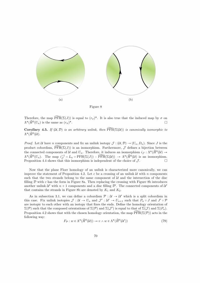
(a) (b)

Figure 8

Therefore, the map ĆPFHpΣpJqq is equal to prσq˚. It is also true that the induced map by σ on

Λ˚p rH0pUnq is the same as prσq˚.

Corollary 4.5. If pU ,Dq is an arbitrary unlink, then ĆPFHpΣpUqq is canonically isomorphic to

Λ˚p rH0pUq.

Proof. Let U have n components and fix an unlink isotopy J : pU ,Dq Ñ pUn, Dnq. Since J is the

product cobordism, ĆPFHpΣpJqq is an isomorphism. Furthermore, J defines a bijection between

the connected components of U and Un. Therefore, it induces an isomorphism iJ : Λ˚p rH0pUq ÑΛ˚p rH0pUnq. The map i´1

J ˝ Ln ˝ PFHpΣpJqq : ĆPFHpΣpUqq Ñ Λ˚p rH0pUq is an isomorphism.Proposition 4.4 shows that this isomorphism is independent of the choice of J .

Now that the plane Floer homology of an unlink is characterized more canonically, we canimprove the statement of Proposition 4.2. Let c be a crossing of an unlink U with n componentssuch that the two strands belong to the same component of U and the intersection of the discfilling D with c has the form in Figure 8a. Then replacing the crossing with Figure 8b introducesanother unlink U 1 with n ` 1 components and a disc filling D1. The connected components of U 1that contains the strands in Figure 8b are denoted by K1 and K2.

As in subsection 3.1, we can define a cobordism P : U Ñ U 1 which is a split cobordism inthis case. Fix unlink isotopies J : U Ñ Un and J 1 : U 1 Ñ Un`1 such that Pn ˝ J and J 1 ˝ Pare isotopic to each other with an isotopy that fixes the ends. Define the homology orientation ofΣpPq such that the composed orientations of ΣpPq and ΣpJ 1q is equal to that of ΣpJ q and ΣpPnq.

Proposition 4.2 shows that with the chosen homology orientation, the map ĆPFHpΣpPqq acts in thefollowing way:

FP : w P Λ˚p rH0pUqq Ñ v ^ w P Λ˚p rH0pU 1qq (79)

70

where v, as an element of rH0pUq, is non-zero only on the connected components K1, K2. Itevaluates to 1 on one of these components and -1 on the other one. There are two possibilitiesfor v and both of them are feasible by different choices of J and J 1. In fact, if we change J 1 bycomposing it with an unlink isotopy that permutes the nth and the pn ` 1qst components, thenv turns into ´v. However, if we fix one of the two possibilities for v, then all different choices ofJ and J 1 define the same cobordism map FP . Consequently, they determine the same homologyorientation on P.

Next, let U be an unlink with n`1 connected components. Suppose c is a crossing such that thetwo strands belong to the different connected components and the intersection of the disc filling Dwith the crossing is as in Figure 8b. As in the previous paragraph, we can construct an unlink U 1and a merge cobordism sP : U Ñ U 1. Choose unlink isotopies J : U Ñ Un`1, J 1 : U 1 Ñ Un, withsP ˝ J 1 and J ˝ sPn being isotopic to each other, and use these to define a homology orientation onΣp sPq as in the previous case. Each connected component of U is connected to one component of U 1via sP and j : H0pUq Ñ H0pU 1q is the map that sends the Poincare dual of the fundamental class ofa component of U to the Poincare dual of the fundamental class of the corresponding componentof U 1. This map induces:

FsP : w P Λ˚p rH0pUqq Ñ j˚pwq P Λ˚p rH0pU 1qq (80)

and by Proposition 4.2, ĆPFHpΣp sPqq is equal to this map.

Let pU ,Dq, pU 1,D1q be unlinks such that pU ,Dq is given by dropping one of the connectedcomponents of pU 1,D1q. We can construct a cap cobordism C : U Ñ U 1 that is the union of twoparts. The first part is IˆU and the second part is the pushing of the extra component of D1 fromt1u ˆ S3 into I ˆ S3. We can proceed as above to define a homology orientation for ΣpCq. Leti : H0pUq Ñ H0pU 1q be the map that extends an element of H0pUq by zero on the extra componentof U 1. Then the cobordism map associated with C is equal to:

FC : w P Λ˚p rH0pUqq Ñ i˚pwq P Λ˚p rH0pU 1qq (81)

By reversing the role of the incoming and the outgoing ends in the previous paragraph, we canalso construct a cup cobordism sC from an unlink U with n ` 1 components to an unlink U 1 withn components. By following the same strategy to define a homology orientation for ΣpsCq, we willhave the following cobordism map:

FsC : w P Λ˚p rH0pUqq Ñ ιKpwq P Λ˚p rH0pU 1qq (82)

where ιK is contraction with respect to the element of H0pUq that is represented by the extracomponent. Note that in the case of merge, cup, and cap cobordisms the chosen homology ori-entations are independent of the unlink isotopes. Because in these cases the cobordism maps areindependent of these choices.

4.2 Odd Khovanov Homology Revisited

In this subsection, we firstly review the definition of reduced odd Khovanov homology. The reducedodd Khovanov homology of the mirror image with coefficients in Λ0 interacts better with plane

71

(a) (b)

Figure 9: A decorated crossing and its decorated resolutions

Floer homology. Therefore, we focus on this version of odd Khovanov homology. The main inputin the original definition of odd Khovanov homology is the notion of decorated link diagrams. In thecontext of this paper, oriented link diagrams can be used as a means to fix homology orientationsfor the cobordisms in the cube of resolutions:

Definition 4.6. A decorated link diagram D for a link K is a planar diagram such that at eachcrossing of D, one of the two possible orientations for the line segment q in Figure 9a is fixed.The resolutions of a decorated planar diagram are also equipped with extra decorations: if the linesegment q is oriented as Figure 9a, then orient the line segment connecting the two strands as inFigure 9b. Otherwise these orientations for the resolutions are reversed.

Fix a decorated diagram D for a link K. Any resolution Km of K, associated with D, is anunlink embedded in R2 ˆ t0u of R3. A disc filling of Km can be fixed in the following way. Themost inner circles in Km bound planar discs, i.e., discs that live in the plane R2 ˆ t0u. Fix thesediscs as the filling of the corresponding components. Next, remove the filled circles and considerthe discs that fill the most inner circles among the remaining ones. We can push the interior ofsuch discs into R2 ˆR` such that they lie above the discs constructed in the first stage and hencethey avoid intersecting with each other. Iteration of this construction determines a disc filling forKm.

For an edge pm,nq of the cube t0, 1u|ND|, consider Snm : Km Ñ Kn which is a pair of pants

cobordism. A straightforward examination of the different possible cases shows that Snm, with

respect to the isotopy class of the fixed disc fillings, is either P or sP constructed in subsection4.1. Homology orientations for the merge cobordisms are already fixed in the previous subsection.If Sn

m is a split cobordism, the ambiguity of the homology orientation of ΣpSnmq can be fixed by

ordering the two components of the outgoing end that intersects the crossing. Denote these twocomponents by A1 and A2. The decorated resolution of the crossing provides us with such anordering. Suppose that the decoration of the line segment between A1 and A2 points from A1 toA2. We fix the homology orientation such that the cobordism map ĆPFHpΣpSn

mqq is equal to:

FS : w P Λ˚p rH0pKmqq Ñ v ^ w P Λ˚p rH0pKnqq

72

where v P rH0pKnq evaluates to 1 (respectively, -1) on the representative of the component A1

(respectively, A2).

In [15], the first step to construct the reduced odd Khovanov chain complex of sK is to as-sign a module to each resolution Km. It can be easily checked that this module is the same asĆPFHpΣpKmqq “ Λ˚p rH0pKmqq. The next step in the definition of odd Khovanov homology is

to define a map from Λ˚p rH0pKmqq to Λ˚p rH0pKnqq for each edge pm,nq of the cube. It is also

straightforward to check that this map is the same as ĆPFHpΣpSnmqq, using the fixed homology

orientations.

Suppose pm,nq is a face of the cube t0, 1u|ND| and k, k1 are the two vertices that m ą k,k1 ą n.Homology orientations of the cobordisms Sk

m, Sk1

m, Snk and Sn

k1 are already fixed. This face of thecube is called commutative if the composed homology orientations of Sk

m and Snk is equal to the

composed homology orientations of Sk1

m and Snk1 . Otherwise this face is called non-commutative.

If the composition ĆPFHpΣpSnk qq ˝

ĆPFHpΣpSkmqq (or equivalently ĆPFHpΣpSn

k1qq ˝ĆPFHpΣpSk1

mqq) isnon-zero then plane Floer homology can be used to detect whether pm,nq is commutative or not.To be more specific, if:

ĆPFHpΣpSnk qq ˝

ĆPFHpΣpSkmqq “

ĆPFHpΣpSnk1qq ˝

ĆPFHpΣpSk1

mqq

then pm,nq is commutative and it is non-commutative if:

ĆPFHpΣpSnk qq ˝

ĆPFHpΣpSkmqq “ ´

ĆPFHpΣpSnk1qq ˝

ĆPFHpΣpSk1

mqq.

Any face pm,nq of the cube t0, 1u|ND| is determined by the resolution of the vertex Km and thecorresponding decorations of the two crossings associated with the face. A typeX face (respectively,type Y face) is a face that its decorated resolution Km is equal to the union of the arrangementin Figure 10a (respectively, Figure 10b) and several (possibly zero) other components that do notintersect the crossings of the face. Type X and type Y crossings are the only types of the facessuch that ĆPFHpΣpSn

k qq ˝ĆPFHpΣpSk

mqq vanishes.

Lemma 4.7. Out of type X and type Y faces, faces of one type are commutative and faces of theother type are non-commutative.

Proof. Suppose that L is the decorated planar diagram of a link consisting of two crossings suchthat its p1, 1q resolution has only one component and it has the form of Figure 10a . Therefore,the only face of this planar diagram has type X. Label these crossings by requiring that thefirst crossing is represented by the vertical red line in Figure 10a and the second crossing is theother one. Let L1 be another decorated diagram for the same link that is given by Figure 10b.The diagram L1 has only one face that is of type Y . We can use these two decorated diagramsto define two homology orientations for each of the cobordisms S10

11 , S0111 , S00

10 and S0001 . Out of

these cobordisms, only the two homology orientations of the cobordism S1011 differ from each other.

Therefore, one of L and L1 has a commutative face and the other one has a non-commutative face.In the following, we assume that L is the decorated diagram with a commutative face. The proofin the other case is similar.

73

(a) A type X face (b) A type Y face

Figure 10

Let pm,nq be a face of a decorated diagram K with type X. Therefore Km has a componentthat intersects the two crossings determined by this face. This component has the form in Figure10a and we fix the labeling such that:

m “ p1, 1, 0 . . . , 0q n “ p0, 0, 0 . . . , 0q

and if:k “ p1, 0, 0 . . . , 0q k1 “ p0, 1, 0 . . . , 0q

then Kk is given by the 1-resolution of the first crossing and the 0-resolution of the second crossingin Figure 10a. Suppose that S : Km Ñ L11, S1 : Kn Ñ L00, S21 : Kk Ñ L10 and S22 : Kk1 Ñ L01

are composition of cup cobordisms that fill the components which do not intersect the crossings.Furthermore, we have:

Sk1

m ˝Snk1 ˝S

1 “ Sk1

m ˝S22 ˝S

0001 “ S ˝S01

11 ˝S0001 “ S ˝S10

11 ˝S0010 “ Sk

m ˝S21 ˝S

0010 “ Sk

m ˝Snk ˝S

1 (83)

We use the homology orientation of the cup cobordisms to define homology orientations forΣpSq, ΣpS1q, ΣpS21 q and ΣpS22 q. The cobordism compositions in (83) define 6 homology orientationson the same cobordism. By assumption the homology orientation determined by the compositionsS ˝ S10

11 ˝ S0010 and S ˝ S01

11 ˝ S0001 are the same. One can also easily check that the non-zero maps

ĆPFHpΣpS1qq ˝ ĆPFHpΣpSnk1qq and ĆPFHpΣpS00

01qq ˝ĆPFHpΣpS22 qq are equal to each other. Thus Sk1

m ˝

Snk1˝S

1 and Sk1

m˝S22 ˝S

0001 determine the same homology orientations. A similar argument shows that

the remaining pair of compositions that appear as consecutive terms in (83) determine the samehomology orientations. In particular, the homology orientations of the compositions Sk1

m ˝ Snk1 ˝ S

1

and Skm ˝ S

nk ˝ S

1 are the same. This proves the claim that the face pm,nq is even.

The following definition is a reformulation of Definition 1.1. in [15]:

74

Definition 4.8. A type X edge assignment for D is a map σ from the set of edge of the cubet0, 1un to t1,´1u such that for any face pm,nq:

σpm,kqσpk,nqĆPFHpΣpSnk qq ˝

ĆPFHpΣpSkmqq ` σpm,k1qσpk1,nqĆPFHpΣpSn

k1qq ˝ĆPFHpΣpSk1

mqq “ 0.(84)

Furthermore, we require that if pm,nq is a face of type X, then:

σpm,kq ¨ σpk,nq “ σpm,k1q ¨ σpk1,nq

and if it is a face of type Y , then:

σpm,kq ¨ σpk,nq “ ´σpm,k1q ¨ σpk1,nq.

In the definition, if we reverse the role of type X and type Y faces, then the resulting edgeassignment has type Y .

Given a type X or a type Y edge assignment σ, the reduced odd Khovanov chain complex ofsK associated with the decorated link diagram D is equal to:

pà

mPt0,1un

ĆPFHpΣpKmqq,à

pm,nqPEc

σpm,nqĆPFHpΣpSnmqq (85)

Relation (84) implies that (85) is in fact a chain complex. The chain complex (85) is equippedwith two gradings in [15] which are called the homological and quantum gradings. If we will writeho and qo for these gradings, then these gradings are equal to:

degho “ p|sD| ´ |m|1q ´ n´p sDq (86)

degqo “ p1` degpq ` p| sD| ´ |m|1q ` n`p sDq ´ 2n´p sDq (87)

Here sD is the digram for sK that is induced by D. This term appears in our formulas because thechain complex (85) competes the odd Khovanov homology of sK using the diagram sD.

Theorem 4.9. There is an isomorphism between the chain complexes (73) and (85). Furthermore,this isomorphism relates the bi-gradings in the following way:

degho “ degh, degqo “ 2pdegh´degδq ` 1

Proof. Note that the definition of the chain complex (73) depends on D and a choice of homologyorientations on the cobordisms ΣpSn

mq that satisfies the assumption of Lemma 2.3. On the otherhand, the chain complex (85) depends on D and a type X or type Y edge assignment. In particular,

the cobordism maps ĆPFHpΣpSnmqq, involved in the definition, are defined by homology orientation

oND pm,nq determined by D. It is shown in [15] that for any decorated diagram, type X and type Yedge assignments exist and the corresponding chain complexes for a fixed diagram are isomorphic.

Now suppose type X faces are non-commutative and a type X edge assignment σ of the diagramis fixed. For an edge pm,nq of the cube t0, 1un define:

opm,nq :“ σpm,nqsgnpm,nqoND pm,nq P opΣpSnmqq

75

Suppose pm,nq is a face of the cube t0, 1un and k and k1 are the vertices that m ą k,k1 ą n.Then we have:

opk,nq ˝ opm,kq “ opk1,nq ˝ opm,k1q. (88)

In the case of a type X face it holds by definition. The case of type Y face is a consequence ofLemma 4.7. For the remaining faces it can be derived from (84). Relation (88) implies that o canbe extended to a homology orientation for the cobordisms ΣpSn

mq for all cubes pm,nq in Zn suchthat:

opk,nq ˝ opm,kq “ opm,nq.

Therefore, we can use this homology orientation to define the chain complex (73). With this choiceof homology orientation the identity map defines an isomorphism of the chain complexes. In thecase that type X faces are commutative, the same argument can be used with the aid of a type Yedge assignment. The claim about the relations between gradings is also an immediate consequenceof the definition.

Corollary 4.10. Given a link K, there is a spectral sequence that its first page is equal to Khop sKqb

Λ and it converges to ĆPFHpΣpKqq.

Proof. In section 2, starting from a pair pY, ζq and a framed link L with n components, we con-structed a pair pYm, ζmq for each m P Zn. The 1-manifold ζm is the union Yiζm,i and ζm,i isnon-empty if and only if mi ” 0 mod 3, and in this case ζm,i is the core of the tours Dm,i. Inthe definition of ζm, we could replace the condition mi ” 0 mod 3 with mi ” 2 mod 3. Thenthe definition of Zn

m can be modified accordingly, and another version of Theorem 2.9 can beproved. This version can be used to prove a variation of Theorem 3.2. In particular, this variationstates that a planar diagram D determines a chain complex p‘mPt0,1un

ĆPFCpΣpKmqq, dpq which

has the same chain homotopy type as ĆPFCpΣpKq, ζq. The differential dp is given by the maps

dnm : ĆPFCpΣpKmqq Ñ ĆPFCpΣpKnqq where dnm is the cobordism map for the family of metricsWn

m parametrized by Gnm (constructed in subsection 2.1). Furthermore, the 1-manifold ζ is the

branched double cover of γ “ Yipi where pi is the path that connects the two strands in the ith

crossing of D (Fig. 3a).

Let rζs denote the Z2Z-homology class of the 1-manifold ζ. The Z2Z action on ΣpKq inducesa Z2Z action τ on the set of simplicial complexes Csimp˚ pΣpKqq. Therefore, we have a map:

i : H˚pp1` τqCsimp˚ pΣpKqq;Z2Zq Ñ H˚pΣpKq;Z2Zq

and rζs lies in the image of i. The homology group H˚pp1`τqCsimp˚ pΣpKqq;Z2Zq is isomorphic to

H˚pS3,Kq, and under this isomorphism rζs corresponds to rγs P H1pS

3,Kq. The boundary of rγsrepresents the trivial class in H0pKq, because the set of crossings is induced by a diagram of the

link K. Therefore, rζs vanishes and by Lemma 1.24, ĆPFHpΣpKq, ζq “ ĆPFHpΣpKqq. Consequently,

the chain complex p‘mPt0,1unĆPFCpΣpKmqq, dpq gives rise to a spectral sequence whose first page

is the complex (73) and it abuts to ĆPFHpΣpKqq.

76

References

[1] M. F. Atiyah. Algebraic topology and operators in Hilbert space. In Lectures in ModernAnalysis and Applications. I, pages 101–121. Springer, Berlin, 1969.

[2] Michael Atiyah, Vijay Kumar Patodi, and Isadore Singer. Spectral asymmetry and Rieman-nian geometry. I. Math. Proc. Cambridge Philos. Soc., 77:43–69, 1975.

[3] Jonathan Bloom. A link surgery spectral sequence in monopole Floer homology. Adv. Math.,226(4):3216–3281, 2011.

[4] S. K. Donaldson. Polynomial invariants for smooth four-manifolds. Topology, 29(3):257–315,1990.

[5] S. K. Donaldson. Floer homology groups in Yang-Mills theory, volume 147 of CambridgeTracts in Mathematics. Cambridge University Press, Cambridge, 2002. With the assistanceof M. Furuta and D. Kotschick.

[6] Simon Donaldson and Peter Kronheimer. The geometry of four-manifolds. Oxford Mathe-matical Monographs. The Clarendon Press Oxford University Press, New York, 1990. OxfordScience Publications.

[7] Andreas Floer. An instanton-invariant for 3-manifolds. Comm. Math. Phys., 118(2):215–240,1988.

[8] Mikhail Khovanov. A categorification of the Jones polynomial. Duke Math. J., 101(3):359–426,2000.

[9] Peter Kronheimer and Tomasz Mrowka. Monopoles and three-manifolds, volume 10 of NewMathematical Monographs. Cambridge University Press, Cambridge, 2007.

[10] Peter Kronheimer and Tomasz Mrowka. Filtrations on instanton homology. 2011,arXiv:1110.1290.

[11] Peter Kronheimer and Tomasz Mrowka. Khovanov homology is an unknot-detector. Publ.Math. Inst. Hautes Etudes Sci., (113):97–208, 2011.

[12] Peter Kronheimer, Tomasz Mrowka, Peter Ozsvath, and Zoltan Szabo. Monopoles and lensspace surgeries. Ann. of Math. (2), 165(2):457–546, 2007.

[13] Robert Lipshitz and Sucharit Sarkar. A Khovanov stable homotopy type. J. Amer. Math.Soc., 27(4):983–1042, 2014.

[14] Saunders Mac Lane. Homology. Classics in Mathematics. Springer-Verlag, Berlin, 1995.Reprint of the 1975 edition.

[15] Peter Ozsvath, Jacob Rasmussen, and Zoltan Szabo. Odd Khovanov homology. Algebr. Geom.Topol., 13(3):1465–1488, 2013.

77

[16] Peter Ozsvath and Zoltan Szabo. On the Heegaard Floer homology of branched double-covers.Adv. Math., 194(1):1–33, 2005.

[17] C. W. Scaduto. Instantons and odd Khovanov homology. ArXiv e-prints, January 2014,1401.2093.

[18] Katrin Wehrheim. Smooth structures on morse trajectory spaces, featuring finite ends andassociative gluing. 2012, arXiv:1205.0713.

78