Embed Size (px)
Citation preview

APPROVED: Randall E. Schumacker, Major Professor Jon Young, Minor Professor Robin K. Henson, Committee Member Kyle Roberts, Committee Member M. Jean Keller, Dean of the College of Education C. Neal Tate, Dean of the Robert B. Toulouse
School of Graduate Studies
ABILITY ESTIMATION UNDER DIFFERENT ITEM PARAMETERIZATION
AND SCORING MODELS
Ching-Fung B. Si, B.S., M.Div.
Dissertation Prepared for the Degree of
DOCTOR OF PHILOSOPHY
UNIVERSITY OF NORTH TEXAS
May 2002

Si, Ching-Fung B., Ability Estimation Under Different Item Parameterization and
Scoring Models. Doctor of Philosophy (Educational Research), May 2002, 107 pp., 12 tables, 18
figures, 5 appendices, references, 54 titles.
A Monte Carlo simulation study investigated the effect of scoring format, item
parameterization, threshold configuration, and prior ability distribution on the accuracy of ability
estimation given various IRT models. Item response data on 30 items from 1,000 examinees was
simulated using known item parameters and ability estimates. The item response data sets were
submitted to seven dichotomous or polytomous IRT models with different item parameterization
to estimate examinee ability. The accuracy of the ability estimation for a given IRT model was
assessed by the recovery rate and the root mean square errors. The results indicated that
polytomous models produced more accurate ability estimates than the dichotomous models,
under all combinations of research conditions, as indicated by higher recovery rates and lower
root mean square errors. For the item parameterization models, the one-parameter model out-
performed the two-parameter and three-parameter models under all research conditions. Among
the polytomous models, the partial credit model had more accurate ability estimation than the
other three polytomous models. The nominal categories model performed better than the general
partial credit model and the multiple-choice model with the multiple-choice model the least
accurate. The results further indicated that certain prior ability distributions had an effect on the
accuracy of ability estimation; however, no clear order of accuracy among the four prior
distribution groups was identified due to an interaction between prior ability distribution and
threshold configuration. The recovery rate was lower when the test items had categories with
unequal threshold distances, were close at one end of the ability/difficulty continuum, and were
administered to a sample of examinees whose population ability distribution was skewed to the
same end of the ability continuum.

ii
ACKNOWLEDGMENTS
I wish to thank all those who have provided me assistance during my research. I would
like to thank my major professor, Randall Schumacker for his guidance and instruction, which I
value greatly. I would like to thank my committee members, Robin Henson, Kyle Roberts, and
my minor professor, Jon Young for their valuable assistance. I would also like to thank my wife
and family for their support and love during this process. And above all, I give thanks to the one
true God who has created me and gives me wisdom and understanding.
iii
TABLE OF CONTENTS
Page
ACKNOWLEDGMENTS ............................................................................................... ii LIST OF TABLES ........................................................................................................... vi LIST OF FIGURES.......................................................................................................... vii Chapter
1. INTRODUCTION.......................................................................................... 1
Overview Statement of the Problem Rationale for the Study
Item Parameterization and Scoring Models Ability Distributions Threshold Distances
Research Questions Delimitation Definition of Terminology
2. REVIEW OF RELATED LITERATURE ..................................................... 12
Overview Item Parameterization: Basis for Family of IRT Models
One-, Two- and Three-Parameter IRT Models Normal ogive models Logistic models
Summary Effects of Scoring: Polytomous IRT Models
Bock�s Nominal Categories Model (NCM) Polytomous IRT Models with Ordinal Response Categories Ordinal polytomous IRT models compared in this study
Partial credit model (PCM) Generalized partial credit model (GPCM) Multiple-choice model
Summary Ability Estimation
Maximum Likelihood method Joint Maximum Likelihood Estimation (JML) Conditional Maximum Likelihood Estimation (CML)
iv
Marginal Maximum Likelihood Estimation (MML) Bayesian estimation
Maximum a posteriori (MAP) estimates Expected a posteriori (EAP) estimates
Summary
3. METHODS AND PROCEDURES................................................................ 44 Data Simulation and Design Number of Replications in Monte Carlo Estimation Criteria for Evaluation Sample Size and Power Analysis for Hypothesis Testing Construction of Test Items Data Simulation Computer Program Item Parameterization and Ability Estimation Programs
4. RESULTS ...................................................................................................... 51 Overview Research Question 1 Research Question 2 Research Question 3
5. CONCLUSIONS AND RECOMMENDATIONS ....................................... 77
Conclusions Findings of the Present Study Recovery Rate and Root Mean Squared Error Scoring Format Item Parameterization Comparison of Polytomous Models Prior Ability Distribution Threshold Configuration
Recommendations
APPENDIX A: ................................................................................................................ 89 SAS Program for Data Simulation SAS Program for Generating Prior Ability Distribution
APPENDIX B: ................................................................................................................ 93 Flowchart of a Cycle of Data Simulation and Data Analysis APPENDIX C: ................................................................................................................. 94 Parameters of Items in the Constructed Tests for Data Simulation

v
APPENDIX D:................................................................................................................. 95 Ability Estimation Programs Multilog Command Programs for Different IRT Models
1-PL logistic model 2-PL logistic model 3-PL logistic model Partial credit model General partial credit model Multiple-choice model Nominal categories model
APPENDIX E: ................................................................................................................. 100
Ability Estimation Results
REFERENCES ................................................................................................................ 102

vi
LIST OF TABLES
Table Page 1. Summary of the Three Types of Ordinal Polytomous IRT Models ...........................27 2. Combinations for Study Design.................................................................................44 3. Computer Programs Used for Different Item Parameterization and Scoring Models
....................................................................................................................................50 4. Descriptive Information of the Recovery Rates across Different Groups..................52 5. Descriptive Information of the RMSE across Different Groups................................53 6. Three-way Fixed Effects ANOVA on Recovery Rate (S, P, T).................................55 7. Three-way Fixed Effects ANOVA on RMSE (S, P, T) .............................................57 8. Three-way Fixed Effects ANOVA on Recovery Rate (I, P, T)..................................63 9. Three-way Fixed Effects ANOVA on RMSE (I, P, T) ..............................................65 10. Three-way Fixed Effects ANOVA on Recovery Rate (Po, P, T)...............................70 11. Simple-Simple Main Effects (PolyMod) on Recovery Rate and Homogeneous
Subsets .......................................................................................................................72 12. Three-way Fixed Effects ANOVA on RMSE (Po, P, T) ...........................................73
vii
LIST OF FIGURES
Figure Page 1. Item characteristic curves with different item parameters .........................................14 2. Item characteristic curves of 2- and 3-PL logistic IRT models..................................15 3. Item characteristic curves in a 1-PL model................................................................16 4. Item category characteristic curves in a polytomous IRT model ...............................19 5. Marginal means of recovery rate by prior distribution (dichotomous model) ...........60 6. Marginal means of RMSE by prior distribution (dichotomous model) .....................60 7. Marginal means of recovery rate by prior distribution (polytomous model) .............61 8. Marginal means of RMSE by prior distribution (polytomous model) .......................62 9. Marginal means of recovery rate by prior distribution (1-pl model) .........................67 10. Marginal means of RMSE by prior distribution (1-pl model) ...................................67 11. Marginal means of recovery rate by prior distribution (2-pl model) .........................68 12. Marginal means of RMSE by prior distribution (2-pl model) ...................................68 13. Marginal means of recovery rate by prior distribution (3-pl model) .........................69 14. Marginal means of RMSE by prior distribution (3-pl model) ...................................69 15. Marginal means of recovery rate by polytomous model (within Threconf) ..............74 16. Marginal means of recovery rate by polytomous model (within Thetadis) ...............75 17. Marginal means of RMSE by polytomous model (within Threconf) ........................75 18. Marginal means of RMSE by polytomous model (within Thetadis) .........................76

1
CHAPTER 1
INTRODUCTION
Overview
Testing is essential in education and other social science fields because many
decisions, and policies are made according to the results of testing. The purpose of testing
is to estimate a person�s ability, i.e. latent trait or construct. In a test setting, responses to
a set of test items are recorded by each individual. Through a scoring scheme, test scores
are assigned to individuals according to their item responses. Test scores provide
information from which we infer a person�s ability. In educational measurement,
Classical Test Theory (CTT) partitions test scores (X) into two components, X = T + E,
to represent the ability estimate�the true score (T), and error (E). This type of
measurement is juxtaposed to measurement in a field like Physics where all factors
contained in a model can be accounted for. Error indicates factors that couldn�t be
accounted for or controlled in the test design, test administration, and/or examinee. Test
score reliability and the true score estimates, however, change from one test form to
another test form even though the test design and administration are the same. Error in
this instance is due to the random sampling of items to form the two tests. The test score
reliability and the true score estimates are test-dependent because the properties of items
are selected but not controlled in the process of ability estimation in CTT. Item Response
Theory (IRT) uses mathematical models to adjust for the item properties making the
ability estimates freer from test-dependence.
Different IRT parameterization models adjust for different item properties leading
to different ability estimation. 1-parameter (1-PL) IRT adjusts for item difficulty; 2-

2
parameter (2-PL) IRT accounts for item difficulty and discrimination; and 3-parameter
(3-PL) IRT takes into account the effect of item guessing, difficulty and discrimination. If
a set of item responses is submitted to a 1-PL, 2-PL, or 3-PL model and item parameters
are estimated, a model fit statistic indicates that item parameterization in the models was
satisfactorily completed. The three different item parameterization models may yield
different ability estimates. It is a known fact that item parameterization will affect the
estimation of ability in IRT (Lord & Novick, 1968), however, other factors, e.g.
dimensionality of the test, and test-scoring format may also affect ability estimation. The
present study deals only with unidimensional IRT models, but will address different test-
scoring formats.
It may not be so much an issue of item parameterization, but rather item response
format (right/wrong, partial credit, rating scale, etc.), that influences ability estimation. In
the first few decades of the development of IRT, research interests were concentrated on
dichotomous models, which involve test item responses scored either right or wrong (1,
0). One year after Lord and Novick (1968) established the 1-, 2-, and 3-parameter logistic
models for dichotomous items, Samejima (1969) introduced the first polytomous model
(Graded Response Model). Although Bock and Samejima (1972) presented a different
polytomous model (Nominal Categories Model), it was not until the 1980�s that interest
in polytomous IRT models began. There have been many polytomous models developed
since 1970 (Andrich, 1978, 1982, 1995; Masters, 1982; Muraki, 1990, 1992; Thissen &
Steinberg, 1984, Thissen, Steinberg & Fitzpatrick, 1989, etc.). In polytomous models,
items in the test are not scored just right or wrong; but instead, each of the categories of
response is evaluated and scored according to its degree of correctness or the amount of

3
information provided toward the full answer. The polytomous models are appropriate for
multiple-choice items and performance assessments where test items are designed to have
steps of difficulty or thresholds. Since choices of categories other than the best answer
are given partial credit in polytomous models, instead of no credit as in dichotomous
models, ability estimates for individuals are expected to be different depending on
whether dichotomous or polytomous models are used in scoring item responses.
Statement of the Problem
If unidimensional tests, e.g. mathematics ability test, are administered to a group
of examinees, the ability estimates of the examinees will vary as a function of item
parameterization (1-, 2-, 3-PL) and scoring (dichotomous versus polytomous) model
applied to the item responses. Since item parameterization and type of scoring model
affects ability estimation; one needs to investigate which approach will produce ability
estimates closest to the levels of the true ability of examinees, i.e., which combination of
the item parameterization and scoring models gives the most accurate ability estimates?
The true measure of ability, however, is latent and therefore not known. A comparison
can only be made among the ability estimates.
Embretson and Reise (2000) compared the latent trait scores obtained from five
different polytomous IRT models and the raw scores. The five models differed in item
parameterization. The Partial Credit Model (PCM) and Rating Scale Model (RSM) are
Rasch Models, which assume the same slope (1.0) for all items. Graded Response Model
(GRM), Modified Graded Response Model (MGRM), and Generalized Partial Credit
Model (GPCM) all allow items to differ in slope parameters. They compared the five
models on item responses of 350 undergraduates to 12 items on the Neuroticism scale of

4
the Neuroticism Openness Five-Factor Inventory (NEO-FEI) (Costa & McCrae, 1992)
and obtained five latent trait scores, i.e. ability estimates. They found that the ability
estimates were highly correlated with each other and with the raw scores. The lowest
Pearson r was .97. Although the significant correlations indicated that the relative
ordering of examinees was basically maintained in all five different polytomous models,
they did not give information about the accuracy of the ability estimation of individual
models. The information on accuracy of the estimation of individual examinee�s ability is
as important as their relative ordering in some test settings, e.g. in a criterion-referenced
test involving a specific cut-off score. Therefore, it is important to compare the accuracy
of ability estimation, not just the correlations of the ability estimates from different
models, because the polytomous models with different parameterization may lead to very
different ability estimates and thus different variance of the ability estimates.
Furthermore, the Embretson and Reise study compared only polytomous models. If
dichotomous models with different parameterization were included in the comparison,
more diversified ability estimates would be expected. The present study, therefore,
investigates different dichotomous and polytomous models to determine which model
produces ability estimates closest to the true latent ability of the examinee, using a
confidence interval to capture the true latent ability of an examinee, and a root mean
square deviation index, for deviation of the ability estimates.
Rationale for the Study
Several factors that affect ability estimation in IRT are of interest in this study.
These factors are hypothesized to have an impact on the accuracy of estimation of a

5
person�s ability or knowledge. The rationales for several hypotheses are given in the
following section.
Item Parameterization and Scoring Models
Studies exist which compared different item parameterization and scoring models,
but the emphases were on items, e.g. model fit, recovery of item parameters, and person
fit (Wright & Master, 1982; Muraki, 1992). No study specifically compared different
models on the ability estimates of examinees. A comparison of dichotomous and
polytomous IRT models with regard to the accuracy of ability estimation is therefore
needed. Using Monte Carlo methods, item responses of examinees with known ability
scores can be simulated, and submitted to different IRT models to compare examinee
ability estimation. The sets of examinee ability estimates from the different models can
then be compared to the empirically known ability estimates to examine the bias and
variance of ability estimation.
Ability Distributions
Different prior ability distributions of the examinees will affect the comparison of
the ability estimates from different models. The difference between scoring a test
dichotomously and polytomously may not be as prominent in extreme ability groups
(low, high) as in medium ability groups. It is reasonable, therefore, to investigate the
effect of the prior ability distributions of the examinees on the model comparisons. Four
types of distributions will be examined, namely normal, skewed to the right, skewed to
the left, and bimodal. The ability estimates of a random sample of examinees are
expected to be normally distributed. A sample that has high ability examinees will
produce an ability distribution skewed to the left, while that of a sample containing low

6
ability examinees will be skewed to the right. The bimodal distribution of ability
represents a sample of examinees with very diversified, even polarized, levels of ability.
This study investigated what effect the ability distributions had on the ability estimates
under different item parameterization and scoring models.
Threshold Distances
When scored polytomously, the categories of each multiple-choice item can
represent different levels of difficulty. The threshold between two adjacent categories is
the ability level at which an examinee has equal probability to choose either one of two
categories. When polytomous models are applied to multiple-choice items, and partial
credits are given to categories other than the best answers, the configuration of the
thresholds of an item affects the information function of the item and thus the precision
of ability estimation. Configuration of the thresholds includes two aspects, namely the
order of the thresholds and the distances between them. Dodd and Koch (1985) found
that item information functions for the partial credit model differs as a function of the
thresholds. The distance between the first and last thresholds affected the shape of the
information function of an item. Items with shorter distances between first and last
thresholds had a more peaked information function for a narrower range of ability
continuum. In a follow-up study of the issue (Dodd & Koch, 1987), they systematically
altered the order of the same set of thresholds to form different items. They concluded
that the items with the same set of thresholds yielded the same total amount of
information across the entire ability continuum, but different ordering of the thresholds
affected the peakedness of the item information curve. They found that the peakedness of
the curve increased as the degree of deviation from the sequential order of the thresholds

7
increased. While peaked information function is desired in some testing, e.g. in
computerized adaptive testing (CAT), flatter information functions that yield maximum
information for a wider range of ability is preferred in tests developed for examinees
from all possible ability groups. It is the latter kind of testing under consideration in the
present study. Therefore, the thresholds of the items in the test constructed for the present
study were in their sequential order, i.e. monotonically increasing from the least to the
most difficult. However, distances between the thresholds were varied to investigate its
effect on ability estimation. The threshold distances could be equal or unequal. If the
threshold distances are unequal and narrower at the lower end, the categories are
expected to be less effective in discriminating lower ability groups in the sample, because
their responses to each of the two adjacent lower difficulty categories may not be very
different. In contrast, narrower threshold distances at the higher end are expected to cause
the categories to be less effective in discriminating higher ability groups. With different
prior ability distributions, it is meaningful to investigate how different polytomous
models perform when the threshold distances are unequal.
Research Questions
The present study hypothesized that the type of item parameterization, scoring
model format, prior ability distribution of the examinees, and configuration of category
threshold distances were factors affecting the accuracy of ability estimation of examinees.
The research questions postulated for this study were as follow:
1. How do dichotomous and polytomous IRT models differ in accuracy of
recovering ability estimates in different combinations of prior ability distributions
and item category threshold distance configurations?

8
2. How do different IRT item parameterization models (i.e. modeling difficulty only;
both difficulty & discrimination; and difficulty, discrimination & guessing) differ
in accuracy of recovering ability estimates in different combinations of prior
ability distributions and item category threshold distance configurations?
3. How do the polytomous IRT models differ in accuracy of recovering ability
estimates in different combinations of prior ability distributions and item category
threshold distance configurations?
Delimitation
The factors identified for examination in this study have fixed levels, which were
selected according to the literature review. The generalizability of the findings of this
study is limited to the seven IRT models (1-, 2-, and 3-PL dichotomous model, partial
credit model, general partial credit model, multiple-choice model, and nominal categories
model), four types of prior ability distributions (normal, skewed to the right, skewed to
the left and bimodal), and the three types of threshold distance configurations (equal,
unequal-close at the lower end, and unequal-close at the higher end). Some factors other
than those examined in this study affect ability estimation but they were controlled in the
study. The number of examinees in the sample was fixed at 1,000 and the number of
items in the test was fixed at 30 according to recommendations in the literature (Dodd
and Koch, 1987; Chen, 1996). The number of response categories in each item was four
to model typical multiple-choice item tests.

9
Definition of Terminology
1. Dichotomous item response model�item response model for test with binary
items. Examinees taking the test will respond in either one of the two response
categories. A test with items scored right or wrong is dichotomous.
2. Polytomous item response model�item response model for items with more than
two response categories, e.g. multiple-choice item that allows partial credits for
each of the response categories, or constructed-response item with multiple steps.
3. Ability estimate�the estimate of the level of a latent trait of an examinee
demonstrated in an observed response pattern to a test.
4. Item response categories�the possible ways pre-assigned by the item writer that
an examinee could respond to an item. In the context of multiple-choice items,
they are the options provided for the examinee to choose; in constructed-response
items, they are the steps or parts of the solution to the item that allow different
partial credits to be awarded upon their completion.
5. Item response function (IRF)�the mathematical equation that governs the
probability of answering an item correctly as a function of the ability of the
examinee attempting the item and the item parameters.
6. Item category response function (ICRF)�the mathematical equation governing
the probability of an item category being chosen as a function of the ability of the
examinee and item category parameters.
7. Threshold distance�the distance on the ability continuum between two
thresholds. The threshold between two adjacent categories is the ability level at
which an examinee has equal probability to choose either one of two categories.

10
8. Item step response function (ISRF)�In polytomous IRT model with ordinal
response categories, item step is defined as two adjacent categories. ISRF is the
mathematical equation governing the probability of an item step being completed,
i.e. an examinee responds in the higher category when the two adjacent categories
are given as the condition. ISRF is a function of the ability of the examinee and
the step parameters, e.g. thresholds, and slope parameters.
9. Item characteristic curve (ICC)�the curve that demonstrates the relationship
between the ability of an examinee and the probability of the examinee answering
the item correctly. Sometimes it is referred as a trace line. It is the graph of IRF
plotting against the ability parameters.
10. Item category characteristic curve (ICCC)�the curve represents the relationship
between the probability of an examinee choosing an item category and the ability
of the examinee. ICCCs of all the categories within an item are usually plotted on
the same graph.
11. Prior ability distribution�the probability distribution of ability levels in the
population of examinees before estimation of parameters. It is usually assumed to
be normal. It can also be estimated by the response data in some programs.
12. Posterior ability distribution�the probability distribution of the ability estimate
for an examinee across the ability continuum. In marginal maximum likelihood
estimation, a probability distribution replaces the point estimate for each
examinee in the sample.

11
13. Item parameterization model�the mathematical model in item response theory
through which item properties are calibrated in the measurement of an examinee�s
ability.
14. Scoring model�the different scoring formats on which the ability estimation and
item parameters are modeled.

12
CHAPTER 2
REVIEW OF RELATED LITERATURE
Overview
A comprehensive review of literature relevant to the present study is provided in
this chapter. First, a brief introduction to item parameterization and dichotomous IRT
scoring models is presented. Second, a summary of different polytomous scoring models
is given. Third, different ability estimation methods are discussed.
Item Parameterization: Basis for Family of IRT Models
Item Response Theory, as its name suggests, models testing at the item level. In
contrast to Classical Test Theory (CTT), which depends on the test scores in ability
estimation, IRT utilizes mathematical models to estimate the effect of different properties
of individual items in the test on ability estimation. IRT item parameterization enables
IRT models to be freer from test-dependence and allows estimation of error on an item-
by-item basis. The modeling of item properties in IRT also permits individual estimates
of standard error of measurement (SEM), instead of assuming an equal SEM for all
examinees as in CTT. Therefore, while the primary purpose of IRT is the estimation of
ability, item parameterization is very important and distinguishes different IRT models.
Unidimensional IRT models address only one latent trait parameter, but vary in
the number of parameters used in item parameterization. The most commonly used
dichotomous IRT models are the 1-, 2-, and 3-PL logistic models. Although a 4-PL
logistic model was introduced (McDonald, 1967; Barton and Lord, 1981), it is of
theoretical interest only, for no practical gain on ability estimation was found by the

13
application of the model (Barton and Lord, 1981). The three item parameters involved in
the IRT models are identified by three item properties, i.e. difficulty (or location
parameter, usually labeled �b�), item discrimination (or slope parameter, usually labeled
�a�), and pseudo-chance (or lower asymptote parameter, usually labeled �c�). These item
properties also apply in the polytomous item response models, which will be reviewed in
the next section. The development of the three models took decades and bridged across
two continents, America, and Europe (Hambleton and Swaminathan, 1985).
One-, Two- and Three-Parameter IRT Models
Normal ogive models.
Hambleton and Swaminathan (1985) traced the history of Item Response Theory
all the way back to 1916, but credited Frederic M. Lord for providing impetus for the
development of the theory in its present form. The model that Lord introduced was the
two-parameter normal ogive model (1952). He used the normal ogive curve to model the
probabilities of the examinees answering an item correctly as a function of their ability,
i.e. the latent trait under measure, and two item parameters. The item response function
(IRF) for a two-parameter normal ogive model is:
( ) ( )( )dzzP ii ba
i ⋅−= ∫−
∞−
θ
πθ 2exp
21 2
,
where Pi(θ) is the probability of an examinee with ability θ answering item i correctly.
The two parameters that characterize item i are ai (the item discrimination), and bi (the
item difficulty). The normal ogive curve obtained by plotting Pi(θ) against θ is called item
characteristic curve (ICC) (Figure 1). The bi value is on the ability continuum where the
Pi(θ) = 0.5, and ai is the slope of the curve at that point.

14
Figure 1. Item characteristic curves with different item parameters.1
The parameter estimation in this model is mathematically complex and computationally
involved. The lack of convenient computer programs and high-capacity computers
needed for the parameter estimation explained the painstakingly slow pace of the early
development of IRT.
Logistic models.
Birnbaum (1957, 1958a, 1958b) made his contribution by introducing the more
mathematically tractable logistic model. He used the logistic distribution function to
approximate the normal ogive. It had been proved that the two curves differ absolutely by
less than .01 for all values of ability θ, if a constant scaler D = 1.7 was applied to the
logistic deviate (Haley, 1952). The logistic model not only simplified the computation
involved in parameter estimation, but also provided an explicit function for item and
ability parameters. The log odds of success in choosing the correct answer over failure is
equal to Dai (θ � bi), which is a linear function of the item parameters ai, bi and ability
parameter θ. The endorsement that Lord had given to the logistic model by including
Birnbaum�s work in his book co-authored with Novick (1968), helped to promote the
logistic models replacing normal ogive models in practical use. Birnbaum (1968) added
1 Adopted from Allen and Yen (1979), 255.
15
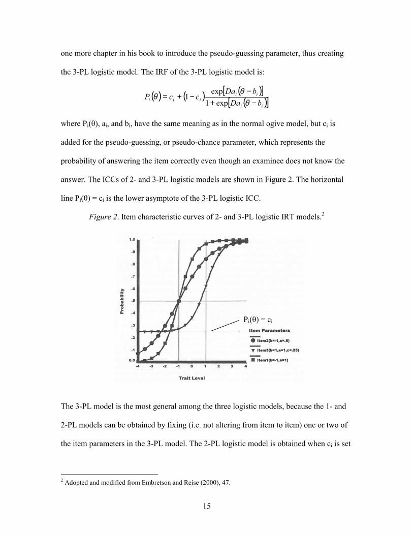
one more chapter in his book to introduce the pseudo-guessing parameter, thus creating
the 3-PL logistic model. The IRF of the 3-PL logistic model is:
( ) ( ) ( )[ ]( )[ ]ii
iiiii bDa
bDaccP
−+−
−+=θ
θθ
exp1exp
1
where Pi(θ), ai, and bi, have the same meaning as in the normal ogive model, but ci is
added for the pseudo-guessing, or pseudo-chance parameter, which represents the
probability of answering the item correctly even though an examinee does not know the
answer. The ICCs of 2- and 3-PL logistic models are shown in Figure 2. The horizontal
line Pi(θ) = ci is the lower asymptote of the 3-PL logistic ICC.
Figure 2. Item characteristic curves of 2- and 3-PL logistic IRT models.2
The 3-PL model is the most general among the three logistic models, because the 1- and
2-PL models can be obtained by fixing (i.e. not altering from item to item) one or two of
the item parameters in the 3-PL model. The 2-PL logistic model is obtained when ci is set
2 Adopted and modified from Embretson and Reise (2000), 47.
Pi(θ) = ci

16
to 0. It assumes no guessing on items in the test. When Dai is fixed (usually set to 1) and
ci is set to 0, a 1-PL logistic model is obtained. The only item parameter in the 1-PL
model used to estimate an examinee�s ability is item difficulty. The ICCs in a 1-PL model
will never intersect each other because they have the same slope at bs (Figure 3).
Figure 3. Item characteristic curves in a 1-PL model.3
The 1-PL logistic IRT model included in the comparison shouldn�t be mistaken as
a Rasch model. While logistic IRT models were developed in America, George Rasch in
Denmark introduced a different logistic model. Rasch�s model (1960), shares a general
form of the logistic model, but was developed prior to and independently from
Birnbaum�s work. Despite a similar logistic function, the Rasch model has a fundamental
difference from the Birnbaum logistic IRT models. The Rasch model forms a common
item and person scale that is equal interval and linear, while Birnbaum logistic IRT
models are designed to describe the data as close as possible. The Rasch model is more
3 Adopted from Embretson and Reise (2000), 46.

17
theory-driven than data-driven (van der Linden & Hambleton, 1997). The Rasch
measurement model specifies the conditions that the data must meet. Data that does not
fit the model is not good enough to make measures from and thus are questioned or
discarded. The existence of sufficient statistics in the Rasch model allows it to separate
the item and ability parameter calibrations thus providing sample-free item estimation
and item-free ability estimation. The present study compares ability estimation of IRT
models under different item parameterization and scoring models. The Rasch model is
not included in this study because of its fundamental difference from IRT models, and
because the parameter estimation method (MML) applied to the 1-, 2- and 3-PL logistic
models is different from that used in the Rasch model.
Summary
When the three IRT item parameterization models are compared on the accuracy
of recovering ability estimates in this simulation study, attention should be given to the
item properties in the test that generated the item responses of the examinees. With other
conditions being equal, the IRT item parameterization model that fits the data better
would have better ability estimates. No model will fit perfectly with actual data in an
empirical situation. Items in the test may also differ in various item properties. Therefore,
a range of item difficulty, item discrimination, and pseudo-chance values should be
chosen to simulate item response data to reflect actual practice.
Effects of Scoring: Polytomous IRT Models
Early IRT models used dichotomously scored items, while modern IRT models
were developed for polytomous items. When the items in a test have more than two item
response categories, IRT models for polytomous items should be used in ability

18
estimation. These polytomous IRT models can be classified into two major types
according to the type of response categories the items have (nominal versus ordinal).
Nominal response categories do not have a natural order, e.g. questions asked in a
personality test, and responses to the questions are classified to reflect different
personality types. Ordinal response categories are ordered along the latent trait
continuum, e.g. number of steps completed in solving a mathematics problem, or the
categories in a Likert scale. Higher ability examinees are more probable to respond in
higher categories and lower ability examinees are more probable to respond in lower
categories. Bock (1972) developed the Nominal Categories Model for items with nominal
response categories, and many polytomous IRT models have been developed for items
with ordinal response categories. They were developed for various types of tests and
items. In the following section, a summary of Bock�s model will be given, followed by a
review of the literature on the classifications of the ordinal polytomous models and their
relationship to Bock�s model. The last part of this section will introduce the polytomous
IRT models compared in this study.
Bock�s Nominal Categories Model (NCM)
Bock (1972) proposed the most general form of the polytomous IRT model that
can be used to specify the probability of an examinee�s response in one of several
mutually exclusive and exhaustive categories as a function of person ability and response
category characteristics. The response categories are not necessarily ordered. Instead of
one IRF in a dichotomous model, the polytomous models have a family of item category
response functions (ICRFs) that are derived to portray the probabilities of responses in
different categories. The family of ICRFs for Bock�s model is:

19
( ) ( )( )∑
=
+
+= m
hihih
ikikik
ca
caP
1exp
exp
θ
θθ , k = 1, 2,�, m
Where Pik(θ) is the probability of an examinee with ability θ responding in category k of
item i; aik and cik are the parameters of category k that are analogs to item discrimination
and difficulty respectively; m is the number of response categories in item i. Each
category has a ICRF. The number of ICRFs in each item is equal to the number of
response categories. The model is not fully identified and therefore must be constrained.
Bock set the sum of the category parameters within each item to zero, i.e.
∑ ∑= =
==m
k
m
kikik ca
1 1
0 for item i. With the constraints set, there is only one set of ICRFs for
each item.
Figure 4. Item category characteristic curves in a polytomous IRT model.4
A category characteristic curve (ICCC) is obtained when an ICRF is plotted
against θ. The ICCCs of an item with four response categories are shown in Figure 4. The
ICCCs are non-monotonic with the exception of the highest and the lowest response
4 Adopted from Wright and Masters (1982), 188.

20
categories. The lowest ICCC represents the response category reflecting lowest ability
level, the probability of response in this category decreases along the ability continuum,
the ICCC of the category is thus monotonically decreasing. The highest ICCC on the
other hand, represents the probability of the response category reflecting highest ability
level. The probability of response in this category increases along the ability continuum,
and the ICCC of this category is thus monotonically increasing. At each level of θ, the
sum of the ICRFs equal to 1, i.e. ( ) 11
==∑=
m
kjikP θθθ , because the categories are mutually
exclusive and exhaustive.
Mellenbergh (1995) demonstrated that Bock�s model could be reformulated in
terms of (m-1) log odds. He conceptually split the nominal response variable with m
categories into a series of (m-1) dichotomous response variables. Each one of these
dichotomous response variables corresponded to the choices between one of the m
categories to a reference category. Because the response categories are nominal, he
arbitrarily chose the first category as the reference and set the parameters of that category
to zero for convenience. The log odds of choosing a category k over the first category is
thus:
( )( )
( )( ) ( ) ( ) ikikiikiik
ii
ikik
i
ik caccaacaca
PP +=−+−=
++
=
θθθθ
θθ
11111 exp
explnln , k = 2, 3,...,m.
The above m-1 dichotomous models together are equivalent to the m ICRFs that
describes Bock�s polytomous model. It is obvious that Birnbaum�s 2-PL logistic model is
a special case of the Bock�s model with m = 2, where the probability of answering the
item correctly, Pi(θ) = Pi2(θ) and the probability of answering the item incorrectly, Qi(θ) =
Pi1(θ). It follows that:

21
( ) ( )( )
( )( )
( )( ) 22
1
2lnln1
ln iii
i
i
i
i
iii caP
PQ
PP
Pba +=
=
=
−
=− θθθ
θθ
θθθ ,
and ai = ai2; bi = -ci2/ai. Conceptually, Mellenbergh has shown that Bock�s model of
describing polytomous responses to an item can be viewed as a group of dichotomous
response models. The probabilities of responses in these dichotomous models are still
governed by logistic distribution functions as in Birnbaum�s logistic models, but the sum
of the probabilities of the two response categories in those dichotomous models are no
longer equal to 1 as in Birnbaum�s model. In an up-to-date description of his model,
Bock (1997) points out that the NCM is �an elaboration of a primitive, formal model for
choice between two alternatives,� confirming what Mellenbergh had demonstrated.
Mellenbergh went on to show that Bock�s model could be used to construct various
models for ordinal item responses, because the ordinal polytomous models can be
conceptually split into groups of dichotomies. The ordinal models are more restricted
since the order of the item responses needs to be preserved. The order is preserved by
using contiguous categories or groups of categories in forming the dichotomies.
Polytomous IRT Models with Ordinal Response Categories
Since so many ordinal polytomous IRT models are available, different studies
have been conducted to classify them systematically. Three major types were identified
out of the many ordinal polytomous models. Bas T. Hemker (2001) credited Molenaar
(1983) for being the first person to compare ordinal polytomous models. Thissen and
Steinberg (1986) provided a taxonomy of item response models, in which they classified
polytomous models by the mathematical form of their ICRFs. Two categories of ordinal
polytomous models are identified that way, namely difference models, and divide-by-
total models. Their attempt was more an empirical approach in classification of

22
polytomous models. On the other hand, classification was also made according to the
theoretical characteristics of the models. Various characteristics have been used to
distinguish them. Mellenbergh (1995) used Bock�s model as a starting point and
distinguished three different order-preserving mechanisms used in splitting the response
categories into dichotomies. The three mechanisms led to the three types of models for
ordinal polytomous responses. He called them the adjacent-category models, the
cumulative probability models and the continuation-ratio models.
In adjacent category models, he split the ordered polytomous item responses into
pairs of adjacent categories, i.e. (kth and (k+1)th categories, for k = 1, 2, �, m-1) and
applied Bock�s model to the log odds of the pairs, as follows:
( ) ( )( )
( ) ( )( )( ) ( )( ) ( )( ) ikikikkiikki
ikik
kiki
ik
ki caccaacaca
PP ''
expexp
lnln 11111 +=−+−=
++
=
+++++ θθ
θθ
θθ ,
for k = 1, 2, �, m-1. The m-1 log odds describe an ordinal polytomous model. The order
of the categories is preserved in the way that the categories are split into pairs. Some of
the ordinal polytomous models in this type are Muraki�s (1992) generalized partial credit
model (GPCM) (when a�ik = the item discrimination ai for all k and the -c�ik are step
difficulties.), Masters� (1982) partial credit model (PCM) (when ai equal to 1 for all i and
the -c�ik are step difficulties), and other extensions in the partial credit model family, e.g.
Andrich�s (1978) rating scale model (RSM). In those extensions the step difficulties are
further broken down into linear combinations of an item difficulty and a response
category parameter.
In cumulative probability models, the ordered polytomous item responses are split
into two parts (first k categories and the last m-k categories, for k = 1, 2, �, m-1). The
categories within each part are collapsed and a cumulative probability is calculated for

23
each part. The cumulative probability of the first k categories P*ik(θ) = Pi1(θ) + � + Pik(θ)
for k = 1, 2, �, m-1, and that of the last m-k categories is equal to 1- P*ik(θ). Bock�s
model is then applied to the log odds of the pairs of cumulative probabilities, as follows:
( )( ) ikik
ik
ik caPP ''''1ln *
*+=
− θθ
θ , k = 1, 2, �, m-1.
The m-1 log odds describe another type of ordinal polytomous model. The order of the
categories is preserved by using contiguous groups of categories. It is obvious that P*ik(θ)
is monotonically increasing as k increases, and the log odds associated with P*ik(θ) is
always larger than or equal to that associated with P*i(k+1)(θ) for all k. Two things follow.
First, the straight lines represented by the linear functions of θ in the model will not
intersect for any value of θ; it is true only when the lines are parallel to each other.
Parallel lines imply that the slope parameters a��ik are equal for all k. Second, a straight
line associated with higher values of k will always be on the right of the lines associated
with lower values of k. This implies that the intercept parameter c��ik changes
monotonically as k increases; and thus the category boundaries are in the same order as
the categories. An example of this type of ordinal polytomous model is the homogeneous
case of Samejima�s (1969) graded response model (GRM).
In the continuation-ratio models, ordinal polytomous item responses are split into
continuation ratios. A continuation ratio is the ratio between the probability of a category
k to the cumulative probability of categories above k for k = 1, 2, �, m-1. The
cumulative probability of categories above k is equal to 1- P*ik(θ). Bock�s model is
applied to the log odds of the continuation ratio and an ordinal polytomous model is
obtained, as follows:

24
( )( ) ikik
ik
ik caPP ''''''1ln
*+=
− θθ
θ , k = 1, 2, �, m-1.
The order of the categories is preserved by using one contiguous category and a group of
categories. One of the examples of this type of model is Tutz� (1990, 1997) sequential
model (SM) (assuming the slope parameters are equal across categories and items, i.e.
a���ik = a��� for all k and i).
Although the structure of the three types of models is similar, Mellenbergh
concluded that the interpretation of the item parameters was different. He suggested that
item features and the cognitive processes involved in answering the item should
determine what type of polytomous IRT model should be used. Van Engelenburg (1997),
on the other hand, argued that item response models should reflect the task features of the
items. He assumed that the process of solving a polytomous item is made up of
dichotomous steps, and the task features of the item determine how the steps are linked
together. The task features he identified included the step process (simultaneous or
sequential); the continuation rule (try-all or try until fail); and the ordering mechanism
(fixed or not fixed). A combination of these task features should determine what type of
polytomous IRT model should be used. For example, if the step process in the items are
sequential with a fixed ordering mechanism, and the examinees are allowed to try the
steps until they fail, then the type of polytomous model is the continuation-ratio model.
Akkermans (1998) carried the reasoning one step further. She argued that the
interest in IRT is more in scores than in items and that polytomous items should be
distinguished by the scoring rule applied to the responses. Which polytomous IRT model
is selected should reflect the scoring rule applied. Three different scoring rules were
identified in her study, namely graded, parallel, and sequential scoring. Based on the

25
overall judgment of an examinee�s response, graded scoring gives a score within a scale.
Parallel scoring gives credit to each feature in the collection to be displayed in the
response. The overall score of the item is the sum of the credit points given. Sequential
scoring gives credit to a collection of features to be displayed in the response with a fixed
order. An overall score will be given as soon as a feature in the collection is not displayed
and further features are not considered. From the definition of the three scoring rules, it
follows that the three types of ordinal polytomous models should correspond to the rules.
The continuation-ratio model should be used for responses scored by sequential scoring;
the cumulative probability model for graded scoring, and adjacent category model for
parallel scoring. Akkerman gave theoretical and practical reasons for connecting the
models to the scoring rules, e.g. GRM and PCM should not be applied to sequentially
scored responses, and SM is the preferred model. Her study simulated two score vectors
for two completely different item response models and submitted them to a computer for
comparison. The computer had to match each score vector to the model that generated it.
The results indicated that the sample size needed for the computer to have a 95% rate of
correct classification doubled when the two models were from different scoring rules
instead of the same scoring rule. Her results indicated that scoring model differences can
affect estimation results!
Hemker (2001) summarized the research comparing the three types of models. He
classified the polytomous models by three definitions of item step, namely the
cumulative, the conditional, and the partial credit. The item steps are the dichotomies that
describe an ordinal polytomous response model. The definitions are based on the three
different ways of how the polytomous item score is split up by the item steps. He
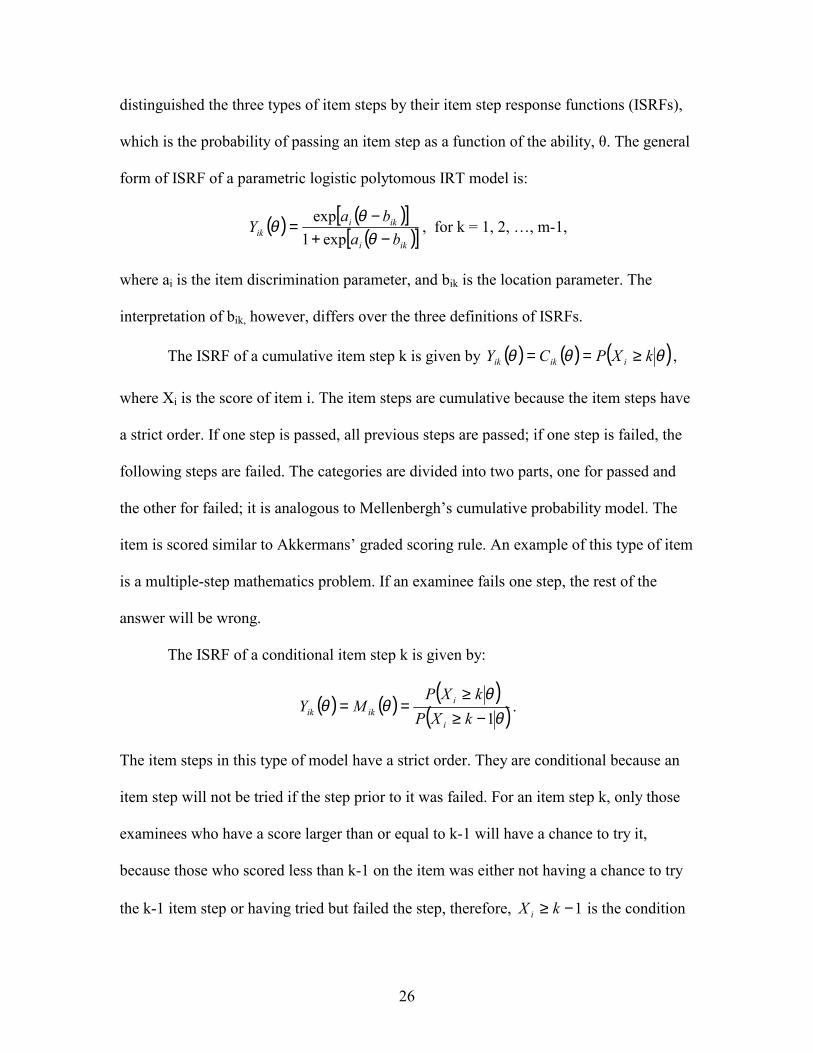
26
distinguished the three types of item steps by their item step response functions (ISRFs),
which is the probability of passing an item step as a function of the ability, θ. The general
form of ISRF of a parametric logistic polytomous IRT model is:
( ) ( )[ ]( )[ ]iki
ikiik ba
baY
−+−
=θ
θθ
exp1exp
, for k = 1, 2, �, m-1,
where ai is the item discrimination parameter, and bik is the location parameter. The
interpretation of bik, however, differs over the three definitions of ISRFs.
The ISRF of a cumulative item step k is given by ( ) ( ) ( )θθθ kXPCY iikik ≥== ,
where Xi is the score of item i. The item steps are cumulative because the item steps have
a strict order. If one step is passed, all previous steps are passed; if one step is failed, the
following steps are failed. The categories are divided into two parts, one for passed and
the other for failed; it is analogous to Mellenbergh�s cumulative probability model. The
item is scored similar to Akkermans� graded scoring rule. An example of this type of item
is a multiple-step mathematics problem. If an examinee fails one step, the rest of the
answer will be wrong.
The ISRF of a conditional item step k is given by:
( ) ( ) ( )( )θ
θθθ
1−≥≥
==kXP
kXPMY
i
iikik .
The item steps in this type of model have a strict order. They are conditional because an
item step will not be tried if the step prior to it was failed. For an item step k, only those
examinees who have a score larger than or equal to k-1 will have a chance to try it,
because those who scored less than k-1 on the item was either not having a chance to try
the k-1 item step or having tried but failed the step, therefore, 1−≥ kX i is the condition

27
for item step k. This type of model is equivalent to Mellenbergh�s continuation ratio
model. Items in these models are scored using Akkerman�s sequential scoring rule.
Akkerman gave an example of this kind of scoring for testing psychomotor skills where
an action is tried until the first success or repeated until the first failure.
The ISRF of a partial credit item step k is given by:
( ) ( ) ( )( ) ( )( )θθ
θθθ
1−+==
kiik
ikikik PP
PAY .
This type of model is equivalent to Mellenbergh�s adjacent category model. Partial credit
is given to each item step being passed. Since the item steps represent a collection of sub-
tasks or features displayed by the item response and each of them will be given partial
credit, this type of model is scored according to Akkerman�s parallel scoring rule.
Examples of this type of item are multiple-choice items with partial credit options, e.g.
essays using a scoring rubric. A summary of the three types of polytomous IRT models
with ordinal responses is given in Table 1.
Table 1
Summary of the Three Types of Ordinal Polytomous IRT Models
Model Type (Mellenbergh)
Scoring Rule (Akkerman)
Item Step (Hemker)
Model
Represented
Adjacent category Parallel Partial credit PCM
Cumulative probability Graded Cumulative GRM
Continuation ratio Sequential Conditional SM Note. PCM = partial credit model; GRM = graded response model; SM = sequential model.
Ordinal polytomous IRT models compared in this study
In this study, three ordinal polytomous IRT models were compared to five other
IRT models. They were the partial credit model, the generalized partial credit model and

28
the multiple-choice model (Samejima, 1979, Thissen and Steinberg, 1984, 1997). A brief
introduction to the three models is described next.
Partial credit model (PCM).
Masters (1982) extended the Rasch dichotomous model to include polytomous
items. He assumed that response categories were ordered by the levels of proficiency they
represent. He conceptualized a multiple-step item; in which each step represented the
difference in proficiency levels between two adjacent categories. Partial credit was given
to each step completed. The resulting PCM is an adjacent category model. If mi is the
number of steps in an item, the response categories of the item can be represented by the
partial credit assigned to them, i.e. 0 to mi. The model is described by mi log odds:
( )( ) ik
ki
ik bP
P−=
−
θθ
θ
)1(
ln , where k = 1, �, mi.
The ISRF of each step is a response function in the 1-PL logistic model. The one
parameter in the model is the item category location parameter bik. It follows that
( )( )
( )( )( )
( )( )( )( )
( )( ) ( ) ( )∑∏
==−
−
−
−=−=⋅⋅⋅⋅=k
hih
k
hih
i
i
ki
ki
ki
ik
i
ik bbPP
PP
PP
PP
110
1
2
1
10
expexp θθθθ
θθ
θθ
θθ
, for all k.
The sum of the quotients for all k is
( )( )
( )( ) ( )∑ ∑
∑∑
= =
=
=
−==i
i
i m
k
k
hih
i
m
kikm
k i
ik bP
P
PP
1 10
1
1 0
exp θθ
θ
θθ
.
Since ( )∑=
im
kikP
0
θ = 1, it follows that ( )∑=
im
kikP
1
θ = 1 � ( )θ0iP .
Therefore, ( )
( ) ( )∑ ∑= =
−=− im
k
k
hih
i
i bP
P1 10
0 exp1
θθ
θ. It follows that:

29
( )( )∑ ∑
= =
−+=
im
k
k
hih
i
bP
1 1
0
exp1
1
θθ ,
and the probability of an examinee with ability θ responding in category k can be
described by:
( ) ( ) ( )( )
( )∑ ∑
∑∑
= =
=
= −+
−=−⋅=
im
k
k
hih
k
hihk
hihiik
b
bbPP
1 1
1
10
exp1
expexp
θ
θθθθ .
For notational convenience, ( ) 00
0≡−∑
=hihbθ , which implies that
( ) ( )∑∑==
−≡−k
hih
k
hih bb
10θθ , and ( ) 1exp
0
0=−∑
=hihbθ , resulting in a simplified PCM:
( )( )
( ) ( )
( )
( )∑ ∑
∑
∑ ∑∑
∑
= =
=
= ==
=
−
−=
−+−
−=
ii m
k
k
hih
k
hih
m
k
k
hih
hih
k
hih
ik
b
b
bb
bP
0 0
0
1 0
0
0
0
exp
exp
expexp
exp
θ
θ
θθ
θθ , for k = 0, 1, �, mi.
The above equation describes the ICRF for responses in category k of a PCM. It is
assumed that one credit is given to each step completed. A response in category k will be
awarded a partial credit of k out of the possible full credit mi. The categories are ordered
either according to the levels of proficiency demonstrated in the categories or by the
sequential order of the item steps needed to be completed. When PCM is applied to
multiple-choice items, the former is assumed.
The location parameter bik can be broken down further to indicate the item
location and category threshold, i.e. bik = bi + dik. The difference in levels of proficiency
between the adjacent kth and (k+1)th categories is called the kth step difficulty or threshold
dik. The thresholds dik is also equal to a value on the ability continuum (θ � bi) where two
30
adjacent ICCCs intersect. An examinee with ability θ = bik will have an equal probability
of choosing either of the adjacent categories, and therefore, the threshold dik is just like
the boundary between those two categories. In PCM, thresholds need not be ordered.
Harder steps could be followed by easier steps or vice versa. The configuration of the
thresholds, however, could have an effect on the discrimination of the item since the
same amount of credit is given to each item step completed despite its difficulty.
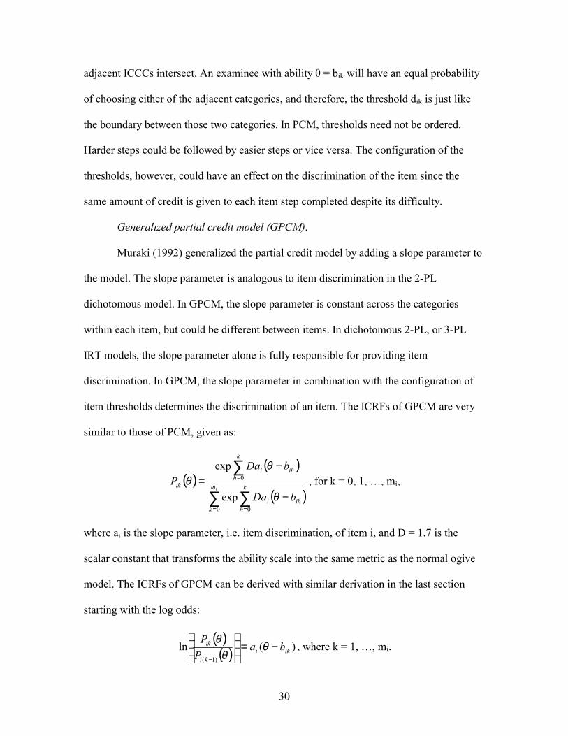
Generalized partial credit model (GPCM).
Muraki (1992) generalized the partial credit model by adding a slope parameter to
the model. The slope parameter is analogous to item discrimination in the 2-PL
dichotomous model. In GPCM, the slope parameter is constant across the categories
within each item, but could be different between items. In dichotomous 2-PL, or 3-PL
IRT models, the slope parameter alone is fully responsible for providing item
discrimination. In GPCM, the slope parameter in combination with the configuration of
item thresholds determines the discrimination of an item. The ICRFs of GPCM are very
similar to those of PCM, given as:
( )( )
( )∑ ∑
∑
= =
=
−
−=
im
k
k
hihi
k
hihi
ik
bDa
bDaP
0 0
0
exp
exp
θ
θθ , for k = 0, 1, �, mi,
where ai is the slope parameter, i.e. item discrimination, of item i, and D = 1.7 is the
scalar constant that transforms the ability scale into the same metric as the normal ogive
model. The ICRFs of GPCM can be derived with similar derivation in the last section
starting with the log odds:
( )( ) )(ln
)1(iki
ki
ik baP
P−=
−
θθ
θ, where k = 1, �, mi.

31
Without presumption of order in the categories, the left hand side of the equation can be:
( )( )
( )( ) ( ) ( ))1()1(
)1()1()1( expexp
lnln −−−−−
−+−=
++
=
kiikkiikkiki
ikik
ki
ik ccaacaca
PP θ
θθ
θθ .
Therefore, for a nominal categories model to be constrained to a more restricted general
partial credit model, it follows that ( )( ) ( )( ) ( )ikikiikkiik baccaa −=−+− −− θθ 11 , and the
relationship between the parameters in the two models can be expressed as:
( )1−−= kiiki aaa , and ( )
( )1
1
−
−
−−
−=kiik
kiikik aa
ccb .
It confirms the observations of Thissen and Steinberg (1984) and Bock (1997).
Multiple-choice model.
In Bock�s nominal category model, the category with lowest aik (most negative)
will have an ICCC that decreases monotonically from the left tail value of 1 to a right tail
value of 0, while the other ICCCs are with a left tail decreasing to 0. When it is applied to
multiple choice items, the ICCCs imply that all examinees with low ability will select the
same incorrect category (the one with lowest aik). Empirical studies have shown that
often this is not the case (Levine and Drasgow, 1983). The non-modeled discrepancy is
caused by examinees selecting different categories as their answer by purely guessing.
Samejima (1979) introduced a latent category to allow nonzero left tails for all
ICCCs. Thissen and Steinberg (1984) called that latent category the �don�t know� (DK)
category. The DK category that Samejima suggested is described by a response
distribution function of the ability parameter θ:
( ) ( )( )∑
=
+
+= m
kikik
iiDK
ca
caP
0
00
exp
exp
θ
θθ ,

32
where DK is treated as one extra nominal response category to the item, and ai0, ci0 are
the parameter for that category. It is assumed that examinees in the DK category select
one of the item categories at random. Therefore, the probability of a specific item
category being selected by a DK examinee is 1/m, where m is the number of item
categories. With this assumption, Samejima suggested a multiple-choice model described
by the following ICRFs:
( )( ) ( )
( )∑=
+
+++= m
hihih
iiikikik
ca
camcaP
0
00
exp
exp1exp
θ
θθθ , for k = 1, 2, �, m.
Thissen and Steinberg (1984) argued that it is implausible to assume the DK
examinees would select their answer randomly. They believed that the DK examinees
would be drawn to different options at differential rates. They introduced another
parameter dik, and used it instead of the constant 1/m to represent the probability of a DK
examinee choosing category k. It is obvious that dik for all ks lie in the interval (0,1) and
the sum of dik within an item is 1, i.e. 11
=∑=
m
kikd . The dual constraint on dik is imposed by
expressing them in terms of a set of psuedo-parameters d*ik, where
∑=
= m
hih
ikik
d
dd
1
*
*
)exp(
)exp(.
The psuedo-parameters are undetermined and the constraint 01
* =∑=
m
kikd is imposed to
make them identifiable. The ICRFs of the multiple-choice model become:
( ) ( ) ( )( )∑
=
+
+++= m
hihih
iiikikikik
ca
cadcaP
0
00
exp
expexp
θ
θθθ , where k = 1, 2, �, m.
It is this multiple-choice model that is compared to other models in the present study.

33
Summary
In the literature, it has been shown that Bock�s nominal category model is the
most general polytomous IRT model, and its relationships to the dichotomous models and
different types of ordinal polytomous IRT models have been investigated. As shown in
Akkerman�s (1998) study, model differences in polytomous IRT models have a
theoretical basis and are practical. How items are scored determines what IRT model
should be used for ability estimation. When the wrong type of IRT model is applied,
specification error is made and bias is introduced in examinee ability estimation.
Mellenbergh (1995) has shown that differences between the three types of models
disappear when the items are scored dichotomously.
In this study, tests with multiple-choice items scored dichotomously and
polytomously are compared. It is assumed that all the items are scored according to the
parallel scoring rule, therefore, only the partial credit type of ordinal polytomous IRT
models will be used for comparison. Thissen & Steinberg�s multiple-choice model was
included for modeling the effect of guessing in a polytomous model. Bock�s model was
included to investigate how much bias is present when the ordinal nature of the response
categories is not specified.
Ability Estimation
Different approaches and techniques are applied in item response theory to
estimate ability. The ability parameter can be estimated jointly with the item parameters
or estimated with known item parameters, which have been previously estimated. If the
ability parameter is not estimated jointly with the item parameters, the item parameters
are first estimated from the item responses with the influence of the ability parameter

34
taken away; the ability parameter is either eliminated through conditioning or integrated
out through marginalization. Techniques used in parameter estimation include the
maximum likelihood procedure (Baker, 1992); logistic regression (Reynolds, Perkins and
Brutten, 1994); minimum chi-quadrant (Zwinderman and van der Wollenberg, 1990), and
Bayesian modal estimation procedure (Mislevy, 1986; Baker, 1992). The maximum
likelihood procedure with Bayesian estimates (MAP, EAP) was used in this study;
therefore, a review of maximum likelihood and Bayesian estimation methods in the
literature will be given in the following section.
Maximum Likelihood method
Likelihood is a probabilistic function of modeled observations; a specific item
response vector in the case of IRT models. When local independence is assumed, the
likelihood function is the product of the probabilities associated with individual item
responses in a vector. Since the probability of an item response is a function of ability
and item parameters, the likelihood function is also a function of those parameters. For
example, the likelihood function of examinee j�s response to n items using Birnbaum�s 2-
PL logistic model is ( ) ( )∏=
=n
iiiji baxfL
1
,,,, θθ bax j , where x = (x1, x2, �, xn) is the
response vector of examinee j to the n items (xi = 1 or 0 for all i), a = (a1, a2, �, an) and b
= (b1, b2, �, bn) are the item parameter vectors and f is the item response function of the
2-PL logistic model. Therefore, L is the probability of obtaining a response vector x given
the parameters θj, a, and b. Maximum likelihood estimation is used to find the value of
the parameters that maximize the value of L.
Since the likelihood function L involves a product of functions, it is easier to work
with a logarithm of L instead of L itself. A logarithm is a monotonic function; therefore,

35
ln L is maximized when L reaches its maximum. A logarithm of the likelihood function is
used to find a solution in practice. Estimators of the parameters are obtained from the
solution of the first derivative equation 0ln =∂
∂θ
L (likelihood equation), which is the
condition for a local maximum to occur. If there is more than one local maximum, the
largest should be chosen. For the entire response data set of N examinees tested on n
dichotomous scored items, the likelihood function is given by:
( ) ( ) ( ) ijij xij
N
j
n
i
xij
N
j
n
ijij
N
jjjNN QPxLLL −
= == ==∏∏∏∏∏ === 1
1 11 112121 ,...,,,...,, θθθθθ xxxx .
And after taking logarithms on both sides of the equation,
( ) ( ) ( )[ ]∑∑= =
−−+=N
j
n
iijijijijNN PxPxL
1 12121 1ln1ln,...,,,...,,ln θθθxxx .
The maximum likelihood estimates of the ability parameters θ1, θ2,�, θN are obtained by
solving the simultaneous equations:
( ) 0,...,,,...,,ln 2121 =∂∂
NNj
L θθθθ
xxx , for j = 1, 2, �, N.
A solution for the likelihood equation is possible using the Newton-Raphson
algorithm, when the likelihood function is twice differentiable, i.e. the second derivative
of the likelihood function is available. The Newton-Raphson algorithm starts with an
initial value for the estimate of the parameter in the model. The number of items correct
is usually used for the ability estimates, and CTT item statistics, e.g. proportion correct
and biserial correlation are used for item estimates. In each iteration, a new estimate for
the parameters is generated based on the estimate obtained from the previous iteration.
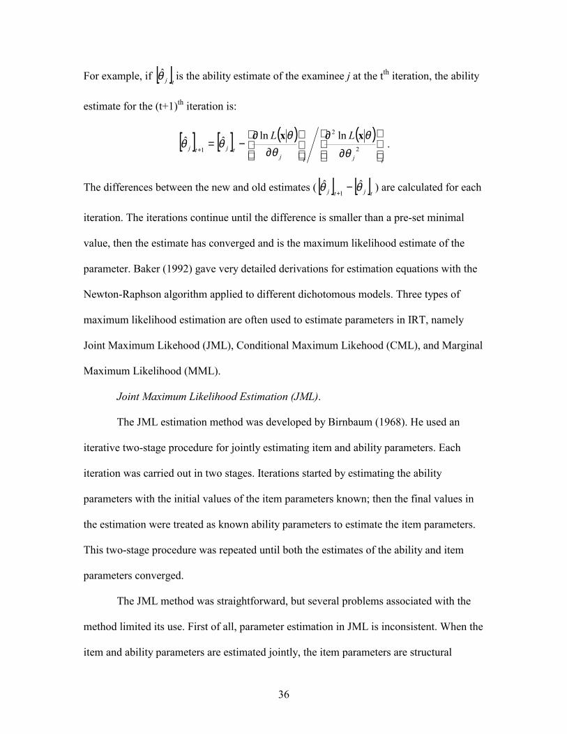
36
For example, if [ ]tjθ� is the ability estimate of the examinee j at the tth iteration, the ability
estimate for the (t+1)th iteration is:
[ ] [ ] ( ) ( )tjtj
tjtj
LL
∂
∂
∂
∂−=
+ 2
2
1
lnln��θ
θθ
θθθ
xx.
The differences between the new and old estimates ( [ ] [ ]tjtj θθ ��
1−
+) are calculated for each
iteration. The iterations continue until the difference is smaller than a pre-set minimal
value, then the estimate has converged and is the maximum likelihood estimate of the
parameter. Baker (1992) gave very detailed derivations for estimation equations with the
Newton-Raphson algorithm applied to different dichotomous models. Three types of
maximum likelihood estimation are often used to estimate parameters in IRT, namely
Joint Maximum Likehood (JML), Conditional Maximum Likehood (CML), and Marginal
Maximum Likelihood (MML).
Joint Maximum Likelihood Estimation (JML).
The JML estimation method was developed by Birnbaum (1968). He used an
iterative two-stage procedure for jointly estimating item and ability parameters. Each
iteration was carried out in two stages. Iterations started by estimating the ability
parameters with the initial values of the item parameters known; then the final values in
the estimation were treated as known ability parameters to estimate the item parameters.
This two-stage procedure was repeated until both the estimates of the ability and item
parameters converged.
The JML method was straightforward, but several problems associated with the
method limited its use. First of all, parameter estimation in JML is inconsistent. When the
item and ability parameters are estimated jointly, the item parameters are structural

37
parameters, which are fixed by the length of the test, and the ability parameters are
incidental parameters, because the number of ability parameters increases as the sample
size increases. Neyman and Scott (1948) have shown that large numbers of incidental
parameters adversely affects the consistency of the estimation of structural parameters.
This implies that the estimates of the item parameters will not converge to their true
values when the sample size of examinees increases to a large number. Moreover, the
item parameter estimates in JML are biased. De Gruijter (1990) found that the bias of
parameter estimates, i.e. the difference between the true value of the parameter and the
estimate, depended on the expected total score distribution. As the test increases in
length, the bias will become less important, because the ability parameter can be
estimated more precisely. Large sample sizes and lengthy tests are required to minimize
bias in parameter estimates in the JML procedure, thus making it less popular, especially
in small-scale studies. The JML method cannot apply to items and examinees with zero
or perfect scores. An examinee with a zero score will have an ability estimate of - ∞ ,
while an examinee with a perfect score will have an estimate of + ∞ . Similarly, an item
that all examinees fail will have an item difficulty estimate of + ∞ , while an item that
everybody answered correctly will have an item difficulty estimate of -∞ .
Conditional Maximum Likelihood Estimation (CML).
In JML, the item parameter estimates could be inconsistent and biased because
they are estimated jointly with the ability parameter. The CML estimation technique
(Andersen, 1972), in contrast, provided consistent and efficient parameter estimates by
factoring out the unknown ability parameters from the likelihood equations. It required
sufficient statistics for the ability and item parameters, which were only available in the

38
1-PL logistic model. The number of items correct (count) is a sufficient statistic for the
ability parameter and the number of correct responses to an item is a sufficient statistic
for the item difficulty parameter. The likelihood function L(x│θ) is replaced by L(x│r) in
CML, where x is a response vector containing the response patterns of each examinee in
the sample, and r is a vector containing the number correct of each examinee. It can be
shown that L(x│r) = L(x│θ)/ L(r│θ), which is independent of θ because the terms in the
numerator and denominator cancel out each other.
While CML has the advantage of separately estimating the ability and item
parameters, it has some limitations. First, no parameter estimates can be obtained for zero
or perfect scores. Second, examinees that have the same number of items correct but
different response patterns will be given the same ability estimate. Third, CML has
problems in estimating parameters for a long test, complicated patterns of missing data,
and polytomous items with many response categories.
Marginal Maximum Likelihood Estimation (MML).
While CML permits item parameter estimation free from the condition of ability
parameters, it requires a sufficient statistic for the ability parameter. That condition limits
its application to the 1-PL logistic models. Bock & Lieberman (1970) introduced an
approach to handle the unknown ability parameters. Instead of using the likelihood
function conditioned on an examinee�s ability θ, i.e. L(x│θ), they suggested the
unconditional likelihood function L(x), which is the probability of observing the pattern x
from an examinee of unknown ability drawn at random from a population. The observed
response data is regarded as a random sample from a population. If the population has an

39
ability distribution described by a continuous density function g(θ), the unconditional
likelihood function is given by the definite integral,
( ) ( ) ( ) θθθ dgLL ⋅= ∫∞
∞−xx .
L(x) is a function of the item parameters only because the ability parameter θ has been
integrated out. The definite integral generally cannot be expressed in closed form, thus a
procedure called Gaussian quadrature is used to find the value of the integral.
Since the unconditional likelihood function is an expected value over a population
rather than an observed value, estimation procedures are different from that used in the
JML estimation method. The original approach that Bock and Lieberman (1970)
introduced posed a formidable computational task, and thus was not practical for lengthy
tests. In a subsequent reformulation of the MML approach, Bock and Aitken (1981)
introduced the EM algorithm as a procedure for MML estimation. The EM algorithm has
two stages, namely the expectation and the maximization stage. In the expectation stage,
expected values of the frequencies at quadrature points and expected frequencies of
examinees passing the items are computed. These expected values are then submitted to
the estimation equations for maximum likelihood estimation in the maximization stage.
The E and M stages repeat until the estimates converge. The Newton-Gauss method is
used to solve the maximum likelihood equation.
MML has some advantages over other maximum likelihood methods. It is
applicable to all IRT models and efficient for any test length. It provides estimates for
perfect scores and thus no loss of information by trimming items and examinees with
perfect scores. The estimates of item standard error in MML are good approximations of
expected sampling variance of the estimates. Despite these advantages, MML has some
40
limitations. First, MML estimation is computationally involved and sophisticated.
Second, an ability distribution must be assumed. It is assumed to be normal if the prior
ability distribution is not known. The effect of departure from normality, however, seems
minimal and the population ability distribution actually can be estimated from data.
Third, Baker (1992) pointed out that MML with EM algorithm resolved the problem of
inconsistent item parameter estimates in JML, but the problem of deviant ability
estimates in some data sets remained unsolved. There is simply no way to estimate
parameters for aberrant response patterns. It is this last limitation that led to the use of
Bayesian estimates in MML (Bock and Aitkin, 1981; Mislevy, 1986).
Bayesian estimation
Bayesian parameter estimation procedures are based on Bayes� theorem, which
states the relationship between the conditional and the unconditional probabilities of the
occurrence of an event. Specifically, Bayes� theorem can be expressed as:
( ) ( ) ( )APABPBAP ⋅∝ ,
where P(A|B) and P(B|A) are conditional probabilities and P(A) is the unconditional
probability of occurrence of event A. The likelihood function L(x| θ) is a conditional
probability. It follows from the Bayes� theorem that:
( ) ( )θθθ PLP ⋅∝ xx)( .
P(θ|x), the probability of θ under the condition of item response vector x, can be
understood as the distribution of ability estimates according to the item responses, i.e. the
density function of the posterior ability distribution. The unconditional probability P(θ) is
the distribution of the ability prior to estimation, i.e. density function of the prior ability

41
distribution. The posterior ability distribution is therefore proportional to the product of
the likelihood function and the prior ability distribution.
Bayesian estimation procedure makes use of this relationship and the information
from the prior ability distribution in the estimation of the ability parameters. The prior
ability distribution is informative if the variance of the distribution is small. A large
variance, however, would make a prior distribution uninformative. An uninformative
prior distribution would have less impact on ability parameter estimation. Informative
prior distributions, on the other hand, will shrink the ability estimates toward the mean of
the prior distribution and thus prevent the ability estimates from diverging to
unreasonable values in the estimation process. This characteristic of Bayesian estimation
helps to solve the problem of deviant estimates in maximum likelihood estimation, and
provides a means for estimating aberrant response patterns, e.g. all zero or all perfect
responses to items in a test. Two Bayesian estimates are commonly applied in MML, i.e.
maximum a posteriori (MAP) and expected a posteriori (EAP).
Maximum a posteriori (MAP) estimates.
MAP is the value of ability estimate θ that maximizes the logarithm of the density
function of the posterior ability distribution:
( ) ( ) ( )[ ] ( ) ( )θθθθθ PLPLP lnlnlnln +=⋅= xxx .
MAP estimate is also called Bayesian modal estimate. It is obtained by the solution of the
likelihood equation using the Newton-Raphson procedure:
( ) ( ) ( ) 0lnlnln=
∂∂+
∂∂
=∂
∂θ
θθ
θθθ PLP xx
.
Since marginal Bayesian modal estimation can be considered an extension of MML, the
estimation procedure utilizes the EM algorithm as described before. The two-stage

42
procedure is repeated until a convergence criterion is met. The criterion is typically
specified as a number of EM cycles. The Bayesian modal estimation procedure always
converges and thus ability estimates are available, even for examinees with zero total
score or a perfect score.
Expected a posteriori (EAP) estimates.
EAP is the mean of the posterior ability distribution of an examinee, i.e. the
expected value of θ in the posterior ability distribution. It is given by:
( ) ( ) ( )( ) ( )∫
∫∞
∞−
∞
∞−=θθθ
θθθθθ
dPL
dPLE
x
xx .
The above equation involves integrations. In practice, the integrations can be
approximated by the Gauss-Hermite quadrature. The approximation is obtained by
( )( ) ( )
( ) ( )k
q
kk
kk
q
kk
XAXL
XXAXLE
∑
∑
=
==
1
1
x
xxθ .
The equation is not iterative and EAP estimates are obtained directly. Bock and Aitkin
(1981) introduced EAP as part of the MML estimation procedure.
Summary
In the present study, ability estimates are obtained using different item
parameterization and scoring models. The ability estimates are compared to see which
combination of item parameterization and scoring model provides the best estimation of
the examinees� ability. It is important for the same estimation approach be used in all the
models under comparison. In the literature, MML was recommended among the three
maximum likelihood methods. Caution was also taken in choosing the IRT computer
43
software that used MML for parameter estimation. The software used for parameter
estimation in this study is MULTILOG (Thissen, 1991). MML in combination with
Bayesian MAP and EAP estimation were used for parameter estimation in the item
calibration and scoring runs. MULTILOG provides analysis for all the models,
dichotomous and polytomous, covered in the present study. The dichotomous models are
treated as special cases of some polytomous models covered by the software.

44
CHAPTER 3
METHODS AND PROCEDURES
Data Simulation and Design
This study employed a 7× 4× 3 factorial design with seven item parameterization
and scoring models, four prior ability distributions (normal, skewed to the right, skewed
to the left, bimodal), and three kinds of threshold distances (equal, unequal-low, unequal-
high). The seven models being compared were the 1-, 2-, 3-PL dichotomous logistic
model, the Generalized Partial Credit Model with item discrimination ai set to a constant
(GPCM-1), the Generalized Partial Credit Model (GPCM), the Multiple Choice Model
(MCM), and the Nominal Categories Model (NCM). The 84 combinations for the three
factors are listed in Table 2.
Table 2
Combinations for Study Design
Normal Skewed to right Skewed to left Bimodal
ET UL UH ET UL UH ET UL UH ET UL UH
1-PL Cne1 Cnl1 Cnh1 Cre1 Crl1 Crh1 Cle1 Cll1 Clh1 Cbe1 Cbl1 Cbh1
2-PL Cne2 Cnl2 Cnh2 Cre2 Crl2 Crh2 Cle2 Cll2 Clh2 Cbe2 Cbl2 Cbh2
3-PL Cne3 Cnl3 Cnh3 Cre3 Crl3 Crh3 Cle3 Cll3 Clh3 Cbe3 Cbl3 Cbh3
GPCM-1 Cne4 Cnl4 Cnh4 Cre4 Crl4 Crh4 Cle4 Cll4 Clh4 Cbe4 Cbl4 Cbh4
GPCM Cne5 Cnl5 Cnh5 Cre5 Crl5 Crh5 Cle1 Cll5 Clh5 Cbe5 Cbl5 Cbh5
MCM Cne6 Cnl6 Cnh6 Cre6 Crl6 Crh6 Cle6 Cll6 Clh6 Cbe6 Cbl6 Cbh6
NCM Cne7 Cnl7 Cnh7 Cre7 Crl7 Crh7 Cle7 Cll7 Clh7 Cbe7 Cbl7 Cbh7 Note. ET= equal threshold distances, UL= unequal threshold-low, UH= unequal threshold-high.

45
With each combination of prior ability distribution and threshold distances, a set
of polytomous item responses of 1,000 subjects to 30 items was simulated using a
computer program described in later section. Therefore, twelve different sets of
polytomous item responses were generated. Those sets of item response data were then
analyzed given the seven IRT parameterization and scoring models using computer
programs described in the next section for estimation of item parameters and ability
estimates. For each combination of the three factors, ability estimates were computed. A
total of 84 different sets of ability estimates were computed, one set for each combination
in Table 2.
Number of Replications in Monte Carlo Estimation
In order to obtain stable ability estimates on each individual in the sample of
1,000 examinees, 50 replications of the data simulation and ability estimation described
in the above paragraph were completed to produce a total of 4,200 (84× 50) different sets
of ability estimates. The number of replications used in simulation studies of IRT models
in the past varied from as few as 5 to as many as 100 replications (Kamata, 1998;
Boughton, Klinger and Gierl, 2001). Kamata, who varied the number of replications in
his study from 3 to 100 across six levels, and Yang (1995), have both shown that
estimates of parameters were stable after 50 replications. Therefore, this study employed
50 replications for each combination of conditions based on suggestions from these
Monte Carlo studies. In each of the 50 replications of data simulation, the random seed
(seed1 in the SAS program in Appendix A) that was used to create the random sample of
original ability estimates for the 1,000 examinees was kept constant and the random seed
(seed3 in the same program in Appendix A) that was used in generating the item response

46
data was changed in each replication, so that the 50 item response data sets were different
but with the same sample of examinees. For each combination of conditions, the mean of
the 50 ability estimates of each examinee generated in the 50 replications was calculated
and served as the estimate of the ability parameter for that person under those specific
conditions. The sampling error of the mean was also calculated and a 95% confidence
interval was computed around the mean. Therefore, for each of the 84 combinations of
conditions, 1,000 confidence intervals were formed.
Criteria for Evaluation
Two criteria were used to determine how close the estimated ability estimates
were to the original ability estimates. First, each of the 1,000 original ability estimates
was examined to determine how many of them fell in the 95% C.I.s of the corresponding
bootstrap ability estimates. The number of original ability estimates that fell in the C.I.s
for each combination of conditions was recorded. The rate of recovery, i.e. the number of
recovered original ability estimates divided by 1,000, served as an indicator of how well
the different models recovered an examinee�s ability estimate under the different research
design combinations. Therefore, 84 of such recovery rates, one for each study design
combination, were generated in each data simulation and analysis cycle.
Second, a root mean square error (RMSE) of ability estimation was calculated
across samples for each of the study design combination. The RMSE indicated the bias
and variance of ability estimation, and thus served as an indicator of precision. The
RMSE was calculated as:
RMSE(Cxyz) = ( )
∑=
−n
j
jj
n1
2� θθ

47
For n = number of examinees;
≡jθ original ability score of the jth examinee
≡jθ� mean of the ability estimates of the jth examinee from 50 replications
Where Cxyz is the research design combination of �x prior distribution�, �y threshold
distance configuration� and �z IRT model�, and therefore 84 RMSE were calculated in
each data simulation and analysis cycle. A flowchart illustrating one cycle of data
simulation and analysis is listed in Appendix B followed by the computer programs used
in each phase of the cycle.
Sample Size and Power Analysis for Hypothesis Testing
In order to answer the research questions, six three-way ANOVAs were run to test
the stated hypotheses. Eighteen cycles of the data simulation and analysis process
described in the previous section were conducted to generate 1,552 (84× 18) recovery
rates and RMSE. The number of cycles was chosen in reference to the F test for the
hypothesis with most levels involved, which was the three-way interaction effect of the
hypothesis comparing the four different polytomous models under the combinations of
four levels of prior distributions, and three levels of threshold configurations (4× 4× 3),
because it involved the largest number of cells. According to Cohen�s (1988) power table
for F test at level of significance, α = .05, and degree of freedom for the numerator, df =
15, and a medium effect size (f = .25), a cell size of 18 will give the F test a power
approximately equal to .76; but if df = 24 and the other conditions remain unchanged, the
power of the test increases to .89. The F test was chosen with reference df = 18, and
therefore the power of the F test will be around .80. From one cycle to the other, the

48
random number seed (seed1), which was kept constant within each cycle, was changed,
so that the samples of 1,000 examinees were different from those in the other cycles.
Construction of Test Items
The parameters of the test items used in the present study were chosen to reflect
typical item discrimination and difficulty of real test data. The item parameters were
generated to model partial credit items. Thirty discrimination parameters ranged from .75
to 2 were randomly assigned to the thirty items representing adequate but varied
discriminations. Different levels of difficulty were implemented in the test by having 10
easy, 10 moderate and 10 difficult items. The thresholds of the easy items were all
negative, those of the difficult items were all positive, and those of the moderate items
were symmetric around values close to zero. The values of the thresholds in the 30 items
were ranging from �2.25 to 2.25 to ensure enough range for measuring all the ability
levels in the simulated samples. Since the number of response categories in each item
was set to four, there were three thresholds in each item, namely b1, b2, and b3. Three
different configurations of thresholds were generated by varying the distances between
the thresholds, i.e. equally distributed, shorter on the lower end, or shorter on the higher
end. The three different configurations of thresholds were acquired by changing the value
of the middle threshold. For the condition of equal threshold distances, the value of the
middle threshold, b2 was set to the mean of b1 and b3. For threshold distances shorter at
the lower end, the value of the middle threshold, b�2 was set to the mean of b1 and b2. For
the third condition, the value of the middle threshold, b�2 was set to the mean of b2 and b3.
The item parameters of the 30 items are listed in Appendix C.

49
Data Simulation Computer Program
The SAS data simulation program was adopted and modified from the
unpublished dissertation of Susan Chen (1999). The first part of the program used the
random number function RANOR (for the other three ability distributions, other random
number generating functions are used, see Appendix A) to generate a set of 1,000 random
numbers to represent the ability parameters for the different IRT item parameterization
and scoring models. The ability parameters generated by RANOR were normally
distributed with the mean equal to zero and standard deviation equal to one. The 1,000
random numbers were then submitted to the second part of the program as the known
ability estimates of 1,000 examinees to generate response patterns for 30 items. The SAS
program did two things. First, it generated the probability of response in each of the four
item categories of an item for each examinee. The probabilities were generated according
to the ICRFs of the general partial credit model, the most general form of partial credit
models. The probability of each item category was conceptually represented by a line
segment with the length equal to the magnitude of the probability. The four probabilities
were concatenated to form a 0 to 1 interval, (the sum of the probabilities equal to 1).
Second, another 1,000 uniformly distributed random numbers between 0 and 1 were used
to generate the item responses. For each examinee, a random number between 0 and 1
was generated and compared to the interval formed by the four probabilities. The number
must fall into one of the four line segments, and the category represented by that line
segment was the item response of that examinee for that item. Since an examinee with
higher ability estimate will have a higher probability in choosing higher categories and
the random number chosen is from a uniform distribution, a higher ability examinee has

50
higher chance to get a proportionally higher response categories in this transformation.
The SAS sub-routines were repeated for each item and each examinee. A dichotomous
response data set was obtained by setting to 1 the category in the polytomous response
data set whose ICCC was monotonic increasing, and the other three categories to 0.
Item Parameterization and Ability Estimation Programs
The commercial computer software package MULTILOG developed by David
Thissen (1991) was used in the present study to estimate parameters for different item
parameterization and scoring models. The package employs MML in the item parameter
estimation phase, maximum likelihood and Bayesian estimation in the scoring phase. It
provides estimation for the three normal and logistic dichotomous models and many
polytomous models. The program files of individual models are listed in Table 3 and
some examples of the programs are listed in Appendix D.
Table 3
Computer Programs Used for Different Item Parameterization and Scoring Models
Scoring format Item
Parameterization
Dichotomous Ordinal Polytomous Nominal Polytomous
1-parameter L1.cmd L1s.cmd
Pc.cmd Pcs.cmd
2-parameter L2.cmd L2s.cmd
Gp.cmd Gps.cmd
Nc.cmd Ncs.cmd
3-parameter L3.cmd L3s.cmd
Mc.cmd Mcs.cmd
51
CHAPTER 4
RESULTS
Overview
The recovery rate of original ability estimates (Thetarec) and the root mean
squared error (RMSE) for the ability estimates were tabulated for each study design
combination (a portion of the table from one data simulation and analysis cycle is listed
in Appendix E). Five grouping variables were created to facilitate comparisons posed by
the research questions. The five grouping variables were the scoring format (ScorFor) [1
= dichomtomous, 2 = polytomous], the item parameterization (ItemPar) [1 = 1-PL, 2 = 2-
PL, 3 = 3PL], the polytomous IRT models compared in the study (PolyMod) [1 = GPCM-
1, 2 = GPCM, 3 = MCM, 4 = NCM], the prior ability distribution (Thetadis) [1 = normal,
2 = skewed to the right, 3 = skewed to the left, 4 = bimodal], and the item threshold
configuration (Threconf) [1 = evenly distributed, 2 = closer at the low end, 3 = closer at
the high end]. A total of 1,512 recovery rates and RMSEs respectively were acquired
through the analysis of the simulated item response data sets using seven different IRT
models. The minimum recovery rate was .049, and the maximum was .945; where a zero
recovery rate represented non-recovery and 1 represented prefect recovery. The RMSE
recorded a minimum value of .029384 and a maximum value of .372022, where lower
RMSE represented higher accuracy in ability estimation. In view of the range of the
original ability estimates, mostly (over 95%) within the range of �4 to 4, the differences
in the RMSEs across the models were not as dramatic as what the recovery rates
indicated shown. Descriptive information for these two variables in different groups by
the five grouping variables was summarized in Table 4 and Table 5.

52
Table 4
Descriptive Information of the Recovery Rates across Different Groups
Group Size
Mean Standard Deviation
Minimum Maximum
Scoring Format 1,512 .50500 .22121 .049 .945
Dichotomous 648 .34240 .12795 .049 .650
Polytomous 864 .62695 .19661 .086 .945
Item Parameterization 1,296 .47747 .22449 .049 .945
One typea (1-PL) 432 .63704 .23816 .271 .945
Two typesb (2-PL) 432 .45351 .14767 .134 .806
Three typesc (3-PL) 432 .34186 .16843 .049 .894
Polytomous Models 864 .62695 .19661 .086 .945
GPCM-1 216 .86056 .08908 .339 .945
GPCM 216 .52787 .12414 .291 .806
MCM 216 .44919 .15859 .086 .894
NCM 216 .67018 .09141 .417 .913
Prior Ability Distribution 1,512 .50500 .22121 .049 .945
Bimodal 378 .50215 .20854 .251 .945
Skewed to the left 378 .48772 .22980 .106 .898
Normal 378 .48484 .24397 .049 .925
Skewed to the right 378 .54529 .19482 .209 .923
Thresholds Configuration 1,512 .50500 .22121 .049 .945
Equal Distances 504 .51631 .22376 .082 .945
Unequal-High end 504 .49305 .22704 .049 .931
Unequal-Low end 504 .50564 .21237 .086 .925 a item difficulty; b item difficulty and discrimination, c item difficulty, discrimination and guessing

53
Table 5
Descriptive Information of the RMSE across Different Groups
Group Size
Mean Standard Deviation
Minimum Maximum
Scoring Format 1,512 .134138 .0837995 .029384 .372022
Dichotomous 648 .212244 .0697662 .111041 .372022
Polytomous 864 .075560 .0250993 .029384 .211636
Item Parameterization 1,296 .144302 .0860949 .029384 .372022
One typea 432 .094320 .0497234 .029384 .196774
Two typesb 432 .142517 .0619508 .047906 .265009
Three typesc 432 .196066 .1037707 .043347 .372022
Polytomous Models 864 .075560 .0250993 .029384 .211636
GPCM-1 216 .047900 .0118312 .029384 .090294
GPCM 216 .083270 .0110293 .047906 .123693
MCM 216 .097910 .0241639 .043347 .211636
NCM 216 .073160 .0186354 .036222 .103875
Prior Ability Distribution 1,512 .134138 .0837995 .029384 .372022
Bimodal 378 .120133 .0828093 .029384 .307099
Skewed to the left 378 .135304 .0621354 .042988 .268961
Normal 378 .136334 .0917573 .034395 .372022
Skewed to the right 378 .144781 .0932271 .040336 .360555
Thresholds Configuration 1,512 .134138 .0837995 .026384 .372022
Equal Distances 504 .132676 .0841862 .026384 .352136
Unequal-High end 504 .138665 .0894819 .031623 .372022
Unequal-Low end 504 .131073 .0772566 .032879 .342053 a item difficulty; b item difficulty and discrimination, c item difficulty, discrimination and guessing

54
The two criteria, recovery rate and root mean squared error, were expected to be
correlated to a certain extent. While both criteria are measuring the accuracy of the
models� ability estimation, they refer to different aspects. They were correlated to
examine their strength of association. A Pearson correlation coefficient of -.730 was
obtained for the two criteria. The negative sign indicates that the two criteria vary in
opposite directions. High recovery rate or low RMSE indicates high accuracy in ability
estimation. One criterion explains about 50% of the variance in the other. Despite their
shared variance, each criterion offers unique information on the accuracy of the ability
estimation.
It is apparent from the wide range of recovery rates and RMSEs that the different
IRT models vary greatly in their ability to recover the original ability estimates. The
group means and standard deviations alone do not reveal how the two criteria varied by
different combinations of grouping variables. Three-way ANOVAs were performed to
examine the effects of the five factors, namely scoring format, item parameterization,
different polytomous models, prior ability distribution, and thresholds configurations, on
the two criteria of ability estimation accuracy. The results of the analyses are summarized
in the following section by research question. ANOVA was chosen instead of MANOVA
because the primary interest of the present study was on how the factors affected the two
criteria individually, not on their combined measure of accuracy.
Research Question 1
How do dichotomous and polytomous IRT models differ in accuracy of
recovering ability estimates in different combinations of prior ability distributions and
item category threshold distance configurations?

55
Two three-way ANOVAs were conducted with Scorfor (S), Thetadis (P),
Threconf (T) as independent variables, and Thetarec and RMSE as dependent variables,
respectively. The results for these analyses are summarized in Tables 6 and 7, and the
discussion addressed the research question.
Table 6
Three-Way Fixed Effects ANOVA on Recovery Rate (S, P, T) Source*
SS
Df
MS
F
p
η2
Power�
S 29.983 1 29.983 59.211 .000 .406 1.000
P 1.349 3 .450 17.326 .000 .018 1.000
T .161 2 .08066 3.109 .045 .002 .599
S×P 2.680 3 .893 34.431 .000 .036 1.000
S×T .512 2 .256 9.867 .000 .007 .984
P×T .337 6 .05619 2.166 .044 .005 .775
S×P×T .653 6 .109 4.193 .000 .009 .980
Error 38.605 1488 .02594
Total 73.937 1511
*S = Scoring Format, P = Prior Ability Distribution, T = Threshold Configuration � Computed using level of significance = .05
The independent variables together explained about 48% (model R square was
.478) of the variance in the recovery rate in this ANOVA. From Table 6, the three-way
interaction effect is statistically significant at the level of .0005 with a small effect size
(η2 = .009, f = .10) according to Cohen (1988)5. Since the three-way interaction was
5 Cohen (1988) defined f as the ratio between variance of group means and pooled variance of the dependence variable. The relationship between f and η2 is given by f2 = η2 / (1 - η2). Cohen gave f = .1, .25, and .4 as general reference for small, medium and large effect for F tests in ANOVA.

56
statistically significant, the other effects could not be interpreted unambiguously. Simple
interaction tests of scoring format (2) × prior ability distribution (4) at the three levels of
threshold configuration were used to explain results. The two-way interaction S×P was
statistically significant at the level of .05 at all levels of the threshold configuration, (F(3,
496) = 11.68, p < .0005; F(3, 496) = 3.25, p = .022; and F(3, 496) = 26.53, p < .0005; for
�equal threshold distances�, �unequal-close at the lower end�, and �unequal-close at the
higher end� respectively). Therefore, simple-simple main effects of scoring format were
examined within each combination of threshold configurations and prior ability
distributions. They were all statistically significant (p < .0005) except within the
combination of an �unequal-close at the lower end� threshold configuration and �skewed
to the right� prior ability distribution (F(1, 124) = .578, p = .448). Comparisons of the
individual cell means for the statistically significant effects showed that the cell means of
the polytomous models (scorfor = 2) were much higher than those of the dichotomous
models (scorfor = 1). The effect sizes ranged from η2 = .178 to .689, or f = .47 to 1.49,
and they were large effects by Cohen�s standard. This result indicated that the
polytomous models had much higher recovery rates than the dichotomous models. The
only exception was when a group of predominantly lower ability examinees were tested
on items with categories other than the most completed answer being close to their levels
of difficulty at the lower end of the ability continuum.
The simple-simple main effects of prior ability distribution were also tested
within each combination of threshold configurations and scoring formats. With each
combination of threshold configurations and dichotomous scoring, the tests were all
statistically significant (with p-value < .0005 in each case) with large effect sizes

57
(ranging from η2 = .294 to .375 or f = .65 to .77). Post hoc tests revealed that the effects
came from the difference between �skewed to the right� prior and the other prior
distributions, and between the bimodal prior to the other priors. The �skewed to the right�
prior group had the highest recovery rates, the bimodal prior group in the middle, and the
other two prior groups had the lowest. With polytomous scoring, the test was statistically
significant (F(3, 284) = 7.698, p < .0005) only when the threshold configuration of the
items were �unequal-closer at the lower end� and the effect size was much smaller (η2 =
.075, or f = .28). Post hoc tests showed that the �skewed to the left� prior group had
statistically significantly (at the level of .05) higher mean recovery rate than the other
three prior groups.
Table 7
Three-Way Fixed Effects ANOVA on RMSE (S, P, T) Source*
SS
Df
MS
F
p
η2
Power�
S 6.918 1 6.918 3009.755 .000 .652 1.000
P .121 3 .04046 17.605 .000 .011 1.000
T .02261 2 .01131 4.919 .007 .002 .808
S×P .101 3 .03355 14.598 .000 .010 1.000
S×T .03495 2 .01748 7.603 .001 .003 .946
P×T .0009136 6 .0001523 .066 .999 .000 .066
S×P×T .0005335 6 .00008892 .039 1.000 .000 .059
Error 3.420 1488 .002299
Total 10.611 1511
*S = Scoring Format, P = Prior Ability Distribution, T = Threshold Configuration � Computed using level of significance = .05

58
The same group of independent variables together explained about 68% (model
R2 = .678) of the variance in RMSE in this ANOVA. The major contributor to the
explained variance was the main effect of scoring format. However, two of the three two-
way interaction effects were statistically significant at the level of .001, with small effect
sizes (η2 = .010 and .003). Therefore, the main effects could not be interpreted
unambiguously. Tests were performed for the simple main effects of scoring format
within each level of prior ability distribution and threshold configuration. The tests were
all statistically significant (with p < 0.0005 in all tests) and had very large effect sizes
(ranging from η2 = .574 to .773 or f = 1.16 to 1.85). Comparison of the cell means
indicated that polytomous models had much smaller RMSE in ability estimation than the
dichotomous models at all levels of the other two independent variables.
The simple main effect of the prior ability distribution was also tested within the
two levels of scoring format. For the dichotomous models, the simple main effect was
statistically significant (F(3, 644) = 8.308, p < 0.0005) with a small effect size (η2 = .037,
or f = .20). Comparison of cell means revealed two homogenous subsets in the four prior
distribution groups. The �skewed to the left� and bimodal prior groups had smaller
RMSEs compared to the normal and �skewed to the right� prior groups. For the
polytomous models, the simple main effect was statistically significant (F(3, 860) = 66.7,
p < .0005) with a large effect size (η2 = .187, or f = .48). Comparison of cell means
indicated that the bimodal prior group had the lowest RMSE, with the normal prior group
in the middle, and the two skewed prior groups with the highest RMSE.
The simple main effect of the threshold configuration was tested for dichotomous
and polytomous models. It was not significant when the scoring format was polytomous.

59
With dichotomous scoring, it was statistically significant (F(2, 645) = 5.011, p = .007)
with a small effect size (η2 = .015, or f = .12). The effect came from the difference
between the �unequal-close at the lower end� group and the �unequal-close at the higher
end� group. The former had a lower RMSE. The result indicated that polytomous scoring
out-performed the dichotomous scoring in the accuracy of ability estimation, indicated by
lower RMSE under all combinations of the research conditions. The prior distribution of
the ability estimates had effect on the RMSE. The bimodal prior had the lowest RMSE.
To answer the first research question, the analysis indicated that polytomous
scoring provided more accurate ability estimation, both in terms of higher recovery rate
and lower RMSE, than the dichotomous scoring under all combinations of prior ability
distribution and threshold configuration. Further tests were conducted to investigate the
effect of the combinations within dichotomous and polytomous scoring models. Figures 5
to 8 visualized the effects that the combinations of the two factors had on the recovery
rate and RMSE.
For dichotomous models, the threshold configuration did not have much effect on
the accuracy of ability estimation, as expected, but the different prior ability distributions
did affect the recovery rate and RMSE differently. Figures 5 and 6 show how the four
prior groups differed from each other. The normal prior group performed almost
identically for both criteria with the lowest recovery rate and highest RMSE. The bimodal
and the �skewed to the right� prior group did better on both criteria, but the latter did
much better in recovery rate.

60
Figure 5. Marginal means of recovery rate by prior distribution (dichotomous model).
Threshold configuration
unequal-low endunequal-high endequal distances
Estim
ated
Mar
gina
l Mea
ns
.6
.5
.4
.3
.2
Prior distribution
bimodal
skewed to the left
normal
skewed to the right
Figure 6. Marginal means of RMSE by prior distribution (dichotomous model).
Threshold configuration
unequal-low endunequal-high endequal distances
Estim
ated
Mar
gina
l Mea
ns
.25
.24
.23
.22
.21
.20
.19
.18
Prior distribution
bimodal
skewed to the left
normal
skewed to the right

61
For the polytomous models, the threshold configuration did not have much effect
on the RMSE, but affected the recovery rate and had statistically significant interaction
(F(6, 852) = 4.829, p < .0005) with a small to medium effect size (η2 = .033, or f = .18)
with prior ability distribution. It is apparent from Figure 7 that the four prior groups had
very similar recovery rates when the threshold distances were equal, but their recovery
rates diverged when the threshold distances were unequal. The dispersion of the group
means was larger when the threshold distances were closer at the lower end (about .2)
than when they were closer at the higher end (about .1). Furthermore, the ascending order
of the recovery rates of the four prior groups (skewed to the left, normal, bimodal and
skewed to the right) was the same as that in the dichotomous models only when the
threshold distances were closer at the higher end. The order reversed when the threshold
distances were equal or closer at the lower end. In the case of the RMSE, the threshold
configuration had no effect, and the four prior groups differed slightly.
Figure 7. Marginal means of recovery rate by prior distribution (polytomous model).
Threshold configuration
unequal-low endunequal-high endequal distances
Estim
ated
Mar
gina
l Mea
ns
.7
.6
.5
Prior distribution
bimodal
skewed to the left
normal
skewed to the right

62
Figure 8. Marginal means of RMSE by prior distribution (polytomous model).
Threshold configuration
unequal-low endunequal-high endequal distances
Estim
ated
Mar
gina
l Mea
ns
.10
.09
.08
.07
.06
.05
Prior distribution
bimodal
skewed to the left
normal
skewed to the right
Research Question 2
How do different IRT item parameterization models (i.e. modeling difficulty only;
both difficulty & discrimination; and difficulty, discrimination & guessing) differ in
accuracy of recovering ability estimates in different combinations of prior ability
distributions and item category threshold distance configurations?
Two three-way ANOVAs were conducted with ItemPar (I), Thetadis (P),
Threconf (T) as independent variables, and Thetarec and RMSE as dependent variables,
respectively. The results for these analyses are summarized in Tables 8 and 9.
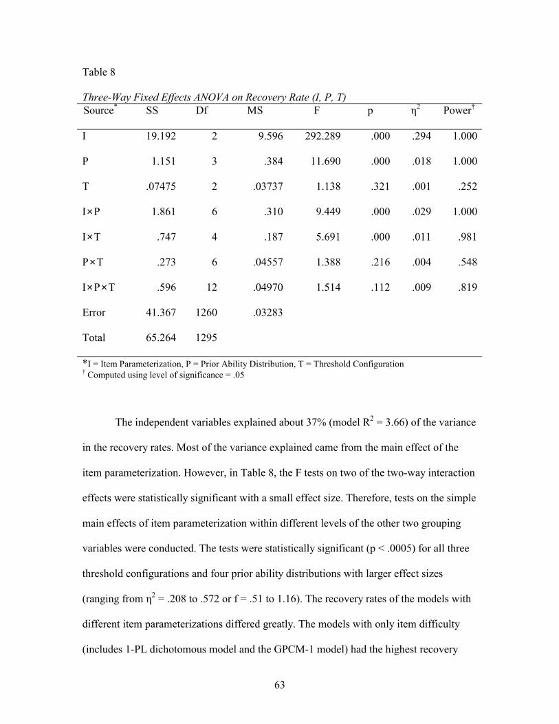
63
Table 8
Three-Way Fixed Effects ANOVA on Recovery Rate (I, P, T) Source*
SS
Df
MS
F
p
η2
Power�
I
19.192 2 9.596 292.289 .000 .294 1.000
P
1.151 3 .384 11.690 .000 .018 1.000
T
.07475 2 .03737 1.138 .321 .001 .252
I×P
1.861 6 .310 9.449 .000 .029 1.000
I×T
.747 4 .187 5.691 .000 .011 .981
P×T
.273 6 .04557 1.388 .216 .004 .548
I×P×T
.596 12 .04970 1.514 .112 .009 .819
Error 41.367 1260 .03283
Total 65.264 1295
*I = Item Parameterization, P = Prior Ability Distribution, T = Threshold Configuration � Computed using level of significance = .05
The independent variables explained about 37% (model R2 = 3.66) of the variance
in the recovery rates. Most of the variance explained came from the main effect of the
item parameterization. However, in Table 8, the F tests on two of the two-way interaction
effects were statistically significant with a small effect size. Therefore, tests on the simple
main effects of item parameterization within different levels of the other two grouping
variables were conducted. The tests were statistically significant (p < .0005) for all three
threshold configurations and four prior ability distributions with larger effect sizes
(ranging from η2 = .208 to .572 or f = .51 to 1.16). The recovery rates of the models with
different item parameterizations differed greatly. The models with only item difficulty
(includes 1-PL dichotomous model and the GPCM-1 model) had the highest recovery

64
rate, the models with item difficulty and discrimination had the medium recovery rate,
and the models with item difficulty, discrimination and guessing had the lowest recovery
rate. The same order was maintained under all levels of the other two variables.
The simple main effect of the prior ability distribution was not significant for the
three-parameter models. It was statistically significant at the level of .05 (F(3, 428) =
2.949, p = 0.033) with a small effect size (η2 = .020, or f = .14) for the one-parameter
models. Comparison of the cell means revealed that the �skewed to the right� prior group
had the highest recovery rate, but the difference between the four prior groups were
small. For the two-parameter models, the test for simple main effect was statistically
significant (F(3, 428) = 47.606, p < .0005) with a large effect size (η2 = .250, or f = .58).
Comparison of cell means revealed that the �skewed to the right� prior had a much higher
recovery rate than the other three prior groups, whose recovery rates were similar. The
magnitude of the recovery rates for the three prior groups reversed its order from that of
the three groups within the one-parameter models. Although the simple main effects of
threshold configuration were statistically significant at the level of .05 within the two-
parameter and three-parameter models, the effect sizes were small. Comparison of cell
means revealed that the differences among them were small and the recovery rate of
�unequal-close at the high end� group was slightly lower than the other two.

65
Table 9
Three-Way Fixed Effects ANOVA on RMSE (I, P, T) Source*
SS
Df
MS
F
p
η2
Power�
I
2.238 2 1.119 197.722 .000 .233 1.000
P
.08907 3 .02969 5.246 .001 .009 1.000
T
.01727 2 .0086356 1.526 .218 .002 .326
I×P
.117 6 .01954 .0453 .002 .012 .947
I×T
.004854 4 .001214 .214 .930 .001 .097
P×T
.0009978 6 .0001663 .029 1.000 .000 .057
I×P×T
.0003369 12 .00002808 .005 1.000 .000 .052
Error 7.131 1260 .00566
Total 9.599 1295
*I = Item Parameterization, P = Prior Ability Distribution, T = Threshold Configuration � Computed using level of significance = .05
The model R2 of the ANOVA was .257, and most of the effect came from item
parameterization (η2 = .233, or f = .55). The interaction effect of item parameterization
and prior ability distribution was statistically significant with a small effect size. The tests
of simple main effects showed that the three levels of item parameterization statistically
significantly (with p < .0005 in each test) differed from each other in RMSE for all prior
groups. They differed most within the �skewed to the right� prior groups (η2 = .330, or f
= .70), but less within the normal prior groups (η2 = .160, or f = .35). In all cases the one-
parameter models had the lowest RMSE, and the three-parameter models had the highest
RMSE. The simple main effects of prior ability distribution within different
parameterization models were statistically significant at the level of .05 with small effect
sizes (ranging from η2 = .021 to .056 or f = .15 to .24). The bimodal prior group gave the

66
lowest RMSE within one- and two-parameter models, and a close second within the
three-parameter models. The �skewed to the right� prior group had the highest RMSE
within the two- and three-parameter models. However, the differences in RMSEs
between the four different prior groups were small. Although the main effects and all the
interaction effects involving the threshold configuration were not significant at the level
of .05, examination of cell means revealed that the �unequal-close at the high end� group
always had a RMSE slightly higher than the other threshold configuration groups.
To answer the second research question, the ANOVA indicated that under all
combinations of prior ability distributions and threshold configurations, the 1-PL models
(with only item difficulty) had the most accurate ability estimation, and the 3-PL models
(with three types of parameters) were less accurate in ability estimation among the three
different item parameterization models. Within each category of item parameterization,
the effect of prior ability distribution and threshold configuration was assessed. Figures 9
to 14 show how the recovery rates and RMSEs differed across these two variables within
each category of item parameterization. The effect of threshold configuration was similar
in all three categories of item parameterization. The ability estimation using items with
�unequal-close at high end� configuration were less accurate, indicated by lower recovery
rates and higher RMSEs, than the other two kinds of configurations. The effect of prior
ability distribution was not clear. The �skewed to the right� prior group had the highest
recovery rate within 1-PL and 2-PL models, lowest within the 3-PL models; but had the
highest RMSE with 2-PL and 3-PL models, second lowest within the 1-PL models. On
the other hand, the bimodal prior group provided the lowest RMSE all the time, and also
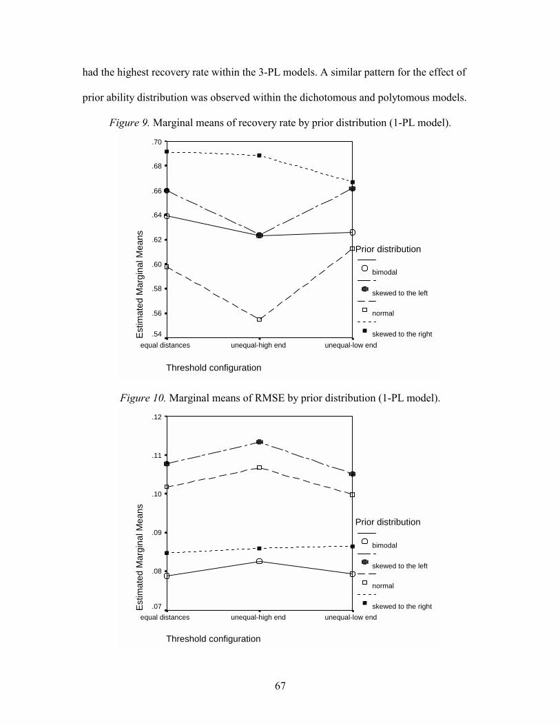
67
had the highest recovery rate within the 3-PL models. A similar pattern for the effect of
prior ability distribution was observed within the dichotomous and polytomous models.
Figure 9. Marginal means of recovery rate by prior distribution (1-PL model).
Threshold configuration
unequal-low endunequal-high endequal distances
Estim
ated
Mar
gina
l Mea
ns.70
.68
.66
.64
.62
.60
.58
.56
.54
Prior distribution
bimodal
skewed to the left
normal
skewed to the right
Figure 10. Marginal means of RMSE by prior distribution (1-PL model).
Threshold configuration
unequal-low endunequal-high endequal distances
Estim
ated
Mar
gina
l Mea
ns
.12
.11
.10
.09
.08
.07
Prior distribution
bimodal
skewed to the left
normal
skewed to the right

68
Figure 11. Marginal means of recovery rate by prior distribution (2-PL model).
Threshold configuration
unequal-low endunequal-high endequal distances
Estim
ated
Mar
gina
l Mea
ns
.7
.6
.5
.4
.3
.2
Prior distribution
bimodal
skewed to the left
normal
skewed to the right
Figure 12. Marginal means of RMSE by prior distribution (2-PL model).
Threshold configuration
unequal-low endunequal-high endequal distances
Estim
ated
Mar
gina
l Mea
ns
.17
.16
.15
.14
.13
.12
Prior distribution
bimodal
skewed to the left
normal
skewed to the right

69
Figure 13. Marginal means of recovery rate by prior distribution (3-PL model).
Threshold configuration
unequal-low endunequal-high endequal distances
Estim
ated
Mar
gina
l Mea
ns
.5
.4
.3
.2
Prior distribution
bimodal
skewed to the left
normal
skewed to the right
Figure 14. Marginal means of RMSE by prior distribution (3-PL model).
Thresholds configuration
unequal-low endunequal-high endequal distances
Estim
ated
Mar
gina
l Mea
ns
.23
.22
.21
.20
.19
.18
.17
Prior distribution
bimodal
skewed to the left
normal
skewed to the right

70
Research Question 3
How do the polytomous IRT models differ in accuracy of recovering ability
estimates in different combinations of prior ability distributions and item category
threshold distance configurations?
Two 3-way ANOVAs were conducted with PolyMod (Po), Thetadis (P), Threconf
(T) as independent variables, and with Thetarec and RMSE as dependent variables. The
results for these analyses are summarized in Tables 10 and 12.
Table 10
Three-Way Fixed Effects ANOVA on Recovery Rate (Po, P,T) Source*
SS
Df
MS
F
p
η2
Power�
Po
21.137 3 7.046 1259.247 .000 .634 1.000
P
.153 3 .05094 9.104 .000 .005 .996
T
.238 2 .119 21.284 .000 .007 1.000
Po×P
3.368 9 .374 66.884 .000 .101 1.000
Po×T
1.505 6 .251 44.827 .000 .045 1.000
P×T
1.084 6 .181 32.301 .000 .033 1.000
Po×P×T
1.309 18 .07272 12.997 .000 .039 1.000
Error 4.566 816 .005595
Total 33.361 863
*Po = Polytomous Models, P = Prior Ability Distribution, T = Threshold Configuration � Computed using level of significance = .05
The model effect of this ANOVA was high (R2 = .863). About 86% of the
variance of the recovery rate could be explained by the three independent variables. Most
of the model effect came from the differences among the four polytomous models. Since
the three-way interaction effect was statistically significant (F(18, 816) = 12.997, p <

71
.0005), tests for the simple interaction effects were conducted. The simple interaction
effects Po×P were statistically significant ((F(9, 272) = 26.268, p < .0005; F(9, 272) =
41.954.25, p < .0005; and F(9, 272) = 19.044, p < .0005) with large effect sizes (ranging
from η2 = .387 to .581 or f = .79 to 1.18) within all three categories of threshold
configuration. The interaction effect was strongest within the �unequal-close at the high
end� group, and weakest within the �unequal-close to the low end� group.
Simple-simple main effects of PolyMod were tested within each combination of
prior ability distribution and threshold configuration. All combinations were statistically
significant (p < .0005) with large effect sizes (ranging from η2 = .299 to .994 or f = .65 to
12.87). The large range of effect sizes indicated that the four different polytomous
models differed on accuracy of ability estimation, and the differences changed from one
combination of threshold configuration and prior abiltiy distribution to the other. Table
11 summarized the effect sizes of the simple-simple main effects of PolyMod. It is
apparent that the effect sizes were large; most of them were larger than .95, i.e. the
recovery rates of the four polytomous models were different from each other in most
cases. Post hoc analyses were conducted to compare the four cell means in each of the
twelve combinations of conditions. Cell means that were not statistically significantly
different at the level of .05 were put together in a homogeneous subset. Therefore, cell
means of the models between homogenous subsets were statistically significantly
different from each other at the level of .05. In the last column of Table 11, polytomous
models in a homogenous subset were put together inside a bracket, and commas separate
the homogenous subsets of models. The cell means of the models within and between
homogenous subsets are listed in descending order. A clear pattern (1, 4, 2, 3) emerged

72
when the homogenous subsets were compared across the twelve combinations of
conditions. GPCM-1 had the highest recovery rate in all cases, most of the time
statistically significantly higher than the other three models. NCM had the second best
recovery rate except in three cases, and in two of those cases it was very close to the
second best. MCM had the lowest recovery rate most of the time except when the
threshold configuration was �unequal-close at the high end.� The same order (GPCM-1,
NCM, GPCM, MCM) was maintained when the threshold configuration was �equal
distances� or �unequal-close at the low end�, with only one pair of models reversing their
Table 11
Simple-Simple Main effect (PolyMod) on Recovery Rate and Homogeneous Subsets Threconf Thetadis Effect size (η2) Homogeneous subsets*
Equal distances bimodal .993 1, 4, (2, 3) �
Equal distances skewed (left) .952 1, 4, (3, 2)
Equal distances normal .413 (1, 4), (2, 3)
Equal distances skewed (right) .982 1, 4, 2, 3
Unequal-high bimodal .990 1, 4, 3, 2
Unequal-high skewed (left) .967 1, 3, 4, 2
Unequal-high normal .299 (1, 3, 4), 2
Unequal-high skewed (right) .985 1, 4, 2, 3
Unequal-low bimodal .994 1, 4, 2, 3
Unequal-low skewed (left) .968 1, (2, 4), 3
Unequal-low normal .715 (1, 4), 2, 3
Unequal-low skewed (right) .979 1, 4, 2, 3
*the means of the models in a homogenous subset are not significantly different at the level of .05. �1 = GPCM-1, 2 = GPCM, 3 = MCM, 4 = NCM; models inside a bracket are in same homogenous group.
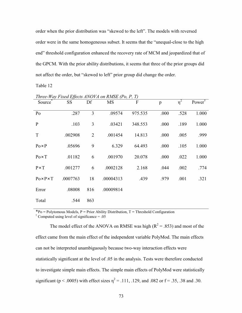
73
order when the prior distribution was �skewed to the left�. The models with reversed
order were in the same homogeneous subset. It seems that the �unequal-close to the high
end� threshold configuration enhanced the recovery rate of MCM and jeopardized that of
the GPCM. With the prior ability distributions, it seems that three of the prior groups did
not affect the order, but �skewed to left� prior group did change the order.
Table 12
Three-Way Fixed Effects ANOVA on RMSE (Po, P, T) Source*
SS
Df
MS
F
p
η2
Power�
Po
.287 3 .09574 975.535 .000 .528 1.000
P
.103 3 .03421 348.553 .000 .189 1.000
T
.002908 2 .001454 14.813 .000 .005 .999
Po×P
.05696 9 6.329 64.493 .000 .105 1.000
Po×T
.01182 6 .001970 20.078 .000 .022 1.000
P×T
.001277 6 .0002128 2.168 .044 .002 .774
Po×P×T
.0007763 18 .00004313 .439 .979 .001 .321
Error .08008 816 .00009814
Total .544 863
*Po = Polytomous Models, P = Prior Ability Distribution, T = Threshold Configuration � Computed using level of significance = .05
The model effect of the ANOVA on RMSE was high (R2 = .853) and most of the
effect came from the main effect of the independent variable PolyMod. The main effects
can not be interpreted unambiguously because two-way interaction effects were
statistically significant at the level of .05 in the analysis. Tests were therefore conducted
to investigate simple main effects. The simple main effects of PolyMod were statistically
significant (p < .0005) with effect sizes η2 = .111, .129, and .082 or f = .35, .38 and .30.

74
Post hoc comparisons indicated that the order of the four models by magnitude of their
RMSE remained unchanged across the three levels of threshold configuration,
specifically the order was GPCM-1, NCM, GPCM, MCM with RMSE ascending. It also
showed that the order of the four prior ability distribution groups by the magnitude of
RMSE remained the same across the levels of threshold configuration. The order was
bimodal, normal, skewed to the right, and skewed to the left with ascending RMSE.
To answer the third research question, the analysis indicated that the four
polytomous IRT models used in the present study differed in accuracy of ability
estimation. The tests of simple effects and post hoc tests revealed that the four models
basically maintained the same order of accuracy in terms of higher recovery rate and
lower RMSE, with different combinations of threshold configurations and prior
distributions, although the magnitudes of the differences between models varied from one
combination of conditions to the other. Figures 15 to 18 show the recovery rates and the
RMSEs of the four models across the categories of threshold configuration and across
different prior groups.
Figure 15. Marginal means of recovery rate by polytomous model (within Threconf).
Threshold configuration
unequal-lowunequal-highequal distances
Estim
ated
Mar
gina
l Mea
ns
1.0
.9
.8
.7
.6
.5
.4
.3
Polytomous models
GPCM-1
GPCM
MCM
NCM
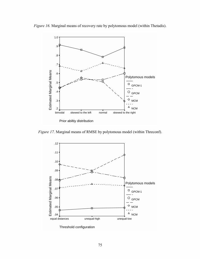
75
Figure 16. Marginal means of recovery rate by polytomous model (within Thetadis).
Prior abiltiy distribution
skewed to the rightnormalskewed to the leftbimodal
Estim
ated
Mar
gina
l Mea
ns
1.0
.9
.8
.7
.6
.5
.4
.3
.2
Polytomous models
GPCM-1
GPCM
MCM
NCM
Figure 17. Marginal means of RMSE by polytomous model (within Threconf).
Threshold configuration
unequal-lowunequal-highequal distances
Estim
ated
Mar
gina
l Mea
ns
.12
.11
.10
.09
.08
.07
.06
.05
.04
Polytomous models
GPCM-1
GPCM
MCM
NCM

76
Figure 18. Marginal means of RMSE by polytomous model (within Thetadis).
Prior abiltiy distribution
skewed to the rightnormalskewed to the leftbimodal
Estim
ated
Mar
gina
l Mea
ns
.14
.12
.10
.08
.06
.04
.02
Polytomous models
GPCM-1
GPCM
MCM
NCM
Examination of the interaction effects in the four figures revealed that they were
mostly ordinal. Ordinal interactions indicate that the order of the groups within a
grouping variable remains unchanged, while the magnitudes of the differences between
the group means varied from one pair of groups to the other. The order of the four models
with ascending RMSEs, and descending recovery rates was GPCM-1, NCM, GPCM, and
MCM. The order only changed when the threshold configuration was �unequal-close at
the high end,� or when the prior ability distribution was normal.

77
CHAPTER FIVE
CONCLUSIONS AND RECOMMENDATIONS
The findings concerning the effects of scoring format and item parameterization,
in combination with prior ability distribution and item threshold configuration, on the
accuracy of ability estimation will be discussed in the first part of this chapter. Some
conclusions will be drawn from the discussion and the practical educational importance
of the findings will be addressed. Recommendations for future study will be made in the
second part of this chapter.
Conclusions
Findings of the Present Study
1. The two criteria of ability estimation accuracy, recovery rate and RMSE, were
negatively correlated as expected. In most of the hypotheses tested in this study,
the effect sizes on recovery rate were larger than that of the RMSE.
2. Polytomous scoring models provided more accurate ability estimation, both in
terms of higher recovery rate and lower RMSE, than the dichotomous scoring
models under all combinations of prior ability distribution and threshold
configuration.
3. Under all combinations of prior ability distributions and threshold configurations,
the 1-PL models (with only item difficulty) had the most accurate ability
estimation, and the 3-PL models (with three types of parameters) were less
accurate in ability estimation among the three different types of item
parameterization models.

78
4. Four polytomous IRT models used in the present study differed in accuracy of
ability estimation. The four models basically maintained the same order of
accuracy under all the combinations of threshold configuration and prior
distribution. The order was GPCM-1, NCM, GPCM, and MCM with ascending
RMSEs and descending recovery rates.
5. Threshold configuration indicated small effect on RMSE. When the threshold
configuration was �unequal-close at the high end�, RMSE was slightly lower than
the RMSE obtained under the other two threshold configurations. Threshold
configuration had a much larger effect on recovery rates. For dichotomous
models, the �unequal-close at the high end� group had recovery rates slightly
lower than the other two groups. For polytomous models, different threshold
configurations had different effects on different prior groups. For the bimodal and
the �skewed to the right� prior group, the �unequal-close at the low end� had the
lowest recovery rate, and the �unequal-close at the high end� had the highest.�
For the �skewed to the left� prior group, the order was reversed. The threshold
configuration had little effect when the prior distribution was normal.
6. Prior ability distribution affected recovery rates and RMSEs in all combinations
of the research conditions. However, no conclusive pattern of its effect was
identified. The �skewed to the right� prior had the highest recovery rate and
highest RMSE most of the time, while bimodal prior had the lowest RMSE most
of the time.

79
Recovery Rate and Root Mean Squared Error
In the present study, the accuracy of IRT models in ability estimation was
compared using the recovery rate of original ability estimates and RMSE. Both criteria
were obtained by comparing two sets of ability estimates. One set was the original ability
estimates of 1,000 examinees that were used to generate the simulated item response
data, and the other set was the means of fifty ability estimates for each of the 1,000
examinees obtained as the output when applying an IRT model to fifty simulated item
response data sets from the same 1,000 examinees. The first set of estimates was used as
known ability estimates and the second set as the bootstrap estimators of the known
ability estimates in the present study. RMSE was a measure of the average deviation of
the 1,000 bootstrap estimators from the 1,000 known ability estimates. The recovery rate,
was the percentage of the 1,000 known ability estimates captured by the 95% confident
interval constructed around their respective estimators, which was obtained by checking
each of the 1,000 pairs of known ability estimates and their respective estimators.
Therefore, while both criteria assessed the overall accuracy of ability estimates, the
recovery rate was more sensitive to individual deviations. This explains why the recovery
rate had larger effect sizes than the RMSE. Since individual deviations are important in
the overall accuracy of an IRT model�s ability estimation, the recovery rates were more
informative than the RMSEs on the accuracy of the IRT model�s ability estimation.
Scoring Format
This study has demonstrated that polytomous models have better accuracy in
ability estimation, both in terms of higher recovery rates and lower RMSEs, in all
combinations of prior distribution and threshold configuration. Dichotomous models had
80
less information about examinees� ability by ignoring their differences in choosing
different categories other than the most completed answer. It has been discussed in the
literature review that a polytomous model can be viewed as a sequence of dichotomous
models and thus is more refined as a measuring tool of the latent construct under
investigation. This study not only pointed out that two scoring formats will give different
ability estimates when applied to multiple-choice items, but also gave reference to the
magnitude of the difference of the ability estimates. The recovery rate for polytomous
scoring almost doubled that of dichotomous scoring (63% versus 34%) when averaged
over all research conditions. The average RMSE for polytomous scoring was about one
third of that for dichotomous scoring (.075 versus .212). These differences are not small
and should not be ignored. This finding has important implications for educational
testing.
Large-scale assessments and achievement tests are predominantly constructed of
multiple-choice items scored dichotomously (correct, incorrect). In view of the large
difference in ability estimation that this study has found between dichotomous scoring
and polytomous scoring models, the scoring format of tests should be changed to improve
the accuracy of ability estimation. Tests are used to guide educational decision-making
and the accuracy of their outcomes should be a priority. Moreover, the use of multiple-
choice items versus constructed response items (e.g. Bennett, R. E. & Ward, W.C. Eds.,
1993) has been an ongoing debate on for a long time. Many issues were discussed, but
the objectivity and reliability of the scoring rubrics is paramount. Scoring multiple-choice
items is relatively inexpensive and highly reliable in comparison to scoring constructed
response items. However, concerns have been raised about the inability of multiple-

81
choice items to test students on multi-level or multi-step questions. Multiple-choice items
with well-constructed response categories, scored polytomously with partial credits,
would be a legitimate option to consider. The ordinal nature of the response categories
could be used to test multi-level or multi-step tasks.
Item parameterization
The three categories of item parameterization were expected to give different
ability estimates, but it was unexpected to have the IRT models with one type of
parameter (1-PL) having the highest recovery rates and lowest RMSEs across all
combinations of research conditions. Because the item response data used in the study
was simulated with known item parameters, in which the item discrimination parameters
varied from .8 to 2 (see Appendix C), the 2-PL models should fit the data better than 1-
PL models. Two factors may be possible explanations for the unexpected outcome. First,
Multilog software analyzes 1-PL dichotomous models as a special case of the graded
response model in which item discrimination is not set free as a parameter to be
estimated. In the item calibration stage of the program, the item discrimination is not set
to 1 but to a constant value estimated from all 30 items in the test. The constant value will
change from test to test, but remains unchanged across the items within the same test.
The constant value probably served as the �average item discrimination� for all 30 items
in the test, and may have enhanced the fit of the IRT model to the item response data.
Second, the 2-PL dichotomous model has 30 extra parameters to be estimated and
therefore has more chances to accumulate error.
For polytomous scoring models, GPCM-1 out-performed GPCM. This finding
seems to contradict Muraki� study (1992), in which he compared the partial credit model

82
and general partial credit model using simulated and real data. His results demonstrated
that the general partial credit model yielded a better fit to the data than the partial credit
model. Present study indicated that the partial credit model (GPCM-1) yielded more
accurate ability estimates than the general partial credit model (GPCM). However,
GPCM-1 only yielded more accurate ability estimates, not better model fit than GPCM.
Similar factors working in the dichotomous 1-PL model are present in GPCM-1. Multilog
software analyzes the partial credit model as a constrained case of the nominal categories
model. The only difference between the GPCM-1 and GPCM was that an �average item
discrimination� was estimated for all 30 items in GPCM-1 with item discrimination free
to vary from item to item in GPCM. The �average item discrimination� may have
enhanced the fit of the GPCM-1 model. GPCM had a slightly better fit than GPCM-1 in
this study; but it was not enough to compensate for the increase in the number of
parameters estimated.
The 3-PL models were expected to be less accurate in ability estimation in this
study because the guessing factor was not modeled in the simulated item response data (a
limitation of this study). The Multilog software analyzed the dichotomous 3-PL model as
a special case of the multiple-choice model with the number of categories equal to two.
The multiple-choice model in this study used .25 as an initial value in the calibration run
to estimate the pseudo-chance parameter for each item, however, there was no guessing
effect in the item response data. The 3-PL models had more parameters to be estimated
and yield a worse fit to the item response data. These findings demonstrated that an IRT
model with a better model fit to the data may give less accurate ability estimation,

83
especially when the IRT model can not compensate for the increased number of
parameters to be estimated.
Comparison of Polytomous Models
In the present study, polytomous models were not only compared to the
dichotomous models but also among themselves. Three of the four polytomous models,
GPCM-1, GPCM, MCM had been compared as part of the 1-PL, 2-PL, and 3-PL models
under the item parameterization study. When only the polytomous models were being
compared, the order of accuracy of those three models remained the same as it was in the
item parameterization study. The fourth model, NCM, was included in the study to
compare the ability estimation of nominal and ordinal polytomous models. It was
discussed in the literature review that NCM is the most general polytomous model, and
the other ordinal polytomous models can be derived from NCM by putting certain
constraints on the item parameters to preserve the order of the categories. In Multilog,
GPCM-1 and GPCM are obtained by imposing constraints on the parameters ak and ck of
the NCM through the application of T-matrixes (polynomial and triangle). The two
constrained versions of NCM were expected to be more accurate in their ability
estimation than the general NCM, because the item categories of the test used to simulate
item response data were ordinal. However, the findings of this study indicated that for
most of the combinations of threshold configuration and prior ability distribution, NCM
out-performed GPCM, although both were out-performed by GPCM-1. This finding
indicated that constraints on parameters may not help to improve the model fit. It also
indicated that polytomous scoring models would give better ability estimation even for

84
multiple-choice items with nominal response categories, because NCM provided ability
estimation as good as, if not better than, ordinal polytomous models.
Prior Ability Distribution
The present study indicated that prior ability distribution had an effect on the
accuracy of ability estimation. It also revealed that prior ability distribution interacted
with other factors in the study, e.g. scoring format, item parameterization, and threshold
configuration. The differences in group means for the four prior groups varied greatly
from one combination of research conditions to the other. No clear overall pattern for the
variation was indicated, however some patterns within some combinations were
identified. Furthermore, caution needs to be taken in the interpretation of this finding,
because prior ability distribution was assumed to be normal by Multilog software in the
item calibration and scoring programs. According to Thissen (1991), there is little or no
theory available to evaluate a population-distribution fitting procedure, so it is difficult to
assess the effect of prior distribution on the item calibration and test scoring in IRT.
Although Thissen introduced the Johnson family of distributions as a possible tool to
characterize the population density in MML estimation, he warned against routine use of
it because it was a �relatively untested scheme in an area fraught with difficulties.� In
Multilog software, all prior ability distributions are assumed to be normal, and Gaussian
quadratures are used to approximate the distribution in MML estimation. Therefore, the
normal prior group should be used as a reference point in the interpretation of the mean
differences of the four prior groups in different combinations of the research conditions.
Although a clear overall pattern cannot be identified for the effect of prior ability
distribution on the accuracy of ability estimation, the differences of group means for the

85
prior groups in the present study have practical and educational importance. In education
testing, the population distribution of the latent construct is often unknown and assumed
to be normal. In practice, however, the sample of examinees is more often from a
population with an ability distribution different from normal. Three of the four prior
groups represented in this study simulated such kinds of populations; specifically they
represented predominantly high ability groups, predominantly low ability groups and
groups with diversified or even polarized ability. The present study indicated the effect
on the accuracy of ability estimation (i.e. enhanced or reduced in comparison to the
normally distributed group) when the sample of examinees represented one of the three
kinds of populations described above.
Threshold Configuration
When the items are scored dichotomously, the unequal distance and equal
distance threshold configurations will not affect the response data because all categories
other than the complete answer will be scored as zero. The small differences in the
findings were due to random error from the simulation process. For the polytomous
models, when threshold configuration categories were examined across item
parameterization and individual models, the same pattern emerged. The three categories
were in the same order (�unequal-close at the low end�, �equal threshold�, and �unequal-
at the high end�) with descending recovery rates and ascending RMSE, if the mean
differences were statistically significant. However, the effect sizes for those effects were
small. The mean differences amounted to less than 10% in recovery rate and hundredths
difference in RMSE. The values for threshold are usually unknown before item
calibration, but it is important to realize that the distance between thresholds has an effect

86
on the accuracy of ability estimation. If a partial credit is given to an easy step as well as
a hard step, it impacts how different levels of ability in the examinees are estimated.
When the effects of threshold configurations were examined across the four prior
distribution groups, the RMSEs of the three categories showed no significant difference.
In contrast, the recovery rates of the three categories differed significantly across the four
prior groups. When the prior was normal, there was no significant difference among the
three group means. When the prior was �skewed to the left�, the three categories
followed the same order as in other combinations of research conditions, however, the
�unequal-high end� category had a much lower recovery rate than the other two. When
the prior was �skewed to the right� and �bimodal�, the order of the three categories
reversed, i.e. �unequal-at the high end�, �equal threshold�, and �unequal-at the low end�
with descending recovery rates. The effect sizes of the mean differences were large. The
reversal of order happened because of the presence of a higher density of low ability
examinees in the �bimodal� and �skewed to the right� prior groups. The presence of a
larger low ability group reduced the recovery rate when the item thresholds were close at
the low end, which decreased the power of the lower categories in discriminating low
ability examinees. The fact that �skewed to the left� prior group had a lowest recovery
when the threshold configuration was �unequal-close at the high end� could be explained
by similar reason. In summary, the effect of threshold configuration indicated that the
accuracy of ability estimation would reduce if multiple-choice items with categories close
to each other at one end of the ability continuum were administrated to a group with
higher population density at the same end of the continuum.

87
Recommendations
Future studies are recommended in three areas. First, the effect of prior ability
distribution on the accuracy of ability estimation cannot be assessed unambiguously until
a new approach for appropriately characterizing population density is developed. Second,
the effect of threshold configuration has not been fully assessed. Threshold
configurations other than the three examined in this study should be applied and varied
systematically throughout a set of items, and the effects of those variations should be
examined. Third, while most large-scale assessments and achievement tests in the past
were constructed of multiple-choice items scored dichotomously, tests with multiple item
formats have become popular in recent years. These tests often include multiple-choice
items mixed with a variety of constructed-response items (e.g. short answer, matching,
multiple-steps, short essay, etc.). Examples of mixed item format tests are the National
Assessment of Educational Progress (NAEP) (Calderone, King & Horkay, 1997), the
Test of English as a Foreign Language (TOEFL) (Tang & Eignor, 1997), and state
assessments administered in states such as Massachusetts, North Carolina, and
Wisconsin. If tests that combine multiple-choice items and constructed-response items
are unidimensional, a single ability estimate per examinee is generated according to all
item responses. There are different approaches to handling mixed model estimates for a
test in order to produce a common score scale. Weighted combinations of the two parts
(testlets) are widely applied. The selection of weights, however, poses a problem.
Lukhele, Thissen, and Wainer (1994) pointed out that the composite ability scores may
have lower reliability than the component ability scores; if the weights applied to create
the composite score are ill chosen. Rosa, Swygert, Nelson, and Thissen (2001) developed

88
a technique based on IRT to use the item response data to determine the relative weights
of the components.
Multiple item formats call for mixed scoring IRT models. The approach typically
taken calibrates all of the items jointly using suitable IRT models for each item.
Dichotomous models are used for the multiple-choice items and polytomous models for
constructed-response items. A likelihood function of response patterns for each
combination of summed scores for the two components is then constructed. A single
ability score for each combination of summed scores is estimated using a likelihood
function. A scale-scoring table is then constructed to list the ability score for all the
possible combinations of summed scores for the two components. Examinees obtain their
ability estimates from the scale-scoring table according to the summed scores, which
came from the two parts of the test. It is meaningful to compare the ability estimates
obtained from a mixed scoring model to those from dichotomous and polytomous models
that have only one item type, e.g. all multiple choice items.

89
APPENDIX A
SAS Program for Data Simulation
/******************************************************************/ /* This program is to generate response patterns */ /* based on Muraki's generalized partial credit model. */ /* The possible responses for item i are 0 to (ncat-1). */ /******************************************************************/ options ps=52 ls=72; %let ne=1000; /*no. of examinees*/ %let ni=30; /*no. of items*/ %let thlist=th(i,1) th(i,2) th(i,3);/*threshold input format*/ %let ncb=3;/*no. of thresholds*/ %let ncat=4;/*no. of categories*/ %let ipmfl='h:\diss_sim\etip.dat'; /* item paramenter input path*/ %let ipmfmt=a(i) 8.2 (&thlist) (&ncb*8.2);/*item parameter input format*/ %let outfl='h:\diss_sim\ner.dat'; /*generated data output path*/ %let seed1=6734; /* seed number for normal dist.. */ %let seed3=3422; /*seed number for r*/ %let putfmt=@1 id 4.0 @6 z 7.3 @14 (r1-r&ni) (&ni*1.0); /******************************************************************/ data know (keep=z); /* created normally distributed sample */ do i=1 to ≠ /* of the examinees’ ability estimates */ z=rannor(&seed1); output; end; filename ipm &ipmfl; /* read in the input parameter file */ data iparm; array th(&ni, &ncb); array a(&ni); do i=1 to ∋ infile ipm; input &ipmfmt; end; filename resp &outfl; /* set up the output file format */ data respdat (keep= z r1-r&ni e1 den pbc1-pbc&ncat r tot); if _n_=1 then set iparm; set know; array sd(&ni, &ncb); array a(&ni); array pbc(&ncat); array rr(*) r1-r∋ do i=1 to ∋ rr(i)=0.0; end; do i=1 to ∋ /* calculate the probabilities of an */ den=1.0; /* examinee choosing each of the four */ do j=1 to &ncb; /* categories for each items. */

90
e1=0.0; do k=1 to j; e1=e1+a(i)*(z-sd(i,k)); end; pbc(j+1)=exp(e1); den=den+exp(e1); end; pbc(1)=1/den; do j=2 to &ncat; pbc(j)=pbc(j)/den; end; tot=0.0; r=ranuni(&seed3); /* converts the probabilities to */ do k=1 to &ncat; /* item responses using a sample */ tot=tot+pbc(k); /* of random numbers within (0,1)*/ if r>tot then rr(i)=k; end; end; id=_n_; /* set up for next examinee */ file resp; put &putfmt; proc univariate normal vardef=n; var z; proc chart; hbar z; run;

91
SAS Program for Generating Prior Ability Distribution
/******************************************************************/ /* This program is to generate random numbers with */ /* with different density functions of distribution */ /* to be used as the prior distribution of ability in */ /* a simulated item responses data set. */ /******************************************************************/ options ps=52 ls=72; %let seed1=6734; /* generate a bimodal prior distribution */ data theta1 (keep=x); do i=1 to 500; /* created a normally distributed half*/ x1=rannor(&seed1); /* sample shifted 1.5 sd to the left. */ x=x1-1.5; output; end; data theta2 (keep=x); /* created a normally distributed half*/ do i=1 to 500; /* sample shifted 1.5 sd to the right.*/ x1=rannor(&seed1); x=x1+1.5; output; end; data theta (keep=x x_std); /* two half samples combined to form a*/ set theta1 theta2; /* bimodal sample centered at zero. */ x_std=x; run; proc standard data=theta mean=0 std=1 out=thetaz; /* standardization*/ var x_std; run; proc univariate normal vardef=n; var x_std; proc chart; hbar x_std; run; /* generate a positively skewed prior distribution using the density function of beta distribution. (beta distribution has two parameter α and β, where α>1 and β>1. The shape of the distribution is obtained by manipulating the values of the two parameters (Novick & Jackson, 1974, 112). */ data thetas (keep=y y_std); do i=1 to 1000; x1=RANGAM(&seed1,1.8); /* α = 1.8 */ x2=RANGAM(&seed1,5); /* β = 5 */ y=x1/(x1+x2); /* the beta density function */ y_std=y; output; end; run; proc standard data=thetas mean=0 std=1 out=thetasz; /*standardization*/ var y_std; run; proc univariate normal vardef=n; var y_std;
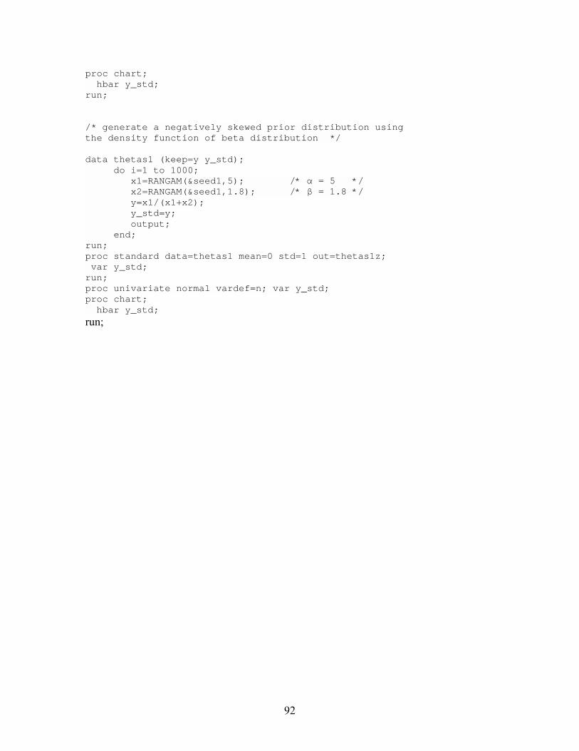
92
proc chart; hbar y_std; run; /* generate a negatively skewed prior distribution using the density function of beta distribution */ data thetas1 (keep=y y_std); do i=1 to 1000; x1=RANGAM(&seed1,5); /* α = 5 */ x2=RANGAM(&seed1,1.8); /* β = 1.8 */ y=x1/(x1+x2); y_std=y; output; end; run; proc standard data=thetas1 mean=0 std=1 out=thetas1z; var y_std; run; proc univariate normal vardef=n; var y_std; proc chart; hbar y_std;
run;
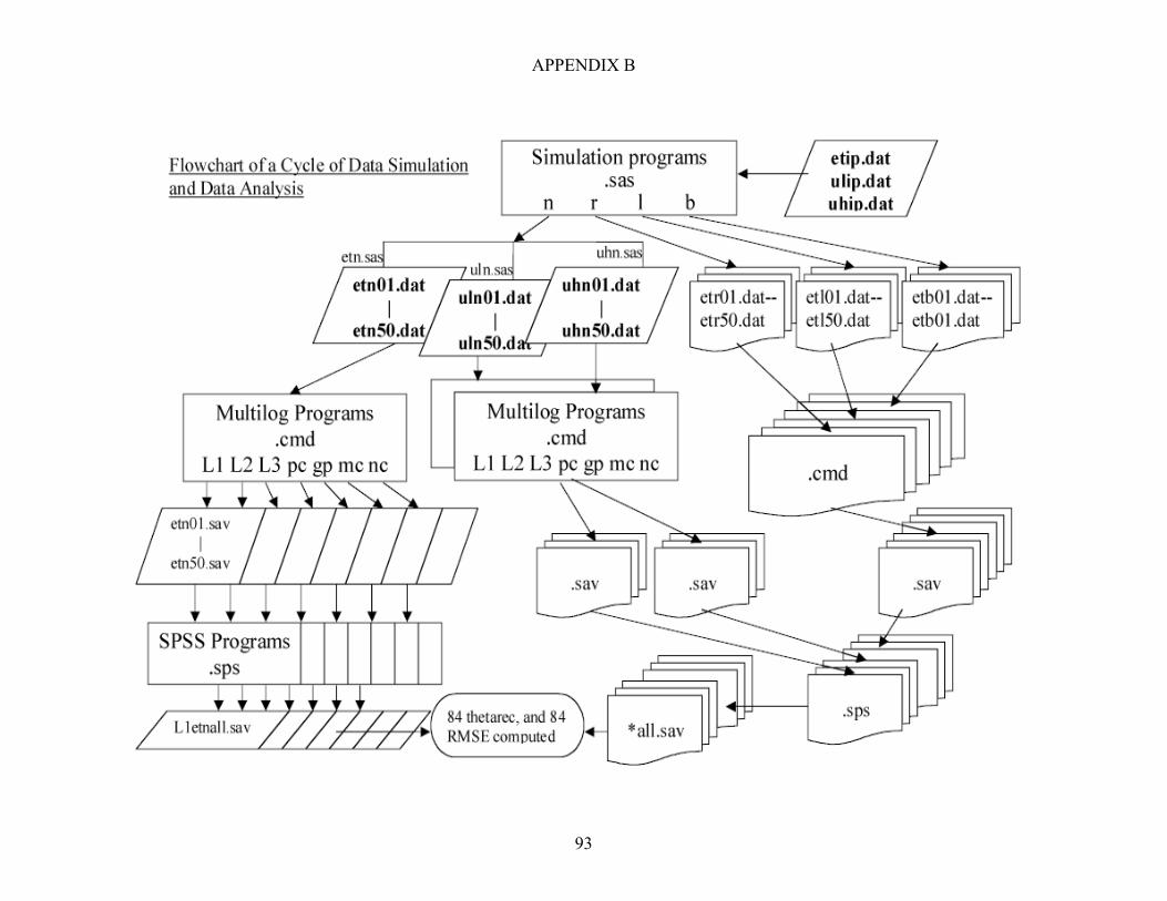
APPENDIX B
93
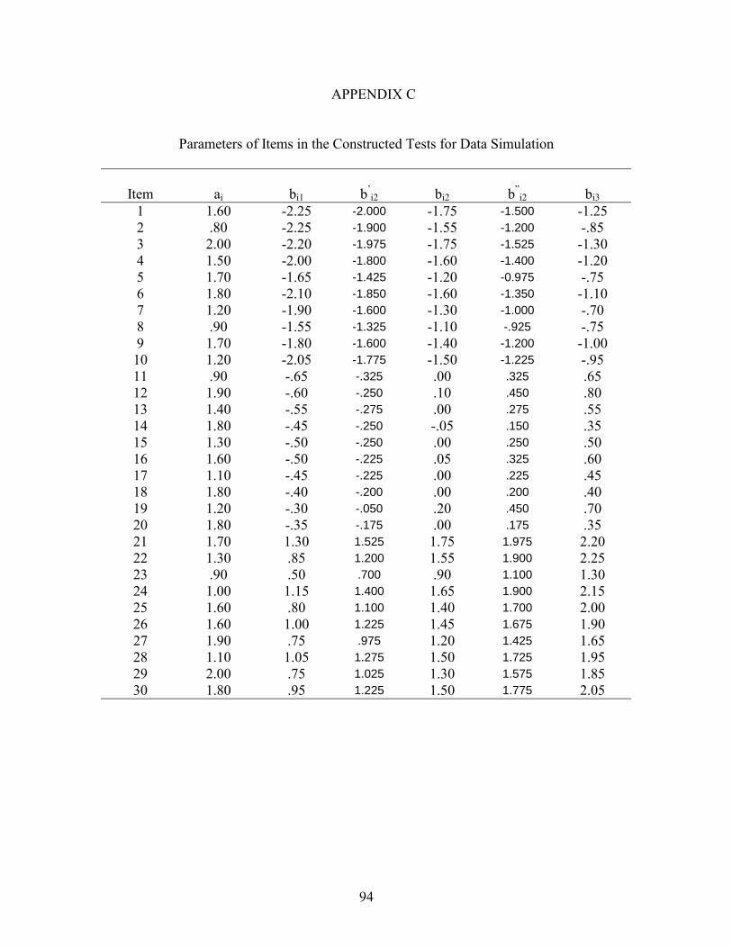
94
APPENDIX C
Parameters of Items in the Constructed Tests for Data Simulation
Item
ai
bi1
b�
i2
bi2
b�
i2
bi3
1 1.60 -2.25 -2.000 -1.75 -1.500 -1.25 2 .80 -2.25 -1.900 -1.55 -1.200 -.85 3 2.00 -2.20 -1.975 -1.75 -1.525 -1.30 4 1.50 -2.00 -1.800 -1.60 -1.400 -1.20 5 1.70 -1.65 -1.425 -1.20 -0.975 -.75 6 1.80 -2.10 -1.850 -1.60 -1.350 -1.10 7 1.20 -1.90 -1.600 -1.30 -1.000 -.70 8 .90 -1.55 -1.325 -1.10 -.925 -.75 9 1.70 -1.80 -1.600 -1.40 -1.200 -1.00 10 1.20 -2.05 -1.775 -1.50 -1.225 -.95 11 .90 -.65 -.325 .00 .325 .65 12 1.90 -.60 -.250 .10 .450 .80 13 1.40 -.55 -.275 .00 .275 .55 14 1.80 -.45 -.250 -.05 .150 .35 15 1.30 -.50 -.250 .00 .250 .50 16 1.60 -.50 -.225 .05 .325 .60 17 1.10 -.45 -.225 .00 .225 .45 18 1.80 -.40 -.200 .00 .200 .40 19 1.20 -.30 -.050 .20 .450 .70 20 1.80 -.35 -.175 .00 .175 .35 21 1.70 1.30 1.525 1.75 1.975 2.20 22 1.30 .85 1.200 1.55 1.900 2.25 23 .90 .50 .700 .90 1.100 1.30 24 1.00 1.15 1.400 1.65 1.900 2.15 25 1.60 .80 1.100 1.40 1.700 2.00 26 1.60 1.00 1.225 1.45 1.675 1.90 27 1.90 .75 .975 1.20 1.425 1.65 28 1.10 1.05 1.275 1.50 1.725 1.95 29 2.00 .75 1.025 1.30 1.575 1.85 30 1.80 .95 1.225 1.50 1.775 2.05

95
APPENDIX D
Ability Estimation Programs
Multilog Command Programs For Different IRT Models 1-PL logistic model (L1.cmd & L1s.cmd).
MML PARAMETER ESTIMATION FOR THE 1PL MODEL >PROBLEM RANDOME IN NITEMS=30 NGROUPS=1 NE=1000, NCHAR=8; >TEST ALL L1; >SAVE; >END; 2 01 111111111111111111111111111111 N (4X,8A1,T45,30A1)
ESTIMATION OF ABILITY 1PL MODEL >PROBLEM SCORE IND NITEMS=30 NGROUPS=1 NE=1000 NCHAR=8; >TEST ALL L1; >SAVE; >START ALL; Y >END; 2 01 111111111111111111111111111111 N (4X,8A1,T45,30A1)
2-PL logistic model (L2.cmd & L2s.cmd).
MML PARAMETER ESTIMATION FOR THE 2PL MODEL >PROBLEM RANDOME IN NITEMS=30 NGROUPS=1 NE=1000, NCHAR=8; >TEST ALL L2; >SAVE; >END; 2 01 111111111111111111111111111111 N (4X,8A1,T45,30A1)
ESTIMATION OF ABILITY 2PL MODEL >PROBLEM SCORE IND NITEMS=30 NGROUPS=1 NE=1000 NCHAR=8; >TEST ALL L2; >SAVE; >START ALL; Y

96
>END; 2 01 111111111111111111111111111111 N (4X,8A1,T45,30A1)
3-PL logistic model (L3.cmd & L3s.cmd).
MML PARAMETER ESTIMATION, 3PL logistic >PROBLEM RANDOM IN NITEMS=30 NGROUPS=1 NE=1000 NC=8; >TEST ALL L3; >SAVE; >PRIORS ALL DK=1 PA=(-1.4,1.0); >END; 2 01 111111111111111111111111111111 N (4X,8A1,T45,30A1)
ESTIMATION OF ABILITY, 3PL logistic >PROBLEM SCORE IND NITEMS=30 NGROUPS=1 NE=1000 NC=8; >TEST ALL L3; >SAVE; >PRIORS ALL DK=1 PA=(-1.4,1.0); >START ALL; Y >END; 2 01 111111111111111111111111111111 N (4X,8A1,T45,30A1)
Partial credit model (pc.cmd & pcs.cmd).
MML PARAMETER ESTIMATION, General PARTIAL CREDIT MODEL >PRO RA IN NI=30 NG=1 NE=1000 NCHARS=8; >TEST ALL NO NC=(4(0)30) HI=(4(0)30); >SAVE; >TMATRIX ALL AK POLY; >EQUAL ALL AK=1; >FIX ALL AK=(2,3) VALUE=0.0; >TMATRIX ALL CK TRIANGLE; >END; 4 1234 111111111111111111111111111111 222222222222222222222222222222 333333333333333333333333333333 444444444444444444444444444444 (4X,8A1,1X,30A1)

97
ESTIMATION OF ABILITY partial credit model >PRO SCORE IND NE=1000 NG=1 NI=30 NCHARS=8; >TEST ALL NO NC=(4(0)30)HI=(4(0)30); >TMATRIX ALL AK POLY; >EQUAL ALL AK=1; >FIX ALL AK=(2,3) VALUE=0.0; >TMATRIX ALL CK TRIANGLE; >SAVE; >START ALL; Y >END; 4 1234 1111111111111111111111111111111111 2222222222222222222222222222222222 3333333333333333333333333333333333 4444444444444444444444444444444444 (4X,8A1,1X,30A1)
General Partial credit model (gp.cmd & gps.cmd).
MML PARAMETER ESTIMATION, General PARTIAL CREDIT MODEL >PRO RA IN NI=30 NG=1 NE=1000 NCHARS=8; >TEST ALL NO NC=(4(0)30) HI=(4(0)30); >SAVE; >TMATRIX ALL AK POLY; >FIX ALL AK=(2,3) VALUE=0.0; >TMATRIX ALL CK TRIANGLE; >END; 4 1234 111111111111111111111111111111 222222222222222222222222222222 333333333333333333333333333333 444444444444444444444444444444 (4X,8A1,1X,30A1)
ESTIMATION OF ABILITY general partial credit model >PRO SCORE IND NE=1000 NG=1 NI=30 NCHARS=8; >TEST ALL NO NC=(4(0)30)HI=(4(0)30); >TMATRIX ALL AK POLY; >FIX ALL AK=(2,3) VALUE=0.0; >TMATRIX ALL CK TRIANGLE; >SAVE; >START ALL; Y >END; 4 1234 1111111111111111111111111111111111 2222222222222222222222222222222222
98
3333333333333333333333333333333333 4444444444444444444444444444444444 (4X,8A1,1X,30A1)
Multiple choice model (mc.cmd & mcs.cmd).
MML PARAMETER ESTIMATION multiple choice model >PRO RA IN NI=30 NG=1 NE=1000 NC=8; >TEST ALL BS NC=(5(0)30) HI=(5(0)30); >EQUAL ALL DK=(1,2,3); >SAVE; >END; 4 1234 222222222222222222222222222222 333333333333333333333333333333 444444444444444444444444444444 555555555555555555555555555555 (4X,8A1,1X,30A1) Estimation of ability multiple choice model >PRO SCORE IND NI=30 NG=1 NE=1000 NC=8; >TEST ALL BS NC=(5(0)30) HI=(5(0)30); >EQUAL ALL DK=(1,2,3); >SAVE; >START ALL; Y >END; 4 1234 222222222222222222222222222222 333333333333333333333333333333 444444444444444444444444444444 555555555555555555555555555555 (4X,8A1,1X,30A1)
Nominal categories model (nc.cmd & ncs.cmd). MML PARAMETER ESTIMATION, Nominal categories model >PRO RA IN NI=30 NG=1 NE=1000 NC=8; >TEST ALL NO NC=(4(0)30) HI=(4(0)30); >SAVE; >END; 4 1234 111111111111111111111111111111 222222222222222222222222222222 333333333333333333333333333333 444444444444444444444444444444 (4X,8A1,1X,30A1) ESTIMATION OF ABILITY NOMINAL CATEGORIES MODEL

99
>PRO SCORE IND NE=1000 NG=1 NI=30 NCHARS=8; >TEST ALL NO NC=(4(0)30)HI=(4(0)30); >SAVE; >START ALL; Y >END; 4 1234 1111111111111111111111111111111111 2222222222222222222222222222222222 3333333333333333333333333333333333 4444444444444444444444444444444444 (4X,8A1,1X,30A1)

100
APPENDIX E
Ability Estimation Result
Cxyz ScorFor ItemPar PolyMod Thetadis Threconf Thetarec RMSE
l1eb6734 1 1 1 1 .374 .120083 l1el6734 1 1 2 1 .445 .134239 l1en6734 1 1 3 1 .282 .168582 l1er6734 1 1 4 1 .483 .196774 l1hb6734 1 1 1 2 .357 .123329 l1hl6734 1 1 2 2 .408 .125419 l1hn6734 1 1 3 2 .281 .154952 l1hr6734 1 1 4 2 .475 .185338 l1lb6734 1 1 1 3 .386 .118448 l1ll6734 1 1 2 3 .452 .184065 l1ln6734 1 1 3 3 .271 .185284 l1lr6734 1 1 4 3 .511 .250619 l2eb6734 1 2 1 1 .406 .215963 l2el6734 1 2 2 1 .231 .197889 l2en6734 1 2 3 1 .181 .197282 l2er6734 1 2 4 1 .575 .265009 l2hb6734 1 2 1 2 .379 .229717 l2hl6734 1 2 2 2 .206 .173263 l2hn6734 1 2 3 2 .134 .175585 l2hr6734 1 2 4 2 .496 .238663 l2lb6734 1 2 1 3 .427 .207196 l2ll6734 1 2 2 3 .247 .282400 l2ln6734 1 2 3 3 .216 .232357 l2lr6734 1 2 4 3 .625 .352136 l3eb6734 1 3 1 1 .303 .338231 l3el6734 1 3 2 1 .159 .298060 l3en6734 1 3 3 1 .082 .244724 l3er6734 1 3 4 1 .347 .372022 l3hb6734 1 3 1 2 .264 .352136 l3hl6734 1 3 2 2 .130 .269314 l3hn6734 1 3 3 2 .049 .221427 l3hr6734 1 3 4 2 .305 .334664 l3lb6734 1 3 1 3 .316 .322800 l3ll6734 1 3 2 3 .170 .030671 l3ln6734 1 3 3 3 .095 .050289 l3lr6734 1 3 4 3 .406 .082000 pceb6734 2 1 1 1 1 .942 .052792 pcel6734 2 1 1 2 1 .868 .032619 pcen6734 2 1 1 3 1 .481 .053787 pcer6734 2 1 1 4 1 .907 .090294

101
pchb6734 2 1 1 1 2 .926 .050398 pchl6734 2 1 1 2 2 .832 .035270 pchn6734 2 1 1 3 2 .339 .051565 pchr6734 2 1 1 4 2 .914 .072581 pclb6734 2 1 1 1 3 .899 .058129 pcll6734 2 1 1 2 3 .842 .069556 pcln6734 2 1 1 3 3 .664 .082171 pclr6734 2 1 1 4 3 .856 .103344 gpeb6734 2 2 2 1 1 .473 .082583 gpel6734 2 2 2 2 1 .570 .082207 gpen6734 2 2 2 3 1 .417 .087601 gper6734 2 2 2 4 1 .682 .118743 gphb6734 2 2 2 1 2 .450 .090956 gphl6734 2 2 2 2 2 .374 .071708 gphn6734 2 2 2 3 2 .327 .084054 gphr6734 2 2 2 4 2 .690 .095300 gplb6734 2 2 2 1 3 .482 .085206 gpll6734 2 2 2 2 3 .714 .079391 gpln6734 2 2 2 3 3 .532 .131681 gplr6734 2 2 2 4 3 .520 .070314 mceb6734 2 3 3 1 1 .405 .107517 mcel6734 2 3 3 2 1 .569 .069065 mcen6734 2 3 3 3 1 .823 .126293 mcer6734 2 3 3 4 1 .300 .069101 mchb6734 2 3 3 1 2 .522 .095802 mchl6734 2 3 3 2 2 .598 .091203 mchn6734 2 3 3 3 2 .843 .136272 mchr6734 2 3 3 4 2 .376 .076864 mclb6734 2 3 3 1 3 .307 .117686 mcll6734 2 3 3 2 3 .510 .044744 mcln6734 2 3 3 3 3 .687 .089566 mclr6734 2 3 3 4 3 .250 .085475 nceb6734 2 4 1 1 .757 .088034 ncel6734 2 4 2 1 .608 .048177 ncen6734 2 4 3 1 .561 .091684 ncer6734 2 4 4 1 .685 .094715 nchb6734 2 4 1 2 .722 .089878 nchl6734 2 4 2 2 .518 .050794 nchn6734 2 4 3 2 .417 .091635 nchr6734 2 4 4 2 .716 .078492 nclb6734 2 4 1 3 .717 .089247 ncll6734 2 4 2 3 .671 .120083 ncln6734 2 4 3 3 .703 .134239 nclr6734 2 4 4 3 .599 .168582

102
REFERENCES
Akkermans, W. (1998). Studies on statistical models for polytomous items.
Unpublished doctoral dissertation, Twente University, The Netherlands.
Andersen, E. B. (1972). The solution of a set of conditional estimation equations.
Journal of the Royal Statistical Society, 34, 42-54.
Andrich, D. (1978). A rating formulation for ordered response categories.
Psychometrika, 43, 561-573.
Andrich, D. (1982). An extension of the Rasch model for ratings providing both
location and dispersion Parameters. Psychometrika, 47, 105-113.
Andrich, D. (1995). Models for measurement, precision, and the
nondichotomization of graded responses. Psychometrika, 60, 7-26.
Baker, F. B. (1992). Item response theory: Parameter estimation techniques. New
York, NY: Marcel Dekker.
Barton, M.A. & Lord, F. M. (1981). An upper asymptote for the three-parameter
logistic item-response model. Research Bulletin 81-20. Princeton, NJ: Educational
Testing Service.
Bennett, R. E. & Ward, W. C. (Eds.), (1993). Construction versus choice in
cognitive measurement: Issues in constructed Response, performance testing, and
portfolio assessment. Hillsdale, NJ: Lawrence Erlbaum Associates.
Birnbaum, A. (1957). Efficient design and use of tests of a mental ability for
various decision-making problems. Series Report No. 58-16. Project No. 7755-23, USAF
School of Aviation Medicine, Randolph Air Force Base, Texas.

103
Birnbaum, A. (1958a). On the estimation of mental ability. Series Report No. 15.
Project No. 7755-23, USAF School of Aviation Medicine, Randolph Air Force Base,
Texas.
Birnbaum, A. (1958b). Further considerations of efficiency in tests of a mental
ability. Technical Report No. 17. Project No. 7755-23, USAF School of Aviation
Medicine, Randolph Air Force Base, Texas.
Birnbaum, A. (1968). Some latent trait models and their use in inferring an
examinee�s ability. In F. M. Lord, & M. R. Novick, Statistical theories of mental test
scores. Reading, MA: Addison-Wesley.
Bock, R. D. (1972). Estimating item parameters and latent ability when responses
are scored in two or more nominal categories. Pschometrika. 37, 29-51.
Bock, R. D. (1997). The nominal categories model. In W. J. van der Linden & R.
K. Hambleton (Eds), Handbook of modern item response theory. (pp. 33-49). New York,
NY: Springer.
Bock, R. D., & Aitken, M. (1981). Marginal maximum likelihood estmation of
item parameters: Application of an EM algorithm. Psychometrika, 46, 443-459.
Bock, R. D., & Lieberman, M. (1970). Fitting a response model for n
dichotomously scored items. Psychometrika, 35, 179-197.
Calderone, J., King, L. M., & Horkay, N. (Eds.), (1997). The NAEP guide.
Washington, DC: U.S. Department of Education, National Center for Education
Statistics.

104
Chen, S. (1996). A comparison of maximum likelihood estimation and expected a
posteriori estimation in computerized adaptive testing using the generalized partial credit
model. Unpublished doctoral dissertation, University of Texas at Austin.
Cohen, J. (1988). Statistical power analysis for the behavioral sciences (2nd ed.).
Hillsdale, NJ: Lawrence Erlbaum Associates.
Dodd, B. G. & Koch, W. R. (1987). Effects of variations in item step values on
item and test information in the partial credit model. Applied Psychological
Measurement, 11, 371-384.
Embretson, S. E., & Reise, S. P. (2000). Item response theory for psychologiests.
Mahwah, NJ: Lawrance Erlbaum.
Hambleton, R. K. & Swaminathan, H. (1985). Item response theory: Principles
and applications. Boston, MA: Kluwer-Nijhoff.
Haley, D.C. (1952). Estimation of the dosage mortality relationship when the dose
is subject to error. Technical Report No. 15. Stanford, CA: Stanford University, Applied
Mathematics and Statistics Laboratory.
Hemker, B. T. (2001). Reversibility revisited and other comparisons of three
types of polytomous IRT models. In A. Boomsma, M. A. J. van Duijn & T. A. B.
Snijders (Eds.), Essays on item response theory. (pp. 277-296). New York, NY: Springer.
Kamata, A. (1998). Some generalizations of the Rasch model: An application of
the hierarchical generalized linear model. A dissertation for Ph.D. Michigan State
University.
Levine, M. V., & Drasgow, F. (1983). The relation between incorrect option
choice and estimated ability. Educational and Psychological Measurement, 43, 675-685.
105
Lord, F. N. (1952). A theory of test scores. Psychometric Monograph, No. 7.
Lord, F. N., & Novick, M. R. (1968). Statistical theories of mental test scores.
Reading, MA: Addison-Wesley.
Lukhele, R., Thissen, D., & Wainer, H. (1994). On the relative value of multiple-
choice, constructed-response, and examinee-selected items on two achievement tests.
Journal of Educational Measurement, 31, 234-250.
Masters, G. N. (1982). A Rasch model for partial credit scoring. Psychometrika,
47, 149-174.
McDonald, R. P. (1967). Non-linear factor analysis. Psychometric Monographs,
No. 15.
Mellenbergh, G. J. (1995). Conceptual notes on models for discrete polytomous
item responses. Applied Psychological Measurement, 19, 91-100.
Mislevy, R. J. (1986). Bayes modal estimation in item response models.
Psychometrika, 51, 177-195.
Molenaar, I. W. (1983). Item steps. (Heymans Bulletin HB-83-630-EX).
Groningen: University of Groningen, Vakgroep Statistiek en Meettheorie.
Muraki, E. (1990). Fitting a polytomous item response model to Likert-type data.
Applied Psychological Measurement, 14, 59-71.
Muraki, E. (1992). A generalized partial credit Model: Application of EM
algorithm. Applied Psychological Measurement, 16, 159-176.
Neyman, J., & Scott, E. L. (1948). Consistent estimates based on partially
consistent observations. Econometrika, 16, 1-32.
106
Rasch, G. (1960). Probabilistic models for some intelligence and attainment tests.
Copenhagen: Danish Institute for Educational Research. (Expanded ed. by the University
of Chicago Press, 1980).
Reynolds, T., Perkins, K., & Brutten, S. (1994). A comparative item analysis
study of a language testing instrument. Applied Psychological Measurement, 11, 1-13.
Rosa, K., Swygert, K.A., Nelson, L., & Thissen D. (2001). Item response theory
applied to combinations of multiple-choice and constructed-response items�Scale scores
for patterns of summed scores. In D. Thissen & H. Wainer (Eds.), Test Scoring (pp. 253-
292). Mahwah, NJ: Lawrence Erlbaum.
Samejima, F. (1969). Estimation of latent ability using a response pattern of
graded scores. Psychometric Monograph, No.17.
Samejima, F. (1979). A new family of models for the multiple choice item
(Research Report No. 79-4). Knoxville, TN: University of Tennessee, Department of
Psychology.
Tang, K. L., & Eignor, D. R. (1997). Concurrent calibration of dichotomously
and polytomously scored TOEFL items using IRT models (TOEFL Tech. Rep. TR-13).
Princeton, NJ: Educational Testing Service.
Thissen, D., & Steinberg, L. (1984). A response model for multiple choice items.
Psychometrika, 49, 501-519.
Thissen, D., & Steinberg, L. (1986). A taxonomy of item response models.
Psychometrika, 51, 567-577.
Thissen, D. (1991). The MULTILOGTM (Version 6) [Computer software].
Mooresville, IN: Scientific Software International.

107
Thissen, D., Steinberg, L., & Fitzpatrick, A. R. (1989). Multiple-choice models:
The distractors are also part of the item. Journal of Educational Measurement, 26, 161-
176.
Tutz, G. (1990). Sequential item response models with an ordered response.
British Journal of Mathematical and Statistical Psychology, 43, 39-55.
Tutz, G. (1997). Sequential models for ordered responses. In W. J. van der Linden
& R. K. Hambleton (Eds.), Handbook of modern item response theory (pp. 139-152).
New York, NY: Springer.
van der Linden, W. J. & Hambleton, R. K. (eds.) (1997). Handbook of modern
item response theory. New York, NY: Springer.
van Engelenburg, G. (1997). On psychometric models for polytomous items with
ordered categories within the framework of item response theory. Unpublished doctoral
dissertation, University of Amsterdam.
Wright, B. D. & Masters, G. N. (1982). Rating scale analysis: Rasch
measurement. Chicago, IL: MESA.
Wright, B. D. (1997). A history of social science measurement. Educational
Measurement: Issues and Practice, 16, 33-52.
Zwinderman, A. H. and van der Wollenberg, A. L. (1990). Robustness of
marginal maximum likelihood estimation in the Rasch model. Applied Psychological
Measurement, 14, 73-81.