i Mi �i ci0 1 2 .3661

1 .63395 1.2679 .6340

.

Table 7: Scaling function moments for the Daubechies 4 wavelet.

i Mi �i ci0 1 2 -.0235

1 1.0054 2.0108 1.0426

2 1.0108 2.0216 -.0199

3 .90736 .5078 .0009

.

Table 8: Scaling function moments for the Daubechies 8 wavelet.

this mapping was denoted in matrix form as the matrix C. The elements ci which

de�ne the rows of this matrix have already been given for the wavelet D6. The

comparable results for the D4 and D8 wavelets are given in the accompanying tables.

51

Appendix B: Moments of the Scaling Function

In this appendix the moments of �(x) will be calculated in closed form. Begin

with the de�nition of the scaling function,

�(x) =Xk

�(2x� k):

Next, calculating the m-th moment of �(x) yields,

Z�(x)xm =

Xk

hk

Z�(2x� k)xmdx:

Change the variable of integration such that y = 2x � k to get,

Z�(x)xm =

Xk

hk

Z�(y)(1=2)m(y + k)m1=2dy;

= (1=2)m+1Xk

hk

Z�(y)(y + k)mdy:

Now, recall the binomial theorem to get,

Z�(x)xm = (1=2)m+1

Xk

hk

Z�(y)

mXl=0

m

l

!ylkm�ldy

Rewrite the moments of �(x) as Ml =Rxl�(x)dx to get,

Mm = (1=2)m+1mXl=0

m

l

!Xk

hkkm�lMl:

Now let �l =P

k hkkl to get

Mm = (1=2)m+1mXl=0

m

l

!�m�lMl:

Now, Mm can be de�ned in terms of Mi for i = 0; :::;m� 1:

Mm(2m+1 � 2) =

m�1Xl=0

m

l

!�m�lMl:

Note that the moments�l can be found by direct calculation given that the Daubechies

�lter coe�cients, hk, are already known.

The moments of �(x) can now be used to �nd the mapping from the evenly-

spaced samples of a function f(x) to the scaling function coe�cients. In section 3

50

Let the moments of �(x) be denoted by Ml =R�(x)xldx to get

mXr=0

m

r

!(�� )m�rMr = 0:

A simple calculation yields � = M1. Using this value of � and summing only up to

m� 1 the previous expression becomes,

m�1Xr=0

m

r

!(�M1)

m�rMr +Mm = 0:

Or,

Mm = �m�1Xr=0

m

r

!(�1)m�r(M1)

m�rMr:

From the hypotheses it is known that M0 =R�(x)dx = 1. Therefore, M� = M�

1 for

� = 0; 1, and with this knowledge it is easy to show that M� =M�1 for � = 2:

Mm = �m�1Xr=0

m

r

!(�1)m�r(M1)

m�rM r1 ;

which holds for m = 1; 2. Combine the powers of M1 to get,

Mm = �Mm1

m�1Xr=0

m

r

!(�1)m�r:

But, this is nothing more than,

Mm = �Mm1 [(1� 1)m � 1];

or simply,

Mm =Mm1 ;

where m = 1; 2. The proof is complete, since higher powers of m can be found by

induction.

49

Note that all of the above calculations could have been carried out for the �rst

derivative of f(x) giving an approximation to the scaling function coe�cients, �s0k, of

f 0(x):

�s0k =�f(� + k) + f (M+1)(� + k)

ZyM�(y + � )dy + ::::

It was assumed above that there exist one �M such that

Z�(x+ �M )xmdx = 0;

for m = 1; :::;M � 1. For m = 1 this �M is easy to �nd:

Z�(x+ �M )xdx =

Z�(x)(x� �M )dx

=Zx�(x)dx� �M

Z�(x)dx:

ButR�(x)dx = 1, therefore,

�M =Zx�(x)dx:

That is, �M is simply the �rst moment of �(x). To �nd �M for m > 1 the calculations

are simple but a bit longer and require the result from the following theorem to show

that there is one �M which is the same for all m = 1; :::;M � 1.

IfR�(x)dx = 1 and there exists � such that

R�(x+� )xmdx = 0 form = 1; :::;M�1

thenR�(x)xmdx = (

R�(x)xdx)m for m = 1; :::;M � 1.

Proof: Start with Z�(x+ � )xmdx = 0;

and let y = x+ � to get, Z�(y)(y � � )m = 0:

Using the binomial theorem this becomes,

Z�(y)

mXr=0

m

r

!yr(�� )m�rdy = 0:

48

Appendix A: Wavelets Supported on (0,3M)

In this appendix our wavelets are supported on [0; 3M ] whereM is the number of

vanishing moments of the wavelet. These are not the usual Daubechies wavelets, but

for these wavelets the scaling function coe�cients of a periodic function f(x) can be

approximated with error of order M simply by sampling f(x) at the correct location.

To begin, assume that there exist a unique �M , �xed for a �xed number of vanishing

moments,M , of the wavelet, such that

Z�(x+ �M )xmdx = 0

for m = 1; 2; :::;M � 1. Furthermore, recall the de�nition of the scaling function

coe�cient and expand the integrand f(x) in a Taylor series about x0 (f00 = f 0(x0)):

s0k =Zf(x)�(x� k)dx =

f0

Z�(x� k)dx+ f 00

Z(x� x0)�(x� k)dx+ f 000

Z(x� x0)

2�(x� k)dx+ ::::

Now, shift the variable of integration by y = x � � � k, and choose the point of

expansion, x0, to be � + k to get,

s0k =

f(� + k)Z�(y + � )dy + f 0(y + k)

Zy�(y + � )dy + f 00(y + k)

Zy2�(y + � )dy + ::::

Now, rename � as �M and the above integrals are of the form,

Z�(x+ �M )xmdx = 0;

and therefore vanish for m = 1; :::;M � 1 leading to,

s0k = f(�M + k) + f (M)(�M + k)ZyM�(y + �M )dy + :::;

i.e., the approximation of the scaling function coe�cient s0k up to order M is made

by sampling f(x) at the position �M + k.

47

[11] G. Fairweather, \Finite Element Galerkin Methods for Di�erential Equations",

Marcel Dekker, 1978, pp. 43-49.

46

References

[1] E. Tadmore, \Stability of Finite-Di�erence, Pseudospectral and Fourier-Galerkin

Approximations for Time-Dependent Problems," SIAM Review, Vol. 29, No. 4,

December 1987.

[2] I. Daubechies, \Orthonormal Basis of Compactly Supported Wavelets", Comm.

Pure Appl. Math., 41 (1988), pp. 909-996.

[3] Esteban, D. and Garland, C., \Applications of Quadrature Mirror Filters to Split

Band Voice Coding Schemes," Proc. Int. Conf. Acoustic Speech and Signal Proc.,

May 1977.

[4] S. Mallat, \Multiresolution Approximations and Wavelet Orthonormal Bases of

L2(R)", Trans. Amer. Math. Soc., Vol. 315, No. 1, pp. 69-87, Sept. 1989.

[5] S. Mallat, \A Theory for Multiresolution Signal Decomposition: The Wavelet

Representation", IEEE Trans. Pattern Anal. and Machine Intel., 11 (1989), pp.

674-693.

[6] G. Strang, \Wavelets and Dilation Equations: A Brief Introduction", SIAM

Review, Vol. 31, No.4, pp. 614-627, Dec. 1989.

[7] G. Strang, \Introduction to Applied Mathematics", Wellesley-Cambridge Press,

1986, pp. 297-298.

[8] P. Davis, \Circulant Matrices", Wiley-Interscience, 1979.

[9] G. Beylkin, \On the Representation of Operators in Bases of Compactly Sup-

ported Wavelets", SIAM J. Num. Anal., 29(6): 1716-1740, 1992.

[10] G. Beylkin, R. Coifman and V. Rokhin, \Fast Wavelet Transforms and Numerical

Algorithms I", Comm. Pure Appl. Math., 64 (1991), pp. 141-184.

45

Acknowledgements

I would like to acknowledge the guidance of my thesis advisor Professor David

Gottlieb at Brown University who asked the questions that led to this work.

44

where R0 is acting as a �nite di�erence operator.

A note concerning notation is in order. In the introduction the matrices C, D,

and the di�erentiation matrix D were de�ned. Under the scenario developed in this

paper, the wavelet matrix C is the same as the matrix C from the introduction. The

matrix D from the introduction becomes the matrix R0. Likewise, the matrix D is

also R0 since for wavelets C and R0 commute. That is, for evenly-spaced samples

and periodicity R0 is the wavelet di�erentiation matrix which has the e�ect of a �nite

di�erence operator.

The importance of the thesis of this paper is that under periodicity and an evenly-

spaced grid one can understand the wavelet di�erentiation matrix in terms of a �nite

di�erence operator with the accuracy given by the superconvergence theorem.

43

5 Conclusion

A restatement of the thesis of this paper is given �rst followed by a brief outline of

the argument.

Given the evenly-spaced samples of a periodic function, ~f , then the matrix R0

derived for the Daubechies waveletD2M has the e�ect, when applied to ~f , of a �nite-

di�erence derivative operator of degree 2M .

The heart of the argument of this paper is contained in x(3) and x(4). In x(3) it

was established that if given the evenly-spaced samples of a periodic function f(x)

then the scaling function coe�cients ~s0 of the function at the �nest scale can be

approximated by a quadrature formula which in matrix form,

~�0 = C ~f;

yields a circulant matrix C, where ~�0 approximates ~s0. Furthermore, in x(3) it was

noted that all circulant matrices with the same dimensions commute. In x(4) it was

noted that the coe�cients which map the scaling function coe�cients at the �nest

scale of a periodic function to the scaling function coe�cients at the �nest scale of the

derivative of the function is also circulant in form when written in matrix notation,

~s00 = R0 ~s0:

Furthermore, it was observed that the matrix R0 can di�erentiate evenly-spaced sam-

ples of a polynomial in a �nite-di�erence sense exactly up to the order of the wavelet.

Also, when R0 is applied to the evenly-spaced samples of a periodic function then R0

is circulant. Now, combine the results of x(3) and x(4) to get the following relation:

~f 0 = C�1R0C ~f:

Throughout the paper it has been noted that C and R0 are circulant in form when

f(x) is periodic and that circulant matrices commute. Therefore, the previous relation

simply becomes,

~f 0 = R0 ~f ;

42

under particular choices of the approximation grid and is known as superconvergence

[11].

To understand the source of superconvergence in the wavelet derivative it is suf-

�cient to have a good understanding of the proofs in the previous subsection. Let us

note the sources of the powers of � in the expression for the DFT of the coe�cients

frlg:

r(�) = i� + c�2M+1 + h:o:t:

Recall the de�nition of frlg,

rl =Z 1

�1�(x� l)

d

dx�(x)dx;

as well as the de�nitions of �(x) and ddx�(x):

�(x) =L�1Xl=0

�(2x� l);

��(x) = 2L�1Xl=0

��(2x � l):

The sources of the powers of � are now apparent: M powers come from �(x) andM+1

powers come from ddx�(x). The 'superconvergence' for the wavelet derivative can be

explained by the similarity between the equations which de�ne �(x) and ddx�(x). That

is, they are de�ned by dilation equations which di�er only by a multiple of 2.

The next section will summarize and conclude this paper.

41

Now, impose the antisymmetry to get,

r(�) =Xl�1

rl(ei�l � e�i�l): (93)

Using the series expansion about zero for the complex exponential one gets,

r(�) =Xl�1

rl(1Xk=0

(i�l)k

k!� (�i�l)k

k!); (94)

or factor to get,

r(�) =Xl�1

rl

1Xk=0

(i�)k

k!(lk � (�l)k): (95)

Interchange the summations to get,

r(�) =1Xk=0

(i�)k

k!

Xl�1

rl(lk � (�l)k): (96)

Recall that the hypothesis was that r(�) = i� + c�m+1 + h:o:t: This implies that,

0 =Xl�1

rl(lk � (�l)k) (97)

for k = 0 and for 2 � k � m. Furthermore, 1 =P

l�1 rl(lk � (�l)k) must hold when

k = 1. But these are exactly the conditions that must hold for a �lter to be able

to di�erentiate exactly polynomials up through order m which are centered at zero.

The proof for polynomials centered at some arbitrary position requires a shift in the

index but the results are the same. This completes the proof.//

This completes the theorems which are at the heart of the paper. The next section

discusses the high order of accuracy of the coe�cients frlg.

4.4.3 `Superconvergence'

Note that the matrixR0 can di�erentiate exactly polynomials up to degree 2M for the

Daubechies waveletD2M when thought of as a �nite-di�erence operator, even though

the scaling function subspace V0 can only represent exactly polynomials only up to

degree M � 1. A Similar phenomenon is encountered in the �nite element method

40

and this implies the desired result leaving us with the conclusion of the proof that,

r(�) = i� + ib�2M+1 + h:o:t:

This completes the proof.//

Lemma: Let frlg be a �nite set of coe�cients. These coe�cients can be called

the coe�cients of a �nite di�erence approximation to a �rst derivative, or these

coe�cients can be called a �nite impulse response �lter, or FIR �lter. Furthermore,

let the coe�cients be antisymmetric: rl = �r�l which implies r0 = 0. If the Discrete

Fourier Transform, or DFT, of frlg is of the form

r(�) = i� + c�m+1 + h:o:t:; (89)

for some constant c 2 C, then the �lter frlg when applied to evenly-spaced samples

of a function can di�erentiate in a �nite di�erence sense with accuracy of order m.

That is, frlg can di�erentiate polynomials exactly up to xm.

Before the proof, note that the DFT of a �lter which is designed to approximate

di�erentiation in the space domain should approximate i� in the frequency domain:

d

dxei�x = i�ei�x: (90)

That is, di�erentiation �lters are attempting to approximate the frequency of a pure

sinusoidal mode.

Proof:

Let the DFT for frlg be de�ned as,

r(�) =Xl

rlei�l: (91)

Break up the summation to write as,

r(�) = r0 +Xl�1

rlei�l +

Xl��1

rlei�l: (92)

39

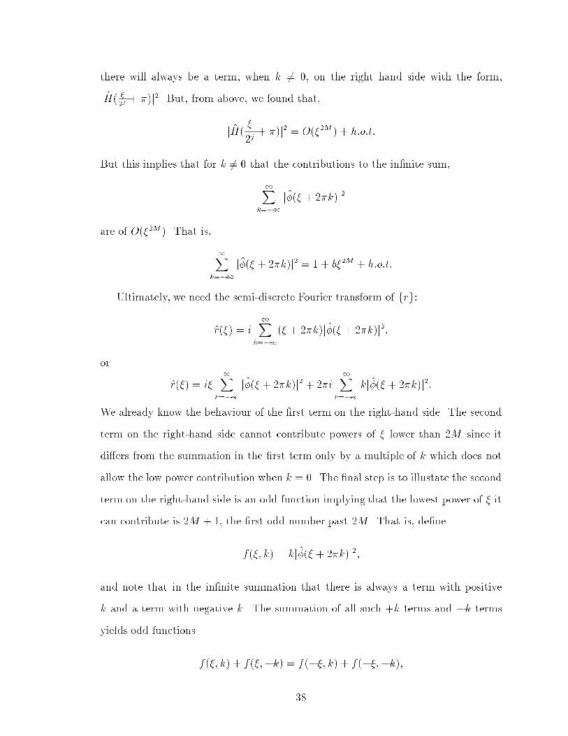
there will always be a term, when k 6= 0, on the right hand side with the form,

jH( �

2j+ �)j2. But, from above, we found that,

jH(�

2j+ �)j2 = O(�2M ) + h:o:t:

But this implies that for k 6= 0 that the contributions to the in�nite sum,

1Xk=�1

j�(� + 2�k)j2

are of O(�2M ). That is,

1Xk=�1

j�(� + 2�k)j2 = 1 + b�2M + h:o:t:

Ultimately, we need the semi-discrete Fourier transform of frg:

r(�) = i1X

k=�1(� + 2�k)j�(� + 2�k)j2;

or

r(�) = i�1X

k=�1j�(� + 2�k)j2 + 2�i

1Xk=�1

kj�(� + 2�k)j2:

We already know the behaviour of the �rst term on the right-hand side. The second

term on the right-hand side cannot contribute powers of � lower than 2M since it

di�ers from the summation in the �rst term only by a multiple of k which does not

allow the low power contribution when k = 0. The �nal step is to illustate the second

term on the right-hand side is an odd function implying that the lowest power of � it

can contribute is 2M + 1, the �rst odd number past 2M . That is, de�ne

f(�; k) = kj�(� + 2�k)j2;

and note that in the in�nite summation that there is always a term with positive

k and a term with negative k. The summation of all such +k terms and �k terms

yields odd functions.

f(�; k) + f(�;�k) = f(��; k) + f(��;�k);

38

and one can see that if, dn

d�njH(�)j2j�=0 = 0; for n = 1; :::; 2M � 1, then

dn

d�nj�(�)j2j�=0 = 0;

for n = 1; :::; 2M � 1. From this information we can see that a series expansion of

j�(�)j2 about � = 0 would be of the form,

j�(�)j2 = a+ b�2M + h:o:t:

But, �(x) is normalized implying that �(0) = 1 and therefore j�(0)j2 = 1. The

expansion becomes,

j�(�)j2 = 1 + b�2M + h:o:t:;

where b 2 C. Recall that we are looking for the semi-discrete Fourier transform of

r(�), which we see from above is,

r(�) =1X

k=�1�(� + 2�k) =

1Xk=�1

i(� + 2�k)j�(� + 2�k)j2:

We now need to �nd the behaviour of j�(� + 2�k)j2 when k 6= 0. Note that in the

expression,

j�(� + 2�k)j2 =1Yj=1

jH(� + 2�k

2j)j2;

the arguement,

� + 2�k

2j=

�

2j+

k�

2j�1;

will for some j be equal to

� + 2�k

2j=

�

2j+ �;

modulus 2�. That is, if k is odd in the expression (k�)=(2j�1) then stop when j = 1

since we can subtract multiples of 2� from (k�) without changing H since H is 2�

periodic. If k is even, then for some j, the number (k)=(2j�1) will be odd at which

point we again subtract some multiple of 2�. Consequently, in the in�nite product,

j�(� + 2�k)j2 =1Yj=1

jH(� + 2�k

2j)j2;

37

Now, we need to know the behaviour of j�(�)j2. Recall from the de�nitions that,

H(�) = (1 + ei�)M (1

2)MQ(ei�);

where Q(ei�) does not have poles or zeros at � = �, see [2]. That is, H(�) has a zero

of order M at � = �. Therefore, H(� + �) has a zero of order M at � = 0, i.e.,

H(� + �) = c�M + h:o:t:;

then

jH(� + �)j2 = a�2M + h:o:t:;

where a = jcj2. Recall from the de�nitions that,

jH(�)j2 + jH(� + �)j2 = 1:

Combine the two previous relations to get,

jH(�)j2 = 1� a�2M + h:o:t:

That is,

dn

d�njH(�)j2j�=0 = 0;

for n = 1; :::; 2M � 1. The Fourier Transform of �(x) was found above:

�(�) =1Yj=1

H(�

2j):

We get an expression for j�(�)j2 from,

�(�)�(�) =1Yj=1

H(�

2j)1Yj=1

H(�

2j);

or

j�(�)j2 =1Yj=1

jH(�

2j)j2:

Now, derivatives of this expression have the form,

dn

d�nj�(�)j2 =

1Yj=1

dn

d�njH(

�

2j)j2;

36

and

g(x) =d

dx�(x);

then

�(y) = f � g(y)

where '�' is the convolution operator. The convolution theorem states that the Fourier

Transform (continuous or discrete) of a convolution is the product of the Fourier

Transforms:

�(�) = f(�)g(�):

If we de�ne rl as,

rl = �(l)

then the semi-discrete Fourier transform of rl is

r(�) =1X

k=�1�(� + 2�k):

where,

�(�) =Z 1

�1�(x)eix�dx;

and

r(�) =1X

k=�1rke

ik�:

Calculate the needed Fourier Transforms to get,

f(�) = �(�);

where �� denotes conjugation, and

g(�) = i��(�):

Combine these results to get the Fourier Transform of f�lg:

�(�) = j�(�)j2i�:

35

Therefore,

�(�) =p2L�1Xk=0

hk

Z 1

�1�(2x� k)ei�kdx:

Let y = 2x� k which implies dx = dy=2 to get

=1p2

L�1Xk=0

hk

Z 1

�1�(y)ei(�=2)(y+k)dy

=1p2

L�1Xk=0

hkeik

�

2

Z 1

�1�(y)eiy

�

2dy;

or simply

�(�) = H(�=2)�(�=2);

recalling that H(�) = 1p2

PL�1k=0 hke

ik�. Furthermore, we get �(�) = H(�=2)H (�=4)�(�=4).

This implies,

�(�) = �(0)1Yj=1

H(�

2j);

but �(x) is normalized, �(0) =R�(x)dx = 1. Therefore,

�(�) =1Yj=1

H(�

2j):

Theorem: The Fourier Transform of frlg is of the form,

r(�) = i� + c�2M+1 + h:o:t:;

where c 2 C is some constant, and 'h.o.t.' denotes higher-order terms and will be

used again in the proof.

Proof: Begin with the expression for frlg:

�(y) =Z 1

�1�(x� y)

d

dx�(x)dx:

If we de�ne,

f(x) = �(�x);

34

Wavelet Derivative Exact up to But not for

D2 x2 x3

D4 x4 x5

D6 x6 x7

D8 x8 x9

D10 x10 x11

D12 x12 x13

D14 x14 x15

D16 x16 x17

D18 x18 x19

Table 6: The degree of polynomials di�erentiated exactly by various Daubechies

scaling function derivative coe�cients.

The pattern in this table is obvious and leads to the following theorem:

Theorem: If �(x) is the scaling function for the Daubechies wavelet denoted

by D2M , where M is the number of vanishing moments of the wavelet, then the

coe�cients frlg derived from

rl =Z 1

�1�(x� l)

d

dx�(x)dx

and applied the to evenly-spaced samples of a function act as a �nite di�erence

derivative operator of order 2M .

The proof of this theorem requires two results, as well as the Fourier Transform

of �(x). First �(�) will be found followed by the two results which are needed and

stated in theorem form. Perhaps the �rst proof would su�ce assuming the second

result is well-known. However, to be complete the second result is also proved.

Fourier Transform of �(x): Recall,

�(x) =p2L�1Xk=0

hk�(2x� k):

De�ne the Fourier Transform of �(x) as,

�(�) =Z 1

�1�(x)ei�xdx:

33

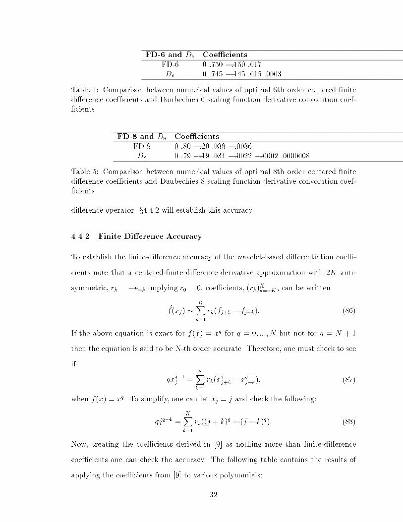
FD-6 and D6 Coe�cients

FD-6 0 :750 �:150 :017D6 0 :745 �:145 :015 :0003

Table 4: Comparison between numerical values of optimal 6th order centered �nite

di�erence coe�cients and Daubechies 6 scaling function derivative convolution coef-

�cients.

FD-8 and D8 Coe�cients

FD-8 0 :80 �:20 :038 �:0036D8 0 :79 �:19 :034 �:0022 �:0002 :0000008

Table 5: Comparison between numerical values of optimal 8th order centered �nite

di�erence coe�cients and Daubechies 8 scaling function derivative convolution coef-�cients.

di�erence operator. x4.4.2 will establish this accuracy.

4.4.2 Finite Di�erence Accuracy

To establish the �nite-di�erence accuracy of the wavelet-based di�erentiation coe�-

cients note that a centered-�nite-di�erence derivative approximation with 2K anti-

symmetric, rk = �r�k implying r0 = 0, coe�cients, (rk)Kk=�K , can be written

�f(xj) �KXk=1

rk(fj+k � fj�k): (86)

If the above equation is exact for f(x) = xq for q = 0; :::; N but not for q = N + 1

then the equation is said to be N-th order accurate. Therefore, one must check to see

if

qxq�1j =KXk=1

rk(xqj+k � xqj�k); (87)

when f(x) = xq. To simplify, one can let xj = j and check the following:

qjq�1 =KXk=1

rk((j + k)q � (j � k)q): (88)

Now, treating the coe�cients derived in [9] as nothing more than �nite-di�erence

coe�cients one can check the accuracy. The following table contains the results of

applying the coe�cients from [9] to various polynomials:

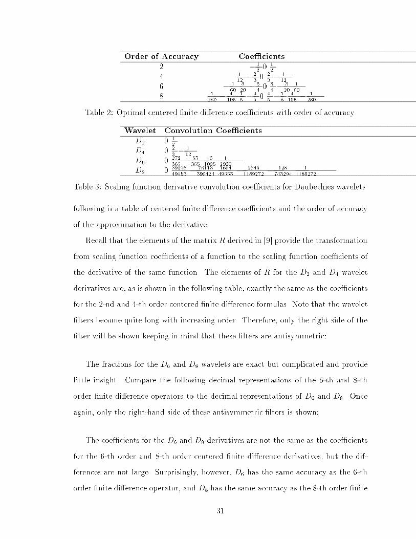
32

Order of Accuracy Coe�cients

2 �120 1

2

4 112�2

30 2

3� 1

12

6 � 160

320�3

40 3

4� 3

20160

8 1280

� 4105

15�4

50 4

5�1

54105

� 1280

Table 2: Optimal centered �nite di�erence coe�cients with order of accuracy.

Wavelet Convolution Coe�cients

D2 0 12

D4 0 23� 1

12

D6 0 272365

� 53365

161095

12920

D8 0 3929649553

� 76113396424

166449553

� 26451189272

� 128743295

11189272

Table 3: Scaling function derivative convolution coe�cients for Daubechies wavelets.

following is a table of centered �nite di�erence coe�cients and the order of accuracy

of the approximation to the derivative:

Recall that the elements of the matrix R derived in [9] provide the transformation

from scaling function coe�cients of a function to the scaling function coe�cients of

the derivative of the same function. The elements of R for the D2 and D4 wavelet

derivatives are, as is shown in the following table, exactly the same as the coe�cients

for the 2-nd and 4-th order centered �nite di�erence formulas. Note that the wavelet

�lters become quite long with increasing order. Therefore, only the right side of the

�lter will be shown keeping in mind that these �lters are antisymmetric:

The fractions for the D6 and D8 wavelets are exact but complicated and provide

little insight. Compare the following decimal representations of the 6-th and 8-th

order �nite di�erence operators to the decimal representations of D6 and D8. Once

again, only the right-hand side of these antisymmetric �lters is shown:

The coe�cients for the D6 and D8 derivatives are not the same as the coe�cients

for the 6-th order and 8-th order centered �nite di�erence derivatives, but the dif-

ferences are not large. Surprisingly, however, D6 has the same accuracy as the 6-th

order �nite di�erence operator, and D8 has the same accuracy as the 8-th order �nite

31

what the wavelet derivative does, one must understand the rami�cations of applying

the matrix R0 to the vector ~s0. In the next subsection the similarity between the

above de�ned matrix R0 and �nite di�erence formulas for taking the derivative will

be explored.

4.4 Wavelet Derivatives and Finite Di�erence

As the previous subsection illustrated, the essential properties of the wavelet deriva-

tive are contained in the elements of the matrix R. Recall that R is the matrix form

of the mapping from ~s0 to ~�s0. The surprising property that the matrix R exhibits is,

however, that it can also di�erentiate evenly-spaced samples of a function. That is,

R acts as a �nite-di�erence operator when applied to the samples of a function.

This subsection is in three parts:

1. The similarity between wavelet derivative coe�cients and �nite di�erence coef-

�cients is noted.

2. The �nite di�erence accuracy of the coe�cients frlg derived in [9] will be illus-

trated, and it will be proved in general that the coe�cients frlg can di�erentiate

polynomials exactly up through order 2M for coe�cients frlg that were derived

for Daubechies wavelets D2M .

3. In the �nite element method under certain conditions one achieves a very high

order of accuracy called 'superconvergence.' In wavelet di�erentiation a similar

phenomenon is encountered. This phenomenon is de�ned and a short explana-

tion is o�ered.

4.4.1 Finite Di�erence Coe�cients

First of all, it is useful to simply note the similarity between the coe�cients of centered

�nite di�erence formulas and the coe�cients used to construct the matrix R. The

30

and M performs the following mapping:

M :

"s31s32

#"d31d32

#26664d21d22d23d24

37775

266666666666664

d11d12d13d14d15d16d17d18

377777777777775

!

"�s31�s32

#"

�d31�d32

#266664

�d21�d22�d23�d24

377775

26666666666666664

�d11�d12�d13�d14�d15�d16�d17�d18

37777777777777775

: (85)

For data compression, this is the most useful set of subspaces. The space now is

represented as W1 �W2 �W3 � V3. For the same reasons as before the coe�cients

of basis functions in the subspace V3 cannot be ignored. It is likely, however, that

the function f(x) being represented is smooth in most of the domain allowing one

to disregard the majority of the coe�cients of the basis functions in the subspace

W1 �W2 �W3. In fact, it is more likely that the coe�cients for the basis functions

in W1 will be negligible than for the coe�cients for the basis functions in W3. This

is because the basis functions in W3 have larger support than the basis functions in

W2 and W1.

In summary, an attempt has been made to illustrate that the derivative coe�cients

of a scaling and wavelet expansion can be calculated at any scale. The proper set of

wavelet subspaces depends on the problem at hand. The goal for this author is to

understand exactly what wavelets are and what they are doing, therefore, scale j = 0,

i.e., the space V0, provides the clearest scenario in which to work without sacri�cing

essential properties of wavelets.

Given, now, that it is su�cient to work on scale j = 0 to understand exactly

29

be contained in spaces at three di�erent scales: W1, W2, W3, and V3. The full set

of coe�cients in this case and all the appropriate decompositions leading to these

coe�cients are,

2666666666666666666666666666666664

s01s02s03s04s05s06s07s08s09s010s011s012s013s014s015s016

3777777777777777777777777777777775

P0;116�16�!

266666666666664

s11s12s13s14s15s16s17s18

377777777777775

266666666666664

d11d12d13d14d15d16d17d18

377777777777775

P1;28�8�!

26664s21s22s23s24

37775

26664d21d22d23d24

37775

266666666666664

d11d12d13d14d15d16d17d18

377777777777775

P2;34�4�!

"s31s32

#"d31d32

#26664d21d22d23d24

37775

266666666666664

d11d12d13d14d15d16d17d18

377777777777775

: (83)

In matrix form the projection onto the coe�cients of the derivative of the expansion

is, where the matrix will be labeled M,

M =

266666664

264"R32�2 C3

2�2B32�2 A3

2�2

#P

2;34�4C

24�4

B24�4(P

2;34�4)

T A24�4

375

" P 2;34�4 00 I

!P1;28�8C

18�8

#

"B18�8(P

1;28�8)

T

P

2;34�4 0

0 I

!T #A18�8

377777775

(84)

28

derivative coe�cients at scale j = 0:

h~�s0

i= (P 0;1

16�16)T �24 ~�s1~�d1

35 ; (82)

and one gets exactly the same coe�cients as before when the matrix R016�16 was

applied to ~s0. To emphasize, the derivative calculated at scale j = 0 and the derivative

calculated at j = 1 yield exactly the same result. The importance of this observation

is that in order to understand the essence of the wavelet derivative one need only be

concerned with the action of the matrix R0N�N on the vector ~s0.

For data compression the spaceW1�V1 is a fair space to work in. The coe�cients

~s1 of the basis functions in V1 represent local averages just as the coe�cients of

the basis functions in the space V0 do. However, the basis functions in V1 have

broader support than the basis functions in V0 and therefore represent averages over

a larger amount of data (twice as much data to be exact). Therefore, once again

the coe�cients ~s1 usually carry essential information. The coe�cients ~d1 of the basis

functions in the space W1, on the other hand, carry information concerning local

oscillations. That is, if the function being represented, f(x), is globally smooth then

the coe�cients ~d1 will be near zero and can be set exactly to zero without altering the

character of f(x). In the solution of nonlinear partial di�erential equations where a

sharp gradient, or shock, can develop, the coe�cients ~d1 away from the shock would

be close to zero whereas the coe�cients near the shock would be large. Therefore,

representing a function in W1 � V1 is more versatile than simply staying in the space

V0. Versatility continues to be enhanced as one decomposes into more and more

wavelet subspaces as in the next and �nal scenario.

4.3.4 Wavelet Expansion and Derivative in W1 �W2 �W3 � V3

Up to now our basis functions have all been at the same scale, i.e., initially our

basis functions were contained in V0, and in the second scenario the basis functions

were contained in V1 and W1. In this subsection, however, the basis functions will

27

4.3.3 Wavelet Expansion and Derivative in W1 � V1

Consider now a decomposition of the vector of scaling function coe�cients ~s0 onto

the scaling function and wavelet coe�cients at scale j = 1 by an application of the

matrix P0;116�16: 2

666666666666666666666666666666664

s01s02s03s04s05s06s07s08s09s010s011s012s013s014s015s016

3777777777777777777777777777777775

P0;116�16�!

266666666666664

s11s12s13s14s15s16s17s18

377777777777775

266666666666664

d11d12d13d14d15d16d17d18

377777777777775

; (78)

As before, we have 16 basis functions in our space which is now V1LW1 rather than

V0. In order to calculate the coe�cients of the derivative expansion in V1LW1 the

following projections are calculated:

~�s1 = R18�8 � ~s1 + C1

8�8 � ~d1; (79)

and

~�d1 = A18�8 � ~d1 +B1

8�8 � ~s1; (80)

where A, B, C, and R were all de�ned in the previous subsection. A more concise

way to represent the derivative projections is in matrix notation:

24 ~�s1~�d1

35 =

"R18�8 C1

8�8B18�8 A1

8�8

#�"~s1~d1

#: (81)

If one now applies the matrix (P 0;116�16)

T (T denotes transpose and hence inverse for

this unitary matrix) to the derivative coe�cients at scale j = 1 then one gets the

26

4.3.2 Wavelet Expansion and Derivative in V0

As stated previously, one can calculate the derivative of a wavelet expansion at any

level in the wavelet decomposition. This subsection will explore the �rst of three of the

options. To be explicit, suppose that a periodic function f(x) has been approximated

on a grid with 16 scaling function coe�cients to get ~s0, and for the current argument

assume that the coe�cients have been calculated exactly, i.e., the notation ~s0 will be

used instead of ~�0. Furthermore due to the periodicity of f(x) the coe�cients ~s0 will

also be periodic. The coe�cients of the expansion of ddxf(x) in V0 are found from ~s0

by an application of the previously de�ned matrix R016�16:

2666666666666666666666666666666664

s01s02s03s04s05s06s07s08s09s010s011s012s013s014s015s016

3777777777777777777777777777777775

R0

16�16�!

2666666666666666666666666666666664

�s01�s02�s03�s04�s05�s06�s07�s08�s09�s010�s011�s012�s013�s014�s015�s016

3777777777777777777777777777777775

; (77)

which completely de�nes the derivative of f(x) in the scaling function basis at scale

j = 0.

For data compression purposes, the space V0 is not a good space to work in. That

is, the coe�cients ~s0 represent the equivalent of a local averages. In a wavelet basis,

it is often true that the coe�cients of local high-frequency oscillations are small and

can be set to zero without altering the character of the function being represented,

but the coe�cients of local averages usually represent essential information.

25

The decomposition matrix in this case is,

Pj;j+18�8 �

266666666666664

h1 h2 h3 h4 0 0 0 0

0 0 h1 h2 h3 h4 0 0

0 0 0 0 h1 h2 h3 h4h3 h4 0 0 0 0 h1 h2g1 g2 g3 g4 0 0 0 0

0 0 g1 g2 g3 g4 0 0

0 0 0 0 g1 g2 g3 g4g3 g4 0 0 0 0 g1 g2

377777777777775: (76)

Other decomposition matrices of di�erent sizes will have the same structure as the

above matrix.

For a bit more matrix notation, let the four matrices AjN�N , B

jN�N , C

jN�N , and

RjN�N contain the derivative projection coe�cients de�ned in x(4.2) where, again,

the subscripts denote the size of the matrix and the superscript denotes the scale on

which the derivative projection is acting. The elements of the four matrices are,

A$ aij = ai�j ;

B $ bij = bi�j;

C $ cij = ci�j ;

and

R$ rij = ri�j ;

and the mappings performed by the matrices are,

Aj : ~dj ! ~�dj ;

Bj : ~sj ! ~�dj;

Cj : ~dj ! ~�sj;

Rj : ~sj ! ~�sj ;

where ~sj and ~dj , as before, de�ne the scaling and wavelet coe�cients at scale j, and

~�sj and~�dj denote the coe�cients of the expansion of the derivative of a function which

is initially de�ned by an expansion in ~sj and ~dj .

This concludes the new notation.

24

4. Wavelet decompositions and di�erentiation matrices will be given for the space

W1 �W2 �W3 � V3 as well as comments on data compression.

4.3.1 New Notation

To simplify the presentation, matrix notation will be used whenever possible. Begin

by de�ning the matrix version of equations (29) and (30). Recall that these equations

are

sjk =n=2MXn=1

hnsj�1n+2k�2;

and

djk =n=2MXn=1

gnsj�1n+2k�2:

Denote the decomposition matrix embodied by these two equations by P j;j+1N�N where

the matrix subscripts denote the size of the matrix, and the superscripts indicate

that P is decomposing from scaling function coe�cients at scale j to scaling function

and wavelet function coe�cients at scale j + 1. As before, let ~sj contain the scaling

function coe�cients at scale j. (Note: When vector notation is used the scale is

given as a subscript, otherwise the location k is the subscript and the scale is the

superscript.) P therefore maps ~sj onto ~sj+1 and ~dj+1:

Pj;j+1N�N :

h~sji!"~sj+1~dj+1

#: (75)

Note that the vectors at scale j + 1 are half as long as the vectors as scale j. To

illustrate further, suppose the wavelet being used is the four coe�cient D4 wavelet,

and suppose one wants to project from 8 scaling function coe�cients at scale j to 4

scaling function coe�cients at scale j + 1 and 4 wavelet coe�cients at scale j + 1.

23

and Xl

lrl = �1; (73)

where

�n = 2L�1�nXi=0

hihi+n; (74)

for n = 1; :::; L� 1. The proof of the above proposition can be found in [9].

This section has given a brief outline of the derivation of the wavelet derivative

projection coe�cients. It is important to note that all the information for the wavelet

derivative is contained in the coe�cients frlg, and this point will be explored more

in next section.

4.3 Derivative at Scale Zero of Scaling Function Only

Wavelet derivatives can be calculated at any level of a wavelet decomposition. The

result will, of course, always be the same. That is, recall the relation from x(2),

Vj = Vj+1�Wj+1. As stated before, it is the convention of this paper to let V0 represent

the �nest scale. Using the above relation, one could decompose V0 any number of

times. One decomposition yields V0 = W1 � V1, and a second decomposition yields

V0 = W1 �W2 � V2. One could calculate the wavelet derivative in any one of these

spaces. Once again, the goal of this paper is to understand the essence of a wavelet

derivative, and since the derivative is the same regardless of the decomposition of the

space, one should choose the simplest approach and calculate the derivative at scale

j = 0 using only the scaling function coe�cients.

This subsection contains four parts:

1. New notation will be introduced.

2. Wavelet decompositions and di�erentiation matrices will be given for the space

V0 as well as comments on data compression in this space.

3. Wavelet decompositions and di�erentiation matrices will be given for the space

W1 � V1 as well as comments on data compression in this space.

22

derivative scaling function coe�cients and wavelet function coe�cients at the same

scale are derived. The matrix elements of these projections are computed from,

2�jai�l = ajil = 2�2j

Z 1

�1 (2�jx� i) � (2�jx� l)dx; (61)

2�jbi�l = bjil = 2�2j

Z 1

�1 (2�jx� i)��(2�jx� l)dx; (62)

2�jci�l = cjil = 2�2j

Z 1

�1�(2�jx� i) � (2�jx� l)dx; (63)

2�jri�l = rjil = 2�2jZ 1

�1�(2�jx� i)��(2�jx� l)dx: (64)

Since the above projections are always at a �xed scale, j, the projection coe�cients

are simply,

al =Z 1

�1 (x� l)

d

dx (x)dx; (65)

bl =Z 1

�1 (x� l)

d

dx�(x)dx; (66)

cl =Z 1

�1�(x� l)

d

dx (x)dx; (67)

rl =Z 1

�1�(x� l)

d

dx�(x)dx; (68)

for l 2 Z. Furthermore, using the dilation equation which de�nes �(x), �(x) =

Pk hk�(2x � k), and the equation which de�nes (x), (x) =

Pk gk�(2x � k), the

�rst three of the above four equations become,

ai =L�1Xk=0

L�1Xl=0

gkglr2i+k�l (69)

bi =L�1Xk=0

L�1Xl=0

gkhlr2i+k�l (70)

ci =L�1Xk=0

L�1Xl=0

hkglr2i+k�l: (71)

It is apparent from the above equations that the coe�cients rl contain all the infor-

mation concerning the derivative. The coe�cients rl can be found [9] from solving

the following system of linear algebraic equations:

rl = 2(r2l +1

2

L=2Xk=1

�2k�1(r2l�2k+1 + r2l+2k�1)); (72)

21

where due to the orthonormality of the basis functions �1k(x) and 1k(x) the coe�cients

s1k and d1k are given by

s1k =Z 1

�1f(x)�1k(x)dx; (57)

and

d1k =Z 1

�1f(x) 1

k(x)dx: (58)

The derivative of PV1�W1f(x) is

d

dxPV1�W1

f(x) =N=2�1Xk=0

s1k��1k(x) +

N=2�1Xk=0

d1k� 1k(x): (59)

Once again, the derivative of PV1�W1f(x) does not belong to V1

LW1, and must,

therefore, be projected back onto this space. The projection is,

PV1�W1

d

dxPV1�W1

f(x) = (60)

N=2�1Xl=0

N=2�1Xk=0

s1k <��1k; �

1l > �1l (x)

+N=2�1Xl=0

N=2�1Xk=0

s1k <��1k;

1l > 1

l (x)

+N=2�1Xl=0

N=2�1Xk=0

d1k <� 1k; �

1l > �1l (x)

+N=2�1Xl=0

N=2�1Xk=0

d1k <� 1k;

1l > 1

l (x):

The four inner products < ��1k; �1l >, <

��1k; 1l >, <

� 1k; �

1l >, and < � 1

k; 1l > are

the key to �nding the derivative of a wavelet expansion, and are provided in [9]. An

outline of the derivation of these inner products is given in the next section.

4.2 Wavelet Coe�cients of the Derivative

An arbitrary wavelet expansion of a function might contain wavelet coe�cients and

scaling coe�cients at many scales. In [9] the projection coe�cients that map from

scaling function coe�cients and wavelet function coe�cients at a given scale to the

20

PV0 be the projection from the space L2(R) to the space V0, PV0 : L2(R)! V0:

PV0f(x) =N�1Xk=0

s0k�0k(x); (50)

where due to the orthonormality of �0k over k in V0,

s0k =Z 1

�1f(x)�0k(x)dx: (51)

Note that in the introduction the projection denoted by PN would be the same as

PV0 using notation that is more amenable to wavelets. The derivative of PV0f(x) is,

d

dxPV0f(x) =

N�1Xk=0

s0k��0k(x): (52)

Of course, ddxPV0f(x) is not in V0 and must be projected onto V0. First de�ne the

inner product < f; g > on L2(R) by

< f; g >=Z 1

�1f(x)g(x)dx: (53)

Now the projection of ddxPV0f(x) onto V0 is,

PV0d

dxPV0f(x) =

N�1Xl=0

<d

dxPV0f; �

0l > �0l (x); (54)

or,

PV0d

dxPV0f(x) =

N�1Xl=0

N�1Xk=0

s0k <��0k; �

0l > �0l (x): (55)

The inner product < ��0k; �0l > is one of the results provided in [10].

In the previous paragraph f(x) was expanded in a scaling-function expansion at

the �nest scale j = 0. Now f(x) will be expanded in terms of scaling functions and

wavelets at scale j = 1. Recall that V0 = V1LW1. Now one must project from L2(R)

onto V1 and from L2(R) onto W1. Let both projections be denoted simultaneously

by PV1�W1. That is, PV1�W1

: L2(R) ! V1LW1. Let PV1�W1

f(x) be the projection

of f(x) on V1LW1. Therefore, the expansion for PV1�W1

f(x) is,

PV1�W1f(x) =

N=2�1Xk=0

s1k�1k(x) +

N=2�1Xk=0

d1k 1k(x); (56)

19

4 Derivative based on Wavelets

In the previous section the mapping from evenly-spaced samples of a periodic function,

f(x), to the approximate scaling function coe�cients on the �nest scale, �0k, was given.

Recall that �jk denotes the approximation to the exact scaling function coe�cient sjk

at scale j and position k. The mapping is nothing more than a quadrature formula

which is exact when f(x) is equal to a polynomial up to order M � 1, where M is

the number of vanishing moments of the wavelet. The question now is how does one

represent the derivative of f(x) in the wavelet basis given that the wavelet expansion

of f(x) is already given.

The answer is given in the following subsections:

x4.1 ) A function f(x) will be expanded in a wavelet basis and the expansion will

be di�erentiated.

x4.2 ) The results from Beylkin [9] on derivative projections will be given.

x4.3 ) First, it will be noted that one can di�erentiate a wavelet expansion at any

level of a wavelet decomposition and achieve the same derivative. Second, explicit

wavelet decomposition will be performed accompanied by the appropriate di�erenti-

ation matrix.

x4.4 ) The similarity between the wavelet-based derivative coe�cients and �nite

di�erence derivative coe�cients will be noted, and it will be shown that when one

di�erentiates the wavelet expansion of a periodic function that the e�ect on the

original function samples is equal to �nite di�erence di�erentiation.

4.1 Expansion in a Wavelet Basis

The goal now is to �nd the wavelet and scaling function expansion of a periodic

function f(x). Given f(x) 2 L2(R) one �rst projects onto the arbitrarily chosen

�nest scale j = 0 of the scaling function �0k(x) which generates the space V0, i.e., let

18

equation (48) is nothing more than,

C �R0 = R0 � C (49)

In this section a quadrature formula has been found to approximate the scaling

function coe�cients of a given function, f(x). In matrix form this quadrature for-

mula leads to a circulant matrix assuming f(x) is periodic. In the next section the

wavelet derivative operator will be derived, and it will be shown that, once again,

the assumption that f(x) is periodic leads to an operator which in matrix form is

circulant.

17

0 � i � N � 1, the above equation can be written as,

�k =M�1Xl=0

clfmod(l+k;N):

Now, shift the indices by letting j = l+ k to get,

�k =k+(M�1)X

j=k

cj�kfmod(j;N):

If the length-M �lter ~c is now 'padded' at the end with zeros so that it is now a

length-N �lter then the above equation can be rewritten as,

�k =N�1Xj=0

cmod(j�k;N)fj :

This is exactly a matrix multiply ~� = C ~f where the ij � th element of the matrix

C is cmod(j�i;N), and this is the de�nition of a circulant matrix. This completes the

proof.//

Note that the di�erence between a circulant matrix and a Toeplitz matrix is the

wrapping around e�ect of the diagonals introduced by the use of the modulus function

for the circulant matrix. That is, a circulant matrix is a special case of a Toeplitz

matrix where the constant diagonals are periodic.

Before leaving the discussion on circulant matrices let one more interpretation be

noted: to say that circulant matrices commute is to simply restate the important re-

sult from signal analysis that convolutions commute. That is, if one has two sequences

c and r, which in the current scenario are periodic, then the order of convolution does

not matter. This is easily proved with the Fourier transform:

dc � r = cr = rc = dr � c; (48)

where r denotes the Fourier transform of r and '�' denotes periodic convolution. For

this paper, c, of course, would be the quadrature operator and r would be the scaling

function derivative operator which is the subject of section (4). In matrix notation

16

have the wonderful property that they can all be diagonalized by the same matrix, the

Fourier matrix: AnN�N Fourier matrix has as its ij�th element the entryw(i�1)(j�1)

where wN = 1. The most important rami�cation for this paper is that matrices which

can be diagonalized by the same matrix commute. That is, the matrix C from the

previous subsection will commute with the matrix R0 which will be derived in section

(1.4).

In general, circulant matrices arise whenever one is performing the matrix version

of periodic discrete convolution. In numerical analysis periodic discrete convolution

arises whenever one di�erentiates the evenly-spaced samples of a periodic equation

which has constant coe�cients. Let us be a bit more precise and illustrate how the

operation of periodic discrete convolution yields a circulant matrix by stating the

following theorem:

Theorem: A �nite-length �lter of length M applied to N evenly-spaced samples

of periodic function, where N > M , will in matrix form yield a circulant matrix.

Proof: First of all, let the notation remain as above: c0; c1; :::; cM�1 will represent

the �nite-length �lter and f0; f1; :::; fN�1 will represent the evenly-spaced samples of

one period of the periodic function f(x). Of course, the samples of f(x) are periodic

with periodN . The application of the �lter ~c on the samples of f(x) is the convolution:

�k =M�1Xl=0

clfk�l;

where fi is the renaming of the elements of fi so that the previous convolution is

the same as the following expression. Furthermore, keep in mind that fi and fi are

periodic with period N .

�k =M�1Xl=0

clfl+k:

Using the modulus function to keep the indices of fi within one period, i.e., keep

15

i Mi �i ci0 1 2 .1080

1 .8174 1.6348 .9667

2 .6681 1.3363 -.0746

Table 1: Scaling function and �lter moments for Daubechies 6 wavelets.

for m = 0; 1; :::;M � 1. Speci�cally, for the D6 wavelet the linear system in matrix

form is, 0B@

1 1 1

0 1 2

0 1 4

1CA0B@c0c1c2

1CA =

0B@M0

M1

M2

1CA ; (45)

which has the solution c0 = :1080, c1 = :9667, and c2 = �:0746. In tabular form, the

complete results for D6 are,

Recall that the quadrature formula used to approximate the scaling function has

the form,

�0k =M�1Xl=0

clf(l + k): (46)

If the function f(x) is periodic then in matrix notation the above operation is ~�0 = C ~f

where C for D6 and on a grid of 6 points is,

C =

0BBBBBBBB@

:108 :967 �:075 0 0 00 :108 :967 �:075 0 00 0 :108 :967 �:075 00 0 0 :108 :967 �:075

�:075 0 0 0 :108 :967

:967 �:075 0 0 0 :108

1CCCCCCCCA: (47)

The important point here is that the above matrix is circulant. The rami�cations

of circularity are very important for the thesis of the paper. The de�nition of circulant

matrices and the properties that they are imbued with is the subject of the next

subsection.

3.3 Circulant Matrices

Strang [7] de�nes a circulant matrix as a constant-diagonal matrix which is `periodic,

since the lower diagonals fold around to appear again as the upper diagonals.' A

thorough discussion of circulant matrices is given by Davis [8]. Circulant matrices

14

Recall from the previous subsection that in order to calculate the coe�cients

fclgM�1l=0 the moments of the scaling function �(x) must �rst be known. Let Ml be

the lth moment of the scaling function �(x),

Ml =Z�(x)xldx; (37)

and let �l be the lth moment of the �lter hk,

�l =Xk

klhk: (38)

The zero-th moment,M0, of �(x) is 1 by the normalization of �(x):

M0 =Z�(x)dx = 1: (39)

The zero-th moment of the coe�cients hk is found by integrating the dilation equation

which de�nes �(x): Z�(x)dx =

Xk

hk

Z�(2x� k)dx; (40)

and let y = 2x � k to get,

1 =1

2

Xk

hk

Z�(y)dy; (41)

which implies,

�0 =Xk

hk = 2: (42)

That is, the zero-th moments M0 and �0 are the same for all Daubechies wavelets.

Higher moments for �l can be found by straight-forward calculation using the coe�-

cients provided by Daubechies [2]. The higher moments,Ml for l > 0, for the scaling

function can be found from the following equation which is derived in appendix B:

Mm = (1

2)m+1

Xl

m

l

!�m�lMl: (43)

For the current example only the moments M0, M1, and M2 are needed: M0 = 1,

M1 = 12�1, and M2 = 1

6((�1)

2 + �2). Given these three moments the coe�cients

fclgM�1l=0 can be found from

M�1Xl=0

lmcl =Zxm�(x)dx (44)

13

for p(x) 2 PM�1. If the integral is shifted the above equation becomes,

Z 1

�1p(y + k)�00(y)dy =

M�1Xl=0

clp(l + k): (34)

More simply, the coe�cients fclgM�1l=0 can be found [9] by solving the following linear

system: Z 1

�1xm�(x)dx =

M�1Xl=0

lmcl; (35)

for m = 0; 1; :::;M � 1, and the coe�cients fclgM�1l=0 provide the desired quadrature

formula. That is, the coe�cients, ~�0, which approximate ~s0 are found from,

�0k =M�1Xl=0

clf(l + k): (36)

When placed in matrix form the coe�cients fclgM�1l=0 yield the circulant matrix C.

A more thorough discussion of circulant matrices will be given in x(3.3) after the

example of the next subsection has been completed.

Note that since the above derived quadrature formula is exact for p(x) 2 PM�1

the coe�cients �0k approximate the coe�cients s0k with error of order M . Also, note

that the derivation of the quadrature coe�cients depends only on the moments of the

scaling function,R1�1 x

m�(x)dx. In the next subsection, the moments of the scaling

function will �rst be calculated and then the coe�cients fclgM�1l=0 will be found for

the D6 wavelet. The wavelet D6 is chosen for no other reason than that D2 and D4

receive considerable attention from other sources and that D6 is slightly less trivial

than D2 and D4 while remaining manageable.

3.2 Example with the Daubechies Wavelet D6

Recall from the previous subsection that the immediate goal is to approximate the

scaling function coe�cients of a function at scale j = 0. Speci�cally, in this section

the objective is to derive the matrix form of the mapping from evenly-spaced samples

of a periodic function f(x) to the scaling function coe�cients on the �nest scale s0k.

The example will be for the Daubechies wavelet D6. Comparable results for the

wavelets D4 and D8 are presented in appendix B.

12

2. Smooth functions can be approximated with error O(hM ), where h denotes the

grid size, i.e., there exist a set sjk, where j is �xed, and there exists a constant

C such that

jf(x)�Xk

sjk�

jk(x)j � ChM jf (M)(x)j; (32)

where the norm j � j is the L2 norm.

3. The associated wavelet has M vanishing moments,

Zxm (x)dx = 0

for m = 0; :::;M � 1.

Other rami�cations can be found in [6]. These approximation properties determine

the accuracy of the quadrature formula used to approximate the scaling function

coe�cients ~s0 which is derived in the following section.

3.1.2 Derivation of Quadrature Formula

It is important to note that all wavelets in this paper are of the usual Daubechies

type, i.e., the support of a usual Daubechies wavelet D2M is [0; 2M � 1] where M is

the number of vanishing moments of the wavelet. For this subsection this support size

is particularly important to keep in mind because there does exist an orthonormal

family of wavelets which are supported on [0; 3M � 1] and which have a very simple

quadrature formula based on the vanishing moments of the wavelet (see appendix A)

but this is not the wavelet being used in this paper.

Given the approximation properties of the scaling function from the previous

subsection, one can now seek a quadrature formula which is exact when f(x) is a

polynomial up to order M � 1: f(x) = p(x) 2 PM�1. That is, there exist a set of

coe�cients fclgM�1l=0 such that

Z 1

�1p(x)�0kdx =

M�1Xl=0

clp(l + k); (33)

11

In this section, however, the decomposition onto more coarse scales will not be cal-

culated. The important step for this section is the approximation of the integral

s0k =R1�1 f(x)�

0k(x)dx. Let �

0k denote the approximation to s0k. The quadrature for-

mula for this integral encompasses the approximation properties of scaling functions,

and hence wavelets.

This section contains 3 subsections:

x3.1 ) The approximation properties of scaling functions will be discussed and the

quadrature formula to estimate the integralR1�1 f(x)�

0k(x)dx will be derived.

x3.2 ) An example using the results from section (3.1) is given for the Daubechies

wavelet D6.

x3.3 ) The example from section (3.2) leads to a circulant matrix for the matrix

C. Circulant matrices will be de�ned and the rami�cations of circularity will be

discussed.

3.1 Quadrature Formula for Scaling Function

In this subsection the coe�cients s0k will be approximated. Before stating the appro-

priate quadrature formula, however, the order of accuracy of a wavelet approximation

is discussed.

3.1.1 Approximation Properties of Scaling Functions

This subsection comes essentially from [6]. The approximation properties of scaling

functions are determined by the Discrete Fourier Transform of the �lter H. That is,

if

H(�) =1

2

L�1Xk=0

hkeik� (31)

has a zero of order M at � = � then there are a number of consequences:

1. The polynomials 1, x, :::, xM�1 are linear combinations of the translates of the

scaling function �0k.

10

3 Approximating in a Wavelet Basis

Scaling functions and wavelets were de�ned in the previous section. The goal of this

section is to �nd the coe�cients in a wavelet expansion. More precisely, the scal-

ing function coe�cients at the �nest scale, ~s0, will be approximated. The key to

this approximation is the matrix C which maps evenly-spaced samples of a periodic

function to the approximate scaling function coe�cients. This matrix C has the de-

sirable property of being circulant in form with the rami�cation that C will commute

with any other circulant matrix, particularly the derivative matrix R0, the subject of

section (4). An example of C is given at the end of section (3.2).

The scenario for this section is as follows: let the �nest scale be scale j = 0, i.e.,

at this scale all relevant small scale structures in the function have been captured and

represented. One seeks an expansion of a function f(x) in terms of �0k in the space

V0. With the projection PV0 de�ned as PV0 : L2(R)! V0 such an expansion has the

following form:

PV0f(x) =Xk2Z

s0k�0k(x); (27)

where due to the orthonormality of the basis functions, �ij =R1�1 �0i (x)�

0j(x)dx, the

coe�cients s0k are given by

s0k =Z 1

�1f(x)�0k(x)dx: (28)

Once the s0k have been found one would usually then �nd the scaling function and

wavelet function coe�cients at more coarse scales. This can be done by using equation

(29) to get sjk for j = 1; :::; J and by using equation (30) to get djk for j = 1; :::; J .

These equations are derived respectively from equations (1) and (2), see [4], [5],

sjk =

2MXn=1

hnsj�1n+2k�2; (29)

and

djk =

2MXn=1

gnsj�1n+2k�2: (30)

9

and would appear as,

PV0f(x) =Xk2Z

sJk�Jk (x) +

JXj=1

Xk2Z

djk jk(x); (26)

where again due to orthonormality of the basis functions djk =R1�1 f(x)

jk(x), and

sJk =R1�1 f(x)�

Jk (x). In this expansion, scale j = 0 is arbitrarily chosen as the �nest

scale that is needed, and scale J would be the scale at which a kind of local average,

�Jk (x), provides su�cient large scale information. In language that is likely to appeal

to the electrical engineer it can be said that �Jk (x) represents the direct current portion

of a signal and that jk(x) represents the alternating current portion of a signal at,

very roughly, frequency j. As stated above, one must also limit the range of the

location parameter k. In this paper this is done by assuming that f(x) is a periodic

function. The periodicity of f(x) induces periodicity on all wavelet coe�cients, sjk

and djk.

This completes the de�nition of wavelets. The next section will discuss function

approximation in a wavelet basis.

8

where

P (y) =k=M�1Xk=0

M � 1 + k

k

!yk; (21)

and R is an odd polynomial such that,

0 � P (y) + yMR(1=2 � y) (22)

for 0 � y � 1, and

sup0�y�1

(P (y) + yMR(1=2 � y)) < 22(M�1); (23)

if M � 2 or

� 2

1� 2jxj � R(x) � 2

1 + 2jxj; (24)

for jxj � 1=2, if M = 1. The important point here is that H(�) has a zero of order

M at � = �.

Of course, in�nite sums and unions are meaningless when one begins to implement

a wavelet expansion on a computer. In some way one must limit range of the scale

parameter j and the location parameter k. Consider �rst the scale parameter j. As

stated above, the wavelet expansion is complete: L2(R) =L

j2ZWj. Therefore, any

f(x) 2 L2(R) can be written as,

f(x) =Xj2Z

Xk2Z

djk jk(x);

where due to orthonormality of the wavelets djk =R1�1 f(x) j

k(x). In this expan-

sion, functions with arbitrarily small-scale structures can be represented. In practice,

however, there is a limit to how small the smallest structure can be. This would

depend, for example, on how �ne the grid is in a numerical computation scenario or

perhaps what the sampling frequency is in a signal processing scenario. Therefore,

on a computer an expansion would take place in a space such as

V0 = W1 �W2 � . . .�WJ � VJ ; (25)

7

The spaces Vj and Wj are related by [2]

::: � V1 � V0 � V�1 � :::; (12)

and that

Vj = Vj+1M

Wj+1: (13)

The previously stated condition that the wavelets form an orthonormal basis of L2(R)

can now be written as,

L2(R) =Mj2Z

Wj : (14)

Two �nal properties of the spaces Vj are that

\j2Z

Vj = f0g; (15)

and [j2Z

Vj = L2(R): (16)

Properties of the Semi-Discrete Fourier Transform (SDFT) of the �lterH will also

be needed. The following de�nition is not exactly the SDFT but a constant times the

SDFT:

H(�) = 2�1=2k=L�1Xk=0

hkeik�: (17)

This DFT satis�es the following equation, see [4]:

jH(�)j2 + jH(� + �)j2 = 1: (18)

Solutions of equation (18) have the following properties, see [2]:

H(�) = (1

2(1 + ei�))MQ(ei�); (19)

whereM is the number of vanishing moments of the wavelet and Q is a trigonometric

polynomial such that,

jQ(ei�j2 = P (sin2(�=2)) + sin2M(�=2)R(1

2cos �); (20)

6

where �kl is the Kronecker delta function. Also, (x) = 00(x) satis�es

Z 1

�1 (x)xmdx = 0; (7)

for m = 0; :::;M � 1. Under the conditions of the previous two equations, for any

function f(x) 2 L2(R) there exists a set fdjkg such that

f(x) =Xj2Z

XK2Z

djk jk(x); (8)

where

djk =Z 1

�1f(x) j

k(x)dx: (9)

The number of vanishing moments of the wavelet (x) de�nes the accuracy of

approximation. The two sets of coe�cients H and G are known in signal processing

literature as quadrature mirror �lters [3]. For Daubechies wavelets the number of

coe�cients in H and G, or the length of the �lters H and G, denoted by L, is related

to the number of vanishing momentsM by 2M = L. For example, the famous Haar

wavelet is found by de�ning H as h0 = h1 = 1. For this �lter, H, the solution to

the dilation equation (1), �(x), is the box function: �(x) = 1 for x 2 [0; 1] and

�(x) = 0 otherwise. The Haar function is very useful as a learning tool, but it

is not very useful as a basis function on which to expand another function for the

important reason that it is not di�erentiable. The coe�cients, H, needed to de�ne

compactly supported wavelets with a higher degree of regularity can be found in [2].

As is expected, the regularity increases with the support of the wavelet. The usual

notation to denote a Daubechies wavelet de�ned by coe�cients H of length L is DL.

It is usual to let the spaces spanned by �jk(x) and jk(x) over the parameter k,

with j �xed, to be denoted by Vj and Wj respectively:

Vj =span

k2Z�jk(x); (10)

Wj =span

k2Z jk(x): (11)

5

2 Wavelet De�nitions and Relations

The term wavelet is used to describe a spatially localized function. `Localized' means

that the wavelet has compact support or that the wavelet almost has compact sup-

port in the sense that outside of some interval the amplitude of the wavelet decays

exponentially. We will consider only wavelets that have compact support and that

are of the type de�ned by Daubechies [2] which are supported on [0; 2M � 1], where

M is the number of vanishing moments de�ned later in this section.

To de�ne Daubechies wavelets, consider the two functions �(x) and (x) which

are solutions to the following equations:

�(x) =p2L�1Xk=0

hk�(2x� k); (1)

(x) =p2L�1Xk=0

gk�(2x� k); (2)

where �(x) is normalized, Z 1

�1�(x)dx = 1: (3)

Let,

�jk(x) = 2�j

2�(2�jx� k); (4)

and

jk(x) = 2�

j

2 (2�jx� k); (5)

where j; k 2 Z, denote the dilations and translations of the scaling function and the

wavelet.

The coe�cients H = fhkgL�1k=0 and G = fgkgL�1k=0 are related by gk = (�1)khL�k for

k = 0; :::; L� 1. Furthermore, H and G are chosen so that dilations and translations

of the wavelet, jk(x), form an orthonormal basis of L2(R) and so that (x) has M

vanishing moments. In other words, jk(x) will satisfy

�kl�jm =Z 1

�1 jk(x)

ml (x)dx; (6)

4

x4) This is the most important section of this paper. It will be proved that the

action of D is equivalent to a �nite di�erence operator.

x5) The results of sections (3) and (4) are combined for the desired conclusion.

In addition, the following two related topics are explored in the �rst two appen-

dices:

Appendix A) For wavelets supported on (0,3M) it will be shown thatR�(x)xmdx =

(R�(x)xdx)m.

Appendix B) The moments of the scaling function �(x) will be calculated.

3

depending on the order of the wavelet chosen.

More precisely, the following outlines the proof of this assertion:

� Given a periodic function f(x), let C be the mapping from evenly-spaced sam-

ples of f(x) to the approximate scaling function coe�cients on the �nest scale:

C : ~f ! ~�0. Due to the periodicity of f(x), C is circulant in form.

� Let D be the mapping from the exact scaling function coe�cients of f(x) to

scaling function coe�cients of f 0(x): D : ~s0 ! ~�s0. Once again, due to the

periodicity of f(x), D is circulant in form.

� The matrix operator D can di�erentiate exactly evenly-spaced samples of poly-

nomials, i.e., D has the e�ect of a �nite-di�erence operator. The order of exact

di�erentiation depends on the order of the wavelet used.

� All circulant matrices with the same dimensions commute, therefore the oper-

ator D can be applied directly to ~f :

~f 0 = C�1DC ~f;

or simply,

~f 0 = D~f;

and this will complete the proof.

This paper contains �ve sections:

x1) This introduction.

x2) Standard de�nitions of wavelets and scaling functions are given.

x3) The general approximation properties of wavelets will be discussed along with

the quadrature formula needed to approximate the scaling function coe�cients of a

function.

2

1 Introduction

The term di�erentiation matrix was coined by E. Tadmor in his review on spectral

methods [1]. The term denotes the transformation between grid point values of a

function and its approximate �rst derivative. This matrix is a product of three ma-

trices.

The �rst matrix C is constructed as follows: assume that the point values of a

function f(x) (where a � x � b) are given at N points xj for 0 � j � N � 1.

Thus a vector of numbers f(xj) is given. From this vector one can reconstruct an

approximation to the function f(x) for every point x in the interval. This approxima-

tion (denoted byPNf) itself belongs to a �nite dimensional space - in pseudospectral

methods it is the global interpolation polynomial that collocates f(xj) and in �nite

di�erences or �nite elements it is a piecewise polynomial. This transformation be-

tween f(xj) and PNf , de�nes the matrix C. Of course this matrix depends on the

special basis chosen to represent PNf . A good example is the Fourier interpolation

procedure in which the basis is the set of complex exponentials.

The second matrix D results from di�erentiating PNf , and projecting it back to

the �nite dimensional space. Thus D is de�ned by the linear transformation between

PNf and PNddxPNf .

The last matrix is the inverse of the �rst matrix. Basically, since we are given the

approximation PNddxPNf we can read it at the grid points xj. Thus the di�erentiation

matrix D can be represented as D = C�1DC.

In this paper the wavelet di�erentiation matrix will be examined. As with other

basis sets, as outlined above, it is a product of three matrices. Under the assumption

of periodicity of f(x), however, the matrices C and D commute allowingD to operate

directly on the vector of numbers f(xj). That is, the di�erentiation matrixD is simply

D: D = D. Furthermore, the matrix D di�erentiates samples of polynomials exactly,

i.e., the action of D is equivalent to a �nite di�erence operator with order of accuracy

1

ON THE DAUBECHIES-BASED WAVELET

DIFFERENTIATION MATRIX

Leland Jameson1

Institute for Computer Applications in Science and Engineering

NASA Langley Research Center

Hampton, VA 23681

ABSTRACT

The di�erentiation matrix for a Daubechies-based wavelet basis will be constructed

and `superconvergence' will be proven. That is, it will be proven that under the

assumption of periodic boundary conditions that the di�erentiation matrix is accurate

of order 2M , even though the approximation subspace can represent exactly only

polynomials up to degreeM�1, whereM is the number of vanishing moments of the

associated wavelet. It will be illustrated that Daubechies-based wavelet methods are

equivalent to �nite di�erence methods with grid re�nement in regions of the domain

where small-scale structure is present.

1This research was supported by the National Aeronautics and Space Administration under

NASA Contract No. NAS1-19480 while the author was in residence at the Institute for Computer

Applications in Science and Engineering (ICASE), NASA Langley Research Center, Hampton, VA

23681. Research was also supported by AFOSR grant 93-1-0090, by DARPA grant N00014-91-4016,

and by NSF grant DMS-9211820.

i