Embed Size (px)
Citation preview
Abnormal Event Detection in Video
A Project Report
submitted in partial fulfillment of the
requirements for the degree of
Master of Technology
in
Computational Science
by
Uday Kiran Kotikalapudi
Supercomputer Education Research Center
Indian Institute of Science
Bangalore - 560012
July 2007
Acknowledgements
First and foremost I would like to express my respect, love and gratitude towards my
beloved Bhagawan Sri Sathya Sai Baba without whose grace my life wouldn’t have
been as joyful as it is now.
I wish to thank my guide Prof. K R Ramakrishnan for his valuable guidance and
his infinite patience. Working with him has been a great experience, both satisfying
and rewarding. I would also like to thank S. Kumar Raja and Dr. Venkatesh Babu
for their suggestions and help in the course of this project work. I would like to
thank the department of Super Computer Education and Research Center (SERC),
for providing an opportunity to pursue my project of interest in Electrical Engineering
department.
I would also like to express my gratitude to Dr. Kevin Smith of IDIAP institute,
whose work helped me take-off initially. Also thanks to all the professors whose
courses have helped me deal with different aspects of the work in one way or the
other.
Thanks to my dear friends Venu, Chandu and Seshikanth whose company has
always given me joy even at times of pressure. Thanks to my friends Jayanta, Mishra
and Joey for all the discussions, especially non-technical, we had in the tea-board.
Thanks to MTech06 (Karthikeyan, Vishwas, Nanditha, Arjun, Shyam, Ramanjulu
and Pinto) for the enjoyable time we had together in ssl. My special thanks to the
ever-helpful Rajan who works beyond time and space.
Last but not the least, I thank my parents for their love and warmth through-
out the course of my life. Thanks to my brother Kalyan and his friends Nagendra,
Jithendra, Srikanth and co. for all the fun we had and continue to have together.
ii
Abstract
Video surveillance has gained importance in security, law enforcement and military
applications and so is an important computer vision problem. As more and more
surveillance cameras are deployed in a facility or area, the demand for automatic
methods for video processing is increasing. The operator constantly watching the
video footages could miss a potential abnormal event (e.g. bag being abandoned by a
person), as the amount of information/data that has to be handled is high. Most often
he has to watch the entire video footage offline, to find the person who abandoned
the bag.
In this thesis, we present a surveillance system that supports a human operator
by automatically detecting abandoned objects and drawing the operator’s attention
to such events. It consists of three major parts: foreground segmentation based on
Gaussian Mixture Models, a tracker based on blob association and a blob-based object
classification system to identify abandoned objects. For foreground segmentation, we
assume that video sequences of the background shot under different natural settings
are available a priori. The tracker uses a single-camera view and it does not differ-
entiate between people and luggage. The classification is done using the shape of
detected objects and temporal tracking results, to successfully categorize objects into
bag and non-bag(human). If a potentially abandoned object is detected, the operator
is notified and the system provides the appropriate key frames for interpreting the
incident.
iii

Contents
1 Introduction 1
1.1 Overview . . . . . . . . . . . . . . . . . . . . . . . . . . . . . . . . . . 3
1.2 Motivation . . . . . . . . . . . . . . . . . . . . . . . . . . . . . . . . . 4
1.3 Organization of the Thesis . . . . . . . . . . . . . . . . . . . . . . . . 4
1.4 Summary . . . . . . . . . . . . . . . . . . . . . . . . . . . . . . . . . 5
2 Smart Video Surveillance 6
2.1 Moving Object Detection . . . . . . . . . . . . . . . . . . . . . . . . . 7
2.1.1 Background Subtraction . . . . . . . . . . . . . . . . . . . . . 7
2.1.2 Statistical Methods . . . . . . . . . . . . . . . . . . . . . . . . 8
2.1.3 Temporal Differencing . . . . . . . . . . . . . . . . . . . . . . 9
2.1.4 Optical Flow . . . . . . . . . . . . . . . . . . . . . . . . . . . 10
2.2 Object Tracking . . . . . . . . . . . . . . . . . . . . . . . . . . . . . . 10
2.2.1 Feature Selection for Tracking . . . . . . . . . . . . . . . . . . 12
2.3 Object Classification . . . . . . . . . . . . . . . . . . . . . . . . . . . 13
2.3.1 Shape-based Classification . . . . . . . . . . . . . . . . . . . . 13
2.3.2 Motion-based Classification . . . . . . . . . . . . . . . . . . . 13
2.4 Summary . . . . . . . . . . . . . . . . . . . . . . . . . . . . . . . . . 14
3 Object Detection 15
3.1 Foreground Detection . . . . . . . . . . . . . . . . . . . . . . . . . . . 16
3.1.1 Temporal Differencing . . . . . . . . . . . . . . . . . . . . . . 18
3.1.2 Adaptive Gaussian Mixture Model . . . . . . . . . . . . . . . 19
3.2 Pixel Level Post-Processing . . . . . . . . . . . . . . . . . . . . . . . 21
3.3 Detecting Connected Regions . . . . . . . . . . . . . . . . . . . . . . 23
3.4 Region Level Post-Processing . . . . . . . . . . . . . . . . . . . . . . 23
3.5 Extracting Object Features . . . . . . . . . . . . . . . . . . . . . . . 24
iv

3.6 Results . . . . . . . . . . . . . . . . . . . . . . . . . . . . . . . . . . . 26
3.7 Summary . . . . . . . . . . . . . . . . . . . . . . . . . . . . . . . . . 27
4 Object Tracking 28
4.1 Correspondence-based Object Matching . . . . . . . . . . . . . . . . . 29
4.2 Results . . . . . . . . . . . . . . . . . . . . . . . . . . . . . . . . . . . 36
4.3 Summary . . . . . . . . . . . . . . . . . . . . . . . . . . . . . . . . . 37
5 Object Classification and Event Detection 38
5.1 Object Classification . . . . . . . . . . . . . . . . . . . . . . . . . . . 38
5.1.1 Bayes Classifier . . . . . . . . . . . . . . . . . . . . . . . . . . 39
5.1.2 Quadratic Discriminant Analysis . . . . . . . . . . . . . . . . 40
5.1.3 Learning Phase . . . . . . . . . . . . . . . . . . . . . . . . . . 41
5.2 Event Detection . . . . . . . . . . . . . . . . . . . . . . . . . . . . . . 43
5.2.1 Bag Detection . . . . . . . . . . . . . . . . . . . . . . . . . . . 44
5.2.2 Alarm Criteria . . . . . . . . . . . . . . . . . . . . . . . . . . 45
5.3 Results . . . . . . . . . . . . . . . . . . . . . . . . . . . . . . . . . . . 46
5.4 Summary . . . . . . . . . . . . . . . . . . . . . . . . . . . . . . . . . 50
6 Conclusion and Future work 51
Bibliography 54
v
List of Figures
2.1 A generic framework for smart video processing algorithms. . . . . . . 6
2.2 Temporal differencing sample. Left Image: A sample scene with two moving objects. Righ
2.3 Taxonomy of tracking methods [3] . . . . . . . . . . . . . . . . . . . . 11
2.4 Different tracking approaches. (a)Multi-point correspondence, (b)Parametric transformation
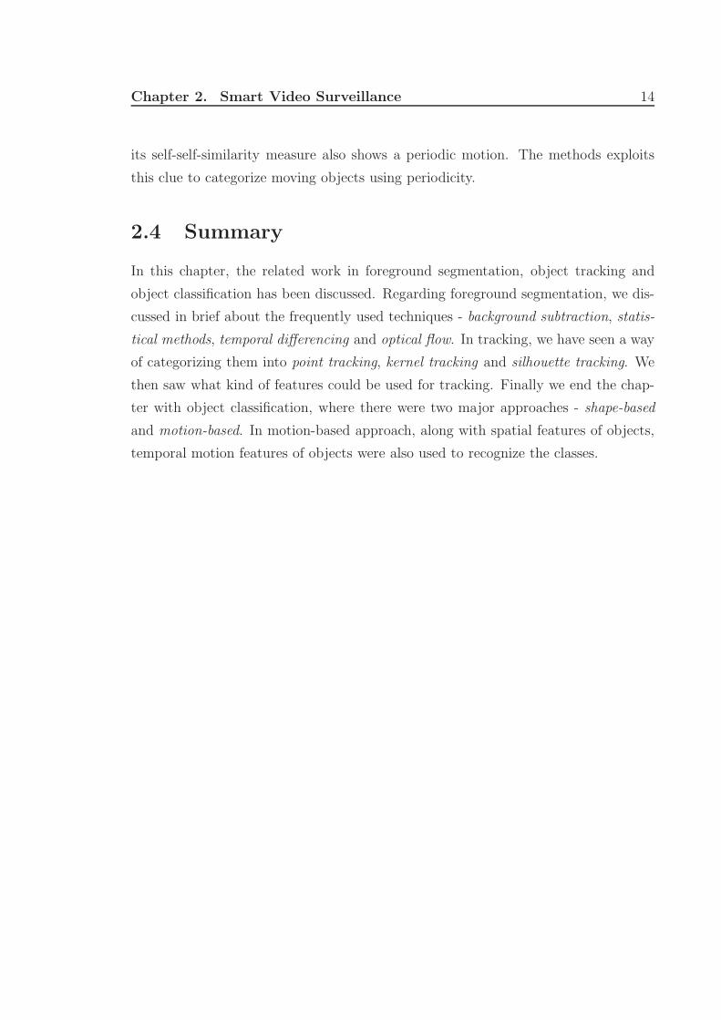
3.1 The system block diagram. . . . . . . . . . . . . . . . . . . . . . . . . 16
3.2 The object detection system diagram. . . . . . . . . . . . . . . . . . . 17
3.3 Sample foreground detection. . . . . . . . . . . . . . . . . . . . . . . 18
3.4 Initial foreground pixel map (without any enhancements) . . . . . . . 21
3.5 Foreground pixel map before and after pixel-level post-processing . . 23
3.6 Foreground pixel map before and after connected component analysis. Different connected
3.7 Final foreground pixel map, before and after region-level post-processing 24
3.8 Bounding Box and Centroid features . . . . . . . . . . . . . . . . . . 25
3.9 Left: Background image. Middle: Current image. Right: Foreground with Bounding Bo
3.10 Left: Background image. Middle: Current image. Right: Foreground with Bounding Bo
3.11 Left: Background image. Middle: Current image. Right: Foreground with Bounding Bo
4.1 The object tracking system diagram . . . . . . . . . . . . . . . . . . . 29
4.2 Before any matching . . . . . . . . . . . . . . . . . . . . . . . . . . . 31
4.3 After Centroid Matching. Left: Case of split. Right: Case of entry. . 32
4.4 Occlusion handling(split case). Top Left: Before merge (left/right object bounded by red/green
4.5 Before any matching . . . . . . . . . . . . . . . . . . . . . . . . . . . 34
4.6 After Centroid Matching : Left figure is the case of merge and the right one is the case
4.7 Occlusion handling(merge case). Left: Before split. Middle: Before merge. Right: After
4.8 Before and after centroid matching . . . . . . . . . . . . . . . . . . . 36
4.9 Case of split . . . . . . . . . . . . . . . . . . . . . . . . . . . . . . . . 36
4.10 Case of split and merge . . . . . . . . . . . . . . . . . . . . . . . . . . 37
vi
4.11 Occlusion handling . . . . . . . . . . . . . . . . . . . . . . . . . . . . 37
5.1 First Row: Bags. Second Row: Corresponding blobs. . . . . . . . . 42
5.2 Left Column: Non-bags(mostly people). Right Column: Corresponding blobs. 43
5.3 Abnormal Event I. (a) Bag-Owner split. (b) Bag detected. (c) Bag unattended 47
5.4 Abnormal Event II. (a) Bag-Owner split. (b) Bag detected. (c) Bag unattended. 48
5.5 Abnormal Event III, (a) Bag-Owner split. (b) Bag detected. (c) Bag unattended. (d) Bag
vii
Chapter 1
Introduction
Video Surveillance can be described as the task of analyzing video sequences to de-
tect abnormal or unusual activities. Video surveillance activities can be manual,
semi-autonomous or fully-autonomous. Manual video surveillance involves analysis
of the video content by a human. Such systems are currently in widespread use.
Semi-autonomous video surveillance involves some form of video processing but with
significant human intervention. Typical examples are systems that perform simple
motion detection. Only in the presence of significant motion the video is recorded
and sent for analysis by a human expert. By a fully-autonomous system, we mean a
system whose only input is the video sequence taken at the scene where surveillance is
performed. In such a system there is no human intervention and the system does both
the low-level tasks, like motion detection and tracking, and also high-level decision
making tasks like abnormal event detection and gesture recognition.
The ultimate goal of the present generation surveillance systems is to allow video
data to be used for on-line alarm generation to assist human operators and for offline
inspection effectively. The making of video surveillance systems fully-automatic or
“smart” requires fast, reliable and robust algorithms for moving object detection,
classification, tracking and activity analysis.
Moving object detection is the basic step for further analysis of video. It han-
dles segmentation of moving objects from stationary background objects. Commonly
used techniques for object detection are background subtraction, statistical methods,
temporal differencing and optical flow. Due to dynamic environmental conditions
such as illumination changes, shadows and waving tree branches in the wind, object
segmentation is a difficult and significant problem that needs to be handled well for
1
Chapter 1. Introduction 2
a robust visual surveillance system.
Object classification step categorizes detected objects into predefined classes such
as human, vehicle, clutter, etc. It is necessary to distinguish objects from each other
in order to track and analyze their actions reliably. There are two major approaches
toward moving object classification: shape-based and motion-based methods. Shape-
based methods make use of object’s 2D spatial information whereas motion-based
methods use temporal tracked features of objects for the classification solution.
The next step in the video analysis is tracking, which can simply be defines as the
creation of temporal correspondence among detected objects from frame to frame.
This procedure provides temporal identification of the segmented regions and gen-
erates cohesive information about the objects in the monitored area. The output
produced by the tracking step is generally used to support and enhance motion seg-
mentation, object classification and higher level activity analysis. The final step of
the fully automatic video surveillance systems is to recognize the behaviors of objects
and create high-level semantic descriptions of their actions. The outputs of these
algorithms can be used both for providing the human operator with high level data
to helm him make the decisions more accurately and in a shorter time, and also for
offline indexing and searching stored video data effectively. Below are some scenarios
that fully-automated or smart surveillance systems and algorithms might handle:
Public and commercial security:
• Monitoring of banks, department stores, airports, museums, stations, private
properties and parking lots for crime prevention and detection
• Patrolling of highways and railways for accident detection
• Surveillance of properties and forests for fire detection
• Observation of the activities of elderly and infirm people for early alarms and
measuring effectiveness of medical treatments
• Access control
Smart video data mining:
• Compiling consumer demographics in shopping centers and amusement parks
• Extracting statistics from sport activities
Chapter 1. Introduction 3
• Counting endangered species
• Logging routine maintenance tasks at nuclear and industrial facilities
Military security:
• Patrolling national borders
• Measuring flow of refugees
• Monitoring peace treaties
The use of smart object detection, tracking and classification algorithms are not
limited to video surveillance only. Other application domains also benefit from the
advances in the research on these algorithms. Some examples are virtual reality,
video compression, human machine interface, augmented reality, video editing and
multimedia databases.
1.1 Overview
In this thesis we present an automatic video surveillance system with moving object
detection, tracking and classification capabilities.
In the presented system, moving object detection is handled by the use of adaptive
background mixture models [20]. In this paper, each pixel is modeled as a mixture of
Gaussians and an on-line approximation to update the model is used. Based on the
persistence and the variance of each of the Gaussians of the mixture, the Gaussians
which correspond to background colors are determined. Pixel values that do not
fit the background distributions are considered foreground until there is a Gaussian
that includes them with sufficient, consistent evidence supporting it. This system
adapts to deal robustly with lightning changes, repetitive motions of scene elements,
tracking through cluttered regions, slow-moving objects, and introducing or removing
objects from the scene. Slow moving objects take longer to be incorporated into the
background, because their color has a larger variance than the background. Also,
the repetitive variations are learned, and a model for the background distribution is
generally maintained even if it is temporarily replaced by another distribution which
leads to faster recovery when objects are removed. The background method consists
of two significant parameters - α, the learning constant and T, the proportion of the

Chapter 1. Introduction 4
data that should be accounted for by the background.
After segmenting moving pixels from the static background of the scene, the track-
ing algorithm tracks the detected objects in successive frames by using a correspondence-
based matching scheme. It also handles multi-occlusion cases where some objects
might be fully occluded by the others. It uses 2D object features such as position,
centroid and size to match corresponding objects from frame to frame. It keeps color
histograms of detected objects in order to resolve object identities after a split of an
occlusion group. The tracking algorithm doesn’t differentiate between objects while
tracking, which means the algorithm treats both person and non-person, like a bag,
alike.
As the primary objective of this work is to detect bag abandoning event, there
should be a classification step. The final stage of this entire automated system is
detection of bag, and detection of the abnormal event which is bag abandoning. The
classification algorithm incorporated here is the quadratic discriminant analysis. A
simple database has been built with detected foreground of 60 images, 30 of bag
and 30 of non-bag (person). The features used for classification are aspect ratio and
compactness, defined as the ratio of area by perimeter. The classification part, help
us in detecting the existence of a bag. From then on, depending on space contraint
and time constraint it is decided whether the bag has been unattended or abandoned.
1.2 Motivation
Understanding activities of objects in a scene by the use of video is both a challenging
scientific problem and a very fertile domain with many promising applications. Thus,
it draws attentions of several researchers, institutions and commercial companies [13].
Our motivation in studying this problem is to create a visual surveillance system
with real-time moving object detection, classification, tracking and activity analysis
capabilities. The presented system handles all the above methods, with few conditions
imposed, except activity recognition which will likely be the future step of this work.
1.3 Organization of the Thesis
The remaining part of the thesis is organized as follows. Chapter 2 presents a brief
literature survey in foreground segmentation, tracking and classification for video

Chapter 1. Introduction 5
surveillance applications. Our methods for moving object detection and object track-
ing are explained in chapters 3 and 4 respectively. In the 5th chapter we present our
object classification method and the event detection. Each chapter is supplemented
with experimental results and summary. Finally, chapter 6 concludes the thesis with
the suggestions for future work.
1.4 Summary
In this chapter, we have discussed in brief what is video surveillance, why we require
it to be automated and what are its applications. Later, an overview of our work, the
motivation for pursuing it and the organization of the thesis has been discussed.
Chapter 2
Smart Video Surveillance
There have been a number of surveys about object detection, classification, tracking
and activity analysis in the literature [13, 23, 3]. The survey we present here covers
only those work that are in the context as our study. However, for the comprehensive
completeness, we also give brief information on some techniques which are used for
similar tasks that are not covered in our study.
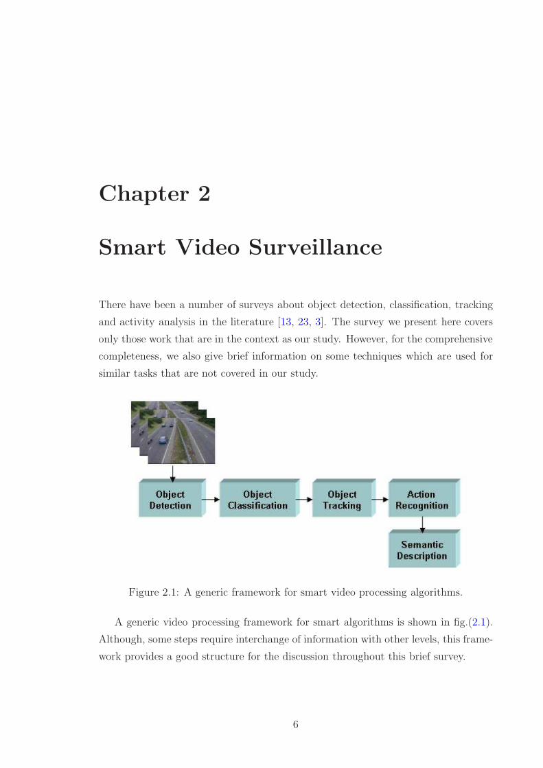
Figure 2.1: A generic framework for smart video processing algorithms.
A generic video processing framework for smart algorithms is shown in fig.(2.1).
Although, some steps require interchange of information with other levels, this frame-
work provides a good structure for the discussion throughout this brief survey.
6
Chapter 2. Smart Video Surveillance 7
2.1 Moving Object Detection
Each application that benefits from smart video processing has different needs, thus
requiring different treatment. However, they have something in common: moving
objects. Detecting regions that correspond to moving objects such as people and
vehicles in video is the first basic step of almost every vision system since it provides
a focus of attention and simplifies the processing on subsequent analysis steps. Due to
dynamic changes in natural scenes such as sudden illumination and weather changes,
repetitive motions that cause clutter (tree leaves in blowing wind), motion detection
is a difficult problem to process reliably. Frequently used techniques for moving object
detection are background subtraction, statistical methods, temporal differencing and
optical flow whose descriptions are given below.
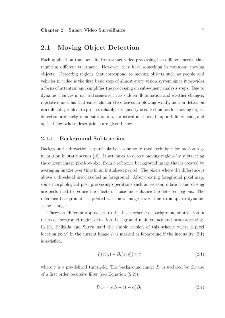
2.1.1 Background Subtraction
Background subtraction is particularly a commonly used technique for motion seg-
mentation in static scenes [15]. It attempts to detect moving regions by subtracting
the current image pixel-by-pixel from a reference background image that is created by
averaging images over time in an initialized period. The pixels where the difference is
above a threshold are classified as foreground. After creating foreground pixel map,
some morphological post processing operations such as erosion, dilation and closing
are performed to reduce the effects of noise and enhance the detected regions. The
reference background is updated with new images over time to adapt to dynamic
scene changes.
There are different approaches to this basic scheme of background subtraction in
terms of foreground region detection, background maintenance and post-processing.
In [9], Heikkila and Silven used the simple version of this scheme where a pixel
location (x,y) in the current image It is marked as foreground if the inequality (2.1)
is satisfied,
|It(x, y) − Bt(x, y)| > τ (2.1)
where τ is a pre-defined threshold. The background image Bt is updated by the use
of a first order recursive filter (see Equation (2.2)),
Bt+1 = αIt + (1 − α)Bt (2.2)

Chapter 2. Smart Video Surveillance 8
where α is an adaptation coefficient. The basic idea is to integrate the new incoming
information into the current background image. The larger it is, the faster new
changes in the scene are updated to the background frame. However, α cannot be
too large because it may cause artificial “tails” to be formed behind the moving
objects. The foreground pixel map creation is followed by morphological closing and
the elimination of small-sized regions.
Although background subtraction techniques perform well at extracting most of
the relevant pixels of moving regions, they are usually sensitive to dynamic changes
when, for instance, stationary objects uncover the background (e.g. a parked car
moves out of the parking lot) or sudden illumination changes occur.
2.1.2 Statistical Methods
More advanced methods that make use of the statistical characteristics of individual
pixels have been developed to overcome the shortcomings of basic background sub-
traction methods. These statistical methods are mainly inspired by the background
subtraction methods in terms of keeping and dynamically updating statistics of the
pixels that belong to the background image process. Foreground pixels are identified
by comparing each pixel’s statistics with that of the background model. This ap-
proach is becoming more popular due to its reliability in scenes that contain noise,
illumination changes and shadow [13]. The W4 [10] system uses a statistical back-
ground model where each pixel is represented with its minimum (M) and maximum
(N) intensity values and maximum intensity difference (D) between any consecutive
frames observed during initial training period where the scene contains no moving
objects. A pixel in the current image It is classified as foreground if it satisfies:
|M(x, y) − It(x, y)| > D(x, y) or |N(x, y) − It(x, y)| > D(x, y) (2.3)
After thresholding, a single iteration of morphological erosion is applied to the de-
tected foreground pixels to remove one-pixel thick noise. In order to grow the eroded
regions to their original size, a sequence of erosion and dilation is performed on the
foreground pixel map. Also, small-sized regions are eliminated after applying con-
nected component labeling to find the regions. The statistics of the background pixels
that belong to the non-moving regions of current image are updated with new image
data. As another example of statistical methods, Stauffer and Grimson [21] described
Chapter 2. Smart Video Surveillance 9
an adaptive background mixture modeled by a mixture of Gaussians which are up-
dated on-line by incoming image data. In order to detect whether a pixel belongs to
a foreground or background process, the Gaussian distributions of the mixture model
for that pixel are evaluated. An implementation of this model is used in our system
and its details are explained in section (3.1.2).
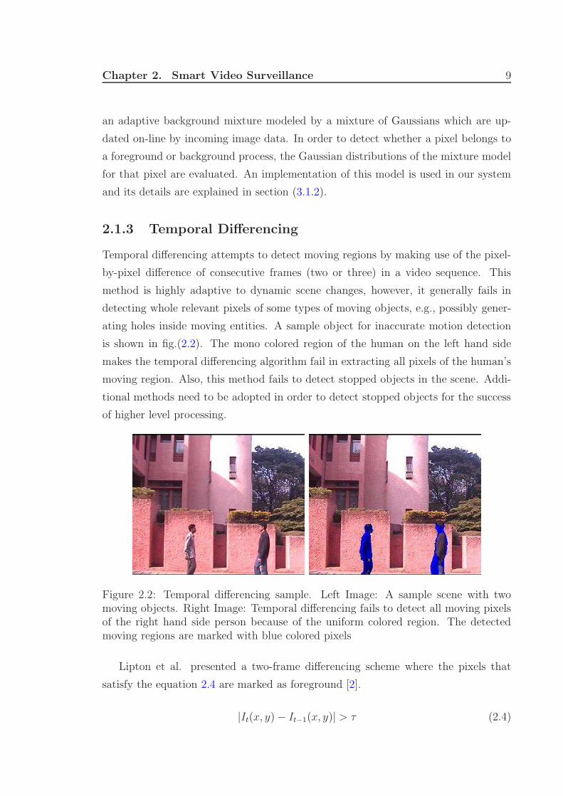
2.1.3 Temporal Differencing
Temporal differencing attempts to detect moving regions by making use of the pixel-
by-pixel difference of consecutive frames (two or three) in a video sequence. This
method is highly adaptive to dynamic scene changes, however, it generally fails in
detecting whole relevant pixels of some types of moving objects, e.g., possibly gener-
ating holes inside moving entities. A sample object for inaccurate motion detection
is shown in fig.(2.2). The mono colored region of the human on the left hand side
makes the temporal differencing algorithm fail in extracting all pixels of the human’s
moving region. Also, this method fails to detect stopped objects in the scene. Addi-
tional methods need to be adopted in order to detect stopped objects for the success
of higher level processing.
Figure 2.2: Temporal differencing sample. Left Image: A sample scene with twomoving objects. Right Image: Temporal differencing fails to detect all moving pixelsof the right hand side person because of the uniform colored region. The detectedmoving regions are marked with blue colored pixels
Lipton et al. presented a two-frame differencing scheme where the pixels that
satisfy the equation 2.4 are marked as foreground [2].
|It(x, y) − It−1(x, y)| > τ (2.4)
Chapter 2. Smart Video Surveillance 10
In order to overcome disadvantages of two-frame differencing in some cases, three
frame differencing can be used. For instance, Collins et al. developed a hybrid
method that combines three-frame differencing with an adaptive background subtrac-
tion model for their VSAM (Video Surveillance And Monitoring) project [17]. The
hybrid algorithm successfully segments moving regions in video without the defects
of temporal differencing and background subtraction.
2.1.4 Optical Flow
Optical flow methods make use of the flow vectors of moving objects over time to
detect moving regions in an image. They can detect motion in video sequences even
from a moving camera, however, most of the optical flow methods are computationally
complex and cannot be used real-time without specialized hardware [13].
2.2 Object Tracking
Tracking is a significant and difficult problem that arouses interest among computer
vision researchers. The objective of tracking is to establish correspondence of objects
and object parts between consecutive frames of video. It is a significant test in
most of the surveillance applications since it provides cohesive temporal data about
moving objects which are used both to enhance lower level processing such as motion
segmentation and to enable higher level data extraction such as activity analysis
and behavior recognition. Tracking has been a difficult task to apply in congested
situations due to inaccurate segmentation of objects. Common problems of erroneous
segmentation are shadows, partial and full occlusion of objects with each other and
with stationary items in the scene. Thus, dealing with shadows at motion detection
level and coping with occlusions both at segmentation level and at tracking level is
important for robust tracking.
Tracking in video can be categorized according to the needs of the applications
and the methods it uses for its solution. Whole body tracking is generally adequate
for outdoor surveillance whereas objects’ part tracking is necessary for some indoor
surveillance and higher level behavior understanding applications. There is a very
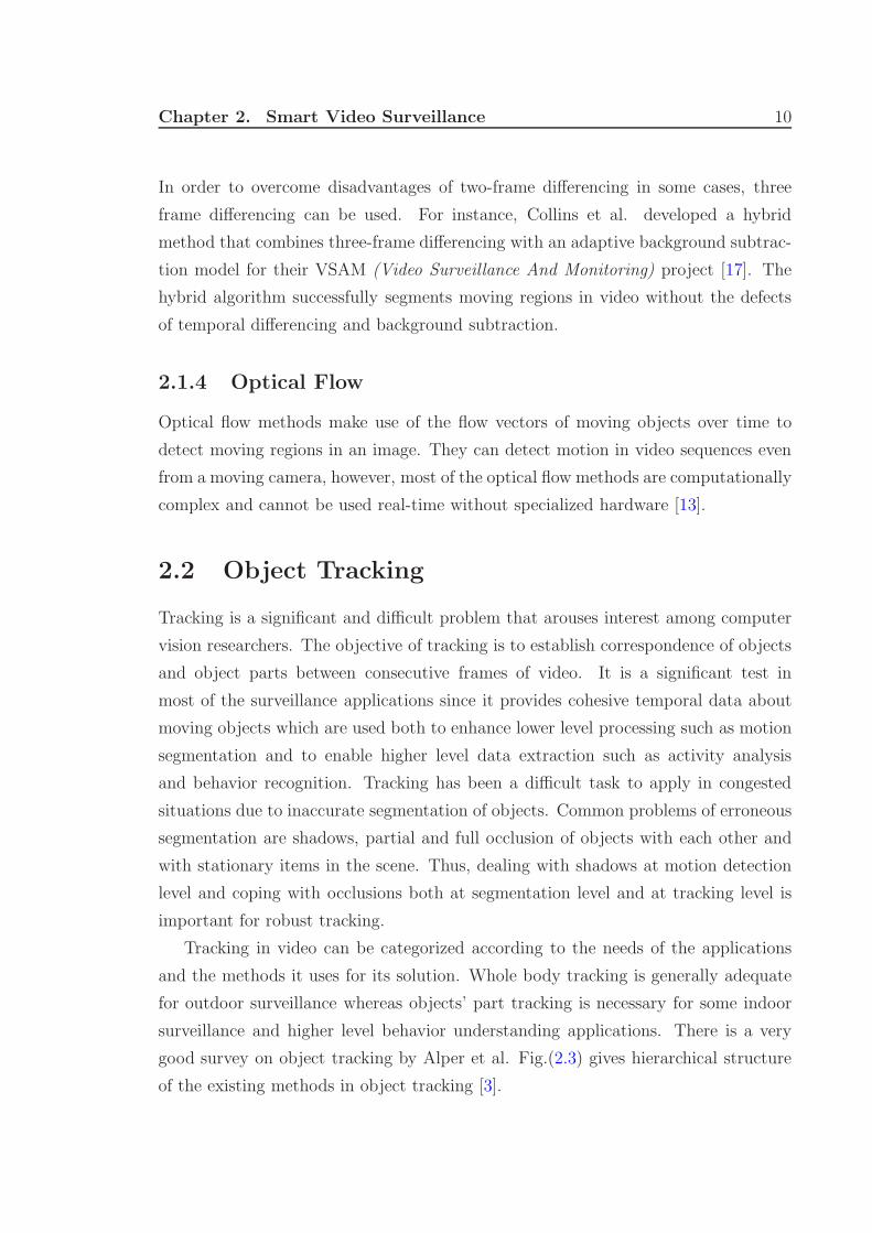
good survey on object tracking by Alper et al. Fig.(2.3) gives hierarchical structure
of the existing methods in object tracking [3].
Chapter 2. Smart Video Surveillance 11
Figure 2.3: Taxonomy of tracking methods [3]
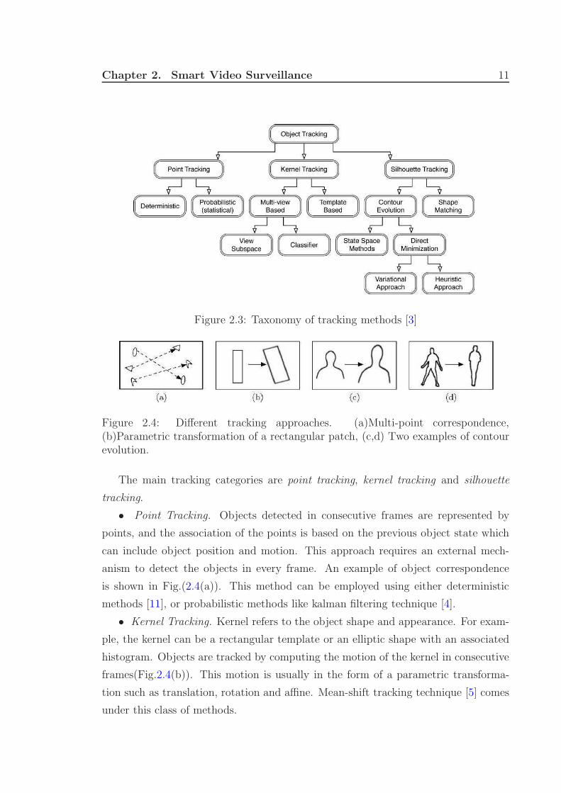
Figure 2.4: Different tracking approaches. (a)Multi-point correspondence,(b)Parametric transformation of a rectangular patch, (c,d) Two examples of contourevolution.
The main tracking categories are point tracking, kernel tracking and silhouette
tracking.
• Point Tracking. Objects detected in consecutive frames are represented by
points, and the association of the points is based on the previous object state which
can include object position and motion. This approach requires an external mech-
anism to detect the objects in every frame. An example of object correspondence
is shown in Fig.(2.4(a)). This method can be employed using either deterministic
methods [11], or probabilistic methods like kalman filtering technique [4].
• Kernel Tracking. Kernel refers to the object shape and appearance. For exam-
ple, the kernel can be a rectangular template or an elliptic shape with an associated
histogram. Objects are tracked by computing the motion of the kernel in consecutive
frames(Fig.2.4(b)). This motion is usually in the form of a parametric transforma-
tion such as translation, rotation and affine. Mean-shift tracking technique [5] comes
under this class of methods.
Chapter 2. Smart Video Surveillance 12
• Silhouette Tracking. Tracking is performed by estimating the object region
in each frame. Silhouette tracking methods use the information encoded inside the
object region. This information can be in the form of appearance density and shape
models which are usually in the form of edge maps. Given the object models, silhou-
ettes are tracked either by shape matching or contour evolution (see Fig.2.4(c),(d)).
Variational methods like active contour [14] are used for this kind of tracking.
2.2.1 Feature Selection for Tracking
Selecting the right features play a critical role in tracking. In general, the most
desirable property of a visual feature is its uniqueness so that the objects can be
easily distinguished in the feature space. Feature selection is closely related to the
object representation. For example, color is used as a feature for histogram-based
appearance representations, while for contour-based representation object edges are
usually used as feature. In general, many tracking algorithms use a combination of
these features. Some common visual features are:
• Color. The apparent color of an object is influenced primarily by two physical
factors, the spectral power distribution of the illuminant and the surface reflectance
properties of the object. A variety of color spaces (RGB, L*u*v, L*a*b, HSV) have
been used in tracking.
• Edges. Object boundaries usually generate strong changes in image intensities.
An important property of edges is that they are less sensitive to illumination changes
compared to color features. Algorithms that track the boundary of the objects usually
use edges as the representative feature.
• Optical Flow. Optical flow is a dense field of displacement vectors which defines
the translation of each pixel in a region. This method is commonly used as a feature
in motion-based segmentation and tracking applications.
• Texture. Texture is measure of the intensity variation of a surface which quan-
tifies properties such as smoothness and regularity. Obtaining texture descriptors
requires some processing step. Similar to edge features, the texture features are less
sensitive to illumination changes in color.
Among all features, color is one of the most widely used feature for tracking.
Despite its popularity, most color bands are sensitive to illumination variation. Hence
in scenarios where this effect is inevitable, other features are incorporated to model
object appearance.
Chapter 2. Smart Video Surveillance 13
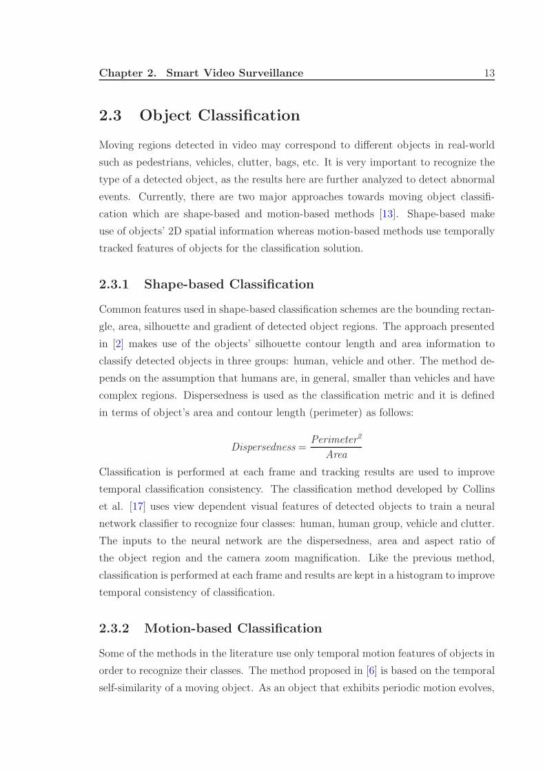
2.3 Object Classification
Moving regions detected in video may correspond to different objects in real-world
such as pedestrians, vehicles, clutter, bags, etc. It is very important to recognize the
type of a detected object, as the results here are further analyzed to detect abnormal
events. Currently, there are two major approaches towards moving object classifi-
cation which are shape-based and motion-based methods [13]. Shape-based make
use of objects’ 2D spatial information whereas motion-based methods use temporally
tracked features of objects for the classification solution.
2.3.1 Shape-based Classification
Common features used in shape-based classification schemes are the bounding rectan-
gle, area, silhouette and gradient of detected object regions. The approach presented
in [2] makes use of the objects’ silhouette contour length and area information to
classify detected objects in three groups: human, vehicle and other. The method de-
pends on the assumption that humans are, in general, smaller than vehicles and have
complex regions. Dispersedness is used as the classification metric and it is defined
in terms of object’s area and contour length (perimeter) as follows:
Dispersedness =Perimeter2
Area
Classification is performed at each frame and tracking results are used to improve
temporal classification consistency. The classification method developed by Collins
et al. [17] uses view dependent visual features of detected objects to train a neural
network classifier to recognize four classes: human, human group, vehicle and clutter.
The inputs to the neural network are the dispersedness, area and aspect ratio of
the object region and the camera zoom magnification. Like the previous method,
classification is performed at each frame and results are kept in a histogram to improve
temporal consistency of classification.
2.3.2 Motion-based Classification
Some of the methods in the literature use only temporal motion features of objects in
order to recognize their classes. The method proposed in [6] is based on the temporal
self-similarity of a moving object. As an object that exhibits periodic motion evolves,
Chapter 2. Smart Video Surveillance 14
its self-self-similarity measure also shows a periodic motion. The methods exploits
this clue to categorize moving objects using periodicity.
2.4 Summary
In this chapter, the related work in foreground segmentation, object tracking and
object classification has been discussed. Regarding foreground segmentation, we dis-
cussed in brief about the frequently used techniques - background subtraction, statis-
tical methods, temporal differencing and optical flow. In tracking, we have seen a way
of categorizing them into point tracking, kernel tracking and silhouette tracking. We
then saw what kind of features could be used for tracking. Finally we end the chap-
ter with object classification, where there were two major approaches - shape-based
and motion-based. In motion-based approach, along with spatial features of objects,
temporal motion features of objects were also used to recognize the classes.

Chapter 3
Object Detection
The overview of our video object detection, tracking and classification is shown in
fig.(3.1). The presented system is able to distinguish transitory and stopped fore-
ground objects from static background objects in dynamic scenes; detect and dis-
tinguish left objects; track objects and generate object information; classify detected
objects (into bag and non-bag) in video imagery. In this and following chapters we de-
scribe the computational models employed in our approach to reach the goals specified
above. The intent of designing these modules is to produce a video-based surveillance
system which works in real time environment. The computational complexity and
even the constant factors of the algorithms we use are important for real-time perfor-
mance. Hence, our decisions on selecting the computer vision algorithms for various
problems are affected by their computational run time performance as well as quality.
Furthermore, our system’s use is limited only to stationary cameras and video inputs
from PTZ (Pan/Tilt/Zoom) cameras, where the view frustum may change arbitrarily
are not supported.
The system is initialized by feeding video imagery from a static camera monitor-
ing a site. The first step of our approach is distinguishing foreground objects from
stationary background. To achieve this, we use a combination of adaptive Gaussian
mixture models and low-level image post-processing methods to create a foreground
pixel map at every frame. We then group the connected regions in the foreground
map to extract individual object features such as bounding box, area, perimeter and
color histogram.
The object tracking algorithm utilizes extracted object features together with
a correspondence matching scheme to track objects from frame to frame. The color
15
Chapter 3. Object Detection 16
Figure 3.1: The system block diagram.
histogram of an object produced in previous step is used to match the correspondence
of objects after an occlusion event. The output of the tracking step is analyzed
further for detecting abnormal events, which in our case is ‘a bag being abandoned by
a person.’
The remainder of this chapter presents the computational models and methods
adopted for object detection. Our tracking and classification approaches are explained
in the subsequent chapters.
3.1 Foreground Detection
Distinguishing foreground objects from the stationary background is both a signifi-
cant and difficult research problem. Almost all of the visual surveillance systems’ first
step is detecting foreground objects. This creates a focus of attention for higher pro-
cessing levels such as tracking, classification and behavior understanding and reduces
computation time considerably since only pixels belonging to foreground objects need
Chapter 3. Object Detection 17
to be dealt with. Short and long term dynamic scene changes such as repetitive mo-
tions (e.g. waiving tree leaves), light reflectance, shadows, camera noise and sudden
illumination variations make reliable and fast object detection difficult. Hence, it is
important to pay necessary attention to object detection step to have reliable, robust
and fast visual surveillance system.
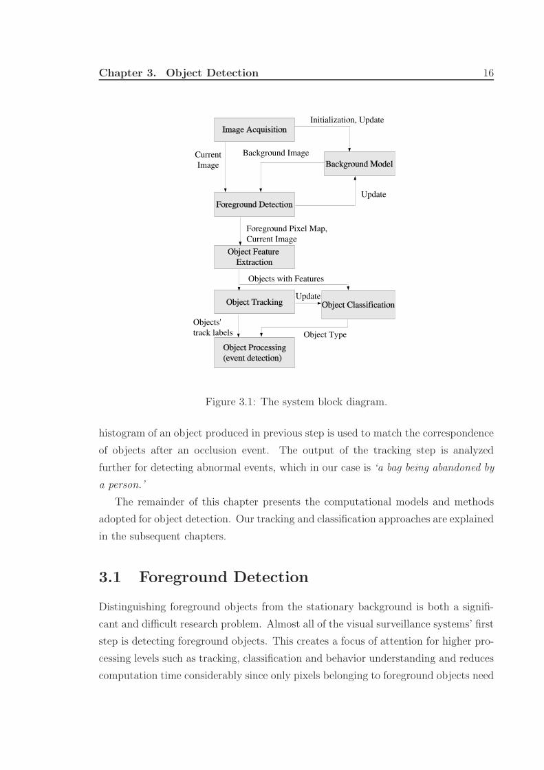
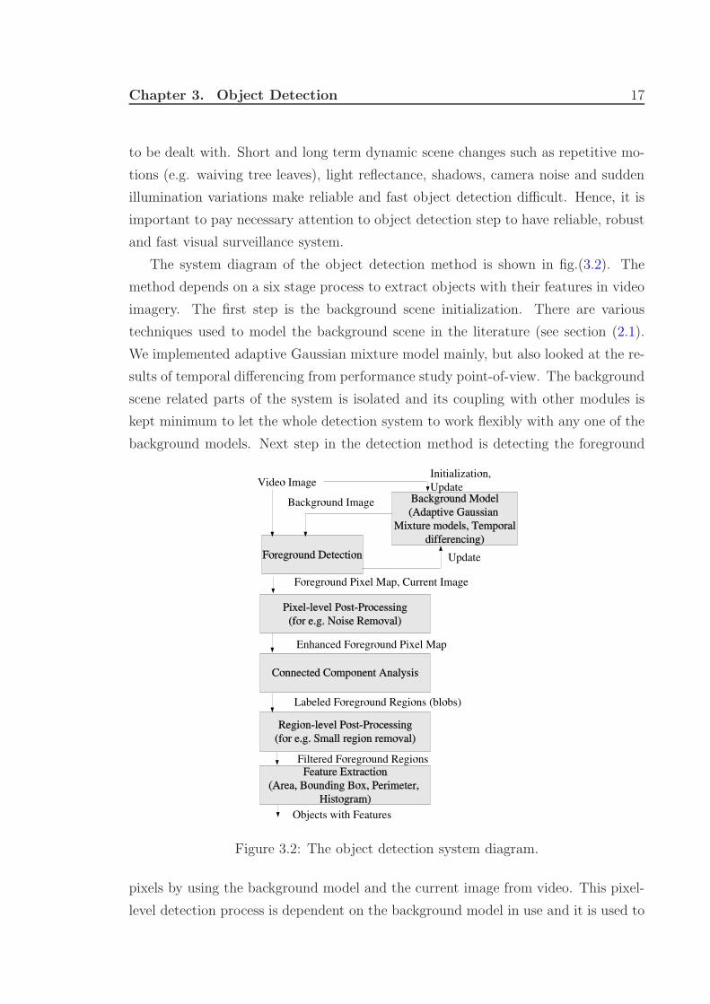
The system diagram of the object detection method is shown in fig.(3.2). The
method depends on a six stage process to extract objects with their features in video
imagery. The first step is the background scene initialization. There are various
techniques used to model the background scene in the literature (see section (2.1).
We implemented adaptive Gaussian mixture model mainly, but also looked at the re-
sults of temporal differencing from performance study point-of-view. The background
scene related parts of the system is isolated and its coupling with other modules is
kept minimum to let the whole detection system to work flexibly with any one of the
background models. Next step in the detection method is detecting the foreground
Figure 3.2: The object detection system diagram.
pixels by using the background model and the current image from video. This pixel-
level detection process is dependent on the background model in use and it is used to
Chapter 3. Object Detection 18
update the background model to adapt to dynamic scene changes. Also, due to cam-
era noise or environmental effects the detected foreground pixel map contains noise.
Pixel-level post-processing operations are performed to remove noise in the foreground
pixels. Once we get the filtered foreground pixels, in the next step, connected regions
are found by using a connected component labeling algorithm and objects’ bounding
rectangles are calculated. The labeled regions may contain near but disjoint regions
due to defects in foreground segmentation process. Hence, some relatively small re-
gions caused by environmental noise are eliminated in the region-level post-processing
step. In the final step of the detection process, a number of object features (like area,
bounding box, perimeter and color histogram of the regions corresponding to objects)
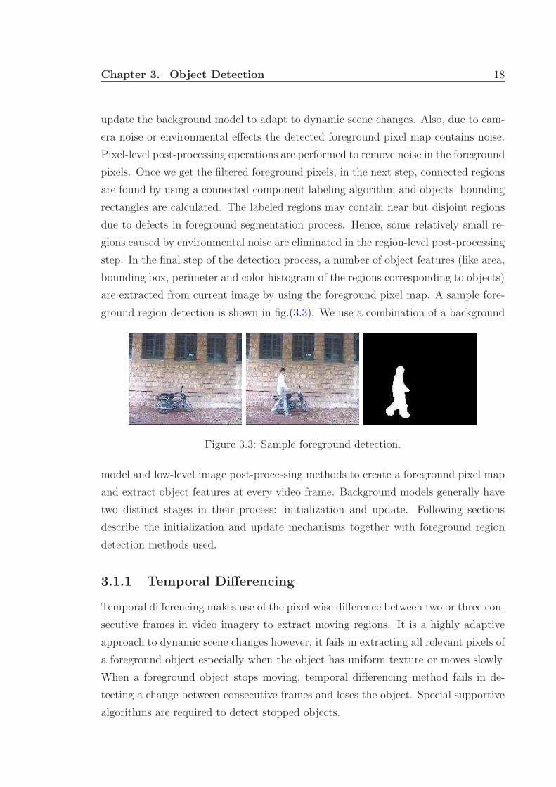
are extracted from current image by using the foreground pixel map. A sample fore-
ground region detection is shown in fig.(3.3). We use a combination of a background
Figure 3.3: Sample foreground detection.
model and low-level image post-processing methods to create a foreground pixel map
and extract object features at every video frame. Background models generally have
two distinct stages in their process: initialization and update. Following sections
describe the initialization and update mechanisms together with foreground region
detection methods used.
3.1.1 Temporal Differencing
Temporal differencing makes use of the pixel-wise difference between two or three con-
secutive frames in video imagery to extract moving regions. It is a highly adaptive
approach to dynamic scene changes however, it fails in extracting all relevant pixels of
a foreground object especially when the object has uniform texture or moves slowly.
When a foreground object stops moving, temporal differencing method fails in de-
tecting a change between consecutive frames and loses the object. Special supportive
algorithms are required to detect stopped objects.
Chapter 3. Object Detection 19
We implemented a two-frame temporal differencing method in our system. Let
In(x) represent the gray-level intensity value at pixel position (x) and at time instance
n of video image sequence I, which is in the range [0, 255]. The two-frame temporal
differencing scheme suggests that a pixel is moving if it satisfies the following:
|In(x) − In−1(x)| > Tn(x) (3.1)
Hence, if an object has uniform colored regions, the Equation 3.1 fails to detect some
of the pixels inside these regions even if the object moves. The per-pixel threshold,
T, is initially set to a pre-determined value and later updated as follows:
Tn+1(x) =
{
αTn(x) + (1 − α)(γ × |In(x) − In−1(x)|), x ∈ BG
Tn(x), x ∈ FG(3.2)
3.1.2 Adaptive Gaussian Mixture Model
Stauffer and Grimson [20] presented a novel adaptive online background mixture
model that can robustly deal with lighting changes, repetitive motions, clutter, in-
troducing or removing objects from the scene and slowly moving objects. Their
motivation was that a unimodal background model could not handle image acquisi-
tion noise, light change and multiple surfaces for a particular pixel at the same time.
Thus, they used a mixture of Gaussian distributions to represent each pixel in the
model. Due to its promising features, we implemented and integrated this model in
our visual surveillance system.
In this model, the values of an individual pixel (e.g. scalars for gray values and
vectors for color images) over time is considered as a “pixel process” and the recent
history of each pixel, X1, . . . , Xt, is modeled by a mixture of K Gaussian distributions.
The probability of observing current pixel value then becomes:
P (Xt) =K
∑
i=1
wi,t ∗ η(Xt, µi,t, Σi,t) (3.3)
where wi,t is an estimate of the weight (what portion of the data is accounted for this
Gaussian) of the ith Gaussian (Gi,t) in the mixture at time t, µi,t is the mean value of
Gi,t and Σi,t is the covariance matrix of Gi,t and η is a Gaussian probability density

Chapter 3. Object Detection 20
function:
η(X, µ, Σ) =1
(2π)n2 |Σ|
1
2
e−1
2(X−µ)T Σ−1(X−µ) (3.4)
Decision on K depends on the available memory and computational power. Also,
the covariance matrix is assumed to be of the following form for computational effi-
ciency:
Σk,t = α2kI (3.5)
which assumes that red, green and blue color components are independent and have
the same variance.
The procedure for detecting foreground pixels is as follows. At the beginning of
the system, the K Gaussian distributions for a pixel are initialized with predefined
mean, high variance and low prior weight. When a new pixel is observed in the image
sequence, to determine its type, its RGB vector is checked against K Gaussians, until
a match is found. A match is defined as a pixel value within γ (=2.5) standard
deviations of a distribution. Next, the prior weights of the K distributions at time
t(wk,t), are updated as follows:
wk,t = (1 − α)wk,t−1 + α(Mk,t) (3.6)
where α is the learning rate and M(k, t) is 1 for the matching Gaussian distribu-
tion and 0 for the remaining distributions. After this step the prior weights of the
distributions are normalized with the new observation as follows:
µt = (1 − ρ)µt−1 + ρ(Xt) (3.7)
σ2t = (1 − ρ)σ2
t−1 + ρ(Xt − µt)T (Xt − µt) (3.8)
where
ρ = αη(Xt|µt−1, σt−1). (3.9)
If no match is found for the new observed pixel, the Gaussian distribution with
the least probability is replaced with new distribution with the current pixel values
Chapter 3. Object Detection 21
as its mean value, an initially high variance and low prior weight.
In order to detect the type (foreground or background) of the new pixel, the K
Gaussian distributions are sorted by the value w/σ. This ordered list of distributions
reflect the most probable background from top to bottom since by Equation (3.6)
background pixel processes make the corresponding Gaussian distribution have larger
prior weight and less variance. Then the first B distributions are chosen as the
background model, where
B = arg minb
(b
∑
k=1
wk > T ) (3.10)
and T is the minimum portion of the pixel data that should be accounted for by
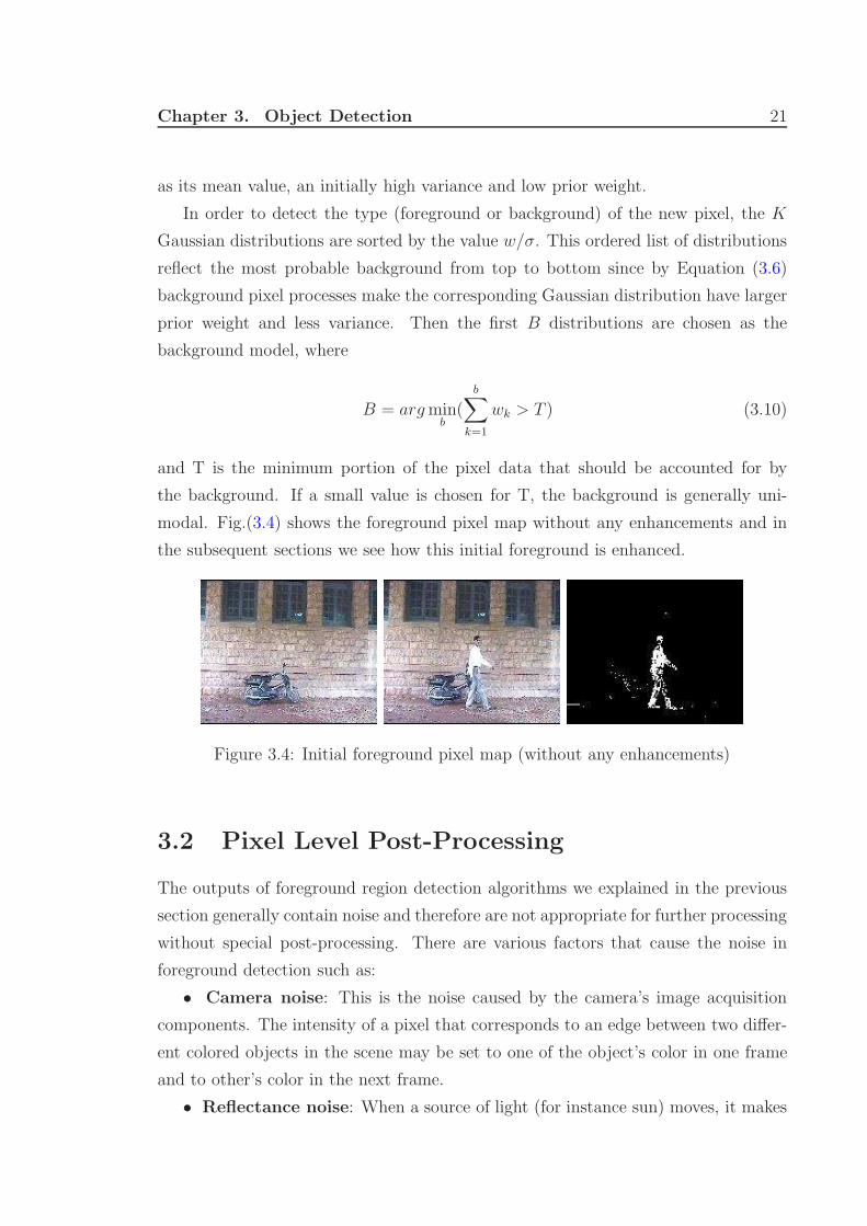
the background. If a small value is chosen for T, the background is generally uni-
modal. Fig.(3.4) shows the foreground pixel map without any enhancements and in
the subsequent sections we see how this initial foreground is enhanced.
Figure 3.4: Initial foreground pixel map (without any enhancements)
3.2 Pixel Level Post-Processing
The outputs of foreground region detection algorithms we explained in the previous
section generally contain noise and therefore are not appropriate for further processing
without special post-processing. There are various factors that cause the noise in
foreground detection such as:
• Camera noise: This is the noise caused by the camera’s image acquisition
components. The intensity of a pixel that corresponds to an edge between two differ-
ent colored objects in the scene may be set to one of the object’s color in one frame
and to other’s color in the next frame.
• Reflectance noise: When a source of light (for instance sun) moves, it makes
Chapter 3. Object Detection 22
some parts in the background scene to reflect light. This phenomenon makes the
foreground detection algorithms fail and detect reflectance as foreground regions.
• Background colored object noise: Some parts of the objects may have the
same color as the reference background behind them. This resemblance causes some
of the algorithms to detect the corresponding pixels as non-foreground and objects
to be segmented inaccurately.
Morphological operations, erosion and dilation [8], are applied to the foreground
pixel map in order to remove noise that is caused by the items listed above. Our
aim in applying these operations is removing noisy foreground pixels that do not
correspond to actual foreground regions, and to remove the noisy background pixels
near and inside object regions that are actually foreground pixels. Erosion, as its
name implies, erodes one-unit thick boundary pixels of foreground regions. Dilation
is the reverse of erosion and expands the foreground region boundaries with one-unit
thick pixels. The subtle point in applying these morphological filters is deciding the
order and amounts of these operations. The order of these operations affects the
quality and the amount affects both the quality and the computational complexity of
noise removal.
For instance, if we apply dilation followed by erosion we cannot get rid of one-
pixel thick isolated noise regions, since the dilation operation would expand their
boundaries with one pixel and the erosion will remove these extra pixels leaving the
original noisy pixels. On the other hand, this order will successfully eliminate some
of the non-background noise inside object regions. In case we apply these operations
in reverse order, which is erosion followed by dilation, we would eliminate one-pixel
thick isolated noise regions but this time we would not be able to close holes inside
object. To solve this problem, we move one step further by filling these holes using
the morphological operation “fill”:
‘fill’ fills isolated interior pixels (individual 0’s that are surrounded by 1’s), such as
the center pixel in this pattern:
1 1 1
1 0 1
1 1 1
Fig.(3.5) shows the result of pixel-level post-processing of the initial foreground
pixel map, shown in fig.(3.4).
Chapter 3. Object Detection 23
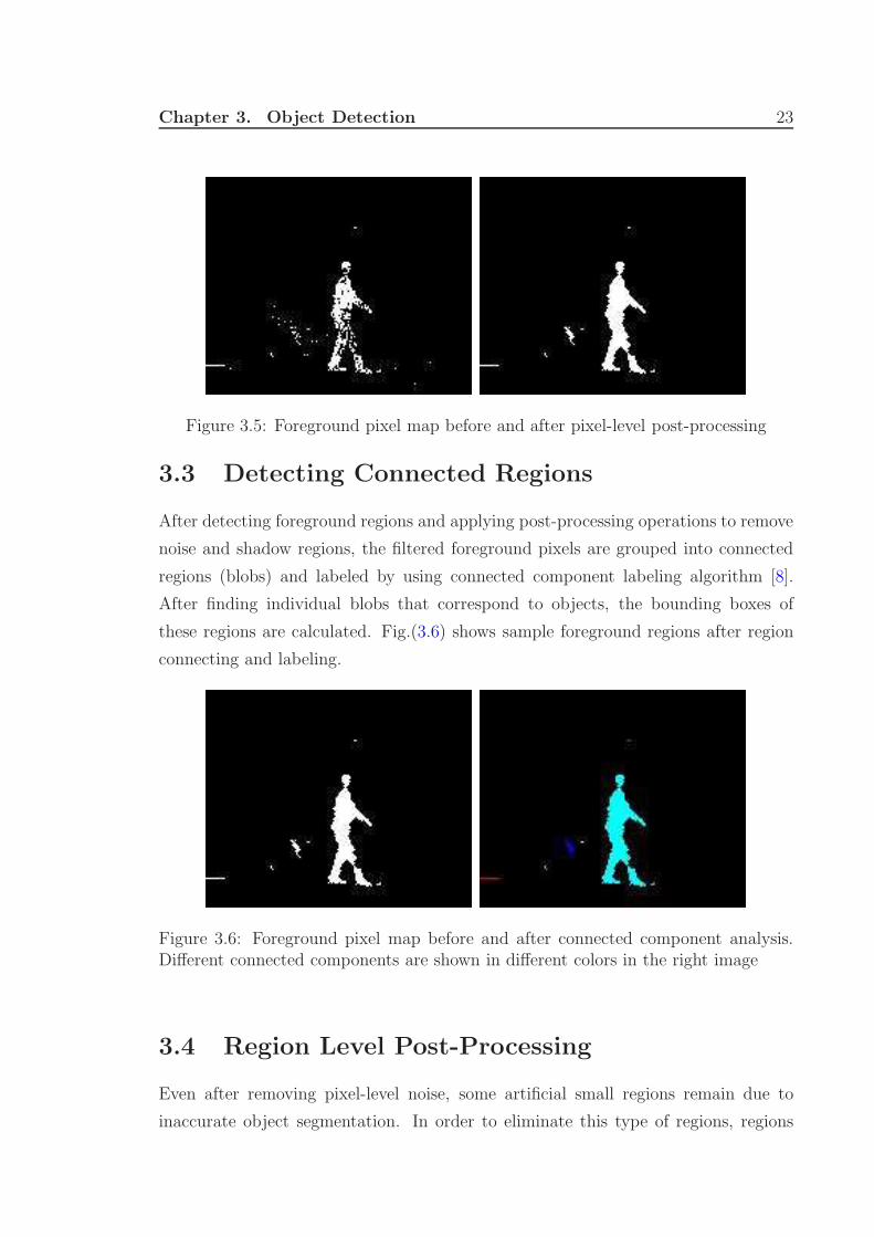
Figure 3.5: Foreground pixel map before and after pixel-level post-processing
3.3 Detecting Connected Regions
After detecting foreground regions and applying post-processing operations to remove
noise and shadow regions, the filtered foreground pixels are grouped into connected
regions (blobs) and labeled by using connected component labeling algorithm [8].
After finding individual blobs that correspond to objects, the bounding boxes of
these regions are calculated. Fig.(3.6) shows sample foreground regions after region
connecting and labeling.
Figure 3.6: Foreground pixel map before and after connected component analysis.Different connected components are shown in different colors in the right image
3.4 Region Level Post-Processing
Even after removing pixel-level noise, some artificial small regions remain due to
inaccurate object segmentation. In order to eliminate this type of regions, regions
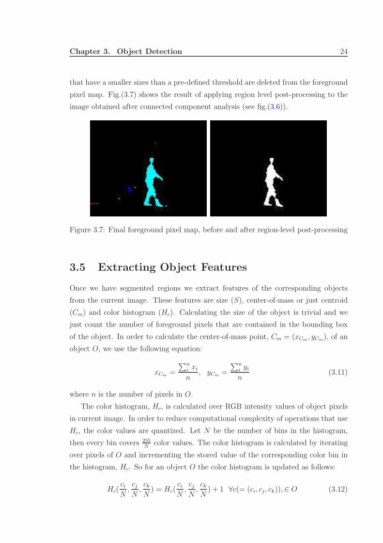
Chapter 3. Object Detection 24
that have a smaller sizes than a pre-defined threshold are deleted from the foreground
pixel map. Fig.(3.7) shows the result of applying region level post-processing to the
image obtained after connected component analysis (see fig.(3.6)).
Figure 3.7: Final foreground pixel map, before and after region-level post-processing
3.5 Extracting Object Features
Once we have segmented regions we extract features of the corresponding objects
from the current image. These features are size (S), center-of-mass or just centroid
(Cm) and color histogram (Hc). Calculating the size of the object is trivial and we
just count the number of foreground pixels that are contained in the bounding box
of the object. In order to calculate the center-of-mass point, Cm = (xCm, yCm
), of an
object O, we use the following equation:
xCm=
∑n
i xi
n, yCm
=
∑n
i yi
n(3.11)
where n is the number of pixels in O.
The color histogram, Hc, is calculated over RGB intensity values of object pixels
in current image. In order to reduce computational complexity of operations that use
Hc, the color values are quantized. Let N be the number of bins in the histogram,
then every bin covers 255N
color values. The color histogram is calculated by iterating
over pixels of O and incrementing the stored value of the corresponding color bin in
the histogram, Hc. So for an object O the color histogram is updated as follows:
Hc(ci
N,cj
N,ck
N) = Hc(
ci
N,cj
N,ck
N) + 1 ∀c(= (ci, cj, ck)),∈ O (3.12)
Chapter 3. Object Detection 25
where c represents the color value of (i, j, k)th pixel. In the above equation i, j and
k are the variables indexing into three color channels. In the next step the color
histogram is normalized to enable appropriate comparison with other histograms in
later steps. The normalized histogram Hc is calculated as follows:
Hc[i][j][k] =Hc[i][j][k]
∑N
ijk Hc[i][j][k](3.13)
Finally, the histogram obtained would be a 3D matrix (N × N × N) where N , as
defined before, is the number of bins.
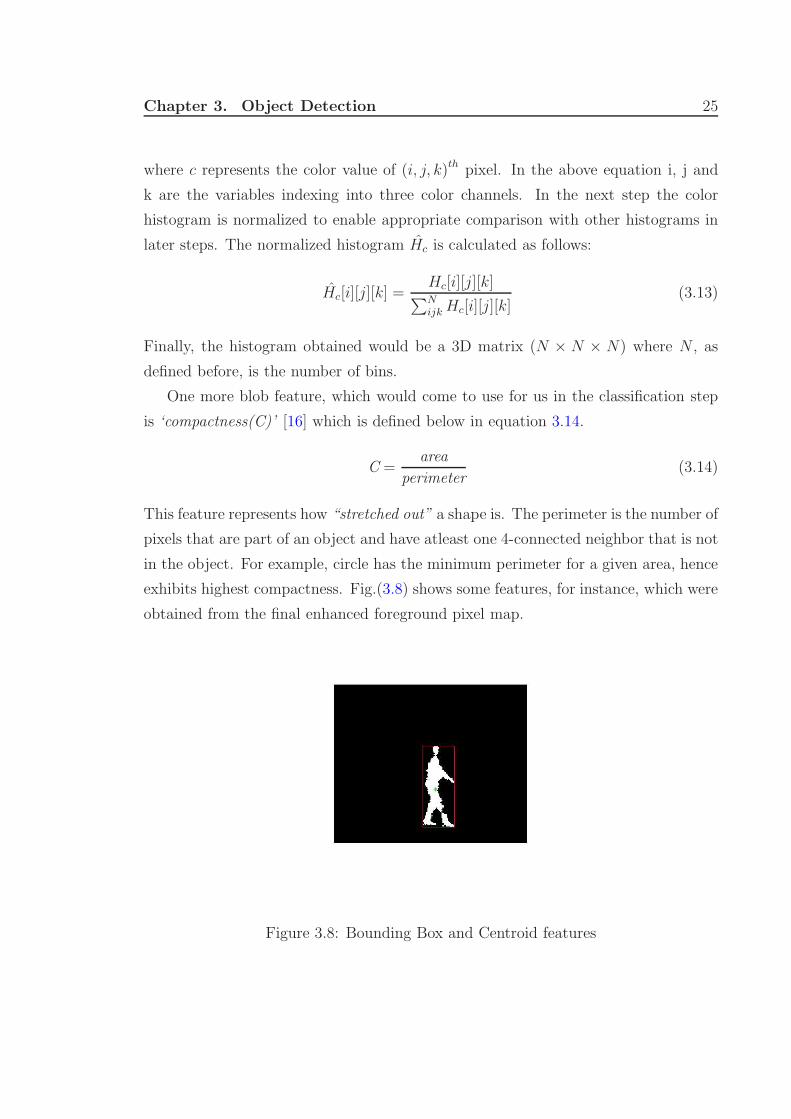
One more blob feature, which would come to use for us in the classification step
is ‘compactness(C)’ [16] which is defined below in equation 3.14.
C =area
perimeter(3.14)
This feature represents how “stretched out” a shape is. The perimeter is the number of
pixels that are part of an object and have atleast one 4-connected neighbor that is not
in the object. For example, circle has the minimum perimeter for a given area, hence
exhibits highest compactness. Fig.(3.8) shows some features, for instance, which were
obtained from the final enhanced foreground pixel map.
Figure 3.8: Bounding Box and Centroid features
Chapter 3. Object Detection 26
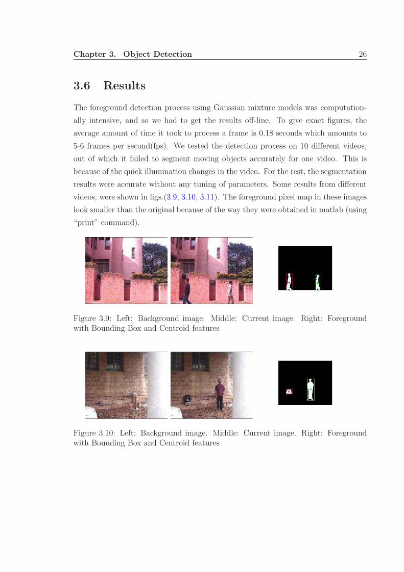
3.6 Results
The foreground detection process using Gaussian mixture models was computation-
ally intensive, and so we had to get the results off-line. To give exact figures, the
average amount of time it took to process a frame is 0.18 seconds which amounts to
5-6 frames per second(fps). We tested the detection process on 10 different videos,
out of which it failed to segment moving objects accurately for one video. This is
because of the quick illumination changes in the video. For the rest, the segmentation
results were accurate without any tuning of parameters. Some results from different
videos, were shown in figs.(3.9, 3.10, 3.11). The foreground pixel map in these images
look smaller than the original because of the way they were obtained in matlab (using
“print” command).
Figure 3.9: Left: Background image. Middle: Current image. Right: Foregroundwith Bounding Box and Centroid features
Figure 3.10: Left: Background image. Middle: Current image. Right: Foregroundwith Bounding Box and Centroid features
Chapter 3. Object Detection 27
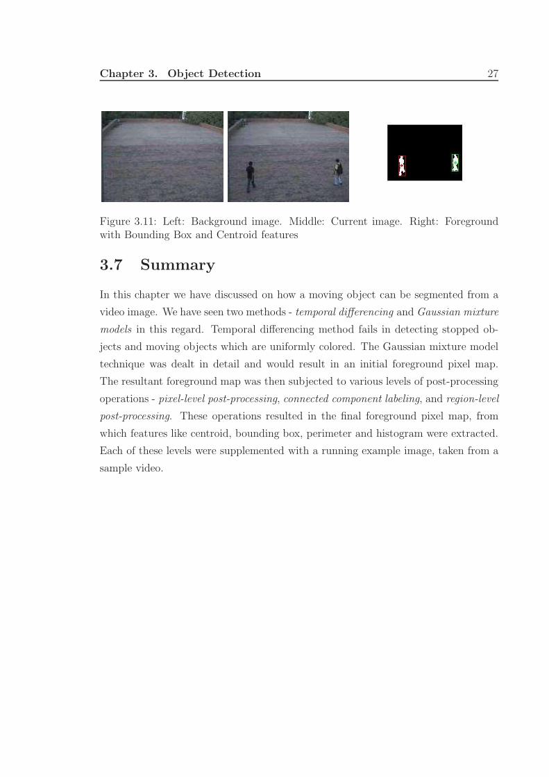
Figure 3.11: Left: Background image. Middle: Current image. Right: Foregroundwith Bounding Box and Centroid features
3.7 Summary
In this chapter we have discussed on how a moving object can be segmented from a
video image. We have seen two methods - temporal differencing and Gaussian mixture
models in this regard. Temporal differencing method fails in detecting stopped ob-
jects and moving objects which are uniformly colored. The Gaussian mixture model
technique was dealt in detail and would result in an initial foreground pixel map.
The resultant foreground map was then subjected to various levels of post-processing
operations - pixel-level post-processing, connected component labeling, and region-level
post-processing. These operations resulted in the final foreground pixel map, from
which features like centroid, bounding box, perimeter and histogram were extracted.
Each of these levels were supplemented with a running example image, taken from a
sample video.
Chapter 4
Object Tracking
The aim of object tracking is to establish a correspondence between objects or object
parts in consecutive frames and to extract temporal information about objects such
as trajectory, posture, speed and direction. Tracking detected objects frame by frame
in video is a significant and difficult task. It is a crucial part of smart surveillance
systems since without object tracking, the system could not extract cohesive tem-
poral information about objects and higher level behavior analysis steps would not
be possible. On the other hand, inaccurate foreground object segmentation due to
shadows, reflectance and occlusions makes tracking a difficult research problem.
We used an object level tracking algorithm in our system. That is, we do not
track object parts, such as limbs of a human, but we track objects as a whole from
frame to frame. The information extracted by this level of tracking is adequate for
most of the smart surveillance applications.
The tracking algorithm we developed is inspired by the ideas presented in [12],
though the methods adopted are entirely different. In short, there it is probabilistic
method, whereas we used deterministic methodology. Our approach makes use of
the object features such as size, center-of-mass, bounding box, color histogram and
compactness, which are extracted in previous steps to establish a matching between
objects in consecutive frames. Furthermore, our tracking algorithm detects object
occlusion and distinguishes object identities after the split of occluded objects.
The system diagram for our tracking method is shown in the fig.(4.1). The
first step in our object tracking algorithm is matching the objects in previous im-
age (In−1) to the new objects detected in the current image (In). We now explain the
correspondence-based object matching part in detail.
28
Chapter 4. Object Tracking 29
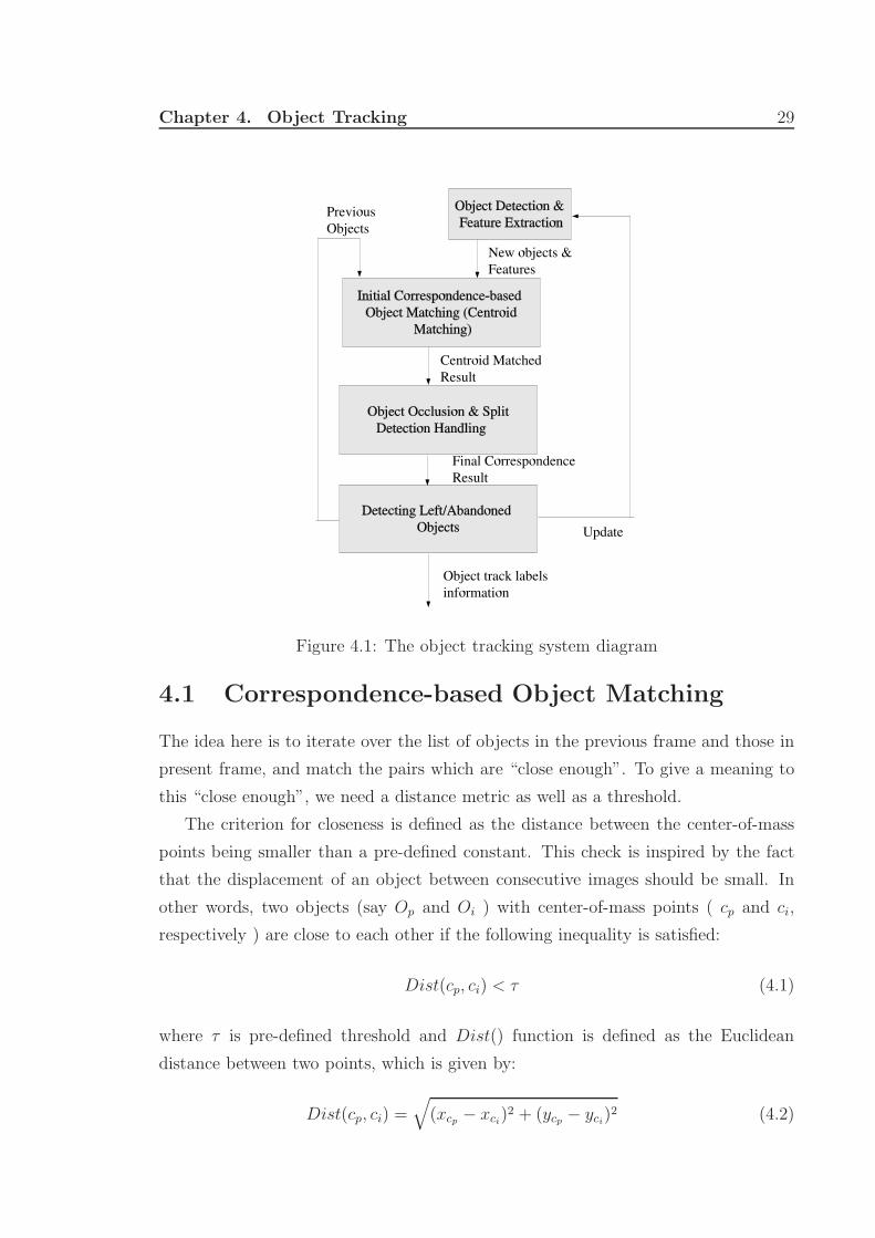
Figure 4.1: The object tracking system diagram
4.1 Correspondence-based Object Matching
The idea here is to iterate over the list of objects in the previous frame and those in
present frame, and match the pairs which are “close enough”. To give a meaning to
this “close enough”, we need a distance metric as well as a threshold.
The criterion for closeness is defined as the distance between the center-of-mass
points being smaller than a pre-defined constant. This check is inspired by the fact
that the displacement of an object between consecutive images should be small. In
other words, two objects (say Op and Oi ) with center-of-mass points ( cp and ci,
respectively ) are close to each other if the following inequality is satisfied:
Dist(cp, ci) < τ (4.1)
where τ is pre-defined threshold and Dist() function is defined as the Euclidean
distance between two points, which is given by:
Dist(cp, ci) =√
(xcp− xci
)2 + (ycp− yci
)2 (4.2)
Chapter 4. Object Tracking 30
Let In−1 and In denote the previous and current frames. And let Ln−1 and Ln be the
number of blobs/objects in these frames, respectively. The obvious three case which
arise are:
Ln > Ln−1
Ln < Ln−1
Ln = Ln−1
(4.3)
For simplicity of explanation, lets assume that the absolute difference between
the number of blobs of any two consecutive frames is atmost one. In that case, the
equations in (4.3) turn out to be
Ln = Ln−1 + 1
Ln = Ln−1 − 1
Ln = Ln−1
(4.4)
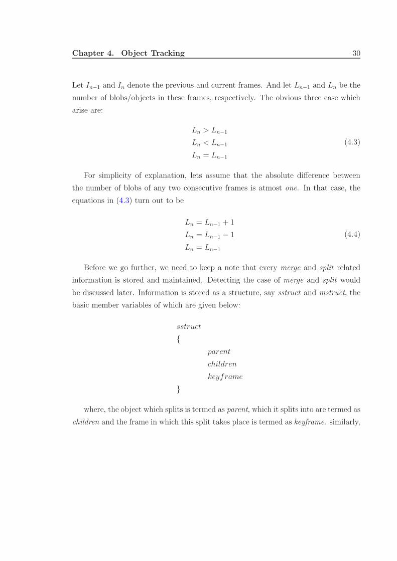
Before we go further, we need to keep a note that every merge and split related
information is stored and maintained. Detecting the case of merge and split would
be discussed later. Information is stored as a structure, say sstruct and mstruct, the
basic member variables of which are given below:
sstruct
{
parent
children
keyframe
}
where, the object which splits is termed as parent, which it splits into are termed as
children and the frame in which this split takes place is termed as keyframe. similarly,
Chapter 4. Object Tracking 31
for merge structure ...
mstruct
{
parents
child
keyframe
}
where the objects which merge together are termed as parents, which they are merged
into is termed as child and the frame in which this merge takes place is termed as
keyframe. Split-structure (sstruct) has some more member variables which will be
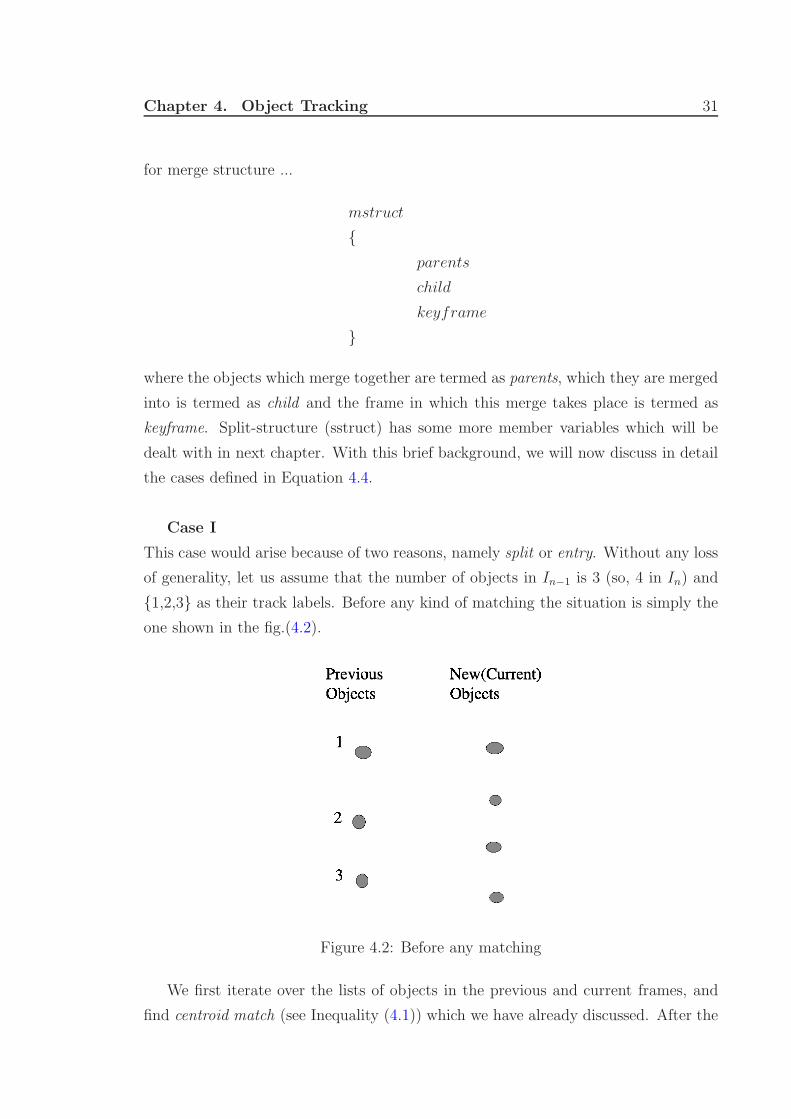
dealt with in next chapter. With this brief background, we will now discuss in detail
the cases defined in Equation 4.4.
Case I
This case would arise because of two reasons, namely split or entry. Without any loss
of generality, let us assume that the number of objects in In−1 is 3 (so, 4 in In) and
{1,2,3} as their track labels. Before any kind of matching the situation is simply the
one shown in the fig.(4.2).
Figure 4.2: Before any matching
We first iterate over the lists of objects in the previous and current frames, and
find centroid match (see Inequality (4.1)) which we have already discussed. After the
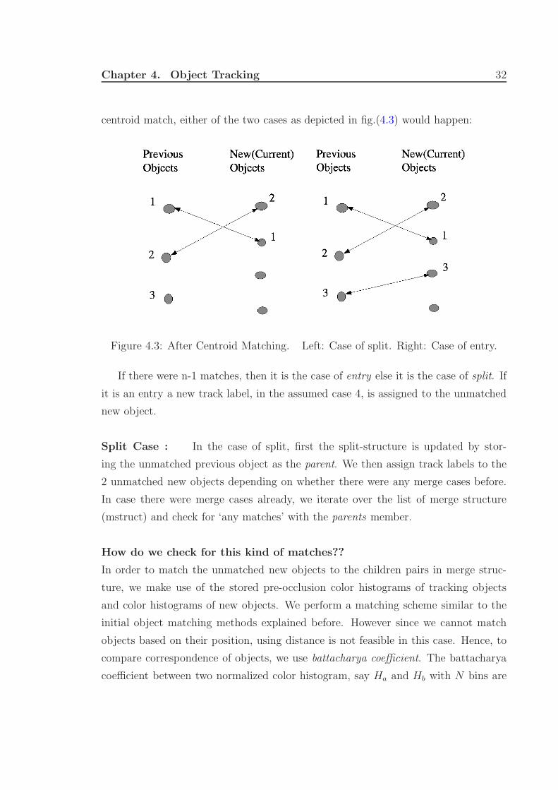
Chapter 4. Object Tracking 32
centroid match, either of the two cases as depicted in fig.(4.3) would happen:
Figure 4.3: After Centroid Matching. Left: Case of split. Right: Case of entry.
If there were n-1 matches, then it is the case of entry else it is the case of split. If
it is an entry a new track label, in the assumed case 4, is assigned to the unmatched
new object.
Split Case : In the case of split, first the split-structure is updated by stor-
ing the unmatched previous object as the parent. We then assign track labels to the
2 unmatched new objects depending on whether there were any merge cases before.
In case there were merge cases already, we iterate over the list of merge structure
(mstruct) and check for ‘any matches’ with the parents member.
How do we check for this kind of matches??
In order to match the unmatched new objects to the children pairs in merge struc-
ture, we make use of the stored pre-occlusion color histograms of tracking objects
and color histograms of new objects. We perform a matching scheme similar to the
initial object matching methods explained before. However since we cannot match
objects based on their position, using distance is not feasible in this case. Hence, to
compare correspondence of objects, we use battacharya coefficient. The battacharya
coefficient between two normalized color histogram, say Ha and Hb with N bins are

Chapter 4. Object Tracking 33
calculated using the following formula:
ρ(Ha, Hb) = ρ(ha, hb) =∑
i
√
haihbi
(4.5)
where ha and hb are vectorized versions of Ha and Hb respectively. To keep the
information complete, battacharya distance is define using the following formula:
d(Ha, Hb) = d(ha, hb) =√
1 − ρ(ha, hb) (4.6)
Higher the battacharya coefficient, more is the correspondence between the objects.
This can be checked out from the Equation (4.5) that the battacharya coefficient
between two same histograms is 1. As always is the case, we pre-define a threshold
for match saying that if the battacharya coefficient between 2 objects satisfies the
Inequality (4.7), then they are matching pairs.
ρ(Ha, Hb) > Th1 (4.7)
Finding a match need not mean that the parent (left-over previous object) and the
parent corresponding to matching children are same, as the track label would have
changed due to some segmentation errors. And, in case there are no merge cases,
new track labels were assigned to the two unmatched new objects. Whatever be the
case, the new track labels of the two objects were stored in split structure as children.
Fig.(4.4) shows a case, where the split objects are actually the objects which merged
previously and is handled by the method explained above.
Case II
This case would arise because of two situations, namely merge and exit. Following
similar reasoning as in the CaseI, before any kind of matching the situation is simply
the one shown in fig.(4.5)
After the centroid matching, as explained previously, the resulting situations
would look like that shown in fig.(4.6). If there were n-1 matches, then it is the
case of exit else it is the case of merge. If it is an exit, then there is nothing to do
and we go ahead with next set of consecutive frames.
Merge Case : On the other hand, in the case of merge, first the merge-structure

Chapter 4. Object Tracking 34
Figure 4.4: Occlusion handling(split case). Top Left: Before merge (left/right objectbounded by red/green box). Top Right: After merge. Bottom Left: Before split.Bottom Right: After split (left/right object bounded by green/red box)
Figure 4.5: Before any matching
is updated by storing the unmatched previous two objects as the parents. We then
assign track label to the unmatched new object depending on whether there were any
split cases before. In case there were split cases already, we iterate over the list of split
structure (sstruct) and check for any matches with the parent member. The matching
procedure is the same, as defined previously while dealing with Case I. Track label is
assigned to the unmatched new object accordingly, and is stored in merge structure
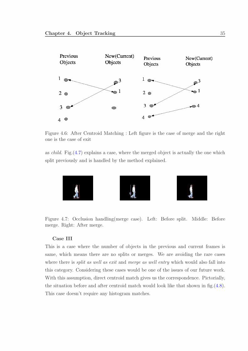
Chapter 4. Object Tracking 35
Figure 4.6: After Centroid Matching : Left figure is the case of merge and the rightone is the case of exit
as child. Fig.(4.7) explains a case, where the merged object is actually the one which
split previously and is handled by the method explained.
Figure 4.7: Occlusion handling(merge case). Left: Before split. Middle: Beforemerge. Right: After merge.
Case III
This is a case where the number of objects in the previous and current frames is
same, which means there are no splits or merges. We are avoiding the rare cases
where there is split as well as exit and merge as well entry which would also fall into
this category. Considering these cases would be one of the issues of our future work.
With this assumption, direct centroid match gives us the correspondence. Pictorially,
the situation before and after centroid match would look like that shown in fig.(4.8).
This case doesn’t require any histogram matches.
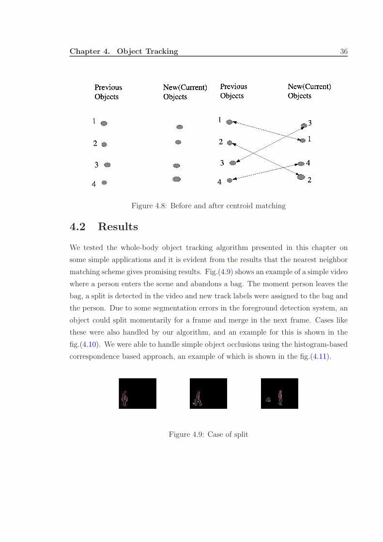
Chapter 4. Object Tracking 36
Figure 4.8: Before and after centroid matching
4.2 Results
We tested the whole-body object tracking algorithm presented in this chapter on
some simple applications and it is evident from the results that the nearest neighbor
matching scheme gives promising results. Fig.(4.9) shows an example of a simple video
where a person enters the scene and abandons a bag. The moment person leaves the
bag, a split is detected in the video and new track labels were assigned to the bag and
the person. Due to some segmentation errors in the foreground detection system, an
object could split momentarily for a frame and merge in the next frame. Cases like
these were also handled by our algorithm, and an example for this is shown in the
fig.(4.10). We were able to handle simple object occlusions using the histogram-based
correspondence based approach, an example of which is shown in the fig.(4.11).
Figure 4.9: Case of split

Chapter 4. Object Tracking 37
Figure 4.10: Case of split and merge
Figure 4.11: Occlusion handling
4.3 Summary
In this chapter we presented a whole-body object level tracking system which success-
fully tracks objects in consecutive frames. The approach we followed is a deterministic
one, and it makes use of features like size, center of mass, bounding box and histogram.
We first associate objects between the previous frame and current frame using cen-
troid matching technique, where Euclidean distance between the centroids of objects
is considered. To handle simple object occlusions, we incorporated histogram-based
correspondence matching approach in object association. Using this approach, the
identity of objects entered into an occlusion could be recognized after a split. The
same approach comes in handy to recover from segmentation errors like “momentary
splits”, where an object is split into two in a frame and then merge in the next frame.
The tracking information, track labels, obtained from the tracking phase is then used
by the classification and abnormality detection phase for further processing.
Chapter 5
Object Classification and Event
Detection
The ultimate aim of different smart visual surveillance applications is to extract se-
mantics from video to be used in higher level activity analysis tasks. Categorizing
the type of a detected video object is a crucial step in achieving this goal. With the
help of object type information, more specific and accurate methods can be developed
to recognize higher level actions of video objects. The information obtained during
classification along with tracking results is then used for abnormal event detection like
anomalous behavior in parking lots, object removal, object abandon, fire detection,
etc. Here, we present a video object classification method based on object shape simi-
larity as part of our visual surveillance system. And, instead of keeping the abnormal
event detection as an abstract goal we pre-define an abnormal event and detect that
event in the video. In our case, the abnormal event is ‘abandoning of a luggage/bag
by a person’.
5.1 Object Classification
Typically in high-level computer vision applications, like that of behavioral study,
classification step comes before tracking. That is, each and every object in each and
every frame are classified before feeding to the tracking module. Which means that
the tracking module knows beforehand what object it is tracking. Support Vector
Machines (SVMs) are popularly used for classification of objects. In [18] Sijun Lu
et al. provide a novel approach to detect unattended packages in public venues. In
38
Chapter 5. Object Classification and Event Detection 39
this paper, they provided an efficient method to online categorize moving objects
into the pre-defined classes using the eigen-features and the support vector machines.
In [17] Collins et al. developed a classification method which uses view dependent
visual features of detected objects to train a neural network classifier to recognize four
classes: human, human group, vehicle and clutter. The inputs to the neural network
are the dispersedness, area and aspect ratio of the object region and the camera zoom
magnification. Like the previous method, classification is performed at each frame.
In the later part of this chapter, we will see that unlike these methods classification
is performed only on a limited number of objects and in a limited number of frames.
5.1.1 Bayes Classifier
Bayes classifier is a statistical technique to classify objects into mutually exclusive
and exhaustive groups based on a set of measurable object’s features. In general, we
assign an object to one of a number of predetermined groups based on observations
made on the object. As this topic is well-known to everybody, we keep this subsection
short and clear. Since we will be dealing with 2-category classification, namely bag
and non-bag, we discuss the theory in brief assuming there are two categories. So,
consider a two-category classification problem :
D = {xi, yi} where xi ∈ Rn and yi ∈ {−1, +1} (5.1)
Let +1 resemble class c1 and -1 resemble class c2, and say p(c1) and p(c2) are their
prior probabilities respectively. After observing a data point, say x, Bayes classifier
just says the following:
if p(c1|x) > p(c2|x) then x ∈ R1 else x ∈ R2 (5.2)
where R1 and R2 are the regions of c1 and c2 respectively in Rn. Though Bayes
classifier is defined as in Equation (5.2), this form is not used directly when classifying.
Bayes theorem relates the conditional and marginal probabilities of two events A and
B by the Equation (5.3).
P (A|B) =P (B|A)P (A)
P (B)(5.3)
where
Chapter 5. Object Classification and Event Detection 40
• P (A) is the prior probability or marginal probability of A.
• P (A|B) s the conditional/posterior probability of A, given B.
• P (B|A) s the conditional/posterior probability of B, given A.
• P (B) is the prior/marginal probability of B.
Applying Bayes rule (5.3) to Bayes classifier (5.2), and assuming P (x) non-zero,
Bayes classifier can be restated as defined in (5.4).
if p(x|c1)p(c1) > p(x|c2)p(c2) then x ∈ R1 else x ∈ R2 (5.4)
Most of the standard probability densities assume exponential form, which inspire to
state Bayes classifier using logarithm function. Finally, we define a function f(x) as
in Equation (5.5) using which we restate the Bayes-classifier as defined in (5.6).
f(x) = logp(x|c1)
p(x|c2)− log
p(c1)
p(c2)(5.5)
if f(x) > 0 then x ∈ c1 else x ∈ x2 (5.6)
5.1.2 Quadratic Discriminant Analysis
Discriminant analysis involves the predicting of a categorical dependent variable by
one or more continuous or binary independent variables. It is useful in determining
whether a set of variables is effective in predicting category membership. Quadratic
discriminant analysis (QDA) is one type of discriminant analysis, where it is assumed
that there are only two classes of points, and that the measurements are normally
distributed (see Equation (5.7)).
η(X, µ, Σ) =1
(2π)n2 |Σ|
1
2
e−1
2(X−µ)T Σ−1(X−µ) (5.7)
Assuming (µ1, Σ1) and (µ2, Σ2) as the respective parameters for classes c1 and c2, and
also prior probabilities, p(c1) and p(c2), to be equal f(x) as defined in Equation (5.5)
would be
f(X) = log
1
(2π)n2 |Σ|
1
2
e−1
2(X−µ1)T Σ−1
1(X−µ1)
1
(2π)n2 |Σ|
1
2
e−1
2(X−µ2)T Σ−1
2(X−µ2)
(5.8)

Chapter 5. Object Classification and Event Detection 41
Simplifying f(X) = 0 with the condition, p(c1) = p(c2), imposed we get Equation
(5.9).
g(X) = XT (Σ−12 − Σ−1
1 )X + 2 ∗ XT (Σ−11 µ1 − Σ−1
2 µ2)
+µT2 Σ−1
2 µ2 − µT1 Σ−1
1 µ1 = 0(5.9)
Finally, we will be using the following classifier :
if g(X) > 0 then X ∈ c1 else X ∈ c2 (5.10)
5.1.3 Learning Phase
During any classification problem, we look for two things :
• What is the classification rule to separate the groups?
• Which set of features determine group membership of the object?
We looked into first aspect in the previous section. The features which we would
be using for the classification are :
• Aspect Ratio
• Compactness (see Equation (3.14)
We have chosen these features keeping in mind that they have to be scale invariant
and translation invariant. We have not built a detailed and elaborate database, but
a small one with 30 bags and 30 non-bags (people-single and group) and this proved
to be sufficient for our work. This is because we are not taking decisions based on
this classification result alone, but consider them as potential candidates. We have
taken 5 different types of bags and took their images from 2 different distances at 2
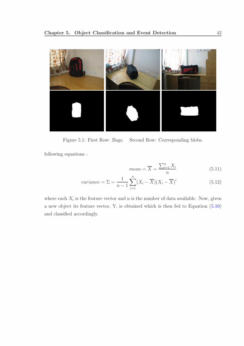
different angles. For instance fig.(5.1) shows few bags and their blobs, which were
extracted using image processing techniques.
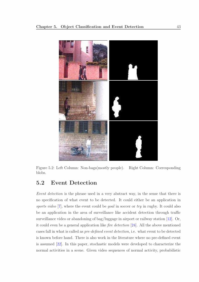
Fig. (5.2) shows some of the people blobs with their original images, which were
obtained using adaptive Gaussian mixture models discussed in third chapter. The
features obtained from these blobs are then used to obtain mean and variance by the
Chapter 5. Object Classification and Event Detection 42
Figure 5.1: First Row: Bags. Second Row: Corresponding blobs.
following equations :
mean = X =
∑n
i=1 Xi
n(5.11)
variance = Σ =1
n − 1
n∑
i=1
(Xi − X)(Xi − X)′ (5.12)
where each Xi is the feature vector and n is the number of data available. Now, given
a new object its feature vector, Y, is obtained which is then fed to Equation (5.10)
and classified accordingly.
Chapter 5. Object Classification and Event Detection 43
Figure 5.2: Left Column: Non-bags(mostly people). Right Column: Correspondingblobs.
5.2 Event Detection
Event detection is the phrase used in a very abstract way, in the sense that there is
no specification of what event to be detected. It could either be an application in
sports video [7], where the event could be goal in soccer or try in rugby. It could also
be an application in the area of surveillance like accident detection through traffic
surveillance video or abandoning of bag/luggage in airport or railway station [12]. Or,
it could even be a general application like fire detection [24]. All the above mentioned
cases fall in what is called as pre-defined event detection, i.e. what event to be detected
is known before hand. There is also work in the literature where no pre-defined event
is assumed [22]. In this paper, stochastic models were developed to characterize the
normal activities in a scene. Given video sequences of normal activity, probabilistic
Chapter 5. Object Classification and Event Detection 44
models are learnt to describe the normal motion at the scene. For any new video
sequences, motion trajectories are extracted and evaluated using these probabilistic
models to identify if they are abnormal or not.
Our objective is to detect the event ‘abandoning of a bag by a person’ in video
which is a very critical surveillance application. The ninth International Workshop
on Performance Evaluation of Tracking and Surveillance (PETS2006) is conducted in
New York in June 2006, where the theme is detection of abandoning of bag [1]. Lots
of details regarding this kind of work can be found in this site. One of the recent work
in this area, which is being published in Pattern Recognition journal in August 2007
is also on the detection of this event. In this paper, an efficient method is provided to
online categorize moving objects into the predefined classes using the eigen-features
and the support vector machines. Then, utilizing the classification results a method
is developed to recognize human activities with hidden Markov models and decide the
package ownership. Finally the unattended package detection is achieved by analyzing
the multiple object relationships: package ownership, spatial and temporal distance
relationships.
5.2.1 Bag Detection
Since we are dealing with bag abandoning event, we just need to focus on object splits.
Bag removal is another abnormal event which is one of the issues of our future work,
in which case object merges need to be considered. In previous chapter, we stated
three members of our split structure (sstruct), namely parent, children, and keyframe.
There are some other members like class count, child1[], child2[], is bag, bag owner[]
which hold classification and decision results.
In general, to classify an object it is not easy or right to decide on it’s class by
performing classification only once (in just one frame). In our work, from the time of
split we perform classification over the “split objects” for the next 25 (1 sec) frames
and then classify the object by voting scheme. Three kinds of splits are possible :
• Bag-Person ( possibly an abnormal event )
• Person-Person ( normal event )
• “Momentary split”
The first two cases don’t need any explanation. They are the probable cases of
bag abandoning event for which classification is performed for the next 25 frames. If
the split is of “bag-person” type, then that person is decided as the owner of the bag.
Chapter 5. Object Classification and Event Detection 45
The third case is a kind of split which arises due to segmentation error and would
be discarded eventually. Such cases arise due to bad segmentation, where an object
would split into two objects and in the next frame merge again (see fig.(4.10)).
There could be situation similar to the third case above, where due to segmentation
error an object would split into two and remain that way without merging for some
time. In such scenario, performing classification for 25 frames and deciding on voting
scheme may result in classifying both the split objects as bags. To avoid such rare
cases, we take into account object velocities in the form of centroid variances. An
abandoned object will always have centroid variance almost zero, which is not the
case with moving objects. This criterion alone might be sufficient if our objective
is to detect any new motionless object. But, our objective is to detect bag/luggage
abandoning which then requires both criteria. There is some work in literature where
classification is not performed at all for this kind of abnormal event detection, but
some heuristics were used. For instance, in [12] left-luggage detection process relies
on three critical assumptions about the properties of a bag :
• Bags probably don’t move.
• Bags probably appear smaller than people.
• Bags must have an owner.
In [16] detection of abandoned package is done by considering characteristics like
lack of motion, minimum distance from nearest person, etc. In [19] an object is
classified as abandoned, depending on factors like minimum extent, sufficiently high
probability of being foreground, no humans nearby a still object, etc.
5.2.2 Alarm Criteria
In this section, we see what are the constraints depending on which an alarm should
be set notifying the operator of a possible abnormal event. We impose two constraints
before deciding that a bag has been abandoned:
Space constraint :
We enclose the bag, once it is detected for 25 frames from the time of split, with a cir-
cle and the person with an ellipse. We have defined two regions, namely “unattended”
region and “abandoned region”. Each region is defined by a radius and the bag is
enclosed with the circle corresponding to that radius. The decision of whether the
person is within a particular region is taken by checking if the ellipse (which encloses
Chapter 5. Object Classification and Event Detection 46
the person) and the corresponding circle (which encloses the bag) intersect. One
more way of imposing space constraint, which we have not explored, is done by 3D
modeling. In [18] the authors have used revised ray-tracing method which converts
a given pixel location on screen into a three-dimensional location in the real-world.
If ground-truth data is available, then using homography the pixel distance on screen
can be converted to the actual distance [12].
Time Constraint :
Once the bag has been detected, we wait for t1 seconds and by that time if the owner
is beyond the unattended region then we say that the bag has been unattended. Then
we wait for t2 seconds more, and by that time if the person is beyond the abandoned
region then we say that the bag has been abandoned. Bag being unattended is like
a caution to the operator, of a possible abnormal event. Alarm would be set if the
person is beyond the unattended region for a considerable amount of time, which is
a pre-defined setting.
5.3 Results
Classification results using quadratic discriminant analysis were found to be quite
accurate. We used a very small training set of 60 cases, where 30 of them belong to
one class - bag, and the rest belong to the second class - non-bag(people). Using a
test set of 50 cases, gave us an accuracy of 95%. Few examples of the extracted blobs
were shown in figs.(5.1,5.2). The classification rule which we used, though simple,
gave good results because of the right selection of features as well as the second
level confirmation done using centroid variances. Once the objects were classified,
time constraint and distance constraint were imposed to detect the abnormal event.
Figs.(5.3,5.4,5.5) show three examples where a bag has been abandoned.
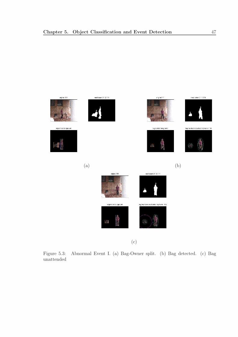
Chapter 5. Object Classification and Event Detection 47
(a) (b)
(c)
Figure 5.3: Abnormal Event I. (a) Bag-Owner split. (b) Bag detected. (c) Bagunattended

Chapter 5. Object Classification and Event Detection 48
(a) (b)
(c)
Figure 5.4: Abnormal Event II. (a) Bag-Owner split. (b) Bag detected. (c) Bagunattended.
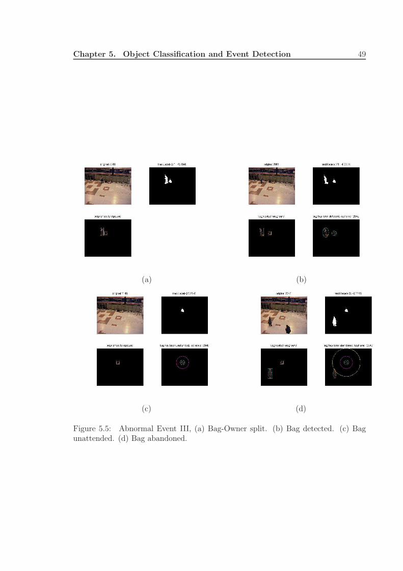
Chapter 5. Object Classification and Event Detection 49
(a) (b)
(c) (d)
Figure 5.5: Abnormal Event III, (a) Bag-Owner split. (b) Bag detected. (c) Bagunattended. (d) Bag abandoned.
Chapter 5. Object Classification and Event Detection 50
5.4 Summary
In this chapter we have discussed a methodology to classify objects into bag and non-
bag(people). Unlike most of the work in literature where all objects are classified in all
the frames, we are not performing classification in that manner. We classify only those
objects which were result of some split case, and even this we do it only for the next
25 frames (1sec). We have discussed the classification rule, quadratic discriminant
analysis, in detail and the learning phase from which we get the required parameters
for the discriminant. We then saw the criteria and constraints based on which the
events ‘bag unattended’ and ‘bag abandoned’ were detected.

Chapter 6
Conclusion and Future work
In this thesis we presented a set of methods and tools for a “smart” visual surveillance
system. We divided the work into three stages: object detection, object tracking and
object classification; and event detection comes as part of classification step.
We implemented two different object detection algorithms, namely temporal dif-
ferencing and adaptive Gaussian mixture models. The adaptive Gaussian mixture
models gave us the most promising results in terms of detection quality. However, no
object detection algorithm is perfect, so is this method since it needs improvements in
handling darker shadows, sudden illumination changes and partial object occlusions.
Higher level semantic extraction steps would be used to support object detection step
to enhance its results and eliminate inaccurate segmentation.
The presented whole-body object tracking algorithm successfully tracks objects
in consecutive frames. Our tests in sample videos show that using nearest neighbor
matching scheme gives promising results and no complicated methods are necessary
for whole-body tracking of objects. Also, in handling object occlusions (object merges
and object splits), the histogram-based correspondence matching approach recognizes
the identities of objects entered into an occlusion successfully after a split. However,
due to the nature of the heuristic we use, the occlusion handling algorithm would fail
in distinguishing occluding objects if they are of the same color. Also, in crowded
scenes handling occlusions becomes infeasible with such an approach, thus a pixel-
based method, like optical flow is required to identify object segments accurately.
The object classification part along with event detection, presented in fourth chap-
ter works well in detecting abandoning of bag. The classification rule which we used
is very simple, but it did give good results because of the features we selected as well
51
Chapter 6. Conclusion and Future work 52
as the second level confirmation done using centroid variances. Although the method
gives promising results in categorizing object types, it has one drawback: the method
is view dependent. View-dependent problems can be solved by developing the above
modules from multi-camera perspective.
The main intent of “smart” visual surveillance systems is that they should be
working not only with minimal errors but also in real-time. Out of the three modules
we presented in our thesis, the last two work in real-time but the object detection
results had to be obtained off-line. The system specifications, on which we tested our
programs on different videos are given below:
• Intel Pentium 4
• 3.00 GHz
• 1MB Cache
• 1GB RAM
• MATLAB-7.1
Though the detection process had to be done offline, converting the modules to
c code might result in real-time setup. Apart from scope in improving the presented
modules, which were discussed above, there are two applications for which the frame-
work presented in our thesis is extendible:
1) Bag Removal (e.g. surveillance in museums)
2) People Counting (e.g. crowd control )

Chapter 6. Conclusion and Future work 53
Bibliography
[1] http://www.cvg.rdg.ac.uk/PETS2006/index.html, 2006.
[2] H. Fujiyoshi ans R. S. Patil A. J. Lipton. Moving target classification and tracking
from real-time video. Proc. of Workshop Applications of Computer Vision, pages
129–136, 1998.
[3] O. Javed A. Yilmaz and M. Shah. Object tracking: A survey. ACM Journal of
Computing Surveys, 38(4), 2006.
[4] T. Broida and R. Chellappa. Estimation of object motion parameters from
noisy images. IEEE Transactions on Pattern Analysis and Machine Intelligence,
8(1):90–99, 1986.
[5] D. Comaniciu and Peter Meer. Mean shift: A robust approach toward feature
space analysis. IEEE Transactions on Pattern Analysis and Machine Intelli-
gence, 24(5), May 2002.
[6] R. Cutler and Larry S. Davis. Robust real-time periodic motion detection, anal-
ysis, and applications. IEEE Transactions on Pattern Analysis and Machine
Intelligence, 22(8), August 2000.
[7] A. Ekin and A. Murat Tekalp. Generic event detection in sports video using
cinematic features. Conference on Computer Vision and Pattern Recognition
Workshop, 4, 2003.
[8] R. C. Gonzalez and R. E. Woods. Digital Image Processing. Pearson Education,
2002.
[9] J. Heikkila and O. Silven. A real-time system for monitoring of cyclists and
pedestrians. Proc. of Second IEEE Workshop on Visual Surveillance, pages 74–
81, JUNE 1999.
54
BIBLIOGRAPHY 55
[10] D. Harwood I. Haritaoglu and Larry S. Davis. W4: Real-time surveillance of
people and their activities. IEEE Transactions on Pattern Analysis and Machine
Intelligence, 22(8):809–830, AUGUST 2000.
[11] J. T. Reindeers J. Veenman and E. Backner. Resolving motion correspondence
for densely moving points. IEEE Transaction on Pattern Analysis and Machine
Intelligence, 23(1), January 2001.
[12] P. Quelhas K. Smith and D. Gateca-Perez. Detecting abandoned luggage items
in a public space. Performance Evaluation of Tracking and Surveillance (PETS)
Workshop, 2006.
[13] W. Hu L. Wang and T. Tan. Recent developments in human motion analysis.
Pattern Recognition, 36(3):585–601, March 2003.
[14] G. Sapiro M. Bertalmio and G. Randall. Morphing active contours. IEEE Trans-
actions on Pattern Analysis and Machine Intelligence, 22(7), July 2000.
[15] A. M. McIvor. Background subtraction techniques. Proc. of Image and Vision
Computing, 2000.
[16] M. Seibert Michael D. Beynon, Daniel J. Van Hook and D. Dudgeon A. Peacock.
Detecting abandoned packages in a multi-camera video surveillance system. Proc.
of the IEEE conference in Advanced Video and Signal based Surveillance (AVSS),
2003.
[17] T. Kanade H. Fujiyoshi D. Duggins Y. Tsin D. Tolliver N. Enomoto O. Hasegawa
P. Burt R. T Collins, A J. Lipton and L. Wixson. A system for video surveillance
and monitoring: Vsam final report. technical report cmu-ri-tr-00-12, robotics
institute, carnegie mellon university. May 2000.
[18] J. Zhang S. Lu and D. Dagan Feng. Detecting unattended packages through
human activity recognition and object association. Pattern Recognition,
40(8):2173–2184, AUGUST 2007.
[19] M. Spengler and B. Schiele. Automatic detection and tracking of abandoned
objects. Joint IEEE International workshop on Visual Surveillance and Perfor-
mance Evaluation of Tracking and Surveillance, October 2003.
BIBLIOGRAPHY 56
[20] C. Stauffer and W. Grimson. Adaptive background mixture models for real-time
tracking. Proc. of the IEEE Computer Society Conference on Computer Vision
and Pattern Recognition, pages 246–252, 1999.
[21] C. Stauffer and W.E.L Grimson. Learning patterns of activity using real-time
tracking. IEEE Transactions on Pattern Analysis and Machine Intelligence,
pages 747–757, August 2000.
[22] R. Supriya and P. S. Shastry. Abnormal activity detection in video sequences
using learnt probability densities. TENCON Conference on Convergent Tech-
nologies for Asia-Pacific Region, 1:369–372, October 2003.
[23] L. Wang W. Hu, T. Tan and S. Maybank. A survey on visual surveillance
of object motion and behaviors. IEEE Transactions on Systems, Man, and
Cybernetics, 34(3), August 2004.
[24] M. Shah W. Phillips III and Da Vitoria Lobo N. Flame recognition in video. Fifth
IEEE Workshop on Applications of Computer Vision, pages 224–229, December
2000.


![Abnormal event detection in surveillance videos based on ...xzhang/publications/PR... · [46] X. Chen, J. Lai, Detecting abnormal crowd behaviors based on the div-curl char- acteristics](https://img.pdfslide.net/doc/110x75/5fbc85e49fdf6918cc3f995d/abnormal-event-detection-in-surveillance-videos-based-on-xzhangpublicationspr.jpg)

![Abnormal Vessel Behavior Detection in Port Areas Based on ...confcats_isif.s3.amazonaws.com/web-files/event/... · yielded by an Event-based Dynamic Bayesian Network (E-DBN) [3] [4]](https://img.pdfslide.net/doc/110x75/5f130b15da954725491c8f47/abnormal-vessel-behavior-detection-in-port-areas-based-on-confcatsisifs3-yielded.jpg)


![Motion modeling for abnormal event detection in crowd scenes€¦ · category is associated to the indexing of abnormal events. In the first category, several authors like [1], [2],](https://img.pdfslide.net/doc/110x75/5ea5efc76a8cc504f84878f9/motion-modeling-for-abnormal-event-detection-in-crowd-scenes-category-is-associated.jpg)