ABOUT THE AUTHOR we take a careful look, no matter how accurate the instrument we use is, be it metre rule, vernier calipers or micrometer screw gauge, there will always be a level

ABOUT THE AUTHOR

It is a tempting idea to believe that getting an A is the end point of Physics education.

It is an even more tempting idea to believe that mere hard work will lead to good performances in Physics examinations.

Unfortunately Physics is not just a content subject. It is an attitude, a process and a way of thinking and looking at phenomena around us. That is why many diligent students eventually fi nd themselves underperforming in examinations.

This is precisely the gap that this book attempts to close in the present market.

The book is carefully crafted and presented in a lecture style, where readers are led to understand the thinking processes leading to certain conclusions. It is through these that misconceptions and common areas of mistakes will surface. You will also fi nd in the book that at specific juncture, commonly accepted knowledge or perceptions are challenged and the assumptions are surfaced for discussion. It is also common to fi nd, in this book, alternate ways of looking at common derivation and assumptions.

The author hopes not only to deepen the understanding of students in the laws of physical world but also widen their thinking horizon. In various examination climates and even in the working environment, it is important that students can think laterally and vertically to cope with different scenarios, questions and context.

Terence Chiew is an experienced Physics teacher who has more than ten years of experience teaching students with diverse learning abilities, ranging from mainstream students to high performing Olympiad participants.

Terence was selected as part of the Singapore observer delegate for the Asian Physics Olympiad when it was held in Singapore. He was later involved in the training of the Singapore Olympiad team after which he assumed the Deputy Team Leader position. He co-led the Singapore team for the International Physics Olympiad held in Taiwan.

In the fi eld of improvement to teaching and innovation, Terence was awarded the Outstanding Contribution Award when he was teaching at a Junior College for his contribution to educational research and alternate learning methods. In addition to this, he was awarded the MOE Innergy Award for innovative learning methods.

Terence is also a trained assistant examiner for the International Baccalaureate program (IB) and has assisted in the marking of IB examination papers.

Terence not only believes in stretching his mental limits but his physical limits as well. He has participated in multiple marathons, ironman competitions and is currently the Singapore record holder of the longest single stage desert run (a 333-km race in the Sahara Desert).

The author’s proceeds from the sale of this book will go to Movement for the Intellectually Disabled of Singapore (MINDS).

“Physics is not just a Content Subject.”

ABOUT THE AUTHORTerence Chiew is an experienced Physics teacher who has more than ten years of experience teaching students with diverse learning abilities, ranging from mainstream students to high performing Olympiad participants.

Terence was selected as part of the Singapore observer delegate for the Asian Physics Olympiad when it was held in Singapore. Olympiad when it was held in Singapore. OlympiadHe was later involved in the training of the Singapore Olympiad team after which he assumed the Deputy Team Leader position. He co-led the Singapore team for the International Physics Olympiad held in Taiwan. Physics Olympiad held in Taiwan. Physics Olympiad

In the fi eld of improvement to teaching and innovation, Terence was awarded the Outstanding Contribution Award when he Contribution Award when he Contribution Awardwas teaching at a Junior College for his contribution to educational research and alternate learning methods. In addition to this, he was awarded the MOE Innergy Award for MOE Innergy Award for MOE Innergy Awardinnovative learning methods.

Terence is also a trained assistant examiner for the International Baccalaureate program (IB) and has assisted in the marking of IB examination papers.

Terence not only believes in stretching his mental limits but his physical limits as well. He has participated in multiple marathons, ironman competitions and is currently the Singapore record holder of the longest single stage desert run (a 333-km race in the Sahara Desert).

The author’s proceeds from the sale of this book will go to Movement for the Intellectually Disabled of Singapore (MINDS).

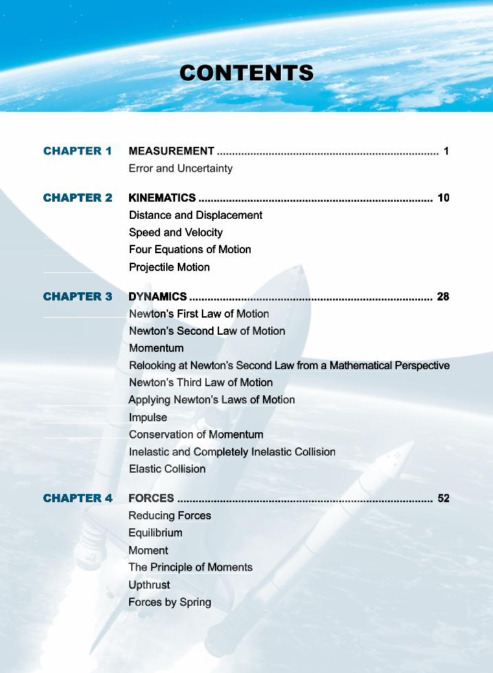
CHAPTER 1 MEASUREMENT ......................................................................... 1 Error and Uncertainty

CHAPTER 2 KINEMATICS ............................................................................. 10 Distance and Displacement Speed and Velocity Four Equations of Motion Projectile Motion

CHAPTER 3 DYNAMICS ................................................................................ 28 Newton’s First Law of Motion Newton’s Second Law of Motion Momentum Relooking at Newton’s Second Law from a Mathematical Perspective Newton’s Third Law of Motion Applying Newton’s Laws of Motion Impulse Conservation of Momentum Inelastic and Completely Inelastic Collision Elastic Collision

CHAPTER 4 FORCES .................................................................................... 52Reducing ForcesEquilibriumMomentThe Principle of MomentsUpthrustForces by Spring

CONTENTSCONTENTS

CHAPTER 2 KINEMATICS ............................................................................. 10 Distance and Displacement Speed and Velocity Four Equations of Motion Projectile Motion

CHAPTER 3 DYNAMICS ................................................................................ 28 Newton’s First Law of Motion Newton’s Second Law of Motion Momentum Relooking at Newton’s Second Law from a Mathematical Perspective Newton’s Third Law of Motion Applying Newton’s Laws of Motion Impulse Conservation of Momentum Inelastic and Completely Inelastic Collision Elastic Collision

CHAPTER 4 FORCES .................................................................................... 52Reducing ForcesEquilibriumMomentThe Principle of MomentsUpthrustForces by Spring

CHAPTER 5 WORK, ENERGY, POWER ........................................................ 71WorkForce — Displacement GraphPower

CHAPTER 6 MOTION IN A CIRCLE ............................................................... 86Derivation of Centripetal Force

CHAPTER 7 OSCILLATION ........................................................................... 98Circular MotionVelocity of Object undergoing Simple Harmonic MotionEnergy of Object undergoing Simple Harmonic MotionResonance and Damping

CHAPTER 8 WAVES ..................................................................................... 115Nature and Types of WavesRepresentation of Waves

CHAPTER 9 SUPERPOSITION .................................................................... 126Constructive and Destructive InterferenceYoung’s Double SlitsStanding Waves

CHAPTER 10 GRAVITATIONAL FORCE ....................................................... 150Newton’s Law of GravitationGravitational Field StrengthGravitational Potential EnergyGeostationary SatelliteOrbital Motion

CHAPTER 11 THERMAL PHYSICS ............................................................... 175Thermal Properties of MatterLatent HeatIdeal GasFirst Law of Thermodynamics

Circular MotionVelocity of Object undergoing Simple Harmonic MotionEnergy of Object undergoing Simple Harmonic MotionResonance and Damping

CHAPTER 8 WAVES ..................................................................................... 115Nature and Types of WavesRepresentation of Waves

CHAPTER 9 SUPERPOSITION .................................................................... 126Constructive and Destructive InterferenceYoung’s Double SlitsStanding Waves

CHAPTER 10 GRAVITATIONAL FORCE ....................................................... 150Newton’s Law of GravitationGravitational Field StrengthGravitational Potential EnergyGeostationary SatelliteOrbital Motion

CHAPTER 11 THERMAL PHYSICS ............................................................... 175Thermal Properties of MatterLatent HeatIdeal GasFirst Law of Thermodynamics

© Singapore Asia Publishers Pte Ltd�

Chapter 1 Measurement

Chapter 1

MeasureMent

Chapter 1

MeasureMent

Introduction

We can never be absolutely sure of what we measure.

This may sound strange considering that we have been making measurements, for example, measuring length using the metre rule since we started learning Science. How is it possible that we are not sure of what we are measuring?

If we take a careful look, no matter how accurate the instrument we use is, be it metre rule, vernier calipers or micrometer screw gauge, there will always be a level of uncertainty as to where the end of the object is, for example, when the end of the object is “somewhere” between two smallest divisions. We can only guess to our best abilities where the end is between the two divisions.

79.4 cm

79.5 cm

79.4 79.5

No matter how close we place these two divisions, there will always be a finite spacing between them. We can only make them closer by creating higher quality measuring instruments but we can never totally eliminate this uncertainty. To do that, the divisions will have to be infinitely close to each other which means that they will end up on each other. This does not make sense.

Therefore the study of uncertainty and how it is affected by mathematical operations addition/subtraction, division/multiplication is highly important and relevant. This will be one of the main focus of this chapter.



error and uncertainty – what’s the difference

It is inevitable that external factors or even the person conducting an experiment can introduce factors which may result in deviation of the measured value to vary from the actual value.

External factors can affect the results in two ways — predictable and unpredictable.

systematic error

Predictable deviation of results from actual value includes calibration error of instrument and improper setup of equipment. Examples of these errors include setting up a ruler in a slanted manner when it should be upright or zero error of instrument.

These errors are not only predictable, they take on exactly the same value every time the experiment is repeated.

These errors are called systematic errors. These are errors which have the same value and sign when the experiment is repeated under the same physical conditions. These errors can be eliminated altogether if the source is identified.

random error

There is another kind of error which causes the results to vary in an unpredictable manner. Examples include disruption to the experiment due to wind and/or vibrations.

These sources of errors can cause the result to be greater or smaller than the actual value. Due to this nature, this error can never be eliminated but it can be reduced by taking the average. The method of averaging helps to reduce errors as the errors take on positive and negative values randomly. If large number of data points are taken, there should be equal probability for errors to be positive or negative. Thus, averaging would even out these variations, giving an answer closer to the actual value.

These errors are called random errors. These are errors which have different value or sign when the experiment is repeated under the same physical conditions.

It is important to understand that both systematic and random errors contribute to the deviation of the results from the actual value BUT in different manner.

Systematic errors shift the data in a fixed manner. For example, a set of measured values of g, the acceleration of free fall, with systematic error would be as follow:

9.910 9.905 9.910 9.905 9.905 9.910

The average of these values is 9.91 corrected to three significant figures. This is 0.1 away from the actual value of 9.81 m s–2. If you take a closer look, the values are generally about 0.1 away from 9.81 m s–2. This means that all data points are shifted by almost the same amount. This is an example of the influence of systematic error on the data.



A graphical representation of the data would be as follow:

9.81 9.905 9.910actual value experimental values

The data points are very close to each other but it is systematically shifted from the true value by approximately the same amount.

We call this set of data points precise but not accurate.

As we can see, precision is a measure of the closeness of the data points to each other and accuracy is a measure of how close the data points are to the actual value.

Let’s take a second look at another set of data.

9.700 9.920 9.51 10.11 9.910 9.710

It is evident that the spread is significantly larger BUT the average of this set to data is 9.810 m s–2. This means that random error, which causes unpredictable fluctuation in data must have been present. In contrast, the systematic error is almost non existent in this set of data.

In summary, finding the average of a set of data and comparing its closeness to the actual data would give a good indication of the extent of systematic error. On the other hand, if the spread of the data is large, it shows that the data is under the influence of random errors.

A graphical representation of the points is as follow:

9.51 9.81 9.9109.700 9.710 9.920 10.11

As we can see, this set of data points has a large spread. Thus this set of data is NOT precise but accurate as the average of these points is 9.81.

uncertainty

Another source of error is a result of the measurement process itself – the reading of values off an instrument.

For example, when we are reading the position of a point off a metre ruler, there is no way we can determine the position to absolute accuracy simply because of the limitation imposed by the measuring instrument itself.

79 80

As we can see from the diagram, there is no way we can tell the position of the object on the metre rule to infinite accuracy. We are not sure if it starts at 79.3 or 79.4.



We can only, at best, guess that the value is between 79.3 and 79.4. Thus, this range of uncertainty in the measured value is what we call the uncertainty.

As a rule of thumb, the uncertainty of instrument with small divisions on the scale (divisions are � mm apart or less) would be half of the division. If the spacing between divisions is large, the uncertainty would be one-fifth the division.

Therefore, the uncertainty of readings off the metre rule would be ±0.5 mm (since the spacing between the smallest divisions is 1 mm).

Readings are different from measurements. Reading is the position of one end of an object while measurement is the difference (subtraction) between the two ends. Therefore, to find the length of an object, we have to find the difference between the position/reading at each end of the object. How then do we process the uncertainty when two values with uncertainty are added or subtracted?

Let's consider two numbers.

A = 5 ± 1 B = 3.0 ± 0.5

Maximum value of A + B = max. value of A + max. value of B = 9.5 Minimum value of A + B = min. value of A + min. value of B = 6.5

Therefore the value of A + B would be 8 ± 1.5.

However, the correct way of quoting this value with its uncertainty would be 8 ± 2. The uncertainty has to be quoted to 1 significant figure.

The reason for doing so is because uncertainty cannot take on a high accuracy. It would make no sense to have an accurate uncertainty. Thus, the uncertainty will always be quoted to 1 significant figure (s.f.).

How about A – B?

Maximum value of A – B = max. value of A – min. value of B = 3.5 Minimum value of A – B = min. value of A – max. value of B = 0.5

Thus the value of A – B = 2 ± 1.5 = 2 ± 2

If you pay close attention to the values, it would not be difficult to notice that the uncertainty is always 2 whether it is the sum of or difference between the values.

This makes sense as whenever we process any uncertainty, for example, adding or subtracting numbers, its uncertainty should increase rather than decrease. Otherwise we may end up with the case of negative uncertainty if we subtract uncertainties.

In summary, the uncertainties will always add whenever values with uncertainties are added or subtracted.



Let’s take a look at another example.

A = 2.000 ± 0.005 B = 0.50 ± 0.05 A – B = (2.000 – 0.50) ± (0.005 + 0.05)

= (1.500 ± 0.055)

Quoting the uncertainty as 0.055 is inappropriate as uncertainty needs to have as low a level of “certainty” as possible. For example, having an uncertainty of 0.00523926 is not correct. Thus the uncertainty is always quoted to 1 significant figure so that it has a low level of “certainty”.

So the answer should be 1.500 ± 0.06 ↑ should be 1 s.f.

Wait a minute!

If the uncertainty has 2 decimal places (d.p.), how is it possible to quote a value to 3 d.p.?

Yes, it is not correct.

The proper way of quoting a value is to ensure that it has the same level of accuracy as the uncertainty.

In this case, the uncertainty is accurate to 2 d.p.; the value can only be quoted to 2 d.p.

Thus, the correct answer is �.�0 ± 0.06.

Going back to the issue of measurement of length. When we take the difference between the positions of two ends of an object, it would also result in the addition of the uncertainties of the readings.

For example, if the positions of the ends of an object on a metre rule are

front: 78.35 ± 0.05 cm end : 23.45 ± 0.05 cm

The length of the object would be

(78.35 – 23.45) ± (0.05 + 0.05) cm = 54.9 ± 0.1 cm

In summary, the reading from a metre ruler will have an uncertainty of 0.0� cm (or 0.� mm) and its measurement will have an uncertainty of 0.� cm (or � mm).

What if we multiply values? How do we process the uncertainty?

Let’s take for example y = x2. If x = 4.0 ± 0.1, what is the value of y with its uncertainty?

To answer this, let’s take a look at the graph of y vs x.

© Singapore Asia Publishers Pte Ltd6


y

16

4.0x

∆x

∆y

We know that x has an uncertainty of ∆x = 0.1.

y = x2

The uncertainty in x causes an uncertainty in y, ∆y.

If we divide ∆y by ∆x, assuming that both ∆y and ∆x are small, the value ∆y

___ ∆x would be dy

___ dx , the gradient of the graph at that point. In this case, (4.0, 16).

Therefore,

∆y

___ ∆x = dy

___ dx = 2x

Thus, ∆y = 2x∆x

∆y

___ y = 2x∆x _____ y = 2x∆x _____ x2 = 2∆x ____ x

Therefore,

∆y

___ y = ∆x ___ x + ∆x ___ x

We can see that if y = x × x, the fractional uncertainty (uncertainty divided by the quantity, in this case it is

∆y ___ y or ∆x ___ x ) of y is the sum of the fractional uncertainty of the terms multiplied.

This is also the case when we divide quantities.



In this case,

∆y

___ y = ∆y

___ 16 = 2 ∆x ___ x

= 2 ( 0.1 ___ 4.0 ) = 0.05

Therefore, ∆y = 16 × 0.05 = 0.8.

So, the value of y is correctly quoted as 16.0 ± 0.8.

Let's take a look at another example.

z = y3

__ x2

where z = 64 ± 1 and x = 9.0 ± 0.5. Find y with its uncertainty.

By the same principle which we surfaced above,

∆z ___ z = 3 ∆y

___ y + 2 ∆x ___ x

∆y

___ y = 1 __ 3 ( ∆z ___ z – 2 ∆x ___ x ) = 1 __ 3 ( 1 ___ 64 – 2 0.5 ___ 9.0 ) = –0.032

We get a negative uncertainty! So what is wrong with the method above?

What should have been done is to express the term we wanted to find as the subject.

Using the same example,

y = 3 √_____

z × x2

Therefore,

∆y

___ y = 1 __ 3 ( ∆z ___ z + 2 ∆x ___ x ) = 1 __ 3 ( 1 ___ 64 + 2 0.5 ___ 9.0 ) = 0.0422

y = 3 √_____

z × x2

= 3 √________

64 × 9.02 = 5184



Therefore,

∆y

___ y = 0.0422

∆y = 0.0422 × 5184= 218= 200 (1 s.f.)

y = 5200 ± 200

Note that the answer has to be quoted to the same accuracy as the uncertainty. In this case, the uncertainty is in the hundreds so that answer can only be rounded to the hundredth position. The accuracy of the answer is limited by the uncertainty.

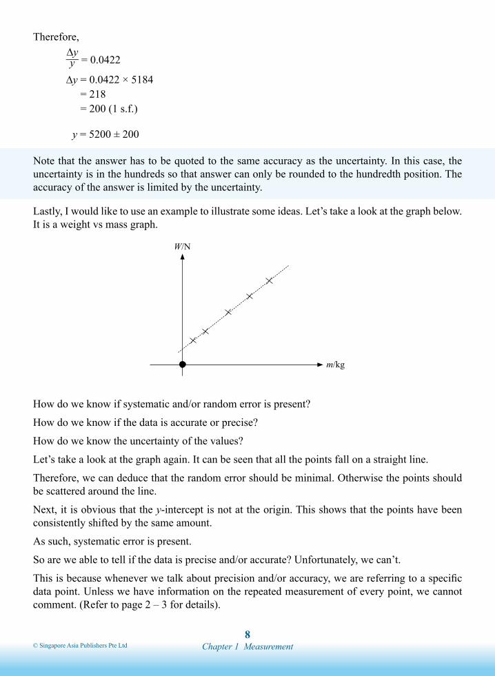
Lastly, I would like to use an example to illustrate some ideas. Let’s take a look at the graph below. It is a weight vs mass graph.

W/N

m/kg

How do we know if systematic and/or random error is present?

How do we know if the data is accurate or precise?

How do we know the uncertainty of the values?

Let’s take a look at the graph again. It can be seen that all the points fall on a straight line.

Therefore, we can deduce that the random error should be minimal. Otherwise the points should be scattered around the line.

Next, it is obvious that the y-intercept is not at the origin. This shows that the points have been consistently shifted by the same amount.

As such, systematic error is present.

So are we able to tell if the data is precise and/or accurate? Unfortunately, we can’t.

This is because whenever we talk about precision and/or accuracy, we are referring to a specific data point. Unless we have information on the repeated measurement of every point, we cannot comment. (Refer to page 2 – 3 for details).



We would not be able to tell the uncertainly at the data points as well. This is because the points are marked out by crosses, representing only the exact value of the data.

Therefore, there is no way we can tell the magnitude of uncertainly from this graph.

In summary, there are three points: 1. Systematic error can be deduced from the deviation of y-intercept from an expected value. 2. Random error can be deduced from the scatter of the points. 3. Accuracy, precision and uncertainty cannot be deduced from the graph.

When performing addition or subtraction, the resultant uncertainty is always the sum of the uncertainty.

The uncertainty is always quoted to 1 s.f.

The quantity is quoted to the same decimal place as the uncertainty.

When performing multiplication or division, the resultant fractional uncertainty is the sum of the fractional uncertainty of all terms involved.

The term which the uncertainty is to be computed has to be the subject in the equation.

Finally, there are five main points to note for uncertainty processing.

Uncertainty is dependent on the instrument used.

Regardless of mathematical operations, the uncertainty or fractional uncertainty always increases. This means that there should never be a subtraction of uncertainty or fractional uncertainty.

In addition and subtraction, absolute uncertainty is added.

In multiplication or division, the fractional uncertainty is added.

Key concepts

Documents

ABOUT THE AUTHOR we take a careful look, no matter how accurate the instrument we use is, be it metre rule, vernier calipers or micrometer screw gauge, there will always be a level