Absolute Strength: Exploring Momentum inStock Returns

Huseyin Gulen ∗

Krannert School of ManagementPurdue University

Ralitsa Petkova†

Weatherhead School of ManagementCase Western Reserve University

March 4, 2015

Preliminary and incomplete.Please do not quote without permission.

∗Krannert School of Management, Purdue University, 403 West State Street, West Lafayette, IN 47907.Tel: (765) 496-2689, e-mail: hgulen@purdue.edu.

†Weatherhead School of Management, Case Western Reserve University, 10900 Euclid Ave, Cleveland,OH 44106. Tel: (216) 368-4778, e-mail: rgp9@case.edu.

1 Introduction

In the finance literature, relative strength momentum is a strategy that exploits the relative

performance of different assets. This strategy buys assets that outperformed their peers

over the last 6 to 12 months and shorts assets that underperformed their peers over the

same period. Jegadeesh and Titman (1993) first show that relative strength momentum is

profitable in the cross section of US stocks: past relative winners continue to outperform

past relative losers in the near future. Relative strength momentum is one of the strongest

and most puzzling asset pricing anomalies.1

Several important behavioral asset pricing theories try to explain the documented

momentum pattern in stock returns. Among these are the models of Barberis, Shleifer,

and Vishny (1998), Daniel, Hirshleifer, and Subrahmanyam (1998), and Hong and Stein

(1999). What these models have in common is that they examine investors’ behavior with

respect to news, signals, or trends they observe for a single risky asset. For example, a series

of positive earnings surprises or positive returns would be interpreted as a period during

which the stock experienced good news. Therefore, these behavioral models imply that the

magnitude and the direction of an asset’s own past performance is a predictor of the asset’s

future performance.

Reacting to significant directional movements in stock prices matches the predictions

of other prominent models. For example, Grinblatt and Han (2005) develop a model with

investors that exhibit the disposition effect. These investors demand for stocks is inversely

related to the magnitude of the unrealized capital gain that a stock has experienced in the

recent past. A stock with a large unrealized capital gain has excess selling pressure relative

to a stock with a large unrealized capital loss. Grinblatt and Han (2005) show that such a

demand for stocks induced by the disposition effect tends to generate price underreaction

to public information. In equilibrium, past winners tend to be undervalued and past losers

1Numerous papers have verified that relative strength momentum exists not only in U.S. stocks butalso in industries (Moskowitz and Grinblatt (1999)), foreign stocks (Rouwenhorst (1998), Griffin, Ji andMartin (2005)), emerging markets (Rouwenhorst (1999)), equity indices (Asness, Liew and Stevens (1997),Bhojraj and Swaminathan (2006), Hvidkjaer (2006)), commodities (Pirrong (2005), Miffre and Rallis (2007)),currencies (Menkoff et al (2011)), global government bonds (Asness, Moskowitz and Pedersen (2012)), andcorporate bonds (Jostova, Nikolova and Philipov (2010)).

1

tend to be overvalued.

Although the behavioral models mentioned above are designed to explain the profitability

of relative strength momentum, sorting on relative performance does not necessarily match

the predictions of these models. This is the case since in the data relative winners have not

necessarily gone up in value and relative losers have not necessarily gone down in value over

the recent past.

For example, the cumulative return of Michigan Gas Utilities Co. over the period June

1969-April 1970 was 0.4%. This return was in the top 10% of the distribution of cumulative

returns over that period. Therefore, in May 1970 Michigan Gas Utilities Co. would have

been classified as a past winner according to the relative momentum strategy. Subsequently,

the cumulative return of Michigan Gas Utilities Co. over the period July 1970-May 1971 was

0.6%. This return was in the bottom 10% of the distribution of cumulative returns over that

period. Therefore, in June 1971 Michigan Gas Utilities Co. would have been classified as a

past loser according to the relative momentum strategy. It seems that over a period of about

two years the stock would not have attracted any investor attention. The price of Michigan

Gas Utilities Co. over that period did not reflect any news and did not exhibit “momentum”

at all: it remained stable resulting in a cumulative return of about 0%. However, the relative

momentum characteristic of the stock varied dramatically from one extreme to the other.

This example, and many others that also cover different time periods2, indicate that the

relative momentum measure of a stock does not always identify assets that have experienced

a large directional move in their stock price. Motivated by this observation, we develop

a momentum characteristic, termed “absolute strength momentum,” that directly matches

the implications of the behavioral models mentioned before. Absolute strength momentum

exploits the direction and magnitude of a stock’s own performance over the recent past. We

find that stocks with large positive returns over the recent past continue to have large positive

returns in the near future. Similarly, stocks with large negative returns over the recent past

continue to have large negative returns in the near future. An investment strategy that

buys stocks with significantly positive returns over the previous year and shorts stocks with

2Other examples are available upon request.

2

significantly negative returns over the previous year generates a risk-adjusted return of 2.42%

per month with a monthly Sharpe ratio of 0.32 from 1965 to 2014. This strategy also performs

well over the 2000-2014 period, which includes the recent Great Recession: its risk-adjusted

return is 1.55% per month with a monthly Sharpe ratio of 0.18.

The key innovation that we implement is the use of data-driven breakpoints to classify

stocks based on their past performance. The traditional relative winner and loser breakpoints

are based on recent cumulative return percentiles and are therefore driven by the recent state

of the market. For example, in February 2009, which was officially a recession month, the

breakpoint to be classified as a relative winner (loser) based on past one-year performance

was 4.88% (-83.48%) return. In April 2004, which was officially an expansion month, the

breakpoint for a relative winner (loser) stock was 220.61% (9.63%) return. Therefore, a

relative winner stock in February 2009 would have been a relative loser in April 2004. In

contrast, we define absolute winners and losers according to stable performance thresholds

over time. First, absolute winners (losers) are stocks that have experienced an absolute price

increase (decline) in the recent past. Second, the corresponding movement in the price is

large in magnitude indicating substantial “momentum.”

Following these objectives, we construct new return breakpoints that separate stocks

based on their absolute strength recent performance. Specifically, at the beginning of each

month t, we compute the cumulative returns of all stocks over the period t-12 to t-2.3 To

determine whether these cumulative returns are high or low, we look at the distribution of

all previous non-overlapping 11-month cumulative returns. For example, at the beginning of

January, we record cumulative returns for all stocks over the period from last January to last

November. These returns are ranked on the basis of the historical distribution of January

to November cumulative returns. If a stock’s cumulative return over t-12 to t-2 falls in the

top (bottom) 10% of the historical distribution, we classify that stock as an absolute winner

(loser). We repeat this process every month. Therefore, our return breakpoints assure that

an absolute winner is an asset that has done well over the recent 11 months according to

the historical record. Similarly, an absolute loser is an asset that has done poorly over the

3Skipping a month between the holding period and the ranking period is common in the momentumliterature.

3

recent 11 months according to the historical record. Therefore, each month we are effectively

comparing the distribution of cumulative stock returns over the recent past to the historical

distribution of 11-month cumulative stock returns.

The stocks identified as absolute winners and absolute losers are not simply a smaller

subset of the stocks defined as relative winners or relative losers. For example, there are

instances in which none of the stocks meet the criteria to be defined as absolute winners

or losers. If this is the case, then the momentum strategy that buys absolute winners and

sells absolute losers cannot be implemented. In order to implement the absolute strength

momentum strategy, we require that both the absolute winner and loser portfolios are well-

diversified, i.e., there are at least 30 stocks in each portfolio.4 If the portfolios are not

well-diversified, then we simply invest in the one-month T-bill.

We show that the absolute strength momentum strategy not only does well over

various sample periods, but also has several features that distinguish it from relative

strength momentum. A recent study by Novy-Marx (2012) suggests that an asset’s relative

performance over the first half of the preceding year seems to better predict returns compared

to its relative performance over the most recent past. For example, Novy-Marx (2012) finds

that stocks that are relative winners over the past six months but relative losers over the first

half of the preceding year, tend to significantly underperform stocks that are relative losers

over the past six months but relative winners over the first half of the preceding year. This

evidence implies that there is an “echo” in returns rather than “momentum.” The absolute

strength momentum strategy, however, does not suffer from the “echo” effect. We show that

intermediate horizon absolute strength and recent absolute strength performance contribute

equally to the predictability of future performance.

Furthermore, there are times when the relative strength momentum strategy experiences

severe crashes that can significantly reduce the accumulated gains from the strategy (e.g.,

Daniel and Moskowitz (2013)). For example, in August of 1932, a strategy that buys previous

11-month relative winners and sells previous 11-month relative losers returned a negative

78%. More recently, in April of 2009, the same strategy returned a negative 46%. The

4Statman (1987) argues that a well-diversified portfolio of randomly chosen stocks must include at least30 stocks.

4

absolute strength momentum strategy we examine is not subject to such severe crashes.

More importantly, we show that we are able to reliably predict and avoid crash periods by

following absolute strength momentum rules.

The superior performance of absolute strength momentum suggests that it could be

viewed as a way to better time the relative strength momentum strategy. We show that

relative strength momentum has similar performance to absolute strength momentum at

times when the distribution of cumulative stock returns over the most recent 11 months is

similar to the historical distribution of 11-month cumulative stock returns. Whenever the

distribution of cumulative stock returns over the most recent 11 months deviates from the

historical distribution of 11-month cumulative stock returns, the relative strength momentum

strategy is not profitable.

A strategy based on the absolute price movement of a certain asset is consistent with the

predictions of behavioral models designed to explain momentum in stock returns. It is also

consistent with extensive experimental and survey evidence that documents that investors

trade based on absolute stock performance. For example, Shefrin and Statman (1985) and

Odean (1998) document the disposition effect, which is the tendency of investors to sell the

stocks that have increased in value but hold on to the stocks that have gone down in value.

In another example, Kahneman and Tversky (1979) document that individuals are subject

to loss aversion, which implies that investors become more risk averse following losses and

less risk averse following gains. Barberis and Huang (2001) conclude that due to loss aversion

investors demand relatively more of an asset that has gone up, versus one that has dropped

in price. The asset that has gone up is perceived as relatively less risky.

Furthermore, there is evidence that some individuals tend to chase trends: they buy

when prices rise and sell when prices fall, engaging in the so called positive feedback trading.

For example, Andreassen and Kraus (1988) show that subjects that observe a certain price

trend over a long period tend to chase the trend, buying more when prices rise and selling

when prices fall. Shiller (1988) surveys investors before the 1987 market crash and finds

that they tend to sell as a result of absolute price declines, presumably anticipating further

price declines. Similarly, a number of papers document that various institutions like mutual

5

funds, pension funds, and others, engage in strategies that buy assets that had an absolute

price increase and sell assets that had an absolute price decline (e.g., Grinblatt, Titman,

and Wermers (1995), Carhart (1997), Coval and Stafford (2007), Lakonishok, Shleifer, and

Vishny (1992), Nofsinger and Sias (1999), Griffin, Harris, and Topaloglu (2003)).

Trend chasing behavior can exist in the models of Tversky and Kahneman (1974) and

Lakonishok, Shleifer, and Vishny (1994). These models argue that investors are prone to

excessive extrapolation and so they tend to overreact to past stock performance. Therefore,

investors demand more of an asset that has gone up in price because they extrapolate the

past trend into the future. Trend chasing does not necessarily have to be irrational. For

example, DeLong, Shleifer, Summers, and Waldmann (1990) develop a model with two types

of traders. Noise traders follow positive feedback strategies - they buy when prices have risen

over a certain period and sell when prices have fallen. Their demand for stocks is directly

proportional to the magnitude of the price change. Rational speculators realize that it pays

to jump on the bandwagon and they purchase ahead of the demand of the noise traders.

This behavior of rational speculators further amplifies the positive feedback trading of the

noise traders.

What these models have in common is that they show that investors’ trading behavior

depends on an asset’s past absolute performance. In addition, the magnitude of the asset’s

past profit is directly proportional to the investors’ demand for the stock. Finally, both

models predict that stocks that have gone up in value in the recent past should continue

to increase while stocks that have gone down in value should continue to drop. Therefore,

these models predict that stock returns should exhibit absolute strength momentum.

Finally, our absolute strength momentum strategy is related to another anomaly called

“time series momentum,” that buys assets with positive excess returns and sells assets

with negative excess returns over the past months. Moskowitz, Ooi, and Pedersen (2011)

show that a diversified portfolio of time series momentum strategies across different asset

classes has significant abnormal returns and performs well during extreme markets. Since

this strategy focuses on a security’s own past return rather than its relative return, it is

different from relative strength momentum. It is also different from our absolute strength

6

momentum strategy, which focuses on large and significant price movements in the positive

or negative direction. We show that absolute strength momentum completely explains time

series momentum in the cross section of US stocks.

The rest of the paper proceeds as follows. Section 2 describes how the absolute strength

momentum strategy is constructed, examines its characteristics that distinguish it from other

momentum strategies, and reports its performance over different sample periods. Sections

3 and 4 show that the absolute strength momentum strategy subsumes the information

contained in relative strength momentum and time series momentum. Section 5 examines

whether the absolute strength momentum strategy is robust to the presence of the “echo”

effect in returns documented by Novy-Marx (2012). Section 6 documents the performance of

absolute strength momentum during the crash periods identified by Daniel and Moskowitz

(2013). Section 7 provides more details about the driving forces behind return momentum.

Section 8 offers several robustness checks and Section 9 concludes.

2 Absolute Strength Momentum Strategy

To construct our main sample, we use only common stocks traded on the NYSE, AMEX, and

NASDAQ. Stock market data comes from CRSP. Stocks priced below $1 at the beginning

of the holding period are excluded. We use the one-month T-bill as the risk-free asset. At

the beginning of each month t, we compute the cumulative returns of all firms from month

t-12 to t-2. Firms must have at least eight observations of return in the t-12 to t-2 window.

Based on their 11-month cumulative returns, firms are placed in different portfolios which

are then value-weighted. The portfolios are held over month t, and they are rebalanced

monthly using the same approach. Following previous studies, we skip one month between

the ranking period for cumulative returns and the start of the portfolio holding period. This

method avoids the one-month reversal effect documented by Jegadeesh (1990) and Lehmann

(1990).5

5The relative momentum strategy that sorts stocks on their 11-month past return, skips a month, andthen holds the stocks for one month is examined by Fama and French (1996) and others. Jagadeesh andTitman (1993) examine relative momentum strategies that sort stocks on their 3-, 6-, 9-, or 12-month pastreturns and hold them for 3, 6, 9, or 12 months after portfolio formation. The main strategy that weexamine focuses on a 11-month sorting period and 1-month holding period. Later we present results for

7

Firms with the highest ranking period cumulative returns are classified as absolute

winners and firms with the lowest ranking period cumulative returns are classified as absolute

losers. We also evaluate the performance of the absolute strength momentum strategy that

buys absolute winners and sells absolute losers. Below we describe in detail how we identify

absolute winners and absolute losers.

2.1 Absolute Winners and Absolute Losers

2.1.1 Cumulative Return Breakpoints

The general idea behind momentum investing is to buy stocks whose prices have been rising

and sell stocks whose prices have been falling. However, the traditional definition of relative

strength does not necessarily imply that relative winners (losers) are stocks that have been

increasing (decreasing) in price. In other words, there are times when the cross-sectional

definition of winners and losers deviates from the notion of absolute strength momentum.

In this section, we focus on what it means to be a winner or a loser stock in the context

of absolute strength momentum. We propose a new way of defining winners and losers in

order to test the original notion behind momentum investing, namely that rising stocks keep

rising and falling stocks keep falling.

How can we judge whether a stock with an 11-month past return qualifies to be a winner

or a loser? The traditional way tells us to compare it to the 11-month past return of all other

stocks. For example, in April of 2009, a stock with a past 11-month return of negative 5% is

classified as a relative “winner.” Even though this performance is better than the previous

11-month performance of 90% of all stocks, it is hard to associate such a low return with

a winning investment. In April of 2009, based on all available historical information about

previously realized 11-month returns, this stock would not have placed in the top 10% of

the historical distribution. Therefore, when the stock’s return over the last 11 months is

compared to what constitutes a positive performance over an 11-month interval based on

the historical benchmark, the stock becomes an actual loser. We use this observation to

motivate a new way of classifying stocks into winners and losers.

other strategies as well.

8

We propose that in order to determine the breakpoint for an absolute winner or loser at

time t, we should look at the historical information about returns using all available data

prior to date t. Specifically, at the beginning of each month t, we compute the cumulative

returns of all stocks over the period t-12 to t-2. To determine whether these cumulative

returns are high or low, we look at the distribution of all previous non-overlapping 11-

month cumulative returns. For example, at the beginning of January, we record cumulative

returns for all stocks over the period from last January to last November. These returns

are ranked on the basis of the historical distribution of January to November cumulative

returns. If a stock’s cumulative return over t-12 to t-2 falls in the top (bottom) 10% of the

historical distribution, we classify that stock as an absolute winner (loser). We repeat this

process every month. Therefore, the historical distribution of 11-month cumulative returns

is updated continuously.

Figure 1 plots the absolute winner and loser cumulative return breakpoints based on the

method described above, from January 1965 to December 2014. Even though we start the

analysis in 1965, we use return data back to 1927 to determine performance breakpoints. At

the beginning of the sample the absolute winner cutoff starts around 60% return, and by

the end of the sample is updated up to around 70% return. The absolute loser cutoff starts

around -30% return and is updated to about -50% return by the end of the sample period.

Even though both cutoffs display slight variation, the definition of an absolute winner or

loser is relatively stable over time. Furthermore, the absolute loser breakpoint is always

negative, while the absolute winner breakpoint is always positive. Therefore, it is always the

case that the stocks identified as absolute winners (losers) according to the new breakpoints

have been increasing (decreasing) in value before portfolio formation. This is consistent with

the idea behind momentum investing, which aims to identify stocks that were rising or falling

in value.

The absolute winner (loser) breakpoints that we derive resemble a filter rule. Figure

1 suggests that stocks are defined as absolute winners or losers if the level of their 11-

month cumulative return is within specific filter breakpoints.6 So, a stock is included in the

6Cooper (1999) uses filter rules on lagged stocks returns to examine security overreaction. He definesstocks as winners or losers if their recent returns are within specific filter breakpoints.

9

absolute winner (loser) portfolio only if its 11-month cumulative return moved up (down)

by a specific amount. However, in contrast to filter rules, the breakpoints that we derive

are not exogenously pre-determined. Instead, they are data-driven since we let historical

performance dictate what is an absolute winner or an absolute loser stock.

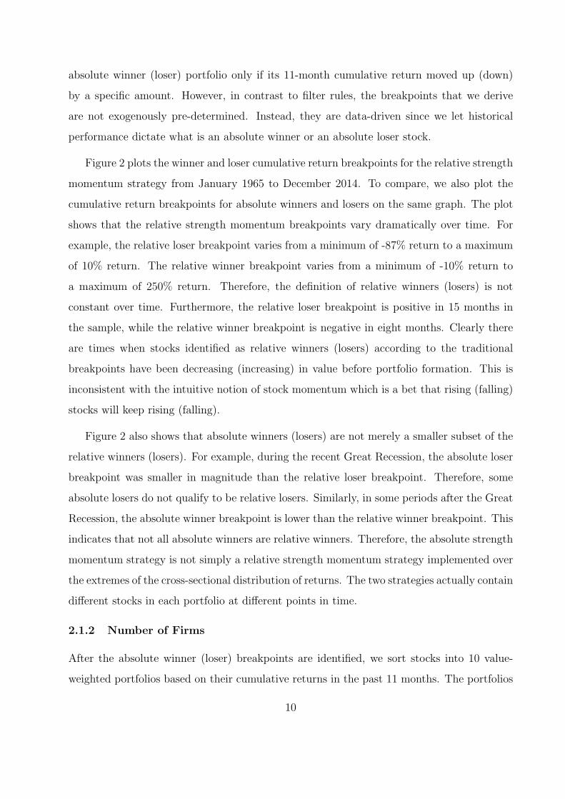
Figure 2 plots the winner and loser cumulative return breakpoints for the relative strength

momentum strategy from January 1965 to December 2014. To compare, we also plot the

cumulative return breakpoints for absolute winners and losers on the same graph. The plot

shows that the relative strength momentum breakpoints vary dramatically over time. For

example, the relative loser breakpoint varies from a minimum of -87% return to a maximum

of 10% return. The relative winner breakpoint varies from a minimum of -10% return to

a maximum of 250% return. Therefore, the definition of relative winners (losers) is not

constant over time. Furthermore, the relative loser breakpoint is positive in 15 months in

the sample, while the relative winner breakpoint is negative in eight months. Clearly there

are times when stocks identified as relative winners (losers) according to the traditional

breakpoints have been decreasing (increasing) in value before portfolio formation. This is

inconsistent with the intuitive notion of stock momentum which is a bet that rising (falling)

stocks will keep rising (falling).

Figure 2 also shows that absolute winners (losers) are not merely a smaller subset of the

relative winners (losers). For example, during the recent Great Recession, the absolute loser

breakpoint was smaller in magnitude than the relative loser breakpoint. Therefore, some

absolute losers do not qualify to be relative losers. Similarly, in some periods after the Great

Recession, the absolute winner breakpoint is lower than the relative winner breakpoint. This

indicates that not all absolute winners are relative winners. Therefore, the absolute strength

momentum strategy is not simply a relative strength momentum strategy implemented over

the extremes of the cross-sectional distribution of returns. The two strategies actually contain

different stocks in each portfolio at different points in time.

2.1.2 Number of Firms

After the absolute winner (loser) breakpoints are identified, we sort stocks into 10 value-

weighted portfolios based on their cumulative returns in the past 11 months. The portfolios

10

are based on each 10th percentile of the historical distribution of past returns. These

portfolios are held for one month and are then rebalanced. We also construct a momentum

strategy portfolio that buys the absolute winner portfolio and sells the absolute loser

portfolio. Next, we examine the number of stocks in each portfolio.

The relative and absolute strength momentum strategies discussed above use different

thresholds to classify stocks into winners and losers. Therefore, at each point in time,

the number of absolute winners (losers) identified by the absolute strength momentum

strategy differs from the number of relative winners (losers) identified by the relative strength

momentum strategy. Each month, the relative classification partitions the universe of stocks

into 10 value-weighted portfolios with an equal number of stocks in each portfolio.7 Figure

3 plots the number of firms in the relative winner and loser portfolios over time. The figure

shows that the relative winner and loser portfolios are always populated by stocks that fit

the relative breakpoints. Since the performance thresholds are relative, the strategy always

identifies some stocks as winners or losers.

The absolute strength momentum strategy, on the other hand, does not impose the

requirement that there should always be some stocks designated as winners or losers. This is

because the performance breakpoints are based on the historical distribution of returns over

time and across stocks. Therefore, there might be instances in which the absolute winner or

loser portfolios are not populated by any stocks. Figure 4 plots the number of firms in the

absolute winner and loser portfolios over time. The figure shows that there are times when

few firms qualify to be in the absolute winner or loser portfolios. For example, in January

2009, only 24 stocks qualify to be classified as absolute winners based on their cumulative

returns from January 2008 to November 2008. In April of 2004, only 18 stocks qualify to be

classified as absolute losers.

In order to assure that the absolute strength momentum strategy is based on well-

diversified portfolios, we implement the strategy only when both the absolute winner and

absolute loser portfolios each contain more than 30 stocks. In the months in which the

absolute momentum strategy cannot be implemented, we simply hold the risk-free asset. In

7The number of stocks in each portfolio might differ slightly if a price filter is imposed on the data.

11

the following section we report the performance of portfolios sorted by relative past returns

as well as the performance of the absolute strength momentum strategy.

2.1.3 Performance

Table 1 presents several characteristics of 10 portfolios sorted on absolute strength

momentum. Portfolios 1 through 10 correspond to absolute performance breakpoints based

on the historical distribution of returns. The characteristics are measured monthly and

include average return and its t-statistic, average excess return, volatility, Fama-French

(1993) alpha, market beta, and Sharpe ratio.8 The strategy that buys absolute winners and

sells absolute losers is presented in the last column. The table shows that absolute winners

continue to be absolute winners, while absolute losers continue to be absolute losers. This is

consistent with the presence of absolute strength momentum in stock returns. Furthermore,

the absolute strength momentum strategy generates significant profits of 2.16% per month

for the period 1965-2014 and 1.51% per month for the period 2000-2014.

The risk-adjusted returns of the portfolios also show that stocks that have been decreasing

in value in the recent past continue to decrease in value after portfolio formation, and

stocks that have been increasing in value in the recent past continue to increase in value

after portfolio formation. Again, this is consistent with the presence of absolute strength

momentum in stock returns. The absolute strength momentum strategy generates significant

risk-adjusted returns of 2.42% per month for the period 1965-2014 and 1.55% per month for

the period 2000-2014. The period from 2000 to 2014 is interesting since it includes the recent

Great Recession. The results indicate that the absolute strength momentum strategy was

profitable, on average, during the period that includes the worst recession in recent memory.

For comparison, Table 2 presents monthly characteristics of ten portfolios sorted on

relative strength momentum using the traditional approach described in the literature

(e.g., Fama and French (1996)). The table shows that the relative momentum strategy

is also profitable in the period 1965-2014. However, its performance is worse than the

performance of absolute strength momentum described in Table 1. Furthermore, in contrast

8The characteristics are computed over the months during which both portfolios 1 and 10 consist of atleast 30 stocks.

12

to absolute strength momentum, in the most recent period from 2000 to 2014, relative

strength momentum does not produce significant profits. The Sharpe ratio of relative

strength momentum is smaller than the Sharpe ratio of absolute strength momentum in

both sample periods that we examine in Table 2.

Another way to compare the performance of absolute strength momentum vs. relative

strength momentum is to look at the cumulative returns of each strategy from the perspective

of a buy-and-hold investor. Figure 5 plots the cumulative monthly log returns for investing

$1 in relative strength and absolute strength momentum for the period 1965-2014. For

comparison, we also plot the cumulative monthly log returns for investments in the risk-free

asset and the market. The final dollar amounts for each buy-and-hold strategy at the end

of 2014 are presented on the right side of the plot. For absolute strength momentum, $1

invested at the beginning of 1965 grows to $96,236 at the end of 2014. For relative strength

momentum, $1 appreciates to $6,127. Both investments do better than holding the risk-free

asset or the market alone.

Note that relative strength momentum experiences a large drop in accumulated wealth

during the first half of 2009 which corresponds to the period of the recent Great Recession.

Absolute strength momentum, on the other hand, is able to do better during that time

period and does not experience a large drop in value. In order to examine the period around

the Great Recession in more detail, we plot the cumulative monthly log returns for investing

1 dollar in relative strength momentum, absolute strength momentum, the risk-free asset,

and the market for the period 2000-2014. Figure 6 shows that over March and April of 2009,

the relative strength momentum strategy loses around 50% of its accumulated value and by

the end of the sample period there is no appreciation in the $1 invested in the strategy. In

contrast, absolute strength momentum does not lose much value during the Great Recession

and there is substantial appreciation in its buy-and-hold return over 2000-2014.

13

3 Does Relative Strength Momentum Explain

Absolute Strength Momentum?

Both the absolute strength strategy that we propose and the relative strength strategy

examined in the literature previously focus on the recent performance of all stocks. Therefore,

a natural question that arises is whether the two strategies are closely related. In this section,

we examine the relation between absolute strength and relative strength momentum.

If relative strength momentum completely captures absolute strength momentum, then

we would expect to see a zero intercept in a time-series regression in which the dependent

variable is absolute strength momentum. To account for the presence of other factors that

might explain the behavior of the absolute strength momentum strategy, we control for the

market portfolio and the Fama-French (1993) value and size factors. Table 3 presents results

for time-series regressions from 1965 to 2014 in which the dependent variable is the absolute

strength strategy and the independent variables are the excess market return, HML, SMB,

and relative strength momentum.

The results in Table 3 show that absolute strength momentum loads significantly on

relative strength momentum. This reflects the fact that the strategies are highly correlated

(74%). However, the time-series intercept in the regression is significantly positive and at

1% per month it is also economically large. Therefore, the absolute strength momentum

strategy contains information which is not subsumed by the relative strength momentum

strategy.

We also consider a specification in which the dependent variable is relative strength

momentum and the independent variables are the excess market return, HML, SMB, and

absolute strength momentum. The results in Table 3 reveal that relative strength momentum

is significantly exposed to absolute strength momentum. Furthermore, the time-series

intercept is not significant and its economic magnitude is negligible. Therefore, the results

suggest that the returns to relative strength momentum are explained by the Fama-French

(1993) model augmented with the absolute strength momentum factor.

In summary, absolute strength momentum subsumes the information contained in relative

strength momentum. However, the reverse does not hold. Therefore, absolute strength

14

momentum seems to present a new anomaly in returns that cannot be explained by

conventional factors.

4 Does Time Series Momentum Explain Absolute

Strength Momentum?

While relative strength strategies rely on predictability from a security’s relative past return,

Moskowitz, Ooi, and Pedersen (2011) show that there is also predictability from a security’s

own past returns. They find that for certain equity index, currency, commodity, and bond

futures the recent past excess return (in excess of the T-bill rate) is a positive predictor of

the future return. Strategies that go long instruments with positive past excess return and

short instruments with negative past excess return produce significantly positive profits.

Therefore, the time series momentum strategy documented by Moskowitz, Ooi, and

Pedersen (2011) identifies the winners (losers) as the instruments that have gone up (down) in

value. In this section, we examine the extend to which the time series momentum strategy

works in the cross section of U.S. stocks. More importantly, we test whether the time

series momentum strategy is able to explain the profits generated by the absolute strength

momentum strategy.

We use common stocks traded on the NYSE, AMEX, and NASDAQ, excluding stocks

priced below $1 at the beginning of the holding period. At the beginning of each month

t, we compute the cumulative excess returns (in excess of the T-bill rate) of all firms from

month t-12 to t-2. We require firms to have at least 8 observations of return in the t-12

to t-2 window. Based on their 11-month cumulative excess returns, firms are placed in

two value-weighted portfolios. The time series loser portfolio (TSL) consists of stocks with

negative 11-month excess returns. The time series winner portfolio (TSW) consists of stocks

with positive 11-month excess returns. The portfolios are held over month t and they are

rebalanced monthly. We skip one month between the ranking period for cumulative returns

and the start of the portfolio holding period. The time series momentum strategy buys

portfolio TSW and sells portfolio TSL.

Table 4 presents several characteristics of portfolios sorted on time series momentum:

15

average return, average excess return, volatility, Fama-French (1993) alpha, CAPM beta, and

Sharpe ratio. The table shows that the time series momentum strategy generates significant

risk-adjusted profits of 0.46% per month for the period 1965-2014 and insignificant profits

for the period 2000-2014. However, the profits of the time series momentum strategy are

smaller than the ones documented previously for absolute and relative strength momentum.9

Next we test whether time series momentum captures absolute strength momentum. This

test is important since both strategies focus on securities’ own returns. Table 5 presents

results for time-series regressions over the period from 1965 to 2014 in which the dependent

variable is the absolute strength momentum strategy, and the independent variables are

the excess market return, HML, SMB, and time series momentum. The absolute strength

momentum strategy load significantly on time series momentum. However, the time-series

intercept in the regression is significantly positive and economically large. Therefore, time

series momentum does not explain the returns to the absolute strength momentum strategy.

Table 5 also presents a specification in which the dependent variable is time series

momentum and the independent variables are the market excess return, HML, SMB,

and absolute strength momentum. The results show that the time series momentum is

significantly exposed to absolute strength momentum. The time-series intercept is not

significant and its economic magnitude is negligible. Overall, the results in Table 5 reveal that

absolute strength momentum subsumes the information contained in time series momentum

but the reverse does not hold. While time series momentum identifies winners and loser

based on positive or negative returns, absolute strength momentum identifies them based on

significantly positive or negative returns.

5 Is Absolute Strength Momentum Really

Momentum?

A recent paper by Novy-Marx (2012) shows that relative strength momentum portfolios

formed on the basis of returns from 12 to seven months prior to portfolio formation

9Although the time series momentum strategy that we implement follows the method of Moskowitz,Ooi, and Pedersen (2011), our results are not directly comparable to theirs since we use different assets toconstruct the strategy.

16

(intermediate horizon returns, denoted as IR) have substantially higher profits than relative

strength momentum portfolios formed based on returns from six to two months prior

to portfolio formation (recent horizon returns, denoted as RR). Therefore, intermediate

horizon relative performance, not recent relative performance, seems to predict future relative

performance. Novy-Marx (2012) points out that this is inconsistent with the traditional view

of momentum that rising stocks keep rising, while falling stocks keep falling. The results

suggest that there is an “echo” effect in stock returns rather than a momentum effect.

In this section we first replicate Novy-Marx’s results in our sample. Second, we test

whether the “echo” effect exists when stocks are sorted based on intermediate horizon

absolute strength and recent absolute strength performance.

To replicate Novy Marx’s results, we compute two types of rankings for each stock.

First, we compute the relative performance of the stock from 12 to seven months prior to

portfolio formation and assign it a ranking from IR1 (loser) to IR5 (winner). Second, we

compute the relative performance of each stock from six to two months prior to portfolio

formation and assign it a ranking from RR1 (loser) to RR5 (winner). We then form value-

weighted portfolios of stocks in each category. We exclude stocks that are priced below $1

at the beginning of the holding period. Table 6 reports the average monthly returns of these

portfolios. It also reports the returns of buying relative winners and selling relative losers in

each group of relative performance. The table shows that for the sample period 1965 to 2014,

using relative strength momentum strategies, the echo effect in returns first uncovered by

Novy-Marx (2012) is still present. The profits associated with the RR momentum strategy

represent about 50% of the profits generated by the IR momentum strategy. These results

suggest that the “echo” effect in returns is stronger than the relative strength momentum

effect.

Since the two ranking periods for returns in Novy-Marx (2012) span a period of 11

months, we propose a possible explanation of his findings based on the existence of absolute

strength momentum. We hypothesize that if a stock is a relative winner over t-12 to t-7,

but the same stock is a relative loser over t-6 to t-2, then this stock will not be an absolute

winner (or loser) over t-12 to t-2. In other words, when the stock is not consistently in the

17

relative winner (or loser) category both in the intermediate term and the short term, then it

will not have absolute strength momentum over the last 11 months. To test this, we compute

the 11-month absolute strength ranks of the portfolios double-sorted on relative IR and RR.

The results are presented in Table 7.

Table 7 shows that in each RR group, the 11-month absolute strength rank increases as

the IR rank of the portfolio increases. Similarly, in each IR group, the 11-month absolute

strength rank increases as the RR rank of the portfolio increases. Portfolios that are both

IR and RR losers or both IR and RR winners also tend to be 11-month absolute losers or

winners, respectively. Not surprisingly, the highest returns spread in Table 6 comes from

going long in portfolio RR5/IR5 and shorting portfolio RR1/IR1. Table 7 reports the relative

strength 11-month ranks of the portfolios as well. The results are similar to the ones reported

for absolute strength ranks.

Next, we examine whether the “echo” effect is an issue for absolute strength momentum.

That is, we test whether intermediate absolute strength performance subsumes the effect of

recent absolute strength performance on future returns. We compute two types of rankings

for each stock. The first ranking is the absolute strength IR ranking for the period t-12

to t-7. The approach we use is similar to the one used for 11-month cumulative returns.

Second, we compute the absolute strength performance of each stock from t-6 to t-2. Stocks

are assigned into 25 portfolios based on their absolute strength IR and RR ranking. Table 8

reports the average monthly returns of these portfolios. It also reports the returns of buying

absolute strength winners and selling absolute strength losers in each group of intermediate

and recent performance. The table shows that absolute strength IR and absolute strength

RR are equally important in predicting future returns. Overall, the results suggest that

absolute strength momentum is robust to the “echo” effect in returns first documented by

Novy-Marx (2012).

6 Momentum Crashes

Daniel and Moskowitz (2013) show that the relative strength momentum strategy based on

performance from 12 to two months before portfolio formation comes with occasional large

18

crashes. For example, during the two worst months for the strategy, July and August of

1932, the relative loser portfolio returned 236%, while the relative winner portfolio returned

30%. More recently, from March 2009 to May 2009, the relative loser portfolio rose 156%,

while the relative winner portfolio gained only 6.5%. These sudden crashes of the relative

strength momentum strategy take decades to recover from, and the large average returns of

the strategy might not be enough to compensate investors for being exposed to this risk.

In Table 9, we report the worst monthly returns (in %) for the relative strength

momentum strategy. To make our results directly comparable to Daniel and Moskowitz

(2013), we have extended the sample back to 1927. We also report the number of firms in

the relative loser and winner portfolios. In addition, the table reports the monthly returns

of absolute strength momentum during the worst months of relative strength momentum,

and the number of firms in the absolute winner and loser portfolios. The table shows that

the relative winner and loser portfolios are well-diversified during the worst months for the

strategy. However, the absolute winner and loser portfolios are not always well-diversified.

For example, in July of 1932, the absolute winner portfolio contains only two stocks. Or, in

September of 1939, the absolute loser portfolio contains only five stocks, while the absolute

winner portfolio contains only 25 stocks. In months like these we hold the risk-free asset

since absolute strength momentum cannot be implemented.

Table 9 also shows that during the months in which both strategies are well-diversified,

the crashes of absolute strength momentum are smaller in magnitude than the ones for

relative strength momentum. In those months, the absolute loser portfolio contains many

more stocks than the relative loser portfolio.

We argue that our new method of identifying absolute winner and loser stocks provides

a reliable way of predicting impending crashes for relative strength momentum. Note that

absolute strength momentum is able to avoid the worst crashes that affect relative strength

momentum and the reason for this is the requirement that we impose that both absolute

winner and loser portfolios be well-diversified. The data shows that absolute winner portfolios

tend to contain few stocks in crisis periods. Therefore, if there are not enough stocks to

qualify as absolute winners, our strategy indicates a switch to the risk-free asset.

19

7 Timing Relative Strength Momentum

The previous section shows that absolute strength momentum is able to avoid the large

negative crashes experienced by relative strength momentum. This suggests that following

the rules of the absolute momentum strategy might be viewed as a way of timing the relative

momentum strategy. For example, such timing would suggest that relative momentum should

not be implemented at times when none of the firms in the market fit the absolute winners

or losers criteria. During such times, the distribution of recent 11-month cumulative returns

differs substantially from the historical distribution of 11-month cumulative returns.

To test this timing hypothesis, we construct a measure called diff, which captures the

difference at each point in time between the median of the distribution of recent 11-month

cumulative returns and the median of the historical distribution of 11-month cumulative

returns. We propose that the absolute value of diff is a factor behind the predictability of

future returns based on recent 11-month cumulative returns.

More specifically, the γ1 coefficient in the following cross-sectional regression captures the

predictability of future returns based on past returns:

Rit = γ0 + γ1 ∗Rt−12,t−2 + vit, (1)

where Rit is a vector of stock returns at time t and Rt−12,t−2 is a vector of cumulative stock

returns between t-12 and t-2. A positive and significant γ1 indicates that there is momentum

(or short-term continuation) in stock return.

We estimate equation (1) using Fama-MacBeth (1973). Our hypothesis is that the

continuation coefficient is negatively related to the absolute value of the diff variable

described above. Therefore, we predict that in the following time-series regression:

γ1t = c0 + c1 ∗ |diff |t + c ∗Xt + et, (2)

the coefficient c1 will be negative, controlling for other factors X that might drive return

predictability. The control variables that we include are the state of the market over the

previous 36 months, momentum gap measured as the difference between the 90th and 10th

percentiles of the distribution of cumulative stock returns from month t-12 to t-2, the average

20

and the standard deviation of the distribution of cumulative stock returns from month t-12

to t-2. The market state variable is motivated by Cooper, Gutierrez, and Hameed (2004),

who show that momentum profits depend on the state of the market. The momentum gap

variables is motivated by Huang (2015), who shows that momentum returns are correlated

with the ranking period return difference between past winners and losers.

Table 10 presents the results from estimating equation (2). We examine two samples,

1965-2014 and 2000-2014. In the presence of all control variables, the magnitude of the

difference between the distribution of recent returns and the historical distribution of returns

is significantly negatively related to the return continuation coefficient. This suggests that

return predictability based on past returns is strongest when the distribution of recent 11-

month returns resembles the historical distribution of 11-month returns. The market state

variable of Cooper, Gutierrez, and Hameed (2004) is significant in an univariate regression,

but its effect on the continuation coefficient disappears in the presence of the diff variable.

Overall, the results support our hypothesis that following the historical distribution in

classifying winners and losers leads to higher momentum profits.

8 Robustness

8.1 Different Ranking and Holding Periods

In this section we examine the profitability of traditional momentum strategies as in

Jagadeesh and Titman (1993) over the sample periods 1965-2014 and 2000-2014. These

strategies select stocks based on their performance over the past 3, 6, 9, or 12 (J) months

and hold them for either 3, 6, 9, or 12 (K) months. Namely, at the beginning of each month

t, we calculate the cumulative return of each stock over the past J months. To calculate

the breakpoints for classifying stocks into relative winners and relative losers in month t, we

record every tenth percentile of the resulting cumulative return distribution. Winners are

stocks with prior cumulative return above the 90th percentile, while losers are stocks with

prior cumulative return below the 10th percentile. The winner and loser breakpoints are re-

calculated every month following the same method. After the cumulative return breakpoints

are identified, we sort stocks into 10 equally-weighted portfolios based on their cumulative

21

returns in the past J months. We hold these portfolios for K months (t+1 to t+K). As

a result, we have K overlapping portfolios where each one is assigned an equal weight in

the portfolio. We construct a momentum strategy that buys the winner portfolio (top past

return decile) and sells the loser portfolio (bottom past return decile). We compute portfolio

returns using monthly CRSP stock data and exclude stocks priced below $1 at the beginning

of the holding period.

Table 11 presents summary statistics for four momentum strategies, where J=K=3,6,9,12.

The table also presents the statistics for the loser and the winner portfolio of each strategy.

The results show that the traditional momentum strategies of Jagadeesh and Titman (1993)

produce significant profits over the full sample period 1965-2014, but their profits are much

smaller and insignificant over the recent period 2000-2014.

In Table 12, we examine the performance of the same Jagadeesh and Titman (1993)

type strategies, but we use absolute strength benchmarks to classify stocks into winners and

losers. The results show that absolute strength momentum still has much higher profits than

relative strength momentum, both in raw and risk-adjusted returns.

8.2 NYSE Breakpoints

The absolute strength momentum strategy that we examine uses the whole cross section of

CRSP common stocks to define our cumulative return breakpoints. In order to alleviate the

concern that the CRSP breakpoints are biased due to the presence of many small NASDAQ

and AMEX stocks, we also use NYSE breakpoints.

We replicate Tables 1 and 2 using NYSE breakpoints. In particular, for relative strength

momentum, cumulative return breakpoints are constructed based on NYSE firms only. These

breakpoints are applied to all NYSE, AMEX, and NASDAQ stock to construct ten relative

strength momentum portfolios. Similarly, for absolute strength momentum, cumulative

return breakpoints are constructed based on the historical distribution of NYSE firms only.

These breakpoints are applied to all NYSE, AMEX, and NASDAQ stock to construct ten

absolute strength momentum portfolios. We still impose the restriction that the absolute

loser and winner portfolios be well-diversified.

22

Results for using NYSE breakpoints are presented in Tables 13 (absolute strength

momentum) and 14 (relative strength momentum). The results show that in both sample

periods, absolute strength momentum has higher profits and higher Sharpe ratio than relative

strength momentum. The magnitude of absolute strength momentum profits is smaller than

that reported in Table 1. The reason behind this is in the definition of absolute winners and

losers according to the historical breakpoints based on NYSE firms. The absolute winner

breakpoint based on NYSE firms is lower in magnitude than the absolute winner breakpoint

based on the whole cross section of firms. Similarly, the absolute loser breakpoint based on

NYSE firms is lower in magnitude than the absolute loser breakpoint based on the whole cross

section of firms. Since absolute strength momentum profits increase monotonically with the

magnitude of winner/loser breakpoints, the NYSE breakpoints produce lower momentum

profits. Overall, the results are robust to using NYSE firms only in deriving historical

absolute strength breakpoints.

9 Conclusion

Motivated by theoretical model of how momentum arises in stock returns, we examine the

magnitude and the direction of securities’ own past returns. We document a new pattern in

stock returns: large (small) positive returns over the recent past continue to be large (small)

and positive in the near future. Similarly, large (small) negative returns over the recent past

continue to be large (small) and negative in the near future. An investment strategy designed

to profit from return momentum buys stocks with significantly positive recent returns and

shorts stocks with significantly negative recent returns. This new strategy that we call

absolute strength momentum generates a risk-adjusted return of 2.42% per month with a

monthly Sharpe ratio of 0.32 from 1965 to 2014. It also performs well over the 2000-2014

period, which includes the recent Great Recession: its risk-adjusted return is 1.51% per

month with a monthly Sharpe ratio of 0.18.

Absolute strength momentum is different from relative strength momentum examined by

Jegadeesh and Titman (1993). A stock with positive momentum under the relative strength

strategy does not necessarily have positive momentum under the absolute strength strategy.

23

The relative strength strategy does not guarantee winner (loser) portfolios to have positive

(negative) sorting period cumulative returns. For example, when the sorting window overlaps

with recessionary periods and/or significant market declines, the 90% cross-sectional return

cutoff to define winners can be negative. As a result, the relative winner portfolio will include

many stocks that declined in value over the sorting period.

We show that absolute strength momentum not only does well over various sample

periods, but also has several other features that distinguish it from relative strength

momentum. A recent study by Novy-Marx (2012) suggests that an asset’s relative

performance over the first half of the preceding year seems to better predict returns compared

to its relative performance over the most recent past. For example, Novy-Marx finds that

stocks that are relative winners over the past six months but relative losers over the first

half of the preceding year, tend to significantly underperform stocks that are relative losers

over the past six months but relative winners over the first half of the preceding year. This

evidence implies that there is an “echo” in returns rather than “momentum.” The absolute

strength momentum strategy, however, is robust to the “echo” effect in returns documented

by Novy-Marx. We show that absolute performance over the first half of the preceding year

and absolute performance over the most recent past are equally important in predicting

future performance.

Furthermore, there are times when the relative strength momentum strategy experiences

severe crashes that can significantly reduce the accumulated gains from the strategy (e.g.,

Daniel and Moskowitz (2013)). For example, in August of 1932, a strategy that buys previous

11-month relative winners and sells previous 11-month relative losers returned a negative

78%. More recently, in April of 2009, the same strategy returned a negative 46%. The

absolute strength momentum strategy we examine is not subject to such severe crashes.

More importantly, we show that we are able to reliably predict and avoid crash periods by

following absolute strength momentum rules.

24

References

Asness, Clifford S., Toby Moskowitz, and Lasse Pedersen, 2008, Value and momentumeverywhere, University of Chicago working paper.

Barberis, Nicholas, Andrei Shleifer, and Robert Vishny, 1998, A model of investor sentiment,Journal of Financial Economics 49, 307-343.

Carhart, Mark M., 1997, On persistence in mutual fund performance, Journal of Finance52, 57-82.

Cooper, Michael J., 1999, Filter rules based on price and volume in individual securityoverreaction, Review of Financial Studies 12, 901935.

Cooper, Michael J., Roberto C. Gutierrez, and Allaudeen Hameed, 2004, Market states andmomentum, Journal of Finance 59, 1345-1365.

Daniel, Kent D., and Tobias Moskowitz, 2014, Momentum crashes, Working paper.

Daniel, Kent D., David Hirshleifer, and Avanidhar Subrahmanyam, 1998, Investorpsychology and security market under- and over-reactions, Journal of Finance 53, 1839-1886.

Daniel, Kent D., David Hirshleifer, and Avanidhar Subrahmanyam, 2001, Overconfidence,arbitrage, and equilibrium asset pricing, Journal of Finance 56, 921-965.

DeLong, Bradford J., Andrei Shleifer, Lawrence H. Summers, and Robert J. Waldmann,1990, Positive feedback investment strategies and destabilizing rational speculation,Journal of Finance 45, 379-395.

Fama, Eugene F., and Kenneth R. French, 1992, The cross-section of expected stock returns,Journal of Finance 47, 427-465.

Fama, Eugene F., and Kenneth R. French, 1993, Common risk factors in the returns onstocks and bonds, Journal of Financial Economics 33, 3-56.

Fama, Eugene F., and Kenneth R. French, 1996, Multifactor explanations of asset pricinganomalies, Journal of Finance 51, 55-84.

Grinblatt, Mark, and Sheridan Titman, 1989, Mutual fund performance: an analysis ofquarterly portfolio holdings, Journal of Business 62, 393-416.

Grinblatt, Mark, and Sheridan Titman, 1993, Performance measurement withoutbenchmarks: An examination of mutual fund returns, Journal of Business 66, 47-68.

Grundy, Bruce, and J. Spencer Martin, 2001, Understanding the nature of the risks and thesource of the rewards to momentum investing, Review of Financial Studies 14, 29-78.

Hong, Harrison, and Jeremy C. Stein, 1999, A unified theory of underreaction, momentumtrading and overreaction in asset markets, Journal of Finance 54, 2143-2184.

25

Huang, Simon, 2015, The momentum gap and return predictability, Working paper,Southern Methodist University

Jegadeesh, Narasimhan, 1990, Evidence of predictable behavior of security returns, Journalof Finance 45, 881-898.

Jegadeesh, Narasimhan and Sheridan Titman, 1993, Returns to buying winners and sellinglosers: Implications for stock market efficiency, Journal of Finance 48, 65-91.

Jegadeesh, Narasimhan and Sheridan Titman, 2001, Profitability of momentum strategies:An evaluation of alternative explanations, Journal of Finance 56, 699-720.

Moskowitz, Tobias J., and Mark Grinblatt, 1999, Do industries explain momentum?,Journal of Finance 54, 1249-1290.

Moskowitz, Tobias J., Yoa Hua Ooi, and Lasse H. Pedersen, 2010, Time series momentum,Journal of Financial Economics 104, 228-250.

Okunev, John, and Derek White, 2003, Do momentum-based strategies still work in foreigncurrency markets?, Journal of Financial and Quantitative Analysis 38, 425-447.

Rouwenhorst, K. Geert, 1998, International momentum strategies, Journal of Finance 53,267-284.

Statman, M., 1987, How many stocks make a diversified portfolio?, Journal of Financialand Quantitative Analysis 22, 353-363.

26

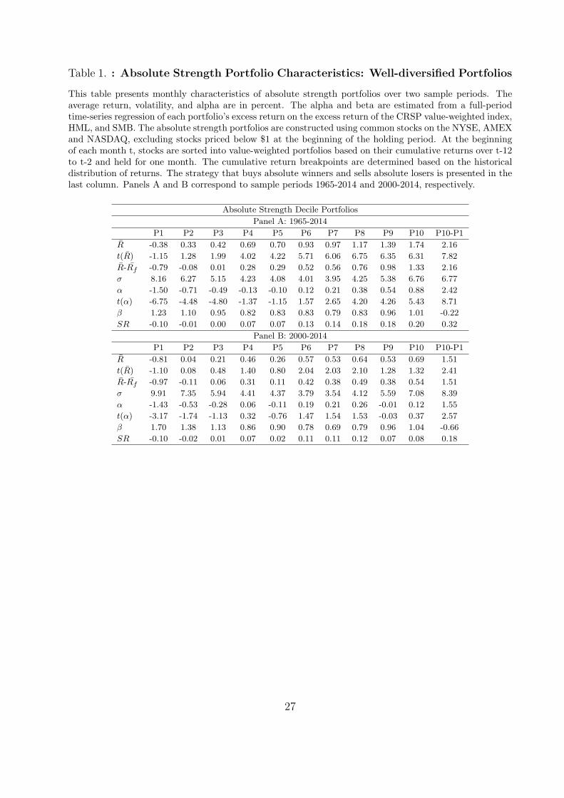
Table 1. : Absolute Strength Portfolio Characteristics: Well-diversified Portfolios

This table presents monthly characteristics of absolute strength portfolios over two sample periods. Theaverage return, volatility, and alpha are in percent. The alpha and beta are estimated from a full-periodtime-series regression of each portfolio’s excess return on the excess return of the CRSP value-weighted index,HML, and SMB. The absolute strength portfolios are constructed using common stocks on the NYSE, AMEXand NASDAQ, excluding stocks priced below $1 at the beginning of the holding period. At the beginningof each month t, stocks are sorted into value-weighted portfolios based on their cumulative returns over t-12to t-2 and held for one month. The cumulative return breakpoints are determined based on the historicaldistribution of returns. The strategy that buys absolute winners and sells absolute losers is presented in thelast column. Panels A and B correspond to sample periods 1965-2014 and 2000-2014, respectively.

Absolute Strength Decile Portfolios

Panel A: 1965-2014

P1 P2 P3 P4 P5 P6 P7 P8 P9 P10 P10-P1

R̄ -0.38 0.33 0.42 0.69 0.70 0.93 0.97 1.17 1.39 1.74 2.16

t(R̄) -1.15 1.28 1.99 4.02 4.22 5.71 6.06 6.75 6.35 6.31 7.82

R̄-R̄f -0.79 -0.08 0.01 0.28 0.29 0.52 0.56 0.76 0.98 1.33 2.16

σ 8.16 6.27 5.15 4.23 4.08 4.01 3.95 4.25 5.38 6.76 6.77

α -1.50 -0.71 -0.49 -0.13 -0.10 0.12 0.21 0.38 0.54 0.88 2.42

t(α) -6.75 -4.48 -4.80 -1.37 -1.15 1.57 2.65 4.20 4.26 5.43 8.71

β 1.23 1.10 0.95 0.82 0.83 0.83 0.79 0.83 0.96 1.01 -0.22

SR -0.10 -0.01 0.00 0.07 0.07 0.13 0.14 0.18 0.18 0.20 0.32

Panel B: 2000-2014

P1 P2 P3 P4 P5 P6 P7 P8 P9 P10 P10-P1

R̄ -0.81 0.04 0.21 0.46 0.26 0.57 0.53 0.64 0.53 0.69 1.51

t(R̄) -1.10 0.08 0.48 1.40 0.80 2.04 2.03 2.10 1.28 1.32 2.41

R̄-R̄f -0.97 -0.11 0.06 0.31 0.11 0.42 0.38 0.49 0.38 0.54 1.51

σ 9.91 7.35 5.94 4.41 4.37 3.79 3.54 4.12 5.59 7.08 8.39

α -1.43 -0.53 -0.28 0.06 -0.11 0.19 0.21 0.26 -0.01 0.12 1.55

t(α) -3.17 -1.74 -1.13 0.32 -0.76 1.47 1.54 1.53 -0.03 0.37 2.57

β 1.70 1.38 1.13 0.86 0.90 0.78 0.69 0.79 0.96 1.04 -0.66

SR -0.10 -0.02 0.01 0.07 0.02 0.11 0.11 0.12 0.07 0.08 0.18

27

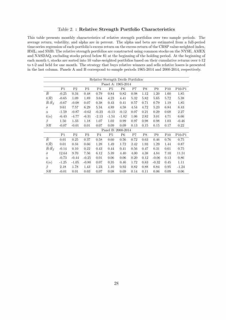
Table 2. : Relative Strength Portfolio Characteristics

This table presents monthly characteristics of relative strength portfolios over two sample periods. Theaverage return, volatility, and alpha are in percent. The alpha and beta are estimated from a full-periodtime-series regression of each portfolio’s excess return on the excess return of the CRSP value-weighted index,HML, and SMB. The relative strength portfolios are constructed using common stocks on the NYSE, AMEXand NASDAQ, excluding stocks priced below $1 at the beginning of the holding period. At the beginning ofeach month t, stocks are sorted into 10 value-weighted portfolios based on their cumulative returns over t-12to t-2 and held for one month. The strategy that buys relative winners and sells relative losers is presentedin the last column. Panels A and B correspond to sample periods 1965-2014 and 2000-2014, respectively.

Relative Strength Decile Portfolios

Panel A: 1965-2014

P1 P2 P3 P4 P5 P6 P7 P8 P9 P10 P10-P1

R̄ -0.25 0.34 0.48 0.79 0.84 0.82 0.98 1.12 1.20 1.60 1.85

t(R̄) -0.65 1.09 1.89 3.64 4.23 4.41 5.32 5.82 5.65 5.72 5.38

R̄-R̄f -0.67 -0.08 0.07 0.38 0.43 0.41 0.57 0.71 0.79 1.19 1.85

σ 9.61 7.57 6.29 5.34 4.89 4.58 4.54 4.72 5.23 6.84 8.43

α -1.59 -0.87 -0.62 -0.23 -0.13 -0.12 0.07 0.21 0.29 0.68 2.27

t(α) -6.43 -4.77 -6.31 -2.13 -1.54 -1.82 1.06 2.82 3.01 4.71 6.66

β 1.50 1.33 1.18 1.07 1.02 0.99 0.97 0.98 0.98 1.03 -0.46

SR -0.07 -0.01 0.01 0.07 0.09 0.09 0.13 0.15 0.15 0.17 0.22

Panel B: 2000-2014

P1 P2 P3 P4 P5 P6 P7 P8 P9 P10 P10-P1

R̄ 0.01 0.25 0.37 0.58 0.60 0.56 0.72 0.63 0.46 0.76 0.75

t(R̄) 0.01 0.34 0.66 1.28 1.49 1.72 2.42 1.93 1.29 1.44 0.87

R̄-R̄f -0.14 0.10 0.22 0.43 0.44 0.41 0.56 0.47 0.31 0.61 0.75

σ 12.64 9.70 7.56 6.12 5.39 4.40 4.00 4.38 4.84 7.10 11.51

α -0.73 -0.44 -0.25 0.01 0.06 0.06 0.20 0.12 -0.06 0.13 0.86

t(α) -1.25 -1.05 -0.80 0.07 0.35 0.46 1.72 0.83 -0.32 0.45 1.11

β 2.18 1.78 1.43 1.23 1.10 0.92 0.82 0.88 0.84 0.95 -1.24

SR -0.01 0.01 0.03 0.07 0.08 0.09 0.14 0.11 0.06 0.09 0.06

28

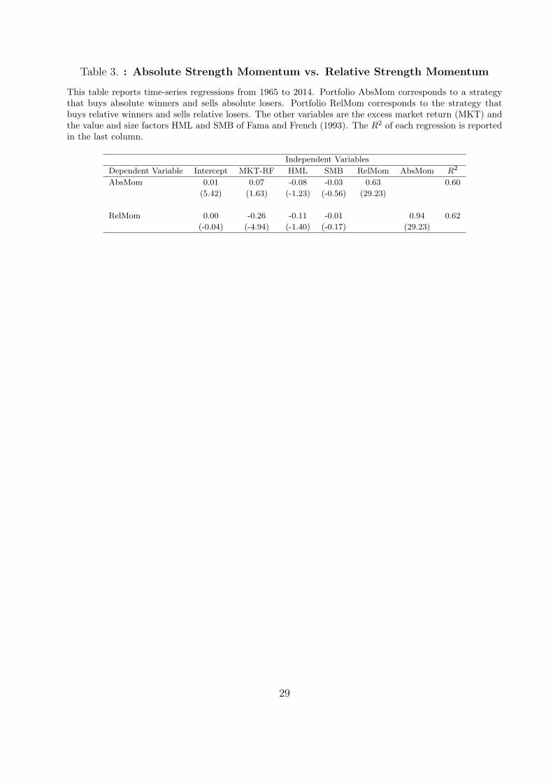
Table 3. : Absolute Strength Momentum vs. Relative Strength Momentum

This table reports time-series regressions from 1965 to 2014. Portfolio AbsMom corresponds to a strategythat buys absolute winners and sells absolute losers. Portfolio RelMom corresponds to the strategy thatbuys relative winners and sells relative losers. The other variables are the excess market return (MKT) andthe value and size factors HML and SMB of Fama and French (1993). The R2 of each regression is reportedin the last column.

Independent Variables

Dependent Variable Intercept MKT-RF HML SMB RelMom AbsMom R2

AbsMom 0.01 0.07 -0.08 -0.03 0.63 0.60

(5.42) (1.63) (-1.23) (-0.56) (29.23)

RelMom 0.00 -0.26 -0.11 -0.01 0.94 0.62

(-0.04) (-4.94) (-1.40) (-0.17) (29.23)

29

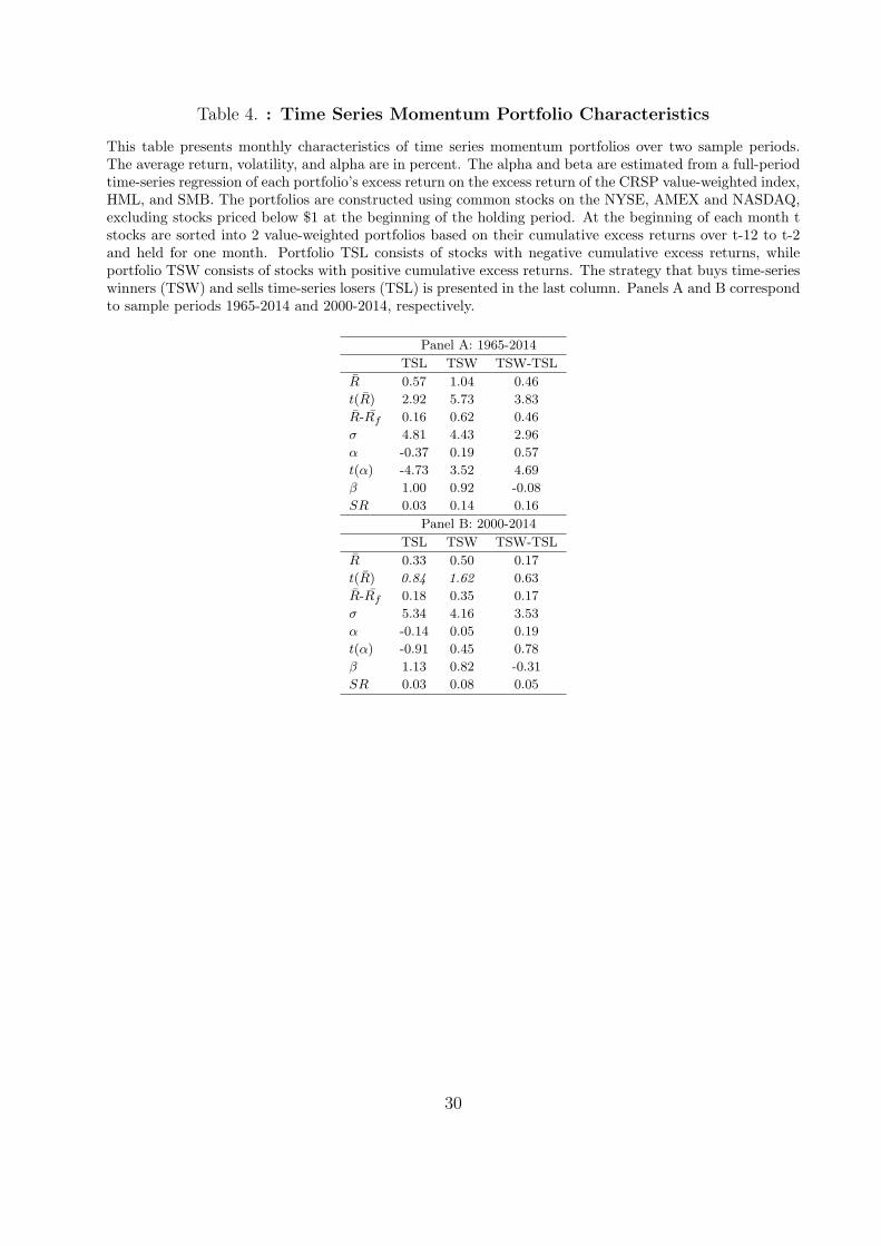
Table 4. : Time Series Momentum Portfolio Characteristics

This table presents monthly characteristics of time series momentum portfolios over two sample periods.The average return, volatility, and alpha are in percent. The alpha and beta are estimated from a full-periodtime-series regression of each portfolio’s excess return on the excess return of the CRSP value-weighted index,HML, and SMB. The portfolios are constructed using common stocks on the NYSE, AMEX and NASDAQ,excluding stocks priced below $1 at the beginning of the holding period. At the beginning of each month tstocks are sorted into 2 value-weighted portfolios based on their cumulative excess returns over t-12 to t-2and held for one month. Portfolio TSL consists of stocks with negative cumulative excess returns, whileportfolio TSW consists of stocks with positive cumulative excess returns. The strategy that buys time-serieswinners (TSW) and sells time-series losers (TSL) is presented in the last column. Panels A and B correspondto sample periods 1965-2014 and 2000-2014, respectively.

Panel A: 1965-2014

TSL TSW TSW-TSL

R̄ 0.57 1.04 0.46

t(R̄) 2.92 5.73 3.83

R̄-R̄f 0.16 0.62 0.46

σ 4.81 4.43 2.96

α -0.37 0.19 0.57

t(α) -4.73 3.52 4.69

β 1.00 0.92 -0.08

SR 0.03 0.14 0.16

Panel B: 2000-2014

TSL TSW TSW-TSL

R̄ 0.33 0.50 0.17

t(R̄) 0.84 1.62 0.63

R̄-R̄f 0.18 0.35 0.17

σ 5.34 4.16 3.53

α -0.14 0.05 0.19

t(α) -0.91 0.45 0.78

β 1.13 0.82 -0.31

SR 0.03 0.08 0.05

30

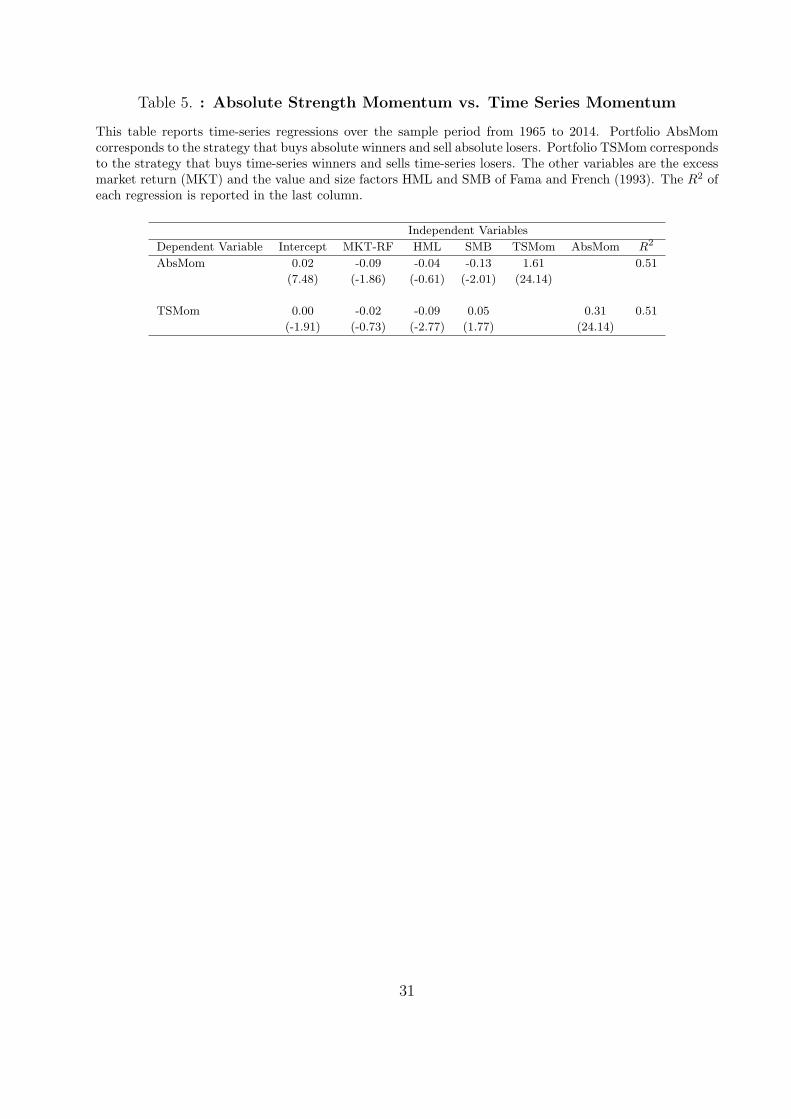
Table 5. : Absolute Strength Momentum vs. Time Series Momentum

This table reports time-series regressions over the sample period from 1965 to 2014. Portfolio AbsMomcorresponds to the strategy that buys absolute winners and sell absolute losers. Portfolio TSMom correspondsto the strategy that buys time-series winners and sells time-series losers. The other variables are the excessmarket return (MKT) and the value and size factors HML and SMB of Fama and French (1993). The R2 ofeach regression is reported in the last column.

Independent Variables

Dependent Variable Intercept MKT-RF HML SMB TSMom AbsMom R2

AbsMom 0.02 -0.09 -0.04 -0.13 1.61 0.51

(7.48) (-1.86) (-0.61) (-2.01) (24.14)

TSMom 0.00 -0.02 -0.09 0.05 0.31 0.51

(-1.91) (-0.73) (-2.77) (1.77) (24.14)

31

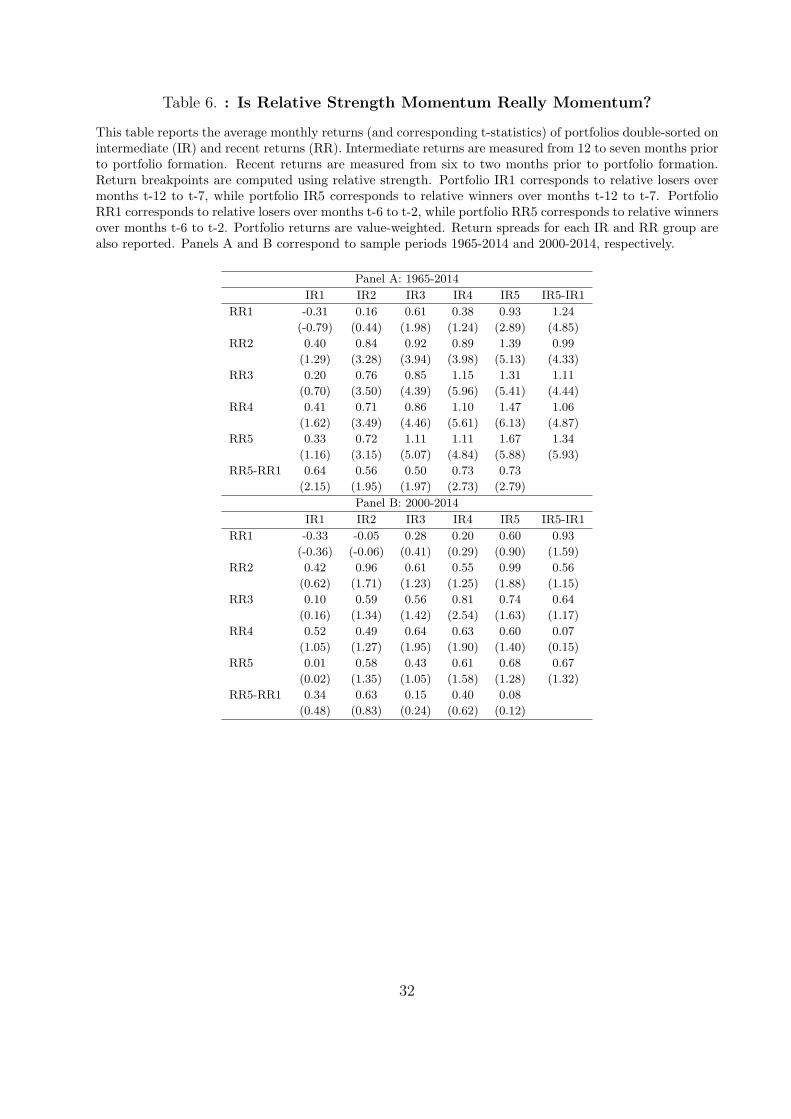
Table 6. : Is Relative Strength Momentum Really Momentum?

This table reports the average monthly returns (and corresponding t-statistics) of portfolios double-sorted onintermediate (IR) and recent returns (RR). Intermediate returns are measured from 12 to seven months priorto portfolio formation. Recent returns are measured from six to two months prior to portfolio formation.Return breakpoints are computed using relative strength. Portfolio IR1 corresponds to relative losers overmonths t-12 to t-7, while portfolio IR5 corresponds to relative winners over months t-12 to t-7. PortfolioRR1 corresponds to relative losers over months t-6 to t-2, while portfolio RR5 corresponds to relative winnersover months t-6 to t-2. Portfolio returns are value-weighted. Return spreads for each IR and RR group arealso reported. Panels A and B correspond to sample periods 1965-2014 and 2000-2014, respectively.

Panel A: 1965-2014

IR1 IR2 IR3 IR4 IR5 IR5-IR1

RR1 -0.31 0.16 0.61 0.38 0.93 1.24

(-0.79) (0.44) (1.98) (1.24) (2.89) (4.85)

RR2 0.40 0.84 0.92 0.89 1.39 0.99

(1.29) (3.28) (3.94) (3.98) (5.13) (4.33)

RR3 0.20 0.76 0.85 1.15 1.31 1.11

(0.70) (3.50) (4.39) (5.96) (5.41) (4.44)

RR4 0.41 0.71 0.86 1.10 1.47 1.06

(1.62) (3.49) (4.46) (5.61) (6.13) (4.87)

RR5 0.33 0.72 1.11 1.11 1.67 1.34

(1.16) (3.15) (5.07) (4.84) (5.88) (5.93)

RR5-RR1 0.64 0.56 0.50 0.73 0.73

(2.15) (1.95) (1.97) (2.73) (2.79)

Panel B: 2000-2014

IR1 IR2 IR3 IR4 IR5 IR5-IR1

RR1 -0.33 -0.05 0.28 0.20 0.60 0.93

(-0.36) (-0.06) (0.41) (0.29) (0.90) (1.59)

RR2 0.42 0.96 0.61 0.55 0.99 0.56

(0.62) (1.71) (1.23) (1.25) (1.88) (1.15)

RR3 0.10 0.59 0.56 0.81 0.74 0.64

(0.16) (1.34) (1.42) (2.54) (1.63) (1.17)

RR4 0.52 0.49 0.64 0.63 0.60 0.07

(1.05) (1.27) (1.95) (1.90) (1.40) (0.15)

RR5 0.01 0.58 0.43 0.61 0.68 0.67

(0.02) (1.35) (1.05) (1.58) (1.28) (1.32)

RR5-RR1 0.34 0.63 0.15 0.40 0.08

(0.48) (0.83) (0.24) (0.62) (0.12)

32

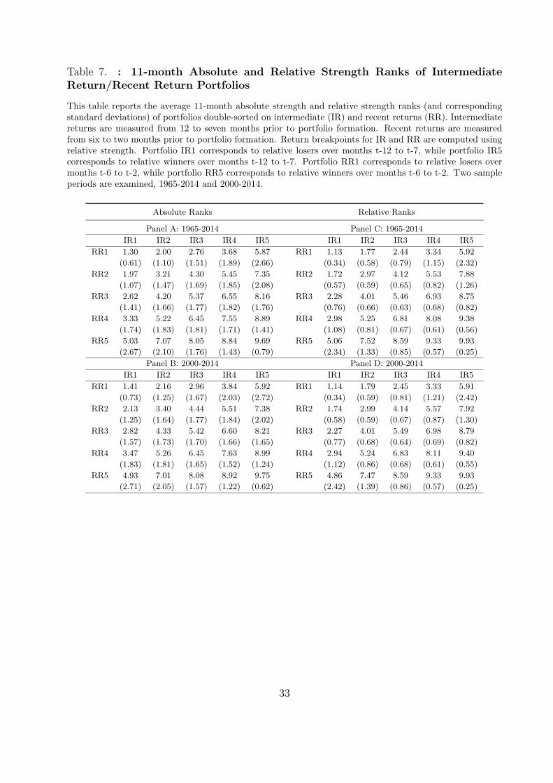
Table 7. : 11-month Absolute and Relative Strength Ranks of IntermediateReturn/Recent Return Portfolios

This table reports the average 11-month absolute strength and relative strength ranks (and correspondingstandard deviations) of portfolios double-sorted on intermediate (IR) and recent returns (RR). Intermediatereturns are measured from 12 to seven months prior to portfolio formation. Recent returns are measuredfrom six to two months prior to portfolio formation. Return breakpoints for IR and RR are computed usingrelative strength. Portfolio IR1 corresponds to relative losers over months t-12 to t-7, while portfolio IR5corresponds to relative winners over months t-12 to t-7. Portfolio RR1 corresponds to relative losers overmonths t-6 to t-2, while portfolio RR5 corresponds to relative winners over months t-6 to t-2. Two sampleperiods are examined, 1965-2014 and 2000-2014.

Absolute Ranks Relative Ranks

Panel A: 1965-2014 Panel C: 1965-2014

IR1 IR2 IR3 IR4 IR5 IR1 IR2 IR3 IR4 IR5

RR1 1.30 2.00 2.76 3.68 5.87 RR1 1.13 1.77 2.44 3.34 5.92

(0.61) (1.10) (1.51) (1.89) (2.66) (0.34) (0.58) (0.79) (1.15) (2.32)

RR2 1.97 3.21 4.30 5.45 7.35 RR2 1.72 2.97 4.12 5.53 7.88

(1.07) (1.47) (1.69) (1.85) (2.08) (0.57) (0.59) (0.65) (0.82) (1.26)

RR3 2.62 4.20 5.37 6.55 8.16 RR3 2.28 4.01 5.46 6.93 8.75

(1.41) (1.66) (1.77) (1.82) (1.76) (0.76) (0.66) (0.63) (0.68) (0.82)

RR4 3.33 5.22 6.45 7.55 8.89 RR4 2.98 5.25 6.81 8.08 9.38

(1.74) (1.83) (1.81) (1.71) (1.41) (1.08) (0.81) (0.67) (0.61) (0.56)

RR5 5.03 7.07 8.05 8.84 9.69 RR5 5.06 7.52 8.59 9.33 9.93

(2.67) (2.10) (1.76) (1.43) (0.79) (2.34) (1.33) (0.85) (0.57) (0.25)

Panel B: 2000-2014 Panel D: 2000-2014

IR1 IR2 IR3 IR4 IR5 IR1 IR2 IR3 IR4 IR5

RR1 1.41 2.16 2.96 3.84 5.92 RR1 1.14 1.79 2.45 3.33 5.91

(0.73) (1.25) (1.67) (2.03) (2.72) (0.34) (0.59) (0.81) (1.21) (2.42)

RR2 2.13 3.40 4.44 5.51 7.38 RR2 1.74 2.99 4.14 5.57 7.92

(1.25) (1.64) (1.77) (1.84) (2.02) (0.58) (0.59) (0.67) (0.87) (1.30)

RR3 2.82 4.33 5.42 6.60 8.21 RR3 2.27 4.01 5.49 6.98 8.79

(1.57) (1.73) (1.70) (1.66) (1.65) (0.77) (0.68) (0.64) (0.69) (0.82)

RR4 3.47 5.26 6.45 7.63 8.99 RR4 2.94 5.24 6.83 8.11 9.40

(1.83) (1.81) (1.65) (1.52) (1.24) (1.12) (0.86) (0.68) (0.61) (0.55)

RR5 4.93 7.01 8.08 8.92 9.75 RR5 4.86 7.47 8.59 9.33 9.93

(2.71) (2.05) (1.57) (1.22) (0.62) (2.42) (1.39) (0.86) (0.57) (0.25)

33

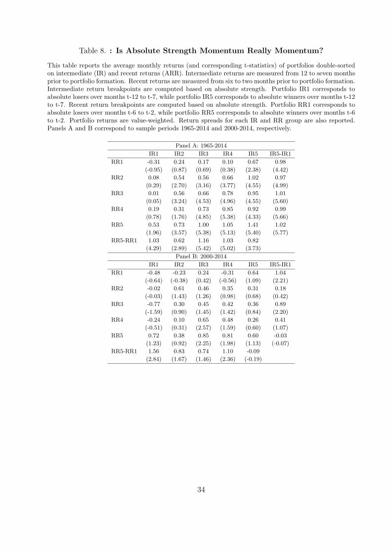
Table 8. : Is Absolute Strength Momentum Really Momentum?

This table reports the average monthly returns (and corresponding t-statistics) of portfolios double-sortedon intermediate (IR) and recent returns (ARR). Intermediate returns are measured from 12 to seven monthsprior to portfolio formation. Recent returns are measured from six to two months prior to portfolio formation.Intermediate return breakpoints are computed based on absolute strength. Portfolio IR1 corresponds toabsolute losers over months t-12 to t-7, while portfolio IR5 corresponds to absolute winners over months t-12to t-7. Recent return breakpoints are computed based on absolute strength. Portfolio RR1 corresponds toabsolute losers over months t-6 to t-2, while portfolio RR5 corresponds to absolute winners over months t-6to t-2. Portfolio returns are value-weighted. Return spreads for each IR and RR group are also reported.Panels A and B correspond to sample periods 1965-2014 and 2000-2014, respectively.

Panel A: 1965-2014

IR1 IR2 IR3 IR4 IR5 IR5-IR1

RR1 -0.31 0.24 0.17 0.10 0.67 0.98

(-0.95) (0.87) (0.69) (0.38) (2.38) (4.42)

RR2 0.08 0.54 0.56 0.66 1.02 0.97

(0.29) (2.70) (3.16) (3.77) (4.55) (4.99)

RR3 0.01 0.56 0.66 0.78 0.95 1.01

(0.05) (3.24) (4.53) (4.96) (4.55) (5.60)

RR4 0.19 0.31 0.73 0.85 0.92 0.99

(0.78) (1.76) (4.85) (5.38) (4.33) (5.66)

RR5 0.53 0.73 1.00 1.05 1.41 1.02

(1.96) (3.57) (5.38) (5.13) (5.40) (5.77)

RR5-RR1 1.03 0.62 1.16 1.03 0.82

(4.29) (2.89) (5.42) (5.02) (3.73)

Panel B: 2000-2014

IR1 IR2 IR3 IR4 IR5 IR5-IR1

RR1 -0.48 -0.23 0.24 -0.31 0.64 1.04

(-0.64) (-0.38) (0.42) (-0.56) (1.09) (2.21)

RR2 -0.02 0.61 0.46 0.35 0.31 0.18

(-0.03) (1.43) (1.26) (0.98) (0.68) (0.42)

RR3 -0.77 0.30 0.45 0.42 0.36 0.89

(-1.59) (0.90) (1.45) (1.42) (0.84) (2.20)

RR4 -0.24 0.10 0.65 0.48 0.26 0.41

(-0.51) (0.31) (2.57) (1.59) (0.60) (1.07)

RR5 0.72 0.38 0.85 0.81 0.60 -0.03

(1.23) (0.92) (2.25) (1.98) (1.13) (-0.07)

RR5-RR1 1.56 0.83 0.74 1.10 -0.09

(2.84) (1.67) (1.46) (2.36) (-0.19)

34

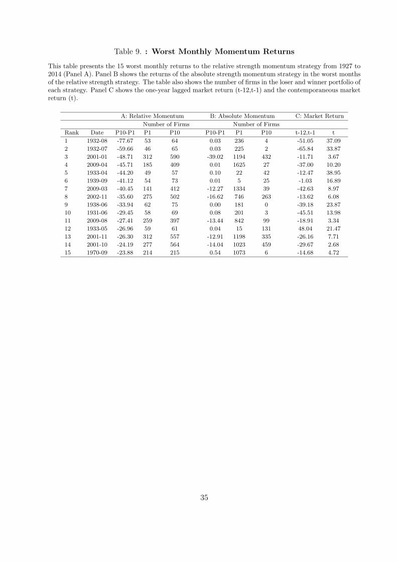
Table 9. : Worst Monthly Momentum Returns

This table presents the 15 worst monthly returns to the relative strength momentum strategy from 1927 to2014 (Panel A). Panel B shows the returns of the absolute strength momentum strategy in the worst monthsof the relative strength strategy. The table also shows the number of firms in the loser and winner portfolio ofeach strategy. Panel C shows the one-year lagged market return (t-12,t-1) and the contemporaneous marketreturn (t).

A: Relative Momentum B: Absolute Momentum C: Market Return

Number of Firms Number of Firms

Rank Date P10-P1 P1 P10 P10-P1 P1 P10 t-12,t-1 t

1 1932-08 -77.67 53 64 0.03 236 4 -51.05 37.09

2 1932-07 -59.66 46 65 0.03 225 2 -65.84 33.87

3 2001-01 -48.71 312 590 -39.02 1194 432 -11.71 3.67

4 2009-04 -45.71 185 409 0.01 1625 27 -37.00 10.20

5 1933-04 -44.20 49 57 0.10 22 42 -12.47 38.95

6 1939-09 -41.12 54 73 0.01 5 25 -1.03 16.89

7 2009-03 -40.45 141 412 -12.27 1334 39 -42.63 8.97

8 2002-11 -35.60 275 502 -16.62 746 263 -13.62 6.08

9 1938-06 -33.94 62 75 0.00 181 0 -39.18 23.87

10 1931-06 -29.45 58 69 0.08 201 3 -45.51 13.98

11 2009-08 -27.41 259 397 -13.44 842 99 -18.91 3.34

12 1933-05 -26.96 59 61 0.04 15 131 48.04 21.47

13 2001-11 -26.30 312 557 -12.91 1198 335 -26.16 7.71

14 2001-10 -24.19 277 564 -14.04 1023 459 -29.67 2.68

15 1970-09 -23.88 214 215 0.54 1073 6 -14.68 4.72

35

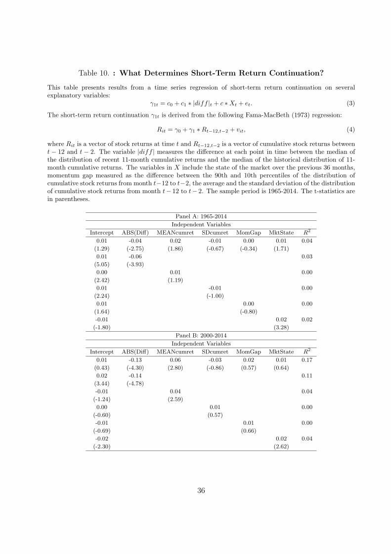
Table 10. : What Determines Short-Term Return Continuation?

This table presents results from a time series regression of short-term return continuation on severalexplanatory variables:

γ1t = c0 + c1 ∗ |diff |t + c ∗Xt + et. (3)

The short-term return continuation γ1t is derived from the following Fama-MacBeth (1973) regression:

Rit = γ0 + γ1 ∗Rt−12,t−2 + vit, (4)

where Rit is a vector of stock returns at time t and Rt−12,t−2 is a vector of cumulative stock returns betweent − 12 and t − 2. The variable |diff | measures the difference at each point in time between the median ofthe distribution of recent 11-month cumulative returns and the median of the historical distribution of 11-month cumulative returns. The variables in X include the state of the market over the previous 36 months,momentum gap measured as the difference between the 90th and 10th percentiles of the distribution ofcumulative stock returns from month t−12 to t−2, the average and the standard deviation of the distributionof cumulative stock returns from month t− 12 to t− 2. The sample period is 1965-2014. The t-statistics arein parentheses.

Panel A: 1965-2014

Independent Variables

Intercept ABS(Diff) MEANcumret SDcumret MomGap MktState R2

0.01 -0.04 0.02 -0.01 0.00 0.01 0.04

(1.29) (-2.75) (1.86) (-0.67) (-0.34) (1.71)

0.01 -0.06 0.03

(5.05) (-3.93)

0.00 0.01 0.00

(2.42) (1.19)

0.01 -0.01 0.00

(2.24) (-1.00)

0.01 0.00 0.00

(1.64) (-0.80)

-0.01 0.02 0.02

(-1.80) (3.28)

Panel B: 2000-2014

Independent Variables

Intercept ABS(Diff) MEANcumret SDcumret MomGap MktState R2

0.01 -0.13 0.06 -0.03 0.02 0.01 0.17

(0.43) (-4.30) (2.80) (-0.86) (0.57) (0.64)

0.02 -0.14 0.11

(3.44) (-4.78)

-0.01 0.04 0.04

(-1.24) (2.59)

0.00 0.01 0.00

(-0.60) (0.57)

-0.01 0.01 0.00

(-0.69) (0.66)

-0.02 0.02 0.04

(-2.30) (2.62)

36

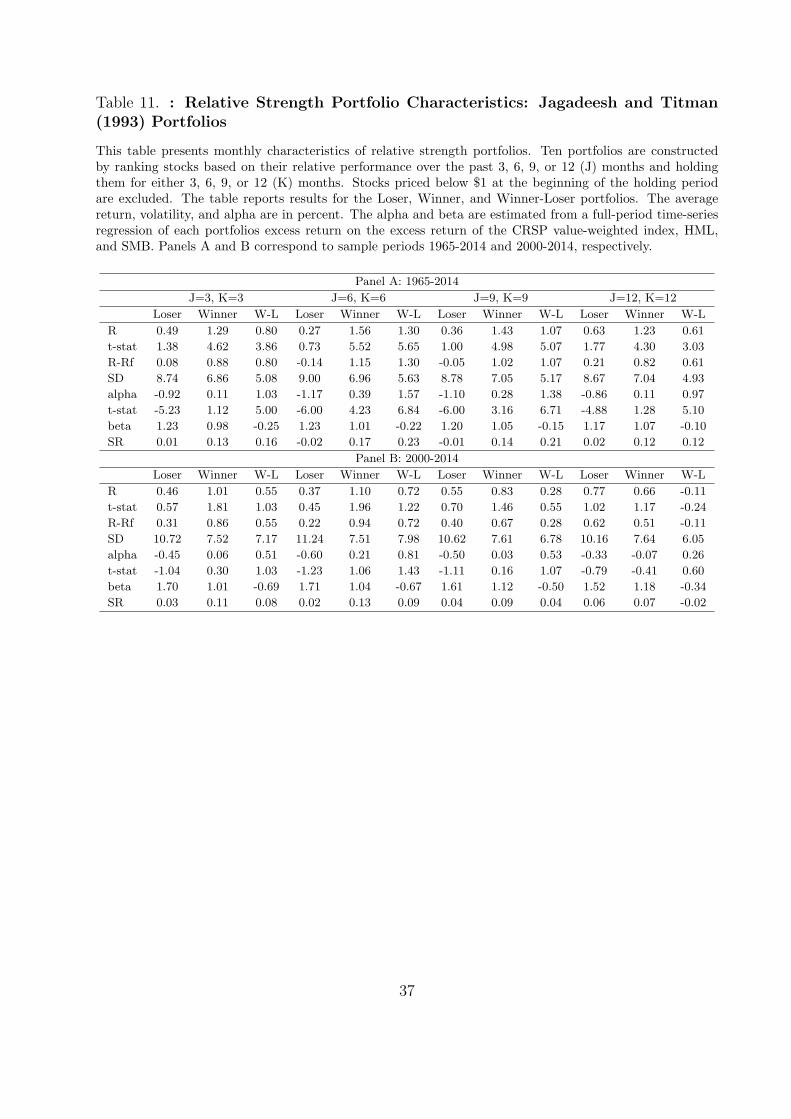
Table 11. : Relative Strength Portfolio Characteristics: Jagadeesh and Titman(1993) Portfolios

This table presents monthly characteristics of relative strength portfolios. Ten portfolios are constructedby ranking stocks based on their relative performance over the past 3, 6, 9, or 12 (J) months and holdingthem for either 3, 6, 9, or 12 (K) months. Stocks priced below $1 at the beginning of the holding periodare excluded. The table reports results for the Loser, Winner, and Winner-Loser portfolios. The averagereturn, volatility, and alpha are in percent. The alpha and beta are estimated from a full-period time-seriesregression of each portfolios excess return on the excess return of the CRSP value-weighted index, HML,and SMB. Panels A and B correspond to sample periods 1965-2014 and 2000-2014, respectively.

Panel A: 1965-2014

J=3, K=3 J=6, K=6 J=9, K=9 J=12, K=12

Loser Winner W-L Loser Winner W-L Loser Winner W-L Loser Winner W-L

R 0.49 1.29 0.80 0.27 1.56 1.30 0.36 1.43 1.07 0.63 1.23 0.61

t-stat 1.38 4.62 3.86 0.73 5.52 5.65 1.00 4.98 5.07 1.77 4.30 3.03

R-Rf 0.08 0.88 0.80 -0.14 1.15 1.30 -0.05 1.02 1.07 0.21 0.82 0.61

SD 8.74 6.86 5.08 9.00 6.96 5.63 8.78 7.05 5.17 8.67 7.04 4.93

alpha -0.92 0.11 1.03 -1.17 0.39 1.57 -1.10 0.28 1.38 -0.86 0.11 0.97

t-stat -5.23 1.12 5.00 -6.00 4.23 6.84 -6.00 3.16 6.71 -4.88 1.28 5.10

beta 1.23 0.98 -0.25 1.23 1.01 -0.22 1.20 1.05 -0.15 1.17 1.07 -0.10

SR 0.01 0.13 0.16 -0.02 0.17 0.23 -0.01 0.14 0.21 0.02 0.12 0.12

Panel B: 2000-2014

Loser Winner W-L Loser Winner W-L Loser Winner W-L Loser Winner W-L

R 0.46 1.01 0.55 0.37 1.10 0.72 0.55 0.83 0.28 0.77 0.66 -0.11

t-stat 0.57 1.81 1.03 0.45 1.96 1.22 0.70 1.46 0.55 1.02 1.17 -0.24

R-Rf 0.31 0.86 0.55 0.22 0.94 0.72 0.40 0.67 0.28 0.62 0.51 -0.11

SD 10.72 7.52 7.17 11.24 7.51 7.98 10.62 7.61 6.78 10.16 7.64 6.05

alpha -0.45 0.06 0.51 -0.60 0.21 0.81 -0.50 0.03 0.53 -0.33 -0.07 0.26

t-stat -1.04 0.30 1.03 -1.23 1.06 1.43 -1.11 0.16 1.07 -0.79 -0.41 0.60

beta 1.70 1.01 -0.69 1.71 1.04 -0.67 1.61 1.12 -0.50 1.52 1.18 -0.34

SR 0.03 0.11 0.08 0.02 0.13 0.09 0.04 0.09 0.04 0.06 0.07 -0.02

37

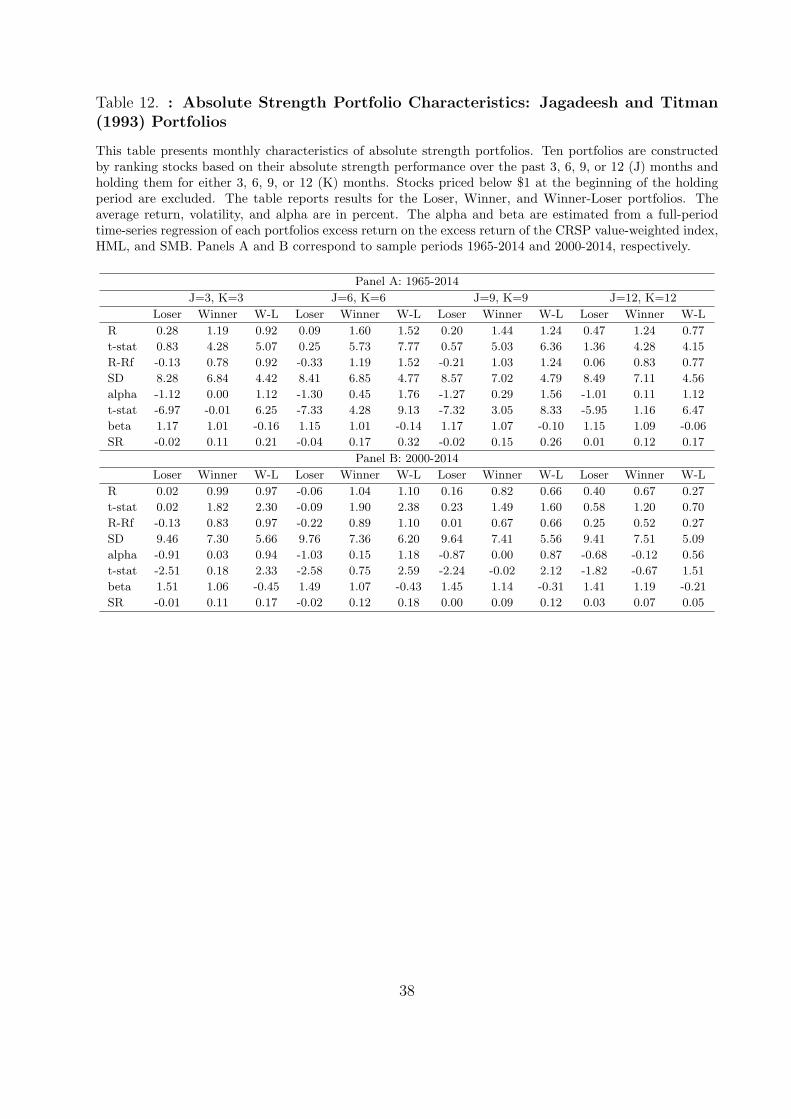
Table 12. : Absolute Strength Portfolio Characteristics: Jagadeesh and Titman(1993) Portfolios

This table presents monthly characteristics of absolute strength portfolios. Ten portfolios are constructedby ranking stocks based on their absolute strength performance over the past 3, 6, 9, or 12 (J) months andholding them for either 3, 6, 9, or 12 (K) months. Stocks priced below $1 at the beginning of the holdingperiod are excluded. The table reports results for the Loser, Winner, and Winner-Loser portfolios. Theaverage return, volatility, and alpha are in percent. The alpha and beta are estimated from a full-periodtime-series regression of each portfolios excess return on the excess return of the CRSP value-weighted index,HML, and SMB. Panels A and B correspond to sample periods 1965-2014 and 2000-2014, respectively.

Panel A: 1965-2014

J=3, K=3 J=6, K=6 J=9, K=9 J=12, K=12

Loser Winner W-L Loser Winner W-L Loser Winner W-L Loser Winner W-L

R 0.28 1.19 0.92 0.09 1.60 1.52 0.20 1.44 1.24 0.47 1.24 0.77

t-stat 0.83 4.28 5.07 0.25 5.73 7.77 0.57 5.03 6.36 1.36 4.28 4.15

R-Rf -0.13 0.78 0.92 -0.33 1.19 1.52 -0.21 1.03 1.24 0.06 0.83 0.77

SD 8.28 6.84 4.42 8.41 6.85 4.77 8.57 7.02 4.79 8.49 7.11 4.56

alpha -1.12 0.00 1.12 -1.30 0.45 1.76 -1.27 0.29 1.56 -1.01 0.11 1.12

t-stat -6.97 -0.01 6.25 -7.33 4.28 9.13 -7.32 3.05 8.33 -5.95 1.16 6.47

beta 1.17 1.01 -0.16 1.15 1.01 -0.14 1.17 1.07 -0.10 1.15 1.09 -0.06

SR -0.02 0.11 0.21 -0.04 0.17 0.32 -0.02 0.15 0.26 0.01 0.12 0.17

Panel B: 2000-2014

Loser Winner W-L Loser Winner W-L Loser Winner W-L Loser Winner W-L

R 0.02 0.99 0.97 -0.06 1.04 1.10 0.16 0.82 0.66 0.40 0.67 0.27

t-stat 0.02 1.82 2.30 -0.09 1.90 2.38 0.23 1.49 1.60 0.58 1.20 0.70

R-Rf -0.13 0.83 0.97 -0.22 0.89 1.10 0.01 0.67 0.66 0.25 0.52 0.27

SD 9.46 7.30 5.66 9.76 7.36 6.20 9.64 7.41 5.56 9.41 7.51 5.09

alpha -0.91 0.03 0.94 -1.03 0.15 1.18 -0.87 0.00 0.87 -0.68 -0.12 0.56

t-stat -2.51 0.18 2.33 -2.58 0.75 2.59 -2.24 -0.02 2.12 -1.82 -0.67 1.51

beta 1.51 1.06 -0.45 1.49 1.07 -0.43 1.45 1.14 -0.31 1.41 1.19 -0.21

SR -0.01 0.11 0.17 -0.02 0.12 0.18 0.00 0.09 0.12 0.03 0.07 0.05

38

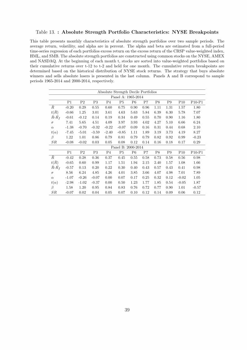
Table 13. : Absolute Strength Portfolio Characteristics: NYSE Breakpoints

This table presents monthly characteristics of absolute strength portfolios over two sample periods. Theaverage return, volatility, and alpha are in percent. The alpha and beta are estimated from a full-periodtime-series regression of each portfolios excess return on the excess return of the CRSP value-weighted index,HML, and SMB. The absolute strength portfolios are constructed using common stocks on the NYSE, AMEXand NASDAQ. At the beginning of each month t, stocks are sorted into value-weighted portfolios based ontheir cumulative returns over t-12 to t-2 and held for one month. The cumulative return breakpoints aredetermined based on the historical distribution of NYSE stock returns. The strategy that buys absolutewinners and sells absolute losers is presented in the last column. Panels A and B correspond to sampleperiods 1965-2014 and 2000-2014, respectively.

Absolute Strength Decile Portfolios

Panel A: 1965-2014

P1 P2 P3 P4 P5 P6 P7 P8 P9 P10 P10-P1

R̄ -0.20 0.29 0.55 0.60 0.75 0.90 0.96 1.11 1.31 1.57 1.80

t(R̄) -0.66 1.25 3.01 3.61 4.63 5.63 5.84 6.39 6.30 5.78 7.07

R̄-R̄f -0.61 -0.12 0.14 0.19 0.34 0.49 0.55 0.70 0.90 1.16 1.80

σ 7.41 5.65 4.51 4.09 3.97 3.93 4.02 4.27 5.10 6.66 6.24

α -1.38 -0.70 -0.32 -0.22 -0.07 0.09 0.16 0.31 0.44 0.68 2.10

t(α) -7.45 -5.01 -3.59 -2.40 -0.85 1.11 1.89 3.19 3.73 4.19 8.27

β 1.22 1.01 0.86 0.79 0.81 0.79 0.79 0.82 0.92 0.99 -0.23

SR -0.08 -0.02 0.03 0.05 0.08 0.12 0.14 0.16 0.18 0.17 0.29

Panel B: 2000-2014

P1 P2 P3 P4 P5 P6 P7 P8 P9 P10 P10-P1

R̄ -0.42 0.28 0.36 0.37 0.45 0.55 0.58 0.73 0.58 0.56 0.98

t(R̄) -0.65 0.60 0.99 1.17 1.51 1.94 2.15 2.40 1.57 1.08 1.66

R̄-R̄f -0.57 0.13 0.20 0.22 0.30 0.40 0.43 0.57 0.43 0.41 0.98

σ 8.56 6.24 4.85 4.26 4.01 3.85 3.66 4.07 4.98 7.01 7.89

α -1.07 -0.26 -0.07 0.00 0.07 0.17 0.25 0.32 0.12 -0.02 1.05

t(α) -2.98 -1.02 -0.37 0.00 0.50 1.23 1.77 1.85 0.54 -0.05 1.87

β 1.58 1.20 0.95 0.84 0.83 0.76 0.72 0.77 0.90 1.01 -0.57

SR -0.07 0.02 0.04 0.05 0.07 0.10 0.12 0.14 0.09 0.06 0.12

39

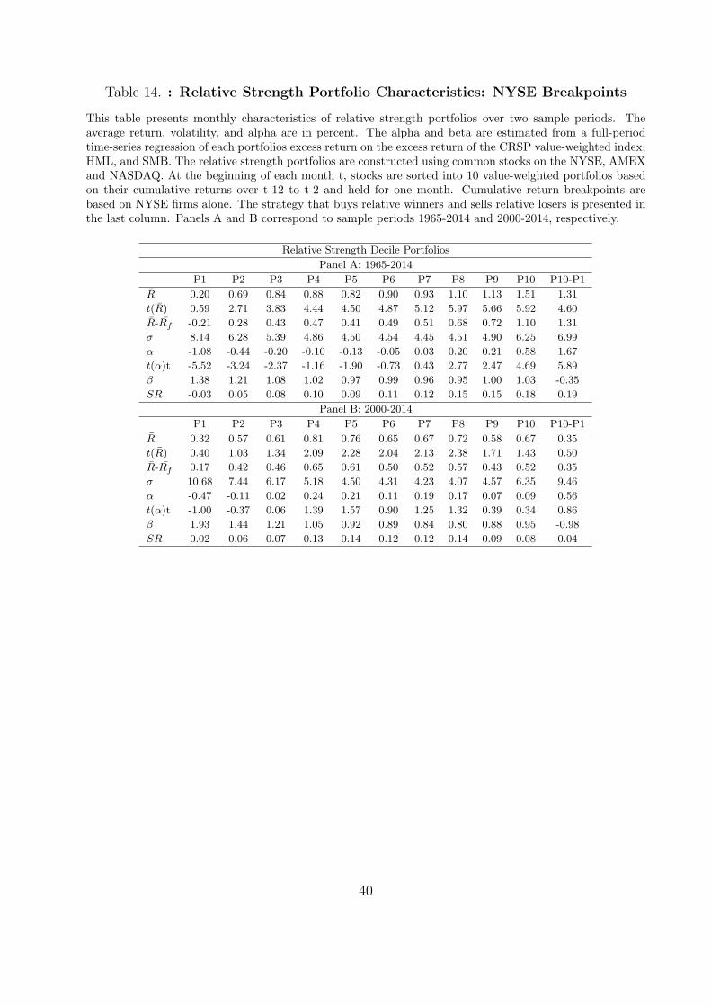
Table 14. : Relative Strength Portfolio Characteristics: NYSE Breakpoints

This table presents monthly characteristics of relative strength portfolios over two sample periods. Theaverage return, volatility, and alpha are in percent. The alpha and beta are estimated from a full-periodtime-series regression of each portfolios excess return on the excess return of the CRSP value-weighted index,HML, and SMB. The relative strength portfolios are constructed using common stocks on the NYSE, AMEXand NASDAQ. At the beginning of each month t, stocks are sorted into 10 value-weighted portfolios basedon their cumulative returns over t-12 to t-2 and held for one month. Cumulative return breakpoints arebased on NYSE firms alone. The strategy that buys relative winners and sells relative losers is presented inthe last column. Panels A and B correspond to sample periods 1965-2014 and 2000-2014, respectively.

Relative Strength Decile Portfolios

Panel A: 1965-2014

P1 P2 P3 P4 P5 P6 P7 P8 P9 P10 P10-P1

R̄ 0.20 0.69 0.84 0.88 0.82 0.90 0.93 1.10 1.13 1.51 1.31

t(R̄) 0.59 2.71 3.83 4.44 4.50 4.87 5.12 5.97 5.66 5.92 4.60

R̄-R̄f -0.21 0.28 0.43 0.47 0.41 0.49 0.51 0.68 0.72 1.10 1.31

σ 8.14 6.28 5.39 4.86 4.50 4.54 4.45 4.51 4.90 6.25 6.99

α -1.08 -0.44 -0.20 -0.10 -0.13 -0.05 0.03 0.20 0.21 0.58 1.67

t(α)t -5.52 -3.24 -2.37 -1.16 -1.90 -0.73 0.43 2.77 2.47 4.69 5.89

β 1.38 1.21 1.08 1.02 0.97 0.99 0.96 0.95 1.00 1.03 -0.35

SR -0.03 0.05 0.08 0.10 0.09 0.11 0.12 0.15 0.15 0.18 0.19

Panel B: 2000-2014

P1 P2 P3 P4 P5 P6 P7 P8 P9 P10 P10-P1

R̄ 0.32 0.57 0.61 0.81 0.76 0.65 0.67 0.72 0.58 0.67 0.35

t(R̄) 0.40 1.03 1.34 2.09 2.28 2.04 2.13 2.38 1.71 1.43 0.50

R̄-R̄f 0.17 0.42 0.46 0.65 0.61 0.50 0.52 0.57 0.43 0.52 0.35

σ 10.68 7.44 6.17 5.18 4.50 4.31 4.23 4.07 4.57 6.35 9.46

α -0.47 -0.11 0.02 0.24 0.21 0.11 0.19 0.17 0.07 0.09 0.56

t(α)t -1.00 -0.37 0.06 1.39 1.57 0.90 1.25 1.32 0.39 0.34 0.86

β 1.93 1.44 1.21 1.05 0.92 0.89 0.84 0.80 0.88 0.95 -0.98

SR 0.02 0.06 0.07 0.13 0.14 0.12 0.12 0.14 0.09 0.08 0.04

40

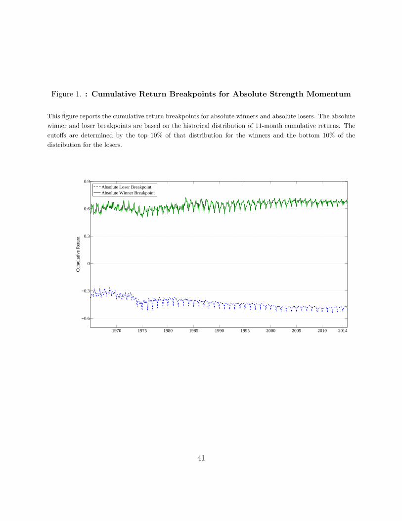
Figure 1. : Cumulative Return Breakpoints for Absolute Strength Momentum

This figure reports the cumulative return breakpoints for absolute winners and absolute losers. The absolute

winner and loser breakpoints are based on the historical distribution of 11-month cumulative returns. The

cutoffs are determined by the top 10% of that distribution for the winners and the bottom 10% of the

distribution for the losers.

1970 1975 1980 1985 1990 1995 2000 2005 2010 2014

−0.6

−0.3

0

0.3

0.6

0.9

Cum

ulat

ive

Ret

urn

Absolute Loser BreakpointAbsolute Winner Breakpoint

41

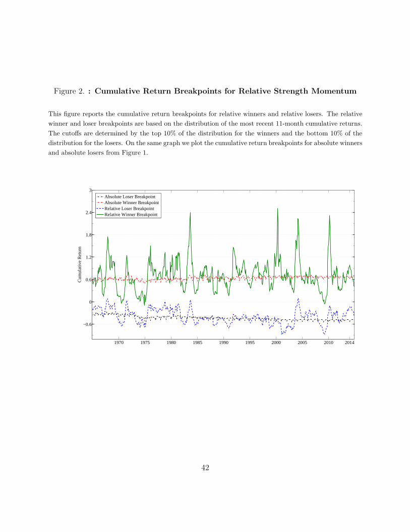
Figure 2. : Cumulative Return Breakpoints for Relative Strength Momentum

This figure reports the cumulative return breakpoints for relative winners and relative losers. The relative

winner and loser breakpoints are based on the distribution of the most recent 11-month cumulative returns.

The cutoffs are determined by the top 10% of the distribution for the winners and the bottom 10% of the

distribution for the losers. On the same graph we plot the cumulative return breakpoints for absolute winners

and absolute losers from Figure 1.

1970 1975 1980 1985 1990 1995 2000 2005 2010 2014

−0.6

0

0.6

1.2

1.8

2.4

3

Cum

ulat

ive

Ret

urn

Absolute Loser BreakpointAbsolute Winner BreakpointRelative Loser BreakpointRelative Winner Breakpoint

42

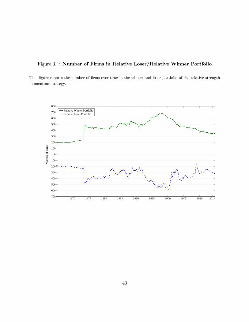
Figure 3. : Number of Firms in Relative Loser/Relative Winner Portfolio

This figure reports the number of firms over time in the winner and loser portfolio of the relative strength

momentum strategy.

1970 1975 1980 1985 1990 1995 2000 2005 2010 2014700

600

500

400

300

200

100

0

100

200

300

400

500

600

700

800

Num

ber

of F

irms

Relative Winner PortfolioRelative Loser Portfolio

43

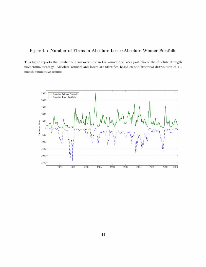
Figure 4. : Number of Firms in Absolute Loser/Absolute Winner Portfolio

This figure reports the number of firms over time in the winner and loser portfolio of the absolute strength

momentum strategy. Absolute winners and losers are identified based on the historical distribution of 11-

month cumulative returns.

1970 1975 1980 1985 1990 1995 2000 2005 2010 2014

2500

2000

1500

1000

500

0

500

1000

1500

2000

2500

Num

ber

of F

irms

Absolute Winner PortfolioAbsolute Loser Portfolio

44

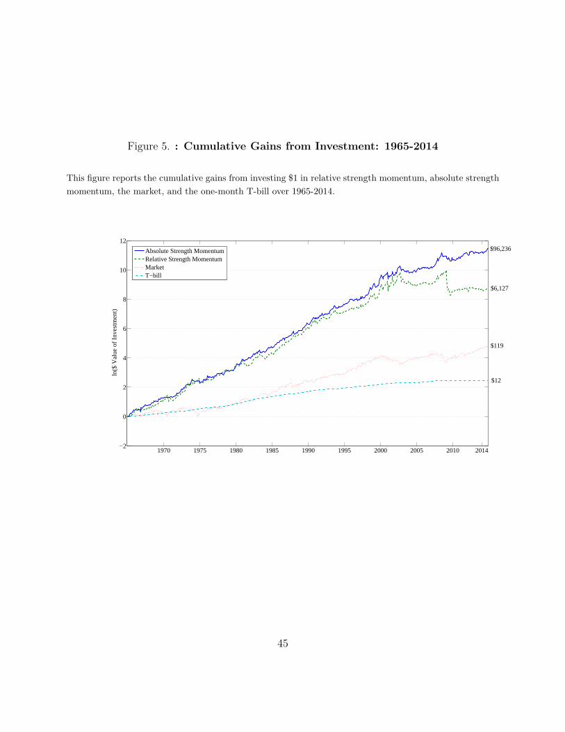
Figure 5. : Cumulative Gains from Investment: 1965-2014

This figure reports the cumulative gains from investing $1 in relative strength momentum, absolute strength

momentum, the market, and the one-month T-bill over 1965-2014.

1970 1975 1980 1985 1990 1995 2000 2005 2010 2014−2

0

2

4

6

8

10

12

ln($

Val

ue o

f Inv

estm

ent)

Absolute Strength MomentumRelative Strength MomentumMarketT−bill

$96,236

$6,127

$119

$12

45

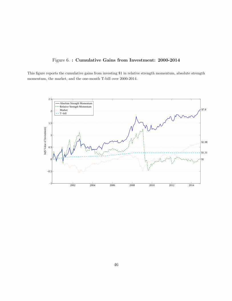
Figure 6. : Cumulative Gains from Investment: 2000-2014

This figure reports the cumulative gains from investing $1 in relative strength momentum, absolute strength

momentum, the market, and the one-month T-bill over 2000-2014.

2002 2004 2006 2008 2010 2012 2014−1

−0.5

0

0.5

1

1.5

2

2.5

ln($

Val

ue o

f Inv

estm

ent)

Absolute Strength MomentumRelative Strength MomentumMarketT−bill

$7.8

$1.98

$1.31

$1

46