129

Abundance estimates of cetaceans from a line-transect survey within the U.S. Hawaiian Islands Exclusive Economic Zone

Amanda L. Bradford (contact author)1

Karin A. Forney2

Erin M. Oleson1 Jay Barlow3

Email address for contact author: amanda.bradford@noaa.gov

1 Pacific Islands Fisheries Science Center National Marine Fisheries Service, NOAA 1845 Wasp Boulevard, Building 176 Honolulu, Hawaii 968182 Southwest Fisheries Science Center National Marine Fisheries Service, NOAA 110 Shaffer Road Santa Cruz, California 950603 Southwest Fisheries Science Center National Marine Fisheries Service, NOAA 8901 La Jolla Shores Drive La Jolla, California 92037

Manuscript submitted 6 January 2016.Manuscript accepted 5 December 2016.Fish. Bull. 115:129–142 (2017).Online publication date: 19 January 2017.doi: 10.7755/FB.115.2.1

The views and opinions expressed or implied in this article are those of the author (or authors) and do not necessarily reflect the position of the National Marine Fisheries Service, NOAA.

Abstract—A ship-based line-transect survey was conducted during the summer and fall of 2010 to obtain abundance estimates of cetaceans in the U.S. Hawaiian Islands Exclusive Economic Zone (EEZ). Given the low sighting rates for cetaceans in the study area, sightings from 2010 were pooled with sightings made during previous line-transect surveys with-in the central Pacific for calculating detection functions, which were esti-mated by using a multiple-covariate approach. The trackline detection probabilities used in this study are the first to reflect the effect of sight-ing conditions in the central Pacific and are markedly lower than esti-mates used in previous studies. Dur-ing the survey, 23 cetacean species (17 odontocetes and 6 mysticetes) were seen, and abundance was esti-mated for 19 of them (15 odontocetes and 4 mysticetes). Group size and Beaufort sea state were the most important factors affecting the de-tectability of cetacean groups. Across all species, abundance estimates and coefficients of variation range from 133 to 72,528 and from 0.29 to 1.13, respectively. Estimated abundance is highest for delphinid species and lowest for the killer whale (Orcinus orca) and rorqual species. Overall, cetacean density in the Hawaiian Is-lands EEZ is low in comparison with highly productive oceanic regions.

Twenty-five cetacean species are known to occur in the U.S. Hawaiian Islands Exclusive Economic Zone (EEZ). Before the 2000s, most re-search on cetaceans in Hawaii focused on humpback whales (Megaptera no-vaeangliae) (e.g., Herman and Antino-ja, 1977; Mobley et al., 1999) and spin-ner dolphins (Stenella longirostris) (e.g., Norris and Dohl, 1980; Norris et al., 1994) because individuals of these species are concentrated (seasonally in the case of humpback whales) in nearshore waters of the main Ha-waiian Islands. Although there were studies of rarer or less accessible spe-cies, such as the pygmy killer whale (Feresa attenuata) and short-finned pilot whale (Globicephala macrorhyn-chus) (e.g., Pryor et al., 1965; Shane and McSweeney, 1990), more frequent and directed surveys for a variety of species were not initiated until 2000 (e.g., Baird, 2005; McSweeney et al., 2007; Baird et al., 2009). Although that recent research has provided sig-

nificant insight into the occurrence, distribution, abundance, stock struc-ture, and social organization of ceta-ceans in Hawaii waters, the surveys were focused primarily on nearshore odontocete species associated with the main Hawaiian Islands.

In 2002, the Southwest Fisher-ies Science Center (SWFSC) of the National Marine Fisheries Service (NMFS) conducted the first Hawaiian Islands Cetacean and Ecosystem As-sessment Survey (HICEAS), a ship-based line-transect survey designed to estimate the abundance of ceta-ceans in the entirety of the Hawaiian Islands EEZ. During the HICEAS in 2002, 23 cetacean species (18 odonto-cetes and 5 mysticetes) were encoun-tered, and the abundance of 19 spe-cies (18 odontocetes and 1 mysticete) was estimated (Barlow, 2006). These estimates represented the first abun-dance estimates for most cetacean stocks in Hawaii waters and were incorporated in the stock assessment

130 Fishery Bulletin 115(2)

reports produced by NMFS in ac-cordance with the Marine Mammal Protection Act of 1972 (e.g., Car-retta et al., 2005).

Abundance estimates used in marine mammal stock assessment reports are considered outdated af-ter 8 years (NMFS1). Therefore, a second HICEAS was carried out in 2010, as a collaborative effort be-tween the SWFSC and the NMFS Pacific Islands Fisheries Science Center (PIFSC), with objectives, timing, and methods comparable to those of the HICEAS conducted in 2002. However, adjustments were made to the data collection protocol for the false killer whale (Pseudorca crassidens) during the HICEAS in 2010—changes that necessitated a separate and specialized abundance analysis for this species (Bradford et al., 2014, 2015). The objective of the present study was to estimate the abundance of the remaining ce-tacean stocks encountered during the HICEAS in 2010. Although the resulting abundance estimates are specific to cetacean stock assess-ment in the Hawaiian Islands EEZ, the analytical methods used are ap-plicable to line-transect surveys of cetaceans in other regions.

Materials and methods

Data collection

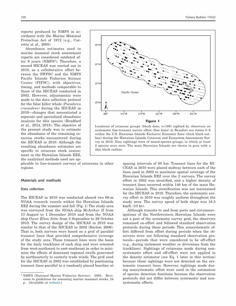
The HICEAS in 2010 was conducted aboard two 68-m NOAA research vessels within the Hawaiian Islands EEZ during the summer and fall (Fig. 1) The study area was surveyed from the NOAA ship McArthur II from 13 August to 1 December 2010 and from the NOAA ship Oscar Elton Sette from 2 September to 29 October 2010. The survey design of the HICEAS in 2010 was similar to that of the HICEAS in 2002 (Barlow, 2006). That is, both surveys were based on a grid of parallel transect lines that provided comprehensive coverage of the study area. These transect lines were the basis for the daily tracklines of each ship and were oriented from west-northwest to east-southeast in order to mini-mize the effects of dominant regional swells generated by northeasterly to easterly trade winds. The grid used for the HICEAS in 2002 was established by positioning transect lines parallel to a randomly placed baseline at

1 NMFS (National Marine Fisheries Service). 2005. Revi-sions to guidelines for assessing marine mammal stocks, 24 p. [Available at website.]

spacing intervals of 85 km. Transect lines for the HI-CEAS in 2010 were placed midway between each of the lines used in 2002 to maximize spatial coverage of the Hawaiian Islands EEZ over the 2 surveys. The survey effort in 2002 was stratified, and a higher density of transect lines occurred within 140 km of the main Ha-waiian Islands. This stratification was not maintained for the HICEAS in 2010. Therefore, the systematic sur-vey effort in 2010 was roughly uniform throughout the study area. The survey speed of both ships was 18.5 km/h (10 kt).

Although transits to and from ports and circumnav-igations of the Northwestern Hawaiian Islands were not a part of the systematic survey grid, the observers remained on-effort and followed standard observation protocols during these periods. This nonsystematic ef-fort differed from effort during periods when the ob-servers were not following standard observation pro-tocols—periods that were considered to be off-effort (e.g., during inclement weather or diversions from the tracklines). Sightings of cetaceans made during non-systematic effort and off-effort were not applied to the density estimator (see Eq. 1 later in this section) because those sightings were not detected on the sys-tematic transect lines. However, sightings made dur-ing nonsystematic effort were used in the estimation of species detection functions because the observation protocols did not differ between systematic and non-systematic efforts.

Figure 1Locations of cetacean groups (black dots; n=198) sighted by observers on systematic line-transect survey effort (fine lines) in Beaufort sea states 0–6 within the U.S. Hawaiian Islands Exclusive Economic Zone (thick black out-line) during the Hawaiian Islands Cetacean and Ecosystem Assessment Sur-vey in 2010. Nine sightings were of mixed-species groups, in which at least 2 species were seen. The main Hawaiian Islands are shown in gray with a thin black outline.

Pacific Ocean

Bradford et al.: Abundance estimates of cetaceans within the U.S. Hawaiian Islands EEZ 131

The observation methods used during the HICEAS in 2010 were developed by the SWFSC and have been in use for the last 3 decades (e.g., Barlow, 2006). To summarize these methods, observation teams consisted of 6 observers who rotated through 3 roles (port and starboard observers and a data recorder) and searched for cetaceans 180° forward of the vessel by using 25× binoculars (port and starboard observers) and with un-aided eyes (data recorder) from the flying bridge (ap-proximately 15 m above the sea surface on both ships). When cetaceans were sighted within 5.6 km (3 nmi) of the trackline by 1 of the 3 on-effort observers, sys-tematic search effort was suspended and the ship di-verted from the trackline toward the sighting so that species, species composition (for mixed-species groups), and group size could be determined. In addition to ba-sic environmental data (e.g., Beaufort sea state, swell height, and visibility), data collected for each sighting included the time, location, initial bearing and radial distance to the cetacean group (used to calculate the perpendicular distance of the sighting to the trackline), species identity, proportion of each species present (mixed-species groups), and identity of observers and their independent estimates of sighting group size (re-corded as a “best,” “high,” and “low” estimate for each observer). If species identity could not be determined for a sighting, the lowest possible taxonomic category was applied (see Table 1 for the categories relevant to the HICEAS in 2010). After the identification of spe-cies and estimation of group size for some sightings, depending on weather, animal behavior, and research priorities, a small boat was launched to collect photo-identification images and biopsy samples.

Additionally, an acoustics team worked independent-ly from the observers, detecting cetacean vocalizations by using a hydrophone array towed behind each ship during daylight hours. This team did not inform the observer team of acoustic detections. The abundance estimation reported in the present study is based solely on the sightings made by the observers. That is, ce-taceans that were detected only acoustically were not included in the abundance analysis. The acoustic de-tections from the HICEAS in 2010 are currently being processed for future line-transect analyses.

Estimation of abundance

Cetacean abundance in the Hawaiian Islands EEZ was estimated by using a multiple-covariate line-transect approach (Buckland et al., 2001; Marques and Buck-land, 2004). Specifically, detection functions were mod-eled as a function of factors known to affect the detect-ability of cetacean groups. Sighting rates are low in the Hawaiian Islands EEZ (Barlow, 2006), and as were the sample sizes during the HICEAS in 2002, sample sizes for each species sighted during the HICEAS in 2010 were inadequate for modeling the detection func-tions. Therefore, as with analysis of sightings from the HICEAS in 2002 (Barlow, 2006), sightings from the HICEAS in 2010 were pooled with sightings col-

lected during previous NMFS ship-based line-transect surveys of the eastern Pacific. The estimation of de-tection functions for the HICEAS in 2002 incorporated sightings made throughout the eastern Pacific during SWFSC surveys conducted from 1986 through 2002, but the sighting pool for the analysis of the 2010 data was restricted to sightings made in the central Pacific (defined here as the area of the eastern Pacific north of 5°S, south of 40°N, west of 120°W, and east of 175°E) during SWFSC and PIFSC surveys from 1986 through 2010. The pooled sightings (collected during both sys-tematic and nonsystematic efforts) were limited to the central Pacific to minimize heterogeneity resulting from geographical differences in species associations and behavior—complex factors that can be difficult to represent as covariates.

Despite survey data from the present study being pooled with previous survey data, sample sizes for most species remained insufficient for estimating the detection function. Therefore, sightings of species with similar detection characteristics (e.g., size, surface be-havior, group sizes) were also combined for modeling the detection function. Specifically, 6 species pools were formed: 1) small delphinids with relatively large group sizes; 2) small and medium delphinids with relatively small group sizes; 3) large delphinids and co-occurring beaked whales with similar behavior (Barlow, 2006); 4) large and highly conspicuous odontocetes (Barlow et al., 2011a); 5) beaked whales with relatively small group sizes; and 6) baleen whales (see Table 2 for the composition of each species pool).

A half-normal model was used to evaluate the de-tection probabilities for the sightings in each species pool as a function of perpendicular distance from the trackline and of relevant covariates. Only half-normal models were used because of the greater stability they exhibit when fitting sighting data for cetaceans (Gerrodette and Forcada, 2005). The 5–10% most dis-tant sightings in each species pool were truncated to improve model fit (Buckland et al., 2001), although no truncation distance exceeded the 5.6-km limit at which the ship would not divert from the trackline for a sighting. Covariate models were built by using a forward stepwise procedure and were selected by us-ing Akaike’s information criterion corrected for a small sample size (AICc; Hurvich and Tsai, 1989).

Although several factors have the potential to af-fect the perpendicular sighting distances to cetaceans (Barlow et al., 2001), a smaller set of covariates identi-fied as important and robust in estimating detection probabilities (Barlow et al., 2011a) was considered for analysis in the present study. Of the covariates iden-tified by Barlow et al. (2011a), visibility and swell anomaly could not be tested because these variables were not recorded during SWFSC surveys before 1991, and region was not applicable because the pooled sight-ings were restricted to the central Pacific. The remain-ing covariates evaluated were Beaufort (Beaufort sea state, treated as a continuous variable), group size (the natural logarithm of the sighting group size, which in-

132 Fishery Bulletin 115(2)

Table 1

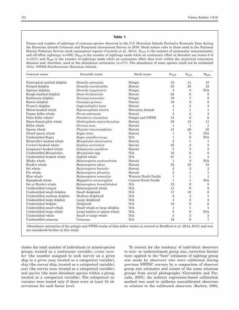
Names and number of sightings of cetacean species observed in the U.S. Hawaiian Islands Exclusive Economic Zone during the Hawaiian Islands Cetacean and Ecosystem Assessment Survey in 2010. Stock names refer to those used in the National Marine Fisheries Service stock assessment reports (Carretta et al., 2014). NTOT is the number of systematic, nonsystematic, and off-effort sightings (n=398); NSYS is the number of sightings made while on systematic effort in Beaufort sea states 0–6 (n=211); and NEST is the number of sightings made while on systematic effort that were within the analytical truncation distance and, therefore, used in the abundance estimation (n=177). The abundance of some species could not be estimated (N/A). NWHI=Northwestern Hawaiian Islands.

Common name Scientific name Stock name NTOT NSYS NEST

Pantropical spotted dolphin Stenella attenuata Pelagic 12 11 10Striped dolphin Stenella coeruleoalba Hawaii 25 20 18Spinner dolphin Stenella longirostris Pelagic 4 0 N/ARough-toothed dolphin Steno bredanensis Hawaii 24 8 8Bottlenose dolphin Tursiops truncatus Pelagic 19 7 6Risso’s dolphin Grampus griseus Hawaii 10 9 9Fraser’s dolphin Lagenodelphis hosei Hawaii 4 3 3Melon-headed whale Peponocephala electra Hawaiian Islands 1 1 1Pygmy killer whale Feresa attenuata Hawaii 5 4 4False killer whale1 Pseudorca crassidens Pelagic and NWHI 14 6 6Short-finned pilot whale Globicephala macrorhynchus Hawaii 36 15 11Killer whale Orcinus orca Hawaii 1 1 1Sperm whale Physeter macrocephalus Hawaii 41 26 23Dwarf sperm whale Kogia sima Hawaii 1 0 N/AUnidentified Kogia Kogia sima/breviceps N/A 1 0 N/ABlainville’s beaked whale Mesoplodon densirostris Hawaii 2 1 1Cuvier’s beaked whale Ziphius cavirostris Hawaii 23 2 2Longman’s beaked whale Indopacetus pacificus Hawaii 3 3 3Unidentified Mesoplodon Mesoplodon spp. N/A 10 6 6Unidentified beaked whale Ziphiid whale N/A 27 4 3Minke whale Balaenoptera acutorostrata Hawaii 1 0 N/ABryde’s whale Balaenoptera edeni Hawaii 32 19 19Sei whale Balaenoptera borealis Hawaii 2 2 2Fin whale Balaenoptera physalus Hawaii 2 1 1Blue whale Balaenoptera musculus Western North Pacific 1 1 1Humpback whale Megaptera novaeangliae Central North Pacific 1 1 N/ASei or Bryde’s whale Balaenoptera borealis/edeni N/A 12 9 8Unidentified rorqual Balaenopterid whale N/A 11 9 6Unidentified small dolphin Small delphinid N/A 17 10 6Unidentified medium dolphin Medium delphinid N/A 6 3 1Unidentified large dolphin Large delphinid N/A 3 2 2Unidentified dolphin Delphinid N/A 19 9 6Unidentified small whale Small whale or large dolphin N/A 1 1 1Unidentified large whale Large baleen or sperm whale N/A 8 6 N/AUnidentified whale Small or large whale N/A 3 2 2Unidentified cetacean Cetacean N/A 16 9 7

1Abundance estimation of the pelagic and NWHI stocks of false killer whales is covered in Bradford et al. (2014, 2015) and was not considered further in this study.

cludes the total number of individuals in mixed-species groups, treated as a continuous variable), cruise num-ber (the number assigned to each survey on a given ship in a given year, treated as a categorical variable), ship (the survey ship, treated as a categorical variable), year (the survey year, treated as a categorical variable), and species (the most abundant species within a group, treated as a categorical variable). The categorical co-variates were tested only if there were at least 10 ob-servations for each factor level.

To correct for the tendency of individual observers to over- or underestimate group size, correction factors were applied to the “best” estimates of sighting group size made by observers who were calibrated during previous SWFSC surveys by a comparison of observer group size estimates and counts of the same cetacean groups from aerial photographs (Gerrodette and For-cada, 2005). An indirect regression-based calibration method was used to calibrate noncalibrated observers in relation to the calibrated observers (Barlow, 1995;

Bradford et al.: Abundance estimates of cetaceans within the U.S. Hawaiian Islands EEZ 133

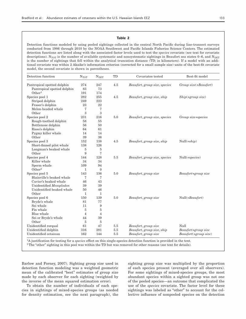
Table 2

Detection functions modeled by using pooled sightings collected in the central North Pacific during line-transect surveys conducted from 1986 through 2010 by the NOAA Southwest and Pacific Islands Fisheries Science Centers. The estimated detection functions are listed along with the associated factor levels used to test the species covariate (see text for covariate descriptions). NTOT is the number of available systematic and nonsystematic sightings in Beaufort sea states 0–6, and NDET is the number of sightings that fell within the analytical truncation distance (TD; in kilometers). If a model with an addi-tional covariate was within 2 Akaike’s information criterion (corrected for a small sample size) units of the best-fit covariate model, the second covariate is shown in parentheses.

Detection function NTOT NDET TD Covariates tested Best-fit model

Pantropical spotted dolphin 274 247 4.5 Beaufort, group size, species Group size(+Beaufort) Pantropical spotted dolphin 83 73 Other1 191 174 Species pool 1 282 255 4.5 Beaufort, group size, ship Ship(+group size) Striped dolphin 249 223 Fraser’s dolphin 23 22 Melon-headed whale 7 7 Other 3 3 Species pool 2 231 216 5.0 Beaufort, group size, species Group size+species Rough-toothed dolphin 58 55 Bottlenose dolphin 56 50 Risso’s dolphin 64 61 Pygmy killer whale 14 14 Other 39 36 Species pool 3 152 138 4.5 Beaufort, group size, ship Null(+ship) Short-finned pilot whale 138 126 Longman’s beaked whale 5 5 Other 9 7 Species pool 4 144 128 5.5 Beaufort, group size, species Null(+species) Killer whale 34 34 Sperm whale 109 94 Other2 1 0 Species pool 5 143 136 5.0 Beaufort, group size Beaufort+group size Blainville’s beaked whale 7 7 Cuvier’s beaked whale 46 43 Unidentified Mesoplodon 39 39 Unidentified beaked whale 50 46 Other 1 1 Species pool 6 150 139 5.0 Beaufort, group size Null(+Beaufort) Bryde’s whale 81 77 Sei whale 11 9 Fin whale 5 5 Blue whale 4 4 Sei or Bryde’s whale 44 39 Other 5 5 Unidentified rorqual 61 47 5.5 Beaufort, group size NullUnidentified dolphin 316 281 5.5 Beaufort, group size, ship Beaufort+group sizeUnidentified cetacean 162 144 5.5 Beaufort, group size Beaufort(+group size)

1A justification for testing for a species effect on this single-species detection function is provided in the text.2 The “other” sighting in this pool was within the TD but was removed for other reasons (see text for details).

Barlow and Forney, 2007). Sighting group size used in detection function modeling was a weighted geometric mean of the calibrated “best” estimates of group size made by each observer for each sighting (weighted by the inverse of the mean squared estimation error).

To obtain the number of individuals of each spe-cies in sightings of mixed-species groups (as needed for density estimation, see the next paragraph), the

sighting group size was multiplied by the proportion of each species present (averaged over all observers). For some sightings of mixed-species groups, the most abundant species within a sighted group was not one of the pooled species—an outcome that complicated the use of the species covariate. The factor level for these sightings was labeled as “other” to account for the col-lective influence of nonpooled species on the detection

134 Fishery Bulletin 115(2)

function (Table 2). For the species pool that includes killer whales (Orcinus orca) and sperm whales (Physe-ter microcephalus), the low number of “other” sightings (n=1) prevented testing the species covariate. Upon fur-ther examination, this sighting was found to contain a species co-occurrence not observed in the Hawaiian Islands EEZ and not represented in any of the other pooled sightings. Therefore, this sighting was removed from the pool used to estimate the detection function so that a species effect could be evaluated. Although the sample size was sufficient to model the detection func-tion of pantropical spotted dolphins (Stenella attenua-ta) separately, the species covariate and the “other” fac-tor level were used to explore the influence of a large number of sightings in which the pantropical spotted dolphin was not the most abundant species.

Given the estimated covariate detection function and the sightings within the established truncation distance from the systematic effort during the HICEAS in 2010, the density (D) of each species was estimated by using a Horvitz–Thompson-like estimator (Marques and Buckland, 2004):

D=

12 ⋅L ⋅ g(0)

f (0,cj) ⋅sj,j=1N∑ (1)

where L = the length of systematic-effort transect lines

in the study area; g(0) = the probability of detection on the trackline; f(0,cj) = the probability density of the detection func-

tion evaluated at zero distance for sighting j with associated covariates c;

sj = the number of individuals of the species in sighting j; and

N = the number of sightings of the species dur-ing systematic-effort within the analytical truncation distance.

The value of f(0,cj) that was applied was a weighted average of all covariate models within 2 AICc units of the best-fit model. The inverse of f(0,cj) is the effec-tive strip width (ESW), which is the distance from the trackline beyond which as many sightings were made as were missed within.

Barlow (2006) used estimates of g(0) adapted from previous studies of delphinids and large whales (Bar-low, 1995), sperm whales (Barlow and Sexton2), and beaked whales and Kogia spp. (Barlow, 1999). Howev-er, results from recent work in which g(0) was derived from apparent densities in different Beaufort sea state conditions (assuming that true density is not affected by sea state) indicate that g(0) had been previously overestimated, particularly for high sea states (Bar-low, 2015). Barlow (2015) estimated g(0) in Beaufort sea states 0–6 for 20 cetacean taxa by using a model

2 Barlow, J., and S. Sexton. 1996. The effect of diving and searching behavior on the probability of detecting track-line groups, g0, of long-diving whales during line-transect sur-veys. Southwest Fish. Sci. Cent. Admin. Rep. LJ-96-14, 21 p. [Available from Southwest Fisheries Science Center, Na-tional Marine Fisheries Service, 8901 La Jolla Shores Dr., La Jolla, CA 92037.]

that accounted for spatial and temporal differences in density. This model was fitted to cetacean sighting data from the eastern Pacific, which included the on-effort sightings from the HICEAS in 2010. Therefore, the re-sulting estimates of g(0) can be applied to the estima-tion of cetacean abundance for the HICEAS in 2010.

The estimates of g(0) by Barlow (2015) were relative to a value of 1 at a Beaufort sea state of 0 for most spe-cies or species groups considered, with the exception of the Cuvier’s beaked whale (Ziphius cavirostris) and Mesoplodon spp., for which scaled absolute estimates of g(0) were determined for Beaufort sea states 0–6. In the absence of absolute estimates of g(0) for most of the remaining taxa, the relative values of g(0) from Barlow (2015) were assumed to be absolute values in the present study. Estimates of g(0) for the HICEAS in 2010 (Table 3) were obtained by taking a weighted average of both the Beaufort-specific values of g(0) and the associated coefficients of variation (CVs) presented in Barlow (2015), where the weights were the propor-tion of systematic effort in each sea state category (0–6) during the HICEAS in 2010.

For species not covered in Barlow (2015) because of small sample sizes, g(0) was assumed to be simi-lar to the g(0) estimates of associated species in the species pools formed to model the detection functions, given the similar detection characteristics (e.g., size, surface behavior, group sizes) of the species in each pool (Table 2). Therefore, g(0) for these species was ob-tained either by using the estimate of another species in the species pool or, if more than one estimate was available, by averaging the available estimates. Spe-cifically, for the HICEAS in 2010, the estimate of g(0) for striped dolphins (Stenella coeruleoalba) was used for Fraser’s dolphins (Lagenodelphis hosei) and melon-headed whales (Peponocephala electra), the estimate for short-finned pilot whales was used for Longman’s beaked whales (Indopacetus pacificus), and the esti-mates for rough-toothed dolphins (Steno bredanensis), bottlenose dolphins (Tursiops truncatus), and Risso’s dolphins (Grampus griseus) were averaged for pygmy killer whales (Table 3).

The abundance of each species was determined by multiplying the density estimate by 2,447,635 km2—the area of the Hawaiian Islands EEZ minus the area of the land masses of the main and Northwestern Hawaiian Islands. However, the ranges of the pelagic stocks of pantropical spotted and bottlenose dolphins, which are the stocks involved in the estimation (Table 1), do not span the entirety of the Hawaiian Islands EEZ (Carretta et al., 2011, 2014). Therefore, the area of the ranges of island-associated stocks of pantropical spotted and bottlenose dolphins was subtracted from the larger area, resulting in areas of 2,392,576 km2 and 2,425,900 km2 for pantropical spotted and bottle-nose dolphins, respectively. The mixed parametric and nonparametric bootstrap routine described in Barlow (2006) and refined by Barlow and Rankin3 was used

3 Barlow, J., and S. Rankin. 2007. False killer whale abun-

Bradford et al.: Abundance estimates of cetaceans within the U.S. Hawaiian Islands EEZ 135

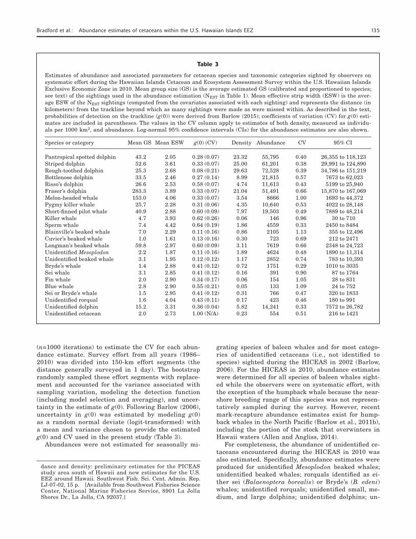
Table 3

Estimates of abundance and associated parameters for cetacean species and taxonomic categories sighted by observers on systematic effort during the Hawaiian Islands Cetacean and Ecosystem Assessment Survey within the U.S. Hawaiian Islands Exclusive Economic Zone in 2010. Mean group size (GS) is the average estimated GS (calibrated and proportioned to species; see text) of the sightings used in the abundance estimation (NEST in Table 1). Mean effective strip width (ESW) is the aver-age ESW of the NEST sightings (computed from the covariates associated with each sighting) and represents the distance (in kilometers) from the trackline beyond which as many sightings were made as were missed within. As described in the text, probabilities of detection on the trackline (g(0)) were derived from Barlow (2015); coefficients of variation (CV) for g(0) esti-mates are included in parentheses. The values in the CV column apply to estimates of both density, measured as individu-als per 1000 km2, and abundance. Log-normal 95% confidence intervals (CIs) for the abundance estimates are also shown.

Species or category Mean GS Mean ESW g(0) (CV) Density Abundance CV 95% CI

Pantropical spotted dolphin 43.2 2.05 0.28 (0.07) 23.32 55,795 0.40 26,355 to 118,123Striped dolphin 52.6 3.61 0.33 (0.07) 25.00 61,201 0.38 29,991 to 124,890Rough-toothed dolphin 25.3 2.68 0.08 (0.21) 29.63 72,528 0.39 34,786 to 151,219Bottlenose dolphin 33.5 2.46 0.27 (0.14) 8.99 21,815 0.57 7673 to 62,023Risso’s dolphin 26.6 2.53 0.58 (0.07) 4.74 11,613 0.43 5199 to 25,940Fraser’s dolphin 283.3 3.89 0.33 (0.07) 21.04 51,491 0.66 15,870 to 167,069Melon-headed whale 153.0 4.06 0.33 (0.07) 3.54 8666 1.00 1693 to 44,372Pygmy killer whale 25.7 2.28 0.31 (0.06) 4.35 10,640 0.53 4022 to 28,148Short-finned pilot whale 40.9 2.88 0.60 (0.09) 7.97 19,503 0.49 7889 to 48,214Killer whale 4.7 3.93 0.62 (0.26) 0.06 146 0.96 30 to 710Sperm whale 7.4 4.42 0.64 (0.19) 1.86 4559 0.33 2450 to 8484Blainville’s beaked whale 7.0 2.29 0.11 (0.16) 0.86 2105 1.13 355 to 12,496Cuvier’s beaked whale 1.0 1.61 0.13 (0.16) 0.30 723 0.69 212 to 2471Longman’s beaked whale 59.8 2.97 0.60 (0.09) 3.11 7619 0.66 2348 to 24,723Unidentified Mesoplodon 2.2 1.87 0.11 (0.16) 1.89 4624 0.48 1890 to 11,314Unidentified beaked whale 3.1 1.95 0.12 (0.12) 1.17 2852 0.74 783 to 10,393Bryde’s whale 1.4 2.88 0.41 (0.12) 0.72 1751 0.29 1010 to 3035Sei whale 3.1 2.85 0.41 (0.12) 0.16 391 0.90 87 to 1764Fin whale 2.0 2.90 0.34 (0.17) 0.06 154 1.05 28 to 831Blue whale 2.8 2.90 0.55 (0.21) 0.05 133 1.09 24 to 752Sei or Bryde’s whale 1.5 2.95 0.41 (0.12) 0.31 766 0.47 320 to 1833Unidentified rorqual 1.6 4.04 0.43 (0.11) 0.17 423 0.46 180 to 991Unidentified dolphin 15.2 3.31 0.36 (0.04) 5.82 14,241 0.33 7572 to 26,782Unidentified cetacean 2.0 2.73 1.00 (N/A) 0.23 554 0.51 216 to 1421

(n=1000 iterations) to estimate the CV for each abun-dance estimate. Survey effort from all years (1986–2010) was divided into 150-km effort segments (the distance generally surveyed in 1 day). The bootstrap randomly sampled these effort segments with replace-ment and accounted for the variance associated with sampling variation, modeling the detection function (including model selection and averaging), and uncer-tainty in the estimate of g(0). Following Barlow (2006), uncertainty in g(0) was estimated by modeling g(0) as a random normal deviate (logit-transformed) with a mean and variance chosen to provide the estimated g(0) and CV used in the present study (Table 3).

Abundances were not estimated for seasonally mi-

dance and density: preliminary estimates for the PICEAS study area south of Hawaii and new estimates for the U.S. EEZ around Hawaii. Southwest Fish. Sci. Cent. Admin. Rep. LJ-07-02, 15 p. [Available from Southwest Fisheries Science Center, National Marine Fisheries Service, 8901 La Jolla Shores Dr., La Jolla, CA 92037.]

grating species of baleen whales and for most catego-ries of unidentified cetaceans (i.e., not identified to species) sighted during the HICEAS in 2002 (Barlow, 2006). For the HICEAS in 2010, abundance estimates were determined for all species of baleen whales sight-ed while the observers were on systematic effort, with the exception of the humpback whale because the near-shore breeding range of this species was not represen-tatively sampled during the survey. However, recent mark-recapture abundance estimates exist for hump-back whales in the North Pacific (Barlow et al., 2011b), including the portion of the stock that overwinters in Hawaii waters (Allen and Angliss, 2014).

For completeness, the abundance of unidentified ce-taceans encountered during the HICEAS in 2010 was also estimated. Specifically, abundance estimates were produced for unidentified Mesoplodon beaked whales; unidentified beaked whales; rorquals identified as ei-ther sei (Balaenoptera borealis) or Bryde’s (B. edeni) whales; unidentified rorquals; unidentified small, me-dium, and large dolphins; unidentified dolphins; un-

136 Fishery Bulletin 115(2)

identified small and large whales; unidentified whales; and unidentified cetaceans (Table 1). Sightings of unidentified Mesoplodon beaked whales, unidentified beaked whales, and rorquals identified as either sei or Bryde’s whales were pooled with associated species for modeling the detection function (Table 2). Sight-ings of unidentified small, medium, and large dolphins and unidentified dolphins were combined into a single category, “unidentified dolphins,” for detection func-tion and abundance estimation. Likewise, sightings of unidentified small and large whales and unidentified whales and cetaceans were combined into the category “unidentified cetaceans.”

The detection functions for unidentified rorquals, “unidentified dolphins,” and “unidentified cetaceans” were estimated separately and without testing for the effect of species. The g(0) estimate for unidenti-fied beaked whales was an average of the estimates for Cuvier’s beaked whales and Mesoplodon spp.; the g(0) estimate of unidentified rorquals was an average of the estimates for fin whales, blue whales, and sei or Bryde’s whales; and the g(0) estimate of “unidentified dolphins” was an average of the estimates for pantropical spotted, striped, rough-toothed, bottlenose, and Risso’s dolphins and short-finned pilot whales (Table 3). A g(0) estimate was not applied to the “unidentified cetaceans” because an appropriate value could not be determined, given the broad taxonomic range of this category.

Results

Survey sightings

During the HICEAS in 2010, the systematic and non-systematic visual search effort spanned 20,568 km of transect lines in Beaufort sea states 0–6 within the Hawaiian Islands EEZ. During this effort and while off-effort, the observers sighted 379 cetacean groups (n=198 during systematic effort, n=101 during nonsys-tematic effort, n=80 during off-effort), which include 13 groups with more than one species present. Accounting for these mixed-species groups, the 379 group sightings represent 398 sightings of 23 species (17 odontocetes and 6 mysticetes) and 13 unidentified species catego-ries (Table 1). With the exception of the pygmy sperm whale (Kogia breviceps) and the extremely rare North Pacific right whale (Eubalaena japonica), all cetacean species known to occur in the Hawaiian Islands EEZ were sighted during the HICEAS in 2010.

The systematic effort that was relevant to the abundance estimation encompassed 16,145 km of tran-sect lines in Beaufort sea states 0–6 for most ceta-ceans sighted (Fig. 1), but for pantropical spotted and bottlenose dolphins, the effort covered 15,747 km and 16,100 km, respectively. As with the HICEAS in 2002 (Barlow, 2006), windy conditions prevailed during the HICEAS in 2010, and most (94.5%) of the systematic effort occurred in Beaufort sea states 3–6. Adjusting for mixed-species groups (n=9), the 198 groups sighted

on systematic effort correspond to 211 sightings of 20 species and 11 unidentified species categories (Table 1; Fig. 2). The 3 species not sighted by the observ-ers while on systematic effort during the HICEAS in 2010 were the spinner dolphin, the dwarf sperm whale (Kogia sima), and the minke whale (Balaenoptera acutorostrata).

By using the 177 sightings within the respective analytical truncation distances (NEST in Table 1), abun-dance was estimated for 19 cetacean species (15 odon-tocetes and 4 mysticetes; see the Materials and meth-ods section for the rationale for excluding humpback whales) and for the 11 unidentified species categories, although the latter were combined into 6 taxonomic categories (as described in the Materials and methods section). Of the 48 sightings of unidentified cetaceans used in the estimation of abundance, 9 sightings cor-respond with acoustic detections of dolphin whistles, odontocete clicks, or baleen whale calls. These detec-tions were examined for possible insights into species identification. However, this effort did not lead to any gains in species identification because of either the poor quality of the recordings, the non-specificity of the vocalizations, or the confounding presence of an associ-ated species.

Detection function

Of the 6 covariates of interest, only 4 (Beaufort, group size, ship, and species) were tested in the 10 models of detection function, although only the noncategori-cal covariates Beaufort and group size could be tested in all cases (Table 2). Insufficient samples sizes by cruise number and year prevented testing for the effect of these covariates on any of the detection functions. Group size and Beaufort most frequently contributed to the model-averaged estimates of detection function. Specifically, group size was selected in 6 detection func-tions and Beaufort, in 5 detection functions.

For the 7 detection functions in which species was a consideration, this covariate was tested in 3 cases and selected in 2 (Table 2). For the 4 species pools that had a limited sample size for testing the effect of spe-cies, follow-up modeling was performed in 3 cases to evaluate the potential for a species effect on the de-tection function. Specifically, for “species pool 1,” a “striped dolphin” and “not striped dolphin” influence was examined. For “species pool 3,” the evaluation was between “pilot whale” and “not pilot whale” sightings. For “species pool 5,” the “other” sighting was excluded and a “Cuvier’s beaked whale,” “Mesoplodon spp.,” and “unidentified beaked whale” effect was explored. By re-ducing the number of factor levels, species did enter 1 of the 4 acceptable models for the “species pool 5” de-tection function, but this covariate otherwise remained unselected for the 3 species pools. Follow-up model-ing was not undertaken for “species pool 6” because there were not enough sightings to evaluate a “sei or Bryde’s” and “not sei or Bryde’s” effect. Overall, this post-hoc analysis of a species effect produced equivocal

Bradford et al.: Abundance estimates of cetaceans within the U.S. Hawaiian Islands EEZ 137

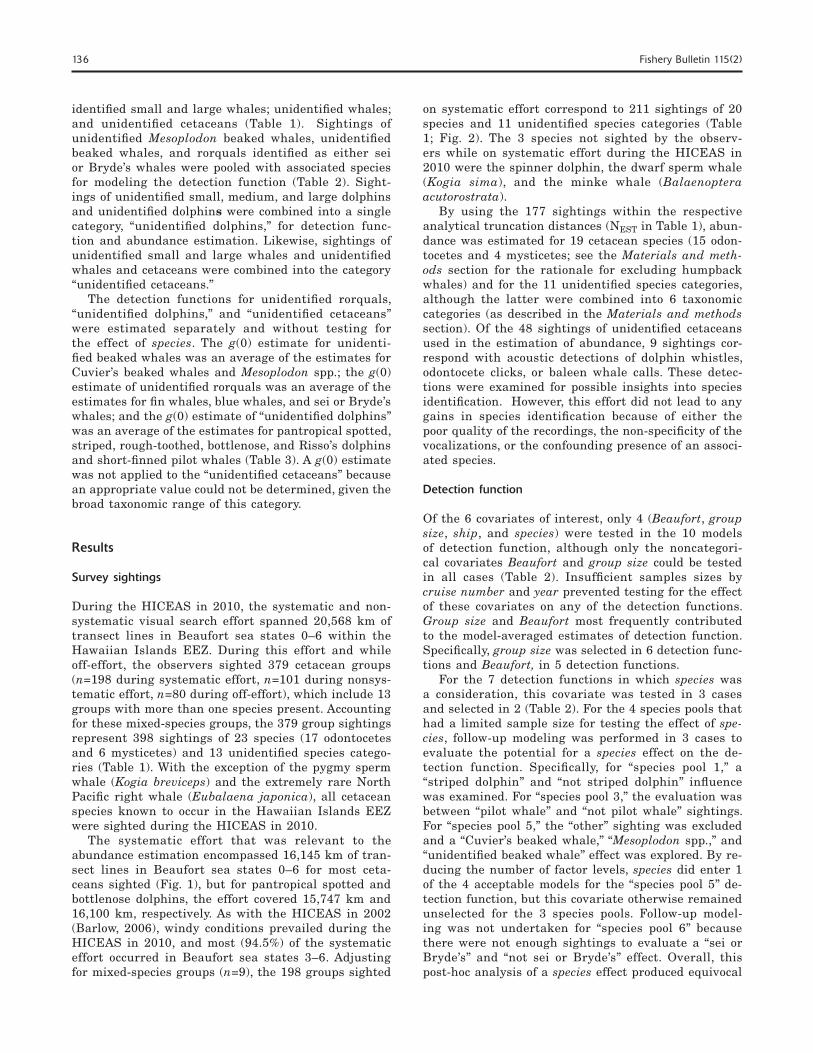
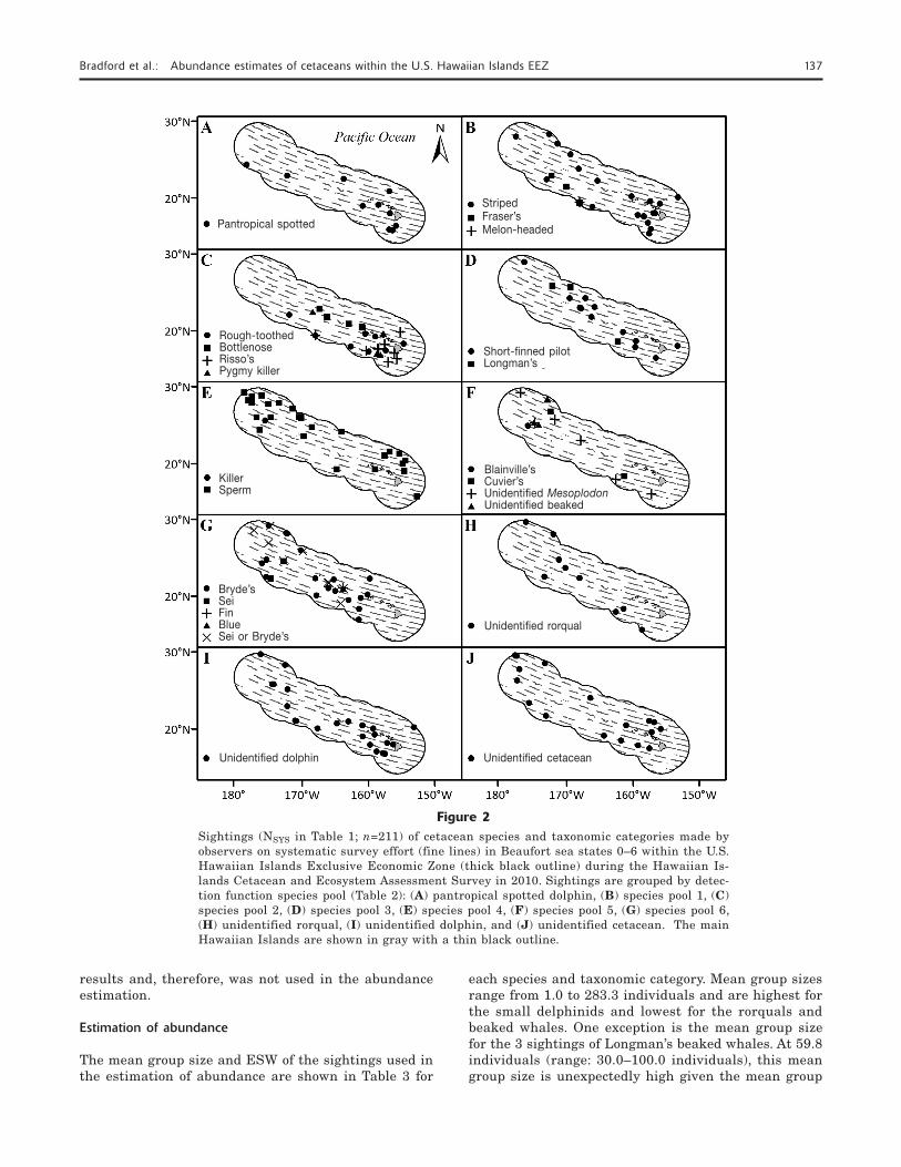
Figure 2Sightings (NSYS in Table 1; n=211) of cetacean species and taxonomic categories made by observers on systematic survey effort (fine lines) in Beaufort sea states 0–6 within the U.S. Hawaiian Islands Exclusive Economic Zone (thick black outline) during the Hawaiian Is-lands Cetacean and Ecosystem Assessment Survey in 2010. Sightings are grouped by detec-tion function species pool (Table 2): (A) pantropical spotted dolphin, (B) species pool 1, (C) species pool 2, (D) species pool 3, (E) species pool 4, (F) species pool 5, (G) species pool 6, (H) unidentified rorqual, (I) unidentified dolphin, and (J) unidentified cetacean. The main Hawaiian Islands are shown in gray with a thin black outline.

results and, therefore, was not used in the abundance estimation.

Estimation of abundance

The mean group size and ESW of the sightings used in the estimation of abundance are shown in Table 3 for

each species and taxonomic category. Mean group sizes range from 1.0 to 283.3 individuals and are highest for the small delphinids and lowest for the rorquals and beaked whales. One exception is the mean group size for the 3 sightings of Longman’s beaked whales. At 59.8 individuals (range: 30.0–100.0 individuals), this mean group size is unexpectedly high given the mean group

Pantropical spotted

StripedFraser’sMelon-headed

Rough-toothedBottlenoseRisso’sPygmy killer

Short-finned pilotLongman’s

KillerSperm

Blainville’sCuvier’sUnidentified MesoplodonUnidentified beaked

Bryde’sSeiFinBlueSei or Bryde’s

Unidentified rorqual

Unidentified dolphin Unidentified cetacean

138 Fishery Bulletin 115(2)

size (10.1 individuals; range: 1.0–20.4 individuals) of all available sightings of Longman’s beaked whales (n=9) made in the eastern Pacific by the SWFSC be-fore 2010. Mean ESWs range from 1.61 to 4.42 km, are highest for the small delphinids (with the largest mean group sizes) and for killer and sperm whales, and are lowest for beaked whales (excluding Longman’s beaked whales).

For most species sighted during the HICEAS in 2010, the proportions of systematic effort in Beaufort sea states 0–6 that were used to obtain survey-specific estimates of g(0) from the values published in Barlow (2015) are 0.001, 0.012, 0.042, 0.122, 0.473, 0.304, and 0.046, respectively. The proportions used for pantropi-cal spotted dolphins are 0.001, 0.012, 0.041, 0.124, 0.474, 0.301, and 0.046, and those used for bottlenose dolphins are 0.001, 0.012, 0.042, 0.122, 0.472, 0.303, and 0.046. The resulting estimates of g(0) (Table 3) are substantially lower than those used in the estimation of abundance for the HICEAS in 2002 (Barlow, 2006, table 2).

Estimated densities of cetaceans by species and over-all in the Hawaiian Islands EEZ during the HICEAS in 2010 are low (Table 3)—a finding that is consistent with results from the HICEAS conducted in 2002 (Bar-low, 2006). Estimates of species density do not exceed approximately 30 individuals/1000 km2, although more than half of the estimates are less than 2 individu-als/ 1000 km2. Accounting for the estimated density of false killer whales (Bradford et al., 2014, 2015), total cetacean density during the HICEAS in 2010 was ap-proximately 146 individuals/1000 km2. The most abun-dant species in the Hawaiian Islands EEZ during the summer–fall period of 2010 were the rough-toothed, striped, pantropical spotted, and Fraser’s dolphins. The least abundant species were the blue whale (Balaenop-tera musculus), killer whale, and fin whale (B. phy-salus). Approximately 4% of the estimated delphinid abundance represents unknown species, but more than 30% of the rorqual abundance and 40% of the beaked whale abundance could not be identified to species. The estimated abundance of cetaceans with unknown taxo-nomic status (i.e., “unidentified cetaceans”) is relatively low. As expected, given the low number of sightings of most species, the CVs for the estimates of density and abundance are generally high.

Discussion

Although the HICEAS in 2010 was a follow-up survey to the HICEAS in 2002, comparisons between the data collected and the parameters estimated from the 2 sur-veys are complicated by several factors. At a basic lev-el, there is random variation in the sampling process (e.g., survey conditions) and in the sighting attributes (e.g., group size) of the 2 surveys, and that variation can have a pronounced influence on the data and esti-mates, given the low sighting rates. For example, the mean group size of the 1 sighting of Longman’s beaked

whales made during the HICEAS in 2002 is 17.8 in-dividuals (Barlow, 2006), compared with the mean of 59.8 individuals for the 3 sightings during the HICEAS in 2010. The single, chance sighting of 100 Longman’s beaked whales in 2010 is alone a basis for expecting marked differences in the abundance estimates be-tween the 2 surveys. In addition, although the total length of systematic survey effort during the HICEAS in 2010 (16,145 km) was similar to that of the HICEAS in 2002 (17,050 km), survey coverage within the pelag-ic portion of the Hawaiian Islands EEZ was somewhat greater in 2010 than in 2002 because 3350 km of the HICEAS in 2002 was dedicated to an intensive survey of the main Hawaiian Islands (Barlow, 2006). This shift in survey coverage along with random variation likely contributed to differences in the total number and spe-cies composition of sightings.

More broadly, there likely was interannual variation in oceanographic conditions between the 2 surveys that led to differences in the distribution and density of spe-cies in the study area (Forney et al., 2015). This factor becomes particularly important because the Hawaiian Islands EEZ is a jurisdictional rather than a biological stock boundary, and individuals from many associated stocks move into and out of the study area. Therefore, apparent differences in species stock density and abun-dance between the 2 surveys may not represent actual changes in the underlying population (or populations), but rather indicate a change in the proportion of the population within the Hawaiian Islands EEZ.

Finally, although data collection protocols were con-sistent and a similar analytical framework was used for each survey, differences in the estimation process make the resulting estimates difficult to compare. Al-though sightings from both the HICEAS in 2002 and 2010 were pooled with sightings from previous surveys for modeling detection functions, the pooled sightings for the 2010 estimation were limited geographically to minimize heterogeneity resulting from geographi-cal differences in species associations and behavior and were further combined with sightings of species with similar detection characteristics. Differences in the pooled sightings used for modeling the detection functions likely partially explain differences in the es-timates of mean ESW in 2002 and 2010 for many spe-cies (Barlow, 2006, table 3; Table 3).

However, the biggest difference in the estimation procedure for each survey is the use of the g(0) esti-mates of Barlow (2015) in the analysis of data from the HICEAS in 2010. The present study is the first to apply these values to species in the central Pacific, and the resulting g(0) estimates (Table 3) are markedly lower than those used by Barlow (2006), as well as those used in all known previous analyses of line-transect surveys of cetaceans. The g(0) estimates in the present study reflect the effect of the sighting conditions dur-ing the HICEAS in 2010, represented by Beaufort sea state, and range from being 1.3 times (78.9%) small-er (i.e., for short-finned pilot whales and Longman’s beaked whales) to almost 9 times (11.2%) smaller (i.e.,

Bradford et al.: Abundance estimates of cetaceans within the U.S. Hawaiian Islands EEZ 139

for rough-toothed dolphins) than the g(0) estimates of Barlow (2006). The estimates of g(0) for 2010 are even more reduced than the values from 2002 for sightings with more than 20 individuals because g(0) previously was assumed to be 1 for larger groups of most species (Barlow, 2006).

The lower g(0) estimates for 2010, in combination with group sizes numbering in the tens to hundreds of individuals, are responsible for the relatively large es-timates of abundance for the small and medium delphi-nids (Table 3)—values that are strikingly higher than the estimates determined by Barlow (2006). Point esti-mates of abundance in Barlow (2006) are larger than those of the present study for only 4 species: the killer and sperm whales, Blainville’s beaked whale (Meso-plodon densirostris), and Cuvier’s beaked whale. The estimates for killer and sperm whales are of the same magnitude in both studies and indicate that random variation in other aspects of the estimation (e.g., the number of encounters and group size for killer whales and the mean ESW for sperm whales) likely countered the effects of the slightly lower g(0) estimates for the HICEAS in 2010.

The encounter rate for beaked whales was much lower for the HICEAS in 2010 because survey effort in Beaufort sea states 0–6 was used in the abundance estimation, but only effort in Beaufort sea states 0–2 was used in the analysis for the HICEAS in 2002 (Bar-low, 2006). The corresponding decrease in g(0) for the HICEAS in 2010 was not enough to reduce the effect of the decreased encounter rate for Cuvier’s beaked whales, and random variation did not mitigate the ef-fect, as the larger group size of the sighting in 2010 did for Blainville’s beaked whales. As a result, the abundance estimate for Cuvier’s beaked whales was more than 20 times larger for 2002 than for 2010. Re-sults of an analysis in which habitat associations were used to estimate the densities and abundances of a subset of species encountered during the HICEAS in 2002 and 2010 (Forney et al., 2015) are also not di-rectly comparable with results from the present study because Forney et al. (2015) used g(0) estimates of the same order of magnitude as those in Barlow (2006).

A major assumption with cetacean line-transect analyses that was challenged by the estimation of g(0) by Barlow (2015) is that g(0) is equal to 1 for large groups of dolphins (Brandon et al.4; Gerrodette and Forcada, 2005). However, the model used to infer the relative values of g(0) in different sighting conditions did not specifically test for the effect of group size on g(0) or allow for potential interactions between group size and sighting conditions. The analysis did determine that group sizes decreased with increasing

4 Brandon, J., T. Gerrodette, W. Perryman, and K. Cram-er. 2002. Responsive movement and g(0) for target spe-cies of research vessel surveys in the eastern tropical Pacific Ocean. Southwest Fish. Sci. Cent. Admin. Rep. LJ-02-02, 28 p. [Available from Southwest Fisheries Science Center, National Marine Fisheries Service, 8901 La Jolla Shores Dr., La Jolla, CA 92037.]

Beaufort sea state for many of the species considered (Barlow, 2015). If individuals of some species do form smaller groups in rougher sea conditions, abundance estimates based on observations of these groups would be positively biased. However, Barlow (2015) suggested that the decrease in group sizes at higher Beaufort sea states is more likely due to the underestimation of group size in rougher sea conditions.

Although more testing is needed, there is no evi-dence that actual group size changes as a function of Beaufort sea state (Barlow, 2015). Further, the Barlow (2015) g(0) model not explicitly incorporating group size is presumably not an issue for the estimation in the present study unless the distribution of group sizes in the data subset from the HICEAS in 2010 is different from that of the full data set of the Barlow (2015) model. This question is difficult to assess quali-tatively because summaries of mean group sizes from other study locales represented in the full data set (e.g., Ferguson et al., 2006; Barlow and Forney, 2007) do not reflect the underlying distribution of group siz-es overall or by Beaufort sea state. Additional analy-ses are needed to quantitatively evaluate the effect of group size on the Beaufort-specific estimates of g(0) and, therefore, to confirm that the estimates can be applied to all group sizes in the study locations cov-ered by Barlow (2015). Validation of the actual g(0) es-timates (e.g., by comparisons with acoustic detections) would also be valuable.

For the species that were sighted during the HI-CEAS in 2010 (Table 3), but were not included in the analysis of Barlow (2015) (i.e., the Fraser’s dolphin, melon-headed and pygmy killer whales, and Long-man’s beaked whale), use or averages of the g(0) es-timates of associated species in the detection function species pools (Table 2) may not have been appropriate and could have biased the estimation of abundance for these species. Future efforts to estimate g(0) for these species when sufficient sample sizes are available would resolve this issue and are recommended.

The rough-toothed dolphin was noted as an outlier in the estimation of g(0) by Barlow (2015), showing the most rapid decline in g(0) with increasing Beaufort sea state of all the species. The impact of this effect is clear in the abundance estimation for the HICEAS in 2010 in that the value of g(0) for the rough-toothed dolphin is the lowest of all the species and the result-ing abundance estimate is the highest (Table 3). Given their relatively small group sizes and subtle surfacing behavior (i.e., surfacing without conspicuous splashes), rough-toothed dolphins have been described by expe-rienced observers as difficult to detect (Yin5), but this characterization has not been explicitly quantified and is not readily apparent from qualitative comparisons of multispecies data. For example, the mean group size and ESW for rough-toothed dolphins in this study are

5 Yin, S. 2015. Personal commun. Hawaii Marine Mammal Consortium, Kamuela, HI 96743.

140 Fishery Bulletin 115(2)

not smaller than those of the other medium delphinids (Table 3).

In a multispecies assessment of odontocetes in Ha-waii that was based on small-boat surveys, Baird et al. (2013) found that measures reflecting the detectability of rough-toothed dolphins (i.e., mean group size, mean distance when first sighted, and sightings per unit of effort) were nearly identical to those for bottlenose dol-phins, and individuals of both species are frequently sighted around the main Hawaiian Islands. Resighting rates of individual rough-toothed dolphins were high enough to indicate that island-associated populations are not exceptionally large (Baird et al., 2008). The re-sults from Baird et al. (2008) pertain to island-associ-ated populations, but Barlow (2006) estimated that the density of rough-toothed dolphins was approximately 2.5 times higher within 140 km of the main Hawaiian Islands than throughout the rest of the Hawaiian Is-lands EEZ. Therefore, there are no available quantita-tive measures that would indicate that rough-toothed dolphins are particularly more difficult to see than in-dividuals of other species or have especially high abun-dance in the Hawaiian Islands EEZ. Further, rough-toothed dolphins frequently associate with individuals of other species and are generally not known to avoid vessels (Baird et al., 2008). Hence, a source of negative bias in the g(0) estimates of Barlow (2015) for rough-toothed dolphins is not obvious.

Rough-toothed dolphins were used as a case study in an evaluation of the use of passive acoustics as an independent detection platform for observers in the eastern tropical Pacific (Rankin et al.6). That study estimated that a majority of groups of rough-toothed dolphins were missed on the trackline. Because ad-ditional species were not assessed, it is unclear how often rough-toothed dolphins were missed in compari-son with individuals of other species. Overall, the low g(0) estimates and correspondingly high abundance estimates of rough-toothed dolphins in the Hawaiian Islands EEZ cannot be explained.

As with the abundance estimates from the HICEAS in 2002 (Barlow, 2006), the precision of the estimates from the HICEAS in 2010 is generally poor (Table 3). For both sets of estimates, this imprecision is largely a result of the low number of sightings of most spe-cies. That is, these low numbers of sightings led to a high variance in each encounter rate that dominated the overall CV estimate (Barlow, 2006). However, the CVs of most estimates of abundance for 2010 are lower than the estimates for 2002, despite the addition of co-variate model selection and averaging in the bootstrap procedure used in the estimation for 2010. This slight increase in precision could be linked to the greater

6 Rankin, S., J. Barlow, J. Oswald, and T. Yack. 2009. A com-parison of the density of delphinids during a combined visual and acoustic shipboard line-transect survey [Abstract]. In 1st international workshop on density estimation of marine mammals using passive acoustics; Pavia, Italy, 10–13 Sep-tember, p. 75. [Available at website, accessed May 2015.]

number of sightings during the HICEAS in 2010. Sam-ple sizes for modeling the detection functions were gen-erally higher in the analysis for 2002 because pooled sightings from throughout the eastern North Pacific were used (Barlow, 2006). Although restricting the as-sessment for 2010 to sightings from the central North Pacific reduced available sample sizes for the estima-tion of detection functions, it likely reduced heteroge-neity that could not be accounted for by covariate test-ing and could have resulted in more precise abundance estimates for 2010.

Cetaceans were sighted throughout the Hawaiian Islands EEZ (Fig. 1), but the distributions of sightings, by species, indicate areas of concentration for some species (Fig. 2). For example, sightings of pantropi-cal spotted dolphins were concentrated south of the main Hawaiian Islands, and sightings of sperm whales were concentrated in the northwestern portion of the Hawaiian Islands EEZ. The underlying distributions represent species-specific habitat associations and can vary temporally and spatially, leading to differences in species distributions between the HICEAS in 2002 and 2010 (Forney et al., 2015). These habitat associations were used to predict higher densities around the Ha-waiian Archipelago for several species, although not for all of them (Forney et al., 2015).

Even with island-influenced productivity, the waters of the Hawaiian Islands EEZ are generally oligotro-phic—a condition that is reflected in the low density of cetaceans in the Hawiian Islands EEZ compared with densities in areas with relatively high production (e.g., Wade and Gerrodette, 1993; Mullin and Fulling, 2004; Barlow and Forney, 2007). For example, total cetacean density in the eastern tropical Pacific was estimated to be 520 individuals/1000 km2 (Wade and Gerrodette, 1993), and total cetacean density in the Southern Cali-fornia portion of the California Current ecosystem was estimated to be 678 individuals/1000 km2 (calculated from values given in Barlow and Forney, 2007). Both of those studies underestimated abundance by over-estimating g(0). Despite the application of the lower Beaufort-specific values of g(0) in the present study, total cetacean density was estimated to be only 146 individuals/1000 km2.

Approximately 93% of the estimated cetacean density for the HICEAS in 2010 consists of dolphin species. On the basis of sighting frequencies from small-boat sur-veys, Baird et al. (2013) suggested that the pantropical spotted dolphin was the most abundant cetacean spe-cies around the main Hawaiian Islands. In the broader Hawaiian Islands EEZ, the pantropical spotted dolphin was the thirdmost abundant species after the rough-toothed and striped dolphins (Table 3). The density of large whales (i.e., sperm and baleen whales) during the HICEAS in 2010 was about 2% of the total estimated cetacean density. The sperm whale was estimated to be the most abundant large whale species in the Ha-waiian Islands EEZ, although the estimated density of 1.86 individuals/1000 km2 for this species is just over half the density of sperm whales in the northeastern

Bradford et al.: Abundance estimates of cetaceans within the U.S. Hawaiian Islands EEZ 141

temperate Pacific (Barlow and Taylor, 2005). However, the Barlow and Taylor (2005) density estimate of 3.38 individuals/1000 km2 is based on a value of g(0) that does not account for varying sighting conditions and, therefore, is likely to be an underestimate.

Density and abundance estimates of the seasonally migrating species of baleen whales (i.e., the sei, fin, and blue whales) are difficult to interpret because the HICEAS in 2010 was not conducted during the winter period of peak abundance for these species. However, the estimates do indicate the presence of individuals of these species in low numbers during the summer and fall (Table 3), as has been determined with acoustic studies of fin and blue whales (Thompson and Friedl, 1982). Bryde’s whales remain year-round at tropical and subtropical latitudes and were estimated to have a density of 0.72 individuals/1000 km2 during the HI-CEAS in 2010. This density is similar to the value of 0.68 individuals/1,000 km2 in the eastern tropical Pa-cific (Wade and Gerrodette, 1993), although this value would presumably increase with the application of ap-propriate g(0) estimates.

Beaked whales accounted for the remaining 5% of cetacean density in the Hawaiian Islands EEZ dur-ing the HICEAS in 2010. The densities of Mesoplodon spp. and Cuvier’s beaked whales during the HICEAS in 2010 were estimated to be 2.75 and 0.30 individu-als/1000 km2, respectively—values that are lower than estimates of 2.96 and 4.55 individuals/1000 km2 from the eastern tropical Pacific (Ferguson et al., 2006), par-ticularly for Cuvier’s beaked whales. Although only 4% of the estimated delphinid abundance in the HICEAS in 2010 could not be identified to species, more than 30% of the rorqual abundance and 40% of the beaked whale abundance could not be identified to species. In addition to the use of new acoustic information or updated g(0) values, future efforts to refine the abun-dance estimates for the HICEAS in 2010 could include the use of a proration approach (e.g., Wade and Ger-rodette, 1993) to assign the abundance of unidentified rorquals and beaked whales to species.

Acknowledgments

A large number of hard-working individuals contrib-uted to the HICEAS in 2010. We thank the observation and acoustic team members, the visiting scientists, the cruise leaders, the cruise coordinator (A. Henry), the acoustics coordinator (S. Rankin), and the line-transect data specialist (A. Jackson). The officers and crew of the NOAA ships McArthur II and Oscar Elton Sette deserve special recognition for their support during the survey. The HICEAS in 2010 was conducted under MMPA permit 14097 issued to the SWFSC. Survey ef-fort within the Papaha |naumokua |kea Marine National Monument was conducted under permit PMNM-2010-053 issued to J. Barlow and E. Oleson. Reviews by R. Baird, J. Carretta, A. Zerbini, and 3 anonymous refer-ees greatly improved the manuscript.

Literature cited

Allen, B. M., and R. P. Angliss.2014. Alaska marine mammal stock assessments, 2013.

NOAA Tech. Memo. NMFS-AFSC-277, 294 p.Baird, R. W.

2005. Sightings of dwarf (Kogia sima) and pygmy (K. breviceps) sperm whales from the main Hawaiian Is-lands. Pac. Sci. 59:461–466. Article

Baird, R. W., D. L. Webster, S. D. Mahaffy, D. J. McSweeney, G. S. Schorr, and A. D. Ligon.2008. Site fidelity and association patterns in a deep-water

dolphin: rough-toothed dolphins (Steno bredanensis) in the Hawaiian Archipelago. Mar. Mamm. Sci. 24:535–-553. Article

Baird, R. W., A. M. Gorgone, D. J. McSweeney, A. D. Ligon, M. H. Deakos, D. L. Webster, G. S. Schorr, K. K. Martien, D. R. Salden, and S. D. Mahaffy.2009. Population structure of island-associated dolphins:

evidence from photo-identification of common bottlenose dolphins (Tursiops truncatus) in the main Hawaiian Is-lands. Mar. Mamm. Sci. 25:251–274. Article

Baird, R. W., D. L. Webster, J. M. Aschettino, G. S. Schorr, and D. J. McSweeney.2013. Odontocete cetaceans around the main Hawaiian Is-

lands: habitat use and relative abundance from small-boat sighting surveys. Aquat. Mamm. 39:253–269. Article

Barlow, J.1995. The abundance of cetaceans in California waters.

Part I: ship surveys in summer and fall of 1991. Fish. Bull. 93:1–14.

1999. Trackline detection probability for long diving whales. In Marine mammal survey and assessment methods (G. W. Garner, S. C. Amstrup, J. L. Laake, B. F. J. Manly, L. L. McDonald, and D. G. Robertson, eds.), p. 209–221. A. A. Balkema, Rotterdam, Netherlands.

2006. Cetacean abundance in Hawaiian waters estimated from a summer/fall survey in 2002. Mar. Mamm. Sci. 22:446–464. Article

2015. Inferring trackline detection probabilities, g(0), for cetaceans from apparent densities in different survey conditions. Mar. Mamm. Sci. 31:923–943. Article

Barlow, J., and B. L. Taylor.2005. Estimates of sperm whale abundance in the north-

eastern temperate Pacific from a combined acoustic and visual survey. Mar. Mamm. Sci. 21:429–445. Article

Barlow, J., and K. A. Forney.2007. Abundance and population density of cetaceans

in the California Current ecosystem. Fish. Bull. 105: 509–526.

Barlow, J., T. Gerrodette, and J. Forcada.2001. Factors affecting perpendicular sighting distances

on shipboard line-transect surveys for cetaceans. J. Cetacean Res. Manage. 3:201–212. [Available from website.]

Barlow, J., L. T. Ballance, and K. A. Forney.2011a. Effective strip widths for ship-based line-transect

surveys of cetaceans. NOAA Tech. Memo. NMFS-SWF-SC-484, 28 p.

Barlow, J., J. Calambokidis, E. A. Falcone, C. Scott Baker, A. M. Burdin, P. J. Clapham, J. K. B. Ford, C. M. Gabriele, R. LeDuc, D. K. Mattila, T. J. Quinn, II, L. Rojas-Bracho, J. M. Straley, B. L. Taylor, Jorge Urbán R., P. Wade, D. Weller, B. Witteveen, and M. Yamaguchi.2011b. Humpback whale abundance in the North Pacific

142 Fishery Bulletin 115(2)

estimated by photographic capture-recapture with bias correction from simulation studies. Mar. Mamm. Sci. 27:793–818.

Bradford, A. L., K. A. Forney, E. M. Oleson, and J. Barlow.2014. Accounting for subgroup structure in line-transect

abundance estimates of false killer whales (Pseudorca crassidens) in Hawaiian waters. PLoS ONE 9:e90464. Article

Bradford, A. L., E. M. Oleson, R. W. Baird, C. H. Boggs, K. A. Forney, and N. C. Young.2015. Revised stock boundaries for false killer whales

(Pseudorca crassidens) in Hawaiian waters. NOAA Tech. Memo. NMFS-PIFSC-47, 29 p. Article

Buckland, S. T., D. R. Anderson, K. P. Burnham, J. L. Laake, D. L. Borchers, and L. Thomas.2001. Introduction to distance sampling: estimating abun-

dance of biological populations, 448 p. Oxford Univ. Press, Oxford, UK.

Carretta, J. V., K. A. Forney, M. M. Muto, J. Barlow, J. Baker, B. Hanson, and M. S. Lowry.2005. U.S. Pacific marine mammal stock assessments: 2004.

NOAA Tech. Memo. NMFS-SWFSC-375, 323 p.Carretta, J. V., K. A. Forney, E. Oleson, K. Martien, M. M.

Muto, M. S. Lowry, J. Barlow, J. Baker, B. Hanson, D. Lynch, L. Carswell, R. L. Brownell Jr., J. Robbins, D. K. Mattila, K. Ralls, and M. C. Hill.2011. U.S. Pacific marine mammal stock assessments: 2010.

NOAA Tech. Memo. NMFS-SWFSC-488, 360 p.Carretta, J. V., E. Oleson, D. W. Weller, A. R. Lang, K. A. For-

ney, J. Baker, B. Hanson, K. Martien, M. M. Muto, A. J. Orr, H. Huber, M. S. Lowry, J. Barlow, D. Lynch, L. Carswell, R. L. Brownell Jr., and D. K. Mattila.2014. U.S. Pacific marine mammal stock assessments,

2013. NOAA Tech. Memo. NMFS-SWFSC-532, 406 p.Ferguson, M. C., J. Barlow, S. B. Reilly, and T. Gerrodette.

2006. Predicting Cuvier’s (Ziphius cavirostris) and Me-soplodon beaked whale population density from habitat characteristics in the eastern tropical Pacific Ocean. J. Cetacean Res. Manage. 7:287–299.

Forney, K. A., E. A. Becker, D. G. Foley, J. Barlow, and E. M. Oleson.2015. Habitat-based models of cetacean density and dis-

tribution in the central North Pacific. Endang. Spec. Res. 27:1–20. Article

Gerrodette, T., and J. Forcada.2005. Non-recovery of two spotted and spinner dolphin

populations in the eastern tropical Pacific Ocean. Mar. Ecol. Prog. Ser. 291:1–21. Article

Herman, L. M., and R. C. Antinoja.1977. Humpback whales in the Hawaiian breeding waters:

population and pod characteristics. Sci. Rep. Whales Res. Inst. 29:59–85.

Hurvich, C. M., and C.-L. Tsai.1989. Regression and time series model selection in small

samples. Biometrika 76:297–307. ArticleMarques, F. F. C., and S. T. Buckland.

2004. Covariate models for the detection function. In Ad-vanced distance sampling: estimating abundance of bio-logical populations (S. T. Buckland, D. R. Anderson, K. P. Burnham, J. L. Laake, D. L. Borchers, and L. Thomas, eds.), p 31–47. Oxford Univ. Press, Oxford, UK.

McSweeney, D. J., R. W. Baird, and S. D. Mahaffy.2007. Site fidelity, associations, and movements of Cuvier’s

(Ziphius cavirostris) and Blainville’s (Mesoplodon densi-rostris) beaked whales off the island of Hawai‘i. Mar. Mamm. Sci. 23:666–687. Article

Mobley, J. R., Jr., G. B. Bauer, and L. M. Herman.1999. Changes over a ten-year interval in the distribution

and relative abundance of humpback whales (Megaptera novaeangliae) wintering in Hawaiian waters. Aquat. Mamm. 25:63–72.

Mullin, K. D., and G. L. Fulling.2004. Abundance of cetaceans in the oceanic northern Gulf

of Mexico, 1996–2001. Mar. Mamm. Sci. 20:787–807. Article

Norris, K. S., and T. P. Dohl.1980. Behavior of the Hawaiian spinner dolphin, Stenella

longirostris. Fish. Bull. 77:821–849.Norris, K. S., B. Würsig, R. S. Wells, and M. Würsig.

1994. The Hawaiian spinner dolphin, 436 p. Univ. Cali-fornia Press, Berkeley, CA.

Pryor, T., K. Pryor, and K. S. Norris.1965. Observations on a pygmy killer whale (Feresa at-

tenuata Gray) from Hawaii. J. Mammal. 46:450–461. Article

Shane, S. H., and D. McSweeney.1990. Using photo-identification to study pilot whale so-

cial organization. Spec. Issue Rep. Int. Whaling Comm. 12:259–263.

Thompson, P. O., and W. A. Friedl.1982. A long-term study of low frequency sounds from

several species of whales off Oahu, Hawaii. Cetology 45:1–19.

Wade, P. R., and T. Gerrodette.1993. Estimates of cetacean abundance and distribution

in the eastern tropical Pacific. Rep. Int. Whaling Comm. 43:477–493.