Lat-Net: Compressing Lattice Boltzmann FlowSimulations using Deep Neural Networks

Oliver HennighMexico

loliverhennigh101@gmail.com

Abstract

Computational Fluid Dynamics (CFD) is a hugely important subject with applica-tions in almost every engineering field, however, fluid simulations are extremelycomputationally and memory demanding. Towards this end, we present Lat-Net, amethod for compressing both the computation time and memory usage of LatticeBoltzmann flow simulations using deep neural networks. Lat-Net employs convo-lutional autoencoders and residual connections in a fully differentiable scheme tocompress the state size of a simulation and learn the dynamics on this compressedform. The result is a computationally and memory efficient neural network thatcan be iterated and queried to reproduce a fluid simulation. We show that onceLat-Net is trained, it can generalize to large grid sizes and complex geometrieswhile maintaining accuracy. We also show that Lat-Net is a general method forcompressing other Lattice Boltzmann based simulations such as Electromagnetism.

1 Introduction

Computational fluid dynamics (CFD) is a branch of fluid mechanics that deals with numericallysolving and analyzing fluid flow problems such as those found in aerodynamics, geology, biology, etc.CFD simulations are known for their high computational requirements, memory usage, and run times.Because of this, there is an ever growing body of work using simulation data to create reduced ordermodels or surrogate models that can be evaluated with significantly less resources. Towards this end,we develop a neural network approach that both compresses the computation time and memory usageof fluid simulations.

We investigate fluid simulations that contain complex time dependent turbulence. Simulations ofthis form are difficult because they require fluid solver to have high resolution and small times steps.Never the less, they frequently occur in nature and are an important area of study. Motivated by needfor these simulations and the recent success of neural network based models in related areas [1] [2][3], we choice this setting to test our model.

The most popular approach to modeling fluid flow is with the Navier stokes equation. The solutionto this partial differential equation gives the flow velocity field for a given domain. Recently, a newmethod for simulating fluid flow has emerged named the Lattice Boltzmann Method (LBM). It isderived from the Boltzmann equation and grew out of Lattice Gas Automaton (LGA) in the late 80s[4]. The main advantages of the LBM are its ability to run on complex geometries, its scalability toparallel architectures (particularly GPUs) and applicability to complex flows that contain phenomenasuch as heat transfer and chemical reactions. Our method is centered around this method of simulatingflow.

Lat-Net works by compressing the state of a simulation while learning the dynamics of the simulationon this compressed form. The model can be broken up into three pieces, an encoder, compressionmapping, and decoder. The encoder compresses both the state of the simulation as well as the givenboundary conditions. The compression mapping learns the dynamics on the compressed state that

arX

iv:1

705.

0903

6v1

[st

at.M

L]

25

May

201

7

correspond to the dynamics in the fluid simulation. The decoder decompresses the compressed stateallowing either the whole simulation state or desired pieces to be extracted.

We focus the content of this paper on LBM fluid simulations because this is the most popular use of theLBM, however, this method of simulation is known to be able to solve a large set of partial differentialequations [5]. In fact, LBM can simulate many physical systems of interest such as Electromagnetism,Plasma, Multiphase flow, Schrödinger equation etc. [6] [7] [8] [9]. With this in mind, we keep ourmethod general and show evidence our method works equally well on Electromagnetic simulations.However, because the dominate use of LBM is on fluid flow problems we center discussion on thissubject.

Our work has the following contributions.

• It allows for simulations to be generated with less memory then the original flow solver.There is a crucial need for such methods because memory requirements grow cubic to gridsize in 3D simulations. In practice, this quickly results in the need for large GPU clusters[10] [11].

• Once our model is trained, it can be used to generate significantly larger simulations.This allows the model to learn from a training set of small simulations and then generatesimulations as much as 16 times bigger with little effect in accuracy.

• Our method is directly applicable to a variety of physics simulations, not just fluid flow. Weshow this with our electromagnetic example and note that the changes to our model aretrivial.

2 Related Work

Recently, there have been several papers applying neural networks to fluid flow problems. Guo etc.[2] proposed to use a neural network to learn a mapping from boundary conditions to steady stateflow. Most related to our own work, Yang etc. [3] and Tompson etc. [1] use a neural network to solvethe Poisson equation in order to accelerate Eulerian fluid simulations. The key difference betweenthis and Lat-Net is its ability to compress the memory usage and the generality of our method to otherphysics simulations.

There has also been an increasing body of work applying neural networks to other physics modelingproblems. For example, neural networks have been readily adopted in many chemistry applicationssuch as predicting molecular properties from descriptors, protein contact prediction and computationalmaterial design [12]. Very recently, neural networks have been applied to quantum mechanicsproblems as seen in Mills etc. [13] and Giuseppe etc. [14] where neural networks are used toapproximate solutions to the Schrödinger equation. In high energy Physics, Paganini etc. [15] uses agenerative adversarial networks (GAN)[16] to model electromagnetic showers in a longitudinallysegmented calorimeter. Many of these applications are relatively recent and indicate a resurgence ofinterest in applications of neural networks to modeling physics.

Reduced order Modeling is an area of research that focuses on techniques to reduce the dimensionalityand computational complexity of mathematical models. A Reduced order model (ROM) is constructedfrom high-fidelity simulations and can subsequently be used to generate simulations for lowercomputation. The most popular ROM method for fluid dynamics is Galerikin projection [17] [18].This method uses Proper Orthogonal Decomposition to reduce the dimensionality of flow simulationsand then finds the dynamics on this reduced space. There are other methods that build on this suchas reduced basis methods and balanced truncation [19] [20]. While these approaches are centeredaround the Navier stokes equation and thus not directly comparable to our own, we note that thecompression mapping present in these methods is typically quite simple. Given the recent successneural networks have had in creating well structured encodings (such as Variational Autoencoders[21] [22]), we feel our approach is well justified.

3 Deep Neural Networks for Compressed Lattice Boltzmann

In this section, we present our model for compressing Lattice Boltzmann simulations.

2

Streaming Step

c1

c2

c3 c

4

c5

c6c

7c

8

c0

f0  

f1  

f2  

f3  

f4  

f5  

f6  

f7  

f8 

Velocity Distribution

c1

c2

c3 c

4

c5

c6c

7c

8

c0

Collision Step

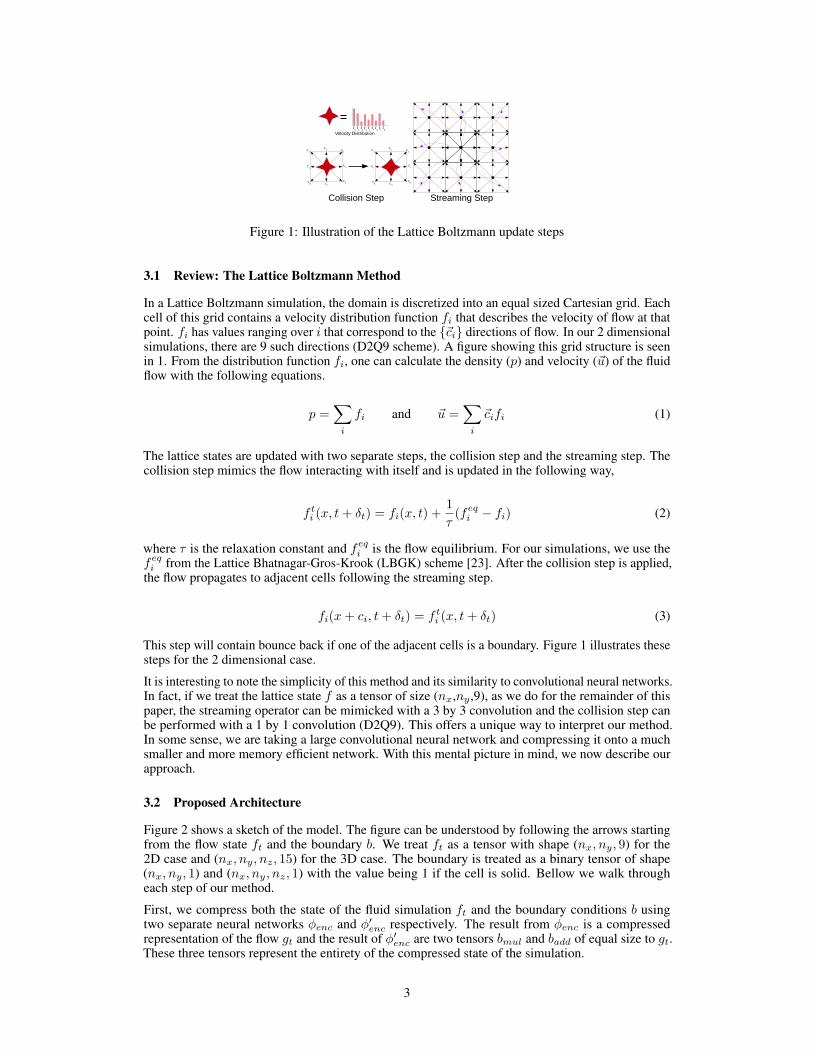
Figure 1: Illustration of the Lattice Boltzmann update steps

3.1 Review: The Lattice Boltzmann Method

In a Lattice Boltzmann simulation, the domain is discretized into an equal sized Cartesian grid. Eachcell of this grid contains a velocity distribution function fi that describes the velocity of flow at thatpoint. fi has values ranging over i that correspond to the {~ci} directions of flow. In our 2 dimensionalsimulations, there are 9 such directions (D2Q9 scheme). A figure showing this grid structure is seenin 1. From the distribution function fi, one can calculate the density (p) and velocity (~u) of the fluidflow with the following equations.

p =∑i

fi and ~u =∑i

~cifi (1)

The lattice states are updated with two separate steps, the collision step and the streaming step. Thecollision step mimics the flow interacting with itself and is updated in the following way,

f ti (x, t+ δt) = fi(x, t) +1

τ(feqi − fi) (2)

where τ is the relaxation constant and feqi is the flow equilibrium. For our simulations, we use thefeqi from the Lattice Bhatnagar-Gros-Krook (LBGK) scheme [23]. After the collision step is applied,the flow propagates to adjacent cells following the streaming step.

fi(x+ ci, t+ δt) = f ti (x, t+ δt) (3)

This step will contain bounce back if one of the adjacent cells is a boundary. Figure 1 illustrates thesesteps for the 2 dimensional case.

It is interesting to note the simplicity of this method and its similarity to convolutional neural networks.In fact, if we treat the lattice state f as a tensor of size (nx,ny,9), as we do for the remainder of thispaper, the streaming operator can be mimicked with a 3 by 3 convolution and the collision step canbe performed with a 1 by 1 convolution (D2Q9). This offers a unique way to interpret our method.In some sense, we are taking a large convolutional neural network and compressing it onto a muchsmaller and more memory efficient network. With this mental picture in mind, we now describe ourapproach.

3.2 Proposed Architecture

Figure 2 shows a sketch of the model. The figure can be understood by following the arrows startingfrom the flow state ft and the boundary b. We treat ft as a tensor with shape (nx, ny, 9) for the2D case and (nx, ny, nz, 15) for the 3D case. The boundary is treated as a binary tensor of shape(nx, ny, 1) and (nx, ny, nz, 1) with the value being 1 if the cell is solid. Bellow we walk througheach step of our method.

First, we compress both the state of the fluid simulation ft and the boundary conditions b usingtwo separate neural networks φenc and φ′enc respectively. The result from φenc is a compressedrepresentation of the flow gt and the result of φ′enc are two tensors bmul and badd of equal size to gt.These three tensors represent the entirety of the compressed state of the simulation.

3

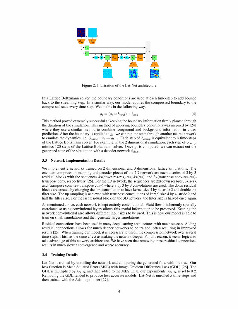
Figure 2: Illustration of the Lat-Net architecture

In a Lattice Boltzmann solver, the boundary conditions are used at each time-step to add bounceback to the streaming step. In a similar way, our model applies the compressed boundary to thecompressed state every time-step. We do this in the following way,

gt = (gt � bmul) + badd (4)

This method proved extremely successful at keeping the boundary information firmly planted throughthe duration of the simulation. This method of applying boundary conditions was inspired by [24]where they use a similar method to combine foreground and background information in videoprediction. After the boundary is applied to gt, we can run the state through another neural networkto emulate the dynamics, i.e. φcomp : gt → gt+1. Each step of φcomp is equivalent to n time-stepsof the Lattice Boltzmann solver. For example, in the 2 dimensional simulation, each step of φcomp

mimics 120 steps of the Lattice Boltzmann solver. Once gt is computed, we can extract out thegenerated state of the simulation with a decoder network φdec.

3.3 Network Implementation Details

We implement 2 networks trained on 2 dimensional and 3 dimensional lattice simulations. Theencoder, compression mapping and decoder pieces of the 2D network are each a series of 3 by 3residual blocks with the sequences 4x(down res-res)-res, 4x(res), and 3x(transpose conv-res-res)-transpose conv, respectively [25]. For the 3D network, the sequences are 2x(down res)-res, 3x(res),and (transpose conv-res-transpose conv) where 3 by 3 by 3 convolutions are used. The down residualblocks are created by changing the first convolution to have kernel size 4 by 4, stride 2 and double thefilter size. The up sampling is achieved with transpose convolutions of kernel size 4 by 4, stride 2 andhalf the filter size. For the last residual block on the 3D network, the filter size is halved once again.

As mentioned above, each network is kept entirely convolutional. Fluid flow is inherently spatiallycorrelated so using convlutional layers allows this spatial information to be preserved. Keeping thenetwork convolutional also allows different input sizes to be used. This is how our model is able totrain on small simulations and then generate larger simulations.

Residual connections have been used in many deep learning architectures with much success. Addingresidual connections allows for much deeper networks to be trained, often resulting in improvedresults [25]. When training our model, it is necessary to unroll the compression network over severaltime-steps. This has the same effect as making the network deeper. For this reason, it seems logical totake advantage of this network architecture. We have seen that removing these residual connectionsresults in much slower convergence and worse accuracy.

3.4 Training Details

Lat-Net is trained by unrolling the network and comparing the generated flow with the true. Ourloss function is Mean Squared Error (MSE) with Image Gradient Difference Loss (GDL) [26]. TheGDL is multiplied by λGDL and then added to the MES. In all our experiments, λGDL is set to 0.2.Removing the GDL tended to produce less accurate models. Lat-Net is unrolled 5 time-steps andthen trained with the Adam optimizer [27].

4

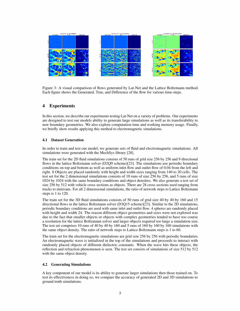
Figure 3: A visual comparison of flows generated by Lat-Net and the Lattice Boltzmann method.Each figure shows the Generated, True, and Difference of the flow for various time-steps.

4 Experiments

In this section, we describe our experiments testing Lat-Net on a variety of problems. Our experimentsare designed to test our models ability to generate large simulations as well as its transferability tonew boundary geometries. We also explore computation time and working memory usage. Finally,we briefly show results applying this method to electromagnetic simulations.

4.1 Dataset Generation

In order to train and test our model, we generate sets of fluid and electromagnetic simulations. Allsimulations were generated with the MechSys library [28].

The train set for the 2D fluid simulations consists of 50 runs of grid size 256 by 256 and 9 directionalflows in the lattice Boltzmann solver (D2Q9 scheme)[23]. The simulations use periodic boundaryconditions on top and bottom as well as uniform inlet flow and outlet flow of 0.04 from the left andright. 8 Objects are placed randomly with height and width sizes ranging from 140 to 20 cells. Thetest set for the 2 dimensional simulations consists of 10 runs of size 256 by 256, and 5 runs of size1024 by 1024 with the same boundary conditions and object densities. We also generate a test set ofsize 256 by 512 with vehicle cross sections as objects. There are 28 cross sections used ranging fromtrucks to minivans. For all 2 dimensional simulations, the ratio of network steps to Lattice Boltzmannsteps is 1 to 120.

The train set for the 3D fluid simulations consists of 50 runs of grid size 40 by 40 by 160 and 15directional flows in the lattice Boltzmann solver (D3Q15 scheme)[23]. Similar to the 2D simulations,periodic boundary conditions are used with same inlet and outlet flow. 4 spheres are randomly placedwith height and width 24. The reason different object geometries and sizes were not explored wasdue to the fact that smaller objects or objects with complex geometries tended to have too coursea resolution for the lattice Boltzmann solver and larger objects required too large a simulation size.The test set comprises 10 runs of 40 by 40 by 160 and 5 runs of 160 by 160 by 160 simulations withthe same object density. The ratio of network steps to Lattice Boltzmann steps is 1 to 60.

The train set for the electromagnetic simulations are grid size 256 by 256 with periodic boundaries.An electromagnetic wave is initialized in the top of the simulations and proceeds to interact withrandomly placed objects of different dielectric constants. When the wave hits these objects, thereflection and refraction phenomenon is seen. The test set consists of simulations of size 512 by 512with the same object density.

4.2 Generating Simulations

A key component of our model is its ability to generate larger simulations then those trained on. Totest its effectiveness in doing so, we compare the accuracy of generated 2D and 3D simulations toground truth simulations.

5

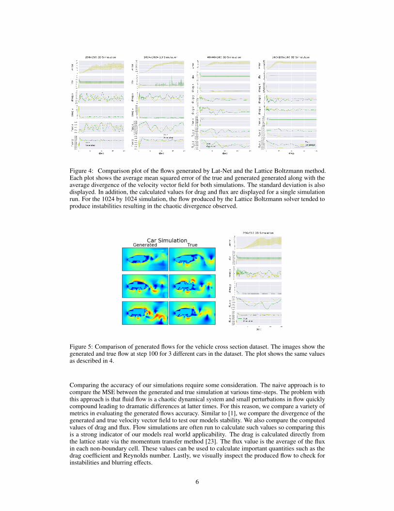
Figure 4: Comparison plot of the flows generated by Lat-Net and the Lattice Boltzmann method.Each plot shows the average mean squared error of the true and generated generated along with theaverage divergence of the velocity vector field for both simulations. The standard deviation is alsodisplayed. In addition, the calculated values for drag and flux are displayed for a single simulationrun. For the 1024 by 1024 simulation, the flow produced by the Lattice Boltzmann solver tended toproduce instabilities resulting in the chaotic divergence observed.

Figure 5: Comparison of generated flows for the vehicle cross section dataset. The images show thegenerated and true flow at step 100 for 3 different cars in the dataset. The plot shows the same valuesas described in 4.

Comparing the accuracy of our simulations require some consideration. The naive approach is tocompare the MSE between the generated and true simulation at various time-steps. The problem withthis approach is that fluid flow is a chaotic dynamical system and small perturbations in flow quicklycompound leading to dramatic differences at latter times. For this reason, we compare a variety ofmetrics in evaluating the generated flows accuracy. Similar to [1], we compare the divergence of thegenerated and true velocity vector field to test our models stability. We also compare the computedvalues of drag and flux. Flow simulations are often run to calculate such values so comparing thisis a strong indicator of our models real world applicability. The drag is calculated directly fromthe lattice state via the momentum transfer method [23]. The flux value is the average of the fluxin each non-boundary cell. These values can be used to calculate important quantities such as thedrag coefficient and Reynolds number. Lastly, we visually inspect the produced flow to check forinstabilities and blurring effects.

6

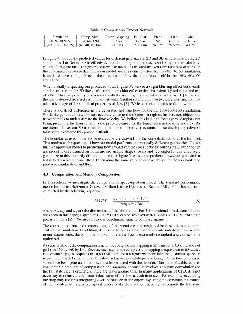
Table 1: Computation Time of Network

Simulation Comp. Size Comp. Mapping Full State Plane Line Point(1024, 1024, 9) (64, 64, 128) 2.7 ms 36.2 ms NA 6.7 ms 6.6 ms

(160, 160, 160, 15) (40, 40, 40, 64) 23.1 ms 272.1 ms 38.2 ms 25.6 ms 24.1 ms

In figure 4, we see the predicted values for different grid sizes in 2D and 3D simulations. In the 2Dsimulations, Lat-Net is able to effectively transfer to larger domain sizes with very similar calculatedvalues of drag and flux. The generated flow also maintains its stability even after hundreds of steps. Inthe 3D simulation we see that, while our model predicts realistic values for the 40x40x160 simulation,it tends to have a slight bias in the direction of flow that manifests itself in the 160x160x160simulation.

When visually inspecting our produced flows (figure 3), we see a slight blurring effect but overallsimilar structure in the 2D flows. We attribute this blur effect to the dimensionality reduction and useof MSE. This can possibly be overcome with the use of generative adversarial network [16] wherethe loss is derived from a discriminator network. Another solution may be to craft a loss function thattakes advantage of the statistical properties of flow [7]. We leave these pursuits to future work.

There is a distinct difference in the generated and true flow for the 3D 160x160x160 simulation.While the generated flow appears accurate close to the objects, in regions far between objects thenetwork tends to underestimate the flow velocity. We believe this is due to these types of regions notbeing present in the train set and is the probable cause for the biases seen in the drag and flux. Asmentioned above, our 3D train set is limited due to memory constraints and so developing a diversetrain set to overcome this proved difficult.

The boundaries used in the above evaluation are drawn from the same distribution as the train set.This motivates the question of how our model performs on drastically different geometries. To testthis, we apply our model to predicting flow around vehicle cross sections. Surprisingly, even thoughare model is only trained on flows around simple shapes (ovals and rectangles) it can effectivelygeneralize to this distinctly different domain. In figure 5, we see the predicted flows are quite similarbut with the same blurring effect. Calculating the same values as above, we see the flow is stable andproduces similar drag and flux.

4.3 Computation and Memory Compression

In this section, we investigate the computational speed-up of our model. The standard performancemetric for Lattice Boltzmann Codes is Million Lattice Updates per Second (MLUPs). This metric iscalculated by the following equation,

MLUP =nx × ny × nz × 10−6

Compute T ime(5)

where nx, ny, and nz are the dimensions of the simulation. For 3 dimensional simulations like theones seen in this paper, a speed of 1,200 MLUPS can be achieved with a Nvidia K20 GPU and singleprecision floats [29]. We use this as our benchmark value to compare against.

The computation time and memory usage of the encoder can be neglected because this is a one timecost for the simulation. In addition, if the simulation is started with uniformly initialized flow as seenin our experiments, the computation to compress the flow is extremely redundant and can easily beoptimized.

As seen in table 1, the computation time of the compression mapping is 23.1 ms for a 3D simulation ofgrid size 160 by 160 by 160. Because each step of the compression mapping is equivalent to 60 LatticeBoltzmann steps, this equates to 10,600 MLUPS and a roughly 9x speed increase (a similar speed-upis seen with the 2D simulation). This does not give a complete picture though. Once the compressedstates have been generated, the flow must be extracted with the decoder. Unfortunately, this requiresconsiderable amounts of computation and memory because it involves applying convolutions tothe full state size. Fortunately, there are ways around this. In many applications of CFD, it is notnecessary to to have the full state information of the flow at each time-step. For example, calculatingthe drag only requires integrating over the surface of the object. By using the convolutional natureof the decoder, we can extract specif pieces of the flow without needing to compute the full state.

7

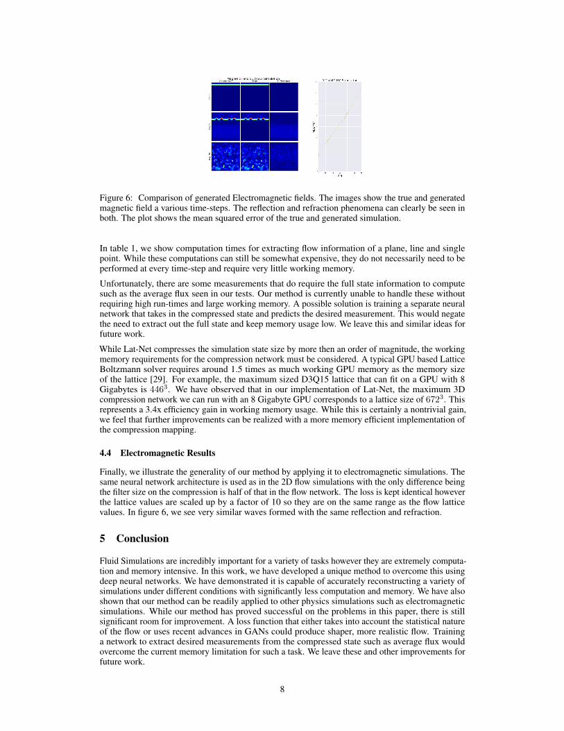
Figure 6: Comparison of generated Electromagnetic fields. The images show the true and generatedmagnetic field a various time-steps. The reflection and refraction phenomena can clearly be seen inboth. The plot shows the mean squared error of the true and generated simulation.

In table 1, we show computation times for extracting flow information of a plane, line and singlepoint. While these computations can still be somewhat expensive, they do not necessarily need to beperformed at every time-step and require very little working memory.

Unfortunately, there are some measurements that do require the full state information to computesuch as the average flux seen in our tests. Our method is currently unable to handle these withoutrequiring high run-times and large working memory. A possible solution is training a separate neuralnetwork that takes in the compressed state and predicts the desired measurement. This would negatethe need to extract out the full state and keep memory usage low. We leave this and similar ideas forfuture work.

While Lat-Net compresses the simulation state size by more then an order of magnitude, the workingmemory requirements for the compression network must be considered. A typical GPU based LatticeBoltzmann solver requires around 1.5 times as much working GPU memory as the memory sizeof the lattice [29]. For example, the maximum sized D3Q15 lattice that can fit on a GPU with 8Gigabytes is 4463. We have observed that in our implementation of Lat-Net, the maximum 3Dcompression network we can run with an 8 Gigabyte GPU corresponds to a lattice size of 6723. Thisrepresents a 3.4x efficiency gain in working memory usage. While this is certainly a nontrivial gain,we feel that further improvements can be realized with a more memory efficient implementation ofthe compression mapping.

4.4 Electromagnetic Results

Finally, we illustrate the generality of our method by applying it to electromagnetic simulations. Thesame neural network architecture is used as in the 2D flow simulations with the only difference beingthe filter size on the compression is half of that in the flow network. The loss is kept identical howeverthe lattice values are scaled up by a factor of 10 so they are on the same range as the flow latticevalues. In figure 6, we see very similar waves formed with the same reflection and refraction.

5 Conclusion

Fluid Simulations are incredibly important for a variety of tasks however they are extremely computa-tion and memory intensive. In this work, we have developed a unique method to overcome this usingdeep neural networks. We have demonstrated it is capable of accurately reconstructing a variety ofsimulations under different conditions with significantly less computation and memory. We have alsoshown that our method can be readily applied to other physics simulations such as electromagneticsimulations. While our method has proved successful on the problems in this paper, there is stillsignificant room for improvement. A loss function that either takes into account the statistical natureof the flow or uses recent advances in GANs could produce shaper, more realistic flow. Traininga network to extract desired measurements from the compressed state such as average flux wouldovercome the current memory limitation for such a task. We leave these and other improvements forfuture work.

8

References

[1] J. Tompson, K. Schlachter, P. Sprechmann, and K. Perlin, “Accelerating eulerian fluid simulationwith convolutional networks,” arXiv preprint arXiv:1607.03597, 2016.

[2] X. Guo, W. Li, and F. Iorio, “Convolutional neural networks for steady flow approximation,” inProceedings of the 22nd ACM SIGKDD International Conference on Knowledge Discovery andData Mining, pp. 481–490, ACM, 2016.

[3] C. Yang, X. Yang, and X. Xiao, “Data-driven projection method in fluid simulation,” ComputerAnimation and Virtual Worlds, vol. 27, no. 3-4, pp. 415–424, 2016.

[4] G. R. McNamara and G. Zanetti, “Use of the boltzmann equation to simulate lattice-gasautomata,” Physical review letters, vol. 61, no. 20, p. 2332, 1988.

[5] S. Galindo-Torres, A. Scheuermann, and R. Puscasu, “A lattice boltzmann solver for maxwellequations in dielectric media,”

[6] M. Mendoza and J. Munoz, “Three-dimensional lattice boltzmann model for electrodynamics,”Physical Review E, vol. 82, no. 5, p. 056708, 2010.

[7] T. Kim, N. Thürey, D. James, and M. Gross, “Wavelet turbulence for fluid simulation,” in ACMTransactions on Graphics (TOG), vol. 27, p. 50, ACM, 2008.

[8] L. Zhong, S. Feng, P. Dong, and S. Gao, “Lattice boltzmann schemes for the nonlinearschrödinger equation,” Physical Review E, vol. 74, no. 3, p. 036704, 2006.

[9] X. Shan and H. Chen, “Lattice boltzmann model for simulating flows with multiple phases andcomponents,” Physical Review E, vol. 47, no. 3, p. 1815, 1993.

[10] N. Onodera, T. Aoki, T. Shimokawabe, and H. Kobayashi, “Large-scale les wind simulationusing lattice boltzmann method for a 10 km× 10 km area in metropolitan tokyo,” TSUBAMEe-Science Journal Global Scientific Information and Computing Center, vol. 9, pp. 1–8, 2013.

[11] W. Xian and A. Takayuki, “Multi-gpu performance of incompressible flow computation bylattice boltzmann method on gpu cluster,” Parallel Computing, vol. 37, no. 9, pp. 521–535,2011.

[12] G. B. Goh, N. O. Hodas, and A. Vishnu, “Deep learning for computational chemistry,” Journalof Computational Chemistry, 2017.

[13] K. Mills, M. Spanner, and I. Tamblyn, “Deep learning and the schr\" odinger equation,” arXivpreprint arXiv:1702.01361, 2017.

[14] G. Carleo and M. Troyer, “Solving the quantum many-body problem with artificial neuralnetworks,” Science, vol. 355, no. 6325, pp. 602–606, 2017.

[15] M. Paganini, L. de Oliveira, and B. Nachman, “CaloGAN: Simulating 3D High Energy ParticleShowers in Multi-Layer Electromagnetic Calorimeters with Generative Adversarial Networks,”ArXiv e-prints, May 2017.

[16] I. Goodfellow, J. Pouget-Abadie, M. Mirza, B. Xu, D. Warde-Farley, S. Ozair, A. Courville, andY. Bengio, “Generative adversarial nets,” in Advances in neural information processing systems,pp. 2672–2680, 2014.

[17] C. W. Rowley, T. Colonius, and R. M. Murray, “Model reduction for compressible flows usingpod and galerkin projection,” Physica D: Nonlinear Phenomena, vol. 189, no. 1, pp. 115–129,2004.

[18] M. F. Barone, I. Kalashnikova, M. R. Brake, and D. J. Segalman, “Reduced order modelingof fluid/structure interaction,” Sandia National Laboratories Report, SAND No, vol. 7189,pp. 44–72, 2009.

[19] K. Veroy and A. Patera, “Certified real-time solution of the parametrized steady incompress-ible navier–stokes equations: rigorous reduced-basis a posteriori error bounds,” InternationalJournal for Numerical Methods in Fluids, vol. 47, no. 8-9, pp. 773–788, 2005.

[20] C. W. Rowley, “Model reduction for fluids, using balanced proper orthogonal decomposition,”International Journal of Bifurcation and Chaos, vol. 15, no. 03, pp. 997–1013, 2005.

[21] D. P. Kingma and M. Welling, “Auto-encoding variational bayes,” arXiv preprintarXiv:1312.6114, 2013.

9

[22] M. Watter, J. Springenberg, J. Boedecker, and M. Riedmiller, “Embed to control: A locallylinear latent dynamics model for control from raw images,” in Advances in Neural InformationProcessing Systems, pp. 2746–2754, 2015.

[23] Z. Guo and C. Shu, Lattice Boltzmann method and its applications in engineering, vol. 3. WorldScientific, 2013.

[24] C. Vondrick, H. Pirsiavash, and A. Torralba, “Generating videos with scene dynamics,” inAdvances In Neural Information Processing Systems, pp. 613–621, 2016.

[25] K. He, X. Zhang, S. Ren, and J. Sun, “Deep residual learning for image recognition,” inProceedings of the IEEE Conference on Computer Vision and Pattern Recognition, pp. 770–778,2016.

[26] M. Mathieu, C. Couprie, and Y. LeCun, “Deep multi-scale video prediction beyond mean squareerror,” arXiv preprint arXiv:1511.05440, 2015.

[27] D. Kingma and J. Ba, “Adam: A method for stochastic optimization,” arXiv preprintarXiv:1412.6980, 2014.

[28] D. Pedroso, R. Durand, and S. Galindo, “Mechsys, multi-physics simulation library,” 2015.[29] M. Januszewski and M. Kostur, “Sailfish: A flexible multi-gpu implementation of the lattice

boltzmann method,” Computer Physics Communications, vol. 185, no. 9, pp. 2350–2368, 2014.

10