Embed Size (px)
Citation preview

ABSTRACT
Title of Document: ADVANCED SHADOW MOIRE WITH
NON-CONVENTIONAL IMAGING
ANGLES
Brian Kwong
Master of Science
Summer 2012
Directed By: Professor Bongtae Han,
Dept of Mechanical Engineering
With the increasingly smaller electronic package size, warpage of electronic packages
becomes an important measurement related to the reliability of the products. Higher
sensitivity out-of-plane deformation techniques are required to capture the smaller
deformations of tiny packages for enhanced design analysis and model verification.
The higher sensitivity is realized using non-zero viewing angles with the conventional
shadow moiré technique. Advanced configurations to accommodate the non-zero
viewing angles are developed to cope with direct reflection encountered on the
conventional setup. An expanded governing equation for the configuration is derived
and verified experimentally. Then the proposed configuration was implemented in
the testing of an actual package to demonstrate the advantages that accrue from the
higher sensitivity.
.

ADVANCED SHADOW MOIRE WITH NON-CONVENTIONAL IMAGING
ANGLES
By
Brian John Kwong
Thesis submitted to the Faculty of the Graduate School of the
University of Maryland, College Park, in partial fulfillment
of the requirements for the degree of
Master of Science
2012
Advisory Committee:
Professor Bongtae Han (Chair)
Associate Professor Miao Yu
Associate Professor Patrick McCluskey

© Copyright by
Brian Kwong
2012

ii
Acknowledgements
I want to express my gratitude and thanks to all the people whose help and support
made this work possible. In particular, I want to specially thank Professor Han, my
advisor for taking the time to educate me and allowing me to grow under his tutelage.
Without his support and guidance I would not be the person I am today.
I also want to thank my friends in the lab for their collaboration throughout the past
two years. This graduate school experience would have been a struggle if I wasn’t in
such an accepting group. Therefore it is my great pleasure to thank and acknowledge
Bong-min, Dae-suk, Kenny, Michelle, Stephen, and Yong. To my friends and family
outside the lab please accept my thanks for providing me the much needed anchor to
the real world.
Finally, I want to thank my parents, Salina and Kelvin, for all their assistance and
love. I am forever grateful and indebted for everything they have given me.

iii
Table of Contents
Acknowledgements ....................................................................................................... ii
Table of Contents ......................................................................................................... iii List of Figures .............................................................................................................. iv Chapter 1: Motivation ............................................................................................. 1
Introduction to Warpage Measurement Techniques ................................................ 1 Phase Shifting ........................................................................................................... 4
Summary of Work..................................................................................................... 6 Chapter 2: Conventional Shadow Moiré ................................................................ 7
Rectilinear Propagation of Light ............................................................................... 7
Diffraction: Talbot Distance and its impact in Shadow Moiré ............................... 12 Constraint of incident angle and grating due to contrast ........................................ 18 Limitation of oblique viewing angles ..................................................................... 21
Chapter 3: Advanced Shadow Moiré Technique .................................................. 24
Shadow Moiré using Non-conventional angles ...................................................... 24 Implementation Verification ................................................................................... 29
Experiment Configuration .................................................................................. 29 Hardware/Software ............................................................................................. 31
Verification of the Governing Equation ................................................................. 33
Application of Advanced Technique ...................................................................... 38
Chapter 4: Potential Future Investigation ............................................................. 43 Chapter 5: Conclusions ......................................................................................... 44 Bibliography ............................................................................................................... 45

iv
List of Figures
Figure 1.1: Example of package and industry trend ..................................................... 1
Figure 1.2 Cross-section of Ball Grid Array package with material CTE [3] ............. 2
Figure 1.3: Shadow Moiré thermal cycling example .................................................... 4
Figure 2.1: Rectilinear Demonstration of Shadow Moiré [36] ..................................... 9
Figure 2.2: Constant sensitivity configuration for shadow moiré by keeping
tan tan constant, (a) oblique viewing, (b) normal viewing [36] ................. 11
Figure 2.3: Constant sensitivity with collimating lenses at oblique angles [36] ........ 12
Figure 2.4: Illustration of Talbot distance for oblique illumination with
complimentary virtual gratings at multiples of ½ the Talbot distance [37]. ............... 13
Figure 2.5: Calculated Talbot distance for range of 45-63°, pitch of 0.1 and 0.2 mm 15
Figure 2.6: Self-imaging of 10 line/mm Ronchi gratings at n-talbot distance where n
is equal to a) 0, b) ¼, c) ½ , d) ¾ [37]......................................................................... 15
Figure 2.7: Warpage of flip chip BGA with g=.1mm and α=63° for a 50um/fringe
contour interval [23] ................................................................................................... 16
Figure 2.8: Talbot Distance for contour interval of 100um/fringe with β = 0° [23] ... 17
Figure 2.9: Aperture effect: (top) large aperture (bottom) pinhole aperture [3] ......... 19
Figure 2.10: Contrast due to aperture effect for de=.003 ........................................... 20
Figure 2.11: Fringe patterns of α = 63°, β = 25°, pitch of 10lines/mm, (a) unmodified
(b) Stretch correction to have square specimen .......................................................... 21
Figure 2.12: Light paths for shadow moiré with non-zero beta .................................. 23
Figure 2.13: Reflection captured at α=63°, β=60°, g=5lines/mm ............................... 23
Figure 3.1: Proposed Shadow Moiré Configuration a) Rotated camera b) Rotated light
source .......................................................................................................................... 25
Figure 3.2: Geometric side view of modified technique............................................. 26
Figure 3.3: Theoretical contour interval values at α=63°, g=0.2mm .......................... 28
Figure 3.4: Illustration of Modified Shadow Moiré setup .......................................... 30
Figure 3.5: Image pairs (a) Fringes for α=40°, β=0°, θ=0°, g= 0.2 mm at starting
position (b) Fringes after contour interval of (1)0.236, (2)0.238, (3) 0.240 (mm) ..... 35
v
Figure 3.6: Image pairs (a) Fringes for α=40°, β=0°, θ=50°, g= 0.2mm at starting
position. (b) Fringes after contour interval of (1) 0.365, (2) 0.367, (3) 0.369(mm) .. 35
Figure 3.7: Experimental data compared with theoretical values for setup of α = 40°,
β = 0° and g= 0.2mm .................................................................................................. 36
Figure 3.8: Experimental data compared with theoretical values for setup of α = 40°,
β = 20° and g= 0.2mm. ............................................................................................... 36
Figure 3.9: Experimental data compared with theoretical values for setup of α = 45°,
β = 0° and g= 0.2mm .................................................................................................. 37
Figure 3.10: Experimental data compared with theoretical values for setup of α = 40°,
β = 30° and g=0.2mm ................................................................................................. 37
Figure 3.11: Marvell PBGA Package (left) front (right) back .................................... 38
Figure 3.12: Setup of α=63°, β=0°, θ=0°, g=0.2mm a) Phase shifted images of
specimen b) Specimen wrapped phase map c) 3D-model of displacement pattern .... 39
Figure 3.13: Setup of α=63°, β=25°, θ=0°, g=0.2mm a) Phase shifted images of
specimen b) Specimen wrapped phase map c) 3D-model of displacement pattern .... 40
Figure 3.14: Setup of α=63°, β=60°, θ=20°, g=0.2mm a) Phase shifted images of
specimen b) Specimen wrapped phase map c) 3D-model of displacement pattern .... 41

1
Chapter 1: Motivation
Introduction to Warpage Measurement Techniques
The need for small displacement measurements came from the microelectronic industry
as electronics and their packages trended smaller [1]. The electronic package is part of a
final commercial device that has several functions including protection of components
and interconnects, signal and power distribution, and mechanical support [2]. The whole
device is comprised of multiple materials with individual coefficient of thermal
expansion (CTE).
Figure 1.1: Example of package and industry trend [1]
Warpages in PBGA packages occur when materials with different CTE are mechanically
bonded together and subject to a temperature change. The coefficient mismatch induces
warpages as higher CTE material will have expanded more. At different temperatures
other than the condition where the surfaces were initially flat, there will be more

2
deformation in one of the materials, leading to warpage. An example of the problem that
arises during manufacturing is shown in Figure 1.2. Due to the CTE mismatch, the solder
balls are no longer at the same height after undergoing thermal cycling. This causes
reliability issues between interconnects due to the small differences in the height of the
solder balls have the potential to affect solder ball fatigue life. Package warpage is
associated with the reliability of the packaged device. Therefore, measurement of
distortion in packages has been used in order to better model the changes to the package
that occurs under extreme loads like thermal loads from the solder reflow process.
Different techniques have been developed to cover the range of out of plane
measurements.
Figure 1.2 Cross-section of Ball Grid Array package with material CTE [3]
Shadow moiré, an out-of-plane displacement fringe pattern measurement technique, came
about from the moiré topography concept first described by Takasaki [4] and Meadows et
al. [5] in 1970. Shadow moiré has become a popular choice for sample distortion
evaluation under mechanical and/or thermal loading in the microelectronics industry. A
JEDEC industry standard for high temperature testing adopted shadow moiré as one of
the techniques to be used for those type of measurements [6]. The technique is robust
with a diffuse sample surface requirement rather than a specular surface. It can be
Substrate (>15 ppm/°C)
Solder Balls (>23 ppm/°C)
Chip (>3ppm/°C)

3
implemented with a variety of light sources [7]-[9] . It is also a whole field technique,
which allows for characterization of the entire specimen surface at one time. Whole field
techniques are better for dynamic system measurements, as the surface displacements are
quantified simultaneously rather than over a period of time with point by point
measurement. The technique determines absolute displacement from the sample surface
to the reference grating which can be utilized to determine relative distances.
Use of shadow moiré on electronic packages is common in the literature, and its use
continues to the present [7]-[22]. Some applications included samples placed in solder
reflow conditions [17]-[19] and thermal loading of printed wiring boards and other
electronic components [10]-[14]. Warpage under thermal treatment, as a result of
differences in CTE between the materials in electronic packages, is important, as it can
be tied to reliability issues. Conventional shadow moiré on the micro scale could be
realized down to 110 µm/fringe, and with the use of the half Talbot distance, the contour
interval could be further brought down to 43 µm/fringe [23] with adequate dynamic
range. Shadow moiré at non-normal angles has been explored [11], but the angles used
were small. An example of shadow moiré, shown in Figure 1.3, details the measurement
of a processor undergoing thermal cycling.

4
Figure 1.3: Shadow Moiré thermal cycling example
Phase Shifting
An important technique called phase shift is used to increase the overall pattern
recognition of fringe based measurement techniques [25]-[30]. The intensity distribution
is assumed to be sinusoidal in shape. The intensity distribution of the fringe pattern is
then defined as:
( , ) ( , ) ( , )cos( ( , ))
where is the background intensity,
is the modulation intensity, and
and represents the angular phase of the fringe pattern;
the is related to fringe order ,
m a
m
a
I x y I x y I x y x y
I
I
N x y
by 2 .N (0.1)
There are three unknowns in the above equation, which means three equations need to be
solved in order to determine mI , aI and . At least three fringe patterns with equal phase
differences are required to implement phase shifting. The term is especially important

5
because it provides information on the points between the fringe patterns. Different
algorithms were developed that used more than the requisite three phase-shifted images,
since more phase steps smooth out those phase shift errors. The most widely used
algorithm takes the information from four images to calculate the phase and is given as:
1
2
3
4
4 2
1 3
( , ) ( , ) ( , )*cos( ( , )
( , ) ( , ) ( , )*cos( ( , ) / 2)
( , ) ( , ) ( , )*cos( ( , ) )
( , ) ( , ) ( , )*cos( ( , ) 3 / 2)
( , ) ( , )( , ) arctan( )
( , ) ( , )
m a
m a
m a
m a
I x y I x y I x y x y
I x y I x y I x y x y
I x y I x y I x y x y
I x y I x y I x y x y
I x y I x yx y
I x y I x y
(0.2)
Errors when acquiring the images after phase shift can result in significant deviations
from the true phase value. Current research has developed numerical analysis that can
apply the phase shift technique even if the phase shift is arbitrary[26] or constant but
unknown[28]. It is also necessary to unwrap the phase diagram after the use of the phase
shifting algorithm. The absolute value of the phase is lost when the phase range extends
over 2π due to the properties of the arctangent function used in its calculation.
A systematic error is introduced in phase shifting techniques by assuming a sinusoidal
intensity distribution. In reality the intensity distribution of shadow moiré is a complex
function of different experimental parameters [31]-[33]. The error of the 4-image phase
shift algorithm was experimentally tested and derived, and known to introduce a
maximum error of 1.7% of the contour interval [23] [32]. The error is therefore more
pronounced when using a lower measurement sensitivity system. High basic
measurement sensitivity is necessary with use of phase shifting.

6
Summary of Work
There is a need for warpage measurement techniques in the microelectronics industry as
packages continue to grow smaller while the designs grow more diverse. To that end, an
existing shadow moiré technique is modified to create a framework for taking
measurement that will surpass current existing limits dictated by the traditional high-
sensitivity moiré setup. The non-coplanarity of the new configuration will solve inherent
issues in the conventional setup of shadow moiré regarding the reflection from the
grating and widens the viewing angles that are viewable in a traditional setup. The
following chapters will be used to illustrate an advanced shadow moiré technique that
uses non-standard viewing angles to decrease contour interval size. The new contour
interval equation associated with the modified shadow moiré that uses a non-coplanar
setup was derived and then experimentally verified. The modified technique was used to
demonstrate the improvement in sensitivity for package warpages measurement.
Sensitivity improvements at very large angle non-normal values are shown to have the
potential of reducing the contour size by half as compared to normal viewing.
Equation Section (Next)

7
Chapter 2: Conventional Shadow Moiré
Rectilinear Propagation of Light
The shadow moiré technique can be described utilizing the assumption of rectilinear
propagation of light. The rectilinear assumption only holds when the distance between
the grating and specimen is small compared to the Talbot distance. This grating self-
imaging distance will be discussed later in the thesis. The method requires an amplitude
grating, a light source, a prepared sample, and an observer, normally a camera, to record
the images. The sample is sprayed with a thin layer of white matte paint. The paint allows
the sample to uniformly diffuse the visible rays of light and is considered thin enough to
not significantly alter the out-of-plane displacement.
The grating required is the Ronchi grating. It is a series of alternating transparent and
opaque bars of equal width; the physical grating is typically made by depositing the metal
pattern layer on one side of a glass plate. The flat grating has to be placed so that the bars
are perpendicular to the imaging plane. Previous researchers have used Ronchi type
flexible [34] and non-flat gratings [35] for specific applications; this thesis will solely be
using flat glass gratings. As stated previously, a variety of light sources can be used. The
typical light source is a bright white light with a small size, approximating a point source
or a slit that is parallel to the grating lines.
The light source illuminates the grating, which casts a shadow grating on the specimen
surface. The camera captures the interference between the shadow grating on the sample

8
and the superimposed reference grating, producing a moiré fringe pattern. For a pinhole
aperture, there is only one light beam which will be scattered from the surface that will
reach the observer. The interference pattern is equivalent to a contour map, the number of
fringes between two points indicate the out of plane displacement between the points.
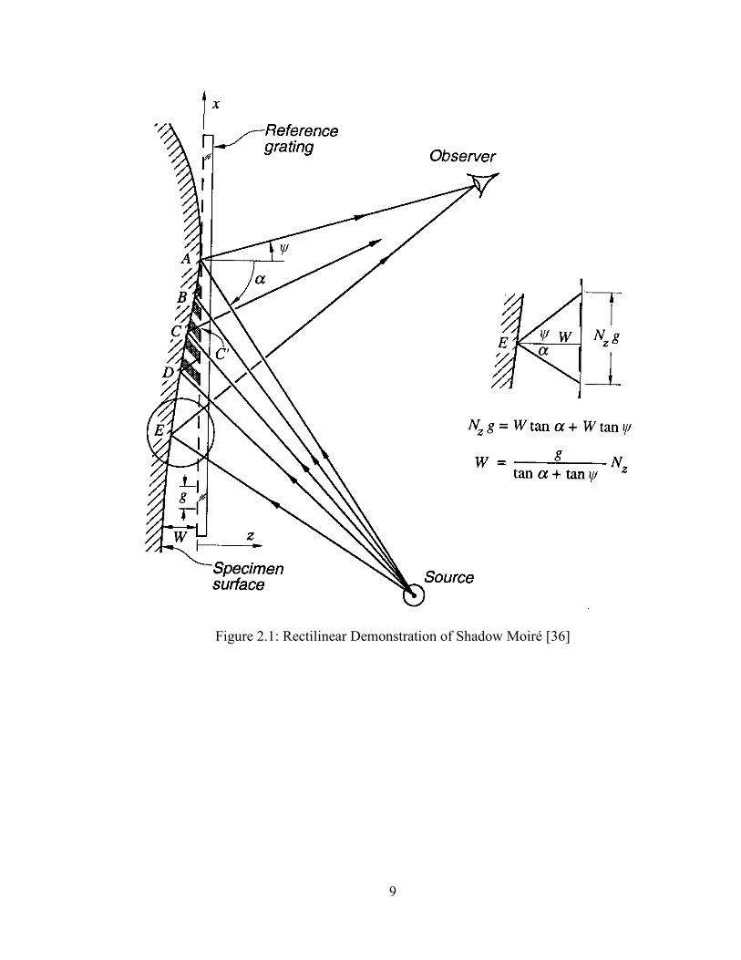
The concept behind the technique is shown in Figure 2, with the setup having the
following variables: z is the displacement between the reference grating and the specimen
surface; g is the reference grating pitch, α is the illumination angle, and ψ (or β) is the
incident light to the camera angle. Example of how the fringes look at the different points
can be seen. The first point of interest is point A. As the light passes through the grating
and reaches the observer, that point is seen as a bright fringe. Point A is assigned the zero
fringe order, as there is zero distance between it and the grating. Similarly points E and C
are seen as bright fringes. Points B and D are dark fringes as the light diffuse from the
surface interferes with the dark part of the grating; a dark fringe would also occur if the
source light has interference with the dark part of the shadow fringe. The fringe order can
be determined by the number of fringes between the entrance of the light and the exit of
the light. A full fringe is the distance between one bright fringe to the next. In the case of
point C, there are four fringes between point A (the zero reference) and the light entrance.
There are three fringes between point A and C, the point where the observer sees the light
passing through the grating, meaning that point C has a fringe order of one.
9
Figure 2.1: Rectilinear Demonstration of Shadow Moiré [36]

10
From geometry, the relationship between z and the fringe order N is determined as:
, ( , )tan( ) tan( )
gz x y N x y
(1.1)
Note that the sensitivity is not constant across due to the specimen as the angles are
constantly changing at every point. A solution to achieving constant sensitivity can be
seen in equation 2.1. The two ways to achieve constant sensitivity would be to keep
tan(α)+tan(β) constant or keep the angles the same at every point. A method to achieve
the theoretical constant sensitivity by keeping tan(α)+tan(β) constant is to place the light
source and observer the same distance away (L) from the reference grating plane [36]. It
can then be approximated that
tan tanD D
L z L
(1.2)
where D is the distance between the light and the observer.
The approximation in equation 2.2 allows the z displacement at every point to be
correlated directly to the fringe order. Combining equation 2.1 and 2.2, the constant
contour interval, which is the amount the fringe order is multiplied by, can be then
calculated as:
*
tan( ) tan( )( )
g g L g
D D
L
(1.3)
The assumption inherent in this approximation is that the range of displacement across all
the points is much smaller than the L distance. The previously described method for
constant sensitivity for the fringe patterns is shown, with oblique angle viewing in Figure
2.2a and normal viewing in Figure 2.2b.

11
The second method to achieve constant sensitivity, but not pursued in this thesis, is to
keep the angle constant at all points by the use of collimating lenses (as shown in Figure
2.3). The divergent light from the source will be collimated onto the sample surface so it
hits the sample at a specific α. The diffuse light from the specimen would then be
observed through a collimating lens as well, resulting in a known constant β. The use of
this version of shadow moiré would not be constrained by any distance requirements for
source and observer placement; however the sample size is limited to the size of the
collimating lenses used.
Figure 2.2: Constant sensitivity configuration for shadow moiré by keeping
tan tan constant, (a) oblique viewing, (b) normal viewing [36]

12
Figure 2.3: Constant sensitivity with collimating lenses at oblique angles [36]
Normal viewing is popular in shadow moiré configurations because there are no visual
distortions of the sample during viewing. However, in order to have the large values of α
at normal incidence, the light placement gets progressively further away. This becomes a
practical setup problem as well as light intensity decrease the further away from the
source it is. Reflection from dielectric surface also means less light is being transmitted
through the grating, which is also limiting the intensity of the light beam that the camera
is picking up. A practical limit of tan (α) = 3 was suggested for normal incidence to have
usable light intensity.[23]
Diffraction: Talbot Distance and its impact in Shadow Moiré
The equation for shadow moiré seems to indicate that the fringes will appear at any
displacement. In reality, the fringe contrast changes based on the sample’s distance away
from the reference grating. The fringe contrast is affected by the Talbot effect, a grating
self-imaging effect that occurs due to diffraction from a periodic structure. The

13
illuminated reference grating splits the light beam into multiple diffracted beams. The
diffracted beams will then interfere with each other, producing a virtual grating at a
specific distance that is the same pitch as the reference grating. Those virtual gratings are
called “Talbot images,” with the replication occurring at the Talbot Distance (TD). The
TD equation for normal incidence is:
22T
gD
[36] (1.4)
For shadow moiré, the TD based on oblique illumination was given by Testorf as:
232
* ( )g
TD cos
[38] (1.5)
Figure 2.4: Illustration of Talbot distance for oblique illumination with complimentary
virtual gratings at multiples of ½ the Talbot distance [37].

14
A simple geometric derivation of Talbot distance can also be utilized to describe the
interaction of the diffracted beams [37]. When collimated light enters the grating at an
angle of α, defined perpendicular from the grating bars, the effective grating is
' co ( )sg g (1.6)
From equation 2.3, the distance between the grating and the virtual grating is:
2 2 222 ' 2( cos( )) 2
* ( )g g g
TD cos
(1.7)
The distance of the virtual grating parallel to the grating surface is calculated to be:
2 22 32 2
*cos( ) ( * ( ) cos( ))* * ( )g g
D TD cos cos
(1.8)
The equation is equivalent to the equation derived in reference [38], which utilized a
mathematical derivation of off-axis light diffraction through a Ronchi grating. This
equation was used to calculate the TD from 45° to 63° with two different pitches, shown
in Figure 2.5. It can be seen that both the decrease of grating pitch and increase of α
greatly affects the TD. The increase of sensitivity through those two means are
constrained by how quickly the Talbot distance is modified.
It is known that complimentary images of the grating appear at ½ TD, while at ¼ and ¾
TD a destructive interference virtual grating will occur [37]. Therefore, at the ¼ and ¾
TD, the virtual grating will cause the contrast to go to zero. Example of self-imaging is
shown in Figure 2.6. The TD is proportional to the grating pitch squared, from equation
2.4, so decreasing the gratings pitch quickly results in very small usable distances. Note
that the TD is not dependent on the β angle, so any gains in sensitivity from using the β
angle will not hinder the contrast of the technique based on diffraction.

15
Figure 2.5: Calculated Talbot distance for range of 45-63°, pitch of 0.1 and 0.2 mm
Figure 2.6: Self-imaging of 10 line/mm Ronchi gratings at n-talbot distance where n is
equal to a) 0, b) ¼, c) ½ , d) ¾ [37]

16
The dynamic range of the technique is dependent on the magnitude of the TD; a larger
TD means a larger dynamic range, assuming that the TD is the constraint. The knowledge
of the dynamic range is crucial as measurements of deformation outside of the dynamic
range can result in fringe disappearance. An example of this is shown from [23], where
there a clear areas where the fringe is no longer visible.
Figure 2.7: Warpage of flip chip BGA with g=0.1mm and α=63° for a 50um/fringe
contour interval [23]
To balance the grating pitch and the alpha angle, a relation was found between the
contour interval and the TD. By combining equation 2.1 and 2.6, the TD relation to the
contour interval is:
23 22
* ( ) *(tan tanTD cos
(1.9)
The critical angle can then be found by differentiating Eq. 2.7 with respect to α. An
assumption of β = 0 was used as the Talbot distance is not dependent on β:
2
2 22
3 2* tan(2
* ( ( )
( sin 2 sin 2sin (3cos 1) 0
)TD
cos
(1.10)

17
The value that solves Eq. 2.8 is c = 54.7°, from [23]. This means that utilizing angles
near that angle will also result in the highest Talbot distance with the corresponding
grating size for a specific contour interval. However, the function shows there is a limit to
the α useable in the higher angle region due to TD.
Figure 2.8: Talbot Distance for contour interval of 100um/fringe with β = 0° [23]
Previous work ([23]-[3], [39]-[40]) utilized the shadow moiré at distances other than the
zeroth distance in order to take advantage of the increase in dynamic range. At the zeroth
order, the maximum dynamic range before contrast goes to zero is only ¼ TD. Since
there is a complimentary image at half TD, placing the samples at that location expands
the dynamic range from ¼ to ¾ TD. In practice, the constraints for the half TD are still α
and grating pitch.

18
Constraint of incident angle and grating due to contrast
In order for fringe pattern techniques to work, a visually distinctive pattern is required;
therefore, the contrast between the dark and light fringe patterns is an important
constraint for the shadow moiré technique. Previously, Han et al. derived and verified
equations for the contrast of shadow moiré patterns at different displacements from the
grating [39]. Equations for fringe contrast in shadow moiré were also established for a
laser light diode source and a white light. It was determined that the virtual grating and
the aperture of the camera lens are the two major factors that affect the contrast of moiré
pattern. The virtual grating depends on the Z displacement, the Talbot distance, and the
secondary Talbot distance. The aperture of the camera lens has an impact on how the
light gets captured in the camera.
From equation 2.6, it can be deduced that the light source’s properties play a large role in
the virtual grating. The contrast is dependent on the spectral bandwidth and the
wavelength of the light source itself [23]-[3]. Contrast consideration also limits the
possible placement of the specimen due to the limitations of the dynamic range.
The aperture of the camera affects the contrast and produces another limiting effect when
certain camera setups are used. In a purely theoretical configuration, the camera would
have a pin-hole aperture, and the only light entering would be that exiting the grating. In
practice, it is possible for the camera to pick up some light being scattered by light
exiting the grating. With this secondary light source, the dark fringes will become slightly
brighter, thus decreasing the contrast. Figure 2.9 illustrates this.

19
Figure 2.9: Aperture effect: (top) pinhole aperture (bottom) large aperture [3]
Smaller apertures will decrease the contrast less by decreasing the amount of secondary
light coming into the camera; however, apertures too small will receive too little light,
resulting difficulties in detecting fringes. Reference [41] mathematically determined the
intensity of the shadow moiré based on the pitch and aperture size. The max and
minimum intensity, respectively, is given for a circular aperture as:
max min
1 2 2,
2 3 3input input
dz dzI I I I
gL gL
(1.11)
With increasing distance between the grating and sample, the max intensity and
minimum intensity will eventually be equal; at that point, the washout distance, the

20
contrast is zero regardless of any effect. The contrast due to a circular aperture can then
be calculated through:
max min
max min
81
3
ea
I I d zC
I I g
(1.12)
where de is the aperture diameter/distance from the camera [23]. The term de, the
effective aperture, allows a more realistic determination of the size of hole that light will
get through to the camera.
Figure 2.10: Contrast due to aperture effect for de=.003
From equation 2.4, smaller effective aperture, larger grating pitch, and appropriate
specimen placement will produce higher contrast. Grating pitch needs to be kept
sufficiently small in order to gain desired sensitivity in measurement. However, as shown
in Figure 2.10, decreasing grating pitch means worse contrast due to the aperture effects.
0 5 10 15 20
0.0
0.2
0.4
0.6
0.8
1.0
Co
ntr
ast
z(mm)
de=.003
Pitch.2mm
Pitch.1mm
Pitch.05mm

21
The grating is a limiting factor for increasing sensitivity and will be kept at smallest
0.1mm for typical applications.
Limitation of oblique viewing angles
Due to the constraints limiting α and grating pitch, the usage of the β angle to improve
sensitivity is the next step. The choice to stick with normal viewing comes from the
distortion that is introduced with non normal viewing. The visual distortion is a linear
distortion along the direction of the imaging plane. For example, a simple square shape
will have its length along the direction of the imaging plane shrink by cosine β. Figure
2.11 shows the image of a square sample, where the left image is shrunk along the
horizontal direction due to the β angle.
(a) (b)
Figure 2.11: Fringe patterns of α = 63°, β = 25°, g=0.1 mm , (a) unmodified
(b) Stretch correction to have square specimen
From the governing equation it would appear that all angles of α and β are viable.
However, light reflection and diffraction issues come into play at specific angle

22
combinations. The grating surface is a dielectric, so a portion of the incident light will
reflect off from the surface. At higher incident angles, the intensity of the reflected light
grows larger. The reflected light off the grating will exit at the incident angle. Therefore,
if the camera is placed in or close to the reflected light’s path, the reflected light’s
intensity would dominate the light contribution from the diffuse scattered light coming
from the specimen. This would result in the lightening of the dark fringe; or, in the worst
scenario, the saturation of the camera’s sensors as can be seen in
Figure 2.13. Thus, if the camera is placed at an angle approximated to the reflected angle
of the light source, the fringes could potentially disappear.
Assuming the system is coplanar, there are two possible areas outside of the reflected
beam’s path to place the camera. Figure 2.12 shows the potential light paths of the
reflected light, with the orange colored area representing the reflected light. The camera
would have to be placed either above or below where the reflected light is propagating.
Large β angles result in distortion of the specimen image and a similar issue to α with the
camera distance being too long. At small β angles, distortion is negligible; however,
tan(β) is close to zero, and there would not be significant improvements of sensitivity
from normal incidence. With the above cited concerns/limitations, neither of these two
camera locations is acceptable for use to improve sensitivity. Therefore, a change in the
setup has to be made in order to access the angles normally unviable.

23
Figure 2.12: Light paths for shadow moiré with non-zero beta
.
Figure 2.13: Reflection captured at α=63°, β=60°, g= 0.2mm

24
Chapter 3: Advanced Shadow Moiré Technique
Shadow Moiré using Non-conventional angles
Due to the issues associated with using oblique viewing at certain angles for traditional
shadow moiré, a modification to the technique is proposed. This advanced technique
introduces a rotation of the components in relation to the initial visual plane. The system
positioning is shown in Figure 3.1. The configuration introduces two new angles: one
affects the light source (θ), while the other affects the camera (γ). Both angles are defined
between the original main axis and the subsequent light or viewing path axes. The two
angles are introduced so the reflected light will be directed away from the camera. The
shadow moiré technique still applies as sufficient light that diffuses off of the specimen
will be captured by the camera.

25
(a)
(b)
Figure 3.1: Proposed Shadow Moiré Configuration a) Rotated camera b) Rotated light
source

26
The governing equation for this new system is obtained from projecting the light vector
and the viewing light vector onto the main plane. The component of the light in the
viewing plane is obtained by multiplying the light vector by cos(θ) or cos( γ), depending
on which component was rotated. Even if both were rotated, the fringes between the light
entrance and exit would still be N*g, as seen in Figure 3.2. The horizontal value, and
subsequently the z displacement, could be calculated as:
* * *z tan cos z tan cos N g (1.13)
gz N
tan cos tan cos
(1.14)
Figure 3.2: Geometric side view of modified technique
By introducing the rotational angle, the amount of light decreases as tan(α) gets larger,
and the rotation will always decrease the overall sensitivity. Therefore, non-coplanar
viewing should only be used at β angles for which the oblique configuration could not be
achieved due to light effects in a coplanar setup. In addition, only the camera or the light
source should be rotated but not both, because the rotation of one already solves the
θ γ

27
problem posed by reflected light. Having both components rotated will unnecessarily
diminish the sensitivity.
Theoretically, rotating either the light or the camera should have a similar effect on the
contour interval. However, in practice, moving the camera adds one more rotational
distortion to the image on top of the horizontal shrinking already introduced by the
oblique viewing. The additional rotational distortion will necessitate image processing
software to reorient and convert the non-normal viewing image to normal viewing.
Therefore, the focus of the advanced technique under investigation will be on the
positioning of the non-coplanar light source with a coplanar camera to avoid introducing
the extra rotational distortion.

28
Figure 3.3: Theoretical contour interval values at α=63°, g=0.2mm
From the theoretical derivation, it can be surmised that when the camera is placed at a
large angle of β, additional increases to the β angle does not decrease the contour interval
linearly. A high γ angle can undo the gains from using the β angle, with more of an
effect when the β angle is set smaller. However, the contour interval changes slightly for
small γ angles when compared to the normal configuration. The small increase of contour
is due to the non-linearity of the cosine function in the derived formula. For example, a γ
angle of 20° still results in a contribution of 0.94 of the α term. The use of the modified
technique should be limited to cases that need to avoid the reflection and that the rotation
should be kept as small as possible.
0 10 20 30 40 50 60 70
0.05
0.10
0.15
0.20
0.25
Co
nto
ur
inte
rva
l (m
m)
Theta ()
Beta0
Beta10
Beta20
Beta30
Beta40
Beta50
Beta60
29
Implementation Verification
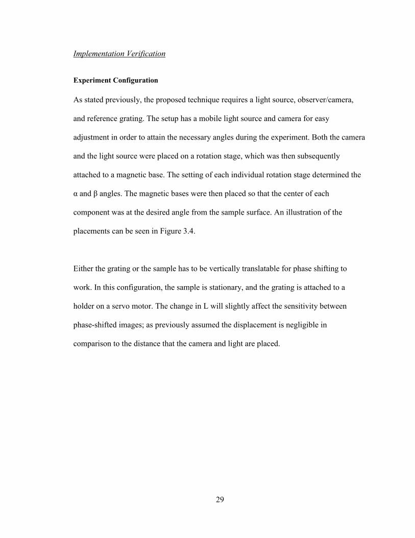
Experiment Configuration
As stated previously, the proposed technique requires a light source, observer/camera,
and reference grating. The setup has a mobile light source and camera for easy
adjustment in order to attain the necessary angles during the experiment. Both the camera
and the light source were placed on a rotation stage, which was then subsequently
attached to a magnetic base. The setting of each individual rotation stage determined the
α and β angles. The magnetic bases were then placed so that the center of each
component was at the desired angle from the sample surface. An illustration of the
placements can be seen in Figure 3.4.
Either the grating or the sample has to be vertically translatable for phase shifting to
work. In this configuration, the sample is stationary, and the grating is attached to a
holder on a servo motor. The change in L will slightly affect the sensitivity between
phase-shifted images; as previously assumed the displacement is negligible in
comparison to the distance that the camera and light are placed.

30
Figure 3.4: Illustration of Modified Shadow Moiré setup
The contour intervals associated with the configuration were determined by comparing a
reference image to an image taken after a known out-of-plane grating shift. A grating
movement equal to the contour interval results in the fringes moving one fringe order.
Utilizing this fact, moving the grating to values close to the estimated contour interval
will result in fringes. The different fringes are then compared to the fringes from the
original grating setting by finding the absolute difference between the corresponding
pixels in the fringe images. Plotting the absolute difference found for the images versus
grating displacements will result in a valley at the desired range of contour interval. An
exact match will not be found due to the contrast change at further distances, hence the
use of the smallest difference as the contour interval indicator.

31
The acquired images were not compared to the same original position image. As a
precaution against the sample moving or the grating not moving exactly back into the
original position, the images were taken in pairs. The first image was at the initial grating
position and the second was the image after grating movement. To prevent backlash, the
servo was moved slightly back past the original position and then moved forward into the
desired position. Therefore, all grating movements to the desired positions were
approached in the direction of increasing displacement.
Theoretically, two images taken in the same configuration should result in an absolute
pixel difference of zero. In practice, this is not the case due to random noise. A
background noise level was taken to ensure that the difference between the image pairs
were significant. Prior to the experiment, two average images were taken at the initial
grating placement and compared. The absolute difference between the two images was
the background noise value. If the absolute differences in the acquired image pairs was
less than the noise difference than the change was deemed too small
Hardware/Software
The light source was a 150W white light (Fiberoptic Systems, Inc. model 1060-150W)
with a 2.375 inch line source attachment. The experiment was placed in a dark
windowless room in order to eliminate background light. The magnitude of light
intensity is adjustable, but was kept at maximum intensity to ensure consistent light
intensity. As previously stated, a small aperture means less light entering the camera, so
a high intensity light would be needed to achieve the desired contrast.

32
The camera used was a Pulnix TM-7CN, a ½” format CCD camera with pixel
arrangement of 752 (H) x 582 (V) with a zoom lens. The camera was connected to a
frame grabber installed on a computer (PIXCI sv4 board). XCAP 2.2 was the software
associated with the frame grabber that was used for image acquisition and processing.
The images used for the fringe analysis and amplitude comparisons are a composite
image composed of the average of twenty images to avoid camera noise. The averaging
eliminates random high frequency noise that occurs with taking a single measurement.
The grating holder setup was attached to a vertical translation stage to allow for fringe
shifting. The NPZ-1/2 vertical translation stage from JA Noll was actuated by a Thorlabs
Z625B servo motor. The vertical translation stage has a two-axis tilt platform to allow for
leveling of the grating. The control of the servo was through the Thorlabs DCS-P110
board with the commands sent through the Thorlabs Advanced Positioning Technology
(APT) software. The stage has a horizontal to vertical ratio of two to one; the servo
displacements reading from the APT software are double the actual movement of the
grating holder. Therefore, for one full phase, the displacement required was double the
contour interval.
The sample holder is rigidly mounted to the table and the height of the specimen holder
could be manually configured. Similar to the grating holder, it incorporates a two-axis tilt
platform to level and tilt the sample. In this way, both holders can be configured to be
initially parallel to each other and then induce a specific rigid body deformation. The

33
sample holder was with a small gap between the grating and the sample. The sample
cannot be placed touching the grating, since fringes would be affected. Having the
grating touching the sample will introduces an extra constraint to the system, which
invalidates the results of the experiment.
Verification of the Governing Equation
To prove the new configuration’s derivation is correct, the first step was to tune the α
angle with the camera at normal incidence. The sample used was a glass slide that was
painted on one side to ensure that the specimen was initially flat. The grating and the
specimen holder were both leveled through the use of the 2-axis stages to ensure that the
fringes seen on the sample came solely from the difference in displacements of the
sample and not from any rigid motion from the set up. A bar fringe pattern was then
created when the sample holder was tilted in a single direction. The light source was
rotated to the desired angle and then moved until the contour interval reflected the
original equation’s derived value. To ensure the same α angle, the distance away from
center of the light source to the sample was kept the same while moving the light source
to test the different θ angles.
In order to show the trend, the light was rotated to four different θ angles. The contour
interval was determined using the previously described method of comparing images
after grating movements to their original grating position image. As part of that analysis,
an area of interest was selected to be compared since the sample is only a small part of
the image. Since the camera does not move, the sample’s location in the capture image

34
does not change. Since the sample image is a rectangle, the region of interest is a square.
The same pixel placement values were used when checking the same configurations.
The first test had the camera at normal viewing incidence with a set α angle of 40°
(Figure 3.7). Subsequent trials utilized a different α angle (45°) and β angles (20° and
30°). Examples of the image comparisons for this test are shown in Figure 3.5 and Figure
3.6. The top images are the initial images with the second row corresponding to images
after different movements of the grating. The middle image of Figure 3.5b shows the
fringe that closest approximates the initial image. The first image shows fringes that have
not moved far enough to be in the initial fringe’s location. The third image shows fringes
that have moved further than the original fringe’s position. Therefore, the movement that
yielded the middle image is determined as the measured contour interval.
The increase in the contour interval size can be readily seen with the fringe pattern when
comparing Figure 3.5 and Figure 3.6. The former has 2.5 fringes on the glass specimen
while the latter, with a large rotation angle, shows closer to 2 fringes. As seen from
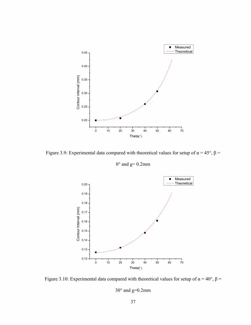
Figure 3.7-Figure 3.10, the measured value followed the trend of the expected values.
With increasing θ angle, the contour interval grew larger which is especially pronounced
after the 45° mark.

35
(a1) (a2) (a3)
(b1) (b2) (b3)
Figure 3.5: Image pairs (a) Fringes for α=40°, β=0°, θ=0°, g= 0.2 mm at starting position
(b) Fringes after contour interval of (1)0.236, (2)0.238, (3) 0.240 (mm)
(a1) (a2) (a3)
(b1) (b2) (b3)
Figure 3.6: Image pairs (a) Fringes for α=40°, β=0°, θ=50°, g= 0.2mm at starting
position. (b) Fringes after contour interval of (1) 0.365, (2) 0.367, (3) 0.369(mm)

36
Figure 3.7: Experimental data compared with theoretical values for setup of α = 40°, β =
0° and g= 0.2mm
Figure 3.8: Experimental data compared with theoretical values for setup of α = 40°, β =
20° and g= 0.2mm.
0 10 20 30 40 50 60 70
0.20
0.25
0.30
0.35
0.40
0.45
0.50
0.55
Co
nto
ur
Inte
rva
l(m
m)
Theta()
Measured
Theoretical
0 10 20 30 40 50 60 70
0.16
0.18
0.20
0.22
0.24
0.26
0.28
Co
nto
ur
inte
rva
l (m
m)
Theta()
Measured
Theoretical
37
Figure 3.9: Experimental data compared with theoretical values for setup of α = 45°, β =
0° and g= 0.2mm
Figure 3.10: Experimental data compared with theoretical values for setup of α = 40°, β =
30° and g=0.2mm
0 10 20 30 40 50 60 70
0.20
0.25
0.30
0.35
0.40
0.45
Co
nto
ur
inte
rva
l (m
m)
Theta
Measured
Theoretical
0 10 20 30 40 50 60 70
0.12
0.13
0.14
0.15
0.16
0.17
0.18
0.19
0.20
Co
nto
ur
Inte
rva
l (m
m)
Theta(
Measured
Theoretical

38
Application of Advanced Technique
The technique was tested on a processor package to demonstrate the increase of
sensitivity with the use of non-normal angles. The specimen tested was a 35mmx35mm
plastic ball grid array (PBGA) package from Marvell. The package was prepared with
white paint on the side with the ball grid array.
Figure 3.11: Marvell PBGA Package (left) front (right) back
The α angle was kept constant at 63° to maintain both high sensitivity and high contrast.
The specimen was placed within the zero-Talbot distance in order to maximize contrast.
The package was examined under three conditions: normal incidence, non-normal
incidence, and non-normal incidence with non-coplanar light. The setup configuration
was the same as the verification experiment. Images were taken at one-quarter of the
contour interval to approximate phase changes of 90°. The four images were then used
with the Moiré program to determine the displacement. The contour intervals achieved
were 0.1mm for normal incidence, 0.082mm for a β=25°, and a contour interval of
0.0542 for the non-coplanar setup.

39
(a) (b)
(c)
Figure 3.12: Setup of α=63°, β=0°, θ=0°, g=0.2mm a) Phase shifted images of specimen
b) Specimen wrapped phase map c) 3D-model of displacement pattern
40
(a) (b)
(c)
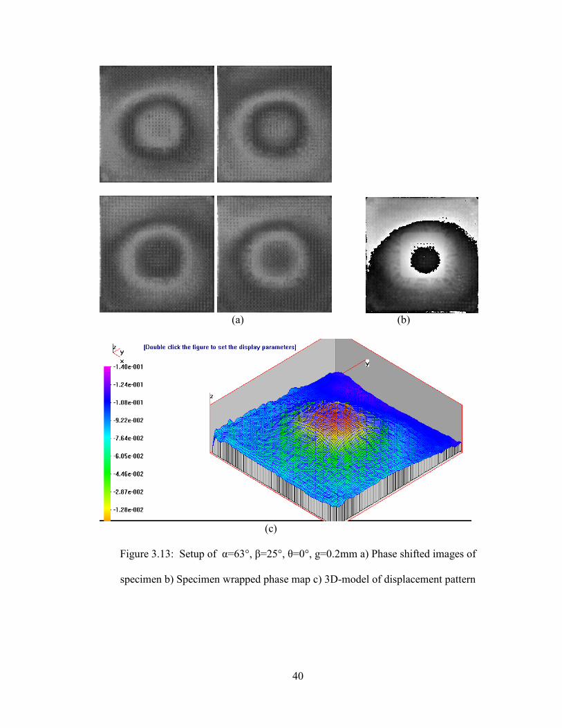
Figure 3.13: Setup of α=63°, β=25°, θ=0°, g=0.2mm a) Phase shifted images of
specimen b) Specimen wrapped phase map c) 3D-model of displacement pattern

41
(a) (b)
(b)
Figure 3.14: Setup of α=63°, β=60°, θ=20°, g=0.2mm a) Phase shifted images of
specimen b) Specimen wrapped phase map c) 3D-model of displacement pattern

42
The relative displacement in all the forward stated conditions was in agreement with each
other showing that the setups are consistent. The peak relative displacement value was
0.1mm. The increase in the number of fringes is readily seen between the normal
configuration, as shown in Figure 3.12, and the new modified technique as shown in
Figure 3.14. As expected, the new configuration has doubled the number of visible
fringes, since the large β gives a contour interval of tanα 63 tanβ 60 3.69
g g
in
comparison to the normal configuration which gives an interval of
tanα 63 tanβ 0 2
g g
. The increase in sensitivity can be seen in the better definition
of the warpage seen in Figure 3.14c. The influence of small β angles can be seen, as only
one fringe appears in Figure 3.13a, which is the same number of fringes seen in the
normal configuration of Figure 3.12a. The gain of a single fringe becomes important
when measurements are needed with partial fringes in the normal viewing configuration.
43
Chapter 4: Potential Future Investigation
One of the applications of shadow moiré is high-temperature warpage measurements. In
existing tests [21], a convection oven is used, where there is typically slits for light to
enter and exit. A new system setup without the constraint imposed by the oven is
necessary for a dynamically configurable shadow moiré system. To achieve this, a
conduction heater could be used as the heating source to replace the oven. The rest of the
setup could then be fitted accordingly with the grating being the moving part. This would
also potentially eliminate warpage of the reference grating from the heating.
The shadow moiré implementation depends on the accurate positioning of both the
illuminator source and the camera. A major issue with the use of non-normal angles is
that the distance between the light source and the camera could get prohibitively large in
order to obtain the correct angles. A modification to the technique would be to use
collimating lens, as shown in the second setup in Figure 2.3. This setup is not distance
based, versus the current setup which requires the camera and light to be placed apart
from each other at four times the distance from the sample to the height of the
camera/light source. However, this change would be application specific as the sample
size that can be measured is dependent on the collimating lens, whereas no such
limitation is present in the current technique. .

44
Chapter 5: Conclusions
The need for better sensitivity warpage measurements comes from the electronics
industry’s smaller package profile. The use of non-normal angles was utilized to increase
the base sensitivity. However, with a range of angles not accessible in a traditional setup,
a modification to the configuration was implemented. A new governing equation was
derived and experimentally verified over different α and β angles. This showed that large
rotations could potentially nullify the benefits of non-normal angles. However, at the
smaller rotation angles, even up to 30°, the difference in contour interval from the normal
viewing is very small. Therefore, a new range of angles could now be utilized. The
warpage of a processor package was then measured to demonstrate the increase in
sensitivity gained by using the non-normal angles. This experiment showed that the
contour interval could be reduced by almost in half as compared to normal viewing. The
new configuration was shown to be application dependent, with improvements to
sensitivity and dynamic range limitations driving its implementation.

45
Bibliography
[1] I. T. R. f. Semiconductors. (2009). Assembly and Packaging 2009 Edition.
[2] R. Tammula, E. Rymaszewski, and A. Klopfenstein, eds., “Microelectronics
Packaging Handbook,” Kluwer Academic, Norwell (1997).
[3] A. Cox, "Development of Advanced Shadow Warpage Measurement Systems:
Shadow Moiré with Nonzero Talbot Distance and Far Infrared Twyman-Green
Interferometry," M.S., Mechanical Engineering, University of Maryland,
College Park, 2006.
[4] H. Takasaki, "Moiré Topography," Appl. Opt., vol. 9, pp. 1467-1472, 1970.
[5] D. M. Meadows, W. O. Johnson, and J. B. Allen, "Generation of Surface
Contours by Moiré Patterns," Appl. Opt., vol. 9, pp. 942-947, 1970.
[6] J. S. S. T. Association, "High Temperature Package Warpage Measurement
Methodology," vol. JESD22-B11, ed, 2005.
[7] J. A. Gómez-Pedrero, J. A. Quiroga, M. José Terrón-López, and D. Crespo,
"Measurement of surface topography by RGB Shadow-Moiré with direct phase
demodulation," Optics and Lasers in Engineering, vol. 44, pp. 1297-1310,
2006.
[8] K. C. Yuk, J. H. Jo, and S. Chang, "Determination of the absolute order of
shadow moiré fringes by using two differently colored light sources," Appl.
Opt., vol. 33, pp. 130-132, 1994.
[9] S. Song, F. Zhu, W. Zhang, and S. Liu, "Warpage measurement of various
substrates based on white light shadow moire technology," pp. 389-392, 2011.

46
[10] M. Amagai and Y. Suzuki, "A study of package warpage for package on
package (PoP)," in Electronic Components and Technology Conference
(ECTC), 2010 Proceedings 60th, 2010, pp. 226-233.
[11] T. Ming-Yi, C. Hsing-Yu, and M. Pecht, "Warpage Analysis of Flip-Chip
PBGA Packages Subject to Thermal Loading," IEEE Transactions on Device
and Materials Reliability, vol. 9, pp. 419-424, 2009.
[12] Y. Chao-Pin, C. Ume, R. E. Fulton, K. W. Wyatt, and J. W. Stafford,
"Correlation of analytical and experimental approaches to determine thermally
induced PWB warpage," Components, Hybrids, and Manufacturing
Technology, IEEE Transactions on, vol. 16, pp. 986-995, 1993.
[13] T. C. Chiu, H. W. Huang, and Y. S. Lai, "Warpage evolution of overmolded
ball grid array package during post-mold curing thermal process,"
Microelectronics Reliability, vol. 51, pp. 2263-2273, Dec 2011.
[14] D. Hai, R. E. Powell, C. R. Hanna, and I. C. Ume, "Warpage measurement
comparison using shadow moire and projection moire methods," Components
and Packaging Technologies, IEEE Transactions on, vol. 25, pp. 714-721,
2002.
[15] D. Hai, I. C. Ume, R. E. Powell, and C. R. Hanna, "Parametric study of
warpage in printed wiring board assemblies," Components and Packaging
Technologies, IEEE Transactions on, vol. 28, pp. 517-524, 2005.
[16] T. Ming-Yi, Y. C. Chen, and S. W. R. Lee, "Correlation Between
Measurement and Simulation of Thermal Warpage in PBGA With

47
Consideration of Molding Compound Residual Strain," Components and
Packaging Technologies, IEEE Transactions on, vol. 31, pp. 683-690, 2008.
[17] Y. Polsky, W. Sutherlin, and I. C. Ume, "A comparison of PWB warpage due
to simulated infrared and wave soldering processes," Electronics Packaging
Manufacturing, IEEE Transactions on, vol. 23, pp. 191-199, 2000.
[18] M. Y. Tsai, C. W. Ting, C. Y. Huang, and Y. S. Lai, "Determination of
residual strains of the EMC in PBGA during manufacturing and IR solder
reflow processes," Microelectronics Reliability, vol. 51, pp. 642-648, Mar
2011.
[19] S. Y. Yang, Y.-D. Jeon, S.-B. Lee, and K.-W. Paik, "Solder reflow process
induced residual warpage measurement and its influence on reliability of flip-
chip electronic packages," Microelectronics Reliability, vol. 46, pp. 512-522,
2006.
[20] C. P. Yeh, K. Banerjee, T. Martin, C. Ume, R. Fulton, J. Stafford, and K.
Wyatt, "Experimental and analytical investigation of thermally induced
warpage for printed wiring boards," in Electronic Components and Technology
Conference, 1991. Proceedings., 41st, 1991, pp. 382-387.
[21] K. Verma, D. Columbus, and B. Han, "Development of real time/variable
sensitivity warpage measurement technique and its application to plastic ball
grid array package," Electronics Packaging Manufacturing, IEEE Transactions
on, vol. 22, pp. 63-70, 1999.
[22] Y. Y. Wang and P. Hassell, "Measurement of thermally induced warpage of
BGA packages/substrates using phase-stepping shadow moire," in Electronic

48
Packaging Technology Conference, 1997. Proceedings of the 1997 1st, 1997,
pp. 283-289.
[23] C. Han, "Shadow Moiré Using Non-Zero Talbot Distance and Application of
Diffraction Theory to Moiré Interferometry," PHD, Mechanical Engineering,
University of Maryland College Park, 2005.
[24] C. W. Han and B. Han, "High Sensitivity Shadow Moiré Using Nonzero-Order
Talbot Distance," Experimental Mechanics, vol. 46, pp. 543-554, 2006.
[25] T. Yoshizawa and T. Tomisawa, "Shadow Moire Topography by Means of the
Phase-Shift Method," Optical Engineering, vol. 32, pp. 1668-1674, Jul 1993.
[26] Z. Wang, "Development and Application of Computer Aided Fringe Analysis,"
PHD, University of Maryland, College Park, 2003.
[27] T. Hoang, Z. Y. Wang, M. Vo, J. Ma, L. Luu, and B. Pan, "Phase extraction
from optical interferograms in presence of intensity nonlinearity and arbitrary
phase shifts," Applied Physics Letters, vol. 99, Jul 18 2011.
[28] H. Du, H. Zhao, B. Li, Z. Li, L. Zheng, and L. Feng, "Algorithm for phase
shifting shadow moiré with an unknown relative step," Journal of Optics, vol.
13, p. 035405, 2011.
[29] C. Kuo-Shen, T. Y. F. Chen, C. Chia-Cheng, and I. K. Lin, "Full-field wafer
level thin film stress measurement by phase-stepping shadow Moire,"
Components and Packaging Technologies, IEEE Transactions on, vol. 27, pp.
594-601, 2004.
[30] J. Liao and A. Voloshin, "Enhancement of the shadow-moiré method through
digital image processing," Experimental Mechanics, vol. 33, pp. 59-63, 1993.

49
[31] E. Hack and J. Burke, " Measurement uncertainty of linear phase-stepping
algorithms," Review of Scientific Instruments, vol. 82, p. 061101, 2011.
[32] C. Han and B. Han, "Error Analysis of Phase Shifting Technique When
Applied to Shadow Moiré," Applied Optics, vol. 45, p. 1124, 2006.
[33] Y. Arai and S. Yokozeki, "Improvement of measurement accuracy in shadow
moire by considering the influence of harmonics in the moire profile," Appl
Opt, vol. 38, pp. 3503-7, Jun 1 1999.
[34] J. C. Martinez-Anton, H. Canabal, J. A. Quiroga, E. Bernabeu, M. A. Labajo,
and V. C. Testillano, "Enhancement of surface inspection by Moiré
interferometry using flexible reference gratings," Opt. Express, vol. 8, pp. 649-
654, 2001.
[35] A. M. F. Wegdam, O. Podzimek, and H. T. Bösing, "Simulation of shadow
moiré systems containing a curved grating surface," Appl. Opt., vol. 31, pp.
5952-5955, 1992.
[36] Daniel Post, B. Han, and P. Ifju, High Sensitivity Moire: Experimental
Analysis for Mechanics and Materials New York: Springer-Verlag 1994.
[37] C. W. Ackerman, "Development of a Real-time High Sensitivity Shadow
Moire System and its Application to Microelectronics Packaging," M.S.,
Mechanical Engineering, Clemson University, 2000
[38] M. Testorf, "Talbot Effect for Oblique Angle of Light Propagation," Optics
Communications, vol. 129, pp. 167-172, Aug 15 1996..
[39] C. Han and B. Han, Contrast of shadow moir at high-order Talbot distances,"
Optical Engineering, vol. 44, p. 028002, 2005.

50
[40] S. Wei, S. Wu, I. Kao, and F. P. Chiang, "Measurement of Wafer Surface Using
Shadow Moire Technique With Talbot Effect," Journal of Electronic Packaging,
vol. 120, pp. 166-170, 1998.
[41] O. Kafri and E. Keren, "Fringe observation and depth of field in moire analysis,"
Appl Opt, vol. 20, pp. 2885-6, Sep 1 1981.