Embed Size (px)
Citation preview
ABSTRACT
Title of Document: RELIABILITY TESTING & BAYESIAN
MODELING OF HIGH POWER LEDS FOR USE IN A MEDICAL DIAGNOSTIC APPLICATION.
Milind Mahadeo Sawant,
Doctor of Philosophy, 2013 Directed By: Dr. Aristos Christou
Materials Science and Engineering Reliability Engineering
While use of LEDs in fiber optics and lighting applications is common, their use in
medical diagnostic applications is rare. Since the precise value of light intensity is
used to interpret patient results, understanding failure modes is very important. The
contributions of this thesis is that it represents the first measurements of reliability of
AlGaInP LEDs for the medical environment of short pulse bursts and hence the
uncovering of unique failure mechanisms. Through accelerated life tests (ALT), the
reliability degradation model has been developed and other LED failure modes have
been compared through a failure modes and effects criticality analysis (FMECA).
Appropriate ALTs and accelerated degradation tests (ADT) were designed and
carried out for commercially available AlGaInP LEDs. The bias conditions were
current pulse magnitude and duration, current density and temperature. The data was
fitted to both an Inverse Power Law model with current density J as the accelerating
agent and also to an Arrhenius model with T as the accelerating agent. The optical
degradation during ALT/ADT was found to be logarithmic with time at each test
temperature. Further, the LED bandgap temporarily shifts towards the longer
wavelength at high current and high junction temperature. Empirical coefficients for
Varshini’s equation were determined, and are now available for future reliability tests
of LEDs for medical applications.
In order to incorporate prior knowledge, the Bayesian analysis was carried out for
LEDs. This consisted of identifying pertinent prior data and combining the
experimental ALT results into a Weibull probability model for time to failure
determination. The Weibull based Bayesian likelihood function was derived. For the
1st Bayesian updating, a uniform distribution function was used as the Prior for
Weibull α-β parameters. Prior published data was used as evidence to get the 1st
posterior joint α-β distribution. For the 2nd Bayesian updating, ALT data was used as
evidence to obtain the 2nd posterior joint α-β distribution. The predictive posterior
failure distribution was estimated by averaging over the range of α-β values.
This research provides a unique contribution in reliability degradation model
development based on physics of failure by modeling the LED output
characterization (logarithmic degradation, TTF β<1), temperature dependence and a
degree of Relevance parameter ‘R’ in the Bayesian analysis.
RELIABILITY TESTING & BAYESIAN MODELING OF HIGH POWER LEDS FOR USE IN A MEDICAL DIAGNOSTIC APPLICATION
By
Milind Mahadeo Sawant
Dissertation submitted to the Faculty of the Graduate School of the University of Maryland, College Park, in partial fulfillment
of the requirements for the degree of Doctor of Philosophy
2013 Advisory Committee: Dr. Aristos Christou, Advisor and Chair Dr. Martin Peckerar, Dean’s Representative Dr. Mohammad Modarres Dr. Ali Mosleh Dr. Jeffrey Herrmann

© Copyright by Milind Mahadeo Sawant
2013
ii
Preface
The topic of Bayesian analysis has been discussed and debated for a few centuries.
Jacob Bernoulli developed the Binomial theorem and laid the rules of permutations
and combinations in the 17th century. Reverend Thomas Bayes (after whom the
Bayes’ theorem is named) provided an answer to Bernoulli’s inverse probability
problem in the 18th century. Pierre Simon Laplace also referred to as the ‘Newton of
France’ developed the ‘Bayesian’ interpretation of probability in the early 19th
century. Bruno De Finitti published his two volume ‘Theory of Probability’ in the
20th century. This provided a further growth and interest in the topic of Bayesian
approach to statistics.
In the Fall of 2009, when I took a course on Data Analysis taught by Dr. Ali Mosleh,
UMD, I became interested in Bayesian analysis. In our day to day life, we take every
action based on our previous experiences, bias and prejudice. Be it a short-term task
such as driving a car or long-term assignment such as raising a child. While our brain
performs these tasks by judgment and intuition, Bayesian analysis allows us to
mathematically use our past experience to predict the probability of an event. I hereby
caution the reader not to perform Bayesian computations while driving a car since
these computations take time!
While working at Siemens, I was posed with the problem of testing the reliability of
LEDs for use in a medical diagnostic application. Around the same time, I was
researching a topic for my Ph.D. research. Considering my interest in Bayesian
iii
analysis, my advisor Dr. Aristos Christou, UMD recommended that I use Bayesian
approach for assessing the reliability of the LEDs. I am so grateful to him for that
suggestion since this allowed me to do research on something that I thoroughly
enjoyed.
Back in 1986, when I was in the 9th grade, a friend of mine had given me a few RED
colored LEDs to use as a light source in an electronic educational kit. LEDs were not
affordable to school students then. I was very impressed with the LEDs since it did
not drain my ‘expensive’ 1.5V battery compared to the mini light bulb. I also
remember that I had to be careful with the polarity of the battery to avoid damage to
the LED (from excessive reverse bias). Twenty-six years later, as I am writing this
dissertation, I cannot help but think that my Ph.D. research on Bayesian analysis of
LED reliability was destiny!
Milind Sawant
Newark DE.
September 2012.

iv
Dedication
This is dedicated to my parents, my wife Sujata, sons Ashwin and Atharva and all my
friends.

v
Acknowledgements
There are times in life when one feels a sense of accomplishment combined with a
sense of gratitude. Writing the acknowledgement page of a Ph.D. dissertation is one
of them. First and foremost, I must thank my advisor Dr. Aristos Christou at
University of Maryland for his guidance. He helped me select the topic and also focus
on it with ideas and concrete suggestions. I also thank Dr. Martin Peckerar, Dr.
Mohammad Modarres, Dr. Ali Mosleh and Dr. Jeffrey Herrmann for giving me
suggestions and their opinions on various aspects of this research.
The laboratory facilities for this research were provided by Siemens for which I
sincerely thank Dr. Robert Hall, Carl Ford and Frank Krufka. I enjoyed technical
discussions with my colleagues Dr. Lucian Kasprzak, Dr. Edward Gargiulo, Dr. C. C.
Lee, Gregory Pease, Joe Marchegiano and Gregory Ariff. Charlotte Gonsecki, Dan
West and Tan Bui provided invaluable support in building test fixtures where as
Aleksey Karulin helped me take good photographs using a digital microscope.
My parents are responsible for my success. Their confidence in me makes me work
harder. My wife Sujata took care of the home front while I spent long hours in the lab
and on the PC. My in-laws provided encouragement whereas my friends helped me
remain sane during stressful times. Thanking my family and friends will belittle their
affection. Finally, I express my love for my sons Ashwin and Atharva who are a
source of continuous joy, inspiration and at times perspiration for me!
vi
Table of Contents Preface........................................................................................................................... ii Dedication .................................................................................................................... iv Acknowledgements....................................................................................................... v Table of Contents......................................................................................................... vi List of Tables ................................................................................................................ x List of Figures .............................................................................................................. xi List of Symbols and Abbreviations............................................................................ xiv Chapter 1: Introduction ................................................................................................. 1
1.1 Background and Motivation ............................................................................. 1 1.2 Goal, Objectives and Accomplishments of Research....................................... 4
1.2.1 FMECA for LED in Medical application ................................................. 5 1.2.2 Develop Test Setup................................................................................... 5 1.2.3 Perform Accelerated Life and Degradation Test...................................... 6 1.2.4 Accelerating Agent Modeling................................................................... 6 1.2.5 Temperature dependence of Bandgap....................................................... 6 1.2.6 Literature Survey for Bayesian Prior ........................................................ 7 1.2.7 Bayesian Likelihood Function .................................................................. 7 1.2.8 Bayesian Updating.................................................................................... 7 1.2.9 Degree of Relevance in Bayesian modeling ............................................. 8
1.3 Publications of Present Research ...................................................................... 8 1.4 Summary of Contribution ................................................................................. 9
1.4.1 LED bias conditions are different ............................................................. 9 1.4.2 Application of LED is different ................................................................ 9 1.4.3 Consequence of LED Failure is different ................................................. 9 1.4.4 Decreasing failure rate β of the Weibull TTF model.............................. 10 1.4.5 Temperature dependence of bandgap characterized............................... 10
1.5 Dissertation Layout......................................................................................... 11 Chapter 2: Literature Review...................................................................................... 15
2.1 Introduction..................................................................................................... 15 2.2 AlGaInP LEDs................................................................................................ 17 2.3 GaN LEDs....................................................................................................... 21 2.4 LED measurements......................................................................................... 26 2.5 Bayesian analysis ............................................................................................ 27
Chapter 3: Theory of Light Emitting Diodes.............................................................. 31
3.1 Basic LED Operation...................................................................................... 31 3.2 Band Structure in Semiconductors..................................................................32 3.3 Wavelength of emitted light............................................................................ 33 3.4 Radiative and Non-radiative recombination in semiconductors..................... 33 3.5 Light output vs. Junction temperature ............................................................ 34 3.6 Basic LED degradation mechanisms .............................................................. 34
vii
3.7 Degradation of AlGaInP LEDs.......................................................................34 Chapter 4: Development of Empirical Modeling for Test Data Analysis .................. 36
4.1 Current density: Inverse Power Law model.................................................... 36 4.2 Temperature: Arrhenius Reaction Rate model ............................................... 37 4.3 Computation of Acceleration Factors ............................................................. 37 4.4 Regression Analysis of Prior Published Data ................................................. 38
4.4.1 LED classification................................................................................... 38 4.4.2 Iterative Regression Analysis ................................................................. 39 4.4.3 Weibull Analysis of Prior Published data............................................... 44
Chapter 5: Accelerated Life and Degradation Testing............................................... 46
5.1 Materials ......................................................................................................... 46 5.2 Methods........................................................................................................... 47 5.3 Test Setup........................................................................................................ 48 5.4 ALT/ADT Results........................................................................................... 49
5.4.1 LED optical power degradation .............................................................. 49 5.4.2 Encapsulation degradation...................................................................... 51 5.4.3 Chip vs. Lens degradation.......................................................................52 5.4.4 Spectral Performance after ALT/ADT.................................................... 53 5.4.5 Summary of Test results .........................................................................55 5.4.6 Additional ALT/ADT testing.................................................................. 56 5.4.7 Weibull analysis of ALT data ................................................................. 58 5.4.8 Analysis of ADT data ............................................................................. 59
Chapter 6: Thermal Shift of Active layer Bandgap .................................................... 62
6.1 Background on Spectral Shifts........................................................................ 62 6.2 Methods........................................................................................................... 63 6.3 Experimental ................................................................................................... 64
6.3.1 Forward Bias Method .............................................................................64 6.3.2 Spectral Measurement............................................................................. 64
6.4 Results and Discussion of Spectral Shift ........................................................ 65 6.4.1 Vf-Jt Linear Relationship........................................................................ 65 6.4.2 Spectral shift in Bandgap........................................................................ 67 6.4.3 Varshini’s empirical model..................................................................... 69 6.4.4 Effect on LED life testing ....................................................................... 70
6.5 Effect of Spectral Shift on Medical application.............................................. 71 6.5.1 Decrease in net optical output................................................................. 71 6.5.2 Change in the Absorbance Chemistry..................................................... 72
6.6 Conclusions of Spectral Shift.......................................................................... 73 Chapter 7: Failure Modes and Effects Criticality Analysis (FMECA)....................... 74
7.1 Introduction..................................................................................................... 74 7.2 LED Failure Modes......................................................................................... 76
7.2.1 Active Region failure.............................................................................. 76 7.2.2 P-N Contacts failure................................................................................ 77
viii
7.2.3 Indium Tin-Oxide failure........................................................................77 7.2.4 Plastic encapsulation failure ...................................................................77 7.2.5 Packaging failures................................................................................... 77
7.3 FMECA before ALT/ADT ............................................................................. 79 7.4 FMECA after ALT/ADT ................................................................................ 80 7.5 Probabilistic Risk Assessment and Event Sequence Diagrams ...................... 81 7.6 Conclusions..................................................................................................... 83
Chapter 8: Bayesian Modeling of LED Reliability..................................................... 84
8.1 Baye’s theorem ............................................................................................... 85 8.2 Bayesian Modeling of LED data.....................................................................86
8.2.1 Likelihood function for LED reliability.................................................. 87 8.2.2 Uniform Prior distribution for α & β ...................................................... 87 8.2.3 Posterior distribution for α & β............................................................... 88 8.2.4 Predictive Posterior distribution for LED life......................................... 88
8.3 Results of Bayesian modeling......................................................................... 88 8.3.1 Compiling the Prior Data........................................................................88 8.3.2 Computation of 1st Posterior Distribution............................................... 91 8.3.3 Computation of 2nd Posterior Distribution.............................................. 93 8.3.4 Conclusion from Prior data, ALT and Bayesian analysis....................... 94
Chapter 9: Degree of Relevance in Bayesian modeling............................................. 96
9.1 The Problem: Partially relevant prior data...................................................... 96 9.2 The Solution: A Three Step Process ............................................................... 97
9.2.1 Step-1: Transform DC data to Pulse data by Multiplication................... 97 9.2.2 Step-2: Use a Degree of Relevance Parameter R.................................... 98 9.2.3 Step-3: Changing the Likelihood function using R ................................ 98
9.3 Results and Discussion ................................................................................... 99 9.4 Conclusions................................................................................................... 101
Chapter 10: Bayesian Parameter Selection and Model Validation........................... 102
10.1 Bayesian Subjectivity................................................................................ 102 10.2 Validation approach.................................................................................. 102 10.3 Validation phases in Bayesian modeling .................................................. 104
10.3.1 Selection of underlying failure distribution.......................................... 104 10.3.2 Selection and verification of prior distribution..................................... 106 10.3.3 Appropriateness of Predictive posterior distribution to test data.......... 107
Chapter 11: Conclusion............................................................................................. 110
11.1 Summary................................................................................................... 110 11.2 Objectives and Accomplishments............................................................. 112 11.3 Research contribution and Significance.................................................... 113 11.4 Future Research ........................................................................................ 114
11.4.1 ALT at different duty cycles ................................................................. 114 11.4.2 Use of a Utility Function while estimating R....................................... 114
ix
11.4.3 Other methods of using degree of Relevance ‘R’................................. 115 11.4.4 Failure Analysis .................................................................................... 116
Appendix-1: Laboratory for LED Reliability Testing .............................................. 117 Appendix-2: Circuit Schematics for LED ALT........................................................ 118 Appendix-3: Circuit diagram for Vf Signal conditioning......................................... 119 Appendix-4: Photos of LED during ALT ................................................................. 120 Appendix-5: Labview program for ALT .................................................................. 122 Appendix-6: Labview Program for Bayesian Modeling........................................... 125 Appendix-7: Transformation of Partially Relevant Data.......................................... 135 Appendix-8: Bayesian updating using partially relevant data .................................. 137 References................................................................................................................. 149
x
List of Tables 1. Table 1.1: Comparison of Lighting/Fiber Optics vs. Medical Diagnostic
application
2. Table 4.1 Regression Analysis of Prior Published Data
3. Table 5.1 Summary of ALT/ADT results for Batch 2
4. Table 5.2 Summary of ALT/ADT results for Batch 3
5. Table 5.3 Summary of ALT/ADT results for Batch 4
6. Table 5.4 Regression Analysis of ALT Data
7. Table 5.5 Degradation Analysis using JMP software
8. Table. 6.1 Spectral Shift in Bandgap at higher temperatures
9. Table. 6.2 Varshini’s coefficients: Ge, Si, GaAs & AlGaInP
10. Table 7.1 Failure Severity classification for general and medical diagnostic
application
11. Table 7.2 FMECA table before ALT/ADT
12. Table 7.3 FMECA table after ALT/ADT
13. Table 8.1 Prior Published Data Transformed for Bayesian Analysis
14. Table 9.1 Summary of Bayesian Analysis using partially relevant data
15. Table 10.1 Used vs. wider limits on prior of α and β
16. Table 10.2 Computation of Chi-square statistic
17. Table A7.1 Set 1 and ALT data
18. Table A7.2 Set 2 and Set3 data
xi
List of Figures
1. Fig. 1.1 LED in Lighting / Fiber Optics Application
2. Fig. 1.2 LED in Medical Diagnostic Application
3. Fig. 3.1 Construction of Common LED [5] vs. LED used in this research
4. Fig. 3.2 LED Operation [5]
5. Fig 4.1 Effect of Current density J: AlGaInP-DH-DC
6. Fig 4.2 Effect of Temperature: AlGaInP-DH-DC
7. Fig 4.3 Effect of Current density J: AlGaInP-MQW-DC
8. Fig 4.4 Effect of Temperature: AlGaInP-MQW-DC
9. Fig 4.5 Effect of Current density J: GaN-DH-DC
10. Fig 4.6 Effect of Temperature: GaN-DH-DC
11. Fig 4.7 Effect of Current density J: GaN-MQW-DC
12. Fig 4.8 Effect of Temperature: GaN-MQW-DC
13. Fig 5.1 Environmental Test
14. Fig 5.2 Pulse/Burst mode timing
15. Fig. 5.3 Setup for LED Testing
16. Fig. 5.4 ALT/ADT for Batch2, 483mA
17. Fig. 5.5 ALT/ADT for Batch3, 725mA
18. Fig 5.6 Photos of Minor, Moderate & Severe Lens degradation
19. Fig 5.7 Chip (Vf) vs. Lens degradation
20. Fig 5.8 Spectral shift to lower wavelength after ALT/ADT
21. Fig 5.9 Spectral shift to higher wavelength after ALT/ADT
22. Fig. 5.10 ALT/ADT for Batch5, 26mA, 50% duty cycle
xii
23. Fig 6.1 Electrical and Optical Characterization of LEDs
24. Fig. 6.2 Vf-Jt relationship for LED 640x1-57. Vf-Jt relationship is plotted for 26,
58, 483 and 725mA
25. Fig. 6.3 Vf-Jt relationship for LED 640x1-58. Vf-Jt relationship is plotted for 26,
58, 483 and 725mA
26. Fig. 6.4 Spectral Shift in Bandgap at higher Jt for LED 640x1-57.
27. Fig. 6.5 Spectral Shift in Bandgap at higher Jt for LED 640x1-58
28. Fig. 6.6 Effect of Spectral Shift on useful optical power
29. Fig 7.1 LED Failure modes
30. Fig 7.2 Scenario / Event Sequence Diagram [4]
31. Fig 7.3 ESD for LED degradation in Medical application
32. Fig 8.1 Bayesian modeling of LED Reliability
33. Fig 8.2 1st Posterior Joint α-β distribution for AlGaInP-MQW-Pulse-Transformed
34. Fig 8.3 1st Average Predictive Posterior of LED TTF
35. Fig 8.4 2nd Posterior Joint α-β distribution for AlGaInP-MQW-Pulse-ALT
36. Fig 8.5. 2nd Average Predictive Posterior of LED TTF
37. Fig 10.1 Lognormal vs. Weibull fit of ALT data
38. Fig 10.2 LED TTF with used vs. wider prior limits on α and β
39. Fig A1.1 Laboratory photos of LED ALT setup
40. Fig A2.1 Wiring diagram for LED ALT setup
41. Fig A3.1 Circuit diagram for Vf Signal conditioning
42. Fig A4.1 SMD AlGaInP-MQW LED used in this research
43. Fig A4.2 LED Photos from ALT Batch 2
xiii
44. Fig A4.3 LED Photos from ALT Batch 3
45. Fig A5.1 Front Panel of labview program for ALT
46. Fig A5.2 Block diagram of main labview program for ALT
47. Fig A5.3 Block diagram of low level labview program for ALT
48. Fig A6.1 Front Panel Page 1 of labview program for Weibull Bayesian Analysis
49. Fig A6.2 Front Panel Page 2 of labview program for Weibull Bayesian Analysis
50. Fig A6.3 Front Panel Page 3 of labview program for Weibull Bayesian Analysis
51. Fig A6.4 Front Panel Page 4 of labview program for Weibull Bayesian Analysis
52. Fig A6.5 Front Panel Page 5 of labview program for Weibull Bayesian Analysis
53. Fig A6.6 Front Panel Page 6 of labview program for Weibull Bayesian Analysis
54. Fig A6.7 Block diagram Page 1 of labview program for Weibull Bayesian
Analysis
55. Fig A6.8 Block diagram Page 2 of labview program for Weibull Bayesian
Analysis
56. Fig A6.9 Block diagram Page 3 of labview program for Weibull Bayesian
Analysis
57. Fig A6.10 Block diagram Page 4 of labview program for Weibull Bayesian
Analysis
58. Fig A6.11 Block diagram Page 5 of labview program for Weibull Bayesian
Analysis
59. Fig A6.12 Block diagram Page 6 of labview program for Weibull Bayesian
Analysis

xiv
List of Symbols and Abbreviations
Symbols:
1. α - Failure mode ratio (section 7.1)
2. α - Scale parameter of Weibull Distribution
3. α – Significance level for Chi-square test (section 10.2)
4. β - Shape parameter of Weibull Distribution
5. β - Failure effect probability (section 7.1)
6. c - speed of light in vacuum (section 6.1)
7. c – Acceptance limit for Chi-square statistic (section 10.2)
8. Cm - Criticality of failure mode (section 7.1)
9. Ea – Activation Energy
10. eV – Electron Volts
11. Eg – Bandgap Energy
12. h - Plank’s constant,
13. If or I – LED forward current
14. Jt – Junction temperature
15. λ - Wavelength
16. λ - Failure rate (section 7.1)
17. nm – Nanometer
18. Vf or V – LED forward voltage drop

xv
Abbreviations:
1. AF – Acceleration Factor
2. Al - Aluminum
3. AlGaAs – Aluminum Gallium Arsenide
4. AlGaInP – Aluminum Gallium Indium Phosphide
5. ADT – Accelerated Degradation Test
6. ALT - Accelerated Life Test
7. CDF – Cumulative Distribution Function
8. CFL – Compact Fluorescent Light
9. COP - Chip on Plate
10. DBR - Distributed Bragg Reflector
11. DC – Direct Current
12. DH – Double Heterostructure
13. DLTS - Deep Level Transient Spectroscopy
14. EC - Electronic Components
15. EL - Electro-Luminescence
16. ES – End State
17. ESD – Event Sequence Diagram
18. FDA – Food and Drugs Administration
19. FLE - Fatigue Life Expended
20. FMECA - Failure Modes and Effects Criticality Analysis
21. GaAs – Gallium Arsenide
22. GaP –Gallium Phosphide
xvi
23. GaN – Gallium Nitride
24. HP – Hewlett Packard
25. IE – Initiating Event
26. IEEE – Institute of Electrical and Electronics Engineers
27. In - Indium
28. InGaN – Indium Gallium Nitride
29. IPL – Inverse Power Law
30. IQE - Internal Quantum Efficiency
31. ISDRS - International Semiconductor Device Research Symposium
32. LED - Light Emitting Diode
33. MLE – Maximum Likelihood Estimate
34. MOCVD - Metal Organic Chemical Vapor Deposition
35. MQW – Multi Quantum Well
36. MTTF – Mean Time to Failure
37. NASA – National Aeronautics and Space Administration
38. NIST – National Institute of Standards and Technology
39. QD - Quantum Dot
40. OP - Optical power
41. PDF – Probability Distribution Function
42. PE – Pivotal Event
43. PRA – Probabilistic Risk Assessment
44. RDT – Reliability Demonstration Test
45. ROCS - Reliability of Compound Semiconductors Workshop

xvii
46. SMD – Surface Mounted Device
47. SPIE - International Society for Optics and Photonics
48. TRC - Thermal Resistance Circuit
49. TTF – Time to Failure
50. VPE - Vapor Phase Epitaxy
51. WOCSDICE - Workshop on Compound Semiconductor Devices and Integrated
Circuits
1
Chapter 1: Introduction
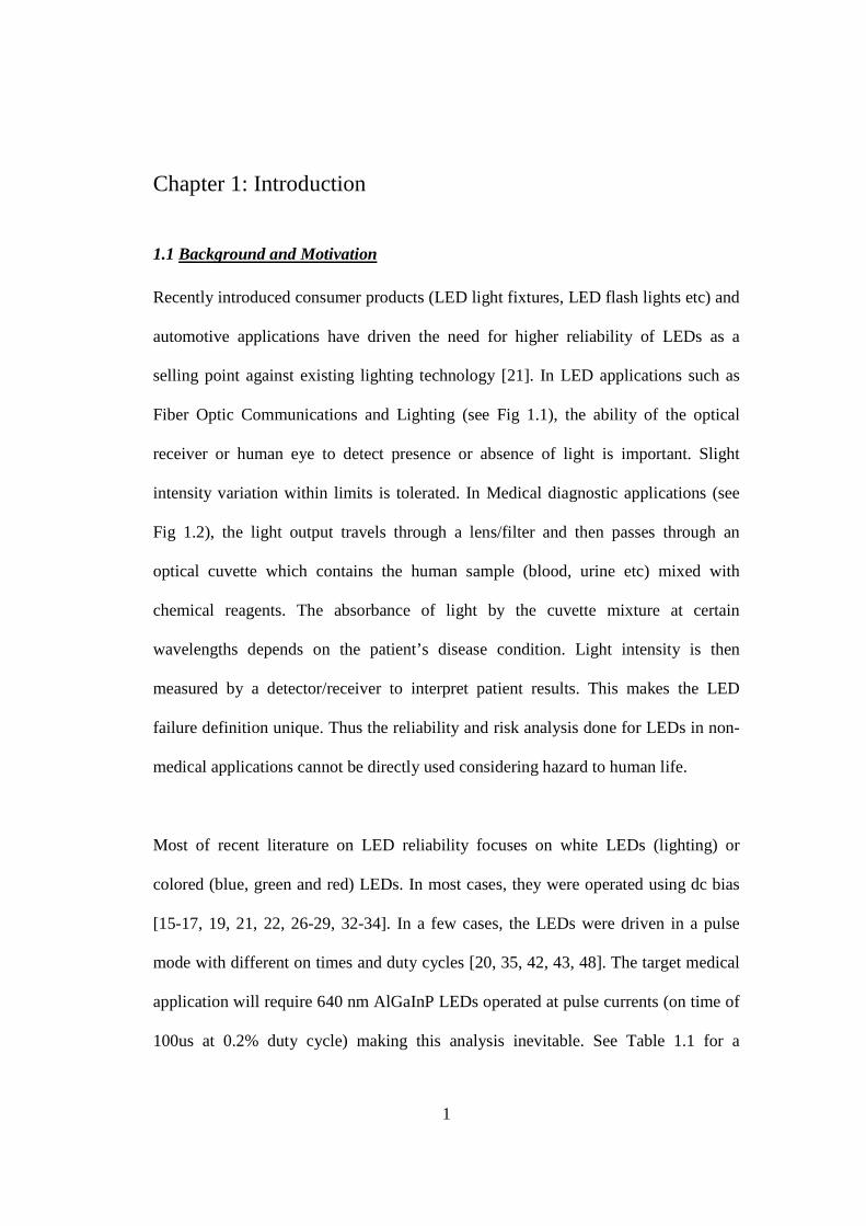
1.1 Background and Motivation
Recently introduced consumer products (LED light fixtures, LED flash lights etc) and
automotive applications have driven the need for higher reliability of LEDs as a
selling point against existing lighting technology [21]. In LED applications such as
Fiber Optic Communications and Lighting (see Fig 1.1), the ability of the optical
receiver or human eye to detect presence or absence of light is important. Slight
intensity variation within limits is tolerated. In Medical diagnostic applications (see
Fig 1.2), the light output travels through a lens/filter and then passes through an
optical cuvette which contains the human sample (blood, urine etc) mixed with
chemical reagents. The absorbance of light by the cuvette mixture at certain
wavelengths depends on the patient’s disease condition. Light intensity is then
measured by a detector/receiver to interpret patient results. This makes the LED
failure definition unique. Thus the reliability and risk analysis done for LEDs in non-
medical applications cannot be directly used considering hazard to human life.
Most of recent literature on LED reliability focuses on white LEDs (lighting) or
colored (blue, green and red) LEDs. In most cases, they were operated using dc bias
[15-17, 19, 21, 22, 26-29, 32-34]. In a few cases, the LEDs were driven in a pulse
mode with different on times and duty cycles [20, 35, 42, 43, 48]. The target medical
application will require 640 nm AlGaInP LEDs operated at pulse currents (on time of
100us at 0.2% duty cycle) making this analysis inevitable. See Table 1.1 for a
2
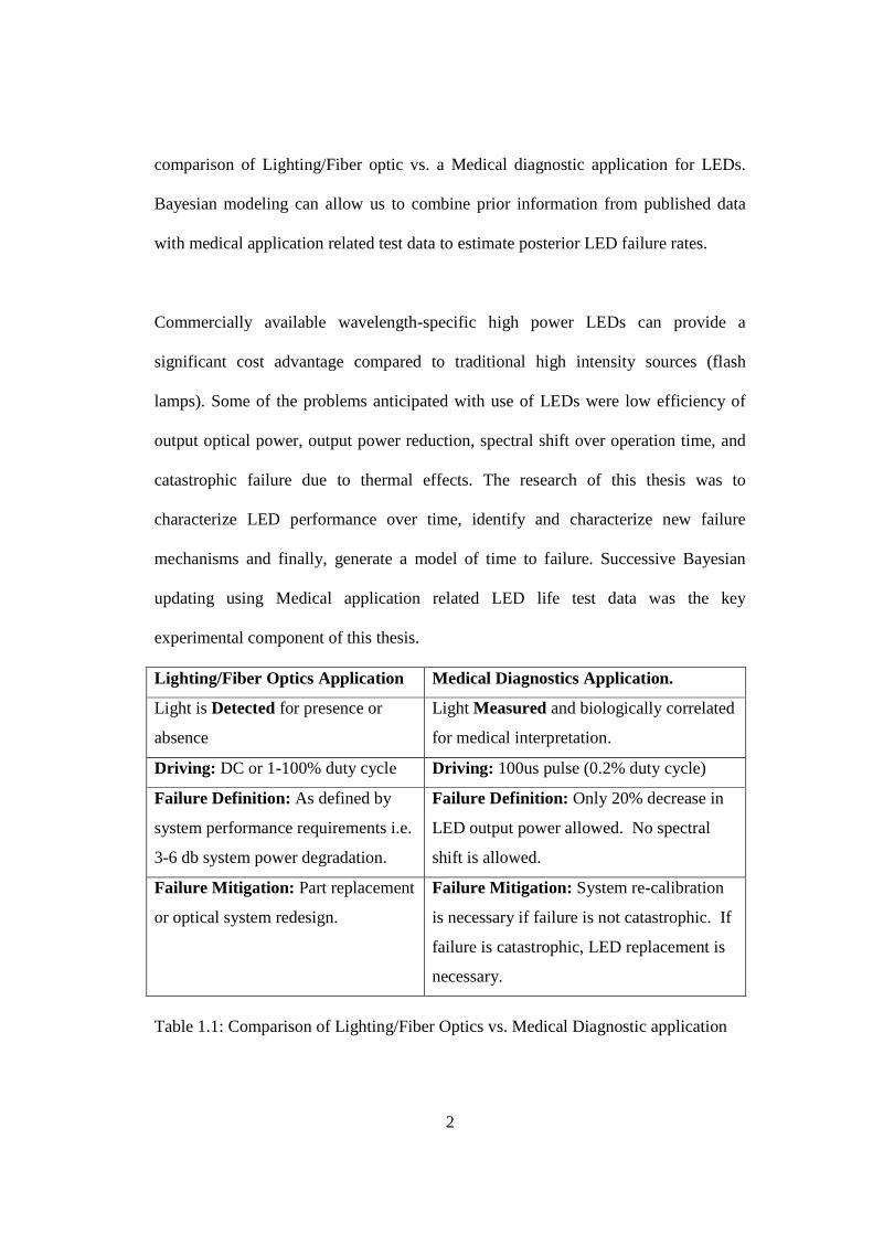
comparison of Lighting/Fiber optic vs. a Medical diagnostic application for LEDs.
Bayesian modeling can allow us to combine prior information from published data
with medical application related test data to estimate posterior LED failure rates.
Commercially available wavelength-specific high power LEDs can provide a
significant cost advantage compared to traditional high intensity sources (flash
lamps). Some of the problems anticipated with use of LEDs were low efficiency of
output optical power, output power reduction, spectral shift over operation time, and
catastrophic failure due to thermal effects. The research of this thesis was to
characterize LED performance over time, identify and characterize new failure
mechanisms and finally, generate a model of time to failure. Successive Bayesian
updating using Medical application related LED life test data was the key
experimental component of this thesis.
Lighting/Fiber Optics Application Medical Diagnostics Application.
Light is Detected for presence or
absence
Light Measured and biologically correlated
for medical interpretation.
Driving: DC or 1-100% duty cycle Driving: 100us pulse (0.2% duty cycle)
Failure Definition: As defined by
system performance requirements i.e.
3-6 db system power degradation.
Failure Definition: Only 20% decrease in
LED output power allowed. No spectral
shift is allowed.
Failure Mitigation: Part replacement
or optical system redesign.
Failure Mitigation: System re-calibration
is necessary if failure is not catastrophic. If
failure is catastrophic, LED replacement is
necessary.
Table 1.1: Comparison of Lighting/Fiber Optics vs. Medical Diagnostic application
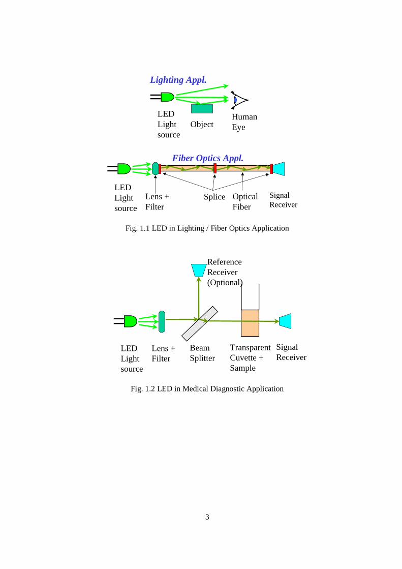
3
Fig. 1.1 LED in Lighting / Fiber Optics Application
Fig. 1.2 LED in Medical Diagnostic Application
LEDLightsource
HumanEyeObject
Lighting Appl.
Fiber Optics Appl.
LEDLightsource
Lens +Filter
Splice SignalReceiver
OpticalFiber
LEDLightsource
Lens +Filter
BeamSplitter
TransparentCuvette + Sample
SignalReceiver
ReferenceReceiver(Optional)

4
1.2 Goal, Objectives and Accomplishments of Research
This section summarizes the goals of the thesis and the approach taken as well as the
summary of the results and the unique contributions. In subsequent chapters, the
experimental and modeling approach is described in detail as well as the results of the
research.
The goal of this research was to evaluate the reliability of 640 nm AlGaInP MQW
LEDs in a medical diagnostic application using Accelerated Life testing and Bayesian
modeling. The following questions needed answers:
1. Will the LED intensity remain within acceptable limits?
2. Will the LED wavelength remain stable?
3. Will the Time to Failure of LEDs exceed the Life of the Medical Instrument?
4. Will there be a cost benefit of using LEDs vs traditional light sources (flash lamps
etc)?
5. Will there be any critical failure modes for the medical application?
5
The following section summarizes the specific accomplishments in order to meet the
objectives stated above
1.2.1 FMECA for LED in Medical application
Failure Modes and Effects Criticality Analysis (FMECA) widely used for risk
analysis was successfully applied to LED reliability and physics of failure
investigation. FMECA was used to understand the criticality of LED failure modes
when used in a medical diagnostic application. Failure modes of other components of
the Medical device were not included in this study. The FMECA was repeated and
refined after conducting accelerated life testing of LEDs. Degradation of the plastic
encapsulation and the active region were found to be the critical failure modes. These
failures could cause unscheduled calibration of the diagnostic instrument and could
cause delay in patient medical test results.
1.2.2 Develop Test Setup
An experimental setup was developed for accelerated life testing of LEDs in
environmental chambers. The test is automated by using test software, data
acquisition/control boards and constant pulse current LED driver boards. The test SW
makes the data acquisition board generate the necessary pulses, which trigger the
LED driver board. The peak current through the LED is maintained constant while it
is on. A separate signal conditioning circuit also measures the forward voltage Vf
across the diode, which is fed back to the test SW to be written to a database. At
regular intervals, the LEDs were removed from the environmental chambers and were
characterized electrically and optically (using a Spectro-radiometer).

6
1.2.3 Perform Accelerated Life and Degradation Test
Accelerated Life Testing (ALT) and Accelerated Degradation Testing (ADT) of the
LEDs in Pulse mode was conducted at 3 temperatures (35°C, 55°C and 75°C) and 2
Peak currents (Batch2: 483mA=418.1A/cm2 and Batch3: 725mA=627.2A/cm2). The
optical power decreased with time due to degradation of the LED chip as well as the
encapsulation. The rate of degradation followed a logarithmic function. 20%
degradation was considered failure for the medical application. For LEDs that did not
reach this failure threshold in a reasonable time (suspend data), the logarithmic
function was used to extrapolate TTF. A log-linear model was used for analysis of
degradation data and JMP software was used for this analysis.
1.2.4 Accelerating Agent Modeling
Prior published data and ALT data had to be converted to medical application
conditions. This required the use of accelerating agent modeling. Inverse Power Law
(IPL) model with J as the accelerating agent and the Arrhenius model with T as the
accelerating agent were used. Regression analysis was used to estimate the parameter
‘n’ of the IPL model and activation energy ‘Ea’ of the Arrhenius model. An iterative
regression analysis approach was used to get best possible regression fits thereby
accommodating the effects of both current density and temperature.
1.2.5 Temperature dependence of Bandgap
Reliability testing of AlGaInP MQW LEDs resulted in a shift of Bandgap towards the
longer wavelength when driven at high current. Characterization of the shift showed
that it was temporary and dependent on the junction temperature Jt. The data was
7
further analyzed with respect to Varshini’s equation, and the empirical coefficients
were determined for the AlGaInP material.
1.2.6 Literature Survey for Bayesian Prior
The Bayesian analysis began by identifying published data, which can be used as
prior information. From the published data, the time required for the optical power
output to degrade by 20% was extracted. Analysis of published data for different LED
Materials (AlGaInP, GaN, AlGaAs), Semiconductor Structures (DH, MQW) and
driving (DC, Pulsed) was carried out.
1.2.7 Bayesian Likelihood Function
Many of the LED degradation mechanisms occur at the same temperature bias range.
The mechanism with the lowest activation energy would dominate. The degradation
mechanism of LEDs, published literature and our ALT data all indicate that Weibull
is the most suitable model for this data analysis, as verified through a regression
analysis. This rationale was used to develop the Weibull based Bayesian likelihood
function. For the first Bayesian updating, uniform distribution was used as the Prior
distribution for α-β parameters of the Weibull model.
1.2.8 Bayesian Updating
Starting with uniform prior for α-β values, prior published data was used as Evidence
to get the first posterior joint α-β distribution. For the second Bayesian updating, the
posterior from the first Bayesian updating was used as the prior. ALT data converted
to medical application conditions was used as Evidence to get the second posterior
joint α-β distribution. This joint α-β distribution gave a series of Weibull time to
8
failure distributions. The predictive posterior failure distribution for the LEDs was
estimated by averaging over the range of α-β values. Software was written for
performing various Bayesian computations.
1.2.9 Degree of Relevance in Bayesian modeling
An approach is proposed for using partially relevant data in Bayesian modeling. A
new parameter ‘R’ (degree of relevance) is used to modify the likelihood function
before using it in Bayesian updating. The ‘R’ value will be used such that the
influence of evidence is decreased as R approaches zero.
1.3 Publications of Present Research
The research carried out as part of this thesis resulted in the publication of three
research papers and one poster presentation. These are listed below:
1. International Semiconductor Device Research Symposium (ISDRS), College Park
MD, Dec 2011 [11].
2. Workshop on Compound Semiconductor Devices and Integrated Circuits
(WOCSDICE), Island of Porquerolles, France, May 2012 [12].
3. Reliability of Compound Semiconductors Workshop (ROCS), Boston MA, April
2012 [13]
4. Poster presented at ResearchFest, College Park, MD, March 2012.
9
1.4 Summary of Contribution
The contributions of this thesis is that it represents the first measurements of
reliability of AlGaInP LEDs for the medical environment of short pulse bursts and
hence the uncovering of unique failure mechanisms.
1.4.1 LED bias conditions are different
Published articles tried to characterize LEDs using DC bias (for reliability) and in
some instances using pulsed bias (for performance evaluation rather than reliability).
The target medical application does not require continuous optical output but only
when the human test sample is provided (in fraction of ms). Failure mechanisms in
this research were influenced by peak currents rather than average currents.
1.4.2 Application of LED is different
In Fiber Optics & Lighting applications, light is used for detection. In Medical
diagnostic applications, the precise value of light intensity is used to interpret patient
results. This research will allow replacement of traditional light sources (filament or
flash lamps) with LEDs. The lamps degrade and have to be replaced 3-6 months
causing a major inconvenience to the customer whereas LEDs will outlast the 7-year
life of the medical diagnostic instrument.
1.4.3 Consequence of LED Failure is different
In Fiber Optics & Lighting applications, failures are usually significant loss of optical
output. Failure usually means inconvenience and redundancy is a common mitigation.
In medical diagnostic applications, calibration and referencing is used to mitigate
LED failure. However, if a subtle change in optical intensity goes undetected, it could
10
cause erroneous patient results. This can cause erroneous diagnosis, incorrect
treatment and possibly severe health complications. If this were to occur, apart from a
possible litigation between patient, hospital and the medical equipment manufacturer,
the FDA will start questioning the entire risk analysis done on the medical equipment.
1.4.4 Decreasing failure rate ββββ of the Weibull TTF model
It was observed that the shape parameter β of the Weibull TTF model is less than one
(implying a decreasing failure rate) in prior published data, ALT and Bayesian model.
During ALT, the rate of optical output degradation was logarithmic and this rate
varied significantly between different LEDs. Some LEDs cross the 20% degradation
(failure threshold for this application) earlier than others. For LEDs that do survive
this initial high rate of optical degradation, the probability that it will survive longer
increases. This explains the decreasing failure rate.
1.4.5 Temperature dependence of bandgap characterized
It was found that the bandgap of AlGaInP MQW LEDs shifts towards the longer
wavelength when driven at high current. Characterization of the shift showed that it
was temporary and dependent on the junction temperature Jt. The data was further
analyzed with respect to Varshini’s equation, and the empirical coefficients were
determined for the AlGaInP material. Since the spectral performance is critical for the
medical application, my spectral shift investigation will provide immense value to the
designer. The junction temperature will need to be maintained.
11
1.5 Dissertation Layout
Chapter 1 provides an introduction to this dissertation. It starts by giving a
background and motivation. It specifically describes how a medical diagnostic
application differs from a lighting or fiber optic application for LEDs. It then states
the goals and objectives of this research. Work accomplished including publication of
three research papers and a poster presentation is listed. Finally, it describes the
contribution and why this research was necessary.
Chapter 2 provides a thorough literature review on the subject. It starts by listing
various research groups who are working on the subject of LED reliability. It also
lists various journals, which have published important articles on LED reliability.
Thereafter it describes the work done on AlGaInP LEDs by various research groups.
It briefly describes their work, their approach and their results. The same is then
described for GaN LEDs. The chapter ends by describing a couple of articles on
Bayesian analysis.
Chapter 3 covers the theory for LEDs. It describes the basic LED operation, the band
structure in semiconductors and the relationship between the band gap energy and the
wavelength of the photon emitted. It describes the radiative and non-radiative
recombination process and its effect on LED reliability. Temperature dependence of
the spectrum is briefly described. It then describes the basic LED degradation
mechanisms and those specifically related to AlGaInP LEDs.
12
Chapter 4 describes Accelerated life modeling. Prior published data and ALT data
had to be converted to medical application conditions. This required the use of
accelerating agent modeling. Inverse Power Law (IPL) model with J as the
accelerating agent and the Arrhenius model with T as the accelerating agent are
described. Acceleration factors are derived. Parameter ‘n’ for the IPL model and
activation energy ‘Ea’ for the Arrhenius model are estimated using regression
analysis for various combinations of LED material and structure. After converting the
published data to medical application conditions, it is subjected to Weibull analysis.
Chapter 5 describes the Accelerated Life Testing (ALT) performed during this
research. It describes the materials and the methods used. ALT was performed at
elevated temperature and current and the LEDs were driven in pulse mode. The test
setup used is also described. This is followed by a detailed discussion on the results of
ALT. It describes the LED optical power degradation, encapsulation degradation, and
chip vs. lens degradation and spectral performance after ALT. The results of the ALT
are then summarized.
Chapter 6 describes the thermal shift of the active layer band gap. It first describes the
forward bias method used to establish the linear relationship between the forward
voltage Vf of the diode and the junction temperature. A series of experiments are
described which establish the relationship between Vf and the peak wavelength of the
LED. It then describes the Varshini’s model and estimates the parameters of this
13
model for the AlGaInP LED material. Findings of previous researchers are described
and they are compared and contrasted with our results.
Chapter 7 describes the Failure Modes, Effects and Criticality Analysis (FMECA)
performed during this research. Severity classification for a general and a medical
diagnostic application are described. Various LED failure modes are discussed.
FMECA table is constructed and critical failure modes are identified. The table is
reconstructed after ALT and findings are discussed. Plastic encapsulation and active
region degradation were estimated as the critical failure modes. Either of these failure
modes will cause system level effects such as excessive drift requiring unscheduled
calibration and delayed medical test results.
Chapter 8 describes Bayesian modeling of LED reliability. First, the basic Baye’s
theorem is derived. Then the likelihood function for α - β parameter based Weibull
model is developed. Equation for the joint α - β posterior distribution is derived.
Thereafter the results of our Bayesian modeling are discussed. The first posterior is
generated using published data as evidence and the second posterior is generated
using the ALT data as evidence. Predictive posterior estimates are derived by
averaging over the range of α & β values.
Chapter 9 proposes the use of a new parameter Degree of Relevance (R) in Bayesian
analysis. Life of LEDs varies significantly depending upon the LED material used,
the semiconductor structure used and the mode of driving. Bayesian modeling
14
computes the LED reliability by combining prior published LED data with the current
test data. It is very difficult to get prior for the exact same material, structure and
driving. The ‘R’ value was used to modify the Bayesian model such that the influence
of evidence is decreased as R approaches zero. This chapter discusses methods of
obtaining the parameter R and one method of using it. Additional approaches are
discussed in section 11.4 (Future research).
Chapter 10 covers the topic of Bayesian model selection and validation. The
subjective nature of the prior distribution may raise doubts about the accuracy of
Bayesian posterior distributions. Validation approach such as the chi-square statistic
is described. Validation of Bayesian modeling for various phases is discussed. These
include selection of the distribution for the underlying failure distribution, suitability
of the prior information and appropriateness of predictive posterior distribution
against the test data.
The final chapter 11 concludes this research. It reviews the objectives,
accomplishments and future areas of research.
15
Chapter 2: Literature Review
2.1 Introduction
Various research groups are working on LED reliability and related topics:
• Osram, HP, Philips R&D groups: High brightness AlGaInP LEDs [15-24]
• University of Padova, Italy: Reliability & Life testing of GaN LEDs [32-41]
• LRC, Rensselaer Polytechnic Institute, Troy, NY: LED Life Testing, [49-50]
• Sandia National Laboratories, NM: AlGaN/InGaN/GaN Life testing [42-44]
• Nakamura, Yanagisawa, other Japanese groups: GaN LEDs [3, 46-48]
• NIST: Calibration / LED measurement Standards, [52-57]
• Miscellaneous / Bayesian [5, 25-27, 58-63]
Articles related to LED reliability have been published in various journals such as
IEEE, SPIE, Microelectronic Reliability, Applied Optics, Electronics Letters,
Electronic Materials & Packaging etc. Ott [14] has written a review article on
capabilities and reliability of LEDs as a part of a NASA report, which summarizes
some of the degradation modes. Vanderwater, Kish et al. [15] have written a nice
review article on high brightness AlGaInP LEDs whereas Meneghini et al. [32] have
reviewed reliability of GaN LEDs. Work by Nakamura [3] and Fukuda [2] served as
good references for this dissertation. Research is this dissertation relied heavily on
work by Mosleh [8] for concepts on Bayesian reliability (explained in chapter 8). A
few examples of use of Bayesian analysis in reliability applications are discussed at
the end of this literature review.
16
LEDs used in this research used AlGaInP material and the Multi Quantum Well
(MQW) semiconductor structure. AlGaInP is a mature technology developed in the
early-mid-nineties compared to GaN, which is still evolving. It was interesting to
observe that a lot of published AlGaInP related articles focused on performance
improvement [15-23, 25-27, 30] compared to articles on AlGaInP Reliability & Life
testing [15-17, 21, 22, 24, 26-30]. On the other hand, we found many recent articles
on GaN LEDs which specifically focus on Reliability and Life testing [32-43, 47-51].
A possible explanation for this could be that since last 5 years, LEDs are being
considered as serious competitors to compact florescent lamps (CFL) which will soon
replace incandescent lamps. LED based ‘bulbs’, which fit in regular electrical
fixtures, have started appearing in retail stores since 2011. LED based break lights
and indicator lights are available in recent automobile models. Many of the flashlights
sold in retail stores since 2009 use LEDs. Such automotive applications and consumer
products [16, 21, 32] may have driven the need for higher reliability as a selling point
against existing lighting technology.
17
2.2 AlGaInP LEDs
Per Vanderwater, Kish et al. [15, 17], attainment of high efficiency performance in
AlGaInP LEDs is a result of the development of advanced Metal Organic Chemical
Vapor Deposition (MOCVD) crystal growth techniques. (AlxGa1_x)0.5In0.5P Double-
Heterostructure (DH) active layers are grown lattice-matched on GaAs substrates by
MOCVD. To improve current spreading and light-extraction, a p-type GaP window is
grown by Vapor Phase Epitaxy (VPE) on the device layers. Subsequently, the
absorbing GaAs substrate is selectively removed and a transparent n-type GaP
substrate is substituted in its place by semiconductor wafer bonding at elevated
temperature and under applied uni-axial pressure. An important step is matching of
the crystallographic orientations of the bonded wafers to facilitate low-resistance
(low-voltage, high efficiency) operation. After wafer bonding, patterned alloyed
ohmic contact metallization is applied to both the p and n sides of the wafer, and the
devices are diced and packaged into standard LED lamps.
A recent review article by Streubel et al [22] mention further advancements in the
AlGaInP LED technology such as texturing the surface of the chips to improve
extraction efficiency. They provide a schematic drawing of the layer structure of a
typical high brightness LED. The outer layers are used to optimize carrier
confinement and decrease leakage. The Setback layers are used to control doping and
diffusion of dopants Mg, Zn and Te. Window layers on top are used to improve
current spreading where as an optional DBR layer is used to recover the light emitted
in the direction of the substrate.
18
Grillot et al [16] used both fixed and variable current density stress conditions to
study light output degradation of AlGaInP LEDs as functions of LED stress current
and LED stress time. For stress times long enough and current densities high enough
to saturate any short-term effects, quantification of the resulting data indicated that
the LED degradation is a linear function of current density and a logarithmic function
of stress time for as long as 60 000 hours. They show that LED degradation can be
caused by changes in Extraction efficiency Cex(t), Defect concentration NT(t) and
Leakage current density JL(t). They argue that monotonic increase or decrease in LED
light output is likely due to corresponding increase or decrease in NT(t) whereas short
term degradation is due to changes in NT(t) as well as changes in JL(t) that saturate
for sufficiently long stress time or high current density.
Lacey et al [28] studied the reliability of AlGaInP DH LEDs operating typically at
600 nm. To investigate degradation, accelerated aging at ambient temperatures of 50,
75 and 125 C was carried out for over 5000 hrs. The activation energy of
homogeneous degradation was determined to be 0.8 eV and an extrapolated half-life
in excess of 1.0E6 hrs was estimated at an ambient temperature of 20 C. Nogueira et
al [30] performed accelerated life testing on AlGaInP LEDs at high temperatures
(120C to 140C). Open circuit catastrophic failures were observed and the root cause
was due Anode corrosion caused by moisture penetrating the package. The data was
analyzed using Inverse Power Law model for current and Arrhenius reaction rate
model for temperature. The data was also fitted to Weibull distribution.
19
Hofler et al [18] concluded that for AlGaInP LEDs, increasing the junction area (from
210 x 210µm2 to 500 x 500µm2) without changing the aspect ratio results in ~25%
decrease in extraction efficiency. They also saw significant color shifts and decrease
in luminous efficiency as junction temperature is increased. Liang et al [25]
specifically compared temperature performance for InGaN and AlGaInP LEDs. In
case of GaN MQW LEDs, the Electro-Luminescence (EL) main peak increased
monotonically with temperature from 10 to 200 K and slightly decreased with further
temperature increase in the 200 K range. This is in contrast with the monotonic
decrease of EL with increasing temperature for conventional AlGaInP QW red LEDs.
The anomalous temperature dependence of the InGaN/GaN LEDs was attributed to
the barrier caused by Quantum Dot (QD) like structure.
Kish et al [20] studied high luminous flux AlGaInP/GaP large area emitters with
currents as high as 7A. Although heating is significant in these devices, their
performance was primarily limited by light extraction. Under pulsed operation (1 µs,
0.1 % duty cycle), a conventional TS AlGaInP LED lamp (213 x 213µm2 chip)
exhibited an external efficiency of ~9.1% (415 A/cm2) compared to ~3.1% for the
large-area LED (375 x 4500µm2 chip) where both chips were fabricated from the
same wafer. Under DC operation, the external efficiency of the large-area LED
further decreases to ~1.9%.
20
Chang et al [19] reviewed the luminescence properties of various AlGaInP LEDs
using Double Heterostructure (DH), Distributed Bragg Reflector (DBR) and various
Multi Quantum Well (MQW) structures. They found that MQW LEDs are brighter
than DH and DBR LEDs, particularly under low current injection. For the MQW
LEDs, their Electro-Luminescence (EL) increases as the number of wells increase.
They found that MQW LEDs are more reliable than DH and DBR LEDs. Under pulse
operation, they found that, as the number of wells increases, the amount of decay
becomes smaller.
Altieri et al [23] studied internal quantum efficiency of high brightness AlGaInP
LEDs. One approach to improve the LED efficiency is to improve the light extraction
efficiency by means of new device concepts comprising wafer bonding, chip
geometry or surface texturing. However, with decreasing emission wavelength, a
strongly temperature dependent loss of LED External Quantum Efficiency (EQE) is
observed. This short wavelength behavior indicates the existence of loss mechanisms
originating from the active layer itself. E.g. Nonradiative recombination and carrier
leakage into the confining layers reduce the internal quantum efficiency (IQE). From
a more detailed analysis of the wavelength dependence of the non-radiative
recombination, they assign the loss to the electron transfer from the quantum well Γ-
band to the confinement layer X-band (Γ-X transfer), dominating over other defect
related mechanisms.
21
Krames et al [21] review the status of LEDs for Solid state lighting applications. The
AlGaInP (red to yellow) and InGaN-GaN (blue to green) material systems dominate
the field. Sophisticated device structures based on these material systems result in
light extraction efficiencies of 60% and 80%, for AlGaInP and InGaN-GaN,
respectively. At the time of their writing, commercially available high-power white
LEDs based on phosphor down-conversion provided luminous efficacies of 70 lm/W.
Recent improvements in LED luminance place them brighter than halogen filaments,
making LEDs attractive for use in automotive headlamps for the first time. The
challenge for solid-state lighting now is clearly in internal quantum efficiency, which
for the InGaN-GaN and AlGaInP (at operating temperatures) is far below what has
been achieved in other III-V systems such as (Al)GaAs. Breakthroughs in internal
quantum efficiency would result in high-power phosphor-white LEDs with
efficiencies reaching 160 lm/W or more, a performance level surpassing anything
known to date for a practical white light source.
2.3 GaN LEDs
Meneghini et al [32] review the degradation mechanisms that limit the reliability of
GaN-based light-emitting diodes (LEDs). They propose a set of specific experiments
for separately analyzing the degradation of the active layer, ohmic contacts and the
package/phosphor system. They show that Low-current density stress can determine
the degradation of the active layer of the devices, implying modifications of the
charge/deep level distribution with subsequent increase of the nonradiative
recombination components. High-temperature storage can significantly affect the
properties of the ohmic contacts and semiconductor layer at the p-side of the devices,
22
thus determining emission crowding and subsequent optical power decrease. High-
temperature stress can significantly limit the optical properties of the package of high-
power LEDs for lighting applications.
Levada et al. [34] carried out accelerated life tests on plastic transparent
encapsulation and pure metallic package GaN LEDs. Parameters chosen as
representative of the observed failure modes were Optical power (OP) measured at 20
mA, Reverse current (Irev) measured at −5 V and Series resistance Rs (differential at
40mA & 10mA). The failure criteria were 20% decrease in OP, Irev increase by
factor of 2.5 and 7% increase in Rs. A consistent Weibull based statistical model was
found for MTTF and the accelerating factors of high current stresses were estimated.
Buso et al. [35] experimentally investigated the performance of commercially
available high brightness GaN LEDs under DC and pulsed bias. Electrical, Thermal
resistance and Optical characterization was done to see the effects of stress. The
authors conclude that square-wave driving can be efficient only for high duty cycles.
For low duty cycles, worse performance was detected due to the saturation of
efficiency at high peak current levels. Three families of devices submitted to dc and
pulsed stresses showed different behaviors, indicating that stress kinetics strongly
depends on the LED structure and package thermal design.
Osinski et al [42] focused on the performance of commercial AlGaN/InGaN/GaN
blue LEDs under high current pulse conditions. The results of deep level transient
23
spectroscopy (DLTS), thermally stimulated capacitance, and admittance spectroscopy
measurements performed on stressed devices, showed no evidence of any deep-level
defects that may have developed as a result of high current pulses. Physical analysis
of stressed LEDs indicated a strong connection between the high intrinsic defect
density in these devices and the resulting mode of degradation.
Following the initial studies of rapid LED failures due to metal migration under high
current pulses, Barton et al. [43] placed a number of Nichia NLPB-500 LEDs
(InGaN/AlGaN) on a series of life tests. The life tests did not produce significant
degradation at currents less than 60 mA indicating a remarkable longevity in spite of
their high density of defects. One of the older technology, double heterostructure
Nichia LEDs showed a greater than 50% light output degradation after 1200 hours.
Failure analysis revealed that a crack had isolated part of the junction and was the
cause of the degradation. Two of the newer generation LEDs showed a greater than
40% loss in output intensity after 3600 and 4400 hours. The LEDs did not exhibit any
significant change in its I-V characteristics indicating that the failure mechanism may
be related to the plastic encapsulation material.
Yanagisawa [48] performed long-term accelerated degradation tests on GaAlAs red
LEDs under continuous and low-speed pulse operation and studied the differences in
the degradation and lifetime. The major factor causing the degradation was decrease
in the radiative recombination probability due to defect generation. In an earlier
paper, Yanagisawa [47] investigated the long-term accelerated degradation of GaN
24
blue LEDs under current stress. From the degradation pattern of optical output over
time, the dependence on current stress was studied and an equation for estimation of
the half-life of the diode was obtained.
Getty et al [56] demonstrated a method for the determination of internal quantum
efficiency (IQE) in III-nitride-based light-emitting diodes. LED devices surrounded
with an optically absorbing material were fabricated to limit collected light to photons
emitted directly from the quantum wells across a known fraction of the recombination
area. The emission pattern for this device configuration was modeled to estimate the
extraction efficiency. IQE was then be calculated from the measured input current
and output power. This method was applied to c-plane InxGa1−xN-based LEDs
emitting at 445 nm. Initial measurements estimated an IQE of 43% + 1% at a current
density of 7.9 A/cm2.
Chen et al. [31] evaluated the thermal resistance and reliability of high power Chip on
Plate (COP) LEDs. The techniques used were Thermal Resistance Circuit (TRC)
method, Finite Element Method (2D Ansys) and Experimental using Wet High
Temperature Operation life (WHTOL) conditions (85°C/85%RH, 350mA) for 1008
hrs. Results from 2D Ansys were closer to experimental data than TRC since real heat
flow paths are difficult to be completely evaluated by TRC. During WHTOL, all COP
packages with phosphorus in the silicone encapsulant failed after 309 hrs. The failure
sites were located at aluminum wire bonding to the chip and copper pad of the
substrate. For the passing packages (without phosphorus), junction to air thermal
25
resistances increased with time by up to 12 °C/W due to decrease in thermal
conductivity of die attach (from moisture absorption).
Narendran et al. [49] conducted two experiments. In the first experiment, several
white LEDs (same make/model) were subjected to life tests at different ambient
temperatures (35, 45, 50, 55, & 60 oC). A temperature sensor was placed on the
cathode lead (T-point). The environment chambers also acted as light integrator
boxes. The drive current was 350mA and the light was measured by a photodiode.
The exponential decay of light output over time was used to estimate life. The life
also decreased exponentially with increasing temperature. In a second experiment,
several high-power white LEDs from different manufacturers were life-tested under
similar conditions (35 oC, 350mA). Results showed that different products have
significantly different life values.
In an earlier paper [50], Narendran et al. measured light output degradation and color
shift over time for commercially available high flux LEDs. From one manufacturer
(single die per package), red, green, blue and white LEDs were used. From a second
manufacturer (multiple dies per package), a different high flux white LED was used.
The LED arrays were tested under three sets of conditions: Normal current (350 mA)
/ normal temperature (35 oC), 350 mA / 50 oC and 450 mA / 35 oC. The LEDs were
characterized optically by NIST accredited 2 meter integration spheres. Overall, the
single die green and white LED arrays showed very little light loss after 2000 hours
even though the current and temperature were increased. The red LED seemed to
26
have a high degradation rate. The white LEDs had a significant color variation (total
12 step MacAdam ellipse, 2 step during initial 2000 hours).
Tsai et al. [51] aged samples from different manufacturers at 65, 85, and 95oC under a
constant driving current of 350 mA. The results showed that the optical power of the
LED modules at the two view angles of ± (45o~75o) decreased more than the other
view angles as the aging time increased. This was due to the reduction of radiation
pattern from the corner effect of lens shape, resulted in lower output power. Results
also showed that the center wavelength of the LED spectrum shift 5 nm after thermal
aging 600 hours at 95oC because of degradation in the lens material.
Wang et al [45] developed a comprehensive optical model for dual wavelength LEDs
using optical ray tracing programs. Optical dispersion of GaN, InGaN, and AlGaN
was also included in this numerical model. Per the authors, the light extraction
efficiency of LEDs can be calculated based on LED structure and material properties.
The LED device structure can be optimized to improve the light extraction efficiency.
2.4 LED measurements
Yoshi Ohno [52] reviewed photometric, radiometric, and colorimetric quantities used
for LEDs and discussed CIE standardization efforts. A large variation in LED
measurements is reported (40-50 % due to spectral/spatial characteristics) compared
with traditional lamps (within a few %). The Averaged LED Intensity is defined by
CIE127 publication and involves measuring the intensity by a circular photometer
head (100 sq.mm) at a distance of 316 mm (condition A, 0.001 steridians) or 100 mm

27
(condition B, 0.01 steridians). This is recommended for individual LEDs having a
lens optic (such as a 5 mm epoxy type) since they do not behave as a point source.
CIE127 also revised total luminous flux measurements and spectral measurements to
include backward and sideways emissions of LEDs by mounting it in the center of the
integrating sphere. For applications where backward or sideways emissions are not
useful, a new quantity ‘Partial LED Flux’ is proposed.
Miller et al. [53] cover the capabilities and services provided by NIST for calibration
of LEDs. Services include official color calibrations, radiometric calibration and total
spectral radiant flux standards. In two earlier papers [54, 55], the authors discuss the
uncertainty in LED measurement. For Average LED Intensity (photometric bench /
alignment procedures), uncertainty range was 0.8 % to 3 %. For total luminous flux
measurement (mounting geometry, backward emission, integrating sphere designs,
including baffles and auxiliary LEDs) the expanded uncertainty range was 0.6 % to
2.3 %. Park et al. [57] also evaluated the uncertainty in measurement of Average LED
Intensity by using a spectral Irridiance standard lamp as a calibration source for the
spectro-radiometer and 12 uncertainty components with correlation taken into
account. The relative uncertainties for the test samples were determined to be in a
range from 4.1% to 5.5%.
2.5 Bayesian analysis
Brian Hall [58] published his Ph.D. dissertation titled ‘Methodology for evaluating
reliability growth programs of discrete systems'. The purpose of this area of research
is to quantify the reliability that could be achieved if failure modes observed during
28
testing are corrected via a specified level of fix effectiveness. New reliability growth
management metrics are prescribed for one-shot systems under two corrective action
strategies. The first is when corrective actions are delayed until the end of the current
test phase. The second is when they are applied to prototypes after associated failure
modes are first discovered. Statistical procedures (i.e., classical and Bayesian) for
point-estimation, confidence interval construction, and model goodness-of-fit testing
are also developed. In particular, a new likelihood function and maximum likelihood
procedure is derived to estimate model parameters.
Hurtado-Cahuao [60] published his Ph.D. dissertation titled ‘Airframe Integrity Based
on Bayesian Approach'. A probabilistic based method has been proposed to manage
fatigue cracks in the fastener holes. As the Bayesian analysis requires information of
a prior initial crack size pdf, such a pdf is assumed and verified to be lognormally
distributed. The prior distribution of crack size as cracks grow is modeled through a
combined Inverse Power Law (IPL) model and lognormal relationships. The first set
of inspections is used as the evidence for updating the crack size distribution at the
various stages of aircraft life. After the updating, it is possible to estimate the
probability of structural failure as a function of flight hours for a given aircraft in the
future. The results show very accurate and useful values related to the reliability and
integrity of airframes in aging aircrafts.
Wang et al. [61] propose a Lognormal distribution model to relate crack-length
distribution to fatigue damage accumulated in aging airframes. The fatigue damage is
29
expressed as fatigue life expended (FLE) and is calculated using the strain-life
method and Miner’s rule. A 2-stage Bayesian updating procedure is used to determine
the unknown parameters in the proposed semi-empirical model of crack length versus
FLE. At the first stage, the crack closure model is used to simulate the crack growth.
The results are then used as data to update the un-informative prior distributions of
the unknown parameters of the proposed semi-empirical model. At the second stage,
the crack-length data collected from field inspections are used as evidence to further
update the posteriors. Two approaches are proposed to build the crack-length
distribution for the fleet based on individual posterior crack distribution of each
aircraft. These can be used to analyze the reliability of aging airframes by predicting,
the probability that a crack will reach an unacceptable length after additional flight
hours.
R. Bris et al [62] demonstrates the use of Bayesian approach to estimate the
acceleration factor in the Arrhenius reliability model based on long-term data given
by a manufacturer of electronic components (EC). Using the Bayes approach they
consider failure rate and acceleration factor to vary randomly according to some prior
distributions. Bayes approach enables for a given type of technology, the optimal
choice of test plan for RDT under accelerated conditions when exacting reliability
requirements must be met.
Anduin E. Touw [63] use Bayesian estimation procedure for mixed Weibull
distributions. Estimation of mixed Weibull distribution by MLE and other methods is
30
frequently difficult due to unstable estimates arising from limited data. Bayesian
techniques can stabilize these estimates through the priors, but there is no closed-form
conjugate family for the Weibull distribution. This paper reduces the number of
numeric integrations required for using Bayesian estimation on mixed Weibull
situations from five to two, thus making it a more feasible approach to the typical
user. It also examines the robustness of the Bayesian estimates under a variety of
different prior distributions.
31
Chapter 3: Theory of Light Emitting Diodes
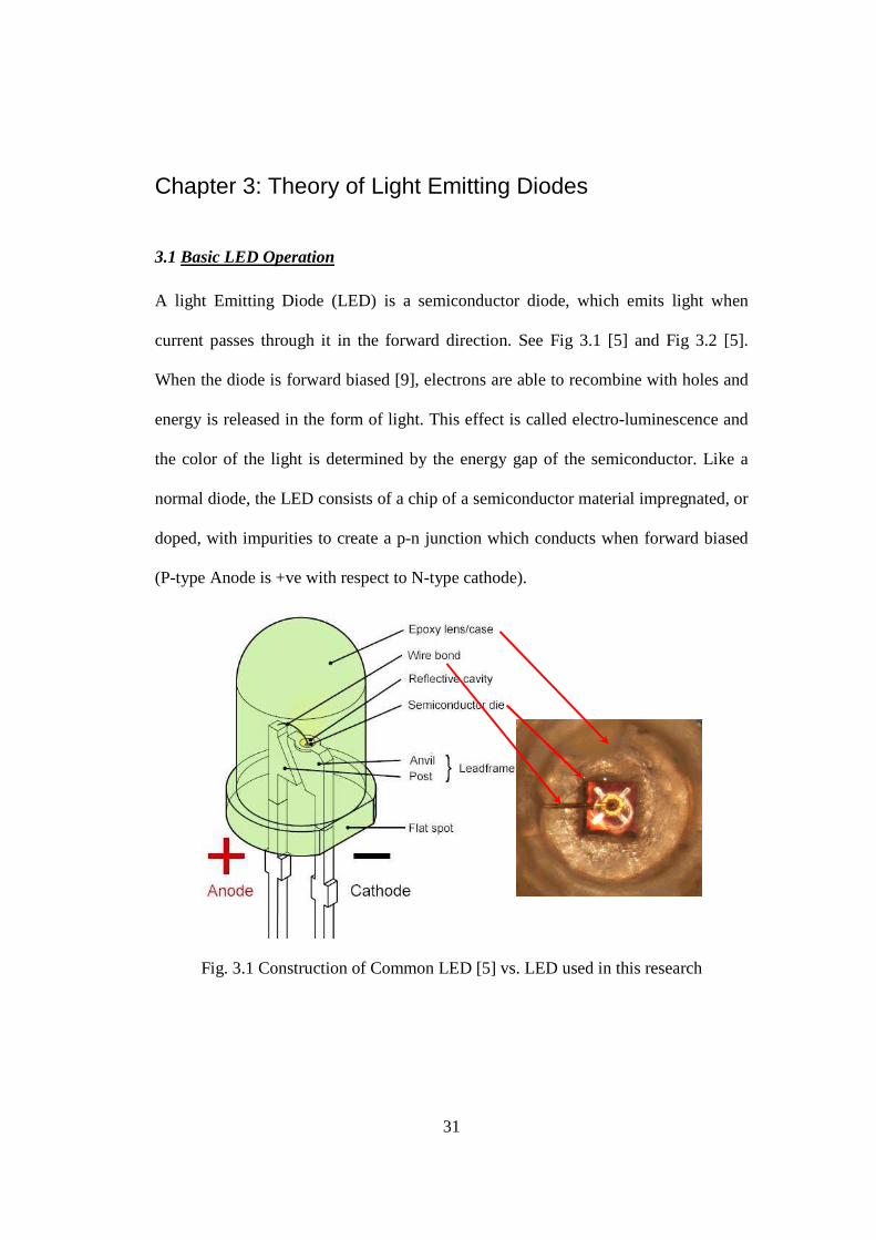
3.1 Basic LED Operation
A light Emitting Diode (LED) is a semiconductor diode, which emits light when
current passes through it in the forward direction. See Fig 3.1 [5] and Fig 3.2 [5].
When the diode is forward biased [9], electrons are able to recombine with holes and
energy is released in the form of light. This effect is called electro-luminescence and
the color of the light is determined by the energy gap of the semiconductor. Like a
normal diode, the LED consists of a chip of a semiconductor material impregnated, or
doped, with impurities to create a p-n junction which conducts when forward biased
(P-type Anode is +ve with respect to N-type cathode).
Fig. 3.1 Construction of Common LED [5] vs. LED used in this research
32
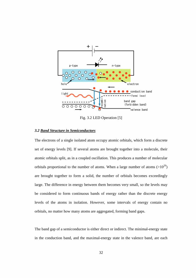
Fig. 3.2 LED Operation [5]
3.2 Band Structure in Semiconductors
The electrons of a single isolated atom occupy atomic orbitals, which form a discrete
set of energy levels [9]. If several atoms are brought together into a molecule, their
atomic orbitals split, as in a coupled oscillation. This produces a number of molecular
orbitals proportional to the number of atoms. When a large number of atoms (>1020)
are brought together to form a solid, the number of orbitals becomes exceedingly
large. The difference in energy between them becomes very small, so the levels may
be considered to form continuous bands of energy rather than the discrete energy
levels of the atoms in isolation. However, some intervals of energy contain no
orbitals, no matter how many atoms are aggregated, forming band gaps.
The band gap of a semiconductor is either direct or indirect. The minimal-energy state
in the conduction band, and the maximal-energy state in the valence band, are each
33
characterized by a certain k-vector in the Brillouin zone [9]. If the k-vectors are the
same, it is called a "direct gap". If they are different, it is called an "indirect gap". For
an indirect band gap, an electron cannot shift from the lowest-energy state in the
conduction band to the highest-energy state in the valence band without a change in
momentum. Hence direct band gap semiconductors are preferred for LEDs.
3.3 Wavelength of emitted light
When an LED is forward biased, the electrons in the conduction band recombine with
holes in the valence band. In the recombination process, energy Eg corresponding to
the band gap is emitted in the form of a photon whose wavelength λ (in nm) is given
by
λ = h c / Eg = 1239.8 / Eg - (3.1)
where h = Plank’s constant, c = speed of light in vacuum and Eg = band gap in eV.
3.4 Radiative and Non-radiative recombination in semiconductors
During a radiative recombination [9], an electron in the conduction band annihilates a
hole in the valence band, releasing the excess energy as a photon. This process is
possible in a direct band gap semiconductor. In contrast, the energy produced in a
non-radiative recombination does not create photons, but is released by lattice
vibration (phonon) in the semiconductor and finally changed to heat [2]. This non-
emitted energy enhances the rate of degradation of optical devices. Thus the non-
radiated recombination process plays a very important role in the device degradation
and hence device reliability.
34
3.5 Light output vs. Junction temperature
Temperature dependence of semiconductor device characteristics is very important
from a reliability standpoint [2]. During operation, heat is generated in the active
layer (also in other parts having ohmic resistance) which raises the junction
temperature. As the junction temperature increases, the internal quantum efficiency ηi
decreases due to the reduction of the radiative recombination coefficient and increase
in overflow of injected carrier from the active layer. Both of these changes cause the
light output of an LED to decrease rapidly. Moreover, the influence of Auger
recombination becomes large in the high-injected region. Thus the suppression or
removal of the heat generated in the active region during operation is very important
to obtain high radiative efficiency. Thermal shift of active layer bandgap was studied
in detail during this research and is discussed in Chapter 6.
3.6 Basic LED degradation mechanisms
Various degradation modes of LEDs have been classified [2] as rapid, gradual and
sudden. Different parts in LEDs prone to degradation are Active region, P-N
Contacts, Indium Tin Oxide layer, Plastic encapsulation and Packaging (Bond wires
and internal Heat Sink). These are described in detail in section 7.2.
3.7 Degradation of AlGaInP LEDs
The resistance to degradation of AlGaInP LEDs has been attributed by Streubel et al
[22] to a decreased sensitivity of the devices to oxidation. This is due to reduced Al
content in the active zone if compared to AlGaAs devices. Also, growth and mobility
of dark line defects is decreased owing to incorporation of In in the compound. Per
35
Vanderwater et al [15], neither the mismatched GaP window layer nor the presence of
the wafer-bonded GaP substrate adversely affects the reliability characteristics.
Similarly Grillot et al [16] feel that Auger recombination does not affect long term
reliability of AlGaInP LEDs. They attribute decrease in light output over time to
changes in Extraction efficiency, Leakage current density out of the active region and
Defect concentration.
Gradual degradation in LEDs causes the light output to decrease over its lifetime.
Arrhenius reaction rate model has been used to describe this process. Catastrophic
degradation could be due to an electrical surge during device handling, setting and
operating. In those cases, the active layer and the p-n junction corresponding to a part
or the entire light emitting region are catastrophically destroyed. The dark spots or
dark regions corresponding to the damaged part of the p-n junction can be observed
by EL topographs.
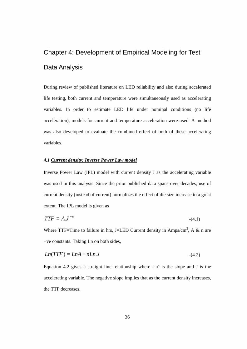
36
Chapter 4: Development of Empirical Modeling for Test
Data Analysis
During review of published literature on LED reliability and also during accelerated
life testing, both current and temperature were simultaneously used as accelerating
variables. In order to estimate LED life under nominal conditions (no life
acceleration), models for current and temperature acceleration were used. A method
was also developed to evaluate the combined effect of both of these accelerating
variables.
4.1 Current density: Inverse Power Law model
Inverse Power Law (IPL) model with current density J as the accelerating variable
was used in this analysis. Since the prior published data spans over decades, use of
current density (instead of current) normalizes the effect of die size increase to a great
extent. The IPL model is given as
nJATTF −= . -(4.1)
Where TTF=Time to failure in hrs, J=LED Current density in Amps/cm2, A & n are
+ve constants. Taking Ln on both sides,
JnLnLnATTFLn .)( −= -(4.2)
Equation 4.2 gives a straight line relationship where ‘-n’ is the slope and J is the
accelerating variable. The negative slope implies that as the current density increases,
the TTF decreases.
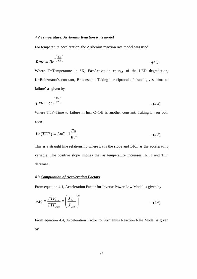
37
4.2 Temperature: Arrhenius Reaction Rate model
For temperature acceleration, the Arrhenius reaction rate model was used.
−= KT
Ea
BeRate -(4.3) Where T=Temperature in °K, Ea=Activation energy of the LED degradation,
K=Boltzmann’s constant, B=constant. Taking a reciprocal of ‘rate’ gives ‘time to
failure’ as given by
= KT
Ea
CeTTF - (4.4) Where TTF=Time to failure in hrs, C=1/B is another constant. Taking Ln on both
sides,
KT
EaLnCTTFLn +=)( - (4.5)
This is a straight line relationship where Ea is the slope and 1/KT as the accelerating
variable. The positive slope implies that as temperature increases, 1/KT and TTF
decrease.
4.3 Computation of Acceleration Factors
From equation 4.1, Acceleration Factor for Inverse Power Law Model is given by
n
Use
Acc
Acc
Use
J
J
TTF
TTFAF
==1 - (4.6)
From equation 4.4, Acceleration Factor for Arrhenius Reaction Rate Model is given
by
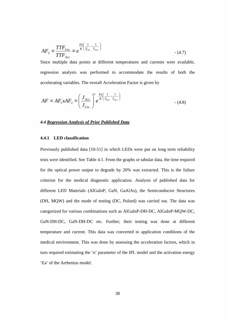
38
−
== AccUse TTK
Ea
Acc
Use eTTF
TTFAF
11
2 - (4.7)
Since multiple data points at different temperatures and currents were available,
regression analysis was performed to accommodate the results of both the
accelerating variables. The overall Acceleration Factor is given by
−
== AccUse TTK
Ean
Use
Acc eJ
JxAFAFAF
11
21 - (4.8)
4.4 Regression Analysis of Prior Published Data
4.4.1 LED classification
Previously published data [10-51] in which LEDs were put on long term reliability
tests were identified. See Table 4.1. From the graphs or tabular data, the time required
for the optical power output to degrade by 20% was extracted. This is the failure
criterion for the medical diagnostic application. Analysis of published data for
different LED Materials (AlGaInP, GaN, GaAlAs), the Semiconductor Structures
(DH, MQW) and the mode of testing (DC, Pulsed) was carried out. The data was
categorized for various combinations such as AlGaInP-DH-DC, AlGaInP-MQW-DC,
GaN-DH-DC, GaN-DH-DC etc. Further, their testing was done at different
temperature and current. This data was converted to application conditions of the
medical environment. This was done by assessing the acceleration factors, which in
turn required estimating the ‘n’ parameter of the IPL model and the activation energy
‘Ea’ of the Arrhenius model.
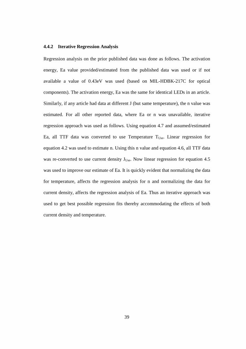
39
4.4.2 Iterative Regression Analysis
Regression analysis on the prior published data was done as follows. The activation
energy, Ea value provided/estimated from the published data was used or if not
available a value of 0.43eV was used (based on MIL-HDBK-217C for optical
components). The activation energy, Ea was the same for identical LEDs in an article.
Similarly, if any article had data at different J (but same temperature), the n value was
estimated. For all other reported data, where Ea or n was unavailable, iterative
regression approach was used as follows. Using equation 4.7 and assumed/estimated
Ea, all TTF data was converted to use Temperature TUse. Linear regression for
equation 4.2 was used to estimate n. Using this n value and equation 4.6, all TTF data
was re-converted to use current density JUse. Now linear regression for equation 4.5
was used to improve our estimate of Ea. It is quickly evident that normalizing the data
for temperature, affects the regression analysis for n and normalizing the data for
current density, affects the regression analysis of Ea. Thus an iterative approach was
used to get best possible regression fits thereby accommodating the effects of both
current density and temperature.
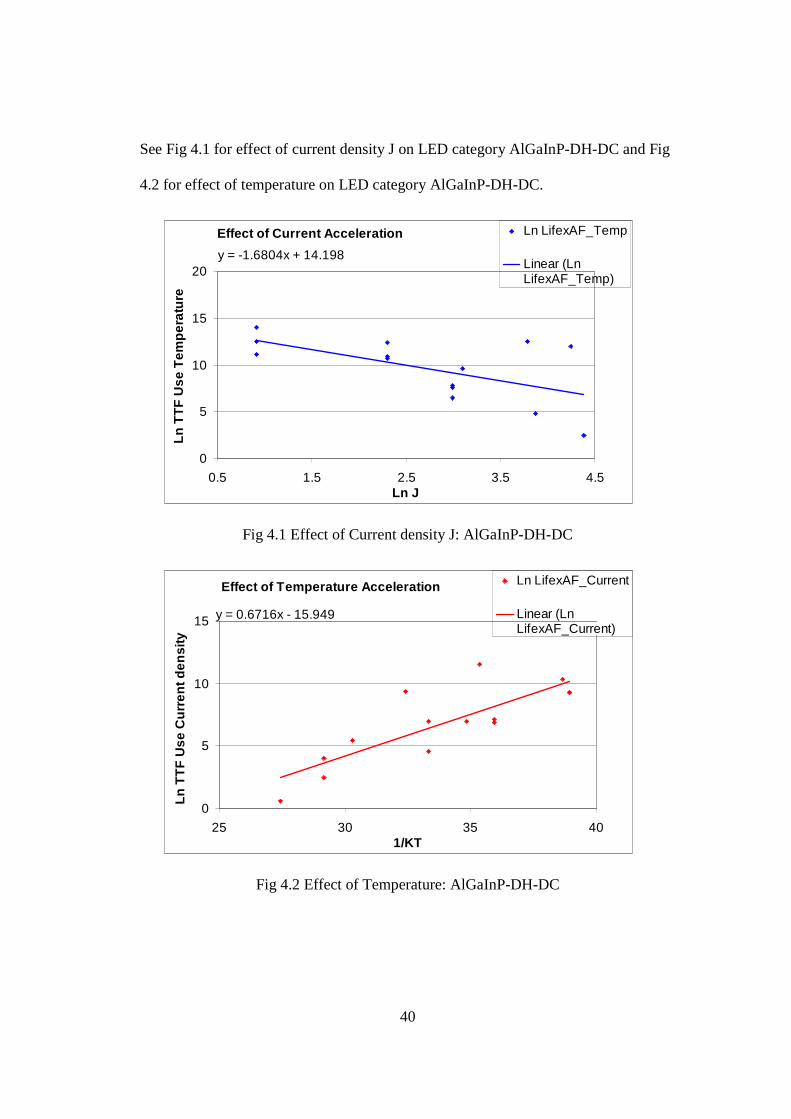
40
See Fig 4.1 for effect of current density J on LED category AlGaInP-DH-DC and Fig
4.2 for effect of temperature on LED category AlGaInP-DH-DC.
Fig 4.1 Effect of Current density J: AlGaInP-DH-DC
Fig 4.2 Effect of Temperature: AlGaInP-DH-DC
Effect of Current Acceleration
y = -1.6804x + 14.198
0
5
10
15
20
0.5 1.5 2.5 3.5 4.5Ln J
Ln T
TF
Use
Tem
pera
ture
Ln LifexAF_Temp
Linear (LnLifexAF_Temp)
Effect of Temperature Acceleration
y = 0.6716x - 15.949
0
5
10
15
25 30 35 401/KT
Ln T
TF
Use
Cur
rent
den
sity
Ln LifexAF_Current
Linear (LnLifexAF_Current)
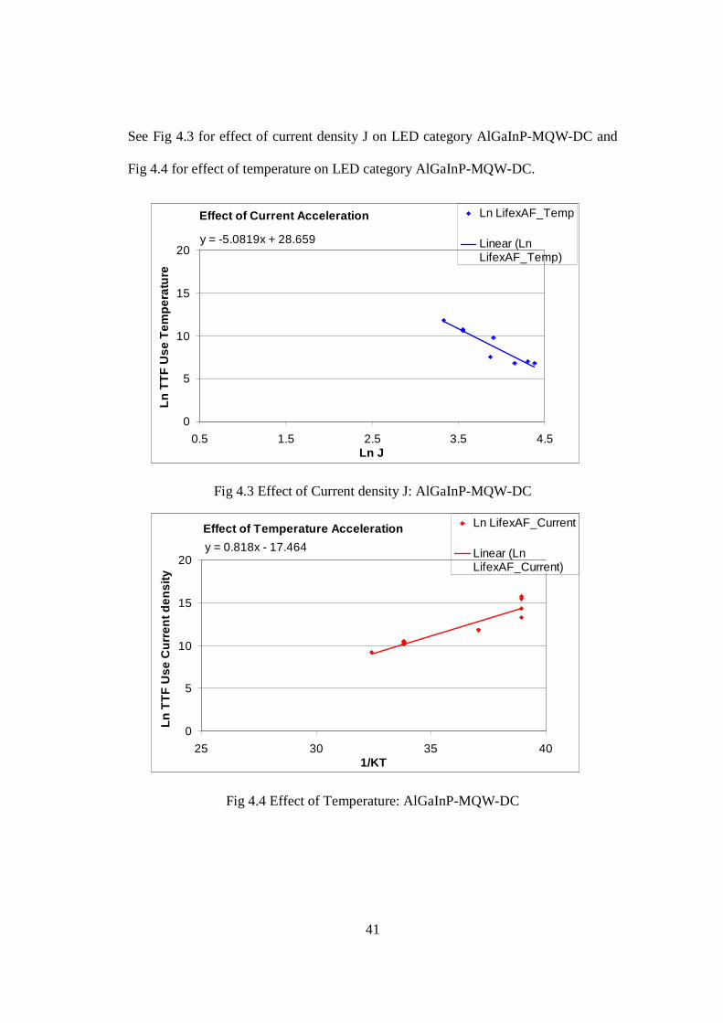
41
See Fig 4.3 for effect of current density J on LED category AlGaInP-MQW-DC and
Fig 4.4 for effect of temperature on LED category AlGaInP-MQW-DC.
Fig 4.3 Effect of Current density J: AlGaInP-MQW-DC
Fig 4.4 Effect of Temperature: AlGaInP-MQW-DC
Effect of Current Acceleration
y = -5.0819x + 28.659
0
5
10
15
20
0.5 1.5 2.5 3.5 4.5Ln J
Ln T
TF
Use
Tem
pera
ture
Ln LifexAF_Temp
Linear (LnLifexAF_Temp)
Effect of Temperature Acceleration
y = 0.818x - 17.464
0
5
10
15
20
25 30 35 401/KT
Ln T
TF
Use
Cur
rent
den
sity
Ln LifexAF_Current
Linear (LnLifexAF_Current)
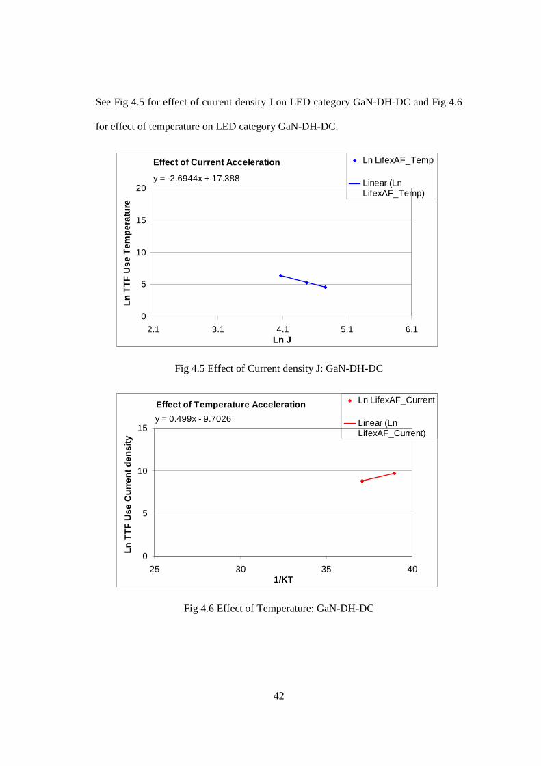
42
See Fig 4.5 for effect of current density J on LED category GaN-DH-DC and Fig 4.6
for effect of temperature on LED category GaN-DH-DC.
Fig 4.5 Effect of Current density J: GaN-DH-DC
Fig 4.6 Effect of Temperature: GaN-DH-DC
Effect of Current Acceleration
y = -2.6944x + 17.388
0
5
10
15
20
2.1 3.1 4.1 5.1 6.1Ln J
Ln T
TF
Use
Tem
pera
ture
Ln LifexAF_Temp
Linear (LnLifexAF_Temp)
Effect of Temperature Acceleration
y = 0.499x - 9.7026
0
5
10
15
25 30 35 401/KT
Ln T
TF
Use
Cur
rent
den
sity
Ln LifexAF_Current
Linear (LnLifexAF_Current)
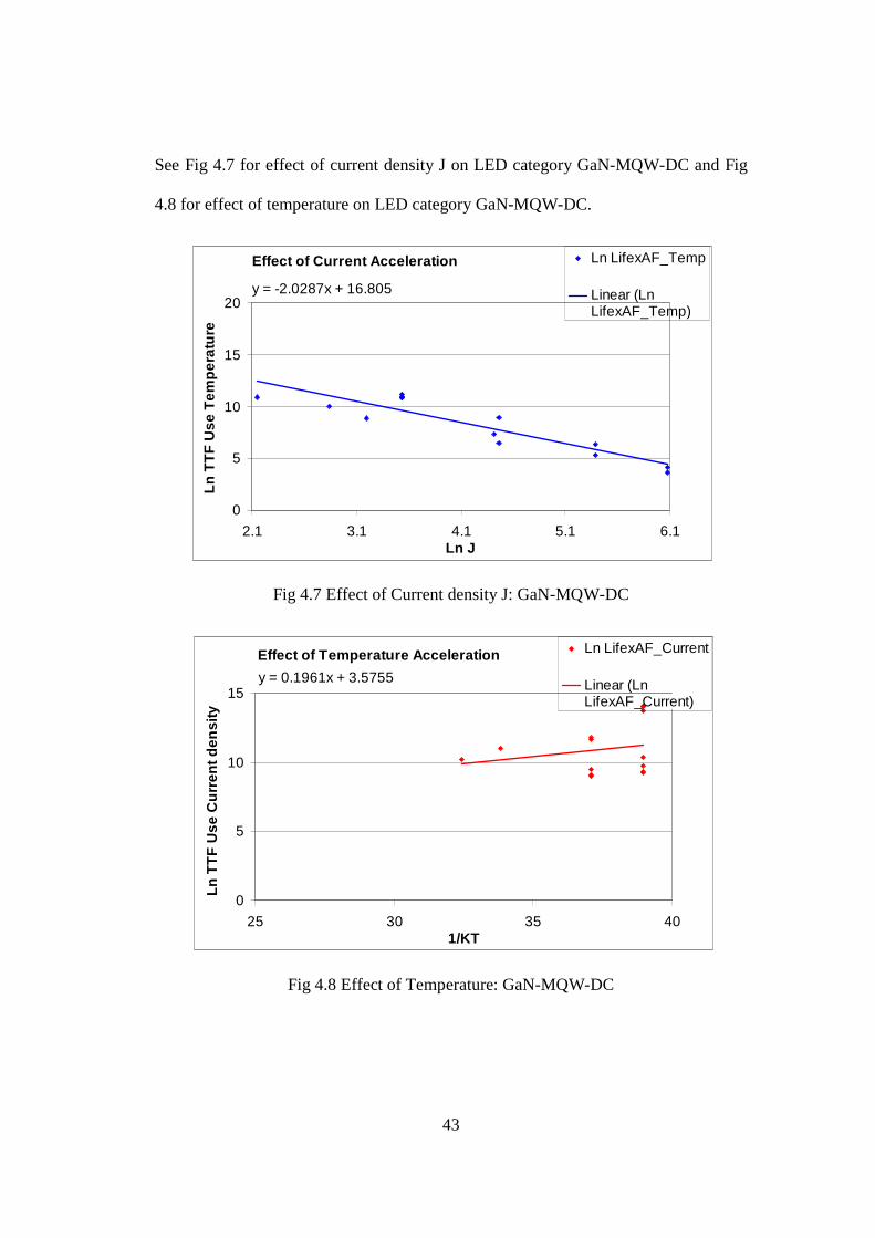
43
See Fig 4.7 for effect of current density J on LED category GaN-MQW-DC and Fig
4.8 for effect of temperature on LED category GaN-MQW-DC.
Fig 4.7 Effect of Current density J: GaN-MQW-DC
Fig 4.8 Effect of Temperature: GaN-MQW-DC
Effect of Current Acceleration
y = -2.0287x + 16.805
0
5
10
15
20
2.1 3.1 4.1 5.1 6.1Ln J
Ln T
TF
Use
Tem
pera
ture
Ln LifexAF_Temp
Linear (LnLifexAF_Temp)
Effect of Temperature Acceleration
y = 0.1961x + 3.5755
0
5
10
15
25 30 35 401/KT
Ln T
TF
Use
Cur
rent
den
sity
Ln LifexAF_Current
Linear (LnLifexAF_Current)
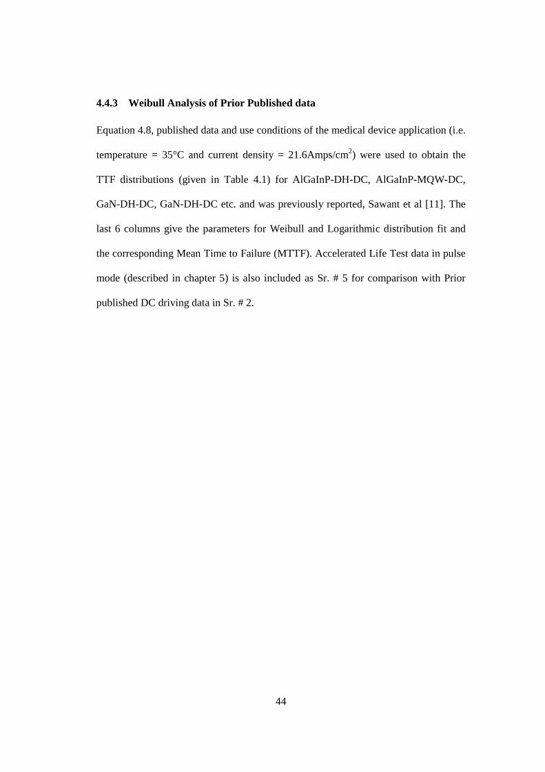
44
4.4.3 Weibull Analysis of Prior Published data
Equation 4.8, published data and use conditions of the medical device application (i.e.
temperature = 35°C and current density = 21.6Amps/cm2) were used to obtain the
TTF distributions (given in Table 4.1) for AlGaInP-DH-DC, AlGaInP-MQW-DC,
GaN-DH-DC, GaN-DH-DC etc. and was previously reported, Sawant et al [11]. The
last 6 columns give the parameters for Weibull and Logarithmic distribution fit and
the corresponding Mean Time to Failure (MTTF). Accelerated Life Test data in pulse
mode (described in chapter 5) is also included as Sr. # 5 for comparison with Prior
published DC driving data in Sr. # 2.
45
LED Material
Source of Data
IPL Act. E.
Weibull (Converted to application conditions)
Lognormal (Conv. to appl. Conditions)
Sr.#
Structure Driving
[Ref.]-Fig n eV αααα ββββ MTTF Hrs
µµµµ σσσσ MTTF Hrs
1 AlGaInP-DH- DC
[17]-2/4, [19]-9a/9b, [26]-3, [28]-3a/3b [29]-5
1.68 0.67 2.76E4 0.50 1.33E4 9.1 2.30 9.41E3
2 AlGaInP-MQW- DC
[19]-9a/9b, [22]-16, [24]-6/8/10 [27]-2
5.08 0.82 7.82E5 0.89 5.17E5 13 1.25 4.27E5
3 GaN- DH- DC
[47]-1 2.69 0.50 - - - - - -
4 GaN- MQW- DC
[24]-7/9/11 [33]-5, [34]-2/6
2.02 0.20 1.61E5 0.57 8.47E4 11.0 2.06 6.22E4
5 ALT: AlGaInP- MQW- Pulsed (0.2%)
ALT performed for this study
4.48 1.15 1.55E9 0.50 7.50E8 20.0 2.50 5.23E8
Table 4.1 Regression Analysis of Prior Published Data
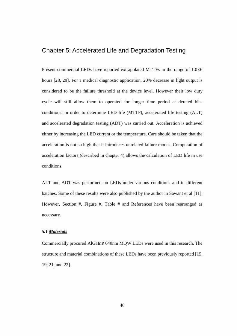
46
Chapter 5: Accelerated Life and Degradation Testing
Present commercial LEDs have reported extrapolated MTTFs in the range of 1.0E6
hours [28, 29]. For a medical diagnostic application, 20% decrease in light output is
considered to be the failure threshold at the device level. However their low duty
cycle will still allow them to operated for longer time period at derated bias
conditions. In order to determine LED life (MTTF), accelerated life testing (ALT)
and accelerated degradation testing (ADT) was carried out. Acceleration is achieved
either by increasing the LED current or the temperature. Care should be taken that the
acceleration is not so high that it introduces unrelated failure modes. Computation of
acceleration factors (described in chapter 4) allows the calculation of LED life in use
conditions.
ALT and ADT was performed on LEDs under various conditions and in different
batches. Some of these results were also published by the author in Sawant et al [11].
However, Section #, Figure #, Table # and References have been rearranged as
necessary.
5.1 Materials
Commercially procured AlGaInP 640nm MQW LEDs were used in this research. The
structure and material combinations of these LEDs have been previously reported [15,
19, 21, and 22].
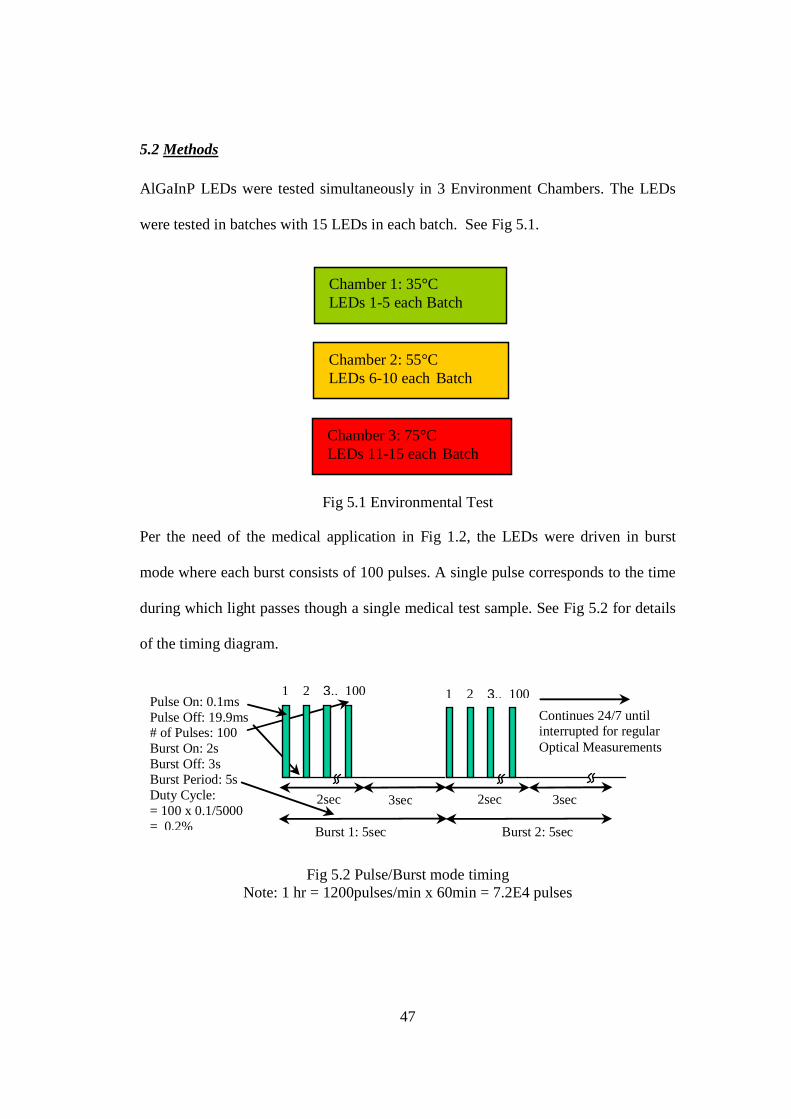
47
5.2 Methods
AlGaInP LEDs were tested simultaneously in 3 Environment Chambers. The LEDs
were tested in batches with 15 LEDs in each batch. See Fig 5.1.
Fig 5.1 Environmental Test
Per the need of the medical application in Fig 1.2, the LEDs were driven in burst
mode where each burst consists of 100 pulses. A single pulse corresponds to the time
during which light passes though a single medical test sample. See Fig 5.2 for details
of the timing diagram.
Fig 5.2 Pulse/Burst mode timing
Note: 1 hr = 1200pulses/min x 60min = 7.2E4 pulses
2sec 3sec Burst 1: 5sec Burst 2: 5sec
Continues 24/7 until interrupted for regular Optical Measurements
1 2 100 3.. Pulse On: 0.1ms Pulse Off: 19.9ms # of Pulses: 100 Burst On: 2s Burst Off: 3s Burst Period: 5s Duty Cycle: = 100 x 0.1/5000 = 0.2%
1 2 100 3..
2sec 3sec
Chamber 1: 35°C LEDs 1-5 each Batch
Chamber 2: 55°C LEDs 6-10 each Batch
Chamber 3: 75°C LEDs 11-15 each Batch
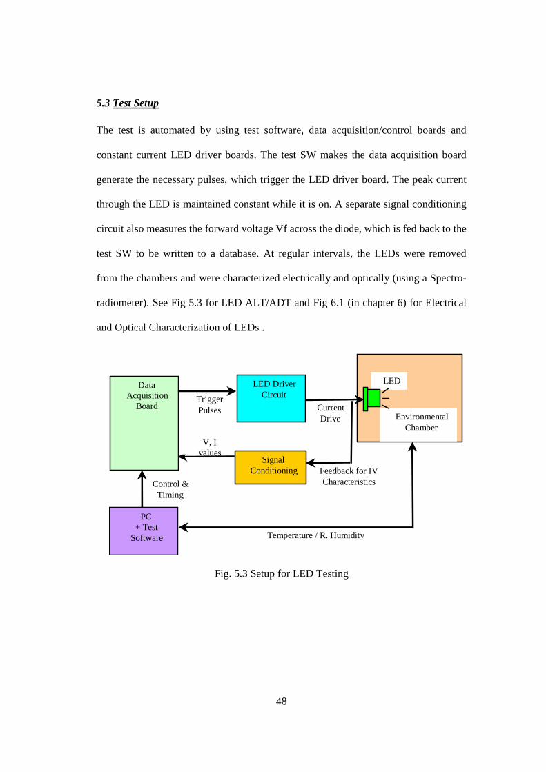
48
5.3 Test Setup
The test is automated by using test software, data acquisition/control boards and
constant current LED driver boards. The test SW makes the data acquisition board
generate the necessary pulses, which trigger the LED driver board. The peak current
through the LED is maintained constant while it is on. A separate signal conditioning
circuit also measures the forward voltage Vf across the diode, which is fed back to the
test SW to be written to a database. At regular intervals, the LEDs were removed
from the chambers and were characterized electrically and optically (using a Spectro-
radiometer). See Fig 5.3 for LED ALT/ADT and Fig 6.1 (in chapter 6) for Electrical
and Optical Characterization of LEDs .
Fig. 5.3 Setup for LED Testing
CurrentDrive Environmental
Chamber
Feedback for IVCharacteristicsControl &
Timing
Temperature / R. Humidity
PC+ Test
Software
SignalConditioning
LEDDataAcquisition
BoardTriggerPulses
LED DriverCircuit
V, Ivalues
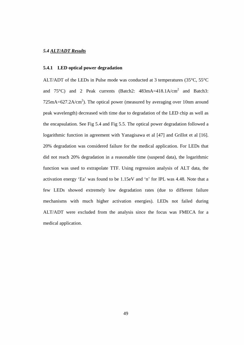
49
5.4 ALT/ADT Results
5.4.1 LED optical power degradation
ALT/ADT of the LEDs in Pulse mode was conducted at 3 temperatures (35°C, 55°C
and 75°C) and 2 Peak currents (Batch2: 483mA=418.1A/cm2 and Batch3:
725mA=627.2A/cm2). The optical power (measured by averaging over 10nm around
peak wavelength) decreased with time due to degradation of the LED chip as well as
the encapsulation. See Fig 5.4 and Fig 5.5. The optical power degradation followed a
logarithmic function in agreement with Yanagisawa et al [47] and Grillot et al [16].
20% degradation was considered failure for the medical application. For LEDs that
did not reach 20% degradation in a reasonable time (suspend data), the logarithmic
function was used to extrapolate TTF. Using regression analysis of ALT data, the
activation energy ‘Ea’ was found to be 1.15eV and ‘n’ for IPL was 4.48. Note that a
few LEDs showed extremely low degradation rates (due to different failure
mechanisms with much higher activation energies). LEDs not failed during
ALT/ADT were excluded from the analysis since the focus was FMECA for a
medical application.
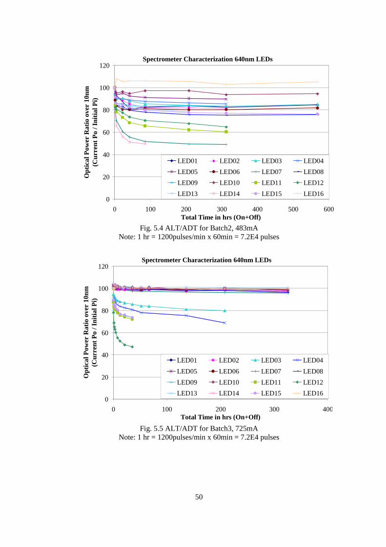
50
Fig. 5.4 ALT/ADT for Batch2, 483mA Note: 1 hr = 1200pulses/min x 60min = 7.2E4 pulses
Fig. 5.5 ALT/ADT for Batch3, 725mA Note: 1 hr = 1200pulses/min x 60min = 7.2E4 pulses
Spectrometer Characterization 640nm LEDs
0
20
40
60
80
100
120
0 100 200 300 400 500 600Total Time in hrs (On+Off)
Opt
ical
Pow
er R
atio
ove
r 10
nm
(Cur
rent
Po
/ Ini
tial P
i)
LED01 LED02 LED03 LED04
LED05 LED06 LED07 LED08
LED09 LED10 LED11 LED12
LED13 LED14 LED15 LED16
Spectrometer Characterization 640nm LEDs
0
20
40
60
80
100
120
0 100 200 300 400Total Time in hrs (On+Off)
Opt
ical
Pow
er R
atio
ove
r 10
nm
(Cur
rent
Po
/ Ini
tial P
i)
LED01 LED02 LED03 LED04
LED05 LED06 LED07 LED08
LED09 LED10 LED11 LED12
LED13 LED14 LED15 LED16
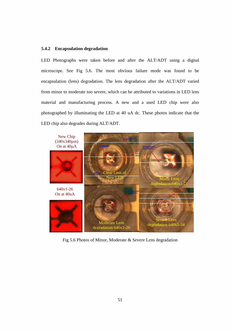
51
5.4.2 Encapsulation degradation
LED Photographs were taken before and after the ALT/ADT using a digital
microscope. See Fig 5.6. The most obvious failure mode was found to be
encapsulation (lens) degradation. The lens degradation after the ALT/ADT varied
from minor to moderate too severe, which can be attributed to variations in LED lens
material and manufacturing process. A new and a used LED chip were also
photographed by illuminating the LED at 40 uA dc. These photos indicate that the
LED chip also degrades during ALT/ADT.
Fig 5.6 Photos of Minor, Moderate & Severe Lens degradation
Clear Lens of New LED Minor Lens
degradation 640x1-21
Severe Lens degradation 640x1-34 Moderate Lens
degradation 640x1-26
640x1-26 On at 40uA
New Chip (340x340µm) On at 40µA
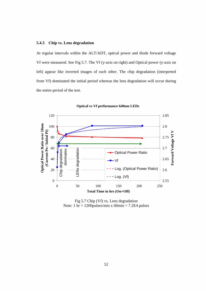
52
5.4.3 Chip vs. Lens degradation
At regular intervals within the ALT/ADT, optical power and diode forward voltage
Vf were measured. See Fig 5.7. The Vf (y-axis on right) and Optical power (y-axis on
left) appear like inverted images of each other. The chip degradation (interpreted
from Vf) dominated the initial period whereas the lens degradation will occur during
the entire period of the test.
Fig 5.7 Chip (Vf) vs. Lens degradation
Note: 1 hr = 1200pulses/min x 60min = 7.2E4 pulses
Optical vs Vf performance 640nm LEDs
0
20
40
60
80
100
120
0 50 100 150 200 250
Total Time in hrs (On+Off)
Opt
ical
Pow
er R
atio
ove
r 10
nm
(Cur
rent
Po
/ Ini
tial P
i)
2.55
2.6
2.65
2.7
2.75
2.8
2.85
For
war
d V
olta
ge V
f V
Optical Power Ratio
Vf
Log. (Optical Power Ratio)
Log. (Vf)Chi
p de
grad
atio
n do
min
ates
LEN
s de
grad
atio
n
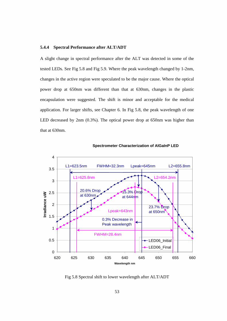
53
5.4.4 Spectral Performance after ALT/ADT
A slight change in spectral performance after the ALT was detected in some of the
tested LEDs. See Fig 5.8 and Fig 5.9. Where the peak wavelength changed by 1-2nm,
changes in the active region were speculated to be the major cause. Where the optical
power drop at 650nm was different than that at 630nm, changes in the plastic
encapsulation were suggested. The shift is minor and acceptable for the medical
application. For larger shifts, see Chapter 6. In Fig 5.8, the peak wavelength of one
LED decreased by 2nm (0.3%). The optical power drop at 650nm was higher than
that at 630nm.
Fig 5.8 Spectral shift to lower wavelength after ALT/ADT
Spectrometer Characterization of AlGaInP LED
0
0.5
1
1.5
2
2.5
3
3.5
4
620 625 630 635 640 645 650 655 660Wavelength nm
Irra
dian
ce u
W
LED06_Initial
LED06_Final
L1=623.5nm Lpeak=645nm L2=655.8nmFWHM=32.3nm
L1=625.8nm L2=654.2nm
Lpeak=643nm
FWHM=28.4nm
20.6% Drop at 630nm
23.7% Drop at 650nm
15.3% Drop at 644nm
0.3% Decrease in Peak wavelength
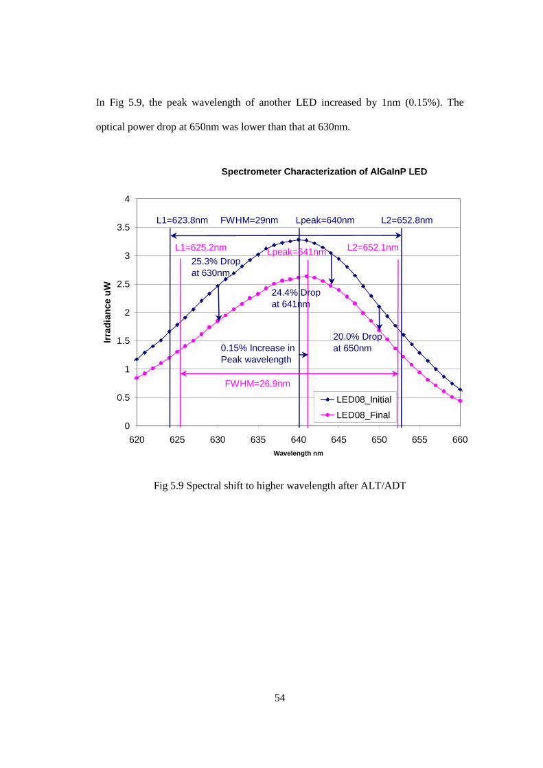
54
In Fig 5.9, the peak wavelength of another LED increased by 1nm (0.15%). The
optical power drop at 650nm was lower than that at 630nm.
Fig 5.9 Spectral shift to higher wavelength after ALT/ADT
Spectrometer Characterization of AlGaInP LED
0
0.5
1
1.5
2
2.5
3
3.5
4
620 625 630 635 640 645 650 655 660Wavelength nm
Irra
dian
ce u
W
LED08_Initial
LED08_Final
L1=623.8nm Lpeak=640nm L2=652.8nmFWHM=29nm
L1=625.2nm L2=652.1nmLpeak=641nm
FWHM=26.9nm
25.3% Drop at 630nm
20.0% Drop at 650nm
24.4% Drop at 641nm
0.15% Increase in Peak wavelength
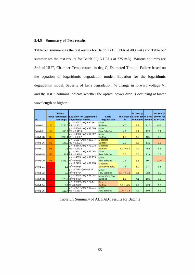
55
5.4.5 Summary of Test results
Table 5.1 summarizes the test results for Batch 2 (15 LEDs at 483 mA) and Table 5.2
summarizes the test results for Batch 3 (15 LEDs at 725 mA). Various columns are
Sr.# of UUT, Chamber Temperature in deg C, Estimated Time to Failure based on
the equation of logarithmic degradation model, Equation for the logarithmic
degradation model, Severity of Lens degradation, % change in forward voltage Vf
and the last 3 columns indicate whether the optical power drop is occurring at lower
wavelength or higher.
UUTTemp
C
TTF hrs Estimated 20% degrd
Equation for Logarithmic degradation model
LENs degradation
Vf Increase %
% Drop @ 630nm rel to 640nm
% drop 640nm
% Drop @ 650nm rel to 640nm
640x1-21 35 1755.6y = -1.4537Ln(x) + 90.86R2 = 0.8617
MinorSurface 4.0 3.2 12.2 -0.2
640x1-22 35 335.9y = -2.8548Ln(x) + 96.606R2 = 0.9119
MinorFew Bubbles 4.6 4.4 12.9 0.4
640x1-23 35 8282.1y = -1.4323Ln(x) + 92.922R2 = 0.9367
MinorSurface 6.5 4.6 10.4 1.0
640x1-26 55 195.0y = -1.5697Ln(x) + 88.277R2 = 0.9025
ModerateSurface 2.9 5.2 13.2 9.6
640x1-27 55 0.3y = -4.3842Ln(x) + 73.933R2 = 0.9732
ModerateSurface 7.9 -> 6.4 4.9 45.8 2.1
640x1-28 55 38.7y = -1.9411Ln(x) + 87.094R2 = 0.9864
MinorFew Bubbles 7.5 5.6 21.6 0.8
640x1-29 55 1225.0
y = -1.4315Ln(x) + 90.179
R2 = 0.9535MinorFew Bubbles 2.5 3.8 10.7 12.5
640x1-31 75 1.5
y = -3.2403Ln(x) + 81.238
R2 = 0.9684ModerateSurface+Bubles 3.6 6.0 33.3 2.6
640x1-32 75 3.2
y = -2.748Ln(x) + 83.18
R2 = 0.9754MinorFew Bubbles 11.7 -> 7.0 6.1 28.9 3.2
640x1-33 75 125.9
y = -1.8618Ln(x) + 89.002
R2 = 0.9464Minor Very Few Bubbles 8.8 4.1 18.1 2.3
640x1-34 75 0.2
y = -4.6769Ln(x) + 71.53
R2 = 0.9691SevereSurface 8.6 -> 4.5 4.6 42.0 3.5
640x1-35 75 113.4y = -1.9047Ln(x) + 89.011R2 = 0.9633
MinorFew Bubbles 11.5 -> 7.8 4.2 19.6 4.1
Table 5.1 Summary of ALT/ADT results for Batch 2
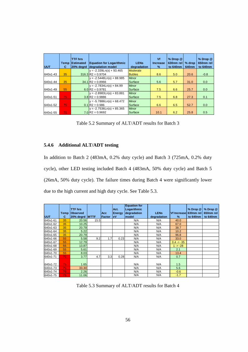
56
Table 5.2 Summary of ALT/ADT results for Batch 3
5.4.6 Additional ALT/ADT testing
In addition to Batch 2 (483mA, 0.2% duty cycle) and Batch 3 (725mA, 0.2% duty
cycle), other LED testing included Batch 4 (483mA, 50% duty cycle) and Batch 5
(26mA, 50% duty cycle). The failure times during Batch 4 were significantly lower
due to the high current and high duty cycle. See Table 5.3.
Table 5.3 Summary of ALT/ADT results for Batch 4
UUTTemp
C
TTF hrs Observed 20% degrd MTTF
AccFactor
Act. EnergyeV
Equation for Logarithmic degradation model
LENs degradation
Vf Increase %
% Drop @ 630nm rel to 640nm
% Drop @ 650nm rel to 640nm
640x1-61 35 20.56 15.5 N/A N/A 40.0640x1-62 35 10.25 N/A N/A 67.0640x1-63 35 20.79 N/A N/A 38.7640x1-64 35 5.22 N/A N/A 10.2640x1-65 35 20.79 N/A N/A 96.8640x1-66 55 5.58 9.2 1.7 0.23 N/A N/A 33.0640x1-67 55 12.79 N/A N/A 0.4 -> -35640x1-68 55 13.87 N/A N/A 1 -> -28640x1-69 55 5.61 N/A N/A 2.1640x1-70 55 8.03 N/A N/A 13.4640x1-71 75 3.77 4.7 3.3 0.28 N/A N/A 0.7
640x1-72 75 1.65 N/A N/A 1.5640x1-73 75 33.30 N/A N/A 5.6640x1-74 75 2.26 N/A N/A -0.6640x1-75 75 11.06 N/A N/A -1.7
UUTTemp
C
TTF hrs Estimated 20% degrd
Equation for Logarithmic degradation model
LENs degradation
Vf Increase
%
% Drop @ 630nm rel to 640nm
% drop 640nm
% Drop @ 650nm rel to 640nm
640x1-43 35 316.3y = -2.339Ln(x) + 93.465R2 = 0.9704
ModerateBubles 8.6 5.0 20.6 -0.8
640x1-44 35 34.1y = -2.5448Ln(x) + 88.985R2 = 0.8966
MinorSurface 5.6 5.7 31.0 0.0
640x1-49 55 6.0y = -2.7834Ln(x) + 84.99R2 = 0.9781
MinorSurface 7.5 6.6 25.7 0.0
640x1-51 75 3.8y = -2.8983Ln(x) + 83.881R2 = 0.9886
MinorSurface 7.5 6.8 27.3 0.1
640x1-52 75 0.1y = -5.7886Ln(x) + 68.472R2 = 0.986
MinorSurface 6.6 6.5 52.7 0.0
640x1-55 75 7.0y = -2.7536Ln(x) + 85.365R2 = 0.9692
MinorSurface 10.1 6.2 25.8 0.5
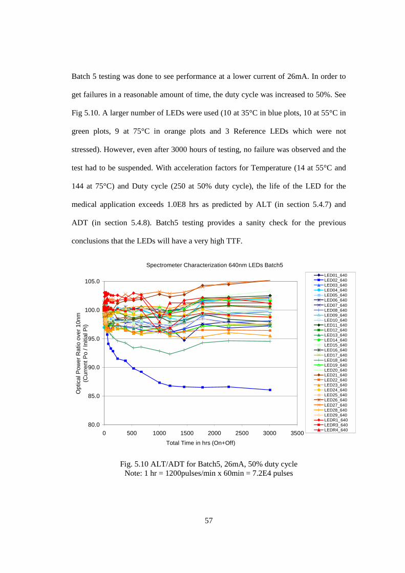
57
Batch 5 testing was done to see performance at a lower current of 26mA. In order to
get failures in a reasonable amount of time, the duty cycle was increased to 50%. See
Fig 5.10. A larger number of LEDs were used (10 at 35°C in blue plots, 10 at 55°C in
green plots, 9 at 75°C in orange plots and 3 Reference LEDs which were not
stressed). However, even after 3000 hours of testing, no failure was observed and the
test had to be suspended. With acceleration factors for Temperature (14 at 55°C and
144 at 75°C) and Duty cycle (250 at 50% duty cycle), the life of the LED for the
medical application exceeds 1.0E8 hrs as predicted by ALT (in section 5.4.7) and
ADT (in section 5.4.8). Batch5 testing provides a sanity check for the previous
conclusions that the LEDs will have a very high TTF.
Fig. 5.10 ALT/ADT for Batch5, 26mA, 50% duty cycle
Note: 1 hr = 1200pulses/min x 60min = 7.2E4 pulses
Spectrometer Characterization 640nm LEDs Batch5
80.0
85.0
90.0
95.0
100.0
105.0
0 500 1000 1500 2000 2500 3000 3500
Total Time in hrs (On+Off)
Opt
ical
Pow
er R
atio
ove
r 10
nm
(Cur
rent
Po
/ Ini
tial P
i)
LED01_640LED02_640LED03_640LED04_640LED05_640LED06_640LED07_640LED08_640LED09_640LED10_640LED11_640LED12_640LED13_640LED14_640LED15_640LED16_640LED17_640LED18_640LED19_640LED20_640LED21_640LED22_640LED23_640LED24_640LED25_640LED26_640LED27_640LED28_640LED29_640LEDR1_640LEDR3_640LEDR4_640
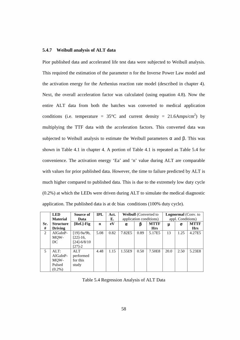
58
5.4.7 Weibull analysis of ALT data
Pior published data and accelerated life test data were subjected to Weibull analysis.
This required the estimation of the parameter n for the Inverse Power Law model and
the activation energy for the Arrhenius reaction rate model (described in chapter 4).
Next, the overall acceleration factor was calculated (using equation 4.8). Now the
entire ALT data from both the batches was converted to medical application
conditions (i.e. temperature = 35°C and current density = 21.6Amps/cm2) by
multiplying the TTF data with the acceleration factors. This converted data was
subjected to Weibull analysis to estimate the Weibull parameters α and β. This was
shown in Table 4.1 in chapter 4. A portion of Table 4.1 is repeated as Table 5.4 for
convenience. The activation energy ‘Ea’ and ‘n’ value during ALT are comparable
with values for prior published data. However, the time to failure predicted by ALT is
much higher compared to published data. This is due to the extremely low duty cycle
(0.2%) at which the LEDs were driven during ALT to simulate the medical diagnostic
application. The published data is at dc bias conditions (100% duty cycle).
LED Material
Source of Data
IPL Act. E.
Weibull (Converted to application conditions)
Lognormal (Conv. to appl. Conditions)
Sr.#
Structure Driving
[Ref.]-Fig n eV αααα ββββ MTTF Hrs
µµµµ σσσσ MTTF Hrs
2 AlGaInP-MQW- DC
[19]-9a/9b, [22]-16, [24]-6/8/10 [27]-2
5.08 0.82 7.82E5 0.89 5.17E5 13 1.25 4.27E5
5 ALT: AlGaInP- MQW- Pulsed (0.2%)
ALT performed for this study
4.48 1.15 1.55E9 0.50 7.50E8 20.0 2.50 5.23E8
Table 5.4 Regression Analysis of ALT Data
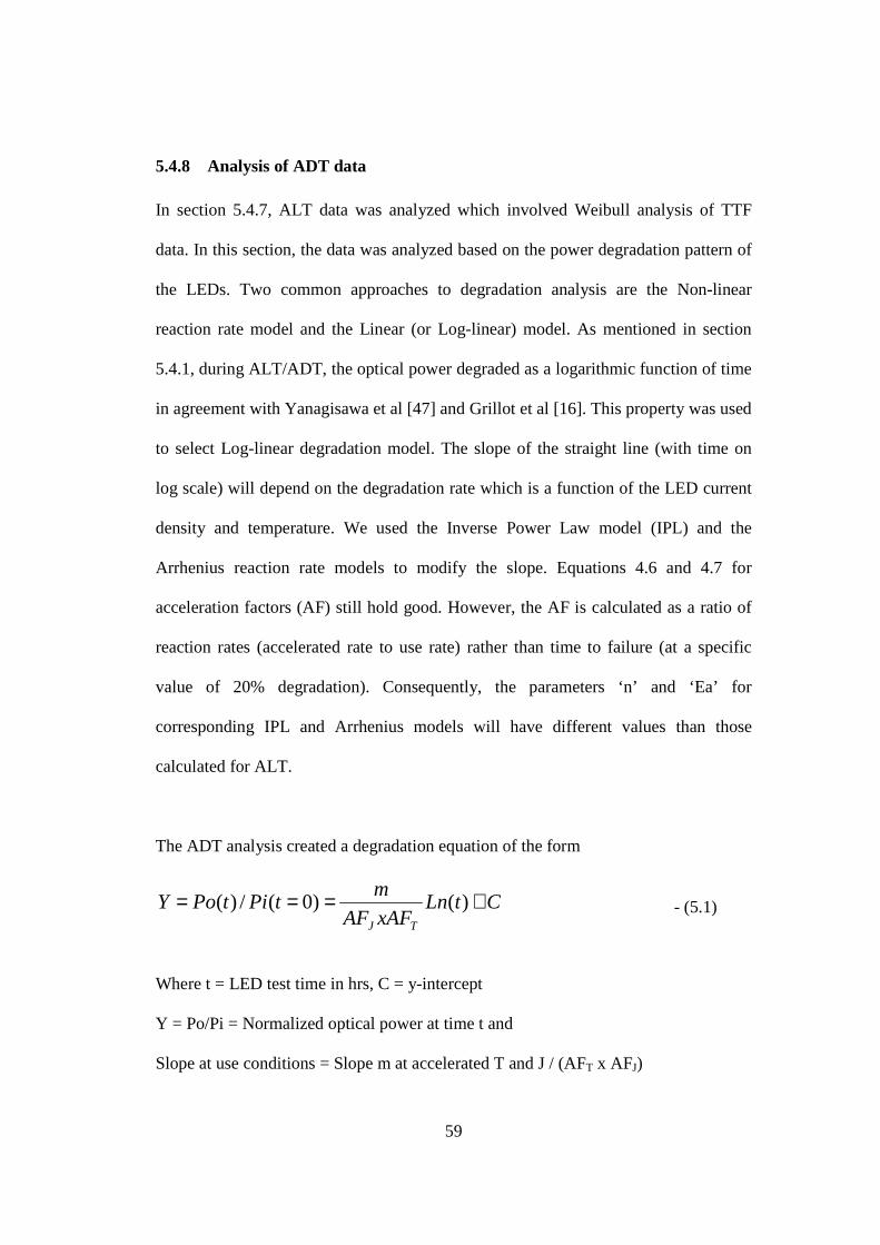
59
5.4.8 Analysis of ADT data
In section 5.4.7, ALT data was analyzed which involved Weibull analysis of TTF
data. In this section, the data was analyzed based on the power degradation pattern of
the LEDs. Two common approaches to degradation analysis are the Non-linear
reaction rate model and the Linear (or Log-linear) model. As mentioned in section
5.4.1, during ALT/ADT, the optical power degraded as a logarithmic function of time
in agreement with Yanagisawa et al [47] and Grillot et al [16]. This property was used
to select Log-linear degradation model. The slope of the straight line (with time on
log scale) will depend on the degradation rate which is a function of the LED current
density and temperature. We used the Inverse Power Law model (IPL) and the
Arrhenius reaction rate models to modify the slope. Equations 4.6 and 4.7 for
acceleration factors (AF) still hold good. However, the AF is calculated as a ratio of
reaction rates (accelerated rate to use rate) rather than time to failure (at a specific
value of 20% degradation). Consequently, the parameters ‘n’ and ‘Ea’ for
corresponding IPL and Arrhenius models will have different values than those
calculated for ALT.
The ADT analysis created a degradation equation of the form
CtLnxAFAF
mtPitPoY
TJ
+=== )()0(/)( - (5.1)
Where t = LED test time in hrs, C = y-intercept
Y = Po/Pi = Normalized optical power at time t and
Slope at use conditions = Slope m at accelerated T and J / (AFT x AFJ)
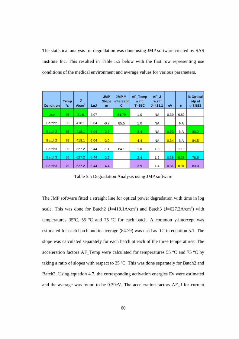
60
The statistical analysis for degradation was done using JMP software created by SAS
Institute Inc. This resulted in Table 5.5 below with the first row representing use
conditions of the medical environment and average values for various parameters.
ConditionTemp
ºC
JA/cm 2 LnJ
JMP Slope
m
JMP Y-intercept
C
AF_Tempw.r.t.
T=35C
AF_Jw.r.t
J=418.1 eV n
% Optical o/p at
t=7.5E8
Use 35 21.6 3.07 84.79 1.0 NA 0.39 0.82
Batch2 35 418.1 6.04 -0.7 85.5 1.0 NA NA
Batch2 55 418.1 6.04 -2.3 3.4 NA 0.53 NA 80.2
Batch2 75 418.1 6.04 -3.0 4.4 NA 0.34 NA 84.5
Batch3 35 627.2 6.44 -1.1 84.1 1.0 1.6 1.19
Batch3 55 627.2 6.44 -2.7 2.4 1.2 0.38 0.38 78.5
Batch3 75 627.2 6.44 -4.4 3.9 1.4 0.31 0.91 83.0
Table 5.5 Degradation Analysis using JMP software
The JMP software fitted a straight line for optical power degradation with time in log
scale. This was done for Batch2 (J=418.1A/cm2) and Batch3 (J=627.2A/cm2) with
temperatures 35ºC, 55 ºC and 75 ºC for each batch. A common y-intercept was
estimated for each batch and its average (84.79) was used as ‘C’ in equation 5.1. The
slope was calculated separately for each batch at each of the three temperatures. The
acceleration factors AF_Temp were calculated for temperatures 55 ºC and 75 ºC by
taking a ratio of slopes with respect to 35 ºC. This was done separately for Batch2 and
Batch3. Using equation 4.7, the corresponding activation energies Ev were estimated
and the average was found to be 0.39eV. The acceleration factors AF_J for current
61
density were calculated by taking a ratio of slopes between Batch3 and Batch2. Note
that Batch2 is also at an accelerated condition of J and AF_J values are only used to
estimate parameter ‘n’ of IPL model using equation 4.6. Once ‘n’ and ‘Ev’ were
available, AFJ and AFT were calculated and equation 5.1 was developed for various
conditions. From table 5.4, MTTF of the LEDs (at use conditions) estimated from
ALT was 7.5E8 hrs. The last column in Table 5.5 gives optical output at t=7.5E8 hrs
for various conditions. This value was found to be close to 80% implying a 20%
degradation which was the failure criterion for the ALT. Thus, the results from ALT
and ADT agree with each other. Further, equation 5.1 for ADT can be used to
calculate LED TTF if the degradation threshold is changed.
62
Chapter 6: Thermal Shift of Active layer Bandgap
Reliability testing of AlGaInP MQW LEDs resulted in a shift of Bandgap towards the
longer wavelength when driven at high current and high duty cycles. The spectral
FWHM also increased. Characterization of the shift showed that it was temporary and
dependent on the junction temperature. Some of these results were also published by
the author in Sawant et al [12]. However, Section #, Figure #, Table # and References
have been rearranged as necessary.
6.1 Background on Spectral Shifts
The band gap of a semiconductor is either direct or indirect. For an indirect band gap,
an electron cannot shift from the lowest-energy state in the conduction band to the
highest-energy state in the valence band without a change in momentum [9]. Hence
direct band gap semiconductors are preferred for LEDs. When an LED is forward
biased, the electrons in the conduction band recombine with holes in the valence
band. In the recombination process, energy Eg corresponding to the band gap is
emitted in the form of a photon whose wavelength λ (in nm) is given by
λ = h c / Eg = 1239.8 / Eg - (6.1)
where h = Plank’s constant, c = speed of light in vacuum and Eg = band gap in eV.
Temperature dependence of semiconductor device characteristics is very important
from a reliability standpoint [2]. During operation, heat is generated in the active
layer (also in other parts having ohmic resistance) which raises the junction
63
temperature. This research tried to characterize the shift in the spectrum resulting
from elevated junction temperature.
6.2 Methods
The forward bias method was used to establish the linear relationship between the
forward voltage Vf and the junction temperature Jt for a given forward current. See
section 6.3.1 for details on this. The Shockley diode equation [10] relates the diode
current I of a p-n junction diode to the diode voltage Vf:
I = Is ( eVf / n Vt – 1)
= Is ( eVf q / n K T – 1)
= Is eVf q / n K T for eVf q / n K T >> 1 - (6.2)
where Is is the saturation current or scale current of the diode (the magnitude of the
current that flows for negative Vf in excess of a few Vt, typically 10-12 A). The scale
current is proportional to the diode area. Vt is the thermal voltage, and n is known as
the diode ideality factor. Thus if I is maintained constant, junction temperature Jt can
be directly interpreted in terms of forward voltage Vf which typically decreases
between 1 and 3mV per 1 deg C rise in temperature. See details in section 6.3.1.
To measure the spectral response, the LEDs were driven at different currents and
measured the optical output of the LED using a Spectro-Radiometer. While
measuring the spectrum, the Vf was also measured thereby allowing us to estimate Jt
during those conditions. The data was further analyzed with respect to Varshini’s
equation, and the empirical coefficients were determined.
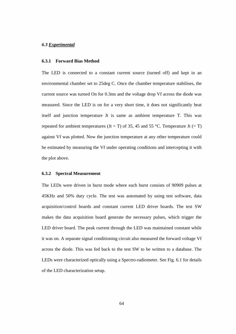
64
6.3 Experimental
6.3.1 Forward Bias Method
The LED is connected to a constant current source (turned off) and kept in an
environmental chamber set to 25deg C. Once the chamber temperature stabilises, the
current source was turned On for 0.3ms and the voltage drop Vf across the diode was
measured. Since the LED is on for a very short time, it does not significantly heat
itself and junction temperature Jt is same as ambient temperature T. This was
repeated for ambient temperatures (Jt = T) of 35, 45 and 55 °C. Temperature Jt (= T)
against Vf was plotted. Now the junction temperature at any other temperature could
be estimated by measuring the Vf under operating conditions and intercepting it with
the plot above.
6.3.2 Spectral Measurement
The LEDs were driven in burst mode where each burst consists of 90909 pulses at
45KHz and 50% duty cycle. The test was automated by using test software, data
acquisition/control boards and constant current LED driver boards. The test SW
makes the data acquisition board generate the necessary pulses, which trigger the
LED driver board. The peak current through the LED was maintained constant while
it was on. A separate signal conditioning circuit also measured the forward voltage Vf
across the diode. This was fed back to the test SW to be written to a database. The
LEDs were characterized optically using a Spectro-radiometer. See Fig. 6.1 for details
of the LED characterization setup.

65
Fig 6.1 Electrical and Optical Characterization of LEDs
6.4 Results and Discussion of Spectral Shift
6.4.1 Vf-Jt Linear Relationship
Linear relationship between the forward voltage Vf and Junction Temperature Jt was
established for 2 LEDs (640x1-57 and 640x1-58) for a given forward current value.
This was repeated at different currents (26mA, 58mA, 483mA and 725mA). See Fig.
6.2 and Fig. 6.3 for details.
Current Drive
Integrating Sphere
Feedback for IV Characterization Control &
Timing
Irradiance Fiber
PC +Test
Software
Spectro- Radiometer
Signal Conditioning
LED
Data Acquisition
Board
Trigger Pulses
V, I Value
LED Driver Circuit
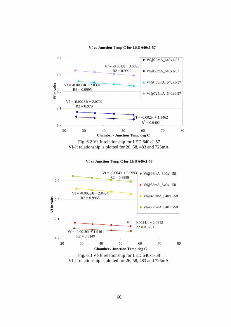
66
Fig. 6.2 Vf-Jt relationship for LED 640x1-57 Vf-Jt relationship is plotted for 26, 58, 483 and 725mA.
Fig. 6.3 Vf-Jt relationship for LED 640x1-58 Vf-Jt relationship is plotted for 26, 58, 483 and 725mA.
Vf vs Junction Temp C for LED 640x1-57
Vf = -0.002Jt + 1.9462
R2 = 0.9402
Vf = -0.0023Jt + 2.0702R2 = 0.979
Vf = -0.004Jt + 3.0893R2 = 0.9999
Vf = -0.0038Jt + 2.8391R2 = 0.9995
1.7
2.1
2.5
2.9
3.3
20 30 40 50 60 70 80Chamber / Junction Temp deg C
Vf i
n vo
ltsVf@26mA_640x1-57
Vf@58mA_640x1-57
Vf@483mA_640x1-57
Vf@725mA_640x1-57
Vf vs Junction Temp C for LED 640x1-58
Vf = -0.0019Jt + 1.9461R2 = 0.9149
Vf = -0.0024Jt + 2.0812R2 = 0.9701
Vf = -0.004Jt + 3.0993R2 = 0.9999
Vf = -0.0038Jt + 2.8434R2 = 0.9968
1.7
2.1
2.5
2.9
20 30 40 50 60 70 80
Chamber / Junction Temp deg C
Vf i
n vo
lts
Vf@26mA_640x1-58
Vf@58mA_640x1-58
Vf@483mA_640x1-58
Vf@725mA_640x1-58
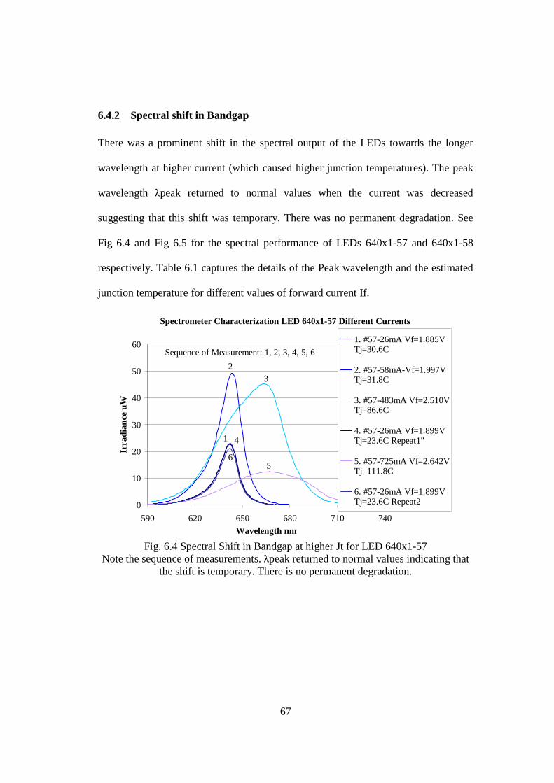
67
6.4.2 Spectral shift in Bandgap
There was a prominent shift in the spectral output of the LEDs towards the longer
wavelength at higher current (which caused higher junction temperatures). The peak
wavelength λpeak returned to normal values when the current was decreased
suggesting that this shift was temporary. There was no permanent degradation. See
Fig 6.4 and Fig 6.5 for the spectral performance of LEDs 640x1-57 and 640x1-58
respectively. Table 6.1 captures the details of the Peak wavelength and the estimated
junction temperature for different values of forward current If.
Fig. 6.4 Spectral Shift in Bandgap at higher Jt for LED 640x1-57 Note the sequence of measurements. λpeak returned to normal values indicating that
the shift is temporary. There is no permanent degradation.
Spectrometer Characterization LED 640x1-57 Different Currents
0
10
20
30
40
50
60
590 620 650 680 710 740
Wavelength nm
Irra
dian
ce u
W
1. #57-26mA Vf=1.885VTj=30.6C
2. #57-58mA-Vf=1.997VTj=31.8C
3. #57-483mA Vf=2.510VTj=86.6C
4. #57-26mA Vf=1.899VTj=23.6C Repeat1"
5. #57-725mA Vf=2.642VTj=111.8C
6. #57-26mA Vf=1.899VTj=23.6C Repeat2
Sequence of Measurement: 1, 2, 3, 4, 5, 6
1
23
56
4
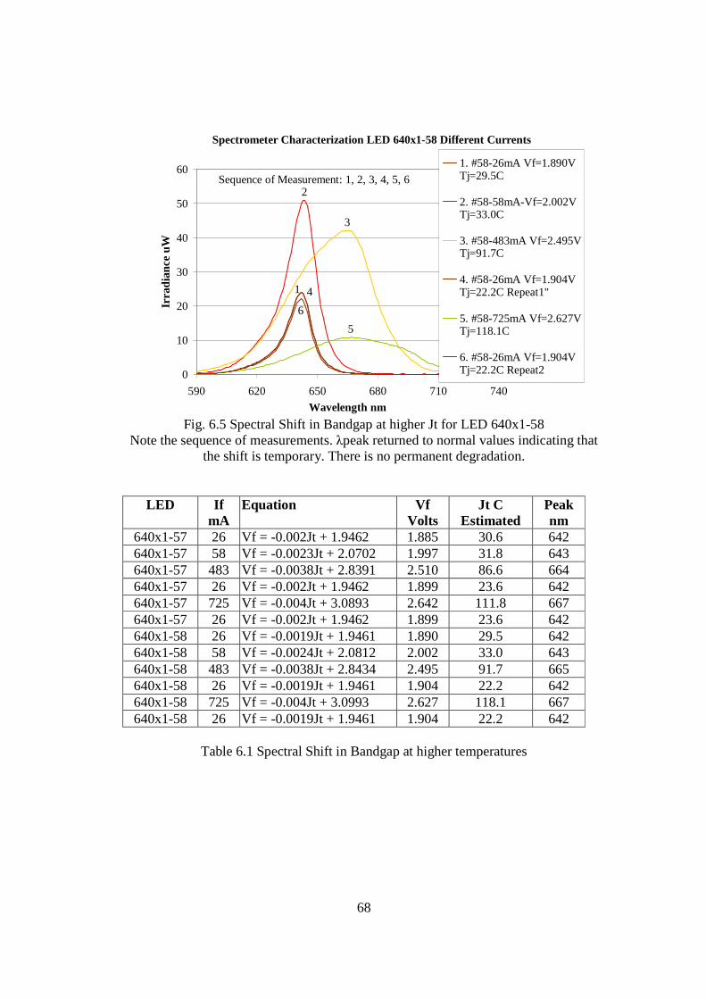
68
Fig. 6.5 Spectral Shift in Bandgap at higher Jt for LED 640x1-58 Note the sequence of measurements. λpeak returned to normal values indicating that
the shift is temporary. There is no permanent degradation.
LED If mA
Equation Vf Volts
Jt C Estimated
Peak nm
640x1-57 26 Vf = -0.002Jt + 1.9462 1.885 30.6 642 640x1-57 58 Vf = -0.0023Jt + 2.0702 1.997 31.8 643 640x1-57 483 Vf = -0.0038Jt + 2.8391 2.510 86.6 664 640x1-57 26 Vf = -0.002Jt + 1.9462 1.899 23.6 642 640x1-57 725 Vf = -0.004Jt + 3.0893 2.642 111.8 667 640x1-57 26 Vf = -0.002Jt + 1.9462 1.899 23.6 642 640x1-58 26 Vf = -0.0019Jt + 1.9461 1.890 29.5 642 640x1-58 58 Vf = -0.0024Jt + 2.0812 2.002 33.0 643 640x1-58 483 Vf = -0.0038Jt + 2.8434 2.495 91.7 665 640x1-58 26 Vf = -0.0019Jt + 1.9461 1.904 22.2 642 640x1-58 725 Vf = -0.004Jt + 3.0993 2.627 118.1 667 640x1-58 26 Vf = -0.0019Jt + 1.9461 1.904 22.2 642
Table 6.1 Spectral Shift in Bandgap at higher temperatures
Spectrometer Characterization LED 640x1-58 Different Currents
0
10
20
30
40
50
60
590 620 650 680 710 740
Wavelength nm
Irra
dian
ce u
W1. #58-26mA Vf=1.890VTj=29.5C
2. #58-58mA-Vf=2.002VTj=33.0C
3. #58-483mA Vf=2.495VTj=91.7C
4. #58-26mA Vf=1.904VTj=22.2C Repeat1"
5. #58-725mA Vf=2.627VTj=118.1C
6. #58-26mA Vf=1.904VTj=22.2C Repeat2
Sequence of Measurement: 1, 2, 3, 4, 5, 6
1
2
3
5
6
4
69
6.4.3 Varshini’s empirical model
The relationship between peak wavelength and current/junction temperature has been
published in various articles. Our research findings agree with Kish et al [20] for the
AlGaInP LEDs. They studied high luminous flux AlGaInP/GaP large area emitters
with currents as high as 7A. The peak wavelength shifted from 602nm to 614nm
when the current was increased to 7A corresponding to a 120°C rise in junction
temperature. Similar results have been observed by Nakamura et al [3] for InGaN
MQW LEDs. The peak wavelength changed from 409nm at 25°C to 410.5nm at
55°C.
Nakamura et al [46] also found an anomaly while testing InGaN DH LEDs. The peak
wavelength shifted to the shorter-wavelength region with increasing forward current.
The peak wavelengths were 458 nm at 0.1 mA, 449 nm at 1 mA and 447 nm at
20mA. They suggested that this anomaly was due to donor-acceptor (DA) pair
recombination in the InGaN active layer co-doped with both Si and Zn. At 20 mA, a
narrower, higher-energy peak emerged around 385 nm. This peak was due to band-to-
band recombination in the InGaN active layer. This peak became resolved at injection
levels where the impurity related recombination was saturated. H. Morkoc [6] shows
current and temperature dependence of Spectra for Green Nichia GaN LEDs. A clear
shift to higher energies was observed (532nm at 0.1mA to 519nm at 10mA). For
pulsed current, EL changed from 534nm at 0.1mA to 492nm at 2000mA. For the
same LEDs, the peak decreases from 541nm at 50°K (-223°C) to 534nm at 300°K
(27°C) whereas the band edge increases from 535nm to 544nm.
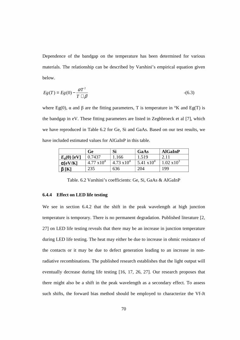
70
Dependence of the bandgap on the temperature has been determined for various
materials. The relationship can be described by Varshini’s empirical equation given
below.
βα
+−=
T
TEgTEg
2
)0()( -(6.3)
where Eg(0), α and β are the fitting parameters, T is temperature in °K and Eg(T) is
the bandgap in eV. These fitting parameters are listed in Zeghbroeck et al [7], which
we have reproduced in Table 6.2 for Ge, Si and GaAs. Based on our test results, we
have included estimated values for AlGaInP in this table.
Ge Si GaAs AlGaInP Eg(0) [eV] 0.7437 1.166 1.519 2.11 αααα[eV/K] 4.77 x10⁴ 4.73 x10⁴ 5.41 x10⁴ 1.02 x10³
ββββ [K] 235 636 204 199
Table. 6.2 Varshini’s coefficients: Ge, Si, GaAs & AlGaInP
6.4.4 Effect on LED life testing
We see in section 6.4.2 that the shift in the peak wavelength at high junction
temperature is temporary. There is no permanent degradation. Published literature [2,
27] on LED life testing reveals that there may be an increase in junction temperature
during LED life testing. The heat may either be due to increase in ohmic resistance of
the contacts or it may be due to defect generation leading to an increase in non-
radiative recombinations. The published research establishes that the light output will
eventually decrease during life testing [16, 17, 26, 27]. Our research proposes that
there might also be a shift in the peak wavelength as a secondary effect. To assess
such shifts, the forward bias method should be employed to characterize the Vf-Jt
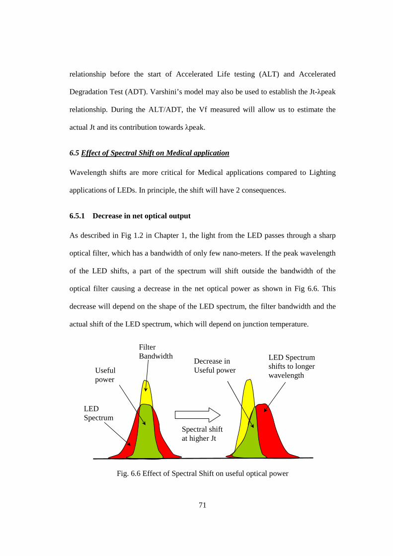
71
relationship before the start of Accelerated Life testing (ALT) and Accelerated
Degradation Test (ADT). Varshini’s model may also be used to establish the Jt-λpeak
relationship. During the ALT/ADT, the Vf measured will allow us to estimate the
actual Jt and its contribution towards λpeak.
6.5 Effect of Spectral Shift on Medical application
Wavelength shifts are more critical for Medical applications compared to Lighting
applications of LEDs. In principle, the shift will have 2 consequences.
6.5.1 Decrease in net optical output
As described in Fig 1.2 in Chapter 1, the light from the LED passes through a sharp
optical filter, which has a bandwidth of only few nano-meters. If the peak wavelength
of the LED shifts, a part of the spectrum will shift outside the bandwidth of the
optical filter causing a decrease in the net optical power as shown in Fig 6.6. This
decrease will depend on the shape of the LED spectrum, the filter bandwidth and the
actual shift of the LED spectrum, which will depend on junction temperature.
Fig. 6.6 Effect of Spectral Shift on useful optical power
LED Spectrum
Filter Bandwidth
Useful power
Decrease in Useful power
LED Spectrum shifts to longer wavelength
Spectral shift at higher Jt
72
6.5.2 Change in the Absorbance Chemistry
As described in section 1.1 in Chapter 1, the absorbance of light by the cuvette
mixture at certain wavelengths depends on patient’s disease condition. Beer’s law [1]
gives a relationship between the transmission T of light through a substance and the
product of the absorption coefficient of the substance, α, and the distance the light
travels through the material (i.e. the path length), ℓ. For a given medical instrument,
the path length is constant and the absorption of light can be calculated from the
incident and transmitted light. Further, the same medical diagnostic instrument
performs various tests (called assays) such as Clinical Chemistry, Drugs of abuse,
therapeutic drug monitoring (TDM) and specific proteins etc. Depending upon the
actual diagnostic test to be performed, the human sample is mixed with proprietary
chemical reagents. The relationship between the light absorbed and the disease
condition is pre-determined by Chemists for all the diagnostic tests that the medical
instrument supports. Some of these tests are very sensitive to the peak wavelength
whereas others are less sensitive. A shift in peak wavelength of the LED light source
will have different consequences depending upon the specific diagnostic test being
conducted, its sensitivity to wavelength and the actual spectral shift. Much of this
information is proprietary and beyond the scope of this research.
73
6.6 Conclusions of Spectral Shift
Reliability testing of AlGaInP MQW LEDs resulted in a shift of Bandgap towards the
longer wavelength when driven at high current. Characterization of the shift showed
that it was temporary and dependent on the junction temperature Jt. The data was
further analyzed with respect to Varshini’s equation, and the empirical coefficients
were determined. Published research establishes that the light output will eventually
decrease during life testing. This research proposes that there might also be a shift in
the peak wavelength as a secondary effect if the LED operates at a high junction
temperature Jt. This research will also help in evaluating LED performance during
ALT/ADT and while choosing LEDs for applications (such as medical diagnostics)
where λpeak needs to be stable. The junction temperature Jt will need to be
maintained within limits to achieve spectral stability.
74
Chapter 7: Failure Modes and Effects Criticality Analysis (FMECA)
7.1 Introduction
Failure Modes Effects and Criticality Analysis (FMECA) was used as a risk analysis
tool for use of LEDs in a medical diagnostic application. Probabilistic Risk
Assessment (PRA) with Event Sequence Diagrams (ESD) is also used for performing
risk analysis. While the focus of this chapter is FMECA, PRA/ESD is discussed
briefly in section 7.5. FMECA is a bottom up approach used to separate critical
failure modes from the rest. The segregation is done based on the approximate
probabilities of the failure modes and the severity of the outcomes. It identifies failure
modes at a component level (LED in this context), and analyzes the system level
effects (failure or partial failure of the medical diagnostic instrument in this case).
Some of these results were also published by the author in Sawant et al [11].
However, Section #, Figure #, Table # and References have been rearranged as
necessary.
A FMECA table was constructed for various LED failure modes (described in section
7.2) and the criticality is calculated for different severity levels as
Cm = βαλt - (7.1)
where
1. Failure effect probability (β) is the conditional probability that the failure effect
will result in the identified severity classification, given that the failure mode occurs.
It represents the analyst's best judgment as to the likelihood that the loss will occur.

75
2. Failure mode ratio (α) is the ratio of the probability of the current failure mode to
the failure probability due to all the failure modes,
3. Failure rate (λ) is the ratio the total failures observed during a test to the total time
of all the devices under test and
4. Operating time (t) is the time during which the test is performed.
Table 7.1 below describes the severity classification for a general application and a
medical diagnostic application.
Level Rating Severity description for General application
Severity for Medical Diagnostic application
Catastrophic 1 A failure mode that may cause death, complete system or mission loss
Inaccurate medical test result, May lead to death of patient or user or Serious deterioration in their state of health
Critical 2 A failure mode that may cause severe injury, major system degradation, damage or reduction in mission performance
Incorrect diagnosis, Inappropriate treatment
Marginal 3 A failure mode that may cause minor injury or degradation in system or mission performance
Inaccurate Medical test result, But test is used in conjunction with other diagnostic information.
Minor 4 A failure mode that does not cause injury or system degradation, but may cause a minor inconvenience such as unscheduled maintenance or repair
Delayed or no medical test result, Incorrect result. But no difference in diagnosis or treatment, Incorrect result requiring confirmatory testing.
None 5 --- ---
Table 7.1 Failure Severity classification for general and medical diagnostic application
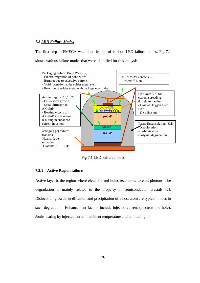
76
7.2 LED Failure Modes
The first step in FMECA was identification of various LED failure modes. Fig 7.1
shows various failure modes that were identified for this analysis.
Fig 7.1 LED Failure modes
7.2.1 Active Region failure
Active layer is the region where electrons and holes recombine to emit photons. The
degradation is mainly related to the property of semiconductor crystals [2].
Dislocation growth, in-diffusion and precipitation of a host atom are typical modes in
such degradation. Enhancement factors include injected current (electron and hole),
Joule heating by injected current, ambient temperature and emitted light.
AlGaInP
p-GaP
n-GaP
P - N Metal contacts [2]: - Interdiffusion
ITO layer [26] for current spreading & light extraction: - Loss of Oxygen from ITO - De-adhesion
Plastic Encapsulation [33]: - Discoloration - Carbonization - Polymer degradation
Packaging [2] failure: Heat sink - Heat sink de-lamination
Active Region [15,16,22]: - Dislocation growth - Metal diffusion in AlGaInP - Heating effects of AlGaInP active region resulting in enhanced current injection
Packaging failure: Bond Wires [2] - Electro-migration of bond wires - Burnout due to excessive current - Void formation at the solder metal stem - Reaction of solder metal with package electrodes
Photon Current
Diagram not to scale
77
7.2.2 P-N Contacts failure
Degraded contacts [2] generally correspond to p-side electrodes because ordinary
devices are composed of n-type substrates and the p-side electrodes exist near the
active region of the devices. For devices with a p-type substrate, the degradation is in
n-type electrode. The main mechanism is caused by metal diffusion in to the inner
region (outer diffusion of semiconductor material) and is enhanced by injected
current, joule heating and ambient temperature.
7.2.3 Indium Tin-Oxide failure
Indium Tin-Oxide layer is used for current spreading and improvement of light
extraction [26]. Failure modes are related to loss of oxygen from the ITO layer and
de-adhesion.
7.2.4 Plastic encapsulation failure
Plastic encapsulation (lens) is usually a polymer used to protect the LED chip from
external atmosphere and to direct the extracted light. Typical failure modes are
discoloration, carbonization and polymer degradation [33].
7.2.5 Packaging failures
Packaging failure is either related to Bond Wires or the Heat Sinks [2]. The bonding
part corresponds to the interface between an LED chip – heat sink and between heat
sink – package stem [2]. Usually some type of solder is used at the interface as a
bonding metal. The degradation is mainly caused by Electro-migration (transport of
metal atoms under high current stress) and is related to the properties of the solder
metal. The main mode is void formation through the migration of the solder metal
78
stem or reaction of solder metal with electrodes / the plated metal on the heat sink /
the stem. The migrated solder often shows a whisker growth. The factors that enhance
this type of degradation are current flow and ambient temperature. Heat sink
degradation is not degradation of the heat sink itself, but the separation of the metal
used for metallization of the heat sink. The generation of this degradation depends on
the heat sink material, the metal used for metallization and the metallization process.
The enhancement factor is not clear but ambient temperature and current flow are
estimated to be factors.
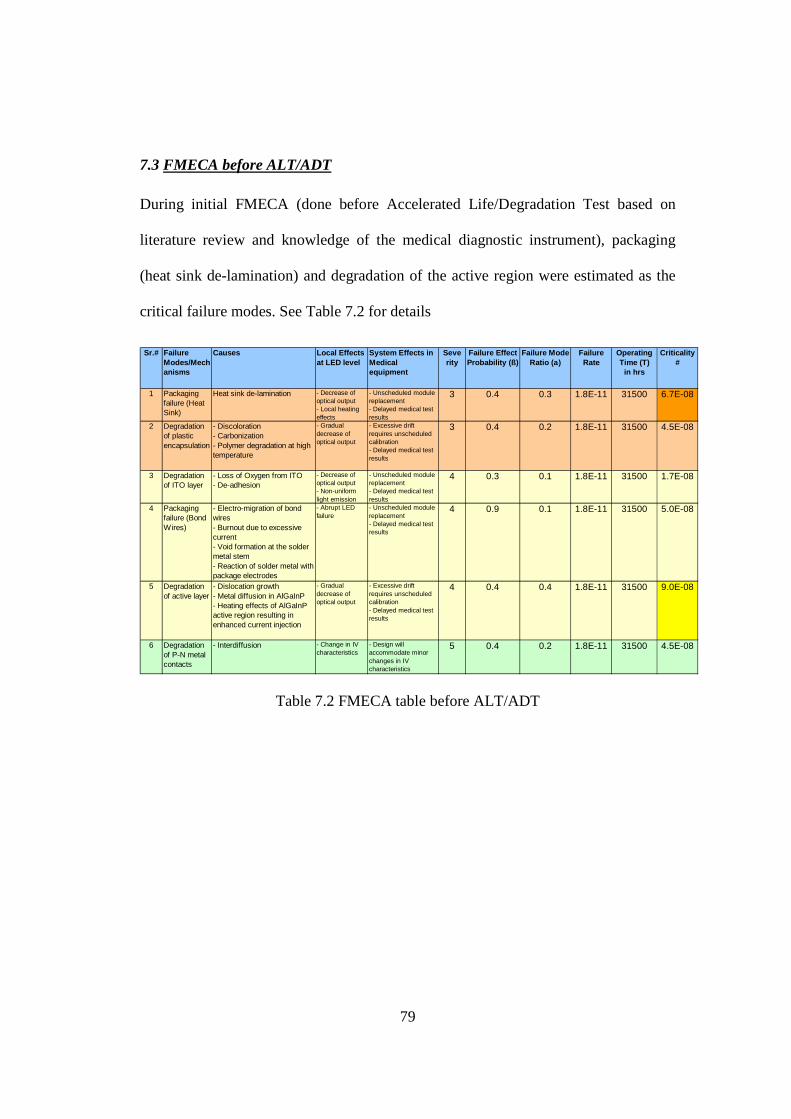
79
7.3 FMECA before ALT/ADT
During initial FMECA (done before Accelerated Life/Degradation Test based on
literature review and knowledge of the medical diagnostic instrument), packaging
(heat sink de-lamination) and degradation of the active region were estimated as the
critical failure modes. See Table 7.2 for details
Table 7.2 FMECA table before ALT/ADT
Sr.# Failure Modes/Mechanisms
Causes Local Effects at LED level
System Effects in Medical equipment
Severity
Failure Effect Probability (ß)
Failure Mode Ratio (a)
Failure Rate
Operating Time (T)
in hrs
Criticality #
1 Packaging failure (Heat Sink)
Heat sink de-lamination - Decrease of optical output- Local heating effects
- Unscheduled module replacement- Delayed medical test results
3 0.4 0.3 1.8E-11 31500 6.7E-08
2 Degradation of plastic encapsulation
- Discoloration- Carbonization- Polymer degradation at high temperature
- Gradual decrease of optical output
- Excessive drift requires unscheduled calibration- Delayed medical test results
3 0.4 0.2 1.8E-11 31500 4.5E-08
3 Degradation of ITO layer
- Loss of Oxygen from ITO- De-adhesion
- Decrease of optical output- Non-uniform light emission
- Unscheduled module replacement- Delayed medical test results
4 0.3 0.1 1.8E-11 31500 1.7E-08
4 Packaging failure (Bond Wires)
- Electro-migration of bond wires- Burnout due to excessive current- Void formation at the solder metal stem- Reaction of solder metal with package electrodes
- Abrupt LED failure
- Unscheduled module replacement- Delayed medical test results
4 0.9 0.1 1.8E-11 31500 5.0E-08
5 Degradation of active layer
- Dislocation growth- Metal diffusion in AlGaInP- Heating effects of AlGaInP active region resulting in enhanced current injection
- Gradual decrease of optical output
- Excessive drift requires unscheduled calibration- Delayed medical test results
4 0.4 0.4 1.8E-11 31500 9.0E-08
6 Degradation of P-N metal contacts
- Interdiffusion - Change in IV characteristics
- Design will accommodate minor changes in IV characteristics
5 0.4 0.2 1.8E-11 31500 4.5E-08
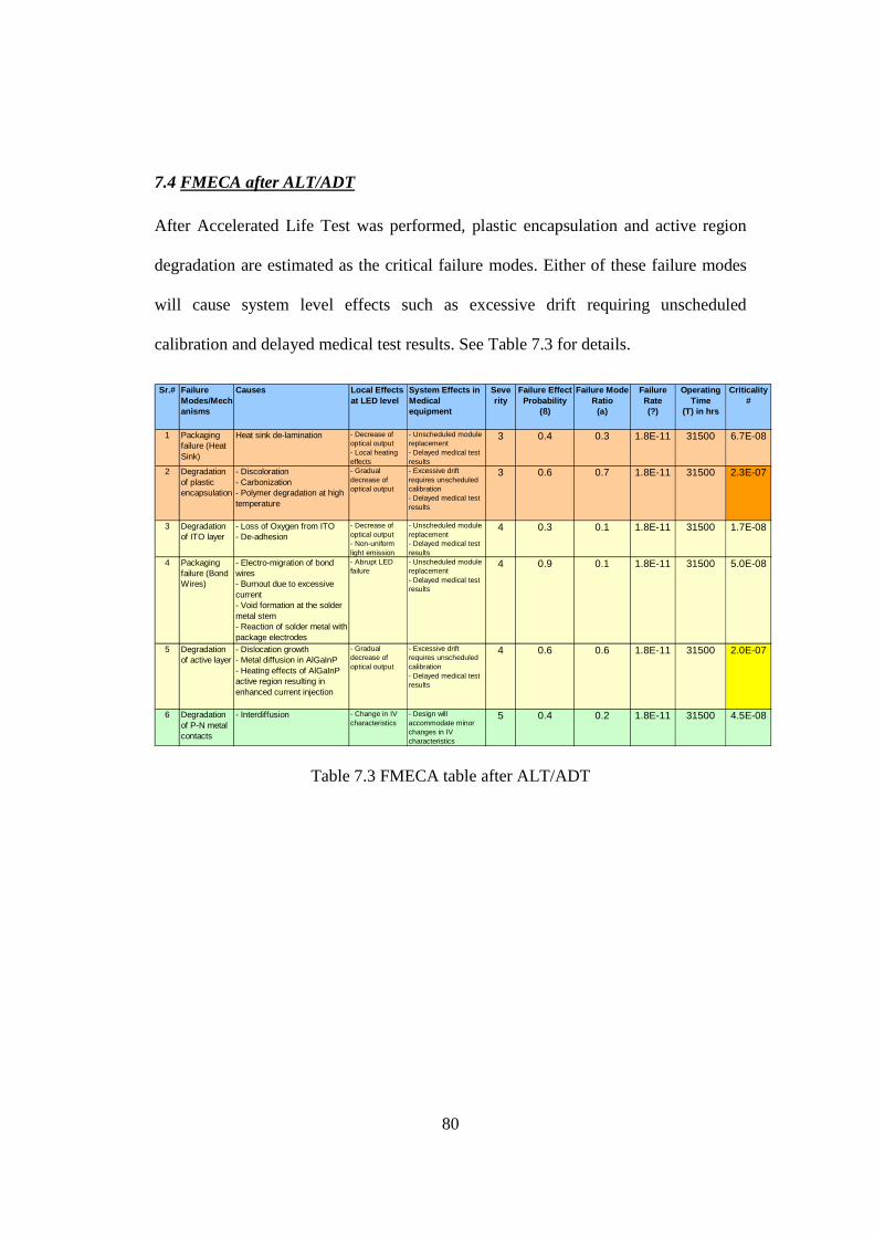
80
7.4 FMECA after ALT/ADT
After Accelerated Life Test was performed, plastic encapsulation and active region
degradation are estimated as the critical failure modes. Either of these failure modes
will cause system level effects such as excessive drift requiring unscheduled
calibration and delayed medical test results. See Table 7.3 for details.
Table 7.3 FMECA table after ALT/ADT
Sr.# Failure Modes/Mechanisms
Causes Local Effects at LED level
System Effects in Medical equipment
Severity
Failure Effect Probability
(ß)
Failure Mode Ratio
(a)
Failure Rate(?)
Operating Time
(T) in hrs
Criticality #
1 Packaging failure (Heat Sink)
Heat sink de-lamination - Decrease of optical output- Local heating effects
- Unscheduled module replacement- Delayed medical test results
3 0.4 0.3 1.8E-11 31500 6.7E-08
2 Degradation of plastic encapsulation
- Discoloration- Carbonization- Polymer degradation at high temperature
- Gradual decrease of optical output
- Excessive drift requires unscheduled calibration- Delayed medical test results
3 0.6 0.7 1.8E-11 31500 2.3E-07
3 Degradation of ITO layer
- Loss of Oxygen from ITO- De-adhesion
- Decrease of optical output- Non-uniform light emission
- Unscheduled module replacement- Delayed medical test results
4 0.3 0.1 1.8E-11 31500 1.7E-08
4 Packaging failure (Bond Wires)
- Electro-migration of bond wires- Burnout due to excessive current- Void formation at the solder metal stem- Reaction of solder metal with package electrodes
- Abrupt LED failure
- Unscheduled module replacement- Delayed medical test results
4 0.9 0.1 1.8E-11 31500 5.0E-08
5 Degradation of active layer
- Dislocation growth- Metal diffusion in AlGaInP- Heating effects of AlGaInP active region resulting in enhanced current injection
- Gradual decrease of optical output
- Excessive drift requires unscheduled calibration- Delayed medical test results
4 0.6 0.6 1.8E-11 31500 2.0E-07
6 Degradation of P-N metal contacts
- Interdiffusion - Change in IV characteristics
- Design will accommodate minor changes in IV characteristics
5 0.4 0.2 1.8E-11 31500 4.5E-08

81
7.5 Probabilistic Risk Assessment and Event Sequence Diagrams
Probabilistic Risk Assessment (PRA) starts with critical end states (ES). For the
medical diagnostic application, critical end states are
1. Correct Medical Test Results,
2. Correct but Delayed Medical Test Results,
3. Incorrect Medical Test Results but Detected before Reporting and
4. Erroneous but Believable Medical Test Results
Once the ES are defined, all possible Initiating Events (IE) are identified which could
create such ES. The propagation of an IE in to an ES is called a scenario. The
scenario is shown graphically in the form of an Event Sequence Diagram (ESD) in
Fig 7.2 below [4].
Fig 7.2 Scenario / Event Sequence Diagram [4]
A scenario contains an IE and one or more pivotal events leading to an end state. As
modeled in most PRAs, an IE is a perturbation (such as LED degradation) that
requires some kind of response from the Medical instrument (such as detection of the
LED degradation and correction using calibration). The Pivotal Events (PE) include
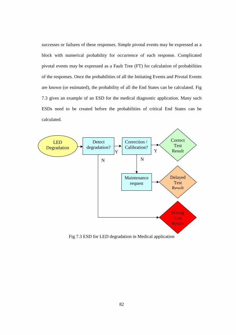
82
successes or failures of these responses. Simple pivotal events may be expressed as a
block with numerical probability for occurrence of each response. Complicated
pivotal events may be expressed as a Fault Tree (FT) for calculation of probabilities
of the responses. Once the probabilities of all the Initiating Events and Pivotal Events
are known (or estimated), the probability of all the End States can be calculated. Fig
7.3 gives an example of an ESD for the medical diagnostic application. Many such
ESDs need to be created before the probabilities of critical End States can be
calculated.
Fig 7.3 ESD for LED degradation in Medical application
Y Y
LED Degradation
Detect degradation?
Correction / Calibration?
Correct Test
Result
Delayed Test
Result
Maintenance request
Wrong Test
Result
N N
83
7.6 Conclusions
FMECA approach, widely used for risk analysis, has been successfully applied to
LED reliability and physics of failure investigation. In this study, we used FMECA to
understand the criticality of LED failure modes when used in a medical diagnostic
application. Failure modes of other components of the Medical device were not
included in this study. The FMECA was repeated and refined after conducting
accelerated life testing of LEDs. Degradation of the plastic encapsulation and the
active region were found to be the critical failure modes. These failures could cause
unscheduled calibration of the diagnostic instrument and would cause delay in patient
medical test results. Probabilistic Risk Assessment using Event Sequence Diagrams is
also briefly discussed. An example ESD describing LED degradation as an initiating
event and its progression towards critical end states is provided.
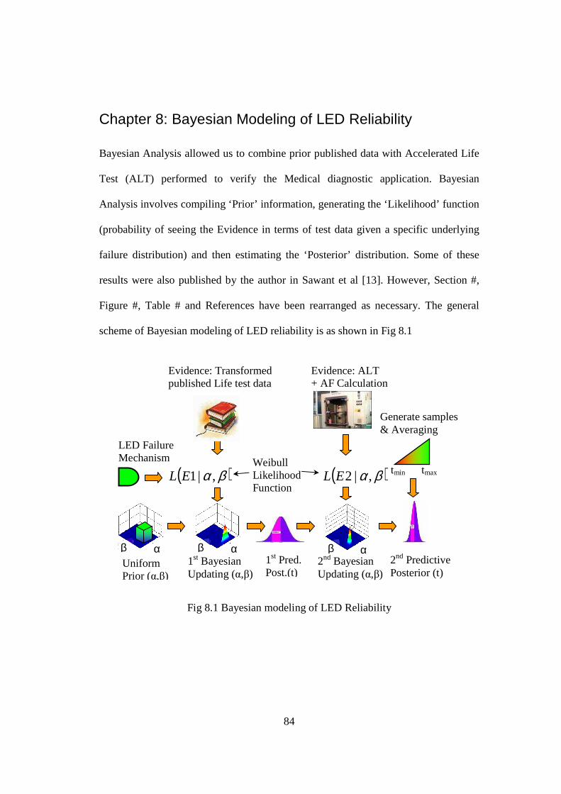
84
Chapter 8: Bayesian Modeling of LED Reliability
Bayesian Analysis allowed us to combine prior published data with Accelerated Life
Test (ALT) performed to verify the Medical diagnostic application. Bayesian
Analysis involves compiling ‘Prior’ information, generating the ‘Likelihood’ function
(probability of seeing the Evidence in terms of test data given a specific underlying
failure distribution) and then estimating the ‘Posterior’ distribution. Some of these
results were also published by the author in Sawant et al [13]. However, Section #,
Figure #, Table # and References have been rearranged as necessary. The general
scheme of Bayesian modeling of LED reliability is as shown in Fig 8.1
Fig 8.1 Bayesian modeling of LED Reliability
Generate samples & Averaging
Evidence: Transformed published Life test data
Uniform Prior (α,β)
LED Failure Mechanism
1st Bayesian Updating (α,β)
2nd Bayesian Updating (α,β)
2nd Predictive Posterior (t)
Weibull Likelihood Function
Evidence: ALT + AF Calculation
α β α β 1st Pred. Post.(t)
α β
tmin tmax ( )βα ,|1EL ( )βα ,|2EL
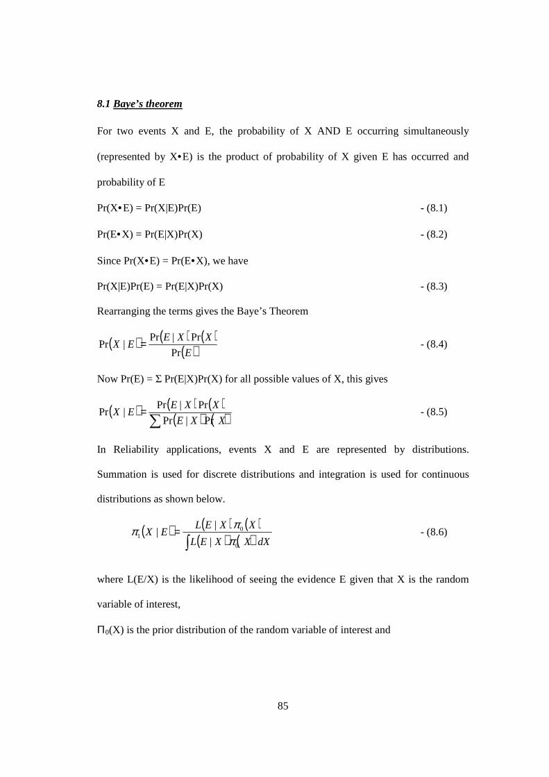
85
8.1 Baye’s theorem
For two events X and E, the probability of X AND E occurring simultaneously
(represented by X•E) is the product of probability of X given E has occurred and
probability of E
Pr(X•E) = Pr(X|E)Pr(E) - (8.1)
Pr(E•X) = Pr(E|X)Pr(X) - (8.2)
Since Pr(X•E) = Pr(E•X), we have
Pr(X|E)Pr(E) = Pr(E|X)Pr(X) - (8.3)
Rearranging the terms gives the Baye’s Theorem
( ) ( ) ( )( )E
XXEEX
Pr
Pr|Pr|Pr = - (8.4)
Now Pr(E) = Σ Pr(E|X)Pr(X) for all possible values of X, this gives
( ) ( ) ( )( ) ( )∑
=XXE
XXEEX
Pr|Pr
Pr|Pr|Pr - (8.5)
In Reliability applications, events X and E are represented by distributions.
Summation is used for discrete distributions and integration is used for continuous
distributions as shown below.
( ) ( ) ( )( ) ( )∫
=dXXXEL
XXELEX
0
01
|
||
πππ - (8.6)
where L(E/X) is the likelihood of seeing the evidence E given that X is the random
variable of interest,
Π0(X) is the prior distribution of the random variable of interest and
86
Π1(X/E) is the posterior distribution of the random variable of interest given that
evidence E was observed.
8.2 Bayesian Modeling of LED data
Many of the LED degradation mechanisms occur simultaneously. The weakest link
causes the actual failure. This leads us to believe that Weibull distribution (with
parameters α & β) is the most suitable distribution for time to failure of the LEDs.
Levada et al. [34] carried out accelerated life tests on plastic transparent
encapsulation and pure metallic package GaN LEDs. A consistent Weibull based
statistical model was found for MTTF. When the data from ALT performed in this
research was analyzed, it revealed that Weibull is a slightly better fit compared to the
Lognormal fit. Thus the degradation mechanism, published literature and our ALT
data all point to Weibull as a most suitable model for this data analysis. See section
10.3.1 for a detailed discussion on the subject.
For the first posterior, using Uniform Prior distribution for α & β is a good choice.
Since only MTTF values were available, min-max values for α & β were estimated
using engineering judgment. Test data was used as Evidence and a joint α-β posterior
distribution was calculated using Bayesian updating. This joint α-β distribution gave a
series of Weibull time to failure distributions. The predictive posterior failure
distribution for the LEDs was estimated by averaging over the range of α-β values.
Numerical techniques were used for various computations.
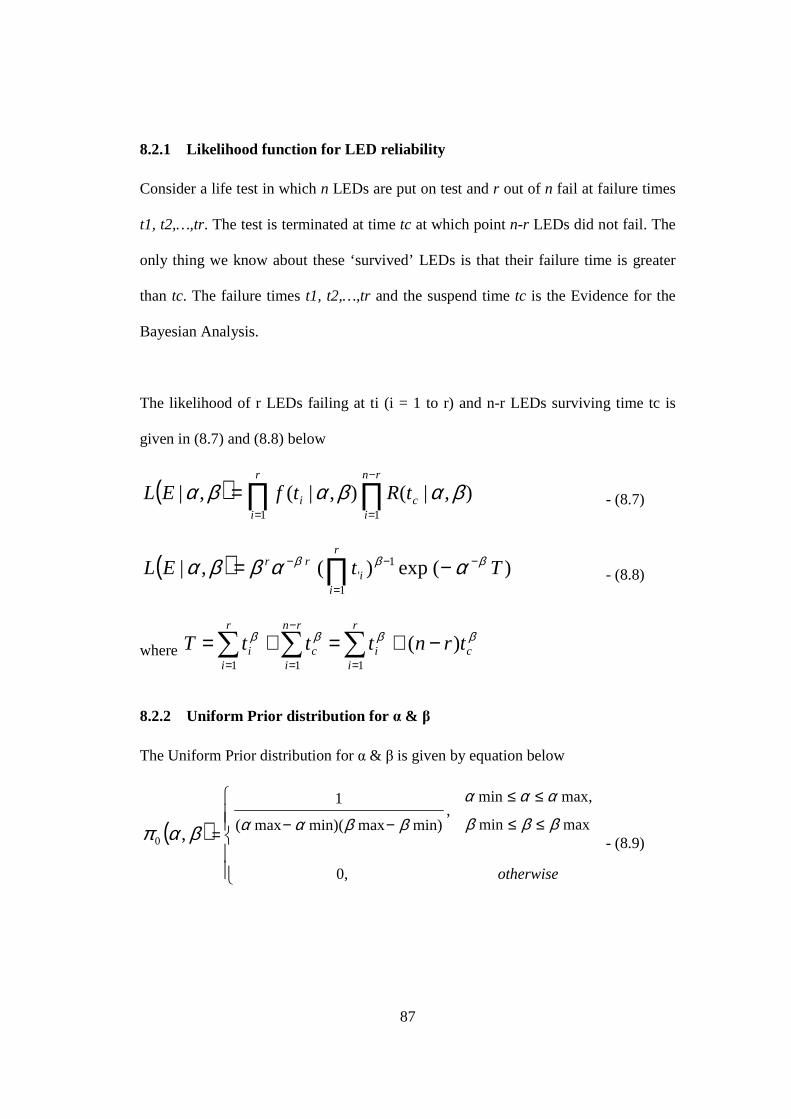
87
8.2.1 Likelihood function for LED reliability
Consider a life test in which n LEDs are put on test and r out of n fail at failure times
t1, t2,…,tr. The test is terminated at time tc at which point n-r LEDs did not fail. The
only thing we know about these ‘survived’ LEDs is that their failure time is greater
than tc. The failure times t1, t2,…,tr and the suspend time tc is the Evidence for the
Bayesian Analysis.
The likelihood of r LEDs failing at ti (i = 1 to r) and n-r LEDs surviving time tc is
given in (8.7) and (8.8) below
( ) ∏∏−
==
=rn
ic
r
ii tRtfEL
11
),|(),|( ,| βαβαβα - (8.7)
( ) )(exp)( ,|1
1' TtEL
r
ii
rr βββ ααββα −
=
−− −= ∏ - (8.8)
where ββββc
r
ii
rn
ic
r
ii trntttT )(
111
−+=+= ∑∑∑=
−
==
8.2.2 Uniform Prior distribution for α & β
The Uniform Prior distribution for α & β is given by equation below
( )
≤≤
≤≤
−−=
otherwise,0
maxmin
max,min,
min)maxmin)(max(
1
,0βββ
ααα
ββααβαπ - (8.9)
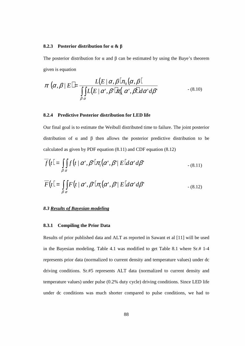
88
8.2.3 Posterior distribution for α & β
The posterior distribution for α and β can be estimated by using the Baye’s theorem
given is equation
( ) ( ) ( )( ) ( )∫ ∫
=
β α
βαβαπβαβαπβαβαπ
''','','|
,,||,
0
0
ddEL
ELE
- (8.10)
8.2.4 Predictive Posterior distribution for LED life
Our final goal is to estimate the Weibull distributed time to failure. The joint posterior
distribution of α and β then allows the posterior predictive distribution to be
calculated as given by PDF equation (8.11) and CDF equation (8.12)
( ) ( ) ( )∫ ∫=β α
βαβαπβα ''|','','| 1 ddEtftf - (8.11)
( ) ( ) ( )∫ ∫=β α
βαβαπβα ''|','','| 1 ddEtFtF - (8.12)
8.3 Results of Bayesian modeling
8.3.1 Compiling the Prior Data
Results of prior published data and ALT as reported in Sawant et al [11] will be used
in the Bayesian modeling. Table 4.1 was modified to get Table 8.1 where Sr.# 1-4
represents prior data (normalized to current density and temperature values) under dc
driving conditions. Sr.#5 represents ALT data (normalized to current density and
temperature values) under pulse (0.2% duty cycle) driving conditions. Since LED life
under dc conditions was much shorter compared to pulse conditions, we had to
89
transform Sr#.1-4 data in to Sr.#:1A-4A to allow using in our Bayesian model. This
also seems reasonable from the fact that during pulse driving, the LED gets time to
cool off. This increases the time to failure of the LEDs during pulse driving compared
to DC driving. The exact method of transformation will be covered in chapter 9. For
now, a simple multiplier of 500 is assumed (1 hr at 100% duty cycle is equivalent to
500hrs at 0.2% duty cycle).
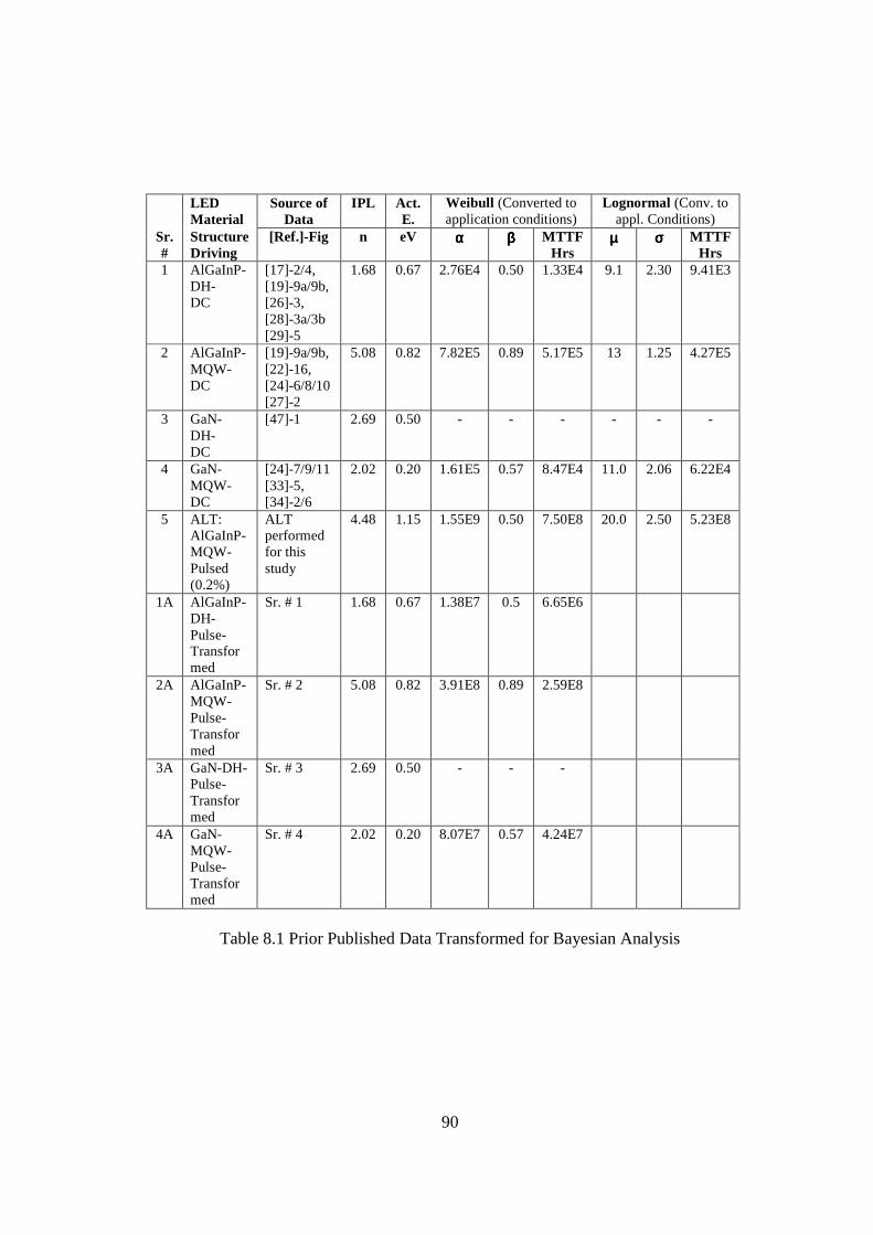
90
LED Material
Source of Data
IPL Act. E.
Weibull (Converted to application conditions)
Lognormal (Conv. to appl. Conditions)
Sr.#
Structure Driving
[Ref.]-Fig n eV αααα ββββ MTTF Hrs
µµµµ σσσσ MTTF Hrs
1 AlGaInP-DH- DC
[17]-2/4, [19]-9a/9b, [26]-3, [28]-3a/3b [29]-5
1.68 0.67 2.76E4 0.50 1.33E4 9.1 2.30 9.41E3
2 AlGaInP-MQW- DC
[19]-9a/9b, [22]-16, [24]-6/8/10 [27]-2
5.08 0.82 7.82E5 0.89 5.17E5 13 1.25 4.27E5
3 GaN- DH- DC
[47]-1 2.69 0.50 - - - - - -
4 GaN- MQW- DC
[24]-7/9/11 [33]-5, [34]-2/6
2.02 0.20 1.61E5 0.57 8.47E4 11.0 2.06 6.22E4
5 ALT: AlGaInP- MQW- Pulsed (0.2%)
ALT performed for this study
4.48 1.15 1.55E9 0.50 7.50E8 20.0 2.50 5.23E8
1A AlGaInP-DH-Pulse-Transformed
Sr. # 1 1.68 0.67 1.38E7 0.5 6.65E6
2A AlGaInP-MQW-Pulse-Transformed
Sr. # 2 5.08 0.82 3.91E8 0.89 2.59E8
3A GaN-DH- Pulse-Transformed
Sr. # 3 2.69 0.50 - - -
4A GaN-MQW- Pulse-Transformed
Sr. # 4 2.02 0.20 8.07E7 0.57 4.24E7
Table 8.1 Prior Published Data Transformed for Bayesian Analysis
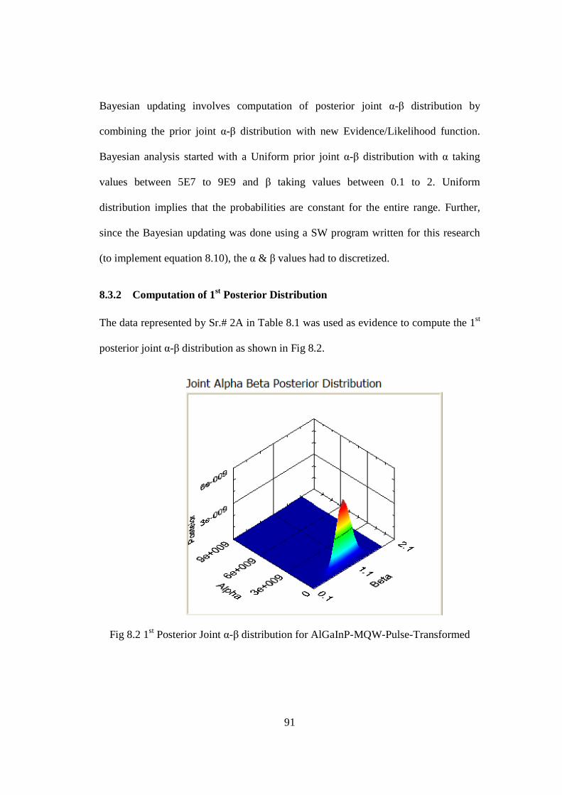
91
Bayesian updating involves computation of posterior joint α-β distribution by
combining the prior joint α-β distribution with new Evidence/Likelihood function.
Bayesian analysis started with a Uniform prior joint α-β distribution with α taking
values between 5E7 to 9E9 and β taking values between 0.1 to 2. Uniform
distribution implies that the probabilities are constant for the entire range. Further,
since the Bayesian updating was done using a SW program written for this research
(to implement equation 8.10), the α & β values had to discretized.
8.3.2 Computation of 1st Posterior Distribution
The data represented by Sr.# 2A in Table 8.1 was used as evidence to compute the 1st
posterior joint α-β distribution as shown in Fig 8.2.
Fig 8.2 1st Posterior Joint α-β distribution for AlGaInP-MQW-Pulse-Transformed
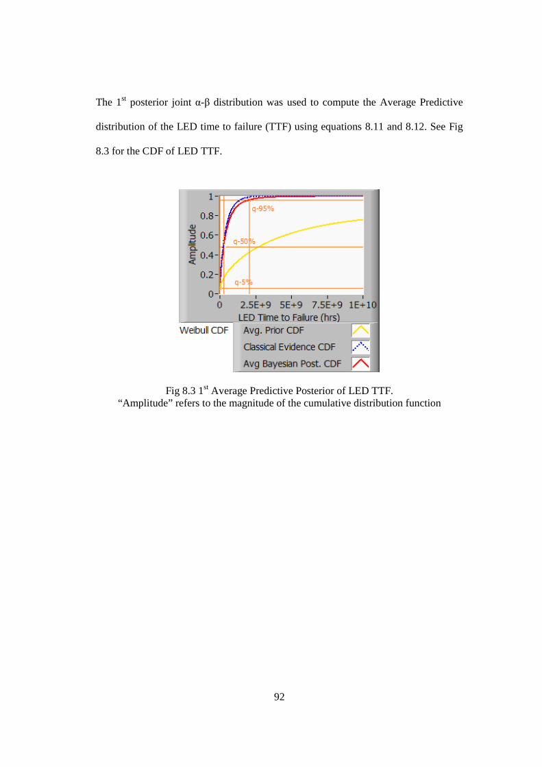
92
The 1st posterior joint α-β distribution was used to compute the Average Predictive
distribution of the LED time to failure (TTF) using equations 8.11 and 8.12. See Fig
8.3 for the CDF of LED TTF.
Fig 8.3 1st Average Predictive Posterior of LED TTF.
“Amplitude” refers to the magnitude of the cumulative distribution function
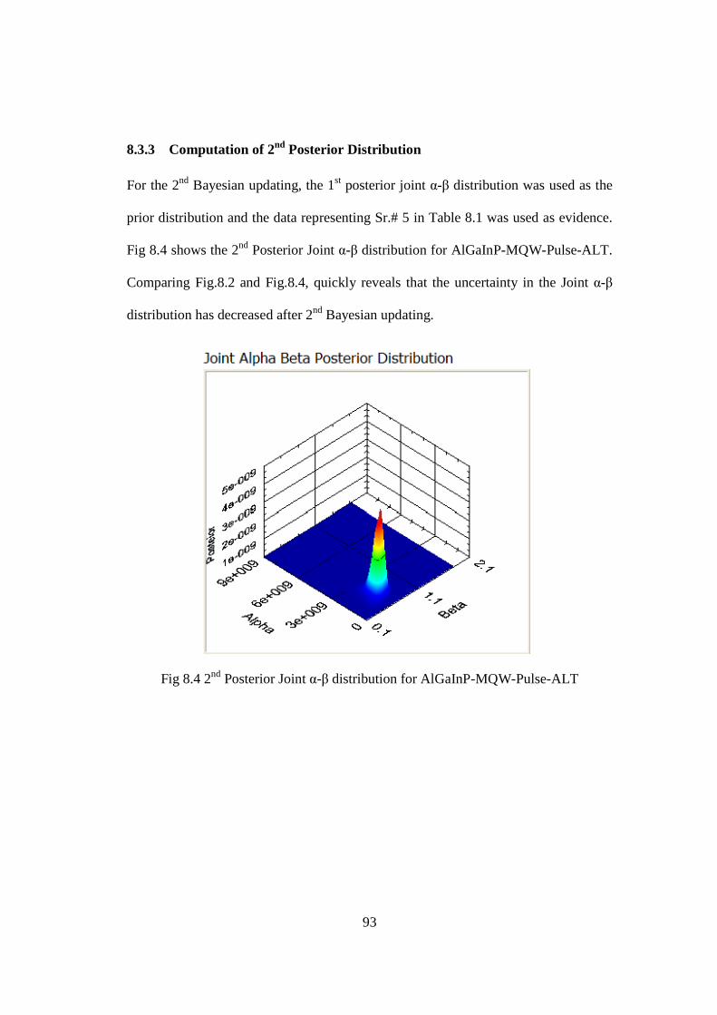
93
8.3.3 Computation of 2nd Posterior Distribution
For the 2nd Bayesian updating, the 1st posterior joint α-β distribution was used as the
prior distribution and the data representing Sr.# 5 in Table 8.1 was used as evidence.
Fig 8.4 shows the 2nd Posterior Joint α-β distribution for AlGaInP-MQW-Pulse-ALT.
Comparing Fig.8.2 and Fig.8.4, quickly reveals that the uncertainty in the Joint α-β
distribution has decreased after 2nd Bayesian updating.
Fig 8.4 2nd Posterior Joint α-β distribution for AlGaInP-MQW-Pulse-ALT
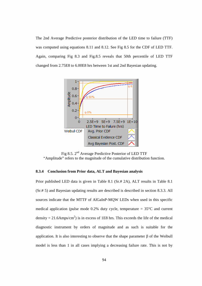
94
The 2nd Average Predictive posterior distribution of the LED time to failure (TTF)
was computed using equations 8.11 and 8.12. See Fig 8.5 for the CDF of LED TTF.
Again, comparing Fig 8.3 and Fig.8.5 reveals that 50th percentile of LED TTF
changed from 2.75E8 to 6.00E8 hrs between 1st and 2nd Bayesian updating.
Fig 8.5. 2nd Average Predictive Posterior of LED TTF
“Amplitude” refers to the magnitude of the cumulative distribution function.
8.3.4 Conclusion from Prior data, ALT and Bayesian analysis
Prior published LED data is given in Table 8.1 (Sr.# 2A), ALT results in Table 8.1
(Sr.# 5) and Bayesian updating results are described is described in section 8.3.3. All
sources indicate that the MTTF of AlGaInP-MQW LEDs when used in this specific
medical application (pulse mode 0.2% duty cycle, temperature = 35°C and current
density = 21.6Amps/cm2) is in excess of 1E8 hrs. This exceeds the life of the medical
diagnostic instrument by orders of magnitude and as such is suitable for the
application. It is also interesting to observe that the shape parameter β of the Weibull
model is less than 1 in all cases implying a decreasing failure rate. This is not by

95
coincidence. In section 5.4.1, we had observed during ALT that the rate of optical
output degradation is logarithmic and that this rate varies significantly between
different LEDs (even if taken from same manufacturing batch). Some LEDs cross the
20% degradation (failure threshold for this application) earlier than others. For LEDs
that do survive this initial high rate of optical degradation, the probability that it will
survive longer increases. This explains the decreasing failure rate.
96
Chapter 9: Degree of Relevance in Bayesian modeling
Chapter 8 treats Bayesian modeling of LEDs for a medical diagnostic application. It
allowed us to combine prior available data with accelerated life test data to predict the
reliability (time to failure) of the AlGaInP LEDs. That is the main approach adopted
in this dissertation and has been published in Sawant et al [13]. In this chapter, an
alternate method for performing Bayesian modeling of LED reliability is proposed.
This is additional work that has not been published by the author yet. This approach
may also be used in other applications of Bayesian analysis.
9.1 The Problem: Partially relevant prior data
LED families are made from different material systems such as AlGaInP, GaN, GaAs
etc. Further, LEDs are manufactured using different semiconductor structures such as
Double Heterostructure (DH) and Multi Quantum Well (MQW). Depending upon the
application, LEDs may be driven in a DC mode (typically lighting or indicator
applications), Pulse mode with high duty cycle (Fiber optic applications) or Pulse
mode with very low duty cycle (our current medical diagnostic application). From
Table 8.1, it is obvious that the time to failure of the LED is significantly different
based on the material, structure and the driving strategy.
Bayesian modeling computes the LED reliability by combining prior published LED
data with the current test data (such as life test to mimic the current application).
While ample prior published LED data is available, it is very difficult to get prior data
for the exact same material system, structure and driving strategy. Limited prior data
97
forces us to take two approaches. Either assume that the prior data is non-informative
(such as using a uniform probability distribution function) or use prior data from a
different LED material family, structure or driving strategy. Using non-informative
prior distribution pretty much defeats the purpose of Bayesian modeling unless
additional and successive Bayesian updating is used. Using prior data, which is not
directly relevant to the medical application, will cause over estimation or under
estimation of the LED reliability. This is a practical problem that applies to any
application of Bayesian modeling.
9.2 The Solution: A Three Step Process
One approach to solving the above problem is using prior data for LEDs, which are
similar but not identical to LEDs in the current application. It will be a 3-step process.
9.2.1 Step-1: Transform DC data to Pulse data by Multiplication
In Chapter 8, we transformed the prior data available for AlGaInP-MQW-DC in to
AlGaInP-MQW-Pulse by multiplying it by a factor of 500. The rationale used was 1
hr at 100% duty cycle (i.e. DC) is equivalent to 500hrs at 0.2% duty cycle (medical
application). While this is a good number to start with, an alternate approach to
calculate the multiplier is to take a ratio of MTTF of Pulse testing to DC testing.
Ratio of Weibull mean of AlGaInP-MQW-Pulse (from normalized ALT) to AlGaInP-
MQW-DC (prior published) was used in this research. This computation
(7.50E8/5.17E5) yields a multiplier of 1451. Both of these multipliers (500 and 1451)
will be used in subsequent analysis in the following sections. Analysis of prior
published data for LED life gave us a set of data consisting of time to failure
98
Set1=AlGaInP-DH-DC, AlGaInP-MQW-DC, GaN-MQW-DC - (9.3)
GaN-DH-DC was ignored since limited data was available.
By using the two multipliers (500 and 1451), we go two additional data sets
Set2=AlGaInP-DH-DCx500, AlGaInP-MQW-DCx500, GaN-MQW-DCx500
- (9.4)
Set3=AlGaInP-DH-DCx1451, AlGaInP-MQW-DCx1451, GaN-MQW-DCx1451
- (9.5)
See Appendix 7 for Set1, Set2 and Set3 data.
9.2.2 Step-2: Use a Degree of Relevance Parameter R
A new parameter called degree of relevance ‘R’ is introduced which takes values
between zero and one. The ‘R’ value will be used to modify the Bayesian model such
that the influence of evidence is decreased as R approaches zero. The parameter ‘R’
can be estimated by engineering judgment and physics of semiconductor structures.
Hypothetical values of ‘R’ based on LED material and structure will be used in this
research to perform the analysis. Methods of estimating ‘R’ such as use of utility
functions are left for future research and are briefly discussed in section 11.4.2.
9.2.3 Step-3: Changing the Likelihood function using R
In Bayesian modeling, the Likelihood function is generated from Evidence. One
approach to using R in Bayesian modeling is changing the likelihood function as a
function of R and then performing the Bayesian updating as shown below.
99
( ) ( ) ( )( ) ( )∫ ∫
=
β α
βαβαπβαβαπβαβαπ
''',']','|[
,],|[|,
0
0
ddEL
ELE
R
R
- (9.6)
If R is 1, it becomes a standard Bayesian updating equation. As R approaches 0, the
influence of likelihood function decreases. If R is 0, the posterior distribution
becomes identical to prior distribution.
9.3 Results and Discussion
As described in section 8.2, Bayesian analysis started with a Uniform prior joint α-β
distribution with α taking values between 5E7 to 9E9 and β taking values between 0.1
to 2. The DC data transformed to Pulse in Set2 (DCx500) and Set3 (DCx1451) was
used as Evidence for the 1st Bayesian updating shown in Fig 8.1. The 2nd Bayesian
updating is done using ALT data as evidence. Predictive Posterior distributions for
LED TTF were computed using the SW developed (described in Appendix 6).
The results are described in Table 9.1 below. Sr. #1a and 1b used AlGaInP-MQW-
DCx500 data as 1st Evidence. The only difference is 1b used an R-value of 0.75. Sr.
#2 used AlGaInP-MQW-DCx1451 data as 1st Evidence. In this case, R-value
assessed is already equal to 1. Hence there was no need to perform a separate
analysis. Sr.#3a and 3b used GaN-MQW-DCx500 data as 1st Evidence. The only
difference is 3b used an R-value of 0.50. Sr. #4a and 4b used GaN-MQW-DCx1451
data as 1st Evidence. The only difference is 4b used an R-value of 0.75. Sr.#5a and 5b
used AlGaInP-DH-DCx500 data as 1st Evidence. The only difference is 5b used an
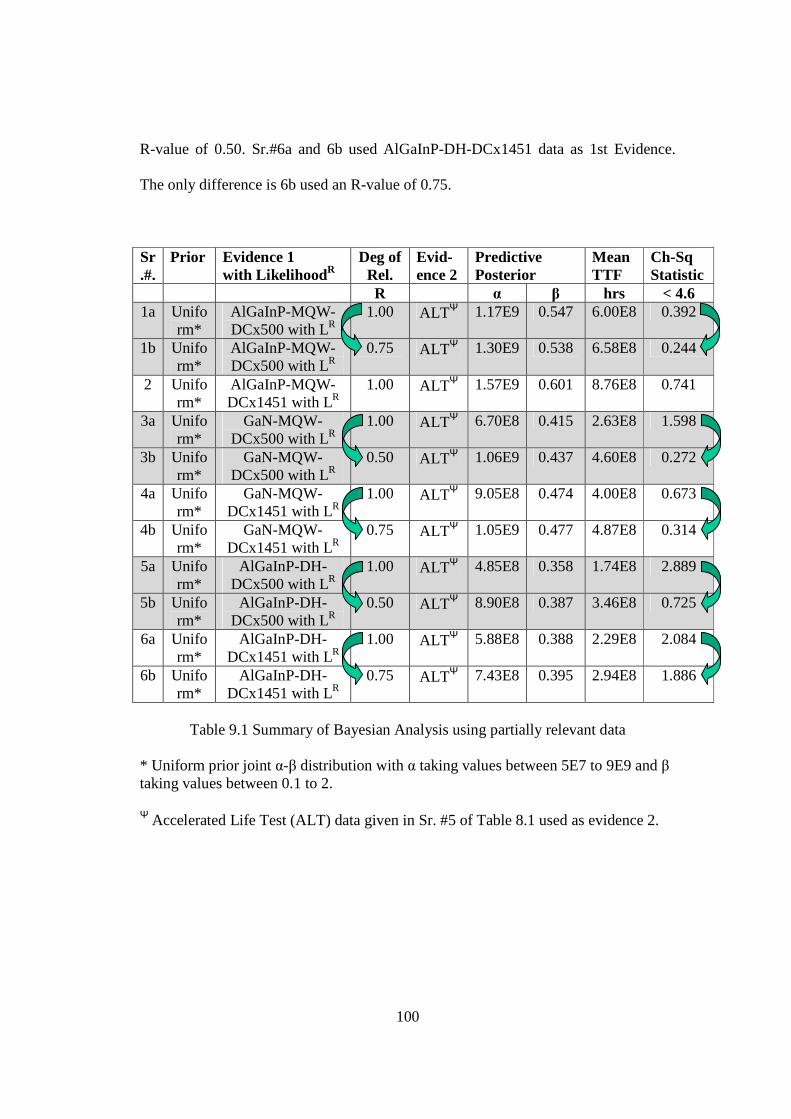
100
R-value of 0.50. Sr.#6a and 6b used AlGaInP-DH-DCx1451 data as 1st Evidence.
The only difference is 6b used an R-value of 0.75.
Sr.#.
Prior Evidence 1 with Likelihood R
Deg of Rel.
Evid-ence 2
Predictive Posterior
Mean TTF
Ch-Sq Statistic
R α β hrs < 4.6 1a Unifo
rm* AlGaInP-MQW-DCx500 with LR
1.00 ALTΨ 1.17E9 0.547 6.00E8 0.392
1b Uniform*
AlGaInP-MQW-DCx500 with LR
0.75 ALTΨ 1.30E9 0.538 6.58E8 0.244
2 Uniform*
AlGaInP-MQW-DCx1451 with LR
1.00 ALTΨ 1.57E9 0.601 8.76E8 0.741
3a Uniform*
GaN-MQW-DCx500 with LR
1.00 ALTΨ 6.70E8 0.415 2.63E8 1.598
3b Uniform*
GaN-MQW-DCx500 with LR
0.50 ALTΨ 1.06E9 0.437 4.60E8 0.272
4a Uniform*
GaN-MQW-DCx1451 with LR
1.00 ALTΨ 9.05E8 0.474 4.00E8 0.673
4b Uniform*
GaN-MQW-DCx1451 with LR
0.75 ALTΨ 1.05E9 0.477 4.87E8 0.314
5a Uniform*
AlGaInP-DH-DCx500 with LR
1.00 ALTΨ 4.85E8 0.358 1.74E8 2.889
5b Uniform*
AlGaInP-DH-DCx500 with LR
0.50 ALTΨ 8.90E8 0.387 3.46E8 0.725
6a Uniform*
AlGaInP-DH-DCx1451 with LR
1.00 ALTΨ 5.88E8 0.388 2.29E8 2.084
6b Uniform*
AlGaInP-DH-DCx1451 with LR
0.75 ALTΨ 7.43E8 0.395 2.94E8 1.886
Table 9.1 Summary of Bayesian Analysis using partially relevant data
* Uniform prior joint α-β distribution with α taking values between 5E7 to 9E9 and β taking values between 0.1 to 2. Ψ Accelerated Life Test (ALT) data given in Sr. #5 of Table 8.1 used as evidence 2.
101
9.4 Conclusions
LED families are made from different material systems (AlGaInP, GaN, GaAs etc.)
and are manufactured using different semiconductor structures such as Double
Heterostructure (DH) and Multi Quantum Well (MQW). Further, they may be driven
in pulse mode or DC mode. The time to failure of the LED is significantly different
based on the material, structure and the driving strategy. While ample prior published
LED data is available, it is very difficult to get prior data for the exact same material
system, structure and driving duty cycle. Using prior data, which is not directly
relevant to the application, will cause over estimation or under estimation of the LED
reliability. A 3-step solution is proposed which includes using a multiplier to convert
from DC to pulse data, estimating the degree of relevance parameter R (engineering
judgment and physics of semiconductor structures) and then modifying the
Likelihood function in the Bayesian model with R. The results are presented in Table
9.1.
All the posterior predictive results in section 9.3 pass the Chi-square statistic test
(described in detail in chapter 10). This test was used to determine how closely the
ALT data represents the predictive Posterior PDF of LED TTF. It was interesting to
observe that the Chi-square value was lower in all the 5 cases when R was
appropriately chosen (compared to R=1). Since a lower value implies a better fit, the
least we can say is that use of R produced better results in this application.
102
Chapter 10: Bayesian Parameter Selection and Model
Validation
10.1 Bayesian Subjectivity
While the Baye’s theorem itself has a sound statistical background, assumptions made
in the prior knowledge and in the underlying distribution bring in subjectivity in
Bayesian modeling. The subjective nature of the prior distribution (which could be
based on relatively sparse expert opinion) may raise doubts about the accuracy of
Bayesian posterior distributions. In the current research, Uniform prior distribution
was used for α and β of the Weibull model. However, the limits for α and β in the
uniform distribution had to be assumed. Further, prior published data transformed to
application conditions was used as Evidence in the 1st Bayesian updating. Errors in
assumptions made at the start of Bayesian analysis can result in the posterior
distribution being a poor representation of the data. Accordingly, the posterior
predictive distribution needs to be subject to some sort of validation [8].
10.2 Validation approach
Work by Mosleh et al [8] has been relied upon for formulating the validation
approach in this dissertation. In statistical analysis, a model is often used to represent
data. Since the entire population data is rarely available, the model is generally
developed based on a small sample data (extracted randomly out of the population).
Deviations between actual data and a model that describes the data well are subject to
the Chi-Square distribution. This is based on the assumption that any deviations in
103
observed data from the expected value predicted by the underlying distribution are
normally distributed. This assumption is generally sound, as many errors in
observation are resultant from the summation of many other random variables, and
hence are subject to the central limit theorem. By inference, if these variations are
described by the Chi-Square distribution, then the model being tested is most likely a
good one. The Bayesian Chi-Square statistic is a single measure that quantifies how
well the posterior predictive distribution agrees with the data [8].
To calculate the Chi-Square statistic, the x – axis (for the random variable) is divided
into K distinct intervals that contain at least 5 data points each from the sample. The
number of data points in each interval I j is written as bj (j = 1 , 2, … , k). The intervals
do not need to be of equal width. Then, with the model distribution being tested, the
number of expected data occurrences in each interval is calculated:
ej = n pj - (10.1)
where ej is the expected number of occurrences of data in interval I j, n is the sample
size and ( )∫=jI
j dxxfp θ|1
The Bayesian Chi-Square statistic is then defined as
( ) 2
11
220 ~ −
=∑
−= k
k
j j
jj
e
ebχχ - (10.2)
This value summarizes the magnitude of natural variations between observed data
and the model being tested. Note that the expected value is used in the denominator in
place of the variance in the definition of the Chi-Square random variable. This is
because we do not know the variance of the data from model expected values. To

104
accommodate this lack of knowledge, we reduce the number of degrees of freedom
by 1, so the Chi-Square statistic above should be described by the Chi-Square
distribution with k – 1 degrees of freedom.
For model validation, a ‘significance level’ is introduced. The significance level, α
(unrelated to the scale parameter of the Weibull distribution which uses the same
symbol), is defined as the probability of data analysis returning a result at most as
extreme as the calculated value for which the decision maker is willing to accept the
null hypothesis. Generally, α is in the range of 1 – 10 %. One way of hypothesis
testing is to calculate the upper limit ‘c’ of the Chi-Square statistic based on the
significance level.
i.e. ( ) αχ −=≤− 1Pr 21 cK - (10.3)
This means that if the Chi-Square statistic exceeds c, then the null hypothesis is
rejected.
10.3 Validation phases in Bayesian modeling
Validation of Bayesian modeling occurs in various phases. These are
1. Selection of the distribution for the underlying failure distribution,
2. Suitability of the prior information and
3. Appropriateness of predictive posterior distribution against the test data.
10.3.1 Selection of underlying failure distribution
Many of the LED degradation mechanisms occur the same test parameter range. The
dominant failure mechanism leads to failure. This leads us to believe that Weibull
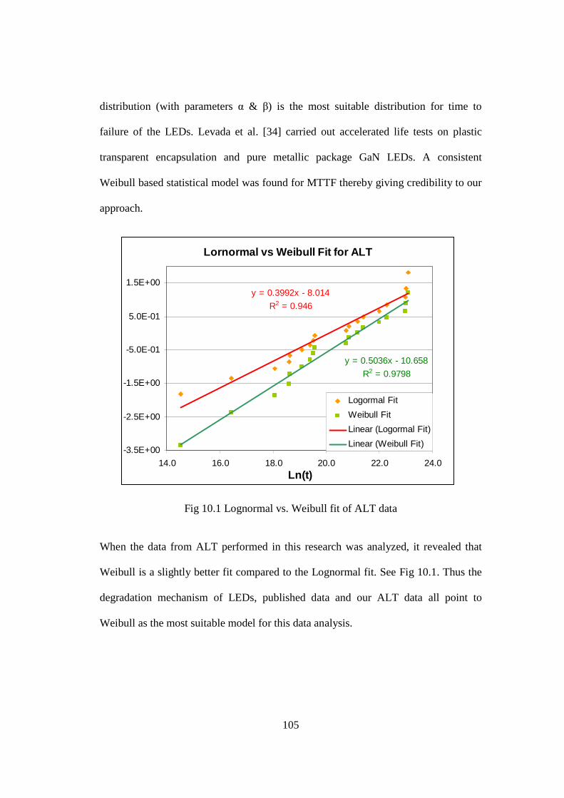
105
distribution (with parameters α & β) is the most suitable distribution for time to
failure of the LEDs. Levada et al. [34] carried out accelerated life tests on plastic
transparent encapsulation and pure metallic package GaN LEDs. A consistent
Weibull based statistical model was found for MTTF thereby giving credibility to our
approach.
Fig 10.1 Lognormal vs. Weibull fit of ALT data
When the data from ALT performed in this research was analyzed, it revealed that
Weibull is a slightly better fit compared to the Lognormal fit. See Fig 10.1. Thus the
degradation mechanism of LEDs, published data and our ALT data all point to
Weibull as the most suitable model for this data analysis.
Lornormal vs Weibull Fit for ALT
y = 0.3992x - 8.014
R2 = 0.946
y = 0.5036x - 10.658
R2 = 0.9798
-3.5E+00
-2.5E+00
-1.5E+00
-5.0E-01
5.0E-01
1.5E+00
14.0 16.0 18.0 20.0 22.0 24.0Ln(t)
Logormal Fit
Weibull Fit
Linear (Logormal Fit)
Linear (Weibull Fit)

106
10.3.2 Selection and verification of prior distribution
Uniform distribution was used as prior knowledge of parameters α and β of the
Weibull model. The limits for α and β in the uniform distribution were selected such
that they encompass the prior published data and the normalized life test data. In
order to verify that the limits were selected correctly, an additional calculation was
performed with the upper limits of α and β widened. See Table 10.1 and Fig 10.2.
There was no difference in the predictive posterior CDF for LED time to failure. α
stayed the same at 1.35E9. β changed slightly from 0.809 to 0.808. This proves that
the limits on α and β in the uniform distribution were correctly chosen.
Property Used limits for prior of α and β Wider limits for prior of α and β Samples 1 to 1E10, Total 800 1 to 1E10, Total 800 Prior Uniform Uniform Alpha 5E7 to 9E9, Incr 5E6 5E6 to 9E10, Incr 5E6 Beta 0.1 to 2, Incr 0.1 0.1 to 4, Incr 0.1 Evidence Source
AlGaInP-MQW-DCx1451 AlGaInP-MQW-DCx1451
Evidence data
n=11, r=11, tc=4.829E+9 n=11, r=11, tc=4.829E+9
Alpha 1.13E+9 1.13E+9 Beta 0.89 0.89 Predictive Posterior
Alpha 1.35E+09 1.35E+09 Beta 0.809 0.808
Table 10.1 Used vs. wider limits on prior of α and β
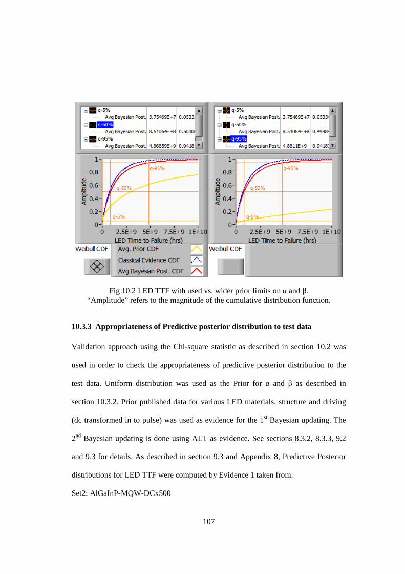
107
Fig 10.2 LED TTF with used vs. wider prior limits on α and β.
“Amplitude” refers to the magnitude of the cumulative distribution function.
10.3.3 Appropriateness of Predictive posterior distribution to test data
Validation approach using the Chi-square statistic as described in section 10.2 was
used in order to check the appropriateness of predictive posterior distribution to the
test data. Uniform distribution was used as the Prior for α and β as described in
section 10.3.2. Prior published data for various LED materials, structure and driving
(dc transformed in to pulse) was used as evidence for the 1st Bayesian updating. The
2nd Bayesian updating is done using ALT as evidence. See sections 8.3.2, 8.3.3, 9.2
and 9.3 for details. As described in section 9.3 and Appendix 8, Predictive Posterior
distributions for LED TTF were computed by Evidence 1 taken from:
Set2: AlGaInP-MQW-DCx500
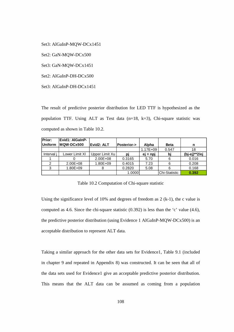
108
Set3: AlGaInP-MQW-DCx1451
Set2: GaN-MQW-DCx500
Set3: GaN-MQW-DCx1451
Set2: AlGaInP-DH-DCx500
Set3: AlGaInP-DH-DCx1451
The result of predictive posterior distribution for LED TTF is hypothesized as the
population TTF. Using ALT as Test data (n=18, k=3), Chi-square statistic was
computed as shown in Table 10.2.
Table 10.2 Computation of Chi-square statistic
Using the significance level of 10% and degrees of freedom as 2 (k-1), the c value is
computed as 4.6. Since the chi-square statistic (0.392) is less than the ‘c’ value (4.6),
the predictive posterior distribution (using Evidence 1 AlGaInP-MQW-DCx500) is an
acceptable distribution to represent ALT data.
Taking a similar approach for the other data sets for Evidence1, Table 9.1 (included
in chapter 9 and repeated in Appendix 8) was constructed. It can be seen that all of
the data sets used for Evidence1 give an acceptable predictive posterior distribution.
This means that the ALT data can be assumed as coming from a population
Prior: Uniform
Evid1: AlGaInP-MQW-DCx500 Evid2: ALT Posterior-> Alpha Beta n
1.17E+09 0.547 18Interval j Lower Limit Xl Upper Limit Xu pj ej = npj bj (bj-ej)**2/ej
1 0 2.00E+08 0.3165 5.70 6 0.0162 2.00E+08 1.80E+09 0.4015 7.23 6 0.2083 1.80E+09 8 0.2820 5.08 6 0.168
1.0000 Chi-Statistic 0.392

109
represented by the predictive posterior distributions predicted by various sources for
Evidence 1.
110
Chapter 11: Conclusion
11.1 Summary
In a medical diagnostic application, the precise value of light intensity is used to
interpret patient results for medical diagnostics. Hence understanding LED failure
modes is very important. Failure Modes and Effects Criticality Analysis (FMECA)
tool was used to identify critical LED failure modes. The next steps were Accelerated
Life Testing (ALT), Accelerated Degradation Testing (ADT) and Bayesian analysis.
ALT/ADT was performed on the LEDs by driving them in pulse mode at higher
current density J and elevated temperature T. Inverse Power Law model with J as the
accelerating agent and the Arrhenius model with T as the accelerating agent were
used. The optical degradation during ALT was found to be logarithmic and this
property was used for the degradation analysis using a log-linear degradation model.
Further, the LED bandgap temporarily shifts towards the longer wavelength at high
current. This shift was dependent on junction temperature. Empirical coefficients for
Varshini’s equation were determined.
The Bayesian analysis starting point was to identify pertinent published data which
may be used for developing the prior information. From the published data, the time
required for the optical power output to degrade by 20 percent was extracted LEDS
with different active layers (AlGaInP, GaN, AlGaAs), different LED structures (DH,
MQW) and bias conditions (DC, Pulsed). The degradation mechanism of LEDs,
published literature and our ALT data all indicate that Weibull is the most suitable
111
model for this data analysis. This rationale was used to develop the Weibull based
Bayesian likelihood function. For the first Bayesian updating, Uniform distribution
was used as the Prior for α-β parameters of the Weibull model. Prior published data
was used as Evidence to get the first posterior joint α-β distribution. For the second
Bayesian updating, ALT data was used as Evidence to get the second posterior joint
α-β distribution. This joint α-β distribution gave a series of Weibull time to failure
distributions. The predictive posterior failure distribution for the LEDs was estimated
by averaging over the range of α-β values. Lastly, a new parameter ‘R’ (degree of
relevance) is used to transform partially relevant prior published data for use in
Bayesian modeling.
Prior published data, the present ALT data, ADT analysis and Bayesian analysis
indicate that the MTTF of AlGaInP-MQW LEDs when used in this specific medical
application (pulse mode, on time 100us with 0.2% duty cycle, temperature = 35°C
and current density = 21.6Amps/cm2) is in excess of 1E8 hrs. This exceeds the
warranty life of the medical diagnostic instrument by orders of magnitude and as such
the LED is suitable for this application. The shape parameter β of the Weibull model
is less than 1 in all cases indicating a decreasing failure rate. This may be explained
by the observed logarithmic optical degradation of the present work. The initial high
failure rate may be due to manufacturing defects, which were not properly screened,
and hence the surviving population would be able to achieve a long life, since
probability of surviving increases after the initial degradation.
112
11.2 Objectives and Accomplishments
The goal of this research was to deepen our understanding of AlGaInP LED
performance over time for impulse currents (medical application), uncover unique
failure mechanisms and generate a model of time to failure. Work carried out during
this study resulted in the publication of three research papers and one poster
presentation. The following are the answers to the questions we started with:
1. Will the LED intensity remain within acceptable limits? Yes it does.
2. Will the LED wavelength remain stable? Yes, if the junction temperature is
maintained. Spectral shift investigation was performed during this research.
3. Will the Time to Failure of LEDs exceed the Life of the Medical Instrument? Yes,
the LEDs will outlast the 7-year life of the medical instrument by orders of
magnitude.
4. Will there be a cost benefit of using LEDs vs traditional light sources (flash lamps
etc)? Traditional lamps have to be replaced every 3-6 months causing a major
inconvenience to the customer. Use of LEDs will eliminate this replacement
saving time and money needed for maintenance.
5. Will there be any critical failure modes for the medical application? A Failure
Modes Effects and Criticality was performed for identifying critical failure modes
which were found to be encapsulation degradation and active layer degradation.
Even a worst case situation would only cause an unscheduled calibration of the
medical instrument, which would delay medical test results.

113
In addition to meeting the stated objectives, extra work was carried out for using
partially relevant prior data. A new parameter ‘R’ (degree of relevance) is used to
control the influence of evidence (by adjusting the Likelihood function) in Bayesian
modeling.
11.3 Research contribution and Significance
This Thesis represents the first measurements of AlGaInP LED reliability for the
medical diagnostic application. This research will allow replacement of traditional
light sources (filament or flash lamps) with LEDs. The lamps degrade and have to be
replaced 3-6 months causing a major inconvenience to the customer whereas LEDs
will outlast the 7-year life of the medical diagnostic instrument.
This research has produced significant contributions in the failure physics and
analysis of LEDs for medical applications. We were able to combine the traditional
ALT/ADT approach with FMECA and Bayesian analysis and hence have shown that
this methodology is valid for such complex situations.
The research represents a new contribution to LED reliability for significantly
different bias conditions. Our research used pulse driving with a very low duty cycle,
and the failures were induced by the magnitude of the peak current. We have reported
a decreasing failure rate β from the Weibull TTF model, through a unique
combination of prior published data, ALT and Bayesian analysis. The cause was
attributed to the observed optical degradation, which followed a logarithmic function
with high degradation in the initial period.
114
We have reported that bandgap shift due to thermal effects can degrade the power
output which may give an erroneous indication of “failure”. Upon returning to
nominal junction temperature most of the wavelength shift is recoverable. The
bandgap shifts toward longer wavelengths, but additional work must be carried out in
order to understand this specific mechanism as well as the initial logarithmic
degradation. Since the spectral performance is critical for the medical application, my
spectral shift investigation will provide immense value to the designer. The junction
temperature will need to be maintained.
11.4 Future Research
11.4.1 ALT at different duty cycles
LED life testing in prior published articles is done under DC conditions. Very few
articles are available for pulse testing. Per the need of the medical application, ALT
performed in this research was performed at very low duty cycles (0.2%). Performing
ALT is difficult and time consuming. Since each experiment takes as high as 6
months, we could only perform ALT at the required low duty cycle conditions. It
would be helpful to perform ALT at various duty cycles and estimate LED lifetime as
a function of duty cycle. This would allow a designer to choose the correct duty cycle
to maximize the reliability while meeting the LED application requirements.
11.4.2 Use of a Utility Function while estimating R
Insufficient data is a very common problem in Reliability studies. The conditions of
prior published data rarely match application conditions. In Chapter 9, the concept of
degree of relevance of prior published data was discussed. A 3-step approach is
115
proposed which includes using a multiplier to convert from DC to pulse data,
estimating the degree of relevance parameter R and then modifying the Likelihood
function in the Bayesian model with R. The three steps should be subjected to further
scrutiny. Refinements may need to be carried out for use in applications other than
LED reliability. One possible refinement is use of a Utility function while estimating
R. This would allow a parametric relationship between individual relevance
parameters for material (Rm), Structure (Rs) and Driving conditions (Rd) and the
estimated R.
11.4.3 Other methods of using degree of Relevance ‘R’
In addition to modifying the likelihood function by R, other methods of using ‘R’
should be studied. A common method is a Weighted posterior approach, which
however was not considered during this research. An approach that we did consider
(but which needs further development) is transforming the uncertain evidence itself
based on the value of R. The purpose of transformation is to move the evidence data
towards a Uniform distribution as R approaches 0. The transformed data when used
as Evidence during Bayesian updating will make the computations much easier.
Boundary conditions for the data transformation are as follows:
If R=0. Transform the data in to ‘Uniform distribution’
If R=1, Transformed data is identical to the original data
For 0 < R < 1, move the PDF of the partially relevant data towards a Uniform
distribution as R approaches 0.
During the Transformation of data, it is necessary to make
Mean of transformed data = M = Mean of ALT/Application data
116
If ti (t1, t2,…,tn) is a set of n partially relevant time to failure of LEDs, the
transformed data set ti’ is given by
ti’ = [(2i-1)M/n]1-R tiR - (11.1)
Again, the boundary conditions are
If R=0, ti’ = [(2i-1)M/n] with Average = M
If R=1, ti’ = ti
11.4.4 Failure Analysis
Additional failure analysis including microscopy is necessary in order to understand
the role of dislocations and other defects in causing the initial decrease in power
output. The diode surface can be analyzed through atomic force microscopy in order
to understand the role of surface roughness in decreasing light output. The analysis
should be designed so that one may differentiate between latent defects and
manufactured in defects. Additional research should be carried out which goes
beyond the surface of the die and into the interior of the die in order to totally
characterize the physics of failure.
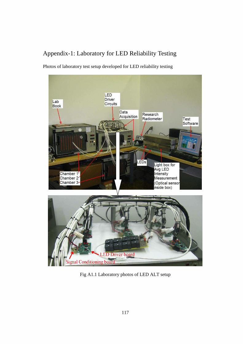
117
Appendix-1: Laboratory for LED Reliability Testing Photos of laboratory test setup developed for LED reliability testing
Fig A1.1 Laboratory photos of LED ALT setup
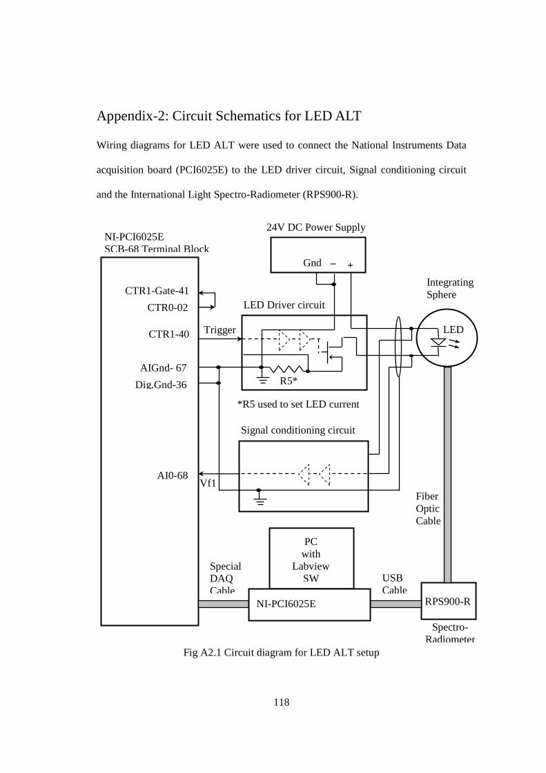
118
Appendix-2: Circuit Schematics for LED ALT Wiring diagrams for LED ALT were used to connect the National Instruments Data
acquisition board (PCI6025E) to the LED driver circuit, Signal conditioning circuit
and the International Light Spectro-Radiometer (RPS900-R).
Fig A2.1 Circuit diagram for LED ALT setup
LED
RPS900-R
Trigger
Fiber Optic Cable
R5*
NI-PCI6025E SCB-68 Terminal Block
24V DC Power Supply
LED Driver circuit
Signal conditioning circuit
Integrating Sphere
+ Gnd _
PC with
Labview SW USB
Cable
Special DAQ Cable
CTR1-40
AIGnd- 67
Dig.Gnd-36
CTR1-Gate-41
CTR0-02
AI0-68
NI-PCI6025E
Spectro-Radiometer
*R5 used to set LED current
Vf1
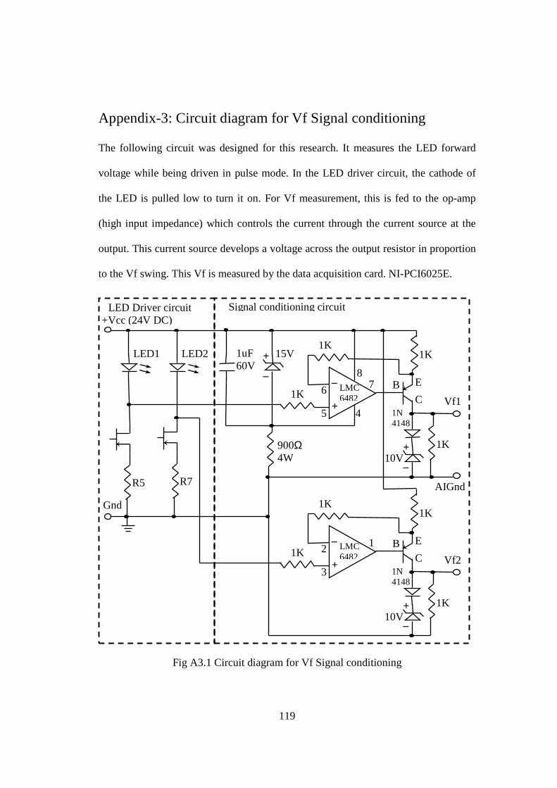
119
Appendix-3: Circuit diagram for Vf Signal conditioning The following circuit was designed for this research. It measures the LED forward
voltage while being driven in pulse mode. In the LED driver circuit, the cathode of
the LED is pulled low to turn it on. For Vf measurement, this is fed to the op-amp
(high input impedance) which controls the current through the current source at the
output. This current source develops a voltage across the output resistor in proportion
to the Vf swing. This Vf is measured by the data acquisition card. NI-PCI6025E.
Fig A3.1 Circuit diagram for Vf Signal conditioning
_
+ 10V
_
+ 15V LED1
1K
LED2 1uF 60V
+
_ LMC 6482
5
6
8
4
7
1K 1K
1N 4148
1K
E
C B
Vf1
AIGnd
900Ω 4W
_
+ 10V
1K +
_ LMC 6482
3
2
1
1K 1K
1N 4148
1K
E
C B
Vf2
R7 R5
+Vcc (24V DC) Signal conditioning circuit LED Driver circuit
Gnd
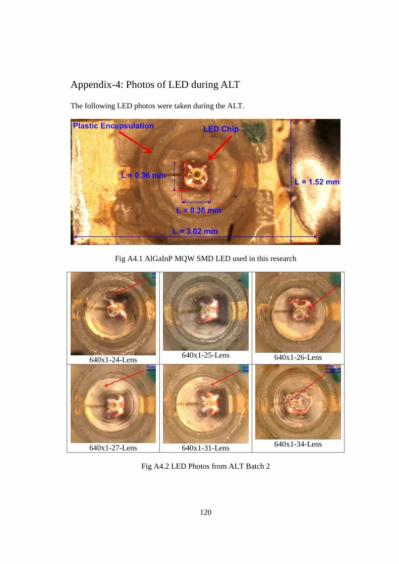
120
Appendix-4: Photos of LED during ALT The following LED photos were taken during the ALT.
Fig A4.1 AlGaInP MQW SMD LED used in this research
640x1-24-Lens
640x1-25-Lens 640x1-26-Lens
640x1-27-Lens 640x1-31-Lens 640x1-34-Lens
Fig A4.2 LED Photos from ALT Batch 2
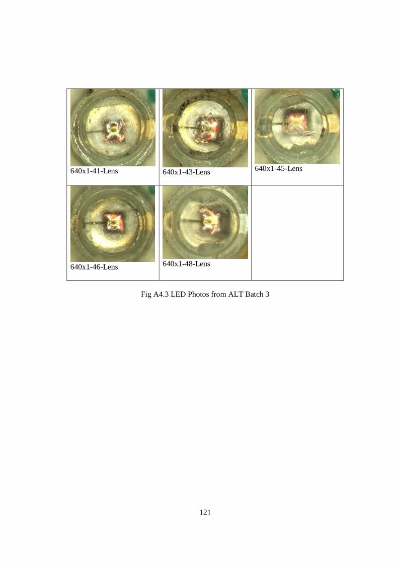
121
640x1-41-Lens 640x1-43-Lens 640x1-45-Lens
640x1-46-Lens 640x1-48-Lens
Fig A4.3 LED Photos from ALT Batch 3
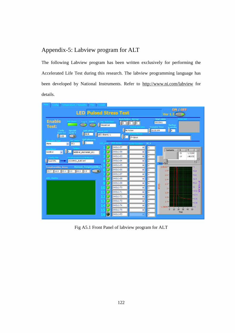
122
Appendix-5: Labview program for ALT The following Labview program has been written exclusively for performing the
Accelerated Life Test during this research. The labview programming language has
been developed by National Instruments. Refer to http://www.ni.com/labview for
details.
Fig A5.1 Front Panel of labview program for ALT
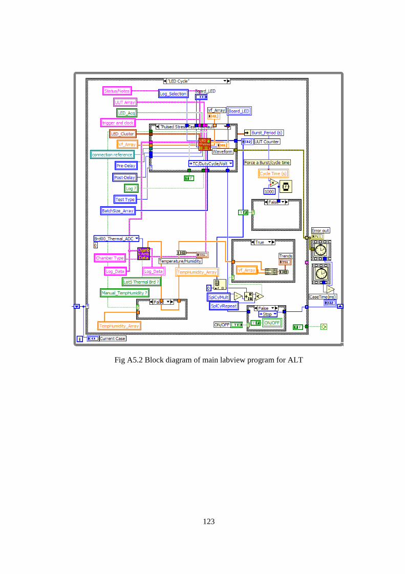
123
Fig A5.2 Block diagram of main labview program for ALT
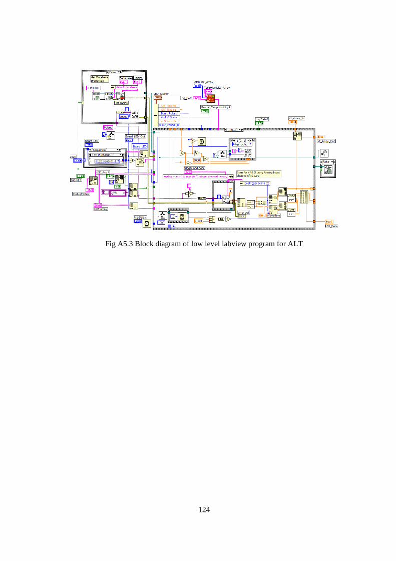
124
Fig A5.3 Block diagram of low level labview program for ALT

125
Appendix-6: Labview Program for Bayesian Modeling The following Labview program has been written by us exclusively for the Bayesian
modeling performed during this study. The labview programming language has been
developed by National Instruments. Refer to http://www.ni.com/labview for details
Fig A6.1 Front Panel Page 1 of labview program for Weibull Bayesian Analysis
Fig A6.2 Front Panel Page 2 of labview program for Weibull Bayesian Analysis

126
Fig A6.3 Front Panel Page 3 of labview program for Weibull Bayesian Analysis
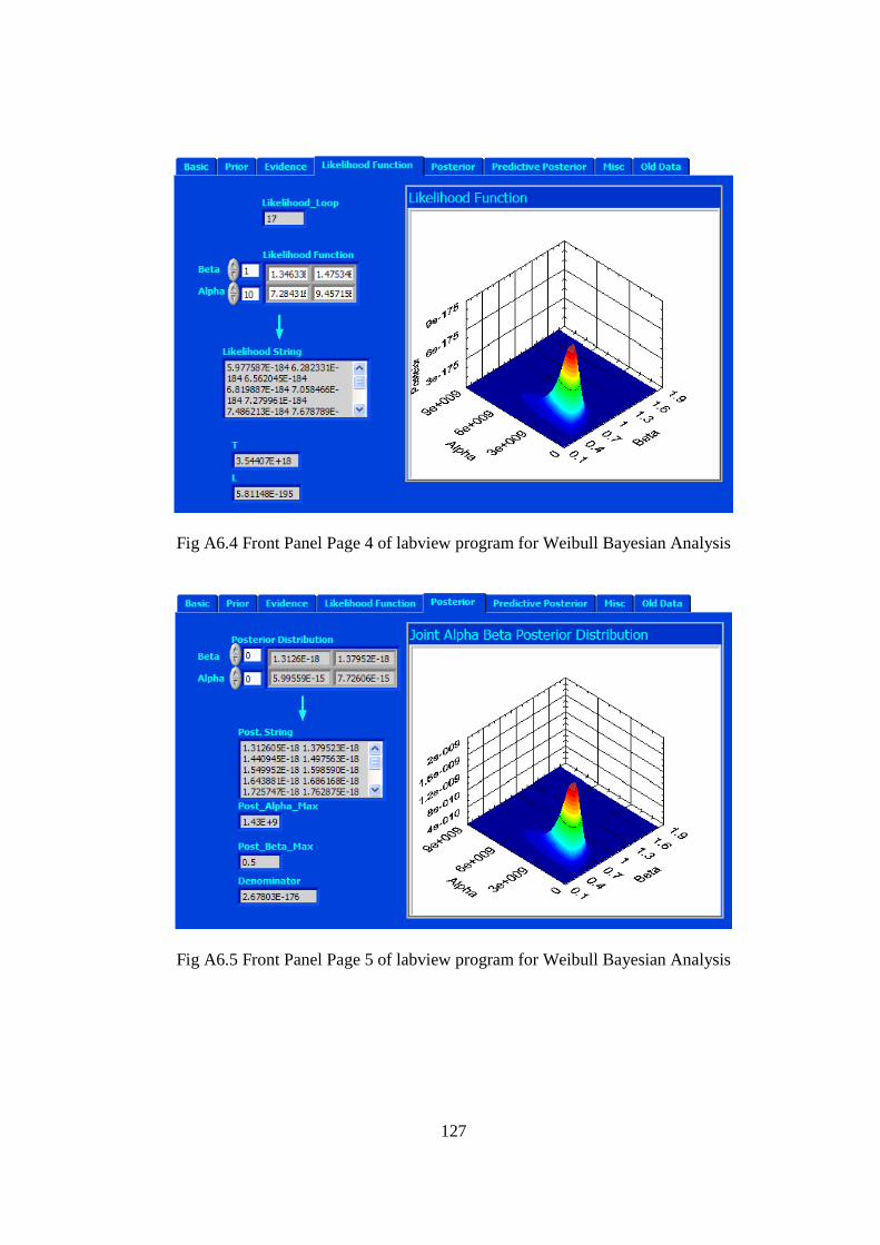
127
Fig A6.4 Front Panel Page 4 of labview program for Weibull Bayesian Analysis
Fig A6.5 Front Panel Page 5 of labview program for Weibull Bayesian Analysis
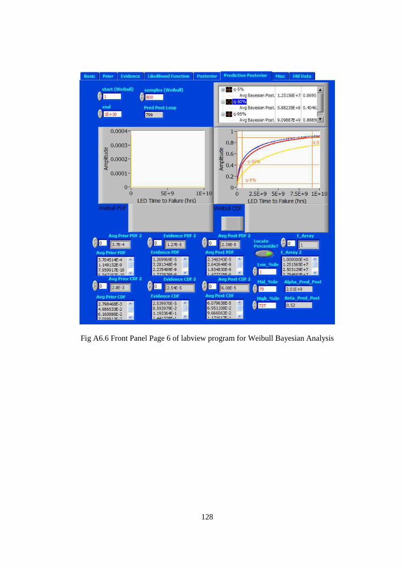
128
Fig A6.6 Front Panel Page 6 of labview program for Weibull Bayesian Analysis
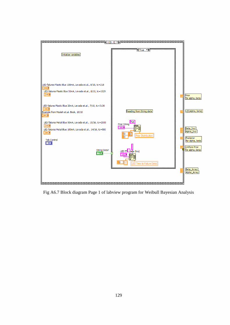
129
Fig A6.7 Block diagram Page 1 of labview program for Weibull Bayesian Analysis
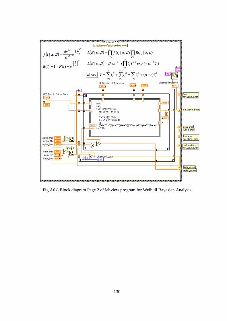
130
Fig A6.8 Block diagram Page 2 of labview program for Weibull Bayesian Analysis
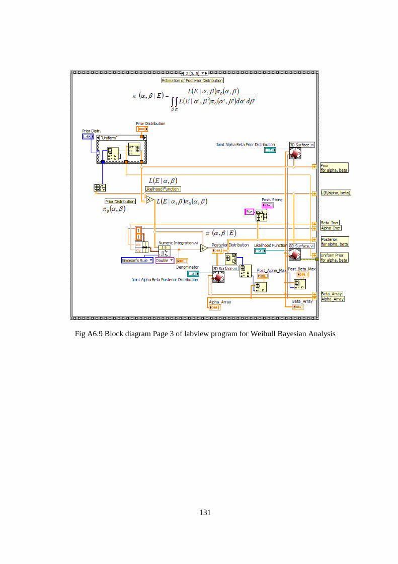
131
Fig A6.9 Block diagram Page 3 of labview program for Weibull Bayesian Analysis
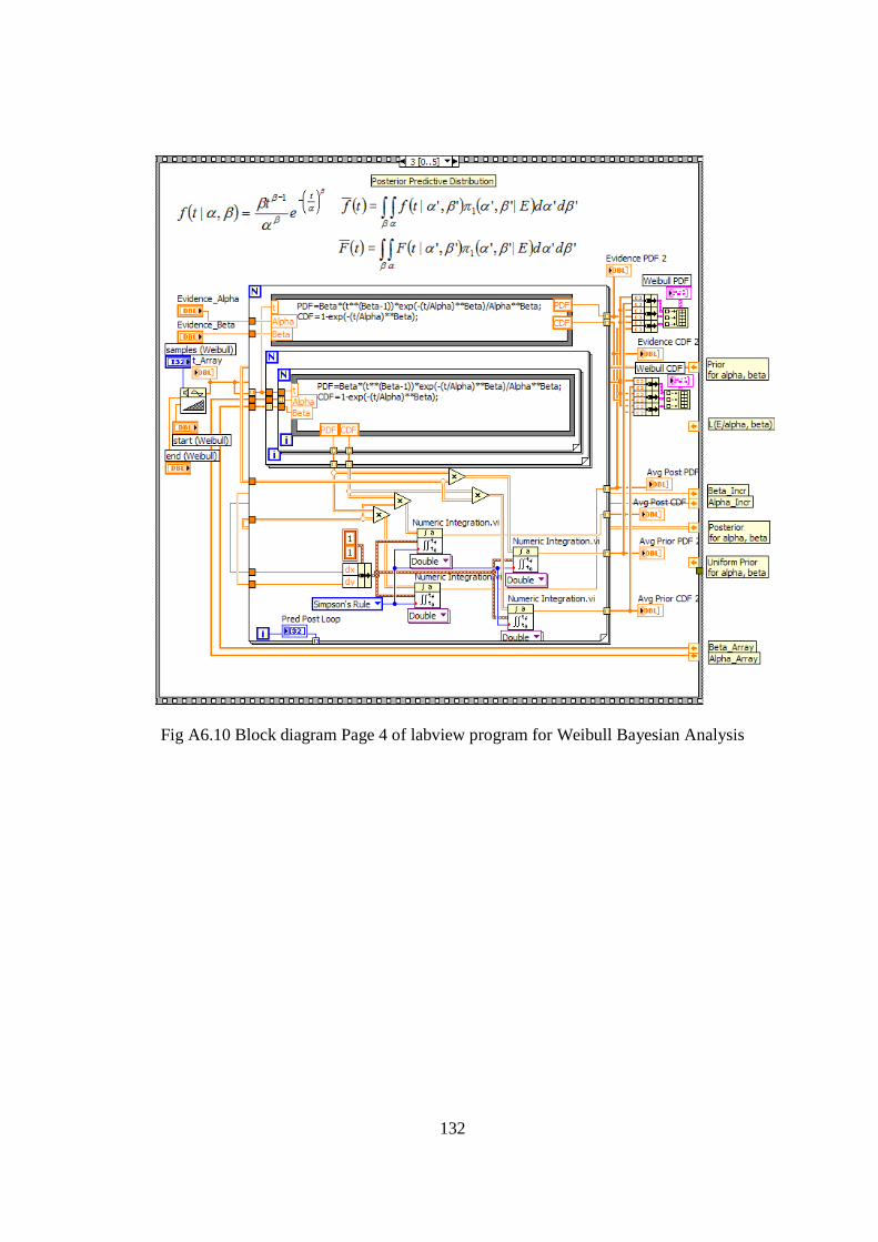
132
Fig A6.10 Block diagram Page 4 of labview program for Weibull Bayesian Analysis
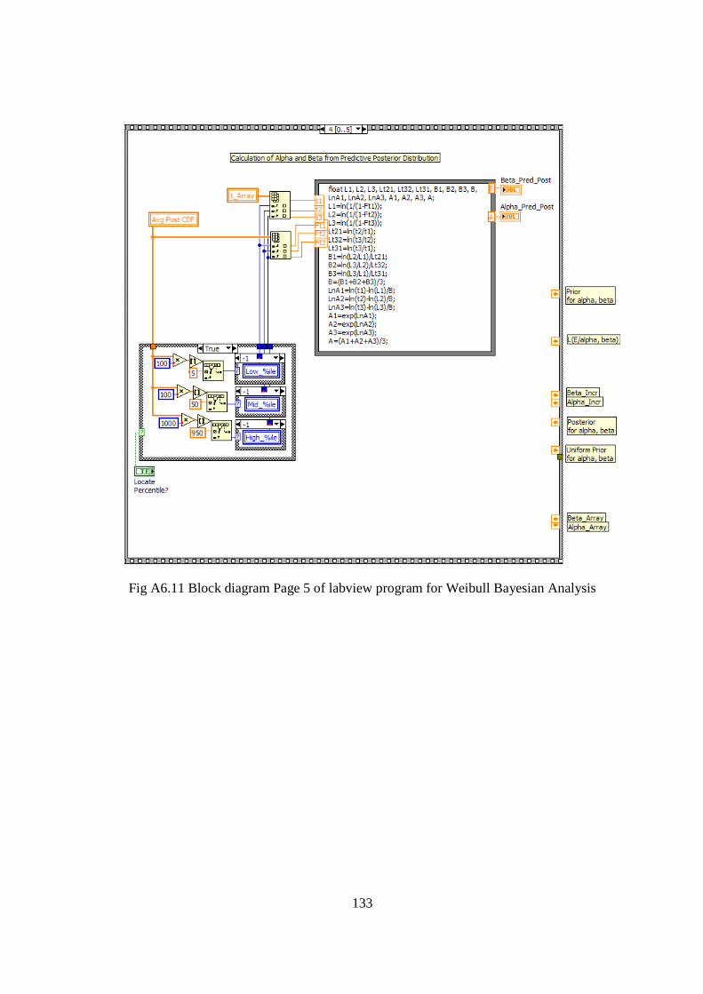
133
Fig A6.11 Block diagram Page 5 of labview program for Weibull Bayesian Analysis
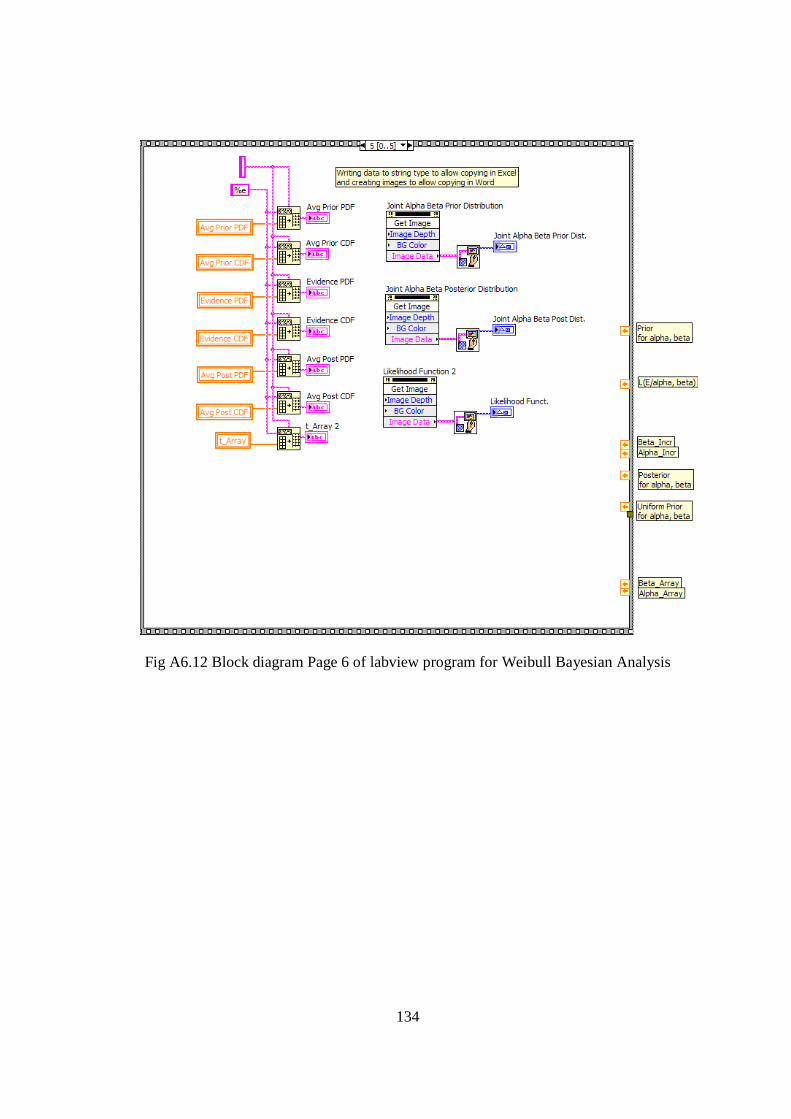
134
Fig A6.12 Block diagram Page 6 of labview program for Weibull Bayesian Analysis
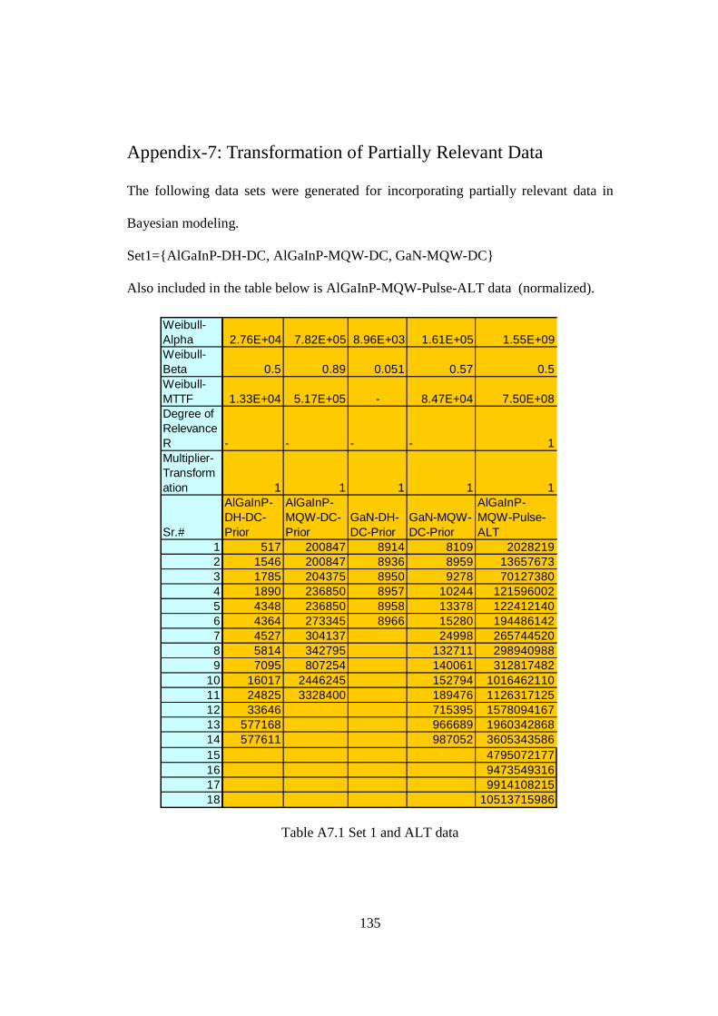
135
Appendix-7: Transformation of Partially Relevant Data The following data sets were generated for incorporating partially relevant data in
Bayesian modeling.
Set1=AlGaInP-DH-DC, AlGaInP-MQW-DC, GaN-MQW-DC
Also included in the table below is AlGaInP-MQW-Pulse-ALT data (normalized).
Table A7.1 Set 1 and ALT data
Weibull-Alpha 2.76E+04 7.82E+05 8.96E+03 1.61E+05 1.55E+09Weibull-Beta 0.5 0.89 0.051 0.57 0.5Weibull-MTTF 1.33E+04 5.17E+05 - 8.47E+04 7.50E+08Degree of Relevance R - - - - 1Multiplier-Transformation 1 1 1 1 1
Sr.#
AlGaInP-DH-DC-Prior
AlGaInP-MQW-DC-Prior
GaN-DH-DC-Prior
GaN-MQW-DC-Prior
AlGaInP-MQW-Pulse-ALT
1 517 200847 8914 8109 20282192 1546 200847 8936 8959 136576733 1785 204375 8950 9278 701273804 1890 236850 8957 10244 1215960025 4348 236850 8958 13378 1224121406 4364 273345 8966 15280 1944861427 4527 304137 24998 2657445208 5814 342795 132711 2989409889 7095 807254 140061 312817482
10 16017 2446245 152794 101646211011 24825 3328400 189476 112631712512 33646 715395 157809416713 577168 966689 196034286814 577611 987052 360534358615 479507217716 947354931617 991410821518 10513715986
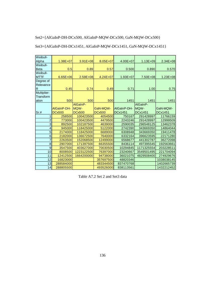
136
Set2=AlGaInP-DH-DCx500, AlGaInP-MQW-DCx500, GaN-MQW-DCx500
Set3=AlGaInP-DH-DCx1451, AlGaInP-MQW-DCx1451, GaN-MQW-DCx1451
Table A7.2 Set 2 and Set3 data
Weibull-Alpha 1.38E+07 3.91E+08 8.05E+07 4.00E+07 1.13E+09 2.34E+08Weibull-Beta 0.5 0.89 0.57 0.500 0.890 0.570Weibull-MTTF 6.65E+06 2.59E+08 4.24E+07 1.93E+07 7.50E+08 1.23E+08Degree of Relevance R 0.45 0.74 0.49 0.71 1.00 0.75Multiplier-Transformation 500 500 500 1451 1451 1451
Sr.#AlGaInP-DH-DCx500
AlGaInP-MQW-DCx500
GaN-MQW-DCx500
AlGaInP-DH-DCx1451
AlGaInP-MQW-DCx1451
GaN-MQW-DCx1451
1 258500 100423500 4054500 750167 291428997 117661592 773000 100423500 4479500 2243246 291428997 129995093 892500 102187500 4639000 2590035 296548125 134623784 945000 118425000 5122000 2742390 343669350 148640445 2174000 118425000 6689000 6308948 343669350 194114786 2182000 136672500 7640000 6332164 396623595 221712807 2263500 152068500 12499000 6568677 441302787 362720988 2907000 171397500 66355500 8436114 497395545 1925636619 3547500 403627000 70030500 10294845 1171325554 203228511
10 8008500 1223122500 76397000 23240667 3549501495 22170409411 12412500 1664200000 94738000 36021075 4829508400 27492967612 16823000 357697500 48820346 103803814513 288584000 483344500 837470768 140266573914 288805500 493526000 838113561 1432212452
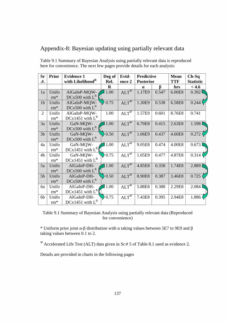
137
Appendix-8: Bayesian updating using partially relevant data Table 9.1 Summary of Bayesian Analysis using partially relevant data is reproduced here for convenience. The next few pages provide details for each analysis: Sr.#.
Prior Evidence 1 with Likelihood R
Deg of Rel.
Evid-ence 2
Predictive Posterior
Mean TTF
Ch-Sq Statistic
R α β hrs < 4.6 1a Unifo
rm* AlGaInP-MQW-DCx500 with LR
1.00 ALTΨ 1.17E9 0.547 6.00E8 0.392
1b Uniform*
AlGaInP-MQW-DCx500 with LR
0.75 ALTΨ 1.30E9 0.538 6.58E8 0.244
2 Uniform*
AlGaInP-MQW-DCx1451 with LR
1.00 ALTΨ 1.57E9 0.601 8.76E8 0.741
3a Uniform*
GaN-MQW-DCx500 with LR
1.00 ALTΨ 6.70E8 0.415 2.63E8 1.598
3b Uniform*
GaN-MQW-DCx500 with LR
0.50 ALTΨ 1.06E9 0.437 4.60E8 0.272
4a Uniform*
GaN-MQW-DCx1451 with LR
1.00 ALTΨ 9.05E8 0.474 4.00E8 0.673
4b Uniform*
GaN-MQW-DCx1451 with LR
0.75 ALTΨ 1.05E9 0.477 4.87E8 0.314
5a Uniform*
AlGaInP-DH-DCx500 with LR
1.00 ALTΨ 4.85E8 0.358 1.74E8 2.889
5b Uniform*
AlGaInP-DH-DCx500 with LR
0.50 ALTΨ 8.90E8 0.387 3.46E8 0.725
6a Uniform*
AlGaInP-DH-DCx1451 with LR
1.00 ALTΨ 5.88E8 0.388 2.29E8 2.084
6b Uniform*
AlGaInP-DH-DCx1451 with LR
0.75 ALTΨ 7.43E8 0.395 2.94E8 1.886
Table 9.1 Summary of Bayesian Analysis using partially relevant data (Reproduced
for convenience) * Uniform prior joint α-β distribution with α taking values between 5E7 to 9E9 and β taking values between 0.1 to 2. Ψ Accelerated Life Test (ALT) data given in Sr.# 5 of Table 8.1 used as evidence 2. Details are provided in charts in the following pages

138
Sr.#.
Prior Evidence 1 with Likelihood R
Deg of Rel.
Evid-ence 2
Predictive Posterior
Mean TTF
Ch-Sq Statistic
R α β hrs < 4.6 1a Unifo
rm* AlGaInP-MQW-DCx500 with LR
1.00 ALTΨ 1.17E9 0.547 6.00E8 0.392
1st Bayesian Updating
2nd Bayesian Updating
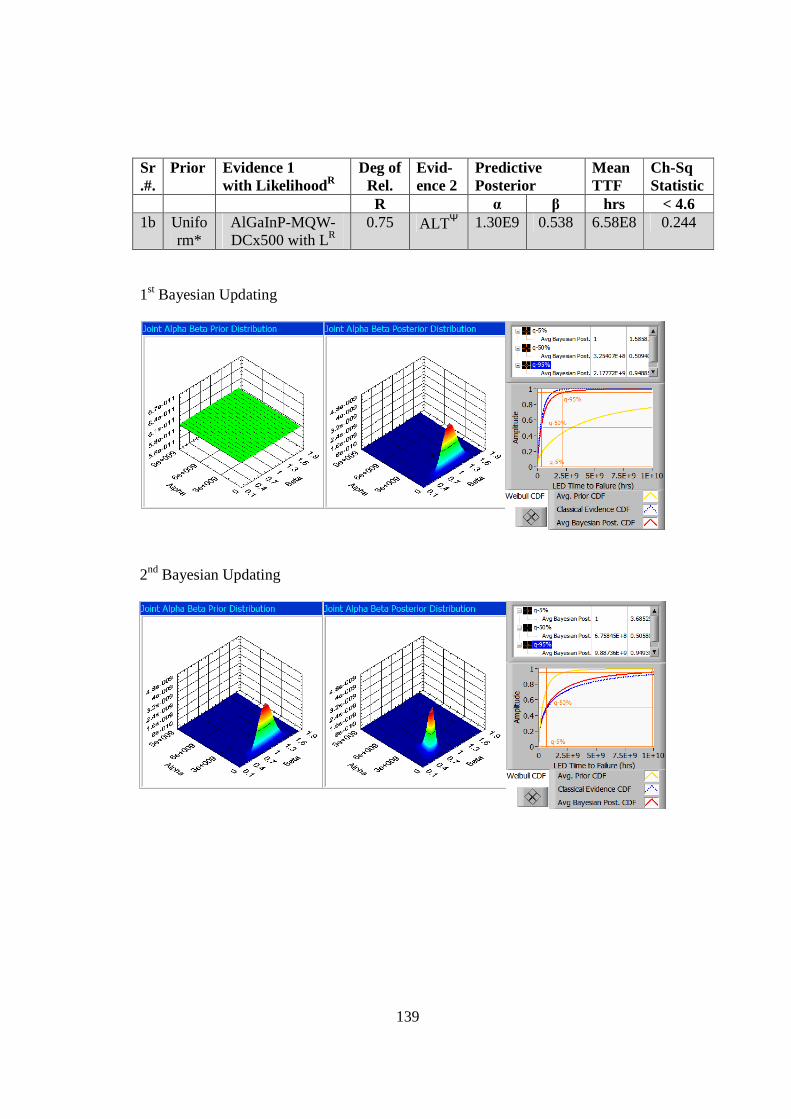
139
Sr.#.
Prior Evidence 1 with Likelihood R
Deg of Rel.
Evid-ence 2
Predictive Posterior
Mean TTF
Ch-Sq Statistic
R α β hrs < 4.6 1b Unifo
rm* AlGaInP-MQW-DCx500 with LR
0.75 ALTΨ 1.30E9 0.538 6.58E8 0.244
1st Bayesian Updating
2nd Bayesian Updating

140
Sr.#.
Prior Evidence 1 with Likelihood R
Deg of Rel.
Evid-ence 2
Predictive Posterior
Mean TTF
Ch-Sq Statistic
R α β hrs < 4.6 2 Unifo
rm* AlGaInP-MQW-DCx1451 with LR
1.00 ALTΨ 1.57E9 0.601 8.76E8 0.741
1st Bayesian Updating
2nd Bayesian Updating

141
Sr.#.
Prior Evidence 1 with Likelihood R
Deg of Rel.
Evid-ence 2
Predictive Posterior
Mean TTF
Ch-Sq Statistic
R α β hrs < 4.6 3a Unifo
rm* GaN-MQW-
DCx500 with LR 1.00 ALTΨ 6.70E8 0.415 2.63E8 1.598
1st Bayesian Updating
2nd Bayesian Updating

142
Sr.#.
Prior Evidence 1 with Likelihood R
Deg of Rel.
Evid-ence 2
Predictive Posterior
Mean TTF
Ch-Sq Statistic
R α β hrs < 4.6 3b Unifo
rm* GaN-MQW-
DCx500 with LR 0.50 ALTΨ 1.06E9 0.437 4.60E8 0.272
1st Bayesian Updating
2nd Bayesian Updating
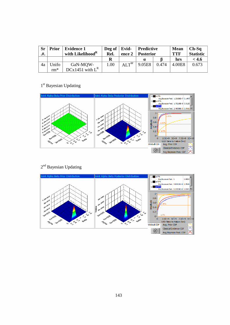
143
Sr.#.
Prior Evidence 1 with Likelihood R
Deg of Rel.
Evid-ence 2
Predictive Posterior
Mean TTF
Ch-Sq Statistic
R α β hrs < 4.6 4a Unifo
rm* GaN-MQW-
DCx1451 with LR 1.00 ALTΨ 9.05E8 0.474 4.00E8 0.673
1st Bayesian Updating
2nd Bayesian Updating

144
Sr.#.
Prior Evidence 1 with Likelihood R
Deg of Rel.
Evid-ence 2
Predictive Posterior
Mean TTF
Ch-Sq Statistic
R α β hrs < 4.6 4b Unifo
rm* GaN-MQW-
DCx1451 with LR 0.75 ALTΨ 1.05E9 0.477 4.87E8 0.314
1st Bayesian Updating
2nd Bayesian Updating

145
Sr.#.
Prior Evidence 1 with Likelihood R
Deg of Rel.
Evid-ence 2
Predictive Posterior
Mean TTF
Ch-Sq Statistic
R α β hrs < 4.6 5a Unifo
rm* AlGaInP-DH-
DCx500 with LR 1.00 ALTΨ 4.85E8 0.358 1.74E8 2.889
1st Bayesian Updating
2nd Bayesian Updating
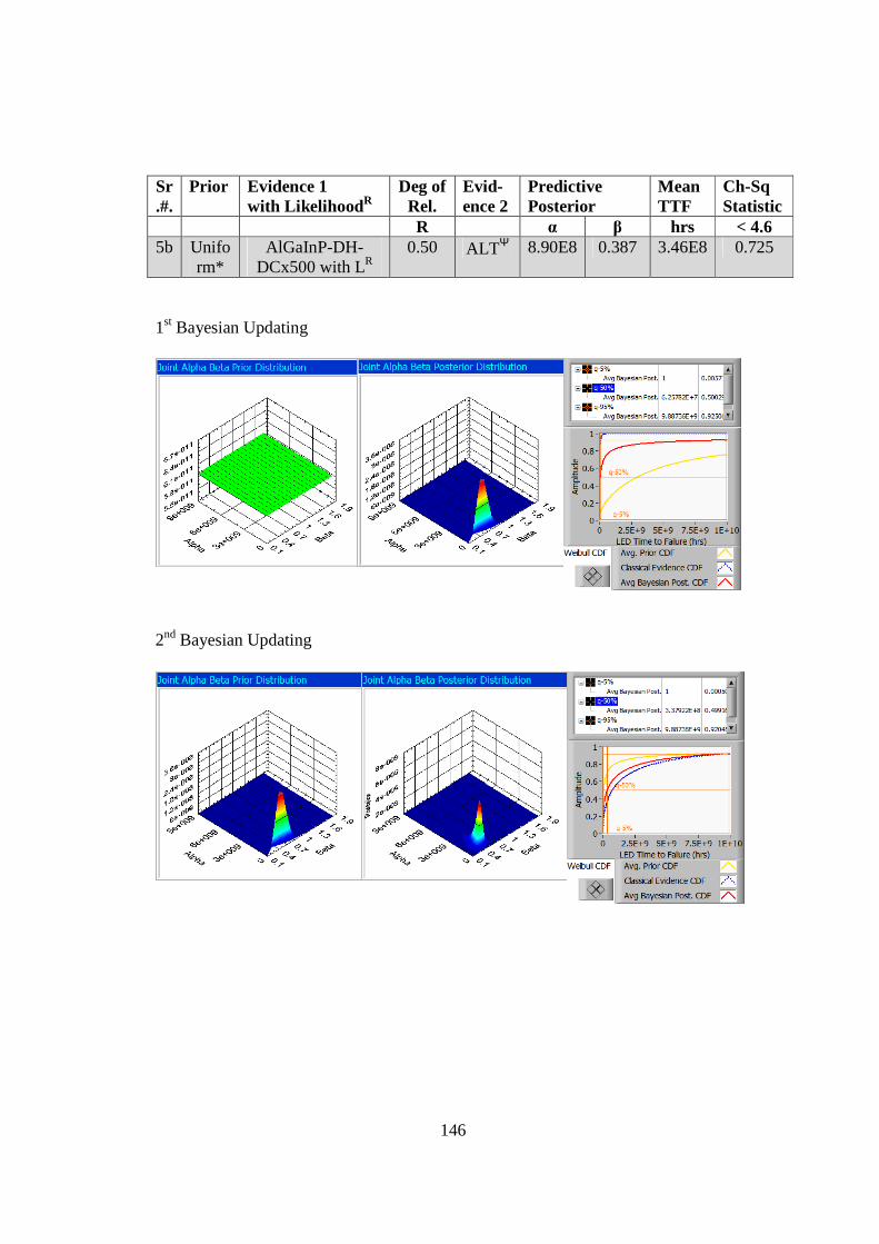
146
Sr.#.
Prior Evidence 1 with Likelihood R
Deg of Rel.
Evid-ence 2
Predictive Posterior
Mean TTF
Ch-Sq Statistic
R α β hrs < 4.6 5b Unifo
rm* AlGaInP-DH-
DCx500 with LR 0.50 ALTΨ 8.90E8 0.387 3.46E8 0.725
1st Bayesian Updating
2nd Bayesian Updating
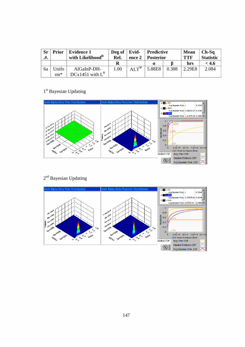
147
Sr.#.
Prior Evidence 1 with Likelihood R
Deg of Rel.
Evid-ence 2
Predictive Posterior
Mean TTF
Ch-Sq Statistic
R α β hrs < 4.6 6a Unifo
rm* AlGaInP-DH-
DCx1451 with LR 1.00 ALTΨ 5.88E8 0.388 2.29E8 2.084
1st Bayesian Updating
2nd Bayesian Updating
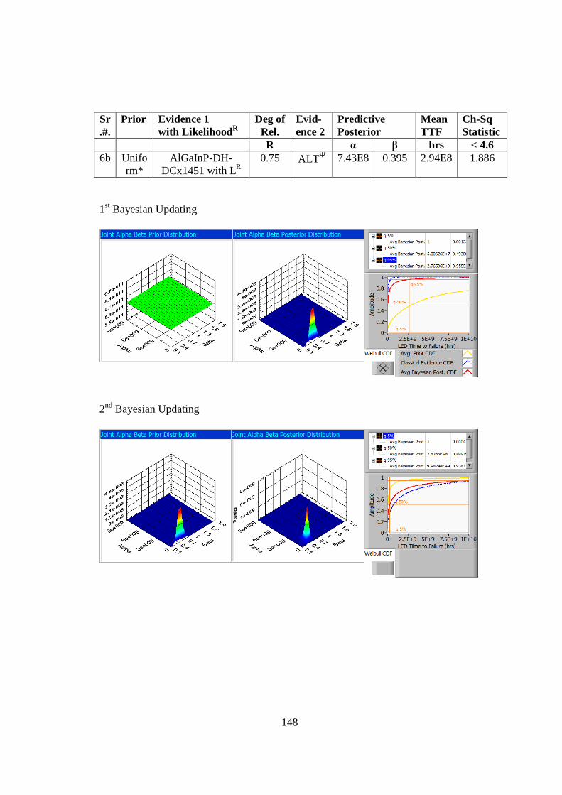
148
Sr.#.
Prior Evidence 1 with Likelihood R
Deg of Rel.
Evid-ence 2
Predictive Posterior
Mean TTF
Ch-Sq Statistic
R α β hrs < 4.6 6b Unifo
rm* AlGaInP-DH-
DCx1451 with LR 0.75 ALTΨ 7.43E8 0.395 2.94E8 1.886
1st Bayesian Updating
2nd Bayesian Updating
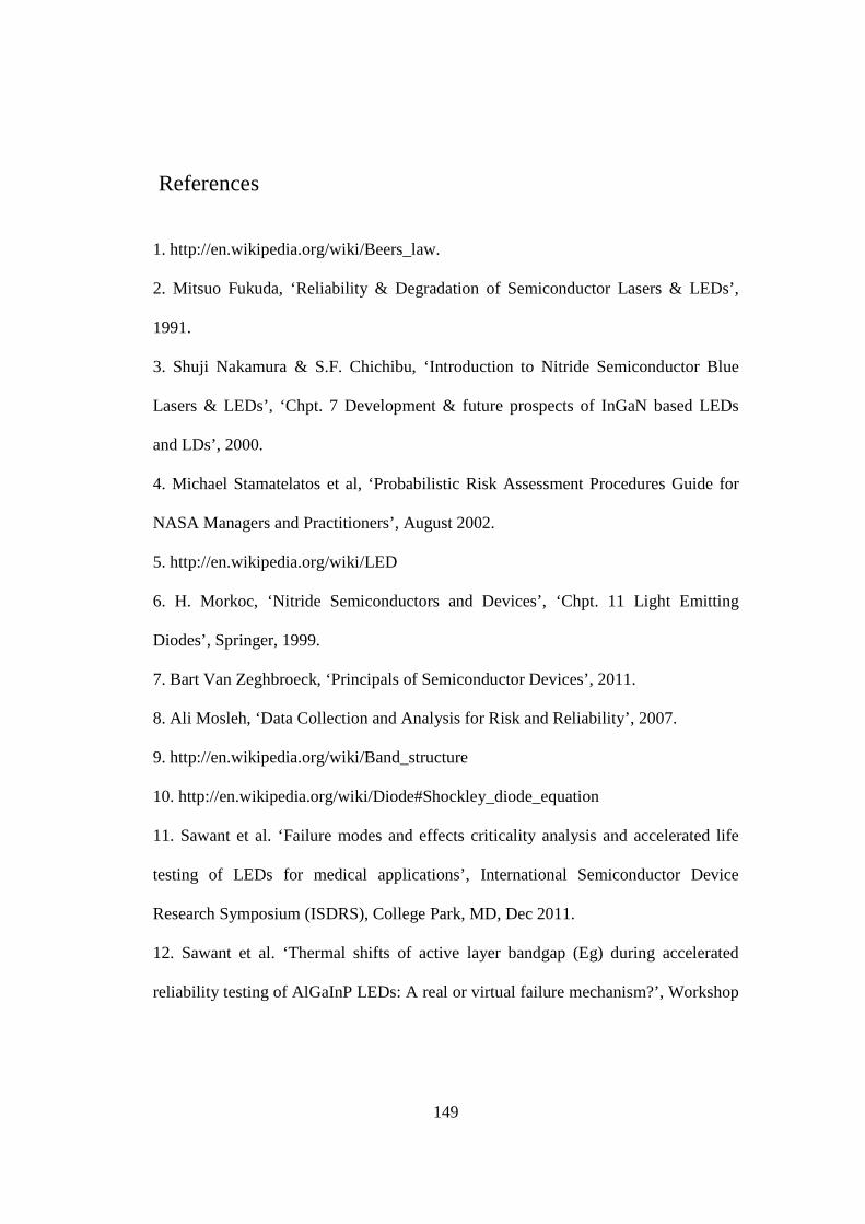
149
References
1. http://en.wikipedia.org/wiki/Beers_law.
2. Mitsuo Fukuda, ‘Reliability & Degradation of Semiconductor Lasers & LEDs’,
1991.
3. Shuji Nakamura & S.F. Chichibu, ‘Introduction to Nitride Semiconductor Blue
Lasers & LEDs’, ‘Chpt. 7 Development & future prospects of InGaN based LEDs
and LDs’, 2000.
4. Michael Stamatelatos et al, ‘Probabilistic Risk Assessment Procedures Guide for
NASA Managers and Practitioners’, August 2002.
5. http://en.wikipedia.org/wiki/LED
6. H. Morkoc, ‘Nitride Semiconductors and Devices’, ‘Chpt. 11 Light Emitting
Diodes’, Springer, 1999.
7. Bart Van Zeghbroeck, ‘Principals of Semiconductor Devices’, 2011.
8. Ali Mosleh, ‘Data Collection and Analysis for Risk and Reliability’, 2007.
9. http://en.wikipedia.org/wiki/Band_structure
10. http://en.wikipedia.org/wiki/Diode#Shockley_diode_equation
11. Sawant et al. ‘Failure modes and effects criticality analysis and accelerated life
testing of LEDs for medical applications’, International Semiconductor Device
Research Symposium (ISDRS), College Park, MD, Dec 2011.
12. Sawant et al. ‘Thermal shifts of active layer bandgap (Eg) during accelerated
reliability testing of AlGaInP LEDs: A real or virtual failure mechanism?’, Workshop
150
on Compound Semiconductor Devices and Integrated Circuits (WOCSDICE), Island
of Porquerolles, France, May 2012.
13. Sawant et al. ‘A Bayes approach and criticality analysis for reliability prediction
of AlGaInP light emitting diodes’, Reliability of Compound Semiconductors
Workshop (ROCS), Boston MA, April 2012.
14. Ott et al. 'Capabilities and Reliability of LEDs and Laser Diodes', NASA report,
Technology Validation Assurance Group, updated 9/3/1997.
15. Vanderwater et al. ‘High-brightness AlGaInP light emitting diodes', Proceedings
of the IEEE, Vol. 85, Issue 11, Pages 1752-1764, Nov. 1997.
16. Grillot et al. ‘Sixty Thousand Hour Light Output Reliability of AlGaInP LEDs',
IEEE Trans. on Device and Mat. Reliability, Vol. 6, No.4, Pages 564-574, Dec 2006.
17. Kish et al. ‘Highly reliable and efficient semiconductor wafer-bonded
AlGaInP/GaP LEDs', Electronics Letters, Vol. 32, Issue 2, Pages132–136, Jan 1996.
18. Hofler et al. ‘High-flux high-efficiency transparent-substrate AlGaInP/GaP
LEDs', Electronics Letters, Vol. 34, Issue 18, Pages 1781-1782, September 1998.
19. Chang et al. ‘AlGalnP multiquantum well light-emitting diodes', IEE Proc.-
Optoelectron., Vol. 144, No. 6, December 1997.
20. Kish et al. ‘High luminous flux semiconductor wafer-bonded AlGaInP/GaP large-
area emitters', Electronics Letters, Vol. 30, Issue 21, Pages 1790-1792, October 1994.
21. Krames et al. ‘Status and Future of High-Power LEDs for Solid-State Lighting',
Journal of Display Technology, Vol. 3, Issue 2, Pages 160–175, June 2007.
22. Streubel et al. ‘High Brightness AlGaInP Light-Emitting Diodes', IEEE Journal of
Selected Topics in Quantum Electronics, Pages 321–332, March-April 2002.
151
23. Altieri et al. ‘Analysis of internal quantum efficiency of high-brightness AlGaInP
LEDs', The 4th International Conference on Numerical Simulation of Optoelectronic
Devices Proceedings NUSOD '04, Pages 13-14, August 2004.
24. Philips, ‘LUXEON Reliability Datasheet RD25’, Pages 9-10, July 2006.
25. Liang et al. ‘Comparison of temperature dependent electroluminescence of
InGaN/GaN and AlGaInP based LEDs', Optoelectronics, The 6th Chinese
Symposium Proceedings Pages 196-199, Sept. 2003.
26. Lin et al. ‘Highly reliable operation of indium tin oxide AlGaInP light emitting
diodes', Electronics Letters, Vol. 30, No.21, October 1994.
27. Su et al. ‘High reliability of AlGaInP LEDs with tensile strain barrier-reducing
Layer', IEEE Photonics Technology Letters, Vol. 16, Issue 1, Pages 30–32, Jan. 2004
28. Lacey et al. 'The reliability of AlGaInP visible LEDs', Quality & Reliability
Engineering, Vol. 16, Issue 1, Pages 45 – 49, 2000.
29. Dutta et al. ‘High Brightness and Reliable AlGaInP-Based LED for POF Data
Links', IEEE Photonics Technology Letters, Vol. 9, No 12, December 1997.
30. Nogueira et al. ‘Accelerated Life Testing LEDs on Temperature and Current',
Proceedings of the 8th Spanish Conference on Electron Devices, Pages 1-4, Feb 2011.
31. Chen et al. 'Thermal resistance and reliability of low-cost high-power LED
packages under WHTOL test', Int. Conf. on Electronic Materials and Packaging,
EMAP 2008, Pages 271-276, Oct. 2008.
32. Meneghini et al. 'A review on the Reliability of GaN based LEDs', IEEE
transactions on device and materials reliability, Vol. 8, No. 2, June 2008.

152
33. Meneghini et al. ' A review on the physical mechanisms that limit the reliability of
GaN based LEDs', IEEE trans. on electron devices, Vol. 51, Issue. 1, Jan 2010.
34. Levada et al. ' Analysis of DC Current Accelerated Life Tests of GaN LEDs
Using a Weibull-Based Statistical Model', IEEE transactions on device and materials
reliability, Vol. 5, No. 4, Dec 2005.
35. Buso et al. 'Performance Degradation of High-Brightness LEDs Under DC and
Pulsed Bias', IEEE trans. on device and materials reliability, Vol. 8, No. 2, June 2008.
36. Trevisanello et al. 'Accelerated life test of High Brightness LEDs', IEEE
transactions on device and materials reliability, Vol. 8, No. 2, June 2008.
37. Meneghesso et al. 'Degradation mechanisms of GaN-based LEDs after accelerated
DC current aging', Electron Devices Meeting Digest, Pages 103-106, Dec 2002.
38. Levada et al. ' High Brightness InGaN LED degradation at high injection current
bias', 44th Ann. Int. Reliability Physics Symposium Proc., Pages 615-616, Mar 2006.
39. Meneghesso et al. 'Failure mechanisms of GaN-based LEDs related with
instabilities in doping profile and deep levels', 42nd Annual International Reliability
Physics Symposium Proceedings, Pages 474-478, April 2004.
40. Trevisanello et al. 'Thermally activated degradation and package instabilities of
low flux LEDS ', Ann. Int. Reliability Physics Symp. Proc, Pages 98-103, April 2009.
41. Meneghini et al. 'High Temperature Degradation of GaN LEDs related to
passivation', IEEE transactions on electron devices, Vol. 53, No. 12, Dec 2006.
42. Osinski et al. 'AlGaN/InGaN/GaN blue light emitting diode degradation under
pulsed current stress', Applied Physics Letters, 69 (7), August 1996.
153
43. Barton et al. 'Life tests and failure mechanisms of GaN-AlGaN-InGaN LEDs',
35th Ann. Int. Reliability Physics Symposium Proc, Pages 276-281, April 1997.
44. Barton et al. 'Degradation mechanisms in GaN/AlGaN/InGaN LEDs and LDs',
10th Conf. on Semiconducting & Insul. Materials Proc., Pages 259-262, June 1998.
45. Wang et al. 'Device design and simulation for GaN based dual wavelength LEDs',
Applied Optics, Vol. 48, No. 6, February 2009.
46. Shuji Nakamura, ‘High-power InGaN/AlGaN double-heterostructure blue-LEDs,
‘IEDM '94. Technical Digest’, Dec 1994.
47. Yanagisawa T., 'Estimation of the degradation of InGaN/A1GaN Blue LEDs',
Microelectronic Reliability, Vol. 37, No. 8, pp. 1239-1241, 1997.
48. Yanagisawa T. ' The degradation of GaAlAs red LEDs under continuous and low-
speed pulse operations ', Microelectronics Reliability 38, pp. 1627-1630, 1998.
49. Narendran et al. 'Life of LED-Based White Light Sources', IEEE/OSA journal of
display technology, Vol. 1, NO. 1, September 2005.
50. Narendran et al. 'Performance characteristics of high power LEDs', 3rd
International conference on solid state lighting. Proc. of SPIE 5187: 267-275, 2004.
51. Tsai et al. 'Decay of radiation pattern and spectrum of high-power LED modules
in aging test', IEEE Lasers and Electro-Optics Society, 2008. LEOS 2008. 21st
Annual Meeting of the 9-13 Nov. 2008 Page(s):658 - 659.
52. Yoshi Ohno, 'Optical metrology for LEDs and solid state lighting', Fifth
Symposium Optics in Industry, Proceedings of SPIE Vol. 6046, 604625, (2006).
53. Miller et al. ' LED Photometric Calibrations at the NIST and Future Measurement
Needs of LEDs', Proc. of SPIE Vol. 5530 2004.
154
54. Miller et al. 'Luminous Intensity Measurement of LEDs at NIST' Proc. 2nd CIE
Expert Symposium on LED Measurement, May 2001, Gaithersburg, MD, USA.
55. Miller et al. ' Luminous Flux calibration of LEDs at NIST' Proc. 2nd CIE Expert
Symposium on LED Measurement, May 2001, Gaithersburg, MD, USA.
56. Getty et al. 'Electroluminescent measurement of the internal quantum efficiency
of light emitting diodes', Applied Physics Letters, 94, 181102, 2009.
57. Park et al. 'Uncertainty evaluation for the spectro-radiometric measurement of the
averaged LED intensity', Applied Optics, Vol. 46, No. 15, May 2007.
58. Brian Hall. ‘Methodology for evaluating reliability growth programs of discrete
systems', Ph.D. Dissertation, Mechanical Engineering, University of Maryland, 2008.
59. Hall et al. ‘A Reliability Growth Projection Model for One-Shot Systems', IEEE
transactions on reliability, Vol. 57, No.1, March 2008.
60. Hurtado-Cahuao, ‘Airframe Integrity Based on Bayesian Approach', Ph.D.
Dissertation, Mechanical Engineering, University of Maryland, 2006.
61. Wang et al. ‘A probabilistic-based airframe integrity management model',
Reliability Engineering & System Safety, Vol. 94, Issue 5, Pages 932-941, 2009.
62. R. Bris ‘Bayes approach in RDT using accelerated and long-term life data'
Reliability Engineering & System Safety, Vol. 67, Issue 1, Pages 9-16, January 2000.
63. Anduin E. Touw ‘Bayesian estimation of mixed Weibull distributions' Reliability
Engineering & System Safety, Vol. 94, Issue 2, Pages 463-473, Feb 2009.

155