ABSTRACT

Title of Document: SUBJECTIVE INTEGRATION OF

PROBABILISTIC INFORMATION FROM DESCRIPTION AND FROM EXPERIENCE

Yaron Shlomi, Doctor of Philosophy, 2009 Directed By: Professor Thomas S. Wallsten, Chair,

Department of Psychology

Subjective integration of probabilistic information obtained via description

and experience underlies potentially consequential judgments and choices. However,

little is known about the quality of the integration and the underlying processes.

I contribute to filling this gap by investigating judgments informed by

integrating probabilistic information from the two sources. Building on existing

information integration frameworks (e.g., N. Anderson, 1971), I develop and

subsequently test computational models that represent the integration process.

Participants in three experiments estimated the percentage of red balls in a bag

containing red and blue balls based on two samples drawn from the bag. They

experienced one sample by observing a sequence of draws and received a description

of the other sample in terms of summary statistics. Subjective integration was more

sensitive to information obtained via experience than via description in a manner that

depended on the extremity of the experienced sample relative to the described one.

Experiment 1 showed that experience preceding description leads to

integration that is less biased towards experience than the reverse presentation

sequence. Following this result, Experiment 2 examined the effect of memory-

retrieval demands on the quality of the integration. Specifically, we manipulated the

presence or absence of description- and experience- based decision aids that eliminate

the need to retrieve source-specific information. The results show that the experience

aid increased the bias, while the description aid had no interpretable effect.

Experiment 3 investigated the effect of the numerical format of the description

(percentage vs. frequency). When description was provided in the frequency format,

the judgments were unbiased and the leading model suggested that the two sources

are psychologically equivalent. However, when the description was provided in the

percentage format, the leading model implied a tradeoff between the two sources.

Finally, participants in Experiment 3 also rated how much they trusted the

source of the description. The participants’ ratings were correlated with how they

used the description and with the quality of their judgments.

The findings have implications for interpreting the description-experience gap

in risky choice, for information integration models, and for understanding the role of

format on the use of information from external sources. In addition, the methods

developed here can be applied broadly to study how people integrate information

from different sources or in different formats.

SUBJECTIVE INTEGRATION OF PROBABILISTIC INFORMATION FROM

DESCRIPTION AND FROM EXPERIENCE

By

Yaron Shlomi

Dissertation submitted to the Faculty of the Graduate School of the University of Maryland, College Park, in partial fulfillment

of the requirements for the degree of Doctor of Philosophy

2009 Advisory Committee: Professor Thomas S. Wallsten, Chair Dr. Thomas A. Carlson Dr. Michael R. Dougherty Dr. Rebecca W. Hamilton Dr. Cheri Ostroff

© Copyright by Yaron Shlomi

2009

ii

Acknowledgements

I have been amazingly fortunate to have Dr. Tom Wallsten as my dissertation advisor.

Tom has been extremely patient throughout all phases of the dissertation, starting

with my search for a dissertation topic and up to the write-up and defense. His

extensive knowledge contributed to the conceptual and methodological aspects of this

research. I am grateful to him for holding me to a high standard of theory

development, experimental design, and data analyses, and thus teaching me how to do

research. I am also thankful for Tom’s careful reading and commenting on previous

drafts of this manuscript. My appreciation for Tom’s warmth as expressed in our

meetings, emails, and phone conversations is beyond words.

I thank my committee members, Drs. Tom Carlson, Michael Dougherty, Rebecca

Hamilton, and Cheri Ostroff for agreeing to be on my committee, for their careful

reading of the proposal and the dissertation, and for their thoughtful comments and

feedback during our meetings.

Many thanks to the undergraduate students who served as participants in my

dissertation experiments. I am grateful to Joshua Boker, Ezra Geis, Leda Kaveh,

Marissa Lewis, Stephanie Odenheimer, Lauren Spicer, Herschel Lisette Sy, and

Kimberly White for their administering the dissertation experiments.

My son, Yotam, my parents, siblings and in-laws, and friends have been patient and

supportive throughout my graduate training. Thank you.

I cannot imagine being a graduate student in a foreign country without my wife, Efrat.

Ever since my applying to graduate school, she has been the most loving partner

during the difficulties and the peaks of my graduate experience. Her patience, faith in

me, and dedication were crucial for my completing this dissertation.

iii

Table of Contents Acknowledgements ....................................................................................................... ii

Table of Contents ......................................................................................................... iii

List of Tables ............................................................................................................... iv

List of Figures ............................................................................................................... v

Chapter 1: Introduction ................................................................................................. 1

Previous Research on Integrating Description and Experience ................................ 2

A Theoretical Framework of Subjective Information Integration ............................ 5

Questions of Interest, Predictions, and Hypotheses ................................................ 13

Chapter 2: Experiment 1 ............................................................................................. 16

Method .................................................................................................................... 16

Results ..................................................................................................................... 18

Discussion ............................................................................................................... 31

Chapter 3: Experiment 2 ............................................................................................. 33

Method .................................................................................................................... 34

Results ..................................................................................................................... 36

Discussion ............................................................................................................... 43

Chapter 4: Experiment 3 ............................................................................................. 46

Method .................................................................................................................... 46

Results ..................................................................................................................... 47

Discussion ............................................................................................................... 55

Chapter 5: General Discussion................................................................................... 57

Broader contribution ............................................................................................... 61

Appendix A ................................................................................................................. 63

Appendix B ................................................................................................................. 64

Appendix C ................................................................................................................. 65

Bibliography ............................................................................................................... 66

iv

List of Tables

Table 1. Hypotheses and corresponding constraints and predictions of the integration models. ........................................................................................................................ 11

Table 2. Description and Experience Coefficients (Experiment 1). ........................... 26

Table 3. Results of Nested Model Comparisons (Experiment 1) ............................... 29

Table 4. Description and Experience Coefficients (Experiment 2). ........................... 41

Table 5. Results of Nested Model Comparisons (Experiment 3) ............................... 51

v

List of Figures

Figure 1. Outline of the information integration model (based on Mellers & Birnbaum, 1982) ........................................................................................................... 6

Figure 2. Observed judgments as a function of the prescribed judgments in Experiment 1. Filled squares – experience more extreme than description; empty squares – experience more moderate than description; asterisk – identical outcomes...................................................................................................................................... 19

Figure 3. Signed bias. Extreme and moderate experience refer to the information assignment on each trial (e.g., experienced sample more extreme than described sample). ....................................................................................................................... 21

Figure 4. Predicted judgments as a function of observed judgments in Experiment 1. Filled squares = experienced outcome more extreme than described outcome; empty squares = experienced outcome more moderate than described outcome. ................. 28

Figure 5. Signed bias in Experiment 2. The four panels correspond to the four levels obtained from the factorial manipulation of the description and experience aids. Rows correspond to levels of the experience aid; columns correspond to levels of the description aid. Triangles – experienced information more extreme than the described one. Circles – experienced information less extreme than described one. . 37 Figure 6. Signed bias as a function of experience aid and experienced sample. ........ 38

Figure 7. Absolute bias in Experiment 2. The four panels correspond to the four levels obtained from the factorial manipulation of the description and experience aids. Rows correspond to levels of the experience aid; columns correspond to levels of the description aid. Triangles – experienced outcome more extreme than described one. Circles – experienced outcome less extreme than described one. .............................. 39

Figure 8. Signed bias in Experiment 3. Triangles – experienced outcome more extreme than described one. Circles – experienced outcome less extreme than described one. ............................................................................................................. 48

Figure 9. Absolute bias in Experiment 3. Triangles – experienced outcome more extreme than described one. Circles – experienced outcome less extreme than described one. ............................................................................................................. 49

Figure 10. Model estimates as a function of perceived trust ...................................... 55

1

Chapter 1: Introduction

Human judgment and decision making can be guided by two distinct sources

of information, personal experience or description. Experience refers to observing

information directly whereas description refers to information that has been observed

and abstracted by a source other than the judge/decision maker. To exemplify the

distinction, consider the information guiding physicians: they obtain experience from

exposure to patients whereas they obtain description by reading professional

literature.

Intuition suggests that humans guide their judgments and decisions by

integrating description and experience (e.g., physicians integrate the two types of

information to choose a treatment plan). Although such integration informs

potentially consequential decisions, we know very little about its quality and the

psychological processes that underlie it. The purpose of the current research was to

assess the quality of judgments informed by integrating probabilistic information

obtained from description and experience and to elucidate the integration process.

The research focus relates to the description-experience gap (Barron, Leider & Stack,

2008; Hertwig, Barron, Erev & Weber, 2004). The theoretical background relates to

information integration in other contexts including subjective averaging (N.

Anderson, 1968; Levin, 1975), belief updating (Wallsten, 1972) and using advice

(Yaniv & Kleinberg, 2000).

2

The current investigation has theoretical, empirical, and practical significance.

The theoretical significance is the use of a normative integration model to develop a

family of computational models of subjective integration. The empirical significance

consists of identifying factors that affect the quality of the integration and the

model(s) that mimic the integration principles. The model development, data

collection methodology, and empirical findings have practical significance: they can

be adapted to address the quality of integration performed outside the lab and to

inform efforts to improve the quality of such integration.

The paper is organized in the following way. After reviewing research

pertinent to integrating description and experience, I develop a hierarchy of models of

subjective information integration. The empirical component of the research

consisting of three experiments, is reported next, each experiment in a separate

chapter. Finally, the general discussion summarizes the findings, provides an

interpretation and discusses their implications for related research on how information

from description and experience is processed and integrated.

Previous Research on Integrating Description and Experience

The task of combining information obtained via description and experience

can be construed in the following way. The task requires integrating two units of

information, p1 and p2, one from description and the other from experience. This

construal leads to three questions about subjective integration of description and

experience: (1) What is the quality of subjective integration, given some normative

standard? (2) Does the integration depend on how the information is distributed

3

between the two sources (e.g., p1 from description and p2 from experience)? (3) What

are the processes that underlie subjective integration?

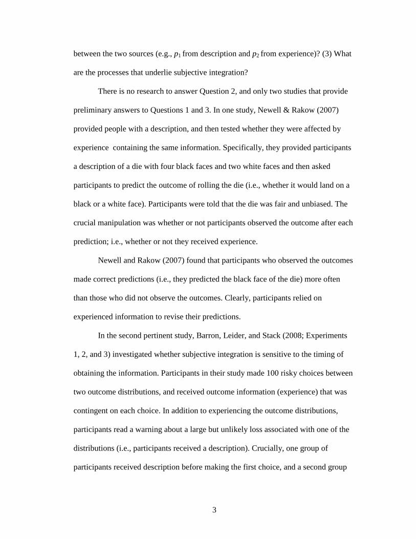
There is no research to answer Question 2, and only two studies that provide

preliminary answers to Questions 1 and 3. In one study, Newell & Rakow (2007)

provided people with a description, and then tested whether they were affected by

experience containing the same information. Specifically, they provided participants

a description of a die with four black faces and two white faces and then asked

participants to predict the outcome of rolling the die (i.e., whether it would land on a

black or a white face). Participants were told that the die was fair and unbiased. The

crucial manipulation was whether or not participants observed the outcome after each

prediction; i.e., whether or not they received experience.

Newell and Rakow (2007) found that participants who observed the outcomes

made correct predictions (i.e., they predicted the black face of the die) more often

than those who did not observe the outcomes. Clearly, participants relied on

experienced information to revise their predictions.

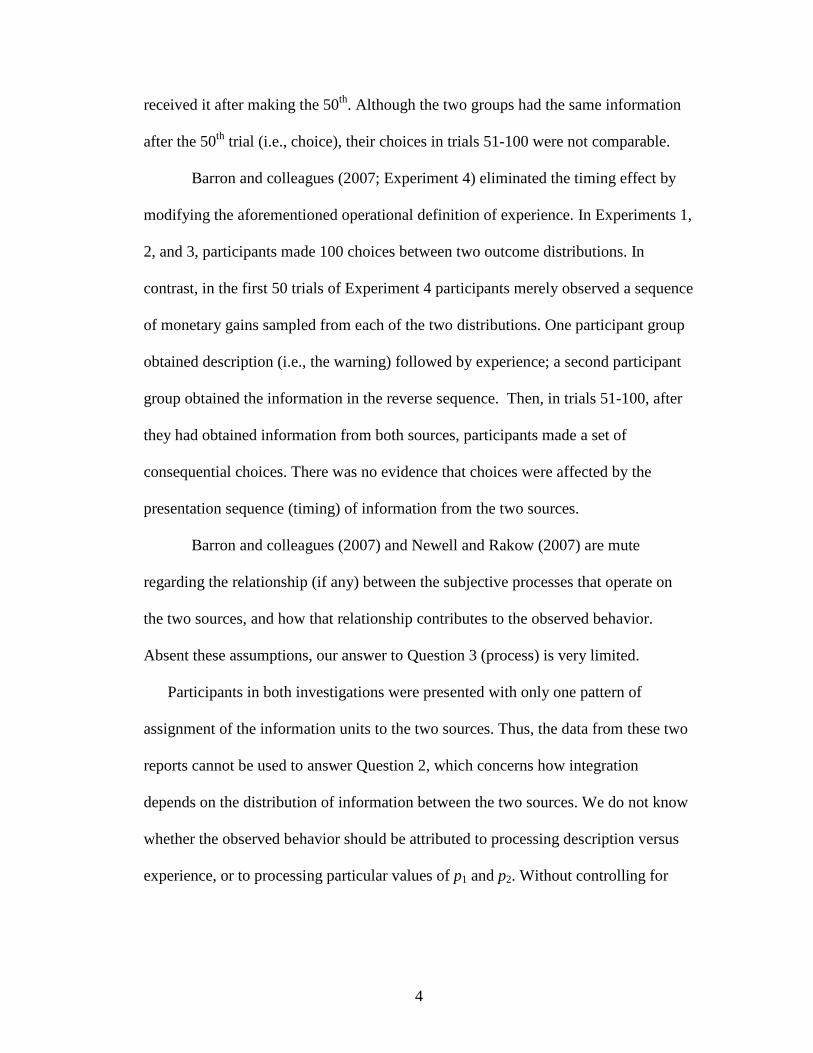
In the second pertinent study, Barron, Leider, and Stack (2008; Experiments

1, 2, and 3) investigated whether subjective integration is sensitive to the timing of

obtaining the information. Participants in their study made 100 risky choices between

two outcome distributions, and received outcome information (experience) that was

contingent on each choice. In addition to experiencing the outcome distributions,

participants read a warning about a large but unlikely loss associated with one of the

distributions (i.e., participants received a description). Crucially, one group of

participants received description before making the first choice, and a second group

4

received it after making the 50th. Although the two groups had the same information

after the 50th trial (i.e., choice), their choices in trials 51-100 were not comparable.

Barron and colleagues (2007; Experiment 4) eliminated the timing effect by

modifying the aforementioned operational definition of experience. In Experiments 1,

2, and 3, participants made 100 choices between two outcome distributions. In

contrast, in the first 50 trials of Experiment 4 participants merely observed a sequence

of monetary gains sampled from each of the two distributions. One participant group

obtained description (i.e., the warning) followed by experience; a second participant

group obtained the information in the reverse sequence. Then, in trials 51-100, after

they had obtained information from both sources, participants made a set of

consequential choices. There was no evidence that choices were affected by the

presentation sequence (timing) of information from the two sources.

Barron and colleagues (2007) and Newell and Rakow (2007) are mute

regarding the relationship (if any) between the subjective processes that operate on

the two sources, and how that relationship contributes to the observed behavior.

Absent these assumptions, our answer to Question 3 (process) is very limited.

Participants in both investigations were presented with only one pattern of

assignment of the information units to the two sources. Thus, the data from these two

reports cannot be used to answer Question 2, which concerns how integration

depends on the distribution of information between the two sources. We do not know

whether the observed behavior should be attributed to processing description versus

experience, or to processing particular values of p1 and p2. Without controlling for

5

these possibilities, we cannot assess the quality of the integration and answer

Question 1.

A Theoretical Framework of Subjective Information Integration

The experimental paradigms employed to test how people integrate

description and experience [i.e., the paradigms used by Barron and colleagues (2007)

and by Newell and Rakow (2007)] are similar in important ways to those employed to

test people’s performance in other integration tasks (e.g., Bayesian inference,

Wallsten, 1972; risky choice, Anderson & Shanteau, 1970; person perception, Fiske,

1980; perceptual judgments; Mellers & Birnbaum, 1982). All of these paradigms

consist of providing participants with some information and subsequently testing

whether and how participants use that information to perform the task specified by

the experimenter.

Performance in the various integration tasks probably relies on a shared set of

processes. Assuming a common process, we can rely on existing frameworks of

integration (e.g., Goldstein & Einhorn, 1987; Massaro & Friedman, 1990; Mellers &

Birnbaum, 1982; N. Anderson, 1971; Wallsten, 1972) to theorize about the processes

that underlie the integration of description and experience.

Many information integration frameworks relate the observed behavior to

experimental stimuli by assuming three underlying processes: scaling, integration and

response (e.g., Goldstein & Einhorn, 1987; Massaro & Friedman, 1990; Mellers &

Birnbaum, 1982; N. Anderson, 1971). The observed behavior can be expressed as a

6

composition of three functions corresponding to the three processing assumptions

(Mellers & Birnbaum, 1982).

Figure 1 provides a visual representation of integration models that follow this

scheme. Scaling transforms a physical stimulus P into a subjective stimulus p

(Mellers & Birnbaum, 1982) by the psychophysical function, Φ , i.e., )(Pp Φ= .

Integration refers to the process that actually combines the subjective stimuli (e.g.,

Massaro & Friedman, 1990). Limiting the exposition to the integration of two stimuli,

the aggregation assumption is expressed as function Ω that takes stimuli ip and jp as

input and yields a new datum, jir , , as output. [i.e., )( ,, jiji ppr Ω= ]. The response

assumption specifies the transformation of the subjectively integrated information to

overt and therefore measurable behavior. Specifically, the transformation

function,Ψ , translates the new datum to an observed response, )(ˆ,, jiji rR Ψ= .

Figure 1. Outline of the information integration model (based on Mellers &

Birnbaum, 1982)

7

We rely on this approach to develop a set of models for the current integration

task. The intuition for the models follows the formal development. For ease of

presentation, we specify the response, aggregation and scaling assumptions in this

order.

Response. The response function formalizes assumptions about the

transformation of covert information into an overt (measurable) response (e.g., Erev,

Wallsten, & Budescu, 1994). Here, we assume that the observed response is identical

to the covertly integrated stimulus (for a similar approach, see Anderson & Shanteau,

1970). Formally,

jiji rR ,, = . (1)

Aggregation. The current integration task involves estimating a population

mean based on two sample outcomes. In all that follows, we assume independent

samples of equal size n. Thus, the normatively prescribed integration procedure for

this task is to average the two sample means.

Our assumption about the subjective integrator generalizes the prescribed

averaging rule in two respects. One is that the judge does not necessarily treat the two

Subjective stimuli

Covert response

Overt response

Physical stimuli

Scaling Φ

Aggregation Ω

pi

pj

Pi

Pj

ri,j

Response Ψ

jiR ,ˆ

8

samples equally. The other is that the subjective integration mechanism operates on

subjectively scaled inputs, i.e., inputs that differ in systematic ways from those used

by the normative rule.

We refer to the subjectively scaled inputs from description and experience as

Dp and Ep , respectively. The corresponding integration weights are Dw and Ew .

Using this notation, we express our integration assumption,

ED

EEDDEDED ww

pwpwpprR

+

+=Ω== )(ˆ

,, . (2)

To facilitate subsequent development we assume that the weights are normalized

(i.e., 1=+ ED ww ) and rewrite the integration assumption,

EEDDEDED pwpwpprR +=Ω== )(ˆ,, . (2a)

Scaling. The final, but crucial component of our subjective integration model

is the scaling assumption,

( ) )1(505050)( iiiiiiii PPPp κκκ −+=+−=Φ=. (3)

The value of κ governs the relationship between the actual and the subjective sample

percentages. We subscript κ to allow the two sources to be modeled by distinct

parameter values (i.e., yielding a source-dependent scaling of the objective stimulus).

The restrictions on κ (e.g., κ>0) and the justification of these restrictions are detailed

more meaningfully below.

Unlike a standard linear model with a separate parameter for the intercept and the

slope, here the intercept and slope are governed by the single parameter, κ . This

structure is required to maintain the assumption that the transformations are

9

symmetric about %50=P (for related claims, see Anderson & Shanteau, 1970;

Rosenbaum & Levin, 1968). The objective and subjective sample percentages are

identical when 1=iκ . The subjective percentage is less extreme (i.e., closer to 50%)

than the objective percentage when 1<iκ ; the converse is true if 1>iκ .

The synthesis of the aforementioned assumptions yields a formal

representation of the function that relates the human’s overt integration behavior to

the information presented to her. We derive this representation by composing the

functions (Mellers & Birnbaum, 1982) associated with the encoding, integration, and

response assumptions to yield the following expression,

=+=Ω== EEDDEDED pwpwpprR )(ˆ,, (4)

)]1(50[)]1(50[ EEEEDDDD PwPw κκκκ −++−+ . The model with 4 parameters, ωD, ωE, κD, κE, is not identifiable. To see this, we

rearrange the algebra,

( ) ( ) 505050ˆ +−+−= EEEDDD ppR κωκω . (4a)

Thus, the model has two estimable parameters, DDD κωα = and EEE κωα = ,

( ) ( ) 505050ˆ +−+−= EEDD PPR αα (5)

)](1[50 EDEEDD PP αααα +−++= .

The algebraic rearrangement in Equation 5 highlights the fact that it is impossible to

unambiguously interpret the model fits as due to stimulus scaling or stimulus

weighting.

10

The primary vehicle for interpreting the data in the subsequent experiments is

the model specified in Equation 5 (i.e., Equation 5 is the full model). Technical

details about fitting the model to the data, including the model’s error theory, are

provided in the results section of Experiment 1.

Model interpretation. The full model does not incorporate any assumption

about the expected relationship between αD and αE. One possibility is that the two

values are statistically independent of each other. An intuitive interpretation is that

the processes that scale the two sources are unrelated to each other. Other possibilities

include specific relations between αD and αE .

We consider three alternative assumptions about the relationship between the

two coefficients. Each assumption corresponds to a specific hypothesis about the

subjective integration processes. In turn, each hypothesis implies a unique constraint

on the parameter space of the full model (i.e., the values of Dα and Eα in Equation

5). The hypotheses, the corresponding model constraints, and the predicted judgments

are summarized in Table 1.

The tradeoff model is related to the integration assumption. The model

coefficients correspond to the weights that the integrator attaches to the scaled stimuli

(e.g., N. Anderson, 1971). The hypothesis is that the scaled stimuli compete for the

integrator’s limited processing resources (attention; e.g., Goldstein & Einhorn, 1987).

Thus, the weights correspond to stimulus characteristics such as the fluency of

parsing stimuli in different formats (Johnson, Payne, & Bettman, 1988); retrieving

11

them from memory (Weiss & N. Anderson, 1969); their credibility/diagnostic value

(Yaniv, Kleinberger, 2000); and concreteness (Hamilton & Thompson, 2007).

The second and third models reflect the hypothesis that the integrator is

equally sensitive to inputs from the two sources. Equivalently, both models are

motivated by the idea that information processing is source-invariant. The difference

between the two models is in whether they assume optimal weighting of the inputs.

The assumption expressed in the equal-non-normative model is that the scaling of the

objective stimuli is independent of its source. The equal-normative model requires the

subjective stimuli to be identical to their objective counterparts.

Table 1. Hypotheses and corresponding constraints and predictions of the integration models.

Model

Hypothesis Constraint Prediction

Full None )](1[50ˆEDEEDD PPR αααα +−++=

Tradeoff 1=+ ED αα

Equal – non-normative 5.≠= ED αα )21(50)(ˆDEDD PPR αα −++=

Equal - normative 5.== ED αα

Information distribution. Are judgments based on description and experience

affected by the distribution of the information? Specifically, let T and T′ refer to two

distributions of information between the two sources. In T, description provides

information about P1 (and experience provides information about P2), and in

EDDD PPR )1(ˆ αα −+=

)(5.ˆED PPR +=

12

distribution T′, the assignment is reversed. Will judgments based on distributions T

and T′ be related to each other in a systematic way?

As mentioned earlier, the normative principle that is applicable for the current

research is to average the information in P1 and P2. Furthermore, averaging obeys

commutativity. Let R*, RT, and RT′ correspond to the normative judgment and the

judgment based on distributions T and T′, respectively. We

obtain, )(5.)(5. 1221* PPPPRRR BA +=+=== . Thus, from a normative

perspective, judgments based on distributions T and T′ should be identical to each

other.

Previous research on subjective integration suggests that normative principles

cannot account for subjective integration (e.g., Anderson & Shanteau, 1970).

However, there are no hints regarding the effect of information distribution.

One possibility is that the information distribution has no effect. As shown in

Appendix A, this requires the assumption that the two sources are treated equally

(i.e., ED αα = ). Note that this is precisely the prediction of the equal-non-normative

model.

Alternatively, the information distribution will produce deviations from the

prescribed judgment that are equal in magnitude but opposite in sign (i.e., the

deviations are symmetric with respect to the prescribed response). Again, as shown in

Appendix A, this requires a tradeoff between processing the two sources,

(i.e., 1=+ ED αα ). This is precisely the prediction of the tradeoff model.

The final possibility is that the deviations given the two information

assignments are not equal to each other. Continuing the previous developments, this

13

implies that ED αα ≠ and 1≠+ ED αα . Note that within our model hierarchy, only

the full model is consistent with this hypothesis.

Questions of Interest, Predictions, and Hypotheses

The research poses three interrelated questions about the subjective integration of

information from description and experience. 1) Does a normative model of

integration provide a reasonable approximation of subjective integration? 2) If not,

does the integration depend on information assignment? (3) How does the integration

occur?

As in previous research on description and experience (Barron et al., 2008; Hau,

Pleskac, Kiefer, & Hertwig, 2008), we operationally define the two modes as

different methods of obtaining information about a population of outcomes.

Experience refers to information obtained from sampling individual outcomes from

the population. Description refers to information obtained from a numerical summary

of a sample (i.e., 80% of the chips are red).

We investigated subjective integration in a task that normatively requires

averaging information from two samples to yield an estimate of the corresponding

population average. The two samples provided information about the composition of

a bag of red and blue chips (c.f., Phillips & Edwards, 1966; Pitz, Dowling, &

Reinhold, 1967). In any one trial, participants experienced a sample by observing a

sequence of sampled chips and received a description of another sample in the form

of a summary its composition. After receiving the information in both samples,

14

participants estimated the percentage of red chips in the bag (i.e., the population

parameter). Participants were told that the description was reliable, and received

information indicating that the two samples associated with each bag consisted of the

same number of chips.

The task was designed such that each pair of samples from a particular bag

appeared in two experimental conditions over the course of a session. In one

condition, sample A was experienced and sample B was described and in the second

condition, sample A was described and sample B was experienced.

This judgment task was implemented in three experiments. Experiments 1 and 2

manipulated the presentation order of the two sources, while Experiment 3

manipulated the format of the description.

Normatively, integration is unaffected by format, by presentation sequence, or by

how information is distributed to the two sources (the sample assignment). This view

implies that participants recognize the formal structure of the task and use the

prescribed averaging rule to integrate the information (c.f., the script in Hertwig &

Hortmann, 2001). Stated differently, the normative viewpoint predicts that the source

of the information (and other features associated with it; e.g., presentation sequence)

will not affect subjective integration.

A large body of empirical evidence yields the opposite expectation. Human

judges are affected by the context (i.e., source, format, presentation sequence)

associated with the information. The expectation is supported by research on tasks

that examine information integration in belief updating (Philips & Edwards, 1966),

impression formation (N. Anderson, 1967), and perceptual judgments (Mellers &

15

Birnbaum, 1982). Additional evidence related to the distinction between description

and experience (e.g., using advice, Yaniv & Kleinberg, 2000; frequency versus

probability formats; Gigerenzer & Hoffrage, 1995; product preference given exposure

to trial versus ads; Hamilton & Thompson, 2007) motivates a more specific

expectation that experience will be more prominent than description in the integrated

output.

We interpret how participants produced their judgments (i.e., their estimates of

the percentage of red chips) by fitting a hierarchy of integration models, as shown in

Table 1, to the participants’ judgments. The fit of any given model yields estimates of

the weights allotted to each information source. Comparing levels of fit across models

allows us to identify the most likely description (among those considered) of the

subjective integration process.

16

Chapter 2: Experiment 1

The purpose of the experiment was to assess the quality of the integration of

probabilistic information obtained from description and from experience. The

experiment was designed to assess whether the integrator’s use of the information

depended on the source that provided it, and whether the integration was sensitive to

the presentation order of the two sources.

Method

Participants. One hundred sixty-two University of Maryland, College Park

undergraduate students participated for course credit. In addition, they received a

reward contingent on the accuracy of their judgment (see below).

Stimuli. Two sets of bags were used in the experiment. Bags in the “identical-

percentage” set were associated with pairs of samples that contained an identical

percentage of red chips. Bags in the “different-percentage” set were associated with

pairs of samples that differed in the percentage of red chips. The two samples were

either categorically congruent (i.e., both PD > 50% and PE >50% or both PD < 50%

and PE < 50%) or categorically incongruent (i.e., one of PD and PE less than 50% and

one greater than 50%). There were 10 and 18 bags in the identical- and different-

percentage sets, respectively. All of the identical-percentage bags and 14 different-

percentage bags were used in the main experiment. The remaining four different-

percentage bags were used for practice. The sample size (i.e., the number of chips in

the samples) ranged over trials from 8 to 13 and was always the same for a pair of

17

samples in a given trial. The sample and population percentages of red chips ranged

from 14% to 86% (see Appendix B).

Procedure. Participants were presented with instruction screens, followed by

one trial with each of the practice bags. Participants typed their responses, and were

then prompted to ask the experimenter for clarifications about the task. The responses

obtained on the practice trials were excluded from the data analyses. After this,

participants completed two trials with each of the experimental bags for a total of 52

trials (i.e., 4+2x24).

The practice trials and experimental trials were identical in design.

Participants initiated each trial by clicking a button. Each trial consisted of three

parts. One, participants clicked a button to draw one chip from one sample, and

continued clicking the button until they had viewed each of the chips in that sample.

The chip appeared on the display 500ms after each click, and remained visible until

the next button click. Two, participants clicked a button to receive the description of

the second sample. The description consisted of a picture of “Mr. Rick” (i.e., the

source of the description), the number of chips that he sampled, and the percentage of

red chips he observed. This information remained visible until the participant’s next

click. Three, participants typed their estimate of the percentage of red chips in the

bag. The experiment was programmed so that only integers in the [1, 99] interval

were accepted.

Participants were randomly allocated to two experimental conditions. One group

of participants (n = 82) obtained information from experience and then from

description (i.e., Experience-1st). A second group (n = 80) obtained information on

18

each trial from description and then experience (i.e., Experience-2nd). Two bag

presentation sequences were counterbalanced across participants. The sequences were

arranged so that the first and second presentation of each bag occurred in the first and

second block of 24 consecutive experimental trials, respectively. The presentation of

bags in the identical- and different-percentage sets was intermixed within each block.

The two blocks differed from each other in the information assignment of each of

the different-percentage bags. In one block, the extreme sample associated with each

bag was experienced and the moderate sample associated with each bag was

described (e.g., %80=EP and %60=DP ). In the second block, this assignment was

reversed. The order of the two blocks was counterbalanced across participants.

The computer scored the accuracy of the participant’s response on each trial using

the following rule, ])(1[100 2*RRs −−= , where R and *R correspond to the observed

and the prescribed response, respectively. At the end of the participant’s session, the

computer computed the participant’s average score from the scores associated with

the 48 experimental trials. The average score is bounded in [0, 100]; the value of

s determined the probability that the participant earned a reward (i.e., a commuter’s

mug). Since participants did not receive any feedback in the course of the experiment,

the reward could not affect the data analyses and is not considered further.

Results

Figure 2 provides some orientation to the analyses. The two panels plot the

across-participant average response as a function of the prescribed response

associated with each bag. The left and right panels correspond to responses obtained

in the Experience-1st and Experience-2nd conditions, respectively. Within each panel,

19

the filled squares correspond to trials in which the experienced sample contained a

more extreme percentage than the described one contained, the empty diamonds

correspond to trials with the reverse assignment (i.e., the experienced sample was less

extreme than the describe one), and the asterisks correspond to trials in which the

experienced and described samples contained identical percentages.

The data in Figure 2 suggest that there was less bias when experience was first

rather than second. Furthermore, when experience and description were identical,

judgments were too moderate. Finally, there is also some indication of the effect of

the information assignment. The responses were too extreme when the experienced

sample was more extreme than the described one. Conversely, the responses were too

moderate when the experienced sample was more moderate than the described one.

Experience 1st Experience 2nd

Figure 2. Observed judgments as a function of the prescribed judgments in Experiment 1. Filled squares – experience more extreme than description; empty squares – experience more moderate than description; asterisk – identical outcomes.

20

The analyses evaluate the quality of the observed judgments by testing for a

systematic bias relative to the prescribed judgments. Thus, the analyses rely on the

difference (δ) between observed judgment, R, relative to the prescribed

judgment,*R . Two bias measures based on δ are used. One, the signed bias, defined

as *RR −=δ if 50* >R , and RR −= *δ if 50* <R . Two, the unsigned

(absolute) bias, || *RR −=δ .

Both bias scores measure the location of the observed judgments relative to the

diagonal. The signed bias indicates whether the responses tend to be too moderate or

too extreme, whereas the unsigned bias indexes the consistency of the integration.

The data from one participant in the Experience-1st and two participants in the

Experience-2nd conditions were excluded from all analyses because their signed bias

scores were lower than -18. These scores deviated from the mean of the entire

sample by more than 4.5 standard deviation units (the next highest score was -12.2).

Signed deviations. Judgments, averaged for each participant across all of the

trials, were too moderate (M = -1.48, SEM = .20); the bias was reliable t(158) = 7.49,

p < .001. The conservative response pattern converges with that obtained by most

research on Bayesian updating (e.g., Philips & Edwards, 1966).

We turn to the question of whether the bias was contingent on the sample

assignment and the presentation sequence. By design, the normative judgments

associated with the different-percentage bags were less extreme than those of the

identical-percentage bags. The reliability of the findings is assessed in separate

analyses for each set of bags to avoid a potential confound of this factor.

21

In the same-percentage trials there was a reliable effect of the presentation

sequence, t(157) = 2.78, p < .01. The Experience-1st sequence (M = -1.91) was

associated with less bias than the Experience-2nd sequence (M = -3.79).

Turning to different-percentage trials, the data in Figure 3 show that the direction

of the bias followed the extremity of the experienced sample. That is, responses

tended to be too extreme when the experienced sample was more extreme than the

described one and too moderate in the reverse case. The bias is attenuated in the

Experience-1st condition relative to the Experience-2nd condition.

Figure 3. Signed bias. Extreme and moderate experience refer to the information assignment on each trial (e.g., experienced sample more extreme than described sample).

The information assignment, source sequence, and assignment by sequence

interaction yielded significant effects, F(1, 157) = 44.55, p < .001, F(1, 157) = 6.33, p

< .05, and F(1, 157) = 4.35, p < .05, respectively. The effect of information

22

assignment was reliable in both the Experience-1st and the Experience-2nd sequences,

t(80) = 3.23, p < .005, and t(77) = 6.22, p < .001, respectively. The effect of the

presentation sequence was reliable when experience was moderate, t(157) = 2.96, p <

.005, but not when it was extreme, t < 1.

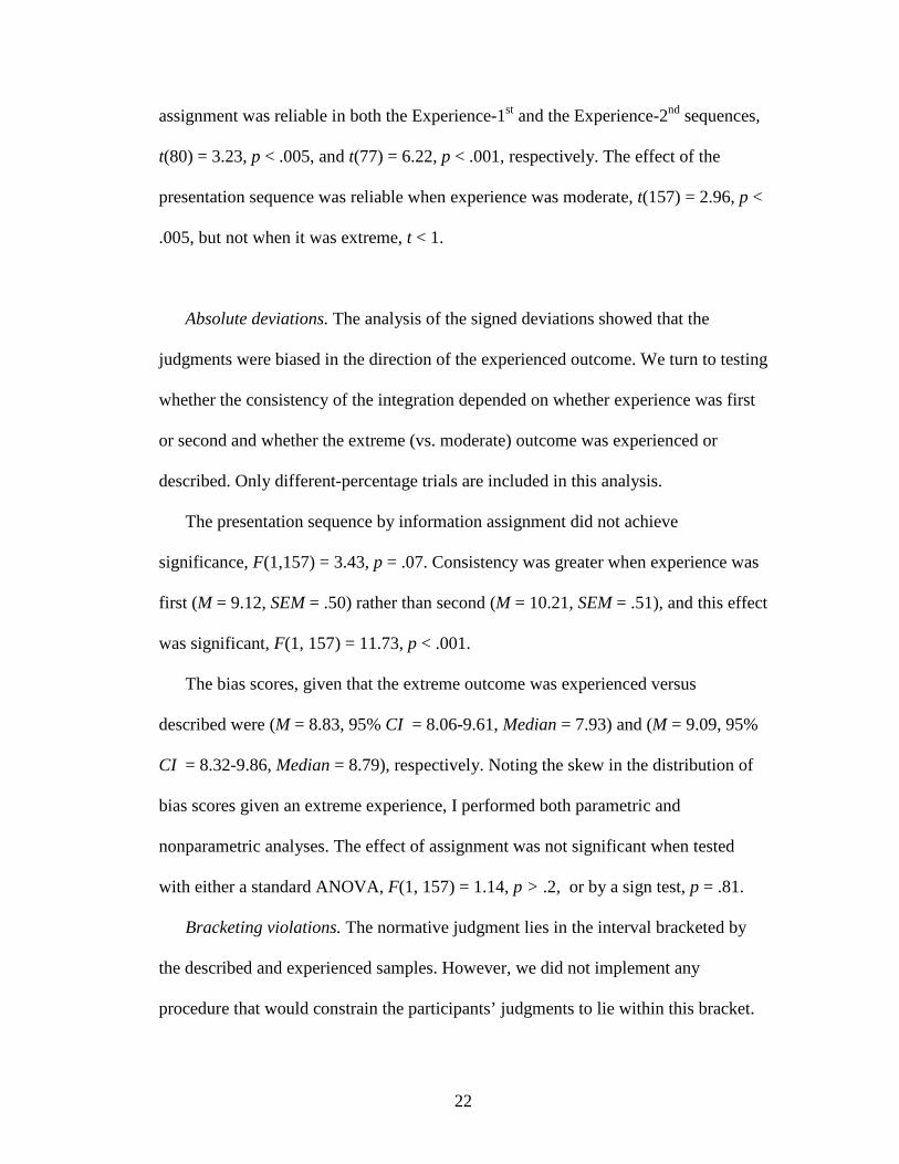
Absolute deviations. The analysis of the signed deviations showed that the

judgments were biased in the direction of the experienced outcome. We turn to testing

whether the consistency of the integration depended on whether experience was first

or second and whether the extreme (vs. moderate) outcome was experienced or

described. Only different-percentage trials are included in this analysis.

The presentation sequence by information assignment did not achieve

significance, F(1,157) = 3.43, p = .07. Consistency was greater when experience was

first (M = 9.12, SEM = .50) rather than second (M = 10.21, SEM = .51), and this effect

was significant, F(1, 157) = 11.73, p < .001.

The bias scores, given that the extreme outcome was experienced versus

described were (M = 8.83, 95% CI = 8.06-9.61, Median = 7.93) and (M = 9.09, 95%

CI = 8.32-9.86, Median = 8.79), respectively. Noting the skew in the distribution of

bias scores given an extreme experience, I performed both parametric and

nonparametric analyses. The effect of assignment was not significant when tested

with either a standard ANOVA, F(1, 157) = 1.14, p > .2, or by a sign test, p = .81.

Bracketing violations. The normative judgment lies in the interval bracketed by

the described and experienced samples. However, we did not implement any

procedure that would constrain the participants’ judgments to lie within this bracket.

23

The participant’s judgment violates the bracket whenever it falls outside the interval

bounded by PD and PE (c.f., Soll & Larrick, 2009). We assess the occurrences of

bracketing violations, because as we see in the next section, these violations must be

considered in applying the subjective integration models.

The analysis of the bracketing violations is based on judgments associated with

the different-proportion trials. The mean, median and modal number of bracket

violations per participant was 5.8, 5.0, and 1.0 (out of 28 trials), respectively. The

minimum and maximum number of violations (per participant) were 0 (n = 18) and

21 (n = 1).

Modeling Subjective Integration of Description and Experience

The purpose of fitting the integration models (Equation 5 and Table 2) to the

observed judgments is twofold. One, the fits yield maximum likelihood parameter

estimates for each participant that allow interpretation of the observed judgments in

terms of the participant’s sensitivity to information provided by the two sources (i.e.,

corresponding to the values ofDα and Eα ). Two, the model comparisons allow tests

of hypotheses about the integration process (more precisely, the relationship between

the two α s).

Maximum likelihood estimation procedure

24

This section details the application of the maximum likelihood procedure to

the full model (Equation 5). The modifications of this procedure for the nested

models are detailed at the end of the section.

The full model yields an expression for the predicted judgment, R , in terms

of the information from the two sources and the associated weights. Allowing for

trial-by-trial variability, ε, the observed judgment1, R, can be expressed as ε+= RR ˆ .

We assume a normal distribution of ε s with mean θ and standard deviationς .

The four parameters of the full model (i.e., ),,, ζθαα ED were selected

separately for each participant to maximize the log likelihood of the distribution of

RR ˆ−=ε for that participant. The expression for the log likelihood of ε given the

model predicted judgment is,

])(ln[28

1∑=

=t

tfL ε , (6)

where )( tf ε refers to the likelihood of the residualε under N(θ, ζ) associated with the

participant’s response on trial t. To reiterate, this procedure identifies four parameters

that maximize the value of L in Equation 6.

The selection of the four parameters was subject to the following constraints.

The starting values ofDα , Eα ,θ , and ζ were .5, .5, 0, and 12, respectively. The

starting value for ζ was informed by some pilot runs with the model. The

permissible range of values of θ and ζ was 90|| <θ and 4001. << ζ .

1 All of the integration models yield a prediction for each participant on each trial. The use of subscripts for the participant, trial, and model is minimized for ease of presentation.

25

The permissible range of values of Dα and Eα was guided by a methodological

and an empirical consideration. By design, participants were required to make

judgments in the [1, 99] interval. This implies that the model should not be permitted

to make predictions outside this interval. Empirically, we observed bracketing

violations. These violations can be interpreted as a subjective stretching or shrinking

of the response scale. I constrained theα s to the [-1, 1] interval. This range is

necessary to allow the model to predict the bracketing violations. At the same time,

this range also allows the model to predict judgments outside the [1, 99] interval.

The only difference between this procedure and the procedures for the nested

models was the constraint that was imposed on the model parameters (e.g., in the

procedure for the tradeoff model, )1 DE αα −= . Values of θ and ζ were selected

separately for each participant and each model.

Maximum likelihood parameter estimates

The maximum-likelihood parameter estimates of Dα and

Eα from the full model,

as well as DE ααα −=∆ , are summarized in Table 2. The summary for each

parameter and their difference includes the across-participant mean and the 95%

confidence interval.

Note that αE is consistently greater than .50 and αD is consistently less than .50,

suggesting that the experienced sample is accorded an excessively extreme subjective

value and the described value is accorded an excessively moderate subjective value.

The deviations were larger for description than for experience.

26

Table 2. Description and Experience Coefficients (Experiment 1).

Dα Eα α∆

Presentation sequence M CI M CI M CI

Experience-1st (n = 81) .40 .36-.45 .56 .51-.61 .16 .06-.25

Experience-2nd (n = 78) .29 .24-.34 .58 .54-.63 .29 .20-.38

Note. CI refers to the 95% confidence interval.Dα and Eα correspond to the

sensitivity to description and experience, respectively. DE ααα −=∆ .

The difference between the two coefficients, DE ααα −=∆ , provides a more

concise indication of the differences in processing experienced versus described

probabilistic information. The mean values are positive and the confidence intervals

do not bracket zero, indicating that the sensitivity to experience was reliably larger

than that of description (see Table 2).

A multivariate analysis of variance (MANOVA) with the two coefficients as the

dependent variables and the presentation sequence as its factor yielded a significant

effect, F(2, 156) = 6.76, p < .005. Univariate analyses yielded a reliable effect on Dα ,

F(1, 157) = 9.44, p < .005, but not on Eα , F < 1.

The across-participant distribution of the coefficients provides some evidence

that the processes that operate on the two sources were related to each other.

Specifically, the Pearson correlation (r) between Dα and Eα was -.69, p < .001.

Thus, across participants, the sensitivity to description is inversely related to the

sensitivity to experience.

27

As noted earlier, the two α s were estimated subject to the restriction that they

ranged in the [-1, 1] interval. This restriction reduces, but does not eliminate the

chances that the model would yield predictions outside the [1, 99] interval.

The effectiveness of the restriction was assessed by computing the actual range of

the model predictions for each participant. The restriction was effective, as indicated

by the finding that the range of the model predictions for all of the participants was

below 1002. However, for one participant, 1=Dα , and for seven subjects, 1=Eα ;

there were no other cases in which the coefficients were on the boundaries of the

permissible range (i.e., [-1, 1]).

We present the correspondence between the model-predicted judgments and the

observed judgments in Figure 4. Each point is a model prediction for a given pair of

samples in a particular assignment to description and experience. The predicted

values are based on the coefficients in Table 2 (i.e., the across-participant mean

values). Overall, the correspondence between observed and predicted judgments

appears adequate, with the exception of more scatter in the Experience-2nd sequence.

Analyses of the error parameters of the full model yielded an unexpected pattern.

The residuals (i.e., theε s associated with the model predictions), averaged over

participants, were biased, 70.=θ (SEM = .22). This bias was reliably different from

zero, t(158) = 3.15, p = .002. The bias in the two presentation sequences was

comparable, t < 1. Second, the scatter of the residuals (i.e.,ς ) in the Experience-1st

condition (Median = 6.40) was lower than in the Experience-2nd condition (Median =

9.07). The difference was reliable, per a Mann-Whitney U test (p < .001).

2 The three participants that were excluded from the analyses had the smallest range of predicted responses.

28

0

25

50

75

100

0 25 50 75 100Predicted

Obs

erve

d

0 25 50 75 100Predicted

Experience-1st Experience-2nd

Figure 4. Predicted judgments as a function of observed judgments in Experiment 1. Filled squares = experienced outcome more extreme than described outcome; empty squares = experienced outcome more moderate than described outcome.

Model comparisons

The tradeoff, equal-normative, and equal-non-normative models shown in Table 1

are nested under the full model. Thus, the full model was compared to each of the

nested models by computing the difference in log likelihood as follows, G2 = 2 (Lfull –

Lm), with m indexing the nested model (e.g., the tradeoff model). The G2 statistic is

chi-square distributed with degrees of freedom equal to the difference in the number

of parameters (Riefer & Batchelder, 1988). For example, the comparison of the full

and the tradeoff models involves df = 4 – 3 = 1). We fit the models to the data of each

participant separately and, in addition, summed the G2 values and degrees of freedom

over participants to yield a single more powerful test at the group level. All model

comparisons rely on α =.05.

29

By-subject analysis. The results of the by-subject comparisons are summarized in

Table 3. The values in each row correspond to the proportion of participants for

whom the model on the given row was not significantly different from the full model

(per the G2 test). Table 3 reveals that the tradeoff model is the only viable candidate

for most participants. This finding is expected considering the inverse relationship

between the coefficients estimated from the full model. Support for the tradeoff

model was comparable across the two presentation sequences (a χ2 test performed on

the proportions in the top row of Table 3 yielded p > .2).

Table 3. Results of Nested Model Comparisons (Experiment 1) Presentation sequence

Model Experience -1st Experience-2nd

Tradeoff .80 .73

Equal-non-normative .44 .40

Equal-normative .43 .33

Note. The value in each cell corresponds to the proportion of participants for whom the model in the given row provides a comparable fit to the full model per the G2 test. Thus, higher values indicate better fitting models.

The G2 statistic is limited to comparisons between nested models and so cannot be

used to compare the tradeoff and equal-non-normative models, which are not nested.

An alternative way to compare these two models is to compute, for each participant,

the log of the likelihood ratio, )/ln( ET=λ , where T and E correspond to the

likelihoods of the data under the tradeoff and equal-non-normative models,

30

respectively (c.f., Glover & Dixon, 2004). Positive values of λ lend support for the

tradeoff model.

For most participants, the tradeoff model was preferred to the equal non-

normative model. The values of λ were positive (λ ≥ .03) for 73.3% of the

participants and negative for the others (λ ≤ -.01). The proportion of positive λ is

reliably different from chance (i.e., equally probable positive and negativeλ ), p <

.001, per a binomial test. The λ s in the two presentation sequences were comparable,

(p > .62, per Mann-Whitney U test).

In principle, the tradeoff model could fit better than the equal-non-normative

because it is more flexible, not because it provides a better description. To test this

possibility, I used each participant’s parameter estimates under each model to

generate new data under that model and then fit this generated data with each model.

If one model is more flexible than the other, it should provide the better fit to data

generated by both models. If neither model is more flexible than the other, each one

should be superior at recovering its own data.

The tradeoff model fits its data better than the equal-non-normative model for

81% of the participants. The equal-non-normative model fits its data better than the

tradeoff model for 67% of the participants. These patterns indicate that the superior fit

of the tradeoff model relative to the equal non-normative is not due to differential

flexibility.

Group analyses. The results of the group-level analyses are consistent with

those of the individual-participant analyses. The three restricted models were

significantly worse than the full model. The dfs involved in comparing the tradeoff,

31

equal-non-normative, equal-normative models to the full model were 159, 159, and

318, respectively. The G2 and p values associated with comparing the three models

were 375.5, 2140.0, and 2429.0; for all comparisons, p < .001.

The λ obtained from comparing the tradeoff model to the equal-non-normative

model was 882.3, indicating that the tradeoff model was preferred to the equal-non-

normative model. A similar pattern of results was obtained when each presentation

sequence was examined in isolation.

Discussion

Experiment 1 assessed how decision makers integrate description- and

experience- based probabilistic outcomes. The data showed that (1) overall, the

judgments were too moderate; (2) the participants’ judgments were biased towards

the experienced over the described sample; (3) the judgments were affected by the

sample assignment, particularly when experience followed description.

The model coefficients and model comparisons suggest that the experienced

outcomes were perceived or weighted as too extreme and described outcomes were

perceived or weighted as too moderate. There was also a tradeoff relationship

between processing the two sources.

The model coefficients suggested further that the weight accorded the experienced

sample was insensitive to whether it came first or second. However, the weight

accorded the described sample showed a recency effect in that it was greater when the

described sample was second than when it was first.

32

The absolute deviations and the scatter of the model predictions were sensitive to

the presentation sequence, such that there was less bias and less scatter in the

Experience-2nd sequence. The absolute deviations were comparable in both outcome

assignments.

The interpretation of the poorer integration in the Experience-2nd sequence is not

clear. The model coefficients (i.e., α s) suggest the possibility of retrieval failures of

the description when it appears first (i.e., in the Experience-2nd sequence).

33

Chapter 3: Experiment 2

The findings of Experiment 1 indicated that participants were less sensitive to

described than to experienced samples of information, particularly when the

description was provided first. Pursuing the possibility that the effect is due to

retrieval failure, Experiment 2 was conducted to clarify the role of memory retrieval

in the integration task. The critical manipulation involved the information that was

available during the response phase of each trial, framed in terms of the presence

(versus absence) of description-based and experience-based memory aids. In aid-

absent conditions, information from one source was displayed and then removed

before the display of the information from the second source. Conversely, in the aid-

present conditions, information was displayed and remained visible throughout the

end of the trial.

We orthogonally manipulated the experience- and description- aids in a

factorial design to produce four conditions referred to as D-E-, D-E+, D+E-, and D+E+.

In this notation, the letter corresponds to the source (e.g., D representing description),

and the + and – indicating the presence and absence of the aid, respectively. In the D-

E- conditions, information from one source was displayed and then removed,

information from the second source was displayed and then removed, and then

participants entered their responses (this cell of the design replicates the conditions of

Experiment 1). In the D+E- and D-E+ conditions, the response was entered while the

description (experience) was visible, eliminating the need to retrieve the description

34

(experience). Finally, both sources were visible while the response was entered in the

D+E+ condition; in this condition there was no need to retrieve either source.

Method

Participants. One hundred sixty undergraduate students participated in return for

course credit.

Stimuli. There were eight training and sixteen experimental bags. The bags

differed from those of Experiment 1 in three ways. (1) The two samples associated

with each bag always consisted of unequal but categorically similar proportions (i.e.,

both samples had the same majority color). (2) The samples always consisted of 13

chips. (3) The sample and population percentages ranged from 0 to 100 and from 4%

to 96%, respectively (see Appendix C).

Design. Three variables were manipulated in a full factorial design: the source

presentation sequence (as in Experiment 1), and the presence (vs. absence) of the

description and the experience aids. Participants were randomly assigned to each of

the 8 conditions (i.e., n = 20 in each condition).

Participants received four trials with each experimental bag (as opposed to

two in Experiment 1). As in Experiment 1, the presentations were blocked so that in

each block the extreme and moderate samples were assigned to the description and

experience formats, respectively, or in the opposite arrangement. Half of the

participants received descriptions and experiences of the extreme sample in blocks 1

and 3 and in blocks 2 and 4, respectively. This arrangement was reversed for the other

half. The bag presentation sequence was counterbalanced as in Experiment 1.

35

Procedure. The procedure started with a brief overview of the task.

Participants were presented with instruction screens and then completed 72 trials. For

ease of exposition, details are provided for the procedure in the Experience-1st

sequence. The Experience-2nd sequence is identical, except that experience follows

description.

Participants clicked a button to start drawing the chips in one sample (i.e., to

obtain experience). Each chip was displayed for 1000 ms, and the inter-chip-interval

was 2000 ms. As the chip was removed, a circle was displayed in a rectangular

region next to the picture of the bag. The color of the circle was determined by the

experience aid condition: in the E+ condition the color of a circle matched the color of

the chip that was just drawn from the bag, and in the E- condition the circle was

always gray. The circle remained visible throughout the end the trial. Thus, the

number of circles in the rectangle corresponded to the number of chips observed in

that trial.

After obtaining experience, participants clicked a button to receive the

description of the second sample. The description remained on the screen till the end

of the trial in the D+E- and D+E+ conditions, but was removed after 2500ms in the D-

E- and D-E+ conditions.

Participants provided their estimates with a slider anchored “0% Red” on the

left end, “50% Red” in the middle, and “100% Red” on the right end. Thus, unlike

Experiment 1, participants were not restricted to the [1, 99] interval and they were not

required to type a numerical response.

36

The first eight trials served as familiarization trials; the responses obtained on

these trials were excluded from the data analyses and will not be mentioned further.

After the eighth trial, participants were prompted to ask the experimenter for

clarifications about the task. The familiarization and experimental trials were

identical in design.

Results

The judgments associated with the two replications (trials) of each bag and

sample assignment were averaged prior to conducting the analyses. Thus, the

analyses were based on 32 judgments per participant.

The data from two participants in the D+E+ condition were excluded from all

analyses because their signed bias scores were lower than -45. These scores deviate

from the mean of the entire sample by more than five standard deviations (the next

highest score was -23.7).

The signed bias across all conditions (M = -.19, SEM = .50) was not reliably

different from zero, t < 1. However, the average judgment of 67% of the participants

was too extreme; this percentage is reliably different from chance (p < .001, per

binomial test).

The signed bias scores are presented as a function of the information assignment,

the source presentation sequence and the two aids in Figure 5. Visual inspection of

the data indicates that as in Experiment 1, the direction of the bias is related to the

experienced information (extreme vs. moderate). However, the effect of presentation

sequence is less clear.

37

D- D+

E-

E+

Figure 5. Signed bias in Experiment 2. The four panels correspond to the four levels obtained from the factorial manipulation of the description and experience aids. Rows correspond to levels of the experience aid; columns correspond to levels of the description aid. Triangles – experienced information more extreme than the described one. Circles – experienced information less extreme than described one.

The bias scores were submitted to ANOVA with assignment as the within-

participant factor and presentation sequence, experience aid, and description aid as

the between-participant factors.

The interaction yielded two reliable effects (p > .15 for all the other effects).

Outcome assignment yielded a reliable effect, F(1, 150) = 59.63, p < .001. Judgments

were too extreme when the experienced sample was extreme (M = 2.63, SEM = .7)

and too moderate when the experience sample was moderate (M = -2.98, SEM = .55).

The bias was qualified by the assignment by experience aid interaction, F(1, 150)

= 4.2, p < .05. To facilitate exposition, the signed bias scores (i.e., Figure 5) are re-

38

arranged and re-presented in Figure 6. The experience aid affected the judgments

when the experienced information was more extreme than the described one, but not

when the reverse was true, respectively, t(156) = 2.12, p < .05, and t(156) < 1. The

difference between the two information assignments was reliable when the aid was

absent, t(79) = 3.71, p < .001, and when it was present, t(77) = 7.87, p = .001. The

bias (M = 1.19, SEM = .94) in the aid-absent extreme-experience condition was not

significantly different from zero, t(79) = 1.27, p = .21. Conversely, the bias in the

three other conditions was reliable (all ts>3.7).

Figure 6. Signed bias as a function of experience aid and experienced sample.

39

Absolute bias. The unsigned bias scores are presented as a function of the two

aids, the source presentation sequence and the information assignment in Figure 7.

The panels are arranged as in Figure 5.

D- D+

E-

E+

Figure 7. Absolute bias in Experiment 2. The four panels correspond to the four levels obtained from the factorial manipulation of the description and experience aids. Rows correspond to levels of the experience aid; columns correspond to levels of the description aid. Triangles – experienced outcome more extreme than described one. Circles – experienced outcome less extreme than described one.

The bias scores were submitted to ANOVA with information assignment as the

within-participant factor and presentation sequence, experience aid, and description

aid as the between-participant factors. The effect of information assignment was

reliable, F(1, 150) = 46.26, p < .001. More bias was observed when the experienced

40

outcome was more extreme (M = 9.59, SEM = .38) relative to more moderate (M =

7.65, SEM = .35). Inspection of the data at the individual-participant level reveals that

this pattern was true for 73% of the participants; i.e., most participants had more bias

when experience was extreme rather than moderate.

The assignment by presentation sequence and assignment by presentation

sequence by description aid interactions were marginally significant, F(1, 150) =

3.13, p < .08 and F(1, 150) = 3.12, p < .08. The assignment by experience aid

interaction was reliable, F(1, 150) = 5.96, p < .05. Experience aid did not yield

reliable effects regardless of whether experience was more extreme or more moderate

than description (p > .2, per paired-sample t-tests). The interpretation of these

interactions is unclear.

Bracketing violations. The mean, median and modal number of bracket violations

per participant was 4.0, 3.0, and 2 (out of 32), respectively. The minimum and

maximum number of violations (per participant) were 0 (n = 22) to 24 (n = 1).

Maximum likelihood parameter estimates

The model derivation and analyses were conducted in the same manner as in

Experiment 1. The description and experience coefficients (i.e., Dα and

Eα )

estimated from the full model indicated that participants were over-sensitive to

experience and under-sensitive to description (see Table 4). The two coefficients were

inversely related to each other, r = -.52 (p < .001).

41

Table 4. Description and Experience Coefficients (Experiment 2).

Dα

Eα α∆

Aid M CI M CI M CI

D-E- .35 .29-.40 .58 .52-.64 .23 .14-.32

D+E- .42 .34-.50 .54 .45-.64 .12 -.04-.29

D-E+ .35 .29-.41 .64 .56-.71 .29 .18-.39

D+E+3 .34 .28-.40 .66 .58-.73 .31 .19-.43

Note. CI refers to the 95% confidence interval. Dα and Eα correspond to the estimated

coefficients of description and experience. DE ααα −=∆ .

The data in Table 4 suggest that Eα was affected by the experience aid. A

MANOVA with the two coefficients as the dependent variables and the presentation

sequence and aids as its factors yielded no significant effect for these factors or their

interactions (p > .1 for all tests). Univariate analyses yielded a reliable effect of the

experience aid onEα , F(1,150) = 4.57, p < .05.

The restriction imposed on the model coefficients was more problematic relative

to Experiment 1. Specifically, the model predicted responses outside the [0, 100]

range for 24 (15%) participants. For 14 participants (9%), 1=Eα .

Analyses of the error parameters of the full model yielded an unexpected pattern.

The residuals (i.e., theε s associated with the model predictions), averaged over

participants, were biased, θ 15.1−= (SEM = .17). This bias was reliably different

from zero, t(157) = 6.76, p < .001. There were no reliable differences as a function of 3 The description- and experience- coefficients for the two participants excluded from this condition were negative. All other participants had at least one positive coefficient.

42

presentation sequence, description aid, or experience aid (p > .08, for each

comparison). Likewise, the scatter of the residuals (i.e.,ς , Median = 6.0) was

unaffected by the presentation sequences or aids (p > .1, Mann-Whitney U test for

each comparison).

By-subject analysis: The full model is reliably better than the three restricted

models in describing the data of most participants (see Table 3). The G2 comparisons

between the fit of the full model and that of the tradeoff, equal-non-normative and

equal-normative models were not significant for 41%, 40% and 19% of the

participants. There were no reliable differences in the support for the full model as a

function of presentation sequence, description aid, and experience aid (i.e., the χ2 tests

on the proportions were not reliable, p > .31).

The comparison between the tradeoff and equal-non-normative models showed

that they were comparable. The values of λ were positive (≥.01) for 45.1% of the

participants and negative for the others (< -.04). The proportion of λ s with positive

and negative values were comparable (p > .1 per a binomial test). Presentation

sequence, experience aid and description aid had no reliable effect on λ (p > .8 by

Mann-Whitney U test).

The test for differential model flexibility revealed that the tradeoff and equal non-

normative models recovered their own data for 84% and 78% of the participants,

respectively. These patterns indicate that the fits of the models to the observed data

are not due to differential flexibility.

43

Group analysis: The dfs involved in comparing the tradeoff, equal-non-

normative, and equal-normative models to the full model were 158, 158, and 316.

The G2 and p values associated with comparing the three models were 1898.2,

2660.2, and 4166.0; for all comparisons, p < .001. Thus, the full model was

significantly better than each of the three restricted models.

The λ obtained from comparing the tradeoff model to the equal-non-normative

model was 381.0, lending support for the tradeoff model over the equal-non-

normative model.

Discussion

Participants’ judgments were biased in the direction of their experience. More

importantly, the magnitude of the bias depended on the information assignment.

Judgments based on extreme experience and moderate description were more biased

than those based on the reverse assignment. This finding shows that the quality of the

integration judgment depends not only on the differential subjective sensitivity to the

two sources, but also on the information that they convey.

The effect of presentation sequence found in Experiment 1 was not replicated.

The interaction of description aid, assignment, and presentation sequence on the

absolute bias measure was marginally significant and its interpretation unclear.

Experience aid yielded a reliable effect on Eα and a reliable interaction with the

information assignment as indexed by both bias measures.

44

Why was the effect of the presentation sequence in Experiment 1 not

replicated? The designs of the two experiments differed from each other in a number

of ways precluding a definite interpretation. However, a likely contributor to the

findings is the use of a different response mode in each experiment. In Experiment 1

participants typed their response while in Experiment 2 they adjusted a slider. The

response format in Experiment 2 appears to be equally compatible with the format of

the two information sources. In contrast, the response format in Experiment 1 appears

to be more compatible with the format of described information relative to that of

experienced information. Importantly, this compatibility is psychologically more

salient in the Experience-1st condition (i.e., because the description immediately

precedes the response) relative to the Experience-2nd condition (i.e., because the

description does not immediately precede the response).

The effect of the response format provides an alternative interpretation to the

findings of Experiment 1 and a context for interpreting some findings of the current

experiment. In Experiment 1, the sensitivity to description in the Experience-1st

condition was superior to that in the Experience-2nd condition because of the temporal

proximity to the compatible response format. According to the response-format

account, there were no effects of presentation sequence in Experiment 2 because the

response scale is equally compatible with both sources.

The response-format and retrieval-failure accounts rival each other. The

possibility that retrieval failures are not a factor in the integration task could explain

why the description aid (which was designed to eliminate the retrieval failures)

yielded no reliable effects.

45

Experience aid increased the signed bias when the experienced outcome was

more extreme than the described one. Stated differently, given an extreme experience

and moderate description, the presence of the experience aid shifts the judgments

closer to the experienced outcome. Experience aid also had a reliable effect on Eα but

no main effect per the signed bias measure. How could the experience aid affect the

signed bias and model coefficients while not affecting the unsigned bias? The

proffered interpretation is that the presence of the aid eliminates confusion involved

in trial-by-trial counting of red chips. Having removed the effect of counting

confusions allows systematic experience-related biases to be more discernible.

46

Chapter 4: Experiment 3

Research on Bayesian inference shows that information presented in a

percentage or probability format leads to judgments that are inconsistent with the

Bayesian prescription (c.f., Gigerenzer & Hoffrage, 1995). Other research on the use

of advice shows that people perceive information from an external source as less

reliable than their own (internal) information (e.g., Yaniv & Kleinberger, 2000). In

the first two experiments, description provided information from an external source in

a percentage format. Consistent with the previous findings, the judgments in the first

two experiments were biased away from description.

Experiment 3 served two purposes. One was to examine whether the bias

observed in the first two experiments was the consequence of using the percentage

format to convey the description. Thus, I tested whether the bias persists when the

description is provided in a relative frequency format rather than a percentage format.

The prediction from research on the role of format in Bayesian inference [e.g.,

Cosmides & Tooby (1996); Gigerenzer & Hoffrage (1995)] is that the frequency

format would lead to superior integration than the percentage format. The second

purpose was to relate the bias to the perceived trustworthiness of the source of the

description.

Method

Participants, Stimuli, and Design. Fifty-eight undergraduate students

participated in return for course credit. The bags in this experiment were the same as

47

those of Experiment 2. The presentation sequence was not manipulated; only the

Experience-2nd sequence was used. Participants received two trials with each of the

experimental bags (as in Experiment 1). The description format, percentage or

frequency, was manipulated between-participants. Other details of the design were

similar to those of condition D-E- in Experiment 2.

Procedure. The procedure was identical to that in the D-E- condition of

Experiment 2, except for the following differences. (1) There were 32 experimental

trials, consisting of two replications of each bag (in Experiment 2, there were four

replications of each bag totaling 64 trials). (2) The gray circles and the surrounding

rectangular region displayed in Experiment 2 were removed. (3) After completing the

last trial, participants judged the following statement, “I trusted Mr. Rick to provide

reliable information about the bag of chips.” Participants responded by marking a 5-

point scale labeled with “Completely disagree”, “Somewhat disagree”, “Neutral”,

“Somewhat agree” and “Completely agree”.

Results

The analyses are based on 32 responses per participant. The presentation of

the data is comparable to that used in Experiment 1 and 2. All of the participants had

signed bias scores within 4SDs of the sample mean and were included in the analyses.

Signed bias score. The judgments were moderate or regressive relative to the

normative values, although the bias (M = -.55, SEM = .93) was not reliable (t < 1). As

in the first two experiments, the direction of the bias was related to the experienced

48

outcome. However, Figure 8 shows that the contingency between the bias and the

experienced outcome was pronounced when the description was presented in the

percentage format but not in the frequency format. The assignment by format

interaction was significant, F(1,56) = 4.42, p < .05. Assignment produced a reliable

effect, F(1, 56) = 9.47, p < .005, while the format did not, F(1, 56) = 1.65, p = .21.

Assignment yielded a reliable effect when the description was formatted as a

percentage, t(29) = 3.09, p < .005, but not when it was formatted as a relative

frequency, p > .2.

The signed deviations were reliably different from zero when the description

was presented in the percentage format and the experience outcome was moderate

and, t(29) = 4.19, p < .001. In the three other conditions, the signed deviations were

not reliably different from zero, p > .2.

Figure 8. Signed bias in Experiment 3. Triangles – experienced outcome more extreme than described one. Circles – experienced outcome less extreme than described one.

Absolute bias. Figure 9 summarizes the bias as a function of format and

outcome assignment. The outcome assignment by presentation format interaction was

49

significant, F(1, 56) = 6.34, p < .05. The difference between the two formats was

marginally significant, F(1,56) = 3.11, p = .08. The effect of the assignment was

reliable, F(1, 56) = 4.17, p < .05. Outcome assignment yielded a reliable effect in the

percentage format, t(29) = 2.99, p < .01, but not in the frequency format, t < 1.

Figure 9. Absolute bias in Experiment 3. Triangles – experienced outcome more extreme than described one. Circles – experienced outcome less extreme than described one.

Bracketing violations. The mean, median and modal number of bracket violations

per participant was 12.0, 11.5, and 10 (out of 32), respectively. The minimum and

maximum number of violations (per participant) were 0 (n = 2) and 24 (n = 1).

50

Maximum likelihood parameter estimates

The model derivation and analysis follows those of Experiment 1 and 2. The

values of Dα and

Eα (estimated from the full model) indicate that the processing of

description and experience can be characterized as too moderate and too extreme,

respectively (Table 6). Pearson’s correlation between Dα and

Eα was -.44, p < .001.

The confidence intervals indicate that the deviations from .5 were reliable only

when the description was in the percentage format. Consistent with the observed

judgments, the values of α∆ indicate that the description-experience difference

persisted in the percentage format but was eliminated in the frequency format.

The MANOVA with Dα and

Eα as the dependent variables and the description

format as its factor yielded a reliable effect of description format, F(2, 55) = 4.0, p <

.05. The format affectedDα , F(1, 56) = 7.8, p < .01, but not

Eα , F(1, 56) < 1.

Table 6. Description and Experience Coefficients (Experiment 3)

Dα

Eα α∆

Format M CI M CI M CI Percentage (n = 30) .33 .26-.41 .59 .46-.71 .25 .08-.43 Frequency (n = 28) .47 .40-.54 .54 .48-.60 .07 -.04-.17

Note. CI refers to the 95% confidence interval. Dα and Eα correspond to the

sensitivities to description and experience, respectively. DE ααα −=∆ .

The model-predicted responses were outside the [0,100] range in seven cases

(12%). In five (9%) cases, 1=Eα .

The residuals (ε s), averaged over participants, were biased, 63.1=θ (SEM = .40).

This bias was reliably different from zero, t(57) = 4.06, p < .001. There were no

51

reliable differences between the description formats, t < 1. The scatter of the residuals

(i.e.,ς , Median = 10.4) was comparable in the two description formats (Mann

Whitney U test, p > .7).

By-subject analysis. The procedure for conducting the model comparisons

followed that of the first two experiments. The G2 comparisons between the full

model and each of the restricted models are summarized in Table 5.

Table 5. Results of Nested Model Comparisons (Experiment 3) Format

Hypothesis Percentage Frequency

Tradeoff .53 .46

Equal-non-normative .50 .71

Equal-normative .30 .43

Note. The value in each cell corresponds to the proportion of participants for whom the

model in the given row provides a comparable fit to the full model per the G2 test. Thus,

higher values indicate better fitting models.

In the percentage format, the tradeoff model and equal non-normative models

accounted for approximately half of the participants. In contrast, in the frequency

format, the equal non-normative model was favored over the tradeoff model; only the

equal non-normative model accounted for a substantial majority of the participants.

Finally, the equal normative model could not fit the judgments of most participants in

either format. The fits of the restricted models relative to the full model do not differ

52

as a function of formats (i.e., a χ2 test performed on the proportions in each row of

Table 5 yielded p > .09).

The comparison of the tradeoff and equal-non-normative model yielded an

important finding. Across both formats, half of the participants had λ s that were

positive (> .07) and the rest had values that were negative (< -.08). Examination of

each format in isolation showed that the median values of λ were .85 and -.47 in the

percentage and frequency conditions, respectively. The difference was reliable, per a

Mann-Whitney U test, p < .05. This pattern suggests that tradeoff model was superior

to the equal-non-normative model in the percentage format, but the reverse was true

in the frequency format. The model flexibility check revealed that the tradeoff and

equal non-normative models recovered their own data for 71% and 78% of the

participants, respectively.

Given the support for the equal-non-normative model, it is of interest to

compare it to the normative-equal model. The normative-equal model is nested under

the equal-non-normative-model permitting a G2 test with one df. The test indicates

that the two models yield a comparable fit (i.e., the G2 test yield a non-significant

result) for 60% of the participants in the percentage format and 50% of the

participants in the frequency format. These two proportions are comparable per a χ2

test (p > .4).

Group analysis. The dfs involved in comparing the tradeoff, equal-non-

normative, and equal-normative models to the full model across both conditions were

58, 58, and 116. The G2 were 474.0, 453.5 and 860.2; for all comparisons, p < .001.

53

Thus, the full model cannot be rejected. A similar pattern was obtained when the

percentage and frequency formats were analyzed separately.

Pooling across the two formats, the tradeoff model was favored over the

equal-non-normative model. Specifically, the λ obtained from comparing the tradeoff

model to the equal-non-normative model was -10.3. However, when the formats were

examined separately, the λs in the percentage and frequency formats were 56.5 and

-66.8, respectively. Thus, the tradeoff model was preferred to the equal-non-

normative model in the percentage format, whereas the opposite was true in

frequency format.

The equal-non-normative model was superior to the equal-normative model in

both formats. The dfs involved in the comparing the models in the percentage and

frequency formats are 30 and 28, respectively. The G2 were 204.7 and 202.0; p < .001

for both comparisons.

Perceived reliability of the description

After completing the integration task, participants judged the assertion that

Mr. Rick provided reliable information about the bag of chips. By design, participants

rated whether they completely disagreed, somewhat disagreed, were neutral,

somewhat agreed, or completely agreed with the statement. For analyses purpose, the

participants’ ratings were coded on a scale from -2 (complete disagreement) through

0 (neutral) to +2 (complete agreement).

Mr. Rick was perceived as more trustworthy when he presented the sample

outcome as a frequency rather than a percentage. The median trust ratings in the

percentage and fraction formats were 1.0 and 2.0, respectively. The difference

54

between the ratings in the two formats was reliable per a Kolmogorov-Smirnov test (z

= 1.40, p < .05).

Across both description formats, the numbers of participants who completely

disagreed, somewhat disagreed, were neutral, somewhat agreed, and completely

agreed with the statement were 5, 5, 5, 20, and 23 respectively. The ratings from the

completely disagree, somewhat disagree and neutral were combined to the not agree

category to provide some stability for the following analyses.

The trust ratings were related to the observed judgments. More trust in Mr.

Rick was related to more consistency. The absolute bias scores of participants giving

not agree, partially agree and completely agree ratings were (M = 14.87, SEM = 1.16),

(M = 11.13, SEM = 1.17), and (M = 7.28, SEM = .79), respectively. The difference

among these bias scores is reliable, F(2, 55) = 11.26, p < .001.

The trust ratings were also related to the participants’ differential sensitivity

to information from the two sources. The data in Figure 10 indicate that participants

who trusted Mr. Rick were equally sensitive to his information (description) as they

were to their experience. Conversely, participants that expressed limited or no trust

were much less sensitive to his information than to their experience.

55

Figure 10. Model estimates as a function of perceived trust

0

0.25

0.5

0.75

1

Not agree Partial agreement Completeagreeement

Stated agreement

Mod

el e

stim

ate

α-D α-E

Discussion

The judgments deviated in the direction of the experience, and the absolute

magnitude of the deviations was contingent on the outcome assignment. However,

these effects were reliable only when the description was presented as a percentage.

The coefficients estimated from the full model show that the description

format affected the participants’ sensitivity to description. Furthermore, the tradeoff

model outperformed the equal-non-normative model in the percentage format, but the

converse pattern was true in the frequency format. The implication is that description

and experience differ when description is presented as a percentage but not as

frequency.

Ratings of Mr. Rick’s trustworthiness were affected by the description format.

Mr. Rick’s descriptions in the frequency format were perceived as more reliable than

56

the same descriptions in the percentage format. Ratings of Mr. Rick as more

trustworthy were related to less bias (in absolute value) and to reduced sensitivity to

the outcome assignment than ratings of him as less trustworthy. Similarly,

participants who expressed limited or no trust in Mr. Rick were less sensitive to

description (per the model coefficient) relative to their experience, whereas

participants who expressed trust in Mr. Rick were equally sensitive to description and

experience.

The format effect on the bias, the model coefficients and comparisons, and the

trust ratings suggests that there was an advantage to using a frequency format rather

than description format for conveying description (for similar findings, see Cosmides

& Tooby 1996; Gigerenzer & Hoffrage, 1995). Processing frequencies may be more

similar, or perhaps identical, with processing experienced information compared to

processing percentages (c.f., Gottlieb et al., 2007). Thus, the advantage of the

frequency format is attributed to the similarity (compatibility) of the processes that

operate on description and on experience. Processing compatibility, in turn, might be

tied to processing fluency; if so, participants may judge the trustworthiness of Mr.

Rick by assessing how fluently they process information that he provides (Werth &

Strack, 2003).

57

Chapter 5: General Discussion

This research assessed the quality of the integration of probabilistic

information obtained via description and experience and specified some of the

underlying processes. The influences of the two information modes on the judgments

were measured by estimating the coefficients of a model that mimics the subjective

integration processes that produce the judgment.

Quality of integration. Judgments were biased in the direction of the

experienced outcome (as indicated by the signed bias). The signed bias varied as a

function of the source presentation sequence (Experiment 1), the presence (vs.

absence) of a judgment aid (Experiment 2), and the numerical format of the

description (Experiment 3). Judgments were also affected by the information

assignment; i.e., whether they were informed by an extreme experience and moderate

description or the opposite assignment.

Process. We assumed that three processes mediate the effect of description

and experience on the observed integration behavior. The labels for these processes,

scaling, aggregation, and response provide a convenient framework for summarizing

and discussing the findings. The framework is a tentative statement about the

underlying processes because as stated in the introduction, the algebra of the

integration model does not allow isolation of the most plausible process for any given

finding. Following the format in the introduction, we present evidence consistent with

the response, aggregation and scaling assumptions in this order.

58

Response. Our response assumption was concerned with translating a covert

judgment to the response scale. We used the identify function to formalize the

assumption that the covert and overt judgments are identical to each other.

The results of our modeling indicate that the identity function might be

inadequate. Our model predicted responses that were outside the permissible range,

yet those responses never occurred (were not allowed). A response transformation

function easily can shrink the predicted judgments to fall within the legal range.

These predictions might reflect a bias analogous to shrinking or stretching the

response scale (c.f., Philips & Edwards, 1966).

Another pertinent finding is the reliable bias of the predicted judgments

relative to the observed judgments. The predictions underestimated the observed

judgments in Experiment 1 and 3, but overestimated them in Experiment 2. An

interpretation in terms of tendency to over- or under-estimate the percentage of red

chips would suffice if the direction of the bias were consistent across experiments.

The inconsistency across experiments is unclear.

Aggregation. The covert response receives its input from the aggregation

mechanism. We formalized our assumption about the aggregation mechanism using a

weighted average operation. The weights could be determined by several subjective

differentiations between description and experience. Such dimensions include

precision (e.g., Du & Budescu, 2005), concreteness (Hamilton & Thompson, 2007),

the effort/fidelity involved in coding information from different formats (e.g.,

Johnson, Payne, & Bettman, 1988), and credibility (Yaniv, & Kleinberger, 2000).

Building on the differences along dimensions, the integration process allots more

59

weight to the source associated with higher values on these dimensions and less

weight to the source associated with lower values.

The notion of a tradeoff between the weights allotted to information from the

two sources was supported in two ways. One was the finding of the inverse

association between the two coefficients of the full model. More direct support was

the finding that the preferred model (for most participants) in Experiment 1 and the

percentage condition of Experiment 3 was a model that requires a tradeoff between

the processes that operate on the two sources.

Intuitively, the weight allotted to information from a particular source should

range from 0 to 1. The bracket violations we observed suggest that this intuition

might be incorrect. They could also lead to the impossible model predictions we

observed. These possibilities suggest that it might be unnecessary to revise our

response assumption (i.e., the identity function).

Scaling. We assumed that the inputs to the aggregation mechanism are

subjective representations of description- and experience- based information.

Crucially, the full model allows the characteristics (i.e., parameterization) of the

scaling transformation to be contingent on whether the information is obtained via

description or experience.

Two of the restricted models, the equal-normative and equal-non-normative,

require identical scaling of description and experience. The equal-normative model

was treated above, in conjunction with the response assumption. Here the focus is on

the equal-non-normative model.

60

The equal-non-normative model did not fit the data, with one important

exception. The finding of a poor fit is consistent with the hypothesis that information

from the two sources is not scaled in a similar way (Gottlieb et al., 2007; Hau et al.,

2008). The exception was the model fit given the relative frequency format in

Experiment 3. This pattern of differential support for the equal-non-normative model

is related to the claim that experience is more similar to descriptions formatted as

relative frequencies than to descriptions formatted as percentages (Gigerenzer &

Hoffrage, 1995).

The model estimates showed that the presentation sequence (Experiment 1),

the experience aid (Experiment 2), and the description format (Experiment 3) affected

processes related to only one source. These patterns appear to be more consistent with

the scaling assumption compared to the weighting and response assumptions.

Information assignment (e.g., experience outcome more extreme than

described one) yielded a reliable influence on the judgments in Experiment 2 and in

the percentage format of Experiment 3. As we have shown in the introduction, and

assuming the validity of our model, the assignment effects is expected when the

sources differ in scaling and the tradeoff between them is imperfect.

The information assignment did not yield a reliable effect in Experiment 1 and

in the frequency format of Experiment 3. The interpretation of the null effect in

Experiment 1 is unclear. Conversely, and as mentioned above, the null effect in the

frequency condition of Experiment 3 is consistent with the claim that experience and

descriptions presented as relative frequencies are psychologically similar to each

other.

61

Broader contribution

This research examined the subjective integration of two units of information that

differed from each other in their source and presentation format. The processes

involved in integrating information that differs in format might be similar to those

involved when processing information in different units of measurements (e.g.,

centimeters vs. inches or monetary currencies). The reliance on information from

different sources is at the core of using advice (e.g., Budescu & Yu, 2006, Yaniv &

Kleinberger, 2000).

The results of Experiment 3 are consistent with the hypothesis that the quality of

human judgment depends on the format compatibility of the inputs to the judgment

(for similar results, see Cosmides & Tooby, 1996). If generalizable, these results raise

concerns about the quality of people’s processing of incompatible formats in

consequential tasks performed outside the lab.

We suggest that the current methodology can be adapted to improve our

understanding of subjective processing of information obtained in potentially

incompatible formats. For example, future research might identify characteristics of

the integration task that moderate the effect of incompatible formats on the quality of

judgment (e.g., instructions, prompts, presentation sequence, and incentives).

People might differ from each other in their ability to process information in

incompatible formats. The current methodology could be expanded to test whether

the quality of the judgments is related to individual differences in dimensions such as

62

numeracy (i.e., Peters, Västfјäll, Slovic, Metrz, Mazzocco, & Dickert, 2006), and

tendency to engage in effortful cognitive activities (i.e., need for cognition, Cacioppo

& Petty, 1982).

Human decision makers might perceive information from internal and external

sources as differentially reliable. The effect of these perceptions on the quality of the

judgments could interact with the format compatibility effects. Thus, the current

methodology could be adapted to investigate the interplay between the perceived

reliability of the information source and the source presentation format.

63

Appendix A

Let TR and 'ˆTR represent the model predictions given distributions A and B.

Formally,

)(1[50ˆ21 EDEDT PPR αααα +−++= , and,

)](1[50ˆ12' EDEDT PPR αααα +−++= .

Let *ˆ RRii −=δ correspond to the deviation between the predicted and the

normative judgment, where i = T, T′ refers to the information distribution. The

hypothesis that the judgments are unaffected by the information distribution implies

that |||| 'TT δδ = . This condition implies that either I) *'

* ˆˆ RRRR TT −=− or

II) '** ˆˆ

TT RRRR −=− .

We can rewrite case (I) as follows, 'ˆˆ

TT RR = . Further algebraic development

shows that 'TT δδ = if 0))(( 21 =−− EDPP αα . In other words, given two different

stimuli (i.e., 21 PP ≠ ), the judgments will be unaffected by information distribution

if ED αα = . The subjective processing of description and experience is similar, and

information distribution has no effect on the judgment.

We rearrange case II as *' 2ˆˆ RRR TT =+ . Algebra leads

to 0)100)(1( 21 =−+−+ PPED αα . Thus, setting 10021 ≠+ PP , the model predictions

will be equally distant from the prescribed response if 1=+ ED αα . Psychologically,

the outcome assignment has a symmetric effect on the judgments only if there is a

perfect tradeoff between the processes that operate on the two sources.

64

Appendix B

Stimuli in Experiment 1

Sample % of Red Chips Bag type Bag Sample n Sample 1 Sample 2 Prescribeda

Experimental trials

Identicalb 1 7 14 14 14

2 7 43 43 43

3 7 57 57 57

4 7 86 86 86

5 9 11 11 11

6 9 89 89 89

7 11 9 9 9

8 11 91 91 91

9 13 8 8 8

10 13 92 92 92

Differentc 11 7 14 57 36

12 7 86 43 65

13 9 22 33 28

14 9 78 67 73

15 9 33 56 45

16 9 67 44 56

17 11 18 36 27

18 11 82 64 73

19 11 27 64 46

20 11 73 36 55

21 13 15 46 31

22 13 85 54 70

23 13 31 62 47

24 13 69 38 54

Practice trials

Differentc P1 6 17 33 25

P2 6 83 50 67 P3 14 21 64 43 P4 14 79 43 61

a Prescribed estimate of red chips in the bag (%). b Identical-percentage bags. c Different- percentage bags.

65

Appendix C

Stimuli in Experiments 2 and 3

Sample % of Red Chips

Bag Sample 1 Sample 2 Prescribed estimate (%)

Experimental trials 1 0 23 12 2 100 77 88 3 8 15 12 4 92 85 88 5 0 38 19 6 100 62 81 7 8 31 19 8 92 69 81 9 15 38 27 10 85 62 73 11 8 46 27 12 92 54 73 13 23 46 35 14 77 54 65 15 31 38 35 16 69 62 65

Practice trials

P1 0 8 4 P2 100 92 96 P3 23 15 19 P4 77 85 81 P5 23 31 27 P6 77 69 73 P7 38 46 42 P8 62 54 58

Note. Only different-percentage bags were used in these experiments. For all of the bags, n=13.

66

Bibliography

Anderson, N.H. (1967). Averaging model analysis of set-size effect in impression

formation. Journal of Experimental Psychology, 75, 159-165.

Anderson, N. H. (1968). Averaging of space and number stimuli with simultaneous

presentation. Journal of Experimental Psychology, 77, 383-392.

Anderson, N.H. (1971). Integration theory and attitude change. Psychological

Review, 78, 171-206.

Anderson, N.H., & Shanteau, J.C. (1970). Information integration in risky decision

making. Journal of Experimental Psychology, 84, 441-451.

Barron, G., Leider, S. & Stack, J. (2008). The effect of safe experience of a warning’s

impact: sex, drugs and rock-n-roll. Organizational Behavior and Human

Decision Processes, 106, 125-142.

Budescu, D.V., & Hsiu-Ting, Y. (2006). To Bayes or not to Bayes? A comparison of

two classes of models of information aggregation. Decision Analysis, 3, 145-

162.

Cacioppo, J.T., & Petty, R.E. (1982). The need for cognition. Journal of Personality

and Social Psychology, 42, 116-131.

Cosmides, L., & Tooby, J. (1996). Are humans good intuitive statisticians after all?

Rethinking some conclusions from the literature on judgment under

uncertainty. Cognition, 58, 1-73.

Du, N., & Budescu, D.V. (2005). The effects of imprecise probabilities and outcomes

in evaluating investment options. Management Science, 51, 1791-1803.

Erev, I. Wallsten, T.S., & Budescu, D.V. (1994). Simultaneous over- and under-

confidence: The role of error in judgment processes. Psychological Review,

101, 519-527.

Fiske, S.T. (1980). Attention and weight in person perception. The impact of negative

and extreme behavior. Journal of Personality and Social Psychology, 6, 889-

906.

Gigerenzer, G. & Hoffrage, U. (1995). How to improve Bayesian reasoning without

instruction: Frequency formats. Psychological Review, 102, 684-704.

67

Glover, S. & Dixon, P. (2004). Likelihood ratios: A simple and flexible statistic for

empirical psychologists. Psychonomic Bulletin and Review, 11, 791-806.

Goldstein W.M., & Einhorn, H.J. (1987). Expression theory and the preference

reversal phenomena. Psychological Review, 94, 236-254.

Gottlieb, D. A., Weiss, T., & Chapman, G.B. (2007). The format in which uncertainty

is presented affects decision biases. Psychological Science, 18, 240-246.

Hamilton R.W., Thompson D.V. (2007). Is there a direct substitute for direct

experience? Comparing consumer’s preferences after direct and indirect

product experience. Journal of Consumer Research, 34, 546-555.

Hau, R., Pleskac, T.J., Kiefer, J., & Hertwig, R. (2008). The description-experience

outcome in risky choice: the role of sample size and experience probabilities.

Journal of Behavioral Decision Making, 21, 493-518.

Hertwig, R., Barron, G., Weber, E.U., & Erev, I. (2004). Decisions from experience

and the effects of rare events in risky choice. Psychological Science, 15,534-

539.

Hertwig, R. & Ortmann, A. (2001). Experimental practices in economics: A

methodological challenge for psychologists. Behavioral and Brain Sciences,

38, 383-451.

Johnson, E.J., Payne, J.W., & Bettman, J.R. (1988). Information displays and

preference reversals. Organizational Behavior and Human Decision

Processes, 42, 1-21.

Levin, I.P. (1975). Information integration in numerical judgments and decision

processes. Journal of Experimental Psychology: General, 104, 39-53.

Massaro, D.W., & Friedman, D. (1990). Models of integration given multiple sources

of information. Psychological Review, 97, 225-252.

Mellers, B.A., & Birnbaum, M.H. (1982). Loci of contextual effects in judgment.

Journal of Experimental Psychology: Human Perception and Performance, 8,

582-601

Newell, B.R. & Rakow, T. (2007). The role of experience in decisions from

description. Psychonomic Bulletin and Review, 14, 1133-1139.

68

Philips, L.D., Edwards, W. (1966). Conservatism in a simple probability inference

task. Journal of Experimental Psychology, 72, 346-354.

Pitz, G., F., Downing, L., & Reinhold, H. (1967). Sequential effects in the revision of

subjective probabilities. Canadian Journal of Psychology, 5, 381-393

Riefer, W.H., & Batchelder, D.M. (1988). Multinomial modeling and the

measurement of cognitive processes. Psychological Review, 95, 318-339.

Rosenbaum, M.E., & Levin, I.P. (1968). Impression formation as a function of source

credibility and order of presentation of contradictory information. Journal of

Personality and Social Psychology, 10, 167-174.

Soll, J.B., & Larrick, R.P. (2009). Strategies for revising judgment: How (and how

well) people use others’ advice. Journal of Experimental Psychology:

Learning, Memory and Cognition, 35, 780-805.

Wallsten, T.S. (1972). Conjoint-measurement framework for the study of

probabilistic information processing. Psychological Review, 79, 245-260.

Werth L. & Strack, F. (2003). An inferential approach to the knew-it-all-along

phenomenon. Memory, 4, 411-419.

Weiss, D.J., & Anderson, N.H. (1969). Subjective averaging of length with serial

presentation. Journal of Experimental Psychology, 82, 52-63.

Yaniv, I. & Kleinberger, E. (2000). Advice taking in decision making. Egocentric

discounting and reputation formation. Organizational Behavior and Human

Decision Processes, 83, 260-281.