Occasional Paper 03/2012 8 October 2012

TRACKING THE HONG KONG ECONOMY

Prepared by

Michael Cheng, Lorraine Chung, Chi-Sang Tam, Raymond Yuen, Simon Chan, Ip-Wing Yu

Research Department

Abstract

Timely knowledge on the current state of the economy is important for policymaking. This paper explores the use of high-frequency methods, namely the US Conference Board type of composite indices of coincident economic indicator (CEI)/leading economic indicator (LEI) and the dynamic factor model (DFM), to track the Hong Kong economy. We find that the composite indices are indicative about the turning points of the Hong Kong business cycle, while the DFM can nowcast/forecast the economy well. Using them together, these methods can provide a comprehensive and timely assessment on the current state of the Hong Kong economy. JEL classification: C51, C52, C53, E32, E37 Keywords: Nowcasting, forecasting, factor model, business cycle, leading indicators, coincident indicators Authors’ Email Addresses: mkscheng@hkma.gov.hk, lstchung@hkma.gov.hk, chi-sang_tam@hkma.gov.hk, rsyyuen@hkma.gov.hk, sstchan@hkma.gov.hk, iwyu@hkma.gov.hk

The views and analysis expressed in this paper are those of the authors, and do not necessarily represent the views of the Hong Kong Monetary Authority.

We thank Alan Clayton-Matthews of the Northeastern University for providing the DSFM programme for

estimating the CEI, Bart Hobijn of the Federal Reserve Bank of San Francisco for sharing his computer codes for the US Tech Pulse Index, Robert Inklaar of the University of Groningen for providing the programme to perform the Bry-Boschan procedures, and Matthew Yiu of the HKMA for providing the programme to estimate the DFM. We also thank Dong He and Lillian Cheung for their valuable comments. All remaining errors are our own.

- 2 -

EXECUTIVE SUMMARY: National account data are usually released with considerable lags, and so in

determining the current state of the economy, policymakers often have to draw insights from other high-frequency data. A problem of this is that the panel of high-frequency data can be huge in size, as well as containing lots of noise. Thus, to track the economy, it will be useful to have some sort of composite indicators, such as the US Conference Board type of composite indices of coincident and leading economic indicators (CEI and LEI).

Under the composite index framework, component variables are pre-selected according to strict criteria, prior to their aggregations into the composite indicators. So the number of component variables is usually small, with an advantage of being transparent on what drives any indicated expansion/contraction in economic activity. Moreover, the CEI/LEI indices have good track records in identifying business cycle turning points. Nevertheless, pre-selection also means that the indices will inevitably lose the information not contained in the component variables. The indicators are also somewhat silent about the exact magnitude of economic growth, as the measurement unit of the indicators are different from that of the real output.

Meanwhile, there exists another approach, the dynamic factor model (DFM), that can track the economy and can also improve on the shortcomings of the CEI/LEI indices. In particular, the DFM does not pre-select the component variables to a small panel, but set to work with a large panel of variables, by using statistical techniques to summarise the information contained in the panel of variables. The summarised information then forms the basis of nowcasting/forecasting economic growth. That said, engaging a large number of variables in nowcasting/forecasting also means that it is much less transparent under the DFM on what drives any indicated expansion/contraction in economic activity, compared with the CEI/LEI indices.

In view of the relative advantages/disadvantages of the CEI/LEI indices and the DFM, it may be useful to supplement each with one another to provide a comprehensive assessment of the economy. This paper gives an exposition for the case of the Hong Kong economy. In particular, our compiled CEI/LEI indices bear high correlations with the Hong Kong business cycle, and are indicative about the turning points as well. Our estimated DFM can nowcast/forecast well compared with other models, such as the revised in-house Bayesian Vector-Autoregressive (BVAR) model. Altogether, there are values in using these methods to track the Hong Kong economy, and such methods should form part of our in-house toolkits in providing timely assessment on the economy.

- 3 -

I. INTRODUCTION Timely information about the state of economy is essential for decision-making for policymakers, business community as well as the general public. National account data for measuring macroeconomic conditions, such as gross domestic product (GDP), are often released after considerable time lags. In Hong Kong, for example, these data are available quarterly with a time lag of six weeks after the reference quarter. Thus, if we want to assess the current state of the economy prior to release of the national account data, we often have to rely on information scattered over many other high-frequency data series. While these high-frequency data may embrace the required information, they could be massive in size and contain non-negligible noises leading to potential misjudgement about the true state of the economy. To help select the relevant variable from the massive high-frequency data, literature has come up with different approaches. The forerunner in this area is the Conference Board composite indices of coincident and leading economic indicators (CEI and LEI), which are designed to track the US economy on a monthly basis.1 One characteristic of such composite indices is that the component variables are all pre-selected according to some strict criteria prior to their aggregation into the composite indicators. The number of component variables is usually small, thereby helping to alleviate problem of noises in the data. Moreover, as a weighted sum of the components, the aggregation method is relatively simple to implement and easy to interpret. However, composite indices are not without shortcomings. In particular, no matter how carefully selected and indicative the component variables are, composite indices are made up of only a handful of economic variables, and are inherently unable to capture every relevant factor. The non-model based aggregation method is also subjected to criticism from an econometric point of view, as studied by Emerson and Hendry (1996) and Marcellino (2006).2 On the other hand, there exists another approach, known as the “dynamic factor model (DFM)”, that can also be used to track the economy without the above limitations. The DFM does not pre-select the component variables to a small set. Instead, it can work with a huge set of variables, while the associated problem of noises is

1 Until late 1995, the composite indices were compiled and disseminated by the US Department of

Commerce. 2 Emerson and Hendry (1996) argued that in the non-model based aggregation method, information would

be lost by the choice of weighting scheme that restricted the way the component variables entered the composite indices. As the causes of business cycles and the relationships between the component variables could evolve over time, they suggested an endogenously determined weighting scheme, rather than a time-invariant scheme that lacks an explicit reference to the target data series (in our paper, the real GDP). They also propose looking into the degree of integration and co-integration in the component variables that could be informative for better tracking and forecasting results. Moreover, without any statistical formalisation in the aggregation method, they found it virtually not possible to derive standard errors or construct confidence intervals for the composite indices.

- 4 -

tackled by statistical techniques, most often the principal components method. The collected information, summarised in a number of different “factors”, can be readily used to nowcast/forecast economic growth.3 However, engaging a large number of variables also means that the DFM is less transparent than the composite indices. While only a few component variables in the composite indices framework would be identified as accountable for any indicated expansion/contraction in economic activity, far more variables could be accounted for under the DFM framework. That said, it could be difficult for policy-makers and business analysts to explain their views using the DFM. In view of the pros and cons of the composite indices and the DFM, it may be useful to supplement one with the other to track the economy. This paper gives an exposition of this approach for Hong Kong. On the composite indices, we select the coincident and leading component variables using similar criteria as the National Bureau of Economic Research (NBER) in Moore and Shiskin (1967), and then aggregate them into statistics using the Conference Board (2001) approach. We also estimate a single factor Stock-Watson (1989, 1991) type of CEI index for comparison. On the DFM, we follow the methodology of Matheson (2011) and Liu et. al. (2011) and extend the model to track both output growth and the inflation rate. Moreover, we aim to track these variables in not just the near term (i.e. the current or one quarter ahead), but also the longer term (up to four quarters ahead). The nowcast/forecast performances of the DFM are compared with other forecasting models, including an improved version of the in-house Bayesian Vector-Autoregressive model (BVAR). Overall, we find that there are substantial values in using both the composite CEI/LEI indices and the DFM to track the Hong Kong economy. In particular, the composite indices are highly correlated with Hong Kong’s business cycle (with reference to the GDP), and also indicative about the turning points as well. On the other hand, the DFM can nowcast/forecast well, matching that of the revised BVAR model. Thus, the composite indices and the DFM should be part of our in-house toolkit in assessing the state of the Hong Kong economy, while the revised BVAR model can retain a position in our forecasting toolkit. The rest of this paper is organised as follows. Section II describes the methodology of the composite CEI/LEI indices, as well as discussing their performance in tracking the economy. Section III discusses the DFM, including the performance in nowcasting/forecasting against other statistical models, including the revised BVAR model. Section IV briefly describes how the composite indices and the DFM can improve our existing toolkit in assessing the Hong Kong economy. Section V discusses how we deploy the composite CEI/LEI indices and the DFM in practice. Section VI concludes.

3 The usefulness of the DFM is discussed in Matheson (2011) and Liu et. al. (2011). In these papers, the

DFM is applied to track growth in a number of economies and found to be fruitful and promising.

- 5 -

II. COINCIDENT AND LEADING INDICATORS i. Methodology There are two major steps in the construction of composite CEI and LEI indices. The first step is selection of the component variables that are in line with the broad economy and its turns (known as the coincident indicators) and those that can provide leads (the leading indicators). In this paper, we use real GDP as the reference series for the broad economy and attempt to track the “classical cycles” by identifying significant turns – peaks and troughs in the tradition of Burns and Mitchell (1946). We then select index components based on the NBER criteria, codified in Moore and Shiskin (1967) as: (1) economic significance; (2) statistical reliability; (3) historical conformity to business cycles; (4) cyclical timing record; (5) smoothness; and (6) promptness of publication. In practice, we examine the cross-correlation of the de-trended candidate series with real GDP at different lead and lag lengths. We also analyse their cyclical behaviours in levels to see whether the turning points, concurrently or with leads, come close to the cyclical peaks and troughs of real GDP. To this end, we first identify the cyclical turns of real GDP and the candidate series using the Bry-Boschan (1971) computational algorithms. This allows us to derive a binary indicator variable of expansions (from trough to peak) and contractions (from peak to trough) for each candidate series. From there we compute the Harding-Pagan (2006) concordance index for each series, which is a non-parametric measure of the percentage of the time when it is in the same expansion or contraction state as real GDP. Thus, we rely on cross-correlations and concordance indices to assess whether candidate variables satisfy the NBER criteria (3) and (4) respectively. It is however difficult to formally measure other criteria and we instead take a heuristic approach to handle this. Once the component variables are identified, the second step involves aggregating them into composite indices. We follow the Conference Board (2001) procedures as below. First, we calculate the month-to-month symmetric percentage changes for each component, xi,t, as: (xi,t - xi,t-1) / (xi,t + xi,t-1) * 200.4 Next, we adjust the month-to-month changes by a standardisation factor to equalise the volatility of each component. This standardisation factor is the inverse of the standard deviation of the month-to-month changes in the series, σi, and we later restated it as a volatility weight: vi =

σ i / ∑jσ j. The standardised components are then summed together, yielding the

month-to-month symmetric percentage changes in the composite index, gt,. Finally, starting from an initial value of 100 for a reference month (say, January 2008), the

4 A nice property of the symmetric difference is that it treats both positive and negative changes

proportionally.

- 6 -

composite index in levels is computed recursively as yt = yt-1 * (200 + gt) / (200 - gt). Besides the Conference Board procedures, which is a non-model based aggregation method, we also estimate a single factor Stock-Watson (1989 and 1991) type of CEI index. A model involving a system of equations is built, with measurement equations for component variables and transition equations for idiosyncratic components and a latent factor that is reflected in each of the component variables. The rationale of this approach is that the co-movements among component variables have a common element that can be captured by the latent factor to represent the general “state of the economy.” Gerlach and Yiu (2004) have applied this approach to develop an index to track the Hong Kong economy. We also follow the same approach, although we differ in the choice of variables. Stock and Watson (1989) further proposed a two-step method to estimate an LEI index, modelling the leading variables and the CEI index as a vector autoregressive system. As we also develop a DFM for forecasting purpose in Section III, we do not go further into this type of LEI index here.

ii. Data When selecting the component variables, we look into a total of 318 macroeconomic and financial series from official sources, third-party data providers and our in-house database. Some 200 series are directly related to or reporting on the Hong Kong economy and the rest on the world economy including the Mainland, US, EU and Japan. They cover a wide spectrum of activities data (e.g. retail sales, exports and employment), price data (e.g. asset prices, interest rates and spreads), monetary aggregates and sentiment data (e.g., confidence indicators). We use seasonally-adjusted data whenever available from the original sources; otherwise, where applicable, we perform seasonal adjustments using the standard x11 method. To evaluate the cross-correlations and concordance indices, we put all the data series in a monthly frequency.5 For series with higher frequencies, we take the period averages for flow variables and the period end values for stock variables. For series with lower frequency, most notably the quarterly real GDP and some major sentiment indicators, we interpolate them into a monthly frequency using the Denton’s (1971) univariate method. The time spans of the data series however vary. While many of the data series have been available since the early 1980s, a few sentiment indicators for Hong Kong, including the Purchasing Managers’ Index (PMI), Quarterly Business Tendency Survey (QBTS) and the CUHK consumer sentiment and employment confidence indices, were first released in the late 1990s or even mid-2000s. We however find that these sentiment indicators are among the very few that have strong leading relationships with Hong Kong’s real GDP. Their unavailability therefore constrains the time spans of our

5 Results are similar when we compare the cross-correlations and concordance indices in a quarterly

frequency.

- 7 -

composite CEI/LEI indices.

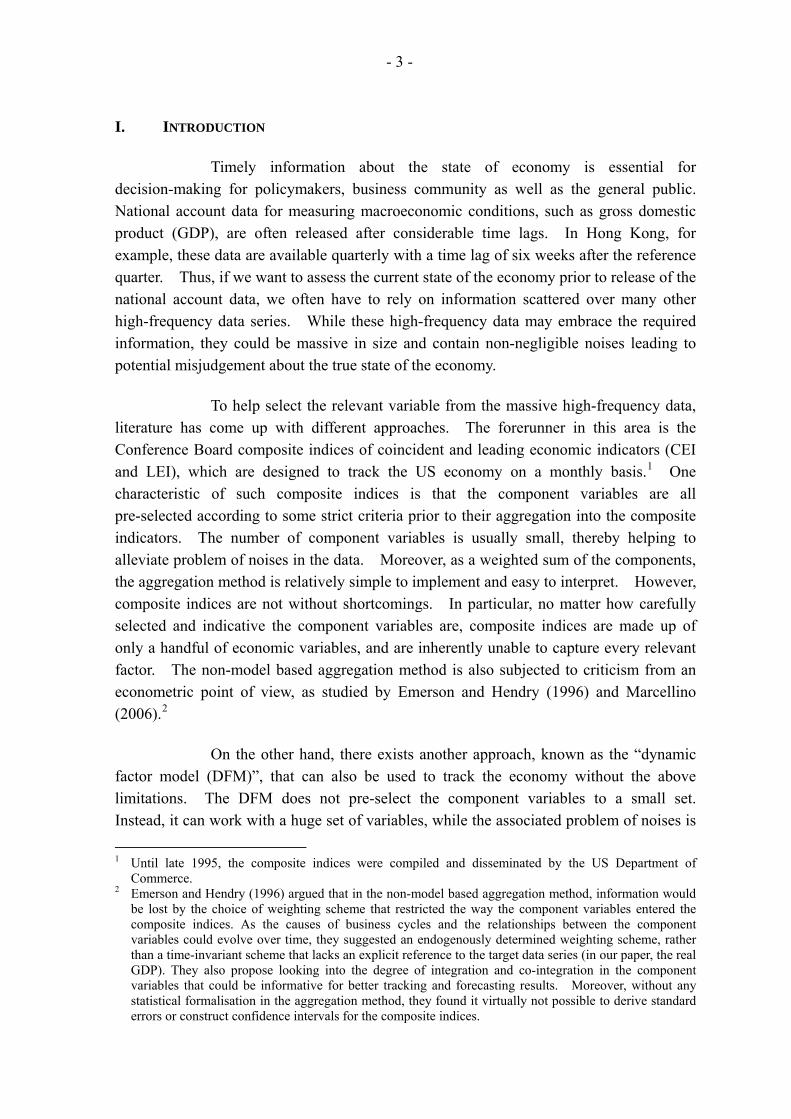
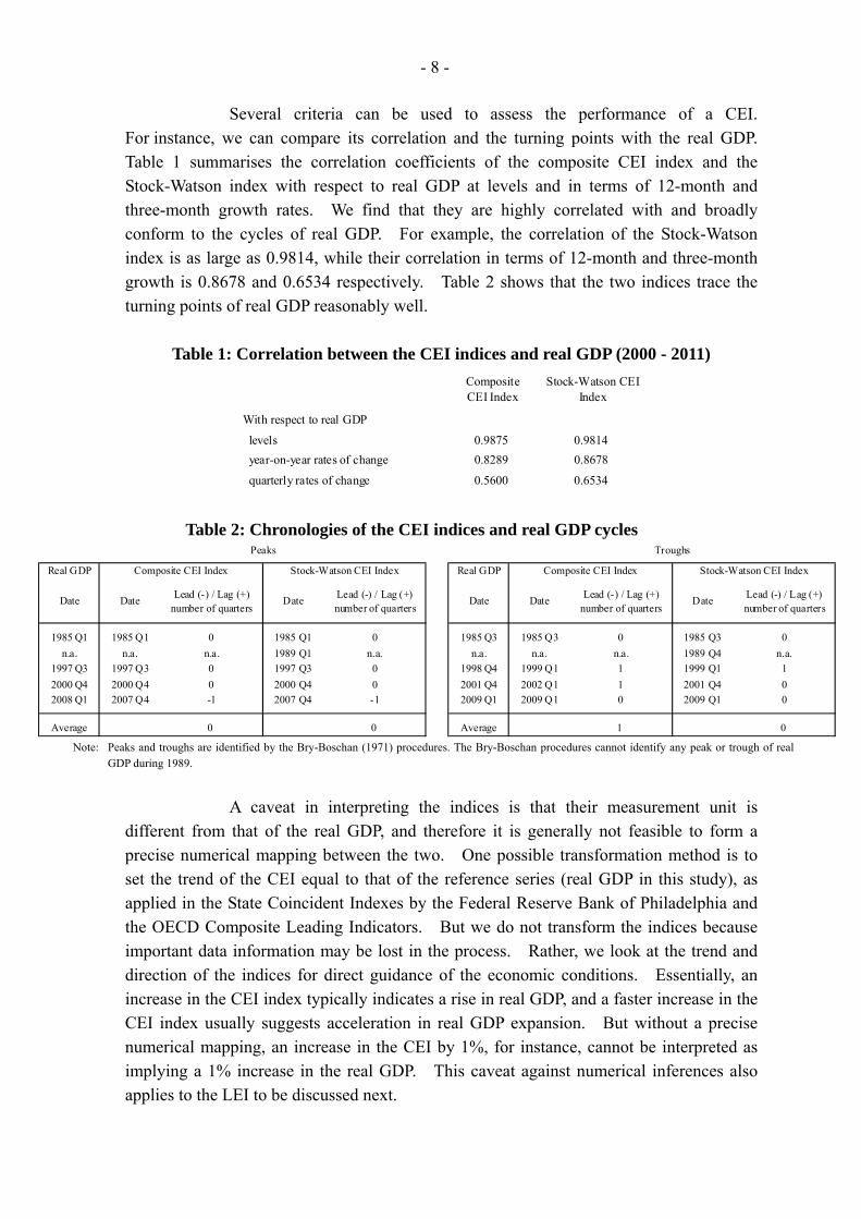
iii. Results Based on the NBER criteria, we can pin down the CEI components to include retail sales volume, equity market turnover, retained import volume and total export volume. These four components are all closely related to the business cycle of Hong Kong. Retail sales volume reflects the development in consumption of goods, while equity market turnover is included as a proxy for services consumption. Retained import volume captures the trend of capital goods investment and inventory stocking. Finally, total export volume indicates the activity of the external trade and related sectors, which accounts for about one-quarter of Hong Kong’s GDP in value-added terms. Appendix A.1 provides plots of their developments since 1982, with recession periods shaded as identified by the Bry-Boschan procedures on real GDP. The CEI components are all sectoral data, representing only some selected types of economic activity. We would prefer to include variables with a broader coverage but they are either not available or found to be lagging rather than coincident indicators. For example, compared with the components of the US Conference Board CEI index, total sales and personal income are not available in Hong Kong, while total employment on average lagged behind real GDP by one quarter. Notwithstanding this, the CEI index so derived can still track the Hong Kong economy closely. The left panel of Chart 1 traces the Composite CEI index aggregated by the Conference Board procedures. Its overall trend and curvature can provide useful information about the direction and pace of change in the contemporaneous economic conditions of Hong Kong. We also estimate a Stock-Watson type of CEI index with two lag terms in the transition equations, as is plotted in the right panel of Chart 1.

Chart 1: The Composite CEI Index, Stock-Watson CEI Index and Real GDP

Composite CEI index Stock-Watson CEI Index

0

20

40

60

80

100

120

140

1980 1985 1990 1995 2000 2005 2010

Recession periodsComposite CEI IndexReal GDP

2008 = 100

0

20

40

60

80

100

120

140

1980 1985 1990 1995 2000 2005 2010

Recession periodsStock-Watson CEI IndexReal GDP

2008 = 100

- 8 -

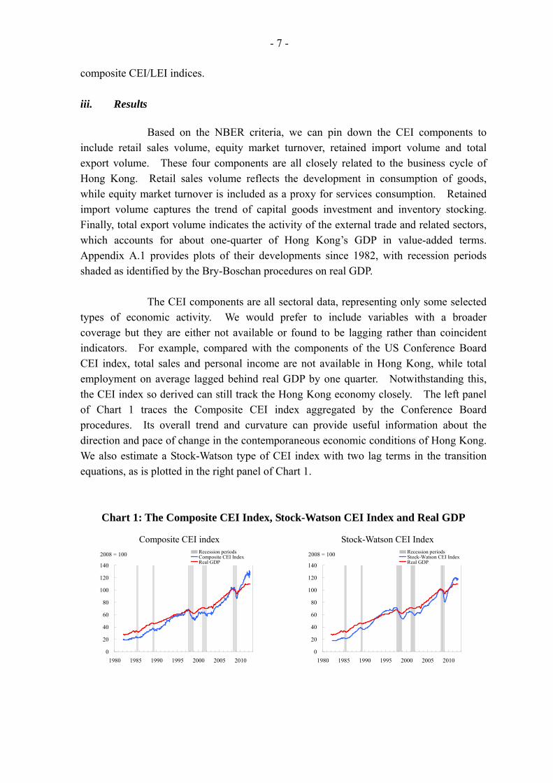
Several criteria can be used to assess the performance of a CEI. For instance, we can compare its correlation and the turning points with the real GDP. Table 1 summarises the correlation coefficients of the composite CEI index and the Stock-Watson index with respect to real GDP at levels and in terms of 12-month and three-month growth rates. We find that they are highly correlated with and broadly conform to the cycles of real GDP. For example, the correlation of the Stock-Watson index is as large as 0.9814, while their correlation in terms of 12-month and three-month growth is 0.8678 and 0.6534 respectively. Table 2 shows that the two indices trace the turning points of real GDP reasonably well.

Table 1: Correlation between the CEI indices and real GDP (2000 - 2011)

CompositeCEI Index

Stock-Watson CEIIndex

With respect to real GDP

levels 0.9875 0.9814

year-on-year rates of change 0.8289 0.8678

quarterly rates of change 0.5600 0.6534

Table 2: Chronologies of the CEI indices and real GDP cycles

Real GDP Real GDP

Date DateLead (-) / Lag (+)

number of quartersDate

Lead (-) / Lag (+)number of quarters

Date DateLead (-) / Lag (+)

number of quartersDate

Lead (-) / Lag (+)number of quarters

1985 Q1 1985 Q1 0 1985 Q1 0 1985 Q3 1985 Q3 0 1985 Q3 0

n.a. n.a. n.a. 1989 Q1 n.a. n.a. n.a. n.a. 1989 Q4 n.a.

1997 Q3 1997 Q3 0 1997 Q3 0 1998 Q4 1999 Q1 1 1999 Q1 1

2000 Q4 2000 Q4 0 2000 Q4 0 2001 Q4 2002 Q1 1 2001 Q4 0

2008 Q1 2007 Q4 -1 2007 Q4 -1 2009 Q1 2009 Q1 0 2009 Q1 0

Average 0 0 Average 1 0

Composite CEI Index Stock-Watson CEI Index

Peaks Troughs

Composite CEI Index Stock-Watson CEI Index

Note: Peaks and troughs are identified by the Bry-Boschan (1971) procedures. The Bry-Boschan procedures cannot identify any peak or trough of real

GDP during 1989.

A caveat in interpreting the indices is that their measurement unit is different from that of the real GDP, and therefore it is generally not feasible to form a precise numerical mapping between the two. One possible transformation method is to set the trend of the CEI equal to that of the reference series (real GDP in this study), as applied in the State Coincident Indexes by the Federal Reserve Bank of Philadelphia and the OECD Composite Leading Indicators. But we do not transform the indices because important data information may be lost in the process. Rather, we look at the trend and direction of the indices for direct guidance of the economic conditions. Essentially, an increase in the CEI index typically indicates a rise in real GDP, and a faster increase in the CEI index usually suggests acceleration in real GDP expansion. But without a precise numerical mapping, an increase in the CEI by 1%, for instance, cannot be interpreted as implying a 1% increase in the real GDP. This caveat against numerical inferences also applies to the LEI to be discussed next.

- 9 -

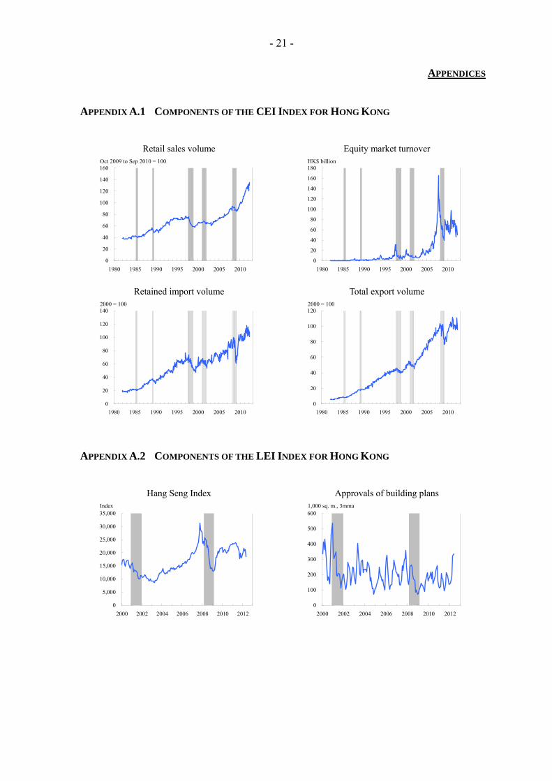
The composite LEI index, aggregated using the Conference Board procedures, comprises 10 component variables: the Hang Seng Index, approvals of building plans, real M2 (deflated by CCPI), HSBC Hong Kong PMI, CUHK Indices of Consumer Sentiment and Employment Confidence, QBTS, HKTDC Export Index, and trend-restored OECD Leading Indices for the US and Mainland China. The components are selected based on the NBER criteria to ensure all the components have a leading relationship with real GDP and demonstrate a leading cyclical behaviour (see Appendix A.2). They broadly reflect the prospects of the external environment, and domestically the developments in new orders, construction activities, consumer confidence, corporate sentiments and financial conditions. Chart 2 compares the composite LEI index so derived with the real GDP. It is capable of providing early signals of economic turning points. Table 3 shows that the correlation coefficient between the three-month lagged LEI index and GDP is as much as 0.9923 in levels, and their correlation in terms of 12-month and three-month growth is 0.8298 and 0.5308 respectively. The LEI Index also leads the GDP peaks and troughs by about one quarter (Table 4). However, caution should be taken when interpreting the LEI index because its time span is relatively short from the perspective of business cycle studies. We should therefore review its performance on a regular basis.

Chart 2: The Composite LEI Index and Real GDP

50

60

70

80

90

100

110

120

130

2000 2002 2004 2006 2008 2010 2012

Recession periodsLEIReal GDP

2008 = 100

led by 1 month

led by 5 months

led by 5 months

Table 3: Correlation between the three-month lagged LEI index and real GDP (2000 - 2011)

With respect to real GDP

levels 0.9923

year-on-year rates of change 0.8298

quarterly rates of change 0.5308

- 10 -

Table 4: Chronologies of the LEI index and real GDP cycles

Real GDP Real GDP

Date DateLead (-) / Lag (+)

number of quartersDate Date

Lead (-) / Lag (+)number of quarters

2000 Q4 n.a. n.a. 2001 Q4 2001 Q3 -1

2008 Q1 2007 Q4 -1 2009 Q1 2009 Q1 0

Average -1 Average -1

Peaks Troughs

Composite LEI Index Composite LEI Index

Note: Peaks and troughs are identified by the Bry-Boschan (1971) procedures. The

composite LEI index is only available from Q1 2000 onwards. Despite the availability of only a few data points, the peak quarter of the LEI is identified as some time before 2000 Q4 by the Bry-Boschan procedures.

III. DYNAMIC FACTOR MODEL i. Methodology The specification of the DFM can be represented as:

ttFtX , where ),0( Nt (1) And

tup

s

BstFsAtF

1

, where ),0( Ntu (2)

tX is a n 1 vector of monthly indicators, is a n r matrix of factor loadings, is

r 1 vector of static factors, which follow a VAR( ) process. is a r q matrix and

is a q 1 vector of primitive shocks (which is also the number of dynamic factors in the system).

tF

p B tu

Rewriting equation (1) in matrix form:

NTNrrTF

NTX

' (3)

We estimate the DFM using the two-step algorithm of Doz et. al. (2011): 1. In the first step, we estimate the model by OLS, using a balanced panel of data. The

number of static factors r is selected by the criteria of Bai and Ng (2002), while the number of dynamic factors is selected by the criteria of Bai and Ng (2007). The lag length in equation (2) is selected by the SIC.

2. In the second step, we apply the Kalman smoother to the data panel and re-estimate the factors, with the transition, covariance matrices etc. being based on the estimates obtained in the first step.

- 11 -

We then use the Kalman recursion to iterate forward the estimated factors, and generate the nowcast/forecast of inflation and output growth. ii. Data The dataset used in estimating the DFM comprises 189 macroeconomic and financial series from third-party data providers and our in-house database. A comprehensive list of all data series can be found in Appendix A.3. Most of the series in this dataset are available in monthly or even higher frequencies (e.g. daily close price of stock indices), while a few of them are only available in quarterly frequency (e.g. real GDP). In order to estimate a monthly model, those quarterly data series are interpolated into monthly frequency by the quadratic match-sum method offered by the econometric software EViews.6, 7 Furthermore, all data series have also been transformed to stationary form prior to estimation. Details of the transformation methods are shown in Appendix A.4. Selection of the type of transformation depends on the nature of each particular series. The time span of the data series varies from one to another, much depending on the earliest and latest date of publication of each particular series. As such, the earliest common starting date of all 189 data series is April 1999. For the purpose of forecast evaluation, we estimate the DFM recursively, with the first sub-sample spanning from April 1999 to January 2006. The time span of the sub-sample is then expanded by one month ahead in each step of recursion. iii. Empirical results As discussed above, we estimate the DFM using the two-step algorithm. The descriptive statistics of the recursively estimated parameters, including the numbers of static factor (r), dynamic factor (q) and lag length (p) in equation (2), are summarised in Table 5.

6 The quadratic match-sum method fits a local quadratic polynomial for each observation of the original

(quarterly) series, using the fitted polynomial to fill in all observations of the higher frequency (monthly) series associated with the period. The quadratic polynomial is formed by taking sets of three adjacent points from the original series and fitting a quadratic so that the sum of the interpolated monthly data points matches the actual quarterly data points.

7 Another commonly used method of interpolation is the Denton univariate method available in the software ECOTRIM developed by the Eurostat. We have performed a trial on a sub-sample, estimating the DFM with the quarterly data series interpolated by the Denton method. The results appeared to be indifferent from those of the quadratic match-sum method. Hence, we stick to the quadratic match-sum method for sake of operational convenience.

- 12 -

Table 5: Estimated parameters of the DFM

Statistics R q p Selected value 9 7 1

To evaluate the forecasting power of the DFM, we replicate the real-time situation of the model as closely as possible using the unbalanced panel of data. In fact, all statistics except some high-frequency financial market indicators are released with regular time lag. In the case of Hong Kong, estimate of GDP is usually released in the second month after the end of the relevant quarter, while the monthly consumer price index is released in the subsequent month. By incorporating the schedule of data release into the dataset, we compute the nowcast and the one-quarter to fourth-quarter ahead forecasts of GDP growth using information available up to the end of each quarter. For the consumer price inflation, we compute the nowcast and the one-month to twelve-month ahead forecasts using information up to the end of each month. Inflation and growth forecasts from the DFM are compared against that from: (a) an autoregressive (AR) model, where the lag lengths are determined by the SIC:

ttt Lba 1)( (4)

ttt yLccy 1)( (5)

Where and are the inflation and output growth rates respectivelyt ty 8.

And (b) a random walk (RW) model:

)112

(*100

tCPItCPIyoy

ht (6)

)14

(*100

tYtYyoy

hty (7)

The existing in-house small forecasting model is not included in the comparison as it is much relying on a set of assumptions on the exogenous variables, such as the future real GDP growth major trading partner, commodity prices and exchange rates. The reliance on assumptions makes the small forecasting model not directly comparable to the self-sufficient DFM and other benchmarking models. Forecasts from the models are evaluated by the root mean squared errors (RMSE), where the RMSE is defined as:

2)ˆ(1 yoy

htyoy

ht XXT

RMSE (8)

8 Samples for the estimation of the univariate AR models begin as early as the data for the real GDP and

consumer prices are available, up to the implementation of the Linked Exchange Rate System in 1983.

- 13 -

where X is the target variable of interest (e.g. real output). A smaller RMSE indicates that the underlying estimator could produce more accurate forecast. Table 6 presents the RMSE of the nowcasts and forecasts of the real GDP growth by the DFM, along with those of the random walk model and univariate auto-regressive models. The row “nowcast” reports the RMSE of the estimation of the real GDP growth for the current quarter, while “1-step” corresponds the next quarter and so on. As indicated by the RMSE, the DFM produces more accurate nowcasts and forecasts than the quarterly random walk model and the univariate autoregressive model.

Table 6: Root-mean-square error of GDP growth nowcast and forecasti (Evaluation period: 2006 Q1 – 2011 Q3)

Model DFM Random

walk Univariate AR

model 1iii Sampleii From April 1999ii - From 1984 Q1ii nowcast 0.99* 2.53 1.64 1-step 1.59* 4.11 2.63 2-step 2.13* 5.49 3.57 3-step 2.92* 6.65 4.58 4-step 3.23* 7.25 4.66

Notes: i. Figures with asterisk (*) denote minimum among all models. ii. The date refers to the starting date of the recursive sample. iii. The univariate AR model (1) is estimated with the quarter-on-quarter

GDP growth rate. For the forecast of consumer price inflation, the DFM model outperforms other models only in the longer term horizon (Table 7). The univariate models appeared to produce more accurate nowcasts and forecasts with a six-month period.

- 14 -

Table 7: Root-mean-square error of inflation nowcast and forecasti (Evaluation period: January 2006 – September 2011)

Model DFM Random

walk Univariate AR

model 1iii Sample From April 1999ii - From January 1992ii nowcast 0.60 0.44 0.26* 1-step 0.64 0.71 0.40* 2-step 0.68 1.02 0.58* 3-step 1.01 1.31 0.76* 4-step 1.07 1.59 0.99* 5-step 1.17* 1.85 1.24 6-step 1.50 2.10 1.49* 7-step 1.58* 2.32 1.76 8-step 1.66* 2.51 2.02 9-step 1.80* 2.69 2.28 10-step 1.83* 2.83 2.50 11-step 1.86* 2.96 2.71 12-step 1.95* 3.06 2.82 Notes: i. Figures with asterisk (*) denote minimum among all models. ii. The date refers to the starting date of the recursive sample. iii. The univariate AR model (1) is estimated with the month-on-month

consumer price inflation. Besides comparing with the benchmarking models, we also assess the forecasting power of the DFM against our recently updated BVAR model. The BVAR model is developed as a part of our in-house toolkit for economic forecasting. This quarterly-based model is small, containing only six major economic indicators: (1) real GDP, (2) underlying composite consumer price index, (3) world GDP, (4) exports volume, (5) retail sales volume, and (6) retail rentals. More details of the model are discussed in Appendix A.5. For a meaningful side-by-side comparison, we put the staggered nature of the data series aside as it could be hard to require the quarterly BVAR model to take into account the staggered nature of the data series on the same basis as the DFM. The forecasts of the real GDP growth and inflation are then computed from these balanced-panel models. Table 8 presents the RMSE of forecasts of the real GDP growth by the BVAR model and the DFM, along with those of the benchmarking models. Among all models, the BVAR model produces the most accurate forecasts within the half-year horizon, followed by the DFM. Their rankings swap beyond two quarters, with the RMSE of the forecasts produced by the DFM becoming smaller than those of the BVAR model.

- 15 -

Table 8: Root-mean-square error of GDP growth forecast (BVAR model included)i

(Evaluation period: 2006 Q1 – 2011 Q3)

Model DFM BVAR modelRandom

walk Univariate AR

model 1iv Sample From April 1999ii - - From 1984 Q1ii 1-step 1.49 1.45* 2.53 1.64 2-step 2.32 2.17* 4.11 2.63 3-step 2.71* 3.03 5.49 3.57 4-step 3.25* 4.04 6.65 4.58

Notes: i. Figures with asterisk (*) denote minimum among all models. ii. The date refers to the starting date of the recursive sample. iii. The date refers to the starting date of the first sub-sample of the 40-quarter rolling

estimation. iv. The univariate AR model 1 is estimated with the quarter-on-quarter GDP growth rate.

On the other hand, the BVAR appeared to be less appealing in the contest of inflation forecast (Table 9). The BVAR model is outperformed by the DFM within the three-quarter forecasting horizon, with its four-quarter ahead forecast barely beating that of the DFM.

Table 9: Root-mean-square error of inflation forecast (BVAR model included)i (Evaluation period: 2006 Q1 – 2011 Q3)

Model DFM BVAR modelRandom

walk Univariate AR

model 1iv Sample From April 1999ii - - From 1984 Q1ii 1-step 0.48* 0.62 0.96 0.52 2-step 0.95* 1.14 1.78 1.20 3-step 1.51* 1.53 2.43 2.00 4-step 1.89 1.72* 2.86 2.71

Notes: i. Figures with asterisk (*) denote minimum among all models. ii. The date refers to the starting date of the recursive sample. iii. The date refers to the starting date of the first sub-sample of the 40-quarter rolling

estimation. iv. The univariate AR model (1) is estimated with the quarter-on-quarter GDP growth rate.

IV. ENHANCING THE FORECASTING TOOLKIT Although none of the DFM and the BVAR model is identified as the best model to capture the aggregate economic movements, the above analyses show that these two models outperform the standard benchmarking models in the literature in almost all contested circumstances. Compared with our existing in-house small forecasting model, the major edge of the DFM is its higher frequency nature. Constrained mostly by the availability of

- 16 -

the national account data, our small forecasting model is a quarterly model. In addition, as the model is structural in which all endogenous variables are linked up in about 20 equations, the model cannot be updated without a completely updated balanced panel of data. Thus, the model can only be updated by at most four times a year with significant time lag. In this regard, the monthly DFM can track the aggregate movements of the economy more timely, allowing users to update real time nowcasts and forecasts whenever there are new data released. The non-structural nature of the DFM offers greater flexibility to user to update the estimations, but it undermines the interpretability of the quantitative results on the other hand. It is difficult to identify the attributes of any changes in any particular variables in this large scale purely statistical model. For instance, it is almost impossible to reveal the driver of the projected GDP growth in the context of the DFM. In contrast, the small forecasting model can provide a better resolution to the changes in the endogenous variables. Moreover, the structural nature of the small forecasting model also allows user to perform impact analysis, evaluating how the change in one variable influences the system, including the output growth and consumer price inflation. The quarterly BVAR model shares the weaknesses of considerable time-lag and low frequency of the small forecasting model. However, its VAR model nature facilitates impact analysis through the impulse response function and variance decomposition, making it a handy tool to evaluate the effect of economic shock. In sum, the DFM should be part of our toolkit for forecasting, while there are also high values of keeping the revised BVAR model in our forecasting toolkits. V. TRACKING THE HONG KONG ECONOMY WITH THE CEI/LEI AND THE DFM AS AN

EXAMPLE In this section, we demonstrate how we deploy the composite CEI/LEI indices and the DFM together in practice. We take the situation when we were back in December 2010 and had to track the growth rate in that quarter as well as in the next quarter (i.e. 2010 Q4 and 2011 Q1). Both the composite CEI/LEI indices and the DFM, derived from the information available at that time, suggested that the growth momentum would accelerate in 2010 Q4 and 2011 Q1. On the basis of these indications, we would reach the diagnosis that the economy had been gaining traction, with resulting upward pressures on inflation. We may look at the composite CEI/LEI indices for clues about the underlying growth dynamics. The CEI picked up speed in 2010 Q4, with domestic demand being the main growth pillar. Component-wise, retail sales volume and retained imports recorded notable increases. Stock market turnover also picked up steadily on

- 17 -

firmer demand for financial services. Merchandise exports however decreased due to softer external demand. As regards the LEI, there was an accelerating upward trend at that time amid continued improvements in the external and domestic environments. For example, the OECD leading indicators showed that the growth momentum of Mainland China was robust and the US economic conditions improved slightly. The HKTDC Export Index also pointed to a steady growth in export orders. On the domestic side, economic activity as captured by the PMI increased firmly, while financial conditions improved with stock prices bouncing up and the real monetary aggregate increasing. Consumer confidence and employment outlook also remained positive, though edging down from the recent high levels. Approvals of building plans however decreased. To derive a set of numbers in economic forecasts from the above useful information in a timely manner, we use the DFM. At that time, the DFM projected that the growth momentum would pick up from 0.9% in 2010 Q3 to 1.3% in 2010 Q4 and 1.5% in 2011 Q1.9 Thus, by supplementing the CEI/LEI and the DFM with each other, we can obtain a comprehensive picture on the near-term outlook, facilitating our macroeconomic surveillance. With all that said, the above snapshot is the one where the CEI/LEI and the DFM agreed with each other on their economic assessments, and there will inevitably be circumstances where the CEI/LEI and the DFM disagree. Under such scenarios, we have to rely on our own judgement to assess which of the model form a better description of the near-term outlook. VI. CONCLUSION This paper elaborates a number of methods to diagnose the current state of the economy and to produce short-term projection in a timely manner. Comprising a small set of highly concurrent economic variables, the composite CEI/LEI indices are able to track the concise trend of the Hong Kong economy on a monthly basis. A key feature of the composite indices is their good track record in identifying the turning points of the economic cycle. While the composite CEI/LEI indices can pinpoint the state of the economy in the cycle, they are incapable of forecasting the precise magnitude of the economic activity. In view of this limitation, it may be useful to supplement them with the DFM framework, to nowcast and forecast the magnitude of real GDP growth (and consumer price inflation). In principle, the DFM framework summarises a huge set of economic variables in a smaller number of factors which can be readily used to nowcast and forecast the magnitude of the real GDP growth and consumer price inflation.

9 The actual outturn was 1.6% in 2010 Q4 and 2.9% in 2011 Q1.

- 18 -

In the contest of forecasting the real GDP, the DFM outperforms the univariate benchmarking models. For the consumer price inflation, forecasts generated by the DFM are also more accurate than those produced by the univariate benchmarks beyond the six-month horizon. Moreover, we also assess the forecasting power of the DFM by comparing its forecasts with those by the updated in-house BVAR model. The Bayesian model produces forecasts with similar accuracy as those produced by the DFM. The introduction of the composite CEI/LEI indices and the DFM enhances our capability in tracking the Hong Kong economy, while the updated BVAR can also retain a position in our forecasting toolkits. Possessing different attributes, these models can complement the others under different circumstances.

- 19 -

REFERENCES Bai, J., and Ng, S. (2002), “Determining the Number of Factors in Approximate Factor Models”, Econometrica Vol. 70 No.1 pp. 191-221. Bai, J., and Ng, S. (2007), “Determining the Number of Primitive Shocks in Factor Models”, Journal of Business and Economic Statistics Vol. 25 No. 1. Bry, G.., and Boschan, C. (1971), Cyclical Analysis of Time Series: Selected Procedures and Computer Programs, New York, NY: National Bureau of Economic Research. Burns, A. F., and Mitchell, W. C. (1946), Measuring Business Cycles. New York, NY: National Bureau of Economic Research. Denton, F.T. (1971), “Adjustment of monthly or quarterly series to annual totals: An Approach based on quadratic minimization”, Journal of the American Statistical Association Vol. 66(333) pp. 99-102. Doan, T., Litterman, R. B., and Sims, C. A. (1984), “Forecasting and Conditional Projections Using Realistic Prior Distributions”, Econometric Reviews Vol. 3 pp. 1-100. Doz, C., Giannone, D., and Reichlin, L. (2011), “A Two-Step Estimator for Large Approximate Dynamic Factor Models Based on Kalman Filtering”, Journal of Econometrics Vol. 164 pp. 188-205. Emerson, R. A., and Hendry D. F. (1996), “An Evaluation of Forecasting Using Leading Indicators”, Journal of Forecasting Vol. 15 pp. 271-291. Genberg, H., and Chang, J. (2007), “A VAR Framework for Forecasting Hong Kong’s Output and Inflation”, HKMA Working Paper. Gerlach, S., and Yiu, M. (2004), “A Dynamic Factor Model for Current-Quarter Estimates of Economic Activity in Hong Kong”, HKIMR Working Paper No. 16/2004. Giannone, D., Reichlin, L., and Small, D. (2006), “Nowcasting GDP and Inflation: the Real-Time Informational Content of Macroeconomic Data Releases”, ECB Working Paper No. 633. Harding, D., and Pagan, A. (2006), “Synchronisation of Cycles,” Journal of Econometrics Vol. 132 pp. 59-79. Hong Kong Monetary Authority, Half Yearly Monetary and Financial Stability Report, March 2012. Kong, J., and Leung, C. (2004), “Revised Small Forecasting Model for Hong Kong”, Research Memorandum 13/2004. Liu, P., Matheson, T., and Rafael, R. (2011), “Real-Time Forecasts of Economic Activity for Latin American Economies”, IMF Working Paper WP/11/98.

- 20 -

Marcellino, M. (2006), “Leading Indicators”, in Handbook of Economic Forecasting, Vol 1, eds. Elliott G., Granger C., and Timmermann, A., Amsterdam: Elsevier B. V. pp. 879-960. Matheson, T. (2011), “New Indicators for Tracking Growth in Real Time”, IMF Working Paper WP/11/43. Moore, G. H., and Shiskin, J. (1967), Indicators of Business Expansions and Contractions, New York, NY: National Bureau of Economic Research. OECD (2012), OECD System of Composite Leading Indicators. Stock, J. H., and Watson, M. W. (1989), “New Indexes of Coincident and Leading Economic Indicators,” NBER Macroeconomics Annual 1989 pp. 351-393. Stock, J. H., and Watson, M. W. (1991), “A probability model of the coincident economic indicators”, in Leading Economic Indicators: New approaches and Forecasting Records, eds. K. Lahiri and G. H. Moore, Cambridge: Cambridge University Press pp. 63-89. The Conference Board (2001), Business Cycle Indicators Handbook, New York, NY: The Conference Board.

- 21 -

APPENDICES APPENDIX A.1 COMPONENTS OF THE CEI INDEX FOR HONG KONG

Retail sales volume Equity market turnover

0

20

40

60

80

100

120

140

160

1980 1985 1990 1995 2000 2005 2010

Oct 2009 to Sep 2010 = 100

0

20

40

60

80

100

120

140

160

180

1980 1985 1990 1995 2000 2005 2010

HK$ billion

Retained import volume Total export volume

0

20

40

60

80

100

120

140

1980 1985 1990 1995 2000 2005 2010

2000 = 100

0

20

40

60

80

100

120

1980 1985 1990 1995 2000 2005 2010

2000 = 100

APPENDIX A.2 COMPONENTS OF THE LEI INDEX FOR HONG KONG

Hang Seng Index Approvals of building plans

0

5,000

10,000

15,000

20,000

25,000

30,000

35,000

2000 2002 2004 2006 2008 2010 2012

Index

0

100

200

300

400

500

600

2000 2002 2004 2006 2008 2010 2012

1,000 sq. m., 3mma

- 22 -

Real M2 (deflated by CCPI) HSBC Hong Kong Purchasing Managers’ Index

70

80

90

100

110

120

130

140

150

160

170

2000 2002 2004 2006 2008 2010 2012

2005 = 100

30

35

40

45

50

55

60

65

2000 20 02 2004 2 006 2008 2010 2012

Diffus io n In dex

>50 expansion<50 contraction

CUHK Index of Consumer Sentiment CUHK Index of Employment Confidence

0

20

40

60

80

100

120

140

2000 2002 2004 2006 2008 2010 2012

Q1 2000 = 100

Interpolated byDenton method

0

20

40

60

80

100

120

140

2000 2002 2004 2006 2008 2010 2012

Q1 2000 = 100

Interpolated byDenton method

Quarterly Business Tendency Survey HKTDC Export Index

0

10

20

30

40

50

60

70

80

2000 2002 2004 2006 2008 2010 2012

Diffusion Index

Interpolated byDenton method

0

10

20

30

40

50

60

70

2000 2002 2004 2006 2008 2010 2012

Diffusion Index

Interpolated byDenton method

Trend-restored OECD Leading Index for the US

Trend-restored OECD Leading Index for Mainland China

70

75

80

85

90

95

100

105

110

2000 2002 2004 2006 2008 2010 2012

Index

0

50

100

150

200

250

300

2000 2002 2004 2006 2008 2010 2012

Index

- 23 -

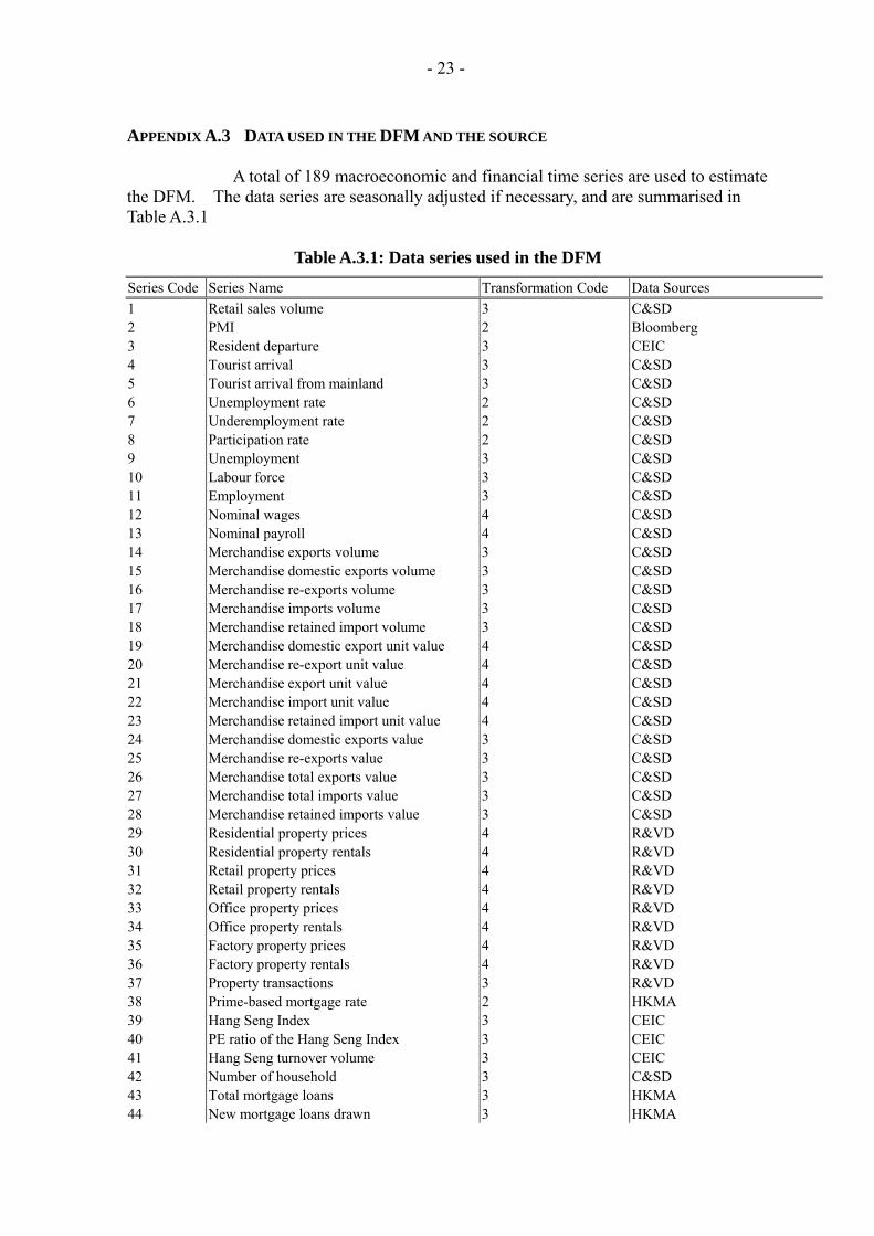
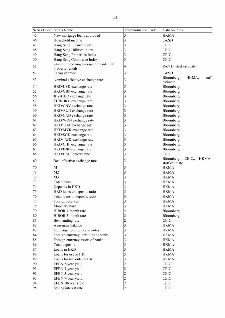
APPENDIX A.3 DATA USED IN THE DFM AND THE SOURCE A total of 189 macroeconomic and financial time series are used to estimate the DFM. The data series are seasonally adjusted if necessary, and are summarised in Table A.3.1

Table A.3.1: Data series used in the DFM

Series Code Series Name Transformation Code Data Sources

1 Retail sales volume 3 C&SD 2 PMI 2 Bloomberg 3 Resident departure 3 CEIC 4 Tourist arrival 3 C&SD 5 Tourist arrival from mainland 3 C&SD 6 Unemployment rate 2 C&SD 7 Underemployment rate 2 C&SD 8 Participation rate 2 C&SD 9 Unemployment 3 C&SD 10 Labour force 3 C&SD 11 Employment 3 C&SD 12 Nominal wages 4 C&SD 13 Nominal payroll 4 C&SD 14 Merchandise exports volume 3 C&SD 15 Merchandise domestic exports volume 3 C&SD 16 Merchandise re-exports volume 3 C&SD 17 Merchandise imports volume 3 C&SD 18 Merchandise retained import volume 3 C&SD 19 Merchandise domestic export unit value 4 C&SD 20 Merchandise re-export unit value 4 C&SD 21 Merchandise export unit value 4 C&SD 22 Merchandise import unit value 4 C&SD 23 Merchandise retained import unit value 4 C&SD 24 Merchandise domestic exports value 3 C&SD 25 Merchandise re-exports value 3 C&SD 26 Merchandise total exports value 3 C&SD 27 Merchandise total imports value 3 C&SD 28 Merchandise retained imports value 3 C&SD 29 Residential property prices 4 R&VD 30 Residential property rentals 4 R&VD 31 Retail property prices 4 R&VD 32 Retail property rentals 4 R&VD 33 Office property prices 4 R&VD 34 Office property rentals 4 R&VD 35 Factory property prices 4 R&VD 36 Factory property rentals 4 R&VD 37 Property transactions 3 R&VD 38 Prime-based mortgage rate 2 HKMA 39 Hang Seng Index 3 CEIC 40 PE ratio of the Hang Seng Index 3 CEIC 41 Hang Seng turnover volume 3 CEIC 42 Number of household 3 C&SD 43 Total mortgage loans 3 HKMA 44 New mortgage loans drawn 3 HKMA

- 24 -

Series Code Series Name Transformation Code Data Sources

45 New mortgage loans approved 3 HKMA 46 Household income 3 C&SD 47 Hang Seng Finance Index 3 CEIC 48 Hang Seng Utilities Index 3 CEIC 49 Hang Seng Properties Index 3 CEIC 50 Hang Seng Commerce Index 3 CEIC

51 24-month moving average of residential property rentals

4 R&VD, staff estimate

52 Terms of trade 3 C&SD

53 Nominal effective exchange rate 3 Bloomberg, HKMA, staff estimate

54 HKD/USD exchange rate 3 Bloomberg 55 HKD/GBP exchange rate 3 Bloomberg 56 JPY/HKD exchange rate 3 Bloomberg 57 EUR/HKD exchange rate 3 Bloomberg 58 HKD/CNY exchange rate 3 Bloomberg 59 HKD/AUD exchange rate 3 Bloomberg 60 HKD/CAD exchange rate 3 Bloomberg 61 HKD/WON exchange rate 3 Bloomberg 62 HKD/THA exchange rate 3 Bloomberg 63 HKD/MYR exchange rate 3 Bloomberg 64 HKD/SGD exchange rate 3 Bloomberg 65 HKD/TWD exchange rate 3 Bloomberg 66 HKD/CHF exchange rate 3 Bloomberg 67 HKD/INR exchange rate 3 Bloomberg 68 HKD/USD forward rate 3 CEIC

69 Real effective exchange rate 3 Bloomberg, CEIC,, HKMA, staff estimate

70 M1 3 HKMA 71 M2 3 HKMA 72 M3 3 HKMA 73 Total loans 3 HKMA 74 Deposits in HKD 3 HKMA 75 HKD loans to deposits ratio 3 HKMA 76 Total loans to deposits ratio 3 HKMA 77 Foreign reserves 3 HKMA 78 Monetary base 3 HKMA 79 HIBOR 1-month rate 2 Bloomberg 80 HIBOR 3-month rate 2 Bloomberg 81 Best lending rate 2 CEIC 82 Aggregate balance 3 HKMA 83 Exchange fund bills and notes 3 HKMA 84 Foreign currency liabilities of banks 3 HKMA 85 Foreign currency assets of banks 3 HKMA 86 Total deposits 3 HKMA 87 Loans in HKD 3 HKMA 88 Loans for use in HK 3 HKMA 89 Loans for use outside HK 3 HKMA 90 EFBN 2-year yield 2 CEIC 91 EFBN 3-year yield 2 CEIC 92 EFBN 5-year yield 2 CEIC 93 EFBN 7-year yield 2 CEIC 94 EFBN 10-year yield 2 CEIC 95 Saving interest rate 2 CEIC

- 25 -

Series Code Series Name Transformation Code Data Sources

96 Underlying CCPI 4 C&SD 97 Tradable component of the CCPI 4 C&SD, staff estimate 98 Nontradable component of the CCPI 4 C&SD, staff estimate 99 Housing component of the CCPI 4 C&SD, staff estimate 100 Output deflator 4 C&SD 101 Oil price 4 Bloomberg 102 World commodity index 4 IMF 103 Non-fuel commodity index 4 IMF 104 Food index 4 IMF 105 Beverage index 4 IMF 106 Industrial material index 4 IMF 107 Agricultural index 4 IMF 108 Metal index 4 IMF 109 Energy index 4 IMF 110 Gold price 4 Bloomberg 111 China CPI 4 CEIC, staff estimate 112 China CPI-food subindex 4 CEIC, staff estimate 113 US CPI 4 Bloomberg 114 Japan CPI 4 Bloomberg 115 Euro area CPI 4 Bloomberg 116 Taiwan CPI 4 Bloomberg 117 Singapore CPI 4 Bloomberg 118 Korea CPI 4 Bloomberg 119 UK CPI 4 Bloomberg 120 Malaysia CPI 4 Bloomberg 121 Thailand CPI 4 Bloomberg 122 Canada CPI 4 Bloomberg 123 Australia CPI 4 Bloomberg 124 Philippines CPI 4 Bloomberg 125 Switzerland CPI 4 Bloomberg 126 India CPI 4 Bloomberg

127 World CPI 4 Bloomberg, HKMA, staff estimate

128 Federal funds rate 2 Bloomberg 129 VIX 2 CBOE 130 ASX: S&P/ASX 200 3 CEIC 131 Shanghai stock exchange 3 CEIC 132 CAC 40 3 CEIC 133 DAX 3 CEIC 134 Nikkei 225 Stock 3 CEIC 135 KOSPI 3 CEIC 136 FTSE Bursa Malaysia: Composite 3 CEIC 137 PSEi 3 CEIC 138 SGX Strait Times 3 CEIC 139 TAIEX Capitalization Weighted 3 CEIC 140 SET 3 CEIC 141 India Sensex 3 CEIC 142 FTSE 100 3 CEIC 143 Dow Jones: Industrial Average 3 CEIC 144 LIBOR 1m 2 Bloomberg 145 LIBOR 3m 2 Bloomberg 146 EURO LIBOR 1m 2 Bloomberg 147 EURO LIBOR 3m 2 Bloomberg

- 26 -

Series Code Series Name Transformation Code Data Sources

148 Two-year yield of US treasury 2 CEIC 149 Three-year yield of US treasury 2 CEIC 150 Five-year yield of US treasury 2 CEIC 151 Seven-year yield of US treasury 2 CEIC 152 Ten-year yield of US treasury 2 CEIC 153 China leading indicator 2 OECD 154 US leading indicator 2 OECD 155 Japan leading indicator 2 OECD 156 Euro area leading indicator 2 OECD 157 UK leading indicator 2 OECD 158 Australia leading indicator 2 OECD 159 Canada leading indicator 2 OECD 160 Korea leading indicator 2 OECD 161 Switzerland leading indicator 2 OECD 162 India leading indicator 2 OECD 163 OECD total leading indicator 2 OECD 164 Australia GDP 3 Bloomberg 165 Canada GDP 3 Bloomberg 166 Switzerland GDP 3 Bloomberg 167 China GDP 3 Bloomberg 168 UK GDP 3 Bloomberg 169 Japan GDP 3 Bloomberg 170 Malaysia GDP 3 Bloomberg 171 Singapore GDP 3 Bloomberg 172 Thailand GDP 3 Bloomberg 173 Taiwan GDP 3 Bloomberg 174 US GDP 3 Bloomberg 175 Korea GDP 3 Bloomberg 176 Euro area GDP 3 Bloomberg 177 Philippines GDP 3 Bloomberg 178 India GDP 3 Bloomberg

179 World GDP 3 Bloomberg, HKMA, staff estimate

180 GDP 3 C&SD 181 Private consumption expenditure 3 C&SD 182 Government consumption expenditure 3 C&SD 183 Gross domestic fixed capital formation 3 C&SD 184 Domestic exports of goods 3 C&SD 185 Re-exports of goods 3 C&SD 186 Imports of goods 3 C&SD 187 Exports of services 3 C&SD 188 Imports of services 3 C&SD 189 Stock of inventory 3 C&SD, staff estimate

- 27 -

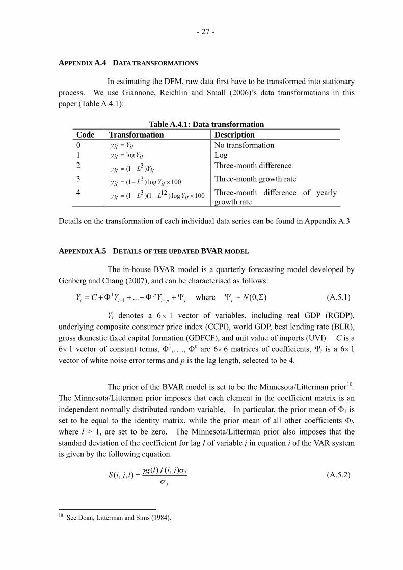
APPENDIX A.4 DATA TRANSFORMATIONS In estimating the DFM, raw data first have to be transformed into stationary process. We use Giannone, Reichlin and Small (2006)’s data transformations in this paper (Table A.4.1):

Table A.4.1: Data transformation Code Transformation Description 0 itYity No transformation 1 itYity log Log 2

itYLity )31( Three-month difference

3 100log)31( itYLity Three-month growth rate

4 100log)121)(31( itYLLity Three-month difference of yearly growth rate

Details on the transformation of each individual data series can be found in Appendix A.3

APPENDIX A.5 DETAILS OF THE UPDATED BVAR MODEL The in-house BVAR model is a quarterly forecasting model developed by Genberg and Chang (2007), and can be characterised as follows:

tptp

tt YYCY ...11 where ),0(~ Nt (A.5.1)

Yt denotes a 6 1 vector of variables, including real GDP (RGDP), underlying composite consumer price index (CCPI), world GDP, best lending rate (BLR), gross domestic fixed capital formation (GDFCF), and unit value of imports (UVI). C is a 6 1 vector of constant terms, Φ1,…., Φp are 6

6 matrices of coefficients, Ψt is a 6 1 vector of white noise error terms and p is the lag length, selected to be 4.

The prior of the BVAR model is set to be the Minnesota/Litterman prior10. The Minnesota/Litterman prior imposes that each element in the coefficient matrix is an independent normally distributed random variable. In particular, the prior mean of Φ1 is set to be equal to the identity matrix, while the prior mean of all other coefficients Φl, where l > 1, are set to be zero. The Minnesota/Litterman prior also imposes that the standard deviation of the coefficient for lag l of variable j in equation i of the VAR system is given by the following equation.

j

ijiflgljiS

),()(

),,( (A.5.2)

10 See Doan, Litterman and Sims (1984).

- 28 -

where and f(i,j) = g(l) = 1 if i = j. γ is the standard deviation of the first

own lag, and is a measure of overall tightness. g(l)=l-d measures the tightness of the first lag relative to lag l, where d is the decay factor. σi, σj are the estimated standard errors of the univariate autoregression for variables Yi,t and Yj,t. The parameters γ and d are set to be 0.2 and 1 respectively, based on the forecasting power test results of Genberg and Chang (2007).

1),(0 jif

While the BVAR model was helpful in forecasting economic activity in the past, it is about time to make some improvements to the model. We focus on the choice of variables in particular, as we expect that there may be gains in replacing the variables GDFCF, BLR and UVI with others. Our rationale is that GDFCF is highly volatile, and any fluctuation of this variable is unlikely to be informative about future economic activity. It is also doubtful of whether the BLR can still be informative about local economic activity, as the BLR has stayed largely unchanged over the past few years, as a result of the accommodative monetary policy pursued in the US. Finally, the UVI includes the value of goods that are re-exported, and so may not be informative about local inflation. We examine the forecasting performance of the model under alternative set of variables, with the target variables remaining to be the year-on-year output growth and inflation rates, as in Genberg and Chang (2007). While Genberg and Chang (2007) estimated the model using both recursive scheme and rolling scheme with a 10-year window, we performed only the latter, as doing so will be less susceptible to the problem of structural changes. In addition, the forecast horizon is extended to include one- to four-quarter ahead, while the forecast evaluation period is also updated to 2006 Q1 to 2011 Q3. Table A.5.1 summarises the specifics of the current forecast evaluation, compared to that in Genberg and Chang (2007).

Table A.5.1: Forecast evaluation specifics of the BVAR models

Genberg and Chang (2007) Revised BVAR

Forecast objects RGDP and CCPI RGDP and CCPI

Measure of objects Year-on-year rate Year-on-year rate

Forecast horizon Four-quarter ahead

One-quarter to four-quarter ahead

Evaluation period 2001 Q3 – 2006 Q3 2006 Q1 – 2011 Q3

Estimation sample Recursive estimation starting from 1985 Q1

Rolling estimation with 10-year window

Rolling estimation with 10-year window

- 29 -

Our preferred specification is summarised in Table A.5.2.11 In Table A.5.3, the forecasting power for RGDP growth of the revised BVAR model is found to dominate that of the “old” model in all forecast horizons, while the forecasting power for inflation has a competitive edge only in the longer term, namely the three- and four-quarter ahead. Thus, on the basis of the results, the revised BVAR model can comfortably supersede the “old” BVAR model.

Table A.5.2: Specification of the “old” and the revised BVAR models

Genberg and Chang (2007) Revised BVAR

Variables Transformation* Variables Transformation*

RGDP 1 Real GDP 1

CCPI 1 CCPI 2

World GDP 1 World GDP 1

GDFCF 1 Retail sales volume 1

BLR 0 Exports volume 1

UVI 1 Retail rentals 2

* 0 No transformation. * 1 Given variable Yt, transformation applied is yt = log Yt. * 2 Given variable Yt, transformation applied is yt = log Yt - log Yt-4.

Table A.5.3: RMSE of growth and inflation forecasts

Genberg and Chang (2007) Revised BVAR Forecast Horizon RGDP Growth Inflation RGDP Growth Inflation

1Q ahead 1.89 0.50* 1.45* 0.62

2Q ahead 3.31 1.07* 2.17* 1.14

3Q ahead 4.83 1.65 3.03* 1.53*

4Q ahead 6.24 2.20 4.04* 1.72* Notes: Figures with asterisk (*) denotes minimum among the two models.

11 A dummy variable, which is equal to one in 2003 Q2, is also included in both the “old” and the “new”

BVAR models, to capture the impact of the SARS epidemic.