Embed Size (px)
Citation preview
ABSTRACT
Title of dissertation: INPUT AND INTAKEIN LANGUAGE ACQUISITION
Ann C. Gagliardi, Doctor of Philosophy, 2012
Dissertation directed by: Professor Jeffrey LidzDepartment of Linguistics
This dissertation presents an approach for a productive way forward in the
study of language acquisition, sealing the rift between claims of an innate linguistic
hypothesis space and powerful domain general statistical inference. This approach
breaks language acquisition into its component parts, distinguishing the input in the
environment from the intake encoded by the learner, and looking at how a statistical
inference mechanism, coupled with a well defined linguistic hypothesis space could
lead a learn to infer the native grammar of their native language. This work draws
on experimental work, corpus analyses and computational models of Tsez, Norwegian
and English children acquiring word meanings, word classes and syntax to highlight
the need for an appropriate encoding of the linguistic input in order to solve any
given problem in language acquisition.
INPUT AND INTAKE IN LANGUAGE ACQUISITION
by
Ann C. Gagliardi
Dissertation submitted to the Faculty of the Graduate School of theUniversity of Maryland, College Park in partial fulfillment
of the requirements for the degree ofDoctor of Philosophy
2012
Advisory Committee:Professor Jeffrey Lidz, Chair/AdvisorProfessor Naomi FeldmanProfessor William IdsardiProfessor Colin PhillipsProfessor Robert DeKeyser, Dean’s Representative

c© Copyright byAnn C. Gagliardi
2012

Acknowledgment
I am indebted to so many people both in the department and around the world
for their guidance, inspiration, ideas, insight, support, assistance, company, good
spirits, jokes and cookies. Thank you all.
ii
Contents
1 Introduction 11.1 The logical problem of language acquisition . . . . . . . . . . . . . . . 11.2 Two traditional approaches to language acquisition . . . . . . . . . . 2
1.2.1 Generative approaches to language acquisition . . . . . . . . . 31.2.2 Distributional approaches to language acquisition . . . . . . . 4
1.3 A logical solution . . . . . . . . . . . . . . . . . . . . . . . . . . . . . 61.4 This dissertation . . . . . . . . . . . . . . . . . . . . . . . . . . . . . 9
2 Noun class acquisition 132.1 Characterizing noun classes . . . . . . . . . . . . . . . . . . . . . . . 14
2.1.1 Noun external distributional properties . . . . . . . . . . . . . 152.1.2 Noun internal distributional properties . . . . . . . . . . . . . 15
2.2 The problem with acquiring noun classes . . . . . . . . . . . . . . . . 162.3 Adult representation and classification of nouns . . . . . . . . . . . . 18
2.3.1 Representation 1: Both noun internal and noun external infor-mation are deterministic . . . . . . . . . . . . . . . . . . . . . 20
2.3.2 Representation 2: Noun internal information is probabilistic,Noun external information is deterministic . . . . . . . . . . . 21
2.3.3 Representation 3: Both noun internal and noun external infor-mation are probabilistic . . . . . . . . . . . . . . . . . . . . . 23
2.4 Acquisition of noun classes . . . . . . . . . . . . . . . . . . . . . . . . 262.4.1 Two possibilities . . . . . . . . . . . . . . . . . . . . . . . . . 262.4.2 The role of the hypothesis space . . . . . . . . . . . . . . . . . 302.4.3 Six hypotheses for the acquisition of noun classes . . . . . . . 312.4.4 Making sense of these hypotheses . . . . . . . . . . . . . . . . 37
2.5 Previous research on the acquisition of noun classes . . . . . . . . . . 372.6 Investigating the acquisition of noun classes . . . . . . . . . . . . . . 40
3 The input, a corpus 413.1 An overview of noun classes in Tsez . . . . . . . . . . . . . . . . . . . 42
3.1.1 Noun external distributional properties in Tsez . . . . . . . . 423.1.2 Noun internal distributional properties . . . . . . . . . . . . . 45
3.2 Information available to the Tsez acquiring child: A corpus experiment 473.2.1 The corpus . . . . . . . . . . . . . . . . . . . . . . . . . . . . 473.2.2 Noun external distributional properties in the corpus . . . . . 48
iii
3.2.3 Noun internal distributional properties in the corpus . . . . . 493.2.4 Correlation of information types . . . . . . . . . . . . . . . . . 58
4 Encoding, a classification experiment in Tsez 604.1 Materials . . . . . . . . . . . . . . . . . . . . . . . . . . . . . . . . . 614.2 Predictions . . . . . . . . . . . . . . . . . . . . . . . . . . . . . . . . 63
4.2.1 Adults . . . . . . . . . . . . . . . . . . . . . . . . . . . . . . . 634.2.2 Children . . . . . . . . . . . . . . . . . . . . . . . . . . . . . . 654.2.3 Summary of predictions . . . . . . . . . . . . . . . . . . . . . 67
4.3 Task . . . . . . . . . . . . . . . . . . . . . . . . . . . . . . . . . . . . 684.4 Participants . . . . . . . . . . . . . . . . . . . . . . . . . . . . . . . . 714.5 Results . . . . . . . . . . . . . . . . . . . . . . . . . . . . . . . . . . . 73
4.5.1 Classification of real words . . . . . . . . . . . . . . . . . . . . 754.5.2 Classification of nonce words without cues . . . . . . . . . . . 764.5.3 Classification of nonce words with cues . . . . . . . . . . . . . 784.5.4 Summary of results . . . . . . . . . . . . . . . . . . . . . . . . 80
4.6 Returning to hypotheses about noun class acquisition . . . . . . . . . 814.7 Encoding input into intake . . . . . . . . . . . . . . . . . . . . . . . . 85
5 Why doesn’t the intake appear to match the input? 865.1 The elements of noun classification . . . . . . . . . . . . . . . . . . . 875.2 A probabilistic model of noun classification . . . . . . . . . . . . . . . 89
5.2.1 Optimal bayesian classifier . . . . . . . . . . . . . . . . . . . . 895.2.2 Features used in the model . . . . . . . . . . . . . . . . . . . . 90
5.3 Predicting suboptimal performance . . . . . . . . . . . . . . . . . . . 925.3.1 Incomplete encoding of the input . . . . . . . . . . . . . . . . 935.3.2 Incomplete encoding of experimental items . . . . . . . . . . . 965.3.3 Inference guided by prior knowledge . . . . . . . . . . . . . . . 97
5.4 Discussion of the models . . . . . . . . . . . . . . . . . . . . . . . . . 99
6 Encoding, a classification experiment in Norwegian 1056.1 Previous research on the use of noun external information . . . . . . 1066.2 Choosing Norwegian . . . . . . . . . . . . . . . . . . . . . . . . . . . 1096.3 Overview of experiments . . . . . . . . . . . . . . . . . . . . . . . . . 110
6.3.1 Norwegian noun classes . . . . . . . . . . . . . . . . . . . . . . 1116.4 Experiment 1: Use of noun internal distributional information . . . . 115
6.4.1 Task . . . . . . . . . . . . . . . . . . . . . . . . . . . . . . . . 1156.4.2 Materials . . . . . . . . . . . . . . . . . . . . . . . . . . . . . 1166.4.3 Predictions . . . . . . . . . . . . . . . . . . . . . . . . . . . . 1176.4.4 Participants . . . . . . . . . . . . . . . . . . . . . . . . . . . . 1186.4.5 Results . . . . . . . . . . . . . . . . . . . . . . . . . . . . . . . 1186.4.6 Discussion of Experiment 1 . . . . . . . . . . . . . . . . . . . 121
6.5 Experiment 2: Use of noun external distributional information . . . . 1226.5.1 Task . . . . . . . . . . . . . . . . . . . . . . . . . . . . . . . . 1226.5.2 Materials . . . . . . . . . . . . . . . . . . . . . . . . . . . . . 123
iv
6.5.3 Predictions . . . . . . . . . . . . . . . . . . . . . . . . . . . . 1256.5.4 Participants . . . . . . . . . . . . . . . . . . . . . . . . . . . . 1256.5.5 Results . . . . . . . . . . . . . . . . . . . . . . . . . . . . . . . 1256.5.6 Discussion . . . . . . . . . . . . . . . . . . . . . . . . . . . . . 129
6.6 Noun external distributional information is probabilistic (at leastinitially) . . . . . . . . . . . . . . . . . . . . . . . . . . . . . . . . . . 1306.6.1 Why isn’t noun external information encoded faithfully? . . . 1326.6.2 Modeling this result . . . . . . . . . . . . . . . . . . . . . . . 1336.6.3 The role of noun internal information . . . . . . . . . . . . . . 1346.6.4 How are noun classes acquired? . . . . . . . . . . . . . . . . . 1356.6.5 Implications for verb classes and the lexicon . . . . . . . . . . 137
6.7 Inference depends on encoding . . . . . . . . . . . . . . . . . . . . . . 140
7 Inferences in language acquisition 1417.1 The importance of inference . . . . . . . . . . . . . . . . . . . . . . . 1417.2 The search for an evaluation metric . . . . . . . . . . . . . . . . . . . 1427.3 The Pieces of Inference . . . . . . . . . . . . . . . . . . . . . . . . . . 1447.4 Word learning as Bayesian inference . . . . . . . . . . . . . . . . . . . 1467.5 Inferring noun and adjective meanings . . . . . . . . . . . . . . . . . 149
7.5.1 Experiment 1: Generalizing noun and adjective meanings . . . 1507.5.2 Modeling noun and adjective learning . . . . . . . . . . . . . . 157
7.6 Inferring multiple word meanings and word classes . . . . . . . . . . . 1677.6.1 Experiment 2: Generalizing multiple word meanings and mul-
tiple word classes . . . . . . . . . . . . . . . . . . . . . . . . . 1687.6.2 Modeling inferences about the meanings of multiple words . . 1747.6.3 Modeling inferences from words to classes . . . . . . . . . . . 179
7.7 From acquiring words to acquiring grammar . . . . . . . . . . . . . . 1857.7.1 Extending Bayesian inference to the acquisition of Wh-movement1867.7.2 Beyond inference . . . . . . . . . . . . . . . . . . . . . . . . . 191
8 Incomplete encoding drives inference 1928.1 Background: Filler-gap dependencies . . . . . . . . . . . . . . . . . . 194
8.1.1 Adult parsing . . . . . . . . . . . . . . . . . . . . . . . . . . . 1978.1.2 Acquisition of filler-gap dependencies . . . . . . . . . . . . . . 198
8.2 Experiment 1: wh-questions . . . . . . . . . . . . . . . . . . . . . . . 2008.2.1 Motivation . . . . . . . . . . . . . . . . . . . . . . . . . . . . . 2008.2.2 Predictions . . . . . . . . . . . . . . . . . . . . . . . . . . . . 2038.2.3 Participants . . . . . . . . . . . . . . . . . . . . . . . . . . . . 2038.2.4 Materials . . . . . . . . . . . . . . . . . . . . . . . . . . . . . 2048.2.5 Apparatus and procedure . . . . . . . . . . . . . . . . . . . . 2058.2.6 Coding . . . . . . . . . . . . . . . . . . . . . . . . . . . . . . . 2098.2.7 Results . . . . . . . . . . . . . . . . . . . . . . . . . . . . . . . 210
8.3 Experiment 2: Relative clauses . . . . . . . . . . . . . . . . . . . . . 2208.3.1 Motivation . . . . . . . . . . . . . . . . . . . . . . . . . . . . . 2208.3.2 Predictions . . . . . . . . . . . . . . . . . . . . . . . . . . . . 220
v
8.3.3 Participants . . . . . . . . . . . . . . . . . . . . . . . . . . . . 2218.3.4 Materials and procedure . . . . . . . . . . . . . . . . . . . . . 2228.3.5 Results . . . . . . . . . . . . . . . . . . . . . . . . . . . . . . . 2228.3.6 Discussion of results . . . . . . . . . . . . . . . . . . . . . . . 2298.3.7 Comparison between groups and experiments . . . . . . . . . 230
8.4 Discussion of the U-shaped pattern . . . . . . . . . . . . . . . . . . . 2308.4.1 Understanding the U-shaped pattern of results . . . . . . . . . 2318.4.2 Hypothesis 1: Success means success, and so does failure . . . 2328.4.3 Hypothesis 2: Success means failure, and failure means success 2338.4.4 Formulating a hypothesis to guide future research . . . . . . . 2378.4.5 Predictions . . . . . . . . . . . . . . . . . . . . . . . . . . . . 2398.4.6 Limitations . . . . . . . . . . . . . . . . . . . . . . . . . . . . 2408.4.7 Theoretical implications . . . . . . . . . . . . . . . . . . . . . 241
8.5 Partial encoding drives inference . . . . . . . . . . . . . . . . . . . . . 242
9 Conclusion 2479.1 What we’ve seen here . . . . . . . . . . . . . . . . . . . . . . . . . . . 2479.2 Where to next? . . . . . . . . . . . . . . . . . . . . . . . . . . . . . . 250
Appendices 253
A Materials used in Tsez classification experiment 253
B Full results of Tsez classification experiment 258
C Jensen-Shannon divergence 262
D Materials used in Norwegian experiment 1 265
E Materials used in Norwegian experiment 2 268
F Materials used in Filler-Gap experiments 270F.1 Verbs (participants) . . . . . . . . . . . . . . . . . . . . . . . . . . . . 270F.2 Test Sentences . . . . . . . . . . . . . . . . . . . . . . . . . . . . . . . 271
F.2.1 Experiment 1: WH-Questions . . . . . . . . . . . . . . . . . . 271F.2.2 Experiment 2: Relative Clauses . . . . . . . . . . . . . . . . . 271
References 273
vi
List of Tables
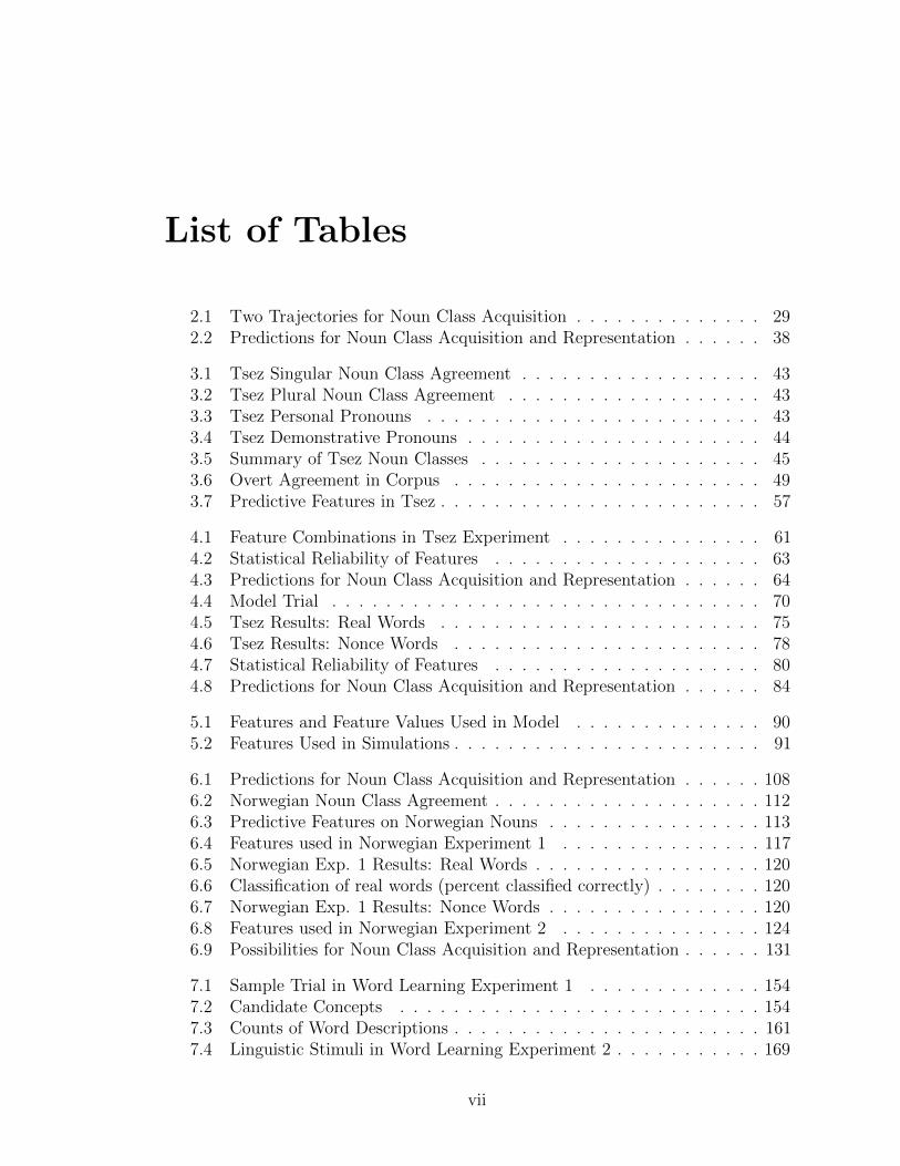
2.1 Two Trajectories for Noun Class Acquisition . . . . . . . . . . . . . . 292.2 Predictions for Noun Class Acquisition and Representation . . . . . . 38
3.1 Tsez Singular Noun Class Agreement . . . . . . . . . . . . . . . . . . 433.2 Tsez Plural Noun Class Agreement . . . . . . . . . . . . . . . . . . . 433.3 Tsez Personal Pronouns . . . . . . . . . . . . . . . . . . . . . . . . . 433.4 Tsez Demonstrative Pronouns . . . . . . . . . . . . . . . . . . . . . . 443.5 Summary of Tsez Noun Classes . . . . . . . . . . . . . . . . . . . . . 453.6 Overt Agreement in Corpus . . . . . . . . . . . . . . . . . . . . . . . 493.7 Predictive Features in Tsez . . . . . . . . . . . . . . . . . . . . . . . . 57
4.1 Feature Combinations in Tsez Experiment . . . . . . . . . . . . . . . 614.2 Statistical Reliability of Features . . . . . . . . . . . . . . . . . . . . 634.3 Predictions for Noun Class Acquisition and Representation . . . . . . 644.4 Model Trial . . . . . . . . . . . . . . . . . . . . . . . . . . . . . . . . 704.5 Tsez Results: Real Words . . . . . . . . . . . . . . . . . . . . . . . . 754.6 Tsez Results: Nonce Words . . . . . . . . . . . . . . . . . . . . . . . 784.7 Statistical Reliability of Features . . . . . . . . . . . . . . . . . . . . 804.8 Predictions for Noun Class Acquisition and Representation . . . . . . 84
5.1 Features and Feature Values Used in Model . . . . . . . . . . . . . . 905.2 Features Used in Simulations . . . . . . . . . . . . . . . . . . . . . . . 91
6.1 Predictions for Noun Class Acquisition and Representation . . . . . . 1086.2 Norwegian Noun Class Agreement . . . . . . . . . . . . . . . . . . . . 1126.3 Predictive Features on Norwegian Nouns . . . . . . . . . . . . . . . . 1136.4 Features used in Norwegian Experiment 1 . . . . . . . . . . . . . . . 1176.5 Norwegian Exp. 1 Results: Real Words . . . . . . . . . . . . . . . . . 1206.6 Classification of real words (percent classified correctly) . . . . . . . . 1206.7 Norwegian Exp. 1 Results: Nonce Words . . . . . . . . . . . . . . . . 1206.8 Features used in Norwegian Experiment 2 . . . . . . . . . . . . . . . 1246.9 Possibilities for Noun Class Acquisition and Representation . . . . . . 131
7.1 Sample Trial in Word Learning Experiment 1 . . . . . . . . . . . . . 1547.2 Candidate Concepts . . . . . . . . . . . . . . . . . . . . . . . . . . . 1547.3 Counts of Word Descriptions . . . . . . . . . . . . . . . . . . . . . . . 1617.4 Linguistic Stimuli in Word Learning Experiment 2 . . . . . . . . . . . 169
vii

8.1 Schematic of one entire trial . . . . . . . . . . . . . . . . . . . . . . . 2088.2 Set of Candidate Linear Mixed Effects Models . . . . . . . . . . . . . 2158.3 Set of Candidate Linear Mixed Effects Models . . . . . . . . . . . . . 2168.4 Set of Candidate Linear Mixed Effects Models . . . . . . . . . . . . . 2238.5 Set of Candidate Linear Mixed Effects Models . . . . . . . . . . . . . 229
viii
List of Figures
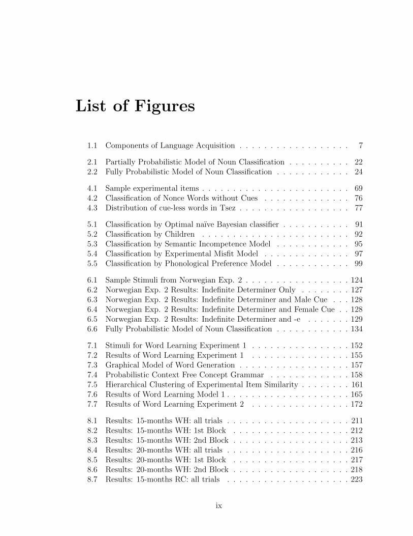
1.1 Components of Language Acquisition . . . . . . . . . . . . . . . . . . 7
2.1 Partially Probabilistic Model of Noun Classification . . . . . . . . . . 222.2 Fully Probabilistic Model of Noun Classification . . . . . . . . . . . . 24
4.1 Sample experimental items . . . . . . . . . . . . . . . . . . . . . . . . 694.2 Classification of Nonce Words without Cues . . . . . . . . . . . . . . 764.3 Distribution of cue-less words in Tsez . . . . . . . . . . . . . . . . . . 77
5.1 Classification by Optimal naıve Bayesian classifier . . . . . . . . . . . 915.2 Classification by Children . . . . . . . . . . . . . . . . . . . . . . . . 925.3 Classification by Semantic Incompetence Model . . . . . . . . . . . . 955.4 Classification by Experimental Misfit Model . . . . . . . . . . . . . . 975.5 Classification by Phonological Preference Model . . . . . . . . . . . . 99
6.1 Sample Stimuli from Norwegian Exp. 2 . . . . . . . . . . . . . . . . . 1246.2 Norwegian Exp. 2 Results: Indefinite Determiner Only . . . . . . . . 1276.3 Norwegian Exp. 2 Results: Indefinite Determiner and Male Cue . . . 1286.4 Norwegian Exp. 2 Results: Indefinite Determiner and Female Cue . . 1286.5 Norwegian Exp. 2 Results: Indefinite Determiner and -e . . . . . . . 1296.6 Fully Probabilistic Model of Noun Classification . . . . . . . . . . . . 134
7.1 Stimuli for Word Learning Experiment 1 . . . . . . . . . . . . . . . . 1527.2 Results of Word Learning Experiment 1 . . . . . . . . . . . . . . . . 1557.3 Graphical Model of Word Generation . . . . . . . . . . . . . . . . . . 1577.4 Probabilistic Context Free Concept Grammar . . . . . . . . . . . . . 1587.5 Hierarchical Clustering of Experimental Item Similarity . . . . . . . . 1617.6 Results of Word Learning Model 1 . . . . . . . . . . . . . . . . . . . . 1657.7 Results of Word Learning Experiment 2 . . . . . . . . . . . . . . . . 172
8.1 Results: 15-months WH: all trials . . . . . . . . . . . . . . . . . . . . 2118.2 Results: 15-months WH: 1st Block . . . . . . . . . . . . . . . . . . . 2128.3 Results: 15-months WH: 2nd Block . . . . . . . . . . . . . . . . . . . 2138.4 Results: 20-months WH: all trials . . . . . . . . . . . . . . . . . . . . 2168.5 Results: 20-months WH: 1st Block . . . . . . . . . . . . . . . . . . . 2178.6 Results: 20-months WH: 2nd Block . . . . . . . . . . . . . . . . . . . 2188.7 Results: 15-months RC: all trials . . . . . . . . . . . . . . . . . . . . 223
ix
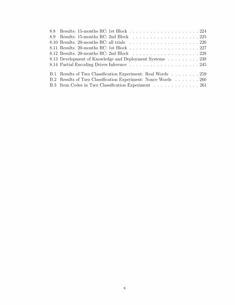
8.8 Results: 15-months RC: 1st Block . . . . . . . . . . . . . . . . . . . . 2248.9 Results: 15-months RC: 2nd Block . . . . . . . . . . . . . . . . . . . 2258.10 Results: 20-months RC: all trials . . . . . . . . . . . . . . . . . . . . 2268.11 Results: 20-months RC: 1st Block . . . . . . . . . . . . . . . . . . . . 2278.12 Results: 20-months RC: 2nd Block . . . . . . . . . . . . . . . . . . . 2288.13 Development of Knowledge and Deployment Systems . . . . . . . . . 2388.14 Partial Encoding Drives Inference . . . . . . . . . . . . . . . . . . . . 245
B.1 Results of Tsez Classification Experiment: Real Words . . . . . . . . 259B.2 Results of Tsez Classification Experiment: Nonce Words . . . . . . . 260B.3 Item Codes in Tsez Classification Experiment . . . . . . . . . . . . . 261
x
Chapter 1
Introduction
1.1 The logical problem of language acquisition
To acquire a language a child needs to be able to take linguistic information available
in the environment and infer what grammar could have generated this input. The
complexity of this problem is captured in the statement of the ‘Logical Problem
of Language Acquisition’, that is, how can a learner, faced with some finite set of
input, correctly generalize to the infinite set of sentences generable by the grammar
that generated the finite set? Chomsky (1965) proposed that children must come
equipped with language specific hypotheses in order to solve this problem. Ever
since then, approaches to the study of language acquisition have taken one of two
tacks: either they follow Chomsky and attempt to define the set of language specific
hypotheses that allow all and only the grammars witnessed in natural language to be
acquirable, or they challenge Chomsky and attempt to show that all the elements of
natural language are learnable by analyzing the linguistic input with general learning
1
mechanisms. While the rift between them has driven both of these approaches to
make important contributions to our understanding of human language acquisition,
it can sometimes seem as though this divide creates a hindrance to scientific progress.
The future of productive research in language acquisition bridges the chasm, looking
carefully at what information is accessible to the learner, and what sorts of hypotheses
can use that information to drive inferences about the nature of the grammar being
acquired.
1.2 Two traditional approaches to language acqui-
sition
Approaches to solving the problem of language acquisition have come in two flavors:
Generative Approaches acknowledge the complexity of the task and attempt to outfit
the learner with a battery of language specific tools to attack it, while Distributional
Approaches attempt to show how much a learner could acquire without any specific
tools, but often end up underestimating the complexity of the task while doing so.
Both of these approaches have made important contributions to the study of language
acquisition, showing us the range of hypotheses learners might posses innately, as
well as showing us what a powerful statistical learner would be able to infer on the
basis of the input alone. However, by ignoring or denying the claims and methods of
each side by the other, each approach seems to fall short of telling the full story of
how a child acquires language.
2
1.2.1 Generative approaches to language acquisition
Chomsky (1965) laid out a program for building a linguistic theory with the idea
that an adequate theory of linguistics would be virtually equivalent to a theory of a
language acquisition device. He proposed that a well spelled out theory of innate
hypotheses (constraints on possible grammars), combined with a way of choosing
between the candidate hypotheses (an evaluation metric) would be sufficient to
allow language acquisition to occur. However, formal investigations have proved the
problem to be significantly more difficult (Wexler & Culicover, 1980; Lightfoot, 1989;
Gibson & Wexler, 1994; J. D. Fodor & Sakas, 2004).
This is not to say that generative approaches have not made progress in our
understanding of language acquisition. Generative approaches to language acquisition
and linguistic theory have greatly illuminated our understanding of what a set of
language specific hypotheses would look like, and what hypotheses would have
to exist for natural languages to be acquirable (Chomsky, 1981; J. D. Fodor &
Sakas, 2004; Baker, 2005; Snyder, 2007). Furthermore they have outlined what
expectations learners may have about language from the outset, and have made
considerable progress in testing and documenting learner’s initial hypotheses in
acquiring, among many other phenomena, phonological rules (Bergelson & Idsardi,
2009), word segmentation and grammatical categories (Hochmann, Endress, & Mehler,
2010), basic syntax and argument structure (Naigles, 1990; J. Lidz & Gleitman, 2003;
Fisher, 2003), subject-auxiliary inversion (Crain & Nakayama, 1987), wh-questions
(J. deVilliers & Roeper, 1995), binding principles (Kazanina & Phillips, 2001; Conroy,
3
Takahashi, Lidz, & Phillips, 2009; Lukyanenko, Conroy, & Lidz, n.d.), and quantifier
raising (Lidz & Musolino, 2006; Goro, 2007). Supporting this view is the observation
that across languages learners make generalizations that could not have been inferred
from the input alone (Crain, 1991).
However, while hypotheses are fairly well outlined to fully capture the complex-
ity of natural languages, and while initial hypotheses are documented, researchers
taking this approach fail to show how a learner makes use of the linguistic data
available in the input to decide between these hypotheses. Accounts only begin to
specify what kind of data would be relevant for determining between two hypotheses.
They rarely, if ever, engage in questions of how a child would know that a given
piece of data from the input bears on a given hypotheses. Even more infrequent
are discussions of the types of inferences that children would have to be capable of
performing to use this data and this hypothesis set to infer which grammar generated
their language. Of course there are exceptions to this pattern, notably (C. D. Yang,
2004; J. D. Fodor & Sakas, 2004; Pinker, 1979; Lightfoot, 1989; Wexler & Culicover,
1980), who probe the ways in which a learner might use the linguistic data to arrive
an an adult grammar. However, all of these approaches assume that the child is able
to use all of the available input to draw these inferences, and thus implicitly rely on
the child’s ability to encode the input in a relevant way. This is not something we can
take for granted, as even though the linguistic input might be full of relevant data,
this data is only useful insofar as the learner is able to represent and subsequently
identify it. Investigating the learner’s ability to represent the data in the input, the
encoding, will from a large part of this thesis.
4
1.2.2 Distributional approaches to language acquisition
Distributional approaches, with their roots in structuralist linguistics (Harris, 1951),
aim to show that the structures that make up language are all observable patterns in
the linguistic input, and that a powerful statistical learner can infer these patterns
from simply observing this input. These approaches have made significant contri-
butions to our understanding, but ultimately fall short of showing that language
can be acquired through statistics of the input alone. Impressive work has been
done showing that based purely on distributional cues children can learn phonetic
categories (Maye, Werker, & Gerken, 2002), word boundaries (Saffran, Newport,
& Aslin, 1996), grammatical categories (Mintz, 2003), grammatical dependencies
(Gomez & Maye, 2005; Saffran, 2001) and simple syntactic structures (Morgan, Meier,
& Newport, 1989). This leads to a commonly held belief in the language acquisition
literature that children are perfect statistical learners (eg. Elman et al., 1996).
While these studies generally do a good job of detailing statistical sensitivity,
they don’t succeed in detailing how this sensitivity translates into inferences and
generalization about structure, often oversimplifying the complexity of the problem
faced by the learner. They often fail to outline the space over which the learner
is using the data in the input to generalize, as well as the true complexity of the
grammar they end up inferring. There is really no learning without some hypothesis
space to generalize over (J. A. Fodor, 1975), whether it is specific to language or
not, but many of these studies appear to overlook this in their explanations of the
learning process. While in some model problems oversimplification is warranted,
5

it does not appear to be appropriate when the issue at hand is that language is
complicated, yet children successfully acquire the complexities of grammar.
1.3 A logical solution
To bridge these two approaches, what is needed is an approach that combines these
two diverging lines of work. It is clear from what we know about the complex patterns
of language that it is impossible to infer a grammar from the input alone (Gold,
1967; Chomsky, 1980). It is also true that a learner must make ample use of the data
available in the linguistic input. The question then is not which approach is right, but
how a learner uses linguistic input (Omaki, 2010; Lidz & Gagliardi, 2012). We need
to both incorporate what we expect to find in a language specific hypothesis space,
given the complexity and variation present in natural language, as well the powerful
statistical inferences we know learners can perform over data in the input. With such
an approach we can then begin to answer questions like the following: How does the
hypothesis space a learner is endowed with allow him to leverage the information
in the input and infer a grammar? How do the developing cognitive capacities and
developing grammatical knowledge affect what the learner can encode from the input
and use to inform these hypotheses? What kind of inference mechanism does the
learner use to determine which of the possible hypotheses are supported in the input
and should be generalized in the grammar?
In order to make use of this approach, it is useful to break down language
acquisition into its component parts. So far I have mentioned that the learner infers
6
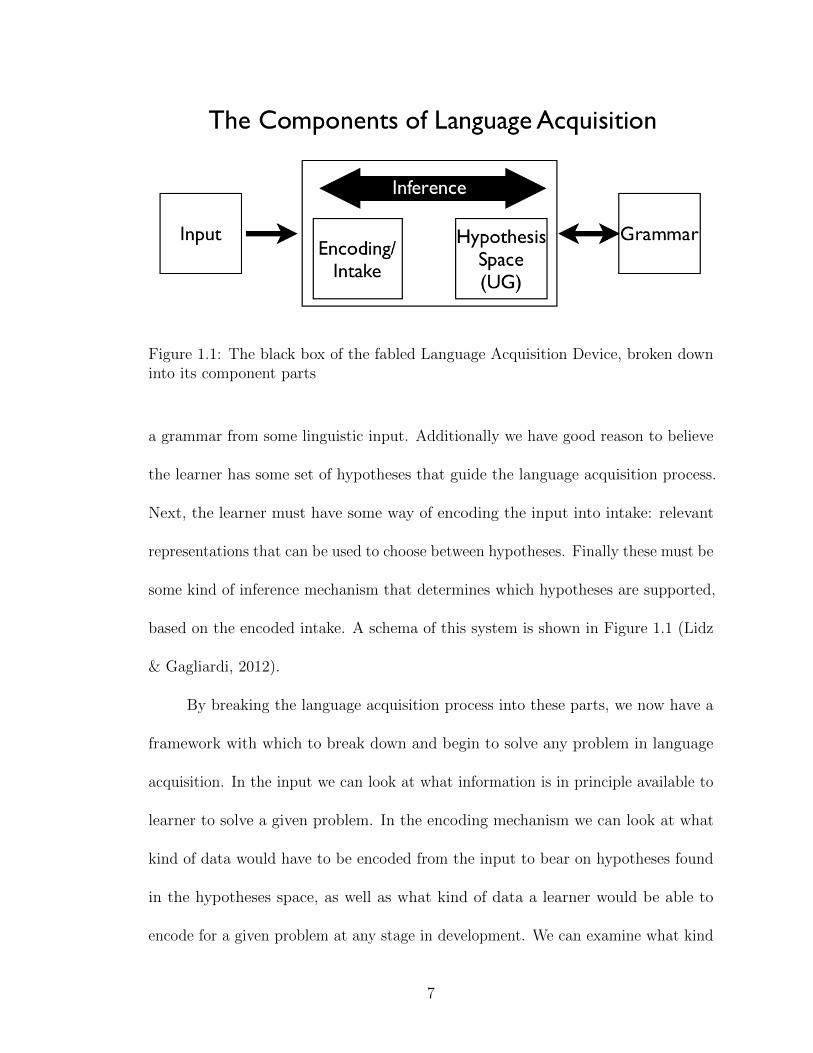
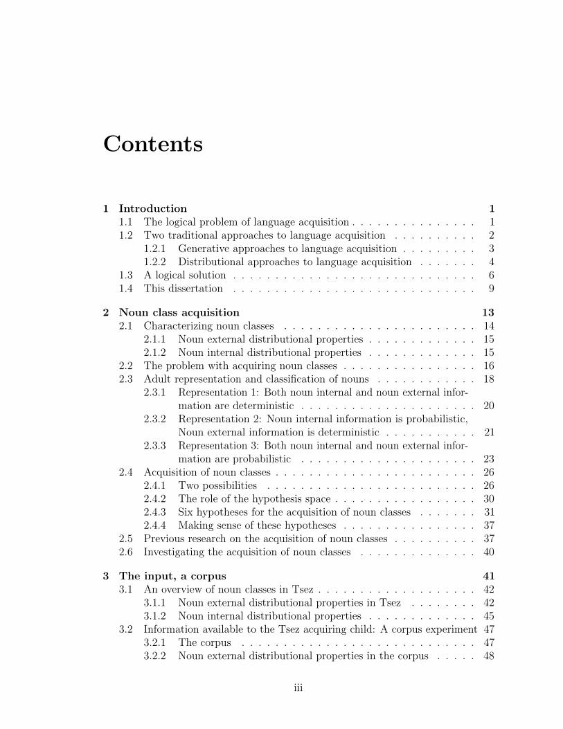
Figure 1.1: The black box of the fabled Language Acquisition Device, broken downinto its component parts
a grammar from some linguistic input. Additionally we have good reason to believe
the learner has some set of hypotheses that guide the language acquisition process.
Next, the learner must have some way of encoding the input into intake: relevant
representations that can be used to choose between hypotheses. Finally these must be
some kind of inference mechanism that determines which hypotheses are supported,
based on the encoded intake. A schema of this system is shown in Figure 1.1 (Lidz
& Gagliardi, 2012).
By breaking the language acquisition process into these parts, we now have a
framework with which to break down and begin to solve any problem in language
acquisition. In the input we can look at what information is in principle available to
learner to solve a given problem. In the encoding mechanism we can look at what
kind of data would have to be encoded from the input to bear on hypotheses found
in the hypotheses space, as well as what kind of data a learner would be able to
encode for a given problem at any stage in development. We can examine what kind
7
of inference mechanism would allow the child to use the available kind and quantity
of encoded intake to determine which hypothesis is supported. In the hypothesis
space we can map out what kind of hypotheses would need to be entertained in
order for any solution for a given problem found in natural languages to be learnable.
Finally, in the grammar we can see what kinds of representations a child would have
to be able to ultimately obtain.
This framework allows us as researchers to combine what we expect to find
in a richly specified hypothesis space with the powerful statistical sensitivities that
distributional learning researchers have found in children. While it is often not
elaborated on, the inference mechanisms that drive these sensitivities demand the
specification of a hypothesis space, and generative linguistics gives us just that.
Furthermore, this hypothesis space requires that the inference process act over
certain levels of representation, as not all levels of representation will bear on every
learning problem in linguistics. This in turn requires that to solve a given learning
problem, the learner must first be able to encode the input at the appropriate level
of representation. For example, the learner can’t begin to learn about the structures
governing sentences if he can’t segment the speech stream into words. Again, while
it is often not elaborated on, both generative and distributional learning approaches
often make this encoding implicit, either giving a computational model appropriately
encoded input, or assuming that children in an experiment have access to this level of
encoding. By carefully considering what level of encoding is necessary and comparing
this with what children are capable of encoding at different stages of acquisition, we
can begin to advance the study of language acquisition.
8

Once we have singled out the child’s ability to encode the linguistic input,
we need to discuss the implications of this encoding. As the child’s encoding is
dependent on the hypothesis space, current knowledge state and current cognitive
capacities, until the child has acquired an adultlike grammar the information that
appears available in the input is going to differ from the information accessible to
the child in the encoded intake. That is, until the child has an adultlike grammar,
the input will only ever be partially encoded and therefore partially available. This
means that in drawing inferences over the hypothesis space, the child only has access
to part of the data that may be relevant. As the child develops, so too will his
linguistic abilities and cognitive capacities, allowing him to encode more of the input,
which will bear on subsequently more complex hypotheses. Incompletely encoded
intake therefore must be what drives inferences to an adultlike grammar, as it is all
that is available until the entire grammar has been inferred. If we can investigate
what children know, and can therefore encode at a given stage, we can then look
at what kind of inference mechanism and what sort of hypothesis space would be
necessary to push the child forward to acquire the next generalization about his
grammar.
1.4 This dissertation
As the program of generative linguistics in the past 50 years has sought to delineate
the space of hypotheses necessary to arrive at all and only the space of possible
grammars in natural language, this dissertation will focus on the other pieces of
9
language acquisition, namely the encoding and the inference mechanism. In particular,
it will look at how while both necessitate a richly defined hypothesis space, the
power of such a hypothesis space depends directly on the nature of the intake and
the inference mechanism. The intake in turn depends on the encoding process.
To explore the inference and encoding mechanisms, this dissertation looks
at work across domains, examining word and word class learning, as well as the
acquisition of syntactic movement. The bulk of the thesis focuses on the acquisition
of noun classes. Without careful consideration, this may appear to be a trivial
problem. However, it provides an ideal lens to study the components of language
acquisition, as we can readily measure the input, probe the intake and model the
relatively straightforward inferences involved. Word learning is used in a similar
way, as a model problem to examine and explain the kind of inference that children
use in language acquisition. Word, or rather noun, class acquisition is explored
as it provides a very clear case of incomplete encoding of the information in the
input. The acquisition of filler gap dependencies is explored as an example of how
incompletely encoded input could drive inferences to acquire a system that allows
complete adultlike encoding.
I introduce the problem of noun class acquisition in Chapter 2. At first it does
not appear to be a problem at all. Children have ample information about noun
classes available in the input, and it looks as though noun class systems should be
trivially easy to learn. In practice however, noun class systems prove to be difficult
to acquire. A tentative model of noun class acquisition is discussed here, and this
model is probed further in Chapters 3-6.
10
In Chapter 3 I introduce noun classes in Tsez, a Nakh-Dagestanian language.
I outline what information characterizes these classes, information both internal
and external to the noun. I go on to introduce a corpus of child directed Tsez, and
measure what information about noun classes is available to the child in the input.
In Chapter 4 I investigate Tsez speakers’ sensitivity to the noun internal
information found in the input in Chapter 3. I present experimental results showing
that children exhibit different sensitivity to noun internal information than adults
do, and show sensitivity to this information in a way that is not predicted by its
statistical distribution in the input. That is, I discover a mismatch between input
and intake in the acquisition of Tsez noun classes, pointing toward incompletely
encoded input.
To further probe the difference I found between input and intake in Chapter
4, in Chapter 5 I develop a probabilistic model of noun classification. I build three
modifications of this model in an effort to better understand what underlies the
differences between input and intake. While I do not determine the precise source of
this difference, I do show that children’s behavior does appear to be optimal with
respect to a filtered, or incompletely encoded, version of the input.
In Chapter 6 I examine Norwegian child speakers’ sensitivity to noun class
information external to the noun, finding that speakers are relatively insensitive to it.
This points toward a fully probabilistic model of noun classes, which I explain in this
chapter, along with an outline of how such a system is likely acquired. I wrap up
this chapter with a discussion of the import of discovering and probing incompletely
encoded intake.
11
As all previous chapters make reference to inference, Chapter 7 explores the
inference process in greater depth. First I look at what kinds of inferences mechanisms
are available to the language learner, using word learning to explain how both a
learner’s expectations and the linguistic data in the environment are combined in
Bayesian inference. I present two experiments that extend this model to learn
multiple categories of words, and then word meanings and word classes. Models of
these results show how the simple inferences for learning words could scale up to
more complex problems faced by a language learner. Finally I close the chapter with
a discussion of how this inference model could be used to solve some of the classic
problems in language acquisition.
I change course in Chapter 8 to examine the acquisition more complicated
syntactic structures (filler-gap dependencies), and uncover a U-shaped pattern in
their acquisition. To explain this U-shaped pattern I put forward a hypothesis that
relies on incompletely encoded input driving inferences to a grammar that allows for
complete, adultlike encoding of the input.
Finally, Chapter 9 brings together the findings discussed in this dissertation
and brings them back to the themes introduced here. I assess where my investigation
of encoding and inference has gotten us thus far and look towards where such
investigations could bring us in the future.
12
Chapter 2
Noun class acquisition
The acquisition of noun classes (grammatical gender) presents an excellent model
problem for looking at how input is encoded into intake in language acquisition. The
input, as we will see in more detail below, is straightforward to measure, and the
encoded intake is fairly straightforward to probe. The next five chapters explore
noun class acquisition, looking at the nature of the input, when and how the input is
encoded, and show that, even in acquiring a relatively straightforward pheonomenon,
children’s abilities to encode the input gate what they are able to infer about their
language throughout acquisition.
In this chapter I will look at how noun classes are characterized by what looks
like an abundance of input, map out hypotheses of about how this information
factors in to the acquisition and representation of noun classes, review literature that
has looked at noun class acquisition and lay out the steps I will take to investigate
the relationship of input and intake in noun class acquisition
13
2.1 Characterizing noun classes
Natural languages all over the world employ noun classification systems. These
systems can generally be divided into two types: noun class (or grammatical gender1)
systems and classifier systems. In noun class systems, the class of a given noun can
influence the form of items in the entire sentence, whereas in classifier systems the
influence of the class of a noun is limited to the noun phrase. This paper focuses
on noun class systems, but similar arguments could be applied to the acquisition
of classifier systems. Noun classes can be characterized in two ways: using the
noun external distributional properties such as the agreement paradigm or syntactic
behavior that defines the class and using noun internal distributional properties, the
characteristics of the nouns that make up each class. As mentioned above, these two
types of information could be used in noun class acquisition2.
1Corbett, 1991 refers to all noun classification systems as grammatical gender, whether the
system makes use of natural gender or not. I agree that this is the correct, as both systems have the
same sorts of grammatical reflexes and their acquisition should be governed by the same mechanism.
In my experience, a significant degree of confusion arises when noun classification systems that make
use of natural gender (but differ from purely gender based systems such as the English pronominal
paradigm) are called ‘genders’. Therefore in this paper I will use the term noun class, as it suggests
no primacy of certain correlating features over others.2Certain types of verb classes might be superficially characterized in a similar way - members
of a class both share external properties such as the tense morphology they exhibit, and internal
properties such as phonological form or even meaning, and so in some cases it might be appropriate
to investigate their acquisition and representation in a parallel fashion
14

2.1.1 Noun external distributional properties
Noun classes are defined as groups of nouns that pattern the same way with respect to
agreement. Languages differ as to where this agreement is seen (Corbett, 1991). Some
languages are limited to DP internal agreement3, appearing on pronouns, possessives,
numerals, determiners and adjectives. Other languages also allow agreement external
to the DP, on verbs, adverbs, adpositions, complementizers and even other nouns.
Languages vary greatly in terms of how many environments agreement appears in.
They also vary in terms of the number of classes, some with as few as two (Spanish,
French) and others with as may as 20 (Fula) (Corbett, 1991).
2.1.2 Noun internal distributional properties
If noun internal distributional information is important for the acquisition of noun
classes, it is imperative to determine whether or not languages have, for each class,
some feature or set of features characteristic of the nouns in that class. The results
of many typological surveys are resoundingly positive: every noun class system
appears to have some regularity in the way at least a subset of nouns are classified
(Corbett, 1991), and that could be enough to aid the learner. For the acquisition
researcher investigating whether or not these regularities are employed in noun class
acquisition, it does not matter whether there is a set of rules that can classify all
nouns based on noun internal distributional information, or merely a subset. If
some noun internal information correlates with class, that is enough to launch an
3Again, contrasting with classifiers, which appear to be restricted to the NP
15

investigation to determine whether or not the child makes use of this information
during acquisition.
2.2 The problem with acquiring noun classes
The acquisition of noun classes ought to be trivially easy. Each noun occurs in
agreeing contexts some proportion of the time and the agreeing element consistently
exhibits the appropriate agreement. A linguist armed with some simple tools of
distributional analysis can identify the noun classes of a language in a relatively
brief time, however children apparently struggle with this into the school years
(MacWhinney, 1978; Karmiloff-Smith, 1979; Mills, 1986). To begin to understand
why children might have such difficulty, I will first consider what information abut
noun classes is available in the input, and then explore how a child might use this
information.
As mentioned above, there are two types of information that can be used to
characterize noun classes: noun internal and noun external distributional information.
As I have not yet determined whether or not children make use of this information as
a cue to noun class, I will conservatively call these noun external and noun internal
properties ‘information’, and not ‘cues’. By looking at noun external distributional
information a trained linguist could sit down with a language and quickly determine
(1) whether the language in question had noun classes (2) how many classes there
were and (3) which class each noun used with agreement went into. With just a
little more work the linguist could also determine similarities among the nouns in
16
each class and use these with varying degrees of success to predict the class of nouns
not previously seen with agreement (see Corbett, 1991 for review). These two kinds
of information: the highly regular noun external distributional properties (syntactic
context) and the probabilistic noun internal distributional properties (similarities
among properties of nouns within a class that vary in their reliability) are presumably
available in abundance to the learner. If they weren’t, the language in question
wouldn’t have a noun class system.
With both highly regular and probabilistic information in principle available
to the learner, we can ask what information the learner makes use of when going
through the same steps of discovering noun classes and the properties that correlate
with them. That is, what of the available information in the input is used as a cue
in the intake. While it may look like there is ample evidence for the existence and
structure of the noun classes in the input, what portion of this evidence is actually
used depends on more than just what information is available - it also depends on
how this input is encoded by the learner (Pearl & Lidz, 2009). This is an area where
we must distinguish between the input and the intake.
Now that I have outlined the two types of information that are in principle
available in the input to the learner of a noun class system, I can hypothesize what
information makes up the intake, and how this information may be used. There are
two senses in which they could be used: by adults to both represent their noun class
systems and to classify novel nouns, and by children to acquire the system of classes
and classify nouns as they learn them. In the discussion that follows, I will assume
that in the adult representation of noun classes, class is stored along with the lexical
17
entry of a given noun and is accessed every time a noun is processed or produced,
but not repeatedly recomputed based on internal or external information. I assume
that children are acquiring the same sort of system that adults have.
In the rest of this chapter and the following, I do not directly investigate how
the learner initially discovers noun classes, but instead look at a learner with a
developing system of noun classes. By looking at how this developing system differs
from the adult system I can glean information about (1) how the learner thinks
nouns are organized into classes and (2) what of the available information the learner
must have used to arrive at this state. These two pieces of evidence allow me to
draw inferences regarding discovery of noun classes earlier in development.
2.3 Adult representation and classification of nouns
It is evident from adult speakers’ use of their native language that they can use noun
external distributional properties when processing sentences, and presumably this
information is diagnostic of the class of novel nouns as well. That is, if an adult
speaker hears a noun used in the syntactic context characteristic of a given class,
he or she will know that the novel noun belongs to that class. This information is
highly regular in the language as it provides the characteristic definition of the class,
and is thus presumably a very reliable cue to the class of a novel word.
Evidence from borrowings and previous research (Tucker, Lambert, & Rigault,
1977; Corbett, 1991; Polinsky & Jackson, 1999) shows that adults can also use noun
internal distributional information to classify novel nouns in the absence of the more
18
reliable syntactic information. Novel nouns that have noun internal properties in
common with a group of nouns in a given class are likely to be put into that class.
Exactly how this works though, is not immediately clear. Do speakers have a set
of classification rules associated with predictive noun internal properties (e.g. If a
noun denotes a female human, then classify it a certain way)? Or do the predictive
noun internal properties inflate the probability that a noun would be in each class
in favor of the class that that property predicts (e.g. within the existing lexicon
it is 100% probable that if a noun denotes a female human it is in a certain class,
therefore novel nouns denoting female humans have a high probability of ending up
in that class)? Finally, is noun external information determined by a rule based
system or probabilistically? Below I outline three representational models, each
which make distinct predictions about both adult speakers’ representations and
children’s acquisition of noun classes.
At this point it may be relevant to relate noun class systems to other lexical
subclass systems that also appear to share both external grammatical properties (e.g.
past tense inflection) and internal properties (e.g. phonological form). For example,
consider the subclass of English irregular verbs ring, sing, drink, sink. All of these
verbs inflect for past tense via ablaut (ring-rang) and also share the [iN[+velar]] form.
However, neither the existence of the i-a ablaut nor the [iN[+velar]] form is predictive
of the other (e.g. spit-spat, link-*lank). Analyses posit that classes like these are
represented as a class of exceptions to a regular rule (Pinker, 1991), multiple rules
acting over a small classes of words that tend to have phonological similarities (Halle
& Mohanan, 1985; C. Yang, 2002) or are part of a system where grammatical reflexes
19
apply probabilistically to classes of words with varying levels of similarities (Hay &
Baayen, 2005). It may be tempting to try to align the representation of noun classes
to one of these analyses. However, differences in the way noun classes and this set of
verb classes work mean that none of these analyses is appropriate for noun classes. I
will expand on this observation in Section 6.6.5, and also suggest that my analysis of
noun classification may be applicable to irregular verb classes.
2.3.1 Representation 1: Both noun internal and noun exter-
nal information are deterministic
A model where both noun internal and noun external information are represented
in a deteministic rule based fashion is relatively straightforward. This model would
imply that a speaker has a set of rules that determine class based on the presence
of certain noun internal features (e.g. if female human, then assign to a certain
class, or, N[+female human] → Class X). Similarly, the speaker could have rules to
determine the class of a novel noun based on noun external information(e.g. if noun
occurs with a certain exponent, assign to a certain class). Alternatively, the speaker
could have rules to assign exponents for class given the presence of a noun)(i.e. Verb
→ Verb+ClassX.exponent / DP[+ClassX] ), and then infer the classes of nouns
based on the presence of exponents and the knowledge of these rules. Which of
these two ways rules for determining noun class based on noun external information
actually work isn’t a focus here, as either one is rule based, and therefore predicted
to be deterministic. Noun internal information that isn’t highly (100%) predictive
20
wouldn’t have associated rules. Although it is perhaps possible to conceive of a rule
that says ‘if a noun has a certain feature, assign it to a certain class 25% of the time’,
this type of rule is essentially a recharacterization of a probabilistic system disguised
as a rule based system, and I will consider it as such.
If both noun internal and noun external information were rule based, I would
expect that speakers classifying novel nouns would consistently classify nouns (per-
haps not with perfect consistency, leaving open the possibility of experimental noise)
according to the rules related to the cues on or cooccuring with a noun, whether the
cue is a noun internal feature or an noun external exponent. Furthermore, I would
expect that nouns that lacked a rule-triggering cue (a highly predictive noun internal
feature or noun external exponent) would be classified by some sort of ‘default rule’.
Predictions for the acquisition of such a system are discussed in Section 2.4 below.
2.3.2 Representation 2: Noun internal information is prob-
abilistic, Noun external information is deterministic
A model where noun internal information is probabilistic and noun external infor-
mation is probabilistic is also conceivable. In such a model, a speaker would have a
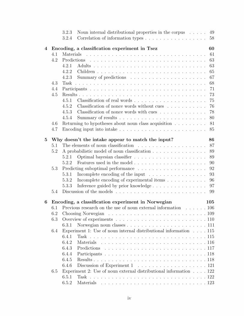
generative representation of noun class like that depicted in Figure 2.1.
In this model a noun class generates nouns with different noun internal features
with a certain set of probabilities. The probabilities assigned to noun internal
distributional information (semantic, phonological and morphological properties
of nouns) will vary in strength. Some classes may predict a given feature quite
21
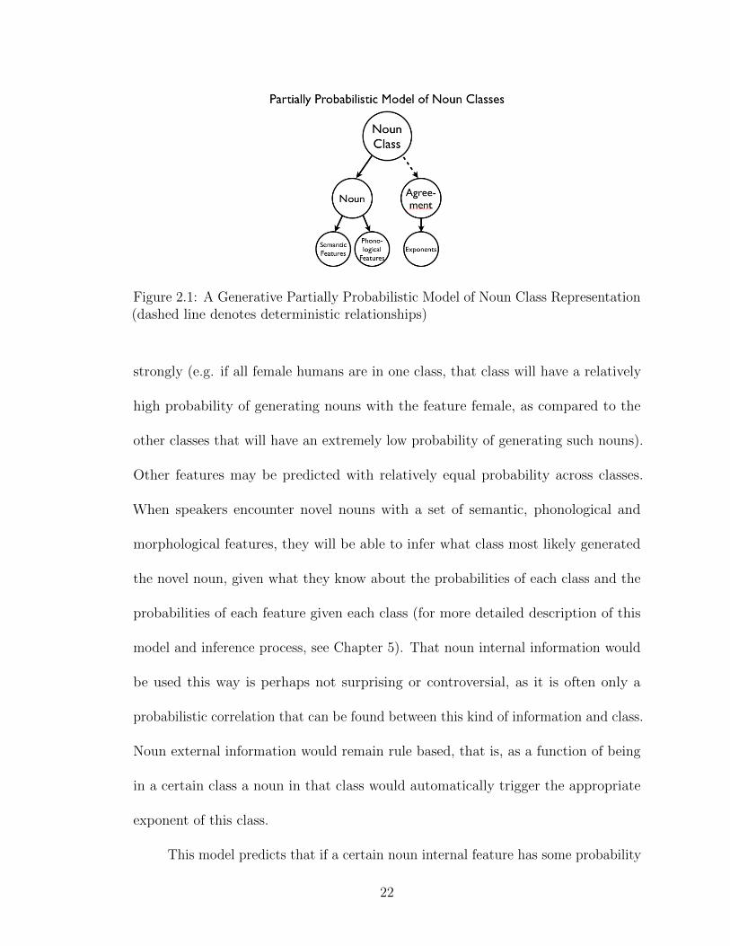
Figure 2.1: A Generative Partially Probabilistic Model of Noun Class Representation(dashed line denotes deterministic relationships)
strongly (e.g. if all female humans are in one class, that class will have a relatively
high probability of generating nouns with the feature female, as compared to the
other classes that will have an extremely low probability of generating such nouns).
Other features may be predicted with relatively equal probability across classes.
When speakers encounter novel nouns with a set of semantic, phonological and
morphological features, they will be able to infer what class most likely generated
the novel noun, given what they know about the probabilities of each class and the
probabilities of each feature given each class (for more detailed description of this
model and inference process, see Chapter 5). That noun internal information would
be used this way is perhaps not surprising or controversial, as it is often only a
probabilistic correlation that can be found between this kind of information and class.
Noun external information would remain rule based, that is, as a function of being
in a certain class a noun in that class would automatically trigger the appropriate
exponent of this class.
This model predicts that if a certain noun internal feature has some probability
22
distribution across classes, and if this feature is observed on or in conjunction with a
novel word, the probability that the novel word is in a given class will be proportional
to the combination of (1) the probabilistic distribution of this feature across classes
(2) the prior probability of each class and (3) the probabilities associated with any
other predictive features this noun contains. As noun external information is still
hypothesized to be deterministic, speakers would be predicted to behave the same
way with respect to it as in Representation 1. When no predictive noun internal or
noun external information is available, nouns without predictive features would be
expected to be classified according to baseline or prior probabilities of class. The
acquisition predictions of this account are spelled out in Section 2.4 below.
2.3.3 Representation 3: Both noun internal and noun exter-
nal information are probabilistic
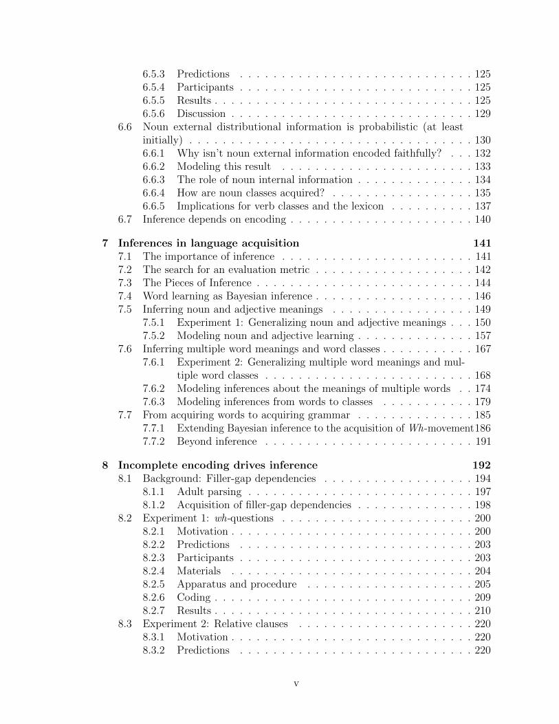
Finally, we can think of a fully probabilistic model of noun classification as a
generative model where each noun is assigned to a class, and each class generates
nouns with noun internal information with some probability, and noun external
information with associated exponents with some probability, as pictured in Figure
2.2.
The probabilistic noun internal information would work exactly the same way
as in Representation 2, and the noun external information would also work in a
probabilistic way. If a noun is seen co-occurring with an exponent of a given class,
to infer the class a speaker would use the probability of each class generating that
23
Figure 2.2: A Generative Fully Probabilistic Model of Noun Class Representation
exponent. This probability should be close to one for adult speakers, but could be
lower for children, for example if they hadn’t properly encoded some proportion
of noun external information. This proposal, that noun external information is
essentially the same kind of information, being predicted by the class probabilistically,
and isn’t part of some deterministic or rule based system, may be be much more
difficult to accept. That is, since noun external information never appears to be
probabilistic cross linguistically, it seems counterintuitive to propose it is generated
this way. However, as we will see below, children appear to treat this information
probabilistically, giving it this place in my model. Of course, it could be that
that with sufficiently high probability a probabilistic computation could become
a deterministic one, and thus the behavior we will see in children is actually just
a stage along the way to becoming an adult who uses noun internal information
probabilistically and noun external information deterministically.
This model predicts that when inferring the class of a novel noun, speakers
24
will use all information, noun internal and noun external, as well as baseline class
probabilities, probabilistically. This means that if a noun has noun internal informa-
tion and no noun external information, it will be classified according the predictions
made by the combination of noun internal information and the baseline probabilities
of each class. However if a noun appears with both noun internal and noun external
information, it will be classified in accordance with the probabilities that the speaker
has associated with each type of information and each class. For an adult speaker
with good control of the language, the noun external information should make the
strongest predictions. However, if a child is still acquiring the language, the noun
external information might not make as a strong a prediction, and the noun internal
information, or even the baseline probabilities of the class could win out. These and
further predictions about the acquisition of noun classes will be discussed below.
I now have hypotheses regarding whether noun internal and noun external
information are determined probabilistically or through a rule based system by
speakers of languages with noun classes. While I won’t expand on these models
here, we can see that each model makes distinct predictions about how noun internal
and noun external information will be used by speakers when classifying novel
nouns. By precisely specifying what these probabilities are, I can precisely model
the classification of novel words. Chapter 5 investigates this classification further.
What is important for this chapter are the hypotheses that predictive information
(both noun internal and noun external) may be used probabilistically, rather than
deterministically. As I will explore below, each of these representational hypotheses
makes different predictions about how noun classes are acquired.
25

2.4 Acquisition of noun classes
No matter whether the adult system is completely rule based, partially probabilistic
or entirely probabilistic, in order to acquire a noun class system, to arrive at the
system that adults exhibit - where noun external information is accurately produced
and interpreted and speakers are sensitive to noun internal cues that correlate with
class - children must at some point pay attention to both noun internal and noun
external distributional properties. How and when they do this is closely tied to what
the ultimate representation of noun class is. In in order to acquire noun classes the
learner must (1) infer that the language has noun classes (2) infer how many classes
there are and (3) infer which nouns go in which classes. Below I will outline how noun
class acquisition would need to proceed in order for a child to acquire each of the
hypothesized types of representations outlined above. Before I go into the specifics of
how noun class acquisition might proceed in each of my hypothesized representations,
it is useful to first consider what information is available to a child acquiring noun
classes, and how that information might be used. Once this is established, it will
become clear how studying of the acquisition of noun classes and their representation
can be mutually informative.
2.4.1 Two possibilities
As has been introduced above, a child is exposed to both noun internal and noun
external information that characterizes the classes in the target language. The
child could use only one of these information types, or both, to acquire such a
26

system. I won’t discuss what it would mean for a child to only use noun internal
distributional information, as without noun external information, a language really
doesn’t have noun classes, and so it isn’t clear what learning a noun class system
without making any use of noun external information would mean. Thus I am
left with two possibilities: (1) the child only uses noun external information and
extracts whatever regularities exist among nouns (noun internal information), after
the system has been acquired, or (2) the child makes use of both noun internal and
noun external information to acquire the noun class system.
Possibility 1 is similar to that outlined in Pinker (1984). Pinker proposes that a
child learns morphological paradigms by filling in each cell with affixes encountered in
the input. When two affixes compete for entry in the same cell, the cell splits and two
classes are formed. That is, a child might be filling in an agreement paradigm, and
have some affix they have put in the ‘verbal agreement’ cell. If he then encounters
another verbal agreement affix (and presumably encounter it enough times that it
seems worth splitting paradigms over), he would split the verbal agreement cell. In
doing so he would have discovered another agreement class. From then on, nouns
triggering one agreement morpheme would be in one class, and nouns triggering the
other would be in the other class. Such a system would not rely on noun internal
distributional information, only noun external distributional information such as
agreement. Instead, for children to acquire adult-like sensitivity to noun internal
distributional properties, they would have to keep track of this information after
the noun class system had been acquired. Once the lexicon has sufficient content
the learner could generalize over items in each class to extract the noun internal
27
distributional information, that is, the statistical regularities describing the nouns in
each class.
Possibility 2 is that the child first uses only noun internal distributional
information, grouping nouns together by their featural content (say, putting all
female humans together), and at a second stage combines these many small groups
of nouns to form classes, by noting the coocurrence of these subclasses of nouns
with class dependent noun external distributional information. At a certain stage,
they would be able to use the external rather than (or in addition to) the internal
distributional information to characterize a class. Such a process was suggested
by Braine (1987) after observing that learners of artificial languages with lexical
classes required both distributional information external to the items in each class
and regularities internal to the items in a class, in order to discover the class
system. Various other researchers have found similar patterns, where learners of
artificial languages need morphological or phonological markers on some proportion
of each subclass in order to learn the class system in the artificial language (Frigo
& McDonald, 1998; Gerken, Wilson, Gomez, & Nurmsoo, 2002; Gerken, Wilson, &
Lewis, 2005). Braine proposed a two step process wherein a learner first uses the
internal information to establish classes by determining what kinds of nouns correlate
with what external information, and later uses the noun external information to infer
class membership of novel nouns.
The steps involved in these two possibilities are compared in Table 2.1.
In the what follows, I will consider how each of these possibilities fits in with
my hypotheses about noun class representation from the previous section. None of
28
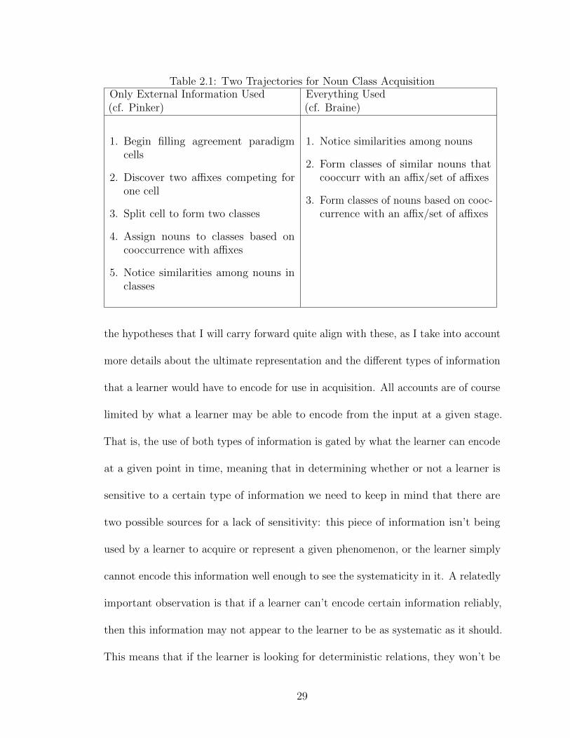
Table 2.1: Two Trajectories for Noun Class AcquisitionOnly External Information Used(cf. Pinker)
Everything Used(cf. Braine)
1. Begin filling agreement paradigmcells
2. Discover two affixes competing forone cell
3. Split cell to form two classes
4. Assign nouns to classes based oncooccurrence with affixes
5. Notice similarities among nouns inclasses
1. Notice similarities among nouns
2. Form classes of similar nouns thatcooccurr with an affix/set of affixes
3. Form classes of nouns based on cooc-currence with an affix/set of affixes
the hypotheses that I will carry forward quite align with these, as I take into account
more details about the ultimate representation and the different types of information
that a learner would have to encode for use in acquisition. All accounts are of course
limited by what a learner may be able to encode from the input at a given stage.
That is, the use of both types of information is gated by what the learner can encode
at a given point in time, meaning that in determining whether or not a learner is
sensitive to a certain type of information we need to keep in mind that there are
two possible sources for a lack of sensitivity: this piece of information isn’t being
used by a learner to acquire or represent a given phenomenon, or the learner simply
cannot encode this information well enough to see the systematicity in it. A relatedly
important observation is that if a learner can’t encode certain information reliably,
then this information may not appear to the learner to be as systematic as it should.
This means that if the learner is looking for deterministic relations, they won’t be
29
found, and if the learner is looking for probabilistic ones they will initially be much
weaker than they may end up being in the adult. These observations will figure
importantly in my subsequent investigation of noun class acquisition.
2.4.2 The role of the hypothesis space
So far, I have mentioned what a child would have to encode and what kinds of
inferences he would have to make to discover noun classes and subsequently assign
nouns to classes, but I haven’t spent much time thinking about what role the
hypothesis space plays in this process. The hypothesis space makes two contributions.
First the child should have some expectation that the lexicon could be partitioned,
causing him to search for systematicity in information either internal or external to
the noun that might point towards these partitions. Second, the child might have
some expectations about what kinds of features are likely to be used to partition the
lexicon. For all of the hypotheses where the child uses only noun external information
to discover classes, the expectations would be that partitions in the lexicon will
correlate with some information external to the noun. For hypotheses that expect
noun internal information is also relevant to lexical partitions, it’s possible that not
all information is equally likely to matter. For example, crosslinguistically many
languages make distinctions among natural gender, humanness and animacy (Corbett,
1991). Why this is isn’t clear, but it could be that children have some expectation
that these features could be used, and other features, such as those based on material
or function, might be less likely. In the discussion of hypotheses that follows, I will
30
make clear what role the hypothesis space plays in acquisition, along with what
needs to be encoded and what information the child uses to infer the existence of
noun classes and the class of each noun.
2.4.3 Six hypotheses for the acquisition of noun classes
Here I outline six ways that noun class acquisition could proceed, based on the three
representational possibilities outlined in section 2.3 and the two possibilities for cues
used in acquisition outlined in section 2.4.1.
Everything is deterministic, Only noun external information is used in
language acquisition
Under this possibility, the learner would use the deterministic relationships between
noun class and noun external information to discover classes, at some point after he
is able to reliably encode dependencies between nouns and noun external information.
The deterministic rules that assign nouns to classes based on some noun internal
features would not be used in noun class acquisition, but would be learned after the
classes had been learned via noun external information. In the hypothesis space the
learner would expect that the lexicon could be partitioned, expect these partitions to
correlate with deterministic noun external information, and perhaps expect that some
noun internal information would be used deterministically to assign nouns to classes.
To infer the existence of classes, the learner would have to be able to reliably encode
both noun external information and the dependencies between this information and
the nouns that it correlates with. This information would also be used to infer
31
the class of novel nouns. Eventually the learner would also have to encode noun
internal information to determine which features could be used deterministically to
classify novel nouns that appeared without noun external information. Somehow the
child will also learn a default classification rule in order to deal with novel nouns
lacking deterministic noun external or internal information. This account predicts
that all classification should be quite regular, as the child only uses deterministic
rules inferred from reliably encoded input to classify novel nouns.
Everything is deterministic, Everything is used in language acquisition
This hypothesis would mean that the learner would use the deterministic relationships
between class and both noun internal and noun external information to discover noun
classes and subsequently assign nouns to classes. Of course, each kind of information
could only be used insofar as it is encodable by the learner, meaning that what is used
could differ at different stages of acquisition. Due to the hypothesis space, the learner
would expect that the lexicon could be partitioned, that deterministic rules related to
noun internal and noun external information would correlate with this partitioning,
and might have some expectations about which types of noun internal information
would be likely to have deterministic relations to noun class. To infer the existence of
noun classes the learner would have to encode both noun internal and noun external
information reliably, in order to discover the deterministic relations between noun
class and this information. To infer the class of novel nouns, speakers would use
whatever deterministic information was given with the noun. Speakers would not
be expected to show any sensitivity to partial correlations between information and
32
class, as these non deterministic relations might not be encoded by a learner looking
only for deterministic ones. Finally, somehow the child would have to come up with
a default classification rule.
Noun internal information is probabilistic, Only noun external informa-
tion is used in language acquisition
This hypothesis is very similar to the first one, where once the learner can encode
dependencies between noun external information and noun class, he can use this
information to acquire noun classes. After discovering these classes and assigning
known nouns to classes based on the noun external information they are seen with,
the child would begin tracking probabilities among nouns in a class and discover
probabilistic relationships between noun internal information and classes. For this
hypothesis to work, the hypothesis space would have to expect that the lexicon
could be partitioned, and expect that deterministic noun external information
would correlate with these partitions. The learner would have to be able to encode
dependencies between noun external information and nouns, and would be able
to use this to infer the class of novel nouns. After acquiring the classes, the
learner would have to also be able to encode noun internal information and keep
track of regularities among features on nouns in a class to infer the probabilistic
relations between features and classes. Subsequently the learner would be able to
use this information to probabilistically infer the class of a novel noun when noun
external information was lacking. This would predict that when noun external
information is available, the child should classify nouns highly regularly, in line with
33
the deterministic predictions made by the noun external information. When noun
external information is lacking, the child should classify probabilistically. The child
would not acquire a default rue for classifying novel nouns but would instead use the
probabilities associated with various noun internal features and the probability of
each class to classify such all nouns in the absence of noun external information.
Noun internal information is probabilistic, Everything is used in language
acquisition
Under this hypothesis, the learner would use both deterministic noun external
information and probabilistic noun internal information to acquire classes, insofar as
each information type is encodable by the learner. In the hypothesis space the learner
would expect partitions within the lexicon, and would expect both deterministic noun
external information and some probabilistic noun internal information to correlate
with these partitions. Again, the learner might have specific expectations about what
kinds of noun internal information will correlate with class. The learner will have to
be able to encode dependencies between noun external information and nouns, as
well as noun internal information on nouns, in order to infer the existence of noun
classes, as well as to infer the class of novel nouns. As in the previous hypothesis,
classification of novel nouns should be regular when noun external information is
present, and probabilistic when it isn’t. The use of this probabilistic information
could vary across development, as the learner’s encoding of noun internal information
could change as he can encode more features in the input. The use of the deterministic
information should remain constant, as once the learner can track these dependencies
34
they are highly regular.
Everything is probabilistic, Only noun external information is used in
language acquisition
This hypothesis posits that the learner first tracks probabilistic correlations between
noun external information and class, as soon as these dependencies are encodable.
Once the classes have been acquired via this probabilistic (but highly predictive)
noun external information, the learner will begin tracking probabilities between class
and noun internal features. This hypothesis requires a hypothesis space that tells the
learner expect to find partitions in the lexicon based on probabilistic correlations
between noun external information and class. The learner would not have to perfectly
encode the dependencies between noun external information and class, as these are
only expected to be probabilistic, not deterministic, leaving room for successful
learning even in the face of misencoding of the input. The learner would have to be
able to infer the existence of noun classes based on this probabilistic information,
and would be able to infer the class of novel nouns from it as well. After acquiring
noun classes, the learner might find probabilistic correlations between encoded noun
internal features and noun class, and be able to infer the class of novel nouns based
on this information as well. When inferring the class of any noun, the learner would
use the combination of probabilistic noun external and internal information. As all
information is probabilistic, it is possible that the child would find noun internal
information to be a more reliable cue to class than external information, if he has
been able to encode and therefore track this information more reliable or for longer.
35
However, in this case I have a prediction that noun external information would be
tracked earlier than internal information in order to discover classes, and would likely
be a very reliable cue to class for the child, if it was robust enough for class to be
discovered using it.
Everything is probabilistic, Everything is used in language acquisition
Under this hypothesis, the learner would track probabilistic relations between class
and both noun internal and noun external information. Each type of information
would be generalized from when the child was able to encode this sort of information
or dependency. The hypothesis space would give the child an expectation that the
lexicon could be subdivided according to any probabilistic relations, either those
among nouns based on noun internal information or those between nouns and noun
external information. Some of these relations might be expected to be more likely
than others. The learner would have to be able to encode noun internal and external
features, and dependencies between nouns or nouns and noun external information
in order to infer the existence of noun classes based on these correlations. The
child would be able to infer the class of a novel noun based on both noun internal
and noun external information and the probabilities associated with these types of
information and each noun class. As the child’s abilities to encode information will
develop across time, so too may their use of noun internal and external information
in noun classification. As all information is used probabilistically, when inferring
the class of novel nouns the child might initially favor information that was highly
predictive earlier in development.
36
2.4.4 Making sense of these hypotheses
Now that I have outlined what the learner would have to encode, infer, and bring to
the problem in the hypotheses space, I am ready to investigate the acquisition and
representation of noun classes. Each hypothesis makes different predictions about
both adult and child representations of noun classes, summarized in Table 2.2. In
the next 4 chapters, I will investigate noun class acquisition through corpus analysis,
behavioral experiments and computational models, narrowing down these hypotheses
to find the one most likely, given what I find at each step.
2.5 Previous research on the acquisition of noun
classes
Previous research on the acquisition of noun classes has shown that children ac-
quiring noun class languages are sensitive to both noun external and noun internal
distributional information, offering tentative support for the hypotheses that predict
children use both noun internal and noun external information in acquiring noun
classes. Work in French (Karmiloff-Smith, 1979), Spanish (Perez-Pereira, 1991),
German (MacWhinney, 1978; Mills, 1985, 1986) and Russian (Rodina & Westergaard,
2012) consistently shows that children are able to make use of noun internal distri-
butional information in the classification of novel nouns. Moreover, younger children
in particular prefer to use morphophonological information rather than semantic
information, despite the fact that the semantic information in some cases is a more
37
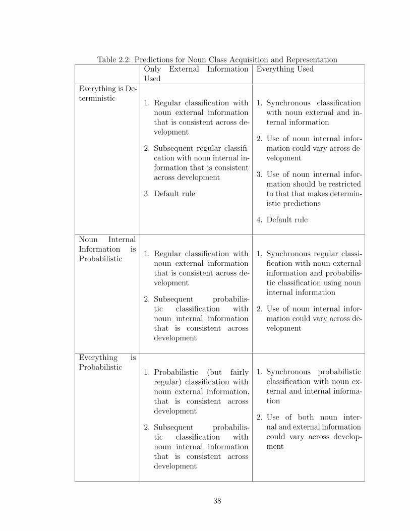
Table 2.2: Predictions for Noun Class Acquisition and RepresentationOnly External InformationUsed
Everything Used
Everything is De-terministic
1. Regular classification withnoun external informationthat is consistent across de-velopment
2. Subsequent regular classifi-cation with noun internal in-formation that is consistentacross development
3. Default rule
1. Synchronous classificationwith noun external and in-ternal information
2. Use of noun internal infor-mation could vary across de-velopment
3. Use of noun internal infor-mation should be restrictedto that that makes determin-istic predictions
4. Default rule
Noun InternalInformation isProbabilistic
1. Regular classification withnoun external informationthat is consistent across de-velopment
2. Subsequent probabilis-tic classification withnoun internal informationthat is consistent acrossdevelopment
1. Synchronous regular classi-fication with noun externalinformation and probabilis-tic classification using nouninternal information
2. Use of noun internal infor-mation could vary across de-velopment
Everything isProbabilistic
1. Probabilistic (but fairlyregular) classification withnoun external information,that is consistent acrossdevelopment
2. Subsequent probabilis-tic classification withnoun internal informationthat is consistent acrossdevelopment
1. Synchronous probabilisticclassification with noun ex-ternal and internal informa-tion
2. Use of both noun inter-nal and external informationcould vary across develop-ment
38
reliable predictor of class. Children also make use of noun external distributional
information, though young children appear less able to do so.
Both the early reliance on noun internal distributional information and the
fact that this reliance does not always align with the statistical reliability of the
information as can be measured in the input point towards the hypotheses that
make use of noun external and noun internal information to acquire noun classes.
Unfortunately, this work does not directly address the questions posed by all of the
hypotheses outlined above, as there are no direct comparisons with adult speakers
and no information about what children or adults do when nouns are presented in
the absence of either noun internal or noun external distributional information.
As mentioned above, several artificial language studies looked at the acquisition
of lexical subclasses and found that learners could not learn completely arbitrary
correlations between words or words and morphemes unless some portion of the
words in each class shared a similar feature (K. H. Smith, 1966; Braine, 1987; Frigo
& McDonald, 1998; Gerken et al., 2002, 2005). The similarities on words could
be semantic, phonological or morphological, and subjects ranged from infants to
adults. At first, this result looks like a promising piece of the noun class acquisition
puzzle: the information tying the subset of words together could be the noun internal
information, and the class agreement the noun external information. These findings
appear to suggest that noun internal information is not only a useful piece of noun
class acquisition, but is a necessary piece. However, as these studies are based on
subjects learning toy languages with small vocabularies in the lab, their import
may be limited. In several attempts, I have found that these effects won’t scale
39

up to even slightly more realistic languages. The reason for this failure is unclear.
It could be due to adult subjects’ limited implicit learning abilities, or to the fact
that the usefulness and necessity of the cue is an artifact of the way these tasks are
designed, not a reflection of a deeper property about language acquisition. With this
in mind, I will continue my investigation of noun class acquisition looking at what
information children use to discover and subsequently classify novel nouns, coming
back to this finding in my discussion of the mechanisms involved. In particular, I
will be interested in whether noun internal information is necessary to learn noun
classes, or just one more helpful piece of the puzzle.
2.6 Investigating the acquisition of noun classes
In the chapters that follow I will investigate noun class acquisition in an effort to
determine what information is available in the input, how much of the input children
can encode, what information children use when acquiring noun classes, and why they
appear to use informative out of proportion with is distribution in the input. In the
next chapter I will examine the information available in the input by building a corpus
of child directed speech in Tsez, a language with four noun classes. In the following
chapter I will examine Tsez children’s sensitivity to this information. I follow this
with a chapter probing the differences between Tsez children’s classification patterns
and those predicted by the noun internal information using four computational
models. Finally I look at Norwegian children’s use of noun external distributional
information and wrap up with a discussion of how a learner’s ability to encode the
40

input governs the inferences they can draw from it.
41
Chapter 3
The input, a corpus
The first step in determining how nouns classes are represented and acquired involves
determining what information is available in the input. In order to examine this
information, I had to first decide on a language with noun classes to investigate.
Then I examined what information was available in the language in principle, that
is, what noun external and noun internal distributional information I expected to
find based on information found in grammatical descriptions, previous research and
a dictionary. Finally I wanted to see what information was actually available to
children, in order to see which of my six possibilities remained viable hypotheses for
the acquisition of noun classes.
I chose Tsez, a Nakh-Dagestanian language spoken by about 6,000 speakers in
the Northeast Caucasus1. Tsez was a good choice for this work for several reasons.
1According to the 2002 census, there are about 15 thousand Tsez speakers, but the real number
estimated by researchers is around six thousand (Bokarev, 1959; Comrie, Polinsky, & Rajabov,
1998; Comrie & Polinsky, 1998; Polinsky, 2000).
42
First, Tsez has four noun classes, and proved to be particularly interesting as there is
a significant amount of syncretism in noun class agreement, that could make learning
from external information only more difficult. Additionally, previous work had been
done investigating the noun internal information of Tsez nouns. After examining
this information, I built a corpus of child directed Tsez speech and examined it to
see how much noun external distributional information was available, what noun
internal distributional information was, and how often the two kinds of information
cooccurred.
3.1 An overview of noun classes in Tsez
Tsez has four noun classes in the singular which collapse to two in the plural. Below
I give an overview of noun external and noun internal distributional properties in
Tsez (Comrie, 2007).
3.1.1 Noun external distributional properties in Tsez
The noun external distributional information characterizing Tsez noun classes is
prefixal agreement on vowel initial2 verbs, adjectives and adverbs, as shown in 3.1.
Thus the agreement prefix for Class 1 is the null prefix, for Class 2 it is [j], for
Class 3 [b] and Class 4 [r]. The same set of prefixes are used on verbs, adjectives
2A small proportion of verbs, adjectives and adverbs are vowel initial but do not take overt
agreement. An interesting observation to make would be whether children overgeneralize agreement
to these exceptions.
43

Table 3.1: Tsez Singular Noun Class Agreement
Class 1 Class 2 Class 3 Class 4-igu uZi j-igu kid b-igu k’et’u r-igu ÙorpaI-good boy(I) II-good girl(II) III-good cat(III) IV-good soup(IV)good boy good girl good cat good soup
Table 3.2: Tsez Plural Noun Class Agreement
Class 1 Class 2 Class 3 Class 4b-igu uZi-bi r-igu kid-bi r-igu k’et’u-bi r-igu Ùorpa-biI-good boy(I)-abs.pl II-good girl(II)-abs.pl III-good cat(III)-abs.pl IV-good soup(IV)-abs.plgood boys good girls good cats good soups
and adverbs. Plural agreement prefixes and some forms of both personal and
demonstrative pronouns also vary by noun class, but there is considerable syncretism
in these paradigms, making them less reliable markers of class3 (Tables 3.2-3.4).
In any language with a noun class system, seeing an agreement marker for
3Tsez only has personal pronouns for 1st and 2nd person. Demonstrative pronouns are used as
3rd person pronouns. Effectively the personal pronouns are only used with classes 1 and 2, as they
will generally have human referents. However, in stories or other contexts where non human nouns
might be referred to in the 1st or 2nd person, they require the same pronouns as Class 2.
Table 3.3: Tsez Personal Pronouns
Class 1 Class 2-4 Class 1 Class 2-4singular singular plural plural
1st PersonAbsolutive di eli ela
Oblique d?- elu- ela-Genitive dej eli,eliz
2nd PersonAbsolutive mi meZi meZa
Oblique debe-,dow- meZiu meZiaGenitive debi meZi,meZiz
44
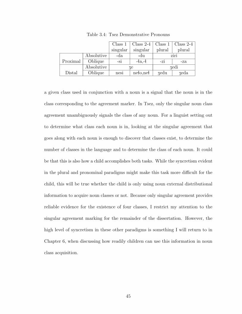
Table 3.4: Tsez Demonstrative Pronouns
Class 1 Class 2-4 Class 1 Class 2-4singular singular plural plural
ProximalAbsolutive -da -du ziri
Oblique -si -ìa,-ì -zi -za
DistalAbsolutive Ze Zedi
Oblique nesi neìo,neì Zedu Zeda
a given class used in conjunction with a noun is a signal that the noun is in the
class corresponding to the agreement marker. In Tsez, only the singular noun class
agreement unambiguously signals the class of any noun. For a linguist setting out
to determine what class each noun is in, looking at the singular agreement that
goes along with each noun is enough to discover that classes exist, to determine the
number of classes in the language and to determine the class of each noun. It could
be that this is also how a child accomplishes both tasks. While the syncretism evident
in the plural and pronominal paradigms might make this task more difficult for the
child, this will be true whether the child is only using noun external distributional
information to acquire noun classes or not. Because only singular agreement provides
reliable evidence for the existence of four classes, I restrict my attention to the
singular agreement marking for the remainder of the dissertation. However, the
high level of syncretism in these other paradigms is something I will return to in
Chapter 6, when discussing how readily children can use this information in noun
class acquisition.
45
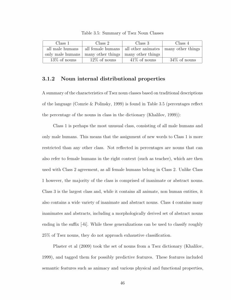
Table 3.5: Summary of Tsez Noun Classes
Class 1 Class 2 Class 3 Class 4all male humans all female humans all other animates many other things
only male humans many other things many other things13% of nouns 12% of nouns 41% of nouns 34% of nouns
3.1.2 Noun internal distributional properties
A summary of the characteristics of Tsez noun classes based on traditional descriptions
of the language (Comrie & Polinsky, 1999) is found in Table 3.5 (percentages reflect
the percentage of the nouns in class in the dictionary (Khalilov, 1999)):
Class 1 is perhaps the most unusual class, consisting of all male humans and
only male humans. This means that the assignment of new words to Class 1 is more
restricted than any other class. Not reflected in percentages are nouns that can
also refer to female humans in the right context (such as teacher), which are then
used with Class 2 agreement, as all female humans belong in Class 2. Unlike Class
1 however, the majority of the class is comprised of inanimate or abstract nouns.
Class 3 is the largest class and, while it contains all animate, non human entities, it
also contains a wide variety of inanimate and abstract nouns. Class 4 contains many
inanimates and abstracts, including a morphologically derived set of abstract nouns
ending in the suffix [-ìi]. While these generalizations can be used to classify roughly
25% of Tsez nouns, they do not approach exhaustive classification.
Plaster et al (2009) took the set of nouns from a Tsez dictionary (Khalilov,
1999), and tagged them for possibly predictive features. These features included
semantic features such as animacy and various physical and functional properties,
46

phonological features such as first and last segments and morphemes, number of
syllables and formal features such as the declension class. The result was a feature
vector for every noun that included values for every possible feature for a given
noun. The set of feature vectors was the input to a supervised learning algorithm,
Quinlan’s C4.5 implementation of a decision tree algorithm (Quinlan, 1993). The
output of such an algorithm is a set of decision rules, dependent on the presence
or absence of a certain feature on a noun, determining classification of the noun or
the next decision to be made. For example, since the feature male human is a very
reliable feature that can be used to reliably classify a large number of words, the
first rule in the decision tree assigns all nouns with the feature male human to Class
1. Nouns without this feature are then subject to the next rule, and so on, until all
nouns have been classified.
By using the sorts of features described above in such an algorithm, Plaster
et al were able to accurately classify about 70% of Tsez nouns. Semantic features,
both those referencing properties like animacy and humanness and those referencing
physical properties like stone or container were found to be more predictive than
formal properties such as certain derivational suffixes and the first segment of the
noun. This number looks promising, considering the large degree of arbitrariness
that the Tsez system at first appeared to have. While Plaster et al see this as only a
good first pass, and endeavor to better characterize the classification of the remaining
30% of nouns, the fact that several features can be reliably used to predict noun
class is as much as I need to move forward investigating their role in the acquisition
of noun classes.
47
3.2 Information available to the Tsez acquiring
child: A corpus experiment
Above I discussed the two types of information characterizing noun classes in Tsez,
and six hypotheses regarding the way in which this information could be used by a
learner. Differences between the input as we can measure it and the intake, as can
be inferred from behavioral data, will help to differentiate between these hypotheses.
In order to determine what of the input is used, I first have to characterize what
exactly the input to a Tsez learner is. A limitation of the prior work on Tsez is
that it is based solely on the distribution of words in the dictionary. Since learners
are likely not exposed to the entire dictionary, we do not yet know what internal
features of nouns are predictive of noun class in speech to children (and if these are
different from the dictionary distributions), how often they hear nouns with these
features, how often they are exposed to noun external distributional information
and how often they hear these two types of information together. To address this
issue, I created a corpus of child-directed speech in Tsez so that I could rigorously
examine how much of this information is available in the input that learners actually
receive. Once I have characterized what information the learner is exposed to, we
can investigate hypotheses about how this information is used.
3.2.1 The corpus
Over a period of 1 month, 10 hours of child directed speech were recorded during
normal daily interactions between a mother, aunt and older sister of two 20-month-
48

old Tsez acquiring children in Shamkhal, Dagestan. Roughly 6 hours of these
recordings were transcribed with the assistance of two native speaker members of the
family, familiar with the situations going on when the recordings took place4. This
transcription has yielded about 3000 lines of text. This text was hand tagged for
part of speech, agreement morphology and class of nouns. While this corpus is small
by the standards of corpus linguistics, it nonetheless provides sufficient information
to estimate the distribution of features in highly frequent Tsez nouns.
3.2.2 Noun external distributional properties in the corpus
As mentioned above, unique agreement for every class is only seen on vowel initial
verbs and adjectives in Tsez. These verbs and adjectives make a minority of total
verbs and adjectives in the dictionary (27% of verbs and 4% of adjectives). There
are three possibilities concerning how this noun external information is distributed
in speech to children. First, it could be that this small proportion is reflected in the
input, and hence noun external cues to noun class are uncommon. Second, it could
be that this proportion is even smaller in the input because the words exhibiting
agreement are infrequent, making the use of noun external cues to noun class even
more difficult. Finally, it could be that these vowel initial verbs and adjectives are
highly frequent, thus providing robust noun external distributional cues to noun
class.
4Ultimately, the entire corpus will be transcribed, but due to limitations of time and speaker
availability, the densest (highest rate of utterances/minute) recordings were transcribed first. Thus
while this corpus is 6 out of 10 recorded hour, it contains the vast majority of the recorded utterances
49

Table 3.6: Proportions of verbs and adjectives that show overt agreement
Agreeing Verbs Agreeing AdjectivesDictionary Types 27% 4%
Corpus Types 60% 35%Corpus Tokens 84% 77%
To address this issue, I calculated the total number of verb and adjective tokens
exhibiting agreement and compared it to the total number of verbs and adjectives.
While the majority of verb types but only a minority of adjective types showed
agreement (60% of verbs, 35% of adjectives), the majority of both verb and adjective
tokens did show agreement (84% of verbs, 77% of adjectives).
These results, seen in Table 3.6, show that the agreeing forms are highly
frequent, and thus that there are robust noun external distributional cues to noun
class in the input to the learner of Tsez. Moreover, these cues are more frequent
than would be expected given the distribution of vowel initial words in the overall
Tsez lexicon.
3.2.3 Noun internal distributional properties in the corpus
Just as Plaster et al looked for noun internal regularities in the list of Tsez nouns
from the dictionary, I wanted to look for such regularities in the nouns that children
are exposed to. To do this, a list of nouns found in the corpus was compiled and
tagged for morphophonological and semantic features. These features were similar
to those used by Plaster et al, and were fed into a decision tree building algorithm
to determine which were the most predictive of class. A description of the features
50
used, as well as a justification and explanation of decision tree modeling is below.
As Plaster et al used decision tree modeling to determine the most predictive
features of a set of Tsez nouns from a dictionary, it seems like a natural extension
to use the same methodology to look for predictive features on Tsez nouns from a
corpus. However, before proceeding forward with this methodology, is useful to first
consider whether it is indeed a suitable classifier for this type of data. There are
many classifiers employed to solve a wide variety of machine learning problems, and
before settling on decision trees I considered (1) what the form of my input data
was (2) what type of output I wanted from a model and (3) the inductive biases
associated with the models under consideration (the assumptions behind a given
model).
Model input
My input data is the set of nouns pulled from the the corpus of Tsez child directed
speech (although I also planned to test the nouns in the dictionary in order to
compare results from the two possible lexicons). I tagged each noun using a set of
binary attributes dependent on whether the set of semantic and morphophonoogical
features were present. The semantic features I used were of two types. First there
were what I will call the biological semantic features: natural gender, humanness and
animacy. These features not only make natural classes, but seem to be important
crosslinguistically both in noun class systems (see Corbett, 1991) and as syntactic
features. Second were what I’ll call the other semantic features. These were features
that appeared to group small numbers of related nouns together (such as container,
51
body part, berry, etc), but appear to be coincidental. Morphophonological features
included number of syllables, which ranged from 1 to 6, first segment (any phoneme
that began a word), last segment (any phoneme that ended a word) and presence of
the derivational morpheme [ìi]. Overall, there were 153 attributes defined for each
item.
Model output
As output, I want to see what class each noun is most likely assigned to based on
what the classifier has learned about each feature in the dataset. Additionally I
would like to see which features were useful in classification and how they rank
against each other. Finally, as I want to see if any combinations of features are
useful in classification, and since we know that some features are not statistically
independent of one another (eg. being a male humans depends on not being a female
human) an important requirement for the classifiers I ’ll compare is that they do not
assume independence of features.
Comparing models
While there are several classifiers that can take feature vectors like those available to
us and use them to learn to classify items, I will compare only two here: decision
trees and rule learners. Below I evaluate each type of model, taking into account
details of its implementation, associated inductive biases and the interpretability of
the output with respect to my outlined desiderata. Both of the models discussed
below are available as part of the Weka machine learning software package, which
52
helped to streamline their evaluation (Witten & Frank, 2005).
Decision Trees One way to classify data is to ask a series of questions about
the data, and depending on the answers to these questions, ask followup questions.
For example, if I wanted to determine whether an animal was a mammal or not I
might first ask whether it is warm or cold blooded. If it’s cold blooded, I am done, I
know I am not dealing with a mammal. If it’s warm blooded, I can then ask whether
or not it has live birth5. Again, if the answer is no, I know it is not a mammal. It’s
easy to see that these questions have an inherent order, as asking about live birth
will only be informative once I’ve narrowed down the set of animals to warm blooded
ones (as some cold blooded animals, like sharks, appear to give birth to live young).
Decision trees are basically a set of questions like this that take some set of data
and divide it into classes based on answers to sets of questions.
Decision trees have three basic pieces: a root node, or the the set of all data
that they begin with, internal nodes, that contain a subset of the data as divided by
a given question, and leaf nodes, that contain a subset that all belongs to the same
class. Decision trees can be induced from a set of labeled training data (a set of data
that is labeled in terms of which class each item in the class is) and subsequently
tested on unlabeled data.
Both the original set of data, contained in the root node, and the subsequent
subsets of data, can be measured for impurity. The impurity of a subset of data
depends on how the items in the set are labeled. If all the items have the same label
5excluding, for the purposes of this discussion the platypus and other monotremes
53

(e.g. all are mammals), the subset has no impurity. If a roughly equal proportion
of items in a set have each possible label, the subset has high impurity. The basic
algorithm for building a decision tree (Hunt’s algorithm, the basis of the C4.5
algorithm mentioned above (Hunt, Marin, & Stone, 1966)) partitions the data into
subsequently purer subsets based on a set of questions like those outlined above.
This sort of algorithm works in the following way (cf. Tang, Steinbach, &
Kumar, 2005). First, the data in the first node is checked to see if all examples are
in the same class (or exceed some given impurity threshhold). If so, the node is a
leaf node is labeled with that class label. If not (as will be the case for a least the
first node in every decision tree), the node will be examined to find the best split.
The best split can be determined by a variety of metrics, one of the most common
being information gain, ∆:
∆ = I(P )−∑
ikN c
N· I(C) (3.1)
which is dependent on the impurity, I of the parent node P and child nodes C,
where N is the total number of examples left to be classified at the parent node, N c
is the number of examples associated with each child node after a given split and k
is the total number of features that the tree could split on. Each child node is then
subject to the same algorithm, until all of the data has been subdivided into leaf
nodes.
Once built, a decision tree can be simplified by pruning, basically eliminating
branches that classify too few examples. These branches are turned into leaves that
54
either have the class of the majority of the examples in that subtree, or the class of
the most frequent subtree in a given branch. The decision tree can then be tested
on unlabeled data, to determine how well it generalizes to whatever patterns exist in
the data.
Overall, decision trees are good classifiers for determining which features may
be indicative of class due to the following. First, as non parametric models, they
do not require any prior assumptions about the possible probability distributions
of classes and attributes. This means that they require no assumptions about the
statistical independence of different attributes in predicting a given class. Second,
the computations involved in inducing decision trees are relatively minimal, making
it possible to build them over a large data set, or in the case of noun classes, a
data set with a large number of potentially predictive attributes. Next, the output
from a decision trees is easy to interpret, with the most predictive attributes being
the highest on the tree, and dependencies between attributes standing out in the
structure.
One serious issue with decision trees is that as the number of examples decreases,
as you go farther down a branch, the splits may not be statistically significant. This
could lead to overfitting or spurious generalizations that only account for a handful
of examples. This issue is avoided with proper pruning or with a threshold that
prohibits further splitting once the set size of a node reaches a certain lower bound.
Another issue is that as attributes are used in splits, they are still available to be
used again, meaning that in a tree smaller subtrees may repeat. Again, if these only
account for a small subset of the data, they may be removed through pruning and
55
may not ultimately pose a problem.
There are many different ways to implement decision trees. The Weka software
package has several, and is straightforward to use. Due to comparable performance
among various decision tree models, the J48 decision tree (an implementation of
Quinlan’s C4.5 algorithm) was used in the comparisons below. The output includes
an easily interpretable tree, where the final feature ranking is visible, as well as a
summary of accuracy and performance.
Rule Learners
Another classifier that could be applied to this kind of data is a rule learner,
or rule based classifier. Rules based classifiers build a set of if-then rules that can be
used in succession to classify a dataset. For example, from the mammal example
outlined above, a rule might be if warmblooded and if no live birth then bird.
Possible rules are assessed using measures of coverage and accuracy. Coverage is
defined as the fraction of examples in the data set that trigger a given rule. Accuracy
is the fraction of examples that trigger a given rule who are in a given class.
Rules must be both mutually exclusive - one example doesn’t trigger more than
one rule, and exhaustive - where each combination of attribute values is covered by a
rule. Rule ordering can be implemented when mutual exclusivity is not met. When
exhaustivity is not met, a default rule can be implemented to cover the remaining
cases.
One common rule learning algorithm is the RIPPER algorithm (Weka’s JRip).
At first, such an algorithm looks promising for our noun class data, as it can deal with
multiple classes, and can deal with skewed class distributions. Like decision trees,
56
the rule learner requires no assumptions of statistical independence of attributes.
Since what I want are the predictive attributes for a given class, the rule based
output looks like it would be easily interpretable for our purposes. However, when
faced with a mutliclass problem, like that posed by Tsez noun classes, this algorithm
would first find the smallest class from the training data, These would be labeled
positive and all examples from the other classes negative. Then the rule learner
would learn rules that distinguish positives from negatives. Next it would move on
to the next smallest class and so one. This has the result that the largest class has
no rules defining it, as everything that the rules built to distinguish the other classes
don’t cover will fall into it. Since we are ideally looking for predictive attributes for
each class, this sort of classifier won’t give those to us.
Classifier selection
Due to the fact that decision trees specify which attributes are predictive for each
class (as long as there are predictive attributes for each class), and the fact that with
proper pruning we can avoid spurious generalizations stemming from overfitting of
the data, I decided to use decision tree in order to determine which features were
most predictive of class. Decision tree induction is easily implemented in Weka
(Witten & Frank, 2005), and the following sections gives a summary of the results
that this modeling provided.
57
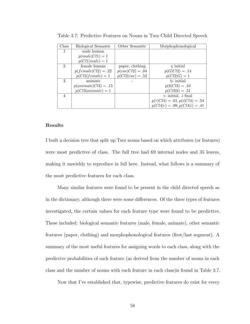
Table 3.7: Predictive Features on Nouns in Tsez Child Directed Speech
Class Biological Semantic Other Semantic Morphophonological1 male human
p(male|Cl1) = 1p(Cl1|male) = 1
2 female human paper, clothing G initialp(female|Cl2) = .22 p(cue|Cl2) = .04 p(G|Cl2) = .14p(Cl2|female) = 1 p(Cl2|cue) = .52 p(Cl2|G) = 1
3 animate - b- initialp(animate|Cl3) = .13 p(b|Cl3) = .10p(Cl3|animate) = 1 p(Cl3|b) = .51
4 r- initial, -i finalp(r|Cl4) = .61, p(i|Cl4) = .54p(Cl4|r) = .09, p(Cl4|i) = .41
Results
I built a decision tree that split up Tsez nouns based on which attributes (or features)
were most predictive of class. The full tree had 69 internal nodes and 35 leaves,
making it unwieldy to reproduce in full here. Instead, what follows is a summary of
the most predictive features for each class.
Many similar features were found to be present in the child directed speech as
in the dictionary, although there were some differences. Of the three types of features
investigated, the certain values for each feature type were found to be predictive.
These included: biological semantic features (male, female, animate), other semantic
features (paper, clothing) and morphophonological features (first/last segment). A
summary of the most useful features for assigning words to each class, along with the
predictive probabilities of each feature (as derived from the number of nouns in each
class and the number of nouns with each feature in each class)is found in Table 3.7.
Now that I’ve established that, typewise, predictive features do exist for every
58
class in the Tsez learner’s input, it is important to show that these features appear
frequently on nouns. It is important to note here that the phonological cues found
to be predictive are identical to the agreement morphemes for these classes, but
these are simply segments on the nouns not agreement morphemes, which are never
present on nouns. The homophony is probably not accidental, and further work could
address why this homophony between noun internal and noun external distributional
information exists. An analysis of the corpus showed that out of 114 noun types
heard, 24% had predictive features on them, and out of 1189 noun tokens heard,
39% had predictive features6.
3.2.4 Correlation of information types
At this point I’ve shown that both noun external distributional properties and noun
internal distributional properties are widely available to the Tsez learner. One set
of hypotheses, that only external information is used to acquire noun classes, only
requires that noun external distributional information be available for the classes to
be acquired, but the other set requires not only that both noun external and noun
internal distributional information are available, but that they are seen together.
Therefore it is necessary to ask, how often does the Tsez acquiring child come across
pairings of nouns with predictive features (noun internal distributional information)
6These and other counts exclude proper names, which may decrease both the proportion of nouns
with predictive features and the proportion of nouns with agreeing features seen with agreement, if
the natural gender of the referent of a proper name can be though of as a predictive feature on the
noun.
59

and agreement (noun external distributional information). Corpus analysis revealed
that such cooccurence was quite frequent: 100% of class 1 nouns occurring with
agreement also had predictive features7, 52% of class 2 nouns, 51% of class 3 nouns
and 45% of class 4 nouns.
Overall, the corpus analysis showed that both noun external and noun internal
distributional properties are widely available to Tsez acquiring children, and are
often available together. Thus the available input is consistent with that required by
all hypotheses set forward in Chapter 2. I must next address whether children’s use
of noun internal distribution in inferring the class of a novel noun mirrors adults’
(that is, the distribution of this information in the input), supporting the hypotheses
that suggest this information is aggregated after noun classes have been acquired
using only noun external information. Additionally I will determine whether use of
both noun internal and noun external information in inferring noun class in general
reflects a deterministic or probabilistic system.
7This is perhaps trivial as all nouns in Class 1 denote male humans
60
Chapter 4
Encoding, a classification
experiment in Tsez
The previous chapter established that the Tsez learner has available both noun
external and noun internal distributional information for every noun class. As all the
information necessary for either set of hypotheses to hold is present, it is necessary to
test the other predictions of these hypotheses. I’ll begin with the hypotheses relating
to noun internal information: when children are able to use noun internal properties
to classify nouns and whether they use them in proportion to their distribution in
the input. In order to test sensitivity to the properties characteristic of groups of
nouns in each class, classification of both frequent and novel nouns with combinations
of the predictive features found above was elicited from adult and child speakers1.
1A pilot version of this task was conducted in summer of 2008 using features predicted by the
decision tree in Plaster et al, and the task was revised both methodologically and in terms of the
features on the words that were used in 2009. Only the results of the 2009 study will be reported
61
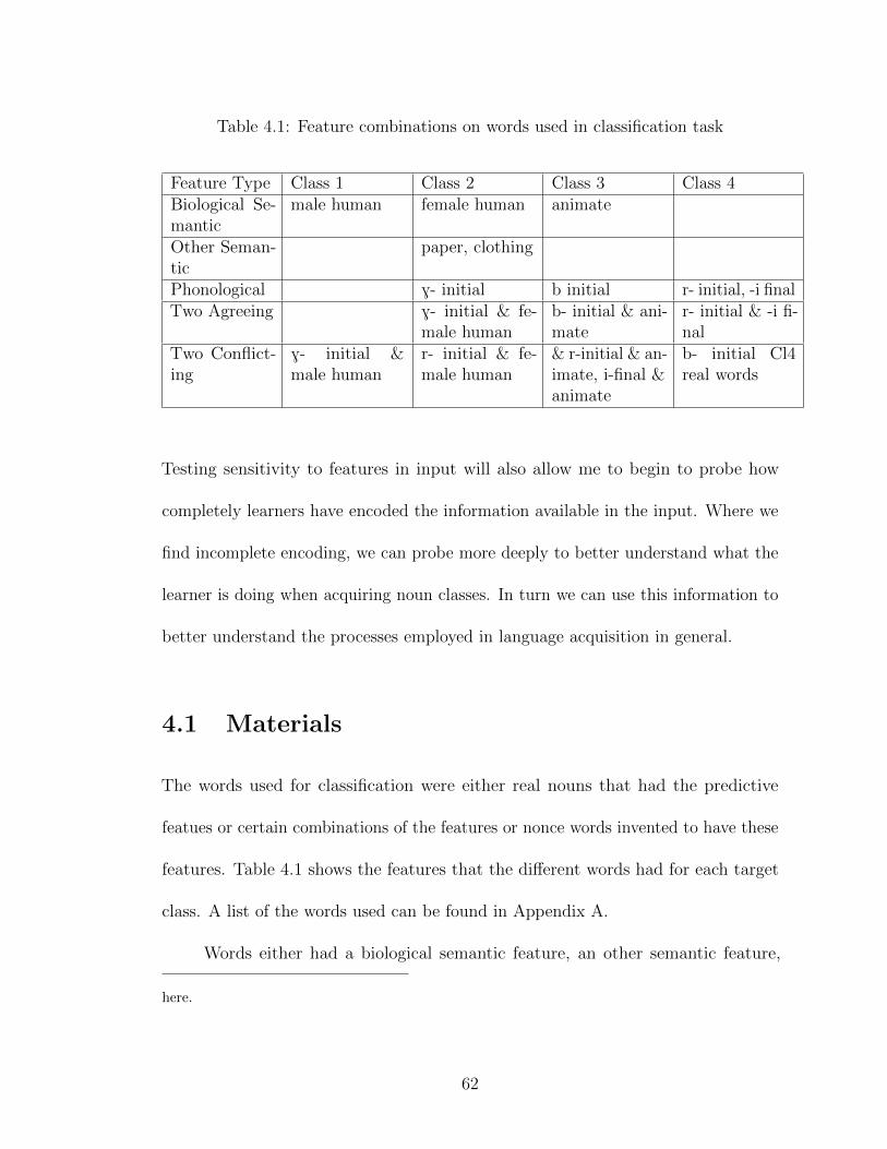
Table 4.1: Feature combinations on words used in classification task
Feature Type Class 1 Class 2 Class 3 Class 4Biological Se-mantic
male human female human animate
Other Seman-tic
paper, clothing
Phonological G- initial b initial r- initial, -i finalTwo Agreeing G- initial & fe-
male humanb- initial & ani-mate
r- initial & -i fi-nal
Two Conflict-ing
G- initial &male human
r- initial & fe-male human
& r-initial & an-imate, i-final &animate
b- initial Cl4real words
Testing sensitivity to features in input will also allow me to begin to probe how
completely learners have encoded the information available in the input. Where we
find incomplete encoding, we can probe more deeply to better understand what the
learner is doing when acquiring noun classes. In turn we can use this information to
better understand the processes employed in language acquisition in general.
4.1 Materials
The words used for classification were either real nouns that had the predictive
featues or certain combinations of the features or nonce words invented to have these
features. Table 4.1 shows the features that the different words had for each target
class. A list of the words used can be found in Appendix A.
Words either had a biological semantic feature, an other semantic feature,
here.
62
a phonological feature, two features agreeing for class or two features predicting
different classes. In the case of real words in Class 4 with conflicting features, they
were actually in Class 4 but had the phonological cue (b- initial) for Class 3. The
real words were frequent words either from the corpus of Tsez child directed speech
or Tsez words whose translations were frequent in English child directed speech
when the right combination of features wasn’t available on Tsez words in the corpus.
The nonce words were invented to conform to Tsez phonotactics and were checked
with a native speaker to be sure they were not real words. Nonce words which had
no predictive semantic or phonological information (other than the predictive value
that comes from lacking certain features) were also included in order to be able to
compare noun class assignment based on predictive information to that without.
The features selected had differing degrees of reliability as determined by
the conditional probability of the feature given the class and by the conditional
probability of the class given the feature. These differences will be important to
keep in mind when considering whether the utility of noun internal distributional
information is rule based or probability based, as well as when making specific
predictions about classification when features make conflicting predictions. Table
4.2 summarizes the predictive information for each feature in the form of conditional
probabilities for the class in question, given the feature and vice versa.
63
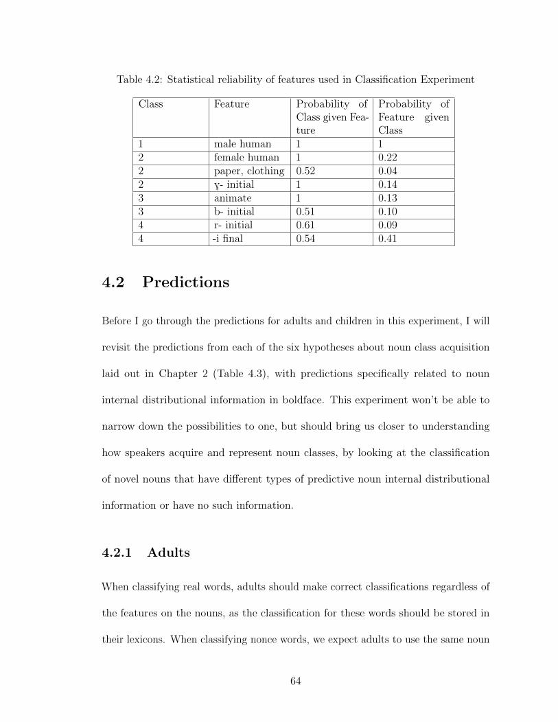
Table 4.2: Statistical reliability of features used in Classification Experiment
Class Feature Probability ofClass given Fea-ture
Probability ofFeature givenClass
1 male human 1 12 female human 1 0.222 paper, clothing 0.52 0.042 G- initial 1 0.143 animate 1 0.133 b- initial 0.51 0.104 r- initial 0.61 0.094 -i final 0.54 0.41
4.2 Predictions
Before I go through the predictions for adults and children in this experiment, I will
revisit the predictions from each of the six hypotheses about noun class acquisition
laid out in Chapter 2 (Table 4.3), with predictions specifically related to noun
internal distributional information in boldface. This experiment won’t be able to
narrow down the possibilities to one, but should bring us closer to understanding
how speakers acquire and represent noun classes, by looking at the classification
of novel nouns that have different types of predictive noun internal distributional
information or have no such information.
4.2.1 Adults
When classifying real words, adults should make correct classifications regardless of
the features on the nouns, as the classification for these words should be stored in
their lexicons. When classifying nonce words, we expect adults to use the same noun
64
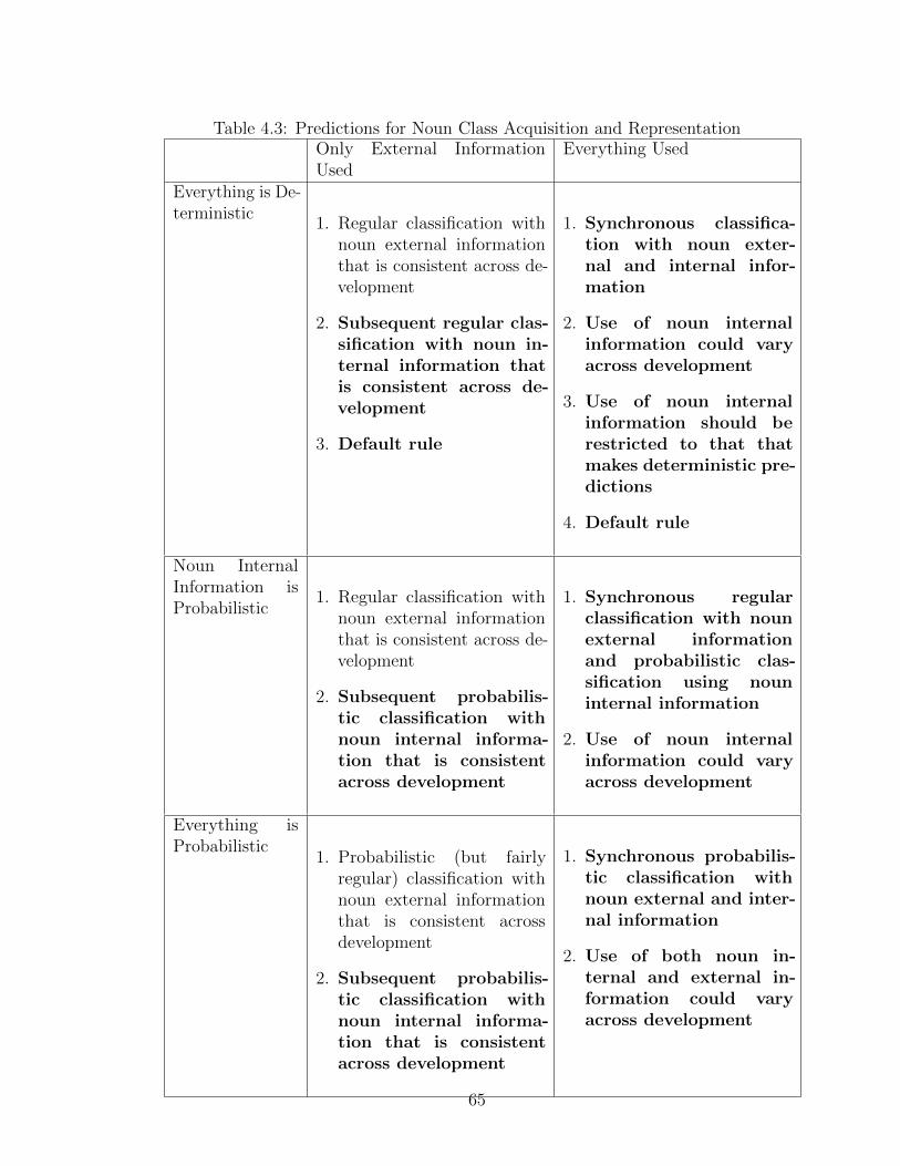
Table 4.3: Predictions for Noun Class Acquisition and RepresentationOnly External InformationUsed
Everything Used
Everything is De-terministic
1. Regular classification withnoun external informationthat is consistent across de-velopment
2. Subsequent regular clas-sification with noun in-ternal information thatis consistent across de-velopment
3. Default rule
1. Synchronous classifica-tion with noun exter-nal and internal infor-mation
2. Use of noun internalinformation could varyacross development
3. Use of noun internalinformation should berestricted to that thatmakes deterministic pre-dictions
4. Default rule
Noun InternalInformation isProbabilistic
1. Regular classification withnoun external informationthat is consistent across de-velopment
2. Subsequent probabilis-tic classification withnoun internal informa-tion that is consistentacross development
1. Synchronous regularclassification with nounexternal informationand probabilistic clas-sification using nouninternal information
2. Use of noun internalinformation could varyacross development
Everything isProbabilistic
1. Probabilistic (but fairlyregular) classification withnoun external informationthat is consistent acrossdevelopment
2. Subsequent probabilis-tic classification withnoun internal informa-tion that is consistentacross development
1. Synchronous probabilis-tic classification withnoun external and inter-nal information
2. Use of both noun in-ternal and external in-formation could varyacross development
65
internal information that was predictive for words in the naturalistic speech examined
in the corpus experiment. The distribution of classification when this information
is present will help to determine whether they are employed in deterministic or
probabilistic system. Under a deterministic system we would expect all words with a
highly predictive feature to be classified according the the rule associated with that
feature, and words without highly predictive features would be classified according
to a default rule. Under a probabilistic system we would expect the distribution
of nouns to classes to shift towards the class predicted by the feature, where the
degree of skew is determined by the conditional probability of a given class given the
feature in question. When classifying nonce words without cues, we will see whether
the classification is determined by one default rule or a distribution mirroring the
distribution of words without these cues into classes in the lexicon, further speaking
to the question of whether classification based on noun internal information is
deterministic or probabilistic.
4.2.2 Children
If children are only making use of only external information to acquire noun classes,
I have predicted that children will perform similarly to adults with respect to the
probabilistic nature of the cues available. This means that children should classify
nonce words the same way adults do. Similarly, if the cues on real words do affect
their classification (perhaps in the case where a word is not well known), this should
also follow the same principles that nonce word classification does. In particular,
66

these hypotheses predict that noun internal distributional properties are tracked later
in development, at a point when the lexicon has full representations for both the form
and meaning of each noun, thus the distribution of these properties in the intake
should match the distribution in the input. Of course, it is possible that the children
I test could still be in the process of finding correspondences between features of
nouns in each class. However, since we don’t think children have acquired noun
classes until they are at least 20 months old (i.e. Cyr & Shi, in press), we expect that
at this stage both semantic and phonological features would be available for children
to encode and therefore track their distributional properties. Thus children might
be less sensitive to statistical correlations between features and classes than adults,
but we wouldn’t expect the kind of feature to matter (i.e. they might be equally
insensitive to semantic and phonological features), the way it might for hypotheses
that predict children use, and therefore track, this information from the earliest
stages of noun class acquisition.
If children are using both noun internal and noun external information to
acquire noun classes, I predict that children’s classification could differ from that
of adults, as they would depend on noun internal distributional properties that
are available from the very beginning of lexical acquisition. While some of these
properties could be the same as those used by adults, it is possible that some would
differ. For example, if children are able to track phonological information about
words in conjunction with agreement morphology, these class internal regularities
could be used even before the child knows the meanings of the words. A similar effect
could be found if children find that meaning is an unreliable property to encode
67
and therefore track early on in lexical acquisition. A learner can be fairly certain
of the phonological form of a word that has been used and should be encoded, but
may require more experience with that word to become as confident in the meaning.
Thus in this case the distribution of noun internal information in the intake may
differ from what is measurable in the input.
4.2.3 Summary of predictions
In summary, if adults and children pattern the same way in their use of noun internal
information, this would support the hypotheses that only noun external information
is used to acquire noun classes, though perhaps not provide strong enough evidence
to argue against the idea that both internal and external information are crucial.
However, if adults and children differ, in particular if we see a difference between the
input and the intake in children, we would have good reason to believe that despite
the highly regular nature of the noun external information, both internal and external
distributional properties are used to acquire a noun class system. Additionally, if use
of noun internal distributional information by both adults and children appears to
be probabilistic, instead of highly regular, we would have good reason to believe that
this information is used in a probabilistic system rather than a deterministic one.
This work extends on the past work that found children favoring phonological
over semantic information in the following ways (MacWhinney, 1978; Karmiloff-Smith,
1979; Perez-Pereira, 1991; Mills, 1985, 1986; Rodina & Westergaard, 2012). First,
in Tsez the biological semantic information has been shown to be more statistically
68
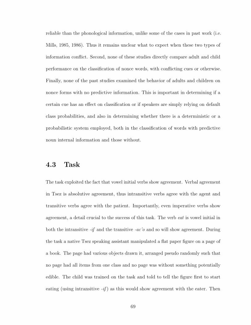
reliable than the phonological information, unlike some of the cases in past work (i.e.
Mills, 1985, 1986). Thus it remains unclear what to expect when these two types of
information conflict. Second, none of these studies directly compare adult and child
performance on the classification of nonce words, with conflicting cues or otherwise.
Finally, none of the past studies examined the behavior of adults and children on
nonce forms with no predictive information. This is important in determining if a
certain cue has an effect on classification or if speakers are simply relying on default
class probabilities, and also in determining whether there is a deterministic or a
probabilistic system employed, both in the classification of words with predictive
noun internal information and those without.
4.3 Task
The task exploited the fact that vowel initial verbs show agreement. Verbal agreement
in Tsez is absolutive agreement, thus intransitive verbs agree with the agent and
transitive verbs agree with the patient. Importantly, even imperative verbs show
agreement, a detail crucial to the success of this task. The verb eat is vowel initial in
both the intransitive -iS and the transitive -ac’o and so will show agreement. During
the task a native Tsez speaking assistant manipulated a flat paper figure on a page of
a book. The page had various objects drawn it, arranged pseudo randomly such that
no page had all items from one class and no page was without something potentially
edible. The child was trained on the task and told to tell the figure first to start
eating (using intransitive -iS ) as this would show agreement with the eater. Then
69
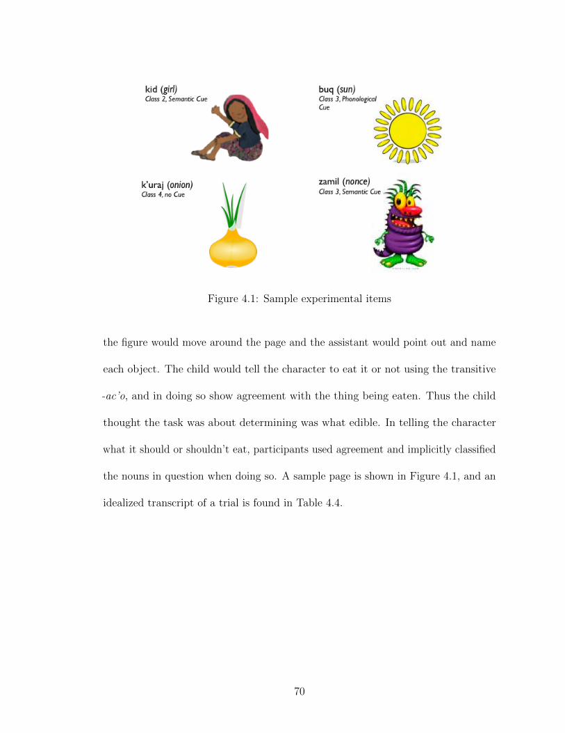
Figure 4.1: Sample experimental items
the figure would move around the page and the assistant would point out and name
each object. The child would tell the character to eat it or not using the transitive
-ac’o, and in doing so show agreement with the thing being eaten. Thus the child
thought the task was about determining was what edible. In telling the character
what it should or shouldn’t eat, participants used agreement and implicitly classified
the nouns in question when doing so. A sample page is shown in Figure 4.1, and an
idealized transcript of a trial is found in Table 4.4.
70
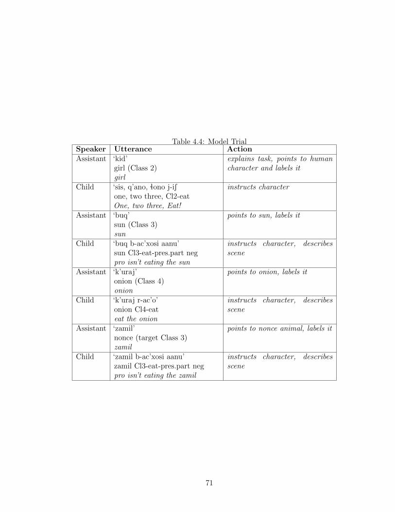
Table 4.4: Model TrialSpeaker Utterance ActionAssistant ‘kid’
girl (Class 2)girl
explains task, points to humancharacter and labels it
Child ‘sis, q’ano, ìono j-iSone, two three, Cl2-eatOne, two three, Eat!
instructs character
Assistant ‘buq’sun (Class 3)sun
points to sun, labels it
Child ‘buq b-ac’xosi aanu’sun Cl3-eat-pres.part negpro isn’t eating the sun
instructs character, describesscene
Assistant ‘k’uraj’onion (Class 4)onion
points to onion, labels it
Child ‘k’uraj r-ac’o’onion Cl4-eateat the onion
instructs character, describesscene
Assistant ‘zamil’nonce (target Class 3)zamil
points to nonce animal, labels it
Child ‘zamil b-ac’xosi aanu’zamil Cl3-eat-pres.part negpro isn’t eating the zamil
instructs character, describesscene
71

4.4 Participants
Participants were native Tsez speakers living in Shamkhal and Kizilyurt, Dagestan2.
They were recruited with the help of a local Tsez speaking assistant who knew Tsez
speaking families in the area. Data from 10 young children (ages 4-7), 12 older
children (ages 8-12) and 10 adults was included in the analysis below. Because
the number of children available to participate was rather small, I created large
age ranges to test, creating a basic distinction between older and younger children.
Subjects were tested either alone in a room with the experimenter and a native
Tsez speaking assistant, and sometimes were accompanied by parents, relatives or
other friends who were instructed to keep silent during the experiment, with some
encouraging remarks being allowed when the child being tested was especially shy.
20 additional children and 3 additional adults participated but were excluded
from the final analysis for one of 3 reasons: (1) because other people were present
during the experiment and prompted the subject with answers (2 children, 1 adult),
(2) because they failed to use agreeing forms on a majority of the items (4 children),
or (3) because they failed to classify 8 out of 10 very frequent words correctly (14
2The Tsez speakers in these communities are immersed in a bi- or tri-lingual environment (with
Russian and Avar), as these are settlements outside of the traditional Tsez speaking region. Access
to the Tsuntinsky region, where Tsez is the native language, is highly restricted by the Russian
government, meaning that at the time of this work the region was inaccessible. However, Tsez, not
Russian or Avar, is still the main language spoken in the homes of the subjects in question, and
was the language child subjects spoke to one another when observed outside of the experimental
context.
72

children, 2 adults). (3) was used as an exclusion criterion because a common strategy
for participants was to classify all of the words in one class (either Class 3 or Class
4). The latter two categories of behavior are puzzling, as they do not seem to show
the classification or agreement system that the speaker has. This is apparent in that
participants exhibiting this behavior were observed using proper agreement when
conversing outside of the task. Because of the extension of this behavior to real,
known words in the task, it it clear that it is not just a reflex of some ‘default’ class.
Rather, it appears that this is some kind of task induced strategy used by certain
participants, and while it doesn’t show much about the classification of individual
items, it might highlight a part of the classification system that has not yet been
discussed. One possibility is that these participants were classifying everything as if
the noun were picture (which is in Class 3), or some other noun that would serve
the same function but is in Class 4. This would mean that instead of classifying
each item, they were just using a form that agreed with picture or some Class 4
noun. Alternatively, some mechanism may be employed under special circumstances
to override actual class assignment and show apparent agreement with nothing
in particular. Similar behavior was exhibited by Norwegian children on a similar
classification task (Chapter 8). The source of this behavior is certainly a puzzle, but
one that remains distinct from the acquisition of noun classes and the assignment
of novel nouns to these classes, as it appears to be some sort of agreement with
nothing in particular, perhaps the agreement that surfaces when nothing is actually
triggering agreement.
73
4.5 Results
Classification data from the experiment was analyzed as follows. For each item
type (i.e. nonce word with semantic feature ‘female’ or real word with phonological
feature ‘b- initial’), the proportion of items put in each class was calculated for
each age group. For example, for young children, for the item type ‘nonce words
with semantic feature ‘female’, 4% were put in Class 1, 52% in Class 2, 22% in
Class 3 and 22% in Class 4. This yielded a unique distribution of proportions of
nouns assigned to each class for each item type and each age group. The differences
between these distributions were quantified using Jensen-Shannon Divergence (J-S
divergence), a metric for quantifying the difference between sample distributions
(Lin, 1991). By comparing the differences between distributions for each cue type, I
could determine which cues caused the distributions to change, and to what degree.
What follows is a summary of the main findings from comparing these distributions.
A full presentation of every item type and age group, as well as an explanation of
the calculation of the J-S divergence used to quantify the differences between them
can be found in Appendices B&C. The data was analyzed in this way instead of by
using t-tests or ANOVAs to compare the proportion of nouns in a given class given
a set of cues because those tests were deemed inappropriate to compare the shift of
classification across a set of classes. That is, it mattered not only that a cue could
raise or lower the proportion of nouns in a given class, but also how the distribution
was skewed with the introduction of a given cue.
In analyzing the results, classification of real words was compared to the
74
words’ actual class. Classification of nonce words with cues was compared to a base
distribution of classification of nonce words without cues. When talking about the
classification of real words, I’ll refer to what proportion of words of each item type
were assigned to the word’s actual class (the class of the word agreed upon by native
speaker consultants). When talking about the classification of nonce words I’ll refer
to what proportion of the words were assigned to the target class (the class that the
cue on the item most strongly predicts) as compared with the proportion of words
assigned to that class when no cue was present. For example, the target class of a
nonce word referring to a female human would be Class 2, and so I look at nonce
words with female referents to see if more are assigned to Class 2 when the cue is
present, than nonce words without this cue.
One phonological cue, the G-initial phonological cue that the decision tree found
to be predictive of Class 2, was not found to be used by any speakers in any situation.
I suspect that this cue does not really predict the class of a noun in Tsez as well as
the decision tree made it look. This is due to the fact that there were a small number
of nouns in the Tsez corpus, heightening the possibility that spurious generalizations
could be made. Furthermore, this was the only cue that I found to be predictive in
child directed speech that wasn’t predicted in the greater Tsez lexicon (as indexed
by the dictionary). Thus I exclude words with this cue from the results presented
below, not because speakers didn’t appear to use the cue but because I have good
reason to believe that the inclusion of this cue was a mistake. This cue represented
only a spurious, not actual generalization about noun internal distributional features
in Tsez, and thus we’d have no expectation that speakers should be sensitive to it.
75
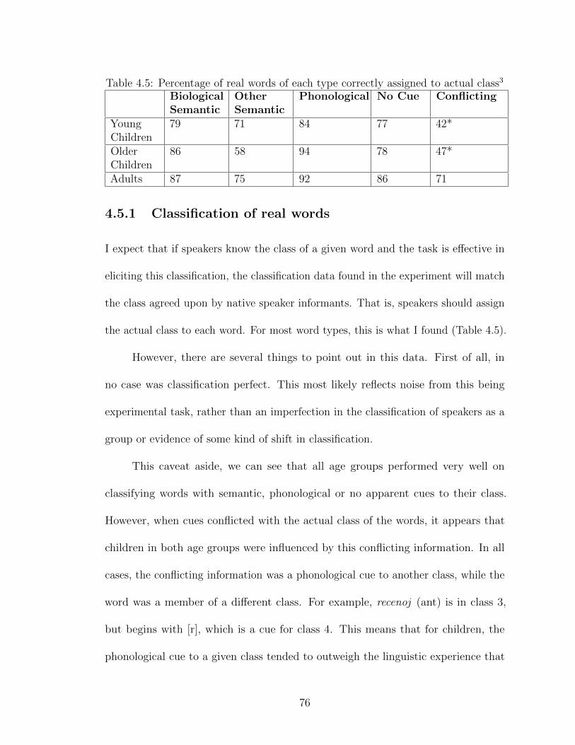
Table 4.5: Percentage of real words of each type correctly assigned to actual class3
BiologicalSemantic
OtherSemantic
Phonological No Cue Conflicting
YoungChildren
79 71 84 77 42*
OlderChildren
86 58 94 78 47*
Adults 87 75 92 86 71
4.5.1 Classification of real words
I expect that if speakers know the class of a given word and the task is effective in
eliciting this classification, the classification data found in the experiment will match
the class agreed upon by native speaker informants. That is, speakers should assign
the actual class to each word. For most word types, this is what I found (Table 4.5).
However, there are several things to point out in this data. First of all, in
no case was classification perfect. This most likely reflects noise from this being
experimental task, rather than an imperfection in the classification of speakers as a
group or evidence of some kind of shift in classification.
This caveat aside, we can see that all age groups performed very well on
classifying words with semantic, phonological or no apparent cues to their class.
However, when cues conflicted with the actual class of the words, it appears that
children in both age groups were influenced by this conflicting information. In all
cases, the conflicting information was a phonological cue to another class, while the
word was a member of a different class. For example, recenoj (ant) is in class 3,
but begins with [r], which is a cue for class 4. This means that for children, the
phonological cue to a given class tended to outweigh the linguistic experience that
76
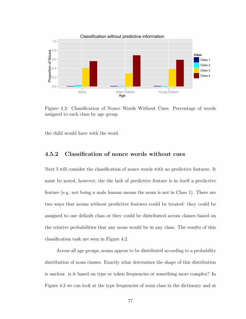
Classification without predictive information
Age
Pro
porti
on o
f Nou
ns
0.0
0.2
0.4
0.6
0.8
1.0
Adults Older Children Young Children
ClassClass 1
Class 2
Class 3
Class 4
Figure 4.2: Classification of Nonce Words Without Cues: Percentage of wordsassigned to each class by age group
the child would have with the word.
4.5.2 Classification of nonce words without cues
Next I will consider the classification of nonce words with no predictive features. It
must be noted, however, the the lack of predictive feature is in itself a predictive
feature (e.g. not being a male human means the noun is not in Class 1). There are
two ways that nouns without predictive features could be treated: they could be
assigned to one default class or they could be distributed across classes based on
the relative probabilities that any noun would be in any class. The results of this
classification task are seen in Figure 4.2.
Across all age groups, nouns appear to be distributed according to a probability
distribution of noun classes. Exactly what determines the shape of this distribution
is unclear: is it based on type or token frequencies or something more complex? In
Figure 4.3 we can look at the type frequencies of noun class in the dictionary and at
77
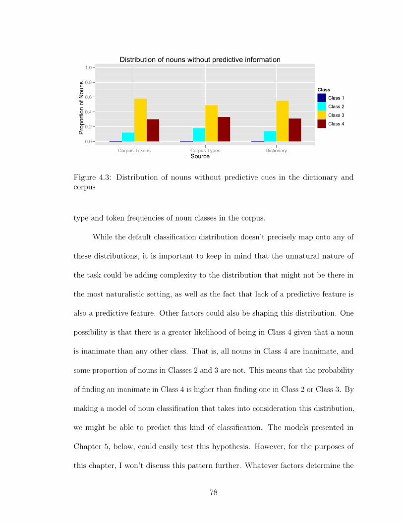
Distribution of nouns without predictive information
Source
Pro
porti
on o
f Nou
ns
0.0
0.2
0.4
0.6
0.8
1.0
Corpus Tokens Corpus Types Dictionary
ClassClass 1
Class 2
Class 3
Class 4
Figure 4.3: Distribution of nouns without predictive cues in the dictionary andcorpus
type and token frequencies of noun classes in the corpus.
While the default classification distribution doesn’t precisely map onto any of
these distributions, it is important to keep in mind that the unnatural nature of
the task could be adding complexity to the distribution that might not be there in
the most naturalistic setting, as well as the fact that lack of a predictive feature is
also a predictive feature. Other factors could also be shaping this distribution. One
possibility is that there is a greater likelihood of being in Class 4 given that a noun
is inanimate than any other class. That is, all nouns in Class 4 are inanimate, and
some proportion of nouns in Classes 2 and 3 are not. This means that the probability
of finding an inanimate in Class 4 is higher than finding one in Class 2 or Class 3. By
making a model of noun classification that takes into consideration this distribution,
we might be able to predict this kind of classification. The models presented in
Chapter 5, below, could easily test this hypothesis. However, for the purposes of
this chapter, I won’t discuss this pattern further. Whatever factors determine the
78
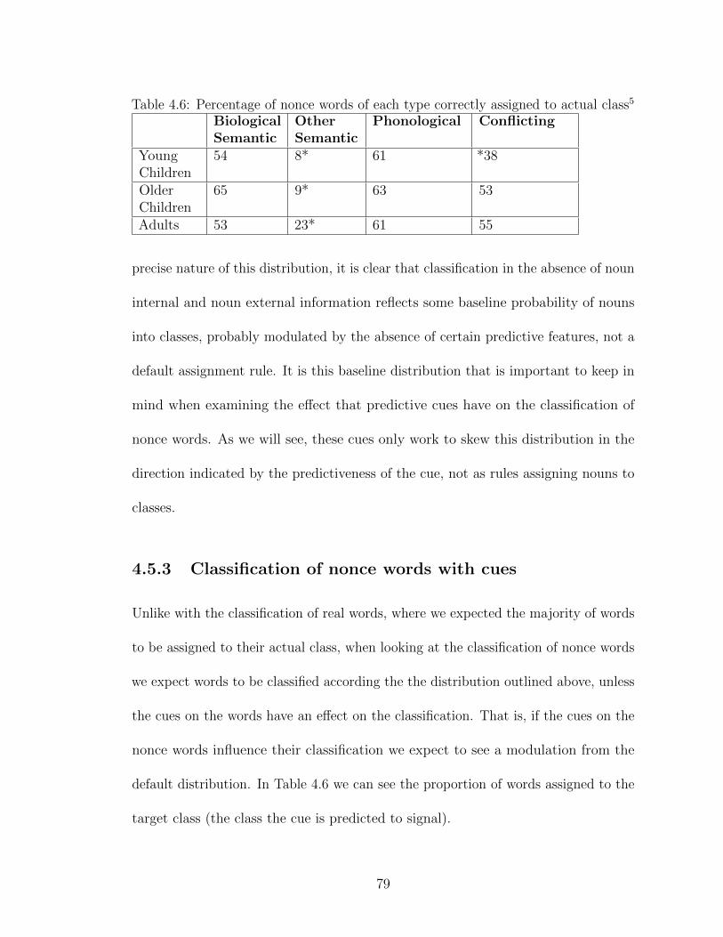
Table 4.6: Percentage of nonce words of each type correctly assigned to actual class5
BiologicalSemantic
OtherSemantic
Phonological Conflicting
YoungChildren
54 8* 61 *38
OlderChildren
65 9* 63 53
Adults 53 23* 61 55
precise nature of this distribution, it is clear that classification in the absence of noun
internal and noun external information reflects some baseline probability of nouns
into classes, probably modulated by the absence of certain predictive features, not a
default assignment rule. It is this baseline distribution that is important to keep in
mind when examining the effect that predictive cues have on the classification of
nonce words. As we will see, these cues only work to skew this distribution in the
direction indicated by the predictiveness of the cue, not as rules assigning nouns to
classes.
4.5.3 Classification of nonce words with cues
Unlike with the classification of real words, where we expected the majority of words
to be assigned to their actual class, when looking at the classification of nonce words
we expect words to be classified according the the distribution outlined above, unless
the cues on the words have an effect on the classification. That is, if the cues on the
nonce words influence their classification we expect to see a modulation from the
default distribution. In Table 4.6 we can see the proportion of words assigned to the
target class (the class the cue is predicted to signal).
79

This data must be interpreted not only as the proportion of words assigned
to the target class, but also in terms of how much this proportion varied from the
default classification. We can see that semantic and phonological cues are effective
in getting the majority of words assigned to the target class by all age groups. For
Classes 1 and 2, this is is also very different from the default distribution. While the
difference is not as extreme for Classes 3 and 4, where the majority of the words
ended up by default, examination of the data by class shows that the vast majority
of words end up there when the relevant cues are present, many more than when no
cues are present. Full profiles of the classification for each cue type by class can be
seen in Appendix B.
It is more difficult to see how other semantic information is used. Remember
that other semantic cues were only tested for Class 2. Children do not appear to use
this information at all, as the 8% and 9% of nonce words assigned to Class 2 with
the information do not significantly differ from the 1% of cueless words assigned
to Class 2 (The J-S divergence between these distributions does not fall in the top
10% of all J-S divergences). For adults on the other hand, while the 23% of words
with the other semantic cue assigned to Class 2 is not the majority, it does differ
significantly from the proportion of words assigned to this class without this cue.
Finally, the effect of conflicting information is also apparent. Nonce words with
conflicting information were those that had cues to two different classes - semantic
and phonological. In all cases, the semantic information was a statistically better
predictor of class, as the probability that a real word with that cue will be in the
class is higher than the probability that a word will be in the class predicted by the
80
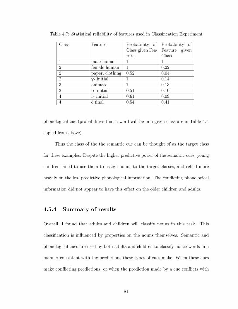
Table 4.7: Statistical reliability of features used in Classification Experiment
Class Feature Probability ofClass given Fea-ture
Probability ofFeature givenClass
1 male human 1 12 female human 1 0.222 paper, clothing 0.52 0.042 G- initial 1 0.143 animate 1 0.133 b- initial 0.51 0.104 r- initial 0.61 0.094 -i final 0.54 0.41
phonological cue (probabilities that a word will be in a given class are in Table 4.7,
copied from above).
Thus the class of the the semantic cue can be thought of as the target class
for these examples. Despite the higher predictive power of the semantic cues, young
children failed to use them to assign nouns to the target classes, and relied more
heavily on the less predictive phonological information. The conflicting phonological
information did not appear to have this effect on the older children and adults.
4.5.4 Summary of results
Overall, I found that adults and children will classify nouns in this task. This
classification is influenced by properties on the nouns themselves. Semantic and
phonological cues are used by both adults and children to classify nonce words in a
manner consistent with the predictions these types of cues make. When these cues
make conflicting predictions, or when the prediction made by a cue conflicts with
81

the actual class of a real word, young children are more likely to use phonological
information, despite the fact that this information is statistically less predictive.
Finally, the classification of nonce words with and without predictive cues follows
some distribution, influenced by both the noun internal distributional cues (or lack
thereof), as well as a baseline distribution of nouns into classes.
4.6 Returning to hypotheses about noun class ac-
quisition
Returning to the hypotheses laid out in Chapter 2, I was investigating predictions
related to speakers’ use of noun internal distributional information. First I can
narrow down my representational hypotheses. Based on speakers’ probabilistic
use of noun internal information, as well as based on their classification of words
without highly predictive information, I can rule out the hypotheses that posited
noun internal information is used deterministically. Next I can move on to think
about what information is used to acquire noun classes.
The set of hypotheses that posited that children relied only on noun external
information to acquire noun classes predicted that children would have access to
statistical regularities of inherent noun properties late in the acquisition of noun
classes, but that when they did their generalizations should mirror the adult ones.
The set that posited both noun external and internal information were necessary
to acquire noun classes predicted that children would be able to access statistical
82
regularities from the onset of lexical acquisition, but that their initial use of these
regularities could differ from adults, as the first available regularities might be
different from those used by adults. While these results do not test children young
enough to speak to the question of whether statistical regularities are used by children
from the very beginning of lexical acquisition they do appear to point towards the
set positing both types of information are necessary for the following reasons.
First, while both children and adults classify novel nouns based on noun internal
properties, the features they take advantage of do not have the same statistical
reliability in the input. That is, when all of these features are fed into a decision tree
building algorithm, the biological semantic ones can classify with 100% accuracy
whereas the phonological ones do not do as well. Yet, children appear to weigh the
phonological cues more heavily when determining the class of a novel noun. This
highlights a a potential distinction in the input and the intake. Some characteristic
of the encoding mechanism puts a higher value on phonological rather than semantic
information. There are three reasons this could be so, all pointing towards the
utility of noun internal distributional information in very early acquisition. First,
phonological properties of words are available to a child who might be able to track
phonological features and their relation to agreement morphemes long before knowing
the meaning of the words in question. Second, once a child is actually learning words,
the phonological form tends to be reliably as it sounds, whereas the meaning of the
word in question may not be as easy to grasp the first few times the word is heard.
Third, the learner could have a bias to track phonological information rather than
semantic information stemming from either the early observation that phonological
83
information is more useful, or from a bias to prefer phonological information over
semantic information.
All three of these possibilities raise interesting questions about the nature of
the developing lexicon, in particular, they raise the issue of what information can
be stored and accessed as part of a lexicon before words have well defined (or any)
semantics attached to them. Do children build up some inventory of strings and
begin calculating statistics over dependencies between strings and pieces of other
strings before these are stored with meaning in a lexicon? Children’s abilities to
segment speech and recognize illicit ‘words’ in artificial languages with no meanings
suggest that they can indeed do this, and this seems a likely step on the way towards
building an adult lexicon (Gerken et al., 2005). If children can and do store strings
this way, it does not seem unlikely that they rely on the kind of information that is
available at the earliest stages of lexical development to begin acquiring noun classes
(even before they have categories like noun they could be forming some subclasses of
strings). This would have the consequence of them using phonological information,
the only information that is available at that point, and hence the most statistically
predictive of the information they are able to encode at that early stage. That is, the
information they encode and use, the intake, does not match the information that is
in principle available in the input. Recall that this is only an issue if children are
using noun internal distributional information in acquiring noun classes, in addition
to noun external information. This is what the second set of hypotheses predicted,
while the first set predicted that the intake should match the input and the behavior
by adults. Thus my data at least tentatively support the hypotheses that posit both
84
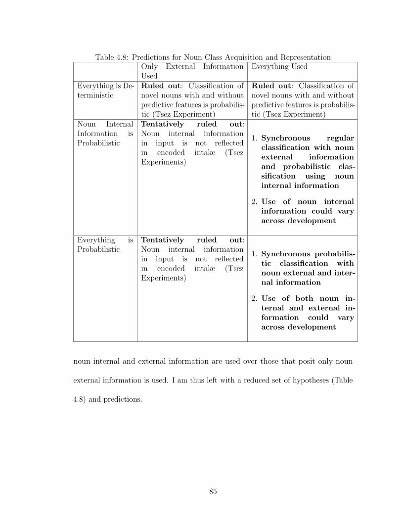
Table 4.8: Predictions for Noun Class Acquisition and RepresentationOnly External InformationUsed
Everything Used
Everything is De-terministic
Ruled out: Classification ofnovel nouns with and withoutpredictive features is probabilis-tic (Tsez Experiment)
Ruled out: Classification ofnovel nouns with and withoutpredictive features is probabilis-tic (Tsez Experiment)
Noun InternalInformation isProbabilistic
Tentatively ruled out:Noun internal informationin input is not reflectedin encoded intake (TsezExperiments)
1. Synchronous regularclassification with nounexternal informationand probabilistic clas-sification using nouninternal information
2. Use of noun internalinformation could varyacross development
Everything isProbabilistic
Tentatively ruled out:Noun internal informationin input is not reflectedin encoded intake (TsezExperiments)
1. Synchronous probabilis-tic classification withnoun external and inter-nal information
2. Use of both noun in-ternal and external in-formation could varyacross development
noun internal and external information are used over those that posit only noun
external information is used. I am thus left with a reduced set of hypotheses (Table
4.8) and predictions.
85
4.7 Encoding input into intake
As mentioned in the last section, the information used in noun class acquisition
highlights the child’s ability to encode features on nouns and use these in acquiring
noun classes. As the features they have access to, and are thus able to encode,
change throughout development, it follows that the features they might use for noun
class acquisition are not in fact the most reliable in the input, merely the most
reliable in the earlier encoding of the input. In order to understand these results,
and to determine whether children might be using only noun external information to
acquire nouns, or both noun internal and noun external information, the distinction
between input and encoded intake was crucial. Without this distinction it would
merely look as though children were not using the information in the input, and we
would be left to wonder why. The next chapter looks more deeply into where in the
acquisition of noun classes children are missing semantic information, or preferring
phonological information over available semantic information, and through modeling
the classification of nouns attempts to show what could account for the differences
in input and intake discovered here.
86
Chapter 5
Why doesn’t the intake appear to
match the input?
In the classification experiments seen in Chapter 5, children exhibited a preference
for using phonological information rather than semantic information to classify
novel nouns when the two types of information made conflicting predictions. This
preference is surprising given the statistical predictiveness of these features - biological
semantic features are better predictors of class than phonological cues. If children
were completely encoding everything available in the input and making inferences
about noun classification only on the basis of this information, then we might expect
that their classification patterns would mirror what we see in the input. In this
chapter, I present a probabilistic model of noun classification that shows us what kind
of classification behavior we would expect if children were able to perfectly encode
the input and draw inferences about a noun’s class on the basis of this information.
In line with my intuitions based on the statistical predictiveness of these cue types,
87
children do not align well with the model in the cases where the different features
make conflicting predictions. Through three manipulations to this model we can
begin to better understand what might cause this difference that we see in children,
reflected as a difference between input and encoded intake.
5.1 The elements of noun classification
So far I have talked at great length about what kind of information children might use
to discover that their language has noun classes, and what implications their use of
statistical information in classifying novel nouns might have on my inferences about
what information is used in the early stages of acquisition. I have been assuming, up
until now, that if a feature of a noun is perceived and represented, it is available to
be used for noun classification and a learner or speaker will readily use any available
and predictive feature to classify novel nouns. However, as children’s behavior in
the Tsez noun classification experiment showed, not all features are used in the way
we might expect. In order to begin investigating why this is the case, it is useful
to break down what a learner is doing when encountering and classifying a novel
noun. As alluded to above, I have been implicitly assuming that the following pieces
of information come into play:
1. Accumulation of knowledge of statistical distribution of features relating to
noun classification
2. Observation of these features in a novel experimental item
88
3. Knowledge of which features are relevant for classification
4. Bayesian computation to determine how to classify novel noun based on
observed features and statistical knowledge
(1) depends on the learner’s ability to observe and encode a statistical distri-
bution of semantic and phonological features. (2) is similar to (1), but refers to
encoding these features given a situation where the learner will be performing a
computation to classify a novel noun. (3) requires the learner to know which features
are relevant for classification and is by no means trivial, as not every feature or
type of feature is relevant to classification. (4) is an assumption that I am making
about the kind of computations that learners use distributional information for. In
this problem, it seems likely that the ‘suboptimal’ performance witnessed in the
children’s classification behavior comes from steps (1) through (3), the information
feeding into the computation of noun class, rather than the computation itself.
To summarize, it could be that children’s non adultlike behavior is caused
by difficulty encoding the input as they acquire nouns and noun classes, difficulty
encoding features on experimental items, or due to to knowledge, either from a
hypothesis space or based on what they have inferred about noun classes so far,
about which features are important in noun classification. In what follows I will
first propose a probabilistic model of noun classification, and then manipulate this
model to see whether constraining any of these components can predict children’s
classification patterns.
89
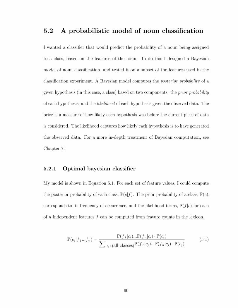
5.2 A probabilistic model of noun classification
I wanted a classifier that would predict the probability of a noun being assigned
to a class, based on the features of the noun. To do this I designed a Bayesian
model of noun classification, and tested it on a subset of the features used in the
classification experiment. A Bayesian model computes the posterior probability of a
given hypothesis (in this case, a class) based on two components: the prior probability
of each hypothesis, and the likelihood of each hypothesis given the observed data. The
prior is a measure of how likely each hypothesis was before the current piece of data
is considered. The likelihood captures how likely each hypothesis is to have generated
the observed data. For a more in-depth treatment of Bayesian computation, see
Chapter 7.
5.2.1 Optimal bayesian classifier
My model is shown in Equation 5.1. For each set of feature values, I could compute
the posterior probability of each class, P(c|f). The prior probability of a class, P(c),
corresponds to its frequency of occurrence, and the likelihood terms, P(f |c) for each
of n independent features f can be computed from feature counts in the lexicon.
P(ci |f1 ...fn) =P(f1 |ci)...P(fn |ci) · P(ci)∑
cj∈{all classes}P(f1 |cj )...P(fn |cj ) · P(cj )(5.1)
90
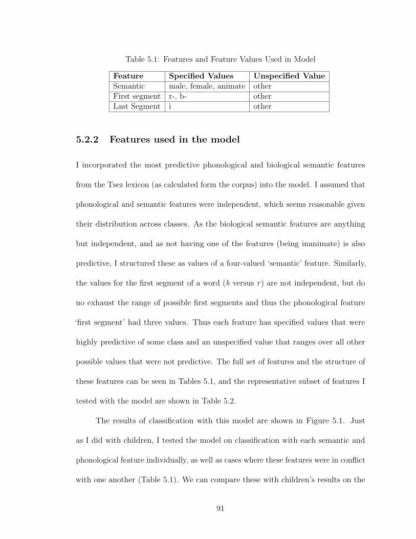
Table 5.1: Features and Feature Values Used in Model
Feature Specified Values Unspecified ValueSemantic male, female, animate otherFirst segment r-, b- otherLast Segment i other
5.2.2 Features used in the model
I incorporated the most predictive phonological and biological semantic features
from the Tsez lexicon (as calculated form the corpus) into the model. I assumed that
phonological and semantic features were independent, which seems reasonable given
their distribution across classes. As the biological semantic features are anything
but independent, and as not having one of the features (being inanimate) is also
predictive, I structured these as values of a four-valued ‘semantic’ feature. Similarly,
the values for the first segment of a word (b versus r) are not independent, but do
no exhaust the range of possible first segments and thus the phonological feature
‘first segment’ had three values. Thus each feature has specified values that were
highly predictive of some class and an unspecified value that ranges over all other
possible values that were not predictive. The full set of features and the structure of
these features can be seen in Tables 5.1, and the representative subset of features I
tested with the model are shown in Table 5.2.
The results of classification with this model are shown in Figure 5.1. Just
as I did with children, I tested the model on classification with each semantic and
phonological feature individually, as well as cases where these features were in conflict
with one another (Table 5.1). We can compare these with children’s results on the
91
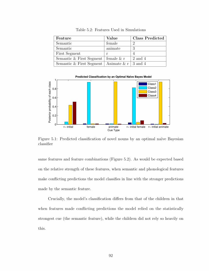
Table 5.2: Features Used in Simulations
Feature Value Class PredictedSemantic female 2Semantic animate 3First Segment r 4Semantic & First Segment female & r 2 and 4Semantic & First Segment Animate & r 3 and 4
r− initial female animate r− initial female r− initial animate0
0.2
0.4
0.6
0.8
1
Po
ste
rio
r p
rob
ab
ility
of
ea
ch
cla
ss
Cue Type
Predicted Classification by an Optimal Naïve Bayes Model
Class1
Class2
Class3
Class4
Figure 5.1: Predicted classification of novel nouns by an optimal naıve Bayesianclassifier
same features and feature combinations (Figure 5.2). As would be expected based
on the relative strength of these features, when semantic and phonological features
make conflicting predictions the model classifies in line with the stronger predictions
made by the semantic feature.
Crucially, the model’s classification differs from that of the children in that
when features made conflicting predictions the model relied on the statistically
strongest cue (the semantic feature), while the children did not rely so heavily on
this.
92
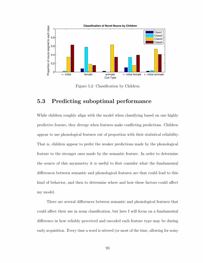
r− initial female animate r− initial female r− initial animate0
0.2
0.4
0.6
0.8
1
Pro
po
rtio
n o
f n
ou
ns s
sig
ne
d t
o e
ach
cla
ss
Cue Type
Classification of Novel Nouns by Children
Class1
Class2
Class3
Class4
Figure 5.2: Classification by Children
5.3 Predicting suboptimal performance
While children roughly align with the model when classifying based on one highly
predictive feature, they diverge when features make conflicting predictions. Children
appear to use phonological features out of proportion with their statistical reliability.
That is, children appear to prefer the weaker predictions made by the phonological
feature to the stronger ones made by the semantic feature. In order to determine
the source of this asymmetry it is useful to first consider what the fundamental
differences between semantic and phonological features are that could lead to this
kind of behavior, and then to determine where and how these factors could affect
my model.
There are several differences between semantic and phonological features that
could affect their use in noun classification, but here I will focus on a fundamental
difference in how reliably perceived and encoded each feature type may be during
early acquisition. Every time a word is uttered (or most of the time, allowing for noisy
93
conditions and fast speech) phonological features are present. However, especially
during the early stages of lexical acquisition, the meaning of a word, and thus the
associated semantic features, is much less likely to be available or apparent. We can
relate this disparity to what happens in first three components of noun classification
that I outlined above.
5.3.1 Incomplete encoding of the input
An asymmetry in the reliability with which semantic and phonological features of
nouns are perceived and encoded during word learning could lead to a disparity in
the way phonological and semantic features are represented as compared with how
they are distributed in the input.
In my first manipulation (the Semantic Incompetence Hypothesis) I
wanted to see how classification by the model would be affected if the learner
was misrepresenting some proportion of the semantic features that they should
have encoded on nouns in their lexicon. I assume that learners classified the
remaining proportion of nouns as predicted (accurately observing features during
the experiment and assuming that both semantic and phonological features were
relevant in classification). In doing this, I assume that learners’ beliefs about which
features are predictive of which class is built up as they observe different feature
values on words belonging to different classes. One way of quantifying this is by
modeling the learner’s belief about the likelihood terms P(f |c) from Equation 5.1
under the assumption that these beliefs are derived from the counts that a learner
94
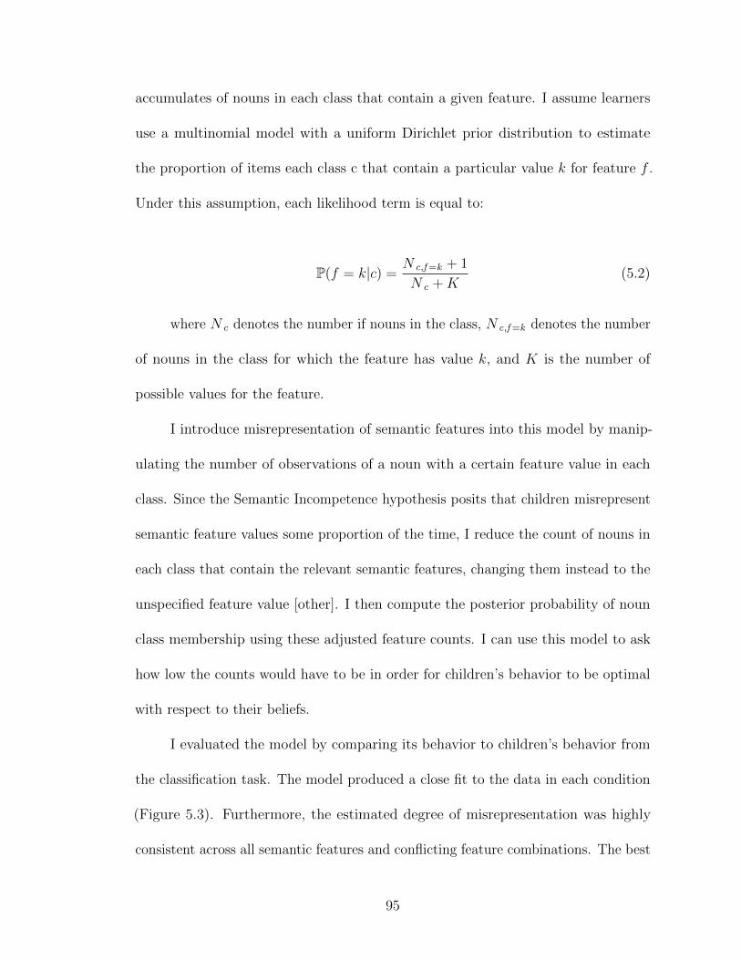
accumulates of nouns in each class that contain a given feature. I assume learners
use a multinomial model with a uniform Dirichlet prior distribution to estimate
the proportion of items each class c that contain a particular value k for feature f .
Under this assumption, each likelihood term is equal to:
P(f = k|c) =N c,f=k + 1
N c +K(5.2)
where N c denotes the number if nouns in the class, N c,f=k denotes the number
of nouns in the class for which the feature has value k, and K is the number of
possible values for the feature.
I introduce misrepresentation of semantic features into this model by manip-
ulating the number of observations of a noun with a certain feature value in each
class. Since the Semantic Incompetence hypothesis posits that children misrepresent
semantic feature values some proportion of the time, I reduce the count of nouns in
each class that contain the relevant semantic features, changing them instead to the
unspecified feature value [other]. I then compute the posterior probability of noun
class membership using these adjusted feature counts. I can use this model to ask
how low the counts would have to be in order for children’s behavior to be optimal
with respect to their beliefs.
I evaluated the model by comparing its behavior to children’s behavior from
the classification task. The model produced a close fit to the data in each condition
(Figure 5.3). Furthermore, the estimated degree of misrepresentation was highly
consistent across all semantic features and conflicting feature combinations. The best
95
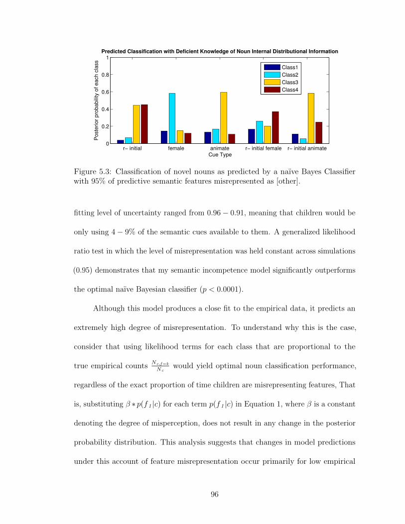
r− initial female animate r− initial female r− initial animate0
0.2
0.4
0.6
0.8
1
Po
ste
rio
r p
rob
ab
ility
of
ea
ch
cla
ss
Cue Type
Predicted Classification with Deficient Knowledge of Noun Internal Distributional Information
Class1
Class2
Class3
Class4
Figure 5.3: Classification of novel nouns as predicted by a naıve Bayes Classifierwith 95% of predictive semantic features misrepresented as [other].
fitting level of uncertainty ranged from 0.96− 0.91, meaning that children would be
only using 4− 9% of the semantic cues available to them. A generalized likelihood
ratio test in which the level of misrepresentation was held constant across simulations
(0.95) demonstrates that my semantic incompetence model significantly outperforms
the optimal naıve Bayesian classifier (p < 0.0001).
Although this model produces a close fit to the empirical data, it predicts an
extremely high degree of misrepresentation. To understand why this is the case,
consider that using likelihood terms for each class that are proportional to the
true empirical countsNc,f=k
Ncwould yield optimal noun classification performance,
regardless of the exact proportion of time children are misrepresenting features, That
is, substituting β ∗ p(f1 |c) for each term p(f1 |c) in Equation 1, where β is a constant
denoting the degree of misperception, does not result in any change in the posterior
probability distribution. This analysis suggests that changes in model predictions
under this account of feature misrepresentation occur primarily for low empirical
96
feature counts, when the model relies heavily on pseudocounts from the Dirichlet
prior distribution.
5.3.2 Incomplete encoding of experimental items
A second possibility is that children have little trouble perceiving, encoding and
representing features on the words in their lexicon, but that the semantic features on
the experimental items (as they are presented as flat pictures in a book) are unreliably
perceived and encoded. I call this the Experimental Misfit Hypothesis.
In this manipulation I investigate what would happen if a learner had a lexicon
that faithfully represented the predictive features as they were distributed in the input
and assumed both semantic and phonological features were relevant to classification,
but didn’t reliably encode semantic features on experimental items. To do this I
use a mixture model, where some proportion of the time (1− β) an item that was
supposed to have the specified semantic feature value [animate] or [female] (denoted
as [spe]) it would be classified as with that value, the rest of the time (β) it would be
classified as if it had the unspecified value [other]. This yields the following model:
P(ci |f1 , f2 ) = (1− β)P(f1 = [spe]|ci)P(f2 |ci) · P(ci)∑cjP(f1 = [spe]|cj )...P(f2 |cj ) · P(cj )
+βP(f1 = [other]|ci)P(f2 |ci) · P(ci)∑cjP(f1 = [other]|cj )P(f2 |cj ) · P(cj )
(5.3)
As with the semantic incompetence model, I found the best-fitting value of β
and evaluated the model by comparing it to children’s behavior. This model again
97
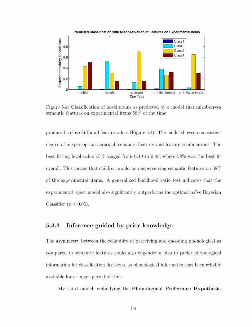
r− initial female animate r− initial female r− initial animate0
0.2
0.4
0.6
0.8
1
Po
ste
rio
r p
rob
ab
ility
of
ea
ch
cla
ss
Cue Type
Predicted Classification with Misobservation of Features on Experimental Items
Class1
Class2
Class3
Class4
Figure 5.4: Classification of novel nouns as predicted by a model that misobservessemantic features on experimental items 58% of the time
produced a close fit for all feature values (Figure 5.4). The model showed a consistent
degree of misperception across all semantic features and feature combinations. The
best fitting level value of β ranged from 0.49 to 0.83, where 58% was the best fit
overall. This means that children would be misperceiving semantic features on 58%
of the experimental items. A generalized likelihood ratio test indicates that the
experimental reject model also significantly outperforms the optimal naıve Bayesian
Classifier (p < 0.05).
5.3.3 Inference guided by prior knowledge
The asymmetry between the reliability of perceiving and encoding phonological as
compared to semantic features could also engender a bias to prefer phonological
information for classification decisions, as phonological information has been reliably
available for a longer period of time.
My third model, embodying the Phonological Preference Hypothesis,
98
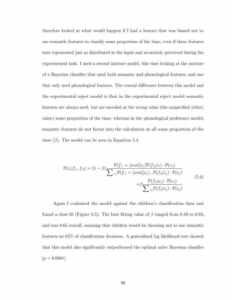
therefore looked at what would happen if I had a learner that was biased not to
use semantic features to classify some proportion of the time, even if these features
were represented just as distributed in the input and accurately perceived during the
experimental task. I used a second mixture model, this time looking at the mixture
of a Bayesian classifier that used both semantic and phonological features, and one
that only used phonological features. The crucial difference between this model and
the experimental reject model is that in the experimental reject model semantic
features are always used, but are encoded as the wrong value (the unspecified [other]
value) some proportion of the time, whereas in the phonological preference model,
semantic features do not factor into the calculation at all some proportion of the
time (β). The model can be seen in Equation 5.4.
P(ci |f1 , f2 ) = (1− β)P(f1 = [sem]|ci)P(f2 |ci) · P(ci)∑cjP(f1 = [sem]|cj )...P(f2 |cj ) · P(cj )
+βP(f2 |ci) · P(ci)∑cjP(f2 |cj ) · P(cj )
(5.4)
Again I evaluated the model against the children’s classification data and
found a close fit (Figure 5.5). The best fitting value of β ranged from 0.49 to 0.83,
and was 0.65 overall, meaning that children would be choosing not to use semantic
features on 65% of classification decisions. A generalized log likelihood test showed
that this model also significantly outperformed the optimal naıve Bayesian classifier
(p < 0.0001)
99
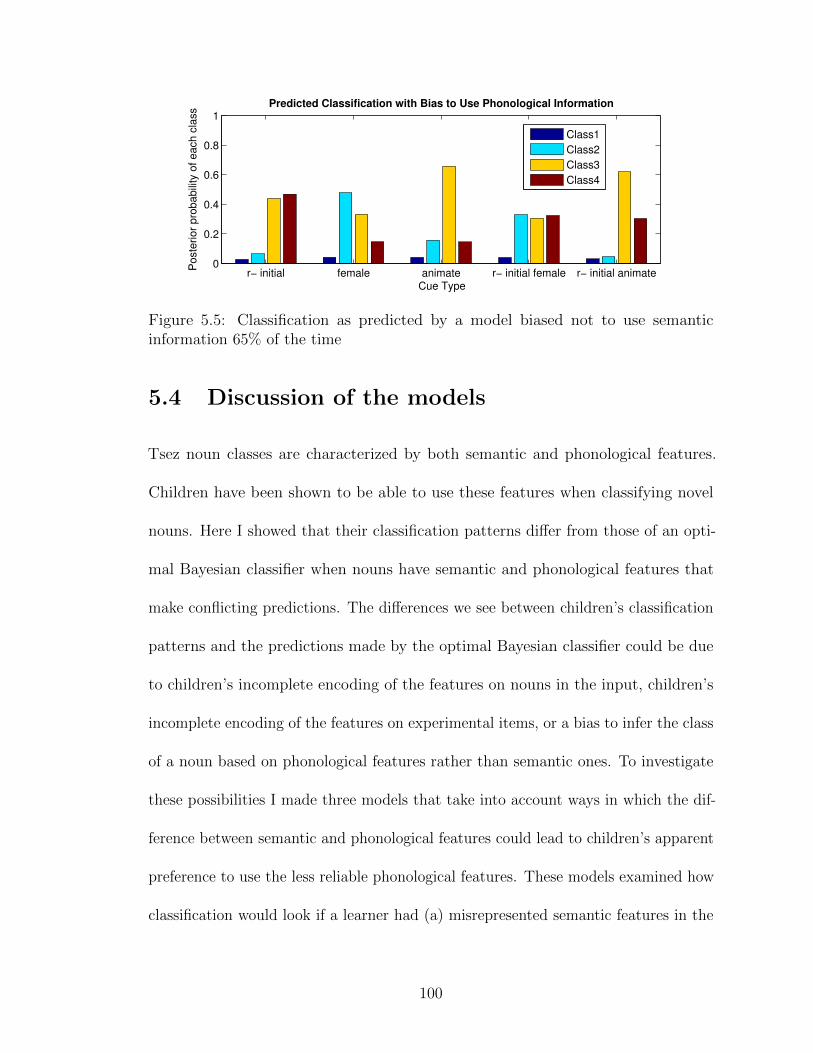
r− initial female animate r− initial female r− initial animate0
0.2
0.4
0.6
0.8
1
Poste
rior
pro
babili
ty o
f each c
lass
Cue Type
Predicted Classification with Bias to Use Phonological Information
Class1
Class2
Class3
Class4
Figure 5.5: Classification as predicted by a model biased not to use semanticinformation 65% of the time
5.4 Discussion of the models
Tsez noun classes are characterized by both semantic and phonological features.
Children have been shown to be able to use these features when classifying novel
nouns. Here I showed that their classification patterns differ from those of an opti-
mal Bayesian classifier when nouns have semantic and phonological features that
make conflicting predictions. The differences we see between children’s classification
patterns and the predictions made by the optimal Bayesian classifier could be due
to children’s incomplete encoding of the features on nouns in the input, children’s
incomplete encoding of the features on experimental items, or a bias to infer the class
of a noun based on phonological features rather than semantic ones. To investigate
these possibilities I made three models that take into account ways in which the dif-
ference between semantic and phonological features could lead to children’s apparent
preference to use the less reliable phonological features. These models examined how
classification would look if a learner had (a) misrepresented semantic features in the
100
lexicon, (b) misencoded semantic features during the classification experiment, or
(c) developed a bias to use phonological information in noun classification due to
its higher reliability in the early stages of lexical acquisition. All three models fit
children’s data significantly better than the optimal naıve Bayesian classifier did.
This suggests that although originally children did not look as though they were
behaving optimally with respect to the input, they may well be behaving optimally
with respect to their intake, that is, the input as they have represented it.
It is not obvious how one would best to evaluate the alternative models with
respect to one another. For example, each model yielded a different best fit parameter,
corresponding to a different degree of misrepresentation or bias. While these best
fitting parameters may differ in terms of their ‘reasonableness’ (i.e. misrepresenting
95% of semantic features in the lexicon at age 6 seems quite high), it isn’t immediately
clear how to measure reasonableness, or how to compare it across models. That is, I
don’t have a metric for determining whether misrepresenting 95% of semantic features
in the lexicon is more or less reasonable than preferring not to use semantic features in
classification decisions 60% of the time. Furthermore, it is likely that a combination
of all three of these processes (and perhaps more that I haven’t considered here)
is influencing children’s classification decisions. This could potentially be explored
through a model that combines all of these processes; however as all of these models
fit the data so closely, it would be difficult to determine which and to what extent
each type of misrepresentation or bias is involved.
This work has several important implications for research statistical learning
and language acquisition. First, I identified an area where children’s behavior does
101
not appear to reflect the ideal inferences licensed by the statistical patterns in the
input. Three models allowed me to investigate the source of this asymmetry, giving
us greater insight into how what a learner can encode from the input could influence
the inferences drawn about what information is important for acquiring each part of
the linguistic system, as well as more specific inferences about how to classify novel
words. Now that I have revealed what kinds of patterns we might see when a child
has misencoded the input or has made incorrect inferences about what information
matters for noun classification, I can conduct further research to determine which of
these might be at the root of Tsez children’s behavior. I can look at, for example,
what predictions each account would have across development. If a child has merely
failed to encode certain semantic features on lexical items, I could independently test
when children can reliably encode these features and see if this correlates with more
adultlike performance on a noun classification task. If instead it is the case that
child can encode all of the relevant features, but they have a bias to use phonological
features for noun classification due to an earlier inference that phonological features
were more important (based on the earliest stages of lexical development when only
phonological dependencies were trackable), then we can look at children solving
other problems that might depend on semantic features, but problems that children
wouldn’t begin solving until later in development due to independent constraints
on the natures of the problems. For example, a child might not begin to track
correlations between animacy of subjects for different verb types (e.g. raising and
control verbs, cf. Becker, 2007) until the child is at a stage where he is building
structure and determining the subject of a given verb. This stage most certainly
102
follows the acquisition of at least a small lexicon with meanings in place. Thus in
learning this kind of phenomenon the learner would have begun learning it at a point
when he was able to encode and thus keep track of correlating semantic features.
Future work will hopefully determine where children can use information like animacy
to learn more about syntax or the lexicon and where they cannot, shedding light on
the nature of the difficulty witnessed with semantic features like animacy here.
Second, while each model differed in where in the language acquisition frame-
work the asymmetry came from, all employed a weakening of the statistical import
of semantic features. That is, children appeared to weaken a generalization that was
very strongly supported in the input. This is a distinct pattern from the finding
that children learning an artificial language amplify an already strong statistical
tendency (Hudson-Kam & Newport, 2009). However another way to view my data
is not by a weakening of the import of semantic features on its own, but rather as
a relative strengthening of the import of phonological features. That is, perhaps
when semantic features weren’t reliably available to children they could only keep
track of the weak generalizations available from the semantics, and, in line with
what children are claimed to do in artificial language learning, strengthened this
generalization in an effort to find some systematicity in the noun classification in the
grammar. Further research and modeling efforts could be employed to determine
whether this is plausible, and if so, what sort of input or inference would be necessary
for children to back off from the strengthened generalization about phonology to
become adultlike in their classification patterns.
Next, I showed that it is possible for a learner to be suboptimal with respect
103
to the input and Bayesian at the same time. That is, I demonstrated that while
children’s behavior does not align with the predictions made by the optimal Bayesian
classifier, it can be predicted by modifying the terms of the Bayesian classifier in
reasonable ways. Thus I was able to model children’s suboptimal behavior using a
Bayesian model, rather than adopting some other system of computation. This is
important if we want to be able to rely on Bayesian computation more generally
in language acquisition (see also Chapter 7 for further discussion). If I had instead
shown that Bayesian computation makes the wrong kinds of predictions for noun
classification and there was no reasonable way to constrain or modify the model to
predict children’s behavior, we would have had to concede that not all computation
is plausibly Bayesian. This might weaken an argument that any other computation
involved in language learning is Bayesian as it would lose any force of argument that
parsimony would have endowed.
Finally, my models showed that it is plausible that these children are indeed
behaving optimally with respect to some statistical distribution, just not one directly
measureable from the input. This point is crucial as researchers attempt to extend
accounts of statistical learning to a greater range of problems, highlighting the fact
that the critical question isn’t whether or not children are using statistics to acquire
language, but what statistics they are using. This problem relates directly back to
the theme of this entire dissertation, that language acquisition is constrained by
what children are able to encode from the input. Thus the statistics available for
children to draw generalizations from will be limited directly by what children are
able to encode from the input, which is in turn constrained by what a child has
104

learned so far and by hypotheses they may entertain about what information should
be considered for what problems.
105
Chapter 6
Encoding, a classification
experiment in Norwegian
In the past few chapters we have looked at how both children’s abilities to reliably
perceive and represent features of the input, as well as hypotheses they bring to
the task of language acquisition, filter what information they can ultimately encode
from the input. As outlined in Chapter 2, noun classes are characterized by both
noun internal and noun external information. In Chapter 3 we looked at children’s
abilities to encode and represent noun internal information. The results of the Tsez
experiment suggested that they used this information probabilistically, and out of
proportion with its distribution in the input.
What we would like to do now is investigate how children use noun external
information. If they use it probabilistically to infer the class of a novel noun,
we will have good evidence that at least at the earlier stages of development it
is represented this way. If they use it deterministically, we won’t be able to tell
106
whether this is the way it is used from the very beginning of acquisition or whether
a probabilistic system with nearly discrete probabilities is built from a prior system
which would look more probabilistic. In what follows, we ask how children use noun
external distributional information in the acquisition of noun classes, namely whether
they have different expectations for information that appears deterministic versus
probabilistic crosslinguistically. As with the classification experiment in Tsez, while
the experiment will directly tell us something about the information used in the
acquisition of noun classes, it can also highlight differences in input and the encoded
intake.
6.1 Previous research on the use of noun external
information
Several studies that have looked at noun class acquisition have looked at children’s
use of noun external distributional information. Cyr & Shi, in press, showed that at
as young as 20 months, French acquiring children showed evidence of being able to
use determiners to classify novel nouns in a habituation task. Children familiarized
to novel words paired with an indefinite determiner noticed a changed when they
heard the same words paired with the definite determiner of the other gender. Thus,
as early as 20 months it looks as thought children have some idea the abstract
representations underlying noun classes. This abstract characterization is realized in
the fact that nouns seen with noun external distributional information characteristic
107

of one class are likely to be seen with another piece of noun external distributional
information for that class, and unlikely to be seen with information for other classes.
Children have been shown to have greater difficulty with noun class agreement
when they need to use it to determine and subsequently produce the class of a novel
noun or match a sentence to a picture. Karmiloff-Smith, 1979 showed that children
from age 3 to 11 can use noun external distributional information to categorize
novel nouns, but younger children have more trouble doing so. Children were
introduced to novel nouns (some of which had predictive noun internal features)
using indefinite determiners, and then phrases included the definite determiner and
novel noun were elicited from the children. Children could use both noun internal
and noun external information to classify the novel nouns, but showed a slight
preference for noun internal phonological information when it conflicted with the
external information. In Xhosa, researchers found that while by age 3;3 children
were producing agreement with noun classes, they had difficulty matching pictures to
sentences when deciding between pictures meant interpreting the noun class marker
on the verb (J. G. deVilliers & Gxilishe, 2009; Gxilishe, Smouse, Xhalisa, & deVilliers,
2009). Performance improved when children were asked to act out the sentences
using toys (Smouse, 2011). These results give us further evidence that children do
not make use of the noun external information as easily as we might expect, given
its reliability in the input.
Thus it remains an open question how children use this information in acquiring
noun classes. Whether this information is used deterministically or probabilistically
may be particularly interesting to look at when it classifies a noun in a way that
108
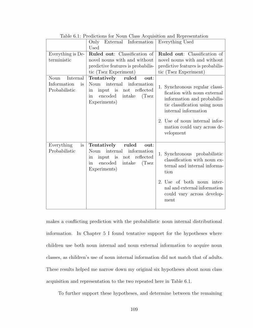
Table 6.1: Predictions for Noun Class Acquisition and RepresentationOnly External InformationUsed
Everything Used
Everything is De-terministic
Ruled out: Classification ofnovel nouns with and withoutpredictive features is probabilis-tic (Tsez Experiment)
Ruled out: Classification ofnovel nouns with and withoutpredictive features is probabilis-tic (Tsez Experiment)
Noun InternalInformation isProbabilistic
Tentatively ruled out:Noun internal informationin input is not reflectedin encoded intake (TsezExperiments)
1. Synchronous regular classi-fication with noun externalinformation and probabilis-tic classification using nouninternal information
2. Use of noun internal infor-mation could vary across de-velopment
Everything isProbabilistic
Tentatively ruled out:Noun internal informationin input is not reflectedin encoded intake (TsezExperiments)
1. Synchronous probabilisticclassification with noun ex-ternal and internal informa-tion
2. Use of both noun inter-nal and external informationcould vary across develop-ment
makes a conflicting prediction with the probabilistic noun internal distributional
information. In Chapter 5 I found tentative support for the hypotheses where
children use both noun internal and noun external information to acquire noun
classes, as children’s use of noun internal information did not match that of adults.
These results helped me narrow down my original six hypotheses about noun class
acquisition and representation to the two repeated here in Table 6.1.
To further support these hypotheses, and determine between the remaining
109
two, I need to investigate children’s use of noun external information. If children
relied on external information alone to acquire noun classes, we would expect them
to be able to make use of it when classifying novel nouns. If, on the other hand,
children used this information in combination with noun internal regularities, it isn’t
clear how robust their knowledge of noun external information would need to be.
They would have to have some probabilistic sensitivity to this information, or at
least be able to use it appropriately to have any kind of noun class system, but
whether or not they need to be able to use this information in the deterministic way
predicted by the input. By looking at whether or not children rely on noun external
distributional information to classify novel nouns, in particular when this information
conflicts with predictions about noun class made by noun internal distributional
information, I can determine which of my remaining two hypotheses can account for
the acquisition and representation of noun classes.
6.2 Choosing Norwegian
Ideally this work would have been continued in Tsez, but unfortunately due to an
increasingly unstable political situation in Dagestan it was no longer safe enough to
travel to conduct research. The work was instead conducted in Norwegian, which was
a sensible choice not only for practical reasons, but for the following considerations as
well. First, and most generally, any theory of noun class acquisition should hopefully
be one that could apply to children learning any kind of noun class system, and
so expanding to a typologically distinct language is good for that reason. Second,
110
Norwegian has a three gender system that is is less well defined in some sense than
Tsez noun classes: noun class is only regularly shown internal to the DP on indefinite
articles and definite suffixes, and while there has been some work attempting to
identify noun internal distributional features that can predict class (Trosterud, 2001),
the psychological status of these cues to classify novel nouns is unknown. Norwegian
also proves to be a difficult language to work on, due to the variability across dialects
in terms of how many classes there are, as several dialects collapse two of the classes,
masculine and feminine, into one. There is further variability across dialects in terms
of which nouns are assigned to which classes. For better or worse, the next stage
of this project was carried out in Norwegian, and despite the differences between
the languages, I predict that acquisition and representation should follow roughly
the same patterns, in terms of what kinds of information are useful to the learner or
speaker.
6.3 Overview of experiments
I wanted to test two aspects of the role noun external distributional information on
acquisition and representation. First, can speakers use noun external information to
classify nouns? And second, what do speakers do when probabilistic noun internal
and deterministic noun external information make conflicting predictions about a
noun’s class? If I were working in Tsez, I could move on directly to test noun
external distributional information, but since I am working in a new language, it is
first necessary to determine (1) whether the language has predictive noun internal
111
features for each class and (2) whether speakers are sensitive to these features when
classifying novel nouns. Once I have established the answers to these two questions,
I look at how speakers use noun external distributional information, and how they
use this information when it is in conflict with the predictions made by the noun
internal distributional information.
6.3.1 Norwegian noun classes
Many spoken dialects of Norwegian have three noun classes (grammatical genders),
labeled in the traditional Indo-European fashion as Masculine, Feminine and Neuter.
In what follows, I will continue to refer to the three class by these three names, with
the clarification that these are formal features only, and do not imply, for example, a
‘male’ feature on all the nouns in the masculine class (only on the nouns that actually
denote male humans). I could just as easily label them as the Tsez noun classes are
labeled, as Class 1, Class 2 and Class 3, without losing any of the descriptive power
that goes along with the traditional names of the classes.
Noun external distributional information
Noun external distributional information in Norwegian is visible in two both unique
definite suffixes for each class, as well as unique indefinite determiners (Table 6.2).
Noun internal distributional information
Past researchers have identified semantic, phonological and morphological features
that can be used to classify Norwegian nouns (Trosterud, 2001). For example, nouns
112
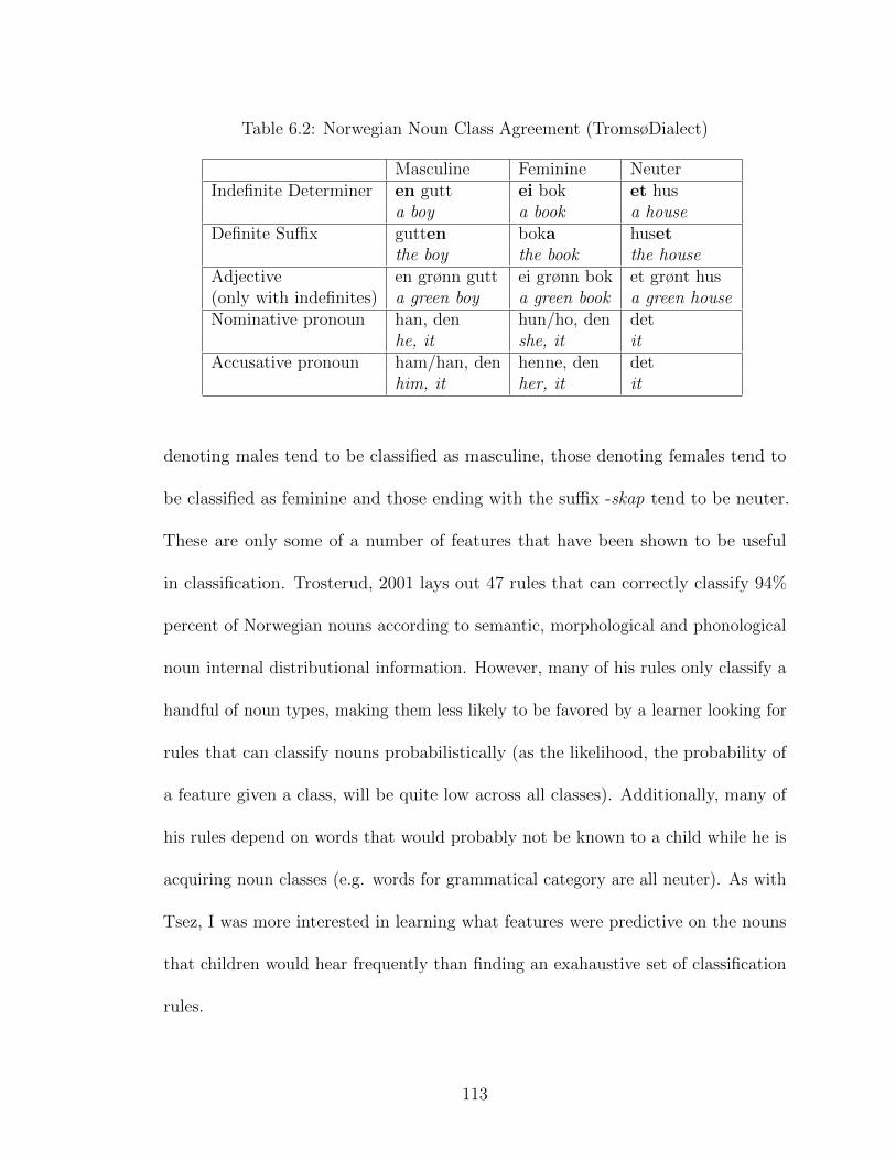
Table 6.2: Norwegian Noun Class Agreement (TromsøDialect)
Masculine Feminine NeuterIndefinite Determiner en gutt ei bok et hus
a boy a book a houseDefinite Suffix gutten boka huset
the boy the book the houseAdjective en grønn gutt ei grønn bok et grønt hus(only with indefinites) a green boy a green book a green houseNominative pronoun han, den hun/ho, den det
he, it she, it itAccusative pronoun ham/han, den henne, den det
him, it her, it it
denoting males tend to be classified as masculine, those denoting females tend to
be classified as feminine and those ending with the suffix -skap tend to be neuter.
These are only some of a number of features that have been shown to be useful
in classification. Trosterud, 2001 lays out 47 rules that can correctly classify 94%
percent of Norwegian nouns according to semantic, morphological and phonological
noun internal distributional information. However, many of his rules only classify a
handful of noun types, making them less likely to be favored by a learner looking for
rules that can classify nouns probabilistically (as the likelihood, the probability of
a feature given a class, will be quite low across all classes). Additionally, many of
his rules depend on words that would probably not be known to a child while he is
acquiring noun classes (e.g. words for grammatical category are all neuter). As with
Tsez, I was more interested in learning what features were predictive on the nouns
that children would hear frequently than finding an exahaustive set of classification
rules.
113
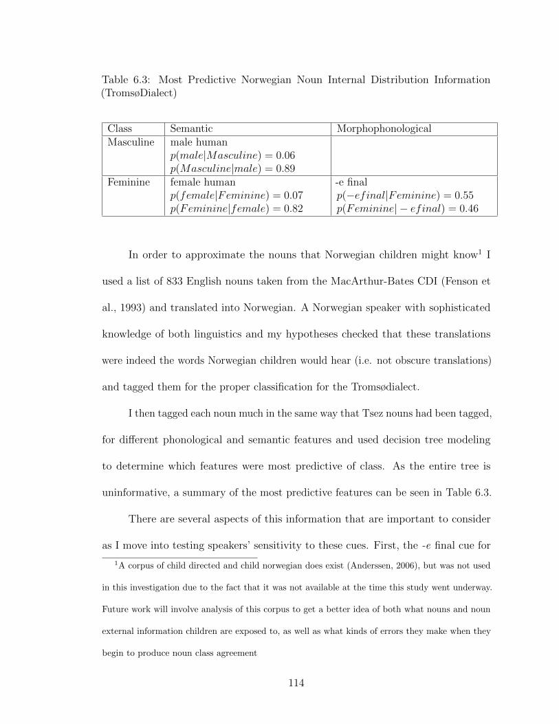
Table 6.3: Most Predictive Norwegian Noun Internal Distribution Information(TromsøDialect)
Class Semantic MorphophonologicalMasculine male human
p(male|Masculine) = 0.06p(Masculine|male) = 0.89
Feminine female humanp(female|Feminine) = 0.07p(Feminine|female) = 0.82
-e finalp(−efinal|Feminine) = 0.55p(Feminine| − efinal) = 0.46
In order to approximate the nouns that Norwegian children might know1 I
used a list of 833 English nouns taken from the MacArthur-Bates CDI (Fenson et
al., 1993) and translated into Norwegian. A Norwegian speaker with sophisticated
knowledge of both linguistics and my hypotheses checked that these translations
were indeed the words Norwegian children would hear (i.e. not obscure translations)
and tagged them for the proper classification for the Tromsødialect.
I then tagged each noun much in the same way that Tsez nouns had been tagged,
for different phonological and semantic features and used decision tree modeling
to determine which features were most predictive of class. As the entire tree is
uninformative, a summary of the most predictive features can be seen in Table 6.3.
There are several aspects of this information that are important to consider
as I move into testing speakers’ sensitivity to these cues. First, the -e final cue for
1A corpus of child directed and child norwegian does exist (Anderssen, 2006), but was not used
in this investigation due to the fact that it was not available at the time this study went underway.
Future work will involve analysis of this corpus to get a better idea of both what nouns and noun
external information children are exposed to, as well as what kinds of errors they make when they
begin to produce noun class agreement
114
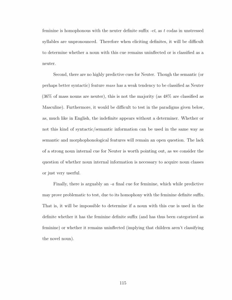
feminine is homophonous with the neuter definite suffix -et, as t codas in unstressed
syllables are unpronounced. Therefore when eliciting definites, it will be difficult
to determine whether a noun with this cue remains uninflected or is classified as a
neuter.
Second, there are no highly predictive cues for Neuter. Though the semantic (or
perhaps better syntactic) feature mass has a weak tendency to be classified as Neuter
(36% of mass nouns are neuter), this is not the majority (as 48% are classified as
Masculine). Furthermore, it would be difficult to test in the paradigms given below,
as, much like in English, the indefinite appears without a determiner. Whether or
not this kind of syntactic/semantic information can be used in the same way as
semantic and morphophonological features will remain an open question. The lack
of a strong noun internal cue for Neuter is worth pointing out, as we consider the
question of whether noun internal information is necessary to acquire noun classes
or just very userful.
Finally, there is arguably an -a final cue for feminine, which while predictive
may prove problematic to test, due to its homophony with the feminine definite suffix.
That is, it will be impossible to determine if a noun with this cue is used in the
definite whether it has the feminine definite suffix (and has thus been categorized as
feminine) or whether it remains uninflected (implying that children aren’t classifying
the novel noun).
115
6.4 Experiment 1: Use of noun internal distribu-
tional information
I first wanted to verify that Norwegian children are sensitive to noun internal
distributional features. To do this I devised a classification task similar to the one
used with Tsez children, where children were introduced to nouns, both known and
novel, without any classifying information and an indefinite form was elicited.
6.4.1 Task
I wanted to introduce children to novel nouns without any noun external information
that would indicate their class, so that I could see how they would classify novel
nouns on the basis of noun internal information alone. Much like in English, nouns in
Norwegian cannot appear without either an indefinite determiner or a definite suffix.
As both of these would give away the class of a noun, I had to find a context where
novel nouns could be introduced without any noun external information. I found
that embedded nouns in compounds provided just such an environment. Norwegian
has productive noun-noun compounding, where the compound takes the class of
the head noun. For example, musboks, a compound formed from mus (feminine,
mouse) and boks (masculine, box ), is masculine, as boks is masculine. Thus there
is no noun external information in musboks that would indicate the class of mus.
Using compounds, I could introduce nouns to subjects without giving away the class
of the non-head noun. I could then elicit a form where the child was required to
break down the compound and use the non-head noun (mus) with an indefinite
116
determiner, showing the child’s beliefs about class of that noun. For example, I could
ask the child What’s in the musboks?, and the child would respond ei mus, using
the feminine indefinite determiner. The class of head noun (e.g. boks) was balanced
across items to avoid effects of that noun’s class being used to classify the non-head
noun.
Children were introduced to a turtle from another planet who had lost all of
his things when his spaceship crashed. Some helpers had found all kinds of boxes,
backpacks, cupboards and baskets with different items in them. A native Norwegian
speaker of the local dialect introduced the child to the item (always a compound
like mus-boks). The child then had to look at what was inside (e.g. a mouse), and
ask the turtle if he wanted it (e.g. ei mus). When the child used the indefinite
article with the noun outside of the compound, its form indicated how the child had
classified the noun. The order of item was pseudorandomized by the experimenter
to ensure a varied order of real and nonce word and words from each class. As the
distinct pronunciations of the indefinite determiners can be subtle for an nonnative
speaker to perceive, the entire task was recorded for post-test coding of the results
by a native Norwegian speaker.
6.4.2 Materials
Both real and nonce nouns were used as non-head (target) nouns in the compounds.
Words were selected or invented to have features (or combinations of features) that
were found to be predictive of class. The full set of features and feature combinations
117
Table 6.4: Feature combinations on words used in Experiment 1
Feature Type Masculine FeminineSemantic male human female humanPhonological e- initialTwo Agreeing e- initial
& female hu-man
Two Conflicting e- initial& male human
used in the task can be seen in Table 6.4. The full set of words used can be found
in Appendix D. Each compound had an accompanying drawing that showed the
compound with the target inside it (e.g. ‘mousebox’ with a mouse inside it).
6.4.3 Predictions
Just as in the Tsez classification experiment, I expect that children should be
sensitive to noun internal distributional properties. Consistent with the results of
the Tsez experiment, I expect that if children are using both noun internal and
noun external information to acquire noun classes, their sensitivity to noun internal
features might differ from what the distribution of these features in the input predicts.
Additionally if the patterns we saw in Tsez acquiring children reflect something
general about children’s ability to encode certain features on nouns, or use these
features for classification, I expect to see an asymmetry in the use of semantic and
morphophonological cues.
118
6.4.4 Participants
Participants were 17 Norwegian children: 9 from a kindergarten, (mean age 5;1,
range 4;2-5;9) and 11 from an elementary school (mean age 6;8, range 6;4-7;2). An
additional 18 kindergarteners participated, but their results were excluded from the
analysis either because the failed to use either an indefinite determiner or definite
suffix on the majority of the items (4 children), because they failed to correctly
classify 10 real words, whose class they were expected to know (11 children)2, or
because they only used masculine and neuter determiners throughout the task (3
children). This last pattern could be indicative of knowledge of another dialect, as
some dialects in norwegian lack the Feminine class altogether.
6.4.5 Results
A native Norwegian speaker unfamiliar with the hypotheses of the experiment
transcribed the recordings of children performing the task. Results were coded based
on what class the child assigned to the target noun, based on their choice of indefinite
determiner. Just as in the Tsez experiment, I compared distributions of classification
with each cue type for each class (real words) or target class (nonce words). One
unforeseen difficulty with the task was that when nouns are in compounds, some
nouns require a ‘support vowel’, that happens to be -e. This means that it may
have been unclear to children when presented with -e final nouns in compounds
2Instead of classifying these words correctly, they classified these, and all other words in the task,
as if they were masculine.This is similar to a pattern observed with the Tsez speaking children,
discussed above in Chapter 5
119
whether this -e was part of the novel noun or a support vowel. As I was eliciting
the indefinite determiner, I could eliminate from the results those nouns where the
child omitted the final -e when producing the indefinite form, inferring that if the
child did not produce the final vowel it has been interpreted as a support vowel, and
therefore wouldn’t influence the classification of the novel noun.
Real words
The results in Table 6.6 reflect the proportion of nouns correctly assigned to each
class, given each cue type. Overall, children do do very well classifying real words
that are masculine and neuter, but appear to struggle with Feminine nouns. Due
to the fact that some dialects of Norwegian lack the Feminine gender, it is not
surprising, as children probably have variable input with respect to where they
encounter these nouns. When children misclassified Feminine nouns, they classified
them as Masculine, consistent with how they appear in the two-gender dialects.
Finally, Masculine and Neuter nouns with Conflicting cues (real nouns that were
Masculine or Neuter but ended in the -e final phonological cue for feminine), were the
source of the only imperfections in classifying Masculine and Neuter nouns. While
the proportions are very small (4% and 6% respectively), this patterns is suggestive
of sensitivity to phonological cues out of proportion with their reliability, much like
we saw in the Tsez case.
120
Table 6.5: Classification of real words (percent classified correctly)
Semantic Phonological NoCue
Conflicting Agreeing
Masculine 100 na 100 96 naFeminine 65 54 47 na 53Neuter na na 1 94 na
Table 6.6: Classification of real words (percent classified correctly)
Table 6.7: Classification of nonce words (percent assigned to target class)
Semantic Phonological Conflicting AgreeingMasculine 100 na 89 naFeminine 8 3 na 8
Nonce words
The results in Table 6.7 reflect the proportion of nouns assigned to the target class
(the class most strongly predicted by noun internal information), given each cue
type.
Overall, Norwegian children are not successful at using noun internal infor-
mation to classify novel nouns. A breakdown of these results shows that this is
due to a strong preference to classify all novel words as masculine, regardless of
the cue type. There is a very slight preference to classify nouns as Feminine with
either semantic or phonological cues for Feminine. Interestingly, we see this tendency
whether the nouns also have a semantic cue predicting masculine or not. That is,
children allow the morphophonological information to override both the predictions
of the semantic information and the very strong bias to make everything masculine
(albeit very rarely). While these effects are small and no conclusions can be drawn
121
from them alone, they are suggestive that children are sensitive to these cues3. Thus
it looks as though children have a very strong bias to classify every novel noun as
masculine, but when this is overidden it is done so in a manner consistent with the
noun internal information4.
6.4.6 Discussion of Experiment 1
In this classification task we saw that while Norwegian children largely ignore noun
internal predictive information, there is a slight sensitivity to predictive morphophono-
logical information. While a much weaker result, this finding is reminiscent of the
finding in Tsez where children prefer to use phonological information when the two
types make conflicting predictions.
Furthermore I tentatively replicated the finding from Tsez where children use
phonological information more than semantic information. Of course, it’s important
to take note that in Norwegian, the morphophonological information appears a sense
to be a statistically stronger cue than the semantic information. That is, while 82%
of females are in the Feminine class, only 7% of Feminine nouns are females. Nouns
ending in -e, on the other hand, make up 55% of the Feminine class, even though
only 46% of -e final nouns are are in that class. In Tsez, semantic cues tended to be
3This pattern begs for computational modeling like that done in Chapter 5 to determine whether
the combination of some feature misrepresentation paired with variability in the input and a very
large Masculine class could predict this sort of classification behavior4Rodina and Westergaard (2011) have found a similar pattern, where children show a preference
to use the masculine indefinite determiner even when exhibiting knowledge of the correct definite
suffix for a given noun
122
statistically stronger cues on both measures.
Now that I have established some sensitivity to noun internal distributional
information by Norwegian speaking children, I want to look at how they use noun
external information.
6.5 Experiment 2: Use of noun external distribu-
tional information
In this second experiment I wanted to test whether children will use noun external
distributional information to classify novel nouns. I wanted to see if they are sensitive
to this information being linked to the class of the noun. That is, whether seeing a
novel noun appearing with an indefinite determiner showing its class is enough to
trigger using the definite forms for the same class. I also wanted to see what happens
when noun internal information makes a conflicting prediction. If the indefinite
determiner predicts one class but a morphophonological cue on the noun predicts
another, what will the children do?
6.5.1 Task
In order to test whether children can use noun external information to classify a novel
noun, I had to devise a situation where a novel noun would be introduced with some
kind of noun external information, and another form of noun external information
would then be elicited from the child subjects. This was not a challenge, as it is quite
123
natural to introduce a novel noun with an indefinite determiner, show something
happen to it, and ask for a description of what happened that will naturally involve
a definite suffix.
To incorporate this basic framework, the task consisted of watching some
scenarios of some children visiting a blind alien turtle’s home planet, and describing
to the blind turtle and an experimenter what happened in each scene. Each scene
involved a boy, a girl, a known noun and a novel noun (as in Figure 6.1). At the
beginning of each scene the native Norwegian speaking experimenter would say (in
Norwegian) ‘Here they found en/ei/et fepp and a dog, a fepp and a dog (pointing
to the novel and known nouns in turn). Let’s see what happens’. Something would
happen in the scene (e.g. the fepp would slide down the hill and kick the dog), and
then the child would be prompted to describe the scene. The goal was to elicit
descriptions of the novel objects using a definite determiner and the novel noun. If
the child used pronouns or just pointed to a referent they were asked for clarification
and reminded that the turtle couldn’t see what was happening. As in Experiment 1,
participants were recorded during the task to allow for a native Norwegian speaker
to transcribe these recordings for accurate coding of responses afterwards.
6.5.2 Materials
Test items involved 36 novel nouns, created to have no predictive features, or to have
the predictive features used in Experiment 1 (repeated in Table 6.8). Three items
from each of the four item types were presented with each indefinite determiner. Thus
124
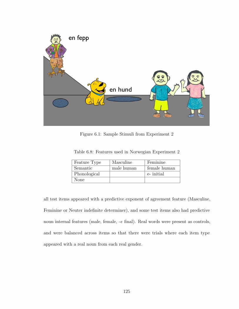
Figure 6.1: Sample Stimuli from Experiment 2
Table 6.8: Features used in Norwegian Experiment 2
Feature Type Masculine FeminineSemantic male human female humanPhonological e- initialNone
all test items appeared with a predictive exponent of agreement feature (Masculine,
Feminine or Neuter indefinite determiner), and some test items also had predictive
noun internal features (male, female, -e final). Real words were present as controls,
and were balanced across items so that there were trials where each item type
appeared with a real noun from each real gender.
125
6.5.3 Predictions
To review my predictions regarding noun external information, if children have
knowledge of noun classes, implying knowledge of the abstract relations between
different exponents of noun class in the noun external information, I would expect
that seeing a novel noun with agreement information for one class would be enough
to classify that noun as part of the class that that agreement information signifies.
If children expect that this information does not probabilistically correlate with
class, but instead determines it, they should use it reliably, and any noun internal
information that makes a conflicting prediction should be ignored. However, if
children represent this information probabilistically and have not perfectly encoded
it, it’s possible that predictions made by noun internal information could outweigh
that of noun external information.
6.5.4 Participants
Fifteen children (mean age 6;8, range 6;4-7;3) were tested individually in a private
room at an elementary school in Tromsø, Norway.
6.5.5 Results
Coding of the classification of novel words was based on what definite suffix the chil-
dren used when describing what happened to the novel object. Children occasionally
used pronouns or pointed to the objects, but used the novel word when prompted by
an experimenter saying something like ‘Remember, the turtle can’t see. This is a
126

fepp’. On a small proportion of trials, children used double definites (a combination
of a definite determiner and a definite suffix), but classification was still visible in the
suffix. On 10% of trials children failed to inflect the novel nouns with a definite suffix
or repeat the indefinite determiner. These trials were excluded from analysis. As
mentioned when outlining noun external information, there is homophony between
the neuter definite -et and an uninflected noun ending in -e. Therefore, outside of
double definites, it was difficult to determine whether a child was not inflecting a
novel -e-final noun or was using the neuter definite. To overcome this issue, I looked
at the child’s pattern on other trials. If there were no other trials where they failed
to inflect the novel noun, I counted these forms as inflected with the neuter definite.
If there were any trials where they unambiguously failed to inflect a novel noun, I
counted these items as instances of omitted inflection and did not include them in
the results.
First I will look at the items that only gave children noun external information
to guide their classification. As we can see in Figure 6.2), we see a preference for
making novel nouns masculine, regardless of the class of the indefinite determiner
used to introduce the noun. However, we do see that at least some of the time
children are willing to use the neuter indefinite to classify novel nouns. This result is
surprising, as it means that 61% of the time children are ignoring highly predictive
noun external information when classifying novel nouns. A Chi-Squared test shows
a significant difference between classification with Masculine and Neuter determiners
χ2 (2, 118) = 19.05, p < 0.0001 but no difference between Feminine and Neuter
χ2 (2, 26) = 4.15, p = 0.125 or Masculine and Feminine χ2 (2, 106) = 2.14, p = 0.343.
127
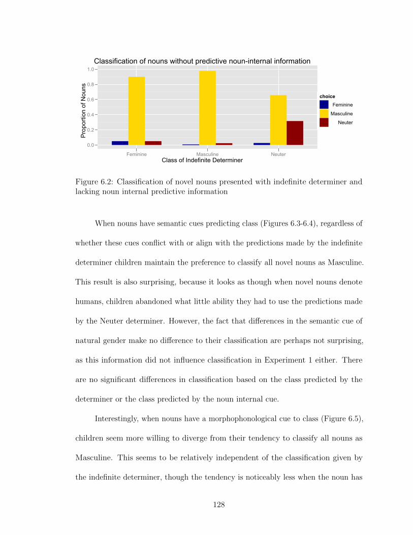
Classification of nouns without predictive noun-internal information
Class of Indefinite Determiner
Pro
porti
on o
f Nou
ns
0.0
0.2
0.4
0.6
0.8
1.0
Feminine Masculine Neuter
choiceFeminine
Masculine
Neuter
Figure 6.2: Classification of novel nouns presented with indefinite determiner andlacking noun internal predictive information
When nouns have semantic cues predicting class (Figures 6.3-6.4), regardless of
whether these cues conflict with or align with the predictions made by the indefinite
determiner children maintain the preference to classify all novel nouns as Masculine.
This result is also surprising, because it looks as though when novel nouns denote
humans, children abandoned what little ability they had to use the predictions made
by the Neuter determiner. However, the fact that differences in the semantic cue of
natural gender make no difference to their classification are perhaps not surprising,
as this information did not influence classification in Experiment 1 either. There
are no significant differences in classification based on the class predicted by the
determiner or the class predicted by the noun internal cue.
Interestingly, when nouns have a morphophonological cue to class (Figure 6.5),
children seem more willing to diverge from their tendency to classify all nouns as
Masculine. This seems to be relatively independent of the classification given by
the indefinite determiner, though the tendency is noticeably less when the noun has
128
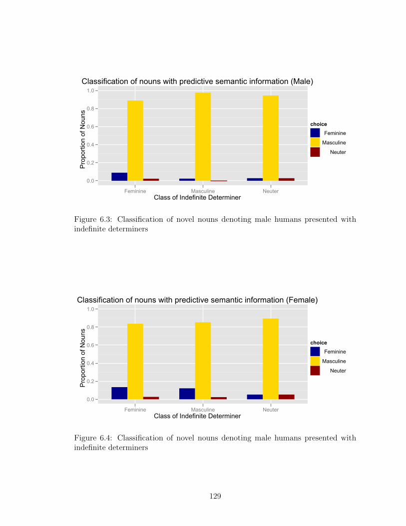
Classification of nouns with predictive semantic information (Male)
Class of Indefinite Determiner
Pro
porti
on o
f Nou
ns
0.0
0.2
0.4
0.6
0.8
1.0
Feminine Masculine Neuter
choiceFeminine
Masculine
Neuter
Figure 6.3: Classification of novel nouns denoting male humans presented withindefinite determiners
Classification of nouns with predictive semantic information (Female)
Class of Indefinite Determiner
Pro
porti
on o
f Nou
ns
0.0
0.2
0.4
0.6
0.8
1.0
Feminine Masculine Neuter
choiceFeminine
Masculine
Neuter
Figure 6.4: Classification of novel nouns denoting male humans presented withindefinite determiners
129

Classification of nouns with morphophonological cue to Feminine
Class of Indefinite Determiner
Pro
porti
on o
f Nou
ns
0.0
0.2
0.4
0.6
0.8
1.0
Feminine Masculine Neuter
choiceFeminine
Masculine
Neuter
Figure 6.5: Classification of novel nouns ending in -e presented with indefinitedeterminers
an indefinite determiner. A Chi-Squared test shows a significant difference between
classification with a Masculine determiner and no phonological cue and a Masculine
determiner and a phonological cue for feminine, χ2 (2, 86) = 21.76, p < 0.0001, and
shows the same for a Feminine determiner and no phonological cue and a Feminine
determiner and a phonological cue for feminine χ2 (2, 82) = 28.37, p < 0.000001, and
no difference between a Neuter determiner paired no phonological cue and a Neuter
determiner paired with a phonological cue for feminine χ2 (2, 79) = 3.12, p = 0.21.
6.5.6 Discussion
Overall, the results from Experiment 2 are in line with what others have shown
about children’s use of noun external information. Children appear very reticent
to use deterministic noun external information to classify novel nouns, allowing a
general bias to classify all novel nouns as Masculine to overrule all predictions made
130
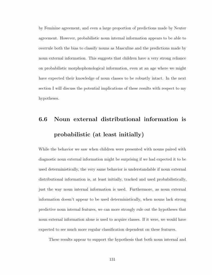
by Feminine agreement, and even a large proportion of predictions made by Neuter
agreement. However, probabilistic noun internal information appears to be able to
overrule both the bias to classify nouns as Masculine and the predictions made by
noun external information. This suggests that children have a very strong reliance
on probabilistic morphophonological information, even at an age where we might
have expected their knowledge of noun classes to be robustly intact. In the next
section I will discuss the potential implications of these results with respect to my
hypotheses.
6.6 Noun external distributional information is
probabilistic (at least initially)
While the behavior we saw when children were presented with nouns paired with
diagnostic noun external information might be surprising if we had expected it to be
used deterministically, the very same behavior is understandable if noun external
distributional information is, at least initially, tracked and used probabilistically,
just the way noun internal information is used. Furthermore, as noun external
information doesn’t appear to be used deterministically, when nouns lack strong
predictive noun internal features, we can more strongly rule out the hypotheses that
noun external information alone is used to acquire classes. If it were, we would have
expected to see much more regular classification dependent on these features.
These results appear to support the hypothesis that both noun internal and
131
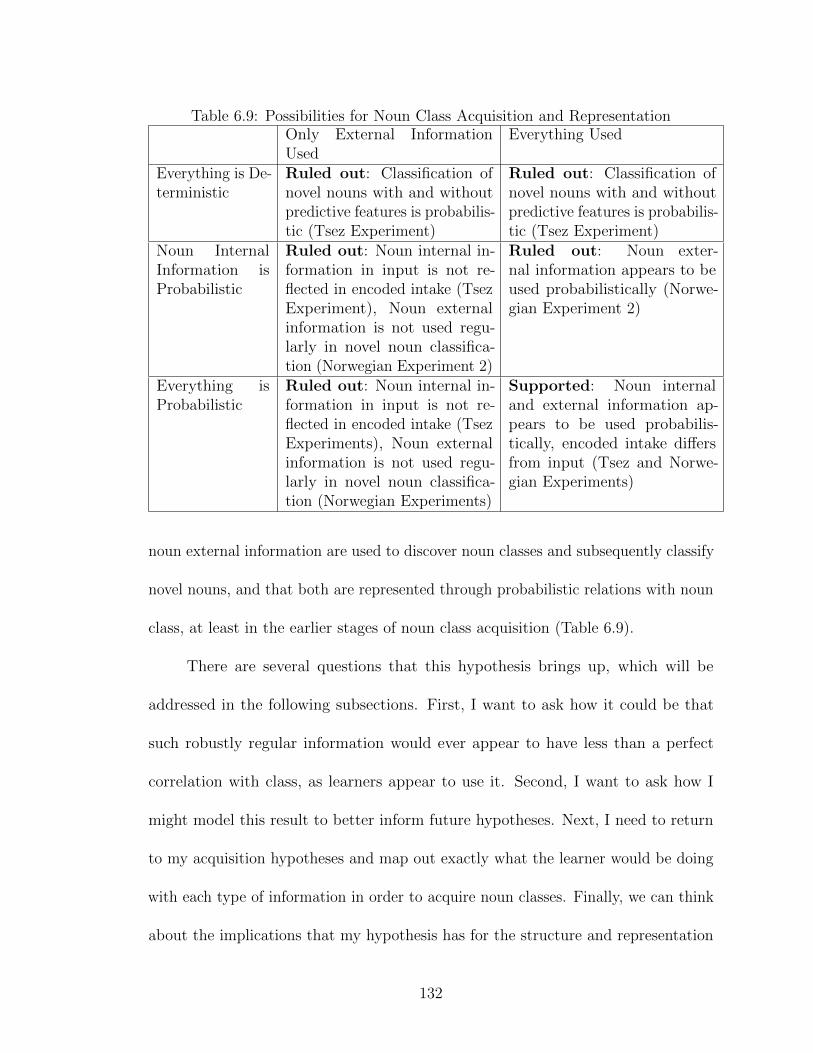
Table 6.9: Possibilities for Noun Class Acquisition and RepresentationOnly External InformationUsed
Everything Used
Everything is De-terministic
Ruled out: Classification ofnovel nouns with and withoutpredictive features is probabilis-tic (Tsez Experiment)
Ruled out: Classification ofnovel nouns with and withoutpredictive features is probabilis-tic (Tsez Experiment)
Noun InternalInformation isProbabilistic
Ruled out: Noun internal in-formation in input is not re-flected in encoded intake (TsezExperiment), Noun externalinformation is not used regu-larly in novel noun classifica-tion (Norwegian Experiment 2)
Ruled out: Noun exter-nal information appears to beused probabilistically (Norwe-gian Experiment 2)
Everything isProbabilistic
Ruled out: Noun internal in-formation in input is not re-flected in encoded intake (TsezExperiments), Noun externalinformation is not used regu-larly in novel noun classifica-tion (Norwegian Experiments)
Supported: Noun internaland external information ap-pears to be used probabilis-tically, encoded intake differsfrom input (Tsez and Norwe-gian Experiments)
noun external information are used to discover noun classes and subsequently classify
novel nouns, and that both are represented through probabilistic relations with noun
class, at least in the earlier stages of noun class acquisition (Table 6.9).
There are several questions that this hypothesis brings up, which will be
addressed in the following subsections. First, I want to ask how it could be that
such robustly regular information would ever appear to have less than a perfect
correlation with class, as learners appear to use it. Second, I want to ask how I
might model this result to better inform future hypotheses. Next, I need to return
to my acquisition hypotheses and map out exactly what the learner would be doing
with each type of information in order to acquire noun classes. Finally, we can think
about the implications that my hypothesis has for the structure and representation
132
of the lexicon.
6.6.1 Why isn’t noun external information encoded faith-
fully?
Noun external distributional information appears highly regular, so it comes as a
surprise that it might not be encoded faithfully. There are two reasons why this could
be so. First, in order to encode this information the learner has to both segment the
morphological exponents of agreement and track the dependencies between these
exponents and nouns in the input. At a subsequent stage it is not the dependency
between the exponents and nouns that would be tracked, but the dependency between
the abstract class generating these exponents and the exponents and nouns. Both
stages require the child to form dependencies across levels in the lexicon, first surface
level dependencies between functional morphemes and lexical items and then abstract
ones between abstract classes and both lexical items and functional morphemes.
If there is any syncretism in the paradigm (and both Tsez and Norwegian have
significant levels of syncretism in their noun external distributional information),
this tracking would be even more difficult. It is not impossible to imagine that
simply tracking surface level dependencies between sounds (e.g. the first or last
segment in a noun) and the phonological forms of morphemes might be easier for a
child at an earlier stage. This means that early on in development the child would
depend on phonological cues on the noun, rather than on the identity of the noun, to
track dependencies in the input. This would have a very similar implication to the
133

difference between phonological and semantic noun internal features, namely that
phonological features are more reliable and therefore more useful early on. The child
would come to rely on what was useful in the early stages and could take a great
while to overcome these learned biases. Future work will determine whether this is
indeed the case, but it at least doesn’t seem implausible to posit at present.
6.6.2 Modeling this result
I have suggested that my data points toward a probabilistic representation of both
noun internal and noun external information, as seen in Figure 6.6 (repeated from
Chapter 2). In future work I can test out the predictions of this hypothesis by
modeling inferences about a novel noun’s class based on both noun internal and noun
external information. Such a model would be a relatively straightforward extension
of the probabilistic model of noun classification given in Chapter 5, repeated here:
P(ci |f1 ...fn) =P(f1 |ci)...P(fn |ci) · P(ci)∑
cj∈{all classes}P(f1 |cj )...P(fn |cj ) · P(cj )(6.1)
The only modification is an independent term in the likelihood that is the
probability of the noun external information given the class. This model is appealing
for several reasons. First, it makes noun external information straightforwardly
probabilistic. With the accumulation of sufficient data, it could look deterministic,
but with sparser or noisier data (that could reasonably be attributed to a child who has
trouble encoding dependencies between noun class and noun external information),
it might look probabilistic the way we have seen it working in Norwegian children.
134
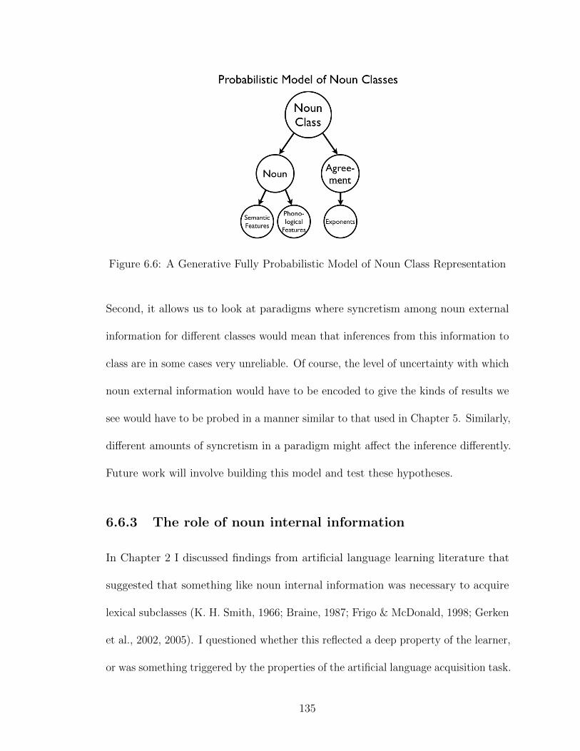
Figure 6.6: A Generative Fully Probabilistic Model of Noun Class Representation
Second, it allows us to look at paradigms where syncretism among noun external
information for different classes would mean that inferences from this information to
class are in some cases very unreliable. Of course, the level of uncertainty with which
noun external information would have to be encoded to give the kinds of results we
see would have to be probed in a manner similar to that used in Chapter 5. Similarly,
different amounts of syncretism in a paradigm might affect the inference differently.
Future work will involve building this model and test these hypotheses.
6.6.3 The role of noun internal information
In Chapter 2 I discussed findings from artificial language learning literature that
suggested that something like noun internal information was necessary to acquire
lexical subclasses (K. H. Smith, 1966; Braine, 1987; Frigo & McDonald, 1998; Gerken
et al., 2002, 2005). I questioned whether this reflected a deep property of the learner,
or was something triggered by the properties of the artificial language acquisition task.
135
At this point, with my hypothesis that noun classes are represented probabilistically
and acquired as such, I can further hypothesize that noun internal information isn’t
a necessary piece of noun class acquisition. Since noun internal information exists in
noun class systems5 it is of course used to acquire a systematic correlation between
nouns and classes, but it is not based in any deep property of a learning mechanism.
Simply, the more observable, encodable systematicity that exists in the system, the
easier the system is to acquire. With this in mind, perhaps a reexamination of the
artificial language learning experiments is called for, as my hypothesis predicts that
such classes should be acquirable without internal correlating information, but that
this would be more difficult.
5As to why this systematicity exists, or why noun class systems exist at all, some speculation
is warranted. One hypothesis is that noun classes exist as a generalization of some historical
variation in the input (variation, say in the determiner system). When attempting to make sense
this variation, learners would fix one determiner to one set of nouns, and another determiner to
another. The learner would be searching for some systematicity in how to do this assignment, and
salient morphophonological or semantic features might stand out and be used for this purpose. The
result would be a noun class system, with regular noun external information and some regularities
in noun internal features. This sort of account is not implausible when considering the kinds of
generalization children make in learning artificial languages (Hudson-Kam & Newport, 2009), or the
regularization of variable determiners that happens in language evolution experiments (K. Smith &
Wonnacott, 2010). Further work will hopefully address this hypothesis
136
6.6.4 How are noun classes acquired?
At last, I can address the question I set out to answer: how are noun classes acquired?
I have indirect evidence that both noun internal and noun external information are
used in their acquisition, and that this information is used probabilistically. I will
return to the pieces of the language acquisition model in order to see how these
might fit together.
First I will return to the hypothesis space. In this case we can assume a
relatively minimal hypothesis space: the learner would expect (1) that the lexicon
could be partitioned, and (2) that this partitioning could be predictable based on
both noun internal and noun external distributional information. This means that
the learner would be looking for systematic correspondences between noun internal
features and noun external distributional information in order to discover how many
classes there were, what information characterized them, and what nouns were in
each class. Additionally, the learner might have expectation to find certain kind of
information correlating with class (e.g. biological semantic features) and not others
(e.g. paper, clothing).
In order to find these systematic correspondences, the learner would have to
be able to encode noun internal information as well as noun external information.
It is possible that at the earliest stage this would just be an encoding of phonologi-
cal strings, and the learner would be tracking surface level dependencies between
phonological noun internal properties and the phonological forms of noun external
information. As outlined above, this surface level encoding, in addition to syncretism
137
in a paradigm, could mean the learner initially has less knowledge of the abstract
classes generating the noun external information. This in turn would mean that noun
internal phonological features would seem like the best predictors of noun external
information until the abstract categories are built, and even then the reliance that a
learner has built up on phonological features might take considerable experience to
overcome.
Lastly, we can talk about the inferences that the learner needs to do with this
encoded information. The child would have to first find the correspondences and
infer that systematic variation in noun external information implied the existence of
multiple classes. The learner would then have to infer how many classes exist, and
also what the class of each noun is. Inferring the class of a noun has been discussed
in depth in Chapter 5 and also above, and the rudiments of a model that infers the
existence and number of classes is sketched out in Chapter 7.
At present, I believe my results are consistent with such a model of noun class
acquisition, though only further work will determine whether or not this hypothesis
really captures what a learner does when acquiring and representing noun classes.
6.6.5 Implications for verb classes and the lexicon
Finally, we can talk about implications that this hypothesis has for the lexicon. First,
I will return to the discussion of verb classes that I mentioned in Chapter 2. As
mentioned earlier, current models of English irregular verb classes are insufficient to
capture noun class behavior. These models are based on the premise that there are
138
as many verb classes as there are clusters of verbs behaving in one way or another,
and within these clusters one can extract phonological and/or semantic regularities
among verbs that characterize the majority of the group. In the case of noun classes,
large groups of nouns cluster together with respect to how they behave (noun external
distributional information), but the clusters of nouns with semantic or phonological
similarities only make up a small subsection of each class. Pinker’s Words and Rules
model (1991), which posits that English speakers have a rule for regular past tense
and a number of memorized exceptions, doesn’t appear appropriate for this kind of
data. While it might be possible to posit a few ‘regular rules’ based on predictive
semantic information and perhaps a default rule, the majority of the lexicon would
have to be listed as exceptions to these rules. Moreover, children do not appear
to be using semantic features as if they were ‘regular rules’ or a ‘default rule’, and
rather appear to be classifying nouns probabilistically. Yang’s Rules and Competition
model (2002) posits that there are many rules that compete to form the past tense
of any given verb. While this might cover the words that can be classified based
on noun internal distributional information, it would depend on rules that classify
only one word to cover the remainder (more than 1/3 of all nouns in both Tsez and
Norwegian). Hay and Baayen (2005) propose a probabilistic system in which verbs
are classified based on how similar they are to other verbs. This seems partially
alignable to noun class systems, in that novel nouns are classified based on shared
properties with other nouns. However, the architecture of this system misses the
overarching class structure: nouns with a given feature don’t simply act like other
nouns with this feature, they act like a whole class of nouns that may or may not have
139

that feature. It is unclear both how this generalization would be captured in such a
model, especially when the majority of a class has no apparent features in common.
While none of these models appear as a good fit for my data on noun classification,
it is possible that my hypotheses regarding noun classification might be capable of
capturing irregular verb classes and this topic deserves future investigation.
I now turn to implications that this hypothesis has for the lexicon. That
is, what does it mean for a lexicon to have noun classes represented completely
probabilistically? Does this imply that all relations in the lexicon are probabilistic?
The question of probabilisty in the lexicon is not a new question, and has been
debated at some length in the realm of irregular past tense of verbs (as above, also
Pinker & Prince, 1988; Rumelhart & McClelland, 1987), and on irregular plurals in
compound formation (Berent & Pinker, 2007; Seidenberg, Macdonald, & Haskell,
2007; Berent & Pinker, 2008). First, it is important to say that a probabilistic
representation in one domain doesn’t necessarily imply that another should also
be probabilistic. Noun class relationships arguably hold a less central position in
the grammar than tense and number agreement, as the tense and number index
something real about the world or context while noun class indexes relationships
internal to the lexicon. This difference is an important one, and future work should
be carried out to see how much it can be shown to correlate with differences between
probabilistic and deterministic systems. Second, as has been mentioned several times
above, the fact that noun class may be completely probabilistic in acquisition doesn’t
necessarily mean that the ultimate system is a probabilistic one. That is, it could be
that ones children can encode and represent dependencies between noun external
140
information and class robustly enough, the very high probability associated with
these relations allows them to pass some threshhold to become deterministic ones.
Further carefully controlled experiments with adult speakers will shed light on the
question of whether the ultimate representation of noun class is fully probabilistic.
6.7 Inference depends on encoding
In investigating the acquisition of noun classes I have been able to carefully quantify
the information available in the input, and then look at how children use this
information in acquiring noun classes. I have discovered several patterns in this
process. First, children don’t simply rely on the most reliable information in the
input (the noun external distributional information). In fact, they seem to be pretty
poor at using this information at all. Second, of the noun internal information,
children once again don’t rely on the most predictive information. That is, they
don’t rely on the most predictive information from the point of view of someone who
has access to all of the information. My models in Chapter 5 suggested that children
do rely on the information that is most predictive based on their encoding of the
input (as well as information that their hypothesis space prefers - in the case of their
indifference to the ‘other’ semantic cues). This is important, as it shows that when
studying language acquisition, and looking at what information children ‘choose’ to
use for a given problem, we must consider whether they use this information because
of some bias they bring to the task, or because of what they are able to encode at
the point in time when they begin to acquire a given phenomenon. Furthermore,
141

since all children do arrive at adultlike systems, we have to think about how this
primitive or incomplete encoding of the input, and the inferences that children can
draw from it, push them to the next stage of knowledge and discovery in language
acquisition. The next chapter brings me one step closer towards investigating this,
by taking an in-depth look at the inferences used in language acquisition.
142
Chapter 7
Inferences in language acquisition
7.1 The importance of inference
Up until this point, I have mentioned that a child will be drawing various inferences
in the acquisition of noun classes: inferring the existence of classes, inferring which
features are relevant to noun classification and inferring the class of a novel noun.
With the exception of Chapter 5, I have not spent much time considering what
kind of inference process could allow learners to discover noun classes, or anything
else about their languages, and whether or not this might be similar to the kind of
inference I modeled in noun classification. The inference mechanism employed by
a language learner is a crucial piece of the language acquisition system. Without
an ability to infer which hypotheses are best supported by the observed data, the
learner has no use for hypotheses and no use for data - in fact the learner is not a
learner at all. In this chapter I turn from my narrow focus on noun classes to look
at inferring word meanings, to understand more about what kinds of inferences the
143
language acquiring child makes use of, and the implications that this has for the
structure of the hypothesis space and the way the input must be encoded.
7.2 The search for an evaluation metric
The quest to characterize the inference mechanism used by a language learner to
determine which of a set of possible grammars is supported by the data in the
linguistic input is not a new problem. Chomsky (1965) expressed the importance
of an evaluation metric as a part of any linguistic theory that would do just that.
Despite it being an important part of any linguistic theory, very little progress has
been made in the past 50 years towards finding such an evaluation metric. To get
around this problem, to find ways to make language learnable, that is, to find ways
that a child could determine which grammar is supported by the observed data,
various solutions have been proposed.
The Principles and Parameters framework (Chomsky, 1981) was in part an
answer to this problem. If a child had only a given set of hypotheses to consider,
if these hypotheses had implicational relations between them, and if determining
between hypotheses was a matter of finding a few crucial data points, a child might
indeed be able to determine which grammar generated the observed input with
relatively little data. One problem that this approach faced was what to do when
one hypothesis was a subset of the other, as there are grammars that generate only a
subset of the data that other grammars generate. For example, languages like French
have grammars that generate both overt and covert wh-movement. Languages like
144
English only generate overt wh-movement. What would a child do if he encountered
examples of only overt wh-movement? These examples would be compatible with
both grammars. If a child started out thinking that he was in a French grammar, no
evidence would ever cause him to switch and thinking he was learning an English-like
grammar, as all examples are compatible with both. If, on the other hand the child
started out thinking he was learning an English-like grammar, the subset grammar,
just one example of covert wh-movement could be enough to cause him to switch and
think he was learning French. Due to this unique solution to the subset problem, the
‘Subset Principle’ was proposed (Berwick, 1963). The Subset Principle was basically
a stipulation that said that in cases where one grammar was a subset of another,
children will start out believing they are hearing sentences generated by the subset
grammar until they encounter the relevant evidence to push them into the superset
grammar.
While this works well logically, there is no mechanistic account of how it
would work, making it difficult to determine if children behave in line with it or not.
Furthermore it makes the hypothesis space very powerful, by attributing to the child
innate knowledge of not only the existence of possible grammars, but an implicit
ranking between them. Below I will introduce Bayesian inference as a mechanism
that the child could use to infer which grammar is supported by data in the input,
and we’ll see that it not only solves problems like the subset problem, but does so in
line with children’s actual behavior.
145
7.3 The Pieces of Inference
In general, it appears as though the child uses two fundamental pieces of information
to solve a given learning problem. First, there is some set of relevant hypotheses
drawn from the hypothesis space. The hypothesis space works to constrain the
number of possible grammars that the learner needs to consider when determining
which one generated the structure or pattern observed in the input. Certain grammars
that could generate the observed data exist in the hypothesis space, while others
don’t. For example, when determining how syntactic dependencies operate, learners
appear to only consider structure dependent grammars, even though a grammar
based on the linear ordering of elements in a string might be equally compatible
with the observed data (Crain & Nakayama, 1987). In addition to constraining
the set of hypotheses a learner considers, the hypothesis space can be shaped by
prior probabilities associated with each hypothesis. These prior probabilities may
be initially equal to one another and uninformative for the child, or they may be
weighted differently, with some hypotheses being a priori more likely than others
to account for the patterns witnessed in the input. Potential evidence that the
hypothesis space may be weighted this way comes from arguments for markedness
(Chomsky & Halle, 1968; Chomsky & Lasnik, 1977).
Next, the child uses data from the input to compare the hypotheses that may
account for the generation of this data. This involves two components: knowing
which data points are relevant for which hypotheses, and being able to encode the
relevant aspects of the input in order for the data to bear on a given hypothesis.
146

These points are deeply intertwined, and neither one is trivial. For many problems
much of the available data is ambiguous in terms of which grammar generated it.
For example, to determine the structures of ditransitives in Kannada, children must
be able to infer structural analyses on the basis of an opaque pattern involving the
animacy of goals and morphological marking on verbs (Viau & Lidz, 2011). The
structure isn’t apparent on its own, nor does it correlate with either one of these
surface features in isolation, and it’s only through an expected link that comes from
the hypothesis space that children would be able to make the correct inferences from
surface strings to structural analyses.
These two pieces of information, expectations from a hypothesis space and data
encoded from the input, are easily combinable using Bayesian inference. Bayesian
inference lets a learner use the prior probability of a hypothesis and the likelihood
of each hypothesis given the available data to find the posterior probability of
each hypothesis. This means that for each relevant hypothesis, a learner would
consider how likely the hypothesis is a priori, and how well it fits the observed data.
Furthermore, this kind of inference allows learners to update their beliefs about each
hypothesis after each encountered data point. This means that while hypotheses may
start out with equal probability, as more data points are seen that are consistent
with one hypothesis, this hypothesis will slowly gain probability and become more
likely, given all the data the learner has observed. This also allows the learner to
be in a noisy environment, as the probability of each hypothesis will not be heavily
influenced by a few data points.
147
7.4 Word learning as Bayesian inference
When building lexical entries for novel words, learners need to determine what
grammatical category the word is in, what sounds make it up and infer what concept
the speaker is trying to convey when using a novel word. In this section I will first
look at a model of inference in word learning that simplifies this problem. Then I
show how this model can begin to scale up to more realistic problems.
In experiments looking at novel noun learning, Xu & Tenenbaum (2007) showed
that children’s generalization patterns could be predicted by a Bayesian model of
word learning. In particular, they showed that this model was superior to other
models of word learning in that it allowed a learner to take advantage of ‘suspicious
coincidences’ encountered when learning novel words. For example, if a learner was
presented with three Dalmatians labeled as blicks, they exhibited a strong bias to
generalize blick only to other Dalmatians. If they were presented with only one
Dalmatian labeled as a blick, the bias was not as strong. The ‘suspicious coincidence’
referred to above is that if blick meant something other than Dalmatian, given a
world where several other dogs and animals were present, it is suspicious to only see
it used to refer to Dalmatians. Other models of word learning such as Hypothesis
Elimination (Berwick, 1963; Pinker, 1989; Siskind, 1996) and Associative Learning
(Colunga & Smith, 2005; Regier, 2005) do not predict this effect of the number of
exemplars.
Xu and Tenenbaum’s model predicts this effect due to the likelihood term in
their Bayesian model. To understand this, it is useful to first consider the components
148
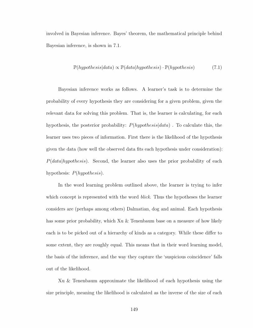
involved in Bayesian inference. Bayes’ theorem, the mathematical principle behind
Bayesian inference, is shown in 7.1.
P(hypothesis|data) ∝ P(data|hypothesis) · P(hypothesis) (7.1)
Bayesian inference works as follows. A learner’s task is to determine the
probability of every hypothesis they are considering for a given problem, given the
relevant data for solving this problem. That is, the learner is calculating, for each
hypothesis, the posterior probability: P (hypothesis|data) . To calculate this, the
learner uses two pieces of information. First there is the likelihood of the hypothesis
given the data (how well the observed data fits each hypothesis under consideration):
P (data|hypothesis). Second, the learner also uses the prior probability of each
hypothesis: P (hypothesis).
In the word learning problem outlined above, the learner is trying to infer
which concept is represented with the word blick. Thus the hypotheses the learner
considers are (perhaps among others) Dalmatian, dog and animal. Each hypothesis
has some prior probability, which Xu & Tenenbaum base on a measure of how likely
each is to be picked out of a hierarchy of kinds as a category. While these differ to
some extent, they are roughly equal. This means that in their word learning model,
the basis of the inference, and the way they capture the ‘suspicious coincidence’ falls
out of the likelihood.
Xu & Tenenbaum approximate the likelihood of each hypothesis using the
size principle, meaning the likelihood is calculated as the inverse of the size of each
149
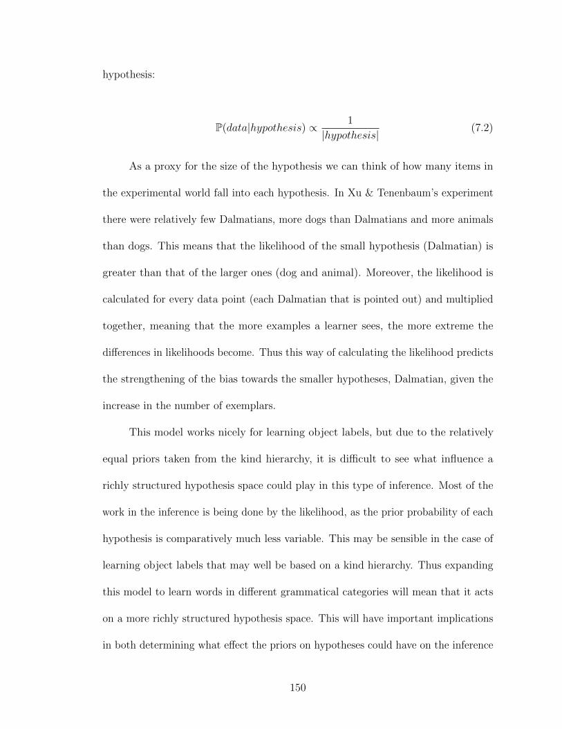
hypothesis:
P(data|hypothesis) ∝ 1
|hypothesis|(7.2)
As a proxy for the size of the hypothesis we can think of how many items in
the experimental world fall into each hypothesis. In Xu & Tenenbaum’s experiment
there were relatively few Dalmatians, more dogs than Dalmatians and more animals
than dogs. This means that the likelihood of the small hypothesis (Dalmatian) is
greater than that of the larger ones (dog and animal). Moreover, the likelihood is
calculated for every data point (each Dalmatian that is pointed out) and multiplied
together, meaning that the more examples a learner sees, the more extreme the
differences in likelihoods become. Thus this way of calculating the likelihood predicts
the strengthening of the bias towards the smaller hypotheses, Dalmatian, given the
increase in the number of exemplars.
This model works nicely for learning object labels, but due to the relatively
equal priors taken from the kind hierarchy, it is difficult to see what influence a
richly structured hypothesis space could play in this type of inference. Most of the
work in the inference is being done by the likelihood, as the prior probability of each
hypothesis is comparatively much less variable. This may be sensible in the case of
learning object labels that may well be based on a kind hierarchy. Thus expanding
this model to learn words in different grammatical categories will mean that it acts
on a more richly structured hypothesis space. This will have important implications
in both determining what effect the priors on hypotheses could have on the inference
150
process, and making the model more realistic with respect to both the structure of
natural language and the task faced by a child acquiring novel words.
7.5 Inferring noun and adjective meanings
In order to investigate the role that prior beliefs about hypotheses play in inferring
word meanings, we need to find a domain in which learners might consider the same
set of hypotheses for two problems, but their prior beliefs about which hypotheses are
most likely differ depending on the problem. For this task, I’ll expand the above case
to inferring both noun and adjective meanings. This is based on an intuition that
while both nouns and adjectives can refer to concepts on either a hierarchy of kinds
or one of properties, nouns tend to draw from the kind hierarchy, and adjectives from
the property heirarchy. For example, both nouns and adjectives can have meanings
from either a kind hierarchy (dog, canine) or a property hierarchy (wood, wooden),
nouns tend to denote kind concepts, and adjectives property ones. We can ask then,
whether children’s knowledge of these tendencies influences the hypotheses they
consider when learning novel words. That is, given the same set of stimuli as input,
are kind meanings more likely in learning novel nouns, and property meanings more
likely in learning novel adjectives? If so, can this behavior be predicted by a model
that incorporates these prior beliefs about the shape of the hypothesis space?
151
7.5.1 Experiment 1: Generalizing noun and adjective mean-
ings
To investigate this question, I conducted a word learning experiment similar to
that of Xu & Tenenbaum. In this experiment children were presented with an
array of animals and vehicles and taught a novel label (noun or adjective) for a
concept. Children were then asked to generalize their inferred concept to novel
items. The stimuli allowed generalization along both kind and property dimensions.
Thus I was able to determine between two hypotheses: (a) children always choose
the narrowest hypothesis consistent with the data or (b) children choose the most
likely hypothesis consistent with both the data and their prior knowledge of the link
between grammatical and conceptual categories. Hypothesis A predicts that children
should choose meanings on the kind dimension for both nouns and adjectives, while
Hypothesis B predicts that children will be more likely to choose meanings on the
kind dimension for nouns and the property dimension for adjectives.
Methods
My experiment tested two groups of children using a between subjects design. The
noun group learned two novel nouns, and the adjective group learned two novel
adjectives.
152
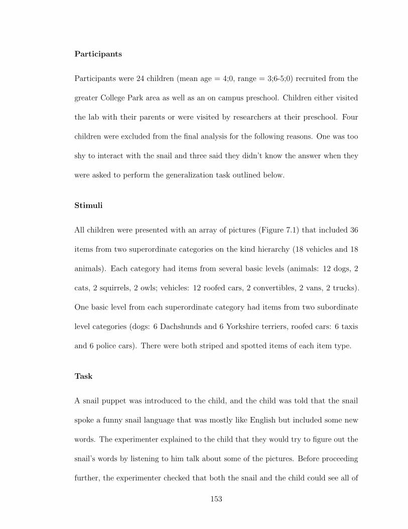
Participants
Participants were 24 children (mean age = 4;0, range = 3;6-5;0) recruited from the
greater College Park area as well as an on campus preschool. Children either visited
the lab with their parents or were visited by researchers at their preschool. Four
children were excluded from the final analysis for the following reasons. One was too
shy to interact with the snail and three said they didn’t know the answer when they
were asked to perform the generalization task outlined below.
Stimuli
All children were presented with an array of pictures (Figure 7.1) that included 36
items from two superordinate categories on the kind hierarchy (18 vehicles and 18
animals). Each category had items from several basic levels (animals: 12 dogs, 2
cats, 2 squirrels, 2 owls; vehicles: 12 roofed cars, 2 convertibles, 2 vans, 2 trucks).
One basic level from each superordinate category had items from two subordinate
level categories (dogs: 6 Dachshunds and 6 Yorkshire terriers, roofed cars: 6 taxis
and 6 police cars). There were both striped and spotted items of each item type.
Task
A snail puppet was introduced to the child, and the child was told that the snail
spoke a funny snail language that was mostly like English but included some new
words. The experimenter explained to the child that they would try to figure out the
snail’s words by listening to him talk about some of the pictures. Before proceeding
further, the experimenter checked that both the snail and the child could see all of
153
Figure 7.1: The stimuli for my experiment included 36 objects in subordinate, basic,and superordinate vehicle and animal categories. Half the items were striped andhalf spotted.
154
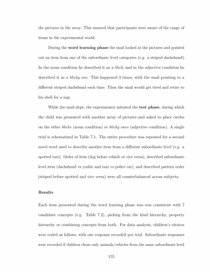
the pictures in the array. This ensured that participants were aware of the range of
items in the experimental world.
During the word learning phase the snail looked at the pictures and pointed
out an item from one of the subordinate level categories (e.g. a striped dachshund).
In the noun condition he described it as a blick, and in the adjective condition he
described it as a blicky one. This happened 3 times, with the snail pointing to a
different striped dachshund each time. Then the snail would get tired and retire to
his shell for a nap.
While the snail slept, the experimenter initiated the test phase, during which
the child was presented with another array of pictures and asked to place circles
on the other blicks (noun condition) or blicky ones (adjective condition). A single
trial is schematized in Table 7.1. The entire procedure was repeated for a second
novel word used to describe another item from a different subordinate level (e.g. a
spotted taxi). Order of item (dog before vehicle or vice versa), described subordinate
level item (dachshund vs yorkie and taxi vs police car), and described pattern order
(striped before spotted and vice versa) were all counterbalanced across subjects.
Results
Each item presented during the word learning phase was was consistent with 7
candidate concepts (e.g. Table 7.2), picking from the kind hierarchy, property
hierarchy or combining concepts from both. For data analysis, children’s choices
were coded as follows, with one response recorded per trial. Subordinate responses
were recorded if children chose only animals/vehicles from the same subordinate level
155
Speaker Utterance ActionSnail ‘This is a blicky one’ points to striped Dachshund 1Snail ‘Look, another blicky one’ points to striped Dachshund 2Snail ‘Here’s another blicky one’ points to striped Dachshund 3Snail ‘I’m going to go have a rest in
my shell’retreats to shell
Experimenter ‘Here are some more pictures,can you put circles on all theblicky ones to surprise the snailwhen he wakes up?’
lays out new array of picturesand gives the child a set of rings
Child — puts rings on items that matchchild’s hypothesis for the mean-ing of blicky
Table 7.1: Sample adjective trial - Noun trials are identical with blick substitutedfor blicky one
Hypothesis Dimension LevelDachshund Kind subordinate
Dog Kind basicAnimal Kind superordinateStriped Property neutral
Striped ∧ Dachshund Kind ∧ Property subordinateStriped ∧ Dog Kind ∧ Property basic
Striped ∧ Animal Kind ∧ Property superordinate
Table 7.2: Candidate concepts given three exemplars of striped Dachshunds
as the example (e.g. only more dachshunds after being presented with dachshunds).
Basic responses were recorded if children chose from only the basic level (i.e. either
dog type after being presented with dachshunds) or from the basic and subordinate
levels. A superordinate response was recorded if children chose only from the
superordinate level (e.g. any animal after being presented with dachshunds) or from
the superordinate level with any combination of the lower levels. Finally, neutral
responses were recorded if children chose from anywhere on the kind hierarchy (e.g.
chose anything from the vehicle hierarchy after being shown a Dachshund).
Results are shown in Figure 7.2. In the noun condition, I replicated Xu &
156
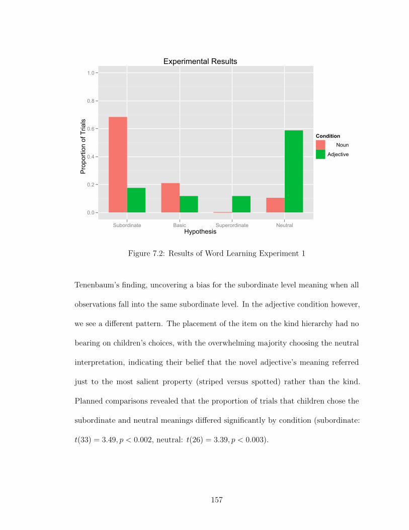
Experimental Results
Hypothesis
Pro
porti
on o
f Tria
ls
0.0
0.2
0.4
0.6
0.8
1.0
Subordinate Basic Superordinate Neutral
ConditionNoun
Adjective
Figure 7.2: Results of Word Learning Experiment 1
Tenenbaum’s finding, uncovering a bias for the subordinate level meaning when all
observations fall into the same subordinate level. In the adjective condition however,
we see a different pattern. The placement of the item on the kind hierarchy had no
bearing on children’s choices, with the overwhelming majority choosing the neutral
interpretation, indicating their belief that the novel adjective’s meaning referred
just to the most salient property (striped versus spotted) rather than the kind.
Planned comparisons revealed that the proportion of trials that children chose the
subordinate and neutral meanings differed significantly by condition (subordinate:
t(33) = 3.49, p < 0.002, neutral: t(26) = 3.39, p < 0.003).
157

Discussion of Experiment 1
These results support Hypothesis B, from above, that posited that children would use
both the observed data and prior knowledge about the link between conceptual and
grammatical categories when inferring the meanings of novel words. I demonstrated
that children use their knowledge of grammatical categories, and the associated
kinds of meanings that correlate with these categories, when inferring the meanings
of novel words. In particular, they favor concepts from a kind hierarchy for novel
nouns, and from a property hierarchy for novel adjectives. In one respect this result
is not new, as infants as young as 14 months have been shown to know the mapping
between grammatical and conceptual categories (Waxman & Markow, 1998; Booth
& Waxman, 2003, 2009). Instead, the novelty is in showing that this mapping
constrains children’s inferences. A very low prior probability for a hypothesis on the
kind hierarchy blocks it from being determined the most likely for a novel adjective
meaning, despite it being the narrowest possible hypothesis.
This finding emphasizes the role of the hypothesis space, as the most likely
hypothesis differs depending on the grammatical category of the word being learned.
In order to determine whether children are behaving optimally with respect to a
specific hypothesis space (conditioned by grammatical category and the information
available to them in the English lexicon), I used a Bayesian model to predict
generalization behavior from the nouns and adjectives that are likely to be present
in the children’s early lexicons.
158
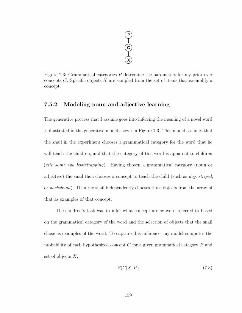
P
C
X
Figure 7.3: Grammatical categories P determine the parameters for my prior overconcepts C. Specific objects X are sampled from the set of items that exemplify aconcept.
7.5.2 Modeling noun and adjective learning
The generative process that I assume goes into inferring the meaning of a novel word
is illustrated in the generative model shown in Figure 7.3. This model assumes that
the snail in the experiment chooses a grammatical category for the word that he
will teach the children, and that the category of this word is apparent to children
(cite some syn bootstrapping). Having chosen a grammatical category (noun or
adjective) the snail then chooses a concept to teach the child (such as dog, striped,
or dachshund). Then the snail independently chooses three objects from the array of
that as examples of that concept.
The children’s task was to infer what concept a new word referred to based
on the grammatical category of the word and the selection of objects that the snail
chose as examples of the word. To capture this inference, my model computes the
probability of each hypothesized concept C for a given grammatical category P and
set of objects X,
P(C|X,P ) (7.3)
159

Concept → Kind→ Property→ Kind ∧ Property
Kind → animal→ dog→ dachshund→ · · ·→ vehicle→ car→ taxi
Property → spotted→ striped
Figure 7.4: The probabilistic context-free grammar I adopt for concepts. Probabilitiesfor each expansion rule are discussed in the Concept Prior section.
As my model is an extension of Xu & Tenenbaum’s word learning model, I also use
Bayes’ rule to compute the posterior probability over concepts (hypothesis) given a
set of examples (data) and a word’s grammatical category,
P(C i |X,P ) =P(X|C i) · P(C i |P )∑
C j∈{all concepts}P(X|C j ) · P(C j |P )(7.4)
This formulation depends on my assumption that the probability of the data X
depends only on the concept C and is independent of the grammatical category,
given the concept. Thus I only need to find the values of P(X|C i) and P(C i |P ) for
the concepts I am considering. The denominator, a normalizing value which will be
the same for each concept, is the sum of numerator across all candidate concepts.
160
Concept Prior: P(C|P )
Following Goodman, Tenenbaum, Feldman, and Griffiths (2008) (cf. Austerweil &
Griffiths, 2010), I represent concepts according to the concept grammar in Figure 7.4,
with nonterminal nodes Kind and Property representing the dimensions a concept
is defined along. Words like dog and striped are defined along only one of these
dimensions (Kind and Property, respectively). Words like kitten, which must describe
a young cat, are defined along both dimensions (Kind∧Property). The derivation of
each concept involves first applying a rule determining the dimension of the concept
and then applying the dimension-specific rules until all terminal nodes have been
identified. For example, in my concept language, the concept dog is formed by first
applying the rule Concept→ Kind and then applying the rule Kind→ dog.
If I assign probabilities to each of the rules in this concept grammar and assume
that the rules are applied independently of one another, then the resulting PCFG
will determine the probabilities of all the concepts in my experiment. The probability
of each concept would be the product of the probabilities of the rules applied to form
it,
P(C) =∏
R∈{rules to form C}P(R) (7.5)
The differences in the types of concepts represented by nouns and adjectives
are represented in my model through differences in the probability distributions over
the set of rules that expand Concept to particular dimensions. I assume children are
computing this prior distribution separately for each part of speech, keeping track of
the number of nouns or adjectives whose meanings denote a kind, a property, or both
161
a kind and a property. They can estimate the rule probabilities from these counts
using a Dirichlet-multinomial model. Under this model, the prior over dimension
expansions based on the counts pd i ,P of the productions seen by the learner of a
particular dimension di for that grammatical category P is:
P(di |P ) =pd i ,P + 1∑
d j∈{all dims}pd j ,P + 3(7.6)
I approximated these production counts from a Mechanical Turk survey where
for each word in a vocabulary list of 429 words (363 nouns and 66 adjectives) that
30-month-old children likely know (Dale & Fenson, 1996) I asked adult English
speaking participants to judge whether the word was best described as a kind, a
property, or both. Different but often overlapping sets of 10 people were asked to
respond to each word, and so I had a total of 22 participants in my study. Two
participants’ judgments were excluded due to an extraordinarily high proportion
of Both responses (proportion Both > 0.36, over two standard deviations outside
the mean proportion of Both responses). While the children in my experiment (3-5
year-olds) were much older than 30 months, I believe that the 30-month-old children’s
vocabulary list is appropriate for my purposes, since the children in my experiments
are almost certainly familiar with these words and differ only in additional words
they might know. I assume that the distribution of noun and adjective dimensions
in this set of words is representative of that of the larger and more varied set of
words that my 3-5 year-old participants are familiar with.Table 7.3 shows the average
counts of each description for each grammatical category.
162
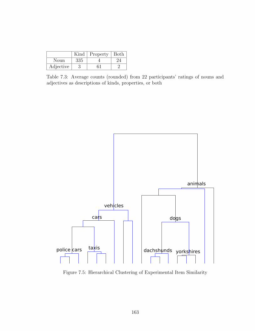
Kind Property BothNoun 335 4 24
Adjective 3 61 2
Table 7.3: Average counts (rounded) from 22 participants’ ratings of nouns andadjectives as descriptions of kinds, properties, or both
animals
vehicles
cars
taxispolice cars
dogs
dachshunds yorkshires
Figure 7.5: Hierarchical Clustering of Experimental Item Similarity
163

For kinds, I assume a structure like Xu and Tenenbaum (2007) where the
probability of a concept depends on its distinctiveness. For these measures I use a
hierarchical cluster tree as in Figure 7.5. To make this tree, I conducted a similarity
judgment study, similar to Xu and Tenenbaum’s using the items that the snail had
labeled in my experiment. My participants, 26 students from the University of
Maryland who received course credit for their participation, rated the similarity of
all possible pairs of the 36 pictures on a scale from 1 (not similar at all) to 9 (very
similar).
To incorporate cluster distinctiveness, Xu and Tenenbaum measure the branch
length (which represents the Euclidean distance) between the concept node and its
parent node. By this measure, the further a particular node is from its parent, the
more distinct it is considered to be. Where K is the set of all Kind concepts, the
probability of a concept C i given that it is defined over the Kind dimension is the
branch length normed over all Kind concepts,
P(C i |Kind) =height(parent(C i))− height(C i)∑C j∈Kheight(parent(C j )− height(C j )
(7.7)
For properties, I assume that in my experiment they are chosen from a Multi-
nomial distribution with each property equally likely to be selected. Since there
were only two very salient properties in my experiment, I give each property the
probability of 12,
P(C|Property) =1
2(7.8)
164

Example Derivation of a Concept Prior Under this model of the concept prior,
the prior probability that the noun blick refers to the concept Dachshund will have
the following derivation. First, I have production counts for nouns that describe
kinds pKind ,Noun that were found in my Mechanical Turk study (I found that on
average 335 out of 363 nouns were categorized as kinds). From this production count
and the total production counts for nouns, we derive the probability of expanding
Concept to Kind.
P(Kind|Noun) =pKind ,Noun + 1∑
d∈{Kind , Property, Both}pd ,Noun + 3
=335 + 1
363 + 3= 0.92
(7.9)
Then we find the probability of the concept being Dachshund given that it is
defined only along the Kind dimension, using the height of the branch Dachshund
and its immediate parent dog. These heights were 0.1259 and 0.3115, respectively.
P(dachshund|Kind) =height(parent(dog))− height(dog)∑
C∈Kheight(parent(C)− height(C)
=0.1856
1.7576= 0.1056
(7.10)
Finally, to compute the prior probability of the concept Dachshund given that
it is a noun, we multiply the probability of expanding Concept to Kind by the
probability of the concept being Dachshund.
165

P(Dachshund|Noun) = P(Kind|Noun) · P(Dachshund|Kind)
= 0.92 · 0.1056 = 0.09715
(7.11)
Concept Likelihood: P(X|C)
I assume that, given a set of objects that are examples of a concept C, each object is
equally likely to be chosen by the snail1. Therefore, the probability of the data given
a concept is proportional to the size of the set of things matching that concept. For
example, for the concept dog, the probability of picking a particular dog, Fido, is
inversely proportional to the number of dogs there are in the scene. So if n objects
are chosen by the snail as examples of a concept C, and these objects are plausible
examples of the concept,
P(X|C) =
(1
|C|
)n (7.12)
Simulations
For each experimental trial I computed the posterior probability over concepts
using both the noun and adjective priors. I assumed that on each trial children
were sampling a concept from the posterior distribution over concepts given the
1Xu and Tenenbaum use a different estimate of category sizes for kinds, which is based on the
same heirarchy as their concept prior. I found little difference when I compared my own likelihood
distributions with those computed by Xu and Tenenbaum’s methods on my experimental items. A
very similar ordering applied over concepts, and each item was on the same order of magnitude for
both measures of the likelihood.
166
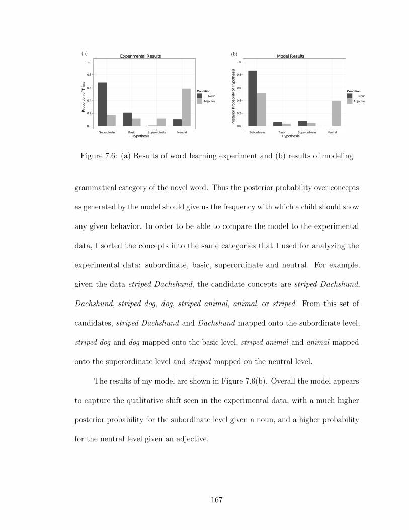
Experimental Results
Hypothesis
ProportionofTrials
0.0
0.2
0.4
0.6
0.8
1.0
Subordinate Basic Superordinate Neutral
Condition
Noun
Adjective
(a)Model Results
Hypothesis
PosteriorProbabilityofHypothesis
0.0
0.2
0.4
0.6
0.8
1.0
Subordinate Basic Superordinate Neutral
Condition
Noun
Adjective
(b)
Figure 7.6: (a) Results of word learning experiment and (b) results of modeling
grammatical category of the novel word. Thus the posterior probability over concepts
as generated by the model should give us the frequency with which a child should show
any given behavior. In order to be able to compare the model to the experimental
data, I sorted the concepts into the same categories that I used for analyzing the
experimental data: subordinate, basic, superordinate and neutral. For example,
given the data striped Dachshund, the candidate concepts are striped Dachshund,
Dachshund, striped dog, dog, striped animal, animal, or striped. From this set of
candidates, striped Dachshund and Dachshund mapped onto the subordinate level,
striped dog and dog mapped onto the basic level, striped animal and animal mapped
onto the superordinate level and striped mapped on the neutral level.
The results of my model are shown in Figure 7.6(b). Overall the model appears
to capture the qualitative shift seen in the experimental data, with a much higher
posterior probability for the subordinate level given a noun, and a higher probability
for the neutral level given an adjective.
167
Discussion of Experiment 1 and Model 1
In this section I showed that child have different generalization patterns depending
on the grammatical category of the words they are learning. Furthermore I showed
that these patterns can be predicted by a model that takes into account children’s
beliefs about what kinds of meanings words in different grammatical categories are
likely to have. We can take this experiment and model as an example of how a
richly defined hypothesis space can play as big a part in children’s inference as the
conclusions that can be drawn from the data alone.
This hypothesis space used by the child in this experiment, likely meanings
for nouns and adjectives, is likely a learned hypothesis space. Children have these
biases about noun and adjective meanings because they know something about the
meanings of nouns and adjectives in English. They may not have these biases when
they are learning their first nouns and adjectives (Waxman & Booth, 2003; Booth &
Waxman, 2009). Similarly, children learning novel words in a language where there
isn’t such a sharp distinction between nouns and adjectives, like Georgian, might no
have these biases. These are questions that further research can investigate.
With an eye towards scaling this kind of inference model up to the more
complex language acquisition problems outlined in the beginning of this chapter, I
also want to ask how innately held hypotheses (and biases among these hypotheses)
can influence children’s behavior in language learning. If we teach children about
something that they have no learned expectations about, will they behave as if
only the data mattered in their inferences, or will they have some expectations that
168
we can attribute to innately specified hypotheses? The next section examines this
question, through an experiment in which children learn multiple words and word
classification.
7.6 Inferring multiple word meanings and word
classes
In the last section we looked at learning word meanings. It seemed plausible that
when learning novel words children may be inferring which concepts they denote,
and they may come up with a set of candidate concepts from these hierarchies. It
also seems likely that all levels of the hierarchy are considered relatively equally
(remember that although the priors differed a little based on cluster distinctiveness
in the kind hierarchy, these differences alone weren’t enough to lead to different
generalizations by children). This all seems reasonable, seeing as there are nouns
and adjectives pointing to every level on these hierarchies, more in fact denoting
the lower levels than the higher ones. So the fact that children consider them all
as fairly likely meanings is perfectly reasonable. But we have to ask, if children are
learning about some other phenomena that uses these hierarchies to some extent,
but that crucially doesn’t tend to use the lower levels much, if at all, how will
children behave? Will they have some expectations about which levels are likely to
be used? One phenomenon we can use is word classification, like noun classification
(grammatical gender). While some systems of grammatical gender make use of the
169
kind hierarchy in dividing nouns into classes, they tend to do this on higher levels,
dividing some nouns by animacy, humanness and natural gender, but do not, for
example, tend to make very specific generalizations, putting dachshunds one place
and yorkshire terriers in another, for example. In order to test children’s hypotheses
in learning word classes, I had to teach them multiple words. As we’ll see below,
just the addition of multiple words to a task like that used in Experiment 1 causes
different behavior in children. I follow the discussion of this experiment with a
discussion of the outline of two models: one that can predict children’s behavior
when inferring multiple word meanings at once, and one that predicts children’s
behavior when inferring the existence of lexical subclasses, the number of subclasses,
and the assignment of words to subclasses.
7.6.1 Experiment 2: Generalizing multiple word meanings
and multiple word classes
Methods
My experiment tested three groups of children using a between subjects design.
The noun group learned four novel nouns, the adjective group learned four novel
adjectives, and the word class group learned two adjective stems and two word class
suffixes.
170

Table 7.4: Words Taught in Each Experimental Condition
Kind Property Noun Adjective Word Class
Dachshundstriped blick blicky one blick-sa onespotted fep feppy one fep-sa one
Taxistriped dax daxy one blick-do onespotted piff piffy one fep-do one
Participants
Participants were 45 children (age 3;6-5;0, mean age 4;1) recruited from the greater
College Park area as well as an on campus preschool. Children either visited the lab
with their parents or were visited by researchers at their preschool. 12 additional
children were tested but were excluded from the final analysis for the following
reasons: 1 was too shy to participate, 3 said they ‘didn’t know’ when asked to
perform the generalization task and 8 appeared to be guessing during generalization,
making choices that were inconsistent with the data given to them by the snail.
Stimuli and Task
All children were presented with an array of pictures identical to that of Experiment
1 (Figure 7.1). Twelve pictures were described from this array, using the word seen
in Table 7.4.
Six exemplars from one vehicle and one animal subordinate category were
described, three of each were striped and three were spotted. For example, in the
Noun condition, three striped Dachshunds would be labeled as blicks, three spotted
Dachshunds as feps, three striped taxis as piffs and three spotted taxis as daxes. The
snail would enthusiastically like the spotted variety of one subordinate category and
171
the striped variety of the other, and vehemently dislike the other labeled exemplars.
At test, the child would have to pick more items that the snail would like, ased on
his descriptions (eg, ‘the Snail really liked the blicks, can you find any more blicks
for the snail?’).
Results
Results were coded as in Experiment 1, but note that these generalization patterns
only take into account what level of the kind hierarchy children’s hypotheses fell
on. That is, although children’s responses indicated that they had inferred complex
concepts (combining kind and property), this display of results focuses on where
on the kind hierarchy the kind piece of the concept fell. Of course it is possible
that one word could have meant generally striped, with no reference to of the kind
hierarchy, and another meant striped and dog, but children did not appear to think
any of the adjectives (or nouns) had these sorts of ‘neutral’ level interpretations
seen in Experiment 1. The reasons for this are discussed in Section 7.6.2 below.
Figure 7.7 shows the generalizations patterns for children in each condition. Children
in the Noun condition behaved just as in Experiment 1, with a preference for the
subordinate level as the kind piece of the concept. Unlike in Experiment 1, children in
the Adjective condition behaved very similarly to the children in the Noun condition,
showing a preference for the subordinate category for the kind piece of the concept.
However, this preference is not quite as strong, as there were more generalizations to
the Basic and Superordinate levels in the Adjective condition. Finally, children in
the Word Class condition exhibited a distinct pattern, splitting their preferences
172

between the subordinate and superordinate levels. This preference doesn’t appear to
stem from some children preferring the subordinate level and some preferring the
superordinate level, as 3 children preferred the subordinate level, 5 preferred the
superordinate and 6 made choices consistent with a different level for each of the
two words at test. Planned comparisons revealed that the proportion of trials that
children chose the subordinate meanings differed significantly between the Noun
and Adjective conditions: t(54) = −2.09, p < 0.05, as well as between the Noun
and Word Class conditions: t(54) = 3.46, p < 0.002, but not between the Word
Class and Adjective condtions. No significant differences between conditions were
found in the proportion of trials where subjects chose the basic level, but significant
differences were found among the proportion of trials assigned the superordinate
level between the the Noun and Word Class conditions: t(50) = −3.01, p < 0.005, as
well as between the Adjective and Word Class conditions: t(54) = −2.04, p < 0.05,
but not between the Noun and Adjective conditions.
Discussion of Experiment 2
In this experiment I looked at how two factors (in addition to grammatical category
and the size principle) influence children’s generalization patterns: the task of
inferring the meanings of multiple words at once, and the difference between inferring
a word’s meaning and the lexical subclass of a word.
In inferring multiple meanings at once, we saw a different pattern than when
children were inferring only the meaning of one word. Recall that in Experiment 1
the smallest hypothesis consistent with the data was actually the complex concept
173
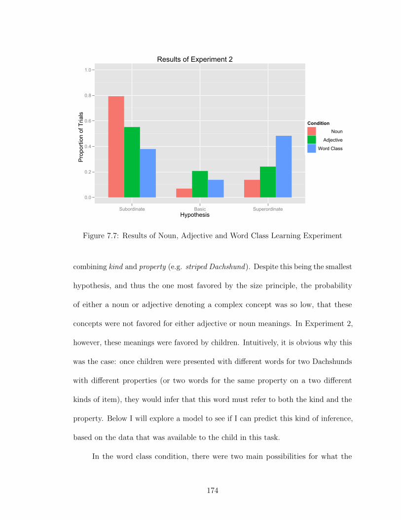
Results of Experiment 2
Hypothesis
Pro
porti
on o
f Tria
ls
0.0
0.2
0.4
0.6
0.8
1.0
Subordinate Basic Superordinate
ConditionNoun
Adjective
Word Class
Figure 7.7: Results of Noun, Adjective and Word Class Learning Experiment
combining kind and property (e.g. striped Dachshund). Despite this being the smallest
hypothesis, and thus the one most favored by the size principle, the probability
of either a noun or adjective denoting a complex concept was so low, that these
concepts were not favored for either adjective or noun meanings. In Experiment 2,
however, these meanings were favored by children. Intuitively, it is obvious why this
was the case: once children were presented with different words for two Dachshunds
with different properties (or two words for the same property on a two different
kinds of item), they would infer that this word must refer to both the kind and the
property. Below I will explore a model to see if I can predict this kind of inference,
based on the data that was available to the child in this task.
In the word class condition, there were two main possibilities for what the
174
child was learning: word classes or multiple words. If the children did not segment
the adjective root and word class agreement, and thus not noticed that there
were multiple classes, we would expect this data to look identical to the adjective
condition, because without segmentation this task would just be one of learning
multiple adjectives. However, since the results do not pattern in the same way as
in the adjective condition, we can infer that children were segmenting the novel
root-suffix pairs and were learning word classes in the word class condition. Once the
child knew he was learning word classes, he had to determine both how many classes
there were and which other items in the experimental world were likely to fall in
each class. The agreement used by the snail showed evidence for at least two classes.
Thus the child had to determine if there were more than two (implying that other
items in the world might fall in some other class), or only two (implying that the
other items in the world would fall into one of the two classes). He also had to decide
what the bounds of these classes were. If there were only two classes, was one class
made up of only Dachshunds while the other class contained taxis and everything
else? Were all the animates in one class and all the inanimates in another? From the
generalization seen in this task it is difficult to answer these questions, but below
I outline a model that makes predictions regarding these possibilities, and outline
future work that will probe these questions further.
175

7.6.2 Modeling inferences about the meanings of multiple
words
As with Experiment 1, I want to see if a Bayesian model can predict children’s
behavior when inferring the meanings of multiple words. In this section I will outline
the components that would be needed to model inferences of multiple words, but
leave the actual implementation of this model for future work. This model will be a
relatively straightforward modification of the model from Section 7.5.2.
Recall from above that children in the Noun and Adjective conditions learned
four novel words, corresponding to combinations of two kinds and two properties.
The challenge for the child then, was to infer the meaning for each novel word. This
is very similar to the task in Experiment 1, however learning multiple words at once
introduced several layers of complexity to the task. That is, if blick was used to
refer to a striped Dachshund, and fep a spotted one, one conceivable hypothesis is
that both blick and fep referred to the concept Dachshund. However, children didn’t
ever generalize two words to the same meaning (e.g. both blick and fep didn’t mean
Dachshund). Alternatively, it could be that these words merely referred to the same
concept on different levels, e.g. blick meant Dachshund, and fep meant dog. But once
again, the results suggest that children took each word to refer to a complex concept
combining a kind and property, eg striped ∧ Dachshund. Finally, children showed a
stronger preference for using the subordinate level kind in noun meanings than in
adjective meanings. Thus there are three aspects of children’s behavior that I want
to see if a model can predict: (a) the avoidance of settling on the same meaning for
176
multiple words (b) the tendency to settle on complex concepts for every novel word
and (c) the less powerful effect of the size principle in adjective generalization.
Inferring multiple words
The first piece that I need to consider in expanding my model is how to predict
complex concepts being the most likely. As mentioned above, the complex concepts
actually represent the smallest hypotheses in the experimental world, and are thus
favored by the size principle. The reason they were ultimately dispreferred by Model
1, and presumably by children in Experiment 1, is because the prior on generating
complex concepts is very low for both adjectives and nouns. What is different about
Experiment 2, however, is that four complex concepts are inferred at once. This
means that if a learner settles on a complex concept for one word, the complex
concept will become slightly more likely for all of the words. This is because the
prior on rules generating concepts is based on counts in the lexicon. Therefore if
the learner thinks he has more counts in the lexicon of complex concepts (based
on the other concepts in the experiment), the prior will increase slightly. However,
even when increasing the counts of complex concepts by 4, they are still much less
likely concepts for adjectives than the simple concept property (with these added
counts, Adjectives would have have 64 property counts and 6 both counts), and also
much less likely concepts for nouns than kind (Nouns would now have 335 kind
counts and 28 both counts). Even though it doesn’t look as though this modification
alone will capture everything going on when children are inferring the meanings of
multiple words, it is the first step in expanding my model to predict the behavior
177
in Experiment 2. This would mean my new model still computes the prior on rule
expansion for each concept based on counts in the lexicon via a Mutlinomial Dirichlet
distribution, with the caveat that it calculates this for all possible concept expansions
of each of the four concepts being inferred.
Mutual exclusivity
Next, I need to make sure that the model will disprefer identical hypotheses for
multiple words. Recall that in the previous experiment, even though hypotheses like
striped and Dachshund were favored by the size principle, they were not chosen by
children, or predicted to be chosen by the model, due to the extremely low prior
on complex nouns or adjectives that referred to both kind and property concepts.
Therefore expanding the model to infer multiple concepts at once may not be enough
to predict children’s behavior. Additionally, children had more information that they
had in the Experiment 1 - they have seen that Dachshunds with one property are
referred to with one word, but that Dachshunds with another property are referred
to with another (or, in the case of adjectives, properties on one kind are referred
to with one adjective, and the same property is referred to using another adjective
when it is on a different kind). It seems likely that children would be able to make
use of this kind of information in their inferences about the possible meanings of
these novel words. In particular, it seems as though multiple words linking to the
same concept might be unlikely, a pattern traditionally called mutual exclusivity
(Merriman & Bowman, 1989). That is, even though the most likely concept, based
on a likelihood calculated via the size principle and a prior derived from expectations
178
about dimensions for a given grammatical category might be the same for two words,
it will be unlikely to be referred to using two different words. This could stem from a
bias held by the learner, something we could call the ‘Mutual Exclusivity Bias’, that
would make a learner inherently disprefer hypotheses for word meanings that linked
to the same concept. Alternatively, following Frank, Goodman, & Tenenbaum, 2009
I could make this bias fall out from the likelihood of a word being chosen to refer
to a concept: the more words that refer to a given concept, the less likely each one
is to be chosen to refer to that concept. Thus hypotheses that pair fewer words to
each concept will be favored. This second piece of the likelihood will be 1Nw
, where
Nw is the number of words referring to a given concept.
This formulation of mutual exclusivity is preferred, in that it is straightforward
to see how it could fall out from inferences over the observed data, while some sort
of mutual exclusivity bias would have to be built in. However, it isn’t clear that
building in a bias for mutual exclusivity would be overly contrived, as something
as simple as a bias to prefer fewer linkings from concepts to words could be easily
conceived of and implemented. Nevertheless, it may be unnecessary under a view
that the likelihood given above would be calculated anyway and with the same result.
A more detailed prior on concept expansion
Including mutual exclusivity in my expanded model could get me part of the way
towards predicting children’s data, but so far there is no way to predict a subtle
difference that we see between children learning nouns and adjective in Experiment
2. Recall that while children were more likely to choose the most specific kind to
179
conjoin with property when learning adjectives in Experiment 2, they did so to a
lesser extent than children learning nouns. That is, in addition to the preference for
adjectives to refer to properties that I demonstrated and modeled in Section 7.5,
it appears that children have some prevailing preference for adjectives to denote
concepts on the higher levels of a kind hierarchy. This preferences results in tension
with the likelihood from size principle, which pushes them toward the lower level
hypotheses. It seems then that in determining which concept expansions are most
likely for grammatical categories, there may be a more complex calculation involved.
In Model 1, I calculated expansion probabilities for nouns and adjectives, and then
assumed that concept priors would be independent of the grammatical category.
From this prior, I wouldn’t be able to predict that when adjectives do make use of
the kind hierarchy they do so in a different way that nouns.
There are two ways that I could modify the model to predict this sort of
behavior. First, I could give different priors to different levels of the kind hierarchy
for adjectives using kind than for nouns using kind. While this might work, it is
quite stipulative, as it seems odd to have some dimension expanding differently
to different concepts depending on the grammatical category. An alternative way
to derive this difference would be an expansion of the part of concept grammar
that does depend on grammatical category. That is, once a rule is selected for a
grammatical category, instead of proceeding directly to select a concept generated
by that rule there would be an undetermined number of intermediate steps, that
would split the rule. Thus if kind was chosen for a noun adjective on one coin flip,
a second coin flip would determine whether kind was to be split into kind∧kind or
180

remain as just kind. Once kind was split, a subsequent flip would determine whether
kind should be split further. With this piece of the grammar, I could then put a
prior on how likely kind and property are to split, given the grammatical category of
the word. The desired effect would be that nouns would have a higher probability of
kind∧kind∧kind meanings (eg. animal∧dog∧Dachshund), while adjectives would
have a higher probability of kind (modulated by the baseline probabilities for picking
kind at all). In order to implement this sort of probabilistic recursive expansion
I would need to know, for a given grammatical category, what the probability of
expanding a rule more than once was. While it is not immediately clear how to
derive these probabilities, work is underway to determine if some measure of the
number of hyponyms on nouns in WordNet (Fellbaum, 1998), and some comparable
measure on adjectives, might serve as a proxy.
While this model is not yet complete, I have been able to lay out several ideas
that would in principle allow a model to predict behavior like that of children inferring
the meanings of multiple words at once. Further work will determine whether these
ideas are implementable, and whether or not they can predict children’s behavior in
Experiment 2.
7.6.3 Modeling inferences from words to classes
Just as I lay out the components I would need to model inferences of multiple word
meanings, I want to lay out the pieces that a model inferring word classes would need.
In order to model inferences about the existence of word classes and the number of
181
classes in a language, I will need to expand my model even more. That is, when
a learner hears something like a blicksa one, he has to infer (a) the concept that
generated the root blick, (b) the word that denotes the concept that the speaker
is referring to with one, (c) that sa and do signal the presence of multiple lexical
subclasses and (d) the way the lexicon is likely to be partitioned into these subclasses.
At the current time, I have no model that can incorporate all of these pieces of the
inference that the child is performing in this task, but I can lay out what I would
need in a model in order to incorporate each one.
Inferring the concepts behind adjectival roots
First, the model needs to infer the concepts of the roots. This piece of the model
might be relatively straightforward. If inferring the concept that a root denotes is
the same as inferring the concept that a word denotes (and there is no reason in a
one word case why it shouldn’t be), I will have a multiple word learning scenario,
similar to that discussed in the section above. The major difference is that the roots
will be used to describe items from different parts of the kind hierarchy (two distinct
objects). Thus the smallest hypothesis consistent with the data would be the set
of all things in the experimental world (something like the concept thing). That is,
the data for the meaning of the root alone is consistent with only three concepts:
the highest level of the kind hierarchy (thing), the appropriate level of the property
hierarchy (striped), or the complex concept made form combining these two. This
means that whether children consider property only adjective meanings, or adjective
meanings that use only kind or combine kind and property, the size principle will
182
actually favor the property or both hypotheses, as these both pick out half of the
items in the experimental worlds. They are half as big as the kind hypothesis which
picks out everything in the experimental world. Thus the size principle will be
pushing the children in the same direction as the prior on adjective meanings. As
children don’t settle on these hypotheses (splitting their generalizations consistently
with the word class marker and observed items), this is only a piece of their inference.
While this part still needs to be worked out, it seems promising that this piece of
the model will be tractable.
Inferring the referent of one
Second, to model inferences about word classes, there have to be some word concepts
being inferred. Even though the nouns aren’t named in this condition, in order to
determine the class of a noun based on agreement, the child first has to infer what
noun the adjective is agreeing with. That is, when the child hears ‘This is a blicksa
one’, and is shown a striped Dachshund, he has to determine whether one referred to
Dashshund, dog or animal. This looks like exactly the task faced by the child when
inferring noun meanings. Thus we might expect that children’s inferences about
the meaning of one would pattern just like their inferences about noun meanings.
That would mean that this piece of the model would be identical to inferring noun
meanings in Model 1.
There is one potential complication, however, that needs to be sorted out. The
child hears the snail use one to refer to both Dachshunds and taxis. If the child
is assuming that the snail had one category in mind when using one throughout
183

the experiment, this would mean that he was trying to infer one concept that could
have generated all instances of one. This would mean that only largest possible
hypothesis (all items) would be consistent with the data. If it this is the case, than
using one alone could cause children to have a preference to pick more items from
superordinate (or higher) levels in the word class condition, and that this preference
had nothing to do with discovering word classes. While this doesn’t appear to be the
case based on the results (as the same behavior might be predicted for adjectives,
that also use one), it would probably be useful to find a way to independently test
children’s inferences about the referent of one in this kind of learning scenario to
rule out this possibility2.
Inferring the existence of multiple classes
The next piece that this model needs to discover is the existence of subclasses of
words. In order for a child to infer that a language (in this case Snail English) has
multiple lexical subclasses, he would have to look some distributional cue in the input
(such as an agreement marker) and notice that certain words (or certain concepts as
accessed through one and an observed item) only occur in certain environments (with
certain cues). The child would have to notice that these environments differed only
in the presence of one cue or another, and that this cue wasn’t indexing anything
other than lexical subclass (e.g. case, number, tense). Of course the child might
initially consider these alternatives as generating the morpheme that is the agreement
2I don’t expect this to be the case, as Mintz (2005) has shown that children make assumptions
about the category held by the speaker when the speakers uses thing, but not one
184
marker, but these would become less likely as it became clearer to the child that
nothing differed in the environment where one cue or another was found other than
the word being modified by the adjective (or the referent of that word, in the case of
one). This is probably an oversimplification of the inferences necessary to discover
lexical subclasses (Consider the discussion outlined in Chapters 2 and 6), but it is
what a model would have to do, at minimum. Of course, it might be possible to
build a model of the word class inferences in Experiment 2 without building in the
discovery of word classes. That is, I could assume that the child does something to
discover that multiple subclasses exist, and focus on modeling inferences related to
how many classes are likely to exist, as well as how the lexicon is partitioned into
these classes. Future work will likely first consider models where the discovery of
nouns classes is built in, and then go about modeling the discovery of these classes.
Inferring the number and makeup of lexical subclasses
Finally, in addition to inferring the existence of classes, the learner has to infer the
number of classes and the makeup of each one. There are two ways in which children
could behave conservatively in their inferences about word classes in Experiment
2. One is with respect to the number of classes they posit, given that they have
only seen evidence for two classes, and the other is with respect to the number of
items they think are in each class, given that they have only seen one kind of item
in each class. I can describe the first kind of conservativity as a bias to posit the
existence of only as many classes as the learner has evidence for. The second kind
would be a bias to only assign items to a class when the learner has evidence they
185
belong in that class. If a learner has both of these biases, in a situation like that
in Experiment 2, where they have seen evidence for two classes but only one kind
of item in each class, the bias not to posit more classes would push them towards
preferring to think all items in the experimental world were members of one of these
two classes. In contrast, the bias not to assign anything to a class that wasn’t seen
in that class would result in a tendency to think a class only contained the kinds
of items previously seen in that class. Thus the learner would be pulled towards
subordinate and superordinate level hypotheses from each of these biases respectively.
If I could build these biases into a model, it seems as though this kind of tension
might predict the behavior we see in children, where even an individual child can be
split as to whether he generalizes the class to items on the superordinate level or
restricts it to items on the same subordinate level.
Another complexity involved in inferring the number and makeup of classes
is where to partition the lexicon, once the learner knows that some partition is
necessary. Say the learner has evidence for two subclasses. It doesn’t necessarily
follow that these two classes should be the most general two classes possible, given
the observed data. That is, if the learner has evidence that Dachshunds and taxis
are in two classes, it doesn’t follow from anything in the data or from any bias about
how many classes to posit given that data that these should split at the highest
possible level (animates versus inanimates), yet it appears that that is what children
do. They could just as easily decide that Dachshunds, or perhaps dogs, made up a
class of their own and the other class held everything else. This isn’t surprising given
that these are just the sorts of features that are used in languages with multiple
186
noun classes. Thus, there might be some sort of bias that the child brings to the task
(something in the hypothesis space) that predicts what level on the kind hierarchy, or
what kinds of features, are likely to split nouns into classes, if there is other encodable
evidence for multiple classes of nouns in the input. Of course, building a bias like
this into a model isn’t the only way I could predict children’s behavior. They could
have a bias as simple as preference to have the lexicon equally partitioned, and to
keep items from the same branches of the kind hierarchy together. There are possibly
other sources of this bias as well, but somehow a model would have to predict this
aspect of children’s behavior.
7.7 From acquiring words to acquiring grammar
This chapter has focused on the inferences involved in word learning. For very
simple word learning problems (inferring one noun or adjective meaning at a time) I
was able to both get a clear picture of children’s behavior, and build a model that
predicts this behavior. This model takes into account both what the child brings
to the task and what the child can infer based on the distribution of data across
the hypotheses under consideration. The child’s pre-existing linguistic knowledge,
gleaned in this case from the meanings of previously acquired words, proved to be
important, as it can be more powerful than inferences the child might draw based
on observed data alone. Of course, word learning on its own is not the most difficult
problem in language acquisition. In an effort to begin to scale this kind of model up
to more difficult problems, and problems that might involve a contribution from (and
187
hence a chance to examine) an innate hypothesis space, I extended the experimental
paradigm to teach children multiple words at once and, crucially word classes, that
they have no experience with in their native English. While I don’t yet have a model
that can predict children’s behavior on the word class learning task, I was able to
lay out what the basic components of such a model would be, and putting them
together will (hopefully) not be an intractable problem.
7.7.1 Extending Bayesian inference to the acquisition of
Wh-movement
The next step in my investigation of the inference process is to discuss how one
might go about scaling these models up to even more complex learning problems to
begin to solve the sort of subset problems posed at the beginning of this chapter.
While I haven’t built any models to approach these problems, I have the tools to
at least lay out what the pieces of this sort of model would be. Once we have the
pieces we could put these together and see in they make predictions consistent with
behavior seen in language acquiring children. For a concrete example let’s return to
the problem of determining if a language has optional wh-movement (Grammar 1),
obligatorily overt wh-movement (Grammar 2), or obligatorily covert wh-movement
(Grammar 3). As outlined above, observing overt wh-movement but not observing
covert wh-movement is probably enough evidence to eliminate Grammar 3 as a
hypothesis. But since overt wh-movement can be generated by both Grammars
1 and 2, how would a learner choose between them? Again, as mentioned in the
188

beginning of this chapter, Grammar 2 is a subset of Grammar 1. That is, all the
strings that Grammar 2 can generate are a subset of the strings that Grammar 1 can
generate, thus no string compatible with Grammar 2 will ever be incompatible with
Grammar 1. Above I mentioned how traditional analyses (Berwick, 1963; Pinker,
1989), have appealed to a ‘subset principle’, that will cause the learner to favor the
hypothesis that is a subset of the other, when faced with situations like this. This
subset principle does not stem from any more general learning principle, nor does it
follow from any grammatical principle. It is merely a stipulation in the hypothesis
space intended to make grammars like Grammar 2 learnable.
As the subset principle isn’t a learning mechanism and is more of a stipulation,
it leaves something to be desired if my goal is really to understand how language
acquisition proceeds. However, after my indepth analysis of the inferences that
underlie word learning, this problem now looks suspiciously familiar. That is, since
Grammar 2 is a subset of Grammar 1, and if a child was using Bayesian inference
to determine which of a set of candidate grammars was supported by the data in
the input, couldn’t the size principle come into play to allow the child to determine
whether Grammar 1 or Grammar 2 was more likely based on the observed instances
of overt wh-movement? This line of reasoning seems promising, and below I will
flesh out what kinds of information the learner would need in order for this to work.
Recall that Bayesian inference requires two pieces of information: the prior
probability of a hypothesis, and the likelihood of that hypothesis given the data.
I’ll say that Hypothesis 1 (H1) is that Grammar 1 generated the observed input
(example of overt wh-movement), Hypothesis 2 (H2) is that Grammar 2 did, and
189
likewise Hypothesis 3 (H3) is that Grammar 3 did.
The Prior
The prior probability of each hypothesis could be distinct, or it could be uniformly
distributed across all possible hypotheses. This means that the contribution of
the hypothesis space is either a weighting of hypotheses or the delineation of a
possible space. If the hypothesis space delineates what is a possible grammar and
what isn’t, I can account for why a learner would consider the three grammars
described above, but would not consider Grammar 4, for example, a grammar that
has overt wh-movement when sentences are more then 5 words long, and covert
wh-movement otherwise. To determine the bounds of such a hypothesis space I rely
on the contributions of theoretical linguistics, that outline what kinds of patterns
grammars of natural languages generate (Grammars 1-3), and predict what kinds of
grammars won’t exist (Grammar 4). Of course, it is an empirical question whether
Grammars like Grammar 4 are not in the hypothesis space at all, or are just very
strongly disfavored3. If I found that learners could acquire languages with Grammar
4, then I would determine that I have a weighted hypothesis space for this aspect
of grammar, and the weighting heavily favors Grammars 1-3. Either way, for the
purpose of this problem, I have no a priori reason to believe that Grammar 1 has a
3Another question is why grammars like Grammar 4 are not in the hypothesis space. Linguists,
beginning with Chomsky (1973) have hypothesized that this sort of non structure dependent
grammar is simply not among the set of possibilities made available by Universal Grammar.
However, one could be asked whether this sort of rule is ruled out for independent reasons and go
about probing that as well
190
higher prior that Grammar 2 (or vice versa).
The Likelihood
The likelihood of each hypothesis given the observed data is less straightforward to
calculate, for three reasons. First there is the issue of deciding that a given data
point bears on some set of hypotheses. For example, should a learner determine
whether H1 or H2 is more likely based on seeing a yes/no question? Probably not,
but what about a relative clause that doesn’t involve a wh-word? Depending on the
language, these could be relevant, even though they might not appear to be on the
surface. Theoretically, a Bayesian learner could consider all data to be relevant, but
this might require more computational capacity than we might reasonably suppose
our learner has. At present I have no solution for this problem but point out that the
learner must have some way of determining which data bears on which hypotheses
in order for this inference to move forward. Note that this problem is not unique to
Bayesian inference, but plagues any learner that considers all hypotheses for all data
points (J. D. Fodor & Sakas, 2005).
Second, the learner has to determine, which data point each hypothesis is likely
to have generated. For some cases this might be easy, for example long distance
overt wh-movement obviously supports H1 and H2 but not H3. But what about the
movement involved in single clause subject questions in English? In most cases there
will be nothing to show that overt movement took place. What will the learner do
with examples like this? They could bear on any of the three hypotheses, though
it could work out that the likelihood will favor those hypotheses that could have
191
generated it.
Finally, if the learner is going to approximate the likelihood of each hypothesis
using the size principle, he has to determine, for a given hypothesis, what the size of
that hypothesis is4. The size of a hypotheses cannot be approximated the way it was
in my word learning models. That is, a learner can’t just count the possible examples
of each hypothesis that he could encounter in the world, as the number of sentences
that each grammar could generate is infinite. This doesn’t mean the learner can’t
approximate hypothesis size, however. The learner could instead count the number
of string types that each hypothesis could generate. Since H1 can generate all the
strings with overt wh-movement that H2 can, in addition to the covert versions of
these strings, H1 will generate a larger set of strings. This means that a likelihood
based on the size principle will favor H2, the smaller hypothesis, given data that is
compatible with both H1 and H2.
Putting these pieces together
What the above example shows is that if we can define a set of possible hypotheses
(and possibly a weighting among them) and if a learner can both identify which
data points bear on which learning problems, and which hypotheses they support
(problems we need to solve independently), we have a straightforward way of inferring
subset grammars like Grammar 2. This is just what the subset principle was intended
to do, but lets us achieve this in a less stipulative way, using mechanisms that we
4The learner could of course have other ways of computing the likelihood. Here I focus on the
size principle as this appears to offer a solution for escaping the classic subset problems
192
have good reason to believe children use in other aspects of language acquisition and
cognition.
7.7.2 Beyond inference
This chapter has outlined how Bayesian inference models can predict children’s
behavior on both very simple and, potentially, more complex word and word class
learning tasks. Moreover, it has pointed the way towards using these models to
solve the more complicated learning problems faced by the child. It is important to
remind ourselves at this point, however, that this is only a very small piece of the
puzzle faced by the child. That is, any kind of inference mechanism would be useless
without a space of hypotheses to choose between and some observed data to inform
the choice of hypotheses. The problem is not even this simple, as the child must be
able to encode the data observed in the input in such a way that it is informative to
these hypotheses. If the child could not determine the grammatical category of a
novel word, for example, it would not make the different inferences dependent on
this category that we saw in Experiment 1. While we looked carefully at encoding in
noun class acquisition, I now turn to a more complex problem, to look at how an
incomplete encoding of syntactic structures could be exactly what a child needs in
combination with a fairly rich hypothesis space and this sort of inference mechanism
to acquire a more complicated syntax.
193

Chapter 8
Incomplete encoding drives
inference
In this chapter, I will turn from the acquisition of word meanings and classes to
the acquisition of syntactic structures. In particular, I will look at how incomplete
encoding of syntax based on incomplete knowledge can be used to acquire adultlike
syntax. In order to explore the earliest stages of the acquisition of syntax, I will have
to look at children’s abilities to comprehend sentences. These comprehension abilities
can be broken down into two main components: the knowledge of the linguistic
system and the deployment of this knowledge. This breakdown is itself a novel
way to study both language acquisition and sentence comprehension, as studies of
adult psycholinguistics have primarily focused on the deployment of this knowledge,
holding grammatical knowledge constant, studies of child psycholinguistics have
primarily focused on when different aspects of linguistic knowledge are learned, and
what information is available to aid the child in learning.
194
When we think of language acquisition in terms of encoding, inference and
a hypothesis space, these two components fall out naturally. Both the knowledge
that a child has about the language being acquired and their ability to deploy this
knowledge online will govern how much of the input can be encoded at any given
stage in development. The encoded intake will in turn bear on the hypotheses
under consideration differently as it grows in complexity. Thus is it not enough to
simply look at what knowledge a child might be able to infer from the encoded input
across development, but we must also consider the learner’s abilities to deploy this
knowledge online, as this ultimately limits what can be encoded from the input.
In order to investigate the relation between the acquisition of grammatical
knowledge and the accompanying deployment system, and to see how partially
encoded input can drive inferences to adultlike grammars, it will be useful to find
two phenomena that rely on the same kind of grammatical representations, but
that diverge in their deployment processes because of surface differences between
them. We find such a distinction in the processing of two filler-gap dependencies:
wh-questions and relative clauses. Due to both their unbounded nature and uniquely
linguistic character, filler-gap dependencies are an ideal place to examine the relation
between grammatical knowledge and deployment in adult processing and language
development. In my investigation of the acquisition of these two types of dependencies,
I observe a case of U-shaped development that can be explained in terms of growth
of grammatical knowledge with a delay in the real-time deployment mechanisms.
Furthermore we can look at this U-shaped development and see how incomplete
knowledge at one stage feeds into inferences that allow the learner to acquire more
195
complete knowledge at a subsequent stage.
This chapter proceeds as follows. Section 1 reviews (a) the linguistic evidence
supporting the view that wh-questions and relative clauses access the same linguistic
knowledge, (b) the psycholinguistic models of how this knowledge is deployed in real
time and, (c) the current understanding of the developmental time course of these
dependencies. In Section 2 I describe a set of experiments revealing that both 15- and
20-month-old infants appear to understand wh-questions. In Section 3 another set of
experiments shows that 15-month-olds, but not 20-month-olds, appear to understand
relative clauses. Section 4 will be a discussion of these surprising results in light of
the relationship between knowledge and deployment in language acquisition, making
a case for a nonadultlike parsing heuristic in younger infants that is replaced by
adultlike mechanisms in older ones.
8.1 Background: Filler-gap dependencies
Filler-gap dependencies are a class of dependencies in human languages that relate
an element in a non-thematic position (henceforth the ‘filler’, shown in italics) to its
canonical thematic position in the sentence (henceforth the ‘gap’, marked by ).
These dependencies can be quite local (1) or arbitrarily long (2).
(1) Which dog did the cat bump ?
(2) Which dog did the monkey think that the horse saw the cat bump ?
Among wh-questions, there are two differences in surface form between ex-
tractions from subject positions and object positions. First, displacement is farther
196
and therefore more apparent for object extraction (4) than for subject extraction
(3). Second, within a single clause subject questions do not require subject-auxiliary
inversion (3) but object questions do (4).
(3) Which dog bumped the cat?
(4) Which dog did the cat bump ?
However, it is widely agreed that the set of grammatical mechanisms responsible
for generating subject extraction is the same as that generating object extraction.
Evidence for this lies in the fact that both types of displaced elements can be related
to their thematic positions across finite clauses, as in (5-6), that both types are
sensitive to island constraints (7-8) and induce island effects for other dependencies
(9-10) (Ross, 1967; Chomsky, 1986; Rizzi, 1990).
(5) Which dog do you think bumped the cat?
(6) Which dog do you think the cat bumped ?
(7) *Which dog did the man make the claim that bumped the cat?
(8) *Which dog did the man make the claim that the cat bumped ?
(9) *Howj did the man wonder [which dogi i bumped the cat j]?
(10) *Howj did the man wonder [which dogi the cat bumped i j]?
wh-questions (1) are only one type of filler-gap dependency. Another structure,
the relative clause (11), is also a filler-gap dependency.
(11) Show me the dog that the cat bumped
197
There are several differences in the surface properties of wh-questions (1) and
relatives (11): the presence of a wh-word in (1) and its absence in (11); the fact
that the filler is always clause initial in a wh-question but not in a relative clause;
the lack of subject-auxiliary inversion in relative clauses; and, when uttered aloud,
prosodic differences between the two sentences. Despite these differences, however,
we have reason to believe that the same grammatical mechanisms are at work in their
generation. Both involve the displacement of the filler from its thematic position
to a higher position. The displacements appear to be parallel, as the fillers in
both dependency types are unbounded, but can only originate in certain, parallel,
structural positions (12-14) (Chomsky, 1977).
(12) a. Which dog did you think (that she said) the cat bumped ?
b. Show me the dog that you think (that she said) the cat bumped
(13) a. *Which dog did the monkey think that bumped the cat?
b. *Show me the dog that the monkey thought that bumped the cat
(14) a. *Which dog did the cat bump the monkey and ?
b. *Show me the dog that the cat bumped the monkey and
The comprehension of both types of filler-gap dependencies is also expected to
be driven by a similar mechanism, as both dependencies require the comprehender to
somehow link up the filler with the gap. Below is an overview of the process thought
to be responsible for the resolution of filler-gap dependencies by adults, and of early
knowledge of these dependencies.
198
8.1.1 Adult parsing
It is widely agreed that adult speakers resolve filler-gap dependencies using an active
filling strategy (Crain & Fodor, 1985; Frazier & Jr., 1989; Frazier & d’Arcais, 1989;
Traxler & Pickering, 1996; Sussman & Sedivy, 2003; Aoshima, Phillips, & Weinberg,
2004). In an active filling strategy, as soon as a filler is encountered, the search
for a potential gap site begins. Comprehenders could identify a filler because of its
displacement from its canonical position in the sentence, the intonation contour of the
utterance and other features such as wh-words and scope markers. Gap sites would
be posited at every structural position where an argument could occur. Convergent
crosslinguistic evidence for this strategy comes from both reading time and ERP
measures, which find a disturbance when the first potential gap site encountered by
the parser is already filled (15) or when it is not the predicted position based on
semantic information found in the filler (16) (Stowe, 1986; Traxler, Morris, & Seely,
2002).
(15) My brother wanted to know who Ruth will bring us home to at Christmas
(16) The scientist that the climate annoyed did not interest the reporter
Active filling is not the only possible strategy for resolving filler-gap depen-
dencies, however. Another strategy that parsers might engage would be gap driven
parsing (Wanner & Maratsos, 1978). In gap driven parsing, the parser begins a
backwards search for a filler only when it encounters the gap site. While there
is ample evidence against gap driven parsing in adults (Frazier & d’Arcais, 1989;
Traxler & Pickering, 1996; Sussman & Sedivy, 2003; Aoshima et al., 2004), it is
199
worth mentioning as a potentially plausible strategy, especially when considering the
development of filler-gap parsing in children.
The processing of all filler-gap dependencies does not seem to be equal, however,
and various researchers have found that subject gaps (17) are easier to resolve than
object gaps (18) (Gibson, 1998).
(17) Show me the dog that bumped the cat
(18) Show me the dog that the cat bumped
This asymmetry (indexed by slower reading times and poorer comprehension
of object gaps), is not absolute, and can be modulated by factors including working
memory load, animacy of arguments, plausibility of predicates, distance of extrac-
tion and the amount and type of intervening material (Konieczny, 2000; Gordon,
Hendrick, & Johnson, 2001; Traxler et al., 2002; Mak, Wonk, & Schriefers, 2002;
Fiebach, Schlesewsky, & Friederici, 2002; Clifton et al., 2003). The study of the
subject-object asymmetry has focused on long distance (multiclausal) extractions,
and has mainly looked at the processing and comprehension of relative clauses.
Asymmetries like this one are evidence of the apparent disjunct between knowledge
and deployment. Whereas the grammatical mechanisms for characterizing subject
and object dependencies are similar, the deployment, or real time resolution of the
dependencies, reveal differences.
While the subject-object asymmetry has been deeply investigated, few studies
directly compare the processing of wh-questions and relative clauses. Based on the
superficial differences between the constructions mentioned above, it is possible that
200

there is an asymmetry between them in online parsing.
8.1.2 Acquisition of filler-gap dependencies
Various researchers have looked at the acquisition of wh-questions and relative
clauses. In particular, the first productions of these constructions have been studied,
both by looking at naturalistic child utterances from transcripts, and by eliciting
relative clauses and wh-questions (Hamburger & Crain, 1982; J. deVilliers, Roeper, &
Vainikka, 1990; Stromswold, 1995; Thornton, 1995). Early comprehension of relative
clauses has mainly been studied by act-out tasks (Tavakolian, 1981; Hamburger
& Crain, 1982), and early comprehension of wh-questions by question answering
tasks (Roeper & deVilliers, 1994; J. deVilliers & Roeper, 1995; Goodluck, 2010).
These studies have focused on finding out when children are able to properly deploy
their knowledge of filler-gap dependencies, and have looked at whether surface form
differences found within a dependency type (i.e. subject vs object extraction) affect
the age of acquisition. While individual findings vary, there does not appear to be
straightforward evidence either for or against a subject-object asymmetry in the
order of acquisition of filler-gap dependencies. What is clear is that from as young
as can be tested children appear to follow adult-like constraints on the formation of
filler-gap dependencies, effectively deploying their knowledge of these constructions.
While the acquisition of both relative clauses and wh-questions has been studied,
no studies have drawn direct comparisons between the dependency types, and it
is thus unclear how parallel the acquisition of these two types of dependency is.
201
Importantly, all of these studies looked at the acquisition of filler-gap dependencies
once children were producing them. As we generally find that production lags behind
comprehension in development, it is likely that children are able to deploy their
knowledge of these dependencies for comprehension earlier than for production.
Only one study that I know of has looked at the pre-production comprehension
of filler-gap dependencies. Seidl, Hollich and Jucszyk (2003) used the intermodal
preferential looking procedure to examine comprehension of wh-questions by 13-, 15-
and 20-month-olds. Each infant was tested on the comprehension of two subject
questions, two object questions and one where question. They found that 20-months
olds appeared to understand all three question types, 15-months olds appeared to
understand only subject and where questions, and 13-month-olds did not appear to
understand any question type. They suggested that the subject-object asymmetry
found in the 15-month-olds was due to either the longer structural distance between
the filler and the gap in object questions as compared with subject questions, or the
fact that the infants were not yet equipped to deal with the do-support employed in
object questions. Exploring whether the 15-month-olds’ failure at object questions
reflects a lack of grammatical knowledge or an inability to properly deploy this
knowledge lies behind the motivation for the current experiments.
202
8.2 Experiment 1: wh-questions
8.2.1 Motivation
Determining whether a lack of knowledge or an inability to deploy knowledge lies
behind the 15-month-olds’ reported difficulty with object questions is the first step
in investigating the mechanisms behind the development of the parsing of filler-
gap dependencies. To do so, we first need to take a closer look at the Seidl et al
study. While Seidl et al cited the longer structural distance and do support as the
two factors which could have made object extraction too difficult for 15-month-
olds, the situation is in fact more complex. Possible explanations of 15-month-olds’
poor performance on object-questions can be roughly broken into two linguistic
hypotheses, the Structural Distance Hypothesis and the Do-Support hypothesis,
and one methodological hypothesis, the Methodological Hypothesis. The linguistic
hypotheses can each in turn be broken down into hypotheses regarding knowledge
and deployment.
The Structural Distance Hypothesis posits that the longer distance between
the filler and the gap in object questions causes the 15-month-olds’ difficulty. This
difficulty could derive from the infant lacking the grammatical knowledge needed to
compute displacement, which is necessary in object questions but could be viewed as
optional in subject questions, as the position of the subject is identical in monoclausal
declaratives and monoclausal wh-questions (George, 1980; Chung & McCloskey, 1983).
Alternatively, the child might possess this knowledge but be unable to deploy it
effectively when the filler is far away from the gap, as in object questions (Gibson,
203
1998).
The Do-Support Hypothesis posits that do-support is responsible for the
difficulty. This difficulty could derive from the child lacking the requisite knowledge
of functional structure that is needed to interpret do-support (e.g., Radford, 1990).
Alternatively, there could be a parsing problem when this knowledge is deployed.
For example, if do is misanalyzed as a main verb the remainder of the parse, and
associated comprehension processes would be disrupted.
The Methodological Hypothesis predicts that factors in the design and materials
employed by Seidl et al could have masked the infants’ underlying linguistic abilities.
As mentioned above, each infant saw two trials of each question type in a within
subjects design. Two trials per questions type may not have given infants sufficient
time to adjust to task demands, and the within subjects design may have caused
interference between the two question types. Additionally, the stimuli consisted
of two-dimensional cartoons of two inanimate objects floating through space and
colliding, followed by a test phase where the two objects were presented side by
side along with wh-question audio. This type of animation was unengaging and also
pragmatically odd. Because only one event took place, the question was pragmatically
infelicitous. Only one thing could possibly be the answer.
In the first experiment I set out to determine whether the asymmetry seen in
the 15-month-olds in the Seidl et al study was due to one of the linguistic hypotheses
or the methodological one. In order to investigate these hypotheses and identify the
source of 15-month-olds’ difficulty with object questions, I made several manipulations
to the basic design of the Seidl et al. study. Target utterances were wh-questions
204
patterned after those in (19):
(19) Subject wh Question: Which dog bumped the cat?
Object wh Question: Which dog did the cat bump?
To probe the methodological hypothesis I attempted to improve upon the
factors I identified as potentially problematic above. First, I employed a between
subjects measure, allowing for six trials per subject, all of the same question type.
This would give the infants ample time to adjust to the task and eliminate the
potential interference of question type. Employing six trials also allowed me to
analyze the data by blocks, enabling me to determine whether having too few trials
can hide children’s knowledge. To improve the stimuli, I used videos of engaging
puppets, with three characters per scene. The addition of an extra character served
two functions. First, it made the question felicitous. If two animals separately
performed the same kind of action, it is plausible that a speaker might be unsure of
who did what to whom, motivating the use of a question. Additionally, the third
character provided the felicity conditions necessary for a relative clause, i.e. the
differentiation between two different dogs requires the sort of information specifiable
in a relative clause.
8.2.2 Predictions
The predictions for this first experiment are straightforward. Regarding 15-month-
olds, if the Methodological issues concerning felicity and engagingness were respon-
sible for the 15-month olds’ asymmetry in the Seidl et al experiment, then these
205
asymmetries should disappear when these concerns have been addressed. In addition,
if the difficulties introduced by these trial properties are amplified by the use of
too few trials, then I predict an effect of block, with 15-month-olds showing greater
success in later trials than in early trials. If either the Do-Support or Structural
Distance hypotheses were behind the asymmetry, then we should see the asymmetry
in the current experiments as well. 20-month-olds are predicted to behave the same
way as they did in the Seidl et al study.
8.2.3 Participants
32 15-month-olds (16 males) with a mean age of 15;0 (range: 14;14 to 15;18) and
32 20-month-olds (16 males) with a mean age of 20;03 (range: 19;07 to 20;22) were
included in the final sample. Participants were recruited from the greater College
Park, MD area and were acquiring English as native language. Parents completed
the MacArthur-Bates Communicative Development Inventory (CDI) (Fenson et al.,
1993). 15-month-olds’ mean production CDI-vocabulary was (19.2) (range: 0 to 60,
out of a total possible 655), and 20-month-olds’ mean production CDI-vocabulary
was (125) (range: 21 to 574, out of a total possible 655). I analyzed the data of
infants that completed at least 4 out of 6 test trials (63/64 infants analyzed watched
6/6 test trials), and the trials where the infant was looking at least 20% of the time
(this excluded 6 trials). Nine additional infants were tested but ultimately excluded
from the analysis due to fussiness or inattention.
206
8.2.4 Materials
Visual stimuli
I first created digital video recordings of puppets performing the actions on one
another. This footage was edited to create the series of events outlined in Table
1 below. All sequences were filmed against a white background and presented on
a 51” plasma television screen. A sample video of an entire trial can be found at
(http://www.ling.umd.edu/labs/acquisition/stimuli/whsbump.mp4).
Auditory stimuli
The audio portion of the stimuli (as outlined below in Table 8.1) was recorded in a
soundproof room by a female speaker of American English in an infant friendly voice.
These recordings were edited and combined with the visual stimuli. For consistency,
wherever the audio was identical across trials, the same recording was used.
8.2.5 Apparatus and procedure
Each infant arrived with his/her parent and was entertained by a researcher with
toys while another researcher explained the experiment to the parent and obtained
informed consent. The infant and parent were then escorted into a sound proof room,
where the infant was either seated on the parent’s lap or in a high chair, centered six
feet from a 51” television, where the stimuli were presented at the infant’s eye-level.
If the infants were on the parents’ laps, the parents wore visors to keep them from
seeing what was on the screen. Each infant was shown six trials, all from the same
207
experimental condition. Each experiment lasted 6 minutes, and the infants were
given a break if they were too restless or started crying. The infant was recorded
during the entire experiment using a digital camcorder centered over the screen. A
researcher watched the entire trial with the audio off on a monitor in an adjacent
room and was able to control the camcorder’s pan and zoom in order to keep the
infants face in focus throughout the trial.
The procedure included three phases: character familiarization, action familiar-
ization and a test phase (See Table 8.1). Each trial consisted of these three phases,
and each infant watched six trials. Each trial consisted of a different combination of
animals and action (e.g., two dogs, a cat and a bumping action; two mice, a bee and
a tickling action). All of the 6 action verbs chosen are words that at least 37% of
15-month-olds (average 56%) are expected to know based on comprehension data
from the Lex2005 database (Dale & Fenson, 1996) (See Appendix whatever for
complete descriptions). To focus infants’ attention before the beginning of each trial,
a four second still of a smiling infant, combined with an audio track of an infant
giggling, was shown. Trials were presented in one of two random orders, balanced
across conditions. The direction of the action (right to left or left to right) was
counterbalanced across the orders. The screen position of the characters was kept
constant from action familiarization to test, and the left-right position of the target
animal was counterbalanced across conditions. Infants were randomly assigned to
one of two orders in the wh-subject or wh-object condition. Infants saw the exact
same videos across conditions, with only the audio portion varying.
208
Character familiarization phase
(20 sec) Infants were introduced to each of the animals that would be involved in the
action (4s each, followed by a 1s black screen break), and then shown a shot of the
three animals together (also 4s). The accompanying audio varied as a function of
both trial and condition. For example, a white dog was introduced and the infants
heard, ‘Hey look! It’s a white dog’. This was followed by similar introductions of
a brown dog and a cat. When the white dog, the cat and the brown dog were all
together, the infant heard, ‘Somebody’s gonna bump the cat’ (subject condition) or
‘The cat’s gonna bump somebody’ (object condition). The characters were always
arranged with the single animal in the middle, flanked by the animals of the same
species (e.g. white dog - cat - brown dog).
Action familiarization phase
(17 sec) Infants saw a clip containing a series of two actions, followed by a black
screen break, followed by the same video clip. In each scene the animal on the far
left or right (e.g. the white dog) would perform an action (e.g. bumping) on the
middle animal (e.g. the cat), who in turn performed that same action on the animal
on its other side (e.g. the brown dog). During the first video clip, the infants heard
the attention direction audio ‘Look what’s happening! Do you see it? Wow!’. During
the black screen break the infants heard audio that varied by condition, e.g ‘Which
dog is gonna bump the cat?’ (subject condition) or ‘Which dog is the cat gonna
bump?’ (object condition).
209
Test phase
(15.3 sec) During the test phase the infants were presented with the two animals of
the same kind (e.g. the two dogs), one on either side of the screen, consistent with
their position during the action phase. After 0.6 seconds the infants heard ‘Now
look!’, followed by the target question, which varied as a function of condition (e.g.
‘Which dog bumped the cat?’, subject condition). This presentation lasted 6 seconds
and was followed by a black screen for 3.3 seconds, during which the target question
was repeated. The offset of the target question was aligned with the presentation of
the two animals once again. One second later the infants heard ‘Can you find him?’
followed by a reiteration of the target question.
8.2.6 Coding
The event and character portions of the videotaped sessions were coded off-line to
track infants’ attentiveness to the familiarizations. Test portions of the video sessions
were also coded off-line. The sound was turned off and coders were blind as to
which condition the videos were from. Using Supercoder (Hollich, 2005) coders went
through the videos frame by frame (29.97 frames per second) and noted whether the
infant’s gaze was directed to the left or right of the screen, or if they were looking
away. Collecting frame by frame results for each infant’s looking patterns in every
trial I was then able to analyze the data in two ways.
First, in each condition I was able to compile the total proportion of looks
toward the target animal for each frame. Combining these proportions gave me a
210
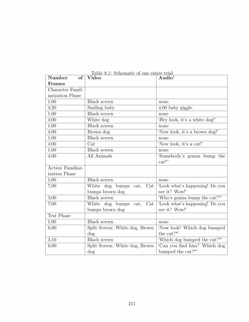
Table 8.1: Schematic of one entire trialNumber ofFrames
Video Audio1
Character Famil-iarization Phase1;00 Black screen none4;20 Smiling baby 4;00 baby giggle1;00 Black screen none4;00 White dog ‘Hey look, it’s a white dog!’1;00 Black screen none4;00 Brown dog ‘Now look, it’s a brown dog!’1;00 Black screen none4;00 Cat ‘Now look, it’s a cat!’1;00 Black screen none4;00 All Animals ‘Somebody’s gonna bump the
cat*’Action Familiar-ization Phase1;00 Black screen none7;00 White dog bumps cat, Cat
bumps brown dog‘Look what’s happening! Do yousee it? Wow!’
3;00 Black screen ‘Who’s gonna bump the cat?*’7;00 White dog bumps cat, Cat
bumps brown dog‘Look what’s happening! Do yousee it? Wow!’
Test Phase1;00 Black screen none6;00 Split Screen: White dog, Brown
dog‘Now look! Which dog bumpedthe cat?*’
3;10 Black screen ‘Which dog bumped the cat?*’6;00 Split Screen: White dog, Brown
dog‘Can you find him? Which dogbumped the cat?*’
211

timeline of proportion of looks towards the target for every frame in the test trial.
This time line allowed me to look for general trends in looking across the trials.
I was also able to analyze particular critical time-windows, by averaging the
proportion of participants looking towards the target for a certain duration of time.
I used this method to look at the average proportion of looks towards the target
animal in a one second baseline before the target question was uttered, and similarly
for windows following each iteration of the target question. It is the averages that I
found in these target windows that I will be comparing below.
Four coders coded this data. Inter-coder reliability was always above 90% and
Cohen’s Kappa ≥ 90%.
8.2.7 Results
By constructing the timelines discussed above for every condition and by averaging
the proportions of looks towards the target over the critical time windows, I was able
to carefully examine data across conditions. In no condition did I find systematic
effects of sex of infant, vocabulary level of infant, individual verbs or order of
presentation, so these factors are not included in the analyses I report here. While
the exact time course of apparent question comprehension varied across conditions
and age groups I consistently saw time-course evidence of comprehension in the one
second window following the offset of the second target question. The averages over
this region are used in the discussion below.
212
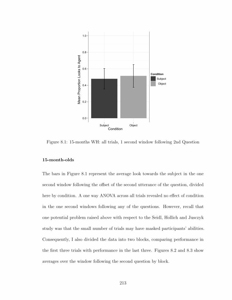
Condition
Mea
n P
ropo
rtion
Loo
ks to
Age
nt
0.0
0.2
0.4
0.6
0.8
1.0
Subject Object
ConditionSubject
Object
Figure 8.1: 15-months WH: all trials, 1 second window following 2nd Question
15-month-olds
The bars in Figure 8.1 represent the average look towards the subject in the one
second window following the offset of the second utterance of the question, divided
here by condition. A one way ANOVA across all trials revealed no effect of condition
in the one second windows following any of the questions. However, recall that
one potential problem raised above with respect to the Seidl, Hollich and Jusczyk
study was that the small number of trials may have masked participants’ abilities.
Consequently, I also divided the data into two blocks, comparing performance in
the first three trials with performance in the last three. Figures 8.2 and 8.3 show
averages over the window following the second question by block.
213
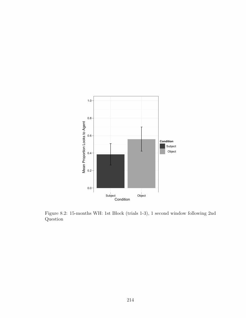
Condition
Mea
n P
ropo
rtion
Loo
ks to
Age
nt
0.0
0.2
0.4
0.6
0.8
1.0
Subject Object
ConditionSubject
Object
Figure 8.2: 15-months WH: 1st Block (trials 1-3), 1 second window following 2ndQuestion
214
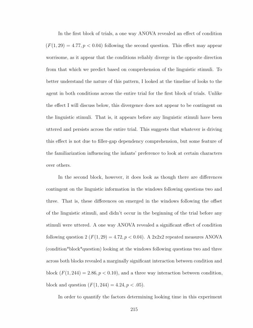
In the first block of trials, a one way ANOVA revealed an effect of condition
(F (1, 29) = 4.77, p < 0.04) following the second question. This effect may appear
worrisome, as it appear that the conditions reliably diverge in the opposite direction
from that which we predict based on comprehension of the linguistic stimuli. To
better understand the nature of this pattern, I looked at the timeline of looks to the
agent in both conditions across the entire trial for the first block of trials. Unlike
the effect I will discuss below, this divergence does not appear to be contingent on
the linguistic stimuli. That is, it appears before any linguistic stimuli have been
uttered and persists across the entire trial. This suggests that whatever is driving
this effect is not due to filler-gap dependency comprehension, but some feature of
the familiarization influencing the infants’ preference to look at certain characters
over others.
In the second block, however, it does look as though there are differences
contingent on the linguistic information in the windows following questions two and
three. That is, these differences on emerged in the windows following the offset
of the linguistic stimuli, and didn’t occur in the beginning of the trial before any
stimuli were uttered. A one way ANOVA revealed a significant effect of condition
following question 2 (F (1, 29) = 4.72, p < 0.04). A 2x2x2 repeated measures ANOVA
(condition*block*question) looking at the windows following questions two and three
across both blocks revealed a marginally significant interaction between condition and
block (F (1, 244) = 2.86, p < 0.10), and a three way interaction between condition,
block and question (F (1, 244) = 4.24, p < .05).
In order to quantify the factors determining looking time in this experiment
215
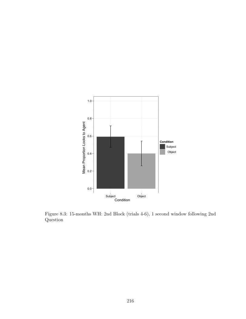
Condition
Mea
n P
ropo
rtion
Loo
ks to
Age
nt
0.0
0.2
0.4
0.6
0.8
1.0
Subject Object
ConditionSubject
Object
Figure 8.3: 15-months WH: 2nd Block (trials 4-6), 1 second window following 2ndQuestion
216
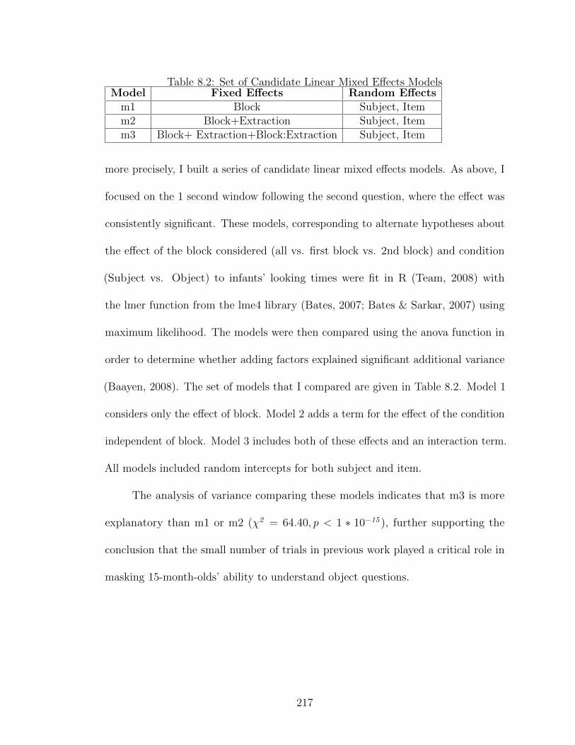
Table 8.2: Set of Candidate Linear Mixed Effects ModelsModel Fixed Effects Random Effects
m1 Block Subject, Itemm2 Block+Extraction Subject, Itemm3 Block+ Extraction+Block:Extraction Subject, Item
more precisely, I built a series of candidate linear mixed effects models. As above, I
focused on the 1 second window following the second question, where the effect was
consistently significant. These models, corresponding to alternate hypotheses about
the effect of the block considered (all vs. first block vs. 2nd block) and condition
(Subject vs. Object) to infants’ looking times were fit in R (Team, 2008) with
the lmer function from the lme4 library (Bates, 2007; Bates & Sarkar, 2007) using
maximum likelihood. The models were then compared using the anova function in
order to determine whether adding factors explained significant additional variance
(Baayen, 2008). The set of models that I compared are given in Table 8.2. Model 1
considers only the effect of block. Model 2 adds a term for the effect of the condition
independent of block. Model 3 includes both of these effects and an interaction term.
All models included random intercepts for both subject and item.
The analysis of variance comparing these models indicates that m3 is more
explanatory than m1 or m2 (χ2 = 64.40, p < 1 ∗ 10−15 ), further supporting the
conclusion that the small number of trials in previous work played a critical role in
masking 15-month-olds’ ability to understand object questions.
217
Condition
Mea
n P
ropo
rtion
Loo
ks to
Age
nt
0.0
0.2
0.4
0.6
0.8
1.0
Subject Object
ConditionSubject
Object
Figure 8.4: 20-months WH: all trials, 1 second window following 2nd Question
20-month-olds
I analyzed 20-month-olds’ data in the same way as the 15-month-olds’. Figure
8.4 shows the average looking time in the one second window following the second
question across all subjects and all trials.
A one way ANOVA for the one second window following the second question
revealed no effect of condition. As with the 15-month-olds’ data, I split the data
into two blocks corresponding to the first three and last three trials (Figures 8.5 and
8.6 respectively).
As with the 15-month-olds, we see some divergences by condition that appear
to go in the opposite direction than we would predict during the first block. However,
218
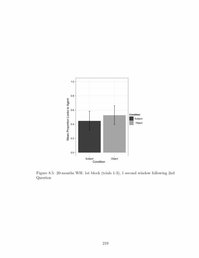
Condition
Mea
n P
ropo
rtion
Loo
ks to
Age
nt
0.0
0.2
0.4
0.6
0.8
1.0
Subject Object
ConditionSubject
Object
Figure 8.5: 20-months WH: 1st block (trials 1-3), 1 second window following 2ndQuestion
219
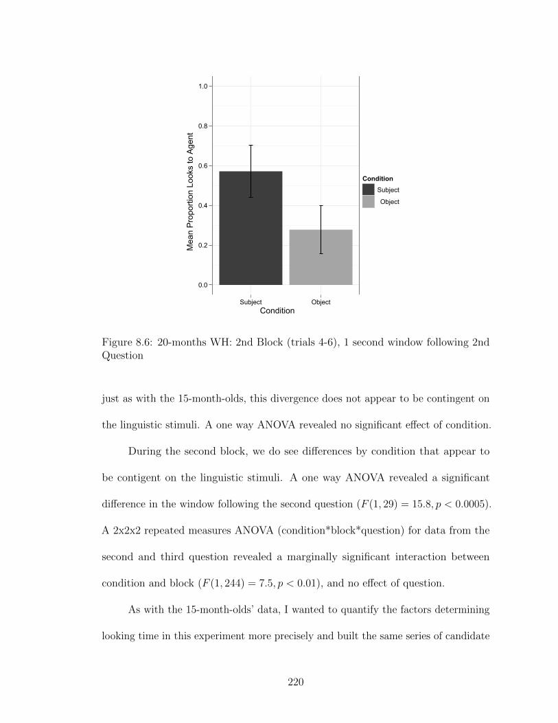
Condition
Mea
n P
ropo
rtion
Loo
ks to
Age
nt
0.0
0.2
0.4
0.6
0.8
1.0
Subject Object
ConditionSubject
Object
Figure 8.6: 20-months WH: 2nd Block (trials 4-6), 1 second window following 2ndQuestion
just as with the 15-month-olds, this divergence does not appear to be contingent on
the linguistic stimuli. A one way ANOVA revealed no significant effect of condition.
During the second block, we do see differences by condition that appear to
be contigent on the linguistic stimuli. A one way ANOVA revealed a significant
difference in the window following the second question (F (1, 29) = 15.8, p < 0.0005).
A 2x2x2 repeated measures ANOVA (condition*block*question) for data from the
second and third question revealed a marginally significant interaction between
condition and block (F (1, 244) = 7.5, p < 0.01), and no effect of question.
As with the 15-month-olds’ data, I wanted to quantify the factors determining
looking time in this experiment more precisely and built the same series of candidate
220
Table 8.3: Set of Candidate Linear Mixed Effects ModelsModel Fixed Effects Random Effects
m1 Block Subject, Itemm2 Block+Extraction Subject, Itemm3 Block+ Extraction+Block:Extraction Subject, Item
linear mixed effects models (Table 8.3).
The analysis of variance comparing these models indicates that m3 is more
explanatory than m1 or m2 (χ2 = 91.45, p < 2 ∗ 10−16 ).
Discussion of results
Based on the results presented above, it looks as though 15-month-olds behave as
though they understand both subject and object wh-questions. This suggests that
the concerns cited with the methodology in the Seidl et al paper were responsible
for the subject-object asymmetry in 15-month-olds’ comprehension in that work.
Crucially, this effect is only evident when looking at second block of trials. This
strengthens the argument that the small number of trials in the Seidl et al study
did not give 15-month-olds the opportunity to fully exhibit their comprehension
abilities. These results suggest that 15-month-olds have the knowledge necessary
to comprehend wh-questions, but that they are only able to properly deploy this
knowledge under optimal conditions. As predicted, 20-month-olds behaved as though
they understand both subject and object wh-questions; their systems of knowledge
and deployment are more solidly aligned with one another.
It is important to keep in mind that the fact that I was able to make the
subject-object asymmetry disappear in 15-month-olds does not argue against the
221
existence of such an asymmetry. The fact that it was object questions and not subject
questions that broke down under suboptimal conditions reveals that 15-month-olds’
comprehension abilities for object questions are still more fragile than their abilities
with subject questions. I explore the source of this fragility in Experiment 2.
There are several issues with the content of the trial and timing of questions and
other auditory material which could have both not allowed subjects sufficient time
to comprehend the question before be presented with further auditory stimuli. Such
complications could have added more noise to an already difficult task, obscuring
subject’s performance. In the Experiment 2 I lengthened the test trial to give subjects
more time following the first and third utterances of the target question.
8.3 Experiment 2: Relative clauses
8.3.1 Motivation
Although issues with the methodology appeared to underlie 15-month-olds’ asym-
metrical performance on subject and object wh-questions in Seidl et al, the question
remains as to why the asymmetry went in the direction that it did in previous work.
That is, why, when experimental conditions were not ideal, were subject questions
easier to comprehend than object questions? To probe this question I examined the
comprehension of an arguably more difficult filler-gap dependency, the relative clause,
using the same methodology as in Experiment 1, which did not elicit an asymmetry
in wh-questions. Thus target utterances were patterned after those in (20):
222
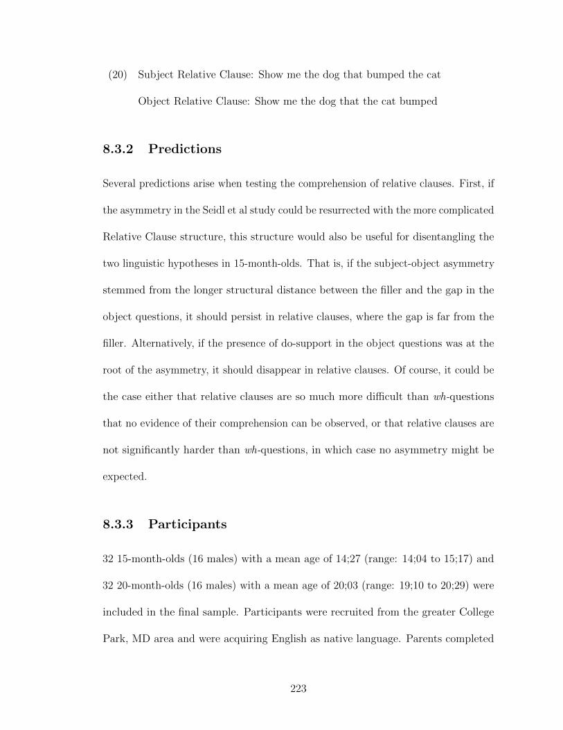
(20) Subject Relative Clause: Show me the dog that bumped the cat
Object Relative Clause: Show me the dog that the cat bumped
8.3.2 Predictions
Several predictions arise when testing the comprehension of relative clauses. First, if
the asymmetry in the Seidl et al study could be resurrected with the more complicated
Relative Clause structure, this structure would also be useful for disentangling the
two linguistic hypotheses in 15-month-olds. That is, if the subject-object asymmetry
stemmed from the longer structural distance between the filler and the gap in the
object questions, it should persist in relative clauses, where the gap is far from the
filler. Alternatively, if the presence of do-support in the object questions was at the
root of the asymmetry, it should disappear in relative clauses. Of course, it could be
the case either that relative clauses are so much more difficult than wh-questions
that no evidence of their comprehension can be observed, or that relative clauses are
not significantly harder than wh-questions, in which case no asymmetry might be
expected.
8.3.3 Participants
32 15-month-olds (16 males) with a mean age of 14;27 (range: 14;04 to 15;17) and
32 20-month-olds (16 males) with a mean age of 20;03 (range: 19;10 to 20;29) were
included in the final sample. Participants were recruited from the greater College
Park, MD area and were acquiring English as native language. Parents completed
223
the MacArthur-Bates Communicative Development Inventory (CDI) (Fenson et al.,
1993). 15-month-olds’ mean production CDI-vocabulary was (24.7) (range: 0 to 190,
out of a total possible 655), and 20-month-olds’ mean production CDI-vocabulary
was (107) (range: 9 to 381, out of a total possible 655). I analyzed the data of infants
that completed at least 4 out of 6 test trials (63/64 infants analyzed watched 6/6
test trials), and the trials where the infant was looking at least 20% of the time (this
excluded 3 trials). Ten additional infants were tested but ultimately excluded from
the analysis due to fussiness or inattention.
8.3.4 Materials and procedure
The materials and procedure for Experiment 2 were identical to those of Experiment
1. The test phase of the stimuli was 2 seconds longer, due to the reasons mentioned
at the end of Section 3.
8.3.5 Results
The results of Experiment 2 were analyzed in exactly the same way as those of
Experiment 1.
15-month-olds
As in Experiment 1, I’ll begin by examining the one second window following the
2nd target utterance averaged across all subjects and all trials.
A one way ANOVA for the one second window following the second target
utterance revealed no effect of condition. As in Experiment 1, I split up the data
224
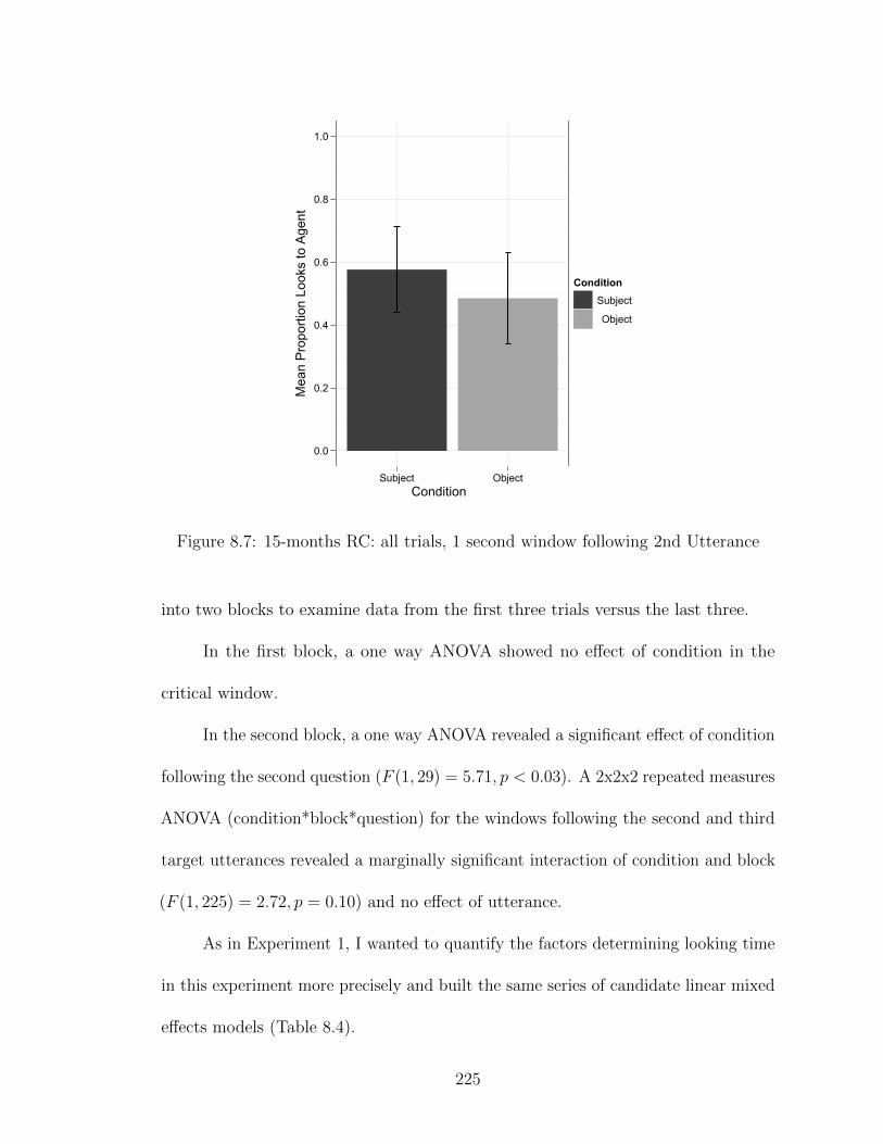
Condition
Mea
n P
ropo
rtion
Loo
ks to
Age
nt
0.0
0.2
0.4
0.6
0.8
1.0
Subject Object
ConditionSubject
Object
Figure 8.7: 15-months RC: all trials, 1 second window following 2nd Utterance
into two blocks to examine data from the first three trials versus the last three.
In the first block, a one way ANOVA showed no effect of condition in the
critical window.
In the second block, a one way ANOVA revealed a significant effect of condition
following the second question (F (1, 29) = 5.71, p < 0.03). A 2x2x2 repeated measures
ANOVA (condition*block*question) for the windows following the second and third
target utterances revealed a marginally significant interaction of condition and block
(F (1, 225) = 2.72, p = 0.10) and no effect of utterance.
As in Experiment 1, I wanted to quantify the factors determining looking time
in this experiment more precisely and built the same series of candidate linear mixed
effects models (Table 8.4).
225

Condition
Mea
n P
ropo
rtion
Loo
ks to
Age
nt
0.0
0.2
0.4
0.6
0.8
1.0
Subject Object
ConditionSubject
Object
Figure 8.8: 15-Months RC: 1st Block (trials 1-3), 1 second window following 2ndUtterance
Table 8.4: Set of Candidate Linear Mixed Effects ModelsModel Fixed Effects Random Effects
m1 Block Subject, Itemm2 Block+Extraction Subject, Itemm3 Block+ Extraction+Block:Extraction Subject, Item
226
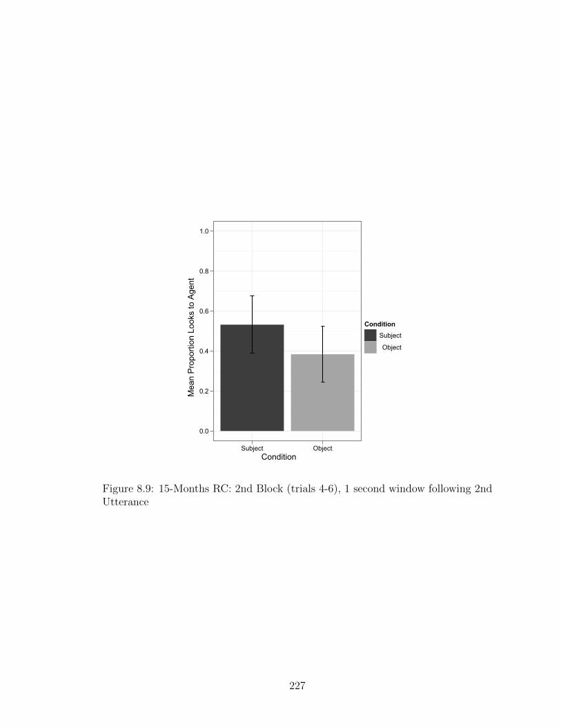
Condition
Mea
n P
ropo
rtion
Loo
ks to
Age
nt
0.0
0.2
0.4
0.6
0.8
1.0
Subject Object
ConditionSubject
Object
Figure 8.9: 15-Months RC: 2nd Block (trials 4-6), 1 second window following 2ndUtterance
227
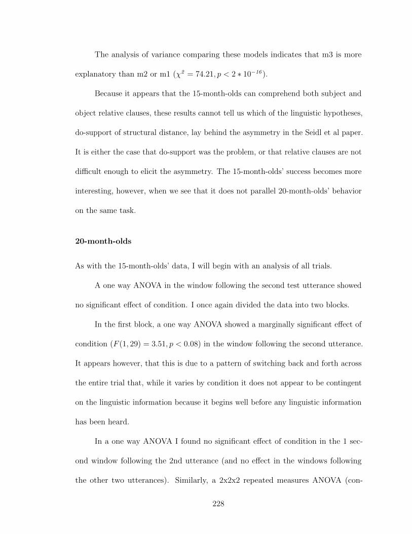
The analysis of variance comparing these models indicates that m3 is more
explanatory than m2 or m1 (χ2 = 74.21, p < 2 ∗ 10−16 ).
Because it appears that the 15-month-olds can comprehend both subject and
object relative clauses, these results cannot tell us which of the linguistic hypotheses,
do-support of structural distance, lay behind the asymmetry in the Seidl et al paper.
It is either the case that do-support was the problem, or that relative clauses are not
difficult enough to elicit the asymmetry. The 15-month-olds’ success becomes more
interesting, however, when we see that it does not parallel 20-month-olds’ behavior
on the same task.
20-month-olds
As with the 15-month-olds’ data, I will begin with an analysis of all trials.
A one way ANOVA in the window following the second test utterance showed
no significant effect of condition. I once again divided the data into two blocks.
In the first block, a one way ANOVA showed a marginally significant effect of
condition (F (1, 29) = 3.51, p < 0.08) in the window following the second utterance.
It appears however, that this is due to a pattern of switching back and forth across
the entire trial that, while it varies by condition it does not appear to be contingent
on the linguistic information because it begins well before any linguistic information
has been heard.
In a one way ANOVA I found no significant effect of condition in the 1 sec-
ond window following the 2nd utterance (and no effect in the windows following
the other two utterances). Similarly, a 2x2x2 repeated measures ANOVA (con-
228
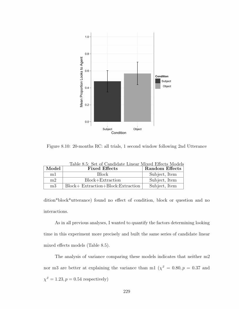
Condition
Mea
n P
ropo
rtion
Loo
ks to
Age
nt
0.0
0.2
0.4
0.6
0.8
1.0
Subject Object
ConditionSubject
Object
Figure 8.10: 20-months RC: all trials, 1 second window following 2nd Utterance
Table 8.5: Set of Candidate Linear Mixed Effects ModelsModel Fixed Effects Random Effects
m1 Block Subject, Itemm2 Block+Extraction Subject, Itemm3 Block+ Extraction+Block:Extraction Subject, Item
dition*block*utterance) found no effect of condition, block or question and no
interactions.
As in all previous analyses, I wanted to quantify the factors determining looking
time in this experiment more precisely and built the same series of candidate linear
mixed effects models (Table 8.5).
The analysis of variance comparing these models indicates that neither m2
nor m3 are better at explaining the variance than m1 (χ2 = 0.80, p = 0.37 and
χ2 = 1.23, p = 0.54 respectively)
229

Condition
Mea
n P
ropo
rtion
Loo
ks to
Age
nt
0.0
0.2
0.4
0.6
0.8
1.0
Subject Object
ConditionSubject
Object
Figure 8.11: 20-months RC: 1st Block (trials 1-3), 1 second window following 2ndUtterance
230

Condition
Mea
n P
ropo
rtion
Loo
ks to
Age
nt
0.0
0.2
0.4
0.6
0.8
1.0
Subject Object
ConditionSubject
Object
Figure 8.12: 20-months RC: 2nd Block (trials 4-6), 1 second window following 2ndUtterance
231
8.3.6 Discussion of results
In the relative clause condition, I found a U-shaped pattern of results in which
15-month-olds seem to successfully interpret both subject and object relative clauses
but 20-month-olds appear unable to comprehend either type of relative clause. This
decline in performance from 15- to 20-months is unexpected for two reasons. First, the
grammatical parallels between wh-questions and relatives leads us to expect that the
processing of wh-questions and relative clauses should rely on the same mechanisms.
Consequently, if an age group is able to process one of these constructions, we
would expect them to be able to process the other. Thus, 20-month-olds’ failure
with relative clauses is surprising. Second, it is unexpected that older infants, who
are presumably more grammatically advanced than younger infants, would not be
able to understand something that younger infants and adults can. This U-shaped
pattern suggests a disjunct between the development of knowledge and the necessary
deployment systems for this knowledge between 15 and 20 months of age.
8.3.7 Comparison between groups and experiments
It is possible that an apparent U-shaped pattern could arise simply due to a main
effect of age or experiment, where we would see the same relative effect in both
age groups or both experiments, but a skewed data set in one age group or one
experiment. To test this hypothesis I used an ANOVA to look at data for all age
groups and experiments, adding these two factors into the analysis. The ANOVA
showed the same interaction of block and condition but no effect of of experiment
232
(WH vs RC) or age (15 vs 20).
8.4 Discussion of the U-shaped pattern
I began this work seeking to determine the cause of a reported subject-object
asymmetry in the comprehension of wh-questions by 15-month-olds. Along the
way I improved the methodology used to investigate this question, and found no
such asymmetry for any age group or construction, highlighting the contribution of
methodology to previous results. Moreover, differences in performance between 15-
and 20-month-olds uncover an apparent discontinuity in development. Fifteen-month-
olds could comprehend relative clauses whereas 20-month-olds could not. As we would
not expect infants to regress in their linguistic knowledge as they progress through
development, we must ask what these results reveal about children’s grammatical
knowledge and the systems that deploy this knowledge. Is it possible that what
looks like success in the 15-month-olds’ behavior reflects a failure to use adultlike
knowledge and deployment systems to parse relative clauses? Could 20-month-olds’
failure with relative clauses be highlighting a crucial step in successfully moving from
heuristic strategies employed by 15-month-olds to an adultlike system? Below we
will explore the implications of these tentative hypotheses.
8.4.1 Understanding the U-shaped pattern of results
A common view of learning, and one that I will adopt here, is that the knowledge,
and hence the appropriate deployment system for this knowledge, that is present
233
at one stage will be cumulative across the course of development. That is to say,
once children have acquired a given piece of grammatical knowledge, they do not
lose this knowledge with subsequent linguistic experience. My results thus lead me
to ask whether it is plausible that 15-month-olds know something about filler-gap
dependencies that they subsequently lose by the time they are 20-month-olds. The
implausibility of such regression across development forces me to examine what other
interaction between their developing knowledge and deployment systems could give
rise to the patterns of success and failure in my task.
Adopting the position that a child’s linguistic knowledge won’t regress, we are
left with two possibilities to explain the observed discontinuity. First, it could be that
15-month-olds initially acquire a correct characterization of filler-gap dependencies,
but some piece of further linguistic knowledge or experience encountered between 15
and 20 months interferes with their ability to use this knowledge. Alternatively, it
could be that 15-month-olds haven’t yet acquired the requisite knowledge to interpret
filler-gap dependencies and instead rely on a temporary heuristic. This heuristic
would be rendered insufficient with the acquisition of relevant linguistic knowledge
by 20-months. To determine the plausibility of these two accounts I must carefully
outline the knowledge and deployment states children would pass through in each
one. By making these possible states explicit I am able to make several predictions
that are informing ongoing work.
234
8.4.2 Hypothesis 1: Success means success, and so does fail-
ure
The first possibility we will consider is that 15-month-olds have acquired adultlike
knowledge of filler-gap dependencies and are successfully deploying this knowledge in
my task. This would imply that they have both an adultlike knowledge system and a
correspondingly adultlike system to deploy this knowledge. Under this hypothesis, 20-
month-olds fail not because they lack appropriate knowledge, but because something
(knowledge or linguistic experience, potentially in the form of frequency information)
is impeding successful online deployment of this knowledge (cf. Lidz, 2011). In order
for this hypothesis to be viable, there would have to be some linguistic knowledge or
experience that could lead to unsuccessful parsing of relative clauses (while leaving
parsing of wh-questions intact). It is not immediately clear what this knowledge or
experience would be, but further exploration of this question might yield promising
results.
8.4.3 Hypothesis 2: Success means failure, and failure means
success
An alternative possibility is that 15-month-olds have not acquired adultlike knowledge
of filler-gap dependencies, and correspondingly lack an adultlike deployment system
for this knowledge. Then we must ask, how do they succeed at my task when they
fail to have adultlike knowledge and deployment systems? Further we have to ask
what is behind 20-month-olds’ failure with relative clauses. Have they failed to
235

acquire some crucial piece of knowledge about filler-gap dependencies? Or have they
successfully acquired an adultlike knowledge state but can only successfully deploy
under certain conditions?
When failure means success
I’ll begin by discussing the question of whether 20-month olds fail because they
lack the appropriate knowledge to interpret relative clauses or because they lack
the appropriate system to deploy this knowledge. Their success with wh-questions
suggests that they do not lack the requisite knowledge or deployment system to
resolve all filler-gap dependencies, so we can narrow down our questions to ask
whether they lack knowledge about relative clauses in particular or whether their
deployment system is one that only works with wh-questions.
Because the structures underlying the filler-gap dependency in wh-questions
and relative clauses are fundamentally alike, we might take 20-month-olds’ success
with wh-questions as indicative that this common structure is in place. Thus,
failure with relative clauses could be caused by children lacking that aspect of
relative clauses that distinguishes them from wh-questions (e.g., clausal embedding,
restrictive modification, the discourse conditions on relativization). Alternatively,
the failure with relative clauses could be explained by a failure to successfully
deploy the filler-gap structure in just this case. The latter possibility does not seem
unreasonable when we consider the superficial differences between relative clauses
and wh-questions that could make the former more difficult to resolve online. These
include the optionality of morphologically marked fillers (i.e. wh-words), the possibly
236

less marked displacement of fillers, the lack of do-support and the lack of question
prosody in relative clauses. While I will not present it here, recent results from the
lab support this hypothesis, showing that 20-month-olds can comprehend relative
clauses when processing demands are reduced, suggesting that they do have the
appropriate knowledge for relativization but have difficulty deploying this knowledge
(Gagliardi & Lidz, 2010).
Leaving answers to these questions for future work, we are now in a position
to consider the following. If 20-month-olds do not lack knowledge of filler-gap
dependencies, but do have difficulty deploying this knowledge, why do 15-month-olds
do better? What is it that 15-month-olds are doing to perform successfully with
both types of filler-gap dependencies?
When success means failure
It could be that 15-month-olds have not yet acquired full knowledge of filler-gap
dependencies. After all, if 20-month-olds are only just sorting out how to deploy this
knowledge it is not unreasonable to think that this knowledge was not intact earlier
on. If this is the case, then we must ask if there is any way it would be possible
to succeed in my task without knowledge of filler-gap dependencies. That is, are
there any other cues, linguistic or otherwise, that could lead a child to look at the
appropriate animal in response to my target utterances that don’t involve knowledge
of filler-gap dependencies or syntactic movement? I believe there may be.
While 15-month-olds may not know about filler-gap dependencies, they may
have the rudiments of verb meanings and argument structure in place (Golinkoff,
237
Hirsh-Pasek, Mervis, Frawley, & Parillo, 1995). Knowing the meaning of a verb
implies knowledge of the argument structure and thematic roles associated with
it. This knowledge in turn implies knowing that transitive verbs denote events
containing two participants. The 15-month-olds’ strategy in my task, then, could
be a parsing heuristic that relies on knowledge of argument structure, and relatedly,
event structure, instead of syntactic dependencies.
The heuristic depends on the identification of a verb missing a noun phrase
needed to fill a required thematic role. The child would recognize a gap in the
argument structure by noticing a substring in which an expected syntactic argument
fails to occur (e.g., the cat bumped in a filler-gap dependency involving an object).
Having identified a verb that is missing a required argument, the heuristic parser
would then search the discourse context for a referent that could fill out this thematic
structure. It is important to note that if 15-month-olds are relying on this heuristic
they are crucially not making the link between the filler and the gap, and do not even
need to parse or interpret the filler to arrive at the correct interpretation. Note also
that in my method, the child hears the verb several times during the familiarization
phase so that the argument structure of the verb is highly activated by the time of
the test phase.
To be consistent with the implied rejection of the possibility that 15-month-olds
have adultlike knowledge, we must determine why children would ever abandon this
strategy if it works as well as it appears to. It is possible that children have some
expectations about the grammatical conditions that can license a null argument.
One possibility is overt movement of the type seen in filler-gap dependencies. If by
238
20-months children have the appropriate grammatical structure and constraints to
be able to interpret syntactic movement, they would have learned about the relation
between movement and subcategorization, realizing that a verb can sometimes find
its arguments in displaced positions in the clause. It follows that once this system
is in place, extragrammatical heuristics like the one proposed above wouldn’t be
available to parse these sentences because of the grammatical constraint requiring
that subcategorized arguments must be syntactically realized. At this point, infants
would need access to a new system to deploy their updated knowledge of filler-gap
dependencies, and this system would be the adult active filling strategy. I will return
to this transition from 15 to twenty months in the discussion below.
8.4.4 Formulating a hypothesis to guide future research
In order to guide further investigation in this vein, it will be very useful to formulate
a hypothesis based on the possibilities outlined above. What follows is what I believe
to be the most likely hypothesis, but as mentioned above it by no means exhausts
the possible explanations for the patterns found in my data.
Hypothesis:
• 20-month-olds have acquired adultlike knowledge of filler-gap dependencies
(henceforth K20), but have yet to fully control an adultlike deployment system
(D20), accounting for their difficulty with relative clauses.
• 15-month-olds have a non adultlike knowledge state (K15) that includes knowl-
edge of thematic roles, verb meanings and event structure, along with a non
239
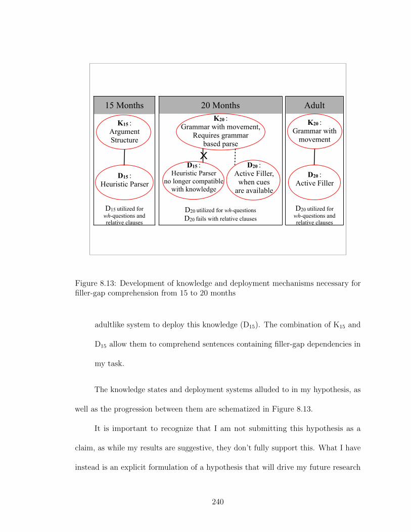
15 Months
D15 utilized for wh-questions and relative clauses
K15 : Argument Structure
D15 : Heuristic Parser
Adult
D20 utilized for wh-questions and relative clauses
K20 : Grammar with
movement
D20 : Active Filler
20 Months
D20 utilized for wh-questionsD20 fails with relative clauses
K20 : Grammar with movement,
Requires grammar based parse
D20 : Active Filler,
when cues are available
D15 : Heuristic Parser
no longer compatible with knowledge
X
Figure 8.13: Development of knowledge and deployment mechanisms necessary forfiller-gap comprehension from 15 to 20 months
adultlike system to deploy this knowledge (D15). The combination of K15 and
D15 allow them to comprehend sentences containing filler-gap dependencies in
my task.
The knowledge states and deployment systems alluded to in my hypothesis, as
well as the progression between them are schematized in Figure 8.13.
It is important to recognize that I am not submitting this hypothesis as a
claim, as while my results are suggestive, they don’t fully support this. What I have
instead is an explicit formulation of a hypothesis that will drive my future research
240
and, if found to be supported, could account for the patterns of data I have presented
in this paper. As a hypothesis it works well to make several predictions that are
informing are further investigations.
8.4.5 Predictions
The hypothesis outlined above makes several predictions regarding the comprehension
of different types of filler-gap dependencies by both 15- and 20-month-olds. First,
since I am positing that 15-month-olds are not using the filler when they comprehend
sentences with filler-gap dependencies, they should not make distinctions dependent
on information in the filler. For example, if they were presented with a situation
where a cat bumped a boy, the cat bumped a truck and then a girl bumped the cat,
and then asked Who did the cat bump?, they should be able to narrow down the
choices to the two possible objects, the boy and the truck, but should not differentiate
between them, despite the fact that an adult using the filler, and by hypothesis a
20-month-old, would use the animacy restriction on who to choose the boy.
Second, since I am positing that 15-month-olds are only using knowledge of
thematic roles, not the structure of the dependency, to resolve the missing argument,
they should not be sensitive to illicit extractions that adults are. In contrast,
if 20-month-olds have adultlike knowledge then they should be sensitive to these
extractions. For example, given the scenario outlined above, for an adult the utterance
What did the cat bump and the boy? (or what did the cat bump and? ) would be
ungrammatical as a violation of the coordinate structure constraint (Ross, 1967).
241
While an interpretation might ultimately be reached, it might not follow the time
course of licit question answering. If a 15-month-old were only filling in thematic
structure with an appropriate referent, they might be able to choose the appropriate
referent in a manner similar to answering a licit question.
Finally, regarding the 20-month-olds’ failure with relative clauses, I would
predict that having a more salient filler, i.e. a wh-relative such as Show me the
dog who bumped the cat, they would have less trouble identifying the presence of a
filler and subsequently resolving the dependency. I am currently testing all of these
predictions in the lab (Gagliardi & Lidz, 2010).
8.4.6 Limitations
There are several aspects of this data that could be seen as serious concerns. First,
the data is very noisy, most likely due to the following factors. The task is complex
and subjects could vary greatly in the time course of their responses. Because the
analysis requires averaging across trials and across participants, variance in the
time course of the responses could cause similar responses that differ in timing to
effectively cancel each other out. Additionally, it’s possible that I didn’t leave enough
time to answer the questions, compounded by the fact that there is a significant
amount of non-test audio during the test phase, which could potentially alter the
course of eye movements as children are processing the target utterances. Finally,
the blank screen that occurs between the two halves of the test trial makes it too
dark to allow coding. Consequently, if there were predictive eye movements based
242

on the form of the question I would not be able to capture them.
A second issue concerns the backwards looking pattern (i.e., systematic looking
at the non-target) that permeates the entire test phase in the first block of trials in
the wh-question condition, for both 15- and 20-month-olds. This pattern could be
due to salience of the target participant in the familiarization and an expectation
that the other participant will in turn be highlighted. This does not appear to be a
general agent or patient bias, as the agent is preferred in the Object condition, and
the patient in the Subject condition. Whatever the precise origins of this curious
pattern, it further highlights the utility of using a sufficient number of test trials to
allow any task general issue to be filtered out through longer exposure to the task.
While these issues with my data do exist, I nevertheless believe that these
data present a compelling picture of filler-gap comprehension at 15- and 20-months.
Whatever the problems in the data are, I find consistent patterns conditioned by
the linguistic stimuli, and I predict that eliminating some of the more complicated
aspects of my test trial would only clarify these results.
8.4.7 Theoretical implications
If the hypothesis outlined above proves to be an accurate characterization of the
development of filler-gap dependencies, it could also provide the beginnings of an
argument against parsing models which do not use details of grammatical represen-
tation to build sentence interpretations, as in the models of ‘good-enough’ parsing
illustrated by Ferreira, Ferraro, & Bailey, 2002 or Townsend & Bever, 2001. These
243
views suggest that the parser computes interpretations of sentences using heuris-
tics that yield interpretations similar to those that would be derived by a system
that uses grammatical detail in real time. This kind of model is similar to what I
posit for 15-month-olds, but doesn’t account for why 20-months olds would stop
using this strategy. If such heuristics were characteristic of mature parsing systems,
then I wouldn’t expect them to appear early in development and later disappear.
Consequently, if the asymmetry at 20-months in the comprehension of wh-questions
and relative clauses derives from the combination of an adultlike grammar and an
inefficient parser, it would look as though the parser does its best to implement the
grammar and does not settle on a good-enough parse. That is, while the good-enough
view could account for 15-month-olds’ behavior, it may not appear to ultimately
characterize the interaction between the grammar and the parser in development.
8.5 Partial encoding drives inference
In this chapter, I have identified a case of U-shaped development in the domain of
filler-gap dependencies. Whereas 15-month-old children seem to correctly interpret
both subject and object wh-questions and subject and object relative clauses, 20-
month-olds seem to have lost the ability to correctly interpret relative clauses. I have
proposed that this developmental pattern can be explained in a framework that iden-
tifies independent contributions of (a) grammatical knowledge, (b) the information
processing mechanisms that deploy that knowledge, and (c) the alignment of those
mechanisms during language development. I have argued that in the case of filler-gap
244
dependencies, both knowledge and deployment vary across development. I have
proposed that 15-month-olds may have impoverished grammatical representations
for these dependencies and that their deployment systems may be appropriate for
those representations. Twenty-month-olds, on the other hand, may have accurate
adult-like knowledge but have yet to become effective at deploying that knowledge
in real-time. By examining the nature of 15- and 20-month-olds’ knowledge and
deployment, we can better understand not only when children begin to show adultlike
knowledge of filler-gap dependencies, but how they arrive at this point.
We can begin to think about how 15-month-olds become 20-month-olds by
returning to the framework outlined in Chapter 1. By applying this framework to
the learning problem involved in the acquisition of filler-gap dependencies, we can
see that the partial knowledge, as well as the associated deployment system for this
knowledge, in place at 15-months provides the necessary data to feed inferences into
a more adultlike 20-month-old’s grammar.
First we can think about the knowledge that I am positing that 15-month-olds
have, and what this knowledge allows them to encode. Above, I suggested that
15-month-olds might have knowledge of the basic argument structure of a verb. Thus
when they hear a verb they know to be transitive (especially, as I mentioned above,
when the argument structure is highly activated as the transitive structure has been
repeated several times in the familiarization phase), they will expect it to appear with
both an internal and external argument. As they encode the input into some kind
of syntactic structure, they will build structure for both and internal and external
argument of the transitive verb. When they fail to hear one argument, due to it
245
being fronted as part of the wh-phrase, they will notice that this means there must
be an empty category in the structure they have encoded. At this point, two things
will be happening. First, in an effort to reach some kind of interpretation, the child
will search in the world to find the referent that matches the empty thematic role.
This is the behavior that allows 15-month-olds to succeed in my task, but this is not
all that is going on when 15-month-olds end up with this sort of partial encoding.
They will also notice the presence of an empty category, and innate knowledge
from their hypothesis space will tell them that empty categories can’t just occur
freely, they must be licensed. In the hypothesis space there will be several possible
sources of empty categories: pro, PRO, and, crucially, overt wh-movement. The
child will then go about inferring which of these processes could have generated this
particular empty category, using knowledge from UG about how each of these is
licensed and looking in the signal for evidence of the relevant licensing conditions. In
the beginning, the child might be unsure, but over time, with more examples (and
perhaps with evidence for or against the other hypotheses), the child will infer that
in this sort of configuration the empty category is licensed by overt movement. Once
the child knows this, they will know that the argument must have moved to a higher
position in the sentence, and will build in the structure necessary to accommodate
the wh-phrase. Once this knowledge is in place, the chid will be able to properly
encode structures involving overt movement. The necessary deployment systems
appear as a consequence of having the correct structure, which the caveats mentioned
above involving the child’s ability to know when beginning to parse a sentence what
kinds of cues to look for. This process is schematized in Figure 8.14.
246
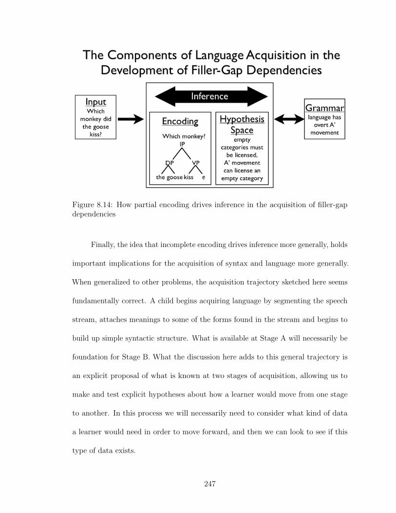
Figure 8.14: How partial encoding drives inference in the acquisition of filler-gapdependencies
Finally, the idea that incomplete encoding drives inference more generally, holds
important implications for the acquisition of syntax and language more generally.
When generalized to other problems, the acquisition trajectory sketched here seems
fundamentally correct. A child begins acquiring language by segmenting the speech
stream, attaches meanings to some of the forms found in the stream and begins to
build up simple syntactic structure. What is available at Stage A will necessarily be
foundation for Stage B. What the discussion here adds to this general trajectory is
an explicit proposal of what is known at two stages of acquisition, allowing us to
make and test explicit hypotheses about how a learner would move from one stage
to another. In this process we will necessarily need to consider what kind of data
a learner would need in order to move forward, and then we can look to see if this
type of data exists.
247
Moreover, this hypothesis suggests that incomplete knowledge isn’t just a piece
of some system being amassed by the learner, but rather the the catalyst driving
language acquisition forward. That is to say that hypotheses like this one allow us
to look at partially acquired knowledge in a novel way, interpreting it as not just
some stage on the way to complete knowledge, but the key that allows the child to
compare hypotheses about what the shape of that complete knowledge is.
In summary, understanding how incomplete encoding could drive inferences
to complete, adultlike encoding will open the doors to understanding many other
acquisition problems as well. We can begin to break down other acquisition problems
and look at what children do know, and what they can encode from the input, before
they can perform in an adultlike way on some task. Our goal is ultimately not
to explain behavior in experimental task, but rather to see what children know at
one point in time, what they are able to encode with this knowledge and (given a
hypothesis space), how this can lead to what they come to know at a later stage. We
can think about how this incomplete encoding based on partial knowledge, combined
with a hypothesis space and the kind of inference mechanism outlined in Chapter 7,
could push a child forward along the developmental continuum towards an adultlike
state.
248
Chapter 9
Conclusion
This dissertation sought to delineate a productive way forward in the study of
language acquisition. Instead of focusing on what must must be innate, or dwelling
on what can be learned with no innate knowledge, this approach seeks to break
language acquisition down into its component parts. In doing so, there is room for
both an innate hypothesis space and a powerful statistical inference mechanism.
What’s more, this approach highlights the need for an appropriate encoding of the
linguistic input in order to solve any given problem in language acquisition.
9.1 What we’ve seen here
Chapters 2 through 6 explored noun class acquisition. At first blush, noun classi-
fication looked like a domain where I didn’t expect to find any learning problems.
Noun class information is abundantly available in the input, even in a language like
Tsez that only has over agreement on a minority of verb and adjective types, and
249

has considerable syncretism in paradigms inflecting for noun class. However, I found
that the intake that children appeared to be using to acquire this system did not
align with what I measured in the input. This pointed towards incomplete encoding,
perhaps due to the learner’s changing abilities to encode different kinds of features
and dependencies across development. This evidence for incomplete encoding (as
witnessed by the poor fit between the input and what children learn) highlights
the necessity to separate what is accessible to the learner given his linguistic and
cognitive abilities from what is available (in principle) in the input. Studies of
statistical learning in the future must therefore concern themselves as much with
what is represented by learners as with what is in the input viewed more literally.
Chapter 7 described Bayesian inference. I showed that models using Bayesian
inference can predict children’s behavior in several word learning tasks, and suggested
ways that these models could be extended to both more complicated word and word
class learning. I also outlined how this same kind of inference could be used to solve
subset problems in other domains of language acquisition. The observation that the
relative power of likelihood in explaining children’s behavior in my word learning
experiments varied as a function of the grammatical category of the word being
learned (and whether children were learning words or word classes) highlights the
importance of the hypothesis space and the interaction of the prior with the likelihood
in explaining language acquisition. This is an important point, as it demonstrates
that evidence of the importance of the likelihood should not be mistaken for evidence
that only the likelihood is important. I ended this chapter with the observation that
a powerful inference mechanism is powerless if there isn’t a hypothesis space to draw
250
inferences about, and data to draw these inferences from. In particular, and in line
with what I found in my investigation of noun class acquisition, the data used for
these inferences must be encoded in such a way that it can bear on the hypotheses
at hand.
In Chapter 8 I explored the acquisition of filler-gap dependencies. The observa-
tion that 15-month-olds understand aspects of these dependencies that 20-month-olds
do not led to the hypothesis that 15-month-olds have an incomplete encoding of
these constructions and that this incomplete encoding provides an important piece
of evidence that allows the learner to move to a more complete representation of
the construction. This points us toward better understanding in other domains of
language acquisition, where an incomplete encoding of the input, which is all that
is available to a child at some early stage of language acquisition, could be exactly
what the child needs to drives inferences forward toward a more complete adultlike
encoding of the input.
Altogether, these chapters paint a vivid picture of the processes involved in
language acquisition and make a compelling argument that each of these pieces, the
input, the encoding, the inference mechanism, the hypothesis space and the acquired
grammar, need to be considered in order to fully understand the processes that allow
a child to infer, from a finite set of sentences, a grammar that can generate an infinite
set.
251
9.2 Where to next?
This work aimed to show that not only is a divide between generative and distri-
butional approaches to language acquisition unnecessary, but that by combining
insights and methodology from each of these domains we can make progress in our
investigation of language acquisition. Even the most powerful statistical inference
mechanism doesn’t threaten a well defined hypothesis space, it in fact depends on one.
Similarly, a learner endowed with a rich hypothesis space must learn from the input
and cannot do so without an effective encoding. Moreover a statistical inference
mechanism provides the link between the input and the innate principles of grammar,
allowing the mechanism underlying the acquisition of a particular grammar can be
studied. The tools of Bayesian inference allow us to precisely specify what kinds of
inferences are optimally made given the available data and a hypothesis space. In
cases where children diverge from these optimal inferences, we identify the potential
role of either incomplete encoding or an incomplete or biased hypothesis space. Here
I focused on several relatively small problems in language acquisition, not because
they are the most fascinating but because by starting this approach in an arena
small enough for us to gain a deep understanding of each component and the role
it plays in this problem, we develop a better understanding of the components and
how to study them. This approach allows us to move forward in our investigation of
language acquisition in several directions.
First, we can to scale this up to investigate more complex problems. In Chapter
7 I outlined what it would take to scale our inference model up to look at a solution of
252
one of the set of subset problems. This sort of project would hopefully be extensible
to other similar problems. While it might not be simple to characterize all of the
components involved for these more complex problems, by specifying what these
components need to be like, we are part of the way towards finding an oversimplified
solution which can in turn be made progressively more complex until it approximates
the complexity of the problem and solution found in language acquisition.
Next, with a better understanding of what children can encode and what
they can infer from the encoded input, I open the doors to some more practical
applications of this work. A well documented difference in children’s patterns in
language acquisition has been related to the quantity and quality of input children
receive (cf. Hoff, 2003 inter alia). If we understand what information children need
to encode to acquire a given phenomenon, we can potentially intervene to provide
more of the right kind of input for children to acquire this phenomenon, putting
them on more equal footing with their peers who naturally have access to this input.
253

Appendices
254
Appendix A
Materials used in Tsez
classification experiment
255
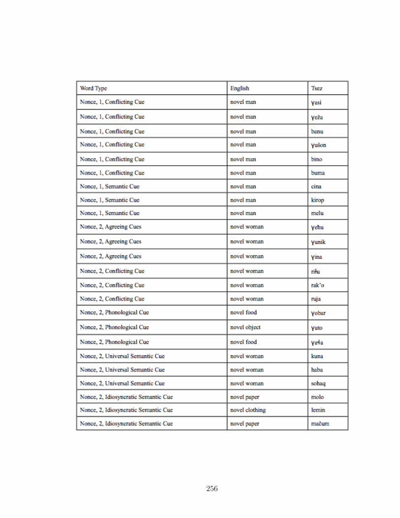
256
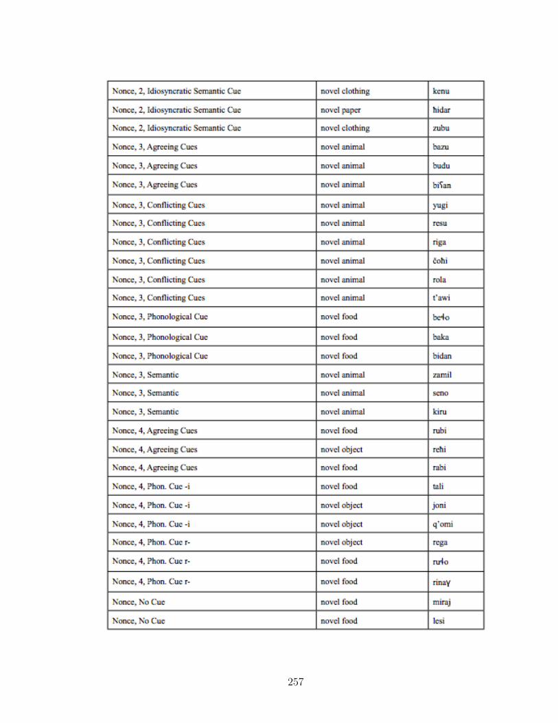
257
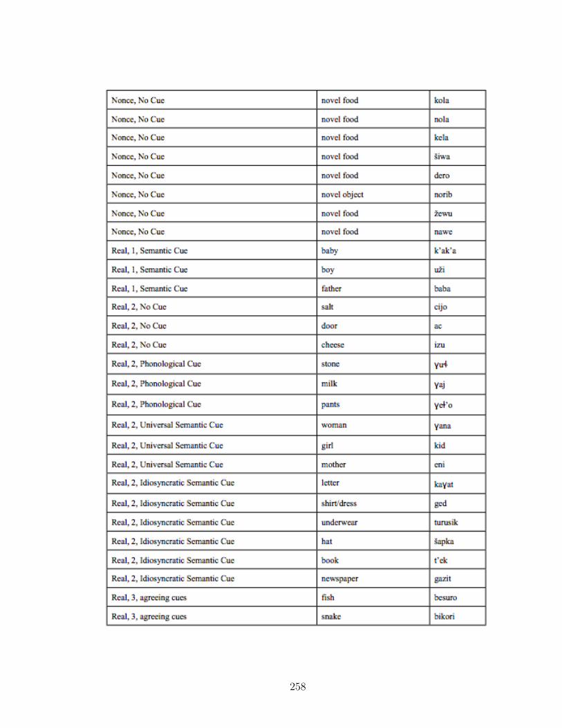
258
259
Appendix B
Full results of Tsez classification
experiment
260
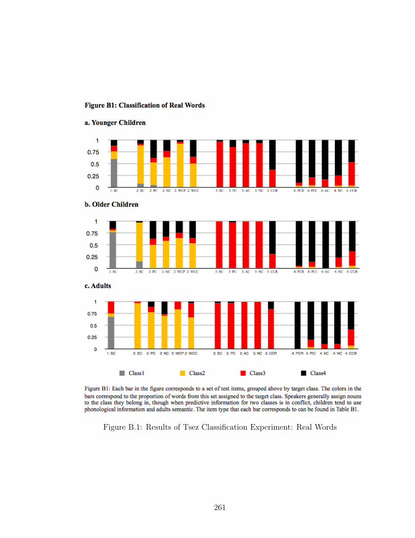
Figure B.1: Results of Tsez Classification Experiment: Real Words
261
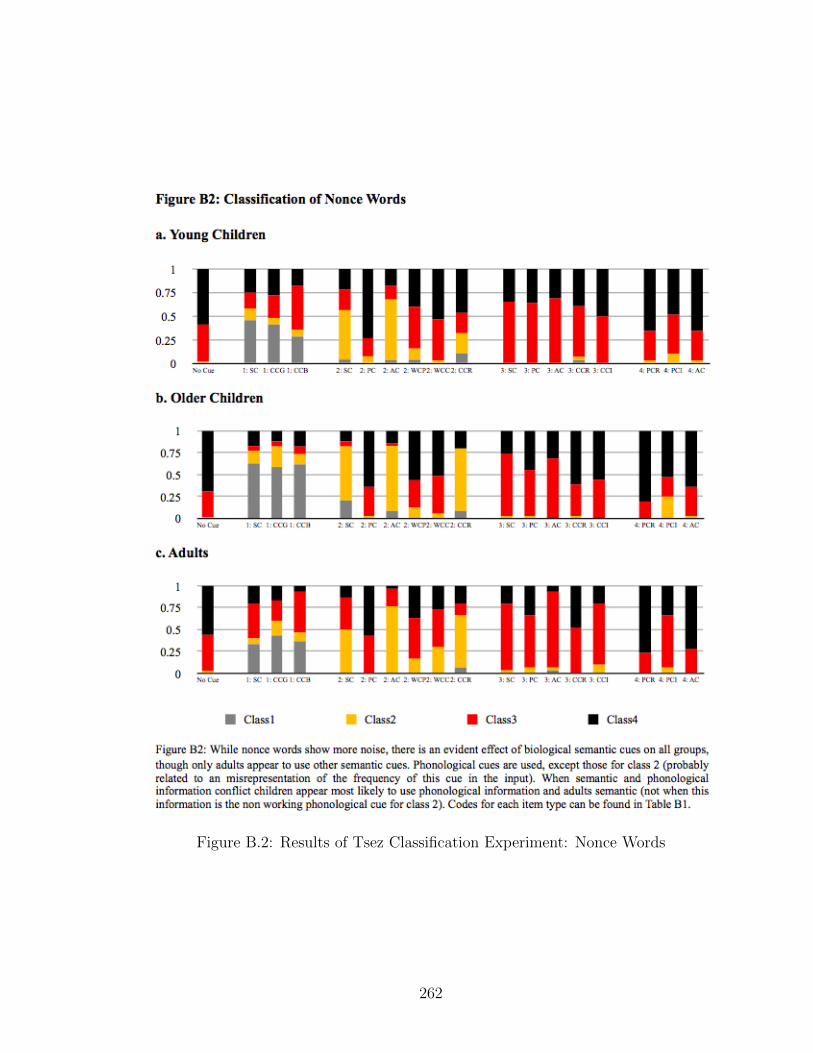
Figure B.2: Results of Tsez Classification Experiment: Nonce Words
262
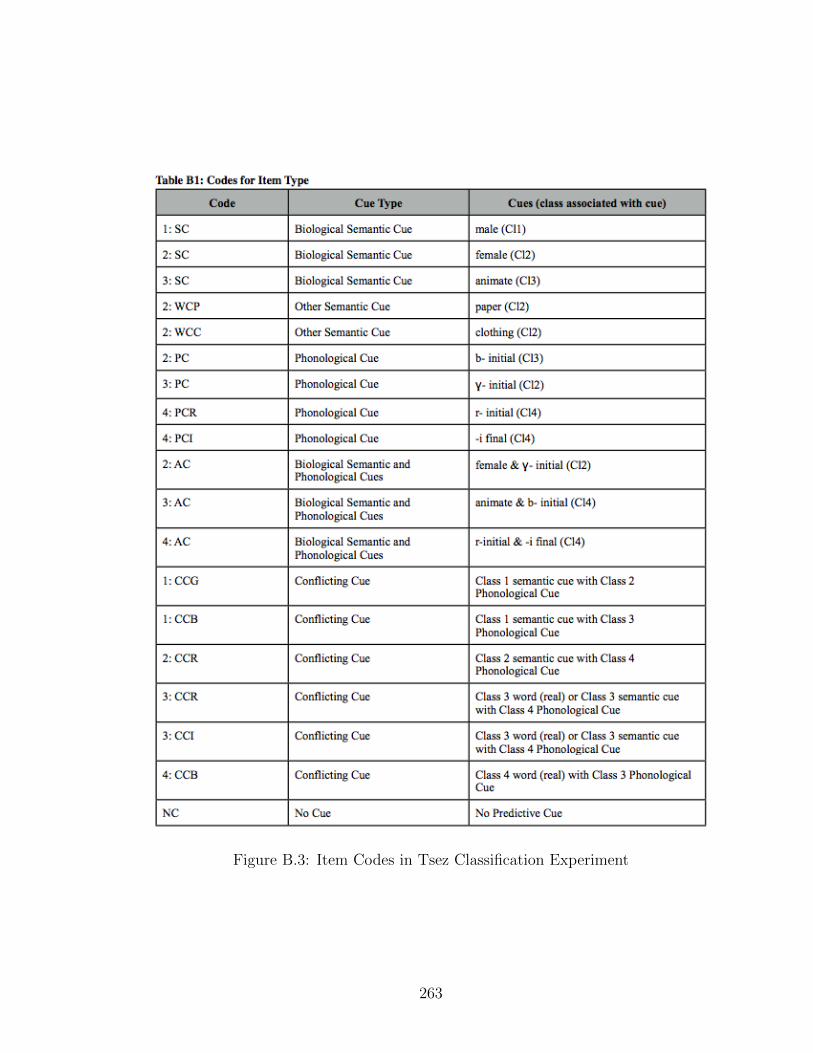
Figure B.3: Item Codes in Tsez Classification Experiment
263
Appendix C
Jensen-Shannon divergence
264

265

266
Appendix D
Materials used in Norwegian
experiment 1
267
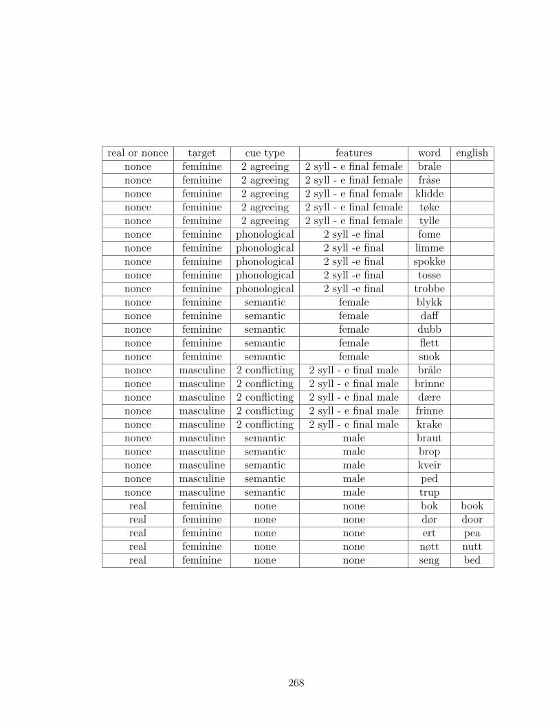
real or nonce target cue type features word englishnonce feminine 2 agreeing 2 syll - e final female bralenonce feminine 2 agreeing 2 syll - e final female frasenonce feminine 2 agreeing 2 syll - e final female kliddenonce feminine 2 agreeing 2 syll - e final female tøkenonce feminine 2 agreeing 2 syll - e final female tyllenonce feminine phonological 2 syll -e final fomenonce feminine phonological 2 syll -e final limmenonce feminine phonological 2 syll -e final spokkenonce feminine phonological 2 syll -e final tossenonce feminine phonological 2 syll -e final trobbenonce feminine semantic female blykknonce feminine semantic female daffnonce feminine semantic female dubbnonce feminine semantic female flettnonce feminine semantic female snoknonce masculine 2 conflicting 2 syll - e final male bralenonce masculine 2 conflicting 2 syll - e final male brinnenonce masculine 2 conflicting 2 syll - e final male dærenonce masculine 2 conflicting 2 syll - e final male frinnenonce masculine 2 conflicting 2 syll - e final male krakenonce masculine semantic male brautnonce masculine semantic male bropnonce masculine semantic male kveirnonce masculine semantic male pednonce masculine semantic male trupreal feminine none none bok bookreal feminine none none dør doorreal feminine none none ert peareal feminine none none nøtt nuttreal feminine none none seng bed
268
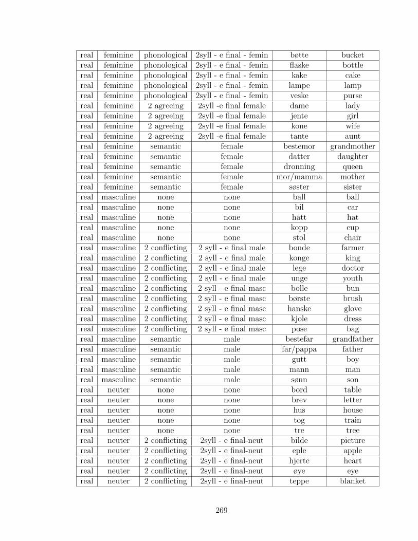
real feminine phonological 2syll - e final - femin bøtte bucketreal feminine phonological 2syll - e final - femin flaske bottlereal feminine phonological 2syll - e final - femin kake cakereal feminine phonological 2syll - e final - femin lampe lampreal feminine phonological 2syll - e final - femin veske pursereal feminine 2 agreeing 2syll -e final female dame ladyreal feminine 2 agreeing 2syll -e final female jente girlreal feminine 2 agreeing 2syll -e final female kone wifereal feminine 2 agreeing 2syll -e final female tante auntreal feminine semantic female bestemor grandmotherreal feminine semantic female datter daughterreal feminine semantic female dronning queenreal feminine semantic female mor/mamma motherreal feminine semantic female søster sisterreal masculine none none ball ballreal masculine none none bil carreal masculine none none hatt hatreal masculine none none kopp cupreal masculine none none stol chairreal masculine 2 conflicting 2 syll - e final male bonde farmerreal masculine 2 conflicting 2 syll - e final male konge kingreal masculine 2 conflicting 2 syll - e final male lege doctorreal masculine 2 conflicting 2 syll - e final male unge youthreal masculine 2 conflicting 2 syll - e final masc bolle bunreal masculine 2 conflicting 2 syll - e final masc børste brushreal masculine 2 conflicting 2 syll - e final masc hanske glovereal masculine 2 conflicting 2 syll - e final masc kjole dressreal masculine 2 conflicting 2 syll - e final masc pose bagreal masculine semantic male bestefar grandfatherreal masculine semantic male far/pappa fatherreal masculine semantic male gutt boyreal masculine semantic male mann manreal masculine semantic male sønn sonreal neuter none none bord tablereal neuter none none brev letterreal neuter none none hus housereal neuter none none tog trainreal neuter none none tre treereal neuter 2 conflicting 2syll - e final-neut bilde picturereal neuter 2 conflicting 2syll - e final-neut eple applereal neuter 2 conflicting 2syll - e final-neut hjerte heartreal neuter 2 conflicting 2syll - e final-neut øye eyereal neuter 2 conflicting 2syll - e final-neut teppe blanket
269

Appendix E
Materials used in Norwegian
experiment 2
270
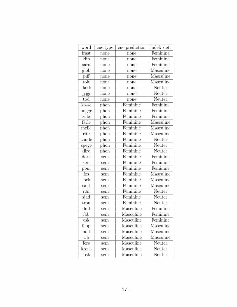
word cue.type cue.prediction indef. det.frast none none Feminineklin none none Femininesarn none none Feminineglob none none Masculinepiff none none Masculinerolt none none Masculine
dakk none none Neuterjygg none none Neutertod none none Neuter
kosse phon Feminine Femininebugge phon Feminine Femininetylbe phon Feminine Femininefarle phon Feminine Masculinemelle phon Feminine Masculinerite phon Feminine Masculine
kande phon Feminine Neuterspege phon Feminine Neuterdire phon Feminine Neuterdork sem Feminine Femininekert sem Feminine Femininepom sem Feminine Feminineføs sem Feminine Masculinelork sem Feminine Masculinesælt sem Feminine Masculinerøn sem Feminine Neutersjad sem Feminine Neutertron sem Feminine Neuterduff sem Masculine Femininefab sem Masculine Feminineosk sem Masculine Femininefepp sem Masculine Masculinenoff sem Masculine Masculinetib sem Masculine Masculinefers sem Masculine Neuter
krens sem Masculine Neuterlosk sem Masculine Neuter
271

Appendix F
Materials used in Filler-Gap
experiments
F.1 Verbs (participants)
1. Bump (white dog, cat, brown dog)
2. Kiss (brown monkey, goose, black monkey)
3. Hug (frog with hat, bear, frog with scarf)
4. Wash (brown monkey, elephant, black monkey)
5. Tickle (white mouse, bee, gray mouse)
6. Feed (frog with hat, elephant, frog with scarf)
272
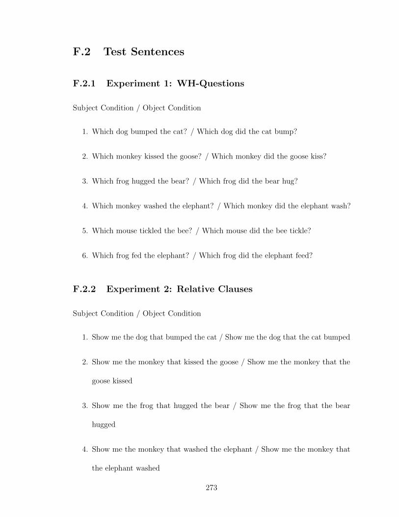
F.2 Test Sentences
F.2.1 Experiment 1: WH-Questions
Subject Condition / Object Condition
1. Which dog bumped the cat? / Which dog did the cat bump?
2. Which monkey kissed the goose? / Which monkey did the goose kiss?
3. Which frog hugged the bear? / Which frog did the bear hug?
4. Which monkey washed the elephant? / Which monkey did the elephant wash?
5. Which mouse tickled the bee? / Which mouse did the bee tickle?
6. Which frog fed the elephant? / Which frog did the elephant feed?
F.2.2 Experiment 2: Relative Clauses
Subject Condition / Object Condition
1. Show me the dog that bumped the cat / Show me the dog that the cat bumped
2. Show me the monkey that kissed the goose / Show me the monkey that the
goose kissed
3. Show me the frog that hugged the bear / Show me the frog that the bear
hugged
4. Show me the monkey that washed the elephant / Show me the monkey that
the elephant washed
273

5. Show me the mouse that tickled the bee / Show me the mouse that the bee
tickled
6. Show me the frog that fed the elephant/ Show me the frog the elephant fed
274

References
Anderssen, M. (2006). The acquisition of compositional definiteness in norwegian.
Aoshima, S., Phillips, C., & Weinberg, A. S. (2004). Processing filler-gap dependencies
in a head-final language. Journal of Memory and Language, 51 , 23 – 54.
Austerweil, J. L., & Griffiths, T. L. (2010). Learning hypothesis spaces and dimensions
through concept learning. In Proceedings of the 32nd Annual Conference of the
Cognitive Science Society (pp. 73–78). Austin, TX: Cognitive Science Society.
Baayen, R. H. (2008). Analyzing linguistic data: A practical guide to statistics using
R. Cambridge, UK: Cambridge University Press.
Baker, M. (2005). Mapping the terrain of language learning. Language Learning and
Development , 1 , 93 – 129.
Bates, D. (2007). Fitting linear mixed models in R. R News , 5 , 27 – 30.
Bates, D., & Sarkar, D. (2007). lme4: Linear mixed-effects models using S4 classes.
(R package version 0.99875-6)
Becker, M. (2007). Animacy, expletives, and the learning of the raising-control
distinction. In A. Belikova, L. Meroni, & M. Umeda (Eds.), Proceedings of the
2nd Conference on Generative Approaches to Language Acquisition North America
275

(GALANA) (pp. 12–20). Somerville, MA: Cascadilla.
Berent, I., & Pinker, S. (2007). The dislike of regular plurals in compounds:
Phonological or morphological? The Mental Lexicon, 2 , 129 – 181.
Berent, I., & Pinker, S. (2008). Compound formation is constrained by morphology:
A reply to seidenberg, macdonald & haskell. The Mental Lexicon.
Bergelson, E., & Idsardi, W. J. (2009). Structural biases in phonology: Infant and
adult evidence from artificial language learning. In J. Chandlee, M. Franchini,
S. Lord, & G. M. Rheiner (Eds.), Proceedings of the 33rd annual Boston University
Conference for Language Development (pp. 85 – 96). Somerville, MA: Cascadilla
Press.
Berwick, R. C. (1963). Learning from positive-only examples: The subset principle
and three case studies. In J. G. Carbonell, R. S. Michalski, & T. M. Mitchell
(Eds.), Machine learning: An artificial intelligence approach (vol. 2). Los Altos,
CA: Morgan Kaufmann.
Bokarev, E. A. (1959). Cezskie (didojskie) jazyki dagestana. Moscow-Leningrad:
Nauka.
Booth, A. E., & Waxman, S. R. (2003). Mapping words to the world in infancy:
Infants’ expectations for count nouns and adjectives. Journal of Cognition &
Development , 4 , 357–381.
Booth, A. E., & Waxman, S. R. (2009). A horse of a different color: Specifying
with precision infants’ mappings of novel nouns and adjectives. Child Development ,
80 (1), 15–22.
Braine, M. D. S. (1987). What is learned in acquiring word classes - a step toward an
276
acquisition theory. In B. MacWhinney (Ed.), Mechanisms of language acquisition.
Hillsdale, NJ: Lawrence Erlbaum.
Chomsky, N. (1965). Aspects of the theory of syntax. Cambridge, MA: MIT Press.
Chomsky, N. (1973). Conditions on transformations. In S. Anderson & P. Kiparsky
(Eds.), A festschrift for Morris Halle (pp. 232–286). New York, NY: Rinehart &
Winston.
Chomsky, N. (1977). On wh-movement. In P. Culicover, T. Wasow, & A. Akmajian
(Eds.), Formal syntax. New York, NY: Academic Press.
Chomsky, N. (1980). Rules and representations. Oxford: Basil Blackwell.
Chomsky, N. (1981). Lectures on government and binding. The Hague: Mouton.
Chomsky, N. (1986). Knowledge of language. New York, NY: Praeger.
Chomsky, N., & Halle, M. (1968). The sound pattern of english. New York, NY:
Harper and Row.
Chomsky, N., & Lasnik, H. (1977). Filters and control. Linguistic Inquiry , 8 , 425 –
504.
Chung, S., & McCloskey, J. (1983). On the interpretation of certain island facts in
hpsg. Linguistic Inquiry , 14 , 704 – 713.
Clifton, C., Traxler, M. J., Mohamed, M. T., Williams, R. S., Morris, R. K., &
Rayner, K. (2003). The use of thematic role information in parsing: Syntactic
processing autonomy revisited. Journal of Memory and Language, 49 , 317 – 334.
Colunga, E., & Smith, L. B. (2005). From the lexicon to expectations about kinds:
A role for associative learning. Psychological Review , 112 , 347–382.
Comrie, B. (2007). Tsez (Dido) morphology. In A. S. Kaye (Ed.), Morphologies of
277
Asia and Africa. Winona Lake, IN: Eisenbrauns.
Comrie, B., & Polinsky, M. (1998). The great Daghestanian case hoax. In A. Siewier-
ska & J. J. Song (Eds.), Case, typology and grammar: In honor of Barry J. Blake.
Amsterdam: John Benjamins.
Comrie, B., & Polinsky, M. (1999). Some observations on class categorization in
Tsez. In H. V. den Berg (Ed.), Studies in Caucasian linguistics: Selected papers of
the eighth caucasian colloquium. The Netherlands: Universitat Leiden.
Comrie, B., Polinsky, M., & Rajabov, R. (1998). Tsezian languages. Max Planck
Institute for Evolutionary Anthropology. (unpublished m.s.)
Conroy, A., Takahashi, E., Lidz, J., & Phillips, C. (2009). Equal treatment for all
antecedents: How children succeed with Principle B. Linguistic Inquiry , 40 , 446 –
486.
Corbett, G. (1991). Gender. Cambridge: Cambridge University Press.
Crain, S. (1991). Language acquisition in the absence of experience. Behavioral and
Brain Sciences , 4 , 597 – 650.
Crain, S., & Fodor, J. D. (1985). How can grammars help parsers? In D. Dowty,
D. Kartunnen, & A. M. Zwicky (Eds.), Natural language parsing: psycholinguis-
tic, computational, and theoretical perspectives (pp. 94–128). Cambridge, UK:
Cambridge Univerisity Press.
Crain, S., & Nakayama, M. (1987). Structure dependence in grammar formation.
Language, 63 , 522 – 543.
Cyr, M., & Shi, R. (in press). Development of abstract grammatical categorization
in infants. Child Development .
278
Dale, P., & Fenson, L. (1996). Lexical development norms for young children.
Behavior Research Methods, Instruments, & Computers , 28 , 125–127.
deVilliers, J., & Roeper, T. (1995). Relative Clauses are barriers to wh-movement
for young children. Journal of Child Language, 22 , 389 – 404.
deVilliers, J., Roeper, T., & Vainikka, A. (1990). The acquisition of long distance rules.
In L. Frazier & J. deVilliers (Eds.), Language processing and language acquisition
(pp. 257–297). Dordrecht, The Netherlands: Kluwer Academic Publishers.
deVilliers, J. G., & Gxilishe, S. (2009). The acquisition of number agreement in
English and Xhosa. In J. M. Brueart, A. Gavarro, & J. Sola (Eds.), Merging
features: Computation, interpretation and acquisition. London: Oxford University
Press.
Elman, J. L., Bates, E. A., Johnson, M. H., Karmiloff-Smith, A., Parisi, D., &
Plunkett, K. (1996). Rethinking innateness: A connectionist perspective on
development. Cambridge, MA: MIT Press.
Fellbaum, C. (Ed.). (1998). WordNet: An electronic lexical database. Cambridge,
MA: MIT Press.
Fenson, L., Dale, P. S., Reznick, J. S., Thal, D., Bates, E., Hartung, J. P., et al.
(1993). The macarthur communicative development inventories: User’s guide and
technical manual. Baltimore, MD: Paul H. Brokes Publishing Co.
Ferreira, F., Ferraro, V., & Bailey, K. G. D. (2002). Good-enough representations
in language comprehension. Current Directions in Psychological Science, 11 , 11 –
15.
Fiebach, C., Schlesewsky, M., & Friederici, A. (2002). Separating syntactic memory
279
costs and syntactic integration costs during parsing: The processing of German
wh-questions. Journal of Memory and Language, 47 , 250 – 272.
Fisher, C. (2003). Structural limits on verb mapping: The role of abstract structure.
Developmental Science, 2 (5), 555 – 564.
Fodor, J. A. (1975). The language of thought. Cambridge, MA: Harvard University
Press.
Fodor, J. D., & Sakas, W. G. (2004). Evaluating models of parameter setting.
In Proceedings of the 28th Annual Boston University Conference on Language
Development (pp. 1–27). Boston, MA: Cascadilla Press.
Fodor, J. D., & Sakas, W. G. (2005). The Subset Principle in syntax: Costs of
compliance. Journal of Linguistics , 41 , 513 - 569.
Frank, M. C., Goodman, N. D., & Tenenbaum, J. (2009). Using speakers’ referential
intentions to model early cross-situational word learning. Psychological Science,
20 , 579–585.
Frazier, L., & d’Arcais, G. B. F. (1989). Filler-driven parsing: A study of gap filling
in Dutch. Journal of Memory and Language, 28 , 331 – 344.
Frazier, L., & Jr., C. C. (1989). Successive cyclicity in the grammar and the parser.
Language and Cognitive Processes , 4 , 93 – 126.
Frigo, L., & McDonald, J. (1998). Properties of phonological markers that affect
the acquisition of gender-like subclasses. Journal of Memory and Language, 39 ,
218–245.
Gagliardi, A., & Lidz, J. (2010). Morphosyntactic cues impact filler-gap dependency
resolution in 20- and 30-month-olds. (Paper presented at the 2010 Boston University
280
Conference on Language Development)
George, L. (1980). Analogical generalization in natural language syntax. Unpublished
doctoral dissertation, MIT.
Gerken, L., Wilson, R., Gomez, R. L., & Nurmsoo, E. (2002). Linguistic category
induction without reference: the importance of correlated cue. (unpublished m.s.)
Gerken, L., Wilson, R., & Lewis, W. (2005). Infants can use distributional cues to
form syntactic categories. Journal of Child Language, 32 , 249 – 268.
Gibson, E. (1998). Linguistic complexity: Locality of syntactic dependencies.
Cognition, 68 , 1 – 76.
Gibson, E., & Wexler, K. (1994). Triggers. Linguistic Inquiry , 25 , 407 – 454.
Gold, E. M. (1967). Language identification in the limit. Information and Control ,
10 , 447 – 474.
Golinkoff, R. M., Hirsh-Pasek, K., Mervis, C. B., Frawley, W., & Parillo, M. (1995).
Lexical principles can be extended to the acquisition of verbs. In M. Tomasello
& W. Merriman (Eds.), Beyond names for things: Young children’s acquisition of
verbs (pp. 185–222). Hillsdale, NJ: Lawrence Earlbaum.
Gomez, R. L., & Maye, J. (2005). The developmental trajectory of nonadjacent
dependency learning. Infancy , 7 , 183 – 206.
Goodluck, H. (2010). Object extraction is not subject to child relativized minimality.
Lingua, 120 (6), 1516 – 1521.
Goodman, N. D., Tenenbaum, J. B., Feldman, J., & Griffiths, T. L. (2008). A
rational analysis of rule-based concept learning. Cognitive Science, 32 , 108–154.
Gordon, P. C., Hendrick, R., & Johnson, M. (2001). Memory interference during
281
language processing. Journal of Experimental Psychology: Learning, Memory and
Cognition, 27 , 1411 – 1423.
Goro, T. (2007). Language-specific constraints on scope interpretation in first
language acquisition. Unpublished doctoral dissertation, University of Maryland.
Gxilishe, S., Smouse, M., Xhalisa, T., & deVilliers, J. G. (2009). Children’s
insensitivity to information from the target of agreement: the case of Xhosa.
In Proceedings of the 3rd GALANA Conference (pp. 46–53). Somerville, MA:
Cascadilla Press.
Halle, M., & Mohanan, K. P. (1985). Segmental phonology of modern english.
Linguistic Inquiry , 16 (1), 57 – 116.
Hamburger, H., & Crain, S. (1982). Relative acquisition. In S. Kuczaj (Ed.), Lan-
guage development: Syntax and semantics (pp. 245–274). Hillsdale, NJ: Lawrence
Earlbaum.
Harris, Z. (1951). Methods in structural linguistics. Chicago, IL: The University of
Chicago Press.
Hay, J. B., & Baayen, R. H. (2005). Shifting paradigms: Gradient structure in
morphology. Trends in Cognitive Science, 9 , 342 – 348.
Hochmann, J. R., Endress, A. D., & Mehler, J. (2010). Word frequency as a cue for
identifying function words in infancy. Cognition, 115 (3), 444 – 457.
Hoff, E. (2003). The specificity of environmental influence: socioeconomic status
affects early vocabulary development via maternal speech. Child Development , 74 ,
1368 – 1378.
Hollich, G. (2005). Supercoder: A program for coding preferential looking (Version
282
1.5). West Lafayette, IN. (Computer Software)
Hudson-Kam, C. L., & Newport, E. L. (2009). Getting it right by getting it wrong:
When learners change languages. Cognitive Psychology , 59 , 30–66.
Hunt, E. B., Marin, J., & Stone, P. J. (1966). Experiments in induction. New York,
NY: Academic Press.
J. Lidz, H. G., & Gleitman, L. (2003). Understanding how input matters: The
footprint of universal grammar on verb learning. Cognition, 87 , 151 – 178.
Karmiloff-Smith, A. (1979). A functional approach to child language: A study of
determiners. Cambridge: Cambridge University Press.
Kazanina, N., & Phillips, C. (2001). Coreference in child Russian: Distinguishing
syntactic and discourse constraints. In A. H.-J. Do, L. Dominguez, & A. Johansen
(Eds.), Proceedings of the 25th annual Boston University Conference for Language
Development (pp. 413 – 424). Somerville, MA: Cascadilla Press.
Khalilov, M. S. (1999). Tsezsko-russkij slovar’. Moscow: Academia.
Konieczny, L. (2000). Locality and parsing complexity. Journal of Psycholinguistic
Research, 30 , 627 – 645.
Lidz, J. (2011). Grammar-parser interactions in the acquisition of syntax. In Y. Otsu
(Ed.), Proceedings of the Twelfth Tokyo Conference on Psycholinguistics. Tokyo:
HItuzi Syobo Publishing.
Lidz, J., & Gagliardi, A. (2012). Inside the language acquisition device: Learning in
generative grammar. (submitted)
Lidz, J., & Musolino, J. (2006). On the quantificational status of indefinites: The
view from child language. Language Acquisition, 13 , 73 – 102.
283

Lightfoot, D. (1989). The child’s trigger experience: Degree-0 learnability. Behavioral
& Brain Sciences , 12 (2), 321 – 334.
Lin, J. (1991). Divergence measures based on the Shannon entropy. IEEE Trans. on
Information Theory , 37 (1), 145 – 151.
Lukyanenko, C., Conroy, A., & Lidz, J. (n.d.). Infants’ adherence to principle c:
Evidence from 30-month-olds. (submitted)
MacWhinney, B. (1978). The acquisition of morphophonology. In Monographs of
the society for research in child development. United Kingdom: Blackwell.
Mak, W. M., Wonk, W., & Schriefers, H. (2002). The influence of animacy on
relative clause processing. Journal of Memory and Language, 30 , 580 – 602.
Maye, J., Werker, J. F., & Gerken, L. (2002). Infant sensitivity to distributional
information can affect phonetic discrimination. Cognition, 82 , B101 – B111.
Merriman, W. E., & Bowman, L. L. (1989). The mutual exclusivity bias in chil-
dren’s word learning (Vol. 54). Monographs of the Society for Research in Child
Development.
Mills, A. E. (1985). The acquisition of German. In D. Slobin (Ed.), The crosslinguistic
study of language acquisition, volume 1. Hillsdale, NJ: Lawrence Erlbaum.
Mills, A. E. (1986). The acquisition of gender: A study of English and German.
Berlin: Springer.
Mintz, T. H. (2003). Frequent frames as a cue for grammatical categories in child
directed speech. Cognition, 90 , 91 – 117.
Mitnz, T. H. (2005). Linguistic and conceptual influences on adjective acquisition in
24- and 36-month-olds. Developmental Psychology , 41 , 17 – 29.
284
Morgan, J. L., Meier, R. P., & Newport, E. L. (1989). Facilitating the acquisition
of syntax with cross-sentential cues to phrase structure. Journal of Memory and
Language, 28 , 360 – 374.
Naigles, L. (1990). Children use syntax to learn verb meanings. Journal of Child
Language, 17 (2), 357 – 374.
Omaki, A. (2010). Commitment and flexibility in the developing parser. Unpublished
doctoral dissertation, University of Maryland.
Pearl, L., & Lidz, J. (2009). When domain general learning fails and when it
succeeds: Identifying the contribution of domain specificity. Language Learning
and Development , 5 (4), 235 – 265.
Perez-Pereira, M. (1991). The acquisition of gender: What Spanish children tell us.
Journal of Child Language, 18 (3), 571 – 590.
Pinker, S. (1979). Formal models of language learning. Cognition, 7 , 217 – 283.
Pinker, S. (1984). Language learnability and language development. Cambridge, MA:
Harvard University Press.
Pinker, S. (1989). Learnability and cognition: The acquisition of argument structure.
Cambridge, MA: MIT Press.
Pinker, S. (1991). Rules of language. Science, 253 , 530 – 535.
Pinker, S., & Prince, A. (1988). On language and connectionism: Analysis of a
parallel distributed processing model of language acquisition. Cognition, 28 , 73 –
193.
Plaster, K., Polinsky, M., & Harizanov, B. (2009). Noun classes grow on trees: Noun
classification in the North-East Caucasus. (unpublished m.s.)
285
Polinsky, M. (2000). Tsez beginnings. In Papers from the 25th Annual Meeting of
the Berkeley Linguistics Society (pp. 14–29).
Polinsky, M., & Jackson, D. (1999). Noun classes: Language change and learning. In
B. Fox, D. Jurafksy, & L. A. Michaelis (Eds.), Cognition and function in language.
Chicago, IL: University of Chicago Press.
Quinlan, J. R. (1993). C4.5: Programs for machine learning. San Mateo, CA:
Morgan Kaufman.
Radford, A. (1990). Syntactic theory and the acquisition of English syntax. Cambridge,
UK: Basil Blackwell.
Regier, T. (2005). The emergence of words: Attentional learning in form and
meaning. Cognitive Science, 29 , 819–865.
Rizzi, L. (1990). Relativized minimality. Cambridge, MA: MIT Press.
Rodina, Y., & Westergaard, M. (2012). A cue-based approach to the acquisition of
grammatical gender in Russian. Journal of Child Language, 1–30.
Roeper, T., & deVilliers, J. G. (1994). Lexical links in the wh-chain. In B. Lust,
G. Hermon, & J. Kornfilt (Eds.), Syntactic theory and first language acquisition:
Cross linguistic perspectives Volume ii: Binding, dependencies and learnability.
Cambridge, MA: Lawrence Earlbaum.
Ross, J. R. (1967). Constraints on variables in syntax. Unpublished doctoral
dissertation, MIT.
Rumelhart, D. E., & McClelland, J. L. (1987). Learning the past tenses of En-
glish verbs: Implicit rules or parallel distributed processing. In B. MacWhinney
(Ed.), Mechanisms of language acquisition (pp. 194–248). Mahwah, NJ: Lawrence
286
Erlbaum.
Saffran, J. (2001). The use of predictive dependencies in language learning. Journal
of Memory and Language, 44 , 493 – 515.
Saffran, J., Newport, E. L., & Aslin, R. N. (1996). Word segmentation: The role of
distributional cues. Journal of Memory and Language, 35 , 606 – 621.
Seidenberg, M. S., Macdonald, M. C., & Haskell, T. R. (2007). Semantics and
phonology constrain compound formation. The Mental Lexicon, 2 , 287 – 312.
Seidl, A., Hollich, G., & Jusczyk, P. (2003). Early understanding of subject and
object wh-questions. Infancy , 4 , 423 – 436.
Siskind, J. M. (1996). A computational study of cross-situational techniques for
learning word-to-meaning mappings. Cognition, 61 , 39–91.
Smith, K., & Wonnacott, E. (2010). Eliminating unpredictable variation through
iterated learning. Cognition, 116 (3), 444 - 449.
Smith, K. H. (1966). Grammatical intrusions in the recall of structures letter pairs:
Mediated transfer or position learning? Journal of Experimental Psychology , 72 ,
580 - 588.
Smouse, M. (2011). Uninterpretable features in comprehension: Subject-verb agree-
ment in Xhosa. (submitted)
Snyder, W. (2007). Child language: The parametric approach. Oxford, UK: Oxford
University Press.
Stowe, L. (1986). Parsing wh-constructions: evidence for on-line gap location.
Language and Cognitive Processes , 1 , 227 – 246.
Stromswold, K. (1995). The acquisition of subject and object wh-questions. Language
287
Acquisition, 4 , 5 – 48.
Sussman, R., & Sedivy, J. (2003). The time course of processing syntactic dependen-
cies. Language and Cognitive Processes , 18 , 143 – 163.
Tang, P. N., Steinbach, M., & Kumar, V. (2005). Introduction to data mining.
Boston, MA: Addison-Wesley Longman Publishing Co., Inc.
Tavakolian, S. L. (1981). The conjoined-clause analysis of relative clauses. In
S. L. Tavakolian (Ed.), Language acquisition and linguistic theory (pp. 167–187).
Cambridge, MA: MIT Press.
Team, R. D. C. (2008). R: A language and environment for statistical computing.
Available from http://www.R-project.org
Thornton, R. (1995). Referentiaity and wh-movement in child English: Juvenile
d-linkuency. Language Acquisition, 4 , 139 – 175.
Townsend, D., & Bever, T. G. (2001). Sentence comprehension: The integration of
habits and rules. Cambridge, MA: MIT Press.
Traxler, M. J., Morris, R. K., & Seely, R. E. (2002). Processing subject and object
relative clauses: Evidence from eye movements. Journal of Memory and Language,
47 , 69 – 90.
Traxler, M. J., & Pickering, M. J. (1996). Plausibility and the processing of
unbounded dependencies. Journal of Memory and Language, 35 , 454 – 475.
Trosterud, T. (2001). Genus i Norsk i regelstyrt. Norsk Lingvistik Tidsskirft , 19 ,
29–58.
Tucker, G. R., Lambert, W. E., & Rigault, A. (1977). The French speaker’s skill with
grammatical gender: An example of rule governed behavior. The Hague: Mouton.
288

Viau, J., & Lidz, J. (2011). Selective learning in the acquisition of kannada
ditransitives. Language, 87 , 679 – 714.
Wanner, E., & Maratsos, M. (1978). An ATN approach to comprehension. In
M. Halle, J. Bresnan, & G. A. Miller (Eds.), Linguistic theory and psychological
reality. Cambridge, MA: MIT Press.
Waxman, S. R., & Booth, A. E. (2003). The origins and evolution of links between
word learning and conceptual organization: New evidence from 11-month-olds.
Developmental Science, 6 (2), 130–137.
Waxman, S. R., & Markow, D. B. (1998). Object properties and object kind:
Twenty-one-month-old infants’ extension of novel adjectives. Child Development ,
69 , 1313–1329.
Wexler, K., & Culicover, P. (1980). Formal principles of language acquisition.
Cambridge, MA: MIT Press.
Witten, I. H., & Frank, E. (2005). Data mining: Practical machine learning tools
and techniques. San Francisco, CA: Morgan Kaufmann.
Xu, F., & Tenenbaum, J. B. (2007). Word learning as Bayesian inference. Psycho-
logical Review , 114 (2), 245–272.
Yang, C. (2002). Knowledge and learning in natural language. Oxford: Oxford
University Press.
Yang, C. D. (2004). Universal grammar, statistics or both? Trends in Cognitive
Sciences , 8 (10), 451 – 456.
289