Abstract This paper estimates the size of the union membership wage premium by comparing wage outcomes for unionised workers with ‘matched’ non-unionised workers. The method assumes selection on observables. For this identifying assumption to be plausible, one must be able to control for all characteristics affecting both union status and wages. This requires very informative data. We illustrate the value of the rich data offered by the linked employer-employee Workplace Employee Relations Survey (WERS) 1998 in implementing this methodology. We estimate the union membership premium for the whole private sector, among workers in workplaces where at least some workers are covered by collective bargaining, and in occupations with pay set by collective bargaining. We find a raw 17-25% union premium in gross hourly wages for the private sector in Britain, depending on the sub-group used. However, post-matching this difference falls to between 3% and 6%. This indicates that the higher pay of unionised workers is largely accounted for by their better underlying earnings capacity, which is associated with their individual characteristics, the jobs they do and the workplaces they find themselves in. Key words: trade unions, wage premium, treatment effect, matching, propensity score JEL classification: C14, C81, J31, J51 This paper was produced under the ‘Future of Trade Unions in Modern Britain’ Programme supported by the Leverhulme Trust. The Centre for Economic Performance acknowledges with thanks, the generosity of the Trust. For more information concerning this Programme please e-mail futureoftradeunions@lse.ac.uk Acknowledgements I would like to thank participants at a PSI seminar in London and participants at the Third WERS98 Users Group Seminar for useful comments on the first draft of this paper. I acknowledge the Department of Trade and Industry, the Economic and Social Research Council, the Advisory, Conciliation and Arbitration Service and the Policy Studies Institute as the originators of the 1998 Workplace Employee Relations Survey data, and the Data Archive at the University of Essex as the distributor of the data. None of these organizations or individuals bears any responsibility for the author’s analysis and interpretations of the data.

Alex Bryson is a member of the Policy Studies Institute, London and a Research Associate at the Centre for Economic Performance, London School of Economics. Contact: a.bryson@psi.org.uk Published by Centre for Economic Performance London School of Economics and Political Science Houghton Street London WC2A 2AE Alex Bryson, submitted January 2002 ISBN 0 7530 1551 X Individual copy price: £5

The Union Membership Wage Premium: An Analysis Using Propensity Score Matching

Alex Bryson

May 2002

1. Introduction 1

2. Causal Inference Through Statistical Matching 3

3. Data 8

3.1 The dependent variable 11

4. Empirical Implementation of Matching 12

5. Results 16

5.1 Is the membership premium among covered employees explained by members’ employment in conditions where unions are better able to extract rents? 18

6. Conclusions 21

Appendix Tables 25

References 32

The Centre for Economic Performance is financed by the Economic and Social Research Council.

1

1. Introduction

This paper addresses the question: how much of the wage differential between union

members and non-members is attributable to union membership, and how much is due to

differences in personal, job and workplace characteristics across members and non-members?

The question is prompted by two recent developments, one substantive, and one

methodological.

The substantive development is the apparent decline in the union membership

premium in Britain in the 1990s. Studies for the United States and Britain have traditionally

found union members’ earnings to be 10-20% higher than non-members’. However,

Machin’s (2001) analysis of longitudinal data from the British Household Panel Survey

(BHPS), indicates that, although there was a wage gain for people moving into union jobs in

the early 1990s, this had disappeared by the late 1990s. The findings complement workplace-

level analyses which indicate that, on average, there was no union wage premium in the

private sector by 1998 arising from workplace bargaining coverage (Forth and Millward,

2000a) and that union-bargained pay settlements in the period 1997-98 were no higher than

settlements which did not involve unions (Forth and Millward, 2000b). Our analysis

contributes to the body of knowledge about the size of the union membership premium by the

late 1990s.

The methodological development is the advent of new data and relatively new

estimation techniques permitting a fresh look at the nature of the union wage premium. The

membership differential is often attributed to the rent-seeking behaviour of unions who,

through negotiation with employers, are able to procure a wage premium for their members.

However, studies also find a membership premium even among workers whose pay is set

through collective bargaining (‘covered workers’). In explaining this phenomenon, some

have argued that employers may conspire to pay lower wages to covered non-members than

to members in return for union co-operation, since this may increase the size of the surplus to

be shared between workers and the firm (eg. Blakemore et al., 1986). However, even if this

sort of collusion occurs in some cases, it seems unlikely that this could account for the size of

membership differentials identified in the literature. Since there appear to be no obvious

mechanisms by which members should command higher wages than non-members other than

coverage, the membership premium may be accounted for by unobserved differences

between members and non-members which boost members’ relative earnings. Biases in

2

estimates of the union membership premium may be accounted for by data deficiencies and,

in particular, the paucity of employer controls in the household and employee data sets often

used to generate them. For instance, the membership premium among covered workers could

be explained if the union differential is positively correlated with union density since the

conditional probability of high density given membership is higher than that given coverage.

We address this deficiency in employer controls with linked employer-employee data in the

Workplace Employee Relations Survey 1998 (WERS). As well as information on individual

employees’ union membership, WERS contains rich information on the employer, including

pay bargaining arrangements at workplace and occupational level.

A second possible source of bias in the estimates of union membership effects on

wages is the potential endogeneity of union status if membership is governed by a selection

process. Following Farber (2001), there are two possible selection processes. The first is

‘worker choice’ in which workers only choose membership if the union wage is greater than

the wage available to the individual outside the union. It is often assumed that workers with a

lower underlying earning capacity have more to gain from membership than higher quality

workers, in which case this selection process will understate the union wage premium. The

second selection process arises through ‘queuing’ since not all workers desiring union

employment can find union jobs (see Bryson and Gomez, 2002 for empirical validation of

this model in Britain). Under this model, union employers may choose the best of the

workers among those desirous of a union job. This employer selection implies a positive bias

in the union premium but, a priori, it is not clear whether this bias is greater or less than the

negative bias implied by worker selection. Either way, if there is endogenous selection the

membership mark up estimated using standard cross-sectional regression techniques ‘can be

interpreted as the average difference in wages between union and non-union workers, but it

can not be interpreted as the effect of union membership on the wage of a particular worker’

(Farber, 2001: 11). Causal inference is problematic because, where workers who become

members differ systematically from those who do not become members in ways which might

affect their earnings independent of membership, we can not infer the non-union wage for

union members simply by comparing union members’ wages with those of non-members. In

the literature for the United States, the problem of selection bias is usually tackled by

modelling union status determination simultaneously with earnings and estimating an

econometric model that takes account of the simultaneity. This usually involves a Heckman

estimator where the earnings function and union status determination function are assumed to

have errors that are jointly normal. This technique relies on untestable exclusion restrictions

3

whereby variables assumed to affect union status have no direct effect on earnings. In his

review of the literature, Lewis (1986) concluded that, because of these arbitrary functional

form assumptions and untestable exclusion restrictions, results from these studies were

unreliable. Until recently, the selection problem was usually ignored in the British literature

(Andrews et al., 1998, review this literature). Using panel data for the first half of the 1990s,

Hildreth (1999) accounts for selection into union membership using fixed effects estimation

and finds a large but declining membership premium among covered workers. However,

Booth and Bryan (2001), using the richer employer controls available in WERS, also account

for endogenous selection into membership and find no membership premium in 1998.1

Our analysis takes a different approach. We use a semi-parametric statistical

matching approach known as propensity score matching (Heckman et al., 1999) to compare

wage outcomes for unionised workers with ‘matched’ non-unionised workers to infer the

causal effect of union membership on wages. The method avoids the need for functional form

assumptions and reliance on exclusion restrictions. However, as with all non-experimental

estimators, causal inference relies on an untestable assumption. In this case, the assumption

is that the selection process is captured with observable data. For this key identifying

assumption to be plausible, one must be able to control for all characteristics affecting both

union status and wages. This requires very informative data. We illustrate the value of the

rich data offered by the linked employer-employee Workplace Employee Relations Survey

(WERS) 1998 in implementing this methodology.

The remainder of this paper is set out as follows. Section 2 introduces the propensity

score matching method. Section 3 describes our data. Section 4 describes the empirical

implementation of matching. Section 5 presents results and Section 6 concludes.

2. Causal Inference Through Statistical Matching

To establish whether the union membership wage premium is due to membership, or is due to

systematic differences in personal, job and workplace characteristics across members and

non-members, we need to isolate the causal effect of union membership on wages. Let us

1 They use two methods to tackle endogenous selection. The first method involves substituting a predicted probability of union membership for actual membership status in the wage equation. The second method takes the generalised residuals from a probit estimation of union membership and adds them to the wage equation, along with some instruments that are hypothesised to affect membership but not the unobserved determinants of wages.

4

conceive of union membership as if it were a ‘treatment’ that the individual receives. We

wish to evaluate the causal effect of this treatment (treatment 1) relative to non-membership

(treatment 0) on an outcome variable, Y, gross earnings. Let Y1 be earnings if the individual

received treatment 1 (that is, where the individual is a union member) and Y0 be the earnings

that would result if the same individual received treatment 0 (non-membership). Let us

denote the binary indicator of the treatment actually received as D∈{0,1}, while X is a set of

attributes which are not affected by the treatment (demographic, job and workplace-related).

The effect of treatment 1 on individual i as measured by Y and relative to treatment 0

is:

(1) ? = Y1i – Y0i

which is simply the difference between the individual’s potential outcome if ‘exposed’ to

membership and the individual’s potential outcome from non-membership. To estimate the

impact of membership on members’ earnings, it is necessary to know what the outcome

would have been if the individual had not been a member. The problem is that we can not

observe the counterfactual, namely the outcome which would have resulted if an individual

had made an alternative choice (that is, if members had chosen non-membership, and vice

versa). Either Y1i or Y0i is missing for each i . Thus our problem is one of estimating

missing data. This counterfactual cannot be inferred directly from the outcomes of non-

members since they are likely to differ substantially in their characteristics from members.

To overcome this selection problem, researchers must choose from a range of evaluation

methods, the choice being determined by a number of factors including the richness of the

data and the nature of the treatment. Because it is impossible to observe the individual

treatment effect, each method relies on generally untestable assumptions to make causal

inferences (Holland, 1986). In order to identify individual treatment effects, it is necessary to

make very strong assumptions about the joint distribution of Y1i and Y0i . However, the

average treatment effect at the population or sub-population level can be identified under

generally less stringent assumptions, some of which are set out below. Among the

parameters that only depend on the marginal distributions of Y1i and Y0i is the parameter

most commonly estimated and the one estimated in this paper, namely the mean impact of

treatment on the treated:

5

(2) θ = E(Y1 – Y0 | D = 1, X)

= E(Y1 | D = 1, X) - E(Y0 | D = 1, X)

where D=1 denotes treatment (membership), D=0 denotes non-treatment (non-membership)

and X is a set of conditioning variables. In assessing the expected treatment effect for

individuals who are union members, we are addressing the question of how members’

earnings compare with what they would have received had they not been members, on

average.2

For members we observe Y1 so that the average observed outcome for participants is

an unbiased estimate of the first component of the effect of treatment on the treated E(Y1 | D

= 1, X). The evaluation problem arises from the term E(Y0 | D = 1, X). This is the mean of

the counterfactual which, since it is unobservable, must be identified and estimated on the

basis of some usually untestable identifying assumptions justifying the use of the observable

pairs (Y1 , D = 1) , (Y0 , D = 0).

As noted above, members may not be a random sample of all employees. If there are

systematic differences in characteristics across members and non-members that are likely to

influence earnings, failure to take account of these will bias any estimate of the union

membership effect on earnings. Thus, E(Y1 | D = 1) - E(Y0 | D = 0) would in general be

biased for the effect of treatment on the treated. An exception is when the independence

assumption Y0 ? D can be invoked. This is credible where the random assignment of

individuals to treatment ensures that potential outcomes are independent of treatment status.

In this situation, E(Y0 | D = 1) = E(Y0 | D = 0) = E(Y | D = 0) so that the treatment effect can

be consistently estimated by the difference between the observed mean of the outcome

variable for the treatment group and the observed mean for the non-treatment group.

In the absence of random assignment, one option is to construct a comparison group

based on statistical matching. Matching estimators try to resemble an experiment by

choosing a comparison group from all non-participants such that the selected group is as

similar as possible to the treatment group in observable characteristics. Matching can yield

unbiased estimates of the treatment impact where differences between individuals affecting

the outcome of interest are captured in their observed attributes. This assumption, which is

2 To obtain the average treatment effect on the non-treated E(Y1 - Y0 | D = 0) the procedure is applied symmetrically. The average treatment effect E(Y1 - Y0) is a weighted average of the treatment effects for the treated and non-treated.

6

often referred to as the Conditional Independence Assumption (CIA), is the key identifying

assumption underpinning the matching methodology. The precise form of the CIA depends

on the parameter being estimated. For the treatment on the treated parameter, the CIA

requires that, conditional on observable characteristics, potential non-treatment outcomes are

independent of treatment participation. Formally,

(3) E(Y0 | X, D = 1) = E(Y0 | X, D = 0)

Thus, CIA requires that the chosen group of matched controls does not differ from the group

of treated by any variable which is systematically linked to the non-participation outcome Y0,

other than on those variables that are used to match them. This permits the use of the

matched non-participants to measure how participants would have fared, on average, had they

not participated.

The plausibility of the CIA depends on the informational richness of the data since the

set of X’s should contain all the variables thought to influence both participation (that is,

membership) and the outcome (earnings) in the absence of participation. We discuss how

likely it is that the CIA is met in this analysis in Sections 4 and 5.

Under CIA,

(4) E(Y1 | D = 1) - E(Y0 | D = 1)

= Ex|D=1{E(Y|X, D = 1) - E(Y|X,D = 0)}

Hence, after adjusting for observable differences, the mean of the no-treatment (potential)

outcome is the same for those receiving treatment as for those not receiving treatment. This

allows non-participants’ outcomes to be used to infer participants’ counterfactual outcomes.

However, this is only valid if there are non-participants for all participants’ values of X (this

is known as the support condition):

(5) 0 < Pr (D = 1 | X ) < 1

This ensures that all treated individuals have a counterpart in the non-treated population for

each X for which we seek to make a comparison. If there are regions where the support of X

does not overlap for the treated and non-treated groups, matching can only be performed, and

7

the treatment parameter, θ, retrieved, over the common support region. If treated individuals

have no support in the non-treated population, they are dropped from analysis and the

estimated treatment effect is redefined as the mean treatment effect for those treated falling

within the common support.

Matching operates by constructing, for those participants with support, a

counterfactual from the non-participants. There are a number of ways of defining this

counterfactual.3 Once the counterfactuals are identified, the mean impact of the programme

can be estimated as the mean difference in the outcomes of the matched pairs.

A refinement to the matching approach was introduced by Rosenbaum and Rubin

(1983). If the CIA is met and there is common support then:

(6) Y0 ? D | P(X) for X in X

where P(X) is the propensity score, the conditional probability of participating in the

programme – in our case, the probability of being a union member – given a vector of

observed characteristics X.4 Formally,

(7) P(Xi) = Pr(Di = 1 | Xi)

Rosenbaum and Rubin show treatment and the observed covariates are conditionally

independent given the propensity score, that is:

(8) Di ? Xi | P(Xi)

The advantage of Rosenbaum and Rubin’s innovation is that the dimensionality of the match

can be reduced to one. Rather than matching on a vector of characteristics, it is possible to

match on just the propensity score. This is because, as Rosenbaum and Rubin show, by

definition treatment and non-treatment observations with the same value of the propensity

score have the same distribution of the full vector of regressors X. Having matched on the

propensity score, the mean impact of the programme is estimated as the mean difference in

the outcomes of the matched pairs.

3 See, for example, Heckman et al., (1997) for a comparison of alternative matching schemes. 4 P(X) is shorthand notation for P(D=1|X) .

8

If the CIA is satisfied, matching offers an attractive means of identifying the impact

of union membership on earnings. The main attraction is that it is non-parametric, avoiding

the need to define a specific form for the outcome equation, selection process or

unobservables in either equation. In addition, it avoids extrapolation beyond the common

support which occurs with simple linear estimators. Heterogeneous treatment effects are

allowed for, so no assumption of constant additive treatment effects for different individuals

is required. Effects for sub-groups can be estimated by running the match on sub-populations

(see Section 5.1). Matching estimators also highlight the problem of common support and

thus the short-comings of parametric techniques which involve extrapolating outside the

common support. Matching is thus able to eliminate two of the three sources of estimation

bias identified by Heckman, Ichimura, Smith and Todd (1998): the bias due to difference in

the supports of X in the treated and control groups (failure of the common support condition)

and the bias due to the difference between the two groups in the distribution of X over its

common support. The other source of bias is the one due to selection on unobservables. This

highlights the importance of the CIA since, if this holds, selection on unobservables ceases to

be a problem. The appropriateness of the CIA is dependent on the richness of the available

data.

3. Data

We use the linked employer-employee data from the Workplace Employee Relations Survey

1998 (WERS). WERS is a nationally representative survey of workplaces with 10 or more

employees covering all sectors of the economy except agriculture (Airey et al, 1999).

We use two elements of the survey. The first is the management interview, conducted

face-to-face with the most senior workplace manager responsible for employee relations.

Interviews were conducted in 2,191 workplaces between October 1997 and June 1999, with a

response rate of 80%. The second element is the survey of employees where a management

interview was obtained. Self-completion questionnaires were distributed to a simple random

sample of 25 employees (or all employees in workplaces with 10-24 employees) in the 1,880

cases where management permitted it. Of the 44,283 questionnaires distributed, 28,237

(64%) usable ones were returned.

The sample of workplaces is a stratified random sample with over-representation of

9

larger workplaces and some industries (Airey et al., 1999). Employees’ probability of

selection for the survey is a product of the probability of their workplace being selected and

the probability of the employee’s own selection. To extrapolate from our analyses to the

population from which the employees were drawn (namely employees in Britain in

workplaces with 10 or more employees) we weight the analysis using the employee weights.5

Our estimating sub-sample is all private sector employees with complete information

on the variables used in the analysis. By estimating the union membership premium for the

whole private sector, we obtain an average return to membership, irrespective of whether the

individual – member or non-member – is covered by collective bargaining. This sample

contains 10,694 non-members and 4,323 members.6

We also exploit the bargaining coverage information in WERS based on management

classifications of the way pay is set for each occupational group in the workplace. The eight

possible responses include collective bargaining at industry, organisation or workplace- level;

from these, we ident ify employees at workplaces where there is collective bargaining for any

occupational group at any level. Estimates of the membership premium for covered workers

defined in this way are based on 2,489 non-members and 3,352 members. W e use the

same information to identify employees whose own occupational group is covered by

collective bargaining at any level. This sample comprises 1,605 non-members and 2,765

members.

Using the survey weights to obtain population estimates, 29% of employees in the

private sector are union members, a similar percentage (28%) belong to a covered

occupation, but 37% are located in a workplace where there is some collective bargaining.

However, only 59% of those employed in covered workplaces are members, and only 65% of

those in covered occupations are members, indicating that between 35% and 41% of covered

workers are free-riders.

5 The weighting scheme used in this paper compensates for sample non-response bias which was detected in the employee survey (Airey et al., 1999: 91-92). 6 Membership is derived from individual employees’ response to the question: ‘Are you a member of a trade union or staff association?’

10

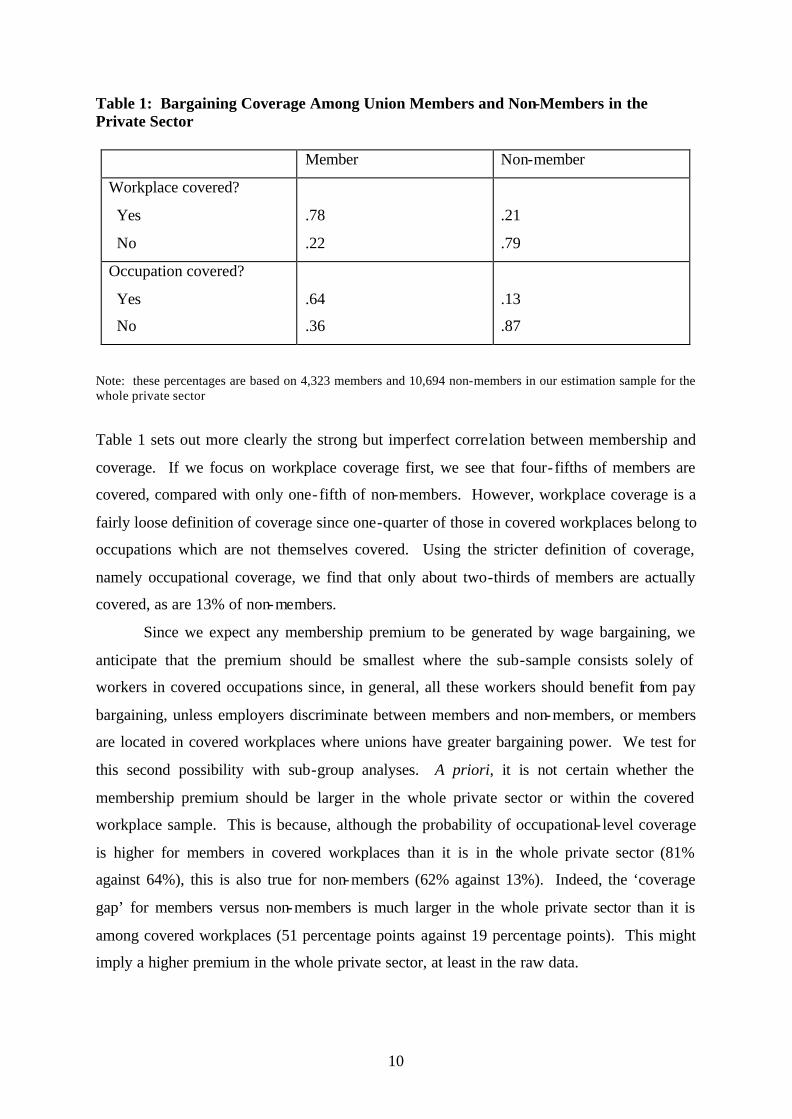
Table 1: Bargaining Coverage Among Union Members and Non-Members in the Private Sector

Member Non-member

Workplace covered?

Yes

No

.78

.22

.21

.79

Occupation covered?

Yes

No

.64

.36

.13

.87

Note: these percentages are based on 4,323 members and 10,694 non-members in our estimation sample for the whole private sector

Table 1 sets out more clearly the strong but imperfect correlation between membership and

coverage. If we focus on workplace coverage first, we see that four- fifths of members are

covered, compared with only one-fifth of non-members. However, workplace coverage is a

fairly loose definition of coverage since one-quarter of those in covered workplaces belong to

occupations which are not themselves covered. Using the stricter definition of coverage,

namely occupational coverage, we find that only about two-thirds of members are actually

covered, as are 13% of non-members.

Since we expect any membership premium to be generated by wage bargaining, we

anticipate that the premium should be smallest where the sub-sample consists solely of

workers in covered occupations since, in general, all these workers should benefit from pay

bargaining, unless employers discriminate between members and non-members, or members

are located in covered workplaces where unions have greater bargaining power. We test for

this second possibility with sub-group analyses. A priori, it is not certain whether the

membership premium should be larger in the whole private sector or within the covered

workplace sample. This is because, although the probability of occupational- level coverage

is higher for members in covered workplaces than it is in the whole private sector (81%

against 64%), this is also true for non-members (62% against 13%). Indeed, the ‘coverage

gap’ for members versus non-members is much larger in the whole private sector than it is

among covered workplaces (51 percentage points against 19 percentage points). This might

imply a higher premium in the whole private sector, at least in the raw data.

11

3.1 The dependent variable

Our dependent variable is log gross hourly wages. Although the employee questionnaire

contains continuous hours data, it only contains banded weekly earnings data, so that we only

know the lower and upper bounds for each individual’s wage. Furthermore, the data are top-

coded so that we only have a lower bound for the highest earners. Therefore, we generate a

predicted hourly wage for each individual using interval regression, a generalisation of the

tobit model for censored data, initially developed by Stewart (1983) for banded earnings

data.7 This estimation was undertaken for each of the three samples (whole private sector,

employees in covered workplaces, and employees in covered occupations). The estimation

for the whole private sector is presented in Appendix Table A1. The purpose of this model is

to generate an accurate estimate of individuals’ actual earnings, which is why union

membership and union recognition enter the equation. As a measure of fit we use the

percentage of employees correctly classified within their original gross weekly earnings

bands once the predicted wage is multiplied by the ir total hours. We find that in 36% of

cases the band is correctly predicted8 and, in 75% of cases, the prediction is exact or within

one earnings band.

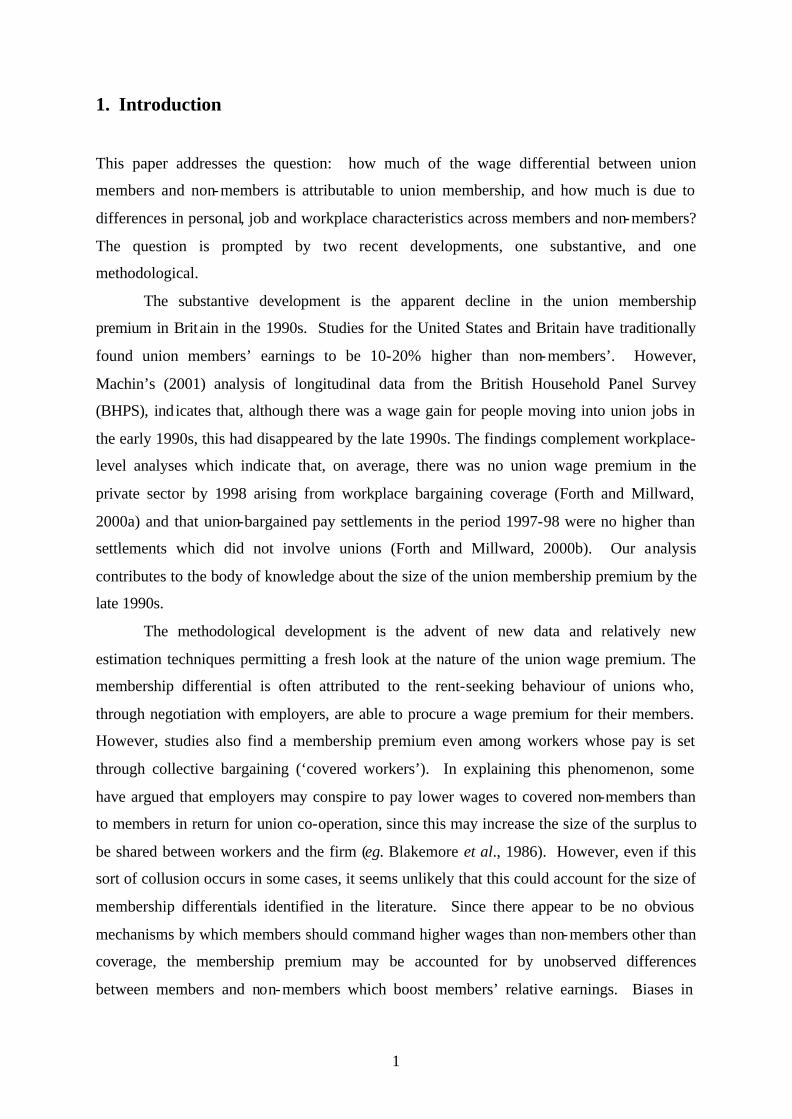
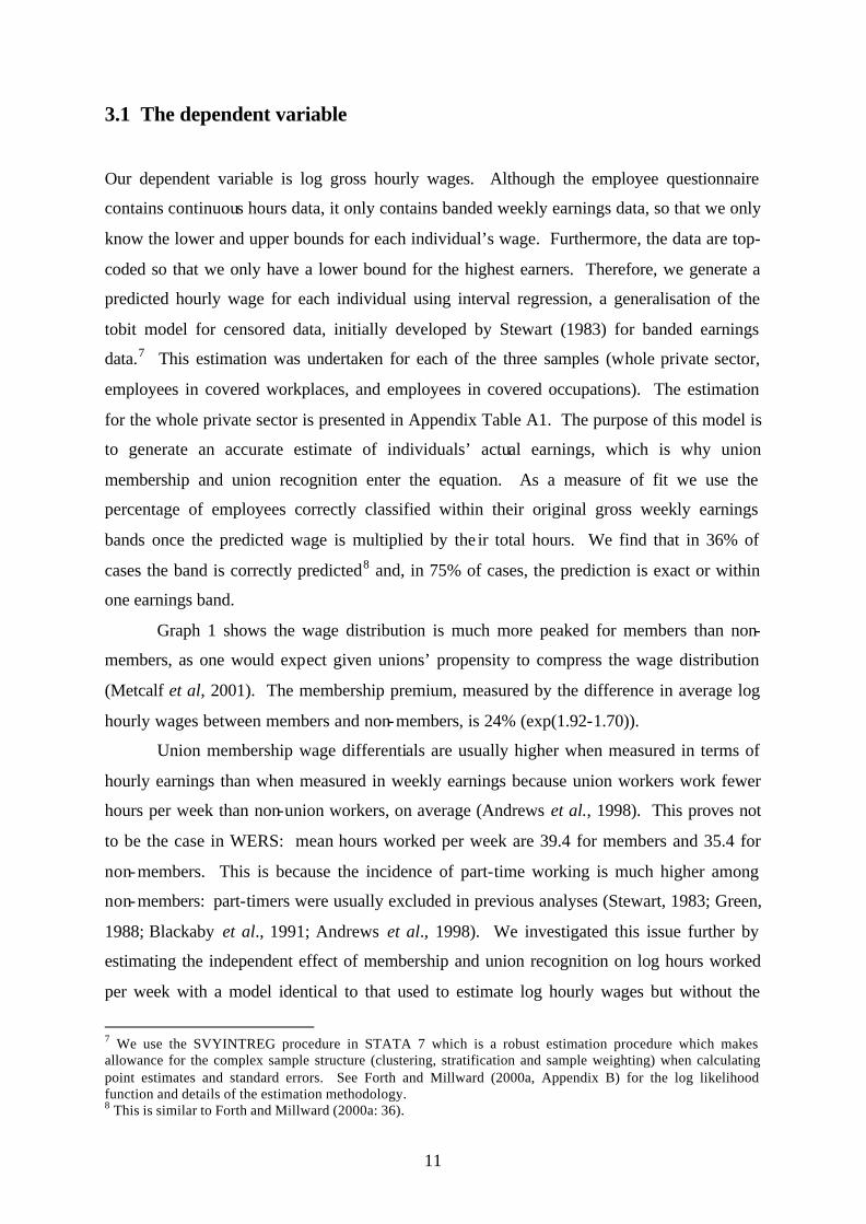
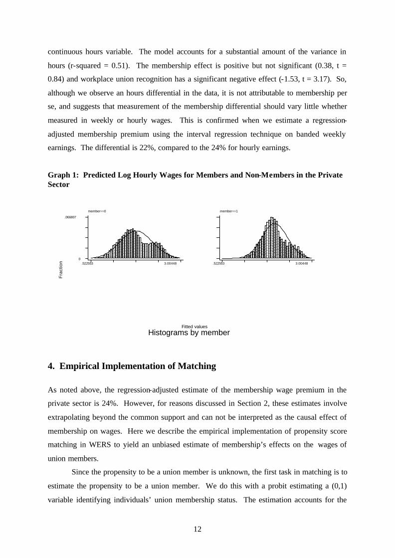
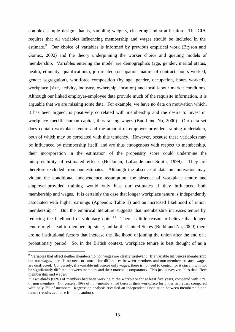
Graph 1 shows the wage distribution is much more peaked for members than non-

members, as one would expect given unions’ propensity to compress the wage distribution

(Metcalf et al, 2001). The membership premium, measured by the difference in average log

hourly wages between members and non-members, is 24% (exp(1.92-1.70)).

Union membership wage differentials are usually higher when measured in terms of

hourly earnings than when measured in weekly earnings because union workers work fewer

hours per week than non-union workers, on average (Andrews et al., 1998). This proves not

to be the case in WERS: mean hours worked per week are 39.4 for members and 35.4 for

non-members. This is because the incidence of part-time working is much higher among

non-members: part-timers were usually excluded in previous analyses (Stewart, 1983; Green,

1988; Blackaby et al., 1991; Andrews et al., 1998). We investigated this issue further by

estimating the independent effect of membership and union recognition on log hours worked

per week with a model identical to that used to estimate log hourly wages but without the

7 We use the SVYINTREG procedure in STATA 7 which is a robust estimation procedure which makes allowance for the complex sample structure (clustering, stratification and sample weighting) when calculating point estimates and standard errors. See Forth and Millward (2000a, Appendix B) for the log likelihood function and details of the estimation methodology. 8 This is similar to Forth and Millward (2000a: 36).

12

continuous hours variable. The model accounts for a substantial amount of the variance in

hours (r-squared = 0.51). The membership effect is positive but not significant (0.38, t =

0.84) and workplace union recognition has a significant negative effect (-1.53, t = 3.17). So,

although we observe an hours differential in the data, it is not attributable to membership per

se, and suggests that measurement of the membership differential should vary little whether

measured in weekly or hourly wages. This is confirmed when we estimate a regression-

adjusted membership premium using the interval regression technique on banded weekly

earnings. The differential is 22%, compared to the 24% for hourly earnings.

Graph 1: Predicted Log Hourly Wages for Members and Non-Members in the Private Sector

4. Empirical Implementation of Matching

As noted above, the regression-adjusted estimate of the membership wage premium in the

private sector is 24%. However, for reasons discussed in Section 2, these estimates involve

extrapolating beyond the common support and can not be interpreted as the causal effect of

membership on wages. Here we describe the empirical implementation of propensity score

matching in WERS to yield an unbiased estimate of membership’s effects on the wages of

union members.

Since the propensity to be a union member is unknown, the first task in matching is to

estimate the propensity to be a union member. We do this with a probit estimating a (0,1)

variable identifying individuals’ union membership status. The estimation accounts for the

Fra

ctio

n

Histograms by member Fitted values

member==0

.522553 3.00448 0

.066807 member==1

.522553 3.00448

13

complex sample design, that is, sampling weights, clustering and stratification. The CIA

requires that all variables influencing membership and wages should be included in the

estimate.9 Our choice of variables is informed by previous empirical work (Bryson and

Gomez, 2002) and the theory underpinning the worker choice and queuing models of

membership. Variables entering the model are demographics (age, gender, marital status,

health, ethnicity, qualifications), job-related (occupation, nature of contract, hours worked,

gender segregation), workforce composition (by age, gender, occupation, hours worked),

workplace (size, activity, industry, ownership, location) and local labour market conditions.

Although our linked employer-employee data provide much of the requisite information, it is

arguable that we are missing some data. For example, we have no data on motivation which,

it has been argued, is positively correlated with membership and the desire to invest in

workplace-specific human capital, thus raising wages (Budd and Na, 2000). Our data set

does contain workplace tenure and the amount of employer-provided training undertaken,

both of which may be correlated with this tendency. However, because these variables may

be influenced by membership itself, and are thus endogenous with respect to membership,

their incorporation in the estimation of the propensity score could undermine the

interpretability of estimated effects (Heckman, LaLonde and Smith, 1999). They are

therefore excluded from our estimates. Although the absence of data on motivation may

violate the conditional independence assumption, the absence of workplace tenure and

employer-provided training would only bias our estimates if they influenced both

membership and wages. It is certainly the case that longer workplace tenure is independently

associated with higher earnings (Appendix Table 1) and an increased likelihood of union

membership.10 But the empirical literature suggests that membership increases tenure by

reducing the likelihood of voluntary quits.11 There is little reason to believe that longer

tenure might lead to membership since, unlike the United States (Budd and Na, 2000) there

are no institutional factors that increase the likelihood of joining the union after the end of a

probationary period. So, in the British context, workplace tenure is best thought of as a

9 Variables that affect neither membership nor wages are clearly irrelevant. If a variable influences membership but not wages, there is no need to control for differences between members and non-members because wages are unaffected. Conversely, if a variable influences only wages, there is no need to control for it since it will not be significantly different between members and their matched comparators. This just leaves variables that affect membership and wages. 10 Two-thirds (66%) of members had been working at the workplace for at least five years, compared with 37% of non-members. Conversely, 39% of non-members had been at their workplace for under two years compared with only 7% of members. Regression analysis revealed an independent association between membership and tenure (results available from the author).

14

mediating variable between membership and wages. As such, it can be omitted without

biasing estimates. Similarly, it is hard to see how employee take-up of training can influence

union membership – unless, that is, non-members are discriminated against by employers or

unions who ensure privileged access for members, whereupon poorly trained non-members

may have an incentive to join the union. In fact, the distribution of days spent in employer-

provided training was nearly identical across members and non-members and the variable is

not statistically significant in models estimating union membership status. 12 So, in spite of

the independent effect it had on employees’ earnings (see Appendix Table 1), there is little

empirical or theoretical justification for its inclusion in the propensity score estimation.

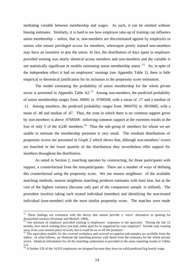
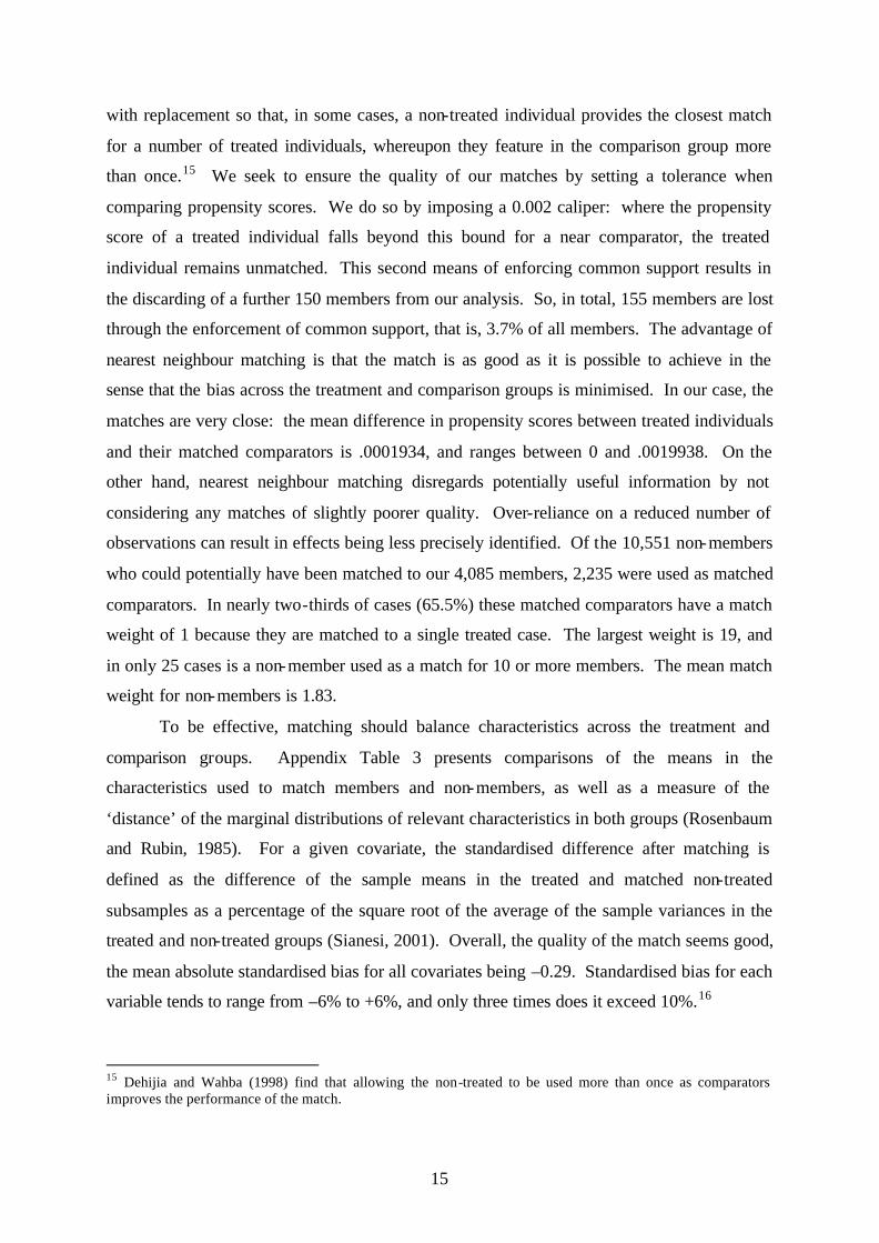
The model estimating the probability of union membership for the whole private

sector is presented in Appendix Table A2.13 Among non-members, the predicted probability

of union membership ranges from .00001 to .9768508, with a mean of .17 and a median of

.11. Among members, the predicted probability ranges from .0004702 to .9910685, with a

mean of .48 and median of .47. Thus, the zone in which there is no common support given

by non-members is above .9768508: enforcing common support at the extremes results in the

loss of only 5 of the 4,240 members.14 Thus the sub-group of members for whom we are

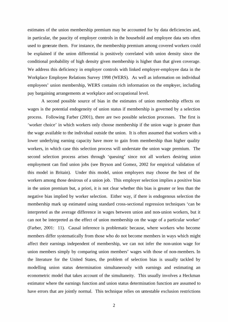
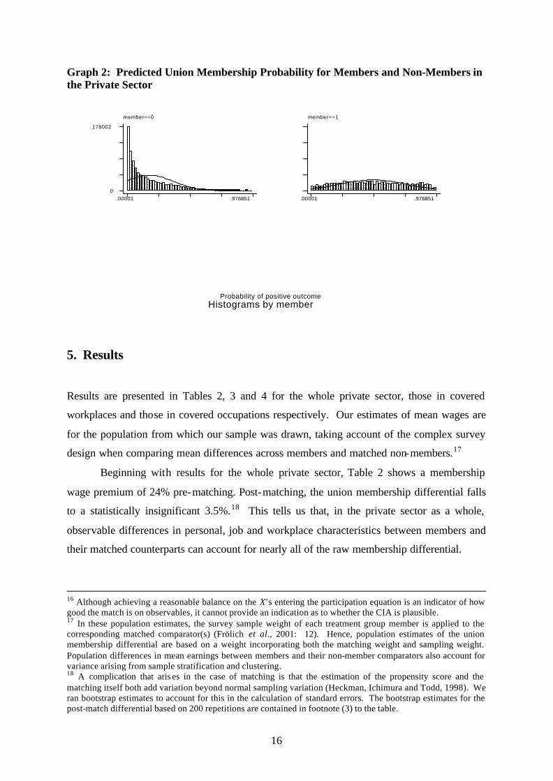
unable to estimate the membership premium is very small. The resultant distributions of

propensity scores are presented in Graph 2 which shows that, although non-members’ scores

are bunched in the lower quartile of the distribution, they nevertheless offer support for

members throughout the distribution.

As noted in Section 2, matching operates by constructing, for those participants with

support, a counterfactual from the non-participants. There are a number of ways of defining

this counterfactual using the propensity score. We use nearest neighbour: of the available

matching methods, nearest neighbour matching produces estimates with least bias, but at the

cost of the highest variance (because only part of the comparison sample is utilised). The

procedure involves taking each treated individual (member) and identifying the non-treated

individual (non-member) with the most similar propensity score. The matches were made

11 These findings are consistent with the theory that unions provide a ‘voice’ alternative to quitting for dissatisfied workers (Freeman and Medoff, 1984). 12 Our measure of employer provided training is employees’ responses to the ques tion: ‘During the last 12 months, how much training have you had, either paid for or organised by your employer? Include only training away from your normal place of work, but it could be on or off the premises.’ 13 The equivalent models for the covered workplace and covered occupation sub-samples are available from the author. In what follows, we illustrate the matching process with detail from the estimates for the whole private sector. Identical information for all the matching undertaken is provided in the notes reporting results in Tables 2-4. 14 A further 226 of the 14,932 employees are dropped because they have no valid predicted log hourly wage.

15

with replacement so that, in some cases, a non-treated individual provides the closest match

for a number of treated individuals, whereupon they feature in the comparison group more

than once.15 We seek to ensure the quality of our matches by setting a tolerance when

comparing propensity scores. We do so by imposing a 0.002 caliper: where the propensity

score of a treated individual falls beyond this bound for a near comparator, the treated

individual remains unmatched. This second means of enforcing common support results in

the discarding of a further 150 members from our analysis. So, in total, 155 members are lost

through the enforcement of common support, that is, 3.7% of all members. The advantage of

nearest neighbour matching is that the match is as good as it is possible to achieve in the

sense that the bias across the treatment and comparison groups is minimised. In our case, the

matches are very close: the mean difference in propensity scores between treated individuals

and their matched comparators is .0001934, and ranges between 0 and .0019938. On the

other hand, nearest neighbour matching disregards potentially useful information by not

considering any matches of slightly poorer quality. Over-reliance on a reduced number of

observations can result in effects being less precisely identified. Of the 10,551 non-members

who could potentially have been matched to our 4,085 members, 2,235 were used as matched

comparators. In nearly two-thirds of cases (65.5%) these matched comparators have a match

weight of 1 because they are matched to a single treated case. The largest weight is 19, and

in only 25 cases is a non-member used as a match for 10 or more members. The mean match

weight for non-members is 1.83.

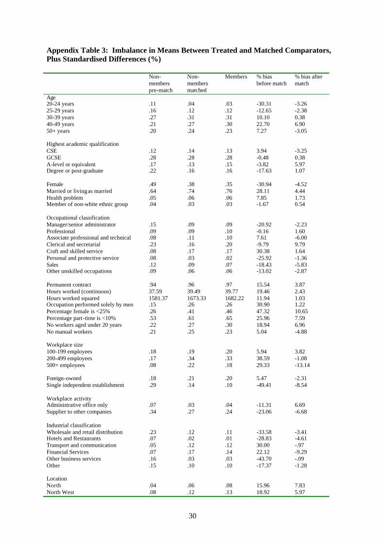
To be effective, matching should balance characteristics across the treatment and

comparison groups. Appendix Table 3 presents comparisons of the means in the

characteristics used to match members and non-members, as well as a measure of the

‘distance’ of the marginal distributions of relevant characteristics in both groups (Rosenbaum

and Rubin, 1985). For a given covariate, the standardised difference after matching is

defined as the difference of the sample means in the treated and matched non-treated

subsamples as a percentage of the square root of the average of the sample variances in the

treated and non-treated groups (Sianesi, 2001). Overall, the quality of the match seems good,

the mean absolute standardised bias for all covariates being –0.29. Standardised bias for each

variable tends to range from –6% to +6%, and only three times does it exceed 10%.16

15 Dehijia and Wahba (1998) find that allowing the non-treated to be used more than once as comparators improves the performance of the match.

16

Graph 2: Predicted Union Membership Probability for Members and Non-Members in the Private Sector

5. Results

Results are presented in Tables 2, 3 and 4 for the whole private sector, those in covered

workplaces and those in covered occupations respectively. Our estimates of mean wages are

for the population from which our sample was drawn, taking account of the complex survey

design when comparing mean differences across members and matched non-members.17

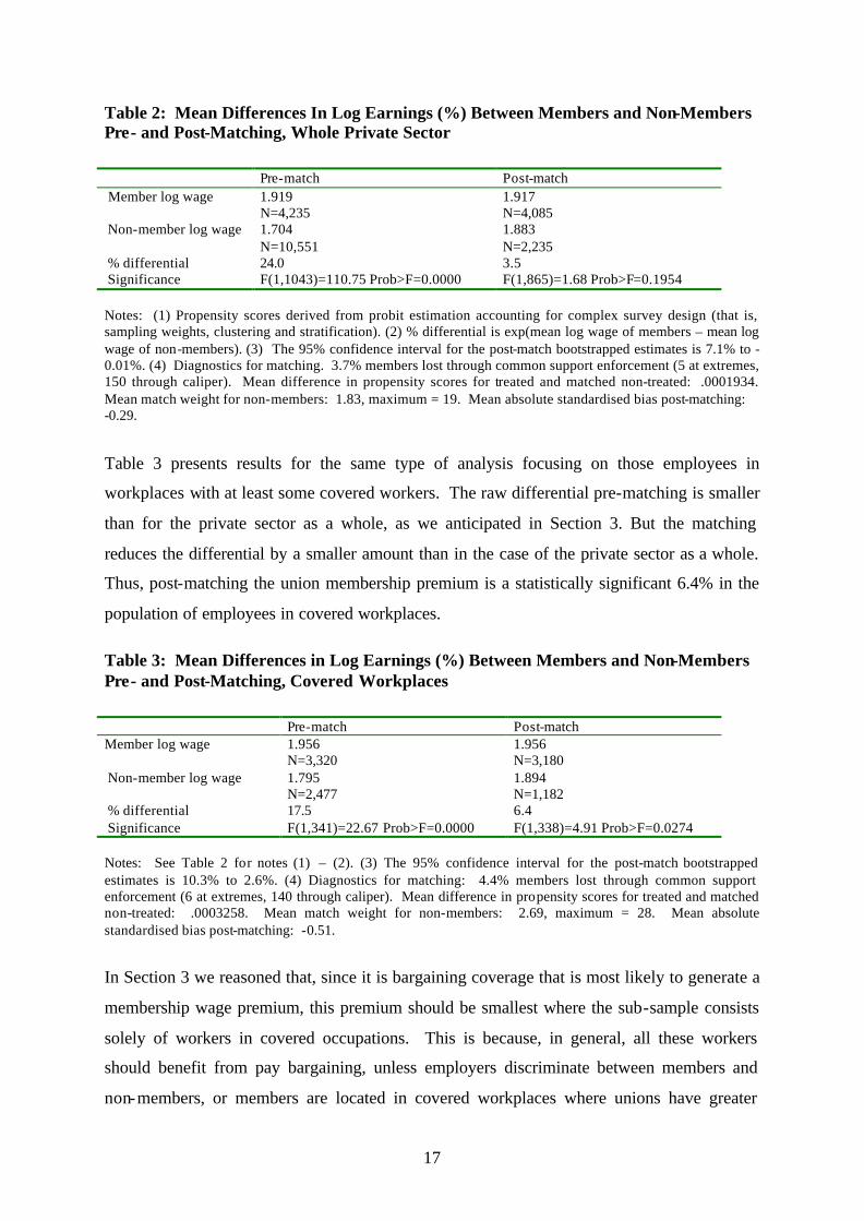
Beginning with results for the whole private sector, Table 2 shows a membership

wage premium of 24% pre-matching. Post-matching, the union membership differential falls

to a statistically insignificant 3.5%.18 This tells us that, in the private sector as a whole,

observable differences in personal, job and workplace characteristics between members and

their matched counterparts can account for nearly all of the raw membership differential.

16 Although achieving a reasonable balance on the X’s entering the participation equation is an indicator of how good the match is on observables, it cannot provide an indication as to whether the CIA is plausible. 17 In these population estimates, the survey sample weight of each treatment group member is applied to the corresponding matched comparator(s) (Frölich et al., 2001: 12). Hence, population estimates of the union membership differential are based on a weight incorporating both the matching weight and sampling weight. Population differences in mean earnings between members and their non-member comparators also account for variance arising from sample stratification and clustering. 18 A complication that aris es in the case of matching is that the estimation of the propensity score and the matching itself both add variation beyond normal sampling variation (Heckman, Ichimura and Todd, 1998). We ran bootstrap estimates to account for this in the calculation of standard errors. The bootstrap estimates for the post-match differential based on 200 repetitions are contained in footnote (3) to the table.

Histograms by memberProbability of positive outcome

member==0

.00001 .9768510

.176002

member==1

.00001 .976851

17

Table 2: Mean Differences In Log Earnings (%) Between Members and Non-Members Pre- and Post-Matching, Whole Private Sector Pre-match Post-match Member log wage Non-member log wage % differential Significance

1.919 N=4,235 1.704 N=10,551 24.0 F(1,1043)=110.75 Prob>F=0.0000

1.917 N=4,085 1.883 N=2,235 3.5 F(1,865)=1.68 Prob>F=0.1954

Notes: (1) Propensity scores derived from probit estimation accounting for complex survey design (that is, sampling weights, clustering and stratification). (2) % differential is exp(mean log wage of members – mean log wage of non-members). (3) The 95% confidence interval for the post-match bootstrapped estimates is 7.1% to -0.01%. (4) Diagnostics for matching. 3.7% members lost through common support enforcement (5 at extremes, 150 through caliper). Mean difference in propensity scores for treated and matched non-treated: .0001934. Mean match weight for non-members: 1.83, maximum = 19. Mean absolute standardised bias post-matching: -0.29.

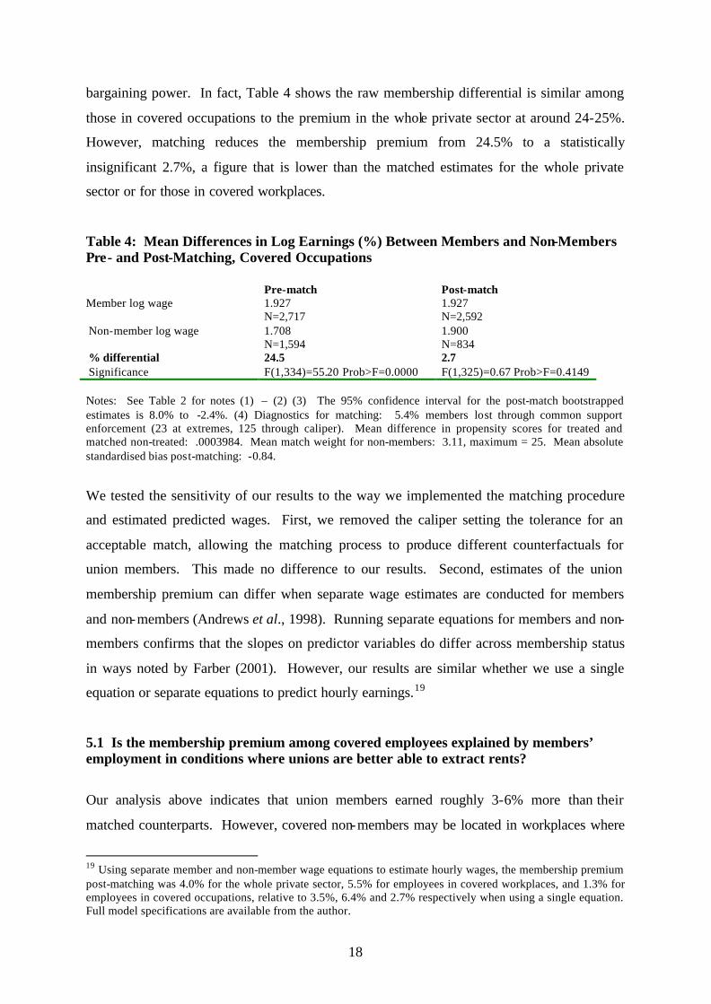
Table 3 presents results for the same type of analysis focusing on those employees in

workplaces with at least some covered workers. The raw differential pre-matching is smaller

than for the private sector as a whole, as we anticipated in Section 3. But the matching

reduces the differential by a smaller amount than in the case of the private sector as a whole.

Thus, post-matching the union membership premium is a statistically significant 6.4% in the

population of employees in covered workplaces.

Table 3: Mean Differences in Log Earnings (%) Between Members and Non-Members Pre- and Post-Matching, Covered Workplaces Pre-match Post-match Member log wage Non-member log wage % differential Significance

1.956 N=3,320 1.795 N=2,477 17.5 F(1,341)=22.67 Prob>F=0.0000

1.956 N=3,180 1.894 N=1,182 6.4 F(1,338)=4.91 Prob>F=0.0274

Notes: See Table 2 for notes (1) – (2). (3) The 95% confidence interval for the post-match bootstrapped estimates is 10.3% to 2.6%. (4) Diagnostics for matching: 4.4% members lost through common support enforcement (6 at extremes, 140 through caliper). Mean difference in propensity scores for treated and matched non-treated: .0003258. Mean match weight for non-members: 2.69, maximum = 28. Mean absolute standardised bias post-matching: -0.51.

In Section 3 we reasoned that, since it is bargaining coverage that is most likely to generate a

membership wage premium, this premium should be smallest where the sub-sample consists

solely of workers in covered occupations. This is because, in general, all these workers

should benefit from pay bargaining, unless employers discriminate between members and

non-members, or members are located in covered workplaces where unions have greater

18

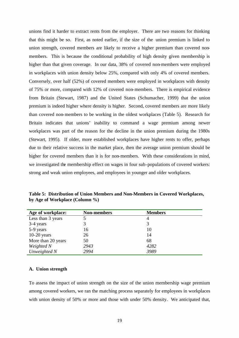
bargaining power. In fact, Table 4 shows the raw membership differential is similar among

those in covered occupations to the premium in the whole private sector at around 24-25%.

However, matching reduces the membership premium from 24.5% to a statistically

insignificant 2.7%, a figure that is lower than the matched estimates for the whole private

sector or for those in covered workplaces.

Table 4: Mean Differences in Log Earnings (%) Between Members and Non-Members Pre- and Post-Matching, Covered Occupations Pre-match Post-match Member log wage Non-member log wage % differential Significance

1.927 N=2,717 1.708 N=1,594 24.5 F(1,334)=55.20 Prob>F=0.0000

1.927 N=2,592 1.900 N=834 2.7 F(1,325)=0.67 Prob>F=0.4149

Notes: See Table 2 for notes (1) – (2) (3) The 95% confidence interval for the post-match bootstrapped estimates is 8.0% to -2.4%. (4) Diagnostics for matching: 5.4% members lost through common support enforcement (23 at extremes, 125 through caliper). Mean difference in propensity scores for treated and matched non-treated: .0003984. Mean match weight for non-members: 3.11, maximum = 25. Mean absolute standardised bias post-matching: -0.84.

We tested the sensitivity of our results to the way we implemented the matching procedure

and estimated predicted wages. First, we removed the caliper setting the tolerance for an

acceptable match, allowing the matching process to produce different counterfactuals for

union members. This made no difference to our results. Second, estimates of the union

membership premium can differ when separate wage estimates are conducted for members

and non-members (Andrews et al., 1998). Running separate equations for members and non-

members confirms that the slopes on predictor variables do differ across membership status

in ways noted by Farber (2001). However, our results are similar whether we use a single

equation or separate equations to predict hourly earnings.19

5.1 Is the membership premium among covered employees explained by members’ employment in conditions where unions are better able to extract rents?

Our analysis above indicates that union members earned roughly 3-6% more than their

matched counterparts. However, covered non-members may be located in workplaces where

19 Using separate member and non-member wage equations to estimate hourly wages, the membership premium post-matching was 4.0% for the whole private sector, 5.5% for employees in covered workplaces, and 1.3% for employees in covered occupations, relative to 3.5%, 6.4% and 2.7% respectively when using a single equation. Full model specifications are available from the author.

19

unions find it harder to extract rents from the employer. There are two reasons for thinking

that this might be so. First, as noted earlier, if the size of the union premium is linked to

union strength, covered members are likely to receive a higher premium than covered non-

members. This is because the conditional probability of high density given membership is

higher than that given coverage. In our data, 38% of covered non-members were employed

in workplaces with union density below 25%, compared with only 4% of covered members.

Conversely, over half (52%) of covered members were employed in workplaces with density

of 75% or more, compared with 12% of covered non-members. There is empirical evidence

from Britain (Stewart, 1987) and the United States (Schumacher, 1999) that the union

premium is indeed higher where density is higher. Second, covered members are more likely

than covered non-members to be working in the oldest workplaces (Table 5). Research for

Britain indicates that unions’ inability to command a wage premium among newer

workplaces was part of the reason for the decline in the union premium during the 1980s

(Stewart, 1995). If older, more established workplaces have higher rents to offer, perhaps

due to their relative success in the market place, then the average union premium should be

higher for covered members than it is for non-members. With these considerations in mind,

we investigated the membership effect on wages in four sub-populations of covered workers:

strong and weak union employees, and employees in younger and older workplaces.

Table 5: Distribution of Union Members and Non-Members in Covered Workplaces, by Age of Workplace (Column %) Age of workplace: Non-members Members Less than 3 years 5 4 3-4 years 3 3 5-9 years 16 10 10-20 years 26 14 More than 20 years 50 68 Weighted N 2943 4282 Unweighted N 2994 3989 A. Union strength

To assess the impact of union strength on the size of the union membership wage premium

among covered workers, we ran the matching process separately for employees in workplaces

with union density of 50% or more and those with under 50% density. We anticipated that,

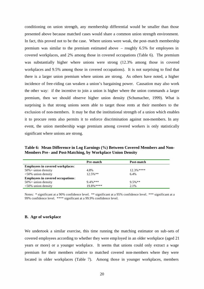
20

conditioning on union strength, any membership differential would be smaller than those

presented above because matched cases would share a common union strength environment.

In fact, this proved not to be the case. Where unions were weak, the post-match membership

premium was similar to the premium estimated above – roughly 6.5% for employees in

covered workplaces, and 2% among those in covered occupations (Table 6). The premium

was substantially higher where unions were strong (12.3% among those in covered

workplaces and 9.5% among those in covered occupations). It is not surprising to find that

there is a larger union premium where unions are strong. As others have noted, a higher

incidence of free-riding can weaken a union’s bargaining power. Causation may also work

the other way: if the incentive to join a union is higher where the union commands a larger

premium, then we should observe higher union density (Schumacher, 1999). What is

surprising is that strong unions seem able to target those rents at their members to the

exclusion of non-members. It may be that the institutional strength of a union which enables

it to procure rents also permits it to enforce discrimination against non-members. In any

event, the union membership wage premium among covered workers is only statistically

significant where unions are strong.

Table 6: Mean Difference in Log Earnings (%) Between Covered Members and Non-Members Pre- and Post-Matching, by Workplace Union Density Pre-match Post-match Employees in covered workplaces : 50%+ union density <50% union density

4.8% 12.5%**

12.3%**** 6.4%

Employees in covered occupations : 50%+ union density <50% union density

9.4%*** 19.8%****

9.5%** 2.1%

Notes: * significant at a 90% confidence level. ** significant at a 95% confidence level. *** significant at a 99% confidence level. **** significant at a 99.9% confidence level.

B. Age of workplace

We undertook a similar exercise, this time running the matching estimator on sub-sets of

covered employees according to whether they were emp loyed in an older workplace (aged 21

years or more) or a younger workplace. It seems that unions could only extract a wage

premium for their members relative to matched covered non-members where they were

located in older workplaces (Table 7). Among those in younger workplaces, members

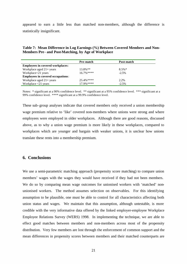
21

appeared to earn a little less than matched non-members, although the difference is

statistically insignificant.

Table 7: Mean Difference in Log Earnings (%) Between Covered Members and Non-Members Pre- and Post-Matching, by Age of Workplace

Pre-match Post-match Employees in covered workplaces : Workplace aged 21+ years Workplace<21 years

13.8%** 16.7%****

8.5%* -2.5%

Employees in covered occupations : Workplace aged 21+ years Workplace <21 years

25.4%**** 17.9%****

2.2% -2.5%

Notes: * significant at a 90% confidence level. ** significant at a 95% confidence level. *** significant at a 99% confidence level. **** significant at a 99.9% confidence level.

These sub-group analyses indicate that covered members only received a union membership

wage premium relative to ‘like’ covered non-members where unions were strong and where

employees were employed in older workplaces. Although there are good reasons, discussed

above, as to why a union wage premium is more likely in these workplaces, compared to

workplaces which are younger and bargain with weaker unions, it is unclear how unions

translate these rents into a membership premium.

6. Conclusions

We use a semi-parametric matching approach (propensity score matching) to compare union

members’ wages with the wages they would have received if they had not been members.

We do so by comparing mean wage outcomes for unionised workers with ‘matched’ non-

unionised workers. The method assumes selection on observables. For this identifying

assumption to be plausible, one must be able to control for all characteristics affecting both

union status and wages. We maintain that this assumption, although untestable, is more

credible with the very informative data offered by the linked employer-employee Workplace

Employee Relations Survey (WERS) 1998. In implementing the technique, we are able to

effect good matches between members and non-members across most of the propensity

distribution. Very few members are lost through the enforcement of common support and the

mean differences in propensity scores between members and their matched counterparts are

22

small. We are also able to achieve a good balance in observable characteristics between

members and matched non-members.

The union membership wage premium falls substantially after matching. The raw

differential is around 24% in the private sector as a whole, 18% among employees in covered

workplaces, and 25% among those in covered occupations. The only membership premium

that is statistically significant in the population after matching is the 6.4% among employees

in covered workplaces. The post-matching differentials of 3.5% and 2.7% in the whole

private sector and those in covered workplaces respectively are not statistically significant.

In Section 2, we suggested that whether individuals received a union wage premium

was likely to depend on whether their pay was set by collective bargaining. If so, then one

would expect the size of the membership premium in the private sector as a whole, covered

workplaces and covered occupations to be driven by the ‘coverage gap’ between members

and non-members in each of the sub-samples. This would lead us to anticipate the smallest

membership premium among workers in covered occupations, and the largest premium in the

private sector as a whole (where the coverage gap between members and non-members is

largest). This proved not to be the case. Pre-matching, the largest membership premium was

within covered occupations. Although this proved to be somewhat illusory, with the gap

becoming insignificant post-matching, the largest membership premium post-matching was

found among employees in covered workplaces. It is not obvious why this should be so.

One possible explanation is that, if the membership premium among covered workers arises

through discrimination on the part of unions, employers, or both against non-members, as

others have suggested, there may be more scope for this discrimination in covered

workplaces than among a sub-population of employees, all of whom belong to a covered

occupation. This is because the dimensions across which discrimination may occur are more

numerous across occupations than within occupation. 20

Further investigations as to the source of the membership premium revealed that the

premium was larger where unions were stronger (as measured by union density) and among

older workplaces relative to younger ones. These findings conform to our expectations about

the likely availability of rents which unions can extract from the employer, but they do not

explain why it is that unions are successful in channelling those rents to their members at the

expense of ‘like’ non-members.

20 I would like to thank Dorothe Bonjour for this point.

23

Although not always statistically significant, our preferred population estimates for

the membership premium range from 2.7% in covered occupations to 6.4% in covered

workplaces. If there is a real membership wage premium, even among covered workers, why

don’t non-members join? Could it be that non-members face higher costs than members in

joining a union? In the private sector as a whole this is quite likely since non-members are

more likely to be located in non-unionised workplaces than members, and the costs of

becoming a member are higher in non-unionised workplaces than they are in joining an

already established union (Farber, 2001). However, it is less likely that there is a cost

differential facing non-members where they are already located in covered workplaces. An

alternative is that non-members are simply less desirous of membership than members,

perhaps because their tastes differ. Bryson and Gomez (2002) present evidence to suggest

that this is indeed the case, since the market for union membership is segmented along

ideological lines. These tastes may have an independent effect on the likelihood of joining a

union, or else they may affect the weight employees attach to the costs and benefits of

membership. If this characteristic, which is unobserved in our data, is also likely to influence

employees’ wages, then its omission from our analysis will bias our estimates of the union

membership wage premium.

Of course, if we focus on our estimates for the whole private sector or covered

occupations, where no significant premium is apparent, we face a different question: why

don’t union members leave the union? Well, they have been leaving: union density is in

decline, even within unionised workplaces (Millward et al., 2000, Chapter 5). However,

evidence for the period 1983-1998 indicates that the rate at which employees have le ft

membership has not risen and that the decline in membership is due to an increase in

employees who have never been members (Bryson and Gomez, 2002). It may well be that

the returns to membership have declined. However, there are at least three reasons why it is

not possible to read off employees’ likely membership intentions from the wage premium

they face. The first is that the premium may rise under, say, more favourable economic

conditions. In any event, one can make the case for remaining in a union if – as we show -

union density has a role to play in the size of the wage premium unions can extract from the

employer. If members were to leave, the prospects of bargaining for better wages will

deteriorate. Second, members are unlikely to value membership purely in terms of the wage

mark up unions command. Members also benefit directly by unions’ efforts to improve non-

pecuniary benefits, job security, the handling of grievance and disciplinary matters, and by

24

encouraging management to treat all employees more fairly. Third, as alluded to above,

many join and remain members because they are ideologically committed to doing so.

25

Appendix Table 1: Gross Hourly Earnings in the Private Sector Union member 0.083 (4.98)** Workplace union recognition 0.030 (1.99)* Age (ref.: under 20) 20-24 years 0.155 (5.68)** 25-29 years 0.269 (9.37)** 30-39 years 0.334 (12.15)** 40-49 years 0.346 (12.24)** 50+ years 0.341 (11.89)** Highest academic qualification (ref: none) CSE 0.054 (3.35)** GCSE 0.095 (7.39)** A-level or equivalent 0.155 (10.19)** Degree or post-graduate 0.263 (12.41)** Any vocational qualifications -0.021 (2.17)* Workplace tenure (ref: under 2 years) 2-4 years 0.053 (3.84)** 5-9 years 0.072 (4.59)** 10+ years 0.092 (5.71)** Employer provided training in last 12 months (ref: none) Less than 1 day 0.004 (0.27) 1 < 2 days 0.045 (3.24)** 2 < 5 days 0.056 (4.41)** 5 < 10 days 0.040 (2.04)* 10+ days 0.015 (0.90) Female -0.082 (6.24)** Dependent children 0.026 (2.37)* Married or living as married 0.050 (5.18)** Health problem -0.064 (3.06)** Member of non-white ethnic group -0.048 (1.50) Occupational classification (ref.: operative) Manager/senior administrator 0.550 (19.79)** Professional 0.488 (16.62)** Associate professional and technical 0.324 (11.75)**

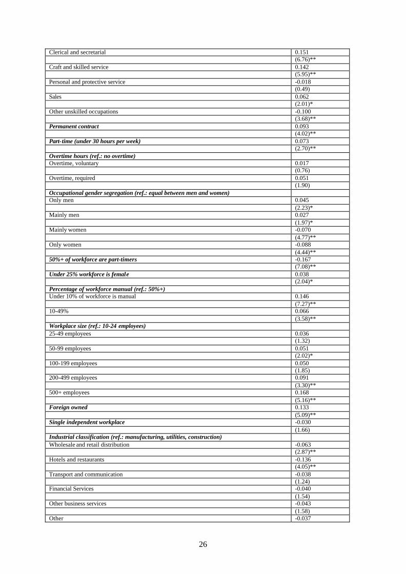
26

Clerical and secretarial 0.151 (6.76)** Craft and skilled service 0.142 (5.95)** Personal and protective service -0.018 (0.49) Sales 0.062 (2.01)* Other unskilled occupations -0.100 (3.68)** Permanent contract 0.093 (4.02)** Part-time (under 30 hours per week) 0.073 (2.70)** Overtime hours (ref.: no overtime) Overtime, voluntary 0.017 (0.76) Overtime, required 0.051 (1.90) Occupational gender segregation (ref.: equal between men and women) Only men 0.045 (2.23)* Mainly men 0.027 (1.97)* Mainly women -0.070 (4.77)** Only women -0.088 (4.44)** 50%+ of workforce are part-timers -0.167 (7.08)** Under 25% workforce is female 0.038 (2.04)* Percentage of workforce manual (ref.: 50%+) Under 10% of workforce is manual 0.146 (7.27)** 10-49% 0.066 (3.58)** Workplace size (ref.: 10-24 employees) 25-49 employees 0.036 (1.32) 50-99 employees 0.051 (2.02)* 100-199 employees 0.050 (1.85) 200-499 employees 0.091 (3.30)** 500+ employees 0.168 (5.16)** Foreign owned 0.133 (5.09)** Single independent workplace -0.030 (1.66) Industrial classification (ref.: manufacturing, utilities, construction) Wholesale and retail distribution -0.063 (2.87)** Hotels and restaurants -0.136 (4.05)** Transport and communication -0.038 (1.24) Financial Services -0.040 (1.54) Other business services -0.043 (1.58) Other -0.037

27

(1.16) London 0.194 (7.86)** Unemployment rate of 5%+ -0.058 (3.39)** Constant 0.928 (21.15)** Sigma 0.333 (41.76)** F stat (60,989) = 101.31

Prob>F = 0.0000 Observations 14875 Note: * significant at 5% level; ** significant at 1% level. Absolute value of t-statistics in parentheses

28

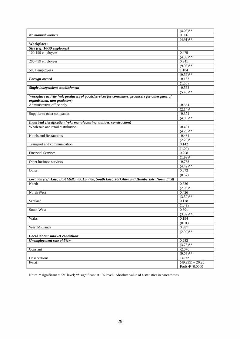
Appendix Table 2: Individual Union Membership Status in the Private Sector Demographics: Age (ref.: under 20) 20-24 years 0.222 (1.98)* 25-29 years 0.495 (4.91)** 30-39 years 0.712 (6.99)** 40-49 years 0.821 (7.81)** 50+ years 0.808 (7.55)** Highest academic qualification (ref: none) CSE 0.096 (1.65) GCSE -0.060 (1.13) A-level or equivalent -0.125 (1.86) Degree or post-graduate -0.317 (3.88)** Female -0.013 (0.24) Married or living as married 0.105 (2.67)** Health problem 0.080 (1.19) Member of non-white ethnic group 0.169 (1.90) Job-related: Occupational classification (ref.: operative) Manager/senior administrator -0.979 (8.77)** Professional -0.492 (4.77)** Associate professional and technical -0.524 (5.22)** Clerical and secretarial -0.917 (9.30)** Craft and skilled service -0.033 (0.41) Personal and protective service -0.938 (6.16)** Sales -0.544 (5.16)** Other unskilled occupations -0.547 (5.66)** Permanent contract 0.275 (2.84)** Hours worked (continuous) 0.023 (3.37)** Hours worked squared -0.000 (3.28)** Occupation performed solely by men 0.122 (2.07)* Workforce composition: Percentage female is <25% 0.476 (4.96)** Percentage part-time is <10% -0.321 (3.25)** No workers aged under 20 years 0.365

29

(4.03)** No manual workers 0.506 (4.91)** Workplace: Size (ref: 10-99 employees) 100-199 employees 0.479 (4.30)** 200-499 employees 0.941 (9.98)** 500+ employees 1.104 (9.59)** Foreign-owned -0.153 (1.56) Single independent establishment -0.533 (5.40)** Workplace activity (ref: producers of goods/services for consumers, producers for other parts of organisation, non-producers)

Administrative office only -0.364 (2.14)* Supplier to other companies -0.371 (4.08)** Industrial classification (ref.: manufacturing, utilities, construction) Wholesale and retail distribution -0.481 (4.20)** Hotels and Restaurants -0.434 (2.29)* Transport and communication 0.142 (1.00) Financial Services 0.258 (1.98)* Other business services -0.738 (4.42)** Other 0.073 (0.57) Location (ref: East, East Midlands, London, South East, Yorkshire and Humberside, North East) North 0.336 (2.08)* North West 0.426 (3.50)** Scotland 0.178 (1.49) South West 0.391 (3.32)** Wales 0.194 (0.91) West Midlands 0.387 (2.90)** Local labour market conditions: Unemployment rate of 5%+ 0.282 (3.75)** Constant -2.076 (9.06)** Observations 14932 F-stat (49,995) = 20.26

Prob>F=0.0000 Note: * significant at 5% level; ** significant at 1% level. Absolute value of t-statistics in parentheses

30

Appendix Table 3: Imbalance in Means Between Treated and Matched Comparators, Plus Standardised Differences (%) Non-

members pre-match

Non-members matched

Members % bias before match

% bias after match

Age 20-24 years .11 .04 .03 -30.31 -3.26 25-29 years .16 .12 .12 -12.65 -2.38 30-39 years .27 .31 .31 10.10 0.38 40-49 years .21 .27 .30 22.70 6.90 50+ years .20 .24 .23 7.27 -3.05 Highest academic qualification CSE .12 .14 .13 3.94 -3.25 GCSE .28 .28 .28 -0.48 0.38 A-level or equivalent .17 .13 .15 -3.82 5.97 Degree or post-graduate .22 .16 .16 -17.63 1.07 Female .49 .38 .35 -30.94 -4.52 Married or living as married .64 .74 .76 28.11 4.44 Health problem .05 .06 .06 7.85 1.73 Member of non-white ethnic group .04 .03 .03 -1.67 0.54 Occupational classification Manager/senior administrator .15 .09 .09 -20.92 -2.23 Professional .09 .09 .10 -0.16 1.60 Associate professional and technical .08 .11 .10 7.61 -6.00 Clerical and secretarial .23 .16 .20 -9.79 9.79 Craft and skilled service .08 .17 .17 30.38 1.64 Personal and protective service .08 .03 .02 -25.92 -1.36 Sales .12 .09 .07 -18.43 -5.83 Other unskilled occupations .09 .06 .06 -13.02 -2.87 Permanent contract .94 .96 .97 15.54 3.87 Hours worked (continuous) 37.59 39.49 39.77 19.46 2.43 Hours worked squared 1581.37 1673.33 1682.22 11.94 1.03 Occupation performed solely by men .15 .26 .26 30.90 1.22 Percentage female is <25% .26 .41 .46 47.32 10.65 Percentage part-time is <10% .53 .61 .65 25.96 7.59 No workers aged under 20 years .22 .27 .30 18.94 6.96 No manual workers .21 .25 .23 5.04 -4.88 Workplace size 100-199 employees .18 .19 .20 5.94 3.82 200-499 employees .17 .34 .33 38.59 -1.08 500+ employees .08 .22 .18 29.33 -13.14 Foreign-owned .18 .21 .20 5.47 -2.31 Single independent establishment .29 .14 .10 -49.41 -8.54 Workplace activity Administrative office only .07 .03 .04 -11.31 6.69 Supplier to other companies .34 .27 .24 -23.06 -6.68 Industrial classification Wholesale and retail distribution .23 .12 .11 -33.58 -3.41 Hotels and Restaurants .07 .02 .01 -28.83 -4.61 Transport and communication .05 .12 .12 30.00 -.97 Financial Services .07 .17 .14 22.12 -9.29 Other business services .16 .03 .03 -43.70 -.09 Other .15 .10 .10 -17.37 -1.28 Location North .04 .06 .08 15.96 7.83 North West .08 .12 .13 18.92 5.97

31

Scotland .09 .11 .11 7.07 1.72 South West .09 .10 .11 4.85 1.81 Wales .04 .05 .05 4.43 -5.29 West Midlands .08 .12 .08 4.13 -10.95 Unemployment rate of 5%+ .48 .57 .56 17.15 -2.90 Average absolute standardised bias pre-match, whole sample

18.16

Average absolute standardised bias post-match, whole sample

4.21

Average absolute standardised bias pre-match, matched sample

2.12

Average absolute standardised bias post-match, matched sample

-0.29

Absolute bias reduction 41.00

32

References Airey, C., Hales, J., Hamilton, R., Korovessis, C., McKernan, A. and Perdon, S. (1999), The

Workplace Employee Relations Survey (WERS), 1997-8: Technical Report. Andrews, M. J., Stewart, M. B., Swaffield, J. K., Upward, R. (1998), ‘The Estimation of

Union Wage Differentials and the Impact of Methodological Choices’, Labour Economics, 5, pp. 449-474.

Blackaby, D., Murphy, P. and Sloane, P. (1991), ‘Union Membership, Collective Bargaining

Coverage and the Trade Union Mark-Up For Britain’, Economic Letters, 36, pp. 203-208.

Blakemore, A. E., Hunt, J. C. and Kiker, B. F. (1986), ‘Collective Bargaining and Union

Membership Effects on the Wages of Male Youths’, Journal of Labor Economics, 4, April, pp. 193-211.

Booth, A. L. and Bryan, M. L. (2001), ‘The Union Membership Wage-Premium Puzzle: Is

There a Free Rider Problem’, Working Paper, Institute for Social and Economic Research, University of Essex.

Bryson, A. and Gomez, R. (2002), ‘You Can’t Always Get What You Want: Frustrated

Demand for Union Membership and Representation in Britain’, Working Paper No. 1182, Centre for Economic Performance, London School of Economics.

Budd, J. W. and Na, I. (2000), ‘The Union Membership Wage Premium for Employees

Covered by Collective Bargaining Agreements’, Journal of Labor Economics, 18(4), pp. 783-807.

Dehejia, R. and Wahba, S. (1998), ‘Propensity Score Matching Methods For Non-

Experimental Causal Studies’, NBER Working Paper No. 6829. Farber, H. (2001), ‘Notes on the Economics of Labor Unions’. Working Paper No. 452.

Princeton University, Industrial Relations Section. Forth, J. and Millward, N. (2000a), ‘The Determinants of Pay Levels and Fringe Benefit

Provision in Britain’, Discussion Paper No.171, NIESR: London. Forth, J. and Millward, N. (2000b), ‘Pay Settlements in Britain’, Discussion Paper No.173,

NIESR: London. Freeman, R. B. and Medoff, J. L. (1984), What Do Unions Do?, Basic Books: New York.

Frölich, M., Heshmati, A. and Lechner, M. (2001), ‘A Microeconometric Evaluation of

Rehabilitation of Long-Term Sickness in Sweden’, St. Gallen Working Paper. Green, F. (1988), ‘The Trade Union Wage Gap In Britain: Some New Estimates’, Economic

Letters, 27, pp. 183-187.

33

Heckman, J., Ichimura, H., Smith, J. and Todd, P. (1998), ‘Characterizing Selection Bias Using Experimental Data’, Econometrica, 66(5): pp. 1017-1098.

Heckman, J., Ichimura, H. and Todd, P. (1997), ‘Matching as an Econometric Evaluation

Estimator: Evidence From Evaluating a Job Training Programme’, Review of Economic Studies, 64: pp. 605-654.

Heckman, J., LaLonde, R. and Smith, J. (1999), ‘The Economics and Econometrics of Active

Labor Market Programs’ in O. Ashenfelter, and D. Card (eds.), The Handbook of Labour Economics, Vol. III, North Holland: Amsterdam.

Hildreth, A. (1999), ‘What Has Happened to the Union Wage Differential in Britain in the

1990s’, Oxford Bulletin of Economics and Statistics, 61, 1, pp. 5-31. Holland, P. W. (1986), ‘Statistics and Causal Inference’, Journal of the American Statistical

Association, December, Vol. 81, No. 396, pp. 945-960. Lewis, H. G. (1986), Union Relative Wage Effects: A Survey, University of Chicago Press:

Chicago, Illinois, USA. Machin, S. (2001), ‘Does It Still Pay to Be in a Union?’, Working Paper No. 1180, Centre for

Economic Performance, London School of Economics. Metcalf, D., Hansen, K. and Charlwood, A. (2001), ‘Unions and the Sword of Justice:

Unions and Pay Systems, Pay Inequality, Pay Discrimination and Low Pay’, National Institute Economic Review, No. 176, April, pp. 61-75.

Millward, N., Bryson, A. and Forth, J. (2000), All Change at Work? British Employment

Relations, 1980-98, as portrayed by the Workplace Industrial Relations Survey Series, Routledge: London.

Rosenbaum, P. and Rubin, D. (1983), ‘The central role of the propensity score in

observational studies for causal effects’. Biometrica 70: pp. 41-50. Rosenbaum, P. and Rubin, D. (1985), ‘Constructing a Control Group Using Multivariate

Matched Sampling Methods that Incorporate the Propensity Score’. The American Statistician 39, 1: 33-38

Schumacher, E. J. (1999), ‘What Explains Wage Differences between Union Members and

Covered Nonmembers?’, Southern Economic Journal, 65(3), pp. 493-512. Sianesi, B. (2001), ‘An Evaluation of the Active Labour Market Programmes in Sweden’,

IFAU Working Paper #2001: 5 Stewart, M. (1983), ‘On Least Squares Estimation when the Dependent Variable is Grouped’,

Review of Economic Studies, 50(4), 737-753 Stewart, M. (1987), ‘Collective bargaining arrangements, closed shops and relative pay’,

Economic Journal, 97, 140-155

34

Stewart, M. (1995), “Union wage differentials in an era of declining unionisation”, Oxford Bulletin of Economics and Statistics, Vol 57, No 2, 143-66

Recent Discussion Papers from the ‘Future of Trade Unions in Modern Britain’ Programme

Centre for Economic Performance

529 H. Gray Family Friendly Working: What a Performance! An Analysis of the Relationship between the Availability of Family Friendly Policies and Establishment Performance

May 2002

525 S. Fernie H. Gray

It’s a Family Affair: the Effect of Union Recognition and Human Resource Management on the Provision of Equal Opportunities in the UK

April 2002

515 A. Bryson R. Gomez M. Gunderson N. Meltz

Youth Adult Differences in the Demand for Unionization: Are American, British and Canadian Workers That Different?

October 2001

512 R. Gomez M. Gunderson N. Meltz

From ‘Playstations’ to ‘Workstations’: Youth Preferences for Unionisation

September 2001

504 A. Charlwood Influences on Trade Union Organising Effectiveness in Great Britain

August 2001

503 D. Marsden S. French K. Kubo

Does Performance Pay De-Motivate and Does it Matter?

August 2001

500 Edited by David Marsden and Hugh Stephenson

Labour Law and Social Insurance in the New Economy: A Debate on the Supiot Report

July 2001

498 A. Charlwood Why Do Non-Union Employees Want to Unionise? Evidence from Britain

June 2001

494 A. Bryson Union Effeects on Managerial and Employee Perceptions of Employee Relations in Britain

April 2001

493 D. Metcalf British Unions: Dissolution or Resurgence Revisited

April 2001

To order a discussion paper, please contact the Publications Unit Tel 020 7955 7673 Fax 020 7955 7595 Email info@cep.lse.ac.uk

Web site http://cep.lse.ac.uk

CENTRE FOR ECONOMIC PERFORMANCE Recent Discussion Papers

529 H. Gray Family Friendly Working: What a Performance! An Analysis of the Relationship Between the Availability of Family Friendly Policies and Establishment Performance

528 E. Mueller A. Spitz

Managerial Ownership and Firm Performance in German Small and Medium-Sized Enterprises

527 D. Acemoglu J-S. Pischke

Minimum Wages and On-the-Job Training

526 J. Schmitt J. Wadsworth

Give PC’s a Chance: Personal Computer Ownership and the Digital Divide in the United States and Great Britain

525 S. Fernie H. Gray

It’s a Family Affair: the Effect of Union Recognition and Human Resource Management on the Provision of Equal Opportunities in the UK

524 N. Crafts A. J. Venables

Globalization in History: a Geographical Perspective

523 E. E. Meade D. Nathan Sheets

Regional Influences on US Monetary Policy: Some Implications for Europe

522 D. Quah Technology Dissemination and Economic Growth: Some Lessons for the New Economy

521 D. Quah Spatial Agglomeration Dynamics

520 C. A. Pissarides Company Start-Up Costs and Employment

519 D. T. Mortensen C. A. Pissarides

Taxes, Subsidies and Equilibrium Labor Market Outcomes

518 D. Clark R. Fahr

The Promise of Workplace Training for Non-College Bound Youth: Theory and Evidence from Germany

517 J. Blanden A. Goodman P. Gregg S. Machin

Change in Intergenerational Mobility in Britain

To order a discussion paper, please contact the Publications Unit Tel 020 7955 7673 Fax 020 7955 7595 Email info@cep.lse.ac.uk

Web site http://cep.lse.ac.uk