Abstract - lup.lub.lu.se

Abstract

This thesis suggests and tests two methods for categorizing instruments in a musical signal. Thefirst method involves spectral analysis and the magnitude spectrum, analysing the structure ofpitches and overtones and how the amplitude of those changes over time. The second method in-volves cepstrum analysis and especially the, for speech recognition popular method computing theMel Frequency Cepstral Coefficients (MFCC). For each method, a weighting procedure using LeastSquares is finally used to determine which instrument that are present in a signal and which arenot. This is done by comparing the unknown signal to a reference bank of tones. So, even if thisthesis is primarily about testing and comparing two methods, it is also about how much a linearLeast Squares weighting method can absorb the non-linear calculations of magnitude spectrum andMFCC.

The results for both methods in combination with the Least Squares weighting procedure arepromising. For some musical signals the instrument categorisation succeeds very well while forother signals improvements of the methods are needed. These improvements may be achieved bycombining features from both methods and adjusting the weighting system.

2

Contents

1 Introduction 4

2 Methods 52.1 FFT, Fast Fourier Transform . . . . . . . . . . . . . . . . . . . . . . . . . . . . . . . 62.2 MFCC, Mel Frequency Cepstral Coefficients . . . . . . . . . . . . . . . . . . . . . . . 11

3 Tests 163.1 Tests for FFT-method . . . . . . . . . . . . . . . . . . . . . . . . . . . . . . . . . . . 173.2 Tests for MFCC-method . . . . . . . . . . . . . . . . . . . . . . . . . . . . . . . . . . 23

4 Results and analysis 29

5 Discussion and future improvements 36

6 Bibliography 39

3

1 Introduction

Music, the universal language that passes no one unnoticed. It ignites emotions within us andmoves us in certain ways that are often very hard to explain and understand. Some compositionof instruments, tones and beats will move some people in a certain way, while leaving others un-affected. Every instrument have different characteristics, these can for instance be shape, whatmaterial it is made of and timbre. A trained musical ear, can in most cases distinguish between theinstruments that make up a melody and most of us would pretty easy hear the difference betweena piano and a guitar playing the same tone. Why is that, and how can it be explained? One of theproperties already mentioned is timbre also known as tone color or tone quality. Quoting [1], onesimple definition of timbre could be

"In simple terms, timbre is what makes a particular musical sound different from another, evenwhen they have the same pitch and loudness."

One way of trying to explain timbre is to apply spectral analysis to music signals and then analyzethe structure of the fundamental pitch and its overtones and then study how they evolve over time.By doing this for different instruments, there can be ways to mathematically explain and separateinstruments from each other.

4

2 Methods

This thesis will test two methods for characterizing instruments in a melody. The first methodinvolves overtone analysis using the Fast Fourier Transform (FFT) and the second method us-ing cepstral analysis and the Mel Frequency Cepstral Coefficients (MFCC) which is the standardmethod used for voice recognition.

To generalize, given a time frame of data in a melody, both of the above methods will compare thattime frame with a corresponding time frame from a set of reference frames. This comparison willdiffer a bit for both methods and will be explained in detail i section 2.1 and 2.2. As an example,given a time frame from a music mix of, say clarinet, guitar, flute and harmonica, that frame isto be compared with a reference frame for all possible instruments involved in the melody. Thisprocess is illustrated in below Figure 1.

Figure 1: A time frame from a mix is being compared with corresponding time frames from eachinstrument present in the melody

A weight is then assigned to each instrument resulting in the matrix equation

htot = w1hclarinet + w2h

guitar + w3hflute + w4h

harmonica, (1)

where htot is a m × 1 vector holding m, number of coefficients of a sought for feature of the mixframe, such as magnitude, amplitude or power in the frame for a given frequency, hclarinet holdsthe corresponding coefficients regarding the clarinet, hguitar corresponds to the guitar, hflute forthe flute and hharmonica for the harmonica all with the same dimension as htot, that is

5

htot1

htot2

.

.

.htotn

=

hclarinet1 hguitar1 hflute1 hharmonica1

hclarinet2 hguitar2 hflute2 hharmonica2

. . . .

. . . .

. . . .

hclarinetm hguitarm hflutem hharmonicam

w1

w2

w3

w4

. (2)

Here, the only unknowns are the weights w1, ..., w4 and these can be estimated using Least Squares.By denoting the matrix by H, the problem becomes to find the vector, say w that minimizes∥∥Hw − htot

∥∥2, (3)

where ‖·‖2 denotes the 2-norm. The idea is, that the weights will now say how much of a certaininstrument is present in a particular frame from a mix.

Using ordinary Least Squares will result in negative weights but since a contribution from aninstrument can not be negative the use of Non-Negative Least Squares[2] is preferable. So, theproblem instead becomes, find the vector w that minimizes∥∥Hw − htot

∥∥2subject to w ≥ 0. (4)

The implementation used in this report for solving the Non-Negative Least Squares problem is theimplementation from matlab, which is itself built upon [2].

2.1 FFT, Fast Fourier Transform

In order to find timbre in instruments, the first approach is simply by calculating the Fast FourierTransform (FFT)[8] of a signal and determine the power of the peaks in the magnitude spectrum(= absolute value of the FFT). Since a tone played by an instrument is said to be non-stationarythe signal is divided into time frames. By taking this into account the fact that the overtones mightchange over time is considered.

To get a better view of what is meant by overtone structure study Figure 2 and compare the powerproportions for one instrument. For the flute playing D6, the fundamental frequency (1176Hz) havea very strong amplitude and for the first and second overtone (2349 Hz and 3520 Hz) the amplitudeis low for both the acoustic and the digital flute. For the guitar playing A3, the fundamental tone(220 Hz) and the first overtone (440 Hz) are dominating the signal for both the acoustic and thedigital guitar.

The idea on which this report builds upon, is that two different instruments of the same category(e.g. two guitars) playing the same tone will have a similar timbre which in this case means thatthey will have the same overtone structure. Hopefully the overtone structure will be unique in someway for every instrument category so that it will be possible to separate two different instrumentcategories.

6

Figure 2: Overtone structure of two different flutes and two different guitars

In order to categorize a tone played by an unknown instrument, the overtone structures are cal-culated for all frames. This is compared with a bank of overtone structures from known referencesignals. By using Non-Negative Least Squares the weights of each reference signal’s overtone struc-tures are calculated for all frames. That is

htotl = w1hclarinetl + w2h

guitarl + ... , (5)

where h is the overtone structure in the frame l (for different instruments) and where htot is theunknown signal consisting of one or more instruments. w1, w2,... are the weights of the references.

Practically the overtone structure for a time segment of the signal is calculated by:

1. The fundamental frequency is identified. This is done e.g. by using the absolute value of theFFT and localize the first significant peak, see Figure 3.

2. The signal is divided into r frames of 40 ms (which becomes K = 1764 data points if thesignal is sampled at sampling frequency, fs = 44100 Hz) and use 75% overlap. The signal isthen multiplied with a Hanning window

W (n) = 0.5(1− cos(2π nK

)), 0 ≤ n ≤ K − 1, (6)

resulting in the new signal y. Now y is zero-padded up to N = 214 = 16384 datapoints. Themagnitude spectrum is, for each time frame l, given by

7

Figure 3: Finding fundamental frequency from the absolute value of the FFT of an unknown signal.The tone D3 = 146.8 Hz is found.

Sl(k) =

∣∣∣∣∣N−1∑n=0

yl(n)e−2πiknN

∣∣∣∣∣ , k = 0, 1, ..., N − 1, (7)

where S is the magnitude spectrum of the discrete Fourier transform of y.

Using the power spectrum (the squared magnitude spectrum) was considered but discardedsince the spectrum raised the highest peak and reduced all other peaks. This contributed tothat the overtone structure became less significant for the different instruments which woulddeteriorate the results.

3. Overtones are localized. These are found as peaks in the magnitude spectrum close to theinteger multiples of the fundamental frequency, see Figure 4.

4. The identified amplitudes of the peaks are saved in the vector

p̂l = [p̂0 p̂1 ... p̂m−1], (8)

where l is the time frame, p̂0 is the amplitude of the fundamental frequency and p̂1,..., p̂m−1are the amplitudes of the first m − 1 overtones. How to choose an optimal m for music in-struments is not investigated in this project.

Since the overall power of the amplitudes vary from different recordings (for example depend-ing on loudness and position of the instrument compared to the recorder) only the proportions

8

Figure 4: Magnitude spectrum with localized peaks

of the amplitudes are investigated. Therefore the amplitudes are divided by the norm forminga normalized amplitude vector

pl =p̂l‖p̂l‖2

(9)

for every time frame l.

5. Since a tone played by an instrument is non-stationary, the overtone structure is calculatedfor all time frames in the unknown signal. The vectors pl results in a matrix Q (of size r×mwhere r is the number of time frames and m is the number of coefficients in pl)

Q =

p1

p2...pr

(10)

that describes how the normalized amplitudes, of the fundamental frequency and the m − 1first overtones, changes over time. By continuing the example with the unknown signal, thecorresponding Q-matrix is shown in Figure 5. In this case the fundamental frequency andthe first 4 overtones are shown. The matrix Q shows how the normalized amplitudes of theovertones vary over time. For the clarinet playing D3 which is shown in this example, thenormalized overtones are quite stationary.

9

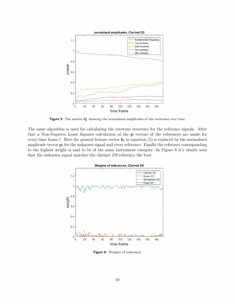
Figure 5: The matrix Q, showing the normalized amplitudes of the overtones over time

The same algorithm is used for calculating the overtone structure for the reference signals. Afterthat a Non-Negative Least Squares calculation of the p vectors of the references are made forevery time frame l. Here the general feature vector hl in equation (5) is replaced by the normalizedamplitude vector pl for the unknown signal and every reference. Finally the reference correspondingto the highest weight is said to be of the same instrument category. In Figure 6 it’s clearly seenthat the unknown signal matches the clarinet D3 reference the best.

Figure 6: Weights of references

10

2.2 MFCC, Mel Frequency Cepstral Coefficients

For speech signals and especially for voice recognition Mel Frequency Cepstral Coefficients, MFCCis widely used and Malcolm Slaney’s matlab library [3] is an accepted library in the area of speechrecognition. Since this method works well in determining the timbre in voiced speech, it mightbe possible to apply it to music and use it to distinguish different instrument categories. In thismethod, the algorithm for determining the MFCC for voiced speech will be applied to music sig-nals and then the obtained coefficients will be used to determine which instruments are included ina tune by again using Non-Negative Least Squares. That is, h in equation (1) now holds the MFCC.

To find the MFCC of a signal, the following steps are performed:

1. The signal x is pre-emphasized by

x(n) = x(0) +M∑n=1

x(n+ 1)− αx(n), (11)

where the standard value of α is 0.97 and M is the total number of samples. This is a high-pass filter and if the signal x would have contained a trend this step would have eliminatedit.

2. The signal is divided in the same way as for the FFT-method (step 2). The magnitudespectrum Sl is calculated for each of the time frames xl, where 1 ≤ l ≤ r. Using equation (7),now with a Hamming window

W (n) =

{0.54− 0.46cos(nπK ) , 0 ≤ n ≤ K

0 , otherwise (12)

of length K. Doing this for all frames will result in a r ×K matrix S containing spectrumsfor all frames.

3. A mel-scale filter bank containing overlapping triangular windows is constructed. At low fre-quencies the human ear detects changes in frequency rather easy but for higher frequencies achange is more difficult to detect. This means that for low frequencies the perception can beregarded as being linear whereas for higher frequencies the perception is more logarithmic.So, after converting to mel-scale the human ear can detect changes in high mels just as goodas for low mels. To possibly be able to describe the timbre noticeable by the human ear inmathematical terms this conversion may be needed.

For speech the number of total filters commonly used is between 26−40 [4] and the frequencyrange is in between fmin = 100 Hz and fmax = 6800 Hz, [5]. For music on the other hand thefrequency range is a lot wider, especially, since the structure of the overtones is interesting.The highest fmax that could be chosen is fs/2 = 44100/2 = 22050 Hz, the Nyquist frequency.The lowest tone on a piano, C0, corresponds to 16.35 Hz which is not far from zero. For thisimplementation fmin = 0 Hz and fmax = 22050 Hz are set. Since music instrument has awider range of frequencies than speech, more filters in the filter bank is likely to be needed.

11

The number of linear spaced filters is set to be 40 and the number of logarithmic spaced filtersis also set to be 40 resulting in a total number of L = 80 filters in the filter-bank. The lengthof each filter is K and by storing all filters in a matrix, F, this matrix will now be of dimensionK × L. The higher overtone considered, the less significant it tends to be and therefore it’smore effected by noise. A logarithmic decaying of the amplitudes of the triangular filters istherefore applied for the higher frequencies.

For an example of how the filter-bank could look like, see Figure 7. There are many differentconversion from Hz to mels. Which conversion that would be optimal to use is not scientifi-cally proven.

Figure 7: Example of a filter-bank matrix F consisting of 20 linear spaced triangular filters withconstant amplitude and 20 logarithmic spaced triangular filters with decaying amplitude

4. The matrix S (with dimensions r × K) is multiplied with the filter-bank matrix F (withdimensions K × L), resulting in a r × L matrix D which is logarithmized,

D = log(S · F). (13)

5. The Discrete Cosine transform (DCT) is applied. Since the filters in the filter-bank areoverlapping, the energies in each row in D are correlated. A way to de-correlate them is touse the DCT. So for each row d in D, the DCT is applied. The coefficients in c now receivedis the sought MFCC. That is

cn = hn

L−1∑l=0

dlcos( π2L

(2l − 1)n), n = 0, 1, ..., L− 1, (14)

where

12

hn =

{ 1√L

, n = 0√2L , 1 ≤ n ≤ L− 1

(15)

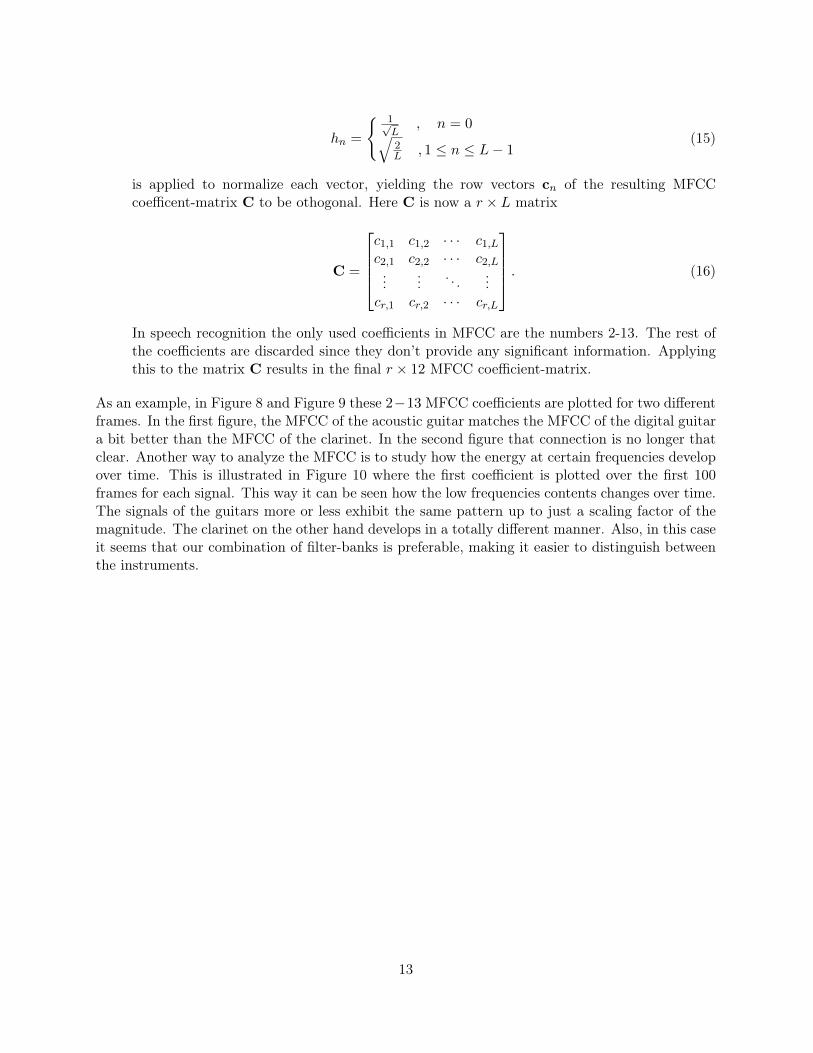
is applied to normalize each vector, yielding the row vectors cn of the resulting MFCCcoefficent-matrix C to be othogonal. Here C is now a r × L matrix

C =

c1,1 c1,2 · · · c1,Lc2,1 c2,2 · · · c2,L...

.... . .

...cr,1 cr,2 · · · cr,L

. (16)

In speech recognition the only used coefficients in MFCC are the numbers 2-13. The rest ofthe coefficients are discarded since they don’t provide any significant information. Applyingthis to the matrix C results in the final r × 12 MFCC coefficient-matrix.

As an example, in Figure 8 and Figure 9 these 2−13 MFCC coefficients are plotted for two differentframes. In the first figure, the MFCC of the acoustic guitar matches the MFCC of the digital guitara bit better than the MFCC of the clarinet. In the second figure that connection is no longer thatclear. Another way to analyze the MFCC is to study how the energy at certain frequencies developover time. This is illustrated in Figure 10 where the first coefficient is plotted over the first 100frames for each signal. This way it can be seen how the low frequencies contents changes over time.The signals of the guitars more or less exhibit the same pattern up to just a scaling factor of themagnitude. The clarinet on the other hand develops in a totally different manner. Also, in this caseit seems that our combination of filter-banks is preferable, making it easier to distinguish betweenthe instruments.

13

Figure 8: 1st frame of signal

Figure 9: 10th frame of signal

14

Figure 10: 1st MFCC and how it changes over time

15

3 Tests

For the tests, some assumptions are made regarding the unknown signal that is about to be tested.Firstly, the instruments possibly present are known and can be a single tone or mix of either, clar-inet, guitar, saxophone and piano. Also, the tones that are played are assumed to be known. Thetones are also sorted in octaves meaning that for example A2 and A3 are considered to be differenttones and not just an A.

The data that will make up our reference bank for the tests are digital tones and mixes createdin Garageband [6] and Audacity [7]. Tones from acoustic instruments will also be used and theseare home recordings. For the tests where mixes of acoustic tones are needed, these are just addedtogether. All signals, digital or acoustic are sampled at sample frequency 44100 Hz.

For both methods the following tests are performed:

1. Given one known tone played by one unknown instrument, determine the instrument.

2. Given two known but different tones from two known instruments, determine which instru-ment that play which tone.

3. Given one known tone played by two unknown instruments, determine the instruments in-volved.

The tests are designed in a way that hopefully will cover as many scenarios as possible. From caseswhere overtones do not overlap to cases where the tones are the same.

Each of the above tests is itself divided in two different cases. The first case will have both thereferences and the unknown signal made up from the same digital tones. Case 1 will therefore coverthe more theoretical aspect of our methods. The second case will have digital references and anacoustic mix of unknowns. Case 2 will therefore deal with a more realistic scenario. The mainreason why each test is divided in two cases comes from the discovery that for some tones, not all,there is a rather big difference in acoustic and digital tones. In particular the lower tones for theclarinet seem to differ more when the digital tones and the acoustic tones are compared.

For every case two signals are tested. For test 2 where two different tones are played the combi-nation of tones have been chosen so that for one signal, many of the overtones overlap and for theother signal only a few overtones overlap.

Totally 2 methods are tested in 3 different ways with 2 cases where each case is tested for 2 differentsignals. The total amount of signals tested becomes 24 (2 · 3 · 2 · 2). This is far from enough forbeing able to statistically say if a method works for a specific test or not. The tests instead givesindications of what might work and what kind of problems that might appear.

In section 3.1 and 3.2 the results of the tests will just be presented. In section 4 the tests will becommented and analyzed.

16

3.1 Tests for FFT-method

As explained in section 2.1 this method depends on selecting a number of overtones. This numberis hard to set for all instrument and it depends on how much information about an instrumentsthat is present in the higher overtones and this is hard to tell. For the tests of the FFT-method thefifth overtone of the highest known tone in the unknown signal will be set as an upper bound onthe total amount of frequencies included. This is chosen to be enough upon just a few observationsand a more thorough analysis of this matter may be valuable but not done here.

Test 1

Case 1

The first two tests for different single-tone signals are shown in Figure 11. Here, the unknownsignals are a clarinet playing the tone B4 (left) and a guitar playing D3 (right). Here both theunknown signal and the references are digital tones. The plot shows how the estimated weightschanges over time.

Figure 11: FFT-method. Test 1, case 1

The test result of this case is not very interesting since the solution in equation (4) for every timeframe l, the weight vector w becomes

argminw≥0

∥∥∥(w1pclarinetl + w2p

guitarl + w3p

saxophonel + w4p

pianol

)− ptotl

∥∥∥2, (17)

where p is the normalized amplitude vector. This is trivial since the signal of the unknown instru-ment is the same as one of the references.

17

Case2

For this case the references are the same as in case 1 but the unknown signal is acoustic. The testsare plotted in Figure 12.


In the left plot, the weight for the clarinet (blue) is dominating for all time frames, except some-where between time frames 10− 40 where contribution from the piano is estimated to be present.In the right plot the estimated weights for the guitar dominates in all time frames except in thebeginning of the signal where the saxophone is the dominating one.

The normalized mean of these weights where the sum of all the means are equal to 1, can then beused as a measure of the likelihood of each instrument participating in the unknown signal. Table 1shows a calculation of the likelihood for the left plot. The corresponding likelihood for the right plotis shown in Table 2. From these tables it is clearly seen that the correct instruments are estimatedto be significant.

Clarinet B4 Guitar B4 Saxophone B4 Piano B40.7177 0 0.1789 0.1034

Table 1: Likelihood of each instrument for left plot in Figure 12

Clarinet D3 Guitar D3 Saxophone D3 Piano D30.0037 0.8576 0.1180 0.0207

Table 2: Likelihood of each instrument for right plot in Figure 12

18

Test 2

The second test is performed just as the first but since this test is about determining what instru-ment playing what tone, in a rewritten equation (5) where hl is replaced by pl resulting in

ptotl =s∑j=1

t∑k=1

wk,jpinstrumentkl,j , (18)

where s indicates the number of tones in the unknown signal and t indicates the number of instru-ments used. As an example, let’s say that the unknown signal consists of the two different tonesplayed by either a clarinet or a guitar. This yields

ptotl = w1,1pclarinetl,1 + w1,2p

clarinetl,2 + w2,1p

guitarl,1 + w2,2p

guitarl,2 . (19)

Each case for test 2 is performed on two signals, where the first is a mix of a clarinet tone D4 anda guitar tone A4. The second signal is a mix of a clarinet playing B4 and a guitar playing D3.

Case1

The results are plotted in Figure 13.


The left plot has a strong contribution from the correct clarinet D4 throughout all time frameswhereas the guitar is wrongfully indicted as playing both the correct tone A4 and the wrong toneD4. In the right plot, the two significant tones (both correctly estimated) are the B4 from theclarinet and D3 from the guitar. The likelihoods are found in Table 3 and 4. By Table 3, thelikelihood of the correct guitar A4 tone is biggest but not significant from D4

19

Clarinet D4 Guitar D4 Clarinet A4 Guitar A40.8802 0.0509 0.0077 0.0611


Clarinet D3 Guitar D3 Clarinet B4 Guitar B40.0290 0.2612 0.7096 0.0003


Case2


In the left plot of Figure 14 and also from Table 5 the wrong guitar tone D4 dominates significantlyfollowed by clarinet D4. Even though the signal actually involves a guitar tone A4, this tone iscalculated to be the least significant. In the right plot and also from Table 6 the correct tones arethe ones appearing as significant.



Clarinet D3 Guitar D3 Clarinet B4 Guitar B40.0290 0.2612 0.7096 0.0003


20

Test 3

Each case for test 3 is performed on two signals, where the first is a mix of a clarinet and a guitar,both playing the tone B4 and in the second test, both are playing D4.

Case1

The test results are shown in Figure 15 and in Table 7 and 8.


From the plots in Figure 15 and also from Table 7 and 8 it can be concluded that the correctinstruments are estimated to be most significant. Even though the contribution from the guitar inthe left plot is estimated to be small, it is still a lot bigger than for the saxophone and piano.

Clarinet B4 Guitar B4 Saxophone B4 Piano B40.9744 0.0249 0.0005 0.0001




21

Case2


The left plot of Figure 16 shows a correct dominating clarinet but the guitar that is supposed tobe present is estimated to be zero as seen in Table 9. The right plot although estimated to holda large contribution from the piano, shows the correct estimated instruments. This becomes clearwhen studying Table 10.

Clarinet B4 Guitar B4 Saxophone B4 Piano B40.6685 0 0.2028 0.1287




22

3.2 Tests for MFCC-method

Test 1

Now the same tests that was done for the FFT-method will be done using the MFCC-method. Thefirst test is for one unknown instrument playing one tone.

Case1

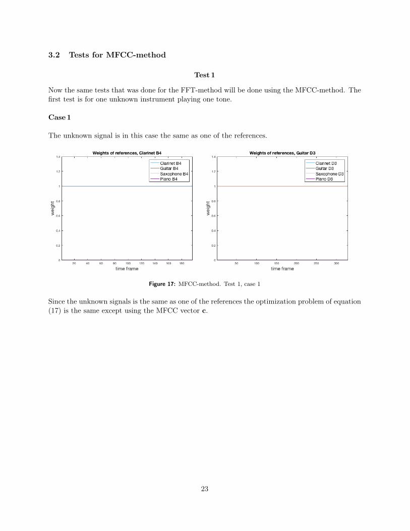
The unknown signal is in this case the same as one of the references.

Figure 17: MFCC-method. Test 1, case 1

Since the unknown signals is the same as one of the references the optimization problem of equation(17) is the same except using the MFCC vector c.

23

Case2

Doing the same test but instead using acoustic signals, different from the references, as unknownsignals results in Figure 18.


In the left plot the correct clarinet tone B4 is dominating in all time frames. In the right plot thecorrect guitar tone D3 is the most significant instrument for almost all time frames.



Clarinet D3 Guitar D3 Saxophone D3 Piano D30 0.8309 0.1498 0.0193


24

Test 2

In the next test the two instrument used and the tones played are assumed to be known. TheMFCC-method will now determine which instrument playing which tone.

Case1

For the first case the unknown signals are the same as in the references.


For the left plot the correct guitar tone A4 is dominating the weights for the first 20 frames andthen the correct clarinet tone D4 is the most dominant. The right plot have a similar look but witha little bit more influence of the wrong guitar and the wrong clarinet.



Clarinet B4 Guitar B4 Clarinet D3 Guitar D30.6482 0.0466 0.0326 0.2725


25

Case2

The result from testing for different reference signals and unknown signals is shown in Figure 20.


As seen in the left plot and in Table 15, the opposite tone for both instruments are estimated tobe significant. In the right plot and in Table 16 the correct tones are estimated.



Clarinet B4 Guitar B4 Clarinet D3 Guitar D30.5964 0.0619 0.0419 0.2999


26

Test 3

Just as before, test 3 is about finding the correct instrument in a mix where two instruments arepresent, playing the same tone.

Case1

See Figure 21 and Table 17 and 18 for the results of case 1, that is when reference and unknownsare both digital signals.


Studying both plots and the tables, there is in this case no doubt about which instruments that areestimated to be present.





27

Case2

The case when the unknown signals come from acoustic recordings is plotted in Figure 22.


By Table 19, the instruments present are estimated to be the clarinet (correct) and the saxophone(incorrect). Studying the right plot and Table 20 makes it quite hard to tell the difference betweenthe clarinet and the saxophone. The instrument estimated as the most significant is though theguitar, which is one of the two correct instruments.





28

4 Results and analysis

In this section the tests will be commented and analyzed. First the results will be judged only bestudying the plots and after that the results will be analyzed on a higher level to see if they arealigned with theory.

Plots of test 1

First the test sections for both the FFT-method and MFCC-method in case 1, Figure 11 and Figure17, will be commented. For this case the unknown signal and one reference are the same whichgives a trivial Least Squares calculation (equation (17)). The reference vector minimizing the erroris of course the clarinet vector and the guitar vector respectively. This yields the weights of thecorresponding references to be equal to 1. When it comes to the second case Figure 12 and Figure18 the references are no longer the same as the unknown. Both methods yields clear significantestimations of the correct instrument even though contributions from other instruments are partlypresent. As mentioned, digital tones and acoustic tones can be quite different. Therefore it mightnot be optimal having a digital reference when testing on acoustic signals, even though the resultsbecomes pretty good. If the reference signal would have been more similar to the unknown signal,the result would have been even better.

Analyzing test 1

The set up for the test for the FFT-method was

ptotl = w1pclarinetl + w2p

guitarl + w3p

saxophonel + w4p

pianol , (20)

where p is the normalized amplitude vector for each signal in time frame l. Calculating the mag-nitude spectrum involves taking the absolute value of the Fourier Transform. Since the number ofunknown instruments in this test is known to be just one, taking the absolute value will not disruptthe linearity in equation (20) so the test results are reliable. The MFCC-method involves not onlythe non-linear operation of taking the absolute value but also it involves taking the logarithm. Inparticular the logarithm is taken of the summed up energies for each filter bank (see step 4, section2.2). Equation (20) can be rewritten using d instead of p. Here d is the summed up logarithmizedenergies for each filter bank of the l’th time frame. The DCT is then calculated (step 5, section2.2) and since the DCT is a linear transformation the linearity is kept. By similar arguments as forthe FFT-method and again using the knowledge that there is just one unknown instrument. Theconclusion for the MFCC-method is that also here the results are aligned with theory and thereforereliable.

Plots of test 2

Judging from the right plot of the first case, Figure 13 and Figure 19, both FFT-method andMFCC-method estimates very well the correct instruments for the signal when the overtones donot overlap at any frequency in the regarded range. For the left plot in the same figures the resultfor the the MFCC-method is also good but the FFT-method estimates both the guitar D4 and A4to be present. So even when the optimal references are used, the FFT-method fails here for some

29

reason. The MFCC-method on the other hand interestingly succeeds in determining the correctinstruments also for the signal in the left plot. In the second case where the reference signals andthe unknown signals are different, see Figure 14 and Figure 20, both methods works very well whenthe overtones does not overlap (see right plot in the figures). Comparing the left plot in Figure20 with the left plot in Figure 19 the MFCC-method seems to fail only due to the fact that thereference is not optimal. The same comparison for the FFT-method gives that it would have failedeven if the reference would have been optimal.

Upon creating the mixes used for the tests, each instrument was set to be equally loud. Thereforeone may suspect the weights of each instrument to be equal throughout the signal but this is notalways the case. The amplitude of a guitar tone is high in the beginning after which it is decaying.The clarinet is more or less high during the whole tone. The weights of the mix will therefore besomewhat equal, close to the onset. Then the weights of the guitar will decrease and the weights ofthe clarinet will increase. The behavior shown in the left plot of Figure 19 for both instruments istherefore the one expected. Using the mean as the likelihood measure may therefore underestimatethe presence of the guitar.

Analyzing test 2

There is a problem about the idea of adding magnitude spectrums of the references in order to getthe magnitude spectrum of an unknown signal. If for example the unknown signal is a combinationof a clarinet and a guitar at time frame l, the mixed signal is

xclarinet+guitarl = xclarinetl + xguitarl (21)

⇔ Xclarinet+guitarl = Xclarinet

l +Xguitarl , (22)

where X is the FFT of the signal x for the corresponding instrument. We have equivalence sincethe Fourier transform is a linear transform. X is now a complex signal which is hard to deal with.To be able to continue doing any further analysis, real values are needed. Therefore the absolutevalue is taken for each X. By taking the absolute value, the equivalence is lost and by the triangularinequality, it instead becomes

⇒ |Xclarinet+guitarl | ≤ |Xclarinet

l |+ |Xguitarl |. (23)

This fact will definitely cause problems to this model since the model assume an equality. But, ifit would be possible to say that

|Xclarinet+guitarl | ≈ w1|Xclarinet

l |+ w2|Xguitarl |, (24)

then it would be possible to continue as if there was an equality instead of an inequality and justhave this generalization in mind as a potential error source. In Figure 23 this generalization is in-vestigated. Here the signals of a clarinet playing D4 and a guitar playing A4 are added to becomea mix of the two instruments. In the left plots the magnitude spectrum for the separated guitarand clarinet is shown. In the right plots the magnitude spectrum of the mix and the magnitude

30

spectrum of the sum of the separated instruments are shown. The two top plots correspond to timeframe 20 and the two bottom plots correspond to the time frame 40.

Figure 23: Example of a clarinet playing D4 and a guitar playing A4. The magnitude spectrum ofthe mixed signal is plotted together with the magnitude spectrum of the sum of the two separatedinstruments

Studying the top right plot in Figure 23 one can see that the two graphs almost coincide with eachother perfectly. By instead looking at the bottom right plot the graphs coincide almost perfectlyexcept at the peak around 880 Hz where the graphs differ a lot. By analyzing more time frames(not shown in this report) the same behavior occur with coinciding graphs except at 880 Hz. Themain reason for this is because the tones D4 and A4 both have an overtone at 880 Hz which in themixed signal will be overlapping. If the mixed signal will have the same amplitude as the summedseparated signals or not mostly depends on the phase. If the wave-formed separated signals wouldhave their peaks at the same time when they are mixed together, then the sum of the separatedabsolute signals would be the same. This might be the case in the top right plot. On the otherhand if the signals are out of phase when they are mixed, meaning that one signal have a peak atthe same time as the other signal has a negative peak, then the amplitude of the mixed signal willbe zero. This might partly be the case in the bottom right plot. Due to small differences in thetune, the phase can change between different time frames making it almost impossible to know theamplitude at an overlapping overtone. In the above example it would have been possible to find thephase-shift by calculating the cross-correlation between the signals in the mix. This is not possiblein a realistic example though, since then the signals in the mix would be unknown.

In the top right plot of Figure 23 the graphs almost coincide also at 880 Hz. This appearance wasalso seen in some other time frames. One reason why the graphs sometimes coincide at 880 Hzand sometimes not could be that the instruments may be close to correctly tuned but not per-fectly. An other reason could be that noise disturb the signal, and therefore resolution from theFFT won’t be perfect. An other factor that could affect is that a tone wobble a bit around thecorrect tone, this phenomenon have especially been seen for string instruments. The fact that theequality in equation (24) holds for non-overlapping frequencies but not for overlapping, explains

31

why the FFT-method might succeed more often for mixed signals when there are few overlappingovertones and the method might be less robust for mixed signals with a lot of overlapping overtones.

Considering the MFCC of a signal consisting of more than one instrument is a bit different com-pared to the FFT-method. In the FFT-method the non-linear operation involved was taking theabsolute value. The MFCC-method will involve the non-linear operations of taking the absolutevalue and the logarithm.

A way to explain how this non-linearity would affect the calculation a mixed signal consisting of aclarinet and a guitar is considered for one time frame l

xclarinet+guitarl = xclarinetl + xguitarl (25)

⇔ Xclarinet+guitarl = Xclarinet

l +Xguitarl , (26)

where X is the Fourier transform of x. The magnitude spectrum is calculated by taking the absolutevalue. Due to that the absolute value is a non-linear operation the equality disappears and insteadthere is an inequality

⇒ |Xclarinet+guitarl | ≤ |Xclarinet

l |+ |Xguitarl |. (27)

In the above analysis regarding the FFT-method it was in some sense shown that this can berewritten as

⇔ |Xclarinet+guitarl | ≈ v1|Xclarinet

l |+ v2|Xguitarl |, (28)

where v is the weight of each magnitude spectrum. The magnitude spectrum is denoted as S andSl is a row vector.

⇔ Sclarinet+guitarl ≈ v1Sclarinetl + v2Sguitarl . (29)

The magnitude spectrum is then multiplied with a filter bank where all the energy of each filter issummed, resulting in

⇔ Sclarinet+guitarl · F ≈ v1Sclarinetl · F + v2Sguitarl · F. (30)

The next step in the MFCC algorithm is taking the logarithm. Since the logarithm is a non-linear operation there is an assumption made that the approximation will hold if the references areweighted once again

⇒ log(Sclarinet+guitarl · F ) ≈ w1log(v1Sclarinetl · F )

+ w2log(v2Sguitarl · F ),

(31)

where w is a weight, similarly as for the absolute value, calculated by Least Squares. By usinglogarithm rules this can be written as

⇔ log(Sclarinet+guitarl · F ) ≈ w1log(v1) + w1log(Sclarinetl · F )

+ w2log(v2) + w2log(Sguitarl · F )

(32)

32

⇔ dclarinet+guitarl ≈ w1log(v1) + w1dclarinetl

+ w2log(v2) + w2dguitarl

, (33)

where dl = log(Sl · F ). The expression wlog(v) becomes an error that is made. If the referenceis good then v should be close to 1. Since log(1) = 0 the error can be assumed to be small. Theformula can therefore be rewritten as

⇒ Dclarinet+guitarl ≈ w1D

clarinetl + w2D

guitarl . (34)

The final step in the MFCC is taking the DCT which is a linear transform.

How the weighting idea for the MFCC-method works will now be investigated. A clarinet playingD4 and a guitar playing A4 are combined to a mix and the separated signals are used as references.In equation (31) the assumption is made that the filter bank energy in the mixed signal can bedescribed as a linear combination of the separated signals. The filter bank energy for the mixedand the separated signals for one time frame is shown in Figure 24.

Figure 24: Filter bank energies for clarinet D4, guitar A4 and a mix of both in the time frame 20

As seen in Figure 24 the energy of the mixed signal follows the energy of the first three peaks fromthe separated signals well which is a similar result as have been seen also for the FFT-method.For the forth peak (filter bank 13), which corresponds to an overlapping overtone for the separatedsignals, the mixed signal is almost as the highest peak. If the MFCC-calculation would have beenperfectly linear then the fourth peak of the mixed signal would have had the height of the sum ofthe clarinet and the guitar. By studying more time frames (which will not be shown in this report)the intuition is that the mixed signal follows the highest peak for each filter bank of the separatedsignals.

33

Continuing in Figure 24 the y-axis is in the logarithmic scale. Since the logarithm is non-linear itis not possible to take the sum of the filter bank energies of the clarinet and the guitar in order toget the energy of the mix. By for example looking at filter bank 4, if the weights w would havebeen 1 for both the clarinet and the guitar, then the approximated mixed energy would have been≈ 1 · 0.2 + 1 · (−1.7) = −1.5 which is a really bad estimate of the mixed peak which should be 0.2.The best estimate would instead be setting w1 = 1 and w2 = 0. But for example in filter bank 7the best estimate would have been achieved setting w1 = 0 and w2 = 1. By using Least Squares forthe whole time frame the weights are set to w1 = 0.4 and w2 = 0.7. Studying more time frames theweights seems to become some kind of mean of the separated signals since both signals influencethe mixed signal at different filter banks. It can be concluded that this weighting does not give avery good estimation of the energy of the mixed signal.

The Least Squares calculate the weights of each instrument that yields the smallest error from theunknown signal. Even if the error becomes large by using a combination of the correct referencesthe error might still be the smallest compared to using wrong references. This could be the reasonwhy the MFCC-method succeeds even if the theory says that it shouldn’t.

Plots of test 3

In all of the four tests for case 1, seen in Figure 15 and Figure 21 the methods succeeds. The guitarin left plot for the FFT-method is maybe estimated a bit low but this is the only minor detail.When it comes to case 2 (see Figure 16 and Figure 22) the analysis becomes a bit harder for all fourtests. Starting with the right plots and the corresponding Table 10 and 20, it might seem that theestimation of the guitar succeeds quite well for both methods. This is probably not correct though,as the typical pattern of the guitar tone should be decaying and look more like the one in Figure 21.This makes the results doubtful. The results in the corresponding left plots is a bit better. Herethe estimated clarinet follows the overall pattern a clarinet tone is supposed to have but the guitaris for the FFT-method non-existing and for the MFCC-method estimated to be non-significant.

Analyzing test 3

The analysis of test 3 is similar to the one done for test 2. The difference is that for all signals intest 3, all the overtones overlap. The analysis for test 2 concluded that problems with non-linearityalmost only occur when the overtones were overlapping. With this into consideration the resultsfrom test 3 would be expected to be worse than for test 2. That was also the the way it turned outfor case 2 where no results was totally correct. For test 3 case 1 all the tests succeeded which is alittle bit confusing since one test for the FFT-method test 2 case 1 failed. Test 2 are supposed to bebetter than test 3 but that seems to not always be the case. To be able to do any further analysisabout this, more tests would have been needed to insure that this was not a random outcome.

By studying both plots in Figure 16 and the left plot in Figure 22 the pattern of the weightsfor both the correct and the incorrect instruments are shifting a lot for the first 60 time frames.After that the weights becomes more stationary. One reason for this might be that, right at thebeginning of a tone when the tone is struck, the signal changes a lot and the variance is high. The

34

signal therefore becomes more non-stationary for these time frames and first after a while the tonebecomes more stationary. The FFT needs stationary signals to calculate appropriate spectrums.Therefore the varying weights for the early time frames in the figures might come from incorrectspectrum estimates.

35

5 Discussion and future improvements

In this project, characteristics for different musical instruments have been described mathemati-cally by analyzing the energy and structure of pitches and overtones. Two methods using differentapproaches, the first using magnitude spectrum analysis and the second using cepstrum analysishave been proposed and tested. The test results, as seen, have been varying in reliability andaccuracy leaving room for future improvements and modifications. For the aspect of only findingone unknown instrument playing one tone, both methods works fine. When dealing with signalsconsisting of two instruments the analysis becomes harder, especially when overtones overlap. Noneof the methods have been working perfectly for these signals and none of the methods have beenfar better than the other.

The FFT-method is very similar to the MFCC-method in many ways but there are some differ-ences. One is that the FFT-method is using the magnitude spectrum and the MFCC-method is, insome sense, using the logarithmized magnitude spectrum. The logarithmized magnitude spectrumis good to use if smaller peaks, which often occur at higher frequencies, are of interest. If only thefirst overtones are of interest then the non-logarithmized spectrum would be better. It is not inves-tigated how many overtones are needed to categorize an instrument in the best way. Depending onhow many overtones that are needed to do a good categorization, it should be decided whether touse logarithmized or non-logarithmized magnitude spectrum.

One main advantage with the FFT-method is that it only uses information in the spectrum thatbelongs to certain wanted peaks. The MFCC-method uses all information in the spectrum, eventhe space between these peaks, which is just unnecessary. When comparing the unknown and thereference signals for the MFCC-method, both the error at the peaks and the space between thepeaks are minimized. It would be much better to minimize the error at the peaks only.

On the other hand one advantage with the MFCC-method is that it uses filter banks. By applyingfilter banks, information not only at the peaks, but also around the peak is retrieved. This is good,since mixing two tones with overlapping overtones will far from always result in a linear additionof the overlapping peaks but instead the power may be distributed around the maximum of the peak.

If the tones are known, the filter banks used in the MFCC-method could be optimized by takinginto account features of the FFT-method. Firstly, the filters in the filter bank can be placed exactlywhere the pitches and overtones are located, resulting in fewer filters. By this approach the energybetween the peaks is ignored. If the tones and overtones are well separated the need of overlappingfilters may also be eliminated. Secondly, the limits of the frequency range for the filter banks couldusing known pitches be set in an optimal way.

As seen in case 1 for almost all tests, having a perfect reference will give a correct weight estima-tion. Extending the amount of reference signals would improve the instrument categorization a lot.Every acoustic instrument have in some way a sound of it’s own. By having many references of thesame instrument category the chance that an unknown instrument would be similar to one of thereferences increases.

36

When the instruments are assumed known and it comes to determine which instrument playingwhich tone (test 2) one possible improvement could be to add up the reference signals for allpossible combinations before doing the weight calculation. This reduces the problem to be of theform in test 1 where non-linear operations does not corrupt the result, that is

ptotl = w1

(pclarinetl,1 + pclarinetl,2

)+ w2

(pclarinetl,1 + pguitarl,2

)+ w3

(pguitarl,1 + pclarinetl,2

)+ w4

(pguitarl,1 + pguitarl,2

) , (35)

where term one and four in the right-hand side disappears if the instruments are known to bedifferent. This will hold also for the MFCC-method, where in equation (35), p is replaced by c. Ofcourse, as the amount of instruments and tones increases the number of combinations in the righthand side also increases, making this approach ineffective.

In order to determine if a reference instrument is significantly present in an unknown signal or not,the mean has been used. This is probably not an optimal measure since the weights are sometimesexpected to vary over time. For example the guitar use to have a strong contribution to a mixedsignal in the beginning and then decaying to be almost zero. An optimal measure about significancelevel would in some way take into account how the weights of the references are expected to varyover time.

The idea about using Least Squares and calculate the weight for every instrument in the referencebank is good if no assumptions of the instruments in the unknown signal can be done. But if it isknown that the unknown signal only consists of one instrument, then it is a bad idea to combinefour references trying to match the unknown signal. A better idea would instead be to rescale eachreference with Least Squares to match the unknown signal and then calculate the mean square error(MSE). The reference with the smallest MSE would then be the best guess. For the case when theunknown signal consists of two instruments they would be weighted with Least Squares and thenadded together before the MSE is calculated.

If the tones are different and the instruments are known, another possible improvement for theFFT-method could be to apply an iterative process starting from the lowest fundamental frequencyin the spectrum of the unknown signal. By analyzing and comparing each of the peaks one by oneand see how the amplitude changes over time it might be possible to within just a narrow range ofpeaks be able to determine one or more of the instruments. This is illustrated in Figure 25. Herethe fundamental tone and a few of the overtones from a guitar and a clarinet is plotted. As seen,there is a big difference in how the pitch is evolving over time between the instruments and thiscan be used in some cases.

37

Figure 25: Overtones and how they change over time

38

6 Bibliography

[1] https://en.wikipedia.org/wiki/Timbre

[2] C.L. Lawson, R.J. Hanson "Solving Least Squares Problem" Prentice Hall, 1974, p. 158-161

[3] https://engineering.purdue.edu/ malcolm/interval/1998-010/

[4] http://practicalcryptography.com/miscellaneous/machine-learning/guide mel-frequency-cepstral-coefficients-mfccs/

[5] S.K. Kopparapu, M. Laxminarayana, "Choice of mel filter bank in computing MFCC of a re-sampled speech" 10th International Conference on Information Science, Signal Processing andtheir Applications p. 121-122, 2010

[6] http://www.apple.com/se/mac/garageband/

[7] http://www.audacityteam.org

[8] G. Lindgren, H. Rootzén, M. Sandsten "Stationary Stochastic Processes For Scientists And En-gineers" CRC Press p. 129, 2014

39

Bachelor’s Theses in Mathematical Sciences 2016:K6ISSN 1654-6229

LUNFMS-4016-2016

Mathematical StatisticsCentre for Mathematical Sciences

Lund UniversityBox 118, SE-221 00 Lund, Sweden

http://www.maths.lth.se/

Documents

Abstract - lup.lub.lu.se