NBER WORKING PAPER SERIES

STAGGERED BOARDS AND THE WEALTH OF SHAREHOLDERS:EVIDENCE FROM TWO NATURAL EXPERIMENTS

Lucian A. BebchukAlma Cohen

Charles C.Y. Wang

Working Paper 17127http://www.nber.org/papers/w17127

NATIONAL BUREAU OF ECONOMIC RESEARCH1050 Massachusetts Avenue

Cambridge, MA 02138June 2011

For helpful comments on earlier drafts, we are grateful to Steven Davidoff, Jeff Gordon, Guhan Subramanian,and participants in a Harvard workshop. We have also benefitted from conversations with a numberof participants in the Airgas takeover battle and the market trading surrounding it, including IsaacCorree, Jeff Gordon, Matthew Mark, David Millstone, Ted Mirvis, and Tim Wallach. The views expressedherein are those of the authors and do not necessarily reflect the views of the National Bureau of EconomicResearch.

NBER working papers are circulated for discussion and comment purposes. They have not been peer-reviewed or been subject to the review by the NBER Board of Directors that accompanies officialNBER publications.

© 2011 by Lucian A. Bebchuk, Alma Cohen, and Charles C.Y. Wang. All rights reserved. Short sectionsof text, not to exceed two paragraphs, may be quoted without explicit permission provided that fullcredit, including © notice, is given to the source.

Staggered Boards and the Wealth of Shareholders: Evidence from Two Natural ExperimentsLucian A. Bebchuk, Alma Cohen, and Charles C.Y. WangNBER Working Paper No. 17127June 2011JEL No. G30,G34,K22

ABSTRACT

While staggered boards have been documented to be negatively correlated with firm valuation, suchassociation might be due to staggered boards either bringing about lower firm value or merely reflectingthe tendency of low-value firms to have staggered boards. In this paper, we use two natural experimentsto shed light on the causality question. In particular, we focus on two recent court rulings, separatedby several weeks, that affected in opposite directions the antitakeover force of staggered boards: (i)a ruling by the Delaware Chancery Court approving the legality of shareholder-adopted bylaws thatweaken the antitakeover force of a staggered board by moving the company’s annual meeting up fromlater parts of the calendar year to January, and (ii) the subsequent decision by the Delaware SupremeCourt to overturn the Chancery Court ruling and invalidate such bylaws.

We find evidence consistent with the hypothesis that the Chancery Court ruling increased the valueof affected companies – namely, companies with a staggered board and an annual meeting in laterparts of the calendar year – and that the Supreme Court ruling produced a reduction in the affectedcompanies’ value. The identified effects were most pronounced for firms for which control contestsare especially relevant due to relative underperformance, small firm size, high asset pledgibility, orhigh takeover intensity in their industry.

Our findings have implications for the long-standing debate on staggered boards. The findings areconsistent with the market’s viewing staggered boards as bringing about a reduction in firm value.Our findings are thus consistent with leading institutional investors’ policies in favor of board de-staggering,and with the view that the ongoing process of board de-staggering in public firms can be expectedto enhance shareholder value.

Lucian A. BebchukHarvard Law School1545 Massachusetts AvenueCambridge, MA 02138and NBERbebchuk@law.harvard.edu

Alma CohenThe Eitan Berglas School of EconomicsTel Aviv UniversityRamat-Aviv, Tel-AvivISRAELand NBERalmac@post.tau.ac.il

Charles C.Y. WangStanford University579 Serra MallStanford, CA 94309charles.cy.wang@stanford.edu

1

1. Introduction

The existence of governance provisions that weaken shareholder rights and insulate

directors from removal is now well known to be negatively correlated with firm value (Gompers,

Ishii, and Metrick (2003)). This correlation is partly driven by the negative correlation between

firm value and staggered board provisions, which prevent shareholders from removing a majority

of directors in any given shareholder meeting (Bebchuk and Cohen (2005); Bebchuk, Cohen, and

Ferrell (2009)). It might be suggested, however, that such correlation does not imply causation,

and that it might be fully driven by the tendency of firms with low value and weak performance

to have entrenching provisions in general and staggered boards in particular. In this paper we

seek to contribute to understanding the causality question by studying two natural experiments –

two court rulings that affected the extent to which staggered boards can impede shareholders

seeking to replace a majority of directors. We find evidence consistent with market participants’

viewing the antitakeover force of staggered boards as value-reducing.

Our results have significant policy implications for the long-standing debate on staggered

boards and for the struggle between institutional investors and companies over the subject. Over

time, institutional investors have become increasingly opposed to staggered boards. While

shareholders were willing to vote for adopting a staggered board during the 1980s, they have

generally been unwilling to do so since the early 1990s and have been increasingly willing to

support shareholder proposals to dismantle staggered boards. According to Georgeson

Shareholder reports, the average percentage of votes cast in favor of proposals to de-stagger

boards exceeded 65% in each of the five proxy seasons from 2006 through 2010. The Council of

Institutional Investors,1 major institutional investors such as the American Funds, BlackRock,

CalPERS, Fidelity, TIAA-CREF, and Vanguard,2 and the two leading proxy advisors ISS and

© 2011 Lucian A. Bebchuk, Alma Cohen, and Charles C.Y. Wang. All rights reserved. 1 See Council of Institutional Investors, Corporate Governance Policies, at p. 3.

2 See American Funds, Proxy Voting Procedures and Principles, p. 3; BlackRock, Proxy Voting

Guidelines for U.S. Securities, at p. 6; California Public Employees Retirement System, Global Principles

of Accountable Corporate Governance, p. 17; Fidelity Investments, Corporate Governance and Proxy

Guidelines, p. 11; TIAA-CREF, Policy Statement on Corporate Governance, p. 31; Vanguard,

Vanguard's proxy voting guidelines, p. 2.

2

Glass Lewis,3 all have policies favoring annual election of all directors and board de-staggering

proposals.

Facing such widespread shareholder opposition to staggered boards, many companies,

especially large companies receiving the most attention from investors seeking governance

improvements, have chosen during the past decade to eliminate staggered boards; according to

FactSet Research Systems, the number of S&P 500 companies with staggered boards declined by

more than 40% from 2000 to 2009. Many companies with staggered boards, however, continue

to resist investor pressure to de-stagger, express strong opposition to proposals to de-stagger their

board, and argue that staggered boards enhance rather than reduce shareholder value.4 At present,

about half of the publicly traded companies in the over 3,000 public companies whose takeover

defenses are tracked by FactSet Research Systems still have a staggered board. The stakes in the

debate on staggered boards are thus large.

We seek to contribute to understanding the effects of a staggered board. Causal

identification is notoriously difficult in empirical work on corporate finance and corporate

governance. We use a quasi-experimental research design, focusing on the effects of two not-

fully-anticipated court rulings. In particular, we focus on the Chancery Court and Supreme Court

rulings on October 8, 2010 and November 23rd

, 2010, respectively, in the takeover battle

between Airgas Inc. (“Airgas”) and Air Products and Chemicals, Inc. (“Air Products”).

The rulings focused on the permissibility of adopting a shareholder-adopted bylaw --

conceived in the course of the Airgas takeover battle – that moves up the date of the next

calendar year’s annual meeting to January. Such a bylaw has the potential of shortening the

tenure of directors and facilitating the process of replacing a majority of the company’s directors.

For companies whose annual meetings ordinarily took place in later parts of the calendar year (as

was the case with Airgas whose annual meetings have typically been held in August or

September), permitting such bylaws would reduce the extent to which staggered boards can

delay the replacement of a majority of directors and thus lower the impediments to a hostile

takeover. Chancellor Chandler of the Delaware Chancery Court initially ruled that such bylaws

3 RiskMetrics Group, 2010 U.S. Proxy Voting Guidelines Summary, p. 18.

4 For examples of statements of boards of directors in opposition to shareholder proposals in favor of

board de-staggering brought to a vote in 2010 annual meetings, see the 2010 proxy statements of

Abercrombie & Fitch Co., Bancorp South, Inc., and Hospitality Properties Trust.

3

may be used. Subsequently, however, the Delaware Supreme Court reversed and held such

shareholder-adopted bylaws to be invalid.

We examine the cross-section of stock returns surrounding the announcements of the

rulings, focusing on the value of the companies affected by the above two rulings – companies

with a staggered boards whose annual meeting has been taking place in later parts of the calendar

year. We find evidence consistent with the hypothesis that the value of these companies was

increased by the first ruling, which validated the novel method for weakening the antitakeover

force of companies’ staggered boards. We also find evidence consistent with the hypothesis that

the second ruling, which invalidated this novel method, had a negative effect on the value of

these companies that was of a similar magnitude to that of the first ruling’s (positive) effect. The

initial increase in value, and the subsequent reduction, was especially pronounced for companies

for which control contests are especially relevant due to relative underperformance, high asset

pledgibility, small firm size, or high deal intensity in the industry.

Overall, our findings are consistent with market participants’ expecting the weakening of

the antitakeover effect of staggered boards to bring about an increase in firm value. These

findings are thus consistent with the large support among institutional investors for proposals to

repeal staggered boards. The findings are also consistent with the view that the continued de-

staggering of boards – an ongoing process that has been taking place over the past decade – can

be expected to benefit shareholders. The identified abnormal positive returns accompanying the

Chancery Court ruling, and the abnormal negative returns accompanying the Supreme Court

ruling, are likely to understate the market’s estimate of the benefits of repealing staggered boards

because (i) as will be discussed, the market ascribed a positive probability to each of the ruling

before they were issued, and (ii) the bylaws that were the subject of the rulings would have

weakened but not eliminated the antitakeover force of staggered boards in the companies

affected by the rulings.

Our work seeks to contribute to the existing body of empirical work on staggered boards.

Focusing on a sample of hand-collected targets of hostile takeovers, Bebchuk, Coates, and

Subramanian (2002a, 2002b) found that, among takeover targets, those with a staggered board

are associated with lower gains to shareholders following the receipt of a tender offer.

Examining the 1,500+ public firms in the IRRC dataset, Bebchuk and Cohen (2005)

4

subsequently documented that staggered boards are associated with lower firm valuation as

proxied by Tobin’s Q. Subsequently, Masulis, Wang, and Xie (2007) found that firms with

staggered boards are associated with value-decreasing acquisition decisions; and Faleye (2007)

reported that staggered boards are associated with lower sensitivity of compensation to

performance and lower sensitivity of CEO turnover to firm performance. Bates, Becher and

Lemmon (2008) reported that staggered boards have a positive correlation with higher takeover

premiums, but this study also reports that staggered boards are associated with a lower likelihood

of an acquisition, and confirms, consistent with earlier work, that staggered boards are overall

associated with lower firm valuation. We seek to contribute to this body of work by using a

quasi-experimental setting to study whether the identified correlation between staggered boards

and lower firm value is at least partly driven by staggered boards bringing about a lower firm

value.5

Our study also builds on the extensive literature using stock price reactions to study the

wealth effects of regulatory changes, beginning with Schwert (1981) (see MacKinlay (1997) and

Bhagat and Romano (2002) for reviews). We add to prior work using event studies to assess the

effects of changes in governance.6 The challenges facing event studies of governance changes

are now well-understood: first, event studies focusing on governance changes adopted by

5 Bebchuk and Cohen (2005) explore the causality issue by using staggered boards in 1990 as an

instrument, obtaining evidence consistent with the correlation between staggered boards and lower firm

value being at least partly driven by staggered boards’ operating to reduce firm value. This evidence,

however, is offered as being merely suggestive on the causality issue.

We also wish to note the results of Guo, Kruse, and Nohel (2008), who find positive stock market

reactions to announcements by companies on plans to de-stagger. While the results of Guo et al. are

consistent with ours, it is difficult to draw causal inferences from their findings because management

decisions to de-stagger are unlikely to be random, but rather may tend to be taken by managements that

anticipate improvements in firm value that would make them less vulnerable to a control contest in any

event, and may thus be a signal to the market about management’s positive inside assessment. An earlier

paper by Bhagat and Jeffries (1991), using data from the 1980s during which antitakeover amendments

often passed, studied the returns accompanying the announcement of such amendments (in general, not

only resulting in a staggered board). 6 For example, Chhaochharia and Grinstein (2007) and Hochberg, Sapienza, and Vissing-Jorgensen

(2009) use stock returns to study the effects of the Sarbanes-Oxley Act; and Larcker, Ornazabal, and

Taylor (2010) and Becker, Bergstresser, and Subramanian (2010) analyze stock returns to study the

expected effects of proxy access reform.

5

companies bundle together the market’s assessment of the changes with the market’s inferences

concerning the private information that might have led management to make such changes (see,

e.g., Binder (1985), Coates (2000)); and, second, events focusing on legislative adoption of new

arrangements (e.g., Karpoff and Malatesta (1989)) might face the additional difficulty that

market participants might at the time of adoption lack sufficient experience with the

consequences of the newly adopted arrangements to form a good assessment of their expected

effects. The court rulings on which we focus provide a good quasi-experimental setting: first, this

setting involves exogenous changes that took place at clear points in time and were not fully

anticipated prior to that point in time; and, second, the changes were to an arrangement –

staggered boards – with whose consequences market participants have had a great deal of

experience over the preceding two decades. In addition, our analysis is assisted by the fact that

we have two events, each affecting the same set of companies, but in the opposite direction than

the other.

The remainder of this paper is organized as follows. Section 2 discusses the relevant

institutional background, including the Delaware Chancery and Supreme Court rulings which are

the focus of our study. Section 3 describes our data and provides summary statistics. Section 4

shows that the stock returns accompanying the two rulings are consistent with the market’s

viewing staggered boards as bringing about a lower firm value. Section 5 concludes.

2. Staggered Board and the Airgas Ruling

2.1. Staggered Boards

A company may have a unitary or a staggered board. In a unitary board structure, all

directors stand for election at each annual meeting. By contrast, in a staggered board structure,

directors are grouped into separate classes, typically three classes, with only one of the classes

coming up for re-election at each shareholder annual meeting. A staggered board structure

therefore provides incumbent directors with substantial protection from attempts to gain control

via either a proxy fight or a takeover bid.

In a proxy fight over a company with a staggered board, a challenger would not be able to

gain control of the board in one annual meeting but would need to win a shareholder vote in two

6

consecutive shareholder meetings. Thus, even a competing team that is viewed as superior by

shareholders would face a substantial delay in its attempt to gain control. Furthermore, the

prospect of a board that is bitterly split in the period between the two shareholder meetings might

discourage some shareholders from voting for a challenger they would support if a clean-cut

transition were possible.

Staggered boards also provide substantial protection against hostile bidders because,

following the development of the poison pill, a hostile bidder can prevail over incumbent

opposition only by getting shareholders to replace the majority of the incumbent directors. U.S.

law has developed during the 1980s and early 1990s to allow incumbents to adopt and maintain

poison pill plans that, as long as they are in place, make it prohibitively expensive for a bidder to

purchase a large block. As a result, the only route left for hostile bidders is to put an attractive

offer on the table and persuade shareholders to replace the incumbents with a slate of directors

receptive to the acquisition bid, typically nominated by the bidder itself. Once elected, such a

slate of directors would redeem the poison pill and make the acquisition possible.

Thus, a hostile takeover requires a ballot box replacement of a majority of directors and is

hence made more difficult by the presence of a staggered board. With a staggered board, no

matter how attractive a bidder’s offer is, the bidder would have to win in two consecutive annual

meetings. In fact, the evidence indicates that takeover targets are substantially more likely to be

able to fend off a hostile takeover bid and remain independent when their board is staggered

(Bebchuk, Coates, and Subramanian 2002).

2.2. The Airgas Bylaw

The takeover battle that has led to the ruling on which we focus has been waged for over

a year, and a good account of it can be obtained from a series of Deal Professor columns written

for the New York Times online by Professor Steven Davidoff.7 The saga began in October 2009,

7 See Davidoff, “The Way Forward for Airgas,” New York Times online, March 19, 2010; Davidoff,

“The Air Products-Airgas Battle Heats Up,” New York Times online, May 14, 2010; Davidoff, “Airgas

Rolls the Dice in Proxy Fight,” New York Times online, August 30, 2010; Davidoff, “Airgas’s Novel

Question,” New York Times online, September 1, 2010; Davidoff, “After Losing Vote, What’s Next for

Airgas?,” New York Times online, September 16, 2010; Davidoff, “Air Products Wins Round in Battle

With Airgas,” New York Times online, October 8, 2010; Davidoff, “The Dwindling Options for Airgas,”

7

when Air Products expressed an interest in acquiring Airgas. Air Products made three offers

over the following four months, which were all rejected by Airgas’ board of directors. In

February of 2010, Airgas rejected Air Products’ $5 billion, all-cash tender offer to acquire 100%

of Airgas’ shares.8

Facing the opposition of the Airgas board, Air Products proceeded to a proxy fight at the

shareholder meeting of Airgas in September 2010. Because Airgas has a staggered board, only

one-third of its nine directors came up for re-election at the meeting. With a majority of Airgas’

shareholders seemingly supportive of its acquisition attempt, Air Products was able to replace

the directors coming up for re-election with three individuals nominated by Air Products.

In past calendar years, Airgas held its annual meetings no earlier than August, and thus,

in the ordinary course of events, Air Products would have been expected to have to wait a year to

get an opportunity to replace another one-third of Airgas’ directors and pave the way for an

acquisition. In this case, however, Air Products made a novel move, which seems to have been

first suggested in one of the Professor Davidoff’s Deal Professor columns.9 At the September

2010 annual meeting, Air Products obtained majority shareholder approval for a new

shareholder-adopted bylaw provision (“the Airgas Bylaw”), which specified that the next annual

meeting will be held on January 18, 2011, a mere four months after the September 2010 annual

meeting.

Airgas turned to the Delaware Chancery Court, seeking to invalidate the bylaw. Airgas

argued that the staggered board structure established in Airgas’ charter is inconsistent with the

shortening of the directors’ terms that the bylaw would have produced, and that the bylaw is thus

impermissible as contrary to the charter. Airgas warned that interpreting the standard language

used in its charter as permitting shareholders to adopt bylaws such as the Airgas bylaw would

dilute the significance of having a staggered board in many companies. In response, Air Products

argued that the charter provision establishing a staggered board should be interpreted as

New York Times online, October 11, 2010. Davidoff, “Airgas’s Strategic Blink,” NY Times online,

October 28, 2010. 8 On February 11, Air Products announced an all-cash tender offer at that price for 100% of the Airgas

shares for $60/share, which was again rejected by Airgas. Air Products continued to raise its bid over the

next few months, all met with a cool rejection: on July 8, it increased its offer to $63.50/share; and on

September 6, 2010, it again raised its bid to $65.50/share. 9 See Steven M. Davidoff, “The Way Forward for Airgas,” New York Times online, March 19, 2010.

8

requiring only that one-third of the directors come up for election in each calendar year’s annual

meeting, without limiting the ability of bylaws to specify the time during the calendar year in

which the annual meeting will take place.

The litigation attracted significant attention because of its implications for other publicly

traded companies – namely, other companies with a staggered boards and an annual meeting

ordinarily taking place in later parts of the calendar year.10

To the extent that bylaws such as the

Airgas bylaw are permitted, the antitakeover force of these companies’ staggered boards would

be weakened, as shareholders favoring a premium offer blocked by incumbent directors would

be able to pass such a bylaw and shorten the delay required for replacing a majority of the board.

Following the Chancery Court ruling permitting such bylaws, the Deal Professor column stated

that the opinion “blows a hole in the defenses of many companies with staggered boards” and

that these companies “will have to live with the fact that a staggered board can be weakened by

forcing a subsequent annual meeting to occur much sooner than people thought.” Conversely, to

the extent that such bylaws are impermissible, as the Delaware Supreme Court ultimately held,

the antitakeover force of these companies’ staggered boards will remain intact and the “hole in

the defenses” will be filled.11

2.3. The October 8th

Chancery Court Ruling

As is common in the courts of Delaware, the litigation over the permissibility of the

Airgas bylaw proceeded quickly, with a final hearing taking place in the Delaware Court of

Chancery on Friday October 8th

, 2010. That evening, after the close of the stock market,

Chancellor Chandler issued an opinion that sided with Air Products and approved the legality of

the Airgas bylaw.12

Chandler concluded that the question of whether the Airgas bylaw is

10

At the time of the Airgas rulings, companies’ ordinary timing of the annual meeting within the calendar

year did not seem to reflect companies’ setting of the level of antitakeover protection. As noted earlier,

the use of an Airgas-type bylaw in the context of a takeover battle was a novel technique first conceived

for and tried in the Airgas 2010 takeover saga. Prior to this battle, the choice of the annual meeting timing

was generally not viewed as relevant for corporate control purposes, and was made on the basis of various

historical and logistical considerations. 11

See Steven M. Davidoff, “Air Products Wins Round in Battle with Airgas,” New York Times online,

October 8, 2010. 12

Airgas, Inc. v. Air Products and Chemicals, Inc., Chancery Court opinion, Decided October 8, 2010.

9

permissible is not unambiguously answered by studying the language of the charter provision

establishing the staggered board, and that this ambiguity should be resolved by reference to a

presumption in favor of the shareholder franchise.

Chancellor Chandler’s ruling was not a complete surprise to the market. For instance, the

widely followed Deal Professor column as well as the M&A Law Prof blog argued prior to the

ruling that such an outcome was warranted on the merits and thus could well be expected.13

While Chancellor Chandler’s ruling was not a complete surprise, however, it was not fully

anticipated by the market either. In fact, at the time of the hearing in the Chancery Court on

Friday, October 8, there was a downward movement in the stock price of Airgas, which a Deal

Professor column covering the hearing attributed to market participants updating upwards the

likelihood of an Airgas victory in light of certain remarks made by the Chancellor.14

Furthermore, that the ruling was not fully anticipated by the market is suggested by the

immediate post-ruling change in Airgas’ stock price. Airgas stock price rose by 2.7% at the very

beginning of the first trading day (October 11, 2010) after the ruling was announced on the

preceding Friday evening.15

The not-fully-anticipated nature of Chancellor Chandler’s ruling gives rise to a natural

experimental setting. The ruling was expected, to the extent that it would not be overturned on

appeal, to weaken the insulating power of staggered boards of those companies whose annual

meetings ordinarily takes place in later parts of the calendar year. Thus, a finding that the ruling

was accompanied by positive abnormal returns to such companies (relative to non-impacted

companies) would be consistent with the market’s viewing the antitakeover force of staggered

boards as value-decreasing.

13

See Davidoff, “Airgas’s Novel Question,” New York Times, September 1, 2010.

Davidoff, “After Losing Vote, What’s Next for Airgas?,” New York Times online, September 16, 2010;

Brian JM Quinn, “Advantage: Air Products,” M&A Law Prof Blog, October 8, 2010. 14

See Davidoff, “The Dwindling Options for Airgas,” New York Times online, October 11, 2010. 15

The view that the Chancery Court ruling was uncertain prior to its announcement – that is, that the

ruling announced was neither a complete surprise nor fully anticipated – was also confirmed in

conversations we had with market participants involved in the Airgas litigation and in M&A arbitrage

trading in Airgas stock during the relevant period.

10

2.4. The November 23rd

Supreme Court Ruling

After the initial Chancery Court decision, Airgas appealed to the Supreme Court of

Delaware, which held a hearing over the case on November 2nd

. Although the Delaware Supreme

Court was expected to announce its decision within days of the hearings, as was commonly the

case in Delaware Supreme Court rulings in fast-paced takeover battles, the Supreme Court

announced its decision only three weeks later, on November 23, 2010.16

Instead of focusing on the language of the standard charter provision establishing a

staggered board, as did the Chancery Court, the Supreme Court’s interpretation of the charter

provision relied substantially on “extrinsic evidence,” such as the description of the chapter

provision by commentators and in company disclosures. The Supreme Court concluded that the

standard language of the staggered board provisions should be understood to require that

directors serve for three years and thus to preclude Airgas-type bylaws that shorten this term

significantly by moving up the annual meeting to the beginning of the calendar year. The

Supreme Court ruling thus closed the door – opened up by the Chancery Court ruling – for using

Airgas-type bylaws to weaken the force of the staggered boards of companies whose annual

meeting ordinarily takes place in later parts of the year.

As was the case with the Chancery Court ruling, the Supreme Court ruling was not

completely unexpected. During the November 8, 2010 hearing at the Delaware Supreme Court,

the Supreme Court Justices directed tough questions to Air Products’ counsel which led some

market participants to raise their estimate of the likelihood of the Supreme Court’s reversing the

lower court ruling.17

Furthermore, the Supreme Court’s delay in announcing a decision was

viewed by market participants as increasing the likelihood of the Supreme Court’s finding the

Airgas bylaw to be invalid; had the Court planned to validate the bylaw and thus pave the way

for a shareholder meeting in two months, the Court would have had strong reason to try to

announce its decision quickly to facilitate preparing for the resulting January 2011 meeting.

16

Airgas, Inc. v. Air Products and Chemicals, Inc., Delaware Supreme Court opinion, Decided November

23, 2010, C.A. No. 5817. 17

See, e.g., Davidoff, “Staggered Boards and Company Value”, New York Times online, November 12,

2010 (stating that “the questioning of the justices makes me ever so slightly more inclined to see the

possibility of a reversal”).

11

As was the case with the Chancery Court ruling, however, the Supreme Court ruling was

not fully anticipated by the market. Although Professor Davidoff revised the likelihood of

reversal afterwards in light of the justices’ questioning at the Supreme Court hearing, his Deal

Professor column continued to predict that the Supreme Court would likely affirm the lower

court’s ruling.18

Furthermore, the stock price of Airgas fell significantly upon the announcement

of the Supreme Court’s opinion at 1:30PM on November 23rd

,19

which is consistent with the

market not being certain that Airgas would win prior to the issuance of the decision.20

The not-fully-anticipated nature of the Supreme Court ruling provides us with another

good natural experiment setting for studying market participants’ view on how staggered boards

affect firm value. By overturning the lower court ruling that weakened the insulating power of

staggered boards of companies whose annual meetings ordinarily takes place in later parts of the

calendar year, the Supreme Court ruling returned this insulating power of the companies’

staggered boards to pre-Airgas levels. Thus, a finding that the ruling was accompanied by

negative abnormal returns to such companies (compared to non-impacted ones) would be

consistent with the market’s viewing the power of staggered boards to delay director replacement

by shareholders as value-decreasing.

3. Data and Summary Statistics

We gather data on corporate governance characteristics, in particular the presence of a

staggered board, from the Shark Repellent dataset of FactSet Research Systems. The data is

18

See Davidoff, “Airgas’s Strategic Blink”, New York Times online, October 28, 2010. 19

It should be noted, however, that the decline in Airgas’ stock price was due both to the Supreme Court

ruling that the Airgas bylaw is invalid and to the comments in the Supreme Court’s opinion, that signaled

acceptance of the blocking of Air Product’s’ bid by Airgas’ directors. These comments could have

reduced the market’s estimate of the likelihood that the litigation ongoing at the time over whether

Airgas’ directors should be required to put out the poison pill would result in such an outcome. 20

As was the case with the Chancery Court ruling, the view that the Supreme Court ruling was uncertain

prior to its announcement – that is, that the ruling announced was neither a complete surprise nor fully

anticipated – was also confirmed in conversations we had with market participants involved in the Airgas

litigation and in M&A arbitrage trading in Airgas stock during the relevant period.

12

available on a cross-section of U.S. based firms listed on NYSE, NYSE AMEX, NYSE ARCA,

NASDAQ, or NASDAQ Capital Market.21

We merge in data on stock prices and returns. In particular, we obtain October and

November 2010 stock prices and returns from Datastream, and PERMNO identifiers and

historical returns from CRSP.

Finally, we obtain GVKEY identifiers, GICS industry classification, and most recently

available annual financial statement information from Compustat. Throughout the paper we use

6-digit GICS industry classification, which has been shown to better explain stock return co-

movements and cross-sectional variation in key financial ratios such as valuation multiples (see,

e.g., Bhojraj, Lee, and Oler (2003)), and therefore provides a better classification system to form

industry comparison groups. However, using the Fama-French 48 industry definitions does not

significantly change our results.

The intersection of the above four datasets provides a sample of 3,216 firms. For our

empirical analysis, we follow the governance literature (see GIM (2003)) and exclude all dual-

class firms and real estate investment trusts (REITS) since they operate under unique corporate

governance arrangements. 22

We also exclude all firms in which insider equity ownership

exceeds 50% for which the possibility of a control contest is irrelevant regardless of whether the

board is staggered; keeping these observations in the dataset does not qualitatively change our

results. Our final sample consists of 2,633 firms.

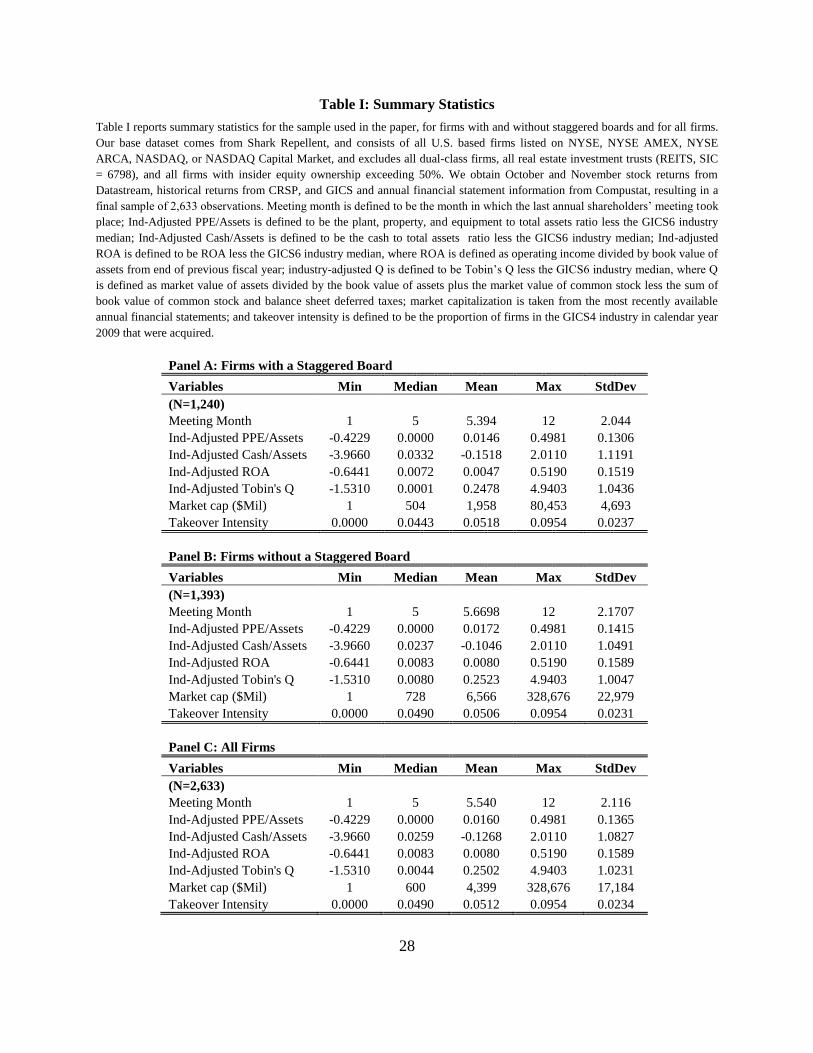
Table I reports summary statistics for our primary variables of interest on our sample of

firms, and for the subset of firms with and without a staggered board. As the Table indicates, our

sample is roughly evenly split between firms with a staggered board (47%) and firms without a

staggered board (53%). Firms with and without a staggered board are similar in terms of the

month in which the last annual meeting took place; the median meeting month for firms with

and without a staggered board is the fifth month of May, and the standard deviation of the

meeting month variable is 2.0 and 2.2 for firms with and without a staggered board, respectively.

21

Shark Repellent data current as of October 12, 2010. 22

REITs are defined as any firms with 4-digit SIC code of 6798.

13

Table I also provides summary statistics concerning the distribution of characteristics that

could make control contests more relevant for a firm: Return on Assets (ROA) 23

and Tobin’s

Q,24

which reflect a company’s performance; PP&E to Total Assets Ratio25

and Cash to Total

Assets Ratio,26

which reflect the extent to which the firm’s assets can be easily pledged and thus

the ease with which a takeover could be financed; market capitalization,27

as small firms are

known to be more likely to be acquired (see, e.g., Bats, Becher, and Lemmon (2008) and

Bebchuk, Cohen, and Wang (2010)); and industry takeover intensity.28

With the exception of

market capitalization and takeover intensity, each of the above variables are industry-median

adjusted; that is, we subtract for each firm-year observation the respective variable’s 6-digit

GICS industry median value from the same fiscal year. Compared with companies with a

staggered board, companies without a staggered board have a somewhat higher median industry-

adjusted Tobin’s Q, median industry-adjusted return on assets, median takeover intensity, and

median market capitalization, somewhat lower industry-adjusted cash to assets ratio, and similar

median industry-adjusted PP&E to assets ratios. In both types of companies, however, there is a

substantial variation in each of these six variables.

4. Announcement Returns around the Two Court Rulings

4.1 The Treatment Group

In our natural experiment setup, the firms that are meaningfully affected by the Chancery

Court ruling (as well as its subsequent reversal by the Delaware Supreme Court) – that is, our

“treatment group” – are firms that, like Airgas itself, have a staggered board and have their

23

Return on assets is defined as operating income divided by book value of assets from end of previous

fiscal year. 24

Following prior work, we use the definition of Tobin’s Q in Kaplan and Zingales (1997), who define

Tobin’s Q as the market value of assets plus the market value of common stock less the sum of book

value of common stock and balance sheet deferred taxes divided by the book value of assets. 25

PP&E to Total Assets Ratio is defined as the ratio of plant, property, and equipment to total assets. 26

Cash to Total Assets Ratio is defined as the ratio of total cash to total assets. 27

Market capitalization is taken from the most recently available annual financial statements in

Compustat. 28

Industry takeover intensity is defined as the percentage of firms in the 4-digit GICS industry that were

taken over in calendar year 2009.

14

annual meeting take place at later parts of the calendar year. We denote firms as belonging to the

Treated-I group if they have a staggered board and their last annual meeting took place in June

or a later month in the calendar year.29

We extend our analysis in Section 4.4 by examining

alternative specifications with a cut-off month other than June.

We also examine groups of firms that can be hypothesized to be especially affected by

the rulings because they satisfy one or more dimensions that make a control contest (and the

magnitude of impediment to them) especially relevant. We define four dimensions that increase a

firm’s exposure to control contests: underperformance (up), high asset pledgibility (pl), small

size (sm), and high industry takeover intensity (ti), and define the following four groups of

“treated” firms:

the Treated-II-up group – firms that are in the Treated-I group and have either a

ROA below the industry median or a Tobin’s Q below the industry median;

the Treated-II-pl group – firms that are in the Treated-I group and have either a cash

to total assets ratio above the industry median or a PP&E to total assets ratio above

the industry median;

the Treated-II-sm group – firms that are in the Treated-I group and have a market

capitalization below our sample’s median; and

the Treated-II-ti group – firms that are in the Treated-I group and belong to an

industry with above median takeover intensity, defined as the percentage of firms in

the 4-digit GICS industry that were acquired in 2009.

The Treated-II-up, Treated-II-pl, Treated-II-sm, and Treated-II-ti groups consist of

subsets of Treated-I that each captures one of the four dimensions making a control contest more

relevant. In addition, we define another treatment group composed of firms that are potentially

most affected:

the Treated-III group – firms that are in the Treated-I group and satisfy at least two of

the four dimensions that magnify the relevance of control contests; in other words, the

29

We choose June since it represents the upper half of our sample – the sample median meeting month is

May. In Section 4.6 we test for the sensitivity of our primary results to changes to this meeting month

cutoff.

15

Treated-III group consists of firms that are in the Treated-I group and in at least two

of the four Treated-II groups defined above.

4.2. Announcement Returns and the Court Rulings

We begin by studying the stock market returns experienced by affected firms during one-

day and two-day windows following the announcements of the Chancery Court and the Supreme

Court rulings. The Chancery Court ruling took place after the close of the stock market on

Friday, October 8, 2010, and the first trading day following the ruling is thus Monday, October

11th

, which was Columbus Day. Because trading volumes on Columbus Day are lower than

usual,30

and because most of the substantive, in-depth media discussion of the Chancery Court

ruling came out only on Monday, October 11 and Tuesday, October 12,31

our primary focus will

be on the two trading-day window ending at the close of the market on October 12th

. Unlike the

Chancery Court ruling, the Supreme Court’s opinion was released during market trading hours,

at 1:30PM on November 23rd

. Given the short two-and-a half-hour window on the first trading

day, we again focus primarily on the two-day trading window from the close of November 22nd

to the close of November 24th

, but we also report results based on the one-day trading window

from the close of November 22nd

to the close of November 23rd

.

We focus on risk-adjusted excess returns as dependent variables to account for the

possibility that differences in raw returns between groups of firms may reflect differences in risk

characteristics. Following standard procedures, risk-adjusted excess returns are computed in two

steps as follows. First, each firm’s loadings on the Fama-French (1993) three factors and the

Fama-French (1996) UMD momentum factor are estimated using the most recently available 120

30

In the case of Columbus Day 2010, for example, the total dollar trading volume was 80% and 81.6% of

the previous and the next trading day’s total dollar trading volumes, respectively, and 79.3% and 75.8%

of the two succeeding Mondays’ total dollar trading volumes. 31

See Amon, “Foreclosure Suits, BP, Airgas, UBS in Court News,” Bloomberg, October 11, 2010;

Gallardo, “Important Chancery Court Opinion for Corporations with Staggered Boards,” HLS Corporate

Governance Blog, October 11, 2010; Kelly, “Update: Airgas to Fight Court Ruling Over Annual

Meeting,” CNBC, October 11, 2010; McCarty and Kaskey, “Airgas to Appeal Delaware Ruling on

Meeting Date in Air Products Dispute,” Bloomberg, October 11, 2010; Quinn, “Airgas to Appeal,” M & A

Law Prof Blog, October 11, 2010; Davidoff, “The Dwindling Options for Airgas,” New York Times

online, October 12, 2010; McCarty and Kaskey, “Airgas to appeal ruling on meeting,” Philadelphia

Inquirer, October 12, 2010.

16

trading days’ data ending on or prior to September 31th

of 2010. That is, for each firm we obtain

from the time-series regression:

(1)

We then obtain excess announcement window returns by taking the residuals from a cross-

sectional regression of raw announcement window returns on the estimated factor sensitivities.

That is, for each firm, we obtain the fitted residual from the cross-sectional regression:

(2)

We integrate the two events in our announcement returns analysis by pooling the

observations from both events. Such an analysis has the advantage of increasing the sample size.

It also enables testing hypotheses concerning the differences in magnitudes between the

treatment effects of the two events.

An earlier work that pools events is that of Larcker, Ormazabal, and Taylor (2010). They

study several events related to proxy access reform, with some operating to increase the

likelihood of such a reform and some operating to reduce the likelihood of such a reform. Their

analysis assumes that all the events had an effect of similar magnitude, though some with the

opposite sign to others. In our initial analysis, we follow the approach of Larcker et al (2010) and

makes the assumption that the Supreme Court decision, which overturned the Chancery Court

ruling, was accompanied by announcement returns of similar magnitudes but of opposite sign to

those of the Chancery Court ruling. We later on (Section 4.3) conduct an analysis without

making this assumption and obtain results consistent with the two events having consequences of

same magnitude but opposite signs.

Given the assumption used in this section that the events’ consequences are of the same

magnitude but opposite signs, we multiply the excess returns from the second ruling by negative

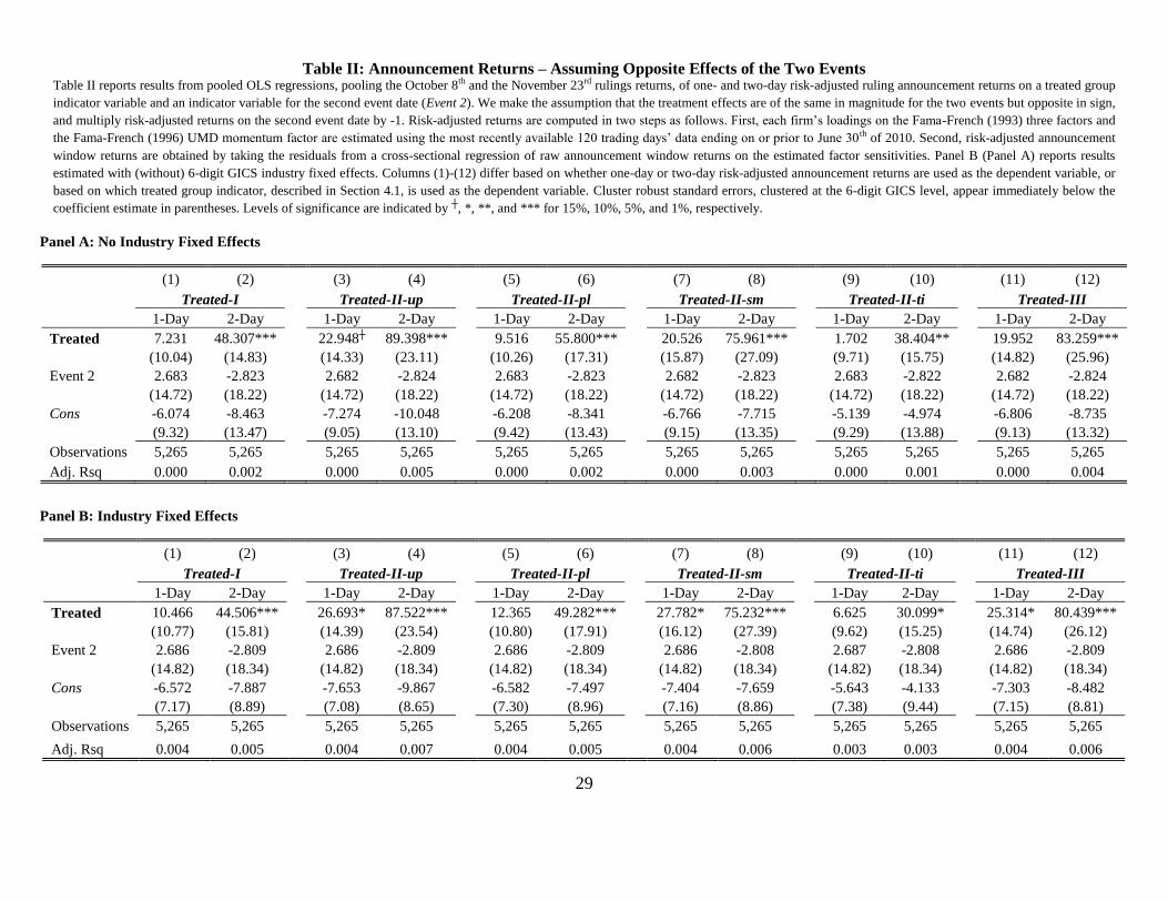
one. We test for differences in announcement window returns between treated and non-treated

firms in Table II by regressing the adjusted one- and two-day excess returns on each of the six

treatment group indicators: Treated-I, Treated-II-up, Treated-II-pl, Treated-II-sm, Treated-II-ti,

and Treated-III. In each specification we include an indicator for the second ruling date, Event-2,

17

to account for possible differences in the mean returns between the two event dates. Panel A of

Table II reports specifications estimated without 6-digit GICS industry fixed effects, and Panel B

of Table II reports specifications with such fixed effects. All standard errors are clustered at the

6-digit GICS industry level.

In both Panels A and Panel B of Table II, we find strong evidence, particular with the

two-day return window, that validating the Airgas bylaw and weakening the antitakeover force

of staggered boards provides significantly positive returns for treated firms compared to non-

treated firms. Over the two-day event window, we find that Treated-I firms on average

outperformed non-treated firms by 48.3 basis points in the specification without fixed effects and

by 44.5 basis points in the specification with fixed effects; both coefficients are significant at the

1% level.

Consistent with the rulings’ impact depending on the presence of firm or industry

characteristics that make control contests more relevant, the difference in the mean excess

returns tends to be higher for the treated groups Treated-II-np, Treated-II-pl, Treated-II-sm, and

Treated-II-ti than for the Treated-I group. Over the two day window, the treated groups Treated-

II-np, Treated-II-pl, Treated-II-sm, and Treated-II-ti outperformed non-treated firms by

38.4~89.4 basis points when industry fixed effects are not included, and by 30.1~87.5 basis

points when industry fixed effect are included. In six of eight specifications, the differences are

statistically significant at the 1% level, and in all eight specifications the differences are

statistically significant at the 10% (or lower) level.

The results are most pronounced, as hypothesized, for the Treated-III group of most

affected firms. In the two-day trading window, firms in the Treated-III group outperformed non-

treated firms by 83.3 basis points in the specification without industry fixed effects, and by 80.4

basis points in the specification with industry fixed effects, with the results being statistically

significant at the 1% level in both specifications.

We note that any differences in mean announcement returns between the treated firms

and the non-treated firms may be potentially attenuated by two factors: first, the extent to which

the Chancery and Supreme Court rulings were viewed by the market as possible prior to the

decisions; and, second, the extent to which the Chancery Court ruling was expected by the

market to be reversed by the Delaware Supreme Court. Thus, whereas the identified positive

18

returns to treated firm are significant, they are likely to understate the market’s estimate of the

value to treated firm of permitting Airgas-type bylaws. Furthermore, note that permitting Airgas-

type bylaws would have merely weakened rather than eliminated the antitakeover force of

staggered boards: permitting such bylaws would have enabled shareholders to decrease, not

eliminate, the extent to which staggered boards can delay the replacement of a majority of

directors sought by a shareholder majority. Thus, whereas our results understate the market’s

estimate of the value to treated firms of permitting Airgas-type bylaws, this estimate in turn is

likely to be lower than the market’s estimate of the value of eliminating board classification.

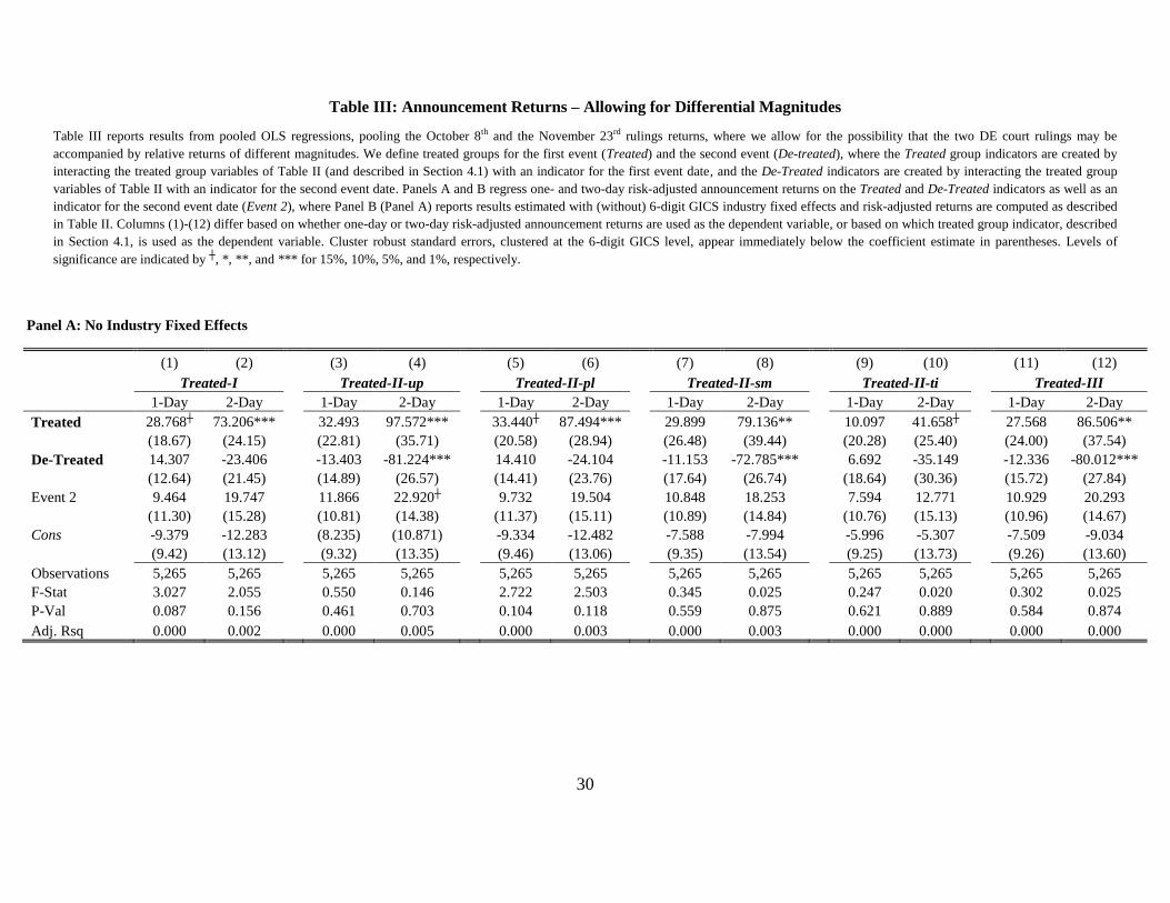
4.3 Announcement Returns and the Court Rulings – Differential Magnitudes

In this section, we allow for the possibility that that the Supreme Court’s reversal of the

Chancery Court ruling might have an effect of a different magnitude than the Chancery Court

ruling, and we test the assumption of equal magnitudes (but opposite sign) for the effects of the

two events. To do so, we run a pooled OLS by regressing risk-adjusted one- and two-day

announcement returns on a treated group indicator interacted with an indicator for the first event

(Treated), a treated group indicator interacted with an indicator for the second event (De-

Treated), and an indicator for the second event (Event-2). We report the results of the estimation

in Table III. Panel A of Table III reports specifications without 6-digit GICS industry fixed

effects and Panel B reports specifications with such fixed effects. As before, all standard errors

are clustered at the 6-digit GICS industry level.

In Panels A and B of Table III, we find strong evidence consistent with the two rulings

being associated with excess returns of similar magnitudes but in opposite signs. Focusing again

on the two-day returns, Panel A of Table III indicates that, relative to non-treated firms, the

excess returns to treated groups associated with the first ruling are positive in all six

specifications, with statistical significance at the 5% level for five of these specifications; the

excess two-day returns to treated groups associated with the second ruling are negative in all six

specifications, with statistical significance at the 5% level for three; and, finally, for all six

specifications, an F-test fails to reject at the 10% level the null hypothesis that the sum of the

differences in average excess returns for the first and second rulings (Treated + De-Treated) is

zero. The results in Panel B of Table III, which include industry fixed effects, are consistent with

19

the above results of Panel A. The excess two-day returns to treated groups associated with the

first ruling are higher relative to non-treated firms for all six specifications, with statistical

significance at the 5% level for five; the excess two-day returns to treated groups associated with

the second ruling are lower relative to non-treated firms for all six specifications, with statistical

significance at the 5% level for three; and, finally, in five of the six specifications, an F-tests fails

to reject at the 5% level the null hypothesis that the sum of the differences in average excess

returns for the first and second rulings (Treated + De-Treated) is zero.

Overall, the results in this Section are consistent with the hypothesis that weakening the

antitakeover force of staggered boards is viewed by market participants as value-enhancing.

Consistent with this hypothesis, the Chancery Court ruling was accompanied by positive relative

returns to the companies whose staggered boards were made less insulating by the ruling, and the

Supreme Court ruling, which eliminated this effect, was accompanied by negative relative

returns to these companies.

We note again that any difference in returns between the treated and non-treated firms

understates the market’s estimate of the value-reduction produced by the antitakeover force of

staggered boards for two reasons. First, as discussed earlier, prior to each of the rulings, the

market likely attached a nontrivial probability to the ruling. Second, permitting Airgas-type

bylaws would have merely weakened rather than eliminated the antitakeover force of staggered

boards. Thus, as was the case earlier, our results in this section provide an under-estimate of the

cost that market participants estimate to be generated by board classification.

4.4 Simulation Exercise

We now turn to another way of testing whether the observed patterns, of positive relative

returns to treated firms from the Chancery Court ruling and negative relative returns to treated

firms from the Supreme Court ruling, were produced by random sampling variation rather than

the rulings. To test for this hypothesis, we conduct a simulation exercise over all non-event days

from the first half of 2010 -- that is, from January 2nd

to June 30th

.

In particular, for each pair of two-day windows in this period, we replicate the

specifications in Panels A and B of Table II and Table III that use the Treated-III group indicator

(reported in column (12)), and generate benchmark distributions of coefficients generated from

20

non-event days. We then consider whether the observed Treated coefficients in Table II, and

coefficients of Treated and De-Treated and Table III, are abnormal when compared to the

simulated benchmark distribution.

To begin the exercise, we compute excess returns for each two-day window in a two-step

procedure similar to that used in Tables II and III and in equations (1) and (2). First, we estimate

each firm’s Fama-French three factor and UMD momentum factor loadings using returns data

from 140 to 20 trading days prior; second, we take the residuals from a cross-sectional regression

of two-day raw returns on the estimated factor sensitivities. Once the two-day excess returns are

generated for each day in the first half of 2010, we replicate the pooled regression results of

Tables II and III using the Treated-III group indicator for each pair of two-day windows in the

period.

In particular, to replicate the specifications of Table II over non-event days, we multiply

the returns from the latter of the two non-event days by negative one, and we regress the adjusted

returns on the Treated-III group indicator and an indicator for the second event date. To replicate

the specifications of Table III, we run a pooled OLS by regressing risk-adjusted two-day returns

on the Treated-III group indicator interacted with an indicator for the first event (Treated-III),

the Treated-III group indicator interacted with an indicator for the second event (De-Treated-III),

and an indicator for the second event.

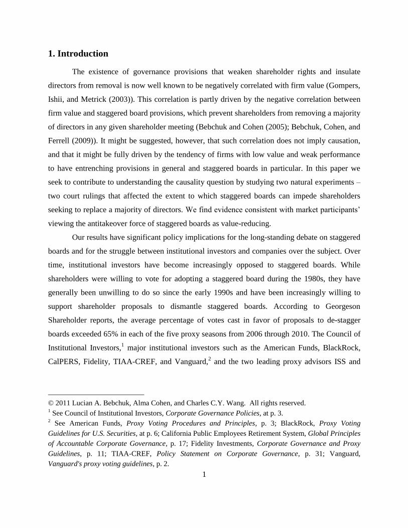
Figure I displays the non-parametric Epanechnikov kernel density estimates of the

simulated non-event Treated-III coefficients, generated following the constrained model of Table

II. The dotted vertical line on each graph represents the location of our observed coefficients. We

see from the figure that the simulated coefficients are approximately normally distributed and

centered around 0. Moreover, our observed coefficients of 83.3 and 80.4 in the no fixed effects

and fixed effects specifications of Table III are abnormally large when compared to the

simulated distributions. Specifically, in Panel A of Table IV, which reports the univariate

distributional summaries of the simulated coefficients, rows [1] and [2] indicate that our

observed coefficients lie outside the 99th

percentiles of the distribution of simulated coefficients.

In fact, only less than 0.5% of coefficients simulated based on the non-fixed-effects model in

Panel A of Table III are larger than our observed coefficient of 83.3; and less than 0.2% of

21

coefficients simulated based on the fixed-effects model in Panel B of Table III are larger than our

observed coefficient of 80.4.

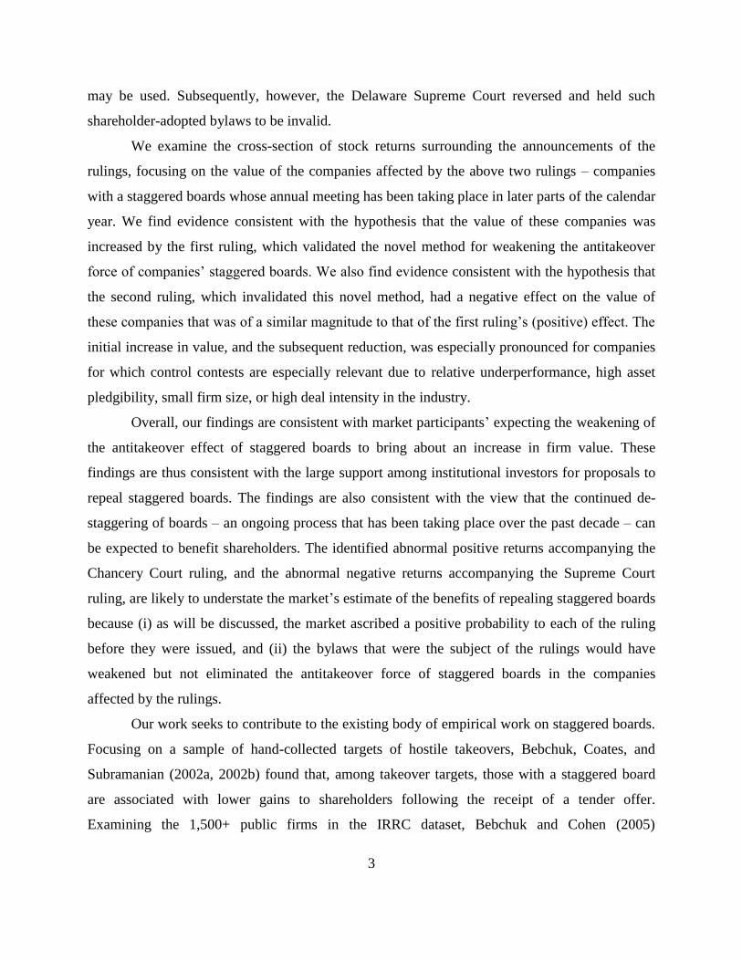
Figure II displays the non-parametric kernel bivariate density estimates of the simulated

Treated and De-Treated coefficients, generated following the unconstrained model of Table III.

The white arrow on each graph indicates the location of our observed pair of coefficients. As we

see in Figure II and in rows [3]-[6] of Panel A of Table IV, the simulated coefficients are

approximately bivariate normal and centered around (0,0). In comparison to this distribution, our

observed Treated and De-Treated coefficients – of 86.5 and -80.0 in the no fixed effects model

and 95.4 and -71.0 in the fixed effects model of Table III – are abnormally large in magnitude.

Table IV Panel B, which reports bivariate distributional summaries of the simulated

Treated and De-Treated coefficients, shows that less than 0.1% of the simulated coefficients

using the no-fixed-effects model are as large in magnitude (that is, having a Treated coefficient

that is no smaller than the observed and a De-Treated coefficient that is no larger than the

observed) as those of Table III Panel A. In the fixed effect model, less than 0.2% of the

simulated coefficients using the fixed effects model are as extreme as those in Table III Panel B.

In summary, our simulation results show that the treatment effects on the Treated-III

group of firms observed in Tables II and III are highly unlikely to have arisen from random

sampling variation. In each specification considered, we can reject the null hypothesis that the

true mean treatment effects are 0 at the 0.5% or lower significance level.

4.6. Different Meeting Date Cut-offs

In our primary empirical tests above, we defined treated firms on the basis of having a

prior annual meeting date taking place in June or a later month in the calendar year. This

threshold represents the upper half of the sample distribution and approximately represents the

latter half of the year. In this section, we examine whether our results are robust to using

different meeting month cutoffs and find that they are.

To test robustness to using different meeting month cutoffs, we define nine versions of

Treated-III. As before, the firms in the Treated-III group all have a staggered board and satisfy at

least two of the four dimensions of firm or industry characteristics that make control contests

especially relevant: underperformance, high asset pledgibility, small size, and high industry

22

takeover intensity. In contrast to before, where all Treated-III firms’ annual meetings took place

in or after June in the calendar year, we now have versions with a different cut-off meeting

month. In particular, the nine versions of the Treated-III group we consider below are based on

different cut-off months from February through October.32

Our robustness tests employ the pooling specifications of Panels A and B of Table II,

using two-day excess returns as dependent variables. Table V reports the excess returns of

Treated-III (relative to non-Treated-III) firms based on the nine variations of the annual meeting

month cutoffs. Panel A of this Table V does not include industry fixed effects, and Panel B of

Table V includes such fixed effects.

Both Panel A and Panel B of Table V display the same pattern: as we increase the cutoff

month from February to October, the difference in the average two-day excess returns between

Treated-III and non-Treated-III firms trends upwards; indeed, with the exceptions of August and

October, the increase is monotonic. In the no-fixed effects specifications of Panel A, the Treated-

III coefficient grows from 35.1 basis points using a February cutoff to 83.3 basis points using a

June cutoff to 84.7 basis points using an October cutoff. Consistent with this pattern, in the

fixed-effects specifications of Panel B, the Treated-III coefficient grows from 34.7 basis points

using a February cutoff to 80.4 basis points using a June cutoff to 88.7 basis points using an

October cutoff.

In addition, Panel C of Table V reports a specification in which we regress the two-day

risk-adjusted returns on a Treated-III indicator (but without the June cutoff requirement), the

month of last annual meeting, an interaction of the treatment indicator with the month of last

annual meeting, and an indicator for the second event date. In both the no-fixed-effects and

fixed-effects specifications in Panel C, the interaction terms are positive and statistically

significant at the 5% level. These results are consistent with the mean difference in

announcement returns between treated and non-treated firms being larger in magnitude among

those firms whose annual meeting took place later in the year.

In summary, the patterns documented in Table V are consistent with the rulings (and the

Airgas bylaw whose validity was at stake) having the greatest potential impact among firms that

32

Using a cut-off meeting month of November or December leaves too few firms in the treated group to

enable testing.

23

have annual meeting months later in the calendar year – that is, firms in which the Airgas bylaw

could be used to significantly reduce the tenure of directors whose removal would be otherwise

delayed by a staggered board. By showing that the magnitude of the identified effects in Table II

increases as the cutoff month increases, these robustness tests reinforce our earlier conclusions

concerning the Delaware Chancery and Supreme Court rulings’ effects.

6. Conclusion

This paper has sought to contribute to understanding the sources of the well-documented

correlation between governance provisions insulating directors from removal, in particular

staggered boards, and lower firm value. We have used a natural experiment – a recent Delaware

Chancery Court ruling enabling shareholders to weaken the extent to which staggered boards

insulate directors from removal and the subsequent reversal of this ruling by the Delaware

Supreme Court – to identify how market participants in the aggregate view the effect of

staggered boards on firm value. We find evidence consistent with market participants’ viewing

staggered boards as bringing about a reduction in firm value.

Our findings are consistent with the ongoing debate on staggered boards and the efforts

of institutional investors to reduce the large number of companies that still have staggered

boards. Our findings are consistent with policies adopted by many institutional investors in favor

of proposals to de-stagger boards. Our findings are also consistent with the view that the ongoing

process of dismantling staggered boards, encouraged by institutional investors, could be

expected to contribute to increasing shareholder wealth.

24

References

Baghat, Sanjai, and Roberta Romano (2002). “Event Studies and the Law: Part II: Empirical

Studies of Corporate Law.” American Law and Economics Review 4: 380-423.

Bates, Thomas W., David A. Becher, and Michael L. Lemmon (2008). “Board Classification and

Managerial Entrenchment: Evidence from the Market for Corporate Control.” Journal of

Financial Economics 87: 656- 677.

Bebchuk, Lucian A., John C. Coates, and Guhan Subramanian (2002a). “The Powerful

Antitakeover Force of Staggered Boards: Theory, Evidence, and Policy.” Stanford Law

Review 54: 887-951.

Bebchuk, Lucian A., John C. Coates, and Guhan Subramanian (2002b). “The Powerful

Antitakeover Force of Staggered Boards: Theory, Evidence, and Policy: A Reply and

extension” Stanford Law Review.

Bebchuk, Lucian A. and Alma Cohen (2005). “The Cost of Entrenched Boards.” Journal of

Financial Economics 78: 409-433.

Bebchuk, Lucian A., Alma Cohen, and Allen Ferrell (2009). “What Matters in Corporate

Governance?” Review of Financial Studies 22: 783-785.

Bebchuk, Lucian A., Alma Cohen, and Charles Wang (2010). “Golden Parachutes and the

Wealth of Shareholders.” Discussion Paper No. 683, John M. Olin Center for Law,

Economics, and Business, Harvard Law School.

Becker, Bo, Daniel Bergstresser, and Guhan Subramanian (2010). “Does Shareholder Proxy

Access Improve Firm Value? Evidence from the Business Roundtable Challenge.” Working

Paper.

Bernard, Victor, and Jacob K. Thomas (1989). “Post-Earnings Announcement Drift: Delayed

Price Response or Risk Premium?” Journal of Accounting Research, Supplement XXVII: 1-

36.

Bhojraj, Sanjeev, Charles M.C. Lee, and Derek K. Oler (2003). “What’s My Line? A

Comparison of Industry Classification Schemes for Capital Market Research.” Journal of

Accounting Research 41:745-774.

Binder, John J. (1985). “Measuring the Effects of Regulation with Stock Price Data.” RAND

Journal of Economics 16: 167-183.

25

Chhaochharia, Vidhi, and Yaniv Grinstein (2007). “Corporate Governance and Firm Value: The

Impact of the 2002 Governance Rules.” Journal of Finance 62: 1789-1825.

Coates, John (2000). “Takeover Defenses in the Shadow of the Pill: A Critique of the Scientific

Evidence.” Texas Law Review 79: 271-382.

DellaVigna, Stefano and Joshua Pollet (2009). "Investor Inattention and Friday Earnings

Announcements." Journal of Finance 64: 709-749.

Faleye, Olubunmi (2007). “Classified Boards, Firm Value, and Managerial Entrenchment.”

Journal of Financial Economics 83: 501-529.

Fama, Eugene and Kenneth R. French (1993). “Common Risk Factors in the Returns on Bonds

and Stocks.” Journal of Financial Economics 33: 3-53.

Fama, Eugene and Kenneth R. French (1996). “Multifactor Explanations of Asset Pricing

Anomalies.” Journal of Finance 51: 55-87.

Gompers, Paul A., Joy L. Ishii, and Andrew Metrick (2003). "Corporate Governance and Equity

Prices." Quarterly Journal of Economics 118(1):107-155.

Guo, Re-Jin, Timothy A. Kruse, and Tom Nohel (2008). “Undoing the Powerful Anti-Takeover

Force of Staggered Boards.” Journal of Corporate Finance 14: 274 - 288.

Hochberg, Yael V., Paola Sapienza, and Annette Vissing-Jorgensen (2009). “A Lobbying

Approach to Evaluating the Sarbanes-Oxley Act of 2002.” Journal of Accounting Research

47: 519-583.

Karpoff, Jonathan M. and Paul H. Malatesta (1989). “The Wealth Effects of Second-Generation

State Takeover Legislation.” Journal of Financial Economics 25: 291-322.

Larcker, David F., Gaizka Ormazabal, and Daniel J. Taylor (2010). “The Market Reaction to

Corporate Governance Regulation.” Journal of Financial Economics. Forthcoming.

MacKinlay, A. Craig (1997). “Event Studies in Economics and Finance,” Journal of

Economic Literature 35: 13-39.

Schwert, William (1981). “Using Financial Data to Measure Effects of Regulation.” Journal of

Law and Economics 121: 121-158.

26

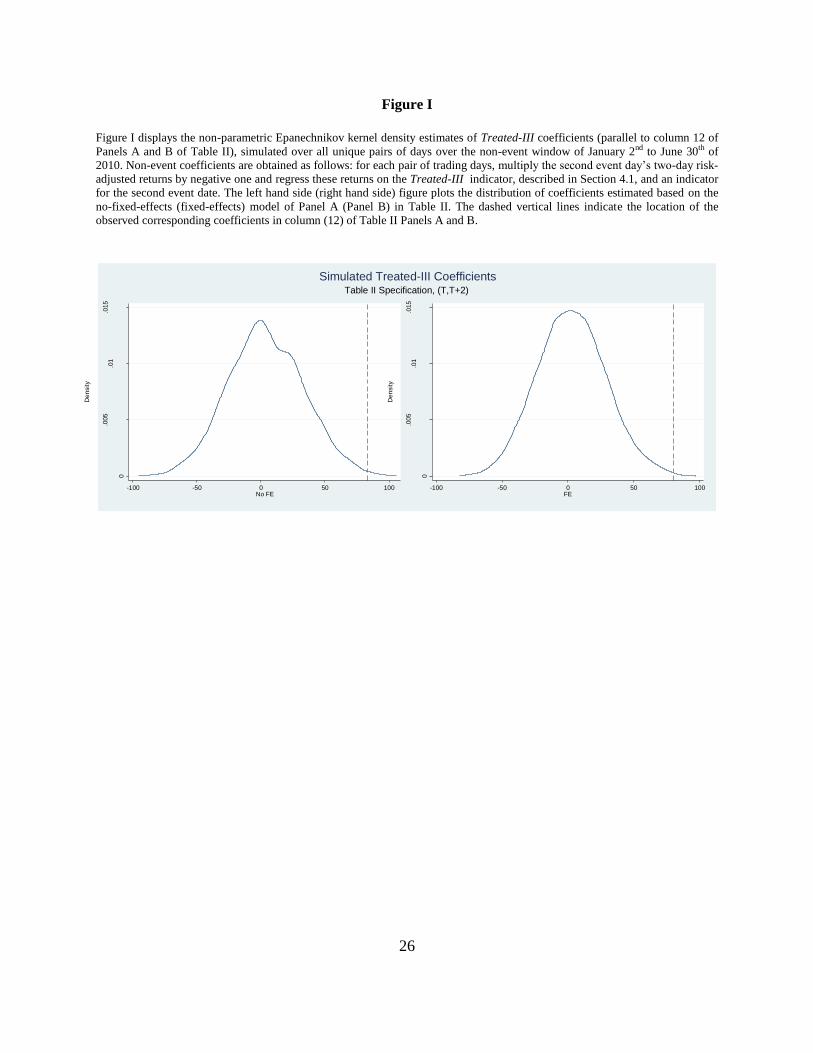
Figure I

Figure I displays the non-parametric Epanechnikov kernel density estimates of Treated-III coefficients (parallel to column 12 of

Panels A and B of Table II), simulated over all unique pairs of days over the non-event window of January 2nd to June 30th of

2010. Non-event coefficients are obtained as follows: for each pair of trading days, multiply the second event day’s two-day risk-

adjusted returns by negative one and regress these returns on the Treated-III indicator, described in Section 4.1, and an indicator

for the second event date. The left hand side (right hand side) figure plots the distribution of coefficients estimated based on the

no-fixed-effects (fixed-effects) model of Panel A (Panel B) in Table II. The dashed vertical lines indicate the location of the

observed corresponding coefficients in column (12) of Table II Panels A and B.

0

.005

.01

.015

De

nsity

-100 -50 0 50 100No FE

0

.005

.01

.015

De

nsity

-100 -50 0 50 100FE

Table II Specification, (T,T+2)

Simulated Treated-III Coefficients

27

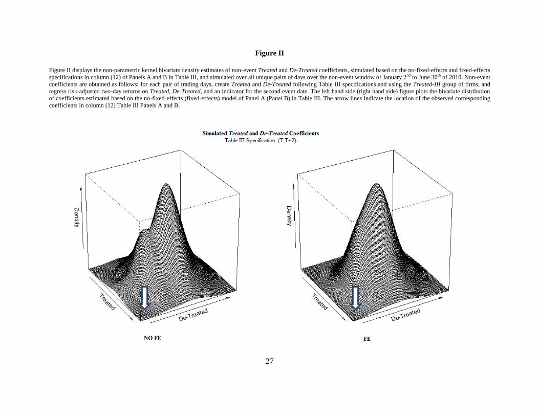
Figure II

Figure II displays the non-parametric kernel bivariate density estimates of non-event Treated and De-Treated coefficients, simulated based on the no-fixed-effects and fixed-effects

specifications in column (12) of Panels A and B in Table III, and simulated over all unique pairs of days over the non-event window of January 2nd to June 30th of 2010. Non-event

coefficients are obtained as follows: for each pair of trading days, create Treated and De-Treated following Table III specifications and using the Treated-III group of firms, and

regress risk-adjusted two-day returns on Treated, De-Treated, and an indicator for the second event date. The left hand side (right hand side) figure plots the bivariate distribution

of coefficients estimated based on the no-fixed-effects (fixed-effects) model of Panel A (Panel B) in Table III. The arrow lines indicate the location of the observed corresponding

coefficients in column (12) Table III Panels A and B.

28

Table I: Summary Statistics

Table I reports summary statistics for the sample used in the paper, for firms with and without staggered boards and for all firms.

Our base dataset comes from Shark Repellent, and consists of all U.S. based firms listed on NYSE, NYSE AMEX, NYSE

ARCA, NASDAQ, or NASDAQ Capital Market, and excludes all dual-class firms, all real estate investment trusts (REITS, SIC

= 6798), and all firms with insider equity ownership exceeding 50%. We obtain October and November stock returns from

Datastream, historical returns from CRSP, and GICS and annual financial statement information from Compustat, resulting in a

final sample of 2,633 observations. Meeting month is defined to be the month in which the last annual shareholders’ meeting took

place; Ind-Adjusted PPE/Assets is defined to be the plant, property, and equipment to total assets ratio less the GICS6 industry

median; Ind-Adjusted Cash/Assets is defined to be the cash to total assets ratio less the GICS6 industry median; Ind-adjusted

ROA is defined to be ROA less the GICS6 industry median, where ROA is defined as operating income divided by book value of

assets from end of previous fiscal year; industry-adjusted Q is defined to be Tobin’s Q less the GICS6 industry median, where Q

is defined as market value of assets divided by the book value of assets plus the market value of common stock less the sum of

book value of common stock and balance sheet deferred taxes; market capitalization is taken from the most recently available

annual financial statements; and takeover intensity is defined to be the proportion of firms in the GICS4 industry in calendar year

2009 that were acquired.

Panel A: Firms with a Staggered Board

Variables Min Median Mean Max StdDev

(N=1,240)

Meeting Month 1 5 5.394 12 2.044

Ind-Adjusted PPE/Assets -0.4229 0.0000 0.0146 0.4981 0.1306

Ind-Adjusted Cash/Assets -3.9660 0.0332 -0.1518 2.0110 1.1191

Ind-Adjusted ROA -0.6441 0.0072 0.0047 0.5190 0.1519

Ind-Adjusted Tobin's Q -1.5310 0.0001 0.2478 4.9403 1.0436

Market cap ($Mil) 1 504 1,958 80,453 4,693

Takeover Intensity 0.0000 0.0443 0.0518 0.0954 0.0237

Panel B: Firms without a Staggered Board

Variables Min Median Mean Max StdDev

(N=1,393)

Meeting Month 1 5 5.6698 12 2.1707

Ind-Adjusted PPE/Assets -0.4229 0.0000 0.0172 0.4981 0.1415

Ind-Adjusted Cash/Assets -3.9660 0.0237 -0.1046 2.0110 1.0491

Ind-Adjusted ROA -0.6441 0.0083 0.0080 0.5190 0.1589

Ind-Adjusted Tobin's Q -1.5310 0.0080 0.2523 4.9403 1.0047

Market cap ($Mil) 1 728 6,566 328,676 22,979

Takeover Intensity 0.0000 0.0490 0.0506 0.0954 0.0231

Panel C: All Firms

Variables Min Median Mean Max StdDev

(N=2,633)

Meeting Month 1 5 5.540 12 2.116

Ind-Adjusted PPE/Assets -0.4229 0.0000 0.0160 0.4981 0.1365

Ind-Adjusted Cash/Assets -3.9660 0.0259 -0.1268 2.0110 1.0827

Ind-Adjusted ROA -0.6441 0.0083 0.0080 0.5190 0.1589

Ind-Adjusted Tobin's Q -1.5310 0.0044 0.2502 4.9403 1.0231

Market cap ($Mil) 1 600 4,399 328,676 17,184

Takeover Intensity 0.0000 0.0490 0.0512 0.0954 0.0234

29

Table II: Announcement Returns – Assuming Opposite Effects of the Two Events

Table II reports results from pooled OLS regressions, pooling the October 8th and the November 23rd rulings returns, of one- and two-day risk-adjusted ruling announcement returns on a treated group

indicator variable and an indicator variable for the second event date (Event 2). We make the assumption that the treatment effects are of the same in magnitude for the two events but opposite in sign,

and multiply risk-adjusted returns on the second event date by -1. Risk-adjusted returns are computed in two steps as follows. First, each firm’s loadings on the Fama-French (1993) three factors and

the Fama-French (1996) UMD momentum factor are estimated using the most recently available 120 trading days’ data ending on or prior to June 30th of 2010. Second, risk-adjusted announcement

window returns are obtained by taking the residuals from a cross-sectional regression of raw announcement window returns on the estimated factor sensitivities. Panel B (Panel A) reports results

estimated with (without) 6-digit GICS industry fixed effects. Columns (1)-(12) differ based on whether one-day or two-day risk-adjusted announcement returns are used as the dependent variable, or

based on which treated group indicator, described in Section 4.1, is used as the dependent variable. Cluster robust standard errors, clustered at the 6-digit GICS level, appear immediately below the

coefficient estimate in parentheses. Levels of significance are indicated by ┼, *, **, and *** for 15%, 10%, 5%, and 1%, respectively.

Panel A: No Industry Fixed Effects

(1) (2) (3) (4) (5) (6) (7) (8) (9) (10) (11) (12)

Treated-I Treated-II-up Treated-II-pl Treated-II-sm Treated-II-ti Treated-III

1-Day 2-Day 1-Day 2-Day 1-Day 2-Day 1-Day 2-Day 1-Day 2-Day 1-Day 2-Day

Treated 7.231 48.307*** 22.948┼ 89.398*** 9.516 55.800*** 20.526 75.961*** 1.702 38.404** 19.952 83.259***

(10.04) (14.83) (14.33) (23.11) (10.26) (17.31) (15.87) (27.09) (9.71) (15.75) (14.82) (25.96)

Event 2 2.683 -2.823 2.682 -2.824 2.683 -2.823 2.682 -2.823 2.683 -2.822 2.682 -2.824

(14.72) (18.22) (14.72) (18.22) (14.72) (18.22) (14.72) (18.22) (14.72) (18.22) (14.72) (18.22)

Cons -6.074 -8.463 -7.274 -10.048 -6.208 -8.341 -6.766 -7.715 -5.139 -4.974 -6.806 -8.735

(9.32) (13.47) (9.05) (13.10) (9.42) (13.43) (9.15) (13.35) (9.29) (13.88) (9.13) (13.32)

Observations 5,265 5,265 5,265 5,265 5,265 5,265 5,265 5,265 5,265 5,265 5,265 5,265

Adj. Rsq 0.000 0.002 0.000 0.005 0.000 0.002 0.000 0.003 0.000 0.001 0.000 0.004

Panel B: Industry Fixed Effects

(1) (2) (3) (4) (5) (6) (7) (8) (9) (10) (11) (12)

Treated-I Treated-II-up Treated-II-pl Treated-II-sm Treated-II-ti Treated-III

1-Day 2-Day 1-Day 2-Day 1-Day 2-Day 1-Day 2-Day 1-Day 2-Day 1-Day 2-Day

Treated 10.466 44.506*** 26.693* 87.522*** 12.365 49.282*** 27.782* 75.232*** 6.625 30.099* 25.314* 80.439***

(10.77) (15.81) (14.39) (23.54) (10.80) (17.91) (16.12) (27.39) (9.62) (15.25) (14.74) (26.12)

Event 2 2.686 -2.809 2.686 -2.809 2.686 -2.809 2.686 -2.808 2.687 -2.808 2.686 -2.809

(14.82) (18.34) (14.82) (18.34) (14.82) (18.34) (14.82) (18.34) (14.82) (18.34) (14.82) (18.34)

Cons -6.572 -7.887 -7.653 -9.867 -6.582 -7.497 -7.404 -7.659 -5.643 -4.133 -7.303 -8.482

(7.17) (8.89) (7.08) (8.65) (7.30) (8.96) (7.16) (8.86) (7.38) (9.44) (7.15) (8.81)

Observations 5,265 5,265 5,265 5,265 5,265 5,265 5,265 5,265 5,265 5,265 5,265 5,265

Adj. Rsq 0.004 0.005 0.004 0.007 0.004 0.005 0.004 0.006 0.003 0.003 0.004 0.006

30

Table III: Announcement Returns – Allowing for Differential Magnitudes

Table III reports results from pooled OLS regressions, pooling the October 8th and the November 23rd rulings returns, where we allow for the possibility that the two DE court rulings may be

accompanied by relative returns of different magnitudes. We define treated groups for the first event (Treated) and the second event (De-treated), where the Treated group indicators are created by

interacting the treated group variables of Table II (and described in Section 4.1) with an indicator for the first event date, and the De-Treated indicators are created by interacting the treated group

variables of Table II with an indicator for the second event date. Panels A and B regress one- and two-day risk-adjusted announcement returns on the Treated and De-Treated indicators as well as an

indicator for the second event date (Event 2), where Panel B (Panel A) reports results estimated with (without) 6-digit GICS industry fixed effects and risk-adjusted returns are computed as described

in Table II. Columns (1)-(12) differ based on whether one-day or two-day risk-adjusted announcement returns are used as the dependent variable, or based on which treated group indicator, described

in Section 4.1, is used as the dependent variable. Cluster robust standard errors, clustered at the 6-digit GICS level, appear immediately below the coefficient estimate in parentheses. Levels of

significance are indicated by ┼, *, **, and *** for 15%, 10%, 5%, and 1%, respectively.

Panel A: No Industry Fixed Effects

(1) (2) (3) (4) (5) (6) (7) (8) (9) (10) (11) (12)

Treated-I Treated-II-up Treated-II-pl Treated-II-sm Treated-II-ti Treated-III

1-Day 2-Day 1-Day 2-Day 1-Day 2-Day 1-Day 2-Day 1-Day 2-Day 1-Day 2-Day

Treated 28.768┼ 73.206*** 32.493 97.572*** 33.440┼ 87.494*** 29.899 79.136** 10.097 41.658┼ 27.568 86.506**

(18.67) (24.15) (22.81) (35.71) (20.58) (28.94) (26.48) (39.44) (20.28) (25.40) (24.00) (37.54)

De-Treated 14.307 -23.406 -13.403 -81.224*** 14.410 -24.104 -11.153 -72.785*** 6.692 -35.149 -12.336 -80.012***

(12.64) (21.45) (14.89) (26.57) (14.41) (23.76) (17.64) (26.74) (18.64) (30.36) (15.72) (27.84)

Event 2 9.464 19.747 11.866 22.920┼ 9.732 19.504 10.848 18.253 7.594 12.771 10.929 20.293

(11.30) (15.28) (10.81) (14.38) (11.37) (15.11) (10.89) (14.84) (10.76) (15.13) (10.96) (14.67)

Cons -9.379 -12.283 (8.235) (10.871) -9.334 -12.482 -7.588 -7.994 -5.996 -5.307 -7.509 -9.034

(9.42) (13.12) (9.32) (13.35) (9.46) (13.06) (9.35) (13.54) (9.25) (13.73) (9.26) (13.60)

Observations 5,265 5,265 5,265 5,265 5,265 5,265 5,265 5,265 5,265 5,265 5,265 5,265

F-Stat 3.027 2.055 0.550 0.146 2.722 2.503 0.345 0.025 0.247 0.020 0.302 0.025

P-Val 0.087 0.156 0.461 0.703 0.104 0.118 0.559 0.875 0.621 0.889 0.584 0.874

Adj. Rsq 0.000 0.002 0.000 0.005 0.000 0.003 0.000 0.003 0.000 0.000 0.000 0.000

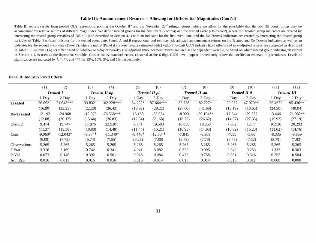
31

Table III: Announcement Returns -- Allowing for Differential Magnitudes (Cont’d)

Table III reports results from pooled OLS regressions, pooling the October 8th and the November 23rd rulings returns, where we allow for the possibility that the two DE court rulings may be

accompanied by relative returns of different magnitudes. We define treated groups for the first event (Treated) and the second event (De-treated), where the Treated group indicators are created by

interacting the treated group variables of Table II (and described in Section 4.1) with an indicator for the first event date, and the De-Treated indicators are created by interacting the treated group

variables of Table II with an indicator for the second event date. Panels A and B regress one- and two-day risk-adjusted announcement returns on the Treated and De-Treated indicators as well as an

indicator for the second event date (Event 2), where Panel B (Panel A) reports results estimated with (without) 6-digit GICS industry fixed effects and risk-adjusted returns are computed as described

in Table II. Columns (1)-(12) differ based on whether one-day or two-day risk-adjusted announcement returns are used as the dependent variable, or based on which treated group indicator, described

in Section 4.1, is used as the dependent variable. Cluster robust standard errors, clustered at the 6-digit GICS level, appear immediately below the coefficient estimate in parentheses. Levels of

significance are indicated by ┼, *, **, and *** for 15%, 10%, 5%, and 1%, respectively.

Panel B: Industry Fixed Effects

(1) (2) (3) (4) (5) (6) (7) (8) (9) (10) (11) (12)

Treated-I Treated-II-up Treated-II-pl Treated-II-sm Treated-II-ti Treated-III

1-Day 2-Day 1-Day 2-Day 1-Day 2-Day 1-Day 2-Day 1-Day 2-Day 1-Day 2-Day

Treated 26.663┼ 71.643*** 33.832┼ 102.228*** 34.222* 87.664*** 32.738 82.727* 20.957 47.070** 36.467┼ 95.436**

(16.90) (23.25) (22.28) (36.42) (18.92) (28.22) (27.00) (41.69) (15.19) (18.65) (24.50) (40.04)

De-Treated 12.192 -24.968 -12.073 -76.568*** 15.183 -23.934 -8.323 -69.194** 17.544 -29.737 -3.446 -71.082**

(12.08) (20.17) (15.44) (26.83) (12.54) (21.68) (18.75) (26.62) (14.57) (27.35) (15.92) (27.19)

Event 2 9.474 19.747 11.876 22.920┼ 9.741 19.503 10.858 18.253 7.602 12.77 10.938 20.293

(11.37) (15.38) (10.88) (14.48) (11.44) (15.21) (10.95) (14.93) (10.82) (15.23) (11.02) (14.76)

Cons -9.060┼ -12.043┼ -8.374┼ -11.340┼ -9.440┼ -12.504┼ -7.841 -8.309 -7.11 -5.86 -8.335 -9.859

(6.09) (7.72) (5.74) (7.55) (6.28) (7.86) (5.73) (7.73) (5.75) (7.52) (5.79) (7.83)

Observations 5,265 5,265 5,265 5,265 5,265 5,265 5,265 5,265 5,265 5,265 5,265 5,265

F-Stat 3.316 2.169 0.742 0.341 4.041 3.082 0.522 0.095 2.942 0.253 1.333 0.303

P-Val 0.073 0.146 0.392 0.561 0.048 0.084 0.472 0.758 0.091 0.616 0.252 0.584

Adj. Rsq 0.016 0.013 0.016 0.016 0.016 0.014 0.015 0.014 0.015 0.011 0.000 0.000

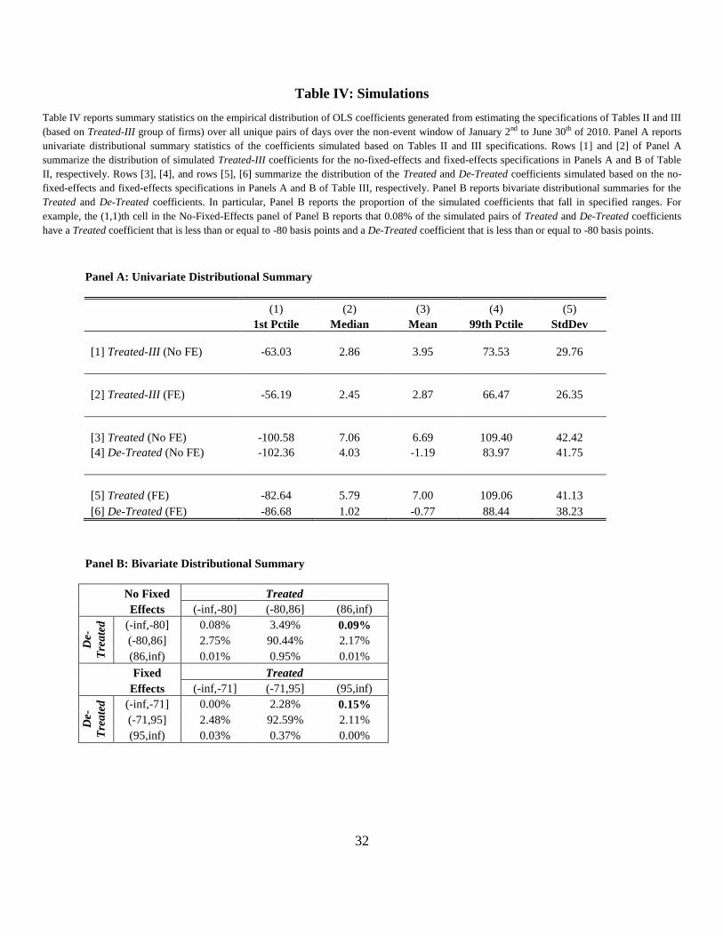
32

Table IV: Simulations

Table IV reports summary statistics on the empirical distribution of OLS coefficients generated from estimating the specifications of Tables II and III

(based on Treated-III group of firms) over all unique pairs of days over the non-event window of January 2nd to June 30th of 2010. Panel A reports

univariate distributional summary statistics of the coefficients simulated based on Tables II and III specifications. Rows [1] and [2] of Panel A

summarize the distribution of simulated Treated-III coefficients for the no-fixed-effects and fixed-effects specifications in Panels A and B of Table

II, respectively. Rows [3], [4], and rows [5], [6] summarize the distribution of the Treated and De-Treated coefficients simulated based on the no-

fixed-effects and fixed-effects specifications in Panels A and B of Table III, respectively. Panel B reports bivariate distributional summaries for the

Treated and De-Treated coefficients. In particular, Panel B reports the proportion of the simulated coefficients that fall in specified ranges. For

example, the (1,1)th cell in the No-Fixed-Effects panel of Panel B reports that 0.08% of the simulated pairs of Treated and De-Treated coefficients

have a Treated coefficient that is less than or equal to -80 basis points and a De-Treated coefficient that is less than or equal to -80 basis points.

Panel A: Univariate Distributional Summary

(1) (2) (3) (4) (5)

1st Pctile Median Mean 99th Pctile StdDev

[1] Treated-III (No FE) -63.03 2.86 3.95 73.53 29.76

[2] Treated-III (FE) -56.19 2.45 2.87 66.47 26.35

[3] Treated (No FE) -100.58 7.06 6.69 109.40 42.42

[4] De-Treated (No FE) -102.36 4.03 -1.19 83.97 41.75

[5] Treated (FE) -82.64 5.79 7.00 109.06 41.13

[6] De-Treated (FE) -86.68 1.02 -0.77 88.44 38.23

Panel B: Bivariate Distributional Summary

No Fixed Treated

Effects (-inf,-80] (-80,86] (86,inf)

De-

Tre

ate

d

(-inf,-80] 0.08% 3.49% 0.09%

(-80,86] 2.75% 90.44% 2.17%

(86,inf) 0.01% 0.95% 0.01%

Fixed Treated

Effects (-inf,-71] (-71,95] (95,inf)

De-

Tre

ate

d

(-inf,-71] 0.00% 2.28% 0.15%

(-71,95] 2.48% 92.59% 2.11%

(95,inf) 0.03% 0.37% 0.00%

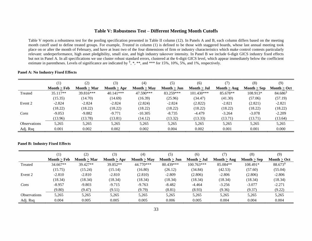
33

Table V: Robustness Test – Different Meeting Month Cutoffs

Table V reports a robustness test for the pooling specification presented in Table II column (12). In Panels A and B, each column differs based on the meeting

month cutoff used to define treated groups. For example, Treated in column (1) is defined to be those with staggered boards, whose last annual meeting took

place on or after the month of February, and have at least two of the four dimensions of firm or industry characteristics which make control contests particularly

relevant: underperformance, high asset pledgibility, small size, and high industry takeover intensity. In Panel B we include 6-digit GICS industry fixed effects

but not in Panel A. In all specifications we use cluster robust standard errors, clustered at the 6-digit GICS level, which appear immediately below the coefficient

estimate in parentheses. Levels of significance are indicated by ┼, *, **, and *** for 15%, 10%, 5%, and 1%, respectively.

Panel A: No Industry Fixed Effects

(1) (2) (3) (4) (5) (6) (7) (8) (9)

Month > Feb Month > Mar Month > Apr Month > May Month > Jun Month > Jul Month > Aug Month > Sep Month > Oct

Treated 35.117** 39.816*** 40.141*** 47.590*** 83.259*** 101.430*** 85.678** 108.913* 84.686┼

(15.35) (14.70) (14.69) (16.39) (25.96) (34.47) (41.30) (57.06) (57.19)

Event 2 -2.824 -2.824 -2.824 (2.824) -2.824 (2.822) -2.821 (2.821) -2.821

(18.22) (18.22) (18.22) (18.22) (18.22) (18.22) (18.22) (18.22) (18.22)

Cons -9.053 -9.882 -9.771 -10.305 -8.735 -4.479 -3.264 -3.078 -2.209

(13.96) (13.78) (13.81) (14.12) (13.32) (13.33) (13.71) (13.71) (13.64)

Observations 5,265 5,265 5,265 5,265 5,265 5,265 5,265 5,265 5,265

Adj. Rsq 0.001 0.002 0.002 0.002 0.004 0.002 0.001 0.001 0.000

Panel B: Industry Fixed Effects

(1) (2) (3) (4) (5) (6) (7) (8) (9)

Month > Feb Month > Mar Month > Apr Month > May Month > Jun Month > Jul Month > Aug Month > Sep Month > Oct

Treated 34.667** 39.427** 39.852** 44.770*** 80.439*** 100.763*** 85.084** 108.491* 88.673┼

(15.75) (15.24) (15.14) (16.80) (26.12) (34.84) (42.53) (57.60) (55.04)

Event 2 -2.810 -2.810 -2.810 (2.810) -2.809 (2.806) -2.806 (2.806) -2.806

(18.34) (18.34) (18.34) (18.34) (18.34) (18.34) (18.34) (18.34) (18.34)

Cons -8.957 -9.803 -9.715 -9.763 -8.482 -4.464 -3.256 -3.077 -2.271

(9.80) (9.47) (9.51) (9.79) (8.81) (8.93) (9.36) (9.37) (9.22)

Observations 5,265 5,265 5,265 5,265 5,265 5,265 5,265 5,265 5,265

Adj. Rsq 0.004 0.005 0.005 0.005 0.006 0.005 0.004 0.004 0.004

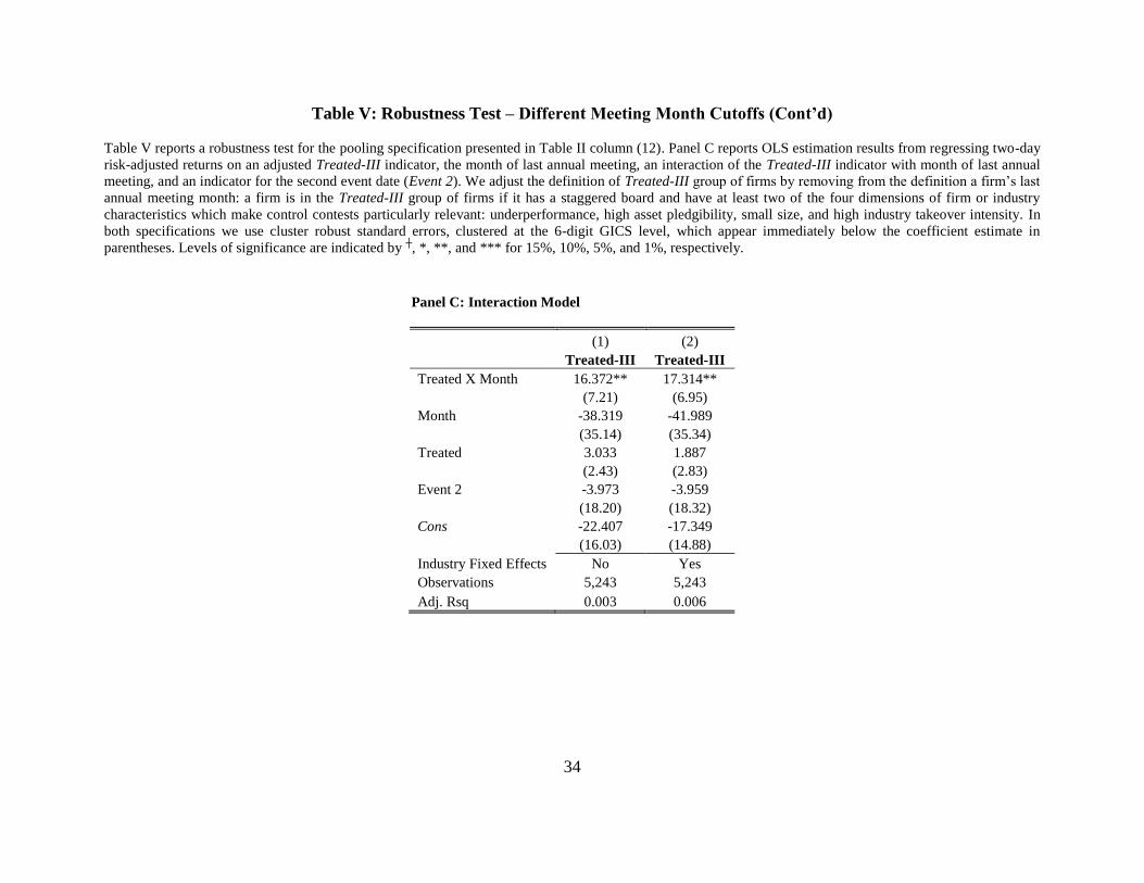
34

Table V: Robustness Test – Different Meeting Month Cutoffs (Cont’d)

Table V reports a robustness test for the pooling specification presented in Table II column (12). Panel C reports OLS estimation results from regressing two-day

risk-adjusted returns on an adjusted Treated-III indicator, the month of last annual meeting, an interaction of the Treated-III indicator with month of last annual

meeting, and an indicator for the second event date (Event 2). We adjust the definition of Treated-III group of firms by removing from the definition a firm’s last

annual meeting month: a firm is in the Treated-III group of firms if it has a staggered board and have at least two of the four dimensions of firm or industry

characteristics which make control contests particularly relevant: underperformance, high asset pledgibility, small size, and high industry takeover intensity. In

both specifications we use cluster robust standard errors, clustered at the 6-digit GICS level, which appear immediately below the coefficient estimate in

parentheses. Levels of significance are indicated by ┼, *, **, and *** for 15%, 10%, 5%, and 1%, respectively.

Panel C: Interaction Model

(1) (2)

Treated-III Treated-III

Treated X Month 16.372** 17.314**

(7.21) (6.95)

Month -38.319 -41.989

(35.14) (35.34)

Treated 3.033 1.887

(2.43) (2.83)

Event 2 -3.973 -3.959

(18.20) (18.32)

Cons -22.407 -17.349

(16.03) (14.88)

Industry Fixed Effects No Yes

Observations 5,243 5,243

Adj. Rsq 0.003 0.006