Embed Size (px)
Citation preview
ABSTRACT
Title of dissertation: ON SUPERSPACE DIMENSIONAL REDUCTION
William Divine Linch, III, Doctor of Philosophy, 2005
Dissertation directed by: Professor S. James Gates, Jr.Center for String and Particle TheoryDepartment of Physics
We describe manifestly globally supersymmetric theories in five dimensions
and their dimensional reduction in superspace. This proceeds by a reduction from
harmonic superspace, the universal superspace for theories in dimension six or fewer
with eight supercharges, through projective superspace to simple superspace. That
is, all symmetries of the original theory are retained but only a proper subgroup
of the original Lorentz supergroup is realized linearly. The latter supergroup is
precisely the four-dimensional Lorentz supergroup with four supercharges, making
this setting ideal for the study of particle-field theories in five or six dimensions with
flat four-dimensional subspaces.
ON SUPERSPACE DIMENSIONAL REDUCTION
by
William Divine Linch, III
Dissertation submitted to the Faculty of the Graduate School of theUniversity of Maryland, College Park in partial fulfillment
of the requirements for the degree ofDoctor of Philosophy
2005
Advisory Committee:
Professor S.James Gates, JrProfessor Markus A. LutyProfessor Rabindra N. MohapatraProfessor Andrew BadenProfessor Jonathan M. Rosenberg

c© Copyright by
William Divine Linch, III
2005
ACKNOWLEDGMENTS
This thesis exists because my father taught me that everything around me
should be understandable and my mother taught me that there is always more than
one way of understanding it. I thank them for being, quite possibly, the best parents
ever. I thank my brother for being, hands down, the funniest person I know and one
of the most intelligent. Without my family’s support I would have been coding some
boring finance model by now.
I thank my advisor, colleague and friend, S. James Gates, Jr. for believing in
me, supporting me, and fighting for me for all these years even when it might have
seemed to be going nowhere.
I thank my colleague and great friend Jo(s)e(ph) Phillips without whom I would
probably not have been so prolific in my writing. It certainly would not have been
as much fun without you. Physics’ loss will be humanity’s gain when you figure out
how cells move.
Obviously, I thank all my colleagues but especially Vincent G. J. Rodgers for
getting me through the summers and making me laugh, Ioseph L. Buchbinder for
ii

teaching me to translate my ideas into mathematics, Te(o)d(or) A. Jacobson for
trying to teach me that there is a difference between physics and formalism, Markus
A. Luty for reminding me that crazy ideas are sometimes right and closed-minded
people are always wrong (in the end at least), Ram Sriharsha for teaching me most of
what I know about field and string theory, and Sergei M. Kuzenko for his friendship
and the work which became the topic of this thesis. I thank all of you for hours of
stimulating conversations and thank you in general for being good friends to me.
I thank my family and friends for being awesome. I cannot imagine the tedium
my life would be without you all.
iii
TABLE OF CONTENTS
List of Figures vi
1 Introduction 1
2 Four-Dimensional Simple Superspace 82.1 Minkowski N = 0 Superspace . . . . . . . . . . . . . . . . . . . . . . 82.2 Simple N = 1 Superspace . . . . . . . . . . . . . . . . . . . . . . . . 112.3 Classical Field Theories in Four-Dimensional Simple Superspace . . . 17
2.3.1 The Scalar Multiplet I: Chiral Multiplet . . . . . . . . . . . . 182.3.2 The Scalar Multiplet II: Linear Multiplet . . . . . . . . . . . . 192.3.3 The Vector Multiplet . . . . . . . . . . . . . . . . . . . . . . . 21
3 Five-Dimensional Simple Superspace 253.1 Classical Field Theories in Five-Dimensional Simple Superspace . . . 25
3.1.1 The Scalar Multiplet I: The Chiral Non-Minimal Case . . . . . 273.1.2 The Scalar Multiplet II: The Fayet-Sohnius Case . . . . . . . 283.1.3 The Vector Multiplet . . . . . . . . . . . . . . . . . . . . . . . 293.1.4 Abelian Chern-Simons Theory . . . . . . . . . . . . . . . . . . 31
4 Four- and Five-Dimensional Harmonic Superspace 324.1 Classical Field Theories in Harmonic Superspace . . . . . . . . . . . . 36
4.1.1 The Scalar Multiplet I: The q+-Hypermultiplet . . . . . . . . . 374.1.2 The Scalar Multiplet II: The Fayet-Sohnius Hypermultiplet . . 374.1.3 The Vector Multiplet . . . . . . . . . . . . . . . . . . . . . . . 384.1.4 Abelian Chern-Simons Theory . . . . . . . . . . . . . . . . . . 41
5 Projective Superspace and Dimensional Reduction 425.1 Singular Harmonic Superfields . . . . . . . . . . . . . . . . . . . . . . 425.2 The Regularization of the Singular Theories . . . . . . . . . . . . . . 475.3 The Reduced Actions . . . . . . . . . . . . . . . . . . . . . . . . . . . 505.4 Explicit Examples . . . . . . . . . . . . . . . . . . . . . . . . . . . . . 54
5.4.1 Reduction of the q+-Hypermultiplet . . . . . . . . . . . . . . . 545.4.2 Reduction of the Fayet-Sohnius Hypermultiplet . . . . . . . . 555.4.3 Reduction of Yang-Mills Theory . . . . . . . . . . . . . . . . . 565.4.4 Reduction of Chern-Simons Theory . . . . . . . . . . . . . . . 56
6 Closing Remarks 63
iv
A 5D notation and conventions 71
Bibliography 76
v
LIST OF FIGURES
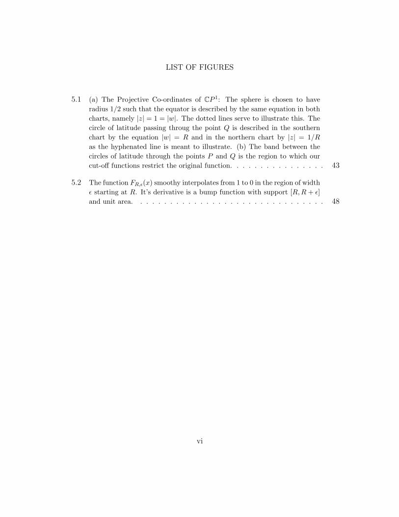
5.1 (a) The Projective Co-ordinates of CP 1: The sphere is chosen to haveradius 1/2 such that the equator is described by the same equation in bothcharts, namely |z| = 1 = |w|. The dotted lines serve to illustrate this. Thecircle of latitude passing throug the point Q is described in the southernchart by the equation |w| = R and in the northern chart by |z| = 1/Ras the hyphenated line is meant to illustrate. (b) The band between thecircles of latitude through the points P and Q is the region to which ourcut-off functions restrict the original function. . . . . . . . . . . . . . . . 43
5.2 The function FR,ε(x) smoothy interpolates from 1 to 0 in the region of widthε starting at R. It’s derivative is a bump function with support [R,R + ε]and unit area. . . . . . . . . . . . . . . . . . . . . . . . . . . . . . . . 48
vi
Chapter 1
Introduction
One of the most amazing observations about our universe is the fact that there
exist two and only two types of particles. Bosons have the property that they like
to “condense” into the same state as other identical bosons making possible, among
other things, the stimulated emission of radiation, superfluidity, and superconduc-
tivity. Fermions, on the other hand, obey the Pauli exclusion principle meaning
that two fermions can never be in the same state. This is the basis of the stability
of matter; the periodic table of the elements and therefore all of chemistry (not to
mention biology) would not exist without it. Indeed, the forces of nature all seem
to be carried by bosons while all of fundamental matter (excluding the elusive Higgs
boson) is fermionic.
Supersymmetry is a symmetry which treats bosons and fermions on an equal
footing. In a theory possessing the simplest of such symmetries, every bosonic degree
of freedom has a fermionic partner and vice versa. Considering how different these
two types of particles are, it is quite surprising that such a symmetry exists. With
respect to how forces are carried by bosons and matter is made up of fermions it is
1
perhaps even more surprising that we would consider such a symmetry relevant to a
description of our universe.
In fact, supersymmetry is the hallmark of a variety of interesting theories from
the purely mathematical to the phenomenological. Besides the æsthetically pleasing
fact that it is the “ultimate” symmetry, it is the most powerful tool available for the
study of the strong coupling limit of gauge theories, has the potential to cure the
standard model1, and seems to be an essential ingredient in the ultraviolet completion
of effective theories of various types, including gravity.
The standard approach to such theories is the component approach or “tensor
calculus”. In such an approach supersymmetry is not manifest. This is not usually
considered to be a problem since many of the virtues of supersymmetric theories are
theorems about renormalizability which hold whether the symmetry is manifest or
not. (In fact, it is common practice in the literature to write only the bosonic part
of the theory under consideration and simply announce that it is supersymmetric,
by which is meant that it has a supersymmetric completion.) One advantage of
this approach is that everything is written in a manner consistent with the usual
1That this symmetry is not in direct conflict with observation is because of the possibility that
it is spontaneously broken, that is, it is a symmetry of the action but not of the ground state of the
system. The situation can then be arranged so that the missing superpartners gain a correction to
their masses which puts them above the scale of current measurements.
2
notation used when one learns about the quantum theory of particles and fields.
This is therefore the most popular approach to the subject for beginners. It also
follows that this formulation is amenable to standard field-theoretic manipulations.
An alternative approach is to use the superfield or superspace formalism. In
this notation supersymmetry is manifest in the same sense that Lorentz invariance
is manifest in 4-vector notation. Besides the usual advantages of having a symmetry
manifest, the superspace approach is indispensable for the quantization of compli-
cated theories such as General Relativity. The disadvantages of this approach, how-
ever, are manifold and non-negligible. Firstly, the amount of formalism one needs to
learn is significant: Two of the three standard references [1, 2] on the subject are over
500 pages long. The third [3] is around 250 pages long but is almost entirely a long
list of big equations. Secondly, the formalism for a given theory is not always known.
For example, it is not known what the off-shell formulation is for the “maximally
supersymmetric” super-Yang-Mills (sYM) theory in four dimensions. Thirdly, when
the theory is known, it is often quite complicated videlicet four-dimensional N = 2
supergravity. Finally, certain manipulations of a theory which one may like to per-
form are more difficult than in the component approach. For example, one would
often like to truncate a theory defined in d dimensions to d− 1 dimensions or fewer.
The physics resulting from this reduction is easy to understand in components but
3
not in superspace.
In the end, the fact remains that some calculations are impossible to perform
in components such as the quantization of theories in the presence of gravity. Other
calculations can be performed this way at the expense of great effort but become
almost trivial when formulated in superspace. In yet other theories, superspace
allows one to make progress on pressing questions which have resisted analysis in the
component formulation. An example of this is the problem of the quantization of
strings in Ramond-Ramond backgrounds. Finally, the ills of the superspace approach
can be argued to be curable, in which case superspace becomes a more attractive
option. Alternatively, we could use the parts we do understand well to attack the
ones we do not in non-conventional ways.
In this thesis I describe what I see as evidence of these last two assertions.
Specifically, we will analyze the special case of flat five2-dimensional superspace with
2Although we will consider only five dimensional superspace with the minimal amount of super-
symmetry, the formalism can be extended almost trivially to six dimensions. In the formulation in
which supersymmetry is manifest, the extension can be achieved by interpreting the central charge
in the algebra 4 as the derivative in the “6-direction”. In the projective superspace approach
(and therefore also the simple superspace approach) in which we will drop the central charge, the
required extension is effected by the substitution ∂5 → ∂5 ± i∂6. Some of the theories we consider
in this thesis cannot be obtained in this way while keeping the fields off their mass shells.
4
the minimal amount of supersymmetry. We will perform, in a relatively simple way,
the reduction of theories in this space to four-dimensional superspace notation. Al-
though the resulting theory is still five-dimensional, only the four-dimentional part of
the Poincare symmetry will be manifest as will only one of its two3 supersymmetries.
Schematically, this reduction proceeds as follows:
Harmonicδ2→ Projective
δ1→ Simple . (1.0.1)
Here “Harmonic” refers to the five-dimensional superspace with manifest minimal
supersymmetry, “Projective” refers to the five-dimensional superspace with half of
the minimal supersymmetry manifest and “Simple” is the five-dimensional super-
space obtained by integrating out an infinite number of auxiliary (non-dynamical)
3The counting of supersymmetries will be unavoidably ambiguous for historical reasons. Five-
dimensional theories with minimal supersymmetry (eight real supercharges) are properly said to
have N = 1 supersymmetry. The truncation of such a theory to four dimensions gives twice the
amount of minimal (id est four real supercharges) supersymmetry allowable in this dimension and
is properly called an N = 2 theory in four dimensions. The relevant superspace is then called con-
ventional N = 2 superspace. For the purpose of describing five-dimensional theories, however, this
superspace (together with one extra bosonic coordinate) has the minimal amount of supersymmetry
in five dimensions and is therefore N = 1 in the five-dimensional sense. Writing a five-dimensional
minimally supersymmetric theory with eight real supercharges in a superspace with only four real
supercharges keeps manifest only one-half of the five-dimensional supersymmetries. However, one
often describes this by saying that we keep manifest only one of the two supersymmetries.
5
superfields which are the hallmark of linearly realized symmetries with more than
four real supercharges. The projection δ1 is the map which implements this proce-
dure while δ2 is the projection developed by Sergei M. Kuzenko [4] which removes
two complex co-dimension-one hyperplanes from the harmonic superspace and is the
subject of section 5.
This report is organized as follows: In chapter 2 we review, very briefly, four-
dimensional N = 0 and N = 1 superspaces. The purpose of section 2.1 is simply to
provide a layout of the presentation of the subsequent sections in a familiar setting.
Section 2.2 provides a review of field theory with manifest global supersymmetry and
serves to set the notation of four-dimensional superspace.
Chapter 3 reviews the construction of five-dimensional theories with global
supersymmetry in simple superspace. The sYM theory in this section is a truncation
of a much more non-trivial result obtained in [5] for ten dimensions. This result was
later re-derived in [6] and applied to phenomenological problems. These two papers
gave the impetus for the study of a gravitational analogue which was developed in [7]
and started the line of research [8, 9, 10] which eventually culminated in this thesis.
Chapter 4 is a review and extension of the harmonic superspace based on the
SU(2)/U(1) coset developed in [11]. All details of this theory can be found in the
textbook [12]. We restrict our attention to the case of global supersymmetry.
6
Chapter 5 covers the main point of this thesis: All results in five- and six-
dimensional globally supersymmetric theories can be reduced to four dimensions by
a simple reduction procedure first described in [4]. This reference provided a detailed
embedding of projective superspace into harmonic superspace. This result was re-
interpreted as a dimensional reduction in [10].
Chapter 6 provides some closing thoughts about the work presented in this
thesis and is, perhaps, the most interesting chapter. Here I describe the relation
of projective superspace to string theory on Calabi-Yau 3-folds and speculate on
the relation of harmonic superspaces in general to the various existing formalisms
for the covariant quatization of the critical superstring. In particular, I consider
the relationship between the existence of generalizations of the chiral and analytic
subspaces of N = 1 and N = 2 superspaces and the measure for the open string
field theory path integral.
7
Chapter 2
Four-Dimensional Simple Superspace
In this section we will review some basics of simple superspace. We will not
attempt to give a comprehensive presentation of this subject as it is done completely
in the excellent references [1, 2] and [3] and would take far too long to repeat. Instead,
we collect here some highlights. We will be adhering to the conventions of reference
[2] throughout.
2.1 Minkowski N = 0 Superspace
The simplest of non-trivial example of a four-dimensional superspace is flat
spacetime R1,3, or Minkowski space. It consists of commuting coordinates only
{xa}3a=0,
[xa, xb] = xaxb − xbxa = 0 , (2.1.1)
transforming in the spin-1 representation of the Lorentz group. In particular one
coordinate, {x0}, is time-like while the other three, {xi}3i=1, are space-like.
For future reference we point out that this space is isometric to the quotient of
the Poincare, or in-homogeneous Lorentz group, ISO(1, 3) by the homogeneous part
8
SO(1, 3). That is
R1,3 ≈ ISO(1, 3)/
SO(1, 3) , (2.1.2)
A representation
ϕ : R1,3 → a
x 7→ ϕ(x) , (2.1.3)
defined on this space and taking values in an algebra a is called a(n a-valued classical)
field. The generator of translations Pa is realized on this field as a derivative Pa =
−i∂a.
In order to define the classical theory of an a-valued field ϕ(x), we often define
an action functional S as a smooth map from the space of fields and its derivatives
to the real numbers. Traditionally, we further require that the action can be written
as the integral of a density:
S[ϕ] =
∫d4xtrL . (2.1.4)
Here L = L[ϕ(x), ∂ϕ(x), ∂2ϕ(x), . . .] is the Lagrangian density which, in turn, is
required to be a local functional of the field and its derivatives. We usually1 require
the action S to be a singlet of the Lorentz group SO(1, 3) as well as the algebra a.
1This requirement cannot always be met in the quantum theory where S might shift under a
transformation. It is then only required that S → S + 2πk for k ∈ Z an integer.
9
We denote the latter projection by tr. The former condition will be satisfied if L is
itself a Lorentz singlet. Alternatively, with rapidly decaying boundary conditions on
the fields, the Lagrangian may transform into a total derivative, a condition we will
assume throughout this work. We will always assume such conditions.
The stationary points of the action functional are the classical equations of
motion2
E[ϕ] =δ
δϕ(x)S[ϕ] = 0 . (2.1.5)
In what follows we will be studying the analogues of the action for a free complex
scalar field ϕ given by
−∫
d4x∂aϕ∂aϕ , (2.1.6)
and that of a connection 1-form Aa given by
− 1
4
∫d4xFabF
ab Fab = ∂aAb − ∂bAa . (2.1.7)
2When E = 0 we say that the theory is on-shell or that the equation of motion is satisfied.
Conversely, if none of the equations of motion are imposed, we say that the theory is off-shell.
10
2.2 Simple N = 1 Superspace
The next-to-simplest superspace is parameterized by the coordinates of Minkowski
space together with a set of anti-commuting parameters θα
{θα, θβ} = θαθβ + θβ θα = 0 , (2.2.8)
where hatted greek letters take the values α = 1, 2, 1, 2. These parameters are defined
to transform in the spin-12 representation of the Lorentz group. Actually, since the
algebra spin(1, 3) ≈ sl(2,C)⊕ sl(2,C) splits, these fermionic parameters split as
(θα) =
θα
θα
, (2.2.9)
where now α = 1, 2 et cetera. θ and θ are called Weyl spinors. We take θ to be
the hermitian conjugate of θ making the original θα a Majorana spinor. Spinorial
indices are raised and lowered using the SL(2,C)-invariant tensors εαβ, εαβ and their
inverses.3 An enormously helpful fact concerning this split is that spin-tensors with
antisymmetric dotted or un-dotted indices are trivial representations of the Lorentz
3 A note of caution: If a spinor ψα is originally defined with its index down, then ψα := εαβψβ
is the definition for this object with its index raised and analogous statements hold for general
spin-tensors. There are a few exceptions to this rule. One is εαβ itself. As one can easily show,
εαγεβδεγδ = −εαβ if, as it is defined in these conventions, εαβεβγ = δαγ .
11
group. For example,
θαθβ = −1
2εαβθγθγ = −1
2εαβθ2 . (2.2.10)
Translations in these fermionic directions are generated by the supercharges
Qα and Qα and are defined to close algebraically on translations Pa in the graded
sense, id est
{Qα, Qα} = 2(σa)ααPa , (2.2.11)
with all other graded commutators vanishing.4 The set {Q, Q, P,M}, with M denot-
ing the Lorentz generator, therefore closes under graded commutation and is called
the super-Poincare algebra. Exponentiation of this algebra gives the (connected part
of the) super-Poincare group.
Simple superspace is now defined as the (left) quotient of this group by its
Lorentz subgroup. Classical fields on this space are as before but now depend on
the fermionic coordinates θ and θ. They are called superfields. Since the fermionic
coordinates are anti-commuting, a McLauren expansion in them terminates at a finite
order. The coefficients of this expansion are ordinary N = 0 fields called component
fields in various representations of the Lorentz group. Using equation (2.2.10) we
4Here σa = (1, ~σ) is the four-dimensional extension of the standard Pauli matrices. They are
constant tensors of the Lorentz group.
12
find that for a real scalar superfield f(x, θ, θ),
f(x, θ, θ) = ϕ(x) + (θψ(x) + h.c.) + (θ2F (x) + h.c.)
+i(θσaθ)Aa(x) + (θ2θλ(x) + h.c.) + θ2θ2D(x) . (2.2.12)
Here ϕ and D are real scalar fields, F is a complex scalar field and ψ and λ are
Weyl fermion fields. The letters used for the component fields are not standard
except F and D. These parts of a superfield are even called the F -term and D-term
respectively and are important as we will see below.
The supercharges are realized on superfields as fermionic derivations
Qα := i∂α + θα(σa)αα∂a
Qα := −i∂α − θα(σa)αα∂a , (2.2.13)
where the fermionic partial derivatives are defined to act as ∂αθβ := δαβ and ∂αθ
β = δαβ
and annihilate everything else.5 In order to preserve the reality of a superfield, the
supersymmetry transformation with infinitesimal Weyl parameter ε is given by
δ = i(εQ+ εQ) . (2.2.14)
We now come to the most important part of the N = 1 superspace formalism.
We want to construct covariant derivatives – derivations which commute with this5 We will not elaborate on this point here, but these partial derivatives are another exception
the the raising/lowering rule. In fact, in the conventions of [2], ∂α = −εαβ and ∂α = −εαβ ∂β . Note
also the fact that with these definitions Q = −(Q)∗.
13
supersymmetry transformation. That these derivatives have to exist is a consequence
of the fact that our superspace is a left coset and the supersymmetry transformations
are generated by a left action. However, we could also consider motions generated
by a right action. Since acting on the left commutes with acting on the right,
the derivations effecting these actions must commute. Alternatively, we could just
compute explicitly and we find that
∂a ,
Dα := ∂α + iθα∂a ,
Dα := −∂α − iθα∂a , (2.2.15)
all commute with the Qs. (With this normalization, D is the complex conjugate of
D.)
The existence of the fermionic derivatives suggests the following alternative to
the component expansion (2.2.12). The fields defined in this expansion can be ex-
tracted by acting with fermionic partial derivatives and setting to zero the explicit
θ dependence in the result. For example ψα(x) = −∂αf(x, θ, θ)|. (The | notation
is a standard notation for the θ, θ → 0 limit.) The drawback of this is that the
resulting components do not transform covariantly under supersymmetry transfor-
mations since {∂α, Qα} 6= 0. It is easy to convince oneself that the covariant set of
components defined instead by acting with Dα and Dα is equivalent to the this non-
14
covariant set, the latter differing from the former by a field redefinition. Therefore,
we will henceforth use the covariant component definitions exclusively. Expressions
such a the component expansion (2.2.12) are to be interpreted as schematic shorthand
for a covariant expansion and not literally as an expansion in the θ-variables. Once
this is agreed, we are in a position to abandon the superspace translation operators
altogether in favor of the covariant derivatives.
The derivatives (2.2.15) obey the algebra6
{Dα, Dβ} = 0 , {Dα, Dβ} = 0 , (2.2.16)
{Dα, Dα} = −2i∂a , (2.2.17)
together with trivial commutators with the bosonic partial derivatives. Important
formulæ which follow from this algebra are
DαDβ =1
2εαβD
2 ; DαDβ = −1
2εαβD
2 (2.2.18)
[D2, Dα] = −4i∂aDα ; [D2, Dα] = 4i∂aD
α (2.2.19)
DαD2Dα = DαD2Dα (2.2.20)
6The space of 4-vectors is isomorphic to the space su(2) of hermitian 2 × 2 matrices. The
isomorphism is given by the contraction with the Pauli matrices. It proves to be very useful,
therefore, to employ a notation in which all indices are spinorial. Many references write expressions
like vαα := (σa)ααva, a notation we will sometimes use. In addition, however, we will also define
va := vαα.
15
{D2, D2} − 2DαD2Dα = 162 (2.2.21)
[D2, D2] = −4i∂a[Dα, Dα] (2.2.22)
The relation (2.2.16) implies the existence of non-trivial solutions to the equa-
tion
DαΦ = 0 (2.2.23)
Indeed, since DαDβDγ ≡ 0, the solution is given by Φ = −14D
2ϕ for a completely ar-
bitrary complex superfield ϕ. Superfields obeying equation (2.2.23) are called chiral
superfields and are of fundamental importance. The subspace of the full superspace
is called the chiral subspace and it is invariant under translations and supersym-
metry transformations. Plugging the complex7 version of the component expansion
(2.2.12) into the chirality condition (2.2.23) and using the representation (2.2.15) of
the covariant derivatives, one finds that only the (complex!) fields analogous to ϕ,
ψα and F survive. Indeed, from the covariant projection
ϕ(x) := Φ|
ψα(x) := DαΦ|
F (x) := −1
4D2Φ| (2.2.24)
7 Real chiral fields are necessarily constant as follows directly from the algebra upon imposing
the constraint.
16
it is immediate that these are the only components since any expression with a D in
it can be reduced, using the algebra and the constraint, to zero or some combination
of spacetime derivatives acting on these components.
2.3 Classical Field Theories in Four-Dimensional Simple Superspace
In order to write classical field theories in superspace, it is nice to know how to
write actions in terms of Lagrangian super-densities. To this end, we need a projec-
tion from superspace to the real numbers. A general superfield L = L(x, θ, θ) has the
property that it’s D-term DL transforms into a spacetime derivative under a super-
symmetry transformation. It follows that the “integral”∫
d4θL := DL transforms
into a total derivative. This term, as described above, can be isolated by covariant
projection DL = 116D
2D2L|. We therefore define the action of L by
∫d4x
∫d4θL =
1
16
∫d4xD2D2L
∣∣∣ . (2.3.25)
Suppose now that W is a chiral superfield. It follows immediately that the
action above vanishes if we were to replace L → W . However, for chiral super-
fields, the supersymmetry transformation of the F -term FW is a total derivative.
We therefore define the integration over the chiral subspace of the full superspace as
17
∫d2θW := FW and, consequently, the action of this so-called “superpotential” as
∫d2θW + h.c. = −1
4D2W
∣∣∣ + h.c. (2.3.26)
Let us now turn to some applications of these observations.
2.3.1 The Scalar Multiplet I: Chiral Multiplet
The standard scalar multiplet is described in superspace by a complex field Φ
satisfying the chirality condition
DαΦ = 0 . (2.3.27)
This condition is entirely equivalent to the statement that Φ = −14D
2ϕ provided
that ϕ is an unconstrained complex superfield. The mass dimension of Φ is taken
to be 1 and the Lagrangian density for this theory is the well known Wess-Zumino
kinetic term
∫d4θΦΦ . (2.3.28)
The equation of motion is obtained by the chiral differentiation rule or simply by
varying with respect to the complex prepotential:
E[ϕ] = −1
4D2Φ . (2.3.29)
It follows from this equation of motion and the chirality of Φ that:
18
1. The superfield Φ obeys the correct mass-shell condition 2Φ = 0.
2. The component spectrum of on-shell degrees of freedom is that of a complex
scalar z ∼ Φ| and a Weyl fermion λα ∼ DαΦ| which obey the Klein-Gordon
equation by virtue of consequence 1.8 In particular the F-term of Φ is an
auxiliary field.
2.3.2 The Scalar Multiplet II: Linear Multiplet
A second description of a scalar multiplet is obtained by replacing the chiral
field with a complex field Γ obeying the linear constraint
D2Γ = 0 . (2.3.30)
This Bianchi identity is solved in terms of an unconstrained spinor superfield ψα as
Γ = Dαψα. This prepotential transforms as δψα = Dβταβ for symmetric ταβ leaving
Γ invariant.
The mass dimension of Γ is taken to be one and the Lagrangian density for
8In fact, the fermion obeys the Weyl equation as derived from (2.3.29) by 0 = DαE[ϕ]| ∼
∂aDαΦ|. In the sequel, we will only explicitly refer to the Klein-Gordon equation. Implicitly, the
component fields are obeying the correct mass-shell conditions.
19
this theory is simply9
−∫d4θΓΓ . (2.3.31)
This time the equation of motion is obtained by varying with respect to the spinor
prepotential:
E[ψ] = −DαΓ . (2.3.32)
It follows from this equation of motion and the Bianchi identity that
1. the superfield Γ obeys the Klein-Gordon equation 2Γ = 0,
2. the component spectrum is that of a complex scalar z ∼ Γ| and a Weyl fermion
λα ∼ DαΓ|,
3. this theory is dual to the chiral scalar theory described above (compare equa-
tions (2.3.27↔2.3.32) and (2.3.29↔2.3.30)) since the first was off-shell chiral
but on-shell linear while in this case it is the other way around.
9The sign preceding this density is not a mistake. Although comparing (2.3.31) to (2.3.28)
suggests this sign gives ghostlike kinetic terms to the scalars, it is in fact necessary to get the
correct sign as is easy to check explicitly. Alternatively, one can perform a duality transformation
from the chiral field Lagrangian of the previous section to the complex linear Γ multiplet which
produces a sign of the type in (2.3.30).
20
2.3.3 The Vector Multiplet
The chiral multiplet action (2.3.28) has a global U(1) symmetry taking Φ 7→
eiaΦ with a ∈ R. Gauging this symmetry while preserving the the chirality of Φ
requires the replacement a → Λ with chiral (non-constant) superfield Λ. Note that
this complexifies the U(1) ↪→ C∗ in addition to making it local. The invariance of
the action can now be restored by introducing a real superfield-valued connection eV
transforming under the C∗ action as (eV )′ = eiΛeV e−iΛ and replacing the Lagrange
super-density ΦΦ → ΦeV Φ. In the abelian case, the field strength of the gauge
pre-potential can be deduced from the linearized transformation law δV = 12i(Λ −
Λ). Since the operator D2Dα annihilates both chiral and anti-chiral fields, Wα =
18D
2DαV is an invariant field strength. We note immediately that this field strength
superfield obeys the following constraints identically10
DαWα = 0 ; DαWα − DαWα = 0 . (2.3.33)
From these equations it follows that the action constructed from the Lagrangian
super-density
1
2
∫d2θW αWα , (2.3.34)
10The second of these follows from the identitiy (2.2.20) and the reality of V .
21
is both real and manifestly gauge invariant. The equation of motion which follows
from this is
E[V ] = DαWα + DαWα . (2.3.35)
Consequently,
1. The superfield strength Wα obeys the Dirac equation.
2. The component spectrum is that of a Weyl fermion λα ∼ Wα| and a symmetric
bi-spinor field strength Fαβ ∼ D(αWβ)| and their conjugates. Such a component
field strength is equivalent to a 2-form Fab ∼ εαβFαβ +εαβFαβ which is the field
strength of a gauge 1-form Fab ∼ ∂[aAb].
3. The dual of this theory is a theory of the same type. More precisely, defining
U = iV and writing the theory in terms of U we switch the second constraint
and the equation of motion and multiply the action by a factor of −1.
An alternative approach to obtaining this theory is by interpreting it as a super-
differential geometric problem. In such an approach we introduce gauge connections
for all of the superspace covariant derivatives DA → DA = DA + iΓA so that the
resulting gauge covariant derivatives transform covariantly under the C∗ action. This
collection of gauge superfields is absurdly redundant. To remove all of the redundant
22
fields, we notice that generically
[DA,DB} = TABCDC + iFAB , (2.3.36)
for some collection of superfields TABC and FAB called torsions and field strengths,
respectively. The strategy now is to find a proper non-trivial subset of these torsions
and field strengths which satisfy the Bianchi identity
[DA, [DB,DC}}+ graded cyclic permutations = 0 . (2.3.37)
The case in which the result implies that the minimal number of independent on-shell
degrees of freedom remain is called “irreducible”. It is irreducible in the sense that
the resulting multiplet forms an irreducible (field) representation of supersymmetry.
If, furthermore, this representation contains the minimal number of independent
off-shell degrees of freedom, it is called “minimal”.
The minimal N = 1 sYM algebra is given by [1, 2]
{Dα,Dβ} = 0 ={Dα, Dβ
};
{Dα, Dα
}= −2iDa (2.3.38)[
Dα,Db
]= 2iεαβWβ ; [Dα,Db] = 2iεαβWβ (2.3.39)
[Da,Db] = −εαβDαWβ − εαβDαWβ (2.3.40)
The constraints (2.3.38) on the first line are called conventional constraints and
are given by setting torsions to constant values. One representation of the unique
23
solution to these constraints can be shown to be given by (Frohbenius’ Theorem)
Dα = Dα ; Dα = e−2VDαe2V ; Da =i
2
{Dα, Dα
}. (2.3.41)
This is called the chiral representation since in this representation Dα has no con-
nection from which it follows that if Φ is chiral in the background where the YM
field is switched off, then it is automatically gauge-covariantly chiral.
The solutions to the constraints (2.3.39) in this representation become
Wα = −1
8D2
(e−2VDαe2V
); Wα =
1
8e−2V D2
(e2VDαe−2V
)e2V . (2.3.42)
In the abelian case, these reduce to Wα = 18D
2DαV and its conjugate.
24
Chapter 3
Five-Dimensional Simple Superspace
The superspace we are calling five-dimensional simple superspace is parame-
terized by the local co-ordinates of 4D, N = 1 superspace {xa, θα, θα} together with
one additional bosonic coordinate x5 which parameterizes the fifth direction. The
basis tangent vector in this direction is denoted as ∂5 and is central in the sense that
it commutes with every other tangent space generator. Contrary to the usual case,
however, the 4D, N = 1 superspace generators form a closed algebra without it. In
the jargon: the central charge is not gauged.
3.1 Classical Field Theories in Five-Dimensional Simple Superspace
Since we are simply extending the superspace of the previous section by an extra
bosonic direction, we will find the following for the analogues of the theories above:
We consider, of course, irreducible representations of the five-dimensional super-
Lorentz group. However, since we are keeping manifest only the “four-dimensional”
part, they will be composed of two multiplets of the previous section. In this sense
the representation is reducible. However, it clearly cannot be reducible since the
25
two “four-dimensional” superfields must transform into each other under a “second”
supersymmetry (in addition to five-dimensional Lorentz transformations).
Since we are still in simple superspace, there is no new fermionic measure to
define in order to write actions. Instead, we find the generic structure S = S0 + cS ′
for S0 and S ′ actions of the previous section for some constant c. If the theory were
truly four-dimensional with only N = 1 supersymmetry, c would be an arbitrary real
number. To find the precise number c one can either
1. project down to the components, assemble the components into irreducible five-
dimensional multiplets, and read off the resulting value of c (not recommended),
2. take the equations of motion resulting from S, hit with appropriate combina-
tions of covariant derivatives, use the constraints, and write the Klein-Gordon
or Dirac equations for the resulting superfield strengths, thereby fixing the
value of c by purely superspace methods.
The former approach was used in [7] to derive a linearized form of five-dimensional
supergravity. The latter approach was described in [9] and used to show the same
thing by more direct methods.
Let us now turn to the description of some five-dimensional matter multiplets
in terms of this superspace.
26
3.1.1 The Scalar Multiplet I: The Chiral Non-Minimal Case
The closest analogue to the 4D scalar multiplet is most naturally described
using a chiral field Φ = −14D
2ϕ and a complex linear field Γ = Dαψα − ∂5ϕ. They
obey the Bianchi identities
DαΦ = 0 , − 1
4D2Γ + ∂5Φ = 0 (3.1.1)
and are both dimension one field strengths. Their Lagrangian is given by
∫d4θ
(ΦΦ− ΓΓ
), (3.1.2)
and the resulting equations of motion are
E[Φ] = −1
4D2Φ− ∂5Γ , E[ψ] = −DαΓ (3.1.3)
Taking −14D
2E[Φ] = 0 and using both Bianchi identities (3.1.1), we find on-shell that
(2 + ∂25)Φ = 0.1 Conversely, taking −1
4D2 on the second Bianchi identityin (3.1.1)
and substituting the equations of motion (3.1.3), we find (2 + ∂25)Γ = 0. Hence, this
theory describes the dynamics of the component fields
a+ ib ∼ Φ| , λ(+)α ∼ DαΦ| , x+ iy ∼ Γ| , λ(−)
α ∼ DαΓ| . (3.1.4)
1In fact, this how the relative coefficient in the Lagrangian (3.1.2) was found. Notice that it is
unnecessary to project to component fields in order to fix this coefficient.
27
This multiplet is self-dual. In the limit ∂5 → 0, this multiplet becomes a 4D, N = 2
scalar multiplet discovered in reference [13] dubbed the “chiral non-minimal” (CNM)
multiplet.
3.1.2 The Scalar Multiplet II: The Fayet-Sohnius Case
An alternative description of the five-dimensional scalar is necessarily on-shell
in the case in which we switch off the central charge.2 It is related by a Lorentz
violating duality to the CNM scalar above. In particular, we switch the equation of
motion and constraint for the complex linear field Γ only. This gives a description
in terms of two chiral fields Φ1 = Φ2 and Φ2 = −Φ1.3 In writing an action for this
representation, one cannot avoid introducing naked ∂5 derivatives and the Lagrangian
is given by:
∑i=1,2
{∫d4θΦiΦ
i +1
2
∫d2θΦi∂5Φi +
1
2
∫d2θΦi∂5Φ
i
}. (3.1.5)
Here Φi = (Φi)†. The resulting equations of motion are
E[Φ1] = −1
4D2Φ1 + ∂5Φ1 ; E[Φ2] = −1
4D2Φ2 − ∂5Φ2 . (3.1.6)
2By the way in which the central charge is related to the translation generator in six dimensions,
it follows that we cannot use this multiplet to write an off-shell theory for the six-dimensional scalar.3Spinor and iso-spinor indices are raised and lowered using the anti-symmetric symbol ε which
is normalized such that ε12 = +1.
28
Together with the chirality constraints these equations imply that the Φi obey the
Klein-Gordon equation and that at the component level they give the same spectrum
as the CNM theory (3.1.4)
a+ ib ∼ Φ1| , λ(+)α ∼ DαΦ1| , x+ iy ∼ Φ2| , λ(−)
α ∼ DαΦ2| . (3.1.7)
In the centrally extended algebra, the chiral fields Φi are constrained by the central
charge to satisfy
i4Φ1 = E[Φ1] , i4Φ2 = E[Φ1] . (3.1.8)
This fact is a manifestation of the statement that without central charges in the
algebra, the Fayet-Sohnius hypermultiplet is on-shell.
3.1.3 The Vector Multiplet
The simple superspace representation for the vector multiplet is given by a real
scalar field V and a chiral scalar Φ. The real part of the latter field carries the fifth
component of the gauge field sitting in V at the θθ level. The gauge transformations
of these prepotentials are of the form
δV =1
2i
(Λ− Λ
),
δΦ =1
2i∂5Λ . (3.1.9)
29
The following field strengths are invariant under these transformations
Wα =1
8D2DαV ,
F =1
2
(Φ + Φ + ∂5V
), (3.1.10)
and satisfy the Bianchi identities
DαWα − DαWα = 0 ,
−1
4D2DαF + ∂5Wα = 0 . (3.1.11)
The Lagrangian is given by
1
4
{∫d2θWαWα + h.c.
}+
∫d4θF 2 , (3.1.12)
and the resulting equations of motion are
E[V ] = DαWα + DαWα − 2∂5F ,
E[ϕ] = −1
4D2F . (3.1.13)
Both field strengths obey the Klein-Gordon equation and the component content of
this theory is
λ(+)α ∼ Wα| , fαβ ∼ D(αWβ)| ,
ϕ ∼ F | , λ(−)α ∼ DαF | , Fa5 ∼ [Dα, Dα]F | . (3.1.14)
As before, it is possible to obtain these results by superspace geometrical meth-
ods. This was done explicitly in [10].
30
3.1.4 Abelian Chern-Simons Theory
Using the results from the previous section, we can write down the action for
abelian Chern-Simons theory. The characteristic form (potential)×(field strength)×
(field strength) implies that there must be a term of the form∫
d2θΦWαWα. Making
this covariant under the gauge transformations (3.1.9) we find (up to normalization
which we choose to agree with that in the literature)
12g2LCS =
∫d2θΦWαWα +
∫d4θV [FDαWα + 2(DαF )Wα]
+ c.c.+ . . . (3.1.15)
Here the ellipsis stands for terms which may be separately invariant. The only
possibility, on dimensional grounds, is
. . . = c
∫d4θF 3 , (3.1.16)
for a real constant c ∈ R. Although we can use the same reasoning as before to fix
c, we will find this value in section 5.4.4 below by superspace dimensional reduction.
(The answer will be c = 4.)
31
Chapter 4
Four- and Five-Dimensional Harmonic Superspace
The traditional harmonic superspace [11, 12] is a universal framework for
• 4D, N = 2,
• 5D, N = 1, and
• 6D, N = (1, 0)
supersymmetry. In this section we consider only the first two possibilities explicitly
but we do so in a uniform notation. Hatted bosonic indices run over five values
a ∈ {0, 1, 2, 3, 5} while unhatted ones run over the 4D subspace a ∈ {0, 1, 2, 3}.
Similarly, hatted spinor indices run over two undotted and two dotted values. Our
conventions for the five-dimensional extension of harmonic superspace were developed
recently in [10] and are collected in Appendix A.1
Using this convention, we can treat 5D and 4D simultaneously. For example,
conventional 4D, N = 2 superspace is described by the centrally extended covariant
1These conventions differ from those established previously by Zupnik [14] but are more closely
related to the conventions of [2] to which we adhered in the previous sections.
32
derivative algebra
{Di
α, Dj
β
}= −2iεij
[(γ c)αβ∂c + εαβ4
]. (4.0.1)
If we want to restrict from 5D to 4D, we need only drop the hat on the vector indices
and decompose hatted spinor indices. This results in the algebra (A.22).
To pass to harmonic superspace, we introduce the auxiliary variables (u±i ) ∈
SU(2) subject to the condition u+iu−i = 1. This means that superfields are now
defined over the conventional superspace multiplied with SU(2). This is not quite
what we want. We further restrict all fields to have integer U(1) charge under the
transformation u±i → eiϕu±i . Then the extended superspace becomes R1,4|4 × S2
where S2 ≈ SU(2)/U(1).
Contracting the covariant derivatives with u±i gives
{D+
α , D+
β
}= 0 ;
{D−
α , D−β
}= 0{
D+α , D
−β
}= 2i
[(/∂)αβ + εαβ4
](4.0.2)
Note the resulting similarity with the simple covariant derivative algebra (2.2.16).
The first two equations imply the existence of subspaces analogous to the chiral
subspaces of section 2.2. We will call a superfield Φ(x, θ±α , u±i ) analytic if it obeys
D+α Φ = 0 . (4.0.3)
33
This definition is to be compared with that of a chiral field (2.2.23). There is one
crucial difference with the chiral subspace of simple superspace. This has to do with
the fact that there exists on harmonic superspace an anti-involution called smile-
conjugation which fixes the analytic subspace. The smile conjugation operation is
the natural involution on harmonic superspace acting as [12]
(u+i) = −u+i ; (u−i ) = u−i (4.0.4)
on the harmonics and as complex conjugation on numbers.
What about the calculus on the harmonic sphere? Introducing the harmonic
derivatives [11]2
D++ = u+i ∂
∂u−i, D−− = u−i ∂
∂u+i, D0 = u+i ∂
∂u+i− u−i ∂
∂u−i,
[D0, D±±] = ±2D±± , [D++, D−−] = D0 , (4.0.5)
one can see thatD0 is the operator of harmonic U(1) charge,D0Ψ(p)(z, u) = pΨ(p)(z, u).
Note that in addition to the algebra (4.1.17), we further have
[D++, D−α ] = D+
α and [D−−, D+α ] = D−
α . (4.0.6)
Notice, that the D++ operator fixes the analytic subspace defined by all so-
lutions to (4.0.3). Therefore, we can consider the subspace kerD++ of the analytic
2These representations are given in the so-called central basis and are short representations. In
the analytic basis, it is the D+α operator which becomes short and the harmonic derivatives acquire
connections.
34
subspace id est analytic solutions to the equation
D++Φ = 0 . (4.0.7)
These functions form a ring. We will refer to solutions of (4.0.7) as holomorphic (har-
monic) superfields. This nomenclature is appropriate because by the first equation
in (4.0.5) fields annihilated by D++ depend only on u+.
Fields defined on in harmonic superspace depend on the S2 harmonics u. As
before, we want a projection from this space to the real numbers so that we can
define actions and, as before, we want the result to be a singlet. This is easily done
for the harmonic sector by averaging over the 2-sphere. We normalize the integral
in the standard way
∫du1 = 1 ,
∫du(non− singlet) = 0 (4.0.8)
Harmonic superspace has, in addition many fermionic dimensions. Let us define the
operators
(D±)2 = D±αD±α = D±αD±
α −D±αD
±α , (4.0.9)
and
(D±)4 = − 1
32(D±)2(D±)2 . (4.0.10)
35
In terms of these, the full fermionic measure is given similarly to the simple super-
space case as
∫du
∫d8ζL =
∫du(D−)4(D+)4L
∣∣∣ , (4.0.11)
for an arbitrary (unconstrained) harmonic superfield L.
More useful to us will be the measure on the analytic subspace. Let L(+4)
be a U(1)-charge 2 analytic superfield. Then the following integral is manifestly
supersymmetric
∫du
∫dζ(−4)L(+4) =
∫du(D−)4L(+4)
∣∣∣ . (4.0.12)
Finally, suppose that, in addition to being harmonic, L++ is holomorphic in u+,
that is, it satisfies both (4.0.3) and (4.0.7). Then, as was shown in [15], the integral
∫du
∫dζ(−2)L++ =
∫du(D−)2L++
∣∣∣ : D++L++ = 0 , (4.0.13)
is supersymmetric.
4.1 Classical Field Theories in Harmonic Superspace
We are now in a position to write down the harmonic superspace analogues of
the theories considered in the previous sections.
36
4.1.1 The Scalar Multiplet I: The q+-Hypermultiplet
Consider the harmonic five-dimensional algebra without central charge. Then
the off-shell analogue of the CMN multiplet of section 3.1.1 is given by a charge
+1 analytic superfield q+. Since the operator D++ takes the analytic subspace into
itself, D++q+ is again an analytic superfield. Therefore, we can make the smile-real
action
∫dudζ(−4)q+D++q+ . (4.1.14)
The equation of motion which follows from this action is
E[q+] = D++q+ , (4.1.15)
so that q+ is holomorphic on-shell. The unique solution to this condition is q+ =
u+1 q
1 + u+2 q
2.
4.1.2 The Scalar Multiplet II: The Fayet-Sohnius Hypermultiplet
Now consider the five-dimensional algebra with central charge 4. Consider,
again, a charge +1 analytic superfield q+ but this time impose the holomorphicity
condition D++q+ = 0 off-shell, id est as a constraint. Then the action considered
in the previous section (4.1.14) vanishes identically. However, since we now have
a central charge in the algebra, we may consider the charge +2 analytic superfield
37
L++ = 12 q
+↔4 q+. By the constraint imposed on the field, we see that L++ is in
addition holomorphic, that is D++L++ = 0. Therefore, the action
1
2
∫du
∫dζ(−2)q+
↔4 q+ (4.1.16)
is supersymmetric.
4.1.3 The Vector Multiplet
The analogue of the constraints (2.3.38-2.3.40) in harmonic superspace are
[11, 12]
{D+α ,D
+
β} = 0 , [D++,D+
α ] = 0 ,
{D+α ,D
−β} = 2i
(Dαβ + εαβ(∆ + iW)
),
[D++,D−α ] = D+
α , [D−−,D+α ] = D−
α . (4.1.17)
In the so-called λ-frame, theD+ derivatives are short while the harmonic deriva-
tives acquire connections
D++ = D++ + iV ++ . (4.1.18)
The connection V ++ is suffers the gauge transformation
δV ++ = −D++λ = −D++λ− i[V ++, λ
]. (4.1.19)
38
The smile-real connection V ++ is seen to be an analytic superfield, D+αV
++ = 0,
of harmonic U(1) charge plus two, D0V ++ = 2V ++ by virtue of the algebra (4.1.17).
The other harmonic connection V −− turns out to be uniquely determined in terms
of V ++ using the zero-curvature condition
[D++,D−−] = D0 ⇔ D++V −− −D−−V ++ + i[V ++, V −−] = 0 , (4.1.20)
as demonstrated in [16]. The result is
V −−(z, u) =∞∑
n=1
(−i)n+1
∫du1 . . . dun
V ++(z, u1)V++(z, u2) · · ·V ++(z, un)
(u+u+1 )(u+
1 u+2 ) . . . (u+
nu+)
,
(4.1.21)
with (u+1 u
+2 ) = u+i
1 u+2 i, and the harmonic distributions on the right of (4.1.21) defined
exempli gratia in [12].
As far as the connections V −α and Va are concerned, they can be expressed in
terms of V −− with the aid of the (anti-)commutation relations (4.1.17). In particular,
one obtains
W =i
8(D+)2V −− . (4.1.22)
Therefore, V ++ is the single unconstrained analytic prepotential of the theory. With
the aid of (4.1.20) one can obtain the following useful expression
W =i
8
∫du(D−)2V ++ + O
((V ++)2
). (4.1.23)
39
In the Abelian case, only the first term on the right survives.
The field strength W satisfies the constraint
D+αD
+
βW =
1
4εαβ(D+)2W ⇒ D+
αD+
βD+
γ W = 0 , (4.1.24)
as a result of the algebra (4.1.17). Using this one can readily construct a covariantly
analytic descendant of W
− iG++ = D+αWD+αW +
1
4{W , (D+)2W} , (4.1.25)
which is analytic D+αG
++ = 0 and holomorphic D++G++ = 0. It follows that we
may take L++YM = 1
4trG++ and construct the super-Yang-Mills action in harmonic
superspace as
1
4
∫du
∫dζ(−2)G++ . (4.1.26)
Henceforth, we will consider for simplicity the case of abelian W . Then the
equation of motion resulting from the action (4.1.26) is given by
E[V −−] = (D+)2W . (4.1.27)
It follows from this that the component content of W is given by the set
ϕ ∼ W| , Ψ±α ∼ D
±αW| , Fab ∼ (D+ΣabD
−)W| . (4.1.28)
40
4.1.4 Abelian Chern-Simons Theory
From the analytic descendent G++ (4.1.25) we can immediately propose a can-
didate action form Chern-Simons theory:
1
12
∫du
∫dζ(−4)V ++G++ . (4.1.29)
This is supersymmetric since V ++ is also analytic and gauge invariant under the
abelian form of (4.1.19) because G++ is holomorphic.
41
Chapter 5
Projective Superspace and Dimensional Reduction
In the previous chapter, harmonic superspace was introduced to solve the con-
straints (4.0.1). As shown in reference [4], this formalism may be reduced to the
so-called “projective” superspace [17] by allowing the harmonic superfields to ac-
quire isolated singularities on the sphere. In this section we review this construction.
5.1 Singular Harmonic Superfields
The harmonic sphere is more properly thought of as the one-complex-dimensional
projective space CP 1 ⊂ C2. Its simplest atlas consists of two co-ordinate charts to
which we will refer as the northern and southern patches in which, respectively,
u+2 6= 0 and u+1 6= 0. Define on these patches the standard stereographic co-
ordinates z = u+1/u+2 and w = u+2/u+1 such that z is a global co-ordinate on the
northern patch, w is a global co-ordinate on the southern patch and the two are
related on the intersection of these patches by z = 1/w (see figure 5.1).
A smooth function f on the harmonic sphere has, by definition, a well-defined
42
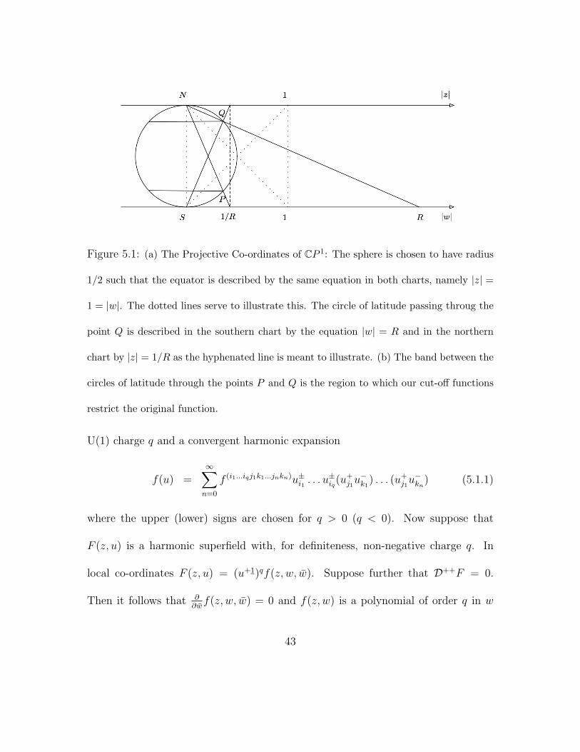
Figure 5.1: (a) The Projective Co-ordinates of CP 1: The sphere is chosen to have radius
1/2 such that the equator is described by the same equation in both charts, namely |z| =
1 = |w|. The dotted lines serve to illustrate this. The circle of latitude passing throug the
point Q is described in the southern chart by the equation |w| = R and in the northern
chart by |z| = 1/R as the hyphenated line is meant to illustrate. (b) The band between the
circles of latitude through the points P and Q is the region to which our cut-off functions
restrict the original function.
U(1) charge q and a convergent harmonic expansion
f(u) =∞∑
n=0
f (i1...iqj1k1...jnkn)u±i1 . . . u±iq(u+
j1u−k1
) . . . (u+j1u−kn
) (5.1.1)
where the upper (lower) signs are chosen for q > 0 (q < 0). Now suppose that
F (z, u) is a harmonic superfield with, for definiteness, non-negative charge q. In
local co-ordinates F (z, u) = (u+1)qf(z, w, w). Suppose further that D++F = 0.
Then it follows that ∂∂wf(z, w, w) = 0 and f(z, w) is a polynomial of order q in w
43
with superfield-valued coefficients. Indeed, it is easy to check explicitly that in local
coordinates this operator is given by
D++ = (u+1)2(1 + ww)2 ∂
∂w. (5.1.2)
That we get such a finite polynomial has to do with the fact that we assumed F
to be globally defined on the sphere.1 If we relax this assumption and allow F to
become singular at the north pole z = 0 ↔ w = ∞ then we would find the more
general solution f(z, w) for f(z, w) which is an infinite power series in w
f(z, w) =∞∑
n=−∞
fn(z)wn (5.1.3)
Functions of this form are well-defined on the punctured complex plane C∗. We will
refer to this space as the (doubly-)punctured sphere S2\{N ∪ S} since this space is
the intersection of the northern and southern patches.
The so-called projective covariant derivative ∇α is defined [17] such that ∇α :=
wD1α − D2
α and ∇α := D1α + wD2α.2 A holomorphic superfield f(z, w) with a well-
defined power series expansion (5.1.3) which satisfies ∇αf = 0 is called a projective
1The statement that a harmonic superfield F (z, u) with non-negative U(1) charge q is globally
defined is equivalent to the statement that in local co-ordinates lim|w|→∞ w−qF (z, w, w) is smooth.2These objects are usually defined in the context of 4D, N = 2 superspace. Here we consider
the extension to 5D superspace but will continue to use the 4D nomenclature.
44
superfield. It follows from the relations
D+α = −u+1∇α ; D+
α = −u+1∇α (5.1.4)
that if F (z, u) is an analytic superfield in the harmonic sense satisfying D++F = 0,
then its associated holomorphic (possibly singular) counterpart f(z, w) is projective.
Let us pause to consider some specific examples of such fields. The projective
analogue of the q+-hypermultiplet of section 4.1.1 is the so-called polar mutiplet
(Υ, Υ) with
Υ(z, w) =∞∑
n=0
Υn(z)wn and Υ(z, w) =∞∑
n=0
(−)nΥn(z)1
wn(5.1.5)
These superfields are also known as arctic and antarctic superfields respectively. If
the series terminates at some finite order k in w, the multiplet is referred to as a
complex O(k) multiplet. Note from the definition of the co-ordinate w that the smile-
conjugation (4.0.4) induces an involution on the punctured sphere acting as w =
−1/w. That this multiplet arises as the projective reduction of the q+ hypermultiplet
of section 4.1.1 can be seen as follows. The general solution to the holomorphic iso-
spinor equation D++q+ = 0 on the harmonic sphere is q+(z, u) = u+1[Φ(z)+wΓ(z)].
However, allowing for the more general solution singular at the south pole S, we find
q+ = u+1Υ(z, w) (5.1.6)
where Υ(z, w) is an arctic superfield. Note that the smile conugate of q+ is described
45
by an antarctic superfield which is the smile conjugate of Υ. Therefore, although the
superfields are well-defined on all of C, the multiplet (q+, q+) is defined only on the
doubly punctured sphere.
The next example is that of a tropical multiplet V (z, w). It is of the form
V (z, w) =∞∑
n=−∞
Vn(z)wn with V−n = (−)nVn (5.1.7)
Note that it is real with respect to smile conjugation forcing it to have antipodal
singularities on the sphere. Therefore, this multiplet is also defined only on C∗.
When the series terminates at the kth order in w and 1/w the multiplet is called a
real O(2k) multiplet. The tropical multiplet describes the five-dimensional Yang-Mills
superfield provided it is defined up to the gauge symmetry
δV =Λ− Λ
2i(5.1.8)
with (Λ, Λ) a polar multiplet. It arises from the smile-real analytic superfield V ++ of
section 4.1.3 similarly to the case considered above: The solution to the constraint
D++V ++ = 0 reads V ++ = (u+1)2v(z, w) for v again a finite polynomial in w. Since
V ++ is real with respect to smile conjugation, as is the combination (iu+1u+2), we
instead define (again, passing to a singular version of this field)
V++ = (iu+1u+2)V (z, w) (5.1.9)
It is easy to check that the resulting superfield V (z, w) is the tropical multiplet.
46
5.2 The Regularization of the Singular Theories
To complete the reduction of theories described by these multiplets it remains
to consider the reduction of the Lagrangian description of their dynamics. As we are
allowing singular fields on the harmonic sphere, we require a regularization procedure
in order to make sense of these Lagrangians. We will perform this regularization
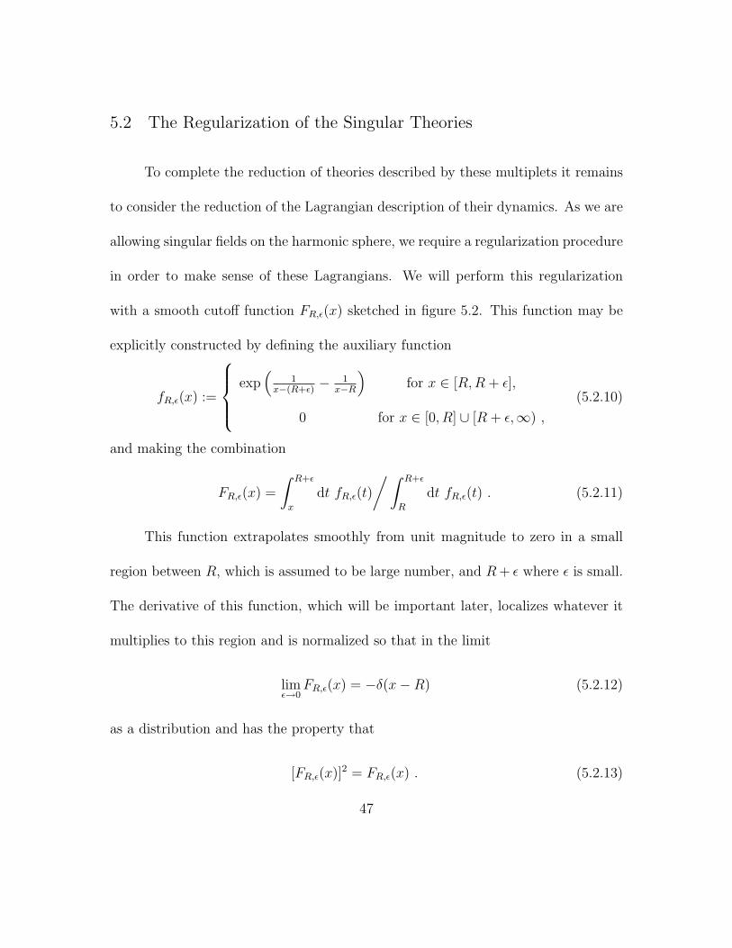
with a smooth cutoff function FR,ε(x) sketched in figure 5.2. This function may be
explicitly constructed by defining the auxiliary function
fR,ε(x) :=
exp
(1
x−(R+ε)− 1
x−R
)for x ∈ [R,R + ε],
0 for x ∈ [0, R] ∪ [R + ε,∞) ,
(5.2.10)
and making the combination
FR,ε(x) =
∫ R+ε
x
dt fR,ε(t)
/ ∫ R+ε
R
dt fR,ε(t) . (5.2.11)
This function extrapolates smoothly from unit magnitude to zero in a small
region between R, which is assumed to be large number, and R+ ε where ε is small.
The derivative of this function, which will be important later, localizes whatever it
multiplies to this region and is normalized so that in the limit
limε→0
FR,ε(x) = −δ(x−R) (5.2.12)
as a distribution and has the property that
[FR,ε(x)]2 = FR,ε(x) . (5.2.13)
47
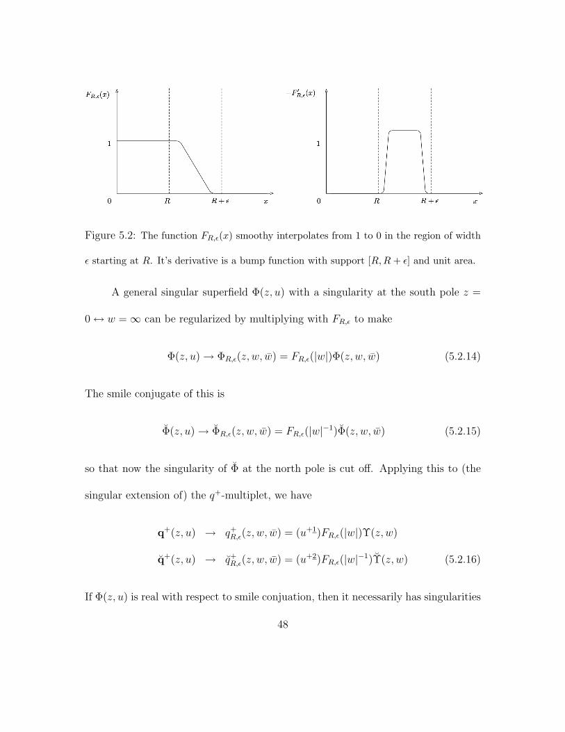
Figure 5.2: The function FR,ε(x) smoothy interpolates from 1 to 0 in the region of width
ε starting at R. It’s derivative is a bump function with support [R,R+ ε] and unit area.
A general singular superfield Φ(z, u) with a singularity at the south pole z =
0 ↔ w = ∞ can be regularized by multiplying with FR,ε to make
Φ(z, u) → ΦR,ε(z, w, w) = FR,ε(|w|)Φ(z, w, w) (5.2.14)
The smile conjugate of this is
Φ(z, u) → ΦR,ε(z, w, w) = FR,ε(|w|−1)Φ(z, w, w) (5.2.15)
so that now the singularity of Φ at the north pole is cut off. Applying this to (the
singular extension of) the q+-multiplet, we have
q+(z, u) → q+R,ε(z, w, w) = (u+1)FR,ε(|w|)Υ(z, w)
q+(z, u) → q+R,ε(z, w, w) = (u+2)FR,ε(|w|−1)Υ(z, w) (5.2.16)
If Φ(z, u) is real with respect to smile conjuation, then it necessarily has singularities
48
at both poles and its regularization is given by replacing
Φ(z, u) → ΦR,ε(z, w, w) = FR,ε(|w|−1)Φ(z, w)FR,ε(|w|) (5.2.17)
The regularized form of the singular tropical superfield, then, is
V++ → V ++R,ε = (iu+1u+2)FR,ε(|w|−1)V (z, w)FR,ε(|w|) (5.2.18)
It is important to note that the projective superfields on the RHS of equations
(5.2.16) and (5.2.18) are holomorphic in w. This is a consequence of the condition
that the harmonic superfields from which they originated were annihilated by the
D++ operator (recall equation (5.1.2) for example).
Let us pause to clarify the geometry of this construction. We have attempted
to illustrate the situation in figure 5.1. The original function g(u) is defined on the
whole sphere S2. It’s projective counterpart is singular at the north pole N and/or
the south pole S. Fix some large R � 1 and some small ε� 1. Consider the circle
of latitude passing through the point marked Q. In stereographic coordinates this
circle is defined in the southern chart by the equation |w| = R and in the northern
chart by |z| = 1/R . Multiplying a function g(u) by FR,ε(|w|) restricts it to the
region south of this circle. (In this picture we ignore the tiny difference between
circles differing by ε in latitude.) Multiplying it instead with FR,ε(|w|) restricts it to
the region north of the circle of latitude passing through P . Multiplying by both, as
49
will be the case for the Lagrangians considered below, restricts to the band between
the circles passing through P and Q. The regulator is removed by taking first ε→ 0
and finally R → ∞. From the figure we see that the latter limit extends the band
to all of S2 except the points N and S.
5.3 The Reduced Actions
Before we can reduce the actions for the singular harmonic superfields described
in chapter 4, we need to be able to reduce the analytic measure. In particular, we need
the (D−)2 operator in local coordinates. Let us consider the form of this operator
acting on analytic superfields Φ(z, u). The analyticity allows us to move all D2α and
D2α derivatives onto Φ and rewrite them in terms of Dα := D1α and Dα := D2α.
When this is done, we find in local coordinates for an analytic superfield of arbitrary
charge
(D−)2Φ = −4(u+1)2 (1 + ww)2
w3Φ (5.3.19)
where the projective operator
3 :=
[− 1
w
(−1
4D2
)+ ∂5 + w
(−1
4D2
)]. (5.3.20)
Here we have repeatedly used the algebra of covariant derivatives (A.22) and the
fact that u−1 = u+1, u−2 = u+1w and |u+1|2 = (1 + ww)−1. Recall that the operator
50
(5.3.19) is related to the analytic measure defined in (4.0.10) and (4.0.12) by
(D−)4 = − 1
32(D−)2(D−)2 . (5.3.21)
Using the analyticity of Φ again, it is easy to show that up to total derivatives
(D−)4Φ = (u+1)4 (1 + ww)4
w2D4Φ (5.3.22)
with
D4 :=
(−1
4D2
) (−1
4D2
)(5.3.23)
We are now in a position to reduce the actions from chapter 4. The general
action on the analytic subspace given in equation (4.0.12) is
S =
∫d5x
∫du(D−)4L(+4)
∣∣∣ (5.3.24)
where the harmonic integral is carried out over the entire S2. Restricting to the
doubly punctured sphere amounts to allowing the fields in L(+4) to become singular
and regulating the integral as described above. At this point the Lagrangian is
replaced with
L(+4) → L(+4)R,ε = (iu+1u+2)2FR,ε(|w|−1)L(z, w)FR,ε(|w|) (5.3.25)
for a tropical superfield L(z, w), the details of which depend on the theory under
consideration. In the final stages we will remove the regulator by taking first ε→ 0
and then R→∞.
51
In the projective coordinates the harmonic integral of a smooth function f(u)
of vanishing U(1) charge takes the form
∫duL(u) =
1
π
∫dwdw
(1 + ww)2L(w, w) =
1
π
∫dwdw
w(1 + ww)
∂L∂w
(5.3.26)
Taking this function to be L = (D−)4L(+4)| and using the explicit forms (5.3.23) and
(5.3.25) we find, up to total derivatives
L(w, w) = FR,ε(|w|−1)FR,ε(|w|)[D4L(z, w)
] ∣∣∣ (5.3.27)
and the integral becomes
∫duL(u) =
1
π
∫dwdw
w(1 + ww)
∂
∂w
[FR,ε(|w|−1)F (|w|)
]D4L(z, w)
∣∣∣ (5.3.28)
Note that it is crucial for this step that L(z, w) is holomorphic. Switching to polar
coordinates w = ρeiϕ and taking the ε→ 0 limit, we find for this expression
1
2π
∫ 2π
0
dϕ
∫ ∞
0
dρ
1 + ρ2
[1
ρδ(ρ− 1/R)F (ρ)− F (ρ−1)δ(ρ−R)
]×D4L(ρ, ϕ)
∣∣∣ (5.3.29)
We can now perform the ρ integral to obtain
1
2π
R2 − 1
R2 + 1
∫ 2π
0
dϕD4L(R,ϕ)∣∣∣ (5.3.30)
The limit R → ∞ is well defined precisely when the Lagrangian we started with
is well-defined on the harmonic sphere. Switching to the holomorphic coordinate
52
w = Reiϕ and taking this limit we find that for the action (5.3.24) with singular
fields on the harmonic sphere
S =1
2πi
∫d5x
∮dw
wD4L(z, w)
∣∣∣ (5.3.31)
in terms of the tropical superfield Lagrangian L(z, w) defined by equation (5.3.25).
This then is the general form of the reduced action. For many purposes, how-
ever, it is convenient to have such an equation not for the full analytic superspace
measure but rather for the special case considered in ref [15] and used in sections 4.1.2
and 4.1.3 for the Fayet-Sohnius hypermultiplet and the Yang-Mills gauge mutliplet
respectively. In this case the Lagrangian is reduced to
S =i
4
∫d5x
∫du(D−)2L++ (5.3.32)
with L++ satisfying
D+αL
++ = 0 and D++L++ = 0 (5.3.33)
Using the explicit form (5.3.19) and the obvious analogue of (5.1.9) for L++ we find
for such theories, in complete analogy with the analysis above,
S =1
2πi
∫d5x
∮dw
w
[− 1
w
(−1
4D2
)+ w
(−1
4D2
)]L(z, w)
∣∣∣ (5.3.34)
Let us give some explicit examples of these results from chapter 4.
53
5.4 Explicit Examples
5.4.1 Reduction of the q+-Hypermultiplet
For clarity of exposition, we work with the free q+-hypermultiplet of section
4.1.1. The action (4.1.14) was of the form∫q+D++q+. Restricting the domain of the
harmonic integral to the punctured sphere is implemented by replacing (q+, q+) with
its regularized version (5.2.16). In the resulting overlap of the northern and south-
ern patches, the D++ operator takes the form (5.1.2). Since this operator appears
explicitly, the reduction of the harmonic integral does not happen automatically as
we will be the case in all other examples. Nevertheless, the resulting integral
− 1
π
∫d5xdwdw(|u+1|2)4 (1 + |w|2)4
wFR,e
(1
|w|
)∂
∂wFR,ε(|w|)D4
[ΥΥ
](5.4.35)
is trivial to do explicitly. Integrating the anti-holomorphic derivative by parts and re-
moving the regulators, we obtain for this integral the beautiful projective superspace
result
1
2πi
∫d5x
∮dw
wD4ΥΥ
∣∣∣ . (5.4.36)
Expanding further Υ = Φ + wΓ + . . . and integrating out the infinite number of de-
coupled auxiliary fields gives precisely the action (3.1.2). Since Υ is a projective field,
it follows that the the dynamical component fields Φ and Γ satisfy the constraints
54
(3.1.1). Therefore, all conclusions of section 3.1.1 hold for the dimensional reduction
of the q+-hypermultiplet.
5.4.2 Reduction of the Fayet-Sohnius Hypermultiplet
The Fayet-Sohnuis multiplet, although superficially resembling the q+-hypermultiplet,
is equivalent to the latter only on-shell. It satisfies D++q+ as a constraint and can
therefore be written as a complex O(2) multiplet q+ = −u+1(Φ+ +wΦT−) with Φ± an
SU(2) doublet of chiral fields. The Lagrangian L++ = 12 q
+↔4 q+ can be represented
by a real O(2) multiplet L++ = iu+1u+2(− 1wW +K+wW ), for chiral W and real K.
Explicitly, W = iL22 and K = −2iL12. Since this Lagrangian is also analytic, the
action reduces to the form (5.3.34) for a homomorphic-analytic action in projective
superspace which, in turn, can be integrated to give
1
2
∫d2θW + h.c. (5.4.37)
The explicit form of W
W = −1
4D2
(Φ+Φ+ + Φ−Φ−
)− ΦT
−
↔∂5 Φ+ , (5.4.38)
follows from the constraints (3.1.8). The resulting Lagrangian is precisely (3.1.5).
55
5.4.3 Reduction of Yang-Mills Theory
As in the previous section, the Lagrangian of super-Yang-Mills theory, equation
(4.1.26), satisfies D++L++ = 0 and can be written as L++ = 14(iu
+1u+2)G(z, w) with
G(z, w) an O(2) multiplet
G(z, w) = − 1
wW +K + wW (5.4.39)
where W := iL22 is chiral in the four-dimensional sense and K := −2iL12 is real. In
terms of the field strengths defined in section 3.1.3,
W = −W αWα +1
2D2(F 2)
K = {(FDγ + 2DγF )Wγ + h.c.}+ 2∂5(F2) , (5.4.40)
as can be checked explicitly. The action for this theory is defined using the reduced
measure (5.3.32). The result (5.3.34) for this measure immediately gives
SYM =
∫d5x
{1
4
∫d2θ WαWα +
1
4
∫d2θ WαW
α +
∫d4θ F 2
}(5.4.41)
The relative factor of 14 is not a convention and is necessary for five-dimensional
Lorentz invariance (compare section 3.1.3).
5.4.4 Reduction of Chern-Simons Theory
The Chern-Simons Lagrangian (4.1.29) is of the type defined over the full ana-
lytic subspace (5.3.24). The singular charge-2 harmonic field gives rise via equation
56
(5.1.9) to a tropical field
V (z, w) = . . .− 1
wϕ(z) + V (z) + wϕ(z) + . . . (5.4.42)
This field suffers the gauge transformation
δV (z, w) =1
2i
(Λ(z, w)− Λ(z, w)
)(5.4.43)
with Λ(z, w) = Λ(z)+wΘ(z)+ . . . a polar field. This induces on the simple superfield
components the transformations
δV (z) =1
2i
(Λ(z)− Λ(z)
)δϕ(z) =
1
2iΘ(z) . (5.4.44)
In the reduced form, the theory will not depend on the field ϕ(z) but rather it will
be given in terms of its chiral projection. For this reason we introduce the simple
chiral field
Φ(z) = −1
4D2ϕ(z) . (5.4.45)
Using the result for the 5D analogue of the chiral non-minimal multiplet (3.1.1)
above, it easily follows that Φ suffers the gauge transformation
δΦ(x) =1
2i∂5Λ(z) . (5.4.46)
We conclude from this that the field strength F (z) is given by
F =1
2
(Φ + Φ + ∂5V
), (5.4.47)
57
up to a constant of proportionality. The constant of proportionality in this expression
is found by normalizing
Wα =1
8D2DαV , (5.4.48)
and satisfying the constraint (3.1.11) relating F and Wα.
Another “more honest” derivation is as follows. In the Abelian case, the gauge
transformation (4.1.19) simplifies
δV ++ = −D++λ , D+αλ = 0 , λ = λ . (5.4.49)
The field strength (4.1.23) also simplifies
W =i
8
∫du(D−)2V ++ . (5.4.50)
It is easy to see that W is gauge invariant.
The gauge freedom (5.4.49) can be used to choose the supersymmetric Lorentz
gauge [11]
D++V ++ = 0 . (5.4.51)
In other words, in this gauge V ++ becomes a real O(2) multiplet,
V ++ = iu+1u+2V (z, w) , V (z, w) =1
wϕ(z) + V (z)− wϕ(z) . (5.4.52)
SinceW is gauge invariant, for its evaluation one can use any potential V ++ from the
same gauge orbit, in particular the one obeying the gauge condition (5.4.51). This
58
Lorentz gauge is particularly useful for our consideration. Using the result (5.3.19)
for the holomorphic-analytic measure and recalling that |u+1|2 = (1+ww)−1, we can
rewrite W in the form
W =1
2
∫du3V (z, w) . (5.4.53)
This can be further transformed to
W =1
4πi
∮dw
w3V (z, w) . (5.4.54)
Indeed, the punctuation procedure of the foregoing sections 5.1-5.3 justifies the fol-
lowing identity
limR→∞
limε→0
∫duφR,ε(u) =
1
2πi
∮dw
wφ(w) , (5.4.55)
with the regularization φR,ε(u) = φR,ε(w, w) of a holomorphic function φ(w) on C∗
defined according to (5.2.17). Since the integrand on the right of (5.4.53) is, by
construction, a smooth scalar field on S2, we have
∫du3V (z, w) = lim
R→∞limε→0
∫du3VR,ε(z, u) . (5.4.56)
Now, we are in a position to evaluate the N = 1 field strengths (3.1.10) in
terms of the prepotentials Vn. It follows from (5.3.19) that
F = W| = 1
4πi
∮dw
w3V (w)
∣∣∣ =1
2
(Φ + Φ + ∂5V
), (5.4.57)
59
where we have defined
Φ =1
4D2V1| , V = V0| . (5.4.58)
The spinor field strength Wα is given by
Wα(z) = D2αW| =
1
4πi
∮dw
w
([D2
α,3] + 3D2α
)V (w)
∣∣∣ . (5.4.59)
However, as [D2α,3] = w∂5D
1α and given that for any projective superfield φ(w) we
have D2αφ(w) = wD1
αφ(w), this expression reduces to
Wα =1
4πi
∮dw
w
(1
4D2Dα
)V (w)
∣∣∣ =1
8D2DαV . (5.4.60)
It can be seen that the gauge transformation (5.4.49) acts on the superfields in
(5.4.58) as follows:
δV =1
2i(Λ− Λ) , δΦ =
1
2i∂5Λ . (5.4.61)
The approach presented in this section can be applied to reduce the supersym-
metric Chern-Simons theory (4.1.29) to projective superspace. With G++ defined in
(4.1.25) and the real O(2) multiplet G(z, w) defined in (5.4.39) the Chern-Simons
action becomes
12g2SCS = − 1
2πi
∫d5xd4θ
∮dw
wV (w)G(w)
∣∣∣ . (5.4.62)
It is then trivial to derive that the Lagrangian becomes∫d2θΦW αWα +
∫d4θV [FDαWα + 2(DαF )Wα] + c.c.+ 4
∫d4θF 3 . (5.4.63)
60
This result is to be compared with that obtained in section 3.1.4.
For completeness, we also present here projective superspace extensions of the
vector multiplet mass term and the Fayet-Iliopoulos term (their harmonic superspace
form is given in [11]). The vector multiplet mass term is
−m2
∫dζ(−4)(V ++)2 −→ m2
2πi
∫d5xd4θ
∮dw
wV 2(w)
∣∣∣ . (5.4.64)
The gauge invariant Fayet-Iliopoulos term is
∫dζ(−4)c++V ++ −→ − 1
2πi
∫d5xd4θ
∮dw
wc(w)V (w)
∣∣∣ , (5.4.65)
where c++ = ciju+i u
+j , with a constant real iso-vector cij. Defining c++ = iu+1u+2c(w),
with c(w) = w−1ξC + ξR − wξC, the FI action then reduces to
ξR
∫d5xd4θV + 2Re
(ξC
∫d5xd2θΦ
). (5.4.66)
So far the considerations in this section have been restricted to the Abelian
case. It is necessary to mention that the projective superspace approach [17] can be
generalized to provide an elegant description of 5D super Yang-Mills theories, which
is very similar to the well-known description of 4D, N = 1 supersymmetric theories.
In particular, the Yang-Mills supermultiplet is described by a real Lie-algebra-valued
tropical superfield V (z, w) with the gauge transformation
eV (w) → eiΛ(w)eV (w)e−iΛ(w) , (5.4.67)
61
which is the non-linear generalization of the Abelian gauge transformation (5.4.49).
The hypermultiplet sector is described by an arctic superfield Υ(z, w) and its conju-
gate, with the gauge transformation
Υ(w) → eiΛ(w)Υ(w) . (5.4.68)
The hypermultiplet gauge–invariant action is
S[Υ, Υ, V ] =1
2πi
∮dw
w
∫d5xd4θΥ(w)eV (w)Υ(w) . (5.4.69)
62
Chapter 6
Closing Remarks
In this work, we have argued in favor of the use of harmonic superspace when
dealing with (quantum) field theories in five and six dimensions. This formalism can
be reduced to a five-dimensional version of projective superspace and therefore to
simple superfields. The dimensional truncation to N = 2 four-dimensional theories
is then trivial to implement. The elucidation of this procedure was the goal of this
work. The main motivation to study this formalism was an effort to extend the
usefulness of the superspace formalism to include cases in which we would like to
lower the number of dimensions from five (or six) to four or, alternatively, to embed
a four-dimensional theory into a higher dimensional one.
In fact, harmonic superspaces of a more general type than the one considered
here exist and have been employed in the literature. Some of these can be embedded
in others as we have seen to be possible in the case of simple, projective and (the
original) harmonic superspace. One example of such a harmonic superspace is that
of 4D, N = 3 superspace extended by the coset SU(3)/[U(1)×U(1)]. As explained in
references [18] and [19], this harmonic superspace (among others) can be embedded
63
in a bigger harmonic superspace in which the harmonic coordinates are formed by
a so-called “pure spinor”, usually denoted by λα, which is a twistor-like complex
commuting Weyl spinor of SO(9, 1) subject to the constraint
λγmλ = 0 . (6.1)
This pure spinor is the main ingredient in the only method known to date of quantiz-
ing the superstring with manifest supersymmetry [18].1 Indeed, the authors of [19]
claim to derive harmonic superspaces for four-dimensional superspaces with N = 2,
3, and 4 from the pure spinor superstring. This philosophy is very close to the one ad-
vocated here. However, there is still much work to be done in this area. A major open
problem in the pure spinor superstring theory is our lack of understanding of the su-
perspace measure. This measure is normalized to 〈(λγmθ)(λγnθ)(λγpθ)(θγmnpθ)〉 = 1
which can be interpreted as a partial cancellation of the harmonic and fermionic mea-
sures, the idea being that the 11 degrees of freedom carried by the pure spinor have
cancelled 11 fermionic zero-modes leaving only five of the original 16. However,
this measure is not manifestly supersymmetric since it involves integration over a
proper subspace of the full superspace which is not obviously analytic in any gen-
1It is sometimes said that this quantization is not manifestly supersymmetric because it is
necessary to solve the pure spinor constraint in terms of spinors of the U(5) subgroup of SO(9, 1) in
order to compute the operator product of Lorentz currents. While this is true, it is also true that
the result of this calculation is manifestly SO(9, 1) covariant.
64
eralized sense. As a consequence of this we cannot, for example, use it to provide
a manifestly supersymmetric action for ten-dimensional supersymmetric Yang-Mills
theory.2 On the other hand, it is clear that there must be some proper subspace of
the full superspace analogous to the chiral and analytic subspaces of 4D, N = 1, 2,
and 3 because otherwise the action would be forced to be of higher derivative type.3
Finding this subspace gives a clue about (and may even be equivalent to) finding
the BRST operator for the ten-dimensional superstring. A study of the embedding
of various superspaces into one another along the lines made explicit herein has the
potential to shed light on these subspaces. Consider, for example, the case of five
dimensions constructed above. Naively, the fermionic measure has eight real zero
modes in it. However, due to the harmonics, we can find an analytic subspace of
half this size. This subspace is the full superspace of four-dimensional theories with
the minimal amount of supersymmetry as the equation for (D−)4 in analytic basis
(5.3.22) shows explicitly. Another example of this is much more trivial: The chiral
subspace of 4D, N = 1 superspace is again the full 2D, N = (1, 1) superspace.
2Notice that the question of the proper measure for a pure spinor superstring is equivalent to
finding a formalism in which we can write a manifestly supersymmetric lagrangian description for
10D sYM.3The analogue of this statement in Ectoplasmic Integration Theory [20, 21] is that the density
projector for these theories must have “enough” terms in it which are independent of the spinor
covariant derivatives.
65
The present situation with the higher harmonic superspaces is that they are not
sufficient to describe off-shell theories with 16 or 32 real supercharges. Perhaps,
turning the above reasoning around, we might try to build the higher superspaces by
starting with the lower superspaces which would be the generalization of the analytic
subspace.
Besides the pure spinor superstring, there exists another formulation for su-
perstrings which keeps manifest part of the super-Poincare symmetry equivalent to
having manifest supersymmetry in compactifications to four or six dimensions [22].
This approach starts with superstrings in the RNS formalism and makes a (compli-
cated) redefinition of the world sheet fields which splits the original RNS variables
into a set of GS-like variables and a new set of RNS-like variables. The restriction
to six or four dimensions comes from requiring that this split lines up with the split
R9,1 → R3,1 × R6. This description of the critical superstring is appropriately called
the “hybrid” formalism. The four-dimensional version seems to be very closely re-
lated to the pure spinor superstring. The more precise statement [22] is that it is
related to a twistor-like GS description discovered by Sorokin, Tkach, Volkov, and
Zheltukhin [23] in which the pure spinor constraint is replaced with the twistor con-
straint
λγmλ = Πm , (6.2)
66
where Πm is the GS world-sheet momentum, by a partial gauge fixing and additional
field redefinitions. Furthermore, the pure spinor BRST operator Q =∮λαdα decom-
poses as Q =∮
(λαdα − λαdα + . . .) in four-dimensional notation while the relation
to the twistor-like string involves the gauge fixing λα = eiρdα and λα = e−iρdα. In
these formulæ, ρ is a chiral boson of the hybrid formalism and dα is the world-sheet
operator conjugate to θα which becomes the spinor covariant derivative in the target
theory. Therefore, in this gauge Q ∼ wD2− 1wD
2+. . . where we have written w = eiρ.
Comparing with the formula (5.3.20) we see that this is very close to the form of the
projective reduction of the (D−)2 operator we have been calling 3, the discrepancy
apparently being a rescaling of the d and d operators which undoes part of the gauge
fixing:4
Q↔ 3 (6.3)
In hindsight, it is should not come as a surprise that this operator is related
to the BRST operator. The reason for this is that the particular operator Q with
which we started is formally related to the pure spinor BRST operator of the ten-
dimensional superparticle. Standard methods then tell us how to normalize the inner
4In fact, in the so-called N = 4 topological method [24] this analogy is even more precise because
there is another chiral boson in the theory which enters the generators G+ = ei(−2ρ+HC)d2 + . . .
and G− = ei(2ρ−HC)d2 + . . .
67
product of the Hilbert space (in this case the square integrable harmonic superfields),
but this is none other than the harmonic superspace measure. Actually, this state-
ment is too glib because for it to hold we need to be able to perform the map from
the formalism we are using to the RNS formalism where we know how to do this nor-
malization. Therefore, we should, in principle, be able to to this for the twistor-like
superstring or the hybrid (which is where we got the 3 ↔ Q statement in the first
place). The pure spinor is a different story because we do not know this map. This,
again, is related to the discussion above about the measure for the pure spinor string
and lends credence to the claim that string (field) theory is intimately connected to
embeddings of harmonic superspaces into one another.
On the other hand, the statement (6.3) cannot be entirely trivial. For starters,
the statistics seem to differ between the LHS and RHS. This mismatch comes from
the identification w ↔ eiρ and the fact that ρ is a chiral boson. Furthermore,
such an identification would imply other relations between the hybrid formalism
and projective superspace. For example, it seems superficially that the hermitian
structure of the hybrid is closely related to the smile conjugation. In particular,
the hermitian conjugation does not preserve the conformal weight of the world-sheet
fields. On the projective superspace side there is the fact that an arctic field gets
mapped to an antarctic field under smile conjugation.
68
Thus, although our considerations tempt us to speculate that superspace har-
monics correspond to world-sheet ghosts of some superstring, there is clearly more
work to be done to make this precise. A first obstacle to implementing this program
is the somewhat confusing relation between the hybrid and pure spinor superstrings.
In particular, it is currently not known how to embed the hybrid into the pure spinor.
The complication is easy to see when we consider that the hybrid is equivalent to the
twistor-like string with constraint (6.2). In order to make the correspondence pre-
cise, one of the things we would have to explain is how this is consistent with (6.1).
Actually, the authors of [23] claim that the pure spinor superstring is just a further
gauge fixing of the twistor superstring but for the moment it seems that the chiral
boson necessary for the correct statistics of the RNS world-sheet spinor Ψm ∼ eiρλm
is missing [25] in the pure spinor. The resolution to this puzzle is currently being
investigated.
Coming back, then, to the question of harmonic superspaces, we immediately
run into the problem that the naive harmonic superspaces do not describe off-shell
theories in dimensions higher than six. In the textbook [12] this is explained heuris-
tically by considering the N = 3 theory and showing that three facts about its
harmonic superspace with harmonics in SU(3)/[U(1)×U(1)] conspire to give a “mir-
acle” which does not occur for the maximally supersymmetric sYM theory which
69
harmonic factor SU(4)/S[U(2) × U(2)]. Perhaps a generalized notion of harmonic
spaces is needed in which the maximally supersymmetric four-dimensional super-
space is build on its analytic subspace which in turn is taken to be the full N = 2
harmonic superspace.
70
Appendix A
5D notation and conventions
The 5D gamma-matrices Γm = (Γm,Γ5), with m = 0, 1, 2, 3, defined by
{Γm,Γn} = −2ηmn1 , (Γm)† = Γ0ΓmΓ0 (A.1)
are chosen in accordance with [2, 3]
(Γm)αβ =
0 (σm)αβ
(σm)αβ 0
, (Γ5)αβ =
−iδαβ 0
0 iδαβ
, (A.2)
such that Γ0Γ1Γ2Γ3Γ5 = 1. The charge conjugation matrix, C = (εαβ), and its
inverse, C−1 = C† = (εαβ) are defined by
CΓmC−1 = (Γm)T , εαβ =
εαβ 0
0 −εαβ
, εαβ =
εαβ 0
0 −εαβ
. (A.3)
The antisymmetric matrices εαβ and εαβ are used to raise and lower the four-
component spinor indices.
A Dirac spinor, Ψ = (Ψα), and its Dirac conjugate, Ψ = (Ψα) = Ψ†Γ0, look
like
Ψα =
ψα
φα
, Ψα = (φα, ψα) . (A.4)
71
One can now combine Ψα = (φα, ψα) and Ψα = εαβΨβ = (ψα,−φα) into a SU(2)
doublet,
Ψαi = (Ψα
i ,−Ψαi) , (Ψαi )∗ = Ψαi , i = 1, 2 , (A.5)
with Ψα1 = φα and Ψα
2 = ψα. It is understood that the SU(2) indices are raised and
lowered by εij and εij, ε12 = ε21 = 1, in the standard fashion: Ψαi = εijΨα
j . The
Dirac spinor Ψi = (Ψiα) satisfies the pseudo-Majorana condition Ψi
T = CΨi. This
will be concisely represented as
(Ψiα)∗ = Ψα
i . (A.6)
With the definition Σmn = −Σnm = −14[Γm,Γn], the matrices {1,Γm,Σmn}
form a basis in the space of 4 × 4 matrices. The matrices εαβ and (Γm)αβ are
antisymmetric, εαβ(Γm)αβ = 0, while the matrices (Σmn)αβ are symmetric. Given
a 5-vector V m and an antisymmetric tensor F mn = −F nm, we can equivalently
represent them as the bi-spinors V = V mΓm and F = 12F
mnΣmn with the following
symmetry properties
Vαβ = −Vβα , εαβVαβ = 0 , Fαβ = Fβα . (A.7)
The two equivalent descriptions Vm ↔ Vαβ and and Fmn ↔ Fαβ are explicitly de-
scribed as follows:
Vαβ = V m(Γm)αβ , Vm = −1
4(Γm)αβVαβ , (A.8)
72
Fαβ =1
2F mn(Σmn)αβ , Fmn = (Σmn)αβFαβ . (A.9)
These results can be easily checked using the identities (see e.g. [?]):
εαβγδ = εαβεγδ + εαγεδβ + εαδεβγ , (A.10)
εαγεβδ − εαδεβγ = −1
2(Γm)αβ(Γm)γδ +
1
2εαβεγδ , (A.11)
and therefore
εαβγδ =1
2(Γm)αβ(Γm)γδ +
1
2εαβεγδ , (A.12)
with εαβγδ the completely antisymmetric fourth-rank tensor.
Complex conjugation gives
(εαβ)∗ = −εαβ , (Vαβ)∗ = V αβ , (Fαβ)∗ = F αβ , (A.13)
provided V m and F mn are real.
The conventional 5D, N = 1 superspace R5|8 is parametrized by coordinates
zA = (xa, θαi ). Then, a hypersurface x5 = const in R5|8 can be identified with the
4D, N = 2 superspace R4|8 parametrized by
zA = (xa, θαi , θ
iα) , (θα
i )∗ = θαi . (A.14)
The Grassmann coordinates of R5|8 and R4|8 are related to each other as follows:
θαi = (θα
i ,−θαi) , θiα =
θiα
θαi
. (A.15)
73
Interpreting x5 as a central charge variable, one can view R5|8 as a 4D, N = 2 central
charge superspace, see below.
The flat covariant derivatives DA = (∂a, Diα) obey the algebra
{Diα, D
j
β} = −2iεij
((Γc)αβ∂c + εαβ∆
), [Di
α, ∂b] = [Diα,∆] = 0 , (A.16)
or equivalently
[DA, DB} = TABCDC + CAB∆ , (A.17)
with ∆ the central charge. The spinor covariant derivatives are
Diα =
∂
∂θαi
− i(Γb)αβθβi∂b − iθi
α∆ . (A.18)
One can relate the operators
Di ≡ (Diα) =
Diα
Dαi
, Di ≡ (Dαi ) = (Dα
i ,−Dαi) (A.19)
to the 4D N = 2 covariant derivatives DA = (∂a, Diα, D
αi ) where
Diα =
∂
∂θαi
+ i(σb)αβ θβi∂b − iθi
α(∆ + i∂5) , (A.20)
Dαi = − ∂
∂θαi− iθβ
i (σb)βα∂b − iθαi(∆− i∂5) . (A.21)
These operators obey the anti-commutation relations
{Diα, D
jβ} = −2iεijεαβ(∆ + i∂5) ,
74
{Dαi, Dβj} = 2iεijεαβ(∆− i∂5) ,
{Diα, Djβ} = −2iδi
j(σc)αβ∂c , (A.22)
which correspond to the 4D, N = 2 supersymmetry with a complex central charge,
see also [26].
In terms of the operators (A.19), the operation of complex conjugation acts as
follows
(DiF )†Γ0 = −(−1)ε(F )DiF∗ , (A.23)
with F an arbitrary superfield and ε(F ) its Grassmann parity. This can be concisely
represented as
(DiαF )∗ = −(−1)ε(F )Dα
i F∗ . (A.24)
75
BIBLIOGRAPHY
[1] S. J. Gates, M. T. Grisaru, M. Rocek and W. Siegel, “Superspace, Or One
Thousand And One Lessons In Supersymmetry,” Front. Phys. 58, 1 (1983)
[arXiv:hep-th/0108200].
[2] I. L. Buchbinder and S. M. Kuzenko, “Ideas and methods of supersymmetry
and supergravity: Or a walk through superspace,” SPIRES entry.
[3] J. Wess and J. Bagger, “Supersymmetry and supergravity,” SPIRES entry.
[4] S. M. Kuzenko, “Projective superspace as a double-punctured harmonic super-
space,” Int. J. Mod. Phys. A 14, 1737 (1999) [arXiv:hep-th/9806147].
[5] N. Marcus, A. Sagnotti and W. Siegel, “Ten-Dimensional Supersymmetric Yang-
Mills Theory In Terms Of Four-Dimensional Superfields,” Nucl. Phys. B 224,
159 (1983) [KEK scan].
[6] N. Arkani-Hamed, T. Gregoire and J. Wacker, “Higher dimensional supersym-
metry in 4D superspace,” JHEP 0203, 055 (2002) [arXiv:hep-th/0101233].
[7] Wm. D. Linch III, M. A. Luty and J. Phillips, “Five dimensional supergravity
in N = 1 superspace,” Phys. Rev. D 68, 025008 (2003) [arXiv:hep-th/0209060].
76
[8] I. L. Buchbinder, S. J. Gates, H. S. J. Goh, Wm. D. Linch III, M. A. Luty,
S. P. Ng and J. Phillips, “Supergravity loop contributions to brane world super-
symmetry breaking,” Phys. Rev. D 70, 025008 (2004) [arXiv:hep-th/0305169].
[9] S. J. Gates, Wm. D. . Linch and J. Phillips, “Field strengths of linearized 5D, N
= 1 superfield supergravity on a 3-brane,” JHEP 0502, 036 (2005) [arXiv:hep-
th/0311153].
[10] S. M. Kuzenko and Wm. D. Linch III, “On five-dimensional superspaces,”
arXiv:hep-th/0507176. [arXiv:hep-th/0507176]
[11] A. Galperin, E. Ivanov, S. Kalitsyn, V. Ogievetsky and E. Sokatchev, “Un-
constrained N = 2 matter, Yang-Mills and supergravity theories in harmonic
superspace,” Class. Quant. Grav. 1, 469 (1984).
[12] A. S. Galperin, E. A. Ivanov, V. I. Ogievetsky and E. S. Sokatchev, Harmonic
Superspace, Cambridge University Press, Cambridge, 2001. SPIRES entry.
[13] B. B. Deo and S. J. Gates, “Comments On Nonminimal N=1 Scalar Multiplets,”
Nucl. Phys. B 254, 187 (1985).
[14] B. Zupnik, “Harmonic superpotentials and symmetries in gauge theories with
eight supercharges,” Nucl. Phys. B 554, 365 (1999) [Erratum-ibid. B 644, 405
(2002)] [arXiv:hep-th/9902038]. [arXiv:hep-th/9902038].
77
[15] N. Dragon, S. M. Kuzenko and U. Theis, “The vector-tensor multiplet in har-
monic superspace,” Eur. Phys. J. C 4, 717 (1998) [hep-th/9706169].
[16] B. M. Zupnik, “The action of the supersymmetric N=2 gauge theory in harmonic
superspace,” Phys. Lett. B 183, 175 (1987).
[17] U. Lindstrom and M. Rocek, “N=2 Superyang-Mills Theory In Projective Su-
perspace,” Commun. Math. Phys. 128, 191 (1990).
I. T. Ivanov and M. Rocek, “Supersymmetric sigma models, twistors, and the
Atiyah-Hitchin metric,” Commun. Math. Phys. 182, 291 (1996) [arXiv:hep-
th/9512075]. [arXiv:hep-th/9512075]
[18] N. Berkovits, “ICTP lectures on covariant quantization of the superstring,”
[arXiv:hep-th/0209059].
[19] P. A. Grassi and P. van Nieuwenhuizen, “Harmonic superspaces from super-
strings,” Phys. Lett. B 593, 271 (2004) [arXiv:hep-th/0402189].
[20] S. J. J. Gates, “Ectoplasm has no topology: The prelude,” [arXiv:hep-
th/9709104].
S. J. J. Gates, “Ectoplasm has no topology,” Nucl. Phys. B 541, 615 (1999)
[arXiv:hep-th/9809056].
78
[21] W. Siegel, “Fields,” [arXiv:hep-th/9912205].
[22] N. Berkovits, “A new description of the superstring,” [arXiv:hep-th/9604123].
[23] D. P. Sorokin, V. I. Tkach, D. V. Volkov and A. A. Zheltukhin, “From The
Superparticle Siegel Symmetry To The Spinning Particle Proper Time Super-
symmetry,” Phys. Lett. B 216, 302 (1989).
[24] N. Berkovits and C. Vafa, “N=4 topological strings,” Nucl. Phys. B 433, 123
(1995) [arXiv:hep-th/9407190].
[25] Brenno Carlini Vallilo and Osvaldo Chandia, Private communication.
[26] N. Dragon, E. Ivanov, S. Kuzenko, E. Sokatchev and U. Theis, “N = 2 rigid
supersymmetry with gauged central charge,” Nucl. Phys. B 538, 411 (1999)
[hep-th/9805152].
79