Embed Size (px)
Citation preview

ABSTRACT
Title of Dissertation: Shape Dynamical Models for Activity Recognition andCoded Aperture Imaging for Light-Field Capture
Ashok Veeraraghavan, Doctor of Philosophy, 2008
Dissertation directed by: Professor Rama ChellappaDepartment of Electrical and Computer Engineering
Classical applications of Pattern recognition in image processing and computer
vision have typically dealt with modeling, learning and recognizing static patterns
in images and videos. There are, of course, in nature, a whole class of patterns that
dynamically evolve over time. Human activities, behaviors of insects and animals,
facial expression changes, lip reading, genetic expression profiles are some examples
of patterns that are dynamic. Models and algorithms to study these patterns must
take into account the dynamics of these patterns while exploiting the classical
pattern recognition techniques. The first part of this dissertation is an attempt to
model and recognize such dynamically evolving patterns. We will look at specific
instances of such dynamic patterns like human activities, and behaviors of insects
and develop algorithms to learn models of such patterns and classify such patterns.
The models and algorithms proposed are validated by extensive experiments on

gait-based person identification, activity recognition and simultaneous tracking
and behavior analysis of insects.
The problem of comparing dynamically deforming shape sequences arises re-
peatedly in problems like activity recognition and lip reading. We describe and
evaluate parametric and non-parametric models for shape sequences. In particu-
lar, we emphasize the need to model activity execution rate variations and propose
a non-parametric model that is insensitive to such variations. These models and
the resulting algorithms are shown to be extremely effective for a wide range of
applications from gait-based person identification to human action recognition.
We further show that the shape dynamical models are not only effective for the
problem of recognition, but also can be used as effective priors for the problem
of simultaneous tracking and behavior analysis. We validate the proposed algo-
rithm for performing simultaneous behavior analysis and tracking on videos of bees
dancing in a hive.
In the last part of this dissertaion, we investigate computational imaging, an
emerging field where the process of image formation involves the use of a computer.
The current trend in computational imaging is to capture as much information
about the scene as possible during capture time so that appropriate images with
varying focus, aperture, blur and colorimetric settings may be rendered as required.
In this regard, capturing the 4D light-field as opposed to a 2D image allows us
to freely vary viewpoint and focus at the time of rendering an image. In this
dissertation, we describe a theoretical framework for reversibly modulating 4D
light fields using an attenuating mask in the optical path of a lens based camera.
Based on this framework, we present a novel design to reconstruct the 4D light field
from a 2D camera image without any additional refractive elements as required

by previous light field cameras. The patterned mask attenuates light rays inside
the camera instead of bending them, and the attenuation recoverably encodes the
rays on the 2D sensor. Our mask-equipped camera focuses just as a traditional
camera to capture conventional 2D photos at full sensor resolution, but the raw
pixel values also hold a modulated 4D light field. The light field can be recovered
by rearranging the tiles of the 2D Fourier transform of sensor values into 4D planes,
and computing the inverse Fourier transform. In addition, one can also recover
the full resolution image information for the in-focus parts of the scene.

Shape Dynamical Models for Activity Analysis and
Coded Aperture Imaging for Light-Field Capture
by
Ashok Veeraraghavan
Dissertation submitted to the Faculty of the Graduate School of theUniversity of Maryland, College Park in partial fulfillment
of the requirements for the degree ofDoctor of Philosophy
2008
Advisory Committee:
Professor Rama Chellappa, Chair / AdvisorProfessor P.S.KrishnaprasadProfessor Min WuProfessor Anuj SrivastavaProfessor Ramesh RaskarProfessor Amitabh Varshney

c©Copyright by
Ashok Veeraraghavan
2008

DEDICATION
To my Grandfather
ii

ACKNOWLEDGEMENTS
I would like to express my deepest gratitude to my advisor, Prof. Rama Chel-
lappa for his guidance and wise counsel without which this journey would not
have been as enriching. His outlook towards research and his dedication to work
have been a constant source of inspiration and his uncanny ability to see only the
positives in every outcome have taught me an important lesson. Needless to say,
I am grateful for his hospitality and generosity that made me feel welcome at the
University of Maryland, a place that never seemed far away from home.
I am also extremely grateful to Prof. Ramesh Raskar, Prof. Mandyam Srini-
vasan and Prof. Anuj Srivastava who at varying points during my graduate studies
hosted me in their labs and shared with me their views on research. I have been
profoundly impacted by their motivation, dedication and most of all by their shared
sense of constant inquisitiveness at all those small surprises that research throws
at you.
I am also grateful to my committee members, Prof. Krishnaprasad, Prof. Min
Wu and Prof. Amitabh Varshney for the time they spent discussing, reading and
commenting on my thesis. I am especially indebted to Prof. Krishnaprasad for
spending an enormous amount of time discussing various aspects of the thesis
and for always being available to discuss and comment upon various aspects of
my research. Special thanks to all those many great teachers I have had the
opportunity to learn from beginning all the way from Alpha school, into IIT Madras
iii

and then at the University of Maryland. I look up to every one of you and one
day hope I can be as good a teacher as you were.
I have immensely benefited from being a part of Center for Automation Re-
search and the many conversations I have shared with my friends and colleagues
here during this journey. I thank Prof. Amit Roy Chowdhury for helping me ease
into graduate school with his support, encouragement and methodic approach to
research. I thank my friends and fellow graduate students Jagan, Aswin, Pa-
van, Mahesh, Narayanan, Gaurav, Naresh, Amit, Aravind, James, Shiv, Lavanya,
Panth, Som, Buvana, Kavitha, Renga, Shyam, Adarsh, Anand, Ashwin and many
more who were all an integral part of making this journey a thouroughly stim-
ulating and enjoyable experience. I also thank my friends back home in India,
Arvind, Deepak, Siva, Viji, Aditya, Bala, Venki, Akilla, Srividya, Arun, Arun,
Geetha, Suku and others for their friendship. I thank all my friends from IIT
Madras, Ganilk, Pusp, Dog, Murr, Jun, Shiva, Kaps, Barr, Rama and Vinod for
their encouragement. I thank my entire cricket team ( Monument Cricket Club
a.k.a Warriors Cricket Club ) for teaching me to always see the lighter side of life.
For all those really close friends of mine, that I forgot to acknowledge here, ”You
all know me and my memory”.
This thesis would not have been possible without the constant and unending
support of my entire family. My love and gratitude to my parents Veeraraghavan
and Usha, my uncle and aunt (Sridhar and Aasha), my brother Arun, my sisters
Aishwarya and Abhinaya, my grandparents and more than a dozen other aunts,
uncles and cousins. Words cannot express my gratitude for all that they had to
sacrifice and endure so that I may have this opportunity. I would like to take this
opportunity to say ”Thank You”. I would like to thank Abbhi for always being a
iv

constant source of support, motivation and most of all an untiring and patient ear
to all my incessant and and continuous ’talking’ !.
This dissertation owes its genesis to my Grandfather, to whom I dedicate this
thesis.
v

TABLE OF CONTENTS
List of Tables x
List of Figures xi
1 Introduction 11.1 Research Motivation . . . . . . . . . . . . . . . . . . . . . . . . . . 11.2 Dissertation Contributions . . . . . . . . . . . . . . . . . . . . . . . 31.3 Comparing Shape Sequences . . . . . . . . . . . . . . . . . . . . . . 4
1.3.1 Previous Work in Shape Analysis . . . . . . . . . . . . . . . 61.3.2 Prior Work in Gait recognition . . . . . . . . . . . . . . . . 8
1.4 Modeling Execution Rate Variations for Action Recognition . . . . 111.4.1 Prior Work in Activity Recognition: . . . . . . . . . . . . . . 12
1.5 Simultaneous Tracking and Behavior Analysis . . . . . . . . . . . . 141.5.1 Prior Work in Tracking: . . . . . . . . . . . . . . . . . . . . 151.5.2 Prior Work in Analyzing Bee Dances . . . . . . . . . . . . . 16
1.6 Coded Aperture Imaging for Light-Field Capture . . . . . . . . . . 171.6.1 Related Work . . . . . . . . . . . . . . . . . . . . . . . . . . 19
1.7 Organization of the Thesis . . . . . . . . . . . . . . . . . . . . . . . 21
2 Comparing Shape Sequences 232.1 Kendall’s Shape Theory - Preliminaries . . . . . . . . . . . . . . . . 24
2.1.1 Definition of Shape . . . . . . . . . . . . . . . . . . . . . . . 242.1.2 Distance between shapes . . . . . . . . . . . . . . . . . . . . 262.1.3 The tangent space of the shape space . . . . . . . . . . . . . 27
2.2 Comparison Of Shape Sequences . . . . . . . . . . . . . . . . . . . . 282.2.1 Non-Parametric method for comparing shape sequences . . . 292.2.2 Dynamic time warping . . . . . . . . . . . . . . . . . . . . . 292.2.3 Parametric models for shape sequences . . . . . . . . . . . . 312.2.4 AR Model on tangent space . . . . . . . . . . . . . . . . . . 322.2.5 ARMA Model . . . . . . . . . . . . . . . . . . . . . . . . . . 332.2.6 Learning the ARMA model . . . . . . . . . . . . . . . . . . 332.2.7 Distance between ARMA Models . . . . . . . . . . . . . . . 34
2.3 Note on the limitations of Proposed Techniques . . . . . . . . . . . 34
vi

2.4 Experiments and Conclusions . . . . . . . . . . . . . . . . . . . . . 362.4.1 Feature Extraction . . . . . . . . . . . . . . . . . . . . . . . 372.4.2 Results on the USF Database . . . . . . . . . . . . . . . . . 392.4.3 Results using Joint angles . . . . . . . . . . . . . . . . . . . 412.4.4 Results on the CMU Dataset . . . . . . . . . . . . . . . . . 42
2.5 Conclusions and Future Work . . . . . . . . . . . . . . . . . . . . . 44
3 Modeling Execution Rate Variations for Action Recognition 463.0.1 Contributions of this chapter . . . . . . . . . . . . . . . . . . 493.0.2 Outline of the chapter . . . . . . . . . . . . . . . . . . . . . 49
3.1 Problem Statement . . . . . . . . . . . . . . . . . . . . . . . . . . . 503.1.1 Feature for representation . . . . . . . . . . . . . . . . . . . 503.1.2 Model for warping functions . . . . . . . . . . . . . . . . . . 513.1.3 Problems . . . . . . . . . . . . . . . . . . . . . . . . . . . . 53
3.2 Differential geometric tools on the space of time-warping functions . 543.2.1 Geometry of Ψ . . . . . . . . . . . . . . . . . . . . . . . . . 563.2.2 Statistical Analysis on Ψ . . . . . . . . . . . . . . . . . . . . 573.2.3 Global Speed of activity . . . . . . . . . . . . . . . . . . . . 60
3.3 Learning and Classification Algorithms . . . . . . . . . . . . . . . . 623.3.1 Estimating Pψ given a(t) . . . . . . . . . . . . . . . . . . . . 633.3.2 Estimating a(t) assuming known warping functions . . . . . 633.3.3 Iteratively estimating a(t) and Pψ . . . . . . . . . . . . . . . 643.3.4 Uniqueness of the Model parameters . . . . . . . . . . . . . 643.3.5 Generating activity samples from the model . . . . . . . . . 653.3.6 Classification Algorithm . . . . . . . . . . . . . . . . . . . . 66
3.4 Function Space of Time-Warps . . . . . . . . . . . . . . . . . . . . 673.4.1 Activity specific time-warping space (W ) . . . . . . . . . . . 683.4.2 Symmetric representation of an Activity Model . . . . . . . 693.4.3 Learning Model Parameters . . . . . . . . . . . . . . . . . . 703.4.4 Classification using the model . . . . . . . . . . . . . . . . . 71
3.5 Experiments . . . . . . . . . . . . . . . . . . . . . . . . . . . . . . . 723.5.1 Common Activities Dataset . . . . . . . . . . . . . . . . . . 733.5.2 INRIA iXmas dataset . . . . . . . . . . . . . . . . . . . . . . 733.5.3 USF Gait Database . . . . . . . . . . . . . . . . . . . . . . . 76
3.6 Other applications . . . . . . . . . . . . . . . . . . . . . . . . . . . 783.6.1 Clustering Activity Sequences . . . . . . . . . . . . . . . . . 783.6.2 Organizing a Large Database of Activities . . . . . . . . . . 80
3.7 Summary and conclusions . . . . . . . . . . . . . . . . . . . . . . . 82
4 Simultaneous Tracking and Behavior Analysis 834.1 Bee Dances as a means of communication . . . . . . . . . . . . . . . 85
4.1.1 Organization of the chapter . . . . . . . . . . . . . . . . . . 88
vii

4.2 Anatomical/Shape Model . . . . . . . . . . . . . . . . . . . . . . . 884.2.1 Limitations of the Anatomical Model . . . . . . . . . . . . . 90
4.3 Behavior Model . . . . . . . . . . . . . . . . . . . . . . . . . . . . . 924.3.1 Deliberation of the Behavior model . . . . . . . . . . . . . . 924.3.2 Choice of Markov Model . . . . . . . . . . . . . . . . . . . . 944.3.3 Mixture Markov Models for Behavior . . . . . . . . . . . . . 954.3.4 Limitations and Implications of the choice of Behavior model 974.3.5 Learning the parameters of the Model . . . . . . . . . . . . 984.3.6 Discriminability among Behaviors . . . . . . . . . . . . . . . 1024.3.7 Detecting/Modeling Anomalous Behavior . . . . . . . . . . . 104
4.4 Shape and Behavior Encoded Particle Filter . . . . . . . . . . . . . 1074.4.1 Prediction and Likelihood Model . . . . . . . . . . . . . . . 1094.4.2 Inference of Dynamics, Motion and Behavior . . . . . . . . . 110
4.5 Experimental Results . . . . . . . . . . . . . . . . . . . . . . . . . . 1114.5.1 Experimental Methodology . . . . . . . . . . . . . . . . . . . 1114.5.2 Relation to Previous Work . . . . . . . . . . . . . . . . . . . 1124.5.3 Tracking dancing bees in a hive . . . . . . . . . . . . . . . . 1134.5.4 Importance of Shape and behavioral Model for Tracking . . 1164.5.5 Comparison with Ground Truth . . . . . . . . . . . . . . . . 1174.5.6 Modes of failure . . . . . . . . . . . . . . . . . . . . . . . . . 1184.5.7 Estimating Parameters of the Waggle Dance . . . . . . . . . 120
4.6 Conclusions and Future Work . . . . . . . . . . . . . . . . . . . . . 123
5 Coded Aperture Photography for Light-Field Capture 1245.1 Introduction . . . . . . . . . . . . . . . . . . . . . . . . . . . . . . . 125
5.1.1 Contributions . . . . . . . . . . . . . . . . . . . . . . . . . . 1275.1.2 Benefits and Limitations . . . . . . . . . . . . . . . . . . . . 128
5.2 Basics . . . . . . . . . . . . . . . . . . . . . . . . . . . . . . . . . . 1285.2.1 Effects of Optical Elements on the Light Field . . . . . . . . 1305.2.2 FLS and Information Content in the Light Field . . . . . . . 131
5.3 Heterodyne Light Field Camera . . . . . . . . . . . . . . . . . . . . 1335.3.1 Modulation Theorem and its Implications . . . . . . . . . . 1345.3.2 Mask based Heterodyning . . . . . . . . . . . . . . . . . . . 1375.3.3 Note on 4D Light Field Capture . . . . . . . . . . . . . . . . 1405.3.4 Formal Derivation for Mask based Heterodyning . . . . . . . 1425.3.5 Aliasing . . . . . . . . . . . . . . . . . . . . . . . . . . . . . 1475.3.6 Light Field based Digital Refocusing . . . . . . . . . . . . . 1475.3.7 Recovering High Resolution Image for Scene Parts in Focus . 148
5.4 Non Rectangular Band-Limits for Light-Field . . . . . . . . . . . . 1495.5 Implementation and Analysis . . . . . . . . . . . . . . . . . . . . . 1515.6 Applications of captured Light-Fields . . . . . . . . . . . . . . . . . 152
5.6.1 Depth from Focus . . . . . . . . . . . . . . . . . . . . . . . . 153
viii

5.6.2 All Focus Image . . . . . . . . . . . . . . . . . . . . . . . . . 1555.6.3 3D Texture mapped model . . . . . . . . . . . . . . . . . . . 155
5.7 Discussion . . . . . . . . . . . . . . . . . . . . . . . . . . . . . . . . 155
6 Discussions and Future Directions 1586.1 Comparing ShapeSequences . . . . . . . . . . . . . . . . . . . . . . 158
6.1.1 Shape descriptor for Comparing Shape Sequences . . . . . . 1586.1.2 View-Invariance . . . . . . . . . . . . . . . . . . . . . . . . . 159
6.2 Action Analysis and Recognition . . . . . . . . . . . . . . . . . . . 1606.2.1 Noise Sensitivity of the Activity Model . . . . . . . . . . . . 1606.2.2 Spatial Alignment of Activities . . . . . . . . . . . . . . . . 160
6.3 Clustering and Indexing of Action Videos . . . . . . . . . . . . . . . 1616.3.1 An Approach we are exploring . . . . . . . . . . . . . . . . . 162
6.4 Computaional Imaging . . . . . . . . . . . . . . . . . . . . . . . . . 1646.4.1 Coded Aperture Imaging for Glare Aware Photography . . . 1646.4.2 Coded Illumination . . . . . . . . . . . . . . . . . . . . . . . 168
Bibliography 172
ix

LIST OF TABLES
2.1 Identification rates on the CMU Data: Numbers outside braces areobtained using Stance Correlation while those within the braces areobtained using the ARMA model. . . . . . . . . . . . . . . . . . . . 44
3.1 Comparison of view invariant recognition of activities in the INRIA
dataset using our approaches (PUnif and PGauss) with the approaches
proposed in [170] and [152]. . . . . . . . . . . . . . . . . . . . . . . . 753.2 Confusion matrix using PGauss(outside parenthesis and PUnif (inside
paranthesis) on the INRIA dataset. . . . . . . . . . . . . . . . . . . . 753.3 Comparison of Identification rates on the USF dataset . . . . . . . 773.4 Efficiency of Organization on the USF dataset . . . . . . . . . . . . 81
4.1 Comparison of our Behavior based tracking algorithm(BT) with Vi-sual tracking (VT) [179] and the same visual tracking algorithmenhanced with our shape model (VT-S) . . . . . . . . . . . . . . . 116
4.2 Comparison of our tracking algorithm with Ground Truth . . . . . 1184.3 Comparison of Waggle Detection with hand labeling by expert . . . 122
x

LIST OF FIGURES
1.1 Sequence of shapes as a person walks frontoparallely . . . . . . . . . 5
2.1 Sequence of shapes as a person walks frontoparallely . . . . . . . . . 252.2 Graphical illustration of the sequence of shapes obtained during gait 382.3 Cumulative Match Scores on the USF gait database using (a)Dynamic
Time Warping on shape space and (b)ARMA model on tangent space 392.4 Results on the USF Gait database. (a)Average CMS curves(Percentage
of Recognition Vs Rank) and (b)Bar Diagram comparing the iden-tification rate . . . . . . . . . . . . . . . . . . . . . . . . . . . . . . 40
2.5 CMS curve using (a) DTW on joint angles and (b) Shape sequenceDTW on simulated data . . . . . . . . . . . . . . . . . . . . . . . . 43
2.6 Sequence of silhouettes simulated using joint angles and truncatedelliptic cone human body model . . . . . . . . . . . . . . . . . . . . 43
3.1 (L) Histogram of the number of frames in different executions ofthe same action in the INRIA iXmas dataset. The histograms for 4different activities are shown. (a) Cross Arms (b) Sit Down (c) GetUp (d) Wave hands. (R) Row 1, Row 2: Two instances of the sameactivity. Row 3: A simple average sequence. Row 4:AverageSequence after accounting for time warps. . . . . . . . . . . . . . . 48
3.2 Figure is Color coded - Each color represents a different class (a)Random samples of time-warping functions belonging to 3 differ-ent classes (color coded) (b) Corresponding samples of square-rootdensity forms (c) Mean time-warping function for each class com-puted by partial integration of the class-specific Karcher mean (d)Class specific Karcher mean computed using the samples shown in(b) (e) Random samples generated from the stored model (f) Ran-dom samples of ψ generated from the stored Karcher means andcovariance. . . . . . . . . . . . . . . . . . . . . . . . . . . . . . . . 61
3.3 10 X 100 Similarity matrix of 100 sequences and 10 different activ-ities using the function space algorithm. . . . . . . . . . . . . . . . 74
3.4 Dendrogram for organizing an activity database . . . . . . . . . . . 81
4.1 Illustration of the ’round dance’, the ’waggle dance’ and their meaning. 87
xi

4.2 A Bee, an Ant, a Beetle and Shape Model . . . . . . . . . . . . . . 894.3 A Bee performing a waggle dance and the behavioral model for the
Waggle dance . . . . . . . . . . . . . . . . . . . . . . . . . . . . . . 914.4 Probability of N-Misclassification . . . . . . . . . . . . . . . . . . . 1044.5 Abnormality Detection Statistic . . . . . . . . . . . . . . . . . . . . 1064.6 Sample Frames from a tracked sequence of a bee in a beehive. Im-
ages show the top 5 particles superimposed on each frame. Bluedenotes the best particle while red denotes the fifth best particle.Frame Numbers row-wise from top left :30, 31, 32, 33, 34 and 90.Figure best viewed in color. . . . . . . . . . . . . . . . . . . . . . . 114
4.7 Ability of the behavior based tracker to maintain tracking duringocclusions in two different video sequences. Images show the top 5particles superimposed on each frame- Blue denotes the best particleand red denotes the fifth best particle. Row 1: Video 1- Frames 170,172, 175 and 187 and Row 2: Video 2- Frames 122, 123, 129 and134. Figure best viewed in color. . . . . . . . . . . . . . . . . . . . 115
4.8 The orientation of the Abdomen and the Thorax of a bee in a videosequence of about 600 frames . . . . . . . . . . . . . . . . . . . . . 121
5.1 Prototype camera designs. (Top Left) Heterodyne light field cameraholds a narrowband 2D cosine mask (shown in bottom left) near theview camera’s line-scan sensor. (Top Right) Encoded blur cameraholds a coarse broadband mask (shown in bottom right) in the lensaperture. . . . . . . . . . . . . . . . . . . . . . . . . . . . . . . . . . 129
5.2 (Top) In ray-space, focused scene rays from a scene point convergethrough lens and mask to a point on sensor. Out of focus raysimprint mask pattern on the sensor image. (Bottom) In Fourierdomain. Lambertian scenes lack θ variation & form a horizontalspectrum. Mask placed at the aperture lacks x variation & formsa vertical spectrum. The spectrum of the modulated light fieldis a convolution of two spectrums. A focused sensor measures ahorizontal spectral slice that tilts when out-of-focus. . . . . . . . . . 130
5.3 Heterodyne light field camera. (Top) In ray-space, the cosine maskat d casts soft shadows on the sensor. (Bottom) In Fourier domain,scene spectrum (green on left), convolved with mask spectrum (cen-ter) made of impulses creates offset spectral tiles (right). Maskspectral impulses are horizontal at d = 0, vertical at d = v, or tilted. 134
xii

5.4 Spectral slicing in heterodyne light field camera. (Left) In Fourierdomain, the sensor measures the spectrum only along the horizon-tal axis (fθ = 0). Without a mask, sensor can’t capture the entire2D light field spectrum (in blue). Mask spectrum (gray) forms animpulse train tilted by the angle α. (Middle) By the modulation the-orem, the sensor light field and mask spectra convolve to form spec-tral replicas, placing light field spectral slices along sensor’s broadfθ = 0 plane. (Right) To re-assemble the light field spectrum, trans-late segments of sensor spectra back to their original fx, fθ locations. 135
5.5 Ray space and Fourier domain illustration of light field capture. Theflatland scene consists of a dark background planar object occludedby a light foreground planar object. In absence of a mask, the sensoronly captures a slice of the Fourier transform of the light field. Inpresence of the mask, the light field gets modulated. This enablesthe sensor to capture information in the angular dimensions of thelight field. The light field can be obtained by rearranging the 1Dsensor Fourier transform into 2D and computing the inverse Fouriertransform. . . . . . . . . . . . . . . . . . . . . . . . . . . . . . . . 136
5.6 (Left) Zoom in of a part of the cosine mask with four harmonics.(Right) Plot of 1D scan line of mask (black), as sum of four har-monics and a constant term. . . . . . . . . . . . . . . . . . . . . . 140
5.7 (Top Left) Magnitude of the 2D Fourier transform of the capturedphoto shown in Figure 5.8. θ1, θ2 denote angular dimensions andx1, x2 denote spatial dimensions of the 4D light field. The Fouriertransform has 81 spectral tiles corresponding to 9 × 9 angular res-olution. (Bottom Left) A tile of the Fourier transform of the 4Dlight field corresponding to fθ1 = 1, fθ2 = 1. (Top Right) Refocusedimages. (Bottom Right) Two out of 81 views. Note that for eachview, the entire scene is in focus. The horizontal line depicts thesmall parallax between the views, being tangent to the white circleon the purple cone in the right image but not in the left image. . . 141
5.8 Our heterodyne light field camera provides 4D light field and full-resolution focused image simultaneously. (First Column) Raw sen-sor image. (Second Column) Scene parts which are in-focus can berecovered at full resolution. (Third Column) Inset shows fine-scalelight field encoding (top) and the corresponding part of the recov-ered full resolution image (bottom). (Last Column) Far focused andnear focused images obtained from the light field. . . . . . . . . . . 142
5.9 Schematic showing a 1D code place in front of a 1D sensor to capturea 2D light field. The light field is parameterized as twin-plane, withthe x plane aligned with the sensor and the θ plane aligned with theaperture. . . . . . . . . . . . . . . . . . . . . . . . . . . . . . . . . . 143
xiii

5.10 Our heterodyne light field camera can be used to refocus on complexscene elements such as the semi-transparent glass sheet in front ofthe picture of the girl. (Left) Raw sensor image. (Middle) Fullresolution image of the focused parts of the scene can be obtained asdescribed in Section 5.3.7. (Right) Low resolution refocused imageobtained from the light field. Note that the text on the glass sheetis clear and sharp in the refocused image. . . . . . . . . . . . . . . . 148
5.11 Analysis of the refocusing ability of the heterodyne light field cam-era. (Left) If the resolution chart is in focus, one can obtain a fullresolution 2D image as described in Section 5.3.7, along with the 4Dlight field. (Middle) We capture out of focus chart images for threedifferent focus settings. (Right) For each setting, we compute the4D light field and obtain the low resolution refocused image. Notethat large amount of defocus blur can be handled. . . . . . . . . . . 150
5.12 Optimal sampling of light fields. (Left) The bandlimit of the lightfield is not rectangular as in [159]. (Middle) The light field is mod-ulated with cosines of appropriate frequencies (non-harmonics) sothat the spectral replicas abut tightly on the sensor slice and thereis no wastage of sensor pixels. Note that the spectral replicas couldoverlap in other parts of the spectrum which are not captured by thesensor. (Right) Demodulation involves reshaping the sensor Fouriertransform as before accounting for unequal spectrum width in dif-ferent angular samples. . . . . . . . . . . . . . . . . . . . . . . . . . 151
5.13 (a) Captured Modulated Image (b) Low Resolution Refocussed Im-age - Focus on Doll (c) Low Resolution Refocussed Image - Focuson face (d) Raw Depth labels quantized to 10 depth levels. (e) Allin focus image. . . . . . . . . . . . . . . . . . . . . . . . . . . . . . 153
5.14 (a) Captured Modulated Image (b) Refocussed Image - Focus onback poster (c) Refocussed Image - Focus on doll (d) RefocussedImage - Focus on front Scotch box (e) Raw Depth labels quantizedto 10 depth levels. (e) All in focus image. . . . . . . . . . . . . . . . 154
6.1 Shown above are a few sequences from Cluster1. Each row shows con-
tiguous frames of a sequence. We see that this cluster dominantly cor-
responds to ‘Sitting Spins’. Image best viewed in color. Please see
http://www.umiacs.umd.edu/∼pturaga/VideoClustering.html for video
results. . . . . . . . . . . . . . . . . . . . . . . . . . . . . . . . . . . 1656.2 Shown above are a few sequences from Cluster2. Each row shows con-
tiguous frames of a sequence. Notice that this cluster dominantly cor-
responds to ‘Standing Spins’. Image best viewed in color. Please see
http://www.umiacs.umd.edu/∼pturaga/VideoClustering.html for video
results. . . . . . . . . . . . . . . . . . . . . . . . . . . . . . . . . . . 166
xiv

6.3 Shown above are a few sequences from Cluster3. Each row shows contigu-
ous frames of a sequence. Notice that this cluster dominantly corresponds
to ‘Spirals’. Image best viewed in color. Please see http://www.umiacs.umd.edu/∼pturaga/VideoClustering.h
for video results. . . . . . . . . . . . . . . . . . . . . . . . . . . . . . 1676.4 Comparison of glare formation in ray-space and sensor image for
a traditional camera and our mask based camera. A focused bluescene patch could contribute to scattering (cyan), reflection (purple)and body glare (green). Since the sensor image is a projection of theray-space along angular dimensions, the sum of these componentscreates a low frequency glare for a traditional camera. However, byinserting a high frequency occluder (gray), in front of the sensor,these components are converted into a high frequency 2D patternand can be separated. . . . . . . . . . . . . . . . . . . . . . . . . . . 169
6.5 We extract glare components from a single-exposure photo in thishigh dynamic range scene. Using a 4D analysis of glare inside thecamera, we can emphasize or reduce glare. The photo in the middleshows a person standing against a sunlit window. We extract reflec-tion glare generated inside lens and manipulate it to synthesize theresult shown on the left. On the right we show the glare-reducedcomponent. Notice that the face is now visible with improved contrast.170
xv

Chapter 1
Introduction
1.1 Research Motivation
Classical applications of Pattern recognition in image processing and computer
vision have typically dealt with modeling, learning and recognizing static patterns
in images and videos. There are, of course, in nature, a whole class of patterns
that dynamically evolve over time. Human activities, behaviors of insects and
animals, facial expression changes, lip reading, genetic expression profiles are some
examples of patterns that are dynamic. Models and algorithms to study these
patterns must take into account the nature of the dynamics of these patterns while
exploiting the classical pattern recognition techniques. In the first part of this
dissertation, I will develop and evaluate algorithms to model, learn and recognize
such dynamic patterns. In particular, I pay special attention to modeling and
comparing shape sequences. Several important computer vision applications in
human activity analysis can be formulated as a problem of modeling and comparing
shape sequences. I will demonstrate and evaluate these shape-dynamical models
for computer vision applications such as human action recognition and gait-based
1

human identification. Next, I show that execution rate invariance is very important
for human action recognition, and describe an algorithm for enforcing execution
rate invariance. The model which is based on the differential geometry of the
space of execution rate functions leads to a Monte Carlo based algorithm for rate-
invariant classifications of human actions. I will also show that such dynamical
models also act as effective priors for the problem of simultaneous tracking and
recognition of behaviors.
The second part of this dissertation concerns an interesting application in com-
putational imaging. Computational Imaging is an emerging field where the process
of image formation involves the use of a computer. The current trend in compu-
tational imaging is to capture as much information about the scene as possible
during capture time so that appropriate images with varying focus, aperture, blur
and colorimetric settings may be rendered as required. In this regard, capturing
the 4D light-field as opposed to a 2D image allows us to freely vary viewpoint and
focus at the time of rendering an image. I describe a theoretical framework for
reversibly modulating 4D light fields using an attenuating mask in the optical path
of a lens based camera. Based on this framework, we present a novel design to
reconstruct the 4D light field from a 2D camera image without any additional re-
fractive elements as required by previous light field cameras. The patterned mask
attenuates light rays inside the camera instead of bending them, and the attenu-
ation recoverably encodes the rays on the 2D sensor. The mask-equipped camera
focuses just as a traditional camera to capture conventional 2D photos at full sen-
sor resolution, but the raw pixel values also hold a modulated 4D light field. The
light field can be recovered by rearranging the tiles of the 2D Fourier transform
of sensor values into 4D planes, and computing the inverse Fourier transform. In
2
addition, one can also recover the full resolution image information for the in-focus
parts of the scene.
1.2 Dissertation Contributions
In this dissertation, I make the following specific contributions,
1. I propose and evaluate several parametric and non-parametric algorithms
for comparing shape sequences. The parametric algorithms are based on
traditional models such as Hidden Markov model (HMM) and Autoregressive
and moving average model (ARMA), while the non-parametric algorithm is
based on dynamic programming. These contributions are described in detail
in Chapter 2.
2. I study and analyse the importance of execution rate variations in human
action analysis and recognition. I model the variations in execution rate by
using a composite model. In the composite model, the variations due to ex-
ternal conditions such as illumination, viewpoint and camera parameters are
modeled as affecting the feature extracted while the variations due to exe-
cution rate are modeled explicitly. The probability distribution of execution
rate variations are learnt explicitly and are used in a Bayesian algorithm for
execution rate-invariant action recognition. The details of the algorithm and
some special cases are discussed in Chapter 3.
3. The importance of shape dynamical models is not restricted to the problem of
activity recognition alone. Accurate shape dynamical models may also serve
as priors that enable accurate tracking of subjects in a video. This leads
to a simultaneous tracking and behavior analysis framework. I describe this
3

simultaneous tracking and behavior analysis framework in Chapter 4 and
apply this framework to the problem of tracking and analysis of dances of
bees in a hive.
4. Finally, this dissertation also makes a significant contribution to the emerg-
ing field of computational imaging. I propose a theoretical framework for
reversibly modulating 4D light fields using an attenuating mask in the opti-
cal path of a lens based camera. Based on this framework, I present a novel
design to reconstruct the 4D light field from a 2D camera image without
any additional refractive elements as required by previous light field cam-
eras. The patterned mask attenuates light rays inside the camera instead of
bending them, and the attenuation recoverably encodes the rays on the 2D
sensor. The light field can be recovered by rearranging the tiles of the 2D
Fourier transform of sensor values into 4D planes, and computing the inverse
Fourier transform.
1.3 Comparing Shape Sequences
In typical video processing tasks the input is a video of an object or a set of objects
that deform or change their relative poses. The essential information conveyed by
the video can be usually captured by analyzing the boundary (shape) of each
object as it changes with time. The manner in which this shape change occurs
provides clues about the nature of the object and sometimes even about the activity
performed by the object. There are many such cases where the nature of shape
changes of silhouette of a human provides information about the activity performed
by the human. Consider the images shown in Fig:1.1. It is not very difficult to
4

Figure 1.1: Sequence of shapes as a person walks frontoparallely
perceive the fact that these represent the silhouette of a walking human. Apart
from providing information about the activity being performed, there are also
several instances when the manner of shape changes provides valuable insights
regarding the identity of the object. Therefore, it is important to be able to learn
the dynamics of shape changes or at the least be able to compute meaningful
distances between such shape sequences. In Chapter 2 we describe algorithms for
comparing shape sequences and evaluate the performance of these algorithms for
the problem of gait-based person identification.
We begin by providing a literature review of the research in shape analysis. The
interested reader may refer to comprehensive surveys of the field [101], [163]. Since
the experimental results are for the problem of gait recognition we also provide a
brief summary of prior work in gait-based person authentication. Special emphasis
is given to understanding the role of shape and kinematics in gait recognition since
our experiments lead to interesting observations on this issue.
5

1.3.1 Previous Work in Shape Analysis
Pavlidis [124] categorized shape descriptors into various taxonomies according to
different criteria. Descriptors that use the points on the boundary of the shape
are called external descriptors (or boundary descriptors) [86] [126] [7] while those
that describe the interior of the object are called internal descriptors (or global
descriptors) [17] [71]. Descriptors that represent shape as a scalar or as a feature
vector are called numeric descriptors while those like the medial axis transform
that describes the shape as another image are called non-numeric descriptors.
Descriptors are also classified as information preserving or not based on whether
the descriptor allows accurate lossless reconstruction of a shape.
Global Methods for shape matching
Global shape matching procedures treat the object as a whole and describe it
using some features extracted from the object. The disadvantage of these methods
is that it assumes that the image given must be segmented into various objects
which by itself is not an easy problem. In general, these methods cannot handle
occlusion and are not very robust to noise in the segmentation process. Popular
moment based descriptors of the object such as [71], [89], [28] are global and
numeric descriptors. Goshtasby [62] used the pixel values corresponding to polar
coordinates centered around the center of mass of the shape, the shape matrix, as
a description of the shape. Parui et. al. [123] used relative areas occupied by the
object in concentric rings around the centroid of the objects as a description of
the shape. Blum and Nagel [17] used the medial axis transform to represent the
shape.
6

Boundary methods for shape matching
Shape matching methods based on the boundary of the object or on a set of pre-
defined landmarks on the object have the advantage that they can be represented
using a one dimensional function. In the early sixties, Freeman [53] used chain
coding (a method for coding line drawings) for the description of shapes. Arkin
et al. [6] used the turning function for comparing polygonal shapes. Persoon and
Fu [126] described the boundary as a complex function of the arc length. Kashyap
and Chellappa [86] used a circular autoregressive model of the distance from the
centroid to the boundary to describe the shape. The problem with a Fourier
representation [126] and the autoregressive representation [86] is that the local
information is lost in these methods. Srivastava et al. [148] propose differential
geometric representations of continuous planar shapes.
Recently several authors have described shape as a set of finite ordered land-
marks. Kendall [87] and Bookstein [20] provided a mathematical theory for the
description of landmark based shapes. Later, Dryden and Mardia [43] furthered
the understanding of such landmark based shape descriptions. There has been a
lot of work on planar shapes [129] and [56]. Prentice and Mardia [129] provided a
statistical analysis of shapes formed by matched pairs of landmarks on the plane.
They provided inference procedures on the complex plane and a measure of shape
change in the plane. Berthilsson [8] and Dryden [42] describe a statistical theory
for shape spaces. Projective shape and their respective invariants are discussed
in [8] while shape models, metrics and their role in high level vision is discussed
in [42]. The shape context [7] of a particular point in a point set captures the dis-
tribution of the other points with respect to it. [7] uses the shape context for the
problem of object recognition. The softassign Procrustes matching algorithm [131]
7

simultaneously establishes correspondences and determines the Procrustes fit.
Dynamics of shapes
The recent explosion in the area of shape discrimination and shape retrieval can
be attributed to their effectiveness in object recognition and shape-based image
retrieval. Inspite of these recent developments there has been very few studies on
the variation of object shape as a cue for object recognition and activity classifi-
cation. Yezzi and Soatto [175] separate the overall motion from deformation in a
sequence of shapes. They use the notion of shape average to differentiate global
motion of a shape from the deformations of a shape. [103] proposes a notion of
dynamic averages for shape sequences using dynamic time warping for alignment.
Vaswani et al. [157] used the dynamics of a configuration of interacting objects
to perform activity classification. They apply the learned dynamics for the prob-
lem of detecting abnormal activities in a surveillance scenario. Recently, Liu and
Ahuja [97] have proposed using autoregressive models on the Fourier descriptors
for learning the dynamics of a ’dynamic shape’. They use this model for perform-
ing object recognition, synthesis and prediction. Refer to [145], [12] and references
therein for the treatment of some related work in the area of tracking subspaces.
Mowbray and Nixon [105] use spatio-temporal Fourier descriptors to model the
shape descriptions of temporally deforming objects and perform gait recognition
experiments using their shape descriptor.
1.3.2 Prior Work in Gait recognition
The study of human gait has recently been driven by its potential use as a biometric
for person identification. Since we evaluate the methods for comparing shape
8
sequences on the problem of gait-based human identification, here we outline some
of the prior work in gait-based human identification.
Shape based methods
Niyogi and Adelson [114] obtained spatio-temporal solids by aligning consecutive
images and use a weighted Euclidean distance for recognition. Phillips et al. [128]
provide a baseline algorithm for gait recognition using silhouette correlation. Han
and Bhanu [67] use the gait energy image while Wang et al. use Procrustes shape
analysis for recognition [167]. Foster et al. [51] use area based features. Bobick
and Johnson [19] use activity specific static and stride parameters to perform
recognition. Collins et al. build a silhouette based nearest neighbor classifier [32]
to do recognition. Several researchers [84] [93] have used Hidden Markov Models
(HMM) for the task of gait based identification. Another shape based method for
identifying individuals from noisy silhouettes is provided in [151].
Kinematics based methods
Apart from these image based approaches Cunado et al. [34] model the movement
of thighs as articulated pendulums and extract a gait signature. But in such an
approach robust estimation of thigh position from a video can be very difficult.
[11] provides a method for gait recognition using dynamic affine invariants. In
another kinematics based approach [10], trajectories of the various parameters of a
kinematic model of the human body are used to learn a dynamical system. A model
invalidation approach for recognition using a model similar to [10] is provided in
[104]. Tanawongsuwan and Bobick [150] have developed a normalization prcedure
that maps gait features across different speeds in order to compensate for the
9

inherent changes in gait features associated with the speed of walking. All the
above methods have both static (shape) aspects and dynamic features used for gait
recognition. Yet the relative importance of shape and dynamics in human motion
has not been investigated. The experimental results presented in this dissertation
shed some light on this issue.
Role of shape and kinematics in human gait
Johansson [80] attached light displays to various body parts and showed that hu-
mans can identify motion with the pattern generated by a set of moving dots.
Since Muybridge [108] captured photographic recordings of human and animal
locomotion, considerable effort has been made in the computer vision, artificial
intelligence and image processing communities to the understanding of human ac-
tivities from videos. A survey of work in human motion analysis can be found
in [55].
Several studies have been done on the various cues that humans use for gait
recognition. Hoenkamp [69] studied the various perceptual factors that contribute
to the labeling of human gait. Medical studies [107] suggest that there are 24 dif-
ferent components to human gait. If all these different components are considered
then it is claimed that the gait signature is unique. Since it is very difficult to
reliably extract these components several other representations have been used. It
has been shown [35] that humans can do gait recognition even in the absence of
familiarity cues. Cutting and Kozlowski also suggest that dynamic cues like speed,
bounciness and rhythm are more important for human recognition than static cues
like height. Cutting and Proffitt [36] argue that motion is not the simple compi-
lation of static forms and claim that it is a dynamic invariant that determines
10

event perception. Moreover, they also found that dynamics was crucial to gender
discrimination using gait. Therefore, it is intuitive to expect that dynamics also
plays a role in person identification though shape information might also be equally
important. Interestingly, Veres et al. [164] recently did a statistical analysis of the
image information that is important in gait recognition and concluded that static
information is more relevant than dynamical information. In the light of such
developments, our experiments explore the importance of shape and dynamics in
human movement analysis from the perspective of computer vision and analyze
their role in existing gait recognition methodologies.
1.4 Modeling Execution Rate Variations for Ac-
tion Recognition
One of the principal disadvantages of traditional methods for comparing shape
sequences is the inability to account for systematic variations in the execution-
rates. In activity recognition, different instances of the same activity may consist
of varying relative speeds at which the various actions are executed, in addition to
other intra- and inter- person variabilities. Most existing algorithms for activity
recognition, even if robust to intra- and inter-personal changes of the same activity,
are extremely sensitive to warping of the temporal axis due to variations in speed
profile. In Chapter 3, we propose a model that can account for variations in feature
due to execution rate variations in vision based human activity recognition. Here,
we provide a brief literature review of some of the related earlier work in human
activity recognition with special emphasis on execution rate variations.
11

1.4.1 Prior Work in Activity Recognition:
Activity recognition has attracted tremendous interest in recent years because of its
potential in applications such as surveillance, security, and human body animation.
Activity recognition has been an active research area since the 90’s. The reader
can refer to the different surveys [4] [25] [54] on activity recognition for a detailed
review of previous research in this area. [4] discusses the important issues in an
action recognition system while [25] provides a detailed review of the motion based
approaches. Broadly, action recognition has either been studied using probabilistic
graphical models such as hidden Markov models [172] [21] [165] [70] and dynamic
Bayesian networks [73] [59] [122] [27] [91]. Since our approach is an attempt to
account for the variabilities that affect action recognition, we provide a more in-
depth review of prior work in this area. Recently, [140] has explicitly enumerated
the three most important sources that contribute to variabilities in human activity
videos as a) Viewpoint change, b) Anthropometry of actors and c) Execution rate.
Viewpoint and Anthropometry
Typical approaches for human action recognition begin by extracting features from
a single frame or a small set of frames. These features could be simple motion-
based features such as optical flow [72], and point trajectories [132], or simple
silhouette-based features such as binary background subtracted images [100] or
shape features [160]. Irrespective of the actual feature used for representation,
it becomes extremely important to ensure that these features are then invariant
to viewpoint of the camera and the body stature of the subject (anthropometry).
Most approaches use simple scaling based laws to account for anthropometry while
more sophisticated approaches including affine invariance are required in order to
12

account for view invariance.
The maximal points of 3D space-time curvature of tracked points are shown to
be invariant to viewpoint and therefore used as features for action recognition [132].
Assuming the subject is far enough from the camera, an approach to synthesize
side views of subjects from non-side views is proposed and used for view-invariant
gait recognition in [83]. [121] presents an approach for extracting 3D model based
invariants from 2D images and describes how these invariants may be used in an
action recognition algorithm. Another popular approach for action recognition is
to represent the action as a 3D spatio-temporal volume and then incorporate some
measure of view invariance into features extracted from these 3D spatio-temporal
volumes as described in [30] [176] [16] [37]. Shechtman and Irani [139] present an
approach based on space-time motion based correlation to match actions with a
template. Recently, body stature statistics have been used in order to account for
variations in features due to anthropometry [64].
Execution Rate
Inspite of this large body of work in accounting for viewpoint and anthropometry
invariance, very little has been done to account for the variability in the execution
rate of the actors. Results on gait-based person identification shown in [18] indicate
that it is very important to take into account the temporal variations in the person’s
gait. In [158], we presented some preliminary work indicating that accounting for
execution rate enhances recognition performance for action recognition. Typical
approaches for accounting for variations in execution rate are either directly based
on the dynamic time warping (DTW) algorithm [130] or some variation of this
algorithm [158]. A method for computing an average shape for a set of dynamic
13

shapes is provided in [103]. A functional curve synchronisation model to estimate
a longitudinal average (referred to as ”functional convex average”) is presented
in [99]. Neither of these methods address the issue of learning the nature of time-
warping transformations for each class from the data. A method to learn the best
class of time-warping transformations for a given classification problem is proposed
in [134].
1.5 Simultaneous Tracking and Behavior Analy-
sis
Accurate shape dynamical models are not only efficient for the problem of recogni-
tion, but they also serve as effective priors that enable accurate tracking of subjects
in video. In Chapter 4, we show how accurate shape dynamical models can be used
for simultaneous tracking and behavior analysis. We apply these principles to the
problem of tracking the position, orientation and the behavior of bees in a hive.
We present a system that can be used to analyze the behavior of insects and,
more broadly, provide a general framework for the representation and analysis of
complex behaviors.
Behavioral research in the study of the organizational structure and communi-
cation forms in social insects like the ants and bees has received much attention
in recent years [166] [144]. Such a study has provided some practical models
for tasks like work organization, reliable distributed communication, navigation
etc [111] [106]. Usually, when such an experiment to study these insects is set up,
the insects in an observation hive are videotaped. The hours of video data are then
manually studied and hand-labeled. This task of manually labeling the video data
14

takes up the bulk of the time and effort in such experiments. In this chapter, we
discuss general methodologies for automatic labeling of such videos and provide
an example by following the approach for analyzing the movement of bees in a
bee hive. Contrary to traditional approaches that first track objects in video and
then recognize behaviors using the extracted trajectories, we propose to simultane-
ously track and recognize behaviors. In such a joint approach, accurate modeling
of behaviors act as priors for motion tracking and significantly enhances motion
tracking while accurate and reliable motion tracking enables behavior analysis and
recognition.
1.5.1 Prior Work in Tracking:
There has been significant work on tracking objects in video. Most tracking
methodologies can be classified as either deterministic or stochastic. Deterministic
approaches solve an optimization problem under a prescribed cost function [66] [33].
Stochastic approaches estimate posterior distribution of the position of the object
in the current frame using a Kalman filter or particle filters [24] [39] [75] [98] [179]
[88]. Most of these do not directly adapt well to tracking insects because they
exhibit very specific forms of motion ( for example, bees can turn by a right angle
within 2 or 3 frames). In order to extend such tracking methods, it is important
to consider the anatomy (body parts) of these insects and incorporate both their
structure and the nature of their motions in the tracking algorithm.
The use of prior shape and motion models to facilitate tracking has been re-
cently explored in several works for the problem of human body tracking. The
shape of the human body has been modeled as anything ranging from a simple
stick-figure model [92] to a complex super-quadric model [142]. Several tracking
15

algorithms use motion models (like constant velocity model, random walk model
etc) for tracking [75] [88] [13] [179]. There have also been some recent attempts
to model specific motion characteristics of the human body to aid as priors in
tracking [178] [29] [22] [177] [125].
Previous work on tracking insects has concentrated on speed and reliability of
estimating just the position of the center of insects in videos [88] [115]. Inspired by
the studies in human body tracking mentioned above, we explore the effectiveness
of higher level shape and motion models for the problem of tracking insects in
their hives. We believe that such methods lead to algorithms where tracking and
behavior analysis can both be performed simultaneously i.e., while these motion
priors aid reliable tracking, the parameters of the motion models also encode in-
formation about the nature of behavior being exhibited. We model the behaviors
exhibited by the insect using Markov motion models and use these models as pri-
ors in a tracking framework to reliably estimate the location and the orientation
of the various body parts of the insect. We also show that it is possible to make
inferences about the behavior of the insect using the parameters estimated via the
motion model.
1.5.2 Prior Work in Analyzing Bee Dances
There is a great deal of interest, and a significant need for developing automated
methods for (a) detecting dancing bees in video sequences (b) accurately tracking
dance trajectories and (c) extracting the dance parameters described above. But in
most of these cases, the experimenters manually study the videos of bee dances and
annotate the various bee dances. This is usually time-consuming, tiring and error-
prone. Some recent efforts into automating such tasks have started emerging with
16

the advances made in vision based tracking systems. [47] suggests the use of Markov
models for identifying certain segments of the dances but this method relies on the
availability of manually labeled data. [88] suggests the use of a Rao-Blackwellized
particle filter to track the center of the bee during dances. The work does not
address the issue of behavioral analysis once tracking is done. Moreover, some of
the parameters of the dances that are essential for decoding the dance like the
orientation of the thorax during the waggle etc., are not estimated directly. [115]
suggests the use of parametric switched linear dynamical system (p-SLDS) for
learning motions that exhibit systematic temporal and spatial variations. They
use the position tracking algorithm proposed by [88] and obtain trajectories of
the bees in the videos. An Expectation-Maximization based algorithm is used for
learning the p-SLDS parameters from these trajectories. Much in the same spirit,
we also model the various behaviors explicitly using hierarchical Markov models
(which can be viewed as SLDS). Nevertheless, while position tracking and behavior
interpretation are completely independent in their system, here, we close the loop
between position tracking and behavior inference thereby enabling persistent and
simultaneous tracking and behavior analysis. In such a ”simultaneous tracking and
behavioral analysis approach” the behavior modeling enhances tracking accuracy
while the tracking results enable accurate interpretation of behaviors.
1.6 Coded Aperture Imaging for Light-Field Cap-
ture
Another contribution of this dissertation is to the field of computational imaging.
The current trend in computational imaging is to capture more optical information
17

at the time of capture to allow greater post-capture image processing abilities. In
this regard, we are interested in the capture of light-fields as opposed to traditional
2D images. Light fields characterizes the irradiance of each ray in space using a 4
dimensional twin plane parameterization (Levoy and Hanrahan [95] and Gortler et.
al. [61]). By capturing a light field of the scene, all information content about the
scene appearance can be obtained. Digital cameras, however, are able to sample
only a 2-dimensional projection of this light-field, as sensors are limited to be 2-
dimensional surfaces and are typically isotropic with respect to direction of incident
rays.
In order to capture the information content in the entire light-field, it is neces-
sary to modulate/transform it so that the information in the angular dimensions
can be sampled by the sensor. Several optical elements perform this modulation
in previously proposed capture devices. A straightforward way to sample angular
dimensions is viewpoint sampling. This can achieved by using a dense array of
cameras, one for each viewpoint as in [171]. Such dense camera arrays, however,
are impractical for consumer applications since they introduce a host of synchro-
nization and networking issues apart from their sheer bulk. In Chapter 5, we
propose ’non-refractive’ modulators and show that these modulators are actually
a very powerful class of modulators that can be used to design many of the opti-
cal devices that were previously designed using precise refractive modulators like
microlens arrays. In particular, we show a design of a light-field camera that uses
just a patterned mask inside a traditional camera. The pattern on the mask acts
as a powerful 4D modulator that modulates the incoming light-field and enables
multiplexing the 4D light-field onto the 2D sensor.
18

1.6.1 Related Work
Light Field Acquisition: Integral Photography [96] was first proposed almost a
century ago to undo the directional integration of all rays arriving at one point on
a film plane or sensor, and instead measure each incoming direction separately to
estimate the entire 4D function. For a good survey of these first integral cameras
and its variants, see [79,102,117]. The concept of the 4D light field as a represen-
tation of all rays of light in free-space was proposed by Levoy and Hanrahan [95]
and Gortler et al [61]. While both created images from virtual viewpoints, Levoy
and Hanrahan [95] also proposed computing images through a virtual aperture,
but a practical method for computing such images was not demonstrated until
the thorough study of 4D interpolation and filtering by Isaksen et al. [74]. Simi-
lar methods have also been called synthetic aperture photography in more recent
research literature [94,153].
To capture 4D radiance onto a 2D sensor, following two approaches are popular.
The first approach uses an array of lenses to capture the scene from an orderly
grid of viewpoints, and the image formed behind each lens provides an orderly
grid of angular samples to provide a result similar to integral photography [77,96].
Instead of fixed lens arrays, Wilburn et al. [171] perfected an optically equivalent
configuration of individual digital cameras. Georgiev et al. [57] and Okano et
al. [118] place an array of positive lenses (aided by prisms in [57]) in front of a
conventional camera. The second approach places a single large lens in front of an
array of micro-lenses treating each sub-lens for spatial samples. These plenoptic
cameras by Adelson et al. [2] and Ng et al. [112] form an image on the array
of lenslets, each of which creates an image sampling the angular distribution of
radiance at that point. This approach swaps the placement of spatial and angular
19

samples on the image plane. Both these approaches trade spatial resolution for
the ability to resolve angular differences. They require very precise alignment of
microlenses with respect to sensor.
Our mask-based heterodyne light field camera is conceptually different from
previous camera designs in two ways. First, it uses non-refractive optics, as op-
posed to refractive optics such as microlens array [112]. Secondly, while previous
designs sample individual rays on the sensor, mask-based design samples linear
combination of rays in Fourier space. Our approach also trades spatial resolu-
tion for angular resolution, but the 4D radiance is captured using information-
preserving coding directly in the Fourier domain. Moreover, we retain the ability
to obtain full resolution information for parts of the scene that were in-focus at
capture time.
Coded Imaging: In astronomy, coded aperture imaging [141] is used to over-
come the limitations of a pinhole camera. Modified Uniformly Redundant Arrays
(MURA) [63] are used to code the light distribution of distant stars. A coded
exposure camera [133] can preserve high spatial frequencies in a motion-blurred
image and make the deblurring process well-posed. Other types of imaging modu-
lators include mirrors [48], holograms [149], stack of light attenuating layers [180]
and digital micro-mirror arrays [109]. Previous work involving lenses and coded
masks is rather limited. Hiura & Matsuyama [68] placed a mask with four pin
holes in front of the main lens and estimate depth from defocus by capturing mul-
tiple images. However, we capture a single image and hence lack the ability of
compute depth at every pixel from the information in defocus blur. Nayar & Mit-
sunaga [110] place an optical mask with spatially varying transmittance close to
the sensor for high dynamic range imaging.
20

Wavefront Coding [40, 41, 154] is another technique to achieve extended
Depth of Field (DOF) that use aspheric lenses to produce images with a depth-
independent blur. While their results in producing extended depth of field images
are compelling, their design cannot provide a light field. Our design provides
greater flexibility in image formation since we just use a patterned mask apart
from being able to recover the light field. Passive ranging through coded apertures
has also been studied in the context of both wavefront coding [81] and traditional
lens based system [46].
Several deblurring and deconvolution techniques have also been used to recover
higher spatial frequency content. Such techniques include extended DOF images
by refocusing a light field at multiple depths and applying the digital photomontage
technique (Agarwala et al. [3]) and fusion of multiple blurred images ( [65]).
1.7 Organization of the Thesis
• Chapter 2 introduces the problem of comparing shape sequences and presents
parametric and non-parametric algorithms for comparing shape sequences.
The presented algorithms are rigorously evaluated on publicly available gait
based person identification datasets. Interesting observations about the role
of shape and kinematics in gait-based person identification are also made.
• Chapter 3 motivates the need to model execution rate variations in order
to perform effective human activity recognition. A model to learn the sys-
tematic execution rate variations in a class specific manner and a Bayesian
algorithm to perform activity recognition in the presence of such execution-
rate variations are presented. A special case which leads to a fast dynamic
21

programming based inference algorithm is also highlighted.
• Chapter 4 describes how accurate shape dynamical models may be used
as effective priors for the problem of simultaneous tracking and behavior
analysis. A system is presented where complex behaviors are modeled as
hierarchical markov motion models and these act as priors in a particle filter
based tracking algorithm. These principles are then applied to the problem
of tracking and analysing the behavior of bees in a hive.
• Chapter 5 describes a new theoretical framework for reversibly modulating
4D light fields using an attenuating mask in the optical path of a lens based
camera. Based on this framework, a novel design to reconstruct the 4D light
field from a 2D camera image without any additional refractive elements as
required by previous light field cameras is proposed.
• Finally, Chapter 6 discusses the conclusions of this thesis and postulates
future directions of study.
22

Chapter 2
Comparing Shape Sequences
In typical video processing tasks the input is a video of an object or a set of objects
that deform or change their relative poses. The essential information conveyed by
the video can be usually captured by analyzing the boundary (shape) of each
object as it changes with time. The manner in which this shape change occurs
provides clues about the nature of the object and sometimes even about the activity
performed by the object. Consider the manner in which the shape of the lip changes
when we speak. The manner in which the shape of the lip changes during speech
provides significant information about the actual words that are being spoken.
Consider the two words ‘arrange’ and ‘ranger’. If we take discrete snapshots of the
shape of the lip during each of these words we see that the two sets of snapshots will
be identical(or almost identical) though the ordering of the discrete snapshots will
be very different for these two utterances. Therefore any method that inherently
does not learn/use the dynamics information of this shape change will declare
that these two utterances are very close to each other while in reality these are
very different words. Therefore, in cases such as this, where shape change is
critical to recognition, it is important to consider the entire shape sequence, i.e.,
23

the shape sequence is more important than the individual shapes at discrete time
instants. There are many such cases where the nature of shape changes of silhouette
of a human provides information about the activity performed by the human.
Consider the images shown in Fig:2.1. It is not very difficult to perceive the fact
that these represent the silhouette of a walking human. Apart from providing
information about the activity being performed, there are also several instances
when the manner of shape changes provides valuable insights regarding the identity
of the object. The discrimination between two such classes is significantly improved
if we take the manner of shape changes into account. Thus it is important to be
able to learn the dynamics of shape changes or at the least to be able to compute
meaningful distances between such shape sequences. We describe both parametric
and non-parametric methods to compute meaningful distance measures between
two such sequences of deforming shapes. The methods provided are generic and
can be used to characterize the time evolution of any set of landmark points, not
necessarily on the silhouette of the object.
2.1 Kendall’s Shape Theory - Preliminaries
2.1.1 Definition of Shape
“Shape is all the geometric information that remains when location, scale and
rotational effects are filtered out from the object” [43]. We use Kendall’s statisti-
cal shape as the shape feature. [43] provides a description of the various tools in
statistical shape analysis. Kendall’s representation of shape describes the shape
configuration of k landmark points in an m-dimensional space as a k×m matrix
containing the coordinates of the landmarks. In our analysis we have a 2 dimen-
24

Figure 2.1: Sequence of shapes as a person walks frontoparallely
sional space and therefore it is convenient to describe the shape vector as a k
dimensional complex vector.
The binarized silhouette denoting the extent of the object in an image is ob-
tained. A shape feature is extracted from this binarized silhouette. This feature
vector must be invariant to translation and scaling since the objects identity should
not depend on the distance of the object from the camera. So any feature vector
that we obtain must be invariant to translation and scale. This yields the pre-
shape of the object in each frame. Pre-shape is the geometric information that
remains when location and scale effects are filtered out. Let the configuration of
a set of k landmark points be given by a k-dimensional complex vector containing
the position of the landmarks. Let us denote this configuration as X. Centered
pre-shape is obtained by subtracting the mean from the configuration and then
25

scaling to norm one. The centered pre-shape is given by
Zc =CX
‖ CX ‖ , where C = Ik −1
k1k1
Tk , (2.1)
where Ik is a k×k identity matrix and 1k is a k dimensional vector of ones.
2.1.2 Distance between shapes
The pre-shape vector that is extracted by the method described above lies on a
sphere. Therefore a concept of distance between two shapes must include the
non-Euclidean nature of the shape space. Several distance metrics have been de-
fined in [43]. Consider two complex configurations X and Y with corresponding
corresponding preshapes α and β. The full Procrustes distance between the config-
urations X and Y is defined as the Euclidean distance between the full Procrustes
fit of α and β. Full Procrustes fit is chosen so as to minimize
d(Y,X) =‖ β − αsejθ − (a+ jb)1k ‖, (2.2)
where s is a scale, θ is the rotation and (a+ jb) is the translation. Full Procrustes
distance is the minimum Full Procrustes fit i.e.,
dF (Y,X) = infs,θ,a,b
d(Y,X). (2.3)
We note that the preshapes are actually obtained after filtering out effects of trans-
lation and scale. Hence, the translation value that minimizes the full Procrustes
fit is given by (a+ jb) = 0, while the scale s = |α∗β| is very close to unity (where
∗ denotes the complex conjugate transpose). The rotation angle θ that minimizes
the Full Procrustes fit is given by θ = arg(|α∗β|).
The partial Procrustes distance between configurations X and Y is obtained by
matching their respective preshapes α and β as closely as possible over rotations,
26

but not scale. So,
dP (X,Y ) = infΓǫSO(m)
‖ β − Γα ‖ . (2.4)
It is interesting to note that the optimal rotation θ is the same whether we compute
the full Procrustes distance or the partial Procrustes distance. The Procrustes
distance ρ(X,Y ) is the shortest great circle distance between α and β on the
preshape sphere. The minimization is done over all rotations. Thus ρ is the
smallest angle between complex vectors α and β over rotations of α and β. The
three distance measures defined above are all trigonometrically related as
dF (X,Y ) = sin ρ, (2.5)
dP (X,Y ) = 2 sin(ρ
2). (2.6)
When the shapes are very close to each other there is very little difference between
the various shape distances. In our work we have used the various shape distances
to compare the similarity of two shape sequences and obtain recognition results
using these similarity scores. Our experiments show that the choice of shape-
distance does not alter recognition performance significantly for the problem of
gait recognition since the shapes of a single individual lie very close to each other.
We show the results corresponding to the partial Procrustes distance in all our
plots.
2.1.3 The tangent space of the shape space
The shape tangent space is a linearization of the spherical shape space around a
particular pole. Usually the Procrustes mean shape of a set of similar shapes(Yi)
is chosen as the pole for the tangent space coordinates. The Procrustes mean
shape(µ) is obtained by minimizing the sum of squares of full Procrustes distances
27

from each shape Yi to the mean shape, i.e.,
µ = arg infµ
Σd2F (Yi, µ). (2.7)
The pre-shape formed by k points lie on a k− 1 dimensional complex hypersphere
of unit radius. If the various shapes in the data are close to each other then
these points on the hypersphere will also lie close to each other. The Procrustes
mean of this dataset will also lie close to these points. Therefore the tangent
space constructed with the Procrustes mean shape as the pole is an approximate
linear space for this data. The Euclidean distance in this tangent space is a good
approximation to the various Procrustes distances dF , dP and ρ in shape space in
the vicinity of the pole. The advantage of the tangent space is that this space is
Euclidean.
The Procrustes tangent coordinates of a preshape α is given by
v(α, µ) = αα∗µ− µ|α∗µ|2. (2.8)
where µ is the Procrustes mean shape of the data.
2.2 Comparison Of Shape Sequences
In this section we provide a method based on dynamic time warping to compute
distances between shape sequences. We also provide methods based on autore-
gressive and autoregressive moving average models to learn the dynamics of these
shape changes and use the distance measures between models as a measure of sim-
ilarity between these shape sequences. The methods described here can be used
generically for any landmark based description of shapes, not just to silhouettes.
28

2.2.1 Non-Parametric method for comparing shape sequences
Consider a situation where there are two shape sequences and we wish to compare
how similar these two shape sequences are. We may not have any other specific
information about these sequences and therefore any attempt at modeling these
sequences is difficult. These shape sequences may be of differing length(number
of frames) and therefore in order to compare these sequences we need to perform
time normalization(scaling). A linear time scaling would be inappropriate because
in most scenarios this time scaling would be inherently non-linear. Dynamic time
warping(DTW) which has been successfully used by the speech recognition [130]
community is an ideal candidate for performing this non-linear time normalization.
However, certain modifications to the original DTW are also necessary in order to
account for the non-Euclidean structure of the shape space.
2.2.2 Dynamic time warping
Dynamic time warping is a method for computing a non-linear time normaliza-
tion between a template vector sequence and a test vector sequence. These two
sequences could be of differing lengths. The algorithm which is based on dynamic
programming computes the best non-linear time normalization of the test sequence
in order to match the template sequence, by performing a search over the space
of all allowed time normalizations. The space of all time normalizations allowed
is cleverly constructed using certain temporal consistency constraints. We list the
temporal consistency constraints that we have used in our implementation of the
DTW below.
• End point constraints: The beginning and the end of each sequence is rigidly
fixed. For example if the template sequence is of length N and the test
29

sequence is of length M then only time normalizations that map the first
frame of the template to the first frame of the test sequence and also map
the Nth frame of the template sequence to the Mth frame of the test sequence
are allowed.
• The warping function(mapping function between the test sequence time to
the template sequence time) should be monotonically increasing. In other
words the sequence of ’events’ in both the template and the test sequences
should be the same.
• The warping function should be continuous.
Dynamic programming is used to efficiently compute the best warping function
and the global warping error.
Pre-shape, as we have already discussed lies on a spherical manifold. The
spherical nature of the shape-space must be taken into account in the implemen-
tation of the DTW algorithm. This implies that during the DTW computation
the local distance measure used must take into account the non-Euclidean nature
of the shape-space. Therefore, it is only meaningful to use the Procrustes shape
distances described earlier. It is important to note that the Procrustes distance
is not a distance metric since it is not commutative. Moreover, the nature of the
definition of constraints make the DTW algorithm non-commutative even when
we use a distance metric for the local feature error. If A(t) and B(t) are two shape
sequences then, we define the distance between these two sequences D(A(t), B(t))
as
D(A(t), B(t)) = DTW (A(t), B(t)) +DTW (B(t), A(t)); (2.9)
30

where DTW (A(t), B(t)) = 1/T∑T
t=1 d(A(f(t)), B(g(t))) (f and g being the opti-
mal warping functions). Such a distance between shape sequences is commutative.
The isolation property i.e., D(A(t), B(t)) = 0 iff A(t) = B(t), is enforced by pe-
nalizing all non-diagonal transitions in the local error metric.
2.2.3 Parametric models for shape sequences
In several situations, it is very useful to model the shape deformations over time.
If such a model could be learned either from the data or from the physics of the
actual scenario, then it would help significantly in problems such as identification
and for synthesizing shape sequences. We describe both autoregressive(AR) and
autoregressive and moving average(ARMA) models on tangent space projections
of the shape. We describe methods to learn these models from sequences and
compute distances between models in this parametric setting. Our approach for
parametric modeling differs from that of [97] in two important ways. The shape
feature on which we build parametric models preserves locality while the Fourier
descriptors that they use is a global shape feature. Therefore our method can
in principle capture the dynamics of shape sequences locally and is better suited
for applications where different local neighborhoods of the shape exhibit different
dynamics. We use parametric modeling for modeling human gait, a very specific
example where different local neighborhoods(different parts of the body) exhibit
different dynamics. Moreover, we also extend the parametric modeling from AR
to the ARMA model. The advantage of the ARMA model is that it can be used
to characterize systems with both poles and zeros while the AR model can be used
to characterize systems with zeros only.
31

2.2.4 AR Model on tangent space
The AR model is a simple time-series model that has been used very successfully
for prediction and modeling especially in speech. The probabilistic interpretation
of the AR model is valid only when the space is Euclidean. Therefore, we build an
AR model on the tangent space projections of the shape sequence. Once the AR
model is learned we can use this either for synthesis of a new shape sequence or for
comparing shape sequences by computing distances between the model parameters.
The time series of the tangent space projections of the pre-shape vector of each
shape is modeled as an AR process. Let, sj, j = 1, 2, ...M be the M such sequences
of shapes. Let us denote the tangent space projection of the sequence of shape sj
by αj. Now, the AR model on the tangent space projections is given by,
αj(t) = Ajαj(t− 1) + w(t) (2.10)
where, w is a zero mean white Gaussian noise process and Aj is the transition
matrix corresponding to the jth sequence. For convenience and simplicity Aj is
assumed to be a diagonal matrix.
For all the sequences in the gallery, the transition matrices are obtained and
stored. Given a probe sequence, the transition matrix for the probe sequence
is computed. The distances between the corresponding transition matrices are
added to obtain a measure of the distance between the models. If A and B (for
j = 1, 2, ...N) represent the transition matrices for the two sequences, then the
distance between the models is defined as D(A,B)
D(A,B) = ||Aj −Bj||F , (2.11)
where ||.||F denotes the Frobenius norm. The model in the gallery that is closest
to the model of the given probe is chosen as the correct identity.
32

2.2.5 ARMA Model
We pose the problem of learning the nature of a shape sequence as one of learning
a dynamical model from shape observations. We also regard the problem of shape
sequence based recognition as one of computing the distances between the dynam-
ical models thus learned. The dynamical model is a continuous state, discrete
time model. Since the parameters of the models lie in a non-Euclidean space, the
distance computations between the models is non-trivial. Let us assume that the
time-series of tangent projections of shapes(about its mean as the pole) is given
by α(t), t = 1, 2, , , , , τ . Then an ARMA model is defined as [23] [10]
α(t) = Cx(t) + w(t);w(t) ∼ N(0, R) (2.12)
x(t+ 1) = Ax(t) + v(t); v(t) ∼ N(0, Q). (2.13)
Also, let the cross correlation between w and v be given by S. The parameters of
the model are given by the transition matrix A and the state matrix C. We note
that the choice of matrices A,C,R,Q, S is not unique. However, we can transform
this model to the “innovation representation” [120] which is unique.
2.2.6 Learning the ARMA model
We use the tools from the system identification literature to estimate the model
parameters.The estimation is closed form and therefore simple to implement. The
algorithm is described in [120] and [143]. Given observations α(1), α(2), .....α(τ),
we have to learn the parameters of the innovation representation given by A, C
and K(K:Kalman gain matrix of the innovation representation [120]). Note that
in the innovation representation, the state covariance matrix limt→∞E[x(t)xT (t)]
is asymptotically diagonal. Let [α(1)α(2)α(3).....α(τ)] = UΣV T be the singular
33

value decomposition of the data. Then
C(τ) = U (2.14)
A = ΣV TD1V (V TD2V )−1Σ−1 (2.15)
where D1 = [0 0;Iτ−1 0] and D2 = [Iτ−1 0;0 0].
2.2.7 Distance between ARMA Models
Subspace angles [58] between two ARMA models are defined as the principal an-
gles (θi, i = 1, 2, ....n) between the column spaces generated by the observability
spaces of the two models extended with the observability matrices of the inverse
models [31]. The subspace angles between two ARMA models ([A1, C1, K1] and
[A2, C2, K2] can be computed by the method described in [31]. Using these sub-
space angles θi, i = 1, 2, ...n, three distances, Martin distance(dM), gap distance(dg)
and Frobenius distance(dF ) between the ARMA models are defined as follows:
d2M = ln
n∏
i=1
1
cos2(θi), (2.16)
dg = sin θmax, (2.17)
d2F = 2
n∑
i=1
sin2 θi. (2.18)
The various distance measures do not alter the results significantly. We show the
results using the Frobenius distance(d2F ).
2.3 Note on the limitations of Proposed Tech-
niques
The parametric models AR and ARMA were both done on the tangent space of
the shape manifold with the mean shape of the sequence being the pole of the
34

tangent space. In problems like gait analysis, where the several shapes in the
sequence lie close to each other, this would be sufficient. But to model sequences
where the shapes vary drastically within a sequence, it might be necesssary to
develop tools to translate the tangent vectors appropriately so that modeling is
performed on a tangent space that varies with time. Preliminary experiments in
this direction indicate that performing such complex non-stationary modeling for
a single activity like gait leads to over-fitting while for studying multiple activities
this is significantly helpful.
The AR model for shape sequences due to its inherent simplicity might not
be able to capture all the temporal structure present in activities such as gait.
But, as is shown in [97], it can handle stochastic shape sequences with little or
no spatial structure. In fact, [97] also used a similar AR model as a generative
model for the synthesis of a fire boundary sequence. The ARMA model is better
able to capture the structure in motion patterns such as gait since the ”C” matrix
encodes such structural details. The DTW algorithm can also handle such highly
structured shape sequences such as gait, but is not directly interpretable as a
generative model.
For the AR and ARMA models the shapes are initially projected to the tangent
spaces of their respective mean shape. Models are fitted in these tangent spaces
and their parameters are learnt. If the mean shapes for different sequences are
different, then these parameters are modeling systems in two different subspaces.
This fact must be borne in mind while computing distances between models. The
ARMA model elegantly does this by invoking the theory of comparing models on
different subspaces from system identification literature. Thus, it is able to handle
modeling on different subspaces. (Note that the C matrix encodes the subspace
35

and is used in the ARMA distance computation). The AR model does not account
for modeling in different subspaces and therefore produces meaningful distance
measures only when the two mean shapes are similar. The DTW method works
directly on the shape manifold and not on the tangent space. Therefore, the DTW
is also general and does not suffer from the above-mentioned limitation of the AR
model.
2.4 Experiments and Conclusions
We describe the various experiments we designed using the algorithms previously
discussed in order to study gait-based human recognition. We also show an exten-
sion of the same analysis for the problem of activity recognition. The goals of the
experiments were:
1. Show the efficacy of our algorithms in comparing shape sequences by applying
it to the problem of automated gait recognition.
2. Study the role of shape and kinematics in automated gait recognition algo-
rithms.
3. Make a similar study on the role of shape and kinematics for activity recog-
nition.
Continuing our approach in [161] we use a purely shape based technique called the
Stance Correlation to study the role of shape in automated gait recognition.
The algorithms for comparing shape sequences were applied on two standard
databases. The USF database [128] consists of 71 people in the Gallery1. Vari-
1A more expanded version is available on which we haven’t yet experimented.However we do
not expect our conclusions to alter significantly.
36

ous covariates like camera position, shoe type, surface and time were varied in a
controlled manner to design a set of challenge experiments2 [128]. The results are
evaluated using cumulative match scores3(CMS) curves and the identification rate.
The CMU database [32] consists of 25 people. Each of the 25 people perform four
different activities(slow walk, fast walk, walking on an inclined surface and walk-
ing with a ball). For the CMU database we provide results for recognition both
within an activity and across activities. We also provide some results on activity
recognition on this dataset.
2.4.1 Feature Extraction
Given a binary image consisting of the silhouette of a person, we need to extract
the shape from this binary image. This can be done either by uniform sampling
along each row or by uniform arc-length sampling. In uniform sampling, landmark
points are obtained by identifying the edges of the silhouette in each row of the
image. In uniform arc length sampling, the silhouette is initially interpolated
using critical landmark points. Uniform sampling on this interpolated silhouette
provides us with the uniform arc-length sampling landmarks. Once the landmarks
are obtained, the shape is extracted using the procedure described in 2.1. The
procedure for obtaining shapes from the video sequence is graphically illustrated
in Figure 2.2. Note that each frame of the video sequence maps to a point on the
spherical(hyper-spherical) shape manifold.
37

Figure 2.2: Graphical illustration of the sequence of shapes obtained during gait
38
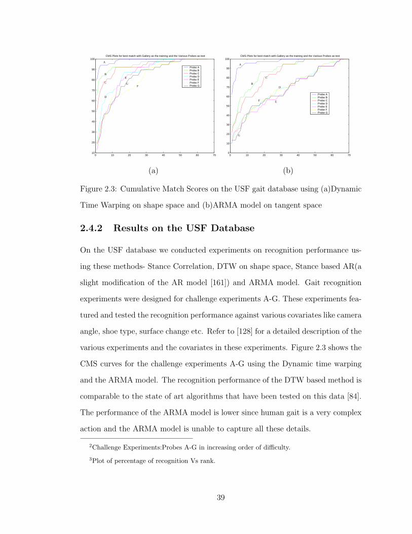
0 10 20 30 40 50 60 7010
20
30
40
50
60
70
80
90
100CMS Plots for best match with Gallery as the training and the Various Probes as test
Probe AProbe BProbe CProbe DProbe EProbe FProbe G
A
B
C
D
E
FG
0 10 20 30 40 50 60 700
10
20
30
40
50
60
70
80
90
100CMS Plots for best match with Gallery as the training and the Various Probes as test
Probe AProbe BProbe CProbe DProbe EProbe FProbe G
A
B
C
D
EF
G
(a) (b)
Figure 2.3: Cumulative Match Scores on the USF gait database using (a)Dynamic
Time Warping on shape space and (b)ARMA model on tangent space
2.4.2 Results on the USF Database
On the USF database we conducted experiments on recognition performance us-
ing these methods- Stance Correlation, DTW on shape space, Stance based AR(a
slight modification of the AR model [161]) and ARMA model. Gait recognition
experiments were designed for challenge experiments A-G. These experiments fea-
tured and tested the recognition performance against various covariates like camera
angle, shoe type, surface change etc. Refer to [128] for a detailed description of the
various experiments and the covariates in these experiments. Figure 2.3 shows the
CMS curves for the challenge experiments A-G using the Dynamic time warping
and the ARMA model. The recognition performance of the DTW based method is
comparable to the state of art algorithms that have been tested on this data [84].
The performance of the ARMA model is lower since human gait is a very complex
action and the ARMA model is unable to capture all these details.
2Challenge Experiments:Probes A-G in increasing order of difficulty.
3Plot of percentage of recognition Vs rank.
39

0 10 20 30 40 50 60 7010
20
30
40
50
60
70
80
90
100Comparison of average(of Probes A−G) CMS curve for various algorithms
Rank
Ave
rage
Per
cent
age
of Id
entif
icat
ion(
Pro
bes
A−
G) AR Model
ARMA ModelStance CorrelationDTW / HMM
DTW
ARMA
AR
StanceCorr.
A B C D E F G0
10
20
30
40
50
60
70
80
90
100Comparison between the AR,ARMA,Baseline,Stance Correlation,DTW(Shape),HMM(Image)
ARLinear Dynamical System(ARMA)BaselineStance CorrelationDTW/HMM (Shape)HMM(Image)
(a) (b)
Figure 2.4: Results on the USF Gait database. (a)Average CMS curves(Percentage
of Recognition Vs Rank) and (b)Bar Diagram comparing the identification rate
In order to understand the significance of shape and kinematics in gait recog-
nition, we ran the same experiments with other purely shape and purely dynam-
ics based methods as described in [161]. Figure 2.4(a) shows the average CMS
curves(average of the 7 Challenge experiments:Probes A-G) for the various shape
and kinematics based methods.
The following conclusions are drawn from Figure 2.4(a):
• The average CMS curve of the Stance Correlation method shows that shape with-
out any kinematic cues provides recognition performance below baseline. The
baseline algorithm is image correlation based and can be found in [128].
• The average CMS curve of the DTW method is better than that of Stance Corre-
lation and close to baseline.
• The improvement in the average CMS curve in the DTW over that of the Stance
Correlation method can be attributed to the presence of this implicit kinematics,
because the algorithm tries to synchronize two warping paths.
40

• Both methods based on kinematics alone(Stance based AR and ARMA model) do
not perform as well as the methods based on shape.
• The results support our belief that kinematics helps to boost recognition perfor-
mance but is not sufficient as a stand-alone feature for person identification.
• The performance of the ARMA model is better than that of the Stance based
AR model. This is because the observation matrix(C) encodes information about
the features in the image, in addition to the dynamics encoded in the transition
matrix(A).
• Similar conclusions may be obtained by looking at the CMS curves for the 7
experiments(Probes A-G) separately. We have shown the average CMS curve for
simplicity.
2.4.3 Results using Joint angles
In this section we describe experiments designed to verify the fact that our inference
about the role of kinematics in gait recognition was not dependent on the feature
that we chose for representation (Kendall’s statistical shape). In order to test
this, we performed some experiments on the actual physical parameters that are
observable during gait i.e., the joint angles at the various joints of the human body.
We used the manually segmented images provided in the USF dataset for these
experiments. We inferred the angles (angle in the image plane) of eight joints
(both shoulders, both Elbows, both Hips and both Knees) as the subjects walked
frontoparallel to the camera. We used these angles (which are physically realizable
parameters) as the features representing the kinematics of gait. We performed
recognition experiments using the DTW directly on this feature. Figure 2.5(a)
shows the CMS curves for three probes for which the manual segmented images
41

were available. The recognition performance is comparable to purely kinematics
based methods using our shape feature vector (refer to Figure 2.3(b) ).
We also generated synthetic images of an individual walking using a truncated
elliptic cone model for the human body and using the joint angles extracted from
the manually segmented images. Figure 2.6 shows some sample images that were
generated using this truncated elliptic cone model. We also performed recogni-
tion experiments on this simulated data using the DTW based shape sequence
analysis method described in section 4.1. Figure 2.5(b) shows the CMS curves for
this experiment. The results of these experiments are consistent with the experi-
ments described earlier (2.3(b) and 2.5(a)), indicating that for the purposes of gait
recognition, the amount of discriminability provided by the dynamics of the shape
feature is similar to the discriminability provided by the dynamics of physical pa-
rameters like joint angles. This means that there is very little (if any) loss in using
the dynamics of the shape feature instead of dynamics of the human body parts.
Therefore, our inferences about the role of kinematics will most probably remain
unaffected irrespective of the features used for representation.
2.4.4 Results on the CMU Dataset
The CMU dataset has 25 subjects performing four different activities- fast walk,
slow walk, walking with a ball and walking on an inclined plane. We perform
an experiment on the recognition performance(i.e., identification rate) using two
methods - the Stance Correlation(pure shape) method and ARMA model. The
results on the CMU dataset are shown in Table 1.
42

0 10 20 30 40 50 60 70 800
10
20
30
40
50
60
70
80
90
100CMS Plots for Angle Correlation Data
Probe BProbe DProbe K
B D K
0 10 20 30 40 50 60 70 800
10
20
30
40
50
60
70
80
90
100CMS Plots for Angle Correlation Data
Probe BProbe DProbe K
B
D
K
(a) DTW on joint angles (b) Shape sequence DTW on simulated data
Figure 2.5: CMS curve using (a) DTW on joint angles and (b) Shape sequence
DTW on simulated data
Figure 2.6: Sequence of silhouettes simulated using joint angles and truncated
elliptic cone human body model
43

Activity Slow Fast Walk with Inclined
Walk Walk Ball plane
Slow Walk 100(100) 80(72) 48(64) 48
Fast Walk 84(75) 100(100) 48(60) 28
Walk with Ball 68(70) 48(50) 92(100) 12
Inclined plane 32 44 20 92
Table 2.1: Identification rates on the CMU Data: Numbers outside braces are
obtained using Stance Correlation while those within the braces are obtained using
the ARMA model.
2.5 Conclusions and Future Work
We have proposed novel methods for comparing two stationary shape sequences
and shown their applicability to problems like gait recognition and activity recog-
nition. The non-parametric method, using DTW is applicable to situations where
there is very little domain knowledge and therefore parametric modeling of shape
sequences is difficult. We have also used parametric AR and ARMA models on
the tangent space projections of a shape sequence. The ability of these methods
to serve as pattern classifiers for sequences of shapes has been shown by applying
them to the problem of gait and activity recognition. We are currently working
on building complex parametric models that capture more details about the ap-
pearance and motion of objects and models that can handle non-stationary shape
sequences. We are also attempting to build models on the shape space instead of
working with the tangent space projections. Moreover, our experiments on gait
recognition lead us to make an interesting observation about the role of shape
and kinematics in human movement analysis from video. The experiments on gait
44

recognition indicate that body shape is a significantly more important cue than
kinematics for automated recognition, but using the kinematics of human body
improves the person identification capability of shape based recognition systems.
45

Chapter 3
Modeling Execution Rate
Variations for Action Recognition
Pattern Recognition in videos is gaining momentum in recent years because of its
applicability to several problems such as gait-based person identification, activity
modeling and recognition, video-based face recognition etc. Pattern recognition
in video streams is often a very challenging task because of the multitude of spa-
tiotemporal changes that can occur in a video capturing the exact same event.
Several algorithms and methods account for the spatial variations due to changes
in lighting, pose and appearance of individual objects. Nevertheless, very little
work has been done to account for the complex temporal variations that occur in
videos. For example, in activity recognition, different instances of the same activity
may consist of varying relative speeds at which the various actions are executed,
in addition to other intra- and inter- person variabilities. Most existing algorithms
for activity recognition are not very robust to intra- and inter-personal changes of
the same activity, and are extremely sensitive to warping of the temporal axis due
to variations in speed profile.
46

In this chapter, we study the variations due to execution rate in a systematic
way. We model an action sequence as a composition of these two sources of vari-
ability - variability on the feature space and variability due to execution rate. By
keeping the model on the feature space completely independent of the model on
the space of execution rates, we are then able to exploit any of the above mentioned
viewpoint invariant features in our method. Therefore, as more sophisticated fea-
tures become available our model will be able to exploit the characteristics of those
features while retaining the ability to deal with variations in execution rate. We
explicitly model execution rates and derive a Baysian classification algorithm for
action recognition. If the chosen features are viewpoint and anthropometry in-
variant, then the resulting algorithm becomes invariant to all the three significant
modes of variations - viewpoint, anthropometry and execution rate. Moreover,
since the model developed is general and not necessarly restricted to action recog-
nition, we believe that similar models may be used for other applications which
require rate-invariance.
Motivation: Consider the INRIA iXmas activity recognition dataset. Shown
in Figure 3.1(L) is the distribution of the number of frames in different executions
of the same activity for four distinct activities. Figure 3.1(L) clearly shows that
for the same activity the rate of execution and consequently the number of frames
during the execution varies significantly. Moreover, in most realistic scenarios this
temporal warping might also be inherently non-linear making simple resampling
methods ineffective. This implies that for uncontrolled scenarios the variations
due to temporal warpings could be even more significant. Ignoring this temporal
warping might lead to structural inconsistencies apart from providing poor recog-
nition performance. The sequence of images shown in the first two rows of Figure
47

15 25 35 45 55 65 75 85 950
1
2
3
4
5
6
7
8
9
10
Number of Frames in each Execution of the Activity
Num
ber
of s
eque
nces
Cross Arms
15 25 35 45 55 65 75 85 950
1
2
3
4
5
6
7
8
9
10
Number of Frames in each Execution of the Activity
Num
ber
of s
eque
nces
Sit Down
15 25 35 45 55 65 75 85 950
1
2
3
4
5
6
7
8
9
10
Number of Frames in each Execution of the Activity
Num
ber
of s
eque
nces
Wave Hand
15 25 35 45 55 65 75 85 950
1
2
3
4
5
6
7
8
9
10
Number of Frames in each Execution of the Activity
Num
ber
of s
eque
nces
Get Up
a) Cross Arms
c) Get Up
b) Sit Down
d) Wave Hands
WarpedAverageSequence
SequenceAverageNormal
Seq2
Seq1
and their normal and warped average sequences.(L) Histogram of number of frames (R) Two sequences with differing rates of executions
Figure 3.1: (L) Histogram of the number of frames in different executions of the
same action in the INRIA iXmas dataset. The histograms for 4 different activities
are shown. (a) Cross Arms (b) Sit Down (c) Get Up (d) Wave hands. (R) Row 1,
Row 2: Two instances of the same activity. Row 3: A simple average sequence.
Row 4:Average Sequence after accounting for time warps.
3.1(R) correspond to two different instances of the same individual performing the
same activity. There is an obvious temporal warping between the two sequences.
If this temporal warping is ignored, the distance between these two sequences will
be large, leading to incorrect matching. Moreover, if we are looking for some sta-
tistical description of the activity like an average sequence, ignoring the temporal
warping could lead to structural inconsistencies like the presence of four arms and
two heads in the average sequence, shown in the third row of Figure 3.1(R). If we
do account for temporal warping then such inconsistencies are avoided and the dis-
tance between the two sequences is rightly small. The fourth row shows a typical
average sequence obtained by our method after accounting for time warping.
Why should the distribution of time-warps be class-specific? To answer this, let
us consider the activity of ‘jumping’. The subject may in principle speed up certain
48

portions of the activity relative to the others. But, during the actual moments the
subject has no contact with the ground, the only external forces on the subject are
those from gravitation and therefore, much as he/she might attempt to, he/she
will not be able to change the execution speed during such times. There are thus
physical, aesthetic and structural constraints that force different activities to have
different warping functions. The constraints themselves vary with each activity
and therefore the eventual probability distribution on warping functions varies
from one activity to another.
3.0.1 Contributions of this chapter
• We propose a systematic generative model for activities that accounts for
variations in speed profile of an activity. The model is composed of a nominal
activity trajectory and a probability distribution on the function space of
temporal warpings capturing the permissible activity-specific time warping
transformations. We show how one can efficiently impose a Riemannian
metric and perform exact and efficient statistical inference efficiently and
correctly using the square-root density form of the time warp functions. We
then derive a Bayesian solution for a rate-invariant classification of activities.
• We highlight a special case of this approach where we assume a uniform
distribution on a convex subset of the warping functions and derive compu-
tationally efficient algorithms for learning and inference.
3.0.2 Outline of the chapter
We begin by providing a formal statement of the problem addressed in this chapter
in Section 3.1. Section 3.2 describes the geometry of the space of time warps
49

and presents algorithms for computing geodesics, distances and prior probability
distributions on this space. Section 3.3 describes how these tools may be used in
order to learn the model parameters. Section 3.4 describes the special case of the
model when the probability distribution on the space of time warpings is uniform.
In Sections 3.5 and 3.6, we discuss how both the models developed earlier can be
used in a Bayesian recognition framework in order to perform activity analysis,
recognition and activity-based person identification. Finally, in Section 3.7, we
present the conclusions and future research directions.
3.1 Problem Statement
Let C1, C2, ..., CM be M classes (in our case M different activity labels). Here
we wish to tackle two tasks while accounting for time-warping - 1. Given several
instances of an activity, we would like to build a model for that activity and 2.
Given a test sequence, we would like to classify the sequence to one of the models
in the database.
3.1.1 Feature for representation
Observations of an activity are typically obtained using video cameras and they
are in the form of video frames. Raw videos are not appropriate features for rep-
resentation. In principle, the feature chosen to describe the action units must
have physical significance and one must be able to directly identify the relation-
ship between the features extracted and the basic human pose. For the problem
of activity recognition, 3-D joint angles would be ideal features. Unfortunately,
estimating features like 3-D joint angles from images is extremely difficult and un-
50

reliable. So researchers have used several other features for describing the action
units [132] [103] [136] [84]. Since the USF gait database consists of monocular
video, we use the shape of the silhouette (along with the appropriate Procrustes
distance ) as a feature [161] for the gait-based person identification experiments.
The INRIA iXmas dataset contains synchronized videos from multiple views and
therefore allows us to compute and use the 3D Fourier based shape features de-
scribed in [170]. We refer the interested reader to [43] [161] and [170] for details
about the shape feature and the 3D circular FFT feature respectively.
For now let us assume that for each frame of the video, an appropriate feature
has been extracted and that the video data has now been converted into a feature
sequence given by f 1, f 2, ..., for frames 1, 2, ... respectively. We will use F to denote
the feature space associated with the chosen feature.
3.1.2 Model for warping functions
Let γ be a diffeomorphism (A diffeomorphism is a smooth, invertible function with
a smooth inverse.) from [0, 1] to itself with γ(0) = 0 and γ(1) = 1. Also, let Γ be
the set of all such functions. We will use elements of Γ to denote time warping
functions. Our model for an activity consists of an average activity sequence given
by a : [0, 1] → F , a parameterized trajectory on the feature space. Any time-
warped realization of this activity is then obtained using:
r(t) = a(γ(t)), γ ∈ Γ . (3.1)
We note in passing that Γ is a group with composition as the group operation
and the function γ(s) = s as the identity element. Equation 3.1 actually defines
an action of Γ on F [0,1], the space of all continuous activities. In our model, the
variability associated with γ in each class will be modeled using a distribution Pγ
51
on Γ. For the convenience of analysis and computation ( refer Section 3.2 ), we
prefer to work with ψ = +√γ instead of γ directly. There is a bijection between γ
and ψ and the probability models on ψ directly relate to equivalent models on γ.
Thus, we will introduce probability distributions Pψ on the set of all ψs, for each
activity class.
The parameters of this model are a(t), the nominal activity trajectory, and Pψ,
the probability distribution on square-root representations of time warping func-
tions. In general, the nominal activity trajectory a(t) can also be chosen to be
random. But, here, we restrict our analysis to cases where, the nominal activity
trajectory a(t) is deterministic but unknown. We will consider parametric forms
of densities for Pψ and reduce the problem of learning Pψ to one of learning the
parameters of the distribution Pψ. In particular, we highlight (in Section 3.4) a
special-case of a uniform distribution on the space of time warpings (called ’func-
tion space of an activity’). This particular special-case appeared as a preliminary
conference paper [158].
Physical Significance of the Model: The nominal activity trajectory, a(t)
and the probability distribution on the space of time-warps, Pψ together capture
all the possible realizations of the activity and provide the description of the ac-
tivity under different variabilities. In general, the nominal activity trajectories
of two different activities will be vastly different. The nominal activity trajec-
tory for ‘walking’ would consist of key postures like heel-strike, toe-off, mid-stance
etc., while that of ‘sit down’ would consist of the following actions - bend knee,
lower body, settle on chair and rest back on backrest. The distribution of activity-
specific temporal warpings Pψ, represents the space of all permissible time-warping
transformations for each activity. By learning this space, we are able to ‘interpo-
52

late’ appropriately between training sequences. Suppose there is a test sequence
that is within this space, but was not a part of the training sequences. Most tem-
plate sequence based recognition techniques tend to misclassify such test sequences.
Learning the function space of an activity provides our algorithm with the gener-
alization power necessary to correctly classify such test sequences. Moreover, by
learning this warping space formally, in a class specific manner, we also obtain bet-
ter discriminative power than other heuristic techniques for handling time-warping.
The model M={a, Pψ} represents a function space of activities whose elements are
composed of functions a(γ(t)), ∀ γ ∈ Γ.
3.1.3 Problems
Here, we state informal descriptions of the various problems we wish to tackle.
The Learning Problem
Given N labeled realizations r1, r2, r3, ...rN , of an activity, we would like to learn
the model for this activity. This is equivalent to learning the nominal activity
trajectory a(t) and the distribution on the warping parameters given by Pψ.
The Classification Problem
Suppose we have models for M different activities {ai, P iψ}Mi=1. Given a test se-
quence r(t), we would like to classify this test sequence as belonging to one of the
M models.
53

Clustering Problem
Given several realizations from K different activities with no class labeling, we
would like to cluster these sequences into K distinct clusters such that sequences
within the same cluster are maximally similar while sequences in different clusters
are dissimilar. Moreover, unlike traditional clustering algorithms this similarity
is invariant to changes in exectution rate of the action since the model for each
cluster is built to be rate-invariant.
3.2 Differential geometric tools on the space of
time-warping functions
The model for a random observation of an activity class consists of a(γ(t)), where a
is the average of that class and γ is a warping function. In order to classify activities
at variable execution rates, we need to analyze the warping functions as random
functions. However, the space of warping functions is not a vector space and that
rules out the use of classical functional analysis for this task. One alternative is
to utilize the differential geometry of this space, impose a Riemannian structure
on it, and use appropriate tools to perform calculus and statistics of warping
functions. In particular, we can compute distances between warping functions,
estimate sample means for given warping functions, and impose parametric and
non-parametric probability distributions on the space of warping functions.
The next question is: What Riemannian structure on the space of warping
functions is suitable and convenient for activity recognition? The Fisher-Rao met-
ric is often used for analyzing probability density functions. (The Cramer-Rao
lower bound on estimation of parameters is derived using this metric.) One major
54

reason for its popularity is that it is invariant to arbitrary warpings of the functions
involved. In other words, under this metric the distance between any two warping
functions γ1(t) and γ2(t) is same as that between γ1(γ(t)) and γ2(γ(t)) for any
arbitrary warping function γ(t). This point is important in activity recognition
because, as we will point out in Section 3.3.4, the representation of an activity
model is not unique, i.e. there is no canonical choice of γ for representing activity
models. The choice of Fisher-Rao metric implies that the resulting distances are
same irrespective of the baseline time axis chosen to represent activity models.
The Fisher-Rao metric, when applied to different mathematical representations
of γ, i.e. γ, γ, log γ, or√γ, takes different forms. Interestingly, in the case of
ψ ≡ √γ, this metric simplifies to the familiar and convenient L
2 metric [9, 146].
Furthermore, the space of all warping functions, represented by their square-root
density forms, under the Fisher-Rao metric, becomes a unit sphere. This is because
‖ψ‖2 =
∫ 1
0
|ψ(t)|2dt =
∫ 1
0
|γ(t)|dt = γ(1) − γ(0) = 1 .
For these two reasons – invariance to arbitrary time scalings and the spherical
nature of the resulting space, we choose the square-root density form to represent
and analyze variability associated with the warping functions.
Let the space of all square-root density forms be given by
Ψ = {ψ : [0, 1] → R|ψ ≥ 0,
∫ 1
0
ψ2(t)dt = 1} . (3.2)
This is the positive orthant of a unit hypersphere in the Hilbert space of all square-
integrable functions on [0, 1]. Let Tψ(Ψ) be the tangent space to Ψ at any given
point ψ. Then, for any v1 and v2 in Tψ(Ψ), the Fisher-Rao metric is given by
〈v1, v2〉 =
∫ 1
0
v1(t)v2(t)dt. (3.3)
55

Since Ψ is a sphere, its geometry is well known and we can directly use known
expressions for tools such as geodesics, exponential maps, and inverse exponential
maps on Ψ. Consequently, the algorithms for computing sample statistics, defining
probability density functions, and generating inferences also become straightfor-
ward.
We begin by describing some elements of differential geometry of Ψ.
3.2.1 Geometry of Ψ
One way to quantify the differences between two warping functions is to compute
the distance between their corresponding representations in Ψ. This distance is
given by the length of a geodesic, the shortest path connecting those two points in
Ψ. We know that the geodesics on a sphere are the great circles and the geodesic
distance is simply the length of the shorter arc connecting the two points on a
great circle. Given two warping functions γ1 and γ2, and their square-root density
forms, ψ1 and ψ2 in Ψ, the geodesic distance between them on Ψ is given by
d(ψ1, ψ2) = cos−1(〈ψ1, ψ2〉), (3.4)
where 〈ψ1, ψ2〉 =∫ 1
0ψ1(t)ψ2(t)dt.
The geodesic path itself can also be computed rather simply. Take the radial
projection of the chord joining points ψ1 and ψ2 onto the unit sphere results in
the geodesic. The chord joining ψ1 and ψ2 is given by (1 − s)ψ1 + sψ2 where s is
the parameter that identifies various points on this chord. The radial distance of
a point on this chord is given by s2 + (1− s)2 + 2s(1− s)(〈ψ1, ψ2〉). Therefore, we
can analytically write the geodesic connecting ψ1 and ψ2 as: X : [0, 1] → Ψ,
X(s) =(1 − s)ψ1 + sψ2
s2 + (1 − s)2 + 2s(1 − s)(〈ψ1, ψ2〉),
56

such that X(0) = ψ1 and X(1) = ψ2. Another way to specify a geodesic path in
Ψ is by giving a starting point ψ ∈ Ψ and a starting direction v ∈ Tψ(Ψ):
X(s) = cos(s‖v‖)ψ + sin(s‖v‖) v
‖v‖ , (3.5)
where ‖v‖ =√
∫ 1
0v(t)2dt.
One use of geodesics is to define and compute the exponential map from Tψ1(ψ)
to ψ. It is simply the value reached at s = 1 by a geodesic that starts from ψ in
the direction v and moves at a constant speed. We can evaluate the exponential
map using:
expψ(v) = cos(‖v‖)ψ + sin(‖v‖) v
‖v‖ . (3.6)
Similarly the inverse of the exponential map exp−1ψ1
(ψ2) = v ∈ Tψ1(ψ) can also be
computed analytically using
u = ψ2 − 〈ψ2, ψ1〉ψ1 (3.7)
v =u cos−1(〈ψ1, ψ2〉)
√
〈u, u〉. (3.8)
3.2.2 Statistical Analysis on Ψ
With the geometry of Ψ as specified above, let us derive some tools for statistical
analysis of data. Given a number of observed warping functions, we will esti-
mate the sample mean and covariance, use these estimates to define a ”wrapped-
Gaussian” density function and derive Bayesian classification algorithms using
these distributions as priors.
To compute the sample means of elements of Ψ, we will use the notion of
Karcher mean [85] that has been used frequently for defining means on nonlin-
ear manifolds. Suppose, we have n different square-root density forms, given by
57

ψ1, ψ2, ...ψn. Then, their Karcher mean ψ is defined as the element that minimizes
the sum of squares of geodesic distances:
ψ = arg minψ∈Ψ
n∑
i=1
d(ψ, ψi)2) (3.9)
where, d is the geodesic distance defined in (3.4). Note that the Karcher mean may
not be unique and can instead be a set of elements. A commonly used approach
for finding a Karcher mean is to use the gradients and this is where the exponential
map and its inverse are needed. The iterative update to the current value of mean
is given by:
ψ → expψ(ǫv), where v =1
n
n∑
i=1
exp−1ψ
(ψi) (3.10)
and where ǫ is usually 0.5. The next step is to define and compute a sample
covariance for the observed ψs. The key idea here is to use the fact that the
tangent space Tψ(Ψ) is a vector space. Using a finite-dimensional approximation,
say V ⊂ Tψ(Ψ), we can use the classical multivariate calculus for this purpose. In
practice, we obtain a natural restriction when v is observed at a finite number, say
T , of times leading to an observation {v(ti)|i = 1, 2, . . . , T}. With a slight abuse
of notation, we will denote this vector by v ∈ RT . The resulting sample covariance
matrix is given by: Σ = 1n−1
∑n
i=1 vivTi , where each vi is a T -dimensional sample of
the function exp−1ψψi. Note that by definition, the mean of vis should be zero. In
cases where the number of samples n is smaller than T , one can apply an additional
dimension-reduction tool to work on a smaller space. For instance, we can use the
singular value decomposition (SVD) of the sample covariance matrix Σ and retain
only the top m significant singular values and the corresponding singular vectors.
In such cases, the covariance matrix is indirectly stored using λ1, λ2, ...λm singular
values and their corresponding singular vectors u1, u2, ...um.
Next, we define a “wrapped-Gaussian” probability density on Ψ. We say
58

“wrapped-Gaussian” because Ψ is a non-Euclidean space and it is not possible to
define a Gaussian density here. We follow the tangent PCA (TPCA) approach [147]
for defining probability densities on nonlinear manifolds. In this approach, one de-
fines a Gaussian probability density on a tangent space of the manifold and then
projects it onto the manifold using the exponential map. However, in our case
we will need only the samples from the eventual density function and the explicit
functional form of that projected density is not needed. In fact, we will apply one
more transformation in taking the samples on Ψ to obtain samples on Γ. For a
mean µ and covariance Σ, we can define a normal density function N(v|µ,Σ) on
the elements of V ⊂ Tµ(Ψ). In case the data is available in the form of prior
samples, we can use the sample means and covariances to define this density on
the space V . The exponential map: expψ : Tψ(Ψ) → Ψ maps this density to the
spherical space of square-root forms, and the mapping ψ 7→ γ(t) =∫ t
0|ψ(τ)|2dτ
takes it further to the space of warping functions. The exponential map results in
wrapping the Gaussian density on the tangent space onto the sphere and therefore
the name wrapped-Gaussian. We will denote the resulting densities on Ψ and Γ
by Pψ and Pγ, respectively.
For a Bayesian classification of activities, as described later in this paper, we
will need to estimate the posterior probability of different classes given the observed
data. In this calculation, the warping function is considered a nuisance variable
that needs to be integrated out. Using a Monte Carlo approach, we will generate
samples from the prior on γ and use those samples to approximate the nuisance
integral. Thus, we have a need to generate samples from the class-specific priors
Pγ on Γ. This, in turn, requires sampling from the probability density Pψ, which
is accomplished as follows. Let ψ and Σ be the sample mean and the sample
59

covariance of the square-root forms observed in a particular class. Assume that
the covariance is stored in the form of m singular values λis and corresponding
singular vectors uis. In such cases, a random sample from the model Pψ is given
as
ψ ∼ expψ(v) where v ∼m
∑
i=1
zi√
λiui and zi ∼ N(0, 1) (3.11)
This random sample can then be converted into a warping function using the
partial integration ψ 7→ γ such that γ(t) =∫ t
0|ψ(τ)|2dτ .
Toy Example Consider the toy example shown in Figure 3.2. Figure 3.2(a)
shows 30 sample time-warping functions from each of three different classes (color
coded). The corresponding square-root density forms are shown in 3.2(b). For
each class using the samples of the square-root density forms we can compute the
Karcher mean and the covariance. The Karcher means are shown in 3.2(d). The
mean time-warping functions for each class obtained by partially integrating the
Karcher means are shown in 3.2(c). The model for each class of time-warping
functions is encoded in the form of the corresponding Karcher means and covari-
ances. Now one can generate random samples from this model as described above.
Shown in 3.2(f) are sample square-root density forms generated using the model
parameters for each class (i.e., the Karcher mean and covariances). As before the
corresponding time-warping functions maybe computed via partial integration and
are shown in 3.2(e).
3.2.3 Global Speed of activity
We have restricted our attention to time-warping functions from [0, 1] to itself, i.e
the functions that do not contract or dilate the full duration of the activity. We
claim that this is not restrictive, since any other time-warping transformation can
60

0 0.2 0.4 0.6 0.8 10
0.05
0.1
0.15
0.2
0.25
(f) Random samples generated using the Karcher mean and the covariance for each class separately
0 0.2 0.4 0.6 0.8 10
0.05
0.1
0.15
0.2
0.25
(d) Karcher mean of the samplesshown in (b)
0 0.2 0.4 0.6 0.8 10
0.05
0.1
0.15
0.2
0.25
(b) The square root density forms of of time warp functions shown in (a)
0 0.2 0.4 0.6 0.8 10
0.1
0.2
0.3
0.4
0.5
0.6
0.7
0.8
0.9
1
(a) 90 time−warp functionsbelonging to 3 different classes
0 0.2 0.4 0.6 0.8 10
0.1
0.2
0.3
0.4
0.5
0.6
0.7
0.8
0.9
1
(e) Random samples of time−warping
samples shown in (f)functions corresponding to the
0 0.2 0.4 0.6 0.8 10
0.1
0.2
0.3
0.4
0.5
0.6
0.7
0.8
0.9
1
(c) Corresponding mean warping functions for the Karcher meansshown in (d)
TimeWarpingFunctions
Squarerootdensityforms
Figure 3.2: Figure is Color coded - Each color represents a different class (a)
Random samples of time-warping functions belonging to 3 different classes (color
coded) (b) Corresponding samples of square-root density forms (c) Mean time-
warping function for each class computed by partial integration of the class-specific
Karcher mean (d) Class specific Karcher mean computed using the samples shown
in (b) (e) Random samples generated from the stored model (f) Random samples
of ψ generated from the stored Karcher means and covariance.
61

be decomposed into two parts: a global linear scaling of the temporal axis and
the non-linear time-warping functions that we have addressed so far. The effect of
such a linear global temporal scaling is identical to the effect of changing the rate
of sampling.
Let a(t), for 0 ≤ t ≤ Ta, be a vector valued function of time. Let b(t), for
0 ≤ t ≤ Tb, be a time-warped version of a(t), with the warping function given by
w(t), i.e., b(t) = a(w(t)), w(t) : [0, Tb] → [0, Ta]. Now w(t) can be decomposed
as w(t) = Taγ(t/Tb) where γ : [0, 1] → [0, 1] i.e., a global linear dilation (or
contraction) and a non-linear warping γ. Without loss of generality we will use
the word time-warping transformation to synonymously denote the non-linear time
warping function given by γ. In all our experiments we have first identified the
global temporal scaling factor by identifying the start and stop instants of each
activity. The identification of the start and stop instants of each activity is also
done automatically by template matching. Once the global temporal scaling factor
is found, each realization of the activity is temporally dilated or contracted linearly
so that the total duration of the activity is a constant for all realizations of the
activity.
3.3 Learning and Classification Algorithms
Given N realizations r1, r2, r3, ...rN , of an activity, we need to learn the parameters
of the model for this activity. This amounts to learning the nominal activity
trajectory a(t) and the probability distribution Pψ.
62

3.3.1 Estimating Pψ given a(t)
Let us assume that the nominal activity trajectory a(t) is known. Now we need to
estimate the parameters of the warping distribution which is given by Pψ. In order
to learn Pψ, we first warp each of the observed realizations of the activity to the
known nominal activity trajectory given by a(t). This warping can be performed
using the DTW algorithm. The DTW algorithm provides us with corresponding
warping functions γi(t) such that∫ 1
0‖ri(t) − a(γi(t))‖2dt is minimized. Then, we
can compute ψis using ψi =√γi.
Now, we have several samples ψ1, ψ2, ... to estimate the distribution Pψ. As-
suming a ”wrapped-Gaussian” distribution on Ψ, this amounts to estimating the
sample mean and the sample covariance of the observed ψis. As described in
Section3.2.2, we can define and compute the Karcher mean of given ψis using the
exponential and the inverse exponential maps. The covariance is obtained simi-
larly by restricting to a T -dimensional approximation V of the vector space Tψ(Ψ).
Using SVD of observations in V , one ends up with the singular values λ1, λ2, ...λm
and their corresponding singular vectors u1, u2, ...um.
Thus, given the nominal activity trajectory a(t), we can estimate the parame-
ters of the warping distribution Pψ, namely its Karcher mean ψK and its covariance
stored indirectly using m singular values λ1, λ2, ...λm and corresponding singular
vectors u1, u2, ...um.
3.3.2 Estimating a(t) assuming known warping functions
For the given observations r1, r2, . . . , of an activity, assume that the corresponding
warping functions γ1, γ2, . . . , are also given. Then, we can estimate the nominal
63

or average activity trajectory a(t) using
a(t) =1
N
N∑
i=1
ri(γ−1i (t)) (3.12)
3.3.3 Iteratively estimating a(t) and Pψ
Given N realizations r1, r2, r3, ...rN , of the same activity, we would like to learn
the parameters of the model for this activity. We do this by iteratively estimating
Pψ and refining our estimate of the nominal activity trajectory a(t) using the steps
described in the previous two sections. We first initialize the nominal activity
trajectory to one of the realizations say ainit(t) = r1(t). Then we estimate Pψ
using the method described in Section 3.3.1. We then refine the estimate of the
nominal activity trajectory using the method described in Section 3.3.2. These two
steps are iterated till convergence. In practice, we find that the iterations converge
very quickly (within 4 or 5 iterations).
3.3.4 Uniqueness of the Model parameters
The model parameters given by a(t) and Pψ ≈ {ψK ,Σψ} are not unique. Two
different sets of model parameters M1 = {a1(t), Pψ1} and M2 = {a2(t), Pψ2
}, could
lead to the same distribution on the observation space. That is, the two models
may lead to the same distribution on the space of all activity realizations. This
could happen if the corresponding nominal activity trajectory and the distribution
on the space of warping transformations are related as
a2(t) = a1(γ(t)) ψ1 =√
˙γ1 ψ2 =√
˙γ2 γ2(t) = γ1(γ−1(t)) Σ2 = Σ1
(3.13)
When the conditions listed in (3.13) are satisfied, we notice that a2(γ2(t)) =
a1(γ1(t)), i.e., the mode of the activity trajectories is the same for both models.
64

Moreover, since the covariance matrices for the two models are identical (Σ1 = Σ2),
this means that samples for either of these models will have identical distributions
and would therefore be indistinguishable. In practice this means that there is an
equivalence class of models such that any two models from the same equivalence
class are indistinguishable. The conditions for belonging to the same equivalence
class are those stated in (3.13). While performing classification and inference based
on these model parameters it becomes essential to maintain uniqueness of model
parameters. Therefore, once we learn the model parameters we always choose a
single canonical representation for each equivalence class. Note that the choice of
this canonical representation does not affect the performance of the algorithm at
all as long as this choice is consistent. We choose the model with γK(t) = t, such
that the Karcher mean of the warping distribution corresponds to simple linear
warping and the covariance matrix of the warping transformations encodes all the
non-linearities in the warping distributions. The canonical model parameters are
unique and can be directly used for classification and inference.
3.3.5 Generating activity samples from the model
The model for an activity is given by the nominal activity trajectory a(t) and
the distribution on warping transformations given by Pψ. We can use this model
to generate random samples from the model. We first generate random samples
ψ1, ψ2, .....ψM from the warping distribution Pψ as described in Section 3.2.2. The
corresponding time warp for each ψ is computed. Let γ1, γ2, ...γM be the corre-
sponding time warps. Then realizations from the model may be drawn as
rj(t) = a(γj(t)) + w(t) where w ∽ N(0,Σ). (3.14)
65

3.3.6 Classification Algorithm
Let us assume that we have K different models M1,M2, ...MK given by their ap-
propriate nominal activity trajectories a1, a2, ...aK and corresponding Pψ given by
P 1ψ, P
2ψ, ..., P
Kψ . Given a test sequence r(t), we would like to classify r(t) to one of
the K possible classes. This classification task can be accomplished using MAP
estimation, i.e.,
ID = arg maxi=1,2,..K
P (Mi|r) = argi=1,2,..K maxP (r|Mi)P (Mi). (3.15)
The likelihood P (r|Mi) can be computed as,
P (r|Mi) =
∫
ψ
P (r|Mi, ψ)P (ψ|Mi)dψ where P (ψ|Mi) = P iψ. (3.16)
This integral can be estimated using Monte Carlo sampling methods. We draw N
samples from the model Mi as described in Section 3.3.5. Using these samples we
estimate the likelihood P (r|Mi) as
P (r|Mi) =1
N
j=N∑
j=1
P (r|ai, ψj) where ψj ∽ P (ψ) = P iψ (3.17)
In order to compute the summation described above, we need a model for com-
puting the conditional likelihood P (r|Mi, ψj). The conditional warp probability is
inversely proportional to the distance between the warped nominal activity trajec-
tory and the test sequence, i.e.,
P (r|Mi, ψj) = e−αD(r,ai(γj)) where D(r, ai(γj)) =
∫ 1
0
(r(t) − ai(γj(t)))2dt
(3.18)
and α is a suitably chosen constant. As the number of samples N increases the
accuracy of the approximation improves. One can also improve the accuracy of
the approximation by performing importance sampling [38]. Let us assume that
66

the proposal distribution from which the samples of the ψ are drawn is given by
G(ψ). Then we draw N samples of ψ from G and the integral is approximated as
P (r|Mi) =1
N
j=N∑
j=1
P (r|Mi, ψj)P (ψj|Mi)
G(ψj)where ψj ∽ G(ψ). (3.19)
In practice, using importance sampling significantly improves the accuracy of the
approximation when using a finite number of samples. The effectiveness of the
importance sampling also critically depends upon the proposal distribution. The
proposal distribution or the importance distribution should ideally be as close to
the posterior distribution we wish to approximate. In practice, we first estimate
the mode of this posterior by computing the best warping transformation between
the nominal activity trajectory of the model (ai(t)) and the test sequence (r(t)).
We set the mean of the importance distribution to be this warping transformation
while letting the covariance of the importance distribution to be the same as the
covariance of the model. We have experimentally found that this choice of impor-
tance distribution enables us to effectively approximate the integrals using Monte
Carlo methods with a reasonable number of random samples.
3.4 Function Space of Time-Warps
The model described in the previous sections represents an activity using a nominal
activity trajectory a(t) and a probability distribution on the space of time warpings
Pψ. There are two inherent difficulties in practical implementations of such a
model inspite of its rigour. Firstly, since the model attemps to learn a probability
distribution on the space of permissible time-warping functions, the algorithm
for learning this Pψ requires a reasonable number of sample realizations of each
action. In the presence of very few samples, the learning algorithm might lead to
67

underfitting of the data. Moreover, as inference using this model is done using
Monte Carlo methods, the algorithms for inference are computationally expensive.
Suppose we relax the assumption about learning the probability distribution of
permissible time-warps and instead attempt to learn a subset in the time-warping
space and assume that the probability distribution of time-warps is uniform within
the learnt subset. Each activity can now be represented by using a nominal ac-
tivity trajectory given by a(t) and W , the set containing all the time warping
transformations permissible for that activity. Each realization of an activity is
given by a trajectory r(t) = a(f(t)) where f ∈ W . Such a model is a special case
of learning Pψ where, we assume that the probability distribution is uniform on a
subset W ∈ Γ in the space of time-warpings. The advantage of using such a model
where the probability distribution is assumed uniform is that both the learning and
the inference algorithms become simple dynamic programming problems when we
constrain the set W to be a convex set.
3.4.1 Activity specific time-warping space (W )
Even though Γ represents the space of all plausible time-warping transformations,
every individual activity may only be able to access a subset W of the candidate
functions in Γ because of the physical constraints imposed on the actor and the
activity. We can then model the activity using a uniform distribution on this
subset W . Then learning the parameters of the uniform distribution boils down
to learning this subset W . Below, we discuss and visualize some properties of this
activity specific time warping space W .
1. W is a subset of Γ, i.e., W ⊂ Γ.
68

2. γ(t) = t is a candidate function in W , i.e., γ(t) = t ∈W . This represents no time
warping.
3. It is reasonable to assume that W is convex, i.e., ∀ γ1, γ2 ∈ W and α ∈ (0, 1),
γ = αγ1 + (1 − α)γ2 ∈ W . Since the derivative is a linear operator, this means
that if the rate of execution of some action unit can be speeded up by factors α1
and α2 then it can also be speeded up by any factor β in between α1 and α2. This
is not just reasonable but in fact desirable.
This implies that W can be bounded above and below by functions u, l ∈ W such
that
u(t) ≥ t ≥ l(t) ∀t ∈ (0, 1) and u ≥ γ ≥ l ∀γ ∈ W (3.20)
where γ1 ≥ γ2 =⇒ γ1(t) ≥ γ2(t) ∀t ∈ (0, 1). So, we can now index any such convex
space W by the functions u and l and call it Wul and learning W is essentially the
same as learning the upper and lower bounding functions u and l.
3.4.2 Symmetric representation of an Activity Model
As described for the ”wrapped-Gaussian” distribution, the representation of the
activity model given by M1 = {a(t),Wul} is not unique. Let unew(t) = f−1(u(t))
and lnew(t) = f−1(l(t)) and let f be a member function in Wul. Consider the new
model M2 ={b(t),Wunewlnew}= {a(f(t)),Wunewlnew
}. For every realization of the
model M1, i.e., a(γ1(t)) there exists a corresponding realization of the model M2
given by b(f−1(γ1(t))). Therefore the two models M1 and M2 are equivalent. As
before, we will resolve this ambiguity by specifying a synchronizing time such that
the average of all the warping functions in Ws is the identity warping function.
The symmetric representation of the model is such that unew(t) − t = t − lnew(t).
69

Therefore the activity specific warping space can be represented as Ws = Wunewlnew
where s(t) = unew(t) − t = t − lnew(t), represents the extent of possible temporal
warpings. This symmetric representation of the model is unique, i.e., if M1 =
{a1(t),Ws1} and M2 = {a2(t),Ws2}, then M1 = M2 ⇐⇒ a1 = a2 and s1 = s2.
Given a non-symmetric representation of the model, i.e., M1 = {a(t),Wul},
we still need to determine a time-warping function f such that upper and lower
bounding functions of the new model are symmetric about the diagonal. This is
achieved as
unew(t) − t = t− lnew(t) (3.21)
(Substituting for unew(t) and applying the u−1 operator)
⇒ f(t) = {2u−1(t) − f−1(l(u−1(t)))}−1
This implicit function equation can be solved by fixed point iterations as f(i)(t) =
{2u−1(t)− f−1(i−1)(l(u
−1(t)))}−1, where f(i) represents the approximation of f in the
ith iteration. We initialize the iteration with f(0)(t) = u(t)+l(t)2
. We observe that
it converges within very few iterations with such an initialization. Once we have
obtained this symmetrizing time warp f then any non-symmetric model parameters
M1 = {a(t),Wul} can be transformed to its symmetric (unique) counterpart as
M = {b(t),Ws}, where b(t) = a(f(t)) and s(t) = unew(t) − t = t − lnew(t) =
f−1(u(t)) − t.
3.4.3 Learning Model Parameters
Learning the model parameters can be done as before by iterating between the two
unknowns ( a(t) and Pγ ). Learning the nominal activity trajectory a(t) is done as
70
described in Section 3.3.2. The only difference between earlier and now is during
the estimation of the parameters Pψ. Earlier we computed the Karcher mean
and the covariance of Pψ for the wrapped-Gaussian distribution, here since the
parameters of Pγ are given by the upper and lower bounding functions we need to
estimate them. Given an estimate of the activity trajectory a(t) and corresponding
warping functions γi(t) for each realization, the the upper and the lower bounding
functions for the activity specific time-warping set can be estimated as
u(t) = maxi=1,2,...N
γi(t), ∀t ∈ (0, 1) and l(t) = mini=1,2,...N
γi(t), ∀t ∈ (0, 1).
(3.22)
Since each γi is constrained to be monotonously increasing and the end points are
fixed, it is easy to see that the estimates u(t) and l(t) also inherit these properties.
Thus the estimated model M is given by M = {b(t),Wul}. This model param-
eters correspond to the non-symmetric version of the model and can be easily
transformed to the equivalent symmetric version of the model using the procedure
described in Section 3.4.2.
3.4.4 Classification using the model
The primary advantage of using the uniform distribution on the space of time-
warping functions instead of learning a class-specific probability density function
is that the classification algorithm becomes computationally efficient. While clas-
sification in the general case is dependent on Monte-carlo methods, we show how
a simple dynamic programming based algorithm will suffice for classification us-
ing the uniform distribution based model. Suppose we have M different activity
models given by Mi = {ai(t),Wsi} for i = 1, ..M . Given a test sequence h(t), the
activity recognition problem is one of identifying the model that generated the test
71

sequence h(t). We do this in two steps. Firstly, assuming that the test sequence
h(t) is generated from the model Mi, we estimate the best warping transformation
fi from Wsithat would warp ai to h, i.e.,
fi = minf∈Wsi
dist(h(t), ai(f(t))) (3.23)
I = arg mini=1,...M
dist(h(t), ai(fi(t))) (3.24)
Activity recognition is performed by minimizing the warping error between the
nominal activity trajectory and the test sequence. Note that the search of warp-
ing functions is performed only over the corresponding activity specific warping
set. The above-mentioned intuitive idea for activity recognition can be easily im-
plemented by a simple variation of the DTW. In the DTW algorithm, instead of
arbitrarily limiting the warping function to lie within some window (typical choices
are uniform window and parallelogram window), we replace the window constraints
by the upper and lower bounds for the warping function that we have learnt for
each model. Thus, the DTW algorithm with the window width being given by
u(t) = s(t) + t and l(t) = t − s(t) computes the distance that is being minimized
in (3.24).
I = mini=1,...M
DTW (ai, h, s) (3.25)
where, DTW (ai, h, s) stands for the implementation of the DTW algorithm with
the warping window constraints given by u(t) = s(t) + t and l(t) = t− s(t).
3.5 Experiments
We tested the algorithms on three different datasets - UMD Common Activities
dataset, the INRIA iXmas dataset and the USF gait dataset. We used a warpped-
Gaussian probability distribution for Pψ with its parameters stored using a set of
72

tangent plane vectors uψ and their covariance matrix Σψ. We denote the experi-
mental results using this algorithm as PGauss in the results. We also implemented
the uniform distribution on the space of time-warping functions using dynamic
programming and performed maximum likelihood inference using this model. We
denote the results using this method as PUnif in the results.
3.5.1 Common Activities Dataset
We used the UMD common activities dataset [158], a dataset of common activities
to perform preliminary experiments to validate our model. The dataset consists of
10 activities and 10 different instances of each activity. We partition the dataset
into 10 disjoint sets each containing 1 instance of every activity. In order to test the
recognition for each set, we first learn the model parameters from the remaining
nine sets and then perform recognition for the test sequences. We repeat the
process for each of the 10 sets. Thus we ensure that there is no overlap between the
training set and the test sequences. Figure 3.3 shows the 10 X 100 similarity matrix
for using the function space algorithm with the uniform distribution on the space
of temporal warps. Each column corresponds to a different test sequence while
each row corresponds to a different activity. The strongly block diagonal nature
of the similarity matrix indicates that the recognition algorithm performs well. In
fact, on this database we obtained 100% recognition using both our algorithms.
3.5.2 INRIA iXmas dataset
The INRIA multiple-camera multiple video database of the PERCEPTION group
consists of 11 daily-live motions performed each 3 times by 10 actors. The actors
freely change position and orientation. Every execution of the activity is done at
73

(f) Kick (g) Bend to the side (h) Throw (i) Turn around (j) Talk on Cellphone(a) Pick up Object (b) Jog in Place (c) Push (d) Squat (e) Wave
(a) (b) (c) (e) (f) (g) (h) (j)(i)(d)
Figure 3.3: 10 X 100 Similarity matrix of 100 sequences and 10 different activities
using the function space algorithm.
a different rate. For this dataset, we extract 16 × 16 × 16 circular FFT features
as described in [170]. Since the actors were free to perform the actions the rate
at which these actions were performed varied significantly as was shown in Figure
3.1. So most approaches that cannot handle this vast temporal rate variations,
instead model the entire segment as a single motion history volume [170]. Instead,
we build a time series of the circular FFT features described in [170]. This allows
us to learn the nature of the temporal rate changes between various executions
of an action. Using these features, we performed a recognition experiment on the
provided data similar to those done in [170]. For the recognition experiment, we
used only one segment for each activity which best represented that activity as
in [169]. The recognition results are summarized in table 5. We used 16× 16× 16
circular FFT features in all our experiments here while the results reported in [170]
used 32 × 32 × 32 features. The confusion matrix showing confusion between the
activities using both the wrapped-Gaussian and the dynamic programming based
uniform distribution model are shown in Table 3.2. Note that uniform distribution
based model described in Section 3.4 is significantly more computationally effi-
cient compared to the Monte-Carlo based inference using the wrapped-Gaussian
distribution on the tangent space of warp space.
74

Activity PCA
[170]
Mahalanobis
[170]
LDA
[170]
System
Dis-
tance
[152]
PUnif
(This
paper)
PGauss
(This
paper)
1 Check Watch 53.33 73.33 76.67 93.33 100 93.33
2 Cross Arms 23.33 86.67 100 100 100 100
3 Scratch Head 46.67 86.67 80 76.67 100 100
4 Sit Down 66.67 93.33 96.67 93.33 96.67 100
5 Get Up 83.33 93.33 93.33 86.67 96.67 100
6 Turn Around 80 96.67 96.67 100 100 100
7 Walk 90 100 100 100 100 100
8 Wave Hand 50 70 73.33 93.33 96.67 96.67
9 Punch 70 86.67 83.33 93.33 83.33 90
10 Kick 50 86.67 90 100 80 100
11 Pick Up 60 90 86.67 96.67 90 100
Average 61.21 87.57 88.78 93.93 94.85 98.18
Table 3.1: Comparison of view invariant recognition of activities in the INRIA dataset
using our approaches (PUnif and PGauss) with the approaches proposed in [170] and [152].
Motifs 1 2 3 4 5 6 7 8 9 10 11
Sit Down 30(28) 0(0) 0(1) 0(1) 0(0) 0(0) 0(0) 0(0) 0(0) 0(0) 0(0)
Get Up 0(0) 30(30) 0(0) 0(0) 0(0) 0(0) 0(0) 0(0) 0(0) 0(0) 0(0)
Turn Around 0(0) 0(0) 30(30) 0(0) 0(0) 0(0) 0(0) 0(0) 0(0) 0(0) 0(0)
Check Watch 1(0) 0(0) 0(0) 29(30) 0(0) 0(0) 0(0) 0(0) 0(0) 0(0) 0(0)
Cross Arms 1(0) 0(0) 0(0) 0(0) 29(30) 0(0) 0(0) 0(0) 0(0) 0(0) 0(0)
Scratch Head 0(0) 0(0) 0(0) 0(0) 0(0) 30(30) 0(0) 0(0) 0(0) 0(0) 0(0)
Walk 0(0) 0(0) 0(0) 0(0) 0(0) 0(0) 30(30) 0(0) 0(0) 0(0) 0(0)
Wave Hand 1(1) 0(0) 0(0) 0(0) 0(0) 0(0) 0(0) 29(29) 0(0) 0(0) 0(0)
Punch 3(1) 0(1) 0(0) 0(0) 0(0) 0(0) 0(0) 1(1) 25(27) 0(0) 0(0)
Kick 5(0) 0(0) 0(0) 0(0) 1(0) 0(0) 0(0) 0(0) 0(0) 24(30) 0(0)
Pick Up 1(0) 0(0) 0(0) 0(0) 2(0) 0(0) 0(0) 0(0) 0(0) 0(0) 27(30)
Table 3.2: Confusion matrix using PGauss(outside parenthesis and PUnif (inside paran-
thesis) on the INRIA dataset.
75

3.5.3 USF Gait Database
Note on gait-based person identification Since the model for learning the
function space time-warpings is not explicitly dependent on the choice of features,
one could potentially use the same model to learn individual specific function spaces
in order to perform activity-based person identification. The only difference would
be that we would choose a feature that is person-specific (e.g., silhouette). The
nominal activity trajectory would be individual specific in this case. Various exter-
nal conditions (like surface, shoe) induce systematic time-warping variations within
the gait signatures of each individual. The function space of temporal warpings for
each individual amounts to learning the class of person specific warping functions.
By learning the function space of these variations we are able to account for the
effects of such external conditions. This will allow the same basic approach to be
applied for both action recognition and activity based person identification by the
use of appropriate features.
In order to compare the performance of our algorithm with the current state of
the art algorithms, we also performed a gait-based person identification experiment
on the publicly available USF gait database [136]. The USF database consists
of 71 people in the Gallery. Various covariates like camera position, shoe type,
surface and time were varied in a controlled manner to design a set of challenge
experiments [136]. We performed a round-robin recognition experiment in which
one of the challenge sets was used as test while the other 7 were used as training
examples. The process was repeated for each of the 7 challenge sets on which results
have been reported. Table 3.3 shows the identification rates of our algorithm with
a uniform distribution on the space of warps (PUnif ), our algorithm with a wrapped
Gaussian distribution on the tangent space of warps with shape as a feature and
76

with binary image feature (PGauss and PGaussIm). For comparison the table also
shows the baseline algorithm [136], simple DTW on shape features [161] and the
image-based HMM [84] algorithm on the USF dataset for the 7 probes A-G. Since
most of these other algorithms could not account for the systematic variations in
time-warping for each class the recognition experiment they performed was not
round robin but rather used only one sample per class for learning. Therefore, to
ensure a fair comparison, we also implemented a round-robin experiment using the
linear warping (PLW ).
Table 3.3: Comparison of Identification rates on the USF dataset
Pr- Base- DTW HMM HMM pHMM PLW PUnif PGauss PGaussIm
obe line Shape Shape Image [100]
Avg. 42 42 41 50 65 51.5 59 59 64
A 79 81 80 96 85 68 70 78 82
B 66 74 72 86 89 51 68 68 78
C 56 52 56 74 72 51 81 82 76
D 29 29 22 32 57 53 40 50 48
E 24 20 20 28 66 46 64 51 54
F 30 19 20 17 46 50 37 42 56
G 10 19 19 21 41 42 53 40 55
The average performance of our algorithms PUnif and PGauss are better than all the
other algorithms that use the same feature, (DTW/HMM (Shape) [161] and Linear
warping PLW ) and is also better than the baseline [136] and HMM [84] algorithms
that use the image as a feature. The image based pHMM algorithm [100] outper-
forms our algorithm. One reason for this is that the image as a feature performs
77

better than shape as a feature for the USF dataset. But, it is a computationally
very intensive feature (of the order of number of pixels) and consequently leads to
algorithms that are very slow. Therefore, we prefer to use the shape as a feature.
Inspite of this obvious handicap, the performance of our algorithm is compara-
ble to the image based pHMM algorithm for many probes. The improvement in
performance while using binary image as a feature is shown in the last column
(PGaussIm). The experimental results presented here clearly show that using mul-
tiple training samples per class and learning the distribution of their time warps
makes significant improvement to gait recognition results. While most algorithms
based on learning from a single sample led to overfitting and therefore performed
much better when the gallery was similar to the probe (Probe A-C), they also per-
formed very poorly when the gallery and the probes were significantly different.
But, since our algorithm had significant generalization ability ( becasue we learn
the distribution of time warps ) the performance of our algorithm did not suffer
from overfitting and therefore did not drop as much when moving from probes A-C
to Probles D-G.
3.6 Other applications
3.6.1 Clustering Activity Sequences
Algorithm for Clustering There are several scenarios where one requires a clus-
tering algorithm to be rate-invariant. Under such scenarios it becomes reasonable
to use the rate-invariant model for activities described above as the basis for clus-
tering. When rate-invariance is not a desirable property traditional clustering
algorithms such as K-nearest neighbour might be reasonable choices for clustering.
78

We performed clustering experiments on the UMD common activities dataset and
the USF gait database using the fast and computationally efficient uniform distri-
bution version of the algorithm denoted by PUnif . The clustering algorithm, based
on expectation maximization (EM) is very similar to the Lloyd-Max algorithm [78]
and can be used to organize a database of sequences for efficient retrieval. Let us
assume that we know the number of clusters, N and the cluster centers c1, c2, ...cN .
Then, each of the sequences in the database can be associated with one of N clus-
ters. This can be done using a maximum-likelihood approach as described earlier
in (3.25). This forms the Maximization step of the EM algorithm. The Expec-
tation step of the algorithm involves recomputing the new cluster centers from
cluster memberships evaluated during the Maximization step. We iterate these 2
steps until convergence. In all our experiments, we initialized the cluster centers
randomly.
Clustering on Common Activities Dataset We performed a clustering
experiment on the 100 activity sequences collected as a part of the Common Ac-
tivities dataset. We chose the number of clusters N to be 10 since there were
10 different activities. If clustering were perfect, then the 100 activity sequences
would be clustered into 10 different clusters, each cluster containing 10 sequences
that correspond to that particular activity. But in reality, clustering would be im-
perfect and some of the 100 sequences would be misaligned in the wrong cluster.
We repeated the clustering experiment several (about 50) times, with a random
initialization of cluster centers during each trial. On an average, the algorithm
converged in about 10 iterations and about 92% of the sequences were clustered
correctly. Even during some adverse initializations the clustering performance was
greater that 80%.
79

3.6.2 Organizing a Large Database of Activities
With the decreasing cost of storage, the size of activity databases is increasing
rapidly. For example, the complete USF gait database [136] consists of about 122
classes and a total of more than 1000 sequences. As the size of the database in-
creases, the number of ‘distance’ computations that must be performed on every
query also increases linearly with the size of the database. This poses a significant
bottleneck for practical activity recognition systems. We show that organizing the
database of sequences using the clustering algorithm described in Section 3.6.1 de-
creases this computational burden significantly. The price paid is a small decrease
in recognition performance. We organize the database of activities in the form of
a dendrogram as shown in Figure 3.4. At each level of the dendrogram the num-
ber of branches (B) was set to 3. The number of levels to which the dendrogram
is ‘grown’ determines the trade-off between computation and accuracy. As the
number of levels is increased, the number of ‘distance’ computations that must be
performed before finding the class membership of a given test sequence decreases.
Therefore, the computational burden of the algorithm also decreases. But this
might introduce a decrease in classification performance. When the dendrogram
is fully grown (i.e., when each leaf of the dendrogram represents one activity),
there will be logBN , levels and therefore BlogBN ‘distance computations’. Let
us consider the USF database which consists of 122 subjects and a total of 1870
sequences. A nearest neighbour classifier on this database must perform 1870 dis-
tance computations in order to classify a new test sequence. But if we assume that
we organize the database in the form of a ‘fully grown dendrogram’, with each
leaf node representing each of the 122 individuals, then one would just have to
perform about BlogBN = 3 ∗ log3122 ≈ 14 ‘distance computations’. This is a very
80

Level 1
Level 2
Level 3
Figure 3.4: Dendrogram for organizing an activity database
significant computational saving.
We performed an experiment to evaluate the efficiency of organizing the database
on a subset of the USF database as in Section 3.5.3. In our experiments, we grow
the dendrogram upto 2 levels. We measure efficiency of organization (η) as a ratio
of the recognition rate before and after organization.
η = 100 ∗ Identification rate after organization
Identification rate before organization(3.26)
The efficiency η is strongly related to clustering performance and it is reasonable
to expect the efficiency η to increase with better clustering. Table 3.4 shows the
efficiency of organization for the various probes in the USF dataset. On this data,
the dendrogram organization of the database reduced the computational time by
a factor of about 30. This means that the processing time for large databases
will be reduced from the order of days to a matter of hours. For such significant
reduction in processing time, the Table 3.4 shows that the decrease in recognition
performance is not drastic.
Table 3.4: Efficiency of Organization on the USF dataset
Probe A B C D E F G Avg
η 76 81 84 100 82 100 95 89
81

3.7 Summary and conclusions
In this chapter, we addressed an important but often neglected problem in mod-
eling activity, that of temporal warping of the activity trajectories. Our model
for an activity describes each activity using a nominal activity trajectory and a
probability distribution on the space of permissible temporal warpings. We dis-
cussed the case of a parameteric wrapped-Gaussian distribution on the tangent
space of time-warps and derive Monte Carlo sampling-based Bayesian algorithm
for classification. We then discussed the spacial case of a convex uniform distribu-
tion on the space of time-warps and show that this special case allows us to derive
computationally efficient algorithms for a slight decrease in modeling efficieny and
classification performance. Finally, we showed several experiments on publicly
available action recognition and gait-based person identification datasets.
82
Chapter 4
Simultaneous Tracking and
Behavior Analysis
Accurate shape dynamical models are not only efficient for the problem of recogni-
tion, but they also serve as effective priors that enable accurate tracking of subjects
in video. In this chapter, we show how accurate shape dynamical models can be
used for simultaneous tracking and behavior analysis. We apply these principles
to the problem of tracking the position, orientation and the behavior of bees in a
hive. We present a system that can be used to analyze the behavior of insects and,
more broadly, provide a general framework for the representation and analysis of
complex behaviors.
Behavioral research in the study of the organizational structure and communi-
cation forms in social insects like the ants and bees has received much attention
in recent years [166] [144]. Such a study has provided some practical models
for tasks like work organization, reliable distributed communication, navigation
etc [111] [106]. Usually, when such an experiment to study these insects is setup,
the insects in an observation hive are videotaped. The hours of video data are then
83

manually studied and hand-labeled. This task of manually labeling the video data
takes up the bulk of the time and effort in such experiments. In this chapter, we
discuss general methodologies for automatic labeling of such videos and provide
an example by following the approach for analyzing the movement of bees in a
bee hive. Contrary to traditional approaches that first track objects in video and
then recognize behaviors using the extracted trajectories, we propose to simultane-
ously track and recognize behaviors. In such a joint approach, accurate modeling
of behaviors act as priors for motion tracking and significantly enhances motion
tracking while accurate and reliable motion tracking enables behavior analysis and
recognition.
We present a system that can be used to analyze the behavior of insects and,
more broadly, provide a general framework for the representation and analysis of
complex behaviors. Such an automated system significantly speeds up the analy-
sis of video data obtained from experiments and also reduces manual errors in the
labeling of data. Moreover, parameters like the orientation of various body parts
of the insects (which are of great interest to behavioral researchers) can be au-
tomatically extracted using such a framework. The system requires the technical
input of a behavioral researcher (who would be the end user) regarding the type
of behaviors that would be exhibited by the insect being studied.
The salient characteristics are the following:
• We suggest a joint tracking and behavior analysis instead of the traditional
”track and then recognize” approach for activity analysis. The principles for
simultaneous tracking and behavior analysis presented in this paper should
be applicable in a wide range of scenarios like analyzing sports videos, activity
monitoring, surveillance etc.
84

• We show how the method can be extended to tackle multiple behaviors using
hierarchical Markov models to model various behaviors. We define instanta-
neous low level motion states like hover, turn, waggle etc., and model each of
the dances as a Markov model over these low level motion states. Switching
between behaviors (dances) is modeled as another Markov model over the
discrete labels corresponding to the various dances.
• We also present methods for detecting and characterizing abnormal behav-
iors.
• In particular, we study the simultaneous tracking and analysis of bee dances
in their hive. This is an appropriate setting in which to study the ”track
and recognize simultaneously” approach suggested by this paper since a)
The extreme clutter and presence of several similar bees make traditional
tracking in such videos extremely difficult and consequently most tracking
algorithms suffer frequent missed tracks and b) The rich variety of structured
behaviors that the bees exhibit enables a rigorous test of behavior modeling.
We have modeled a few of the dances of the foraging bees and estimated the
parameters of the waggle dance.
4.1 Bee Dances as a means of communication
When a worker honeybee returns to her nest after a visit to a nourishing food
source, she performs a so-called ’dance’, on the vertical face of the honeycomb, to
inform her nest mates about the location of the food source [166]. This behavior
serves to recruit additional workers to the location, thus enabling the colony to
exploit the food source effectively. Bees perform essentially two types of dances,
85
in the context of communicating the location of food sites. When the site is very
close to the nest (typically within a radius of 50 metres), the bee performs a so-
called ’round dance’. This dance consists of a series of alternating left-hand and
right-hand loops, as shown in Figure 4.1(a). It informs the nest mates that there
is an attractive source of food located within a radius of about 50 m from the
nest. When the site is at a considerable distance away from the nest (typically
greater than 100 meters) the bee performs a different kind of dance, the so-called
’waggle dance’, as shown in Figure 4.1(b). In this dance, the transition between
one loop and the next is punctuated by a ’waggle phase’ in which the bee waggles
her abdomen from side to side whilst moving in a more-or-less straight line. Thus,
the bee executes a left-hand loop, performs a waggle, executes a right-hand loop,
performs a waggle, executes a left-hand loop, and so on. During the waggle phase,
the abdomen is waved from side to side at an approximately constant frequency of
about 12 Hz. The waggle phase contains valuable information about the location
of the food source: The duration of the waggle phase (or, equivalently, the number
of waggles in the phase) is roughly proportional to the bee’s perceived distance of
the food source: the longer the duration, the greater the distance. The orientation
of the waggle axis (the average direction of the bee’s long axis during the waggle
phase) with respect to the vertically upward direction conveys information about
the direction of the food source. The angle between the waggle axis and the
vertically upward direction is equal to the azimuthal angle between the sun and
the direction of the food source. Thus, the waggle dance is used to convey the
position of the food source in a polar co-ordinate system (in terms of distance and
direction), with the nest being regarded as the origin and the sun being used as a
directional compass [166]. The ’attractiveness’ of the food source is also conveyed
86

Figure 4.1: Illustration of the ’round dance’, the ’waggle dance’ and their meaning.
in the waggle dance: the greater the attractiveness, the greater is the number of
loops that the bee performs in a given dance, and the shorter the duration of the
return phase (the non-waggle period) of each loop. The waggle frequency of 12 Hz is
remarkably constant from bee to bee and from hive to hive [166]. The attractiveness
of a food source, however, may depend upon the specific foraging circumstances,
such as the availability of other sources and their relative profitability, as well as
an individual’s knowledge and experience with the various sites. Thus, the number
of dance loops and the duration of the return phase may vary from bee to bee, and
from one day to the next in a given bee [166].
There are additional dances that bees use to communicate other kinds of infor-
mation [166]. For example, there is the so-called ’jostling dance’, where a returning
bee runs rapidly through the nest, pushing nest mates aside, apparently signaling
that she has just discovered an excellent food source; the ’tremble’ dance [138],
where a returning forager shakes her body from side to side, at the same time
rotating her body axis by about 50 deg every second or so, is used by a returning
87
bee to inform her nest mates that there is too much nectar coming in, and she is
consequently unable to unload her food to a food-storing bee [138]; the ’grooming
dance’ in which a standing bee raises her middle legs and shakes her body rapidly
to and fro, beckoning other bees to assist her with her grooming activities; and the
’jerking dance’, performed by a queen, consisting of up-and-down movements of the
abdomen, usually preceding swarming or a nuptial flight. However, the pinnacle of
communication in insects resides undoubtedly in the waggle dance. The surpris-
ingly symbolic and abstract way in which this dance is used to convey information
about the location of a food source has earned it the status of a ’language’ [166].
4.1.1 Organization of the chapter
In Section 4.2, we discuss the shape model to track insects in videos and show
how using the model helps in inferring parameters of interest about the motions
exhibited by the insects. Section 4.3 discusses the issue of modeling behaviors,
detecting and characterizing abnormal behaviors. Section 4.4 discusses the tracking
algorithm. Detailed experimental results for the problem of tracking and analysing
bee dances are provided in Section 4.5.
4.2 Anatomical/Shape Model
Modeling the anatomy of insects is very important for reliable tracking, because
the structure of their body parts and their relative positions present some physical
limits on their possible relative orientations. In spite of their great diversity, the
anatomy of most insects is rather similar. All insects possess six legs. An insect
body has a hard exoskeleton protecting a soft interior. The body is divided into
88

*
x3
(x1,
x2)
x4x5
Abd
omen
Tho
rax
Hea
d
Shape ModelBeetleAntBee
Figure 4.2: A Bee, an Ant, a Beetle and Shape Model
three main parts- the head, thorax and the abdomen. The abdomen is divided into
several smaller segments. Figure 4.2 shows the image of a bee, an ant and a beetle.
Though there are individual differences in their body structure, the three main
parts of the body are evidently visible. Each of these three parts can be regarded
as rigid body parts for the purposes of video based tracking. The interconnection
between parts provide some physical limits for the relative movement of these
parts. Most insects also move towards the direction of their head. Therefore,
during specific movements such as turning, the orientation of the abdomen usually
follows the orientation of the head and the thorax with some lag. Such interactions
between body parts can be easily captured using a structural model for insects.
We model the bees with three ellipses, one for each body part. We neglect the
effect of the wings and legs on the bees. Figure 4.2 shows the shape model of a
bee. Note that the same shape model can be used to adequately model most other
insects also. The dimensions of the various ellipses are fixed during initialization.
Currently the initialization for the first frame is manual. It consists of clicking two
points to indicate the enclosing rectangle for each ellipse. Automatic initialization
is a challenging problem in itself and is outside the scope of our current work.
The location of the bee and its parts in any frame can be given by five parameters-
89

namely, the location of the center of the thorax(2 parameters), the orientation of
the head, the orientation of the thorax and the orientation of the abdomen (refer
Figure 4.2). Tracking the bee over a video essentially amounts to estimating these
five model parameters(X = [x1 x2 x3 x4 x5]′) for each frame. This 5−parameter
model has a direct physical significance in terms of defining the location and the
orientation of the various body parts in each frame. These physical parameters
are of importance to behavioral researchers.
4.2.1 Limitations of the Anatomical Model
We have assumed that the actual sizes of these ellipses do not change with time.
This would of course be the case as long as the bee remains at the same distance
from the camera. Since the behaviors we study in our work (like the waggle
dance) are performed on a vertical plane inside the beehive, and the optical axis
of the video camera was perpendicular to this plane, the bees projected the same
part sizes during the entire length of video captures. Nevertheless, it is very easy
to incorporate the effect of distance from the camera in our shape model, by
introducing a scale factor as one more parameter in our state space. Moreover,
the bees are quite small and were far enough from the camera that perspective
effects could be ignored. The spatial resolution with which the bees appear in the
video also limit the accuracy with which the physical model parameters can be
recovered. For example, when the spatial resolution of the video is low, we may
not be able to recover the orientation of the body parts individually.
90

1 2
3
Straight
Turn Waggle
Motionless
0.34
0.66
0.25
0.25
0.34
0.66 0.34
0.250.25
4
0.66
*
x3
(x1,x2)
x4x5
Abdomen
Thorax
Head
A foraging bee executing a waggle dance
BEHAVIOR
SHAPE
Behavior model for Activity Analysis
Shape model for tracking
Figure 4.3: A Bee performing a waggle dance and the behavioral model for the
Waggle dance
91

4.3 Behavior Model
Insects, especially social insects like bees and ants, exhibit rich behaviors as de-
scribed in Section 4.1. Modeling such behaviors explicitly is helpful in accurate and
robust tracking. Moreover, explicitly modeling such behaviors also leads to algo-
rithms where position tracking and behavior analysis are tackled in a unified frame-
work. Several algorithms use motion models (like constant velocity model, random
walk model etc) for tracking [75] [88] [13] [179]. We propose the use of behavioral
models for the problem of tracking insects. Such behavioral models have been
used for certain other specific applications like human locomotion [22] [177] [125].
The difference between motion models and behavioral models is the range of time
scales at which modeling is done. Motion models typically model the probability
distribution (pdf) of the position in the next frame as a function of the position in
the current frame. Instead, behavioral models capture the probability distribution
of position over time as a function of the behavior that the tracked object is ex-
hibiting. We believe that the use of behavioral models presents a significant layer
of abstraction that enhances the variety and complexity of the motions that can
be tracked automatically.
4.3.1 Deliberation of the Behavior model
The state space for tracking the position and body angles of the insect in each frame
of the video sequence is determined by the choice of the shape model. In our specific
case, this state space comprises of the x,y position of the center of the thorax and
the orientation of the three body parts in each frame (X = [x1 x2 x3 x4 x5]′). A
given behavior can be modeled as a dynamical model on this space. At one extreme
one can attempt to learn a dynamical model like an autoregressive model or an
92

autoregressive and moving average (ARMA) model directly on this state space. A
suitably and carefully selected model of this form might be able to capture large
time scale interactions that are a characteristic of complex behaviors. But these
models constructed directly on the position state space suffer from two significant
handicaps. Firstly, to incorporate long range interactions these models would
necessarily have a large number of parameters and learning all these parameters
from limited data would be brittle. It would be nice to somehow learn a compact set
of parameters that can capture such large time range interactions. Secondly, these
models are opaque to the behavioral researcher who is continuously interacting
with the system during the learning phase. Since the system does not replace the
behavioral researcher but rather assists him by tracking and analyzing behaviors
of bees that the researcher selects, it is very important for the model to be easily
amenable to the intended user of the system.
One can achieve both these objectives by abstracting out local motions like
turning, hovering, moving straight ahead etc, and modeling the behavior as a dy-
namical model on such local motions. Such a model would be simple and intuitive
to the behavior researcher and the number of parameters required to model behav-
iors would be dependent only on the number of local motions modeled. When the
need to specify and learn new behaviors arises, he/she would have to focus only on
the dynamical model of the local motions, since the model for the local motions
themselves would already be a part of system. In short, the local motions act as
some sort of a vocabulary that enables the end user to effectively interact with the
system.
93

4.3.2 Choice of Markov Model
As described in the previous section, we first define probability distributions for
some basic motions such as moving straight ahead, turning, waggle and hovering
at the same location. Once these descriptions have been learnt we define each
behavior using an appropriate model on this space of possible local motions. Prior
work [47] on analyzing the behaviors of bees has used Markov models to model the
behaviors. That study reports promising results on recognizing behaviors using
such Markov models. More recently, [115] used SLDS to model and analyze bee
dances. They then noted that the models can be made more specific and accurate
by incorporating a duration model within the framework of a linear dynamical
system. They use this parametrized duration modeling with a switched linear
dynamical system and show improved performance [116]. We could in principle
choose any of these models for analyzing bee dances. Note that the tracking
algorithm would be identical irrespective of the specific choice of model since it is
based on particle filtering and therefore just requires that we be able to efficiently
sample from these motion models. The various dances that the bees perform are
very structured behaviors and consequently we need these models to have enough
expressive power to capture these structures. Nevertheless, we also note that at
this stage these models are acting as priors to the tracking algorithm and therefore
if these models were very peaky/specific, then even a small change in the actual
motion of the bees might cause a loss of track. Therefore, the model must also be
fairly generic, in the sense that it must be able to continue tracking even if the
insect deviates from the model. Taking these factors into account we used Markov
models very similar to those used by [47] to model bee behaviors. We noticed
that even such a simple Markov model significantly aided tracking performance
94

and enabled the tracker to continue to maintain track in several scenarios where
the traditional tracking algorithms failed (see Section 4.5.4). Another significant
advantage of choosing a simple Markov model to act as behavior priors rather
than more sophisticated and specific models, is the fact that the very generality
of the model makes the tracking algorithm fairly insensitive with respect to the
initialization of the model parameters. In practice, we found that the tracking
algorithm was fairly insensitive to the initialization of the model parameters and
was quickly able to refine the corresponding model parameters within about 100-
200 frames.
4.3.3 Mixture Markov Models for Behavior
Mixture models have been proposed and used successfully for tracking [76] [14].
Here, we advocate the use of Markovian mixture models in order to enable persis-
tent tracking and behavior analysis. Firstly, basic motions are modeled creating a
vocabulary of local motions. These basic motions are then regarded as states and
behaviors are modeled as being Markovian on this motion state space. Once each
specific behavior has been modeled as a Markov process, then our tracking system
can simultaneously track the position and the behavior of insects in videos.
We model the probability distributions of location parameters X for certain ba-
sic motions(m1−m4). We model four different motions- 1) Moving straight ahead,
2) Turning, 3) Waggle, and 4) Motionless. The basic motions, straight, waggle
and motionless are modeled using Gaussian pdfs (pm1, pm3, pm4) while a mixture
of two Gaussians (pm2) is used for modeling the turning motion (to accommodate
95

the two possible turning directions).
pmi(Xt/Xt−1) = N(Xt−1 + ~µmi,Σmi); for i = 1, 3, 4. (4.1)
pm2(Xt/Xt−1) = 0.5N(Xt−1 + ~µm2,Σm2) +
0.5N(Xt−1 − ~µm2,Σm2) (4.2)
Each behavior Bi is now modeled as a Markov process of order Ki on these
motions, i.e.,
st =
Ki∑
k=1
AkBist−k; (4.3)
where st is a vector whose jth element is P (motion state = mj) and Ki is the model
order for the ith behavior Bi. The parameters of each behavior model are made of
autoregressive parameters AkBifor k = 1..Ki. We discuss methods for learning the
parameters of the behavior model later.
We have modeled three different behaviors - the waggle dance, the round dance
and a stationary bee using a first order Markov model. For illustration, we discuss
the manner in which the waggle dance is modeled. Figure 4.3 shows the trajectory
followed by a bee during a single run of the waggle dance. It also shows some
followers who follow the dancer but do not waggle. A typical Markov model for
the waggle dance is also shown in Figure 4.3.
The trajectory of the bee can now be viewed as a realization from a random
process following a mixture of behaviors. In addition, we assume that the behavior
exhibited by the bee changes in a Markovian manner, i.e.,
Bt = TBBt−1; (4.4)
where TB is the transition probability matrix between behaviors. Note that TB has
a dominant diagonal. Estimating the trajectory and the specific behavior exhibited
96

by the bee at any instant is then a state inference problem. This can be solved
using one of several techniques for estimating the state given the observations.
Thus the model consists of a 3 tier hierarchy. At the first level, the dynamics
of local motions are characterized. These act as a vocabulary enabling the behav-
ior researcher to easily interact with the system in order to add new behaviors,
and analyze the output of the tracking algorithm without being bogged down by
the particulars of the data capture. Behaviors that bees exhibit are modeled as
Markovian on the space of local motions forming the second tier of the hierarchy.
Finally, switching between behaviors is modeled as a diagonal dominant Markov
model completing the model. The first two tiers of the hierarchy, dynamics and
behavior may be collapsed into a single tier. But this would be disadvantageous
since it would a) couple the specifics of data capture with the behavior models and
b) also make it significantly more difficult for the behavior researcher (end user)
to efficiently interact with the system.
4.3.4 Limitations and Implications of the choice of Behav-
ior model
As described above, the choice of Markov model on a vocabulary of a set of low level
motions was motivated primarily from two design considerations - a) ease of use for
the end user b) generality of the model allowing the tracking algorithm to be robust
to initialization parameters. But this choice also leads to certain limitations. For
one, it might indeed be possible to collapse the entire three tier hierarchy of motion
modeling into one large set of motion models all at the dynamics stage. But, such
a model would suffer from significant disadvantages since the number of required
parameters would significantly increase. Moreover, each new behavior must be
97

modeled from scratch, while if we maintained the hierarchy, then the vocabulary
of local motions learnt at the lower tiers of the hierarchy can be used to simplify
the learning problem for new behaviors. [50] provides a detailed characterization of
the limitations and expressive power of such hierarchical Markov models while [90]
describes a methodology to analyze such linear hybrid dynamical systems. The
hierarchical model also assumes that the various tiers of the hierarchy are semi-
independent and that the particular current motion state does not have a direct
influence on the behavior in subsequent frames. This would not necessarily be
true, since particular behaviors might have specific end patterns of motion. In
future, we would like to study how one might introduce such state based transition
characteristics into the behavior model, while retaining both the hierarchical nature
of the model itself and keeping complexity of the model manageable.
4.3.5 Learning the parameters of the Model
Learning the behavior model is now equivalent to learning the autoregressive pa-
rameters AkBifor k = 1..Ki. for each behavior Bi and also learning the transition
probability matrix between behaviors given by TB. This step can either be super-
vised or unsupervised.
Unsupervised Learning/Clustering
In unsupervised learning we are provided only the sequence of motion states that
are exhibited by the bee for frames 1 to N , i.e., we are provided with a time
series s1, s2, s3, ...., sN , where each si is one of the motion states m1...m4. We are
not provided with any annotation of the behaviors exhibited by the bee, i.e., we
do not know the behavior exhibited by the bee in each of these frames. This is
98
essentially a clustering problem. A maximum likelihood approach to this clustering
problem involves maximizing the probability of the state sequence given the model
parameters.
Q = arg maxQ
P (s1:N/Q); (4.5)
where Q = [AkBi]i=1:Bk=1..Ki
represents the model parameters. Such an approach to
learning the parameters of a mixture model for a ”juggling sequence” was shown
in [15]. They show how expectation-maximization(EM) can be combined with
CONDENSATION to learn the parameters of a mixture model. But as they point
out there is no guarantee that the clusters found will correspond to semantically
meaningful behaviors. For our specific problem of interest, viz., tracking and
annotating activities of insects we would like to learn models for specific behaviors
like waggle dance. Therefore, we use a supervised method to learn the parameters
of each behavior. Nevertheless, unsupervised learning is useful while attempting
to learn anomalous behaviors and we will revisit this issue later.
Supervised Learning
Since it is important to maintain the semantic relationship between learnt models
and actual behaviors exhibited by the bee, we resort to supervised learning of
the model parameters. For a small training database of videos of bee dances, we
obtain manual tracking and labeling of both the motion states and the behaviors
exhibited, i.e., for a training database we first obtain the labeling over the three
tiers of the hierarchy. For each frame j of the training video we have the position
Xj, the motion state mj and the behavior Bj.
Learning Dynamics: The first tier of the three tier model involves the local
motion states like moving straight, turning, waggle and motionless. As described in
99

(4.1) and (4.2), each of these local motion states is modeled either using a Gaussian
or using a mixture of Gaussians. The mean and the variance of the corresponding
Normal distributions are directly learnt from the training as
µmi = E[(Xj −Xj−1)|mj = i] (4.6)
=1
Ni
mj=mi∑
j=1,2,...N
(Xj −Xj−1) (4.7)
Σmi = E[(Xj −Xj−1 − µmi)(Xj −Xj−1 − µmi)
T ] (4.8)
=
∑mj=mij=1,2,...N (Xj −Xj−1 − µmi)(X
j −Xj−1 − µmi)T
Ni − 1(4.9)
where, the summations are carried out only for the frames in which the annotated
motion state for that frame is mi, and the total number of such frames is denoted
by Ni. In the case of a mixture of Gaussians model (for turning), we use the EM
algorithm to learn the model parameters. In practice, learning dynamics is the
simplest of the three tiers of learning.
Learning Behavior: The second tier of the hierarchy involves the Markov
model for each behavior. For the ith behavior Bi we learn the model parameters
using maximum likelihood estimation. As an example let us assume that the insect
exhibited behavior Bi for frame 1 to N . In the training database, we have obtained
a corresponding sequence of motion states s1, s2, s3, ...., sN where sj is one of the
four possible motion states (straight,turn,waggle,motionless) exhibited in frame j.
We can learn the model parameters of the Markov model for behavior Bi by
Qi = arg maxQi
P (s1:N/Qi); (4.10)
where Qi = [AkBi]k=1..Ki represents the model parameters for behavior Bi. In our
current implementation, we have modeled behaviors for waggle dance, round dance
and a stationary bee. We have used Markov models of order 1, so that we need
to only estimate the transition probabilities between each motion state. These are
100

estimated as given below.
ABi(l, k) = E(P (st = k/st−1 = l)) (4.11)
=Nkl
Nl
(4.12)
where, E is the expectation operator, Nl is the number of frames in which the
annotated motion state was ml and Nkl is the number of times in which the an-
notated motion state mk appeared immediately after motion state ml. Note that
since this step of the learning procedure concerns only a particular behavior Bi,
only the frames whose annotated behavior is Bi are taken into account. Learn-
ing the model parameters of a particular behavior depends upon two factors -the
inherent variability in the behavior and the amount of training data available for
that particular behavior. Some behaviors have significant variability in their ex-
ecutions and learning model parameters for these behaviors could be unreliable.
Moreover, some behaviors are uncommon and therefore, the amount of training
data available for these behaviors might be too little to accurately learn the model
parameters. Experiments to indicate the minimum number of frames one needs to
observe a behavior before one can learn the model parameters are shown in Section
4.3.7.
Switching between behaviors The third tier of the model involves the
switching between behaviors. The switching between behaviors is also modeled
as being Markovian with the transition matrix denoted as TB. The transition
matrix TB can be learned as,
TB(l, k) = E[Bj = k|Bj−1 = l]. (4.13)
Learning the switching model is the most challenging part of the learning phase.
Firstly, within a given length of training data, there might be very few transitions
101

observed and therefore, sufficient data might not be available to learn the switching
matrix TB accurately. Secondly, there is really no particular ethological justifica-
tion to model the transitions between behaviors using a Markov model, though
in practice the model seems adequate. Therefore, once we learn the transition
matrix TB from the training data, we also ensure that every transition is possible,
i.e., TB(l, k) 6= 0∀(l, k), by adding a small value ǫ to every element in the matrix
and then normalizing the matrix so that it still represents a transition probability
matrix (sum of each row = 1 ).
4.3.6 Discriminability among Behaviors
The disadvantage in using supervised learning is that since learning for each be-
havior is independent of others, there is no guarantee that the learnt models are
sufficiently distinct for us to be able to distinguish among different behaviors.
There is reason, however, to believe that this would be the case since in actual
practice these behaviors are distinct enough. Nevertheless we need some quantita-
tive measure to characterize the discriminability between models. This would be
of great help especially when we have several behaviors.
Rabiner-Juang Distance
There are several measures for computing distances between Hidden Markov Mod-
els. In particular, one distance measure that is popular is the Rabiner-Juang
distance [82]. But such a distance measure is based on the KL distance and there-
fore captures the distance between the asymptotic observation densities. However,
in actual practice, we are always called upon to recognize the source model using
observation or state sequences of finite length. In fact, in our specific scenario, we
102

need to re-estimate the behavior exhibited by the bee every few frames. There-
fore, in such situations we need to know how long a state/observation sequence is
required before we can disambiguate between two models.
Probability of N-Misclassification
Suppose we have D different Markov models M1..MD, Mi being of order Ki. We
define the Probability of N-Misclassification for Model Mi as the probability that a
state sequence of length N that is generated by model Mi is misclassified to some
model Mj, j 6= i using a maximum likelihood rule.
PMi(NMiscl) = 1 −
∑
s1:N
P (s1:N/Mi)I(s1:N , i) (4.14)
where the summation is over all state sequences of length N and I(s1:N , i) is an
indicator function which is 1 only when P (s1:N/Mi) is greater than P (s1:N/Mj) for
all j 6= i. The number of terms in the summation is SN where S is the number
of states in the state space. Even for moderate sizes of S and N , this is difficult
to compute. But the summation will be dominated by few of the most probable
state sequences. So a tight lowerbound can be obtained by Monte Carlo methods
of sampling. An approximation to Probability of N-Misclassification can also be
obtained using Monte-Carlo sampling methods. This is done by generating K
independent state sequences Seq1, Seq2..SeqK each of length N randomly using
model Mi. For reasonably large K,
PMi(NMiscl) ≈ 1 − 1/K
∑
k=1,...K
I(Seqk, i) (4.15)
Figure 4.4 shows the Probability of N-Misclassification for the three modeled be-
haviors Waggle, Round and the Stationary bee for different values of N . We choose
a window length N = 25 which provides us with sufficiently low misclassification
103

0 5 10 15 20 25 30 35 40 45 500
0.05
0.1
0.15
0.2
0.25
0.3
0.35
0.4
0.45Probability of N−Misclassification
Sequence Length N
Pro
babi
lity
of N
−M
iscl
assi
ficat
ion
WaggleRoundStationary
WAGGLE
ROUND
STATIONARY
Figure 4.4: Probability of N-Misclassification
errors while being small enough compared to average length of behaviors so as to
not smooth across behaviors.
4.3.7 Detecting/Modeling Anomalous Behavior
A change in behavior of the insect would result in the behavior model not being
able to explain the observed motion of the insect. When this happens we need to
be able to detect and characterize these abnormal behaviors so that the tracking
algorithm is able to continue to maintain track. A change in behavior can either
be slow or drastic. We use the observation likelihood and the ELL (Expected
negative log-likelihood of the observation given the model parameters) as proposed
in [156] [155] in order to detect drastic and slow changes in behavior.
Drastic Change: When there is a drastic change in the behavior of the insect,
104

this would cause the tracking algorithm to lose track. Once it loses track, the image
within the shape model of the bee does not resemble the bee anymore. Therefore,
the observation likelihood decreases rapidly. This can be used as a statistic to
detect drastic changes in behavior. Once the anomalous behavior is detected, it
would of course be left to the expert to manually identify and characterize the
newly observed behavior.
Slow Change: When the change in system parameters is slow, i.e., the anoma-
lous behavior is not drastic enough to cause the tracker to lose track, we use a
statistic very closely related to the ELL proposed in [156] [155]. Let us assume
that we have modeled behavior M0. Supposing the actual behavior exhibited by
the insect is M1. We are required to decide whether the behavior exhibited is M0
or not with knowledge of the state sequence x1:N alone. Let Hypothesis H0 be
that the behavior being exhibited is M0 while Hypothesis H1 be that the behav-
ior exhibited is not M0, i.e.,M0. The likelihood ratio test for such a hypothesis is
given below. The state sequence x1:N was generated by model M0 iff,
P (M0/x1:N)
P (M0/x1:N)≥ η η > 0 (4.16)
⇒ 1 − P (M0/x1:N)
P (M0/x1:N)≥ η η > 0 (4.17)
⇒ P (M0/x1:N) ≤ 1/(η + 1) (4.18)
⇒ P (x1:N/M0)P (M0)/P (x1:N) ≤ 1/(η + 1) (4.19)
⇒ P (x1:N/M0) ≤ β β > 0 (4.20)
⇒ D = −log(P (x1:N/M0)) ≥ T T = −log(β) (4.21)
where, D is the decision statistic and T is the decision threshold.
When the bee exhibits an anomalous behavior, then the likelihood that the
state sequence observed was generated by the original model decreases as shown
105

0 50 100 150 200 250 300 350 400 450 5000
5
10
15
20
25
30
Frame Number
Neg
ativ
e of
Exp
ecte
d Lo
g−Li
kelih
ood
Negative of Expected Log Likelihood
Figure 4.5: Abnormality Detection Statistic
above. Therefore, we can use D as a statistic to detect slow changes. When
D increases beyond a certain threshold T we detect anomalous behavior. Once
slow changes are detected, they can then be automatically modeled. This can be
done by learning a mixture model for the observed state sequence using principles
outlined in [15].
Since we did not have any real video sequence of an abnormal behavior we
performed an experiment on synthetic data. We generated an artificial sequence
of motion states for 500 frames. The first 250 frames correspond to the model
learnt for the waggle dance. The succeeding 250 frames were from a Markov
model of order 1, with transition probability matrix A. We computed the nega-
tive log-likelihood of the windowed state sequence, with a window length of 25.
This statistic D is shown in figure 4.5. Changes in model parameters are clearly
106
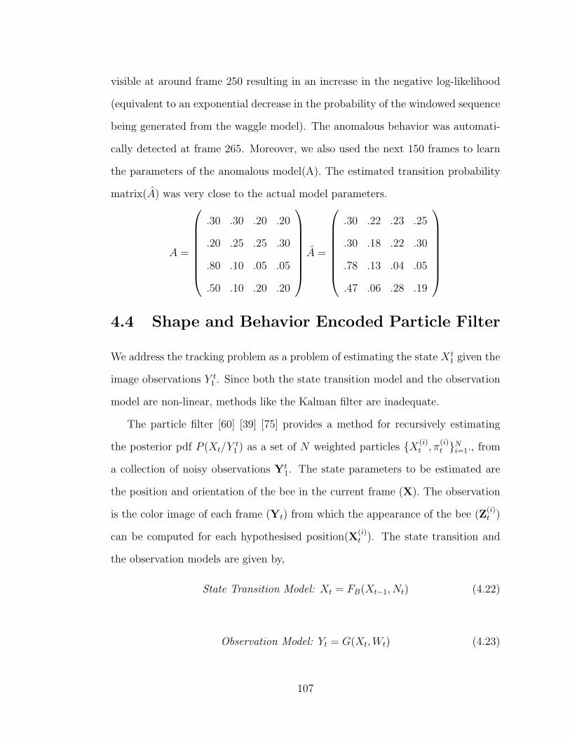
visible at around frame 250 resulting in an increase in the negative log-likelihood
(equivalent to an exponential decrease in the probability of the windowed sequence
being generated from the waggle model). The anomalous behavior was automati-
cally detected at frame 265. Moreover, we also used the next 150 frames to learn
the parameters of the anomalous model(A). The estimated transition probability
matrix(A) was very close to the actual model parameters.
A =
.30 .30 .20 .20
.20 .25 .25 .30
.80 .10 .05 .05
.50 .10 .20 .20
A =
.30 .22 .23 .25
.30 .18 .22 .30
.78 .13 .04 .05
.47 .06 .28 .19
4.4 Shape and Behavior Encoded Particle Filter
We address the tracking problem as a problem of estimating the state X t1 given the
image observations Y t1 . Since both the state transition model and the observation
model are non-linear, methods like the Kalman filter are inadequate.
The particle filter [60] [39] [75] provides a method for recursively estimating
the posterior pdf P (Xt/Yt1 ) as a set of N weighted particles {X(i)
t , π(i)t }Ni=1., from
a collection of noisy observations Yt1. The state parameters to be estimated are
the position and orientation of the bee in the current frame (X). The observation
is the color image of each frame (Yt) from which the appearance of the bee (Z(i)t )
can be computed for each hypothesised position(X(i)t ). The state transition and
the observation models are given by,
State Transition Model: Xt = FB(Xt−1, Nt) (4.22)
Observation Model: Yt = G(Xt,Wt) (4.23)
107

where, Nt is the system noise and Wt is the observation noise. The state
transition function FB characterizes the state evolution for a certain behavior B.
In usual tracking problems, the motion model is used to characterize the state
transition function. In our current algorithm, the behavioral model described in
Section 3.1 is used as the state transition function. Therefore, the state at time t,
(Xt) depends upon the state at the previous frame (Xt−1), the behavioral model
and the system noise. The observation function G models the appearance of the
the bee (in the current frame) as a function of its current position(state Xt), and
observation noise. Once such a description for state evolution has been made, the
particle filter provides a method for representing and estimating the posterior pdf
P (Xt/Yt1 ) as a set of N weighted particles {X(i)
t , π(i)t }Ni=1. Then the state Xt can
be estimated as the MAP estimate as given below,
XMAPt = arg max
Xt
π(i)t (4.24)
The complete algorithm is given below
1. Initialize the tracker with a sample set according to a prior distribution p(X0).
2. For Frame = 1, 2, ...
(a) For sample i = 1, 2, 3, ...N
• Resample Xt−1 = {π(i)t−1}
• Predict the sample X(i)t by sampling from FB(X
(i)t−1, Nt) where FB is a Markov
model for the behavior B estimated in the previous frame.
• Compute Weights for the particle using the likelihood model i.e., π(i)t =
p(Yt/X(i)t ). This is done by first computing the predicted appearance of the bee
using the function G and then evaluating its probability from the observation
noise model.
(b) Normalize the weights using π(i)t = π
(i)t /
∑N
i=1 π(i)t so that the particles represent
a probability mass function.
108

(c) Estimate the MAP or MMSE estimate of the state Xt. using the particles and
their weights.
(d) Compute the maximum likelihood estimate (st)for the current motion state given
the position and orientation in the current and previous frame.
(e) Estimate the behavior of the bee using a ML estimate from the various behavior
models as B = arg maxj P (stt−24/Bj)., where Bjforj = 1, 2, .. indicate the behaviors
modeled.
4.4.1 Prediction and Likelihood Model
In typical tracking applications it is customary to use motion models for prediction
[75] [88] [13] [179]. We use behavioral models in addition to motion models. The
use of such models for prediction improves tracking performance significantly.
Given the location of the bee in the current frame (Xt) and the image observa-
tion given by (Yt), we first compute the appearance (Zt) of the bee in the current
frame (i.e., the color image of the three ellipse anatomical model of the bee ).
Therefore, given this appearance (Z(i)t ) for each hypothesised position X
(i)t , the
weight for the ith particle (π(i)t ) is updated as
π(i)t = p(Yt/X
(i)t ) = p(Z
(i)t /X
(i)t ) (4.25)
where, Yt is the observation. Since the appearance of the bee changes drastically
over the video sequence, we use an appearance model consisting of multiple color
exemplars(A1, A2, .., A5). The RGB components of color are treated independently
and identically. The appearance of the bee in any given frame is assumed to be
Gaussian centered around one of these five exemplars, i.e.,
P (Zt) =1
5
i=5∑
i=1
0.2 N(Z;Ai,Σi) (4.26)
109

whereN(Z;Ai,Σi) stands for the Normal distribution with mean Ai and covariance
Σi. In practice, we modeled the covariance matrix as a diagonal matrix with equal
elements on the diagonal, i.e., Σi = σI, where I is the identity matrix. The mean
observation intensities A1 − A5 are learnt by specifying the location of the bee
in 5 arbitary frames of the video sequence. In practice, we also used 4 of these 5
exemplars from the training database, while the 5th exemplar was estimated from
the initialization provided in the first frame of the current video sequence. In either
case the performance was similar. For extremely challenging sequences, with large
variations in lighting the former method performed better than the latter.
4.4.2 Inference of Dynamics, Motion and Behavior
Inference on the three tier hierarchical model is performed using a greedy approach.
The inference for the lower tiers is first performed independently and these esti-
mates are then used in the inference for the next tier. Estimating the current
position and orientation of the insect (X t) is performed using a particle filter with
observation and state transition models as described in the previous section. Once
the position and the orientation are estimated using the particle filter, we then use
these estimates to infer about the current motion state. The maximum likelihood
estimate for the current motion state given the position and orientation in the
current and previous state is estimated as
stML = arg maxmi i=1,2,3...
P (X t − X t−1|st = mi) (4.27)
Finally, we also need to estimate the behavior of the insect in the current frame.
Once again, we assume that the inference for the lower tiers has been completed
and based on the estimated motion states s1:t, we infer the maximum likelihood
estimate for the current behavior. In order to perform this, we also need to decide
110

an appropriate window length W . From section 4.3.7, we see that a window length
W of 25 is a good trade-off between recognition performance and smoothing across
behavior transitions. Therefore, we do a maximum likelihood estimation for the
behavior using a window length of 25 frames as
B = arg maxjP (stt−W+1|Bj). (4.28)
Since the behavior model Bj, is a simple Markov model of order 1 given by the
transition matrix TBj, this maximum likelihood estimate is easily obtained as
B = arg maxjP (stt−W+1|TBj
) (4.29)
= arg maxj
∏
i=1,2,..W
TBj(st−i, st+1−i) (4.30)
4.5 Experimental Results
4.5.1 Experimental Methodology
For a training database of videos, manual tracking was performed, i.e., at each
frame the position, motion and the behavior of the bee was manually labeled.
Following the steps outlined in Section 4.3.5, the model for dynamics, behavior
and the behavior transitions was learnt. During the test phase, for every test video
sequence, the user first identifies the bee to be tracked and initializes the position
of the bee by identifying four extreme points on the abdomen, thorax and head
respectively. Then the tracking algorithm uses this initialization with a suitably
chosen variance, as the prior distribution p(X0) and automatically tracks both the
position and the behavior of the bee as described in Section 4.4. This is a significant
difference in experimental methodology from most other previous work. In [47],
they first obtain manually tracked data for the entire video sequence to be analysed.
111

Then the Markov model is used in order to classify the various behaviors. In other
related work, like [115] and [116], for each test video sequence, the tracking is
independently accomplished using a tracking algorithm [88], that has no knowledge
of the behavior models. Once the entire video sequence is tracked, then analysis of
the tracked data is performed using specific behavior models. The training phase
for our algorithm is similar to those in [47], [115] and [116] in the sense that all
these algorithms use some kind of labeled data to learn the model parameters for
each behavior. But, our algorithm differs from all the others mentioned above in
that the behavior model thus learnt is used as a prior for tracking, thus enhancing
the tracking accuracy. Moreover, this also means that manual labeling is required
only for the training sequences and not for any of the test videos.
4.5.2 Relation to Previous Work
Previous work in tracking and analyzing the behaviors of bees, have dealt either
with the visual tracking problem [88] or with that of accurately modeling and
analyzing the tracked trajectories of the insects [115] [116] [47]. This is the first
study that tackles both tracking and behavior modeling in a closed loop manner.
By closing the loop, and enabling the tracking algorithm to be aware of the behavior
models, we have improved the tracking performance significantly. Experiments in
the next section will demonstrate the improvement of the tracking performance for
two video sequences that have drastic motions. Once the results of the tracking
algorithm are available, one can in principle analyze the tracked trajectories using
any appropriate behavior model - the hierarchical Markov model or the p-SLDS. In
all the experiments reported in this paper, we have used the hierarchical Markov
motion model to analyze the behavior of the bees.
112

4.5.3 Tracking dancing bees in a hive
We conducted tracking experiments on video sequences of bees in a hive. In all the
experiments reported the training data and the test data were mutually exclusive.
In the videos, the bees exhibited three behaviors- the waggle dance, the round
dance and a stationary bee. In all our simulations we used 300 to 600 particles.
The video sequences ranged between 50 frames to about 700 frames long. It is
noteworthy that when a similar tracking algorithm without a behavioral model
was used for tracking, it lost track within 30-40 frames (See Table 4.1 for details).
With our behavior-based tracking algorithm, we were able to track the bees during
the entire length of these videos. We were also able to extract parameters like
the orientation of the various body parts during each frame over the entire video
sequences. We used these parameters to automatically identify the behaviors. We
also verified this estimate manually and found it to be robust and accurate.
Figure 4.6 shows the structural model of the tracked bee superimposed on the
original image frame. In this particular video, the bee was exhibiting a waggle
dance. The results are best viewed in color since the tracking algorithm had
color images as observations. The figure shows the top five tracked particles (
blue being the best particle and red being the fifth best particle). As is apparent
from the sample frames the appearance of the dancer varies significantly within
the video. These images display the ability of the tracker to maintain track even
under extreme clutter and in the presence of several similar looking bees. Frames
30-34 show the bee executing a waggle dance. Notice that the abdomen of the bee
waggles from one side to another.
113

Figure 4.6: Sample Frames from a tracked sequence of a bee in a beehive. Images
show the top 5 particles superimposed on each frame. Blue denotes the best
particle while red denotes the fifth best particle. Frame Numbers row-wise from
top left :30, 31, 32, 33, 34 and 90. Figure best viewed in color.
Occlusions
Figure 4.7 shows the ability of the behavior based tracker to maintain track during
occlusions in two different video sequences. There is significant occlusion in frames
170, 172 and 187 of video sequence 1. In fact, in fame 172, occlusion forces the
posterior pdf to become bimodal (another bee in close proximity). But we see
that the track is regained when the bee emerges out of occlusion in frame 175.
In frame 187, we see that the thorax and the head of the bee are occluded while
the abdomen of the bee is visible. Therefore the estimate of the abdomen is very
precise (all five particles shown indicate the same orientation of abdomen). Since
the thorax is not visible we see that there is a high variance in the estimate of the
orientation of the thorax and the head. Structural modeling has ensured that, in
114

Figure 4.7: Ability of the behavior based tracker to maintain tracking during
occlusions in two different video sequences. Images show the top 5 particles super-
imposed on each frame- Blue denotes the best particle and red denotes the fifth
best particle. Row 1: Video 1- Frames 170, 172, 175 and 187 and Row 2: Video
2- Frames 122, 123, 129 and 134. Figure best viewed in color.
spite of the occlusion, only physically realizable orientations of the thorax and the
head are maintained. In frame 122 of video sequence 2, we see that another bee
completely occludes the bee being tracked. This creates confusion in the posterior
distribution of the position and orientation. But, behavior modeling ensures that
most particles still track the correct bee. Moreover, at the end of occlusion in
frame 123, the track is regained. Frame 129 in video sequence 2, shows another
case of severe occlusion. But, once again, we see that the tracker maintains track
during occlusion and immediately after occlusion ( Frame 134). Thus behavior
modeling helps to maintain tracking under extreme clutter and severe occlusions.
115

Table 4.1: Comparison of our Behavior based tracking algorithm(BT) with Visual
tracking (VT) [179] and the same visual tracking algorithm enhanced with our
shape model (VT-S)
Video Name Video 1 Video 2
Total Frames 550 200
Algorithm VT VT-S BT VT VT-S BT
Number of 500 500 500 500 500 500
Particles
Successful No No Yes No No Yes
Tracking
Number of 14 10 0 5 5 0
Missed Tracks
Average No. of 37 50 550 33 33 200
Frames Tracked
4.5.4 Importance of Shape and behavioral Model for Track-
ing
To quantify the importance of the shape and the behavioral model in the
above-mentioned tracking experiments, we also implemented another recent and
successful tracking algorithm also based on a particle-filter based inference. We
implemented the visual tracking algorithm based on an adaptive appearance model
described in [179]. We also implemented a minor variation of this algorithm by
incorporating our shape model within their framework. In either case we spent a
significant amount of time and effort in varying the parameters of the algorithm so
116

as to obtain the best possible tracking results with these algorithms. We compare
the performance of our tracking algorithm to the two approaches mentioned above
on two different video sequences in Table 4.1. Both these videos consisted of a
hand-held camera held over the vertical face of the bee-hive. There were several
bees within the field of view of each of these videos, but we were interested in track-
ing the dancing bees in both videos. So, we initialized the tracking algorithm on the
dancers in all these experiments. Moreover, these video sequences were also specif-
ically chosen since the bees exhibited drastic motion changes during the videos and
the illumination and lighting remained fairly consistent during the course of these
videos. This gives us a nice testbed to evaluate the performance of the shape and
behavior model fairly independent of other challenges in tracking like illumina-
tion. The incorporation of the shape constraints improves the performance of the
tracking algorithm showing that an anatomically correct model improves tracking
performance. We declared that a tracking algorithm ”Lost Track” when the dis-
tance between the estimated position of the bee and the actual position of the bee
on the image was greater than half the length of the bee. We see that while the
proposed tracking algorithm was able to successfully track the bee over the length
of the entire video sequences, the other approaches implemented were not able to.
The table also clearly shows that the behavior aided tracking algorithm that we
propose significantly outperforms the adaptive appearance based tracking [179].
4.5.5 Comparison with Ground Truth
We validated a portion of the tracking result by comparing it with a ”ground
truth” track obtained using manual (”point and click”) tracking by an experienced
human observer. We find that the tracking result obtained using the proposed
117

method is very close to manual tracking. The mean differences between manual
and automated tracking using our method are given in Table 4.2. The positional
differences are small compared the average length of the bee, which is about 80
pixels (from front of head to tip of abdomen).
Table 4.2: Comparison of our tracking algorithm with Ground Truth
Average positional difference
between Ground Truth
and our algorithm
Center of Abdomen 4.5 pixels
Abdomen Orientation 0.20 radians (11.5 deg)
Center of Thorax 3.5 pixels
Thorax orientation 0.15 radians (8.6 deg)
4.5.6 Modes of failure
Even in the presence of the improved behavior model based tracking algorithm,
there are some extremely challenging video sequences, where the improved tracking
algorithm resulted in some missed tracks. The primary modes of failure are
• Illunination: We are interested in studying and analyzing bee dances. Bee
dances are typically performed in the dark environment of the bee-hive.
Since the bees typically prefer to dance only in minimal lighting, some of
the videos end up being quite dark. Moreover, there are also significant il-
lumination changes depending upon the exact position of the dancer on the
118

bee hive. These illumination changes posed the most significant challenge for
the tracking algorithm and most of the tracking failures can be attributed to
illumination based challenges in tracking. Even in such videos, the tracking
algorithm with the behavior and anatomical model, outperforms the adap-
tive appearance based tracking algorithm [179]. Recently, a lot of research
effort has been invested in studying and developing appearance models that
are either robust or invariant to illumination changes [52] [173]. Augmenting
the appearance model with illumination invariant appearance models might
reduce some of the errors caused due to illumination changes. Since the focus
of this work was on behavior modeling, we did not systematically analyze
the effect of incorporating such illumination invariant appearance models in
our algorithm.
• Occlusions: Another reason for some of the observed tracking failures, is
occlusions. The bee hive is full of several bees which are very similar in
appearance. Sometimes, the dancing bee disappears below other bees and
then reappears after a few frames. As described in Section 4.5.3, when the
dancing bee is occluded for a relatively small number of frames, the algorithm
is able to regain track when the bee emerges out of occlusions (refer Figure
4.7). But in some videos, the dancing bee remains occluded for over 30 frames
or more. during such cases of extreme occlusions, the tracking algorithm is
unable to regain track. During such cases of extreme occlusions, the only
reasonable way to regain track would be to design an initialization algorithm
that can potentially discover dancing bees in a hive. This would be an
extremely challenging task, considering the complex nature of motions in a
bee hive and the fact that there are several moving bees in every frame of the
119

video. In practice, it might be a good idea to perform manual reinitialization
in such videos.
4.5.7 Estimating Parameters of the Waggle Dance
Foraging honeybees communicate the distance, direction and the attractiveness of
the food source through the waggle dance. The details of the waggle dance were
discussed in detail in Section 4.1. The duration of the waggle portion of the dance
and the orientation of the waggle axis are some of the parameters of interest while
analyzing the bee dances. The duration of the waggle portion of the dance may be
estimated by carefully filtering the orientation of the thorax and the abdomen of
a honeybee as it moves around in its hive. Moreover, the orientation of the waggle
axis can also be estimated from the orientation of the thorax during the periods
of waggle.
Figure 4.8 shows the estimated orientation of the abdomen and the thorax in a
video sequence of around 600 frames. The orientation is measured with respect to
the vertically upward direction in each image frame and a clockwise rotation would
increase the angle of orientation while an anticlockwise rotation would decrease the
angle of orientation.
The waggle dance is characterized by the central waggling portion which is
immediately followed by a turn, a straight run another turn and a return to the
waggling section as shown in Figure 4.3. After every alternate waggling section the
direction of the turning is reversed. This is clearly seen in the orientation of both
abdomen and the thorax. The sudden change in slope (from positive to negative
or vice-versa) of the angle of orientation denotes the reversal of turning direction.
During the waggle portion of the dance, the bee moves its abdomen from one side
120

0 100 200 300 400 500 600−100
0
100
200
300
400
500
Frame number
Orie
ntat
ion
in D
egre
es
Abdomen Orientation
0 100 200 300 400 500 600−100
0
100
200
300
400
500
Frame Number
Orie
ntat
ion
in D
egre
es
Thorax Orientation
Figure 4.8: The orientation of the Abdomen and the Thorax of a bee in a video
sequence of about 600 frames
to another while continuing to move forward slowly. The large local variation in
the orientation of the abdomen just before every reversal of direction shows the
waggling nature of the abdomen. Moreover, the average angle of the thorax during
the waggle segments denotes the direction of the waggle axis.
In order to estimate the parameters of the waggle dance, we use some heuristics
described below. During the waggling portion of the dance, the bee moves its
abdomen from one side to another in the direction transverse to the direction of
motion. The average absolute motion of the center of the abdomen about an axis
transverse to the axis of motion is used as a waggle detection statistic. When this
statistic is large then the probability of waggle during that particular frame is large.
121

Table 4.3: Comparison of Waggle Detection with hand labeling by expert
Automated Labeling Expert Labeling
(Frame Numbers) (Frame Numbers)
Waggle 1 46 - 55 46 - 56
Waggle 2 88 - 95 89 - 97
Waggle 3 127 - 141 127 - 140
Waggle 4 171 - 180 171 - 181
Waggle 5 210 - 222 211 - 222
Waggle 6 255 - 274 257 - 274
Waggle 7 406 - 424 407 - 423
Waggle 8 444 - 461 444 - 461
Waggle 9 486 - 502 486 - 502
Waggle 10 532 - 543 534 - 544
Moreover, we also recognize that the waggle portion of the dance is followed by a
change in the direction of turning. Therefore, only those frames that are followed
by a change in direction of turning and have a high ’waggle detection statistic’ are
labeled as waggle frames. Once the frames in which the bee waggles are estimated,
it is then relatively straightforward to estimate the waggle axis. The waggle axis
is estimated as the average orientation of the thorax during a single waggle run.
Table 4.3 shows the frames that were detected as waggle frames automatically. We
also hand-labeled the same video sequence by an expert. The Table also shows
the frames that were labeled as ’waggle’ by the expert. There were a total of 138
frames that were labeled as ’waggle’ by the expert. Of these 138 frames, 133 frames
were correctly labeled automatically using the procedure described above.
122

4.6 Conclusions and Future Work
We proposed a method using behavioral models to reliably track the position/orientation
and the behavior of an insect and applied it to the problem of tracking bees in a
hive. We also discussed issues in learning models, discriminating between behav-
iors and detecting and modeling abnormal behaviors. Specifically, for the waggle
dance, we also proposed and used some simple statistical measures to estimate
the parameters of interest in a waggle dance. The modeling methodology is quite
generic and can be used to model activities of humans by using appropriate fea-
tures. We are working to extend the behavior model by modeling interactions
among insects. We are also looking to extend the method to problems like analyz-
ing human activities.
123

Chapter 5
Coded Aperture Photography for
Light-Field Capture
In this chapter, we describe a theoretical framework for reversibly modulating 4D
light fields using an attenuating mask in the optical path of a lens based camera.
Based on this framework, we present a novel design to reconstruct the 4D light field
from a 2D camera image without any additional refractive elements as required
by previous light field cameras. The patterned mask attenuates light rays inside
the camera instead of bending them, and the attenuation recoverably encodes the
rays on the 2D sensor. Our mask-equipped camera focuses just as a traditional
camera to capture conventional 2D photos at full sensor resolution, but the raw
pixel values also hold a modulated 4D light field. The light field can be recovered
by rearranging the tiles of the 2D Fourier transform of sensor values into 4D planes,
and computing the inverse Fourier transform. In addition, one can also recover
the full resolution image information for the in-focus parts of the scene.
124

5.1 Introduction
The trend in computational photography is to capture more optical information
at the time of capture to allow greater post-capture image processing abilities.
The pioneering work of Ng et al. [112] has shown a hand-held plenoptic camera
where the user can adjust focus and aperture settings after the picture has been
taken. The key idea is to capture the entire 4D light field entering via the lens
and incident on the camera sensor. In a conventional camera, the sensed 2D image
is a 2D projection of the 4D light field [113] and it is not possible to recover the
entire 4D light field. Using a clever arrangement of optical elements, it is possible
to re-bin the 4D rays and capture them using a 2D sensor [57, 112]. These lens
arrays perform the optical implementation of the two plane parameterization of
the light field [61,95].
Eventually, advances in computational photography may free us from nearly all
of the adjustments, settings, and hard choices a photographer must make before
”taking the picture”. Recent publications explain ways to change long-standing
photographic procedures so that we can re-light, re-color [5,45,127], re-expose, re-
position, re-arrange [3], re-time [133], and gently re-animate our captured visual
experiences long after the time of capture itself. We are particularly interested in
how conventional single-lens film-like cameras might better capture what we want
to see when we press the camera’s shutter release.
For example, inspired by Adelson’s early plenoptic camera [2], Ng et al. [112]
and Georgiev et al. [57] both developed a hand-held SLR camera that gathers a
fully 4D light field in a single shutter-click. ’Re-binning’ sensor data from these
cameras can approximate the output of a conventional 2D camera, but it also allows
users to modify their focussing distances, change the depth of focus (aperture), and
125

make mild viewpoint changes. This adjustability comes at a high cost in image
resolution, however. Each camera uses clever sets of lens elements to arrange the
4D set of rays that enter the camera into an interleaved set of ’sub-images’ on the
sensor, and both apply the 2-plane parameterization introduced with lightfields
and lumigraphs [61, 95]. The number of interleaved images divides the resolution
of each; Ng’s 16Mpixel camera achieves fine angular resolution (14x14) but modest
spatial resolution (320x240), while Georgiev et al. chose lower angular resolution
and higher spatial resolution. This tradeoff is difficult to modify for either camera
design, because it would require precise replacements for lens arrays.
However, optical re-binning of rays forces a fixed and permanent tradeoff be-
tween spatial and angular resolution via the array of lenses. In this chapter, we
describe novel hybrid imaging/light field camera designs that are much more easily
adjustable; users change a single attenuating mask rather than arrays of lenses.
We call this Dappled Photography, as the mask shadows the incoming light and
dapples the sensor. We exploit the fact that light rays can be linearly combined:
rather than sense each 4D ray on its own pixel sensor, our design allows sensing
linearly independent weighted sums of rays, rays combined in a coded fashion that
can be separated by later decoding. Our mapping from 4D ray space to a 2D sensor
array exploits heterodyning methods [49] that are best described in the frequency
domain. By exploiting the modulation and convolution theorems [119] in the fre-
quency domain, we derive simple attenuating mask elements that can be placed
in the camera’s optical path to achieve Fourier domain re-mapping. No additional
lenses are necessary, and we can compute decoded rays as needed in software.
The mask-encoded 2D/4D hybrid camera provide: (a) 4D light field at low
spatial resolution, in addition to a full resolution 2D image of the parts of the
126

scene that were in focus at capture time; and (b) full resolution digital refocusing
for layered Lambertian scenes.
5.1.1 Contributions
We present a set of techniques to encode and manipulate useful portions of a 4D
light field.
• We derive a 4D Fourier domain description of the effect of placing an atten-
uating mask at any position within a conventional 2D camera.
• We identify a new class of 4D cameras that re-map the Fourier transform of
4D ray space onto 2D sensors. Previous 4D cameras used 2D lens arrays to
project 4D ray-space itself rather than it’s Fourier transform.
• We achieve this frequency domain re-mapping using a single transmissive
mask, and our method does not require additional optical elements such as
lens arrays.
Heterodyne Light Field Camera: This design is based on the modulation
theorem in the 4D frequency domain. We capture the light field using a 4D version
of the method known as ’heterodyning’ in radio. We create spectral tiles of the
light field in the 4D frequency domain by placing high-frequency sinusoidal pattern
between the sensor and the lens of the camera. To recover the 4D light field, we
take the Fourier transform of the 2D sensed signal, re-assemble the 2D tiles into
a 4D stack of planes, and take the inverse Fourier transform. Unlike previous 4D
cameras that rely on lens arrays, this hybrid imaging/light field design does not
force resolution tradeoffs for in-focus parts of the scene. The mask does not bend
127

rays as they travel from scene to sensor, but only attenuates them in a fine, shadow-
like pattern. If we compensate for this shadowing, we retain a full-resolution 2D
image of the parts of the scene that were in focus, as well as the lower-resolution
4D light field we recover by Fourier-domain decoding. A prototype for this design
is shown in Figure 5.1.
5.1.2 Benefits and Limitations
Mask-based hybrid imaging/light field cameras offer several advantages over pre-
vious methods. An attenuating mask is far simpler and less costly than lenses or
lens arrays, and avoid errors such as spherical, chromatic aberration, coma, and
mis-alignment. Simpler mounts and flexible masks may allow camera designs that
offer user-selectable masks; photographers could then select any desired tradeoff
in angle vs. spatial resolution. The design of Ng et al. [112] matches main-lens
aperture (f-stop) to the micro-lens array near the detector to avoid gaps or overlaps
in their coverage of the image sensor; mask-only designs avoid these concerns. Our
mask based designs also impose limitations. Masks absorb roughly 50% of usable
light that enters the lens.
5.2 Basics
The Plenoptic function [1] is a 5D function (ignoring wavelength, polarization, and
time) that represents the radiance in every direction (θ, φ ), at every point (x, y,
z ) in free space. This function is redundant in a space free of occluders, and
reduces to a 4D function called the light field [95] [61]. This light-field is a 4D
quantity that completely characterizes light transport in a space free of occluding
128

Scanner
Lens
Mask Sensor Mask SensorLens
Light Field Camera Encoded Blur Camera
bellow
Scanner sensorMask
Figure 5.1: Prototype camera designs. (Top Left) Heterodyne light field camera
holds a narrowband 2D cosine mask (shown in bottom left) near the view camera’s
line-scan sensor. (Top Right) Encoded blur camera holds a coarse broadband mask
(shown in bottom right) in the lens aperture.
objects. A popular light field parameterization is the two-plane parameterization.
Two parallel planes separated by a finite distance describe all the rays between
them. This 4D parameterization, L(u; v; s; t), is frequently used to describe and
understand image formation in cameras and image based rendering techniques.
For visualization purposes, we consider a 2D light field space (LS), with one
spatial dimension x and one angular dimension θ and a 1D detector as shown
in Figure 5.2. We denote variables by lower case letters and their corresponding
Fourier domain representations by upper case letters. Let l(x, θ) denote the 2D
light field parameterized by the twin plane parameterization as shown in Figure 5.2.
The θ-plane is chosen to be the plane of the main lens (or the aperture stop
for cameras composed of multiple lens) of the camera. For the case of planar
Lambertian object, we assume that the x-plane coincides with the object plane.
129

Lens S0Object
x-plane θ-plane
Snear Sfar
Mask
Sensor Positions
l(xi,θ0)
l(xi,θj)
l(xi,-θ0)
fx
fθSensor Slices
Light-Field of a Planar Lambertian Scene
Mask Modulation Function
fx
fθfx
fθ
Modulated Light-Field
θ0
-θ0
λ
Figure 5.2: (Top) In ray-space, focused scene rays from a scene point converge
through lens and mask to a point on sensor. Out of focus rays imprint mask
pattern on the sensor image. (Bottom) In Fourier domain. Lambertian scenes lack
θ variation & form a horizontal spectrum. Mask placed at the aperture lacks x
variation & forms a vertical spectrum. The spectrum of the modulated light field
is a convolution of two spectrums. A focused sensor measures a horizontal spectral
slice that tilts when out-of-focus.
5.2.1 Effects of Optical Elements on the Light Field
We now discuss the effect of various optical elements such as lens, aperture and
sensor to the 2D light field in frequency domain, which we refer as Fourier domain
light field space (FLS). The (x, θ) space is referred to as the primal domain.
Sensor: The image formed on a 1D sensor is a 1D projection of the 2D light
field entering the camera, which also corresponds to a slice of the light field in
Fourier domain. For different focus settings, the obtained images correspond to
slices at different angles/trajectories [113].
Lens: A thin lens shifts the x-plane of the light field to the conjugate plane
according to the thin-lens equation. The lens also inverts the x-plane of the light
field.
Aperture: The aperture of a camera acts as a limiter, allowing only the light
rays that pass through the aperture to enter the camera. The light field l after
130

passing through the aperture is given by
la(x, θ) = l(x, θ)a(x, θ), (5.1)
where a(x, θ) is the aperture modulation function given by a(x, θ) = rect( θ2θ0
),
and 2θ0 is the size of the aperture. From (5.1), the Fourier transform of the light
field after the aperture is given by
LA(fx, fθ) = L(fx, fθ) ⊗ A(fx, fθ), (5.2)
where ⊗ denotes convolution. L and A are the Fourier transforms of the light field
(before the aperture) and the aperture modulation function respectively. Since
a(x, θ) is a rect function,
A(fx, fθ) = 2a0sinc(2a0fθ). (5.3)
5.2.2 FLS and Information Content in the Light Field
A light field is a 4D representation of the light rays in the free-space. A 2D
sensor can only sample a 2D slice of this light field. Depending on the scene, the
information content in the light field is concentrated in different parts of the light
field.
Planar Lambertian Object
Let us assume that the scene being imaged consists of a planar Lambertian object
at the focus plane. Since there are no angular variations in the irradiance of rays
from a Lambertian object, the information content of its light field is restricted to
be along the fx axis (Figure 5.2). Thus, L(fx, fθ) = 0,∀fθ 6= 0. Since L(fx, fθ)
is independent of fθ and A(fx, fθ) is independent of fx, from (5.2) and (5.3) we
131

obtain,
LA(fx, fθ) = L(fx, fθ) ⊗ A(fx, fθ), (5.4)
= L(fx, 0)A(0, fθ), (5.5)
= 2a0L(fx, 0)sinc(2a0fθ). (5.6)
The sensed image is a slice of this modulated light field. When the sensor is in
focus, all rays from a scene point converge to a sensor pixel. Thus, the in-focus
image corresponds to a slice of LA(fx, fθ) along fx (fθ = 0). Let y(s) and Y (fs)
denotes the sensor observation and its Fourier transform respectively. For an in-
focus sensor
Y (fs) = LA(fs, 0) = 2a0L(fs, 0). (5.7)
Thus, no information is lost when the Lambertian plane is in focus.
When the sensor is out of focus, the sensor image is a slanted slice of the
modulated light field as shown in Figure 5.2, where the slant angle λ depends on
the degree of mis-focus. Thus,
Y (fs) = LA(fs cosλ, fs sinλ),
= 2a0L(fs cosλ, 0)sinc(2a0fs sinλ)
(5.8)
Thus, for out of focus setting, the light field gets attenuated by the frequency
transform of the aperture modulation function, which is a sinc function for an
open aperture. This explains the attenuation of the high spatial frequencies in
the captured signal when the scene is out of focus. Thus, we need to modify
the aperture so that the resulting aperture modulation function has a broadband
frequency response, ensuring that high spatial frequencies are preserved in out of
focus images.
132

Incidentally, for a pinhole camera, the aperture function is a Dirac delta func-
tion and the aperture modulation function is broadband in fθ. This explains why
the images captured via a pinhole camera are always in-focus. However, a pinhole
camera suffers from severe loss of light, reducing the signal to noise ratio (SNR) of
the image.
Bandlimited Light Fields
For general scenes, we assume that the light field is bandlimited to fx0 and fθ0 as
shown in Figure 5.4: L(fx, fθ) = 0 ∀|fx| ≥ fx0, |fθ| ≥ fθ0. A traditional camera
can only take a 2D slice of the 4D light field. To recover the entire information
content of the light field, we need to modulate the incoming light field so as to
redistribute the energy from the 4D FLS to the 2D sensor.
5.3 Heterodyne Light Field Camera
In this section, we show that the required modulation can be achieved in frequency
domain by the use of an appropriately chosen 2D mask placed at an appropriate
position between the lens and the sensor. Although a mask is only a 2D modulator,
in tandem with the lens, it can achieve the desired 4D modulation. We believe
that this is the first design of a single-snapshot light field camera that does not
use any additional lenses or other refractive elements.
133

Modulated Light-Field
α = 900
Mask at aperture
Incoming Light-Field
α
Mask between aperture and conjugate plane
fθ
fx
fθ
fx
fθ
fx
fθ
fx
Mask Modulation Function
fθ
fx
fx
fθ
LensObject
θ-plane
Mask Sensor
dv
x-plane
Figure 5.3: Heterodyne light field camera. (Top) In ray-space, the cosine mask at
d casts soft shadows on the sensor. (Bottom) In Fourier domain, scene spectrum
(green on left), convolved with mask spectrum (center) made of impulses creates
offset spectral tiles (right). Mask spectral impulses are horizontal at d = 0, vertical
at d = v, or tilted.
5.3.1 Modulation Theorem and its Implications
According to the modulation theorem [119], when a baseband signal s(x) is multi-
plied by a cosine of frequency f0, it results in copies of the signal at that frequency.
F[cos(2πf0x)s(x)](fx) =1
2(F (fx − f0) + F (fx + f0)), (5.9)
where F[s(x)](fx) = F (fx) denotes the Fourier transform of s(x). This principle
has been widely used in telecommunications and radio systems. The baseband
signal is modulated using a carrier signal of much higher frequency so that it can
be transmitted over long distances without significant loss of energy. The receiver
demodulate the received signal to recover the baseband signal. In essence, what
134

fθ
fx
fθ0
fx0
Mask Modulation Function
Desired
Band-limited
Light Field
α
fθR
fθ Modulated
Light Field
fx
fθ0
fx0Sensor Slice
Mask Modulation
Function
fθR
Demodulation from Sensor Slice
fθ
fxRecovered
Light Field
Figure 5.4: Spectral slicing in heterodyne light field camera. (Left) In Fourier
domain, the sensor measures the spectrum only along the horizontal axis (fθ = 0).
Without a mask, sensor can’t capture the entire 2D light field spectrum (in blue).
Mask spectrum (gray) forms an impulse train tilted by the angle α. (Middle)
By the modulation theorem, the sensor light field and mask spectra convolve to
form spectral replicas, placing light field spectral slices along sensor’s broad fθ = 0
plane. (Right) To re-assemble the light field spectrum, translate segments of sensor
spectra back to their original fx, fθ locations.
we wish to achieve is very similar. We would like to modulate the information in
the angular variations of the light field (fθ frequencies) to higher frequencies in fx
so that the high resolution 1D sensor may be able to sense this information.
Figure 5.4 shows a bandlimited light field in frequency domain. For simplicity,
let us assume the x plane to be the conjugate plane, so that the sensor image
corresponds to a slice along fx (horizontal slice). Now consider a modulator whose
frequency response is composed of impulses arranged on a slanted line as shown
in Figure 5.4. If the light field is modulated by such a modulator, each of these
impulses will create a spectral replica of the light field at its center frequency.
Therefore, the result of this convolution will be several spectral replicas of the light
field along the slanted line. The elegance of this specific modulation is that the
horizontal slice (dashed box) of the modulated light field spectrum now captures
all the information in the original light field. Note that the angle α is designed
135

Sensor
θ -plane x-plane
Lens
Focus Plane
Traditional Capture
θ -plane
SensorLens
Focus Plane
Mask
v
d
Mask-based Light Field Capture
x-plane
Sensor Slice
Mask Modulation Function
Traditional Capture
Mask-based Capture
Recovering Light FieldRearranging FFT
Light
Field FFTFFT
Modulated Sensor Image Sensor FFT
Recovered Light Field Recovered FFT of Light Field
x
x
Sensor
FFTSensor
Image
fθ
fx
fx
fx
x
θ
IFFTIFFT
x
θ
Inte
nsity
Inte
nsity
Figure 5.5: Ray space and Fourier domain illustration of light field capture. The
flatland scene consists of a dark background planar object occluded by a light
foreground planar object. In absence of a mask, the sensor only captures a slice
of the Fourier transform of the light field. In presence of the mask, the light field
gets modulated. This enables the sensor to capture information in the angular
dimensions of the light field. The light field can be obtained by rearranging the
1D sensor Fourier transform into 2D and computing the inverse Fourier transform.
based upon the required frequency resolution in θ and x, and the bandwidth of
the incoming light field.
136

Heterodyne receivers in telecommunications demodulate the incoming signal to
recover the baseband signal. In our case, demodulation must also redistribute the
energy in the sensed 1D signal to the 2D light field space. The process of demod-
ulation consists of rearranging the frequency response of the sensor to recover the
bandlimited light field as shown in Figure 5.4.
5.3.2 Mask based Heterodyning
Now we show that the required modulation can be achieved by placing a suitably
chosen attenuating mask in the optical path of a conventional camera.
Masks as Light Field Modulators: A mask is essentially a special 1D code
c(y) (2D for 4D light field) placed in the optical path. In flatland, although the
mask is 1D, its modulation function is 2D (Figure 5.3). The mask affects the
light field differently depending on where it is placed. If the mask is placed at
the aperture stop (θ plane), then the effect of mask is to multiply the aperture
modulation function by the mask modulation function. The mask modulation
function m(x, θ) is then given by m(x, θ) = c(y = θ), i.e., the modulation function
is independent of x. Intuitively, when placed at the θ-plane, the mask affects all
rays at an angle θ in similar way, independent of the scene point from which they
are originating.
If the mask is placed at the conjugate plane, it attenuates all rays (independent
of θ) for same x equally. This is because at the conjugate plane, all rays originating
from a point on the plane of focus converge to a single point. Thus, the mask
modulation function changes to m(x, θ) = c(y = x).
Thus, we see that the modulation function corresponding to placing the same
code at the aperture and the conjugate plane are related by a rotation of 90◦ in the
137

2D light field space. Moreover, as the 1D code is moved from the aperture plane
to the plane of the sensor, the resulting mask modulation function gets rotated in
2D as shown in Figure 5.3.
Let v be the distance between the aperture and the conjugate plane. If the
mask c(y) is placed at a distance d from the conjugate plane, the mask modulation
function is given by
M(fx, fθ) = µ2C(µ√
f 2x + f 2
θ )δ(fθ cosα− fx sinα), (5.10)
where C denotes the Fourier transform of the 1D mask and µ = 1/√
(d/v)2 + (1 − (d/v))2.
The angle α is given by
α = arctan(d/(v − d)) (5.11)
In other words, the mask modulation function has all its energy concentrated
on a line in the 2D FLS space. The angle α of this line with respect to the fx axis
depends upon the position of the mask. When the mask is placed at the conjugate
plane (d = 0), the angle α is equal to 0. As the mask moves away from the
conjugate plane towards the aperture, this angle increases to 90◦ at the aperture
plane as shown in Figure 5.3,
Optimal Mask Position: In order to capture the 2D light field, we need the
modulation function M(fx, fθ) to be a series of impulses at an angle α given by
α = arctanfθR2fx0
, (5.12)
where fx0 is the bandwidth of the light field along the fx axis and fθR represents
the desired frequency resolution along the fθ axis. For example, in Figure 5.4, the
frequency resolution has been depicted as being equal to fθR = (2/5)fθ0, where fθ0
is the bandwidth of the light field along the fθ axis. Thus, for capturing a light
field of a given bandwidth, the physical position of the mask can be calculated
138

from (5.12) and (5.11). In practice, since the spatial resolution is much larger than
the angular resolution, α is very small, and therefore the mask needs to be placed
close to the sensor.
Optimal Mask Pattern: To achieve M(fx, fθ) as a set of 1D impulses on
a slanted 2D line, the Fourier transform C(f) of the 1D mask should be a set
of impulses. Let 2p + 1 be the number of impulses in M(fx, fθ). The Fourier
transform of the 1D mask is then given by
C(f) =
k=p∑
k=−p
δ(f − kf0), (5.13)
where f0 denotes the fundamental frequency and is given by f0 = µ√
4fx02 + fθR
2.
From Figure 5.4, (2p + 1)fθR = 2fθ0. The bandwidth in fθ is discretized by fθR.
Hence, the number of angular samples obtained in the light field will be equal to
2fθ
fθR= 2p+1. Since the Fourier transform of the optimal mask is a set of symmetric
Dirac delta functions (along with DC), this implies that the physical mask is a
sum of set of cosines of a given fundamental frequency f0 and its harmonics. The
number of required harmonics is in fact p, which depends upon the band-width of
the light field in the fθ axis and the desired frequency resolution fθR.
Solving for 2D Light Field: To recover the 2D light field from the 1D
sensor image, we compute the Fourier transform of the sensor image, reshape the
1D Fourier transform into 2D as shown in Figure 5.4 and compute the inverse
Fourier transform. Thus,
l(x, θ) = IFT(reshape(FT(y(s)))), (5.14)
where FT and IFT represent the Fourier and inverse Fourier transforms respectively,
and y(s) is the observed sensor image. Figure 5.5 shows a simple example of light
139

0 0.2 0.4 0.6 0.8 1
−0.2
0
0.2
0.4
0.6
0.8
1
cycles/mm
f0
2f0
3f0
4f0
DC
Sum
Figure 5.6: (Left) Zoom in of a part of the cosine mask with four harmonics.
(Right) Plot of 1D scan line of mask (black), as sum of four harmonics and a
constant term.
field capture where the scene consists of a dark background plane occluded by a
light foreground plane.
5.3.3 Note on 4D Light Field Capture
Even though the analysis and the construction of mask-based heterodyning for light
field capture was elucidated for 2D light fields, the procedure remains identical
for capturing 4D light fields with 2D sensors. The extension to the 4D case is
straightforward. In case of a 4D light field, the information content in the 4D light
field is heterodyned to the 2D sensor space by the use of a 2D mask placed between
the aperture and the sensor. The Fourier transform of the 2D mask would contain
a set of impulses on a 2D plane.
C(f1, f2) =
k1=p1∑
k1=−p1
k2=p2∑
k2=−p2
δ(f1 − k1fx0 , f2 − k2f
y0 ). (5.15)
140

fθ10 1 2 43
012
43
fθ2
fx2
fx1
-4 -3 -2 -1
-1-2-3-4
Figure 5.7: (Top Left) Magnitude of the 2D Fourier transform of the captured
photo shown in Figure 5.8. θ1, θ2 denote angular dimensions and x1, x2 denote
spatial dimensions of the 4D light field. The Fourier transform has 81 spectral
tiles corresponding to 9×9 angular resolution. (Bottom Left) A tile of the Fourier
transform of the 4D light field corresponding to fθ1 = 1, fθ2 = 1. (Top Right)
Refocused images. (Bottom Right) Two out of 81 views. Note that for each view,
the entire scene is in focus. The horizontal line depicts the small parallax between
the views, being tangent to the white circle on the purple cone in the right image
but not in the left image.
Since negative values in the mask cannot be realized as required, we need to boost
the DC component of C(f1, f2) so as to make the mask positive throughout. Fig-
ure 5.6 shows a part of the 2D cosine mask we used for experiments, along with
the plot of one of its scanline. This 2D mask consists of four harmonics in both
dimensions (p1 = 4, p2 = 4) with fundamental frequencies fx0 and f y0 being equal
to 1 cycle/mm. This allows an angular resolution of 9 × 9 in the 4D light field.
Figure 5.7 shows the magnitude of the Fourier transform of the captured photo
of the cones (as shown in Figure 5.8). The Fourier transform clearly shows 9 × 9
spectral tiles created due to the modulation by the mask. These spectral tiles
141

Figure 5.8: Our heterodyne light field camera provides 4D light field and full-
resolution focused image simultaneously. (First Column) Raw sensor image. (Sec-
ond Column) Scene parts which are in-focus can be recovered at full resolution.
(Third Column) Inset shows fine-scale light field encoding (top) and the corre-
sponding part of the recovered full resolution image (bottom). (Last Column) Far
focused and near focused images obtained from the light field.
encode the information about the angular variation in the incident light field. To
recover the 4D light field, demodulation involves reshaping of the sensor Fourier
transform in 4D. Let t1 = 2p1 + 1 and t2 = 2p2 + 1 be the number of angular
samples in the light field and let the captured 2D sensor image be N ×N pixels.
We first compute the 2D FFT of the sensor image. Then we rearrange t1 × t2 tiles
of the 2D Fourier transform into 4D planes to obtain a (N/t1) × (N/t2) × t1 × t2
4D Fourier transform. Inverse FFT of this 4D Fourier transform gives the 4D light
field. In Figure 5.8, using a 1629 ∗ 2052 pixel image captured with a cosine mask
having four harmonics, we obtain a light field with 9 × 9 angular resolution and
181 × 228 spatial resolution.
5.3.4 Formal Derivation for Mask based Heterodyning
This analysis is done for a 1D mask placed in front of a 1D sensor to capture a
2D light field. Let v be the total distance between the aperture and the sensor
142

Main Lens
1D Sensor
θ -plane
x-plane
A
v
Mask = c(y)
d = βv
Schematic Layout of Lens, Mask and Sensor
β = d/vθ
xy
(1-β) v
y = βθ + (1-β) x
Figure 5.9: Schematic showing a 1D code place in front of a 1D sensor to capture
a 2D light field. The light field is parameterized as twin-plane, with the x plane
aligned with the sensor and the θ plane aligned with the aperture.
143

and d be the distance between the mask and the sensor. Define β = dv. From
Figure 5.3.4, if we place the 1D code c(y) at a distance d from the sensor, the
resulting 2D light field gets attenuated by the 2D mask m(x, θ) given by
m(x, θ) = c(βθ + (1 − β)x). (5.16)
As we will derive below, the Fourier transform of the mask lies on a line in the 2D
Fourier light field space.
Let C(fy) be the 1D Fourier transform of c(y)
C(fy) =
∫ inf
− inf
c(y) exp(−j2πfyy)dy (5.17)
and let M(fx, fθ) be the 2D Fourier transform of m(x, θ):
M(fx, fθ) =
∫ inf
− inf
∫ inf
− inf
m(x, θ) exp(−j2πfxx) exp(−j2πfθθ)dxdθ. (5.18)
We wish to find the expression of M(fx, fθ) in terms of C(y). Let
y = βθ + (1 − β)x (5.19)
Use auxiliary variable
z = (1 − β)θ − βx (5.20)
Define
µ =1
√
β2 + (1 − β)2(5.21)
Then
θ = µ2(βy + (1 − β)z) (5.22)
x = µ2((1 − β)y − βz) (5.23)
Jacobian
144

J = det
∂θ∂y
∂θ∂z
∂x∂y
∂x∂z
(5.24)
J = µ2 (5.25)
By change of variables, we have
M(fx, fθ) = J
∫ inf
− inf
∫ inf
− inf
c(y) exp(−j2πfyy) exp(−j2πfzz)dydz (5.26)
Substituting x and θ from (5.22) and (5.23) in (5.18), and comparing common
terms, we get
fy = µ2(fx(1 − β) + fθβ) (5.27)
fz = µ2(−fxβ + fθ(1 − β)) (5.28)
Integrating out z term will give a δ term. Thus
M(fx, fθ) = JC(fy)δ(fz) (5.29)
Now substitute tanα = β
1−βThen sinα = µβ and cosα = µ(1 − β)
Substituting in equation for fy, we get
fy = µ(fx cosα+ fθ sinα) (5.30)
Simplifying δ(fz), we get
δ(fz) = δ(fθ cosα− fx sinα) (5.31)
Finally
M(fx, fθ) = µ2C(µ(fx cosα+ fθ sinα))δ(fθ cosα− fx sinα) (5.32)
145

The δ function constraints the 2D Fourier transform of mask to lie along a line
given by fθ cosα − fx sinα = 0 Using this constraint the above equation can be
simplified to
M(fx, fθ) = µ2C(µ√
f 2x + f 2
θ )δ(fθ cosα− fx sinα). (5.33)
Thus,
tanα =β
1 − β=
d
v − d. (5.34)
and
µ =1
√
β2 + (1 − β)2=
1√
(d/v)2 + (1 − (d/v))2(5.35)
Practical Design
In a practical design, first α is calculated using the frequency resolution in θ, fθR
and the bandlimit fx0 of the light field in the spatial dimension. fθR is relate to
the size of the aperture A. fθR = 1/A.
tanα =fθR2fx0
(5.36)
Once we know α and the total distance between the sensor and the aperture
v, we can find d using (5.34). The fundamental frequency can be obtained using
(5.33) by substituting fx = 2fx0 and fθ = fθR
f0 = µ√
4f 2x0 + f 2
θR (5.37)
In practice, µ is close to 1 and α is ≈ 4 − 5 degrees.
146

5.3.5 Aliasing
Traditionally, undersampling results in masquerading of higher frequencies as lower
frequencies in the same channel and leads to visually obtrusive artifacts like ghost-
ing. In heterodyne light field camera, when the band-limit assumption is not valid
in the spatial dimension, the energy in the higher spatial frequencies of the light
field masquerade as energy in the lower angular dimensions. No purely spatial
frequency leaks to other purely spatial frequency. Thus, we do not see familiar
jaggies, moire-like low-frequency additions and/or blocky-ness in our results. The
effect of aliasing is discussed in detail in [162], where using the statistics of nat-
ural images, it is shown that the energy in the aliasing components is small. To
further combat the effects of aliasing, we post-filter the recovered light field using
a Kaiser-Bessel filter with a filter width of 1.5 [113].
5.3.6 Light Field based Digital Refocusing
Refocused images can be obtained from the recovered Fourier transform of the light
field by taking appropriate slices [113]. Figure 5.8 and Figure 5.7 shows refocused
cone images. The depth variation for this experiment is quite large. Notice that
the orange cone in the far right was in focus at the time of capture and we are
able to refocus on all other cones within the field of view. Figure 5.11 shows the
performance of digital refocusing with varying amounts of blur on the standard
ISO-12233 resolution chart. Using the light field, we were able to significantly
enhance the DOF. It is also straightforward to synthesize novel views from the
recovered light field. Two such views generated from the recovered light field are
also shown in the bottom right part of Figure 5.7. The horizontal line on the
images depicts small vertical parallax between the two views. Digital refocusing
147

Figure 5.10: Our heterodyne light field camera can be used to refocus on complex
scene elements such as the semi-transparent glass sheet in front of the picture of
the girl. (Left) Raw sensor image. (Middle) Full resolution image of the focused
parts of the scene can be obtained as described in Section 5.3.7. (Right) Low
resolution refocused image obtained from the light field. Note that the text on the
glass sheet is clear and sharp in the refocused image.
based on recovered light fields allow us to refocus even in the case of complicated
scenes such as the one shown in Figure 5.10. In this example, a poster of the girl
in the back is occluded by a glass sheet in front. Notice that the text ’Mask based
Light Field’ written on the glass sheet is completely blurred in the captured photo.
By computing the light field, we can digitally refocus on the glass sheet bringing
the text in focus.
5.3.7 Recovering High Resolution Image for Scene Parts
in Focus
Our heterodyne light field camera has an added advantage that we can recover high
resolution information for the in-focus Lambertian parts of the scene. Consider a
scene point that is in sharp focus. All rays from this scene point reach the same
sensor pixel but are attenuated differently due to the mask. Therefore, the sensor
pixel value is the product of the scene irradiance and the average value of the mask
within the cone of rays reaching that pixel. This attenuation γ(x, y) varies from
148

pixel to pixel and can either be computed analytically or recovered by capturing a
single calibration image of a uniform intensity Lambertian scene. We can recover
the high resolution image I(x, y) of the scene points in focus as
I(x, y) = s(x, y)/γ(x, y), (5.38)
where s(x, y) is the captured sensor image. Parts of the scene that were not in
focus at the capture time will have a spatially varying blur in I(x, y). We use the
image of a uniform intensity Lambertian light box as γ.
In Figure 5.8, zoomed in image region shows the attenuation of the sensor
image due to the cosine mask. The recovered high resolution picture is also shown
in Figure 5.8 and the inset shows the fine details recovered in the parts of the
image that were in focus. Figure 5.11 shows the recovered high resolution picture
of a resolution chart that was in focus during capture. This ability to obtain high
resolution images of parts of the scene along with the 4D light field makes our
approach different from previous light field cameras.
5.4 Non Rectangular Band-Limits for Light-Field
The design in [159] was optimized assuming that the shape of the band-limit was
rectangular as shown in Figure 5.4. But in real-world scenarios, the incident light
field spectrum has specific shape characteristics that are heavily dependent upon
the depth of objects in the scene [26, 44]. We show how to optimize the mask
so as to match the shape of the band-limit in the frequency domain. Usually, the
spatial resolution of light field is reduced by a factor equal to the number of angular
samples in captured light field. However, by optimizing the mask, better spatial
resolution can be achieved as shown below. For illustration, we assume 2D light
149

Figure 5.11: Analysis of the refocusing ability of the heterodyne light field camera.
(Left) If the resolution chart is in focus, one can obtain a full resolution 2D image
as described in Section 5.3.7, along with the 4D light field. (Middle) We capture
out of focus chart images for three different focus settings. (Right) For each setting,
we compute the 4D light field and obtain the low resolution refocused image. Note
that large amount of defocus blur can be handled.
fields captured by 1D sensor, but it easily extends to 4D light fields captured by
2D sensor.
Let us assume that the band-limit light field is shaped as shown in Figure 5.12(a),
with reducing spatial bandwidth as the angular frequency increases. Let the
band-limits be given by (fx0, fx1, fx2) corresponding to the angular frequencies
(fθ = 0, fθ = fθR, fθ = 2fθR) as shown in Figure 5.12. Now consider a ray modu-
lation function given by
R(fx, fθ, :) =
i=p∑
i=−p
δ(fx − fi, fθ − fi tan(α), :), (5.39)
where fi = 0, i = 0 and fi = fx0 + 2∑j=i−1
j=1 fxj + fxi,∀i > 0. This ray modula-
tion function will lead to a series of unequally placed impulses and corresponding
spectral copies of the light field as shown in Figure 5.12. The sensor image (red
box) is a slice of the modulated light field (from Fourier Slice Theorem [113]).
Note that the modulation function is now optimized so that the spectral copies are
150

fθ
fxfx0
Modulation Function optimized to the shape of
the bandwidth of the
lightfield.
fx0+fx1
fx0+2fx1+fx2
fθ0 fx1
fx2
fθModulated LightField
fx
fθ0
fx0Sensor Slice
Modulation
Function
fθ
fxRecovered
LightField Spectrum
Demodulation from Sensor Slice
Figure 5.12: Optimal sampling of light fields. (Left) The bandlimit of the light field
is not rectangular as in [159]. (Middle) The light field is modulated with cosines of
appropriate frequencies (non-harmonics) so that the spectral replicas abut tightly
on the sensor slice and there is no wastage of sensor pixels. Note that the spectral
replicas could overlap in other parts of the spectrum which are not captured by
the sensor. (Right) Demodulation involves reshaping the sensor Fourier transform
as before accounting for unequal spectrum width in different angular samples.
tightly abut on the sensor without any gaps. If we have used a mask with impulses
equally placed, it would have resulted in gaps on sensor slice corresponding to no
information in the light field. Moreover, if the depth range of the scene is known
apriori, this leads to a specific shape of the light field band-limit [26, 44] and one
can potentially use this information to optimally sample the light field.
5.5 Implementation and Analysis
Heterodyne Light Field Camera: We build a large format camera using a
flatbed scanner (Canon CanoScan LiDE 70) similar to [168,174] and place a 8×10
inch2 mask behind the scanner glass surface. The mask was printed at a resolution
of 80 dots/mm using Kodak LVT continuous tone film recorder (BowHaus Inc.).
The scanner itself was then placed on the back of a large format view camera fitted
with a 210 mm f/5.6 Nikkor-W lens as shown in Figure 5.1. In practice, the motion
151

of the scanner sensor is not smooth leading to pattern noise (horizontal/vertical
lines) in the captured photo. This may lead to some artifacts in the recovered
light fields. However, many of these issues will disappear with a finer mask placed
inside a conventional digital camera. Calibration involves accounting for the in-
plane rotation and shift of the mask with respect to the sensor which manifest as
search for the rotation angle of the captured 2D image and the phase shift of the
Fourier transform. Since the computation of the light field and refocusing is done
in Fourier domain, computational burden is low.
Failure Cases: The heterodyne light field camera assumes a bandlimited light
field. When this assumption is not true, it leads to aliasing artifacts in the recovered
light field. To recover larger angular resolution in the light field, the 2D cosine mask
needs to be moved away from the sensor, which might result in diffraction.
5.6 Applications of captured Light-Fields
In this section, we show two examples of captured light-field using the implemen-
tation described. Firstly, we printed a 2D sum of cosines mask with frequencies
of 5, 10, 15, 20 cycles/mm allowing us to obtain 2 × 4 + 1 = 9 angular samples in
the light field with spatial resolution of 240 × 180 (Results shown in Figure 5.13).
We also printed another 2D sum of cosines mask with frequencies of 8, 16, 24 cy-
cles/mm allowing us to obtain 2× 3+1 = 7 angular samples in the light field with
spatial resolution of 340 × 250 (Results shown in Figure 5.14).
152

(a) Captured Modulated Image
(b) Focus on Doll
(c) Focus on face
(d) Depth map
(e) All in Focus
Figure 5.13: (a) Captured Modulated Image (b) Low Resolution Refocussed Image
- Focus on Doll (c) Low Resolution Refocussed Image - Focus on face (d) Raw
Depth labels quantized to 10 depth levels. (e) All in focus image.
5.6.1 Depth from Focus
Once we have captured the light field, images focused at any depth can be obtained
by taking appropriate slices from the Fourier transform of the captured light field
[113]. Figure 5.13(a) and 5.14(a) show the captured images of two scenes with
significant texture and depth variations. Figures 5.13(b,c) and 5.14(b,c,d) show
different refocused images for each dataset. We can extract depth from refocussed
images since scene points that are not in focus are blurred while scene points in
focus are sharp in the refocused images. So for a given pixel ’p’, if we study a small
region around the pixel, then, this region will be sharp in the refocused image at
the correct depth while it will be blurred at all other depths. We use the variance
of the neighborhood around each pixel as a measure of sharpness. Each pixel is
assigned the depth corresponding to the refocused image in which the variance of
its neighborhood is maximum. Such an assignment (10 depth levels) is shown in
153

(b) Focus Back (c) Focus Center (d) Focus Front
(e) Estimated Depth Map
(f) All in Focus Image
(a) Captured Modulated Image
Figure 5.14: (a) Captured Modulated Image (b) Refocussed Image - Focus on back
poster (c) Refocussed Image - Focus on doll (d) Refocussed Image - Focus on front
Scotch box (e) Raw Depth labels quantized to 10 depth levels. (e) All in focus
image.
154

5.13(d) and 5.14(e).
5.6.2 All Focus Image
We can also obtain the all-in-focus image just as is obtained in [113] from the
estimated depth map and the corresponding refocussed images. For each pixel we
choose the intensity from the refocused image corresponding to its estimated depth
resulting in an all-in-focus images as shown in Figure 5.13(e) and Figure 5.14(f).
Supplementary materials include Matlab code and input images as well as videos
showing digital refocusing.
5.6.3 3D Texture mapped model
We can also obtain a 3D texture mapped estimate of the scene, since we have
the depth estimates and the corresponding irradiance(intensity) estimates. This
allows us to recover a 3D texture mapped surface corresponding to the scene by
appropriately combining the depth and irradiance estimates to create a 3D texture
mapped surface. We can also synthesize novel views from the estimated 3D texture
mapped model.
5.7 Discussion
Future Directions: To capture the light field, we need to use masks that match
the resolution of the sensor. It is already possible to print RGB Bayer mosaics at
pixel resolution. This is ideal for the future trend of digital cameras where pixels
are becoming smaller to achieve higher resolution. Such high resolution masks will
support heterodyning as well as Bayer mosaic operations in a single mask. Our
155

current masks are effectively 2D in a 4D space, but in the future one may use masks
that are angle and location dependent like a hologram to achieve a complete 4D
effect. We hope our work in broadband and cosine masks will also stimulate more
ideas in mask functions including colored and polarized masks to estimate scene
properties.
Our broadband coding can be pushed in higher dimension, for example, by
coding both in time [133] and space. The benefit of masks compared to lenses is
the lack of wavelength dependent focusing and chromatic aberrations. This fact is
commonly used in astronomy. Hence, masks can be ideal for hyper-spectral imag-
ing. Shallow depth of field is a serious barrier in medical and scientific microscopy.
The facility to refocus while maintaining full resolution will be a great benefit. In
combination with confocal coded aperture illumination one maybe able to capture
digitally refocused images in a fewer incremental steps of the focal planes.
Conclusions: We showed that two different kinds of coded masks placed inside
a conventional camera will each allow us to make a different kind of computational
improvement to the camera’s pictures. First, if we place a fine, narrowband mask
slightly above the sensor plane, then we can computationally recover the 4D light
field that enters the main camera lens. The mask preserves our camera’s ability
to capture the focused part of the image at the full resolution of the sensor, in the
same exposure used to capture the 4D light field. Second, if we place a coarse,
broadband mask at the lens aperture, we can computationally refocus an out of
focus image at full resolution. As this refocusing relies on deconvolution, we can
correct the focusing for images that require constant or piecewise-planar focusing.
These and other masks are not magical: mask reduces sensor illumination by ≈ 1
f-stop and refocusing exacerbates noise. However, high-quality masks may be less
156

demanding than lens arrays to mount, align, or arrange in interchangeable sets and
they avoid optical errors such as radial error, spherical and chromatic aberration,
and coma. We believe that masks offer a promising new avenue for computational
methods to substantially improve digital photography.
Appendix: Source Code
% Source Code for Computing 4D Light-Field from Captured 2D Photo% Mask contains Cosines with 4 Harmonics leading to 9X9 Angular Samples
m = 2133; n=1719 % Size of Captured ImagenAngles = 9; cAngles = (nAngles+1)/2; % Number of Angular Samples
F1Y = 237; F1X = 191; %Cosine Frequency in Pixels from Calibration Image
phi1 = 300; phi2 = 150; % PhaseShift due to Mask In-Plane Transltn wrt SensorF12X = floor(F1X/2); F12Y = floor(F1Y/2);
%Compute Spectral Tile Centers, Peak Strengths and Phasefor i=1:nAngles ; for j=1:nAngles
CentY(i,j) = (m+1)/2 + (i-cAngles)*F1Y;CentX(i,j) = (n+1)/2 + (j-cAngles)*F1X;
Mat(i,j) = exp(sqrt(-1)*((phi1*pi/180)*(i-cAngles) + (phi2*pi/180)*(j-cAngles))); end; end
Mat(cAngles,cAngles) = Mat(cAngles,cAngles) * 20;
f = fftshift(fft2(imread(‘InputCones.png’))); %Read Photo and Perform 2D FFT
%Rearrange Tiles of 2D FFT into 4D Planes to obtain FFT of 4D Light-Fieldfor i = 1: nAngles; for j = 1: nAngles
FFT_LF(:,:,i,j) = f(CentY(i,j)-F12Y:CentY(i,j)+F12Y,…
CentX(i,j)-F12X:CentX(i,j)+F12X)/Mat(i,j);end; end
LF = ifftn(ifftnshift(FFT_LF)); %Compute Light-Field by 4D Inverse FFT
157

Chapter 6
Discussions and Future Directions
The first part of this dissertation studied the problem of characterizing, learning
and classifying dynamic patterns that appear in video. Specific attention was
paid to apllications such as gait based person identification, activity recognition,
comparing shape sequences, simultaneous tracking and behavior analysis. It was
shown that solutions to these issues may be posed as a problem in inferring and
mathematically characterizing the nature of the dynamics of the relevant patterns
in video. Some of the areas for future work are listed below.
6.1 Comparing ShapeSequences
6.1.1 Shape descriptor for Comparing Shape Sequences
We used Kendall’s statistical shape as the shape feature for comparing shape se-
quences. Kendall’s statistical shape is a sparse descriptor of the shape. We could,
in theory choose a denser shape descriptor like the shape context [7] which has
been proven to be more resilient to noise. But, such a dense descriptor also intro-
158

duces significant and non-trivial relationships between the individual components
of the descriptor. This usually makes learning the dynamics very difficult. Since
the emphasis of this proposal is on modeling the dynamics in shape sequences, we
restricted ourselves to the treatment of dynamics in Kendall’s statistical shape.
We could look at models for comparing shape sequences that are based on more
complex shape descriptors like the shape context. It is expected that using such
complex and robust shape descriptors will improve the performance of these algo-
rithms significantly while also making the learning and the inference tasks more
complex.
6.1.2 View-Invariance
The models developed for comparing shape sequences in this dissertation have
not incorporated the important property of view invariance that is usually highly
desirable in several computer vision applications. Incorporating view invariance
into these models is an important avenue for future research. One way to make
these models view-invariant is to use features that are themselves view invariant.
Once the feature chosen is view-invariant, then all the algorithms described in the
previous sections in turn become view invariant. Another way to incorporate view-
invariance is to build these models for a discrete set of views separately. Once we
have a model for each activity in every possible view, then the inference algorithms
could be suitably modified to incorporate view-invariance. But, this would require
a huge amount of data to learn the model for each activity, since the learning
algorithm must learn the activity from every possible viewpoint. Which of these
two approaches turn out to be more efficient would depend upon the application
being considered. For applications in far field surveillance and activity analysis,
159

where the number of discrete views required is small, learning a model for each of
these discrete viewpoints might be a viable alternative. For applications in near
field activity analysis, where the number of discrete views one must account for is
large, the best alternative might be to choose appropriate view invariant features.
6.2 Action Analysis and Recognition
6.2.1 Noise Sensitivity of the Activity Model
The noise sensitivity of the learning algorithm for simultaneous inference of the
nominal activity trajectory and the activity specific time warping space has not
been studied in detail. It would be interesting to study and analyse the sensitivity
of the learning algorithm to noise in the data. Noise in the data could be of
two forms. There could be observation noise because of the characteristics of the
imaging sensors and the limited resolution offered by these sensors. There could
also be labelling noise because of incorrect labelling of activity sequences. Robust
techniques to detect incorrect labelling need to be developed so that the inference
process is robust to outliers. Moreover, studying the noise sensitivity of the learning
algorithm will also enable us to improve the learning algorithm. This issue is
related to modeling the distribution of time-warping transformations and we are
looking at algorithms that are able to tackle both these issues simultaneously.
6.2.2 Spatial Alignment of Activities
Another issue of concern is the spatial alignment of sequences. There is significant
variety in the spatial alignment within an activity. For example the action of sitting
might be accompanied by the two legs being very close to each other or further
160

apart as is the preference of the individual. Since the activity model proposed
corrects only the temporal misalignments in the execution of an activity, in its
current form it is not adequate to reliably tackle spatial alignment preferences
of an individual. In the current model, small spatial misalignments are tackled
as temporal misalignments. We are addressing the larger spatial misalignments,
using a mixture of models, where each mixture represents one type of spatial
alignment preference. It might also be possible to simultaneously perform both
spatial and temporal alignments, though this would be at the cost of significant
computational expense. The method would, in principle, be very similar to the
clustering of activity sequences described earlier. The various sequences of an
activity would be clustered into several different clusters each cluster representing
one particular spatial alignment preference.
6.3 Clustering and Indexing of Action Videos
The focus of this dissertation has been on the problem of recognition or classifi-
cation with respect to activity analysis. Another allied problem is the problem
of automatic activity baased video clustering or indexing which has applications
in several domains such as surveillance, traffic monitoring and multimedia enter-
tainment. This problem is gaining in importance because of the ever increasing
role of videos in our everyday lives with applications ranging from broadcast news,
entertainment, scientific research, security and surveillance. There has been signif-
icant research into indexing of multimedia data such as news clips, sports videos
etc according to their content. Applications for automatic discovery of activity
patterns are numerous. For example, security and surveillance videos typically
have repetitive activities. If the typical activities can be clustered, then several
161

problems such as unusual activity detection, efficient indexing and retrieval can be
addressed. In applications of video forensics, instead of expecting an analyst to
sift through the voluminous data, we ask - can ‘clusters’ of activities be presented
that embody the essential characteristics of the videos.
6.3.1 An Approach we are exploring
Given a continuous video stream, if we knew what activities occur in it, we can
discover the boundaries between them and if we were given the boundaries, the
individual activities could be learnt as well. For unsupervised video clustering, we
need to solve the segmentation and model estimation problems simultaneously. We
use coherent patterns of motion to discover individual segment boundaries and the
transitions between segments are used to learn activity models. Each individual
segment is modeled using a linear dynamical system. Each activity then consists
of a specific sequence of dynamical systems.
The entire video is first segmented in short coherent patterns. The entire set of
segments is assumed to be derived from an underlying vocabulary. This vocabulary
is learnt using unsupervised clustering of the segments. Once the vocabulary is
learnt, we then learn grammatical rules from the video to discover longer activities.
In our case, the grammatical rules are simple sequences of segment labels.
We augment the traditional dynamical systems model in important ways. We
derive methods to incorporate view and rate invariance into these models so that
similar actions are clustered together irrespective of the viewpoint or the rate of
execution of the activity. We also derive algorithms to learn the model parameters
from a video stream and demonstrate how a single video sequence may be clustered
into different clusters where each cluster represents an activity. We show here
162

some preliminary results using our approach on a dataset of skating videos. We
performed a clustering and retrieval experiment on the figure skating dataset. This
data is very challenging since it is unconstrained and involves rapid motion of both
the skater and real-world motion of the camera including pan, tilt and zoom.
We built color models of the foreground and background using normalized
color histograms. The color histograms are used to segment the background and
foreground pixels. Median filtering followed by connected component analysis is
performed to reject small isolated blobs. From the segmented results, we fit a
bounding box to the foreground pixels by estimating the 2D mean and second
order moments along x and y directions.We perform temporal smoothing of the
bounding box parameters to remove jitter effects. The final feature is a rescaled
binary image of the pixels inside the bounding box.
Clustering Experiment: Most figure skating videos consist of a few estab-
lished elements or moves such as jumps, spins, lifts and turns. A typical perfor-
mance by skater or pair of skaters includes several of these elements each performed
several times. Due to the complex body postures involved it is a challenge even
for humans to identify clear boundaries between atomic actions. It was difficult
even for us to semantically define temporal boundaries of an activity, let alone
define a metric for temporal segmentation. Thus, this makes it very difficult to
break the video into temporally consistent segments. Instead of performing ex-
plicit segmentation, we build models for fixed length subsequences using sliding
windows. The results of a temporal segmentation algorithm that can split such
a complex video into meaningful segments, can be easily plugged in. We use 20
frame long overlapping windows for building models of the video. Also, most of
the interesting activities such as sitting spins, standing spins, leaps etc are usually
163

few and far between. Further, due to the subsequence approach, there will neces-
sarily be several segments that do not contain any meaningful action. As a simple
example, a subsequence that contains the transition from a spin to a jump will
not fit into either of these action-clusters. To discover the interesting activities,
we first need to remove these outlier segments. First, we cluster all the available
subsequences into a fixed number of clusters (say 10). Then, from each cluster
we remove the outliers using a simple criterion of average distance to the cluster.
Then, we recluster the remaining segments. We show some sample sequences in
the obtained clusters in figures 14 18. We observe that Clusters 1 - 4 correspond
dominantly to Sitting Spins, Standing Spins, Camel Spins and Spirals respectively
(in a spiral the skater glides on one foot while raising the free leg above hip level).
Cluster 5 on the other hand seems to capture the rest of the uninteresting actions.
6.4 Computaional Imaging
6.4.1 Coded Aperture Imaging for Glare Aware Photogra-
phy
Glare arises due to multiple scattering of light inside the cameras body and lens
optics and reduces image contrast. While previous approaches have analyzed glare
in 2D image space, we have begun analysing glare as a 4D ray-space phenomenon.
By statistically analyzing the ray-space inside a camera, we can classify and remove
glare artifacts. In ray-space, glare behaves as high frequency noise and can be
reduced by outlier rejection. While such analysis can be performed by capturing
the light field inside the camera, it results in the loss of spatial resolution. Unlike
light field cameras, we do not need to reversibly encode the spatial structure of
164

Figure 6.1: Shown above are a few sequences from Cluster1. Each row
shows contiguous frames of a sequence. We see that this cluster dominantly
corresponds to ‘Sitting Spins’. Image best viewed in color. Please see
http://www.umiacs.umd.edu/∼pturaga/VideoClustering.html for video results.
165

Figure 6.2: Shown above are a few sequences from Cluster2. Each row
shows contiguous frames of a sequence. Notice that this cluster dominantly
corresponds to ‘Standing Spins’. Image best viewed in color. Please see
http://www.umiacs.umd.edu/∼pturaga/VideoClustering.html for video results.
166

Figure 6.3: Shown above are a few sequences from Cluster3. Each row
shows contiguous frames of a sequence. Notice that this cluster domi-
nantly corresponds to ‘Spirals’. Image best viewed in color. Please see
http://www.umiacs.umd.edu/∼pturaga/VideoClustering.html for video results.
167

the rayspace, leading to simpler designs. We explore masks for uniform and non-
uniform ray sampling and show a practical solution to analyze the 4D statistics
without significantly compromising image resolution. Although diffuse scattering
of the lens introduces 4D low-frequency glare, we can produce useful solutions in
a variety of common scenarios. Such an approach handles photography looking
into the sun and photos taken without a hood, removes the effect of lens smudges
and reduces loss of contrast due to camera body reflections. Figure 6.4 shows a
comparison of glare formation in ray-space. It shows how inserting a high frequency
occluder in the optical path of the camera the low frequency glare components are
converted to high frequency 2D image information and can therefore be easily
removed by simple filtering. Figure 6.5 shows an example of an image captured
in the presence of a high frequency occluder. Using a 4D analysis of glare inside
the camera, we can emphasize or reduce glare. The photo in the middle shows
a person standing against a sunlit window. We extract reflection glare generated
inside lens and manipulate it to synthesize the result shown on the left. On the
right we show the glare-reduced component. Notice that the face is now visible
with improved contrast.
6.4.2 Coded Illumination
This dissertation was focussed on the effect of a non-refractive coded aperture and
how to enhance the flexibility available during photography using such coded aper-
tures. In some applications such as capturing Bidirection Reflectance Distribution
Functions (BRDF) it might be acceptable to use active illumination. Bidirection
Reflectance Distribution Function (BRDF) is a 4-dimensional function that de-
scribes how an opaque surface point reflects incoming light [135]. The incoming
168

Figure 6.4: Comparison of glare formation in ray-space and sensor image for a
traditional camera and our mask based camera. A focused blue scene patch could
contribute to scattering (cyan), reflection (purple) and body glare (green). Since
the sensor image is a projection of the ray-space along angular dimensions, the
sum of these components creates a low frequency glare for a traditional camera.
However, by inserting a high frequency occluder (gray), in front of the sensor, these
components are converted into a high frequency 2D pattern and can be separated.
169

Figure 6.5: We extract glare components from a single-exposure photo in this
high dynamic range scene. Using a 4D analysis of glare inside the camera, we
can emphasize or reduce glare. The photo in the middle shows a person standing
against a sunlit window. We extract reflection glare generated inside lens and
manipulate it to synthesize the result shown on the left. On the right we show
the glare-reduced component. Notice that the face is now visible with improved
contrast.
lighting direction θ is a two-dimensional quantity (azimuth and elevation) while
the outgoing lighting direction φ is another two-dimensional quantity making the
BRDF 4-dimensional function B(θ, φ). The slice of the BRDF corresponding to
the viewing direction being fixed ( as would be the case when the scene is being
observed by a fixed camera ), while the incident illumination changes freely, is
called the reflectance field and is a two-dimensional function R(θ). Observing and
measuring the reflectance field of an object or a scene typically involves acquiring
images of the object/scene under varying illumination conditions. Typical meth-
ods for capturing such reflectance fields are based on acquiring images with a single
light source ’ON’ in each image. Recently, [137] have shown that using multiple
light sources per each acquired image and performing a linear inversion in order
to recover the reflectance field results in higher signal to noise ratios of the cap-
tured reflectance fields. Nevertheless, the number of images to be acquired to infer
170

the reflectance field remains identical to the number of illumination sources. Re-
cently, we have been working on a method for acquiring accurate reflectance fields
of objects with significantly lower number of captured images than the number of
illumination sources. This reduction in the number of required images is achieved
by exploiting recent developments in compressive sensing, which essentially show
that if the signal to be acquired is sparse in some basis, then the signal can be
accurately reconstructed using sub-Nyquist linear samples of the signal. We have
emperically found that reflectance fields are sparse in the Haar wavelet basis. We
wish to motivate our analysis using the Phong illumination model and empirically
verify the degree of sparsity. We are currently developing a scheme for capturing
reflectance fields using multiplexed illumination, thereby achieving the signal-to-
noise ratio advantages of multiplexed illumination and use a compressive sensing
based recovery algorihm to infer reflectance fields. Such methods using active il-
lumination to capture visual properties of surfaces might be another avenue for
active future research.
171

BIBLIOGRAPHY
[1] E.H. Adelson and J.R. Bergen. The plenoptic function and the elements ofearly vision. Computational Models of Visual Processing, 1, 1991.
[2] T. Adelson and J.Y.A Wang. Single lens stereo with a plenoptic camera.IEEE Trans. on Pattern Analysis and Machine Intelligence, 14:99–106, 1992.
[3] Aseem Agarwala, Mira Dontcheva, Maneesh Agrawala, Steven Drucker, AlexColburn, Brian Curless, David Salesin, and Michael Cohen. Interactive dig-ital photomontage. ACM Trans. Graph., 23(3):294–302, 2004.
[4] J.K. Aggarwal and Q. Cai. Human motion analysis: A review. ComputerVision and Image Understanding, 73(3):428–440, 1999.
[5] A. Agrawal, R. Raskar, S.K. Nayar, and Y. Li. Removing photographyartifacts using gradient projection and flash-exposure sampling. ACM Trans.Graph., 24(3):828–835, 2005.
[6] E.M. Arkin, L.P. Chew, D.P. Huttenlocher, K. Kedem, and J.S.B. Mitchell.An efficiently computable metric for polygonal shapes. IEEE Trans. onPattern Analysis and Machine Intelligence, 27:209–216, 1986.
[7] S. Belongie, J. Malik, and J. Puzicha. Shape matching and object recogni-tion using shape contexts. IEEE Trans. on Pattern Analysis and MachineIntelligence, 24:509–522, April 2002.
[8] R. Berthilsson. A statistical theory of shape. Statistical Pattern Recognition,pages 677–686, 1998.
[9] A. Bhattacharya. On a measure of divergence between two statistical popu-lations defined by their probability distributions. Bull. Calcutta Math. Soc.,35:99–109, 1943.
[10] A. Bissacco, A. Chiuso, Y. Ma, and S. Soatto. Recognition of human gaits.Conference on Computer Vision and Pattern Recognition, 2:52–57, 2001.
[11] A. Bissacco, P. Saisan, and S. Soatto. Gait recognition using dynamic affineinvariants. Proc. Of MTNS 2004, Belgium, July 2004.
172

[12] M. Black and A. Jepson. Eigentracking: Robust matching and tracking ofarticulated objects using a view-based representation. International Journalof Computer Vision, 26(1):63–84, 1998.
[13] M.J. Black and A.D. Jepson. A probabilistic framework for matching tempo-ral trajectories. International Conference on Computer Vision, 22:176–181,1999.
[14] S.S. Blackman and R. Popoli. Design and Analysis of Modern TrackingSystems. Artech House, 1999.
[15] A. Blake, B. North, and M. Isard. Learning multi-class dynamics. Advancesin NIPS, pages 389–395, 1999.
[16] M. Blank, L. Gorelick, E. Shechtman, M. Irani, and R. Basri. Actions asSpace-Time Shapes. Computer Vision, 2005. ICCV 2005. Tenth IEEE In-ternational Conference on, 2, 2005.
[17] H. Blum and R. Nagel. Shape description using weighted symmetric axisfeatures. Pattern Recognition, 10:167–180, 1978.
[18] A. Bobick and Tanawongsuwan. Performance analysis of time-distance gaitparameters under different speeds. 4th International Conference on Audioand Video based Biometric Person Authentication,Guilford,UK, June 2003.
[19] A.F. Bobick and A. Johnson. Gait recognition using static activity-specificparameters. Conference on Computer Vision and Pattern Recognition, Dec.2001.
[20] F.L. Bookstein. Size and shape spaces for landmark data in two dimensions.Statistical Science, 1:181–242, 1986.
[21] M. Brand, N. Oliver, and A. Pentland. Coupled hidden markov models forcomplex action recognition. Computer Vision and Pattern Recognition, pages994–999, 1997.
[22] C. Bregler. Learning and recognizing human dynamics in video sequences.CVPR, 1997.
[23] P.J. Brockwell and R.A. Davis. Time Series: Theory and Methods. Springer-Verlang, 1987.
[24] T.J. Broida, S. Chandra, and R. Chellappa. Recursive techniques for theestimation of 3-d translation and rotation parameters from noisy image se-quences. IEEE Transactions on Aerospace and Electronic systems, AES26:639–656, 1990.
173

[25] C. Cedras and M. Shah. Motion-based recognition a survey. Image andVision Computing, 13(2):129–155, 1995.
[26] Jin-Xiang Chai, Shing-Chow Chan, Heung-Yeung Shum, and Xin Tong.Plenoptic sampling. In SIGGRAPH, pages 307–318, 2000.
[27] MT Chan, A. Hoogs, R. Bhotika, A. Perera, J. Schmiederer, and G. Doretto.Joint Recognition of Complex Events and Track Matching. Computer Visionand Pattern Recognition, 2006 IEEE Computer Society Conference on, 2,2006.
[28] C. C. Chen. Improved moment invariants for shape discrimination. PatternRecognition, 26(5):683–686, 1993.
[29] J.C. Cheng and J.M.F. Moura. Capture and representation of human walkingin live video sequence. IEEE Transactions on Multimedia, 1(2):144–156,1999.
[30] O. Chomat and J.L. Crowley. Probabilistic recognition of activity usinglocal appearance. Proceedings of the IEEE Computer Society Conference onComputer Vision and Pattern Recognition, 2:104–109, 1999.
[31] K.D. Cock and D.B. Moor. Subspace angles and distances between armamodels. Proc. of the Intl. Symp. of Math. Theory of networks and systems,2000.
[32] R.T. Collins, R. Gross, and J. Shi. Silhoutte based human identificationusing body shape and gait. Intl. Conf. on Automatic Face and GestureRecognition, pages 351–356, October 2002.
[33] D. Comaniciu, V. Ramesh, and P. Meer. Real-time tracking of non-rigid ob-jects using mean-shift. Conference on Computer Vision and Pattern Recog-nition, 2:142–149, 2000.
[34] D. Cunado, M.J. Nash, S.M. Nixon, and N.J Carter. Gait extraction anddescription by evidence gathering. Proc. of the Intl. Conf. on AVBPA, pages43–48, 1994.
[35] J.E. Cutting and L.T. Kozlowski. Recognizing friends by their walk : Gaitperception without familiarity cues. Bulletin of the Psychonomic Society,9(5):353–356, 1977.
[36] J.E. Cutting and D.R. Proffitt. Gait perception as an example of how wemay perceive events. Intersensory perception and sensory integration, 1981.
174

[37] P. Dollar, V. Rabaud, G. Cottrell, and S. Belongie. Behavior recognitionvia sparse spatio-temporal features. Visual Surveillance and PerformanceEvaluation of Tracking and Surveillance, 2005. 2nd Joint IEEE InternationalWorkshop on, pages 65–72, 2005.
[38] A. Doucet and N. De Freitas. Sequential Monte Carlo Methods in Practice.Springer, 2001.
[39] A. Doucet, N.D. Freitas, and N. Gordon. Sequential Monte Carlo methodsin practice. Springer-Verlag, New York, 2001.
[40] E. R. Dowski and W.T. Cathey. Extended depth of field through wavefrontcoding. Appl. Optics, 34(11):1859–1866, April 1995.
[41] E. R. Dowski and G. E. Johnson. Wavefront coding: A modern methodof achieving high performance and/or low cost imaging systems. In SPIEAnnual Meeting, August 1999.
[42] I.L. Dryden. Statistical shape analysis in high level vision. IMA Workshop:Image analysis and High level vision, 2000.
[43] I.L. Dryden and K.V. Mardia. Statistical shape analysis. John Wiley andsons, 1998.
[44] Fredo Durand, Nicolas Holzschuch, Cyril Soler, Eric Chan, and Francois X.Sillion. A frequency analysis of light transport. ACM Trans. Graph.,24(3):1115–1126, 2005.
[45] E. Eisemann and F. Durand. Flash photography enhancement via intrinsicrelighting. ACM Trans. Graph., 23(3):673–678, August 2004.
[46] H Farid and E.P. Simoncelli. Range estimation by optical differentiation.Journal of the Optical Society of America A, 15(7):1777–1786, 1998.
[47] A. Feldman and T. Balch. Automatic identification of bee movement usinghuman trainable models of behavior. Mathematics and Algoritms of SocialInsects, Dec 2003.
[48] R. Fergus, A. Torralba, and W.T. Freeman. Random lens imaging. Technicalreport, MIT, 2006.
[49] R.A. Fessenden. Wireless telephony. Trans. American Institute of ElectricalEngineers, 27:553–629, 1908.
[50] S. Fine, Y. Singer, and N. Tishby. The hierarchical hidden markov model:Analysis and applications. Machine Learning, 32(1):41–62, 1998.
175

[51] J.P. Foster, M.S. Nixon, and A. Prugel-Bennett. Automatic gait recognitionusing area-based metrics. Pattern Recognition Letters, 24:2489–2497, 2003.
[52] D. Freedman and M.W. Turek. Illumination-invariant tracking via graphcuts. IEEE International Conference on Computer Vision and PatternRecognition, 2005.
[53] H. Freeman. On the encoding of arbitary geometric configurations. IRETransactions, 10:260–268, 1961.
[54] D.M. Gavrila. The visual analysis of human movement: A survey. CVIU,73(1):82–98, January 1999.
[55] D.M. Gavrilla. The visual analysis of human movement: A survey. Else-vier Journal on Computer Vision and Image Understanding, 73(1):82–98,January 1999.
[56] D. Geiger, T. Liu, and R.V. Kohn. Representation and self-similarity ofshapes. IEEE Trans. on Pattern Analysis and Machine Intelligence, 25-1:86–99, January 2003.
[57] T. Georgiev, C. Zheng, S. Nayar, B. Curless, D. Salasin, and C. Intwala.Spatio-angular resolution trade-offs in integral photography. In EurographicsSymposium on Rendering, pages 263–272, 2006.
[58] G. Golub and C.V. Loan. Matrix Computations. The Johns Hopkins Uni-versity Press, Baltimore, 1989.
[59] S. Gong and T. Xiang. Recognition of group activities using dynamic prob-abilistic networks. Computer Vision, 2003. Proceedings. Ninth IEEE Inter-national Conference on, pages 742–749, 2003.
[60] N.J. Gordon, D.J. Salmond, and A.F.M Smith. Novel approach to non-linear/non-gaussian babayesian state estimation. IEE Proceedings on Radarand Signal Processing, 140:107–113, 1993.
[61] S.J. Gortler, R. Grzeszczuk, R. Szeliski, and M.F. Cohen. The lumigraph.In SIGGRAPH, pages 43–54, 1996.
[62] A. Goshtasby. Description and discrimination of planar shapes using shapematrices. IEEE Trans. on Pattern Analysis and Machine Intelligence, 7:738–743, 1985.
[63] Stephen R. Gottesman and E. E. Fenimore. New family of binary arrays forcoded aperture imaging. Appl. Optics, 28(20):4344–4352, Oct 1989.
176

[64] A. Gritai, Y. Sheikh, and M. Shah. On the use of anthropometry in theinvariant analysis of human actions. ICPR, 2004.
[65] Paul Haeberli. A multifocus method for controlling depth of field. Grafi-caObscura, 1994.
[66] G.D. Hager and P.N. Belhumeur. Efficient region tracking with parametricmodels of geometry and illumination. IEEE Trans. on Pattern Analysis andMachine Intelligence, 20:1025–1039, 1998.
[67] J. Han and B. Bhanu. Individual recognition using gait energy image. Work-shop on Multimodal User Authentication (MMUA 2003), pages 181–188, De-cember 2003.
[68] S. Hiura and T. Matsuyama. Depth measurement by the multi-focus camera.In Conference on Computer Vision and Pattern Recognition, pages 953–961,1998.
[69] E. Hoenkamp. Perceptual cues that determine the labelling of human gait.Journal of Human Movement Studies, 4:59–69, 1978.
[70] S. Hongeng and R. Nevatia. Large-scale event detection using semi-hiddenMarkov models. Computer Vision, 2003. Proceedings. Ninth IEEE Interna-tional Conference on, pages 1455–1462, 2003.
[71] M.K. Hu. Visual pattern recognition by moment invariants. IRE Transac-tions on Information Theory, 8:179–187, 1962.
[72] T. Huang, D. Koller, J. Malik, G. Ogasawara, B. Rao, S. Russell, and J. We-ber. Automatic symbolic traffic scene analysis using belief networks. Pro-ceedings 12th National Conference in AI, pages 966–972, 1994.
[73] S.S. Intille and A.F. Bobick. A framework for recognizing multi-agent actionfrom visual evidence. AAAI/IAAI, 99:518–525, 1999.
[74] A. Isaksen, L. McMillan, and S.J. Gortler. Dynamically reparameterizedlight fields. In SIGGRAPH, pages 297–306, 2000.
[75] M. Isard and A. Blake. Contour tracking by stochastic propogation of con-ditional density. European Conference on Computer Vision, pages 343–356,1996.
[76] M. Isard and A. Blake. Icondensation: Unifying low-level and high-leveltracking in a stochastic framework. European Conference on Computer Vi-sion, 1:767–781, 1998.
177

[77] H. Ives. Camera for making parallax panoramagrams. J. Opt. Soc. Amer.,17:435–439, 1928.
[78] A.K. Jain. Fundamentals of digital image processing. Prentice-Hall, Inc.Upper Saddle River, NJ, USA, 1989.
[79] B. Javidi and F. Okano, editors. Three-Dimensional Television, Video andDisplay Technologies. Springer-Verlag, 2002.
[80] G. Johansson. Visual perception of biological motion and a model for itsanalysis. PandP, 14(2):201–211, 1973.
[81] G. E. Johnson, E. R. Dowski, and W. T. Cathey. Passive ranging throughwave-front coding: Information and application. Applied Optics, 39:1700–1710, 2000.
[82] B.H. Juang and L.R. Rabiner. A probabilistic distance measure for hiddenmarkov models. ATT Technical Journal, 64:391–408, 1985.
[83] A. Kale, AKR Chowdhury, and R. Chellappa. Towards a view invariant gaitrecognition algorithm. Proceedings. IEEE Conference on Advanced Videoand Signal Based Surveillance, 2003., pages 143–150, 2003.
[84] A. Kale, A.N Rajagopalan, Sundaresan.A., N. Cuntoor, A. Roy Cowdhury,V. Krueger, and R. Chellappa. Identification of humans using gait. IEEETransactions on Image Processing, Under review.
[85] Karcher, H. Riemannian center of mass and mollifier smoothing. Communi-cations on Pure and Applied Mathematics, 30:509–541, 1977.
[86] R. Kashyap and R. Chellappa. Stochastic models for closed boundary anal-ysis: Representation and reconstruction. IEEE Transactions on InformationTheory, 27:627–637, 1981.
[87] D.G. Kendall. Shape manifolds, procrustean metrics and complex projectivespaces. Bulletin of London Mathematical society, 16:81–121, 1984.
[88] Z. Khan, T. Balch, and F. Dellaert. A rao-blackwellized particle filter foreigen tracking. Conference on Computer Vision and Pattern Recognition,2004.
[89] A. Khotanzad and Y.H. Hong. Invariant image recognition by zernikemoments. IEEE Trans. on Pattern Analysis and Machine Intelligence,12(5):489–497, 1990.
178

[90] X. Koutsoukos and P. Antsaklis. Hierarchical control of piecewise linearhybrid dynamical systems based on discrete abstractions. ISIS TechnicalReport, Feb 2001.
[91] B. Laxton, J. Lim, and D. Kriegman. Leveraging temporal, contextualand ordering constraints for recognizing complex activities in video. Com-puter Vision and Pattern Recognition, 2007. CVPR’07. IEEE Conferenceon, pages 1–8, 2007.
[92] H.J. Lee and Z. Chen. Determination of 3d human body posture from a singleview. Computer Vision, Graphics, Image Processing, 30:148–168, 1985.
[93] L. Lee, G. Dalley, and K. Tieu. Learning pedestrian models for silhoutterefinement. International Conference on Computer Vision, 2003.
[94] M. Levoy, B. Chen, V. Vaish, M. Horowitz, M. McDowall, and M. Bolas.Synthetic aperture confocal imaging. ACM Trans. Graph., 23:825–834, 2004.
[95] M. Levoy and P. Hanrahan. Light field rendering. In SIGGRAPH 96, pages31–42, 1996.
[96] G. Lippmann. Epreuves reversible donnant la sensation du relief. J. Phys,7:821–825, 1908.
[97] C. Liu and N. Ahuja. A model for dynamic shape and its applications.Conference on Computer Vision and Pattern Recognition, 2004.
[98] J.S. Liu and R. Chen. Sequential monte carlo for dynamical systems. Journalof the American Statistical Association, 93:1031–1041, 1998.
[99] X. Liu and H.G. Mller. Functional convex averaging and synchronization fortime-warped random curves. J. American Statistical Association, 99:687–699, 2004.
[100] Z. Liu and S. Sarkar. Improved gait recognition by gait dynamics normal-ization. IEEE Transactions on Pattern Analysis and Machine Intelligence,28(6):863–876, 2006.
[101] S. Loncaric. A survey of shape analysis techniques. Pattern Recognition,31(8):983–1001, 1998.
[102] M. Martnez-Corral, B. Javidi, R. Martnez-Cuenca, and G. Saavedra. Inte-gral imaging with improved depth of field by use of amplitude-modulatedmicrolens arrays. Applied Optics, 43:5806–5813, 2004.
[103] P. Maurel and G. Sapiro. Dynamic shapes average.www.ima.umn.edu/preprints/may2003/1924.pdf.
179

[104] C. Mazzaro, M. Sznaier, O. Camps, S. Soatto, and A. Bissacco. A model(in)validation approach to gait recognition. 1st International Symposium on3D Data Processing Visualization and Transmission, 2002.
[105] S. D. Mowbray and M. S. Nixon. Extraction and recognition of periodi-cally deforming objects by continuous, spatio-temporal shape description.Conference on Computer Vision and Pattern Recognition, 2:895–901, 2004.
[106] F. Mura and N. Franceschini. Visual control of altitude and speed in aflight agent. Proceedings of 3rd International Conference on Simulation ofAdaptive Behaviour: From Animal to Animats, pages 91–99, 1994.
[107] M. Murray, A. Drought, and R. Kory. Walking patterns of normal men.Journal of Bone and Joint surgery, 46-A(2):335–360, 1964.
[108] E. Muybridge. The Human Figure in Motion. Dover Publications, 1901.
[109] Shree K. Nayar, Vlad Branzoi, and Terry E. Boult. Programmable imag-ing: Towards a flexible camera. International Journal of Computer Vision,70(1):7–22, 2006.
[110] S.K. Nayar and T. Mitsunaga. High dynamic range imaging: spatially vary-ing pixel exposures. In Conference on Computer Vision and Pattern Recog-nition, volume 1, pages 472–479, 2000.
[111] T.R. Neumann and H.H. Bulthoff. Insect inspired visual control of trans-latory flight. Proceedings of the 6th European Conference on Artificial LifeECAL 2001, pages 627–636, 2001.
[112] R. Ng, M. Levoy, M. Brdif, G. Duval, M. Horowitz, and P. Hanrahan. Lightfield photography with a hand-held plenoptic camera. Technical report, Stan-ford Univ., 2005.
[113] Ren Ng. Fourier slice photography. ACM Trans. Graph., 24:735–744, 2005.
[114] S.A. Niyogi and E.H. Adelson. Analyzing and recognizing walking figuresin xyt. Technical Report 223, MIT Media Lab Vision and Modeling Group,1994.
[115] S. M. Oh, J. M. Rehg, T. Balch, and F. Dellaert. Learning and inference inparametric switching linear dynamic systems. IEEE International Confer-ence on Computer Vision, 2005.
[116] S. M. Oh, J. M. Rehg, T. Balch, and F. Dellaert. Parameterized durationmodeling for switching linear dynamic systems. IEEE International Confer-ence on Computer Vision and Pattern Recognition, 2006.
180

[117] F. Okano, J. Arai, H. Hoshino, and I. Yuyama. Three dimensional videosystem based on integral photography. Optical Engineering, 38:1072–1077,1999.
[118] F. Okano, H. Hoshino, and A.J. Yuyama. Real-time pickup method fora three-dimensional image based on integral photography. Applied Optics,36:15981603, 1997.
[119] Alan V. Oppenheim, Ronald W. Schafer, and John R. Buck. Discrete-TimeSignal Processing. Prentice-Hall, 1999.
[120] P.V. Overschee and B.D. Moor. Subspace algorithms for the stochastic iden-tification problem. Automatica, 29:649–660, 1993.
[121] V. Parameswaran and R. Chellappa. View invariants for human action recog-nition. CVPR, 2003.
[122] S. Park and JK Aggarwal. Recognition of two-person interactions using ahierarchical Bayesian network. International Multimedia Conference, pages65–76, 2003.
[123] S. Parui, E. Sarma, and D. Majumder. How to discriminate shapes usingthe shape vector. Pattern Recognition Letters, 4:201–204, 1986.
[124] T. Pavlidis. A review of algorithms for shape analysis. Computer Graphicsand Image Processing, 7:243–258, 1978.
[125] V. Pavlovic, J. Rehg, T.J. Cham, and K. Murphy. A dynamic bayesiannetwork approach to figure tracking using learned dynamic models. ICCV,1999.
[126] E. Persoon and K.S. Fu. Shape Discrimination Using Fourier Descriptors.IEEE Transactions on Systems, Man and Cybernetics, 7(3):170–179, 1977.
[127] G. Petschnigg, M. Agrawala, H. Hoppe, R. Szeliski, M. Cohen, andK. Toyama. Digital photography with flash and no-flash image pairs. ACMTrans. Graph., 23(3):664–672, August 2004.
[128] J. Phillips, S. Sarkar, I. Robledo, P. Grother, and K.W. Bowyer. The gaitidentification challenge problem: Data sets and baseline algorithm. Intl.Conference on Pattern Recognition, August 2002.
[129] M.J. Prentice and K.V. Mardia. Shape changes in the plane for landmarkdata. The annals of statistics, 23-6:1960–1974, 1995.
[130] L. Rabiner and B. Juang. Fundamentals of speech recognition. Prentice Hall,1993.
181

[131] A. Rangarajan, H. Chui, and F.L. Bookstein. The softassign procrustesmatching algorithm. Information Processing in medical imaging, pages 29–42, Springer 1997.
[132] C. Rao, A. Yilmaz, and M. Shah. View-invariant representation and recog-nition of actions. IJCV, 2002.
[133] Ramesh Raskar, Amit Agrawal, and Jack Tumblin. Coded exposure pho-tography: motion deblurring using fluttered shutter. ACM Trans. Graph.,25(3):795–804, 2006.
[134] C.A. Ratanamahatana and E. Keogh. Making time-series classification moreaccurate using learned constraints. Proceedings of SIAM International Con-ference on Data Mining, pages 11–22, 2004.
[135] S. Rusinkiewicz. A survey of brdf representation for computergraphics. available via the WWW at http://graphics. stanford.edu/smr/cs348c/surveypaper. html.
[136] S. Sarkar, P.J. Phillips, Z. Liu, I.R. Vega, P. Grother, and K.W. Bowyer.The humanid gait challenge problem: data sets, performance, and analysis.IEEE Trans. on Pattern Analysis and Machine Intelligence, pages 162–177,Feb 2005.
[137] Y.Y. Schechner, S.K. Nayar, and P.N. Belhumeur. Multiplexing for Opti-mal Lighting. IEEE TRANSACTIONS ON PATTERN ANALYSIS ANDMACHINE INTELLIGENCE, pages 1339–1354, 2007.
[138] T. D. Seeley. The tremble dance of the honeybee: message and meanings.Behavioral Ecology and Sociobiology, 31:375–383, 1992.
[139] E. Shechtman and M. Irani. Space-time behavior based correlation. Com-puter Vision and Pattern Recognition, 2005. CVPR 2005. IEEE ComputerSociety Conference on, 1, 2005.
[140] Y. Sheikh and M. Shah. Exploring the space of an action for human actionrecognition. ICCV, Oct 2005.
[141] G. K. Skinner. X-Ray Imaging with Coded Masks. Scientific American,259:84, August 1988.
[142] C. Sminchisescu and B. Triggs. Covariance scaled tracking for monocular3d body tracking. Conference on Computer Vision and Pattern Recognition,2001.
[143] S. Soatto, G. Doretto, and Y.N. Wu. Dynamic textures. International Con-ference on Computer Vision, 2:439–446, 2001.
182

[144] M.V. Srinivasan, S.W. Zhang, M. Lehrer, and T.S. Collett. Honeybee navi-gation en route to the goal: visual flight control and odometry. The Journalof Experimental Biology, 199:237–244, 1996.
[145] A. Srivasatava and E. Klassen. Bayesian geometric subspace tracking. Ad-vances in Applied Probability, 36(1):43–56, March 2004.
[146] A. Srivastava, I. Jermyn, and S. H. Joshi. Riemannian analysis of probabilitydensity functions with applications in vision. In CVPR, 2007.
[147] A. Srivastava, S. H. Joshi, W. Mio, and X. Liu. Statistical shape analysis:Clustering, learning and testing. IEEE Transactions on Pattern Analysisand Machine Intelligence, 27(4):590–602, 2005.
[148] A. Srivastava, W. Mio, E. Klassen, and S. Joshi. Geometric analysis ofcontinuous, planar shapes. Proc. 4th International Workshop on EnergyMinimization Methods in Computer Vision and Pattern Recognition, 2003.
[149] W. Sun and G. Barbastathis. Rainbow volume holographic imaging. Opt.Lett., 30:976–978, 2005.
[150] R. Tanawongsuwan and A. Bobick. Modelling the effects of walking speedon appearance-based gait recognition. Conference on Computer Vision andPattern Recognition, 2:783–790, 2004.
[151] D. Tolliver and R.T. Collins. Gait shape estimation for identification. 4thIntl. Conf. on AVBPA, June 2003.
[152] P. Turaga, A. Veeraraghavan, and R. Chellappa. Unsupervised View andRate Invariant clustering of Video Sequences. Elsevier Journal on ComputerVision and Image Understanding, Under Review.
[153] V. Vaish, B. Wilburn, N. Joshi, and M Levoy. Using plane + parallax forcalibrating dense camera arrays. In Conference on Computer Vision andPattern Recognition, pages 2–9, 2004.
[154] J. van der Gracht, E.R. Dowski, M. Taylor, and D. Deaver. Broad-band behavior of an optical-digital focus-invariant system. Optics Letters,21(13):919–921, July 1996.
[155] N. Vaswani. Change detection in partially observed nonlinear dynamic sys-tems with unknown change parameters. American Control Conference, 2004.
[156] N. Vaswani. Additive change detection in nonlinear systems with unknownchange parameters. IEEE Transactions on Signal Processing, page accepted,2006.
183

[157] N. Vaswani, A. RoyChowdhury, and R. Chellappa. “shape activities” : Acontinuous state hmm for moving/deforming shapes with application to ab-normal activity detection. IEEE Trans. on Image Processing, Accepted forPublication- 2004.
[158] A. Veeraraghavan, R. Chellappa, and A.K. Roy-Chowdhury. The FunctionSpace of an Activity. Proceedings of the 2006 IEEE Computer Society Confer-ence on Computer Vision and Pattern Recognition-Volume 1, pages 959–968,2006.
[159] A. Veeraraghavan, R. Raskar, A. Agrawal, A. Mohan, and J. Tumblin. Dap-pled photography: Mask enhanced cameras for heterodyned light fields andcoded aperture refocusing. ACM Trans. Graph., 26(3):69, 2007.
[160] A. Veeraraghavan, AK Roy-Chowdhury, and R. Chellappa. Matching ShapeSequences in Video with Applications in Human Movement Analysis. Pat-tern Analysis and Machine Intelligence, IEEE Transactions on, 27(12):1896–1909, 2005.
[161] A. Veeraraghavan, A. RoyChowdhury, and R. Chellappa. Role of shape andkinematics in human movement analysis. CVPR, 2004.
[162] Ashok Veeraraghavan, Ramesh Raskar, Amit Agrawal, Ankit Mohan, andJack Tumblin. Non-refractive modulators for coding and capturing sceneappearance. Technical Report UMIACS-TR-2007-21, Univ. of Maryland,2007.
[163] R. C. Veltkamp and M. Hagedoorn. State of the art in shape matching.Technical Report UU-CS-1999-27, Utrecht, 27, 1999.
[164] G.V. Veres, L. Gordon, J.N. Carter, and M.S. Nixon. What image infor-mation is important in silhouette based gait recognition? Conference onComputer Vision and Pattern Recognition, 2:776–782, 2004.
[165] C. Vogler and D. Metaxas. ASL recognition based on a coupling betweenHMMs and 3D motion analysis. International Conference on Computer Vi-sion, pages 363–369, 1998.
[166] K. Von Frisch. The Dance Language and orientation of bees. CambridgeMA:Harvard University Press, 1993.
[167] L. Wang, H. Ning, W. Hu, and T. Tan. Gait recognition based on Procrustesshape analysis. International Conference on Image Processing, 2002.
[168] Shuzhen Wang and Wolfgang Heidrich. The design of an inexpensive veryhigh resolution scan camera system. Eurographics, 23:441–450, 2004.
184

[169] D. Weinland, R. Ronfard, and E. Boyer. Automatic Discovery of ActionTaxonomies from Multiple Views. Proceedings of the 2006 IEEE ComputerSociety Conference on Computer Vision and Pattern Recognition-Volume 2,pages 1639–1645, 2006.
[170] D. Weinland, R. Ronfard, and E. Boyer. Free viewpoint action recognitionusing motion history volumes. Computer Vision and Image Understanding,104(2-3):249–257, 2006.
[171] Bennett Wilburn, Neel Joshi, Vaibhav Vaish, Eino-Ville Talvala, EmilioAntunez, Adam Barth, Andrew Adams, Mark Horowitz, and Marc Levoy.High performance imaging using large camera arrays. ACM Trans. Graph.,24(3):765–776, 2005.
[172] A.D. Wilson and A.F. Bobick. Learning visual behavior for gesture analysis.Perceptual Computing Section, Media Laboratory, Massachusetts Instituteof Technology, 1995.
[173] Y. Xu and A. Roy-Chowdhury. Integrating motion, illumination and struc-ture in video sequences, with applications in illumination-invariant tracking.Accepted for Publication at IEEE Transactions on Pattern Analysis and Ma-chine Intelligence, 2006.
[174] Jason C. Yang. A light field camera for image based rendering. Master’sthesis, Massachussettes Institute of Technology, 2000.
[175] A.J. Yezzi and S. Soatto. Deformotion: Deforming motion, shape average andthe joint registration and approximation of structure in images. InternationalJournal of Computer Vision, 53(2):153–167, 2003.
[176] L. Zelnik-Manor and M. Irani. Event-based analysis of video. ComputerVision and Pattern Recognition, 2001. CVPR 2001. Proceedings of the 2001IEEE Computer Society Conference on, 2, 2001.
[177] T. Zhao and R. Nevatia. 3d tracking of human locomotion: a tracking asrecognition approach. ICPR, 2002.
[178] T. Zhao, T.S. Wang, and H.Y. Shum. Learning a highly structured motionmodel for 3d human tracking. Proc. of 5th Asian Conference on ComputerVision, 2002.
[179] S.K. Zhou, R. Chellappa, and B. Moghaddam. Visual tracking and recog-nition using appearance-adaptive models in particle filters. IEEE Trans. onImage Processing, 11:1434–1456, 2004.
185

[180] A. Zomet and S.K. Nayar. Lensless imaging with a controllable aperture.In Conference on Computer Vision and Pattern Recognition, pages 339–346,2006.
186


![1896 IEEE TRANSACTIONS ON PATTERN ANALYSIS AND …av21/Documents/pre2011... · Apart from these image-based approaches, Cunado et al. [41] model the movement of thighs as articulated](https://img.pdfslide.net/doc/110x75/5fae91e0b4691120d632412d/1896-ieee-transactions-on-pattern-analysis-and-av21documentspre2011-apart.jpg)