Embed Size (px)
Citation preview

ABSTRACT
SPEECH FEATURE COMPUTATIONS FOR VISUAL SPEECH ARTICULATION TRAINING
Stefan Auberg Old Dominion University, 1996
Director: Dr. Stephen A. Zahorian
A new version of the Visual Speech Articulation Training
Aid was implemented which provides real-time visual feedback for
speech articulation training. This version was migrated to a
Windows Multimedia PC from a previous version which used a
Personal Computer (PC) system and additional specialized and
expensive custom hardware. This new version will make the system
more available to schools and private users. A new method was
developed for computing spectral/temporal features which
characterize the speech sounds. In addition to the typical
frame-based spectral analysis parameters, the new method
represents temporal changes of the spectrum with a small number
of features. The flexible method implemented can easily be
adapted to compute features for a wide range of speech
processing tasks. Linguistically-based distinctive features were
also investigated as candidate features for the visual display
system. Some experimental results are given for vowels using the
new system.

SPEECH FEATURE COMPUTATION FOR VISUAL SPEECH ARTICULATION TRAINING
by
Stefan Auberg
A Thesis submitted to the Faculty of Old Dominion University in Partial Fulfillment of the
Requirements for the Degree of
MASTER OF SCIENCE ELECTRICAL ENGINEERING
OLD DOMINION UNIVERSITY April 1996
Approved by: Stephen A. Zahorian (Director)

TRADEMARKS
80386, 80486 and Pentium are registered trademarks of
Intel Corporation.
Microsoft, MS-DOS, Windows NT, Windows 95 and Visual C/C++
are registered trademarks of Microsoft Corporation.

DEDICATION
I dedicate this work to my wonderful wife Aoi who
supported me with all her love and patience.
iii

ACKNOWLEDGMENTS
I would like to express my gratitude to my advisor, Dr.
Stephen A. Zahorian, for invaluable guidance and advice. During
the last two years I could greatly expand my knowledge in the
area of Automatic Speech Recognition through his expertise and
support. This thesis would not have been possible without his
patience, encouragement and availability.
I would also like to thank the additional members of the
thesis advisory committee, Dr. Peter L. Silsbee and Dr. Oscar R.
González, for their much appreciated time and assistance.
In addition I like to thank all my coworkers in the Speech
Communications Lab for their help with knowledge, comments and
suggestions.
This research was made possible by grant number NSF-BES-
9411607 from the National Science Foundation.
iv

TABLE OF CONTENTS
LIST OF TABLES......................................... vii
LIST OF FIGURES....................................... viii
1. INTRODUCTION.......................................... 1
1.1 Objectives......................................... 1
1.2 Software Implementations........................... 2
1.2.1 WinBar ......................................... 3
1.2.2 WinRec ......................................... 5
1.2.3 WinPlay ........................................ 6
1.2.4 Tfrontc ........................................ 6
1.2.5 Neural ......................................... 7
1.3 Overview of Following Chapters..................... 7
2. MIGRATION TO WINDOWS.................................. 9
2.1 Overview of the TMS System......................... 9
2.2 Limitation of the TMS System....................... 9
2.3 Windows Multimedia and Sound Cards................ 10
2.4 Advantages of 32bit Windows....................... 11
3. IMPROVED SIGNAL PROCESSING........................... 13
3.1 Introduction...................................... 13
3.2 Goals............................................. 14
3.3 Signal Processing................................. 15
3.3.1 Frame Level Processing ........................ 18
3.3.2 Block Level Processing ........................ 29
v

3.3.3 Final Features ................................ 33
3.4 cp_Feat........................................... 34
4. THE WinBar PROGRAM................................... 39
4.1 Introduction...................................... 39
4.2 Real-time Signal Processing....................... 40
4.3 Artificial Neural Network Classifier.............. 46
4.4 Graphical Display................................. 49
4.5 WinBar Program Structure.......................... 49
5. TRAINING OF THE WHOLE SYSTEM......................... 54
5.1 Overview.......................................... 54
5.2 Recording of Speech Files......................... 54
5.3 Feature Computation with Tfrontc.................. 55
5.4 Scaling of the Features........................... 56
5.5 Neural Network Training........................... 56
5.6 Setting up WinBar................................. 58
6. INVESTIGATION OF DISTINCTIVE FEATURES................ 61
6.1 Introduction...................................... 60
6.2 Acoustic Features................................. 63
6.3 Distinctive Features.............................. 64
6.4 Experiments....................................... 65
6.5 Results and Comparison............................ 70
6.6 Conclusion........................................ 72
7. ACHIEVEMENTS AND FUTURE IMPROVEMENTS................. 75
7.1 Achievements...................................... 74
7.2 Working not only with Vowels...................... 75
7.3 Other Display Types............................... 77
vi

LIST OF TABLES
Table 1: Ten American English Vowels .......................... 3
Table 2: Neural Network Training Results ..................... 58
Table 3: Experimental Set of 13 American English Vowels ...... 63
Table 4: The Representation of the Vowels with Distinctive
Features ................................................. 64
Table 5: Thirteen Features ................................... 66
Table 6: An Independent Set of Six Features .................. 68
Table 7: Four Strictly Binary Features ....................... 68
Table 8: Four Scrambled Binary Features ...................... 69
Table 9: Six Modified Internal Features ...................... 72
vii

LIST OF FIGURES
Figure 1: Correct Pronunciation of /ee/ ....................... 4
Figure 2: Incorrect Pronunciation of /ee/ ..................... 5
Figure 3: Signal Processing Block Diagram .................... 17
Figure 4: Square Magnitude Spectrum .......................... 19
Figure 5: Morphological Smoothing of the Spectrum ............ 21
Figure 6: Spectrum after Smoothing ........................... 22
Figure 7: Original and Frequency Smoothed Spectrum ........... 23
Figure 8: Time Smoothing ..................................... 25
Figure 9: The Effect of Smoothing ............................ 26
Figure 10: Basis Vectors over Frequency, Warping = 0 ......... 28
Figure 11: Basis Vectors over Frequency, Warping = 0.45 ...... 29
Figure 12: Basis Vectors over Time, Warping = 0 .............. 31
Figure 13: Basis Vectors over Time, Warping = 5 .............. 32
Figure 14: Blocks with Increasing Length ..................... 33
Figure 15: ComputeLogSpectrum() .............................. 35
Figure 16: TimeSmoothing() ................................... 36
Figure 17: ComputeDCTCs() .................................... 37
Figure 18: ComputeDCSs() ..................................... 37
Figure 19: Double-Buffering Scheme ........................... 42
Figure 20: Sequential Buffers (A) ............................ 45
Figure 21: Sequential Buffers (B) ............................ 46
Figure 22: Structure of a Neuron ............................. 47
viii
Figure 23: MLP with One Hidden Layer ......................... 48
Figure 24: WinBar Program Structure .......................... 53
Figure 25: Training of the Whole System ...................... 60
Figure 26: Evaluation Results over N ......................... 71
ix

1. INTRODUCTION
Take this page out and adjust page numbers !
1
CHAPTER ONE
INTRODUCTION
1.1 Objectives
The main objective of this research was to develop a new
and improved version of the Visual Speech Articulation Training
Aid. The previous version (Correal, 1994) was limited by the
need for expensive custom hardware and the use of very
specialized signal processing for the classification of steady
state vowels. The newly developed version is able to run on a
“standard” Windows Multimedia Personal Computer without any
specialized hardware. Furthermore, the signal processing
routines incorporate a large amount of flexibility so they can
process other types of phonemes. A new approach to compute
temporal/spectral speech features was implemented. In addition,
the performance of an artificial neural network using these
temporal/spectral features as inputs was compared to different
types of neural networks using various kinds of features as
inputs. In particular, distinctive features were investigated as
a possibility for a more basic phonetic-based training of
hearing impaired or foreign speakers.
A large portion of the work, and the most obvious
“product,” was the development of software for the improved

2
signal processing algorithms and the incorporation of
these routines into the new Windows based Visual Speech
Articulation Training Aid. The next sections of Chapter One give
an overview of the programs developed during this work.
1.2 Software Implementation
From the user point of view, the newly implemented Visual
Speech Articulation Training Aid system primarily consists of
one executable program which displays the “correctness” of the
pronunciation of ten American English vowels graphically on a
computer screen. This program first computes temporal/spectral
features from a speech signal in real-time. These features are
used as inputs to an artificial neural network which classifies
the speech signal using a measure of the correctness of the
pronunciation for each of the vowels. The neural network outputs
are then graphically displayed on the computer screen. These
outputs thus inform the user if the intended vowel sound was
pronounced correctly.
The neural network used for classification in the main
routine mentioned above must first be trained to classify the
phonemes correctly. This training phase requires a large number
of speech samples, spoken correctly by native speakers. The
recording and labeling of sample data is accomplished with a
separate program. The neural network is trained with another
program. Therefore, several support programs were also developed
as described in the following sections.

3
1.2.1 WinBar
WinBar is the main program of the Visual Speech Display
under Windows. It provides visual feedback for the correctness
of pronunciation of the ten monophthong English vowels in the
English language, as listed in Table 1.
IPA a i u æ g
I ε 7
ARPABET aa iy uw ae er ih eh ao ah uh
ODU ah ee ue ae ur ih eh aw uh oo
Word bah beet blue had hurt hid head law shut book
Table 1: Ten American English Vowels
The first row in the table gives the International
Phonetic Alphabet notation for the vowels used for the visual
speech display work. In the second row the ARPABET notation for
these vowels is listed. The third row shows our in-house
notation, which is used in this work at ODU. This “ODU”
notation, which has been used in previous work with the Visual
Training Aid, was selected for the user interface, since this
notation corresponds to common usage patterns for these vowels.
A typical word including the vowel is given in the last row.
The graphical display for Winbar shows a bar for each of
the vowels with the height of each bar indicating the “amount”
of each vowel sound in the vowel articulated. Thus a correctly
articulated vowel will result in the corresponding bar reaching

4
its maximum height and all other bars remaining at their
minimum height. Incorrectly pronounced vowels will result in
either multiple nonzero bars or the incorrect vowel bar
activated. Figure 1 shows the screen of the WinBar program.
This display was obtained when a male speaker correctly
pronounced the vowel /ee/.
Figure 1: Correct Pronunciation of /ee/
Figure 2 shows the display of the WinBar program in the
case of an incorrectly pronounced vowel. For this case, a male
user wanted to say /ee/ (as in beet) but it sounded somewhat
like /ih/ (as in hid), at least as judged by the automatic
scoring of the computer algorithms.

5
Figure 2: Incorrect Pronunciation of /ee/
Instead of using expensive specialized hardware (for
example a DSP board) the speech signal is recorded with a
microphone and a standard sound card. The program performs the
following three major steps in real-time: First, the signal
processing routines compute the temporal/spectral features.
Second, an Artificial Neural Network is used to classify these
features. Third, the classification results are graphically
displayed. In addition, by using the Windows standard, the user
interface is very user friendly.
1.2.2 WinRec
WinRec is another Windows Multimedia based program. It is
used to gather the sample speech data needed to train the neural

6
network which is used in the WinBar program. This
flexible program prompts the user to speak a certain sound or
word into the microphone. The program then scans the stream of
incoming samples from the sound card and automatically begins
recording to a file when the user begins speaking. Using a
unique labeling procedure and a header for each file, a large
number of these files can be created and easily organized for
later use.
1.2.3 WinPlay
This program is used to display and playback the content
of the speech files recorded with the WinRec program. Since this
program is also Windows based with a typical windows user
interface, it is used to rapidly and easily check a large number
of speech files for quality and correctness of the labeling.
1.2.4 Tfrontc
The Tfrontc program uses the same code for computing
features as does the WinBar program. However, the Tfrontc
program is designed to work on speech data stored in previously
recorded files, as opposed to real-time data. After the features
are calculated with Tfrontc, a feature file is created for each
vowel, containing all the examples collected for that vowel.
These files are used as the inputs to the neural network
training program Neural.
7
1.2.5 Neural
The training of the neural network is done with the Neural
program. It reads in the features for each vowel and uses these
to train the network using the back propagation iterative
procedure. The network parameters are stored in a weight file.
This training, which requires a large amount of time, does not
need to be done in real-time. The neural network in the WinBar
program uses these values to classify the speech data.
1.3 Overview of Following Chapters
This section gives an overview of the contents of the
following chapters in this thesis.
Chapter Two describes the motivation and the benefits of
migrating the Visual Speech Articulation Training Aid to Windows
based applications. In addition, an overview of the older
version of the Visual Speech Display is given and its
limitations are discussed.
In Chapter Three the improved signal processing is
described. This is first done from a signal processing point of
view. The implementation of the signal processing with flexible
routines is also explained. Even though the routines are
currently used only to compute temporal/spectral features for
vowel classification, they can be used without code changes for
stop consonant classification and also to compute features for
other speech processing tasks such as speaker verification.
Chapter Four contains more detailed information of the
Windows based version of the bargraph display. This includes the

8
real-time use of the signal processing routines and more
information about the artificial neural network used.
In Chapter Five the process of training the overall
system is described. This includes gathering training data,
computing features, scaling the features and finally the
training of the neural network.
The topic of Chapter Six is an investigation of
distinctive features versus temporal/spectral features. The
performance of various kinds of neural network architectures and
features are compared. One motivation for the work presented in
this chapter is to justify using temporal/spectral features for
vowel classification. In addition, the material in this chapter
provides some new insights in the use of distinctive features
and the internal representation of features inside a neural
network. The use of distinctive features is also a possibility
for a type of training display.
Chapter Seven closes this thesis with a short summary of
the achievements of this work and a description of possible
further improvements. Also the use of the signal processing
routine with phonemes other than vowels are discussed.

9
2. MIGRATION TO WINDOWS
Take this page out and adjust page numbers !

9
CHAPTER TWO
MIGRATION TO WINDOWS
2.1 Overview of the TMS System
The previous version of the Visual Speech Display was
implemented on a Personal Computer (PC) hosting a Digital Signal
Processing board. This DSP board from Texas Instruments was
based on the TMS320C25 floating point DSP chip. The microphone
was connected using a custom built external amplifier to the DSP
board. All signal processing and neural network computations
were done on the DSP board. Using complex synchronization and
data transfer routines, the results were sent to the PC. The PC
was only required for the user interface and for the graphical
displays. This system was successfully used for teaching and
improving the pronunciation of vowels of hearing impaired
children (Correal, 1994). Using virtually the same processing
routines on the DSP board, a variety of displays were developed
using different PC programs. These included a bargraph display,
a two-dimensional ellipse display, and three games.
2.2 Limitation of the TMS System
Although the performance of the system was good, there
were several limitations. An important factor was the high cost
10
of the specialized hardware of about $1,000 (1994). This
represented a big obstacle in making the system available to the
average person. Another limitation was the complex development
of the software. In particular, two separate programs were
needed to create one application. The first program, which ran
on the DSP board, was built using a specialized compiler from
TI. The second program for the PC was created using a standard C
compiler. However, great care was needed for reliable
synchronization and data transfer routines, which enabled both
programs to work together. In addition the memory model of MS-
DOS and for the DSP board are totally different. This structure
makes it extremely difficult to debug and to maintain the code.
A third limitation was that for each PC program a great amount
of programming time was required to create a friendly user
interface.
2.3 Windows Multimedia and Sound Cards
To overcome the limitations of the TMS system, the Windows
environment was selected as the platform for a improved version
of the Visual Speech Display. Windows has become the most
popular operating system on Personal Computers. One design goal
for Windows was to provide the user with a standard mouse
controlled user interface, such that even unknown applications
would look familiar. Using this interface standard, a large
amount of development time can be saved for writing the user
interface. But more importantly, the advancements in technology
have increased the computation speed of PCs dramatically.
Instead of using the computer power of a 386 PC and a DSP card

11
with floating point chip together in parallel, a 486 or
Pentium based PC is able to finish both tasks in the same time
or faster. This factor allows the use of a commercial sound card
as the speech input device.
Consisting mainly of an A/D and D/A converter and some
secondary chips, the much simpler construction and the large
number of sound cards sold result in a price about one-tenth
that of a DSP board (about $100 for a mainstream sound card
(1996)). In addition, an external amplifier is not required
since the sound card has a designated microphone input port and
on-board amplifier. Using Windows Application Programming
Interface (API) routines, a sound card can easily be controlled.
Now all functions of a Visual Speech Display application can be
combined into one program without the need to write specialized
routines for synchronization or data transfer functions. Using
the sampled speech data from the sound card, all signal
processing, the classification with a neural network and the
graphical display can be done in real-time from within this one
program.
2.4 Advantages of 32 bit Windows
The earlier versions of Windows required the MS-DOS
operating system. This is a 16 bit real mode operating system
with limitations on speed and memory management. The newer
versions of Windows, that is Windows 95 and Windows NT, are 32
bit operating systems which operate in protected mode. The
change from 16 bits to 32 bits has increased performance
approximately twofold with all else equal. A linear memory model

12
is also used, which removes array size limitations and
other problems for the programmer. In addition, the 32 bit API
allows easier program development. Newer systems are rapidly
migrating to the 32 bit platform. For all of these reasons, 32
bit Windows was chosen for this work. To receive maximum
benefits from both Windows multimedia and the advantages of a 32
bit operating system, Windows NT was chosen as the platform for
the new Visual Speech Display.1
1 However, except for minor graphics problems like slightly wrong
positioned buttons or labels in the recording program, all developed
code will also operate using Windows 95.

13
3. IMPROVED SIGNAL PROCESSING
Take this page out and adjust page numbers !
13
CHAPTER THREE
IMPROVED SIGNAL PROCESSING
3.1 Introduction
The migration of the Visual Speech Display to a Windows
based System with integrated digital signal processing routines
in one PC program allowed the implementation of much more
powerful and flexible algorithms. The signal processing routines
of the previous system were optimized to process only steady
state vowels. In contrast, the new system developed in this
study is able to process not only steady state vowels but also
short, coarticulated vowels extracted from words and other
phonemes such as stop consonants. The new signal processing
routines are therefore much more flexible, even though the first
stage of processing is based on the older system. In the first
stage spectral features are computed based on individual frames
of speech data. This processing is similar to the cepstral
analysis computations in many automatic speech recognition
systems. But, in addition, the new system incorporates a newly-
developed second stage of signal processing. This second stage
involves the computation of features which represent the time
history of the spectra of the speech signal. These are called
temporal/spectral features. These features were investigated in

14
several previous studies in our lab and found to be
effective for improving classification rates for both vowels
(Zahorian and Jagharghi, 1993; Nossair et al., 1995) and stops
(Nossair and Zahorian, 1991; Correal, 1994).
3.2 Goals
The main goal for developing a new set of processing
routines was to make them flexible enough that they could be
used for a broad range of applications by just adjusting a few
parameters instead of writing similar but specialized routines
for each problem. The first programs mentioned in Chapter One
which used these signal processing routines were the WinBar and
the Tfrontc programs. As described in section 1.2.1, the WinBar
program uses the features computed by the signal processing
routines as inputs to a neural network classifier. The outputs
of the neural network are displayed as bars on the computer
screen with each bar representing the classification result for
one particular vowel.
The features for the training of the neural network are
computed by the Tfrontc program. The feature computation is done
by exactly the same routines as used in the WinBar program. The
WinBar program works with steady state vowels. However, other
phonemes like stop consonants are much harder to classify and
require slightly different features. Another application which
requires similar features, but with different optimizations, is
speaker identification and verification (Rudasi, 1991 and
Norton, et al., 1994).
15
The signal processing routines developed in this
project are able to handle all of these cases without any code
changes. Instead, the details of the feature computation are
adjustable by a number of important parameters which are saved
in a convenient self-documented setup file. However, the most
important accomplishment of the flexible signal processing
routines implemented in this study was that they include the new
ideas and refinements determined over the several years of
research (for example Nossair and Zahorian, 1991; Nossair et
al., 1995; Zahorian, Nossair, and Norton, 1993).
3.3 Signal Processing
The goal of signal processing for speech recognition is to
represent the characteristics of speech data with a small number
of parameters called features. That is, the important properties
of the signal are represented by the features. These important
properties depend heavily on the particular problem. For speaker
verification, the important property of a speech signal is
information about the person who said these words. This has been
shown to depend on spectral details (Rudasi, 1991). For speech
recognition, speaker information is simply an added variability,
since the primary goal is to compactly represent the phonetic
information of the speech segment. These features have been
shown to depend primarily on the global spectral shape (Zahorian
and Jagharghi, 1993).
To extract this information from the time waveform of a
speech signal a technique known as the short-time spectral
analysis is used. To achieve high resolution in the spectrum, a

16
long segment of time domain data is needed. However, to
capture signal changes over time, much shorter segments should
be used. In typical short-time spectral analysis the signal is
partitioned into short (typically 20 to 40ms) intervals called
frames. For each frame the spectrum is computed. These frame
lengths are long enough to obtain good spectral resolution for
speech analysis. However, in some cases it is preferable to have
better time resolution at the expense of frequency resolution.
This can be done by using shorter frames (on the order of 5 to
10 ms) which overlap by a large amount. This leads to frames
which are long enough to have moderate spectral resolution but
spaced close enough together to enable good time resolution.
All further spectral computations are based on these frames.
These processing steps are called the frame level processing.
To also include the temporal properties, i.e., parameters
which characterize how the frequency content changes from frame
to frame, a number of frames are combined to blocks. In the
block level processing the temporal properties of the block are
extracted. Figure 3 shows a block diagram of the more detailed
steps involved in the signal processing. These steps are
explained in the following sections.

17
Log scaling
One frame of time domain data
DC removal
Hamming window
Real-valued FFT
Select desired frequency range
Square magnitude calculation
Frequency smoothing
Time smoothing
DCTCs
Combining several frames into blocks
Final features
DCSs
Additionalframes
Basis vectorsover frequency
Additionalframes
Basis vectorsover time
Select desired terms
Frame levelprocessing
Block levelprocessing
Figure 3: Signal Processing Block Diagram

18
3.3.1 Frame Level Processing
In the first step of the frame level processing the
sampled speech data is partitioned into a number of frames.
Commonly the length of a frame is on the order of 20 ms for
vowel recognition. Also, these can overlap (typically by 50% or
less) to enhance the time resolution of the analysis. The next
step of processing is to remove the DC level of each frame,
since the DC level is caused by the recording system and carries
no information. To minimize the effect of signal processing
artifacts created by partitioning the signal into frames, the
time waveform for each frame is multiplied by a Kaiser window.
The Kaiser window has a single parameter which controls the
shape ranging from a rectangular window to a very smoothly
tapered function. For the case of vowel processing, the Kaiser
window is usually adjusted to be very similar to the more common
Hamming window (thus the Hamming window notation in Figure 3).
Next the Fast Fourier Transform (FFT) is computed for each
frame. Since the length of a frame may be less than the desired
FFT length, the frame is zero padded to match the FFT length if
necessary. To increase the speed of the FFT computation an FFT
routine specialized for real input signals is used (Sorenson,
1987). The FFT length, although usually 256 or 512 points, could
also be chosen by setting a variable in the command file. Before
the magnitude is computed from the appropriate real and
imaginary terms, a lower and upper frequency bound is defined
based on the selected frequency range from the command file. As
explained below, since later steps might require a few

19
additional values outside the final range of interest,
the processing range is slightly larger than the desired range.
To reduce computation time, the squared magnitude spectrum is
only computed for frequency values within the processing range.
Thus, after the steps described in this paragraph, a frame
consists of the squared magnitude spectrum for the corresponding
speech data.
Figure 4 illustrates in stylized form a squared magnitude
spectrum for a single frame. In this figure the processing range
and the desired range are shown. A few additional values
outside the processing range are also included, in order to show
that not all values are processed.
|X[k]|²
k
Desired range
Processing range
Figure 4: Squared Magnitude Spectrum
The phase of the spectrum does not carry significant
information about the speech and is therefore neglected. In
addition the general shape of the magnitude spectrum is more
relevant than spectral details. To emphasize the general shape,

20
the squared magnitude spectrum is smoothed over
frequency. This is achieved with a morphological smoothing
window, explained as follows. The current frequency sample is
called the window origin. The window contains additional samples
previous to the origin and after the origin. The actual
smoothing operation is done by finding the maximum sample
amplitude over all samples included in the window. The result is
stored in a new array at a position corresponding to the
position of the window origin. The window origin is then moved
to the next sample. In this way all samples of the desired range
are smoothed. In Figure 5, the smoothing window includes the
window origin, |X[j]|2 , one previous value, |X[j-1]|2, and one
following sample, |X[j+1]|2. The smoothed value of the spectrum
|Y[j]|2 is found as the maximum value of the samples included in
the current window, i.e.,
[ ] [ ]( )Y j X lj l j
2
1 1
2=
− ≤ ≤ +max
This smoothing is done over all samples in the desired
range, i.e., j ∈ desired range. Now it is also clear why the
processing range includes a few more values than the desired
range. This allows the correct smoothing of the first and last
samples in the desired range. Note that the smoothed values,
|Y[j]|2, are stored in another array, since the smoothing
procedure must process the original values |X[j]|2 .

21
|X[k]|²
kj-1 j j+1
Window origin
Desiredrange
Movingwindow
Figure 5: Morphological Smoothing of the Spectrum
The use of this kind of smoothing results in a broadening
of the peaks in the spectrum and in a reduction of the depth of
valleys. Figure 6 illustrates the results of this smoothing
process for the data from Figure 4. An important theoretical
reason for using this type of filtering is that that spectral
peaks, which are thought to be important perceptually are
emphasized, whereas spectral valleys, which are not thought to
carry much speech information, are de-emphasized. Furthermore,
from a signal processing point of view, the morphological
filtering removes noisy spectral dips between pitch harmonics in
the spectrum, prior to the log scaling step, as discussed
next.

22
|Y[k]|²
k
Desired range
Figure 6: Spectrum after Smoothing
Figure 7 shows two graphs. The lower curve is the log
scaled spectrum of an actual frame of speech data. This spectrum
contains many details. As mentioned above, these details are not
considered to contain significant phonetic information. By using
frequency smoothing the general shape of the spectrum is
emphasized. This can be seen in the upper curve, where a
symmetric smoothing window with a length of seven samples
including the origin was used. The curves were separated such
that they don’t overlap. For that reason a constant term (one
unit on the y axis) was added to the smoothed curve.

23
Frame Level Spectra
Frequency
Log
ampl
itude
Figure 7: Original and Frequency Smoothed Spectrum
The log scaling compresses the dynamic range of the sample
amplitudes. More importantly, however, the human auditory system
has a logarithmic amplitude resolution. Since the human auditory
system is presumably biologically optimized for speech
processing, an increase in performance of the digital signal
processing algorithms would be expected by modeling the human
auditory system.
After the scaling step, each frame consists of log scaled,
smoothed magnitude spectrum for that frame of speech. This
processing is consistent with the well established idea that
phonetic information is contained in the short time log
magnitude spectrum. However, as mentioned previously, not only
do the “instantaneous” values of the spectrum carry
information, but also the pattern of spectral changes over time

24
is important. As for the spectrum itself, the general
trend of these changes is more important than fine details.
Therefore the spectral frames are smoothed over time using a
morphological smoothing process similar to the one previously
described for frequency smoothing within each frame. However,
the smoothing is now applied to samples at the same frequency
but over different frames. This is illustrated in Figure 8,
where the morphological smoothing window origin is at the third
frequency sample (k) of the fifth frame (j). The window contains
frequency samples from three previous frames. Typically the
smoothing over time is done with an asymmetric window. The
result of the time smoothing of frame j at frequency index k is
found in this example as:
[ ] [ ]( )Z k j Y k lj l j
, ,max2
3
2=
− ≤ ≤
More generally, the value of l covers all samples included
in the smoothing window. The resulting values |Z[k,j]|2 are
stored separately from the original values to ensure correct
smoothing of all original values. The smoothing is also applied
to all frequency samples of a frame. The process continues for
all frames which are contained in the processing buffer (as
explained in the next section.) Note that to better understand
the speech processing described in this thesis, speech
parameters should be viewed as a two dimensional time-frequency
matrix. Each row in the matrix is a single time frame. Different
rows are different times. After the steps described in this

25
paragraph, each frame thus contains the time-smoothed
result of the log-scaled frequency-smoothed squared magnitude
spectrum.
Current frequency index kMovingwindow
Window origin
Time inframes
Frequency
Current frame j
One row =one frame
…
…
Figure 8: Time Smoothing
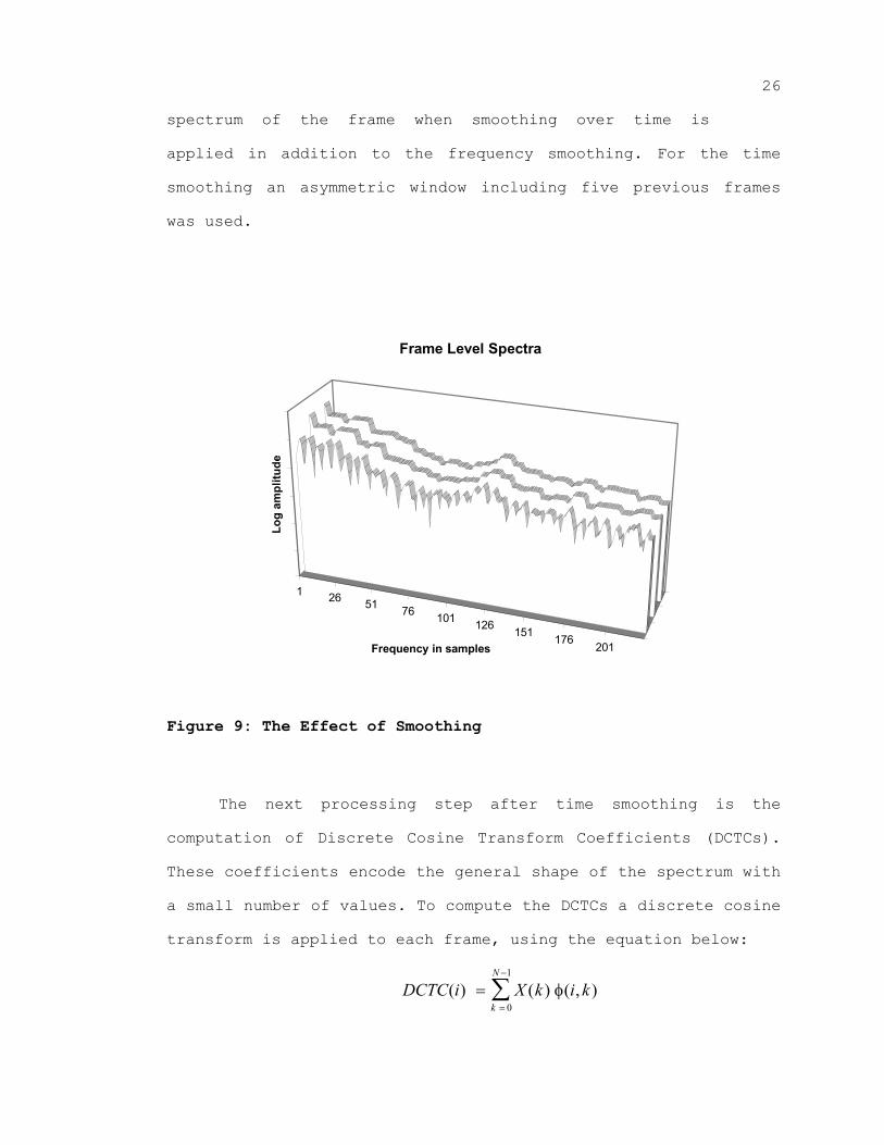
In Figure 9 the effect of the two smoothing operations is
shown for some real speech data. The curve in “front” is the
log scaled squared magnitude spectrum of a 30 ms frame of the
vowel /ah/. The spectrum was computed with a 512 point FFT.
Since no smoothing was applied to this data, the details of the
spectrum can be seen. The second graph shows the spectrum of the
same frame, after a symmetric smoothing window of width 150 Hz
was used to smooth the spectrum over frequency. At a sampling
frequency of 11.025 kHz, this corresponds to a window width of
seven frequency samples. It can be seen that deep valleys are
“filled” and peaks are broadened. The last graph shows the
26
spectrum of the frame when smoothing over time is
applied in addition to the frequency smoothing. For the time
smoothing an asymmetric window including five previous frames
was used.
1 26 51 76 101 126 151 176201
Log
ampl
itude
Frequency in samples
Frame Level Spectra
Figure 9: The Effect of Smoothing
The next processing step after time smoothing is the
computation of Discrete Cosine Transform Coefficients (DCTCs).
These coefficients encode the general shape of the spectrum with
a small number of values. To compute the DCTCs a discrete cosine
transform is applied to each frame, using the equation below:
DCTC i X k i kk
N
( ) ( ) ( , )==
−
∑ φ0
1

27
The i-th DCTC is computed as the sum over all
frequency samples X(k), in the desired frequency range k,
multiplied by the basis vectors over frequency N(i,k). The basis
vectors given in the equation, which, for the most
straightforward case, are samples of integer multiples of a
half-cycle of a cosine,
φπ
( , ) cos( . )
i ki kN
=+
5
are generally modified as discussed below.
Since only a small number of DCTCs are needed (typically
10 to 15), and also because of the frequency range limitations,
the DCTCs were computed with the straightforward dot-product
approach rather than a fast transform based method. However, to
increase the speed of these calculations the required cosine
basis vectors are precomputed.
An important theoretical issue that affects the DCTC
calculations is that a non-linear scaling of the frequency axis
improves the performance of the whole classification system
significantly (for example, Nossair et al., 1995). This agrees
again with biologically motivated considerations in that the
human ear has a much higher frequency resolution at low
frequencies than at higher frequencies. To take this non-linear
scaling of the frequency axis into account, the frequency axis
of the frame level spectrum should be “warped” before the DCTCs
are computed. That is, the spectrum could be re-sampled such
that samples are closer in frequency at low frequencies and

28
farther apart in frequency at high frequencies. This
approach, which is used in many current speech systems and in a
previous version of the Visual Speech Display, is
computationally inefficient and results in approximate matches
to desired warping functions. Research in our lab has shown that
a better approach is to incorporate the warping into the basis
vectors (Rudasi, 1992). Since the basis vectors are pre-
computed, no additional computations are required to implement
time frequency warping. Figure 10 and Figure 11 illustrate basis
vectors computed without and with warping incorporated
respectively. As can be seen in Figure 11 the warping causes the
basis vectors to vary more rapidly and to have higher amplitude
at lower frequencies than at higher frequencies. This results in
effectively higher resolution of lower frequencies than for high
frequencies. More details are given in (Rudasi, 1992) Wang et
al., (1996).
Basis vectors over Frequency, no warping
BVF0 BVF1 BVF2
Figure 10: Basis Vectors over Frequency, Warping = 0

29
Basis Vectors over Frequency, 0.45 warping
BVF0 BVF1 BVF2
Figure 11: Basis Vectors over Frequency, Warping = 0.45
Except for several refinements such as the morphological
filtering over frequency and method for accomplishing frequency
warping, the processing in the previous version of the Visual
Speech Display was similar to that described thus far for the
new system. That is, the frame level DCTCs just described were
used as the inputs to the neural network classifier used for the
actual phonetic recognition. In addition to this much greater
efficiency, accuracy, and flexibility incorporated into the
frame level processing, a “block level” processing step was
incorporated for the present study, as described in the next
section of this thesis.
3.3.2 Block Level Processing
As mentioned previously, research (for example Zahorian
and Jagharghi, 1993) has shown that the performance of phonetic
classifiers can be improved dramatically if not only the DCTCs
of the current frame are used but also the change of the DCTCs
30
over time are used as features. Therefore a number of
frames of DCTCs are combined to form a block. The goal of the
block level processing is to represent the change of the DCTCs
from frame to frame with a small number of values. As mentioned
before only the general trend of the change is important for
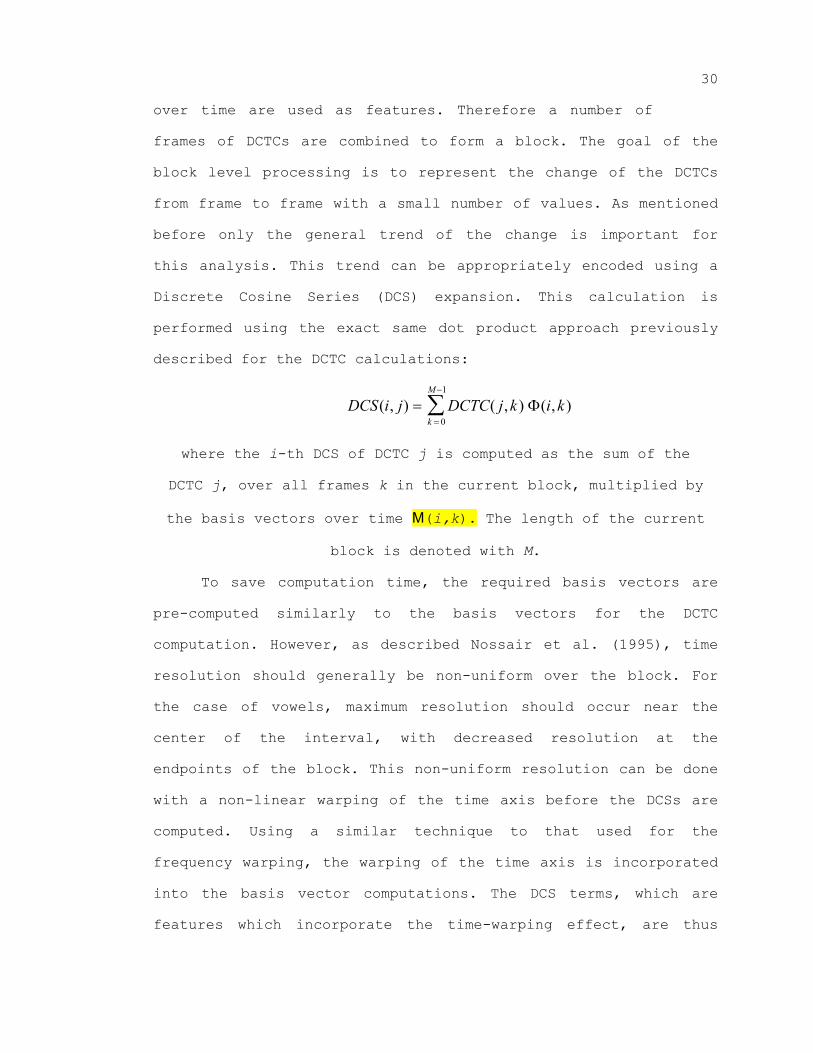
this analysis. This trend can be appropriately encoded using a
Discrete Cosine Series (DCS) expansion. This calculation is
performed using the exact same dot product approach previously
described for the DCTC calculations:
DCS i j DCTC j k i kk
M
( , ) ( , ) ( , )==
−
∑ Φ0
1
where the i-th DCS of DCTC j is computed as the sum of the
DCTC j, over all frames k in the current block, multiplied by
the basis vectors over time M(i,k). The length of the current
block is denoted with M.
To save computation time, the required basis vectors are
pre-computed similarly to the basis vectors for the DCTC
computation. However, as described Nossair et al. (1995), time
resolution should generally be non-uniform over the block. For
the case of vowels, maximum resolution should occur near the
center of the interval, with decreased resolution at the
endpoints of the block. This non-uniform resolution can be done
with a non-linear warping of the time axis before the DCSs are
computed. Using a similar technique to that used for the
frequency warping, the warping of the time axis is incorporated
into the basis vector computations. The DCS terms, which are
features which incorporate the time-warping effect, are thus

31
efficiently and easily computed by a dot product of the
history of a certain DCTC and the DCS basis vectors. Figure 12
and Figure 13 show the basis vectors over time without and with
warping respectively. Figure 13, which depicts the basis vectors
with warping, shows that the basis vectors vary more rapidly and
are larger in the middle of the interval than at the endpoints.
This results in an increased time resolution of the values in
the center of a block and a decreased time resolution at both
ends.
Basis Vectors over Time, no warping
BVT0 BVT1 BVT2
Figure 12: Basis Vectors over Time, Warping = 0

32
Basis Vectors over Time, 5 warping
BVT0 BVT1 BVT2
Figure 13: Basis Vectors over Time, Warping = 5
Yet another consideration taken into account in the
development of the signal processing software is that, in
certain cases, for example stop consonants, the speech signal
changes very rapidly at the onset and then changes more slowly.
Therefore, the block level processing was written to allow
blocks with increasing length. The start of the first and
shortest block is synchronized with the speech onset. The
following blocks are of increasing length up to the desired
maximum block length. This results in a very detailed
representation of the speech onset compared to the normal
resolution of the block processing. Figure 14 shows how frames
are combined to form blocks of increasing length. The shaded
frames contain the speech signal of interest, starting in frame
five. As can be seen the block length is increased from one
frame to the maximum block length of five frames. The rate of
increase (labeled Block_jump) equals two frames in this case.
The same value is used to advance the blocks after the length of
a block reaches the maximum block length. This can be seen for
the last two blocks.

33
0 2 983 4 5 6 7 10 111 12
Speech onset
Block 0
Block 1Block_jump
Block_length_max
Block 3
Block 2
Frames
Figure 14: Blocks with Increasing Length
3.3.3 Final Features
The block level processing results in a set of DCS terms
for each DCTC. However, for some phonetic classification
applications (for example Zahorian and Jagharghi, 1993), better
results are obtained with a subset of these terms. Therefore,
another option was added such that only specific DCS terms are
used. To save computation time, only these needed terms are
actually computed. These DCS terms over the DCTCs are the final
features representing the speech signal for each block. They are
used as the inputs to a neural network classifier.
In the remaining section of this chapter, the actual
software routines used to implement the signal processing just
summarized are described. Some additional issues concerning
efficient data management for real-time operation are also

34
described. All of this code was developed using
Microsoft Visual C/C++, Version 4.0, for Windows NT and Windows
95.
3.4 cp_Feat
All the primary signal processing routines are contained in the
cp_Feat.c source file. Other routines, such as the routines to
compute the basis vectors, are located in secondary source
files. A very detailed description of the routines of cp_Feat
can be found in (Auberg, 1996). This section provides a relation
between the signal processing steps and the implementation of
the C routines. In the comments in the code and in the detailed
help file (Auberg, 1996) the following notation is used. A
segment is an array of time domain data. All computations are
based on the data included in a segment. For real-time use, a
segment denotes the non-overlapping (i.e., the “new”) portion of
the data obtained each time the program communicates with the
sound card. A buffer is an internally used array of time domain
data which is composed of one frame length of “old” data taken
from the end of the previous segment and the current segment
itself. A buffer therefore contains overlapping (the “old” frame
length of data) and non-overlapping data (the current segment).
A frame contains a small amount of data taken from the buffer.
For each frame the FFT is computed. A frame can therefore
contain time or frequency domain data. Finally, a block consists
of a group of frames containing frequency domain data. For each
block a set of the final temporal/spectral features is computed.
This notation is also used in Chapter Four.
35
The frame level processing is partitioned into
three routines. All block level processing is accomplished with
one routine. The routines were designed to be called only once
per segment. This meant that a certain amount of data management
had to be included in the routines.
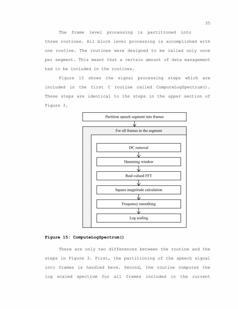
Figure 15 shows the signal processing steps which are
included in the first C routine called ComputeLogSpectrum().
These steps are identical to the steps in the upper section of
Figure 3.
Log scaling
DC removal
Hamming window
Real-valued FFT
Square magnitude calculation
Frequency smoothing
Partition speech segment into frames
For all frames in the segment
Figure 15: ComputeLogSpectrum()
There are only two differences between the routine and the
steps in Figure 3. First, the partitioning of the speech signal
into frames is handled here. Second, the routine computes the
log scaled spectrum for all frames included in the current

36
segment before the next processing steps take place.
Therefore, this processing results in a group of frames
containing log scaled spectra.
Some additional data management is also included in the
ComputeLogSpectrum() routine. This data management enables the
following routine to work continuously on a speech signal which
is longer than the one segment given to the routine. However, a
more detailed explanation is delayed until Chapter Four. To
smooth these log scaled frame level spectra over time, they are
passed to the time smoothing routine. The block diagram is shown
in Figure 16.
Time smoothing
For all frames in the segment
Figure 16: TimeSmoothing()
After all frame level spectra have been smoothed over
time, the DCTCs can be computed for each frame. The routine
called ComputeDCTCs() uses a set of pre-computed basis vectors
over frequency. Recall that these basis vectors incorporate the
warping of the frequency axis if that option is selected. Figure
17 shows the signal processing steps implemented in the last
frame level processing routine.

37
Compute DCTCsusing the precomputed basis vectors over
frequency
For all frames in the segment
Figure 17: ComputeDCTCs()
The next processing routine incorporates all block level
processing. First, a number of frames are combined to form
blocks. The routine, called ComputeDCSs(), uses the pre-computed
basis vectors over time, to compute the DCS terms. These basis
vectors also incorporate the non-uniform resolution over the
block, as discussed previously. After the DCS features for a
given block are computed, the next block is processed. Note that
the blocks may overlap and that the length of blocks can
increase with time. Figure 18 shows the processing steps
implemented in the ComputeDCSs() routine.
Final features
Compute DCSusing the pre-computed basis vectors over time
Select desired terms
Partition frames into blocks
For all blocks
Figure 18: ComputeDCSs()

38
The next chapter describes how these routines are
used in real-time. The WinBar program is used as an example of a
typical program using real-time signal processing.

39
4. THE WinBar PROGRAM
Take this page out and adjust page numbers !

39
CHAPTER FOUR
THE WinBar PROGRAM
4.1 Introduction
Chapter Three described the basics of the signal
processing. Also the implementation of the signal processing
ideas into signal processing routines was described. These
routines are used in two different types of programs for the
overall system. First, the routines are used to compute features
from pre-recorded speech data. Thus this program runs off-line
using data stored in computer files. These features are required
to train the neural network classifier. Next, the same signal
processing routines are used in a classification program. In
this chapter, the WinBar program is used as an example. In
WinBar, the features are computed from a unknown speech signal
in real-time. These features are then “processed” by a trained
neural network classifier and the classification results are
displayed on the screen. To ensure consistency, the processing
routines in both application must be the same. However, real-
time operation requires some additional data management. The
next section describes this additional data management.
40
4.2 Real-time Signal Processing
The main difference between real-time and off-line
processing is that for the real-time case, it is not known what
the speaker will say and when the sounds will be produced.
Therefore a classification program such as the WinBar program
needs to constantly ‘listen’ to the incoming signal to detect a
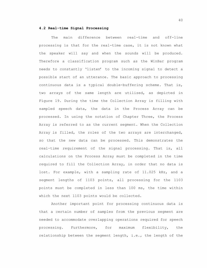
possible start of an utterance. The basic approach to processing
continuous data is a typical double-buffering scheme. That is,
two arrays of the same length are utilized, as depicted in
Figure 19. During the time the Collection Array is filling with
sampled speech data, the data in the Process Array can be
processed. In using the notation of Chapter Three, the Process
Array is referred to as the current segment. When the Collection
Array is filled, the roles of the two arrays are interchanged,
so that the new data can be processed. This demonstrates the
real-time requirement of the signal processing. That is, all
calculations on the Process Array must be completed in the time
required to fill the Collection Array, in order that no data is
lost. For example, with a sampling rate of 11.025 kHz, and a
segment lengths of 1103 points, all processing for the 1103
points must be completed in less than 100 ms, the time within
which the next 1103 points would be collected.
Another important point for processing continuous data is
that a certain number of samples from the previous segment are
needed to accommodate overlapping operations required for speech
processing. Furthermore, for maximum flexibility, the
relationship between the segment length, i.e., the length of the

41
Collection and Process Array in Figure 19, and the frame
lengths and frame spacing should be arbitrary. That is, the
segment length is based on real-time considerations (such as
time between screen updates) whereas frame length and frame
spacing should be based on time/frequency resolution
considerations as mentioned previously. Also, for the best
performance, the processing should be synchronized with the
speech onset. This is especially important for many of the
consonants. The extra data management required to allow this
flexibility is illustrated as follows. After the onset is found,
the speech data is partitioned into frames starting a certain
amount of samples before the detected speech onset. Typically
the data from the speech onset to the end of the Process Array
cannot be partitioned into an integer number of frames which
will use all the data. Therefore, there are a certain number of
samples at the end section of the Process Array (up to a maximum
of the frame length minus one) which cannot be processed until
the next array is filled. To accommodate for this difficulty, a
number of samples (one frame length) from the end of the
previous Process Array are saved, as shown in the lower left
hand corner of Figure 19. Thus a Buffer is defined for the
actual processing which consists of this overlapping data, i.e.,
data from the previous array, and the current data taken from
the Process Array. The steps for actual data management are also
shown in Figure 19.

42
Sound Card
Microphone
Exchange of arrayswhen the CollectionArray is filled.
2.
Collection Array
Process Array
Non-overlap
1.
Buffer
Overlap
Buffer
Figure 19: Double-Buffering Scheme
After the Buffer is formed, as outlined in the previous
paragraph, the next step is to identify one of the following
unique cases: (1) a silent Buffer with no speech data, (2) a
Buffer with speech starting after the beginning of the Buffer,
(3) a full Buffer, with valid speech data for the entire Buffer,
or (4) a Buffer with speech data in the beginning but ending
before the end of the Buffer. An implicit assumption is that
each valid utterance, and that pauses between utterances, are at

43
least one segment length long. Therefore, cases such as
a single utterance beginning and ending within a single segment
are not allowed. To determine which of the cases above are
contained in the buffer, an algorithm was developed to locate
the speech onset. The routine in the WinBar program handling
this speech detection is called LocateSpeech(). Three variables
used by this function are now introduced. More details can be
found in (Auberg, 1996). The first variable is called
First_frame. This variable points to the start of the first
frame in the current buffer containing speech. The second
variable, Next_frame, points to the beginning of the first frame
which does not fit into the current buffer. The third variable,
First_call is set to one if a speech signal started in the
current buffer, and is set to zero otherwise.
As an initial condition case (1) is assumed. Therefore
First_call is set to one. Assume that a speech signal starts
somewhere in the current buffer and is about two and half
segments long. In the LocateSpeech() routine First_frame is set
to point to the first new sample in the buffer, i.e., it is
pointing to the start of the current segment. Starting from
First_frame, the data is partitioned into short non-overlapping
windows. For each window, from left to right, the energy of the
window is computed. Using a threshold it is decided if the
current window contains the speech onset. If the energy is below
the threshold the next window is tested. If the threshold is
reached, the value of First_frame is updated accordingly to the
point at the located onset, minus an offset equal to the number
44
of samples defined for a pre-trigger. Using the value of
First_frame the number of frames fully contained in the buffer
is computed. The beginning of the first frame not contained in
the buffer is stored in the Next_frame variable. This is now the
case (2) mentioned above.
After the processing is done and the next buffer is
available, the value of First_frame is calculated based on the
buffer length, segment length and the value of Next_frame, which
is relative to the last buffer. Starting at First_frame the
buffer is partitioned into windows as described above. The
implicit model now only allows two possible states, case (3) or
case (4). To determine which case applies to the situation, the
energy of the windows is checked against the threshold. However,
the energy value is now checked starting from the end of the
buffer. This way it can easily determined if the signal lasts
until the end of the buffer or not. In our example the whole
buffer contains speech data, therefore case (3) is determined.
The variable First_call is set to zero, since the data in the
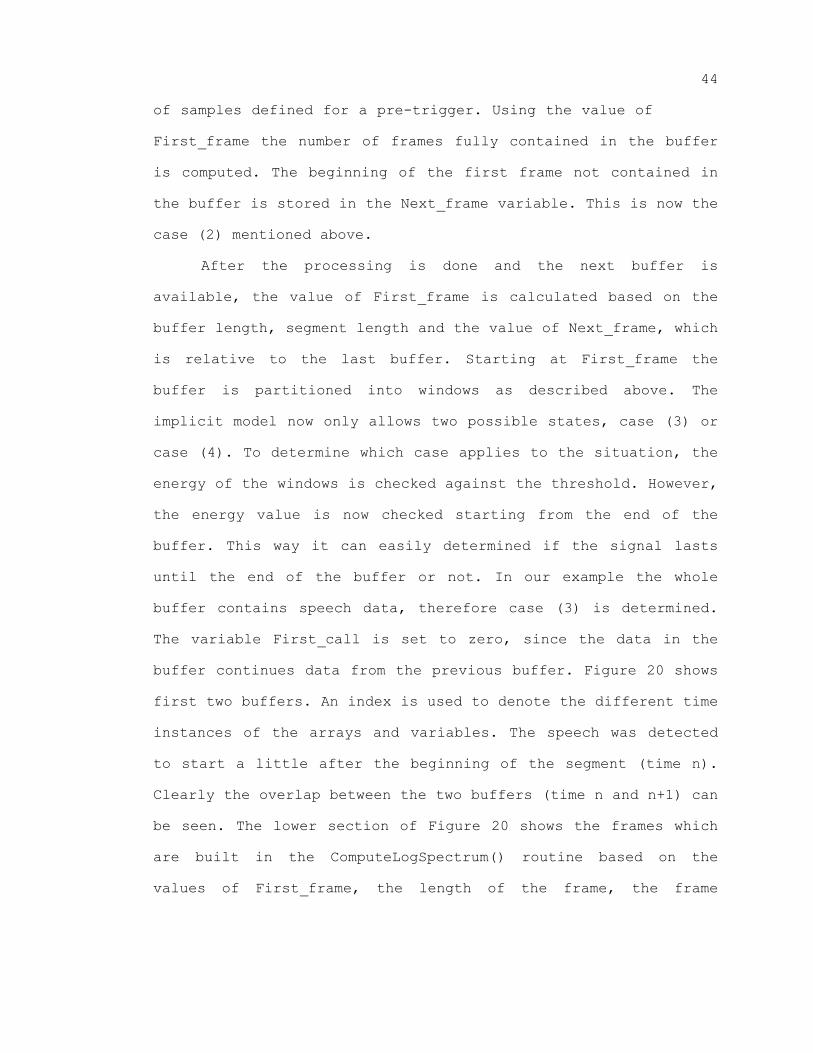
buffer continues data from the previous buffer. Figure 20 shows
first two buffers. An index is used to denote the different time
instances of the arrays and variables. The speech was detected
to start a little after the beginning of the segment (time n).
Clearly the overlap between the two buffers (time n and n+1) can
be seen. The lower section of Figure 20 shows the frames which
are built in the ComputeLogSpectrum() routine based on the
values of First_frame, the length of the frame, the frame

45
spacing and the number of frames determined by the
LocateSpeech() routine.
First_frame[n]
First_frame[n+1]
Buffer[n+1]
0
1
2
3
4
0
1
2
3
4
5
x
Next_frame[n+1]
Buffer[n]
Figure 20: Sequential Buffers (A)
After the next buffer is available, the same two states
are possible as before, i.e., case (3) or case (4). As assumed
above the speech signal ends after about two and half segments
in the third buffer. After the current value of First_frame is
calculated, the energy of the windows is computed for this
buffer. By scanning from the end of the buffer, it is found that
the speech signal stops in the middle of the buffer. Therefore
case (4) is now given. Now the number of frames containing at
least some speech is found. Next_frame is set to point to the
first frame not containing any speech. Figure 21 shows this
situation. Here the last buffer of Figure 20 is shown again for
illustration of the continuous nature of the processing. From
the buffer at time n+2 only five frames are processed, since the

46
next frame (marked with an ‘x’) does not contain any
speech but would still fit into the buffer.
After case (4) was detected for a buffer, case (1)
(initial condition) is assumed for the next buffer.
Buffer[n+1]
0
1
2
3
4
5
0
First_frame[n+2]
Buffer[n+2]
1
2
3
4
Next_frame[n+2]
x
Figure 21: Sequential Buffers (B)
After a speech onset was found in a buffer, the frame
level processing is applied to the data. As the next step, the
block level processing is done to calculate the final features.
These features are the inputs to the Artificial Neural Network.
4.3 Artificial Neural Network Classifier
Artificial Neural Network Classifiers are widely used in
automatic speech recognition based on their flexibility. The
type of network used in this thesis is known as a Multi-Layer
Perceptron (MLP). It consists of a large number of identical
nodes called neurons. Each neuron has a number of inputs with
associated weights, an internal offset and one output. The
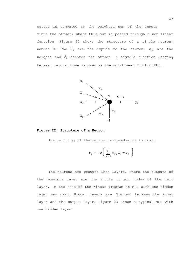
47
output is computed as the weighted sum of the inputs
minus the offset, where this sum is passed through a non-linear
function. Figure 22 shows the structure of a single neuron,
neuron k. The Xi are the inputs to the neuron, wki are the
weights and 2k denotes the offset. A sigmoid function ranging
between zero and one is used as the non-linear function N().
N(.)
2k
-1
X1
X2
X3
Xp
wk1
wkp
vk
yk
Figure 22: Structure of a Neuron
The output yk of the neuron is computed as follows:
y w xk k j jj
p
= −
=∑ϕ θ
1k
The neurons are grouped into layers, where the outputs of
the previous layer are the inputs to all nodes of the next
layer. In the case of the WinBar program an MLP with one hidden
layer was used. Hidden layers are ‘hidden’ between the input
layer and the output layer. Figure 23 shows a typical MLP with
one hidden layer.

48
Figure 23: MLP with One Hidden Layer
Since a non-linear function is used to compute the output
of each neuron, a MLP can create a non-linear mapping of the
input space to the output space. The complexity of the decision
region for each class depends on the number of layers and the
number of nodes in the layers. Previous research by Zahorian and
Jagharghi (1993) showed that to classify ten vowels a MLP with
one hidden layer is sufficient. The number of nodes in the
hidden layer can be between 30 and 50.
The network used in the WinBar program typically has about
20 inputs. These are the final features computed by the block
level processing. The actual number varies with the way the
features are computed. The hidden layer has 50 neurons. The
output layer consists of ten neurons with one neuron for each
vowel. The values of the weights and offset are computed during
49
the training of the neural network. The training is
described in section 5.5.
4.4 Graphical Display
As mentioned above, the neural network has ten output
neurons, one for each vowel. The WinBar program displays the
neural network outputs using bars. The height of each bar
represents the value of an output neuron and therefore the
classification result for a particular vowel. The user can see
the quality of his/her articulation attempt by watching all ten
bars. For a good pronunciation only the bar associated with the
desired vowel should reach a maximum height and the height of
all other bars should be close to zero. The WinBar program works
in real-time. That means that all processing, the classification
of the features by the neural network and the graphical display
of the results are finished in the time needed to fill one array
used for the double-buffering.
4.5 WinBar Program Structure
This section gives a short introduction to the structure
of the WinBar program. Detailed information can be found in
(Auberg, 1996). Right after the WinBar program is started, two
initialization files are read. The primary information in the
first file consists of the names of the neural network weight
files. The second file contains the parameters which control the
signal processing. A typical parameter file is shown below. The
values of the more than twenty parameters can be adjusted to
make the signal processing extremely flexible.

50
ID FeatureComputation_SpecFile[cp_Fea1300] // Basic parameters Sample_rate: 11025 // Hz 8000 - 22050 Hz long Segment_time: 100 // ms 50 - 500 ms long Frame_time: 20 // ms 5 - 40 ms long Frame_space: 10 // ms 2 - 100 ms long FFT_length: 256 // points 64 - 1024 points long Kaiser_Window_beta: 6 // without unit 0 - 6 float Num_DCTC: 14 // without unit 8 - 25 long DCTC_warp_fact: 0.45 // without unit 0 - 1 float BVF_norm_flag: 0 // without unit 0 or 1 long Low_freq: 100 // Hz 0 - 300 Hz long High_freq: 5000 // Hz 3000 - 8000 Hz long // Morphological filter parameters Freq_kernel_before: 0 // Hz 0 - 100 Hz long Freq_kernel_after: 0 // Hz 0 - 100 Hz long Time_kernel_before: 0 // frames 0 - 5 frames long Time_kernel_after: 0 // frames currently fixed to 0 long // Block parameters Block_length_min: 1 // frames 1 - 20 frames long Block_length_max: 5 // frames 1 - 20 frames long Block_jump: 2 // frames 1 - 20 frames long Num_DCS: 1 // without unit 1 - 5 long Time_warp_fact: 0 // without unit 0 - 10 float BVT_norm_flag: 0 // without unit 0 or 1 long Use_term: // DCS0 DCS1 DCS2 DCS3 DCS4 DCS5 DCS6 DCS7 DCTC00 0 1 1 1 1 0 0 0 DCTC01 0 1 1 1 1 1 0 0 DCTC02 1 1 1 1 1 1 1 1 DCTC03 1 1 1 1 1 1 1 1 DCTC04 1 1 1 1 1 1 1 0 DCTC05 1 1 1 1 1 1 0 0 DCTC06 1 1 1 1 1 0 0 0 DCTC07 1 1 1 1 1 0 0 0 DCTC08 1 1 1 0 0 0 0 0 DCTC09 1 1 1 0 0 0 0 0 DCTC10 1 1 0 0 0 0 0 0 DCTC11 1 1 0 0 0 0 0 0 DCTC12 1 1 1 1 1 1 1 1 DCTC13 1 1 1 1 1 1 1 1 DCTC14 1 1 1 1 1 1 1 1 DCTC15 1 1 1 1 1 1 1 1
After these files are read, the basis vectors over
frequency are computed. These are needed to compute the DCTCs
which incorporate the warping over frequency. In the following
step the basis vectors over time are computed, which are needed
to compute the DCSs. These basis vectors over time can also
incorporate a warping of the time axis if desired. If an
51
increasing block length is desired, a set of basis
vectors over time for each possible block length is needed.
In the next step the neural network classifier is
initialized with the weights and offsets read from a neural
network weight file. Recall that this file was created during
the training phase of the neural network. In addition a file
containing scale factors is read. This file was also created
during the training phase of the network. These scale factors
are needed later on to scale the final features to the same
ranges as those used for training the neural network. This step
completes the initialization phase of the WinBar program.
The next operation of the program is the processing phase
which starts with data received from the sound card using the
double-buffering scheme described above. If a speech signal is
detected, the frame and block level processing is applied to the
speech segment. The resulting features are scaled using the
scale factors mentioned above. The scaled features are then
input to the neural network. The classification results are
passed to the graphics routine, which controls the heights of
the bars on the screen. Next new speech data can be processed by
looping continuously through the processing phase. If the user
quits the program, certain clean up operations such as freeing
memory are done before the end of the program.
The program structure is shown in Figure 24. However, this
structure is greatly simplified relative to the actual program.
For example the user can switch between different neural
networks. This is done to optimize the classification

52
performance with male, female or child speakers.
Typically speech samples of speakers of age 12 and under are
used for the child group. Speakers 18 years and older are used
for both adult groups. Speaker between 13 and 17 will be used in
the child or the adult groups depending on the sound of their
pronunciation. These speaker groups have very different speech
characteristics. Therefore a male speaker should chose the
network trained with male speakers for optimal performance. This
is especially important, if the program is used for
pronunciation training for hearing impaired or foreign speakers.
For example a child cannot expect to learn the correct
pronunciation of adult male French vowels. Another feature of
the WinBar program not shown here is the possibility to display
not only the final classification result but also intermediate
results such as the log scaled spectrum or the DCTCs of a frame.
In the case of the WinBar program, where currently only
steady state vowels are processed, it should be noted that some
of the newly implemented options of the signal processing are
not used. For example the time smoothing is disabled, all blocks
have the same length and the basis vectors over time are not
warped. Preliminary experiments showed that for steady state
vowels the use of these advanced techniques does not improve the
classification performance. However, since the routines can be
used with other phonemes than steady state vowels these options
of the signal processing will be used to process stop consonants
or other phonemes.

53
Display
Get speech data from sound card
Locate speech onset
Frame level processing
Block level processing
Neural Network classifier
Initialize Neural Network
As long as desired
Compute basis vectors over time
Compute basis vectors over frequency
Read Feature Computation Specification File
Read ‘WinBar.ini’ file
Clean up and end program
Figure 24: WinBar Program Structure

54
5. TRAINING OF THE WHOLE SYSTEM
Take this page out and adjust page numbers !

54
CHAPTER FIVE
TRAINING OF THE WHOLE SYSTEM
5.1 Overview
In this chapter the steps required to train the neural
network used in the WinBar program are explained. The network in
the WinBar program operates using fixed weights and offsets, and
propagating the features through the network. This of course
requires that the weights and offsets are correctly pre-computed
for the specific classification task. The values for the weights
and offsets are determined in the training phase of the neural
network. This chapter describes all steps needed before the
WinBar program can be used. These are the same steps required if
the neural network needs to be retrained to incorporate more
training speakers or to classify a different set of phonemes.
5.2 Recording of Speech Files
The first step in the training procedure is to collect
training data. The training data is collected by the WinRec
program. This program was implemented for this thesis to enable
a convenient, reliable and fast way to collect a large amount of
speech samples under a large number of conditions. A detailed
55
description of this program can be found in (Auberg,
1995). The program first prompts the user to correctly pronounce
a certain phoneme — vowels for the data actually collected in
this study. The steady state section of this vowel is located
and written to a file. The data files are labeled uniquely and
stored in a certain directory structure organized according to
gender and speaker. The filename specifies which vowel is
contained in the file. In addition, a secondary file containing
labeling information is created. Both files follow the TIMIT
standard for speech files (Lamel et al., 1986). Typically five
to ten repetitions of each of the ten vowels are saved per
recording session for each speaker.
5.3 Feature Computation with Tfrontc
The Tfrontc program is used to compute the features from
the training data files. A certain group of speakers can be
selected, such as, for example, male speakers, to train a
specialized neural network. The training data files are then
read for all these speakers. For each file the final features
are computed using the signal processing routines described in
Chapter Three. The features are stored in files using a
flexible format developed in the speech lab at ODU for speech
processing applications. One feature file is created for each
vowel. Each file then contains all selected training tokens for
that vowel, thus encompassing a broad range of pronunciations of
the vowel independently of a particular speaker.

56
5.4 Scaling of the Features
The features for one particular phoneme vary with speaker
to speaker and even with different utterances spoken by the same
speaker. Therefore statistics such as the mean and standard
deviation can be computed for each feature. It has been shown
(for example, Haykin, 1994) that neural networks work best if
the features are scaled to have zero mean and a standard
deviation of about 0.2 . If a Gaussian distribution of the
features is assumed, which is generally valid according to the
Central Limit Theorem, the scaled values will then be between -1
and +1 in more than 99% of all cases. Thus the Scale program
reads the feature files and computes the mean and standard
deviation of each feature over all phonemes. These statistics,
which are used as scale factors, are written to a “scale” file.
The actual scaling is done with the Transfor program. This
program reads the scale file and creates a new set of feature
files which now contain the scaled version of the original
features. The scale file is also needed later on in the real-
time system. After the features are scaled, the neural network
can be trained.
5.5 Neural Network Training
The Back-propagation (Lippmann, 1987) learning algorithm
was used to train the neural network. For experiments done with
the Visual Speech Display, typically the initial learning rate
was .25. This rate was gradually reduced during training by
multiplying the previous learning rate by .96 after each 5,000
iterations. In our case, where 250,000 iterations were used, the

57
minimum rate was therefore .032. The momentum term was
.65, and uni-polar sigmoid non-linearities were used. Networks
were typically trained with 250,000 updates, although
performance of the network changed relatively little after the
first 25,000 updates. Of course, the same network topology was
used in the WinBar program. For experimental testing of the
WinBar program, an MLP with one input node for each feature, 50
hidden nodes and ten outputs (one for each vowel) was used.
The network described and the Back-Propagation training
algorithm were found to perform quite well for vowel
classification, using the features computed in this study. A
very important consideration is generalization, that is the
ability of a trained neural network to correctly classify speech
data from a speaker who was not included in the training set.
This generalization is the most important characteristic of the
neural network, since it is impossible to include all possible
speakers in the training set. Typically 15 to 20 speaker per
gender group were found to be enough to achieve a good
performance with unknown speakers.
To achieve higher accuracy, typically four neural networks
were trained - one for male speaker, one for female speakers,
one for children and one using all groups of speakers. These
networks were all the same size and structure. These specialized
networks allow the user of the WinBar program to select the
optimal network for his/her pronunciation. The current version
of the system (April 1996) contains only three neural networks.
The first was trained with four male speakers, the second

58
network was trained with two female speakers, and the
third network was trained with all six speakers. The performance
of the system was then informally tested with a small group of
speaker including the training speakers. Even though there were
insufficient training speakers, good performance was obtained.
That is, there were very few noted instances of discrepancy
between vowel sounds (as judged by the testers of the system),
and the observed displays. To give an approximation to the
potential performance of the system, Table 2 shows the training
classification results of these networks.
Male Female All
Training 99.27% 96.46% 96.78%
Table 2: Neural Network Training Results
The reason that only this small amount of training data
was used is that the data collection is still an ongoing
process. From previous experience, better generalization
performance is expected after the networks are trained with a
sufficient amount of data.
(Stefan—some place in this section might be a good place
for the data I can give you)
5.6 Setting up WinBar
The WinBar program requires the names of the weight and
scale files for the different speaker groups which were created

59
during the training phase. These names are specified in
a setup file. Storing the filenames in a setup file allows great
flexibility since the names can be changed without recompiling
the program. For the same reason the parameters, which control
the feature computation, are also stored in a file. This is the
same file which is used by the Tfrontc program to control the
feature computation during the training phase. To ensure that
the WinBar program works correctly, the values of the parameters
for the feature computations inside WinBar must be the same as
for the Tfrontc program. Otherwise there will be a discrepancy
between the features the neural network was training with and
the features given to the network for classification. This would
presumably result in more classification errors. After neural
network training is complete, the WinBar program can be started
and the newly trained networks are used to classify the unknown
speech signal of a speaker in real-time. The block diagram in
Figure 25 summarizes the steps needed to train the networks for
use in the WinBar program.

60
Train the Neural Network
Scale the features
Compute scaling factors
Compute features
Record speech files
Setup and run the WinBar program
Figure 25: Training of the Whole System

61
6. INVESTIGATION OF DISTINCTIVE FEATURES
Take this page out and adjust page numbers !
60
CHAPTER SIX
INVESTIGATION OF DISTINCTIVE FEATURES
6.1 Introduction
Researchers from the signal processing area generally use
frequency domain features to represent phonemes, such as those
discussed in the preceding chapters of this thesis. The
frequency domain features favored by speech scientists are
formants, which denote the location of the largest peaks in the
frequency spectrum. In our work we use the temporal/spectral
features as described in Chapter Three. Linguists usually refer
to focus on perceptual or production features rather than
acoustic features. One group of such features, which are
commonly discussed in the speech science literature, are called
distinctive features (for example Chomsky and Halle, 1968).
These features attempt to characterize phonemes in the way they
are actually produced in the human vocal tract. Vowels are
usually represented by six distinctive features. These features
are usually viewed as binary attributes. That is, according to
the theory, each vowel can be represented by a six bit binary
code indicating the presence or absence of each of the features.
In the area of vowel pronunciation training, one
reasonable hypothesis is that displays which focus on

61
distinctive features could be beneficial to the user.
That is, rather than only vowel classification based displays,
it might be helpful to show the trainee whether a particular
distinctive feature is contained in a production. For example,
one important feature which hearing impaired speakers often have
difficulty with over the entire vowel space is called “TENSE.”
The work reported in this chapter describes attempts to
investigate the viability of distinctive features for use in the
vowel training system.
Another important point to note, before discussing more
specifics of this part of this study, is that automatic
determination of distinctive features must still be based on
acoustic features, since the acoustic speech signal is the only
easily measurable signal. Neural networks are also a “natural”
method to convert acoustic features to distinctive features
since they are good universal function approximators, and since
they are also typically trained for binary target outputs.
Therefore, in this chapter, we present an experimental
investigation of the use of neural networks to convert acoustic
spectral/temporal features to distinctive features.
In our first set of experiments we attempt to replicate
results from (Meng, 1991), using a two stage classifier. The
first stage consists of a group of independent MLPs, each one
trained to extract a distinctive feature from the acoustic input
features. The outputs of these feature networks are then
processed with a secondary MLP stage which performs vowel
classification task using the six distinctive features as
62
determined by the networks in the first stage. By
comparing the classification results of this two stage
classifier with those obtained with a single network, the degree
to which vowel information is preserved in the distinctive
features can be assessed.
Another classifier structure which bears some similarities
to the two stage method described in the previous paragraph, is
the Binary Pair Partition Neural Network (BPPNN) approach. This
partitioned approach was shown to be very effective for
automatic speaker identification (Norton, 1994) and is now also
used in our vowel classification research (Zahorian, 1993). For
the BPPNN, a group of independent MLPs is used with each one
discriminating only two vowels. The final result is computed by
a method described in (Zahorian, 1993). Thus the BPPNN is
similar to the distinctive feature approach in that multiple
networks are trained, and a second stage is also needed.
Therefore, in this chapter, BPPNN results and the results of
several different sets of distinctive features are compared to
the performance of a standard single MLP.
For this portion of the work we used 13 American English
vowels extracted from the TIMIT database. To make our results
comparable with the previous study cited (Meng, 1991), we used
the same vowels extracted from the identical subset of the TIMIT
data base. The set which includes 500 training speakers and 49
test speakers was used to compare the performance of the above
mentioned classifiers. The set spans all dialect regions
included in the TIMIT data base. The distribution of female and

63
male speakers also matches the distribution of the
entire TIMIT data base. The following table shows the phonetic
and the ARPABET labels for the set of the 13 vowels
investigated:
IPA I I e ε æ a o 7 u g
ü
ARPABET iy ih ey eh ae aa ao ow ah uw er uh ux
Table 3: Experimental Set of 13 American English Vowels
In this experiments three additional vowels are used in
addition to the ten phonemes used in the WinBar program. These
three are (using the ARPABET notation) /ey/, /ow/ and /ux/.
6.2 Acoustic Features
To compute acoustic (temporal/spectral) features the
speech data was extracted from the TIMIT database using the
provided labeling information. These temporal features were
computed with the same signal processing routines as described
in Chapter Three of this thesis. In this case a frame length of
10 ms and a frame spacing of 2 ms were used. For each frame 12
DCTCs were calculated. The trajectory over the last 150 frames
of each of these 12 DCTCs were represented by four DCS terms.
This resulted in a compact representation of a vowel with 48
features. These features were used as inputs of the single MLP
and the BPPNN. In addition, these features were also the inputs

64
of each of the networks which extracted the desired
distinctive feature in the two stage classifier.
6.3 Distinctive Features
Instead of being directly related to the frequency
spectrum of the vowels, the idea behind distinctive features is
based on linguistics. They describe the way in which phonemes
are actually produced in the human vocal tract. For example the
position of the tongue hump is used to classify /i/ as a typical
front vowel and /o/ as a typical back vowel (Rabiner, 1993). For
this work we use the notation of previous work (Meng, 1991) and
the common distinctive features [HIGH], [TENSE], [LOW], [BACK],
[ROUND] and [RETROFLEX]. Each vowel was characterized to either
have a particular feature, denoted with , or not to have it,
symbolized with . This gave a unique but redundant binary
representation of each vowel. This representation is summarized
in Table 4:
ARPABET iy ih ey eh ae aa ao ow ah uw er uh ux
HIGH
TENSE
LOW
BACK
ROUND
RETROFLEX
Table 4: The Representation of the Vowels with Distinctive
Features

65
For each distinctive feature a MLP with one output
node was trained to give a output value close to one if the
vowel had the specific feature (i.e., a black circle in Table 4)
or an output of nearly zero otherwise. The six feature networks
comprised the first stage of the distinctive feature classifier.
The second stage consisted of one MLP with six inputs. These
were connected to the outputs of the six feature networks. This
MLP had one hidden layer with 50 nodes and 13 outputs and
classified the vowels.
6.4 Experiments
In our first group of experiments the performance of the
two stage classifier with the original set of six distinctive
features mentioned in Table 3 was compared to the performance of
a BPPNN approach and the result of a single MLP. All network
configurations, i.e., the number of hidden nodes, amount of
training, etc. were optimized in pilot experiments with another
set of training data mentioned in (Meng, 1991). The first stage
of the two stage classifier consisted of a group of memoryless
fully interconnected feed-forward MLPs with 48 input nodes, one
hidden layer with 50 nodes and one output node. The output of
each of these MLPs represented one distinctive feature. The
networks were trained with the back propagation algorithm with
200,000 iterations. For the network in the second stage, the
same type of one hidden layer MLP was used, but with 300,000
iterations. The number of inputs is the number of distinctive
features, i.e. the outputs of the networks in the first layer.

66
For a different set of distinctive features, the
structure of the two stage classifier was modified such that 13
feature networks were used in the first stage. These are shown
in Table 5. Each of these was trained to distinguish one
particular vowel from all the other 12.
ARPABET iy ih ey eh ae aa ao ow ah uw er uh ux
Feature a)
Feature b)
Feature c)
Feature d)
Feature e)
Feature f)
Feature g)
Feature h)
Feature i)
Feature j)
Feature k)
Feature l)
Feature m)
Table 5: Thirteen Features
The Binary Pair Partitioned Neural Network approach used
(13 * 12) / 2 (78 ) networks to distinguish the 13 vowels. That
is, for each group of two vowels, one network was trained to
discriminate them. Each of these 78 networks had 48 inputs, one
67
hidden layer with 25 nodes and one output node. 100,000
iterations were used for training. The final result was obtained
using a method described in (Nossair, 1995). The fourth
classifier was a single MLP. This network had 48 inputs and 100
nodes in the hidden layer. This network was trained with 300,000
iterations.
In the second group of experiments we wanted to
investigate whether the original set of six distinctive features
was “optimum,” or whether other definitions of features were
significantly better or worse. To create different sets of six
features we circularly rotated the feature patterns for each
vowel but left the vowel labels in place. That means that the
features which characterized the vowel /iy/ are now used as the
features for /ih/, and the features originally used for /ux/ are
the new features for /iy/, and so on. This rotation of the
features by one vowel to the left was done several times. Also
another independent set of six features was developed as shown
in Table 6.

68
ARPABET iy ih ey eh ae aa ao ow ah uw er uh ux
Feature a)
Feature b)
Feature c)
Feature d)
Feature e)
Feature f)
Table 6: An Independent Set of Six Features
In a third group of experiments we observed that to encode
13 categories only four bits are necessary. So we determined two
sets of four features which are shown in Table 7 and Table 8.
Note a feature labeled ‘Feature a)’ in one table is totally
independent from another ‘Feature a)’ in a different table.
ARPABET iy ih ey eh ae aa ao ow ah uw er uh ux
Feature a)
Feature b)
Feature c)
Feature d)
Table 7: Four Strictly Binary Features
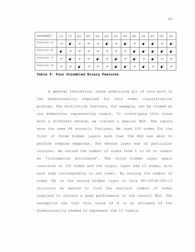
69
ARPABET iy ih ey eh ae aa ao ow ah uw er uh ux
Feature a)
Feature b)
Feature c)
Feature d)
Table 8: Four Scrambled Binary Features
A general theoretical issue underlying all of this work is
the dimensionality required for this vowel classification
problem. The distinctive features, for example, can be viewed as
six dimensions representing vowels. To investigate this issue
with a different method, we trained a special MLP. The inputs
were the same 48 acoustic features. We used 100 nodes for the
first of three hidden layers such that the MLP was able to
perform complex mappings. The second layer was of particular
interest. We varied the number of nodes from 1 to 20 to create
an ‘information bottleneck’. The third hidden layer again
consisted of 100 nodes and the output layer had 13 nodes, with
each node corresponding to one vowel. By varying the number of
nodes (N) in the second hidden layer in this 48-100-N-100-13
structure we wanted to find the smallest number of nodes
required to achieve a peak performance of the overall MLP. The
assumption was that this value of N is an estimate of the
dimensionality needed to represent the 13 vowels.

70
6.5 Results and Comparison
In the first group of experiments, which compared the
original set of six distinctive features with a set of 13
features and the BPPNN and single MLP classifiers, we found that
the BPPNN approach gave the highest result with 84.48% / 71.99%
(training / evaluation result). This classifier structure had
however the most complex structure, requiring the most weights.
The single MLP, which used far less weights than the BPPNN, gave
a very close evaluation result with 76.19% / 71.34%. The two
stage classifier with 13 feature networks in the first stage
gave 73.36% / 70.56% which is about 2.3% better than the
original set of six distinctive features. This use of six
distinctive features yielded results of 71.13% / 68.16%.
Although the results summarized in the previous paragraph
indicated that the six distinctive features did not perform as
well as other network configurations tested, results from the
second group of experiments did show that the original set of
six distinctive features were superior to all other six feature
configurations tested. The rotated set gave on average two to
three percent less than the original set. The other independent
set resulted in 68.12% / 65.41%, i.e., about 3% less.
In the third group of experiments only four features were
used. The strict binary set (Table 7) gave 65.76% / 64.99% and
the scrambled set (Table 8) resulted in 63.02% / 58.17%. Thus
four features did perform more poorly than six features.
The fourth group of experiments showed that with an
increasing number of hidden nodes in the second layer (N) the

71
classification performance reached at maximum at N = 6
and remained approximately constant with increasing N. For N = 4
we achieved evaluation result of 66.13%, whereas N = 6 gave a
result of 69.66%. Figure 26 shows the evaluation results of this
experiment where N, the number of hidden nodes in the second
hidden layer, varies from one to 12.
Evaluation Results over N
0
10
20
30
40
50
60
70
80
1 2 3 4 5 6 7 8 9 10 11 12
Number of node in second hidden layer
Eval
uatio
n re
sult
in %
Figure 26: Evaluation Results over N
The result for N = 6 in the preceding paragraph was very
close to the result using the six distinctive features. To find
out how the network represents the phonemes internally in the
second hidden layer, we extracted the outputs of these six
neurons. The mean of the output over each vowel was computed. We
can view the six mean values for a particular vowel as internal
features. These features were not strictly binary as for the
distinctive features. However, using a threshold, we determined
a modified set of features based on these mean values. These

72
features were sorted and if necessary were inverted.
They are shown in Table 9.
ARPABET iy ih ey eh ae aa ao ow ah uw er uh ux
Feature a)
Feature b)
Feature c)
Feature d)
Feature e)
Feature f)
Table 9: Six Modified Internal Features
It is interesting to note that these modified internal
features, which were created unsupervised by the neural network,
are extremely similar to the six distinctive features shown in
Table 4.
In a new experiment we trained a set of feature networks
to create the six modified internal features. As in the
experiment with the six distinctive features a second neural
network was used to classify the 13 vowels based on theses six
modified internal features. The results of this experiment were
71.16% / 68.28%, which is slightly less than for the original
set of six features.
6.6 Conclusion
Keeping the performance of the classifiers in the first
group of experiments in mind, it can be said that for strict
automatic vowel classification there is no gain in first
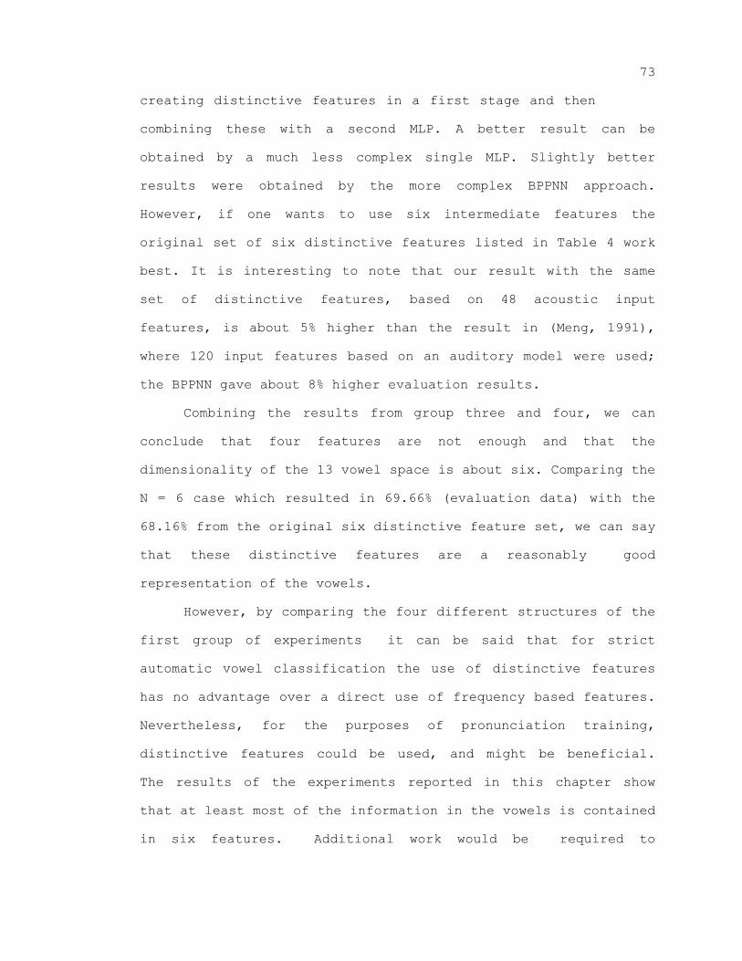
73
creating distinctive features in a first stage and then
combining these with a second MLP. A better result can be
obtained by a much less complex single MLP. Slightly better
results were obtained by the more complex BPPNN approach.
However, if one wants to use six intermediate features the
original set of six distinctive features listed in Table 4 work
best. It is interesting to note that our result with the same
set of distinctive features, based on 48 acoustic input
features, is about 5% higher than the result in (Meng, 1991),
where 120 input features based on an auditory model were used;
the BPPNN gave about 8% higher evaluation results.
Combining the results from group three and four, we can
conclude that four features are not enough and that the
dimensionality of the 13 vowel space is about six. Comparing the
N = 6 case which resulted in 69.66% (evaluation data) with the
68.16% from the original six distinctive feature set, we can say
that these distinctive features are a reasonably good
representation of the vowels.
However, by comparing the four different structures of the
first group of experiments it can be said that for strict
automatic vowel classification the use of distinctive features
has no advantage over a direct use of frequency based features.
Nevertheless, for the purposes of pronunciation training,
distinctive features could be used, and might be beneficial.
The results of the experiments reported in this chapter show
that at least most of the information in the vowels is contained
in six features. Additional work would be required to

74
determine whether or not these distinctive features
would help in vowel articulation training.

75
7. ACHIEVEMENTS AND FUTURE IMPROVEMENTS
Take this page out and adjust page numbers !

74
CHAPTER SEVEN
ACHIEVEMENTS AND FUTURE IMPROVEMENTS
7.1 Achievements
In this section the achievements in implementing this new
and improved version of the signal processing are summarized.
The developed signal processing routines are an
implementation of the newest research about temporal/spectral
features for automatic speech recognition. Without code changes
all relevant parameters (more than 20) can be specified in a
self-explaining setup file. The routines have a clear interface
and clearly separated tasks. This very structured and modular
approach allows easy integration of additional routines and easy
modification of single routines if necessary in the future.
All essential data management was included in these
routines for compactness and processing speed. Based on the
modular approach, additional data management functions, as the
LocateSpeech() routine to detect the speech onset in the real-
time system, can easily be integrated in the existing code.
Another important consideration was that the signal
processing routines are very portable. This allows the use of
these advanced routines in many situations, like in MS-DOS
programs, combined C/FORTRAN code and Windows (16 and 32bit)

75
applications. In addition, the routines can even run a
totally different environment like the ELF DSP board from ASPI
which is based on the TMS320C3X chips from TI. Even though for
the Visual Speech Articulation Training Aid there is no need to
use a DSP board, other application might require a DSP board or
a stand alone operation on a dedicated DSP system.
This leads to another big advantage over the previous
system. Since the signal processing routines were speed
optimized to run on a DSP board the training features could not
be computed off-line on a PC. Each time a variation in signal
processing was investigated, thus requiring that another neural
network be trained, a group of speaker was needed. The features
were then computed in real-time on the DSP board and saved to a
file. This approach made algorithmic refinements extremely
difficult to explore. By using the WinRec recording program, the
speech samples are only collected once and the time waveform is
saved to a file. Since the signal processing routines are
portable, they were integrated to an off-line program (Tfrontc).
Using this program it is easy to compute new features for the
neural network. In particular, this technique allows the
optimization of the signal processing parameters. The
classification results of the different experiments are now
directly comparable since the features are based on the same
speech files.
7.2 Working with phonemes other than Vowels
The main reason to integrate such a large amount of
flexibility into the signal processing routines was to be able

76
to work with other phonemes than steady-state vowels.
From a speech recognition point of view the steady state vowels
are the convenient to classify, since they don’t change their
characteristics significantly over time and the length of the
vowel is typically sufficient. In addition the onset detection
is not critical and no coarticulation occurs. This is different
if the vowels are extracted from short words. Here the length of
the vowel is limited and coarticulation with the previous and
following phoneme occurs.
For the real-time system some additional logic needs to be
implemented to located the vowel inside the word and to extract
the useful section of the vowel, i.e., where the least
coarticulation occurs. In addition, the signal processing
parameters need to be adjusted. For example, the length of a
frame should be shorter (about 5 to 10 ms). Also the trajectory
features computed with block level processing is advantageous to
determine the spectral/temporal pattern of the vowel in the
word.
For work with stop consonants the detection of the onset
is critical (Correal, 1994). Therefore logic to find this onset
with great accuracy is needed. It was shown in the above
mentioned work that the Teager energy operator (Kaiser, 1990)
can be used for a reliable onset detection. The signal
processing parameters need to be adjusted for optimal feature
computation. The technique of the increasing block length can be
used to increase the time resolution in the critical onset
section of the consonant.

77
7.3 Other Display Types
The WinBar program is only one of many possible ways to
display the classification result. Here a bar for each vowel is
displayed. The height of a bar is proportional to the
correctness of the pronunciation. This display can be used to
improve the pronunciation of hearing impaired persons or of
foreign speakers (Correal, 1994). A correct pronunciation is
achieved when the bar of the desired vowel reaches its maximum
height and all others bar have a height of zero. Another type of
an analytic display is the so called ellipse display. Here
elliptic target regions are shown on the screen. The two
dimensional display is based on the common f1/f2 dimensional
plot of vowel positions in this two-dimensional formant space.
In this case, the neural network has an additional layer which
maps the ten-dimensional output space to the two-dimensional
f1/f2 space. A program to implement this kind of display to run
on a Windows Multimedia PC is currently under development.
However, Figure 27 shows the current implementation of the
ellipse display in the WinBall program. Here the green ball must
be moved by the pronunciation to the labeled target ellipse.
This in shown for a correct pronunciation of /ee/.

78
Figure 27: Current WinBall Program
Even though the two computer displays described can help
improve the pronunciation of the target phonemes, a more game
oriented approach could also be used. This can range from a game
teaching only one vowel to more involved games using two, four
or more vowels. In a game to teach the pronunciation of one
vowel, the correctness of the pronunciation can be mapped to a
number of levels, where a higher level leads to more points or
to a ‘friendlier’ reaction of the computer. Games teaching two
vowels can include a voice controlled pinball machine or any
other type of game where a player moves up and down or left and
right. The correctness of the pronunciation would then control
how far or how fast the player moves. Any game based on a
joystick control can be modeled as a four vowel game. For
79
example a voice controlled PAC-man game is possible.
Some ideas, like the PAC-man game, were implemented in the old
system. However the Windows based approach of the new system can
lead to user friendlier and more interesting graphics in the
games with more accuracy in the signal processing.
The actual implementation of a game type display would be
closely based on the existing WinBar program. This program
already handles the real-time signal processing and a
classification through a neural network. After the game graphics
are developed, the outputs of the neural network can directly
used to control the movements of the player.

80
BIBLIOGRAPHY
Auberg, S. (1995), "Help file for WinBar", Speech Lab Documentation, Old Dominion University.
Auberg, S. (1996), "Help file for Feature Computation", Speech
Lab Documentation, Old Dominion University. Chomsky, N., and Halle, M., (1968), "Sound Pattern of English,"
(Harper & Row) Correal, N., (1994), "Real-time Visual Speech Articulation
Training Aid," Masters Thesis, Old Dominion University. Haykin, S., (1993), "Neural Networks, A Comprehensive
Foundation," (Macmillan, New York) Kaiser, J., (1990), "On a simple algorithm to calculate the
‘energy of a signal’," ICASSP-90, pp. 381-384. Lamel, L., Kassel, R., and Seneff, S., (1986), "Speech Database
Development: Design and Analysis of the Acoustic-Phonetic Corpus," DARPA Speech Recognition Workshop, Report No. SAIC-86/1546, pp. 100-109
Leung, H. and Zue, V., (1988), "Some Phonetic Recognition
Experiments Using Artificial Neural Nets," ICASSP-88, pp. I: 422-425.
Leung, H. and Zue, V., (1990), "Phonetic Classification Using
Multi-Layer Perceptrons," ICASSP-90, pp. I: 525-528. Lippmann, R., (1987), "An introduction to computing with neural
nets," IEEE ASSP magazine, April, 4-22. Meng, H., and Zue, V., (1991), "Signal representation Comparison
for Phonetic Classification," ICASSP-91, pp. 285-288. Meng, H., and Zue, V., (1990), "A Comparative study of Acoustic
Representation of Speech for Vowel Classification Using Multi-Layer Perceptrons", ICSLP-90, pp. 1053-1056
Norton, C., Zahorian, S., and Nossair, Z., (1994), "The
Application of Binary-pair Partitioned Neural Networks to the Speaker Verification Task," ANNIE-94, pp. 441-446

81
Nossair, Z., and Zahorian, S., (1991), "Dynamic Spectral Shape Features as Acoustic correlates for Initial Stop Consonants," J. Acoust. Soc. Amer. 89-6, pp. 2978-2991.
Nossair, Z., Silsbee, P., and Zahorian, S.,(1995), "Signal
modeling enhancements for automatic speech recognition," ICASSP-95, pp. 824-827.
Rabiner, L. and Juang, B., (1993) "Fundamentals of Speech
Recognition," (Prentice Hall, New Jersey) Rudasi, L. and Zahorian, S., (1991) "Text-independent talker
identification with neural networks," ICASSP-91, pp. 389-392.
Rudasi, L., (1992) "Text-independent automatic speaker
identification using partitioned neural networks," Ph.D. Dissertation, Old Dominion University.
Sorensen, H., et. al., (1987) "Real-valued Fast Fourier
Transform Algorithms," IEEE ASSP magazine, June, pp. 849-863.
Wang, X., Zahorian, S., and Auberg, S., (1996) "Analysis of
Speech Segments using Variable Spectral\temporal Resolution," ICSLP-96, pp. (TBA).
Zahorian, S., and Jagharghi, A., (1993) "Spectral-shape features
versus formants as acoustic correlates for vowels," J. Acoust. Soc. Amer. 94-4, pp. 1966-1982.
Zahorian, S., Nossair, Z., and Norton, C., (1993) "A partitioned
neural network approach for vowel classification using smoothed time/frequency features," Eurospeech-93, pp. II: 1225-1228