ABSTRACT

Title of Dissertation: THE DESIGN AND STUDY OF THE SUB-

MILLIMETER WAVE LENGTH GYROTRON

AND FUNDAMENTAL AND SECOND

CYCLOTRON HARMONICS.

Ruifeng Pu, Doctor of Philosophy, 2014

Directed By: Professor Victor Granatstein, Department of

Electrical and Computer Engineering

Dr. Gregory Nusinovich, IREAP, Co-Advisor

This dissertation documents research activities directed toward designing high

power, high efficiency gyrotrons to operate in the sub-millimeter wavelength region.

The gyrotron is to produce pulsed RF power at 670 GHz, with possible application to

a novel scheme for detecting concealed radioactive materials. High efficiency is to be

achieved by designing a cavity resonator in which the electrons interact with the high-

order TE31,8 mode. The choice of resonating mode helps to alleviate Ohmic losses in

the cavity walls, and simulation results show that the output efficiency could be more

than 30%. The design study takes into account a variety of known effects that could

affect efficiency, such as orbital velocity spread, voltage depression and after-cavity

interaction. The 670GHz gyrotron was built using the resonator design; operation

confirmed that record high efficiency was achieved at an output power level of about

200 kilowatts.

In addition, the issue of radial spread in electron guiding centers, which is

related to the design of the magnetron injection gun used in the 670GHz gyrotron,

was also examined. This spread degrades the interaction between the electrons and

the RF field. This often overlooked issue is important for future electron gun designs;

this thesis presents analytical methods for estimating how much the degradation

affects gyrotron efficiency. The analytical method was verified with numerical

simulation, showing that the efficiency's sensitivity to spread in guiding centers is

highly dependent on the location of an annular electron beam: when the beam is

injected in the inner peak of the desired mode, the radial spread should be kept to less

than 1/3 of the RF wavelength.

Finally, the dissertation investigates the possibility of further extending the

operating parameters of the gyrotron by using the second harmonic of the electron

cyclotron resonance. An average output power could be increased by operating the

gyrotron continuously rather than in pulses. Using the second cyclotron harmonic

allows the magnetic field requirement for resonance condition to be reduced by a

factor of two, so that in 670 GHz gyrotrons the pulsed solenoid can be replaced with a

cryo-magnet. The investigation shows that for the TE31,8 mode at the second

cyclotron harmonic, the operating mode has only one competing mode at the

fundamental cyclotron harmonic that could present a mode stability issue. Numerical

simulation shows that this mode is TE11,6, the operating mode can suppress this mode,

while achieving 20% interaction efficiency. Results also reveal that the resonator for

the operating mode at second cyclotron harmonic must be modified to increase the Q-

factor. Continuously operating gyrotrons using cryo-magnets have been used for

plasma heating in controlled thermonuclear fusion research, albeit at lower frequency

than the 670 GHz of the current study.

THE DESIGN AND STUDY OF THE SUB-MILLIMETER WAVE LENGTH

GYROTRON AND FUNDAMENTAL AND SECOND CYCLOTRON

HARMONICS

By

Ruifeng Pu

Dissertation submitted to the Faculty of the Graduate School of the

University of Maryland, College Park, in partial fulfillment

of the requirements for the degree of

Doctor of Philosophy

2014

Advisory Committee:

Professor Victor L. Granatstein, Chair/Advisor

Dr. Gregory S. Nusinovich, Advisor

Dr. John C. Rodgers

Professor Thomas M. Antonsen Jr.

Professor Isaak D. Mayergoyz

Professor Ki-Yong Kim, Dean's Representative

© Copyright by

Ruifeng Pu

2014

ii

Preface

The research studies contained in this thesis strive to push practical (efficiency

> 20%) gyrotron operation into the sub-terahertz (300-800 GHz) frequency regime,

something which has not been previously accomplished. Previous efforts by scientists

and engineers resulted in devices that, while demonstrating that gyrotron operation

can be realized, also showed the limitations and challenges left to be solved.

One of the most important of previous contribution is the pulsed gyrotron

study at the Institute of Applied Physics (IAP) in Russia [1]. One of the leaders of

that study, Dr. Gregory Nusinovich, also directed much of the research contained

within this thesis. As will be explained in more detail, the first challenge to be

overcome by any gyrotron developer is to meet the magnetic field requirement for

cyclotron resonance. Given that the gyrotron frequency scales directly with the

cyclotron frequency, which in turn is directly related to the magnetic field strength

needed, pushing the gyrotron to higher frequency will inevitably increase the

difficulty of procuring a necessary magnetic field source. The group at IAP worked

around this problem by employing a pulsed solenoid, which has been shown to be

capable of producing a stable peak magnetic field of at least 30 Tesla. However in the

same experiments the efficiency of the gyrotron was only 8%, implying that the

traditional design for the interaction circuit was highly un-optimized for and that new

designs were needed.

iii

With this as the basis, the next challenge is to design and operate a gyrotron,

utilizing the IAP pulsed gyrotron design as a starting point, to demonstrate that a high

power, high efficiency pulsed gyrotron can be realized for practical applications.

Following the establishment of the Center of Applied Electromagnetics (CAE)

at the University of Maryland in 2008, the pulsed gyrotron design found a unique

application for which it was suited. That application is remote detection of concealed

radioactive materials [2]; it requires producing a high power pulsed RF field, which

can be focused in a small focal spot at a distance, where the power density inside the

focal region is high enough to cause ionization of the air by way of free electrons.

The renewed support and purpose provided by CAE guided much of the research to

be presented in this thesis.

iv

Foreword

The thesis will be structured as follows. Chapter 1 will give the reader

background knowledge of gyrotron physics, the state of the art the time of research,

and brief introduction to the problems that are to be answered by this research, as well

as the background of this particular gyrotron program. Chapter 2 will constitute the

bulk of the thesis, discussing the theory, design, testing and verification of the

resonating circuit for the sub-terahertz gyrotron. Chapter 3 discusses the effect of

non-uniformity of the radii of electron beam guiding centers, a topic that was a

concern to electron-gun design for this gyrotron. Chapter 4 explores a way to alleviate

the magnetic field requirement for a sub-terahertz gyrotron (i.e. operation at the

second cyclotron harmonic), which may possibly lead to CW gyrotron operation.

Finally I will summarized these studies and discuss their impacts and significance.

v

Dedication

This work is dedicated to all those who supported me throughout the years. This is to

my advisor and mentors and IREAP, my friends, my mom and dad, and my beautiful

and lovely Bangdi.

vi

Acknowledgements

First and foremost, I wish to thank my advisor, Professor Victor Granatstein. I took

an interest in studying applied Electromagnetics after taking his ENEE381 class all

the way back in the junior year of my undergraduate study. He gave me the

opportunity to join IREAP first as an undergraduate student, and then as a graduate

research assistant. I appreciate very much that he was the person who put me on the

path of doctoral program, and helped me so much polishing and editing this

dissertation.

I want to say that Dr. Nusinovich has been the single most important person in

guiding me through these past five years of scientific research. I started my research

by familiarizing his book on gyrotrons, and now as I am presenting the finished

product, I am again visiting his book. None of my research would have gotten off the

ground without his guidance.

I also want to acknowledge and thank Professor Antonsen, Professor Romero-

Talamas and Dr. Rodgers. Professor Antonsen was present at the weekly meetings,

and his great depth of scientific knowledge had always amazed me. Dr. Rodgers led

the experimental team that assembled and operated the gyrotron that was built. The

two month I spent with him setting up the gyrotron lab was the most intense and fun

time I had during my time here.

Last, but not least, I have made friends here in the last five years, including Dr.

Kashyn and Dr. Sinitsyn. These friendships made the experience here unique and

unforgettable.

vii

Table of Contents

Preface........................................................................................................................... ii

Foreword ...................................................................................................................... iv Dedication ..................................................................................................................... v Acknowledgements ...................................................................................................... vi Table of Contents ........................................................................................................ vii List of Figures ............................................................................................................... 9

Chapter 1: Thesis Introduction and Background .......................................................... 1

Section 1.1, Research motivation: Radioactive materials detection ......................... 1

Section 1.2, Frequency Choice ................................................................................. 2

Section 1.3, Previous attempts at realizing high power sub-terahertz radiation ....... 5

Section 1.4, Basics of gyrotron physics and design .................................................. 6

Section 1.5, Components of 670GHz gyrotron....................................................... 12

1.5.1 Magnetron Injection Gun ........................................................................... 12 1.5.2, Pulsed Magnet and Power Supply ............................................................ 15

Chapter 2: Sub-Terahertz resonant circuit .................................................................. 18

Section 2.1, General theory, orbital efficiency and normalized parameters ........... 18

Section 2.2, Surface resistance losses, mode choice ............................................... 24

Section 2.3, Resonator Design ................................................................................ 29

Section 2.4, Cold cavity calculation results, quality factor and mode conversion . 35

Section 2.5, Efficiency simulation .......................................................................... 39

2.5.1, "hot" simulation setup and input parameters ............................................ 39 2.3.2, Efficiency results for the different profiles ............................................... 40

2.5.4, Voltage depression due to space-charge field ........................................... 47 2.5.5, After-cavity interaction ............................................................................. 49

Section 2.6 Experimentation, calibration and verification of simulation results. ... 53

2.6.1, Experimental set-ups ................................................................................. 53 2.6.2, Cathode characteristics ............................................................................. 55 2.6.3, Limited results of RF energy .................................................................... 59

Chapter 3: Electron beam spread ................................................................................ 64

Section 3.1, Introduction to gyrotron beam radius ................................................. 64

Section 3.2, General theory of guiding center spread and its effect on efficiency. 68

Section 3.3, Results of the approximations and MAGY verification ..................... 75

3.3.1, Analytical predictions ............................................................................... 75 3.3.2, Numerical simulation and verification of the analytical model ................ 82

Chapter 4: Second harmonic interaction ..................................................................... 93

Section 4.1, Description of the problem ................................................................. 93

viii

Section 4.2, Mode competition advantage of mode at fundamental harmonic ....... 97

Section 4.3, Listing possible competitor mode, selecting among suspect modes, . 99

Section 4.4, General theory of interaction between modes at different harmonic 105

Section 4.4, Start-current oscillation calculation for the fundamental mode ........ 110

Section 4.5, Redesigned resonator profile and numerical calculation .................. 118

Summary and Conclusion ......................................................................................... 122 Bibliography ............................................................................................................. 125

ix

List of Figures

Figure 1 The source power (solid lines) and the range-to-antenna radius ratio (dashed lines) as

functions of the wave frequency for several values of the volume in which breakdown conditions

are fulfilled. An empty triangle shows the 0.67 THz, 300 kW gyrotron under development at the

University of Maryland. .................................................................................................................. 3

Figure 2 Absorption spectrum in the atmosphere of the various gaseous components. The red

mark denotes 670 GHz, the operating frequency of the gyrotron................................................... 4

Figure 3 Electron beam at the entrance of the interaction circuit are shown in (a). In (b), the

electrons are bunched due to slight differences in relativistic mass. The bunch is then

decelerated to extract energy in (c). ............................................................................................... 9

Figure 4 Dispersion relation of a typical gyrotron oscillator. Slightly exaggerated. Gyrotrons

are typically designed to operate near cut-off. The Parabola relations shows that gyrotron can

operate with smooth wall wave guide without corrugated structures. ......................................... 10

Figure 5 A schematic drawing of a typical gyromonotron, or gyrotron oscillator. MIG emits

electron beam with a guiding center with a certain radius, the electron gyrate around the

guiding center with a Larmor radius when it encounters a applied magnetic field in the

resonator, after the interaction takes place, the electron is deposited on the collector. .............. 11

Figure 6 Design of the MIG cathode, provided by GYCOM, designed in collaboration with the

UMD research team. Points 6 through 10 are part of the anode. Points 1 through 5 form the

cathode. Electron beam is emitted from the emitter surface between points 2 and 3. .................. 14

Figure 7 Pulsed solenoid for 670GHz Gyrotron. The larger outer structure forms the Nitrogen

bath, while the solenoid is placed inside. During operation, liquid nitrogen is used to maintain a

constant resistance for the solenoid coil so that the magnetic field generated can be maintained

from pulse to pulse. ....................................................................................................................... 15

Figure 8 Circuit for magnetic power supply................................................................................. 17

Figure 9 Plane of orbital efficiency for different normalized length and amplitude. The color

scale corresponds to the orbital efficiency, highest frequency is dark red, while the lowest

efficiency region is blue. ............................................................................................................... 23

Figure 10 Resonator design featuring step change in radius. Due to the lack of any tapering, this

profile is also the shortest, and has the lowest quality factor. ...................................................... 29

Figure 11 Resonator design featuring a slanted change in radius. The overall length was

increased to accommodate the linear taper while maintaining the same length for the interaction

region. It was decided that the taper would run from 0.15cm to 0.25 cm, and the radius of the

input is increased. ......................................................................................................................... 30

x

Figure 12 Resonator design featuring a rounded, gradual change in the radius. The input section

had much bigger radius compared to the previous two iteration to keep the angle less than 5

degree. ........................................................................................................................................... 31

Figure 13 Cold-cavity simulation showing the axial shape of the RF field. This shows that most

of the field is confined inside the interaction section so interaction can take place. As expected,

since the input section is well below the cut-off, the field decays rapidly in that stage. .............. 35

Figure 14 Efficiency for several different length of resonator Profile 3, as function of magnetic

field. Blue curve represent L = 0.4cm. Frequency changes significantly with different length L.

And even if L is the same, Profile 3 has significant improvement over Profile 1. ........................ 40

Figure 15 This shows the efficiency of Profile 1 given a optimal length of 0.5cm. The efficiency

for different RMS orbital velocity spread are shown in different curves: 0%, 5% and 10%. The

efficiency varies with the applied magnetic field. For Profile 1, the efficiency peaks at about

262.4 kG. With 10% RMS spread, the peak efficiency is over 29%. ............................................ 42

Figure 16 This shows the efficiency of Profile 2 given a optimal length of 0.5cm. The efficiency

for different RMS orbital velocity spread are shown in different curves: 0%, 5% and 10%. The

efficiency varies with the applied magnetic field. For Profile 1, the efficiency peaks at about

262.9 kG. With 10% RMS spread, the peak efficiency is over 32%. ............................................ 43

Figure 17 This shows the efficiency of Profile 3 given a optimal length of 0.5cm. The efficiency

for different RMS orbital velocity spread are shown in different curves: 0%, 5% and 10%. The

efficiency varies with the applied magnetic field. For Profile 1, the efficiency peaks at about

262.9 kG. With 10% RMS spread, the peak efficiency is over 35%. ............................................ 44

Figure 18 figure shows the interaction efficiency at each axial point. Each curve indicates

optimal length of the different profile shape of resonator circuit. The ripple present in Profile 1

may be the reason why it's less efficient. ...................................................................................... 47

Figure 19 Efficiency shown for the optimal wall profile, as a function of different point of

magnetic field. This includes the effect of voltage depression due to space-charge field, with

separate curves for different values of velocity spread. ............................................................... 49

Figure 20 The vertical line marks the end of the straight section, the figure shows the interaction

efficiency at each axial point. The up-tick shows that there is additional interaction in the up-

tapered region. But efficiency does not suffer. ............................................................................. 50

Figure 21 Experimental Setup: Counter-clockwise direction: 1) the triggering switch for timing

of the firing of the various device and instruments; 2) the solenoid power supply; 3) the RF

power is measured a RF detector, while the beam current is measured by a rogowski coil; 4) the

cathode filament heater power supply; 5) the high voltage modulator that produces 70 kV

potential; center) the gyrotron. ..................................................................................................... 53

xi

Figure 22 V-I characteristic of the electron gun. Green curve is the measured current output vs

applied voltage blue curve represents space-charge limited emission, red curve represents

temperature limited emission ........................................................................................................ 57

Figure 23 Emitter ring inside the testing chamber, the glowing red ring is the emitter. Electrons

are emitted from the emitter surface. ............................................................................................ 58 Figure 24 Calorimeter during testing. The calorimeter is made from materials transparent to the

RF frequency of the gyrotron. It contains a absorbent liquid. The liquid expands according to the

amount of energy absorbed. .......................................................................................................... 59

Figure 25 Green trace is the RF energy detected, magenta is the voltage applied by the

modulator, cyan is the current emitted by the cathode, and yellow represent the current running

through the solenoid. .................................................................................................................... 61

Figure 26 RF pulses in experiment done in Russia. The gyrotron power had been verified to be

200 kW, which corresponds to 20% efficiency ............................................................................. 62

Figure 27 Electron beam configuration in a conventional gyrotron. Each electron's path is

represented by the small circles these circles has radius a, representing Larmor radius. The

distance between the centers of the small circles and the center of the resonator is Rb . is the

spread in guiding center. .............................................................................................................. 66

Figure 28 The coupling coefficient for TE31,8, this is the term described by the Eq. 3.6.

Hereafter referred to as G, this also shows the caustic radius of the gyrotron, since the function

also describe the axial distribution of the RF field, and it shows that there are not field inside

region where is less than 0.4. .......................................................................................... 75

Figure 29 The spread in guiding center as compare to the inner peak of the coupling coefficient.

The curve is a zoomed in view of Figure 28, and the grey region represent the maximum

displacement of the guiding centers from the ideal position (location of the peak) for the given

spread value. ................................................................................................................................. 76

Figure 30 The spread in guiding center as compare to the second peak of the coupling coefficient.

The curve is a zoomed in view of Figure 28, and the grey region represent the maximum

displacement of the guiding centers from the ideal position (location of the peak) for the given

spread value. ................................................................................................................................. 78

Figure 31 Efficiency normalized as function of spread, when the beam guiding center is in the

first peak. The spread is normalized to wavelength so that it could be compared with the common

wisdom about the limiting spread. The effect of spread is much severe in the case of self-

excitation in the hard regime. ....................................................................................................... 80

Figure 32 Efficiency normalized as function of spread, when the beam guiding center is in the

second peak. The spread is normalized to wavelength so that it could be compared with the

common wisdom about the limiting spread. The effect of spread is much severe in the case of

self-excitation in the hard regime. ................................................................................................ 81

xii

Figure 33 Efficiency for different RMS value of spread for injection in the inner peak. For

spread up to 3% RMS value, the efficiency is still 95% of the no spread value. However, for

higher value, the rate of efficiency degradation increases very rapidly. At 5% RMS spread, the

efficiency drops to 85% of the no spread value. Also of note is that the optimal detuning shifts, it

went from 264.6 kG to 265.75 kG. ................................................................................................ 85

Figure 34 Efficiency for different RMS value of spread for injection in the second peak. For

spread up to 3% RMS value, the efficiency already drops to 77% of the no spread value. For

higher value, the rate of efficiency degradation increases very rapidly. At 5% RMS spread, the

efficiency drops to 32% of the no spread value. Also of note is that the optimal detuning shifts by

a larger extent, it went from 264.5 kG to 267 kG. ........................................................................ 86

Figure 35 The minimum B field for excitation for different values of RMS spread. The circles

represent the case of injection in the first peak. The asterisk represent the case of injection in the

second peak. The minimum B field for excitation shift up with increasing spread. The effect is

much more severe in the case of injection in the second peak...................................................... 88

Figure 36 MAGY data points are converted from RMS spread value to spread as ratio of

wavelength. This corresponds to the case of injection in the inner peak. In this figure, the MAGY

data follows the analytical theory remarkably well. ..................................................................... 89

Figure 37 MAGY data points are converted from RMS spread value to spread as ratio of

wavelength. This corresponds to the case of injection in the second peak. In this figure, the

MAGY data do not follow the analytical theory as well. .............................................................. 90

Figure 38 Magnetic and frequency for different gyrotron harmonic, blue curve shows the

increase in magnetic field for pushing to higher frequency, for the fundamental cyclotron

harmonic. Red and green curves illustrate the increase for 2nd

and 3rd

cyclotron harmonics. .... 95

Figure 39 Spectrum of mode at fundamental harmonic. These modes are shown with the amount

of frequency separation from the operating mode at second harmonic, as defined by . Of the modes listed, some modes such as TE25,3 is too separated from TE31,8 to be possible

competitors. ................................................................................................................................. 100

Figure 40 Coupling Coefficient from the possible competitor modes. Blue are the competitor, red

is the operating mode. The beam would be injected at the first peak of the operating mode. From

top left clock wise, shown are TE9,7+, TE14,5+ TE11,6- and TE14,4-. These modes all have stronger

interaction between the electron beam and the mode at fundamental harmonic than the

interaction between the electron beam and the operating mode at second harmonic. ............... 101

Figure 41 The table summarizing the competitor mode that most likely to cause mode instability

in a possible second harmonic gyrotron. For reference, the coupling coefficient of those modes

are the value corresponding the location where the peak value of coupling coefficient is located.

..................................................................................................................................................... 102

xiii

Figure 42 The start oscillation current in amps as function of magnetic field. TE9,7 is in shown

to be spaced far separated from the operating mode. Further, TE11,6 has higher start oscillation

current in the region from 13.5 T to 13.T. This means that in principle, the operating mode could

be excited in the soft self-excitation region before the competitor mode at fundamental harmonic.

..................................................................................................................................................... 103

Figure 43 Plane of orbital efficiency for current and normalized detuning. The color scale

corresponds to the orbital efficiency, highest frequency is dark red, while the lowest efficiency

region is blue. The orbital efficiency shown here tops out at 35%, compare to more than 60% for

fundamental operation shown in Figure 9. ................................................................................. 108

Figure 44 The start-oscillation current of TE11,6 at fundamental harmonic, shown as

normalized unit as a function of detuning. The red curve correspond to Figure 42, the start-

oscillation current. Blue curve represent the start oscillation current of TE11,6 when the second

harmonic operating mode is already present. For detuning less than 0.4, the operating has

suppressing effect. For detuning greater than 0.4, the operating mode helps exciting the

fundamental mode. ...................................................................................................................... 110

Figure 45 The start-oscillation current of TE17,4 at fundamental harmonic, shown as

normalized unit as a function of detuning. The red curve correspond to Figure 42, the start-

oscillation current. Blue curve represent the start oscillation current of TE11,6 when the second

harmonic operating mode is already present. The frequency separation between these modes are

too great to observe the effect. .................................................................................................... 111

Figure 46 The start oscillation current shown in Figure 45 (blue) is overlaid with another set of

calculation of start oscillation current, when the interaction length is longer (red). For TE11,6,

the start oscillation is substantially lowered in the longer resonator. ....................................... 113

Figure 47 The start oscillation current shown in Figure 45 (blue) is overlaid with another set of

calculation of start oscillation current, when the interaction length is longer (red). For TE17,4,

the start oscillation is substantially lowered in the longer resonator. ....................................... 115

Figure 48 The analytical results predicting the start-oscillation current of the fundamental

harmonic competitor mode. Red and black represent the current value in absence of second

harmonic operation, for TE11,6 mode at and . The Blue and green curve represent

the current value when second harmonic mode already excited. Current is converted into amps.

..................................................................................................................................................... 116

Figure 49 Modified resonator for 2nd harmonic simulation. The bump is included at the end of

the interaction section to increase the reflection, thus increasing the diffractive Q. This bump

increased the quality factor by 30% ........................................................................................... 118

Figure 50 Numerical simulation confirming that operating mode is safe. The Red curve

represents the second harmonic operation, the blue curve is the fundamental competitor. The

competitor mode remain unchanged. .......................................................................................... 120

1

Chapter 1: Thesis Introduction and Background

Section 1.1, Research motivation: Radioactive materials detection

The research contained in this dissertation was motivated by the desire to develop a

method for remote detection of concealed radioactive materials [3]. The issue arises from the

national security need to effectively screen the shipping containers that pass through the ports of

the United States. At the inception of this research program, the vast majority of shipping

containers were going unscreened, as the existing screening procedures depend on techniques

and technologies that are prohibitively labor intensive. It has been estimated that less than 2% of

the shipping containers are actually scanned for radioactive materials [4]. The gyrotron program

offers a solution to this dilemma by employing a near terahertz gyrotron that can produce high

power sub-millimeter pulses, which would be focused and directed toward the target [5]. The

target’s response to these pulses would be used to determine if the target is cleared of suspicion

or requires additional screening. Compared to existing methods of utilizing individual agents

screening by handheld tools, this scheme would greatly increase the throughput volume of the

screening. Such a device, if realized, could be adapted to be placed on a mobile platform such as

a helicopter or a patrol boat.

The basis of the scheme is the underlying assumption is that if a RF field with enough

intensity can be focused in a region where there is a probability of accelerating a free electron,

that electron will collide with neutral atoms or ions, releasing more electrons by way of

collisional ionization. The subsequent avalanche process will lead to electrical breakdown in air.

2

Free electrons do exist in nature at ambient condition in the atmosphere. These are results of

earth’s radioactive elements or cosmic ray from space ionizing the air molecules. The density of

these free electrons can be altered drastically in a region exposed to additional source of gamma

ray sources, such as concealed radioactive materials. Thus, it is expected that due to the presence

of higher free electron density, a volume of air near the radioactive materials will see more

frequent breakdown events under probing of the gyrotron created RF field. Given moderate

shielding such as a steel shipping container, a gamma ray will still propagate through the wall

and ionize air, which will in turn create high energy secondary electrons, which in turn can create

lower energy electrons.

This sets apart this proposed breakdown study from previous breakdowns studied with

microwave and optical sources. Previous works with microwave breakdown had been done at

much lower frequencies, where the focusing volume is so large that there would almost always

be free electrons present in the focusing region [6] [7] [8]. In the optical regime, the lasers have

enough energy per photon that multi-photon ionization will occur for neutral atoms even in

absence of any free electron. The success of the system depends on the significant variation in

breakdown probability in relation to ambient free electron density and the ability to deliver

required high power density at sub-millimeter wavelengths; therefore neither the traditional

microwave nor optical devices would be compatible with this new idea.

Section 1.2, Frequency Choice

For a given power density, breakdown probability depends both on the free electron

density and the volume for detection. That is if a volume is chosen too large, then the probability

3

of breakdown is always high regardless of the free electron density, since in a large enough

volume one can always expect a presence of free electrons. If the focal spot is too small, the

probability will always be low even in the presence of additional gamma sources. The sub-

millimeter wave region on the other hand, is well suited to this problem. It has been shown [5]

that in the ambient environment, there are about one free electron in a volume of one cubic

centimeter. This means that a focal spot volume on the same order of magnitude will be too large.

As it is well known, the focal spot size of the RF field is proportional to its wavelength. This

gives the first criteria of selecting a frequency for the proposed gyrotron: the wavelength has to

be such that the RF field can focus with the required focal spot size. A sub-terahertz RF field

( could be focused in a volume much smaller than 1 cubic centimeter to avoid

ionizing the air in absence of an elevated free electron density.

Figure 1 The source power (solid lines) and the range-to-antenna radius ratio (dashed lines) as functions of the wave

frequency for several values of the volume in which breakdown conditions are fulfilled. An empty triangle shows the 0.67

THz, 300 kW gyrotron under development at the University of Maryland.

4

The second constraint on the RF frequency is that the breakdown optimal power is

frequency dependent, as shown in Figure 1 from Ref [9]. Calculations in that study found that

roughly ~100 kW power was needed near the bottom of the breakdown curve, roughly in the

range of 670 GHz. At other frequencies, the power requirement for breakdown is higher. The

empty triangle denotes the proposed gyrotron.

Finally, at this frequency, there is a relative transmission window in air where loss is at

the 50 dB/km level as shown in Figure 2. For a wave beam that propagates over a distance of

about 20 m the wave power would be attenuated by about 1 dB [5].

Figure 2 Absorption spectrum in the atmosphere of the various gaseous components. The red mark denotes 670 GHz, the

operating frequency of the gyrotron.

5

Since one of the goals of this gyrotron is to enable remote detection of radioactive

materials, it is important to be able to transmit the RF power over the longest range possible.

Section 1.3, Previous attempts at realizing high power sub-terahertz radiation

High power sources for the terahertz region had not been as actively developed compared

to the optical or microwave region. Traditional vacuum devices such as klystrons have found a

niche in supplying very high power at microwave frequencies, and solid state devices have taken

over a wide range frequency at low power output. These devices, however, have inherent

physical properties that limit their role in the high power, sub-millimeter wave region, and

gyrotron devices are uniquely suited to fill this empty region.

Traditional vacuum microwave resonant devices require structures in which the RF field

interacts with the electron beam and drift spaces which are cut-off to the RF wave. As such, as

the frequency increases, the structures must also shrink, and there is a limit on how small these

structures can be made [10]. Optical devices rely on materials with large band-gaps in the

emission spectrum, but in the sub-terahertz region, suitable materials are not readily available

[11].

As a sign of new interest in the sub-millimeter of electro-magnetic spectrum, there have

been a slew of new activities aimed at this frequency range: recently, a sub-millimeter wave

device operating at frequency up to 1.4 THz [12] was demonstrated to be able to deliver milli-

watt power in continuous operation. An earlier attempt with pulsed solenoid gyrotron was able

to reach 500 GHz with 100kW, and it set a record of 8.2% efficiency [1]. More recently, a

6

Russian team demonstrated pulsed gyrotron operation at 1-1.3 THz with pulsed power up to

5kW [13].

One of leading authorities in this field, Dr. Gregory Nusinovich has published numerous

articles as well as a book which focus exclusively on gyrotrons. Most of the convention and

notations in this thesis shall follow that which is found this book [14]. Another very important

aspect of this research that the author has relied on extensively is the self-consistent, multi-

frequency code MAGY [15]. This code was developed at the University of Maryland and the

Naval Research Laboratory (NRL), and is being constantly updated since its first conception.

Section 1.4, Basics of gyrotron physics and design

Electromagnetic waves in gyrotron are produced by oscillation of electrons in the

presence of a constant magnetic field; the emitted waves are a form of bremsstrahlung [16]. The

oscillation of electrons follows the cyclotron motion as described by the following equation for

the oscillation frequency [14]

(1.1)

The is the cyclotron frequency, is the electron charge, is the Lorentz factor of the electron ,

is the value of applied DC magnetic field, and is the rest mass of electron. The frequency

of the radiation is related to the cyclotron frequency by

7

(1.2)

The term is the Doppler shift term, it is the product of the axial wave number and the

electron’s axial velocity.

is electron energy. The energy of the electron described , and so

the energy change of the electron can be written as , here being the

interaction time. From this relation, the sign of is negative when > 0, and is positive

when < 0. The electron only loses energy to radiation when it is moving in the same

direction as the electric field, which is the case when it is decelerated. From Eq. 1.3, the change

in cyclotron frequency due to the change in electron energy is:

(1.3)

The particle that gained energy longer will rotate more slowly while the particle that

radiated energy will rotate faster. The change in rotational phase of the electron from the initial

value can be estimated as . After the initial modulation from the electric field, this

change in phase, or slippage, can continue in absence of any electromagnetic field, and these

differences in cyclotron frequencies lead to formation of orbital bunching. If the initial cyclotron

frequency, , is greater than the microwave frequency this orbital electron bunch forms in

decelerating phase of the electron resonance; when , the bunching forms in the

accelerating phase. The synchronism between the rotating electrons and the rotating component

of electric field can be maintained as long as, , the phase shift between them is small enough:

8

(1.4)

where T is the transit time of the electron through the interaction length. These equations

describe the manner in which the gyrotron operates. As long as the electron bunch is in the

decelerating phase, the beam will radiate energy.

The evolution of the electron bunch is shown in Figure 3.

9

Figure 3 Electron beam at the entrance of the interaction circuit are shown in (a). In (b), the electrons are bunched due to

slight differences in relativistic mass. The bunch is then decelerated to extract energy in (c).

10

electrons transit through the region with both axial and perpendicular velocity ( and

respectively); the axial component of the velocity alters the cyclotron resonance as described in

Eq. 1.2. Therefore, energy change also affects the axial velocity. This Doppler term will

compensate for change in cyclotron frequency. It maintains the cyclotron resonance condition by

compensating for the changes in orbital velocities with changes in the axial velocities. This

effect, while important, can be largely ignored in the case where the electromagnetic wave is

excited with near cut-off frequency of the resonator circuit, so this is done in order to

minimize the effect of axial velocity spread in the electron beam. The dispersion relation of

gyrotron operation is further illustrated in Figure 4

Figure 4 Dispersion relation of a typical gyrotron oscillator. Slightly exaggerated. Gyrotrons are typically designed to

operate near cut-off. The Parabola relation shows that gyrotron can operate with smooth wall wave guide without

corrugated structures.

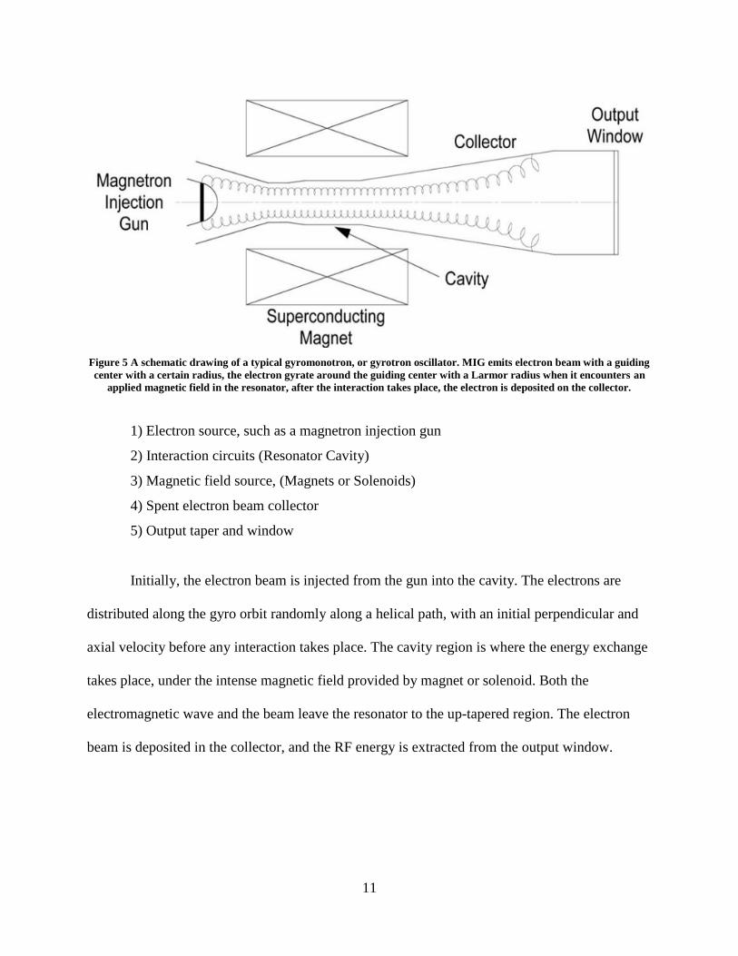
Shown in Figure 5, a typical gyrotron oscillator, or gyromonotron, typically consists of

the following major components:

11

Figure 5 A schematic drawing of a typical gyromonotron, or gyrotron oscillator. MIG emits electron beam with a guiding

center with a certain radius, the electron gyrate around the guiding center with a Larmor radius when it encounters an

applied magnetic field in the resonator, after the interaction takes place, the electron is deposited on the collector.

1) Electron source, such as a magnetron injection gun

2) Interaction circuits (Resonator Cavity)

3) Magnetic field source, (Magnets or Solenoids)

4) Spent electron beam collector

5) Output taper and window

Initially, the electron beam is injected from the gun into the cavity. The electrons are

distributed along the gyro orbit randomly along a helical path, with an initial perpendicular and

axial velocity before any interaction takes place. The cavity region is where the energy exchange

takes place, under the intense magnetic field provided by magnet or solenoid. Both the

electromagnetic wave and the beam leave the resonator to the up-tapered region. The electron

beam is deposited in the collector, and the RF energy is extracted from the output window.

12

Section 1.5, Components of 670GHz gyrotron.

1.5.1 Magnetron Injection Gun

The electron gun was designed jointly by the Institute for Research in Electronics and

Applied Physics (IREAP) at the University of Maryland and the Russian company Gyrotron

Complexes (GYCOM); it was manufactured by GYCOM. An important issue in the

development an electron gun and electron optics for this sub-millimeter gyrotron is the need to

adapt the gun to the high frequency and pulsed solenoid [17]. When compared to conventional

gyrotrons operating at millimeter wavelengths with the use of superconducting solenoids, the

frequency scaling plays a crucial role. The first consequence of the scaling is that the solenoid is

directly attached the tube body; it is very compact in dimension. The second consequence is that

it is necessary to have an electron beam with small enough spread in electron guiding centers in

the interaction space to allow for high efficiency operation. The first constraint causes a strong

divergence of the magnetic force lines outside of the solenoid, i.e., in the region where an emitter

should be located, and therefore makes it necessary to have a large angle of the emitter with

respect to the tube axis (this reduces the orbital to axial velocity ratio, which reduces the fraction

of energy available to be extracted). The second constraint will be discussed in more detail in

the next chapter. With these considerations in mind, the final gun design was performed and is

shown in

Figure 6.

Electron guns for gyrotron are usually magnetron injection gun, and it is the case for this

particular design. They are named because they bear resemblance to magnetron's cathode

assemblies. The electrons are emitted from the emitter area, which appears as a ring around the

cathode head. The ejected electron forms a beam shaped like a hollow ring, due to this emitter

13

arrangement. The final design called for a maximum current output of 15 ampere with operating

voltage between 50kV to 70 kV. The cathode operates on the principle of thermionic emission,

the emitter area needed to be heated so that electrons can be thermally excited to overcome the

work function. The heating is provided by a built in filament, powered by an external power

source.

The goal of the design is the maximizing of current output while minimizing the energy

spread. Since the gyrotron's electron sources tend to operate with temperature limited emission,

current output can increase by increasing temperature. But the higher thermal energy will lead to

more severe energy spread.

The electron gun uses lanthanum hexaboride to form the emitter surface. This new

material is used in the latest TEM microscope as cathode materials due to its excellent thermal

properties.

14

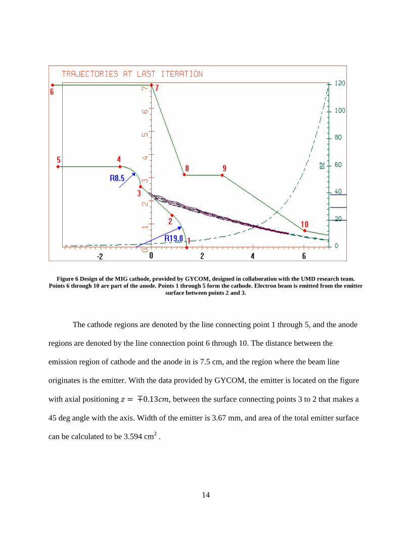
Figure 6 Design of the MIG cathode, provided by GYCOM, designed in collaboration with the UMD research team.

Points 6 through 10 are part of the anode. Points 1 through 5 form the cathode. Electron beam is emitted from the emitter

surface between points 2 and 3.

The cathode regions are denoted by the line connecting point 1 through 5, and the anode

regions are denoted by the line connection point 6 through 10. The distance between the

emission region of cathode and the anode in is 7.5 cm, and the region where the beam line

originates is the emitter. With the data provided by GYCOM, the emitter is located on the figure

with axial positioning , between the surface connecting points 3 to 2 that makes a

45 deg angle with the axis. Width of the emitter is 3.67 mm, and area of the total emitter surface

can be calculated to be 3.594 cm2 .

15

1.5.2, Pulsed Magnet and Power Supply

As described in the introduction, gyrotron operation is based on the principle of electron

wave interaction is a strong applied magnetic fields. The frequency of output radiation is directly

related to strength of the magnetic field. For fundamental harmonic operation at 670 GHz, the

required field value is around 27 T. This field is produced by a pulsed solenoid. The basic design

is based on the solenoid used for achieving a 1 THz frequency operation in Russia [18]. The

pulsed solenoid has an inner bore diameter 17.5 mm, and an outer diameter 41 mm and the

length of 53 mm. A photo of this solenoid is shown in Figure 7.

Figure 7 Pulsed solenoid for 670GHz Gyrotron. The larger outer structure forms the Nitrogen bath, while the solenoid is

placed inside. During operation, liquid nitrogen is used to maintain a constant resistance for the solenoid coil so that the

magnetic field generated can be maintained from pulse to pulse.

16

The solenoid consists of 174 turns of a 40%Nb-60%Ti alloy wire with a 3×1 mm2 cross-

section reinforced in an outer copper shell; its filling factor is close to 80%. This composite cable

is wired on a stainless steel pipe having a 0.5 mm thickness and 16 mm inner diameter. Each

layer of wires is covered by an epoxy, then, the solenoid is wrapped with a 15 mm thick bandage

made of a glass textolite. After careful conditioning, the inductance of solenoid is equal to 0.336

mh. The solenoidal constant was 34 Oe/A. At the nominal solenoid voltage of 3.1-3.15 kV, the

solenoidal current is about 8 kA. Liquid nitrogen is used to control ohmic heating and stabilize

the operation. The resistance of the solenoid at room temperature and liquid nitrogen temperature

is equal to 0.07-0.08 and 0.01 Ohm, respectively [5].

The power supply of the pulsed solenoid (PSPS) provides for formation of a solenoidal

current creating the required magnetic field. Schematic of the PSPS is shown in Figure 8. Here,

the pulsed solenoid with inductance sL and active resistance sR is shown on the right. On the left,

the charging block 4000CCPS is shown which consists of a high-frequency transistor converter

with dozing capacitors and transformer output. It provides charging of the block of capacitors up

to the nominal voltage in the range of 0.5-3.8 kV. The block consists of three parallel connected

6 kV capacitors having a capacitance of 1,100 F each. This block is denoted in Figure 8 asC .

The discharge of the energy accumulated in C into the solenoid is controlled by the thyristor

switch VS shown in Figure 8. The charging block 4000CCPS provides pulse-to-pulse

reproducibility of the solenoidal current with an accuracy of %1.0 .

17

Rs

C

Ls

VS

VD

Rcr

CCPS4000

Figure 8 Circuit for magnetic power supply

To provide the desired maximum value of the solenoidal current, the block of capacitors

should be charged up to the voltage QCLIV sch 2/exp/max where the circuit quality

factor can be defined as ss RRCLQ 0// . Here 0R is an equivalent active resistance of

the discharge circuit which accounts for the losses in the capacitors, all contacts and the thyristor.

In the course of experimental studies it was determined that the quality factor of this circuit is

close to 3.

For reducing the solenoidal Ohmic heating a crowbar circuit consisting of a diode VD

and a resistor scr RR is added parallel to the bank of capacitors as shown in Fig. 6. Active

resistance of this resistor is equal to 0.1 Ohm. The energy of joule heating of the resistor during a

single pulse is equal to crsscr RRILW /12/2

max . The maximum current is equal to 8 kA

which creates a magnetic field about 28 T [5].

18

Chapter 2: Sub-Terahertz resonant circuit

This chapter presents the works that studied the following:

1. the theoretical limits of the resonator efficiency,

2. the choice of parameters that was important in realizing the efficient operation,

3. the iteration of design and the simulated results

4. experiments based on the design

5. verification of the design

Section 2.1, General theory, orbital efficiency and normalized parameters

The resonator structures for gyrotrons, unlike those of slow-wave devices, can be very

simple. Since there is no need to slow down the wave for interaction with electrons, there is no

need for corrugations or any other periodic structures [14]. The resonator for this 670 GHz [19]

gyrotron, as is the case for most gyrotrons, is an irregular length of “pipe” of circular cylindrical

cross-section with variation in radius along the longitudinal axis. The axial dependence of the

cylindrical radius defines the RF field profile in the resonator. The input section that leads from

cathode region to the resonator has a smaller radius so that the operating mode does not

propagate into the electron gun. At the other end of the resonator, the output region is tapered up.

The tapering allows for the axial wave number to increase, thereby increasing the wave’s

group velocity to facilitate the extraction of RF power. The optimal design would include an

ideal length for the middle section in order to allow optimal amount of interaction between the

electron beam and the RF field, an input section that prevents the RF field from entering the

cathode region so that the electron optics is not disturbed by the resonator field, and an output

19

section that ideally balances the need to extract the largest amount of power possible while not

compromising the RF field inside the resonator.

Before diving into the specification and dimension of the resonant circuit, it is important

to approach it from a theoretical perspective. It was necessary to first get an idea of what are the

theoretical and practical limits of efficiency that one can hope to achieve, and only then can the

results be evaluated in context. The theory allows an estimate of what can be expected and what

should be the goals. With this in mind, I would first describe electron-wave efficiency in terms of

dimensionless normalized parameters.

A more detailed derivation of the equations can be found in Chapter 3 of Introduction to

the Physics of Gyrotron [14], only the steps that are most relevant are included here for the

reader's convenience.

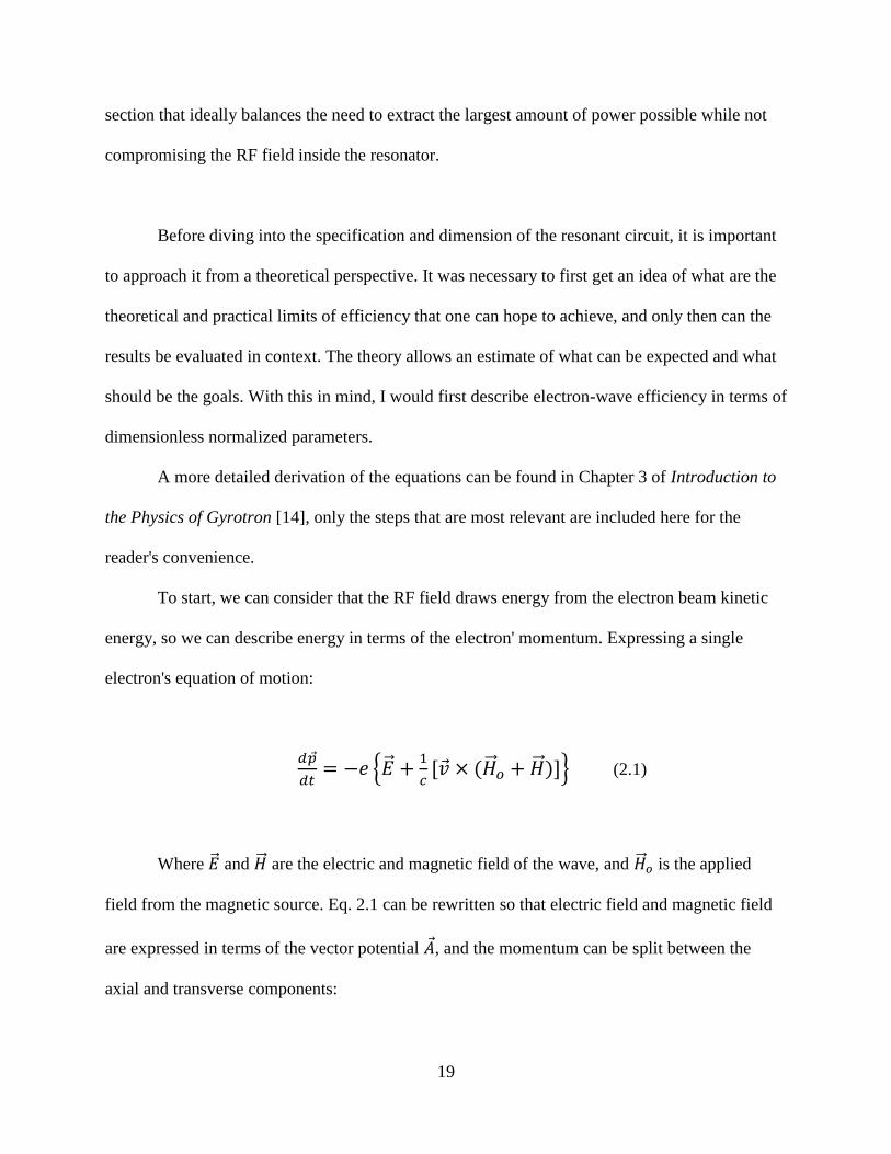
To start, we can consider that the RF field draws energy from the electron beam kinetic

energy, so we can describe energy in terms of the electron' momentum. Expressing a single

electron's equation of motion:

(2.1)

Where and are the electric and magnetic field of the wave, and is the applied

field from the magnetic source. Eq. 2.1 can be rewritten so that electric field and magnetic field

are expressed in terms of the vector potential , and the momentum can be split between the

axial and transverse components:

20

(2.2)

(2.3)

The previous chapter has introduced the relationship , Using this

relationship together with Eq. 2.3 leads to the integral of motion of the electron:

(2.4)

However, in a typical design, the gyrotron operates with a transverse electric (TE) wave

mode [14]. When such a wave is excited near cutoff, the electron’s axial momentum remains

almost constant in the process of electron beam-wave interaction. Taking the general Gyro-

averaged equation, assuming that the electromagnetic field is a superposition of different

harmonics, and that only the harmonics that are in cyclotron resonance with the gyrating

electrons are left after averaging, the expression are given as:

(2.5)

(2.6)

Eq. 2.5 relates the change in transverse momentum of the electron to the energy change,

assuming the axial momentum is constant. Eq. 2.6 divides both sides by the initial energy. The

21

first term on the right hand side is called the single electron efficiency, it is the ratio of the orbital

kinetic energy to the total kinetic energy. The orbital kinetic energy is the transverse component

that is available for extraction. The second term on the right hand side is the change in the

transverse momentum of the electron, hereafter referred to as the orbital efficiency.

From Eq. 2.6 we have an expression of the ratio of change in energy of the electron due

to interaction with a TE wave, or the interaction efficiency, int. We see that this efficiency

depends on how much of the electron kinetic energy is due to the transverse motion as opposed

to the axial motion; and on how much the transverse momentum changes. Eq. 2.6 is rewritten

into:

(2.7)

In Eq. 2.7, cv /00 is the initial electron orbital velocity normalized to the speed of light,

2

0 /1 mceVb is the Lorentz factor determined by the beam voltage bV and is the orbital

efficiency characterizing the fraction of the energy of electron gyration transformed into

electromagnetic radiation. The orbital efficiency depends on three normalized parameters [14]:

the normalized length // 0

2

0 Lz , which is the upper bound of an integral; the

normalized cyclotron resonance mismatch 0s , and the normalized beam current

parameter0 bI I G

L

, where G is the coupling coefficient. The normalized beam current is

directly related to the normalized amplitude of the RF field.

22

With an expression for the interaction efficiency, the next step is to find the orbital

efficiency term. For this we go back to Ref [14], where the orbital efficiency is calculated by

finding the change in electron energy at the entrance to the interaction length and at the exit. For

a fixed Gaussian field profile, the expressions for particles are given as:

(2.8)

(2.9)

where is a normalized unit related to the electron’s kinetic energy, is the axial

coordinate normalized to the wavelength and electron velocity ratio, is the normalized

amplitude of the RF field, and is a function that describes the axial field structure, which is

Gaussian for this case. is the phase of the electron. The initial conditions assumes that

is 1, meaning 100% of the electron energy is in the beam, and is evenly distributed

between to .

(2.10)

The orbital efficiency in Eq. 2.10 is the change of energy from to integrated over

all of the initial phase distributions of the electrons. Using MATLAB, the integral is evaluated,

presented as Figure 9, which shows the contour of efficiency for different normalized interaction

length and normalized amplitude.

23

Figure 9 Plane of orbital efficiency for different normalized length and amplitude. The color scale corresponds to the

orbital efficiency, highest frequency is dark red, while the lowest efficiency region is blue.

Figure 9 covers a very wide range for both the normalized amplitude and normalized

length. Being dimensionless, it's not readily apparent where on the contour the proposed gyrotron

would fall, but it's very unlikely that it would fall on a value beyond the range shown. Figure 9

also shows promise in that there are regions where the orbital efficiency is 60% and above,

suggesting that the theoretical efficiency limit is quite high. Now that the efficiency has been

described in terms of normalized units, the next step is to relate that to real world units.

24

Section 2.2, Surface resistance losses, mode choice

As stated in the introduction, the lack of readily available high magnetic fields had been a

fundamental limit on developing gyrotrons into the sub-millimeter and the terahertz frequency

range. Another important limiting factor is that at these frequencies, the efficiency had been very

low. The few successful examples of gyrotrons at this frequency range were operating with

efficiencies in the single digits [1]. One major culprit for the low efficiency had been that much

of the power extracted from the electrons is lost due to surface resistance, which is inversely

proportional to skin depth. The loss of RF energy due to surface resistance is well known [20], as

well as the fact that this loss increases with frequency of the RF field. In that respect, gyrotrons

in general have an advantage over the traditional slow-wave device [10]. Slow-wave devices

require periodic structures to slow the wave down for interaction, thus the field tend to localize

near the wall structures, therefore requiring the electron beam to also be injected near the wall.

This causes the slow-wave devices to shrink in size more rapidly than gyrotrons as frequency

increases. With small size, the power density increases, and the Ohmic losses become

impractical. Still, for gyrotrons near the terahertz region as the one described in Ref [1], this

advantage is not enough.

To minimize the Ohmic loss, the Ohmic Q can be increased by designing the resonator

cross-section to be larger. On the other hand however, since the resonator must be designed to

operate near the cutoff frequency of the operating mode, higher frequency results in smaller size.

In order to compensate for the higher while maintaining the power density, the only choice is

to choose a higher ordered mode for gyrotron operation. Utilizing a high ordered mode enables a

larger resonator cross-section, thus a larger volume. However, this approach has generally not

been taken since large cross-section and volume can support more modes, all of which could be

25

competitors to the operating mode. Having a possible competitor mode is especially harmful for

a gyrotron during the start-up, where undesired modes maybe kicked start before the operating

mode, and end up sustaining themselves causing degraded efficiency for the operating mode.

Thus gyrotrons operating in a dense mode spectrum require elaborate start-up scheme to avoid

this effect. Even then, mode competition may still occur to the detriment of the operating mode

[21]. Thus the maximum size of the resonator is limited by mode stability.

With these constraints in mind, the first step is to find workable parameters for the 670

GHz gyrotron to start the design process. The operating mode chosen is the TE31,8 mode; it has

the Eigen-number 7675.638,31 that yields wall radius equal to 4.543 mm. The main reason for

the choice of this particular mode is superior stability: recent development of MW-class

gyrotrons [22] for plasma experiments in the large-scale experimental fusion reactor ITER

proved that this mode can be selectively excited and operate stably.

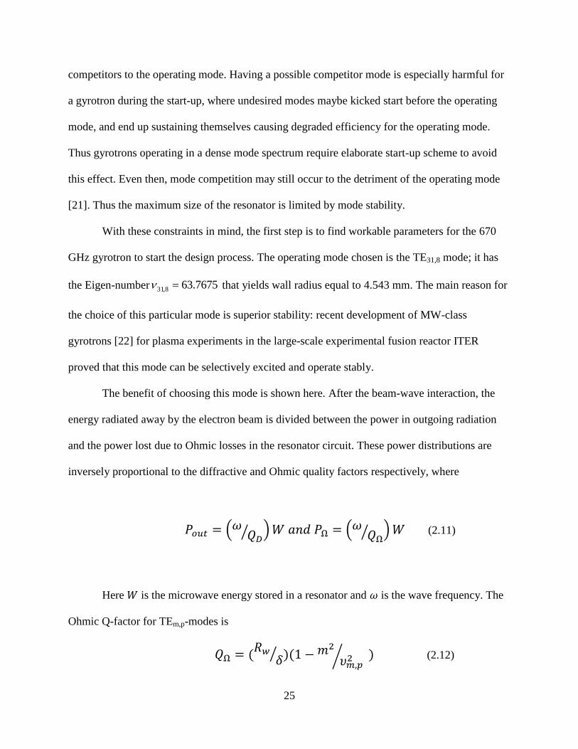
The benefit of choosing this mode is shown here. After the beam-wave interaction, the

energy radiated away by the electron beam is divided between the power in outgoing radiation

and the power lost due to Ohmic losses in the resonator circuit. These power distributions are

inversely proportional to the diffractive and Ohmic quality factors respectively, where

(2.11)

Here is the microwave energy stored in a resonator and is the wave frequency. The

Ohmic Q-factor for TEm,p-modes is

(2.12)

26

while the minimum diffractive Q-factor of the resonator is estimated to be 2/30 LQD . Here

wR is the resonator wall radius, is the azimuthal index of the mode, is the radial index, and

is the zero of the Bessel functions of the first kind corresponding to TEm,p. is the skin depth,

given as

(2.13)

Output efficiency is defined as the ratio of the power extracted in the form of radiation

from the output window to the beam power. This number will be lower than interaction

efficiency shown in Eq. 2.7, since a portion of RF power would be lost to ohmic heating. From

Eq. 2.11, output efficiency can be written as

(2.14)

At the given frequency of 670 GHz, the skin depth of copper is 1.1 micron, taking into

account the roughness of the resonator wall surface that reduces conductivity by half from the

tabulated values. For this skin depth, the ohmic Q is approximately equal to 30,000. Assume that

a typical resonator length of about 10 wavelength, which gives a diffractive Q of about 3000.

Then, close to 90% of the energy extracted from the electron beam is expected to be output

radiation, while only about 10% will be lost to surface resistance.

27

The last piece of information needed to estimate the efficiency is the parameter of the

electron source. At the time this study was conducted, the contractor for manufacturing [5]

specified that the electron gun is design to be limited to 60-70 kV beam voltage with maximum

20 amps current. The electron beam would have an orbital-to-axial velocity ratio 3.1/ 00 z -

1.35. With these data, we can find an efficient operating point on the contour of Figure 9.

Starting off assuming the best case scenario for the electron gun, a 70 kV beam yields

1.137 and 3.1/ 00 z 5, the single electron efficiency in Eq. 2.6 comes to just under

60%. Again assuming a length to wavelength ratio, 10/ L , which is a valid assumption [14],

yields a normalized length (normalized to wavelength) of 14.4. According to Figure 9, the

orbital efficiency can reach 60% for that value of normalized length when the normalized

amplitude of the RF field is around 0.175. Normalized amplitude can be related to the orbital

efficiency by the expression:

(2.15)

0 bI I G

L

, it is a normalized beam parameter related the beam current, coupling factor

G and the ratio wavelength to interaction length. The coupling factor is an important concept for

the topic of Chapter 3, and will be discussed in detail there. Likewise would become important

later in Chapter 4. Substituting 0.175 for and 0.6 for , gives the normalized beam parameter.

For this particular choice of mode, interaction length electron voltage and beam parameter, the

beam current comes to about 12 amps. This result offers hope that under the ideal condition

where the electron source is optimal, 60% orbital efficiency is achievable. Optimal electron

28

source assumes no spread in the electrons' gyrating radii, and no spread in the electron's energy

(or velocity). The value of the optimal cyclotron resonance mismatch is not important at this

stage because in experiments, this mismatch can be easily optimized by varying the external

magnetic field.

Assuming under the ideal condition orbital efficiency is about 60% , and the single

electron efficiency of also around 60%, Eq. 2.7 shows that the best interaction efficiency we

could expect is around 36%. Factoring in wall losses, the ideal output efficiency we can aim for

would be around 33%. Supposing the electron beam supplies a power of 1.05 MW(15 amps at 70

kV), the output radiation can be more than 350 kW.

Thus far the results shows promise, 33% output efficiency is considered good for

gyrotrons that are without a sophisticated energy recovery system for the spent electron beam,

and more importantly, no one else has been able to achieve this high level of efficiency at this

high frequency. The next step is to finalize the resonator design that can realize the theoretical

results, and then verify the performance estimate with a simulation code.

29

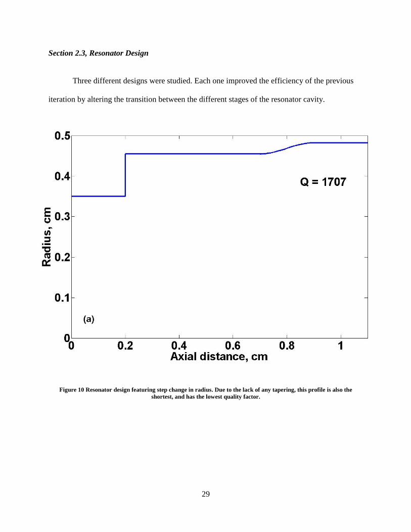
Section 2.3, Resonator Design

Three different designs were studied. Each one improved the efficiency of the previous

iteration by altering the transition between the different stages of the resonator cavity.

Figure 10 Resonator design featuring step change in radius. Due to the lack of any tapering, this profile is also the

shortest, and has the lowest quality factor.

30

Figure 11 Resonator design featuring a slanted change in radius. The overall length was increased to accommodate the

linear taper while maintaining the same length for the interaction region. It was decided that the taper would run from

0.15cm to 0.25 cm, and the radius of the input is increased.

31

Figure 12 Resonator design featuring a rounded, gradual change in the radius. The input section had much bigger radius

compared to the previous two iteration to keep the angle less than 5 degree.

In the course of the design process, several resonator profiles were considered: Profile 1,

Profile 2 and Profile 3 are shown above in Figure 10, Figure 11 and Figure 12. For all three of

these designs, the geometry can be divided into three sections along the axis. The input section is

where the wall radius is below the cut-off for the operating mode, as to insure that the cathode is

protected from perturbation by the resonator RF field. The straight section is where the

interaction between the wave the electrons are expected to take place. The last section where the

radius increases is the up-tapered region, where the RF power is expected to leave. On that note,

32

it's worth mentioning that the actual length of vacuum tube runs much longer than the lengths

shown here. Typically, right after the up-taper section, a beam collector is installed where spent

electrons are collected, and after that the output vacuum window. These components will need to

be integrated smoothly at the ends of these profiles. But those items are beyond the scope of the

present research study.

Profile 1, has the simplest geometry, it is the starting point of the study. Profile 1's simple

geometry was useful in optimizing the length of the resonator. The approach was to focus on one

aspect of the design at a time, finding the best geometric profile will be done in the next step.

Referring to Figure 10, one sees that there is no transition between the input region and the

interaction region; the radius changes stepwise at the resonator entrance. The input stage runs

from 0 to 0.2 cm, with radius of 0.35 cm, well below the cut-off radius. The radius of the straight

section is equal the cut-off cross-section of the operating mode TE31,8, which is 0.4543 cm. The

radius for the output section is 0.48234 cm. The radius for the input section and up-tapered

section are not arbitrarily chosen. The design is based on the experimental ITER gyrotron [22],

with the interaction section scaled down to accommodate operation at 670GHz from 110 GHz.

The ratio between the three sections are preserved during scaling and used here. The wall profile

between the interaction section and the flat portion of the up-tapered region has radii that created

by a sine squared function. This up-taper shape will be used in simulation while its final design

will be finished by independently together with the design of the collectors. The design starts

with the assumption that the interaction region has , this is the same assumption that

was used in the preceding theoretical section. For 670 GHz, the ratio results in L = 0.4478 cm.

33

In profile 2, improvement was made to the transition between the input section and the

interaction section. The sharp step change is replaced by a linear tapering. The taper has a length

of 1 mm at a 27 degree angle. The radius of the input section is increased to 0.4 cm so that the

angle of the taper would not become too great. The length of the input section is shortened to

accommodate the linear taper without shortening the interaction section. The up-tapered section

remains the same as in Profile 1.

In Profile 3, the radius of the input stage is further increased so that the tapering angle is

small; the sharp corners where the radius changes are replaced by smooth curves, and the overall

length is increased. It is commonly known the mode conversion at the transition is an important

issue. In order to minimize its effect, angle of the taper has to be kept small, to be only 5 degree

or less. To achieve it, the overall length was increased, so that the interaction length is shifted

right to make room for a longer taper to run from 0.15 to 0.3cm. The radius of the input stage is

increased to a value such that the angle it makes with the flat portions on both ends of the taper is

equal to 5 degree. Lastly, the corners at the end of the tapering are removed. This is done by

creating a circle for each corner; the centers of these circles would be enclosed by their

respective corner. The coordinate of the center of a circle is such that it would have a radius that

would be tangential to both the flat portions and the tapered portion. Once the center of a circle is

located, the arc of circumference of the circle that is between the two points where the radius

normally insect the flat portion and the taper will the new resonator wall. The sharp corners will

thus be removed. It has been suggested in the literature that smoothing of the sharp corners at

the edge of the tapering can reduce mode conversion [23].

Mode conversion occurs when some of the RF field changes mode structure from the

operating mode to a different resonator mode. These modes are largely undesired because the

34

non-linear mode interacting gyrotron can be unpredictable. If modes are created above the cut-

off the input section, fields can leak into the gun region and disturb the electron bunching.

During the study, the length of the interaction section is progressively increased from the

initial value. The increment of increase is 0.5 cm. "Cold cavity" Simulations on these different

lengths are performed to characterize their frequency response. The simulations yielded the

structure's quality factor, its cavity resonance frequency and possible mode conversion.

Once the optimal length for the interaction length is set, this will be the new length for

resonator with Profile 2 and Profile 3. Subsequently, cold-cavity calculations were performed on

Profile 2 and 3 with the optimal length to find their cavity resonance frequency, quality factor,

and compare any mode conversion due to tapering of the structure with that of Profile 1 with the

same length.

35

Section 2.4, Cold cavity calculation results, quality factor and mode conversion

Figure 13 Cold-cavity simulation showing the axial shape of the RF field. This shows that most of the field is confined

inside the interaction section so interaction can take place. As expected, since the input section is well below the cut-off,

the field decays rapidly in that stage.

The tool utilized for the "cold cavity" simulation is MAGY [15]. MAGY is a simulation

code that models the gyrotron's RF field in a waveguide representation. It solves a series of

coupled one dimensional differential equations rather than the full set of Maxwell's equations,

and is therefore much less time consuming. In the case where the simulation does not include

36

active charged particles, the code only solves for the fields in a waveguide, and is thus even

faster. This case is called "cold cavity." Since the interest for now is only in how the fields

evolve in the resonator circuit, "cold cavity" will suffice.

Without particles to excite the RF field, the "cold" simulations were done by placing an

artificial TE31,8 source with Gaussian distribution in the middle of the resonator structure. The

frequency of the artificial source is varied to scan for the frequency response of the resonator.

The range of frequency scanned is from 669 GHz to 671GHz, with the interval 0.05 GHz for

each simulation run. Simulation results include the amplitude of field along the length of the

resonator, example of is shown in in Figure 13. The above shows the axial field structure of the

operating mode inside profile 1. Figure 13 shows that most of the field is confined inside the

interaction section so interaction can take place. As expected, since the input section is well

below the cut-off, the field decays rapidly in the input section stage. The peak amplitude of each

of the simulation run is recorded, and the run with the highest amplitude would have the

frequency corresponding to the resonant frequency of the resonator. The quality factor of the

resonator can be determined from the energy output file by calculating the ratio of stored energy

vs. flow at the simulation frequency. This is repeated for the differently lengths of Profile 1, and

also repeated for Profile 2 and Profile 3.

Figure 10, Figure 11 and Figure 12 show the quality factor for Profile 1, 2 and 3

respectively. These are the value at the optimal length. The rounding clearly reduces the

diffractive Q value of the resonator cavity: the rounding of the edge causes about 10% reduction

in diffractive Q. This result is consistent with the fact that the presence of sharp edges increases

wave reflection in the structure, and results in increased diffractive Q. In the designing process,

37

attention must be paid to changes in Q value in order to optimize the output efficiency; see Eq.

2.14. These results show that in the straight section, where the beam-wave interaction takes place,

mode conversion due to reflection is unlikely to be significant.

Next, the adjacent radial modes which are caused by the conversion of the operating

TE31,8 mode due to the wall tapering [23] [24] [25] were included in the simulations. Due the

very close radial mode number, these modes are the most likely spurious mode that may be

created.

Table 1 Ratio of amplitude of different modes to the operating mode, scaled to the operating mode.

Table 1 shows the ratio of wave amplitudes of different modes to the operating mode at z

= 4.5mm (center of the resonator). In Profile 1, which has the steepest tapering, the other modes

are less than 1% of the operating mode. In profile 2, the TE31,7 mode reaches 10% of the

operating mode, while amplitude of TE31,9 remains at a very low level. In profile 3, the

extraneous modes drop down to less than 1% of the operating mode. The results showed that the

smoothing of the corner had practically no effect on reducing mode conversion in this particular

case. For profile 3, which has a tapering angle that is much smaller, the calculations show the

smoothing of edges significantly reduces the mode conversion: the amplitude of the TE31,7 mode

Profile 1 Profile 2 Profile 3

TE31,7 < 10

-2 10

-1 < 10

-2

TE31,8

(operating mode)

1 1 1

TE31,9 <10

-4 10

-3 10

-3

38

is one order of magnitude larger in the unsmoothed profile than in the smoothed profile. These

results show that in order to minimize mode conversion, the tapering should be kept at either a

very steep or a very small angle.

The up-taper section at the end of the cavity caused more significant mode conversion.

MAGY simulations indicate that the amplitudes of the TE31,7 and TE31,9 modes are 1/2 and 1/3 of

the operating mode, respectively. Results also indicate that there will not be significant coupling

to any TM modes, as their levels remain very low throughout the up-taper region. It is obvious

that the geometry of this region is un-optimized. Gyrotron radiation has to be collected and

coupled to transmission line or other quasi optical component for application. These couplers and

optical converters have to be optimized for a particular mode, meaning that if significant RF

power exist in modes that are not the operating mode, that RF power could not be efficiently

collected and would simply radiate out as wasted energy. The issue however, was addressed in

the design of the gyrotron’s other components. Since the up-tapering directly leads to the beam

collector, GYCOM (See Appendix I) took responsibility for ensuring that mode conversion in

those components is kept to a minimum. Their design of the up-taper and collector showed that

close to 90% of the RF power that reaches the optical converter remains TE31,8.

39

Section 2.5, Efficiency simulation

2.5.1, "hot" simulation setup and input parameters

In the ‘hot-cavity’ simulation, the design assumed a beam voltage of 70 kV, current of 15

amps and a velocity ratio of 1.3. The simulation takes into account the surface resistance loss. To

minimize calculation time in these simulations, the study neglected temporal variations of the

magnetic field and assumed it to be constant during the high-voltage and RF pulse duration. This

is a valid assumption since the magnetic field pulse is expected to last milliseconds, while the RF

pulse last duration is only eight to ten microseconds, effectively the beam will experience a near

static field during the operation.

For each simulation, the program requires a reference frequency; this is obtained for each

profile in a prior "cold" calculation as the natural resonance frequency. However, in the presence

of the electron beam under magnetic field, the beam will resonate with the RF field at the

cyclotron frequency. This result in a frequency pulling effect which may affect the simulation

results. This pulling can be seen in the output phase advance of the amplitude. If the phase

advance is too great, the simulation must be redone with a different reference frequency.

In these sets of calculation, the electron beam is assumed to have no guiding center

spread, the radii of the electrons guiding center is set to coincide with the first radial peak of the

operating mode. The effect of spread in guiding center is the focus of another chapter. However,

the orbital velocity of the electron beam is taken into account in the simulation as well. The input

file can be modified to specify certain RMS spread value. Simulation results are obtained for 0%

spread, then repeated for 5% and 10% RMS spread. This velocity spread will likely prevent a

fraction of electrons from giving up their kinetic by causing them to be out of phase with the

main bunch, resulting in lower efficiency.

40

A source term for the operating mode is also included in the "hot" simulation. The source

terms are designed to act in two different ways, to simulate excitation condition in the gyrotron.

For some simulations, the source term resembles a constant noise level seed to simulate

operation in the soft self-excitation regime. For other simulations, the source is configured to be

a high amplitude source that is turned-off after a predetermined time; this is to simulate gyrotron

operation in the hard self-excitation region regime. This will be explained more in detail later.

2.3.2, Efficiency results for the different profiles

Figure 14 Efficiency for several different length of resonator Profile 3, as function of magnetic field. Blue curve represent

L = 0.4cm. Frequency changes significantly with different length L. And even if L is the same, Profile 3 has significant

improvement over Profile 1.

41

The effect of the resonator design on the efficiency can be seen in Figure 14, the different

length of the resonator and different profiles. For the Profile 1 curve, L = 4 mm. First, as far as

length of the interaction is concerned, we see that the initial of 10 estimate is a very good

starting point. The most efficient length appears to be between 0.5 cm and 0.45 cm. The

relationship between the interaction length and the efficiency can be understood in the following

way: as an electron first enters the resonator, it first needs to go through the bunching process as

described in Chapter 1. After bunching is formed, the phase slippage causes the bunch to be in

the deceleration phase of the cyclotron resonance, thus giving up energy to the RF field. As the

slippage continue however, the electron bunch slip further in phase and enter the acceleration

phase, drawing the energy out of the RF field. All of these takes time, meaning that the

interaction section must be long enough for these processes to take place, but not too long so that

the electron bunch doesn't leave the deceleration phase. It appears to be the case that for L less

than 0.45 cm, the electron bunch has not fully interacted with the RF field, hence lower

efficiency is shown.

Moreover, the fact that even for the same L, Profile 3 perform better than Profile 1, this

may be attributed to the fact that Profile 3 has a much larger quality factor (3640 vs. 1707),

meaning that more field is trapped in the resonator of Profile 3 than in Profile 1. The higher field

intensity may cause stronger interaction between the RF field and the beam, causing the beam to

form bunches sooner, effectively allowing for the bunching to interact for a longer time inside

the same length of space.

42

Figure 15 This shows the efficiency of Profile 1 given an optimal length of 0.5cm. The efficiencies for different RMS

orbital velocity spread are shown in different curves: 0%, 5% and 10%. The efficiency varies with the applied magnetic

field. For Profile 1, the efficiency peaks at about 262.4 kG. With 10% RMS spread, the peak efficiency is over 29%.

43

Figure 16 This shows the efficiency of Profile 2 given an optimal length of 0.5cm. The efficiencies for different RMS

orbital velocity spread are shown in different curves: 0%, 5% and 10%. The efficiency varies with the applied magnetic

field. For Profile 1, the efficiency peaks at about 262.9 kG. With 10% RMS spread, the peak efficiency is over 32%.

44

Figure 17 This shows the efficiency of Profile 3 given an optimal length of 0.5cm. The efficiencies for different RMS

orbital velocity spread are shown in different curves: 0%, 5% and 10%. The efficiency varies with the applied magnetic

field. For Profile 1, the efficiency peaks at about 262.9 kG. With 10% RMS spread, the peak efficiency is over 35%.

Results shown in Figure 15 are the interaction efficiency, as a function of the magnetic

field in Profile 1, for different value of RMS orbital velocity spread. The spread value of 0%, 5%

and 10% value are chosen to illustrate the effect on efficiency. Note that 10% RMS spread is

considered a very high value, and it is expected that the electron gun will produce less spread

than this. With no spread, the efficiency can be 32.5%, but with a severe spread of 10%, the

efficiency drops to 29%.

45

Results shown in Figure 16 are the interaction efficiency, as a function of the magnetic

field in Profile 2, for different value of RMS orbital velocity spread. The spread value of 0%, 5%

and 10% value are chosen to illustrate the effect of on efficiency. Note that 10% RMS spread is

considered a very high value, and it is expected that the electron gun will produce less spread

than this. With no spread, the efficiency can be 34%, but with a severe spread of 10%, the

efficiency drops to 32%.

Results shown in Figure 17 are the interaction efficiency, as a function of the magnetic

field in Profile 3, for different value of RMS orbital velocity spread. The spread value of 0%,

5% and 10% value are chosen to illustrate the effect of this spread for efficiency. Note that 10%

RMS spread is considered a very high value, and it is expected that the electron gun will produce

less spread than this. With no spread, the efficiency can be 36.5%, but with a severe spread of

10%, the efficiency drops to 35%.

Gyrotron efficiency is the highest for Profile 3. In all three profiles, the effects of velocity

spread on efficiency are weak; even with a large 10% RMS orbital velocity spread, the efficiency

can still be close to 95% of the non-spread case.

The figures also illustrate another important point, and that is the efficiency peaks at a

lower magnetic field value than the exact cyclotron resonance frequency. It is known that the

gyrotron’s maximum efficiency takes place in the hard self-excitation region. Hard self-

excitation region corresponds to the beam current being less than the starting current; while the

soft self-excitation corresponds where to the case beam current exceeds the starting oscillating

current. Hard self-excitation occurs when there is a large slippage in the gyrophase in

comparison to the phase of the RF field, and that requires large wave amplitude to trap the

electron. This slippage in phase is related to normalized detuning value Δ introduced earlier, and

46

larger Δ means lower magnetic field value. In actual gyrotron operation, the hard-self excitation

is achieved by using an appropriate start-up scenario of the electron gun. The voltage-current

relationship during start up would first excite the modes in the soft excitation regime, and then

move to the maximum efficiency point in the hard excitation regime. In the simulations, this

start-up scenario is ignored for simplicity. To excite the mode in the hard-self excitation regime

in the MAGY simulation, an initial Gaussian source was placed inside the resonator cavity to

supply the 'kick' required for the self-excitation in the hard region. This artificial source is turned

off after a certain time period so the RF field has to be maintained by the electron beam.

There are weak extraneous modes in the resonator cavity resulting from reflections from

irregularities of wall radius, which was discussed in the earlier section. These modes have the

possibility of coupling with the electron beam and growing in strength. The same simulations

parameters were used again, but this time with consideration of parasitic modes to check their

effects on the operating mode in Profile 3. In the simulation, the efficiency does not change in

presence of these extraneous modes, and the amplitudes of TE31,7 and TE31,9 modes are small in

comparison to the operating mode, which agrees with the results of cold-cavity simulations at the

center of the cavity.

It is interesting to compare the axial dependencies of the interaction efficiency for each

cavity profile. Since it reinforces the notion that the optimal length is when the electrons have

ample time to form bunches and slip in phase, but not long enough for the phase to slip beyond

the optimum phase. Figure 18 shows that for different profiles, the electron bunching yielding

the growth of the interaction efficiency starts at different locations within the cavity, which

partially explains the variations in efficiency across the various geometries. Notice the large dip

47

in efficiency for the curve representing Profile 1; that would be the reason why it is less efficient

than the other two designs.

Figure 18 figure shows the interaction efficiency at each axial point. Each curve indicates optimal length of the different

profile shape of resonator circuit. The ripple present in Profile 1 may be the reason why it's less efficient.

2.5.4, Voltage depression due to space-charge field

The requirement of operating at 670 GHz with a pulsed magnetic solenoid demands that

the gyrotron fires in pulses. This places the additional restriction that the beam pulse duration

must be significantly less than the magnetic field pulse duration to ensure that the beam-wave

48

interaction is not affected by the temporal variations of the magnetic field. Calculations thus far

have assumed that ionization occurs to compensate for the DC space charge field caused by the

beam current. For continuous wave operation device, this is a reasonable assumption. However,

for very short single pulses, this may not be the case. The presence of this DC field will cause the

depression of the beam voltage and hence a decrease in the beam energy, meaning that even if

1.1 MW is drawn from the power supply, the amount of energy available for the RF field is less

than that. Moreover, voltage depression may also alter the orbital to axial velocity ratio, given

that the electrons are emitted at angle from the axis, and the electron optics are carefully

designed so that the electrons travel a designed path.

MAGY has a feature in which the space charge effect for the beam is calculated once the

wall radius is specified, so a simulation using Profile 3 with the optimal lengths is performed,

also with different values of RMS velocity spread. Figure 19 shows the efficiency as the function

of the magnetic field for Profile 3 when voltage depression is included. The decrease in the axial

velocity due to voltage depression results in enhancing the interaction efficiency by a few

percentage points and changes the optimal magnetic field value slightly. Overall, voltage

depression does not alter the efficiency value in any significant way.

49

Figure 19 Efficiency shown for the optimal wall profile, as a function of different point of magnetic field. This includes the

effect of voltage depression due to space-charge field, with separate curves for different values of velocity spread.

2.5.5, After-cavity interaction

The final issue addressed in this chapter is whether the efficiency is affected by after

cavity interaction [26] [27]. Due to the increase in the wall radius in the up-tapered region, the

axial wave number kz increases such that Doppler term in the cyclotron condition can no longer

be ignored. In a constant magnetic field profile which has been used thus far in all simulations,

50

the increased kz means that the cyclotron resonance will no longer be satisfied as given by the

cyclotron resonance condition: z zs k v . In a tapered magnetic field, the field strength

decreases as a function the axial distance. It raises the possibility that the cyclotron resonance

condition may yet still be satisfied and additional interaction between the beam and the wave

might take place well after the exit from the resonator region. This effect has been studied in

detail in [26] [27]; its effect on the overall efficiency can be negative.

Figure 20 The vertical line marks the end of the straight section, the figure shows the interaction efficiency at each axial

point. The up-tick shows that there is additional interaction in the up-tapered region. But efficiency does not suffer.

51

The constant magnetic field used in the previous simulations is only for the purpose of

saving calculation time; in reality, the magnetic field is tapered, with the strongest field at the

center of the interaction section, and decreases in both direction. To more accurately simulate an

experimental condition, the MAGY input file is updated with a more accurate magnetic field

profile.

Figure 20 shows the interaction efficiency as a function of the axial distance for a

realistic magnetic field profile. The interaction length was long enough to allow the efficiency to

reach its maximum, showing that the length of the straight section that had been chosen is

optimized. The vertical line marks the end of the straight section and the beginning of the up-

tapered region. To study the effect of after-cavity interaction by using the code MAGY, the

constant magnetic field was replaced by a parabolic approximation given by

max 0( ) / 1 ( )B z B a z z where 01090.3, 0.00475a z . B is in SI unit Tesla, while z and z0

are in meter. This approximation closely models the experimental data provided by the magnet

manufacture closely in the regions that covers the entire resonator cavity as well as the after-

cavity up-tapered region. Figure 20 shows that additional interactions do in fact occur in the up-

tapered region. It provides a small boost in efficiency, and the velocity spread does not have a

significant effect on the efficiency as it pertains to after-cavity effects.

Results of this chapter demonstrate the feasibility of the design for a high-power, high-

efficiency gyrotron at 670 GHz. The choice of a high-order TE31,8 mode reduced the ratio of the

ohmic power losses to the power of outgoing radiation to about 10%, which is not too far from a

level typical for high-power millimeter-wave gyrotrons. With the calculated 35% efficiency, the

gyrotron could deliver over 300 kW power. Numerical simulations indicate that the electron

velocity spread, after cavity interaction and voltage depression will not be significant as far as

52

efficiency is concerned, and finally that the amplitudes of parasitic modes caused by the mode

conversion in slightly irregular cavities would be well below 1% of the operating mode level.

Utilizing the results provide above, a 670GHz gyrotron was built by the Russian

consortium GYCOM, and was delivered in to the University of Maryland December 2011.

Figure 21 illustrate the final configuration of the device. The resonator was manufactured using a

beryllium-copper alloy. In addition to the efficiency issue discussed so far, the Russian team also

had to consider other major challenges, most importantly the magnetic field penetration into the

resonator and the its structural strength. These issues arise from the fact that the magnetic field is

pulsed, so it is time varying. If the resonator materials are highly conductive, they may help

lower surface resistance losses, but will also block magnetic field from penetrating through them.

To compensate, the wall could be made thinner, but the pulsed magnetic field will create a strong

magnetic force that the resonator must be able to withstand, limiting how thin the wall can be

made. At the end of the up-tapered section, the beam collector is made of molybdenum.

53

Section 2.6 Experimentation, calibration and verification of simulation results.

2.6.1, Experimental set-ups

In this section, the author gives a brief description of initial installation and testing of the

gyrotron, and some limited experiments.

The experimental team was led by Dr. John Rodgers, and in addition consists of Dr.

Talamas-Romero, Dr. Dmytro Kashyn and myself.

Figure 21 Experimental Setup: Counter-clockwise direction: 1) the triggering switch for timing of the firing of the various

device and instruments; 2) the solenoid power supply; 3) the RF power is measured a RF detector, while the beam current

is measured by a rogowski coil; 4) the cathode filament heater power supply; 5) the high voltage modulator that produces

70 kV potential; center) the gyrotron.

54

The high voltage power modulator is capable of driving 70 kV bias to the cathode and

maintaining a flat pulse top for 8 us. The modulator consists of a bank of inductor and capacitors,

where the energy for the pulse is stored during the period of charging. A very short period of

discharge releases the energy when the gyrotron fires. The discharge is controlled by a thyrotron

through a control signal. The discharge energy is channeled through a transformer to achieve the

high voltage needed. The gyrotron is mounted directly above the transformer module, and high

voltage wires connect the cathode to the high voltage modulator. The cathode filament is heated

by a heating power supply. The heating power is controlled by dialing the voltage output of the

heater power source, and the actual power supplied to the firmament is calculated by measuring

the current output with a rogowski coil and multiplying it with the voltage.

A vacuum port is connected to a molecular vacuum pump. Before any experimental run,

the pump evacuates the tube to a pressure of torr. After each time the cathode

discharges, the pressure spikes up to torr, and then is allowed to return to the previous

value before another shot is fired. The vacuum apparatus is also attached to a spectrometer, the

gas content of the tube can be seen in real time as the gyrotron pulses in experiments.

The pulsed solenoid is to be immersed in liquid nitrogen to a) control the heating of the

solenoid current and b) maintain a constant temperature so that the same magnetic field value

can be repeated for different experimental run. The LN2 Dewar can hold enough liquid nitrogen

for 3 pulsed operations before too much LN2 is boiled away. Additional cooling is required for

the anode, a port is provided on the side of the gun anode body, tubes are attached and chilled

water is pumped into the region.

55

To synchronize the gyrotron's RF pulse with the peak magnetic field, appropriate timing

is needed to synchronize the modulator, solenoid and diagnostic equipment. A multi-channel

waveform generator is used as the control. Preparation time is needed before the beginning of

each experiment so that the cathode is heated to the emission temperature as determined by

preliminary testing, and for the vacuum condition to reach the desired level.

An initial inhibition signal is used so that the experiment will not trigger while the high

power modulator is charging. During that time, the solenoid power supply is also allowed to

charge up to the desired value for that particular experimental run. After both devices are given

enough time to become fully charged, the timer can then be triggered by the waveform generator.

The solenoid pulse fires first, and when the magnetic field reaches the peak value after a 1.8 ms

delay, the thyrotron is triggered and the high voltage modulator discharge the pulse to the

cathode. At the same time, the diagnostic equipment is also triggered so the results can be

recorded.

2.6.2, Cathode characteristics

In general, cathodes for microwave tubes can be either based on the principle of

thermionic emission or secondary emission. Gyrotrons, like most other vacuum tubes relies on

thermionic cathodes, and the temperature of the emitting surface often exceeds 1000 K [3]. The

large thermal energies injected give electrons enough energy to overcome the work function of

the solid cathode surface and allow them escape. The emission current can be obtained by the

product of the density of states and the electron probability distribution. The classical

Richardson-Dushman equation shows the temperature dependence of the beam’s current density.

56

(2.16)

Where

and is the work function of the solid and T is the

temperature at the emitter. The Richardson-Dushman equation describes the gun operation in the

temperature limited regime, which is generally the case that applies to gyrotron operation. In the

experiment however, the cathode experiences a voltage rise from 0V to the operating voltage.

During this voltage rise, the emission is governed by the space charge effect, meaning that the

emission is voltage dependent instead of being temperature dependent. This effect is described

by the Child-Langmuir Law:

(2.17)

is the gun perveance, d is the spacing between the electrodes and V is voltage.

The first order of business before experimenting with the gyrotron is to characterize the

emission property of the cathodes, and to do that, it is necessary to estimate the work function of

the emitter surface and perveance of the electron gun. A separate power supply and a pyrometer

are used for gathering data. The testing power supply is programmed for a voltage sweep from 0

to 1000V while the cathode is heated to different temperature. At the time, the exact power

needed to heat the filament to the optimal range is unknown, but after gradually increasing the

heating power, it was determined that the gun should be heated with 410 W of power.

57

This testing result of the voltage sweep is plotted in Figure 22, which also shows the

curve fit using the space-charge and the temperature limited equation. For voltages from 0 to 500

V, the gun is clearly operating in the space-charge regime, and this perveance used in the line fit

is pervs.

Figure 22 V-I characteristic of the electron gun. Green curve is the measured current output vs applied voltage blue curve

represents space-charge limited emission, red curve represents temperature limited emission

Temperature in the emission region is obtained from the pyrometer reading. This was

only possible when the cathode was removed from the main gyrotron body and placed in a test

stand, shown in Figure 23. The testing chamber is a vacuum chamber with a glass viewing port.

The setup allows the cathodes to be observed, which would not have been possible inside the

gyrotron. Through the window, a pyrometer can be used to read the glowing area of the cathode.

The pyrometer converts the reading into voltages, which scales with detected temperature.

58

Figure 23 Emitter ring inside the testing chamber, the glowing red ring is the emitter. Electrons are emitted from the

emitter surface.

The Pyrometer has a current reading range of 4 -20 mA, which correspond linearly to

temperature of 1000 -2500 C. The device has a scaling of 93.75 deg/mA. The temperature

calculated for these reading shows that the cathode was at 1520 K.

(2.18)

Using that information to convert current into current density, and using the temperature limited

equation to estimate the work function:

(2.19)

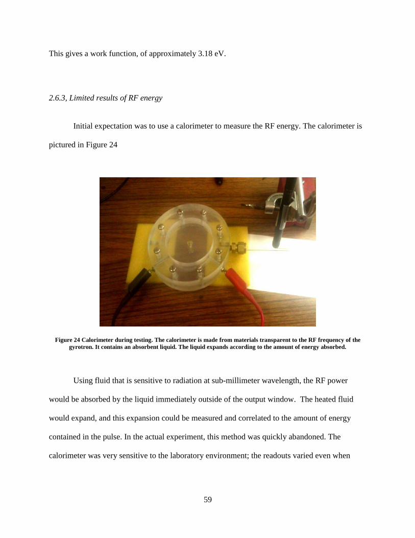
59

This gives a work function, of approximately 3.18 eV.

2.6.3, Limited results of RF energy

Initial expectation was to use a calorimeter to measure the RF energy. The calorimeter is

pictured in Figure 24

Figure 24 Calorimeter during testing. The calorimeter is made from materials transparent to the RF frequency of the

gyrotron. It contains an absorbent liquid. The liquid expands according to the amount of energy absorbed.

Using fluid that is sensitive to radiation at sub-millimeter wavelength, the RF power

would be absorbed by the liquid immediately outside of the output window. The heated fluid

would expand, and this expansion could be measured and correlated to the amount of energy

contained in the pulse. In the actual experiment, this method was quickly abandoned. The

calorimeter was very sensitive to the laboratory environment; the readouts varied even when

60

experiments were not going on. The RF signal is virtually indistinguishable from the noise. A

calibrated RF detector was used instead.

The next problem encountered during the experiment was the ubiquitous issue with

breakdown inside the gyrotron tube. For a majority of the experimental pulses, there appears to

be a sudden collapses in the cathode voltage, accompanied by a large spike in current. These

readings point to plasma formation in the tube, creating a path for current to travel from cathode

to the anode, effectively shorting the gyrotron. Although this issue plagued the experiments from

the very beginning, the cause remained unclear. At first, the culprit for the breakdown was

thought to be faulty electron optics. The cathode position could possibly be misaligned, causing

the initial electron trajectory to veer straight into the resonator wall. In addition to misalignment,

the team also suspected that the magnetic field was not penetrating in the resonator fully, so the

electron guiding was close to the wall radius, causing some part of the beam to scrap the

resonator wall. To verify the electron trajectory, test plates were inserted into the middle of the

tube in the path of the electrons. When the beam collides with the plates, it will leave scraping

marks, which would reveal the electrons actual path. The results from the test plate shows that

the electron optics is in alignment; the electrons are not scraping the resonator wall. In addition,

magnetic simulation using Maxwell 3D shows that the magnetic field is penetrating into the

gyrotron tube as predicted, suggesting that the plasma formation is not caused by the beam.

Other possible causes include undetected vacuum leaks, breakdown of the structure, or

manufacture defect. None which of could be confirmed.

61

Despite persistent problem of breakdown, the team did observe occasion RF power

output. Figure 25 is an oscilloscope trace show RF power, in green. The purple shows the beam

voltage of the pulse, blue represent beam current of the pulse. Both the beam voltage and current

remain flat during the pulse duration, meaning that there was no breakdown for that particular

pulse.

Figure 25 Green trace is the RF energy detected, magenta is the voltage applied by the modulator, cyan is the current

emitted by the cathode, and yellow represent the current running through the solenoid.

In the subsequent pulse shots during the following month, more RF pulses were observed,

with estimated power in the range of 20kW - 80 kW. The diagnostic equipment could only

measure RF amplitude, so the mode content or the frequency of the RF signal is unknown.

Unfortunately, the successful shots with RF production are outnumbered by far more cases of

breakdown events. In an effort to remedy the situation, a new resonator was designed and

installed [28]. However, the very high force caused by the pulsed magnetic field damaged the

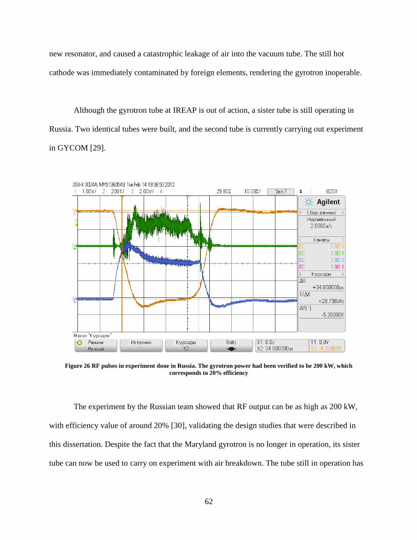
62

new resonator, and caused a catastrophic leakage of air into the vacuum tube. The still hot

cathode was immediately contaminated by foreign elements, rendering the gyrotron inoperable.

Although the gyrotron tube at IREAP is out of action, a sister tube is still operating in

Russia. Two identical tubes were built, and the second tube is currently carrying out experiment

in GYCOM [29].

Figure 26 RF pulses in experiment done in Russia. The gyrotron power had been verified to be 200 kW, which

corresponds to 20% efficiency

The experiment by the Russian team showed that RF output can be as high as 200 kW,

with efficiency value of around 20% [30], validating the design studies that were described in

this dissertation. Despite the fact that the Maryland gyrotron is no longer in operation, its sister

tube can now be used to carry on experiment with air breakdown. The tube still in operation has

63

proved that high power THz range radiation can be produced by using gyrotron with reasonably

high efficiency.

64

Chapter 3: Electron beam spread

This chapter presents the works that studied:

1. the definition of the problem

2. the general theory of regarding the beam interaction with the RF field

3. the analytical results and MAGY simulations

Section 3.1, Introduction to gyrotron beam radius

As outlined in the introduction, efficiency of the 670 GHz Gyrotron is the main concern

for this research. One area of the issue with efficiency has been addressed in the previous chapter

describing design of the resonator circuit. The focus there was on the effort to maximize the

amount of optimal interaction time by providing optimized interaction space; and reduce power

loss due to the frequency dependent skin penetration by selecting high order mode that can be

excited stably. Or in other word, letting electron beam and RF field interact as long as possible

longer for maximum energy extraction while preventing energy loss to the circuit itself. In this

following chapter, thesis focuses on another aspect of efficiency, but this time looking at the

issue from the beam-wave interaction itself. This research can be generalized to most gyrotron

oscillator devices, but is especially applicable to the 670 GHz due to the immediate issue of

needing a new electron gun.

The interaction efficiency is defined as the fraction of the electron kinetic energy

transformed into electromagnetic wave; see Eq. 2.14 and Eq. 2.13. In both of those equations

65

assumes that the electrons gyrate around centers, and these centers are located at a radius,

hereafter called guiding radius. The highest theoretical efficiency requires a very high quality

electron beam, and non-uniformity in velocities or the guiding radius of the beam usually lowers

the efficiency value from its optimal value. In the past, more attention had been focused on

spread in the velocity of the electron in the beam; velocity spread causes inhomogeneous

Doppler broadening in the cyclotron resonance, and given that the stimulated emission is weaker

than the absorption process, even if a small portion of the beam is in the wrong phase of the

cyclotron resonance, significant energy maybe lost [31] [3] [32] [33]. This effect has been seen

in Figure 15 Figure 16 and Figure 17. Much less attention, however, is paid to the role of the

configuration of the beam location (guiding radii). The effects of the beam displacement on the

gyrotron operation were studied in Ref [34] [35], and the effect of spread was studied Ref. [36],

but the focus of the papers was the effect of beam thickness on the mode coupling and stability

of operation, not its effect on efficiency. This is something that the research attempted to remedy.

Figure 27 illustrates guiding center spread. The large outer circle represents the wall of

the resonator, it has the radius . The small circles represent individual electrons gyrating

under an applied magnetic field. The electrons travel along the rotate along the circumference

with a Larmor radius . The distance between the center of the resonator and the center of

rotation of an electron is shown as radius . The guiding center is this center around which the

electron rotation, and when we say there is no spread in guiding center, it means about all of the

guiding center of all electrons in the beam are located a circle formed by the radius. The spread

in guiding center is marked by . This chapter formulates the problem for conventional

gyrotrons that have axially symmetric interaction space shown Figure 27. It's interesting to note

66

this is only one type of beam arrangement, as there are gyrotrons where the centers of the

electron gyration is at the center of the resonator [37], these gyrotrons are called large orbit

gyrotrons.

Figure 27 Electron beam configuration in a conventional gyrotron. Each electron's path is represented by the small circles

these circles has radius a, representing Larmor radius. The distance between the centers of the small circles and the

center of the resonator is Rb. is the spread in guiding center.

The gyrotron community did not pay much attention to this effect, possibly, because most

active gyrotron developments are focused on the frequency range from 100 to 200 GHz, or even

lower frequencies (see, e.g., Refs [38] [39]). At those frequencies, design choices can be made

with [40] [41] a magnetron-type electron gun to have a thin emitter ring and an electron-optical

system forming at the resonator entrance, such that the thickness of the electron beam can to

controlled to be typically less than 6/ with being a wavelength. Under those circumstances,

Rw

Rb

a

67

it was not urgent to understand what large value spread means for gyrotron operation since large

spread is easily avoided. The issues can no longer be avoided when the wavelength is decreased.

Obviously the 6/ design spec will place more stringent limit in gun designing and

manufacturing if the wavelength becomes much smaller before. The added cost of trying to

maintain the same value of guiding center spread may not be worth the investment without fully

understanding the compromises to be made. Therefore, it is important to visit issue in more

detail as gyrotron development pushes into higher frequency region, especially what effects this

spread has on efficiency of gyrotron operation.

The design of 670GHz gyrotron calls for 1 MW beam power delivered at 70 kV with

current of 15 Amp. For this high output requirement, the emitter area cannot be reduced too

much to keep for beam thickness spread, the design team cannot expect a beam guiding center

spread to be under the 6/ value. With that in mind, it is paramount to understand how larger

value of spread will degrade the gyrotron performance. The basis for analytical theory upon

which this study was based on was developed for comparing the efficiency of gyrotrons with

various interaction circuits operating in soft excitation regimes in Ref [42] and then generalized

for the case of hard excitation in Ref. [43].

68

Section 3.2, General theory of guiding center spread and its effect on efficiency.

The theoretical analysis start by assuming that when scaling the electron gun with

frequency, the designer keeps the beam voltage, orbital-to-axial velocity ratio, and the angle of

the magnetic force line to the emitter surface constant. This assumption has to be made so that

any changes of efficiency can be attributed to spread of guiding centers. Furthermore, the study

only takes into consideration the cases described by the adiabatic theory of magnetron-type

electron guns [44] [40]. Adiabatic theory is based on the assumption that during one cyclotron

period 1) the electron velocity varies only slightly, and 2) the magnetic invariant of motion

Bp /2

is constant. It follows then, taking into account the Busch’s theorem [particle physics]

postulating the conservation of the magnetic flux, we can derive that the magnetic compression

factor to be cB BB /0 , which is the ratio of the external magnetic field in the resonator to that

in the cathode region. The compression factor scales with the frequency as 3/2fB . More

rigorous derivation can be found in Ref [45].

Following the Busch’s theorem, the spread in the guiding center radii at the resonator

entrance can be expressed via projection of the emitter width l on the plane perpendicular to the

magnetic force lines near the cathode as Bg lR /sin (here is the angle between the

magnetic force line and the emitter surface). Since the wavelength of the gyrotron radiation is

inversely proportional to the external magnetic field, it can be shown that that in order to keep

the ratio /gR constant, the emitter width should scale with the frequency as3/2 fl .

Since the emitter radius scales in the same fashion, we arrive at the conclusion that the emitter

area scales with the frequency as3/4 fA . (This issue is discussed in detail in Ref. [46].) It is

evident that from the scaling formula that stringent adherence to the 6/ specification will result

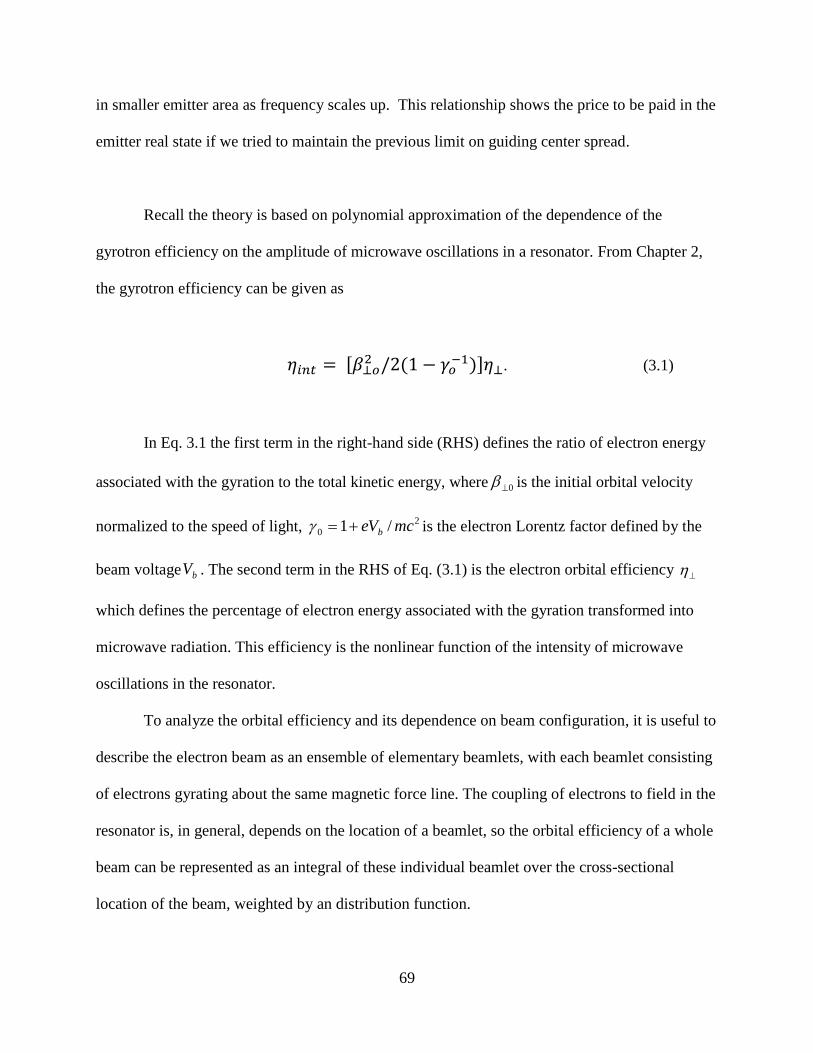
69

in smaller emitter area as frequency scales up. This relationship shows the price to be paid in the

emitter real state if we tried to maintain the previous limit on guiding center spread.

Recall the theory is based on polynomial approximation of the dependence of the

gyrotron efficiency on the amplitude of microwave oscillations in a resonator. From Chapter 2,

the gyrotron efficiency can be given as

. (3.1)

In Eq. 3.1 the first term in the right-hand side (RHS) defines the ratio of electron energy

associated with the gyration to the total kinetic energy, where 0 is the initial orbital velocity

normalized to the speed of light, 2

0 /1 mceVb is the electron Lorentz factor defined by the

beam voltage bV . The second term in the RHS of Eq. (3.1) is the electron orbital efficiency

which defines the percentage of electron energy associated with the gyration transformed into

microwave radiation. This efficiency is the nonlinear function of the intensity of microwave

oscillations in the resonator.

To analyze the orbital efficiency and its dependence on beam configuration, it is useful to

describe the electron beam as an ensemble of elementary beamlets, with each beamlet consisting

of electrons gyrating about the same magnetic force line. The coupling of electrons to field in the

resonator is, in general, depends on the location of a beamlet, so the orbital efficiency of a whole

beam can be represented as an integral of these individual beamlet over the cross-sectional

location of the beam, weighted by an distribution function.

70

(3.2)

Notice the similarity between Eq. 3.2 and Eq. 2.10. In that previous, case, the electrons

are only distributed at different angles along a radius, this is no longer the assumption in Eq. 3.2.

In Eq. 3.2 el is the orbital efficiency of the elementary beamlet and bRW

, normalized to

unity, is the distribution function for electron guiding centers in the resonator cross-sectionS .

el has non-linear dependence on the amplitude of the field in the resonator. For the purpose of

the study, this dependence is linearized assuming small perturbation of the field amplitude. In

order to describe saturation effects in oscillators with soft self-excitation, it is enough to take into

account the first nonlinear terms in the dependence of the orbital efficiency on the intensity of

the resonator field M . Then el can be represent as

(3.3)

The coefficients and in Eq. 3.3 depend on the axial structure of the resonator field and on

the cyclotron resonance mismatch between the wave frequency f 2 and the resonant

harmonic of the electron cyclotron frequency s . (Ref [14]) The intensity of the resonator field

acting upon electrons depends not only on the intensity of microwave oscillations 0M , but also

on the beam coupling to the mode, i.e. this intensity can be given as

(3.4)

Where In Eq. 3.4 is given as

71

(3.5)

This term is the coupling coefficient, which characterizes the transverse structure of the

microwave field acting upon electron with transverse coordinates of the guiding center X and Y .

The membrane function YX , is defined by the Helmholtz equation 02 with a

corresponding boundary condition. For TEm,p modes in a cylindrical resonator

(3.6)

In Eq. 3.6, the sign in the order of Bessel function depends on the direction of electron

gyration with respect to rotation of a non-symmetric ( 0m ) mode in the resonator: minus and

plus correspond to the co- and counter-rotating waves, respectively; wcutpm Rc/, is the

Eigen number of a given mode ( p ’th root of 0 mJ which is the boundary condition for this

mode at the resonator wall) which defines the cutoff frequency of this mode in a resonator with

the wall radius wR . Since gyrotrons operate at frequencies close to cutoff, cut . See Figure

27 for and .

From Eq. 3.3, taking the derivative and setting it equal to 0, we find that the highest

orbital efficiency occurs when

2

M , so 4/2max el . In addition, from Eqs. (3.2)-(3.4),

the orbital efficiency of a whole beam can be written as

72

(3.7)

where

dsLRWa s

S

b

2 and

dsLRWb s

S

b

4. From that, the maximum orbital efficiency

of a whole beam can be expressed as ba /4/ 22max . The ratio ba /2 characterizes the

influence of the transverse non-uniformity of the resonator field on the efficiency of a gyrotron

operating in the regime of soft self-excitation.

In the regime of hard self-excitation the first nonlinear term (coefficient in Eq. 3.3)

has an opposite sign. Therefore to describe qualitatively the saturation one should take into

account the next nonlinear term, i.e. use a cubic approximation instead of Eq. (3.3).

(3.8)

Correspondingly, the orbital efficiency of a whole beam can now be presented as

(3.9)

where

dsLRWc s

S

b

6. taking the derivatives of the resonator field intensity in Eq.

3.8 and Eq. 3.9, setting them to zero yields corresponding formulas for the maximum efficiency

of the beamlet and the whole beam [18]. The ratio of these maximum efficiencies characterizes

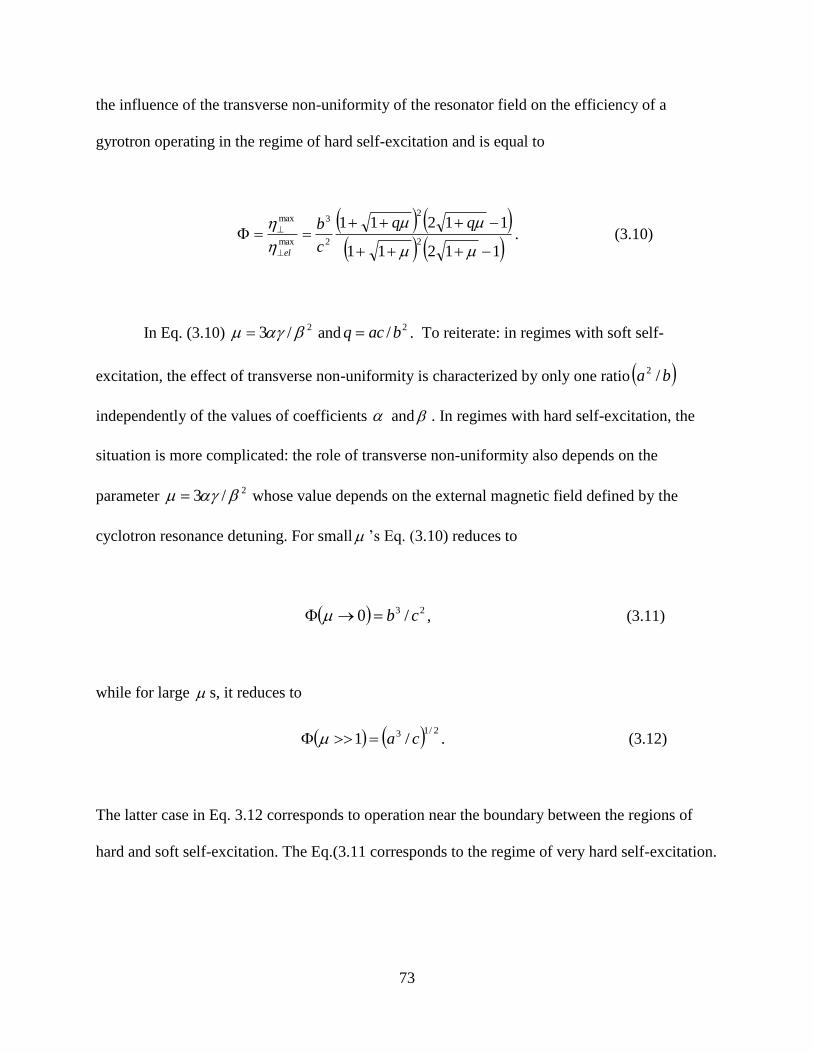
73

the influence of the transverse non-uniformity of the resonator field on the efficiency of a

gyrotron operating in the regime of hard self-excitation and is equal to

11211

112112

2

2

3

max

max

qq

c

b

el

. (3.10)

In Eq. (3.10) 2/3 and

2/ bacq . To reiterate: in regimes with soft self-

excitation, the effect of transverse non-uniformity is characterized by only one ratio ba /2

independently of the values of coefficients and . In regimes with hard self-excitation, the

situation is more complicated: the role of transverse non-uniformity also depends on the

parameter 2/3 whose value depends on the external magnetic field defined by the

cyclotron resonance detuning. For small ’s Eq. (3.10) reduces to

23 /0 cb , (3.11)

while for large s, it reduces to

2/13 /1 ca . (3.12)

The latter case in Eq. 3.12 corresponds to operation near the boundary between the regions of

hard and soft self-excitation. The Eq.(3.11 corresponds to the regime of very hard self-excitation.

74

As shown in Ref. [47], in gyrotrons with the Gaussian axial structure of the resonator

field the highest orbital efficiency corresponds to 2.0 , 2020 and 4106 that yields

0088.0opt . So for this regime our approximation is applicable. In the regimes of hard

excitation which are closer to the boundary between hard and soft self-excitation the value of the

parameter can be on the order of unity.

75

Section 3.3, Results of the approximations and MAGY verification

3.3.1, Analytical predictions

In this Section, results from the analytical equations derived previously is presented, as

well as results of numerical simulations done with the use of the code MAGY. The comparison

offers verification of the analytical approach taken above. The analysis is performed for the

specific operating mode TE31,8, the mode of choice for the 670GHz gyrotron. The function that

describes coupling coefficient Eq. 3.6 for such co-rotating mode is shown in Figure 28.

Figure 28 The coupling coefficient for TE31,8, this is the term described by the Eq. 3.6. Hereafter referred to as G,

this also shows the caustic radius of the gyrotron, since the function also describe the axial distribution of the RF field,

and it shows that there are not field inside region where is less than 0.4.

76

Figure 28 shows that the coefficient is highest at the first peak, corresponding to about

the half of the wall radius. The electro-optics should be designed such that the guiding centers of

the electron beam are injected at the location with highest coupling strength. Stronger the

coupling, higher the efficiency will be.

Figure 29 The spread in guiding center as compare to the inner peak of the coupling coefficient. The curve is a zoomed in

view of Figure 28, and the grey region represent the maximum displacement of the guiding centers from the ideal position

(location of the peak) for the given spread value.

The study analyzes the effect of the guiding center spread of the beam on the efficiency

for two cases: when the beam is place in the first (widest) peak of the function, and then the case

where the beam is placed at the second peak from the resonator axis. These are the only two

realistic locations where the beam centers should be located, as they offer the strongest coupling.

77

For a simple illustration of the concept of how the guiding center spread degrades coupling, in

Figure 29, a distribution of electrons for the case when electron spread in guiding center radii

bR is equal to 5% (a much exaggerated value) of its mean value bR , the curve is a zoomed in

view of Figure 28, and the grey region represent the maximum displacement of the guiding

centers from the ideal position (location of the peak) for the given spread value. Figure 30 shows

the same spread for the second peak. The curve is a zoomed in view of Figure 28 of the second

peak, and the grey region represent the maximum displacement of the guiding centers from the

ideal position (location of the peak) for the given spread value. It is readily apparent in Figure

30 that the beam with 5% spread is wider than the second peak of the function that describes

coupling coefficient.

78

Figure 30 The spread in guiding center as compare to the second peak of the coupling coefficient. The curve is a zoomed

in view of Figure 28, and the grey region represent the maximum displacement of the guiding centers from the ideal

position (location of the peak) for the given spread value.

The radial spread used in Figure 29 and Figure 30 is defined terms of the ratio of the spread

to the wavelength:

(3.13)

79

When the beam is injected in the inner peak, its radius is close to the caustic radius

wpmcb RmRR ,/ , and, correspondingly, mRRR bbb /2// . The caustic radius is

the region of the resonator where the RF field doesn't exist.

The effect of the radial spread on the efficiency in the framework of the analytical mode

is illustrated by Figure 31 and Figure 32 where the dependences of the ba /2, 23 / cb and

2/13 / ca ratios are shown for the cases of beam injection in the inner and second peaks of the

coupling impedances. The solid line corresponds to the efficiency normalized to the case of no

spread, in the soft self-excitation regime. Dotted line corresponds to the efficiency normalized to

the case of no spread, in the hard self-excitation regime. Dotted line corresponds to the efficiency

normalized to the case of no spread, in between the hard-excitation regime and soft self-

excitation.

Again, recall from Chapter 2: hard self-excitation region corresponds to the beam current

is less than the starting current; while the soft self-excitation corresponds where to the case beam

current exceeds the starting oscillating current. Hard self-excitation occurs when there is a large

slippage in the gyrophase in comparison to the phase of the RF field, and that requires large

wave amplitude to trap the electron. This slippage in phase is related to normalized detuning

value Δ introduced earlier, and larger Δ means lower magnetic field value.

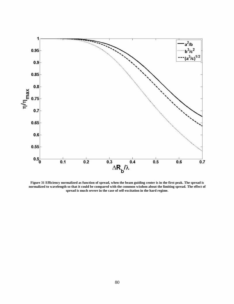
80

Figure 31 Efficiency normalized as function of spread, when the beam guiding center is in the first peak. The spread is

normalized to wavelength so that it could be compared with the common wisdom about the limiting spread. The effect of

spread is much severe in the case of self-excitation in the hard regime.

81

Figure 32 Efficiency normalized as function of spread, when the beam guiding center is in the second peak. The spread is

normalized to wavelength so that it could be compared with the common wisdom about the limiting spread. The effect of

spread is much severe in the case of self-excitation in the hard regime.

As one can see, the efficient operation in the regime of soft self-excitation is less

sensitive to guiding center spread than near the border between the regions of soft and hard

excitation. In turn, the border region between the different excitation is less sensitive than the

operation in the regime of deep hard self-excitation. For example, in Figure 31, even when the

spread is 1/3 of the wavelength, the degradation in efficiency is still very minor in the soft

regime, but is already 10% in the hard regime. In addition, the case of beam placement in the

inner peak is much less sensitive to the spread than the case of injection in the second peak. In

the case of injection in the inner peak, when the spread in guiding center radii is equal to one half

82

of the wavelength, the analytical model predicts only 15% degradation from the maximum

efficiency in the soft self excitation region and 30% degradation in the hard self excitation region.

For the same value of spread, when the beam is injected in the second peak in Figure 32, the

analytical model predicts that efficiency will degrade by 40% in the soft self excitation region,

and 60% in the hard self excitation region. It is interestingly shows that the efficiency recovers

past the 0.5 λ spread in Figure 32, that is the efficiency began to increase again if guiding center

spread is greater than ½ wavelengths. The phenomenon can be partial explained by Figure 30. As

the beam center spreads more, it becomes so thicker, so thick that it begins to couple with the

adjacent peaks of the coupling function, and thus results in stronger interaction than if the center

has less spread.

These preliminary result suggest that for traditional low frequency gyrotrons, the rule

prevent the efficiency from degrading at all due to guiding center spread (injection in the first

peak), and at the worst case (injection at second peak) only a few percent. For the sub-terahertz

gyrotron, even if the spread is allowed to be twice as much, the efficiency would only drop to

95% of ideal case.

3.3.2, Numerical simulation and verification of the analytical model

To verify the analytical predictions, numerical simulations were performed by using the

multi-frequency, self-consistent, time dependent code MAGY. The parameters for 670 GHz

gyrotron of Chapter 2 are used. The gyrotron Profile 1 [48] is used to perform these calculations.

The excitation is driven by a 70 kV electron beam with the pitch angle equal to 1.3 in keeping

the operating parameter with the proposed gyrotron. For this simulation, it is assumed that

83

guiding center spread has a rectangular distribution with the width 3R where

determines its RMS value. For the case of the beam injection in the inner peak, the beam current

is 15 A. This is the actual setup of the Chapter 2's simulation, and the actual operation condition

the gyrotron was design to do. For simulation describing beam placement in the second peak,

where efficiency is more sensitive to the guiding center spread, the current value as to be scaled.

To compensate for the different coupling coefficient value at the different peaks, the current for

the second peak injection was increased, in accordance with the desire to keep the same value of

the product maxGIb , to 26 A. This scaling does not affect the results of the study, since the

concern is not comparing the efficiency of injecting beam at different positions. This increase in

current allows for keeping other parameter constant, so the only variable is the guiding center

spread value.

Simulations to find the maximum efficiency point is performed the same way as

described in Chapter 2, except this time no velocity spread is included. The magnetic field is

varied across all detuning value where the RF field can be excited. In the region where soft self-

excitation occurs, the resonator is excited by placing an initial source with the Gaussian axial

structure inside the interaction region in addition to the beam current. To check if soft self

excitation occurs at any given magnetic field value, the initial source is a small amplitude (10-4

)

and kept it on for the entire simulation run. Then the system is allowed enough time to observe if

excitation occurred with this modified source (amplitude increases from noise to operation level

when excitation occurs). The scanning of the magnetic field starts with near the cyclotron

resonance condition, corresponding to small detuning, i.e. higher magnetic fields. Magnetic field

is decreased in simulation incrementally to simulate increasing in detuning. When the system fail

84

to excite (amplitude remains noise level), it means that the gyrotron is no longer in the self

excitation-regime.

In those cases, the last few magnetic field data points are redone, it's time to simulate

hard self-excitation. In real life, hard self-excitation regime requires a start-up operation to gain

large enough amplitude [49]. In simulation, this is achieved by giving a large jolt. A seeded

Gaussian source that has large amplitude (10-1

) is positioned in the middle of a resonator. This

source was turned off after 15 ns, so any wave that existed in the cavity after that would be

sustained only by the electron beam. Redoing the last few magnetic field data points in this

manner will determine the boundary between soft and hard self excitation regions. For the

gyrotron specified in the 670 GHz gyrotron, I found that at magnetic field values greater than or

equal to 265 kG, the device exhibits soft-self excitation, and when the magnetic field is less than

265 kG, the device is within the region of hard self-excitation. This boundary between two

regions appears to slightly depends on the radial spread.

85

Figure 33 Efficiency for different RMS value of spread for injection in the inner peak. For spread up to 3% RMS value,

the efficiency is still 95% of the no spread value. However, for higher value, the rate of efficiency degradation increases

very rapidly. At 5% RMS spread, the efficiency drops to 85% of the no spread value. Also of note is that the optimal

detuning shifts, it went from 264.6 kG to 265.75 kG.

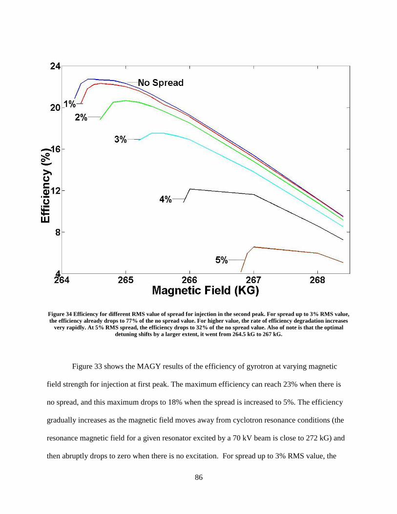
86

Figure 34 Efficiency for different RMS value of spread for injection in the second peak. For spread up to 3% RMS value,

the efficiency already drops to 77% of the no spread value. For higher value, the rate of efficiency degradation increases

very rapidly. At 5% RMS spread, the efficiency drops to 32% of the no spread value. Also of note is that the optimal

detuning shifts by a larger extent, it went from 264.5 kG to 267 kG.

Figure 33 shows the MAGY results of the efficiency of gyrotron at varying magnetic

field strength for injection at first peak. The maximum efficiency can reach 23% when there is

no spread, and this maximum drops to 18% when the spread is increased to 5%. The efficiency

gradually increases as the magnetic field moves away from cyclotron resonance conditions (the

resonance magnetic field for a given resonator excited by a 70 kV beam is close to 272 kG) and

then abruptly drops to zero when there is no excitation. For spread up to 3% RMS value, the

87

efficiency is still 95% of the no spread value. However, for higher value, the rate of efficiency

degradation increases very rapidly. At 5% RMS spread, the efficiency drops to 85% of the no

spread value. Also of note is that the optimal detuning shifts, it went from 264.6 kG to 265.75 kG,

a change of 1.15 kG, which corresponds to a frequency detuning of 2.83 GHz.

Figure 34 shows that the efficiency of the gyrotron, with the beam injected in the second

peak, is nearly identical to the first peak injection when there was no spread. When the guiding

center spread was taken into account, we see that the efficiency degrades much faster than it does

in the first peak because the operation in a narrower peak is more sensitive to the spread. When

the guiding center spread is 5%, efficiency is only 6%. For spread up to 3% RMS value, the

efficiency already drops to 77% of the no spread value. For higher value, the rate of efficiency

degradation increases very rapidly. At 5% RMS spread, the efficiency drops to 32% of the no

spread value. Also of note is that the optimal detuning shifts by a larger extent, it went from

264.5 kG to 267 kG, a change of 2.5 kG, which corresponds to a frequency detuning of 6.15

GHz.

The spread in guiding center also had an effect on the excitation condition of the gyrotron.

The minimum magnetic field below which no excitation takes place, min,0B , is shown in Figure

35. This minimum value increases with the guiding center spread. Remember that hard self-

excitation occurs at lower magnetic field, so this shift of the regime in which hard self-excitation

occurs. For injection in the inner peak, the shift is about 0.8 kG.

88

Figure 35 The minimum B field for excitation for different values of RMS spread. The circles represent the case of

injection in the first peak. The asterisk represents the case of injection in the second peak. The minimum B field for

excitation shifts up with increasing spread. The effect is much more severe in the case of injection in the second peak.

As with efficiency, the change in the minimum values of the magnetic field for the

second peak injection is also much higher than in the case of injection at the first peak, as shown

in Figure 35. For the case of injection in the second peak, the change is almost 3kG, more than

three times the effect of the case of injection in the inner peak. This phenomenon can be

interpreted as the following: the electron spread in a narrow peak causes much rapid decrease of

the electron coupling to the wave. Therefore, to maintain the cyclotron resonance between

89

electrons and the wave, the electron cyclotron frequency should be closer to the wave frequency

that results in higher values of the minimum magnetic field shown in Figure 35.

Figure 36 MAGY data points are converted from RMS spread value to spread as ratio of wavelength. This corresponds to

the case of injection in the inner peak. In this figure, the MAGY data follows the analytical theory remarkably well.

Lastly, to compare the results from MAGY simulation with the prediction from the

analytical equations, Figure 31 and Figure 32 are overlaid with data points from MAGY, and

then presented in Figure 36 and Figure 37.

Figure 36 corresponds to the case of the first peak injection and the data points are

numerical results from MAGY at four different magnetic fields. The simulation data of guiding

center spread are converted from RMS spread to fraction of wavelength. Since the Bo min varies

90

with spread, MAGY data points for low magnetic field under large spread do not exist. These

data points generally follow the analytical curve, especially for 0 266B kG and 0 264.8B kG .

Recall that at 265 kG, the gyrotron operates in the hard excitation regime, and above 265 kG the

gyrotron is in the region of soft self excitation. The "x" and the dot data points should be

compared to the solid line, circle data points compares the dashed line, and the "+" data points

correspond the dotted line. Figure 36 also shows the gradual transition from hard to soft self

excitation as magnetic field strength increases.

Figure 37 MAGY data points are converted from RMS spread value to spread as ratio of wavelength. This corresponds to

the case of injection in the second peak. In this figure, the MAGY data do not follow the analytical theory as well.

91

Figure 37 shows the analytical predictions and MAGY data for the injection in the second

peak. It appears that numerical simulation results deviated from the analytical model much more

than the results from first peak injection. The "x" and the dot data points should be compared to

the solid line, circle data points compares the dashed line, and the "+" data points correspond the

dotted line. The data points show that when the beam is injected in the second peak, most of the

excitation in the cavity is well inside the region of soft self excitation. This shrinkage of the

region of hard self excitation can be explained by the increased sensitivity of the device

operation to the spread discussed above. In general, however, the agreement between the

analytical predictions and numerical simulation data is reasonable.

In general, despite the deviations shown in Figure 37, the results of this theory agree

reasonably well with numerical data obtained with the use of the self-consistent code MAGY.

These results show that the gyrotron operation is less sensitive to the spread when the device is

in the region of soft self-excitation than in the region of hard excitation. Since most efficient

operation point is in the hard excitation, this result is important. It is also shown that the

gyrotron operation is less sensitive to this spread when the beam is injected in the inner peak of

the function describing the beam coupling to the wave. In this case, even the spread of about one

third of the wavelength reduces the gyrotron efficiency by about 10% or less of its nominal value

(i.e. such a gyrotron with a relatively “thick” beam can operate with the interaction efficiency of

27% versus 30% achievable in a gyrotron with ideally thin beam). This positive result could be

attributed to the choice of mode. The transverse structure of TE31,8 mode [39] happens to have a

fairly 'wide' profile at where the beam is to be placed. Had the structure be narrower, the effect of

92

the spread would be much more severe, as demonstrated the simulations results of case where

beam is placed at the second peak. Lastly, the "rule of thumb” of gyrotron designers had

followed is to have this spread not exceeding one sixth of the wavelength is shown here to be

overly cautious, at least for this case. For THz-range gyrotrons with well selected operating

mode, the fact that one can at least double the emitter width while keeping the efficiency

reasonably high greatly alleviates design of magnetron-type electron guns.

93

Chapter 4: Second harmonic interaction

This chapter presents the study of the second harmonic gyrotron in the following order:

1. excitation of the gyrotron at higher cyclotron harmonics

2. disadvantages encountered by a second harmonic mode in mode competition

3. the spectrum of competing modes facing the operating mode TE31,8

4. mode interaction between different cyclotron harmonics in gyrotrons

5. suppression or enhancement of the excitation condition of a fundamental mode in

the presence of a second harmonic mode

6. verification of the analytical predictions.

Section 4.1, Description of the problem

After verifying that stable and high efficiency gyrotron operation can be achieved using

the TE31,8 mode, the next logical step is to improve the device’s average power so that it could be

adapted for more applications. The electron beam source already produces a peak beam power of

more than 1 MW; it makes much more sense to purse an increase in pulse duration and pulse

repetition rate, with an ultimate goal of adapting the gyrotron design to operate continuously.

Recall from Chapter 1 that sub-millimeter wave gyrotrons have been limited by: a) the

need for very high magnetic field (greater than 22 Tesla if λ < 0.5 mm), and b) the need to reduce

Ohmic losses in the wall in order to maintain high efficiency. In the 670 GHz gyrotron described

in the previous chapters, the issue with the magnetic field requirement was able to be satisfied

only by using a pulsed solenoid, which is capable of delivering 28 Tesla in single shots. The

issue of wall loss was solved by operating the gyrotron with a high order mode in the resonant

94

cavity [19]. In the pulsed solenoid, the pulse duration is limited to avoid overheating the solenoid

coil. Not only does heating damage the equipment, heating also changes the resistance of the coil,

causing the output magnetic field to vary, which will undermine the cyclotron resonance

condition. Similar limitation also applies to the pulse repetition rate, since long interval between

shots is needed to remove the heat generated.

In order to replace the pulsed magnetic field source with an affordable constant magnetic

field source, the field strength requirement must be drastically reduced. One possible way to do

this is to operate the gyrotron at higher cyclotron harmonics. The relationship between the

gyrotron’s required magnetic field and the harmonic number, s, is given as

(4.1)

This relationship is plotted in Figure 38. By operating the gyrotron at second harmonic, the

required magnetic field is cut in half, to 13-15 T, which is an achievable value for existing cryo-

magnets [10].

95

Figure 38 Magnetic and frequency for different gyrotron harmonic, blue curve shows the increase in magnetic field for

pushing to higher frequency, for the fundamental cyclotron harmonic. Red and green curves illustrate the increase for 2nd

and 3rd cyclotron harmonics.

Higher harmonic gyrotrons are not new; many have been built [50] [51] [52] [53]. In

these examples, the gyrotrons could operate with low ordered modes to make the mode selection

and mode stability problems relatively simple, by choosing modes with spectra around which

there are few competing modes. This choice, however, would lead to high Ohmic loss when the

frequency is high. For fundamental cyclotron harmonic operation, it was shown that certain high

ordered mode such as TE31,8 can be excited stably [22], and this mode choice can reduce Ohmic

wall losses [19]. A higher order mode has a denser mode spectrum; therefore, mode competition

is a very important issue for advanced gyrotron development [21].

For higher harmonic gyrotrons, mode competition is an even more important issue, since

competing modes interacting at different cyclotron harmonics cannot be ignored. The operating

96

mode at second harmonic is disadvantaged when competing with a mode at fundamental

harmonic. It has been shown in Ref [54] [55] that even with an inherent disadvantage, the mode

at a higher harmonic can suppress competitors from fundamental harmonic if the higher

harmonic mode is excited before its competitors in an appropriate start-up scenario. On the other

hand, the presence of the higher harmonic mode has also been known to enhance the excitation

of a competitor mode at the fundamental harmonic [54] [56].

The advantage of the fundamental harmonic modes in competition will be explained in

this chapter. Then using second harmonic TE31,8 as the operating mode, we will examine the

likely competitor modes at the fundamental harmonic. Of those candidates, the one mode with

the most favorable conditions will be examined first by using gyrotron equations, and then with

the numerical simulation code MAGY.

97

Section 4.2, Mode competition advantage of mode at fundamental harmonic

When an electron interacts with the RF field at the fundamental harmonic, the electron

interaction is dipolar (2 poles). Meanwhile at the second harmonic, the interaction is quadripolar

in nature [14] [57]. Therefore, the coupling between the field and electrons would be weaker for

the second harmonic mode interaction. Recall from Chapter 3 that the beam-wave coupling in a

smooth wall cylindrical resonator is described by:

(4.2)

Now, suppose a resonator with radius R was designed for a high order, second harmonic

mode A; A will have . There is a likely chance that there would exist a mode B, and B

would have such that would be about half of . This mode B also has a cutoff

frequency in R that is half of of mode A. If mode A with satisfies the cyclotron

resonance condition at the second harmonic (remember that resonators are designed such that

cutoff frequency is equal to the operating frequency to minimized ), then mode B with

would also be able to satisfy the cyclotron resonance condition at the fundamental harmonic.

This mode B is a competitor at the fundamental harmonic.

When this competing mode exists, its coupling coefficient as given by Eq. 4.2, can be

higher. This is because the competing mode has lower ( and lower azimuthal index (m). The

resulting denominator would be much smaller than the denominator of the second harmonic

mode. This effect may not doom the second harmonic completely. The numerator in Eq. 4.2 is

the transverse structure of the RF field; see Figure 28 for the one of TE31,8. If the second

98

harmonic operating mode A couples with the beam at a radius where the transverse field of mode

B is very low (near one of the zeroes of the Bessel function), then the advantage of mode B's

coupling strength is moot.

From this very simple analysis, it should be obvious that choosing the right operating

mode and the right beam location are even more urgent in a second harmonic gyrotron.

99

Section 4.3, Listing possible competitor mode, selecting among suspect modes,

Leveraging the results of the study of the 670 GHz gyrotron in Chapter 2 and 3, the

present study tried to use the parameters of the TE31,8 fundamental harmonic gyrotron so that the

possible variation due to other factors are limited. These limits include restricting the beam

voltage to be under 80 kV and the current to be under 20 Amps. The operating mode is assumed

to still be TE31,8 mode. The resonator wall profile remains essentially the same as the one

presented in Figure 12, with slight modifications that will be explained later. With the operating

mode and frequency remaining the same, the cut-off radius of the interaction section is also the

same. For the TE31,8 mode, is 63.7809; to be a competitor, the mode at the fundamental

frequency should have about half of that value.

A resonator optimized for second harmonic mode limits the possible competitor, since

modes below the cut-off will not be supported by the resonator cavity, and modes above the cut-

off would have large value, value, which means that the mode would be radiated out of the

resonator and would have very limited interaction with the electrons. As such, only modes with

similar cutoff frequencies should be considered.

The list of modes in the general vicinity ( in the frequency spectrum) at fundamental

cyclotron harmonic is shown in Figure 39, these are the 12 modes in the entire mode spectrum

that have cutoff frequencies close to that which correspond to the resonator. In terms of

dangerous competition to the operating mode, the competitor with the nearest resonator cut-off

frequency to the operating mode is the one that requires the most attention. That mode would be

the one most likely among the list of competing modes to resonate with the electrons inside the

resonator. Modes TE25,3 TE21,3 TE16,4 TE12,6 and TE7,8 are simply too far away from the resonator

100

cutoff frequency; those modes are unlikely to resonate. The modes closest to the cut-off

frequency are TE6,8, TE11,6, TE14,5, TE 17,4, TE20,3 and TE 24,2.

These six candidates are left to be examined further; their coupling coefficients given by

Eq. 4.2 are plotted as a function of the resonator's transverse axis normalized to the resonator

radius. Each of these plots is overlaid with the coupling coefficient of TE31,8 at second harmonic.

Both the co-rotating and counter-rotating polarization for the modes are checked. The coupling

coefficient of co-rotating and counter-rotating waves are separated by the by the different Bessel

function , where the plus and minus sign represent the different direction of rotation.

Figure 39 Spectrum of mode at fundamental harmonic. These modes are shown with the amount of frequency separation

from the operating mode at second harmonic, as defined by

. Of the modes listed, some modes such as TE25,3

is too separated from TE31,8 to be possible competitors.

-15 -10 -5 0 5 10

TE6,8

TE7,8

TE9,7

TE11,6

TE12,6

TE14,5

TE16,4

TE17,4

TE20,3

TE21,3

TE24,2

TE25,3

101

The results show TE6,8, TE 20,3 and TE24,2 have unfavorable coupling; the location where

the beam guiding center is injected doesn't overlap with the location where the coupling to the

fundamental is high. These modes are unlikely to be the most dangerous modes. The other

modes, however, which all have greater coupling strength to the electron beam, are shown in

Figure 40. These modes have stronger interaction with the electron beam than the operating

mode at second harmonic at the radius where the electron beam is injected.

Figure 40 Coupling Coefficient from the possible competitor modes. Blue are the competitor, red is the operating mode.

The beam would be injected at the first peak of the operating mode. From top left clock wise, shown are TE9,7+, TE14,5+

TE11,6- and TE14,4-. These modes all have stronger interaction between the electron beam and the mode at fundamental

harmonic than the interaction between the electron beam and the operating mode at second harmonic.

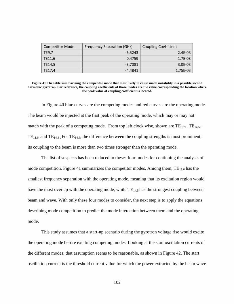
102

Competitor Mode Frequency Separation (GHz) Coupling Coefficient

TE9,7 -6.5243 2.4E-03

TE11,6 0.4759 1.7E-03

TE14,5 -3.7081 3.0E-03

TE17,4 -4.4841 1.75E-03

Figure 41 The table summarizing the competitor mode that most likely to cause mode instability in a possible second

harmonic gyrotron. For reference, the coupling coefficients of those modes are the value corresponding the location where

the peak value of coupling coefficient is located.

In Figure 40 blue curves are the competing modes and red curves are the operating mode.

The beam would be injected at the first peak of the operating mode, which may or may not

match with the peak of a competing mode. From top left clock wise, shown are TE9,7+, TE14,5+

TE11,6- and TE14,4-. For TE14,5, the difference between the coupling strengths is most prominent;

its coupling to the beam is more than two times stronger than the operating mode.

The list of suspects has been reduced to theses four modes for continuing the analysis of

mode competition. Figure 41 summarizes the competitor modes. Among them, TE11,6 has the

smallest frequency separation with the operating mode, meaning that its excitation region would

have the most overlap with the operating mode, while TE14,5 has the strongest coupling between

beam and wave. With only these four modes to consider, the next step is to apply the equations

describing mode competition to predict the mode interaction between them and the operating

mode.

This study assumes that a start-up scenario during the gyrotron voltage rise would excite

the operating mode before exciting competing modes. Looking at the start oscillation currents of

the different modes, that assumption seems to be reasonable, as shown in Figure 42. The start

oscillation current is the threshold current value for which the power extracted by the beam wave

103

interaction is equal to the power loss in the resonator circuit; it is the basic excitation condition

that must be satisfied. If the beam current is less than the start oscillation-current of a particular

mode, that mode will not be excited.

Figure 42 The start oscillation current in amps as function of magnetic field. TE9,7 is in shown to be spaced far separated

from the operating mode. Further, TE11,6 has higher start oscillation current in the region from 13.5 T to 13.T. This

means that in principle, the operating mode could be excited in the soft self-excitation region before the competitor mode

at fundamental harmonic. Beam radius of operating mode is 0.2247cm.

It is clear from Figure 42 that the self-excitation condition for the second harmonic mode

can be satisfied before the start oscillation value for any of the competitor for the range of B-

field from 13.6 T to 13.8 T. This suggests that in principle, the operating mode TE31,8 should be

able to be excited during the initial voltage rise. In addition, Figure 42 shows that TE9,7 mode has

a very large frequency separation from the operating mode, and to a lesser extent to TE17,4 and

TE14,5 modes have large separation as well. Due to the very large frequency mismatch, the

current needed to excite these modes is much higher in the magnetic field region where TE31,8

resonate with electrons. In contrast, TE11,6 mode’s oscillation current curve overlaps with the

104

operating mode’s in the same region of magnetic field, and its start oscillation current is lower

than that of the operating mode in region of magnetic field corresponding to hard self-excitation.

Figure 42 shows that in a very simple analysis without regard to mode interaction, the operating

mode has favorable excitation condition compared to most of the competitors, with TE11,6 being

the most dangerous competing mode. From Ref [58] however, it is known that the second

harmonic mode can actually help the excitation of modes at the fundamental harmonic. The RF

field of the second harmonic mode can modulate the electron bunching in such a way that the

beam-wave interaction at fundamental cyclotron harmonic can occur more efficiently. The

understanding of the excitation conditions of the fundamental harmonic modes needs to be more

complete by including consideration of these complications.

105

Section 4.4, General theory of interaction between modes at different harmonic

A more general description of mode competition between different harmonics in gyrotron

using linear theory was laid out in Ref [57]; that will be the basis for analysis in the present study.

The analysis assumes that the electron beam is weakly relativistic and there are no spread in

velocity or guiding center. In addition, the quality factor of the resonator is high enough so that

the oscillation time of the field is much greater than the electron transit time, so that a single

electron experiences a constant amplitude RF field. Another important assumption is that the

azimuthal indices of the mode pair are not multiple of each other: where is the

index for s = 1 mode and is the index for s = 2 mode. None of the modes considered in the

previous section has azimuthal index that is multiple of the operating mode. The goal is to derive

an expression that describes the change of amplitude for the different modes at different

harmonics.

Starting with the equation of motion, with a slight variation from where it’s previously

shown Eq. 2.8 and Eq. 2.9:

(4.3)

(4.4)

is a normalized unit related to the electron’s kinetic energy, is the axial coordinate

normalized to the wavelength and electron velocity ratio, is the normalized amplitude of the

RF field, and is a function that describes the axial field structure, which is Gaussian for this

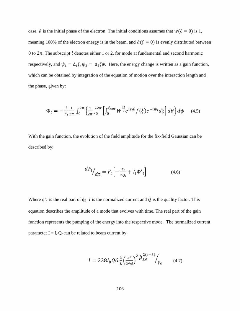
106

case. is the initial phase of the electron. The initial conditions assumes that is 1,

meaning 100% of the electron energy is in the beam, and is evenly distributed between

to . The subscript denotes either 1 or 2, for mode at fundamental and second harmonic

respectively, and . Here, the energy change is written as a gain function,

which can be obtained by integration of the equation of motion over the interaction length and

the phase, given by:

(4.5)

With the gain function, the evolution of the field amplitude for the fix-field Gaussian can be

described by:

(4.6)

Where ’l is the real part of l, is the normalized current and is the quality factor. This

equation describes the amplitude of a mode that evolves with time. The real part of the gain

function represents the pumping of the energy into the respective mode. The normalized current

parameter I = Il Ql can be related to beam current by:

(4.7)

107

From Eq. 4.6, the mode competition between the modes at different harmonics can be

analyzed by keeping track of the amplitudes. Setting the initial amplitude of the competing mode

to be much less than the operating mode simulates the condition where the operating mode is

excited first and reaches high amplitude first. The amplitude of fundamental mode could either

remain small in the case of suppression by the second harmonic mode, or grow in the case of

competition where the competitor becomes excited. In Eq. 4.6, if the term

is

greater than zero, then the amplitude of the corresponding mode would rise. G

The gain function is more or less already defined, so the key term is the normalized current; if

the current injected is less than the threshold value, then the competitor mode at the fundamental

harmonic should be suppressed in the presence of the operating mode; if the current is greater

than the threshold value, then the competitor could possibly take over. This threshold current is

the start-oscillation-current of the fundamental mode modified by the presence of the second

harmonic mode.

The calculations are performed using Eq. 4.3 – 4.6. The modes are calculated in pairs: a

competing mode and the operating mode for different values of the current parameter.

Furthermore, the calculation of the mode pairs spans the normalized detuning space of the

excitation region of the operating mode, which represents the magnetic field in real parameter

space. In the calculation, the two modes are separated by their cold cavity frequency, and this

frequency separation corresponds to frequency mismatch in cyclotron resonance, which

corresponds to the magnetic field. For each data point in the detuning space, the value of

normalized current for the second harmonic mode is fixed, and this value corresponds to 20

108

Amps. The assumption is that the beam will be 80 kV, 20 Amps and have a velocity ratio of 1.4.

The normalized length is assumed to be 14, the same as the previous design value in Chapter 2.

With these parameters, the 2nd

harmonic gyrotron’s efficiency space can be calculated as shown

in Figure 43.

Figure 43 Plane of orbital efficiency for current and normalized detuning. The color scale corresponds to the orbital

efficiency; highest frequency is dark red, while the lowest efficiency region is blue. The orbital efficiency shown here tops

out at 35%, compare to more than 60% for fundamental operation shown in Figure 9.

The orbital efficiency of second harmonic gyrotron with the chosen interation length and

beam parameter peaks at 35%; compare this to the 60% orbital effiency for the 670 GHz

gyrotron operating at the fundamental harmonic. Figure 43 also shows that the calculation only

needs to be performed for from 0.2 to 0.7, since for any larger value of detuning, the current

needed to achieve the higher effieciency is unrealisticaly high. Note that the detuning shown

above is the detuning for second harmonic operation, while during the calculation, the detuning

values are needed for both the operating mode and the fundamental competing mode. Due to the

fact that the detuning is normalized to the cyclotron resonance condition, the detuning relation

between the modes are not equal; i.e., . This requires a new modified detuning, . This

109

modified detuning can relate the detuning space of the second harmonic mode to that of the

fundamental harmonic mode, where:

(4.5)

The values of the normalized current, for the fundamental harmonic mode varies for

each calculation. is initially set to its steady-state value, while is initially set to a tiny

fraction of . Both of the amplitude values are tracked as a function of time. For cases where

stays at a very low level, the operating mode successfully suppresses the competing mode. If

rises from the initial value, then the second harmonic mode operation is unstable. The value of

for any given for which the operation is unstable, is the start oscillation current of the

fundamental harmonic mode in the presences of an already established second

harmonicoperating mode. Repeating the for the span of detuning shown in Figure 43 will reveal

a modified start-oscillation of the mode at fundamental harmonic in presence of a second

harmonic mode, in the range of detuning space where the operating mode is excited. It follows

then, that if the beam current is greater than this modified start current, then gyrotron operation at

second harmonic would be unstable due to the excitation of compating mode at the fundamental

harmonic.

110

Section 4.4, Start-current oscillation calculation for the fundamental mode

Results of the calculation are presented in Figure 44 and Figure 45. The figures show the

comparison of the start-oscillation current of the competing modes for single mode oscillation

and when the mode is in presence of the second harmonic mode. The results exist only for TE11,6

and TE17,4. The other two modes, TE9,7 and TE14,5 have too much frequency separation; for the

range of detuning of Figure 43, neither of these modes can be excited with the available current.

Therefore, these two modes are also eliminated as possible competitors. These results presented

are the results from solving for the gain function in Eqs. 4.6.

Figure 44 The start-oscillation current of TE11,6 at fundamental harmonic, shown as normalized unit as a function of

detuning. The red curve corresponds to Figure 42, the start-oscillation current. Blue curve represent the start oscillation

current of TE11,6 when the second harmonic operating mode is already present. For detuning less than 0.4, the operating

has suppressing effect. For detuning greater than 0.4, the operating mode helps exciting the fundamental mode.

111

Figure 45 The start-oscillation current of TE17,4 at fundamental harmonic, shown as normalized unit as a function of

detuning. The red curve corresponds to Figure 42, the start-oscillation current. Blue curve represent the start oscillation

current of TE11,6 when the second harmonic operating mode is already present. The frequency separation between these

modes is too great to observe the effect.

Furthermore, TE17,4 is also found not to be a particular dangerous competitor mode. In

Figure 45, blue is the curve for the start-oscillation current for TE17,4, and only a very short range

of detuning is available. This is because in the calculation, the two modes’ excitation conditions

can only be satisfied within this small range of cyclotron detuning; outside of this range of

detuning, the second harmonic would be too far out of resonance with the electrons. Conversely,

this also means for detuning optimized for the second harmonic mode, the TE17,4, mode would

112

also be out of resonance with the electrons. It implies that TE17,4 is not dangerous to second

harmonic operation.

This left only TE11,6 as the competing mode of interest to study. For TE11,6, the results of

Figure 44, show that both TE11,6 and the operating mode have similar ranges of detuning values

where excitation can occur. The red curve corresponds to the start-oscillation current shown in

Figure 42. Blue curve represents the start-oscillation current of TE11,6 when the second harmonic

operating mode is already present. For detuning less than 0.4, the operating mode has a

suppressing effect. For detuning greater than 0.4, the operating mode helps to excite the

fundamental mode. For detuning less than 0.4. It is shown that the start-oscillation current in the

presence of second harmonic mode is higher when the second harmonic is absent, indicating the

suppression effect. For larger detuning, the presence of the second harmonic mode lowers the

start oscillation current of the fundamental harmonic mode, so it actually helps the competitor

mode to grow. This is unfortunate since the gyrotron efficiency is higher in the hard-self

excitation region, which is located in the larger detuning value regime where the second

harmonic mode helps the competitor mode. The results here concur with earlier work in Ref [56],

where this effect was first suggested.

The analytical results presented above show that the only mode that would be of concern

is TE11,6, implying that the more time intensive simulations by MAGY would only need to be

performed for one mode. If the results can show that TE11,6 does not cause instability, then it can

be reasonably assumed that the other modes would not either.

While attempting to set-up the simulation, an effect was observed of second harmonic

excitation. The issue arises from the fact that second harmonic operation is much less efficient

113

compared to the fundamental harmonic using the same mode at the same frequency; see Figure

43. Correspondingly it is harder to excite the operating mode at second harmonic. It was found

during simulation that the TE31,8 mode at second harmonic cannot be excited by a 20 amp beam

using the same resonator structure from the previous study.

Figure 46 The start oscillation current shown in Figure 45 (blue) is overlaid with another set of calculation of start

oscillation current, when the interaction length is longer (red). For TE11,6, the start oscillation is substantially lowered in

the longer resonator.

To compensate, the resonator has to be modified by either a) lengthening the interaction

length, or b) altering the geometry to increase reflection at the output. For option a), if interaction

length is increased to = 25, the gyrotron can be excited by 20 Amp beam and still maintain

35% orbital efficiency. However, the increase in the interaction length also helps the excitation

114

of modes at the fundamental harmonic, making mode instability more complicated. The

analytical calculations with the mode pairs are repeated, for the longer interaction length. The

parameters are kept exactly the same. For the TE11,6 mode the result is shown in Figure 46, for

TE17,4, the results are shown in Figure 47. The blue curve shows the start oscillation of the

fundamental harmonic mode in the presence of a second harmonic mode, as shown in Figure 44

and Figure 45. The start-oscillation current for in the presence of the second harmonic

mode is in red. In both cases, the start-oscillation current when is much higher than the

case when . This result clearly shows that the step of lengthening interaction length

should not be taken; the fundamental mode is much more likely to be excited for a longer length.

Instead, effort has to be made to alter the reflection at the end of the resonator without increasing

the interaction length.

115

Figure 47 The start oscillation current shown in Figure 45 (blue) is overlaid with another set of calculation of start

oscillation current, when the interaction length is longer (red). For TE17,4, the start oscillation is substantially lowered in

the longer resonator.

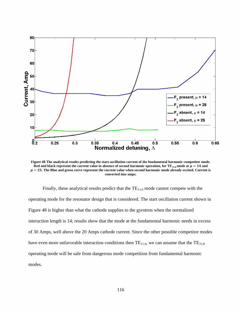
116

Figure 48 The analytical results predicting the start-oscillation current of the fundamental harmonic competitor mode.

Red and black represent the current value in absence of second harmonic operation, for TE11,6 mode at and

. The Blue and green curve represent the current value when second harmonic mode already excited. Current is

converted into amps.

Finally, these analytical results predict that the TE11,6 mode cannot compete with the

operating mode for the resonator design that is considered. The start oscillation current shown in

Figure 48 is higher than what the cathode supplies to the gyrotron when the normalized

interaction length is 14; results show that the mode at the fundamental harmonic needs in excess

of 30 Amps, well above the 20 Amps cathode current. Since the other possible competitor modes

have even more unfavorable interaction conditions then TE11,6, we can assume that the TE31,8

operating mode will be safe from dangerous mode competition from fundamental harmonic

modes.

117

Figure 48 also illustrates the sensitivity of the start current to the interaction length. For

, region where the effect of mode suppressioin is much larger, ranging from = 0 to 0.43.

For , the range where suppressions occurs is only limited to the range from 0 to 0.24.

More importantly, the results clearly show that for longer interaction length, the start-oscillation

current for the fundamental harmonic mode is well below the beam current, meaning that these

modes can be excited and can grow to interfere with gyrotron operation.

118

Section 4.5, Redesigned resonator profile and numerical calculation

Figure 49 Modified resonator for 2nd harmonic simulation. The bump is included at the end of the interaction

section to increase the reflection, thus increasing the diffractive Q. This bump increased the quality factor by 30%

The analytical results indicate that the operating mode would be safe from dangerous

competition. The next step is to verify these conclusions with MAGY. The simulations are done

assuming an electron beam of 20 Amps at 80 kV. The velocity ratio in the simulation is 1.4, and

the beam is assumed to be ideal in that it has no spread in guiding centers or in velocities. To

further simplify the problem, the simulation is not concerned with designing a start-up scenario.

It is known from Figure 42 that the start-oscillation current for the second harmonic mode is

lower than any of its competitors at the fundamental harmonic, so it is assumed in the

simulations that a start-up scenario for the excitation of the operating mode exists.

The resonator design for the 670 GHz gyrotron is unsuitable for this study. TE31,8 could

not be excited by the beam. The resonator had to be redesigned to increase the diffractive quality

119

factor [55]. Increasing the length of the straight section has been ruled out because that is likely

to increase the mode instability. Instead, the end of the straight section is modified slightly by

including a bump [56], as shown in Figure 49. This bump increased the diffractive Q by more

than 30% while keeping the length of the interaction constant.

Verification of the effect of the bump is done in MAGY. First, a single mode calculation

containing only the second harmonic mode is performed. The simulation kicks start the

oscillation at the second harmonic using an artificial source at high amplitude, and this source is

turned off after a short time so that the operating mode is sustained by the energy from the beam.

This corresponds to the hard self-excitation region of the gyrotron operation. This is the same

method used in Chapter 2 and 3 as well to avoid the time consuming calculation of voltage-

current rise. This set of calculations yields the optimal magnetic field at which the efficiency for

the second harmonic gyrotron is highest. With this modified resonator, the single mode

simulations show that peak interaction efficiency of 20.53% occurs at 13.5 T. The next step is a

similar single mode calculation of the competing mode at the fundamental harmonic, except that

the code is instructed to simulate the mode at the fundamental harmonic by initially be seeding at

noise level. The magnetic field of the simulation corresponds to the optimal operating point for

the second harmonic mode. These results provide a references point to compare with subsequent

results.

Finally the simulations are repeated, but now including both of the modes in question. At

optimal magnetic field value of 13.5 T, when the fundamental harmonic mode TE11,6 is included,

the result is that the operating mode remains undisturbed, as predicted by the analytical results.

120

The overall efficiency of this particular gyrotron at the output is 15.6%, with 250 kW of outgoing

radiation as shown in Figure 50.

Figure 50 Numerical simulation confirming that operating mode is safe. The Red curve represents the second harmonic

operation, the blue curve is the fundamental competitor. The competitor mode remains unchanged.

Moreover, another simulation is performed for the magnetic field value corresponding to

the range of detuning where the suppression of the fundamental harmonic mode occurs. Without

the presence of the operating mode, the TE11,6 mode is excited from noise and operate with 5%

efficiency. However, when the operating mode is included, the competing mode remains at noise

level. This agrees with the results from the analytical model, showing that for a certain range of

magnetic field, the presence of the second harmonic mode suppresses the fundamental harmonic

mode.

Despite the unfavorable interaction of second harmonic modes compared to fundamental

modes, the gyrotron operating with TE31,8 should be able to operate continuously without losing

out in competition with competing modes. TE11,6 is found to be the competing mode of greatest

121

concern, but it is still not able to compete with the operating mode under certain condition. The

MAGY simulation confirms that the presence of second harmonic operation alters the excitation

conditions for the modes at the fundamental harmonic. Moreover, the interaction length has a

profound effect on the stability of gyrotron operation.

122

Summary and Conclusion

The theoretical analyses and simulation results provided herein constitute a major step in

improving gyrotron technology by pushing operation well into the sub-millimeter wavelength

range with significantly higher efficiency than previously achieved. Existing gyrotron theories

were used to select a parameter space where the gyrotron can operate with high efficiency. The

orbital efficiency was predicated to be at least 60%, this correspond to an interaction efficiency

of 36%. An appropriate operating mode was selected in order to minimize the Ohmic wall loss in

the resonator circuit; the output efficiency should be able to reach at least 32%. The profile

geometry was optimized so that mode conversion is minimized while the field profile is

optimized. Numerical simulations verified that for one of the profile designs, the best efficiency

could range from 35% to 36.5%, for different values of the orbital velocity spread in the electron

beam. The result showed that voltage depression has little effect on the efficiency. The numerical

MAGY results validated the gyrotron theoretical studies.

In addition to the resonator design, a study of the spread in electron guiding centers

showed that a spread of about one third of the wavelength reduces the gyrotron efficiency by

about 10% or less of its nominal value; so 35% efficiency would be reduced to 32%. More

importantly, the "rule of thumb” that gyrotron designers had followed has been shown to be

overly cautious, at least for TE modes with "wide" injection peaks. For sub-millimeter wave

gyrotrons with well selected operating mode, one could increase the emitter width of the

previous design while keeping the efficiency reasonably high, greatly alleviating design

constraints on the magnetron-injection type electron gun. The analytical results concerning the

effects of guiding center spread were validated by MAGY simulation results.

123

The gyrotron was built, with two identical copies made. One was delivered to the

University of Maryland, while the other one is currently at the Russian company GYCOM.

Experimental results so far have shown that power output of 200 kW can be achieved, with an

efficiency of 20%. This measured efficiency included losses in the up-taper region, mode

converter, output window and the detection circuit. None of these were included in the cavity

design calculations or simulations carried out at the University of Maryland as part of the present

thesis. After the up-taper region, the change in radius causes the RF field to degenerate into

several different modes, which need to be re-converted back into TE31,8; the conversion loss is

calculated to be about 10%. At the output window, some power is absorbed by the window

material, further reducing power output. These factors together can explain the discrepancy

between the simulation results for output efficiency and the realized experimental value. In

addition to the agreement between design and experiment, a record breaking gyrotron was

created. It has already been used in air breakdown studies.

In addition to operating near the electron cyclotron frequency, terahertz gyrotrons could

also be designed to operate at the second cyclotron harmonic so as to avoid having to be limited

to pulsed operation. Study of second harmonic gyrotron operation presented in this thesis showed

stable operation with the TE31,8 mode as a second harmonic operating mode. Simulations confirm

the phenomenon that the presence of a second harmonic mode can improve the excitation

condition of a fundamental mode, by showing that for a certain detuning space, the start-

oscillation current of the fundamental mode was reduced; nevertheless, second harmonic

operation without interference from modes at the fundamental cyclotron frequency could be

achieved. The output efficiency of this particular second harmonic gyrotron design at is 20%,

124

with 250 kW of output power. The magnetic field requirement drops from 26T to only 13T,

allowing for the possibility that the gyrotron could utilize a cryo-magnet to operate continuously

Despite the results showing promise of stable second harmonic operation, further work

could be done to increase stability. One area of promise is the further modification of the

resonator structure [59] so that the quality factors for the operating mode and the fundamental

competitor modes are designed differently. The basic concept is that if the fundamental mode

could be radiated out while the operating mode is contained inside the radiator, then the

interaction would only occur for the operating mode. One way to achieve it is to build

corrugations into the resonator wall, with the corrugations designed for reflection of the

operating mode [60] [61]. The radius and the interval of the corrugation would correspond to the

azimuthal index of the operating model. The other modes however, would be scattered out of the

resonator.

125

Bibliography

[1] V. A. Flyagin, A. G. Luchinin and G. S. Nusinovich, Int. J. Infared Millim. waves, vol. 4,

no. 4, pp. 629-637, 1983.

[2] V. L. Granatstein and G. S. Nusinovich, Journal of Applied Physics, vol. 108, p. 063304,

2010.

[3] V. L. Granastein and G. S. Nusinovich, in APS-DPP Meeting, Atlanta, GA, 2009.

[4] J. F. Fritelli, Port and Maritime Security: Background and Issues, New York: Noinka

Books, 2005.

[5] G. S. Nusinovich, R. Pu, T. M. Antonsen Jr., O. V. Sinitsyn, J. Rodgers, A. Mohamed, J.

Silverman, M. Al-Sheikhly, Y. S. Dimant, G. M. Milikh, M. Y. Glyavin, A. G. Luchinin, E.

A. Kopelovich and V. L. Granatstein, J Infared Milli Terahz Waves, vol. 32, no. 3, pp. 380-

402, 2010.

[6] Technical report, "Nanosecond pulse breakdown initiation and growth," RADC-TDR-63-

525, 1964.

[7] A. G. Litvak, "Freely Localized Gas Discharge in Microwave Beams," in Application of

High Power Microwaves, A. V. Gaponov-Grekhov and V. L. Granatstein, Eds., Norwood,

MA: Artech House, 1994.

[8] G. S. Nusinovich, G. M. Milikh and B. Levush, J. Appl. Phys, vol. 80, p. 4189, 1996.

[9] G. S. Nusinovich, P. Sprangle, C. A. Romero-Talamas and V. L. Granatstein, J. Appl. Phys.,

vol. 8, no. 109, p. 3303, 2011.

[10] J. A. S. Gilmour, Microwave Tubes, Norwood, MA: Artech House Inc., 1986.

[11] C. Sirtori, Nature, vol. 417, no. 6885, 2002.

[12] A. A. Negirev and A. S. Fedorov, Radiotekhnika, no. 4, p. 41, 1999.

[13] M. Y. Glyavin and A. G. Luchinin, Terahertz Science and Technology, vol. 2, no. 4, pp.

150-155, 2009.

[14] G. S. Nusinovich, Introduction to the Physics of Gyrotrons, Baltimore, MD: The Johns

Hopkins University Press, 2004.

[15] M. Button, T. M. Antonsen Jr., B. Levush, K. T. Nguyen and A. N. Vlasov, IEEE Trans.

Plasma Sci., vol. 26, pp. 882-892, 1998.

[16] J. D. Jackson, Classical Electrodynamics, New York, NY: Wiley, 1999.

[17] A. Kesar and J. J. Petillo, IEEE Transac. Plasma, vol. 39, no. 12, 2011.

[18] M. Glyavin, A. G. Luchinin and G. Y. Golubiatnikov, Phys. Rev. Letter, vol. 100, no.

015101, 2008.

[19] R. Pu, G. S. Nusinovich, O. V. Sinitsyn and T. M. Antonsen Jr., Physics. Plasmas, vol. 18,

no. 023107, 2011.

[20] D. K. Cheng, Fields and Wave, Reading, MA: Addison-Wesley, 1989.

[21] O. V. Sinitsyn, G. S. Nusinovich and T. M. Antonsen Jr., Phys. Plasmas, vol. 19, 2012.

[22] K. Sakamoto, A. Kasugai, K. Takahashi, R. Minami, N. Kobayashi and K. Kajiwara, Nat.

Phys, vol. 3, no. 411, 2007.

126

[23] O. Dumbrajs, M. Thumm, J. Prettenebner and D. Wagner, Int. J. Infrared Millim. Waves,

vol. 13, p. 825, 1992.

[24] V. G. Pavel'ev, S. E. Tsimring and V. E. Zapevalov, Int. J. Electron, no. 63, p. 379, 1987.

[25] M. V. Kartikeyan, E. Borie and M. K. A. Thumm, Gyrotrons: High Power Microwave and

Millimeter Wave Technology, New York: Springer, 2004.

[26] E. M. Choi, M. A. Shapiro, J. R. Sirigiri and R. J. Temkin, Phys. Plasmas, vol. 14, no. 093,

p. 302, 2007.

[27] O. V. Sinitsyn and G. S. Nusinovich, Phys. Plasmas, vol. 16, no. 023, p. 101, 2009.

[28] D. Kashyn, "Contributions to Resolving Issues Impeding the Operation of High Power

Microwave and Submillimeter Devices," University of Marynd PhD Thesis, College Park,

MD, 2014.

[29] G. S. Nusinovich, D. G. Kahsyn, Y. Tatematsu and T. Idehara, Phys. Plasma, vol. 21, no.

013108, 2014.

[30] M. Y. Glyavin, A. G. Luchinin, G. S. Nusinovich, J. Rodgers, D. G. Kashyn, C. A. Romero-

Talamas and R. Pu, J. Appl. Phys. Lett., 101, 153503, 2012.

[31] V. S. Ergakov, M. A. Moiseev and R. E. Erm, Elektron. Tekhnika, Ser. I Elektron. SVch,

vol. 3, pp. 22-27, 1980.

[32] E. Borie and G. Gantenbein, Int. J. Infrared Millimeter Waves, vol. 12, pp. 65-78, 1991.

[33] S. Y. Cai, T. M. Antonsen Jr., G. Saraph and B. Levush, Int. J. Electron, no. 72, pp. 759-

777, 1992.

[34] O. Dumbrajs and S. Liu, IEEE Trans. Plasma Sci., no. 20, pp. 126-132, 1992.

[35] G. S. Nusinovich, O. Dumbrajs and B. Levush, Phys. Plasmas, no. 2, pp. 4621-4630, 1995.

[36] G. S. Nusinovich, O. V. Sinitsyn, M. Yeddulla, L. Velikovich, T. M. Antonsen Jr., A. N.

Vlasov, S. Cauffman and K. Felch, Phys. Plasmas, no. 10, pp. 3335-3343, 2003.

[37] V. L. Bratman, Y. K. Kalynov and V. N. Manuilov, "Large-Orbit Gyrotron operation in

terahertz frequency range," in ICOPS, San Diego, 2009.

[38] K. L. Felch, B. G. Danly, H. R. Jory, K. E. Kreischer, W. Lawson, B. Levush and R. J.

Temkin, Proc. IEEE , no. 87, pp. 752-781, 1999.

[39] K. Sakamoto, Fusion Sceinece Technology, no. 52, pp. 145-153, 2007.

[40] S. E. Tsimring, Electron Beams and Microwave Vaccum Electronics, Hoboken, NJ: Wiley-

Interscience, 2007.

[41] J. M. Baird and W. Lawson, Int. J. Electron, no. 61, pp. 953-968, 1986.

[42] A. G. Luchinin and G. S. Nusinovich, Int. J. Electron, vol. 57, pp. 827-834, 1984.

[43] G. S. Nusinovich, Electron. Tekhn SVch, vol. 1, no. 4, pp. 10-13, 1986.

[44] A. L. Goldenberg and M. I. Petelin, Radiophys. Quantum Electron, no. 16, pp. 106-111,

1973.

[45] D. G. Kashyn, G. S. Nusinovich, O. V. Sinitsyn and T. M. Antonsen Jr., IEEE Trans.

Plasma Sci., 2010.

[46] G. S. Nusinovich, in AIP Conf. Proc., Melville, New York, 2001.

[47] M. A. Moiseev and G. S. Nusinovich, Radiophys. Quantum Electron., vol. 17, pp. 1305-

1311, 1974.

127

[48] R. Pu, G. S. Nusinoch, O. V. Sinitsyn and T. M. Antonsen Jr., Phys. Plasma, vol. 17, p.

3015, 2010.

[49] G. S. Nusinovich, M. Yeddulla, T. M. Antonsen Jr and A. N. Vlasov, Phys. Rev. Lett., vol.

12, p. 12501, 2006.

[50] T. Idehara, T. Saito, I. Ogawa, S. Mitsudo, Y. Tatematsu, L. Agusu, H. Mori and S.

Kobayashi, Appl. Magn. Reson., vol. 34, p. 265, 2009.

[51] T. Notake, T. Saito, Y. Tatematsu, A. Fujii, S. Ogasawara, L. Agusu, T. Idehara and V. N.

Manuilov, Phys. Rev. Lett. , vol. 103, p. 255002, 2009.

[52] V. L. Bratman, Y. K. Kalynov and V. N. Manuilov, Phys. Rev. Lett. , vol. 102, p. 245101,

2009.

[53] A. C. Torrezan, S. T. Han, I. Mastovsky, M. A. Shapiro, J. R. Sirigiri, R. J. Temkin, A. B.

Barnes and R. G. Griffin, IEEE Trans. Plasma Sci., vol. 38, p. 1150, 2010.

[54] S. H. Kao, C. C. Chiu, K. F. Pao and K. R. Chu, Phys. Rev. Lett., vol. 107, p. 135101, 2001.

[55] P.-K. Liu and E. Borie, Int. J. Infrared Millimeter Waves, vol. 21, no. 6, 2000.

[56] S. H. Kao, C. C. Chiu, P. C. Chang, K. L. Wu and K. R. Chu, Phys. Plas., vol. 19, p.

103103, 2012.

[57] G. S. Nusinovich and I. G. Zarnitsyna, Radiofzika, vol. 20, no. 3, pp. 461-467, 1976.

[58] T. Idehara, S. Mitsudo, M. Pereyaslavets, Y. Shimizu and I. Ogawa, Int. Journal. Infared

Millimeter Wave, vol. 20, no. 7, 1999.

[59] G. S. Nusinovich, Radiophys. Quantum Ele., vol. 20, pp. 313-317, 1977.

[60] G. G. Denisov and I. M. Orlova, Radiofizika, vol. 31, no. 6, pp. 698-703, 1986.

[61] G. S. Nusinovich, O. V. Sinitsyn and T. M. Antonsen Jr., Phys. Rev. Lett, vol. 98, no.

205101, 2007.

[62] P. Siegel, IEEE Trans. Microwave Theory Tech, vol. 50, no. 3, p. 910, 2002.

[63] A. V. Gaponov, M. I. Petelin and V. K. Yulpatov, Radiophys. Quantum Electron., vol. 10,

pp. 794-813, 1967.

[64] S. N. Vlasov, G. M. Zhislin, I. M. Orlova, M. I. Petelin and G. G. Rogacheva, Radiofizika,

vol. 12, no. 8, 1969.

[65] E. Borie, Int. J. Infrared Mili Waves, vol. 29, pp. 113-130, 2008.