ABSTRACT

Title: SIMULATION OF DYNAMIC PRESSURE-

SWING GAS SORPTION IN POLYMERS

Heather Jane St. Pierre, Master of Science, 2005 Directed By: Professor Timothy A. Barbari

Department of Chemical Engineering A transport model was developed to simulate a dynamic pressure-swing sorption

process that separates binary gas mixtures using a packed bed of non-porous spherical

polymer particles. The model was solved numerically using eigenfunction expansion,

and its accuracy verified by the analytical solution for mass uptake from a finite

volume. Results show the process has a strong dependence on gas solubility. The

magnitudes and differences in gas diffusivities have the greatest effect on determining

an optimal particle radius, time to attain steady-state operation, and overall cycle

time. Sorption and transport parameters for three different polyimides and one

copolyimide were used to determine the degree of separation for CO2/CH4 and O2/N2

binary gas mixtures. The separation results for this process compare favorably to

those for membrane separation using the same polymer, and significantly improved

performance when a second stage is added to the pressure-swing process.

SIMULATION OF DYNAMIC PRESSURE-SWING GAS SORPTION IN POLYMERS

by

Heather Jane St. Pierre

Thesis submitted to the Faculty of the Graduate School of the University of Maryland, College Park, in partial fulfillment

of the requirements for the degree of Master of Science

2005

Advisory Committee: Professor Timothy A. Barbari, Chair Associate Professor Raymond A. Adomaitis Associate Professor Peter Kofinas

© Copyright by Heather Jane St. Pierre

2005

ii

Acknowledgements

I would like to thank my advisor, Professor Barbari, for all of his help and guidance

during the course of this research. In the short time I have worked for him, I have

learned much from the sharing of his knowledge and experience. I would also like to

thank my �co-advisor,� Professor Adomaitis for the use of his Matlab code for the

simulations presented in this work. Even though I was not officially a student of his,

he always had time to help, and I have learned much from working with him as well.

iii

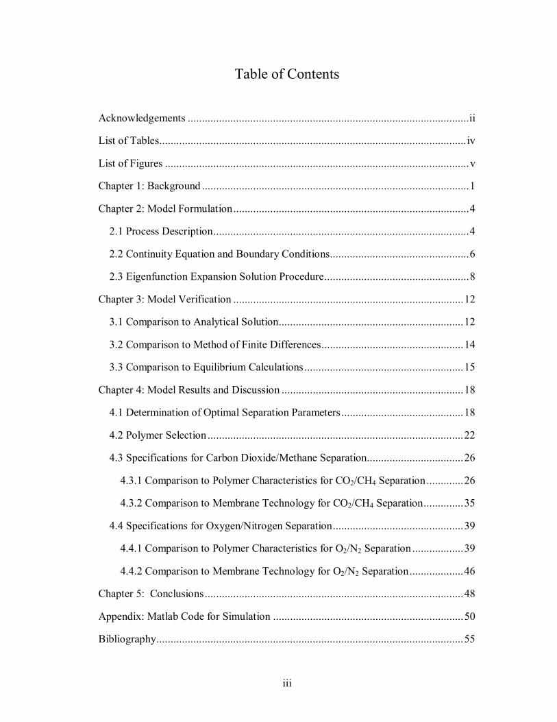
Table of Contents

Acknowledgements ...................................................................................................ii

List of Tables............................................................................................................iv

List of Figures ...........................................................................................................v

Chapter 1: Background ..............................................................................................1

Chapter 2: Model Formulation...................................................................................4

2.1 Process Description..........................................................................................4

2.2 Continuity Equation and Boundary Conditions.................................................6

2.3 Eigenfunction Expansion Solution Procedure...................................................8

Chapter 3: Model Verification .................................................................................12

3.1 Comparison to Analytical Solution.................................................................12

3.2 Comparison to Method of Finite Differences..................................................14

3.3 Comparison to Equilibrium Calculations........................................................15

Chapter 4: Model Results and Discussion ................................................................18

4.1 Determination of Optimal Separation Parameters...........................................18

4.2 Polymer Selection ..........................................................................................22

4.3 Specifications for Carbon Dioxide/Methane Separation..................................26

4.3.1 Comparison to Polymer Characteristics for CO2/CH4 Separation.............26

4.3.2 Comparison to Membrane Technology for CO2/CH4 Separation..............35

4.4 Specifications for Oxygen/Nitrogen Separation..............................................39

4.4.1 Comparison to Polymer Characteristics for O2/N2 Separation ..................39

4.4.2 Comparison to Membrane Technology for O2/N2 Separation...................46

Chapter 5: Conclusions...........................................................................................48

Appendix: Matlab Code for Simulation ...................................................................50

Bibliography............................................................................................................55

iv

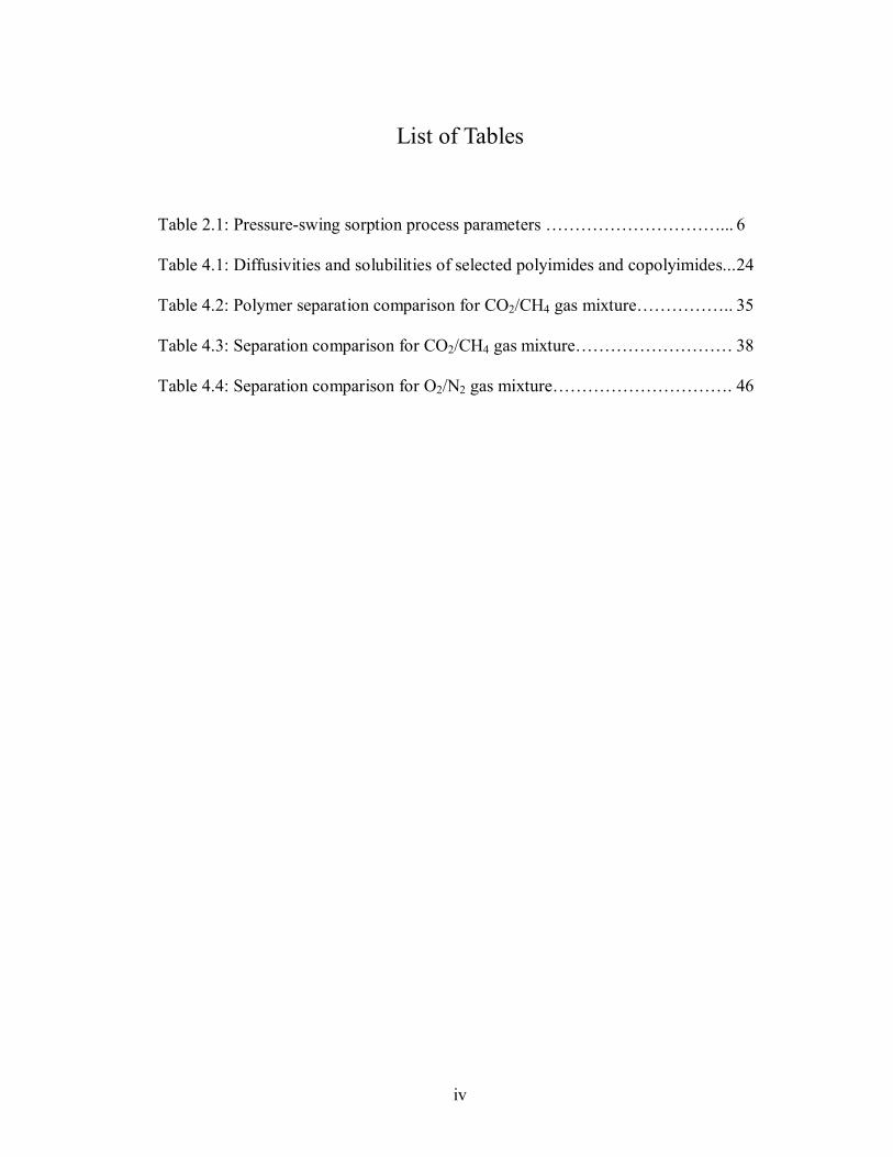
List of Tables

Table 2.1: Pressure-swing sorption process parameters ����������... 6

Table 4.1: Diffusivities and solubilities of selected polyimides and copolyimides... 24

Table 4.2: Polymer separation comparison for CO2/CH4 gas mixture�����.. 35

Table 4.3: Separation comparison for CO2/CH4 gas mixture��������� 38

Table 4.4: Separation comparison for O2/N2 gas mixture����������. 46

v

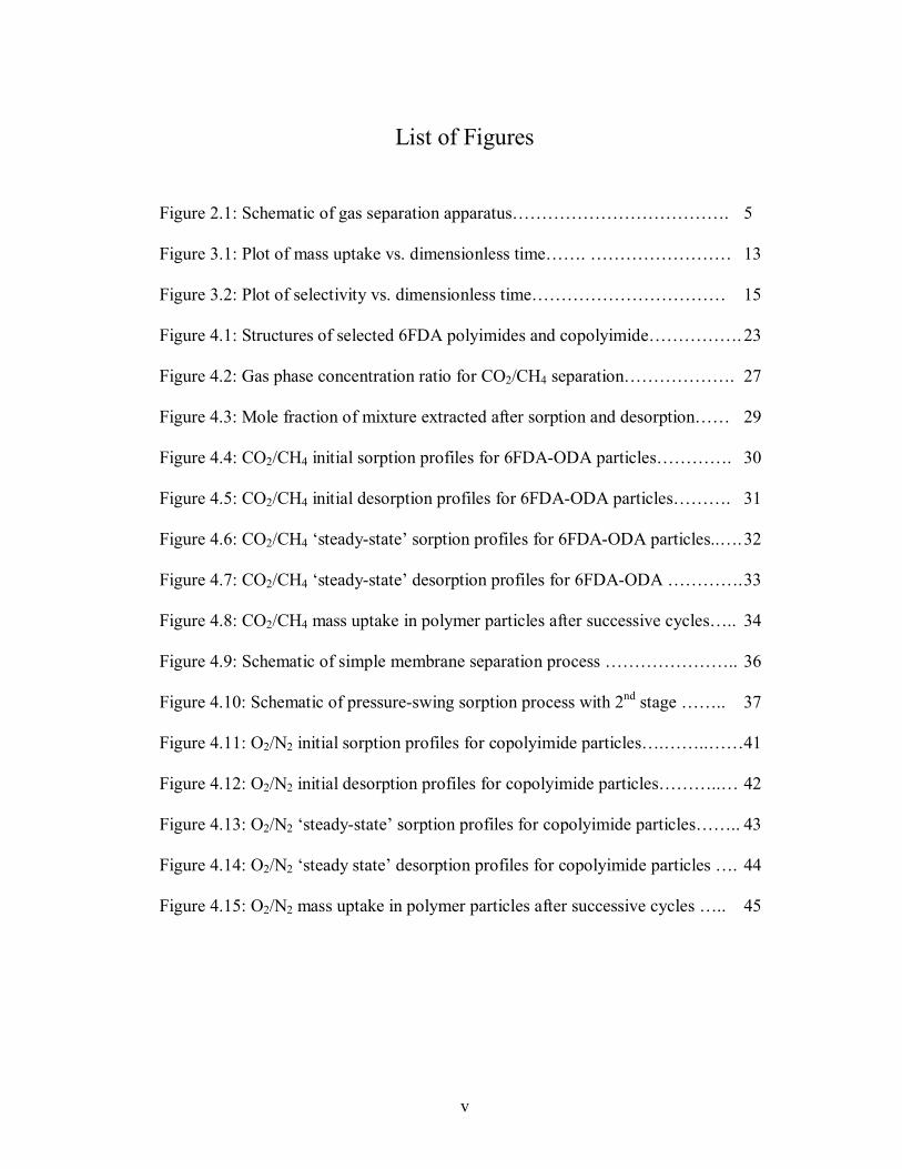
List of Figures

Figure 2.1: Schematic of gas separation apparatus������������. 5

Figure 3.1: Plot of mass uptake vs. dimensionless time��. �������� 13

Figure 3.2: Plot of selectivity vs. dimensionless time����������� 15

Figure 4.1: Structures of selected 6FDA polyimides and copolyimide�����. 23

Figure 4.2: Gas phase concentration ratio for CO2/CH4 separation������. 27

Figure 4.3: Mole fraction of mixture extracted after sorption and desorption�� 29

Figure 4.4: CO2/CH4 initial sorption profiles for 6FDA-ODA particles����. 30

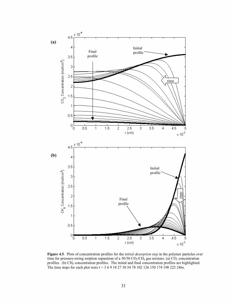
Figure 4.5: CO2/CH4 initial desorption profiles for 6FDA-ODA particles���. 31

Figure 4.6: CO2/CH4 �steady-state� sorption profiles for 6FDA-ODA particles..�. 32

Figure 4.7: CO2/CH4 �steady-state� desorption profiles for 6FDA-ODA ����. 33

Figure 4.8: CO2/CH4 mass uptake in polymer particles after successive cycles�.. 34

Figure 4.9: Schematic of simple membrane separation process �������.. 36

Figure 4.10: Schematic of pressure-swing sorption process with 2nd stage ��.. 37

Figure 4.11: O2/N2 initial sorption profiles for copolyimide particles�.��..�� 41

Figure 4.12: O2/N2 initial desorption profiles for copolyimide particles���..� 42

Figure 4.13: O2/N2 �steady-state� sorption profiles for copolyimide particles��.. 43

Figure 4.14: O2/N2 �steady state� desorption profiles for copolyimide particles �. 44

Figure 4.15: O2/N2 mass uptake in polymer particles after successive cycles �.. 45

1

Chapter 1: Background

Gas separation processes have evolved over the years to continually improve

component separation, as well as increase cost effectiveness and efficiency. Many of

these techniques have included variations of membrane separation, pressure-swing

adsorption (PSA), liquid absorption, and cryogenic separation. These processes are often

economically compared based on the rate of production of separated components and

quality of separation.1

Two separations of particular commercial interest include carbon dioxide/methane

separation and air (oxygen/nitrogen) separation. Current CO2/CH4 separation

applications include biogas separation from landfills or farms for energy use, natural gas

sweetening where CO2 is removed from natural gas wells, or enhanced oil recovery

where supercritical or near critical CO2 is pumped into oil wells to reduce oil viscosity

for easier extraction.2,3 Air separation applications currently in use include oxygen

enrichment for combustion or medical needs, inert gas blanketing on some oil tankers, or

nitrogen blanketing for shipping or storing food.2 These separations have been achieved

by using polymeric membrane materials in addition to the more traditional methods.2

The economic choice of separation process for both CO2/CH4 and O2/N2 is highly

dependent on the scale of that process. In general, membranes have been favored at

smaller scales.1

Separation using polymer membranes has become an effective means of

achieving gas separation in recent years. Typical polymers used in commercial

2

membrane separation have been polysulfones, polycarbonates and cellulose acetates.3,4

Recently, focus has turned to polyimides due to their excellent properties for separation.

Some of these polyimides have been formed into hollow-fiber membranes,5,6 but few are

commercially available because of their cost and difficulty to manufacture.2,4

The formation of integrally-asymmetric hollow fibers in itself is not a simple task.

Separation is not determined by the polymer properties alone, but on how the fibers

themselves are prepared to provide a defect-free thin film with the proper orientation to

maximize separation.3,6,7 Creating a polymer solution with the desired thermodynamic

and rheological properties to form hollow fibers is another challenge associated with this

process.3 Once the fibers themselves are constructed, there is also the issue of bundling

them together to be used as a separation device for either bore or shell feed, depending on

the application.2 Lastly, an appropriate fiber length must be chosen to prohibit significant

pressure drop in the bore of the hollow fibers.2

Given this difficulty in production, an alternative method for separation is

proposed here that utilizes the separation characteristics of highly selective polymers by

forming them into dense particles and using them in a packed bed. These particles could

potentially be formed by spray drying a polymer solution, or in situations where a

solution cannot be formed, by simply grinding the polymer into smaller particles. The

use of sorbent polymer particles was developed and modeled by Barbari et al.8 for liquid-

liquid extraction in a well-mixed batch process. In this work, the focus instead will be on

gas separation.

In this thesis, the separation of binary gas pairs, CO2/CH4 and O2/N2, is modeled

using a dynamic pressure-swing sorption process with dense polymer particles. Two

3

different polyimides are used for each gas pair, and their separation performance

compared to a simple membrane process which utilizes the separation properties of the

same polyimide. Although this process does not utilize a steady-state flux, separation

results from this model will be shown to be comparable to a membrane separation

process.

4

Chapter 2: Model Formulation

2.1 Process Description

As an alternative to membrane separation, the gas separation process described

here uses dynamic pressure-swing sorption. This single-stage process utilizes a

separation bed consisting of a vessel packed with nonporous polymer spheres of uniform

radius; the schematic can be seen in Figure 2.1. The concept for this process is based on

the liquid batch extraction process developed by Barbari et al.8 For the development of

this specific model, two gases will be separated based on their differing solubility and

diffusivity in the polymer phase. To take advantage of the different diffusivities, the

process is stopped prior to equilibrium, given that at equilibrium, only solubility

differences dominate separation. The proposed separation process cycle is composed of

three basic steps:

1) The packed bed is charged with a compressed gas mixture to a set pressure

with valves 2 and 3 closed. When the desired pressure is reached, valve 1 is

closed.

2) The gas in the external phase is sorbed by the polymer particles. At the end of

the sorption step, the remaining external phase is purged by opening valve 2

and lowering the pressure to P2 (taken to be 0 atm for the simulations of this

work). After the remaining gas in the external phase has been expelled, valve

2 is closed.

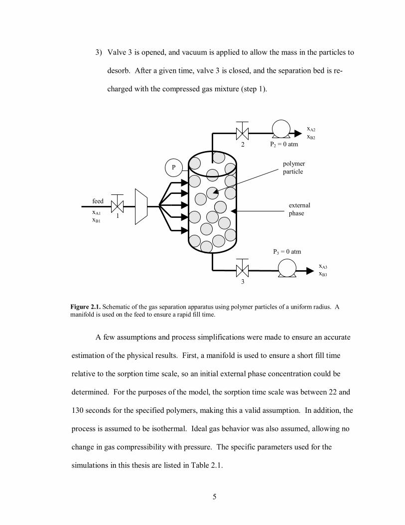
5

3) Valve 3 is opened, and vacuum is applied to allow the mass in the particles to

desorb. After a given time, valve 3 is closed, and the separation bed is re-

charged with the compressed gas mixture (step 1).

A few assumptions and process simplifications were made to ensure an accurate

estimation of the physical results. First, a manifold is used to ensure a short fill time

relative to the sorption time scale, so an initial external phase concentration could be

determined. For the purposes of the model, the sorption time scale was between 22 and

130 seconds for the specified polymers, making this a valid assumption. In addition, the

process is assumed to be isothermal. Ideal gas behavior was also assumed, allowing no

change in gas compressibility with pressure. The specific parameters used for the

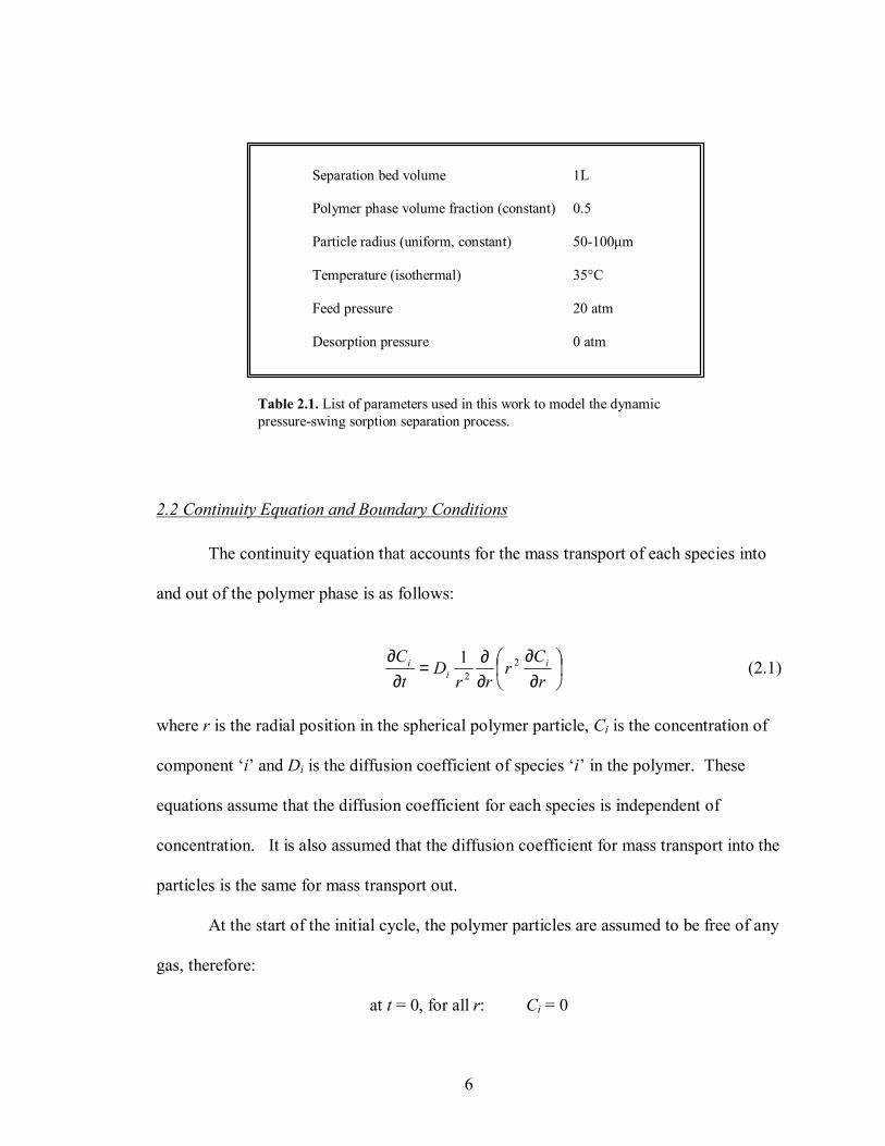
simulations in this thesis are listed in Table 2.1.

Figure 2.1. Schematic of the gas separation apparatus using polymer particles of a uniform radius. A manifold is used on the feed to ensure a rapid fill time.

polymer particle

external phase

feed

xA2 xB2

P3 = 0 atm

P

1

2

3

xA3 xB3

xA1 xB1

P2 = 0 atm

6

2.2 Continuity Equation and Boundary Conditions

The continuity equation that accounts for the mass transport of each species into

and out of the polymer phase is as follows:

∂∂

∂∂=

∂∂

rC

rrr

Dt

C ii

i 22

1 (2.1)

where r is the radial position in the spherical polymer particle, Ci is the concentration of

component �i� and Di is the diffusion coefficient of species �i� in the polymer. These

equations assume that the diffusion coefficient for each species is independent of

concentration. It is also assumed that the diffusion coefficient for mass transport into the

particles is the same for mass transport out.

At the start of the initial cycle, the polymer particles are assumed to be free of any

gas, therefore:

at t = 0, for all r: Ci = 0

Table 2.1. List of parameters used in this work to model the dynamic pressure-swing sorption separation process.

Separation bed volume 1L

Polymer phase volume fraction (constant) 0.5

Particle radius (uniform, constant) 50-100µm

Temperature (isothermal) 35°C

Feed pressure 20 atm

Desorption pressure 0 atm

7

In addition, there is no flux at the plane of symmetry, or center of the spherical particles:

at r = 0, for all t: 0=∂

∂r

Ci

The final boundary condition allows for a mass balance between the external and

polymer phases, as this specific process involves mass uptake from a finite external

volume. This boundary condition is at the interface between the polymer and external

phase, where the rate the gas leaves the external phase is equal to the rate the gas enters

the polymer phase at the boundary:

at r = R, for all t: Rr

ipi

Rr

i

i

e

rC

RVD

tC

SV

==

∂∂

−=

∂∂ 3 (2.2)

where Si is the partition (or solubility) coefficient of component �i� in the polymer phase,

and Ve and Vp are the external and polymer phase volumes, respectively. The partition

coefficients used here are defined as the ratio of the concentration in the particle relative

to the concentration in the external phase, and is assumed to be independent of

concentration.

The external (or gas) phase is assumed to be well-mixed at all times; therefore,

convective mass transfer resistance at the polymer surface is negligible. This assumption

is reasonable because the diffusion coefficient in many polymers (and those used in this

study) is on the order of 10-7 to 10-8 cm2/s, while that in the gas phase is 10-1 cm2/s. In

addition, the gas sorbed into the polymer is assumed to have no swelling effects on the

polymer, allowing the external and polymer phase volumes to be assumed constant.

Given the operating time scales of the experiment, the densities of the polymers chosen, a

polymer volume fraction of 0.5, and an initial pressure of 20 atm, the maximum possible

8

increase in polymer mass if all of the gas was sorbed by the polymer particles is only

1.6%. These specific parameters will be discussed later in Chapter 3.

2.3 Eigenfunction Expansion Solution Procedure

The process developed here is dynamic, and therefore cannot be represented or

estimated by an equilibrium analytical solution. The methods of finite differences and

finite element can be used to solve the partial differential equation listed in the previous

section, but these methods do not account for the entire volume of the particle, nor can

they capture concentration profile behavior at the particle interface. In addition, the

stability of the finite differences and finite element solution is based on the size of the

time step relative to the spatial step size. Eigenfunction expansion models the

concentration profiles over the entire particle radius, and its solution accuracy is only

controlled by the truncation number, or number of basis functions, therefore it is the

method of choice for this simulation.

The concentration profiles in time and space can be approximated as the

summation of an infinite number of functions:

∑∞

=+=

1)()()(),(

iii tfrtatrC ψ (2.3)

where )(tai are coefficients determined from the given initial condition and f(t) is the

finite-volume, concentration boundary condition that varies with time. The )(riψ in

Equation 2.3 are the orthogonal basis functions generated by the non-trivial solutions to

the Sturm-Liouville equation over 0 < r < 1:

9

λψψ =

drdr

drd

r2

2

1 or iii ψλψ =∇ 2 (2.4)

subject to:

0)0()0( =+ ψψ bdr

da

0)1()1( =+ ψψ ddr

dc

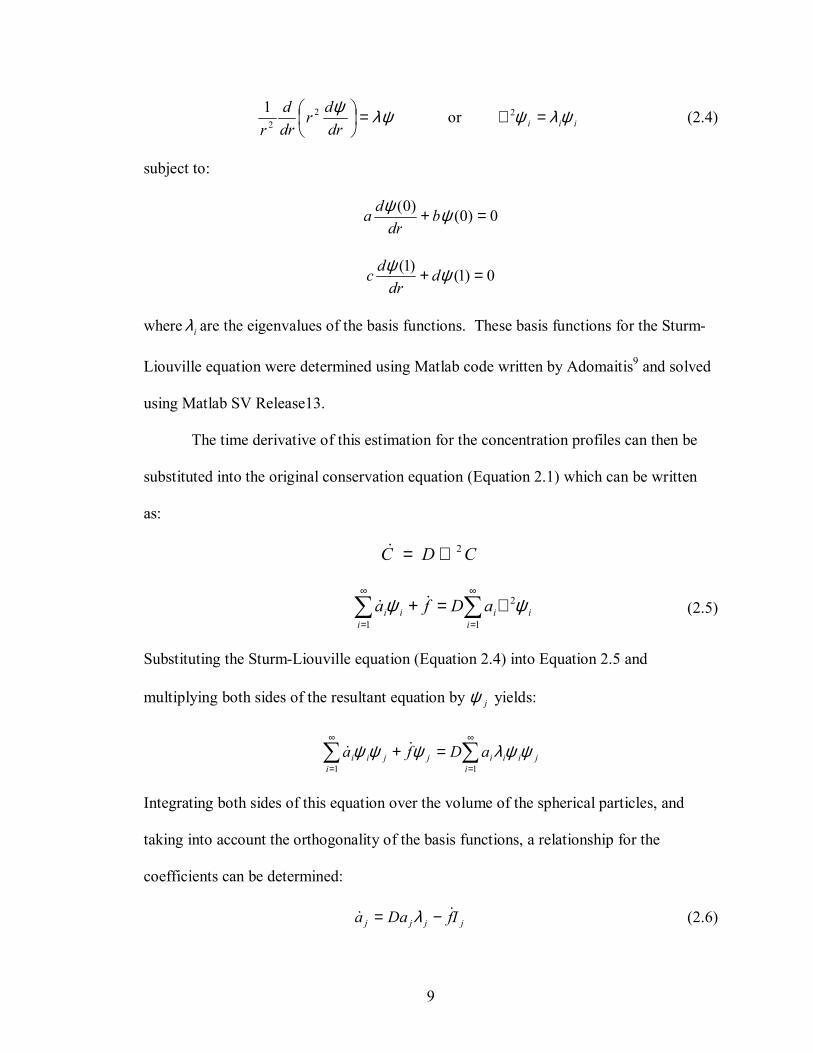
where iλ are the eigenvalues of the basis functions. These basis functions for the Sturm-

Liouville equation were determined using Matlab code written by Adomaitis9 and solved

using Matlab SV Release13.

The time derivative of this estimation for the concentration profiles can then be

substituted into the original conservation equation (Equation 2.1) which can be written

as:

CDC 2∇=&

∑∑∞

=

∞

=

∇=+1

2

1 iiii

ii aDfa ψψ && (2.5)

Substituting the Sturm-Liouville equation (Equation 2.4) into Equation 2.5 and

multiplying both sides of the resultant equation by jψ yields:

jiii

iji

jii aDfa ψψλψψψ ∑∑∞

=

∞

==+

11

&&

Integrating both sides of this equation over the volume of the spherical particles, and

taking into account the orthogonality of the basis functions, a relationship for the

coefficients can be determined:

jjjj IfDaa && −= λ (2.6)

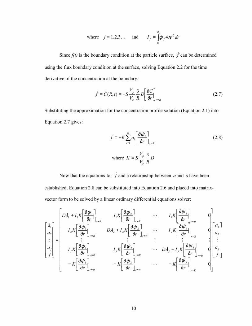
10

where j = 1,2,3� and ∫=R

jj drrI0

24πψ

Since f(t) is the boundary condition at the particle surface, f& can be determined

using the flux boundary condition at the surface, solving Equation 2.2 for the time

derivative of the concentration at the boundary:

Rre

p

rCD

RVV

StRCf=

∂∂−== 3),(&& (2.7)

Substituting the approximation for the concentration profile solution (Equation 2.1) into

Equation 2.7 gives:

Rr

i

ii r

aKf=

∞

=

∂∂

−= ∑ ψ1

& (2.8)

where DRV

VSK

e

p 3=

Now that the equations for f& and a relationship between a& and a have been

established, Equation 2.8 can be substituted into Equation 2.6 and placed into matrix-

vector form to be solved by a linear ordinary differential equations solver:

∂

∂−

∂∂−

∂∂−

∂

∂+

∂∂

∂∂

∂

∂

∂∂

+

∂∂

∂

∂

∂∂

∂∂+

=

===

===

===

===

fa

aa

rK

rK

rK

rKID

rKI

rKI

rKI

rKID

rKI

rKI

rKI

rKID

fa

aa

j

Rr

j

RrRr

Rr

jjj

Rrj

Rrj

Rr

j

RrRr

Rr

j

RrRr

j

M

L

L

MMMMM

L

L

&&

M

&

&

2

1

21

21

22

221

2

12

11

11

2

1

0

0

0

0

ψψψ

ψλψψ

ψψλψ

ψψψλ

11

This system of ordinary differential equations (ODE) was solved with Matlab using a

linear ODE solver written by Adomaitis.9 Once the coefficients ia( ) and concentration at

the boundary (f) are determined for each time step, this information is then substituted

back into the original equation for the estimation of the concentration profiles (Equation

2.3) used to model the process discussed in this thesis.

Once the concentration profiles are determined, they can be used to find the mass

uptake in the polymer particles. The number of moles of i in the polymer phase at a

given time can be found by integrating the corresponding concentration profile over the

volume of a particle, multiplied by the number of particles, Np:

∫=R

ipi drrtrCNtn0

2),(4)( π (2.9)

This calculation is used to determine the majority of the results in this work, including the

mass balance of each gas in the polymer and gas phases and the separation performance

of the dynamic pressure-swing process described in this chapter.

12

Chapter 3: Model Verification

Due to the dynamic nature of the sorption/desorption process modeled here, it was

important to verify the behavior of the mass transport model presented in the Chapter 2.

To affirm the accuracy of the model, the numerical solution was compared to two

different known solutions: an analytical solution and the solution to these partial

differential equations using the method of finite differences.

3.1 Comparison to Analytical Solution

The numerical solution was compared to the results of the analytical solution for

the time-dependent mass uptake of a spherical particle in a well-mixed solution of limited

volume found by Crank10 and given as:

∑∞

=∞ ++−+

−=1

22

2

99)exp()1(6

1)(n n

n

qq

ntn

ββτββ

(3.1)

where the qn�s are the nontrivial solutions to

233

tann

nn q

qqβ+

= (3.2)

τ is a dimensionless time variable defined as

2RDt=τ (3.3)

and β is the ratio of the external mass of penetrant to the polymer phase penetrant mass,

applying the partition coefficient S

13

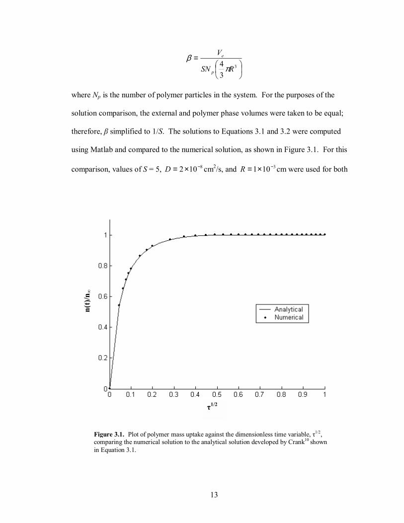
Figure 3.1. Plot of polymer mass uptake against the dimensionless time variable, τ1/2, comparing the numerical solution to the analytical solution developed by Crank10 shown in Equation 3.1.

n(t)

/n∞

τ1/2

=3

34 RSN

V

p

e

πβ

where Np is the number of polymer particles in the system. For the purposes of the

solution comparison, the external and polymer phase volumes were taken to be equal;

therefore, β simplified to 1/S. The solutions to Equations 3.1 and 3.2 were computed

using Matlab and compared to the numerical solution, as shown in Figure 3.1. For this

comparison, values of S = 5, 8102 −×=D cm2/s, and 3101 −×=R cm were used for both

14

the analytical and numerical solutions. To obtain the best estimate for the exact solution,

the first 5000 terms of the summation were used. 250 basis functions were used to

compute the eigenfunction expansion solution. Figure 3.1 verifies the accuracy of the

numerical solution when compared to the exact solution, where the largest root mean

squared error observed between the two solutions using 250 basis functions was

3100.4 −× (0.5% error) at τ1/2 = 0.1.

3.2 Comparison to Method of Finite Differences

To further verify the accuracy of the numerical solution, the eigenfunction

expansion solution was also compared to the solution obtained by Barbari et al.8 who

used the method of finite differences. To determine an optimal time and polymeric

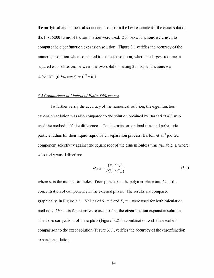
particle radius for their liquid-liquid batch separation process, Barbari et al.8 plotted

component selectivity against the square root of the dimensionless time variable, τ, where

selectivity was defined as:

)/()/(

/BeAe

BABA CC

nn=α (3.4)

where ni is the number of moles of component i in the polymer phase and Cie is the

concentration of component i in the external phase. The results are compared

graphically, in Figure 3.2. Values of SA = 5 and SB = 1 were used for both calculation

methods. 250 basis functions were used to find the eigenfunction expansion solution.

The close comparison of these plots (Figure 3.2), in combination with the excellent

comparison to the exact solution (Figure 3.1), verifies the accuracy of the eigenfunction

expansion solution.

15

3.3 Comparison to Equilibrium Calculations

The final test for accuracy compared the calculations from the model at

equilibrium conditions to known values of concentration or mass uptake at equilibrium.

To best understand these comparisons, it is important to introduce the ideal selectivity

between components A and B (α*A/B), which is defined as:

BB

AABA DS

DS=∗/α (3.4)

Figure 3.2. Plot of selectivity, αA/B, (Equation 3.4) vs. τ1/2 (Equation 3.3) using eigenfunction expansion and finite differences. The solid lines are the results from the eigenfunction expansion solution, and the points are the results found by Barbari et al.8 using the method of finite differences.

DA/DB = 10

DA/DB = 2

DA/DB = 1

α A/B

τ1/2

16

where Si is the solubility (or partition) coefficient and Di is the diffusivity of component i.

For a membrane, α*A/B is equal to the membrane permeability ratio, PA/PB, where the

permeability for component i is:

iii DSP = (3.5)

For this dynamic process, α*A/B physically represents the ratio of initial fluxes at the

interface r = R.

When looking at selectivity, for short time scales both the difference in diffusion

coefficients (DA/DB) and difference in solubilities (SA/SB) play a significant role. For long

time scales, the diffusion coefficients no longer dominate, and selectivity approaches an

equilibrium value of SA/SB. This behavior was observed by Barbari et al.,8 and is also

seen in these model results, shown in Figure 3.2. In Figure 3.2, the selectivity approaches

the solubility ratio SA/SB = 5 for all diffusivity ratios at long time scales.

To calculate the exact mass uptake in the polymer particles at infinite time, a

basic algebraic relation was developed for a finite volume, where the initial mass of

component i is equal to the sum of the masses in the polymer and external phases at

equilibrium:

pipeieeie VCVCVC +=o (3.6)

where oieC represents the initial concentration in the external phase, and Cip represents the

concentration in the polymer phase. The solubility coefficient is defined as the ratio of

polymer phase to external phase concentration:

ie

ipi C

CS ≡ (3.7)

17

Substituting this relation into equation (3.6) gives the concentration in the polymer phase

at equilibrium, and can be defined in terms of Cieº:

pie

eieiip VSV

VCSC+

=o

(3.8)

Since the equilibrium mass uptake of component i can be determined by:

3

34 RNCn pipi π=∞ (3.9)

where Np is the number of spherical polymer particles, the mass uptake of a component

at equilibrium can then be found by:

3

34 RN

VSVVCS

n ppie

eieii π

+=∞

o

(3.10)

Equation 3.10 was used to determine the exact value of the equilibrium mass

uptake for each component for the sorption step of the process. To simulate equilibrium

conditions, the model time scale was chosen to be 104 seconds. For runs using two sets

of parameters for each of the two gases, the infinite mass uptake values matched those of

the exact solution for the sorption step to four decimal places.

The desorption step solution was verified by assuming an infinite reservoir (open

volume, simulated as 33010/ cmVV pe = ) with an external pressure of 0 atm. The time

scale used to simulate equilibrium conditions was 104 seconds. The expected behavior at

infinite time for an infinite external phase would result in the evacuation of all mass in

the polymer particles. For two different sets of parameters for each of the two gases, the

final mass in the particles was on the order of 10-21 mol, verifying the accuracy of the

behavior of the desorption step.

18

Chapter 4: Model Results and Discussion

4.1 Determination of Optimal Separation Parameters

Once the accuracy of the model was verified, the next step was to determine

which parameters will provide the best indication for gas separation potential, specifically

for carbon dioxide/methane separation and oxygen/nitrogen separation. Since this

pressure-swing separation process deals with many of the same concepts as membrane

separation, similar parameters were taken into consideration.

When selecting a polymer for a membrane, the main criteria are membrane

stability, mechanical properties, cost, and most importantly, component selectivity

(Equation 3.4). For a membrane in steady-state operation with a constant flux, the best

inherent separation is obtained by maximizing α*A/B. Like membranes, component

solubility and diffusivity are also key factors for the pressure-swing sorption process

discussed in this work, but the optimal relationship is not as straightforward.

Since the goal is to maximize the separation of the two gases, it is important to

find a polymeric material that has different intermolecular and physical interactions (such

as size selectivity) with each of the gases. A high solubility and a high diffusion

coefficient in a given polymer result in higher mass uptake of a component at a given

period of time compared to one with low solubility and low diffusivity. The ideal

polymer for separation would sorb only one gas and leave the other in the external phase,

but this is not always possible for gases with small molecular volumes such as CO2, CH4,

N2 and O2.

19

Since this pressure-swing process does not utilize a steady-state flux as does a

membrane process, ideal selectivity is not the sole factor to consider when maximizing

separation. In Equation 3.4, selectivity can also be represented as a ratio of mole

fractions for each phase (or for a membrane, permeate and retentate), which does not take

into account the relative amounts of mass in those phases. For example, in the model

presented here, a very small amount of total mass in the polymer could have a high mass

ratio (nA/nB) due to component A having a very high diffusivity and solubility, but a large

amount of mass could still remain in the external phase with a mass ratio near unity. This

combination would still result in a high selectivity based on the mass fractions, but would

not result in good separation for this process because the amount of mass in the polymer

phase relative to the mass in the external phase is ignored. Therefore, the better indicator

to determine the optimal length of the sorption cycle is the external phase concentration

ratio (CB/CA). Maximizing this ratio provides the highest extent of separation in the first

outlet stream, where, during the sorption step, the external phase is purged at the time of

maximum separation.

The optimal length of the desorption step is much more difficult to determine due

to the fact that the separation bed is open to vacuum and effectively, an infinite external

phase volume. The main reason for applying vacuum is to minimize mass build-up in the

polymer particles prior to subsequent sorption steps. In determining a desorption time, it

is important to consider both mass build-up as well as total cycle time. A long desorption

step will allow more mass to leave the particle, but could result in an inefficient

separation process overall due to an excessively long cycle time, resulting in low product

output. Therefore, desorption step times were chosen based on the attainment of a

20

constant mass retention after successive cycles and the minimization of the number of

cycles before this �steady-state� was reached.

While it is desirable to have one component with high solubility and diffusion

coefficients as well as a high solubility ratio, this separation process is not optimized

when the ratio of diffusion coefficients is large. This behavior is more pronounced when

the sorption and desorption times are equal. The reason for this is that a large difference

in diffusion coefficients lends itself to excessive mass buildup of the more slowly

diffusing species. After successive sorption and desorption cycles, this accumulation is

amplified. Simulation runs with a moderate difference in the diffusivities of the two

species will still result in separation, but will not cause mass buildup of the slower

species.

The magnitudes of the ideal selectivity and diffusion coefficients also play a role

in polymer selection. Solubility and diffusivity ratios were held constant for comparative

runs, but their magnitudes were altered to determine their individual contributions to

separation by this process. For all parameter combinations, particle radius was held

constant and the desorption time was twice that of the sorption time to inhibit mass build

up in the polymer phase. The sorption time scale was determined by maximizing the

external phase concentration ratio for each set of polymer parameters.

The first comparison considered the magnitude of the diffusivities while the

diffusivity ratio remained the same (DA/DB = 2). To isolate diffusion effects, the

solubilities of both components were set equal to 1. The results showed nearly

equivalent separation for both the sorption and desorption steps of the separation process,

even after the magnitudes of the diffusion coefficients were increased by a factor of 5.

21

Based on these calculations, it appears that the magnitudes of the diffusion coefficients

themselves do not play a major role in separation for this process. However, the absolute

value of the diffusivity does determine the optimal sorption/desorption time scale and the

polymer particle radius, both of which are important practical factors to be considered for

the application of this process.

The second comparison was to determine the effect of the magnitudes of the

solubility coefficients, while keeping the solubility ratio constant (SA/SB = 5). For these

tests, the diffusion coefficients were set equal to one another, and the sorption time scale

was determined by maximizing the external concentration ratio. The results of this

comparison showed the process has a strong dependence on the magnitude of the

solubility coefficients. For a 50/50 mixture, increasing the magnitude of the solubilities

by a factor of 5 increased separation in the sorption step by 12%, but reduced the

separation in the desorption step by 12%. Lower solubilities lead to greater separation in

the polymer particle, and therefore greater separation in the desorption step when most of

the gas is removed from the polymer phase. The low solubilities also resulted in a 468s

(7.8 min) increase in the overall cycle time when the particle radius was held constant.

Lastly, a comparison of the magnitudes of the product of Si and Di were made to

determine its effect on the separation ability of the process. For the purposes of this test,

(SADA)/(SBDB) = 10. When the product, SADA, was increased by a factor of 25 (increase

in diffusivity by a factor of 5 and solubility by a factor of 5), the separation at the end of

the sorption step was increased by 14% and the separation at the end of the desorption

step was reduced by 10%. Although an increase in the diffusion coefficient alone shows

little relative change in separation, the magnitude of the diffusion coefficient appears to

22

play a minor role in separation for this process when coupled with solubility. The 25-fold

increase in magnitude of the SADA product also shortened the sorption time scale by a

factor of 10.7.

Based on these results, the magnitudes of SA and SADA have the greatest effect on

achieving the best separation for this pressure-swing sorption process. High SADA and SA

result in greater separation in the sorption step, while low SADA and SA result in greater

separation in the desorption step. Depending on the specific application, good separation

can be achieved with low or high values of solubility and the product of solubility and

diffusivity. The relative sizes of these values will affect whether or not better separation

is attained in the stream rich in the more soluble and faster-diffusing component

(desorption step) or in the stream rich in the slower-diffusing, less soluble species

(sorption step). The magnitudes of these values will also have a large effect on

determining polymer particle radius and sorption/desorption time scale length.

4.2 Polymer Selection

As previously mentioned, important factors to consider when choosing a polymer

for a separation process are the solubility, solubility ratio, diffusivity, and diffusivity

ratio. There is a considerable amount of literature on the separation of CO2/CH4 and

O2/N2 using many different polymers as membrane materials, with polyimides providing

excellent separation properties for both sets of gases discussed here.

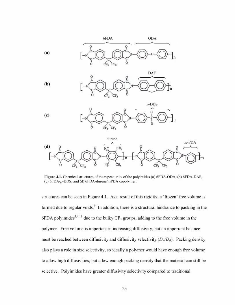
Polyimides show excellent mechanical strength as well temperature and chemical

resistance.3 Aromatic polyimides, such as 6FDA-ODA, 6FDA-DAF, 6FDA-p-DDS, and

copolyimide 6FDA-durene/mPDA (80/20) have rigid backbones, and their overall

23

structures can be seen in Figure 4.1. As a result of this rigidity, a �frozen� free volume is

formed due to regular voids.3 In addition, there is a structural hindrance to packing in the

6FDA polyimides3,4,11 due to the bulky CF3 groups, adding to the free volume in the

polymer. Free volume is important in increasing diffusivity, but an important balance

must be reached between diffusivity and diffusivity selectivity (DA/DB). Packing density

also plays a role in size selectivity, so ideally a polymer would have enough free volume

to allow high diffusivities, but a low enough packing density that the material can still be

selective. Polyimides have greater diffusivity selectivity compared to traditional

(a)

(b)

(c)

[ [ ]m]n

[

[

[ ]n

]n

]n

(d)

Figure 4.1. Chemical structures of the repeat units of the polyimides (a) 6FDA-ODA, (b) 6FDA-DAF, (c) 6FDA-p-DDS, and (d) 6FDA-durene/mPDA copolymer.

6FDA ODA

DAF

p-DDS

durenem-PDA

24

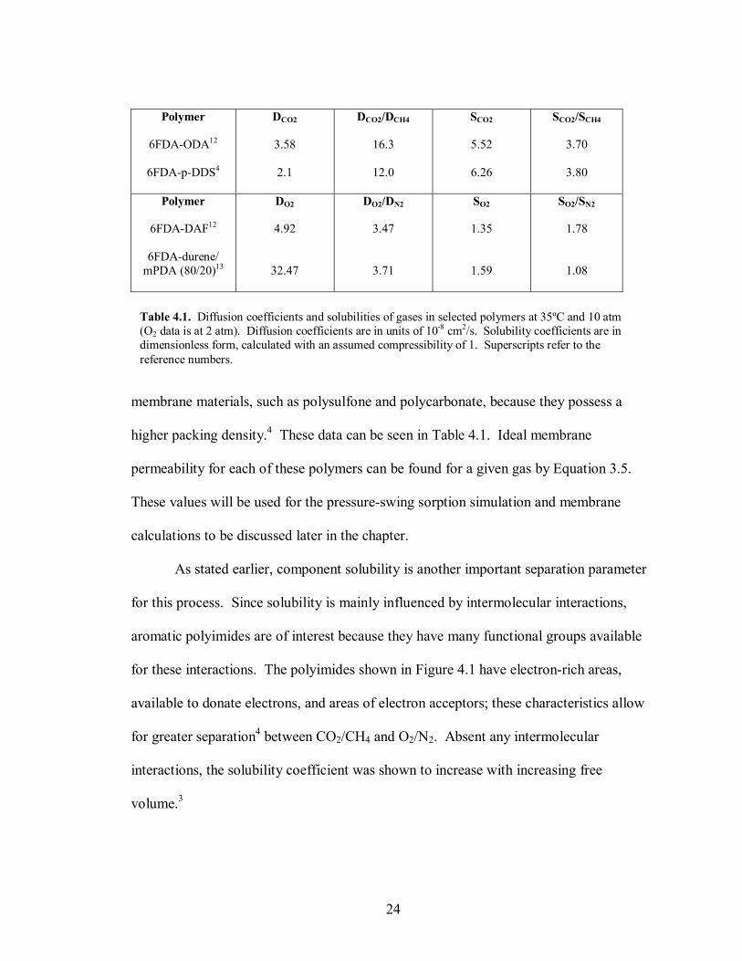
membrane materials, such as polysulfone and polycarbonate, because they possess a

higher packing density.4 These data can be seen in Table 4.1. Ideal membrane

permeability for each of these polymers can be found for a given gas by Equation 3.5.

These values will be used for the pressure-swing sorption simulation and membrane

calculations to be discussed later in the chapter.

As stated earlier, component solubility is another important separation parameter

for this process. Since solubility is mainly influenced by intermolecular interactions,

aromatic polyimides are of interest because they have many functional groups available

for these interactions. The polyimides shown in Figure 4.1 have electron-rich areas,

available to donate electrons, and areas of electron acceptors; these characteristics allow

for greater separation4 between CO2/CH4 and O2/N2. Absent any intermolecular

interactions, the solubility coefficient was shown to increase with increasing free

volume.3

Polymer

6FDA-ODA12

6FDA-p-DDS4

DCO2

3.58

2.1

DCO2/DCH4

16.3

12.0

SCO2

5.52

6.26

SCO2/SCH4

3.70

3.80

Polymer

6FDA-DAF12

6FDA-durene/ mPDA (80/20)13

DO2

4.92

32.47

DO2/DN2

3.47

3.71

SO2

1.35

1.59

SO2/SN2

1.78

1.08

Table 4.1. Diffusion coefficients and solubilities of gases in selected polymers at 35ºC and 10 atm (O2 data is at 2 atm). Diffusion coefficients are in units of 10-8 cm2/s. Solubility coefficients are in dimensionless form, calculated with an assumed compressibility of 1. Superscripts refer to the reference numbers.

25

Due to the fact that CO2 and CH4 have very small differences in kinetic diameter14

(3.3Å and 3.8Å, respectively) the difference in solubility between the two components is

mainly due to the interactions with the polymer. Since CO2 is a quadrupole, it has strong

quadrupole-dipole interactions with the polar carbonyl and CF3 groups in the 6FDA

polyimides. In comparison, CH4 is a non-polar molecule, and engages in weaker van der

Waals interactions with the non-polar groups in the polymer, resulting in a lower relative

solubility.

Although helpful in enhancing differences in solubility, these molecular

interactions between polyimides and CO2 can potentially have negative effects on the

process, such as polymer swelling. This swelling has been shown by Wind et al.15 to

affect the long-term diffusivity and selectivity of similar polyimides. The plasticizer

effect of CO2 has been shown to cause an increase in CO2 diffusivity over time.15 It is

not the purpose of this work to model this time-dependent effect, but it is an important

factor to consider in future applications for CO2 separation.

Due to their similar respective kinetic diameters14 of 3.46 and 3.64, O2 and N2

have typically been very difficult to separate using polymers. A small difference in

critical temperature and condensability between the two molecules results in differing

solubilities in polyimides;3, 13 this difference shows the potential for the use of polyimides

as air separation membranes.

Based on the separation parameters discussed earlier, it is important to weigh

optimal separation with practical factors such as particle radius, process time scale, and

time to reach �steady-state.� High diffusivities will result in better separation in the

sorption step and will lead to a shorter time scale length; therefore, the magnitudes of

26

these coefficients are important. Also as important is the ratio of diffusivities. A high

diffusion coefficient ratio results in greater separation, but if the ratio is too high, the

desorption time scale must be significantly lengthened to inhibit excessive mass retention

of the more slowly diffusing species in the polymer particles. As a result, a high

diffusivity ratio will also result in a longer time to reach �steady-state� for the entire

sorption/desorption process, as it will take more cycles for the mass retention to reach a

pseudo-equilibrium. The optimal separation parameters are high diffusivities, a moderate

diffusivity ratio, high solubilities, and a high solubility ratio.

4.3 Specifications for Carbon Dioxide/Methane Separation

As discussed previously, CO2 and CH4 have different molecular characteristics

which allow for their separation. Two examples of polyimides that best capitalize on

these differences are 6FDA-ODA and 6FDA-p-DDS, whose structures can be seen in

Figure 4.1. The ODA has a higher diffusion coefficient ratio, a lower solubility

coefficient ratio, higher diffusivities, and lower solubilities relative to p-DDS (Table 4.1).

4.3.1 Comparison to Polymer Characteristics for CO2/CH4 Separation

Polymer comparisons were conducted on the basis of several process factors,

including sorption separation, desorption separation, and overall cycle time based on the

attainment of an equilibrium mass retention inside the polymer particles. Many of the

separation processes for CO2/CH4 mentioned in Chapter 1 utilize feed compositions near

a 50/50 mixture;3 therefore, the model calculations completed here use the same molar

27

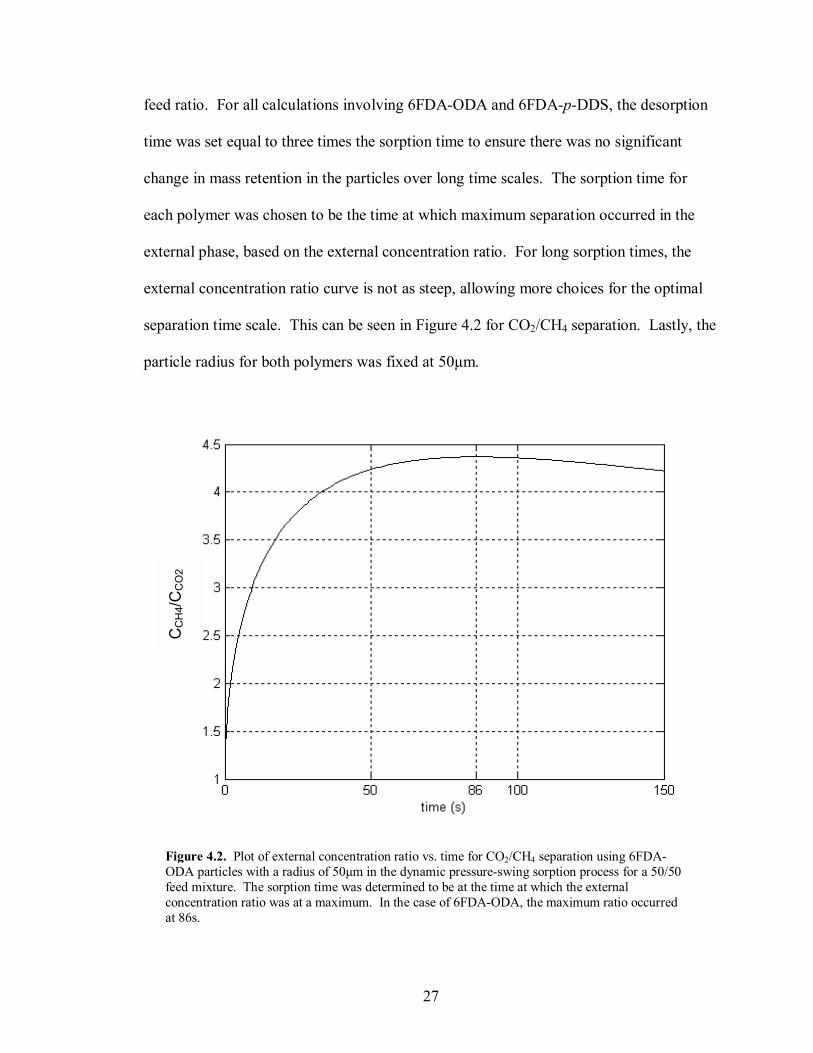
feed ratio. For all calculations involving 6FDA-ODA and 6FDA-p-DDS, the desorption

time was set equal to three times the sorption time to ensure there was no significant

change in mass retention in the particles over long time scales. The sorption time for

each polymer was chosen to be the time at which maximum separation occurred in the

external phase, based on the external concentration ratio. For long sorption times, the

external concentration ratio curve is not as steep, allowing more choices for the optimal

separation time scale. This can be seen in Figure 4.2 for CO2/CH4 separation. Lastly, the

particle radius for both polymers was fixed at 50µm.

Figure 4.2. Plot of external concentration ratio vs. time for CO2/CH4 separation using 6FDA-ODA particles with a radius of 50µm in the dynamic pressure-swing sorption process for a 50/50 feed mixture. The sorption time was determined to be at the time at which the external concentration ratio was at a maximum. In the case of 6FDA-ODA, the maximum ratio occurred at 86s.

CC

H4/C

CO

2

28

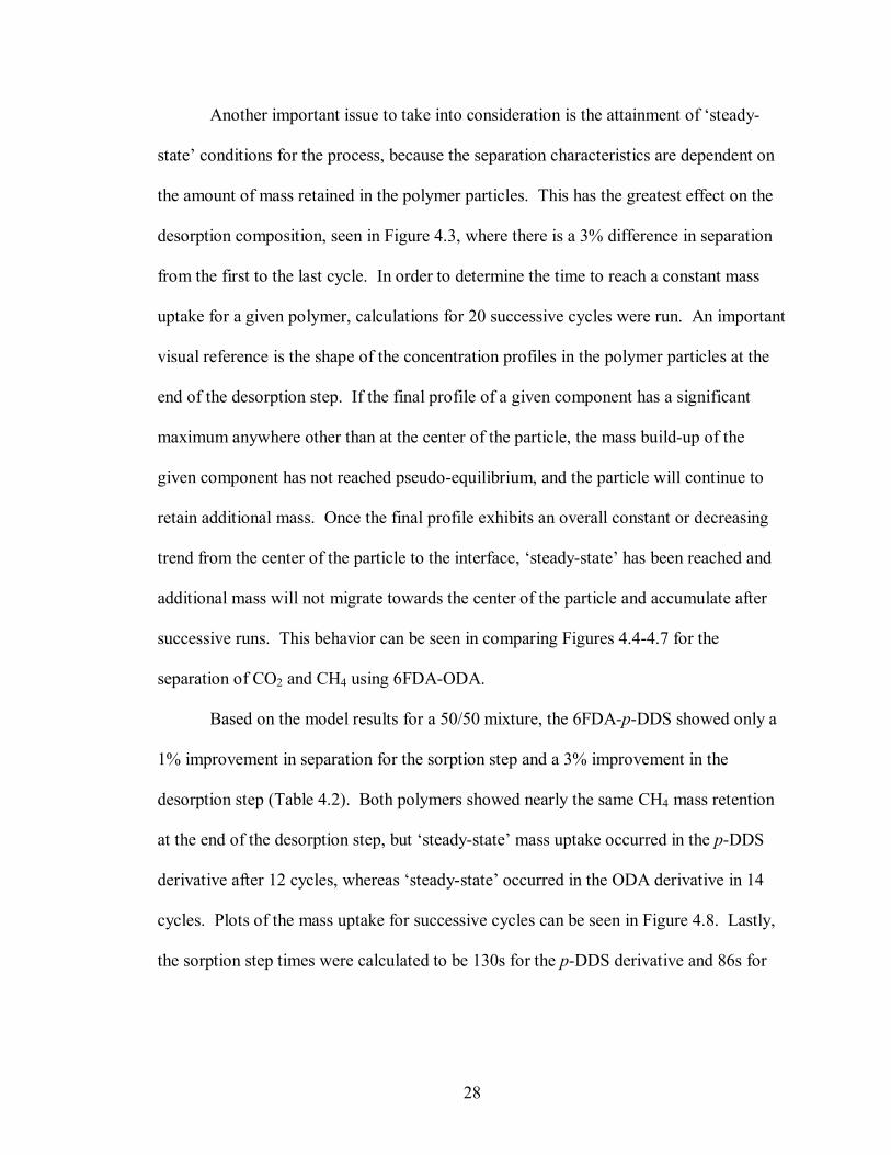
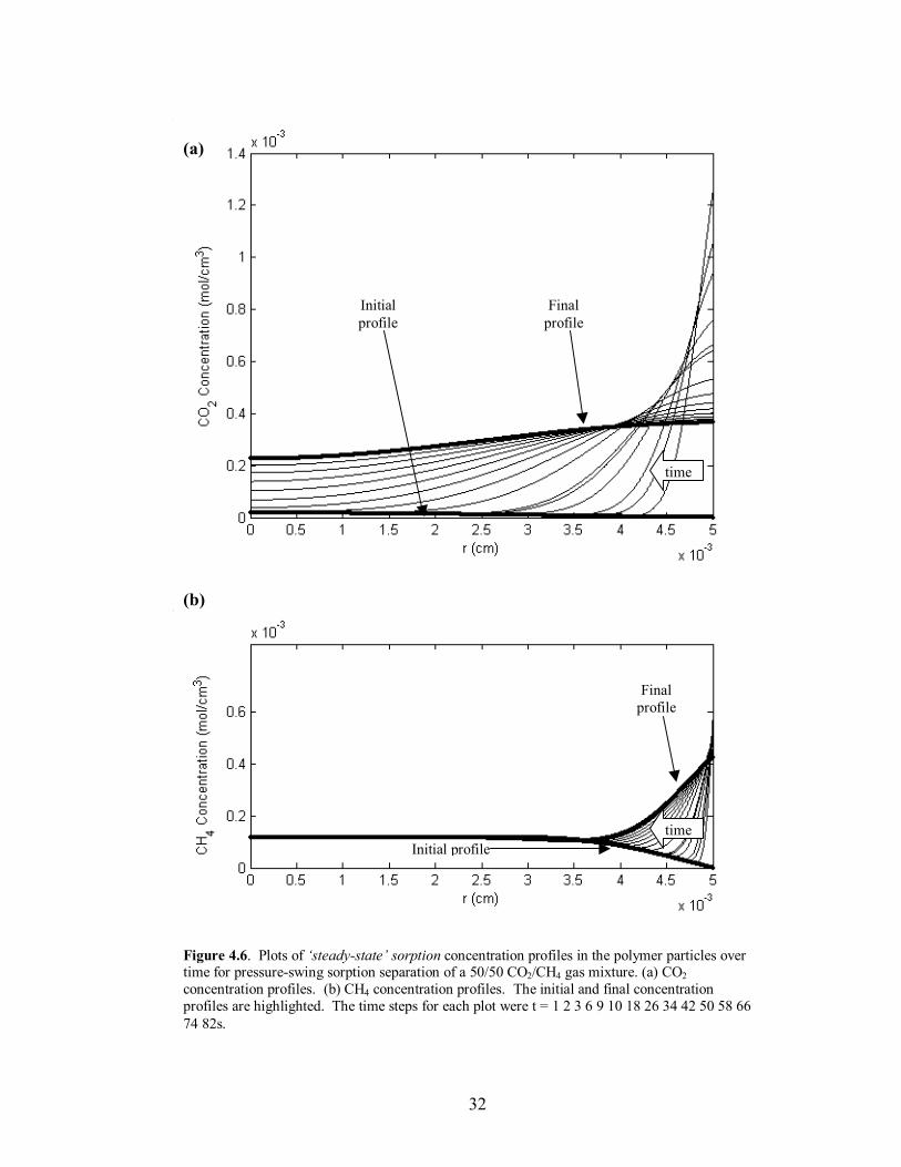
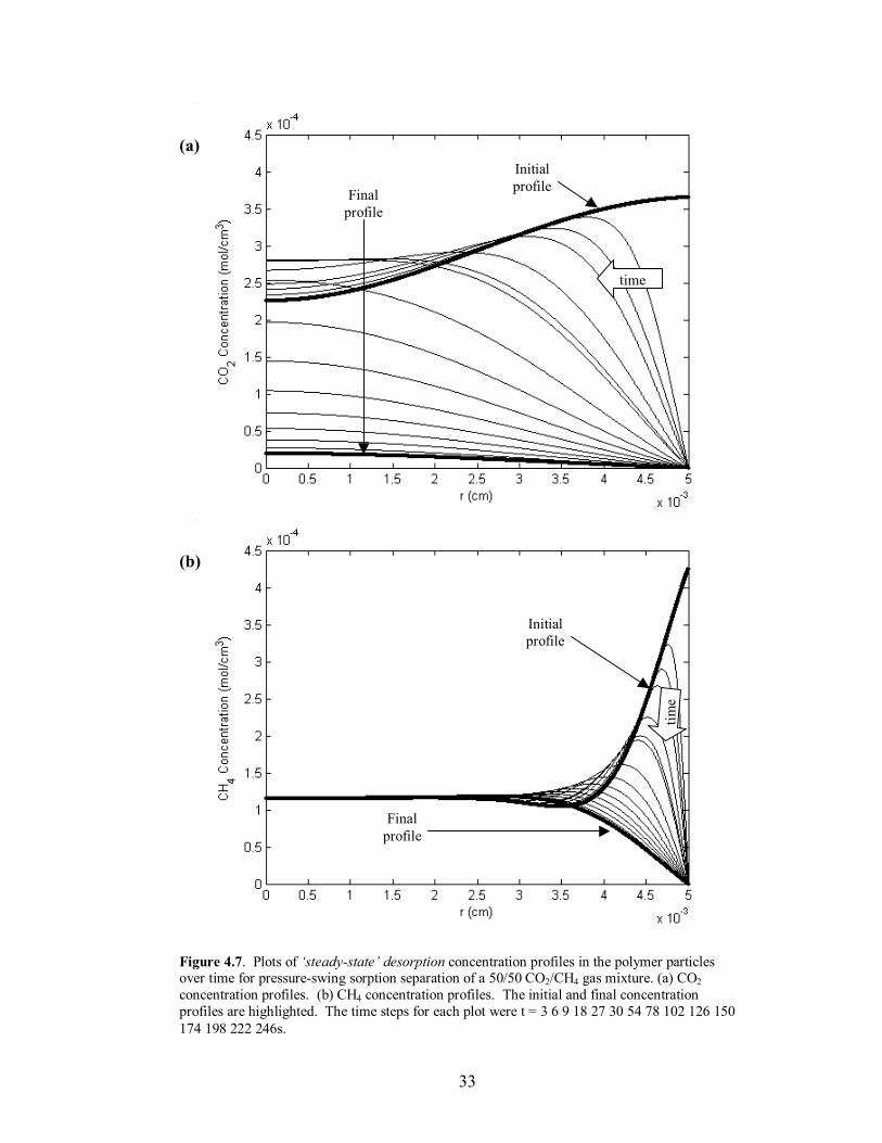
Another important issue to take into consideration is the attainment of �steady-

state� conditions for the process, because the separation characteristics are dependent on

the amount of mass retained in the polymer particles. This has the greatest effect on the

desorption composition, seen in Figure 4.3, where there is a 3% difference in separation

from the first to the last cycle. In order to determine the time to reach a constant mass

uptake for a given polymer, calculations for 20 successive cycles were run. An important

visual reference is the shape of the concentration profiles in the polymer particles at the

end of the desorption step. If the final profile of a given component has a significant

maximum anywhere other than at the center of the particle, the mass build-up of the

given component has not reached pseudo-equilibrium, and the particle will continue to

retain additional mass. Once the final profile exhibits an overall constant or decreasing

trend from the center of the particle to the interface, �steady-state� has been reached and

additional mass will not migrate towards the center of the particle and accumulate after

successive runs. This behavior can be seen in comparing Figures 4.4-4.7 for the

separation of CO2 and CH4 using 6FDA-ODA.

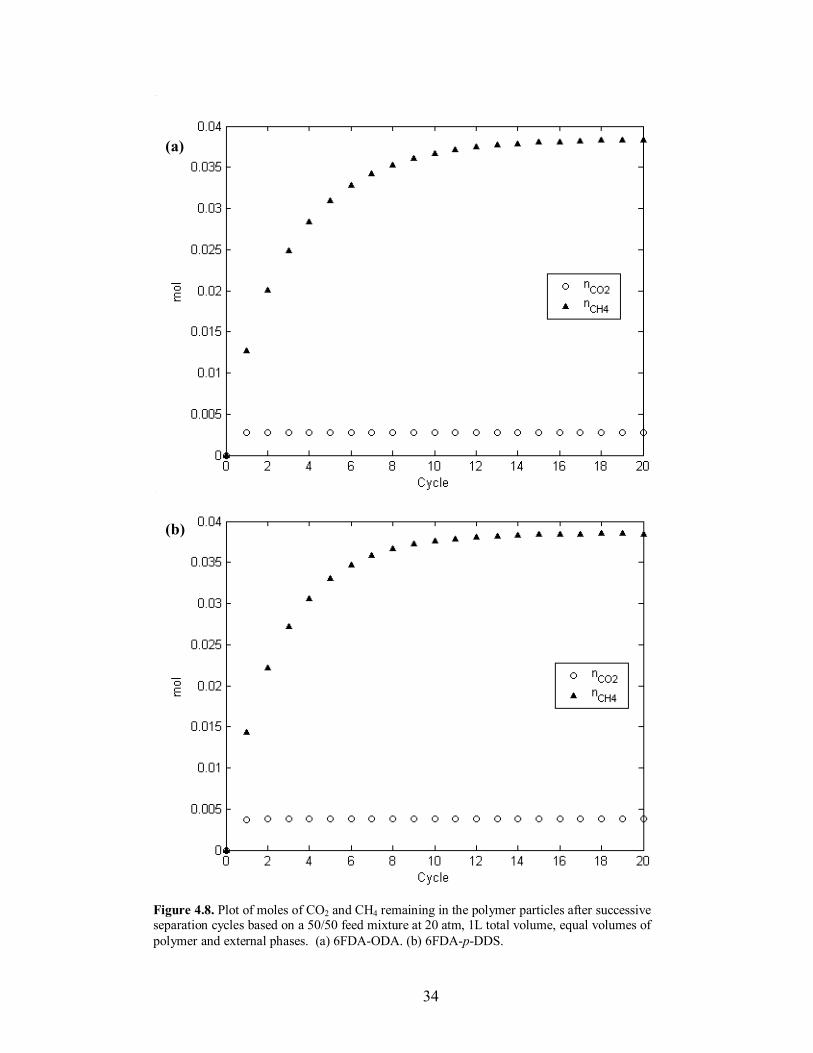
Based on the model results for a 50/50 mixture, the 6FDA-p-DDS showed only a

1% improvement in separation for the sorption step and a 3% improvement in the

desorption step (Table 4.2). Both polymers showed nearly the same CH4 mass retention

at the end of the desorption step, but �steady-state� mass uptake occurred in the p-DDS

derivative after 12 cycles, whereas �steady-state� occurred in the ODA derivative in 14

cycles. Plots of the mass uptake for successive cycles can be seen in Figure 4.8. Lastly,

the sorption step times were calculated to be 130s for the p-DDS derivative and 86s for

29

Figure 4.3. Plots of mole fraction at the end of the (a) sorption and (b) desorption steps for successive cycles using 6FDA-ODA for separation of a 50/50 mixture of CO2/CH4 using the dynamic pressure-swing sorption process.

(a)

(b)

0.81

0.19

0.78 0.75

0.22 0.25

30

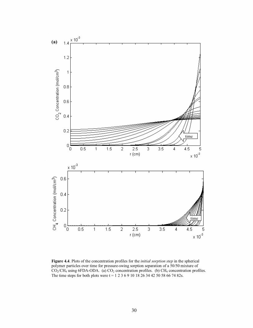
Figure 4.4. Plots of the concentration profiles for the initial sorption step in the spherical polymer particles over time for pressure-swing sorption separation of a 50/50 mixture of CO2/CH4 using 6FDA-ODA. (a) CO2 concentration profiles. (b) CH4 concentration profiles. The time steps for both plots were t = 1 2 3 6 9 10 18 26 34 42 50 58 66 74 82s.

(b)

(a)

time

time

31

Figure 4.5. Plots of concentration profiles for the initial desorption step in the polymer particles over time for pressure-swing sorption separation of a 50/50 CO2/CH4 gas mixture. (a) CO2 concentration profiles. (b) CH4 concentration profiles. The initial and final concentration profiles are highlighted. The time steps for each plot were t = 3 6 9 18 27 30 54 78 102 126 150 174 198 222 246s.

(a)

(b)

Initial profile Final

profile

time

Initial profile

Finalprofile

time

32

Figure 4.6. Plots of �steady-state� sorption concentration profiles in the polymer particles over time for pressure-swing sorption separation of a 50/50 CO2/CH4 gas mixture. (a) CO2 concentration profiles. (b) CH4 concentration profiles. The initial and final concentration profiles are highlighted. The time steps for each plot were t = 1 2 3 6 9 10 18 26 34 42 50 58 66 74 82s.

(a)

(b)

time

time

Finalprofile

Final profile

Initialprofile

Initial profile

33

Figure 4.7. Plots of �steady-state� desorption concentration profiles in the polymer particles over time for pressure-swing sorption separation of a 50/50 CO2/CH4 gas mixture. (a) CO2 concentration profiles. (b) CH4 concentration profiles. The initial and final concentration profiles are highlighted. The time steps for each plot were t = 3 6 9 18 27 30 54 78 102 126 150 174 198 222 246s.

(a)

(b)

Initialprofile Final

profile

Finalprofile

Initialprofile

time

time

34

Figure 4.8. Plot of moles of CO2 and CH4 remaining in the polymer particles after successive separation cycles based on a 50/50 feed mixture at 20 atm, 1L total volume, equal volumes of polymer and external phases. (a) 6FDA-ODA. (b) 6FDA-p-DDS.

(a)

(b)

35

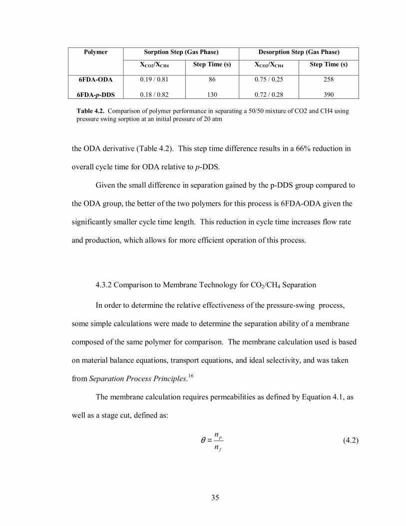
Sorption Step (Gas Phase) Desorption Step (Gas Phase) Polymer

XCO2/XCH4 Step Time (s) XCO2/XCH4 Step Time (s)

6FDA-ODA

6FDA-p-DDS

0.19 / 0.81

0.18 / 0.82

86

130

0.75 / 0.25

0.72 / 0.28

258

390

the ODA derivative (Table 4.2). This step time difference results in a 66% reduction in

overall cycle time for ODA relative to p-DDS.

Given the small difference in separation gained by the p-DDS group compared to

the ODA group, the better of the two polymers for this process is 6FDA-ODA given the

significantly smaller cycle time length. This reduction in cycle time increases flow rate

and production, which allows for more efficient operation of this process.

4.3.2 Comparison to Membrane Technology for CO2/CH4 Separation

In order to determine the relative effectiveness of the pressure-swing process,

some simple calculations were made to determine the separation ability of a membrane

composed of the same polymer for comparison. The membrane calculation used is based

on material balance equations, transport equations, and ideal selectivity, and was taken

from Separation Process Principles.16

The membrane calculation requires permeabilities as defined by Equation 4.1, as

well as a stage cut, defined as:

f

p

nn

=θ (4.2)

Table 4.2. Comparison of polymer performance in separating a 50/50 mixture of CO2 and CH4 using pressure swing sorption at an initial pressure of 20 atm

36

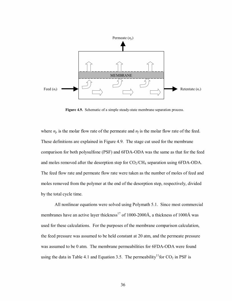
where np is the molar flow rate of the permeate and nf is the molar flow rate of the feed.

These definitions are explained in Figure 4.9. The stage cut used for the membrane

comparison for both polysulfone (PSF) and 6FDA-ODA was the same as that for the feed

and moles removed after the desorption step for CO2/CH4 separation using 6FDA-ODA.

The feed flow rate and permeate flow rate were taken as the number of moles of feed and

moles removed from the polymer at the end of the desorption step, respectively, divided

by the total cycle time.

All nonlinear equations were solved using Polymath 5.1. Since most commercial

membranes have an active layer thickness17 of 1000-2000Å, a thickness of 1000Å was

used for these calculations. For the purposes of the membrane comparison calculation,

the feed pressure was assumed to be held constant at 20 atm, and the permeate pressure

was assumed to be 0 atm. The membrane permeabilities for 6FDA-ODA were found

using the data in Table 4.1 and Equation 3.5. The permeability11for CO2 in PSF is

Figure 4.9. Schematic of a simple steady-state membrane separation process.

MEMBRANE

Feed (nf)

Permeate (np)

Retentate (nr)

37

8108.4 −× cm3 (STP) cm-1 atm-1 s-1 and the permeability ratio11 for CO2/CH4 separation is

21.9.

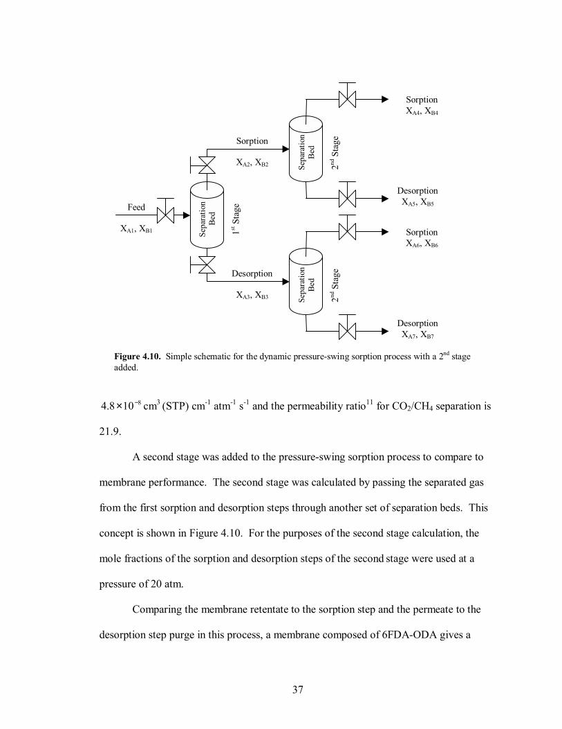
A second stage was added to the pressure-swing sorption process to compare to

membrane performance. The second stage was calculated by passing the separated gas

from the first sorption and desorption steps through another set of separation beds. This

concept is shown in Figure 4.10. For the purposes of the second stage calculation, the

mole fractions of the sorption and desorption steps of the second stage were used at a

pressure of 20 atm.

Comparing the membrane retentate to the sorption step and the permeate to the

desorption step purge in this process, a membrane composed of 6FDA-ODA gives a

Figure 4.10. Simple schematic for the dynamic pressure-swing sorption process with a 2nd stage added.

Sepa

ratio

n B

ed

Sepa

ratio

n B

ed

Sepa

ratio

n B

ed

Feed

XA1, XB1

Sorption

XA2, XB2

Desorption

XA3, XB3

SorptionXA4, XB4

Desorption XA5, XB5

Sorption XA6, XB6

Desorption XA7, XB7

1st S

tage

2nd S

tage

2nd

Sta

ge

38

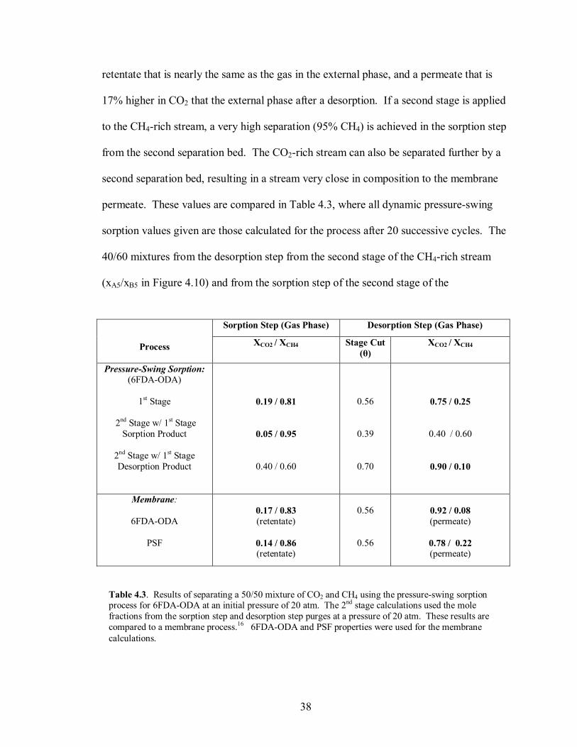
retentate that is nearly the same as the gas in the external phase, and a permeate that is

17% higher in CO2 that the external phase after a desorption. If a second stage is applied

to the CH4-rich stream, a very high separation (95% CH4) is achieved in the sorption step

from the second separation bed. The CO2-rich stream can also be separated further by a

second separation bed, resulting in a stream very close in composition to the membrane

permeate. These values are compared in Table 4.3, where all dynamic pressure-swing

sorption values given are those calculated for the process after 20 successive cycles. The

40/60 mixtures from the desorption step from the second stage of the CH4-rich stream

(xA5/xB5 in Figure 4.10) and from the sorption step of the second stage of the

Sorption Step (Gas Phase) Desorption Step (Gas Phase)

Process

XCO2 / XCH4 Stage Cut (θ)

XCO2 / XCH4

Pressure-Swing Sorption: (6FDA-ODA)

1st Stage

2nd Stage w/ 1st Stage

Sorption Product

2nd Stage w/ 1st Stage Desorption Product

0.19 / 0.81

0.05 / 0.95

0.40 / 0.60

0.56

0.39

0.70

0.75 / 0.25

0.40 / 0.60

0.90 / 0.10

Membrane:

6FDA-ODA

PSF

0.17 / 0.83 (retentate)

0.14 / 0.86 (retentate)

0.56

0.56

0.92 / 0.08 (permeate)

0.78 / 0.22 (permeate)

Table 4.3. Results of separating a 50/50 mixture of CO2 and CH4 using the pressure-swing sorption process for 6FDA-ODA at an initial pressure of 20 atm. The 2nd stage calculations used the mole fractions from the sorption step and desorption step purges at a pressure of 20 atm. These results are compared to a membrane process.16 6FDA-ODA and PSF properties were used for the membrane calculations.

39

CO2-rich stream (xA6/xB6 in Figure 4.10) suggest the potential to recycle these back to the

feed for greater process efficiency. With only one second stage applied to the CO2-rich

stream from the first stage, the pressure-swing sorption is comparable to a membrane

separation with the same polymer (Table 4.3).

Since PSF is used to make a commercial CO2/CH4 membrane,2 a calculation

using its properties was also completed to compare to the pressure-swing process. The

single-stage process compares very well in terms of separation performance and is within

5% of the retentate composition and within 3% of the permeate composition. A second

stage for the two gas streams extracted after the sorption and desorption steps shows

significant improvement over the PSF membrane, as shown in Table 4.3.

4.4 Specifications for Oxygen/Nitrogen Separation

Since O2 and N2 have very similar characteristics, they have historically been very

difficult to separate. However, polyimides have shown promise in providing greater

separation, as compared to typical membrane materials such as polycarbonate and

polysulfone.11 Two such types of polyimides are 6FDA-DAF and the copolyimide

(80/20) 6FDA-durene/mPDA (Figure 4.1). The attached durene and mPDA groups

provide a higher diffusion coefficient ratio, a lower solubility ratio (near unity), higher

diffusivities, and higher solubilities relative to the DAF group (Table 4.1).

4.4.1 Comparison to Polymer Characteristics for O2/N2 Separation

The same factors from the CO2/CH4 process were considered for the O2/N2

separation process: separation in the external phase during the sorption step, overall cycle

40

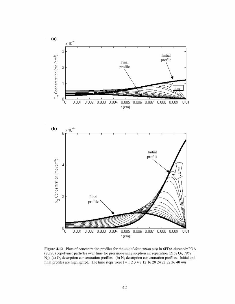
time, and the attainment of �steady-state� mass uptake of the slower diffusing species at

the end of desorption. The desorption time scale was set equal to twice the sorption time

scale due to the closeness in diffusivities of O2 and N2. The profile behavior and

verification of the �steady-state� operation for O2/N2 separation using the copolymer

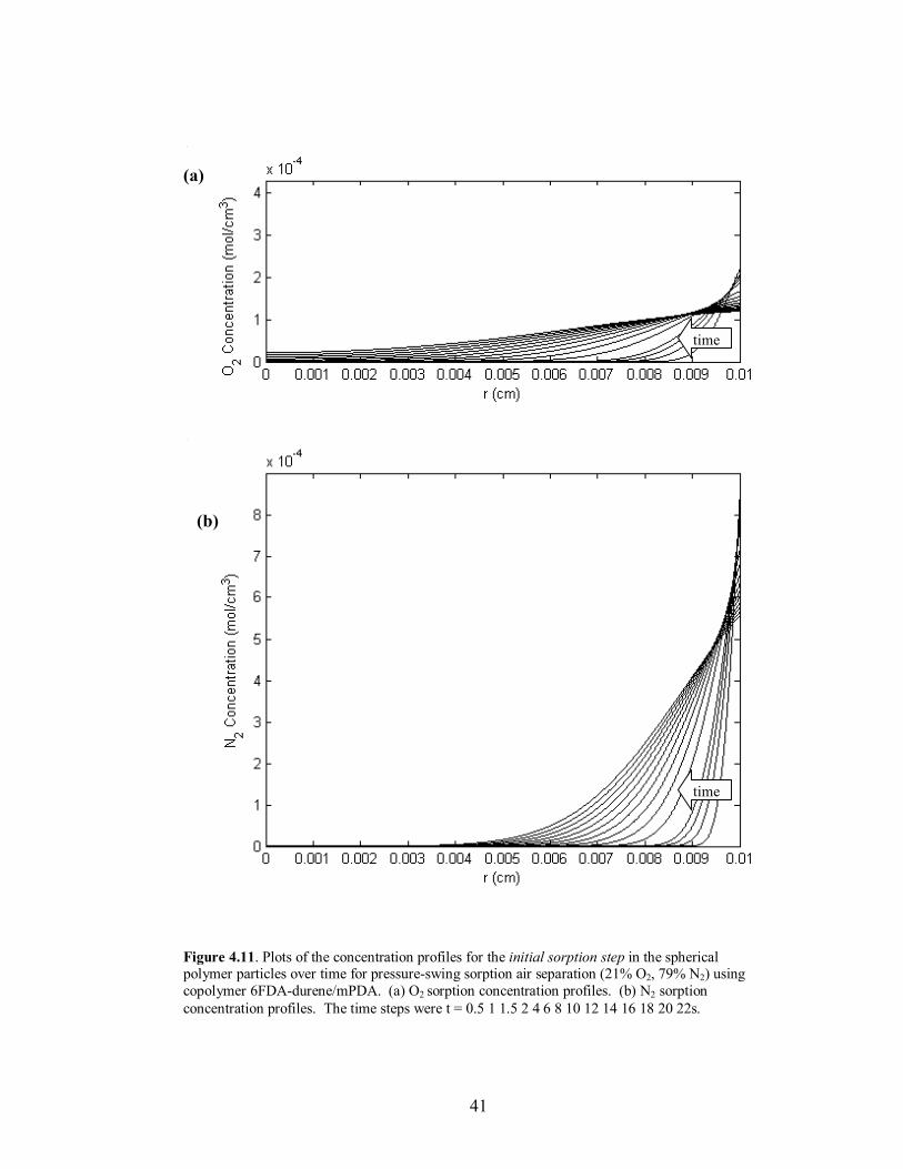
6FDA-durene/mPDA (80/20) can be seen in Figures 4.11-4.14. The sorption time for

each polymer was also set to the value where maximum separation occurred in the

external phase. Lastly, to adjust for the high diffusivities and to increase the time scale to

a reasonable length relative to the fill time, the particle radius was increased to 100µm for

the copolymer 6FDA-durene/mPDA; the particle radius remained 50µm for 6FDA-DAF.

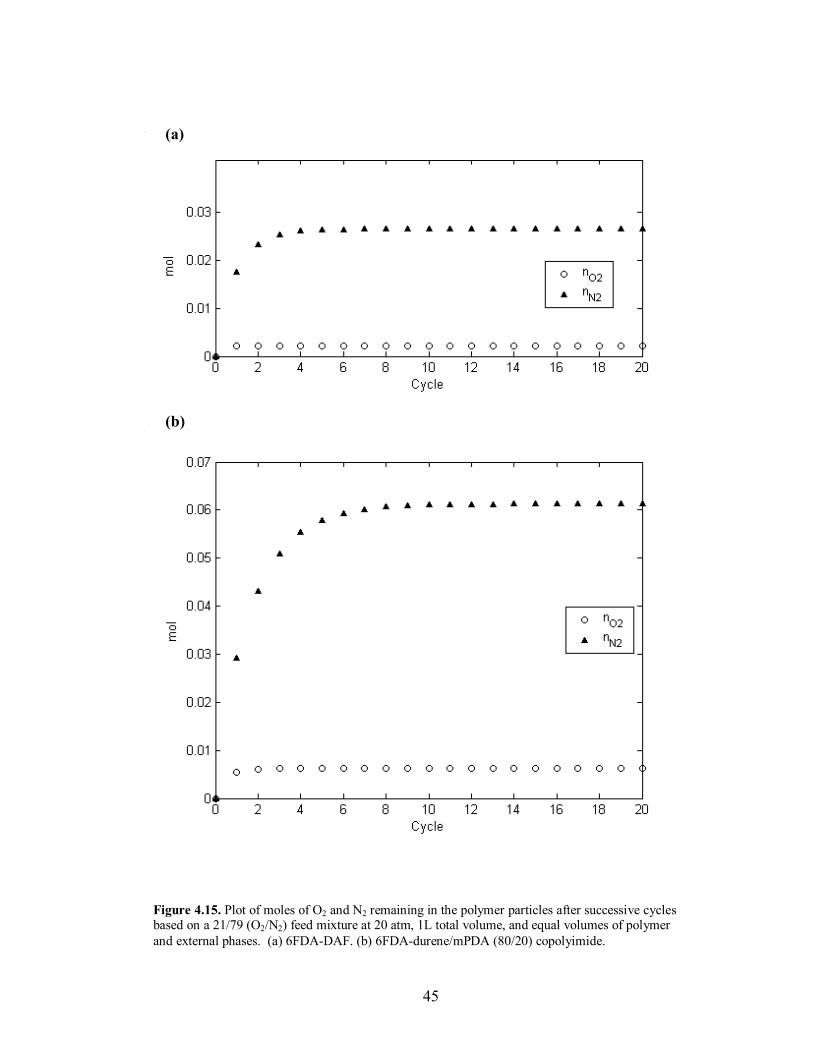
For air separation (21% O2 and 79% N2) the model results show only a 2% increase in

separation from the sorption step when using the DAF polyimide compared to the

copolymer. This is shown in Table 4.4, where the separation values given for the

pressure-swing process are those calculated after 20 successive cycles. The copolymer

has nearly three times the mass build-up in the particle compared to 6FDA-DAF, but this

mass retention is only 8% of the original N2 mass. Near �steady-state� operation

conditions for 6FDA-DAF are reached within 5 cycles, whereas the copolymer takes

approximately 8 cycles. This comparison can be seen in Figure 4.15. In terms of the

length of the entire cycle, the copolymer reaches steady operation after 9.7 min, while

6FDA-DAF reaches steady operation after 16 min. The copolymer�s diffusion and

selectivity characteristics also allow for a larger particle radius, and a shorter overall time

scale (66s vs. 192s), making 6FDA-durene/mPDA (80/20) the polymer of choice for this

process (Table 4.4).

41

Figure 4.11. Plots of the concentration profiles for the initial sorption step in the spherical polymer particles over time for pressure-swing sorption air separation (21% O2, 79% N2) using copolymer 6FDA-durene/mPDA. (a) O2 sorption concentration profiles. (b) N2 sorption concentration profiles. The time steps were t = 0.5 1 1.5 2 4 6 8 10 12 14 16 18 20 22s.

(b)

(a)

time

time

42

Figure 4.12. Plots of concentration profiles for the initial desorption step in 6FDA-durene/mPDA (80/20) copolymer particles over time for pressure-swing sorption air separation (21% O2, 79% N2). (a) O2 desorption concentration profiles. (b) N2 desorption concentration profiles. Initial and final profiles are highlighted. The time steps were t = 1 2 3 4 8 12 16 20 24 28 32 36 40 44s

(a)

(b)

time

Initial profile

Initial profile

Final profile

Final profile

time

43

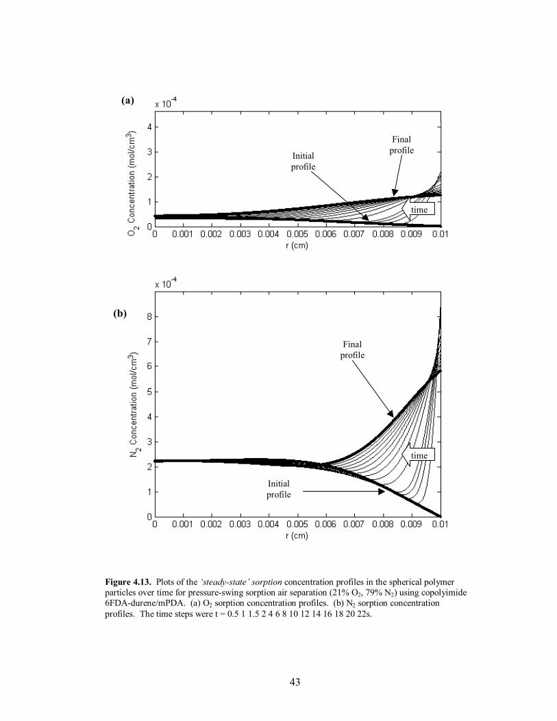
Figure 4.13. Plots of the �steady-state� sorption concentration profiles in the spherical polymer particles over time for pressure-swing sorption air separation (21% O2, 79% N2) using copolyimide 6FDA-durene/mPDA. (a) O2 sorption concentration profiles. (b) N2 sorption concentration profiles. The time steps were t = 0.5 1 1.5 2 4 6 8 10 12 14 16 18 20 22s.

(a)

(b)

time

Initial profile

Final profile

Initial profile

Finalprofile

time

44

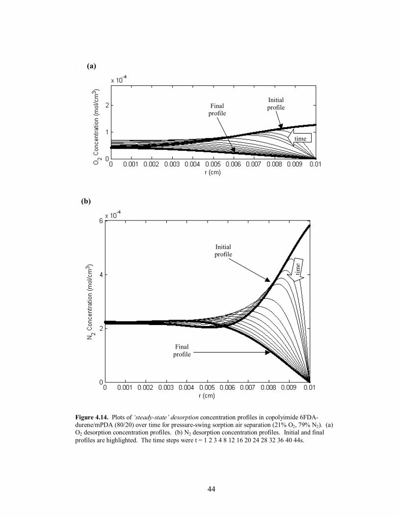
Figure 4.14. Plots of �steady-state� desorption concentration profiles in copolyimide 6FDA-durene/mPDA (80/20) over time for pressure-swing sorption air separation (21% O2, 79% N2). (a) O2 desorption concentration profiles. (b) N2 desorption concentration profiles. Initial and final profiles are highlighted. The time steps were t = 1 2 3 4 8 12 16 20 24 28 32 36 40 44s.

(a)

(b)

time

Initial profile

Initialprofile

Finalprofile

Finalprofile

time

45

Figure 4.15. Plot of moles of O2 and N2 remaining in the polymer particles after successive cycles based on a 21/79 (O2/N2) feed mixture at 20 atm, 1L total volume, and equal volumes of polymer and external phases. (a) 6FDA-DAF. (b) 6FDA-durene/mPDA (80/20) copolyimide.

(b)

(a)

46

4.4.2 Comparison to Membrane Technology for O2/N2 Separation

The same procedure in Section 4.3.2 was used to compare this process with a

membrane composed of the same polymer; the active layer of the membrane was

assumed to be 1000Å as before. The flow rates for feed and permeate were set using the

number of moles of feed and moles removed from the polymer at the end of the

desorption step, respectively, divided by the total cycle time.

Sorption Step (Gas Phase) Desorption Step (Gas Phase) Process

XO2 / XN2 Step Time (s)

Stage Cut (θ)

XO2 / XN2 Step Time (s)

Pressure-Swing Sorption:

6FDA-DAF (1st Stage)

6FDA-durene/ mPDA

(80/20) (1st Stage)

6FDA-durene/ mPDA (80/20)

(2nd Stage w/ 1st Stage Sorption Product)

6FDA-durene/ mPDA (80/20)

(2nd Stage w/ 1st Stage Desorption Product)

0.15 / 0.85

0.17 / 0.83

0.13 / 0.87

0.22 / 0.78

64

22

22

22

0.33

0.40

0.39

0.42

0.34 / 0.66

0.28 / 0.72

0.22 / 0.78

0.35 / 0.65

128

44

44

44

Membrane:

6FDA-durene/ mPDA

(80/20)

0.12 / 0.88 (retentate)

--

0.40

0.35 / 0.65 (permeate)

--

Table 4.4. Results for air separation (O2 = 21%, N2 = 79%) using the pressure-swing sorption process. 2nd

stage calculations for 6FDA-durene/mPDA used the mole fractions from the sorption step and desorption purges from the 1st stage as a feed ratio and a pressure of 20 atm. These results can be compared to a membrane calculation;16 results are listed in the last row of the table. 6FDA-durene/mPDA (80/20) copolymer characteristics were used for the membrane calculations.

47

These calculations show the pressure-swing separation process for O2/N2 is

comparable to membrane separation using 6FDA-durene/mPDA (80/20). The membrane

has a 4.9% higher degree of separation relative to the sorption step (equivalent to the

membrane retentate) when using polymer particles. Additional separation can be

achieved by adding a second stage to the pressure-swing process by further separating the

purge from the sorption step, improving separation relative to the membrane (within 1%).

The gas from the desorption step can also be separated further using a second separation

bed, obtaining the same separation results as a membrane composed of the same polymer.

These results can also be seen in Table 4.4. Similar to the CO2/CH4 pressure-swing

separation results, the second stage desorption of the first stage sorption step (xA5, xB5 in

Figure 4.10) and the second stage sorption of the first stage desorption step (xA6, xB6 in

Figure 4.10) have compositions nearly identical to the original O2/N2 feed (Table 4.4).

This suggests that these streams may be recycled back to the feed for greater process

efficiency.

These membrane calculations assume that membranes composed of 6FDA-ODA

and 6FDA-durene/mPDA can be constructed with an active layer as small as 1000Å. As

a result of their stiff backbones, polyimides are very brittle and are difficult materials to

use in membrane or fiber construction. Many current membrane gas separation processes

use polysulfones, cellulosics, or polyamides because of their lower production costs and

relative ease of manufacture.2,4 The polymer particle process can potentially allow more

ease in producing a gas separation system that can utilize the separation characteristics of

polyimides.

48

Chapter 5: Conclusions

Based on the simulation results presented here, the pressure-swing sorption

separation process has potential for application since its separation compares favorably

with polymeric membrane gas separation. The transport properties of the polyimide

6FDA-ODA and copolyimide 6FDA-durene/mPDA (80/20), result in the excellent

separation of the binary gas mixtures, CO2/CH4 and O2/N2, respectively. In addition,

there also exists the potential to increase separation by adding multiple stages to the

process.

The polymers selected for use in this process are very specific to the components

of interest and are selected based on their intermolecular and physical interactions with

the gases to be separated. High diffusivities, moderate diffusion ratios, high solubilities,

and high solubility ratios are the polymer characteristics that provide the best separation

for this process. A large difference in diffusivities can result in an excess mass retention

of the more slowly diffusing species and significantly lengthen the desorption time scale

needed to overcome this issue.

Since this process is untried in practice, there is much additional research that

should be completed to further affirm its potential. Future models should include the

issue of a distribution of polymer particle radii and its effects on the separation process.

Scale-up issues such as temperature distribution and production rate should also be

addressed. A more rigorous approach to optimizing the desorption time scale could

potentially result in decreasing the overall cycle time for the process, allowing for greater

49

process efficiency. Once many of these issues have been modeled, a physical replica of

this process should be developed and compared to the model results. Finally, to assess its

potential commercial use, the issue of recompressing both product streams must also be

addressed, as pressure-swing adsorption and membrane separation only require the re-

pressurization of a single stream.

The fact that this process uses polymer particles rather than a thin membrane or

hollow fiber construction, allows for more ease in manufacturing. This process also

lends itself to the use of other �super separating� polymers that have yet to be formed into

membranes due to their stiff backbones and overall brittleness. Even though there are

many more issues to address, pressure-swing sorption in polymer particles shows promise

as an alternative method for gas separation. In addition, the potential of two-phase, core-

shell particles and polymer coated porous adsorbents traditionally used in pressure-swing

adsorption may further expand the possibilities of the dynamic sorption process presented

in this work.

50

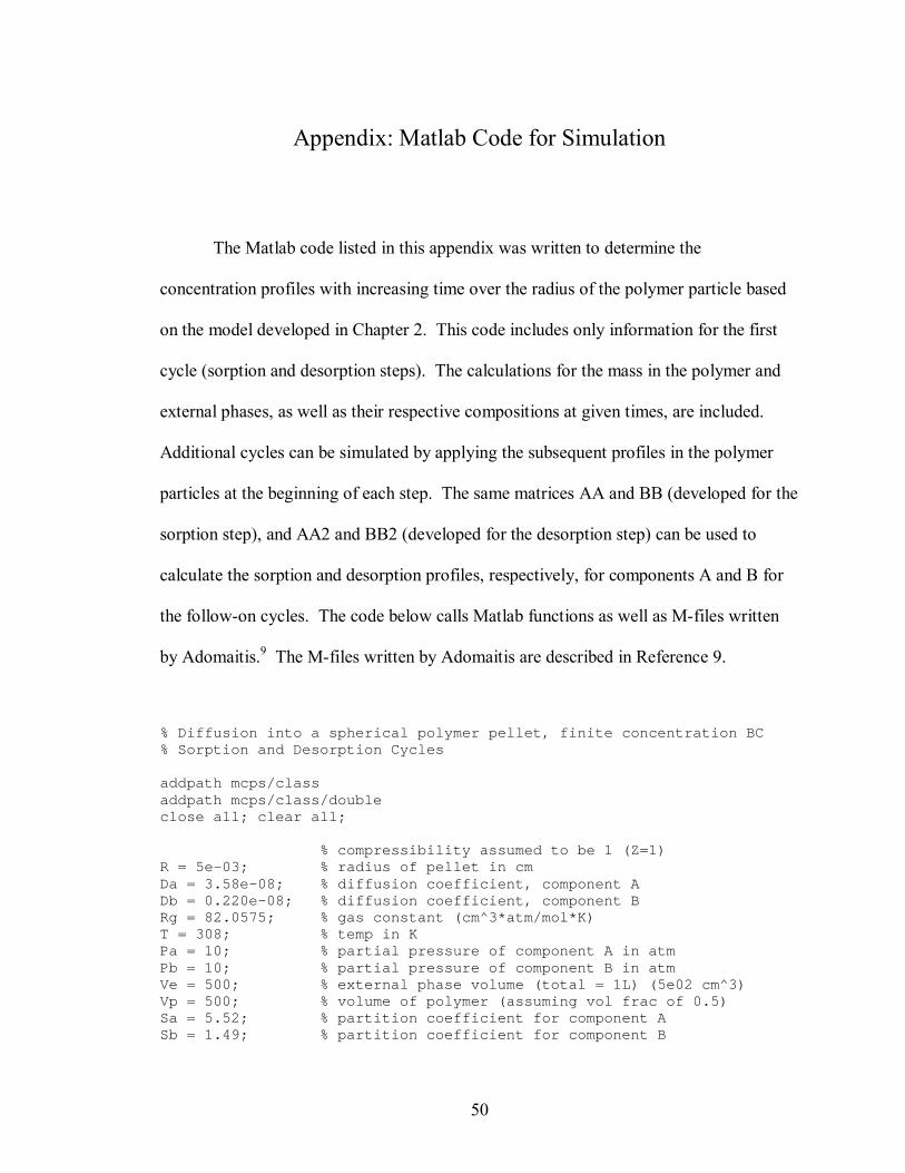
Appendix: Matlab Code for Simulation

The Matlab code listed in this appendix was written to determine the

concentration profiles with increasing time over the radius of the polymer particle based

on the model developed in Chapter 2. This code includes only information for the first

cycle (sorption and desorption steps). The calculations for the mass in the polymer and

external phases, as well as their respective compositions at given times, are included.

Additional cycles can be simulated by applying the subsequent profiles in the polymer

particles at the beginning of each step. The same matrices AA and BB (developed for the

sorption step), and AA2 and BB2 (developed for the desorption step) can be used to

calculate the sorption and desorption profiles, respectively, for components A and B for

the follow-on cycles. The code below calls Matlab functions as well as M-files written

by Adomaitis.9 The M-files written by Adomaitis are described in Reference 9.

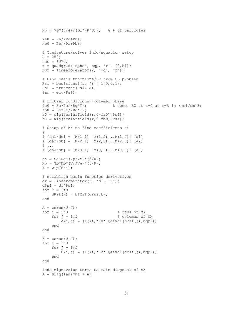
% Diffusion into a spherical polymer pellet, finite concentration BC % Sorption and Desorption Cycles addpath mcps/class addpath mcps/class/double close all; clear all; % compressibility assumed to be 1 (Z=1) R = 5e-03; % radius of pellet in cm Da = 3.58e-08; % diffusion coefficient, component A Db = 0.220e-08; % diffusion coefficient, component B Rg = 82.0575; % gas constant (cm^3*atm/mol*K) T = 308; % temp in K Pa = 10; % partial pressure of component A in atm Pb = 10; % partial pressure of component B in atm Ve = 500; % external phase volume (total = 1L) (5e02 cm^3) Vp = 500; % volume of polymer (assuming vol frac of 0.5) Sa = 5.52; % partition coefficient for component A Sb = 1.49; % partition coefficient for component B

51

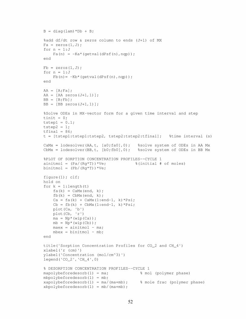
Np = Vp*(3/4)/(pi*(R^3)); % # of particles xa0 = Pa/(Pa+Pb); xb0 = Pb/(Pa+Pb); % Quadrature/solver info/equation setup J = 250; nqp = 10*J; r = quadgrid('sphe', nqp, 'r', [0,R]); DDr = linearoperator(r, 'dd', 'r'); % Find basis functions/BC from SL problem Psi = basisfunsl(r, 'r', 1,0,0,1); Psi = truncate(Psi, J); lam = eig(Psi); % Initial conditions--polymer phase fa0 = Sa*Pa/(Rg*T); % conc. BC at t=0 at r=R in (mol/cm^3) fb0 = Sb*Pb/(Rg*T); a0 = wip(scalarfield(r,0-fa0),Psi); b0 = wip(scalarfield(r,0-fb0),Psi); % Setup of MX to find coefficients ai % % [da1/dt] = [M(1,1) M(1,2)...M(1,J)] [a1] % [da2/dt] = [M(2,1) M(2,2)...M(2,J)] [a2] % ... % [daJ/dt] = [M(J,1) M(J,2)...M(J,J)] [aJ] Ka = Sa*Da*(Vp/Ve)*(3/R); Kb = Sb*Db*(Vp/Ve)*(3/R); I = wip(Psi); % establish basis function derivatives dr = linearoperator(r, 'd', 'r'); dPsi = dr*Psi; for k = 1:J dPsf(k) = bf2sf(dPsi,k); end A = zeros(J,J); for i = 1:J % rows of MX for j = 1:J % columns of MX A(i,j) = (I(i))*Ka*(getval(dPsf(j),nqp)); end end B = zeros(J,J); for i = 1:J for j = 1:J B(i,j) = (I(i))*Kb*(getval(dPsf(j),nqp)); end end %add eigenvalue terms to main diagonal of MX A = diag(lam)*Da + A;

52

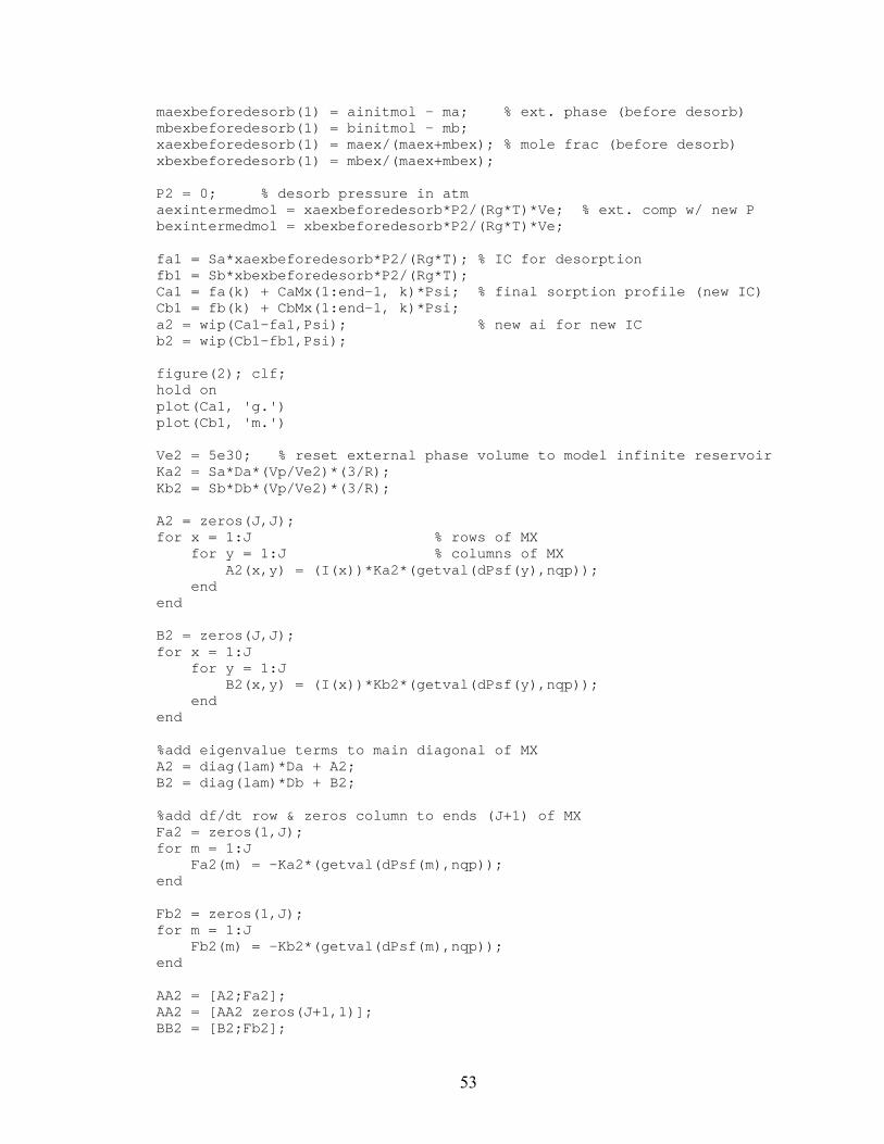
B = diag(lam)*Db + B; %add df/dt row & zeros column to ends (J+1) of MX Fa = zeros(1,J); for n = 1:J Fa(n) = -Ka*(getval(dPsf(n),nqp)); end Fb = zeros(1,J); for n = 1:J Fb(n)= -Kb*(getval(dPsf(n),nqp)); end AA = [A;Fa]; AA = [AA zeros(J+1,1)]; BB = [B;Fb]; BB = [BB zeros(J+1,1)]; %Solve ODEs in MX-vector form for a given time interval and step tinit = 0; tstep1 = 0.1; tstep2 = 1; tfinal = 86; t = [tstep1:tstep1:tstep2, tstep2:tstep2:tfinal]; %time interval (s) CaMx = lodesolver(AA,t, [a0;fa0],0); %solve system of ODEs in AA Mx CbMx = lodesolver(BB,t, [b0;fb0],0); %solve system of ODEs in BB Mx %PLOT OF SORPTION CONCENTRATION PROFILES--CYCLE 1 ainitmol = (Pa/(Rg*T))*Ve; %(initial # of moles) binitmol = (Pb/(Rg*T))*Ve; figure(1); clf; hold on for k = 1:length(t) fa(k) = CaMx(end, k); fb(k) = CbMx(end, k); Ca = fa(k) + CaMx(1:end-1, k)*Psi; Cb = fb(k) + CbMx(1:end-1, k)*Psi; plot(Ca, 'b') plot(Cb, 'r') ma = Np*(wip(Ca)); mb = Np*(wip(Cb)); maex = ainitmol - ma; mbex = binitmol - mb; end title('Sorption Concentration Profiles for CO_2 and CH_4') xlabel('r (cm)') ylabel('Concentration (mol/cm^3)') legend('CO_2','CH_4',0) % DESORPTION CONCENTRATION PROFILES--CYCLE 1 mapolybeforedesorb(1) = ma; % mol (polymer phase) mbpolybeforedesorb(1) = mb; xapolybeforedesorb(1) = ma/(ma+mb); % mole frac (polymer phase) xbpolybeforedesorb(1) = mb/(ma+mb);

53

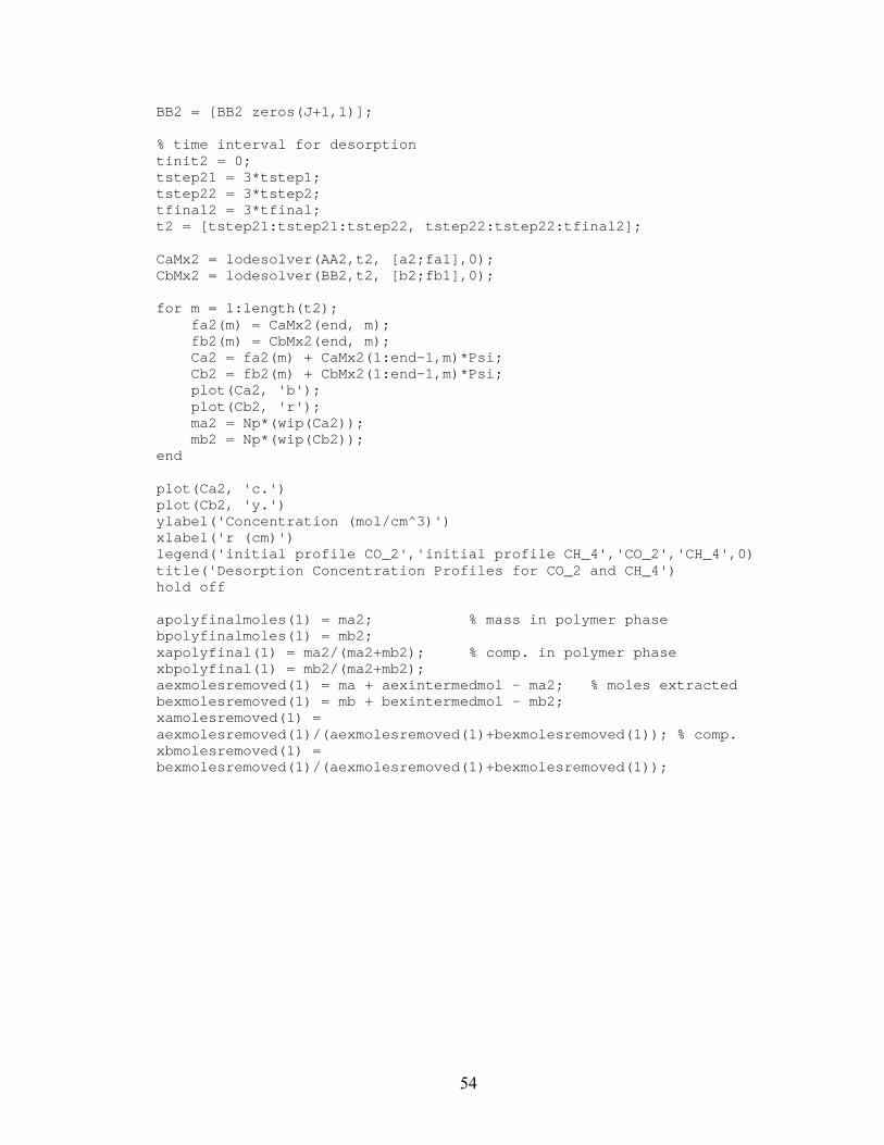
maexbeforedesorb(1) = ainitmol - ma; % ext. phase (before desorb) mbexbeforedesorb(1) = binitmol - mb; xaexbeforedesorb(1) = maex/(maex+mbex); % mole frac (before desorb) xbexbeforedesorb(1) = mbex/(maex+mbex); P2 = 0; % desorb pressure in atm aexintermedmol = xaexbeforedesorb*P2/(Rg*T)*Ve; % ext. comp w/ new P bexintermedmol = xbexbeforedesorb*P2/(Rg*T)*Ve; fa1 = Sa*xaexbeforedesorb*P2/(Rg*T); % IC for desorption fb1 = Sb*xbexbeforedesorb*P2/(Rg*T); Ca1 = fa(k) + CaMx(1:end-1, k)*Psi; % final sorption profile (new IC) Cb1 = fb(k) + CbMx(1:end-1, k)*Psi; a2 = wip(Ca1-fa1,Psi); % new ai for new IC b2 = wip(Cb1-fb1,Psi); figure(2); clf; hold on plot(Ca1, 'g.') plot(Cb1, 'm.') Ve2 = 5e30; % reset external phase volume to model infinite reservoir Ka2 = Sa*Da*(Vp/Ve2)*(3/R); Kb2 = Sb*Db*(Vp/Ve2)*(3/R); A2 = zeros(J,J); for x = 1:J % rows of MX for y = 1:J % columns of MX A2(x,y) = (I(x))*Ka2*(getval(dPsf(y),nqp)); end end B2 = zeros(J,J); for x = 1:J for y = 1:J B2(x,y) = (I(x))*Kb2*(getval(dPsf(y),nqp)); end end %add eigenvalue terms to main diagonal of MX A2 = diag(lam)*Da + A2; B2 = diag(lam)*Db + B2; %add df/dt row & zeros column to ends (J+1) of MX Fa2 = zeros(1,J); for m = 1:J Fa2(m) = -Ka2*(getval(dPsf(m),nqp)); end Fb2 = zeros(1,J); for m = 1:J Fb2(m) = -Kb2*(getval(dPsf(m),nqp)); end AA2 = [A2;Fa2]; AA2 = [AA2 zeros(J+1,1)]; BB2 = [B2;Fb2];

54

BB2 = [BB2 zeros(J+1,1)]; % time interval for desorption tinit2 = 0; tstep21 = 3*tstep1; tstep22 = 3*tstep2; tfinal2 = 3*tfinal; t2 = [tstep21:tstep21:tstep22, tstep22:tstep22:tfinal2]; CaMx2 = lodesolver(AA2,t2, [a2;fa1],0); CbMx2 = lodesolver(BB2,t2, [b2;fb1],0); for m = 1:length(t2); fa2(m) = CaMx2(end, m); fb2(m) = CbMx2(end, m); Ca2 = fa2(m) + CaMx2(1:end-1,m)*Psi; Cb2 = fb2(m) + CbMx2(1:end-1,m)*Psi; plot(Ca2, 'b'); plot(Cb2, 'r'); ma2 = Np*(wip(Ca2)); mb2 = Np*(wip(Cb2)); end plot(Ca2, 'c.') plot(Cb2, 'y.') ylabel('Concentration (mol/cm^3)') xlabel('r (cm)') legend('initial profile CO_2','initial profile CH_4','CO_2','CH_4',0) title('Desorption Concentration Profiles for CO_2 and CH_4') hold off apolyfinalmoles(1) = ma2; % mass in polymer phase bpolyfinalmoles(1) = mb2; xapolyfinal(1) = ma2/(ma2+mb2); % comp. in polymer phase xbpolyfinal(1) = mb2/(ma2+mb2); aexmolesremoved(1) = ma + aexintermedmol - ma2; % moles extracted bexmolesremoved(1) = mb + bexintermedmol - mb2; xamolesremoved(1) = aexmolesremoved(1)/(aexmolesremoved(1)+bexmolesremoved(1)); % comp. xbmolesremoved(1) = bexmolesremoved(1)/(aexmolesremoved(1)+bexmolesremoved(1));

55

Bibliography

1. R. Prasad, R.L. Shaner, and K.J. Doshi in Polymeric Separation Membranes, edited by D.R. Paul, Yuri P. Yampol�skii, (CRC Press, Boca Raton, 1994), pp 598-599.

2. J.M.S. Henis in Polymeric Separation Membranes, edited by D.R. Paul, Yuri

P. Yampol�skii, (CRC Press, Boca Raton, 1994), pp 451, 478, 483, 485, 490.

3. H. Ohya, V.V. Kudryavtsev, S.I. Semenova, Polyimide Membranes: Applications, Fabrications, and Properties, (Gordon and Breach, Amsterdam, 1996), pp 1, 103-104, 110, 112, 123, 260-261.

4. H. Kawakami, J. Anzai and S. Nagaoka, �Gas transport properties of soluble

aromatic polyimides with sulfone diamene moieties,� J. Appl. Polym. Sci., 57, 789 (1995).

5. H. Kawakami, K. Nakajima, and S. Nagaoka, �Gas separation characteristics

of isomeric polyimide membrane prepared under shear stress,� J. Membr. Sci., 211, 291, (2003).

6. J-J. Qin, T-S. Chung, C. Cao, and R.H. Vora, �Effect of temperature of

intrinsic permeation properties of 6FDA-durene/1,3 phenylenediamene (mPDA) copolyimide and fabrication of its hollow fiber membranes for CO2/CH4 separation,� J. Membr. Sci., 250, 95 (2005).

7. H. Kawakami, K. Nagajima, H. Shimizu, and S. Nagaoka, �Gas permeation

stability of asymmetric polyimide membrane with thin skin layer: effect of polyimide structure,� J. Membr. Sci. 212, 195, (2003).

8. T.A. Barbari, S.S. Kasargod, and G.T. Fieldson, �Effect of unequal transport

rates and intersolute salvation on the selective batch extraction of a dilute mixture with a dense polymeric solvent,� Ind. Eng. Chem. Res. 35, 1188 (1996).

9. R.A. Adomaitis, �Objects for MWR,� Computers & Chem. Eng., 26, 981

(2002). 10. J. Crank, The Mathematics of Diffusion, 2nd ed. (Oxford University Press,

New York, 1975), pp 93-94.

56

11. M.R. Pixton and D.R. Paul in Polymeric Separation Membranes, edited by D.R. Paul, Yuri P. Yampol�skii, (CRC Press, Boca Raton, 1994), pp 102, 105, 109, 116-119, 124, 126, 128-129.

12. T.H. Kim, �Gas Sorption and Permeation in a Series of Aromatic

Polyimides,� Ph. D. Dissertation, University of Texas at Austin, 1988.

13. T-S. Chung, W-H. Lin, R.H. Vora, �Gas transport properties of 6FDA-durene/1,3 phenylenediamene (mPDA) copolyimides,� J. Appl. Polym. Sci., 81, 3552 (2001).

14. W.S.W. Ho and K.K. Sirkar in Membrane Handbook, edited by W.S.W. Ho

and K.K. Sirkar, (Van Nostrand Reinhold, New York, 1992), p 28.

15. J.D. Wind, et al. �Relaxation dynamics of CO2 diffusion, sorption and polymer swelling for plasticized polyimide membranes,� Macormolecules, 36 6442 (2003).

16. J.D. Seader and E.J. Henley, Separation Process Principles, (John Wiley and

Sons, Hoboken, 1988), pp735-738.

17. R.R. Zolandz and G.K. Fleming in Membrane Handbook, edited by W.S.W. Ho and K.K. Sirkar, (Van Nostrand Reinhold, New York, 1992), p 56.