ABSTRACT TOPICS IN LATTICE QCD AND EFFECTIVE - DRUM

ABSTRACT

Title of dissertation: TOPICS IN LATTICE QCD ANDEFFECTIVE FIELD THEORY

Michael I. Buchoff, Doctor of Philosophy, 2010

Dissertation directed by: Associate Professor Paulo BedaqueDepartment of Physics

Quantum Chromodynamics (QCD) is the fundamental theory that governs

hadronic physics. However, due to its non-perturbative nature at low-energy/long

distances, QCD calculations are difficult. The only method for performing these

calculations is through lattice QCD. These computationally intensive calculations

approximate continuum physics with a discretized lattice in order to extract hadronic

phenomena from first principles. However, as in any approximation, there are mul-

tiple systematic errors between lattice QCD calculation and actual hardronic phe-

nomena. Developing analytic formulae describing the systematic errors due to the

discrete lattice spacings is the main focus of this work.

To account for these systematic effects in terms of hadronic interactions, ef-

fective field theory proves to be useful. Effective field theory (EFT) provides a

formalism for categorizing low-energy effects of a high-energy fundamental theory

as long as there is a significant separation in scales. An example of this is in chiral

perturbation theory (χPT ), where the low-energy effects of QCD are contained in a

mesonic theory whose applicability is a result of a pion mass smaller than the chiral

breaking scale. In a similar way, lattice χPT accounts for the low-energy effects of

lattice QCD, where a small lattice spacing acts the same way as the quark mass.

In this work, the basics of this process are outlined, and multiple original calcula-

tions are presented: effective field theory for anisotropic lattices, I=2 ππ scattering

for isotropic, anisotropic, and twisted mass lattices. Additionally, a combination of

effective field theory and an isospin chemical potential on the lattice is proposed

to extract several computationally difficult scattering parameters. Lastly, recently

proposed local, chiral lattice actions are analyzed in the framework of effective field

theory, which illuminates various challenges in simulating such actions.

TOPICS IN LATTICE QCD

AND EFFECTIVE FIELD THEORY

by

Michael I. Buchoff

Dissertation submitted to the Faculty of the Graduate School of theUniversity of Maryland, College Park in partial fulfillment

of the requirements for the degree ofDoctor of Philosophy

2010

Advisory Committee:Associate Professor Paulo Bedaque, Chair/AdvisorProfessor Thomas CohenAssociate Professor Zackaria ChackoAssistant Professor Carter HallProfessor Donald Perlis

c© Copyright by

Michael I. Buchoff2010

Acknowledgments

There are so many people who made my success in Physics possible, that it is

impossible to mention all of them.

First, I would like to thank my parents, Barbara and Barry, who made many

sacrifices to give me the opportunity to pursue my interests. They allowed me to

follow any path I chose and were endlessly supportive at each step of the way. While

I am sure there are plenty of times that I made them worry, I hope they feel that

I have made the best decisions I could with the opportunity they gave me. As

someone who takes nothing for granted, I appreciate every ounce of support and

love they have given me along the way.

Second, I would like to thank Gary Houk, my high school physics teacher,

mentor, and friend, who is responsible for launching my life as a physicist. Not only

did I pick up my enthusiasm and love for physics from him, but he was the first one

who truly believed I was capable of the highest levels of success in physics, both in

good times and bad. For this, I am forever grateful.

Third, I would like to thank several of my colleagues starting with Andre

Walker-Loud, whose willingness to take time to train me to be a good researcher

will never be forgotten. Whenever I needed a kick in the pants (something that I

needed more often than I would like to admit), Andre was there. I would not be even

a fraction of what I am if not for the effort Andre put into my development, especially

during my first year of research. Next, I would like to thank Brian Tiburzi, whose

research knowledge and expertise allowed me to continue to develop after Andre left

ii

Maryland. I would also like to thank Aleksey Cherman and Tom Cohen, two people

who I have learned an immense of knowledge from and helped me along the way in

more ways than I can count.

Fourth, I would like to thank all my friends and family who supported me

in Baltimore, Pittsburgh, and at College Park. There were many tough times,

especially in Pittsburgh, where their support and playful energy kept me from losing

my sanity. So to my friends, especially the Boss 2 community, I cannot thank you

enough.

Most of all, I would like to thank my advisor, Paulo Bedaque. From the

moment I met Paulo, I feel like I have become better person in every possible way.

Academically, his creativity and scholarly knowledge are abilities I aim to learn

and his ambition for physics inspires me endlessly. Additionally, his cool, kind

personality coupled with his unmatched wisdom and advise are traits I admire to

the upmost extent. All these qualities make Paulo the type of person I aspire to be,

which I feel is the highest compliment I am capable of giving.

iii

Table of Contents

List of Figures vi

List of Abbreviations vii

1 Introduction 11.1 Lattice QCD . . . . . . . . . . . . . . . . . . . . . . . . . . . . . . . 2

1.1.1 Chiral Symmetry in Lattice QCD . . . . . . . . . . . . . . . . 61.2 Effective Field Theory . . . . . . . . . . . . . . . . . . . . . . . . . . 9

1.2.1 Continuum Chiral Perturbation Theory . . . . . . . . . . . . . 101.2.2 Symanzik Action from Lattice QCD . . . . . . . . . . . . . . . 16

1.2.2.1 Lattice Chiral Perturbation Theory . . . . . . . . . . 191.3 Organization . . . . . . . . . . . . . . . . . . . . . . . . . . . . . . . 20

2 Effective Field Theory for the Anisotropic Wilson Lattice Action 222.1 Overview . . . . . . . . . . . . . . . . . . . . . . . . . . . . . . . . . . 222.2 Anisotropic Wilson lattice Action . . . . . . . . . . . . . . . . . . . . 24

2.2.1 Anisotropic Symanzik Action . . . . . . . . . . . . . . . . . . 262.2.1.1 O(a2) Symanzik Lagrangian . . . . . . . . . . . . . . 29

2.3 Anisotropic Chiral Lagrangian . . . . . . . . . . . . . . . . . . . . . 312.3.1 Meson Chiral Lagrangian . . . . . . . . . . . . . . . . . . . . 32

2.3.1.1 Aoki Regime . . . . . . . . . . . . . . . . . . . . . . 372.3.2 Heavy Baryon Lagrangian . . . . . . . . . . . . . . . . . . . . 40

2.4 Discussion . . . . . . . . . . . . . . . . . . . . . . . . . . . . . . . . 47

3 Isotropic and Anisotropic Lattice Spacing Corrections for I=2 ππ Scatteringfrom Effective Field Theory 493.1 Overview . . . . . . . . . . . . . . . . . . . . . . . . . . . . . . . . . . 493.2 Scattering on the Lattice . . . . . . . . . . . . . . . . . . . . . . . . . 513.3 Chiral Perturbation Theory Results for k cot δ0 and ∆(k cot δ0) . . . . 56

3.3.1 Continuum . . . . . . . . . . . . . . . . . . . . . . . . . . . . 563.3.2 Isotropic Discretization . . . . . . . . . . . . . . . . . . . . . . 613.3.3 Anisotropic Discretization . . . . . . . . . . . . . . . . . . . . 65

3.4 Discussion . . . . . . . . . . . . . . . . . . . . . . . . . . . . . . . . 70

4 ππ Scattering in Twisted Mass Chiral Perturbation Theory 714.1 Overview . . . . . . . . . . . . . . . . . . . . . . . . . . . . . . . . . . 714.2 Twisted mass lattice QCD and the continuum effective action . . . . 724.3 ππ Scattering in Twisted Mass χPT . . . . . . . . . . . . . . . . . . . 78

4.3.1 I = 2, I3 = ±2 Channels . . . . . . . . . . . . . . . . . . . . . 784.3.2 I3 = 0 scattering channels . . . . . . . . . . . . . . . . . . . . 82

4.4 Conclusions . . . . . . . . . . . . . . . . . . . . . . . . . . . . . . . . 85

iv

5 Meson-Baryon Scattering Parameters from Lattice QCD with an IsospinChemical Potential 875.1 Overview . . . . . . . . . . . . . . . . . . . . . . . . . . . . . . . . . . 875.2 Isospin Chemical Potential . . . . . . . . . . . . . . . . . . . . . . . . 895.3 Baryons in an isospin chemical potential: SU(2) . . . . . . . . . . . . 91

5.3.1 Nucleons . . . . . . . . . . . . . . . . . . . . . . . . . . . . . . 925.3.2 Hyperons . . . . . . . . . . . . . . . . . . . . . . . . . . . . . 94

5.4 Strange Quark and SU(3) . . . . . . . . . . . . . . . . . . . . . . . . 975.5 Discussion . . . . . . . . . . . . . . . . . . . . . . . . . . . . . . . . . 100

6 Search for Chiral Fermion Actions on Non-Orthogonal Lattices 1026.1 Overview . . . . . . . . . . . . . . . . . . . . . . . . . . . . . . . . . . 1026.2 Graphene . . . . . . . . . . . . . . . . . . . . . . . . . . . . . . . . . 1036.3 Graphene-Inspired Lattice Actions . . . . . . . . . . . . . . . . . . . 1046.4 Borici-Creutz Action . . . . . . . . . . . . . . . . . . . . . . . . . . . 105

6.4.1 Radiative Corrections . . . . . . . . . . . . . . . . . . . . . . . 1066.4.2 Additional Symmetry? . . . . . . . . . . . . . . . . . . . . . . 107

6.5 Other Non-Orthogonal Actions . . . . . . . . . . . . . . . . . . . . . 1096.5.1 Modified Borici-Creutz Action . . . . . . . . . . . . . . . . . . 1106.5.2 “Hyperdiamond” Action . . . . . . . . . . . . . . . . . . . . . 110

6.6 The Wilczek Action . . . . . . . . . . . . . . . . . . . . . . . . . . . . 1126.7 Conclusion . . . . . . . . . . . . . . . . . . . . . . . . . . . . . . . . . 114

7 Discussion and Outlook 115

A Scalar Field on the Lattice 117

B Three or more flavor χPT at NLO 119

Bibliography 120

v

List of Figures

2.1 Proposed Aoki phase diagram in Ref. [26] for isotropic lattice action.Region A represents continuum-like QCD and region B representsthe parity and flavor broken phase. Isotropic actions are generallytuned to lie between the first two-fingers of the Aoki-regime in them0−g2 plane [62]. However, the anisotropic diagram could look quitedifferent than this picture, and caution should be taken to ensure thecorrect phase. . . . . . . . . . . . . . . . . . . . . . . . . . . . . . . 38

2.2 Diagrams contributing to the nucleon mass at LO ((a) and (b)) andNLO ((c) and (d)). Figure (a) is an insertion of the leading quarkmass term proportional to σM . Figure (b) is an insertion of thelattice spacing terms proportional to σW and σξW . The loop graphsarise from the pion-nucleon and pion-nucleon-delta couplings. Theseloop graphs generically scale as m3

π but also depend upon ∆, andaway from the continuum limit upon the lattice spacing as well. Allvertices in these graphs are from the Lagrangian in Eq. (2.48). . . . . 44

3.1 The one-loop diagrams which contributing to the ππ scattering am-plitude (same diagrams that contribute to the finite volume effectsin Ref. [113]). The top three represent the s-channel (a), t-channel(b), and u-channel diagrams (c). The diagram resulting from the six-pion vertex is given in (d) and the wavefunction corrections are indiagram (e). These are the only diagrams for continuum, isotropic,and anisotrpoic Wilson actions. . . . . . . . . . . . . . . . . . . . . . 58

4.1 New unphysical graphs from twisted mass interactions in the t(u)-channel (a) and s-channel (b). Fig. (b) can only contribute to I3 = 0scattering. . . . . . . . . . . . . . . . . . . . . . . . . . . . . . . . . . 79

4.2 Modified four-point function, (a) consisting of all off-shell graphs.These vertices can then be iterated and summed (b), to determine theππ interactions. This summation gives rise to the Luscher relation,valid below the inelastic threshold. . . . . . . . . . . . . . . . . . . . 84

6.1 (left) Graphene lattice composed of two sub-lattices. The “a-site”lattice is represented by black circles and the “b-site” lattice is rep-resented by red squares. (right) Illustrates the proposal by Creutz[37] to group horizontal neighbors into two-atom sites, given by theellipses. With these sites, a grid can be constructed, which is givenby the pink lines. . . . . . . . . . . . . . . . . . . . . . . . . . . . . . 103

6.2 Two-dimensional projection of Borici-Creutz action with the blueduel basis vectors eµ = eµ − e5. (left) Projection of the first linein of the two-component action shows nearest neighbor interactionsleading to Z3 rotational symmetry. (right) Projection of the secondline shows next-to-nearest neighbor interactions breaking Z3. . . . . . 109

vi

List of Abbreviations

QCD Quantum chromodynamicsEFT Effective field theoryLECs Low-energy constantsχPT Chiral perturbation theoryLχPT Lattice chiral perturbation theoryHBχPT Heavy baryon chiral perturbation theoryLO Leading orderNLO Next-to-leading orderNnLO (Next-to)n-leading order

vii

Chapter 1

Introduction

Quantum chromodynamics (QCD) is the fundamental theory that governs

hadrons (mesons and baryons) and hadronic interactions. In QCD, fermions in the

one-index fundamental representation of the SU(3) gauge group1, also known as

quarks, are coupled with spin-1 bosons of the same gauge group, known as gluons.

This non-abelian SU(3) gauge group, whose rank is referred to as color, contains

8 generators, each of which are associated with a gluon in the theory. All hadrons

are “color neutral”; baryons contain three quarks in a state antisymmetric in color,

and mesons contain a quark and anti-quark that form a color singlet. The QCD

Lagrangian including the three lightest quarks (up, down, strange) is given by

L = −1

4F aµνF

µνa +

3∑

f=1

ψfi(

iD/+mqf

)

ijψfj (1.1)

where ψ is the quark fields with flavor index f and color index i, j, Dµ,ij = ∂µIij +

igAµ,ij with Aµ,ij = AcµTcij and T cij being the eight generators of SU(3), and the

kinetic and self interactions of the gauge fields are given by F aµν = ∂µA

aν − ∂νA

aµ +

i[Aµ, Aν ]a.

The most significant properties of QCD are that the theory is both asymptoti-

cally free and confining. In other words, at short distance/high-energy, the coupling

becomes perturbatively small and at long distances/low-energy, the coupling be-

1This is equivalent to two-index antisymmetric representation for an SU(3) gauge group

1

comes strong. A perturbative calculation of the QCD beta function at high energy

yields a negative sign (for the number of flavors of quarks in the standard model),

which leads to a decaying coupling constants as the energy increases (asymptotic

freedom). While not mathematically proven, QCD is believed to be confining, where

it requires more and more energy to separate a quark or anti-quark in a hadron.

What makes this statement so difficult to prove is the fact that at long distances the

theory is strongly coupled, and thus, the usual perturbative arguments break down.

As a result, another method is required to compute non-perturbative physics, and

lattice QCD is the best option available.

1.1 Lattice QCD

In quantum field theory, there exists multiple methods for regulating divergent

calculations. One such method is to use a lattice; that is, to break up the continuum

of space and time into many individual sites, which is often referred to as discretizing

space and time. For every finite sized lattice, there are two parameters introduced:

the lattice spacing between sites and the total length of the lattice. For a simple cubic

lattice (hypercubic if time is included), these two parameters in a given direction are

simply related by the number of sites in that direction. By definition, this particular

regulator breaks the continuous translational symmetry to a discrete translational

symmetry, but as we take the continuum limit (the spacing between sites goes to

zero as the length of the lattice goes to infinity), we hope to recover the continuum

result.

2

Non-perturbative lattice calculations take advantage of this regulator along

with the path integral representation to perform calculations that do not require

a perturbatively small parameter. The path integral approach requires defining a

partition function given by

Z =

∫

d[ψ]d[ψ]d[A]eiS(ψ,ψ,A), (1.2)

where d[ψ] =∏

n dψn represents all possible paths of ψ and the action is related to

the Lagrangian by S(ψ, ψ,A) =∫

d4xL(ψ, ψ,A). Another useful quantity to define

is the correlation function given by

〈f(ψ, ψ,A)〉 = Z−1

∫

d[ψ]d[ψ]d[A]f(ψ, ψ,A)eiS(ψ,ψ,A), (1.3)

which is analogous to the definition of the expectation value in statistical mechanics.

Both of these equations require (infinitely) many multiple-dimensional integrals to

compute, which is computationally difficult for non-perturbative systems. Rather

than the diagrammatic approach from perturbation theory, lattice calculations uti-

lize a Monte Carlo integration method2, where the exponential of the Euclidean

rotated3 path integral acts as a probability distribution. As a result of analyzing

correlation functions in this framework, energy differences and matrix elements can

be extracted. The example of the scalar case, as in Ref. [2], is shown in Appendix

A.

There are several key issues that arise in non-perturbative lattice calculations.

One that is relevant to the results in this paper is the fermion doubling problem.

2For more detailed information, see Ref. [1].3Transformation defined by going to imaginary time, t → iτ . As a result the integrand eiS →

e−S .

3

As mentioned previously, to perform numerical lattice calulations, the space and

time directions are discretized, with the inverse of the lattice spacing between them

acting as the ultraviolet cutoff of the theory. However, depending on exactly how

the action is discretized (in particular, the fermion terms), a single fermion attached

to each node can describe multiple fermions in the continuum limit. The most basic

example of this effect is from the naıve fermion lattice action. The fermionic part

of this discretized action (without gauge interactions) is given by

SNF = a4∑

x,µ

1

2a

[

ψxγµψx+µ − ψx+µγµψx

]

, (1.4)

where, in conventional lattice notation, a is the lattice spacing, x is the location of

a given site and x + µ represents a site that is one lattice spacing away from x in

the µ direction4, and ψx and γµ are the fermionic fields and Dirac matricies, respec-

tively. This action is equivalent to taking the continuum kinetic action (ψγµ∂µψ)

and approximating the derivative in the naıve way (∂xψ(x) ≈ 1a

(

ψ(x+ a) − ψ(x))

).

Using the discrete Fourier expansion

ψx =1

L4

∑

p

eix·pψp, (1.5)

the action becomes

SNF =1

L4

∑

p,µ

ψpγµ1

2a(eiapµ − e−iapµ)ψp =

1

L4

∑

p,µ

ψpγµ

[ i

asin(apµ)

]

ψp, (1.6)

where iaψpγµ sin(apµ) is the reciprocal of the propagator. Taking the continuum limit

naıvely (a → 0) yields the correct continuum (Euclidean) behavior for the kinetic

4µ = 1, · · · , 4, where the fourth direction is the Euclidean rotation of the Minkowski time

direction

4

term ( iasin(apµ) ≈ ipµ). However, it is important to note that the for every pole of

the propagator, there is a particle. In other words, a particle is present whenever

sin(apµ) = 0. Thus, values of apµ = (0, π) lead to two poles in each direction. For

a four-dimensional lattice, there are 24 poles, which lead to 16 particles that are

often referred to as “doublers.” In this particular discretization, by representing a

single fermion field at each node, the action is actually describing 16 fermions. Since

the goal of lattice QCD is to simulate two or three flavors, another discretization is

required.

In order to achieve the correct continuum behavior of the theory being simu-

lated on the lattice, an natural extension is to add another term to the naıve quark

action that vanishes in the continuum limit. As a result, the Wilson action was

developed, which, in lattice terminology is given by

SW = a4∑

x,µ

1

2a

[

ψx(γµ − r)ψx+µ − ψx+µ(γµ + r)ψx + rψxψx

]

, (1.7)

where r is the Wilson parameter. While this action appears significantly different

from the naıve quark action, it is equivalent to adding the discretized version of the

term arψ∂µ∂µψ. Applying the same Fourier transform as before,

SW =1

L4

∑

p,µ

ψp

[ i

aγµ sin(apµ) +

r

a

(

cos(apµ) − 1)

]

ψp. (1.8)

This action only contains one pole (when apµ = 0) and reproduces the correct con-

tinuum behavior as the lattice spacing approaches zero. Thus, this action describes

only one particle. If we included two or three flavors of this action, we can simulate

two or three flavor QCD.

5

While this action appears to have removed the fermion doubling problem, it

leads to a new problem. The issue that arises from this discretization is that it

unphysically breaks chiral symmetry5. For a free action, this effect will vanish in

the continuum limit. However, QCD is a gauge theory with gauge interactions that

can and will lead to radiative corrections. Chiral symmetry restricts many operators

that could be radiatively generated. However, if chiral symmetry is broken in an

unphysical way, as is the case with the Wilson action, this will lead to unphysical

operators that will contaminate the final results. What makes it even worse is

that these operators can diverge in the continuum limit and require a difficult non-

perturbative tuning to remove. These issues will be explained in more detail in

section 2.

1.1.1 Chiral Symmetry in Lattice QCD

One important question in Lattice QCD is whether or not it is possible to

both resolve the fermion doubling problem and keep chiral symmetry intact. Over

the last two decades, this topic has been one of great interest and has led to several

review articles [3, 4, 5, 6] as it is now considered a pivotal subject in lattice QCD.

The Wilson lattice action is an example where chiral symmetry is sacrificed in

order to remove the doublers. However, this behavior is not unique to the Wilson

5The Lagrangian LF = ψDFψ is chirally symmetric if γ5DFγ5 = −DF . A quick way to see

if an operator is chirally symmetric is to check whether it contains an odd number of γµ’s. If it

has an even number of γµ’s, it is not chirally symmetric (note, the number of γ5’s does NOT alter

chirality).

6

lattice action and, in fact, Nielsen and Ninomiya proposed a no-go theorem for chiral

symmetry on the lattice. Specifically, the theorem states that a lattice action will

contain doublers as long as three properties are held true: 1) Discrete translational

symmetry, 2) Locality, 3) Chiral symmetry. In other words, one or more of these

three properties must be sacrificed in order to remove doublers. Another way of

understanding the Nilsen-Ninomiya theorem is in terms of the chiral anomaly. For

example, the naıve lattice action has an exact U(1)A symmetry which persist all

the way to the continuum limit. Continuum QCD, on the other hand, has an

anomolus U(1)A symmetry that is broken by quantum corrections (in particular

the one loop fermionic triangle diagrams). Thus, in order to produce the correct

continuum physics for QCD, a source for chiral symmetry breaking must be present

to reproduce the correct flavor-singlet chiral anomaly defined in the standard way6.

One way to do this is to break chiral symmetry explicitly, as in the Wilson action.

However, as mentioned before, this leads to unwanted radial corrections. A more

favorable discretization takes advantage of the Ginsparg-Wilson relation [8].

If a fermionic action has exact chiral symmetry, it obeys the relation

γ5D +Dγ5 = 0. (1.9)

Another relation akin to the one above is the Ginsberg-Wilson relation, which is

given by

γ5D +Dγ5 = aDγ5D , (γ5D)† = γ5D. (1.10)

6As shown in Ref. [7], if one defines a non-singlet axial current for the naive action, the correct

chiral anomaly can be reproduced. In other words, in the usual notation, the naive action has a

flavor non-singlet chiral anomaly.

7

This relation introduces a small source of chiral symmetry breaking at O(a), and

in the continuum limit removes doublers, yields radiative corrections ala continuum

QCD, and yields a source for the flavor-singlet chiral anomaly. Two solutions to

the Ginsparg-Wilson relation have been found, both of which are equivalent in the

appropriate limit. The first of such solutions is domain wall fermions [9, 10, 11]

where four-dimensional chiral fermions are given by a mass step function in an

additional fifth direction. In the limit of an infinite fifth direction, this yields a

single four-dimensional Dirac fermion (a left-handed and right handed “wall” in

the fifth direction due to periodic boundary conditions). In reality, simulations are

performed with a finite fifth directions, but the residual chiral symmetry breaking

is exponentially suppressed. Another equally valid realization of Ginsparg-Wilson

fermions are known as overlap fermions [12, 13, 14], which satisfy the relations with

a non-local four-dimensional operator. In has been shown [15, 16], that including all

the non-local contributions of the overlap operator is equivalent to the domain wall

action with an infinite fifth direction (the two actions are related via a KaluzaKlein

reduction).

While both domain wall and overlap lattice actions have favorable features,

the major drawback to both actions are computational costs. Either simulating

an extra dimension or multiple non-local operators leads to computational costs

about a factor of ten greater than four-dimensional, local actions. Thus, it would

be beneficial if some cheap, local chiral action could be found, and this scenario of

minimally doubled, non-orthogonal actions will be discussed in chapter 6.

8

1.2 Effective Field Theory

Throughout physics, there are multiple scales that arise when analyzing phe-

nomena. An effective field theory (EFT) is a theory that maps the symmetries of

a more fundamental theory (usually at a higher energy scale) in terms of more rel-

evant degrees of freedom (usually at a lower energy scale). An example of this is

the low-energy limit of the Standard Model, where the heavy, high-energy modes of

the W and Z particles are “integrated out” and act as small corrections to the low

energy theory inversely proportional to powers of the W and Z mass.

To construct an EFT from a more fundamental theory, the first step is to

identify the symmetries and explicit symmetry breaking in the fundamental the-

ory. Next, for this approach to be controlled and fruitful, a seperation of scales is

necessary. For example, if a theory has a lower scale of p and a higher scale of Λ,

then the expansion parameter in the EFT would be p/Λ. In terms of the relevant

degrees of freedom in the EFT, which depend on the particular energy ranges of

interest, one must write down all the possible operators that reflect the symmetries

of the fundamental theory (the explicit symmetry breaking can be mapped through

a spurion analysis) for a given order in the power counting parameter. Each of

these parameters have a coefficient known as low-energy constants (LECs) that are

O(c/Λn) in the power counting where n is determined by the order of the EFT and

c is O(1). These LECs are not known a priori and require external input to fix. For

non-perturbative theories, like QCD, the non-perturbative effects in the calculation

are contained in these terms, and require a non-perturbative calculation, such as

9

the lattice, to determine.

Throughout this work, the high-energy, fundamental theory is QCD (more

specifically, lattice QCD) and the relevant degrees of freedom of interest in our

EFT are hadrons, nucleons and mesons. The particular EFT of interest will depend

which limits we explore. For example, if we are looking at characteristic momenta

far below the mass of the particles of interest, non-relativistic field theory is appro-

priate. Additionally, if pion mass is small compared to the relevant cut-off scales,

such as the chiral breaking scale, the pion mass can be viewed as a correction to the

chiral limit (mπ = 0). Most of this work will focus on these limits, and the result-

ing EFTs, namely chiral perturbation theory and heavy baryon chiral perturbation

theory (HBχPT ).

1.2.1 Continuum Chiral Perturbation Theory

Chiral perturbation theory (χPT ) is the mesonic EFT of QCD when the

characteristic momenta are on the same order as the pion mass (mπ ∼ 135 MeV),

which are both well below the chiral breaking scale (Λχ ∼ 4π2fπ ∼ 1 GeV). Thus, the

characteristic momenta, p and the pion mass, mπ act as the expansion parameters

for continuum χPT .

As mentioned previously, the first step to constructing χPT is to identify

the symmetries of QCD. The QCD lagrangian (Eq. (1.1)) has, in addition to the

SU(3) gauge symmetry, Lorentz symmetry, and is invariant under parity, charge

conjugation, and time reversal. However, the main symmetry of focus will be chiral

10

symmetry. In the massless limit, the QCD Lagrangian is chirally symmetric, while

the mass term breaks the chiral symmetry explicitly. This effect can be best seen

by rewriting the fermionic part of the QCD lagrangian in terms the left and right-

handed components of ψ:

LF = ψ(D/ +mq)ψ = ψLD/ψL + ψRD/ψR +(

ψLmqψR + ψRmqψL)

, (1.11)

where

ψL =(1 + γ5

2

)

ψ, ψR =(1 − γ5

2

)

ψ,

ψR = ψ(1 − γ5

2

)

, ψL = ψ(1 + γ5

2

)

,

The chiral symmetric transformation in terms of these components is given by

ψL = LψL, ψL = ψLL†

ψR = RψR, ψR = ψRR†,

where the chiral flavor transformations L and R obey the relation L†L = 1 and

R†R = 1. The generators of the transformations are those of the SU(NF ) flavor

group. In this work, we will only focus on either two or three lightest flavors, and

these transformations obey SU(2) and SU(3) flavor, respectively.

In the massless limit, the action is invariant under an L and R transfor-

mations that are independent of each other. As a result, the action pocesses an

SU(NF )L ⊗ SU(NF )R ⊗ U(1)B, where the last U(1)B represents baryon number

conservation. Since QCD is a confining theory, the chiral condensate (〈ψψ〉) is non-

zero, and thus this flavor symmetry is spontaneously broken. Both phenomenogical

and lattice evidence supports that this symmetry is spontaneously broken to the

11

vector subgroup (SU(NF )L ⊗ SU(NF )R → SU(NF )V leading to N2F − 1 Nambu-

Goldstone particles. In three flavor QCD, these particles include the pions, kaons,

and eta (the eta-prime is a flavor singlet whose mass differs from the eta due to the

chiral anomaly). With the knowledge in hand that non-zero chiral condensate is in

the vector subgroup (〈uu〉 = 〈dd〉 = 〈ss〉), then it is adventagous to write

〈ψLiψRj〉 ≡ Ωij = ωδij, ω 6= 0. (1.12)

Performing a chiral transformation, this condensate becomes

(

LΩR†)

ij= ω

(

LR†)

ij≡ ωΣij. (1.13)

If L = R, then Σij = δij leaving the vector subgroup unbroken as expected. If L 6= R,

then Σij represents a different vacuum from the vector subgroup. As mentioned

before, this vacuum, whose generators are that of SU(NF ), is a matrix of the Nambu-

Golstone particles (pion, kaon, eta, etc.) fields, which are the relevant degrees of

freedom for χPT . In massless QCD, these different vacua are degenerate and each

of these particles are massless. However, since QCD does contain an explicit chiral

breaking term proportional to the quark mass, this term “tips” the potential, giving

these psuedoscalar particles a mass. To see how this occurs, it is important to follow

the procedure for mapping the mass term into the chiral theory.

When constructing an effective field theory, one must write down all the pos-

sible operators at a given order that obey all the symmetries of the fundamental

theory. Thus, for mesonic observable in χPT , the theory must be written in terms

of the mesonic matrix Σij . Since there are no space-time indices in this matrix, the

Lorentz symmetry is preserved as long as derivatives of these matrices are contracted

12

in a Lorentz invariant way7. Under parity, Σ → Σ†, and an effective field theory of

QCD should be invariant under this transformation8. Under chiral transformations,

Σ → LΣR† , Σ† → RΣ†L†. (1.14)

Thus, when constructing the chirally invariant χPT Lagrangian without a mass with

the monenta p2 as the expansion parameter, the only combination at leading order

(LO) is given by

Lm=0LO =

f 2

4tr(

∂µΣ†∂µΣ

)

, (1.15)

where the coefficient f can be related to the pion decay constant fπ. Another

possible operator is tr(Σ†Σ), but since Σ†Σ = 1, this term has no field dependence

is just shifts the Lagrangian by an overall constant. Thus, at LO in p2, there is only

one term when mq = 0. To include the mq dependence, it is best to rewrite the

mass term in QCD in a specific way:

Lm = ψLmqψR + ψRm†qψL, (1.16)

where mq is the diagonal mass matrix (in the SU(2) isospin limit, mq = mI). This

way of writing the mass term in QCD seems illogical, but it makes sense when mq is

promoted to a spurion in order to account for its effects in χPT . Upgrading mq to

7In Chapter 2 we will explore lattice theories that break the Euclidean equivance of Lorentz

symmetry and the consequences. As a notational point of emphasis, up and down contracted

indices (such as ∂µ∂µ) will represent Minkowski space and only down contracted indices (such as

∂µ∂µ) will represent Euclidean space.8This is not the case for the twisted mass lattice action in Chapter 4 or the convenient lattice

action for finite isospin density in Chapter 5

13

the spurion9 s+ ip, this term transforms under chirality the same way as Σ; namely

(s + ip) → L(s + ip)R†. Thus, we can now construct the next terms in the chiral

Lagangian of the form

tr(

(s+ ip)Σ† + (s− ip)Σ)

(1.17)

In the real world and most lattice QCD simulations, mq is purely scalar, so we can

set s = Bmq and p = 0, which correctly accounts for the chiral symmetry breaking

effect of mq. B is proportional to the chiral condensate. As a result, all the LO

contributions to χPT are given by

LLOχ =f 2

8tr(

∂µΣ†∂µΣ

)

+Bf 2

4tr(

mq(Σ† + Σ)

)

. (1.18)

The matrix Σ = e2iφ is

φ =

π0√

2π+

π− − π0√

2

, mq =

mu 0

0 md

, (1.19)

for two flavors, and

φ =

π0√

2+ η√

6π+ K+

π− − π0√

2+ η√

6K0

K− K0 − 2η√

6

, mq =

mu 0 0

0 md 0

0 0 ms

. (1.20)

for three flavors. The particular convention used in this Lagrangian is consistent

with f ∼ 132 MeV.

As an example of a LO two-flavor tree-level calculation for the pion mass, one

must first expand (1.18) in terms of pion fields, giving

LLOχ = ∂µπ+∂µπ− −B0(mu +md)π

+π− + · · · , (1.21)

9The s stands for scalar part and p stands for the parity violating pseudoscalar part and should

not be confused with the momenta.

14

where the dots represent three or more pion interactions along with neutral pion

interactions. From this Lagrangian, the LO pion mass is given by

m2π = B0(mu +md), (1.22)

which is a famous result illustrating that m2π ∝ mq. Extending this analysis to

three-flavor, the LO K and η mass are given by

m2K+ = B0(mu +ms) , m2

K0 = B0(md +ms)

m2η = B0

(

4

3ms +

1

3mu +

1

3md

)

=2

3m2K+ +

2

3m2K0 − 1

3m2π, (1.23)

where the last equation yields the Gell-Mann-Okubo formula, which agrees with

experiment up to 10%. The next-to-leading order (NLO) calculation of the mass

requires one-loop corrections involving the LO terms in the Lagrangian and tree-

level contributions from the NLO terms in the Lagrangian (terms proportional tom4π

or p4). Constructing the NLO requires the same procedure as the LO case, namely,

writing down all possible independent operators that obey the overall symmetry.

However, the process is more complicated since the number of operators that can be

written down has increased significantly. In two-flavor χPT , a simplification occurs

((Σ† + Σ) happens to be proportional to the identity matrix in flavor space) that

leads to only four necessary operators at NLO:

Lcont =f 2

8tr(∂µΣ∂

µΣ†) +Bf 2

4tr(mqΣ

† + Σmq)

+ℓ14

[

tr(∂µΣ∂µΣ†)

]2+ℓ24

tr(∂µΣ∂νΣ†)tr(∂µΣ†∂νΣ)

+(ℓ3 + ℓ4)B

2

4

[

tr(mqΣ† + Σmq)

]2+ℓ4B

4tr(∂µΣ∂

µΣ†)tr(mqΣ† + Σmq),

(1.24)

15

where the LECs ℓ1 − ℓ4 are the original Gasser-Leutwyler coefficients defined in

Ref. [17]. This Lagrangian will be one of the main focuses in Chapter 3. For three-

or more flavors, this simplification does not occur and 8 operators are necessary10.

The three-flavor NLO Lagrangian will not be the focused on in this thesis, but will

be included in Appendix B for completeness.

1.2.2 Symanzik Action from Lattice QCD

As mentioned previously, Lattice QCD is a discretized approximation to QCD.

For certain lattice actions in the continuum limit (the lattice spacing approaches

zero), one expects to achieve continuum QCD. However, it is impossible to simulate

with zero lattice spacings, so it would be convenient to develop a continuum EFT

for the lattice action at small lattice spacings that would account for both the

continuum theory and the finite a corrections that are proportional to powers of the

lattice spacings. This EFT is referred to as the Symanzik action [18, 19, 20, 21].

To illustrate how the Symanzik action is developed, the Wilson lattice action,

Eq. (1.7) will be used. To begin the process, the symmetries of the Wilson lattice

action (now acting as our fundamental theory) must be mapped onto the continuum

EFT. Many of the symmetries are similar to continuum QCD in Euclidean space, but

there are two key differences. The first one, that was mentioned previously, is that

the action breaks chiral symmetry. Second, the lattice does not contain a continuum

translation symmetry, but rather contains a discretized translational symmetry. To

10If the action were to contain external, dyamical gauge fields, there would be more operators

needed.

16

be more specific, the O(4) rotational symmetry of the Euclidean continuum (the

Euclidean version of Lorentz symmetry) is broken to the hypercubic group. Thus,

whatever Symanzik action we write down must account for these broken symmetries.

When constructing an EFT, any possible operator can and will be generated

unless a symmetry prevents them. As a result, a convenient way of organizing the

Symanzik action is as follows:

LSym =1

aL(3) + L(4) + aL(5) + a2L(6) + · · · , (1.25)

where a is the lattice spacing, and L(n) represents the linear combination of all the

linearly independent operators with mass dimension n. The dots represents all other

powers of positive n (there are no operators allowed operators the Wilson action for

mass dimensions of 1 or 2). Each L(n) can be written as

L(n) =∑

i

c(n)i O(n)

i , (1.26)

with O(n)i represents the set of allowed independent operators at mass dimension

n and c(n)i are the undetermined, unitless coefficients of these operators. As in the

continuum χPT case, some effort has to be made in order to show that one has

the minimum set of operators (often, operators can be related through change of

variables). Focusing on just the fermionic part of the action, the operators needed

through O(a) are given by

3 : O(3)1 = ψψ

4 : O(4)1 = ψD/ψ

5 : O(5)1 = iψσµνFµνψ. (1.27)

17

There is only one dimension-5 operator needed, which is referred to as the Sheikholeslami-

Wohlert [20] term for short. Since there is only one term at O(a), one approach is

to add this operator to the actual lattice action to remove all the O(a) effects in

the calculation11. At O(a2), there are 14 additional operators (which are catalogued

in Ref. [22]), which consist of both bilinears and four-fermion operators. The most

notable of these operators is ψγµDµDµDµψ, which is the first term that breaks the

O(4) rotation symmetry to the hypercubic group.

One important issue that becomes clear from the Symanzik action is the com-

plication that arise when taking the continuum limit (when a → 0). Ultimately,

the desired continuum limit is QCD. However, as can be seen in Eq. (1.25), there

are non-physical terms that can either remain or diverge in the continuum limit.

There are three categories these operators fall in: “Relevant” operators that have

a mass dimension less than four and diverge in the continuum limit, “Marginal”

operators that have a mass dimension of four and remain finite in the continuum

limit, and “Irrelevant” operators that have a mass dimension greater than four and

vanish in the continuum limit. For unwanted, unphysical operators, irrelevant op-

erators can be suppressed by reducing the lattice spacings. However, relevant and

marginal operators require an additional non-perturbative fine tuning. For example,

the Wilson action has one relevant and no marginal operators. The one relevant

operator ∼ 1aψψ has the same form as the QCD mass term. Effectively, this rele-

11This approach is often referred to as “O(a) improved” or “Clover improved” Wilson action.

Since the coefficient of the Sheikholeslami-Wohlert term depends on non-perturbative physics, this

process requires a non-trivial, non-perturabtive fine tuning of the coefficients in the lattice action.

18

vant operator acts as a large (on the order of the ultraviolet cutoff of the inverse

lattice spacings) additive renormalization of the quark mass. However, in reality,

we want to simulate QCD at finite and small quark masses. Thus, when simulating

the action, one needs to add an additional mass term to the action to cancel this

divergence, which requires a non-perturbative tuning (such as verifying the mea-

surement of the pion mass in the chiral limit is zero). A similar process would be

required for each additional relevant or marginal operator an action might generate.

It should be noted, however, that each additional fine tuning becomes significantly

more difficult to satisfy. Thus, too many fine tunings of a lattice action can prevent

a lattice action from being practically useful.

1.2.2.1 Lattice Chiral Perturbation Theory

Just as χPT was the EFT of continuum QCD, lattice chiral perturbation

theory (LχPT ) is the EFT to the continuum Symanzik action in the previous

section. The power-counting for LχPT that will be analyzed throughout this thesis

is p2 ∼ mq ∼ a, known as the generic small mass (GSM) power-counting. Another

power-counting of interest when performing calculations when quark masses are

much smaller than lattice spacings, namely mq ∼ a2, is known as the Aoki regime.

From LχPT , one can calculate the analytic lattice spacing dependence of mesonic

observables, which aid in continuum extrapolations. This approach has been a large

focus for categorizing these systematic effects in lattice QCD [23, 24, 25, 26, 27, 22].

For a Wilson lattice action whose relevant operator has been fine tuned, the

19

new terms as compared to continuum QCD are (primarily) the Sheikholeslami-

Wohlert term and the O(4) breaking term. The O(4) breaking term, ψγµDµDµDµψ,

first appears at O(a2p4), which in the GMS power-counting, is at a high order

(N3LO) and is a small effect in most standard lattice calculations. The greater

focus will be on the Sheikholeslami-Wohlert term, which obeys the same symmetries

as the QCD mass term. Thus, many of the operators in LχPT are analogous to

the mass terms in χPT with different LECs (indicated by w or W ). The resulting

theory can be given in terms the continuum χPT Lagrangian and the contribution

from an isotropic lattice spacing,

Liso =Lcont + ∆Liso. (1.28)

∆Liso =asWf 2

4tr(Σ† + Σ) +

(w3 + w4)asWB0

4tr(mqΣ

† + Σmq)tr(Σ† + Σ)

+w′

3(asW )2

4

[

tr(Σ† + Σ)]2

+w4asW

4tr(∂µΣ∂

µΣ†)tr(Σ† + Σ). (1.29)

This Lagrangian (along with its anisotropic counterpart) and observables calculated

is the focus of Chapter 3.

1.3 Organization

The structure of this thesis is organized in the following way. Chapter 2, which

is primarily based on Ref. [28] with P. Bedaque and A. Walker-Loud, develops the

EFT for anisotropic lattice actions; namely, lattice actions with temporal lattice

spacings different from spacial lattice spacings. Chapter 3, based on Ref. [29], uti-

lizes this anisotrpic EFT to calculate analytic extrapolation formulae for several

20

observables, including pion masses, decay constants, and, most notably, phase shifts

for I=2 ππ scattering. Chapter 4, based on Ref. [30] with A. Walker-Loud and

J-W. Chen, also calculates extrapolation formulae for phase shifts for ππ scatter-

ing, but for the twisted mass lattice action, whose results were used in practice to

extrapolate to the continuum limit in Ref. [31, 32]. Chapter 5, based on Ref. [33]

with P. Bedaque and B. Tiburzi, proposes a novel method of extracting several

scattering parameters between baryons and mesons, which is currently prohibitively

expensive in computing time due to the presence of disconnected contributions.

Chapter 6, based on Ref. [34] and previous work in Ref. [35, 36] with P. Bedaque,

B. Tiburzi, and A. Walker-Loud , EFT methods are used to pin down unphysical

effects from lattice spacings for several non-orthogonal lattice actions, including the

recent graphene-inspired lattice action proposed by Creutz [37]. As a final note, the

reader should be aware that some notation has been altered from chapter to chapter

to remove ambiguity of symbols (for example, in Chapter 4, the lattice spacing is

referred to as b as opposed to the usual a since a in that chapter is reserved for the

scattering length). As a result the conventions are defined in each chapter.

21

Chapter 2

Effective Field Theory for the Anisotropic Wilson Lattice Action

2.1 Overview

All lattice QCD calculations are performed with finite lattice spacings and

finite spacial extent (both of which are examples of lattice artifacts). In addition

to the extrapolations from the unphysically large quark masses that present lattice

QCD calculations require, extrapolations from a discretized lattice theory to the

desired continuum result is also necessary. In this work, we will focus mainly on

the effects from the finite lattice spacings. The formalism that is employed here is

a generalization of chiral perturbation theory that includes both quark mass and

lattice spacing dependence. This patricular formalism, which has been utilized to

calculate a plethora of lattice observables [38, 26, 27, 22, 39, 40], is valid for a specific

power counting of the lattice spacing effects, specifically these effects are on the same

order as the contribution from the quark mass (p2 ∼ Bmq ∼ Wa). These resulting

formula often depend on LECs which are not known a priori. These LECs, which

depend on the details of the short distance physics of the non-perturbative calcula-

tion, can be separated into two categories: ones that contribute to the actual low

energy physics of interest (physical contributions), and ones that are a result of the

finite lattice spacing of the particular lattice calculation (unphysical contributions).

The goal of this formalism of χPT is to isolate these unphysical contributions, so

22

they can be removed in the proper continuum extrapolation.

As mentioned in Appendix A, the lowest energy of the system can be extrapo-

lated from the long time behavior of the Euclidean correlation functions. Such cor-

relation functions can suffer from signal-to-noise degeneration for certain baryonic

observables at long times (see Ref. [41] for more details) and can be contaminated

by excited states at short times. Thus, one method to tame such issues is to uti-

lize an anisotropic lattice where the lattice spacing in time differs from the lattice

spacing in space by a proportionality factor ξ, whose relation is given by at = as/ξ.

Such lattices can give more temportal resolution. This is highly beneficial for mul-

tiple calculations such as heavy systems consisting of light quarks (for example,

nucleon-nucleon calculations) where few time slices remain after the excited state

contamination dies off. In other words, anisotropic lattices can give additional in-

formation, which might lead to an earlier identification of the ground state plateau.

Anisotropic lattices have been used extensively in the study of heavy quarks and

quarkonia [42, 43], glueballs [44, 45], and excited state baryon spectroscopy [46].

Also, anisotropic lattices may aid in the study of nucleon-nucleon [47, 48] and

hyperon-nucleon [49] interactions on the lattice.

Since anisotropic lattices are in production and currently being used [50, 51,

52, 53], the goal of this work is to create an effective field theory that encompasses

the details and lattice artifacts present in these lattices. This work allows for one

to perform a systematic analysis to identify and remove the new unphysical lat-

tice artifacts that these anisotropic lattices present. We begin by constructing the

anisotropic version of the Symanzik action [18, 19] for both the Wilson [54] and O(a)

23

improved Wilson [20] actions in Sec. 2.2. Then in Sec. 2.3, we construct the chiral

Lagrangians [55, 17, 56] relevant for these anisotropic lattices for both mesons and

baryons, focussing on the new effects arising from the anisotropy. We also provide

extrapolation formulae for these hadrons with their modified dispersion relations.

In Sec. 2.3.1.1, we highlight an important feature of anisotropic actions; for a fixed

spatial lattice spacing and bare fermion mass, if the isotropic action is in the QCD-

phase, this does not guarantee the anisotropic action is outside the Aoki-phase [57].

2.2 Anisotropic Wilson lattice Action

The starting point for our discussion is the anisotropic lattice action and its

symmetries, from which we will construct the continuum effective Symanzik ac-

tion [18, 19], which will then allow us to construct the low-energy EFT describing

the hadronic interactions including the dominant lattice spacing artifacts [26]. For

the isotropic Wilson (and O(a) improved [20] Wilson) action, this program has been

carried out to O(a2) for the mesons [26, 27, 22] and baryons [39, 40]. This work

is a generalization of the previous work, extending the low-energy Wilson EFT to

include the dominant lattice artifacts associated with the anisotropy.

The O(a)-improved anisotropic lattice action, in terms of dimensionless fields,

24

is given by [58, 59]

Sξ =Sξ1 + Sξ2 , (2.1)

Sξ1 =β∑

t,i<j

1

ξ0Pij(U) + β

∑

t,i

ξ0Pti(U) +∑

n

ψn

[

atm0 +Wt(U) +ν

ξ0Wi(U)

]

ψn,

(2.2)

Sξ2 = − ψn

[

ct σtiFti(U) +∑

i<j

crξ0σijFij(U)

]

ψn . (2.3)

Here, ξ0 is the bare anisotropy, Pij and Pti are space-space and space-time plaque-

ttes of the gauge links U . The bare (dimensionless) quark mass is atm0, Wt(U)

and Wi(U) are Wilson lattice derivatives and ν is a parameter which must be tuned

to obtain the correct the “speed of light.” The fields Fti(U) and Fij(U) are lattice

equivalents of the gauge field-strength tensor in the space-time and space-space di-

rections. Sξ1 is the unimproved Wilson action and Sξ2 is the anisotropic generalization

of the Sheikholeslami-Wohlert term. The coefficients, ct and cr, appearing in Sξ2 are

needed for O(a) improvement of the anisotropic Wilson lattice action [20]. At the

classical level, they have been determined to be [59]

ct =1

2

(

1

ξ+ ν

)

,

cr = ν , (2.4)

where ξ = as/at is the renormalized anisotropy.1 The choice of using ξ as opposed

to ξ0 is conventional and the difference amounts to a slightly different value of ν.

This anisotropic lattice theory retains all the symmetries of the Wilson action,

1These parameters can also be tadpole improved with no more effort than in the isotropic

action [60].

25

except for the hypercubic invariance, and thus respects parity, time-reversal, transla-

tional invariance, charge-conjugation and cubic invariance. In addition, for suitably

tuned bare fermion masses, atm0, the theory has an approximate chiral symmetry,

SU(Nf )L ⊗ SU(Nf )R, which spontaneously breaks to the vector subgroup.

2.2.1 Anisotropic Symanzik Action

We begin by constructing the Symanzik Lagrangian for the unimproved anisotropic

Wilson Sξ1 lattice action. This will allow us to set our conventions and introduce a

new basis of improvement terms which is advantageous to studying the new lattice

artifacts which are remnants of the anisotropy. In terms of dimensionful fields, the

anisotropic Symanzik action is given by

SξSym =

∫

d4xLξSym ,

LξSym = Lξ(4)Sym + asLξ(5)Sym + a2sL

ξ(6)Sym , (2.5)

where we have conventionally chosen to use the spatial lattice spacing as our Symanzik

expansion parameter. In terms of the dimensionful fermion fields

q ∼ 1

a3s

ψ , q ∼ 1

a3s

ψ , (2.6)

the anisotropic Lagrangian is given through O(a) by

LξSym = q [D/+mq] q + as q[

ct σtiFti + cr∑

i<j

σijFij

]

q . (2.7)

We have assumed that the parameter ν has been tuned in such a way as to make

the breaking of O(4) symmetry to vanish in the continuum limit. Otherwise, the

26

quark kinetic term would separate into two terms, with an additional free parameter

appearing in eq. (2.7). To clearly identify the new lattice spacing effects associated

with the anisotropy, it is useful to work with the basis,

LξSym = q [D/+mq] q + ascr2q σµνFµν q + as(ct − cr) q σtiFti q , (2.8)

from which we recognize the first O(a) term as the Sheikholeslami-Wohlert [20]

term which survives the isotropic limit, cSW = cr/2. The second O(a) term cξSW =

(ct− cr), is an artifact of the anisotropy and the focus of this work. We can classify

the effects from this operator and subsequent anisotropy operators at higher orders

into two categories: those which contribute to physical quantities in a fashion sim-

ilar to the lattice spacing artifacts already present, and those which introduce new

hypercubic breaking effects. The first type of effect will be difficult to distinguish

from the already present lattice spacing artifacts which survive the isotropic limit.2

The second category of effects are unique to anisotropic actions, and therefore more

readily identifiable from correlation functions.

A useful manner to quantify these new anisotropic effects is to recognize that

the anisotropy introduces a direction into the theory, which we can denote with the

four-vector

uξµ = (1, 0) . (2.9)

This allows us to re-write the anisotropic Lagrangian in a beneficial form for the

2Assuming a given set of lattice calculations are close to the continuum limit, and that a

range of anisotropies is employed, one can disentangle the lattice artifacts associated with the new

anisotropic operator from those which survive the isotropic limit.

27

spurion analysis,

LξW = q [D/+mq] q + as q[

cSW σµνFµν + cξSWuξµu

ξν σµλFνλ

]

q . (2.10)

We then promote both ascSW and ascξSWu

ξµu

ξν to spurion fields, transforming under

chiral transformations in such a way as to conserve chiral symmetry,

ascSW −→ L(ascSW )R† , (ascSW )† −→ R(ascSW )†L† (2.11)

ascξSWu

ξµu

ξν −→ L(asc

ξSWu

ξµu

ξν)R

† , (ascξSWu

ξµu

ξν)

† −→ R(ascξSWu

ξµu

ξν)

†L† (2.12)

By constraining ascSW and ascξSWu

ξµu

ξν and their hermitian conjugates to be pro-

portional the flavor identity, they both explicitly break the SU(NF )L ⊗ SU(NF )R

chiral symmetry down to the vector subgroup, just as the quark mass term. In

addition, we promote ascξSWu

ξµu

ξν to transform under hypercubic transformations,

so as to conserve hypercubic symmetry,

ascξSWu

ξµu

ξν −→ asc

ξSWu

ξρu

ξσ ΛµρΛνσ . (2.13)

By constraining uξµ = (1, 0), this spurion explicitly breaks the hypercubic symmetry

of the action down to the cubic sub-group.

It is worth noting that, in fact, at O(a), the anisotropic Symanzik action re-

tains an accidental O(3) symmetry in the spatial directions. Close to the continuum,

isotropic lattice actions retain an accidental Euclidean O(4) (Lorentz) symmetry as

the operators required to break this symmetry are of higher dimension and thus be-

come irrelevant in the continuum limit [18, 19]. This phenomena is observed in the

isotropic limit where the O(4) symmetry is broken by the operator a2q γµDµDµDµ q.

28

For unimproved anisotropic Wilson fermions, the breaking of the hypercubic to cu-

bic symmetry (which can be viewed as the breaking of the accidental O(4) to the

accidental O(3) symmetry) occurs one order lower in the lattice spacing, at O(a),

and therefore this will likely be a larger lattice artifact than the O(4) breaking of

the isotropic action. We now perform a similar analysis for the O(a2) Symanzik

action.

2.2.1.1 O(a2) Symanzik Lagrangian

In Ref. [22], the complete set of O(a2) operators in the isotropic Symanzik

action for Wilson fermions was enumerated, including the quark bi-linears and four-

quark operators. From an EFT point of view, it is useful to classify these operators in

three categories, those operators which do not break any of the continuum (approx-

imate) symmetries, those which explicitly break chiral symmetry and those which

break Lorentz symmetry. Most of the O(a2) operators belong to the first category.

Because of their nature, they are the most difficult to determine and ultimately

lead to a polynomial dependence in the lattice spacing of all correlation functions

computed on the lattice (which can be parameterized as a polynomial dependence

in a of all the coefficients of the chiral Lagrangian). The second set of operators,

those which explicitly break chiral symmetry, can be usefully parameterized within

an EFT framework as is commonly done with chiral Lagrangians extended to in-

clude lattice spacing artifacts [26, 27, 22, 39, 40]. The last set of operators which

break Lorentz symmetry, can also be usefully studied in an EFT framework. In

29

the meson Lagrangian, these effects are expected to be small as they do not appear

until O(p4a2) [22], while in the heavy baryon Lagrangian, these effects appear at

O(a2) [40]. To distinguish these Lorentz breaking terms from the general lattice

spacing artifacts appearing at O(a2), one must study the dispersion relations of the

hadrons, and not only their ground states. This is also generally true of all the

anisotropic lattice artifacts.

In the construction of the anisotropic action, it is also beneficial to sperate

the operators into several categories along the lines of those in the isotropic action

mentioned above. We do not show all of the new operators, as their explicit form

will not be needed, but instead provide a representative set of the new anisotropic

operators which illustrate the new lattice-spacing artifacts. In the first category, we

begin with operators which in the isotropic limit do not break any of the continuum

symmetries. Using the notation of Ref. [22], and using a superscript-ξ to denote the

new operators due to the anisotropy, we find for example

O(6)3 −→ O(6)

3 , ξO(6)3 = q DµD/Dµ q , q DtD/Dt q

O(6)11 −→ O(6)

11 , ξO(6)11 = (q γµq)(q γµq) , (q γtq)(q γtq) . (2.14)

In the second category, operators which explicitly break chiral symmetry, we find

O(6)13 −→ O(6)

13 , ξO(6)13 = (q σµνq)(q σµνq) , (q σtiq)(q σtiq) , (2.15)

from which we observe that there is an operator which both breaks chiral and hy-

percubic symmetry. The last category of operators stems from the Lorentz breaking

operator in the isotropic limit,

O(6)4 −→ O(6)

4 , ξO(6)4 = q γµDµDµDµ q , q γiDiDiDi q , (2.16)

30

from which we note that there is only one operator which breaks the accidental O(3)

symmetry down to the cubic group, ξO(6)4 , and therefore the dominant O(3) breaking

artifacts, in principle, can be completely removed from the theory by studying the

dispersion relation of only one hadron, for example the pion. Each of these new

operators can be written in their spuriously hypercubic-invariant form by making

use of the anisotropic vector we introduced in Eq. (2.9),

ξO(6)3 = uξµu

ξν q DµD/Dν q,

ξO(6)11 = uξµu

ξν (q γµq)(q γνq),

ξO(6)13 = uξµu

ξν (q σµλq)(q σνλq),

ξO(6)4 = δξµµ′ δ

ξµν′ δ

ξµρ′ δ

ξµσ′ q γµ′Dν′Dσ′Dρ′ q, (2.17)

and similarly for the rest of the dimension-6 anisotropic operators, ξO(6)1−8, and

ξO(6)11−18. In this equation, for we have defined

δξµν ≡ δµν − uξµuξν . (2.18)

Most of these operators do not break chiral symmetry, and therefore are present for

chirally symmetric fermions such as domain-wall [9, 10, 11] and overlap [12, 13, 14]

fermions. We now proceed to construct the anisotropic chiral Lagrangian.

2.3 Anisotropic Chiral Lagrangian

Now that we have the complete set of Symanzik operators through O(a2)

relevant to the anisotropic Wilson action and the O(a) improved version thereof, we

can construct the equivalent operators in the chiral Lagrangian which encode these

31

new anisotropic artifacts. We begin with the meson Lagrangian and then move to

the heavy baryon Lagrangian.

2.3.1 Meson Chiral Lagrangian

We construct the chiral Lagrangian using a spurion analysis of the quark level

Lagrangian given in Eqs. (2.10) and (2.17). We generally assume a power counting

mq ∼ aΛ2 , (2.19)

but work to the leading order necessary to parameterize the dominant artifacts from

the anisotropy. At LO, the meson Lagrangian is given by3

Lξφ =f 2

8tr(

∂µΣ∂µΣ†)− f 2

4tr(

mqBΣ† + Σ(mqB)†)

− f 2

4tr(

asWΣ† + Σ(asW)†)

− f 2

4tr(

asWξΣ† + Σ(asW

ξ)†)

. (2.20)

By taking functional derivatives with respect to the spurion fields in both the quark

level and chiral level actions, one can show [61]

B = limmq→0

|〈qq〉|f 2

, (2.21)

and similarly the new dimension-full chiral symmetry breaking parameters are de-

fined as,

W = limmq→0

cSW〈qσµνFµνq〉

f 2, (2.22)

Wξ = lim

mq→0cξSW

〈qσtiFtiq〉f 2

= limmq→0

cξSWuξµu

ξν

〈qσµλFνλq〉f 2

. (2.23)

3We remind the reader we are working in Euclidean spacetime. We are using the convention

f ∼ 132 MeV.

32

This anisotropic Lagrangian, Eq. (2.20), has one more operator than in the isotropic

limit [26, 27], which is simply a reflection that there are now two distinct O(a)

operators in the Symanzik action. However, for a fixed anisotropy, ξ = as/at, these

two O(a) operators are indistinguishable and can be combined into one. Inserting

the tree level values of the coefficients in the Symanzik action [59], one finds

W ∝ cSW = ν , (2.24)

Wξ ∝ cξSW =

1

2

(

asat

− ν

)

, (2.25)

where the speed-of-light parameter, ν, is determined in the tuning of the anisotropic

action. The first clear signal of the anisotropy begins at the next order, O(ap2) for

the unimproved action and O(a2p2) for the improved action. We first discuss the

unimproved case.

These next set of operators are only present for the unimproved action. In the

isotropic limit, it was shown there are five additional operators at this order [27]

Lφ,am = 2W4tr(

∂µΣ∂µΣ†) tr

(


+ 2W5tr(

∂µΣ∂µΣ† [asWΣ† + Σ(asW)†

])

+ 4W6tr(

mqBΣ† + Σ(mqB)†)

tr(


+ 4W7tr(

mqBΣ† − Σ(mqB)†)

tr(

asWΣ† − Σ(asW)†)

+ 4W8tr(

mqBΣ†asWΣ† + Σ(mqB)†Σ(asW)†)

. (2.26)

For the anisotropic action, there are an additional five operators similar to the above

five with the replacement of LECs W4−8 → W ξ4−8 and a simultaneous replacement

of the condensate W → Wξ. These five new operators, as with the O(a) operators,

33

are indistinguishable from those in Eq. (2.26) at a fixed anisotropy. There are two

additional operators at this order however, which introduce new effects associated

with the anisotropy,

Lξφ,am = W ξ1 tr(

∂µΣ∂νΣ†) tr

(

uξµuξν

[

asWξΣ† + Σ(asW

ξ)†])

+W ξ2 tr(

∂µΣ∂νΣ† uξµu

ξν

[

asWξΣ† + Σ(asW

ξ)†])

. (2.27)

When the anisotropic vectors are set to their constant value, (uξµ)T = (1, 0), one sees

that these operators lead to a modification of the pion (meson) dispersion relation,

(E2π + p2

π)

(

1 +WasW

f 2π

)

−→

(E2π + p2

π)

(

1 +WasW

f 2π

+W ξ asWξ

f 2π

)

+ E2π W

ξ asWξ

f 2π

, (2.28)

where

W = 32(NfW4 +W5) , W ξ = 32(NfWξ4 +W ξ

5 ) ,

W ξ = 16(NfWξ1 +W ξ

2 ) , (2.29)

and Nf is the number of fermion flavors. With the O(a) improved anisotropic action,

these effects all vanish and the leading lattice artifacts begin at O(a2). The chiral

Lagrangian at this next order in the isotropic limit was determined in Ref. [22]

for which there were three new operators. In the anisotropic theory, there are

an additional six operators but just as with the O(a) Lagrangian, the three new

anisotropic operators can not be distinguished from those which survive the isotropic

limit unless multiple values of the anisotropy are used. The Lagrangian at this order

34

is

Lξφ,a2 = − 4W ′6

[

asW tr(

Σ + Σ†)]2

− 4W ξ6

[

asWξ tr(

Σ + Σ†)]2

− 4W ′7

[

asW tr(

Σ − Σ†)]2

− 4W ξ7

[

asWξ tr(

Σ − Σ†)]2

− 4W ′8 (asW)2 tr

(

ΣΣ + Σ†Σ†)− 4W ξ8 (asW

ξ)2 tr(

ΣΣ + Σ†Σ†)

− 4W ξ6 (asW)(asW

ξ)[

tr(

Σ + Σ†)]2


ξ)[

tr(

Σ − Σ†)]2


ξ) tr(

ΣΣ + Σ†Σ†) . (2.30)

The last three operators in this Lagrangian vanish for an O(a)-improved action as

they are directly proportional to the product of the two O(a) terms in the Symanzik

Lagrangian, Eq. (2.10). The other six operators in this Lagrangian receive contri-

butions both from products of the O(a) Symanzik operators as well as from terms

in the O(a2) Symanzik Lagrangian.4 Therefore they are still present for an O(a)-

improved action but the numerical values of their LECs, W ′6−8 and W ξ

6−8, will be

different in the improved case.

At O(a2p2), there are nine new operators, three of which survive the isotropic

limit, and three of which explicitly break the accidental O(4) symmetry down to

4For conventional reasons [22] we have normalized these operators to the square of the conden-

sates appearing at O(a), but one should not confuse this to mean that these operators vanish for

the O(a)-improved action.

35

O(3),

Lξφ,a2p2 = Q1(asW)2tr(

∂µΣ∂µΣ†)+Q2(asW)2tr

(


(

Σ + Σ†)

+Q3(asW)2tr(

∂µΣ∂µΣ† [Σ + Σ†])+Qξ

1(asWξ)2tr

(

∂µΣ∂µΣ†)

+Qξ2(asW

ξ)2tr(


(

Σ + Σ†)+Qξ3(asW

ξ)2tr(

∂µΣ∂µΣ† [Σ + Σ†])

+ Qξ1(asW

ξ)2uξµuξν tr

(

∂µΣ∂νΣ†)+ Qξ

2(asWξ)2uξµu

ξν tr

(

∂µΣ∂νΣ†) tr

(

Σ + Σ†)

+ Qξ3(asW

ξ)2uξµuξν tr

(

∂µΣ∂νΣ† [Σ + Σ†]) . (2.31)

The first operator in each set of three with coefficients Q1, Qξ1 and Qξ

1 are modifica-

tions of the LO kinetic operator, while the remaining operators additionally break

chiral symmetry. The first operator in Eq. (2.31) is an example of the operators

mentioned before which do not break any of the (approximate) lattice symmetries,

and are therefore amount to polynomial renormalizations of the continuum LECs.

In this example, we see with the replacement

f 2 → f 2 + 8Q1(asW)2 , (2.32)

the entire effects from this O(a2p2) operator are renormalized away to all orders in

the EFT. In the anisotropic theory, this also works for the operator with LEC Qξ1,

as this operator does not explicitly break O(4) symmetry. This provides a further

example of effects which arise because of the anisotropy but contribute to the low-

energy dynamics in an isotropic fashion. The operators with explicit anisotropic

vectors will modify the dispersion relation as in Eq. (2.28) but at O(a2). For the

O(a)-improved action, these operators will provide the dominant modification to

the pseudo-Goldstone dispersion relations.

36

The last set of operators we wish to address for the meson Lagrangian are

those which explicitly break the accidental O(3) symmetry down to the cubic group.

There are two operators in the meson chiral Lagrangian but they stem from only

one quark level operator at O(a2) and therefore all the LO O(3) breaking effects for

all hadrons can be removed with the inclusion and tuning of one new operator in

the action, ξO(6)4 from Eq. (2.17). The O(3) breaking operators in the meson chiral

Lagrangian are

Lξφ,O(3) = Cξ1(asW

ξ)2δξµµ′ δξµν δ

ξµρδ

ξµσ tr

(

∂µ′Σ∂νΣ†) tr

(

∂ρΣ∂σΣ†)

+ Cξ2(asW

ξ)2δξµµ′ δξµν δ

ξµρδ

ξµσ tr

(

∂µ′Σ∂νΣ†∂ρΣ∂σΣ

†) , (2.33)

2.3.1.1 Aoki Regime

Aoki first pointed out the possibility that at finite lattice spacing, lattice ac-

tions can undergo spontaneous symmetry breaking of flavor and parity in certain

regions of parameter space [57], as in Fig. 2.1.

In Ref. [26], Sharpe and Singleton addressed this possibility within an EFT

framework by extending the meson chiral Lagrangian to include lattice spacing con-

tributions. We begin by summarizing the discussion of Sharpe and Singleton which

will allow us to highlight the new effects that arise from the anisotropy. For clarity

of discussion, we consider the unimproved two-flavor theory in the isospin limit.

Following the notation of Ref. [26], the non-kinetic part of the chiral potential can

be written

Vχ = −c14

tr(

Σ + Σ†)+c216

[

tr(

Σ + Σ†)]2 , (2.34)

37

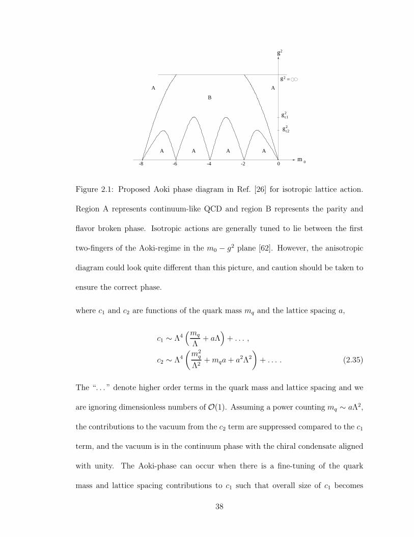
-2

A A A A

2

c2

2

m

g

-8

g

=g2

c1

0

g

2

0-4-6

B

A A

Figure 2.1: Proposed Aoki phase diagram in Ref. [26] for isotropic lattice action.

Region A represents continuum-like QCD and region B represents the parity and

flavor broken phase. Isotropic actions are generally tuned to lie between the first

two-fingers of the Aoki-regime in the m0 − g2 plane [62]. However, the anisotropic

diagram could look quite different than this picture, and caution should be taken to

ensure the correct phase.

where c1 and c2 are functions of the quark mass mq and the lattice spacing a,

c1 ∼ Λ4(mq

Λ+ aΛ

)

+ . . . ,

c2 ∼ Λ4

(

m2q

Λ2+mqa+ a2Λ2

)

+ . . . . (2.35)

The “. . . ” denote higher order terms in the quark mass and lattice spacing and we

are ignoring dimensionless numbers of O(1). Assuming a power counting mq ∼ aΛ2,

the contributions to the vacuum from the c2 term are suppressed compared to the c1

term, and the vacuum is in the continuum phase with the chiral condensate aligned

with unity. The Aoki-phase can occur when there is a fine-tuning of the quark

mass and lattice spacing contributions to c1 such that overall size of c1 becomes

38

comparable to c2. Parameterizing the Σ-field as

Σ = A+ iτ · B , (2.36)

with the constraint A2 + B2 = 1, the potential, Eq. (2.34) becomes

Vχ = −c1A+ c2A2 . (2.37)

If the minimum of the potential occurs for −1 < A0 < 1, then the vacuum

Σ0 = 〈Σ 〉 = A0 + iτ ·B0 , (2.38)

develops a non-zero value of B0, spontaneously breaking both parity and the rem-

nant vector-chiral symmetry, SU(2)V → U(1) [26], giving rise to one massive pseudo-

Goldstone pion and two massless Goldstone pions. If the minimum of the potential

occurs for Amin ≤ −1 or Amin ≥ 1 then the vacuum lies along (or opposite) the

identitiy, |A0| = 1, |B0| = 0 with the same symmetry breaking pattern as QCD.

For unimproved Wilson fermions in the isotropic limit, the leading contribu-

tions to c1 are

c1 = f 2(

mqB + asW)

. (2.39)

In the anisotropic theory, there is an additional contribution to the LO potential,

such that

c1 → cξ1 = c1 + f 2asWξ

= f 2(

mqB + asW + asWξ)

. (2.40)

If the two terms which contribute to W ∝ 2〈qσtiFtiq + qσijFijq〉 are of opposite

sign, then Wξ ∝ 〈qσtiFtiq〉 may be the dominant lattice spacing contribution to c1.

39

Therefore, the anisotropic theory may be in the Aoki-regime even when the isotropic

limit of the theory (with the same as) is not, and vice versa. This same discussion

holds for O(a)-improved actions as well but with a different power counting.

This analysis carries important consequences for anisotropic actions with domain-

wall and overlap fermions as well. These actions are generally tuned to lie between

the first two-fingers of the Aoki-regime in the m0 − g2 plane [62] as in Fig. 2.1. The

optimal value of the bare fermion mass, which provides the least amount of residual

chiral symmetry breaking, may be shifted in the anisotropic theory relative to the

isotropic value, and furthermore the allowed values of the coupling for which there

is a QCD-phase may shift as well.

2.3.2 Heavy Baryon Lagrangian

We now construct the operators in the baryon Lagrangian which encode the

leading lattice artifacts from the anisotropy. We use the heavy baryon formal-

ism [63, 64] and explicitly construct the two-flavor theory in the isospin limit in-

cluding nucleons, delta-resonances and pions. The extension of this to include the

octet and decuplet baryons is also possible. This construction builds upon previ-

ous work in which the heavy baryon Lagrangian has been extended in the isotropic

limit to include the O(a) [39] and O(a2) [40] lattice artifacts for various baryon

observables.5 The Lagrangian is constructed as a perturbative expansion about the

5In those works [39, 40], the heavy baryon Lagrangian was extended explicitly for Wilson

fermions and in the latter also for a mixed action scheme with chirally symmetric valence fermions.

In this work, we explicitly address the anisotropic effects for these two scenarios. One can also

40

static limit of the baryon, treating it as a heavy, static source as with heavy quark

effective theory [71, 72]. In building the heavy baryon chiral Lagrangian it is useful

to introduce a new chiral field,6

σ =√

Σ = exp

(

iφ

f

)

, (2.41)

which transforms under chiral rotations as

σ → LσV † = V σR† , (2.42)

with V defined by Eq. (2.42). One then dresses the baryon fields with σ such that

under chiral transformations, the nucleon and delta fields transform as

Ni → VijNj ,

Tijk → Vii′Vjj′Vkk′Ti′j′k′ , (2.43)

where N is a two-component flavor field and T is a flavor-symmetric rank-three

tensor, normalized such that

N1 = p, N2 = n,

T111 = ∆++, T112 =1√3∆+, T122 =

1√3∆0, T222 = ∆−. (2.44)

include the anisotropic effects for twisted mass [65] and staggered fermions [66, 67] following the

heavy baryon construction in Refs. [68] and [69, 70] respectively. However, we are unaware of

specific plans to generate anisotropic twisted mass or staggered fermions so we do not pursue this

here.6This field is generally denoted as ξ but to avoid confusion with the anisotropy parameter, we

use σ.

41

Both the nucleon and delta are treated as heavy matter fields and are constrained

by the relations

N =1 + /v

2N ,

Tµ =1 + /v

2Tµ (2.45)

where vµ is the four velocity of the baryon which can be chosen in its rest frame

to be vµ = (1, 0). This has the effect of projecting onto the particle component

of the field in the rest frame of the baryon. The spin-3/2 fields can be described

with a Rarita-Schwinger field, which in the heavy baryon formalism gives rise to the

constraints

v · T = 0 , S · T = 0 , (2.46)

where Sµ is a covariant spin vector [63, 64]. The simultaneous inclusion of the

nucleon and delta fields introduces a new parameter into the Lagrangian, the delta-

nucleon mass splitting in the chiral limit,

∆ = mT −mN

∣

∣

∣

mq=0, (2.47)

which is generally counted as ∆ ∼ mπ in the chiral power counting [63, 64, 73].

Because this mass parameter is a chiral singlet, it leads to a modification of all the

LECs in the heavy baryon Lagrangian. These particular effects can be systematically

accounted for be treating all LECs as polynomials in ∆ [74, 75, 76, 77]. In the isospin

limit, the heavy baryon Lagrangian, including the leading quark mass terms, the

42

leading lattice spacing terms and the leading baryon-pion couplings is given by

LNTφ = Nv ·DN + atσEN(v · uξuξ ·D)N − 2σMNNtr(M+)

+ Tµ[

v ·D + ∆]

Tµ + atσETµ(v · uξuξ ·D)Tµ − 2σM TµTµtr(M+)

+ 2gANS · AN − 2g∆∆TµS · ATµ + g∆N

[

T kjiµ A i′

i,µǫji′Nk + h.c.]

.

− 2σW NNtr(W+) − 2σξW NNtr(Wξ+) − 2σW TµTµtr(W+) − 2σξW TµTµtr(Wξ

+)

(2.48)

In this Lagrangian, the chiral symmetry breaking spurions are given by

M+ =1

2

(

σm†qσ + σ†mqσ

†) ,

W+ =as2

(

σW†σ + σ†

Wσ†) ,

Wξ+ =

as2

(

σ(Wξ)†σ + σ†W

ξσ†) , (2.49)

the chiral covariant derivative is

(DµN)i = ∂µNi + VµijNj ,

(DµT )ijk = ∂µTijk + Vµii′Ti′jk + Vµjj′Tij′k + Vµkk′Tijk′ (2.50)

and the vector and axial fields are respectively given by

Vµ =1

2

(

σ∂µσ† + σ†∂µσ

)

,

Aµ =i

2

(

σ∂µσ† − σ†∂µσ

)

. (2.51)

Relative to the Wilson extension of the heavy baryon Lagrangian in the isotropic

limit [39, 40] there is one additional mass operator for the nucleon and delta fields.

There are additionally extra derivative operators which give rise to the leading mod-

ification of the dispersion relation for the baryon fields. As in the meson chiral La-

grangian, Eq. (2.20), at fixed anisotropy, these two additional mass operators (with

43

(a) (b) (c) (d)

Figure 2.2: Diagrams contributing to the nucleon mass at LO ((a) and (b)) and NLO

((c) and (d)). Figure (a) is an insertion of the leading quark mass term proportional

to σM . Figure (b) is an insertion of the lattice spacing terms proportional to σW and

σξW . The loop graphs arise from the pion-nucleon and pion-nucleon-delta couplings.

These loop graphs generically scale as m3π but also depend upon ∆, and away from

the continuum limit upon the lattice spacing as well. All vertices in these graphs

are from the Lagrangian in Eq. (2.48).

coefficients σξW and σξW ) can not be distinguished from their counterparts which sur-

vive the isotropic limit (with coefficients σW and σW ). At this order in the lattice

spacing, O(a), the baryon-pion couplings, gA, g∆N and g∆∆, are not modified [39].

This Lagrangian, Eq. (2.48) gives rise to the LO and NLO mass corrections to the

baryon masses. For example, in Fig. 2.2 we display the graphs contributing to the

nucleon mass at O(mq), Fig. 2.2(a), O(a), Fig. 2.2(b) and O(m3/2q ), Fig. 2.2(c) and

Fig. 2.2(d). The expressions for the quark mass dependence of the nucleon and delta

masses can be found for example in Ref. [76], and the lattice spacing dependent cor-

rections to these masses for Wilson fermions in the isotropic limit can be found in

Refs. [39, 40].

At O(amq), there are two types of mass corrections, those from loop graphs

from the lattice spacing dependent operators in Eq. (2.48) and tree level terms from

44

operators in the O(amq) Lagrangian. These corrections will be identical in form to

those present in the isotropic limit, but with different numerical values due to the

new anisotropic operators which do not explicitly break the hypercubic symmetry.

The loop graphs for the nucleon and delta mass corrections are depicted in Ref. [40]

in Figs. 1 and 2 respectively. In the isospin limit, there are two tree level operators

for the nucleon and deltas each,

L(am)NTφ = − nMW NNtr(M+)tr(W+) − nξMW NNtr(M+)tr(Wξ

+)

+ tMW TµTµtr(M+)tr(W+) + tξMW TµTµtr(M+)tr(Wξ+) , (2.52)

which also function as counterterms for divergences from the above mentioned loop

graphs. As with the mesons, we must consider the O(a2) effects to see the first

explicit breaking of the anisotropy. Even in the isotropic limit, the lattice spacing

corrections to the baryons at this order proved to be quite interesting, with the

presence of the first operators which arise from the O(4) breaking down to the

hypercubic group at this order [40]. There are several generic O(a2) operators

which do not explicitly break the hypercubic group,

La2NTφ = − nWW NNtr(W+)tr(W+) − nξWW NNtr(Wξ+)tr(Wξ

+)

+ tWW TµTµtr(W+)tr(W+) + tξWW TµTµtr(Wξ+)tr(Wξ

+)

− nξWW NNtr(W+)tr(Wξ+) + tξWW TµTµtr(W+)tr(Wξ

+) , (2.53)

where the last two operators vanish for the O(a) improved action and the first two

survive the isotropic limit. The O(4) breaking operators appear at this order in the

heavy baryon Lagrangian because in the heavy baryon theory, there is an additional

45

vector, the four-velocity of the baryon one can use to construct operators. For the

mesons, the only vector is ∂µ and so the O(4) breaking operators in the meson

Lagrangian don’t appear until O(a2p4) [22]. These heavy baryon O(4) breaking

operators are [40]

LO(4)NTφ = a2

sn4 NvµvµvµvµN + a2st4 TρvµvµvµvµTρ . (2.54)

Similar to these, the O(3) breaking operators appear at this order,

LO(3)NTφ = a2

sn3 N δξµν δ

ξµν δ

ξµν δ

ξµν N + a2

st3 Tρδξµν δ

ξµν δ

ξµν δ

ξµν Tρ . (2.55)

However, even though these two sets of operators explicitly break the O(4) and O(3)

symmetries respectively, they do not lead to modifications of the dispersion relations

until higher orders [40], and thus function as mass corrections. There is a subtlety

of the heavy baryon Lagrangian related to reparameterization invariance (RPI) [78],

which constrains coefficients of certain operators in the heavy baryon Lagrangian.

For example, in the continuum limit, the LO kinetic operator of Eq. (2.48) is related

to a higher dimensional operator in such a way as to provide the correct dispersion

relation,7

L = Nv ·DN −→ Nv ·DN + ND2

⊥2MN

N , (2.56)

such that the energy of the non-relativistic nucleon is given by

E = MN +p2

2MN

+ . . . (2.57)

For the anisotropic theory, this dispersion relation is then modified by an additional

operator. While in the continuum limit, RPI constrains the coefficient in front of

7In this equation, D2

⊥ = D2 − (v ·D)2.

46

the 1/MN operator, the anisotropic action gives rise to modifications of this relation.

L = Nv ·DN + ND2

⊥2MN

N −→

Lξ = Nv ·DN + ND2

⊥2MN

N + atσENv · uξuξ ·DN + asσKEN(uξ ·D)2N . (2.58)

The resulting nucleon dispersion relation from this action yields

EN = MN +p2

2MN

−→

EN(1 + atσE) = MN (1 + atσE)− 2Nfas(σW + σξW ) +p2

2MN

+ asσKE (EN −MN )2 .

(2.59)

For the O(a)-improved action, the form of this dispersion relation stays the same

with at, as → a2t , a

2s. Comparing this dispersion relation to that of the pion,

Eq. (2.28), it is clear that even if the pion dispersion relation were tuned to be

continuum like, the nucleon dispersion relation would still contain lattice spacing

artifacts. This is a simple consequence of the fact that the LECs in the heavy

baryon Lagrangian (both the physical and unphysical) have no relation to those in

the meson chiral Lagrangian.

2.4 Discussion

In this chapter, the low-energy hadronic effective field theory including the

finite lattice spacing effects from anisotropic lattice action was developed. This

theory allows for one to calculate extrapolation formulas for hadronic processes in-

cluding pions, nucleons, and deltas. The main feature that this extension of effective

field theory includes is the effects of the hypercubic symmetry breaking present in

47

these anisotropic lattices. Additional extensions of this effective field theory could

be made for mixed action lattices (lattices in with different actions for the valence

fermions) as in Refs. [79, 80, 81, 82]. Additionally, we point out that the that these

anisotropic lattices can have an altered Aoki-phase as compared to the isotropic

case. Thus, if the isotropic action is in a QCD phase, the anisotropic theory might

still be in an Aoki-phase. Overall, this work will aid in the continuum extrapolation

of correlation functions computed with anisotropic lattices, which will be computed

in the following chapter for the pion mass, the pion decay constant, and scattering

lengths and effective ranges for I=2 ππ scattering.

48

Chapter 3

Isotropic and Anisotropic Lattice Spacing Corrections for I=2 ππ

Scattering from Effective Field Theory

3.1 Overview

Numerical scattering calculations in lattice QCD are being performed by sev-

eral collaborations. These calculations are performed through the analysis of two

hadrons in finite volume [83, 84, 85, 86]. One such scattering that has gained much

attention in the field is I=2 ππ scattering. The two-pion system is both numerically

the simplest and the best understood theoretically. In fact, in 1966, the scattering of

two pions at low energies was calculated at leading order in χPT by Weinberg [87].

The subsequent orders in the chiral expansion have been worked out next-to-leading

order by Gasser and Leutwyler [17] and next-to-next-to-leading order [88, 89, 90].

Each new order introduces more undetermined LECs. To have predictive power,

these LECs must be determined either by comparison with experiment or lattice

QCD calculational results.

Such numerical lattice QCD calculations (usually involving phase shifts and

scattering lengths) have been calculated using Wilson lattice actions [91, 92, 47,

93, 94, 95, 96, 97, 98, 99, 100, 101, 102, 103, 104, 105] along with a several other

lattice actions [106, 107, 108, 109]. Additionally, there are currently only two fully

49

dynamical, 2+1 flavor calculations of I=2 ππ scattering, which use mixed lattice

actions [110, 111] . Regardless of the action, unphysical lattice artifacts due to the

finite lattice spacings exist in the numerical results of these calculations. Therefore,

measures should be taken in order to remove these effects so that the results from

the lattice can best represent the continuum limit. The analysis in this chapter is

applicable for both isotropic and anisotropic Wilson actions.

Effective field theory provides a framework by which one can remove these

unphysical effects. Lattice spacing effects were first made explicit in chiral per-

turbation theory by Sharpe and Singleton [26]. For the Wilson action, the chiral

breaking terms that depend on the lattice spacing can be accounted for in a sim-

ilar way to the chiral breaking quark mass. Such methods have been extended

to mixed-action, partially quenched theories for mesons through O(a) and O(a2)

[27, 22, 80], and baryons through O(a) [39] and O(a2) [40, 112, 82]. Addition-

ally, Ref. [80] carries out multiple meson scattering calculations (including I=2 ππ

scattering) for mixed lattice actions and shows that for actions with chiral valence

fermions, mesonic scattering parameters in terms of the lattice-physical parameters

will have no counter-terms dependent on lattice spacing through next-to-leading

order. Alternatively, this work calculates these lattice spacing effects1 for I=2 ππ

scattering for the chiral breaking Wilson fermions in both valance and sea sectors,

and shows that these finite lattice spacing effects first appear in the next-to-leading

order counter-terms for this action.

Many collaborations are now using anisotropic lattices (lattices with different

1These effects are in addition to the finite volume corrections to I=2 ππ scattering from Ref. [113]

50

temporal and spacial lattice spacings) as opposed the the usual isotropic lattices.

Such lattices can probe higher energy states (inverse time spacings a−1t ∼ 6 GeV)

and allow for a greater resolution (more data points). However, anisotropic lat-

tices lead to new lattice artifacts, including terms that explicitly break hypercubic

symmetry. Recent work has derived these anisotropic lattice artifacts in χPT for

O(a) and O(a2) for mesons and baryons [28]. There are several I=2 ππ scattering

results published for anisotropic Wilson lattices [95, 102, 105], which can benefit

from removing these additional lattice artifacts.

This chapter presents the I=2 ππ scattering results from the isotropic χPT and

the anisotropic χPT . The pion mass and decay constant are also determined in this

context. Sec. 3.2 presents scattering on the lattice and defines the relevant quantity,

k cot δ0, used to make comparisons between χPT and the actual lattice calculation.

Next, in Sec. 3.3.1, the continuum scattering theory from χPT is formulated in

the context of this work (originally worked out before [87, 17, 90, 114]). Then, in

Sec. 3.3.2, the continuum result is extended for the isotropic Wilson lattice and

finally, in Sec. 3.3.3, the result is extended for the anisotropic Wilson lattice.

3.2 Scattering on the Lattice

The Euclidean two-hadron correlation function in infinite volume gives no

information about the Minkowski scattering amplitude (except at kinematic thresh-

olds) [115]. However, when the correlation functions of two hadrons in a finite box

are analyzed, the resulting energy levels are given by the sum of the energies of these

51

two hadrons plus an additional energy of interaction, ∆E, which is related to the

scattering phase shift, δl [83, 84, 85, 86]. The l subscript here represents the partial

wave contribution of the phase shift. In the infinite volume, the relation between

the total scattering amplitude, T (s, θ), and the partial waves amplitude, tl(s), is

given by

T (s, θ) =∞∑

l=0

(2l + 1)Pl(cos θ)tl(s), (3.1)

where s = 4(mπ2 + k2), and k is the magnitude of the 3-momentum of the incoming

particle in the center-of-mass frame. The partial scattering amplitude tl(s) is related

to the phase shift, δl by

tl(s) = 32π

√

s

s− 4mπ2

1

2i[e2iδl(s) − 1] = 32π

√

s

s− 4mπ2

1

cot δl − i. (3.2)

These relations allow one to compare the calculated scattering amplitude (in

χPT ) to the lattice calculation of δl. The s-wave (l = 0) scattering amplitude

is the dominant contribution to the total scattering amplitude in most low energy

scattering processes and gives the cleanest signal in the lattice calculation. The

s-wave projection of the continuum scattering amplitude, t0(s), is

t0(s) =1

2

∫ 1

−1

T (s, θ) d(cos θ). (3.3)

This s-wave scattering amplitude will be the scattering amplitude analyzed

throughout the rest of this paper. Following the discussion in Ref. [113], through

one loop order in perturbation theory in Minkowski space, t0(s) can be written as

52

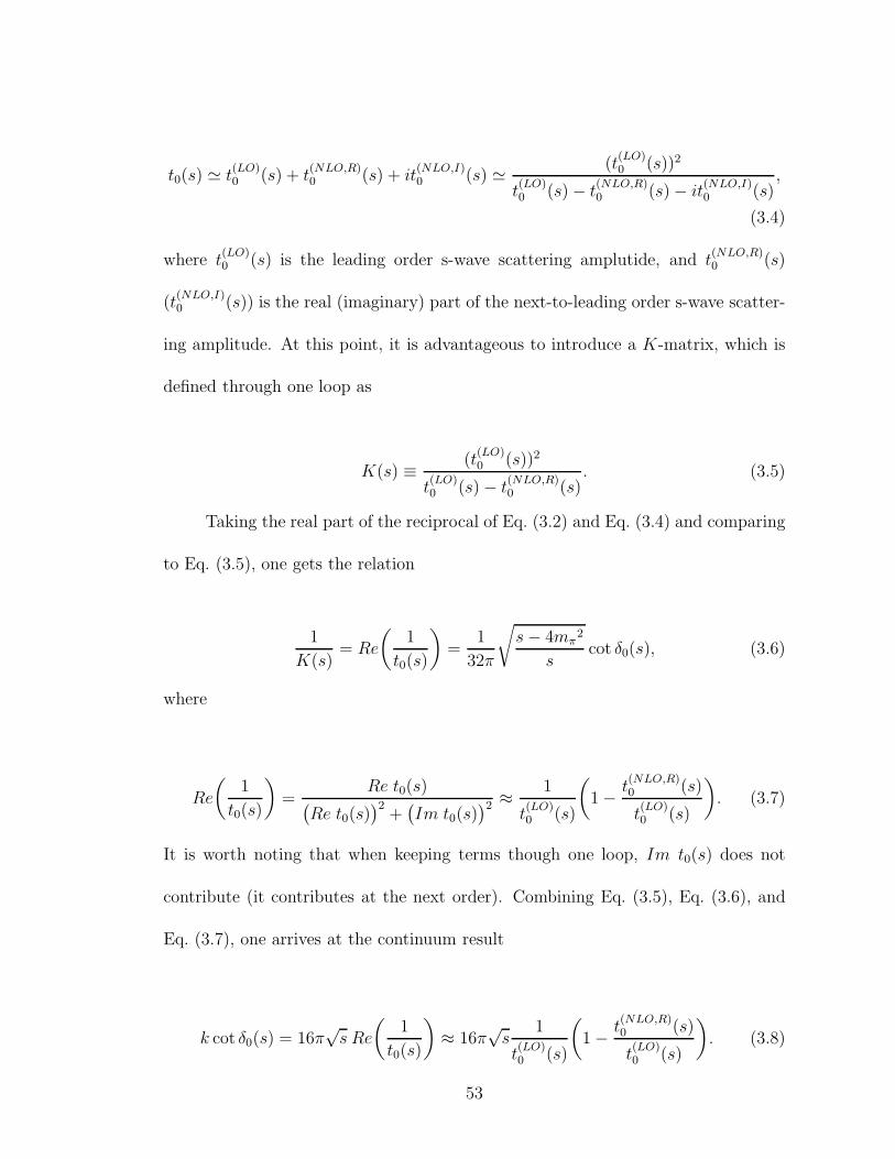
t0(s) ≃ t(LO)0 (s) + t

(NLO,R)0 (s) + it

(NLO,I)0 (s) ≃ (t

(LO)0 (s))2

t(LO)0 (s) − t

(NLO,R)0 (s) − it

(NLO,I)0 (s)

,

(3.4)

where t(LO)0 (s) is the leading order s-wave scattering amplutide, and t

(NLO,R)0 (s)

(t(NLO,I)0 (s)) is the real (imaginary) part of the next-to-leading order s-wave scatter-

ing amplitude. At this point, it is advantageous to introduce a K-matrix, which is

defined through one loop as

K(s) ≡ (t(LO)0 (s))2

t(LO)0 (s) − t

(NLO,R)0 (s)

. (3.5)

Taking the real part of the reciprocal of Eq. (3.2) and Eq. (3.4) and comparing

to Eq. (3.5), one gets the relation

1

K(s)= Re

(

1

t0(s)

)

=1

32π

√

s− 4mπ2

scot δ0(s), (3.6)

where

Re

(

1

t0(s)

)

=Re t0(s)

(

Re t0(s))2

+(

Im t0(s))2 ≈ 1

t(LO)0 (s)

(

1 − t(NLO,R)0 (s)

t(LO)0 (s)

)

. (3.7)

It is worth noting that when keeping terms though one loop, Im t0(s) does not

contribute (it contributes at the next order). Combining Eq. (3.5), Eq. (3.6), and

Eq. (3.7), one arrives at the continuum result

k cot δ0(s) = 16π√s Re

(

1

t0(s)

)

≈ 16π√s

1

t(LO)0 (s)

(

1 − t(NLO,R)0 (s)

t(LO)0 (s)

)

. (3.8)

53

As previously mentioned, lattice scattering calculations are performed in Eu-

clidean space at finite volume. The Euclidean amputated four-point correlator from

the lattice, τ0(s), is given by

τ0(s) ≃(t

(LO)0 (s))2

t(LO)0 (s) − t

(NLO,R)0 (s) − ∆t0(s) − (t

(LO)0 )2

16π2L√sS(

(s−4mπ2)L2

4π2

) , (3.9)

where ∆t0(s) represents all of the non-physical lattice artifacts (lattice spacing er-

rors, finite volume errors ,etc.), s is related to the energy of interaction, ∆E, and

S is a universal function of s [85, 116, 117]. If both pions in the box start with no

external momentum, then s = (∆E+2mπ)2. In this paper, the only effect from lat-

tice artifacts that will be included in ∆t0 is the lattice spacing effect. Manipulating

Eq. (3.9):

τ0(s) ≃1

1K(s)

− ∆t0(s)

(t(LO)0 )2

− 116π2L

√sS(

(s−4mπ2)L2

16π2

)

=16π

√s

k cot δ0(s) − 16π√s ∆t0(s)

(t(LO)0 )2

− 1πL

S(

(s−4mπ2)L2

16π2

) . (3.10)

The energy states are given by the poles of Eq. (3.10), which are given by [113]

k cot δ0 + ∆(k cot δ0) =1

πLS(

(s− 4mπ2)L

16π2

)

, (3.11)

where

∆(k cot δ0) = −16π√s

∆t0(s)

(t(LO)0 )2

. (3.12)

In general, most lattice calculations give their results in terms of the scattering

length, aI=2ππ . One can extract the scattering length and the effective range, rI=2

ππ ,

54

via the expansion of k cot δ0:

k cot δ0 =1

aI=2ππ

+1

2rI=2ππ k

2 + · · · . (3.13)

It is important to note that the prescription given above for finding the scat-

tering length and effective range implies that the lattice artifacts, ∆(k cot δ0), have

already been subtracted before the expansion. In this paper, continuum results are

given in terms of k cot δ0 and lattice artifacts are given in terms of ∆(k cot δ0).

For results given in terms of the scattering length and effective range, one can

relate Eq. (3.13) to the left hand side of Eq. (3.11) to arrive at

k cot δ0 + ∆(k cot δ0) =

(

1

aI=2ππ

+ ∆( 1

aI=2ππ

)

)

+1

2

(

rI=2ππ + ∆rI=2

ππ

)

k2 + · · · , (3.14)

where

∆( 1

aI=2ππ

)

= ∆(k cot δ0)|k2=0, (3.15)

and

∆rI=2ππ = 2

d(

∆(k cot δ0))

dk2

∣

∣

∣

∣

k2=0

. (3.16)

While these relations are not too complicated, they do add additional steps

to the calculation when compared to working with only k cot δ0 and ∆(k cot δ0).

Therefore, if one wants to extract the scattering length and effective range from the

lattice calculation, one should first subtract ∆(k cot δ0) from the right hand side of

55

Eq. (3.11) and then expand to determine the individual parameters2. This paper

relates k cot δ0 and ∆(k cot δ0) to the effective field theory of the lattice.

3.3 Chiral Perturbation Theory Results for k cot δ0 and ∆(k cot δ0)

In leading order and next-to-leading-order chiral perturbation theory, it is

necessary to introduce several undetermined LECs in order properly account for

corrections and counter-terms. The number of independent LECs in the continuum

depends on whether there are two flavors or more. For I=2 ππ scattering being

calculated here, only two flavor χPT (SU(2)L⊗SU(2)R chiral symmetry) is needed

for extrapolation.

3.3.1 Continuum

From the continuum χPT Lagrangian, one can predict numerous results for

different low energy processes involving hadrons. However, the extent of the accu-

racy of these predictions are ultimately tied to how well the LECs are known. For

this reason, there has been much effort in the lattice community to try to determine

these values [118, 119, 120, 121, 122].

The continuum Lagrangian in χPT is determined order by order in Bmq and

p2. The Lagrangian through O(p4) for two flavors is given by [17]

2Current numerical calculations can only determine k cot δ0 for a limited number of k values.

This leads to inaccuracies in expansions of k2 and adds difficulty to finding the effective range.

56

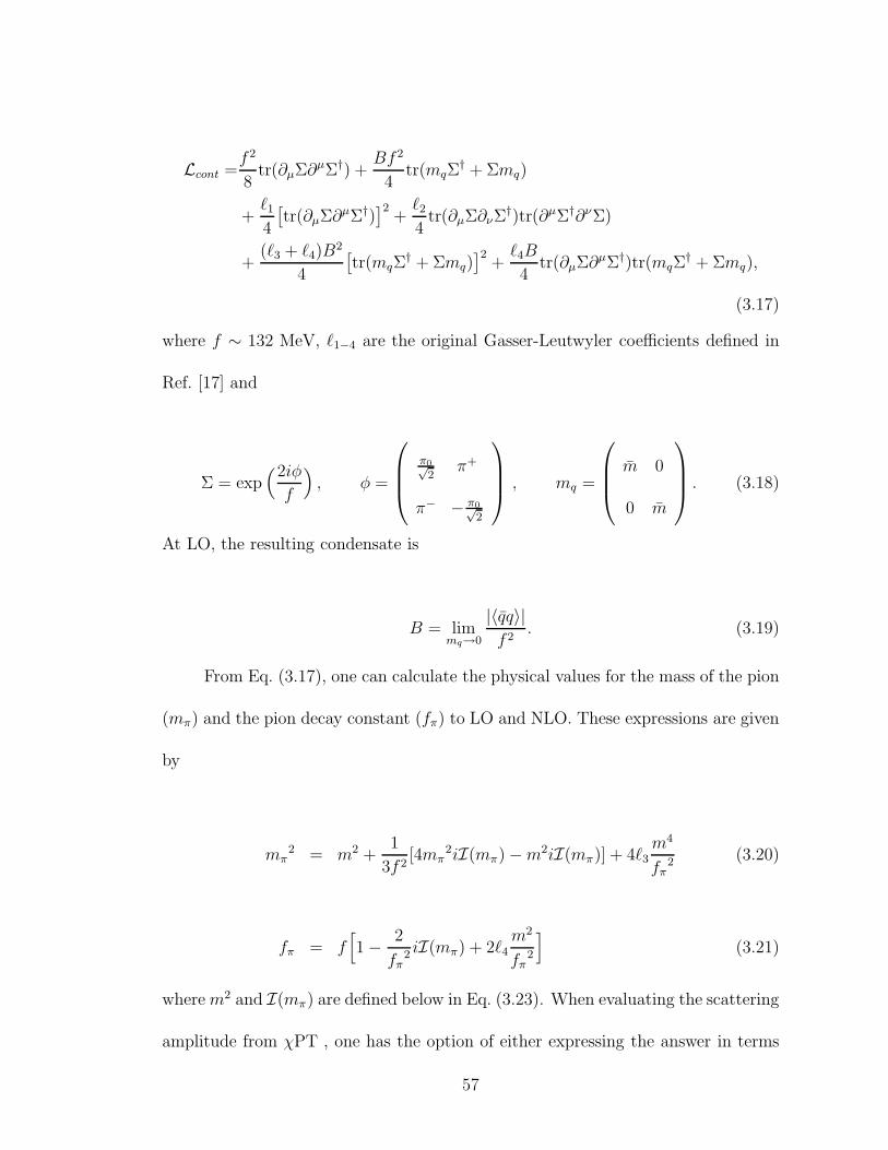
Lcont =f 2

8tr(∂µΣ∂

µΣ†) +Bf 2

4tr(mqΣ

† + Σmq)

+ℓ14

[

tr(∂µΣ∂µΣ†)

]2+ℓ24

tr(∂µΣ∂νΣ†)tr(∂µΣ†∂νΣ)

+(ℓ3 + ℓ4)B

2

4

[

tr(mqΣ† + Σmq)

]2+ℓ4B

4tr(∂µΣ∂

µΣ†)tr(mqΣ† + Σmq),

(3.17)

where f ∼ 132 MeV, ℓ1−4 are the original Gasser-Leutwyler coefficients defined in

Ref. [17] and

Σ = exp(2iφ

f

)

, φ =

π0√2

π+

π− − π0√2

, mq =

m 0

0 m

. (3.18)

At LO, the resulting condensate is

B = limmq→0

|〈qq〉|f 2

. (3.19)

From Eq. (3.17), one can calculate the physical values for the mass of the pion

(mπ) and the pion decay constant (fπ) to LO and NLO. These expressions are given

by

mπ2 = m2 +

1

3f 2[4mπ

2iI(mπ) −m2iI(mπ)] + 4ℓ3m4

fπ2 (3.20)

fπ = f[

1 − 2

fπ2 iI(mπ) + 2ℓ4

m2

fπ2

]

(3.21)

wherem2 and I(mπ) are defined below in Eq. (3.23). When evaluating the scattering

amplitude from χPT , one has the option of either expressing the answer in terms

57

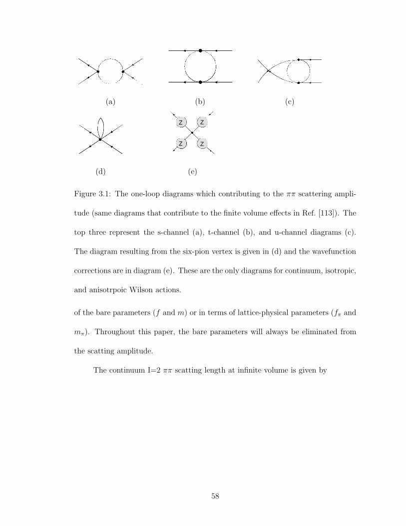
(a) (b) (c)

Z

Z

Z

Z

(d) (e)

Figure 3.1: The one-loop diagrams which contributing to the ππ scattering ampli-

tude (same diagrams that contribute to the finite volume effects in Ref. [113]). The

top three represent the s-channel (a), t-channel (b), and u-channel diagrams (c).

The diagram resulting from the six-pion vertex is given in (d) and the wavefunction

corrections are in diagram (e). These are the only diagrams for continuum, isotropic,

and anisotrpoic Wilson actions.

of the bare parameters (f and m) or in terms of lattice-physical parameters (fπ and

mπ). Throughout this paper, the bare parameters will always be eliminated from

the scatting amplitude.

The continuum I=2 ππ scatting length at infinite volume is given by

58

Tcont = − 2

fπ2

s− 2mπ2 − 2(3s− 4mπ

2)

3fπ2 iI(mπ) +

(s− 2mπ2)2

fπ2 iJ (mπ, ps)

+1

3fπ2

[

3(t2 −mπ4) + t(t− s) − 2tmπ

2 + 4smπ2 − 2mπ

4]

iJ (mπ, pt)

+1

3fπ2

[

3(u2 −mπ4) + u(u− s) − 2umπ

2 + 4smπ2 − 2mπ

4]

iJ (mπ, pu)

− 1

9(4πfπ)2

[

2s2 + 6smπ2 − 8mπ

4 − t2 − u2]

− 4ℓ1

fπ2

[

(t− 2mπ2)2 + (u− 2mπ

2)2]

− 2ℓ2

fπ2

[

2(s− 2mπ2)2 + (t− 2mπ

2)2 + (u− 2mπ2)2]

− 8ℓ3mπ

4

fπ2 + 4ℓ4

mπ2(s− 2mπ

2)

fπ2

(3.22)

where

m2 = 2Bm

I(mπ) =

∫

R

d4k

(2π)4

1

k2 −m2

J (mπ, P ) =

∫

R

d4k

(2π)4

1

[(k + P )2 −m2]

1

[k2 −m2]. (3.23)

This scatting amplitude includes all the partial wave contributions (this T is

the same as the T (s, θ) that appears in Eq. (3.1)). When projecting on the s-wave,

expanding through O(k2/mπ2) and using Eq. (3.8), the result for k cot δ0(for the

regularization and renormalization scheme defined in Ref. [90]) is

59

k cot δ0 ≈ −8πfπ2

mπ

(

1 − mπ2

(4πfπ)2

[

3 ln(mπ

2

µ2

)

− 1 + ℓaππ(µ)]

)

− 1

2

(

3 +mπ

2

(4πfπ)2

[17

3ln(mπ

2

µ2

)

+31

3+ ℓrππ(µ)

]

)

k2

mπ2

+ · · ·

,

(3.24)

where ℓaππ(µ) and ℓrππ(µ) are linear combinations of the Gasser-Leutwyler co-

efficients given by [90]

ℓaππ(µ) = − 4(4π)2(

4(

ℓR1 (µ) + ℓR2 (µ))

+(

ℓR3 (µ) − ℓR4 (µ))

)

,

ℓrππ(µ) =4(4π)2(

12ℓR1 (µ) + 4ℓR2 (µ) + 7ℓR3 (µ) − 3ℓR4 (µ))

. (3.25)

The superscript R represents the renormalized Gasser-Leutwyler coefficients with

scale-dependence.

In order for these continuum predictions from χPT to be useful in a phys-

ical context, one needs to determine the values for ℓaππ(µ) and ℓrππ(µ), which are

undetermined from χPT alone. While numerous values have been quoted for the

Gasser-Leutwyler coefficients [122], it is still beneficial to determine these values

with more precesion. Therefore, it is prudent to use various lattice calculations at

different pion masses determine these values. However, since the lattice calculations

are performed with discretized space and time, one needs to remove these lattice

artifacts to extract the continuum result.

60

3.3.2 Isotropic Discretization

To calculate finite lattice spacing corrections to I=2 ππ scattering for the

isotropic Wilson action, one can follow the same steps done in the continuum

case, but starting from a Lagrangian which includes these lattice spacing artifacts.

The analysis on lattice spacing effects was done for the Symanzik action by Sheik-

holeslami and Wohlert [20]. From this analysis, the Lagrangian was made explicit

in χPT by Sharpe and Singleton [26], followed by Bar, Rupak, and Shoresh [27, 22].

The power counting they used for this χPT Lagrangian is

asW ∼ Bmq ∼ p2 ∼ ǫ, (3.26)

where as is the lattice spacing (same spacing in space and time direction) and W is

a condensate defined below. The simplified two flavor Lagrangian to O(ǫ2) is

Liso =Lcont + ∆Liso. (3.27)

∆Liso =asWf 2

4tr(Σ† + Σ) +

(w3 + w4)asWB0

4tr(mqΣ

† + Σmq)tr(Σ† + Σ)

+w′

3(asW )2

4

[

tr(Σ† + Σ)]2

+w4asW

4tr(∂µΣ∂

µΣ†)tr(Σ† + Σ) (3.28)

This Lagrangian is similar to Eq. (3.17) with one new term at LO and three

new terms at NLO. All new terms are proportional to as or a2s, which will vanish in

the continuum limit as as → 0. At LO, there is a new condensate given by

W = limmq→0

cSW〈qσµνF µνq〉

f 2. (3.29)

61

The new LECs at NLO are given by w3, w′3, and w4. All these new terms obey

the same symmetries as the Lagrangian in the continuum case and break chiral

symmetry in a similar way to the quark mass. It should also be noted that these

new LECs depend on as ln as as well (as opposed to the Gasser-Leutwyler coefficients

that have no dependence on the mass term).

Furthermore, Ref. [123] showed that the axial current (needed to calculate fπ)

has an additional term at this order in χPT given by

∆Aaµ = 2awA∂µtr(

σa(Σ − Σ†))

. (3.30)

This term (which can also be inferred from Ref. [124]) leads to modifications of

the LECs as well as the coefficient in front of the chiral logarithm in fπ. Thus,

this coefficient has dependence on the lattice artifacts at NNLO. Ref. [123] also

points out that the condition for fixing the renormalization factor, ZA, of the lattice

currents needs to be mapped onto χPT 3. From this Lagrangian, fπ and mπ through

NLO are [27, 22, 123]

mπ2 = (m2 + 2asW ) +

1

3f 2[4mπ

2iI(mπ) − (m2 + 2asW )iI(mπ)]

+4ℓ3m4

fπ2 + 8w3

asWm2

fπ2 + 16w′

3

(asW )2

fπ2 (3.31)

fπ = f[

1 − 2

fπ2 iI(mπ) + 2ℓ4

m2

fπ2 + 4weff

asW

fπ2

]

, (3.32)

3The condition for fixing ZA is chosen by individual lattice calculations. Ref. [123] shows an

example of this in χPT by using the chiral Ward identities in infinite volume, which leads to fπ

being free lattice artifacts until NNLO.

62

where weff in fπ includes w4 and wA and can vary based on the given renormalization

condition for the axial current.

To acquire the continuum result of these quantities, one needs to remove all

the terms with dependence on as or a2s. The resulting I=2 ππ scatting amplitude

with the physical parameters restored is given by

Tiso = Tcont + ∆Tiso, (3.33)

where the mπ and fπ in Tcont are given by Eq. (3.31) and Eq. (3.32) and ∆Tiso is

given by

∆Tiso = − 2

fπ2

− 16(w3 − 2ℓ3)asWmπ

2

fπ2 − 32(w′

3 − w3 + ℓ3)(asW )2

fπ2

+ 8(weff − ℓ4)asW (s− 2mπ

2)

fπ2

. (3.34)

It is worth noting that by restoring the physical parameters, m2 does not

appear, and asW only appears in the terms containing the LECs (the ℓ and w

terms). This is a bit different than the continuum case where one could eliminate

m2 with only mπ2. Now, one eliminates m2 with (mπ

2 − 2asW ), and thus, several

LECs are multiplied by factors of asW . In addition, all of the continuum results

without LECs remain unchanged since each vertex will only contribute mπ2 when

the physical parameters are restored. Using the relation in Eq. (3.12), the resulting

artifact for the isotropic Wilson lattice, ∆(k cot δ0)iso is given by

63

∆(k cot δ0)iso ≈mπ

2π

(

waππ(µ)asW

mπ2

+ w′aππ(µ)

(asW )2

mπ4

)

− 1

2

(

wrππ(µ)asW

mπ2

+ 7w′aππ(µ)

(asW )2

mπ4

)

k2

mπ2

+ · · ·

, (3.35)

where

waππ(µ) = − 8(4π)2(

wR3 (µ) − wReff(µ) − 2ℓR3 (µ) + ℓR4 (µ))

,

w′aππ(µ) = − 16(4π)2

(

w′R3 (µ) − wR3 (µ) + ℓR3 (µ)

)

,

wrππ(µ) = − 8(4π)2(

7wR3 (µ) − 3wReff(µ) − 14ℓR3 (µ) + 3ℓR4 (µ))

. (3.36)

As seen in the results, the artifacts from the isotropic lattice that are present

in the final form are either linear or quadratic in as. By using results that differ in

lattice spacing, one can pick off the coefficients of these artifacts and remove them

from the final result. If one is working with a perfectly clover-improved Wilson

lattice, this would remove all O(as) effects leaving only the O(a2s) effects. It is also

important to note that there is no physical information gained by determining spe-

cific LECs that are a result of the isotropic lattice spacing (the individual w terms)

unlike determining specific Gasser-Leutwyler coefficents. Therefore, the useful co-

efficient to extract is the linear combination of these terms so they can be removed

from the final result.

At this point, one can compare these lattice spacing effects for the Wilson

action to those found for the mixed action (with chiral valence fermions) in Ref. [79,

80]. For this mixed action case, when in terms of the lattice-physical parameters,

64

there is no lattice spacing dependence through the NLO counter-terms. In contrast,

when the lattice-physical parameters are restored in the Wilson action, these effects

first appear at the NLO counter-terms. Thus, these additional effects that are not

present at NLO in the mixed action calculation will need to be removed for the

Wilson action calculation.

3.3.3 Anisotropic Discretization

With the recent formulation of χPT for the anisotropic lattice [28], one can

begin calculating corrections to various quantities of interest on the lattice. This

process is, in general, very similar to calculations in the continuum and isotropic

lattices, but one now picks up additional terms that are a result of having different

spacial and temporal spacings. To help extract these effects in a more simplistic

notation, the superscript ξ has been added to all the new terms resulting from this

anisotropy. In practice, the anisotropic lattice picks up two new non-perturbative

parameters: the parameter ξ = as/at which is the measure of anisotropy and the

parameter ν, which is used to correct the “speed of light” [58, 59, 125]. By set-

ting both parameters to 1, the isotropic limit is recovered. In addition to the W

condensate defined in Eq. (3.29), we pick up a W ξ condensate that is given by

W ξ = limmq→0

cξSW (uξ)µ(uξ)ν〈qσµλF νλq〉

f 2. (3.37)

where uξµ is a vector that breaks hypercubic invariance. It is important to note that

the convention chosen for uξµ appears in the anisotropic χPT and its observables.

For convenience, we choose this vector to be uξµ = (1, 0). The condensates and the

65

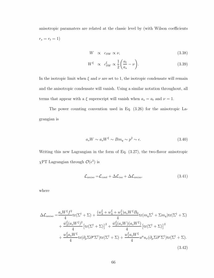
anisotropic paramaters are related at the classic level by (with Wilson coefficients

rs = rt = 1)

W ∝ cSW ∝ ν, (3.38)

W ξ ∝ cξSW ∝ 1

2

(

atas

− ν

)

. (3.39)

In the isotropic limit when ξ and ν are set to 1, the isotropic condensate will remain

and the anisotropic condensate will vanish. Using a similar notation throughout, all

terms that appear with a ξ superscript will vanish when as = at and ν = 1.

The power counting convention used in Eq. (3.26) for the anisotropic La-

grangian is

asW ∼ asWξ ∼ Bmq ∼ p2 ∼ ǫ. (3.40)

Writing this new Lagrangian in the form of Eq. (3.27), the two-flavor anisotropic

χPT Lagrangian through O(ǫ2) is

Laniso =Lcont + ∆Liso + ∆Laniso. (3.41)

where

∆Laniso =asW

ξf 2

4tr(Σ† + Σ) +

(wξ3 + wξ4 + wξ1)asWξB0

4tr(mqΣ

† + Σmq)tr(Σ† + Σ)

+wξ3(asW

ξ)2

4

[

tr(Σ† + Σ)]2

+wξ3(asW )(asW

ξ)

4

[

tr(Σ† + Σ)]2

+wξ4asW

ξ

4tr(∂µΣ∂

µΣ†)tr(Σ† + Σ) +wξ1asW

ξ

4uµuν(∂µΣ∂

νΣ†)tr(Σ† + Σ).

(3.42)

66

In addition to the anisotropic condensate W ξ mentioned above at LO, there

are five new LECs at NLO as a result of this anisotropy. Four of these new LECs

obey the same symmetry structure as the isotropic terms, however the ωξ1 term

additionally breaks hypercubic invariance. Therefore, this term only corrects the

time derivative, but not the spacial one (for the convention of uξµ chosen). As a

result, fπ is parameterized by two constants; f tπ, which is fπ measured in time,

and f sπ, which is fπ measured in space. This leads to one correction for the space-

measured f sπ and a separate correction for the f tπ. The pion mass (mπ), the time-

measured pion decay constant (f tπ), and the space-measured pion decay constant

(f sπ) through NLO are

mπ2 = (m2 + 2asW + 2asW

ξ) +1

3f 2[4mπ

2iI(mπ) − (m2 + 2asW + 2asWξ)iI(mπ)]

+4ℓ3m4

f tπ2 + 8w3

asWm2

f tπ2 + 16w′

3

(asW )2

f tπ2

+8wξ3asW

ξm2

f tπ2 + 16wξ3

(asWξ)2

f tπ2 + 16wξ3

(asW )(asWξ)

f tπ2 (3.43)

f tπ = f[

1 − 2

f tπ2 iI(mπ) + 2ℓ4

m2

f tπ2 + 4w4

asW

f tπ2 + 4(wξeff + wξ1)

asWξ

f tπ2

]

(3.44)

f sπ = f[

1 − 2

f tπ2 iI(mπ) + 2ℓ4

m2

f tπ2 + 4w4

asW

f tπ2 + 4wξeff

asWξ

f tπ2

]

, (3.45)

where, as in the isotropic case, the wξeff depends on the renormalization condition

for the axial current (this LEC is the same for both f tπ and f sπ).

For the rest of this section, all calculations are given in terms of mπ and f tπ.

67

As mentioned before, how one accounts for the effect of this hypercubic breaking

term depends on the convention. In the convention used here, only f tπ sees the effect

of this term and f sπ does not. The scatting amplitude is given by

Tiso = Tcont + ∆Tiso + ∆Taniso (3.46)

where the mπ and f tπ in Tcont are given by Eq. (3.43) and Eq. (3.44) and ∆Taniso is

given by

∆Taniso = − 2

(f tπ)2

− 16(wξ3 − 2ℓ3)asW

ξmπ2

(f tπ)2

− 32(wξ3 − wξ3 + ℓ3)(asW

ξ)2

(f tπ)2

− 32(wξ3 − w3 − wξ3 + 2ℓ3)(asW )(asW

ξ)

(f tπ)2

+ 8(wξeff + wξ1 − ℓ4)asW

ξ(s− 2mπ2)

(f tπ)2

− 16wξ1asW

ξk2

(f tπ)2

. (3.47)

Most of the effects in this scattering amplitude are similar to the isotropic

case, except now there are also expansions in asWξ in addition to the expansions in

asW . Thus, as expected, if all the anisotropic effects are removed, only the isotropic

limit remains. The only new symmetry breaking effect is the w1 term which is not

a hypercubic invariant term. In other words, all of the hypercubic breaking due to

anisotropy at this order is contained in this term. However, it’s effects in ∆Taniso

appear as just another contribution to the linear combination of the LECs in front of

the term asWξ. Therefore, it is difficult to determine the effect of the the hypercubic

breaking term alone from ∆Taniso since its effects will be mixed in with the other

anisotropic LECs4. The resulting artifacts for the anisotropic Wilson lattice are

4The total hypercubic breaking effect would be more visible from the differences of f tπ and fs

π

68

the isotropic artifacts, ∆(k cot δ0)iso, and the anisotropic artifacts, ∆(k cot δ0)aniso.

Therefore, the total effect of the lattice artifacts due to lattice spacings are

∆(k cot δ0) = ∆(k cot δ0)iso + ∆(k cot δ0)aniso. (3.48)

The anisotropic lattice artifacts are given by

∆(k cot δ0)aniso ≈mπ

2π

(

wξaππ(µ)asW

ξ

mπ2

+ wξaππ(µ)(asW

ξ)2

mπ4

+ wξaππ(µ)(asW )(asW

ξ)

mπ4

)

− 1

2

(

wξrππ(µ)asW

ξ

mπ2

+ 7w′ξaππ (µ)

(asWξ)2

mπ4

+ 7wξaππ(µ)(asW )(asW

ξ)

mπ4

)

k2

mπ2

+ · · ·

, (3.49)

where

wξaππ(µ) = − 8(4π)2(

wξR3 (µ) − wξReff(µ) + wξR1 (µ) − 2ℓR3 (µ) + ℓR4 (µ))

,

wξaππ(µ) = − 16(4π)2(

w′R3 (µ) − wR3 (µ) + ℓR3 (µ)

)

,

wξaππ(µ) = − 16(4π)2(

wξR3 (µ) − wR3 (µ) − wξR3 (µ) + 2ℓR3 (µ))

,

wξrππ(µ) = − 8(4π)2(

7wξR3 (µ) + 9wξReff(µ) + wξR1 (µ) − 14ℓR3 (µ) − 9ℓR4 (µ))

. (3.50)

As a result, the ultimate effects of the anisotropic lattice on ∆(k cot δ0) are

more terms that will require variation of as and at independently to fit. Three

more terms require fitting to correct the constant term in the expansion and one

more term requires fitting for the O(k2/mπ2) term in order to remove it’s effects. As

mentioned with the isotropic correction, no physical information is gained by picking

69

off the individual anisotropic LECs. Analogous to the isotropic case, the anisotropic

Wilson action first has lattice spacing dependence at the NLO counter-terms. The

aim here is to determine these linear combinations and remove their effects from the

lattice measurements.

3.4 Discussion

In this work, I=2 ππ scattering was calculated from the χPT for isotropic

and anisotropic lattice spacings. Also, connections between these χPT calculations

and the k cot δ0 value measured from lattice calculations were illustrated. When

∆(k cot δ0) is given in terms of the lattice-physical parameters, these lattice spacing

effects first appear at the NLO LECs and can be removed from the result of the

lattice calculation. However, ∆(k cot δ0) has numerous undetermined linear combi-

nations of LECs, which would need to be determined (by fitting several different

lattice spacings) in order to successfully remove it from the lattice result. Therefore,

as more lattice calculations of ππ scattering are completed (for both isotropic and

anisotropic lattice spacings), these combinations of LECs can be determined better,

which will result in a more accurate result after these lattice artifacts are removed.

70

Chapter 4

ππ Scattering in Twisted Mass Chiral Perturbation Theory

4.1 Overview

Calculations of hadron interactions from lattice QCD have received signif-

icant attention in recent years [126], with dynamical calculations of two-meson

systems [101, 110, 111, 127, 128], two-baryon systems [48, 49] and systems of up

to 12 pions [129, 130] and kaons [131]. Additionally, lattice methods are cur-

rently being applied to the low-energy effective field theory of multinucleon in-

teractions [132, 133, 134, 135, 136, 137, 138, 139], for which there exists a nice

review [140]. The majority of the dynamical lattice QCD calculations of hadron

interactions to date, have either been performed with Wilson fermions or a mixed

lattice action [141, 142] of domain-wall valence fermions [9, 10, 11] and the Asqtad

improved [143, 144] rooted staggered MILC configurations [145, 146]. Twisted mass

lattice QCD [147, 65] has recently emerged as a viable fermion discretization method

for lattice calculations with two flavors of light quarks, (up and down) [119, 148, 149]

and hopeful prospects of 2 + 1 + 1 (up, down, strange and charm) flavors of dy-

namical sea fermions [150] in the chiral regime. Therefore, it is natural that hadron

interactions will be computed with the twisted mass fermion discretization method,

and initial twisted mass results for I=2 ππ interactions have been recently published

71

[31, 32]1.

To truly understand the twisted mass results of I=2 ππ interactions, the sys-

tematic effects due to lattice artifacts must first be understood. Lattice discretiza-

tion effects can be incorporated into the chiral Lagrangian through a two-step pro-

cess first detailed in Ref. [26]. One first constructs the effective continuum Symanzik

Lagrangian [18, 19] for a given lattice action. One then builds the low energy chiral

Lagrangian from the Symanzik theory, giving rise to new unphysical operators with

their own LECs. These new operators capture the discretization effects for a given

lattice action. This process is spelled out for the Wilson action in Chapter 1.

In this chapter, we briefly review the construction of the twisted mass chiral

Lagrangian in Sec. 4.2. We then determine the lattice spacing (b) corrections to low-

energy ππ scattering specific to the twisted mass lattice action. We work through

O(b2) ∼ O(bm2π).

4.2 Twisted mass lattice QCD and the continuum effective action

The twisted mass chiral Lagrangian was determined previously in Refs. [151,

152, 153, 154, 124], and for baryons in Ref. [68]. In this work, we focus on twisted

mass lattice QCD with degenerate light flavors given by the lattice action

S =∑

x

ψ(x)

[

1

2

∑

ν

γν(∇∗ν + ∇ν) −

r

2

∑

ν

∇∗ν∇ν

+m0 + iγ5τ3µ0

]

ψ(x) , (4.1)

1These references made use of the work developed in this chapter

72

where ψ and ψ are the dimensionless lattice fermion fields, ∇ν(∇∗ν) are the covariant

forward (backward) lattice derivatives in the ν direction, m0 is the dimensionless

bare quark mass and µ0 is the dimensionless bare twisted quark mass. The fermion

fields are flavor doublets, τ3 is the third Pauli-spin matrix and the bare mass term is

implicitly accompanied by a flavor identity matrix. Our twisted mass χPT analysis

also holds for dynamical lattice calculations with 2+1+1 flavors, the only difference

being the numerical values of the LECs determined when fitting the extrapolation

formula to the calculation results. This action is beneficial in several ways. While it

has a term that breaks parity, it contains a parity⊗

flavor symmetry that prevents

unwanted radiative corrections. However, this term, which is referred to as the

twisted mass term, is a mass term that multiplicatively renormalized akin to how the

quark mass term is in continuum QCD. This prevents issues involving exceptional

configurations. Additionally, for certain choices of m0 and µ0 parameters, known as

maximal twist, this action can additionally be O(a) improved without including a

Sheikholeslami-Wohlert term.

The continuum chiral Lagrangian, supplemented by discretization effects is

determined with the two step procedure of Ref. [26]. This was done for the twisted

mass lattice action in Ref. [153], to NLO in which a power counting mq ∼ bΛ2QCD

was used and which we shall adopt. The resulting effective Lagrangian is

Leff = Lglue + q(D/ +m+ iγ5τ3µ)q

+ cSW b q iσµνFµνq + O(b2, bmq, m2q) , (4.2)

where Lglue is the Yang-Mills Lagrangian. The quark fields are an isodoublet, qT =

73

(qu, qd) and the quark masses are given by

m = Zm(m0 −mc)/b ,

µ = Zµµ0/b . (4.3)

The symmetry properties of the twisted mass lattice action protect the twisted mass

from additive mass renormalization. With Eq. (4.2), one can construct the two flavor

chiral Lagrangian. This is the Gasser-Leutwyler Lagrangian [17] supplemented by

chiral and flavor symmetry breaking terms proportional to the lattice spacing. The

Lagrangian through NLO relevant to our work takes the form [153, 124],

Ltwχ =f 2

8tr(∂µΣ∂µΣ

†) − f 2

8tr(χ′†Σ + Σ†χ′) − l1

4tr(∂µΣ∂µΣ

†)2 − l24

tr(∂µΣ∂νΣ†)tr(∂µΣ∂νΣ

†)

− l3 + l416

[

tr(χ′†Σ + Σ†χ′)]2

+l48

tr(∂µΣ∂µΣ†)tr(χ′†Σ + Σ†χ′)

+ W tr(∂µΣ∂µΣ†)tr(A†Σ + Σ†A) −W tr(χ′†Σ + Σ†χ′)tr(A†Σ + Σ†A)

−W ′[

tr(A†Σ + Σ†A)]2

, (4.4)

where the LECs, l1–l4 are the SU(2) Gasser-Leutwyler coefficients and the

coefficients W , W and W ′ are unphysical LECs arising from the explicit chiral

symmetry breaking of the twisted mass lattice action. The spurion fields are defined

as

χ′ = 2B0(m+ iτ3µ) + 2W0b ≡ m+ iτ3µ+ b

A = 2W0b ≡ b . (4.5)

As discussed in Ref. [124], the vacuum of the theory as written is not aligned with

74

the flavor identity but is given at LO by

Σ0 ≡ 〈0|Σ|0〉 =m+ b+ iτ3µ

M ′ = exp(iω0τ3) , (4.6)

with

M ′ =

√

(m+ b)2 + µ2 . (4.7)

Therefore, to determine the Feynman rules which leave the interactions of the theory

the most transparent, one expands the Lagrangian around the physical vacuum.

Extending this analysis to NLO, one finds the vacuum angle shifts to ω = ω0 + ǫ

where one can determine ǫ either by finding the minimum of the potential, as was

done in Ref. [124] or by requiring the single pion vertices to vanish,

ǫ(ω0) = −32

f 2b sinω0

[

W + 2W ′ cosω0b

M ′

]

. (4.8)

One can expand about the physical vacuum by making the replacement

Σ = ξmΣph ξm, with ξm = exp(iωτ3/2), (4.9)

and

Σph = exp

(

2iφ

f

)

, φ =

π0√

2π+

π− − π0√

2

. (4.10)

One then finds the Lagrangian is given by

L = Lcont. + W b cosω tr(∂µΣph∂µΣ†ph)tr(Σph + Σ†

ph) − b cosω(

WM ′ +W ′b cosω)[

tr(Σph + Σ†ph)]2

+ W b sinω tr(∂µΣph∂µΣ†ph)tr(iτ3(Σph − Σ†

ph)) −W ′b2 sin2 ω[

tr(iτ3(Σph − Σ†ph))]2

− tr(iτ3(Σph − Σ†ph))

[

ǫ(ω)M ′f 2

8+ b sinω

(

WM ′ + 2W ′b cosω)

tr(Σph + Σ†ph)

]

,

(4.11)

75

where Lcont. is the continuum SU(2) chiral Lagrangian to NLO. Of particular in-

terest to us are the new two, three and four pion interactions which result from the

discretization errors in the twisted mass Lagrangian. We find, in agreement with

Ref. [124]

L = Lcont. + ∆L2φ + ∆L3φ + ∆L4φ , (4.12)

where

∆L2φ = cosω16W b

f 2tr(∂µφ∂µφ) +

1

2∆M ′(ω) tr(φ2)

+1

2∆M ′

0(ω)

[

tr

(

τ3φ√2

)]2

, (4.13)

∆L3φ = − sinω16W b

f 3tr(τ3φ)tr(∂µφ∂µφ)

+ǫ(ω)M ′

2ftr(τ3φ)tr(φ2) , (4.14)

∆L4φ = − ∆M ′(ω)

3f 2[tr(φ2)]2 − ∆M ′

0(ω)

3f 2[tr(

τ3φ√2)]2tr(φ2)

+ cosω32W b

3f 4tr(φ ∂µφ[φ, ∂µφ])

− cosω16W b

f 4tr(∂µφ∂µφ)tr(φ2) , (4.15)

and the mass corrections are given by

∆M ′(ω) = cosω64b

f 2

(

WM ′ + cosωW ′b)

,

∆M ′0(ω) = − sin2 ω

64W ′b2

f 2. (4.16)

From this Lagrangian, one can determine the pion masses, decay constants and

wave-function corrections. One finds the masses are (using the modified dimensional

76

regularization of Ref. [17])

m2π± = M ′

[

1 +M ′

(4πf)2ln

(

M ′

µ2

)

+ lr3(µ)4M ′

f 2

]

+ ∆M ′(ω) − cosω32W bM ′

f 2, (4.17)

m2π0 = m2

π± + ∆M ′0(ω) , (4.18)

the decay constants are2

fπ = f

[

1 − 2M ′

(4πf)2ln

(

M ′

µ2

)

+ lr4(µ)2M ′

f 2

+ cosω16W b

f 2

]

, (4.19)

and the wave-function correction is

δZπ =4M ′

3(4πf)2ln

(

M ′

µ2

)

− lr4(µ)4M ′

f 2− cosω

32W b

f 2(4.20)

These expressions will be needed to express the scattering in terms of the lattice-

physical parameters (by lattice-physical, we mean the renormalized mass and decay

constant as measured from the correlation functions, and not extrapolated to the

continuum or infinite volume limit). As we discuss in the next section, these in-

teractions lead to three types of new contributions to ππ scattering states: there

are discretization corrections to the scattering parameters, the scattering lengths,

effective ranges, etc., which appear in a mild manner as those from the Wilson chiral

Lagrangian [29]. There are corrections which can potentially significantly modify

the chiral behavior, arising from the three-pion interactions, and there are new cor-

2There is an exact Ward identity one can exploit to compute the charged pion decay constant

and avoid issues of the axial current renormalization discussed for example in Ref. [123].

77

rections which mix different scattering channels, for example, the I = 2, I3 = 0 and

the I = 0 scattering states.

4.3 ππ Scattering in Twisted Mass χPT

In this section we calculate corrections to the two-pion scattering channels.

We begin with the maximally stretched I = 2 states, which have the simplest

corrections.

4.3.1 I = 2, I3 = ±2 Channels

There are two types of discretization corrections which modify the I = 2, I3 =

±2 scattering, those which are similar to the corrections for the Wilson lattice ac-

tion [29, 155] and those which arise from the three-pion interactions, Eq. (4.14) and

give rise to new Feynman diagrams. We will express the scattering parameters in

terms of the lattice-physical pion mass and decay constant. As was shown in de-

tail, this has dramatic consequences on the formula for the scattering parameters in

both partially quenched and mixed action χPT [79, 80, 82], such that the extrapola-

tion formulae were free of unphysical counterterms through NLO. There is a second

benefit to expressing the scattering parameters in lattice-physical parameters. This

allows one to perform a chiral extrapolation in terms of the ratio mπ/fπ, and thus

avoid the need for scale setting. This was crucial in allowing the NPLQCD Collab-

oration to make a precision prediction of the I = 2 scattering length [110, 111].

The simple corrections to the scattering amplitude are determined from ∆L4φ,

78

(a) (b)

Figure 4.1: New unphysical graphs from twisted mass interactions in the t(u)-

channel (a) and s-channel (b). Fig. (b) can only contribute to I3 = 0 scattering.

Eq. (4.15). The three-pion interactions from Eq. (4.14) lead to new graphs in the

scattering amplitude, which we depict in Fig. 4.1. The I = 2, I3 = ±2 scattering

channels receive corrections from Fig. 4.1(a) and its u-channel counterpart. The

internal propagating pion is a π0, which, for present lattice actions, is known to be

lighter than the charged pions in dynamical twisted mass lattice calculations with

degenerate light quark masses [119, 149].

Putting all the corrections together, one finds the scattering amplitude, which

we express in Minkowski-space, is given by

T 2,±2 = T 2,±2cont. + ∆T 2,±2 , (4.21)

where the discretization corrections are

∆T 2,±2(ω) = 4∆M ′(ω)

f 2π

+ cosω64W b

f 4π

s

+2ǫ2(ω)m4

π

f 2π

(

1

m2π0 − t

+1

m2π0 − u

)

. (4.22)

The first two terms arise from Eq. (4.15) as well as from the conversion to the

lattice-physical parameters. The second two terms arise from Fig. 4.1(a). These

79

terms are formally NNLO. However, depending upon the precision with which the

twist angle is tuned, these terms may become large and require promotion to lower

order. Expanding the NLO contribution to the twist angle, Eq. (4.8), one finds

ǫ2(ω)m4π =

(

64W ′b2

f 2π

)2

sin2 ω cos2 ω + O(m2π) . (4.23)

We can then determine the corrections to the I = 2, I3 = ±2 scattering lengths, for

which we find

∆mπaI=2,±2ππ (ω) =

∆M ′(ω)

8πf 2π

− cos(ω)8W bm2

π

πf 4π

+(32W ′)2

2π

sin2 ω cos2 ω

m2π0/f 2

π

b4

f 8π

. (4.24)

The first observation we make is that at maximal twist, ω = π/2, these leading

discretization errors exactly cancel through NLO (this is true of the corrections to

the scattering amplitude and not just the scattering length)3

∆mπaI=2,±2ππ (π/2) = 0 . (4.25)

This is independent of the use of lattice-physical parameters, and holds also for

the scattering length expressed in bare parameters, or any combination of bare

and physical. At zero twist, ω = 0, our expressions reduce to those of Ref. [29].

Converting fπ → f , our answer agrees with that in Ref. [155]. The scattering length

3We have assumed that a suitable definition of the maximal twist angle has been used in the

numerical lattice computations such that one is not restricted to the regime mq >> b2Λ3

QCD, but

rather one is allowed mq & bΛ2

QCD [156, 154, 124, 157].

80

at maximal twist is simply given by the continuum formula

mπaI=2ππ = −2π

(

mπ

4πfπ

)2

1 +

(

mπ

4πfπ

)2

×[

3 ln

(

m2π

µ2

)

− 1 − lI=2ππ (µ)

]

, (4.26)

where the combination of Gasser-Leutwyler coefficients is [89, 90]

lI=2ππ = 4(4π)2(4lr1 + 4lr2 + lr3 − lr4) . (4.27)

Furthermore, the discretization errors only enter at tree level at this order (when the

expression is expressed in lattice-physical parameters), and thus at arbitrary twist,

the exponentially suppressed finite volume corrections to Luscher’s method are also

given by those determined in continuum finite volume χPT [113].

Returning to the new graphs arising from the three-pion interactions, we can

estimate the size of the corrections to the scattering amplitude using the known mass

splitting between the charged and neutral pions [119, 149]. Estimating the splitting

with the leading correction, Eq. (4.18), and solving for W ′ from Eq. (4.16), we can

estimate the corrections to the I = 2, I3 = ±2 scattering length near maximal twist.

As a ratio to the LO prediction for the scattering length, one finds

∆mπaI=2,±2ππ (ω)

m2π/8πf

2π

≃ cot2 ω (∆M ′0(ω)/m2

π)2

1 + ∆M ′0(ω)/m2

π

. (4.28)

At the lightest mass point calculated in Refs. [119, 149], which corresponds to mπ ≃

300 MeV, the pion mass splitting is

∆M ′0(ω ∼ π/2)

m2π

≃ −0.33 , (4.29)

81

and therefore one must have cotω ≥ 0.3 for this term to make more than a 1%

correction. Therefore, for current twisted mass lattice calculations, corrections to

the I = 2, I3 = ±2 scattering length (and other parameters) should be negligible

provided higher order corrections are as small as expected.

4.3.2 I3 = 0 scattering channels

There are several features which make scattering in the I3 = 0 channels more

complicated than in the I = 2, I3 = ±2 channels, most of which stem from the fact

that the twisted mass lattice action explicitly breaks the full SU(2) symmetry down

to U(1), the conserved I3 symmetry. The first technical complication is not specific

to twisted mass calculations, but is simply the need to compute quark disconnected

diagrams. The second complication stems from the mass splitting of the charged and

neutral pions. Generally, one determines the scattering phase shift for two particles

with the Luscher method [115, 84, 86, 85], by determining the interaction energy

∆Eππ = 2√

p2 +m2π − 2mπ . (4.30)

In the isospin limit, the |2, 0〉 and |0, 0〉 states (in the |I, I3〉 basis) are given by

|2, 0〉 =1√6

(

|π+π−〉 + |π−π+〉 − 2|π0π0〉)

,

|0, 0〉 =1√3

(

|π+π−〉 + |π−π+〉 + |π0π0〉)

. (4.31)

However, given the relatively large mass splitting in current twisted mass lattice

calculations, Eq. (4.29), the propagating eigenstates will be arbitrarily shifted from

the physical states, perhaps shifting nearly to the |π+π−〉, |π−π+〉, |π0π0〉 basis.

82

This would have to be disentangled numerically. Even ignoring this issue, which we

deem the most serious, and working with the continuum |2, 0〉, |0, 0〉 basis, there

is a mixing of these states, which first appears at NLO as the second operator in

Eq. (4.15). Working with the states

|I, 0〉 =

|2, 0〉

|0, 0〉

(4.32)

one finds

∆T 2,0;0,0∆L4φ

=8∆M ′

0(ω)

9f 2

4 − 7√2

− 7√2

5

. (4.33)

Given the correction ∆M ′0(ω), one sees this mixing is in fact maximal at maximal

twist. This is nominally a NLO effect, thus possibly leaving the states mostly

unmixed. However, a comparison of this term with the LO amplitude of the I =

2, I3 = ±2 scattering, one finds close to maximal twist

∆T 2,0;0,0∆L4φ

/(32π)

−2π(mπ/4πfπ)2≃ 1

m2π/f

2π

1.11 −1.37

−1.37 1.38

. (4.34)

For mπ/fπ = 2, all terms in this scattering matrix are approximately 1/3 the size

of the LO amplitude. Since we now know that the physical NLO corrections to the

I = 2 scattering length for example, only provide a few percent deviation from the

LO term [110, 111, 79, 80], we conclude that this NLO operator in fact provides a

relatively large contribution to the scattering amplitude, and furthermore provides a

large mixing term, and thus cannot be neglected. This, combined with the problem

we mentioned previously, means a coupled channel version of Luscher’s method

of determining the scattering parameters would be needed to explore the I3 = 0

83

= + + + + . . .

(a)

+ + + . . .

(b)

Figure 4.2: Modified four-point function, (a) consisting of all off-shell graphs. These

vertices can then be iterated and summed (b), to determine the ππ interactions. This

summation gives rise to the Luscher relation, valid below the inelastic threshold.

scattering channels with twisted mass lattice QCD.

The ∆L4φ Lagrangian is not the only source of mixing. The three-pion inter-

actions, depicted in Fig. 4.1, in the s, t and u channels, will also lead to a mixing

of the |2, 0〉 and |0, 0〉 states, as one can check with an explicit calculation. One

may be concerned that the new s channel graph will invalidate Luscher’s method.

This is not the case however, as the internal pion propagator is always off-shell,

and thus these diagrams do not contribute to the power-law volume dependence of

the two-particle energy levels. An alternative way to understand this is diagram-

matically. One can define a modified (momentum dependent) four-point function,

which is order by order all the diagrams which do not go on-shell below the inelastic

threshold. We depict this modified vertex in Fig. 4.2(a). These 2PI diagrams can

then be resummed to all orders to produce the scattering matrix, Fig. 4.2(b). It

is this resummation that produces the Luscher relation, relating the finite volume

84

scattering to the infinite volume scattering parameters [115, 84, 86, 85]. In this way,

one can see that the new interactions will not lead to a modification of the structure

of the Luscher relation.

Our last note of caution regards the construction of the interpolating fields.

In the physical basis, the states which become those of definite isospin in the con-

tinuum limit are given by Eq. (4.31). However, the interpolating fields are generally

constructed with quark fields in the twisted basis, with a known definite twist from

the physical basis fields. While this is also true of the π+π+ scattering channel, the

phase is trivial since there is only one term contributing to the |2, 2〉 state. Thus if

one were to undertake a calculation of these coupled scattering channels, care should

be taken in constructing the correct interpolating fields.

4.4 Conclusions

In this report, we have detailed ππ interactions in twisted mass χPT. We have

shown that through NLO, at maximal twist the corrections to the I = 2, I3 = ±2

scattering parameters from discretization errors are identically zero. However, near

maximal twist there are corrections which can modify the expected chiral behavior

which we demonstrated by an explicit calculation of the correction to the scattering

length. We found however, that for the dynamical twisted mass lattice configurations

which exist today, the expected corrections are negligible.

The I3 = 0 scattering channels proved to have more significant discretization

corrections, most notably a mixing term between the |2, 0〉 and |0, 0〉 states which is

85

relatively large. In fact, these mixing terms combined with the need for computing

quark disconnected diagrams and the expected nonperturbative shift of the twisted

mass eigenstates, as discussed in Sec. 4.3.2, may make a calculation of these I3 = 0

scattering channels prohibitively complicated.

86

Chapter 5

Meson-Baryon Scattering Parameters from Lattice QCD with an

Isospin Chemical Potential

5.1 Overview

As stated in Chapter 4, the determination of hadronic interactions via lattice

QCD has shown substantial progress in recent years. The main focus on this chap-

ter will involve meson-baryon scattering. Several meson-bayon scattering channels

are numerically feasible, and have been simulated in Ref. [158]. The computation

of a different class of hadronic interactions, however, is hindered by the existence

of annihilation diagrams, which, using current lattice methods, require all-to-all

propagators. While some progress has been made in the computation of these prop-

agators [159], the scaling to larger lattices is still prohibitively expensive for practical

calculations of hadronic interactions. As a result, information on pion-nucleon scat-

tering, and KN scattering, a process thought to be important for kaon condensation

in neutron stars [160, 161, 162, 163, 164], has remained elusive to a first principles

lattice calculation.

In this work, we propose a novel method for extracting the low-energy con-

stants for scattering processes with or without annihilation diagrams by employ-

ing an isospin chemical potential. In terms of lattice calculations, the addition

87

of an isospin chemical potential results in a positive definite determinant, which

avoids the fermion sign problem that plagues other finite density calculations1.

An additional feature of an isospin chemical potential intrinsic to our analysis is

the formation of a pion condensate when the chemical potential reaches a criti-

cal value [170, 171]. This feature has been observed in previous lattice calcula-

tions [172, 173, 174, 175, 176, 177]. In the presence of this dynamically generated

pion condensate, propagating baryons have their masses shifted by an amount de-

pending on the value of the condensate, chemical potential, and a linear combination

of LECs, with a dependence that can be calculated in heavy baryon chiral perturba-

tion theory. As a result, precision measurement of baryon masses for several values

of the chemical potential coupled with the HBχPT analysis gives an avenue for

extracting scattering parameters, even for processes with annihilation diagrams.

The organization of this chapter is as follows. In Sec. 5.2, the continuum QCD

action with an isospin chemical potential is detailed along with the leading-order

values for the condensates. In Sec. 5.3, we present the two-flavor HBχPT analysis

of nucleon and hyperon masses in the presence of the pion condensate. Our results

show the linear combinations of LECs that can be extracted from doing several

measurements at different chemical potentials above the critical point. In Sec. 5.4,

the results of three-flavor HBχPT are derived by matching conditions to the two-

flavor results.

1For more information and examples, see [165, 166, 167, 168, 169].

88

5.2 Isospin Chemical Potential

The primary focus of the next two section will be QCD with two light-quark

flavors with a finite isospin chemical potential. Using a continuum Minkowski space

action, the matter part of the QCD Lagrangian is

L = ψ

[

i

(

D/+ iµIγ0τ 3

2

)

−mq + iǫγ5τ 2

2

]

ψ, (5.1)

where D/ is the SU(3)c gauge covariant derivative, mq = diag(m,m) is the quark

mass matrix in the isospin limit, and ψ = (u, d)T an isodoublet of quarks. The

isospin chemical potential, µI , appears as the time-component of a uniform gauge

field. The term proportional to ǫ is an explicit isospin breaking term. It is included

here because the spontaneous breaking of isospin is an essential part of our analysis.

Because symmetries do not break spontaneously at finite volumes, a small explicit

breaking is necessary. This explicit breaking should go to zero as the size of the

lattice goes to infinity.2

For vanishing quark masses, m = 0, and vanishing external sources, µI =

ǫ = 0, the QCD action has an SU(2)L ⊗ SU(2)R symmetry that is spontaneously

broken down to SU(2)V . For non-vanishing chemical potential, the QCD action has

only a U(1)L ⊗ U(1)R symmetry associated with I3. This will be broken down to

U(1)V by both spontaneous chiral symmetry breaking and the explicit symmetry

2In Euclidean space, the action can be written in the form SE = ψ(D +mq)ψ, where

D = D/+ µIγ4

τ3

2+ iǫγ5

τ2

2. (5.2)

The Dirac operator D satisfies the condition τ1γ5 D τ1γ5 = D†, which ensures that the product of

u and d fermionic determinants is positive.

89

breaking introduced by the quark mass. At finite µI and finite ǫ, the only continuous

symmetry of L is the U(1)B associated with baryon number.3 We can write down

an effective field theory of QCD that takes into account this pattern of spontaneous

and explicit symmetry breaking. This effective theory is χPT , and at leading order

has the form

L =f 2

8

[

< DµUDµU † > +2λ < M †U + U †M >

]

. (5.3)

Here the angled brackets denote flavor traces, and the external sources have been

included in the terms

M = s+ ip,

DµU = ∂µU + i[Vµ, U ], (5.4)

where the external vector potential is given by: Vµ = µIτ3

2δµ,0, the pseusdoscalar

source is given by: p = ǫ τ2

2, and the scalar source is just the quark mass, s = mq.

The isospin chemical potential favors the presence of up quarks as opposed to

down quarks. When it is larger than about mπ, it becomes energetically favorable

for the ground state to contain positive pions. Assuming a uniform value U0 for

the vacuum expectation value of U(x), we can minimize the effective potential to

3With both µI and ǫ non-vanishing there is no symmetry that prevents their renormalization.

These parameters are only multiplicatively renormalized because, for example, the isospin chemical

potential is the only term in the action that breaks C ⊗ τ3, and the explicit isospin breaking term

is the only term in the action that breaks parity. Furthermore because we are interested in the

limit of small ǫ, the action will be approximately symmetric under the U(1)V associated with τ3.

Consequently µI cannot be appreciably renormalized.

90

determine the vacuum (ground) state. Using the standard parametrization of SU(2),

namely U0 = exp[iα βMn · βMτ ], with βMn · βMn = 1, we find

U0 =

1, |µI | < mπ,

exp[iα τ 2], |µI | > mπ

. (5.5)

The angle α is determined, at lowest order in the chiral expansion, by the transcen-

dental equation

cosα =m2π

µ2I

− λǫ

µ2I

cotα, (5.6)

where the pion mass satisfies the Gell-Mann–Oakes–Renner relation, m2π = 2λm.

For small values of ǫ, one can determine α using a perturbative expansion of Eq. (5.6).

This expansion, however, breaks down as one nears the critical value of the chemical

potential from above. In the condensed phase, the condensates have values

〈ψψ〉 = f 2λ cosα,

i〈ψτ 2γ5ψ〉 = f 2λ sinα. (5.7)

5.3 Baryons in an isospin chemical potential: SU(2)

When a hadron propagates in the background of a pion condensate its prop-

erties are changed due to the interactions of the hadron with the pions in the con-

densate. Their mass, for instance, is shifted by an amount closely related to the

forward scattering amplitude of pions on the hadron. Unfortunately, the pions in

the condensate are not exactly on-shell and no model independent relation can be

found between pion-hadron scattering amplitudes and the mass shift. However, the

91

chiral expansion of these two quantities are related in the way described in this

section.

5.3.1 Nucleons

We can address effects of the isospin chemical potential on nucleons by using

the heavy nucleon chiral Lagrangian [178]. This effective theory accounts for spon-

taneous and explicit chiral symmetry breaking in the nucleon sector. The theory

is written in terms of static nucleon fields, and thereby the nucleon mass can be

treated in accordance with the chiral symmetry breaking scale.

The leading-order heavy nucleon chiral Lagrangian is written in terms of the

nucleon doublet, N = (p, n)T , and has the form

L(1) = N † (iv ·D + 2gAS · A)N. (5.8)

The vector vµ is the nucleon four-velocity, while the vector, Vµ, and axial-vector,

Aµ, fields of pions are defined by

Vµ =1

2

(

ξ†LDLµξL + ξRD

Rµ ξ

†R

)

,

Aµ =i

2

(

ξ†LDLµξL − ξRD

Rµ ξ

†R

)

. (5.9)

The former appears in the chirally covariant derivative Dµ, which has the following

action on the nucleon field

(DµN)i = ∂µNi + (Vµ)ijNj . (5.10)

Appearing in the vector and axial-vector pion fields are ξL, and ξR which arise from

the definition U = ξLξR. Under a chiral transformation, (L,R) ∈ SU(2)L⊗SU(2)R,

92

the pion fields transform as: ξL(x) → L ξL(x)U(x), and ξR(x) → U †(x)ξR(x)R†,

where U(x) is the matrix entering the transformation of the nucleon field, Ni →

U(x)ijNj . The left-handed and right-handed derivatives act according to the rules

DLµξL = ∂µξL + iLµξL,

DRµ ξR = ∂µξR − iξRRµ. (5.11)

For the case of an external vector field, the left- and right-handed vector sources

coincide: Lµ = Rµ = Vµ. In an isospin chemical potential, the spurions are given

the final values

ξL(x) = ξ0 ξ(x),

ξR(x) = ξ(x)ξ0, (5.12)

so that the vacuum value is U0 = ξ20.

At leading-order using Lagrangian Eq. (5.8), the shift in nucleon mass due to

the chemical potential is the trivial result

MN = M(0)N − µI cosα

τ 3

2, (5.13)

where M(0)N is the chiral limit value. Beyond leading-order, the nucleon mass re-

ceives corrections that depend on low-energy constants. These constants are the

coefficients of terms in the second-order nucleon chiral Lagnrangian. Including rel-

ativistic corrections with fixed coefficients, the complete4 second-order Lagrangian

4When one considers external sources with non-vanishing field strength tensors, additional terms

are present. The external sources we consider, however, are uniform in spacetime.

93

is

L(2) = N †

[

− D2⊥

2M(0)N

+1

2M[Sµ, Sν ] [Dµ, Dν ] −

igA

M(0)N

v · A, S ·D

+ 4c1 <M+ >

+4

(

c2 −g2A

8M(0)N

)

(v · A)2 + 4c3A2 + 4c4[S

µ, Sν ]AµAν + 4c5M+

]

N,

(5.14)

where M+ = M+ − 12< M+ >, and M+ = 1

2λ(ξ†LMξ†R + ξRM

†ξL). The last term

with coefficient c5 only contributes in the presence of strong isospin breaking.

Utilizing the second-order nucleon Lagrangian, we arrive at the nucleon mass

MN = M(0)N − µI cosα

τ 3

2+ 4c1

(

m2π cosα + λǫ sinα

)

+

(

c2 −g2A

8M+ c3

)

µ2I sin2 α

(5.15)

The second-order correction is entirely isoscalar, and allows access to the low-energy

constant c1, and the combination c2 + c3. One can vary the quark mass and isospin

chemical potential to isolate these coefficients from the observed behavior of the

nucleon mass in lattice QCD.5

5.3.2 Hyperons

Recently there has been interest in treating hyperons using SU(2) χPT , effec-

tively integrating out the kaon interactions and grouping interactions by strangeness

5One can go further and impose isospin twisted boundary conditions on the quark fields,

e.g. ψ(x + Lz) = exp[iθτ3]ψ(x). This has the advantage of introducing non-vanishing spatial

components of the vacuum value of Aµ, and leads to the ability to isolate more low-energy con-

stants. For the example mentioned, the c3 coefficient can be determined from the mixing angle

between nucleons.

94

[116, 179, 180, 181, 182, 183]. We consider hyperons in an isospin chemical poten-

tial, and determine which low-energy constants of SU(2) χPT can be determined

from their masses. This is a natural approach because the isospin chemical potential

produces only pion-hyperon interactions.

In the stangeness S = 1 sector are the Λ and Σ baryons. The Λ baryon is an

isosinglet, while the Σ baryons form an isotriplet. The leading-order Lagrangian in

the S = 1 sector has the form

L(1) = Λ†iv · ∂Λ+ < Σ† (iv ·D − ∆ΛΣ)Σ > . (5.16)

Here we have packaged the Σ fields into an adjoint matrix

Σ =

1√2Σ0 Σ+

Σ− − 1√2Σ0

, (5.17)

and use angled brackets to denote flavor traces. The covariant derivative acts as

DµΣ = ∂µΣ + [Vµ,Σ]. The parameter ∆ΛΣ is the SU(2) chiral limit value of the

mass splitting, ∆ΛΣ = M(0)Σ −M

(0)Λ . In writing the leading-order Lagrangian, we

have omitted the axial couplings to pions as these terms are not relevant for our

computation. Similarly we write down only the contributing terms from the second-

order S = 1 Lagrangian

L = Λ†Λ[

4cΛ1 <M+ > +2cΛ2 < v · A2 > +2cΛ3 < A2 >]

+ < Σ†Σ >[

4cΣ1 <M+ > +2cΣ2 < v · A2 > +2cΣ3 < A2 >]

+4c6 < Σ†v ·A >< v · AΣ > +4c7 < Σ†Aµ >< AµΣ > . (5.18)

Using the first- and second-order Lagrangians, we find the mass of the Λ baryon

MΛ = M(0)Λ + 4cΛ1

(


)

+ (cΛ2 + cΛ3 )µ2I sin2 α, (5.19)

95

and see that the low-energy constant cΛ1 , and the combination cΛ2 +cΛ3 can be accessed.

For the Σ0 baryon, we find the mass

MΣ0 = M(0)Σ + 4cΣ1

(


)

+ (cΣ2 + cΣ3 )µ2I sin2 α. (5.20)

At this order in the chiral expansion, the charged Σ baryons mix. We find the mass

eigenvalues

M± = MΣ0 + (cΣ6 + cΣ7 )µ2I sin2 α± µI

√

cos2 α + (cΣ6 + cΣ7 )2µ2I sin4 α. (5.21)

The corresponding eigenstates are

|+〉 = cosΘ

2|Σ+〉 − sin

Θ

2|Σ−〉

|−〉 = sinΘ

2|Σ+〉 − cos

Θ

2|Σ−〉, (5.22)

where the mixing angle can be found from

cos Θ = − cosα√

cos2 α + (cΣ6 + cΣ7 )2µ2I sin4 α

. (5.23)

Finally because the cΣj coefficients should scale with the inverse of the chiral sym-

metry breaking scale, the mixing between Σ baryons should be small for moderately

sized µI .

In the strangeness S = 2 sector are the cascades. The case of the cascade

is similar to the nucleon as the cascades transform as an isospin doublet, Ξ =

(Ξ0,Ξ−)T . Consequently the first- and second-order Lagrangians have the same

form as those for the nucleon, Eqs. (5.8) and (5.14). One merely replaces the chiral

limit mass of the nucleon, M(0)N , with the chiral limit mass of the cascade, M

(0)Ξ ,

the nucleon axial charge, gA with the cascade axial charge, gΞΞ. Finally each of the

96

low-energy constants cj have different values for the cascades; these we denote by

cΞj . The cascade masses are thus given by

MΞ = M(0)Ξ −µI cosα

τ 3

2+ 4cΞ1

(

m2π cosα+ λǫ sinα

)

+

(

cΞ2 − g2ΞΞ

8M(0)Ξ

+ cΞ3

)

µ2I sin2 α.

(5.24)

Varying the quark mass and isospin chemical potential allows one to access cΞ1 , and

the combination cΞ2 + cΞ3 .

5.4 Strange Quark and SU(3)

We can repeat the above analysis including a third light quark. The isospin

chemical potential is added proportional to the λ3 Gell-Mann matrix, while the

explicit isospin breaking term we choose in the direction of λ2. For a massless

strange quark, the QCD action with µI and ǫ both non-vanishing possesses a U(1)L⊗

U(1)R symmetry associated with strangeness. The strange quark mass breaks this

symmetry down to U(1)V . This symmetry precludes tilting the vacuum value of U

in any strange direction. In SU(3), we must have

U0 =

eiατ2

0

0 1

. (5.25)

Consequently the non-vanishing values of the condensates are

1

3〈ψ(1 −

√3λ8)ψ〉 = λf 2,

1

3〈ψ(2 +

√3λ8)ψ〉 = λf 2 cosα,

i〈ψλ2γ5ψ〉 = λf 2 sinα. (5.26)

97

It is now straightforward to determine the effects of the isospin chemical po-

tential on the octet baryons. The octet baryons can be packaged into an SU(3)

adjoint matrix B, given by

B =

1√2Σ0 + 1√

6Λ Σ+ p

Σ− − 1√2Σ0 + 1√

6Λ n

Ξ− Ξ0 − 2√6Λ

. (5.27)

The relevant term of the leading-order SU(3) Lagrangian is

L(1) =< B†[iv ·D,B] >, (5.28)

with DµB = ∂µB+[Vµ, B]. The kinetic term reproduces the isospin-dependent mass

shifts for the octet baryons found above.

The contributing terms of the second-order SU(3) chiral Lagrangian are

L(2) = 2bF < B†[M+, B] > +2bD < B†M+, B > +2b0 < B†B ><M+ >

+b1 < B†[Aµ, [Aµ, B]] > +b2 < B†[Aµ, Aµ, B] > +b3 < B†Aµ, Aµ, B >

+b4 < B†[v ·A, [v · A,B]] > +b5 < B†[v · A, v · A,B] >

+b6 < B†v · A, v ·A,B > +b7 < B†B >< A2 > +b8 < B†B >< v ·A2 > .

(5.29)

Evaluating the masses of the octet baryons, we arrive at results identical to the

SU(2) case but with SU(3) relations between parameters. The matching of param-

eters for the baryon masses have been given in [180], while those for pion-baryon

scattering have been given in [182]. Terms proportional to the strange quark mass

give rise to shifts of the SU(3) chiral limit value of the baryon mass. Such terms are

98

the leading contributions in SU(3) to the SU(2) chiral limit values of the baryon

masses employed above. As our interest is with the µI dependence, we do not dupli-

cate the matching relations between the chiral limit baryon masses here. Matching

of M+ operators in the upper 2 × 2 block yields the relations [180]

4c1 = bD + bF + 2b0,

4cΛ1 =2

3bD + 2b0,

4cΣ1 = 2bD + 2b0,

4cΞ1 = bD − bF + 2b0, . (5.30)

Matching of operators involving the product of two axial-vector pion fields gives the

relations [182]

4(c2 + c3) = (b1 + b4) + (b2 + b5) + (b3 + b6) + 2(b7 + b8),

4(cΛ2 + cΛ3 ) =4

3(b3 + b6) + 2(b7 + b8),

4(cΣ2 + cΣ3 ) = 4(b1 + b4) + 2(b7 + b8),

4(cΣ6 + cΣ7 ) = −2(b1 + b4) + 2(b3 + b6),

4(cΞ2 + cΞ3 ) = (b1 + b4) − (b2 + b5) + (b3 + b6) + 2(b7 + b8). (5.31)

From these matching conditions, we see that all three of the LECs for the quark

mass dependent operators can be determined, along with four combinations of the

eight double axial-insertion operators. The overdetermination of these parameters,

moreover, serves as a useful check on SU(3) symmetry.

99

5.5 Discussion

Above, we show what aspects of meson-baryon scattering can be determined

from simulating lattice QCD with an isospin chemical potential. Our approach al-

lows for the determination of the relevant LECs from first principles; and, specifically

for pion-nucleon processes, avoids the need to evaluate all-to-all propagators. Several

attempts at extracting the non-derivative pion-nucleon couplings from analysis of

experimental data have been attempted in the past. In [184], nucleon-nucleon scat-

tering data was used to determine the pion-nucleon constants through their effect on

two-pion exchange contributions to the nuclear force. Pion-nucleon scattering data

has also been used for this purpose, for instance [185]. Significant uncertainties and

discrepancies between different extractions remain. Our method can help resolve

this situation. The values of the antikaon-nucleon couplings are considerably more

uncertain, although attempts of extracting them from experimental data have been

made, see, for example, [186, 187, 188, 189]. Our framework can shed light on this

issue by testing SU(3) symmetry predictions.

Of particular interest is the coefficient c1, related to the nucleon σ-term, which

is important for addressing dark matter interactions with nuclei, and has been the

subject of numerous studies. The value estimated in [190] has been challenged [191].

The pion-nucleon constants also affect the dependence of the nucleon mass on the

quark mass at fourth order in the chiral expansion, and this dependence has been

used to extract them from lattice QCD calculations at different quark masses (for a

recent extraction, see [192]). These extractions are complicated, however, by the fact

100

that the quark mass dependence of nucleon mass is barely compatible with chiral

perturbation theory predictions at the current values of quark masses [193, 194].

The method proposed here adds another tool that is somewhat complementary to

the quark mass variation of the nucleon mass. In fact, in order to extract the

pion-nucleon couplings one needs to know the nucleon mass for several values of

the quark mass small enough so that chiral perturbation theory is trustable. But,

apparently, this range might be small [194]. The dependence of the nucleon mass

on the isospin chemical potential adds another handle that can be used for this

purpose. The computational costs of changing the quark mass or the chemical

potential are comparable. Of course, gauge configurations at different quark masses

are also useful for other purposes besides nucleon mass extraction. The dependence

on µI , moreover, can also help in the extraction of other observables, making gauge

configurations with µI more generally useful, and our proposal a realistic option.

101

Chapter 6

Search for Chiral Fermion Actions on Non-Orthogonal Lattices

6.1 Overview

One obstacle in lattice QCD is fermion doubling, where the continuum limit

describes multiple fermions despite only one fermion being attached to each node.

While more complicated discretizations can reduce the amount of doubling, this

often comes at the expense of exact chiral invariance as shown in the Nielsen-

Ninomiya “no-go” theorem [195, 196, 197]. In the past, attempts were made by

Karsten [198] and Wilczek [199] to minimize the doubling (only two fermions) al-

lowed by the Nielsen-Ninomiya “no-go” theorem while preserving chiral symmetry.

However, these actions broke additional symmetries leading to the generation of

non-physical dimension three and four operators in the continuum limit.

Recently, Creutz [37] and, shortly after, Borici [200] introduced a non-orthogonal

graphene-inspired action in four-dimensions in order to achieve both minimal dou-

bling and chiral symmetry. Unfortunately, as shown in Ref. [35], this new action

suffers from similar symmetry breaking issues that plagued the actions proposed

by Karsten and Wilczek. However, an intriguing realization upon studying the

Borici-Creutz action is that if a four-dimension action contains the minimum Z5

permutation symmetry, the generation of the divergent dimension 3 operators could

be prevented in the continuum limit. As a result, Ref. [36], explores several non-

102

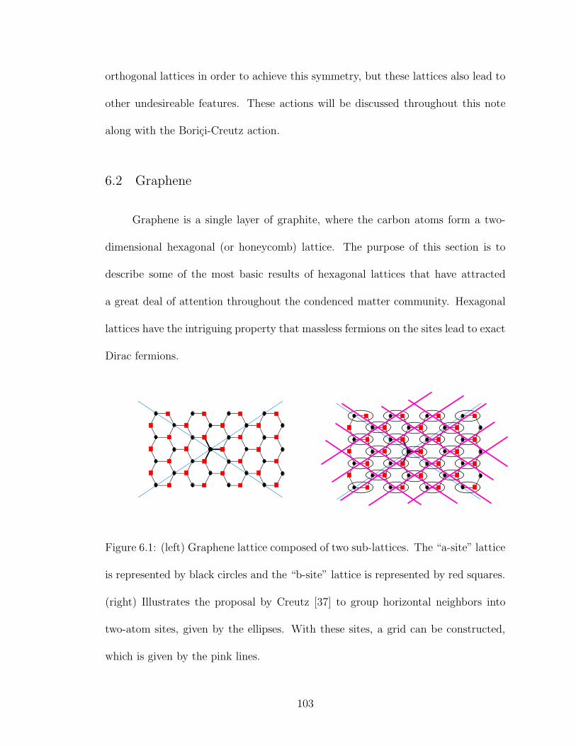
orthogonal lattices in order to achieve this symmetry, but these lattices also lead to

other undesireable features. These actions will be discussed throughout this note

along with the Borici-Creutz action.

6.2 Graphene

Graphene is a single layer of graphite, where the carbon atoms form a two-

dimensional hexagonal (or honeycomb) lattice. The purpose of this section is to

describe some of the most basic results of hexagonal lattices that have attracted

a great deal of attention throughout the condenced matter community. Hexagonal

lattices have the intriguing property that massless fermions on the sites lead to exact

Dirac fermions.

Figure 6.1: (left) Graphene lattice composed of two sub-lattices. The “a-site” lattice

is represented by black circles and the “b-site” lattice is represented by red squares.

(right) Illustrates the proposal by Creutz [37] to group horizontal neighbors into

two-atom sites, given by the ellipses. With these sites, a grid can be constructed,

which is given by the pink lines.

103

These lattices are better analyzed by a two sub-lattice description. As shown in

Fig. 6.1, one sub-lattice (often referred to as the “a-sites” or “l-sites”) only commu-

nicates with its three nearest neighbors which are members of the other sub-lattice

(often referred to as the “b-sites” or “r-sites”). Another important feature is that

these three nearest neighbors possess a Z3 permutation symmetry, which means that

these lattices are invariant under 120 rotations. As a result, the addition of the

three primary vectors, eα, created by the three connections to the neareast neigh-

bors yields zero (∑

α eα = 0). Without going into detail, these features of a 1 + 1

dimensional graphene lattice, along with two component Dirac spinors, result in

chiral Dirac fermions in the massless limit. The question that is of interest to this

chapter is how to extend this construction to four-dimensions.

6.3 Graphene-Inspired Lattice Actions

Several years ago, Creutz in Ref. [37] proposed a viable method of extending

this construction to four dimensional lattice gauge theory. The main idea behind

this method was to combine the horizontally connected “a” and “b” sites into an

individual two-atom “site” (as shown in Fig. 6.1 as the ellipses around these two-

atom sites). Through this process, the connecting segments between these two atom

sides form a non-orthogonal grid, which is illustrated by the pink lines imposed on

the lattice in Fig. 6.1. With this formulation, Creutz generalized this non-orthogonal

grid to four-dimensions while maintaining a construction similar to graphene.

104

6.4 Borici-Creutz Action

The action of this graphene-inspired, non-orthogonal grid in four dimensions

proposed by Creutz [37], and later Borici [200] is given by

SBC =1

2

∑

x

[

4∑

µ=1

(

ψx−µ eµ · Γψx − ψx+µ eµ · Γ† ψx)

+ ψx e5 · Γψx − ψx e5 · Γ† ψx

]

,

(6.1)

where Γµ = (~γ, iγ4) and the four-vectors eα are defined in terms of two parameters

B and C as

e1 = ( 1, 1, 1, B ), e2 = ( 1,−1,−1, B ), e3 = (−1,−1, 1, B ),

e4 = (−1, 1,−1, B ), e5 = −( 0, 0, 0, 4BC).

Note, each eα above is a four vector and the α does not refer to the individual

components of this vector. These eα vectors are generated from this non-orthogonal

grid1, which are related to the diagonal pink lines in Fig. 6.1. While written in a way

that is similar to the naıve fermion lattice action, there are several key differences

in this action. First, the definition of Γµ contains an iγ4, as opposed to the naıve

fermion action that does not contain this factor of i. This leads to an important

sign difference in the fourth component of these vectors. Second, these eα vectors

contain the non-orthogonal structure of this lattice action, which lead to non-trivial

linear combinations of Dirac matricies. To understand the behavior of this lattice

action, it is beneficial to write this action in momentum space, which is given by

SBC =

∫

p

ψp

[

i

4∑

µ=1

(

sin(pµ)~eµ · ~γ +Bγ4(cos(pµ) − C)

)

]

ψp. (6.2)

1See Ref. [36] for more details.

105

When written in momentum space, one can immediately confirm that this action

has exact chiral symmetry. In addition, for B 6= 0 and 0 < C < 1, this action has

two poles at

p(1)µ = p( 1, 1, 1, 1 ) p(2)

µ = −p( 1, 1, 1, 1 ),

where cos(p) = C. The existence of only two poles results in the action having

minimal fermion doubling under the Nielsen-Ninomiya “no-go” theorem [195, 196,

197].

While the features of exact chiral symmetry and minimal doubling are both

convenient and attractive features in a lattice action, there are undesirable con-

sequences as well. These consequences stem from the action breaking additional

discrete symmetries, namely parity (ψ(~p, p4) → γ4ψ(−~p, p4)), charge conjugation

(ψ(~p, p4) → CψT (~p, p4)), and time reversal (ψ(~p, p4) → γ5γ4ψ(~p,−p4)). These bro-

ken symmetries will lead to new unwanted operators that are a result of radiative

corrections.

6.4.1 Radiative Corrections

The presence of additional broken symmetries in lattice actions allow for new

operators to be generated through radiative corrections. The new unphysical oper-

ators due to this lattice discretization fall into three categories; relevant, marginal,

or irrelevant operators. Irrelevant operators, which are operators of mass dimen-

sion five or higher, are proportional to positive powers of the lattice spacing a and

would vanish in the continuum limit, a→ 0. The other two categories, relevant and

106

marginal, remain in the continuum limit and add unphysical terms to the final re-

sults that require fine tuning to eliminate. Marginal operators, dimension four, can

have logarithmic lattice spacing dependence. Relevant operators, dimension three

or less, are particularly bad since they are proportional to negative powers of a and

diverge in the continuum limit.

The exact chirality of the Borici-Creutz action prevents the relevant operator

from the Wilson action proportional to a−1ψψ, but the breaking of parity and time

reversal allow to two additional relevant operators, a−1∑

j c(j)3 O(j)

3 , where

O(1)3 = 4iBψγ4ψ = i

4∑

µ=1

ψ(eµ · γ)ψ, O(2)3 = 4iBψγ4γ5ψ = i

4∑

µ=1

ψ(eµ · γ)γ5ψ.

An emphasis should be placed on the fact that µ = 1, 2, 3, 4 and does not include e5

in this sum. This illustrates the S4 permutation symmetry the Borici-Creutz action

possesses, which is apparent in this form since these relevant operators are invariant

under any exchange of the four µ values. In addition to these two relevant operators,

there are additionally ten marginal operators2, which we will not focus on in this

note. All these operators will be generated unless the action possesses an additional

symmetry.

6.4.2 Additional Symmetry?

In physical two-dimensional graphene, there exists an additional Z3 rotational

symmetry. The question that now remains is whether an analogous symmetry ex-

ists for the graphene-inspired Borici-Creutz action. Analysis on the subject [36]

2See Ref. [35] for more detail on the marginal operators.

107

shows that if an action in four dimensions poscesses the minimal Z5 permutation

symmetry (or the larger two-operation A5 or S5 permutation symmetry), then for

α = 1, 2, 3, 4, 5,5∑

α=1

eα = 0, (6.3)

which results in the relevant operators

O(1)3 = i

5∑

α=1

ψ(eα · γ)ψ = 0, O(2)3 = i

5∑

α=1

ψ(eα · γ)γ5ψ = 0.

Thus, a lattice action with this minimal symmetry would not have any relevant

operators.

So does the Borici-Creutz action have this minimal Z5 permutation symme-

try? To explore this question, it is useful to write the action in terms of two two-

component spinors, one which acts as the “a-site” and one which acts as the “b-site”

as illustrated in Fig. 6.1. The action written in this way is

SBC =1

2

∑

x

[

4∑

µ=1

(

φx−µ Σ · eµ χx − χx+µ Σ · eµ φx)

+ φx Σ · e5 χx − χx Σ · e5 φx

+

4∑

µ=1

(

χx−µ Σ · eµ φx − φx+µ Σ · eµ χx)

+ χx Σ · e5 φx − φx Σ · e5 χx

]

,

(6.4)

with Σ = (~σ,−1) and Σ = (~σ, 1) and

ψp =

φp

χp

, and ψp =(

φp, χp)

.

With this two-component form of the action, examining whether or not this action

has this symmetry is most easily accomplished by looking at a two-dimensional

108

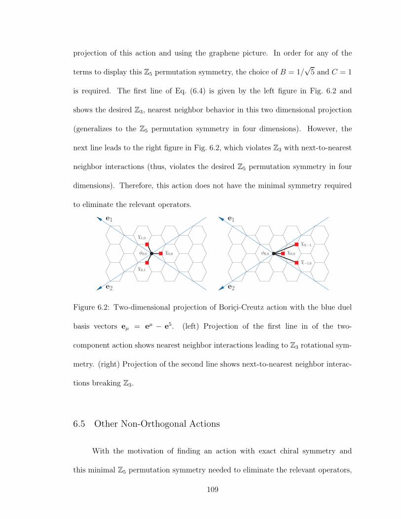
projection of this action and using the graphene picture. In order for any of the

terms to display this Z5 permutation symmetry, the choice of B = 1/√

5 and C = 1

is required. The first line of Eq. (6.4) is given by the left figure in Fig. 6.2 and

shows the desired Z3, nearest neighbor behavior in this two dimensional projection

(generalizes to the Z5 permutation symmetry in four dimensions). However, the

next line leads to the right figure in Fig. 6.2, which violates Z3 with next-to-nearest

neighbor interactions (thus, violates the desired Z5 permutation symmetry in four

dimensions). Therefore, this action does not have the minimal symmetry required

to eliminate the relevant operators.

e2

e1

φ0,0 χ0,0

χ1,0

χ0,1

e2

e1

φ0,0 χ0,0

χ0,−1

χ−1,0

Figure 6.2: Two-dimensional projection of Borici-Creutz action with the blue duel

basis vectors eµ = eµ − e5. (left) Projection of the first line in of the two-

component action shows nearest neighbor interactions leading to Z3 rotational sym-

metry. (right) Projection of the second line shows next-to-nearest neighbor interac-

tions breaking Z3.

6.5 Other Non-Orthogonal Actions

With the motivation of finding an action with exact chiral symmetry and

this minimal Z5 permutation symmetry needed to eliminate the relevant operators,

109

Ref. [36] explored several non-orthogonal actions which will be reviewed here.

6.5.1 Modified Borici-Creutz Action

With B = 1/√

5 and C = 1, the first line of Eq. (6.4) obeys the Z5 symmetry

and the second line breaks this symmetry. A logical extension is to simply delete

this last line. Therefore, using the same notation as Eq. (6.4), this action with

B = 1/√

5 and C = 1 is given by

SMBC =1

2

∑

x

[

4∑

µ=1

(

φx−µ Σ · eµ χx − χx+µ Σ · eµ φx)

+ φx Σ · e5 χx − χx Σ · e5 φx

]

.

(6.5)

However, the analysis of this action about the pole pµ ≃ 0 yields the behavior

ψ(i~γ · ~k + γ5γ4k4)ψ. This behavior, refered to as mutilated fermions [201, 202], is

not the desired Dirac structure.

6.5.2 “Hyperdiamond” Action

A further modification to the modified Borici-Creutz action to ensure the

correct Dirac structure in the continuum limit and preserve at least the minimal

Z5 permutation symmetry led to the “hyperdiamond” action, which is given by

S =∑

x

[

4∑

µ=1

(

φx−µ σ · eµ χx − χx+µ σ · eµ φx)

+ φx σ · e5 χx − χx σ · e5 φx

]

,

(6.6)

110

where

e1 =1

4(

√5,

√5,

√5, 1), e2 =

1

4(

√5,−

√5,−

√5, 1),

e3 =1

4(−

√5,−

√5,

√5, 1), e4 =

1

4(−

√5,

√5,−

√5, 1),

e5 = −( 0, 0, 0, 1).

and σ = (~σ,−i), σ = (~σ, i). The key difference between this action and the modified

Borici-Creutz action is the imaginary fourth component of the sigma four-vectors.

This alteration allows for the action to correctly reproduce the Dirac equation about

pµ ≃ 0 (which is clear in Eq. (6.8)). In addition, the vectors eα satisfy the desired

behavior needed for Z5 (or A5 or S5) permutation symmetry,∑

α eα = 0 and

eα · eβ =

1, for α = β

−1/4, for α 6= β

. (6.7)

While the exact details of the transformation won’t be covered here, one can show

that this action has an A5 permutation symmetry3 invariant under pairs of permu-

tations, which is enough symmetry to prevent the relevant operators from being

generated. In momentum space, the action is given by

S =

∫

p

ψp

[

i

4∑

µ=1

sin(pµ)eµ · γ −

(

4∑

µ=1

cos(pµ)eµ + e5

)

· γ γ5

]

ψp, (6.8)

with

ψp =

φp

χp

, ψp =(

φp, χp)

, and γµ =

0 σµ

σµ 0

.

From this form of the action, it is clear that it maintains exact chiral symmetry

and correctly reproduces the Dirac equation in the continuum limit. Additionally,

3See Ref. [35] for details.

111

due to the A5 permutation symmetry, relevant operators will not be generated.

Unfortunately, this action yields excessive fermion doubling, not unlike the naıve

fermion action. An example of six poles in addition to the one at pµ = 0 is p1 =

−p2 = −p3 = p4 = cos−1(−2/3).

6.6 The Wilczek Action

Karsten [198] and Wilczek [199] pointed out, over twenty years ago, the pos-

sibility of minimal doubling with an explicit construction. The Wilczek action has

the form

SW =1

2

∑

x,µ

[

ψ(x)γµψ(x+ µ) − ψ(x)γµψ(x− µ)]

+ 3λ∑

x

ψ(x)iγ4ψ(x)

− λ

2

∑

x,j

[

ψ(x)iγ4ψ(x+ j) + ψ(x)iγ4ψ(x− j)]

, (6.9)

with λ > 12

as a parameter. The action is diagonal in momentum space

SW =

∫ π

−π

d4k

(2π)4ψ(k)D−1(k)ψ(k), (6.10)

with the propagator D(k) given by

D(k) =

[

∑

µ

iγµ sin kµ − iγ4λ∑

j

(cos kj − 1)

]−1

. (6.11)

There are exactly two poles of the propagator, namely at the values k(1)µ = (0, 0, 0, 0),

and k(2)µ = (0, 0, 0, π). As this action has been analyzed in detail previously [203],

we shall not pursue the decomposition of the fields in terms of flavor and chirality.

Instead we will focus on the discrete symmetries of the action:

1. Cubic invariance

112

2. CT invariance

3. P invariance

4. Θ invariance,

where Θ is the time link-reflection symmetry operator. For the Borici and Creutz

actions, Θ is not a symmetry.

Given these discrete symmetries, it is straightforward to write down the rele-

vant and marginal terms in the Symanzik action. There is one relevant operator

O3 = ψiγ4ψ,

and several marginal operators

O(1)4 = FµνFµν

O(2)4 = F4µF4µ

O(3)4 = ψ D4γ4 ψ

O(4)4 = ψDµγµψ

As with anisotropic lattices, the breaking of hypercubic symmetry down to cubic

symmetry requires a speed of light tuning. It has been argued in Ref. [203] that the

relevant operator can be absorbed by a field redefinition, namely

ψ −→ exp

(

− ic3x4

a(1 + c(3)4 )

)

ψ, (6.12)

where c3 is the non-perturbatively determined coefficient of the operator O3 in the

Symanzik action, while c(3)4 that of O(3)

4 . The field redefinition, however, modifies

113

the boundary condition and just moves the fine tuning problem from the bulk of

the action to the boundary. The physical reality of this term can be ascertained

by noticing that it plays the role of an imaginary chemical potential. The relevant

operator thus cannot be avoided in the case of the Wilczek action.

6.7 Conclusion

Non-orthogonal lattice actions can be used to enforce desirable features from

a lattice action. As shown for the Borici-Creutz action, clever discretizations can

enforce exact chiral symmetry and minimal doubling. However, upon gaining these

benefits, additional symmetries are broken, which can (and often will) lead to the

generation of relevant or marginal operators from radiative corrections. An intricate

balance of symmetry is needed in a discrete lattice action in order to have exact

chiral symmetry, minimal doubling, and no relevant operators. At this time, no

non-orthogonal lattice action has accomplished this task. However, this is by no

means a proof that such a lattice action does not exist. The possibility still stands

that an action with just enough symmetry to rule out these relevant operators exists

and if found, it would be a very efficient, cheap way to simulate chiral fermions.

114

Chapter 7

Discussion and Outlook

Effective field theory provides a formalism not only to account for lattice spac-

ing effects from lattice QCD, but also can be used extract information indirectly from

lattice calculations or account for potential issues using new lattice actions. In this

work, examples from all three of these categories have been presented.

Lattice QCD is now entering a truly interesting time as a result of increased

computational power and improved algorithms. In fact, several groups are currently

performing simulations at the physical pion mass [204, 205]. For the first time, physi-

cally accurate non-perturbative calculations involving nuclear interactions, hadronic

spectra, and QCD thermodynamics realistically appear to be on the horizon.

In one sense, extrapolation formula to the physical point from effective field

theory are not necessary if the calculations are at physical pion masses. While both

finite volume and lattice spacing effects are just as, if not more, significant as a

systematic error, increased computing power can reduce these effects substantially.

However, from the point of view of the effective field theory, there are several in-

teresting questions that can finally be addressed. For example, the pion mass is

thought of as a small expansion parameter in hadronic effective field theories; is this

mass small enough to capture all the chiral dynamics?

An additional question of interest is how to extract parameters from effective

115

field theory at the physical point. For example, the sigma parameter in HBχPT is

one of great interest restricting dark matter models and the KN coupling is impor-

tant for kaon condensation scenarios in neutron stars. One suggestion proposed in

this work in Chapter 5, is to employ an isospin chemical potential as an additional

parameter (or knob) that can be varied to help extract these parameters.

Ultimately, effective field theory and lattice QCD are subjects often inter-

twined. Effective field theory can be used to make clever proposals for lattice QCD

measurements and alternatively, lattice QCD results can have interesting, unex-

pected effects that can alter the underlying assumptions of an effective field theory.

For this reason, the two fields will remain intertwined as we enter this new era of

hadronic physics.

116

Appendix A

Scalar Field on the Lattice

As in Ref. [2], the partition function for a theory with only a scalar field is

given by (neglecting source terms)

Z =

∫

d[φ]eiS(φ), (A.1)

where d[φ] =∏

n dφn represents all possible paths of φ and

S(φ) =

∫

d4xL(φ, ∂φ). (A.2)

Performing the Euclidean rotation, x0 → ix4,

eiS(φ) → e−SE(φ). (A.3)

The Euclidean correlation function is related to the vacuum expectation value of

the time ordered fields,

〈φ(xE)φ(0)〉 = Z−1E

∫

d[φ]φ(xE)φ(0)e−SE(φ) = 〈0|T [φ(xE)φ(0)|0〉 (A.4)

The operator φ(xE) can be written as,

φ(xE) = e−Hx4−ip·xφ(0)e−Hx4+ip·x (A.5)

which results in the correlation function,

〈φ(xE)φ(0)〉 = 〈0|φ(0)e−Hx4+ip·xφ(0)|0〉. (A.6)

117

Inserting two complete set of states,

〈φ(xE)φ(0)〉 =∑

n,m

Nnm〈0|φ(0)|n〉〈n|e−Hx4+ip·x|m〉〈m|φ(0)|0〉

=∑

n

Nn

∣

∣〈0|φ(0)|n〉∣

∣

2e−Enx4ep·x (A.7)

where Nn represents the proper finite volume normalization. The key result is that

the calculation of the correlation function is a sum of decaying exponentials whose

arguments are the energy at each level multiplied by the length in the Euclidean time

direction. Since the ground state is the smallest energy, if we examine the correlation

function at long times, the dominant term will be proportional to e−E0x4. Thus, by

taking logarithms of appropriate ratios at large x4, we can extract the ground state

energy, which for a two point correlator is the mass.

118

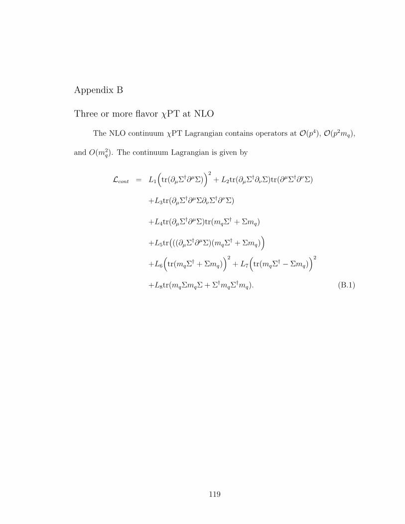
Appendix B

Three or more flavor χPT at NLO

The NLO continuum χPT Lagrangian contains operators at O(p4), O(p2mq),

and O(m2q). The continuum Lagrangian is given by

Lcont = L1

(

tr(∂µΣ†∂µΣ)

)2

+ L2tr(∂µΣ†∂νΣ)tr(∂µΣ†∂νΣ)

+L3tr(∂µΣ†∂µΣ∂νΣ

†∂νΣ)

+L4tr(∂µΣ†∂µΣ)tr(mqΣ

† + Σmq)

+L5tr(

((∂µΣ†∂µΣ)(mqΣ

† + Σmq))

+L6

(

tr(mqΣ† + Σmq)

)2

+ L7

(

tr(mqΣ† − Σmq)

)2

+L8tr(mqΣmqΣ + Σ†mqΣ†mq). (B.1)

119

Bibliography

[1] Thomas DeGrand and Carleton E. Detar. Lattice methods for quantum chro-modynamics. New Jersey, USA: World Scientific (2006) 345 p.

[2] Stephen R. Sharpe. Introduction to lattice field theory. Prepared for UehlingSummer School on Phenomenology and Lattice QCD, Seattle, WA, 21 Jun -2 Jul 1993.

[3] Maarten Golterman. Lattice chiral gauge theories. Nucl. Phys. Proc. Suppl.,94:189–203, 2001.

[4] Martin Luscher. Chiral gauge theories revisited. 2000.

[5] David B. Kaplan. Chiral Symmetry and Lattice Fermions. 2009.

[6] Erich Poppitz and Yanwen Shang. Chiral lattice gauge theories via mirror-fermion decoupling: A mission (im)possible? 03 2010.

[7] H. S. Sharatchandra, H. J. Thun, and P. Weisz. Susskind Fermions on aEuclidean Lattice. Nucl. Phys., B192:205, 1981.

[8] Paul H. Ginsparg and Kenneth G. Wilson. A Remnant of Chiral Symmetryon the Lattice. Phys. Rev., D25:2649, 1982.

[9] David B. Kaplan. A Method for simulating chiral fermions on the lattice.Phys. Lett., B288:342–347, 1992.

[10] Yigal Shamir. Chiral fermions from lattice boundaries. Nucl. Phys., B406:90–106, 1993.

[11] Vadim Furman and Yigal Shamir. Axial symmetries in lattice QCD withKaplan fermions. Nucl. Phys., B439:54–78, 1995.

[12] Rajamani Narayanan and Herbert Neuberger. Infinitely many regulator fieldsfor chiral fermions. Phys. Lett., B302:62–69, 1993.

[13] Rajamani Narayanan and Herbert Neuberger. A Construction of lattice chiralgauge theories. Nucl. Phys., B443:305–385, 1995.

[14] Herbert Neuberger. Exactly massless quarks on the lattice. Phys. Lett.,B417:141–144, 1998.

[15] Herbert Neuberger. Vector like gauge theories with almost massless fermionson the lattice. Phys. Rev., D57:5417–5433, 1998.

[16] Yoshio Kikukawa and Tatsuya Noguchi. Low energy effective action of domain-wall fermion and the Ginsparg-Wilson relation. 1999.

120

[17] J. Gasser and H. Leutwyler. Chiral Perturbation Theory to One Loop. Ann.

Phys., 158:142, 1984.

[18] K. Symanzik. Continuum Limit and Improved Action in Lattice Theories. 1.Principles and phi**4 Theory. Nucl. Phys., B226:187, 1983.

[19] K. Symanzik. Continuum Limit and Improved Action in Lattice Theories. 2.O(N) Nonlinear Sigma Model in Perturbation Theory. Nucl. Phys., B226:205,1983.

[20] B. Sheikholeslami and R. Wohlert. Improved Continuum Limit Lattice Actionfor QCD with Wilson Fermions. Nucl. Phys., B259:572, 1985.

[21] Martin Luscher, Stefan Sint, Rainer Sommer, and Peter Weisz. Chiral sym-metry and O(a) improvement in lattice QCD. Nucl. Phys., B478:365–400,1996.

[22] Oliver Bar, Gautam Rupak, and Noam Shoresh. Chiral perturbation theoryat O(a**2) for lattice QCD. Phys. Rev., D70:034508, 2004.

[23] Weon-Jong Lee and Stephen R. Sharpe. Partial Flavor Symmetry Restorationfor Chiral Staggered Fermions. Phys. Rev., D60:114503, 1999.

[24] C. Bernard. Chiral Logs in the Presence of Staggered Flavor Symmetry Break-ing. Phys. Rev., D65:054031, 2002.

[25] C. Aubin and C. Bernard. Pion and Kaon masses in Staggered Chiral Pertur-bation Theory. Phys. Rev., D68:034014, 2003.

[26] Stephen R. Sharpe and Robert L. Singleton, Jr. Spontaneous flavor and paritybreaking with Wilson fermions. Phys. Rev., D58:074501, 1998.

[27] Gautam Rupak and Noam Shoresh. Chiral perturbation theory for the Wilsonlattice action. Phys. Rev., D66:054503, 2002.

[28] Paulo F. Bedaque, Michael I. Buchoff, and Andre Walker-Loud. Effective FieldTheory for the Anisotropic Wilson Lattice Action. Phys. Rev., D77:074501,2008.

[29] Michael I. Buchoff. Isotropic and Anisotropic Lattice Spacing Corrections forI=2 pi-pi Scattering from Effective Field Theory. Phys. Rev., D77:114502,2008.

[30] Michael I. Buchoff, Jiunn-Wei Chen, and Andre Walker-Loud. pi-pi Scatteringin Twisted Mass Chiral Perturbation Theory. Phys. Rev., D79:074503, 2009.

[31] Xu Feng, Karl Jansen, and Dru B. Renner. The pi+ pi+ scattering lengthfrom maximally twisted mass lattice QCD. Phys. Lett., B684:268–274, 2010.

121

[32] Xu Feng, Karl Jansen, and Dru B. Renner. Scattering from finite size methodsin lattice QCD. 2009.

[33] Paulo F. Bedaque, Michael I. Buchoff, and Brian C. Tiburzi. Meson-BaryonScattering Parameters from Lattice QCD with an Isospin Chemical Potential.Phys. Rev., D80:114501, 2009.

[34] Michael I. Buchoff. Search for Chiral Fermion Actions on Non-OrthogonalLattices. PoS, LATTICE2008:068, 2008.

[35] Paulo F. Bedaque, Michael I. Buchoff, Brian C. Tiburzi, and Andre Walker-Loud. Broken Symmetries from Minimally Doubled Fermions. Phys. Lett.,B662:449–455, 2008.

[36] Paulo F. Bedaque, Michael I. Buchoff, Brian C. Tiburzi, and Andre Walker-Loud. Search for Fermion Actions on Hyperdiamond Lattices. Phys. Rev.,D78:017502, 2008.

[37] Michael Creutz. Four-dimensional graphene and chiral fermions. JHEP,04:017, 2008.

[38] Michael Creutz. Wilson fermions at finite temperature. 1996.

[39] Silas R. Beane and Martin J. Savage. Nucleons properties at finite latticespacing in chiral perturbation theory. Phys. Rev., D68:114502, 2003.

[40] Brian C. Tiburzi. Baryon masses at O(a**2) in chiral perturbation theory.Nucl. Phys., A761:232–258, 2005.

[41] Paulo F. Bedaque and Andre Walker-Loud. Restless pions: orbifold boundaryconditions and noise suppression in lattice QCD. Phys. Lett., B660:369–375,2008.

[42] Mark G. Alford, T. R. Klassen, and G. P. Lepage. Improving lattice quarkactions. Nucl. Phys., B496:377–407, 1997.

[43] Timothy R. Klassen. The anisotropic Wilson gauge action. Nucl. Phys.,B533:557–575, 1998.

[44] Colin J. Morningstar and Mike J. Peardon. Efficient glueball simulations onanisotropic lattices. Phys. Rev., D56:4043–4061, 1997.

[45] Colin J. Morningstar and Mike J. Peardon. The glueball spectrum from ananisotropic lattice study. Phys. Rev., D60:034509, 1999.

[46] Subhasish Basak et al. Lattice QCD determination of states with spin 5/2 orhigher in the spectrum of nucleons. 2006.

[47] M. Fukugita, Y. Kuramashi, M. Okawa, H. Mino, and A. Ukawa. Hadronscattering lengths in lattice QCD. Phys. Rev., D52:3003–3023, 1995.

122

[48] S. R. Beane, P. F. Bedaque, K. Orginos, and M. J. Savage. Nucleon nucleonscattering from fully-dynamical lattice QCD. Phys. Rev. Lett., 97:012001,2006.

[49] Silas R. Beane et al. Hyperon nucleon scattering from fully-dynamical latticeQCD. Nucl. Phys., A794:62–72, 2007.

[50] Huey-Wen Lin, Saul D. Cohen, Jozef Dudek, Robert G. Edwards, Balint Joo,David G. Richards, John Bulava, Justin Foley, Colin Morningstar, Eric Engel-son, Stephen Wallace, K. Jimmy Juge, Nilmani Mathur, Michael J. Peardon,and Sinead M. Ryan. First results from 2+1 dynamical quark flavors on ananisotropic lattice: light-hadron spectroscopy and setting the strange-quarkmass. Phys.Rev.D, 79:034502, 2009.

[51] Silas R. Beane, William Detmold, Thomas C Luu, Kostas Orginos, AssumptaParreno, Martin J. Savage, Aaron Torok, and Andre Walker-Loud. Highstatistics analysis using anisotropic clover lattices: (ii) three-baryon systems.Phys.Rev.D, 80:074501, 2009.

[52] Silas R. Beane, William Detmold, Huey-Wen Lin, Thomas C. Luu, KostasOrginos, Martin J. Savage, Aaron Torok, and Andre Walker-Loud. High statis-tics analysis using anisotropic clover lattices: (iii) baryon-baryon interactions.12 2009.

[53] Silas R. Beane, William Detmold, Thomas C. Luu, Kostas Orginos, AssumptaParreno, Martin J. Savage, Aaron Torok, and Andre Walker-Loud. High statis-tics analysis using anisotropic clover lattices: (i) single hadron correlationfunctions. Phys.Rev.D, 79:114502, 2009.

[54] Kenneth G. Wilson. CONFINEMENT OF QUARKS. Phys. Rev., D10:2445–2459, 1974.

[55] Steven Weinberg. Phenomenological Lagrangians. Physica, A96:327, 1979.

[56] J. Gasser and H. Leutwyler. Chiral Perturbation Theory: Expansions in theMass of the Strange Quark. Nucl. Phys., B250:465, 1985.

[57] Sinya Aoki. New Phase Structure for Lattice QCD with Wilson Fermions.Phys. Rev., D30:2653, 1984.

[58] Timothy R. Klassen. Non-perturbative improvement of the anisotropic WilsonQCD action. Nucl. Phys. Proc. Suppl., 73:918–920, 1999.

[59] Ping Chen. Heavy quarks on anisotropic lattices: The charmonium spectrum.Phys. Rev., D64:034509, 2001.

[60] X. Liao and T. Manke. Relativistic bottomonium spectrum from anisotropiclattices. Phys. Rev., D65:074508, 2002.

123

[61] Murray Gell-Mann, R. J. Oakes, and B. Renner. Behavior of current diver-gences under SU(3) x SU(3). Phys. Rev., 175:2195–2199, 1968.

[62] David J. Antonio et al. Localization and chiral symmetry in 3 flavor domainwall QCD. Phys. Rev., D77:014509, 2008.

[63] Elizabeth Ellen Jenkins and Aneesh V. Manohar. Baryon chiral perturbationtheory using a heavy fermion Lagrangian. Phys. Lett., B255:558–562, 1991.

[64] Elizabeth Ellen Jenkins and Aneesh V. Manohar. Chiral corrections to thebaryon axial currents. Phys. Lett., B259:353–358, 1991.

[65] Roberto Frezzotti, Pietro Antonio Grassi, Stefan Sint, and Peter Weisz. Lat-tice QCD with a chirally twisted mass term. JHEP, 08:058, 2001.

[66] John B. Kogut and Leonard Susskind. Hamiltonian Formulation of Wilson’sLattice Gauge Theories. Phys. Rev., D11:395, 1975.

[67] Leonard Susskind. Lattice Fermions. Phys. Rev., D16:3031–3039, 1977.

[68] Andre Walker-Loud and Jackson M. S. Wu. Nucleon and Delta masses intwisted mass chiral perturbation theory. Phys. Rev., D72:014506, 2005.

[69] Jon A. Bailey. Staggered baryon operators with flavor SU(3) quantum num-bers. Phys. Rev., D75:114505, 2007.

[70] Jon A. Bailey. Staggered heavy baryon chiral perturbation theory. Phys. Rev.,D77:054504, 2008.

[71] Howard Georgi. AN EFFECTIVE FIELD THEORY FOR HEAVY QUARKSAT LOW- ENERGIES. Phys. Lett., B240:447–450, 1990.

[72] Aneesh V. Manohar and Mark B. Wise. Heavy quark physics. Camb. Monogr.

Part. Phys. Nucl. Phys. Cosmol., 10:1–191, 2000.

[73] Thomas R. Hemmert, Barry R. Holstein, and Joachim Kambor. Chiral La-grangians and Delta(1232) interactions: Formalism. J. Phys., G24:1831–1859,1998.

[74] Andre Walker-Loud. Octet baryon masses in partially quenched chiral pertur-bation theory. Nucl. Phys., A747:476–507, 2005.

[75] Brian C. Tiburzi and Andre Walker-Loud. Decuplet baryon masses in partiallyquenched chiral perturbation theory. Nucl. Phys., A748:513–536, 2005.

[76] Brian C. Tiburzi and Andre Walker-Loud. Strong isospin breaking in thenucleon and Delta masses. Nucl. Phys., A764:274–302, 2006.

[77] Andre Walker-Loud. Topics in effective field theory for lattice QCD. 2006.

124

[78] Michael E. Luke and Aneesh V. Manohar. Reparametrization invariance con-straints on heavy particle effective field theories. Phys. Lett., B286:348–354,1992.

[79] Jiunn-Wei Chen, Donal O’Connell, Ruth S. Van de Water, and Andre Walker-Loud. Ginsparg-Wilson pions scattering on a staggered sea. Phys. Rev.,D73:074510, 2006.

[80] Jiunn-Wei Chen, Donal O’Connell, and Andre Walker-Loud. Two meson sys-tems with Ginsparg-Wilson valence quarks. Phys. Rev., D75:054501, 2007.

[81] Kostas Orginos and Andre Walker-Loud. Mixed meson masses with domain-wall valence and staggered sea fermions. Phys. Rev., D77:094505, 2008.

[82] Jiunn-Wei Chen, Donal O’Connell, and Andre Walker-Loud. Universality ofMixed Action Extrapolation Formulae. JHEP, 04:090, 2009.

[83] Kerson Huang and C. N. Yang. Quantum-mechanical many-body problemwith hard-sphere interaction. Phys. Rev., 105:767–775, 1957.

[84] H. W. Hamber, E. Marinari, G. Parisi, and C. Rebbi. CONSIDERATIONSON NUMERICAL ANALYSIS OF QCD. Nucl. Phys., B225:475, 1983.

[85] Martin Luscher. Two particle states on a torus and their relation to thescattering matrix. Nucl. Phys., B354:531–578, 1991.

[86] M. Luscher. Volume Dependence of the Energy Spectrum in Massive QuantumField Theories. 2. Scattering States. Commun. Math. Phys., 105:153–188,1986.

[87] Steven Weinberg. Pion scattering lengths. Phys. Rev. Lett., 17:616–621, 1966.

[88] M. Knecht, B. Moussallam, J. Stern, and N. H. Fuchs. The Low-energy pi piamplitude to one and two loops. Nucl. Phys., B457:513–576, 1995.

[89] J. Bijnens, G. Colangelo, G. Ecker, J. Gasser, and M. E. Sainio. Elastic ππscattering to two loops. Phys. Lett., B374:210–216, 1996.

[90] J. Bijnens, G. Colangelo, G. Ecker, J. Gasser, and M. E. Sainio. Pion pionscattering at low energy. Nucl. Phys., B508:263–310, 1997.

[91] Rajan Gupta, Apoorva Patel, and Stephen R. Sharpe. I = 2 pion scatteringamplitude with Wilson fermions. Phys. Rev., D48:388–396, 1993.

[92] M. Fukugita, Y. Kuramashi, H. Mino, M. Okawa, and A. Ukawa. An Ex-ploratory study of nucleon-nucleon scattering lengths in lattice QCD. Phys.

Rev. Lett., 73:2176–2179, 1994.

[93] H. R. Fiebig, K. Rabitsch, H. Markum, and A. Mihaly. Exploring the pi+ pi+interaction in lattice QCD. Few Body Syst., 29:95–120, 2000.

125

[94] S. Aoki et al. I = 2 pion scattering length with Wilson fermions. Nucl. Phys.

Proc. Suppl., 83:241–243, 2000.

[95] Chuan Liu, Jun-hua Zhang, Ying Chen, and J. P. Ma. Calculating the I = 2pion scattering length using tadpole improved clover Wilson action on coarseanisotropic lattices. Nucl. Phys., B624:360–376, 2002.

[96] S. Aoki et al. I = 2 pion scattering length and phase shift with Wilson fermions.Nucl. Phys. Proc. Suppl., 106:230–232, 2002.

[97] S. Aoki et al. I=2 Pion Scattering Length with the Wilson Fermion. Phys.

Rev., D66:077501, 2002.

[98] S. Aoki et al. I = 2 pion scattering phase shift with Wilson fermions. Nucl.

Phys. Proc. Suppl., 119:311–313, 2003.

[99] S. Aoki et al. I=2 Pion Scattering Phase Shift with Wilson Fermions. Phys.

Rev., D67:014502, 2003.

[100] N. Ishizuka and T. Yamazaki. I = 2 pion scattering length from two-pion wavefunction. Nucl. Phys. Proc. Suppl., 129:233–235, 2004.

[101] T. Yamazaki et al. I = 2 pi pi scattering phase shift with two flavors of O(a)improved dynamical quarks. Phys. Rev., D70:074513, 2004.

[102] Xining Du, Guang-wei Meng, Chuan Miao, and Chuan Liu. I = 2 pion scatter-ing length with improved actions on anisotropic lattices. Int. J. Mod. Phys.,A19:5609–5614, 2004.

[103] S. Aoki et al. I = 2 pion scattering length from two-pion wave function. Nucl.

Phys. Proc. Suppl., 140:305–307, 2005.

[104] S. Aoki et al. I = 2 pion scattering length from two-pion wave functions. Phys.

Rev., D71:094504, 2005.

[105] Xin Li et al. Hadron Scattering in an Asymmetric Box. JHEP, 06:053, 2007.

[106] Stephen R. Sharpe, Rajan Gupta, and Gregory W. Kilcup. Lattice calculationof I = 2 pion scattering length. Nucl. Phys., B383:309–356, 1992.

[107] Y. Kuramashi, M. Fukugita, H. Mino, M. Okawa, and A. Ukawa. LatticeQCD calculation of full pion scattering lengths. Phys. Rev. Lett., 71:2387–2390, 1993.

[108] K. Jimmy Juge. I = 2 pion scattering length with the parametrized fixed pointaction. Nucl. Phys. Proc. Suppl., 129:194–196, 2004.

[109] Xu Feng, Karl Jansen, and Dru B. Renner. The pi+ pi+ scattering lengthfrom maximally twisted mass lattice qcd. 09 2009.

126

[110] Silas R. Beane, Paulo F. Bedaque, Kostas Orginos, and Martin J. Savage. I =2 pi pi scattering from fully-dynamical mixed-action lattice QCD. Phys. Rev.,D73:054503, 2006.

[111] Silas R. Beane et al. Precise Determination of the I=2 pipi Scattering Lengthfrom Mixed-Action Lattice QCD. Phys. Rev., D77:014505, 2008.

[112] Brian C. Tiburzi. Baryons with Ginsparg-Wilson quarks in a staggered sea.Phys. Rev., D72:094501, 2005.

[113] Paulo F. Bedaque, Ikuro Sato, and Andre Walker-Loud. Finite volume cor-rections to pi pi scattering. Phys. Rev., D73:074501, 2006.

[114] G. Colangelo, J. Gasser, and H. Leutwyler. pi pi scattering. Nucl. Phys.,B603:125–179, 2001.

[115] L. Maiani and M. Testa. Final state interactions from Euclidean correlationfunctions. Phys. Lett., B245:585–590, 1990.

[116] S. R. Beane, P. F. Bedaque, A. Parreno, and M. J. Savage. Exploring hyperonsand hypernuclei with lattice QCD. Nucl. Phys., A747:55–74, 2005.

[117] S. R. Beane, P. F. Bedaque, A. Parreno, and M. J. Savage. Two Nucleons ona Lattice. Phys. Lett., B585:106–114, 2004.

[118] C. Bernard et al. Low energy constants from the MILC Collaboration. 2006.

[119] Ph. Boucaud et al. Dynamical twisted mass fermions with light quarks. Phys.

Lett., B650:304–311, 2007.

[120] L. Del Debbio, Leonardo Giusti, M. Luscher, R. Petronzio, and N. Tantalo.QCD with light Wilson quarks on fine lattices (I): first experiences and physicsresults. JHEP, 02:056, 2007.

[121] L. Del Debbio, Leonardo Giusti, M. Luscher, R. Petronzio, and N. Tantalo.QCD with light Wilson quarks on fine lattices. II: DD-HMC simulations anddata analysis. JHEP, 02:082, 2007.

[122] H. Leutwyler. Insights and puzzles in light quark physics. 2007.

[123] Sinya Aoki and Oliver Bar. The vector and axial vector current in WilsonChPT. PoS, LAT2007:062, 2007.

[124] Stephen R. Sharpe and Jackson M. S. Wu. Twisted mass chiral perturbationtheory at next-to-leading order. Phys. Rev., D71:074501, 2005.

[125] T. Umeda et al. Two flavors of dynamical quarks on anisotropic lattices. Phys.

Rev., D68:034503, 2003.

127

[126] Silas R. Beane, Kostas Orginos, and Martin J. Savage. Hadronic Interactionsfrom Lattice QCD. Int. J. Mod. Phys., E17:1157–1218, 2008.

[127] Silas R. Beane et al. Pi-K Scattering in Full QCD with Domain-Wall ValenceQuarks. Phys. Rev., D74:114503, 2006.

[128] Silas R. Beane et al. The K+K+ Scattering Length from Lattice QCD. Phys.

Rev., D77:094507, 2008.

[129] Silas R. Beane et al. Multi-Pion Systems in Lattice QCD and the Three-PionInteraction. Phys. Rev. Lett., 100:082004, 2008.

[130] William Detmold et al. Multi-Pion States in Lattice QCD and the Charged-Pion Condensate. Phys. Rev., D78:014507, 2008.

[131] William Detmold, Kostas Orginos, Martin J. Savage, and Andre Walker-Loud.Kaon Condensation with Lattice QCD. Phys. Rev., D78:054514, 2008.

[132] Ryoichi Seki and U. van Kolck. Effective field theory of nucleon nucleonscattering on large discrete lattices. Phys. Rev., C73:044006, 2006.

[133] Jiunn-Wei Chen and David B. Kaplan. A lattice theory for low energy fermionsat finite chemical potential. Phys. Rev. Lett., 92:257002, 2004.

[134] Jiunn-Wei Chen, Dean Lee, and Thomas Schafer. Inequalities for Light Nucleiin the Wigner Symmetry Limit. Phys. Rev. Lett., 93:242302, 2004.

[135] Dean Lee, Bugra Borasoy, and Thomas Schafer. Nuclear lattice simulationswith chiral effective field theory. Phys. Rev., C70:014007, 2004.

[136] Dean Lee and Thomas Schafer. Neutron matter on the lattice with pionlesseffective field theory. Phys. Rev., C72:024006, 2005.

[137] Bugra Borasoy, Evgeny Epelbaum, Hermann Krebs, Dean Lee, and Ulf-G.Meissner. Lattice simulations for light nuclei: Chiral effective field theory atleading order. Eur. Phys. J., A31:105–123, 2007.

[138] Bugra Borasoy, Evgeny Epelbaum, Hermann Krebs, Dean Lee, and Ulf-G.Meissner. Chiral effective field theory on the lattice at next-to- leading order.Eur. Phys. J., A35:343–355, 2008.

[139] Bugra Borasoy, Evgeny Epelbaum, Hermann Krebs, Dean Lee, and Ulf-G.Meissner. Dilute neutron matter on the lattice at next-to-leading order inchiral effective field theory. Eur. Phys. J., A35:357–367, 2008.

[140] Dean Lee. Lattice simulations for few- and many-body systems. Prog. Part.

Nucl. Phys., 63:117–154, 2009.

[141] Dru Bryant Renner et al. Hadronic physics with domain-wall valence andimproved staggered sea quarks. Nucl. Phys. Proc. Suppl., 140:255–260, 2005.

128

[142] Robert G. Edwards et al. Hadron structure with light dynamical quarks. PoS,LAT2005:056, 2006.

[143] Kostas Orginos and Doug Toussaint. Testing improved actions for dynamicalKogut-Susskind quarks. Phys. Rev., D59:014501, 1999.

[144] Kostas Orginos, Doug Toussaint, and R. L. Sugar. Variants of fattening andflavor symmetry restoration. Phys. Rev., D60:054503, 1999.

[145] Claude W. Bernard et al. The QCD spectrum with three quark flavors. Phys.

Rev., D64:054506, 2001.

[146] C. Aubin et al. Light hadrons with improved staggered quarks: Approachingthe continuum limit. Phys. Rev., D70:094505, 2004.

[147] Roberto Frezzotti, Pietro Antonio Grassi, Stefan Sint, and Peter Weisz. Alocal formulation of lattice QCD without unphysical fermion zero modes. Nucl.

Phys. Proc. Suppl., 83:941–946, 2000.

[148] B. Blossier et al. Light quark masses and pseudoscalar decay constants fromNf=2 Lattice QCD with twisted mass fermions. JHEP, 04:020, 2008.

[149] Ph. Boucaud et al. Dynamical Twisted Mass Fermions with Light Quarks:Simulation and Analysis Details. Comput. Phys. Commun., 179:695–715, 2008.

[150] T. Chiarappa et al. Numerical simulation of QCD with u, d, s and c quarksin the twisted-mass Wilson formulation. Eur. Phys. J., C50:373–383, 2007.

[151] Gernot Munster and Christian Schmidt. Chiral perturbation theory for latticeQCD with a twisted mass term. Europhys. Lett., 66:652–656, 2004.

[152] Luigi Scorzato. Pion mass splitting and phase structure in twisted mass QCD.Eur. Phys. J., C37:445–455, 2004.

[153] Stephen R. Sharpe and Jackson M. S. Wu. The phase diagram of twisted masslattice QCD. Phys. Rev., D70:094029, 2004.

[154] Sinya Aoki and Oliver Bar. Twisted-mass QCD, O(a) improvement and Wilsonchiral perturbation theory. Phys. Rev., D70:116011, 2004.

[155] Sinya Aoki, Oliver Bar, and Benedikt Biedermann. Pion scattering in WilsonChPT. Phys. Rev., D78:114501, 2008.

[156] R. Frezzotti and G. C. Rossi. Chirally improving Wilson fermions. I: O(a)improvement. JHEP, 08:007, 2004.

[157] Stephen R. Sharpe. Observations on discretization errors in twisted-masslattice QCD. Phys. Rev., D72:074510, 2005.

129

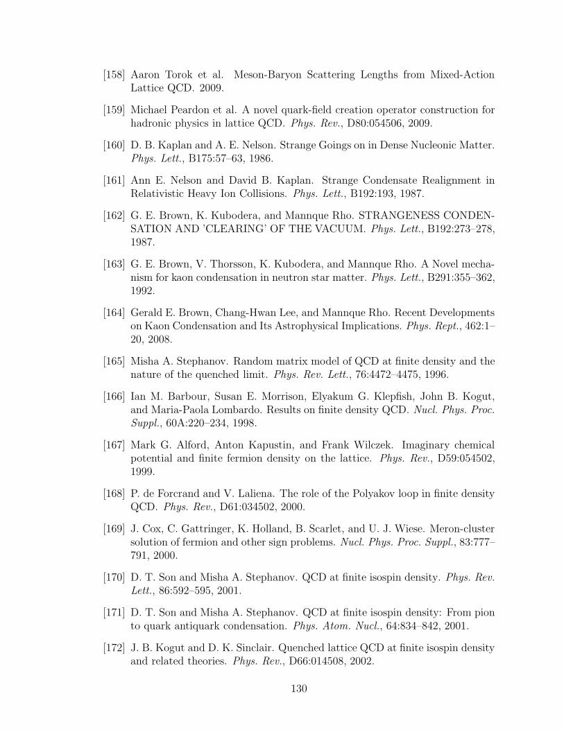
[158] Aaron Torok et al. Meson-Baryon Scattering Lengths from Mixed-ActionLattice QCD. 2009.

[159] Michael Peardon et al. A novel quark-field creation operator construction forhadronic physics in lattice QCD. Phys. Rev., D80:054506, 2009.

[160] D. B. Kaplan and A. E. Nelson. Strange Goings on in Dense Nucleonic Matter.Phys. Lett., B175:57–63, 1986.

[161] Ann E. Nelson and David B. Kaplan. Strange Condensate Realignment inRelativistic Heavy Ion Collisions. Phys. Lett., B192:193, 1987.

[162] G. E. Brown, K. Kubodera, and Mannque Rho. STRANGENESS CONDEN-SATION AND ’CLEARING’ OF THE VACUUM. Phys. Lett., B192:273–278,1987.

[163] G. E. Brown, V. Thorsson, K. Kubodera, and Mannque Rho. A Novel mecha-nism for kaon condensation in neutron star matter. Phys. Lett., B291:355–362,1992.

[164] Gerald E. Brown, Chang-Hwan Lee, and Mannque Rho. Recent Developmentson Kaon Condensation and Its Astrophysical Implications. Phys. Rept., 462:1–20, 2008.

[165] Misha A. Stephanov. Random matrix model of QCD at finite density and thenature of the quenched limit. Phys. Rev. Lett., 76:4472–4475, 1996.

[166] Ian M. Barbour, Susan E. Morrison, Elyakum G. Klepfish, John B. Kogut,and Maria-Paola Lombardo. Results on finite density QCD. Nucl. Phys. Proc.

Suppl., 60A:220–234, 1998.

[167] Mark G. Alford, Anton Kapustin, and Frank Wilczek. Imaginary chemicalpotential and finite fermion density on the lattice. Phys. Rev., D59:054502,1999.

[168] P. de Forcrand and V. Laliena. The role of the Polyakov loop in finite densityQCD. Phys. Rev., D61:034502, 2000.

[169] J. Cox, C. Gattringer, K. Holland, B. Scarlet, and U. J. Wiese. Meron-clustersolution of fermion and other sign problems. Nucl. Phys. Proc. Suppl., 83:777–791, 2000.

[170] D. T. Son and Misha A. Stephanov. QCD at finite isospin density. Phys. Rev.

Lett., 86:592–595, 2001.

[171] D. T. Son and Misha A. Stephanov. QCD at finite isospin density: From pionto quark antiquark condensation. Phys. Atom. Nucl., 64:834–842, 2001.

[172] J. B. Kogut and D. K. Sinclair. Quenched lattice QCD at finite isospin densityand related theories. Phys. Rev., D66:014508, 2002.

130

[173] J. B. Kogut and D. K. Sinclair. Lattice QCD at finite isospin density at zeroand finite temperature. Phys. Rev., D66:034505, 2002.

[174] John B. Kogut, Dominique Toublan, and D. K. Sinclair. The phase diagramof four flavor SU(2) lattice gauge theory at nonzero chemical potential andtemperature. Nucl. Phys., B642:181–209, 2002.

[175] J. B. Kogut, D. Toublan, and D. K. Sinclair. The pseudo-Goldstone spectrumof 2-colour QCD at finite density. Phys. Rev., D68:054507, 2003.

[176] J. B. Kogut and D. K. Sinclair. The finite temperature transition for 2-flavorlattice QCD at finite isospin density. Phys. Rev., D70:094501, 2004.

[177] Philippe de Forcrand, Mikhail A. Stephanov, and Urs Wenger. On the phasediagram of QCD at finite isospin density. PoS, LAT2007:237, 2007.

[178] Veronique Bernard, Norbert Kaiser, Joachim Kambor, and Ulf G. Meissner.Chiral structure of the nucleon. Nucl. Phys., B388:315–345, 1992.

[179] Matthias Frink, Bastian Kubis, and Ulf-G. Meissner. Analysis of the pionkaon sigma-term and related topics. Eur. Phys. J., C25:259–276, 2002.

[180] Brian C. Tiburzi and Andre Walker-Loud. Hyperons in Two Flavor ChiralPerturbation Theory. Phys. Lett., B669:246–253, 2008.

[181] Fu-Jiun Jiang and Brian C. Tiburzi. Hyperon Axial Charges in Two-FlavorChiral Perturbation Theory. Phys. Rev., D80:077501, 2009.

[182] Maxim Mai, Peter C. Bruns, Bastian Kubis, and Ulf-G. Meissner. Aspects ofmeson-baryon scattering in three- and two- flavor chiral perturbation theory.Phys. Rev., D80:094006, 2009.

[183] B. C. Tiburzi. Two-Flavor Chiral Perturbation Theory for Hyperons. 2009.

[184] M. C. M. Rentmeester, R. G. E. Timmermans, and J. J. de Swart. Deter-mination of the chiral coupling constants c(3) and c(4) in new p p and n ppartial-wave analyses. Phys. Rev., C67:044001, 2003.

[185] Nadia Fettes, Ulf-G. Meissner, and Sven Steininger. Pion nucleon scattering inchiral perturbation theory. I: Isospin-symmetric case. Nucl. Phys., A640:199–234, 1998.

[186] J. A. Oller and Ulf G. Meissner. Chiral dynamics in the presence of boundstates: Kaon nucleon interactions revisited. Phys. Lett., B500:263–272, 2001.

[187] Ulf G. Meissner, Udit Raha, and Akaki Rusetsky. Spectrum and decays ofkaonic hydrogen. Eur. Phys. J., C35:349–357, 2004.

[188] B. Borasoy, R. Nissler, and W. Weise. Chiral dynamics of kaon nucleon inter-actions, revisited. Eur. Phys. J., A25:79–96, 2005.

131

[189] Jose A. Oller, Joaquim Prades, and Michela Verbeni. Surprises in thresholdantikaon nucleon physics. Phys. Rev. Lett., 95:172502, 2005.

[190] J. Gasser, H. Leutwyler, and M. E. Sainio. Sigma term update. Phys. Lett.,B253:252–259, 1991.

[191] Paul Buettiker and Ulf-G. Meissner. Pion nucleon scattering inside the Man-delstam triangle. Nucl. Phys., A668:97–112, 2000.

[192] H. Ohki et al. Nucleon sigma term and strange quark content in 2+1-flavorQCD with dynamical overlap fermions. 2009.

[193] A. Walker-Loud et al. Light hadron spectroscopy using domain wall valencequarks on an Asqtad sea. Phys. Rev., D79:054502, 2009.

[194] Andre Walker-Loud. New lessons from the nucleon mass, lattice QCD andheavy baryon chiral perturbation theory. PoS, LATTICE2008:005, 2008.

[195] Holger Bech Nielsen and M. Ninomiya. Absence of Neutrinos on a Lattice. 1.Proof by Homotopy Theory. Nucl. Phys., B185:20, 1981.

[196] Holger Bech Nielsen and M. Ninomiya. Absence of Neutrinos on a Lattice. 2.Intuitive Topological Proof. Nucl. Phys., B193:173, 1981.

[197] Holger Bech Nielsen and M. Ninomiya. No Go Theorem for RegularizingChiral Fermions. Phys. Lett., B105:219, 1981.

[198] Luuk H. Karsten. LATTICE FERMIONS IN EUCLIDEAN SPACE-TIME.Phys. Lett., B104:315, 1981.

[199] Frank Wilczek. ON LATTICE FERMIONS. Phys. Rev. Lett., 59:2397, 1987.

[200] Artan Borici. Creutz fermions on an orthogonal lattice. Phys. Rev.,D78:074504, 2008.

[201] William Celmaster. GAUGE THEORIES ON THE BODY - CENTEREDHYPERCUBIC LATTICE. Phys. Rev., D26:2955, 1982.

[202] William Celmaster and Frank Krausz. FERMION MUTILATION ON ABODY CENTERED TESSERACT. Phys. Rev., D28:1527, 1983.

[203] M. Pernici. Chiral invariance and lattice fermions with minimal doubling.Phys. Lett., B346:99–105, 1995.

[204] S. Aoki et al. Physical Point Simulation in 2+1 Flavor Lattice QCD. 2009.

[205] Laurent Lellouch. Kaon physics: a lattice perspective. PoS, LAT-TICE2008:015, 2009.

132

Documents

ABSTRACT TOPICS IN LATTICE QCD AND EFFECTIVE - DRUM