Application of the multiscale FEMto the modeling of nonlinear composites with a random microstructure

S. Klinge*, K. Hackl*

* Institute of Mechanics, Ruhr University Bochum, Bochum, Germany

Abstract

In this contribution the properties and application of the multiscale finite element program MS-FEAP are presented. This code is developed on basis of the coupling the homogenization theory withthe finite element method. According to this concept, the investigation of an appropriately chosen rep-resentative volume element yields the material parameters needed for the simulation of a macroscopicbody. The connection of scales is based on the principle of volume averaging and the Hill-Mandelmacrohomogeneity condition. The latter leads to the determination of different types of boundaryconditions for the representative volume element and in this way to the postulation of a well-posedproblem at this level. The numerical examples presented in the contribution investigate the effectivematerial behavior of microporous media. An isotropic and a transversally anisotropic microstruc-ture are simulated by choosing an appropriate orientation and geometry of the representative volumeelement in each Gauss point. The results are verified by comparing them with Hashin-Shtrikman’sanalytic bounds. However, the chosen examples should just be understood as an illustration of theprogram application, while its main feature is a modular structure suitable for further development.

1 IntroductionIn contrast to linear composite materials, whose modeling is already well investigated [2, 5, 6, 10,11, 20, 22, 29], the modeling of nonlinear composites is a relatively new subject. The first resultsin this field were obtained by Talbot and Willis [28] whose procedure is an extension of the Hashin-Shtrikman method [7, 8, 9] developed for linear composites. The approach of Talbot and Willissuggests the energy bounds of a nonlinear composite by using the concept of a comparison linear ho-mogeneous body. The main disadvantage arising here is the duality gap between the bounds obtainedby using principles of minimum potential energy and minimum complementary energy. This problemis overcome in the work by Castaneda presenting the so-called new variational principle [3, 4]. Herethe idea of the linear heterogeneous comparison body is introduced but the construction of the upperbound still is an open issue. Note that these and similar analytic solutions have just a limited field ofapplication, due to their complexity. This gives rise to the intensive development of numerical meth-ods such as the secant method [23, 27], the partitioning method [13, 14, 15], the adaptive hierarchicalmodeling method [24, 31] and the micro-macro domain decomposition method [32, 33].

In the scope of this contribution, attention is particularly paid on the concept and application ofthe multiscale finite element (FEM) [16, 18, 21, 25]. This method shows two important advantages incomparison with other numerical approaches. It is applicable for the solution of problems where finitedeformations occur and for the limit cases when the ratio of the characteristic lengths of the scalestends to zero. The method will be presented in the following way: Sec. 2 briefly explains the idea ofthe homogenization theory, the field of its application, and a possible limitation. After the definition

S. Klinge and K. Hackl, Application of the Multiscale FEM to the Modeling of NonlinearComposites with a Random Microstructure, Int. J. Multiscale Comp. Eng., 10(3),(2012), 213-227.

How to cite this paper:

of macroscopic quantities depending on the microscopic ones, the periodic boundary conditions for arepresentative volume element (RVE) are discussed. The chapter also includes the description of thecorresponding program code. Sec. 3 and 4 deal with the application of the method for the particularcase of energy functional in three-field description. Sec. 3 explains in detail the standard, single-scale formulation while Sec. 4 focuses on the multiscale formulation by emphasizing the differencesbetween the scales. Finally, the effective material parameters of randomly microporous media asan example of the practical application are investigated in Sec. 5. To this end, a square RVE withan elliptic void is proposed and the change of the effective material parameters with the increasingporosity is studied. A further elucidating example considers transversal anisotropy and is presentedin Sec. 6. The paper closes with a brief outlook and conclusions.

2 Concept of the homogenization theoryand structure of the program

As a kind of homogenization method, the multiscale FEM is applied for statistically uniform mate-rials. This notion is strongly related to the notion of RVE which should be understood as a materialsample whose investigation yields the effective material properties. However, in order to define anRVE, attention must be paid on a few limitations: the ratio of the characteristic lengths of the assumedRVE and of a corresponding homogeneous macroscopic body must tend to zero, but simultaneouslythe RVE must be big enough to contain all necessary information on the material microstructure.If such an RVE can be defined, it is possible to give the following definitions for the macroscopicquantities [12, 21, 25]

F =1

V

[∫B

FdV −∫L

x⊗NdA

]=

1

V

∫∂B

x⊗NdA, (1)

P =1

V

∫B

PdV =1

V

∫∂B

T⊗XdA, (2)

where the notation typical for the theory of the finite deformations is used. X is the position vector,N is the normal vector to the surface, F is the deformation gradient, P the first Piola Kirchhoff stresstensor and T the traction. The uppercase letters are related to the reference configuration and thelower case letters to the current configuration. The averaging is performed over the volume V of theRVE B with the boundary ∂B and the boundary of the voids inside the RVE L. The definitions satisfythe Hill postulate that the macroquantities have to be defined depending on the microquantities actingon the boundary of the RVE. The connection of the scales also requires the equality of the macropowerwith the volume average of the micropower, which can be expressed in two different ways

P :.

F=1

V

∫B

P :.

F dV ⇔ 1

V

∫∂B

(T− PN) · ( .x−.

F X)dA = 0. (3)

The previous condition is known as Hill-Mandel macrohomogeneity condition and it is used to definethe possible boundary conditions on the microlevel. Two of them, the static and the kinematic one,can be determined directly from (3)2

T = P ·N on ∂B - static b.c. (4)

x = F ·X on ∂B - kinematic b.c. (5)

but for the purposes of this contribution only the periodic boundary conditions shall be considered.In this case the deformation takes the form dependent on the macrodeformation gradient F and mi-crofluctuations w

x = FX + w (6)

which after the implementation in (3)1 yields the conclusion that the microfluctuations w have to beperiodic and the tractions T antiperiodic on the periodic boundary of the RVE in order to fulfill Hillmacrohomogeneity condition:

w+ = w− and T+ = −T− on ∂B. (7)

Assumption (6) for the deformation leads to the additive decomposition of the microdeformationgradient

F = Grad x = F + Grad w = F + F. (8)

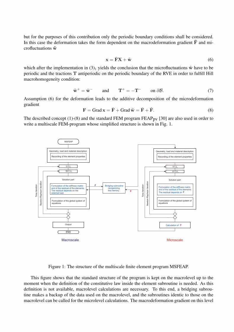
The described concept (1)-(8) and the standard FEM program FEAPpv [30] are also used in order towrite a multiscale FEM-program whose simplified structure is shown in Fig. 1.

Figure 1: The structure of the multiscale finite element program MSFEAP.

This figure shows that the standard structure of the program is kept on the macrolevel up to themoment when the definition of the constitutive law inside the element subroutine is needed. As thisdefinition is not available, macrolevel calculations are necessary. To this end, a bridging subrou-tine makes a backup of the data used on the macrolevel, and the subroutines identic to those on themacrolevel can be called for the microlevel calculations. The macrodeformation gradient on this level

is understood as a given quantity while the primary results are the distribution of the microfluctuationsw and the first Piola Kirchhoff microstress tensor P. The volume average of the latter is the soughtcounterpart on the macrolevel. After finishing the calculations at the microlevel the data related tothis level can be deleted and the bridging subroutine recalls the data needed for the macrolevel. In thisway macroscale calculations can be continued. The microscale subprogram is called for calculatingthe effective stresses as well as their derivatives (see Chap. 4). Such calculations are repeated in eachGauss point for each step of the Newton-Raphson iteration (nonlinear materials) and if necessary,for each step of the time iteration (time dependent problems). In the case of the linear material, theprocedure is much simpler [17]. Here the effective elasticity tensor must be calculated only once as itis independent from deformation.

Flow chart (Fig. 1) shows the flexible structure of the program, allowing for a simple implemen-tation of the new elements at both levels, and accordingly possible implementations in many differentfields. Moreover, it shows that all commands needed for the pre- and postprocessing can be applied attwo levels. Their transcription as well as the user interface remain as in the original program FEAPpv.Finally, it is important to note that the program can still be used for single-scale calculations by choos-ing original elements of the program FEAPpv at the macrolevel. These elements are not connectedwith the bridging subroutine and they do not activate the program part responsible for microscalecalculations.

3 Standard formulation of the P0Q1 elementThe implementation of the method will be shown in a particular example concerning the energypotential in a three-field description as proposed by Simo, Taylor and Pister [26]

Π(u,Θ, p) =

∫V

[Ψvol(Θ) + Ψdev(C∗(u)) + p(J(u)−Θ)] dV + Πext. (9)

Apart from the displacements which are primary variables, this formulation also depends on the vol-ume change Θ and the pressure p. The functional is split in a volumetric and a deviatoric part wherethe volumetric part only depends on the volume change Θ and the deviatoric part on the deviatoricright Cauchy-Green deformation tensor C∗ = J −2/3C where J = det F represents the Jacobian. Thelast part of (9) represents the Lagrange term introduced in order to stipulate the equality of the de-terminant of the Jacobian and the volume change. For the purpose of formulating the correspondingfinite element, the second variation of (9) is needed∫

V

Grad δu : [Grad ∆u · (Sdev + Svol)]dV

+

∫V

(GradTδu · F) : (Adev + Avol) : (FT · Grad∆u)dV

+

∫V

(GradTδu · F) : JC−1dV

(1

V

∂2Ψvol

∂Θ2

) ∫V

JC−1 : (FT · Grad∆u)dV (10)

+∆δuΠext = −δΠresu .

Keep in mind that the first variation is necessary in order to satisfy the stationarity condition and thesecond one in order to linearize the problem. The elasticity tensors Adev and Avol appearing in (10) aredefined in the terms of the second Piola Kirchhoff stress tensors Sdev and Svol as follows

Adev = 2∂Sdev

∂C, Avol = 2

∂Svol

∂C(11)

and the derivative of pressure has to be calculated according to

∂2Ψ

∂Θ2=∂p

∂J=

2

3J∂p

∂C: C∗. (12)

The final step in the formulation of the element is the implementation of the approximation dependenton the shape functions and nodal values. Without going into details, which can be found in theliterature about the FEM [1, 19, 30], this approximation can be expressed in the following way

u = N · ue,

B = Grad N,

Grad ∆u = B ·∆ue,

Grad δu = B · δue.

(13)

Here N is a matrix containing the shape functions and B is a matrix containing the derivatives ofthe shape functions. A hat symbol denotes the nodal values and e indicates that all the DOFs of anelement are considered. The implementation of (13) into (10) leads to the final form of the stiffnessmatrix Ke

Ke =

∫V e

GT · (Sdev + Svol) ·G dV

+

∫V e

(BT · F) : A : (FT ·B)dV (14)

+

∫V e

(BT · F) : JC−1 dV

(1

V

∂2Ψvol∂Θ2

) ∫V e

JC−1 : (FT ·B)dV

with matrix G being defined in the following way∫V e

Grad δu : [Grad ∆u · (Sdev + Svol)]dV = δu ·∫V e

[GT · (Sdev + Svol) ·G]dV ·∆u. (15)

4 Multiscale formulationRelating now the theory explained in Chap. 2 with the formulation given in Chap. 3, the following for-mulation of the problem of the simulation of a heterogeneous body can be given. At the macroscale,expression (10) remains unchanged except that the typical notation (overbar symbol) has to be used.The completion of the problem still requires that Dirichlet and Neumann boundary conditions aresatisfied ∫

V

¯Grad δu : [ ¯Grad ∆u · (Sdev + Svol)]dV

+

∫V

( ¯GradTδu · F) : (Adev + Avol) : (FT · ¯Grad∆u)dV

+

∫V

( ¯GradTδu · F) : JC−1dV

(1

V

∂2Ψvol

∂Θ2

) ∫V

JC−1 : (FT · ¯Grad∆u)dV (16)

+∆δuΠext = −δuΠres

u = u0, δu = 0, ∆u = 0 on ∂Bu.

Contrary to the situation in the case of the standard single-scale method, here the terms dependent onthe constitutive law (Sdev, Svol, Adev, Avol,

∂2Ψvol∂Θ2 ) cannot be calculated directly but by using the data

from the microscale. The formulation at this level is similar to (16) and consequently to (10) but it isnot identical: ∫

V

Grad δw : [Grad ∆w · (Sdev + Svol)]dV

+

∫V

(GradTδw · F) : (Adev + Avol) : (FT · Grad∆w)dV

+

∫V

(GradTδw · F) : JC−1dV

(1

V

∂2Ψvol

∂Θ2

) ∫V

JC−1 : (FT · Grad∆w)dV (17)

+δwΠresmac = −δwΠres

w+ = w−, δw = 0, ∆w = 0 on ∂B; δwΠresmac = f(F).

Here the problem depends on the microfluctuations w, and the macrodeformation gradient F is re-sponsible for the residual part δwΠres

mac which should be treated analogously to the residual due to thedeformation from the previous step of the Newton-Raphson iteration. The influences of the bodyforces are neglected and the periodic boundary conditions have to be satisfied.

5 Simulation of random microporous media

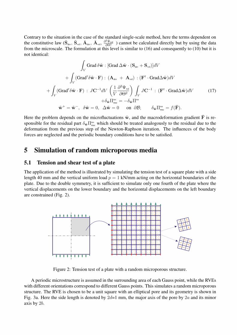
5.1 Tension and shear test of a plateThe application of the method is illustrated by simulating the tension test of a square plate with a sidelength 40 mm and the vertical uniform load p = 1 kN/mm acting on the horizontal boundaries of theplate. Due to the double symmetry, it is sufficient to simulate only one fourth of the plate where thevertical displacements on the lower boundary and the horizontal displacements on the left boundaryare constrained (Fig. 2).

Figure 2: Tension test of a plate with a random microporous structure.

A periodic microstructure is assumed in the surrounding area of each Gauss point, while the RVEswith different orientations correspond to different Gauss points. This simulates a random microporousstructure. The RVE is chosen to be a unit square with an elliptical pore and its geometry is shown inFig. 3a. Here the side length is denoted by 2d=1 mm, the major axis of the pore by 2a and its minoraxis by 2b.

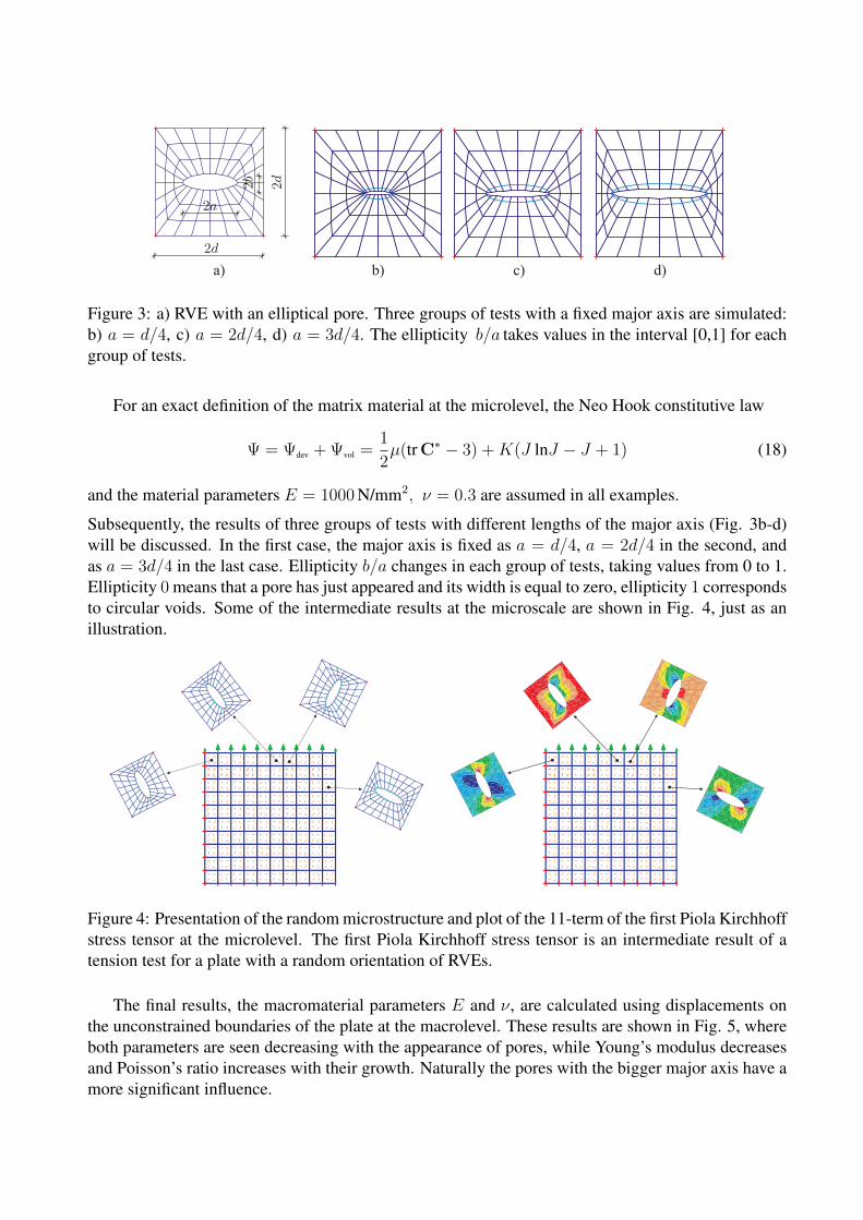
Figure 3: a) RVE with an elliptical pore. Three groups of tests with a fixed major axis are simulated:b) a = d/4, c) a = 2d/4, d) a = 3d/4. The ellipticity b/a takes values in the interval [0,1] for eachgroup of tests.

For an exact definition of the matrix material at the microlevel, the Neo Hook constitutive law

Ψ = Ψdev + Ψvol =1

2µ(tr C∗ − 3) +K(J lnJ − J + 1) (18)

and the material parameters E = 1000 N/mm2, ν = 0.3 are assumed in all examples.

Subsequently, the results of three groups of tests with different lengths of the major axis (Fig. 3b-d)will be discussed. In the first case, the major axis is fixed as a = d/4, a = 2d/4 in the second, andas a = 3d/4 in the last case. Ellipticity b/a changes in each group of tests, taking values from 0 to 1.Ellipticity 0 means that a pore has just appeared and its width is equal to zero, ellipticity 1 correspondsto circular voids. Some of the intermediate results at the microscale are shown in Fig. 4, just as anillustration.

Figure 4: Presentation of the random microstructure and plot of the 11-term of the first Piola Kirchhoffstress tensor at the microlevel. The first Piola Kirchhoff stress tensor is an intermediate result of atension test for a plate with a random orientation of RVEs.

The final results, the macromaterial parameters E and ν, are calculated using displacements onthe unconstrained boundaries of the plate at the macrolevel. These results are shown in Fig. 5, whereboth parameters are seen decreasing with the appearance of pores, while Young’s modulus decreasesand Poisson’s ratio increases with their growth. Naturally the pores with the bigger major axis have amore significant influence.

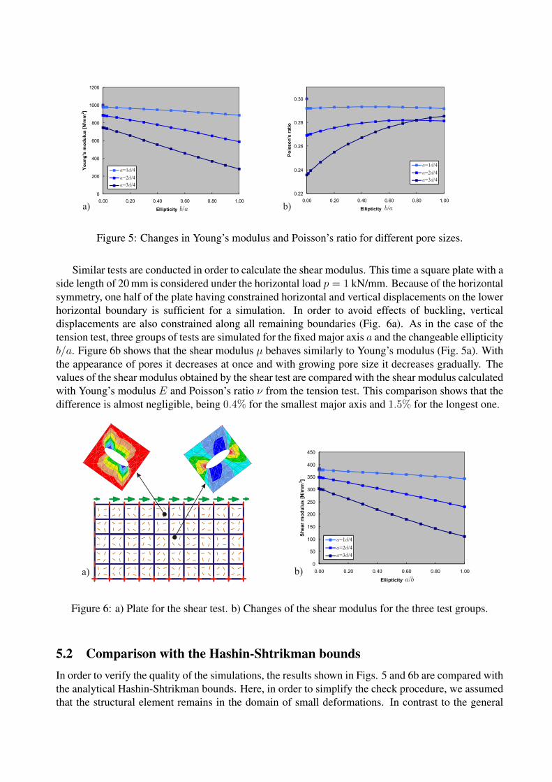
Figure 5: Changes in Young’s modulus and Poisson’s ratio for different pore sizes.

Similar tests are conducted in order to calculate the shear modulus. This time a square plate with aside length of 20 mm is considered under the horizontal load p = 1 kN/mm. Because of the horizontalsymmetry, one half of the plate having constrained horizontal and vertical displacements on the lowerhorizontal boundary is sufficient for a simulation. In order to avoid effects of buckling, verticaldisplacements are also constrained along all remaining boundaries (Fig. 6a). As in the case of thetension test, three groups of tests are simulated for the fixed major axis a and the changeable ellipticityb/a. Figure 6b shows that the shear modulus µ behaves similarly to Young’s modulus (Fig. 5a). Withthe appearance of pores it decreases at once and with growing pore size it decreases gradually. Thevalues of the shear modulus obtained by the shear test are compared with the shear modulus calculatedwith Young’s modulus E and Poisson’s ratio ν from the tension test. This comparison shows that thedifference is almost negligible, being 0.4% for the smallest major axis and 1.5% for the longest one.

Figure 6: a) Plate for the shear test. b) Changes of the shear modulus for the three test groups.

5.2 Comparison with the Hashin-Shtrikman boundsIn order to verify the quality of the simulations, the results shown in Figs. 5 and 6b are compared withthe analytical Hashin-Shtrikman bounds. Here, in order to simplify the check procedure, we assumedthat the structural element remains in the domain of small deformations. In contrast to the general

case, the Hashin-Shtrikman bounds for two-phase materials have a much simpler form

Kl = K1 +c2

1K2−K1

+ 3c13K1+4µ1

, a) Ku = K2 +c1

1K1−K2

+ 3c23K2+4µ2

, b) (19)

µl = µ1 +c2

1µ2−µ1 + 6(K1+2µ1)c1

5µ1(3K1+4µ1)

, a) µu = µ2 +c1

1µ1−µ2 + 6(K2+2µ2)c2

5µ2(3K2+4µ2)

. b) (20)

Here, the subscripts l, u denote the lower and upper bound respectively, and phases are chosen so thatK2 > K1 and µ2 > µ1. Their volume concentrations are denoted by c1 and c2. The microporous ma-terial represents a two-phase material so that the expressions above can be applied directly. However,as the material parameters of voids are equal to zero, the lower bounds (19)a and (20)a reduce to zeroand only the upper bounds remain.

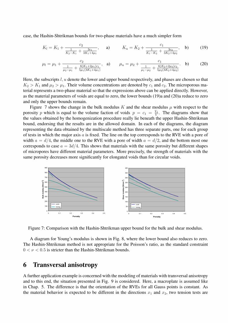
Figure 7 shows the change in the bulk modulus K and the shear modulus µ with respect to theporosity p which is equal to the volume faction of voids p = c1 = V1

V. The diagrams show that

the values obtained by the homogenization procedure really lie beneath the upper Hashin-Shtrikmanbound, endorsing that the results are in the allowed domain. In each of the diagrams, the diagramrepresenting the data obtained by the multiscale method has three separate parts, one for each groupof tests in which the major axis a is fixed. The line on the top corresponds to the RVE with a pore ofwidth a = d/4, the middle one to the RVE with a pore of width a = d/2, and the bottom most onecorresponds to case a = 3d/4. This shows that materials with the same porosity but different shapesof micropores have different material parameters. More precisely, the strength of materials with thesame porosity decreases more significantly for elongated voids than for circular voids.

Figure 7: Comparison with the Hashin-Shtrikman upper bound for the bulk and shear modulus.

A diagram for Young’s modulus is shown in Fig. 8, where the lower bound also reduces to zero.The Hashin-Shtrikman method is not appropriate for the Poisson’s ratio, as the standard constraint0 < ν < 0.5 is stricter than the Hashin-Shtrikman bounds.

6 Transversal anisotropyA further application example is concerned with the modeling of materials with transversal anisotropyand to this end, the situation presented in Fig. 9 is considered. Here, a macroplate is assumed likein Chap. 5. The difference is that the orientation of the RVEs for all Gauss points is constant. Asthe material behavior is expected to be different in the directions x1 and x2, two tension tests are

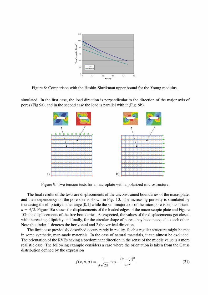
Figure 8: Comparison with the Hashin-Shtrikman upper bound for the Young modulus.

simulated. In the first case, the load direction is perpendicular to the direction of the major axis ofpores (Fig 9a), and in the second case the load is parallel with it (Fig. 9b).

a) b)

Figure 9: Two tension tests for a macroplate with a polarized microstructure.

The final results of the tests are displacements of the unconstrained boundaries of the macroplate,and their dependency on the pore size is shown in Fig. 10. The increasing porosity is simulated byincreasing the ellipticity in the range [0,1] while the semimajor axis of the micropore is kept constant:a = d/2. Figure 10a shows the displacements of the loaded edges of the macroscopic plate and Figure10b the displacements of the free boundaries. As expected, the values of the displacements get closedwith increasing ellipticity and finally, for the circular shape of pores, they become equal to each other.Note that index 1 denotes the horizontal and 2 the vertical direction.

The limit case previously described occurs rarely in reality. Such a regular structure might be metin some synthetic, man-made materials. In the case of natural materials, it can almost be excluded.The orientation of the RVEs having a predominant direction in the sense of the middle value is a morerealistic case. The following example considers a case where the orientation is taken from the Gaussdistribution defined by the expression

f(x, µ, σ) =1

σ√

2πexp−(x− µ)2

2σ2(21)

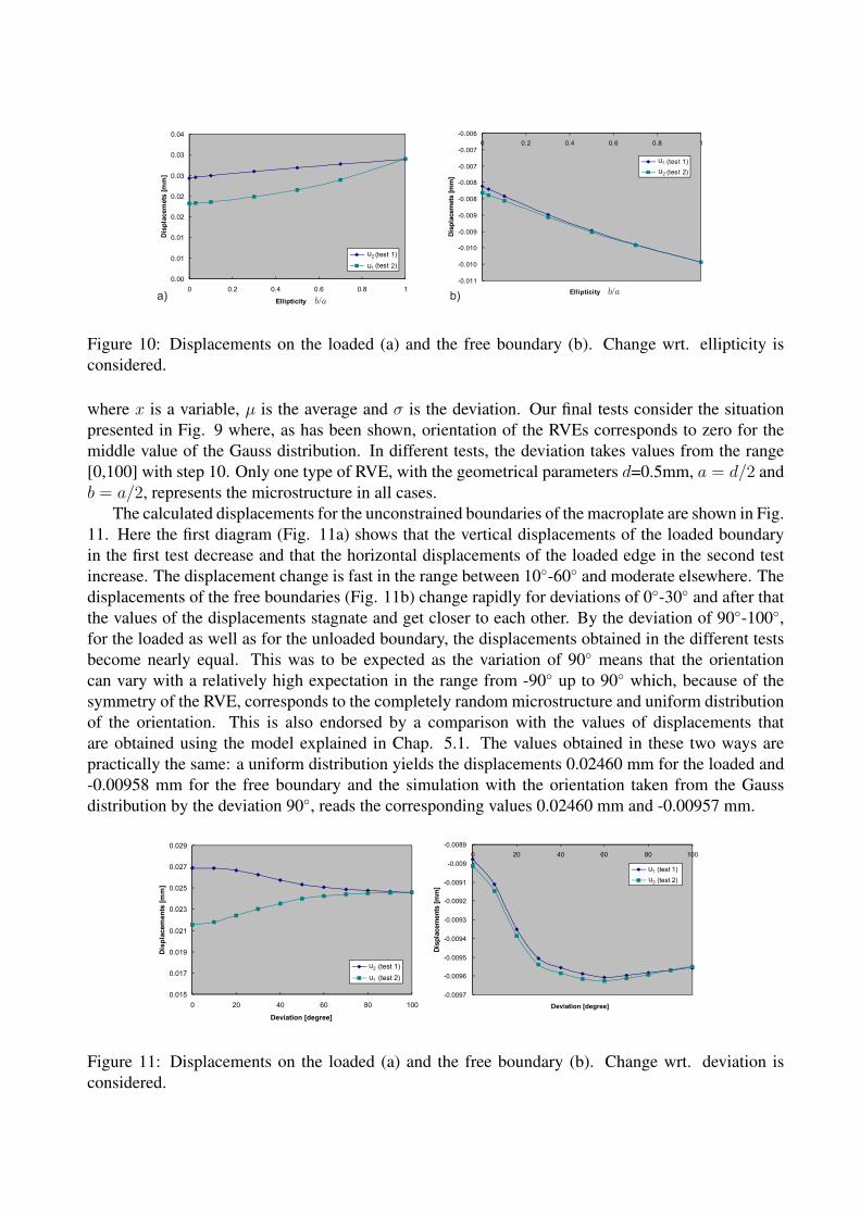
Figure 10: Displacements on the loaded (a) and the free boundary (b). Change wrt. ellipticity isconsidered.

where x is a variable, µ is the average and σ is the deviation. Our final tests consider the situationpresented in Fig. 9 where, as has been shown, orientation of the RVEs corresponds to zero for themiddle value of the Gauss distribution. In different tests, the deviation takes values from the range[0,100] with step 10. Only one type of RVE, with the geometrical parameters d=0.5mm, a = d/2 andb = a/2, represents the microstructure in all cases.

The calculated displacements for the unconstrained boundaries of the macroplate are shown in Fig.11. Here the first diagram (Fig. 11a) shows that the vertical displacements of the loaded boundaryin the first test decrease and that the horizontal displacements of the loaded edge in the second testincrease. The displacement change is fast in the range between 10◦-60◦ and moderate elsewhere. Thedisplacements of the free boundaries (Fig. 11b) change rapidly for deviations of 0◦-30◦ and after thatthe values of the displacements stagnate and get closer to each other. By the deviation of 90◦-100◦,for the loaded as well as for the unloaded boundary, the displacements obtained in the different testsbecome nearly equal. This was to be expected as the variation of 90◦ means that the orientationcan vary with a relatively high expectation in the range from -90◦ up to 90◦ which, because of thesymmetry of the RVE, corresponds to the completely random microstructure and uniform distributionof the orientation. This is also endorsed by a comparison with the values of displacements thatare obtained using the model explained in Chap. 5.1. The values obtained in these two ways arepractically the same: a uniform distribution yields the displacements 0.02460 mm for the loaded and-0.00958 mm for the free boundary and the simulation with the orientation taken from the Gaussdistribution by the deviation 90◦, reads the corresponding values 0.02460 mm and -0.00957 mm.

0.015

0.017

0.019

0.021

0.023

0.025

0.027

0.029

0 20 40 60 80 100

Deviation [degree]

Dis

pla

cem

en

ts[m

m]

u2 (test 1)

u1 (test 2)

-0.0097

-0.0096

-0.0095

-0.0094

-0.0093

-0.0092

-0.0091

-0.009

-0.0089

0 20 40 60 80 100

Deviation [degree]

Dis

pla

cem

en

ts[m

m]

u1 (test 1)

u2 (test 2)

u2

u1

u1

u2

Figure 11: Displacements on the loaded (a) and the free boundary (b). Change wrt. deviation isconsidered.

7 ConclusionsIn this contribution, the main features and some examples of application of the multiscale finite ele-ment code MSFEAP are presented. The underlying procedure belongs to the group of homogenizationmethods according to which the problem of modeling a heterogeneous body is split into two parts.The first part represents an analysis of the RVE leading to the effective material parameters, and thesecond part consists in the application of the so obtained effective values for the simulation of themacroscopic, now homogenized body. These two parts known as the macro and micro boundaryvalue problem are bridged by the Hill macrohomogeneity condition and the concept of the volumeaverage. The presented program has a modular structure which allows a simple adaptation for the usein different fields. Another advantage is the possibility of the application of commands typical for anFE software at two levels.

An illustrative example concerns the simulation of a macroscopic plate under tension and shearload. In all examples the unit square-shaped RVE with the elliptical pore represents the microstruc-ture. The influence of the RVE orientation and the pore size on the effective behavior are especiallyconsidered. The first group of tests elaborates the isotropic material behavior which is achievedchoosing an arbitrary orientation of RVE in each Gauss point. The here obtained results show that in-creasing porosity induces a decreasing Young’s and shear modulus and an increasing Poisson’s ratio.By the same porosity, the pores with a smaller ellipticity have a stronger influence on the parameterchange. A comparison with the Hashin-Shtrikman bounds shows that all results are in the permit-ted domain. The further examples concern the transversal anisotropy. To this end the orientation ofRVEs is constant or taken from the Gauss distribution. The final results provide an insight in themacroscopic deformation and its dependency on the deviation of the RVE-orientation.

References[1] K.J. Bathe, Finite element procedures, Prentice-Hall International, (1996).

[2] B. Budianski, On the elastic moduli of some heterogeneous materials, J. Mech. Phys. Solids, 13,(1965), 223-227.

[3] P.P. Castaneda, The effective mechanical properties of nonlinear isotropic composites, J. Mech.Phys. Solids., 39(1), (1991), 45-71.

[4] P.P. Castaneda, New variational principles in plasticity and their application to composite mate-rials, J. Mech. Phys. Solids., 40(8) , (1992), 1757-1788.

[5] P.P. Gilbert and A. Panachenko, Effective acoustic equations for a two-phase medium with mi-crostructure, Math. Comput. Model., 39, (2004), 1431-1448.

[6] P.P. Gilbert, A. Panachenko and X. Xie Homogenization of viscoelastic matrix in linear frictionalcontact, Math. Meth. Appl. Sci., 28, (2005), 309-328.

[7] Z. Hashin and S. Shtrikman, On some variational principles in anisotropic and nonhomogeneouselasticity, J. Mech. Phys. Solids, 10, (1962), 335-342.

[8] Z. Hashin and S. Shtrikman, A variational approach to the theory of the elastic behaviour ofpolycrystals, J. Mech. Phys. Solids, 10, (1962), 343-352.

[9] Z. Hashin and S. Shtrikman, A variational approach to the theory of the elastic behaviour ofmultiphase materials, J. Mech. Phys. Solids, 11, (1963), 127-140.

[10] R. Hill, The elastic behaviour of a crystalline aggregate, Proc. Phys. Soc., London, A, 65, (1952),349-354.

[11] R. Hill, Elastic properties of reinforced solids: some theoretical principles, J. Mech. Phys. Solids,11, (1963), 357-372.

[12] R. Hill, On Constitutive Macro-Variables for Heterogeneous Solids at Finite strain, Proc. R. Soc.Lond., A, 326, (1972), 131-147.

[13] C. Huet, Universal conditions for assimilation of a heterogeneous material to an effectivemedium, Mech. Res. Commun., 9(3), (1982), 165-170.

[14] C. Huet, On the definition and experimental determination of effective constitutive equations forassimilating heterogeneous materials, Mech. Res. Commun., 11(3), (1984), 195-200.

[15] C. Huet, Application of variational concepts to size effects in elastic heterogeneous bodies, J.Mech. Phys. Solids, 38(6), (1990), 813-841.

[16] S. Ilic, Application of the multiscale FEM to the modeling of composite materials, Ph.D. Thesis,Ruhr-University Bochum, Germany, (2008).

[17] S. Ilic, K. Hackl and R.P. Gilbert, Application of the multiscale FEM to the modelling of cancel-lous bone, Biomechan. Model. Mechanobiol., 11(3), (2009), DOI: 10.107/s10237-009-0161-6.

[18] S. Ilic, User manual for the multiscale FE program MSFEAP, www.am.bi.ruhr-uni-bochum.de/Mitarbeiter/ilic.html, (2010).

[19] T.J.R. Hughes, The Finite Element Method, Prentice Hall, Englewood Cliffs, NJ, (1987).

[20] E. Kroner, Elastic moduli of perfectly disordered composite materials, J. Mech. Phys. Solids,15, (1967), 319-329.

[21] C. Miehe, J. Schotte and M. Lambrecht, Homogenisation of inelastic Solid Materials at FiniteStrains based on Incremental Minimization Principles, J. Mech. Phys. Solids, 50, (2002), 2123-2167.

[22] T. Mori and K. Tanaka, Average stress in matrix and average elastic energy of materials withmisfitting inclusions, Acta Metallurgica, 21, (1973), 571-574.

[23] H. Moulinec and P. Suquet, Intraphase strain heterogeneity in nonlinear composites: a compu-tational approach, Europ. J. of Mech., A/Solids , 22, (2003), 751-770.

[24] J.T. Oden and T.I. Zohdi, Analysis and adaptive modeling of highly heterogeneous elastic struc-tures, Comp. Met. Appl. Mech. Eng., 148, (1997), 367-391.

[25] J. Schroder, Homogenisierungsmethoden der nichtlinearen Kontinuumsmechanik unter Beach-tung von Stabilitats Problemen, Habilitationsshrift, Universitat Stuttgart, (2000).

[26] J.C. Simo and T.J.R Hughes, Computational Inelasticity, Springer Verlag, (1997).

[27] P. Suquet, Effective Properties of Nonlinear Composites, in P. Suquet (ed.), Continuum Mi-cromechanics, CISM, 377, Springer Wien New York, (1997).

[28] D.R.S. Talbot and J.R. Willis, Variational Principles for Inhomogeneous Non-linear Media,IMA-Journal of Applied Mathematics, 35, (1985), 39-54.

[29] J.R. Willis, Bounds and self-consistent estimates for the overall properties of anisotropic com-posites, J. Mech. Phys. Solids, 25, (1977), 185-202.

[30] O.C. Zienkiewicz and R.L. Taylor, The finite element method, Butterworth-Heinemann, (2000).

[31] T.I. Zohdi, J.T. Oden and G.J. Rodin, Hierarchical modeling of heterogeneous bodies, Comp.Met. Appl. Mech. Eng., 138, (1996), 273-298.

[32] T.I. Zohdi and P. Wriggers, A domain decomposition method for bodies with heterogeneousmicrostructure based on the material regularization, Int. J. Sol. Struct., 36, (1999), 2507-2525.

[33] T.I. Zohdi, P. Wriggers and C. Huet, A method of substructuring large-scale computationalmicromechanical problems, Comp. Met. Appl. Mech. Eng., 190(13), (2001), 5639-5656.