ABSTRACT

Title of Thesis: METHODS IN REALISTIC COMPUTATIONAL

MODELING OF THE AVIAN NUCLEUS LAMINARIS

Degree candidate: Victor Grau Serrat

Degree and year: Master of Science, 2003

Thesis directed by: Professor Jonathan Z. SimonDepartment of Electrical and Computer Engineering

On the basis of a previous model of coincidence detection neurons of nucleus

laminaris (NL) in the auditory brainstem, a biophysically more realistic imple-

mentation was developed. The aim of the model was to faithfully characterize

the diversity of cells observed within the nucleus, and account for their tonotopic

arrangement. Anatomical and electrophysiological data was compiled and distilled

from the literature. Due to the scarcity of experimental data and the high level

of detail sought, a large set of parameters loosely defined a huge variable space.

The biological relevant subspace was found by combining the biological constraints

with a brute force exploration in a distributed environment. The result is a method

that accurately described the high frequency cells of NL. Important physiological

divergences between modeled cells within the nucleus, which result from reported

anatomical differences, are discussed. The varying morphology of the cells seems

to impose underestimated constraints on the physiology of the cells throughout

the tonotopic axis of NL. Physiological gradients are considered as possible expla-

nations to unexpected outcomes of the model, arguing their limited effect.

METHODS IN REALISTIC COMPUTATIONAL

MODELING OF THE AVIAN NUCLEUS LAMINARIS

by

Victor Grau Serrat

Thesis submitted to the Faculty of the Graduate School of theUniversity of Maryland, College Park in partial fulfillment

of the requirements for the degree ofMaster of Science

2003

Advisory Committee:

Professor Jonathan Z. Simon, ChairProfessor Catherine E. CarrProfessor Shihab A. Shamma

ACKNOWLEDGEMENTS

To Jonathan Z. Simon,

You cannot teach a man anything,

you can only help him find it for himself. Galileo Galilei

To Catherine E. Carr,

One of the advantages of being disorderly is that

one is always making new and exciting discoveries. A. A. Milne

To Kate MacLeod,

Who does not understand a glance,

cannot understand a long explanation. Arab proverb

To Shantanu Ray,

What is a friend?

A single soul dwelling in two bodies. Aristotle

To the rest of the crew of CSSL and NSL who helped me in ways small and

large, but above all have made this thesis enjoyable. Finally, my parents have

always taught me to be thankful. Thus, special thanks goes to myself, without

whom this thesis would certainly not have been possible.

It’s the possibility of having a dream

come true that makes life interesting. The Alchemist, P. Coelho

ii

TABLE OF CONTENTS

List of Tables iv

List of Figures v

1 Introduction 11.1 Auditory computation . . . . . . . . . . . . . . . . . . . . . . . . . 21.2 Motivations and objectives . . . . . . . . . . . . . . . . . . . . . . . 4

2 Modeling background 62.1 Linear cable theory . . . . . . . . . . . . . . . . . . . . . . . . . . . 72.2 Hodgkin and Huxley channel types . . . . . . . . . . . . . . . . . . 92.3 The NEURON environment . . . . . . . . . . . . . . . . . . . . . . 122.4 Distributed simulations . . . . . . . . . . . . . . . . . . . . . . . . . 16

3 Initial implementation 183.1 Morphology . . . . . . . . . . . . . . . . . . . . . . . . . . . . . . . 183.2 Electrical Properties . . . . . . . . . . . . . . . . . . . . . . . . . . 243.3 Channel Dynamics . . . . . . . . . . . . . . . . . . . . . . . . . . . 27

4 Physiological characterization 334.1 Subthreshold response . . . . . . . . . . . . . . . . . . . . . . . . . 344.2 Stimulus-evoked postsynaptic potentials . . . . . . . . . . . . . . . 374.3 Suprathreshold response . . . . . . . . . . . . . . . . . . . . . . . . 404.4 Firing rates . . . . . . . . . . . . . . . . . . . . . . . . . . . . . . . 47

5 Adjusting Tonotopicity 545.1 Preliminary analysis . . . . . . . . . . . . . . . . . . . . . . . . . . 545.2 Redistribution of conductances . . . . . . . . . . . . . . . . . . . . 585.3 Reshaping the dendrites . . . . . . . . . . . . . . . . . . . . . . . . 605.4 Tonotopic variation of channel conductances . . . . . . . . . . . . . 63

6 Conclusions 67

Bibliography 69

iii

LIST OF TABLES

3.1 Parametrization of channel kinetics. . . . . . . . . . . . . . . . . . . 32

4.1 Three different sets of parameters for KLV A that give a valid voltage-current relation. . . . . . . . . . . . . . . . . . . . . . . . . . . . . . 37

4.2 Biophysically relevant range of sodium parameters. . . . . . . . . . 444.3 Simulated set of values for sodium parameters. . . . . . . . . . . . . 464.4 Outcome of the search for sodium parameters. . . . . . . . . . . . . 474.5 Progression in the number of combinations that match successive

constraints on firing rates. . . . . . . . . . . . . . . . . . . . . . . . 504.6 Number of combinations matching V-I specifications with KHV A

and Na. . . . . . . . . . . . . . . . . . . . . . . . . . . . . . . . . . 51

iv

LIST OF FIGURES

2.1 Equivalent circuit of the point representation of a neuron. . . . . . . 72.2 Equivalent circuit of a neuronal fiber. . . . . . . . . . . . . . . . . . 82.3 Hodgking and Huxley model of the neuronal membrane. . . . . . . 102.4 Hodkin and Huxley action potential . . . . . . . . . . . . . . . . . . 13

3.1 Biocytin filled nucleus laminaris neurons from the chicken. . . . . . 193.2 Comparison between the devised ideal soma (left) and the seg-

mented implementation by NEURON (right). . . . . . . . . . . . . 213.3 Number of primary dendrites and dendritic length as functions of

characteristic frequency. . . . . . . . . . . . . . . . . . . . . . . . . 233.4 Dimensions of the equivalent cylinder. . . . . . . . . . . . . . . . . . 253.5 Equivalent circuit and behavior of the passive membrane. . . . . . . 28

4.1 Comparison between the V-I plot for the initial set of parameters(black circles) and the reference curve (red crosses). . . . . . . . . . 35

4.2 Valid voltage-current curves and their correspoding time plots. . . . 384.3 Evolution of the shape of an action potential. . . . . . . . . . . . . 434.4 Two examples of unacceptable firing rate plots. . . . . . . . . . . . 484.5 Two combinations with valid firing rates. . . . . . . . . . . . . . . . 504.6 Invalid (top) and valid (bottom) V-I plot with KHV A and Na. . . . 52

5.1 Simplified circuit of a soma and two dendrites, and its equivalentwith only one dendrite. . . . . . . . . . . . . . . . . . . . . . . . . . 56

5.2 V-I plot for the 500 Hz cell with the configuration from the 2000 Hzcell. . . . . . . . . . . . . . . . . . . . . . . . . . . . . . . . . . . . 57

5.3 V-I plot for the 500 Hz cell after redistributing potassium conduc-tances. . . . . . . . . . . . . . . . . . . . . . . . . . . . . . . . . . . 59

5.4 Superimposed voltage responses to a 2 nA current clamp for a lowand high frequency cell. . . . . . . . . . . . . . . . . . . . . . . . . 60

5.5 Dendritic diameter tapering along dendritic length. Comparisonbetween the ideal profile and the segmented implementation byNEURON. . . . . . . . . . . . . . . . . . . . . . . . . . . . . . . . . 62

5.6 Voltage-current relation of a low frequency cell with varying diam-eter of the dendrites. . . . . . . . . . . . . . . . . . . . . . . . . . . 64

v

5.7 Comparison of voltage responses between a low and high frequencycell after reshaping the dendrites. . . . . . . . . . . . . . . . . . . . 64

5.8 Comparison of voltage responses between a low and a high frequencycell while assessing the effect of KHV A. . . . . . . . . . . . . . . . . 66

vi

Chapter 1

Introduction

Computational neuroscience is a discipline that aims to understand how

information is processed in the nervous system by developing formal models at

many different structural scales. Using a multidisciplinary approach, the

biological systems are modeled incorporating the constraints imposed by

psychophysical, neurobiological and formal computational analyses. In order to

fully comprehend the very diverse and highly specialized tasks of the nervous

systems, multiple levels of analysis have to be addressed ranging from detailing

the biophysical mechanisms responsible for these computations to evaluating the

overall system performance.

The end product of computational analysis should be a sufficiently specified

model, internally consistent, and complete enough to enable formal mathematical

characterization or computer simulation. Such properties ensure that the

computed outcome accurately reproduces the functions of the modeled system.

Often is the case that specific features of the real world are not fully understood

by the modeler, who therefore must guess about them when designing and

testing the model. Conjectures are to be made, notwithstanding, following

psychophysical and neurobiological constraints, as the theoretical outcomes of the

1

model would otherwise fail to capture the nature of biological computation. A

certain degree of ignorance about the real phenomenon is implicit in the

modeling process, because it is indeed the aim of such a process to gain a deeper

insight into the mechanisms governing the object of study.

1.1 Auditory computation

Characterized by processing information about two orders of magnitude faster

than the rest of the brain, the auditory system is responsible for providing a

representation of the pattern of incoming sound signals, and specifying the

locations of the corresponding sound sources relative to the listener. Specifically,

sound localization is computed by means of interaural temporal and level

differences over the entire spectrum of the signal from the sound coming to both

ears.

The picture of what is accomplished in the brain stem auditory nuclei as

acoustic information ascends the auditory pathway is still fragmentary, but there

is no doubt that auditory neurons are specialized for precisely timed electrical

signaling. Despite some similarities in the organization of the brain stem

auditory nuclei between diverse animal classes, the avian system is regarded as

having a simpler structure and the function of each nucleus involved is better

understood than the mammalian analog [27, 39]. The present study focuses

exclusively on sound localization in avians.

Timing information in sound is captured in the cochlea and is conveyed to the

auditory nerve, which projects to the cochlear nuclei. One branch of the auditory

nerve innervates nucleus angularis (NA) and another innervates nucleus

magnocellularis (NM), whose afferents project to nucleus laminaris (NL).

2

Evidence is accumulating that many neurons in NA are specialized for intensity

analysis of complex sounds, whereas NM and NL are adapted for analysis of

interaural time differences (ITDs) [39]. Detection and computation of ITDs is the

underlying mechanism used in azimuthal sound localization in the brain.

The most prominent and important model of binaural interaction was

suggested by Jeffress [18] as a mechanism for sensitivity to interaural time delays.

The model postulates the existence of neuronal fibers that contain temporal

information about the waveform of the acoustic stimulus in their discharge

pattern. These fibers project with ladder-like branching patterns to cells in a

binaural nucleus that only discharge when receiving coincident spikes from their

monoaural afferents. The lengths of the mentioned fibers are supposed to

introduce internal neuronal delays that compensate for the acoustic delay of

incoming signals between both ears. The model suggests the computation of

ITDs by means of delay lines and coincidence detectors, transforming a time code

into a space code.

Anatomical and physiological evidence shows that the cochlear nucleus is the

likely site of Jeffress’ model: nucleus magnocellularis axons are hypothesized to

work as delay lines, and nucleus laminaris cells are thought to play the role of

coincidence detectors [3, 28]. Nucleus laminaris is mainly composed by cells that

extend their dendrites dorsally and ventrally in a bipolar fashion. Each cluster of

dendrites receives inputs from one ear: the ipsilateral NM projects onto the

dorsal side, whereas the contralateral NM innervates the ventral side.

Additionally, neurons within both nuclei are arranged tonotopically: their

neuronal location depends on the frequency band to which they are tuned.

3

1.2 Motivations and objectives

In nucleus laminaris, a strong functional hypothesis can be formulated and

biological data can be feasibly obtained from experiments in vitro. As a result,

NL has already been the objective of many anatomical [9, 10, 11, 38, 43, 44] and

electrophysiological experiments [3, 23, 28, 36, 47], as well as the target of some

computer modeling efforts. Previous models have yielded significant results in

explaining some particular features of NL: the role of dendrites in auditory

coincidence detection [1], phase locking capabilities and synaptic location [42]

and short-term synaptic plasticity as an adaptive mechanism for preserving ITD

information [6].

Whereas anatomical data roughly covers the entire nucleus laminaris,

physiological data tends to be recorded from the high frequency region of the

nucleus. The outlined computational models, which are built on the experimental

data available, are therefore restricted to the same neuronal zones. Instead of

concentrating on the variability of features observed within the nucleus, some

degree of uniformity is assumed between cells, and the results are subsequently

generalized to the whole.

Merging previous approaches with the reported morphological gradients of

the cells under study, the present work intends to provide a broader description,

coherent with the varied amount of biological data available. The main goal of

this study is to construct a biophysically realistic model of neuronal coincidence

detection within the framework of an existing model of nucleus laminaris [42]. A

neuron-level approach is aimed at faithfully characterizing the morphology,

electrical properties and channel dynamics that underlie the characteristic

behavior of nucleus laminaris cells.

4

While seeking to account for the variability observed between cells within the

nucleus and gain deeper understanding of their specialization, a biophysically

coherent description of the entire nucleus is the goal of the modeling efforts to

ultimate unveil the intricacies of neuronal coincidence detection. The cost of the

intended level of detail is, from a modeling point of view, an increase in the

number of parameters. Despite the significant sources of information, the variable

space of the model is not tightly constrained. An exhaustive exploration of all

possible combinations is thus unconceivable. Instead, a strategic scattered

examination is performed taking advantage of the available computer resources in

a distributed system.

Within this operational framework, the relation between biology and

computer modeling is conceived to be bidirectional. Experimental data is the

basis upon which the model is built, and the end product of the model are

predictions that can be used to guide future experiments.

5

Chapter 2

Modeling background

Electrical signals are the basis of information transfer in the nervous system.

Nerve cells have evolved elaborate mechanisms for generating and processing

electrical signals based on the flow of ions across their plasma membranes.

Biological membranes exhibit distinctive features similar to those of electrical

circuits, and this analogy is the basis for describing and modeling the behavior

and functionality of nerve cells: neurons are often described in terms of their

equivalent circuits.

The cornerstone of any biophysically realistic neuronal model is the point

representation of the cell, where the morphology of the neuron is reduced to a

single point or compartment. The specialization of the plasma membrane to deal

with electrical signals makes it permeable to some ion species but not to others.

Therefore, a separation of charge normally occurs across the membrane: there is

a difference between the intracellular (Vi) and extracellular (Vo) potentials,

termed the membrane potential (Vm):

Vm = Vi − Vo (2.1)

In particular, at rest, all cells have a negative resting potential (Vrest). The

6

isolation properties of the membrane are well described with a capacitor (C), and

the membrane permeability can initially be described with a resistor (R): the

current that flows through the membrane bears a linear relation with the voltage

across the membrane, following Ohm’s law. These three elements constitute the

equivalent circuit of the passive membrane as depicted in Figure 2.1.

CR

Vrest

Vm

Figure 2.1: Equivalent circuit of the point representation of a neuron.

For a full review on Sections 2.1 and 2.2, the reader is referred to [19, 21].

2.1 Linear cable theory

The vast majority of neurons present a much more complicated structure than a

single compartment spherical cell. In general, neurons have extensive dendritic

trees that receive a myriad of excitatory and inhibitory synaptic inputs. These

extended systems have a cablelike structure. Consequently, the dynamics of the

membrane potential along them are governed by linear cable theory, in which the

electrical properties of a given system are analyzed in relation to its specific

cylindrical geometry. Many parts of a neuron can be approximated by a cylinder,

characterized by a conductive core surrounded by a membrane that has different

electrical properties from its core. The analogy with a standard copper wire is

7

the foundation for extending the mathematical description of the current flow

through the wire to the flow of ions through neuronal fibers.

The relation between current and voltage in one-dimensional cable is

described by the cable equation, a partial differential equation, first order in time

and second order in space. Three basic assumptions are made to derive it: the

membrane parameters are assumed to be linear and uniform throughout the

fiber; current flows only along a single spatial dimension, the length of the cable

(radial current is zero); for convenience, the extracellular resistance is assumed to

be zero. In order to numerically solve the cable equation, a spatial discretization

of the cable into different segments is performed, which results in a family of

differential equations, one for each segment. Figure 2.2 depicts the single passive

cable, formed by a set of connected compartments or segments. Each

compartment is the point representation of the passive membrane described in

the previous section. This more elaborate model incorporates the intracellular

cytoplasm, modeled as a resistor (Ri) that connects adjacent compartments.

CR

Vrest

VmCR

Vrest

CR

Vrest

jj-1 j+1j+1j-1 j

RRR Ri-1 i+1i i+2

Figure 2.2: Equivalent circuit of a neuronal fiber.

Within the cable theory framework, Rall [33] proposed that any neuronal

8

dendritic tree could be simplified to a single equivalent cable with regard to its

electrical properties. Two additional assumptions are made to those of the cable

theory. Firstly, at any branch point, the parent cable diameter (d0) relates to

that of its daughters (di) by the relation:

d3/20 =

∑i

d3/2i (2.2)

Secondly, all terminal branches end at the same electrotonic distance from the

origin in the main branch. Real dendritic trees rarely conform to these

assumptions. Nonetheless, this simplification is often accepted to model complex

dendritic arborizations as a first approach to explain the contribution of the

dendrites, while avoiding the burden of detailing their involved geometry.

2.2 Hodgkin and Huxley channel types

The primary electrical signal generated by nerve cells is the action potential,

which results from a change in membrane permeability to specific ions. Hodgkin

and Huxley [17] set the foundation to mathematically describe and quantify the

kinetics governing the generation of action potentials. They postulated a

phenomenological model based on their experiments in the squid giant axon.

Two independent major voltage-dependent ionic conductances, a sodium

conductance GNa and a potassium conductance GK , are involved in the

generation of the action potential. Additionally, there is a third smaller

conductance, termed leak (Gleak), that does not depend on the membrane

potential. Each conductance has a reversal potential associated with it given by

Nernst’s equation for the corresponding ion type, which depends on the different

extracellular and intracellular ion concentrations. The point model of the neuron

9

is thereby extended to accommodate the sodium and potassium permeabilities as

depicted in Figure 2.3, where the resistors are named by their inverses, the

conductances.

C Vm

Vleak

GNaGK

EK ENa

Gleak

Figure 2.3: Hodgking and Huxley model of the neuronal membrane.

Both GNa and GK are expressed in terms of a maximum conductance (GNa

and GK) multiplied by a numerical coefficient that represents the fraction of the

maximum conductance open at a given time. This coefficient is seen as a gating

variable that switches between its two possible states: permissive or open, and

nonpermissive or closed. The transition between both states is governed by

first-order kinetics, and, for the potassium case, it can be written as:

nβnαn

1 − n (2.3)

where n is the probability that the gate is open, and 1-n is the probability of

being closed. αn and βn are voltage-dependent rate variables (in units of s−1)

that specify how many transitions occur between the closed and open states and

vice versa. Mathematically, this scheme translates into a first-order differential

equation of the form:

dn

dt= αn(V )(1 − n) − βn(V )n (2.4)

10

where V is the membrane potential of the neuron. Eq. 2.4 yields the following

solution:

n(t) = n0 −[(n0 − n∞)

(1 − e−t/τn

) ](2.5)

n∞ =αn

αn + βn(2.6)

τn =1

αn + βn

(2.7)

Hodking and Huxley parametrized the dependence of α and β with the

membrane potential as follows (expressed in the most general form):

αn(V ) =αn0(

V −αnV1/2

αnk)

1 − e

αnV1/2−V

αnk

(2.8)

βn(V ) = βn0e

βnV1/2−V

βnk (2.9)

where αnV1/2and βnV1/2

are the midpoints for activation and deactivation, αnk

and βnk define the voltage range in which activation and deactivation takes place,

and αn0 and βn0 give the slope of activation and deactivation. To sum up, the

current that will flow across the plasma membrane through the potassium

channels (IK) is expressed as:

IK = GKn4(EK − V ) (2.10)

where the power to the 4 of n indicates that there are 4 independent variables

(required to account for the observed kinetics), and the joint probability of the

channel being open or closed is the product of each single probability. EK is the

reversal potential for potassium.

The description of the dynamics of the sodium conductance are slightly more

complex. In order to fit the kinetics of the sodium current, Hodgkin and Huxley

11

had to postulate the existence of a sodium activation variable m and a sodium

inactivation variable h. As a result, the sodium analogous equation of Eq. 2.10 is:

INa = GNam3h(ENa − V ) (2.11)

Similar to before, the temporal evolution of m and h is governed by the

corresponding first-order differential equations, for whose solution Hodgkin and

Huxley empirically derived the following equations for the rate variables

(expressed in the most general form):

αm(V ) =αm0(

V −αmV1/2

αmk)

1 − e

αmV1/2−V

αmk

(2.12)

βm(V ) = βm0e

βmV1/2−V

βmk (2.13)

αh(V ) = αh0e

αhV1/2−V

αhk (2.14)

βh(V ) =βh0

1 + e

βhV1/2−V

βhk

(2.15)

This set of equations gives a quantitative account for voltage- and

time-dependent sodium and potassium conductances, and fully describes the

waveforms of action potentials. Figure 2.4 shows the time plots that correspond

to a current injection of 0.5 ms in duration and 0.4 nA in amplitude to the

equivalent circuit represented in Figure 2.3. For this plot, all parameters are set

equal to those reported in the original paper [17].

2.3 The NEURON environment

Information processing in the brain results from complex changes of membrane

properties constrained to operate within the limitations of the intricate anatomy

12

Figure 2.4: Hogkin and Huxley action potential. Computed action potential in

response to a 0.5 ms current pulse of 0.4 nA. The upper graph shows the evolution

of the membrane potential. The middle graph shows the potassium and sodium

currents, and the lower graph plots the evolution of the gating particles n, m, and

h.

13

of neurons. As outlined in previous sections, the mathematical framework used to

describe such brain mechanisms usually consists of a large set of equations that

generally do not have analytical solutions. In most of the cases, because of the

nonlinearities and spatiotemporal complexities of such equations, intuition does

not provide much help in understanding the cells’ behavior. Nonetheless, having

defined the set of algebraic equations, it can easily be solved numerically by using

the appropriate computational tools. NEURON is such a tool that provides a

flexible environment for implementing biologically realistic models of electrical

and chemical signaling in neurons and networks of neurons [14]. Specifically

designed to simulate nerve cells, NEURON allows the user to deal directly with

concepts at the neuroscience level, provides with a customizable graphical user

interface (GUI) and is particularly efficient because of the use of special methods

that take advantage of the structure of nerve equations [13].

Spatiotemporally continuous variables are computed over a set of discrete

points in space, called nodes, for a finite number of instants in time. NEURON

allows for a conceptual division of the different parts of the cell into different

cable sections, which can be connected together to form any branched structure.

Each section can be divided into nseg segments, whose midpoints are the

mentioned nodes. Using the second order integration method provided by

NEURON (a variant of Crank-Nicholson), the discrete solutions are a piecewise

linear approximation to the continuous system with second order accuracy

proportional to ∆t2, where ∆t is the chosen time step. The size of ∆t and the

fineness of the spatial grid jointly determine the accuracy of the solution.

Therefore, a tradeoff must be met between spatiotemporal accuracy and

computational efficiency. The spatial grid was chosen by repeatedly increasing

14

the number of grid points (by tripling them, [16]) until further increases caused

no significant change in simulation results. Accordingly, nseg is set to 9 in all

sections, except for the axon node that is already small enough and nseg is set to

1 (cf. Section 3.1). Depending on the types of simulations to be run, the

performance of the integration method can be changed in the model by using a

fixed or an adaptive time step. If a fixed time step is chosen, ∆t is set by default

at 0.0125 ms, being more than one order of magnitude smaller than the time

constant for the faster events to be simulated (e.g. mean half-width of an action

potential is around 0.3 ms). For the adaptive case, the specification comes in

terms of an absolute error rather than ∆t. A maximum absolute error of 0.01 in

the adaptative case and ∆t=0.0125 ms for the fixed time step yield similar

degrees of accuracy [16].

NEURON incorporates a programming language based on Hoc [20], a floating

point calculator with C-like object oriented syntax that can be used to

implement abstract data types. The starting point for the present work is a

previous model of nucleus laminaris written in Hoc: about 7500 lines (100 pages)

of code that construct an array of cells in nucleus laminaris with a high degree of

customization and an adapted GUI designed to test and evaluate the

performance of the modeled cells [42]. Additionally, NEURON incorporates a

high-level language (NMODL [15]) for incorporating new biophysical mechanisms

in models. NMODL offers a syntax that closely resembles familiar mathematical

and chemical notation. NMODL files are automatically translated into C and

further compiled for computational efficiency. The channels and synaptic

mechanisms embodied in the model are customized using this language.

15

2.4 Distributed simulations

A great level of detail in the model is required to accomplish the ultimate goal of

making it biophysically realistic. Almost one hundred different parameters are

needed to accurately model the morphology of the cell, the kinetics of the

channels involved, and the variety of the stimuli delivered. Consequently, the

resulting parameter space is intractably huge, even though only a small volume of

this space is biologically relevant. Experimental data imposes an important

constraint on defining the initial space to be searched. However, due to the

limited empirical data available, it is still unfeasible to ransack the constrained

space in order to locate where the biologically significant subspace lies.

In order to maximize the chances of successfully pursuing the parameter

search, a system was devised to automatically explore different sets of points in a

given subspace. This process is carried out by a program written in Perl that

continuously performs three main tasks: it progressively generates all possible

combinations that result from a given reduced set of parameters; it distributes

each combination among a pool of available machines for its simulation; it

processes the outcome of each simulation by either saving the combination if it

matches a given criterion or discarding it otherwise. A brute force approach is

employed to compensate for the uncertainty about the size and continuity of the

possible solution space. The program runs asynchronously, it is fault tolerant and

crash resistant, and can run for several days. By distributing the simulations

among an average of 20 workstations, the program takes great advantage from

the available university computing facilities in an inherent distributed

environment such as the Unix system in the Glue project (cf.

http://www.glue.umd.edu). Slightly less than a linear factor decrease in the

16

overall running time is achieved through the distribution process (e.g. a factor of

3.5 with 5 machines, independent of the number of simultaneous simulations per

machine). It cannot compensate for the exponential increase in the number of

simulations (as a function of their quantity and depth), but it still provides a

very powerful scanning tool.

17

Chapter 3

Initial implementation

The modeling process starts by dissecting the object of study into its constituent

parts. The initial specifications for each of the components consists in assigning

the appropriate level of detail to each section. A tradeoff between biological

accuracy and computational efficiency is implicit throughout the whole process.

Anatomical and electrophysiological data is collected from surveying the

available literature. Experimental data sets the foundations for characterizing

each modeled section in accordance to the observed features of real cells (cf.

Figure 3.1). The choices for each parameter are discussed herein in order to

provide a preliminary notion about their estimated relevance.

3.1 Morphology

The preponderant neuron in nucleus laminaris is generally characterized by a

cylindrical, ellipsoid or ovoid cell soma, which is spineless. The diameter of the

soma is between 15 µm and 20 µm [30, 43, 44] and the size of the somata remains

relatively constant throughout the nucleus. The length of the soma is in the same

range of values as the diameter.

18

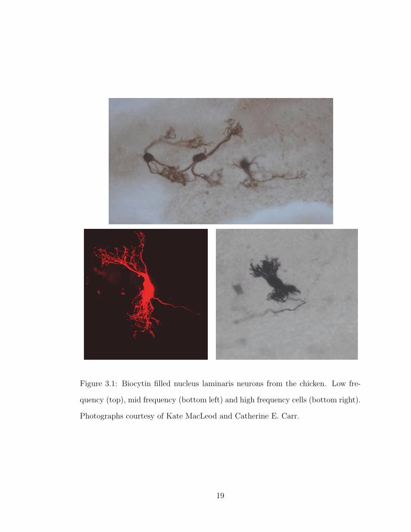
Figure 3.1: Biocytin filled nucleus laminaris neurons from the chicken. Low fre-

quency (top), mid frequency (bottom left) and high frequency cells (bottom right).

Photographs courtesy of Kate MacLeod and Catherine E. Carr.

19

The somatic region in the model is a truncated ovoid, and is formed by the

revolution of a half period sinusoidal profile about the major axis of the cell:

d(x) = (dmax − dmin)sin(πx) + dmin (3.1)

where d(x) is the cell diameter as a function of the position parameter x.

NEURON defines the position in each compartment in the range 0 ≤ x ≤ 1 from

one end to the other [14]. dmax is set to 20 µm and dmin is set to 10 µm [11]. The

sine function is chosen for being continuous and derivable to ensure the

smoothness reported in the shape of real cells. The length of the somatic

compartment, Lsoma, is set to 20 µm.

The most important feature of the soma shape is its corresponding surface

area. All membrane properties that characterize the cell are defined in the model

in terms of concentrations per unit area. Thus, the membrane mechanisms placed

in the soma will be a function of the total somatic external membrane. The

associated area for the modeled soma can be calculated as:

Areaideal =∫ L

02πd

( x

Lsoma

)√1 + d′

( x

Lsoma

)2(3.2)

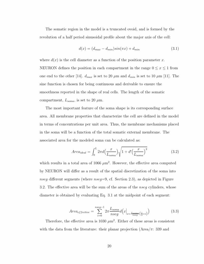
which results in a total area of 1066 µm2. However, the effective area computed

by NEURON will differ as a result of the spatial discretization of the soma into

nseg different segments (where nseg=9, cf. Section 2.3), as depicted in Figure

3.2. The effective area will be the sum of the areas of the nseg cylinders, whose

diameter is obtained by evaluating Eq. 3.1 at the midpoint of each segment:

Areaeffective =nseg−1∑

i=0

2πLsoma

nsegd(x∣∣∣x= Lsoma

nseg( 1

2+i)

)(3.3)

Therefore, the effective area is 1030 µm2. Either of these areas is consistent

with the data from the literature: their planar projection (Area/π: 339 and

20

Figure 3.2: Comparison between the devised ideal soma (left) and the segmented

implementation by NEURON (right).

328 µm, respectively) fall in the range of reported measurements

(306 ± 67.9 µm2 [44]).

The neurons in nucleus laminaris are tonotopically organized: there is a high

correlation between the neural position of the cell and the frequency to which the

cell is tuned, termed the characteristic frequency (CF) of the cell. Thus, the

position of the cell within the nucleus is a good predictor of the characteristic

frequency of the cell [38], as defined in Eq. 3.3:

f = 40pos (3.4)

where pos refers to the relative position (in percent) along the tonotopic axis,

from the caudolateral (low frequencies) to the rostromedial end (high

frequencies). Nucleus laminaris neurons are homogeneous in segregating their

dendrites in a bipolar fashion: one tuft of dendrites extends dorsally and the

other ventrally. Along the tonotopic axis, there is a gradient of decreasing length

of the dendrites and increasing number of primary dendrites. Eqs. 3.5 and 3.6

21

characterize these relations as a function of the neural position of the cell [44]:

Nden = max(0.37pos − 5.5, 2) (3.5)

Lden =(−11.19pos + 1447)

max(0.37pos − 5.5, 2)(3.6)

where Nden is the number of primary dendrites, and Lden, the equivalent length of

each dendrite, is the quotient between the total dendritic length and the number

of primary dendrites.

The dendrites are modeled as unbranched cylinders in accordance to the

simplified ball-and-stick model proposed by Rall (cf. Section 2.1). The dendrites

are grouped around both ends of the major axis of the soma. Their section

diameter is kept constant at 1.78 µm for all cells [44] and their length and

number are computed as a function of the characteristic frequency of the cell.

This relation is obtained by combining Eq. 3.4 into Eqs. 3.5 and 3.6; the result is

plotted in Figure 3.3. Thus, the number of dendrites ranges tonotopically from 2

at CFs below 800 Hz to 14 at CF of 2 kHz. Similarly, the dendritic length varies

from around 650 µm at CFs below 800 Hz down to 70 µm at CF of 2 kHz. The

minimum number of primary dendrites is set to 2 to preserve symmetry (one on

each side), which causes a minor artifact on the relation of the length of the

dendrites as a function of the characteristic frequency of the cell.

Despite the outlined uniformity in the size of the soma and the reported

constant diameter of the dendrites throughout the whole nucleus laminaris, there

is some additional anatomical evidence that shows larger cells progressively

tapering their diameter from the somatic region towards the dendrites. The

implication of this phenomenon is a marked increase in the membrane surface,

which in turn alters the total conductances of the cell and its behavior. Initially,

22

500 1000 1500 20000

5

10

15

20

25

30

Num

ber

of D

endr

ites

Best Frequency (Hz)500 1000 1500 2000

0

100

200

300

400

500

600

700

Len

gth

of D

endr

ites

(um

)

Best Frequency (Hz)

Figure 3.3: Number of primary dendrites and dendritic length as functions of

characteristic frequency.

this effect is disregarded. It will be exhaustively analyzed in Section 5.3.

The axon of NL protrudes from the soma in between the two dendritic zones

and initially extends medially for up to a few hundred micrometers [44]. The

axon has an initial segment, also termed axon hillock, after which it becomes

myelinated. The initial segment is reported to be 30 µm long and to have a mean

diameter of 2 µm [2]. The diameter shows no variation between the axon hillock

and the myelinated axon, and the internodal length of each myelinated segment

is 60 µm (data from the barn owl) [2].

In the model, three different sections compose the axon: the axon hillock, the

myelinated axon and the first node of Ranvier. All three sections are modeled as

cylinders of constant diameter (2 µm). Whereas the axon usually projects to

other parts of the brain several hundreds of micrometers away, the study of

nucleus laminaris cells is limited to the first node of Ranvier, where the output of

the cell is evaluated. In this study, the node is only regarded as a very small

compartment where a spike is generated if the signal coming from the soma raises

23

above a certain threshold. Thus, the length of the node is set to 2 µm (data from

the rat) [31]; the intended functionality compensates the lack of accuracy in the

exact morphology of the node.

3.2 Electrical Properties

The membrane of the cell is mainly constituted of proteins and lipids. The latter

form the basis of the membrane arranged in two parallel layers that isolate the

intracellular cytoplasm from the extracellular medium. From an electrical point

of view, the thin membrane acts like a capacitor. In membrane biophysics, the

capacitance is usually characterized by the specific capacitance per unit area Cm,

measured in microfarads per square centimeter (µF/cm2). The generally agreed

upon value for Cm is 1 µF/cm2 [21]. Among the many kinds of proteins that

populate the membrane, of special electrical relevance are those that enable ions

to cross the membrane. The proteins that allow a current flow through the

membrane are known as ion channels, and are modeled as resistors. The

membrane resistance is usually specified in terms of the specific membrane

resistance Rm, expressed in terms of resistance per unit area (Ωcm2). Equally

common is to express this same value in terms of the inverse of Rm, namely the

specific leak conductance, Gleak = 1/Rm, measured in units of siemens per square

centimeter (S/cm2). The latter nomenclature is the one which is used in the

model.

The cytoplasm of the cell is characterized in terms of the specific intracellular

resistivity (Ri), defined as the total resistance across 1 centimeter cube of

intracellular cytoplasm. The value conventionally used for Ri in avian and

mammalian neurons is 200 Ωcm [21], which is set uniformly through all sections

24

of the model. Given a cylindrical axon or dendrite of diameter d and length L, its

total resistance will be 4RiL/πd2.

The simplest of all neuronal models characterizes the electrical properties of

neurons with a resistance and a capacitance in parallel (the so-called RC circuit).

This is the skeleton for each segment of every section modeled by NEURON.

Adjacent segments are connected by means of a series resistance, and the

dynamics of the voltage along segments are described by linear cable theory (for

a review see [19, 21]).

All sections of the model share the same values for Cm and Gleak, except for

the myelinated axon. The myelin membrane of an axon consists of several

concentric wrappings of the axonal membrane. Its electrical properties can be

obtained by adding together the contribution of each of its layers. The

capacitance associated with one single layer of the membrane is:

Cmembrane = CmArea = CmdπL (3.7)

where one can use a planar approximation of the external surface of the cylinder

because the width of the membrane is more than 100 times smaller than the

axonal radius. For the myelinated case, the planar approximation does not hold

anymore, and thus the associated capacitance should be calculated as (cf. Figure

3.4):

Figure 3.4: Dimensions of the equivalent cylinder.

25

Cmyelin =Cm2πwL

ln(d′/d)(3.8)

Anatomical observations yield a relatively constant ratio d′/d of 0.7

throughout all the nervous system [26, 31], and a relatively constant width of the

axonal membrane around 8 nm [26, 37]. Combining Eqs. 3.7 and 3.8, the ratio

between the two cases can be expressed as follows:

Cmyelin

Cmembrane=

2w

dln(d′/d)=

1

45(3.9)

which means that the myelination of the axon is equivalent to 45 wraps of one

single membrane. Consequently, the equivalent capacitance for the myelinated

section is the sum of 45 capacitors in series (Cm/45), and the resulting resistance

is the sum of 45 resistors in series (45Rm). The lower capacitance and bigger

membrane resistance result in an increased conduction velocity of the action

potential through the fiber.

To get an estimate for the membrane resistance, one has to refer to

physiological recordings. This value is obtained experimentally by injecting a

series of current pulses into the cell, and measuring their voltage response. Using

Ohm’s Law, one can calculate the input resistance of the cell, namely the total

membrane resistance. Current clamps should be recorded close below the resting

potential to avoid the interfering effects of other conductances that become active

at either more depolarized or more hyperpolarized voltages. For a set of cells

with characteristic frequencies between 800 Hz and 3000 Hz [36], the mean input

resistance (Rin) is measured to be 72 ± 34 MΩ. A 2000 Hz cell is chosen as the

representative case from the mentioned set. To derive the specific membrane

resistance, the input resistance must be multiplied by the total area of the cell:

Rm = Rin (Areasoma + Areaden + Areaaxon) (3.10)

26

Gleak = 1/Rm (3.11)

which gives a result of Gleak=2.1E-04 S/cm2. This value carries some degree of

uncertainty for two reasons: the original measurement had a relative error

(standard deviation) of about 50%, and this value is completely dependent on the

area of the cell for which there is a large interval of incertitude.

The last element that remains to be characterized in order to describe the

electrical properties of the passive membrane is a fictive battery Vleak that

accounts for the resting potential. The value is obtained from a voltage-current

plot of the experiment described above (cf. Figure 2E 1 in [36]). Vleak is the

intersection of the slope below the resting potential with the abscissa I=0 nA, as

if there were no other channels that actually shift this value towards more

negative values. The intersection occurs at -50 mV.

The equivalent circuit of all elements of the passive membrane and the

intracellular cytoplasm is depicted in Figure 3.5, as well as the evolution of the

membrane potential when a current step of different amplitudes (-0.5, -0.1, 0.3,

and 0.7 nA) is switched on at t=5 ms and turned off at 25 ms. Plotting the

relation between this series of currents and voltages (in steady state) results in a

linear regression of 72 MΩ, which shows self-consistency of the model.

3.3 Channel Dynamics

The hallmark of nucleus laminaris neurons, as part of the auditory system, is

their ability to phase-lock and maintain high discharge rates. The next step in

1The plot is shifted -10 mV to match the resting potential (injected current of 0 nA) with the

reported mean value in the same article: -59 ± 5 mV.

27

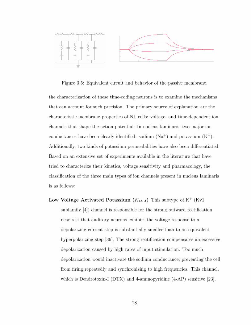
Figure 3.5: Equivalent circuit and behavior of the passive membrane.

the characterization of these time-coding neurons is to examine the mechanisms

that can account for such precision. The primary source of explanation are the

characteristic membrane properties of NL cells: voltage- and time-dependent ion

channels that shape the action potential. In nucleus laminaris, two major ion

conductances have been clearly identified: sodium (Na+) and potassium (K+).

Additionally, two kinds of potassium permeabilities have also been differentiated.

Based on an extensive set of experiments available in the literature that have

tried to characterize their kinetics, voltage sensitivity and pharmacology, the

classification of the three main types of ion channels present in nucleus laminaris

is as follows:

Low Voltage Activated Potassium (KLV A) This subtype of K+ (Kv1

subfamily [4]) channel is responsible for the strong outward rectification

near rest that auditory neurons exhibit: the voltage response to a

depolarizing current step is substantially smaller than to an equivalent

hyperpolarizing step [36]. The strong rectification compensates an excessive

depolarization caused by high rates of input stimulation. Too much

depolarization would inactivate the sodium conductance, preventing the cell

from firing repeatedly and synchronizing to high frequencies. This channel,

which is Dendrotoxin-I (DTX) and 4-aminopyridine (4-AP) sensitive [23],

28

presents rapid activation near rest (low threshold) and slow or partial

deactivation.

High Voltage Activated Potassium (KHV A) Belonging to the Kv3

subfamily of K+ channels, KHV A is characterized by positively shifted

voltage dependencies and very fast deactivation rates [29, 40]. These

properties allow this channel to enable fast repolarization of action

potentials without compromising spike initiation or height, which maximize

the quick recovery of resting conditions after an action potential.

Narrowing the width of action potentials, KHV A enables repetitive firing at

high frequencies. Because of its high threshold of activation this channel is

also known as delayed rectifier. It is tetraethylammonium (TEA) sensitive.

Sodium (Na) Not much is known about the intricacies of sodium dynamics due

to its inherent faster kinetics, which pose greater difficulties in conducting

the corresponding neurophysiological experiments. When the membrane

potential reaches the firing threshold, the sodium channels boosts the

membrane voltage to trigger an action potential, and repolarizes it to rest

afterwards.

The Hodgkin and Huxley original study (cf. Section 2.2, [17]) of the ionic

conductances underlying the action potential serves as the basic framework for

modeling the ionic conductances in the model. The challenge resides in

accommodating the abundant data from very diverse sources to conclusively

depict the observed functionality of the neurons under study. Due to the limited

number of neurophysiology experiments reported in nucleus laminaris [23, 36],

most of the data comes from the previous nucleus in the auditory pathway that

projects onto it, namely nucleus magnocellularis (NM) [22, 34, 35, 50].

29

Additional data is gathered from physiology and modeling in the medial superior

olive (MSO) [45], the mammalian analog of NL. Data from the rat [25, 41] is also

observed to characterize the sodium channel. Finally, previous models are taken

either as a starting point [42] or as a partial reference [1, 6].

The first step in incorporating the sodium and potassium channels into the

model is to try to quantify their presence in real cells. Membrane channels are

expressed in the model in terms of concentrations per unit area. A procedure

similar to the one explained to calculate Gleak (cf. Section 3.2) is used here to

estimate both potassium conductances. Using data from a set of experiments in

nucleus magnocellularis where the effects of KLV A and KHV A have been isolated

and characterized independently, one can extract the associated total

conductance for each channel: 0.1 µS and 0.45 µS, respectively (slope in

current-voltage plot: Figures 5A and 7A in [34]). To express these magnitudes in

terms of concentrations per unit area, the total membrane surface is computed

through the measured capacitance [34]:

Areatotal =C

Cm

=14 pF

1 µF/cm2= 1.4E-05 cm2 (3.12)

GKLV A=

0.1 µS

Areatotal= 7.1E-03 S/cm2 (3.13)

GKHV A=

0.45 µS

Areatotal

= 3.4E-02 S/cm2 (3.14)

It is important to note that neurons in NM tend to be bigger than their NL

counterparts, and are usually spherical without any dendrites [39]. Therefore, the

calculated channel densities refer only to the soma and the axon. However,

without any other initial assumption, these densities are uniformly extended to

the dendrites in the model, setting them equally across the soma, the axon

hillock and dendrites.

30

No specific values for sodium densities have been found in the literature in

any similar nucleus. To set the order of magnitude of this value, the channel

density reported in the original Hodgkin and Huxley experiments in the squid

giant axon (1.2E-01 S/cm2 [17]) is used as a reference, because the corresponding

densities for potassium and leak (3.6E-02 and 3.0E-04 S/cm2) are in the same

range of values as the ones in the model calculated previously (4.1E-02 and

2.1E-04 S/cm2).

The reversal potentials for each of the channels are initially set accordingly to

the values reported in the corresponding paper: EK=-83 mV [34] and

ENa=40 mV [17]. The rest of parameters that determine the specific kinetics of

each channel are summarized in Table 3.1. The parameter exponent refers to the

power of each gating variable, namely the number of independent fictional gating

variables that make first-order transitions between an open and a closed state (cf.

Eqs. 2.10 and 2.11).

The protein channels that modulate the flux of ions through the membrane of

the cell are temperature-sensitive. Thus, whenever a rate is given, it is

accompanied by the specification of the temperature of the experiment (T0). In

biology, the effect of temperature (T ) on rates is frequently given as the

10-degree temperature coefficient (Q10) defined as rate(T+10 C)/rate(T ) [12].

In the model, the temperature for the simulations is set at 35 C to reproduce

the conditions of the cell in vivo. The temperature coefficient in the simulations

is set by:

Qsimulations = (Q10)35−T0

10 (3.15)

where Qsimulations multiplies the differential equation governing the kinetics of n

for potassium (cf. Eq. 2.4), and the corresponding ones for m and h for sodium.

31

Thus, for a Q10 of 3 and temperature increases of 1, 5, 15 and 25 C, the rates of

gating increase are 1.12-, 1.7-, 5-, and 16-fold, respectively.

KLV A KHV A Na

n n m h

αV1/2(mV) -60 -19 -40 -65

αk (mV) 21.8 9.1 10 20

α0 (ms−1) 0.2 0.11 4 0.07

βV1/2(mV) -60 -19 -65 -35

βk (mV) 14 20 18 10

β0 (ms−1) 0.17 0.103 4 1

exponent 1 1 3 1

Q10 2 2 3

T0 (C) 23 23 6.3

Table 3.1: Parametrization of channel kinetics.

32

Chapter 4

Physiological characterization

Once the model has been built with all the parameters set matching the values

reported in the literature, the model should be expected to behave like real cells.

However, due to the variety of sources employed, the resulting initial set of

parameters does not match the cell’s behavior reported in any of the sources (as

an illustrative example, cf. Figure 4.1). Many simulations have to be run to

progressively assess the importance, the degree of variability and reliability of

each choice of values for a given parameter space.

The large extent of the initial parameter space makes it impossible to address

the characterization of all different variables involved at once. Thus, the tuning

of the parameters is done in consecutive stages following the guidelines set up by

the reports found in the literature. Diverse physiological experiments try to

characterize each aspect of the functionality of the cell as separately as possible,

and they are reproduced up to a reasonable extent in the model in order to attain

the characteristic behavior of nucleus laminaris cells as coincidence detectors.

33

4.1 Subthreshold response

The first feature to be studied in detail in nucleus laminaris neurons is their

outward rectification. Physiological experiments characterize the subthreshold

response of the cell by injecting a series of current steps of different amplitudes

and recording the voltage response at its steady state. The rectification is clearly

visible by plotting the relation between the injected current (I) and the

membrane voltage (V ) in an V-I plot. These experiments are mimicked in the

model, where the hypothesis is made that KHV A and Na do not have any

influence on rectification, and they are therefore temporarily removed. The

hypothesis is based on two assumptions. Firstly, KHV A channels become active

at much more positive values, and they should be inactive at the range of

voltages under study. Secondly, although some current injections may indeed

depolarize the membrane voltage above the voltage threshold triggering a spike

at the very beginning of the step, sodium channels quickly inactivate and the

membrane voltage stabilizes at the rectified value. The correctness of the

hypothesis is tested once the channels have been faithfully characterized.

The reference is taken from the V-I plot pictured in Figure 2E in [36],

although the whole figure is shifted by -10 mV so that the resting potential

matches the mean value reported in the same paper (Vrest=-59±5 mV). The first

simulations run with the parameters set at their initial values (cf. Chapter 3),

show two main differences with the reference plot: Vrest=-77 mV and rectification

occuring at much more hyperpolarized values (cf. Figure 4.1).

The first thing to be considered is that the midpoints for activation and

deactivation of KLV A have been taken from nucleus magnocellularis in absolute

terms, but they should be considered relative to the cell’s resting potential

34

Figure 4.1: Comparison between the V-I plot for the initial set of parameters (black

circles) and the reference curve (red crosses, Figure 2E in [36] shifted -10 mV).

(reported to be -66±7 mV [34]). The resting potential results from the

equilibrium of intracellular and extracellular concentrations of all ions that can

flow through the membrane, and thus there is a reciprocal dependence between

the channel dynamics and the value where Vrest is.

The second observation refers to the calculated conductance associated with

KLV A channels. The total conductance was measured for nucleus magnocellularis

cells and divided by their mean area (cf. Eqs. 3.12 and 3.13). The channel

density was exported to NL, assuming the same channel density for both types of

cells. However, due to the larger area in NL cells because of their dendrites, the

total conductance is much bigger, which results in greater rectification. Instead,

35

if the value exported is the total conductance, and it is later divided by NL cells’

mean area, the total conductance is similar, and so is the cell’s behavior.

A preliminary exploration of the parameter space around the initial values for

the variables governing the KLV A channel kinetics and KLV A densities revealed

that a good fit to the reference plot was hard to find. The reference plot did not

seem to be a good representative for the general case. Accordingly, the reference

was adapted to the mean values reported in the text of the paper, whose main

features are: Vrest=-59±5 mV, slope resistance below resting potential at

72±34 MΩ and slope above resting potential at 11±8 MΩ. To quantify the

degree of similarity between the outcome of the model and the reference plot, the

mean square error was computed for each of the constraints weighted against the

reference values as follows:

Error =

(slopebelow rest − 72

10

)2

+

(slopeabove rest − 11

2

)2

+(

Vrest + 59

2

)2

(4.1)

Comparing the V-I plots for NM and NL (Figure 1B in [34] or Figure 4B in

[49] and Figure 2E in [36]), one can observe that rectification is more abrupt in

NL. Thus, faster and stronger rectification can be obtained by simultaneously

decreasing the channel density and reducing the range in which KLV A becomes

active (making αnk and βnk smaller).

There are more parameters to specify the dynamics of KLV A than constraints

available from biological data. Therefore, no ideal solution exists for this set of

parameters, except that they provide with reasonable behavior for the cell. A few

guidelines about the parameters governing the dynamics of KLV A can be outlined

as follows: the midpoints for activation and deactivation (αnV1/2and βnV1/2

) are

36

between 10 and 15 mV above rest; the activation and deactivation ranges αnk and

βnk tend to be inversely proportional to the difference between Vrest and αnV1/2or

βnV1/2; the bigger the activation and deactivation ranges, the smaller (i.e. faster)

the activation and deactivation rates (αn0 and βn0). Such relations between KLV A

parameters define a relatively small valid variable space. Three different sets of

parameters that give a valid voltage-current relation are summarized in Table 4.1

and depicted in Figure 4.2: red traces mark the reference, and blue traces plot

the slopes where the mean square error is computed below and above rest.

Set 1 Set 2 Set 3

αV1/2(mV) -50 -50 -45

αk (mV) 5 10 8

α0 (ms−1) 0.20 0.05 0.20

βV1/2(mV) -50 -50 -45

βk (mV) 5 10 8

β0 (ms−1) 0.17 0.10 0.17

GKLV A(S/cm2) 0.0015 0.0035 0.004

Table 4.1: Three different sets of parameters for KLV A that give a valid voltage-

current relation.

4.2 Stimulus-evoked postsynaptic potentials

The ultimate goal of this study is to examine the responses of NL neurons to

stimuli that closely resemble acoustic stimuli. Nucleus laminaris receives its

inputs from nucleus magnocellularis axons projecting onto NL dendrites. In vivo

37

Figure 4.2: Valid voltage-current curves and their correspoding time plots.

38

recordings reveal that NM fire action potentials phase locked to acoustic stimuli

and that the average firing rate (AFR) of NM neurons does not vary

systematically with their characteristic frequencies [3, 47]. Accordingly, in the

model, AFR is set fixed at 250 Hz [36] and does not vary with the stimulus

frequency.

In order to replicate the postsynaptic potentials (PSPs) elicited by nucleus

magnocellularis, the next step is to model the shape and size of the unitary

PSPs. Postsynaptic potentials are described by a change in the membrane

voltage shaped by an alpha function of the form:

Gsyn(t) =Gsynt

τe(1− t

τ ) (4.2)

Isyn = Gsyn(V − Vsyn) (4.3)

where Gsyn is the amplitude of the PSP, τ determines the shape, t is time, and

Vsyn is the reversal potential for the synaptic current that is set to 0 mV

according to the referred paper. Gsyn is set to 7 nS so that the evoked PSPs have

a mean amplitude around 1.5 mV (Figure 3B [36]). The reported half-width of

the alpha function is 0.76±0.50 ms; a τ of 0.33 ms is proposed in that study to

match their measurements. However, a straightforward computation of such a

function gives an ideal half-width of 0.89 ms. Additionally, the plasma membrane

adds a low pass filter effect (RC circuit) that widens the response. Due to the

physical impossibility of implementing the suggested value, a value of 0.1 ms is

chosen for τ , which results in a half-width of around 1.2 ms. It is relevant to

mention that other experiments report postsynaptic potentials with much slower

time constants: half-widths between 2.2±0.4 ms and 5.4±0.5 ms depending on

the age of the chick (post-hatch days (P) 2-7 and embryonic days (E) 16 and 17,

39

respectively) [23]. The reference experiments were made with embryos E19-21

[36].

In the simulations, the size of PSPs are adjusted by varying the injected

current given by Eq. 4.3 while the cell membrane potential is at rest, mimicking

the physiological experiments. These measurements give an estimate on how fast

the membrane can respond to a given stimulus. The speed of the membrane is

directly related to the total membrane conductance at a given time. Because

KLV A starts becoming active near rest, these measurements are a good estimate

on how much KLV A conductance is active above the resting potential, as the leak

conductance by itself cannot account for such a fast response. In the previous

section, the reference for matching KLV A conductances was taken just above rest

to ensure a sufficient amount of conductance at this point for the membrane to

follow the synaptic stimuli.

4.3 Suprathreshold response

The hallmark of nucleus laminaris neurons is their ability to fire action potentials

phase locked to the incoming stimuli. Despite being the main agents in shaping

the action potential, sodium currents are less well known due to the fact that

they are large and fast, which makes them hard to voltage clamp without

introducing artifacts. The most arduous task in constructing the model is

probably the accurate characterization of the kinetics of sodium channels.

The axon hillock is believed to be the site for spike initiation, from where the

action potential propagates forward through the axon and backwards to the

soma. High density of Na in the initial segment compared to the soma accounts

for this phenomenon. Although there is increasing evidence for the presence of

40

sodium in the dendrites, it is speculated to be of another type [7].

Electrophysiological studies have differentiated between a fast or transient Na+

current and a persistent Na+ current. The transient current mediates the fast

action potential, while the persistent current activates below threshold and is

thought to help boost currents in the dendrites. However, the magnitude of the

persistent Na+ current is approximately 1% of the transient one (for a review, see

[7]). In order to maintain simplicity in the model, only one type of sodium

channels (transient) has been incorporated, and the channel densities of the soma

are a fraction (1/3) of these present in the axon.

The first adjustment to the initial set of sodium parameters is a shift in the

reference temperature T0 from 6.3 to 23 C. The motivation for this change is to

bring some internal coherence to the model, so that all three channels included

therein have the same reference temperature, and they can be directly compared

if necessary. Additionally, 23 C is the temperature of most in vitro experiments

in avian and mammalian nerve cells, and it is the reference for most of the data

from the literature. Q10 is shifted from 3 to 2, accordingly. This first

modification will make the original specifications for sodium much slower at the

simulation temperature (35 C) because the differential equation that governs the

sodium kinetics is now multiplied by a smaller factor (cf. Eq. 3.15).

Without any further modifications, some preliminary simulations are run to

gain some intuition about the changes to be made. The results show that the cell

cannot fire even a single action potential, and the resting potential is critically

shifted towards more positive values (cf. Figure 4.3, upper plot). Two

straightforward explanations can account for the observed disparities. Firstly, the

original values are referenced to a resting potential of -65 mV instead of -59 mV,

41

which causes a similar misbehavior as observed in the KLV A case (cf. Section

4.1). Secondly, the sodium channels were originally tied to some other potassium

ones that had an activation range (αnk) of 10 mV, which now has been reduced

in KLV A to 5 mV (Set 1), which makes potassium stronger in the zone where it

becomes active, shutting down a weaker sodium. To illustrate these two

arguments, if all activation and inactivation ranges are halved for sodium and

their midpoints of activation and inactivation are shifted at least +6 mV, some

spiking starts to occur (cf. Figure 4.3, middle plot). However, some undesired

oscillation occurs after the initial spike resulting from breaking the fragile

equilibrium between both channels. In order to fix these undesired effects, a more

careful treatment of the channel kinetics is required.

In order to acquire a complete picture of the mechanisms involved in shaping

the action potential, KHV A must also be taken into consideration. Unlike KLV A,

KHV A cannot be depicted isolated because it interacts with Na in the same

voltage range near the peak of the spike. Without any additional information

from the original specifications for KHV A, the channel is incorporated in the

simulations. However, after having changed KLV A densities (cf. Section 4.1), the

channel densities are readjusted to meet the original proportions (82% of KHV A

versus 18% of KLV A) as reported in the reference [34].

The complexity in adjusting the parameters for the sodium channels comes

from the two imaginary gating variables needed to account for the involved

dynamics observed in physiological experiments, instead of the single one in the

potassium case. Twice as many parameters have a devastating effect in trying all

possible combinations, which increase exponentially with the number of variables.

The main concern in finding an appropriate set of sodium parameters is to

42

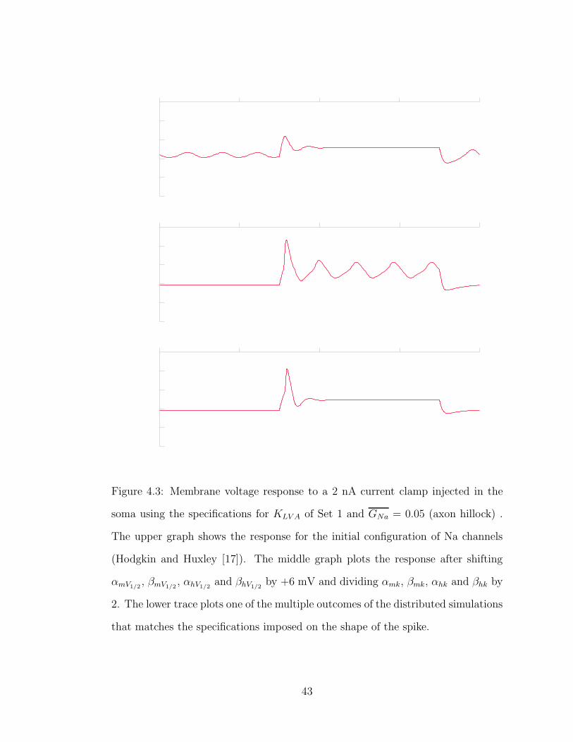
Figure 4.3: Membrane voltage response to a 2 nA current clamp injected in the

soma using the specifications for KLV A of Set 1 and GNa = 0.05 (axon hillock) .

The upper graph shows the response for the initial configuration of Na channels

(Hodgkin and Huxley [17]). The middle graph plots the response after shifting

αmV1/2, βmV1/2

, αhV1/2and βhV1/2

by +6 mV and dividing αmk, βmk, αhk and βhk by

2. The lower trace plots one of the multiple outcomes of the distributed simulations

that matches the specifications imposed on the shape of the spike.

43

constrain the limits of the space to be searched. There are many examples in the

literature that have characterized the sodium kinetics, either by means of

physiological experiments alone, or combining them with computational models

[5, 8, 17, 24, 25, 32, 41, 45, 46, 48]. Despite having the commonality of using a

Hodgkin and Huxley typification of the channels described, some differ in the

exact formulation of the equations. Nonetheless, there is an overlap in the range

of valid variables between these models (it is important to reminder that

ultimately they are describing the same physical phenomenon). The biophysical

meaningful range is summarized in Table 4.2, and it has been corroborated in the

model by manually running several test simulations.

m h

αV1/2(mV) [-30,-50] [-20,-60]

αk (mV) [3,10] [10,20]

α0 (ms−1) [0.5,5] [0.05,0.15]

βV1/2(mV) [0,-60] [0,-60]

βk (mV) [5,20] [5,10]

β0 (ms−1) [1,4] [1,4]

GNa (S/cm2) [0.03,2.0]

Table 4.2: Biophysically relevant range of sodium parameters.

Having defined the starting point for the given variable space, all that

remains is to specify the required outcome of the model. Mimicking the

physiological experiments once again, a set of current clamps of different

amplitudes are applied to the cell, and the action potential that the cell might or

might not fire in response is evaluated as follows:

44

• Current clamp of 0.50 nA: no action potential is expected. The amount of

injected current should not be enough to depolarize the cell up to the firing

threshold (-42±6 mV [36]). The detection threshold is set at -40 mV, and if

the membrane voltage of any cell crosses the threshold at this stage, the

combination of parameters that define the sodium kinetics for this cell are

discarded.

• Current clamp of 1.25 nA: the cell might or might not fire, but if it does, it

can only fire once. The injected current brings the plasma membrane near

the firing threshold. It is equally possible that there is enough current to

activate the sodium channels or that they remain inactive. However, if one

spike is triggered, the membrane voltage should repolarize to the clamped

value afterwards without oscillating. The detection threshold is set at

-40 mV, and it should be crossed at most once.

• Current clamp of 2.00 nA: the cell must fire one single action potential.

The injected current has to depolarize the cell enough to activate the

sodium channels, the cell must fire in response, and the voltage must

repolarize to rest afterwards without oscillating. Two detection thresholds

are set at -25 mV and -40 mV, each of which must be crossed only once.

The first one is to ensure a minimum height of the spike (reported action

potential peak of -15±17 mV [36]), and the second one is to detect lower

second spikes. If the spike is not high enough or secondary spikes are

detected, the associated combination of sodium parameters is discarded.

Current clamps are applied with a 25 ms delay after the simulation starts so

as to be able to detect unwanted combinations of sodium parameters that make

the cell spike at rest. The duration of the current clamp is set to 15 ms to be able

45

to detect oscillations when the membrane voltage repolarizes to the clamped

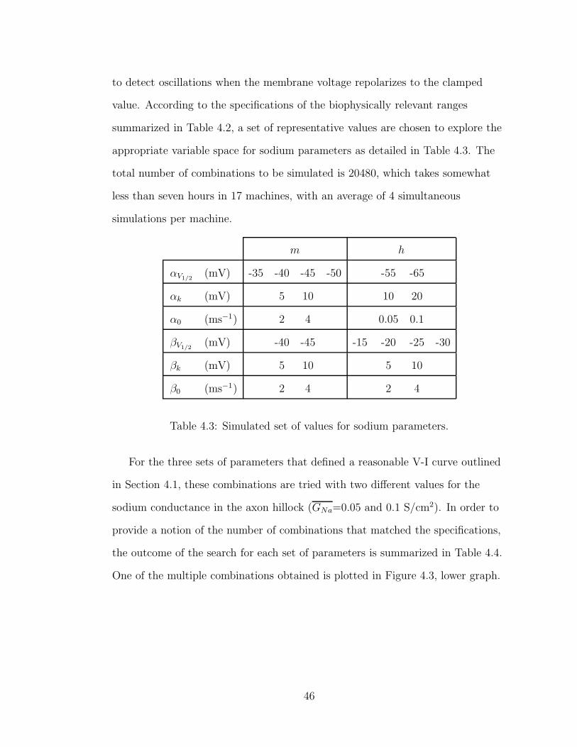
value. According to the specifications of the biophysically relevant ranges

summarized in Table 4.2, a set of representative values are chosen to explore the

appropriate variable space for sodium parameters as detailed in Table 4.3. The

total number of combinations to be simulated is 20480, which takes somewhat

less than seven hours in 17 machines, with an average of 4 simultaneous

simulations per machine.

m h

αV1/2(mV) -35 -40 -45 -50 -55 -65

αk (mV) 5 10 10 20

α0 (ms−1) 2 4 0.05 0.1

βV1/2(mV) -40 -45 -15 -20 -25 -30

βk (mV) 5 10 5 10

β0 (ms−1) 2 4 2 4

Table 4.3: Simulated set of values for sodium parameters.

For the three sets of parameters that defined a reasonable V-I curve outlined

in Section 4.1, these combinations are tried with two different values for the

sodium conductance in the axon hillock (GNa=0.05 and 0.1 S/cm2). In order to

provide a notion of the number of combinations that matched the specifications,

the outcome of the search for each set of parameters is summarized in Table 4.4.

One of the multiple combinations obtained is plotted in Figure 4.3, lower graph.

46

Set 1 Set 2 Set 3

Set 1a Set 1b Set 2a Set 2b Set 3a Set 3b

GNa (S/cm2) 0.05 0.1 0.05 0.1 0.05 0.1

Number of combinations 5530 6988 9414 9829 3570 6010

Table 4.4: Outcome of the search for sodium parameters.

4.4 Firing rates

Gathering together the data obtained in the previous two sections, the next step

in constructing a biophysically realistic model of nucleus laminaris is to evaluate

the ability of the cell to respond to stimuli that closely resemble acoustic stimuli.

The aim of the present section is to measure the relation between the stimulus

frequency and the corresponding evoked firing rate of the cell, evaluating the

phase locking capabilities of NL cells. The reference is taken from a set of

physiological experiments where stimulus of different frequencies were applied

directly to the somatic area of high frequency cells while varying the number of

simulated inputs (Figure 4A in [36]).

The ability of the cell to phase lock to its synaptic inputs is closely tied to the

dynamics of the sodium channels. Thus, the specifications for sodium channels

are not yet complete. The requirement of firing an action potential at the onset

of a current clamp does not guarantee the phase locking properties observed in

vitro in nucleus laminaris cells. Figure 4.4 illustrate two combinations that

matched the specifications for the shape of the action potential in the preceding

section (two of the multiple combinations summarized in Table 4.4), but do not

behave as expected in terms of their firing rates. Physiological experiments

report that during 500 Hz stimulation the firing rate plateaus near 500 Hz. From

47

this maximum, the average firing rate decreases with increasing stimulus

frequency. The left graph in Figure 4.4 plots a combination of parameters that is

unable to phase lock no matter how many inputs are applied onto the soma,

while the right plot depicts a combination that seems to plateau below 500 Hz,

but shows an even higher firing rate for the 750 Hz stimulus case.

Figure 4.4: Two examples of unacceptable firing rate plots.

The computational cost of generating a firing rate plot, like the ones depicted

in Figure 4.4, for every set of combinations found in the previous section is very

high. Instead, specific points of the plot are chosen as a criterion to match the

whole graph, through which all the combinations will be filtered. The reasons for

chosing these particular points and not others rely on the intuition acquired

running many simulations manually over the past months. However, the

correctness of such a selection is the validity of the outcomes that result from the

described process.

The first restriction is to impose a minimum and a maximum for the firing

48

rate of the cell in response to 750 Hz stimuli. The firing rate should be above

100 Hz and below 500 Hz when applying 70 simulated inputs onto the soma. On

the initial phase of the present search, the constraints should not be too

restrictive to avoid getting the empty set as the outcome of the filtering, but yet

they have to make a selection on the existing sets. Despite the fact that the

constraint might seem not very restraining, the result is a reduction in the

number of combinations of about one fifth.

The second restriction is imposed on the 500 Hz stimulus case. For

explanatory purposes, the search has been progressively constrained in

consecutive phases. The first step forces a 500 Hz firing rate with 70 simulated

synapses onto the somatic region, which is quite far from the minimum 30

synapses simulated in the reference paper. The same constraint is then imposed

with 56 and 42 synapses. The number of synapses is a multiple of the number of

dendrites (14) for simplicity resulting from the actual implementation of the

model. The progression in the number of valid combinations is shown in

Table 4.5.

Two of the outcomes of this search are plotted in Figure 4.5, where the left

plot belongs to Set 1b and the right one to Set 3b. Not only do the firing rates

plots match the reference, but the time plots of the voltage response are also

similar to the ones recorded from physiological experiments. The divergence in

the firing rates at every frequency from the local maximum or the steady state is

also reported in the referred experiments, where data points extending past the

asymptotic region of the curves were not analyzed because large fluctuations often

obscured action potentials [36].

The last thing that remains to be done before completing the physiological

49

Criterion Set 1a Set1b Set 2a Set 2b Set 3a Set 3b

From previous section 5530 6988 9414 9829 3570 6010

AFR of 750 Hzwith 70 synapses

332 1276 1115 3066 339 1368

AFR of 500 Hzwith 70 synapses

131 805 336 2018 336 1337

AFR of 500 Hzwith 54 synapses

20 360 25 377 202 1068

AFR of 500 Hzwith 42 synapses

0 5 0 0 8 37

Table 4.5: Progression in the number of combinations that match successive con-

straints on firing rates.

Figure 4.5: Two combinations with valid firing rates. Left graph belongs to Set

1a, and right graph belongs to Set 3b.

50

characterization of the high frequency cell under study is to corroborate the

hypothesis formulated at the begining of the chapter. For simplicity, KHV A and

Na had been temporarily removed when characterizing KLV A, arguing that they

do not have any influence in the membrane voltage near rest. In some cases,

KHV A and Na introduce less than a 5% variation in the values used to test the

validity of the corresponding V-I curves. A difference of 5% is less than the

variability reported in physiological experiments, and it is thus perfectly

acceptable. However, there are some other cases in which the presence of KHV A

and Na disrupts the resulting voltage-current relation. If that is the case, these

combinations are consequently discarded because they do not match the

specifications anymore. Table 4.6 shows the number of combinations that result

from checking the voltage-current relation after completion, and Figure 4.6

depicts both a valid and a non-valid voltage-current relation taken from Set 3b.

Set 1a Set1b Set 2a Set 2b Set 3a Set 3b

Number of combinations 0 5 0 0 1 22

Table 4.6: Number of combinations matching V-I specifications with KHV A and

Na.

Analyzing the results obtained, no pattern on how the variable space evolves

through the different stages of the search becomes evident. The higher number of

combinations that match the different phases of the search oscillate between

different stages, which makes the search especially difficult. Set 1 has given the

best match in the voltage-current relation, but only results in 5 combinations

matching the firing rates specifications. On the other hand, Set 2 gave the higher

number of combinations for the shape of the action potential, but none of them

51

Figure 4.6: Invalid (top) and valid (bottom) V-I plot with KHV A and Na.

52

matches the constraints imposed on the average firing rates. Somewhat in the

middle of the first two, Set 3 gives the overall better results. The progression of

the variable space shows that the difficulty in doing the search lies in imposing

the appropriate degree of restriction, which can also be thought in terms of

accuracy, at every stage. The appropriateness in the successive restrictions is

only guided by intuition, which in turn is gained by experience. Nonetheless, the

success of the search heavily relies on the computational power managed through

the distributed simulations. The wise combination of both tools, biological

intuition and computational power, in the extensive search of the parameter

space is what ultimately ensures a successful outcome.

53

Chapter 5

Adjusting Tonotopicity

An average high frequency cell (CF=2000 Hz) has been chosen as the reference

for characterizing nucleus laminaris behavior. The choice comes from the fact

that most of the physiological recordings are conducted in the high frequency

region of NL. However, a single cell cannot account for the variety of cells’

performance observed throughout the nucleus. The first reported differences

between cells in nucleus laminaris refer to anatomical variations along the

tonotopic axis of NL (cf. Section 3.1). Physiological experiments also report

divergent functionalities between cells located in different sites of NL. In order to

analyze the implications of such variations, a second reference cell is chosen close

to the other end of the tonotopic axis with a characteristic frequency of 500 Hz.

The implicit framework of the present chapter is the gradient in the number of

dendrites and dendritic length observed in NL cells [44].

5.1 Preliminary analysis

The 500 Hz cell has 2 dendrites of about 650 µm long, as opposed to the 2000 Hz

cell that has 14 dendrites of 68 µm. The associated dendritic area for the two

54

cases is 4103 and 2990 µm2, respectively. The first impression is that the larger

dendritic area would result in bigger total conductances, which would mean

smaller input resistances and faster time constants (τ = RC). The implication is

that the low frequency cells that compute slower time signals should be faster

than the high frequency ones, which contradicts the observations from

physiological experiments.

The first concept to bear in mind to understand this contradiction comes

from the constraint imposed by the cable equation on the voltage along the cable:

the stationary voltage distribution decays exponentially away from the site of

injection. Therefore, the current will not flow through the membrane uniformly

along the cable. In fact, it will only flow through the nearest portion of the

membrane to the site of injection. The parameter controlling the decay is the

space constant λ:

λ =

√Rm

Ri

d

4(5.1)

The voltage decreases to e−1 (37% of its original value) at a distance λ from

the site of injection, and to e−2 (13%) at 2λ. Different λs can be associated to

the different conductances, namely leak and KLV A, using the associated

membrane resistances for each case (Rm). For the corresponding values reported

in Section 4.1, λleak=325 µm and λKLV A=121 µm.

It is clearly seen that in the high frequency cells the voltage flows through

most of the dendritic length, whereas in the low frequency cells the ’effective’

dendritic membrane is much smaller. Thus, the effective conductance is smaller

for the low frequency cells, which makes them slower compared to high frequency

cells.

Not only do the lengths of the dendrites make a difference in the behavior of

55

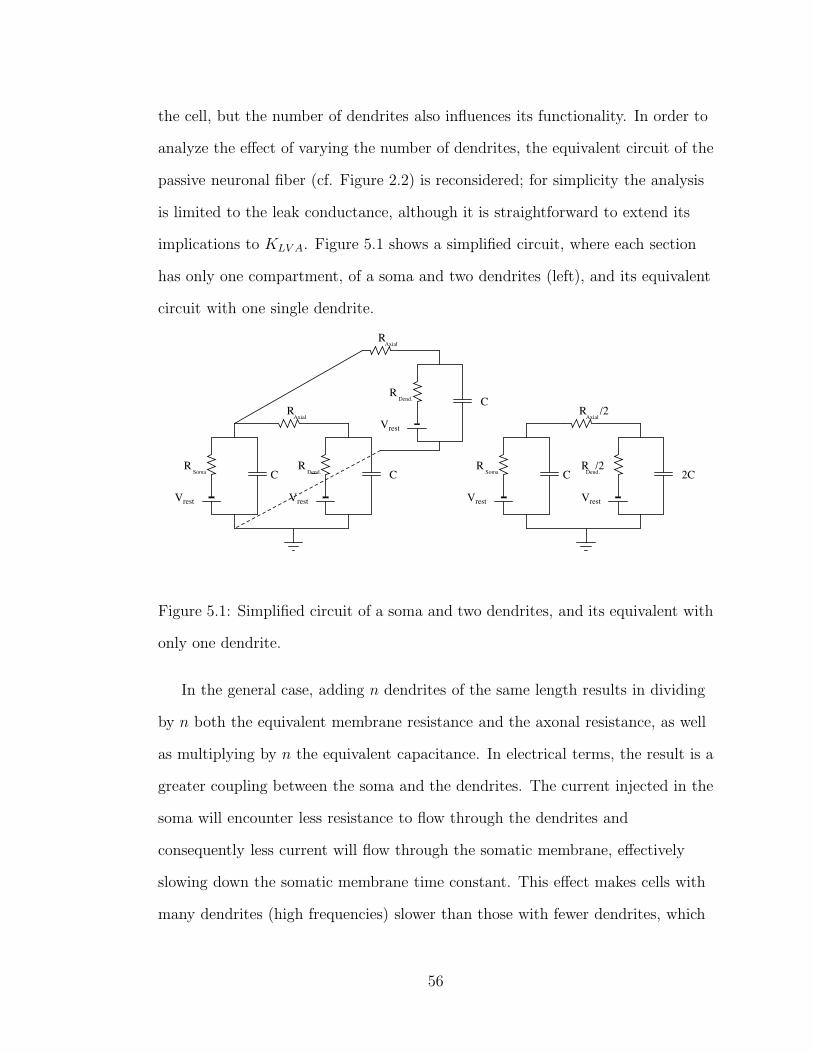
the cell, but the number of dendrites also influences its functionality. In order to

analyze the effect of varying the number of dendrites, the equivalent circuit of the

passive neuronal fiber (cf. Figure 2.2) is reconsidered; for simplicity the analysis

is limited to the leak conductance, although it is straightforward to extend its

implications to KLV A. Figure 5.1 shows a simplified circuit, where each section

has only one compartment, of a soma and two dendrites (left), and its equivalent

circuit with one single dendrite.

R

Dend.

Axial

Soma

Vrest

R

Dend.

Axial

Vrest

Vrest

Soma

Vrest

R

Dend.

Axial

Vrest

/2

/2

R

RR R R

C

CC C 2C

Figure 5.1: Simplified circuit of a soma and two dendrites, and its equivalent with

only one dendrite.

In the general case, adding n dendrites of the same length results in dividing

by n both the equivalent membrane resistance and the axonal resistance, as well

as multiplying by n the equivalent capacitance. In electrical terms, the result is a

greater coupling between the soma and the dendrites. The current injected in the

soma will encounter less resistance to flow through the dendrites and

consequently less current will flow through the somatic membrane, effectively

slowing down the somatic membrane time constant. This effect makes cells with

many dendrites (high frequencies) slower than those with fewer dendrites, which

56

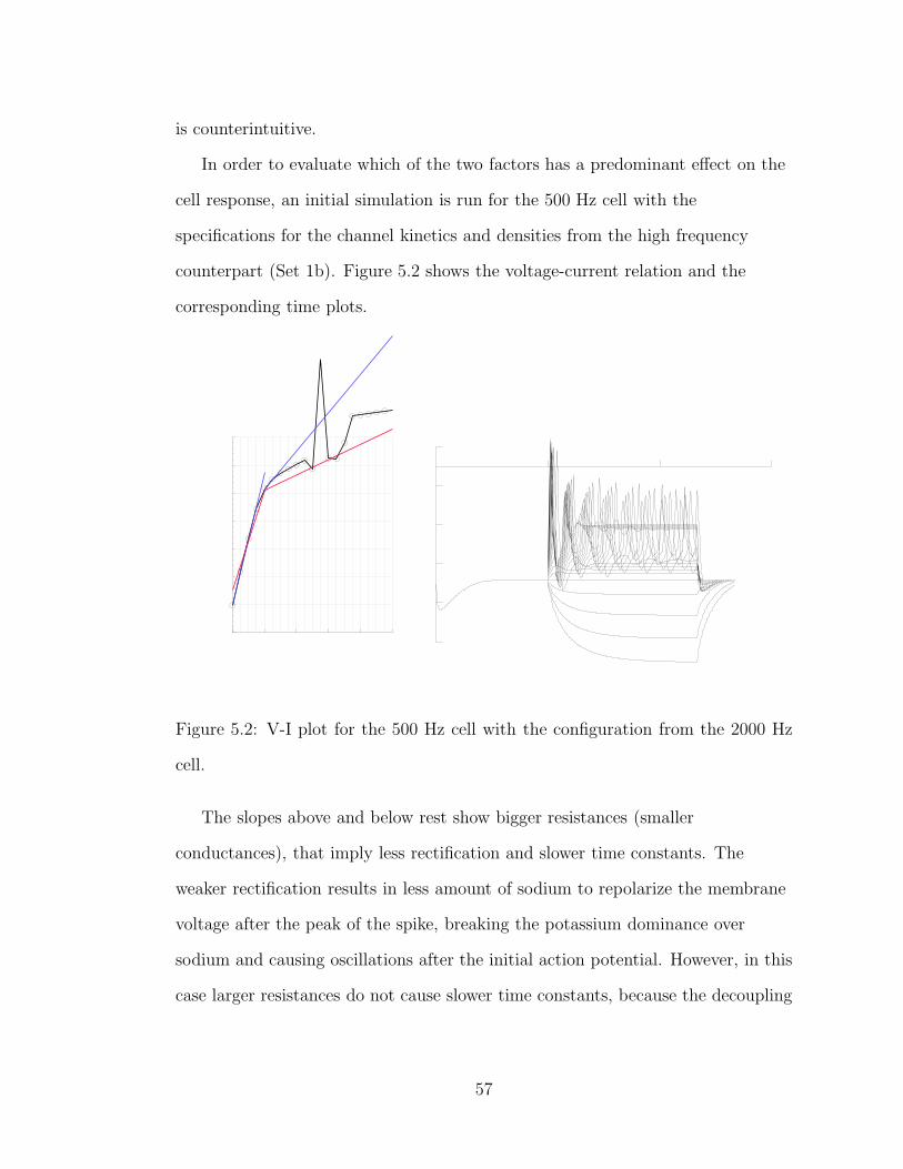
is counterintuitive.

In order to evaluate which of the two factors has a predominant effect on the

cell response, an initial simulation is run for the 500 Hz cell with the

specifications for the channel kinetics and densities from the high frequency

counterpart (Set 1b). Figure 5.2 shows the voltage-current relation and the

corresponding time plots.

Figure 5.2: V-I plot for the 500 Hz cell with the configuration from the 2000 Hz

cell.

The slopes above and below rest show bigger resistances (smaller

conductances), that imply less rectification and slower time constants. The

weaker rectification results in less amount of sodium to repolarize the membrane

voltage after the peak of the spike, breaking the potassium dominance over

sodium and causing oscillations after the initial action potential. However, in this

case larger resistances do not cause slower time constants, because the decoupling

57

effect of the dendrites from the soma is stronger, which makes the cell faster (the

time-to-peak is shorter for the low frequency cells compared to the high

frequency ones).

To sum up, the fact that the low frequency cells are faster than the high

frequency ones does not match the observations from physiology, and some

modifications are needed to adjust the model to experimental data.

5.2 Redistribution of conductances

The first proposed modification to reconfigure the model is to change the

distribution of the conductances between the soma and the dendrites, as done

elsewhere in the literature [6]. The purpose is to make both cells (500 Hz and

2000 Hz) more similar, placing a larger amount of potassium conductance in the

common section: the soma. The leak conductance is kept uniform all over the

cell, as no physiological evidence shows any variation. The procedure is to change

the distribution of KLV A (and KHV A accordingly) in the high frequency cell in

such a way that the total conductance remains the same, namely the

voltage-current relation remains unchanged. The sum of the products of the new

densities by the corresponding area surfaces (dendritic and somatic) is kept

constant. With the new configuration of conductances, the low frequency cell is

tested.

While leaving the high frequency cell almost intact, due to its compactness,

the suggested modification brings a greater amount of potassium available at the

soma for the low frequency cells. In order to place enough potassium in the soma

to counteract the fast sodium dynamics, the minimum ratio of conductance

redistribution found is 1/4 of the original dendritic densities, and the

58

corresponding 4.18-fold increase in the soma. Figure 5.3 shows the

voltage-current relation for the new configuration, and the corresponding time

plots.

Figure 5.3: V-I plot for the 500 Hz cell after redistributing potassium conductances.

Despite bringing some degree of similarity between the two kinds of cells,

there is still an important divergence that remains unaddressed. The time course

of the membrane voltage is faster for the low frequency cell than for the high

frequency one, which is counterintuitive and contradicts the behavior observed in

real cells. Varying the ratio of conductances between the dendrites and the soma

cannot solve the above-mentioned problem: in the limit, all conductances are

concentrated in the soma and the two types of cells exhibit the same behavior,

but the underlying phenomenon is never inverted. The mismatch in the cell’s

time constants is exemplified in Figure 5.4, where the voltage response to a 2 nA

current clamp is plotted for a low and high frequency cell.

59

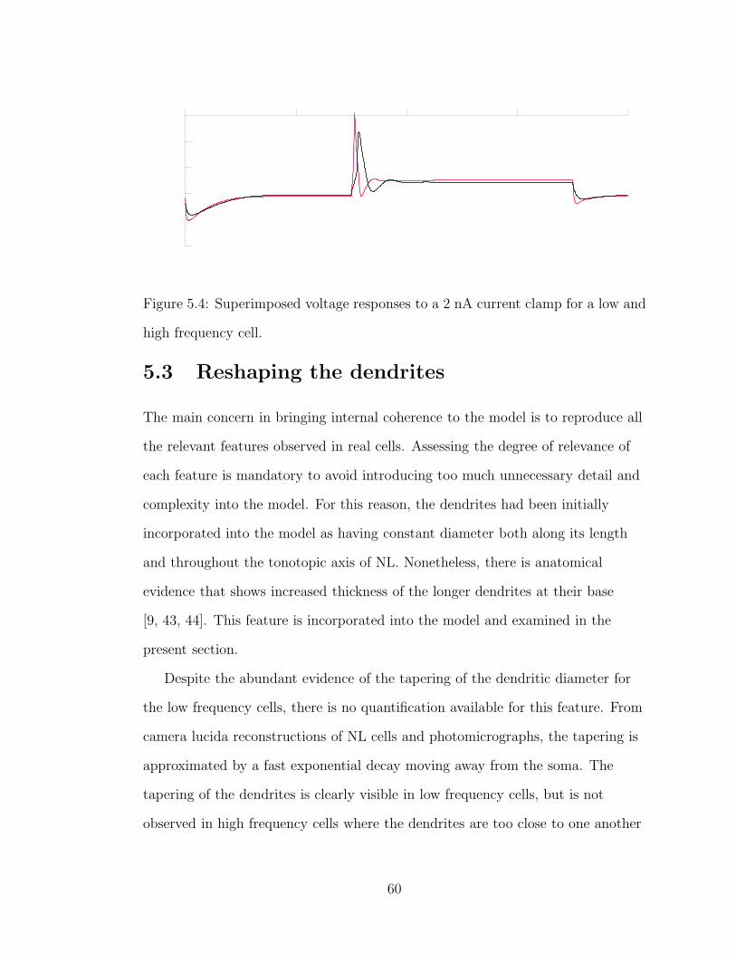
Figure 5.4: Superimposed voltage responses to a 2 nA current clamp for a low and

high frequency cell.

5.3 Reshaping the dendrites

The main concern in bringing internal coherence to the model is to reproduce all

the relevant features observed in real cells. Assessing the degree of relevance of

each feature is mandatory to avoid introducing too much unnecessary detail and

complexity into the model. For this reason, the dendrites had been initially

incorporated into the model as having constant diameter both along its length

and throughout the tonotopic axis of NL. Nonetheless, there is anatomical

evidence that shows increased thickness of the longer dendrites at their base

[9, 43, 44]. This feature is incorporated into the model and examined in the

present section.

Despite the abundant evidence of the tapering of the dendritic diameter for

the low frequency cells, there is no quantification available for this feature. From

camera lucida reconstructions of NL cells and photomicrographs, the tapering is

approximated by a fast exponential decay moving away from the soma. The

tapering of the dendrites is clearly visible in low frequency cells, but is not

observed in high frequency cells where the dendrites are too close to one another

60

to distinguish any differences in their bases. Due to the lack of evidence about in

which area of nucleus laminaris the tapering starts, and the consequent difficulty

in where to set the threshold for this feature, a phenomenological approximation

is set by a linear regression along the tonotopic axis. At the high frequency end

the tapering is absent, and progressively increases towards the caudolateral end,

as described by Eq. 5.2:

d(x, f) =2

3

(14 − Nden(f)

)e−ax + dmin (5.2)

where the dendritic diameter d is a function of the position along the dendrite (x,

ranging from 0 to 1) and the characteristic frequency of the cell (f). The

constants are set so that the maximum dendritic diameter for the 2 dendrites

case matches the minimum diameter of the soma (10 µm, cf. Section 3.1). The

initial dendritic diameter is inversely proportional to the number of dendrites

(Nden as defined in Eq. 3.5). Finally, the exponent a controls the speed of the

decay. A value of about 9 for a gives a match between the voltage responses of

the two cells, and an even smaller value would make the low frequency cells

slower. The increased proximal dendritic surface implies a larger effective area;

an increase in diameter results in a larger space constant (cf. Eq. 5.1), although

the calculation is not straightforward because the diameter is no longer constant.

A larger effective area implies an increase in the total leak and KLV A

conductances, which can counteract the fast sodium dynamics. This result shows

that the tapering of the dendrites makes a great difference and thus is a relevant

parameter to be incorporated into the model. However, such small values for a

are not biophysically realistic: the dendrites are abnormally thick. In order to set

a value for the decay coherent with anatomical and physiological observations,

the slope below rest is taken as a reference and matched with the corresponding

61

value for the high frequency cell, because no systematic variation of this value

has been observed along the tonotopic axis [36]. A value of a=20 is selected

accordingly. Figure 5.5 plots the profile of the dendritic diameter along the

dendritic length as specified in Eq. 5.2 (500 Hz cell, blue trace), and the

corresponding segmented implementation by NEURON (red trace). Figure 5.6

shows the voltage-current relation of the low frequency cell and the

corresponding time plots. Despite the still uncontrolled oscillations at higher

voltages, an improvement can be seen with respect to Figure 5.2 because the

oscillations appear at more positive voltages than before.

0 100 200 300 400 500 600 7000

1

2

3

4

5

6

7

8

9

10

Dendritic length (um)

Den

driti

c di

amet

er (

um)

Figure 5.5: Dendritic diameter tapering along dendritic length. Comparison be-

tween the ideal profile and the segmented implementation by NEURON.

Finally, Figure 5.7 shows the two traces superimposed for the voltage

response to a 2 nA current clamp for both a low and a high frequency cell. It can

be observed the increase of the membrane time constant with respect to

62

Figure 5.4 (the conductances are kept redistributed as in the previous section to

isolate the low frequency trace from secondary spikes).

5.4 Tonotopic variation of channel conductances

The morphological differences in nucleus laminaris cells is the main attributable

cause of their diverse behavior. The present section discusses other variations

that might be present along the tonotopic axis and could account for some

questions that remain unresolved.

Physiological experiments reveal a variation in the degree of rectification

between cells throughout the nucleus. No systematic variation of Rabove rest, an

estimate of the degree of rectification (cf. Section 4.1), along the tonotopic axis

has been observed [36]. Nevertheless, there seems to be a trend in increasing

rectification with increasing characteristic frequency of the cells (Kate MacLeod,

unpublished data). Despite the different rectification ratios, both types of cells

show only one single spike at the onset of currents clamps. Less rectification

makes it easier for sodium channels to activate again after the initial spike and

trigger secondary spikes. This can be observed in the model if the low frequency

cell is implemented without the redistribution of potassium conductances

analyzed in Section 5.2.

The main agent that causes the membrane voltage to oscillate around the

higher clamped voltages is an excess in the density of sodium channels, which can

be observed in the higher amplitudes of action potential peaks (15 mV difference

between the 500 Hz cell and the 2000 Hz equivalent). In order to equilibrate

potassium and sodium kinetics, one possibility is to reduce the channel density

for sodium in the low frequency cells. However, simulations show that the needed

63

Figure 5.6: Voltage-current relation of a low frequency cell with varying diameter

of the dendrites.

Figure 5.7: Comparison of voltage responses between a low and high frequency cell

after reshaping the dendrites.

64

amount to eliminate unwanted oscillations is too high (70% reduction) that

results in an over reduction in the spike height (5 mV below the reference for the

2000 Hz cell). Thus, a tonotopic gradient in the sodium conductance does not

seem to be the main feature to counteract the anatomical differences between

cells.

Among all the peculiarities of NL cells detailed in the model, there is one that

is less well understood and for which changes have been kept to a minimum.

KHV A is thought to facilitate high frequency spiking by controling the width of

the spike and quickly repolarizing the voltage to rest after the spike. However, in

the high frequency cells, removing or doubling the presence of KHV A does not

make a substantial difference in the shape of the spike.

KHV A seems to have a great influence in the low frequency cells. Removing

KHV A from the low frequency cells diminishes the rectification only attributed to

KLV A. On the other hand, increasing the presence of KHV A reduces the voltage

oscillations after the primary spike and helps resetting the voltage to the clamped

value. Therefore, one possibility is to increase the channel densities for KHV A in

the low frequency cells where they have greater effect, but doing so would

contradict immunoreactivity experiments that evidence higher densities in the

high frequency cells of NL [29]. The fact that the present configuration of the

model sets a uniform channel density for KHV A along the tonotopic axis does not

necessarily contradict immunoreactivity observations, as more cells with a higher

number of dendrites are located in the high frequency region of NL compared to

the low frequency area. Another possibility is to increase the potential effect of

KHV A by changing the dynamics of the channel, which have been untouched from

the reference data. The idea is to increase the range of voltages in which KHV A

65

becomes active, and/or shift the range of voltages towards the rectified voltages.

Because the reference values are taken from nucleus magnocellularis, where less

rectification is observed, the area of influence was shifted to more positive values.

Following this reasoning, the midpoints of activation and deactivation are shifted

to more negative values (from -19 to -25 mV) and the ranges of activation and

deactivation are increased roughly by a 25% (αnk=12 ms−1 and βnk=25 ms−1).

Due to a too strong presence of sodium in the actual configuration, the

mentioned feature can be better observed by either halving the sodium

conductance or doubling the KHV A conductance (cf. Figure 5.8). The effect of

KHV A can be clearly seen in eliminating oscillations at low frequencies (red and

blue traces), as well as allowing a less rectified clamped voltage compared to the

high frequency cell (black trace). It is important to mention that such a change

does not cause significant alterations in the voltage response in the high

frequency cell, and it thus applied uniformly to all cells.

Figure 5.8: Comparison of voltage responses between a low (red) and a high (black)

frequency cell while assessing the effect of KHV A. The blue trace shows the refer-

ence setting for KHV A in the low frequency cell.

66

Chapter 6

Conclusions

The aim of the present work has been to improve an existing computational

model of nucleus laminaris to make it biophysically more realistic, where special

interest is drawn towards the tonotopic arrangement of NL cells. The starting

point for characterizing NL cells is the high frequency region of the nucleus, from

where most of the biological data is derived. The degree of accuracy sought in

the present model implies a high number of parameters that define an intractably

huge space of possible combinations. The approach to find where the biologically

relevant subspace lies has been to combine the experimental data available in the

literature with an exhaustive distributed exploration of the variable space.

Whereas the variable space for the low voltage activated potassium channels

seems quite compact, the relevant subspace for sodium remains hard to

delimitate mostly because of its higher dimensionality. Interacting in the same

voltage range as sodium, high voltage activated potassium channels have not

been precisely studied due to the lack of biological constraints.

Having faithfully characterized an average high frequency cell, its main

features are adapted to the low frequency region to provide with a description of

the behavior of the entire nucleus laminaris. The morphological variations along

67

the tonotopic axis reported in the literature constitute the framework for

studying both types of cells (2000 Hz and 500 Hz cells). Important unexpected

physiological divergences are observed in the low frequency cells. The

counterintuitive disparities between both cell types are studied by introducing

physiological modifications that might correct the observed phenomena. Such

modifications include a redistribution of conductances between the soma and the

dendrites, and tonotopic gradients of conductances.

None of the physiological modifications proposed can account for the disparity

between the model and real cells in the low frequency region. Only anatomical

adaptations can indeed give a partial explanation, although they have to be

pushed away from biological limits to fully resolve the observed paradox: low

frequency cells are faster than the high frequency analogous. The particular

morphological configuration of the cells seems to have an underestimated effect

on their behavior. A more accurate description of the anatomy of these neurons

is needed to complete the model.

Deriving from the attained biological accuracy in the model, a new

functionality of high potassium activated channels is hypothesized for the low

frequency cells. In the most caudal cells where less rectification is observed,

KHV A is thought to help repolarization complementing the effect of a less dense

low threshold activated conductance.

68

BIBLIOGRAPHY

[1] Agmon-Snir, H., Carr, C. E., and Rinzel, J. (1998) The role of dendrites inauditory coincidence detection. Nature. 393: 268–272.

[2] Carr, C. E., and Boudreau, R. E. (1993) An axon with a myelinated initialsegment in the bird auditory system. Brain Res. 628: 330–334.

[3] Carr, C. E., and Konishi, M. (1990) A circuit for detection of interaural timedifferences in the brain stem of the barn owl. J. Neurosci. 10(10):3227–3246.

[4] Carr, C. E., Soares, D., Parameshwaran, S., and Perney, T. (2001) Evolutionand development of time coding systems. Curr. Opin. Neurobiol. 11(6):727–733.

[5] Colbert, C. M., and Pan, E. (2002) Ion channel properties underlying axonalaction potential initiation in pyramidal neurons. Nat. Neurosci. 5(6):533–538.

[6] Cook, D. L., Schwindt, P. C., Grande, L. A., and Spain, W. J. (2003)Synaptic depression in the localization of sound. Nature. 421: 66–70.

[7] Crill, W. E. (1996) Persistent sodium current in mammalian central neurons.Ann. Rev. Physiol. 58: 349–362.

[8] Cummins, T. R., Xia, Y., and Haddad, G. G. (1994) Functional propertiesof rat and human neocortical voltage-sensitive sodium currents.J. Neurophysiol. 71: 1052–1064.

[9] Deitch, J. S., and Rubel, E. W. (1984) Afferent influences on brain stemauditory nuclei of the chicken: time course and specificity of dendriticatrophy following deafferentation. J. Comp. Neurol. 229(1): 66–79.

[10] Deitch, J. S., and Rubel, E. W. (1989) Changes in neuronal cell bodies in n.laminaris during deafferentation-induced dendritic atrophy. J. Comp. Neur.281: 259–268.

69

[11] Deitch, J. S., and Rubel, E. W. (1989) Rapid changes in ultrastructureduring deafferentation-induced dendritic atrophy. J. Comp. Neur. 281:234–258.

[12] Hille, B. (2001) Ion channels of excitable membranes, 3rd edition.Sunderland, MA: Sinauer Associates.

[13] Hines, M. L. (1983) Efficient computation of branched nerve equations. Int.J. Bio-Med. Comput. 15(1): 69–76.

[14] Hines, M. L., and Carnevale, N. T. (1997) The NEURON simulationenvironment. Neural Comput. 9(6): 1179–1209.

[15] Hines, M. L., and Carnevale, N. T. (2000) Expanding NEURON’s repertoireof mechanisms with NMODL. Neural Comput. 12(5): 995–1007.

[16] Hines, M. L., and Carnevale, N. T. (2001) NEURON: a tool forneuroscientists. Neuroscientist. 7(2): 123–135.

[17] Hodgkin, A. L., and Huxley, A. F. (1952) A quantitative description ofmembrane current and its application of conduction and excitation in nerve.J. Physiol. Lond. 117: 500–544.

[18] Jeffress, L. A. (1948) A place theory of sound localization. J. Comp. Physiol.Psychol. 41: 35–39.

[19] Johnston, D., and Wu, S. M. (1999) Foundations of cellular neurophysiology,4th edition. Cambridge, MA: The MIT Press.

[20] Kernighan, B. R., and Pike, R. (1984) Appendix 2: Hoc manual. In: TheUNIX programming environment. Englewood Cliffs: NJ: Prentice-Hall, pp.329–333.

[21] Koch, C. (1999) Biophysics of computation. New York: Oxford UniversityPress.

[22] Koyano, K., Funabiki, K., and Ohmori, H. (1996) Voltage-gated ioniccurrents and their roles in timing coding in auditory neurons of the nucleusmagnocellularis of the chick. Neurosci. Res. 26(1): 29–45.

[23] Kuba, H., Koyano, K., and Ohmori, H. (2002) Development of membraneconductances improves coincidence detection in the nucleus laminaris of thechicken. J. Physiol. 540(2): 529–42.

[24] Lytton, W. W., and Sejnowski, T. J. (1991) Simulations of corticalpyramidal neurons synchronized by inhibitory interneurons. J. Neurophysiol.66(3): 1059–1079.

70

[25] Martina, M., and Jonas, P. (1997) Functional differences in Na+ channelgating between fast spiking interneurones and principal neurones of rathippocampus. J. Physiol. 505(3): 593–603.

[26] Moore, J. W., Joyner, R. W., Brill, M. H., Waxman, S. D., and Najar-Joa,M. (1978) Simulations of conduction in uniform myelinated fibers.J. Biophys. 21: 147–160.

[27] Oertel, D. (1999) The role of timing in the brain stem auditory nuclei ofvertebrates. Annu. Rev. Physiol. 61: 497–519.

[28] Overholt, E. M., Rubel, E. W., and Hyson, R. L. (1992) A circuit for codinginteraural time differences in the chick brainstem. J. Neurosci. 12(5):1968–1708.

[29] Parameshwaran, S., Carr, C. E., and Perney, T. M. (2001) Expression of theKv3.1 potassium channel in the avian auditory brainstem. J. Neurosci.21(2): 485–494.

[30] Parks, T. N., Collins, P., and Conlee, J. W. (1983) Morphology and origin ofaxonal endings in nucleus laminaris of the chicken. J. Comp. Neur. 214:32–42.

[31] Peters, A., Palay, S. L., and Webster, H. D. (1991) The fine structure of thenervous system, 3rd edition. New York: Oxford University Press.

[32] Protopapas, A. D., Vanier, M., and Bower, J. M. (1999) Simulating largenetworks of neurons. In: Methods in neuronal modeling. Koch, C., andSegev, I., editors. Cambridge, MA: The MIT Press, pp. 461–498, 2nd edition.

[33] Rall, W. (1959) Branching dendritic trees and motoneuron membraneresistivity. Exp. Neurol. 1: 491–527.

[34] Rathouz, M., and Trussell, L. (1998) Characterization of outward currents inneurons of the avian nucleus magnocellularis. J. Neurophysiol. 80(6):2824–35.

[35] Reyes, A. D., Rubel, E. W., and Spain, W. J. (1994) Membrane propertiesunderlying the firing of neurons in the avian cochlear nucleus. J. Neurosci.14(9): 5352–5364.

[36] Reyes, A. D., Rubel, E. W., and Spain, W. J. (1996) In vitro analysis ofoptimal stimuli for phase-locking and time-delayed modulation of firing inavian nucleus laminaris neurons. J. Neurosci. 16(3): 993–1007.

71

[37] Rogart, R. B., and Ritchie, J. M. (1977) Physiological basis of conduction inmyelinated nerve fibers. In: Myelin. Morell, P., editor. New York: PlenumPress, pp. 117–160.

[38] Rubel, E. W., and Parks, T. N. (1975) Organization and development ofbrain stem auditory nuclei of the chicken: tonotopic organization of n.magnocellularis and n. laminaris. J. Comp. Neur. 164: 411–434.

[39] Rubel, E. W., and Parks, T. N. (1988) Organization and development of theavian brain-stem auditory system. In: Auditory function: neurobiologicalbases of hearing. Edelman, G. M., Gall, W. E., and Cowan, W. M., editors.New York: Wiley Press, pp. 3–92.

[40] Rudy, B., and McBain, C. J. (2001) Kv3 channels: voltage-gated K+channels designed for high-frequency repetitive firing. Trends Neurosci.24(9): 517–526.

[41] Schwarz, J. R., and Eikhof, G. (1987) Na currents and action potentials inrat myelinated nerve fibres at 20 and 37 degrees C. Pflugers Arch. 409(6):569–577.

[42] Simon, J. Z., Carr, C. E., and Shamma, S. A. (1999) A dendritic model ofcoincidence detection in the avian brainstem. Neurocomputing. 26-27:263–269.

[43] Smith, D. J. (1981) Organization and development of brain stem auditorynuclei of the chicken: dendritic development in n. laminaris. J. Comp. Neur.203: 309–333.

[44] Smith, D. J., and Rubel, E. W. (1979) Organization and development ofbrain stem auditory nuclei of the chicken: dendritic gradients in nucleuslaminaris. J. Comp. Neur. 186: 213–240.

[45] Svirskis, G., Kotak, V., and Rinzel, J. (2002) Enhancement of signal-to-noiseratio and phase locking for small inputs by a low-threshold outward currentin auditory neurons. J. Neurosci. 22(24): 11019–11025.

[46] Traub, R. D., Wong, R. K. S., Miles, R., and Michelson, H. (1991) A modelof a CA3 hippocampal pyramidal neuron incorporating voltage-clamp dataon intrinsic conductances. J. Neurophysiol. 66: 635–650.

[47] Warchol, M. E., and Dallos, P. (1990) Neural coding in the chick cochlearnucleus. J. Comp. Physiol. 166: 721–734.

[48] Yamada, W. M., Koch, C., and Adams, P. R. (1999) Multiple channels andcalcium dynamics. In: Methods in neuronal modeling. Koch, C., and Segev,I., editors. Cambridge, MA: The MIT Press, pp. 137–170, 2nd edition.

72

[49] Zhang, S., and Trussell, L. O. (1994) A characterization of excitatorypostsynaptic potentials in the avian nucleus magnocellularis.J. Neurophysiol. 72(2): 705–718.

[50] Zhang, S., and Trussell, L. O. (1994) Voltage clamp analysis of excitatorysynaptic transmission in the avian nucleus magnocellularis. J. Physiol.480(1): 123–136.

73