Embed Size (px)
Citation preview

FUZZY ~= sets and systems
ELSEVIER Fuzzy Sets and Systems 77 (1996) 15-33
Fuzzy prediction and filtering in impulsive noise
H y u n M u n K i m , B a r t K o s k o *
Department of Electrical Engineering-Systems, Signal and Image Processing Institute, University of Southern California, Los Angeles, CA 90089-2564, USA
Abstract
Additive fuzzy systems can filter impulsive noise from signals. Alpha-stable statistics model the impulsiveness as a parametrized family of probability density functions or unit-area bell curves. The bell-curve parameter ct ranges through the interval (0, 2] and gives the Gaussian bell curve when 0t = 2 and gives the Cauchy bell curve when ~t = 1. The impulsiveness grows as ~ falls and the bell curves have thicker tails. Only the Gaussian statistics have finite variances or finite higher moments. An additive fuzzy system can learn ellipsoidal fuzzy rule patches from a new pseudo-covariation matrix or measure of alpha-stable covariation. Mahalanobis distance gives a joint set function for the learned if-part fuzzy sets of the if-then rules. The joint set function preserves input correlations that factored set functions ignore. Competitive learning tunes the local means and pseudo-covariations of the alpha-stable statistics and thus tunes the fuzzy rules. Then the covariation rules can both predict nonlinear signals in impulsive noise and filter the impulsive noise in time-series data. The fuzzy system filtered such noise better than did a benchmark radial basis neural network.
1. Filtering impulsive noise
Impulsive noise is not Gaussian. The bell-curve density o f impulsive noise has thicker tails than a Gaus- sian bell curve has. The thicker tails give rise to more frequent bursts o f noise. The Cauchy density f ( x ) =
1 / n ( l + x 2) has this property and so do all alpha-stable probability densities [17] for index parameter ~ in 0 < ~t < 2. The Cauchy density is the special case when ct = 1. The thicker polynomial tails give an infinite variance and give infinite higher-order moments. The lower-order fractional moments are still finite.
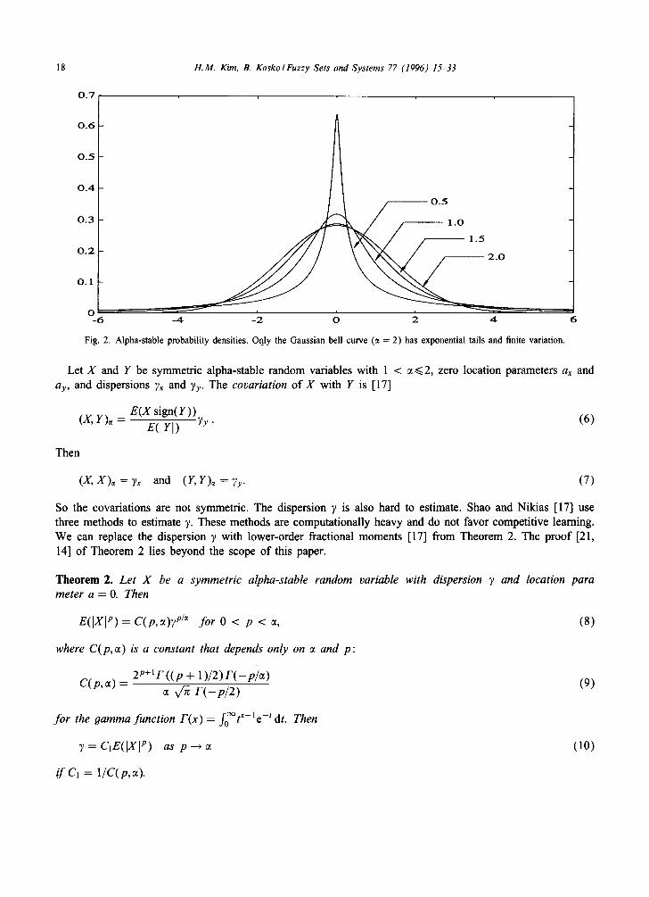
The Gaussian density is the special case o f an alpha-stable density when ct = 2. It is unique in this family because it has exponential tails and has finite variance and higher-order moments. Fig. 1 shows how alpha-stable noise grows more impulsive as the index ~t falls from 2 to 1.
The Gaussian bell curve is by far the most common bell curve in science and engineering. It fits some data well and depends on just the first and second moments o f a process. This gives simple closed-form solutions to many problems. Limiting sums o f independent random variables converge to a standard Gaussian
variable if the variables have finite variance. The key term e -x2 is in effect invariant under linear transforms
* Corresponding author.
0165-0114/96/$09.50 (~) 1996 Elsevier Science B.V. All rights reserved SSD! 0165-0 114(95)001 23 -9

16 H.M. Kim, R KoskolFuzzy Sets and Systems 77 (1996) 15 33
4 60
2 40
0 2O
-2
-4 0
-6 -20 0 1 O0 200 300 400 0 1 O0 200 300 400
(a) (b)
20 200
-200 -10
-20 -400
-30 -600 0 1 O0 200 3,00 400 0 1 O0 200 300 400
(c) (d)
Fig. 1. Impulsive noise modeled as independent samples from alpha-stable bell-curve densities. The noise magnitudes are not to scale. A noise density with a thicker tail has more frequent bursts of high energy. (a) Classical Gaussian case when ct = 2. Then the noise has finite variance. (b) Impulsive noise when ct = 1.9 and the noise has infinite variance. (c) More impulsiveness when ct = 1.5. (d) Still more impulsiveness in the Cauchy case when ct = 1.
and appears in the structure of Brownian motion. The Gaussian bell curve is the maximum-entropy density when we know just the first two (finite) moments of a process [16]. And it minimizes the "uncertainty principle" of physics and signal processing [7].
But locally a Gaussian curve looks like a Cauchy curve or other alpha-stable bell curve. Both have infinitely long tails and so are not "realistic". The tails have nonzero mass and so both can emit or explain a noise impulse of any magnitude. And both involve a central limit theorem [3]: Limiting sums of independent alpha-stable variables converge in distribution to an alpha-stable random variable. Indeed sums of independent identically distributed random variables can converge only to an alpha-stable random variable. The popular Gaussian central limit theorem is the special case of this alpha-stable theorem when ~ = 2. The real difference is that researchers first found and applied the Gaussian curve and that alpha-stable curves with ~ < 2 better model impulsive noise as found in telephone lines [19], underwater acoustics, low-frequency atmospheric signals [13] and lightning flashes, and fluctuations in gravitational fields [20] and stock prices [12] and in many other processes. Alpha-stable models seem to work well [17] when the signal data contains outliers. We seek the best alpha-stable fit to a measured noise pattern. In general this best-fit value ct* will not pick out the Gaussian case and so ~* < 2 will hold [18].
The main problem with alpha-stable models is their math complexity. Alpha-stable statistics do not have covariance matrices. Joint alpha-stable variables do have a measure of covariation that acts much like a covariance. But the covariation is not symmetric.
Below we define a pseudo-covariation measure that is symmetric and then use competitive learning to update it. This new measure gives a positive definite matrix and that gives a fuzzy ellipsoidal rule [5, 6]. We also use a new way to project the rule ellipsoids onto joint multivariable fuzzy sets. This helps preserve correlations in the input data. We apply this method to predicting and filtering signals awash in impulsive noise.
H.M. Kim, B. KoskolFuzzy Sets and Systems 77 (1996) 15~3 17
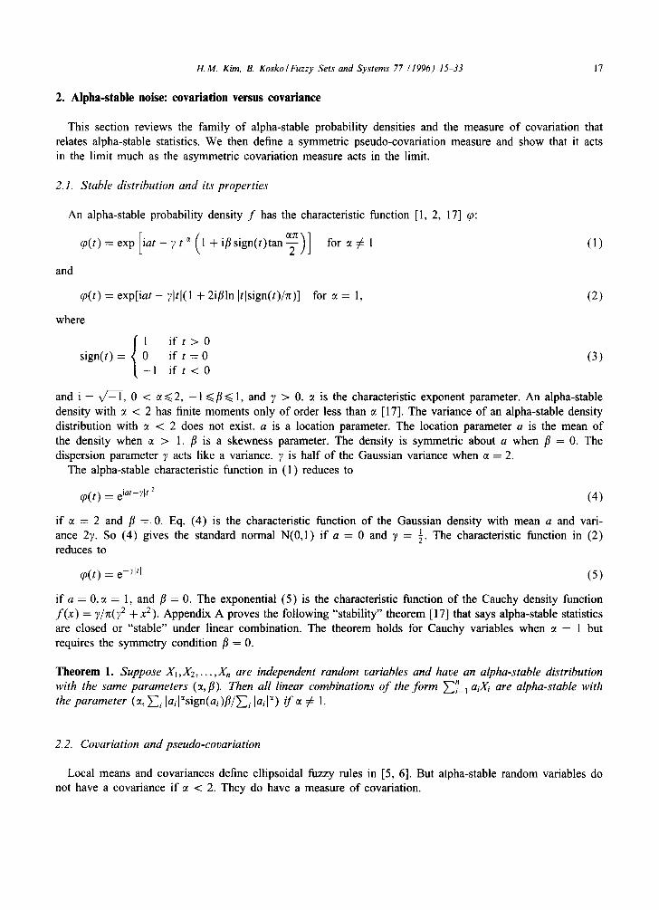
2. Alpha-stable noise: covariation versus eovarianee
This section reviews the family of alpha-stable probability densities and the measure of covariation that relates alpha-stable statistics. We then define a symmetric pseudo-covariation measure and show that it acts in the limit much as the asymmetric covariation measure acts in the limit.
2.1. Stable distribution and its properties
An alpha-stable probability density f has the characteristic function [1, 2, 17] q~:
qg( t )=exp[ ia t -71 t l~(1 + ifl sign(/)tan -~-) ] for ct # 1 (1)
and
¢p(t) = exp[iat - ?]t[(1 + 2iflln [tlsign(t)/rO] for ct = 1, (2)
where
1 i f t > O sign(t) = 0 if t = 0 (3)
- 1 if t < 0
and i = v/Z1, 0 < ~ ~<2, - 1 ~< fl ~< 1, and 7 > 0. ct is the characteristic exponent parameter. An alpha-stable density with ~ < 2 has finite moments only of order less than ~ [17]. The variance of an alpha-stable density distribution with ct < 2 does not exist, a is a location parameter. The location parameter a is the mean of the density when ~ > 1. fl is a skewness parameter. The density is symmetric about a when fl = 0. The dispersion parameter 7 acts like a variance. ~ is half o f the Gaussian variance when ~ = 2.
The alpha-stable characteristic function in (1) reduces to
tp( t ) = e iat-~' l t l2 (4)
if ct = 2 and fl = 0. Eq. (4) is the characteristic function of the Gaussian density with mean a and vari- ance 27. So (4) gives the standard normal N(0,1) if a = 0 and 7 = ½. The characteristic function in (2) reduces to
tp(t) = e -zltl (5)
if a = 0, ~ = 1, and fl = 0. The exponential (5) is the characteristic function of the Cauchy density function f ( x ) = 7/Tz(y 2 + x2). Appendix A proves the following "stability" theorem [17] that says alpha-stable statistics are closed or "stable" under linear combination. The theorem holds for Cauchy variables when • = 1 but requires the symmetry condition fl = 0.
Theorem 1. Suppose XI,X2 . . . . . X, are independent random variables and have an alpha-stable distribution with the same parameters (ot, fl). Then all linear combinations o f the form Y']i"=l aiXi are alpha-stable with the parameter (ct, ~ i ]ail%ign(ai)fl/~--~i [ai[ ~) / f ~ ¢ 1.
2.2. Covariation and pseudo-covariation
Local means and covariances define ellipsoidal fuzzy rules in [5, 6]. But alpha-stable random variables do not have a covariance if ~ < 2. They do have a measure of covariation.
18 H.M. Kim, B. KoskolFuzzy Sets and Systems 77 (1996) 15-33
0 . 7
0 . 6
0 . 5
0 . 4
0 . 5
0 . 3 - - 1 . 0
- - 1 .5 0 . 2
0 . 1
0 - 6 - 4 - 2 O 2 4 6
Fig. 2. Alpha-stable probability densities. Only the Gaussian bell curve (c~ = 2) has exponential tails and finite variation.
Let X and Y be symmetric alpha-stable random variables with 1 < ~ ~< 2, zero location parameters ax and ay, and dispersions 7x and 7y. The covariation of X with Y is [17]
E(X sign(Y)) (x,Y)=- E(IYI) WY (6)
Then
(X, X)~ = Vx and (Y, Y), = Vy. (7)
So the covariations are not symmetric. The dispersion 7 is also hard to estimate. Shag and Nikias [17] use three methods to estimate 7- These methods are computationally heavy and do not favor competitive learning. We can replace the dispersion 7 with lower-order fractional moments [17] from Theorem 2. The proof [21, 14] of Theorem 2 lies beyond the scope of this paper.
Theorem 2. Let X be a symmetric alpha-stable random variable with dispersion 7 and location para meter a = O. Then
E(IXI p) = C(p, oO7 p/~ for 0 < p < ~, (8)
where C(p ,~) is a constant that depends only on ~ and p:
2p+l r ( (p + 1)/2) F ( - p / ~ ) (9) C(p,~) = a v/~ F ( - p / 2 )
for the gamma function F(x) = f0°°tX-le - t dt. Then
y = CIE([X[ p) as p--+ a (10)
i f C1 = 1/C(p,~).
H.M. Kim, B. Kosko/Fuzzy Sets and Systems 77 (1996) 15-33 19
Now define a pseudo-covariation that is symmetric. The pseudo-covariation of X with Y is
(-J(, Y):t, pseudo: E(sign(XY)IXIp/2IYI p/2) for 0 < p < ~. (11)
Then (10) implies
( X , X ) ~ = Cl(X,X)~,pseud o as p ~ e. (12)
We use lower-order fractional moments instead of dispersion for competitive learning. We use the same power for each random variable to make the pseudo-covariation symmetric. Note that the pseudo-covariation equals the covariance when p = 2. Below we use p = 1 to learn fuzzy rules that can filter Cauchy-level impulsive noise.
We can define a pseudo-covariation matrix Cx for X = (Xi . . . . . X, ) v that acts as a symmetric and positive- definite covariance matrix:
(X1,Xl ):t, pseudo " '" (X1,Xn)~t, pseudo 1
CX= .. . ...''" (X2'Xn)~'pseud°[. (13) (X2, XI )~, pseudo
! L (Xn,Xl )~ pseudo " '" (Xn,Xn)~¢ pseudo.]
Appendix C presents the competitive learning system [8] to estimate the local covariation matrix. Then the local mean and covariation matrix define hyperellipsoids in the input-output space. We use Mahalanobis distance to produce joint if-part fuzzy sets from the ellipsoidal covariation rules. Section 6 tests how well these covariation rules filter alpha-stable impulsive noise.
3. Additive fuzzy systems
This section reviews the standard additive model (SAM) of the fuzzy system F : R" --~ R that we use to predict and filter nonlinear signals in alpha-stable noise. The pseudo-covariation measure (11) - (12) acts as standard covariance and yields ellipsoidal fuzzy rules. We use a new scheme based on Mahalanobis distance to project the ellipsoidal rule onto joint if-part fuzzy sets that maintain the correlation structure among the inputs, Other projection schemes factor the input sets and ignore the correlation.
3.1. Additive fuzzy systems
A fuzzy system F : R n ~ R stores m rules of the word from " I f X = A j, then Y = Bj" or the patch form As × By C X x Y = R ~ x R. The if-part fuzzy sets Aj C R" and then-part fuzzy sets Bj C R have set functions a~ : R ~ ~ [0, 1] and bj : R ~ [0, 1]. The system can use the joint set function aj or some factored form such as a j (x )= a ) (x l ) . . , a~(x~) or aj (x )= min(a) (x l ) . . . . . a~(x,)) or any other conjunctive form for input vector x = (xl . . . . . x , ) E R ~.
An additive fuzzy system [8, 9] sums .the "fired" then part sets B}:
m
B = .= ~'~aj(x) Bj. (14) j=l j=l
20 H . M . Kim, B. K o s k o l F u z z y Sets and S y s t e m s 77 (1996) 15-33
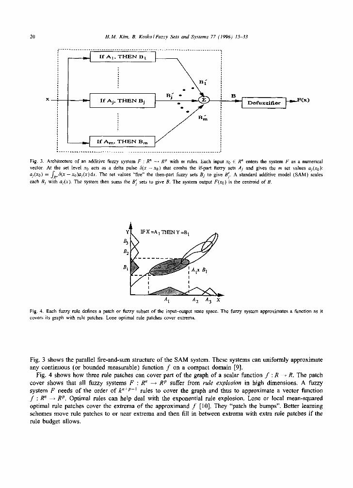
r . . . . . . . . . . . . . . . . . . . . . . . . . . . . . . . . . . . . . . . . . . . . . . . . . . . . . . . . . . . . . . . . . . . . . . . . . . .
[ I f A j , T H E N B j ~ I r [ [ D e f u z z i f i e r
A m , T EN Bm
~ . . . . . . . . . . . . . . . . . . . . . . . . . . . . . . . . . . . . . . . . . . . . . . . . . . . . . . . . . . . . . . . . . . . . . . . . . . . t
Fig. 3. Architecture of an additive fuzzy system F : R n ---* R p with m rules. Each input x0 E Rn enters the system F as a numerical vector. At the set level x0 acts as a delta pulse 6(x - x o ) that combs the if-part fuzzy sets Aj and gives the m set values aj(xo): aj(xo) = fR,,~(x-xo)aj(x)dx. The set values "fire" the then-part fuzzy sets Bj to give B~. A standard additive model (SAM) scales each Bj with aj(x). The system then sums the B} sets to give B. The system output F(xo) is the centroid of B.
IFX
B2 . . . . . . . . .
B, a : . , 7 , r - :
I !
v A 1 A 2 A 3 X
Fig. 4. Each fuzzy rule defines a patch or fuzzy subset of the input-output state space. The fuzzy system approximates a function as it covers its graph with rule patches. Lone optimal rule patches cover extrema.
Fig. 3 shows the parallel fire-and-sum structure o f the SAM system. These systems can uniformly approximate any continuous (or bounded measurable) function f on a compact domain [9].
Fig. 4 shows how three rule patches can cover part o f the graph o f a scalar function f : R ~ R. The patch cover shows that all fuzzy systems F : R n --+ R p suffer from rule explosion in high dimensions. A fuzzy system F needs o f the order o f k n+p-I rules to cover the graph and thus to approximate a vector function f : R n --~ R p. Optimal rules can help deal with the exponential rule explosion. Lone or local mean-squared optimal rule patches cover the extrema o f the approximand f [10]. They "patch the bumps". Better leaming schemes move rule patches to or near extrema and then fill in between extrema with extra rule patches i f the rule budget allows.
H.M. Kim, B. Kosko/Fuzzy Sets and Systems 77 (1996) 1~33 21
The scaling choice Bj = aj(x)Bj gives a standard additive model or SAM. Appendix B shows that taking the centroid of B in (14) gives [8-11] the SAM ratio
m V ~-~j=laJ(x) JC/ (15)
m F(x) = ~ j = l a j ( x ) V j
Vj is the nonzero volume or area of then-part set Bj. cj is the centroid of Bj or its center of mass. The SAM theorem (15) implies that the fuzzy structure of the then-part sets Bj does not matter. The ratio
depends on just the volume Vj and location cj of the then-part sets Bj. Our SAM has then-part sets of the same area and so the volume terms Vj cancel from (15). We need to pick only the scalar centers cj. The projection method in the next section picks the multivariable if-part sets aj.
3.2. Covariation rules and Mahalanobis sets." product space clustering and projection
Fuzzy rule patches AM x Bj can take the form of ellipsoids [5, 6]. Input-output data (xi, yi) drives the competitive learning process in Appendix C. We form the concatenated vector z T rxT ' 1 = t i YiJ in the product space R n x R. Then we lose p quantization vectors mj on the same product space. These vectors learn or adapt as they code for the local sample statistics and give rise to an adaptive vector quantization (AVQ). The AVQ vectors mj act as the synaptic fan-in columns of a connection matrix in a neural network with p competing neurons. The points mj learn if and only if they move in the product space. The points mj track the distribution of the incoming data points zi and tend to be sparse or dense where the zi are sparse or dense.
Fuzzy rules form through AVQ product space clustering [8]. Each AVQ vector mj converges to the lo- cal centroid of the sample data zi. So the AVQ vectors mj estimate the local first-order moments of some unknown probability density p(z) that generates the random sample data zi. The AVQ algorithm is a form of nearest-neighbor pattern matching or K-means clustering. The mj are random estimators since the data z~ are random. The AVQ point mj hops about more in the presence of noisy or sparse data and thus has a larger "error" ball. The covariance matrix Kj measures this error ball. The same competitive AVQ algorithm
in Appendix C updates the positive-definite matrix Kj. The inverse matrix K f I defines an ellipsoid E in the product space R n x R as the locus of all points z that obey
e 2 = (z - mj)TKfl (z -- mj) (16)
for centering constant e > 0. Then the j th ellipsoid defines the j th rule in the additive fuzzy system F : R n --~ R. We use the pseudo-covariation matrix in (11) with p = 1 to grow ellipsoidal covariation rules.
Fuzzy sets arise when the ellipsoids project down onto the axes. The projection is not unique because an ellipsoid E C R n x R does not factor into the Cartesian product of n + 1 sets E1 × ' " x En x E,+I. The SAM theorem in (15) lets us replace the then-part set En+l (or Bj) with just an area or volume Vj and a centroid cj. This presents a problem since noisy rules will have larger Vj values than smaller and more certain rule patches have. Then the SAM ratio (15) would give more weight to the least certain rules. Dickerson and Kosko [5, 6] deal with this by weighting each rule in (14) and (15) with a weight wj that varies with the inverse of ~ or with its square. We deal with it by normalizing all then-part sets to have the same area or volume. Then V1 . . . . . Vm > 0. This ignores some of the statistical structure of E but simplifies both the SAM ratio (15) for computing F(x). It also finds each then-part set Bj as just the centroid cj of the projection of the jth ellipsoid onto the output axis R.
22 H.M. Kim, B. Kosko/Fuzzy Sets and Systems 77 (1996) 15-33
14 , , ,
I i, ' " 12 .................................................... ,7:" .......... -x ¢
1. , ¢ ~1~ 1 1 1 i . I I
10 ,, : ,,
• ; p / 7 ~ J
6
2 At
r 2 4 6 8 10 12 14 16
xl
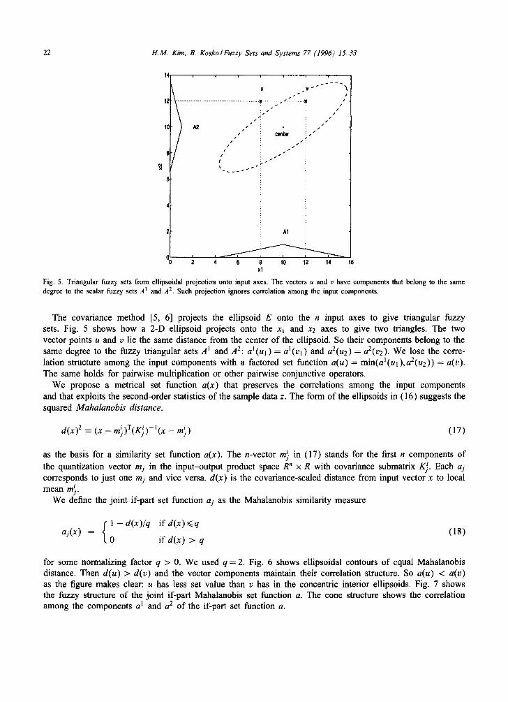
Fig. 5. Triangular fuzzy sets from ellipsoidal projection onto input axes. The vectors u and v have components that belong to the same degree to the scalar fuzzy sets A l and A 2. Such projection ignores correlation among the input components.
The covariance method [5, 6] projects the ellipsoid E onto the n input axes to give triangular fuzzy sets. Fig. 5 shows how a 2-D ellipsoid projects onto the xl and x2 axes to give two triangles. The two vector points u and v lie the same distance from the center of the ellipsoid. So their components belong to the same degree to the fuzzy triangular sets A l and A2: al(ul ) = al(vl) and a2(u2) = a2(v2). We lose the corre- lation structure among the input components with a factored set function a(u)= min(al(ul ),a2(u2)) = a(v). The same holds for pairwise multiplication or other pairwise conjunctive operators.
We propose a metrical set function a(x) that preserves the correlations among the input components and that exploits the second-order statistics of the sample data z. The form of the ellipsoids in (16) suggests the squared Mahalanobis distance.
d(x) 2 = (x - m) )T(Kj)-l(x -- m~j) (17)
as the basis for a similarity set function a(x). The n-vector m) in (17) stands for the first n components of the quantization vector mj in the input-output product space R" x R with covariance submatrix Kj. Each aj corresponds to just one mj and vice versa, d(x) is the covariance-scaled distance from input vector x to local mean m).
We define the joint if-part set function aj as the Mahalanobis similarity measure
1 - d ( x ) / q if d(x)<<.q = (18)
aj(x) 0 if d(x) > q
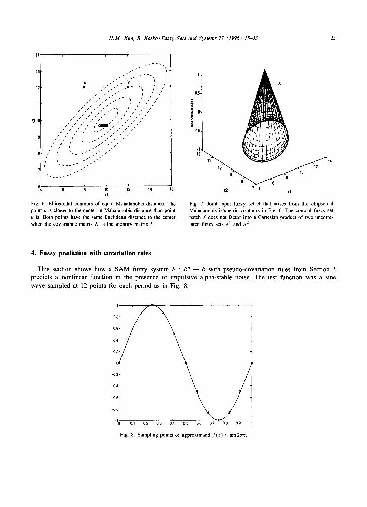
for some normalizing factor q > 0. We used q = 2. Fig. 6 shows ellipsoidal contours of equal Mahalanobis distance. Then d(u) > d(v) and the vector components maintain their correlation structure. So a(u) < a(v) as the figure makes clear: u has less set value than v has in the concentric interior ellipsoids. Fig. 7 shows the fuzzy structure of the joint if-part Mahalanobis set function a. The cone structure shows the correlation among the components a ] and a 2 of the if-part set function a.
H.M. Kim, B. KoskolFuzzy Sets and Systems 77 (1996) 15-33 23
14 , , ,
U . ' " . • ' v / / A
~" / " - " I ,' / 0,5, , ' / / ,,I s-'- ~ I i i I
11 // "'i" I / / / / t . I / / / " i /~ • I / / / " I ~ O'
/ / / / I / , I i / / i / / s / / / / s / / / ~
~ I 0 / " " " " / " / " / " " 1 / 11 I i I ~ / / / / 1 / ~ f~
/ / / I / " i " . , 1 / / / ,(~ 9 / / t - . . " ,, , . "
/ / I ~ . - i / 11 . i i i I ~ / i i r -I:
8 ¢ / I . _ . . . 1 " . 12 11 1 0 ~ ' ~ ~
6 6 8 10 12 1'4 16 X2 7 4 xl xl
Fig. 6. Ellipsoidal contours of equal Mahalanobis distance. The Fig. 7. Joint input fuzzy set A that arises from the ellipsoidal point v is closer to the center in Mahalanobis distance than point Mahalanobis isometric contours in Fig. 6. The conical fuzzy-set u is. Both points have the same Euclidean distance to the center patch A does not factor into a Cartesian product of two uncorre- when the covariance matrix K is the identity matrix 1. lated fuzzy sets ,41 and A 2.
4. Fuzzy prediction with covariation rules
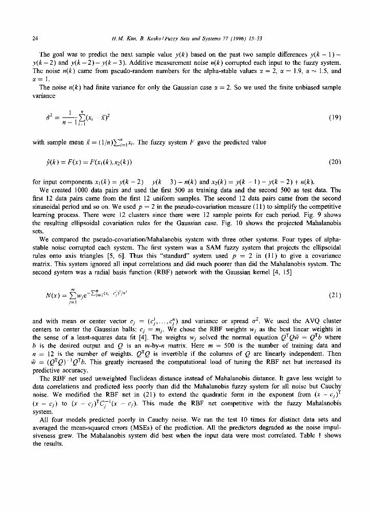
This section shows how a SAM fuzzy system F : R n ~ R with pseudo-covariation rules from Section 3 predicts a nonlinear function in the presence of impulsive alpha-stable noise. The test function was a sine wave sampled at 12 points for each period as in Fig. 8.
1 x , ,
0.8 /
0.6
0.4
0.2
0
-0.2 /
-0.4
\ / -0.8
-I i I t i i 0.1 0.2 0.3 0.4 o.5 0.6 0.7 0.8 0.9
Fig. 8. Sampling points of approximand f ( x ) = sin 2nx.
24 H.M. Kim. B. KoskolFuzzy Sets and Systems 77 (1996) 15-33
The goal was to predict the next sample value y(k) based on the past two sample differences y ( k - 1)- y(k- 2) and y ( k - 2 ) - y ( k - 3). Additive measurement noise n(k) corrupted each input to the fuzzy system. The noise n(k) came from pseudo-random numbers for the alpha-stable values ct = 2, ~ = 1.9, ~t = 1.5, and ~ = 1 .
The noise n(k) had finite variance for only the Gaussian case 7 = 2. So we used the finite unbiased sample variance
n
e 2 - - rl 1 1 i~=l ( x i - ; ) 2 (19)
?1 with sample mean £ = (1/n)~-~i=lx i. The fuzzy system F gave the predicted value
f;(k) = F(x) = F(x l (k) ,x2(k) ) (20)
for input components xl (k ) = y(k - 2) - y(k - 3) + n(k ) and x2(k) = y(k - 1 ) - y (k - 2) + n(k ). We created 1000 data pairs and used the first 500 as training data and the second 500 as test data. The
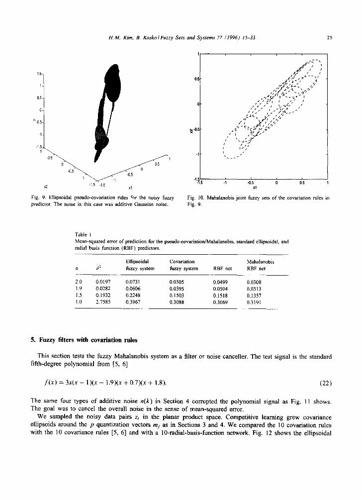
first 12 data pairs came from the first 12 uniform samples. The second 12 data pairs came from the second sinusoidal period and so on. We used p = 2 in the pseudo-covariation measure (11 ) to simplify the competitive learning process. There were 12 clusters since there were 12 sample points for each period. Fig. 9 shows the resulting ellipsoidal covariation rules for the Gaussian case. Fig. 10 shows the projected Mahalanobis sets.
We compared the pseudo-covariation/Mahalanobis system with three other systems. Four types of alpha- stable noise corrupted each system. The first system was a SAM fuzzy system that projects the ellipsoidal rules onto axis triangles [5, 6]. Thus this "standard" system used p = 2 in (11) to give a covariance matrix. This system ignored all input correlations and did much poorer than did the Mahalanobis system. The second system was a radial basis function (RBF) network with the Gaussian kernel [4, 15]
m n I 2 2 N(x) = ~~wje -~i=l(x'-%) /a (21)
j = l
and with mean or center vector cj = (c) . . . . . c~) and variance or spread a a. We used the AVQ cluster centers to center the Gaussian balls: cj = mj. We chose the RBF weights wj as the best linear weights in the sense of a least-squares data fit [4]. The weights wj solved the normal equation QTQff, = QT b where b is the desired output and Q is an m-by-n matrix. Here m = 500 is the number of training data and n = 12 is the number of weights. QTQ is invertible if the columns of Q are linearly independent. Then
= (QTQ)-IQTb. This greatly increased the computational load of tuning the RBF net but increased its predictive accuracy.
The RBF net used unweighted Euclidean distance instead of Mahalanobis distance. It gave less weight to data correlations and predicted less poorly than did the Mahalanobis fuzzy system for all noise but Cauchy noise. We modified the RBF net in (21) to extend the quadratic form in the exponent from ( x - c j ) T ( x - cj) to ( x - c j ) T c f l ( x - cj). This made the RBF net competitive with the fuzzy Mahalanobis system.
All four models predicted poorly in Cauchy noise. We ran the test 10 times for distinct data sets and averaged the mean-squared errors (MSEs) of the prediction. All the predictors degraded as the noise impul- siveness grew. The Mahalanobis system did best when the input data were most correlated. Table 1 shows the results.
H.M. Kim, B. KoskolFuzzy Sets and Systems 77 (1996) 15-33 25
1
r / i
J , , 1.5. ~,- ," s $ , / . ~ / 4
0.5. ,-,.,5J ~' " - ' ; 7 J i s ~ I I I I t
0 " " • " l i I I / ~I I i s l i i I • i I \ I (t / O- , , , " , ," /,-0__-
:~ -0 ,5 , / " I / ,~/"r t I t " ~ " l ,
• " /~ i /,, / -1- 111 I,, I I I J l " ' l " ~
0.5 I " - ' "
-o .s~ / o -0.5
-I " " ' - ~ - - ~ - I -I.! ' -1 -015 0 015 x2 -15 -1.5 xl xl
Fig. 9. Ellipsoidal pseudo-covariation rules ¢,~r the noisy fuzzy Fig. 10. Mahalanobis joint fuzzy sets of the covariation rules in predictor. The noise in this case was additive Gaussian noise. Fig. 9.
Table 1 Mean-squared error of prediction for the pseudo-covariation/Mahalanobis, standard ellipsoidal, and radial basis function (RBF) predictors.
Ellipsoidal Covariation Mahalanobis ct o ~2 fuzzy system fuzzy system RBF net RBF net
2.0 0.0197 0.0731 0.0305 0.0499 0.0308 1.9 0.0282 0.0606 0.0395 0.0504 0.0313 1.5 0.1932 0.2248 0.1503 0.1518 0.1357 1.0 2.7585 0.3967 0.3088 0.3069 0.3191
5. Fuzzy filters with eovariation rules
This section tests the fuzzy Mahalanobis system as a filter or noise canceller. The test signal is the standard fifth-degree po lynomia l from [5, 6]
f ( x ) = 3x(x - 1)(x - 1.9)(x -t- 0.7)(x + 1.8). (22)
The same four types o f addit ive noise n ( k ) in Section 4 corrupted the polynomial signal as Fig. 1 1 shows. The goal was to cancel the overall noise in the sense o f mean-squared error.
We sampled the noisy data pairs zi in the planar product space. Compet i t ive learning grew covariance ell ipsoids around the p quant izat ion vectors mj as in Sect ions 3 and 4. We compared the 10 covariat ion rules with the 10 covariance rules [5, 6] and with a 10-radial-basis-function network. Fig. 12 shows the ell ipsoidal

26 H.M. Kim, B. Kosko/Fuzzy Sets and Systems 77 (1996) 15-33
o o
10 10
0
-10 -10
-20 -20 -2 -1 O 1 2 -2 -1 0 1 2
(a) (b)
20 20
-10 -10
-20 -20 -2 -1 0 1 2 -2 -1 0 1 2
(c) (d)
Fig. 11. Four types of" alpha-stable impulsive noise corrupt a polynomial signal: (a) Gaussian noise when c~ = 2; (b) more impulsive noise when ct = 1.9; (c) still more impulsive noise when ct = 1.5; (d) C a u c h y noise when ct = 1.
rules from the covariance matrices. These rule patches cover the signal polynomial in Fig. 13. Fig. 14 shows the ellipsoidal rules from the covariation matrices. These rule patches cover the same signal polynomial in Fig. 15. The impulsive Cauchy noise (~ = 1) moves the covariation ellipsoids further apart from one another than it moves the covariance ellipsoids. The covariation rules gave a better filtering patch cover in terms of mean-squared error. The rules in Figs. 12 and 14 grew from 500 training data with Cauchy noise. We used the other 500 sample points as test data.
The covariation rule system filtered noise better than did both the covariance rule system and the RBF net in terms of mean-squared error. Fig. 16 compares the filtered noise from the covariance rule system with the noiseless polynomial signal. Fig. 17 compares the filtered noise from the covariation rule system with the noiseless signal. Fig. 18 compares the RBF filtered noise with the noiseless signal. The scalar input values did not give rise to an input covariance matrix. So there was no RBF net with Mahalanobis distance as there was for the prediction problem in Section 4.
Figs. 19-21 plot the power spectra of the three filters. The high frequency terms in Fig. 19 came from the separation among the covariation ellipsoids and thus came from the impulsive noise itself. We then used the smoothing-by-3s system
y ( k ) = l ( x ( k - 1) + x (k ) + x ( k + 1)) (23)
to smooth the high-frequency components in the covariation rule system. This greatly improved how the filter canceled the four types of alpha-stable noise as in Figs. 22 and 23. Table 2 compares the four filters in terms of mean-squared error.

H.M. Kim, B. Kosko/Fuzzy Sets and Systems 77 (1996) 15-33 27
1,5 2 0 ~ I
10 ~ r " x - . 15
"-- . . . . ~-.--_ ___ ._,~, -,.'. ".. , ,ol ;: " , ~ ~, ' ~', ',,' #: 5
' -" ,"l i tii 0
" I lTK /li i I I I > ' 0 X% >' -5 i i i t
.,o , . •
i i I I I l l l ,o it "7',:,7
I • I I I I
-2~ i I -15
I i i I I i
"~.~ .~o .~oo -50 o 50 1® ~o "~.~ .~ .~ ~ ~.~ ~ ~.~ -1.5 -0.5 0 0 .5
x t
Fig. 12. Ellipsoidal rules from covariance matrices and Cauchy Fig. 13. Patch cover of covariance rules. noise.
10 ~ - - ' ' ' ' " ' 201
/ ).;0, . . . . . 101 , - ~
o ," " ~ " , "" ".
>, ~ f p,' t - ~ . ' - - # ",~ ," , ,',' ,, . . . . ,.. ~ ~ . '--..~>.~...~ " ' ' " ' - - - . . : - . . " ~ , , , \ > . ' 4 -
! I
,, ,. .101
- 1 5 i ~'
.151
-21 -40 -30 -20 -10 0 1 20 30 40 -2 -15 -1 -05 0 0.5 1 1.5 2 2,5 x t
Fig . 14. Ellipsoidal rules from pseudo-covariation matrices and Fig. 15. Patch cover of pseudo-covariation rules. Cauchy noise.
6. Conclusion
Dealing with impulsive noise remains one of the great challenges of modem engineering. It is hard to model, predict, and filter-and yet it pervades the world. Fuzzy systems omit the modeling step that burdens

28 H.M. Kim, B. Kosko/Fuzzy Sets and Systems 77 (1996) 15-33
lO . . . . . I0
5 5
i i~ji i: ,:
-10 ~ line: original ~ dotted: ~ered Q~lted: filtered
"0.5 0 0.5 2 "1:5 -1 "015 0 0:5 1 1:5 t t
Fig. 16. Covariance fuzzy filter of Cauchy noise. Fig. 17. Pseudo-covariation fuzzy filter of Cauchy noise.
xl0' 10f 4.. ~
3.~ >,. ,?~i
2.~
solid lice: original 1.5
t dolled: Altered 1
-15 0.5
"202 -1.5 ol .0.5 0 O.S 1 1.5 200 400 600 800 1000 1200 t
Fig. 18. Radial basis function filter of Cauchy noise. Fig. 19. Power spectrum of covariance-filtered signal.
most standard system. They also dispense with the old working fiction that real noise is Gaussian noise of finite variance. Adaptive fuzzy systems can grow and tune their rules from any source of signals or noise.
The ellipsoidal rule structure constrained our fuzzy systems. This need not be the case. Rules with highly irregular or impulsive shapes may better predict and filter impulsive noise. Or fuzzy systems might keep the

H.M. Kim, B. KoskoIFuzzy Sets and Systems 77 (1996) 15-33 29
x 10' x lo' , 4. . ~ ,
5i !
3.. ~ I
4'
!
3 ~
1.E
1
200 400 600 800 1000 1200 C 1200
Fig. 20. Power spectrum of pseudo-covariation-filtered signal. Fig. 21. Power spectrum of RBF-filtered signal.
10 4.5 x "",v '~ i
4 5
3.5
0 3
2.5 > ' - 5
2
-1( solid line: original 1.5
dotted: filtered
-1!
0.I
-2( -1'.5 -1 "015 0 015 I 115 200-'- 400 - - - '600 800 1000 1200 t
Fig. 22, Smoothed pseudo-covariation filter of Cauchy noise. Fig. 23. Power spectrum of covariation-filtered signal with smoothing.
ellipsoidal rule structure but estimate other statistics [17] of alpha-stable random variables. The search for such rules and estimators is an open research area.

30 H.M. Kim, B. Kosko/Fuzzy Sets and Systems 77 (1996) 15-33
Table 2 Mean-squared error of filtering for the pseudo-covariation/Mahalanobis, standard ellipsoidal, and radial basis function (RBF) filters
Ellipsoidal Covariation Smoothed covariation d 2 fuzzy system fuzzy system RBF net fuzzy system
2.0 1.86 5.25 4.33 4.68 4.24 1.9 2.21 6.94 5.63 6.77 5.13 1.5 11.45 11.88 8.23 10.91 6.12 1.0 775.27 16.35 14.27 14.59 11.85
Appendix A. Proof of "stability" theorem
Theorem 1. Suppose X1,X2 . . . . . Xn are independent random variables and have an alpha-stable distribution with the same parameters (or, 8). Then all linear combinations of the form ~ = 1 ajXj are alpha-stable with the parameter (~, ~'~-~=l [ajl%ign(aj)[3/~-'~=l layl = ) / f = ¢: 1.
Proof. Suppose a random variable X has a probability density function px(x) and characteristic function ~Ox(t). Define a new random variable Y = aX. Then it has the characteristic function ~oy(t) = q~x(at). So the sum random variable ~ = 3 ajXj has the factored characteristic function ~Ox, (al t)Cpx2(a2t)'" ~Ox.(a,t) since the random variables are independent. Then replacing t with ajt in the alpha-stable characteristic function
[ia,- ltf (1 +i, sig°,/ tanT) ] gives
tl
q~ET=,a,x, ( t ) = 1-I ~ox, ( a j ) (A.2) j = l
n 0~X = [-[exp [iaajt-ylajtl ~ (1 + i[3sign(ajt)tan-~)] (A.3)
j = l
n . . . 0~R
= ]-Iexp [iaajt- ylajl~[tl ~ (1 +lflslgn(aj,slgn(t)tan--f)] (A.4) j = l
=exp[~j(iaajt-ylajl~[t,~(l+iflsign(aj)sign(t)tanT))] (A.5)
= exp ( i a a j t ) - yltl = (lajl" + lajl~lflslgn(aj)slgn(t)tan--f (A.6)
=exp[~j(iaalt)-yltl~(~(lajla)+\j ~-~.([ajl~iflsign(aj)sign(t)tanT))]j (A.7)
=exp[ia(~jaj ) t _ (~jlaj[~)~ltl~(l+i~-'~qlajl~sign(aJ)B . otTr ~jlaj{ ~ v slgn(t)tan-~) ] . (A.8)
So the sum ~ = , ajSj is alpha-stable and has the parameter (~, Y~=~ la:l'sign(aj)~/~=, lajl~). []
H.M, Kim, B. KoskolFuzzy Sets and Systems 77 (1996) 15-33 31
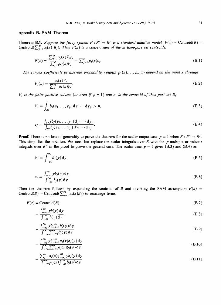
Appendix B. SAM Theorem
Theorem B.1. Suppose the fuzzy system F : R ~ ~ R p is a standard additive model." F(x) = Centroid(B) = Cen t ro id (~ '= ja j (x ) Bj). Then F(x) is a convex sum of the m then-part set centroids:
m
F(x) = }-~j=laj(x)Vjcj m
m Y'~j=I aj(x)Vj }--~)= 1 py(x)cj. (B. 1 )
The convex coefficients or discrete probability weights p l (x ) . . . . . pm(X) depend on the input x through
Pj(x) = m aj(x)Vj . (B.2) Y~k:lak(x)Vk
Vj is the finite positive volume (or area i f p = 1 ) and cj is the centroid o f then-part set Bj:
Vj = fRR,'bj(Yl . . . . . y p ) d y l " " d y p > 0, (B.3)
fRpybj(Yl . . . . . yp) dyl "'" dyp (B.4) cj = fRpbj(y 1 . . . . . yp )dy l " " d y p
Proof. There is no loss of generality to prove the theorem for the scalar-output case p = 1 when F : R n --+ R p. This simplifies the notation. We need but replace the scalar integrals over R with the p-multiple or volume integrals over R p in the proof to prove the general case. The scalar case p -- 1 gives (B.3) and (B.4) as
/? Vj = b j ( y ) d y (B.5)
f_~ ybj(y) dy cj = f~_~ b j ( y ) d y (B.6)
Then the theorem follows by expanding the centroid of B and invoking the SAM assumption F(x) = Centroid(B) = Centro id(~= 1 aj(x)Bj) to rearrange terms:
F(x) = Centroid(B) ( B. 7)
_ f-~o~ y b ( y ) d y f~_~ b(y) dy (B.8)
= f-~o~ YY~ff=l b~(y) dy (B.9)
m
_ f~-~ YY'~j=I aj(x)bj(y) dy (B. 10) - - O 0 m
f~_~ ~j=~ aj(x )bj(y ) d y
_ }-~ff=laj(x)f~_~ yb j (y ) dy - }_~jmlaj(x)f~_~bj(y)dy (B.11)

32 H.M. Kim, B. Kosko/Fuzzy Sets and Systems 77 (1996) 15-33
m a ~ x ' V f~ybj(y)dy Z j = I J~, ) J -- Vjj
m = ~j=laj(x)V j (B.12)
m
-- -- ~-~j=laj(x)Vjcj [] ( 8 . 1 3 ) m ~j=, aj(x) Vj
Appendix C. Competitive AVQ algorithm for local means and covariations
The following procedure describes the competitive adaptive vector quantization (AVQ) algorithm for local means and pseudo-covariations.
1. Initialize cluster centers from sample data: mi(O) = x(i) for i = 1 . . . . . p. 2. Find the "winning" or closest synaptic vector mj(k) to sample vector x(k):
Ilmj(k) - x(k) l l = min Ilmi(k) - x (k) l l ,
2 where I1" II denotes the Euclidean norm: Ilxll 2 -- x~ + . . . + x , . 3. Update the winner mj(k),
mj(k) + ck[x(k) - mj(k)] if the jth neuron wins, (C.1) mj(k + 1) = mj(k) if the jth neuron loses,
and its pseudo-covariation estimate Cj(k),
C j ( k ) + d k [ ( x ( k ) - m j ( k ) ) p / 2 ( ( x ( k ) - m j ( k ) ) p / 2 ) T - C j ( k ) ]
Cj(k + 1 ) = if the jth neuron wins, (C.2)
Cj(k) if the jth neuron loses,
where (x(k)) p/2 ~= (sign(xl(k))lXl(k)l p/2 . . . . . sign(xn(k)) Ix.(k)lp/2) w. We used p = 1 in all simulations.
References
[1] V. Akgiray and C.G. Lamoureux, Estimation of stable-law parameters: a comparative study, J. Business Econ. Statist. 7 (1989) 85-93.
[2] H. Bergstrom, On some expansions of stable distribution functions, Ark. Math. 2 (1952) 375-378. [3] L. Breiman, Probability (Addison-Wesley, Reading, MA, 1968). [4] S. Chen, C.F.N. Cowan and P.M. Grant, Orthogonal least squares learning algorithm for radial basis function networks, IEEE Trans.
Neural Networks 2 (1991) 302-309. [5] J.A. Dickerson and B. Kosko, Fuzzy function learning with covariance ellipsoids, Proc. 2nd IEEE Internat. Conf. on Fuzzy Systems
(IEEE FUZZ-93) (1993) 1162-1167. [6] J.A. Dickerson and B. Kosko, Fuzzy function approximation with supervised ellipsoidal learning, World Congress on Neural
Networks (WCNN "93), Vol. II (1993) 9-13. [7] R.W. Hamming, Digital Filters (Prentice-Hall, Englewood Cliffs, N J, 2nd ed., 1983). [8] B. Kosko, Neural Networks and Fuzzy Systems (Prentice-Hall, Englewood Cliffs, NJ, 1991 ). [9] B. Kosko, Fuzzy systems as universal approximators, 1EEE Trans. Comput. 43 (1994) 1329-1333. An early version appears in
Proc. 1st IEEE Internat. Conf. on Fuzzy Systems (IEEE FUZZ-92) (1992) 1153-1162. [10] B. Kosko, Optimal fuzzy rules cover extrema, lnternat. J. Intelligent Systems 10 (1995) 249-255. [11] B. Kosko, Combining fuzzy systems, Proc. 1EEE Internat. Conf. on Fuzzy Systems (IEEE FUZZ-95), Vol. IV (1995) 1855-1863. [12] B. Mandelbrot, The variation of certain speculative prices, J. Business 36 (1963) 394-419. [13] B. Mandelbrot and J.W. Van Ness, Fractional Brownian motions, fractional noises and applications, SlAM Rev. 10 (1968) 422-437.
ll.M. Kim, R Kosko/Fuzzy Sets and Systems 77 (1996) 15-33 33
[14] E. Masry and S. Cambanis, Spectral density estimation for stationary stable processes, Stochastic Processes Applic. 18 (1984) 1-31. [15] J. Moody and C.J. Darken, Fast learning in networks of locally-tuned processing units, Neural Comput. 1 (1989) 281-294. [16] A. Papoulis, Probability, Random Variables, and Stochastic processes (McGraw-Hill, New York, 2nd ed., 1984). [17] M. Shao and C.L. Nikias, Signal processing with fractional lower order moments: stable processes and their applications, Proc.
IEEE 81 (1993) 984-1010. [18] J. Shen and C.L. Nikias, Estimation of multilevel digital signals in the presence of arbitrary impulsive interference, IEEE Trans.
Signal Processing 43 (1995) 196-203. [19] B.W. Stuck and L. Kleiner, A statistical analysis of telephone noise, Bell Systems Tech. J. 53 (19743 1263-1320. [20] A. Wernon and K. Wernon, Stable measures and processes in statistical physics, in: S. Cambanis, Ed., Probability Theory on Vector
Spaces IV (Springer, Berlin, 1987) 440-452. [21] V.M. Zolotarev, Mellin-Stieltjes transforms in probability theory, Theory Probab. Applic. 2 (1957) 433-460.