The infinitestimal operator for the semigroup of theFrobenius-Perron operator from image sequence data:

Vector fields and computational measurable dynamics from movies

N. Santitissadeekorn and E. M. Bollt

Department of Mathematics and Computer Science,Clarkson University,Potsdam, NY 13699-5815,USA

Abstract

We present in this paper an approach to approximate the Frobenius-Perrontransfer operator from a sequence of time-ordered images, that is, a moviedataset. Unlike time-series data, successive images do not provide a direct ac-cess to a trajectory of a point in a phase space; more precisely, a pixel in animage plane. Therefore, we reconstruct the velocity field from image sequencesbased on the infinitesimal generator of the Frobenius-Perron operator. More-over, we relate this problem to the well-known optical flow problem from thecomputer vision community and we describe a validity of using the continuityequation derived from the infinitesimal operator as a constraint equation forthe optical flow problem. Once the vector field, and then a discrete transferoperator are found then, in addition, we present a graph modularity methodas a tool to discover basin structure in the phase space. Together with a toolto reconstruct a velocity field, this graph-based partition method provides usa way to study transport behavior and other ergodic properties of measurabledynamical systems captured only through image sequences.

1 Introduction

A development of computational methods in the burgeoning field of measurable dy-namics to model and identify transport activity in both deterministic and stochasti-cally perturbed dynamical systems, specifically through approximating the Frobenius-Perron transfer operator, demonstrate numerous applications in number of domains [1–3]. Our primary interest is to develop a numerical tool in a framework of theFrobenius-Perron transfer operator to study basin structure, transport behavior, andother ergodic properties all through processing time-series data from movies of adynamical evolution of a probability density profile I(x, y, t), for example, when ob-serving a satellite image, one may ask about what is the underlying velocity field, andalso are there any almost invariant sets. In this paper we will relate the optical flowproblem to reconstruct the displacement field that transform an image to the nextimage to problems of measurable dynamics through the Frobenius-Perron operator.

To construct the Ulam-Galerkin approximation of the transfer operator we are re-quired to have a knowledge of a family of transformations, see Section 2.3. However,

1

a sequence of images does not provide a direct access to the trajectory of a pointin a phase space. Successive images instead only describe an evolution in time of adistribution of brightness of image pixels. For this reason, the primary interest ofthis paper is to reconstruct a velocity field from a two-dimensional image sequencethat transforms the intensity pattern from one image to the next image in a sequence,which is called optical flow computation [4]. The problem of determining the opticalflow has been intensively studied in the last two decades in many areas of computer vi-sion to perform motion detection and tracking, object segmentation, time-to-collisionestimation, and etc. Recently, the analysis of the optical flow has been applied tomany other science areas such as meteorology, oceanography, climatology, where im-age sequences from satellite platforms are the main source of their information [5–12].However, the application of this optical flow analysis has not yet been demonstratedin the area of the measurable dynamical system, in particular, to approximate theFrobenius-Perron transfer operator from a sequential image data.

In this paper we assume that the desired velocity field is autonomous throughoutthe image region and so the trajectory of a point in the image region is governed bythe following equation:

dx

dt= u(x, y)

dy

dt= v(x, y),

(1)

where u(x, y) and v(x, y) are two unknown velocity fields to be approximated from asequence of images, which provides to us only a temporal variation of the brightnesspattern. We describe this temporal variation in a framework of the Frobenius-Perronoperator. In section 2 we will show that this evolution can be expressed as thesolution of the partial differential equation derived from the infinitesimal operatorof the Frobenius-Perron operator [13]. This partial differential equation turns outto be the well-known continuity equation in fluid mechanics, and it will serve as theconstraint equation for the optical flow computation, see Section 3. We will focus hereon the application of using optical flow to generate the finite-rank approximation ofthe Frobenius-Perron operator instead of developing an advance algorithm to find theoptical flow.

Obtaining an approximated velocity field from an image sequence permits us toapproximate the Frobenius-Perron operator based on the Ulam-Galerkin method,which will be described below. The approximation will be in the matrix form calledthe Ulam-Galerkin matrix. Then we may generate a graph network corresponding tothe Ulam-Galerkin matrix. Furthermore, we also determine the phase space parti-tion of the dynamical system of the image sequence described by the approximatedoptical flow. This partition identifies the regions in the phase space that should be

2

dynamically grouped(those in the same basin). In the view point of the graph theory,we must discover the community structure of the graph-the partition that groups to-gether those nodes within which they are densely connected, but their connection toother nodes are comparatively sparse [14]. The approach to discover the communitystructure of the network used in this paper is called the modularity method [14–17]based on the optimization of the modularity measure of the network. Note that ina different approach, recent efforts have focused to identify the number and locationof almost invariant sets; those subsets of a state space where trajectories tend tostay for comparatively long periods of time before they leave into other regions, in acontext of the congestion of a graph based on a multi-commodity flow on the graph[18–21]. In this sense, the graph community structure and the almost invariant setsare essentially the same tool to approximate the basin structure of the phase space.

2 Background

We review in this section some properties of the Frobenius-Perron operator that willhelp us to relate the inverse problem of the optical flow computation, which will bereviewed in Section 3, to the approximation of the Frobenius-Perron transfer operator.

2.1 Frobenius-Perron and Koopman operators

Let (X, A, µ) be a measure space. Let F : X → X be a non-singular measurabletransformation on (X, A, µ),that is,

µ(F−1(A)) = 0 for each A ∈ A such that µ(A) = 0. (2)

The Frobenius Perron operator, P : L1(X) → L1(X) with respect to F is definedby [13],

Pf(x) =

∫X

δ(x− F (y))f(y)dy, (3)

where f(x) is a probability density function (PDF) defined in L1(X). Thus Pf(x)gives us a new probability density function, which is unique a.e., and depend onthe discrete time transformation F and the probability density function f(x). Forall measurable sets A ⊂ A the Frobenius-Perron operator satisfies the discrete-timecontinuity equation [13]∫

F−1(A)

f(x)dx =

∫A

Pf(x)dx, for each A ∈ A (4)

The operator K : L∞ → L∞, called the Koopman Operator with respect to F , isdefined by

Kg(x) = g(F (x)) (5)

3

for g ∈ L∞. For us, the key property of the Koopman operator is that it is adjointto the Frobenius-Perron operator. That is for every ρ ∈ L1, g ∈ L∞,

〈Pρ, g〉 = 〈ρ, Kg〉, (6)

where we denote the bilinear form 〈·, ·〉L1(X)×L∞(X) by 〈·, ·〉 throughout this paper.

2.2 Infinitesimal generators

In this section we review some background of the infinitesimal generator of the semi-group of the Frobenius-Perron operator, of which the details can be found in Lasotaand Mackey [13]. The key result in this section will form the main constraint equationused in the optical flow computation.

Consider a d-dimensional system of ordinary differential equations

dxi

dt= Fi(x), i = 1, . . . , d, (7)

where x = (x1, . . . , xd) ∈ Rd. This system gives a continuous time process Stt≥0

defined by

St(x0) = x(t), (8)

where x(t) is the solution of Eq. (7) with the initial condition x0 = x(0). Assum-ing that existence and uniqueness of solutions of Eq. (7) are satisfied, one can showthat the family Stt≥0 forms a continuous semigroup of transformations correspond-ing to Eq.(7). Additionally, we can also defined the Frobenius-Perron operator andthe Koopman operator for a continuous time process associated to the semigroup oftransformation Stt≥0 in the same fashion of a discrete time process as previouslydescribed, that is,∫

S−1t (A)

f(x)dµ =

∫A

Ptf(x)dµ for eachA ∈ A, (9)

andKtg(x0) = g(St(x

0)). (10)

Now we can state the aim of this section more precisely. That is we want todiscuss about the evolution of time-dependent density function I(t, x) ≡ Ptf(x) forsome initial density function f(x) in L1(X). This can be developed by using theinfinitesimal operator as discussed in Lasota and Mackey [13]. We will briefly repeatthis concept here for a sake of completeness, and we will emphasize how we will relateit to the optical flow computation.

4

For a semigroup of contractions Ttt≥0 we define by D(A) the set of all f(x) ∈Lp(X), 1 ≤ p ≤ ∞, such that the limit

Af = limt→0

Ttf − f

t, (11)

exists in the sense of strong convergence, that is,

limt→0

∥∥∥∥Af − Ttf − f

t

∥∥∥∥L

= 0. (12)

The operator A : D(A) → L is called the infinitesimal generator. Let I(t) ≡ I(t, x) =Ttf(x) for fixed f(x) ∈ D(A). The function I ′(t) ≡ I ′(t)(x) ∈ Lp(X) is said to be thestrong derivative of I(t) if it satisfies the following condition:

limt→0

∥∥∥∥I ′(t)− I(t)− f(x)

t

∥∥∥∥Lp

= 0. (13)

In this sense, I ′(t) describes the derivative of the ensemble of points with respect totime t. It is shown in [13] that for t ≥ 0 and I(t, x) ∈ D(A) we have that I ′(t) existsand satisfies the equation

I ′(t) = AI(t) (14)

with the initial condition I(0) = f(x).We are now in a position to discuss about the infinitesimal generator of the

Frobenius-Perron operator generated by the family of transformation Stt≥0 and theevolution of time-dependent density function I(t, x) under an action of the Frobenius-Perron operator. This will be done indirectly through the adjoint property of theForbenius-Perron and Koopman operators.

It follows directly from the definition of the Koopman operator Eq. 10 that theinfinitesimal of the Koopman operator AK is

AKg(x) = limt→0

g(St(x0))− g(x0)

t=

g(x(t))− g(x0)

t. (15)

If g is continuously differentiable with compact support, we can apply the mean valuetheorem to obtain

AKg(x) =d∑

i=1

∂g

∂xi

Fi(x). (16)

Combining equations (14) and (16) we conclude that the function

I(t, x) = Ktf(x) (17)

5

satisfies the first-order partial differential equation

∂I

∂t−

d∑i=1

∂I

∂xi

Fi(x) = 0. (18)

Now we are able to discuss about derivation of the infinitesimal generator for thesemigroup of Frobenius-Perron operators generated by the family Stt≥0 associatedthe ode given by Eq. (7).

Let f ∈ D(AFP ) and g ∈ D(AK), where AFP and AK denote the infinitesimaloperators of the semigroups of the Frobenius-Perron and Koopman operators, respec-tively. Using the adjoint property of the two operators it can be shown that

〈(Ptf − f)/t, g〉 = 〈f, (Ktg − g)/t〉. (19)

Taking the limit as t → 0 we obtain

〈AFP , g〉 = 〈f, Akg〉. (20)

Provided that g and f are continuously differentiable and g has compact support wecan show that [13]

〈AFP , g〉 = 〈−d∑

i=1

∂fFi

∂xi

, g〉. (21)

Hence, we can conclude that

AFP = −d∑

i=1

∂fFi

∂xi

= 0. (22)

Again, we can use equations (14) and (22) to conclude that the function

I(t, x) = Ptf(x) (23)

satisfies the partial differential equation (continuity equation)

∂I

∂t+

d∑i=1

∂IFi

∂xi

= 0. (24)

Note that this equation is actually the same as the well-known continuity equationin fluid mechanics, but now it is a statement of conservation of density function ofensembles of trajectories. This equation will play an important role as a constraintequation to the approximation of the optical flow from an image sequence. Notealso that we are using I(t, x, y) to denote the continuous time density profile, which

6

we have denoted I in deference and relating this measurable dynamic notion to theusual notation for similar ideas in image processing using optical flow technique.Comparing the two approaches will help guide us toward a robust method for ourproblem in measurable dynamics.

Let us summarize here an application of materials presented in this section toour problem of the optical flow computation. First, recall that we view a sequenceof two-dimensional images as a family of time-dependent density functions I(t, x, y)and we assume that these density functions evolve in time under the action of theFrobenius-Perron operator associated to the continuous semigroup of transformationStt≥0 corresponding to Eq. (7). Note that the continuous time-dependent densityrelates to the discrete time density by sampling at t ∈ Z. Therefore, base on this idea,we can relate evolution of time-dependent images I(t, x, y) to the velocity field, whichwe want to reconstruct, via Eq. (24). For this particular case, it can be rewritten by,

∂I

∂t+ div(Iv) = 0, (25)

where v = [u(x, y), v(x, y)] is the unknown velocity field to be reconstructed from asequence of images. Therefore, we have to solve an inverse problem of the Frobenius-Perron operator. This problem is clearly an ill-posed problem since we need to solvefor two unknown velocity fields from Eq. (25) alone. We defer our discussion of thisproblem to later section.

In the subsequent section we will discuss about the finite-rank approximation ofthe Frobenius-Perron operator. Note that our main interest is to construct this matrixapproximation of the Frobenius-Perron operator, called the Ulam-Galerkin matrix,from an image sequence and to identifies the almost invariant set corresponding tothis matrix. However, in order to achieve the Ulam-Galerkin matrix, we must firstreconstruct the underlying velocity fields from an image sequence, which subsequentlyallows us to estimate the semigroup Stt≥0 corresponding to Eq. (7). We will discussabout this idea in later section.

2.3 Finite-rank approximation

We use the Ulam-Galerkin method, which is a particular case of Galerkin’s method [22,23], to approximate the Frobenius-Perron operator. We use the projection of the in-finite dimensional linear space L1(X) with basis functions φi(x)∞i=1 ⊂ L1(X) on toa finite dimensional linear subspace with a subset of the basis functions,

4N = spanφi(x)Ni=1. (26)

For the Galerkin’s method this projection,

Π : L1(X) →4N , (27)

7

maps an operator from the infinite-dimensional space to an operator of finite rankN ×N matrix by using the inner product

Ai,j = 〈Pφi, φj〉 =

∫X

Pφi(x)φj(x)dx. (28)

The quality of this approximation is discussed in many excellent references including[24–28]. For the Ulam’s method [22] the basis functions are a family of characteristicfunctions

φi(x) = χBi(x) = 1 for x ∈ Bi and zero otherwise. (29)

By using Eq. (28) the matrix approximation of the Frobenius-Perron operator hasthe form of

Ai,j =m(Bi ∩ F−1(Bj))

m(Bi). (30)

where m denotes the Lebesgue measure on X and BiNi=1 is a family of boxes or

triangles of the partition that covers X and indexed in terms of nested refinements[22]. This Ai,j can be interpreted as the ratio of the fraction of the box Bi that willbe mapped inside the box Bj after an application of a map to the measure of Bi.Note that if we only have a test orbit xjN

j=1, which is actually the main interest ofthis paper, the Lebesgue measure can be approximated by a counting measure λ andthe matrix approximation of the Frobenius-Perron operator becomes

Ai,j =λ(xk|xk ∈ Bi and F (xk) ∈ Bj)

λ(xk ∈ Bi). (31)

3 Optical flow

The main body of this section describes an approach to extract the velocity fieldthat transforms an intensity pattern of one image into the next image in a sequence.This problem is referred to as the optical flow problem in image processing. Basedon the framework of the Frobenius-Perron operator reviewed in the last section, thisproblem is inherently an inverse problem and it is also ill-posed. There are numerousmethods to the optical flow problem which can be developed to emphasize differentaspects of the expected solution. We will review some of these below in order tobetter understand how to apply optical flow methods to measurable dynamics.

8

3.1 Optical flow constraint

As previously mentioned, we assume that the flow of an image pixel can be describedby a two-dimensional system of ordinary differential equations

dx

dt= u(x, y)

dy

dt= v(x, y),

(32)

where u(x, y) and v(x, y) are two unknown velocity fields to be approximated from asequence of images. Let I(x, y, t) represent a gray-scale intensity function of an image,a function of brightness of a pixel at point (x, y) and (discrete) time t. Since the aim ofthis work is to approximate the Frobenius-Perron operator from a sequence of images,the optical flow constraint for this matter, which will be called the Frobenius-Perronconstraint (FPC), is the continuity equation (24) derived in the previous section:

∂I

∂t+ div(Iv) = 0 (33)

where v = [u(x, y), v(x, y)] is the unknown velocity field. Recall that this equationis derived from the infinitesimal generator of the Frobenius-Perron operator [13],and so it describes the temporal variation of the distribution of brightness under[u(x, y), v(x, y)]. In the language of fluid mechanics, this equation also describes thetemporal variation of the brightness within an infinitesimal volume as evolved bythe flux of the brightness through the boundary surface of the volume. As a specialcase of this constraint when div(v) is zero throughout the image plane, we arrive atthe classical brightness constancy constraint, which is popularized by the Horn andSchunck formulation of optical flow [4],

dI

dt=

∂I

∂xu +

∂I

∂yv +

∂I

∂t= 0. (34)

The above equation assumes that the intensity pattern of local-time varying imageregions are constant under a motion in a short time duration, which follows from thefirst-order Taylor series expansion about I(x, y, t) and Eq. (34):

I(x + δx, y + δy, t + δt) = I(x, y, t) +∂I

∂xδx +

∂I

∂yδy +

∂I

∂tδt + O2. (35)

The challenge is that the optical flow computation based only either on the con-straint equation (33) or (34) is an ill-posed problem because on each location and each

9

time, we have to solve a single scalar equation for two scalar unknowns u and v. Inthe case of the brightness constancy assumption, this is called the aperture problem,where only the normal component of the velocity field, given in the direction of thegradient ∇v can be solved from the constraint equation (34), but not the tangen-tial component. Numerous methods have been proposed to overcome this ill-posedproblem, which can be categorized into two general classifications. The local methodssuch as the Lucas-Kanade method [29] and the structure of tensor method [30] employthe optimization of some local energy-like expression, whereas the global approachesattempt to minimize a global energy functional [4]. Survey and comparison of variousmethods was demonstrated by Barron [31], and Galvin [32].

We resort to the Tikhonov regularization technique [33], which belongs to the classof global methods, to cope with the ill-posed problem. The idea is to approximatethe solution of the constraint equation by solving a minimization problem of the form

infv

∫Ω

(F (v) + S(v))dΩ, (36)

where F (v) is the data fidelity term based either on the constraint equation (33)or (34) and S(v) is an additional regularization term to stabilize the solution and torelax the constraint used in the data fidelity term. The classical regularization termproposed by Horn and Schunck [4] is the so-called smoothness constraint:

S(v) = α(‖∇u(x, y)‖2 + ‖∇v(x, y)‖2), (37)

where α is a constant and the norm is the standard L2 norm. This constraint claimsthat neighboring pixels of a point in a sequence of images are likely to move in a similarway, i.e. the motion vectors are spatially varying in a smooth way. Thus it encouragesthe isotropic smoothness of the recovered optical flow without taking into accountthe discontinuities at the edges where the gradient of intensity is large. Anotheralternative to the smoothness regularizer is the so-called div-curl regularizer [34]

S(v) = α‖divv‖2 + β‖curlv‖2, (38)

which reduces to the smoothness constraint when α = β.

In this paper, we consider the case that image pixels in consecutive images do notpresent a very strong loss or gain of luminance due to a large divergence of velocityfield, which is true in a video sequence with a high frame rate, and so the classicalbrightness constancy equation is our preferable choice. However, it should be notedthat in satellite images of motion of cloud or a sequence of fluid imagery, cloud orfluid may exhibit a high temporal deformation and large displacement between two

10

Table 1: Matched pairs of pre-filter(p) and derivative kernels(di) of the ith order ofvarious sizes.

3-tapp: 0.2298 0.5402 0.2298d1: 0.4252 0.0000 -0.4252d2: 0.3557 -0.7114 0.3557

5-tapp: 0.0376 0.2491 0.4263 0.2491 0.0376d1: 0.1096 0.2766 0.0000 -0.2766 -0.1096d2: 0.2190 -0.0007 -0.4366 -0.0007 0.2190

7-tapp: 0.0047 0.0693 0.2454 0.3611 0.2454 0.0693 0.0047d1: 0.0187 0.1253 0.1930 0.0000 -0.1930 -0.1253 -0.0187d2: 0.0543 0.1370 -0.0534 -0.2758 -0.0534 0.1370 0.0543

consecutive frames, and the brightness constancy cannot be nearly satisfied. In suchcases, the development of the minimization technique embedded by the FPC Eq. (24)becomes more attractive [5, 6, 12]. Thus, in this paper we will solve the minimizationproblem Eq. (36) using the brightness constancy constraint Eq. (34) for the datafidelity term and the div-curl regularizer Eq. (38) for the regularization term:

infv

∫Ω

(Ixu + Iyv + It)dΩ +

∫Ω

α‖∇divv‖2 + β‖∇curlv‖2dΩ, (39)

The associate Euler-Lagrange equation for minimization of the problem Eq. (39) isthe following pair of PDEs:

αuxx + βuyy + (α− β)vxy = Ix(Ixu + Iyv + It)

βvxx + αvyy + (α− β)uxy = Iy(Ixu + Iyv + It).(40)

3.2 Implementation

Numerical solution of the PDE Eq. (40) is presented in this section. First, regardlessof the technique to implement Eq. (40), appropriate evaluation of image derivatives isrequired. We use the Simoncelli’s matched filter method [35] that was demonstrated tohave superior accuracy to the traditional central and backward differences. Simoncelliformulated a set of matched pair of derivative filters and lower pass pre-filters as afilter design problem. Below are pairs of matched pre-filters and derivative kernelsof various sizes. To obtain Ix we convolve the n-tap smoothing kernel in the timedimension t,which combines n images into one image,and then convolves again theresultant image with the smoothing kernel in the y dimension, and then convolvesthat result with the differentiation kernel to obtain the final result, Ix. This procedurecan be summarized in the following equation:

Ix(x, y, t) ≈ d1 ∗ pT ∗ (p(0)I(x, y, t− n− 1

2) + . . . + p(n)I(x, y, t +

n− 1

2)). (41)

11

The computation of Iy and It can be done in the same fashion.Let us now discuss an algorithm to compute the solution of the PDE Eq. (40).

We denote by uij the approximation of u at the pixel (i, j). A numerical solutionof the Euler-Lagrange equation Eq. (40) via a finite different method resorting theSimoncelli’s derivative kernels takes the following forms

(α + β + I2x)uij + IxIyvij = (α + β)uij + (α− β)δxyvij − IxIt

IxIyuij + (α + β + I2y )vij = (α + β)vij + (α− β)δxyuij − IxIt,

(42)

where uij = (αuxij + βuy

ij)/(α + β), uxij = (u ∗ wxx)ij, wxx = d2 ∗ pT but setting the

element (n/2 + 1/2, n/2 + 1/2) to zero, uyij = (u ∗wyy)ij, wyy = dT

2 ∗ p but setting theelement (n/2+1/2, n/2+1/2) to zero, and δxyuij = (u∗wxy)ij for wxy = d1∗pT ∗dT

1 ∗p.

Thus we may estimate [uij, vij] iteratively by

un+1ij = un

ij −Ix(Ixu

nij + Iyv

nij + It) + L1

α + β + I2x + I2

y

vn+1ij = vn

ij −Iy(Ixu

nij + Iyv

nij + It) + L2

α + β + I2x + I2

y

,

(43)

where L1 and L2 are given by

L1 =α− β

α + β

[(α + β + I2

y )δxyvnij − IxIyδxyu

nij

]L2 =

α− β

α + β

[(α + β + I2

x)δxyunij − IxIyδxyv

nij

].

(44)

4 Graph modularity method

Here we present a computational method for discovering almost invariant regionsfor understanding basin structures and basin leakage. After obtaining the opticalflow we may use it as a velocity field to transform randomly chosen points on agrid partitioning of the phase space using Eq. (32)so that we can generate the Ulam-Galerkin matrix, a finite-rank approximation of Frobenius-Perron operator. Note thatsince we have merely a sequence of images to start with and lack of the knowledgeof the physical domain of the phase space, we can just choose the doain of the phasespace arbitrarily. As such we choose our domain to be the unit box [0, 1] × [0, 1],and we select random points in this domain. Next, we generate a graph networkcorresponding to the Ulam-Galerkin matrix by solving Eq. (32) using those randomlyselected points in the grid partitioning of the unit box as the initial points. Thenodes in the graph represent the grids used to partition the phase space and the

12

edges describe the transport between each grid. However, to obtain a meaningfulgraph we need to determine the time duration of the trajectory of the initial points.If the time duration is too short, some initial points may remain in the same gridin which they initially reside, see Figure 1. This circumstance induces some self-connected edges in the graph network that do not provide useful information for agraph partition method. Nevertheless, a self-connected edge generated by a grid thatcontains a fix point cannot be avoided. A useful criteria to choose the time durationcan be formulated using the well-known Gronwall’s inequality [36].

Figure 1: When solving Equation (32) the time duration has to be chosen in a waythat the (triangular) grid is expanded far enough so that it lie across itself as lessas possible. Then the solution of the majority of randomly chosen points will notremain inside the initial grid. This prevents us from generating a graph network withinapplicable self-connected edges.

Now our purpose is to discover community structure in the graph network to iden-tify the existing basin structure in the phase space. Therefore, our point of view is tomap the problem of phase space partition of the dynamical system captured througha sequence of image into a problem of partitioning a graph network representing theaction of the transfer operator. Note that although points in the phase space maynot travel across from one basin to another, it is possible to have edges in the graphthat connect between each community; this represents a basin in the phase space,due to the grids that lie across the basin boundary as seen in Figure 2. However, thisis only a small boundary effect. Likewise, there can be a small amount of spuriousbasin leakage due to finite grid effects.

Many methods have been proposed in recent years [14–16, 37] to appropriatelypartition a graph network. Loosely, community structure is a partition of the networkinto subgraphs such that there are relatively more connections within each definedcomponent than between components, a sort of self clustering. We again note that the

13

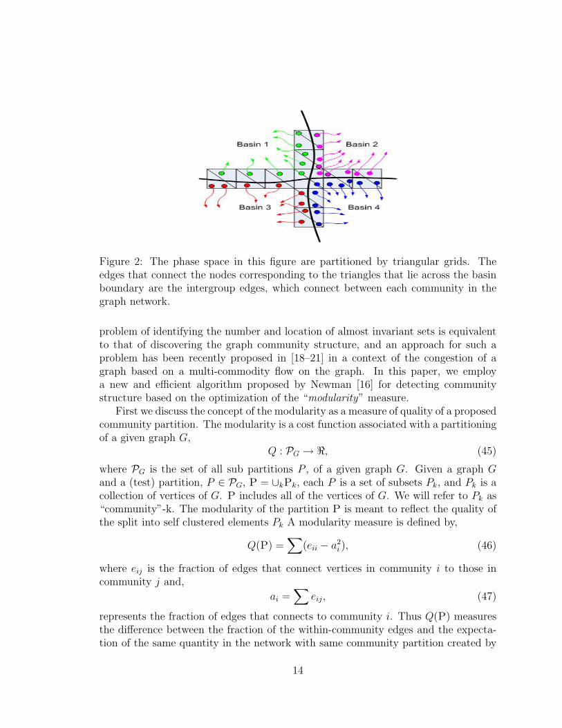
Figure 2: The phase space in this figure are partitioned by triangular grids. Theedges that connect the nodes corresponding to the triangles that lie across the basinboundary are the intergroup edges, which connect between each community in thegraph network.

problem of identifying the number and location of almost invariant sets is equivalentto that of discovering the graph community structure, and an approach for such aproblem has been recently proposed in [18–21] in a context of the congestion of agraph based on a multi-commodity flow on the graph. In this paper, we employa new and efficient algorithm proposed by Newman [16] for detecting communitystructure based on the optimization of the “modularity” measure.

First we discuss the concept of the modularity as a measure of quality of a proposedcommunity partition. The modularity is a cost function associated with a partitioningof a given graph G,

Q : PG → <, (45)

where PG is the set of all sub partitions P , of a given graph G. Given a graph Gand a (test) partition, P ∈ PG, P = ∪kPk, each P is a set of subsets Pk, and Pk is acollection of vertices of G. P includes all of the vertices of G. We will refer to Pk as“community”-k. The modularity of the partition P is meant to reflect the quality ofthe split into self clustered elements Pk A modularity measure is defined by,

Q(P) =∑

(eii − a2i ), (46)

where eij is the fraction of edges that connect vertices in community i to those incommunity j and,

ai =∑

eij, (47)

represents the fraction of edges that connects to community i. Thus Q(P) measuresthe difference between the fraction of the within-community edges and the expecta-tion of the same quantity in the network with same community partition created by

14

randomizing all connections between vertices. Therefore, Q(P) approaches 0 for arandomly connected network, and approaches Q(P) = 1, if the network has a strongcommunity structure. We may then optimize Q over all possible partitions to discoverthe best community structure

Q = maxP∈PG

Q(P). (48)

The true optimization is, however, very costly to implement in practice for verylarge networks as an NP problem. Clauset, Newman, and Moore [17] proposed anapproximate optimization algorithm based on greedy optimization. Suppose that wehave a graph with n vertices and m edges. This algorithm starts with each vertexbeing the only member of one of n communities. At each step, the change in Q(P)is computed after joining a pair of communities together and then choosing the pairthat gives the greatest increase or smallest decrease in Q(P). The algorithm stopsafter n − 1 such joins in which a single community is left. This algorithm thereforeruns in time O((m + n)n), or O(n2) on a sparse graph (n ∼ m). Note that usingmore sophisticated data structure as introduced in [17] can reduce a run time toO(n log2 n).

5 Results

5.1 Example 1

Consider the following differential equation as the first example:

dx

dt= −sin(2πx)cos(2πy)

dy

dt= cos(2πx)sin(2πy).

(49)

Now we may use the flow continuity equation (24) to numerically translate an initialdistribution in time to generate a synthetic movie data set I(x, y, t) representing atime evolving spatial density function. Figures 3(a) and 3(b) illustrate, respectively,the velocity field of this system and a given initial distribution function and Figures4(a)- 4(d) show a sequence of some images that are captured from our numericalsimulation of Eq. (24).

Based on this sequence of images we benchmark our approach by comparingthe approximated optical flow field extracted from the images by the regularizationmethod explained in Section 3 and the exact velocity field in Equation (49). First,let us investigate the sensitivity of the method with respect to variation of the pa-rameters α and β defined in Eq. (38). We quantitatively evaluate our result via the

15

(a) (b)

Figure 3: (a) The velocity field of the dynamical system (49). It can be seen thatthere consists of four basins separated by two nullclines x = 0.5 and y = 0.5. (b) Theinitial distribution at time t = 0.

(a) (b)

(c) (d)

Figure 4: A sequence of some images captured from the numerical simulation of theflow continuity equation (24) with the velocity field given by the ode (49).

16

Figure 5: A plot of the average angular error with respect to parameters α and β.The thick line represents the case of the smoothness constraint (37) where α = β.Although it is not conclusive that the smoothness constraint performs better than thediv-curl regularizer in this experiment, our experimental result demonstrates that theoptimal value is obtained when using the smoothness regularizer with α = β = 0.01

average angular error:

eang = arccos

(uexue + vexve + 1√

(u2ex + v2

ex + 1)(u2e + v2

e + 1)

), (50)

where (uex, vex) denotes the exact velocity field and (ueve) is the estimated velocity.Remark that we do not evaluate the error via a norm because in general we would lackinformation about the physical domain of the image plane and we can only recoverthe velocity field whose dynamics is in some representative of the true dynamicalsystem, perhaps in the sense of “almost conjugacy” [38]. Observe that for the imagessequence in this example the smoothness regularizer performs better than the div-curlregularizer at the experimentally optimal value β = 0.01, see Figure 5. Nevertheless,the div-curl regularizer produces better results for other value of β. To evaluate theresults qualitatively we lay the exact velocity field on the estimated velocity fields forα = β = 0.01 and α = 1, β = 0.01 as illustrated in Figure 6. We notice that the div-curl regularizer does not isotropically smooth the velocity field; hence we obtain only avelocity field where the motion take places meaning that there is a nontrivial supportof the dataset I(x, y, t). However, the smoothness regularizer produces the velocityfield throughout the whole image region, notwithstanding an absence of motion in

17

some regions, see also Figure 7. Moreover, we observe that the approximated velocityfield from the smoothness constraint maintains qualitative qualities of the exact ve-locity fields. Therefore, we want to investigate the topological structure of the result.Note that the phase portrait of the exact velocity field has four centers with eigen-values ±2πi at points (0.25, 0.25), (0.25, 0.75), (0.75, 0.25), (0.75, 0.75)and a saddlepoint with eigenvalue ±2π at the central point (0.5, 0.5) of the phase space. We com-pute the eigenvalue of the points in the image region corresponding to those pointsfor the velocity field approximated from the smoothness constraint with α = 0.01and plot the result in Figure 8. The result shows that we recover the saddle node atthe central point of the image region, but we obtain four spiral sinks at those pointsinstead of center nodes; however, the real part of their eigenvalues are much smallerthan the imaginary parts, which indicates that they are suggestive of a type of centernode.

(a) (b)

Figure 6: (a) Exact velocity field(in green arrows) and the optical flow field forα = 1, β = 0.01 shown in black arrows. (b) Exact velocity field(in green arrows) andthe optical flow field for α = β = 0.01 shown in black arrows.

Now let us discuss how to apply the optical flow result to approximate the Ulam-Galerkin approximation of the Frobenius-Perron transfer operator. We use the ap-proximated velocity field to advance randomly distributed points in time to generatea finite-rank approximation of the Frobenius-Perron operator as described in Sec-tion 2.3. Figures 9(b) and 9(a) show the Ulam-Galerkin matrix generated by theexact velocity fields in Eq. 49 and by the approximated optical flow field, respec-tively. As seen in Figure 3(a) there exist four basins and hence we may expect theUlam-Galerkin matrix to be diagonalizable to four diagonal blocks. To reveal this

18

(a) A plot of the velocity field u =−sin(2πx)cos(2πy) and its approximationfrom the image sequence

(b) A plot of velocity field v =cos(2πx)sin(2πy) and its approximationfrom the image sequence

Figure 7: Comparison between the exact and approximated velocity fields from theimage sequence using the smoothness parameter α = β = 0.01. The transparent solidlines illustrate the exact velocity field and the colored plots represent the approxima-tion.

correct block-diagonal form based on the modularity method we first partition thephase space into small triangles and index them to generate a graph network that rep-resents the transport between these triangles. Then we apply the modularity methodto discover the community structure of the graph network and use this structure toreorder the Ulam-Galerkin matrix. The results of the Ulam-Galerkin after reorderingare shown in Figures 10(a) and 10(b). They reveal to us the four basins and thesorted Ulam-Galerkin matrix generated by the exact velocity is now in the correctblock-diagonal form, whereas the sorted matrix generated by the optical flow is in the“almost” block-diagonal form due to the imperfection of the approximated velocityfield that causes the transport between the basins.

5.2 Example 2

Our next example is a simulation result obtained from a numerical solution of thecomplex Ginzburg-Landau eqaution(CGLE). Figures 11 illustrates the initial distri-bution and a time series of brightness patterns. By a careful observation one mayexpect that there exists two sinks in the phase space located by the arrows in Fig-ure 11(a). Since the analytic solution for this example is not priorly known, weascertain our result only qualitatively.

19

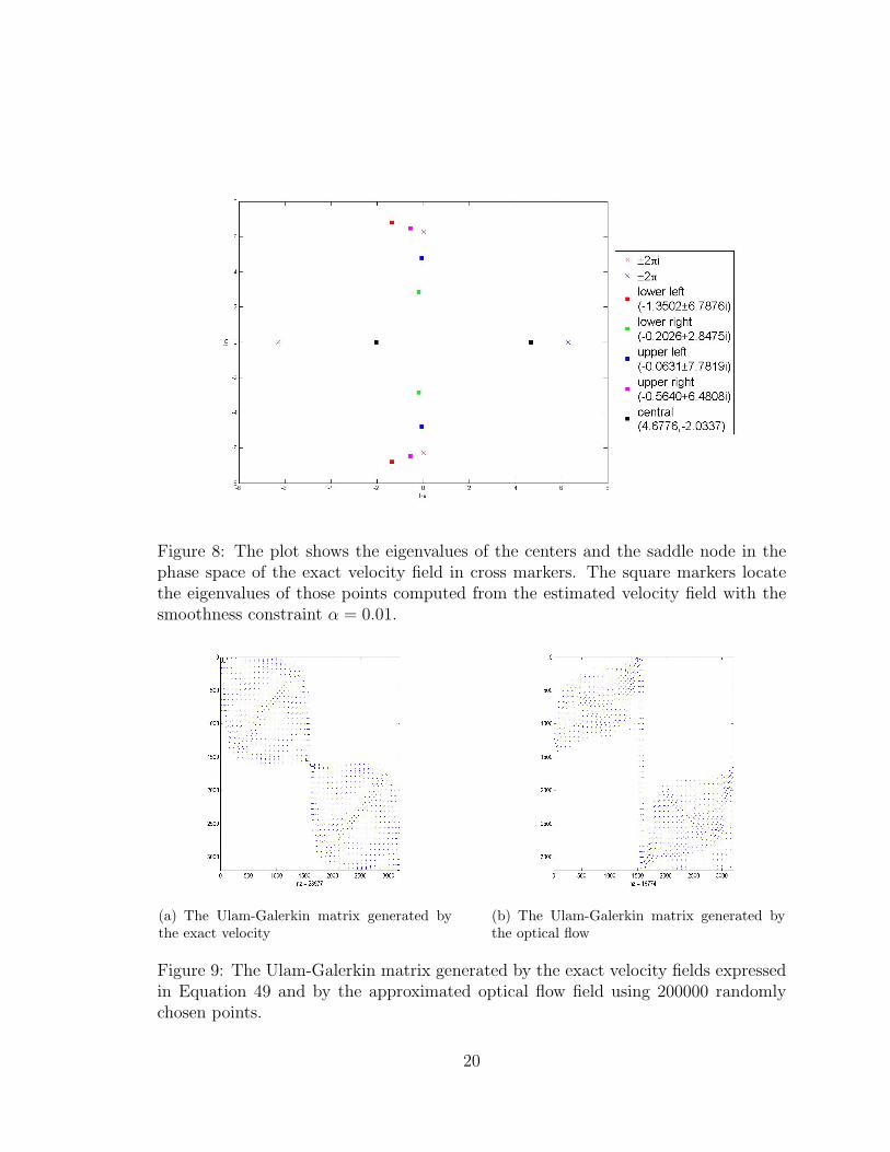
Figure 8: The plot shows the eigenvalues of the centers and the saddle node in thephase space of the exact velocity field in cross markers. The square markers locatethe eigenvalues of those points computed from the estimated velocity field with thesmoothness constraint α = 0.01.

(a) The Ulam-Galerkin matrix generated bythe exact velocity

(b) The Ulam-Galerkin matrix generated bythe optical flow

Figure 9: The Ulam-Galerkin matrix generated by the exact velocity fields expressedin Equation 49 and by the approximated optical flow field using 200000 randomlychosen points.

20

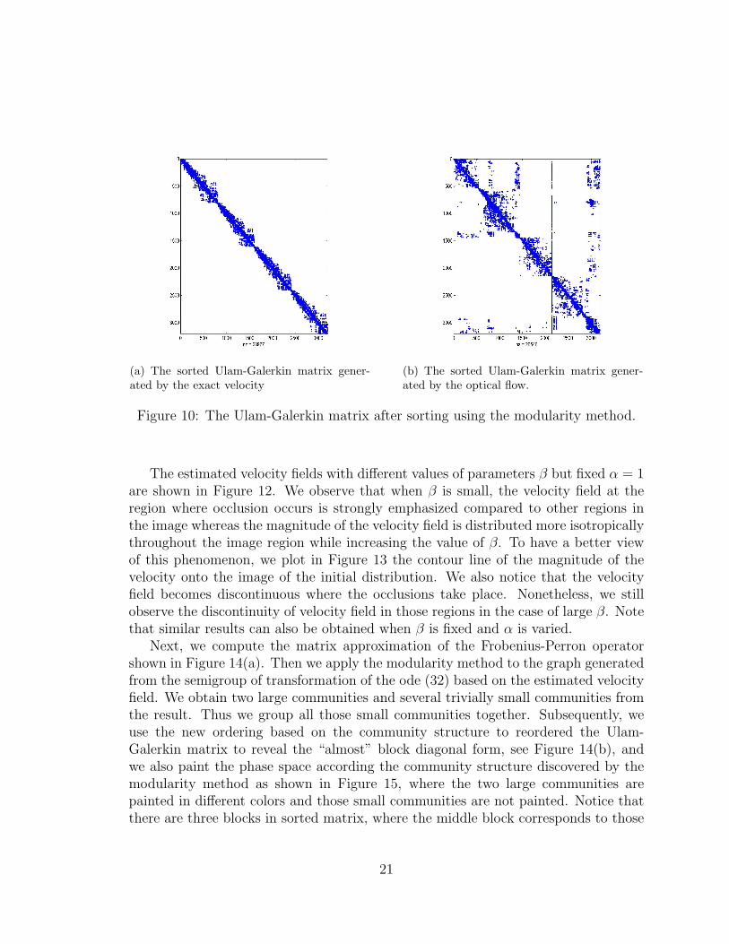
(a) The sorted Ulam-Galerkin matrix gener-ated by the exact velocity

(b) The sorted Ulam-Galerkin matrix gener-ated by the optical flow.

Figure 10: The Ulam-Galerkin matrix after sorting using the modularity method.

The estimated velocity fields with different values of parameters β but fixed α = 1are shown in Figure 12. We observe that when β is small, the velocity field at theregion where occlusion occurs is strongly emphasized compared to other regions inthe image whereas the magnitude of the velocity field is distributed more isotropicallythroughout the image region while increasing the value of β. To have a better viewof this phenomenon, we plot in Figure 13 the contour line of the magnitude of thevelocity onto the image of the initial distribution. We also notice that the velocityfield becomes discontinuous where the occlusions take place. Nonetheless, we stillobserve the discontinuity of velocity field in those regions in the case of large β. Notethat similar results can also be obtained when β is fixed and α is varied.

Next, we compute the matrix approximation of the Frobenius-Perron operatorshown in Figure 14(a). Then we apply the modularity method to the graph generatedfrom the semigroup of transformation of the ode (32) based on the estimated velocityfield. We obtain two large communities and several trivially small communities fromthe result. Thus we group all those small communities together. Subsequently, weuse the new ordering based on the community structure to reordered the Ulam-Galerkin matrix to reveal the “almost” block diagonal form, see Figure 14(b), andwe also paint the phase space according the community structure discovered by themodularity method as shown in Figure 15, where the two large communities arepainted in different colors and those small communities are not painted. Notice thatthere are three blocks in sorted matrix, where the middle block corresponds to those

21

(a) The initial distribution at frame 1. (b) The distribution at frame 40.

(c) The distribution at frame 80. (d) The distribution at frame 120.

Figure 11: A sequence of some images captured from the numerical simulation ofthe Complex Ginzburg-Landau equation. The arrows point at the sinks that can befound through a careful observation and as revealed by the Ulam-Galerkin matrixanalysis as in Figure 12- 15

22

of several small communities that we group them together and the other two blocksrepresent the two large communities.

6 Conclusion

In this paper, we have presented a computational method to construct the finite-rankapproximation of the Frobenius-Perron operator from successive images, which essen-tially requires a technique to recover velocity fields from image sequences. We haverelated this to the famous optical flow problem in various forms. Thus we present amathematical model to this problem and we demonstrate its validity based on thetheory of the infinitesimal generator of the Frobenius-Perron operator. We employa regularization method to solve an ill-posed problem to reconstruct the desired ve-locity field. Subsequently, we resort to the resultant velocity field to identify numberand location of the almost invariant sets using the graph modularity method. Wehave demonstrated our methods on synthetic data to demonstrate their usefulness tostudy a qualitative behavior, transport phenomena, and other ergodic properties ofmeasurable dynamical systems captured through image sequences.

7 Acknowledgements

We thank Aaron Clauset and Mark Newman for sharing their codes used in [16, 17]for the modularity method computations. We are grateful to the National ScienceFoundation of the USA for their support of both of the authors of this pro ject throughDMS-0404778.

23

(a) (b)

(c) (d)

(e) (f)

Figure 12: The velocity fields approximated from the div-curl regularization withvarious values of parameters α and β are plotted side by side with the correspondingmagnitude of the velocity fields.

24

(a) (b)

Figure 13: (a) For a small β at α = 1, the magnitude of the velocity field is moreemphasized at the region where occlusion occurs. In this region the velocity becomediscontinuous. (b) For a large β at α = 1, we observe that the velocity field isisotropically distributed throughout the image region. Nonetheless, the discontinuitycan still be observed at the region where occlusion take places.

(a) The unsorted Ulam-Galerkin matrix (b) The sorted Ulam-Galerkin matrix

Figure 14: The Ulam-Galerkin matrix before and after sorting. Notice that the“almost” block diagonal form is unveiled after sorting. The middle block correspondsto those of several small communities that we group them together. The other blocksrepresent the two large communities.

25

Figure 15: The phase space are partitioned into three regions corresponding twobasins of the sinks corresponding to two communities discovered by the modularitymethod and the region that an initial point does not converge to neither basins.

26

References

[1] E. Bollt, L. Billings, and I. Schwartz. A manifold independent approach tounderstanding transport in stochastic dynamical systems. Physica D, 173:153–177, 2002.

[2] L. Billings, E. Bollt, and I.B. Schwartz. Phase-space transport of stochastic chaosin population dynamics of virus spread. Physical Review Letters, 88(234101),2002.

[3] G. Froyland. Extracting dynamical behaviour via markov models. In Proc. Non-linear dynamics and statistics, pages 283–324, Boston, MA, 2001. Birkhauser.

[4] B.K.P. Horn and B.G. Schunck. Determining optical flow. Artificial intelligence,17:185–203, 1981.

[5] T.Corpetti, E.Memin, and P.Perez. Dense estimation of fluid flows. IEEE Trans.Pattern Anal. Mach. Intell., 24(3):365–380, 2002.

[6] T.Corpetti, D.Heitz, G. Arroyo, E.Memin, and A.Sant-Cruz. Fluid experimentalflow estimation based on an optical-flow scheme. Experiments in Fluids, 40:80–97, 2006.

[7] D. Bereziat and J.-P. Berroir. Motion estimation on meteorological infrared datausing a total brightness invariance hypothesis. Env. Mod. Soft., 15.

[8] J.J. Simpson and J.I. Gobat. Robust velocity estimates, stream functions, andsimulated lagrangian drifters from sequential spacecraft data. IEEE Transactionson Geoscience and Remote Sensing, 32(3).

[9] P. Heas, E. Memin, and N. Papadakis. Dense estimation of layer motions in theatmosphere. In Int. Conf. Pattern Recognition (ICPR’ 06), Hong-Kong, China,2006.

[10] S. Gutierrez and D.G. Long. Optical flow and scale-space theory applied to sea-ice motion estimation in antarctica. Geoscience and Remote Sensing Symposium,2003. IGARSS ’03. Proceedings., 4:2805– 2807, 2003.

[11] A. Suvichakorn and A. Tatnall. The application of cloud texture and mo-tion derived from geostationary satellite images in rain estimation - a study onmid-latitude depressions. In Geoscience and Remote Sensing Symposium, 2005.IGARSS apos;05. Proceedings, volume 3.

27

[12] R.P.Wildes, M.J.Ambabile, A.M. Lanzillotto, and T.S. Leu. Recovering estimateof fluid flow from image sequence data. Computer vision and Image understand-ing, 80:246–266, 2000.

[13] A.Lasota and M.C.Mackey. Chaos, fractals, and noise, Stochastic Aspects ofDynamics. Springer, New York, 2 edition, 1994.

[14] M.E.J. Newman and M. Girvan. Finding and evaluating community structurein networks. Phys. Rev. E, 69(026113), 2004.

[15] M.E.J. Newman and M. Girvan. Statistical Mechanics of Complex Networks.Springer, Berlin, 2004.

[16] M.E.J. Newman. Fast algorithm for detecting community structure in networks.Phys. Rev. E, 69(066133), 2004.

[17] Aaron Clauset, M. E. J. Newman, and Cristopher Moore. Finding communitystructure in very large networks. Phys. Rev. E, 70(066111), 2004.

[18] M. Dellnitz and O. Junge. On the approximation of complicated dynamicalbehavior. SIAM Journal on Numerical Analysis, 36(2):491–515, 1999.

[19] R. Preis and M. Dellnitz. Congestion and Almost Invariant Sets in Dynam-ical Systems. Proceedings of Symbolic and Numerical Scientific Computation(SNSC’01). Springer, 2003.

[20] R. Preis, M. Dellnitz, M. Hessel, Ch. Schtte, and E. Meerbach. Dominant pathsbetween almost invariant sets of dynamical systems. Preprint 154 of the DFGSchwerpunktprogramm 1095, 2004.

[21] K. Padberg, R. Preis, and M. Dellnitz. Integrating multilevel graph partitioningwith hierarchical set oriented methods for the analysis of dynamical systems.Preprint 152 of the DFG Schwerpunktprogramm 1095, 2004.

[22] S.M. Ulam. Problems in Modern Mathematics. Science Editions. Wiley, NewYork, 1970.

[23] T.Y. Li. Finite approximation for the Frobenius-Perron operator. a solution toUlam’s conjecture. J. Approx. Theory, 17(2):177–186, 1976.

[24] C. Chui, Q. Du, and T. Li. Error estimates of the Markov finite approximationof the Frobenius Perron operator. Nonlinear Analysis, 19(4):291–308, 1992.

28

[25] J. Ding and A. Zhou. The projection method for computing multidimensionalabsolutely continuous invariant measures. J. of Statistical Physics, 77(3/4):899–908, 1994.

[26] G. Froyland. Finite approximation of Sinai-Bowen-Ruelle measure for Anosovsystems in two dimension. Random Comput. Dynam., 3(4):251–263, 1995.

[27] F. Hunt. Approximating the invariant measures of randomly perturbed dissipa-tive maps. J. Math. Anal. Appl., 198(2):534–551, 1996.

[28] G. Froyland. Estimating Physical Invariant Measures and Space Averages ofDynamical Systems Indicators. PhD thesis, University of Western Australia,1996.

[29] B.D. Lucas and T. Kanade. An iterative image registration technique with anapplication to stereo vision. In IJCAI81, pages 674–679, 1981.

[30] J. Bign, G.H. Granlund, and J. Wiklund. Multidimensional orientation estima-tion with applications to texture analysis and optical flow. IEEE Transactionson Pattern Analysis and Machine Intelligence, 13(8):775–790, 1991.

[31] J.L.Barron, D.J.Fleet, and D.J.Beauchemin. Performance of optical flow tech-niques. Int. J. Comput. Vis., 12(1):43–77, 1994.

[32] B. Galvin, B. McCane, K. Novins, D. Mason, and S. Mills. Recovering motionfields: An evaluation of eight optical flow algorithms. In In Proc. the NinthBritish Machine Vision Conference (BMVC ’98), volume 1, pages 195–204, 1998.

[33] A.N.Tikhonov and V.Y.Arsenin. Solutions of ill-posed problem. Winston, Wash-ington, DC, 1977.

[34] D. Suter. Motion estimation and vector splines. pages 939–942, 1994.

[35] E.P.Simoncelli. Design of multi-dimensional derivative filters. IEEE Int. Conf.Image Processing, 1:790–793, 1994.

[36] M.W.Hirchh and S.Smale. Differential Eqations, Dynamical Systems, and LinearAlgebra. Academic Press, Orlando, 1974.

[37] J.P. Bagrow and E. M. Bollt. A local method for detecting communities. Phys.Rev. E, 72(046108), 2005.

[38] Joseph D. Skufca and Erik M. Bollt. Mostly conjugate: Relating dynamicalsystems — beyond homeomorphism. submitted to SIAM Journal on AppliedDynamical Systems, 2006.

29