Embed Size (px)
Citation preview

Solar Power Plant with Energy Storage Arya, Hsieh, Sehgal, Yin
Professor Leonard A. FabianoProfessor Raymond J. GorteDepartment of Chemical & Biomolecular EngineeringUniversity of Pennsylvania, PA 19104
Monday, April 14, 2008
Professor Fabiano and Professor Gorte,
With the completion of our zero-emissions solar power plant design, we have chosen to locate the plant in the Mexican border region of Arizona where the annual average solar flux is between 7.0 and 8.2 kWh/m2/day, the highest in the area. Out of the power plant size of 10, 50 and 100 MW, we recommend the 50 MW. 50 MW of electricity would be produced from 311.97 MW of direct solar flux, indicating a solar-to-electricity efficiency of 17%.
One of the key design issues in a zero emissions solar plant is the method and hour of storage. Our thermal energy storage utilizes a two tank direct system using Hitec molten salt as the heat transfer fluid. In addition, our economic analysis indicates that it is not profitable to store enough energy for the plant to run on a 24/7 basis due to the significant increase in solar field size. We have therefore chosen to only operate during the day time hours with three hours of storage for load leveling and for selling electricity in the nighttime.
Our total capital investment is $270,345,499 with a levelized electricity cost of $0.15/kWh compared with conventional fuel levelized cost of $0.11. Once the plant is in operation our annual power generation cost is $69,818,196. Finally, the NPV of the project is (170 MM). Therefore, we will require a governmental subsidy to be competitive.
Sincerely,
______________________________Vishrut Arya
______________________________Alan Hsieh
______________________________Ray Sehgal
______________________________Li Yin

Solar Power Plant with Energy Storage Arya, Hsieh, Sehgal, Yin
Solar Power Plant With Energy Storage
Authors:
Vishrut Arya
Alan Hsieh
Ray Sehgal
Li Yin
Faculty Advisor:
Raymond Gorte
Monday, April 14, 2008
Department of Chemical & Biomolecular Engineering
University of Pennsylvania

Solar Power Plant with Energy Storage Arya, Hsieh, Sehgal, Yin
Abstract 3
INTRODUCTION.................................................................................................................................................. 3
AVAILABLE TECHNOLOGIES................................................................................................................................. 3
Concentrated Solar Power..................................................................................................................................3Energy Storage...................................................................................................................................................3HTF Selection......................................................................................................................................................3
DESIGN............................................................................................................................................................... 3
Process Flow Diagram Energy Balances..............................................................................................................3Process Description.............................................................................................................................................3
UNIT DESCRIPTIONS AND SPECIFICATION SHEETS................................................................................................3
Unit Descriptions................................................................................................................................................3Specification Sheets............................................................................................................................................3
EQUIPMENT COST SUMMARY............................................................................................................................. 3
FIXED CAPITAL INVESTMENT SUMMARY............................................................................................................. 3
Solar Field Components......................................................................................................................................3Heat Transfer Fluid.............................................................................................................................................3Storage Tanks.....................................................................................................................................................3Pumps, Heat Exchangers, and Turbine...............................................................................................................3
OTHER IMPORTANT CONSIDERATIONS................................................................................................................ 3
Environmental Problems and Safety & Health Concerns....................................................................................3Additional Equipment & Costs............................................................................................................................3Renewable Energy Government Incentives.........................................................................................................3
OPERATING COST & ECONOMIC ANALYSIS.......................................................................................................... 3
Utilities...............................................................................................................................................................3
ECONOMIC ANALYSIS.......................................................................................................................................... 3
Market Competitive Analysis..............................................................................................................................3Comparable Costs...............................................................................................................................................3Levelized Electricity Cost (LEC)............................................................................................................................3Cash Flow & Profitability Measures....................................................................................................................3
SENSITIVITY ANALYSIS......................................................................................................................................... 3
Sample Sensitivity Analysis Around Base Case....................................................................................................3Summary Data....................................................................................................................................................3Discussion of Summary Data..............................................................................................................................3Scenario Analysis................................................................................................................................................3Long Term Viability.............................................................................................................................................3Economic Sensitivity Summary...........................................................................................................................3
CONCLUSION & RECOMMENDATIONS................................................................................................................. 3
Conclusion..........................................................................................................................................................3Recommendations..............................................................................................................................................3
ACKNOWLEDGEMENTS....................................................................................................................................... 3
BIBLIOGRAPHY.................................................................................................................................................... 3

Solar Power Plant with Energy Storage Arya, Hsieh, Sehgal, Yin

Solar Power Plant with Energy Storage Arya, Hsieh, Sehgal, Yin
Abstract
The following report contains a parabolic solar trough power plant design located on the
Mexican border of Arizona, United States. Three different power plant scales of 10 MW, 50
MW, and 100 MW were assessed and compared.
An economic analysis of the attractiveness of a solar trough power plant at various scales
and specifications suggest that a 50 MW plant with 3 hours of storage of energy storage is
optimal. For these specifications, the solar field consists of 2080 Solar Collection Assemblies
from ENEA, a new solar trough design that takes advantage of the use of molten salt as the Heat
Transfer Fluid (HTF). The field achieves a heat duty of 430 MW. Hitec is used as the HTF and
exits the field at 400°C. It is used in a Rankine cycle that generates steam at 390°C, ultimately
achieving a solar-to-out efficiency of 17%. Part of the hot HTF stream siphons into the thermal
energy storage (TES) system, which consists of a two-tank direct storage of HTF system,
utilizing a total of 6 1-million-gallon steel tanks with appropriate insulation to generate the 3
hours of energy as specified above.
The plant requires a total capital investment of $270MM and achieves a levelized cost of
$0.15/kWh. Assuming a discount rate of 15%, NPV is (170 MM). A subsidy of 15 cents per
kWh is needed for the plant to achieve a NPV of zero.

Solar Power Plant with Energy Storage Arya, Hsieh, Sehgal, Yin
Introduction
Recognizing that the world’s fossil-fuel supply is limited and CO2 emissions are
beginning to have visible negative impact on the Earth’s ecosystem, renewable energy sources,
such as solar power, are becoming increasingly attractive and necessary. However the
challenges of capturing and storing insolation are both financially and technically considerable.
Therefore, the following report presents a design of a solar thermal power plant, with an energy
storage system to provide power during low insolation periods. The problem statement outlining
the parameters of the design is located in the Appendix page 54.
Typical solar power plants have a back-up power generation system to provide
continuous operation during low insolation periods. A zero-emissions plant must forgo this
source of energy generation, and thus must use some sort of energy storage. In the design
presented, energy storage was designed around storage of hot HTF, the selection of which is
outlined in the Appendix on page 53 and justified in the report on page 73. This thermal energy
storage system presents the primary design challenge that faced the design team.
The plant is located in Arizona, and designed at 10, 50, and 100 MW scales. There are
virtually an infinite number of combinations of heat transfer fluid, operating temperatures, fluid
flow rates, and field sizes. Therefore, a thorough sensitivity analysis was performed in order to
find local and absolute profitability minima over the multivariate space of these choices.
Finally, it was determined that solar energy currently remains net present value (NPV)
negative due to tremendous capital costs and meager price expectations. As such, conditions for
project viability, including necessary subsidies, cost reduction on major components, and

Solar Power Plant with Energy Storage Arya, Hsieh, Sehgal, Yin
combinations of these factors with external legal and market factors, were used to develop
sensitivity analyses of the system as a whole and to generated recommendations
Solar Power Plant with Energy Storage Arya, Hsieh, Sehgal, Yin
Available Technologies
Concentrated Solar Power
The design employs parabolic trough technology mainly due to the fact that it is a proven
technology, which has seen long periods of real world operation. Specifically, as mentioned on
the Appendix page 2, the dish system is less viable on larger scales and both tower and CLFR
technology, while suitable for large scale, are newer and less developed technologies. Given the
successful operation of nine commercial-scale parabolic trough solar power plants (SEGS I –
IX), which operate at outputs between 14 and 80 megawatts (MW), there is sufficient literature
surrounding the technology with regards to materials as well as finances. Data on parabolic
trough power plants in operation and under development in the United States are provided in
Appendix page 48.
Energy Storage
The TES system was selected over other energy storage options due to avoidance of
energy conversion losses. Specifically, a two-tank direct TES system was designed due to
shared piping and HTF with the field and simplicity of model. These systems have been tested
in the field, and employed in small-scale plants. For further information see Appendix page 6.
HTF Selection
Hitec molten salt was selected over other molten salt candidates, which the design team
evaluated to be both feasible and superior to existing synthetic oil designs based on Therminol
Solar Power Plant with Energy Storage Arya, Hsieh, Sehgal, Yin
VP-1. Furthermore, literature exists discussing the relative environmental benevolence and non-
corrosiveness of nitrate based molten salts. For more information about HTF selection and
properties of the various fluids, please see the economic section on page 73, and the HTF
selection in the Appendix on page 53.

Solar Power Plant with Energy Storage Arya, Hsieh, Sehgal, Yin
Design
As outlined prior, the project consists of a power plant design as well as an energy
storage design. The power plant forms the basis of the design, depending on the heat transfer
and efficiency assumptions for the power generation and solar field sides of the plant. The
energy storage design, however, feeds back into power plant design as it demands additional
solar field area be added on to sustain the additional field heat required at any given scaling.
Therefore, the basic power plant was designed first, at three scales, with heat storage as a “bolt-
on” option for any given hours of energy storage.
Figure 1: Overall Plant Schematic
A diagram of the overall plant schematic can be seen above in Figure 1. The chief
components of the overall solar power plant design can be broadly divided into three parts: the
solar field, the TES system (seen as the Cold and Hot Storage tanks), and the power generation
cycle (shown as turbine and heat exchanger).
Solar Power Plant with Energy Storage Arya, Hsieh, Sehgal, Yin
Process Flow Diagram Energy Balances
All diagrams and figures are generated for the base case of a 10 MW plant with 3 hours
of TES. This case is constant throughout the rest of the design, process description, unit
descriptions and specification sheet sections. The treatment of different design cases is
performed in the economic analysis, beginning on page 60.
Process Flow Diagram
Figure 2: Mass Flowrate Diagram for 10MW Plant with 3 Hour Storage
The above diagram shows the mass flow rates in the Rankine cycles along with the
pressure at each state. The diagram to the left of the HTF HX represents the solar field input to
the power generation block, the power block output to the solar field, as well as the side streams
that are siphoned off or added to the field streams due to the TES systems.

Solar Power Plant with Energy Storage Arya, Hsieh, Sehgal, Yin
Figure 3: Solar Field Quadrant Massflow Diagram
Figure 3 shows an example solar field quadrant with the thermodynamic states of each of
the stream coming into and out of the quadrant as well as the temperature and pressure changes
that occur over the length of a single loop. These changes are non-additive as the system will
run in parallel over the quadrant. On the other hand the mass flow through the loops, 3.82 kg/s is
additive and gives the final header mass flow as the sum over all of the loops as 99.33 kg/s.

Solar Power Plant with Energy Storage Arya, Hsieh, Sehgal, Yin
Energy Balances & Utility Requirements
Energy Balances
Figure 4: Daytime Operation Energy Balance
The overall balance is shown in Figure 4 above. The balance comes out to a 0.19 MW
deficit. This value is well within the errors of the correlations used in determining the overall
heat losses.

Solar Power Plant with Energy Storage Arya, Hsieh, Sehgal, Yin
Figure 5: Low Insolation Energy Balance
Figure 5 above illustrates the energy balance during low insolation operation. This
balance has no inputs, however the overall heat loss is negligible for the TES tanks so that it can
be effectively ignored during operation, and the heat loss in the field elements is accounted for in
the freeze protection low insolation operation mode. For a more detailed description of this heat
loss analysis see page 18 of the Process Description section.

Solar Power Plant with Energy Storage Arya, Hsieh, Sehgal, Yin
Table 1: Electricity and water utility requirements
The utility requirements for the overall process include electricity to power pumps,
cooling water for the condenser and wash water for the mirrors. As can be seen from Table 1, the
majority of the electricity utility comes from the pump in the turbine facility. All of the
electricity utility requirements are satisfied by the overall process and have been accounted for
by increasing necessary turbine shaft work which consequently demanded more solar collection
loops.
Field & TES Pumps 84 kWOvernight/Morning Pumping 7 kWRankine Cycle Pump 248 kW
Total 338 kW
Condenser Cooling Water 289,597,214 L/yearTotal Mirror Wash Water 4,650,655 L/year
Water
Utility RequirementsElectricity

Solar Power Plant with Energy Storage Arya, Hsieh, Sehgal, Yin
Process Description
Daytime Operation
Overview
The overall process can be broken down into three sections as displayed in Figure 2: the
solar field, the thermal energy storage (TES) system, and the turbine facility where the electricity
is produced. The solar field captures insolation via parabolic mirrors that concentrate the sun’s
rays onto a pipe (heat collection element, HCE) running through the parabola’s focus. The
captured energy increases the teat transfer fluid’s (HTF) temperature which leaves the field at
approximately 400 °C where it enters the two remaining sections of the overall process, the TES
system and the turbine facility. Large underground storage tanks comprise the majority of the
TES system and these tanks store a portion of the flow rate of the HTF leaving the field. The
remaining HTF bypasses the TES system and enters the turbine facility where it heats water from
approximately 135 °C to 390 °C via a shell and tube heat exchanger. After leaving the heat
exchanger the HTF is sent back to the solar field where it will once again undergo heating. The
water vaporized and superheated in the heat exchanger circulates in the turbine facility where it
is expanded to power the steam turbine which outputs the plant’s electricity. After undergoing
condensation and compression, the water again returns to the heat exchanger to continue the
cycle.

Solar Power Plant with Energy Storage Arya, Hsieh, Sehgal, Yin
Detailed Description
Figure 6: Solar Field and TES system Block Diagram
The HTF entering the solar field is a combination of two streams, a 292 kg/s stream at
260 °C from the output of the main heat exchanger and a 105 kg/s stream at 260 °C from the
cold storage tank. The combined input stream is split evenly into four 99 kg/s cold headers that
each supplies one quadrant of the solar field, this process is shown above in Figure 6. Each
header is made of stainless steel 304, has a 0.70 m inner diameter and is insulated with five 2”
thick Thermal Ceramics Superwool Blanket®. The cold header feeds 26 loops in parallel per
quadrant with HTF at 260 °C. Each loop consists of 4 SCAs which are 100 m in length. The
loops output hot HTF at 400 °C into the hot header located the quadrant in which the loops are
situated. The four hot quadrant headers combine and leave the field and before reaching the

Solar Power Plant with Energy Storage Arya, Hsieh, Sehgal, Yin
turbine facility, 105 kg/s is siphoned into the hot storage tank. The balance, 292 kg/s, provides
the load for the heat exchanger to generate steam for the power generation cycle.
The power generation side is a standard Rankine cycle using 26 kg/s of 390°C steam at
8000 kPa. This steam expands through a steam turbine and produces enough shaft work to sell
10 MW and power the facility itself. The steam exits the turbine at 135 °C and 300 kPa and
flows to a condenser where it condenses to a saturated liquid at 135 °C and 200 kPa. This low-
pressure water is then pumped back to 8100 kPa and 135 °C, and is sent back through the heat
exchanger.
Low Insolation and Freeze Protection Operation
Overview
There are two operational modes for low insolation: low insolation power generation, and
“freeze protection” operation. Low insolation power generation involves the utilization of the
TES system to provide the hot HTF necessary to generate power during periods when insolation
levels are too low for the solar field to be effective. This operational mode can be utilized to both
“load level” temporary fluctuations in insolation and to generate power at night.
Additionally because of the high freezing point of the molten salt HTF (142 °C),
precautions must be taken to prevent HTF from freezing during the night. To ensure all the HTF
remains molten, HTF is circulated from areas of higher heat loss to areas of lower heat loss at
regular intervals through the night.
Detailed Description
During load-leveling operation, insolation is below that during daytime operation though
it is still sufficient to render the field useful and consequently a hot HTF mass flow from the field
can be utilized. However, lower insolation reduces the flow rate of hot HTF mass from the

Solar Power Plant with Energy Storage Arya, Hsieh, Sehgal, Yin
daytime operation flow rate of 226 kg/s. The remaining required flow is drawn from the hot TES
tanks, ensuring that temporary fluctuations in insolation do not affect the generation of the full
10 MW load.
During overnight power generation, insolation is insufficient to provide power to the
steam turbine and consequently no hot HTF flows from the field to the steam generating heat
exchanger. Instead, the hot TES tank supplies all of the HTF utilized in the steam generating heat
exchanger. A mass flow of 226 kg/s (the same as is necessary for daytime power generation) is
drawn from the hot TES tank and flows through the steam generation heat exchanger and into the
cold TES tank.
Unlike load leveling or overnight power generation, the freeze protection operation does
not involve the production of power. Instead, freeze protection operation ensures the mass-
weighted average temperature of all field elements, after 16 hours of inadequate to no insolation,
is no less than the daytime operation solar field input temperature of 260 °C and thereby removes
the need to reheat upon daytime operation; this also prevents the freezing of the solar field. The
analysis revolves around temperature drops per time in each of the field elements (HCEs, hot
header and cold header); see pages 23 and 27 for detailed calculations. From this temperature
drop, the temperature in the HCEs, hot header, and cold header were calculated after 8 hours of
overnight conditions. After the HTF sits in the field for 8 hours, the pumps are run backwards
(sending the hot header fluid into the HCEs, the HCE fluid into the cold header, and the cold
header fluid back into the hot header, the opposite of flow in daytime operation). We assume
there is negligible heat loss during this transfer period of 0.8 hours, or 48 minutes. The 8 hour
temperature drops are applied again and are utilized to yield the temperature in all of the field

Solar Power Plant with Energy Storage Arya, Hsieh, Sehgal, Yin
elements after 16 hours. At this point, the system has cycled through an entire night and is set to
resume daytime operation.
Solar Power Plant with Energy Storage Arya, Hsieh, Sehgal, Yin
Unit Descriptions and Specification Sheets
Unit Descriptions
Solar Collection System
Solar Collector Structure
Figure 7: Solar Collector Structure
The solar collector structure provides the support structure for the reflectors and heat
collection element. Composed of Cor-Ten steel and zinc-coated carbon steel, the structure
includes torque tubes to sustain wind loads up to 33 m/s and precise reflector support arms. Each
solar collector structure is produced in modules of approximately 12 m in length. An example of
a solar collector structure can be seen in Figure 7

Solar Power Plant with Energy Storage Arya, Hsieh, Sehgal, Yin
Reflectors
Figure 8: Solar Reflector Cross Section
The reflectors form the parabolic nature of the solar collection system and focus most of
the received insolation onto the heat collection element. Four rectangular reflectors makeup the
width of the trough and consequently each has less curvature than the overall parabola.
Currently, all reflectors used in parabolic trough applications are produced by the German
company Flabeg. Reflectors are made of a glass substrate with a silver reflective layer, and are
protected by a titanium dioxide interference layer on the glass surface and a copper cladding with
varnish on the back of the silver surface.

Solar Power Plant with Energy Storage Arya, Hsieh, Sehgal, Yin
Heat Collection Element
Figure 9: HCE Diagram
The heat collection element (HCE) is located at the reflector parabola’s focus, a distance
of 1.8 m from the vertex. The HCE consists of two concentric pipes separated by an evacuated
annulus to eliminate conductive and convective heat loss. The 70 mm diameter inner pipe is
constructed from stainless steel and is coated with black cement and ceramic based coating
engineered to provide low infrared heat emission while maintaining high absorbance of
insolation. The outer pipe is made of glass and has an inner diameter of 112 mm.

Solar Power Plant with Energy Storage Arya, Hsieh, Sehgal, Yin
Pylons and Foundation
Figure 10: SCA Pylon and Foundation
As pictured above in Figure 10, the pylons, which support the SCA, are mounted on a concrete
foundation. The pylons are the major supporting element of the SCA and as such must be able to
withstand the expected wind loads on the SCAs.
Drive
Each SCA uses a hydraulic drive to track the sun to ensure that the maximum amount of
solar radiation is focused on the HCE. This drive is not only used to track the sun, but also for
stabilization of the SCA under wind loads.
Controls
Each SCA has its own local controller which uses controls the operation of the trough,
and monitors the operational parameters to ensure that the SCA is operating within the specified
operational parameters. This local controller is responsible for the tracking of the sun by the
individual assembly.

Solar Power Plant with Energy Storage Arya, Hsieh, Sehgal, Yin
Collector Interconnect
In order to properly track the sun each SCA moves independently from the adjacent
collectors. To allow this independent motion, ball joints are used to ensure the proper alignment
of the individual SCAs.
Solar Collector Module
A solar collector module (module) is made up of the solar collector structure, reflectors
and HCE. It is 12 m in length and has an aperture width of 5.76 m. Each module contains 28
rectangular reflectors in four horizontal rows and seven vertical columns; three four-meter long
HCEs, and a 12 m long support structure.
Solar Collector Assembly
Figure 11: Diagram of a SCA with modules and mirrors shown (note: not to scale)
A solar collector assembly (SCA) is an assembly of eight modules in series to yield an
overall solar collection area of 545 m2. In the above Figure 11, the modules are the tall and thin
rectangles, and the mirrors are bordered by the thing grey lines. The length of a SCA is roughly
100 m as there is some spacing between modules and the entire SCA is supported with 13 pylons
attached to grounded concrete piers.
Solar Power Plant with Energy Storage Arya, Hsieh, Sehgal, Yin
Solar Collection Loop
Figure 12: Four SCA Loop Schematic
A solar collection loop refers to four SCAs connected in series. The first SCA in the loop
receives HTF from the cold header and the last SCA discharges HTF into the hot header. A
control valve keeps flow rate constant over every loop in the field. The above Figure 12 shows
each of these elements, their connection to the hot and cold header, and the overall layout of a
single loop.
Associated Calculations
The heat loss in the HCEs was determined based on test results of SEGS LS-2 Solar
Collector and resulted in a value of 60 W/m2 during average overnight conditions. Utilizing a
similar mathematical approach as seen in the header heat loss analysis, the HCE heat loss
contributed to a 62 K temperature drop in the HCE over eight hours. To see a more detailed
description of the low insolation operation, please see the Low Insolation and Freeze Protection
Operation section on page 18.

Solar Power Plant with Energy Storage Arya, Hsieh, Sehgal, Yin
Hot and Cold Headers
Figure 13: Hot & Cold Header Cross Section
As can be seen from Figure 6, the hot and cold headers are identical in all quadrants and
run 432 m in each. The headers consist of a 0.4 m inner diameter stainless steel pipe which has a
wall thickness of 1 cm. The pipe is insulated by five 2” Thermal Ceramics Superwool Blanket,
and is shielded against the elements by a simple corrugated steel duct.
Associated Calculations
The pressure drop across the entire header length was calculated using the same
equations and assumptions as were used in the loop pressure drop calculation.
The heat loss over the header was calculated using equations on page 13 of the Appendix.
To calculate the convection heat transfer coefficient we assumed an average wind speed based on
meteorological data. Additionally the overnight heat losses were calculated both for the losses
through the field HCEs and from conduction and convection through the headers. The header
heat losses are calculated using the same framework as above, but with a different ambient

Solar Power Plant with Energy Storage Arya, Hsieh, Sehgal, Yin
temperature. This heat loss was combined with knowledge of heat capacity and HTF header
mass to calculate the temperature drop of 8 K for the hot header and 5 K for the cold header over
eight hours. To see a more detailed description of the low insolation operation, please see the
Low Insolation and Freeze Protection Operation section on page 18.
Pumps
Four 17 kW centrifugal pumps transport HTF throughout their respective quadrants and a
fifth pump transports HTF to and from the TES tanks. These pumps are used to overcome the
pressure drop along the cold header, the pressure drop across a loop, the pressure drop across the
hot header, the pressure drop across the heat exchanger and the pressure drop between the TES
tanks and turbine facility.
Table 2: Field pump information
Associated Calculations
The calculation of the pressure drops across each of these elements is described in their
unit description. The brake horsepower (HP) is calculated using equations in the Appendix on
page 15.
HCELine Pressure Drop 49,947 PaControl Valve Pressure Drop 172,369 PaTotal Pressure Drop/Loop 222,317 Pa
HeaderMass Flow 96 kg/sLine Pressure Drop 3,565 Pa
HTF Total Pressure Drop/Quadrant 229,447 Pa2 atm
Pump PowerIsentropic Pump Power 13 kWPump Efficiency 0.80 %Actual Pump Power 17 kW
Field Pump Summary

Solar Power Plant with Energy Storage Arya, Hsieh, Sehgal, Yin
TES System
HTF Storage Tanks
One hot and one cold storage tank make up the bulk of the thermal energy storage system
and in total are designed to hold 1,848 m3 of HTF. The tanks are made of concrete with a
stainless steel liner which is able to withstand the temperature and corrosiveness of the HTF. The
concrete is insulated by five 2” Thermal Ceramics Superwool Blanket.
Associated Calculations
The heat loss from the hot and cold tanks were calculated using equations in the
Appendix on page 16, and was found to be 182 kW and 115 kW for the hot and cold tanks,
respectively. This heat loss will lead to a 2 K temperature decrease in the cold tank per 24 hours,
and a temperature drop of 0.6 K in the hot tank per 24 hours. Both of these values are low
enough to be counted as having negligible effect on the operation of the system.
TES Pumps
One field pump is capable of handling the TES pumping requirements and the pump
transports HTF to the major header (either hot or cold depending on which tank it’s coming
from) where it joins the rest of the header flow. These pumps are also used to pump the hot HTF
across the heat exchanger during low insolation power generation. The calculations for the
storage pumps use the same equations as the field pumps above (equations on page 15 of the
Appendix) and are specified to satisfy the low insolation power generation requirements.

Solar Power Plant with Energy Storage Arya, Hsieh, Sehgal, Yin
Rankine Cycle
Heat Exchanger
Table 3: Heat exchanger summary information
Associated Calculations
Using a literature value for the heat transfer coefficient for steam generation, U = 2000
kJ/kg-K, and a given ΔTLM for steam generation; we calculated the area of the exchangers.
Because this heat exchanger is being used to generate steam, the heat exchanger was broken up
into three segments, a pre-heater, a boiler, and a super heater. Each is assumed to have one third
of the overall area calculated using equations in the Appendix on page 14.
Temperature of Cooling Water In 305 KOverall Heat Transfer Coefficient (U) 2,000 W/(m2-K)Heat Duty 58,840,727 W∆TLM 70 K
Heat Exchange Area 422 m2
4,545 ft2
Heat Exchanger Summary

Solar Power Plant with Energy Storage Arya, Hsieh, Sehgal, Yin
Steam Turbine
Table 4: Steam turbine summary information
Associated Calculations
The steam turbine expands 26 kg/s of 8000 kPa superheated steam at 390 °C to saturated
steam at 300 kPa and 135 °C. This generates 11.45 MW of shaft work which is then used in a
generator to create electricity. See Appendix page 17 for a step by step calculation of the steam
mass flow rate.
SteamIn
Temperature 390 °CPressure 8000 kPa
OutTemperature 133 °CPressure 300 kPa
Shaft Work 11.25 MWIsentropic Efficiency 80 %
Steam Turbine Summary

Solar Power Plant with Energy Storage Arya, Hsieh, Sehgal, Yin
Condenser
Table 5: Condenser summary information
Compressor
Table 6: Rankine cycle pump summary information
The compressor in the power generation cycle serves to compress 26 kg/s saturated liquid
from 200 kPa to 8100 kPa. It has a brake power requirement of 258 kW.
ΔTLM 93 KHeat Duty 51,993,372 WOverall Heat Transfer Coefficient (U) 5705 W/(m2-K)Heat Transfer Area 98 m2
Length of Tubes (L) 6.10 m
In OutTemperature (K) 305 322m (kg/s) 746 746
Vapor LiquidTemperature (K) 407 407m (kg/s) 24 24ΔHvap (J/kg) 2163900 2163900
Tube Data: Cooling Water
Shell Data: Steam
Condenser SummaryGeneral Design Data
SteamTemperature In 135 °CMass Flow 26 kg/sΔP Increase 8,000 kPa
Isentropic Pump Power 206 kWPump Efficiency 80 %Actual Pump Work 258 kW
Rankine Cycle Pump

Solar Power Plant with Energy Storage Arya, Hsieh, Sehgal, Yin
Specification Sheets
Table 7: Rankine cycle steam turbine summary information
Item type Non-CondensingMaterial Carbon SteelPower output 11,454 kWSteam gauge pressure 8,000 kPa GaugeSpeed 3,600 RPMTotal weight 64,600 kg
Cost per Turbine 1,002,235$ $/turbine
Design Data
Summary Costs
Rankine Cycle Steam Turbine

Solar Power Plant with Energy Storage Arya, Hsieh, Sehgal, Yin
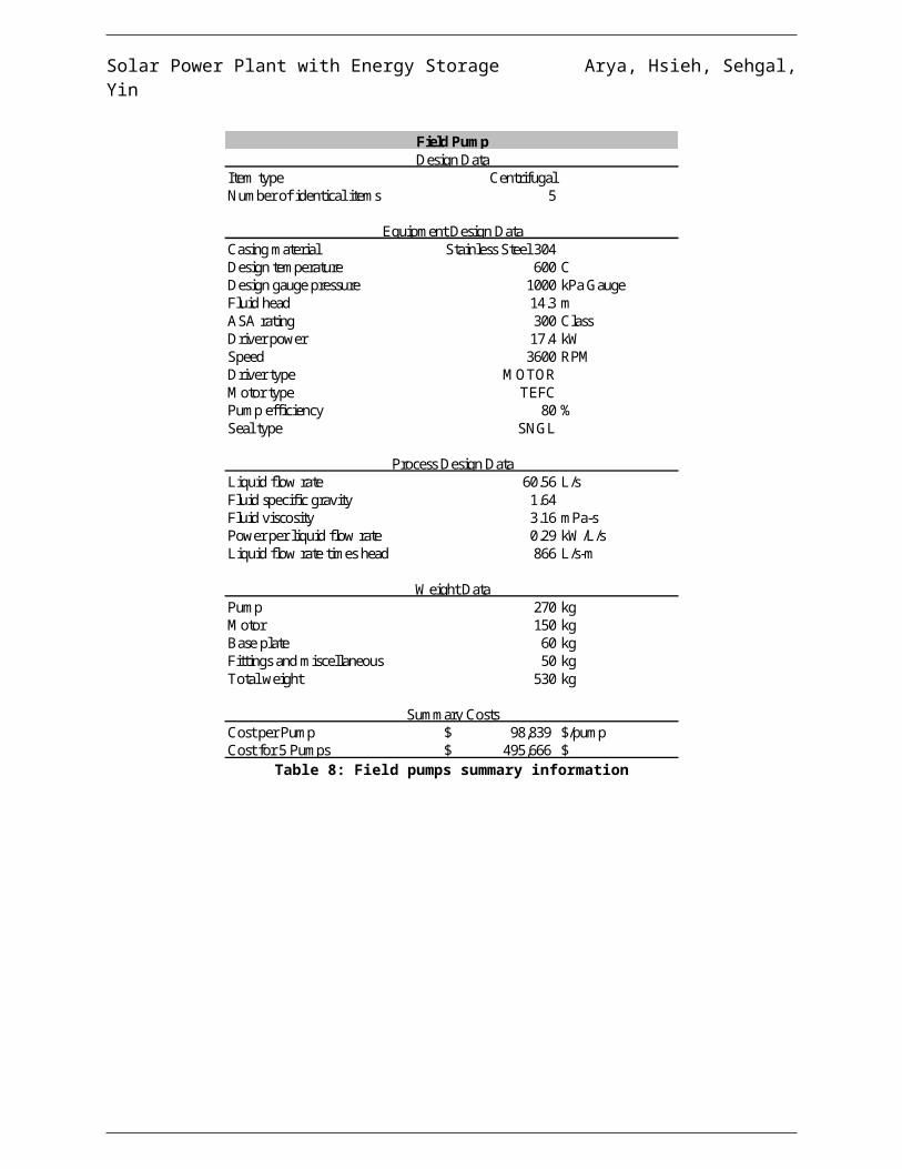
Table 8: Field pumps summary information
Item type CentrifugalNumber of identical items 5
Casing material Stainless Steel 304Design temperature 600 CDesign gauge pressure 1000 kPa GaugeFluid head 14.3 mASA rating 300 ClassDriver power 17.4 kWSpeed 3600 RPMDriver type MOTORMotor type TEFCPump efficiency 80 %Seal type SNGL
Liquid flow rate 60.56 L/sFluid specific gravity 1.64Fluid viscosity 3.16 mPa-sPower per liquid flow rate 0.29 kW/L/sLiquid flow rate times head 866 L/s-m
Pump 270 kgMotor 150 kgBase plate 60 kgFittings and miscellaneous 50 kgTotal weight 530 kg
Cost per Pump 98,839$ $/pumpCost for 5 Pumps 495,666$ $
Summary Costs
Field PumpDesign Data
Equipment Design Data
Process Design Data
Weight Data

Solar Power Plant with Energy Storage Arya, Hsieh, Sehgal, Yin

Solar Power Plant with Energy Storage Arya, Hsieh, Sehgal, Yin
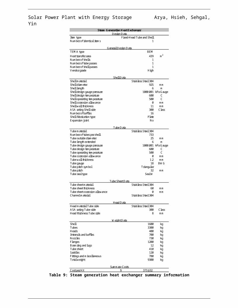
Table 9: Steam generation heat exchanger summary information
Item type Fixed-Head Tube and ShellNumber of identical items 1
TEMA type BEMHeat transfer area 439 m2
Number of shells 1Number of tube passes 1Number of shell passes 1Vendor grade High
Shell material Stainless Steel 304Shell diameter 925 mmShell length 6 mShell design gauge pressure 1000.001 kPa GaugeShell design temperature 600 CShell operating temperature 500 CShell corrosion allowance 0 mmShell wall thickness 11 mmASA rating Shell side 300 ClassNumber of baffles 16Shell fabrication type PlateExpansion joint No
Tube material Stainless Steel 304Number of tubes per shell 733Tube outside diameter 25 mmTube length extended 6 mTube design gauge pressure 1000.001 kPa GaugeTube design temperature 600 CTube operating temperature 500 CTube corrosion allowance 0 mmTube wall thickness 1.2 mmTube gauge 18 BWGTube pitch symbol TriangularTube pitch 32 mmTube seal type Seal W
Tube sheet material Stainless Steel 304Tube sheet thickness 60 mmTube sheet corrosion allowance 0 mmChannel material Stainless Steel 304
Head material Tube side Stainless Steel 304ASA rating Tube side 300 ClassHead thickness Tube side 8 mm
Shell 1600 kgTubes 3300 kgHeads 400 kgInternals and baffles 700 kgNozzles 730 kgFlanges 1200 kgBase ring and lugs 12 kgTube sheet 410 kgSaddles 120 kgFittings and miscellaneous 780 kgTotal weight 9300 kg
Cost per HX 373,632$
Steam Generation Heat Exchanger
Weight Data
Summary Costs
Design Data
General Design Data
Shell Data
Tube Data
Tube Sheet Data
Head Data

Solar Power Plant with Energy Storage Arya, Hsieh, Sehgal, Yin
Table 10: Rankine cycle pump summary information
Item type CentrifugalNumber of identical items 1
Casing material Carbon SteelDesign temperature 135 CDesign gauge pressure 7992.73 kPa GaugeFluid head 815 mASA rating 600 ClassDriver power 258 kWSpeed 3600 RPMDriver type MotorMotor type TEFCPump efficiency 75 %Seal type Single
Liquid flow rate 25.48 L/sFluid density 1000.004 kg/m3
Fluid viscosity 1 mPa-sPower per liquid flow rate 9.26 kW/L/sLiquid flow rate times head 20766 L/s-m
Pump 1500 kgMotor 900 kgBase plate 320 kgFittings and miscellaneous 270 kgTotal weight 3000 kg
Subtotal 161,118$ Summary Costs
Rankine Cycle PumpDesign Data
Equipment Design Data
Process Design Data
Weight Data

Solar Power Plant with Energy Storage Arya, Hsieh, Sehgal, Yin
Table 11: Hot & cold headers summary information
Inner Diameter 40 cmTube Thickness 1 cmLength / Quadrant 433 m
Thickness of Blanket 51 mmNumber of Blankets 5Insulation Thickness 25 cmInsulation Thermal Conductivity 0.13 W/m-K
Insulation Cost 227,910$ Header Cost 1,470,456$
Total Cost 1,698,366$
Hot & Cold HeadersGeneral Design Data
Insulation Data
Cost Summary

Solar Power Plant with Energy Storage Arya, Hsieh, Sehgal, Yin
Table 12: Condenser summary information
Inner Diameter 1.57 cmOuter Diameter 1.91 cmShell Diameter 0.94 mTriangular Pitch 2.54 cmΔTLM 93 KHeat Duty 51,993,372 WOverall Heat Transfer Coefficient (U) 5705 W/(m2-K)Fouling Factor (Ft) 1Heat Transfer Area 98 m2
Number of Tubes per Pass (Nt) 164Length of Tubes (L) 6.10 mNumber of Passes 2
In OutTemperature (K) 305 322Cp (J/kg-K) 4178 4180μ (kg/m-s) 7.61E-04 5.55E-04k (W/m-K) 0.62 0.64Specific Gravity 0.995 0.989ρ (kg/m3) 995 989m (kg/s) 746 746Pr 5.2 3.77
Vapor LiquidTemperature (K) 407 407Cp (J/kg-K) 2158 4256μ (kg/m-s) 1.34E-05 2.00E-04kinematic viscosity (m2/s) 0 2.94E-07k (W/m-K) 0.028 0.688ρ (kg/m3) 1.650709805 931.96645m (kg/s) 24 24ΔHvap (J/kg) 2163900 2163900Pr 1 1
Tube Data: Cooling Water
Shell Data: Steam
Condenser SummaryGeneral Design Data

Solar Power Plant with Energy Storage Arya, Hsieh, Sehgal, Yin
Table 13: SCA summary information
Aperture Area 545 m2
Number per Loop 4Number of Loops 104
Material Cor-Ten steel and zinc-coated Number of Pylons 13Foundation Material Concrete PierFoundation Dimension 8’ x 30” OD with no capWind Load Basis 33 m/sErection Method No jig
Parabola x2/(4f) mFocal Length (f) 1.8 mInterconnect Ball JointDrive HydraulicSun Sensor Acciona
Inner Diameter 70 mmOutter Diameter 112Annulus Width 18Annulus Pressure 0.013 PaTube Material Stainless Steel 304Tube Coating Low-Emission ConcreteTube Coating Absorbance 95 %Tube Coating Emissivity 0.14Shell Material GlassLength 4 m
Cost 30,949,242$ Cost Summary
General SCA Data
Solar Collector Structure Data
Solar Collector Module
HCE
Sollar Collector Assembly

Solar Power Plant with Energy Storage Arya, Hsieh, Sehgal, Yin
Table 14: TES tank summary information
TES HTF Mass 3,029,917Tank Size 1,848 m3
Number of Tanks 2
Radius of Tank Cylinder 8 mHeight of Tank Cylinder 20 m
Concrete Thickness 30 cmConcrete Thermal Conductivity 1 W/m-K
InsulationThickness of Blanket 51 mmNumber of Blankets 5Insulation Thickness 25 cmInsulation Thermal Conductivity 0.13 W/m-K
Hot Tank 182 kWCold Tank 115 kW
Cost 2,499,934$
TES Tank Data
Insulation Data
Process Design Data
General Design Data
Cost Summary
Solar Power Plant with Energy Storage Arya, Hsieh, Sehgal, Yin
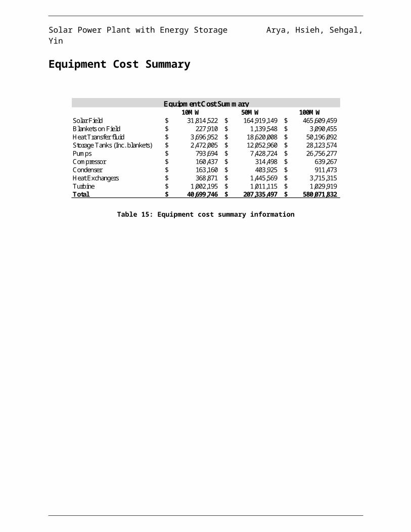
Equipment Cost Summary
Table 15: Equipment cost summary information
10MW 50MW 100MWSolar Field 31,814,522$ 164,919,149$ 465,609,459$ Blankets on Field 227,910$ 1,139,548$ 3,090,455$ Heat Transfer fluid 3,696,952$ 18,620,008$ 50,196,092$ Storage Tanks (Inc. blankets) 2,472,005$ 12,052,960$ 28,123,574$ Pumps 793,694$ 7,428,724$ 26,756,277$ Compressor 160,437$ 314,498$ 639,267$ Condenser 163,160$ 403,925$ 911,473$ Heat Exchangers 368,871$ 1,445,569$ 3,715,315$ Turbine 1,002,195$ 1,011,115$ 1,029,919$ Total 40,699,746$ 207,335,497$ 580,071,832$
Equipment Cost Summary

Solar Power Plant with Energy Storage Arya, Hsieh, Sehgal, Yin
Fixed Capital Investment Summary
The major cost contributor in a parabolic solar trough plant is the solar field, making up
about 83% of total equipment cost for a 10 MW plant to 87% for a 100 MW plant. HTF costs
includes both the fluid running through the field as well as the fluid in the TES system and
makes up about 7% of costs for all plant sizes. The remaining cost mostly is derived from the
power generation cycle.
Figure 14: Equipment Cost Breakdown: 100MW Plant with 3 Hours of Storage
87%
0% 7%3%
2% 0%0% 1% 0%
Equipment Cost Breakdown for 100MW Plant with 3 Hour Storage
Solar Field
Blankets on Field
Heat transfer fluid
Storage Tanks (Inc. blankets)
Pumps
Compressor
Condenser
Heat Exchangers
Turbine
Solar Power Plant with Energy Storage Arya, Hsieh, Sehgal, Yin
The base case shown for all cost presentation, with the exception of the sensitivity
analysis section in the latter part of the report, assumes three hours of thermal storage. This
storage is intended for load leveling operation and low insolation energy production.
Total capital investment increases as the number of hours increase due to storage tank
requirements and increased field heat duty. While the storage tanks only makes up about three
percent of total cost, the associated solar field and HTF cause the bulk of the cost increase. At
three hours of storage, about 27% of the solar field is dedicated to stored energy. An analysis of
TES desirability is in the Economic Sensitivity section on page 85
Solar Field Components
The major cost breakdown in the solar field is illustrated below in Figure 15 for a 10 MW
plant with 3 hours of storage. The key cost elements in the solar field are the receivers (18%),
the mirrors (19%) and the concentrator structure (30%). These percentage breakdowns are
representative of the 50MW and 100MW plants as well with only minor differences.
Figure 15: Solar Field Cost Breakdown: 10 MW Plant with 3 Hours of Storage
18%
19%
30%
8%
2% 2%3%
5% 11%
2%
Solar Field Cost Breakdown for 10MW Plant with 3 Hours of Storage
Receivers
Mirrors
Concentrator Structure
Concentrator Erection
Drive
Interconnection Piping
Electronics & Control
Header Piping

Solar Power Plant with Energy Storage Arya, Hsieh, Sehgal, Yin
Table 16: Solar field cost summary information
Solar field component cost breakdown is calculated from Sunlab and Sargent & Lundy
studies as shown below in Table 17. Table 17 includes actual cost data for SEGS VI and
projects the cost of each component on a field area basis for plants of various output sizes and
year of completion. Sunlab and S&L projections use existing cost data for SEGS VI as the base
case, with consideration of economies of scale, technological improvements and production
volume. While these projections were performed in 2003, Table 17 presents the most up to date
detailed actual and projected cost data available.
Table 17: Sunlab & S&L solar field data and projection
A multivariate regression on this cost data, with respect to output production and year of
completion, generates cost for various plant outputs of 10, 50 and 100 MW. Output production
10MW 50MW 100MWSolar Field Area, m2 216,241 1,094,962 2,947,360 Receivers 5,408,982$ 28,828,198$ 85,764,335$ Mirrors 5,881,691$ 30,253,996$ 84,110,449$ Concentrator Structure 8,943,812$ 45,586,056$ 124,396,649$ Concentrator Erection 2,441,894$ 12,718,436$ 36,241,220$ Drive 1,297,443$ 6,569,770$ 17,684,160$ Interconnection Piping 648,722$ 3,284,885$ 8,842,080$ Electronics & Control 864,962$ 4,379,847$ 11,789,440$ Header Piping 1,444,566$ 7,233,829$ 19,012,486$ Foundation/Other Civil 3,293,467$ 16,840,233$ 46,256,503$ Other 1,588,983$ 9,223,899$ 31,512,139$ Total 31,814,522$ 164,919,149$ 465,609,459$
Solar Field Cost
Field Component Breakdown Units SEGS VI Trough 100 Trough 100 Trough 150 Trough 200 Trough 400Year 1999 2004 2007 2010 2015 2020Plant Output, MW 15 100 100 150 200 400Solar Collection System $/m2 field 250 234 184 161 140 122Receivers $/m2 field 43 43 34 28 22 18Mirrors $/m2 field 40 40 36 28 20 16Concentrator Structure $/m2 field 50 47 44 42 39 36Concentrator Erection $/m2 field 17 14 13 12 11 10Drive $/m2 field 14 13 6 6 6 5Interconnection Piping $/m2 field 11 10 3 3 3 2Electronics & Control $/m2 field 16 14 4 4 4 3Header Piping $/m2 field 8 7 7 6 6 5Foundation/Other Civil $/m2 field 21 18 17 15 14 12Other (spares, HTF, freight) $/m2 field 17 17 11 10 9 8

Solar Power Plant with Energy Storage Arya, Hsieh, Sehgal, Yin
and year of completion were the primary factors affecting economy of scale and technological
improvements over time. The regression statistics are shown below in Table 18. For drive,
interconnection piping, and electronics & control, per m2 cost was set to the 2010 level in the
projections. This is because cost stays relatively constant past 2004. This cost reduction is due to
technological improvement rather than scale as both 2004 and 2007 projection are for a 100MW
plant but the cost reduction is significant.
Table 18: Cost regression statistics information
Heat Transfer Fluid
Costs for the HTF were calculated based on literature values for the price per unit mass,
of $ 0.93/kg for HITEC. This was combined with total mass in both the field and TES system to
develop a cost for the HTF, please see page 53 in the Appendix for further information.
Storage Tanks
Storage tanks for HTF form an integral part of the TES system. Their costs were
calculated using correlations presented by Seider et al. for standard tanks.
Year Output InterceptReceivers 0.2214 -10.2006 20641Mirrors 0.0316 -1.8693 3782Concentrator Structure 0.0104 -1.4889 3020Concentrator Erection 0.0065 -0.7845 1618Header Piping 0.0489 -1.4513 2916Foundation/Other Civil -0.0018 -0.1049 217Other (spares, HTF, freight) 0.0036 -0.4747 969Total 0.0259 -0.9052 1827
Cost Regression Statistics

Solar Power Plant with Energy Storage Arya, Hsieh, Sehgal, Yin
Pumps, Heat Exchangers, and Turbine
The pumps for pumps, heat exchangers, and turbine were calculated. All of these units
were costed using similar methodology. The pertinent design variables for each unit was
determined for various sizes and then fed into ASPEN IPE, then the outputs were tabulated and
regressions were constructed to give price as a function of the design specifications of the unit.

Solar Power Plant with Energy Storage Arya, Hsieh, Sehgal, Yin
Other Important Considerations
Environmental Problems and Safety & Health Concerns
Chemicals
Any of the fluids employed by the overall process (Water, Hitec, Hitec XL and Solar
Salt) are considered environmentally benign.
Infrastructure
Plant components primarily consist of stainless steel, carbon steel and glass reflectors.
Therefore, the plant does not pose any significant environmental concerns.
Safety & Health Concerns
Given the aforementioned conditions, there are no known safety or health concerns posed
by the overall process.
Additional Equipment & Costs
In addition to plant equipment costs, ancillary capital equipment includes equipment for
mirror washing and construction vehicles. This equipment cost is calculated based on per m2
data from Sunlab and S&L studies. The dump truck and operator vehicle costs were calculated
based on the total solar field area, which includes spacing between structures, whereas mirror
wash equipment was calculated based on solar collection area.

Solar Power Plant with Energy Storage Arya, Hsieh, Sehgal, Yin
Table 19: Capital equipment cost summary information
Cost of Site Preparation and Service Facilities are calculated based on correlations by
Seider et al. using ten percent and five percent of bare module costs. Contingencies &
Contractor’s Fees are calculated based on Sunlab & S&L data at $8/m2 of field. Plant Startup
cost for a typical plant is estimated to be between two and ten percent of Total Depreciable
Capital (TDC) according to Seider et al. cost correlations.
Dump Truck 0.02Operator Vehicle 0.05Mirror Wash Equip (Twister Rig) 0.08Mirror Wash Equip (Deluge Rig) 0.05Mirror Container Carrier 0.01Tractor 0.02Total 0.23
10MW 95,356$ 50MW 478,708$ 100MW 1,295,150$
Capital Equipment, $/m2
Total Capital Equipment Cost
Solar Power Plant with Energy Storage Arya, Hsieh, Sehgal, Yin
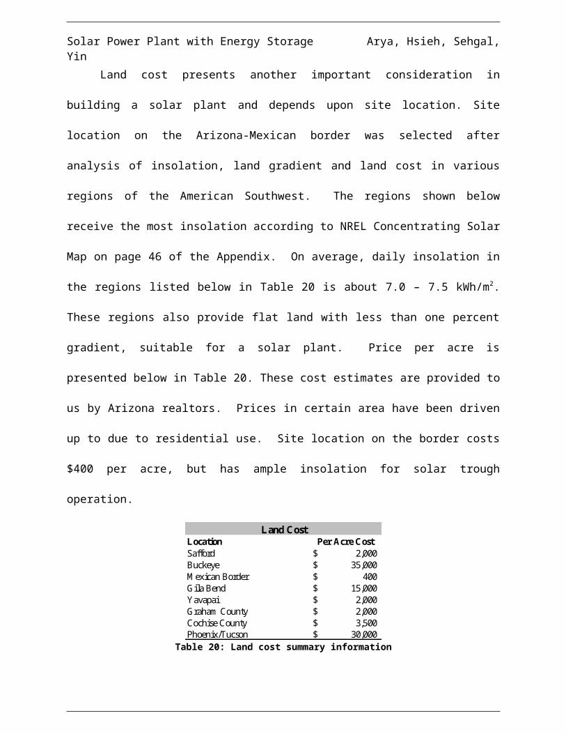
Land cost presents another important consideration in building a solar plant and depends
upon site location. Site location on the Arizona-Mexican border was selected after analysis of
insolation, land gradient and land cost in various regions of the American Southwest. The
regions shown below receive the most insolation according to NREL Concentrating Solar Map
on page 46 of the Appendix. On average, daily insolation in the regions listed below in Table 20
is about 7.0 – 7.5 kWh/m2. These regions also provide flat land with less than one percent
gradient, suitable for a solar plant. Price per acre is presented below in Table 20. These cost
estimates are provided to us by Arizona realtors. Prices in certain area have been driven up to
due to residential use. Site location on the border costs $400 per acre, but has ample insolation
for solar trough operation.
Table 20: Land cost summary information
Renewable Energy Government Incentives
Subsidies and Taxation
The legal landscape can have a major affect on the viability of a parabolic solar trough
power plant. Legislation in some states mandates that a certain percentage of power
consumption comes from renewable sources, which include solar energy. Table 21 shows the
Renewable Portfolio Standards across several states as a percentage of total energy production.
Location Per Acre CostSafford 2,000$ Buckeye 35,000$ Mexican Border 400$ Gila Bend 15,000$ Yavapai 2,000$ Graham County 2,000$ Cochise County 3,500$ Phoenix/Tucson 30,000$
Land Cost

Solar Power Plant with Energy Storage Arya, Hsieh, Sehgal, Yin
Despite economically favorable status of traditional fossil fuel burning, requirements such as
these incentivize solar energy.
Table 21: Renewable Portfolio Standards across several American States. Given the legislative climate, States subscribing to RPS can be expected to increase
In addition, a subsidy could drastically affect the viability of solar energy. In 2002, Spain
introduced a subsidy of 12 € cents/kWh for solar thermal plants. When the subsidy did not
stimulate investor interest and plant construction, Spain issued the Spanish Royal Decree 436 in
2004 subsidizing the first 200MW of solar capacity at 18 € cents/kWh. Over a dozen 50 MW
plants were announced, leading to discussions to increase the subsidy to the first 500 MW of
capacity. There is no indication that this will occur in the domestic market, but this is what
would be required for private investors to sponsor solar trough technology. In particular,
State Amount YearArizona 15% 2025California 20% 2010Colorado 20% 2020Connecticut 23% 2020District of Columbia 11% 2022Delaware 20% 2019Hawaii 20% 2020Iowa 105 MWI llinois 25% 2025Massachusetts 4% 2009Maryland 9.50% 2022Maine 10% 2017Minnesota 25% 2025Missouri* 11% 2020Montana 15% 2015New Hampshire 16% 2025New J ersey 22.50% 2021New Mexico 20% 2020Nevada 20% 2015New York 24% 2013North Carolina 12.50% 2021Oregon 25% 2025Pennsylvania 18% 2020Rhode Island 15% 2020Texas 5,880 MW 2015Vermont* 10% 2013Virginia* 12% 2022Washington 15% 2020Wisconsin 10% 2015

Solar Power Plant with Energy Storage Arya, Hsieh, Sehgal, Yin
subsidies of 19¢/kWh, 15¢/kWh, 17¢/kWh are needed to make the 10MW, 50MW, and 100MW
break-even NPV, respectively, assuming a discount rate of 15%.
Other Incentives
As of 2008, there are no US Federal level laws specifically sponsoring solar energy,
although some do support renewable energy in general. For example, the government allows
accelerated depreciation of renewable energy assets with a “depreciation bonus” by the MACRS
protocol, which allows for fewer taxes in early years of a plants operational life. Moreover,
individual states offer tax, loan, and other incentives to corporations and utilities, as documented
by DSIRE (Database of State Incentives for Renewable and Efficiency), although none are as
compelling as the Spanish subsidy mentioned above. The most realistic taxation benefits are
incorporated in the design.

Solar Power Plant with Energy Storage Arya, Hsieh, Sehgal, Yin
Operating Cost & Economic Analysis
Table 22: Annual production cost summary information
10MW 50MW 100MWUtilities
Raw water 1,522$ 7,709$ 20,749$ Cooling water 12,738$ 64,502$ 173,622$
Total utilities 14,261$ 72,210$ 194,371$
OperationsDirect wages & benefits (DW&B) 1,080,000$ 2,880,000$ 4,860,000$ Direct salaries & benefits 162,000$ 432,000$ 729,000$ Operating supplies & services 100,439$ 121,950$ 167,298$
Total 1,342,439$ 3,433,950$ 5,756,298$
MaintenanceWages & benefits (MW&B) 1,260,000$ 3,060,000$ 5,400,000$ Salaries & benefits 315,000$ 765,000$ 1,350,000$ Maintenance overhead 142,486$ 182,640$ 267,289$ Replacement costs 202,994$ 3,673,135$ 25,441,819$
Total 1,920,480$ 7,680,775$ 32,459,108$
Operating OverheadGeneral plant overhead 200,007$ 506,727$ 876,069$ Employee relations department 166,203$ 421,083$ 728,001$ Business services 208,458$ 528,138$ 913,086$
Total 574,668$ 1,455,948$ 2,517,156$
Property Taxes & Insurance 516,193$ 2,628,921$ 7,344,433$
Depreciation 10,400,036$ 52,836,024$ 147,696,165$
Cost of Manufacturing (COM) 14,768,076$ 68,107,828$ 195,967,531$
General ExpensesAdministrative expense 177,000$ 177,000$ 177,000$ Mgmt incentive comp. 25,962$ 7,910$ 2,443$
Total 202,962$ 184,910$ 179,443$
Total Production Cost 14,971,037$ 68,292,737$ 196,146,975$
Annual Production Cost

Solar Power Plant with Energy Storage Arya, Hsieh, Sehgal, Yin
Annual production costs are estimated based on 2010 Sunlab and S&L projections of cost
from historical data from SEGS IV, where possible. SEGS VI, outputting 15 MW, is similar in
scale to the base case 10 MW plant with three hours of storage. The 2010 projections for Solar
100, outputting 100 MW present upper bound cost data for the 50 and 100 MW plants designed
herein. Turbine output power provided a scaling metric to estimate costs of plant designs.
Utilities cost, personnel needs, operating supplies & services, maintenance overhead,
replacement rates and costs, property taxes & insurance, and administrative expenses are all
estimated in this manner. The reminder costs are estimated based on Seider et al. cost
correlations with the exception of management incentive compensations.
Utilities
Table 23: Utility cost summary information
The overall process requires two utilities: electricity and water. Electricity mainly
powers field pumps and the Rankine cycle pump. Electricity usage such as lights and computers
are assumed to be relatively negligible. The amount of electricity needed is 0.41 MW, 3.02 MW
and 8.4 MW for outputs of 10 MW, 50 MW and 100 MW, respectively. Electricity utility costs
are captured through capital investment as they demand increased turbine output and
consequently, increased solar collection loops.
10MW 50MW 100MWCooling Load, MW 51 259 696
Total Cooling Water Cost 12,738$ 64,502$ 173,622$
Mirror Wash Water, m3 4,757 24,089 64,842 Total Raw Water Cost 1,522$ 7,709$ 20,749$
Total Utilities Cost 14,261$ 72,210$ 194,371$
Utilities

Solar Power Plant with Energy Storage Arya, Hsieh, Sehgal, Yin
Water utilities and cost are based on data from the SEGS III – VII plants for the period
1997–2001 collected by Sunlab Studies. Cooling water consumption for the condenser is
estimated to be $.043 per m3 of cooling tower makeup. Cooling tower makeup is estimated to be
2.9 m3 per MWh of cooling load. Operating hours are assumed to be 11 hours per day, seven
days per week and 50 weeks per year. Cooling load is calculated from ASPEN outputs for the
condenser. Mirror wash water consumption is estimated to be 0.022 m3 per m2 of collector per
year and raw water cost is $.32 per m3. Summary of water usage and total costs is shown above
in Table 23.
Labor
Table 24: Labor cost summary information
SunLab projections for a 2010 solar plant are shown in the first column of Table 24.
According to S&L review of SunLab projections, the number of personnel for administrative,
plant operations and power plant maintenance purposes are comparable to a 120 MW combined-
cycle power plant. A scale factor of 0.6 based on plant output size was used to project personnel
needs for plants. 0.6 as scale factor is known as “six-tenths rule” and represents the average
across all plants for approximating economies of scale.
Other assumptions were made in the calculation of labor costs. When calculating labor
costs, two hours were added to operating hours for administrative tasks, opening and closing the
plant, daily maintenance, etc. Assumption of a 40 hour work week generates required number of
shifts. In particular, number of shifts was rounded upward to three taking into account sick days,
vacation days or any other reason when an employee cannot make their shift and is absent with
SunLab 10MW 50MW 100MWAdministrative 7 2 5 7Plant Operations 17 4 11 16Power Plant Maintenance 8 2 5 8Solar Field Maintenance 19 5 12 18
Total 51 13 33 49
Personnel

Solar Power Plant with Energy Storage Arya, Hsieh, Sehgal, Yin
pay. (Note: the actual number is 2.6, but rounding up is consistent with industry practice).
Lastly, wages is set to $30 per worker per hour and is utilized in the calculation of Direct Wages
& Benefits. Salaries & benefits are assumed to be 15% of Direct Wages & Benefits for
operating staff and 25% for maintenance staff.
Operating Supplies & Services, Maintenance Overhead & Administrative Expense
Table 25: Miscellaneous cost and service contracts summary information
SunLab data and projections for miscellaneous cost and service contracts are shown
above in Table 25. These costs have been categorized into Operating Supplies & Services,
Maintenance Overhead and Administrative Expense. For italicized items, cost increases with
respect to scale, as these costs are highly driven by solar field size. Therefore, we regressed them
against plant output to obtain our cost numbers as shown below in Table 26. For the remaining
items, cost remains constant regardless of whether the output is 15 MW for Solar Tres or 100
Solar Tres Solar 50 Solar 10015MW 50MW 100MW
Operating Supplies & ServicesVehicle Fuel $17,000 $21,708 $33,380Vehicle Parts and Supplies $28,000 $35,755 $54,980Site Improvements $2,000 $2,000 $2,000Rentel Equipment $34,000 $34,000 $34,000Control System Computers $24,000 $24,000 $24,000
Maintenance OverheadNitrogen Supply $27,000 $27,000 $27,000Sanitary Service $6,000 $6,000 $6,000Waste Disposal $34,000 $34,000 $34,000Weed Control $55,000 $70,232 $107,995Road Maint. $27,000 $34,478 $53,016Vehicle Maint. $2,000 $2,554 $3,927
Administrative ExpensePersonal Computer/Office Equip. $5,000 $5,000 $5,000Safety & Training $10,000 $10,000 $10,000Travel $5,000 $5,000 $5,000Office Supplies $28,000 $28,000 $28,000Telephones $67,000 $67,000 $67,000First Aid $6,000 $6,000 $6,000Other Misc $56,000 $56,000 $56,000
Miscellaneous Cost & Service Contracts
Solar Power Plant with Energy Storage Arya, Hsieh, Sehgal, Yin
MW for Solar 100 because the need for these equipment is mostly fixed and not driven by size of
the plant.
Table 26: Variable miscellaneous cost and service contracts summary information
Replacement Costs
Table 27: Replacement costs summary information
The high cost of receivers (HCEs) drives the majority of replacement costs. The HCE
replacement rate is assumed to be one percent. Unit cost and replacement rate data shown above
are an average of Sunlab and S&L projections for 2010 based on SEGS III –SEGS VII actual
data. Mirrors also contribute to the replacement cost, though they have a lower per unit cost and
a lower replacement rate compared to the HCEs. Solar Collector Structure and Erection was
assumed to be a onetime investment cost that does not need replacement during the lifetime of
the plant. Therefore, these costs are not considered in replacement costs, and it is assumed that
their maintenance will be included in maintenance costs. An assumption of miscellaneous
replacement cost of 5%, covering piping, electronics and control, civil works, and drives is
utilized.
Slope Intercept 10MW 50MW 100MWVehicle Fuel 195 13277 15,277$ 23,403$ 40,534$ Vehicle Parts and Supplies 322 21868 25,162$ 38,547$ 66,764$ Weed Control 632 42955 49,425$ 75,717$ 131,141$ Road Maint. 311 21087 24,263$ 37,170$ 64,379$ Vehicle Maint. 23 1562 1,797$ 2,753$ 4,769$
Variable Miscellaneous Cost & Service Contracts
Unit Cost Annual Rep. Rate 10MW 50MW 100MWMirrors 80$ 0.5% 55,910$ 270,950$ 731,136$ Receivers 847$ 1% 137,417$ 3,227,273$ 23,499,168$ Miscellaneous is est. to be 5% of total 9,666$ 174,911$ 1,211,515$ Total Annual Replacement Cost 202,994$ 3,673,135$ 25,441,819$
Replacement Costs
Solar Power Plant with Energy Storage Arya, Hsieh, Sehgal, Yin
Operating Overhead , Property Taxes & Insurance
General Plant Overhead, Employee Relations Department and Business Services were
calculated using correlations by Seider et al. Property taxes & insurance are each estimated to be
0.5% of initial investment costs.
Depreciation
Depreciation is calculated using 5 year MACRS schedule.
Table 28: 5 Years MACRS summary information
Management Incentive Compensation
Management Incentive Compensation is calculated as an inverse of total cost of
production, excluding depreciation, property taxes or insurance, this compensates managements
for decreasing costs, as they have little impact on revenue.
Working Capital
Working capital is assumed to be 30 days of cash reserves for utilities, operations,
maintenance, operating overhead, salaries & wages, property taxes & insurance. In addition,
included is also 30-day inventory of replacement costs. This covers essentially all production
costs for a 30 day period. Working capital is shown below along with total capital investment.
Year Depreciation1 20%2 32%3 19%4 12%5 12%6 6%
5 Year MACRS

Solar Power Plant with Energy Storage Arya, Hsieh, Sehgal, Yin
Total Capital Investment
Table 29: Total capital investment information summary
Total Bare Module Costs 10MW 50MW 100MWSolar Field 31,814,522$ 164,919,149$ 465,609,459$ Blankets on Field 227,910$ 1,139,548$ 3,090,455$ Heat transfer fluid 3,696,952$ 18,620,008$ 50,196,092$ Storage Tanks (Inc. blankets) 2,472,005$ 12,052,960$ 28,123,574$ Pumps 793,694$ 7,428,724$ 26,756,277$ Compressor 160,437$ 314,498$ 639,267$ Condenser 163,160$ 403,925$ 911,473$ Heat Exchangers 368,871$ 1,445,569$ 3,715,315$ Turbine 1,002,195$ 1,011,115$ 1,029,919$
Total 40,699,746$ 207,335,497$ 580,071,832$
Ancilliary Capital Equipment 95,356$ 478,708$ 1,295,150$
Cost of Site Preparation 4,069,975$ 20,733,550$ 58,007,183$ Cost of Service Facilities 2,034,987$ 10,366,775$ 29,003,592$
Total Direct Permanent Investment 46,900,064$ 238,914,529$ 668,377,757$
Contingencies & Contractors's Fees 1,729,924$ 8,759,693$ 23,578,880$
Total Depreciable Capital (TDC) 48,629,988$ 247,674,222$ 691,956,637$
Cost of Land 71,477$ 357,384$ 969,224$ Cost of Plant Startup 2,917,799$ 14,860,453$ 41,517,398$
Total Permanent Investment 51,619,264$ 262,892,059$ 734,443,259$
Working Capital 380,917$ 1,288,059$ 4,037,567$
Total Capital Investment 52,000,181$ 264,180,118$ 738,480,827$
Total Capital Investment
Solar Power Plant with Energy Storage Arya, Hsieh, Sehgal, Yin
Economic Analysis
Market Competitive Analysis
Solar faces significant competition against existing and proven technologies, as its
viability is measured against traditional fossil fuels. Tellingly, modern use of solar technology
started after the Oil crisis in 1973 and 1979, which resulted in the build of SEGS in California
and some smaller projects. Due to low energy prices after 1990, no new commercial plans were
made until 2005 and onwards, following dramatic inflation in oil prices. Please see Figure 16
for further elaboration.
Figure 16: Oil Prices in the Past Five Decades
Viability of solar power depends on market pricing for electricity, which is a composite
of available energy prices in the locality in question. Renewable energies have traditionally
constituted a very small fraction of domestic energy, as can be seen in Figure 17

Solar Power Plant with Energy Storage Arya, Hsieh, Sehgal, Yin
Figure 17: Consumption Patterns for Energy in the Past Five Decades
As a result of this, we can elect to consider national energy prices as a fair representation
of the weighted cost of fossil fuels, as we can see in Figure 17. Generally speaking, electricity
costs to end users have not dramatically changed in the last 30 years, and the market would find
it difficult to bear the acceptance of a dramatically more expensive energy source. Therefore,
economic competiveness of Solar is only possible at points whether the cost of traditional fossil
fuels and the cost of renewable intersect.
Figure 18: Electricity Prices in the Past Five Decades
Comparable Costs
California is a state with extensive experience with renewable, and a large portfolio of
renewable energy standards. Levelized costs, as discussed in the following section beginning on
0
2
4
6
8
10
12
1960
1962
1964
1966
1968
1970
1972
1974
1976
1978
1980
1982
1984
1986
1988
1990
1992
1994
1996
1998
2000
2002
2004
2006
P
₵/kW
h
Electricity Costs (2006 $)
Solar Power Plant with Energy Storage Arya, Hsieh, Sehgal, Yin
page 62, is a measure of the cost of power generation, a proxy for competitiveness. Figure 18,
displays the levelized costs of various types of energy. Of particular interest are the lines
pertaining to solar trough and solar photovoltaics, both significantly higher than the energy costs
seen in Figure 18, which we are taking as a proxy for fossil fuels. This rudimentary analysis
suggests that Solar Power is currently not economically competitive with fossil fuels, represented
by Conventional Cycles. Please see the economics for further details, on page 73.
Table 30: LEC comparison across energy sources
Levelized Electricity Cost (LEC)
Levelized Electricity Cost (LEC) is defined as the unit cost, that if charged for all
production within the analysis period, would produce enough revenue to cover all production
expenses and capital related costs. In other words, if the price of electricity is sold at levelized
cost over the analysis period, the net present value of revenues would equal the net present value
of the actual annual costs.

Solar Power Plant with Energy Storage Arya, Hsieh, Sehgal, Yin
For our purposes, the LEC unit, C, is in units of $/kWh. Production costs covers all
operating and maintenance costs and capital related costs covers federal and state income taxes,
depreciation, property taxes and insurance.
where n is the number of years within the analysis period, Ei is amount of power produced and
sold in each such year, Ci is the actual annual cost for each year, comprised of current expenses
for labor, utilities, etc. plus a component for recovery of the investment cost. 1/(1+r)I is a
discount factor.
Because LEC is constant, C can be solved by bringing it outside the summation on the
left side. The expression on the right represents the sum of present value of actual annual costs.
On the left side, the expression remaining in the summation when C is brought out represents the
present value of energy production. Dividing the two gives levelized cost.
The following assumptions were built into the model to calculate levelized cost. The
number of years within the analysis period, n, is 20 years, consistent with most plant analysis.
Fixed O&M, variable O&M, and property tax & insurance, for year 1 are produced based on
calculations and assumptions above, and grown at a growth of 2% for each year thereafter. 2%
assumption derives from an expected annual inflation rate of 2½-3% and increases in technology
and management expertise that would reduce cost. Depreciation is calculated using 5 year
MACRS. The plant is assumed to be financed entirely by equity. The cost of capital of equity is
15%. Tax rate is assumed to be 35%. Therefore, the weighted average cost of capital, rWACC, is
calculated to be 15%, and is used as the suitable discount rate. The recovery of initial investment
cost is spread evenly among 20 years within the analysis period.

Solar Power Plant with Energy Storage Arya, Hsieh, Sehgal, Yin
Under these assumptions, LEC for the 10, 50 and 100MW power plants are calculated to
be 18, 14 and 15 cents/kWh, respectively. This represents the price requirement for the next 20
years after plant construction in order to break even.
Solar Power Plant with Energy Storage Arya, Hsieh, Sehgal, Yin
10 MW Levelized Cost
Year 2010 2011 2012 2013 2014 2015 2016 2017 2018 2019 2020 2021 2022 2023 2024 2025 2026 2027 2028 2029PV Year 2 3 4 5 6 7 8 9 10 11 12 13 14 15 16 17 18 19 20 21Project Year 1 2 3 4 5 6 7 8 9 10 11 12 13 14 15 16 17 18 19 20
D&A & Debt CalculationsDep. Rates (5 Yr MACRS) 20% 32% 19% 12% 12% 6% 0% 0% 0% 0% 0% 0% 0% 0% 0% 0% 0% 0% 0% 0%
Beg. Of Year Values (000s) 48.63$ 38.90$ 23.34$ 14.01$ 8.40$ 2.80$ -$ -$ -$ -$ -$ -$ -$ -$ -$ -$ -$ -$ -$ -$ Tax depreciation (5 yr MACRS) 9.73$ 15.56$ 9.34$ 5.60$ 5.60$ 2.80$ -$ -$ -$ -$ -$ -$ -$ -$ -$ -$ -$ -$ -$ -$ Eng of year values 38.90$ 23.34$ 14.01$ 8.40$ 2.80$ -$ -$ -$ -$ -$ -$ -$ -$ -$ -$ -$ -$ -$ -$ -$
EnergyElectric energy production (GWh) 39.38 39.38 39.38 39.38 39.38 39.38 39.38 39.38 39.38 39.38 39.38 39.38 39.38 39.38 39.38 39.38 39.38 39.38 39.38 39.38
IS & CF ($MM)Annuity Cost 7.66$ 7.66$ 7.66$ 7.66$ 7.66$ 7.66$ 7.66$ 7.66$ 7.66$ 7.66$ 7.66$ 7.66$ 7.66$ 7.66$ 7.66$ 7.66$ 7.66$ 7.66$ 7.66$ 7.66$ Fixed O&M (4.01)$ (4.09)$ (4.18)$ (4.26)$ (4.35)$ (4.43)$ (4.52)$ (4.61)$ (4.70)$ (4.80)$ (4.89)$ (4.99)$ (5.09)$ (5.19)$ (5.30)$ (5.40)$ (5.51)$ (5.62)$ (5.73)$ (5.85)$ Variable O&M (0.04)$ (0.04)$ (0.04)$ (0.04)$ (0.04)$ (0.04)$ (0.05)$ (0.05)$ (0.05)$ (0.05)$ (0.05)$ (0.05)$ (0.05)$ (0.05)$ (0.05)$ (0.05)$ (0.06)$ (0.06)$ (0.06)$ (0.06)$ Property Tax & Insurance (0.52)$ (0.53)$ (0.54)$ (0.55)$ (0.56)$ (0.57)$ (0.58)$ (0.59)$ (0.60)$ (0.62)$ (0.63)$ (0.64)$ (0.65)$ (0.67)$ (0.68)$ (0.69)$ (0.71)$ (0.72)$ (0.74)$ (0.75)$ Tax D&A (9.73)$ (15.56)$ (9.34)$ (5.60)$ (5.60)$ (2.80)$ -$ -$ -$ -$ -$ -$ -$ -$ -$ -$ -$ -$ -$ -$
Total Expenses (14.30)$ (20.22)$ (14.09)$ (10.45)$ (10.55)$ (7.85)$ (5.15)$ (5.25)$ (5.36)$ (5.46)$ (5.57)$ (5.68)$ (5.80)$ (5.91)$ (6.03)$ (6.15)$ (6.28)$ (6.40)$ (6.53)$ (6.66)$ Operating Income (EBIT) (6.64)$ (12.56)$ (6.43)$ (2.79)$ (2.89)$ (0.19)$ 2.51$ 2.41$ 2.30$ 2.20$ 2.09$ 1.98$ 1.86$ 1.75$ 1.63$ 1.51$ 1.39$ 1.26$ 1.13$ 1.00$ Taxable Income (6.64)$ (12.56)$ (6.43)$ (2.79)$ (2.89)$ (0.19)$ 2.51$ 2.41$ 2.30$ 2.20$ 2.09$ 1.98$ 1.86$ 1.75$ 1.63$ 1.51$ 1.39$ 1.26$ 1.13$ 1.00$ Tax -$ -$ -$ -$ -$ -$ (0.88)$ (0.84)$ (0.81)$ (0.77)$ (0.73)$ (0.69)$ (0.65)$ (0.61)$ (0.57)$ (0.53)$ (0.48)$ (0.44)$ (0.40)$ (0.35)$ Earnings (6.64)$ (12.56)$ (6.43)$ (2.79)$ (2.89)$ (0.19)$ 1.63$ 1.57$ 1.50$ 1.43$ 1.36$ 1.28$ 1.21$ 1.14$ 1.06$ 0.98$ 0.90$ 0.82$ 0.74$ 0.65$ Add Back Depr 9.73$ 15.56$ 9.34$ 5.60$ 5.60$ 2.80$ -$ -$ -$ -$ -$ -$ -$ -$ -$ -$ -$ -$ -$ -$ Cash Flows 3.09$ 3.00$ 2.90$ 2.81$ 2.71$ 2.61$ 1.63$ 1.57$ 1.50$ 1.43$ 1.36$ 1.28$ 1.21$ 1.14$ 1.06$ 0.98$ 0.90$ 0.82$ 0.74$ 0.65$ Repayment of debt principalDiscount Factor 0.7561 0.6575 0.5718 0.4972 0.4323 0.3759 0.3269 0.2843 0.2472 0.2149 0.1869 0.1625 0.1413 0.1229 0.1069 0.0929 0.0808 0.0703 0.0611 0.0531
PV ($MM) 2.34$ 1.97$ 1.66$ 1.40$ 1.17$ 0.98$ 0.53$ 0.45$ 0.37$ 0.31$ 0.25$ 0.21$ 0.17$ 0.14$ 0.11$ 0.09$ 0.07$ 0.06$ 0.04$ 0.03$ Cum. PV 2.34$ 4.31$ 5.97$ 7.36$ 8.54$ 9.52$ 10.05$ 10.50$ 10.87$ 11.18$ 11.43$ 11.64$ 11.81$ 11.95$ 12.06$ 12.15$ 12.23$ 12.28$ 12.33$ 12.36$ PV Energy (GWh) 29.78$ 25.89$ 22.52$ 19.58$ 17.03$ 14.81$ 12.87$ 11.20$ 9.73$ 8.47$ 7.36$ 6.40$ 5.57$ 4.84$ 4.21$ 3.66$ 3.18$ 2.77$ 2.41$ 2.09$ Cum. Energy 29.78$ 55.67$ 78.19$ 97.77$ 114.80$ 129.60$ 142.48$ 153.67$ 163.41$ 171.87$ 179.23$ 185.63$ 191.20$ 196.04$ 200.25$ 203.91$ 207.09$ 209.86$ 212.26$ 214.36$
Recovery of Investment Cost (2.43)$ (2.43)$ (2.43)$ (2.43)$ (2.43)$ (2.43)$ (2.43)$ (2.43)$ (2.43)$ (2.43)$ (2.43)$ (2.43)$ (2.43)$ (2.43)$ (2.43)$ (2.43)$ (2.43)$ (2.43)$ (2.43)$ (2.43)$ Cost (7.00)$ (7.09)$ (7.19)$ (7.28)$ (7.38)$ (7.48)$ (8.46)$ (8.53)$ (8.59)$ (8.66)$ (8.73)$ (8.81)$ (8.88)$ (8.96)$ (9.03)$ (9.11)$ (9.19)$ (9.27)$ (9.36)$ (9.44)$ PV Cost (5.29)$ (4.66)$ (4.11)$ (3.62)$ (3.19)$ (2.81)$ (2.77)$ (2.42)$ (2.12)$ (1.86)$ (1.63)$ (1.43)$ (1.26)$ (1.10)$ (0.97)$ (0.85)$ (0.74)$ (0.65)$ (0.57)$ (0.50)$ Cum PV (5.29)$ (9.96)$ (14.07)$ (17.69)$ (20.88)$ (23.69)$ (26.46)$ (28.88)$ (31.00)$ (32.87)$ (34.50)$ (35.93)$ (37.18)$ (38.29)$ (39.25)$ (40.10)$ (40.84)$ (41.49)$ (42.06)$ (42.56)$
Annuity $7.66 $MM$7,660,098 $
Energy Prod. 39 GWh39,382,782 kWh
Levelized Cost $0.19 $/kWh
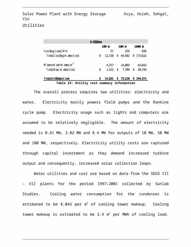
Solar Power Plant with Energy Storage Arya, Hsieh, Sehgal, Yin
50 MW Levelized Cost
Year 2010 2011 2012 2013 2014 2015 2016 2017 2018 2019 2020 2021 2022 2023 2024 2025 2026 2027 2028 2029PV Year 2 3 4 5 6 7 8 9 10 11 12 13 14 15 16 17 18 19 20 21Project Year 1 2 3 4 5 6 7 8 9 10 11 12 13 14 15 16 17 18 19 20
D&A & Debt CalculationsDep. Rates (5 Yr MACRS) 20% 32% 19% 12% 12% 6% 0% 0% 0% 0% 0% 0% 0% 0% 0% 0% 0% 0% 0% 0%
Beg. Of Year Values (000s) 247.67$ 198.14$ 118.88$ 71.33$ 42.80$ 14.27$ -$ -$ -$ -$ -$ -$ -$ -$ -$ -$ -$ -$ -$ -$ Tax depreciation (5 yr MACRS) 49.53$ 79.26$ 47.55$ 28.53$ 28.53$ 14.27$ -$ -$ -$ -$ -$ -$ -$ -$ -$ -$ -$ -$ -$ -$ Eng of year values 198.14$ 118.88$ 71.33$ 42.80$ 14.27$ -$ -$ -$ -$ -$ -$ -$ -$ -$ -$ -$ -$ -$ -$ -$
EnergyElectric energy production (GWh) 199.42 199.42 199.42 199.42 199.42 199.42 199.42 199.42 199.42 199.42 199.42 199.42 199.42 199.42 199.42 199.42 199.42 199.42 199.42 199.42
IS & CF ($MM)Annuity Cost 30.62$ 30.62$ 30.62$ 30.62$ 30.62$ 30.62$ 30.62$ 30.62$ 30.62$ 30.62$ 30.62$ 30.62$ 30.62$ 30.62$ 30.62$ 30.62$ 30.62$ 30.62$ 30.62$ 30.62$ Fixed O&M (12.75)$ (13.00)$ (13.26)$ (13.53)$ (13.80)$ (14.07)$ (14.36)$ (14.64)$ (14.94)$ (15.23)$ (15.54)$ (15.85)$ (16.17)$ (16.49)$ (16.82)$ (17.16)$ (17.50)$ (17.85)$ (18.21)$ (18.57)$ Variable O&M (0.08)$ (0.08)$ (0.08)$ (0.09)$ (0.09)$ (0.09)$ (0.09)$ (0.09)$ (0.09)$ (0.10)$ (0.10)$ (0.10)$ (0.10)$ (0.10)$ (0.11)$ (0.11)$ (0.11)$ (0.11)$ (0.11)$ (0.12)$ Property Tax & Insurance (2.63)$ (2.68)$ (2.74)$ (2.79)$ (2.85)$ (2.90)$ (2.96)$ (3.02)$ (3.08)$ (3.14)$ (3.20)$ (3.27)$ (3.33)$ (3.40)$ (3.47)$ (3.54)$ (3.61)$ (3.68)$ (3.75)$ (3.83)$ Tax D&A (49.53)$ (79.26)$ (47.55)$ (28.53)$ (28.53)$ (14.27)$ -$ -$ -$ -$ -$ -$ -$ -$ -$ -$ -$ -$ -$ -$
Total Expenses (64.99)$ (95.02)$ (63.63)$ (44.93)$ (45.26)$ (31.33)$ (17.41)$ (17.75)$ (18.11)$ (18.47)$ (18.84)$ (19.22)$ (19.60)$ (19.99)$ (20.39)$ (20.80)$ (21.22)$ (21.64)$ (22.08)$ (22.52)$ Operating Income (EBIT) (34.37)$ (64.40)$ (33.02)$ (14.32)$ (14.64)$ (0.71)$ 13.21$ 12.86$ 12.51$ 12.15$ 11.78$ 11.40$ 11.02$ 10.62$ 10.22$ 9.82$ 9.40$ 8.97$ 8.54$ 8.10$ Taxable Income (34.37)$ (64.40)$ (33.02)$ (14.32)$ (14.64)$ (0.71)$ 13.21$ 12.86$ 12.51$ 12.15$ 11.78$ 11.40$ 11.02$ 10.62$ 10.22$ 9.82$ 9.40$ 8.97$ 8.54$ 8.10$ Tax -$ -$ -$ -$ -$ -$ (4.62)$ (4.50)$ (4.38)$ (4.25)$ (4.12)$ (3.99)$ (3.86)$ (3.72)$ (3.58)$ (3.44)$ (3.29)$ (3.14)$ (2.99)$ (2.84)$ Earnings (34.37)$ (64.40)$ (33.02)$ (14.32)$ (14.64)$ (0.71)$ 8.59$ 8.36$ 8.13$ 7.89$ 7.65$ 7.41$ 7.16$ 6.91$ 6.65$ 6.38$ 6.11$ 5.83$ 5.55$ 5.27$ Add Back Depr 49.53$ 79.26$ 47.55$ 28.53$ 28.53$ 14.27$ -$ -$ -$ -$ -$ -$ -$ -$ -$ -$ -$ -$ -$ -$ Cash Flows 15.16$ 14.85$ 14.54$ 14.22$ 13.89$ 13.55$ 8.59$ 8.36$ 8.13$ 7.89$ 7.65$ 7.41$ 7.16$ 6.91$ 6.65$ 6.38$ 6.11$ 5.83$ 5.55$ 5.27$ Repayment of debt principalDiscount Factor 0.7561 0.6575 0.5718 0.4972 0.4323 0.3759 0.3269 0.2843 0.2472 0.2149 0.1869 0.1625 0.1413 0.1229 0.1069 0.0929 0.0808 0.0703 0.0611 0.0531
PV ($MM) 11.46$ 9.77$ 8.31$ 7.07$ 6.00$ 5.09$ 2.81$ 2.38$ 2.01$ 1.70$ 1.43$ 1.20$ 1.01$ 0.85$ 0.71$ 0.59$ 0.49$ 0.41$ 0.34$ 0.28$ Cum. PV 11.46$ 21.23$ 29.54$ 36.61$ 42.61$ 47.71$ 50.51$ 52.89$ 54.90$ 56.60$ 58.03$ 59.23$ 60.24$ 61.09$ 61.80$ 62.40$ 62.89$ 63.30$ 63.64$ 63.92$ PV Energy (GWh) 150.79$ 131.12$ 114.02$ 99.15$ 86.21$ 74.97$ 65.19$ 56.69$ 49.29$ 42.86$ 37.27$ 32.41$ 28.18$ 24.51$ 21.31$ 18.53$ 16.11$ 14.01$ 12.18$ 10.60$ Cum. Energy 150.79$ 281.91$ 395.93$ 495.08$ 581.29$ 656.26$ 721.45$ 778.14$ 827.43$ 870.30$ 907.57$ 939.98$ 968.17$ 992.67$ 1,013.98$ 1,032.51$ 1,048.63$ 1,062.64$ 1,074.83$ 1,085.42$
Recovery of Investment Cost (12.38)$ (12.38)$ (12.38)$ (12.38)$ (12.38)$ (12.38)$ (12.38)$ (12.38)$ (12.38)$ (12.38)$ (12.38)$ (12.38)$ (12.38)$ (12.38)$ (12.38)$ (12.38)$ (12.38)$ (12.38)$ (12.38)$ (12.38)$ Cost (27.84)$ (28.15)$ (28.46)$ (28.79)$ (29.11)$ (29.45)$ (34.41)$ (34.64)$ (34.87)$ (35.11)$ (35.35)$ (35.59)$ (35.84)$ (36.10)$ (36.36)$ (36.62)$ (36.89)$ (37.17)$ (37.45)$ (37.74)$ PV Cost (21.05)$ (18.51)$ (16.27)$ (14.31)$ (12.59)$ (11.07)$ (11.25)$ (9.85)$ (8.62)$ (7.55)$ (6.61)$ (5.78)$ (5.07)$ (4.44)$ (3.89)$ (3.40)$ (2.98)$ (2.61)$ (2.29)$ (2.00)$ Cum PV (21.05)$ (39.56)$ (55.84)$ (70.15)$ (82.73)$ (93.81)$ (105.06)$ (114.90)$ (123.52)$ (131.07)$ (137.67)$ (143.46)$ (148.52)$ (152.96)$ (156.85)$ (160.25)$ (163.23)$ (165.84)$ (168.13)$ (170.14)$
Annuity $30.62 $MM$30,618,059 $
Energy Prod. 199 GWh199,419,765 kWh
Levelized Cost $0.15 $/kWh
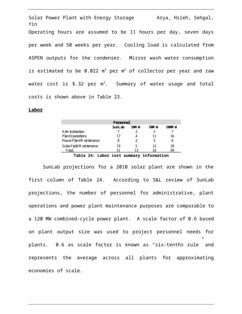
Solar Power Plant with Energy Storage Arya, Hsieh, Sehgal, Yin
100 MW Levelized Cost
Year 2010 2011 2012 2013 2014 2015 2016 2017 2018 2019 2020 2021 2022 2023 2024 2025 2026 2027 2028 2029PV Year 2 3 4 5 6 7 8 9 10 11 12 13 14 15 16 17 18 19 20 21Project Year 1 2 3 4 5 6 7 8 9 10 11 12 13 14 15 16 17 18 19 20
D&A & Debt CalculationsDep. Rates (5 Yr MACRS) 20% 32% 19% 12% 12% 6% 0% 0% 0% 0% 0% 0% 0% 0% 0% 0% 0% 0% 0% 0%
Beg. Of Year Values (000s) 691.80$ 553.44$ 332.06$ 199.24$ 119.54$ 39.85$ -$ -$ -$ -$ -$ -$ -$ -$ -$ -$ -$ -$ -$ -$ Tax depreciation (5 yr MACRS) 138.36$ 221.37$ 132.82$ 79.69$ 79.69$ 39.85$ -$ -$ -$ -$ -$ -$ -$ -$ -$ -$ -$ -$ -$ -$ Eng of year values 553.44$ 332.06$ 199.24$ 119.54$ 39.85$ -$ -$ -$ -$ -$ -$ -$ -$ -$ -$ -$ -$ -$ -$ -$
EnergyElectric energy production (GWh) 536.79 536.79 536.79 536.79 536.79 536.79 536.79 536.79 536.79 536.79 536.79 536.79 536.79 536.79 536.79 536.79 536.79 536.79 536.79 536.79
IS & CF ($MM)Annuity Cost 90.87$ 90.87$ 90.87$ 90.87$ 90.87$ 90.87$ 90.87$ 90.87$ 90.87$ 90.87$ 90.87$ 90.87$ 90.87$ 90.87$ 90.87$ 90.87$ 90.87$ 90.87$ 90.87$ 90.87$ Fixed O&M (40.62)$ (41.43)$ (42.26)$ (43.10)$ (43.96)$ (44.84)$ (45.74)$ (46.65)$ (47.59)$ (48.54)$ (49.51)$ (50.50)$ (51.51)$ (52.54)$ (53.59)$ (54.66)$ (55.76)$ (56.87)$ (58.01)$ (59.17)$ Variable O&M (0.20)$ (0.20)$ (0.20)$ (0.21)$ (0.21)$ (0.22)$ (0.22)$ (0.23)$ (0.23)$ (0.24)$ (0.24)$ (0.24)$ (0.25)$ (0.25)$ (0.26)$ (0.26)$ (0.27)$ (0.28)$ (0.28)$ (0.29)$ Property Tax & Insurance (7.34)$ (7.49)$ (7.64)$ (7.79)$ (7.95)$ (8.11)$ (8.27)$ (8.43)$ (8.60)$ (8.78)$ (8.95)$ (9.13)$ (9.31)$ (9.50)$ (9.69)$ (9.88)$ (10.08)$ (10.28)$ (10.49)$ (10.70)$ Tax D&A (138.36)$ (221.37)$ (132.82)$ (79.69)$ (79.69)$ (39.85)$ -$ -$ -$ -$ -$ -$ -$ -$ -$ -$ -$ -$ -$ -$
Total Expenses (186.51)$ (270.49)$ (182.93)$ (130.80)$ (131.82)$ (93.01)$ (54.23)$ (55.32)$ (56.42)$ (57.55)$ (58.70)$ (59.87)$ (61.07)$ (62.29)$ (63.54)$ (64.81)$ (66.11)$ (67.43)$ (68.78)$ (70.15)$ Operating Income (EBIT) (95.65)$ (179.63)$ (92.06)$ (39.93)$ (40.95)$ (2.15)$ 36.64$ 35.55$ 34.45$ 33.32$ 32.17$ 30.99$ 29.79$ 28.57$ 27.33$ 26.06$ 24.76$ 23.44$ 22.09$ 20.71$ Taxable Income (95.65)$ (179.63)$ (92.06)$ (39.93)$ (40.95)$ (2.15)$ 36.64$ 35.55$ 34.45$ 33.32$ 32.17$ 30.99$ 29.79$ 28.57$ 27.33$ 26.06$ 24.76$ 23.44$ 22.09$ 20.71$ Tax -$ -$ -$ -$ -$ -$ (12.82)$ (12.44)$ (12.06)$ (11.66)$ (11.26)$ (10.85)$ (10.43)$ (10.00)$ (9.56)$ (9.12)$ (8.67)$ (8.20)$ (7.73)$ (7.25)$ Earnings (95.65)$ (179.63)$ (92.06)$ (39.93)$ (40.95)$ (2.15)$ 23.81$ 23.11$ 22.39$ 21.66$ 20.91$ 20.15$ 19.37$ 18.57$ 17.76$ 16.94$ 16.09$ 15.24$ 14.36$ 13.46$ Add Back Depr 138.36$ 221.37$ 132.82$ 79.69$ 79.69$ 39.85$ -$ -$ -$ -$ -$ -$ -$ -$ -$ -$ -$ -$ -$ -$ Cash Flows 42.71$ 41.75$ 40.77$ 39.76$ 38.74$ 37.70$ 23.81$ 23.11$ 22.39$ 21.66$ 20.91$ 20.15$ 19.37$ 18.57$ 17.76$ 16.94$ 16.09$ 15.24$ 14.36$ 13.46$ Repayment of debt principalDiscount Factor 0.7561 0.6575 0.5718 0.4972 0.4323 0.3759 0.3269 0.2843 0.2472 0.2149 0.1869 0.1625 0.1413 0.1229 0.1069 0.0929 0.0808 0.0703 0.0611 0.0531
PV ($MM) 32.30$ 27.45$ 23.31$ 19.77$ 16.75$ 14.17$ 7.78$ 6.57$ 5.53$ 4.65$ 3.91$ 3.27$ 2.74$ 2.28$ 1.90$ 1.57$ 1.30$ 1.07$ 0.88$ 0.72$ Cum. PV 32.30$ 59.75$ 83.06$ 102.83$ 119.58$ 133.75$ 141.53$ 148.10$ 153.64$ 158.29$ 162.20$ 165.47$ 168.21$ 170.49$ 172.39$ 173.96$ 175.27$ 176.34$ 177.21$ 177.93$ PV Energy (GWh) 405.89$ 352.95$ 306.91$ 266.88$ 232.07$ 201.80$ 175.48$ 152.59$ 132.69$ 115.38$ 100.33$ 87.24$ 75.86$ 65.97$ 57.36$ 49.88$ 43.38$ 37.72$ 32.80$ 28.52$ Cum. Energy 405.89$ 758.84$ 1,065.75$ 1,332.62$ 1,564.69$ 1,766.49$ 1,941.97$ 2,094.56$ 2,227.24$ 2,342.62$ 2,442.95$ 2,530.19$ 2,606.06$ 2,672.02$ 2,729.39$ 2,779.27$ 2,822.64$ 2,860.36$ 2,893.16$ 2,921.68$
Recovery of Investment Cost (34.59)$ (34.59)$ (34.59)$ (34.59)$ (34.59)$ (34.59)$ (34.59)$ (34.59)$ (34.59)$ (34.59)$ (34.59)$ (34.59)$ (34.59)$ (34.59)$ (34.59)$ (34.59)$ (34.59)$ (34.59)$ (34.59)$ (34.59)$ Cost (82.74)$ (83.71)$ (84.69)$ (85.69)$ (86.71)$ (87.76)$ (101.64)$ (102.35)$ (103.07)$ (103.80)$ (104.55)$ (105.31)$ (106.09)$ (106.88)$ (107.69)$ (108.52)$ (109.36)$ (110.22)$ (111.10)$ (111.99)$ PV Cost (62.57)$ (55.04)$ (48.42)$ (42.60)$ (37.49)$ (32.99)$ (33.23)$ (29.09)$ (25.48)$ (22.31)$ (19.54)$ (17.12)$ (14.99)$ (13.14)$ (11.51)$ (10.08)$ (8.84)$ (7.74)$ (6.79)$ (5.95)$ Cum PV (62.57)$ (117.61)$ (166.03)$ (208.63)$ (246.12)$ (279.11)$ (312.34)$ (341.43)$ (366.91)$ (389.22)$ (408.76)$ (425.88)$ (440.87)$ (454.01)$ (465.52)$ (475.60)$ (484.44)$ (492.18)$ (498.97)$ (504.92)$
Annuity $90.87 $MM$90,867,263 $
Energy Prod. 537 GWh536,787,592 kWh
Levelized Cost $0.17 $/kWh

Solar Power Plant with Energy Storage Arya, Hsieh, Sehgal, Yin
Cash Flow & Profitability Measures
Cash flow calculations were based on the same assumptions mentioned above for
levelized cost calculations with the single difference in revenue. In levelized cost, annual
revenue remains constant and is calculated such that the PV of a 20 year annuity of constant
annual revenues sum to the PV of actual costs. For the cash flow statement, we projected
revenues based on historical electricity price and growth rate assumptions.
Revenues
Revenues are calculated using an assumed growth rate of 5%. Pulling electricity price
data over the period from 1996 to 2006, we calculated the average growth rate of energy price to
be 2%, with a standard deviation of 3.7%. Using the last 5 years of data available (2001 to
2006), the average growth rate of electricity price is 4%, with a standard deviation of 4%. These
numbers indicate and support our prior introduction to the energy market, where energy prices
are continuing in a high growth trend in the short term, driven both by the increase of fuel costs
and the development of alternative energy sources that need further research and improved
technology before costs can be reduced. We conclude a growth rate of 5% is a reasonable
assumption for revenues given oil price inflation demonstrated in market completive analysis,
see page 60 for further information.
Intraday Marginal Revenue Determination
For the hours of generation, the revenue generated by each additional hour during a
particularly time of day is of interest in considering the economic value added by storage tanks
and TES. In addition, the different between peak and off-peak market price of electricity. Data
from a number of public utilities was aggregated to arrive at an approximate 5:1 relationship

Solar Power Plant with Energy Storage Arya, Hsieh, Sehgal, Yin
between peak and off-peak pricing. Use of these figures arrives at the following estimates of the
value provided per kWh of electricity at any time of the day, seen in Table 31. The number of
hours of operation used the weighted average price of electricity at which the plant sells
electricity.
Table 31: Intraday electricity prices, weighted averge result summary information
Intraday Electrcity Prices, Weighted Average ResultHr of Production Time (24 hrs) Spot Price (cents) Weighted Total
1 8.00 14.780 14.7802 9.00 14.780 14.7803 10.00 14.780 14.7804 11.00 14.780 14.7805 12.00 14.780 14.7806 13.00 14.780 14.7807 14.00 14.780 14.7808 15.00 14.780 14.7809 16.00 14.780 14.78010 17.00 14.780 14.78011 18.00 14.780 14.78012 19.00 14.780 14.78013 20.00 14.780 14.78014 21.00 14.780 14.78015 22.00 2.950 13.99116 23.00 2.950 13.30117 0.00 2.950 12.69218 1.00 2.950 12.15119 2.00 2.950 11.66620 3.00 2.950 11.23121 4.00 2.950 10.83622 5.00 2.950 10.47823 6.00 2.950 10.15124 7.00 14.780 10.343

Solar Power Plant with Energy Storage Arya, Hsieh, Sehgal, Yin
10MW Cash Flows, NPV & IRR
Year 2008 2009 2010 2011 2012 2013 2014 2015 2016 2017 2018 2019 2020 2021 2022 2023 2024 2025 2026 2027 2028 2029PV Year 0 1 2 3 4 5 6 7 8 9 10 11 12 13 14 15 16 17 18 19 20 21Project Year 1 2 3 4 5 6 7 8 9 10 11 12 13 14 15 16 17 18 19 20
D&A & Debt CalculationsDep. Rates (5 Yr MACRS) 20% 32% 19% 12% 12% 6% 0% 0% 0% 0% 0% 0% 0% 0% 0% 0% 0% 0% 0% 0%
Beg. Of Year Values (000s) 48.63$ 38.90$ 23.34$ 14.01$ 8.40$ 2.80$ -$ -$ -$ -$ -$ -$ -$ -$ -$ -$ -$ -$ -$ -$ Tax depreciation (5 yr MACRS) 9.73$ 15.56$ 9.34$ 5.60$ 5.60$ 2.80$ -$ -$ -$ -$ -$ -$ -$ -$ -$ -$ -$ -$ -$ -$ Eng of year values 38.90$ 23.34$ 14.01$ 8.40$ 2.80$ -$ -$ -$ -$ -$ -$ -$ -$ -$ -$ -$ -$ -$ -$ -$
EnergyElectric energy production (GWh) 39.38278237 39.38278237 39.38278237 39.38278237 39.38278237 39.3827824 39.38278237 39.38278237 39.38278237 39.38278237 39.3827824 39.38278237 39.38278237 39.38278237 39.3827824 39.38278237 39.38278237 39.38278237 39.38278237 39.38278237
IS & CF ($MM)Revenue 5.30$ 5.56$ 5.84$ 6.13$ 6.44$ 6.76$ 7.10$ 7.45$ 7.83$ 8.22$ 8.63$ 9.06$ 9.51$ 9.99$ 10.49$ 11.01$ 11.56$ 12.14$ 12.75$ 13.38$ Fixed O&M (4.01)$ (4.09)$ (4.18)$ (4.26)$ (4.35)$ (4.43)$ (4.52)$ (4.61)$ (4.70)$ (4.80)$ (4.89)$ (4.99)$ (5.09)$ (5.19)$ (5.30)$ (5.40)$ (5.51)$ (5.62)$ (5.73)$ (5.85)$ Variable O&M (0.04)$ (0.04)$ (0.04)$ (0.04)$ (0.04)$ (0.04)$ (0.05)$ (0.05)$ (0.05)$ (0.05)$ (0.05)$ (0.05)$ (0.05)$ (0.05)$ (0.05)$ (0.05)$ (0.06)$ (0.06)$ (0.06)$ (0.06)$ Property Tax & Insurance (0.52)$ (0.53)$ (0.54)$ (0.55)$ (0.56)$ (0.57)$ (0.58)$ (0.59)$ (0.60)$ (0.62)$ (0.63)$ (0.64)$ (0.65)$ (0.67)$ (0.68)$ (0.69)$ (0.71)$ (0.72)$ (0.74)$ (0.75)$ Tax D&A (9.73)$ (15.56)$ (9.34)$ (5.60)$ (5.60)$ (2.80)$ -$ -$ -$ -$ -$ -$ -$ -$ -$ -$ -$ -$ -$ -$
Total Expenses (14.30)$ (20.22)$ (14.09)$ (10.45)$ (10.55)$ (7.85)$ (5.15)$ (5.25)$ (5.36)$ (5.46)$ (5.57)$ (5.68)$ (5.80)$ (5.91)$ (6.03)$ (6.15)$ (6.28)$ (6.40)$ (6.53)$ (6.66)$ Operating Income (EBIT) (9.00)$ (14.66)$ (8.25)$ (4.32)$ (4.11)$ (1.09)$ 1.95$ 2.20$ 2.47$ 2.75$ 3.06$ 3.38$ 3.72$ 4.07$ 4.46$ 4.86$ 5.29$ 5.74$ 6.22$ 6.73$ Taxable Income (9.00)$ (14.66)$ (8.25)$ (4.32)$ (4.11)$ (1.09)$ 1.95$ 2.20$ 2.47$ 2.75$ 3.06$ 3.38$ 3.72$ 4.07$ 4.46$ 4.86$ 5.29$ 5.74$ 6.22$ 6.73$ Tax -$ -$ -$ -$ -$ -$ (0.68)$ (0.77)$ (0.86)$ (0.96)$ (1.07)$ (1.18)$ (1.30)$ (1.43)$ (1.56)$ (1.70)$ (1.85)$ (2.01)$ (2.18)$ (2.35)$ Earnings (9.00)$ (14.66)$ (8.25)$ (4.32)$ (4.11)$ (1.09)$ 1.27$ 1.43$ 1.61$ 1.79$ 1.99$ 2.19$ 2.41$ 2.65$ 2.90$ 3.16$ 3.44$ 3.73$ 4.04$ 4.37$ Add Back Depr 9.73$ 15.56$ 9.34$ 5.60$ 5.60$ 2.80$ -$ -$ -$ -$ -$ -$ -$ -$ -$ -$ -$ -$ -$ -$ Cash Flows (26.00)$ (26.00)$ 0.73$ 0.90$ 1.08$ 1.28$ 1.49$ 1.71$ 1.27$ 1.43$ 1.61$ 1.79$ 1.99$ 2.19$ 2.41$ 2.65$ 2.90$ 3.16$ 3.44$ 3.73$ 4.04$ 4.37$ Repayment of debt principalDiscount Factor 1.0000 0.8696 0.7561 0.6575 0.5718 0.4972 0.4323 0.3759 0.3269 0.2843 0.2472 0.2149 0.1869 0.1625 0.1413 0.1229 0.1069 0.0929 0.0808 0.0703 0.0611 0.0531
PV ($MM) (26.00)$ (22.61)$ 0.55$ 0.59$ 0.62$ 0.64$ 0.64$ 0.64$ 0.41$ 0.41$ 0.40$ 0.38$ 0.37$ 0.36$ 0.34$ 0.33$ 0.31$ 0.29$ 0.28$ 0.26$ 0.25$ 0.23$ Cum. PV (26.00)$ (48.61)$ (48.06)$ (47.47)$ (46.85)$ (46.21)$ (45.57)$ (44.92)$ (44.51)$ (44.10)$ (43.71)$ (43.32)$ (42.95)$ (42.59)$ (42.25)$ (41.93)$ (41.62)$ (41.32)$ (41.05)$ (40.78)$ (40.54)$ (40.30)$
NPV (40.30)$ IRR -1%
$-$0.50 $1.00 $1.50 $2.00 $2.50 $3.00 $3.50 $4.00 $4.50 $5.00
1 2 3 4 5 6 7 8 9 10 11 12 13 14 15 16 17 18 19 20
10MW Plant Cash Flows, $MM
Solar Power Plant with Energy Storage Arya, Hsieh, Sehgal, Yin
50MW Cash Flows, NPV & IRR
Year 2008 2009 2010 2011 2012 2013 2014 2015 2016 2017 2018 2019 2020 2021 2022 2023 2024 2025 2026 2027 2028 2029PV Year 0 1 2 3 4 5 6 7 8 9 10 11 12 13 14 15 16 17 18 19 20 21Project Year 1 2 3 4 5 6 7 8 9 10 11 12 13 14 15 16 17 18 19 20
D&A & Debt CalculationsDep. Rates (5 Yr MACRS) 20% 32% 19% 12% 12% 6% 0% 0% 0% 0% 0% 0% 0% 0% 0% 0% 0% 0% 0% 0%
Beg. Of Year Values (000s) 247.67$ 198.14$ 118.88$ 71.33$ 42.80$ 14.27$ -$ -$ -$ -$ -$ -$ -$ -$ -$ -$ -$ -$ -$ -$ Tax depreciation (5 yr MACRS) 49.53$ 79.26$ 47.55$ 28.53$ 28.53$ 14.27$ -$ -$ -$ -$ -$ -$ -$ -$ -$ -$ -$ -$ -$ -$ Eng of year values 198.14$ 118.88$ 71.33$ 42.80$ 14.27$ -$ -$ -$ -$ -$ -$ -$ -$ -$ -$ -$ -$ -$ -$ -$
EnergyElectric energy production (GWh) 199.4197647 199.4197647 199.4197647 199.4197647 199.4197647 199.419765 199.4197647 199.4197647 199.4197647 199.4197647 199.419765 199.4197647 199.4197647 199.4197647 199.419765 199.4197647 199.4197647 199.4197647 199.4197647 199.4197647
IS & CF ($MM)Revenue 26.82$ 28.16$ 29.57$ 31.05$ 32.60$ 34.23$ 35.94$ 37.74$ 39.63$ 41.61$ 43.69$ 45.87$ 48.17$ 50.57$ 53.10$ 55.76$ 58.55$ 61.47$ 64.55$ 67.77$ Fixed O&M (12.75)$ (13.00)$ (13.26)$ (13.53)$ (13.80)$ (14.07)$ (14.36)$ (14.64)$ (14.94)$ (15.23)$ (15.54)$ (15.85)$ (16.17)$ (16.49)$ (16.82)$ (17.16)$ (17.50)$ (17.85)$ (18.21)$ (18.57)$ Variable O&M (0.08)$ (0.08)$ (0.08)$ (0.09)$ (0.09)$ (0.09)$ (0.09)$ (0.09)$ (0.09)$ (0.10)$ (0.10)$ (0.10)$ (0.10)$ (0.10)$ (0.11)$ (0.11)$ (0.11)$ (0.11)$ (0.11)$ (0.12)$ Property Tax & Insurance (2.63)$ (2.68)$ (2.74)$ (2.79)$ (2.85)$ (2.90)$ (2.96)$ (3.02)$ (3.08)$ (3.14)$ (3.20)$ (3.27)$ (3.33)$ (3.40)$ (3.47)$ (3.54)$ (3.61)$ (3.68)$ (3.75)$ (3.83)$ Tax D&A (49.53)$ (79.26)$ (47.55)$ (28.53)$ (28.53)$ (14.27)$ -$ -$ -$ -$ -$ -$ -$ -$ -$ -$ -$ -$ -$ -$
Total Expenses (64.99)$ (95.02)$ (63.63)$ (44.93)$ (45.26)$ (31.33)$ (17.41)$ (17.75)$ (18.11)$ (18.47)$ (18.84)$ (19.22)$ (19.60)$ (19.99)$ (20.39)$ (20.80)$ (21.22)$ (21.64)$ (22.08)$ (22.52)$ Operating Income (EBIT) (38.17)$ (66.86)$ (34.06)$ (13.89)$ (12.66)$ 2.90$ 18.54$ 19.98$ 21.52$ 23.14$ 24.85$ 26.65$ 28.56$ 30.58$ 32.71$ 34.96$ 37.33$ 39.83$ 42.47$ 45.26$ Taxable Income (38.17)$ (66.86)$ (34.06)$ (13.89)$ (12.66)$ 2.90$ 18.54$ 19.98$ 21.52$ 23.14$ 24.85$ 26.65$ 28.56$ 30.58$ 32.71$ 34.96$ 37.33$ 39.83$ 42.47$ 45.26$ Tax -$ -$ -$ -$ -$ (1.01)$ (6.49)$ (6.99)$ (7.53)$ (8.10)$ (8.70)$ (9.33)$ (10.00)$ (10.70)$ (11.45)$ (12.23)$ (13.06)$ (13.94)$ (14.86)$ (15.84)$ Earnings (38.17)$ (66.86)$ (34.06)$ (13.89)$ (12.66)$ 1.88$ 12.05$ 12.99$ 13.99$ 15.04$ 16.15$ 17.33$ 18.57$ 19.88$ 21.26$ 22.72$ 24.26$ 25.89$ 27.61$ 29.42$ Add Back Depr 49.53$ 79.26$ 47.55$ 28.53$ 28.53$ 14.27$ -$ -$ -$ -$ -$ -$ -$ -$ -$ -$ -$ -$ -$ -$ Cash Flows (132.09)$ (132.09)$ 11.36$ 12.40$ 13.49$ 14.65$ 15.87$ 16.15$ 12.05$ 12.99$ 13.99$ 15.04$ 16.15$ 17.33$ 18.57$ 19.88$ 21.26$ 22.72$ 24.26$ 25.89$ 27.61$ 29.42$ Repayment of debt principalDiscount Factor 1.0000 0.8696 0.7561 0.6575 0.5718 0.4972 0.4323 0.3759 0.3269 0.2843 0.2472 0.2149 0.1869 0.1625 0.1413 0.1229 0.1069 0.0929 0.0808 0.0703 0.0611 0.0531
PV ($MM) (132.09)$ (114.86)$ 8.59$ 8.15$ 7.71$ 7.28$ 6.86$ 6.07$ 3.94$ 3.69$ 3.46$ 3.23$ 3.02$ 2.82$ 2.62$ 2.44$ 2.27$ 2.11$ 1.96$ 1.82$ 1.69$ 1.56$ Cum. PV (132.09)$ (246.95)$ (238.36)$ (230.21)$ (222.50)$ (215.21)$ (208.35)$ (202.28)$ (198.34)$ (194.65)$ (191.19)$ (187.96)$ (184.94)$ (182.13)$ (179.50)$ (177.06)$ (174.79)$ (172.68)$ (170.72)$ (168.90)$ (167.21)$ (165.65)$
NPV (165.65)$ IRR 3%
$-
$5.00
$10.00
$15.00
$20.00
$25.00
$30.00
$35.00
1 2 3 4 5 6 7 8 9 10 11 12 13 14 15 16 17 18 19 20
50MW Plant Cash Flows, $MM
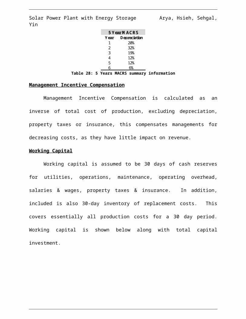
Solar Power Plant with Energy Storage Arya, Hsieh, Sehgal, Yin
100MW Cash Flows, NPV & IRR
Year 2008 2009 2010 2011 2012 2013 2014 2015 2016 2017 2018 2019 2020 2021 2022 2023 2024 2025 2026 2027 2028 2029PV Year 0 1 2 3 4 5 6 7 8 9 10 11 12 13 14 15 16 17 18 19 20 21Project Year 1 2 3 4 5 6 7 8 9 10 11 12 13 14 15 16 17 18 19 20
D&A & Debt CalculationsDep. Rates (5 Yr MACRS) 20% 32% 19% 12% 12% 6% 0% 0% 0% 0% 0% 0% 0% 0% 0% 0% 0% 0% 0% 0%
Beg. Of Year Values (000s) 691.80$ 553.44$ 332.06$ 199.24$ 119.54$ 39.85$ -$ -$ -$ -$ -$ -$ -$ -$ -$ -$ -$ -$ -$ -$ Tax depreciation (5 yr MACRS) 138.36$ 221.37$ 132.82$ 79.69$ 79.69$ 39.85$ -$ -$ -$ -$ -$ -$ -$ -$ -$ -$ -$ -$ -$ -$ Eng of year values 553.44$ 332.06$ 199.24$ 119.54$ 39.85$ -$ -$ -$ -$ -$ -$ -$ -$ -$ -$ -$ -$ -$ -$ -$
EnergyElectric energy production (GWh) 536.7875921 536.7875921 536.7875921 536.7875921 536.7875921 536.787592 536.7875921 536.7875921 536.7875921 536.7875921 536.787592 536.7875921 536.7875921 536.7875921 536.787592 536.7875921 536.7875921 536.7875921 536.7875921 536.7875921
IS & CF ($MM)Revenue 72.19$ 75.80$ 79.59$ 83.57$ 87.75$ 92.14$ 96.75$ 101.58$ 106.66$ 112.00$ 117.60$ 123.48$ 129.65$ 136.13$ 142.94$ 150.09$ 157.59$ 165.47$ 173.74$ 182.43$ Fixed O&M (40.62)$ (41.43)$ (42.26)$ (43.10)$ (43.96)$ (44.84)$ (45.74)$ (46.65)$ (47.59)$ (48.54)$ (49.51)$ (50.50)$ (51.51)$ (52.54)$ (53.59)$ (54.66)$ (55.76)$ (56.87)$ (58.01)$ (59.17)$ Variable O&M (0.20)$ (0.20)$ (0.20)$ (0.21)$ (0.21)$ (0.22)$ (0.22)$ (0.23)$ (0.23)$ (0.24)$ (0.24)$ (0.24)$ (0.25)$ (0.25)$ (0.26)$ (0.26)$ (0.27)$ (0.28)$ (0.28)$ (0.29)$ Property Tax & Insurance (7.34)$ (7.49)$ (7.64)$ (7.79)$ (7.95)$ (8.11)$ (8.27)$ (8.43)$ (8.60)$ (8.78)$ (8.95)$ (9.13)$ (9.31)$ (9.50)$ (9.69)$ (9.88)$ (10.08)$ (10.28)$ (10.49)$ (10.70)$ Tax D&A (138.36)$ (221.37)$ (132.82)$ (79.69)$ (79.69)$ (39.85)$ -$ -$ -$ -$ -$ -$ -$ -$ -$ -$ -$ -$ -$ -$
Total Expenses (186.51)$ (270.49)$ (182.93)$ (130.80)$ (131.82)$ (93.01)$ (54.23)$ (55.32)$ (56.42)$ (57.55)$ (58.70)$ (59.87)$ (61.07)$ (62.29)$ (63.54)$ (64.81)$ (66.11)$ (67.43)$ (68.78)$ (70.15)$ Operating Income (EBIT) (114.32)$ (194.69)$ (103.33)$ (47.22)$ (44.07)$ (0.87)$ 42.52$ 46.27$ 50.24$ 54.45$ 58.90$ 63.60$ 68.58$ 73.84$ 79.40$ 85.28$ 91.48$ 98.04$ 104.97$ 112.28$ Taxable Income (114.32)$ (194.69)$ (103.33)$ (47.22)$ (44.07)$ (0.87)$ 42.52$ 46.27$ 50.24$ 54.45$ 58.90$ 63.60$ 68.58$ 73.84$ 79.40$ 85.28$ 91.48$ 98.04$ 104.97$ 112.28$ Tax -$ -$ -$ -$ -$ -$ (14.88)$ (16.19)$ (17.58)$ (19.06)$ (20.61)$ (22.26)$ (24.00)$ (25.84)$ (27.79)$ (29.85)$ (32.02)$ (34.31)$ (36.74)$ (39.30)$ Earnings (114.32)$ (194.69)$ (103.33)$ (47.22)$ (44.07)$ (0.87)$ 27.64$ 30.08$ 32.66$ 35.39$ 38.28$ 41.34$ 44.58$ 48.00$ 51.61$ 55.43$ 59.47$ 63.73$ 68.23$ 72.98$ Add Back Depr 138.36$ 221.37$ 132.82$ 79.69$ 79.69$ 39.85$ -$ -$ -$ -$ -$ -$ -$ -$ -$ -$ -$ -$ -$ -$ Cash Flows (369.14)$ (369.14)$ 24.04$ 26.69$ 29.49$ 32.47$ 35.63$ 38.97$ 27.64$ 30.08$ 32.66$ 35.39$ 38.28$ 41.34$ 44.58$ 48.00$ 51.61$ 55.43$ 59.47$ 63.73$ 68.23$ 72.98$ Repayment of debt principalDiscount Factor 1.0000 0.8696 0.7561 0.6575 0.5718 0.4972 0.4323 0.3759 0.3269 0.2843 0.2472 0.2149 0.1869 0.1625 0.1413 0.1229 0.1069 0.0929 0.0808 0.0703 0.0611 0.0531
PV ($MM) (369.14)$ (320.99)$ 18.18$ 17.55$ 16.86$ 16.14$ 15.40$ 14.65$ 9.03$ 8.55$ 8.07$ 7.61$ 7.16$ 6.72$ 6.30$ 5.90$ 5.52$ 5.15$ 4.81$ 4.48$ 4.17$ 3.88$ Cum. PV (369.14)$ (690.13)$ (671.95)$ (654.41)$ (637.54)$ (621.40)$ (606.00)$ (591.35)$ (582.31)$ (573.76)$ (565.69)$ (558.08)$ (550.93)$ (544.21)$ (537.91)$ (532.01)$ (526.50)$ (521.34)$ (516.54)$ (512.06)$ (507.89)$ (504.02)$
NPV (504.02)$ IRR 1%
$-
$10.00
$20.00
$30.00
$40.00
$50.00
$60.00
$70.00
$80.00
1 2 3 4 5 6 7 8 9 10 11 12 13 14 15 16 17 18 19 20
100MW Plant Cash Flows, $MM
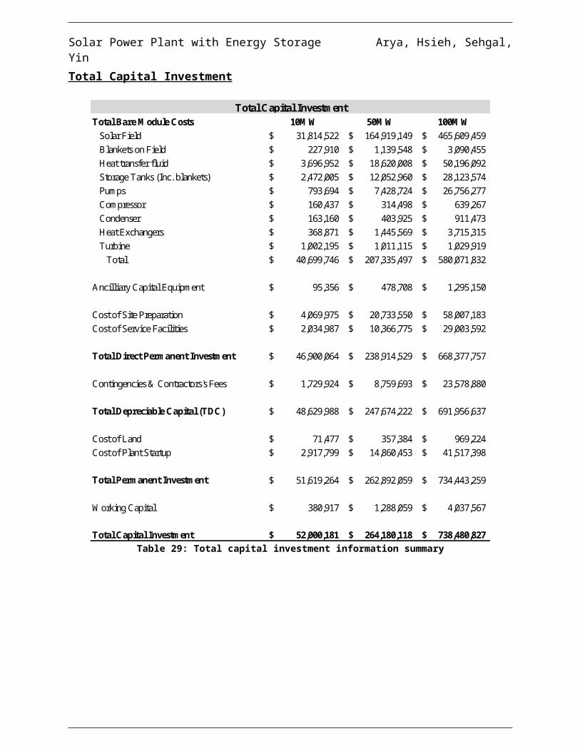
Solar Power Plant with Energy Storage Arya, Hsieh, Sehgal, Yin
Sensitivity Analysis
Justification of HTF fluid – Selection of Hitec
Table 32: Selection of a HTF summary information
As shown in Table 32, using a molten salt such as Solar Salt, Hitec or Hitec XL instead
of synthetic oil Therminol VP-1 will net cost savings, lead to approximately a six percent
decrease in LEC and a 13 to 16% decrease in negativity of the NPV. In addition, Therminol VP-
1’s upper temperature limit of 400 °C eliminates it as an ideal candidate for higher operating
temperature. Therefore, Hitec was selected as the HTF, due to its economic viability and a
desirable breakdown point of 535°C and freezing point of 142°C, as mentioned above in the
design section.
Sample Sensitivity Analysis Around Base Case
As shown in the prior cost analysis, given the current market and legal conditions, solar
energy is not profitable competing against other power generation technologies. In this
following section, an examination of the key drivers of financial viability and profitability is
presented. LEC and NPV are used as profitability measures. The base case input summary is
given in Table 33. All variables in following sensitivity analyses follow these inputs, unless
otherwise specified.
Case MetricLevelized Cost NPV ($MM)
Therminol VP-1 0.20775$ (48.421)$ Solar Salt* 0.19460$ (40.646)$
% of base 93.67% 83.94%
Hitec 0.19450$ (40.304)$ % of base 93.62% 83.24%
Hitec XL 0.19731$ (41.969)$ % of base 94.97% 86.67%
* Note that Solar Salt has freezing temp of 220 which is adjusted for.

Solar Power Plant with Energy Storage Arya, Hsieh, Sehgal, Yin
Table 33: Model input summary
Output Variables
Levelized Electricity Cost (LEC)
LEC indicates per unit price of the electricity generated, taking into account certain legal
situations such as taxation and depreciation. However, it is not affected by revenue projection,
since it calculates the hypothetical revenue generated to cover the cost of the plant over its
lifetime. It can also be compared to the LECs of alternative power generation methods, as given
on page 61.
Net Present Value (NPV)
NPV demonstrates the viability of the plant to investors. It takes into consideration both
the cost of the plant as well as its revenue generation ability. Thus, external factors affecting
electricity pricing also affect NPV. Some of the financial variables below only affect revenues,
and as such, they have no impact on LEC, but do have significant impact on project NPV.
Cases in which NPV and LEC give divergent conclusions are those in which electricity
generation is not profitable. However, due to federal action, such as taxation or subsidy, the
Levelized Cost ($/kWh) $0.194504NPV ($MM) ($29.44774)NPV SUB $2.70573Inputs scale unitsFinal Plant Output Size 10 MWPlant Output Size 11.25222343 MWDaytime Optl.Heat Duty 60.19 MWStorage Heat Duty 22.57 MW
Total Field Heat Duty 82.76 MWImplied Solar to Out Eff. 17.00% %Sunlight Hrs 8 hrs
Hours Storage 3 hrsDelta T Drop 140.00 °CSolar In 260.00 °C
Solar In (K) 533.00 K
Solar Out 400.00 °CSolar Out (K) 673.00 K
Delta T Min 10 K
HTF Selection 2 Hitec

Solar Power Plant with Energy Storage Arya, Hsieh, Sehgal, Yin
project may become attractive to investors. In such cases, NPV is compelling and indicates
profitability, while LEC does not.
Plant Design Variables
Plant Scale (MW)
Scale represents power output. The 100 MW has a higher required TCI, but may
generate a higher NPV or return due to scale benefits in equipment costs.
Operating Temperature
Operating temperature is determined by the amount of heat collected by the solar field.
An increase in operating temperature will require more solar collectors on the field side, but will
yield a higher efficiency in the Rankine cycle, which may offset the increase solar collector
demand.
Temperature Drop
Similar to operating temperature, increasing the temperature drop means more energy extraction
per pass from the field through the heat exchanger. This means the field may demand more
loops to reheat the “colder” HTF.
Storage Hours
Increasing the storage hours allows increased revenue via increased energy production,
though off-peak energy is sold at a lower price and therefore may be less profitable. Increase in
storage hours will also increase field demand and TES system costs of tanks and HTF.
$Cost/SCA
Because the solar field is the largest cost component, the cost per SCA which would
allow a solar plant to achieve financial viability is of primary interest.

Solar Power Plant with Energy Storage Arya, Hsieh, Sehgal, Yin
TDC (Total Depreciable Capital) Multiplier
Similar to the $Cost/SCA variable, varying the TDC multiplier demonstrates how much
overall investment costs affects LEC and NPV.
Ambient Variables
Flux, temperature, incident angle, sunlight hours represent the operating conditions
surrounding the plant, and will vary by day, season and weather. Varying ambient variables
against LEC and NPV help determine how ideal placement or non-ideal weather conditions can
affect power generation expectations.
Financial Variables
Return on Equity
ROE supplies the discount rate for this project, a measure of return required for risk
assumed. Sensitivity to a lower discount rate of 10% will be tested for, as a proxy for the
assumption of debt or the operation by a public utility, both of which would lower the required
return.
$/kWh Subsidy (NPV only)
The viability of the plant is affected by whether the operation receives tax-free subsidies
from the government for power generation. A 15 cent subsidy is selected based on the 0.12-0.18
Euro subsidy received in Spain.
Tax Rate Decreases
The external tax factor will affect cash flow expectations. Public utilities are taxed at
different rates than investor-owned utilities, and we believe a publically owned structure would
benefit NPV and LEC.

Solar Power Plant with Energy Storage Arya, Hsieh, Sehgal, Yin
Electricity Start Price (NPV only)
8.85 cents per kWh, which was the average price of electricity in 2006, is used as base
year price to drive revenue projections going forward with assumption of a growth rate. Since
the plant goes into operation in 2010, this assumption might not accurately reflect pricing.
Testing this base year unit price assumption shows how much it affects projected profitability.
Ratio of Peak-to-Off-Peak Pricing (NPV only)
A 5:1 ratio is assumed for peak-time prices against off-peak prices. This ratio will affect
the attractiveness of thermal energy storage, since marginal hours will be cheaper or more
expensive.
Energy Inflation (NPV only)
Market electricity prices is assumed to grow at 5%, but the last few years have seen
remarkable price inflation for energy. Growth rate assumption is varied to demonstrate how
sensitive profitability is to revenue growth rate.
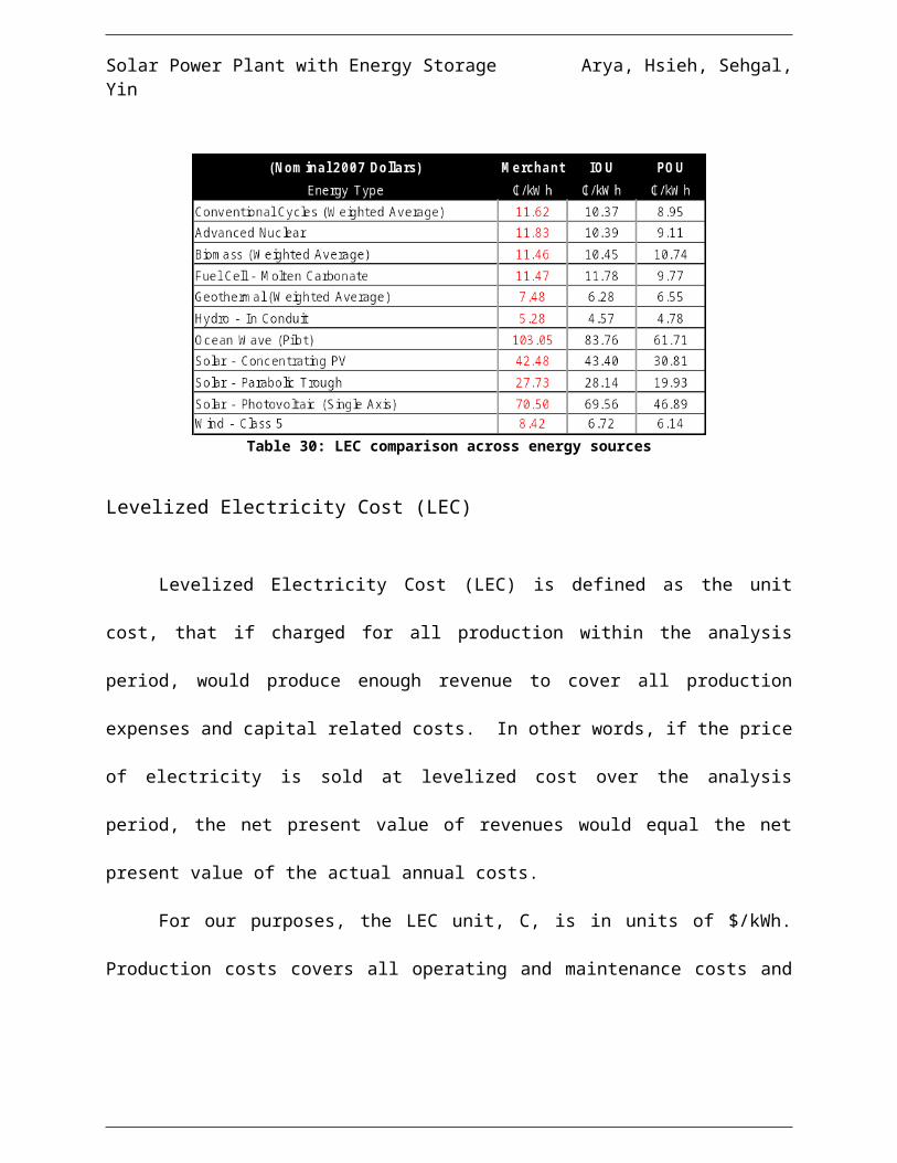
Solar Power Plant with Energy Storage Arya, Hsieh, Sehgal, Yin
Summary Data
Table 34: LEC sensitivity at base case to input variables summary information
Table 35: NPV sensitivity at base case to input variables summary information
Variables Summary ( Levelized Cost ) Base Assumption Input Variable % of base Levelized Cost % of b ase
Plant Design VariablesPlant Scale (MW) 10 50 500% 0.15354 78 .94%
Operating Temperature 400 500 125% 0.19982 10 2.73%
Temperature Drop (Solar out - Solar in)* 140 225 161% 0.19146 98 .43%
Storage Hours 3 5 167% 0.18116 93 .14%
$ Cost / SCA 147 100 68% 0.17426 89 .59%TDC sensitivity (% inflation) 100% 75% 75% 0.17350 89 .20%
AmbientFlux (W/m2) 940 1034 110% 0.18673 96 .00%
Temperature (°C) 22.6 20.34 90% 0.19468 10 0.09%
Incident Angle 0.6730 0.7403 110% 0.18673 96 .00%Sunlight Hours 8 10 125% 0.16081 82 .67%
Financial VariablesROE (%) 15% 10% 67% 0.19788 10 1.74%Tax rate decrease 35% 10% 29% 0.18930 97 .33%
* Note that Hitec has freezing temp of 142 which lead us to adju st Solar out for this to 500
Variables Summary ( NPV ) Base Assumption Input Variable % of base NPV ($MM) % of b ase
Plant Design VariablesPlant Scale (MW) 10 50 500% (165.647) 41 0.99%
Operating Temperature 400 500 125% (43.982) 10 9.13%
Temperature Drop (Solar out - Solar in)* 140 225 161% (38.690) 95 .99%
Storage Hours 3 5 167% (45.739) 11 3.48%
$ Cost / SCA 147 100 68% (28.042) 69 .58%TDC sensitivity (% inflation) 100% 75% 75% (27.583) 68 .44%
AmbientFlux (W/m2) 940 1034 110% (35.823) 88 .88%
Temperature (°C) 22.6 20.34 90% (40.418) 10 0.28%
Incident Angle 0.6730 0.7403 110% (35.823) 88 .88%Sunlight Hours 8 10 125% (32.106) 79 .66%
Financial VariablesROE (%) 15% 10% 66.7% (36.447) 90 .43%
$/kWh Subsidy 0.00 0.15 NA (8.151) 20 .22%
Tax Rate Decrease 35% 10% 29% (38.527) 95 .59%Electricity Start price (cents) 8.85 10.00 113% (36.163) 89 .73%
Ratio of Peak:OffPeak Pricing 5.01 4.00 80% (46.728) 11 5.94%
Energy Inflation 5% 10% 200% (29.448) 73 .06%
* Note that Hitec has freezing temp of 142 which lead us to adju st Operating Temperature for th is to 500

Solar Power Plant with Energy Storage Arya, Hsieh, Sehgal, Yin
Discussion of Summary Data
Plant Design Variables
Plant Scale and Storage Hours
Scale lowers lowers LEC (Table 34). Although NPV is further negative (Table 35), its
proportion is less than the increased proportion in generated powered.
Operating Temperature & Temperature Drop
Given current HTF options, changing the operating temperature and temperature drop do
not lead to significant performance benefits for either LEC or NPV measures. Please see Long
Term Viability (page 90) for further discussion on conditions in which operating temperature and
temperature drop become significant drivers.
$ Cost/SCA and TDC sensitivity
Plant viability appears highly sensitive to these two variables, decreasing both LEC as
well as NPV negativity. The impact on the metric is nearly scalar with the change in the input.
Ambient Variables
There are no unanticipated drivers to viability here. Temperature does not have a
significant effect as it is small compared with operating temperatures. Gains in flux, incident
angle, and sunlight hours all yield the expected conclusion: more sunlight is better, less is worse.
Financial Variables
ROE
At current levels conditions, ROE does not appear to dramatically affect the two metrics.
The negative cash flows from upfront investment are significantly larger than the positive cash

Solar Power Plant with Energy Storage Arya, Hsieh, Sehgal, Yin
flows that follow. The negativity of the plant cash flows only becomes more negative as ROE
increases.
Electricity Start Price and Ratio of Peak-to-Off-Peak Pricing
These measures have a very small affect on overall NPV even though they directly affect
revenue projection. Thus, the original assumptions are valid assumptions for the model, as both
come from historical data.
$/kWh Subsidy
A subsidy drastically and rapidly lowers the negativity of NPV and could turn the plant
NPV positive. Please see the scenario analysis in the follow section for more information (page
81 and 87).
Tax Rate Decrease and Energy Inflation
With high probabilities of occurrence in the real world, further discussion of these
variables is required. Please see the scenario analysis in the follow section for more information
(page 81 and 87).
Based on the sensitivity analysis of various drivers of profitability, the identifiable key
drivers for LEC are scaling of Plant, $Cost/SCA, TDC multiplier, Storage Hours, and Tax Rate
decrease.
Key drivers for NPV are Plant Scale, $Cost/SCA, TDC multiplier, Storage Hours, $/kWh
subsidy, Tax Rate decrease, and Energy inflation.
Scenario Analysis
In order to see in which cases solar LEC becomes competitive with fossil fuels, two
idealized cases are examined. Input variables are plotted against each other to identify points for
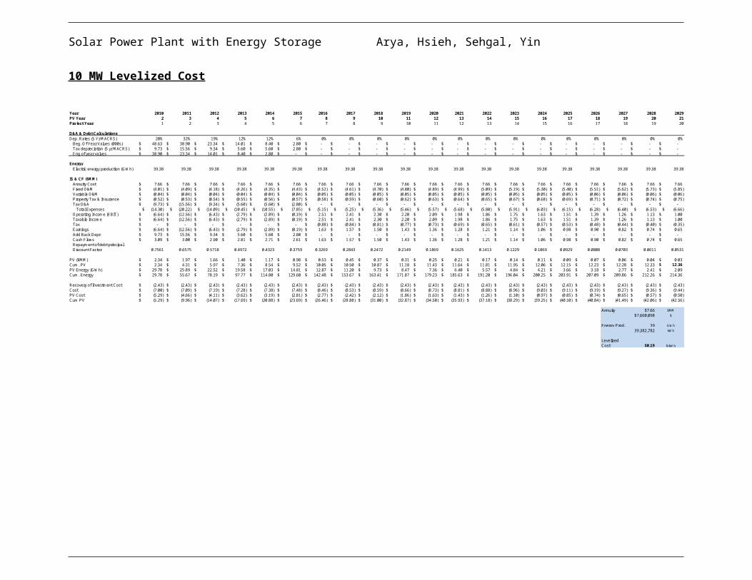
Solar Power Plant with Energy Storage Arya, Hsieh, Sehgal, Yin
competitive LEC and NPVs greater than 0. These points indicate the combination of input
variables which allow the project to be financially viable and are highlighted in light green.
Scenario 1: Idealized Legal Environment, Significant decrease in SCA Costs, paired with
Energy Inflation
In this scenario, two key assumptions are: 1) the legal environment allows for beneficial
taxation and subsidies to renewable solar energy and 2) increased suppliers producing SCAs
improve technology and drives down costs. Concurrently, constant energy price inflation of
10% allows more revenues while costs stay constant.
Case Variables
50MW Plant 8 hrs sunlight 3 hrs storage 10% taxation $0.15/kWh subsidy 10% energy inflation $100/m2 of Solar Collector
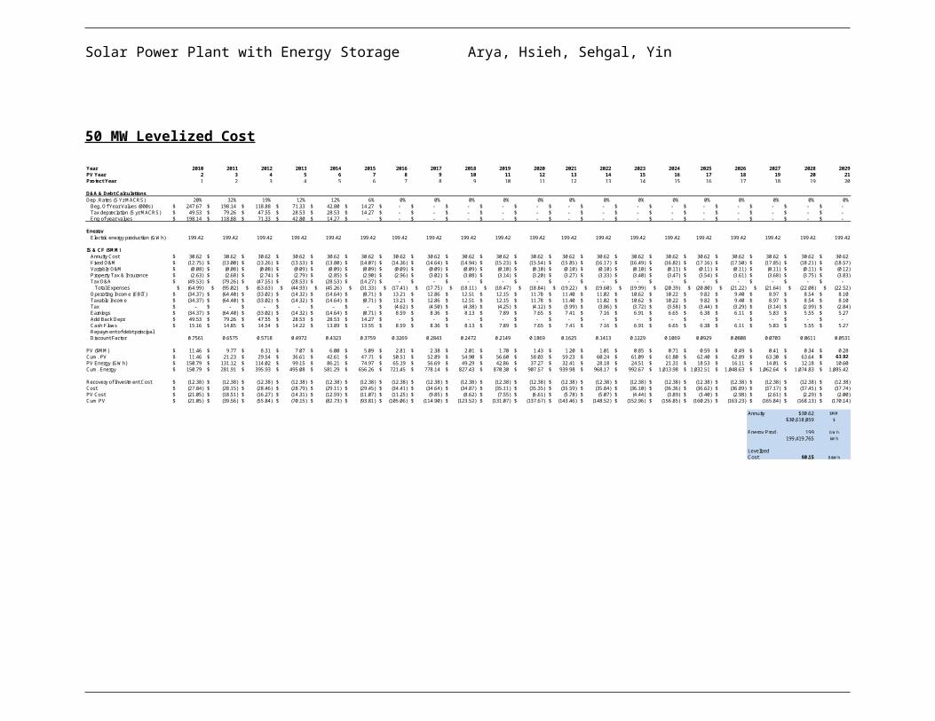
Solar Power Plant with Energy Storage Arya, Hsieh, Sehgal, Yin
LEC Sensitivity to $ Cost/SCA and Plant Scaling
Figure 19: LEC Sensitivity to $ Cost/SCA and Plant Scaling
Table 36: LEC sensitivity to $ cost/SCA and plant scaling summary information
As can be seen above in Figure 19 and Table 36, parabolic solar trough technology
becomes attractive from a LEC perspective as SCA costs decrease to the $50-100/m2 range. The
50 MW plant scale is favored over 100 MW scaling. This is because parasitic losses stemming
from piping issues become tremendous at 100 MW and outweigh other scaling gains. However,
both plant scales are advantageous compared to 10 MW scaling.
10
50
100
0.000
0.050
0.100
0.150
0.200
5075
100125
150
Plant Scaling
Leve
lized
Cos
t
$ Cost/SCA
Levelized Cost Solar Collector Price ($/m 2)
Plant Output (MW) 50 75 100 125 15010 0.151 0.161 0.171 0.181 0.19050 0.108 0.118 0.128 0.138 0.147
100 0.121 0.131 0.141 0.150 0.161* Levelized Cost is ($/kWh)
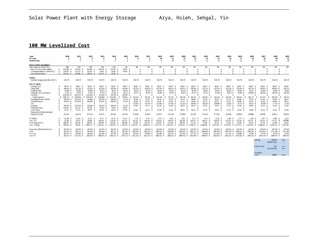
Solar Power Plant with Energy Storage Arya, Hsieh, Sehgal, Yin
NPV Sensitivity to $ Cost/SCA and Plant Scaling
Figure 20: NPV Sensitivity to $ Cost/SCA and Plant Scaling
Table 37: NPV sensitivity to $ cost/SCA and plant scaling summary information
Similarly, an NPV perspective yields a similar cut-off region with respect to $Cost/SCA
for viability, even without government subsidy. As we can see from Figure 20 and Table 37, the
$75 SCA cost is the approximate cutoff for viability in this case, where NPV becomes positive
without governmental subsidy. It is worthwhile to note that the larger plant size scaling respond
more quickly to SCA price decrease than the smallest plant size, further indicating that they take
advantage of economies of scale.
10
50
100-300.0
-200.0
-100.0
0.0
100.0
200.0
5075
100
125
150
Plant Scaling
Plan
t NPV
$ Cost/SCA
NPV Solar Collector Price ($/m 2)
Plant Output (MW) 50 75 100 125 15010 1.1 -5.4 -11.9 -18.5 -25.050 53.2 20.5 -12.3 -45.3 -78.3
100 106.9 18.9 -71.6 -158.8 -247.8* NPV is ($MM), Subsidy is fixed @ $ 0
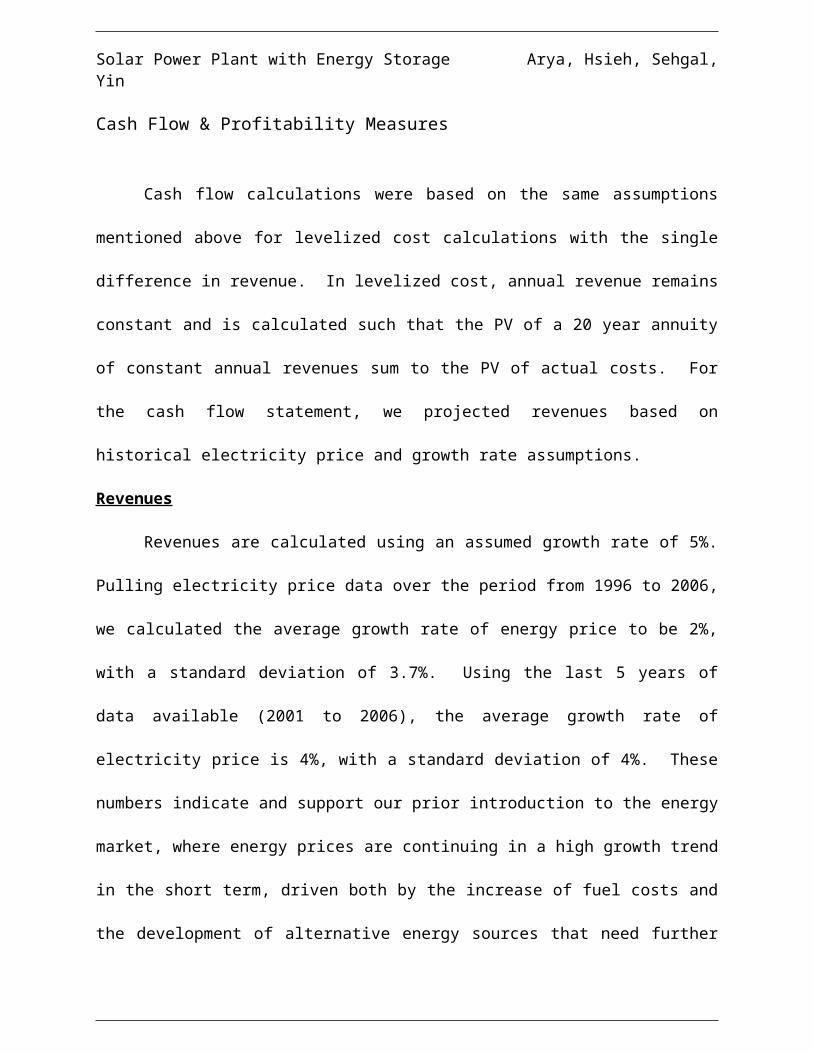
Solar Power Plant with Energy Storage Arya, Hsieh, Sehgal, Yin
NPV Sensitivity to $ Cost/SCA and $/kWh Subsidy
Figure 21: NPV Sensitivity to $ Cost/SCA and $/kWh Subsidy
Table 38: NPV sensitivity to $cost/SCA and $/kWh subsidy summary information
Factoring in an assumed government subsidy, the case is even more favorable. As we
can see from Figure 21 and Table 38, at a 10 cent per kWh subsidy, all SCA prices become
irrelevant as the project is always positive NPV, so even without SCA price declines a $0.10
subsidy will lead to commercial competitiveness of the technology.
0
5
10
15
20
-100.0
-50.0
0.0
50.0
100.0
150.0
200.0
250.0
300.0
5075
100125
150Cents /kWh Subsidy
Plan
t NPV
$ Cost/SCA
NPV w/ Subsidy Solar Collector Price ($/m 2)
$/kWh Subsidy 50 75 100 125 1500 53.2 20.5 -12.3 -45.3 -78.35 107.5 74.8 42.0 9.0 -24.1
10 161.8 129.0 96.3 63.3 30.215 216.0 183.3 150.6 11 7.6 84.520 270.3 237.6 204.8 171.8 138.8
* NPV is ($MM), Plant output is fixed @ 50MW

Solar Power Plant with Energy Storage Arya, Hsieh, Sehgal, Yin
LEC Sensitivity to Hours of Storage and Plant Scaling
Figure 22: LEC Sensitivity to Hours of Storage and Plant Scaling
Table 39: LEC sensitivity to hours of storage and plant scaling summary information
In Figure 22 and Table 39, 10, 50 and 100 MW plants demonstrate divergent trends with
respect to LEC as storage hour increase. The 10 MW plant’s relatively low TES and pumping
burden causes it to be cheaper from a LEC perspective than the larger scaled 50 and 100 MW
plants. It is then cheaper to add on TES storage hours to the 10 MW plant, lowering the LEC
rather than raising it. This may be a significant consideration for future project managers.
However, the 50 MW plant shows that levelized cost decreases with increasing storage hours to
about six hours before it increases again, indicating an optimal point. On the other hand, LEC
follows an increasing trend for the 100 MW plant as storage increases.
0.000
0.050
0.100
0.150
0.200
0.250
0 2 4 6 8 10 12 14 16
Leve
lized
Cos
t
Hours of Storage
10 50 100
Levelized Cost Hours StoragePlant Output (MW) 0 3 6 10 14
10 0.202 0.171 0.152 0.139 0.13250 0.131 0.128 0.127 0.132 0.143
100 0.125 0.141 0.144 0.146 0.147* Levelized Cost is ($/kWh), SCA Cost fixed @ $100/m 2, Plant output is fixed @ 50MW

Solar Power Plant with Energy Storage Arya, Hsieh, Sehgal, Yin
NPV Sensitivity to Subsidy and Energy Inflation
Figure 23: NPV Sensitivity to Subsidy and Energy Inflation
Table 40: NPV sensitivity to subsidy and energy inflation summary information
Figure 23 and Table 40 demonstrate the importance of inflation effects on our plant
viability. Assuming an inflationary electricity environment of 10% or greater, profitability
increases rapidly due to extremely higher future revenues. NPV is most sensitive to the cash
flows of the first few years since future cash flows are discounted significantly. Thus, even 5
years of high price inflation will generate a very high NPV.
0
5
10
15
20
-200.0
-100.0
0.0
100.0
200.0
300.0
400.0
500.0
600.0
00.05
0.10.15
0.2
Cents /kWh Subsidy
Plan
t NPV
Energy Inflation
NPV w/ Subsidy Energy Inflation
$/kWh Subsidy 0 0.05 0.1 0.15 0.20 -129.5 -84.3 -12.3 105.9 304.65 -75.2 -30.0 42.0 160.1 358.9
10 -21.0 24.2 96.3 214.4 413.215 33.3 78.5 150.6 268.7 467.520 87.6 132.8 204.8 322.9 521.7
* NPV is ($MM), SCA Cost fixed @ $100/m2, Plant output is fixed @ 50MW
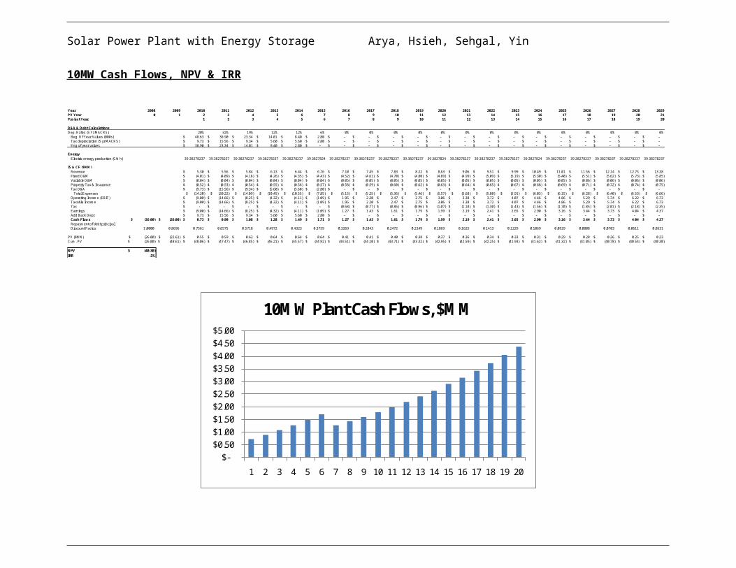
Solar Power Plant with Energy Storage Arya, Hsieh, Sehgal, Yin
Scenario 2: Moderately favorable legal environment, Moderate decreases in SCA Cost,
Energy inflation muted.
This scenario is a less aggressive version of Scenario 1.
Case Variables:
50MW Plant 8 hrs sunlight 3 hrs storage 10% taxation, $0.05/kWh subsidy 5% energy inflation $125/m2 of Solar Collector
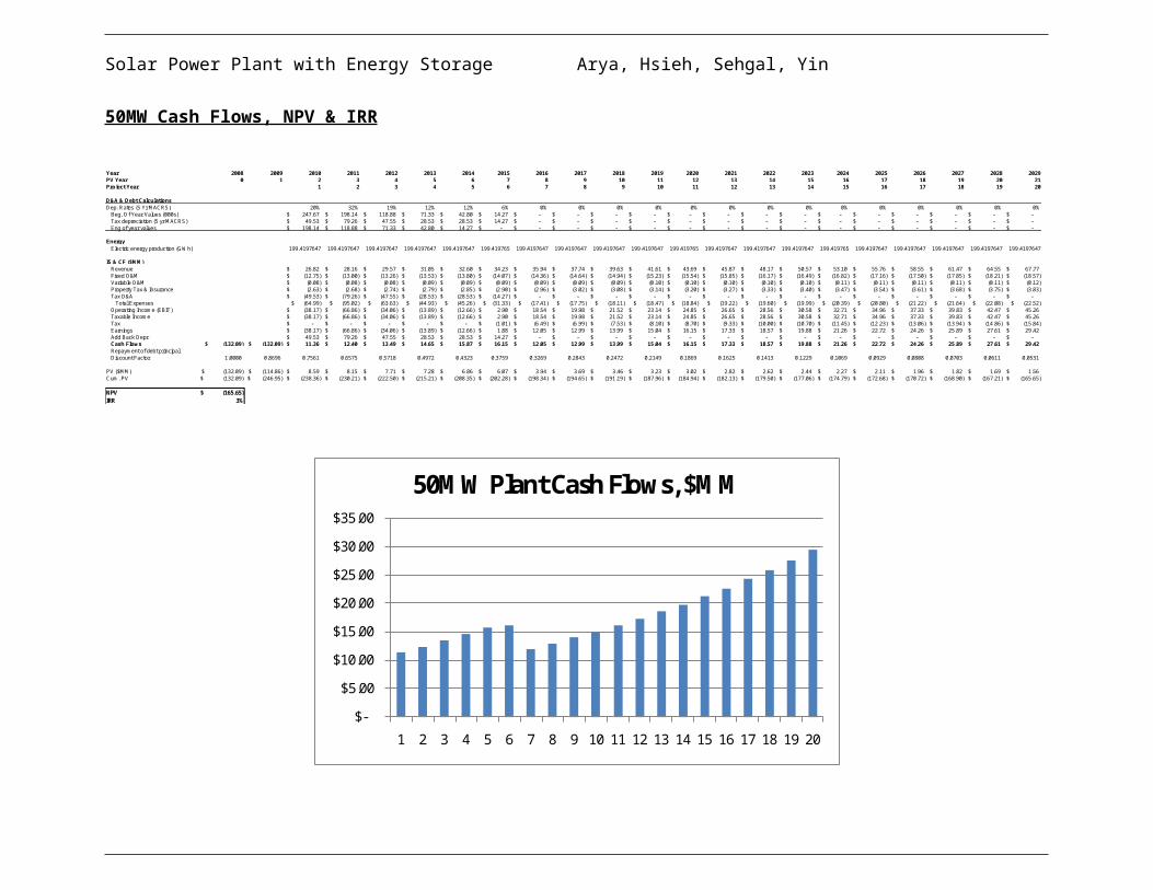
Solar Power Plant with Energy Storage Arya, Hsieh, Sehgal, Yin
Figure 24: NPV Sensitivity to Plant Scaling and $ Cost/SCA
Table 41: NPV sensitivity to subsidy and $ cost/SCA
Figure 25: NPV Sensitivity to $/kWh Subsidy and $ Cost/SCA
10
50
100
0.000
0.050
0.100
0.150
0.200
100115
125135
150
Plant Scaling
Leve
lized
Cos
t
$ Cost/SCA
Levelized Cost Solar Collector Price ($/m2)
Plant Output (MW) 100 115 125 135 15010 0.171 0.177 0.181 0.185 0.19050 0.128 0.134 0.138 0.142 0.147
100 0.141 0.146 0.150 0.155 0.160* Levelized Cost is ($/kWh)
02.5
57.5
10
-200.0
-150.0
-100.0
-50.0
0.0
50.0
100115
125135
150
Cents /kWh Subsidy
Plan
t NPV
$ Cost/SCA

Solar Power Plant with Energy Storage Arya, Hsieh, Sehgal, Yin
Table 42: NPV sensitivity to $/kWh subsidy and $ cost/SCA
Table 43: NPV sensitivity to plant scaling and $ cost/SCA
Figure 26: LEC Sensitivity to Hours Storage and Plant Scaling
Table 44: LEC sensitivity to hours storage and plant scaling
Table 45: NPV sensitivity to $/kWh subsidy and energy inflation
Levelized Cost Hours StoragePlant Output (MW) 0 3 6 10 14
10 0.212 0.181 0.161 0.149 0.14150 0.141 0.138 0.137 0.142 0.154
100 0.135 0.151 0.154 0.156 0.157* Levelized Cost is ($/kWh), SCA Cost fixed @ $125/m 2, Plant output is fixed @ 50MW
NPV Solar Collector Price ($/m2)
Plant Output (MW) 100 115 125 135 15010 -26.2 -30.1 -32.7 -35.4 -39.350 -84.3 -104.2 -117.4 -130.6 -150.5
100 -263.9 -319.2 -353.0 -388.6 -443.9* NPV is ($MM), Subsidy is fixed @ $ 0
0.000
0.050
0.100
0.150
0.200
0.250
0 2 4 6 8 10 12 14 16
Leve
lized
Cos
t
Hours of Storage
10 50 100
NPV w/ Subsidy Solar Collector Price ($/m2)
$/kWh Subsidy 100 115 125 135 1500 -84.3 -104.2 -117.4 -130.6 -150.5
2.5 -57.2 -77.0 -90.3 -103.5 -123.35 -30.0 -49.9 -63.1 -76.4 -96.2
7.5 -2.9 -22.8 -36.0 -49.2 -69.110 24.2 4.4 -8.8 -22.1 -41.9
* NPV is ($MM), Plant output is fixed @ 50MW
NPV w/ Subsidy Energy In flation
$/kWh Subsidy 0 0.01 0.025 0.04 0.050 -162.7 -155.1 -142.5 -128.1 -117.4
2.5 -135.5 -128.0 -115.4 -101.0 -90.35 -108.4 -100.8 -88.2 -73.9 -63.1
7.5 -81.3 -73.7 -61.1 -46.7 -36.010 -54.1 -46.6 -34.0 -19.6 -8.8
* NPV is ($MM), SCA Cost fixed @ $125/m2, Plant output is fixed @ 50MW

Solar Power Plant with Energy Storage Arya, Hsieh, Sehgal, Yin
The intention of generating a less aggressive scenario with moderately favorable
conditions is to test if solar power viability can be achieved under these slightly more realistic,
while less ideal conditions. As seen in the above tables and figures, the project only becomes
competitive on the outer band of the assumption sensitivities, which edge into Scenario 1’s
range. Thus, solar power will only become competitive in circumstances where the legal,
manufacturing, and electricity market all have favorable conditions in the near-term, similar to
the assumptions made in Scenario 1. Less favorable scenarios yield non-desirable results and
will not drive to project viability.
A close examination shows that with a 10 cent subsidy, the project becomes NPV viable
at SCA prices of 100-115, as seen in Table 41 and Table 45, whereas in scenario 1, a 10 cent
subsidy makes SCA prices irrelevant up to $150, as seen in Table 38.
Long Term Viability
With existing materials, solar trough power plants are only attractive given ideal conditions.
However, in the long-run, scientific innovation can do much to make solar trough a more
attractive technology. The primary requirements are:
Improvements in efficiency, which include:
o Rankine cycle efficiency
Higher operating temperature and better turbine design
o Improvements in collector efficiency and heat loss prevention
Discovery of ideal HTF

Solar Power Plant with Energy Storage Arya, Hsieh, Sehgal, Yin
The improvements in efficiency will lower the field heat duty requirements. This in turn
lowers SCA and pumping requirements, which are significant contributors to cost. The
discovery of an ideal HTF also can have a similar result. Ideal HTF would require less fluid and
operate at higher temperatures for efficiency gains. Ongoing research is exploring better molten
salts, but at the moment, nitrate salts are the best options given conventional piping.
Economic Sensitivity Summary
Key Drivers, Short Term:
SCA cost decreases (< $100/m2)
Favorable Legal environment: $/kWh subsidy (10 cents), favored tax status (10%)
Market Electricity price inflation (10% or greater)
Key Drivers, Long Term:
Cycle Improvements
HTF Discovery

Solar Power Plant with Energy Storage Arya, Hsieh, Sehgal, Yin
Conclusion & Recommendations
Conclusion
The specified power plants at 10, 50 and 100MW scales are:
Table 46: Financial metrics at different plant scalings
This indicates that given current conditions solar trough and thermal energy storage are
not viable in the market. However, as illustrated in our economic sensitivity analyses, there are
conditions that have some likelihood of occurrence in the future that will result in profitable
operation of any scaling of plant, largely dependent on subsidy legislation and reductions in SCA
cost. For more information, please see the sensitivity analysis beginning on page 80
Recommendations
In order to achieve a more extensive report, we would make the following recommendations:
It would be preferable to have lab-scale testing of thermodynamic data to verify we can
achieve the heat capacities we are assuming.
More accurate insight on legal considerations will likely be the primary drivers to
viability outside of technological innovation.
A more detailed investigation of turbine design and waste heat recycling would yield
efficiency improvements.
More up-to-date quotes on equipment for comparison and benchmarking data would be
ideal for analysis.
More trough power plant related non-equipment related costs to flesh out a full operating plant costing would be idea
Financial Metric vs Plant Scaling10 50 100
LEC 0.19$ 0.15$ 0 .17$ NPV (41) (169) (470)

Solar Power Plant with Energy Storage Arya, Hsieh, Sehgal, Yin
Acknowledgements
We would like to thank Mr Adam Brostow of Air Products and Chemicals, Inc. for his
thoughtful problem statement and his help in ASPEN. In addition, we would like to extend our
thanks to Dr Raymond J. Gorte of the University of Pennsylvania for his continued guidance and
Professor Fabiano for his mentorship through the design process. Finally, we thank our friends in
the Chemical Biomolecular Engineering Senior Class of the School of Engineering and Applied
Science of the University of Pennsylvania, 2008 for their wonderful company these past four
years.

Solar Power Plant with Energy Storage Arya, Hsieh, Sehgal, Yin
Bibliography
Ausra, Inc. (2007). An Introduction to Solar Thermal Electric Power. Palo Alto, CA.
Dudley, V. E. (1994). SEGS LS-2 Solar Collector Test Results. Springfield, VA: US Department of Commerce.
Energy Information Administration. (2007). EIA-State & Historical Energy Information & Statistics. Retrieved March 2008, from Energy Information Administration: http://www.eia.doe.gov/overview_hd.html
Forristall, R. (2003). Heat Transfer Analysis and Modeling of a Parabolic Trough Solar Receiver Implemented in Engineering Equation Solver. Golden, CO: NREL.
Herrmann, U., & Kearney, D. (2002). Survey of Thermal Energy Storage for Parabolic Trough Power Plants. ASME.
Kearney, D. e. (2003). Overview on Use of a Molten Salt. Golden, CO: NREL.
Kearney, D. (2007). Parabolic Trough Collector Overview. Golden, CO.
Kelly, B. (2004). Parabolic Trough Solar System Piping Model. Golden, CO: NREL.
Lüpfert, E. (2001). Eurotrough Design Issues and Prototype Testing at PSA. ASME.
NC State University. (2007). Database of State Incentives for Renewables & Efficiency. Retrieved March 2008, from DSIRE: http://www.dsireusa.org/
NREL. (2008, March). TroughNet. Retrieved January 2008, from TroughNet: http://www.nrel.gov/csp/troughnet/
Owens, B. (2003). The Value of Thermal Storage. Golden, CO: The McGraw Hill Companies.
Price, H. (2002). Concentrating Solar Power Systems Analysis & Implications. SunLab/NREL.
Sargent & Lundy LLC Consulting Group. (2003). Assessment of Parabolic Trough and Power Tower Solar Technology Cost and Performance Forecasts. Golden, CO: NREL.
Seider, W. e. (2004). Product & Process Design Principles. New York, NY: John Wiley & Sons, Inc.
Solargenix Energy. (2006). An Overview of the Concentrating Solar Power Industry. Las Vegas, NV.

Solar Power Plant with Energy Storage Arya, Hsieh, Sehgal, Yin