Embed Size (px)
Citation preview
Academic Press30 Corporate Drive, Suite 400Burlington, MA 01803, USA
Linacre House, Jordan HillOxford OX2 8DP, UK
Copyright # 2009, Elsevier Inc. All rights reserved.
Designations used by companies to distinguish their products are often claimed astrade-marks or registered trademarks. In all instances in which Academic Press isaware of a claim, the product names appear in initial capital or all capital letters.Readers, however, should contact the appropriate companies for more completeinformation regarding trademarks and registration.
No part of this publication may be reproduced, stored in a retrieval system, ortransmitted in any form or by any means, electronic, mechanical, photocopying,recording, or otherwise, without the prior written permission of the publisher.
� Recognizing the importance of preserving what has been written, Elsevier prints itsbooks on acid-free paper whenever possible.
Permissions may be sought directly from Elsevier’s Science & Technology RightsDepartment in Oxford, UK: phone: (þ44) 1865 843830, fax: (þ44) 1865 853333,e-mail: [email protected]. You may also complete your request on-line via the Elsevier homepage (http://www.elsevier.com), by selecting ‘‘Support &Contact’’ then ‘‘Copyright and Permission’’ and then ‘‘Obtaining Permissions.’’
MATLAB and Simulink are registered trademarks of The MathWorks, Inc. Seewww.mathworks.com/trademarks for a list of additional trademarks. The MathWorksPublisher Logo identifies books that contain MATLABo and/or Simulinko. Used withpermission. The MathWorks does not warrant the accuracy of the text or exercises in thisbook. This book’s use or discussion of MATLABo and/or Simulinko software or relatedproducts does not constitute endorsement or sponsorship by The MathWorks of a particularuse of the MATLABo and/or Simulinko software or related products.
For MATLABo and Simulinko product information, or information on other relatedproducts, please contact: The MathWorks, Inc., 3 Apple Hill Drive, Natick, MA,01760-2098 USA; Tel: 508-647-7000; Fax: 508-647-7001; E-mail: [email protected],Web: www.mathworks.com
Library of Congress Cataloging-in-Publication DataApplication submitted.
ISBN: 978-0-12-374446-3
British Library Cataloguing-in-Publication DataA catalogue record for this book is available from the British Library.
For information on all Academic Press publications,visit our Web site at www.elsevierdirect.com.
Printed in the United States of America09 10 11 12 13 10 9 8 7 6 5 4 3 2 1
Preface
This second edition continues the author’s attempt to present linear elasticity with sound,
concise theoretical development, numerous and contemporary applications, and enlightening
numerics to aid in understanding solutions. In addition to making corrections to typographical
errors, several new items have been included. Perhaps the most significant addition is a new
chapter on nonhomogeneous elasticity, a topic rarely found in existing elasticity texts. Over the
past couple of decades, this field has attracted considerable attention, with engineering interest
in the use of functionally graded materials. The new Chapter 14 contains basic theoretical
formulations and several application problems that have recently appeared in the literature.
A new appendix covering a review of mechanics of materials has also been added, which
should help make the text more self-contained by allowing students to review appropriate
undergraduate material as needed.
Almost 100 new exercises, spread out over most chapters, have been added to the second
edition. These problems should provide instructors with many new options for homework,
exams, or material for in-class discussions. Other additions include a new section on curvi-
linear anisotropic problems and an expanded discussion on interface boundary conditions for
composite bodies. The online solutions manual has been updated and corrected and includes
solutions to all exercises in this book.
This new edition is again an outgrowth of lecture notes that I have used in teaching a two-
course sequence in the theory of elasticity. Part I is designed primarily for the first course,
normally taken by beginning graduate students from a variety of engineering disciplines. The
purpose of the first course is to introduce students to theory and formulation and to present
solutions to some basic problems. In this fashion students see how and why the more
fundamental elasticity model of deformation should replace elementary strength of materials
analysis. The first course also provides the foundation for more advanced study in related areas
of solid mechanics. The more advanced material included in Part II has normally been used for
a second course taken by second- and third-year students. However, certain portions of the
second part could also be easily integrated into the first course.
What is the justification for my entry of another text in the elasticity field? For many years,
I have taught this material at several U.S. engineering schools, related industries, and a
government agency. During this time, basic theory has remained much the same; however,
ix
changes in problem-solving emphasis, elasticity applications, numerical/computational meth-
ods, and engineering education have created the need for new approaches to the subject. I have
found that current textbook titles commonly lack a concise and organized presentation of
theory, proper format for educational use, significant applications in contemporary areas, and a
numerical interface to help develop solutions and understand the results.
The elasticity presentation in this book reflects the words used in the title—theory,applications, and numerics. Because theory provides the fundamental cornerstone of this
field, it is important to first provide a sound theoretical development of elasticity with sufficient
rigor to give students a good foundation for the development of solutions to a broad class of
problems. The theoretical development is carried out in an organized and concise manner in
order to not lose the attention of the less mathematically inclined students or the focus of
applications. With a primary goal of solving problems of engineering interest, the text offers
numerous applications in contemporary areas, including anisotropic composite and function-
ally graded materials, fracture mechanics, micromechanics modeling, thermoelastic problems,
and computational finite and boundary element methods. Numerous solved example problems
and exercises are included in all chapters.
What is perhaps the most unique aspect of this book is its integrated use of numerics. Bytaking the approach that applications of theory need to be observed through calculation and
graphical display, numerics is accomplished through the use of MATLABo, one of the most
popular engineering software packages. This software is used throughout the text for applica-
tions such as stress and strain transformation, evaluation and plotting of stress and displace-
ment distributions, finite element calculations, and comparisons between strength of materials
and analytical and numerical elasticity solutions. With numerical and graphical evaluations,
application problems become more interesting and useful for student learning.
Contents SummaryPart I of the book emphasizes formulation details and elementary applications. Chapter 1
provides a mathematical background for the formulation of elasticity through a review of
scalar, vector, and tensor field theory. Cartesian tensor notation is introduced and is used
throughout this book’s formulation sections. Chapter 2 covers the analysis of strain and
displacement within the context of small deformation theory. The concept of strain compati-
bility is also presented in this chapter. Forces, stresses, and equilibrium are developed in
Chapter 3. Linear elastic material behavior leading to the generalized Hooke’s law is discussed
in Chapter 4, which also briefly discusses nonhomogeneous, anisotropic, and thermoelastic
constitutive forms. Later chapters more fully investigate these types of applications.
Chapter 5 collects the previously derived equations and formulates the basic boundary
value problems of elasticity theory. Displacement and stress formulations are made and
general solution strategies are identified. This is an important chapter for students to put the
theory together. Chapter 6 presents strain energy and related principles, including the recipro-
cal theorem, virtual work, and minimum potential and complementary energy. Two-dimen-
sional formulations of plane strain, plane stress, and antiplane strain are given in Chapter 7.
An extensive set of solutions for specific two-dimensional problems is then presented in Chapter
8, and many applications of MATLAB are used to demonstrate the results. Analytical solutions
are continued in Chapter 9 for the Saint-Venant extension, torsion, and flexure problems.
The material in Part I provides a logical and orderly basis for a sound one-semester
beginning course in elasticity. Selected portions of the text’s second part could also be
incorporated into such a course.
x PREFACE
Part II delves into more advanced topics normally covered in a second elasticity course. The
powerful method of complex variables for the plane problem is presented in Chapter 10, and
several applications to fracture mechanics are given. Chapter 11 extends the previous isotropic
theory into the behavior of anisotropic solids with emphasis on composite materials. This is an
important application, and again, examples related to fracture mechanics are provided. Curvi-
linear anisotropy has been added in this chapter to explore some basic solutions to problems
with this type of material structure.
An introduction to thermoelasticity is developed in Chapter 12, and several specific
application problems are discussed, including stress concentration and crack problems. Poten-
tial methods, including both displacement potentials and stress functions, are presented in
Chapter 13. These methods are used to develop several three-dimensional elasticity solutions.
A new Chapter 14, which covers nonhomogeneous elasticity, has been added. The material
in it is unique among standard elasticity texts. After briefly covering theoretical formulations,
several two-dimensional solutions are generated along with comparison field plots with the
corresponding homogeneous cases. Chapter 15 presents a distinctive collection of elasticity
applications to problems involving micromechanics modeling. Included in it are applications
for dislocation modeling, singular stress states, solids with distributed cracks, micropolar,
distributed voids, and doublet mechanics theories.
Chapter 16 provides a brief introduction to the powerful numerical methods of finite and
boundary element techniques. Although only two-dimensional theory is developed, the
numerical results in the example problems provide interesting comparisons with previously
generated analytical solutions from earlier chapters.
This second edition of Elasticity concludes with four appendices that contain a concise
summary listing of basic field equations; transformation relations between Cartesian,
cylindrical, and spherical coordinate systems; a MATLAB primer; and a new review of the
mechanics of materials.
The SubjectElasticity is an elegant and fascinating subject that deals with determination of the stress,
strain, and displacement distribution in an elastic solid under the influence of external forces.
Following the usual assumptions of linear, small-deformation theory, the formulation estab-
lishes a mathematical model that allows solutions to problems that have applications in many
engineering and scientific fields.
. Civil engineering applications include important contributions to stress and deflection
analysis of structures, such as rods, beams, plates, and shells. Additional applications lie
in geomechanics involving the stresses in materials such as soil, rock, concrete, and
asphalt.. Mechanical engineering uses elasticity in numerous problems in analysis and design of
machine elements. Such applications include general stress analysis, contact stresses,
thermal stress analysis, fracture mechanics, and fatigue.. Materials engineering uses elasticity to determine the stress fields in crystalline solids,
around dislocations, and in materials with microstructure.. Applications in aeronautical and aerospace engineering include stress, fracture, and
fatigue analysis in aerostructures.
The subject also provides the basis for more advanced work in inelastic material behavior,
including plasticity and viscoelasticity, and the study of computational stress analysis employ-
ing finite and boundary element methods.
PREFACE xi
Elasticity theory establishes a mathematical model of the deformation problem, and this
requires mathematical knowledge to understand formulation and solution procedures. Govern-
ing partial differential field equations are developed using basic principles of continuum
mechanics commonly formulated in vector and tensor language. Techniques used to solve
these field equations can encompass Fourier methods, variational calculus, integral transforms,
complex variables, potential theory, finite differences, finite elements, and so forth. To prepare
students for this subject, the text provides reviews of many mathematical topics, and additional
references are given for further study. It is important for students to be adequately prepared for
the theoretical developments, or else they will not be able to understand necessary formulation
details. Of course, with emphasis on applications, we will concentrate on theory that is most
useful for problem solution.
The concept of the elastic force-deformation relation was first proposed by Robert Hooke in
1678. However, the major formulation of the mathematical theory of elasticity was not
developed until the 19th century. In 1821 Navier presented his investigations on the general
equations of equilibrium; he was quickly followed by Cauchy, who studied the basic elasticity
equations and developed the notation of stress at a point. A long list of prominent scientists and
mathematicians continued development of the theory, including the Bernoullis, Lord Kelvin,
Poisson, Lame, Green, Saint-Venant, Betti, Airy, Kirchhoff, Rayleigh, Love, Timoshenko,
Kolosoff, Muskhelishvilli, and others.
During the two decades after World War II, elasticity research produced a large number of
analytical solutions to specific problems of engineering interest. The 1970s and 1980s included
considerable work on numerical methods using finite and boundary element theory. Also
during this period, elasticity applications were directed at anisotropic materials for applications
to composites. More recently, elasticity has been used in modeling of materials with internal
microstructures or heterogeneity and in inhomogeneous, graded materials.
The rebirth of modern continuum mechanics in the 1960s led to a review of the foundations
of elasticity and has established a rational place for the theory within the general framework.
Historical details can be found in the texts by Todhunter and Pearson, History of the Theory ofElasticity; Love, A Treatise on the Mathematical Theory of Elasticity; and Timoshenko,
A History of Strength of Materials.
Exercises and Web SupportOf special note in regard to this text is the use of exercises and the publisher’s website,
www.textbooks.elsevier.com. Numerous exercises are provided at the end of each chapter for
homework assignments to engage students with the subject matter. The exercises also provide
an ideal tool for the instructor to present additional application examples during class lectures.
Many places in the text make reference to specific exercises that work out details to a particular
problem. Exercises marked with an asterisk (*) indicate problems that require numerical and
plotting methods using the suggested MATLAB software. Solutions to all exercises are
provided online at the publisher’s website, thereby providing instructors with considerable
help in using this material. In addition, downloadable MATLAB software is available to aid
both students and instructors in developing codes for their own particular use to allow easy
integration of the numerics.
FeedbackThe author is ardently interested in continual improvement of engineering education and definitely
welcomes feedback from users of this book. Please feel free to send comments concerning
xii PREFACE

suggested improvements or corrections via surface mail or email ([email protected]). It is likely
that such feedback will be shared with the text’s user community via the publisher’s website.
Acknowledgments
Many individuals deserve acknowledgment for aiding in the completion of this textbook. First,
I would like to recognize the many graduate students who have sat in my elasticity classes.
They are a continual source of challenge and inspiration and certainly influenced my efforts to
find more effective ways to present this material.
A very special recognition goes to one particular student, Ms. Qingli Dai, who developed
most of the original exercise solutions and did considerable proofreading. Several photoelastic
pictures have been graciously provided by our Dynamic Photomechanics Laboratory (Profes-
sor Arun Shukla, director). Development and production support from several Elsevier staff
was greatly appreciated. would also like to acknowledge the support of my institution, the
University of Rhode Island, for granting me a sabbatical leave to complete the first edition.
As with the first edition, this book is dedicated to the late Professor Marvin Stippes of the
University of Illinois; he was the first to show me the elegance and beauty of the subject.
His neatness, clarity, and apparently infinite understanding of elasticity will never be forgotten
by his students.
Martin H. Sadd
PREFACE xiii
About the Author
Martin H. Sadd is professor of mechanical engineering and applied mechanics at the University
of Rhode Island. He received his Ph.D. in mechanics from the Illinois Institute of Technology
in 1971 and then began his academic career at Mississippi State University. In 1979 he joined
the faculty at Rhode Island and served as department chair from 1991 to 2000. professor Sadd’s
teaching background is in the area of solid mechanics with emphasis in elasticity, continuum
mechanics, wave propagation, and computational methods. He has taught elasticity at two
academic institutions, several industries, and at a government laboratory.
Sadd’s research has been in the area of computational modeling of materials under static
and dynamic loading conditions using finite, boundary, and discrete element methods. Much of
his work has involved micromechanical modeling of geomaterials including granular soil,
rock, and concretes. He has authored more than 70 publications and has given numerous
presentations at national and international meetings.
xv
1 Mathematical Preliminaries
Similar to other field theories such as fluid mechanics, heat conduction, and electromagnetics,
the study and application of elasticity theory requires knowledge of several areas of applied
mathematics. The theory is formulated in terms of a variety of variables including scalar,
vector, and tensor fields, and this calls for the use of tensor notation along with tensor algebra
and calculus. Through the use of particular principles from continuum mechanics, the theory is
developed as a system of partial differential field equations that are to be solved in a region of
space coinciding with the body under study. Solution techniques used on these field equations
commonly employ Fourier methods, variational techniques, integral transforms, complex
variables, potential theory, finite differences, and finite and boundary elements. Therefore, to
develop proper formulation methods and solution techniques for elasticity problems, it is
necessary to have an appropriate mathematical background. The purpose of this initial chapter
is to provide a background primarily for the formulation part of our study. Additional review of
other mathematical topics related to problem solution technique is provided in later chapters
where they are to be applied.
1.1 Scalar, Vector, Matrix, and Tensor Definitions
Elasticity theory is formulated in terms of many different types of variables that are either
specified or sought at spatial points in the body under study. Some of these variables are scalarquantities, representing a single magnitude at each point in space. Common examples include
the material density r and temperature T. Other variables of interest are vector quantities thatare expressible in terms of components in a two- or three-dimensional coordinate system.
Examples of vector variables are the displacement and rotation of material points in the elastic
continuum. Formulations within the theory also require the need for matrix variables, whichcommonly require more than three components to quantify. Examples of such variables
include stress and strain. As shown in subsequent chapters, a three-dimensional formulation
requires nine components (only six are independent) to quantify the stress or strain at a point.
For this case, the variable is normally expressed in a matrix format with three rows and three
columns. To summarize this discussion, in a three-dimensional Cartesian coordinate system,
scalar, vector, and matrix variables can thus be written as follows:
3
mass density scalar ¼ r
displacement vector ¼ u ¼ ue1 þ ve2 þ we3
stress matrix ¼ [s] ¼sx txy txztyx sy tyztzx tzy sz
264
375
where e1, e2, e3 are the usual unit basis vectors in the coordinate directions. Thus, scalars,
vectors, and matrices are specified by one, three, and nine components, respectively.
The formulation of elasticity problems not only involves these types of variables, but also
incorporates additional quantities that require even more components to characterize. Because
of this, most field theories such as elasticity make use of a tensor formalism using index notation.
This enables efficient representation of all variables and governing equations using a
single standardized scheme. The tensor concept is defined more precisely in a later section,
but for now we can simply say that scalars, vectors, matrices, and other higher-order variables
can all be represented by tensors of various orders. We now proceed to a discussion on the
notational rules of order for the tensor formalism. Additional information on tensors and index
notation can be found in many texts such as Goodbody (1982) or Chandrasekharaiah and
Debnath (1994).
1.2 Index Notation
Index notation is a shorthand scheme whereby a whole set of numbers (elements or compon-
ents) is represented by a single symbol with subscripts. For example, the three numbers
a1, a2, a3 are denoted by the symbol ai, where index i will normally have the range 1, 2, 3.
In a similar fashion, aij represents the nine numbers a11, a12, a13, a21, a22, a23, a31, a32, a33.Although these representations can be written in any manner, it is common to use a scheme
related to vector and matrix formats such that
ai ¼a1a2a3
24
35, aij ¼ a11 a12 a13
a21 a22 a23a31 a32 a33
24
35 (1:2:1)
In the matrix format, a1j represents the first row, while ai1 indicates the first column. Other
columns and rows are indicated in similar fashion, and thus the first index represents the row,
while the second index denotes the column.
In general a symbol aij...k with N distinct indices represents 3N distinct numbers. It
should be apparent that ai and aj represent the same three numbers, and likewise aij andamn signify the same matrix. Addition, subtraction, multiplication, and equality of index
symbols are defined in the normal fashion. For example, addition and subtraction are
given by
ai � bi ¼a1 � b1a2 � b2a3 � b3
24
35, aij � bij ¼
a11 � b11 a12 � b12 a13 � b13a21 � b21 a22 � b22 a23 � b23a31 � b31 a32 � b32 a33 � b33
24
35 (1:2:2)
and scalar multiplication is specified as
4 FOUNDATIONS AND ELEMENTARY APPLICATIONS
lai ¼la1la2la3
24
35, laij ¼ la11 la12 la13
la21 la22 la23la31 la32 la33
24
35 (1:2:3)
The multiplication of two symbols with different indices is called outer multiplication, and a
simple example is given by
aibj ¼a1b1 a1b2 a1b3a2b1 a2b2 a2b3a3b1 a3b2 a3b3
24
35 (1:2:4)
The previous operations obey usual commutative, associative, and distributive laws, for
example:
ai þ bi ¼ bi þ ai
aijbk ¼ bkaij
ai þ (bi þ ci) ¼ (ai þ bi)þ ci
ai(bjkcl) ¼ (aibjk)cl
aij(bk þ ck) ¼ aijbk þ aijck
(1:2:5)
Note that the simple relations ai ¼ bi and aij ¼ bij imply that a1 ¼ b1, a2 ¼ b2, . . . anda11 ¼ b11, a12 ¼ b12, . . . However, relations of the form ai ¼ bj or aij ¼ bkl have ambiguous
meaning because the distinct indices on each term are not the same, and these types of
expressions are to be avoided in this notational scheme. In general, the distinct subscripts on
all individual terms in an equation should match.
It is convenient to adopt the convention that if a subscript appears twice in the same term,
then summation over that subscript from one to three is implied; for example:
aii ¼X3i¼1
aii ¼ a11 þ a22 þ a33
aijbj ¼X3j¼1
aijbj ¼ ai1b1 þ ai2b2 þ ai3b3
(1:2:6)
It should be apparent that aii ¼ ajj ¼ akk ¼ . . . , and therefore the repeated subscripts or
indices are sometimes called dummy subscripts. Unspecified indices that are not repeated are
called free or distinct subscripts. The summation convention may be suspended by underlining
one of the repeated indices or by writing no sum. The use of three or more repeated indices in
the same term (e.g., aiii or aiijbij) has ambiguous meaning and is to be avoided. On a given
symbol, the process of setting two free indices equal is called contraction. For example, aii isobtained from aij by contraction on i and j. The operation of outer multiplication of two
indexed symbols followed by contraction with respect to one index from each symbol
generates an inner multiplication; for example, aijbjk is an inner product obtained from the
outer product aijbmk by contraction on indices j and m.A symbol aij...m...n...k is said to be symmetric with respect to index pair mn if
aij...m...n...k ¼ aij...n...m...k (1:2:7)
Mathematical Preliminaries 5
while it is antisymmetric or skewsymmetric if
aij...m...n...k ¼ �aij...n...m...k (1:2:8)
Note that if aij...m...n...k is symmetric in mn while bpq...m...n...r is antisymmetric in mn, then the
product is zero:
aij...m...n...kbpq...m...n...r ¼ 0 (1:2:9)
A useful identity may be written as
aij ¼ 1
2(aij þ aji)þ 1
2(aij � aji) ¼ a(ij) þ a[ij] (1:2:10)
The first term a(ij) ¼ 1=2(aij þ aji) is symmetric, while the second term a[ij] ¼ 1=2(aij � aji) isantisymmetric, and thus an arbitrary symbol aij can be expressed as the sum of symmetric
and antisymmetric pieces. Note that if aij is symmetric, it has only six independent components.
On the other hand, if aij is antisymmetric, its diagonal terms aii (no sum on i) must be zero, and it
has only three independent components. Note that since a[ij] has only three independent compon-
ents, it can be related to a quantity with a single index, for example, ai (see Exercise 1-15).
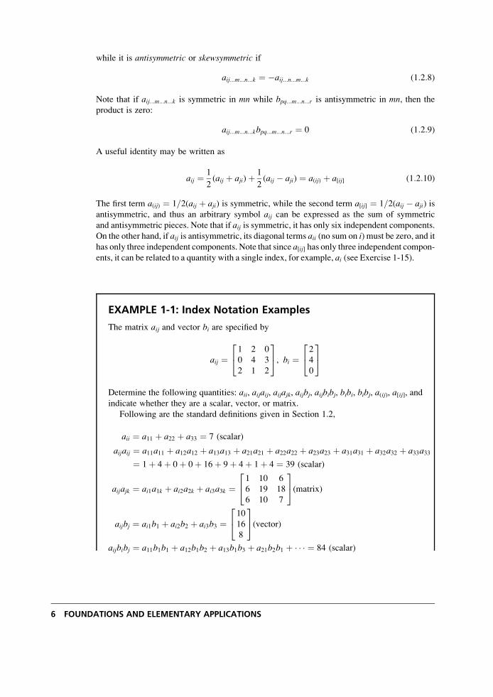
EXAMPLE 1-1: Index Notation Examples
The matrix aij and vector bi are specified by
aij ¼1 2 0
0 4 3
2 1 2
24
35, bi ¼
2
4
0
2435
Determine the following quantities: aii, aijaij, aijajk, aijbj, aijbibj, bibi, bibj, a(ij), a[ij], andindicate whether they are a scalar, vector, or matrix.
Following are the standard definitions given in Section 1.2,
aii ¼ a11 þ a22 þ a33 ¼ 7 (scalar)
aijaij ¼ a11a11 þ a12a12 þ a13a13 þ a21a21 þ a22a22 þ a23a23 þ a31a31 þ a32a32 þ a33a33
¼ 1þ 4þ 0þ 0þ 16þ 9þ 4þ 1þ 4 ¼ 39 (scalar)
aijajk ¼ ai1a1k þ ai2a2k þ ai3a3k ¼1 10 6
6 19 18
6 10 7
24
35(matrix)
aijbj ¼ ai1b1 þ ai2b2 þ ai3b3 ¼10
16
8
24
35(vector)
aijbibj ¼ a11b1b1 þ a12b1b2 þ a13b1b3 þ a21b2b1 þ � � � ¼ 84 (scalar)
6 FOUNDATIONS AND ELEMENTARY APPLICATIONS
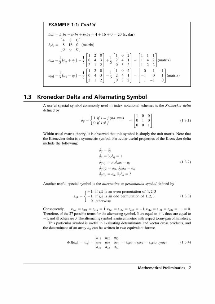
EXAMPLE 1-1: Cont’d
bibi ¼ b1b1 þ b2b2 þ b3b3 ¼ 4þ 16þ 0 ¼ 20 (scalar)
bibj ¼4 8 0
8 16 0
0 0 0
24
35(matrix)
a(ij) ¼ 1
2aij þ aji� � ¼ 1
2
1 2 0
0 4 3
2 1 2
24
35þ 1
2
1 0 2
2 4 1
0 3 2
24
35 ¼
1 1 1
1 4 2
1 2 2
24
35(matrix)
a[ij] ¼ 1
2aij � aji� � ¼ 1
2
1 2 0
0 4 3
2 1 2
24
35� 1
2
1 0 2
2 4 1
0 3 2
24
35 ¼
0 1 �1
�1 0 1
1 �1 0
24
35(matrix)
1.3 Kronecker Delta and Alternating Symbol
A useful special symbol commonly used in index notational schemes is the Kronecker deltadefined by
dij ¼ 1, if i ¼ j (no sum)0, if i 6¼ j
�¼
1 0 0
0 1 0
0 0 1
24
35 (1:3:1)
Within usual matrix theory, it is observed that this symbol is simply the unit matrix. Note that
the Kronecker delta is a symmetric symbol. Particular useful properties of the Kronecker delta
include the following:
dij ¼ djidii ¼ 3, dii ¼ 1
dijaj ¼ ai, dijai ¼ aj
dijajk ¼ aik, djkaik ¼ aij
dijaij ¼ aii, dijdij ¼ 3
(1:3:2)
Another useful special symbol is the alternating or permutation symbol defined by
eijk ¼þ1, if ijk is an even permutation of 1, 2, 3
�1, if ijk is an odd permutation of 1, 2, 3
0, otherwise
((1:3:3)
Consequently, e123 ¼ e231 ¼ e312 ¼ 1, e321 ¼ e132 ¼ e213 ¼ �1, e112 ¼ e131 ¼ e222 ¼ . . . ¼ 0.
Therefore, of the 27 possible terms for the alternating symbol, 3 are equal to þ1, three are equal to
�1, andall othersare0.Thealternating symbol is antisymmetricwith respect to anypairof its indices.
This particular symbol is useful in evaluating determinants and vector cross products, and
the determinant of an array aij can be written in two equivalent forms:
det[aij] ¼ jaijj ¼a11 a12 a13a21 a22 a23a31 a32 a33
������������ ¼ eijka1ia2ja3k ¼ eijkai1aj2ak3 (1:3:4)
Mathematical Preliminaries 7
where the first index expression represents the row expansion, while the second form is the
column expansion. Using the property
eijkepqr ¼dip diq dirdjp djq djrdkp dkq dkr
������������ (1:3:5)
another form of the determinant of a matrix can be written as
det[aij] ¼ 1
6eijkepqraipajqakr (1:3:6)
1.4 Coordinate Transformations
It is convenient and in fact necessary to express elasticity variables and field equations in several
different coordinate systems (see Appendix A). This situation requires the development of
particular transformation rules for scalar, vector, matrix, and higher-order variables. This
concept is fundamentally connected with the basic definitions of tensor variables and their
related tensor transformation laws. We restrict our discussion to transformations only between
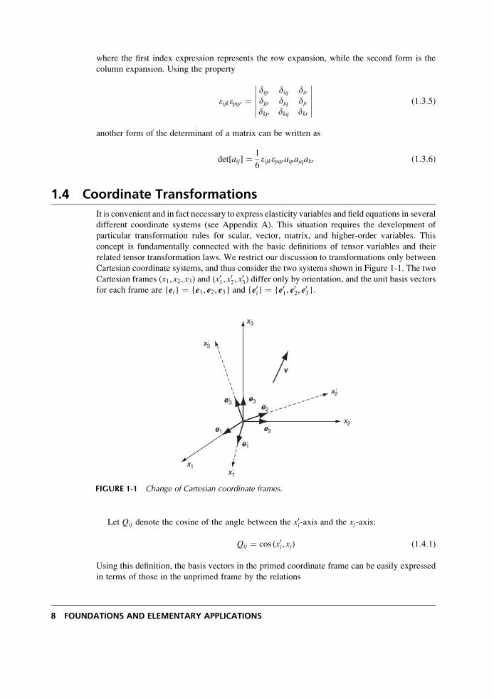
Cartesian coordinate systems, and thus consider the two systems shown in Figure 1-1. The two
Cartesian frames (x1, x2, x3) and (x01, x
02, x
03) differ only by orientation, and the unit basis vectors
for each frame are {ei} ¼ {e1, e2, e3} and {e0i} ¼ {e01, e02, e
03}.
Let Qij denote the cosine of the angle between the x0i-axis and the xj-axis:
Qij ¼ cos (x0i, xj) (1:4:1)
Using this definition, the basis vectors in the primed coordinate frame can be easily expressed
in terms of those in the unprimed frame by the relations
v
e3e2
e1
e3
e2e1
x3
x2
x1
x3
x2�
�
x1�
�
��
FIGURE 1-1 Change of Cartesian coordinate frames.
8 FOUNDATIONS AND ELEMENTARY APPLICATIONS
e01 ¼ Q11e1 þ Q12e2 þ Q13e3
e02 ¼ Q21e1 þ Q22e2 þ Q23e3
e03 ¼ Q31e1 þ Q32e2 þ Q33e3
(1:4:2)
or in index notation
e0i ¼ Qijej (1:4:3)
Likewise, the opposite transformation can be written using the same format as
ei ¼ Qjie0j (1:4:4)
Now an arbitrary vector v can be written in either of the two coordinate systems as
v ¼ v1e1 þ v2e2 þ v3e3 ¼ viei
¼ v01e01 þ v02e
02 þ v03e
03 ¼ v0ie
0i
(1:4:5)
Substituting form (1.4.4) into (1:4:5)1 gives
v ¼ viQjie0j
but from (1:4:5)2, v ¼ v0je0j, and so we find that
v0i ¼ Qijvj (1:4:6)
In similar fashion, using (1.4.3) in (1:4:5)2 gives
vi ¼ Qjiv0j (1:4:7)
Relations (1.4.6) and (1.4.7) constitute the transformation laws for the Cartesian components
of a vector under a change of rectangular Cartesian coordinate frame. It should be understood
that under such transformations, the vector is unaltered (retaining original length and orienta-
tion), and only its components are changed. Consequently, if we know the components of a
vector in one frame, relation (1.4.6) and/or relation (1.4.7) can be used to calculate components
in any other frame.
The fact that transformations are being made only between orthogonal coordinate systems
places some particular restrictions on the transformation or direction cosine matrix Qij. These
can be determined by using (1.4.6) and (1.4.7) together to get
vi ¼ Qjiv0j ¼ QjiQjkvk (1:4:8)
From the properties of the Kronecker delta, this expression can be written as
dikvk ¼ QjiQjkvk or (QjiQjk � dik)vk ¼ 0
and since this relation is true for all vectors vk, the expression in parentheses must be zero,
giving the result
QjiQjk ¼ dik (1:4:9)
Mathematical Preliminaries 9
In similar fashion, relations (1.4.6) and (1.4.7) can be used to eliminate vi (instead of v0i) to get
QijQkj ¼ dik (1:4:10)
Relations (1.4.9) and (1.4.10) comprise the orthogonality conditions that Qij must satisfy.
Taking the determinant of either relation gives another related result:
det[Qij] ¼ �1 (1:4:11)
Matrices that satisfy these relations are called orthogonal, and the transformations given by
(1.4.6) and (1.4.7) are therefore referred to as orthogonal transformations.
1.5 Cartesian Tensors
Scalars, vectors, matrices, and higher-order quantities can be represented by a general index
notational scheme. Using this approach, all quantities may then be referred to as tensors of
different orders. The previously presented transformation properties of a vector can be used to
establish the general transformation properties of these tensors. Restricting the transformations
to those only between Cartesian coordinate systems, the general set of transformation relations
for various orders can be written as
a0 ¼ a, zero order (scalar)
a0i ¼ Qipap, Wrst order (vector)
a0ij ¼ QipQjqapq, second order (matrix)
a0ijk ¼ QipQjqQkrapqr, third order
a0ijkl ¼ QipQjqQkrQlsapqrs, fourth order
..
.
a0ijk...m ¼ QipQjqQkr � � �Qmtapqr...t general order
(1:5:1)
Note that, according to these definitions, a scalar is a zero-order tensor, a vector is a tensor
of order one, and a matrix is a tensor of order two. Relations (1.5.1) then specify the transform-
ation rules for the components of Cartesian tensors of any order under the rotation Qij. This
transformation theory proves to be very valuable in determining the displacement, stress, and
strain in different coordinate directions. Some tensors are of a special form in which their
components remain the same under all transformations, and these are referred to as isotropictensors. It can be easily verified (see Exercise 1-8) that the Kronecker delta dij has such a
property and is therefore a second-order isotropic tensor. The alternating symbol eijk is found tobe the third-order isotropic form. The fourth-order case (Exercise 1-9) can be expressed in terms
of products of Kronecker deltas, and this has important applications in formulating isotropic
elastic constitutive relations in Section 4.2.
The distinction between the components and the tensor should be understood. Recall that a
vector v can be expressed as
v ¼ v1e1 þ v2e2 þ v3e3 ¼ viei
¼ v01e01 þ v02e
02 þ v03e
03 ¼ v0ie
0i
(1:5:2)
10 FOUNDATIONS AND ELEMENTARY APPLICATIONS
In a similar fashion, a second-order tensor A can be written
A ¼ A11e1e1 þ A12e1e2 þ A13e1e3
þ A21e2e1 þ A22e2e2 þ A23e2e3
þ A31e3e1 þ A32e3e2 þ A33e3e3
¼ Aijeiej ¼ A0ije
0ie0j
(1:5:3)
and similar schemes can be used to represent tensors of higher order. The representation used
in equation (1.5.3) is commonly called dyadic notation, and some authors write the dyadic
products eiej using a tensor product notation ei�ej. Additional information on dyadic notation
can be found in Weatherburn (1948) and Chou and Pagano (1967).
Relations (1.5.2) and (1.5.3) indicate that any tensor can be expressed in terms of compon-
ents in any coordinate system, and it is only the components that change under coordinate
transformation. For example, the state of stress at a point in an elastic solid depends on the
problem geometry and applied loadings. As is shown later, these stress components are those
of a second-order tensor and therefore obey transformation law (1:5:1)3. Although the com-
ponents of the stress tensor change with the choice of coordinates, the stress tensor (represent-
ing the state of stress) does not.
An important property of a tensor is that if we know its components in one coordinate
system, we can find them in any other coordinate frame by using the appropriate transform-
ation law. Because the components of Cartesian tensors are representable by indexed symbols,
the operations of equality, addition, subtraction, multiplication, and so forth, are defined in a
manner consistent with the indicial notation procedures previously discussed. The terminology
tensor without the adjective Cartesian usually refers to a more general scheme in which the
coordinates are not necessarily rectangular Cartesian and the transformations between coordin-
ates are not always orthogonal. Such general tensor theory is not discussed or used in this text.
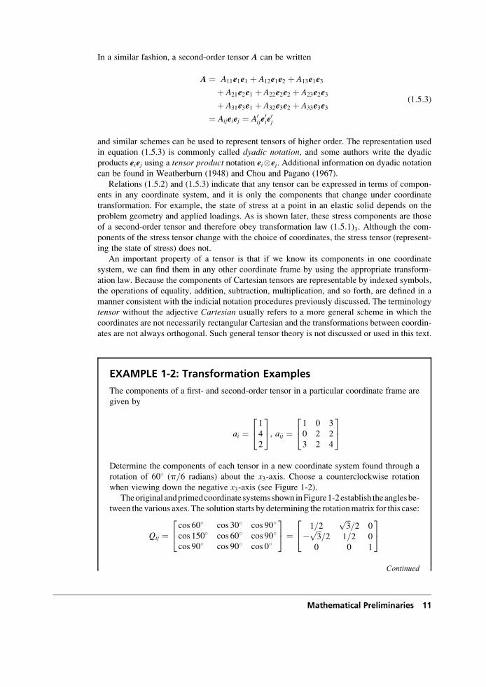
EXAMPLE 1-2: Transformation Examples
The components of a first- and second-order tensor in a particular coordinate frame are
given by
ai ¼1
4
2
2435, aij ¼ 1 0 3
0 2 2
3 2 4
24
35
Determine the components of each tensor in a new coordinate system found through a
rotation of 608 (p=6 radians) about the x3-axis. Choose a counterclockwise rotation
when viewing down the negative x3-axis (see Figure 1-2).Theoriginal andprimedcoordinate systemsshowninFigure1-2establish theanglesbe-
tween the various axes. The solution starts by determining the rotationmatrix for this case:
Qij ¼cos 608 cos 308 cos 908cos 1508 cos 608 cos 908cos 908 cos 908 cos 08
24
35 ¼
1=2ffiffiffi3
p=2 0
� ffiffiffi3
p=2 1=2 0
0 0 1
24
35
Continued
Mathematical Preliminaries 11
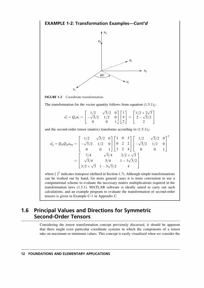
EXAMPLE 1-2: Transformation Examples—Cont’d
x3
x2
x1
60�
x3′
x2′
x1′
FIGURE 1-2 Coordinate transformation.
The transformation for the vector quantity follows from equation (1:5:1)2:
a0i ¼ Qijaj ¼1=2
ffiffiffi3
p=2 0
� ffiffiffi3
p=2 1=2 0
0 0 1
24
35 1
4
2
2435 ¼
1=2þ 2ffiffiffi3
p2� ffiffiffi
3p
=22
24
35
and the second-order tensor (matrix) transforms according to (1:5:1)3:
a0ij ¼ QipQjqapq ¼1=2
ffiffiffi3
p=2 0
� ffiffiffi3
p=2 1=2 0
0 0 1
264
375
1 0 3
0 2 2
3 2 4
264
375 1=2
ffiffiffi3
p=2 0
� ffiffiffi3
p=2 1=2 0
0 0 1
264
375T
¼7=4
ffiffiffi3
p=4 3=2þ ffiffiffi
3pffiffiffi
3p
=4 5=4 1� 3ffiffiffi3
p=2
3=2þ ffiffiffi3
p1� 3
ffiffiffi3
p=2 4
264
375
where [ ]T indicates transpose (defined in Section 1.7). Although simple transformations
can be worked out by hand, for more general cases it is more convenient to use a
computational scheme to evaluate the necessary matrix multiplications required in the
transformation laws (1.5.1). MATLAB software is ideally suited to carry out such
calculations, and an example program to evaluate the transformation of second-order
tensors is given in Example C-1 in Appendix C.
1.6 Principal Values and Directions for SymmetricSecond-Order Tensors
Considering the tensor transformation concept previously discussed, it should be apparent
that there might exist particular coordinate systems in which the components of a tensor
take on maximum or minimum values. This concept is easily visualized when we consider the
12 FOUNDATIONS AND ELEMENTARY APPLICATIONS
components of a vector shown in Figure 1-1. If we choose a particular coordinate system that has
been rotated so that the x3-axis lies along the direction of the vector, then the vector will have
components v ¼ {0, 0, jvj}. For this case, two of the components have been reduced to zero,
while the remaining component becomes the largest possible (the total magnitude).
This situation is most useful for symmetric second-order tensors that eventually represent
the stress and/or strain at a point in an elastic solid. The direction determined by the unit vector
n is said to be a principal direction or eigenvector of the symmetric second-order tensor aij ifthere exists a parameter l such that
aijnj ¼ lni (1:6:1)
where l is called the principal value or eigenvalue of the tensor. Relation (1.6.1) can be
rewritten as
(aij � ldij)nj ¼ 0
and this expression is simply a homogeneous system of three linear algebraic equations in the
unknowns n1, n2, n3. The system possesses a nontrivial solution if and only if the determinant
of its coefficient matrix vanishes; that is:
det[aij � ldij] ¼ 0
Expanding the determinant produces a cubic equation in terms of l:
det[aij � ldij] ¼ �l3 þ Ial2 � IIalþ IIIa ¼ 0 (1:6:2)
where
Ia ¼ aii ¼ a11 þ a22 þ a33
IIa ¼ 1
2(aiiajj � aijaij) ¼
a11 a12
a21 a22
��������þ a22 a23
a32 a33
��������þ a11 a13
a31 a33
��������
IIIa ¼ det[aij]
(1:6:3)
The scalars Ia, IIa, and IIIa are called the fundamental invariants of the tensor aij, and relation
(1.6.2) is known as the characteristic equation. As indicated by their name, the three invariants
do not change value under coordinate transformation. The roots of the characteristic equation
determine the allowable values for l, and each of these may be back-substituted into relation
(1.6.1) to solve for the associated principal direction n.Under the condition that the components aij are real, it can be shown that all three roots
l1, l2, l3 of the cubic equation (1.6.2) must be real. Furthermore, if these roots are distinct, the
principal directions associated with each principal value are orthogonal. Thus, we can con-
clude that every symmetric second-order tensor has at least three mutually perpendicular
principal directions and at most three distinct principal values that are the roots of the
characteristic equation. By denoting the principal directions n(1), n(2), n(3) corresponding to
the principal values l1, l2, l3, three possibilities arise:
1. All three principal values are distinct; thus, the three corresponding principal directions
are unique (except for sense).
2. Two principal values are equal (l1 6¼ l2 ¼ l3); the principal direction n(1) is unique(except for sense), and every direction perpendicular to n(1) is a principal directionassociated with l2, l3.
Mathematical Preliminaries 13
3. All three principal values are equal; every direction is principal, and the tensor is
isotropic, as per discussion in the previous section.
Therefore, according to what we have presented, it is always possible to identify a right-
handed Cartesian coordinate system such that each axis lies along the principal directions
of any given symmetric second-order tensor. Such axes are called the principal axes of
the tensor. For this case, the basis vectors are actually the unit principal directions
{n(1), n(2), n(3)}, and it can be shown that with respect to principal axes the tensor reduces to
the diagonal form
a0ij ¼l1 0 0
0 l2 0
0 0 l3
24
35 (1:6:4)
Note that the fundamental invariants defined by relations (1.6.3) can be expressed in terms of
the principal values as
Ia ¼ l1 þ l2 þ l3IIa ¼ l1l2 þ l2l3 þ l3l1IIIa ¼ l1l2l3
(1:6:5)
The eigenvalues have important extremal properties. If we arbitrarily rank the principal values
such that l1 > l2 > l3, then l1 will be the largest of all possible diagonal elements, while l3will be the smallest diagonal element possible. This theory is applied in elasticity as we seek
the largest stress or strain components in an elastic solid.
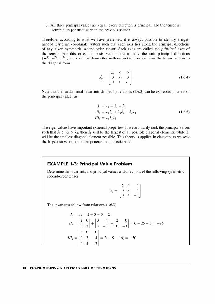
EXAMPLE 1-3: Principal Value Problem
Determine the invariants and principal values and directions of the following symmetric
second-order tensor:
aij ¼2 0 0
0 3 4
0 4 �3
24
35
The invariants follow from relations (1.6.3)
Ia ¼ aii ¼ 2þ 3� 3 ¼ 2
IIa ¼2 0
0 3
��������þ 3 4
4 �3
��������þ 2 0
0 �3
�������� ¼ 6� 25� 6 ¼ �25
IIIa ¼2 0 0
0 3 4
0 4 �3
�������������� ¼ 2(� 9� 16) ¼ �50
14 FOUNDATIONS AND ELEMENTARY APPLICATIONS
EXAMPLE 1-3: Cont’d
The characteristic equation then becomes
det[aij � ldij] ¼ �l3 þ 2l2 þ 25l� 50 ¼ 0
) (l� 2)(l2 � 25) ¼ 0
;l1 ¼ 5, l2 ¼ 2, l3 ¼ �5
Thus, for this case all principal values are distinct.
For the l1 ¼ 5 root, equation (1.6.1) gives the system
�3n(1)1 ¼ 0
�2n(1)2 þ 4n(1)3 ¼ 0
4n(1)2 � 8n(1)3 ¼ 0
which gives a normalized solution n(1) ¼ � (2e2 þ e3)=ffiffiffi5
p. In similar fashion, the other
two principal directions are found to be n(2) ¼ �e1, n(3) ¼ � (e2 � 2e3)=
ffiffiffi5
p. It is easily
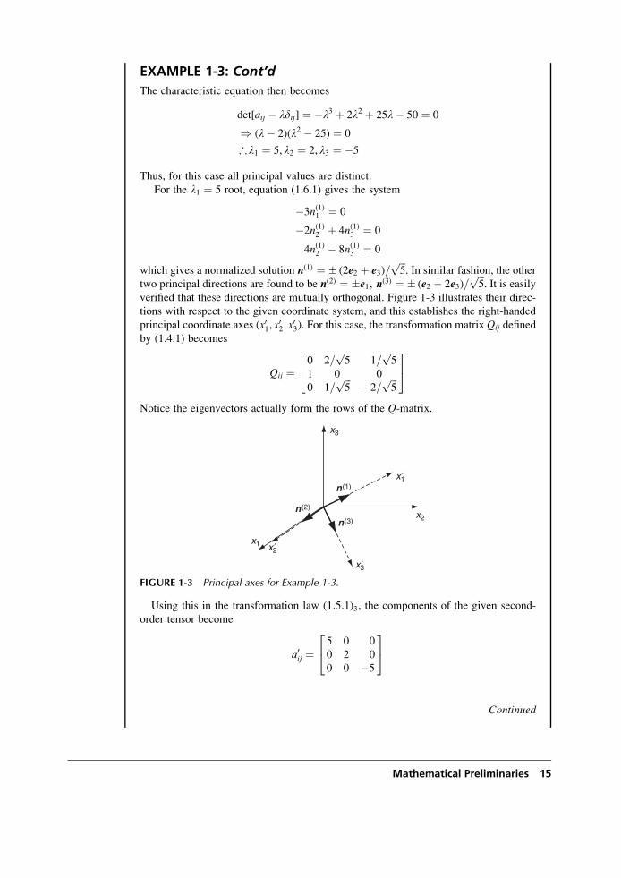
verified that these directions are mutually orthogonal. Figure 1-3 illustrates their direc-
tions with respect to the given coordinate system, and this establishes the right-handed
principal coordinate axes (x01, x02, x
03). For this case, the transformation matrix Qij defined
by (1.4.1) becomes
Qij ¼0 2=
ffiffiffi5
p1=
ffiffiffi5
p1 0 0
0 1=ffiffiffi5
p �2=ffiffiffi5
p
24
35
Notice the eigenvectors actually form the rows of the Q-matrix.
x3
x1
x2
x1n(1)
n(3)
n(2)
′
x3′
x2′
FIGURE 1-3 Principal axes for Example 1-3.
Using this in the transformation law (1:5:1)3, the components of the given second-
order tensor become
a0ij ¼5 0 0
0 2 0
0 0 �5
24
35
Continued
Mathematical Preliminaries 15
EXAMPLE 1-3: Principal Value Problem—Cont’d
This result then validates the general theory given by relation (1.6.4) indicating that the
tensor should take on diagonal form with the principal values as the elements.
Only simple second-order tensors lead to a characteristic equation that is factorable,
thus allowing solution by hand calculation. Most other cases normally develop a general
cubic equation and a more complicated system to solve for the principal directions.
Again, particular routines within the MATLAB package offer convenient tools to solve
these more general problems. Example C-2 in Appendix C provides a simple code to
determine the principal values and directions for symmetric second-order tensors.
1.7 Vector, Matrix, and Tensor Algebra
Elasticity theory requires the use of many standard algebraic operations among vector, matrix,
and tensor variables. These operations include dot and cross products of vectors and numerous
matrix/tensor products. All of these operations can be expressed efficiently using compact
tensor index notation. First, consider some particular vector products. Given two vectors a andb, with Cartesian components ai and bi, the scalar or dot product is defined by
a � b ¼ a1b1 þ a2b2 þ a3b3 ¼ aibi (1:7:1)
Because all indices in this expression are repeated, the quantity must be a scalar, that is, a
tensor of order zero. The magnitude of a vector can then be expressed as
jaj ¼ (a � a)1=2 ¼ (aiai)1=2 (1:7:2)
The vector or cross product between two vectors a and b can be written as
a� b ¼e1 e2 e3a1 a2 a3b1 b2 b3
������������ ¼ eijkajbkei (1:7:3)
where ei are the unit basis vectors for the coordinate system. Note that the cross product gives a
vector resultant whose components are eijkajbk. Another common vector product is the scalartriple product defined by
a � b� c ¼a1 a2 a3b1 b2 b3c1 c2 c3
������������ ¼ eijkaibjck (1:7:4)
Next consider some common matrix products. Using the usual direct notation for matrices and
vectors, common products between a matrix A¼ [A] with a vector a can be written as
Aa ¼ [A]{a} ¼ Aijaj ¼ ajAij
aTA ¼ {a}T[A] ¼ aiAij ¼ Aijai(1:7:5)
where aT denotes the transpose, and for a vector quantity this simply changes the column
matrix (3� 1) into a row matrix (1� 3). Note that each of these products results in a vector
16 FOUNDATIONS AND ELEMENTARY APPLICATIONS
resultant. These types of expressions generally involve various inner products within the index
notational scheme, and as noted, once the summation index is properly specified, the order of
listing the product terms does not change the result. We will encounter several different
combinations of products between two matrices A and B:
AB ¼ [A][B] ¼ AijBjk
ABT ¼ AijBkj
ATB ¼ AjiBjk
tr(AB) ¼ AijBji
tr(ABT) ¼ tr(ATB) ¼ AijBij
(1:7:6)
where AT indicates the transpose and trA is the trace of the matrix defined by
ATij ¼ Aji
trA ¼ Aii ¼ A11 þ A22 þ A33
(1:7:7)
Similar to vector products, once the summation index is properly specified, the results in
(1.7.6) do not depend on the order of listing the product terms. Note that this does not imply
that AB ¼ BA, which is certainly not true.
1.8 Calculus of Cartesian Tensors
Most variables within elasticity theory are field variables, that is, functions depending on
the spatial coordinates used to formulate the problem under study. For time-dependent
problems, these variables could also have temporal variation. Thus, our scalar, vector, matrix,
and general tensor variables are functions of the spatial coordinates (x1, x2, x3). Because many
elasticity equations involve differential and integral operations, it is necessary to have an
understanding of the calculus of Cartesian tensor fields. Further information on vector differen-
tial and integral calculus can be found in Hildebrand (1976) and Kreyszig (1999).
The field concept for tensor components can be expressed as
a ¼ a(x1, x2, x3) ¼ a(xi) ¼ a(x)
ai ¼ ai(x1, x2, x3) ¼ ai(xi) ¼ ai(x)
aij ¼ aij(x1, x2, x3) ¼ aij(xi) ¼ aij(x)
..
.
It is convenient to introduce the comma notation for partial differentiation:
a, i ¼ @
@xia; ai, j ¼ @
@xjai; aij, k ¼ @
@xkaij; � � �
It can be shown that if the differentiation index is distinct, the order of the tensor is increased
by one. For example, the derivative operation on a vector ai, j produces a second-order tensor ormatrix given by
Mathematical Preliminaries 17
ai, j ¼
@a1@x1
@a1@x2
@a1@x3
@a2@x1
@a2@x2
@a2@x3
@a3@x1
@a3@x2
@a3@x3
2666664
3777775
Using Cartesian coordinates (x,y,z), consider the directional derivative of a scalar field func-
tion f with respect to a direction s:
df
ds¼ @f
@x
dx
dsþ @f
@y
dy
dsþ @f
@z
dz
ds
Note that the unit vector in the direction of s can be written as
n ¼ dx
dse1 þ dy
dse2 þ dz
dse3
Therefore, the directional derivative can be expressed as the following scalar product:
df
ds¼ n � rrrf (1:8:1)
where rrrf is called the gradient of the scalar function f and is defined by
rrrf ¼ grad f ¼ e1@f
@xþ e2
@f
@yþ e3
@f
@z(1:8:2)
and the symbolic vector operator rrr is called the del operator
rrr ¼ e1@
@xþ e2
@
@yþ e3
@
@z(1:8:3)
These and other useful operations can be expressed in Cartesian tensor notation. Given the
scalar field f and vector field u, the following common differential operations can be written in
index notation:
Gradient of a Scalar rrr� ¼ �, iei
Gradient of a Vector rrru ¼ ui, jeiej
Laplacian of a Scalarnabla2f ¼ rrr � rrrf ¼ f, iiDivergence of a Vector rrr � u ¼ ui, i
Curl of a Vector rrr� u ¼ eijkuk, jei
Laplacian of a Vector r2u ¼ ui, kkei
(1:8:4)
18 FOUNDATIONS AND ELEMENTARY APPLICATIONS
If f and c are scalar fields and u and v are vector fields, several useful identities exist:
rrr(fc) ¼ (rrrf)cþ f(rrrc)
r2(fc) ¼ (r2f)cþ f(r2c)þ 2rrrf � rrrc
rrr � (fu) ¼ rrrf � uþ f(rrr � u)rrr� (fu) ¼ rrrf� uþ f(rrr� u)
rrr � (u� v) ¼ v � (rrr� u)� u � (rrr� v)
rrr�rrrf ¼ 0
rrr � rrrf ¼ r2f
rrr � rrr� u ¼ 0
rrr� (rrr� u) ¼ rrr(rrr � u)�r2u
u� (rrr� u) ¼ 1
2rrr(u � u)� u � rrru
(1:8:5)
Each of these identities can be easily justified by using index notation from definition relations
(1.8.4).
EXAMPLE 1-4: Scalar and Vector Field Examples
Scalar and vector field functions are given by � ¼ x2� y2 and u ¼ 2xe1þ 3yze2þ xye3.Calculate the following expressions, rrr�, rrr2�, rrr � u, rrru, rrr � u.
Using the basic relations (1.8.4)
rrr� ¼ 2xe1 � 2ye2
rrr2� ¼ 2� 2 ¼ 0
rrr � u ¼ 2þ 3zþ 0 ¼ 2þ 3z
rrru ¼ ui, j ¼2 0 0
0 3z 3y
y x 0
264
375
rrr� u ¼e1 e2 e3
@=@x @=@y @=@z
2x 3yz xy
�������������� ¼ (x� 3y)e1 � ye2
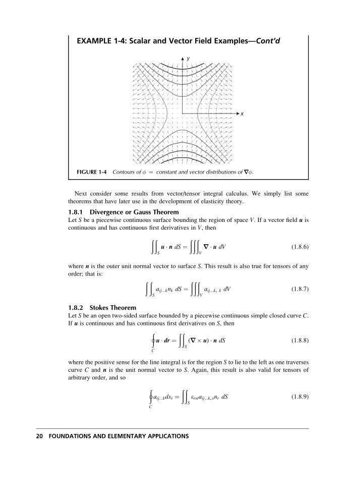
Using numerical methods, some of these variables can be conveniently computed and
plotted in order to visualize the nature of the field distribution. For example, contours of
� ¼ constant can easily be plotted using MATLAB software, and vector distributions
of rrr� can be shown as plots of vectors properly scaled in magnitude and orientation.
Figure 1-4 shows these two types of plots, and it is observed that the vector field rrr� is
orthogonal to the �-contours, a result that is true in general for all scalar fields. Numeric-
ally generated plots such as these will prove to be useful in understanding displacement,
strain, and/or stress distributions found in the solution to a variety of problems in
elasticity.
Continued
Mathematical Preliminaries 19
EXAMPLE 1-4: Scalar and Vector Field Examples—Cont’d
x
y
FIGURE 1-4 Contours of � ¼ constant and vector distributions of rrr�:
Next consider some results from vector/tensor integral calculus. We simply list some
theorems that have later use in the development of elasticity theory.
1.8.1 Divergence or Gauss TheoremLet S be a piecewise continuous surface bounding the region of space V. If a vector field u is
continuous and has continuous first derivatives in V, then
ððS
u � n dS ¼ððð
V
rrr � u dV (1:8:6)
where n is the outer unit normal vector to surface S. This result is also true for tensors of any
order; that is: ð ðS
aij...knk dS ¼ððð
V
aij...k, k dV (1:8:7)
1.8.2 Stokes TheoremLet S be an open two-sided surface bounded by a piecewise continuous simple closed curve C.If u is continuous and has continuous first derivatives on S, thenþ
C
u � dr ¼ðð
S
(rrr� u) � n dS (1:8:8)
where the positive sense for the line integral is for the region S to lie to the left as one traversescurve C and n is the unit normal vector to S. Again, this result is also valid for tensors of
arbitrary order, and so
þC
aij...kdxt ¼ðð
S
erstaij...k, snr dS (1:8:9)
20 FOUNDATIONS AND ELEMENTARY APPLICATIONS
It can be shown that both divergence and Stokes theorems can be generalized so that the dot
product in (1.8.6) and/or (1.8.8) can be replaced with a cross product.
1.8.3 Green’s Theorem in the PlaneApplying Stokes theorem to a planar domain S with the vector field selected as u ¼ f e1 þ ge2gives the result
ððS
@g
@x� @f
@y
� �dxdy ¼
ðC
(fdxþ gdy) (1:8:10)
Further, special choices with either f ¼ 0 or g ¼ 0 imply
ððS
@g
@xdxdy ¼
ðC
gnxds ,
ððS
@f
@ydxdy ¼
ðC
fnyds (1:8:11)
1.8.4 Zero-Value TheoremLet fij...k be a continuous tensor field of any order defined in an arbitrary region V. If the integralof fij...k over V vanishes, then fij...k must vanish in V; that is:
ðððV
fij...kdV ¼ 0 ) fij...k ¼ 0 2 V (1:8:12)
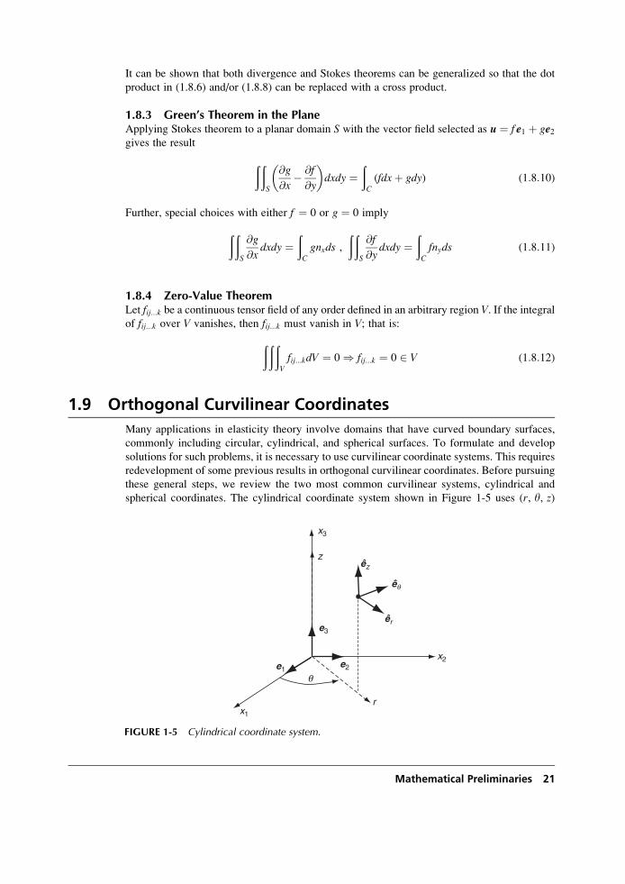
1.9 Orthogonal Curvilinear Coordinates
Many applications in elasticity theory involve domains that have curved boundary surfaces,
commonly including circular, cylindrical, and spherical surfaces. To formulate and develop
solutions for such problems, it is necessary to use curvilinear coordinate systems. This requires
redevelopment of some previous results in orthogonal curvilinear coordinates. Before pursuing
these general steps, we review the two most common curvilinear systems, cylindrical and
spherical coordinates. The cylindrical coordinate system shown in Figure 1-5 uses (r, y, z)
e2
e3
e1
x3
x1
x2
r
q
zêz
êr
êq
FIGURE 1-5 Cylindrical coordinate system.
Mathematical Preliminaries 21
coordinates to describe spatial geometry. Relations between the Cartesian and cylindrical
systems are given by
x1 ¼ r cos y, x2 ¼ r sin y, x3 ¼ z
r ¼ffiffiffiffiffiffiffiffiffiffiffiffiffiffiffix21 þ x22
q, y ¼ tan�1 x2
x1, z ¼ x3
(1:9:1)
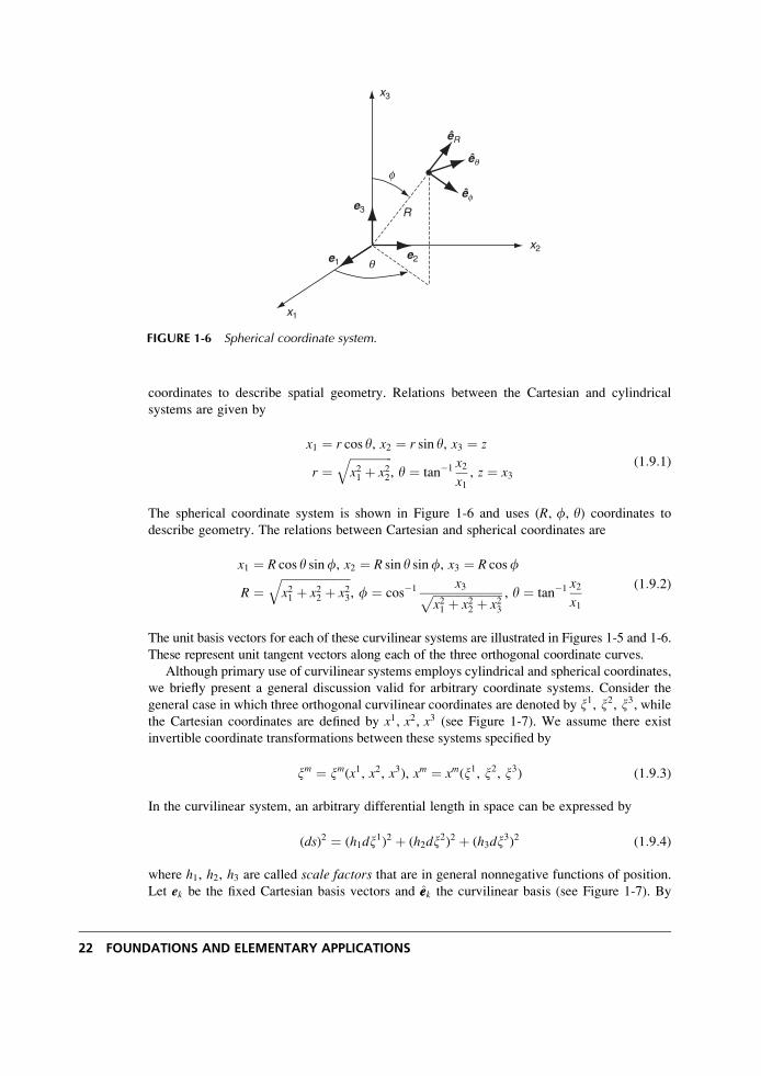
The spherical coordinate system is shown in Figure 1-6 and uses (R, f, y) coordinates to
describe geometry. The relations between Cartesian and spherical coordinates are
x1 ¼ R cos y sinf, x2 ¼ R sin y sinf, x3 ¼ R cosf
R ¼ffiffiffiffiffiffiffiffiffiffiffiffiffiffiffiffiffiffiffiffiffiffiffiffix21 þ x22 þ x23
q, f ¼ cos�1 x3ffiffiffiffiffiffiffiffiffiffiffiffiffiffiffiffiffiffiffiffiffiffiffiffi
x21 þ x22 þ x23p , y ¼ tan�1 x2
x1
(1:9:2)
The unit basis vectors for each of these curvilinear systems are illustrated in Figures 1-5 and 1-6.
These represent unit tangent vectors along each of the three orthogonal coordinate curves.
Although primary use of curvilinear systems employs cylindrical and spherical coordinates,
we briefly present a general discussion valid for arbitrary coordinate systems. Consider the
general case in which three orthogonal curvilinear coordinates are denoted by x1, x2, x3, whilethe Cartesian coordinates are defined by x1, x2, x3 (see Figure 1-7). We assume there exist
invertible coordinate transformations between these systems specified by
xm ¼ xm(x1, x2, x3), xm ¼ xm(x1, x2, x3) (1:9:3)
In the curvilinear system, an arbitrary differential length in space can be expressed by
(ds)2 ¼ (h1dx1)2 þ (h2dx
2)2 þ (h3dx3)2 (1:9:4)
where h1, h2, h3 are called scale factors that are in general nonnegative functions of position.
Let ek be the fixed Cartesian basis vectors and eek the curvilinear basis (see Figure 1-7). By
e3
e2e1
x3
x1
x2
R
êR
êq
êf
q
f
FIGURE 1-6 Spherical coordinate system.
22 FOUNDATIONS AND ELEMENTARY APPLICATIONS
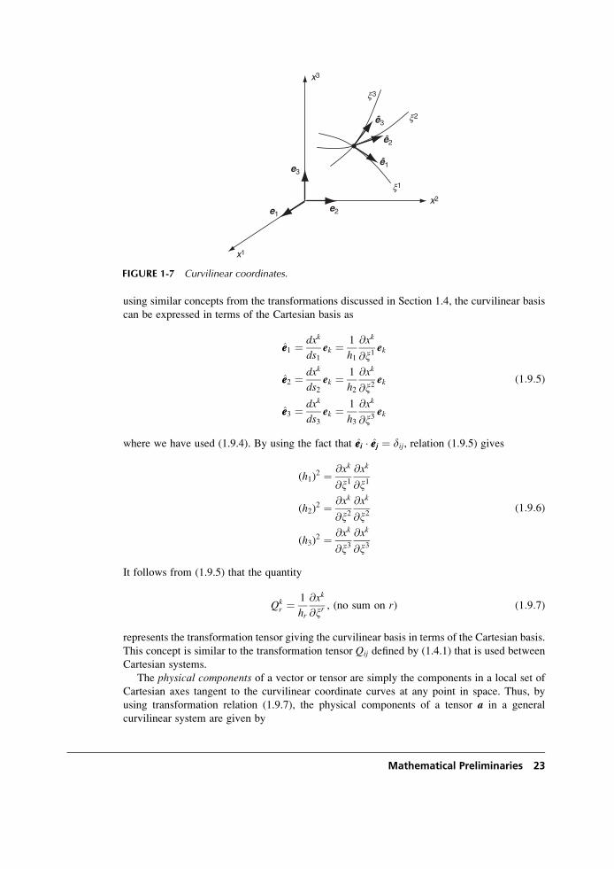
using similar concepts from the transformations discussed in Section 1.4, the curvilinear basis
can be expressed in terms of the Cartesian basis as
ee1 ¼ dxk
ds1ek ¼ 1
h1
@xk
@x1ek
ee2 ¼ dxk
ds2ek ¼ 1
h2
@xk
@x2ek
ee3 ¼ dxk
ds3ek ¼ 1
h3
@xk
@x3ek
(1:9:5)
where we have used (1.9.4). By using the fact that eiei � ejej ¼ dij, relation (1.9.5) gives
(h1)2 ¼ @xk
@x1@xk
@x1
(h2)2 ¼ @xk
@x2@xk
@x2
(h3)2 ¼ @xk
@x3@xk
@x3
(1:9:6)
It follows from (1.9.5) that the quantity
Qkr ¼
1
hr
@xk
@xr, (no sum on r) (1:9:7)
represents the transformation tensor giving the curvilinear basis in terms of the Cartesian basis.
This concept is similar to the transformation tensor Qij defined by (1.4.1) that is used between
Cartesian systems.
The physical components of a vector or tensor are simply the components in a local set of
Cartesian axes tangent to the curvilinear coordinate curves at any point in space. Thus, by
using transformation relation (1.9.7), the physical components of a tensor a in a general
curvilinear system are given by
e2
e3
e1
x3
x2
x1
x3
x2
x1
ê3
ê2
ê1
FIGURE 1-7 Curvilinear coordinates.
Mathematical Preliminaries 23
a<ij...k> ¼ Qpi Q
qj � � �Qs
kapq...s (1:9:8)
where apq...s are the components in a fixed Cartesian frame. Note that the tensor can be
expressed in either system as
a ¼ aij...keiej � � � ek¼ a<ij...k>eeieej � � � eek
(1:9:9)
Because many applications involve differentiation of tensors, we must consider the differenti-
ation of the curvilinear basis vectors. The Cartesian basis system ek is fixed in orientation and
therefore @ek=@xj ¼ @ek=@xj ¼ 0. However, derivatives of the curvilinear basis do not in
general vanish, and differentiation of relations (1.9.5) gives the following results:
@eem@xm
¼ � 1
hn
@hm@xn
een � 1
hr
@hm@xr
eer; m 6¼ n 6¼ r
@eem@xn
¼ 1
hm
@hn@xm
een; m 6¼ n, no sum on repeated indices
(1:9:10)
Using these results, the derivative of any tensor can be evaluated. Consider the first derivative
of a vector u:
@
@xnu ¼ @
@xn(u<m>eem) ¼ @u<m>
@xneem þ u<m>
@eem@xn
(1:9:11)
The last term can be evaluated using (1.9.10), and thus the derivative of u can be expressed in
terms of curvilinear components. Similar patterns follow for derivatives of higher-order tensors.
All vector differential operators of gradient, divergence, curl, and so forth, can be expressed
in any general curvilinear system by using these techniques. For example, the vector differen-
tial operator previously defined in Cartesian coordinates in (1.8.3) is given by
r ¼ ee11
h1
@
@x1þ ee2
1
h2
@
@x2þ ee3
1
h3
@
@x3¼Xi
eei1
hi
@
@xi(1:9:12)
and this leads to the construction of the other common forms:
Gradient of a Scalar rrrf ¼ ee11
h1
@f
@x1þ ee2
1
h2
@f
@x2þ ee3
1
h3
@f
@x3¼Xi
eei1
hi
@f
@xi(1:9:13)
Divergence of a Vector rrr � u ¼ 1
h1h2h3
Xi
@
@xih1h2h3hi
u<i>
� �(1:9:14)
Laplacian of a Scalar r2f ¼ 1
h1h2h3
Xi
@
@xih1h2h3
(hi)2
@f
@xi
� �(1:9:15)
Curl of a Vector r� u ¼Xi
Xj
Xk
eijkhjhk
@
@x j (u<k>hk)eei (1:9:16)
24 FOUNDATIONS AND ELEMENTARY APPLICATIONS
Gradient of a Vector ru ¼Xi
Xj
eeihi
@u<j>
@xieej þ u<j>
@eej
@xi
� �(1:9:17)
Laplacian of a Vector r2u ¼Xi
eeihi
@
@xi
!�Xj
Xk
eekhk
@u<j>
@xkeej þ u<j>
@eej
@xk
!(1:9:18)
It should be noted that these forms are significantly different from those previously given in
relations (1.8.4) for Cartesian coordinates. Curvilinear systems add additional terms not found
in rectangular coordinates. Other operations on higher-order tensors can be developed in a
similar fashion (see Malvern 1969, app. II). Specific transformation relations and field equa-
tions in cylindrical and spherical coordinate systems are given in Appendices A and B. Further
discussion of these results is taken up in later chapters.
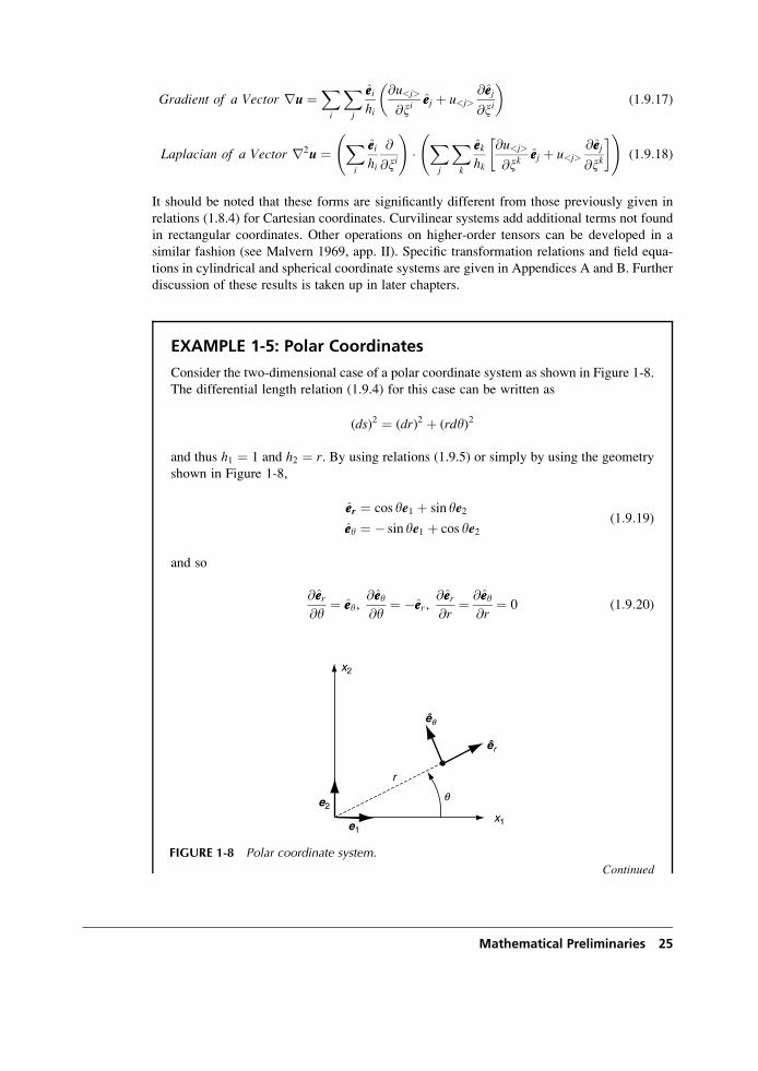
EXAMPLE 1-5: Polar Coordinates
Consider the two-dimensional case of a polar coordinate system as shown in Figure 1-8.
The differential length relation (1.9.4) for this case can be written as
(ds)2 ¼ (dr)2 þ (rdy)2
and thus h1 ¼ 1 and h2 ¼ r. By using relations (1.9.5) or simply by using the geometry
shown in Figure 1-8,
eer ¼ cos ye1 þ sin ye2eey ¼ � sin ye1 þ cos ye2
(1:9:19)
and so
@eer@y
¼ eey,@eey@y
¼ �eer ,@eer@r
¼ @eey@r
¼ 0 (1:9:20)
Continued
e1
e2
x2
x1
r
êr
êq
q
FIGURE 1-8 Polar coordinate system.
Mathematical Preliminaries 25
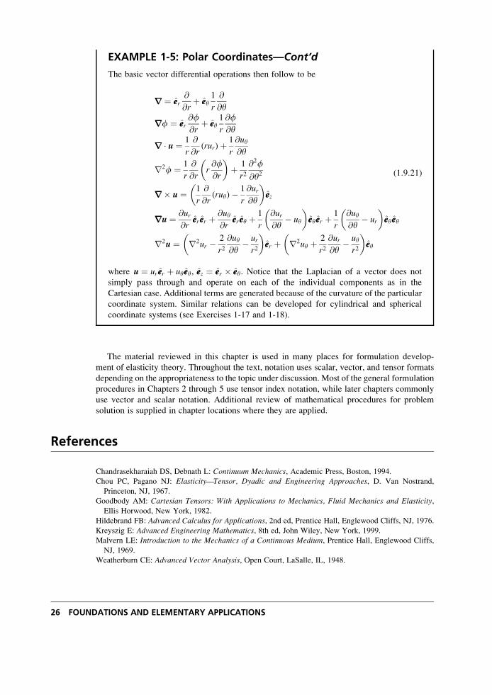
EXAMPLE 1-5: Polar Coordinates—Cont’d
The basic vector differential operations then follow to be
rrr ¼ eer@
@rþ eey
1
r
@
@y
rrrf ¼ eer@f@r
þ eey1
r
@f@y
rrr � u ¼ 1
r
@
@r(rur)þ 1
r
@uy@y
r2f ¼ 1
r
@
@rr@f@r
� �þ 1
r2@2f
@y2
rrr� u ¼ 1
r
@
@r(ruy)� 1
r
@ur@y
� �eez
rrru ¼ @ur@r
eer eer þ @uy@r
eer eey þ 1
r
@ur@y
� uy
� �eeyeer þ 1
r
@uy@y
� ur
� �eeyeey
r2u ¼ r2ur � 2
r2@uy@y
� urr2
� �eer þ r2uy þ 2
r2@ur@y
� uyr2
� �eey
(1:9:21)
where u ¼ ur eer þ uyeey, eez ¼ eer � eey. Notice that the Laplacian of a vector does not
simply pass through and operate on each of the individual components as in the
Cartesian case. Additional terms are generated because of the curvature of the particular
coordinate system. Similar relations can be developed for cylindrical and spherical
coordinate systems (see Exercises 1-17 and 1-18).
The material reviewed in this chapter is used in many places for formulation develop-
ment of elasticity theory. Throughout the text, notation uses scalar, vector, and tensor formats
depending on the appropriateness to the topic under discussion. Most of the general formulation
procedures in Chapters 2 through 5 use tensor index notation, while later chapters commonly
use vector and scalar notation. Additional review of mathematical procedures for problem
solution is supplied in chapter locations where they are applied.
References
Chandrasekharaiah DS, Debnath L: Continuum Mechanics, Academic Press, Boston, 1994.
Chou PC, Pagano NJ: Elasticity—Tensor, Dyadic and Engineering Approaches, D. Van Nostrand,
Princeton, NJ, 1967.
Goodbody AM: Cartesian Tensors: With Applications to Mechanics, Fluid Mechanics and Elasticity,Ellis Horwood, New York, 1982.
Hildebrand FB: Advanced Calculus for Applications, 2nd ed, Prentice Hall, Englewood Cliffs, NJ, 1976.
Kreyszig E: Advanced Engineering Mathematics, 8th ed, John Wiley, New York, 1999.
Malvern LE: Introduction to the Mechanics of a Continuous Medium, Prentice Hall, Englewood Cliffs,
NJ, 1969.
Weatherburn CE: Advanced Vector Analysis, Open Court, LaSalle, IL, 1948.
26 FOUNDATIONS AND ELEMENTARY APPLICATIONS
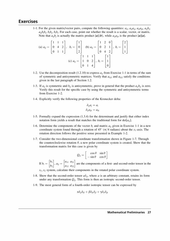
Exercises
1-1. For the given matrix/vector pairs, compute the following quantities: aii, aijaij, aijajk, aijbj,aijbibj, bibj, bibi. For each case, point out whether the result is a scalar, vector, or matrix.
Note that aijbj is actually the matrix product [a]{b}, while aijajk is the product [a][a].
(a) aij ¼1 1 1
0 4 2
0 1 1
264
375, bi ¼
1
0
2
264375 (b) aij ¼
1 2 0
0 2 1
0 4 2
264
375, bi ¼
2
1
1
264375
(c) aij ¼1 1 1
1 0 2
0 1 4
264
375, bi ¼
1
1
0
264375
1-2. Use the decomposition result (1.2.10) to express aij from Exercise 1-1 in terms of the sum
of symmetric and antisymmetric matrices. Verify that a(ij) and a[ij] satisfy the conditions
given in the last paragraph of Section 1.2.
1-3. If aij is symmetric and bij is antisymmetric, prove in general that the product aijbij is zero.Verify this result for the specific case by using the symmetric and antisymmetric terms
from Exercise 1-2.
1-4. Explicitly verify the following properties of the Kronecker delta:
dijaj ¼ ai
dijajk ¼ aik
1-5. Formally expand the expression (1.3.4) for the determinant and justify that either index
notation form yields a result that matches the traditional form for det[aij].
1-6. Determine the components of the vector bi and matrix aij given in Exercise 1-1 in a new
coordinate system found through a rotation of 458 (p=4 radians) about the x1-axis. Therotation direction follows the positive sense presented in Example 1-2.
1-7. Consider the two-dimensional coordinate transformation shown in Figure 1-7. Through
the counterclockwise rotation y, a new polar coordinate system is created. Show that the
transformation matrix for this case is given by
Qij ¼ cos y sin y� sin y cos y
If bi ¼ b1b2
, aij ¼ a11
a12
a21a22
are the components of a first- and second-order tensor in the
x1, x2 system, calculate their components in the rotated polar coordinate system.
1-8. Show that the second-order tensor adij, where a is an arbitrary constant, retains its form
under any transformation Qij. This form is then an isotropic second-order tensor.
1-9. The most general form of a fourth-order isotropic tensor can be expressed by
adijdkl þ bdikdjl þ gdildjk
Mathematical Preliminaries 27
where a, b, and g are arbitrary constants. Verify that this form remains the same under
the general transformation given by (1.5.1)5.
1-10. For the fourth-order isotropic tensor given in Exercise 1-9, show that if ß ¼ �, then thetensor will have the following symmetry Cijkl ¼ Cklij.
1-11. Show that the fundamental invariants can be expressed in terms of the principal values
as given by relations (1.6.5).
1-12. Determine the invariants and principal values and directions of the following matrices.
Use the determined principal directions to establish a principal coordinate system, and
following the procedures in Example 1.3, formally transform (rotate) the given matrix
into the principal system to arrive at the appropriate diagonal form.
(a)
�1 1 0
1 �1 0
0 0 1
24
35 (b)
�2 1 0
1 �2 0
0 0 0
24
35 (c)
�1 1 0
1 �1 0
0 0 0
24
35
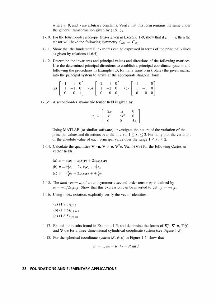
1-13*. A second-order symmetric tensor field is given by
aij ¼2x1 x1 0
x1 �6x21 0
0 0 5x1
24
35
Using MATLAB (or similar software), investigate the nature of the variation of the
principal values and directions over the interval 1 � x1 � 2. Formally plot the variation
of the absolute value of each principal value over the range 1 � x1 � 2.
1-14. Calculate the quantities rrr � u, rrr � u, rrr2u, rrru, tr(rrru) for the following Cartesian
vector fields:
(a) u ¼ x1e1 þ x1x2e2 þ 2x1x2x3e3
(b) u ¼ x21e1 þ 2x1x2e2 þ x33e3
(c) u ¼ x22e1 þ 2x2x3e2 þ 4x21e3
1-15. The dual vector ai of an antisymmetric second-order tensor aij is defined by
ai ¼ �1=2eijkajk. Show that this expression can be inverted to get ajk ¼ �eijkai.
1-16. Using index notation, explicitly verify the vector identities:
(a) (1:8:5)1, 2, 3
(b) (1:8:5)4, 5, 6, 7
(c) (1:8:5)8, 9, 10
1-17. Extend the results found in Example 1-5, and determine the forms of rrrf , rrr� u, r2f ,and rrr�u for a three-dimensional cylindrical coordinate system (see Figure 1-5).
1-18. For the spherical coordinate system (R, f, y) in Figure 1-6, show that
h1 ¼ 1, h2 ¼ R, h3 ¼ R sinf
28 FOUNDATIONS AND ELEMENTARY APPLICATIONS
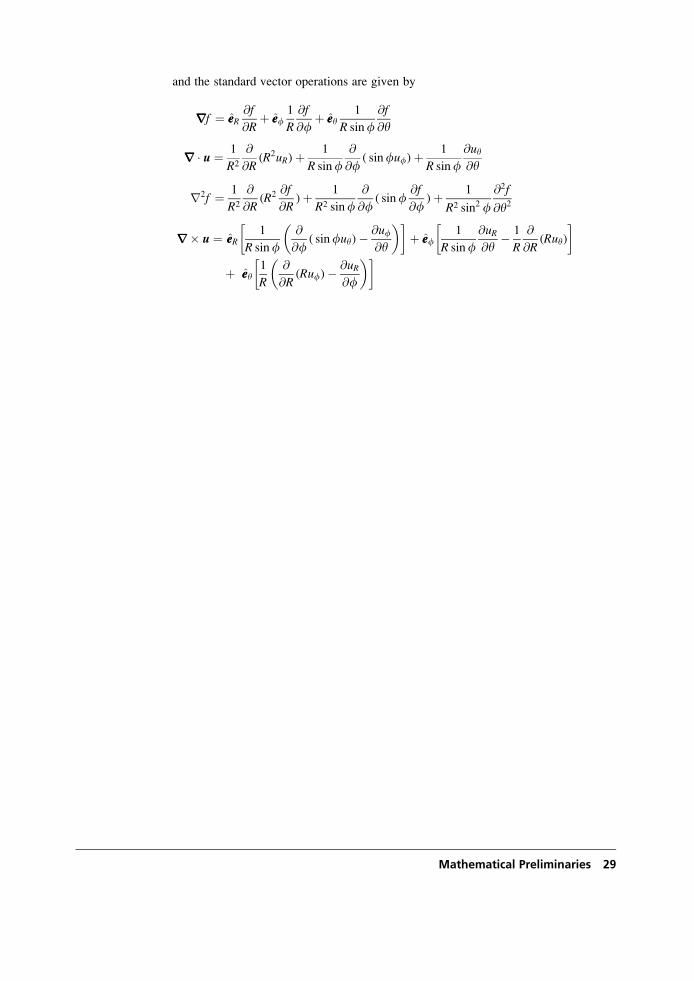
and the standard vector operations are given by
rrrf ¼ eeR@f
@Rþ eef
1
R
@f
@fþ eey
1
R sinf@f
@y
rrr � u ¼ 1
R2
@
@R(R2uR)þ 1
R sinf@
@f( sinfuf)þ 1
R sinf@uy@y
r2f ¼ 1
R2
@
@R(R2 @f
@R)þ 1
R2 sinf@
@f( sinf
@f
@f)þ 1
R2 sin2 f@2f
@y2
rrr� u ¼ eeR1
R sinf@
@f( sinfuy)� @uf
@y
� � þ eef
1
R sinf@uR@y
� 1
R
@
@R(Ruy)
þ eey1
R
@
@R(Ruf)� @uR
@f
� �
Mathematical Preliminaries 29
2 Deformation: Displacements and Strains
We begin development of the basic field equations of elasticity theory by first investigating the
kinematics of material deformation. As a result of applied loadings, elastic solids will change
shape or deform, and these deformations can be quantified by knowing the displacements of
material points in the body. The continuum hypothesis establishes a displacement field at all
points within the elastic solid. Using appropriate geometry, particular measures of deformation
can be constructed leading to the development of the strain tensor. As expected, the strain
components are related to the displacement field. The purpose of this chapter is to introduce the
basic definitions of displacement and strain, establish relations between these two field
quantities, and finally investigate requirements to ensure single-valued, continuous displace-
ment fields. As appropriate for linear elasticity, these kinematical results are developed under
the conditions of small deformation theory. Developments in this chapter lead to two funda-
mental sets of field equations: the strain-displacement relations and the compatibility equa-
tions. Further field equation development, including internal force and stress distribution,
equilibrium, and elastic constitutive behavior, occurs in subsequent chapters.
2.1 General Deformations
Under the application of external loading, elastic solids deform. A simple two-dimensional
cantilever beam example is shown in Figure 2-1. The undeformed configuration is taken with
the rectangular beam in the vertical position, and the end loading displaces material points to
the deformed shape as shown. As is typical in most problems, the deformation varies from
point to point and is thus said to be nonhomogeneous. A superimposed square mesh is shown in
the two configurations, and this indicates how elements within the material deform locally. It is
apparent that elements within the mesh undergo extensional and shearing deformation. An
elastic solid is said to be deformed or strained when the relative displacements between points
in the body are changed. This is in contrast to rigid-body motion where the distance between
points remains the same.
In order to quantify deformation, consider the general example shown in Figure 2-2. In the
undeformed configuration, we identify two neighboring material points Po and P connected
with the relative position vector r as shown. Through a general deformation, these points are
mapped to locations P0o and P0 in the deformed configuration. For finite or large deformation
31
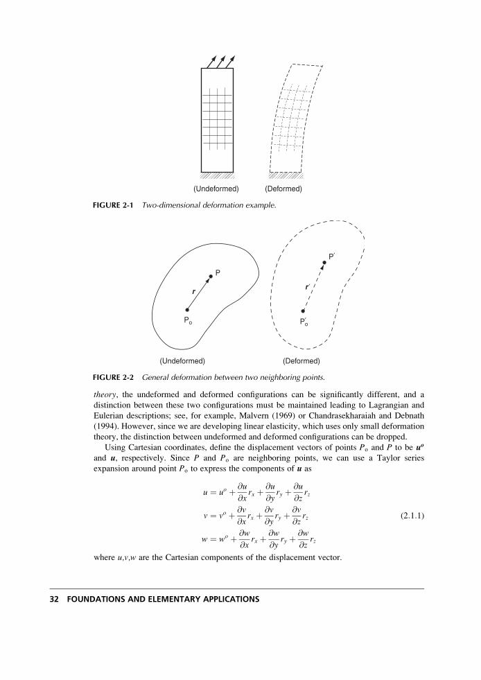
theory, the undeformed and deformed configurations can be significantly different, and a
distinction between these two configurations must be maintained leading to Lagrangian and
Eulerian descriptions; see, for example, Malvern (1969) or Chandrasekharaiah and Debnath
(1994). However, since we are developing linear elasticity, which uses only small deformation
theory, the distinction between undeformed and deformed configurations can be dropped.
Using Cartesian coordinates, define the displacement vectors of points Po and P to be uo
and u, respectively. Since P and Po are neighboring points, we can use a Taylor series
expansion around point Po to express the components of u as
u ¼ uo þ @u
@xrx þ @u
@yry þ @u
@zrz
v ¼ vo þ @v
@xrx þ @v
@yry þ @v
@zrz
w ¼ wo þ @w
@xrx þ @w
@yry þ @w
@zrz
(2:1:1)
where u,v,w are the Cartesian components of the displacement vector.
(Undeformed) (Deformed)
FIGURE 2-1 Two-dimensional deformation example.
P
Po
P
Po
r r
(Undeformed) (Deformed)
′
′
′
FIGURE 2-2 General deformation between two neighboring points.
32 FOUNDATIONS AND ELEMENTARY APPLICATIONS
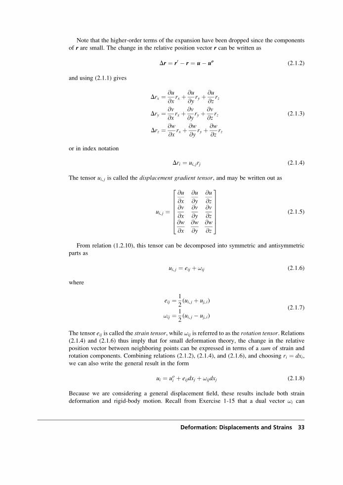
Note that the higher-order terms of the expansion have been dropped since the components
of r are small. The change in the relative position vector r can be written as
Dr ¼ r0 � r ¼ u� uo (2:1:2)
and using (2.1.1) gives
Drx ¼ @u
@xrx þ @u
@yry þ @u
@zrz
Dry ¼ @v
@xrx þ @v
@yry þ @v
@zrz
Drz ¼ @w
@xrx þ @w
@yry þ @w
@zrz
(2:1:3)
or in index notation
Dri ¼ ui, jrj (2:1:4)
The tensor ui, j is called the displacement gradient tensor, and may be written out as
ui, j ¼
@u
@x
@u
@y
@u
@z@v
@x
@v
@y
@v
@z@w
@x
@w
@y
@w
@z
26666664
37777775
(2:1:5)
From relation (1.2.10), this tensor can be decomposed into symmetric and antisymmetric
parts as
ui, j ¼ eij þ !ij (2:1:6)
where
eij ¼ 1
2(ui, j þ uj, i)
!ij ¼ 1
2(ui, j � uj, i)
(2:1:7)
The tensor eij is called the strain tensor, while !ij is referred to as the rotation tensor. Relations(2.1.4) and (2.1.6) thus imply that for small deformation theory, the change in the relative
position vector between neighboring points can be expressed in terms of a sum of strain and
rotation components. Combining relations (2.1.2), (2.1.4), and (2.1.6), and choosing ri ¼ dxi,we can also write the general result in the form
ui ¼ uoi þ eijdxj þ !ijdxj (2:1:8)
Because we are considering a general displacement field, these results include both strain
deformation and rigid-body motion. Recall from Exercise 1-15 that a dual vector !i can
Deformation: Displacements and Strains 33
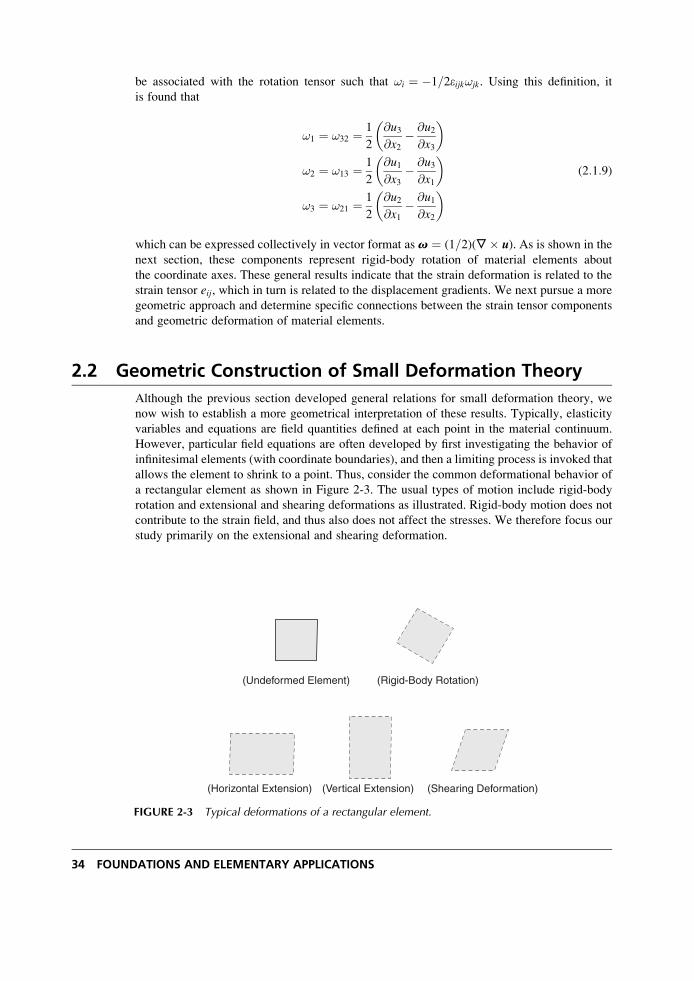
be associated with the rotation tensor such that !i ¼ �1=2eijk!jk. Using this definition, it
is found that
!1 ¼ !32 ¼ 1
2
@u3@x2
� @u2@x3
� �
!2 ¼ !13 ¼ 1
2
@u1@x3
� @u3@x1
� �
!3 ¼ !21 ¼ 1
2
@u2@x1
� @u1@x2
� � (2:1:9)
which can be expressed collectively in vector format as v ¼ (1=2)(,� u). As is shown in thenext section, these components represent rigid-body rotation of material elements about
the coordinate axes. These general results indicate that the strain deformation is related to the
strain tensor eij, which in turn is related to the displacement gradients. We next pursue a more
geometric approach and determine specific connections between the strain tensor components
and geometric deformation of material elements.
2.2 Geometric Construction of Small Deformation Theory
Although the previous section developed general relations for small deformation theory, we
now wish to establish a more geometrical interpretation of these results. Typically, elasticity
variables and equations are field quantities defined at each point in the material continuum.
However, particular field equations are often developed by first investigating the behavior of
infinitesimal elements (with coordinate boundaries), and then a limiting process is invoked that
allows the element to shrink to a point. Thus, consider the common deformational behavior of
a rectangular element as shown in Figure 2-3. The usual types of motion include rigid-body
rotation and extensional and shearing deformations as illustrated. Rigid-body motion does not
contribute to the strain field, and thus also does not affect the stresses. We therefore focus our
study primarily on the extensional and shearing deformation.
(Rigid-Body Rotation)(Undeformed Element)
(Horizontal Extension) (Vertical Extension) (Shearing Deformation)
FIGURE 2-3 Typical deformations of a rectangular element.
34 FOUNDATIONS AND ELEMENTARY APPLICATIONS
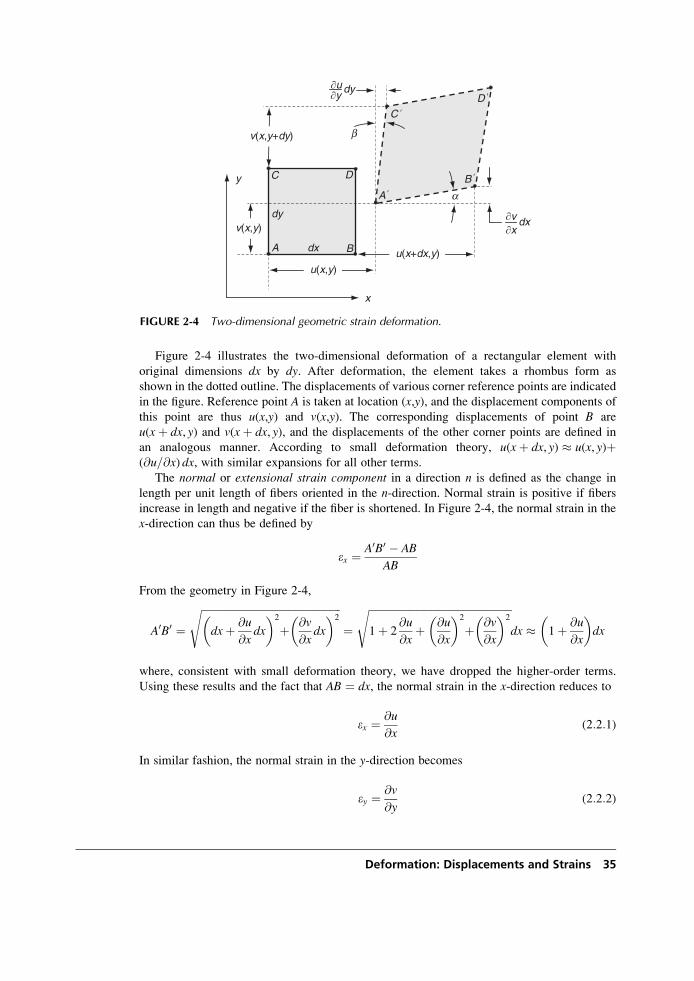
Figure 2-4 illustrates the two-dimensional deformation of a rectangular element with
original dimensions dx by dy. After deformation, the element takes a rhombus form as
shown in the dotted outline. The displacements of various corner reference points are indicated
in the figure. Reference point A is taken at location (x,y), and the displacement components of
this point are thus u(x,y) and v(x,y). The corresponding displacements of point B are
u(xþ dx, y) and v(xþ dx, y), and the displacements of the other corner points are defined in
an analogous manner. According to small deformation theory, u(xþ dx, y) � u(x, y)þ(@u=@x) dx, with similar expansions for all other terms.
The normal or extensional strain component in a direction n is defined as the change in
length per unit length of fibers oriented in the n-direction. Normal strain is positive if fibers
increase in length and negative if the fiber is shortened. In Figure 2-4, the normal strain in the
x-direction can thus be defined by
ex ¼ A0B0 � AB
AB
From the geometry in Figure 2-4,
A0B0 ¼ffiffiffiffiffiffiffiffiffiffiffiffiffiffiffiffiffiffiffiffiffiffiffiffiffiffiffiffiffiffiffiffiffiffiffiffiffiffiffiffiffiffiffiffiffiffiffiffiffiffiffiffiffidxþ @u
@xdx
� �2
þ @v
@xdx
� �2s
¼ffiffiffiffiffiffiffiffiffiffiffiffiffiffiffiffiffiffiffiffiffiffiffiffiffiffiffiffiffiffiffiffiffiffiffiffiffiffiffiffiffiffiffiffiffiffiffiffiffiffiffiffiffiffiffiffiffiffiffi1þ 2
@u
@xþ @u
@x
� �2
þ @v
@x
� �2
dx
s� 1þ @u
@x
� �dx
where, consistent with small deformation theory, we have dropped the higher-order terms.
Using these results and the fact that AB ¼ dx, the normal strain in the x-direction reduces to
ex ¼ @u
@x(2:2:1)
In similar fashion, the normal strain in the y-direction becomes
ey ¼ @v
@y(2:2:2)
u(x,y)
u(x+dx,y)
v(x,y)
v(x,y+dy)
dx
dy
A B
C D
A
B
C
Ddy
dx∂v∂x
x
b
y
∂u∂y ′
′
′
′ a
FIGURE 2-4 Two-dimensional geometric strain deformation.
Deformation: Displacements and Strains 35
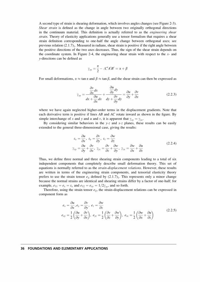
A second type of strain is shearing deformation, which involves angles changes (see Figure 2-3).
Shear strain is defined as the change in angle between two originally orthogonal directions
in the continuum material. This definition is actually referred to as the engineering shearstrain. Theory of elasticity applications generally use a tensor formalism that requires a shear
strain definition corresponding to one-half the angle change between orthogonal axes; see
previous relation (2:1:7)1. Measured in radians, shear strain is positive if the right angle between
the positive directions of the two axes decreases. Thus, the sign of the shear strain depends on
the coordinate system. In Figure 2-4, the engineering shear strain with respect to the x- andy-directions can be defined as
gxy ¼p2� ffC0A0B0 ¼ aþ b
For small deformations, a � tan a and b � tan b, and the shear strain can then be expressed as
gxy ¼@v
@xdx
dxþ @u
@xdx
þ@u
@ydy
dyþ @v
@ydy
¼ @u
@yþ @v
@x(2:2:3)
where we have again neglected higher-order terms in the displacement gradients. Note that
each derivative term is positive if lines AB and AC rotate inward as shown in the figure. By
simple interchange of x and y and u and v, it is apparent that gxy ¼ gyx.By considering similar behaviors in the y-z and x-z planes, these results can be easily
extended to the general three-dimensional case, giving the results:
ex ¼ @u
@x, ey ¼ @v
@y, ez ¼ @w
@z
gxy ¼@u
@yþ @v
@x, gyz ¼
@v
@zþ @w
@y, gzx ¼
@w
@xþ @u
@z
(2:2:4)
Thus, we define three normal and three shearing strain components leading to a total of six
independent components that completely describe small deformation theory. This set of
equations is normally referred to as the strain-displacement relations. However, these results
are written in terms of the engineering strain components, and tensorial elasticity theory
prefers to use the strain tensor eij defined by (2:1:7)1. This represents only a minor change
because the normal strains are identical and shearing strains differ by a factor of one-half; for
example, e11 ¼ ex ¼ ex and e12 ¼ exy ¼ 1=2gxy, and so forth.
Therefore, using the strain tensor eij, the strain-displacement relations can be expressed in
component form as
ex ¼ @u
@x, ey ¼ @v
@y, ez ¼ @w
@z
exy ¼ 1
2
@u
@yþ @v
@x
� �, eyz ¼ 1
2
@v
@zþ @w
@y
� �, ezx ¼ 1
2
@w
@xþ @u
@z
� � (2:2:5)
36 FOUNDATIONS AND ELEMENTARY APPLICATIONS
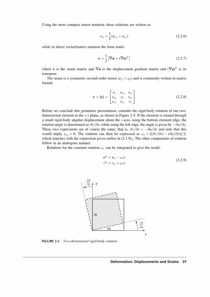
Using the more compact tensor notation, these relations are written as
eij ¼ 1
2(ui, j þ uj, i) (2:2:6)
while in direct vector/matrix notation the form reads:
e ¼ 1
2,uþ (,u)T� �
(2:2:7)
where e is the strain matrix and ,u is the displacement gradient matrix and (,u)T is its
transpose.
The strain is a symmetric second-order tensor (eij ¼ eji) and is commonly written in matrix
format:
e ¼ [e] ¼ex exy exzexy ey eyzexz eyz ez
24
35 (2:2:8)
Before we conclude this geometric presentation, consider the rigid-body rotation of our two-
dimensional element in the x-y plane, as shown in Figure 2-5. If the element is rotated through
a small rigid-body angular displacement about the z-axis, using the bottom element edge, the
rotation angle is determined as @v=@x, while using the left edge, the angle is given by �@[email protected] two expressions are of course the same; that is, @v=@x ¼ �@u=@y and note that this
would imply exy ¼ 0. The rotation can then be expressed as !z ¼ [(@v=@x)� (@u=@y)]=2,which matches with the expression given earlier in (2:1:9)3. The other components of rotation
follow in an analogous manner.
Relations for the constant rotation !z can be integrated to give the result:
u* ¼ uo � !zy
v* ¼ vo þ !zx(2:2:9)
x
dx
dy
y− ∂u∂y
∂v∂x
FIGURE 2-5 Two-dimensional rigid-body rotation.
Deformation: Displacements and Strains 37
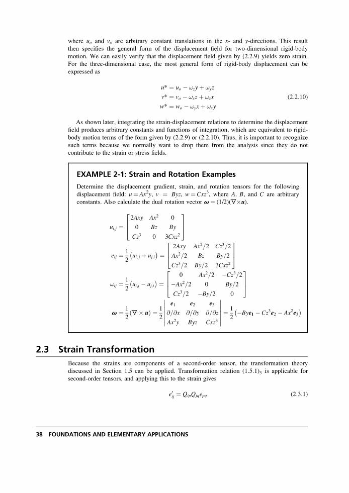
where uo and vo are arbitrary constant translations in the x- and y-directions. This result
then specifies the general form of the displacement field for two-dimensional rigid-body
motion. We can easily verify that the displacement field given by (2.2.9) yields zero strain.
For the three-dimensional case, the most general form of rigid-body displacement can be
expressed as
u* ¼ uo � !zyþ !yz
v* ¼ vo � !xzþ !zx
w* ¼ wo � !yxþ !xy
(2:2:10)
As shown later, integrating the strain-displacement relations to determine the displacement
field produces arbitrary constants and functions of integration, which are equivalent to rigid-
body motion terms of the form given by (2.2.9) or (2.2.10). Thus, it is important to recognize
such terms because we normally want to drop them from the analysis since they do not
contribute to the strain or stress fields.
EXAMPLE 2-1: Strain and Rotation Examples
Determine the displacement gradient, strain, and rotation tensors for the following
displacement field: u¼ Ax2y, v ¼ Byz, w¼ Cxz3, where A, B, and C are arbitrary
constants. Also calculate the dual rotation vector v¼ (1/2)(,�u).
ui;j ¼2Axy Ax2 0
0 Bz By
Cz3 0 3Cxz2
264
375
eij ¼ 1
2ui; j þ uj;i� � ¼ 2Axy Ax2=2 Cz3=2
Ax2=2 Bz By=2
Cz3=2 By=2 3Cxz2
264
375
!ij ¼ 1
2ui;j � uj;i� � ¼ 0 Ax2=2 �Cz3=2
�Ax2=2 0 By=2
Cz3=2 �By=2 0
264
375
v ¼ 1
2,� uð Þ ¼ 1
2
e1 e2 e3
@=@x @=@y @=@z
Ax2y Byz Cxz3
¼
1
2�Bye1 � Cz3e2 � Ax2e3� �
2.3 Strain Transformation
Because the strains are components of a second-order tensor, the transformation theory
discussed in Section 1.5 can be applied. Transformation relation (1:5:1)3 is applicable for
second-order tensors, and applying this to the strain gives
e0ij ¼ QipQjqepq (2:3:1)
38 FOUNDATIONS AND ELEMENTARY APPLICATIONS
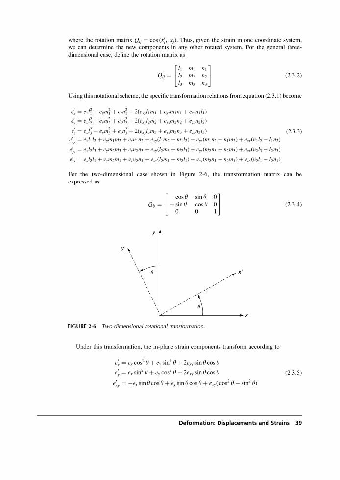
where the rotation matrix Qij ¼ cos (x0i, xj). Thus, given the strain in one coordinate system,
we can determine the new components in any other rotated system. For the general three-
dimensional case, define the rotation matrix as
Qij ¼l1 m1 n1l2 m2 n2l3 m3 n3
24
35 (2:3:2)
Using this notational scheme, the specific transformation relations from equation (2.3.1) become
e0x ¼ exl21 þ eym
21 þ ezn
21 þ 2(exyl1m1 þ eyzm1n1 þ ezxn1l1)
e0y ¼ exl22 þ eym
22 þ ezn
22 þ 2(exyl2m2 þ eyzm2n2 þ ezxn2l2)
e0z ¼ exl23 þ eym
23 þ ezn
23 þ 2(exyl3m3 þ eyzm3n3 þ ezxn3l3)
e0xy ¼ exl1l2 þ eym1m2 þ ezn1n2 þ exy(l1m2 þ m1l2)þ eyz(m1n2 þ n1m2)þ ezx(n1l2 þ l1n2)
e0yz ¼ exl2l3 þ eym2m3 þ ezn2n3 þ exy(l2m3 þ m2l3)þ eyz(m2n3 þ n2m3)þ ezx(n2l3 þ l2n3)
e0zx ¼ exl3l1 þ eym3m1 þ ezn3n1 þ exy(l3m1 þ m3l1)þ eyz(m3n1 þ n3m1)þ ezx(n3l1 þ l3n1)
(2:3:3)
For the two-dimensional case shown in Figure 2-6, the transformation matrix can be
expressed as
Qij ¼cos y sin y 0
� sin y cos y 0
0 0 1
24
35 (2:3:4)
Under this transformation, the in-plane strain components transform according to
e0x ¼ ex cos2 yþ ey sin
2 yþ 2exy sin y cos y
e0y ¼ ex sin2 yþ ey cos
2 y� 2exy sin y cos y
e0xy ¼ �ex sin y cos yþ ey sin y cos yþ exy( cos2 y� sin2 y)
(2:3:5)
x
y
x
y
q
q
′
′
FIGURE 2-6 Two-dimensional rotational transformation.
Deformation: Displacements and Strains 39
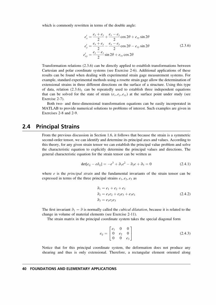
which is commonly rewritten in terms of the double angle:
e0x ¼ex þ ey
2þ ex � ey
2cos 2yþ exy sin 2y
e0y ¼ex þ ey
2� ex � ey
2cos 2y� exy sin 2y
e0xy ¼ey � ex
2sin 2yþ exy cos 2y
(2:3:6)
Transformation relations (2.3.6) can be directly applied to establish transformations between
Cartesian and polar coordinate systems (see Exercise 2-6). Additional applications of these
results can be found when dealing with experimental strain gage measurement systems. For
example, standard experimental methods using a rosette strain gage allow the determination of
extensional strains in three different directions on the surface of a structure. Using this type
of data, relation (2:3:6)1 can be repeatedly used to establish three independent equations
that can be solved for the state of strain (ex, ey, exy) at the surface point under study (see
Exercise 2-7).
Both two- and three-dimensional transformation equations can be easily incorporated in
MATLAB to provide numerical solutions to problems of interest. Such examples are given in
Exercises 2-8 and 2-9.
2.4 Principal Strains
From the previous discussion in Section 1.6, it follows that because the strain is a symmetric
second-order tensor, we can identify and determine its principal axes and values. According to
this theory, for any given strain tensor we can establish the principal value problem and solve
the characteristic equation to explicitly determine the principal values and directions. The
general characteristic equation for the strain tensor can be written as
det[eij � edij] ¼ �e3 þ W1e2 � W2eþ W3 ¼ 0 (2:4:1)
where e is the principal strain and the fundamental invariants of the strain tensor can be
expressed in terms of the three principal strains e1, e2, e3 as
W1 ¼ e1 þ e2 þ e3
W2 ¼ e1e2 þ e2e3 þ e3e1
W3 ¼ e1e2e3
(2:4:2)
The first invariant W1 ¼ W is normally called the cubical dilatation, because it is related to the
change in volume of material elements (see Exercise 2-11).
The strain matrix in the principal coordinate system takes the special diagonal form
eij ¼e1 0 0
0 e2 0
0 0 e3
24
35 (2:4:3)
Notice that for this principal coordinate system, the deformation does not produce any
shearing and thus is only extensional. Therefore, a rectangular element oriented along
40 FOUNDATIONS AND ELEMENTARY APPLICATIONS
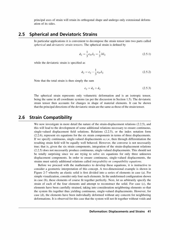
principal axes of strain will retain its orthogonal shape and undergo only extensional deform-
ation of its sides.
2.5 Spherical and Deviatoric Strains
In particular applications it is convenient to decompose the strain tensor into two parts called
spherical and deviatoric strain tensors. The spherical strain is defined by
~eeij ¼ 1
3ekkdij ¼ 1
3Wdij (2:5:1)
while the deviatoric strain is specified as
eeij ¼ eij � 1
3ekkdij (2:5:2)
Note that the total strain is then simply the sum
eij ¼ ~eeij þ eeij (2:5:3)
The spherical strain represents only volumetric deformation and is an isotropic tensor,
being the same in all coordinate systems (as per the discussion in Section 1.5). The deviatoric
strain tensor then accounts for changes in shape of material elements. It can be shown
that the principal directions of the deviatoric strain are the same as those of the strain tensor.
2.6 Strain Compatibility
We now investigate in more detail the nature of the strain-displacement relations (2.2.5), and
this will lead to the development of some additional relations necessary to ensure continuous,
single-valued displacement field solutions. Relations (2.2.5), or the index notation form
(2.2.6), represent six equations for the six strain components in terms of three displacements.
If we specify continuous, single-valued displacements u,v,w, then through differentiation the
resulting strain field will be equally well behaved. However, the converse is not necessarily
true; that is, given the six strain components, integration of the strain-displacement relations
(2.2.5) does not necessarily produce continuous, single-valued displacements. This should not
be totally surprising since we are trying to solve six equations for only three unknown
displacement components. In order to ensure continuous, single-valued displacements, the
strains must satisfy additional relations called integrability or compatibility equations.Before we proceed with the mathematics to develop these equations, it is instructive to
consider a geometric interpretation of this concept. A two-dimensional example is shown in
Figure 2-7 whereby an elastic solid is first divided into a series of elements in case (a). For
simple visualization, consider only four such elements. In the undeformed configuration shown
in case (b), these elements of course fit together perfectly. Next, let us arbitrarily specify the
strain of each of the four elements and attempt to reconstruct the solid. For case (c), the
elements have been carefully strained, taking into consideration neighboring elements so that
the system fits together thus yielding continuous, single-valued displacements. However, for
case (d), the elements have been individually deformed without any concern for neighboring
deformations. It is observed for this case that the system will not fit together without voids and
Deformation: Displacements and Strains 41
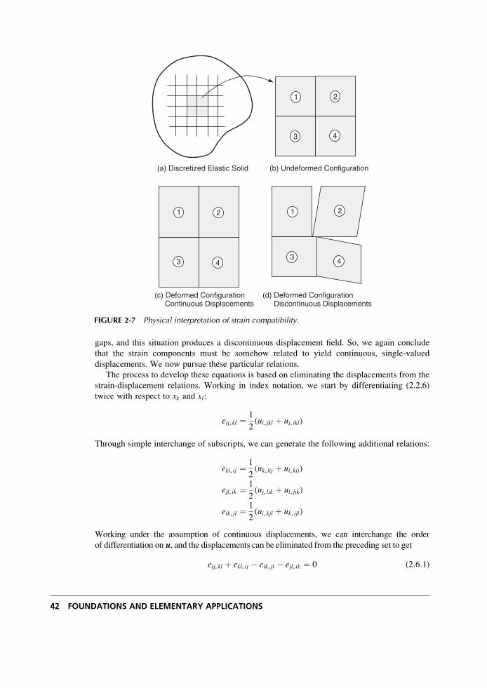
gaps, and this situation produces a discontinuous displacement field. So, we again conclude
that the strain components must be somehow related to yield continuous, single-valued
displacements. We now pursue these particular relations.
The process to develop these equations is based on eliminating the displacements from the
strain-displacement relations. Working in index notation, we start by differentiating (2.2.6)
twice with respect to xk and xl:
eij, kl ¼ 1
2(ui, jkl þ uj, ikl)
Through simple interchange of subscripts, we can generate the following additional relations:
ekl, ij ¼ 1
2(uk, lij þ ul, kij)
ejl, ik ¼ 1
2(uj, lik þ ul, jik)
eik, jl ¼ 1
2(ui, kjl þ uk, ijl)
Working under the assumption of continuous displacements, we can interchange the order
of differentiation on u, and the displacements can be eliminated from the preceding set to get
eij, kl þ ekl, ij � eik, jl � ejl, ik ¼ 0 (2:6:1)
2
3
1
4
(b) Undeformed Configuration
2
3
1
4
(c) Deformed Configuration Continuous Displacements
2
3
1
4
(a) Discretized Elastic Solid
(d) Deformed Configuration Discontinuous Displacements
FIGURE 2-7 Physical interpretation of strain compatibility.
42 FOUNDATIONS AND ELEMENTARY APPLICATIONS
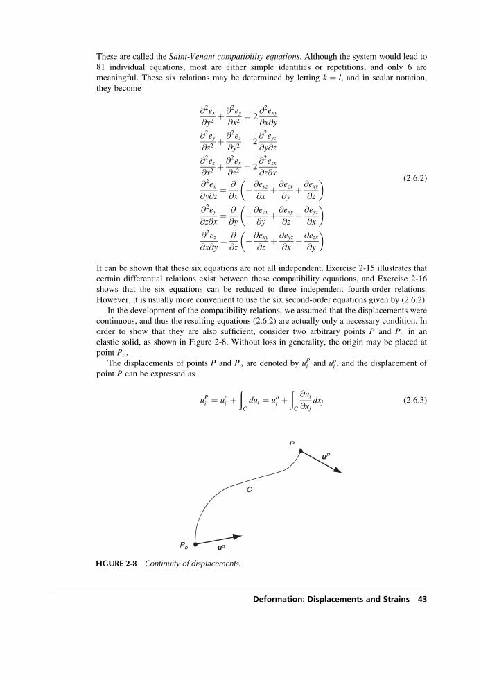
These are called the Saint-Venant compatibility equations. Although the system would lead to
81 individual equations, most are either simple identities or repetitions, and only 6 are
meaningful. These six relations may be determined by letting k ¼ l, and in scalar notation,
they become
@2ex@y2
þ @2ey@x2
¼ 2@2exy@x@y
@2ey@z2
þ @2ez@y2
¼ 2@2eyz@y@z
@2ez@x2
þ @2ex@z2
¼ 2@2ezx@z@x
@2ex@y@z
¼ @
@x� @eyz
@xþ @ezx
@yþ @exy
@z
� �@2ey@z@x
¼ @
@y� @ezx
@yþ @exy
@zþ @eyz
@x
� �@2ez@x@y
¼ @
@z� @exy
@zþ @eyz
@xþ @ezx
@y
� �
(2:6:2)
It can be shown that these six equations are not all independent. Exercise 2-15 illustrates that
certain differential relations exist between these compatibility equations, and Exercise 2-16
shows that the six equations can be reduced to three independent fourth-order relations.
However, it is usually more convenient to use the six second-order equations given by (2.6.2).
In the development of the compatibility relations, we assumed that the displacements were
continuous, and thus the resulting equations (2.6.2) are actually only a necessary condition. In
order to show that they are also sufficient, consider two arbitrary points P and Po in an
elastic solid, as shown in Figure 2-8. Without loss in generality, the origin may be placed at
point Po.
The displacements of points P and Po are denoted by uPi and uoi , and the displacement of
point P can be expressed as
uPi ¼ uoi þðC
dui ¼ uoi þðC
@ui@xj
dxj (2:6:3)
Po
P
C
uo
uP
FIGURE 2-8 Continuity of displacements.
Deformation: Displacements and Strains 43
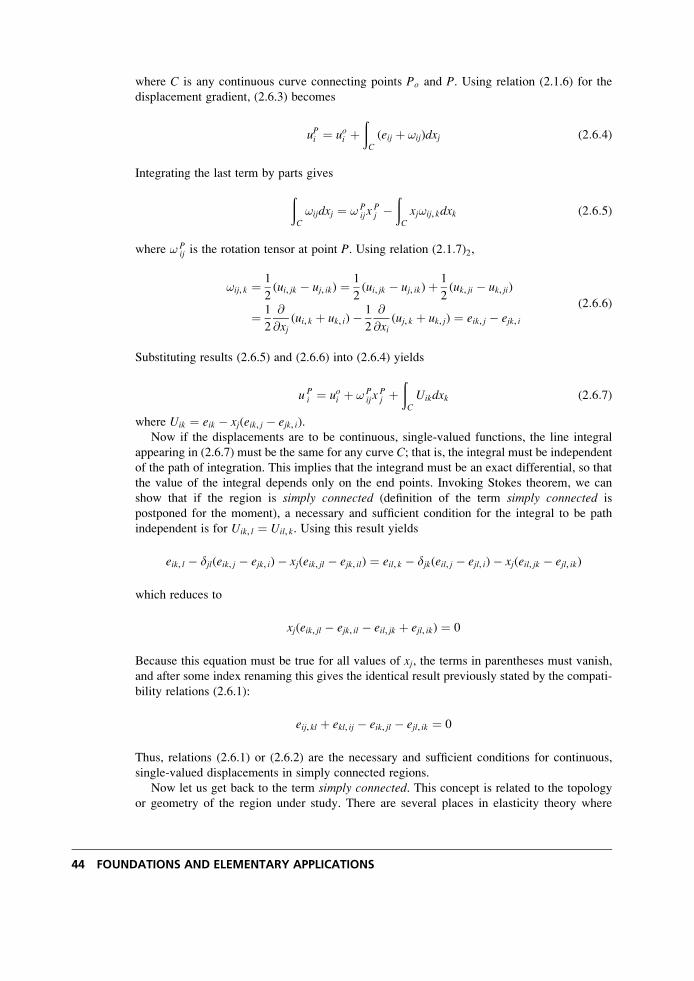
where C is any continuous curve connecting points Po and P. Using relation (2.1.6) for the
displacement gradient, (2.6.3) becomes
uPi ¼ uoi þðC
(eij þ !ij)dxj (2:6:4)
Integrating the last term by parts gives
ðC
!ijdxj ¼ ! Pijx
Pj �
ðC
xj!ij, kdxk (2:6:5)
where ! Pij is the rotation tensor at point P. Using relation (2:1:7)2,
!ij, k ¼ 1
2(ui, jk � uj, ik) ¼ 1
2(ui, jk � uj, ik)þ 1
2(uk, ji � uk, ji)
¼ 1
2
@
@xj(ui, k þ uk, i)� 1
2
@
@xi(uj, k þ uk, j) ¼ eik, j � ejk, i
(2:6:6)
Substituting results (2.6.5) and (2.6.6) into (2.6.4) yields
u Pi ¼ uoi þ ! P
ijxPj þ
ðC
Uikdxk (2:6:7)
where Uik ¼ eik � xj(eik, j � ejk, i).Now if the displacements are to be continuous, single-valued functions, the line integral
appearing in (2.6.7) must be the same for any curve C; that is, the integral must be independent
of the path of integration. This implies that the integrand must be an exact differential, so that
the value of the integral depends only on the end points. Invoking Stokes theorem, we can
show that if the region is simply connected (definition of the term simply connected is
postponed for the moment), a necessary and sufficient condition for the integral to be path
independent is for Uik, l ¼ Uil, k. Using this result yields
eik, l � djl(eik, j � ejk, i)� xj(eik, jl � ejk, il) ¼ eil, k � djk(eil, j � ejl, i)� xj(eil, jk � ejl, ik)
which reduces to
xj(eik, jl � ejk, il � eil, jk þ ejl, ik) ¼ 0
Because this equation must be true for all values of xj, the terms in parentheses must vanish,
and after some index renaming this gives the identical result previously stated by the compati-
bility relations (2.6.1):
eij, kl þ ekl, ij � eik, jl � ejl, ik ¼ 0
Thus, relations (2.6.1) or (2.6.2) are the necessary and sufficient conditions for continuous,
single-valued displacements in simply connected regions.
Now let us get back to the term simply connected. This concept is related to the topology
or geometry of the region under study. There are several places in elasticity theory where
44 FOUNDATIONS AND ELEMENTARY APPLICATIONS
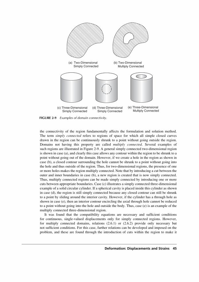
the connectivity of the region fundamentally affects the formulation and solution method.
The term simply connected refers to regions of space for which all simple closed curves
drawn in the region can be continuously shrunk to a point without going outside the region.
Domains not having this property are called multiply connected. Several examples of
such regions are illustrated in Figure 2-9. A general simply connected two-dimensional region
is shown in case (a), and clearly this case allows any contour within the region to be shrunk to a
point without going out of the domain. However, if we create a hole in the region as shown in
case (b), a closed contour surrounding the hole cannot be shrunk to a point without going into
the hole and thus outside of the region. Thus, for two-dimensional regions, the presence of one
or more holes makes the region multiply connected. Note that by introducing a cut between the
outer and inner boundaries in case (b), a new region is created that is now simply connected.
Thus, multiply connected regions can be made simply connected by introducing one or more
cuts between appropriate boundaries. Case (c) illustrates a simply connected three-dimensional
example of a solid circular cylinder. If a spherical cavity is placed inside this cylinder as shown
in case (d), the region is still simply connected because any closed contour can still be shrunk
to a point by sliding around the interior cavity. However, if the cylinder has a through hole as
shown in case (e), then an interior contour encircling the axial through hole cannot be reduced
to a point without going into the hole and outside the body. Thus, case (e) is an example of the
multiply connected three-dimensional region.
It was found that the compatibility equations are necessary and sufficient conditions
for continuous, single-valued displacements only for simply connected regions. However,
for multiply connected domains, relations (2.6.1) or (2.6.2) provide only necessary but
not sufficient conditions. For this case, further relations can be developed and imposed on the
problem, and these are found through the introduction of cuts within the region to make it
(a) Two-Dimensional Simply Connected
(b) Two-Dimensional Multiply Connected
(e) Three-Dimensional Multiply Connected
(d) Three-Dimensional Simply Connected
(c) Three-Dimensional Simply Connected
FIGURE 2-9 Examples of domain connectivity.
Deformation: Displacements and Strains 45
simply connected as per our earlier discussion. For the two-dimensional case shown in Figure
2-9(b), this process will lead to a relation commonly called a Cesaro integral taken around anyclosed irreducible curve enclosing the internal cavity. Thus for multiply connected domains,
strain compatibility is guaranteed if compatibility relations (2.6.2) are satisfied and all Cesaro
integrals vanish. Details on this topic are given by Fung (1965), Fung and Tong (2001), or
Asaro and Lubarda (2006).
Although the compatibility relations guarantee (under appropriate conditions) continuous
displacements, they do not ensure uniqueness of the displacement field. At the end of
Section 2.2 we mentioned that, through integration of the strain displacement relations,
the displacements can be determined only up to an arbitrary rigid-body motion. In some
elasticity problems (e.g., thermal stress, crack problems, and dislocation modeling), it is
necessary to use multivalued displacement fields to properly model the problem. Chapters
10, 12, and 15 contain a few examples of such problems, and a specific case is given in
Exercise 2-18.
2.7 Curvilinear Cylindrical and Spherical Coordinates
The solution to many problems in elasticity requires the use of curvilinear cylindrical and
spherical coordinates. It is therefore necessary to have the field equations expressed in terms of
such coordinate systems. We now pursue the development of the strain-displacement relations
in cylindrical and spherical coordinates. Starting with form (2.2.7)
e ¼ 1
2,uþ (,u)T� �
the desired curvilinear relations can be determined using the appropriate forms for the
displacement gradient term ,u.The cylindrical coordinate system previously defined in Figure 1-5 establishes new com-
ponents for the displacement vector and strain tensor
u ¼ urer þ uyey þ uzez
e ¼er ery erz
ery ey eyz
erz eyz ez
264
375 (2:7:1)
Notice that the symmetry of the strain tensor is preserved in this orthogonal curvilinear system.
Using results (1.9.17) and (1.9.10), the derivative operation in cylindrical coordinates can be
expressed by
,u ¼ @ur@r
erer þ @uy@r
erey þ @uz@r
erez
þ 1
r
@ur@y
� uy
� �eyer þ 1
rur þ @uy
@y
� �eyey þ 1
r
@uz@y
eyez
þ @ur@z
ezer þ @uy@z
ezey þ @uz@z
ezez
(2:7:2)
46 FOUNDATIONS AND ELEMENTARY APPLICATIONS
Placing this result into the strain-displacement form (2.2.7) gives the desired relations in
cylindrical coordinates. The individual scalar equations are given by
er ¼ @ur@r
, ey ¼ 1
rur þ @uy
@y
� �, ez ¼ @uz
@z
ery ¼ 1
2
1
r
@ur@y
þ @uy@r
� uyr
� �
eyz ¼ 1
2
@uy@z
þ 1
r
@uz@y
� �
ezr ¼ 1
2
@ur@z
þ @uz@r
� �(2:7:3)
For spherical coordinates defined by Figure 1-6, the displacement vector and strain tensor can
be written as
u ¼ uReR þ ufef þ uyey
e ¼eR eRf eRy
eRf ef efy
eRy efy ey
264
375 (2:7:4)
Following identical procedures as used for the cylindrical equation development, the strain-
displacement relations for spherical coordinates become
eR ¼ @uR@R
, ef ¼ 1
RuR þ @uf
@f
� �
ey ¼ 1
R sinf@uy@y
þ sinfuR þ cosfuf
� �
eRf ¼ 1
2
1
R
@uR@f
þ @uf@R
� ufR
� �
efy ¼ 1
2R
1
sinf@uf@y
þ @uy@f
� cotfuy
� �
eyR ¼ 1
2
1
R sinf@uR@y
þ @uy@R
� uyR
� �
(2:7:5)
We can observe that these relations in curvilinear systems contain additional terms that do not
include derivatives of individual displacement components. For example, in spherical coordin-
ates a simple uniform radial displacement uR gives rise to transverse extensional strains
ef ¼ ey ¼ uR=R. This deformation can be simulated by blowing up a spherical balloon and
observing the separation of points on the balloon’s surface. Such terms were not found in the
Cartesian forms given by (2.2.5), and their appearance is thus related to the curvature of the
spatial coordinate system. A more physical interpretation can be found by redeveloping these
equations using the geometric procedures of Section 2.2 on an appropriate differential element.
A two-dimensional polar coordinate example of this technique is given in Exercise 2-19.
Clearly, the curvilinear forms (2.7.3) and (2.7.5) appear more complicated than the corres-
ponding Cartesian relations. However, for particular problems, the curvilinear relations, when
Deformation: Displacements and Strains 47
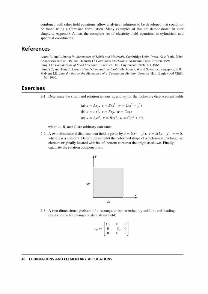
combined with other field equations, allow analytical solutions to be developed that could not
be found using a Cartesian formulation. Many examples of this are demonstrated in later
chapters. Appendix A lists the complete set of elasticity field equations in cylindrical and
spherical coordinates.
References
Asaro R, and Lubarda V: Mechanics of Solids and Materials, Cambridge Univ. Press, New York, 2006.
Chandrasekharaiah DS, and Debnath L: Continuum Mechanics, Academic Press, Boston, 1994.
Fung YC: Foundations of Solid Mechanics, Prentice Hall, Englewood Cliffs, NJ, 1965.
Fung YC, and Tong P: Classical and Computational Solid Mechanics,World Scientific, Singapore, 2001.
Malvern LE: Introduction to the Mechanics of a Continuous Medium, Prentice Hall, Englewood Cliffs,
NJ, 1969.
Exercises
2-1. Determine the strain and rotation tensors eij and !ij for the following displacement fields
(a) u ¼ Axy, v ¼ Bxz2, w ¼ C(x2 þ y2)
(b) u ¼ Ax2, v ¼ Bxy, w ¼ Cxyz
(c) u ¼ Ayz3, v ¼ Bxy2, w ¼ C(x2 þ z2)
where A, B, and C are arbitrary constants.
2-2. A two-dimensional displacement field is given by u ¼ k(x2 þ y2), v ¼ k(2x� y), w ¼ 0,
where k is a constant. Determine and plot the deformed shape of a differential rectangular
element originally located with its left bottom corner at the origin as shown. Finally,
calculate the rotation component !z.
x
y
dx
dy
2-3. A two-dimensional problem of a rectangular bar stretched by uniform end loadings
results in the following constant strain field:
eij ¼C1 0 0
0 �C2 0
0 0 0
24
35
48 FOUNDATIONS AND ELEMENTARY APPLICATIONS
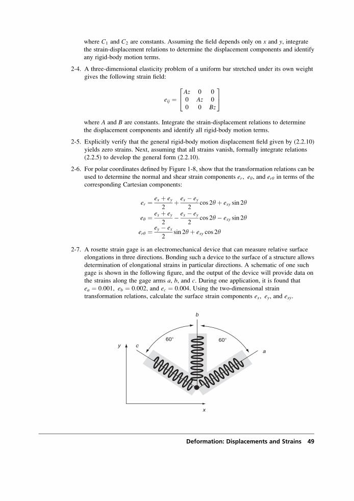
where C1 and C2 are constants. Assuming the field depends only on x and y, integratethe strain-displacement relations to determine the displacement components and identify
any rigid-body motion terms.
2-4. A three-dimensional elasticity problem of a uniform bar stretched under its own weight
gives the following strain field:
eij ¼Az 0 0
0 Az 0
0 0 Bz
24
35
where A and B are constants. Integrate the strain-displacement relations to determine
the displacement components and identify all rigid-body motion terms.
2-5. Explicitly verify that the general rigid-body motion displacement field given by (2.2.10)
yields zero strains. Next, assuming that all strains vanish, formally integrate relations
(2.2.5) to develop the general form (2.2.10).
2-6. For polar coordinates defined by Figure 1-8, show that the transformation relations can be
used to determine the normal and shear strain components er , ey, and ery in terms of the
corresponding Cartesian components:
er ¼ ex þ ey2
þ ex � ey2
cos 2yþ exy sin 2y
ey ¼ ex þ ey2
� ex � ey2
cos 2y� exy sin 2y
ery ¼ ey � ex2
sin 2yþ exy cos 2y
2-7. A rosette strain gage is an electromechanical device that can measure relative surface
elongations in three directions. Bonding such a device to the surface of a structure allows
determination of elongational strains in particular directions. A schematic of one such
gage is shown in the following figure, and the output of the device will provide data on
the strains along the gage arms a, b, and c. During one application, it is found that
ea ¼ 0:001, eb ¼ 0:002, and ec ¼ 0:004. Using the two-dimensional strain
transformation relations, calculate the surface strain components ex, ey, and exy.
x
a y c
b
60�60�
Deformation: Displacements and Strains 49
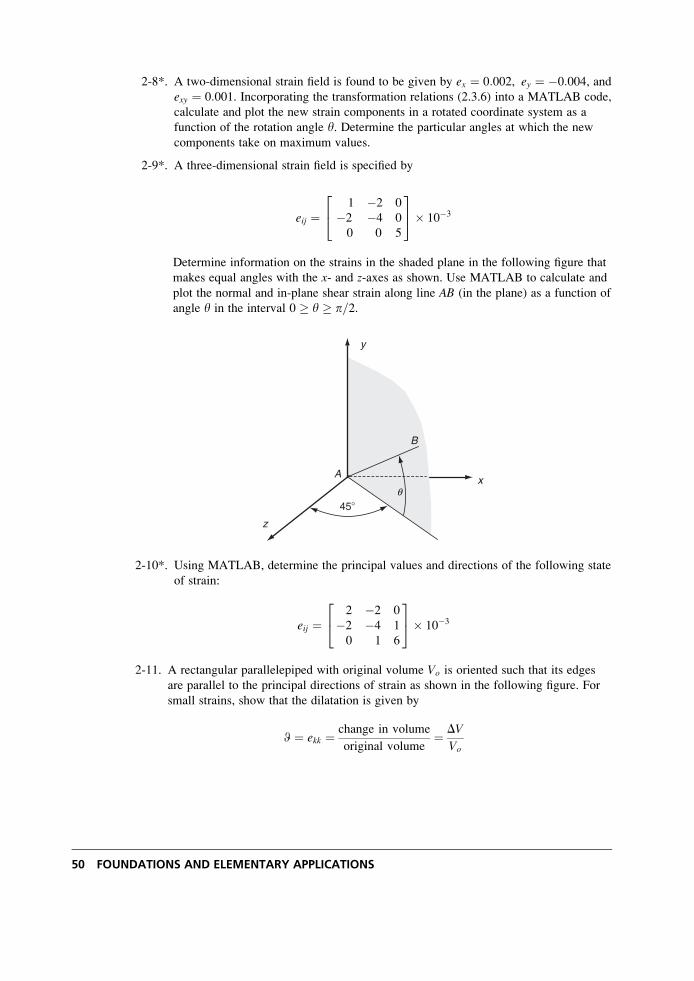
2-8*. A two-dimensional strain field is found to be given by ex ¼ 0:002, ey ¼ �0:004, andexy ¼ 0:001. Incorporating the transformation relations (2.3.6) into a MATLAB code,
calculate and plot the new strain components in a rotated coordinate system as a
function of the rotation angle y. Determine the particular angles at which the new
components take on maximum values.
2-9*. A three-dimensional strain field is specified by
eij ¼1 �2 0
�2 �4 0
0 0 5
24
35� 10�3
Determine information on the strains in the shaded plane in the following figure that
makes equal angles with the x- and z-axes as shown. Use MATLAB to calculate and
plot the normal and in-plane shear strain along line AB (in the plane) as a function of
angle y in the interval 0 � y � p=2.
A
45�
x
y
z
B
q
2-10*. Using MATLAB, determine the principal values and directions of the following state
of strain:
eij ¼2 �2 0
�2 �4 1
0 1 6
24
35� 10�3
2-11. A rectangular parallelepiped with original volume Vo is oriented such that its edges
are parallel to the principal directions of strain as shown in the following figure. For
small strains, show that the dilatation is given by
W ¼ ekk ¼ change in volume
original volume¼ DV
Vo
50 FOUNDATIONS AND ELEMENTARY APPLICATIONS
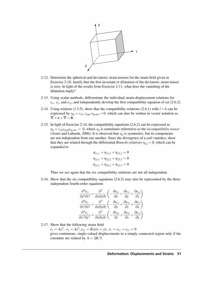
2-12. Determine the spherical and deviatoric strain tensors for the strain field given in
Exercise 2-10. Justify that the first invariant or dilatation of the deviatoric strain tensor
is zero. In light of the results from Exercise 2-11, what does the vanishing of the
dilatation imply?
2-13. Using scalar methods, differentiate the individual strain-displacement relations for
ex, ey, and exy, and independently develop the first compatibility equation of set (2.6.2).
2-14. Using relation (1.3.5), show that the compatibility relations (2.6.1) with l¼ k can be
expressed by �ij¼ "ikl "jmp elp,km¼ 0, which can also be written in vector notation as
,� e�,¼ 0.
2-15. In light of Exercise 2-14, the compatibility equations (2.6.2) can be expressed as
�ij¼ "ikl"jmpelp,km ¼ 0, where �ij is sometimes referred to as the incompatibility tensor(Asaro and Lubarda, 2006). It is observed that �ij is symmetric, but its components
are not independent from one another. Since the divergence of a curl vanishes, show
that they are related through the differential Bianchi relations �ij,j¼ 0, which can be
expanded to
Z11;1 þ Z12;2 þ Z13;3 ¼ 0
Z21;1 þ Z22;2 þ Z23;3 ¼ 0
Z31;1 þ Z32;2 þ Z33;3 ¼ 0
Thus we see again that the six compatibility relations are not all independent.
2-16. Show that the six compatibility equations (2.6.2) may also be represented by the three
independent fourth-order equations
@ 4ex@y2@z2
¼ @ 3
@x@y@z� @eyz
@xþ @ezx
@yþ @exy
@z
� �@ 4ey@z2@x2
¼ @ 3
@x@y@z� @ezx
@yþ @exy
@zþ @eyz
@x
� �@ 4ez
@x2@y2¼ @ 3
@x@y@z� @exy
@zþ @eyz
@xþ @ezx
@y
� �
2-17. Show that the following strain field
ex ¼ Ay3, ey ¼ Ax3, exy ¼ Bxy(xþ y), ez ¼ exz ¼ eyz ¼ 0
gives continuous, single-valued displacements in a simply connected region only if the
constants are related by A ¼ 2B=3.
1
2
3
Deformation: Displacements and Strains 51
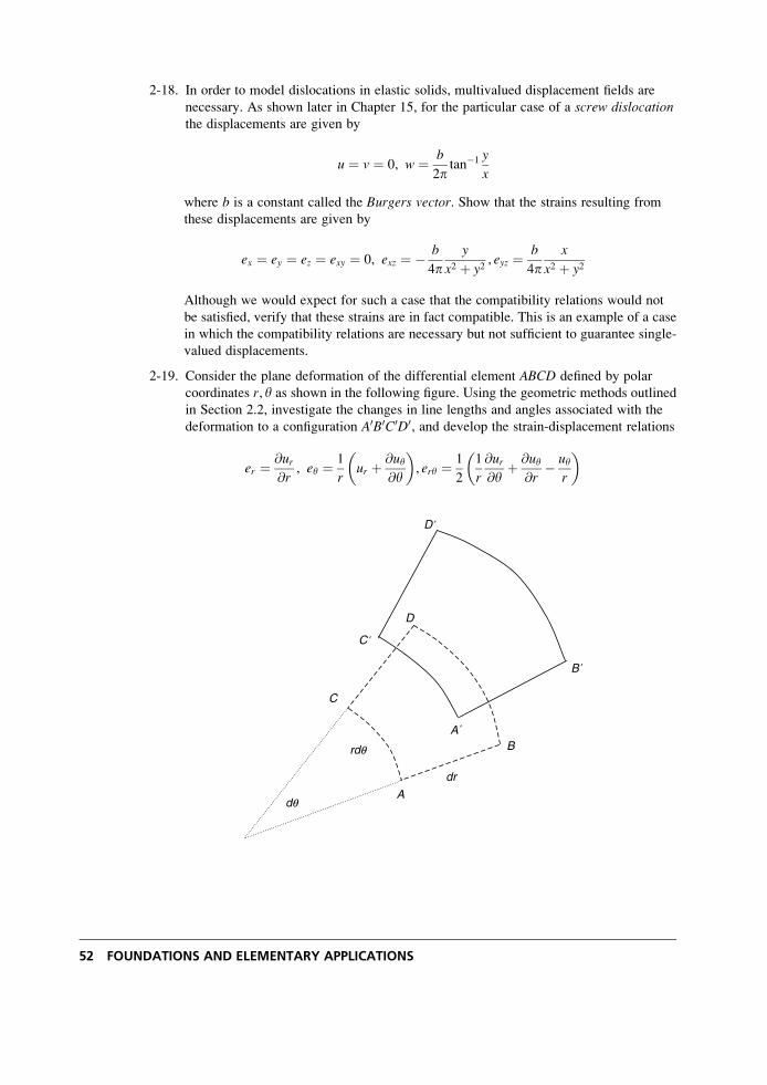
2-18. In order to model dislocations in elastic solids, multivalued displacement fields are
necessary. As shown later in Chapter 15, for the particular case of a screw dislocationthe displacements are given by
u ¼ v ¼ 0, w ¼ b
2ptan�1 y
x
where b is a constant called the Burgers vector. Show that the strains resulting from
these displacements are given by
ex ¼ ey ¼ ez ¼ exy ¼ 0, exz ¼ � b
4py
x2 þ y2, eyz ¼ b
4px
x2 þ y2
Although we would expect for such a case that the compatibility relations would not
be satisfied, verify that these strains are in fact compatible. This is an example of a case
in which the compatibility relations are necessary but not sufficient to guarantee single-
valued displacements.
2-19. Consider the plane deformation of the differential element ABCD defined by polar
coordinates r, y as shown in the following figure. Using the geometric methods outlined
in Section 2.2, investigate the changes in line lengths and angles associated with the
deformation to a configuration A0B0C0D0, and develop the strain-displacement relations
er ¼ @ur@r
, ey ¼ 1
rur þ @uy
@y
� �, ery ¼ 1
2
1
r
@ur@y
þ @uy@r
� uyr
� �
A
C
D
dr
rdq
dq
A
B
C
D
B
′
′
′
′
52 FOUNDATIONS AND ELEMENTARY APPLICATIONS
2-20. Using the results from Exercise 2-19, determine the two-dimensional strains er, e�, er�for the following displacement fields
(a) ur ¼ A
r, uy ¼ B cos y
(b) ur ¼ Ar2, uy ¼ Br sin y
(c) ur ¼ A sin yþ B cos y, uy ¼ A cos y� B sin yþ Cr
where A, B, and C are arbitrary constants.
Deformation: Displacements and Strains 53
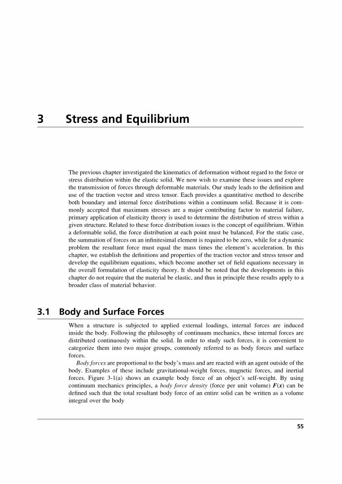
3 Stress and Equilibrium
The previous chapter investigated the kinematics of deformation without regard to the force or
stress distribution within the elastic solid. We now wish to examine these issues and explore
the transmission of forces through deformable materials. Our study leads to the definition and
use of the traction vector and stress tensor. Each provides a quantitative method to describe
both boundary and internal force distributions within a continuum solid. Because it is com-
monly accepted that maximum stresses are a major contributing factor to material failure,
primary application of elasticity theory is used to determine the distribution of stress within a
given structure. Related to these force distribution issues is the concept of equilibrium. Within
a deformable solid, the force distribution at each point must be balanced. For the static case,
the summation of forces on an infinitesimal element is required to be zero, while for a dynamic
problem the resultant force must equal the mass times the element’s acceleration. In this
chapter, we establish the definitions and properties of the traction vector and stress tensor and
develop the equilibrium equations, which become another set of field equations necessary in
the overall formulation of elasticity theory. It should be noted that the developments in this
chapter do not require that the material be elastic, and thus in principle these results apply to a
broader class of material behavior.
3.1 Body and Surface Forces
When a structure is subjected to applied external loadings, internal forces are induced
inside the body. Following the philosophy of continuum mechanics, these internal forces are
distributed continuously within the solid. In order to study such forces, it is convenient to
categorize them into two major groups, commonly referred to as body forces and surface
forces.
Body forces are proportional to the body’s mass and are reacted with an agent outside of the
body. Examples of these include gravitational-weight forces, magnetic forces, and inertial
forces. Figure 3-1(a) shows an example body force of an object’s self-weight. By using
continuum mechanics principles, a body force density (force per unit volume) F(x) can be
defined such that the total resultant body force of an entire solid can be written as a volume
integral over the body
55
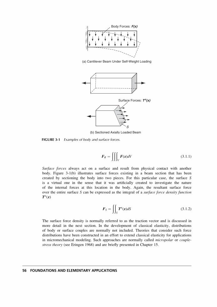
FR ¼ððð
V
F(x)dV (3:1:1)
Surface forces always act on a surface and result from physical contact with another
body. Figure 3-1(b) illustrates surface forces existing in a beam section that has been
created by sectioning the body into two pieces. For this particular case, the surface Sis a virtual one in the sense that it was artificially created to investigate the nature
of the internal forces at this location in the body. Again, the resultant surface force
over the entire surface S can be expressed as the integral of a surface force density functionTn(x)
FS ¼ðð
S
Tn(x)dS (3:1:2)
The surface force density is normally referred to as the traction vector and is discussed in
more detail in the next section. In the development of classical elasticity, distributions
of body or surface couples are normally not included. Theories that consider such force
distributions have been constructed in an effort to extend classical elasticity for applications
in micromechanical modeling. Such approaches are normally called micropolar or couple-stress theory (see Eringen 1968) and are briefly presented in Chapter 15.
(b) Sectioned Axially Loaded Beam
Surface Forces: Tn(x)
S
(a) Cantilever Beam Under Self-Weight Loading
Body Forces: F(x)
FIGURE 3-1 Examples of body and surface forces.
56 FOUNDATIONS AND ELEMENTARY APPLICATIONS
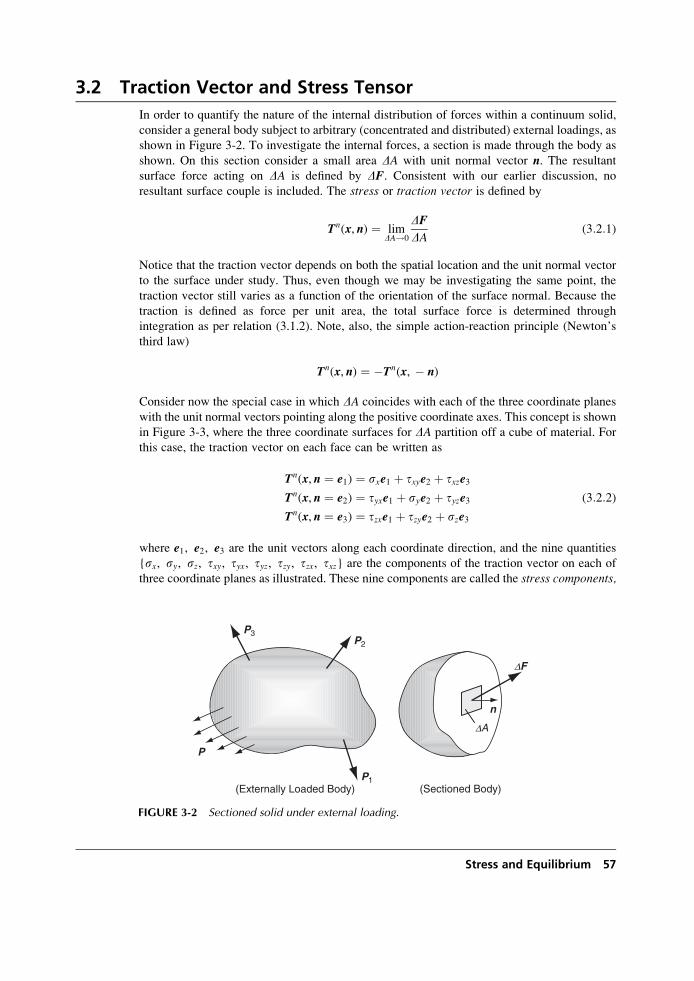
3.2 Traction Vector and Stress Tensor
In order to quantify the nature of the internal distribution of forces within a continuum solid,
consider a general body subject to arbitrary (concentrated and distributed) external loadings, as
shown in Figure 3-2. To investigate the internal forces, a section is made through the body as
shown. On this section consider a small area DA with unit normal vector n. The resultant
surface force acting on DA is defined by DF. Consistent with our earlier discussion, no
resultant surface couple is included. The stress or traction vector is defined by
Tn(x, n) ¼ limDA!0
DFDA
(3:2:1)
Notice that the traction vector depends on both the spatial location and the unit normal vector
to the surface under study. Thus, even though we may be investigating the same point, the
traction vector still varies as a function of the orientation of the surface normal. Because the
traction is defined as force per unit area, the total surface force is determined through
integration as per relation (3.1.2). Note, also, the simple action-reaction principle (Newton’s
third law)
Tn(x, n) ¼ �Tn(x, � n)
Consider now the special case in which DA coincides with each of the three coordinate planes
with the unit normal vectors pointing along the positive coordinate axes. This concept is shown
in Figure 3-3, where the three coordinate surfaces for DA partition off a cube of material. For
this case, the traction vector on each face can be written as
Tn(x,n ¼ e1) ¼ sxe1 þ txye2 þ txze3Tn(x,n ¼ e2) ¼ tyxe1 þ sye2 þ tyze3Tn(x,n ¼ e3) ¼ tzxe1 þ tzye2 þ sze3
(3:2:2)
where e1, e2, e3 are the unit vectors along each coordinate direction, and the nine quantities
{sx, sy, sz, txy, tyx, tyz, tzy, tzx, txz} are the components of the traction vector on each of
three coordinate planes as illustrated. These nine components are called the stress components,
DF
DA
n
(Sectioned Body)
P3
P
P2
P1(Externally Loaded Body)
FIGURE 3-2 Sectioned solid under external loading.
Stress and Equilibrium 57
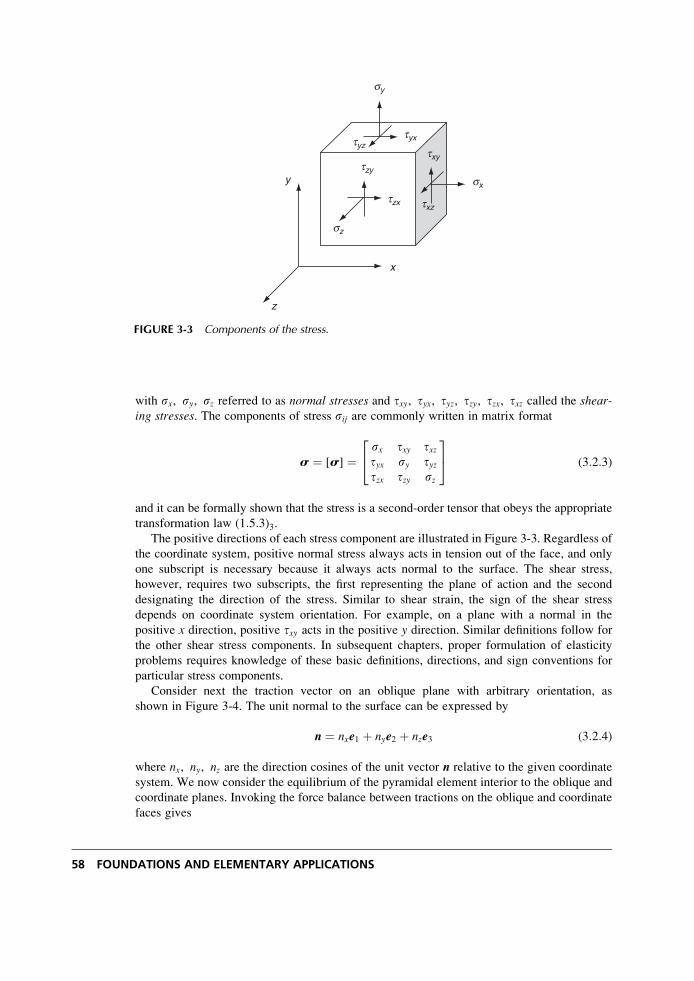
with sx, sy, sz referred to as normal stresses and txy, tyx, tyz, tzy, tzx, txz called the shear-ing stresses. The components of stress sij are commonly written in matrix format
s ¼ [s] ¼sx txy txztyx sy tyztzx tzy sz
24
35 (3:2:3)
and it can be formally shown that the stress is a second-order tensor that obeys the appropriate
transformation law (1:5:3)3.The positive directions of each stress component are illustrated in Figure 3-3. Regardless of
the coordinate system, positive normal stress always acts in tension out of the face, and only
one subscript is necessary because it always acts normal to the surface. The shear stress,
however, requires two subscripts, the first representing the plane of action and the second
designating the direction of the stress. Similar to shear strain, the sign of the shear stress
depends on coordinate system orientation. For example, on a plane with a normal in the
positive x direction, positive txy acts in the positive y direction. Similar definitions follow for
the other shear stress components. In subsequent chapters, proper formulation of elasticity
problems requires knowledge of these basic definitions, directions, and sign conventions for
particular stress components.
Consider next the traction vector on an oblique plane with arbitrary orientation, as
shown in Figure 3-4. The unit normal to the surface can be expressed by
n ¼ nxe1 þ nye2 þ nze3 (3:2:4)
where nx, ny, nz are the direction cosines of the unit vector n relative to the given coordinate
system. We now consider the equilibrium of the pyramidal element interior to the oblique and
coordinate planes. Invoking the force balance between tractions on the oblique and coordinate
faces gives
sy
sx
tyx
txy
txztzx
tzy
tyz
x
z
y
sz
FIGURE 3-3 Components of the stress.
58 FOUNDATIONS AND ELEMENTARY APPLICATIONS
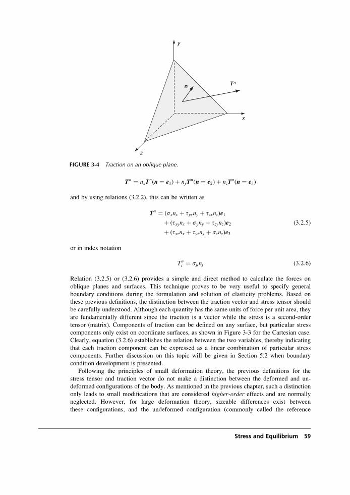
Tn ¼ nxTn(n ¼ e1)þ nyT
n(n ¼ e2)þ nzTn(n ¼ e3)
and by using relations (3.2.2), this can be written as
Tn ¼ (sxnx þ tyxny þ tzxnz)e1þ (txynx þ syny þ tzynz)e2þ (txznx þ tyzny þ sznz)e3
(3:2:5)
or in index notation
Tni ¼ sjinj (3:2:6)
Relation (3.2.5) or (3.2.6) provides a simple and direct method to calculate the forces on
oblique planes and surfaces. This technique proves to be very useful to specify general
boundary conditions during the formulation and solution of elasticity problems. Based on
these previous definitions, the distinction between the traction vector and stress tensor should
be carefully understood. Although each quantity has the same units of force per unit area, they
are fundamentally different since the traction is a vector while the stress is a second-order
tensor (matrix). Components of traction can be defined on any surface, but particular stress
components only exist on coordinate surfaces, as shown in Figure 3-3 for the Cartesian case.
Clearly, equation (3.2.6) establishes the relation between the two variables, thereby indicating
that each traction component can be expressed as a linear combination of particular stress
components. Further discussion on this topic will be given in Section 5.2 when boundary
condition development is presented.
Following the principles of small deformation theory, the previous definitions for the
stress tensor and traction vector do not make a distinction between the deformed and un-
deformed configurations of the body. As mentioned in the previous chapter, such a distinction
only leads to small modifications that are considered higher-order effects and are normally
neglected. However, for large deformation theory, sizeable differences exist between
these configurations, and the undeformed configuration (commonly called the reference
x
z
y
n Tn
FIGURE 3-4 Traction on an oblique plane.
Stress and Equilibrium 59
configuration) is often used in problem formulation. This gives rise to the definition of an
additional stress called the Piola-Kirchhoff stress tensor that represents the force per unit
area in the reference configuration (see Chandrasekharaiah and Debnath 1994). In the
more general scheme, the stress sij is referred to as the Cauchy stress tensor. Throughout
the text only small deformation theory is considered, and thus the distinction between
these two definitions of stress disappears, thereby eliminating any need for this additional
terminology.
3.3 Stress Transformation
Analogous to our previous discussion with the strain tensor, the stress components must also
follow the standard transformation rules for second-order tensors established in Section 1.5.
Applying transformation relation (1.5.1)3 for the stress gives
s0ij ¼ QipQjqspq (3:3:1)
where the rotation matrix Qij ¼ cos (x0i, xj). Therefore, given the stress in one coordinate
system, we can determine the new components in any other rotated system. For the general
three-dimensional case, the rotation matrix may be chosen in the form
Qij ¼l1 m1 n1l2 m2 n2l3 m3 n3
24
35 (3:3:2)
Using this notational scheme, the specific transformation relations for the stress then become
s0x ¼ sxl21 þ sym2
1 þ szn21 þ 2(txyl1m1 þ tyzm1n1 þ tzxn1l1)
s0y ¼ sxl22 þ sym2
2 þ szn22 þ 2(txyl2m2 þ tyzm2n2 þ tzxn2l2)
s0z ¼ sxl23 þ sym2
3 þ szn23 þ 2(txyl3m3 þ tyzm3n3 þ tzxn3l3)
t0xy ¼ sxl1l2 þ sym1m2 þ szn1n2 þ txy(l1m2 þ m1l2)þ tyz(m1n2 þ n1m2)þ tzx(n1l2 þ l1n2)
t0yz ¼ sxl2l3 þ sym2m3 þ szn2n3 þ txy(l2m3 þ m2l3)þ tyz(m2n3 þ n2m3)þ tzx(n2l3 þ l2n3)
t0zx ¼ sxl3l1 þ sym3m1 þ szn3n1 þ txy(l3m1 þ m3l1)þ tyz(m3n1 þ n3m1)þ tzx(n3l1 þ l3n1)
(3:3:3)
For the two-dimensional case originally shown in Figure 2-6, the transformation matrix was
given by relation (2.3.5). Under this transformation, the in-plane stress components transform
according to
s0x ¼ sx cos2 yþ sy sin2 yþ 2txy sin y cos y
s0y ¼ sx sin2 yþ sy cos2 y� 2txy sin y cos y
t0xy ¼ �sx sin y cos yþ sy sin y cos yþ txy( cos2 y� sin2 y)
(3:3:4)
which is commonly rewritten in terms of the double angle
60 FOUNDATIONS AND ELEMENTARY APPLICATIONS
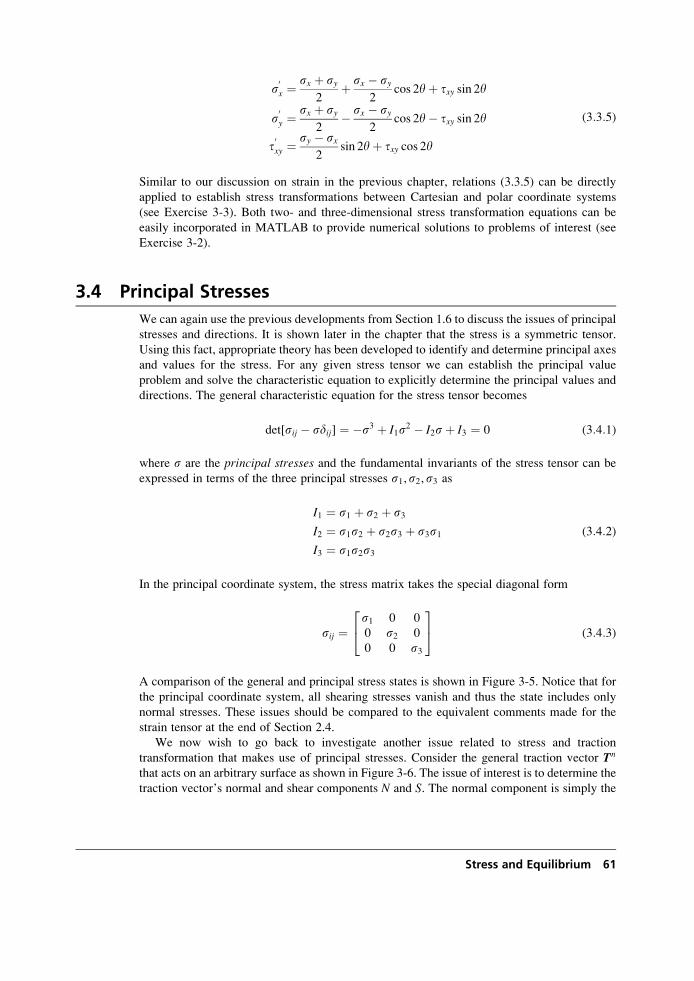
s0x ¼
sx þ sy2
þ sx � sy2
cos 2yþ txy sin 2y
s0y ¼
sx þ sy2
� sx � sy2
cos 2y� txy sin 2y
t0xy ¼
sy � sx2
sin 2yþ txy cos 2y
(3:3:5)
Similar to our discussion on strain in the previous chapter, relations (3.3.5) can be directly
applied to establish stress transformations between Cartesian and polar coordinate systems
(see Exercise 3-3). Both two- and three-dimensional stress transformation equations can be
easily incorporated in MATLAB to provide numerical solutions to problems of interest (see
Exercise 3-2).
3.4 Principal Stresses
We can again use the previous developments from Section 1.6 to discuss the issues of principal
stresses and directions. It is shown later in the chapter that the stress is a symmetric tensor.
Using this fact, appropriate theory has been developed to identify and determine principal axes
and values for the stress. For any given stress tensor we can establish the principal value
problem and solve the characteristic equation to explicitly determine the principal values and
directions. The general characteristic equation for the stress tensor becomes
det[sij � sdij] ¼ �s3 þ I1s2 � I2sþ I3 ¼ 0 (3:4:1)
where s are the principal stresses and the fundamental invariants of the stress tensor can be
expressed in terms of the three principal stresses s1,s2,s3 as
I1 ¼ s1 þ s2 þ s3I2 ¼ s1s2 þ s2s3 þ s3s1I3 ¼ s1s2s3
(3:4:2)
In the principal coordinate system, the stress matrix takes the special diagonal form
sij ¼s1 0 0
0 s2 0
0 0 s3
24
35 (3:4:3)
A comparison of the general and principal stress states is shown in Figure 3-5. Notice that for
the principal coordinate system, all shearing stresses vanish and thus the state includes only
normal stresses. These issues should be compared to the equivalent comments made for the
strain tensor at the end of Section 2.4.
We now wish to go back to investigate another issue related to stress and traction
transformation that makes use of principal stresses. Consider the general traction vector Tn
that acts on an arbitrary surface as shown in Figure 3-6. The issue of interest is to determine the
traction vector’s normal and shear components N and S. The normal component is simply the
Stress and Equilibrium 61
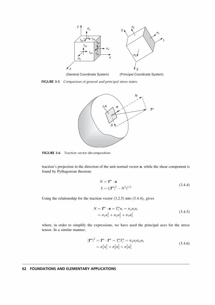
traction’s projection in the direction of the unit normal vector n, while the shear component is
found by Pythagorean theorem:
N ¼ Tn � nS ¼ (jTnj2 � N2)1=2
(3:4:4)
Using the relationship for the traction vector (3.2.5) into (3:4:4)1 gives
N ¼ Tn � n ¼ Tni ni ¼ sjinjni
¼ s1n21 þ s2n22 þ s3n23(3:4:5)
where, in order to simplify the expressions, we have used the principal axes for the stress
tensor. In a similar manner,
jTnj2 ¼ Tn � Tn ¼ Tni T
ni ¼ sjinjskink
¼ s21n21 þ s22n
22 þ s23n
23
(3:4:6)
sy
sx
txy
tyx
sz
tyz
tzx
tzy
txzx
z
y
(General Coordinate System)
s3
s2
s1
1
3
2
(Principal Coordinate System)
FIGURE 3-5 Comparison of general and principal stress states.
TnnΔA
S
N
FIGURE 3-6 Traction vector decomposition.
62 FOUNDATIONS AND ELEMENTARY APPLICATIONS
Using these results back into relation (3.4.4) yields
N ¼ s1n21 þ s2n22 þ s3n23S2 þ N2 ¼ s21n
21 þ s22n
22 þ s23n
23
(3:4:7)
In addition, we add the condition that the vector n has unit magnitude
1 ¼ n21 þ n22 þ n23 (3:4:8)
Relations (3.4.7) and (3.4.8) can be viewed as three linear algebraic equations for the
unknowns n21, n22, n
23. Solving this system gives the following result:
n21 ¼S2 þ (N � s2)(N � s3)(s1 � s2)(s1 � s3)
n22 ¼S2 þ (N � s3)(N � s1)(s2 � s3)(s2 � s1)
n23 ¼S2 þ (N � s1)(N � s2)(s3 � s1)(s3 � s2)
(3:4:9)
Without loss in generality, we can rank the principal stresses as s1 > s2 > s3. Noting that the
expressions given by (3.4.9) must be greater than or equal to zero, we can conclude the following
S2 þ (N � s2)(N � s3) � 0
S2 þ (N � s3)(N � s1) � 0
S2 þ (N � s1)(N � s2) � 0
(3:4:10)
For the equality case, equations (3.4.10) represent three circles in an S-N coordinate system,
and Figure 3-7 illustrates the location of each circle. These results were originally generated by
Otto Mohr over a century ago, and the circles are commonly called Mohr’s circles of stress.The three inequalities given in (3.4.10) imply that all admissible values of N and S lie in
the shaded regions bounded by the three circles. Note that, for the ranked principal stresses, the
largest shear component is easily determined as Smax ¼ 1=2js1 � s3j. Although these circles
can be effectively used for two-dimensional stress transformation, the general tensorial-based
equations (3.3.3) are normally used for general transformation computations.
EXAMPLE 3-1: Stress Transformation
For the following state of stress, determine the principal stresses and directions and find
the traction vector on a plane with unit normal n ¼ (0, 1, 1)=ffiffiffi2
p.
sij ¼3 1 1
1 0 2
1 2 0
24
35
Continued
Stress and Equilibrium 63
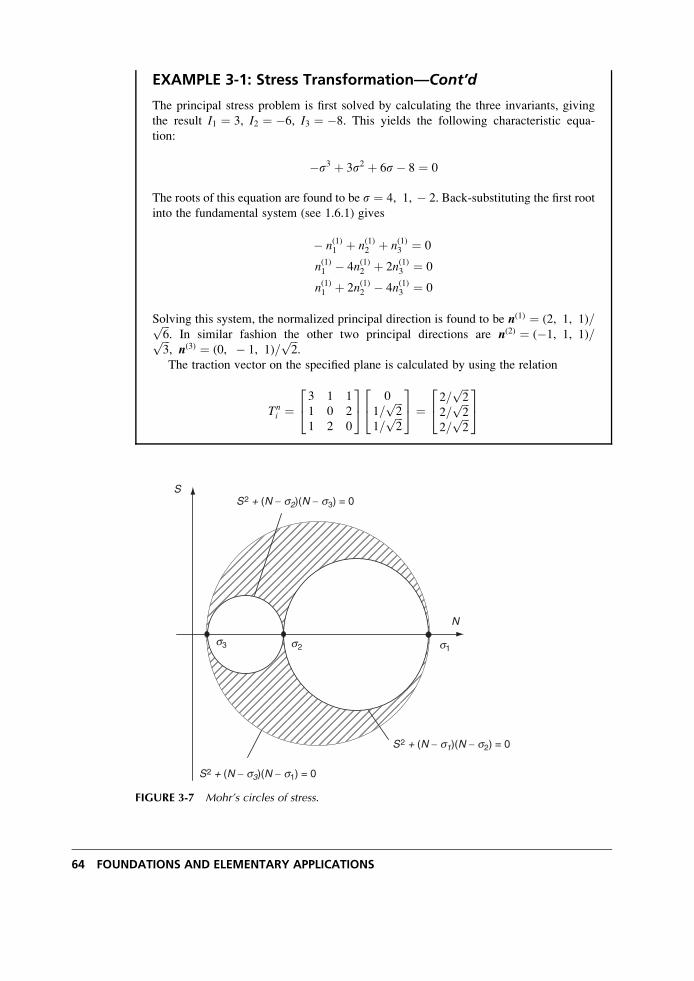
EXAMPLE 3-1: Stress Transformation—Cont’d
The principal stress problem is first solved by calculating the three invariants, giving
the result I1 ¼ 3, I2 ¼ �6, I3 ¼ �8. This yields the following characteristic equa-
tion:
�s3 þ 3s2 þ 6s� 8 ¼ 0
The roots of this equation are found to be s ¼ 4, 1, � 2. Back-substituting the first root
into the fundamental system (see 1.6.1) gives
� n(1)1 þ n(1)2 þ n(1)3 ¼ 0
n(1)1 � 4n(1)2 þ 2n(1)3 ¼ 0
n(1)1 þ 2n(1)2 � 4n(1)3 ¼ 0
Solving this system, the normalized principal direction is found to be n(1) ¼ (2, 1, 1)=ffiffiffi6
p. In similar fashion the other two principal directions are n(2) ¼ (�1, 1, 1)=ffiffiffi3
p, n(3) ¼ (0, � 1, 1)=
ffiffiffi2
p.
The traction vector on the specified plane is calculated by using the relation
Tni ¼
3 1 1
1 0 2
1 2 0
24
35 0
1=ffiffiffi2
p1=
ffiffiffi2
p
24
35 ¼
2=ffiffiffi2
p2=
ffiffiffi2
p2=
ffiffiffi2
p
24
35
N
S
s1s2s3
S2 + (N − s2)(N − s3) = 0
S2 + (N − s3)(N − s1) = 0
S2 + (N − s1)(N − s2) = 0
FIGURE 3-7 Mohr’s circles of stress.
64 FOUNDATIONS AND ELEMENTARY APPLICATIONS
3.5 Spherical, Deviatoric, Octahedral,and von Mises Stresses
As mentioned in our previous discussion on strain, it is often convenient to decompose the
stress into two parts called the spherical and deviatoric stress tensors. Analogous to relations
(2.5.1) and (2.5.2), the spherical stress is defined by
~ssij ¼ 1
3skk dij (3:5:1)
while the deviatoric stress becomes
ssij ¼ sij � 1
3skk dij (3:5:2)
Note that the total stress is then simply the sum
sij ¼ ~ssij þ ssij (3:5:3)
The spherical stress is an isotropic tensor, being the same in all coordinate systems (as per the
discussion in Section 1.5). It can be shown that the principal directions of the deviatoric stress
are the same as those of the stress tensor itself (see Exercise 3-14).
We next briefly explore a couple of particular stress components or combinations that have
been defined in the literature and are commonly used in formulating failure theories related to
inelastic deformation. It has been found that ductile materials normally exhibit inelastic
yielding failures that can be characterized by these particular stresses.
Consider first the normal and shear stresses (tractions) that act on a special plane whose
normal makes equal angles with the three principal axes. This plane is commonly referred to as
the octahedral plane. Determination of these normal and shear stresses is straightforward if we
use the principal axes of stress. Since the unit normal vector to the octahedral plane makes
equal angles with the principal axes, its components are given by ni ¼ �(1, 1, 1)=ffiffiffi3
p. Refer-
ring to Figure 3-6 and using the results of the previous section, relations (3.4.7) give the desired
normal and shear stresses as
N ¼ soct ¼ 1
3(s1 þ s2 þ s3) ¼ 1
3skk ¼ 1
3I1
S ¼ toct ¼ 1
3[(s1 � s2)2 þ (s2 � s3)2 þ (s3 � s1)2]1=2
¼ 1
32I21 � 6I2� �1=2
(3:5:4)
It can be shown that the octahedral shear stress toct is directly related to the distortionalstrain energy (defined by equation (6.1.17) ), which is often used in failure theories for ductile
materials.
Another specially defined stress also related to the distortional strain energy failure criteria
is known as the effective or von Mises stress and is given by the expression
se ¼ svonMises ¼ 1ffiffiffi2
p [(s1 � s2)2 þ (s2 � s3)2 þ (s3 � s1)2]1=2 (3:5:5)
Stress and Equilibrium 65
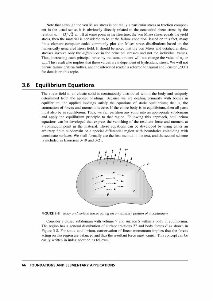
Note that although the von Mises stress is not really a particular stress or traction compon-
ent in the usual sense, it is obviously directly related to the octahedral shear stress by the
relation se ¼ (3=ffiffiffi2
p)toct. If at some point in the structure, the von Mises stress equals the yield
stress, then the material is considered to be at the failure condition. Based on this fact, many
finite element computer codes commonly plot von Mises stress distributions based on the
numerically generated stress field. It should be noted that the von Mises and octahedral shear
stresses involve only the differences in the principal stresses and not the individual values.
Thus, increasing each principal stress by the same amount will not change the value of se ortoct. This result also implies that these values are independent of hydrostatic stress. We will not
pursue failure criteria further, and the interested reader is referred to Ugural and Fenster (2003)
for details on this topic.
3.6 Equilibrium Equations
The stress field in an elastic solid is continuously distributed within the body and uniquely
determined from the applied loadings. Because we are dealing primarily with bodies in
equilibrium, the applied loadings satisfy the equations of static equilibrium; that is, the
summation of forces and moments is zero. If the entire body is in equilibrium, then all parts
must also be in equilibrium. Thus, we can partition any solid into an appropriate subdomain
and apply the equilibrium principle to that region. Following this approach, equilibrium
equations can be developed that express the vanishing of the resultant force and moment at
a continuum point in the material. These equations can be developed by using either an
arbitrary finite subdomain or a special differential region with boundaries coinciding with
coordinate surfaces. We shall formally use the first method in the text, and the second scheme
is included in Exercises 3-19 and 3-21.
F
Tn
V
S
FIGURE 3-8 Body and surface forces acting on an arbitrary portion of a continuum.
Consider a closed subdomain with volume V and surface S within a body in equilibrium.
The region has a general distribution of surface tractions Tn and body forces F as shown in
Figure 3-8. For static equilibrium, conservation of linear momentum implies that the forces
acting on this region are balanced and thus the resultant force must vanish. This concept can be
easily written in index notation as follows:
66 FOUNDATIONS AND ELEMENTARY APPLICATIONS
ððS
Tni dSþ
ðððV
FidV ¼ 0 (3:6:1)
Using relation (3.2.6) for the traction vector, we can express the equilibrium statement in terms
of stress:
ððS
sjinjdSþððð
V
FidV ¼ 0 (3:6:2)
Applying the divergence theorem (1.8.7) to the surface integral allows the conversion to a
volume integral, and relation (3.6.2) can then be expressed as
ðððV
(sji, j þ Fi)dV ¼ 0 (3:6:3)
Because the region V is arbitrary (any part of the medium can be chosen) and the integrand
in (3.6.3) is continuous, then by the zero-value theorem (1.8.12), the integrandmust vanish:
sji, j þ Fi ¼ 0 (3:6:4)
This result represents three scalar relations called the equilibrium equations. Written in scalar
notation, they are
@sx@x
þ @tyx@y
þ @tzx@z
þ Fx ¼ 0
@txy@x
þ @sy@y
þ @tzy@z
þ Fy ¼ 0
@txz@x
þ @tyz@y
þ @sz@z
þ Fz ¼ 0
(3:6:5)
Thus, all elasticity stress fields must satisfy these relations in order to be in static equilib-
rium.
Next consider the angular momentum principle that states that the moment of all
forces acting on any portion of the body must vanish. Note that the point about which the
moment is calculated can be chosen arbitrarily. Applying this principle to the region shown in
Figure 3-8 results in a statement of the vanishing of the moments resulting from surface and
body forces:
ððS
eijkxjTnk dSþ
ðððV
eijkxjFkdV ¼ 0 (3:6:6)
Again using relation (3.2.6) for the traction, (3.6.6) can be written as
ððS
eijkxjslknldSþððð
V
eijkxjFkdV ¼ 0
Stress and Equilibrium 67
and application of the divergence theorem gives
ðððV
[(eijkxjslk), l þ eijkxjFk]dV ¼ 0
This integral can be expanded and simplified as
ðððV
[eijkxj, lslk þ eijkxjslk, l þ eijkxjFk]dV ¼ðððV
[eijkdjlslk þ eijkxjslk, l þ eijkxjFk]dV ¼ðððV
[eijksjk � eijkxjFk þ eijkxjFk]dV ¼ððð
V
eijksjkdV
where we have used the equilibrium equations (3.6.4) to simplify the final result. Thus, (3.6.6)
now gives
ðððV
eijksjkdV ¼ 0
As per our earlier arguments, because the region V is arbitrary, the integrand must vanish,
giving eijksjk ¼ 0. However, because the alternating symbol is antisymmetric in indices jk, theother product term sjk must be symmetric, thus implying
txy ¼ tyxsij ¼ sji ) tyz ¼ tzy
tzx ¼ txz
(3:6:7)
We thus find that, similar to the strain, the stress tensor is also symmetric and therefore has
only six independent components in three dimensions. Under these conditions, the equilibrium
equations can then be written as
sij, j þ Fi ¼ 0 (3:6:8)
3.7 Relations in Curvilinear Cylindricaland Spherical Coordinates
As mentioned in the previous chapter, in order to solve many elasticity problems, formulation
must be done in curvilinear coordinates typically using cylindrical or spherical systems. Thus,
by following similar methods as used with the strain-displacement relations, we now wish to
develop expressions for the equilibrium equations in curvilinear cylindrical and spherical
coordinates. By using a direct vector/matrix notation, the equilibrium equations can be
expressed as
, � s þ F ¼ 0 (3:7:1)
68 FOUNDATIONS AND ELEMENTARY APPLICATIONS
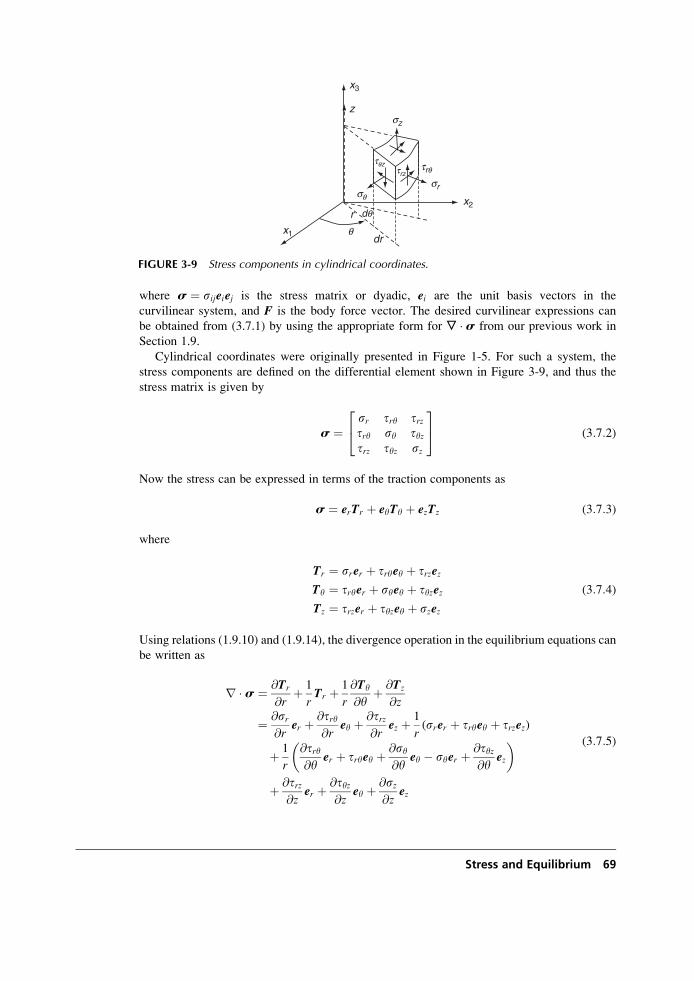
where s ¼ sijeiej is the stress matrix or dyadic, ei are the unit basis vectors in the
curvilinear system, and F is the body force vector. The desired curvilinear expressions can
be obtained from (3.7.1) by using the appropriate form for , � s from our previous work in
Section 1.9.
Cylindrical coordinates were originally presented in Figure 1-5. For such a system, the
stress components are defined on the differential element shown in Figure 3-9, and thus the
stress matrix is given by
s ¼sr try trztry sy tyztrz tyz sz
24
35 (3:7:2)
Now the stress can be expressed in terms of the traction components as
s ¼ erTr þ eyTy þ ezTz (3:7:3)
where
Tr ¼ srer þ tryey þ trzezTy ¼ tryer þ syey þ tyzezTz ¼ trzer þ tyzey þ szez
(3:7:4)
Using relations (1.9.10) and (1.9.14), the divergence operation in the equilibrium equations can
be written as
r � s ¼ @Tr
@rþ 1
rTr þ 1
r
@Ty
@yþ @Tz
@z
¼ @sr@r
er þ @try@r
ey þ @trz@r
ez þ 1
r(srer þ tryey þ trzez)
þ 1
r
@try@y
er þ tryey þ @sy@y
ey � syer þ @tyz@y
ez
� �
þ @trz@z
er þ @tyz@z
ey þ @sz@z
ez
(3:7:5)
x3
x1
x2r
zsz
sr
trqtqz
trz
dr
dq
sq
q
FIGURE 3-9 Stress components in cylindrical coordinates.
Stress and Equilibrium 69
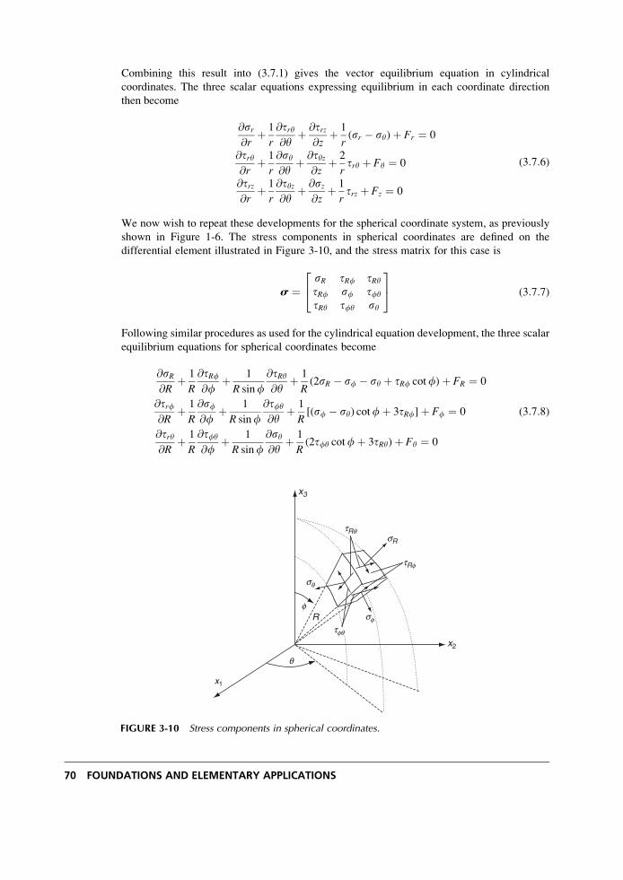
Combining this result into (3.7.1) gives the vector equilibrium equation in cylindrical
coordinates. The three scalar equations expressing equilibrium in each coordinate direction
then become
@sr@r
þ 1
r
@try@y
þ @trz@z
þ 1
r(sr � sy)þ Fr ¼ 0
@try@r
þ 1
r
@sy@y
þ @tyz@z
þ 2
rtry þ Fy ¼ 0
@trz@r
þ 1
r
@tyz@y
þ @sz@z
þ 1
rtrz þ Fz ¼ 0
(3:7:6)
We now wish to repeat these developments for the spherical coordinate system, as previously
shown in Figure 1-6. The stress components in spherical coordinates are defined on the
differential element illustrated in Figure 3-10, and the stress matrix for this case is
s ¼sR tRf tRytRf sf tfytRy tfy sy
24
35 (3:7:7)
Following similar procedures as used for the cylindrical equation development, the three scalar
equilibrium equations for spherical coordinates become
@sR@R
þ 1
R
@tRf@f
þ 1
R sinf@tRy@y
þ 1
R(2sR � sf � sy þ tRf cotf)þ FR ¼ 0
@trf@R
þ 1
R
@sf@f
þ 1
R sinf@tfy@y
þ 1
R[(sf � sy) cotfþ 3tRf]þ Ff ¼ 0
@try@R
þ 1
R
@tfy@f
þ 1
R sinf@sy@y
þ 1
R(2tfy cotfþ 3tRy)þ Fy ¼ 0
(3:7:8)
x3
x1
x2
Rtfq
tRq
tRf
sf
sR
sq
f
q
FIGURE 3-10 Stress components in spherical coordinates.
70 FOUNDATIONS AND ELEMENTARY APPLICATIONS
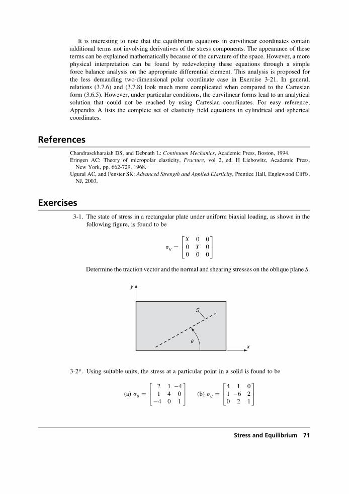
It is interesting to note that the equilibrium equations in curvilinear coordinates contain
additional terms not involving derivatives of the stress components. The appearance of these
terms can be explained mathematically because of the curvature of the space. However, a more
physical interpretation can be found by redeveloping these equations through a simple
force balance analysis on the appropriate differential element. This analysis is proposed for
the less demanding two-dimensional polar coordinate case in Exercise 3-21. In general,
relations (3.7.6) and (3.7.8) look much more complicated when compared to the Cartesian
form (3.6.5). However, under particular conditions, the curvilinear forms lead to an analytical
solution that could not be reached by using Cartesian coordinates. For easy reference,
Appendix A lists the complete set of elasticity field equations in cylindrical and spherical
coordinates.
References
Chandrasekharaiah DS, and Debnath L: Continuum Mechanics, Academic Press, Boston, 1994.
Eringen AC: Theory of micropolar elasticity, Fracture, vol 2, ed. H Liebowitz, Academic Press,
New York, pp. 662-729, 1968.
Ugural AC, and Fenster SK: Advanced Strength and Applied Elasticity, Prentice Hall, Englewood Cliffs,
NJ, 2003.
Exercises
3-1. The state of stress in a rectangular plate under uniform biaxial loading, as shown in the
following figure, is found to be
sij ¼X 0 0
0 Y 0
0 0 0
24
35
Determine the traction vector and the normal and shearing stresses on the oblique plane S.
3-2*. Using suitable units, the stress at a particular point in a solid is found to be
(a) sij ¼2 1 �4
1 4 0
�4 0 1
24
35 (b) sij ¼
4 1 0
1 �6 2
0 2 1
24
35
y
q
S
x
Stress and Equilibrium 71
Determine the traction vector on a surface with unit normal (cos �, sin �, 0), where � is ageneral angle in the range 0 � � � �. Plot the variation of the magnitude of the traction
vector jTnj as a function of �.
3-3. Show that the general two-dimensional stress transformation relations can be used to
generate relations for the normal and shear stresses in a polar coordinate system in terms
of Cartesian components
sr ¼ sx þ sy2
þ sx � sy2
cos 2yþ txy sin 2y
sy ¼ sx þ sy2
� sx � sy2
cos 2y� txy sin 2y
try ¼ sy � sx2
sin 2yþ txy cos 2y
3-4. A two-dimensional state of plane stress in the x,y plane is defined by sz ¼ tyz ¼ tzx ¼ 0.
Using general principal value theory, show that for this case the in-plane principal
stresses and maximum shear stress are given by
s1, 2 ¼ sx þ sy2
�ffiffiffiffiffiffiffiffiffiffiffiffiffiffiffiffiffiffiffiffiffiffiffiffiffiffiffiffiffiffiffiffisx � sy
2
� �2þt2xy
r
tmax ¼ffiffiffiffiffiffiffiffiffiffiffiffiffiffiffiffiffiffiffiffiffiffiffiffiffiffiffiffiffiffiffiffisx � sy
2
� �2þt2xy
r
3-5. Explicitly verify relations (3.5.4) for the octahedral stress components. Also show that
they can be expressed in terms of the general stress components by
soct ¼ 1
3(sx þ sy þ sz)
toct ¼ 1
3[(sx � sy)2 þ (sy � sz)2 þ (sz � sx)2 þ 6t2xy þ 6t2yz þ 6t2zx]
1=2
3-6. For the plane stress case in Exercise 3-4, demonstrate the invariant nature of the
principal stresses and maximum shear stresses by showing that
s1, 2 ¼ 1
2I1 �
ffiffiffiffiffiffiffiffiffiffiffiffiffiffiffiffiffi1
4I21 � I2
rand tmax ¼
ffiffiffiffiffiffiffiffiffiffiffiffiffiffiffiffiffi1
4I21 � I2
r
Thus, conclude that
s1, 2 ¼ sx þ sy2
�ffiffiffiffiffiffiffiffiffiffiffiffiffiffiffiffiffiffiffiffiffiffiffiffiffiffiffiffiffiffiffiffiffiffiffisx � sy
2
� �2þ t2xy
r¼ sr þ sy
2�
ffiffiffiffiffiffiffiffiffiffiffiffiffiffiffiffiffiffiffiffiffiffiffiffiffiffiffiffiffiffiffiffisr � sy
2
� �2þt2ry
r
tmax ¼ffiffiffiffiffiffiffiffiffiffiffiffiffiffiffiffiffiffiffiffiffiffiffiffiffiffiffiffiffiffiffiffiffiffiffisx � sy
2
� �2þ t2xy
r¼
ffiffiffiffiffiffiffiffiffiffiffiffiffiffiffiffiffiffiffiffiffiffiffiffiffiffiffiffiffiffiffiffisr � sy
2
� �2þt2ry
r
3-7. Exercise 8-2 provides the plane stress (see Exercise 3-4) solution for a cantilever beam
of unit thickness, with depth 2c, and carrying an end load of P is given by
72 FOUNDATIONS AND ELEMENTARY APPLICATIONS
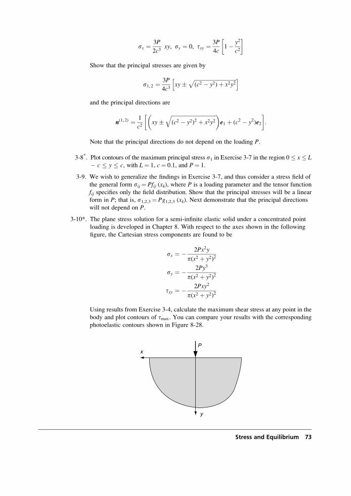
sx ¼ 3P
2c3xy, sy ¼ 0, txy ¼ 3P
4c1� y2
c2
Show that the principal stresses are given by
s1, 2 ¼ 3P
4c3xy�
ffiffiffiffiffiffiffiffiffiffiffiffiffiffiffiffiffiffiffiffiffiffiffiffiffiffiffiffiffiffiffiffi(c2 � y2)þ x2y2
ph i
and the principal directions are
n(1, 2) ¼ 1
c2xy�
ffiffiffiffiffiffiffiffiffiffiffiffiffiffiffiffiffiffiffiffiffiffiffiffiffiffiffiffiffiffiffiffiffiffi(c2 � y2)2 þ x2y2
q� �e1 þ (c2 � y2)e2
:
Note that the principal directions do not depend on the loading P.
3-8*. Plot contours of the maximum principal stress s1 in Exercise 3-7 in the region 0 � x � L� c � y � c, with L¼ 1, c¼ 0.1, and P¼ 1.
3-9. We wish to generalize the findings in Exercise 3-7, and thus consider a stress field of
the general form sij¼ Pfij (xk), where P is a loading parameter and the tensor function
fij specifies only the field distribution. Show that the principal stresses will be a linear
form in P; that is, s1,2,3¼ Pg1,2,3 (xk). Next demonstrate that the principal directions
will not depend on P.
3-10*. The plane stress solution for a semi-infinite elastic solid under a concentrated point
loading is developed in Chapter 8. With respect to the axes shown in the following
figure, the Cartesian stress components are found to be
sx ¼ � 2Px2y
p(x2 þ y2)2
sy ¼ � 2Py3
p(x2 þ y2)2
txy ¼ � 2Pxy2
p(x2 þ y2)2
Using results from Exercise 3-4, calculate the maximum shear stress at any point in the
body and plot contours of tmax. You can compare your results with the corresponding
photoelastic contours shown in Figure 8-28.
x
y
P
Stress and Equilibrium 73
3-11. Show that shear stress S acting on a plane defined by the unit normal vector n (see
Figure 3-6) can be written as
S ¼ n21n22(s1 � s2)2 þ n22n
23(s2 � s3)2 þ n23n
21(s3 � s1)2
� �1=23-12. It was discussed in Section 3.4 that for the case of ranked principal stresses (s1 > s2 > s3),
the maximum shear stress was given by Smax ¼ (s1 � s3)/2, which was the radius of
the largest Mohr’s circle shown in Figure 3-7. For this case, show that the normal stress
acting on the plane of maximum shear is given by N ¼ (s1 þ s3)/2. Finally, usingrelations (3.4.9) show that the components of the unit normal vector to this plane are
ni ¼ �ð1, 0, 1Þ= ffiffiffi2
p. This result implies that the maximum shear stress acts on a plane
that bisects the angle between the directions of the largest and the smallest principal
stress.
3-13. Explicitly show that the stress state given in Example 3-1 will reduce to the proper
diagonal form under transformation to principal axes.
3-14. Show that the principal directions of the deviatoric stress tensor coincide with the
principal directions of the stress tensor. Also show that the principal values of the
deviatoric stress sd can be expressed in terms of the principal values s of the total stress
by the relation sd ¼ s� 13skk.
3-15. Determine the spherical and deviatoric stress tensors for the stress states given in
Exercise 3-2.
3-16. For the stress state given in Example 3-1, determine the von Mises and octahedral
stresses defined in Section 3.5.
3-17. For the case of pure shear, the stress matrix is given by
sij ¼0 t 0
t 0 0
0 0 0
24
35
where t is a given constant. Determine the principal stresses and directions, and
compute the normal and shear stress on the octahedral plane.
3-18*. For the stress state in Exercise 3-7, plot contours of the von Mises stress in the region
0 � x � L, � c � y � c, with L ¼ 1, c ¼ 0.1, and P ¼ 1.
3-19. Consider the equilibrium of a two-dimensional differential element in Cartesian
coordinates, as shown in the following figure. Explicitly sum the forces and moments
and develop the two-dimensional equilibrium equations
@sx@x
þ @tyx@y
þ Fx ¼ 0
@txy@x
þ @sy@y
þ Fy ¼ 0
txy ¼ tyx
74 FOUNDATIONS AND ELEMENTARY APPLICATIONS
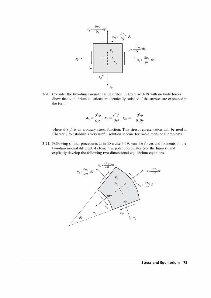
3-20. Consider the two-dimensional case described in Exercise 3-19 with no body forces.
Show that equilibrium equations are identically satisfied if the stresses are expressed in
the form
sx ¼ @2f@y2
, sy ¼ @2f@x2
, txy ¼ � @2f@x@y
where �(x,y) is an arbitrary stress function. This stress representation will be used in
Chapter 7 to establish a very useful solution scheme for two-dimensional problems.
3-21. Following similar procedures as in Exercise 3-19, sum the forces and moments on the
two-dimensional differential element in polar coordinates (see the figures), and
explicitly develop the following two-dimensional equilibrium equations
Fr
Fq
dr
rdq
dq
dq∂sq
∂qsq +
sq
sr
dq∂τqr∂qtqr +
dr∂sr∂r
sr +
dr∂trq∂r
trq +
trq
tqr
sx
sy
dx∂x
sx +∂sx
tyx
txy
dy∂sy
∂ysy +
dxtxy + ∂x
∂txy
dy∂y
∂tyxtyx +
Fx
Fy
Stress and Equilibrium 75
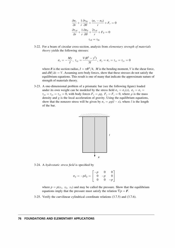
@sr@r
þ 1
r
@tyr@y
þ (sr � sy)r
þ Fr ¼ 0
@try@r
þ 1
r
@sy@y
þ 2tryr
þ Fy ¼ 0
try ¼ tyr
3-22. For a beam of circular cross-section, analysis from elementary strength of materialstheory yields the following stresses:
sx ¼ �My
I, txy ¼ V(R2 � y2)
3I, sy ¼ sz ¼ txz ¼ tyz ¼ 0
where R is the section radius, I ¼ pR4=4, M is the bending moment, V is the shear force,
and dM=dx ¼ V. Assuming zero body forces, show that these stresses do not satisfy the
equilibrium equations. This result is one of many that indicate the approximate nature of
strength of materials theory.
3-23. A one-dimensional problem of a prismatic bar (see the following figure) loaded
under its own weight can be modeled by the stress field sx ¼ sx(x), sy ¼ sz ¼txy ¼ tyz ¼ tzx ¼ 0, with body forces Fx ¼ rg, Fy ¼ Fz ¼ 0, where r is the mass
density and g is the local acceleration of gravity. Using the equilibrium equations,
show that the nonzero stress will be given by sx ¼ rg(l� x), where l is the lengthof the bar.
x
l
3-24. A hydrostatic stress field is specified by
sij ¼ �pdij ¼�p 0 0
0 �p 0
0 0 �p
24
35
where p ¼ p(x1, x2, x3) and may be called the pressure. Show that the equilibrium
equations imply that the pressure must satisfy the relation rp ¼ F.
3-25. Verify the curvilinear cylindrical coordinate relations (3.7.5) and (3.7.6).
76 FOUNDATIONS AND ELEMENTARY APPLICATIONS
4 Material Behavior—Linear Elastic Solids
The previous two chapters establish elasticity field equations related to the kinematics of
small deformation theory and the equilibrium of the associated internal stress field. Based
on these physical concepts, six strain-displacement relations (2.2.5), six compatibility equa-
tions (2.6.2), and three equilibrium equations (3.6.5) were developed for the general three-
dimensional case. Because moment equilibrium simply results in symmetry of the stress
tensor, it is not normally included as a separate field equation set. Also, recall that the
compatibility equations actually represent only three independent relations, and these equa-
tions are needed only to ensure that a given strain field will produce single-valued continuous
displacements. Because the displacements are included in the general problem formulation, the
solution normally gives continuous displacements, and the compatibility equations are not
formally needed for the general system. Thus, excluding the compatibility relations, it is found
that we have now developed nine field equations. The unknowns in these equations include
three displacement components, six components of strain, and six stress components, yielding
a total of fifteen unknowns. Thus, the nine equations are not sufficient to solve for the fifteen
unknowns, and additional field equations are needed. This result should not be surprising since
up to this point in our development we have not considered the material response.
We now wish to complete our general formulation by specializing to a particular material
model that provides reasonable characterization of materials under small deformations. The
model we will use is that of a linear elastic material, a name that categorizes the entire theory.
This chapter presents the basics of the elastic model specializing the formulation for isotropic
materials. Related theory for anisotropic media is developed in Chapter 11, and nonhomoge-
neous materials are examined in Chapter 14. Thermoelastic relations are also briefly presented
for later use in Chapter 12.
4.1 Material Characterization
Relations that characterize the physical properties of materials are called constitutive equa-tions. Because of the endless variety of materials and loadings, the study and development of
constitutive equations is perhaps one of the most interesting and challenging fields in mechan-
ics. Although continuum mechanics theory has established some principles for systematic
development of constitutive equations (Malvern 1969), many constitutive laws have been
77
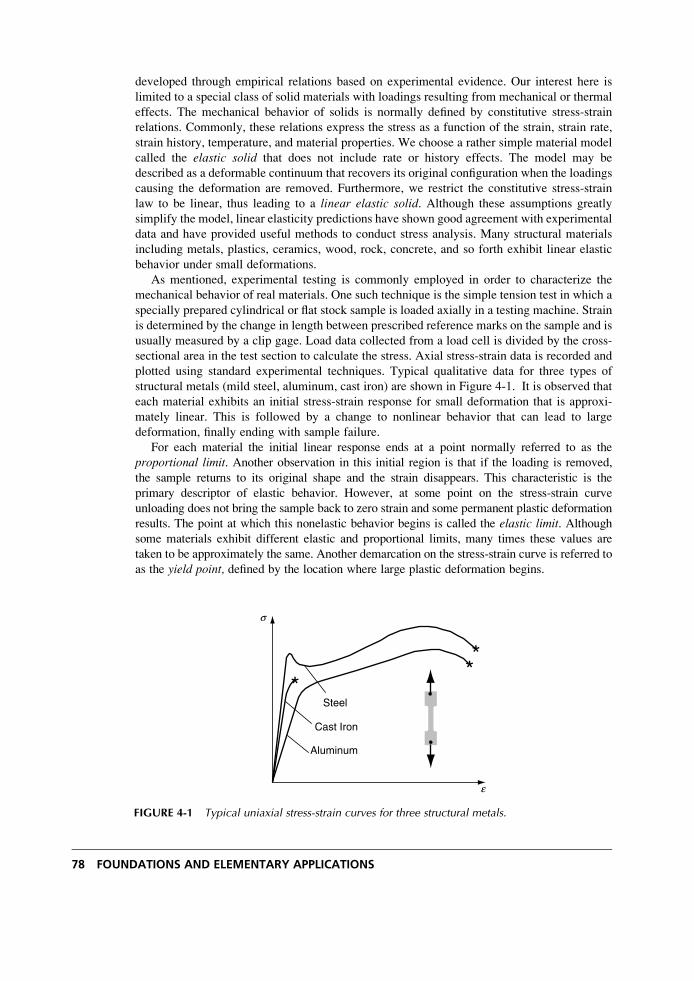
developed through empirical relations based on experimental evidence. Our interest here is
limited to a special class of solid materials with loadings resulting from mechanical or thermal
effects. The mechanical behavior of solids is normally defined by constitutive stress-strain
relations. Commonly, these relations express the stress as a function of the strain, strain rate,
strain history, temperature, and material properties. We choose a rather simple material model
called the elastic solid that does not include rate or history effects. The model may be
described as a deformable continuum that recovers its original configuration when the loadings
causing the deformation are removed. Furthermore, we restrict the constitutive stress-strain
law to be linear, thus leading to a linear elastic solid. Although these assumptions greatly
simplify the model, linear elasticity predictions have shown good agreement with experimental
data and have provided useful methods to conduct stress analysis. Many structural materials
including metals, plastics, ceramics, wood, rock, concrete, and so forth exhibit linear elastic
behavior under small deformations.
As mentioned, experimental testing is commonly employed in order to characterize the
mechanical behavior of real materials. One such technique is the simple tension test in which a
specially prepared cylindrical or flat stock sample is loaded axially in a testing machine. Strain
is determined by the change in length between prescribed reference marks on the sample and is
usually measured by a clip gage. Load data collected from a load cell is divided by the cross-
sectional area in the test section to calculate the stress. Axial stress-strain data is recorded and
plotted using standard experimental techniques. Typical qualitative data for three types of
structural metals (mild steel, aluminum, cast iron) are shown in Figure 4-1. It is observed that
each material exhibits an initial stress-strain response for small deformation that is approxi-
mately linear. This is followed by a change to nonlinear behavior that can lead to large
deformation, finally ending with sample failure.
For each material the initial linear response ends at a point normally referred to as the
proportional limit. Another observation in this initial region is that if the loading is removed,
the sample returns to its original shape and the strain disappears. This characteristic is the
primary descriptor of elastic behavior. However, at some point on the stress-strain curve
unloading does not bring the sample back to zero strain and some permanent plastic deformation
results. The point at which this nonelastic behavior begins is called the elastic limit. Althoughsome materials exhibit different elastic and proportional limits, many times these values are
taken to be approximately the same. Another demarcation on the stress-strain curve is referred to
as the yield point, defined by the location where large plastic deformation begins.
Steel
Cast Iron
Aluminum
**
*
s
e
FIGURE 4-1 Typical uniaxial stress-strain curves for three structural metals.
78 FOUNDATIONS AND ELEMENTARY APPLICATIONS
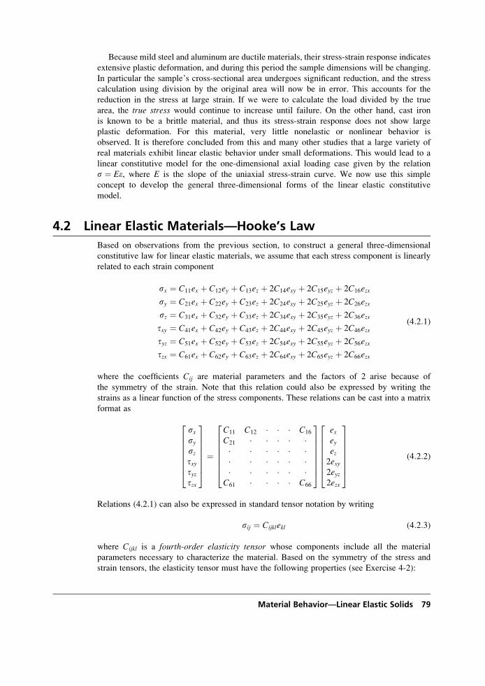
Because mild steel and aluminum are ductile materials, their stress-strain response indicates
extensive plastic deformation, and during this period the sample dimensions will be changing.
In particular the sample’s cross-sectional area undergoes significant reduction, and the stress
calculation using division by the original area will now be in error. This accounts for the
reduction in the stress at large strain. If we were to calculate the load divided by the true
area, the true stress would continue to increase until failure. On the other hand, cast iron
is known to be a brittle material, and thus its stress-strain response does not show large
plastic deformation. For this material, very little nonelastic or nonlinear behavior is
observed. It is therefore concluded from this and many other studies that a large variety of
real materials exhibit linear elastic behavior under small deformations. This would lead to a
linear constitutive model for the one-dimensional axial loading case given by the relation
s ¼ Ee, where E is the slope of the uniaxial stress-strain curve. We now use this simple
concept to develop the general three-dimensional forms of the linear elastic constitutive
model.
4.2 Linear Elastic Materials—Hooke’s Law
Based on observations from the previous section, to construct a general three-dimensional
constitutive law for linear elastic materials, we assume that each stress component is linearly
related to each strain component
sx ¼ C11ex þ C12ey þ C13ez þ 2C14exy þ 2C15eyz þ 2C16ezx
sy ¼ C21ex þ C22ey þ C23ez þ 2C24exy þ 2C25eyz þ 2C26ezx
sz ¼ C31ex þ C32ey þ C33ez þ 2C34exy þ 2C35eyz þ 2C36ezx
txy ¼ C41ex þ C42ey þ C43ez þ 2C44exy þ 2C45eyz þ 2C46ezx
tyz ¼ C51ex þ C52ey þ C53ez þ 2C54exy þ 2C55eyz þ 2C56ezx
tzx ¼ C61ex þ C62ey þ C63ez þ 2C64exy þ 2C65eyz þ 2C66ezx
(4:2:1)
where the coefficients Cij are material parameters and the factors of 2 arise because of
the symmetry of the strain. Note that this relation could also be expressed by writing the
strains as a linear function of the stress components. These relations can be cast into a matrix
format as
sxsysztxytyztzx
26666664
37777775¼
C11 C12 � � � C16
C21 � � � � �� � � � � �� � � � � �� � � � � �
C61 � � � � C66
26666664
37777775
exeyez2exy2eyz2ezx
26666664
37777775
(4:2:2)
Relations (4.2.1) can also be expressed in standard tensor notation by writing
sij ¼ Cijklekl (4:2:3)
where Cijkl is a fourth-order elasticity tensor whose components include all the material
parameters necessary to characterize the material. Based on the symmetry of the stress and
strain tensors, the elasticity tensor must have the following properties (see Exercise 4-2):
Material Behavior—Linear Elastic Solids 79
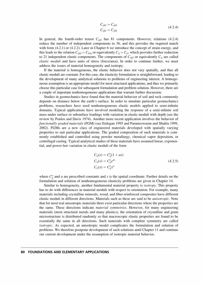
Cijkl ¼ Cjikl
Cijkl ¼ Cijlk
(4:2:4)
In general, the fourth-order tensor Cijkl has 81 components. However, relations (4.2.4)
reduce the number of independent components to 36, and this provides the required match
with form (4.2.1) or (4.2.2). Later in Chapter 6 we introduce the concept of strain energy, and
this leads to the relation Cijkl¼ Cklij or equivalently Cij¼ Cji, which provides further reduction
to 21 independent elastic components. The components of Cijkl or equivalently Cij are called
elastic moduli and have units of stress (force/area). In order to continue further, we must
address the issues of material homogeneity and isotropy.
If the material is homogeneous, the elastic behavior does not vary spatially, and thus all
elastic moduli are constant. For this case, the elasticity formulation is straightforward, leading to
the development of many analytical solutions to problems of engineering interest. A homoge-
neous assumption is an appropriate model for most structural applications, and thus we primarily
choose this particular case for subsequent formulation and problem solution. However, there are
a couple of important nonhomogeneous applications that warrant further discussion.
Studies in geomechanics have found that the material behavior of soil and rock commonly
depends on distance below the earth’s surface. In order to simulate particular geomechanics
problems, researchers have used nonhomogeneous elastic models applied to semi-infinite
domains. Typical applications have involved modeling the response of a semi-infinite soil
mass under surface or subsurface loadings with variation in elastic moduli with depth (see the
review by Poulos and Davis 1974). Another more recent application involves the behavior of
functionally graded materials (FGM) (see Erdogan 1995 and Parameswaran and Shukla 1999,
2002). FGMs are a new class of engineered materials developed with spatially varying
properties to suit particular applications. The graded composition of such materials is com-
monly established and controlled using powder metallurgy, chemical vapor deposition, or
centrifugal casting. Typical analytical studies of these materials have assumed linear, exponen-
tial, and power-law variation in elastic moduli of the form
Cij(x) ¼ Coij(1þ ax)
Cij(x) ¼ Coije
ax
Cij(x) ¼ Coijx
a
(4:2:5)
where Coij and a are prescribed constants and x is the spatial coordinate. Further details on the
formulation and solution of nonhomogeneous elasticity problems are given in Chapter 14.
Similar to homogeneity, another fundamental material property is isotropy. This propertyhas to do with differences in material moduli with respect to orientation. For example, many
materials including crystalline minerals, wood, and fiber-reinforced composites have different
elastic moduli in different directions. Materials such as these are said to be anisotropic. Notethat for most real anisotropic materials there exist particular directions where the properties are
the same. These directions indicate material symmetries. However, for many engineering
materials (most structural metals and many plastics), the orientation of crystalline and grain
microstructure is distributed randomly so that macroscopic elastic properties are found to be
essentially the same in all directions. Such materials with complete symmetry are called
isotropic. As expected, an anisotropic model complicates the formulation and solution of
problems. We therefore postpone development of such solutions until Chapter 11 and continue
our current development under the assumption of isotropic material behavior.
80 FOUNDATIONS AND ELEMENTARY APPLICATIONS
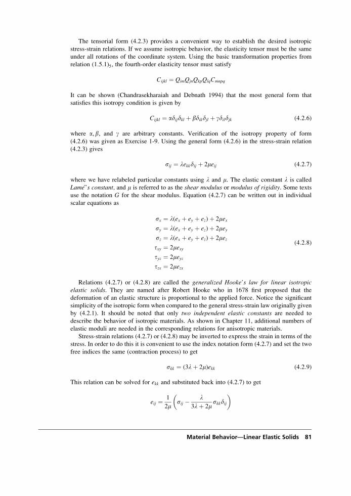
The tensorial form (4.2.3) provides a convenient way to establish the desired isotropic
stress-strain relations. If we assume isotropic behavior, the elasticity tensor must be the same
under all rotations of the coordinate system. Using the basic transformation properties from
relation (1:5:1)5, the fourth-order elasticity tensor must satisfy
Cijkl ¼ QimQjnQkpQlqCmnpq
It can be shown (Chandrasekharaiah and Debnath 1994) that the most general form that
satisfies this isotropy condition is given by
Cijkl ¼ adijdkl þ bdikdjl þ gdildjk (4:2:6)
where a,b, and g are arbitrary constants. Verification of the isotropy property of form
(4.2.6) was given as Exercise 1-9. Using the general form (4.2.6) in the stress-strain relation
(4.2.3) gives
sij ¼ lekkdij þ 2meij (4:2:7)
where we have relabeled particular constants using l and m. The elastic constant l is called
Lame’s constant, and m is referred to as the shear modulus or modulus of rigidity. Some texts
use the notation G for the shear modulus. Equation (4.2.7) can be written out in individual
scalar equations as
sx ¼ l(ex þ ey þ ez)þ 2mexsy ¼ l(ex þ ey þ ez)þ 2meysz ¼ l(ex þ ey þ ez)þ 2meztxy ¼ 2mexytyz ¼ 2meyztzx ¼ 2mezx
(4:2:8)
Relations (4.2.7) or (4.2.8) are called the generalized Hooke’s law for linear isotropicelastic solids. They are named after Robert Hooke who in 1678 first proposed that the
deformation of an elastic structure is proportional to the applied force. Notice the significant
simplicity of the isotropic form when compared to the general stress-strain law originally given
by (4.2.1). It should be noted that only two independent elastic constants are needed to
describe the behavior of isotropic materials. As shown in Chapter 11, additional numbers of
elastic moduli are needed in the corresponding relations for anisotropic materials.
Stress-strain relations (4.2.7) or (4.2.8) may be inverted to express the strain in terms of the
stress. In order to do this it is convenient to use the index notation form (4.2.7) and set the two
free indices the same (contraction process) to get
skk ¼ (3lþ 2m)ekk (4:2:9)
This relation can be solved for ekk and substituted back into (4.2.7) to get
eij ¼ 1
2msij � l
3lþ 2mskkdij
� �
Material Behavior—Linear Elastic Solids 81
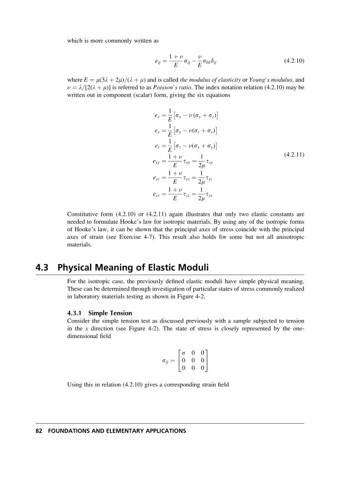
which is more commonly written as
eij ¼ 1þ �
Esij � �
Eskkdij (4:2:10)
where E ¼ m(3lþ 2m)=(lþ m) and is called the modulus of elasticity or Young’s modulus, and� ¼ l=[2(lþ m)] is referred to as Poisson’s ratio. The index notation relation (4.2.10) may be
written out in component (scalar) form, giving the six equations
ex ¼ 1
Esx � � (sy þ sz)� �
ey ¼ 1
Esy � �(sz þ sx)� �
ez ¼ 1
Esz � �(sx þ sy)� �
exy ¼ 1þ �
Etxy ¼ 1
2mtxy
eyz ¼ 1þ �
Etyz ¼ 1
2mtyz
ezx ¼ 1þ �
Etzx ¼ 1
2mtzx
(4:2:11)
Constitutive form (4.2.10) or (4.2.11) again illustrates that only two elastic constants are
needed to formulate Hooke’s law for isotropic materials. By using any of the isotropic forms
of Hooke’s law, it can be shown that the principal axes of stress coincide with the principal
axes of strain (see Exercise 4-7). This result also holds for some but not all anisotropic
materials.
4.3 Physical Meaning of Elastic Moduli
For the isotropic case, the previously defined elastic moduli have simple physical meaning.
These can be determined through investigation of particular states of stress commonly realized
in laboratory materials testing as shown in Figure 4-2.
4.3.1 Simple TensionConsider the simple tension test as discussed previously with a sample subjected to tension
in the x direction (see Figure 4-2). The state of stress is closely represented by the one-
dimensional field
sij ¼s 0 0
0 0 0
0 0 0
24
35
Using this in relation (4.2.10) gives a corresponding strain field
82 FOUNDATIONS AND ELEMENTARY APPLICATIONS
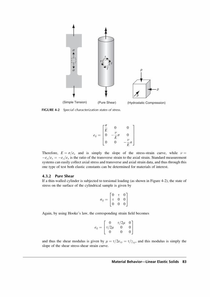
eij ¼
sE
0 0
0 � �
Es 0
0 0 � �
Es
26664
37775
Therefore, E ¼ s=ex and is simply the slope of the stress-strain curve, while � ¼�ey=ex ¼ �ez=ex is the ratio of the transverse strain to the axial strain. Standard measurement
systems can easily collect axial stress and transverse and axial strain data, and thus through this
one type of test both elastic constants can be determined for materials of interest.
4.3.2 Pure ShearIf a thin-walled cylinder is subjected to torsional loading (as shown in Figure 4-2), the state of
stress on the surface of the cylindrical sample is given by
sij ¼0 t 0
t 0 0
0 0 0
24
35
Again, by using Hooke’s law, the corresponding strain field becomes
eij ¼0 t=2m 0
t=2m 0 0
0 0 0
24
35
and thus the shear modulus is given by m ¼ t=2exy ¼ t=gxy, and this modulus is simply the
slope of the shear stress-shear strain curve.
s
s
(Simple Tension)
tt
t
t
(Pure Shear)
p
p
p
(Hydrostatic Compression)
FIGURE 4-2 Special characterization states of stress.
Material Behavior—Linear Elastic Solids 83
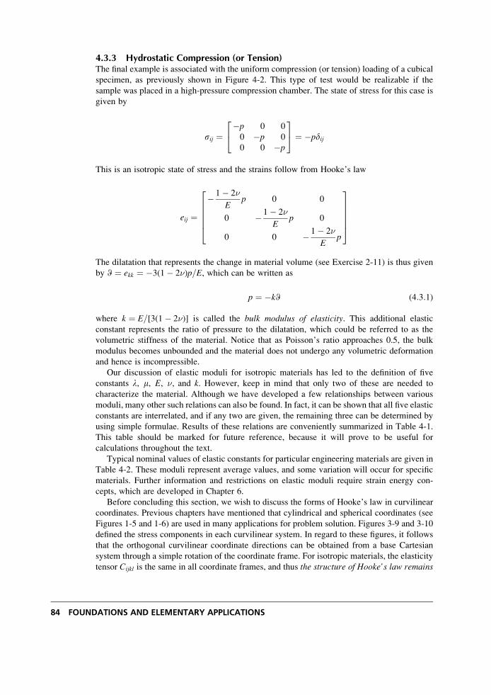
4.3.3 Hydrostatic Compression (or Tension)The final example is associated with the uniform compression (or tension) loading of a cubical
specimen, as previously shown in Figure 4-2. This type of test would be realizable if the
sample was placed in a high-pressure compression chamber. The state of stress for this case is
given by
sij ¼�p 0 0
0 �p 0
0 0 �p
24
35 ¼ �pdij
This is an isotropic state of stress and the strains follow from Hooke’s law
eij ¼� 1� 2�
Ep 0 0
0 � 1� 2�
Ep 0
0 0 � 1� 2�
Ep
266664
377775
The dilatation that represents the change in material volume (see Exercise 2-11) is thus given
by W ¼ ekk ¼ �3(1� 2�)p=E, which can be written as
p ¼ �kW (4:3:1)
where k ¼ E=[3(1� 2�)] is called the bulk modulus of elasticity. This additional elastic
constant represents the ratio of pressure to the dilatation, which could be referred to as the
volumetric stiffness of the material. Notice that as Poisson’s ratio approaches 0.5, the bulk
modulus becomes unbounded and the material does not undergo any volumetric deformation
and hence is incompressible.
Our discussion of elastic moduli for isotropic materials has led to the definition of five
constants l, m, E, �, and k. However, keep in mind that only two of these are needed to
characterize the material. Although we have developed a few relationships between various
moduli, many other such relations can also be found. In fact, it can be shown that all five elastic
constants are interrelated, and if any two are given, the remaining three can be determined by
using simple formulae. Results of these relations are conveniently summarized in Table 4-1.
This table should be marked for future reference, because it will prove to be useful for
calculations throughout the text.
Typical nominal values of elastic constants for particular engineering materials are given in
Table 4-2. These moduli represent average values, and some variation will occur for specific
materials. Further information and restrictions on elastic moduli require strain energy con-
cepts, which are developed in Chapter 6.
Before concluding this section, we wish to discuss the forms of Hooke’s law in curvilinear
coordinates. Previous chapters have mentioned that cylindrical and spherical coordinates (see
Figures 1-5 and 1-6) are used in many applications for problem solution. Figures 3-9 and 3-10
defined the stress components in each curvilinear system. In regard to these figures, it follows
that the orthogonal curvilinear coordinate directions can be obtained from a base Cartesian
system through a simple rotation of the coordinate frame. For isotropic materials, the elasticity
tensor Cijkl is the same in all coordinate frames, and thus the structure of Hooke’s law remains
84 FOUNDATIONS AND ELEMENTARY APPLICATIONS
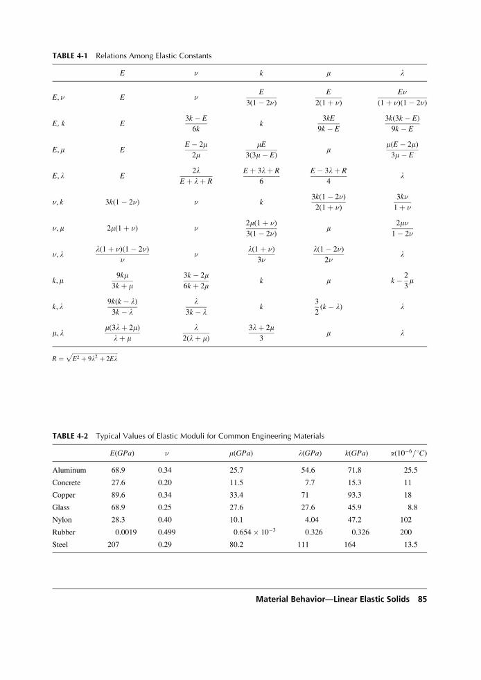
TABLE 4-1 Relations Among Elastic Constants
E � k m l
E, � E �E
3(1� 2�)
E
2(1þ �)
E�
(1þ �)(1� 2�)
E, k E3k � E
6kk
3kE
9k � E
3k(3k � E)
9k � E
E,m EE� 2m2m
mE3(3m� E)
mm(E� 2m)3m� E
E, l E2l
Eþ lþ R
Eþ 3lþ R
6
E� 3lþ R
4l
�, k 3k(1� 2�) � k3k(1� 2�)
2(1þ �)
3k�
1þ �
�,m 2m(1þ �) �2m(1þ �)
3(1� 2�)m
2m�1� 2�
�, ll(1þ �)(1� 2�)
��
l(1þ �)
3�
l(1� 2�)
2�l
k,m9km
3k þ m3k � 2m6k þ 2m
k m k � 2
3m
k, l9k(k � l)3k � l
l3k � l
k3
2(k � l) l
m, lm(3lþ 2m)
lþ ml
2(lþ m)3lþ 2m
3m l
R ¼ffiffiffiffiffiffiffiffiffiffiffiffiffiffiffiffiffiffiffiffiffiffiffiffiffiffiffiffiffiffiffiffiE2 þ 9l2 þ 2El
p
TABLE 4-2 Typical Values of Elastic Moduli for Common Engineering Materials
E(GPa) � m(GPa) l(GPa) k(GPa) a(10�6=8C)
Aluminum 68.9 0.34 25.7 54.6 71.8 25.5
Concrete 27.6 0.20 11.5 7.7 15.3 11
Copper 89.6 0.34 33.4 71 93.3 18
Glass 68.9 0.25 27.6 27.6 45.9 8.8
Nylon 28.3 0.40 10.1 4.04 47.2 102
Rubber 0.0019 0.499 0:654� 10�3 0.326 0.326 200
Steel 207 0.29 80.2 111 164 13.5
Material Behavior—Linear Elastic Solids 85
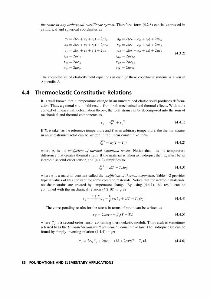
the same in any orthogonal curvilinear system. Therefore, form (4.2.8) can be expressed in
cylindrical and spherical coordinates as
sr ¼ l(er þ ey þ ez)þ 2mer sR ¼ l(eR þ ef þ ey)þ 2meRsy ¼ l(er þ ey þ ez)þ 2mey sf ¼ l(eR þ ef þ ey)þ 2mefsz ¼ l(er þ ey þ ez)þ 2mez sy ¼ l(eR þ ef þ ey)þ 2meytry ¼ 2mery tRf ¼ 2meRftyz ¼ 2meyz tfy ¼ 2mefytzr ¼ 2mezr tyR ¼ 2meyR
(4:3:2)
The complete set of elasticity field equations in each of these coordinate systems is given in
Appendix A.
4.4 Thermoelastic Constitutive Relations
It is well known that a temperature change in an unrestrained elastic solid produces deform-
ation. Thus, a general strain field results from both mechanical and thermal effects. Within the
context of linear small deformation theory, the total strain can be decomposed into the sum of
mechanical and thermal components as
eij ¼ e(M)ij þ e(T)ij (4:4:1)
If To is taken as the reference temperature and T as an arbitrary temperature, the thermal strains
in an unrestrained solid can be written in the linear constitutive form
e(T)ij ¼ aij(T � To) (4:4:2)
where aij is the coefficient of thermal expansion tensor. Notice that it is the temperature
difference that creates thermal strain. If the material is taken as isotropic, then aij must be an
isotropic second-order tensor, and (4.4.2) simplifies to
e(T)ij ¼ a(T � To)dij (4:4:3)
where a is a material constant called the coefficient of thermal expansion. Table 4-2 provides
typical values of this constant for some common materials. Notice that for isotropic materials,
no shear strains are created by temperature change. By using (4.4.1), this result can be
combined with the mechanical relation (4.2.10) to give
eij ¼ 1þ �
Esij � �
Eskkdij þ a(T � To)dij (4:4:4)
The corresponding results for the stress in terms of strain can be written as
sij ¼ Cijklekl � bij(T � To) (4:4:5)
where bij is a second-order tensor containing thermoelastic moduli. This result is sometimes
referred to as the Duhamel-Neumann thermoelastic constitutive law. The isotropic case can be
found by simply inverting relation (4.4.4) to get
sij ¼ lekkdij þ 2meij � (3lþ 2m)a(T � To)dij (4:4:6)
86 FOUNDATIONS AND ELEMENTARY APPLICATIONS
Thermoelastic solutions are developed in Chapter 12, and the current study will now continue
under the assumption of isothermal conditions.
Having developed the necessary six constitutive relations, the elasticity field equation
system is now complete with fifteen equations (strain-displacement, equilibrium, Hooke’s
law) for fifteen unknowns (displacements, strains, stresses). Obviously, further simplification
is necessary in order to solve specific problems of engineering interest, and these processes are
the subject of the next chapter.
References
Chandrasekharaiah DS, and Debnath L: Continuum Mechanics, Academic Press, Boston, 1994.
Erdogan F: Fracture mechanics of functionally graded materials, Composites Engng, vol 5, pp. 753-770,1995.
Malvern LE: Introduction to the Mechanics of a Continuous Medium, Prentice Hall, Englewood Cliffs,
NJ, 1969.
Parameswaran V, and Shukla A: Crack-tip stress fields for dynamic fracture in functionally gradient
materials, Mech. of Materials, vol 31, pp. 579-596, 1999.Parameswaran V, and Shukla A: Asymptotic stress fields for stationary cracks along the gradient in
functionally graded materials, J. Appl. Mech., vol 69, pp. 240-243, 2002.Poulos HG, and Davis EH: Elastic Solutions for Soil and Rock Mechanics, John Wiley, New York, 1974.
Exercises
4-1. Show that the components of the Cij matrix in equation (4.2.2) are related to the
components of Cijkl by the relation
Cij ¼
C1111 C1122 C1133 C1112 C1123 C1131
C2211 C2222 C2233 C2212 C2223 C2231
C3311 C3322 C3333 C3312 C3323 C3331
C1211 C1222 C1233 C1212 C1223 C1231
C2311 C2322 C2333 C2312 C2323 C2331
C3111 C3122 C3133 C3112 C3123 C3131
26666664
37777775
4-2. Explicitly justify the symmetry relations (4.2.4). Note that the first relation follows
directly from the symmetry of the stress, while the second condition requires a simple
expansion into the form sij ¼ 12(Cijkl þ Cijlk)elk to arrive at the required conclusion.
4-3. Substituting the general isotropic fourth-order form (4.2.6) into (4.2.3), explicitly develop
the stress-strain relation (4.2.7).
4-4. For isotropic materials, show that the fourth-order elasticity tensor can be expressed in the
following forms:
Cijkl ¼ l�ij �kl þ �(�il �jk þ �ik �jl)
Cijkl ¼ �(�il �jk þ �ik �jl)þ (k � 2
3�)�ij �kl
Cijkl ¼ E�
(1þ �)(1� 2�)�ij �kl þ E
2(1þ �)(�il �jk þ �ik �jl)
Material Behavior—Linear Elastic Solids 87
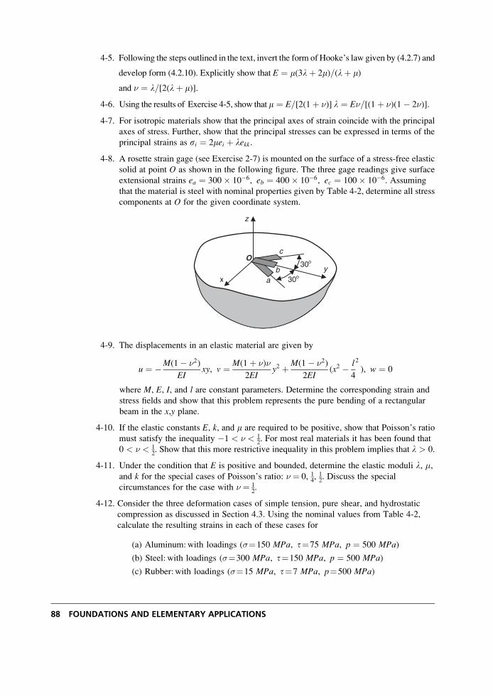
4-5. Following the steps outlined in the text, invert the form of Hooke’s law given by (4.2.7) and
develop form (4.2.10). Explicitly show that E ¼ m(3lþ 2m)=(lþ m)
and � ¼ l=[2(lþ m)].
4-6. Using the results of Exercise 4-5, show that m ¼ E=[2(1þ �)] l ¼ E�=[(1þ �)(1� 2�)].
4-7. For isotropic materials show that the principal axes of strain coincide with the principal
axes of stress. Further, show that the principal stresses can be expressed in terms of the
principal strains as si ¼ 2mei þ lekk.
4-8. A rosette strain gage (see Exercise 2-7) is mounted on the surface of a stress-free elastic
solid at point O as shown in the following figure. The three gage readings give surface
extensional strains ea ¼ 300� 10�6, eb ¼ 400� 10�6, ec ¼ 100� 10�6. Assuming
that the material is steel with nominal properties given by Table 4-2, determine all stress
components at O for the given coordinate system.
x y
z
30o
30o
ab
cO
4-9. The displacements in an elastic material are given by
u ¼ �M(1� �2)
EIxy, v ¼ M(1þ �)�
2EIy2 þM(1� �2)
2EI(x2 � l
4
2
), w ¼ 0
where M, E, I, and l are constant parameters. Determine the corresponding strain and
stress fields and show that this problem represents the pure bending of a rectangular
beam in the x,y plane.
4-10. If the elastic constants E, k, and m are required to be positive, show that Poisson’s ratio
must satisfy the inequality �1 < � < 12. For most real materials it has been found that
0 < � < 12. Show that this more restrictive inequality in this problem implies that l > 0.
4-11. Under the condition that E is positive and bounded, determine the elastic moduli l, �,and k for the special cases of Poisson’s ratio: � ¼ 0, 1
4, 12. Discuss the special
circumstances for the case with � ¼ 12.
4-12. Consider the three deformation cases of simple tension, pure shear, and hydrostatic
compression as discussed in Section 4.3. Using the nominal values from Table 4-2,
calculate the resulting strains in each of these cases for
(a) Aluminum:with loadings (�¼150 MPa, t¼75 MPa, p ¼ 500 MPa)
(b) Steel:with loadings (�¼300 MPa, t¼150 MPa, p ¼ 500 MPa)
(c) Rubber:with loadings (�¼15 MPa, t¼7 MPa, p¼500 MPa)
88 FOUNDATIONS AND ELEMENTARY APPLICATIONS
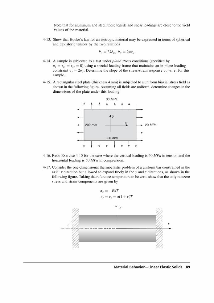
Note that for aluminum and steel, these tensile and shear loadings are close to the yield
values of the material.
4-13. Show that Hooke’s law for an isotropic material may be expressed in terms of spherical
and deviatoric tensors by the two relations
~ssij ¼ 3k~eeij, ssij ¼ 2meeij
4-14. A sample is subjected to a test under plane stress conditions (specified by
sz ¼ tzx ¼ tzy ¼ 0) using a special loading frame that maintains an in-plane loading
constraint sx ¼ 2sy. Determine the slope of the stress-strain response sx vs. ex for thissample.
4-15. A rectangular steel plate (thickness 4mm) is subjected to a uniform biaxial stress field as
shown in the following figure. Assuming all fields are uniform, determine changes in the
dimensions of the plate under this loading.
x
y
300 mm
200 mm 20 MPa
30 MPa
4-16. Redo Exercise 4-15 for the case where the vertical loading is 50 MPa in tension and the
horizontal loading is 50 MPa in compression.
4-17. Consider the one-dimensional thermoelastic problem of a uniform bar constrained in the
axial x direction but allowed to expand freely in the y and z directions, as shown in the
following figure. Taking the reference temperature to be zero, show that the only nonzero
stress and strain components are given by
sx ¼ �EaT
ey ¼ ez ¼ a(1þ �)T
x
y
Material Behavior—Linear Elastic Solids 89
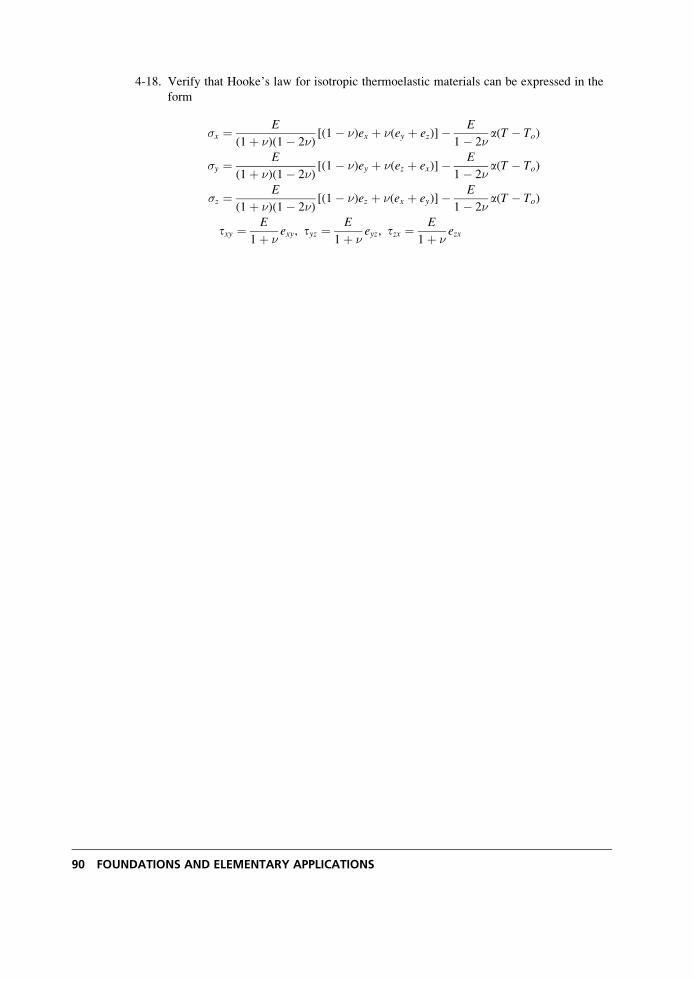
4-18. Verify that Hooke’s law for isotropic thermoelastic materials can be expressed in the
form
�x ¼ E
(1þ �)(1� 2�)[(1� �)ex þ �(ey þ ez)]� E
1� 2�a(T � To)
�y ¼ E
(1þ �)(1� 2�)[(1� �)ey þ �(ez þ ex)]� E
1� 2�a(T � To)
�z ¼ E
(1þ �)(1� 2�)[(1� �)ez þ �(ex þ ey)]� E
1� 2�a(T � To)
txy ¼ E
1þ �exy, tyz ¼ E
1þ �eyz, tzx ¼ E
1þ �ezx
90 FOUNDATIONS AND ELEMENTARY APPLICATIONS
5 Formulation and Solution Strategies
The previous chapters have now developed the basic field equations of elasticity theory. These
results comprise a system of differential and algebraic relations among the stresses, strains, and
displacements that express particular physics at all points within the body under investigation.
In this chapter we now wish to complete the general formulation by first developing boundaryconditions appropriate for use with the field equations. These conditions specify the physics
that occur on the boundary of the body, and generally provide the loading inputs that physicallycreate the interior stress, strain, and displacement fields. Although the field equations are the
same for all problems, boundary conditions are different for each problem. Therefore, proper
development of boundary conditions is essential for problem solution, and thus it is important
to acquire a good understanding of such development procedures. Combining field equations
with boundary conditions then establishes the fundamental boundary value problems of the
theory. This eventually leads us into two different formulations: one in terms of displacements
and the other in terms of stresses. Because boundary value problems are difficult to solve,
many different strategies have been developed to aid in problem solution. We review in a
general way several of these strategies, and later chapters incorporate many of them into the
solution of specific problems.
5.1 Review of Field Equations
Before beginning our discussion on boundary conditions we list here the basic field equations
for linear isotropic elasticity. Appendix A includes a more comprehensive listing of all field
equations in Cartesian, cylindrical, and spherical coordinate systems. Because of its ease of use
and compact properties, our formulation uses index notation.
Strain-displacement relations:
eij ¼ 1
2(ui, j þ uj, i) (5:1:1)
Compatibility relations:
eij, kl þ ekl, ij � eik, jl � ejl, ik ¼ 0 (5:1:2)
91

Equilibrium equations:
sij, j þ Fi ¼ 0 (5:1:3)
Elastic constitutive law (Hooke’s law):
sij ¼ lekkdij þ 2meij
eij ¼ 1þ �
Esij � �
Eskkdij
(5:1:4)
As mentioned in Section 2.6, the compatibility relations ensure that the displacements are
continuous and single-valued and are necessary only when the strains are arbitrarily specified.
If, however, the displacements are included in the problem formulation, the solution normally
generates single-valued displacements and strain compatibility is automatically satisfied. Thus,
in discussing the general system of equations of elasticity, the compatibility relations (5.1.2)
are normally set aside, to be used only with the stress formulation that we discuss shortly.
Therefore, the general system of elasticity field equations refers to the fifteen relations (5.1.1),
(5.1.3), and (5.1.4). It is convenient to define this entire system using a generalized operator
notation as
J{ui, eij, sij; l, m, Fi} ¼ 0 (5:1:5)
This system involves fifteen unknowns including three displacements ui, six strains eij, and six
stresses sij. The terms after the semicolon indicate that the system is also dependent on two
elastic material constants (for isotropic materials) and on the body force density, and these are to
be given a priori with the problem formulation. It is reassuring that the number of equations
matches the number of unknowns to be determined. However, this general system of equations
is of such complexity that solutions by using analytical methods are essentially impossible and
further simplification is required to solve problems of interest. Before proceeding with devel-
opment of such simplifications, it is useful first to discuss typical boundary conditions connected
with the elasticity model, and this leads us to the classification of the fundamental problems.
5.2 Boundary Conditions and FundamentalProblem Classifications
Similar to other field problems in engineering science (e.g., fluid mechanics, heat conduction,
diffusion, electromagnetics), the solution of system (5.1.5) requires appropriate boundary
conditions on the body under study. The common types of boundary conditions for elasticity
applications normally include specification of how the body is being supported or loaded. Thisconcept is mathematically formulated by specifying either the displacements or tractions at
boundary points. Figure 5-1 illustrates this general idea for three typical cases including
tractions, displacements, and a mixed case for which tractions are specified on boundary Stand displacements are given on the remaining portion Su such that the total boundary is given
by S ¼ St þ Su.Another type of mixed boundary condition can also occur. Although it is generally not
possible to specify completely both the displacements and tractions at the same boundary
point, it is possible to prescribe part of the displacement and part of the traction. Typically, this
92 FOUNDATIONS AND ELEMENTARY APPLICATIONS
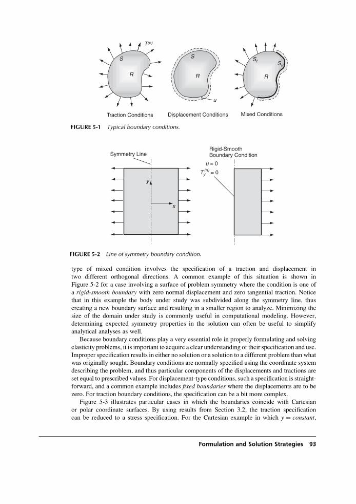
type of mixed condition involves the specification of a traction and displacement in
two different orthogonal directions. A common example of this situation is shown in
Figure 5-2 for a case involving a surface of problem symmetry where the condition is one of
a rigid-smooth boundary with zero normal displacement and zero tangential traction. Notice
that in this example the body under study was subdivided along the symmetry line, thus
creating a new boundary surface and resulting in a smaller region to analyze. Minimizing the
size of the domain under study is commonly useful in computational modeling. However,
determining expected symmetry properties in the solution can often be useful to simplify
analytical analyses as well.
Because boundary conditions play a very essential role in properly formulating and solving
elasticity problems, it is important to acquire a clear understanding of their specification and use.
Improper specification results in either no solution or a solution to a different problem than what
was originally sought. Boundary conditions are normally specified using the coordinate system
describing the problem, and thus particular components of the displacements and tractions are
set equal to prescribed values. For displacement-type conditions, such a specification is straight-
forward, and a common example includes fixed boundaries where the displacements are to be
zero. For traction boundary conditions, the specification can be a bit more complex.
Figure 5-3 illustrates particular cases in which the boundaries coincide with Cartesian
or polar coordinate surfaces. By using results from Section 3.2, the traction specification
can be reduced to a stress specification. For the Cartesian example in which y ¼ constant,
Displacement Conditions Mixed ConditionsTraction Conditions
R
S
R
SuSt
T(n)
R
S
u
FIGURE 5-1 Typical boundary conditions.
Symmetry Line
Ty(n) = 0
u = 0
x
y
Rigid-SmoothBoundary Condition
FIGURE 5-2 Line of symmetry boundary condition.
Formulation and Solution Strategies 93
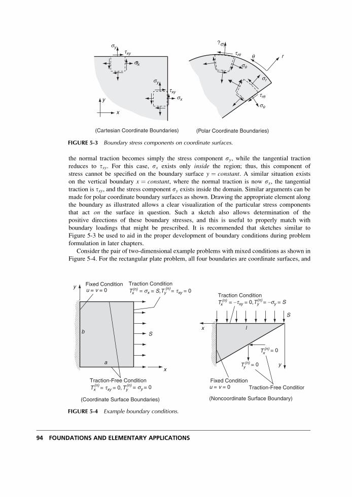
the normal traction becomes simply the stress component sy, while the tangential traction
reduces to txy. For this case, sx exists only inside the region; thus, this component of
stress cannot be specified on the boundary surface y ¼ constant. A similar situation exists
on the vertical boundary x ¼ constant, where the normal traction is now sx, the tangential
traction is txy, and the stress component sy exists inside the domain. Similar arguments can be
made for polar coordinate boundary surfaces as shown. Drawing the appropriate element along
the boundary as illustrated allows a clear visualization of the particular stress components
that act on the surface in question. Such a sketch also allows determination of the
positive directions of these boundary stresses, and this is useful to properly match with
boundary loadings that might be prescribed. It is recommended that sketches similar to
Figure 5-3 be used to aid in the proper development of boundary conditions during problem
formulation in later chapters.
Consider the pair of two-dimensional example problems with mixed conditions as shown in
Figure 5-4. For the rectangular plate problem, all four boundaries are coordinate surfaces, and
?
r?
x
y
(Cartesian Coordinate Boundaries) (Polar Coordinate Boundaries)
sq
sq
sr
sx
sy
sx
sytxy
txy
sr
trq
trq q
FIGURE 5-3 Boundary stress components on coordinate surfaces.
y Fixed Conditionu = v = 0
Traction ConditionT(n) (n)
x = sx
= sy = 0
= S,Ty = txy = 0
(n)Tx(n)Ty= txy = 0,
b
a
S
x
Traction-Free Condition
(Coordinate Surface Boundaries)
(n)Tx
u = v = 0
(n) = −sy = S
= 0
= 0
= −txy = 0,Ty
Traction Condition
(n)Tx
(n)Ty
S
x l
y
Fixed ConditionTraction-Free Condition
(Noncoordinate Surface Boundary)
FIGURE 5-4 Example boundary conditions.
94 FOUNDATIONS AND ELEMENTARY APPLICATIONS
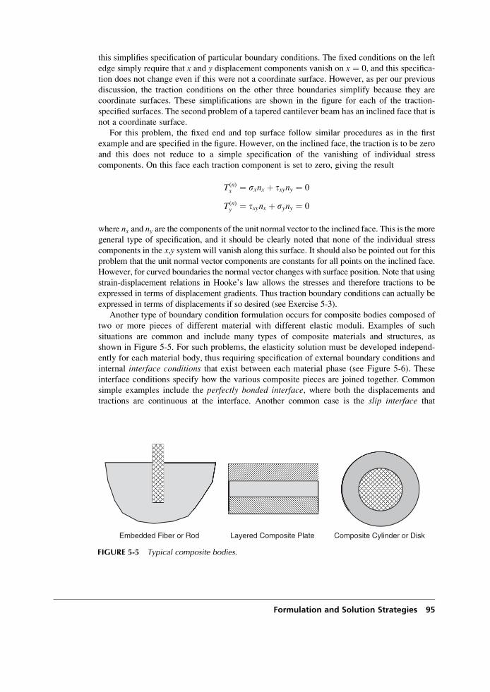
this simplifies specification of particular boundary conditions. The fixed conditions on the left
edge simply require that x and y displacement components vanish on x ¼ 0, and this specifica-
tion does not change even if this were not a coordinate surface. However, as per our previous
discussion, the traction conditions on the other three boundaries simplify because they are
coordinate surfaces. These simplifications are shown in the figure for each of the traction-
specified surfaces. The second problem of a tapered cantilever beam has an inclined face that is
not a coordinate surface.
For this problem, the fixed end and top surface follow similar procedures as in the first
example and are specified in the figure. However, on the inclined face, the traction is to be zero
and this does not reduce to a simple specification of the vanishing of individual stress
components. On this face each traction component is set to zero, giving the result
T(n)x ¼ sxnx þ txyny ¼ 0
T(n)y ¼ txynx þ syny ¼ 0
where nx and ny are the components of the unit normal vector to the inclined face. This is the more
general type of specification, and it should be clearly noted that none of the individual stress
components in the x,y system will vanish along this surface. It should also be pointed out for this
problem that the unit normal vector components are constants for all points on the inclined face.
However, for curved boundaries the normal vector changes with surface position. Note that using
strain-displacement relations in Hooke’s law allows the stresses and therefore tractions to be
expressed in terms of displacement gradients. Thus traction boundary conditions can actually be
expressed in terms of displacements if so desired (see Exercise 5-3).
Another type of boundary condition formulation occurs for composite bodies composed of
two or more pieces of different material with different elastic moduli. Examples of such
situations are common and include many types of composite materials and structures, as
shown in Figure 5-5. For such problems, the elasticity solution must be developed independ-
ently for each material body, thus requiring specification of external boundary conditions and
internal interface conditions that exist between each material phase (see Figure 5-6). These
interface conditions specify how the various composite pieces are joined together. Common
simple examples include the perfectly bonded interface, where both the displacements and
tractions are continuous at the interface. Another common case is the slip interface that
Embedded Fiber or Rod Layered Composite Plate Composite Cylinder or Disk
FIGURE 5-5 Typical composite bodies.
Formulation and Solution Strategies 95
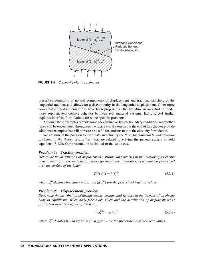
prescribes continuity of normal components of displacement and traction, vanishing of the
tangential traction, and allows for a discontinuity in the tangential displacement. Other more
complicated interface conditions have been proposed in the literature in an effort to model
more sophisticated contact behavior between real material systems. Exercise 5-4 further
explores interface formulations for some specific problems.
Although these examplesprovide somebackgroundon typical boundary conditions,manyother
types will be encountered throughout the text. Several exercises at the end of this chapter provide
additional examples that will prove to be useful for students new to the elasticity formulation.
We are now in the position to formulate and classify the three fundamental boundary-valueproblems in the theory of elasticity that are related to solving the general system of field
equations (5.1.5). Our presentation is limited to the static case.
Problem 1: Traction problemDetermine the distribution of displacements, strains, and stresses in the interior of an elasticbody in equilibrium when body forces are given and the distribution of tractions is prescribedover the surface of the body:
T(n)i (x(s)i ) ¼ fi(x
(s)i ) (5:2:1)
where x(s)i denotes boundary points and fi(x(s)i ) are the prescribed traction values.
Problem 2: Displacement problemDetermine the distribution of displacements, strains, and stresses in the interior of an elasticbody in equilibrium when body forces are given and the distribution of displacements isprescribed over the surface of the body:
ui(x(s)i ) ¼ gi(x
(s)i ) (5:2:2)
where x(s)i denotes boundary points and gi(x(s)i ) are the prescribed displacement values.
Interface Conditions: Perfectly Bonded, Slip Interface, etc.
n
s
Material (2): sij , ui(2) (2)
Material (1): sij , ui(1) (1)
FIGURE 5-6 Composite elastic continuum.
96 FOUNDATIONS AND ELEMENTARY APPLICATIONS
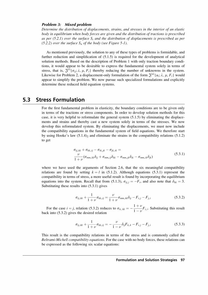
Problem 3: Mixed problemDetermine the distribution of displacements, strains, and stresses in the interior of an elasticbody in equilibrium when body forces are given and the distribution of tractions is prescribedas per (5.2.1) over the surface St and the distribution of displacements is prescribed as per(5.2.2) over the surface Su of the body (see Figure 5-1).
As mentioned previously, the solution to any of these types of problems is formidable, and
further reduction and simplification of (5.1.5) is required for the development of analytical
solution methods. Based on the description of Problem 1 with only traction boundary condi-
tions, it would appear to be desirable to express the fundamental system solely in terms of
stress, that is, J(t){sij; l, m, Fi} thereby reducing the number of unknowns in the system.
Likewise for Problem 2, a displacement-only formulation of the form J(u){ui; l, m, Fi} would
appear to simplify the problem. We now pursue such specialized formulations and explicitly
determine these reduced field equation systems.
5.3 Stress Formulation
For the first fundamental problem in elasticity, the boundary conditions are to be given only
in terms of the tractions or stress components. In order to develop solution methods for this
case, it is very helpful to reformulate the general system (5.1.5) by eliminating the displace-
ments and strains and thereby cast a new system solely in terms of the stresses. We now
develop this reformulated system. By eliminating the displacements, we must now include
the compatibility equations in the fundamental system of field equations. We therefore start
by using Hooke’s law (5.1.4)2 and eliminate the strains in the compatibility relations (5.1.2)
to get
sij, kk þ skk, ij � sik, jk � sjk, ik ¼�
1þ �(smm, kkdij þ smm, ijdkk � smm, jkdik � smm, ikdjk)
(5:3:1)
where we have used the arguments of Section 2.6, that the six meaningful compatibility
relations are found by setting k ¼ l in (5.1.2). Although equations (5.3.1) represent the
compatibility in terms of stress, a more useful result is found by incorporating the equilibrium
equations into the system. Recall that from (5.1.3), sij, j ¼ �Fi, and also note that dkk ¼ 3.
Substituting these results into (5.3.1) gives
sij, kk þ 1
1þ �skk, ij ¼ �
1þ �smm, kkdij � Fi, j � Fj, i (5:3:2)
For the case i ¼ j, relation (5.3.2) reduces to sii, kk ¼ � 1þ �
1� �Fi, i. Substituting this result
back into (5.3.2) gives the desired relation
sij, kk þ 1
1þ �skk, ij ¼ � �
1� �dijFk, k � Fi, j � Fj, i (5:3:3)
This result is the compatibility relations in terms of the stress and is commonly called the
Beltrami-Michell compatibility equations. For the case with no body forces, these relations canbe expressed as the following six scalar equations:
Formulation and Solution Strategies 97
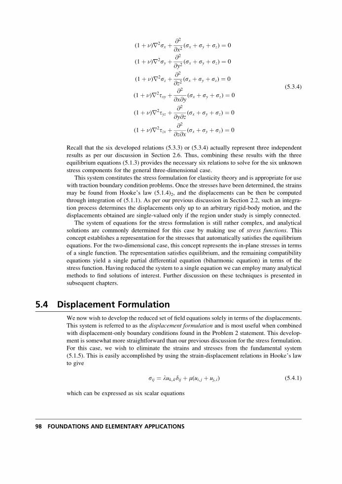
(1þ �)r2sx þ @2
@x2(sx þ sy þ sz) ¼ 0
(1þ �)r2sy þ @2
@y2(sx þ sy þ sz) ¼ 0
(1þ �)r2sz þ @2
@z2(sx þ sy þ sz) ¼ 0
(1þ �)r2txy þ @2
@x@y(sx þ sy þ sz) ¼ 0
(1þ �)r2tyz þ @2
@y@z(sx þ sy þ sz) ¼ 0
(1þ �)r2tzx þ @2
@z@x(sx þ sy þ sz) ¼ 0
(5:3:4)
Recall that the six developed relations (5.3.3) or (5.3.4) actually represent three independent
results as per our discussion in Section 2.6. Thus, combining these results with the three
equilibrium equations (5.1.3) provides the necessary six relations to solve for the six unknown
stress components for the general three-dimensional case.
This system constitutes the stress formulation for elasticity theory and is appropriate for use
with traction boundary condition problems. Once the stresses have been determined, the strains
may be found from Hooke’s law (5.1.4)2, and the displacements can be then be computed
through integration of (5.1.1). As per our previous discussion in Section 2.2, such an integra-
tion process determines the displacements only up to an arbitrary rigid-body motion, and the
displacements obtained are single-valued only if the region under study is simply connected.
The system of equations for the stress formulation is still rather complex, and analytical
solutions are commonly determined for this case by making use of stress functions. Thisconcept establishes a representation for the stresses that automatically satisfies the equilibrium
equations. For the two-dimensional case, this concept represents the in-plane stresses in terms
of a single function. The representation satisfies equilibrium, and the remaining compatibility
equations yield a single partial differential equation (biharmonic equation) in terms of the
stress function. Having reduced the system to a single equation we can employ many analytical
methods to find solutions of interest. Further discussion on these techniques is presented in
subsequent chapters.
5.4 Displacement Formulation
We now wish to develop the reduced set of field equations solely in terms of the displacements.
This system is referred to as the displacement formulation and is most useful when combined
with displacement-only boundary conditions found in the Problem 2 statement. This develop-
ment is somewhat more straightforward than our previous discussion for the stress formulation.
For this case, we wish to eliminate the strains and stresses from the fundamental system
(5.1.5). This is easily accomplished by using the strain-displacement relations in Hooke’s law
to give
sij ¼ luk, kdij þ m(ui, j þ uj, i) (5:4:1)
which can be expressed as six scalar equations
98 FOUNDATIONS AND ELEMENTARY APPLICATIONS
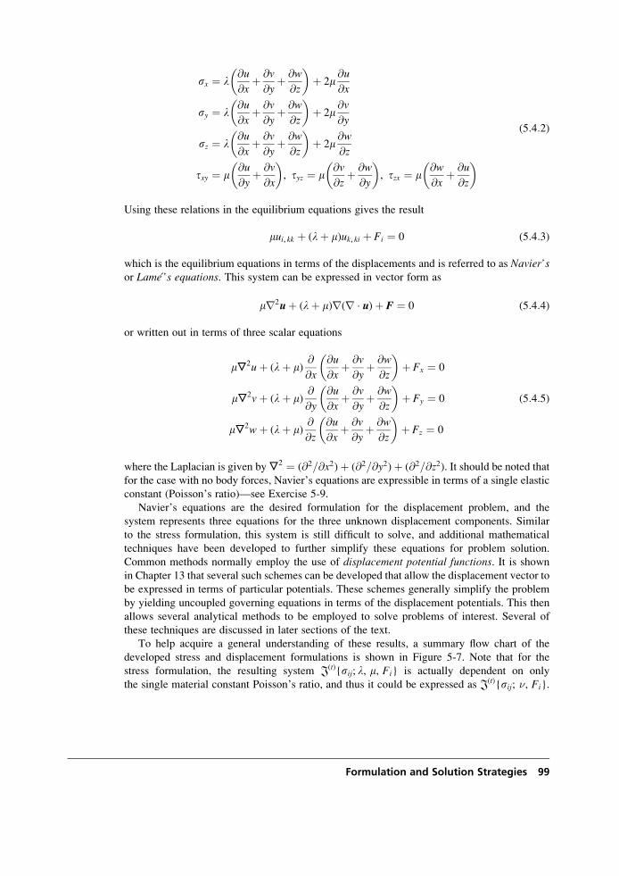
sx ¼ l@u
@xþ @v
@yþ @w
@z
� �þ 2m
@u
@x
sy ¼ l@u
@xþ @v
@yþ @w
@z
� �þ 2m
@v
@y
sz ¼ l@u
@xþ @v
@yþ @w
@z
� �þ 2m
@w
@z
txy ¼ m@u
@yþ @v
@x
� �, tyz ¼ m
@v
@zþ @w
@y
� �, tzx ¼ m
@w
@xþ @u
@z
� �(5:4:2)
Using these relations in the equilibrium equations gives the result
mui, kk þ (lþ m)uk, ki þ Fi ¼ 0 (5:4:3)
which is the equilibrium equations in terms of the displacements and is referred to as Navier’sor Lame ’s equations. This system can be expressed in vector form as
mr2uþ (lþ m)r(r � u)þ F ¼ 0 (5:4:4)
or written out in terms of three scalar equations
m,2uþ (lþ m)@
@x
@u
@xþ @v
@yþ @w
@z
� �þ Fx ¼ 0
m,2vþ (lþ m)@
@y
@u
@xþ @v
@yþ @w
@z
� �þ Fy ¼ 0
m,2wþ (lþ m)@
@z
@u
@xþ @v
@yþ @w
@z
� �þ Fz ¼ 0
(5:4:5)
where the Laplacian is given by,2 ¼ (@2=@x2)þ (@2=@y2)þ (@2=@z2). It should be noted thatfor the case with no body forces, Navier’s equations are expressible in terms of a single elastic
constant (Poisson’s ratio)—see Exercise 5-9.
Navier’s equations are the desired formulation for the displacement problem, and the
system represents three equations for the three unknown displacement components. Similar
to the stress formulation, this system is still difficult to solve, and additional mathematical
techniques have been developed to further simplify these equations for problem solution.
Common methods normally employ the use of displacement potential functions. It is shownin Chapter 13 that several such schemes can be developed that allow the displacement vector to
be expressed in terms of particular potentials. These schemes generally simplify the problem
by yielding uncoupled governing equations in terms of the displacement potentials. This then
allows several analytical methods to be employed to solve problems of interest. Several of
these techniques are discussed in later sections of the text.
To help acquire a general understanding of these results, a summary flow chart of the
developed stress and displacement formulations is shown in Figure 5-7. Note that for the
stress formulation, the resulting system J(t){sij; l, m, Fi} is actually dependent on only
the single material constant Poisson’s ratio, and thus it could be expressed as J(t){sij; �, Fi}.
Formulation and Solution Strategies 99
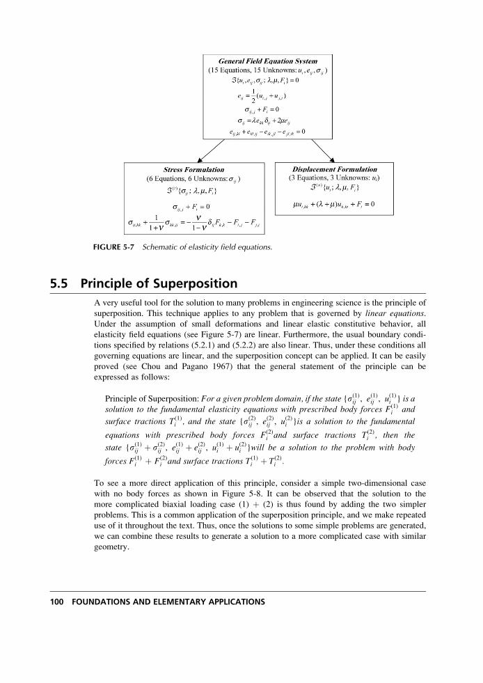
5.5 Principle of Superposition
A very useful tool for the solution to many problems in engineering science is the principle of
superposition. This technique applies to any problem that is governed by linear equations.Under the assumption of small deformations and linear elastic constitutive behavior, all
elasticity field equations (see Figure 5-7) are linear. Furthermore, the usual boundary condi-
tions specified by relations (5.2.1) and (5.2.2) are also linear. Thus, under these conditions all
governing equations are linear, and the superposition concept can be applied. It can be easily
proved (see Chou and Pagano 1967) that the general statement of the principle can be
expressed as follows:
Principle of Superposition: For a given problem domain, if the state {s(1)ij , e(1)ij , u
(1)i } is a
solution to the fundamental elasticity equations with prescribed body forces F(1)i and
surface tractions T(1)i , and the state {s(2)ij , e
(2)ij , u
(2)i }is a solution to the fundamental
equations with prescribed body forces F(2)i and surface tractions T(2)
i , then the
state {s(1)ij þ s(2)ij , e(1)ij þ e(2)ij , u(1)i þ u(2)i }will be a solution to the problem with body
forces F(1)i þ F(2)
i and surface tractions T(1)i þ T(2)
i .
To see a more direct application of this principle, consider a simple two-dimensional case
with no body forces as shown in Figure 5-8. It can be observed that the solution to the
more complicated biaxial loading case (1) þ (2) is thus found by adding the two simpler
problems. This is a common application of the superposition principle, and we make repeated
use of it throughout the text. Thus, once the solutions to some simple problems are generated,
we can combine these results to generate a solution to a more complicated case with similar
geometry.
FIGURE 5-7 Schematic of elasticity field equations.
100 FOUNDATIONS AND ELEMENTARY APPLICATIONS
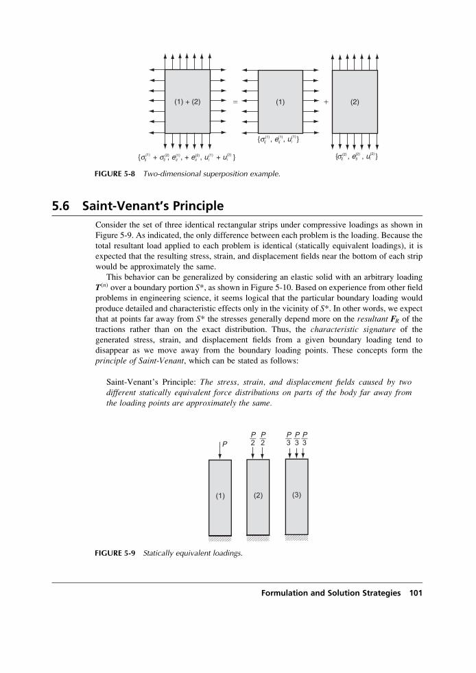
5.6 Saint-Venant’s Principle
Consider the set of three identical rectangular strips under compressive loadings as shown in
Figure 5-9. As indicated, the only difference between each problem is the loading. Because the
total resultant load applied to each problem is identical (statically equivalent loadings), it is
expected that the resulting stress, strain, and displacement fields near the bottom of each strip
would be approximately the same.
This behavior can be generalized by considering an elastic solid with an arbitrary loading
T(n) over a boundary portion S*, as shown in Figure 5-10. Based on experience from other field
problems in engineering science, it seems logical that the particular boundary loading would
produce detailed and characteristic effects only in the vicinity of S*. In other words, we expectthat at points far away from S* the stresses generally depend more on the resultant FR of the
tractions rather than on the exact distribution. Thus, the characteristic signature of the
generated stress, strain, and displacement fields from a given boundary loading tend to
disappear as we move away from the boundary loading points. These concepts form the
principle of Saint-Venant, which can be stated as follows:
Saint-Venant’s Principle: The stress, strain, and displacement fields caused by twodifferent statically equivalent force distributions on parts of the body far away fromthe loading points are approximately the same.
= +
{s (1) ij , e(1)
ij , u (1)
i }
{s , e , u }
(1) + (2) (1) (2)
{s + s , e , + e , u + u }ij ij ij i i(1) (1) (1)
ij(2) (2)
ij i(2)(2)
ij(2)(2)
FIGURE 5-8 Two-dimensional superposition example.
P
(1)
2P2P
3P3P3P
(2) (3)
FIGURE 5-9 Statically equivalent loadings.
Formulation and Solution Strategies 101
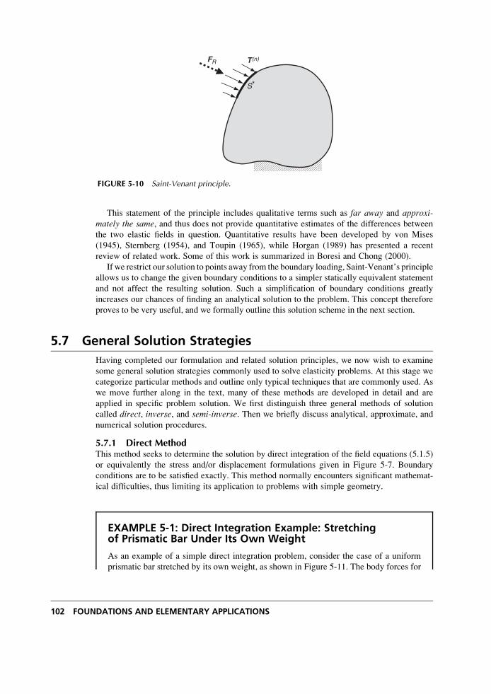
This statement of the principle includes qualitative terms such as far away and approxi-mately the same, and thus does not provide quantitative estimates of the differences between
the two elastic fields in question. Quantitative results have been developed by von Mises
(1945), Sternberg (1954), and Toupin (1965), while Horgan (1989) has presented a recent
review of related work. Some of this work is summarized in Boresi and Chong (2000).
If we restrict our solution to points away from the boundary loading, Saint-Venant’s principle
allows us to change the given boundary conditions to a simpler statically equivalent statement
and not affect the resulting solution. Such a simplification of boundary conditions greatly
increases our chances of finding an analytical solution to the problem. This concept therefore
proves to be very useful, and we formally outline this solution scheme in the next section.
5.7 General Solution Strategies
Having completed our formulation and related solution principles, we now wish to examine
some general solution strategies commonly used to solve elasticity problems. At this stage we
categorize particular methods and outline only typical techniques that are commonly used. As
we move further along in the text, many of these methods are developed in detail and are
applied in specific problem solution. We first distinguish three general methods of solution
called direct, inverse, and semi-inverse. Then we briefly discuss analytical, approximate, and
numerical solution procedures.
5.7.1 Direct MethodThis method seeks to determine the solution by direct integration of the field equations (5.1.5)
or equivalently the stress and/or displacement formulations given in Figure 5-7. Boundary
conditions are to be satisfied exactly. This method normally encounters significant mathemat-
ical difficulties, thus limiting its application to problems with simple geometry.
EXAMPLE 5-1: Direct Integration Example: Stretchingof Prismatic Bar Under Its Own Weight
As an example of a simple direct integration problem, consider the case of a uniform
prismatic bar stretched by its own weight, as shown in Figure 5-11. The body forces for
S*
T(n)FR
FIGURE 5-10 Saint-Venant principle.
102 FOUNDATIONS AND ELEMENTARY APPLICATIONS
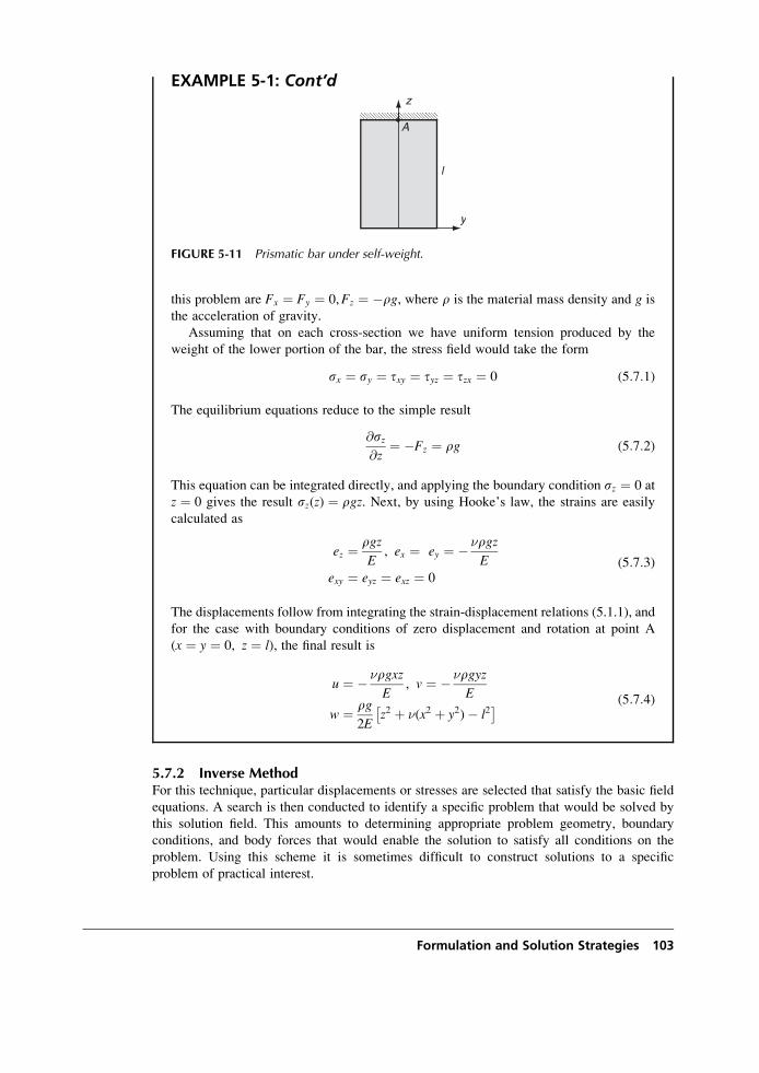
EXAMPLE 5-1: Cont’dz
A
l
y
FIGURE 5-11 Prismatic bar under self-weight.
this problem are Fx ¼ Fy ¼ 0,Fz ¼ �rg, where r is the material mass density and g is
the acceleration of gravity.
Assuming that on each cross-section we have uniform tension produced by the
weight of the lower portion of the bar, the stress field would take the form
sx ¼ sy ¼ txy ¼ tyz ¼ tzx ¼ 0 (5:7:1)
The equilibrium equations reduce to the simple result
@sz@z
¼ �Fz ¼ rg (5:7:2)
This equation can be integrated directly, and applying the boundary condition sz ¼ 0 at
z ¼ 0 gives the result sz(z) ¼ rgz. Next, by using Hooke’s law, the strains are easily
calculated as
ez ¼ rgzE
, ex ¼ ey ¼ � �rgzE
exy ¼ eyz ¼ exz ¼ 0(5:7:3)
The displacements follow from integrating the strain-displacement relations (5.1.1), and
for the case with boundary conditions of zero displacement and rotation at point A
(x ¼ y ¼ 0, z ¼ l), the final result is
u ¼ � �rgxzE
, v ¼ � �rgyzE
w ¼ rg2E
z2 þ �(x2 þ y2)� l2� � (5:7:4)
5.7.2 Inverse MethodFor this technique, particular displacements or stresses are selected that satisfy the basic field
equations. A search is then conducted to identify a specific problem that would be solved by
this solution field. This amounts to determining appropriate problem geometry, boundary
conditions, and body forces that would enable the solution to satisfy all conditions on the
problem. Using this scheme it is sometimes difficult to construct solutions to a specific
problem of practical interest.
Formulation and Solution Strategies 103
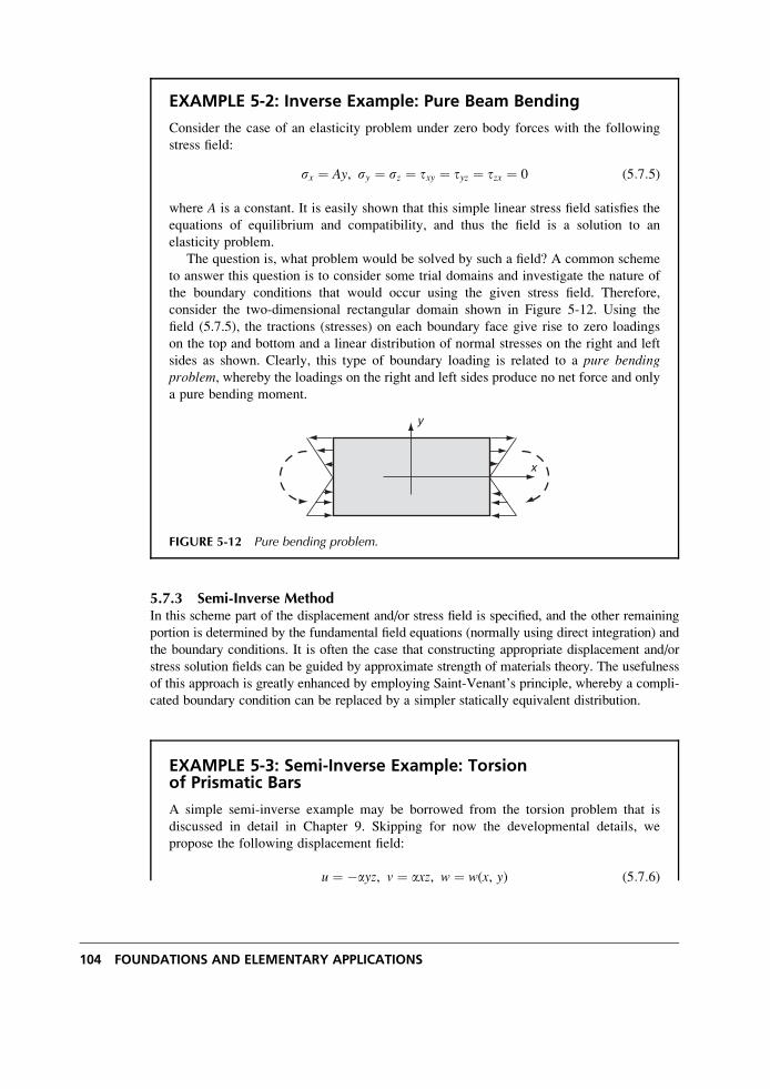
EXAMPLE 5-2: Inverse Example: Pure Beam Bending
Consider the case of an elasticity problem under zero body forces with the following
stress field:
sx ¼ Ay, sy ¼ sz ¼ txy ¼ tyz ¼ tzx ¼ 0 (5:7:5)
where A is a constant. It is easily shown that this simple linear stress field satisfies the
equations of equilibrium and compatibility, and thus the field is a solution to an
elasticity problem.
The question is, what problem would be solved by such a field? A common scheme
to answer this question is to consider some trial domains and investigate the nature of
the boundary conditions that would occur using the given stress field. Therefore,
consider the two-dimensional rectangular domain shown in Figure 5-12. Using the
field (5.7.5), the tractions (stresses) on each boundary face give rise to zero loadings
on the top and bottom and a linear distribution of normal stresses on the right and left
sides as shown. Clearly, this type of boundary loading is related to a pure bendingproblem, whereby the loadings on the right and left sides produce no net force and only
a pure bending moment.
x
y
FIGURE 5-12 Pure bending problem.
5.7.3 Semi-Inverse MethodIn this scheme part of the displacement and/or stress field is specified, and the other remaining
portion is determined by the fundamental field equations (normally using direct integration) and
the boundary conditions. It is often the case that constructing appropriate displacement and/or
stress solution fields can be guided by approximate strength of materials theory. The usefulness
of this approach is greatly enhanced by employing Saint-Venant’s principle, whereby a compli-
cated boundary condition can be replaced by a simpler statically equivalent distribution.
EXAMPLE 5-3: Semi-Inverse Example: Torsionof Prismatic Bars
A simple semi-inverse example may be borrowed from the torsion problem that is
discussed in detail in Chapter 9. Skipping for now the developmental details, we
propose the following displacement field:
u ¼ �ayz, v ¼ axz, w ¼ w(x, y) (5:7:6)
104 FOUNDATIONS AND ELEMENTARY APPLICATIONS
EXAMPLE 5-3: Cont’d
where a is a constant. The assumed field specifies the x and y components of displace-
ment, while the z component is left to be determined as a function of the indicated
spatial variables. By using the strain-displacement relations and Hooke’s law, the stress
field corresponding to (5.7.6) is given by
sx ¼ sy ¼ sz ¼ txy ¼ 0
txz ¼ m@w
@x� ay
� �
tyz ¼ m@w
@yþ ax
� � (5:7:7)
Using these stresses in the equations of equilibrium gives the following result:
@2w
@x2þ @2w
@y2¼ 0 (5:7:8)
which is actually the form of Navier’s equations for this case. This result represents a
single equation (Laplace’s equation) to determine the unknown part of the assumed
solution form. It should be apparent that by assuming part of the solution field, the
remaining equations to be solved are greatly simplified. A specific domain in the x, yplane along with appropriate boundary conditions is needed to complete the solution to
a particular problem. Once this has been accomplished, the assumed solution form
(5.7.6) has been shown to satisfy all the field equations of elasticity.
There are numerous mathematical techniques used to solve the elasticity field equations.
Many techniques involve the development of exact analytical solutions, while others involve theconstruction of approximate solution schemes. A third procedure involves the establishment of
numerical solution methods. We now briefly provide an overview of each of these techniques.
5.7.4 Analytical Solution ProceduresA variety of analytical solution methods are used to solve the elasticity field equations. The
following sections outline some of the more common methods.
Power Series MethodFor many two-dimensional elasticity problems, the stress formulation leads to the use of a
stress function f(x, y). It is shown that the entire set of field equations reduces to a single
partial differential equation (biharmonic equation) in terms of this stress function. A general
mathematical scheme to solve this equation is to look for solutions in terms of a power series in
the independent variables, that is, f(x, y) ¼PCmnxmyn (see Neou 1957). Use of the boundary
conditions determines the coefficients and number of terms to be used in the series. This
method is employed to develop two-dimensional solutions in Section 8.1.
Fourier MethodA general scheme to solve a large variety of elasticity problems employs the Fourier method.
This procedure is normally applied to the governing partial differential equations by using
Formulation and Solution Strategies 105
separation of variables, superposition, and Fourier series or Fourier integral theory. Althoughthis is an ad hoc method, it has been shown to provide solutions to a large class of problems
(see, for example, Pickett 1944 and Little 1973). We make use of this scheme for two-
dimensional problem solution in Chapter 8, for a torsion problem in Chapter 9, and for several
three-dimensional solutions in Chapter 13.
Integral Transform MethodA very useful mathematical technique to solve partial differential equations is the use of
integral transforms. By applying a particular linear integral transformation to the governing
equations, certain differential forms can be simplified or eliminated, thus allowing simple
solution for the unknown transformed variables. Through appropriate inverse transformation,
the original unknowns are retrieved, giving the required solution. Typical transforms that have
been successfully applied to elasticity problems include Laplace, Fourier, and Hankel trans-forms. We do not make specific use of this technique in the text, but example applications can
be found in Sneddon (1978) and Sneddon and Lowengrub (1969).
Complex Variable MethodSeveral classes of problems in elasticity can be formulated in terms of functions of a complex
variable. These include two-dimensional plane problems, the torsion problem, and some
particular thermoelastic cases. The complex variable formulation is very powerful and useful
because many solutions can be found that would be intractable by other techniques. Most of
the original development of this method was done by a series of Russian elasticians and is
summarized in the classic work of Muskhelishvili (1963). Chapter 10 formally develops this
technique and employs the method to construct several solutions for plane isotropic elasticity
problems. We also use the method in Chapter 11 to determine solutions of plane anisotropic
problems and in Chapter 12 for some thermoelastic applications.
5.7.5 Approximate Solution ProceduresWith the recognized difficulty in finding exact analytical solutions, considerable work has been
done to develop approximate solutions to elasticity problems. Much of this work has been in
the area of variational methods, which are related to energy theorems (see Chapter 6). The
principal idea of this approach is the connection of the elasticity field equations with a
variational problem of finding an extremum of a particular integral functional. One specific
technique is outlined in the following section.
Ritz MethodThis scheme employs a set of approximating functions to solve elasticity problems by deter-
mining stationary values of a particular energy integral. The set of approximating functions is
chosen to satisfy the boundary conditions on the problem, but only approximately make the
energy integral take on an extremum. By including more terms in the approximating solution
set, accuracy of the scheme is improved. Specific examples of this and related methods can be
found in Reismann and Pawlik (1980), Reddy (1984), and Mura and Koya (1992). Because of
the difficulty in finding proper approximating functions for problems of complex geometry,
variational techniques have made only limited contributions to the solution of general problems.
However, they have made very important applications in the finite element method.
5.7.6 Numerical Solution ProceduresOver the past several decades numerical methods have played a primary role in developing
solutions to elasticity problems of complex geometry. Various schemes have been theoretically
106 FOUNDATIONS AND ELEMENTARY APPLICATIONS
developed, andnumerous private and commercial codes have beenwritten for implementation on
avarietyof computer platforms.Several of themore importantmethods are brieflydiscussedhere.
Finite Difference MethodThe finite difference method (FDM) replaces derivatives in the governing field equations by
difference quotients, which involve values of the solution at discrete mesh points in the domain
under study. Repeated applications of this representation set up algebraic systems of equations
in terms of unknown mesh point values. The method is a classical one, having been established
almost a century ago, and Timoshenko and Goodier (1970) provide some details on its
applications in elasticity. The major difficulty with this scheme lies in the inaccuracies in
dealing with regions of complex shape, although this problem can be eliminated through the
use of coordinate transformation techniques.
Finite Element MethodThe fundamental concept of the finite element method (FEM) lies in dividing the body under
study into a finite number of pieces (subdomains) called elements. Particular assumptions are
then made on the variation of the unknown dependent variable(s) across each element using so-
called interpolation or shape functions. This approximated variation is quantified in terms of
solution values at special locations within the element called nodes. Through this discretizationprocess, the method sets up an algebraic system of equations for unknown nodal values that
approximates the continuous solution. Because element size and shape are variable, the finite
element method can handle problem domains of complicated shape, and thus it has become a
very useful and practical tool (see Reddy 2006). We briefly present an introduction to finite
element methods in Chapter 16.
Boundary Element MethodThe boundary element method (BEM) is based upon an integral statement of the governing
equations of elasticity. The integral statement may be cast into a form that contains unknowns
only over the boundary of the body domain. This boundary integral equation may then be
solved by using concepts from the finite element method; that is, the boundary may be
discretized into a number of elements and the interpolation approximation concept can then
be applied. This method again produces an algebraic system of equations to solve for the
unknown boundary nodal values, and the system is generally much smaller than that generated
by internal discretization such as the finite element method. By avoiding interior discretization,
the boundary element method has significant advantages over finite element schemes for
infinite or very large domains and for cases in which only boundary information is sought
(see Brebbia and Dominguez 1992). A brief discussion of this technique is given in Chapter 16.
Elasticity is a mature field and thus analytical solutions have been developed for a large
number of problems. Kachanov, Shafiro, and Tsukrov (2003) have published an interesting
compilation handbook of elasticity solutions collected from textbooks and journal articles.
References
Boresi AP, and Chong KP: Elasticity in Engineering Mechanics, Wiley, New York, 2000.
Brebbia CA, and Dominguez J: Boundary Elements: An Introductory Course, 2nd ed, Computational
Mechanics Publications, Boston, 1992.
Chou PC, and Pagano NJ: Elasticity Tensor, Dyadic and Engineering Approaches, D. Van Nostrand,
Princeton, NJ, 1967.
Formulation and Solution Strategies 107
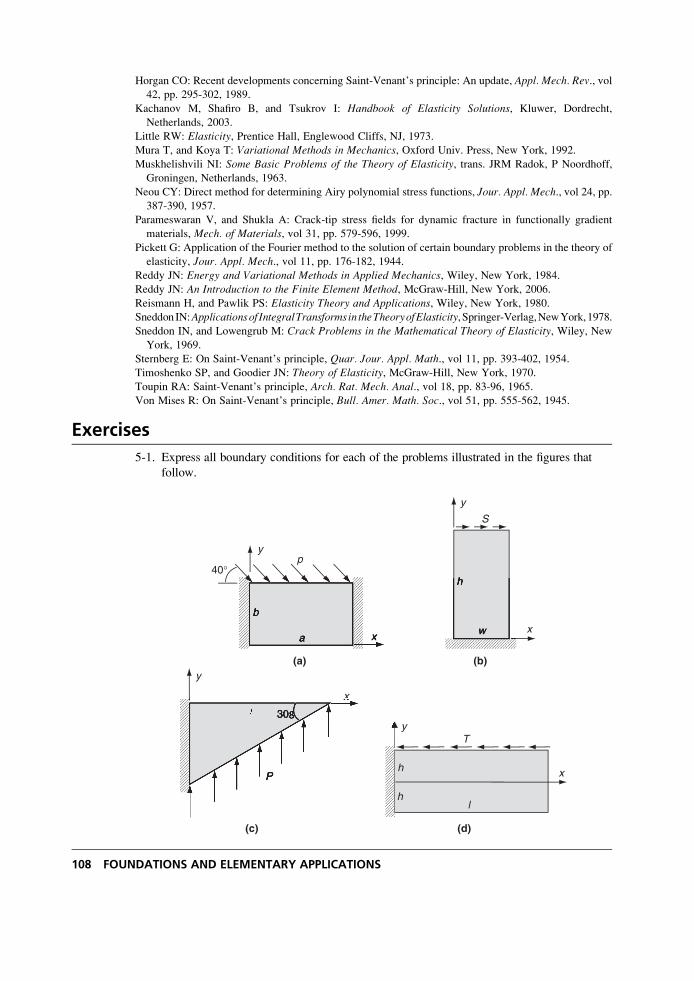
Horgan CO: Recent developments concerning Saint-Venant’s principle: An update, Appl. Mech. Rev., vol42, pp. 295-302, 1989.
Kachanov M, Shafiro B, and Tsukrov I: Handbook of Elasticity Solutions, Kluwer, Dordrecht,
Netherlands, 2003.
Little RW: Elasticity, Prentice Hall, Englewood Cliffs, NJ, 1973.
Mura T, and Koya T: Variational Methods in Mechanics, Oxford Univ. Press, New York, 1992.
Muskhelishvili NI: Some Basic Problems of the Theory of Elasticity, trans. JRM Radok, P Noordhoff,
Groningen, Netherlands, 1963.
Neou CY: Direct method for determining Airy polynomial stress functions, Jour. Appl. Mech., vol 24, pp.387-390, 1957.
Parameswaran V, and Shukla A: Crack-tip stress fields for dynamic fracture in functionally gradient
materials, Mech. of Materials, vol 31, pp. 579-596, 1999.Pickett G: Application of the Fourier method to the solution of certain boundary problems in the theory of
elasticity, Jour. Appl. Mech., vol 11, pp. 176-182, 1944.Reddy JN: Energy and Variational Methods in Applied Mechanics, Wiley, New York, 1984.
Reddy JN: An Introduction to the Finite Element Method, McGraw-Hill, New York, 2006.
Reismann H, and Pawlik PS: Elasticity Theory and Applications, Wiley, New York, 1980.
Sneddon IN:Applicationsof IntegralTransforms in theTheoryofElasticity, Springer-Verlag,NewYork,1978.
Sneddon IN, and Lowengrub M: Crack Problems in the Mathematical Theory of Elasticity, Wiley, New
York, 1969.
Sternberg E: On Saint-Venant’s principle, Quar. Jour. Appl. Math., vol 11, pp. 393-402, 1954.Timoshenko SP, and Goodier JN: Theory of Elasticity, McGraw-Hill, New York, 1970.
Toupin RA: Saint-Venant’s principle, Arch. Rat. Mech. Anal., vol 18, pp. 83-96, 1965.Von Mises R: On Saint-Venant’s principle, Bull. Amer. Math. Soc., vol 51, pp. 555-562, 1945.
Exercises
5-1. Express all boundary conditions for each of the problems illustrated in the figures that
follow.
(a) (b)
p40°
x
y
a
b
x
y
S
w
h
(c)
x
y
P
308l
x
yT
l
h
h
(d)
108 FOUNDATIONS AND ELEMENTARY APPLICATIONS
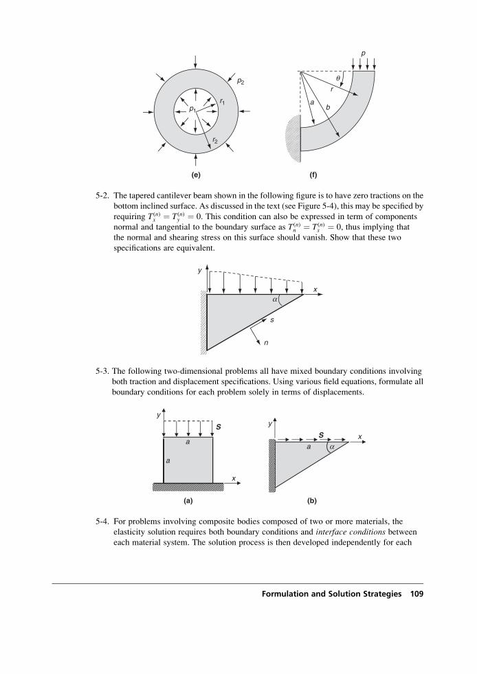
p
ab
r
(f)
r1
r2
p1
p2
(e)
q
5-2. The tapered cantilever beam shown in the following figure is to have zero tractions on the
bottom inclined surface. As discussed in the text (see Figure 5-4), this may be specified by
requiring T(n)x ¼ T(n)
y ¼ 0. This condition can also be expressed in term of components
normal and tangential to the boundary surface as T(n)n ¼ T(n)
s ¼ 0, thus implying that
the normal and shearing stress on this surface should vanish. Show that these two
specifications are equivalent.
x
y
n
s
a
5-3. The following two-dimensional problems all have mixed boundary conditions involving
both traction and displacement specifications. Using various field equations, formulate all
boundary conditions for each problem solely in terms of displacements.
(b)
x
y
aS
a
(a)
S
a
a
x
y
5-4. For problems involving composite bodies composed of two or more materials, the
elasticity solution requires both boundary conditions and interface conditions betweeneach material system. The solution process is then developed independently for each
Formulation and Solution Strategies 109
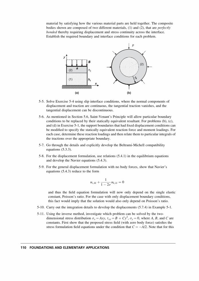
material by satisfying how the various material parts are held together. The composite
bodies shown are composed of two different materials, (1) and (2), that are perfectlybonded thereby requiring displacement and stress continuity across the interface.
Establish the required boundary and interface conditions for each problem.
r1
r2
(1)
p
(2)
(b)
S
(a)
a
h1
x
y
h2
(1)
(2)
5-5. Solve Exercise 5-4 using slip interface conditions, where the normal components of
displacement and traction are continuous, the tangential traction vanishes, and the
tangential displacement can be discontinuous.
5-6. As mentioned in Section 5.6, Saint-Venant’s Principle will allow particular boundary
conditions to be replaced by their statically equivalent resultant. For problems (b), (c),
and (d) in Exercise 5-1, the support boundaries that had fixed displacement conditions can
be modified to specify the statically equivalent reaction force and moment loadings. For
each case, determine these reaction loadings and then relate them to particular integrals of
the tractions over the appropriate boundary.
5-7. Go through the details and explicitly develop the Beltrami-Michell compatibility
equations (5.3.3).
5-8. For the displacement formulation, use relations (5.4.1) in the equilibrium equations
and develop the Navier equations (5.4.3).
5-9. For the general displacement formulation with no body forces, show that Navier’s
equations (5.4.3) reduce to the form
ui, kk þ 1
1� 2�uk, ki ¼ 0
and thus the field equation formulation will now only depend on the single elastic
constant, Poisson’s ratio. For the case with only displacement boundary conditions,
this fact would imply that the solution would also only depend on Poisson’s ratio.
5-10. Carry out the integration details to develop the displacements (5.7.4) in Example 5-1.
5-11. Using the inverse method, investigate which problem can be solved by the two-
dimensional stress distribution �x¼ Axy, txy¼ B þ Cy2, �y¼ 0, where A, B, and C are
constants. First show that the proposed stress field (with zero body force) satisfies the
stress formulation field equations under the condition that C¼�A/2. Note that for this
110 FOUNDATIONS AND ELEMENTARY APPLICATIONS
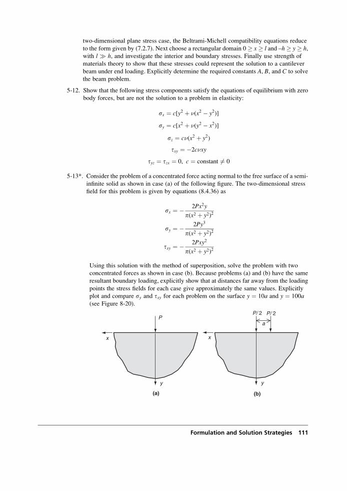
two-dimensional plane stress case, the Beltrami-Michell compatibility equations reduce
to the form given by (7.2.7). Next choose a rectangular domain 0 � x � l and –h � y � h,with l � h, and investigate the interior and boundary stresses. Finally use strength of
materials theory to show that these stresses could represent the solution to a cantilever
beam under end loading. Explicitly determine the required constants A, B, and C to solve
the beam problem.
5-12. Show that the following stress components satisfy the equations of equilibrium with zero
body forces, but are not the solution to a problem in elasticity:
sx ¼ c[y2 þ �(x2 � y2)]
sy ¼ c[x2 þ �(y2 � x2)]
sz ¼ c�(x2 þ y2)
txy ¼ �2c�xy
tyz ¼ tzx ¼ 0, c ¼ constant 6¼ 0
5-13*. Consider the problem of a concentrated force acting normal to the free surface of a semi-
infinite solid as shown in case (a) of the following figure. The two-dimensional stress
field for this problem is given by equations (8.4.36) as
sx ¼ � 2Px2y
p(x2 þ y2)2
sy ¼ � 2Py3
p(x2 þ y2)2
txy ¼ � 2Pxy2
p(x2 þ y2)2
Using this solution with the method of superposition, solve the problem with two
concentrated forces as shown in case (b). Because problems (a) and (b) have the same
resultant boundary loading, explicitly show that at distances far away from the loading
points the stress fields for each case give approximately the same values. Explicitly
plot and compare sy and txy for each problem on the surface y ¼ 10a and y ¼ 100a(see Figure 8-20).
x
y
P
(a)
x
y
P/ 2 P/ 2
a
(b)
Formulation and Solution Strategies 111
6 Strain Energy and Related Principles
Before proceeding to the solution of specific elasticity problems, we wish to explore the
associated concepts of work and energy. Boundary tractions and body forces will do work
on an elastic solid, and this work will be stored inside the material in the form of strain
energy. For the elastic case, removal of these loadings results in complete recovery of the
stored energy within the body. Development of strain energy concepts can yield new and
useful information not found by other methods. This study also leads to some new energy
methods or principles that provide additional techniques to solve elasticity problems. In
some sense these methods may be thought of as replacements of particular field equations
that have been previously derived. For problems in structural mechanics involving rods,
beams, plates, and shells, energy methods have proved to be very useful in developing the
governing equations and associated boundary conditions. These schemes have also provided a
method to generate approximate solutions to elasticity problems. More recently, particular
energy and variational techniques have been used extensively in the development of finite and
boundary element analysis. Our presentation here will only be a brief study on this extensive
subject, and the interested reader is recommended to review Langhaar (1962), Washizu (1968),
Reddy (1984), Mura and Koya (1992), or Fung and Tong (2001) for additional details and
applications.
6.1 Strain Energy
As mentioned, the work done by surface and body forces on an elastic solid are stored inside
the body in the form of strain energy. For an idealized elastic body, this stored energy is
completely recoverable when the solid is returned to its original unstrained configuration. In
order to quantify this behavior, we now wish to determine the strain energy in terms of the
resulting stress and strain fields within the elastic solid. Consider first the simple uniform
uniaxial deformation case with no body forces, as shown in Figure 6-1. The cubical element of
dimensions dx, dy, dz is under the action of a uniform normal stress s in the x direction as
shown.
During this deformation process, we assume that the stress increases slowly from zero to sx,such that inertia effects can be neglected. The strain energy stored is equal to the net work done
on the element, and this is given by the following equation.
113
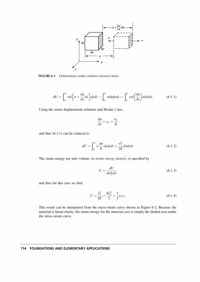
dU ¼ðsx0
sd uþ @u
@xdx
� �dydz�
ðsx0
sdudydz ¼ðsx0
sd@u
@x
� �dxdydz (6:1:1)
Using the strain displacement relations and Hooke’s law,
@u
@x¼ ex ¼ sx
E
and thus (6.1.1) can be reduced to
dU ¼ðsx0
sdsE
dxdydz ¼ s2x2E
dxdydz (6:1:2)
The strain energy per unit volume, or strain energy density, is specified by
U ¼ dU
dxdydz(6:1:3)
and thus for this case we find
U ¼ s2x2E
¼ Ee2x2
¼ 1
2sxex (6:1:4)
This result can be interpreted from the stress-strain curve shown in Figure 6-2. Because the
material is linear elastic, the strain energy for the uniaxial case is simply the shaded area under
the stress-strain curve.
dxu
dz
dx
ss
u +
dy
x
y
z
∂x∂u
FIGURE 6-1 Deformation under uniform uniaxial stress.
114 FOUNDATIONS AND ELEMENTARY APPLICATIONS
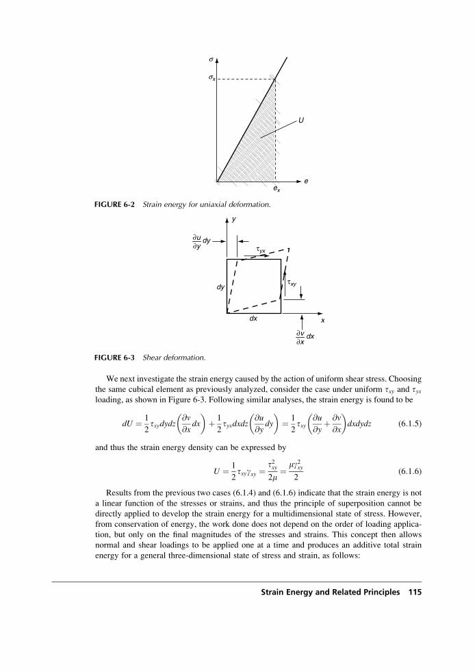
We next investigate the strain energy caused by the action of uniform shear stress. Choosing
the same cubical element as previously analyzed, consider the case under uniform txy and tyxloading, as shown in Figure 6-3. Following similar analyses, the strain energy is found to be
dU ¼ 1
2txydydz
@v
@xdx
� �þ 1
2tyxdxdz
@u
@ydy
� �¼ 1
2txy
@u
@yþ @v
@x
� �dxdydz (6:1:5)
and thus the strain energy density can be expressed by
U ¼ 1
2txygxy ¼
t2xy2m
¼ mg2xy2
(6:1:6)
Results from the previous two cases (6.1.4) and (6.1.6) indicate that the strain energy is not
a linear function of the stresses or strains, and thus the principle of superposition cannot be
directly applied to develop the strain energy for a multidimensional state of stress. However,
from conservation of energy, the work done does not depend on the order of loading applica-
tion, but only on the final magnitudes of the stresses and strains. This concept then allows
normal and shear loadings to be applied one at a time and produces an additive total strain
energy for a general three-dimensional state of stress and strain, as follows:
eex
U
s
sx
FIGURE 6-2 Strain energy for uniaxial deformation.
dx
dy
x
y
τyx
τxy
∂u∂y
dx∂v∂x
dy
FIGURE 6-3 Shear deformation.
Strain Energy and Related Principles 115
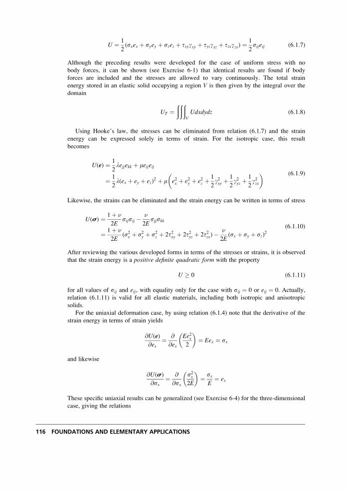
U ¼ 1
2(sxex þ syey þ szez þ txygxy þ tyzgyz þ tzxgzx) ¼
1
2sijeij (6:1:7)
Although the preceding results were developed for the case of uniform stress with no
body forces, it can be shown (see Exercise 6-1) that identical results are found if body
forces are included and the stresses are allowed to vary continuously. The total strain
energy stored in an elastic solid occupying a region V is then given by the integral over the
domain
UT ¼ððð
V
Udxdydz (6:1:8)
Using Hooke’s law, the stresses can be eliminated from relation (6.1.7) and the strain
energy can be expressed solely in terms of strain. For the isotropic case, this result
becomes
U(e) ¼ 1
2lejjekk þ meijeij
¼ 1
2l(ex þ ey þ ez)
2 þ m e2x þ e2y þ e2z þ1
2g2xy þ
1
2g2yz þ
1
2g2zx
� � (6:1:9)
Likewise, the strains can be eliminated and the strain energy can be written in terms of stress
U(s) ¼ 1þ �
2Esijsij � �
2Esjjskk
¼ 1þ �
2E(s2x þ s2y þ s2z þ 2t2xy þ 2t2yz þ 2t2zx)�
�
2E(sx þ sy þ sz)2
(6:1:10)
After reviewing the various developed forms in terms of the stresses or strains, it is observed
that the strain energy is a positive definite quadratic form with the property
U � 0 (6:1:11)
for all values of sij and eij, with equality only for the case with sij ¼ 0 or eij ¼ 0. Actually,
relation (6.1.11) is valid for all elastic materials, including both isotropic and anisotropic
solids.
For the uniaxial deformation case, by using relation (6.1.4) note that the derivative of the
strain energy in terms of strain yields
@U(e)
@ex¼ @
@ex
Ee2x2
� �¼ Eex ¼ sx
and likewise
@U(s)
@sx¼ @
@sx
s2x2E
� �¼ sx
E¼ ex
These specific uniaxial results can be generalized (see Exercise 6-4) for the three-dimensional
case, giving the relations
116 FOUNDATIONS AND ELEMENTARY APPLICATIONS
sij ¼ @U(e)
@eij, eij ¼ @U(s)
@sij(6:1:12)
These results are again true for all elastic materials (isotropic and anisotropic); see Langhaar
(1962) or Boresi and Chong (2000) for a general derivation. Thus, the strain energy function can
be interpreted as playing a fundamental constitutive role in establishing general stress-strain
relations for elastic materials. Such an approach in which the stresses are derivable from a strain
energy function, that is, relation (6.1.12), is referred to as hyperelasticity. Note that this approachdoes not necessarily require that the relations between stress and strain be linear, and thus this
scheme is commonly used in the development of constitutive relations for nonlinear elastic
solids. Only linear relations given by Hooke’s law (4.2.1) are incorporated in the text.
Using equations (6.1.12), the following symmetry relations can be developed (Exercise 6-5)
@sij@ekl
¼ @skl@eij
@eij@skl
¼ @ekl@sij
(6:1:13)
Going back to the general constitutive form sij ¼ Cijklekl, relations (6.1.13) can be used to
develop the additional symmetry relations
Cijkl ¼ Cklij (6:1:14)
Using constitutive form (4.2.2), result (6.1.14) implies that Cij ¼ Cji, and thus there are only 21
independent elastic constants for general anisotropic elastic materials.
The strain energy in an elastic solid may be decomposed into two parts, one associated
with volumetric changeUv and the other caused by distortional (change in shape) deformationUd.
U ¼ Uv þ Ud (6:1:15)
The development of this decomposition is accomplished by using the definitions of spherical
and deviatoric strain and stress tensors presented previously in Sections 2.5 and 3.5. For
isotropic materials, the spherical stress produces only volumetric deformation, while the
deviatoric stress causes only distortional changes. The volumetric strain energy is found by
considering the spherical or hydrostatic components of stress and strain
Uv ¼ 1
2~ssij~eeij ¼ 1
6sjjekk ¼ 1� 2�
6Esjjskk ¼ 1� 2�
6E(sx þ sy þ sz)2 (6:1:16)
The distortional strain energy results from the deviatoric components or can be easily deter-
mined using relations (6.1.10), (6.1.15), and (6.1.16) to get
Ud ¼ 1
12m[(sx � sy)2 þ (sy � sz)2 þ (sz � sx)2 þ 6(t2xy þ t2yz þ t2zx)] (6:1:17)
Particular failure theories of solids incorporate the strain energy of distortion by proposing that
material failure or yielding will initiate when Ud reaches a critical value. It can be shown that
the distortional strain energy is related to the octahedral shear stress previously discussed in
Section 3.5 (see Exercise 6-8).
Strain Energy and Related Principles 117
6.2 Uniqueness of the Elasticity Boundary-Value Problem
Although it would seem that the question of uniqueness of the elasticity boundary-value
problem should have been covered in Chapter 5, the proof normally makes use of strain
energy concepts and is therefore presented here. Consider the general mixed boundary-value
problem in which tractions are specified over the boundary St and displacements are prescribed
over the remaining part Su. Assume that there exist two different solutions {s(1)ij , e(1)ij , u
(1)i } and
{s(2)ij , e(2)ij , u
(2)i } to the same problem with identical body forces and boundary conditions. Next
define the difference solution
sij ¼ s(1)ij � s(2)ij
eij ¼ e(1)ij � e(2)ij
ui ¼ u(1)i � u(2)i
(6:2:1)
Because the solutions s(1)ij and s(2)ij have the same body force, the difference solution must
satisfy the equilibrium equation
sij, j ¼ 0 (6:2:2)
Likewise, the boundary conditions satisfied by the difference solution are given by
Tni ¼ sijnj ¼ 0 on St
ui ¼ 0 on Su(6:2:3)
Starting with the definition of strain energy, we may write
2
ðV
UdV ¼ðV
sijeijdV ¼ðV
sij(ui, j � !ij)dV
¼ðV
sijui, jdV ¼ðV
(sijui), jdV �ðV
sij, juidV
¼ðS
sijnjuidS�ðV
sij, juidV
(6:2:4)
where we have used the fact that sij!ij ¼ 0 (symmetric times antisymmetric ¼ 0) and have
utilized the divergence theorem to convert the volume integral into a surface integral. Incorp-
orating relations (6.2.2) and (6.2.3) and noting that the total surface S ¼ St þ Su, (6.2.4) givesthe result
2
ðV
UdV ¼ 0 (6:2:5)
Relation (6.2.5) implies that U must vanish in the region V, and since the strain energy is a
positive definite quadratic form, the associated strains and stresses also vanish; that is,
eij ¼ sij ¼ 0. If the strain field vanishes, then the corresponding displacements ui can be at
most rigid-body motion. However, if ui ¼ 0 on Su, then the displacement field must vanish
everywhere. Thus, we have shown that s(1)ij ¼ s(2)ij , e(1)ij ¼ e(2)ij , u
(1)i ¼ u(2)i and therefore the
118 FOUNDATIONS AND ELEMENTARY APPLICATIONS
problem solution is unique. Note that if tractions are prescribed over the entire boundary, then
u(1)i and u(2)i may differ by rigid-body motion.
6.3 Bounds on the Elastic Constants
Strain energy concepts allow us to generate particular bounds on elastic constants. For
the isotropic case, consider the following three stress states previously investigated in
Section 4.3 (see Figure 4-2).
6.3.1 Uniaxial TensionUniform uniaxial deformation in the x direction is given by the stress state
sij ¼s 0 0
0 0 0
0 0 0
24
35 (6:3:1)
For this case, the strain energy reduces to
U ¼ 1þ �
2Es2 � �
2Es2 ¼ s2
2E(6:3:2)
Because the strain energy is positive definite, relation (6.3.2) implies that the modulus of
elasticity must be positive
E > 0 (6:3:3)
6.3.2 Simple ShearConsider next the case of uniform simple shear defined by the stress tensor
sij ¼0 t 0
t 0 0
0 0 0
24
35 (6:3:4)
The strain energy becomes
U ¼ 1þ �
2E(2t2) ¼ t2
E(1þ �) (6:3:5)
Again, invoking the positive definite property of the strain energy and using the previous result
of E > 0 gives
1þ � > 0 ) � > �1 (6:3:6)
6.3.3 Hydrostatic CompressionThe final example is chosen as uniform hydrostatic compression specified by
Strain Energy and Related Principles 119
sij ¼�p 0 0
0 �p 0
0 0 �p
24
35 (6:3:7)
Note that hydrostatic tension could also be used for this example. Evaluating the strain energy
yields
U ¼ 1þ �
2E3p2 � �
2E(� 3p)2 ¼ 3p2
2E(1� 2�) (6:3:8)
Using the positive definite property with E > 0 gives the result
1� 2� > 0 ) � <1
2(6:3:9)
Combining relations (6.3.6) and (6.3.9) places the following bounds on Poisson’s ratio:
�1 < � <1
2(6:3:10)
Using relations between the elastic constants given in Table 4-1, the previous results also
imply that
k > 0, m > 0 (6:3:11)
Experimental evidence indicates that most real materials have positive values of Poisson’s
ratio, and thus 0 < � < 1=2. This further implies that l > 0. Bounds on elastic moduli for the
anisotropic case are more involved and are discussed in Chapter 11.
6.4 Related Integral Theorems
Within the context of linear elasticity, several integral relations based on work and energy can
be developed. We now wish to investigate three particular results referred to as Clapeyron’stheorem, Betti’s reciprocal theorem, and Somigliana’s identity.
6.4.1 Clapeyron’s TheoremThe strain energy of an elastic solid in static equilibrium is equal to one-half the work done by
the external body forces Fi and surface tractions Tni
2
ðV
UdV ¼ðS
Tni uidSþ
ðV
FiuidV (6:4:1)
The proof of this theorem follows directly from results in relation (6.2.4).
6.4.2 Betti/Rayleigh Reciprocal TheoremIf an elastic body is subject to two body and surface force systems, then the work done by the
first system of forces {T(1), F(1)} acting through the displacements u(2) of the second system is
equal to the work done by the second system of forces {T(2), F(2)} acting through the
displacements u(1) of the first system; that is:
120 FOUNDATIONS AND ELEMENTARY APPLICATIONS
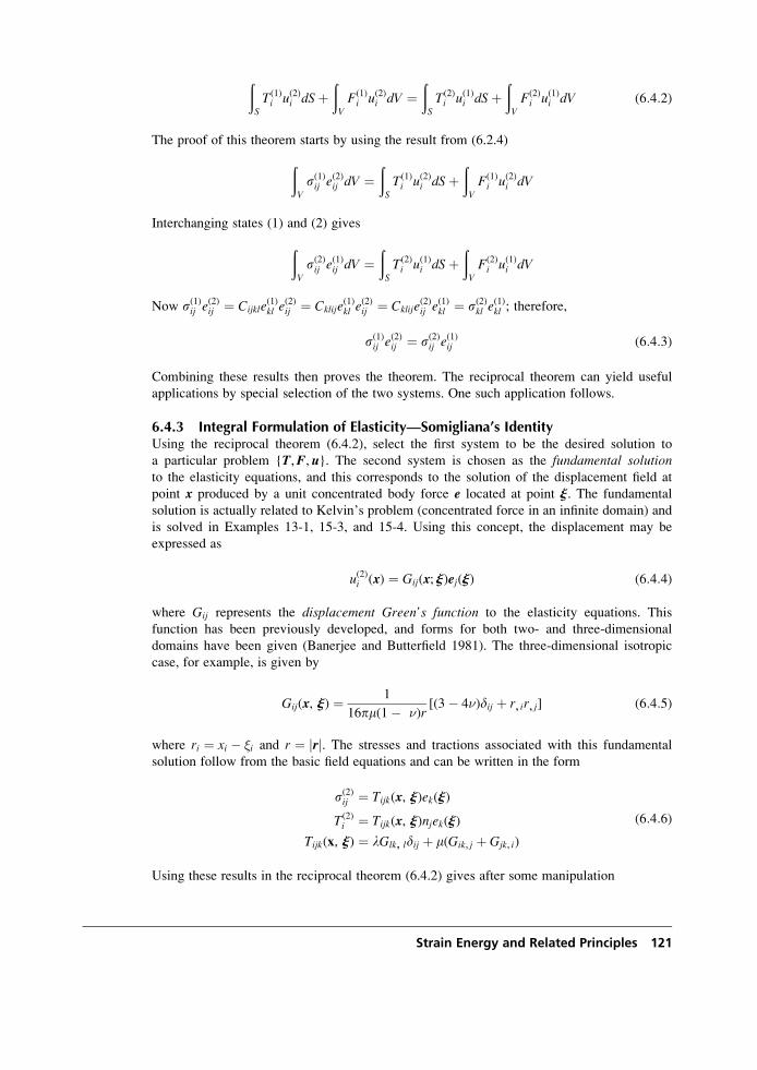
ðS
T(1)i u(2)i dSþ
ðV
F(1)i u(2)i dV ¼
ðS
T(2)i u(1)i dSþ
ðV
F(2)i u(1)i dV (6:4:2)
The proof of this theorem starts by using the result from (6.2.4)
ðV
s(1)ij e(2)ij dV ¼
ðS
T(1)i u(2)i dSþ
ðV
F(1)i u(2)i dV
Interchanging states (1) and (2) gives
ðV
s(2)ij e(1)ij dV ¼
ðS
T(2)i u(1)i dSþ
ðV
F(2)i u(1)i dV
Now s(1)ij e(2)ij ¼ Cijkle
(1)kl e
(2)ij ¼ Cklije
(1)kl e
(2)ij ¼ Cklije
(2)ij e
(1)kl ¼ s(2)kl e
(1)kl ; therefore,
s(1)ij e(2)ij ¼ s(2)ij e
(1)ij (6:4:3)
Combining these results then proves the theorem. The reciprocal theorem can yield useful
applications by special selection of the two systems. One such application follows.
6.4.3 Integral Formulation of Elasticity—Somigliana’s IdentityUsing the reciprocal theorem (6.4.2), select the first system to be the desired solution to
a particular problem {T,F, u}. The second system is chosen as the fundamental solutionto the elasticity equations, and this corresponds to the solution of the displacement field at
point x produced by a unit concentrated body force e located at point j. The fundamental
solution is actually related to Kelvin’s problem (concentrated force in an infinite domain) and
is solved in Examples 13-1, 15-3, and 15-4. Using this concept, the displacement may be
expressed as
u(2)i (x) ¼ Gij(x; j)ej(j) (6:4:4)
where Gij represents the displacement Green’s function to the elasticity equations. This
function has been previously developed, and forms for both two- and three-dimensional
domains have been given (Banerjee and Butterfield 1981). The three-dimensional isotropic
case, for example, is given by
Gij(x, j) ¼ 1
16pm(1� �)r[(3� 4�)dij þ r, ir, j] (6:4:5)
where ri ¼ xi � �i and r ¼ jrj. The stresses and tractions associated with this fundamental
solution follow from the basic field equations and can be written in the form
s(2)ij ¼ Tijk(x, j)ek(j)
T(2)i ¼ Tijk(x, j)njek(j)
Tijk(x, j) ¼ lGlk, ldij þ m(Gik, j þ Gjk, i)
(6:4:6)
Using these results in the reciprocal theorem (6.4.2) gives after some manipulation
Strain Energy and Related Principles 121
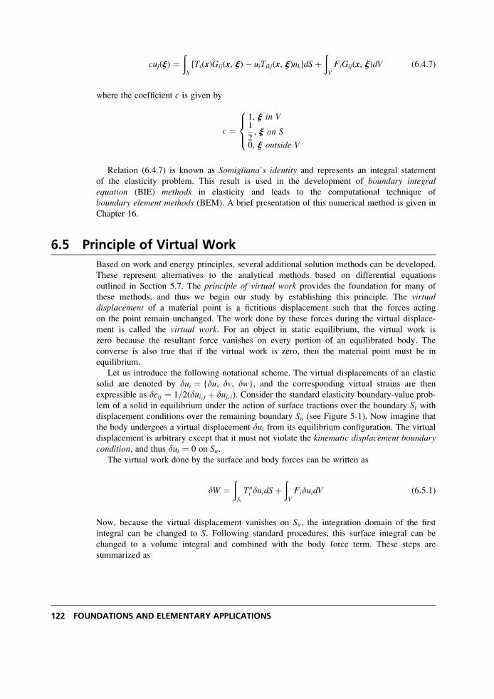
cuj(j) ¼ðS
[Ti(x)Gij(x, j)� uiTikj(x, j)nk]dSþðV
FiGij(x, j)dV (6:4:7)
where the coefficient c is given by
c ¼1, j in V1
2, j on S
0, j outside V
8><>:
Relation (6.4.7) is known as Somigliana’s identity and represents an integral statement
of the elasticity problem. This result is used in the development of boundary integralequation (BIE) methods in elasticity and leads to the computational technique of
boundary element methods (BEM). A brief presentation of this numerical method is given in
Chapter 16.
6.5 Principle of Virtual Work
Based on work and energy principles, several additional solution methods can be developed.
These represent alternatives to the analytical methods based on differential equations
outlined in Section 5.7. The principle of virtual work provides the foundation for many of
these methods, and thus we begin our study by establishing this principle. The virtualdisplacement of a material point is a fictitious displacement such that the forces acting
on the point remain unchanged. The work done by these forces during the virtual displace-
ment is called the virtual work. For an object in static equilibrium, the virtual work is
zero because the resultant force vanishes on every portion of an equilibrated body. The
converse is also true that if the virtual work is zero, then the material point must be in
equilibrium.
Let us introduce the following notational scheme. The virtual displacements of an elastic
solid are denoted by dui ¼ {du, dv, dw}, and the corresponding virtual strains are then
expressible as deij ¼ 1=2(dui, j þ duj, i). Consider the standard elasticity boundary-value prob-
lem of a solid in equilibrium under the action of surface tractions over the boundary St withdisplacement conditions over the remaining boundary Su (see Figure 5-1). Now imagine that
the body undergoes a virtual displacement dui from its equilibrium configuration. The virtual
displacement is arbitrary except that it must not violate the kinematic displacement boundarycondition, and thus dui ¼ 0 on Su.
The virtual work done by the surface and body forces can be written as
dW ¼ðSt
Tni duidSþ
ðV
FiduidV (6:5:1)
Now, because the virtual displacement vanishes on Su, the integration domain of the first
integral can be changed to S. Following standard procedures, this surface integral can be
changed to a volume integral and combined with the body force term. These steps are
summarized as
122 FOUNDATIONS AND ELEMENTARY APPLICATIONS
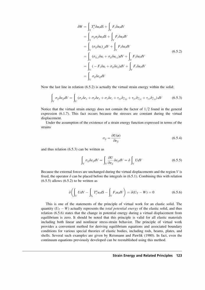
dW ¼ðS
Tni duidSþ
ðV
FiduidV
¼ðS
�ijnjduidSþðV
FiduidV
¼ðV
(�ijdui), jdV þðV
FiduidV
¼ðV
(�ij, jdui þ �ijdui, j)dV þðV
FiduidV
¼ðV
(� Fidui þ �ijdeij)dV þðV
FiduidV
¼ðV
�ijdeijdV
(6:5:2)
Now the last line in relation (6.5.2) is actually the virtual strain energy within the solid:
ðV
�ijdeijdV ¼ðV
(�xdex þ �ydey þ �zdez þ txydgxy þ tyzdgyz þ tzxdgzx) dV (6:5:3)
Notice that the virtual strain energy does not contain the factor of 1=2 found in the general
expression (6.1.7). This fact occurs because the stresses are constant during the virtual
displacement.
Under the assumption of the existence of a strain energy function expressed in terms of the
strains
�ij ¼ @U(e)
@eij(6:5:4)
and thus relation (6.5.3) can be written as
ðV
�ijdeijdV ¼ðV
@U
@eijdeijdV ¼ d
ðV
UdV (6:5:5)
Because the external forces are unchanged during the virtual displacements and the region V is
fixed, the operator d can be placed before the integrals in (6.5.1). Combining this with relation
(6.5.5) allows (6.5.2) to be written as
dðV
UdV �ðSt
Tni uidS�
ðV
FiuidV
� �¼ d(UT �W) ¼ 0 (6:5:6)
This is one of the statements of the principle of virtual work for an elastic solid. The
quantity (UT �W) actually represents the total potential energy of the elastic solid, and thus
relation (6.5.6) states that the change in potential energy during a virtual displacement from
equilibrium is zero. It should be noted that this principle is valid for all elastic materials
including both linear and nonlinear stress-strain behavior. The principle of virtual work
provides a convenient method for deriving equilibrium equations and associated boundary
conditions for various special theories of elastic bodies, including rods, beams, plates, and
shells. Several such examples are given by Reismann and Pawlik (1980). In fact, even the
continuum equations previously developed can be reestablished using this method.
Strain Energy and Related Principles 123
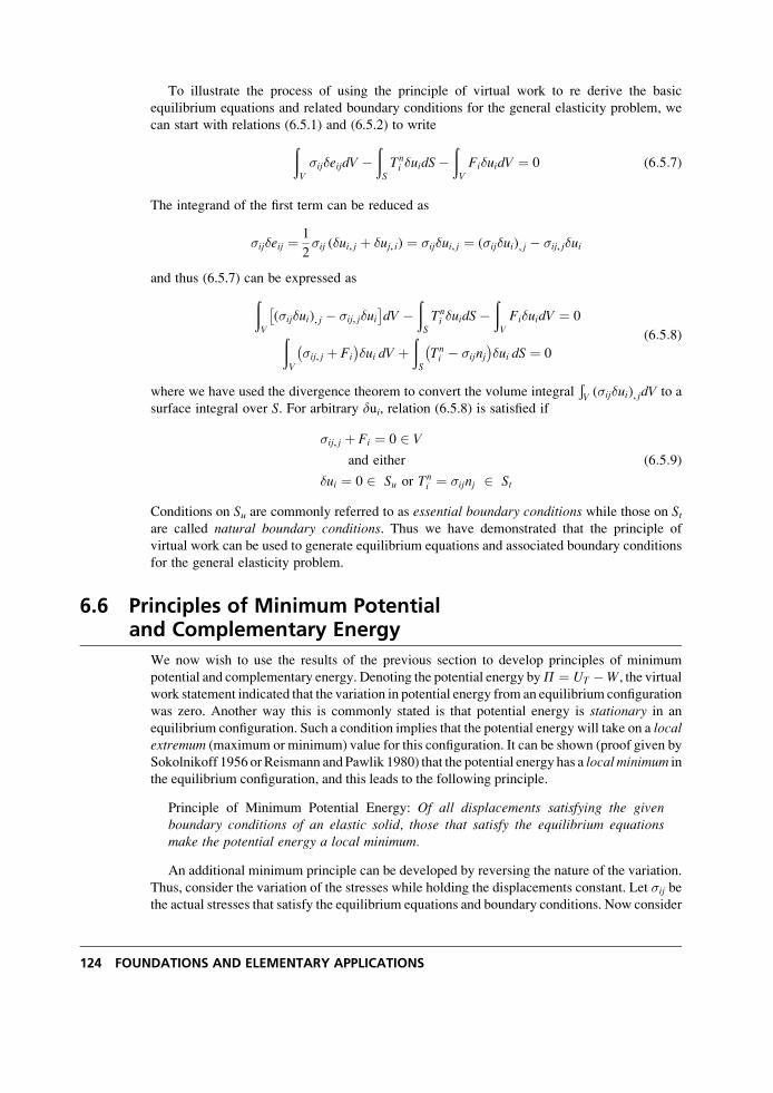
To illustrate the process of using the principle of virtual work to re derive the basic
equilibrium equations and related boundary conditions for the general elasticity problem, we
can start with relations (6.5.1) and (6.5.2) to writeðV
�ij�eijdV �ðS
Tni �uidS�
ðV
Fi�uidV ¼ 0 (6:5:7)
The integrand of the first term can be reduced as
�ij�eij ¼ 1
2�ij (�ui, j þ �uj, i) ¼ �ij�ui, j ¼ (�ij�ui), j � �ij, j�ui
and thus (6.5.7) can be expressed asðV
(�ij�ui), j � �ij, j�ui� �
dV �ðS
Tni �uidS�
ðV
Fi�uidV ¼ 0ðV
�ij, j þ Fi
� ��ui dV þ
ðS
Tni � �ijnj
� ��ui dS ¼ 0
(6:5:8)
where we have used the divergence theorem to convert the volume integralÐV (�ij�ui), jdV to a
surface integral over S. For arbitrary dui, relation (6.5.8) is satisfied if
�ij, j þ Fi ¼ 0 2 V
and either
�ui ¼ 0 2 Su or Tni ¼ �ijnj 2 St
(6:5:9)
Conditions on Su are commonly referred to as essential boundary conditions while those on Stare called natural boundary conditions. Thus we have demonstrated that the principle of
virtual work can be used to generate equilibrium equations and associated boundary conditions
for the general elasticity problem.
6.6 Principles of Minimum Potentialand Complementary Energy
We now wish to use the results of the previous section to develop principles of minimum
potential and complementary energy. Denoting the potential energy byP ¼ UT �W, the virtual
work statement indicated that the variation in potential energy from an equilibrium configuration
was zero. Another way this is commonly stated is that potential energy is stationary in an
equilibrium configuration. Such a condition implies that the potential energy will take on a localextremum (maximum or minimum) value for this configuration. It can be shown (proof given by
Sokolnikoff 1956 orReismann and Pawlik 1980) that the potential energy has a localminimum in
the equilibrium configuration, and this leads to the following principle.
Principle of Minimum Potential Energy: Of all displacements satisfying the givenboundary conditions of an elastic solid, those that satisfy the equilibrium equationsmake the potential energy a local minimum.
An additional minimum principle can be developed by reversing the nature of the variation.
Thus, consider the variation of the stresses while holding the displacements constant. Let �ij be
the actual stresses that satisfy the equilibrium equations and boundary conditions. Now consider
124 FOUNDATIONS AND ELEMENTARY APPLICATIONS
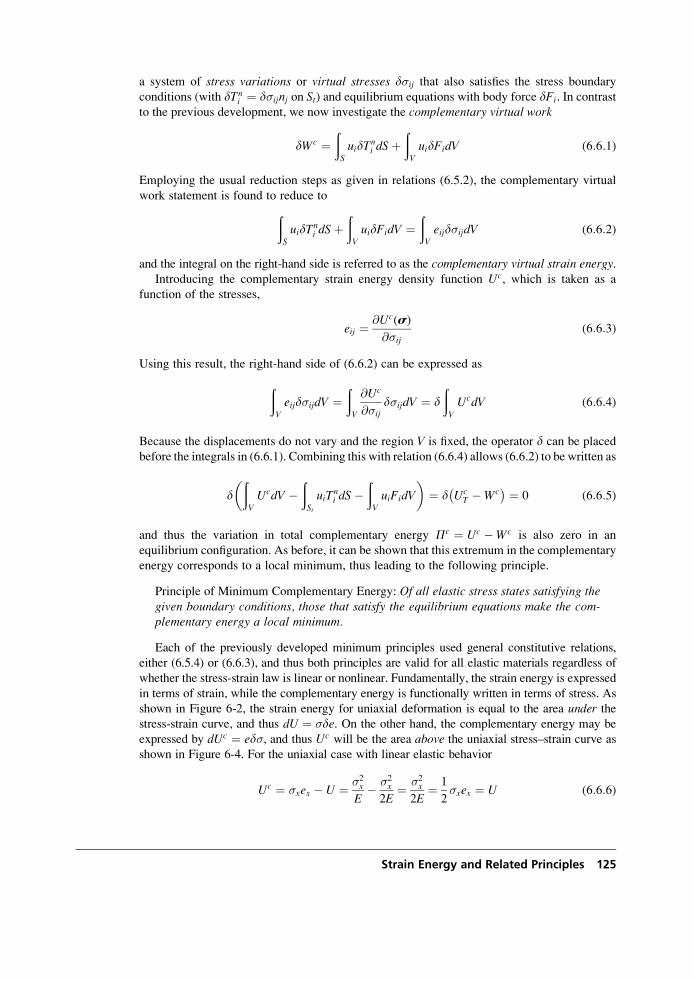
a system of stress variations or virtual stresses d�ij that also satisfies the stress boundary
conditions (with dTni ¼ d�ijnj on St) and equilibrium equations with body force dFi. In contrast
to the previous development, we now investigate the complementary virtual work
dWc ¼ðS
uidTni dSþ
ðV
uidFidV (6:6:1)
Employing the usual reduction steps as given in relations (6.5.2), the complementary virtual
work statement is found to reduce toðS
uidTni dSþ
ðV
uidFidV ¼ðV
eijd�ijdV (6:6:2)
and the integral on the right-hand side is referred to as the complementary virtual strain energy.Introducing the complementary strain energy density function Uc, which is taken as a
function of the stresses,
eij ¼ @Uc(s)
@�ij(6:6:3)
Using this result, the right-hand side of (6.6.2) can be expressed as
ðV
eijd�ijdV ¼ðV
@Uc
@�ijd�ijdV ¼ d
ðV
UcdV (6:6:4)
Because the displacements do not vary and the region V is fixed, the operator d can be placed
before the integrals in (6.6.1). Combining this with relation (6.6.4) allows (6.6.2) to be written as
dðV
UcdV �ðSt
uiTni dS�
ðV
uiFidV
� �¼ d Uc
T �Wc� � ¼ 0 (6:6:5)
and thus the variation in total complementary energy Pc ¼ Uc �Wc is also zero in an
equilibrium configuration. As before, it can be shown that this extremum in the complementary
energy corresponds to a local minimum, thus leading to the following principle.
Principle of Minimum Complementary Energy: Of all elastic stress states satisfying thegiven boundary conditions, those that satisfy the equilibrium equations make the com-plementary energy a local minimum.
Each of the previously developed minimum principles used general constitutive relations,
either (6.5.4) or (6.6.3), and thus both principles are valid for all elastic materials regardless of
whether the stress-strain law is linear or nonlinear. Fundamentally, the strain energy is expressed
in terms of strain, while the complementary energy is functionally written in terms of stress. As
shown in Figure 6-2, the strain energy for uniaxial deformation is equal to the area under thestress-strain curve, and thus dU ¼ �de. On the other hand, the complementary energy may be
expressed by dUc ¼ ed�, and thus Uc will be the area above the uniaxial stress–strain curve as
shown in Figure 6-4. For the uniaxial case with linear elastic behavior
Uc ¼ �xex � U ¼ �2x
E� �2
x
2E¼ �2
x
2E¼ 1
2�xex ¼ U (6:6:6)
Strain Energy and Related Principles 125
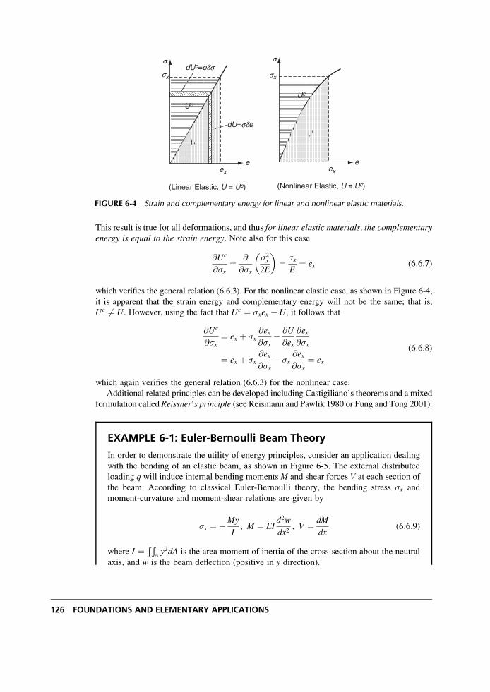
This result is true for all deformations, and thus for linear elastic materials, the complementaryenergy is equal to the strain energy. Note also for this case
@Uc
@�x¼ @
@�x
�2x
2E
� �¼ �x
E¼ ex (6:6:7)
which verifies the general relation (6.6.3). For the nonlinear elastic case, as shown in Figure 6-4,
it is apparent that the strain energy and complementary energy will not be the same; that is,
Uc 6¼ U. However, using the fact that Uc ¼ �xex � U, it follows that
@Uc
@�x¼ ex þ �x
@ex@�x
� @U
@ex
@ex@�x
¼ ex þ �x@ex@�x
� �x@ex@�x
¼ ex
(6:6:8)
which again verifies the general relation (6.6.3) for the nonlinear case.
Additional related principles can be developed including Castigiliano’s theorems and a mixed
formulation called Reissner’s principle (see Reismann and Pawlik 1980 or Fung and Tong 2001).
EXAMPLE 6-1: Euler-Bernoulli Beam Theory
In order to demonstrate the utility of energy principles, consider an application dealing
with the bending of an elastic beam, as shown in Figure 6-5. The external distributed
loading q will induce internal bending momentsM and shear forces V at each section of
the beam. According to classical Euler-Bernoulli theory, the bending stress �x and
moment-curvature and moment-shear relations are given by
�x ¼ �My
I, M ¼ EI
d2w
dx2, V ¼ dM
dx(6:6:9)
where I ¼ Ð ÐA y2dA is the area moment of inertia of the cross-section about the neutral
axis, and w is the beam deflection (positive in y direction).
ex
e
(Nonlinear Elastic, U π Uc)
ex
e
(Linear Elastic, U = Uc)
dUc=eds
dU=sde
Uc
U
Uc
U
s s
sx sx
FIGURE 6-4 Strain and complementary energy for linear and nonlinear elastic materials.
126 FOUNDATIONS AND ELEMENTARY APPLICATIONS
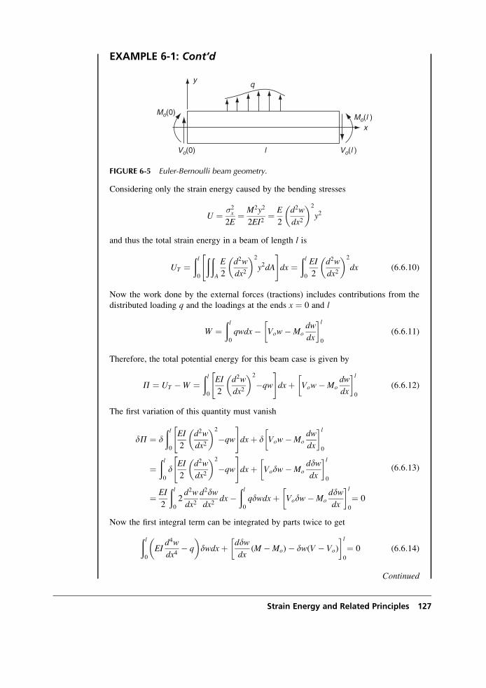
EXAMPLE 6-1: Cont’d
x
yq
Mo(0)
Vo(0) Vo(l )
Mo(l )
l
FIGURE 6-5 Euler-Bernoulli beam geometry.
Considering only the strain energy caused by the bending stresses
U ¼ �2x2E
¼ M2y2
2EI2¼ E
2
d2w
dx2
� �2
y2
and thus the total strain energy in a beam of length l is
UT ¼ðl0
ððA
E
2
d2w
dx2
� �2
y2dA
" #dx ¼
ðl0
EI
2
d2w
dx2
� �2
dx (6:6:10)
Now the work done by the external forces (tractions) includes contributions from the
distributed loading q and the loadings at the ends x ¼ 0 and l
W ¼ðl0
qwdx� Vow�Modw
dx
� l0
(6:6:11)
Therefore, the total potential energy for this beam case is given by
P ¼ UT �W ¼ðl0
EI
2
d2w
dx2
� �2
�qw
" #dxþ Vow�Mo
dw
dx
� l0
(6:6:12)
The first variation of this quantity must vanish
dP ¼ dðl0
EI
2
d2w
dx2
� �2
�qw
" #dxþ d Vow�Mo
dw
dx
� l0
¼ðl0
dEI
2
d2w
dx2
� �2
�qw
" #dxþ Vodw�Mo
ddwdx
� l0
¼ EI
2
ðl0
2d2w
dx2d2dwdx2
dx�ðl0
qdwdxþ Vodw�Moddwdx
� l0
¼ 0
(6:6:13)
Now the first integral term can be integrated by parts twice to get
ðl0
EId4w
dx4� q
� �dwdxþ ddw
dx(M �Mo)� dw(V � Vo)
� l0
¼ 0 (6:6:14)
Continued
Strain Energy and Related Principles 127
EXAMPLE 6-1: Euler-Bernoulli Beam Theory—Cont’d
The integral and boundary terms must all vanish, thus implying
ðl0
EId4w
dx4� q
� �dwdx ¼ 0
V ¼ Vo or dw ¼ 0, x ¼ 0, l
M ¼ Mo or ddw
dx
� �¼ 0, x ¼ 0, l
(6:6:15)
For this integral to vanish for all variations dw, the fundamental lemma in the calculusof variations implies that the integrand must be zero, giving
EId4w
dx4� q ¼ 0 (6:6:16)
This result is simply the differential equilibrium equation for the beam, and thus the sta-
tionary value for the potential energy leads directly to the governing equilibrium equation
in terms of displacement and the associated boundary conditions. Of course, this entire
formulation is based on the simplifying assumptions found in Euler-Bernoulli beam theory,
and resulting solutions would not match with the more exact theory of elasticity results.
6.7 Rayleigh-Ritz Method
The previous beam example indicates a correspondence between the governing differential equa-
tion(s) and a variational problem of minimizing the potential energy of the system. Such a corres-
pondence exists for many other types of problems in structural mechanics and elasticity.
For problems of complicated shape or loading geometry, the solution to the governing differential
equationcannotbefoundbyanalyticalmethods.Forsuchcases,approximatesolutionschemeshave
been developed based on the variational form of the problem. Several such approximate schemes
have been constructed, and one of the more important techniques is the Rayleigh-Ritz method.This particular technique is based on the idea of constructing a series of trial approximating
functions that satisfy the boundary conditions but not the differential equation(s). For the
elasticity displacement formulation (Section 5.4), this concept would express the displace-
ments in the form
u ¼ uo þ a1u1 þ a2u2 þ a3u3 þ . . . ¼ uo þXNj¼1
ajuj
v ¼ vo þ b1v1 þ b2v2 þ b3v3 þ . . . ¼ vo þXNj¼1
bjvj
w ¼ wo þ c1w1 þ c2w2 þ c3w3 þ . . . ¼ wo þXNj¼1
cjwj
(6:7:1)
where the functions uo, vo, wo are chosen to satisfy any nonhomogeneous displacement bound-
ary conditions and uj, vj, wj satisfy the corresponding homogeneous boundary conditions. Note
128 FOUNDATIONS AND ELEMENTARY APPLICATIONS
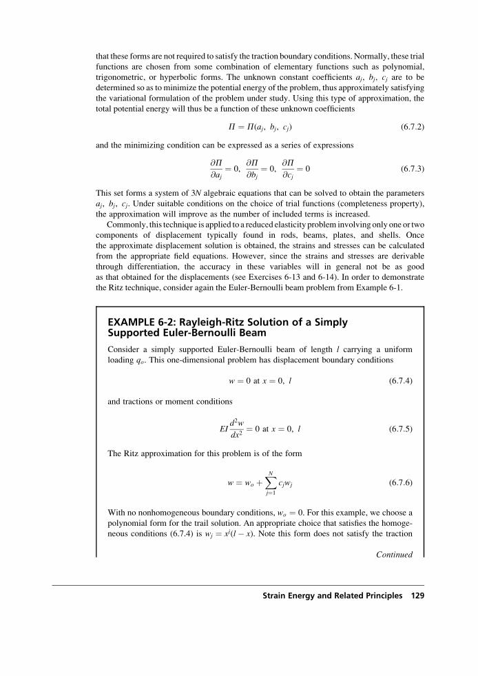
that these forms are not required to satisfy the traction boundary conditions. Normally, these trial
functions are chosen from some combination of elementary functions such as polynomial,
trigonometric, or hyperbolic forms. The unknown constant coefficients aj, bj, cj are to be
determined so as to minimize the potential energy of the problem, thus approximately satisfying
the variational formulation of the problem under study. Using this type of approximation, the
total potential energy will thus be a function of these unknown coefficients
P ¼ P(aj, bj, cj) (6:7:2)
and the minimizing condition can be expressed as a series of expressions
@P@aj
¼ 0,@P@bj
¼ 0,@P@cj
¼ 0 (6:7:3)
This set forms a system of 3N algebraic equations that can be solved to obtain the parameters
aj, bj, cj. Under suitable conditions on the choice of trial functions (completeness property),
the approximation will improve as the number of included terms is increased.
Commonly, this technique is applied to a reduced elasticity problem involving only one or two
components of displacement typically found in rods, beams, plates, and shells. Once
the approximate displacement solution is obtained, the strains and stresses can be calculated
from the appropriate field equations. However, since the strains and stresses are derivable
through differentiation, the accuracy in these variables will in general not be as good
as that obtained for the displacements (see Exercises 6-13 and 6-14). In order to demonstrate
the Ritz technique, consider again the Euler-Bernoulli beam problem from Example 6-1.
EXAMPLE 6-2: Rayleigh-Ritz Solution of a SimplySupported Euler-Bernoulli Beam
Consider a simply supported Euler-Bernoulli beam of length l carrying a uniform
loading qo. This one-dimensional problem has displacement boundary conditions
w ¼ 0 at x ¼ 0, l (6:7:4)
and tractions or moment conditions
EId2w
dx2¼ 0 at x ¼ 0, l (6:7:5)
The Ritz approximation for this problem is of the form
w ¼ wo þXNj¼1
cjwj (6:7:6)
With no nonhomogeneous boundary conditions, wo ¼ 0. For this example, we choose a
polynomial form for the trail solution. An appropriate choice that satisfies the homoge-
neous conditions (6.7.4) is wj ¼ xj(l� x). Note this form does not satisfy the traction
Continued
Strain Energy and Related Principles 129
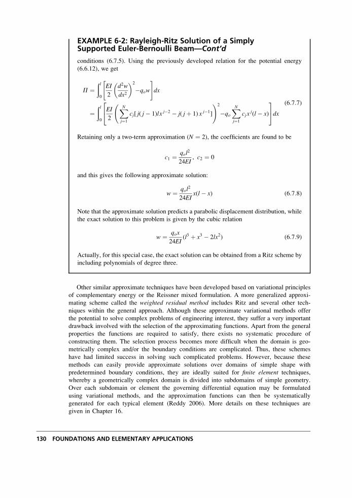
EXAMPLE 6-2: Rayleigh-Ritz Solution of a SimplySupported Euler-Bernoulli Beam—Cont’d
conditions (6.7.5). Using the previously developed relation for the potential energy
(6.6.12), we get
P ¼ðl0
EI
2
d2w
dx2
� �2
�qow
" #dx
¼ðl0
EI
2
XNj¼1
cj[ j( j� 1)lx j�2 � j( jþ 1) x j�1]
!2
�qoXNj¼1
cjxj(l� x)
24
35dx
(6:7:7)
Retaining only a two-term approximation (N ¼ 2), the coefficients are found to be
c1 ¼ qol2
24EI, c2 ¼ 0
and this gives the following approximate solution:
w ¼ qol2
24EIx(l� x) (6:7:8)
Note that the approximate solution predicts a parabolic displacement distribution, while
the exact solution to this problem is given by the cubic relation
w ¼ qox
24EI(l3 þ x3 � 2lx2) (6:7:9)
Actually, for this special case, the exact solution can be obtained from a Ritz scheme by
including polynomials of degree three.
Other similar approximate techniques have been developed based on variational principles
of complementary energy or the Reissner mixed formulation. A more generalized approxi-
mating scheme called the weighted residual method includes Ritz and several other tech-
niques within the general approach. Although these approximate variational methods offer
the potential to solve complex problems of engineering interest, they suffer a very important
drawback involved with the selection of the approximating functions. Apart from the general
properties the functions are required to satisfy, there exists no systematic procedure of
constructing them. The selection process becomes more difficult when the domain is geo-
metrically complex and/or the boundary conditions are complicated. Thus, these schemes
have had limited success in solving such complicated problems. However, because these
methods can easily provide approximate solutions over domains of simple shape with
predetermined boundary conditions, they are ideally suited for finite element techniques,
whereby a geometrically complex domain is divided into subdomains of simple geometry.
Over each subdomain or element the governing differential equation may be formulated
using variational methods, and the approximation functions can then be systematically
generated for each typical element (Reddy 2006). More details on these techniques are
given in Chapter 16.
130 FOUNDATIONS AND ELEMENTARY APPLICATIONS
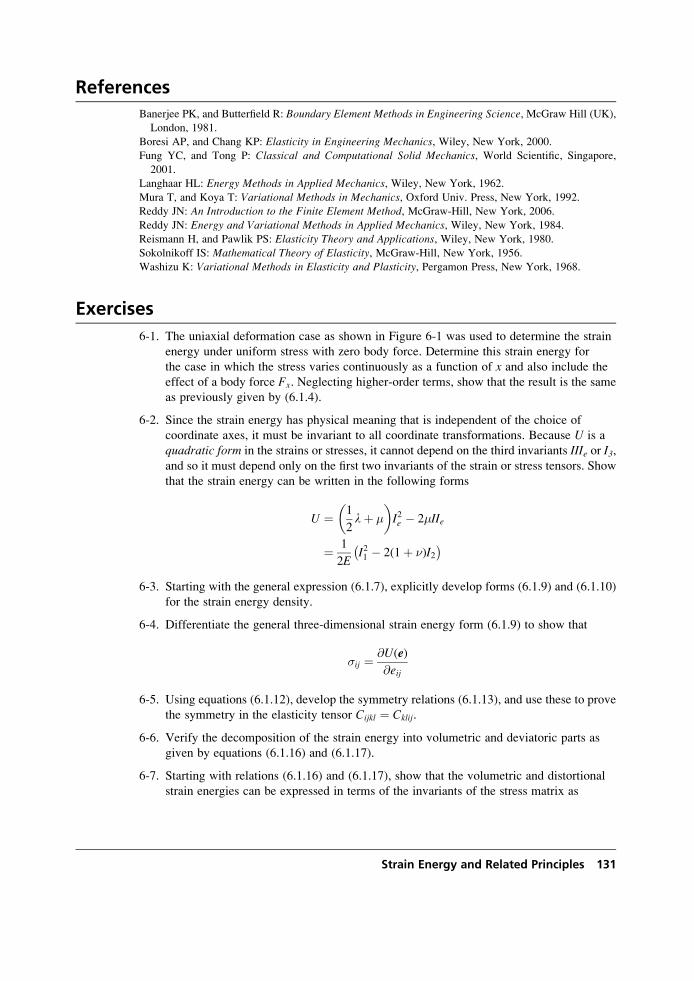
References
Banerjee PK, and Butterfield R: Boundary Element Methods in Engineering Science, McGraw Hill (UK),
London, 1981.
Boresi AP, and Chang KP: Elasticity in Engineering Mechanics, Wiley, New York, 2000.
Fung YC, and Tong P: Classical and Computational Solid Mechanics, World Scientific, Singapore,
2001.
Langhaar HL: Energy Methods in Applied Mechanics, Wiley, New York, 1962.
Mura T, and Koya T: Variational Methods in Mechanics, Oxford Univ. Press, New York, 1992.
Reddy JN: An Introduction to the Finite Element Method, McGraw-Hill, New York, 2006.
Reddy JN: Energy and Variational Methods in Applied Mechanics, Wiley, New York, 1984.
Reismann H, and Pawlik PS: Elasticity Theory and Applications, Wiley, New York, 1980.
Sokolnikoff IS: Mathematical Theory of Elasticity, McGraw-Hill, New York, 1956.
Washizu K: Variational Methods in Elasticity and Plasticity, Pergamon Press, New York, 1968.
Exercises
6-1. The uniaxial deformation case as shown in Figure 6-1 was used to determine the strain
energy under uniform stress with zero body force. Determine this strain energy for
the case in which the stress varies continuously as a function of x and also include the
effect of a body force Fx. Neglecting higher-order terms, show that the result is the same
as previously given by (6.1.4).
6-2. Since the strain energy has physical meaning that is independent of the choice of
coordinate axes, it must be invariant to all coordinate transformations. Because U is a
quadratic form in the strains or stresses, it cannot depend on the third invariants IIIe or I3,and so it must depend only on the first two invariants of the strain or stress tensors. Show
that the strain energy can be written in the following forms
U ¼ 1
2lþ �
� �I2e � 2�IIe
¼ 1
2EI21 � 2(1þ �)I2� �
6-3. Starting with the general expression (6.1.7), explicitly develop forms (6.1.9) and (6.1.10)
for the strain energy density.
6-4. Differentiate the general three-dimensional strain energy form (6.1.9) to show that
�ij ¼ @U(e)
@eij
6-5. Using equations (6.1.12), develop the symmetry relations (6.1.13), and use these to prove
the symmetry in the elasticity tensor Cijkl ¼ Cklij.
6-6. Verify the decomposition of the strain energy into volumetric and deviatoric parts as
given by equations (6.1.16) and (6.1.17).
6-7. Starting with relations (6.1.16) and (6.1.17), show that the volumetric and distortional
strain energies can be expressed in terms of the invariants of the stress matrix as
Strain Energy and Related Principles 131
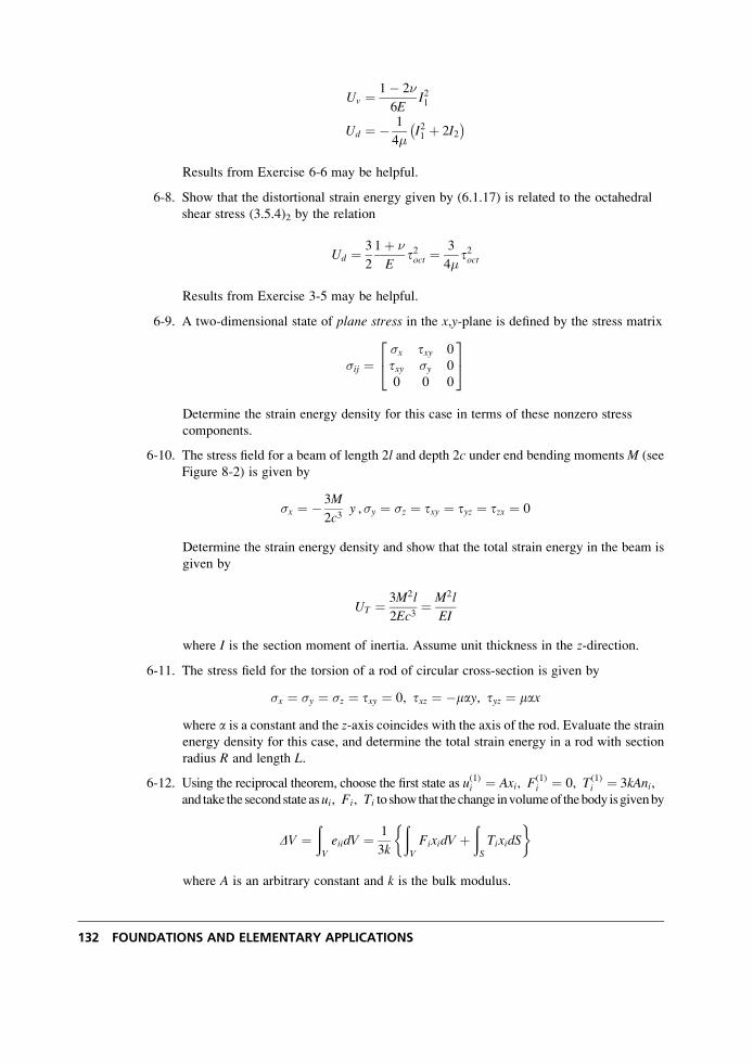
Uv ¼ 1� 2�
6EI21
Ud ¼ � 1
4�I21 þ 2I2� �
Results from Exercise 6-6 may be helpful.
6-8. Show that the distortional strain energy given by (6.1.17) is related to the octahedral
shear stress (3.5.4)2 by the relation
Ud ¼ 3
2
1þ �
Et2oct ¼
3
4�t2oct
Results from Exercise 3-5 may be helpful.
6-9. A two-dimensional state of plane stress in the x,y-plane is defined by the stress matrix
�ij ¼�x txy 0
txy �y 0
0 0 0
24
35
Determine the strain energy density for this case in terms of these nonzero stress
components.
6-10. The stress field for a beam of length 2l and depth 2c under end bending momentsM (see
Figure 8-2) is given by
�x ¼ � 3M
2c3y ,�y ¼ �z ¼ txy ¼ tyz ¼ tzx ¼ 0
Determine the strain energy density and show that the total strain energy in the beam is
given by
UT ¼ 3M2l
2Ec3¼ M2l
EI
where I is the section moment of inertia. Assume unit thickness in the z-direction.
6-11. The stress field for the torsion of a rod of circular cross-section is given by
�x ¼ �y ¼ �z ¼ txy ¼ 0, txz ¼ �may, tyz ¼ max
where a is a constant and the z-axis coincides with the axis of the rod. Evaluate the strainenergy density for this case, and determine the total strain energy in a rod with section
radius R and length L.
6-12. Using the reciprocal theorem, choose the first state as u(1)i ¼ Axi, F(1)i ¼ 0, T(1)
i ¼ 3kAni,and take thesecondstateasui, Fi, Ti to showthat thechange involumeof thebody isgivenby
DV ¼ðV
eiidV ¼ 1
3k
ðV
FixidV þðS
TixidS
�
where A is an arbitrary constant and k is the bulk modulus.
132 FOUNDATIONS AND ELEMENTARY APPLICATIONS

6-13. Rework Example 6-2 using the trigonometric Ritz approximation wj ¼ sin jpxl . Develop
a two-term approximate solution, and compare it with the displacement solution
developed in the text. Also compare each of these approximations with the exact
solution (6.7.9) at midspan x ¼ l=2.
6-14. Using the bending formulae (6.6.9), compare the maximum bending stresses from the
cases presented in Example 6-2 and Exercise 6-13. Numerically compare these results
with the exact solution; see (6.7.9) at midspan x ¼ l=2.
Strain Energy and Related Principles 133
7 Two-Dimensional Formulation
Because of the complexity of the elasticity field equations, analytical closed-form solutions to
fully three-dimensional problems are very difficult to accomplish. Thus, most solutions are
developed for reduced problems that typically include axisymmetry or two-dimensionality to
simplify particular aspects of the formulation and solution. We now wish to examine in detail
the formulation of two-dimensional problems in elasticity. Our initial formulation will result in
a boundary-value problem cast within a two-dimensional domain in the x,y-plane using
Cartesian coordinates. This work will then be reformulated in polar coordinates to allow for
the development of important solutions in that coordinate system. Because all real elastic
structures are three-dimensional, the theories set forth here will be approximate models. The
nature and accuracy of the approximation depends on problem and loading geometry.
Although four different formulations are developed, the two basic theories of plane strainand plane stress represent the fundamental plane problem in elasticity. These two theories
apply to significantly different types of two-dimensional bodies; however, their formulations
yield very similar field equations. It will be shown that these two theories can be reduced to
one governing equation in terms of a single unknown stress function. This reduction then
allows many solutions to be generated to problems of engineering interest, and such solutions
are presented in the following chapter.
7.1 Plane Strain
Consider an infinitely long cylindrical (prismatic) body shown in Figure 7-1. If the body forces
and tractions on the lateral boundaries are independent of the z-coordinate and have no zcomponent, then the deformation field within the body can be taken in the reduced form
u ¼ u(x, y), v ¼ v(x, y), w ¼ 0 (7:1:1)
This deformation is referred to as a state of plane strain in the x,y-plane. It should be
obvious that for such a case all cross-sections R will have identical displacements, and thus
the three-dimensional problem is reduced to a two-dimensional formulation in region R in the
x,y-plane.
135
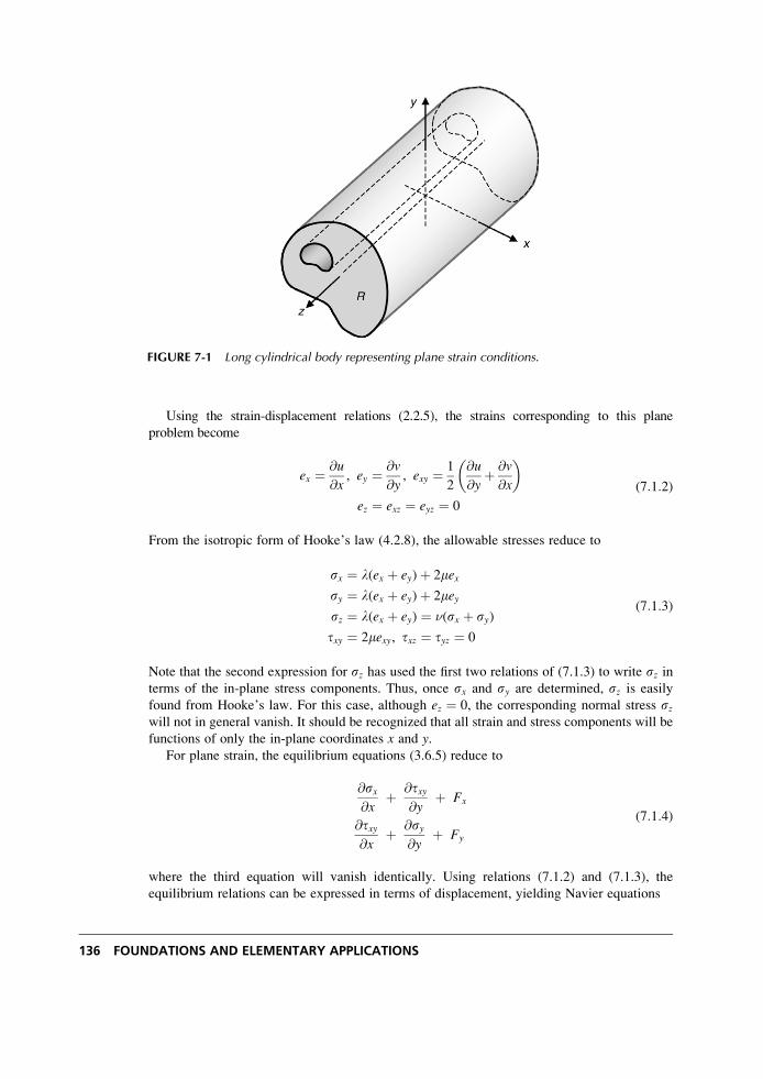
Using the strain-displacement relations (2.2.5), the strains corresponding to this plane
problem become
ex ¼ @u
@x, ey ¼ @v
@y, exy ¼ 1
2
@u
@yþ @v
@x
� �ez ¼ exz ¼ eyz ¼ 0
(7:1:2)
From the isotropic form of Hooke’s law (4.2.8), the allowable stresses reduce to
sx ¼ l(ex þ ey)þ 2mexsy ¼ l(ex þ ey)þ 2meysz ¼ l(ex þ ey) ¼ �(sx þ sy)
txy ¼ 2mexy, txz ¼ tyz ¼ 0
(7:1:3)
Note that the second expression for sz has used the first two relations of (7.1.3) to write sz interms of the in-plane stress components. Thus, once sx and sy are determined, sz is easily
found from Hooke’s law. For this case, although ez ¼ 0, the corresponding normal stress szwill not in general vanish. It should be recognized that all strain and stress components will be
functions of only the in-plane coordinates x and y.For plane strain, the equilibrium equations (3.6.5) reduce to
@sx@x
þ @txy@y
þ Fx
@txy@x
þ @sy@y
þ Fy
(7:1:4)
where the third equation will vanish identically. Using relations (7.1.2) and (7.1.3), the
equilibrium relations can be expressed in terms of displacement, yielding Navier equations
FIGURE 7-1 Long cylindrical body representing plane strain conditions.
136 FOUNDATIONS AND ELEMENTARY APPLICATIONS
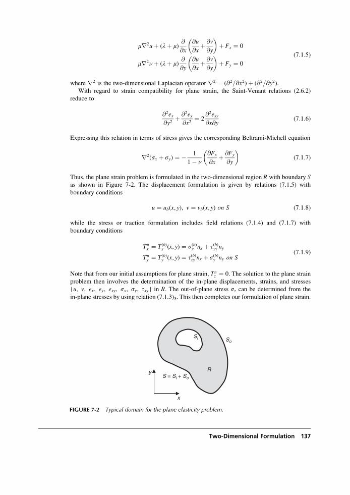
mr2uþ (lþ m)@
@x
@u
@xþ @v
@y
� �þ Fx ¼ 0
mr2� þ (lþ m)@
@y
@u
@xþ @v
@y
� �þ Fy ¼ 0
(7:1:5)
where r2 is the two-dimensional Laplacian operator r2 ¼ (@2=@x2)þ (@2=@y2).With regard to strain compatibility for plane strain, the Saint-Venant relations (2.6.2)
reduce to
@2ex@y2
þ @2ey@x2
¼ 2@2exy@x@y
(7:1:6)
Expressing this relation in terms of stress gives the corresponding Beltrami-Michell equation
r2(sx þ sy) ¼ � 1
1� �
@Fx
@xþ @Fy
@y
� �(7:1:7)
Thus, the plane strain problem is formulated in the two-dimensional region R with boundary Sas shown in Figure 7-2. The displacement formulation is given by relations (7.1.5) with
boundary conditions
u ¼ ub(x, y), v ¼ vb(x, y) on S (7:1:8)
while the stress or traction formulation includes field relations (7.1.4) and (7.1.7) with
boundary conditions
Tnx ¼ T(b)
x (x, y) ¼ s(b)x nx þ t(b)xy ny
Tny ¼ T(b)
y (x, y) ¼ t(b)xy nx þ s(b)y ny on S(7:1:9)
Note that from our initial assumptions for plane strain, Tnz ¼ 0. The solution to the plane strain
problem then involves the determination of the in-plane displacements, strains, and stresses
{u, v, ex, ey, exy, sx, sy, txy} in R. The out-of-plane stress sz can be determined from the
in-plane stresses by using relation (7.1.3)3. This then completes our formulation of plane strain.
R
SoSi
S = Si + So
x
y
FIGURE 7-2 Typical domain for the plane elasticity problem.
Two-Dimensional Formulation 137
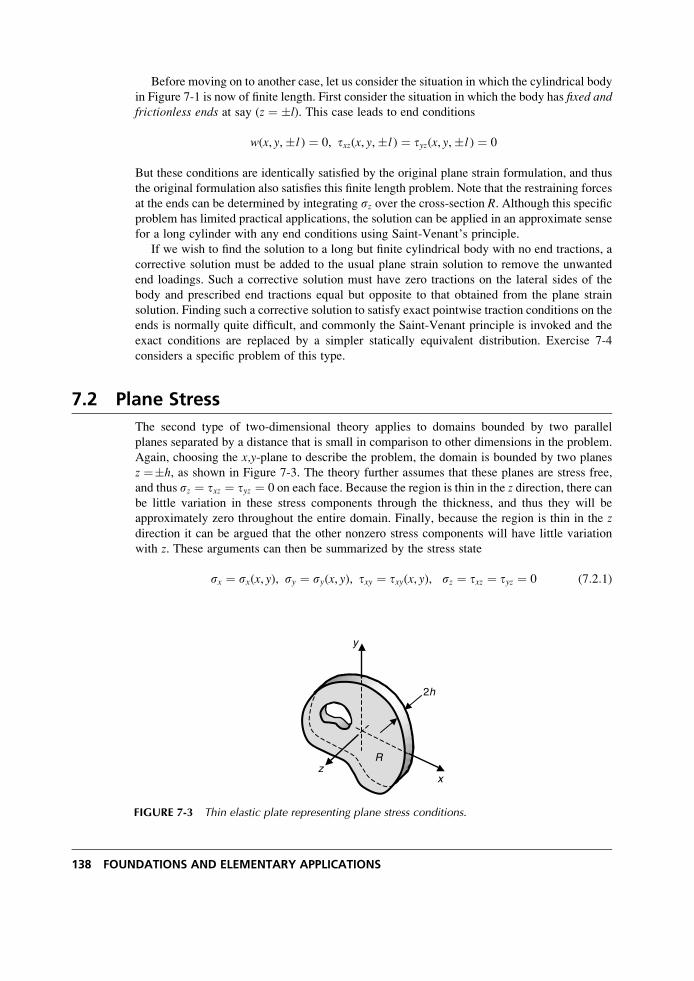
Before moving on to another case, let us consider the situation in which the cylindrical body
in Figure 7-1 is now of finite length. First consider the situation in which the body has fixed andfrictionless ends at say (z ¼ �l). This case leads to end conditions
w(x, y,�l ) ¼ 0, txz(x, y,�l ) ¼ tyz(x, y,�l ) ¼ 0
But these conditions are identically satisfied by the original plane strain formulation, and thus
the original formulation also satisfies this finite length problem. Note that the restraining forces
at the ends can be determined by integrating sz over the cross-section R. Although this specificproblem has limited practical applications, the solution can be applied in an approximate sense
for a long cylinder with any end conditions using Saint-Venant’s principle.
If we wish to find the solution to a long but finite cylindrical body with no end tractions, a
corrective solution must be added to the usual plane strain solution to remove the unwanted
end loadings. Such a corrective solution must have zero tractions on the lateral sides of the
body and prescribed end tractions equal but opposite to that obtained from the plane strain
solution. Finding such a corrective solution to satisfy exact pointwise traction conditions on the
ends is normally quite difficult, and commonly the Saint-Venant principle is invoked and the
exact conditions are replaced by a simpler statically equivalent distribution. Exercise 7-4
considers a specific problem of this type.
7.2 Plane Stress
The second type of two-dimensional theory applies to domains bounded by two parallel
planes separated by a distance that is small in comparison to other dimensions in the problem.
Again, choosing the x,y-plane to describe the problem, the domain is bounded by two planes
z ¼�h, as shown in Figure 7-3. The theory further assumes that these planes are stress free,
and thus sz ¼ txz ¼ tyz ¼ 0 on each face. Because the region is thin in the z direction, there canbe little variation in these stress components through the thickness, and thus they will be
approximately zero throughout the entire domain. Finally, because the region is thin in the zdirection it can be argued that the other nonzero stress components will have little variation
with z. These arguments can then be summarized by the stress state
sx ¼ sx(x, y), sy ¼ sy(x, y), txy ¼ txy(x, y), sz ¼ txz ¼ tyz ¼ 0 (7:2:1)
x
y
zR
2h
FIGURE 7-3 Thin elastic plate representing plane stress conditions.
138 FOUNDATIONS AND ELEMENTARY APPLICATIONS
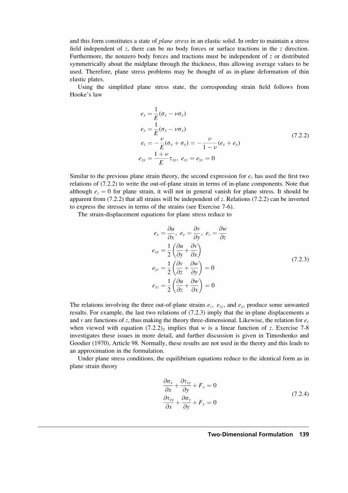
and this form constitutes a state of plane stress in an elastic solid. In order to maintain a stress
field independent of z, there can be no body forces or surface tractions in the z direction.
Furthermore, the nonzero body forces and tractions must be independent of z or distributedsymmetrically about the midplane through the thickness, thus allowing average values to be
used. Therefore, plane stress problems may be thought of as in-plane deformation of thin
elastic plates.
Using the simplified plane stress state, the corresponding strain field follows from
Hooke’s law
ex ¼ 1
E(sx � �sy)
ey ¼ 1
E(sy � �sx)
ez ¼ � �
E(sx þ sy) ¼ � �
1� �(ex þ ey)
exy ¼ 1þ �
Etxy, exz ¼ eyz ¼ 0
(7:2:2)
Similar to the previous plane strain theory, the second expression for ez has used the first two
relations of (7.2.2) to write the out-of-plane strain in terms of in-plane components. Note that
although ez ¼ 0 for plane strain, it will not in general vanish for plane stress. It should be
apparent from (7.2.2) that all strains will be independent of z. Relations (7.2.2) can be invertedto express the stresses in terms of the strains (see Exercise 7-6).
The strain-displacement equations for plane stress reduce to
ex ¼ @u
@x, ey ¼ @v
@y, ez ¼ @w
@z
exy ¼ 1
2
@u
@yþ @v
@x
� �
eyz ¼ 1
2
@v
@zþ @w
@y
� �¼ 0
exz ¼ 1
2
@u
@zþ @w
@x
� �¼ 0
(7:2:3)
The relations involving the three out-of-plane strains ez, exz, and eyz produce some unwanted
results. For example, the last two relations of (7.2.3) imply that the in-plane displacements uand v are functions of z, thus making the theory three-dimensional. Likewise, the relation for ezwhen viewed with equation (7:2:2)3 implies that w is a linear function of z. Exercise 7-8
investigates these issues in more detail, and further discussion is given in Timoshenko and
Goodier (1970), Article 98. Normally, these results are not used in the theory and this leads to
an approximation in the formulation.
Under plane stress conditions, the equilibrium equations reduce to the identical form as in
plane strain theory
@sx@x
þ @txy@y
þ Fx ¼ 0
@txy@x
þ @sy@y
þ Fy ¼ 0
(7:2:4)
Two-Dimensional Formulation 139
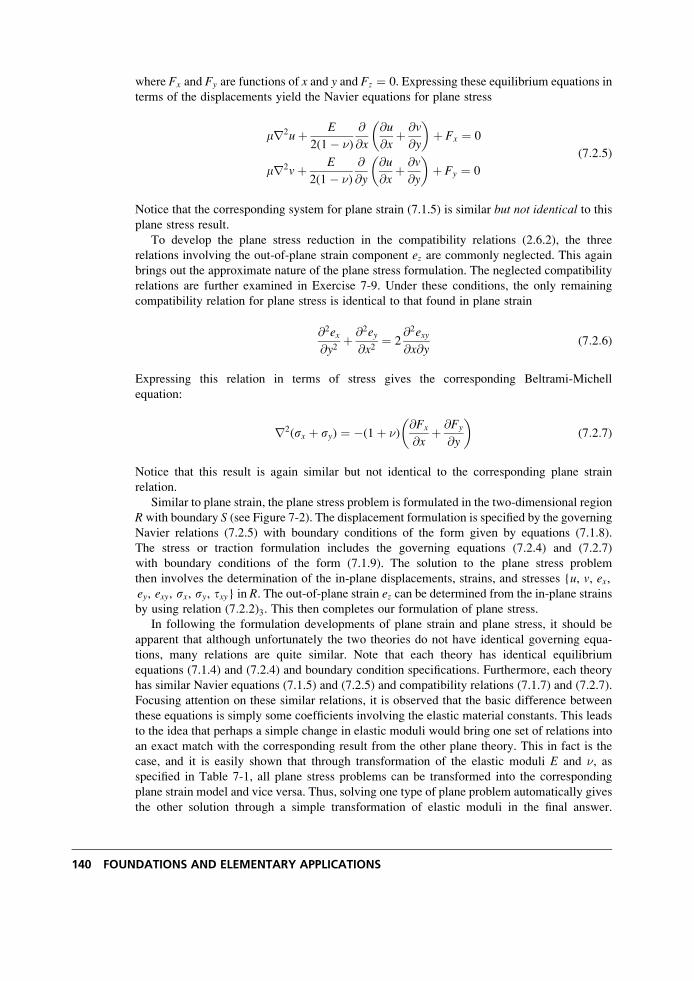
where Fx and Fy are functions of x and y and Fz ¼ 0. Expressing these equilibrium equations in
terms of the displacements yield the Navier equations for plane stress
mr2uþ E
2(1� �)
@
@x
@u
@xþ @v
@y
� �þ Fx ¼ 0
mr2vþ E
2(1� �)
@
@y
@u
@xþ @v
@y
� �þ Fy ¼ 0
(7:2:5)
Notice that the corresponding system for plane strain (7.1.5) is similar but not identical to this
plane stress result.
To develop the plane stress reduction in the compatibility relations (2.6.2), the three
relations involving the out-of-plane strain component ez are commonly neglected. This again
brings out the approximate nature of the plane stress formulation. The neglected compatibility
relations are further examined in Exercise 7-9. Under these conditions, the only remaining
compatibility relation for plane stress is identical to that found in plane strain
@2ex@y2
þ @2ey@x2
¼ 2@2exy@x@y
(7:2:6)
Expressing this relation in terms of stress gives the corresponding Beltrami-Michell
equation:
r2(sx þ sy) ¼ �(1þ �)@Fx
@xþ @Fy
@y
� �(7:2:7)
Notice that this result is again similar but not identical to the corresponding plane strain
relation.
Similar to plane strain, the plane stress problem is formulated in the two-dimensional region
Rwith boundary S (see Figure 7-2). The displacement formulation is specified by the governing
Navier relations (7.2.5) with boundary conditions of the form given by equations (7.1.8).
The stress or traction formulation includes the governing equations (7.2.4) and (7.2.7)
with boundary conditions of the form (7.1.9). The solution to the plane stress problem
then involves the determination of the in-plane displacements, strains, and stresses {u, v, ex,ey, exy, sx, sy, txy} in R. The out-of-plane strain ez can be determined from the in-plane strains
by using relation (7:2:2)3. This then completes our formulation of plane stress.
In following the formulation developments of plane strain and plane stress, it should be
apparent that although unfortunately the two theories do not have identical governing equa-
tions, many relations are quite similar. Note that each theory has identical equilibrium
equations (7.1.4) and (7.2.4) and boundary condition specifications. Furthermore, each theory
has similar Navier equations (7.1.5) and (7.2.5) and compatibility relations (7.1.7) and (7.2.7).
Focusing attention on these similar relations, it is observed that the basic difference between
these equations is simply some coefficients involving the elastic material constants. This leads
to the idea that perhaps a simple change in elastic moduli would bring one set of relations into
an exact match with the corresponding result from the other plane theory. This in fact is the
case, and it is easily shown that through transformation of the elastic moduli E and �, asspecified in Table 7-1, all plane stress problems can be transformed into the corresponding
plane strain model and vice versa. Thus, solving one type of plane problem automatically gives
the other solution through a simple transformation of elastic moduli in the final answer.
140 FOUNDATIONS AND ELEMENTARY APPLICATIONS
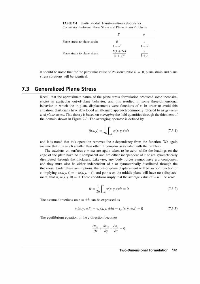
It should be noted that for the particular value of Poisson’s ratio � ¼ 0, plane strain and plane
stress solutions will be identical.
7.3 Generalized Plane Stress
Recall that the approximate nature of the plane stress formulation produced some inconsist-
encies in particular out-of-plane behavior, and this resulted in some three-dimensional
behavior in which the in-plane displacements were functions of z. In order to avoid this
situation, elasticians have developed an alternate approach commonly referred to as general-ized plane stress. This theory is based on averaging the field quantities through the thickness ofthe domain shown in Figure 7-3. The averaging operator is defined by
j(x, y) ¼ 1
2h
ðh�h
j(x, y, z)dz (7:3:1)
and it is noted that this operation removes the z dependency from the function. We again
assume that h is much smaller than other dimensions associated with the problem.
The tractions on surfaces z ¼ �h are again taken to be zero, while the loadings on the
edge of the plate have no z component and are either independent of z or are symmetrically
distributed through the thickness. Likewise, any body forces cannot have a z component
and they must also be either independent of z or symmetrically distributed through the
thickness. Under these assumptions, the out-of-plane displacement will be an odd function of
z, implying w(x, y, z) ¼ �w(x, y,� z), and points on the middle plane will have no z displace-ment; that is, w(x, y, 0) ¼ 0. These conditions imply that the average value of w will be zero:
w ¼ 1
2h
ðh�h
w(x, y, z)dz ¼ 0 (7:3:2)
The assumed tractions on z ¼ �h can be expressed as
sz(x, y,�h) ¼ txz(x, y,�h) ¼ tyz(x, y,�h) ¼ 0 (7:3:3)
The equilibrium equation in the z direction becomes
@txz@x
þ @tyz@y
þ @sz@z
¼ 0
TABLE 7-1 Elastic Moduli Transformation Relations forConversion Between Plane Stress and Plane Strain Problems
E �
Plane stress to plane strain E
1� �2�
1� �
Plane strain to plane stressE(1þ 2�)
(1þ �)2�
1þ �
Two-Dimensional Formulation 141
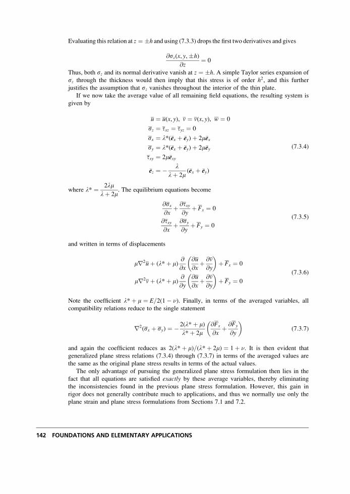
Evaluating this relation at z ¼ �h and using (7.3.3) drops the first two derivatives and gives
@sz(x, y,�h)
@z¼ 0
Thus, both sz and its normal derivative vanish at z ¼ �h. A simple Taylor series expansion of
sz through the thickness would then imply that this stress is of order h2, and this further
justifies the assumption that sz vanishes throughout the interior of the thin plate.
If we now take the average value of all remaining field equations, the resulting system is
given by
u ¼ u(x, y), v ¼ v(x, y), w ¼ 0
sz ¼ txz ¼ tyz ¼ 0
sx ¼ l*(�eex þ �eey)þ 2m�eexsy ¼ l*(�eex þ �eey)þ 2m�eeytxy ¼ 2m�eexy
�eez ¼ � llþ 2m
(�eex þ �eey)
(7:3:4)
where l* ¼ 2lmlþ 2m
. The equilibrium equations become
@sx@x
þ @txy@y
þ Fx ¼ 0
@txy@x
þ @sy@y
þ Fy ¼ 0
(7:3:5)
and written in terms of displacements
mr2uþ (l*þ m)@
@x
@u
@xþ @v
@y
� �þ Fx ¼ 0
mr2vþ (l*þ m)@
@y
@u
@xþ @v
@y
� �þ Fy ¼ 0
(7:3:6)
Note the coefficient l*þ m ¼ E=2(1� �). Finally, in terms of the averaged variables, all
compatibility relations reduce to the single statement
r2(sx þ sy) ¼ � 2(l*þ m)l*þ 2m
@Fx
@xþ @Fy
@y
� �(7:3:7)
and again the coefficient reduces as 2(l*þ m)=(l*þ 2m) ¼ 1þ �. It is then evident that
generalized plane stress relations (7.3.4) through (7.3.7) in terms of the averaged values are
the same as the original plane stress results in terms of the actual values.
The only advantage of pursuing the generalized plane stress formulation then lies in the
fact that all equations are satisfied exactly by these average variables, thereby eliminating
the inconsistencies found in the previous plane stress formulation. However, this gain in
rigor does not generally contribute much to applications, and thus we normally use only the
plane strain and plane stress formulations from Sections 7.1 and 7.2.
142 FOUNDATIONS AND ELEMENTARY APPLICATIONS
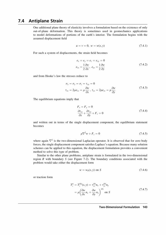
7.4 Antiplane Strain
One additional plane theory of elasticity involves a formulation based on the existence of only
out-of-plane deformation. This theory is sometimes used in geomechanics applications
to model deformations of portions of the earth’s interior. The formulation begins with the
assumed displacement field
u ¼ v ¼ 0, w ¼ w(x, y) (7:4:1)
For such a system of displacements, the strain field becomes
ex ¼ ey ¼ ez ¼ exy ¼ 0
exz ¼ 1
2
@w
@x, eyz ¼ 1
2
@w
@y
(7:4:2)
and from Hooke’s law the stresses reduce to
�x ¼ �y ¼ �z ¼ txy ¼ 0
txz ¼ 2�exz ¼ �@w
@x, tyz ¼ 2meyz ¼ m
@w
@y
(7:4:3)
The equilibrium equations imply that
Fx ¼ Fy ¼ 0
@txz@x
þ @tyz@y
þ Fz ¼ 0(7:4:4)
and written out in terms of the single displacement component, the equilibrium statement
becomes
mr2wþ Fz ¼ 0 (7:4:5)
where again r2 is the two-dimensional Laplacian operator. It is observed that for zero body
forces, the single displacement component satisfies Laplace’s equation. Because many solution
schemes can be applied to this equation, the displacement formulation provides a convenient
method to solve this type of problem.
Similar to the other plane problems, antiplane strain is formulated in the two-dimensional
region R with boundary S (see Figure 7-2). The boundary conditions associated with the
problem would take either the displacement form
w ¼ wb(x, y) on S (7:4:6)
or traction form
Tnz ¼ T(b)
z (x, y) ¼ t(b)xz nx þ t(b)yz ny
¼ m@w
@xnx þ @w
@yny
� �(b)
on S(7:4:7)
Two-Dimensional Formulation 143
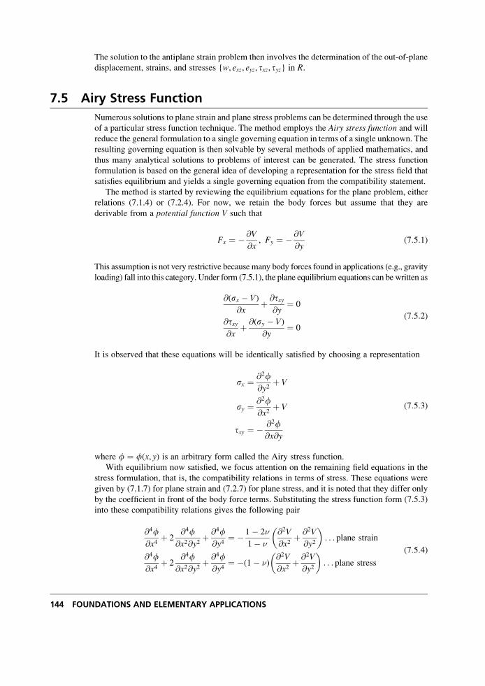
The solution to the antiplane strain problem then involves the determination of the out-of-plane
displacement, strains, and stresses {w, exz, eyz, txz, tyz} in R.
7.5 Airy Stress Function
Numerous solutions to plane strain and plane stress problems can be determined through the use
of a particular stress function technique. The method employs the Airy stress function and will
reduce the general formulation to a single governing equation in terms of a single unknown. The
resulting governing equation is then solvable by several methods of applied mathematics, and
thus many analytical solutions to problems of interest can be generated. The stress function
formulation is based on the general idea of developing a representation for the stress field that
satisfies equilibrium and yields a single governing equation from the compatibility statement.
The method is started by reviewing the equilibrium equations for the plane problem, either
relations (7.1.4) or (7.2.4). For now, we retain the body forces but assume that they are
derivable from a potential function V such that
Fx ¼ � @V
@x, Fy ¼ � @V
@y(7:5:1)
This assumption is not very restrictive becausemany body forces found in applications (e.g., gravity
loading) fall into this category. Under form (7.5.1), the plane equilibrium equations can bewritten as
@(sx � V)
@xþ @txy
@y¼ 0
@txy@x
þ @(sy � V)
@y¼ 0
(7:5:2)
It is observed that these equations will be identically satisfied by choosing a representation
sx ¼ @2f@y2
þ V
sy ¼ @2f@x2
þ V
txy ¼ � @2f@x@y
(7:5:3)
where f ¼ f(x, y) is an arbitrary form called the Airy stress function.
With equilibrium now satisfied, we focus attention on the remaining field equations in the
stress formulation, that is, the compatibility relations in terms of stress. These equations were
given by (7.1.7) for plane strain and (7.2.7) for plane stress, and it is noted that they differ only
by the coefficient in front of the body force terms. Substituting the stress function form (7.5.3)
into these compatibility relations gives the following pair
@4f@x4
þ 2@4f
@x2@y2þ @4f
@y4¼ � 1� 2�
1� �
@2V
@x2þ @2V
@y2
� �. . . plane strain
@4f@x4
þ 2@4f
@x2@y2þ @4f
@y4¼ �(1� �)
@2V
@x2þ @2V
@y2
� �. . . plane stress
(7:5:4)
144 FOUNDATIONS AND ELEMENTARY APPLICATIONS
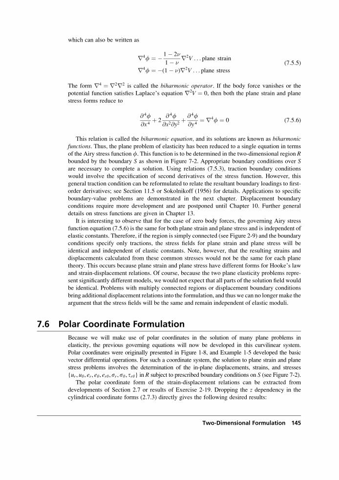
which can also be written as
r4f ¼ � 1� 2�
1� �r2V . . . plane strain
r4f ¼ �(1� �)r2V . . . plane stress
(7:5:5)
The form r4 ¼ r2r2 is called the biharmonic operator. If the body force vanishes or the
potential function satisfies Laplace’s equation r2V ¼ 0, then both the plane strain and plane
stress forms reduce to
@ 4f@x4
þ 2@ 4f
@x2@y2þ @ 4f
@y4¼ r4f ¼ 0 (7:5:6)
This relation is called the biharmonic equation, and its solutions are known as biharmonicfunctions. Thus, the plane problem of elasticity has been reduced to a single equation in terms
of the Airy stress function f. This function is to be determined in the two-dimensional region Rbounded by the boundary S as shown in Figure 7-2. Appropriate boundary conditions over Sare necessary to complete a solution. Using relations (7.5.3), traction boundary conditions
would involve the specification of second derivatives of the stress function. However, this
general traction condition can be reformulated to relate the resultant boundary loadings to first-
order derivatives; see Section 11.5 or Sokolnikoff (1956) for details. Applications to specific
boundary-value problems are demonstrated in the next chapter. Displacement boundary
conditions require more development and are postponed until Chapter 10. Further general
details on stress functions are given in Chapter 13.
It is interesting to observe that for the case of zero body forces, the governing Airy stress
function equation (7.5.6) is the same for both plane strain and plane stress and is independent of
elastic constants. Therefore, if the region is simply connected (see Figure 2-9) and the boundary
conditions specify only tractions, the stress fields for plane strain and plane stress will be
identical and independent of elastic constants. Note, however, that the resulting strains and
displacements calculated from these common stresses would not be the same for each plane
theory. This occurs because plane strain and plane stress have different forms for Hooke’s law
and strain-displacement relations. Of course, because the two plane elasticity problems repre-
sent significantly different models, we would not expect that all parts of the solution field would
be identical. Problems with multiply connected regions or displacement boundary conditions
bring additional displacement relations into the formulation, and thus we can no longer make the
argument that the stress fields will be the same and remain independent of elastic moduli.
7.6 Polar Coordinate Formulation
Because we will make use of polar coordinates in the solution of many plane problems in
elasticity, the previous governing equations will now be developed in this curvilinear system.
Polar coordinates were originally presented in Figure 1-8, and Example 1-5 developed the basic
vector differential operations. For such a coordinate system, the solution to plane strain and plane
stress problems involves the determination of the in-plane displacements, strains, and stresses
{ur , uy, er, ey, ery,sr ,sy, try} in R subject to prescribed boundary conditions on S (see Figure 7-2).The polar coordinate form of the strain-displacement relations can be extracted from
developments of Section 2.7 or results of Exercise 2-19. Dropping the z dependency in the
cylindrical coordinate forms (2.7.3) directly gives the following desired results:
Two-Dimensional Formulation 145
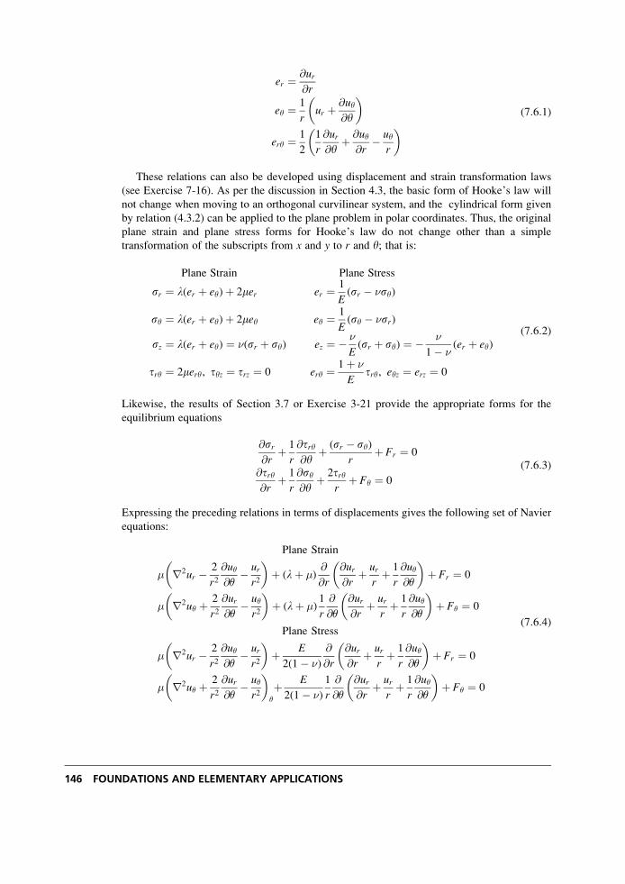
er ¼ @ur@r
ey ¼ 1
rur þ @uy
@y
� �
ery ¼ 1
2
1
r
@ur@y
þ @uy@r
� uyr
� � (7:6:1)
These relations can also be developed using displacement and strain transformation laws
(see Exercise 7-16). As per the discussion in Section 4.3, the basic form of Hooke’s law will
not change when moving to an orthogonal curvilinear system, and the cylindrical form given
by relation (4.3.2) can be applied to the plane problem in polar coordinates. Thus, the original
plane strain and plane stress forms for Hooke’s law do not change other than a simple
transformation of the subscripts from x and y to r and y; that is:
Plane Strain Plane Stress
sr ¼ l(er þ ey)þ 2mer er ¼ 1
E(sr � �sy)
sy ¼ l(er þ ey)þ 2mey ey ¼ 1
E(sy � �sr)
sz ¼ l(er þ ey) ¼ �(sr þ sy) ez ¼ � �
E(sr þ sy) ¼ � �
1� �(er þ ey)
try ¼ 2mery, tyz ¼ trz ¼ 0 ery ¼ 1þ �
Etry, eyz ¼ erz ¼ 0
(7:6:2)
Likewise, the results of Section 3.7 or Exercise 3-21 provide the appropriate forms for the
equilibrium equations
@sr@r
þ 1
r
@try@y
þ (sr � sy)r
þ Fr ¼ 0
@try@r
þ 1
r
@sy@y
þ 2tryr
þ Fy ¼ 0
(7:6:3)
Expressing the preceding relations in terms of displacements gives the following set of Navier
equations:
Plane Strain
� r2ur � 2
r2@u�@�
� urr2
� �þ (lþ �)
@
@r
@ur@r
þ urrþ 1
r
@u�@�
� �þ Fr ¼ 0
� r2uy þ 2
r2@ur@�
� u�r2
� �þ (lþ �)
1
r
@
@�
@ur@r
þ urrþ 1
r
@u�@�
� �þ F� ¼ 0
Plane Stress
� r2ur � 2
r2@u�@�
� urr2
� �þ E
2(1� �)
@
@r
@ur@r
þ urrþ 1
r
@u�@�
� �þ Fr ¼ 0
� r2u� þ 2
r2@ur@�
� u�r2
� ��
þ E
2(1� �)
1
r
@
@�
@ur@r
þ urrþ 1
r
@u�@�
� �þ F� ¼ 0
(7:6:4)
146 FOUNDATIONS AND ELEMENTARY APPLICATIONS
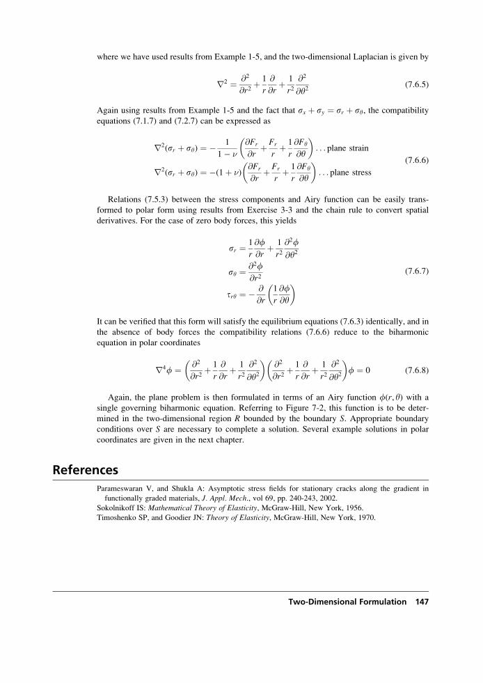
where we have used results from Example 1-5, and the two-dimensional Laplacian is given by
r2 ¼ @2
@r2þ 1
r
@
@rþ 1
r2@2
@y2(7:6:5)
Again using results from Example 1-5 and the fact that sx þ sy ¼ sr þ sy, the compatibility
equations (7.1.7) and (7.2.7) can be expressed as
r2(sr þ sy) ¼ � 1
1� �
@Fr
@rþ Fr
rþ 1
r
@Fy
@y
� �. . . plane strain
r2(sr þ sy) ¼ �(1þ �)@Fr
@rþ Fr
rþ 1
r
@Fy
@y
� �. . . plane stress
(7:6:6)
Relations (7.5.3) between the stress components and Airy function can be easily trans-
formed to polar form using results from Exercise 3-3 and the chain rule to convert spatial
derivatives. For the case of zero body forces, this yields
sr ¼ 1
r
@f@r
þ 1
r2@2f
@y2
sy ¼ @2f@r2
try ¼ � @
@r
1
r
@f@y
� � (7:6:7)
It can be verified that this form will satisfy the equilibrium equations (7.6.3) identically, and in
the absence of body forces the compatibility relations (7.6.6) reduce to the biharmonic
equation in polar coordinates
r4f ¼ @2
@r2þ 1
r
@
@rþ 1
r2@2
@y2
� �@2
@r2þ 1
r
@
@rþ 1
r2@2
@y2
� �f ¼ 0 (7:6:8)
Again, the plane problem is then formulated in terms of an Airy function f(r, y) with a
single governing biharmonic equation. Referring to Figure 7-2, this function is to be deter-
mined in the two-dimensional region R bounded by the boundary S. Appropriate boundary
conditions over S are necessary to complete a solution. Several example solutions in polar
coordinates are given in the next chapter.
References
Parameswaran V, and Shukla A: Asymptotic stress fields for stationary cracks along the gradient in
functionally graded materials, J. Appl. Mech., vol 69, pp. 240-243, 2002.Sokolnikoff IS: Mathematical Theory of Elasticity, McGraw-Hill, New York, 1956.
Timoshenko SP, and Goodier JN: Theory of Elasticity, McGraw-Hill, New York, 1970.
Two-Dimensional Formulation 147
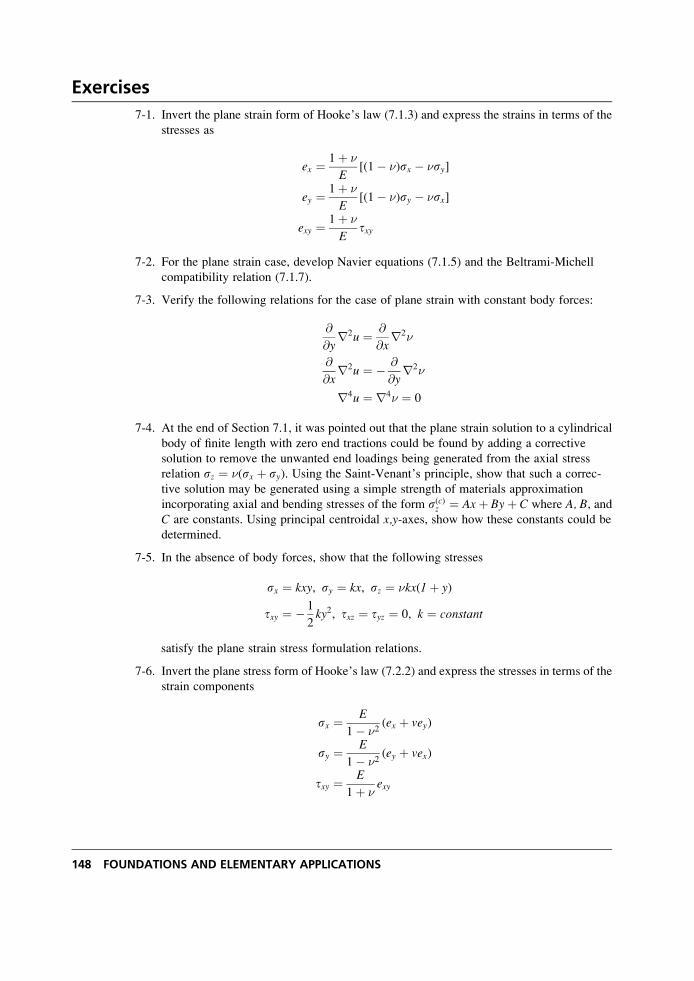
Exercises
7-1. Invert the plane strain form of Hooke’s law (7.1.3) and express the strains in terms of the
stresses as
ex ¼ 1þ �
E[(1� �)sx � �sy]
ey ¼ 1þ �
E[(1� �)sy � �sx]
exy ¼ 1þ �
Etxy
7-2. For the plane strain case, develop Navier equations (7.1.5) and the Beltrami-Michell
compatibility relation (7.1.7).
7-3. Verify the following relations for the case of plane strain with constant body forces:
@
@yr2u ¼ @
@xr2�
@
@xr2u ¼ � @
@yr2�
r4u ¼ r4� ¼ 0
7-4. At the end of Section 7.1, it was pointed out that the plane strain solution to a cylindrical
body of finite length with zero end tractions could be found by adding a corrective
solution to remove the unwanted end loadings being generated from the axial stress
relation sz ¼ �(sx þ sy). Using the Saint-Venant’s principle, show that such a correc-
tive solution may be generated using a simple strength of materials approximation
incorporating axial and bending stresses of the form s(c)z ¼ Axþ Byþ C where A, B, andC are constants. Using principal centroidal x,y-axes, show how these constants could be
determined.
7-5. In the absence of body forces, show that the following stresses
sx ¼ kxy, sy ¼ kx, sz ¼ �kx(1þ y)
txy ¼ � 1
2ky2, txz ¼ tyz ¼ 0, k ¼ constant
satisfy the plane strain stress formulation relations.
7-6. Invert the plane stress form of Hooke’s law (7.2.2) and express the stresses in terms of the
strain components
sx ¼ E
1� �2(ex þ vey)
sy ¼ E
1� �2(ey þ vex)
txy ¼ E
1þ �exy
148 FOUNDATIONS AND ELEMENTARY APPLICATIONS
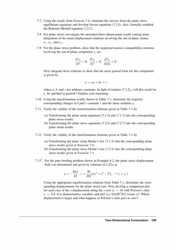
7-7. Using the results from Exercise 7-6, eliminate the stresses from the plane stress
equilibrium equations and develop Navier equations (7.2.5). Also, formally establish
the Beltrami-Michell equation (7.2.7).
7-8. For plane stress, investigate the unwanted three-dimensional results coming from
integration of the strain-displacement relations involving the out-of-plane strains
ez, exz, and eyz.
7-9. For the plane stress problem, show that the neglected nonzero compatibility relations
involving the out-of-plane component ez are
@2ez@x2
¼ 0,@2ez@y2
¼ 0,@2ez@x@y
¼ 0
Next integrate these relations to show that the most general form for this component
is given by
ez ¼ axþ byþ c
where a, b, and c are arbitrary constants. In light of relation (7.2.2)3, will this result for
ez be satisfied in general? Explain your reasoning.
7-10. Using the transformation results shown in Table 7-1, determine the required
corresponding changes in Lame’s constant l and the shear modulus �.
7-11. Verify the validity of the transformation relations given in Table 7-1 by
(a) Transforming the plane strain equations (7.1.5) and (7.1.7) into the corresponding
plane stress results.
(b) Transforming the plane stress equations (7.2.5) and (7.2.7) into the corresponding
plane strain results.
7-12. Verify the validity of the transformation relations given in Table 7-1 by
(a) Transforming the plane strain Hooke’s law (7.1.3) into the corresponding plane
stress results given in Exercise 7-6.
(b) Transforming the plane stress Hooke’s law (7.2.2) into the corresponding plane
stress results given in Exercise 7-1.
7-13*. For the pure bending problem shown in Example 8-2, the plane stress displacement
field was determined and given by relations (8.1.22)2 as
u ¼ �Mxy
EI, v ¼ M
2EI[�y2 þ x2 � l2], � l � x � l
Using the appropriate transformation relations from Table 7-1, determine the corre-
sponding displacements for the plane strain case. Next develop a comparison plot
for each case of the y-displacement along the x-axis (y ¼ 0) with Poisson’s ratio
� ¼ 0.4. Use dimensionless variables and plot v(x, 0)/(Ml2/EI) versus x/l. Which
displacement is larger and what happens as Poisson’s ratio goes to zero?
Two-Dimensional Formulation 149
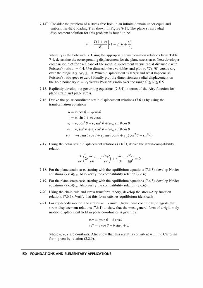
7-14*. Consider the problem of a stress-free hole in an infinite domain under equal and
uniform far-field loading T as shown in Figure 8-11. The plane strain radial
displacement solution for this problem is found to be
ur ¼ T(1þ �)
E(1� 2�)r þ r21
r
� �
where r1 is the hole radius. Using the appropriate transformation relations from Table
7-1, determine the corresponding displacement for the plane stress case. Next develop a
comparison plot for each case of the radial displacement versus radial distance r withPoisson’s ratio � ¼ 0.4. Use dimensionless variables and plot ur /(Tr1/E) versus r/r1over the range 0 � r/r1 � 10. Which displacement is larger and what happens as
Poisson’s ratio goes to zero? Finally plot the dimensionless radial displacement on
the hole boundary r ¼ r1 versus Poisson’s ratio over the range 0 � � � 0.5
7-15. Explicitly develop the governing equations (7.5.4) in terms of the Airy function for
plane strain and plane stress.
7-16. Derive the polar coordinate strain-displacement relations (7.6.1) by using the
transformation equations
u ¼ ur cos y� uy sin y
v ¼ ur sin yþ uy cos y
er ¼ ex cos2 yþ ey sin
2 yþ 2exy sin y cos y
ey ¼ ex sin2 yþ ey cos
2 y� 2exy sin y cos y
ery ¼ �ex sin y cos yþ ey sin y cos yþ exy( cos2 y� sin2 y)
7-17. Using the polar strain-displacement relations (7.6.1), derive the strain-compatibility
relation
@
@r2r
@ery@y
� r2@ey@r
� �þ r
@er@r
� @2er
@y2¼ 0
7-18. For the plane strain case, starting with the equilibrium equations (7.6.3), develop Navier
equations (7.6.4)1,2. Also verify the compatibility relation (7.6.6)1.
7-19. For the plane stress case, starting with the equilibrium equations (7.6.3), develop Navier
equations (7.6.4)3,4. Also verify the compatibility relation (7.6.6)2.
7-20. Using the chain rule and stress transform theory, develop the stress-Airy function
relations (7.6.7). Verify that this form satisfies equilibrium identically.
7-21. For rigid-body motion, the strains will vanish. Under these conditions, integrate the
strain-displacement relations (7.6.1) to show that the most general form of a rigid-body
motion displacement field in polar coordinates is given by
ur* ¼ a sin yþ b cos y
uy* ¼ a cos y� b sin yþ cr
where a, b, c are constants. Also show that this result is consistent with the Cartesian
form given by relation (2.2.9).
150 FOUNDATIONS AND ELEMENTARY APPLICATIONS
8 Two-Dimensional Problem Solution
The previous chapter developed the general formulation for the plane problem in elasticity.
This formulation results in two types of in-plane problems—plane strain and plane stress. It
was further shown that solution to each of these problem types could be conveniently handled
using the Airy stress function approach. This scheme reduces the field equations to a single
partial differential equation, and for the case of zero body forces, this result was the biharmo-
nic equation. Thus, the plane elasticity problem was reduced to finding the solution to the
biharmonic equation in a particular domain of interest. Such a solution must also satisfy the
given boundary conditions associated with the particular problem under study. Several general
solution techniques were briefly discussed in Section 5.7. These include the use of power series
or polynomials and Fourier methods. We now pursue the solution to several two-dimensional
problems using these methods. Our formulation and solution are conducted using both Carte-
sian and polar coordinate systems. In many cases we use MATLAB software to plot the stress
and displacement field distributions in order to better understand the nature of the solution.
Plane problems can also be solved using complex variable theory, and this powerful method is
discussed in Chapter 10.
8.1 Cartesian Coordinate Solutions Using Polynomials
We begin the solution to plane elasticity problems with no body forces by considering
problems formulated in Cartesian coordinates. When taking boundary conditions into account,
this formulation is most useful for problems with rectangular domains. The method is based on
the inverse solution concept where we assume a form of the solution to the biharmonic
equation
@4f@x4
þ 2@4f
@x2@y2þ @4f
@y4¼ 0 (8:1:1)
and then try to determine which problem may be solved by this solution. The assumed solution
form for the Airy stress function is taken to be a general polynomial of the in-plane coordin-
ates, and this form can be conveniently expressed in the power series
151
f(x, y) ¼X1m¼0
X1n¼0
Amn xmyn (8:1:2)
where Amn are constant coefficients to be determined. This representation was given by Neou
(1957), who proposed a systematic scheme to solve such plane problems.
Using the stress-stress function relations (7.5.3) with zero body forces
sx ¼ @2f@y2
, sy ¼ @2f@x2
, txy ¼ � @2f@x@y
(8:1:3)
Note that in the Airy function form the three lowest-order terms with mþ n � 1 do not
contribute to the stresses and therefore are dropped. It is observed that second-order terms
produce a constant stress field, third-order terms give a linear distribution of stress, and so on
for higher-order polynomials.
Terms with mþ n � 3 automatically satisfy the biharmonic equation (8.1.1) for any choice
of constants Amn. However, for higher-order terms with mþ n > 3, the constants Amn must be
related in order to have the polynomial satisfy the biharmonic equation. For example, the
fourth-order polynomial terms A40x4 þ A22x
2y2 þ A04y4 will not satisfy the biharmonic equa-
tion unless 3A40 þ A22 þ 3A04 ¼ 0. This condition specifies one constant in terms of the other
two, thus leaving two constants to be determined by the boundary conditions.
Considering the general case, substituting the series form (8.1.2) into the governing
biharmonic equation (8.1.1) yields
X1m¼4
X1n¼0
m(m� 1)(m� 2)(m� 3)Amn xm�4yn
þ 2X1m¼2
X1n¼2
m(m� 1)n(n� 1)Amn xm�2yn�2
þX1m¼0
X1n¼4
n(n� 1)(n� 2)(n� 3)Amn xmyn�4 ¼ 0
(8:1:4)
Collecting like powers of x and y, the preceding equation may be written as
X1m¼2
X1n¼2
[(mþ 2)(mþ 1)m(m� 1)Amþ2, n�2 þ 2m(m� 1)n(n� 1)Amn
þ (nþ 2)(nþ 1)n(n� 1)Am�2, nþ2]xm�2yn�2 ¼ 0
(8:1:5)
Because this relation must be satisfied for all values of x and y, the coefficient in brackets must
vanish, giving the result
(mþ 2)(mþ 1)m(m� 1)Amþ2, n�2 þ 2m(m� 1)n(n� 1)Amn
þ (nþ 2)(nþ 1)n(n� 1)Am�2, nþ2 ¼ 0(8:1:6)
For each m,n pair, (8.1.6) is the general relation that must be satisfied to ensure that the
polynomial grouping is biharmonic. Note that the fourth-order case (m ¼ n ¼ 2) was previously
discussed.
Because this method produces polynomial stress distributions, we would not expect the
scheme to satisfy general boundary conditions. However, this limitation can be circumvented
152 FOUNDATIONS AND ELEMENTARY APPLICATIONS
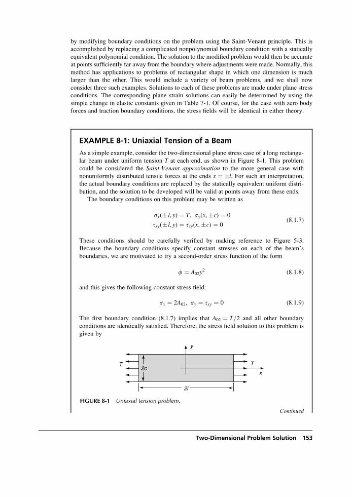
by modifying boundary conditions on the problem using the Saint-Venant principle. This is
accomplished by replacing a complicated nonpolynomial boundary condition with a statically
equivalent polynomial condition. The solution to the modified problem would then be accurate
at points sufficiently far away from the boundary where adjustments were made. Normally, this
method has applications to problems of rectangular shape in which one dimension is much
larger than the other. This would include a variety of beam problems, and we shall now
consider three such examples. Solutions to each of these problems are made under plane stress
conditions. The corresponding plane strain solutions can easily be determined by using the
simple change in elastic constants given in Table 7-1. Of course, for the case with zero body
forces and traction boundary conditions, the stress fields will be identical in either theory.
EXAMPLE 8-1: Uniaxial Tension of a Beam
As a simple example, consider the two-dimensional plane stress case of a long rectangu-
lar beam under uniform tension T at each end, as shown in Figure 8-1. This problem
could be considered the Saint-Venant approximation to the more general case with
nonuniformly distributed tensile forces at the ends x ¼ �l. For such an interpretation,
the actual boundary conditions are replaced by the statically equivalent uniform distri-
bution, and the solution to be developed will be valid at points away from these ends.
The boundary conditions on this problem may be written as
sx(� l, y) ¼ T, sy(x,�c) ¼ 0
txy(� l, y) ¼ txy(x,�c) ¼ 0(8:1:7)
These conditions should be carefully verified by making reference to Figure 5-3.
Because the boundary conditions specify constant stresses on each of the beam’s
boundaries, we are motivated to try a second-order stress function of the form
f ¼ A02y2 (8:1:8)
and this gives the following constant stress field:
sx ¼ 2A02, sy ¼ txy ¼ 0 (8:1:9)
The first boundary condition (8.1.7) implies that A02 ¼ T=2 and all other boundary
conditions are identically satisfied. Therefore, the stress field solution to this problem is
given by
Continued
x
y
TT
2l
2c
FIGURE 8-1 Uniaxial tension problem.
Two-Dimensional Problem Solution 153
EXAMPLE 8-1: Uniaxial Tension of a Beam–Cont’d
sx ¼ T, sy ¼ txy ¼ 0 (8:1:10)
Next we wish to determine the displacement field associated with this stress distribution.
This is accomplished by a standard procedural technique. First, the strain field is calculated
using Hooke’s law. Then the strain-displacement relations are used to determine various
displacement gradients, and these expressions are integrated to find the individual displace-
ments. Using this scheme, the in-plane displacement gradients are found to be
@u
@x¼ ex ¼ 1
E(sx � �sy) ¼ T
E@v
@y¼ ey ¼ 1
E(sy � �sx) ¼ ��
T
E
(8:1:11)
These results are easily integrated to get
u ¼ T
Exþ f (y)
v ¼ ��T
Eyþ g(x)
(8:1:12)
where f(y) and g(x) are arbitrary functions of the indicated variable coming from the
integration process. To complete the problem solution, these functions must be deter-
mined, and this is accomplished using the remaining Hooke’s law and the strain-
displacement relation for the shear stress and strain
@u
@yþ @v
@x¼ 2exy ¼ tx y
m¼ 0 ) f 0(y)þ g0(x) ¼ 0 (8:1:13)
This result can be separated into two independent relations g0(x) ¼ �f 0(y) ¼ constant
and integrated to get
f (y) ¼ �!oyþ uo
g(x) ¼ !oxþ vo(8:1:14)
where !o, uo, vo are arbitrary constants of integration. The expressions given by
relation (8.1.14) represent rigid-body motion terms where !o is the rotation about the
z-axis and uo and vo are the translations in the x and y directions. Such terms will always
result from the integration of the strain-displacement relations, and it is noted that they
do not contribute to the strain or stress fields. Thus, the displacements are determinedfrom the strain field only up to an arbitrary rigid-body motion. Additional displacement
boundary conditions, referred to here as fixity conditions, are needed to explicitly
determine these rigid-body motion terms. For two-dimensional problems, fixity condi-
tions would require three independent statements commonly involving specification of
the x- and y-displacements and rotation at a particular point. The choice of such
conditions is normally made based on the expected deformation of the physical prob-
lem. For example, if we agree that the center of the beam does not move and the x-axisdoes not rotate, all rigid-body terms will vanish and f ¼ g ¼ 0.
154 FOUNDATIONS AND ELEMENTARY APPLICATIONS
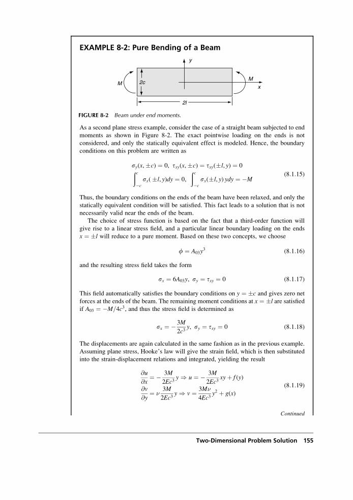
EXAMPLE 8-2: Pure Bending of a Beam
As a second plane stress example, consider the case of a straight beam subjected to end
moments as shown in Figure 8-2. The exact pointwise loading on the ends is not
considered, and only the statically equivalent effect is modeled. Hence, the boundary
conditions on this problem are written as
sy(x,�c) ¼ 0, txy(x,�c) ¼ txy(�l, y) ¼ 0ðc�c
sx(�l, y)dy ¼ 0,
ðc�c
sx(�l, y) ydy ¼ �M(8:1:15)
Thus, the boundary conditions on the ends of the beam have been relaxed, and only the
statically equivalent condition will be satisfied. This fact leads to a solution that is not
necessarily valid near the ends of the beam.
The choice of stress function is based on the fact that a third-order function will
give rise to a linear stress field, and a particular linear boundary loading on the ends
x ¼ �l will reduce to a pure moment. Based on these two concepts, we choose
f ¼ A03y3 (8:1:16)
and the resulting stress field takes the form
sx ¼ 6A03y, sy ¼ txy ¼ 0 (8:1:17)
This field automatically satisfies the boundary conditions on y ¼ �c and gives zero net
forces at the ends of the beam. The remaining moment conditions at x ¼ �l are satisfiedif A03 ¼ �M=4c3, and thus the stress field is determined as
sx ¼ � 3M
2c3y, sy ¼ txy ¼ 0 (8:1:18)
The displacements are again calculated in the same fashion as in the previous example.
Assuming plane stress, Hooke’s law will give the strain field, which is then substituted
into the strain-displacement relations and integrated, yielding the result
@u
@x¼ � 3M
2Ec3y ) u ¼ � 3M
2Ec3xyþ f (y)
@v
@y¼ �
3M
2Ec3y ) v ¼ 3M�
4Ec3y2 þ g(x)
(8:1:19)
Continued
x
y
MM
2l
2c
FIGURE 8-2 Beam under end moments.
Two-Dimensional Problem Solution 155
EXAMPLE 8-2: Pure Bending of a Beam–Cont’d
where f and g are arbitrary functions of integration. Using the shear stress-strain
relations
@u
@yþ @v
@x¼ 0 ) � 3M
2Ec3xþ f 0(y)þ g0(x) ¼ 0 (8:1:20)
This result can again be separated into two independent relations in x and y, and upon
integration the arbitrary functions f and g are determined as
f (y) ¼ �!oyþ uo
g(x) ¼ 3M
4Ec3x2 þ !oxþ vo
(8:1:21)
Again, rigid-body motion terms are brought out during the integration process. For this
problem, the beam would normally be simply supported, and thus the fixity displacement
boundary conditions could be specified as v(�l, 0) ¼ 0 and u(�l, 0) ¼ 0. This specifica-
tion leads to determination of the rigid-body terms as uo ¼ !o ¼ 0, vo ¼ �3Ml2=4Ec3.We now wish to compare this elasticity solution with that developed by elementary
strength of materials (often called mechanics of materials). Appendix D, Section D.3,
conveniently provides a brief review of this undergraduate theory. Introducing the
cross-sectional area moment of inertia I ¼ 2c3=3 (assuming unit thickness), our stress
and displacement field can be written as
sx ¼�M
Iy, sy ¼ txy ¼ 0
u ¼�Mxy
EI, v ¼ M
2EI[�y2 þ x2 � l2]
(8:1:22)
Note that for this simple moment-loading case, we have verified the classic assumption
from elementary beam theory that plane sections remain plane. Note, however, that thiswill not be the case for more complicated loadings. The elementary strength of mater-
ials solution is obtained using Euler-Bernoulli beam theory and gives the bending stress
and deflection of the beam centerline as
sx ¼ �M
Iy, sy ¼ txy ¼ 0
v ¼ v(x, 0) ¼ M
2EI[x2 � l2]
(8:1:23)
Comparing these two solutions, it is observed that they are identical, with the exception
of the x displacements. In general, however, the two theories will not match for other
beam problems with more complicated loadings, and we investigate such a problem in
the next example.
156 FOUNDATIONS AND ELEMENTARY APPLICATIONS
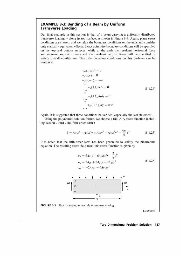
EXAMPLE 8-3: Bending of a Beam by UniformTransverse Loading
Our final example in this section is that of a beam carrying a uniformly distributed
transverse loading w along its top surface, as shown in Figure 8-3. Again, plane stress
conditions are chosen, and we relax the boundary conditions on the ends and consider
only statically equivalent effects. Exact pointwise boundary conditions will be specified
on the top and bottom surfaces, while at the ends the resultant horizontal force
and moment are set to zero and the resultant vertical force will be specified to
satisfy overall equilibrium. Thus, the boundary conditions on this problem can be
written as
txy(x,� c) ¼ 0
sy(x, c) ¼ 0
sy(x,�c) ¼ �wðc�c
sx(�l, y)dy ¼ 0ðc�c
sx(�l, y)ydy ¼ 0ðc�c
txy(�l, y)dy ¼ �wl
(8:1:24)
Again, it is suggested that these conditions be verified, especially the last statement.
Using the polynomial solution format, we choose a trial Airy stress function includ-
ing second-, third-, and fifth-order terms:
f ¼ A20x2 þ A21x
2yþ A03y3 þ A23x
2y3 � A23
5y5 (8:1:25)
It is noted that the fifth-order term has been generated to satisfy the biharmonic
equation. The resulting stress field from this stress function is given by
sx ¼ 6A03yþ 6A23(x2y� 2
3y3)
sy ¼ 2A20 þ 2A21yþ 2A23y3
txy ¼ �2A21x� 6A23xy2
(8:1:26)
Continued
x
y
w
2c
2l
wl wl
FIGURE 8-3 Beam carrying uniformly transverse loading.
Two-Dimensional Problem Solution 157
EXAMPLE 8-3: Bending of a Beam by UniformTransverse Loading–Cont’d
Applying the first three boundary conditions in the set (8.1.24) gives three equations
among the unknown coefficients A20, A21, and A23. Solving this system determines these
constants, giving the result
A20 ¼ �w
4, A21 ¼ 3w
8c, A23 ¼ � w
8c3(8:1:27)
Using these results, it is found that the stress field will now also satisfy the fourth and sixth
conditions in (8.1.24). The remaining condition of vanishing end moments gives the
following
A03 ¼ �A23(l2 � 2
5c2) ¼ w
8c
l2
c2� 2
5
� �(8:1:28)
This completes determination of the four constants in the trial Airy stress function, and
the resulting stress field is now given by
sx ¼ 3w
4c
l2
c2� 2
5
� �y� 3w
4c3x2y� 2
3y3
� �
sy ¼ �w
2þ 3w
4cy� w
4c3y3
txy ¼ � 3w
4cxþ 3w
4c3xy2
(8:1:29)
We again wish to compare this elasticity solution with that developed by elementary
strength of materials, and thus the elasticity stress field is rewritten in terms of the cross-
sectional area moment of inertia I ¼ 2c3=3, as
sx ¼ w
2I(l2 � x2)yþ w
I
y3
3� c2y
5
� �
sy ¼ � w
2I
y3
3� c2yþ 2
3c3
� �
txy ¼ � w
2Ix(c2 � y2)
(8:1:30)
The corresponding results from strength of materials for this case (see Appendix D,
Section D.3) are given by
sx ¼ My
I¼ w
2I(l2 � x2)y
sy ¼ 0
txy ¼ VQ
It¼ � w
2Ix(c2 � y2)
(8:1:31)
where the bendingmomentM ¼ w(l2 � x2)=2, the shear forceV ¼ �wx, the first moment
of a sectioned cross-sectional area isQ ¼ (c2 � y2)=2, and the thickness t is taken as unity.Comparing the two theories, we see that the shear stresses are identical, while the two
normal stresses are not. The two normal stress distributions are plotted in Figures 8-4
and 8-5. The normalized bending stress sx for the case x ¼ 0 is shown in Figure 8-4.
158 FOUNDATIONS AND ELEMENTARY APPLICATIONS
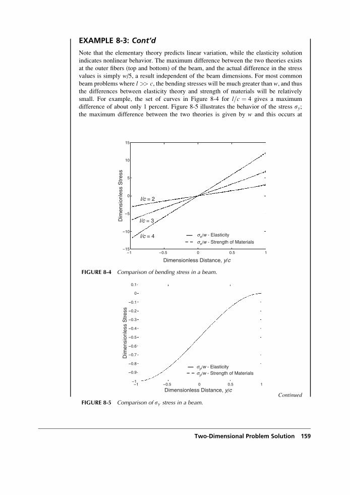
EXAMPLE 8-3: Cont’d
Note that the elementary theory predicts linear variation, while the elasticity solution
indicates nonlinear behavior. The maximum difference between the two theories exists
at the outer fibers (top and bottom) of the beam, and the actual difference in the stress
values is simply w/5, a result independent of the beam dimensions. For most common
beam problems where l >> c, the bending stresses will be much greater than w, and thusthe differences between elasticity theory and strength of materials will be relatively
small. For example, the set of curves in Figure 8-4 for l=c ¼ 4 gives a maximum
difference of about only 1 percent. Figure 8-5 illustrates the behavior of the stress sy;the maximum difference between the two theories is given by w and this occurs at
Continued
sx/w - Elasticity
sx/w - Strength of Materials
l/c = 2
l/c = 4
l/c = 3Dim
ensi
onle
ss S
tres
s
Dimensionless Distance, y/c
10
5
0
-5
-10
15
-15-0.5 0.5-1 10
FIGURE 8-4 Comparison of bending stress in a beam.
sy/w - Strength of Materialssy/w - Elasticity
Dimensionless Distance, y/c
Dim
ensi
onle
ss S
tres
s
-0.5 0 0.5-1 1
-0.9
-0.8
-0.7
-0.6
-0.5
-0.4
-0.3
-0.2
-0.1
0
-1
0.1
FIGURE 8-5 Comparison of sy stress in a beam.
Two-Dimensional Problem Solution 159
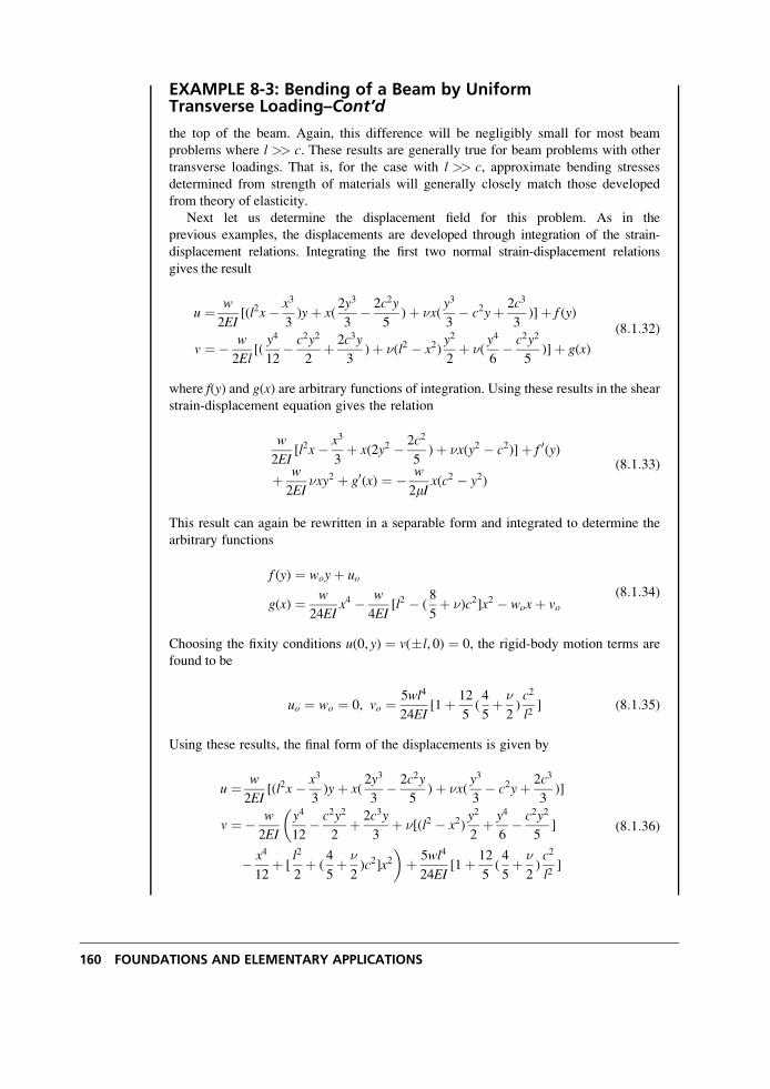
EXAMPLE 8-3: Bending of a Beam by UniformTransverse Loading–Cont’d
the top of the beam. Again, this difference will be negligibly small for most beam
problems where l >> c. These results are generally true for beam problems with other
transverse loadings. That is, for the case with l >> c, approximate bending stresses
determined from strength of materials will generally closely match those developed
from theory of elasticity.
Next let us determine the displacement field for this problem. As in the
previous examples, the displacements are developed through integration of the strain-
displacement relations. Integrating the first two normal strain-displacement relations
gives the result
u ¼ w
2EI[(l2x� x3
3)yþ x(
2y3
3� 2c2y
5)þ �x(
y3
3� c2yþ 2c3
3)]þ f (y)
v ¼� w
2El[(y4
12� c2y2
2þ 2c3y
3)þ �(l2 � x2)
y2
2þ �(
y4
6� c2y2
5)]þ g(x)
(8:1:32)
where f(y) and g(x) are arbitrary functions of integration. Using these results in the shearstrain-displacement equation gives the relation
w
2EI[l2x� x3
3þ x(2y2 � 2c2
5)þ �x(y2 � c2)]þ f 0(y)
þ w
2EI�xy2 þ g0(x) ¼ � w
2mIx(c2 � y2)
(8:1:33)
This result can again be rewritten in a separable form and integrated to determine the
arbitrary functions
f (y) ¼ woyþ uo
g(x) ¼ w
24EIx4 � w
4EI[l2 � (
8
5þ �)c2]x2 � woxþ vo
(8:1:34)
Choosing the fixity conditions u(0, y) ¼ v(�l, 0) ¼ 0, the rigid-body motion terms are
found to be
uo ¼ wo ¼ 0, vo ¼ 5wl4
24EI[1þ 12
5(4
5þ �
2)c2
l2] (8:1:35)
Using these results, the final form of the displacements is given by
u ¼ w
2EI[(l2x� x3
3)yþ x(
2y3
3� 2c2y
5)þ �x(
y3
3� c2yþ 2c3
3)]
v ¼� w
2EI
y4
12� c2y2
2þ 2c3y
3þ �[(l2 � x2)
y2
2þ y4
6� c2y2
5]
�
� x4
12þ [
l2
2þ (
4
5þ �
2)c2]x2
�þ 5wl4
24EI[1þ 12
5(4
5þ �
2)c2
l2]
(8:1:36)
160 FOUNDATIONS AND ELEMENTARY APPLICATIONS
EXAMPLE 8-3: Cont’d
The maximum deflection of the beam axis is given by
v(0, 0) ¼ vmax ¼ 5wl4
24EI1þ 12
5
4
5þ �
2
� �c2
l2
� �(8:1:37)
while the corresponding value calculated from strength of materials is
vmax ¼ 5wl4
24EI(8:1:38)
The difference between the two theories given by relations (8.1.37) and (8.1.38) is
specified bywl4
2EI
4
5þ �
2
� �c2
l2, and this term is caused by the presence of the shear force.
For beams where l >> c, this difference is very small. Thus, we again find that for long
beams, strength of materials predictions match closely to theory of elasticity results.
Note from equation (8.1.36), the x component of displacement indicates that plane
sections undergo nonlinear deformation and do not remain plane. It can also be shown
that the Euler-Bernoulli relationM ¼ EId2v(x, 0)
dx2used in strength of materials theory is
not satisfied by this elasticity solution. Timoshenko and Goodier (1970) provide add-
itional discussion on such differences.
Additional rectangular beam problems of this type with different support and loading
conditions can be solved using various polynomial combinations. Several of these are given
in the exercises.
8.2 Cartesian Coordinate Solutions Using Fourier Methods
A more general solution scheme for the biharmonic equation may be found by using Fouriermethods. Such techniques generally use separation of variables along with Fourier series orFourier integrals. Use of this method began over a century ago, and the work of Pickett (1944),
Timoshenko and Goodier (1970), and Little (1973) provide details on the technique.
In Cartesian coordinates, the method may be initiated by looking for an Airy stress function
of the separable form
f(x, y) ¼ X(x)Y(y) (8:2:1)
Although the functions X and Y could be left somewhat general, the solution is obtained more
directly if exponential forms are chosen as X ¼ eax, Y ¼ eby. Substituting these results into thebiharmonic equation (8.1.1) gives
(a4 þ 2a2b2 þ b4)eaxeby ¼ 0
and this result implies that the term in parentheses must be zero, giving the auxiliary or
characteristic equation
(a2 þ b2)2 ¼ 0 (8:2:2)
The solution to this equation gives double roots of the form
a ¼ �ib (8:2:3)
Two-Dimensional Problem Solution 161
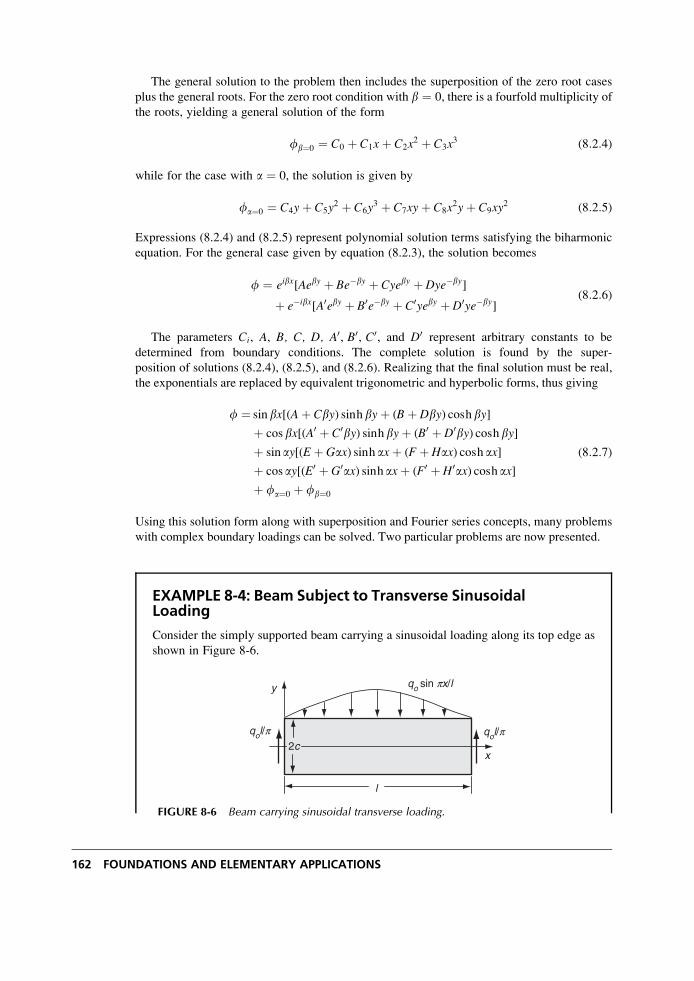
The general solution to the problem then includes the superposition of the zero root cases
plus the general roots. For the zero root condition with b ¼ 0, there is a fourfold multiplicity of
the roots, yielding a general solution of the form
fb¼0 ¼ C0 þ C1xþ C2x2 þ C3x
3 (8:2:4)
while for the case with a ¼ 0, the solution is given by
fa¼0 ¼ C4yþ C5y2 þ C6y
3 þ C7xyþ C8x2yþ C9xy
2 (8:2:5)
Expressions (8.2.4) and (8.2.5) represent polynomial solution terms satisfying the biharmonic
equation. For the general case given by equation (8.2.3), the solution becomes
f ¼ eibx[Aeby þ Be�by þ Cyeby þ Dye�by]
þ e�ibx[A0eby þ B0e�by þ C0yeby þ D0ye�by](8:2:6)
The parameters Ci, A, B, C, D, A0, B0, C0, and D0 represent arbitrary constants to be
determined from boundary conditions. The complete solution is found by the super-
position of solutions (8.2.4), (8.2.5), and (8.2.6). Realizing that the final solution must be real,
the exponentials are replaced by equivalent trigonometric and hyperbolic forms, thus giving
f ¼ sinbx[(Aþ Cby) sinhbyþ (Bþ Dby) coshby]
þ cos bx[(A0 þ C0by) sinhbyþ (B0 þ D0by) coshby]þ sin ay[(Eþ Gax) sinh axþ (Fþ Hax) cosh ax]
þ cos ay[(E0 þ G0ax) sinh axþ (F0 þ H0ax) cosh ax]þ fa¼0 þ fb¼0
(8:2:7)
Using this solution form along with superposition and Fourier series concepts, many problems
with complex boundary loadings can be solved. Two particular problems are now presented.
EXAMPLE 8-4: Beam Subject to Transverse SinusoidalLoading
Consider the simply supported beam carrying a sinusoidal loading along its top edge as
shown in Figure 8-6.
x
y qo sin px/l
qol/pqol/p
l
2c
FIGURE 8-6 Beam carrying sinusoidal transverse loading.
162 FOUNDATIONS AND ELEMENTARY APPLICATIONS
EXAMPLE 8-4: Cont’d
The boundary conditions for this problem can be written as
sx(0, y) ¼ sx(l, y) ¼ 0
txy(x, �c) ¼ 0
sy(x,�c) ¼ 0
sy(x, c) ¼ �qo sin (px=l)ðc�c
txy(0, y)dy ¼ �qol=pðc�c
txy(l, y)dy ¼ qol=p
(8:2:8)
Note that these conditions do not specify the pointwise distribution of shear stress on the
ends of the beam, but rather stipulate the resultant condition based on overall problem
equilibrium. Thus, we again are generating a solution valid away from the ends that would
be most useful for the case where l >> c. Because the vertical normal stress has a
sinusoidal variation in x along y ¼ c, an appropriate trial solution from the general case is
f ¼ sinbx[(Aþ Cby) sinhbyþ (Bþ Dby) coshby] (8:2:9)
The stresses from this trial form are
sx ¼ b2 sinbx[A sinhbyþ C(by sinhbyþ 2 coshby)
þ B coshbyþ D(by coshbyþ 2 sinhby)]
sy ¼� b2 sinbx[(Aþ Cby) sinhbyþ (Bþ Dby) cosh by]
txy ¼� b2 cos bx[A coshbyþ C(by coshbyþ sinhby)
þ B sinhbyþ D(by sinhbyþ coshby)]
(8:2:10)
Condition (8:2:8)2 implies that
[A cosh byþ C(by coshbyþ sinhby)
þ B sinhbyþ D(by sinhbyþ cosh by)]y¼�c ¼ 0(8:2:11)
This condition can be equivalently stated by requiring that the even and oddfunctions of y independently vanish at the boundary, thus giving the result
A coshbcþ D(bc sinhbcþ cosh bc) ¼ 0
B sinhbcþ C(bc coshbcþ sinhbc) ¼ 0(8:2:12)
Solving for the constants A and B gives
A ¼ �D(bc tanhbcþ 1)
B ¼ �C(bc cothbcþ 1)(8:2:13)
and thus the vertical normal stress becomes
Continued
Two-Dimensional Problem Solution 163
EXAMPLE 8-4: Beam Subject to Transverse SinusoidalLoading–Cont’d
sy ¼� b2 sinbx{D[by coshby� (bc tanhbcþ 1) sinhby]
þ C[by sinhby� (bc coth bcþ 1) coshby]}(8:2:14)
Applying boundary condition (8:2:8)3 to this result gives the relation between C and D
C ¼ � tanh bcbc� sinhbc cosh bcbcþ sinhbc cosh bc
� �D (8:2:15)
while condition (8:2:8)4 gives
qo sinpxl¼ 2b2 sinbx
bc� sinhbc coshbccosh bc
� �D (8:2:16)
In order for relation (8.2.16) to be true for all x, b ¼ p=l, and so the constant D is thus
determined as
D ¼qo cosh
pcl
2p2
l2pcl� sinh
pclcosh
pcl
h i (8:2:17)
This result can be substituted into (8.2.15) to give the remaining constant C
C ¼�qo sinh
pcl
2p2
l2pclþ sinh
pclcosh
pcl
h i (8:2:18)
Using these results, the remaining boundary conditions (8:2:8)1 and (8:2:8)5, 6 will nowbe satisfied. Thus, we have completed the determination of the stress field for this problem.
Following our usual solution steps, we now wish to determine the displacements, and
these are again developed through integration of the plane stress strain-displacement
relations. Skipping the details, the final results are given by
u ¼� bEcos bx{A(1þ �) sinhbyþ B(1þ �) coshby
þ C[(1þ �)by sinh byþ 2 coshby]
þ D[(1þ �)by coshbyþ 2 sinhby]}� !oyþ uo
v ¼� bEsinbx{A(1þ �) coshbyþ B(1þ �) sinhby
þ C[(1þ �)by coshby� (1þ �) sinhby]
þ D[(1þ �)by sinhby� (1� �) cosh by]}þ !oyþ vo
(8:2:19)
To model a simply supported beam, we choose displacement fixity conditions as
u(0, 0) ¼ v(0, 0) ¼ v(l, 0) ¼ 0 (8:2:20)
164 FOUNDATIONS AND ELEMENTARY APPLICATIONS
EXAMPLE 8-4: Cont’d
These conditions determine the rigid-body terms, giving the result
!o ¼ vo ¼ 0, uo ¼ bE[B(1þ �)þ 2C] (8:2:21)
To compare with strength of materials theory, the vertical centerline displacement is
determined. Using (8:2:19)2 and (8:2:13)1, the deflection of the beam axis reduces to
v(x, 0) ¼ DbE
sin bx[2þ (1þ �)bc tanhbc] (8:2:22)
For the case l >> c, D � �3qol5=4c3p5, and so the previous relation becomes
v(x, 0) ¼ � 3qol4
2c3p4Esin
pxl
1þ 1þ �
2
pcltanh
pcl
� �(8:2:23)
The corresponding deflection from strength of materials theory is given by
v(x, 0) ¼ � 3qol4
2c3p4Esin
pxl
(8:2:24)
Considering again the case l >> c, the second term in brackets in relation (8.2.23) can
be neglected, and thus the elasticity result matches with that found from strength of
materials.
8.2.1 Applications Involving Fourier SeriesMore sophisticated applications of the Fourier solution method commonly incorporate Fourier
series theory. This is normally done by using superposition of solution forms to enable more
general boundary conditions to be satisfied. For example, in the previous problem the solution
was obtained for a single sinusoidal loading. However, this solution form could be used to
generate a series of solutions with sinusoidal loadings having different periods; that is,
b ¼ bn ¼ np=l, (n ¼ 1, 2, 3, � � � ). Invoking the principle of superposition, we can form a
linear combination of these sinusoidal solutions, thus leading to a Fourier series representation
to a general transverse boundary loading on the beam.
In order to use such a technique, we shall briefly review some basic concepts of Fourier
series theory. Further details may be found in Kreyszig (1999) or Churchill (1963). A function
f(x) periodic with period 2l can be represented on the interval (�l, l) by the Fourier trigono-metric series
f (x) ¼ 1
2ao þ
X1n¼1
an cosnpxl
þ bn sinnpxl
� �(8:2:25)
where
an ¼ 1
l
ðl�l
f (x) cosnpxl
dx, n ¼ 0, 1, 2, � � �
bn ¼ 1
l
ðl�l
f (x) sinnpxl
dx, n ¼ 1, 2, 3, � � �(8:2:26)
Two-Dimensional Problem Solution 165
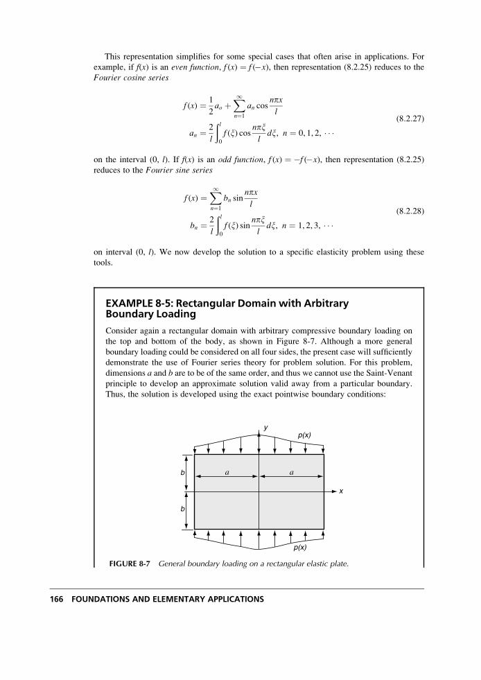
This representation simplifies for some special cases that often arise in applications. For
example, if f(x) is an even function, f (x) ¼ f (�x), then representation (8.2.25) reduces to the
Fourier cosine series
f (x) ¼ 1
2ao þ
X1n¼1
an cosnpxl
an ¼ 2
l
ðl0
f (x) cosnpxl
dx, n ¼ 0, 1, 2, � � �(8:2:27)
on the interval (0, l). If f(x) is an odd function, f (x) ¼ �f (�x), then representation (8.2.25)
reduces to the Fourier sine series
f (x) ¼X1n¼1
bn sinnpxl
bn ¼ 2
l
ðl0
f (x) sinnpxl
dx, n ¼ 1, 2, 3, � � �(8:2:28)
on interval (0, l). We now develop the solution to a specific elasticity problem using these
tools.
EXAMPLE 8-5: Rectangular Domain with ArbitraryBoundary Loading
Consider again a rectangular domain with arbitrary compressive boundary loading on
the top and bottom of the body, as shown in Figure 8-7. Although a more general
boundary loading could be considered on all four sides, the present case will sufficiently
demonstrate the use of Fourier series theory for problem solution. For this problem,
dimensions a and b are to be of the same order, and thus we cannot use the Saint-Venant
principle to develop an approximate solution valid away from a particular boundary.
Thus, the solution is developed using the exact pointwise boundary conditions:
x
y
a a
p(x)
p(x)
b
b
FIGURE 8-7 General boundary loading on a rectangular elastic plate.
166 FOUNDATIONS AND ELEMENTARY APPLICATIONS
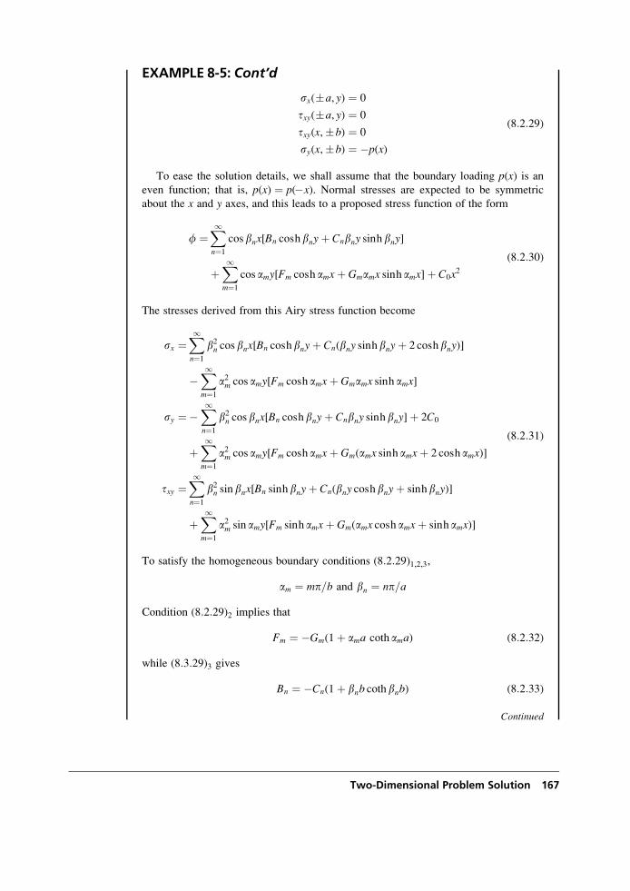
EXAMPLE 8-5: Cont’d
sx(�a, y) ¼ 0
txy(�a, y) ¼ 0
txy(x,�b) ¼ 0
sy(x,�b) ¼ �p(x)
(8:2:29)
To ease the solution details, we shall assume that the boundary loading p(x) is aneven function; that is, p(x) ¼ p(�x). Normal stresses are expected to be symmetric
about the x and y axes, and this leads to a proposed stress function of the form
f ¼X1n¼1
cos bnx[Bn coshbnyþ Cnbny sinh bny]
þX1m¼1
cos amy[Fm cosh amxþ Gmamx sinh amx]þ C0x2
(8:2:30)
The stresses derived from this Airy stress function become
sx ¼X1n¼1
b2n cos bnx[Bn coshbnyþ Cn(bny sinhbnyþ 2 coshbny)]
�X1m¼1
a2m cos amy[Fm cosh amxþ Gmamx sinh amx]
sy ¼�X1n¼1
b2n cos bnx[Bn coshbnyþ Cnbny sinhbny]þ 2C0
þX1m¼1
a2m cos amy[Fm cosh amxþ Gm(amx sinh amxþ 2 cosh amx)]
txy ¼X1n¼1
b2n sinbnx[Bn sinh bnyþ Cn(bny coshbnyþ sinhbny)]
þX1m¼1
a2m sin amy[Fm sinh amxþ Gm(amx cosh amxþ sinh amx)]
(8:2:31)
To satisfy the homogeneous boundary conditions (8:2:29)1,2,3,
am ¼ mp=b and bn ¼ np=a
Condition (8:2:29)2 implies that
Fm ¼ �Gm(1þ ama coth ama) (8:2:32)
while (8:3:29)3 gives
Bn ¼ �Cn(1þ bnb cothbnb) (8:2:33)
Continued
Two-Dimensional Problem Solution 167
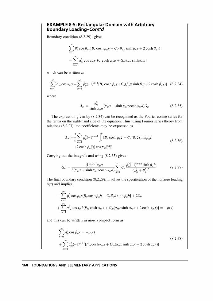
EXAMPLE 8-5: Rectangular Domain with ArbitraryBoundary Loading–Cont’d
Boundary condition (8:2:29)1 gives
X1n¼1
b2n cos bna[Bn coshbnyþ Cn(bny sinh bnyþ 2 coshbny)]
¼X1m¼1
a2m cos amy[Fm cosh amaþ Gmama sinh ama]
which can be written as
X1m¼1
Am cos amy¼X1n¼1
b2n(�1)nþ1[Bn coshbnyþCn(bny sinhbnyþ2 coshbny)] (8:2:34)
where
Am ¼ a2msinh ama
(amaþ sinh ama cosh ama)Gm (8:2:35)
The expression given by (8.2.34) can be recognized as the Fourier cosine series for
the terms on the right-hand side of the equation. Thus, using Fourier series theory from
relations (8.2.27), the coefficients may be expressed as
Am ¼ 2
b
X1n¼1
b2n(�1)nþ1
ðb0
[Bn coshbnxþ Cn(bnx sinhbnx
þ2 coshbnx)] cos amxdx
(8:2:36)
Carrying out the integrals and using (8.2.35) gives
Gm ¼ �4 sinh amab(amaþ sinh ama cosh ama)
X1n¼1
Cnb3n(�1)mþn sinhbnb
(a2m þ b2n)2
(8:2:37)
The final boundary condition (8.2.29)4 involves the specification of the nonzero loading
p(x) and implies
�X1n¼1
b2n cos bnx[Bn coshbnbþ Cnbnb sinh bnb]þ 2C0
þX1m¼1
a2m cos amb[Fm cosh amxþ Gm(amx sinh amxþ 2 cosh amx)] ¼ �p(x)
and this can be written in more compact form as
X1n¼0
A�n cos bnx ¼ �p(x)
þX1m¼1
a2m(�1)mþ1[Fm cosh amxþ Gm(amx sinh amxþ 2 cosh amx)]
(8:2:38)
168 FOUNDATIONS AND ELEMENTARY APPLICATIONS
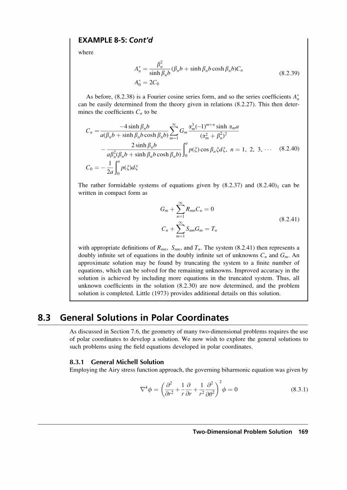
EXAMPLE 8-5: Cont’d
where
A�n ¼
b2nsinh bnb
(bnbþ sinhbnb coshbnb)Cn
A�0 ¼ 2C0
(8:2:39)
As before, (8.2.38) is a Fourier cosine series form, and so the series coefficients A�n
can be easily determined from the theory given in relations (8.2.27). This then deter-
mines the coefficients Cn to be
Cn ¼ �4 sinhbnba(bnbþ sinhbnb coshbnb)
X1m¼1
Gma3m(�1)mþn sinh ama
(a2m þ b2n)2
� 2 sinhbnb
ab2n(bnbþ sinhbnb coshbnb)
ða0
p(x) cos bnxdx, n ¼ 1, 2, 3, � � �
C0 ¼� 1
2a
ða0
p(x)dx
(8:2:40)
The rather formidable systems of equations given by (8.2.37) and (8.2.40)1 can be
written in compact form as
Gm þX1n¼1
RmnCn ¼ 0
Cn þX1m¼1
SnmGm ¼ Tn
(8:2:41)
with appropriate definitions of Rmn, Snm, and Tn. The system (8.2.41) then represents a
doubly infinite set of equations in the doubly infinite set of unknowns Cn and Gm. An
approximate solution may be found by truncating the system to a finite number of
equations, which can be solved for the remaining unknowns. Improved accuracy in the
solution is achieved by including more equations in the truncated system. Thus, all
unknown coefficients in the solution (8.2.30) are now determined, and the problem
solution is completed. Little (1973) provides additional details on this solution.
8.3 General Solutions in Polar Coordinates
As discussed in Section 7.6, the geometry of many two-dimensional problems requires the use
of polar coordinates to develop a solution. We now wish to explore the general solutions to
such problems using the field equations developed in polar coordinates.
8.3.1 General Michell SolutionEmploying the Airy stress function approach, the governing biharmonic equation was given by
r4f ¼ @2
@r2þ 1
r
@
@rþ 1
r2@2
@y2
� �2
f ¼ 0 (8:3:1)
Two-Dimensional Problem Solution 169
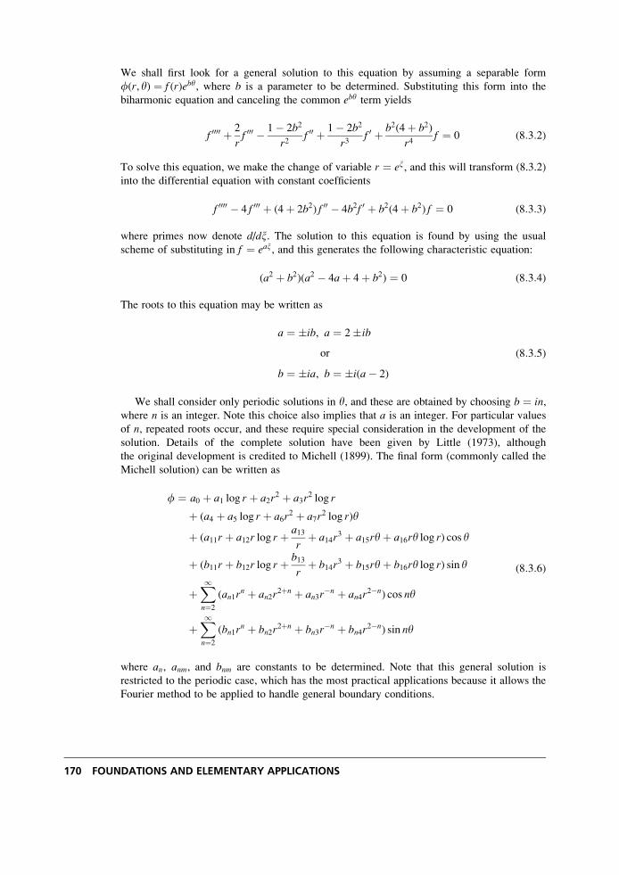
We shall first look for a general solution to this equation by assuming a separable form
f(r, y) ¼ f (r)eby, where b is a parameter to be determined. Substituting this form into the
biharmonic equation and canceling the common eby term yields
f 0000 þ 2
rf 000 � 1� 2b2
r2f 00 þ 1� 2b2
r3f 0 þ b2(4þ b2)
r4f ¼ 0 (8:3:2)
To solve this equation, we make the change of variable r ¼ ex, and this will transform (8.3.2)
into the differential equation with constant coefficients
f 0000 � 4 f 000 þ (4þ 2b2) f 00 � 4b2f 0 þ b2(4þ b2) f ¼ 0 (8:3:3)
where primes now denote d/dx. The solution to this equation is found by using the usual
scheme of substituting in f ¼ eax, and this generates the following characteristic equation:
(a2 þ b2)(a2 � 4aþ 4þ b2) ¼ 0 (8:3:4)
The roots to this equation may be written as
a ¼ �ib, a ¼ 2�ib
or
b ¼ �ia, b ¼ �i(a� 2)
(8:3:5)
We shall consider only periodic solutions in y, and these are obtained by choosing b ¼ in,where n is an integer. Note this choice also implies that a is an integer. For particular values
of n, repeated roots occur, and these require special consideration in the development of the
solution. Details of the complete solution have been given by Little (1973), although
the original development is credited to Michell (1899). The final form (commonly called the
Michell solution) can be written as
f ¼ a0 þ a1 log r þ a2r2 þ a3r
2 log r
þ (a4 þ a5 log r þ a6r2 þ a7r
2 log r)y
þ (a11r þ a12r log r þ a13r
þ a14r3 þ a15ryþ a16ry log r) cos y
þ (b11r þ b12r log r þ b13r
þ b14r3 þ b15ryþ b16ry log r) sin y
þX1n¼2
(an1rn þ an2r
2þn þ an3r�n þ an4r
2�n) cos ny
þX1n¼2
(bn1rn þ bn2r
2þn þ bn3r�n þ bn4r
2�n) sin ny
(8:3:6)
where an, anm, and bnm are constants to be determined. Note that this general solution is
restricted to the periodic case, which has the most practical applications because it allows the
Fourier method to be applied to handle general boundary conditions.
170 FOUNDATIONS AND ELEMENTARY APPLICATIONS
8.3.2 Axisymmetric SolutionFor the axisymmetric case, field quantities are independent of the angular coordinate, and the
Airy function solution follows from (8.3.6) by dropping all y-terms, giving
f ¼ a0 þ a1 log r þ a2r2 þ a3r
2 log r (8:3:7)
Using relations (7.6.7), the resulting stresses for this case are
sr ¼ 2a3 log r þ a1r2
þ a3 þ 2a2
sy ¼ 2a3 log r � a1r2
þ 3a3 þ 2a2
try ¼ 0
(8:3:8)
The displacements corresponding to these stresses can be determined by the usual methods of
integrating the strain-displacement relations. For the case of plane stress, the result is
ur ¼ 1
E� (1þ �)
ra1 þ 2(1� �)a3r log r � (1þ �)a3r þ 2a2(1� �)r
� �þ A sin yþ B cos y
uy ¼ 4ryE
a3 þ A cos y� B sin yþ Cr
(8:3:9)
where A, B, and C are arbitrary constants associated with the rigid-body motion terms
(see Exercise 7-21).
Plane strain results follow by simple change of elastic constants as per Table 7-1. If the
body includes the origin, then a3 and a1 must be set to zero for the stresses to remain finite, and
thus the stress field would be constant. Also note that the a3 term in the tangential displacement
relation leads to multivalued behavior if the domain geometry is such that the origin can be
encircled by any contour lying entirely in the body. Exercise 8-21 is concerned with a
particular problem that requires such multivalued behavior in the tangential displacement.
It should be pointed out that not all axisymmetric stress fields come from the Airy stress
function given by (8.3.7). Reviewing the general form (8.3.6) indicates that the a4� term
generates the stress field �r ¼ �� ¼ 0, tr� ¼ a4/r2, which is also axisymmetric. This solution
could be used to solve problems with shear fields that produce tangential displacements that
are independent of �. Exercise 8-14 demonstrates such an example.
It has been previously pointed out that for multiply connected regions, the compatibility
equations are not sufficient to guarantee single-valued displacements. With this in mind, we
can investigate the displacement solution directly from the Navier equations. With zero body
forces, Navier equations (5.4.4) or (7.6.4) for the axisymmetric case u ¼ ur(r)er reduce to
d2urdr2
þ 1
r
durdr
� 1
r2ur ¼ 0 (8:3:10)
The solution to this equation is given by
ur ¼ C1r þ C2
1
r(8:3:11)
where C1 and C2 are constants. Notice this solution form is not the same as that given by
(8.3.9), because we have a priori assumed that uy ¼ 0. Furthermore, the stresses corresponding
to displacement solution (8.3.11) do not contain the logarithmic terms given in relations
(8.3.8). Thus, these terms are not consistent with single-valued displacements.
Two-Dimensional Problem Solution 171
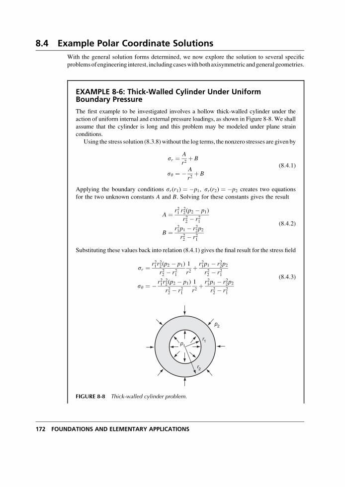
8.4 Example Polar Coordinate Solutions
With the general solution forms determined, we now explore the solution to several specific
problemsofengineering interest, includingcaseswithbothaxisymmetric andgeneralgeometries.
EXAMPLE 8-6: Thick-Walled Cylinder Under UniformBoundary Pressure
The first example to be investigated involves a hollow thick-walled cylinder under the
action of uniform internal and external pressure loadings, as shown in Figure 8-8.We shall
assume that the cylinder is long and this problem may be modeled under plane strain
conditions.
Using the stress solution (8.3.8)without the log terms, the nonzero stresses are given by
sr ¼ A
r2þ B
sy ¼ � A
r2þ B
(8:4:1)
Applying the boundary conditions sr(r1) ¼ �p1, sr(r2) ¼ �p2 creates two equations
for the two unknown constants A and B. Solving for these constants gives the result
A ¼ r21 r22(p2 � p1)
r22 � r21
B ¼ r21p1 � r22p2r22 � r21
(8:4:2)
Substituting these values back into relation (8.4.1) gives the final result for the stress field
sr ¼ r21r22(p2 � p1)
r22 � r21
1
r2þ r21p1 � r22p2
r22 � r21
sy ¼ � r21r22(p2 � p1)
r22 � r21
1
r2þ r21p1 � r22p2
r22 � r21
(8:4:3)
r1
r2
p1
p2
FIGURE 8-8 Thick-walled cylinder problem.
172 FOUNDATIONS AND ELEMENTARY APPLICATIONS
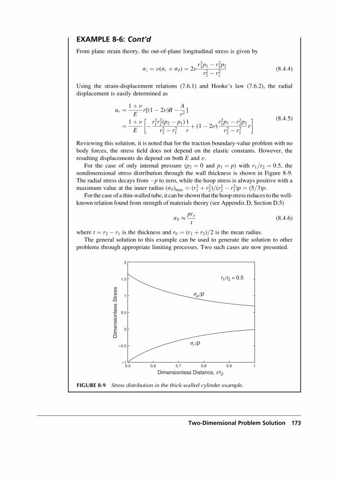
EXAMPLE 8-6: Cont’d
From plane strain theory, the out-of-plane longitudinal stress is given by
sz ¼ �(sr þ sy) ¼ 2�r21p1 � r22p2r22 � r21
(8:4:4)
Using the strain-displacement relations (7.6.1) and Hooke’s law (7.6.2), the radial
displacement is easily determined as
ur ¼ 1þ �
Er[(1� 2�)B� A
r2]
¼ 1þ �
E� r21r
22(p2 � p1)
r22 � r21
1
rþ (1� 2�)
r21p1 � r22p2r22 � r21
r
� � (8:4:5)
Reviewing this solution, it is noted that for the traction boundary-value problem with no
body forces, the stress field does not depend on the elastic constants. However, the
resulting displacements do depend on both E and �.For the case of only internal pressure (p2 ¼ 0 and p1 ¼ p) with r1=r2 ¼ 0:5, the
nondimensional stress distribution through the wall thickness is shown in Figure 8-9.
The radial stress decays from �p to zero, while the hoop stress is always positive with amaximum value at the inner radius (sy)max ¼ (r21 þ r22)=(r
22 � r21)p ¼ (5=3)p.
For the case of a thin-walled tube, it can be shown that the hoop stress reduces to thewell-
known relation found from strength of materials theory (see Appendix D, Section D.5)
sy � prot
(8:4:6)
where t ¼ r2 � r1 is the thickness and r0 ¼ (r1 þ r2)=2 is the mean radius.
The general solution to this example can be used to generate the solution to other
problems through appropriate limiting processes. Two such cases are now presented.
r1/r2 = 0.5
Dim
ensi
onle
ss S
tres
s
Dimensionless Distance, r/r2
-0.5
0
0.5
1
1.5
-1
2
0.6 0.7 0.8 0.90.5 1
sq /p
sr /p
FIGURE 8-9 Stress distribution in the thick-walled cylinder example.
Two-Dimensional Problem Solution 173
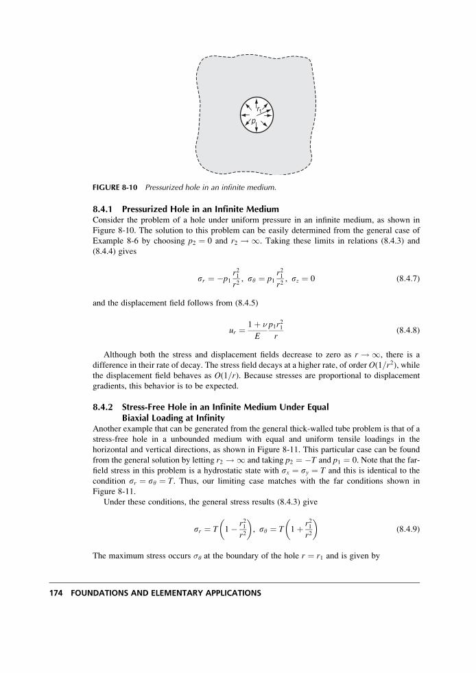
8.4.1 Pressurized Hole in an Infinite MediumConsider the problem of a hole under uniform pressure in an infinite medium, as shown in
Figure 8-10. The solution to this problem can be easily determined from the general case of
Example 8-6 by choosing p2 ¼ 0 and r2 ! 1. Taking these limits in relations (8.4.3) and
(8.4.4) gives
sr ¼ �p1r21r2, sy ¼ p1
r21r2, sz ¼ 0 (8:4:7)
and the displacement field follows from (8.4.5)
ur ¼ 1þ �
E
p1r21
r(8:4:8)
Although both the stress and displacement fields decrease to zero as r ! 1, there is a
difference in their rate of decay. The stress field decays at a higher rate, of order O(1=r2), whilethe displacement field behaves as O(1=r). Because stresses are proportional to displacement
gradients, this behavior is to be expected.
8.4.2 Stress-Free Hole in an Infinite Medium Under EqualBiaxial Loading at Infinity
Another example that can be generated from the general thick-walled tube problem is that of a
stress-free hole in a unbounded medium with equal and uniform tensile loadings in the
horizontal and vertical directions, as shown in Figure 8-11. This particular case can be found
from the general solution by letting r2 ! 1 and taking p2 ¼ �T and p1 ¼ 0. Note that the far-
field stress in this problem is a hydrostatic state with sx ¼ sy ¼ T and this is identical to the
condition sr ¼ sy ¼ T. Thus, our limiting case matches with the far conditions shown in
Figure 8-11.
Under these conditions, the general stress results (8.4.3) give
sr ¼ T 1� r21r2
� �, sy ¼ T 1þ r21
r2
� �(8:4:9)
The maximum stress occurs �� at the boundary of the hole r ¼ r1 and is given by
r1
p
FIGURE 8-10 Pressurized hole in an infinite medium.
174 FOUNDATIONS AND ELEMENTARY APPLICATIONS
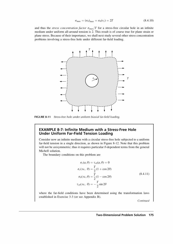
smax ¼ (sy)max ¼ sy(r1) ¼ 2T (8:4:10)
and thus the stress concentration factor smax=T for a stress-free circular hole in an infinite
medium under uniform all-around tension is 2. This result is of course true for plane strain or
plane stress. Because of their importance, we shall next study several other stress concentration
problems involving a stress-free hole under different far-field loading.
EXAMPLE 8-7: Infinite Medium with a Stress-Free HoleUnder Uniform Far-Field Tension Loading
Consider now an infinite medium with a circular stress-free hole subjected to a uniform
far-field tension in a single direction, as shown in Figure 8-12. Note that this problem
will not be axisymmetric; thus it requires particular y-dependent terms from the general
Michell solution.
The boundary conditions on this problem are
sr(a, y) ¼ try(a, y) ¼ 0
sr(1, y) ¼ T
2(1þ cos 2y)
sy(1, y) ¼ T
2(1� cos 2y)
try(1, y) ¼ �T
2sin 2y
(8:4:11)
where the far-field conditions have been determined using the transformation laws
established in Exercise 3-3 (or see Appendix B).
Continued
T
T
r1
FIGURE 8-11 Stress-free hole under uniform biaxial far-field loading.
Two-Dimensional Problem Solution 175
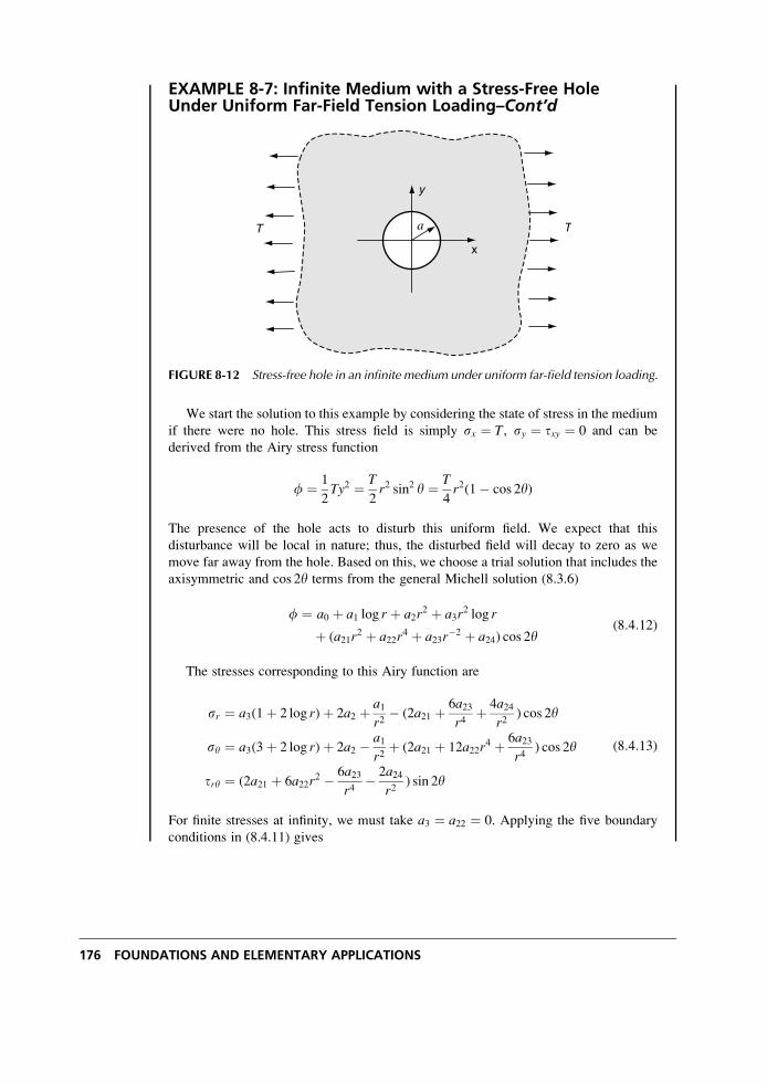
EXAMPLE 8-7: Infinite Medium with a Stress-Free HoleUnder Uniform Far-Field Tension Loading–Cont’d
We start the solution to this example by considering the state of stress in the medium
if there were no hole. This stress field is simply sx ¼ T, sy ¼ txy ¼ 0 and can be
derived from the Airy stress function
f ¼ 1
2Ty2 ¼ T
2r2 sin2 y ¼ T
4r2(1� cos 2y)
The presence of the hole acts to disturb this uniform field. We expect that this
disturbance will be local in nature; thus, the disturbed field will decay to zero as we
move far away from the hole. Based on this, we choose a trial solution that includes the
axisymmetric and cos 2y terms from the general Michell solution (8.3.6)
f ¼ a0 þ a1 log r þ a2r2 þ a3r
2 log r
þ (a21r2 þ a22r
4 þ a23r�2 þ a24) cos 2y
(8:4:12)
The stresses corresponding to this Airy function are
sr ¼ a3(1þ 2 log r)þ 2a2 þ a1r2
� (2a21 þ 6a23r4
þ 4a24r2
) cos 2y
sy ¼ a3(3þ 2 log r)þ 2a2 � a1r2
þ (2a21 þ 12a22r4 þ 6a23
r4) cos 2y
try ¼ (2a21 þ 6a22r2 � 6a23
r4� 2a24
r2) sin 2y
(8:4:13)
For finite stresses at infinity, we must take a3 ¼ a22 ¼ 0. Applying the five boundary
conditions in (8.4.11) gives
TaT
x
y
FIGURE 8-12 Stress-free hole in an infinite medium under uniform far-field tension loading.
176 FOUNDATIONS AND ELEMENTARY APPLICATIONS
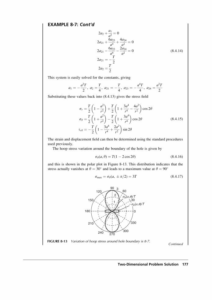
EXAMPLE 8-7: Cont’d
2a2 þ a1a2
¼ 0
2a21 þ 6a23a4
þ 4a24a2
¼ 0
2a21 � 6a23a4
� 2a24a2
¼ 0
2a21 ¼ �T
2
2a2 ¼ T
2
(8:4:14)
This system is easily solved for the constants, giving
a1 ¼ � a2T
2, a2 ¼ T
4, a21 ¼ �T
4, a23 ¼ � a4T
4, a24 ¼ a2T
2
Substituting these values back into (8.4.13) gives the stress field
sr ¼ T
21� a2
r2
� �þ T
21þ 3a4
r4� 4a2
r2
� �cos 2y
sy ¼ T
21þ a2
r2
� �� T
21þ 3a4
r4
� �cos 2y
try ¼ � T
21� 3a4
r4þ 2a2
r2
� �sin 2y
(8:4:15)
The strain and displacement field can then be determined using the standard procedures
used previously.
The hoop stress variation around the boundary of the hole is given by
sy(a, y) ¼ T(1� 2 cos 2y) (8:4:16)
and this is shown in the polar plot in Figure 8-13. This distribution indicates that the
stress actually vanishes at y ¼ 30 and leads to a maximum value at y ¼ 90
smax ¼ sy(a, � p=2) ¼ 3T (8:4:17)
Continued
270240
210
180
120
150
90 3
300
330
0
30
60
sq (a,q)/T
− sq (a,q)/T
1
2
FIGURE 8-13 Variation of hoop stress around hole boundary is 8-7.
Two-Dimensional Problem Solution 177
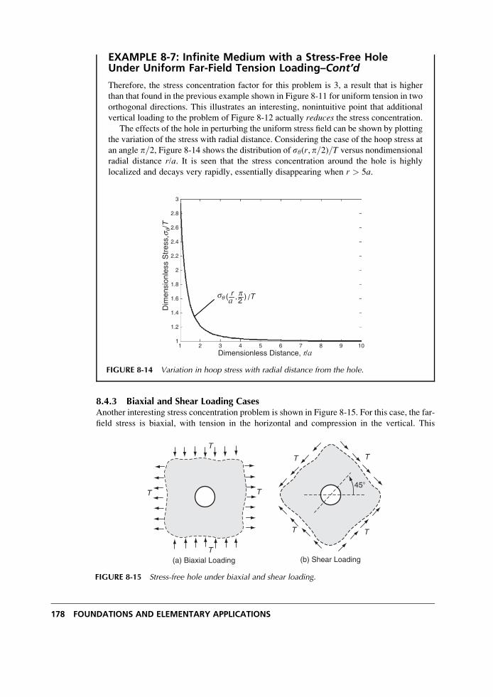
EXAMPLE 8-7: Infinite Medium with a Stress-Free HoleUnder Uniform Far-Field Tension Loading–Cont’d
Therefore, the stress concentration factor for this problem is 3, a result that is higher
than that found in the previous example shown in Figure 8-11 for uniform tension in two
orthogonal directions. This illustrates an interesting, nonintuitive point that additional
vertical loading to the problem of Figure 8-12 actually reduces the stress concentration.The effects of the hole in perturbing the uniform stress field can be shown by plotting
the variation of the stress with radial distance. Considering the case of the hoop stress at
an angle p=2, Figure 8-14 shows the distribution of sy(r, p=2)=T versus nondimensional
radial distance r/a. It is seen that the stress concentration around the hole is highly
localized and decays very rapidly, essentially disappearing when r > 5a.
8.4.3 Biaxial and Shear Loading CasesAnother interesting stress concentration problem is shown in Figure 8-15. For this case, the far-
field stress is biaxial, with tension in the horizontal and compression in the vertical. This
sq ar p
/T)2,(
Dimensionless Distance, r/a
Dim
ensi
onle
ss S
tres
s,s q
/T
3
2.8
2.6
2.4
2.2
2
1.8
1.6
1.4
1.2
11 2 3 4 5 6 7 8 9 10
FIGURE 8-14 Variation in hoop stress with radial distance from the hole.
TT
T
T
TT
T T
45�
(a) Biaxial Loading (b) Shear Loading
FIGURE 8-15 Stress-free hole under biaxial and shear loading.
178 FOUNDATIONS AND ELEMENTARY APPLICATIONS
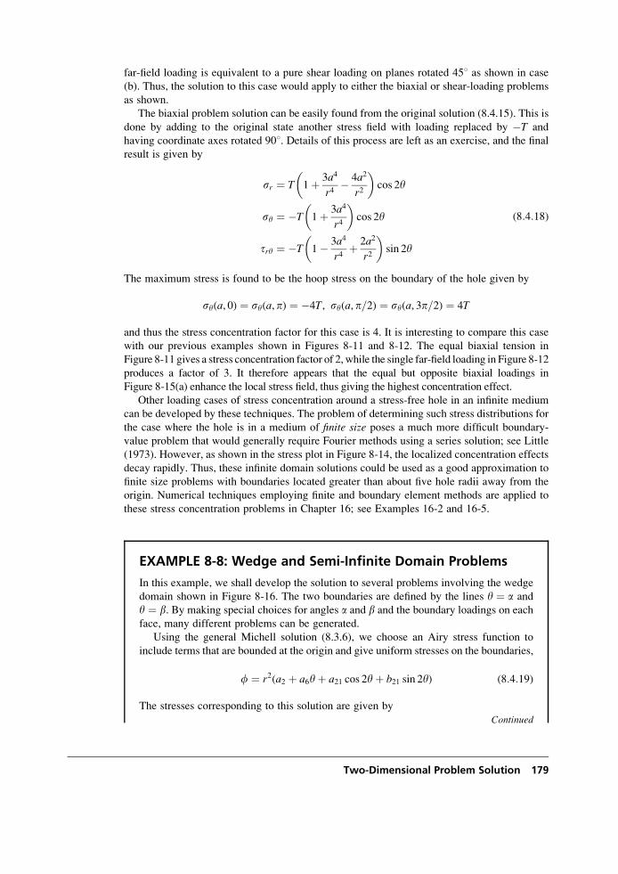
far-field loading is equivalent to a pure shear loading on planes rotated 458 as shown in case
(b). Thus, the solution to this case would apply to either the biaxial or shear-loading problems
as shown.
The biaxial problem solution can be easily found from the original solution (8.4.15). This is
done by adding to the original state another stress field with loading replaced by �T and
having coordinate axes rotated 908. Details of this process are left as an exercise, and the final
result is given by
sr ¼ T 1þ 3a4
r4� 4a2
r2
� �cos 2y
sy ¼ �T 1þ 3a4
r4
� �cos 2y
try ¼ �T 1� 3a4
r4þ 2a2
r2
� �sin 2y
(8:4:18)
The maximum stress is found to be the hoop stress on the boundary of the hole given by
sy(a, 0) ¼ sy(a, p) ¼ �4T, sy(a, p=2) ¼ sy(a, 3p=2) ¼ 4T
and thus the stress concentration factor for this case is 4. It is interesting to compare this case
with our previous examples shown in Figures 8-11 and 8-12. The equal biaxial tension in
Figure 8-11 gives a stress concentration factor of 2, while the single far-field loading in Figure 8-12
produces a factor of 3. It therefore appears that the equal but opposite biaxial loadings in
Figure 8-15(a) enhance the local stress field, thus giving the highest concentration effect.
Other loading cases of stress concentration around a stress-free hole in an infinite medium
can be developed by these techniques. The problem of determining such stress distributions for
the case where the hole is in a medium of finite size poses a much more difficult boundary-
value problem that would generally require Fourier methods using a series solution; see Little
(1973). However, as shown in the stress plot in Figure 8-14, the localized concentration effects
decay rapidly. Thus, these infinite domain solutions could be used as a good approximation to
finite size problems with boundaries located greater than about five hole radii away from the
origin. Numerical techniques employing finite and boundary element methods are applied to
these stress concentration problems in Chapter 16; see Examples 16-2 and 16-5.
EXAMPLE 8-8: Wedge and Semi-Infinite Domain Problems
In this example, we shall develop the solution to several problems involving the wedge
domain shown in Figure 8-16. The two boundaries are defined by the lines y ¼ a and
y ¼ b. By making special choices for angles a and b and the boundary loadings on each
face, many different problems can be generated.
Using the general Michell solution (8.3.6), we choose an Airy stress function to
include terms that are bounded at the origin and give uniform stresses on the boundaries,
f ¼ r2(a2 þ a6yþ a21 cos 2yþ b21 sin 2y) (8:4:19)
The stresses corresponding to this solution are given by
Continued
Two-Dimensional Problem Solution 179
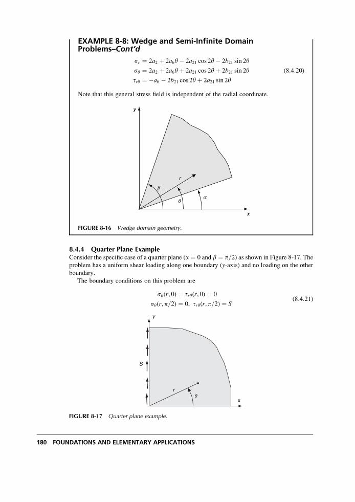
EXAMPLE 8-8: Wedge and Semi-Infinite DomainProblems–Cont’d
sr ¼ 2a2 þ 2a6y� 2a21 cos 2y� 2b21 sin 2y
sy ¼ 2a2 þ 2a6yþ 2a21 cos 2yþ 2b21 sin 2y
try ¼ �a6 � 2b21 cos 2yþ 2a21 sin 2y
(8:4:20)
Note that this general stress field is independent of the radial coordinate.
x
aq
b
y
r
FIGURE 8-16 Wedge domain geometry.
8.4.4 Quarter Plane ExampleConsider the specific case of a quarter plane (a ¼ 0 and b ¼ p=2) as shown in Figure 8-17. Theproblem has a uniform shear loading along one boundary (y-axis) and no loading on the other
boundary.
The boundary conditions on this problem are
sy(r, 0) ¼ try(r, 0) ¼ 0
sy(r,p=2) ¼ 0, try(r,p=2) ¼ S(8:4:21)
x
y
S
rq
FIGURE 8-17 Quarter plane example.
180 FOUNDATIONS AND ELEMENTARY APPLICATIONS
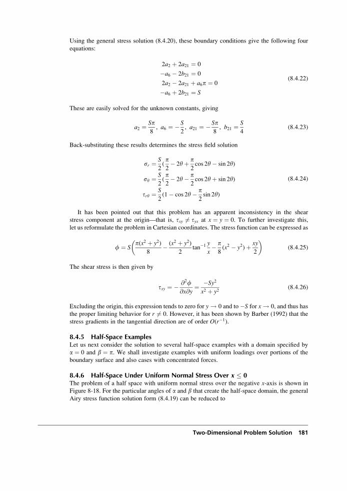
Using the general stress solution (8.4.20), these boundary conditions give the following four
equations:
2a2 þ 2a21 ¼ 0
�a6 � 2b21 ¼ 0
2a2 � 2a21 þ a6p ¼ 0
�a6 þ 2b21 ¼ S
(8:4:22)
These are easily solved for the unknown constants, giving
a2 ¼ Sp8, a6 ¼ � S
2, a21 ¼ � Sp
8, b21 ¼ S
4(8:4:23)
Back-substituting these results determines the stress field solution
sr ¼ S
2(p2� 2yþ p
2cos 2y� sin 2y)
sy ¼ S
2(p2� 2y� p
2cos 2yþ sin 2y)
try ¼ S
2(1� cos 2y� p
2sin 2y)
(8:4:24)
It has been pointed out that this problem has an apparent inconsistency in the shear
stress component at the origin—that is, txy 6¼ tyx at x ¼ y ¼ 0. To further investigate this,
let us reformulate the problem in Cartesian coordinates. The stress function can be expressed as
f ¼ Sp(x2 þ y2)
8� (x2 þ y2)
2tan�1 y
x� p
8(x2 � y2)þ xy
2
� �(8:4:25)
The shear stress is then given by
txy ¼ � @2f@x@y
¼ �Sy2
x2 þ y2(8:4:26)
Excluding the origin, this expression tends to zero for y ! 0 and to�S for x ! 0, and thus has
the proper limiting behavior for r 6¼ 0. However, it has been shown by Barber (1992) that the
stress gradients in the tangential direction are of order O(r�1).
8.4.5 Half-Space ExamplesLet us next consider the solution to several half-space examples with a domain specified by
a ¼ 0 and b ¼ p. We shall investigate examples with uniform loadings over portions of the
boundary surface and also cases with concentrated forces.
8.4.6 Half-Space Under Uniform Normal Stress Over x � 0The problem of a half space with uniform normal stress over the negative x-axis is shown in
Figure 8-18. For the particular angles of a and b that create the half-space domain, the general
Airy stress function solution form (8.4.19) can be reduced to
Two-Dimensional Problem Solution 181
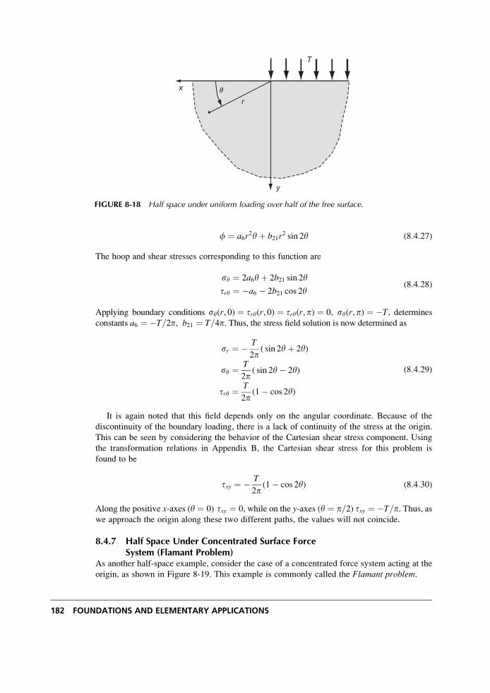
f ¼ a6r2yþ b21r
2 sin 2y (8:4:27)
The hoop and shear stresses corresponding to this function are
sy ¼ 2a6yþ 2b21 sin 2y
try ¼ �a6 � 2b21 cos 2y(8:4:28)
Applying boundary conditions sy(r, 0) ¼ try(r, 0) ¼ try(r,p) ¼ 0, sy(r, p) ¼ �T, determines
constants a6 ¼ �T=2p, b21 ¼ T=4p. Thus, the stress field solution is now determined as
sr ¼ � T
2p( sin 2yþ 2y)
sy ¼ T
2p( sin 2y� 2y)
try ¼ T
2p(1� cos 2y)
(8:4:29)
It is again noted that this field depends only on the angular coordinate. Because of the
discontinuity of the boundary loading, there is a lack of continuity of the stress at the origin.
This can be seen by considering the behavior of the Cartesian shear stress component. Using
the transformation relations in Appendix B, the Cartesian shear stress for this problem is
found to be
txy ¼ � T
2p(1� cos 2y) (8:4:30)
Along the positive x-axes (y ¼ 0) txy ¼ 0, while on the y-axes (y ¼ p=2) txy ¼ �T=p. Thus, aswe approach the origin along these two different paths, the values will not coincide.
8.4.7 Half Space Under Concentrated Surface ForceSystem (Flamant Problem)
As another half-space example, consider the case of a concentrated force system acting at the
origin, as shown in Figure 8-19. This example is commonly called the Flamant problem.
x
y
T
r
q
FIGURE 8-18 Half space under uniform loading over half of the free surface.
182 FOUNDATIONS AND ELEMENTARY APPLICATIONS
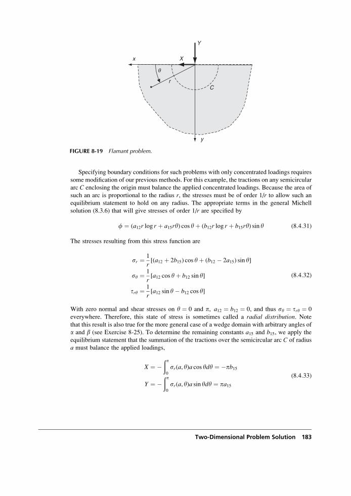
Specifying boundary conditions for such problems with only concentrated loadings requires
some modification of our previous methods. For this example, the tractions on any semicircular
arc C enclosing the origin must balance the applied concentrated loadings. Because the area of
such an arc is proportional to the radius r, the stresses must be of order 1/r to allow such an
equilibrium statement to hold on any radius. The appropriate terms in the general Michell
solution (8.3.6) that will give stresses of order 1/r are specified by
f ¼ (a12r log r þ a15ry) cos yþ (b12r log r þ b15ry) sin y (8:4:31)
The stresses resulting from this stress function are
sr ¼ 1
r[(a12 þ 2b15) cos yþ (b12 � 2a15) sin y]
sy ¼ 1
r[a12 cos yþ b12 sin y]
try ¼ 1
r[a12 sin y� b12 cos y]
(8:4:32)
With zero normal and shear stresses on y ¼ 0 and p, a12 ¼ b12 ¼ 0, and thus sy ¼ try ¼ 0
everywhere. Therefore, this state of stress is sometimes called a radial distribution. Notethat this result is also true for the more general case of a wedge domain with arbitrary angles of
a and b (see Exercise 8-25). To determine the remaining constants a15 and b15, we apply the
equilibrium statement that the summation of the tractions over the semicircular arc C of radius
a must balance the applied loadings,
X ¼ �ðp0
sr(a, y)a cos ydy ¼ �pb15
Y ¼ �ðp0
sr(a, y)a sin ydy ¼ pa15
(8:4:33)
x
y
Y
X
r
q
C
FIGURE 8-19 Flamant problem.
Two-Dimensional Problem Solution 183
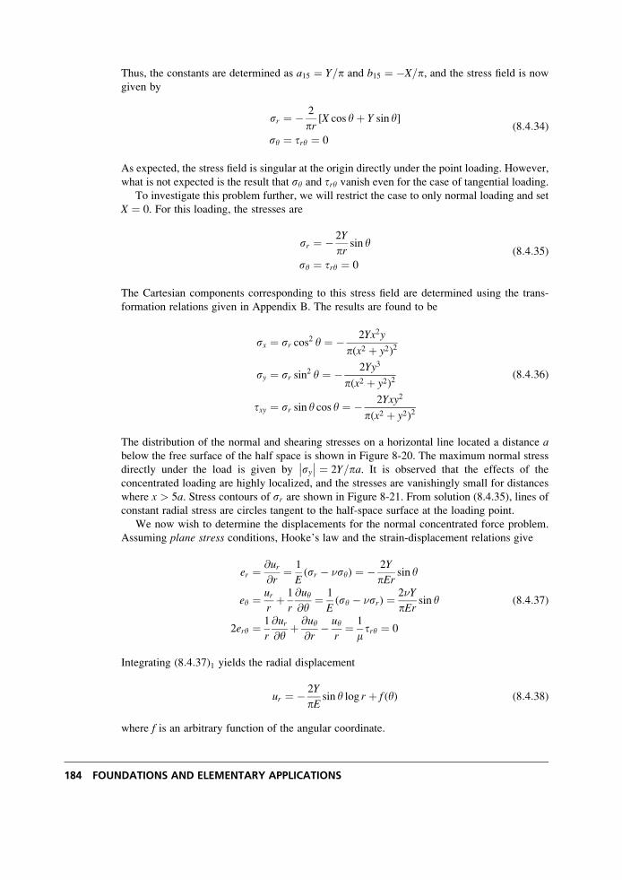
Thus, the constants are determined as a15 ¼ Y=p and b15 ¼ �X=p, and the stress field is now
given by
sr ¼ � 2
pr[X cos yþ Y sin y]
sy ¼ try ¼ 0
(8:4:34)
As expected, the stress field is singular at the origin directly under the point loading. However,
what is not expected is the result that sy and try vanish even for the case of tangential loading.
To investigate this problem further, we will restrict the case to only normal loading and set
X ¼ 0. For this loading, the stresses are
sr ¼ � 2Y
prsin y
sy ¼ try ¼ 0
(8:4:35)
The Cartesian components corresponding to this stress field are determined using the trans-
formation relations given in Appendix B. The results are found to be
sx ¼ sr cos2 y ¼ � 2Yx2y
p(x2 þ y2)2
sy ¼ sr sin2 y ¼ � 2Yy3
p(x2 þ y2)2
txy ¼ sr sin y cos y ¼ � 2Yxy2
p(x2 þ y2)2
(8:4:36)
The distribution of the normal and shearing stresses on a horizontal line located a distance abelow the free surface of the half space is shown in Figure 8-20. The maximum normal stress
directly under the load is given by sy�� �� ¼ 2Y=pa. It is observed that the effects of the
concentrated loading are highly localized, and the stresses are vanishingly small for distances
where x > 5a. Stress contours of sr are shown in Figure 8-21. From solution (8.4.35), lines of
constant radial stress are circles tangent to the half-space surface at the loading point.
We now wish to determine the displacements for the normal concentrated force problem.
Assuming plane stress conditions, Hooke’s law and the strain-displacement relations give
er ¼ @ur@r
¼ 1
E(sr � �sy) ¼ � 2Y
pErsin y
ey ¼ urrþ 1
r
@uy@y
¼ 1
E(sy � �sr) ¼ 2�Y
pErsin y
2ery ¼ 1
r
@ur@y
þ @uy@r
� uyr¼ 1
mtry ¼ 0
(8:4:37)
Integrating (8:4:37)1 yields the radial displacement
ur ¼ � 2Y
pEsin y log r þ f (y) (8:4:38)
where f is an arbitrary function of the angular coordinate.
184 FOUNDATIONS AND ELEMENTARY APPLICATIONS
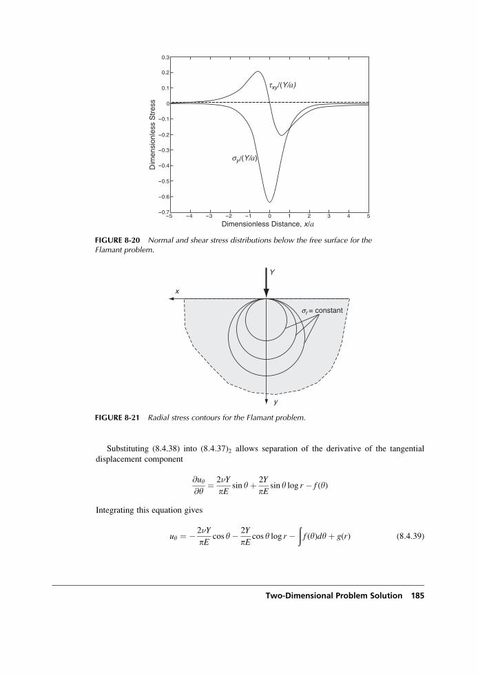
Substituting (8.4.38) into (8:4:37)2 allows separation of the derivative of the tangential
displacement component
@uy@y
¼ 2�Y
pEsin yþ 2Y
pEsin y log r � f (y)
Integrating this equation gives
uy ¼ � 2�Y
pEcos y� 2Y
pEcos y log r �
ðf (y)dyþ g(r) (8:4:39)
Dimensionless Distance, x/a
sy/(Y/a)
txy/(Y/a)
Dim
ensi
onle
ss S
tres
s
-0.6
-0.5
-0.4
-0.3
-0.2
-0.1
0
0.1
0.2
-0.7
0.3
-4 -3 -2 -1 0 1 2 3 4-5 5
FIGURE 8-20 Normal and shear stress distributions below the free surface for theFlamant problem.
x
y
Y
sr = constant
FIGURE 8-21 Radial stress contours for the Flamant problem.
Two-Dimensional Problem Solution 185
where g(r) is an arbitrary function of the indicated variable. Determination of the arbitrary
functions f and g is accomplished by substituting equations (8.4.38) and (8.4.39) into (8:4:37)3.Similar to our previous Cartesian examples, the resulting equation can be separated into the
two relations
g(r)� rg0(r) ¼ K
� (1� �)2Y
pEcos yþ f 0(y)þ
ðf (y)dy ¼ K
(8:4:40)
where K is an arbitrary constant. The solutions to this system are
g(r) ¼ Cr þ K
f (y) ¼ (1� �)Y
pEy cos yþ A sin yþ B cos y
(8:4:41)
where A, B, and C are constants of integration.
Collecting these results, the displacements thus can be written as
ur ¼ (1� �)Y
pEy cos y� 2Y
pElog r sin yþ A sin yþ B cos y
uy ¼ � (1� �)Y
pEy sin y� 2Y
pElog r cos y� (1þ �)Y
pEcos y
þ A cos y� B sin yþ Cr þ K
(8:4:42)
The terms involving the constants A, B, and C represent rigid-body motion (see Exercise 7-21).
These terms can be set to any arbitrary value without affecting the stress distribution. Rather
than setting them all to zero, they will be selected to satisfy the expected symmetry condition
that the horizontal displacements along the y-axis should be zero. This condition can be
expressed by uy(r, p=2) ¼ 0, and this relation requires
C ¼ K ¼ 0, B ¼ � (1� �)Y
2E
The vertical rigid-body motion may be taken as zero, thus implying that A ¼ 0. Values for all
constants are now determined, and the final result for the displacement field is
ur ¼ Y
pE[(1� �)(y� p
2) cos y� 2 log r sin y]
uy ¼ Y
pE[�(1� �)(y� p
2) sin y� 2 log r cos y� (1þ �) cos y]
(8:4:43)
It should be pointed out that these results contain unbounded logarithmic terms that would
lead to unrealistic predictions at infinity. This unpleasant situation is a result of the two-
dimensional model. The corresponding three-dimensional problem (Boussinesq’s problem) is
solved in Chapter 13, and the resulting displacement field does not have logarithmic terms and
is bounded at infinity; see equations (13.4.16).
The radial displacement along the free surface is given by
ur(r, 0) ¼ ur(r,p) ¼ � Y
2E(1� �) (8:4:44)
186 FOUNDATIONS AND ELEMENTARY APPLICATIONS
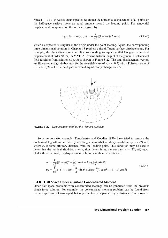
Since (1� �) > 0, we see an unexpected result that the horizontal displacement of all points on
the half-space surface move an equal amount toward the loading point. The tangential
displacement component on the surface is given by
uy(r, 0) ¼ �uy(r,p) ¼ � Y
pE[(1þ �)þ 2 log r] (8:4:45)
which as expected is singular at the origin under the point loading. Again, the corresponding
three-dimensional solution in Chapter 13 predicts quite different surface displacements. For
example, the three-dimensional result corresponding to equation (8.4.45) gives a vertical
displacement of order O(1=r). A MATLAB vector distribution plot of the general displacement
field resulting from solution (8.4.43) is shown in Figure 8-22. The total displacement vectors
are illustrated using suitable units for the near-field case (0 < r < 0:5) with a Poisson’s ratio of0.3, and Y=E ¼ 1. The field pattern would significantly change for r > 1.
Some authors (for example, Timoshenko and Goodier 1970) have tried to remove the
unpleasant logarithmic effects by invoking a somewhat arbitrary condition ur(ro, p=2) ¼ 0,
where ro is some arbitrary distance from the loading point. This condition may be used to
determine the vertical rigid-body term, thus determining the constant A ¼ (2Y=pE) log ro.Under this condition, the displacement solution can then be written as
ur ¼ Y
pE[(1� �)(y� p
2) cos y� 2 log (
ror) sin y]
uy ¼ Y
pE[�(1� �)(y� p
2) sin yþ 2 log (
ror) cos y� (1þ �) cos y]
(8:4:46)
8.4.8 Half Space Under a Surface Concentrated MomentOther half-space problems with concentrated loadings can be generated from the previous
single-force solution. For example, the concentrated moment problem can be found from
the superposition of two equal but opposite forces separated by a distance d as shown in
Y
FIGURE 8-22 Displacement field for the Flamant problem.
Two-Dimensional Problem Solution 187
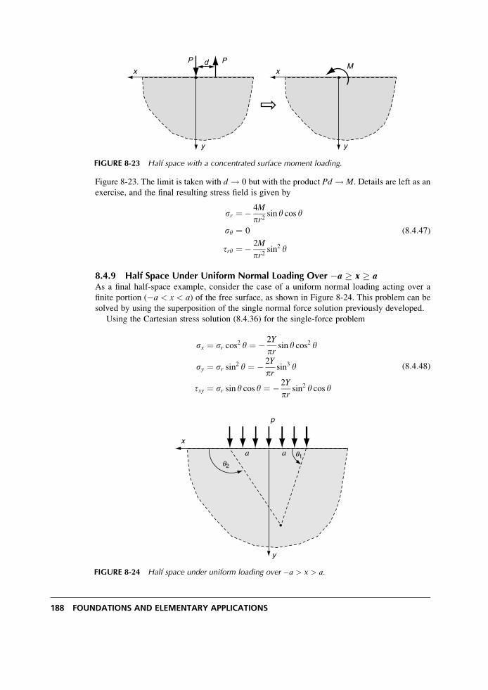
Figure 8-23. The limit is taken with d ! 0 but with the product Pd ! M. Details are left as an
exercise, and the final resulting stress field is given by
sr ¼� 4M
pr2sin y cos y
sy ¼ 0
try ¼� 2M
pr2sin2 y
(8:4:47)
8.4.9 Half Space Under Uniform Normal Loading Over �a x aAs a final half-space example, consider the case of a uniform normal loading acting over a
finite portion (�a < x < a) of the free surface, as shown in Figure 8-24. This problem can be
solved by using the superposition of the single normal force solution previously developed.
Using the Cartesian stress solution (8.4.36) for the single-force problem
sx ¼ sr cos2 y ¼ � 2Y
prsin y cos2 y
sy ¼ sr sin2 y ¼ � 2Y
prsin3 y
txy ¼ sr sin y cos y ¼ � 2Y
prsin2 y cos y
(8:4:48)
P d P
x
y
Mx
y
FIGURE 8-23 Half space with a concentrated surface moment loading.
p
x
y
aaq2
q1
FIGURE 8-24 Half space under uniform loading over �a > x > a.
188 FOUNDATIONS AND ELEMENTARY APPLICATIONS
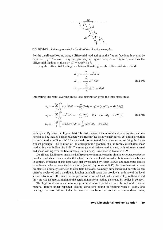
For the distributed loading case, a differential load acting on the free surface length dx may be
expressed by dY ¼ pdx. Using the geometry in Figure 8-25, dx ¼ rdy= sin y, and thus the
differential loading is given by dY ¼ prdy= sin y.Using the differential loading in relations (8.4.48) gives the differential stress field
dsx ¼ � 2p
pcos2 ydy
dsy ¼ � 2p
psin2 ydy
dtxy ¼ � 2p
psin y cos ydy
(8:4:49)
Integrating this result over the entire load distribution gives the total stress field
sx ¼ � 2p
p
ðy2y1cos2 ydy ¼ � p
2p[2(y2 � y1)þ ( sin 2y2 � sin 2y1)]
sy ¼ � 2p
p
ðy2y1sin2 ydy ¼ � p
2p[2(y2 � y1)� ( sin 2y2 � sin 2y1)]
txy ¼ � 2p
p
ðy2y1sin y cos ydy ¼ p
2p[ cos 2y2 � cos 2y1]
(8:4:50)
with y1 and y2 defined in Figure 8-24. The distribution of the normal and shearing stresses on a
horizontal line located a distance a below the free surface is shown in Figure 8-26. This distribution
is similar to that in Figure 8-20 for the single concentrated force, thus again justifying the Saint-
Venant principle. The solution of the corresponding problem of a uniformly distributed shear
loading is given in Exercise 8-28. The more general surface loading case, with arbitrary normal
and shear loading over the free surface (�a � s � a), is included in Exercise 8.29.Distributed loadings on an elastic half space are commonly used to simulate contact mechanics
problems, which are concerned with the load transfer and local stress distribution in elastic bodies
in contact. Problems of this type were first investigated by Hertz (1882), and numerous studies
have been conducted over the last century (see text by Johnson 1985). Because interest in these
problems is normally restricted to near-field behavior, boundary dimensions and curvatures can
often be neglected and a distributed loading on a half space can provide an estimate of the local
stress distribution. Of course, the simple uniform normal load distribution in Figure 8-24 would
only provide an approximation to the actual nonuniform loading generated by bodies in contact.
The high local stresses commonly generated in such problems have been found to cause
material failure under repeated loading conditions found in rotating wheels, gears, and
bearings. Because failure of ductile materials can be related to the maximum shear stress,
dx
r
dq
q
q
FIGURE 8-25 Surface geometry for the distributed loading example.
Two-Dimensional Problem Solution 189
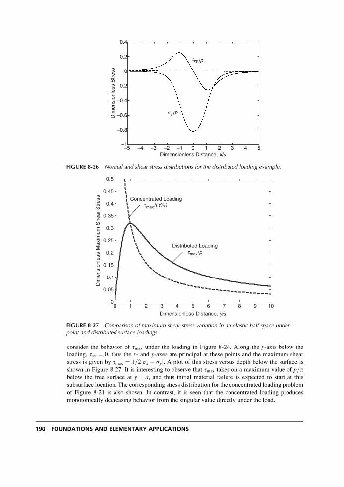
consider the behavior of tmax under the loading in Figure 8-24. Along the y-axis below the
loading, txy ¼ 0, thus the x- and y-axes are principal at these points and the maximum shear
stress is given by tmax ¼ 1=2jsx � syj. A plot of this stress versus depth below the surface is
shown in Figure 8-27. It is interesting to observe that tmax takes on a maximum value of p=pbelow the free surface at y ¼ a, and thus initial material failure is expected to start at this
subsurface location. The corresponding stress distribution for the concentrated loading problem
of Figure 8-21 is also shown. In contrast, it is seen that the concentrated loading produces
monotonically decreasing behavior from the singular value directly under the load.
Dimensionless Distance, x/a
Dim
ensi
onle
ss S
tres
ssy /p
txy /p
0.4
0.2
0
−0.2
−0.4
−0.6
−0.8
−1−5 −4 −3 −2 −1 0 1 2 3 4 5
FIGURE 8-26 Normal and shear stress distributions for the distributed loading example.
0 1 2 3 4 5 6 7 8 9 100
0.05
0.1
0.15
0.2
0.25
0.3
0.35
0.4
0.45
0.5
Dimensionless Distance, y/a
Dim
ensi
onle
ss M
axim
um S
hear
Str
ess
Distributed Loadingτmax/p
Concentrated Loadingτmax /(Y/a)
FIGURE 8-27 Comparison of maximum shear stress variation in an elastic half space underpoint and distributed surface loadings.
190 FOUNDATIONS AND ELEMENTARY APPLICATIONS
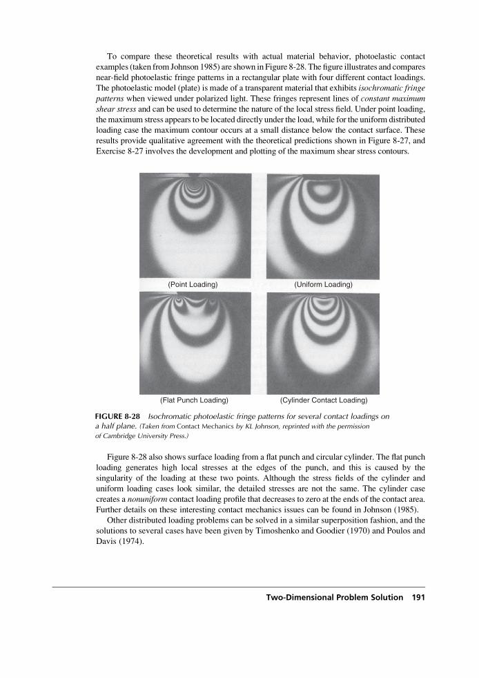
To compare these theoretical results with actual material behavior, photoelastic contact
examples (taken from Johnson 1985) are shown in Figure 8-28. The figure illustrates and compares
near-field photoelastic fringe patterns in a rectangular plate with four different contact loadings.
The photoelastic model (plate) is made of a transparent material that exhibits isochromatic fringepatterns when viewed under polarized light. These fringes represent lines of constant maximumshear stress and can be used to determine the nature of the local stress field. Under point loading,
themaximum stress appears to be located directly under the load, while for the uniform distributed
loading case the maximum contour occurs at a small distance below the contact surface. These
results provide qualitative agreement with the theoretical predictions shown in Figure 8-27, and
Exercise 8-27 involves the development and plotting of the maximum shear stress contours.
Figure 8-28 also shows surface loading from a flat punch and circular cylinder. The flat punch
loading generates high local stresses at the edges of the punch, and this is caused by the
singularity of the loading at these two points. Although the stress fields of the cylinder and
uniform loading cases look similar, the detailed stresses are not the same. The cylinder case
creates a nonuniform contact loading profile that decreases to zero at the ends of the contact area.
Further details on these interesting contact mechanics issues can be found in Johnson (1985).
Other distributed loading problems can be solved in a similar superposition fashion, and the
solutions to several cases have been given by Timoshenko and Goodier (1970) and Poulos and
Davis (1974).
(Flat Punch Loading) (Cylinder Contact Loading)
(Point Loading) (Uniform Loading)
FIGURE 8-28 Isochromatic photoelastic fringe patterns for several contact loadings ona half plane. (Taken from Contact Mechanics by KL Johnson, reprinted with the permission
of Cambridge University Press.)
Two-Dimensional Problem Solution 191
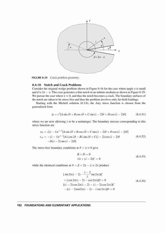
8.4.10 Notch and Crack ProblemsConsider the original wedge problem shown in Figure 8-16 for the case where angle a is small
and b is 2p� a. This case generates a thin notch in an infinite medium as shown in Figure 8-29.
We pursue the case where a � 0, and thus the notch becomes a crack. The boundary surfaces of
the notch are taken to be stress free and thus the problem involves only far-field loadings.
Starting with the Michell solution (8.3.6), the Airy stress function is chosen from the
generalized form
f ¼ rl[A sin lyþ B cos lyþ C sin (l� 2)yþ D cos (l� 2)y] (8:4:51)
where we are now allowing l to be a noninteger. The boundary stresses corresponding to this
stress function are
sy ¼ l(l� 1)rl�2[A sin lyþ B cos lyþ C sin (l� 2)yþ D cos (l� 2)y]
try ¼ �(l� 1)rl�2[Al cos ly� Bl sin lyþ C(l� 2) cos (l� 2)y
�D(l� 2) sin (l� 2)y]
(8:4:52)
The stress-free boundary conditions at y ¼ a � 0 give
Bþ D ¼ 0
lAþ (l� 2)C ¼ 0(8:4:53)
while the identical conditions at y ¼ b ¼ 2p� a � 2p produce
[ sin 2p(l� 2)� l� 2
lsin 2pl]C
þ [ cos 2p(l� 2)� cos 2pl]D ¼ 0
[(l� 2) cos 2p(l� 2)� (l� 2) cos 2pl]C
� [(l� 2)sin2p(l� 2)� l sin 2pl]D ¼ 0
(8:4:54)
y
b = 2p − a
r
x
qaJ
FIGURE 8-29 Crack problem geometry.
192 FOUNDATIONS AND ELEMENTARY APPLICATIONS
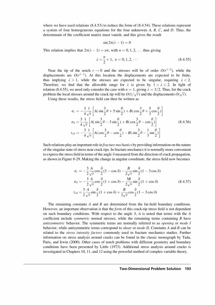
where we have used relations (8.4.53) to reduce the form of (8.4.54). These relations represent
a system of four homogeneous equations for the four unknowns A, B, C, and D. Thus, thedeterminant of the coefficient matrix must vanish, and this gives the result
sin 2p(l� 1) ¼ 0
This relation implies that 2p(l� 1) ¼ np, with n ¼ 0, 1, 2, . . . thus giving
l ¼ n
2þ 1, n ¼ 0, 1, 2, � � � (8:4:55)
Near the tip of the notch r ! 0 and the stresses will be of order O(rl�2), while the
displacements are O(rl�1). At this location the displacements are expected to be finite,
thus implying l > 1, while the stresses are expected to be singular, requiring l < 2.
Therefore, we find that the allowable range for l is given by 1 < l < 2. In light of
relation (8.4.55), we need only consider the case with n ¼ 1, giving l ¼ 3=2. Thus, for the crackproblem the local stresses around the crack tip will be O(1=
ffiffir
p) and the displacementsO(
ffiffir
p).
Using these results, the stress field can then be written as
sr ¼ � 3
4
1ffiffir
p A( sin3
2yþ 5 sin
y2)þ B( cos
3
2yþ 5
3cos
y2)
� �
sy ¼ 3
4
1ffiffir
p A( sin3
2y� 3 sin
y2)þ B( cos
3
2y� cos
y2)
� �
try ¼ � 3
4
1ffiffir
p A( cos3
2y� cos
y2)� B( sin
3
2y� 1
3sin
y2)
� � (8:4:56)
Such relations play an important role in fracture mechanics by providing information on the nature
of the singular state of stress near crack tips. In fracture mechanics it is normally more convenient
to express the stress field in terms of the angle Wmeasured from the direction of crack propagation,
as shown in Figure 8-29. Making the change in angular coordinate, the stress field now becomes
sr ¼ � 3
2
Affiffir
p cosW2(3� cos W)� B
2ffiffir
p sinW2(1� 3 cos W)
sy ¼ � 3
2
Affiffir
p cosW2(1þ cos W)� 3B
2ffiffir
p sinW2(1þ cos W)
try ¼ 3
2
Affiffir
p sinW2(1þ cos W)þ B
2ffiffir
p cosW2(1� 3 cosW)
(8:4:57)
The remaining constants A and B are determined from the far-field boundary conditions.
However, an important observation is that the form of this crack-tip stress field is not dependent
on such boundary conditions. With respect to the angle W, it is noted that terms with the Acoefficient include symmetric normal stresses, while the remaining terms containing B have
antisymmetric behavior. The symmetric terms are normally referred to as opening or mode Ibehavior, while antisymmetric terms correspond to shear or mode II. Constants A and B can be
related to the stress intensity factors commonly used in fracture mechanics studies. Further
information on stress analysis around cracks can be found in the classic monograph by Tada,
Paris, and Irwin (2000). Other cases of notch problems with different geometry and boundary
conditions have been presented by Little (1973). Additional stress analysis around cracks is
investigated in Chapters 10, 11, and 12 using the powerful method of complex variable theory.
Two-Dimensional Problem Solution 193
EXAMPLE 8-9: Curved Beam Problems
We shall now investigate the solution to some curved beam problems defined by an
annular region cut by two radial lines. Similar to the previous beam examples, we use
resultant force boundary conditions at the ends and exact pointwise specifications along
the lateral curved boundaries. Comparisons with strength of materials predictions are
made for specific cases.
8.4.11 Pure Bending ExampleThe first example is the simple case of a curved beam loaded by end moments as shown in
Figure 8-30. The solution to such a problem is independent of the angular coordinate. As usual,
we satisfy the pointwise boundary conditions on the sides of the beam but address only the
resultant effects at each cross-sectional end. Thus, the boundary conditions on this problem are
formulated as
sr(a) ¼ sr(b) ¼ 0
try(a) ¼ try(b) ¼ 0ðba
sydr ¼ 0ðba
syrdr ¼ �M
(8:4:58)
Using the general axisymmetric stress solution (8.3.8) in boundary relations (8.4.58) gives
2A log aþ C
a2þ Aþ 2B ¼ 0
2A log bþ C
b2þ Aþ 2B ¼ 0
b(2A log bþ C
b2þ Aþ 2B)� a(2A log aþ C
a2þ Aþ 2B) ¼ 0
� C log (b
a)þ A(b2 log b� a2 log a)þ B(b2 � a2) ¼ �M
(8:4:59)
Because the third equation is a linear combination of the first two, only three of these four
relations are independent. Solving these equations for the three constants gives
a
b
r
MM
FIGURE 8-30 Curved beam with end moments.
194 FOUNDATIONS AND ELEMENTARY APPLICATIONS
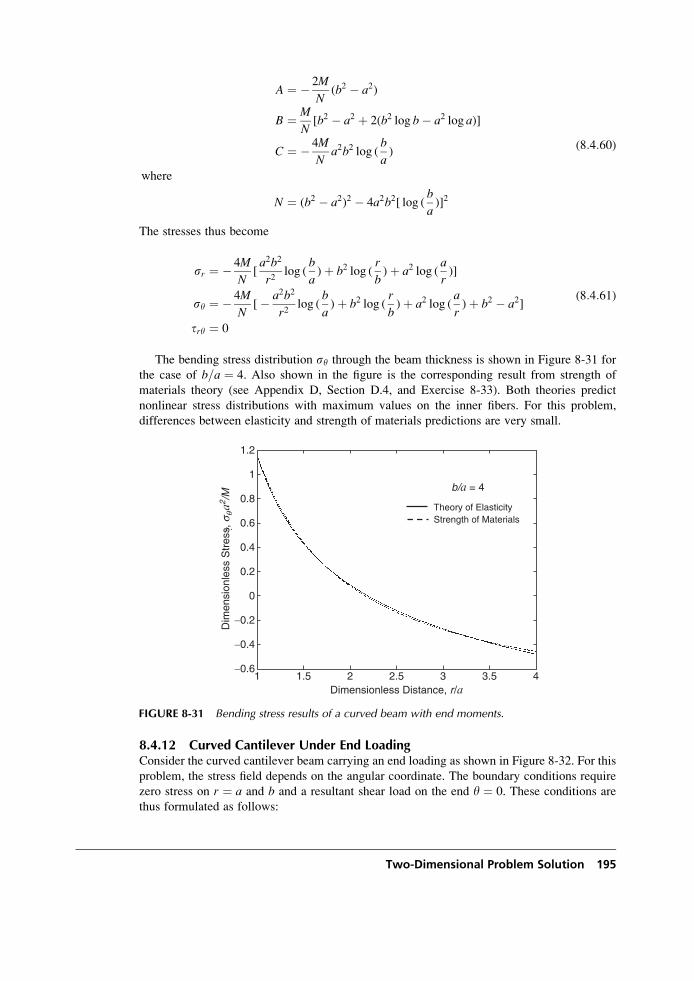
A ¼ � 2M
N(b2 � a2)
B ¼ M
N[b2 � a2 þ 2(b2 log b� a2 log a)]
C ¼ � 4M
Na2b2 log (
b
a)
where
N ¼ (b2 � a2)2 � 4a2b2[ log (b
a)]2
(8:4:60)
The stresses thus become
sr ¼ � 4M
N[a2b2
r2log (
b
a)þ b2 log (
r
b)þ a2 log (
a
r)]
sy ¼ � 4M
N[� a2b2
r2log (
b
a)þ b2 log (
r
b)þ a2 log (
a
r)þ b2 � a2]
try ¼ 0
(8:4:61)
The bending stress distribution sy through the beam thickness is shown in Figure 8-31 for
the case of b=a ¼ 4. Also shown in the figure is the corresponding result from strength of
materials theory (see Appendix D, Section D.4, and Exercise 8-33). Both theories predict
nonlinear stress distributions with maximum values on the inner fibers. For this problem,
differences between elasticity and strength of materials predictions are very small.
8.4.12 Curved Cantilever Under End LoadingConsider the curved cantilever beam carrying an end loading as shown in Figure 8-32. For this
problem, the stress field depends on the angular coordinate. The boundary conditions require
zero stress on r ¼ a and b and a resultant shear load on the end y ¼ 0. These conditions are
thus formulated as follows:
Dimensionless Distance, r/a
Dim
ensi
onle
ss S
tres
s, s
q a2 /
M?
Theory of ElasticityStrength of Materials
b/a = 4
1.2
1
0.8
0.6
0.4
0.2
0
−0.2
−0.4
−0.61 1.5 2 2.5 3 3.5 4
FIGURE 8-31 Bending stress results of a curved beam with end moments.
Two-Dimensional Problem Solution 195
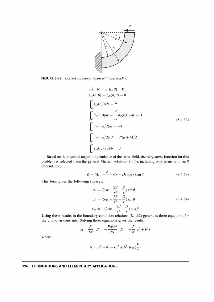
sr(a, y) ¼ sr(b, y) ¼ 0
try(a, y) ¼ try(b, y) ¼ 0ðba
try(r, 0)dr ¼ Pðba
sy(r, 0)dr ¼ðba
sy(r, 0)rdr ¼ 0ðba
sy(r, p=2)dr ¼ �Pðba
sy(r, p=2)rdr ¼ P(aþ b)=2ðba
try(r,p=2)dr ¼ 0
(8:4:62)
Based on the required angular dependence of the stress field, the Airy stress function for this
problem is selected from the general Michell solution (8.3.6), including only terms with sin ydependence,
f ¼ (Ar3 þ B
rþ Cr þ Dr log r) sin y (8:4:63)
This form gives the following stresses:
sr ¼ (2Ar � 2B
r3þ D
r) sin y
sy ¼ (6Ar þ 2B
r3þ D
r) sin y
try ¼ �(2Ar � 2B
r3þ D
r) cos y
(8:4:64)
Using these results in the boundary condition relations (8.4.62) generates three equations for
the unknown constants. Solving these equations gives the results
A ¼ P
2N, B ¼ �Pa2b2
2N, D ¼ � P
N(a2 þ b2)
where
N ¼ a2 � b2 þ (a2 þ b2) log (b
a)
P
ab
rq
FIGURE 8-32 Curved cantilever beam with end loading.
196 FOUNDATIONS AND ELEMENTARY APPLICATIONS
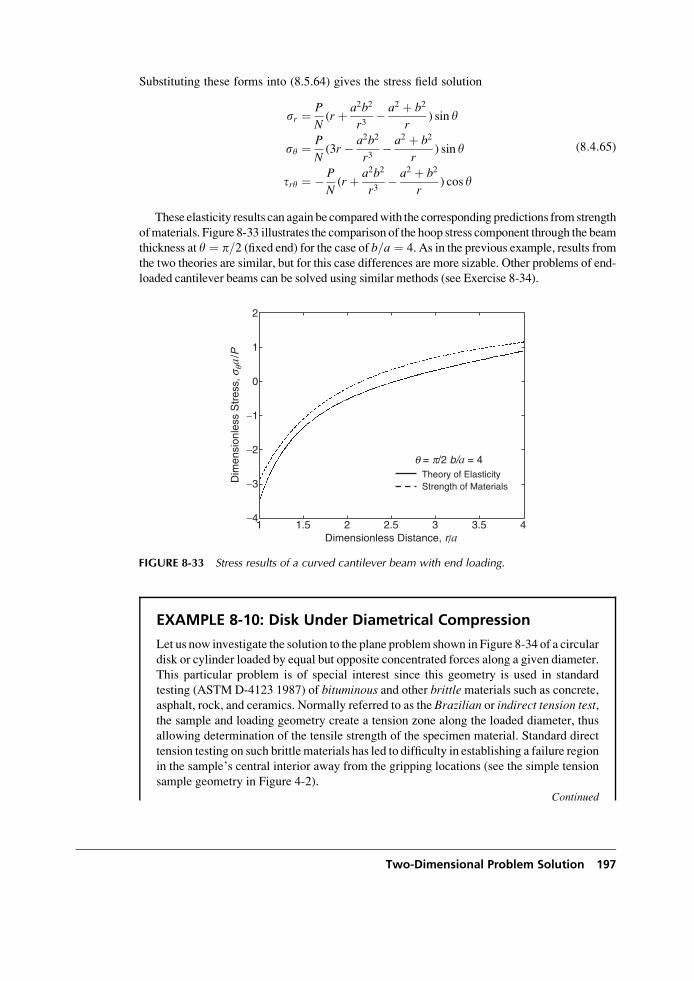
Substituting these forms into (8.5.64) gives the stress field solution
sr ¼ P
N(r þ a2b2
r3� a2 þ b2
r) sin y
sy ¼ P
N(3r � a2b2
r3� a2 þ b2
r) sin y
try ¼ � P
N(r þ a2b2
r3� a2 þ b2
r) cos y
(8:4:65)
These elasticity results can again be comparedwith the corresponding predictions fromstrength
ofmaterials. Figure 8-33 illustrates the comparison of the hoop stress component through the beam
thickness at y ¼ p=2 (fixed end) for the case of b=a ¼ 4. As in the previous example, results from
the two theories are similar, but for this case differences are more sizable. Other problems of end-
loaded cantilever beams can be solved using similar methods (see Exercise 8-34).
EXAMPLE 8-10: Disk Under Diametrical Compression
Let us now investigate the solution to the plane problem shown in Figure 8-34 of a circular
disk or cylinder loaded by equal but opposite concentrated forces along a given diameter.
This particular problem is of special interest since this geometry is used in standard
testing (ASTM D-4123 1987) of bituminous and other brittlematerials such as concrete,
asphalt, rock, and ceramics. Normally referred to as the Brazilian or indirect tension test,the sample and loading geometry create a tension zone along the loaded diameter, thus
allowing determination of the tensile strength of the specimen material. Standard direct
tension testing on such brittlematerials has led to difficulty in establishing a failure region
in the sample’s central interior away from the gripping locations (see the simple tension
sample geometry in Figure 4-2).
Continued
Dimensionless Distance, r/a
Dim
ensi
onle
ss S
tres
s, s
q a /P
Theory of ElasticityStrength of Materials
q = p/2 b/a = 4
2
1
0
−1
−2
−3
−41 1.5 2 2.5 3 3.5 4
FIGURE 8-33 Stress results of a curved cantilever beam with end loading.
Two-Dimensional Problem Solution 197
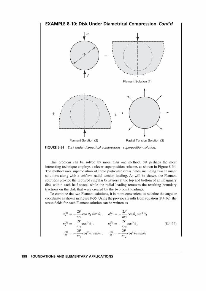
EXAMPLE 8-10: Disk Under Diametrical Compression–Cont’d
This problem can be solved by more than one method, but perhaps the most
interesting technique employs a clever superposition scheme, as shown in Figure 8-34.
The method uses superposition of three particular stress fields including two Flamant
solutions along with a uniform radial tension loading. As will be shown, the Flamant
solutions provide the required singular behaviors at the top and bottom of an imaginary
disk within each half space, while the radial loading removes the resulting boundary
tractions on the disk that were created by the two point loadings.
To combine the two Flamant solutions, it is more convenient to redefine the angular
coordinate as shown in Figure 8-35. Using the previous results from equation (8.4.36), the
stress fields for each Flamant solution can be written as
s(1)x ¼ � 2P
pr1cos y1 sin2 y1, s(2)x ¼ � 2P
pr2cos y2 sin2 y2
s(1)y ¼ � 2P
pr1cos3 y1, s(2)y ¼ � 2P
pr2cos3 y2
t(1)xy ¼ � 2P
pr1cos2 y1 sin y1, t(2)xy ¼ � 2P
pr2cos2 y2 sin y2
(8:4:66)
Radial Tension Solution (3)
P
P
D =
Flamant Solution (1)
+ +
Flamant Solution (2)
FIGURE 8-34 Disk under diametrical compression—superposition solution.
198 FOUNDATIONS AND ELEMENTARY APPLICATIONS
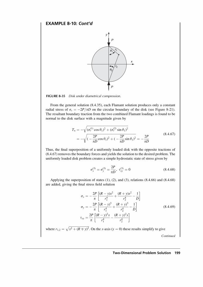
EXAMPLE 8-10: Cont’d
From the general solution (8.4.35), each Flamant solution produces only a constant
radial stress of sr ¼ �2P=pD on the circular boundary of the disk (see Figure 8-21).
The resultant boundary traction from the two combined Flamant loadings is found to be
normal to the disk surface with a magnitude given by
Tn ¼ �ffiffiffiffiffiffiffiffiffiffiffiffiffiffiffiffiffiffiffiffiffiffiffiffiffiffiffiffiffiffiffiffiffiffiffiffiffiffiffiffiffiffiffiffiffiffiffiffiffiffiffiffiffiffi(s(1)r cos y1)2 þ (s(2)r sin y1)2
q
¼ �ffiffiffiffiffiffiffiffiffiffiffiffiffiffiffiffiffiffiffiffiffiffiffiffiffiffiffiffiffiffiffiffiffiffiffiffiffiffiffiffiffiffiffiffiffiffiffiffiffiffiffiffiffiffiffiffiffiffiffiffiffiffiffiffi(� 2P
pDcos y1)2 þ (� 2P
pDsin y1)2
r¼ � 2P
pD
(8:4:67)
Thus, the final superposition of a uniformly loaded disk with the opposite tractions of
(8.4.67) removes the boundary forces and yields the solution to the desired problem. The
uniformly loaded disk problem creates a simple hydrostatic state of stress given by
s(3)x ¼ s(3)y ¼ 2P
pD, t(3)xy ¼ 0 (8:4:68)
Applying the superposition of states (1), (2), and (3), relations (8.4.66) and (8.4.68)
are added, giving the final stress field solution
sx ¼ � 2P
p(R� y)x2
r41þ (Rþ y)x2
r42� 1
D
� �
sy ¼ � 2P
p(R� y)3
r41þ (Rþ y)3
r42� 1
D
� �
txy ¼ 2P
p(R� y)2x
r41� (Rþ y)2x
r42
� �(8:4:69)
where r1,2 ¼ffiffiffiffiffiffiffiffiffiffiffiffiffiffiffiffiffiffiffiffiffiffiffiffiffiffix2 þ (R� y)2
p. On the x-axis (y ¼ 0) these results simplify to give
Continued
P
P
q2
q1
y
x
r1
r2
FIGURE 8-35 Disk under diametrical compression.
Two-Dimensional Problem Solution 199
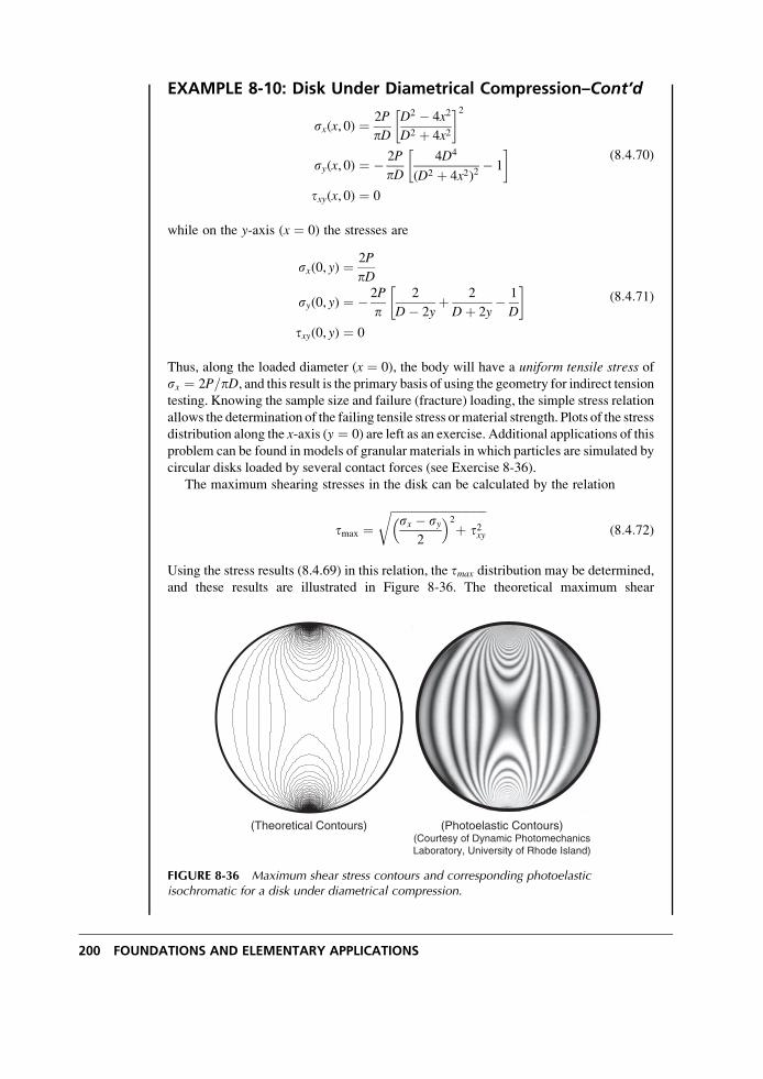
EXAMPLE 8-10: Disk Under Diametrical Compression–Cont’d
sx(x, 0) ¼ 2P
pDD2 � 4x2
D2 þ 4x2
� �2
sy(x, 0) ¼ � 2P
pD4D4
(D2 þ 4x2)2� 1
� �txy(x, 0) ¼ 0
(8:4:70)
while on the y-axis (x ¼ 0) the stresses are
sx(0, y) ¼ 2P
pD
sy(0, y) ¼ � 2P
p2
D� 2yþ 2
Dþ 2y� 1
D
� �txy(0, y) ¼ 0
(8:4:71)
Thus, along the loaded diameter (x ¼ 0), the body will have a uniform tensile stress ofsx ¼ 2P=pD, and this result is the primary basis of using the geometry for indirect tension
testing. Knowing the sample size and failure (fracture) loading, the simple stress relation
allows the determination of the failing tensile stress ormaterial strength. Plots of the stress
distribution along the x-axis (y ¼ 0) are left as an exercise. Additional applications of this
problem can be found in models of granular materials in which particles are simulated by
circular disks loaded by several contact forces (see Exercise 8-36).
The maximum shearing stresses in the disk can be calculated by the relation
tmax ¼ffiffiffiffiffiffiffiffiffiffiffiffiffiffiffiffiffiffiffiffiffiffiffiffiffiffiffiffiffiffiffiffiffisx � sy
2
� �2þ t2xy
r(8:4:72)
Using the stress results (8.4.69) in this relation, the tmax distribution may be determined,
and these results are illustrated in Figure 8-36. The theoretical maximum shear
(Theoretical Contours) (Photoelastic Contours)(Courtesy of Dynamic PhotomechanicsLaboratory, University of Rhode Island)
FIGURE 8-36 Maximum shear stress contours and corresponding photoelasticisochromatic for a disk under diametrical compression.
200 FOUNDATIONS AND ELEMENTARY APPLICATIONS
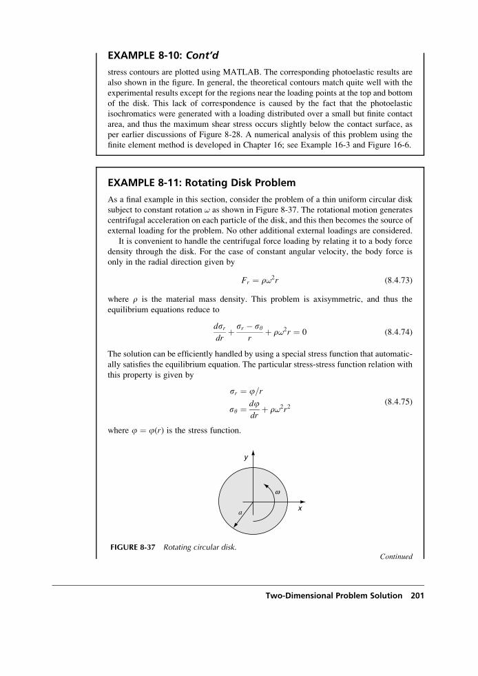
EXAMPLE 8-10: Cont’d
stress contours are plotted using MATLAB. The corresponding photoelastic results are
also shown in the figure. In general, the theoretical contours match quite well with the
experimental results except for the regions near the loading points at the top and bottom
of the disk. This lack of correspondence is caused by the fact that the photoelastic
isochromatics were generated with a loading distributed over a small but finite contact
area, and thus the maximum shear stress occurs slightly below the contact surface, as
per earlier discussions of Figure 8-28. A numerical analysis of this problem using the
finite element method is developed in Chapter 16; see Example 16-3 and Figure 16-6.
EXAMPLE 8-11: Rotating Disk Problem
As a final example in this section, consider the problem of a thin uniform circular disk
subject to constant rotation ! as shown in Figure 8-37. The rotational motion generates
centrifugal acceleration on each particle of the disk, and this then becomes the source of
external loading for the problem. No other additional external loadings are considered.
It is convenient to handle the centrifugal force loading by relating it to a body force
density through the disk. For the case of constant angular velocity, the body force is
only in the radial direction given by
Fr ¼ r!2r (8:4:73)
where r is the material mass density. This problem is axisymmetric, and thus the
equilibrium equations reduce to
dsrdr
þ sr � syr
þ r!2r ¼ 0 (8:4:74)
The solution can be efficiently handled by using a special stress function that automatic-
ally satisfies the equilibrium equation. The particular stress-stress function relation with
this property is given by
sr ¼ j=r
sy ¼ djdr
þ r!2r2(8:4:75)
where j ¼ j(r) is the stress function.
Continued
x
y
a
w
FIGURE 8-37 Rotating circular disk.
Two-Dimensional Problem Solution 201
EXAMPLE 8-11: Rotating Disk Problem–Cont’d
As usual, the governing equation for the stress function is determined from the
compatibility statement. For this axisymmetric case, the displacement field is of the
form ur ¼ ur(r) and uy ¼ 0. Therefore, the strain field is given by
er ¼ durdr
, ey ¼ urr, ery ¼ 0
Eliminating ur from these equations develops the simple compatibility statement
d
dr(rey)� er ¼ 0 (8:4:76)
Recall that the more general polar coordinate case was given as Exercise 7-17. Using
Hooke’s law for plane stress, the strains are given by
er ¼ 1
E(sr � �sy) ¼ 1
E
jr� �
djdr
� �r!2r2� �
ey ¼ 1
E(sy � �sr) ¼ 1
E
djdr
þ r!2r2 � �jr
� � (8:4:77)
Using this result in the compatibility relation (8.4.76) generates the desired governing
equation
d2jdr2
þ 1
r
djdr
� jr2
þ (3þ �)r!2r ¼ 0
which can be written as
d
dr
1
r
d
dr(rj)
� �¼ �(3þ �)r!2r (8:4:78)
This equation is easily integrated, giving the result
j ¼ � (3þ �)
8r!2r3 þ 1
2C1r þ C2
1
r(8:4:79)
where C1 and C2 are constants. The stresses corresponding to this solution are
sr ¼ � (3þ �)
8r!2r2 þ C1
2þ C2
r2
sy ¼ � 1þ 3�
8r!2r2 þ C1
2� C2
r2
(8:4:80)
For a solid disk, the stresses must be bounded at the origin and so C2 ¼ 0. The
condition that the disk is stress free at r ¼ a gives the remaining constant C1 ¼(3þ �)r!2a2=4. The final form of the stress field is then
202 FOUNDATIONS AND ELEMENTARY APPLICATIONS
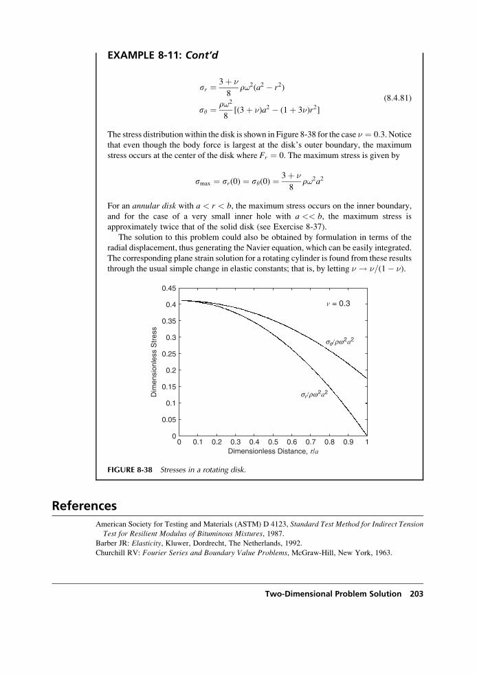
EXAMPLE 8-11: Cont’d
sr ¼ 3þ �
8r!2(a2 � r2)
sy ¼ r!2
8[(3þ �)a2 � (1þ 3�)r2]
(8:4:81)
The stress distributionwithin the disk is shown in Figure 8-38 for the case � ¼ 0:3. Noticethat even though the body force is largest at the disk’s outer boundary, the maximum
stress occurs at the center of the disk where Fr ¼ 0. The maximum stress is given by
smax ¼ sr(0) ¼ sy(0) ¼ 3þ �
8r!2a2
For an annular disk with a < r < b, the maximum stress occurs on the inner boundary,
and for the case of a very small inner hole with a << b, the maximum stress is
approximately twice that of the solid disk (see Exercise 8-37).
The solution to this problem could also be obtained by formulation in terms of the
radial displacement, thus generating the Navier equation, which can be easily integrated.
The corresponding plane strain solution for a rotating cylinder is found from these results
through the usual simple change in elastic constants; that is, by letting � ! �=(1� �).
sq/rw2a2
sr/rw2a2
n = 0.3
Dimensionless Distance, r/a
Dim
ensi
onle
ss S
tres
s
0.45
0.4
0.35
0.3
0.25
0.2
0.15
0.1
0.05
00 0.1 0.2 0.3 0.4 0.5 0.6 0.7 0.8 0.9 1
FIGURE 8-38 Stresses in a rotating disk.
References
American Society for Testing and Materials (ASTM) D 4123, Standard Test Method for Indirect TensionTest for Resilient Modulus of Bituminous Mixtures, 1987.
Barber JR: Elasticity, Kluwer, Dordrecht, The Netherlands, 1992.Churchill RV: Fourier Series and Boundary Value Problems, McGraw-Hill, New York, 1963.
Two-Dimensional Problem Solution 203
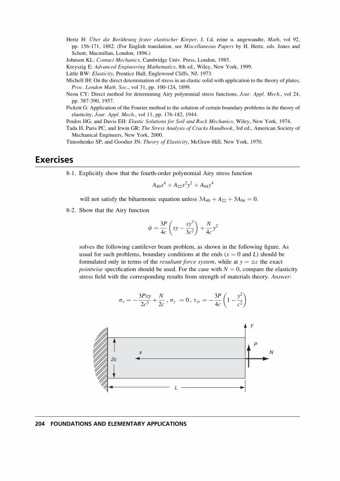
Hertz H: Uber die Beruhrung fester elastischer Korper, J. f.d. reine u. angewandte, Math, vol 92,
pp. 156-171, 1882. (For English translation, see Miscellaneous Papers by H. Hertz, eds. Jones and
Schott, Macmillan, London, 1896.)
Johnson KL: Contact Mechanics, Cambridge Univ. Press, London, 1985.
Kreyszig E: Advanced Engineering Mathematics, 8th ed., Wiley, New York, 1999.
Little RW: Elasticity, Prentice Hall, Englewood Cliffs, NJ, 1973.
Michell JH: On the direct determination of stress in an elastic solid with application to the theory of plates,
Proc. London Math. Soc., vol 31, pp. 100-124, 1899.Neou CY: Direct method for determining Airy polynomial stress functions, Jour. Appl. Mech., vol 24,pp. 387-390, 1957.
Pickett G: Application of the Fourier method to the solution of certain boundary problems in the theory of
elasticity, Jour. Appl. Mech., vol 11, pp. 176-182, 1944.Poulos HG, and Davis EH: Elastic Solutions for Soil and Rock Mechanics, Wiley, New York, 1974.
Tada H, Paris PC, and Irwin GR: The Stress Analysis of Cracks Handbook, 3rd ed., American Society of
Mechanical Engineers, New York, 2000.
Timoshenko SP, and Goodier JN: Theory of Elasticity, McGraw-Hill, New York, 1970.
Exercises
8-1. Explicitly show that the fourth-order polynomial Airy stress function
A40x4 þ A22x
2y2 þ A04y4
will not satisfy the biharmonic equation unless 3A40 þ A22 þ 3A04 ¼ 0.
8-2. Show that the Airy function
f ¼ 3P
4cxy� xy3
3c2
� �þ N
4cy2
solves the following cantilever beam problem, as shown in the following figure. As
usual for such problems, boundary conditions at the ends (x ¼ 0 and L) should be
formulated only in terms of the resultant force system, while at y ¼ �c the exactpointwise specification should be used. For the case with N ¼ 0, compare the elasticity
stress field with the corresponding results from strength of materials theory. Answer:
sx ¼ � 3Pxy
2c3þ N
2c, sy ¼ 0 , txy ¼ � 3P
4c1� y2
c2
� �
x
y
N
P
L
2c
204 FOUNDATIONS AND ELEMENTARY APPLICATIONS
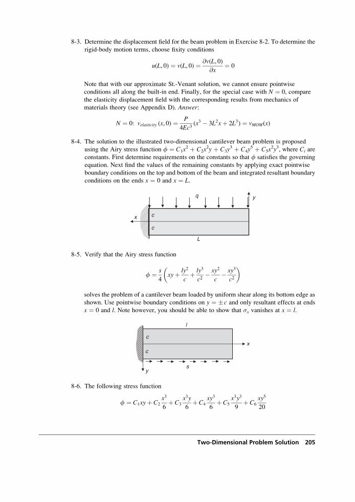
8-3. Determine the displacement field for the beam problem in Exercise 8-2. To determine the
rigid-body motion terms, choose fixity conditions
u(L, 0) ¼ v(L, 0) ¼ @v(L, 0)
@x¼ 0
Note that with our approximate St.-Venant solution, we cannot ensure pointwise
conditions all along the built-in end. Finally, for the special case with N ¼ 0, compare
the elasticity displacement field with the corresponding results from mechanics of
materials theory (see Appendix D). Answer:
N ¼ 0: velasticity (x, 0) ¼ P
4Ec3(x3 � 3L2xþ 2L3) ¼ vMOM(x)
8-4. The solution to the illustrated two-dimensional cantilever beam problem is proposed
using the Airy stress function f ¼ C1x2 þ C2x
2y þ C3y3 þ C4y
5 þ C5x2y3, where Ci are
constants. First determine requirements on the constants so that f satisfies the governing
equation. Next find the values of the remaining constants by applying exact pointwise
boundary conditions on the top and bottom of the beam and integrated resultant boundary
conditions on the ends x ¼ 0 and x ¼ L.
x
y
c
c
L
q
8-5. Verify that the Airy stress function
f ¼ s
4xyþ ly2
cþ ly3
c2� xy2
c� xy3
c2
� �
solves the problem of a cantilever beam loaded by uniform shear along its bottom edge as
shown. Use pointwise boundary conditions on y ¼ �c and only resultant effects at ends
x ¼ 0 and l. Note however, you should be able to show that �x vanishes at x ¼ l.
s
c
l
y
xc
8-6. The following stress function
f ¼ C1xyþ C2
x3
6þ C3
x3y
6þ C4
xy3
6þ C5
x3y3
9þ C6
xy5
20
Two-Dimensional Problem Solution 205
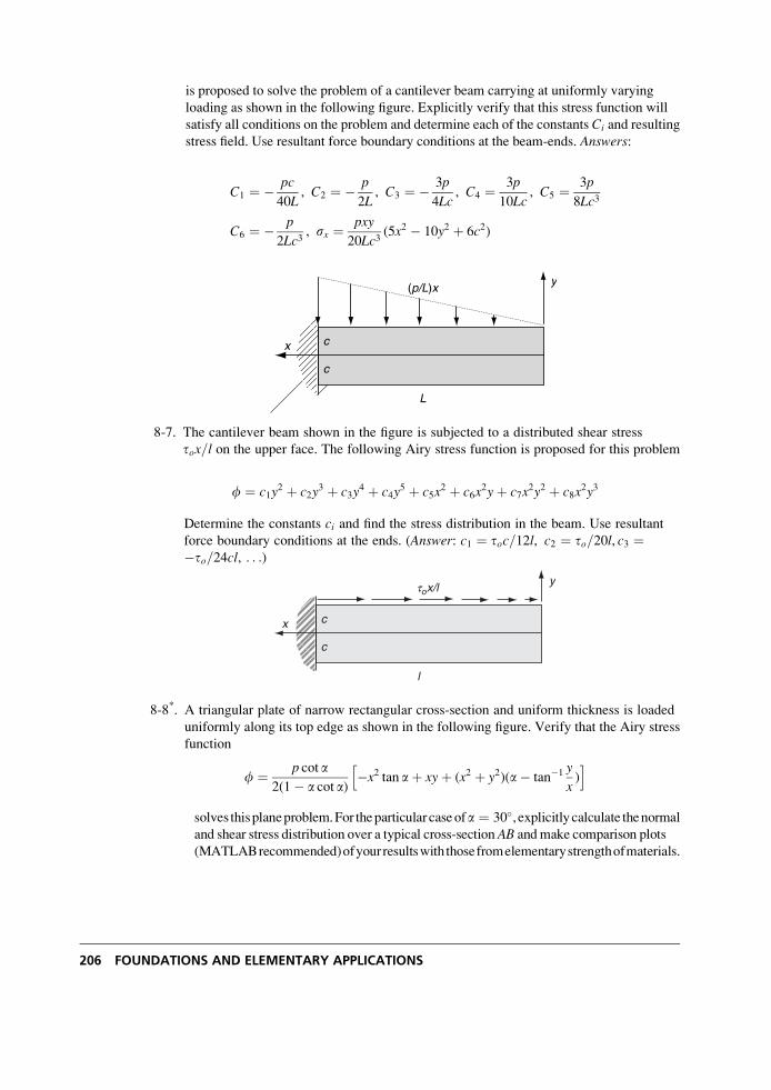
is proposed to solve the problem of a cantilever beam carrying at uniformly varying
loading as shown in the following figure. Explicitly verify that this stress function will
satisfy all conditions on the problem and determine each of the constants Ci and resulting
stress field. Use resultant force boundary conditions at the beam-ends. Answers:
C1 ¼ � pc
40L, C2 ¼ � p
2L, C3 ¼ � 3p
4Lc, C4 ¼ 3p
10Lc, C5 ¼ 3p
8Lc3
C6 ¼ � p
2Lc3, sx ¼ pxy
20Lc3(5x2 � 10y2 þ 6c2)
x
y
c
c
L
(p/L)x
8-7. The cantilever beam shown in the figure is subjected to a distributed shear stress
tox=l on the upper face. The following Airy stress function is proposed for this problem
f ¼ c1y2 þ c2y
3 þ c3y4 þ c4y
5 þ c5x2 þ c6x
2yþ c7x2y2 þ c8x
2y3
Determine the constants ci and find the stress distribution in the beam. Use resultant
force boundary conditions at the ends. (Answer: c1 ¼ toc=12l, c2 ¼ to=20l, c3 ¼�to=24cl, . . .)
x
y
c
c
l
tox/l
8-8*. A triangular plate of narrow rectangular cross-section and uniform thickness is loaded
uniformly along its top edge as shown in the following figure. Verify that the Airy stress
function
f ¼ p cot a2(1� a cot a)
�x2 tan aþ xyþ (x2 þ y2)(a� tan�1 y
x)
h i
solves thisplaneproblem.For theparticular caseofa ¼ 30, explicitly calculate thenormal
and shear stress distribution over a typical cross-sectionAB andmake comparison plots
(MATLABrecommended)ofyourresultswiththosefromelementarystrengthofmaterials.
206 FOUNDATIONS AND ELEMENTARY APPLICATIONS
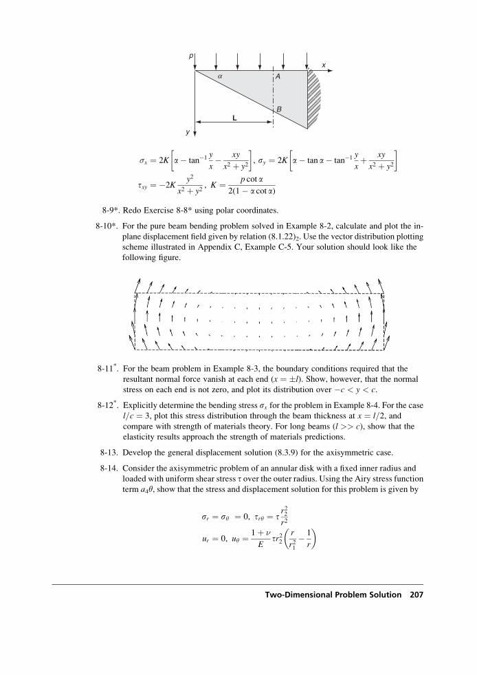
x
y
L
p
A
B
a
�x ¼ 2K a� tan�1 y
x� xy
x2 þ y2
� �, sy ¼ 2K a� tan a� tan�1 y
xþ xy
x2 þ y2
� �
txy ¼ �2Ky2
x2 þ y2, K ¼ p cot a
2(1� a cot a)
8-9*. Redo Exercise 8-8* using polar coordinates.
8-10*. For the pure beam bending problem solved in Example 8-2, calculate and plot the in-
plane displacement field given by relation (8.1.22)2. Use the vector distribution plotting
scheme illustrated in Appendix C, Example C-5. Your solution should look like the
following figure.
8-11*. For the beam problem in Example 8-3, the boundary conditions required that the
resultant normal force vanish at each end (x ¼ �l). Show, however, that the normal
stress on each end is not zero, and plot its distribution over �c < y < c.
8-12*. Explicitly determine the bending stress sx for the problem in Example 8-4. For the case
l=c ¼ 3, plot this stress distribution through the beam thickness at x ¼ l=2, andcompare with strength of materials theory. For long beams (l >> c), show that the
elasticity results approach the strength of materials predictions.
8-13. Develop the general displacement solution (8.3.9) for the axisymmetric case.
8-14. Consider the axisymmetric problem of an annular disk with a fixed inner radius and
loaded with uniform shear stress t over the outer radius. Using the Airy stress functionterm a4�, show that the stress and displacement solution for this problem is given by
sr ¼ sy ¼ 0, try ¼ tr22r2
ur ¼ 0, uy ¼ 1þ �
Etr22
r
r21� 1
r
� �
Two-Dimensional Problem Solution 207
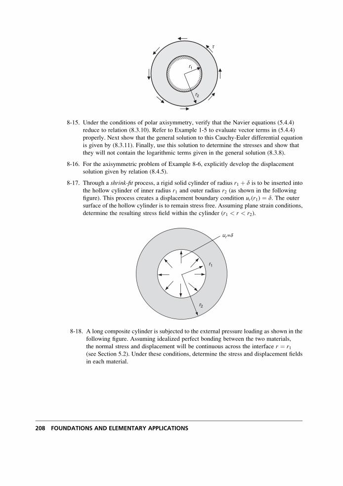
r2
r1
t
8-15. Under the conditions of polar axisymmetry, verify that the Navier equations (5.4.4)
reduce to relation (8.3.10). Refer to Example 1-5 to evaluate vector terms in (5.4.4)
properly. Next show that the general solution to this Cauchy-Euler differential equation
is given by (8.3.11). Finally, use this solution to determine the stresses and show that
they will not contain the logarithmic terms given in the general solution (8.3.8).
8-16. For the axisymmetric problem of Example 8-6, explicitly develop the displacement
solution given by relation (8.4.5).
8-17. Through a shrink-fit process, a rigid solid cylinder of radius r1 þ d is to be inserted into
the hollow cylinder of inner radius r1 and outer radius r2 (as shown in the following
figure). This process creates a displacement boundary condition ur(r1) ¼ d. The outersurface of the hollow cylinder is to remain stress free. Assuming plane strain conditions,
determine the resulting stress field within the cylinder (r1 < r < r2).
r2
r1
ur =d
8-18. A long composite cylinder is subjected to the external pressure loading as shown in the
following figure. Assuming idealized perfect bonding between the two materials,
the normal stress and displacement will be continuous across the interface r ¼ r1(see Section 5.2). Under these conditions, determine the stress and displacement fields
in each material.
208 FOUNDATIONS AND ELEMENTARY APPLICATIONS
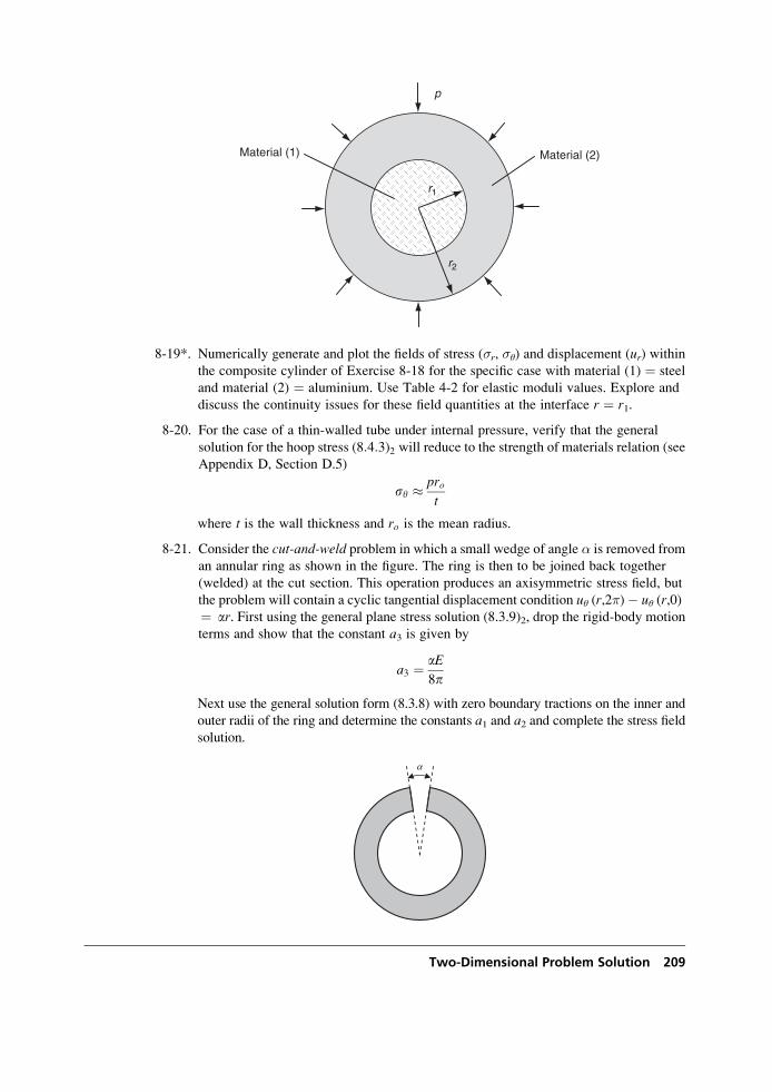
r2
r1
Material (1)
p
Material (2)
8-19*. Numerically generate and plot the fields of stress (�r, ��) and displacement (ur) withinthe composite cylinder of Exercise 8-18 for the specific case with material (1) ¼ steel
and material (2) ¼ aluminium. Use Table 4-2 for elastic moduli values. Explore and
discuss the continuity issues for these field quantities at the interface r ¼ r1.
8-20. For the case of a thin-walled tube under internal pressure, verify that the general
solution for the hoop stress (8:4:3)2 will reduce to the strength of materials relation (see
Appendix D, Section D.5)
sy � prot
where t is the wall thickness and ro is the mean radius.
8-21. Consider the cut-and-weld problem in which a small wedge of angle � is removed from
an annular ring as shown in the figure. The ring is then to be joined back together
(welded) at the cut section. This operation produces an axisymmetric stress field, but
the problem will contain a cyclic tangential displacement condition u� (r,2�)� u� (r,0)¼ ar. First using the general plane stress solution (8.3.9)2, drop the rigid-body motion
terms and show that the constant a3 is given by
a3 ¼ aE8p
Next use the general solution form (8.3.8) with zero boundary tractions on the inner and
outer radii of the ring and determine the constants a1 and a2 and complete the stress field
solution.
a
Two-Dimensional Problem Solution 209
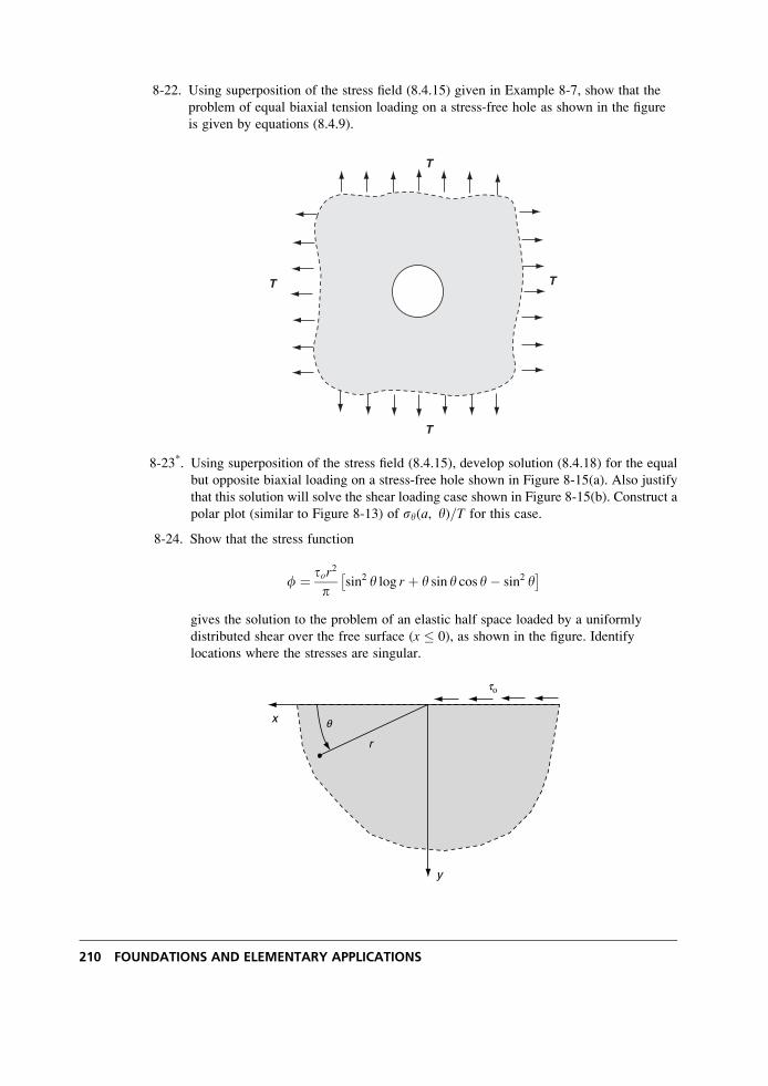
8-22. Using superposition of the stress field (8.4.15) given in Example 8-7, show that the
problem of equal biaxial tension loading on a stress-free hole as shown in the figure
is given by equations (8.4.9).
TT
T
T
8-23*. Using superposition of the stress field (8.4.15), develop solution (8.4.18) for the equal
but opposite biaxial loading on a stress-free hole shown in Figure 8-15(a). Also justify
that this solution will solve the shear loading case shown in Figure 8-15(b). Construct a
polar plot (similar to Figure 8-13) of sy(a, y)=T for this case.
8-24. Show that the stress function
f ¼ tor2
psin2 y log r þ y sin y cos y� sin2 y �
gives the solution to the problem of an elastic half space loaded by a uniformly
distributed shear over the free surface (x � 0), as shown in the figure. Identify
locations where the stresses are singular.
x
y
r
q
tο
210 FOUNDATIONS AND ELEMENTARY APPLICATIONS
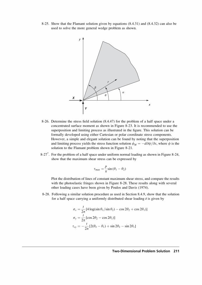
8-25. Show that the Flamant solution given by equations (8.4.31) and (8.4.32) can also be
used to solve the more general wedge problem as shown.
x
y
r
X
Y
b
qa
8-26. Determine the stress field solution (8.4.47) for the problem of a half space under a
concentrated surface moment as shown in Figure 8-23. It is recommended to use the
superposition and limiting process as illustrated in the figure. This solution can be
formally developed using either Cartesian or polar coordinate stress components.
However, a simple and elegant solution can be found by noting that the superposition
and limiting process yields the stress function solution fM ¼ �d@f=@x, where f is the
solution to the Flamant problem shown in Figure 8-21.
8-27*. For the problem of a half space under uniform normal loading as shown in Figure 8-24,
show that the maximum shear stress can be expressed by
tmax ¼ p
psin (y1 � y2)
Plot the distribution of lines of constant maximum shear stress, and compare the results
with the photoelastic fringes shown in Figure 8-28. These results along with several
other loading cases have been given by Poulos and Davis (1974).
8-28. Following a similar solution procedure as used in Section 8.4.9, show that the solution
for a half space carrying a uniformly distributed shear loading t is given by
sx ¼ t
2p[4 log(sin y1=sin y2)� cos 2y2 þ cos 2y1)]
sy ¼ t
2p[cos 2y2 � cos 2y1)]
txy ¼ � t
2p[2(y2 � y1)þ sin 2y2 � sin 2y1]
Two-Dimensional Problem Solution 211
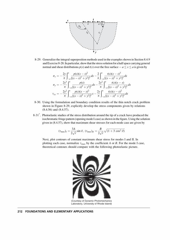
x
y
aa θ1θ2
t
r1r2
8-29. Generalize the integral superpositionmethods used in the examples shown in Section 8.4.9
andExercise8-28. Inparticular, showthat thestress solution forahalfspacecarryinggeneral
normal and shear distributions p(x) and t(x) over the free surface� a� x� a is given by
sx ¼ � 2y
p
ða�a
p(s)(x� s)2
[(x� s)2 þ y2]2ds� 2
p
ða�a
t(s)(x� s)3
[(x� s)2 þ y2]2ds
sy ¼ � 2y3
p
ða�a
p(s)
[(x� s)2 þ y2]2ds� 2y2
p
ða�a
t(s)(x� s)
[(x� s)2 þ y2]2ds
txy ¼ � 2y2
p
ða�a
p(s)(x� s)2
[(x� s)2 þ y2]2s� 2y
p
ða�a
t(s)(x� s)2
[(x� s)2 þ y2]2ds
8-30. Using the formulation and boundary condition results of the thin notch crack problem
shown in Figure 8-29, explicitly develop the stress components given by relations
(8.4.56) and (8.4.57).
8-31*. Photoelastic studies of the stress distribution around the tip of a crack have produced the
isochromatic fringe pattern (openingmode I case) as shown in the figure.Using the solution
given in (8.4.57), show that maximum shear stresses for each mode case are given by
(tmax)I ¼3A
2ffiffir
p sin#, (tmax)II ¼B
2ffiffir
pffiffiffiffiffiffiffiffiffiffiffiffiffiffiffiffiffiffiffiffiffiffiffiffiffiffiffiffi(1þ 3 cos2 #)
pNext, plot contours of constant maximum shear stress for modes I and II. In
plotting each case, normalize tmax by the coefficient A or B. For the mode I case,
theoretical contours should compare with the following photoelastic picture.
(Courtesy of Dynamic PhotomechanicsLaboratory, University of Rhode Island)
212 FOUNDATIONS AND ELEMENTARY APPLICATIONS
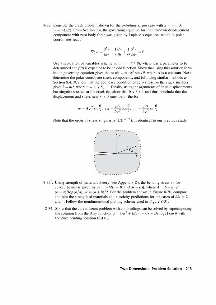
8-32. Consider the crack problem shown for the antiplane strain case with u ¼ v ¼ 0,
w ¼ w(x,y). From Section 7.4, the governing equation for the unknown displacement
component with zero body force was given by Laplace’s equation, which in polar
coordinates reads
r2w ¼ @2w
@r2þ 1
r
@w
@rþ 1
r2@2w
@u2¼ 0
Use a separation of variables scheme with w ¼ rl f (�), where l is a parameter to be
determined and f(�) is expected to be an odd function. Show that using this solution form
in the governing equation gives the result w ¼ Arl sin ly, where A is a constant. Next
determine the polar coordinate stress components, and following similar methods as in
Section 8.4.10, show that the boundary condition of zero stress on the crack surfaces
gives l¼ n/2, where n¼ 1, 3, 5, . . . Finally, using the arguments of finite displacements
but singular stresses at the crack tip, show that 0 < l < 1 and thus conclude that the
displacement and stress near r � 0 must be of the form
w ¼ Affiffir
psin
y2, tzy ¼ mA
2ffiffir
p cosy2, tzr ¼ mA
2ffiffir
p siny2
Note that the order of stress singularity, O r�1=2�
, is identical to our previous study.
y
r
xq
•
8-33*. Using strength of materials theory (see Appendix D), the bending stress sy forcurved beams is given by sy ¼ �M(r � B)=[rA(R� B)], where A ¼ b� a, B ¼(b� a)=log (b=a), R ¼ (aþ b)=2. For the problem shown in Figure 8-30, compare
and plot the strength of materials and elasticity predictions for the cases of b/a ¼ 2
and 4. Follow the nondimensional plotting scheme used in Figure 8-31.
8-34. Show that the curved beam problem with end loadings can be solved by superimposing
the solution from the Airy function f ¼ [Ar3 þ (B=r)þ Cr þ Dr log r] cos y with
the pure bending solution (8.4.61).
Two-Dimensional Problem Solution 213
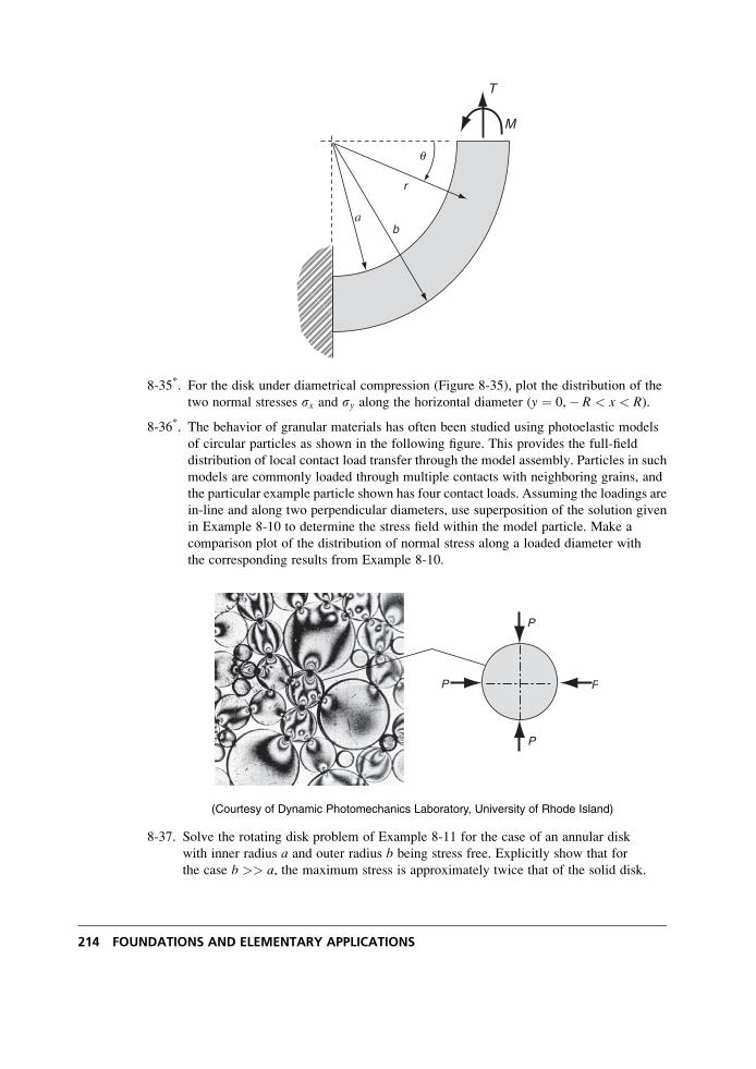
T
ab
r
M
q
8-35*. For the disk under diametrical compression (Figure 8-35), plot the distribution of the
two normal stresses sx and sy along the horizontal diameter (y ¼ 0,� R < x < R).
8-36*. The behavior of granular materials has often been studied using photoelastic models
of circular particles as shown in the following figure. This provides the full-field
distribution of local contact load transfer through the model assembly. Particles in such
models are commonly loaded through multiple contacts with neighboring grains, and
the particular example particle shown has four contact loads. Assuming the loadings are
in-line and along two perpendicular diameters, use superposition of the solution given
in Example 8-10 to determine the stress field within the model particle. Make a
comparison plot of the distribution of normal stress along a loaded diameter with
the corresponding results from Example 8-10.
P
P
P
P
(Courtesy of Dynamic Photomechanics Laboratory, University of Rhode Island)
8-37. Solve the rotating disk problem of Example 8-11 for the case of an annular disk
with inner radius a and outer radius b being stress free. Explicitly show that for
the case b >> a, the maximum stress is approximately twice that of the solid disk.
214 FOUNDATIONS AND ELEMENTARY APPLICATIONS
9 Extension, Torsion, and Flexureof Elastic Cylinders
This chapter investigates particular solutions to the problem of cylindrical bars subjected to
forces acting on the end planes. The general problem is illustrated in Figure 9-1 where an
elastic cylindrical bar with arbitrary cross-section R and lateral surface S carries general
resultant end loadings of force P and moment M. The lateral surface is taken to be free of
external loading. The cylindrical body is a prismatic bar, and the constant cross-section may be
solid or contain one or more holes. Considering the components of the general loading leads to
a definition of four problem types including extension, torsion, bending, and flexure. Theseproblems are inherently three-dimensional, and thus analytical solutions cannot be generally
determined. In an attempt to obtain an approximate solution in central portions of the bar,
Saint-Venant presumed that the character of the elastic field in this location would depend only
in a secondary way on the exact distribution of tractions on the ends of the cylinder and that the
principal effects are caused by the force resultants on the ends (Saint-Venant’s principle). As
such, he relaxed the original problem by no longer requiring the solution to satisfy pointwise
traction conditions on the ends, but rather seeking one which had the same resultant loading.
This approach is similar to our previous two-dimensional studies of beam problems in Chapter 8.
Under these conditions, the solution is not unique but provides reasonable results away from the
ends of the cylinder.
9.1 General Formulation
Formulation and solution of the extension, torsion, bending, and flexure problems are
normally made using the semi-inverse method, as previously discussed in Section 5.7. Recall thismethod assumes a portion of the solution field and determines the remaining unknowns by
requiring that all fundamental field equations be satisfied. For a prismatic barwith zero body forces
and under only end loadings as shown in Figure 9-1, it is reasonable to assume that
sx ¼ sy ¼ txy ¼ 0 (9:1:1)
215
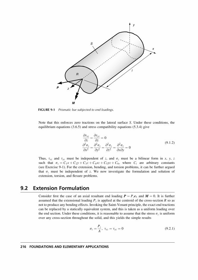
Note that this enforces zero tractions on the lateral surface S. Under these conditions, the
equilibrium equations (3.6.5) and stress compatibility equations (5.3.4) give
@txz@z
¼ @tyz@z
¼ 0
@2sz@x2
¼ @2sz@y2
¼ @2sz@z2
¼ @2sz@x@y
¼ 0
(9:1:2)
Thus, txz and tyz must be independent of z, and sz must be a bilinear form in x, y, zsuch that sz ¼ C1xþ C2yþ C3zþ C4xzþ C5yzþ C6, where Ci are arbitrary constants
(see Exercise 9-1). For the extension, bending, and torsion problems, it can be further argued
that sz must be independent of z. We now investigate the formulation and solution of
extension, torsion, and flexure problems.
9.2 Extension Formulation
Consider first the case of an axial resultant end loading P ¼ Pze3 and M ¼ 0. It is further
assumed that the extensional loading Pz is applied at the centroid of the cross-section R so as
not to produce any bending effects. Invoking the Saint-Venant principle, the exact end tractions
can be replaced by a statically equivalent system, and this is taken as a uniform loading over
the end section. Under these conditions, it is reasonable to assume that the stress sz is uniformover any cross-section throughout the solid, and this yields the simple results
sz ¼ Pz
A, txz ¼ tyz ¼ 0 (9:2:1)
x
y
zP
M
l
S
R
FIGURE 9-1 Prismatic bar subjected to end loadings.
216 FOUNDATIONS AND ELEMENTARY APPLICATIONS
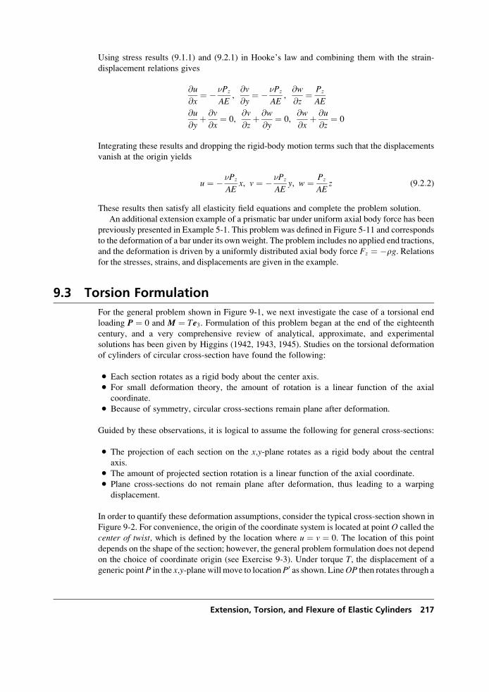
Using stress results (9.1.1) and (9.2.1) in Hooke’s law and combining them with the strain-
displacement relations gives
@u
@x¼ � �Pz
AE,@v
@y¼ � �Pz
AE,@w
@z¼ Pz
AE
@u
@yþ @v
@x¼ 0,
@v
@zþ @w
@y¼ 0,
@w
@xþ @u
@z¼ 0
Integrating these results and dropping the rigid-body motion terms such that the displacements
vanish at the origin yields
u ¼ � �Pz
AEx, v ¼ � �Pz
AEy, w ¼ Pz
AEz (9:2:2)
These results then satisfy all elasticity field equations and complete the problem solution.
An additional extension example of a prismatic bar under uniform axial body force has been
previously presented in Example 5-1. This problem was defined in Figure 5-11 and corresponds
to the deformation of a bar under its own weight. The problem includes no applied end tractions,
and the deformation is driven by a uniformly distributed axial body force Fz ¼ �rg. Relationsfor the stresses, strains, and displacements are given in the example.
9.3 Torsion Formulation
For the general problem shown in Figure 9-1, we next investigate the case of a torsional end
loading P ¼ 0 and M ¼ Te3. Formulation of this problem began at the end of the eighteenth
century, and a very comprehensive review of analytical, approximate, and experimental
solutions has been given by Higgins (1942, 1943, 1945). Studies on the torsional deformation
of cylinders of circular cross-section have found the following:
. Each section rotates as a rigid body about the center axis.
. For small deformation theory, the amount of rotation is a linear function of the axial
coordinate.. Because of symmetry, circular cross-sections remain plane after deformation.
Guided by these observations, it is logical to assume the following for general cross-sections:
. The projection of each section on the x,y-plane rotates as a rigid body about the central
axis.. The amount of projected section rotation is a linear function of the axial coordinate.. Plane cross-sections do not remain plane after deformation, thus leading to a warping
displacement.
In order to quantify these deformation assumptions, consider the typical cross-section shown in
Figure 9-2. For convenience, the origin of the coordinate system is located at point O called the
center of twist, which is defined by the location where u ¼ v ¼ 0. The location of this point
depends on the shape of the section; however, the general problem formulation does not depend
on the choice of coordinate origin (see Exercise 9-3). Under torque T, the displacement of a
generic pointP in the x,y-plane will move to locationP0 as shown. LineOP then rotates through a
Extension, Torsion, and Flexure of Elastic Cylinders 217
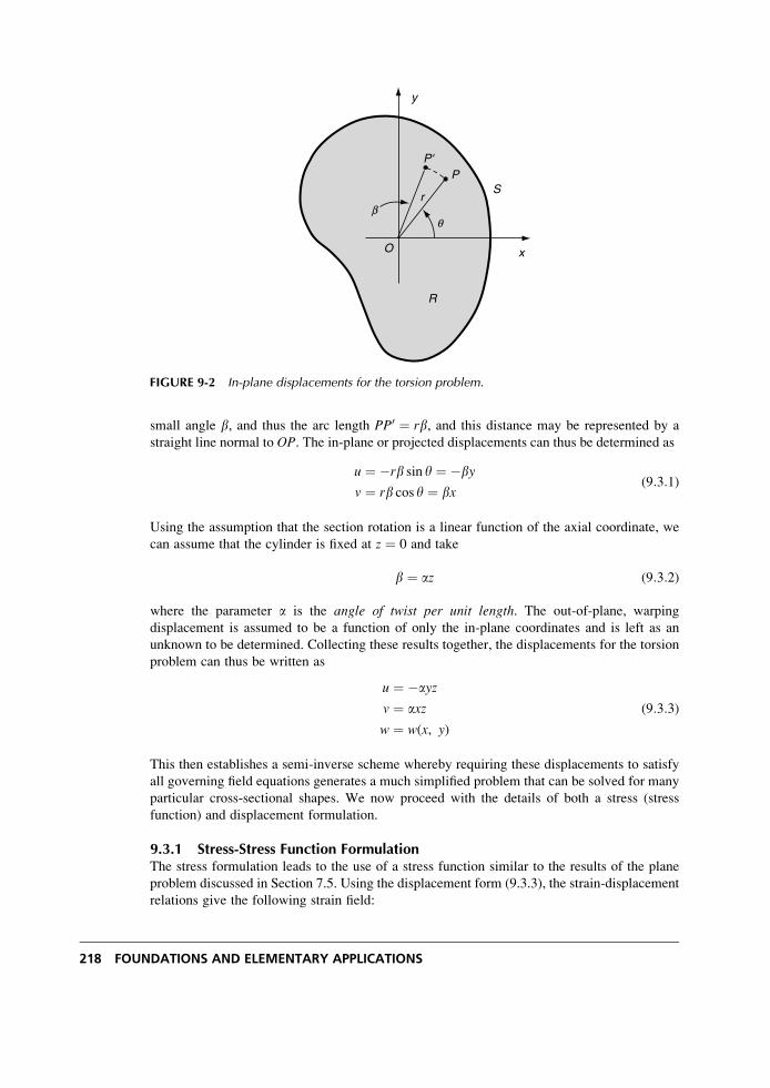
small angle b, and thus the arc length PP0 ¼ rb, and this distance may be represented by a
straight line normal to OP. The in-plane or projected displacements can thus be determined as
u ¼ �rb sin y ¼ �by
v ¼ rb cos y ¼ bx(9:3:1)
Using the assumption that the section rotation is a linear function of the axial coordinate, we
can assume that the cylinder is fixed at z ¼ 0 and take
b ¼ az (9:3:2)
where the parameter a is the angle of twist per unit length. The out-of-plane, warping
displacement is assumed to be a function of only the in-plane coordinates and is left as an
unknown to be determined. Collecting these results together, the displacements for the torsion
problem can thus be written as
u ¼ �ayz
v ¼ axz
w ¼ w(x, y)
(9:3:3)
This then establishes a semi-inverse scheme whereby requiring these displacements to satisfy
all governing field equations generates a much simplified problem that can be solved for many
particular cross-sectional shapes. We now proceed with the details of both a stress (stress
function) and displacement formulation.
9.3.1 Stress-Stress Function FormulationThe stress formulation leads to the use of a stress function similar to the results of the plane
problem discussed in Section 7.5. Using the displacement form (9.3.3), the strain-displacement
relations give the following strain field:
x
y
O
P'P
r
R
S
bq
FIGURE 9-2 In-plane displacements for the torsion problem.
218 FOUNDATIONS AND ELEMENTARY APPLICATIONS
ex ¼ ey ¼ ez ¼ exy ¼ 0
exz ¼ 1
2
@w
@x� ay
� �
eyz ¼ 1
2
@w
@yþ ax
� � (9:3:4)
The corresponding stresses follow from Hooke’s law:
sx ¼ sy ¼ sz ¼ txy ¼ 0
txz ¼ m@w
@x� ay
� �
tyz ¼ m@w
@yþ ax
� � (9:3:5)
Note the strain and stress fields are functions only of x and y.For this case, with zero body forces, the equilibrium equations reduce to
@txz@x
þ @tyz@y
¼ 0 (9:3:6)
Rather than using the general Beltrami-Michell compatibility equations, it is more direct to
develop a special compatibility relation for this particular problem. This is easily done by
simply differentiating (9:3:5)2 with respect to y and (9:3:5)3 with respect to x and subtracting
the results to get
@txz@y
� @tyz@x
¼ �2ma (9:3:7)
This represents an independent relation among the stresses developed under the continuity
conditions of w(x,y).Relations (9.3.6) and (9.3.7) constitute the governing equations for the stress formulation.
The coupled system pair can be reduced by introducing a stress function approach. For this
case, the stresses are represented in terms of the Prandtl stress function f ¼ f(x, y) by
txz ¼ @f@y
, tyz ¼ � @f@x
(9:3:8)
Note that here we are using the same notation for the stress function as used for the Airy
function in the previous chapter that dealt with plane elasticity. Since the problem types are
completely different, there should be little confusion. The equilibrium equations are then
identically satisfied and the compatibility relation gives
r2f ¼ @2f@x2
þ @2f@y2
¼ �2ma (9:3:9)
This single relation is then the governing equation for the problem and (9.3.9) is a Poissonequation that is amenable to several analytical solution techniques.
To complete the stress formulation we now must address the boundary conditions on the
problem. As previously mentioned, the lateral surface of the cylinder S (see Figure 9-1) is to befree of tractions, and thus
Extension, Torsion, and Flexure of Elastic Cylinders 219
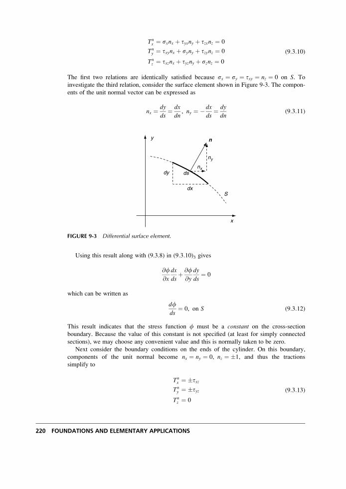
Tnx ¼ sxnx þ tyxny þ tzxnz ¼ 0
Tny ¼ txynx þ syny þ tzynz ¼ 0
Tnz ¼ txznx þ tyzny þ sznz ¼ 0
(9:3:10)
The first two relations are identically satisfied because sx ¼ sy ¼ txy ¼ nz ¼ 0 on S. Toinvestigate the third relation, consider the surface element shown in Figure 9-3. The compon-
ents of the unit normal vector can be expressed as
nx ¼ dy
ds¼ dx
dn, ny ¼ � dx
ds¼ dy
dn(9:3:11)
Using this result along with (9.3.8) in (9:3:10)3 gives
@f@x
dx
dsþ @f
@y
dy
ds¼ 0
which can be written as
dfds
¼ 0, on S (9:3:12)
This result indicates that the stress function f must be a constant on the cross-section
boundary. Because the value of this constant is not specified (at least for simply connected
sections), we may choose any convenient value and this is normally taken to be zero.
Next consider the boundary conditions on the ends of the cylinder. On this boundary,
components of the unit normal become nx ¼ ny ¼ 0, nz ¼ �1, and thus the tractions
simplify to
Tnx ¼ �txz
Tny ¼ �tyz
Tnz ¼ 0
(9:3:13)
x
y
dx
ny
n
nxdy ds
S
FIGURE 9-3 Differential surface element.
220 FOUNDATIONS AND ELEMENTARY APPLICATIONS
Recall that we are only interested in satisfying the resultant end-loading conditions, and thus
the resultant force should vanish while the moment should reduce to a pure torque T about the
z-axis. These conditions are specified by
Px ¼ð ð
R
Tnx dxdy ¼ 0
Py ¼ð ð
R
Tny dxdy ¼ 0
Pz ¼ð ð
R
Tnz dxdy ¼ 0
Mx ¼ð ð
R
yTnz dxdy ¼ 0
My ¼ð ð
R
xTnz dxdy ¼ 0
Mz ¼ð ð
R
(xTny � yTn
x )dxdy ¼ T
(9:3:14)
With Tnz ¼ 0, conditions (9:3:14)3, 4, 5 are automatically satisfied. Considering the first condi-
tion in set (9.3.14), the x component of the resultant force on the ends may be written asð ðR
Tnx dxdy ¼ �
ð ðR
txzdxdy ¼ �ð ð
R
@f@y
dxdy (9:3:15)
Using Green’s theorem (1.8.11),
ððR
@f@y
dxdy ¼þS
fnyds, and because f vanishes on
boundary S, the integral is zero and the resultant force Px vanishes. Similar arguments can
be used to show that the resultant force Py will vanish. The final end condition (9:3:14)6involving the resultant torque can be expressed as
T ¼ð ð
R
(xTny � yTn
x )dxdy ¼ �ð ð
R
(x@f@x
þ y@f@y
)dxdy (9:3:16)
Again using results from Green’s theorem
ð ðR
x@f@x
dxdy ¼ð ð
R
@
@x(xf)dxdy�
ð ðR
fdxdy
¼þS
xfnxds�ð ð
R
fdxdyð ðR
y@f@y
dxdy ¼ð ð
R
@
@y(yf)dxdy�
ð ðR
fdxdy
¼þS
yfnyds�ð ð
R
fdxdy
(9:3:17)
Because f is zero on S, the boundary integrals in (9.3.17) will vanish and relation (9.3.16)
simplifies to
T ¼ 2
ð ðR
fdxdy (9:3:18)
Extension, Torsion, and Flexure of Elastic Cylinders 221
We have now shown that the assumed displacement form (9.3.3) produces a stress field that
when represented by the Prandtl stress function relation (9.3.8) yields a governing Poisson
equation (9.3.9) with the condition that the stress function vanishes on the boundary of the
cross-section. All resultant boundary conditions on the ends of the cylinder are satisfied by the
representation, and the overall torque is related to the stress function through relation (9.3.18).
This then concludes the stress formulation of the torsion problem for simply connected
sections.
9.3.2 Displacement FormulationThe displacement formulation starts by expressing the equilibrium equation in terms of the
warping displacement w. Using (9.3.5) in (9.3.6) gives
@2w
@x2þ @2w
@y2¼ 0 (9:3:19)
and thus the displacement component satisfies Laplace’s equation in the cross-section R. Theassociated boundary condition on the lateral side S is given by (9:3:10)3, and expressing this interms of the warping displacement gives
@w
@x� ya
� �nx þ @w
@yþ xa
� �ny ¼ 0 (9:3:20)
Using relations (9.3.11), this result can be rewritten as
@w
@x
dx
dnþ @w
@y
dy
dn¼ a x
dx
dsþ y
dy
ds
� �dw
dn¼ a
2
d
ds(x2 þ y2)
(9:3:21)
It can again be shown that the boundary conditions on the ends specified by equations
(9:3:14)1�5 will all be satisfied, and the resultant torque condition (9:3:14)6 will give
T ¼ mð ð
R
a(x2 þ y2)þ x@w
@y� y
@w
@x
� �dxdy (9:3:22)
This result is commonly written as
T ¼ aJ (9:3:23)
where J is called the torsional rigidity and is given by
J ¼ mð ð
R
x2 þ y2 þ x
a@w
@y� y
a@w
@x
� �dxdy (9:3:24)
This completes the displacement formulation for the torsion problem.
Comparing the two formulations, it is observed that the stress function approach results in a
governing equation of the Poisson type (9.3.9) with a very simple boundary condition requiring
only that the stress function be constant or vanish. On the other hand, the displacement
222 FOUNDATIONS AND ELEMENTARY APPLICATIONS
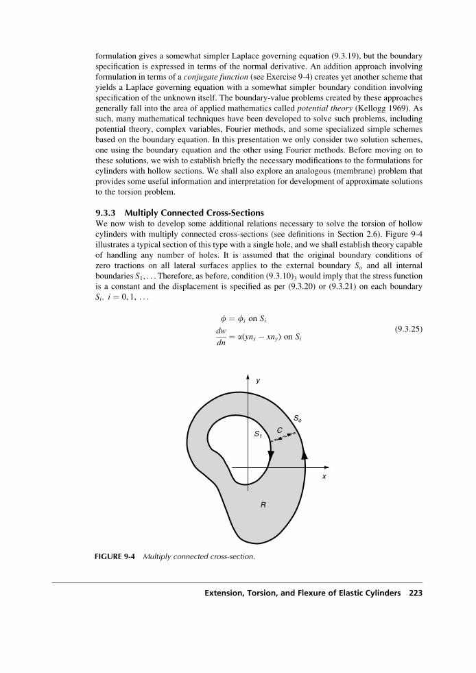
formulation gives a somewhat simpler Laplace governing equation (9.3.19), but the boundary
specification is expressed in terms of the normal derivative. An addition approach involving
formulation in terms of a conjugate function (see Exercise 9-4) creates yet another scheme that
yields a Laplace governing equation with a somewhat simpler boundary condition involving
specification of the unknown itself. The boundary-value problems created by these approaches
generally fall into the area of applied mathematics called potential theory (Kellogg 1969). As
such, many mathematical techniques have been developed to solve such problems, including
potential theory, complex variables, Fourier methods, and some specialized simple schemes
based on the boundary equation. In this presentation we only consider two solution schemes,
one using the boundary equation and the other using Fourier methods. Before moving on to
these solutions, we wish to establish briefly the necessary modifications to the formulations for
cylinders with hollow sections. We shall also explore an analogous (membrane) problem that
provides some useful information and interpretation for development of approximate solutions
to the torsion problem.
9.3.3 Multiply Connected Cross-SectionsWe now wish to develop some additional relations necessary to solve the torsion of hollow
cylinders with multiply connected cross-sections (see definitions in Section 2.6). Figure 9-4
illustrates a typical section of this type with a single hole, and we shall establish theory capable
of handling any number of holes. It is assumed that the original boundary conditions of
zero tractions on all lateral surfaces applies to the external boundary So and all internal
boundaries S1, . . . Therefore, as before, condition (9:3:10)3 would imply that the stress function
is a constant and the displacement is specified as per (9.3.20) or (9.3.21) on each boundary
Si, i ¼ 0, 1, . . .
f ¼ fi on Si
dw
dn¼ a(ynx � xny) on Si
(9:3:25)
x
y
C
So
R
S1
FIGURE 9-4 Multiply connected cross-section.
Extension, Torsion, and Flexure of Elastic Cylinders 223
where fi are constants. These conditions imply that the stress function and warping displace-
ment can be determined up to an arbitrary constant on each boundary Si. With regard to the
stress function, the value of fi may be arbitrarily chosen only on one boundary, and commonly
this value is taken as zero on the outer boundary So similar to the simply connected case.
For multiply connected sections, the constant values of the stress function on each of the
interior boundaries are determined by requiring that the displacement w be single-valued.
Considering the doubly connected example shown in Figure 9-4, the displacement will be
single-valued if þS1
dw(x, y) ¼ 0 (9:3:26)
This integral can be written as
þS1
dw(x, y) ¼þS1
@w
@xdxþ @w
@ydy
� �
¼ 1
m
þS1
(txzdxþ tyzdy)� aþS1
(xdy� ydx)
(9:3:27)
Now txzdxþ tyzdy ¼ tds, where t is the resultant shear stress. Using Green’s theorem (1.8.10),
þS1
(xdy� ydx) ¼ð ð
A1
@x
@xþ @y
@y
� �dxdy ¼ 2
ð ðA1
dxdy ¼ 2A1 (9:3:28)
where A1 is the area enclosed by S1. Combining these results, the single-valued condition
(9.3.26) implies that þS1
tds ¼ 2maA1 (9:3:29)
The value of f1 on the inner boundary S1 must therefore be chosen so that (9.3.29) is satisfied.
If the cross-section has more than one hole, relation (9.3.29) must be satisfied for each; that is,
þSk
tds ¼ 2maAk (9:3:30)
where k ¼ 1, 2, 3, . . . is the index corresponding to each of the interior holes.
It can be shown that boundary conditions on the ends of the cylinder given by (9:3:14)1�5
will all be satisfied, and the resultant torque condition (9:3:14)6 will give
T ¼ 2
ð ðR
fdxdyþ 2f1A1 (9:3:31)
For the case with N holes, this relation becomes
T ¼ 2
ð ðR
fdxdyþXNk¼1
2fkAk (9:3:32)
Justifying these developments for multiply connected sections requires contour integration in a
cut domain following the segments So, C, S1, as shown in Figure 9-4.
224 FOUNDATIONS AND ELEMENTARY APPLICATIONS
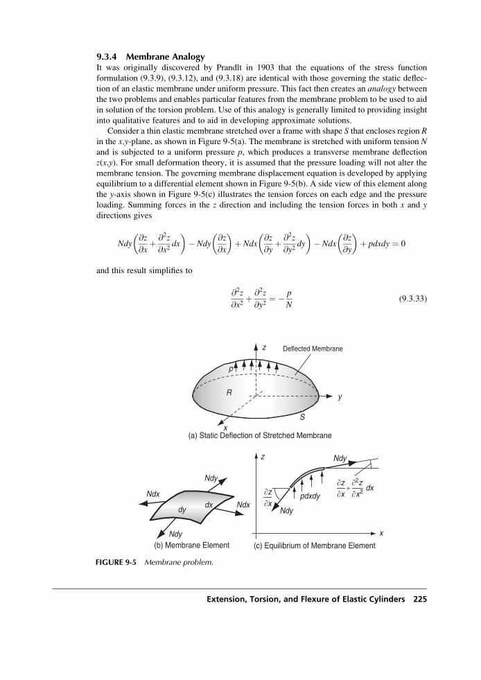
9.3.4 Membrane AnalogyIt was originally discovered by Prandlt in 1903 that the equations of the stress function
formulation (9.3.9), (9.3.12), and (9.3.18) are identical with those governing the static deflec-
tion of an elastic membrane under uniform pressure. This fact then creates an analogy betweenthe two problems and enables particular features from the membrane problem to be used to aid
in solution of the torsion problem. Use of this analogy is generally limited to providing insight
into qualitative features and to aid in developing approximate solutions.
Consider a thin elastic membrane stretched over a frame with shape S that encloses region Rin the x,y-plane, as shown in Figure 9-5(a). The membrane is stretched with uniform tension Nand is subjected to a uniform pressure p, which produces a transverse membrane deflection
z(x,y). For small deformation theory, it is assumed that the pressure loading will not alter the
membrane tension. The governing membrane displacement equation is developed by applying
equilibrium to a differential element shown in Figure 9-5(b). A side view of this element along
the y-axis shown in Figure 9-5(c) illustrates the tension forces on each edge and the pressure
loading. Summing forces in the z direction and including the tension forces in both x and ydirections gives
Ndy@z
@xþ @2z
@x2dx
� �� Ndy
@z
@x
� �þ Ndx
@z
@yþ @2z
@y2dy
� �� Ndx
@z
@y
� �þ pdxdy ¼ 0
and this result simplifies to
@2z
@x2þ @2z
@y2¼ � p
N(9:3:33)
x
z Ndy
Ndy∂x∂z dx
∂x2∂x∂z ∂2z
+pdxdy
(c) Equilibrium of Membrane Element
x
y
S
z
R
p
Deflected Membrane
(a) Static Deflection of Stretched Membrane
Ndy
Ndy
NdxNdx
(b) Membrane Element
dxdy
FIGURE 9-5 Membrane problem.
Extension, Torsion, and Flexure of Elastic Cylinders 225
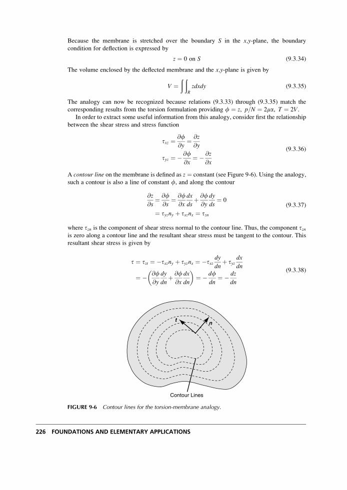
Because the membrane is stretched over the boundary S in the x,y-plane, the boundary
condition for deflection is expressed by
z ¼ 0 on S (9:3:34)
The volume enclosed by the deflected membrane and the x,y-plane is given by
V ¼ð ð
R
zdxdy (9:3:35)
The analogy can now be recognized because relations (9.3.33) through (9.3.35) match the
corresponding results from the torsion formulation providing f ¼ z, p=N ¼ 2ma, T ¼ 2V.In order to extract some useful information from this analogy, consider first the relationship
between the shear stress and stress function
txz ¼ @f@y
¼ @z
@y
tyz ¼ � @f@x
¼ � @z
@x
(9:3:36)
A contour line on the membrane is defined as z ¼ constant (see Figure 9-6). Using the analogy,
such a contour is also a line of constant f, and along the contour
@z
@s¼ @f
@s¼ @f
@x
dx
dsþ @f
@y
dy
ds¼ 0
¼ tyzny þ txznx ¼ tzn
(9:3:37)
where tzn is the component of shear stress normal to the contour line. Thus, the component tznis zero along a contour line and the resultant shear stress must be tangent to the contour. This
resultant shear stress is given by
t ¼ tzt ¼ �txzny þ tyznx ¼ �txzdy
dnþ tyz
dx
dn
¼ � @f@y
dy
dnþ @f
@x
dx
dn
� �¼ � df
dn¼ � dz
dn
(9:3:38)
nt
Contour Lines
FIGURE 9-6 Contour lines for the torsion-membrane analogy.
226 FOUNDATIONS AND ELEMENTARY APPLICATIONS
Reviewing the previous findings related to the membrane analogy, the following concepts
can be concluded. The shear stress at any point in the cross-section is given by the negative of
the slope of the membrane in the direction normal to the contour line through the point. The
maximum shear stress appears always to occur on the boundary where the largest slope of the
membrane occurs. Actually, this result can be explicitly proven (see Exercise 9-5). The torque
T is given as twice the volume under the membrane. Using these membrane visualizations, a
useful qualitative picture of the stress function distribution can be determined and approximate
solutions can be constructed (see Exercise 9-7). However, it should be realized that trying to
make slope measurements of an actual pressurized membrane would not provide an accurate
method to determine the stresses in a bar under torsion.
We now explore the solution to several torsion problems using boundary equation schemes,
Fourier methods, and membrane analogy techniques. These methods provide solutions to
sections of simple geometry. More complicated sections can be solved using complex variable
theory; see Sokolnikoff (1956) for a brief presentation of these techniques.
9.4 Torsion Solutions Derived from Boundary Equation
For simply connected sections, the stress function formulation requires that the function
satisfy Poisson equation (9.3.9) and vanish on boundary S. If the boundary is expressed by
the relation f (x, y) ¼ 0, this suggests a possible simple solution scheme of expressing the stress
function in terms of the boundary equation f ¼ Kf (x, y) where K is an arbitrary constant.
Clearly, this form satisfies the boundary condition on S, and for some simple geometric
shapes it will also satisfy the governing equation (9.3.9) with an appropriate choice of K.Unfortunately, this is not a general solution method but rather an ad hoc scheme that works
only for special cross-sections of simple geometry. Nevertheless, it provides several solutions
to problems of interest, and we now investigate some particular solutions using this scheme.
EXAMPLE 9-1: Elliptical Section
The first example of this solution method is that of an elliptical cross-section as shown
in Figure 9-7. The boundary equation has the usual form
x2
a2þ y2
b2¼ 1 (9:4:1)
where a and b are the semi major and minor axes as shown.
Using the boundary equation scheme, we look for a stress function of the form
f ¼ Kx2
a2þ y2
b2� 1
� �(9:4:2)
Continued
Extension, Torsion, and Flexure of Elastic Cylinders 227
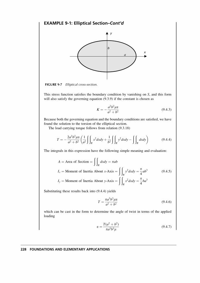
EXAMPLE 9-1: Elliptical Section–Cont’d
This stress function satisfies the boundary condition by vanishing on S, and this form
will also satisfy the governing equation (9.3.9) if the constant is chosen as
K ¼ � a2b2maa2 þ b2
(9:4:3)
Because both the governing equation and the boundary conditions are satisfied, we have
found the solution to the torsion of the elliptical section.
The load carrying torque follows from relation (9.3.18)
T ¼ � 2a2b2maa2 þ b2
1
a2
ð ðR
x2dxdyþ 1
b2
ð ðR
y2dxdy�ð ð
R
dxdy
� �(9:4:4)
The integrals in this expression have the following simple meaning and evaluation:
A ¼ Area of Section ¼ð ð
R
dxdy ¼ pab
Ix ¼ Moment of Inertia About x-Axis ¼ð ð
R
y2dxdy ¼ p4ab3
Iy ¼ Moment of Inertia About y-Axis ¼ð ð
R
x2dxdy ¼ p4ba3
(9:4:5)
Substituting these results back into (9.4.4) yields
T ¼ pa3b3maa2 þ b2
(9:4:6)
which can be cast in the form to determine the angle of twist in terms of the applied
loading
a ¼ T(a2 þ b2)
pa3b3m(9:4:7)
x
y
a
b
FIGURE 9-7 Elliptical cross-section.
228 FOUNDATIONS AND ELEMENTARY APPLICATIONS
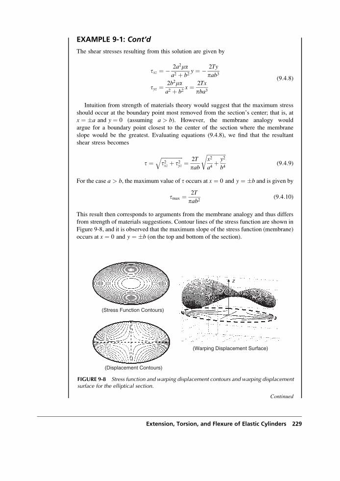
EXAMPLE 9-1: Cont’d
The shear stresses resulting from this solution are given by
txz ¼ � 2a2maa2 þ b2
y ¼ � 2Ty
pab3
tyz ¼ 2b2maa2 þ b2
x ¼ 2Tx
pba3
(9:4:8)
Intuition from strength of materials theory would suggest that the maximum stress
should occur at the boundary point most removed from the section’s center; that is, at
x ¼ �a and y ¼ 0 (assuming a > b). However, the membrane analogy would
argue for a boundary point closest to the center of the section where the membrane
slope would be the greatest. Evaluating equations (9.4.8), we find that the resultant
shear stress becomes
t ¼ffiffiffiffiffiffiffiffiffiffiffiffiffiffiffiffiffit2xz þ t2yz
q¼ 2T
pab
ffiffiffiffiffiffiffiffiffiffiffiffiffiffiffix2
a4þ y2
b4
r(9:4:9)
For the case a > b, the maximum value of t occurs at x ¼ 0 and y ¼ �b and is given by
tmax ¼ 2T
pab2(9:4:10)
This result then corresponds to arguments from the membrane analogy and thus differs
from strength of materials suggestions. Contour lines of the stress function are shown in
Figure 9-8, and it is observed that the maximum slope of the stress function (membrane)
occurs at x ¼ 0 and y ¼ �b (on the top and bottom of the section).
Continued
(Displacement Contours)
(Stress Function Contours)
z
(Warping Displacement Surface)
FIGURE 9-8 Stress function and warping displacement contours and warping displacementsurface for the elliptical section.
Extension, Torsion, and Flexure of Elastic Cylinders 229
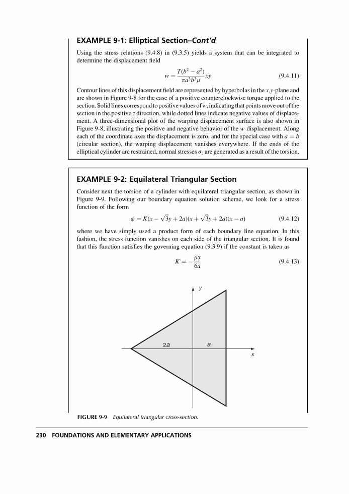
EXAMPLE 9-1: Elliptical Section–Cont’d
Using the stress relations (9.4.8) in (9.3.5) yields a system that can be integrated to
determine the displacement field
w ¼ T(b2 � a2)
pa3b3mxy (9:4:11)
Contour lines of this displacement field are represented by hyperbolas in the x,y-plane andare shown in Figure 9-8 for the case of a positive counterclockwise torque applied to the
section.Solid linescorrespond topositivevaluesofw, indicating thatpointsmoveoutof the
section in the positive z direction, while dotted lines indicate negative values of displace-ment. A three-dimensional plot of the warping displacement surface is also shown in
Figure 9-8, illustrating the positive and negative behavior of the w displacement. Along
each of the coordinate axes the displacement is zero, and for the special case with a ¼ b(circular section), the warping displacement vanishes everywhere. If the ends of the
elliptical cylinder are restrained, normal stresses sz are generated as a result of the torsion.
EXAMPLE 9-2: Equilateral Triangular Section
Consider next the torsion of a cylinder with equilateral triangular section, as shown in
Figure 9-9. Following our boundary equation solution scheme, we look for a stress
function of the form
f ¼ K(x�ffiffiffi3
pyþ 2a)(xþ
ffiffiffi3
pyþ 2a)(x� a) (9:4:12)
where we have simply used a product form of each boundary line equation. In this
fashion, the stress function vanishes on each side of the triangular section. It is found
that this function satisfies the governing equation (9.3.9) if the constant is taken as
K ¼ �ma6a
(9:4:13)
x
y
2a a
FIGURE 9-9 Equilateral triangular cross-section.
230 FOUNDATIONS AND ELEMENTARY APPLICATIONS
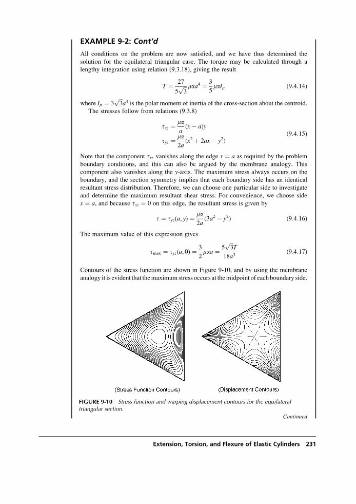
EXAMPLE 9-2: Cont’d
All conditions on the problem are now satisfied, and we have thus determined the
solution for the equilateral triangular case. The torque may be calculated through a
lengthy integration using relation (9.3.18), giving the result
T ¼ 27
5ffiffiffi3
p maa4 ¼ 3
5maIp (9:4:14)
where Ip ¼ 3ffiffiffi3
pa4 is the polar moment of inertia of the cross-section about the centroid.
The stresses follow from relations (9.3.8)
txz ¼ maa(x� a)y
tyz ¼ ma2a
(x2 þ 2ax� y2)(9:4:15)
Note that the component txz vanishes along the edge x ¼ a as required by the problem
boundary conditions, and this can also be argued by the membrane analogy. This
component also vanishes along the y-axis. The maximum stress always occurs on the
boundary, and the section symmetry implies that each boundary side has an identical
resultant stress distribution. Therefore, we can choose one particular side to investigate
and determine the maximum resultant shear stress. For convenience, we choose side
x ¼ a, and because txz ¼ 0 on this edge, the resultant stress is given by
t ¼ tyz(a, y) ¼ ma2a
(3a2 � y2) (9:4:16)
The maximum value of this expression gives
tmax ¼ tyz(a, 0) ¼ 3
2maa ¼ 5
ffiffiffi3
pT
18a3(9:4:17)
Contours of the stress function are shown in Figure 9-10, and by using the membrane
analogy it is evident that themaximumstress occurs at themidpoint of each boundary side.
Continued
FIGURE 9-10 Stress function and warping displacement contours for the equilateraltriangular section.
Extension, Torsion, and Flexure of Elastic Cylinders 231
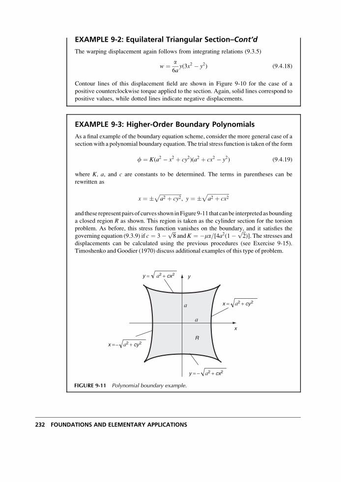
EXAMPLE 9-2: Equilateral Triangular Section–Cont’d
The warping displacement again follows from integrating relations (9.3.5)
w ¼ a6a
y(3x2 � y2) (9:4:18)
Contour lines of this displacement field are shown in Figure 9-10 for the case of a
positive counterclockwise torque applied to the section. Again, solid lines correspond to
positive values, while dotted lines indicate negative displacements.
EXAMPLE 9-3: Higher-Order Boundary Polynomials
As a final example of the boundary equation scheme, consider the more general case of a
section with a polynomial boundary equation. The trial stress function is taken of the form
f ¼ K(a2 � x2 þ cy2)(a2 þ cx2 � y2) (9:4:19)
where K, a, and c are constants to be determined. The terms in parentheses can be
rewritten as
x ¼ �ffiffiffiffiffiffiffiffiffiffiffiffiffiffiffiffiffia2 þ cy2
p, y ¼ �
ffiffiffiffiffiffiffiffiffiffiffiffiffiffiffiffiffia2 þ cx2
pand these represent pairs of curves shown inFigure9-11 that canbe interpretedasbounding
a closed region R as shown. This region is taken as the cylinder section for the torsion
problem. As before, this stress function vanishes on the boundary, and it satisfies the
governing equation (9.3.9) if c ¼ 3� ffiffiffi8
pandK ¼ �ma=[4a2(1�
ffiffiffi2
p)]. The stresses and
displacements can be calculated using the previous procedures (see Exercise 9-15).
Timoshenko and Goodier (1970) discuss additional examples of this type of problem.
x
y
a2 + cx2y =
a2 + cy2x =
a2 + cy2x =
a2 + cx2y =
R
a
a
−
−
FIGURE 9-11 Polynomial boundary example.
232 FOUNDATIONS AND ELEMENTARY APPLICATIONS
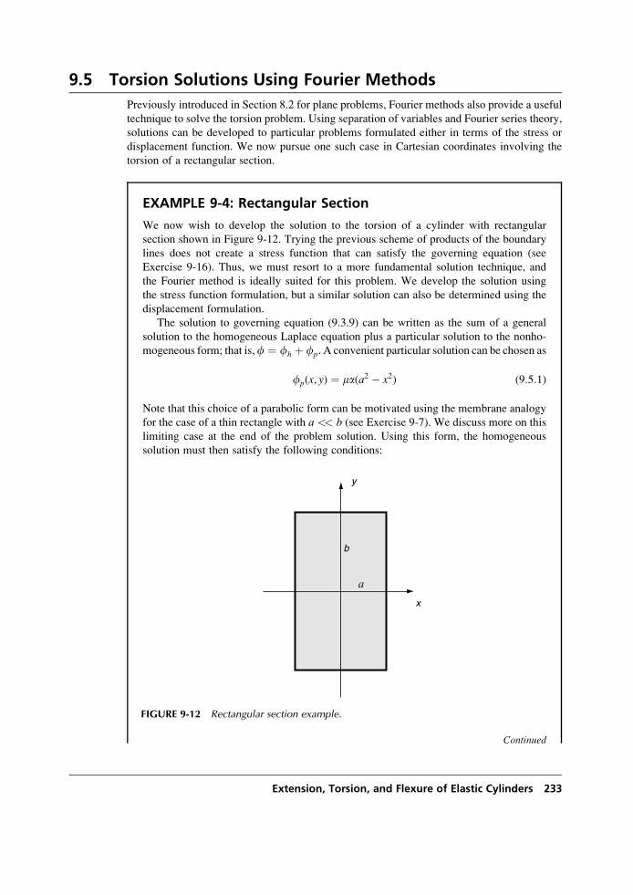
9.5 Torsion Solutions Using Fourier Methods
Previously introduced in Section 8.2 for plane problems, Fourier methods also provide a useful
technique to solve the torsion problem. Using separation of variables and Fourier series theory,
solutions can be developed to particular problems formulated either in terms of the stress or
displacement function. We now pursue one such case in Cartesian coordinates involving the
torsion of a rectangular section.
EXAMPLE 9-4: Rectangular Section
We now wish to develop the solution to the torsion of a cylinder with rectangular
section shown in Figure 9-12. Trying the previous scheme of products of the boundary
lines does not create a stress function that can satisfy the governing equation (see
Exercise 9-16). Thus, we must resort to a more fundamental solution technique, and
the Fourier method is ideally suited for this problem. We develop the solution using
the stress function formulation, but a similar solution can also be determined using the
displacement formulation.
The solution to governing equation (9.3.9) can be written as the sum of a general
solution to the homogeneous Laplace equation plus a particular solution to the nonho-
mogeneous form; that is,f ¼ fh þ fp. A convenient particular solution can be chosen as
fp(x, y) ¼ ma(a2 � x2) (9:5:1)
Note that this choice of a parabolic form can be motivated using the membrane analogy
for the case of a thin rectangle with a << b (see Exercise 9-7). We discuss more on this
limiting case at the end of the problem solution. Using this form, the homogeneous
solution must then satisfy the following conditions:
Continued
x
y
a
b
FIGURE 9-12 Rectangular section example.
Extension, Torsion, and Flexure of Elastic Cylinders 233

EXAMPLE 9-4: Rectangular Section–Cont’d
r2fh ¼ 0
fh(�a, y) ¼ 0
fh(x, �b) ¼ �ma(a2 � x2)
(9:5:2)
and this ensures that the combined stress function f satisfies the general formulation
conditions. Standard separation of variables methods are used to generate the homoge-
neous solution by looking for solutions of the form
fh(x, y) ¼ X(x)Y(y) (9:5:3)
Substituting this form into (9:5:2)1 allows the variables to be separated into the
following pair of differential relations:
X00(x)þ l2X(x) ¼ 0
Y00( y)� l2Y(y) ¼ 0(9:5:4)
where l is the separation constant. The solution to (9.5.4) is given by
X(x) ¼ A sin lxþ B cos lx
Y( y) ¼ C sinh lyþ D cosh ly(9:5:5)
where A, B, C, D are constants. Because of the given problem symmetry, we
can immediately argue that the solution should be an even function of x and y, and thus
the odd function termsmust be dropped by takingA ¼ C ¼ 0. In order to satisfy condition
(9:5:2)2, the separation constantmust be given by l ¼ np= 2a, n ¼ 1, 3, 5, . . . Combining
these results, the homogeneous solution can then be expressed by
fh(x, y) ¼X1n¼1
Bn cosnpx2a
coshnpy2a
(9:5:6)
where we use the superposition of all solution forms and the coefficient Bn has absorbed
the product term BD.The final boundary condition (9:5:2)3 yields the result
�ma(a2 � x2) ¼X1n¼1
B�n cos
npx2a
(9:5:7)
where B�n ¼ Bn cosh (npb=2a). Equation (9.5.7) is recognized as the Fourier cosine series
for the expression on the left-hand side. Using relations (8.2.27), Fourier series theory
provides a simple scheme to determine the series coefficients, giving the result
B�n ¼ � 2ma
a
ða0
(a2 � x2) cosnpx2a
dx (9:5:8)
Evaluating this integral, the original coefficient can then be expressed as
234 FOUNDATIONS AND ELEMENTARY APPLICATIONS
EXAMPLE 9-4: Cont’d
Bn ¼ � 32maa2(�1)(n�1)=2
n3p3 coshnpb2a
(9:5:9)
The stress function has now been determined, and combining the previous results gives
f ¼ ma(a2 � x2)� 32maa2
p3X1
n¼1, 3, 5���
(�1)(n�1)=2
n3 coshnpb2a
cosnpx2a
coshnpy2a
(9:5:10)
The stresses follow from relation (9.3.8)
txz ¼ @f@y
¼ � 16maap2
X1n¼1, 3, 5���
(�1)(n�1)=2
n2 coshnpb2a
cosnpx2a
sinhnpy2a
tyz ¼ � @f@x
¼ 2max� 16maap2
X1n¼1, 3, 5���
(�1)(n�1)=2
n2 coshnpb2a
sinnpx2a
coshnpy2a
(9:5:11)
and using (9.3.18), the torque is given by
T ¼ 16maa3b3
� 1024maa4
p5X1
n¼1, 3, 5���
1
n5tanh
npb2a
(9:5:12)
Using our experience from the previous examples or from the membrane analogy, the
maximum stress will occur on the boundary at the midpoint of the longest side. Under
the assumption that a < b, these points are located at x ¼ �a and y ¼ 0, and thus
tmax ¼ tyz(a, 0) ¼ 2maa� 16maap2
X1n¼1, 3, 5���
1
n2 coshnpb2a
(9:5:13)
Figure 9-13 illustrates the stress function contours for this case, and it is observed that the
maximum stresses occur at the midpoint of each of the longest boundary sides. For
the square section case (a ¼ b), the maximum stresses would occur at the midpoint of
each side.
Again thedisplacementfield follows fromintegrating relations (9.3.5), giving the result
w ¼ axy� 32aa2
p3X1
n¼1, 3, 5���
(�1)(n�1)=2
n3 coshnpb2a
sinnpx2a
sinhnpy2a
(9:5:14)
Contour lines of this displacement field are shown in Figure 9-13 for three sections with
different aspect ratios. Again, solid lines correspond to positive displacements, while
dotted lines indicate negative values. The square section case with a=b ¼ 1 produces a
displacement pattern with eight zones of symmetry. As the aspect ratio a/b is reduced,
four of the displacement patterns disappear and the resulting displacement contours for
a=b ¼ 0:5 look similar to that from the elliptical section case shown in Figure 9-8.
Continued
Extension, Torsion, and Flexure of Elastic Cylinders 235
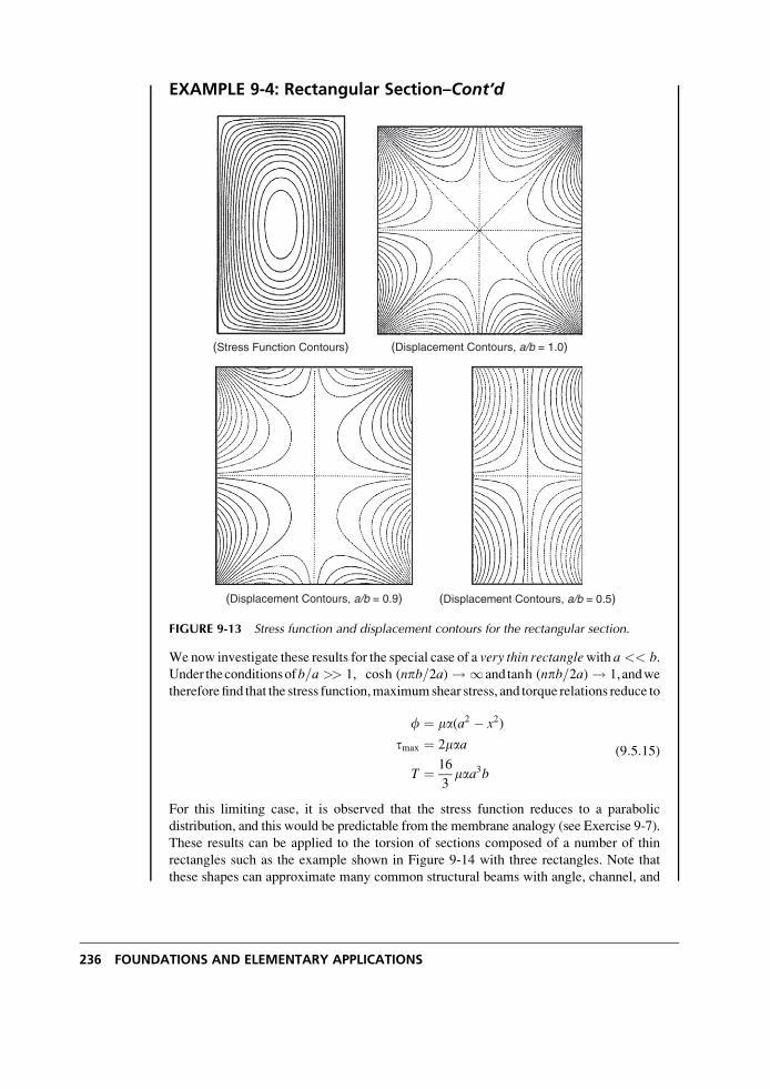
EXAMPLE 9-4: Rectangular Section–Cont’d
(Stress Function Contours) (Displacement Contours, a/b = 1.0)
(Displacement Contours, a/b = 0.5)(Displacement Contours, a/b = 0.9)
FIGURE 9-13 Stress function and displacement contours for the rectangular section.
We now investigate these results for the special case of a very thin rectanglewith a << b.Under theconditionsofb=a >> 1, cosh (npb=2a) ! 1and tanh (npb=2a) ! 1,andwe
therefore find that the stress function,maximumshear stress, and torque relations reduce to
f ¼ ma(a2 � x2)
tmax ¼ 2maa
T ¼ 16
3maa3b
(9:5:15)
For this limiting case, it is observed that the stress function reduces to a parabolic
distribution, and this would be predictable from the membrane analogy (see Exercise 9-7).
These results can be applied to the torsion of sections composed of a number of thin
rectangles such as the example shown in Figure 9-14 with three rectangles. Note that
these shapes can approximate many common structural beams with angle, channel, and
236 FOUNDATIONS AND ELEMENTARY APPLICATIONS
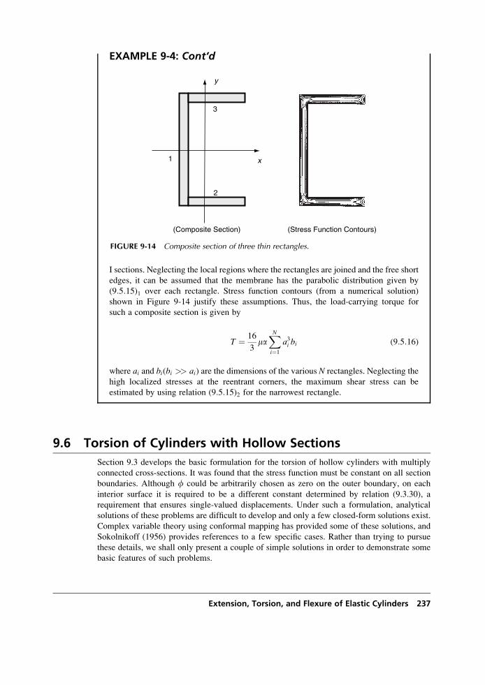
EXAMPLE 9-4: Cont’d
I sections. Neglecting the local regions where the rectangles are joined and the free short
edges, it can be assumed that the membrane has the parabolic distribution given by
(9:5:15)1 over each rectangle. Stress function contours (from a numerical solution)
shown in Figure 9-14 justify these assumptions. Thus, the load-carrying torque for
such a composite section is given by
T ¼ 16
3maXNi¼1
a3i bi (9:5:16)
where ai and bi(bi >> ai) are the dimensions of the various N rectangles. Neglecting the
high localized stresses at the reentrant corners, the maximum shear stress can be
estimated by using relation (9:5:15)2 for the narrowest rectangle.
9.6 Torsion of Cylinders with Hollow Sections
Section 9.3 develops the basic formulation for the torsion of hollow cylinders with multiply
connected cross-sections. It was found that the stress function must be constant on all section
boundaries. Although f could be arbitrarily chosen as zero on the outer boundary, on each
interior surface it is required to be a different constant determined by relation (9.3.30), a
requirement that ensures single-valued displacements. Under such a formulation, analytical
solutions of these problems are difficult to develop and only a few closed-form solutions exist.
Complex variable theory using conformal mapping has provided some of these solutions, and
Sokolnikoff (1956) provides references to a few specific cases. Rather than trying to pursue
these details, we shall only present a couple of simple solutions in order to demonstrate some
basic features of such problems.
x
y
1
2
3
(Stress Function Contours)(Composite Section)
FIGURE 9-14 Composite section of three thin rectangles.
Extension, Torsion, and Flexure of Elastic Cylinders 237
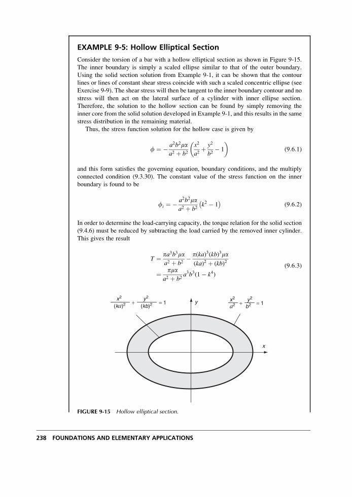
EXAMPLE 9-5: Hollow Elliptical Section
Consider the torsion of a bar with a hollow elliptical section as shown in Figure 9-15.
The inner boundary is simply a scaled ellipse similar to that of the outer boundary.
Using the solid section solution from Example 9-1, it can be shown that the contour
lines or lines of constant shear stress coincide with such a scaled concentric ellipse (see
Exercise 9-9). The shear stress will then be tangent to the inner boundary contour and no
stress will then act on the lateral surface of a cylinder with inner ellipse section.
Therefore, the solution to the hollow section can be found by simply removing the
inner core from the solid solution developed in Example 9-1, and this results in the same
stress distribution in the remaining material.
Thus, the stress function solution for the hollow case is given by
f ¼ � a2b2maa2 þ b2
x2
a2þ y2
b2� 1
� �(9:6:1)
and this form satisfies the governing equation, boundary conditions, and the multiply
connected condition (9.3.30). The constant value of the stress function on the inner
boundary is found to be
fi ¼ � a2b2maa2 þ b2
k2 � 1� �
(9:6:2)
In order to determine the load-carrying capacity, the torque relation for the solid section
(9.4.6) must be reduced by subtracting the load carried by the removed inner cylinder.
This gives the result
T ¼ pa3b3maa2 þ b2
� p(ka)3(kb)3ma(ka)2 þ (kb)2
¼ pmaa2 þ b2
a3b3(1� k4)
(9:6:3)
x
y = 1+(ka)2 (kb)2 = 1+y2 y2x2 x2
a2 b2
FIGURE 9-15 Hollow elliptical section.
238 FOUNDATIONS AND ELEMENTARY APPLICATIONS
EXAMPLE 9-5: Cont’d
and this relation can also be determined from equation (9.3.31). As mentioned, the stress
distribution in the hollow cylinder will be the same as that found in the corresponding
material of the solid section; see relations (9.4.8). For the case a > b, the maximum
stress still occurs at x ¼ 0 and y ¼ �b and is given by
tmax ¼ 2T
pab21
1� k4(9:6:4)
This solution scheme could be applied to other cross-sections whose inner boundary
coincides with a contour line of the corresponding solid section problem.
EXAMPLE 9-6: Hollow Thin-Walled Sections
The torsion of hollow thin-walled cylinders can be effectively handled using an approxi-
mate solution based on the membrane analogy. Consider the general thin-walled tube
shown in Figure 9-16. We assume that thickness t is small, although not necessarily
constant. A general section aa is taken through the tube wall at AB, and the expected
membrane shape is shown. From our previous theory, the membrane (stress function)
will be zero at the outer boundary (point B) and equal to a nonzero constant, say fo, on
the inner boundary (point A). Because the thickness is small there will be little variation
in the membrane slope, and thus shape BC can be approximated by a straight line.
Because the membrane slope equals the resultant shear stress, we can write
t ¼ fo
t(9:6:5)
The load-carrying relation (9.3.31) gives
T ¼ 2
ð ðR
fdxdyþ 2foAi (9:6:6)
where Ai is the area enclosed by the inner boundary. Using our assumption that the
membrane slope is constant over the section and neglecting variation in the
wall thickness (see Figure 9-16), the integral over the cross-section R can be approxi-
mated by Afo=2, where A is the section area. This allows the torque relation to be
expressed by
T ¼ 2 Afo
2
� �þ 2foAi ¼ 2foAc (9:6:7)
where Ac is the area enclosed by the section’s centerline. Combining relations (9.6.5)
and (9.6.7) gives
t ¼ T
2Act(9:6:8)
Continued
Extension, Torsion, and Flexure of Elastic Cylinders 239
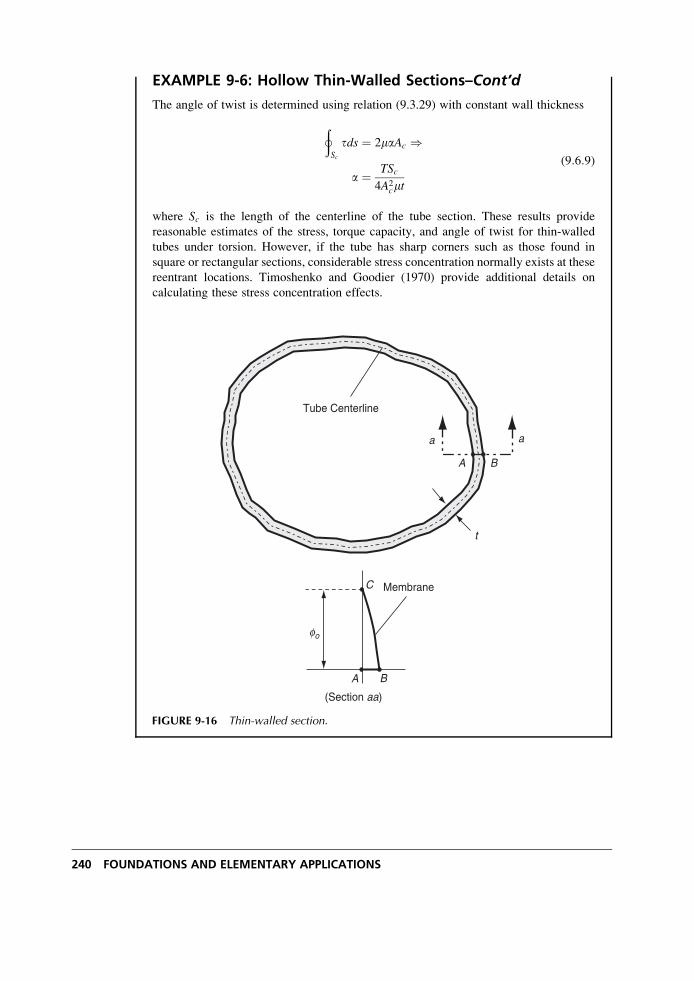
EXAMPLE 9-6: Hollow Thin-Walled Sections–Cont’d
The angle of twist is determined using relation (9.3.29) with constant wall thickness
þSc
tds ¼ 2maAc )
a ¼ TSc4A2
cmt
(9:6:9)
where Sc is the length of the centerline of the tube section. These results provide
reasonable estimates of the stress, torque capacity, and angle of twist for thin-walled
tubes under torsion. However, if the tube has sharp corners such as those found in
square or rectangular sections, considerable stress concentration normally exists at these
reentrant locations. Timoshenko and Goodier (1970) provide additional details on
calculating these stress concentration effects.
aa
A B
Tube Centerline
t
(Section aa)
A B
fo
MembraneC
FIGURE 9-16 Thin-walled section.
240 FOUNDATIONS AND ELEMENTARY APPLICATIONS
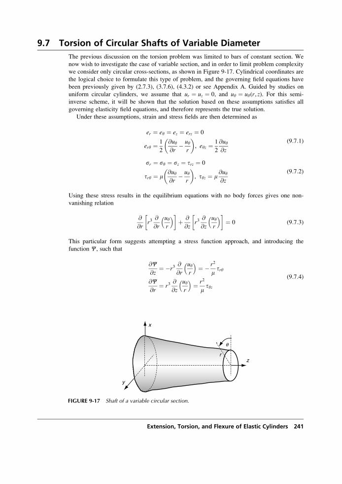
9.7 Torsion of Circular Shafts of Variable Diameter
The previous discussion on the torsion problem was limited to bars of constant section. We
now wish to investigate the case of variable section, and in order to limit problem complexity
we consider only circular cross-sections, as shown in Figure 9-17. Cylindrical coordinates are
the logical choice to formulate this type of problem, and the governing field equations have
been previously given by (2.7.3), (3.7.6), (4.3.2) or see Appendix A. Guided by studies on
uniform circular cylinders, we assume that ur ¼ uz ¼ 0, and uy ¼ uy(r, z). For this semi-
inverse scheme, it will be shown that the solution based on these assumptions satisfies all
governing elasticity field equations, and therefore represents the true solution.
Under these assumptions, strain and stress fields are then determined as
er ¼ ey ¼ ez ¼ erz ¼ 0
ery ¼ 1
2
@uy@r
� uyr
� �, eyz ¼ 1
2
@uy@z
(9:7:1)
sr ¼ sy ¼ sz ¼ trz ¼ 0
try ¼ m@uy@r
� uyr
� �, tyz ¼ m
@uy@z
(9:7:2)
Using these stress results in the equilibrium equations with no body forces gives one non-
vanishing relation
@
@rr3
@
@r
uyr
� � þ @
@zr3
@
@z
uyr
� � ¼ 0 (9:7:3)
This particular form suggests attempting a stress function approach, and introducing the
function C, such that
@C@z
¼ �r3@
@r
uyr
� �¼ � r2
mtry
@C@r
¼ r3@
@z
uyr
� �¼ r2
mtyz
(9:7:4)
x
y
zr
q
FIGURE 9-17 Shaft of a variable circular section.
Extension, Torsion, and Flexure of Elastic Cylinders 241
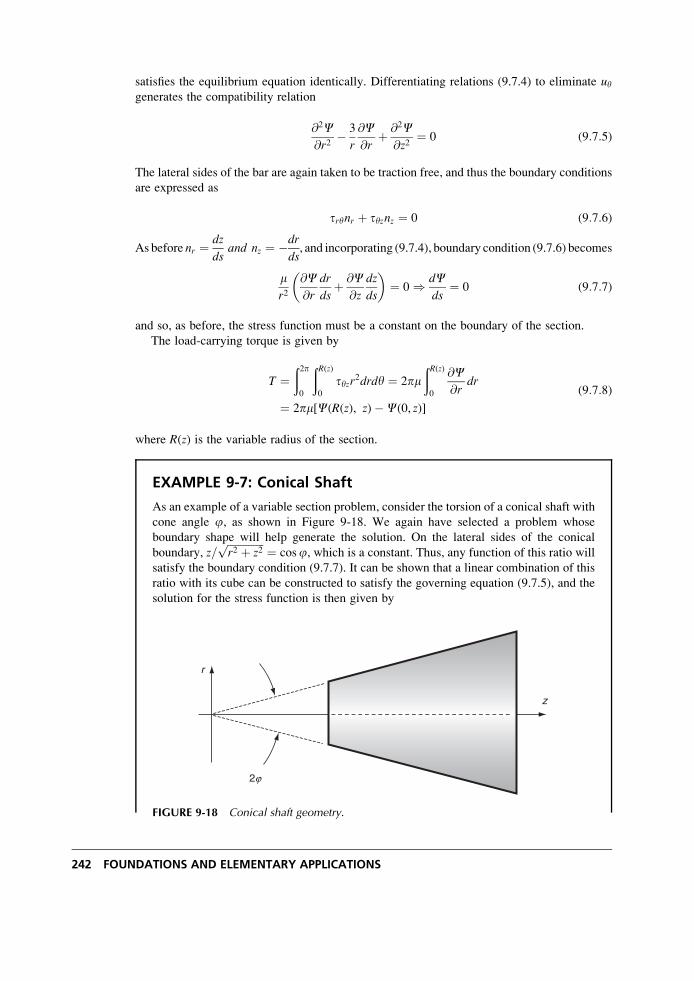
satisfies the equilibrium equation identically. Differentiating relations (9.7.4) to eliminate uygenerates the compatibility relation
@2C@r2
� 3
r
@C@r
þ @2C@z2
¼ 0 (9:7:5)
The lateral sides of the bar are again taken to be traction free, and thus the boundary conditions
are expressed as
trynr þ tyznz ¼ 0 (9:7:6)
As before nr ¼ dz
dsand nz ¼ �dr
ds, and incorporating (9.7.4), boundary condition (9.7.6) becomes
mr2
@C@r
dr
dsþ @C
@z
dz
ds
� �¼ 0 ) dC
ds¼ 0 (9:7:7)
and so, as before, the stress function must be a constant on the boundary of the section.
The load-carrying torque is given by
T ¼ð2p0
ðR(z)0
tyzr2drdy ¼ 2pmðR(z)0
@C@r
dr
¼ 2pm[C(R(z), z)�C(0, z)]
(9:7:8)
where R(z) is the variable radius of the section.
EXAMPLE 9-7: Conical Shaft
As an example of a variable section problem, consider the torsion of a conical shaft with
cone angle j, as shown in Figure 9-18. We again have selected a problem whose
boundary shape will help generate the solution. On the lateral sides of the conical
boundary, z=ffiffiffiffiffiffiffiffiffiffiffiffiffiffir2 þ z2
p ¼ cosj, which is a constant. Thus, any function of this ratio willsatisfy the boundary condition (9.7.7). It can be shown that a linear combination of this
ratio with its cube can be constructed to satisfy the governing equation (9.7.5), and the
solution for the stress function is then given by
z
2j
r
FIGURE 9-18 Conical shaft geometry.
242 FOUNDATIONS AND ELEMENTARY APPLICATIONS
EXAMPLE 9-7: Cont’d
C ¼ Czffiffiffiffiffiffiffiffiffiffiffiffiffiffi
r2 þ z2p � 1
3
z3
(r2 þ z2)3=2
� �(9:7:9)
where the constant C has been determined to satisfy the load-carrying relation (9.7.8)
C ¼ � T
2pm( 23� cosjþ 1
3cos3 j)
(9:7:10)
The stresses follow from relations (9.7.4)
try ¼ � Cmr2
(r2 þ z2)5=2
tyz ¼ � Cmrz
(r2 þ z2)5=2
(9:7:11)
and the displacement uy can be determined by integrating equations (9.7.2) to get
uy ¼ � Cr
3(r2 þ z2)3=2þ !r (9:7:12)
where !r is the rigid-body rotation term about the z-axis and ! can be determined
by specifying the shaft rotation at a specific z location. Additional examples of
such problems are discussed in Timoshenko and Goodier (1970) and Sokolnikoff (1956).
Before leaving the torsion problem, it should be mentioned that this problem can also be easily
formulated and solved using the numerical finite element method. Chapter 16 discusses this
important numerical scheme and provides a series of such solutions in Example 16-4 and
Figure 16-7. These examples illustrate the power and usefulness of this numerical method to
solve problemswith complicated geometry that could not be easily solved using analytical means.
9.8 Flexure Formulation
We now investigate a final case of deformation of elastic cylinders under end loadings
by considering the flexure of elastic beams subject to transverse end forces, as shown in
Figure 9-19. The problem geometry is formulated as a cantilever beam of arbitrary section with
a fixed end at z ¼ 0 and transverse end loadings Px and Py at z ¼ l. Following our usual
procedure, the problem is to be solved in the Saint-Venant sense, in that only the resultant end
loadings Px and Py are used to formulate the boundary conditions at z ¼ l.From our general formulation in Section 9.1, sx ¼ sy ¼ txy ¼ 0. The other three nonzero
stresses will be determined to satisfy the equilibrium and compatibility relations and all
associated boundary conditions. From our earlier work, the equilibrium and compatibility
relations resulted in equations (9.1.2) from which it was argued that txz and tyz were independ-ent of z, and sz was a bilinear form in x, y, z (see Exercise 9-1). Motivated from strength of
materials theory, we choose the arbitrary form for sz as follows
Extension, Torsion, and Flexure of Elastic Cylinders 243
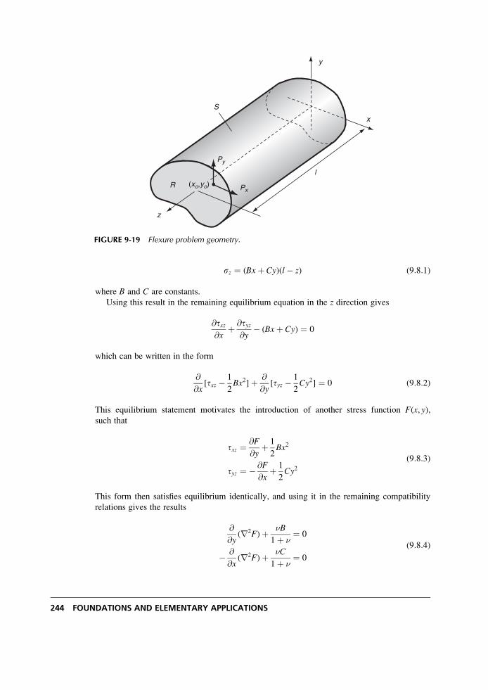
sz ¼ (Bxþ Cy)(l� z) (9:8:1)
where B and C are constants.
Using this result in the remaining equilibrium equation in the z direction gives
@txz@x
þ @tyz@y
� (Bxþ Cy) ¼ 0
which can be written in the form
@
@x[txz � 1
2Bx2]þ @
@y[tyz � 1
2Cy2] ¼ 0 (9:8:2)
This equilibrium statement motivates the introduction of another stress function F(x, y),such that
txz ¼ @F
@yþ 1
2Bx2
tyz ¼ � @F
@xþ 1
2Cy2
(9:8:3)
This form then satisfies equilibrium identically, and using it in the remaining compatibility
relations gives the results
@
@y(r2F)þ �B
1þ �¼ 0
� @
@x(r2F)þ �C
1þ �¼ 0
(9:8:4)
x
y
z
l
S
R Px
Py
(xo,yo)
FIGURE 9-19 Flexure problem geometry.
244 FOUNDATIONS AND ELEMENTARY APPLICATIONS
This system can be integrated to get
r2F ¼ �
1þ �(Cx� By)þ k (9:8:5)
where k is a constant of integration. In order to determine this constant, consider the rotation
about the z-axis. From the general relation (2.1.9), !z ¼ [(@v=@x)� (@u=@y)]=2, differentiat-ing with respect to z and using Hooke’s law and our previous results gives
@!z
@z¼ 1
2
@2v
@x@z� @2u
@y@z
� �
¼ 1
2m@tyz@x
� @txz@y
� �
¼ � 1
2mr2F ¼ � 1
2m�
1þ �(Cx� By)þ k
(9:8:6)
From the torsion formulation, the angle of twist per unit length was specified by the
parameter a, and selecting the section origin (x ¼ y ¼ 0) at the center of twist, relation
(9.8.6) then implies that k ¼ �2ma. Thus, the governing equation (9.8.5) can be written as
r2F ¼ �
1þ �(Cx� By)� 2ma (9:8:7)
The zero loading boundary condition on the lateral surface S is expressed by
txznx þ tyzny ¼ 0
and using the stress function definition, this can be written as
@F
@x
dx
dsþ @F
@y
dy
dsþ 1
2Bx2
dy
ds� Cy2
dx
ds
� �¼ 0 or
dF
ds¼ � 1
2Bx2
dy
ds� Cy2
dx
ds
� �(9:8:8)
It is convenient to separate the stress function F into a torsional part f and a flexural part c,such that
F(x, y) ¼ f(x, y)þ c(x, y) (9:8:9)
where the torsional part is formulated by
r2f ¼ �2ma in R
dfds
¼ 0 on S(9:8:10)
while the flexural portion satisfies
r2c ¼ �
1þ �(Cx� By) in R
dcds
¼ � 1
2(Bx2
dy
ds� Cy2
dx
ds) on S
(9:8:11)
Extension, Torsion, and Flexure of Elastic Cylinders 245
Because we have already investigated the torsional part of this problem in the preceding
sections, we now pursue only the flexural portion. The general solution to (9:8:11)1 may be
expressed as the sum of a particular solution plus a harmonic function
c(x, y) ¼ f (x, y)þ 1
6
�
1þ �(Cx3 � By3) (9:8:12)
where f is a harmonic function satisfying r2f ¼ 0. The boundary conditions on end z ¼ l canbe stated as
ð ðR
txzdxdy ¼ Pxð ðR
tyzdxdy ¼ Pyð ðR
[xtyz � ytxz]dxdy ¼ xoPy � yoPx
(9:8:13)
Using the first relation of this set gives
ð ðR
[@
@y(fþ c)þ 1
2Bx2]dxdy ¼ Px (9:8:14)
but from the torsion formulation
ð ðR
@f@y
dxdy ¼ 0, and so (9.8.14) can be written as
ð ðR
[@
@x(x@c@y
)� @
@y(x@c@x
)]dxdyþð ð
R
1
2Bx2dxdy ¼ Px (9:8:15)
Using Green’s theorem and the boundary relation (9:8:11)2, the first integral can be
expressed as
ð ðR
[@
@x(x@c@y
)� @
@y(x@c@x
)]dxdy ¼ �ð ð
R
[3
2Bx2 þ Cxy]dxdy
and thus equation (9.8.15) reduces to
BIy þ CIxy ¼ �Px (9:8:16)
In a similar manner, boundary condition (9:8:13)2 gives
BIxy þ CIx ¼ �Py (9:8:17)
The expressions Ix, Iy, and Ixy are the area moments of inertia of section R
Ix ¼ð ð
R
y2dxdy, Iy ¼ð ð
R
x2dxdy, Ixy ¼ð ð
R
xydxdy (9:8:18)
Relations (9.8.16) and (9.8.17) can be solved for the constants B and C
246 FOUNDATIONS AND ELEMENTARY APPLICATIONS
B ¼ �PxIx � PyIxyIxIy � I2xy
C ¼ �PyIy � PxIxyIxIy � I2xy
(9:8:19)
The final boundary condition (9:8:13)3 can be expressed as
�ð ð
R
[x@f@x
þ y@f@y
]dxdy�ð ð
R
[x@c@x
þ y@c@y
]dxdy
þð ð
R
1
2(Cxy2 � Bx2y)dxdy ¼ xoPy � yoPx
(9:8:20)
From the torsion formulation, �ð ð
R
x@f@x
þ y@f@y
dxdy ¼ 2
ð ðR
fdxdy ¼ T ¼ aJ, so (9.8.20)
becomes
aJ þð ð
R
1
2(Cxy2 � Bx2y)� (x
@c@x
þ y@c@y
)
� �dxdy ¼ xoPy � yoPx (9:8:21)
Once the flexural stress function c is known, (9.8.21) will provide a relation to determine the
angle of twist a.Relation (9.8.21) can also be used to determine the location (xo, yo) for no induced
torsional rotation, a point commonly called the shear center or center of flexure. Choosinga ¼ 0, this equation can be independently used for the two cases of (Px ¼ 0, Py 6¼ 0) and
(Px 6¼ 0, Py ¼ 0) to generate two equations for locations xo and yo. If the x-axis is an axis of
symmetry, then yo ¼ 0; and likewise, if the y-axis is one of symmetry, then xo ¼ 0. For a
section with two perpendicular axes of symmetry, the location (xo, yo) lies at the intersection ofthese two axes, which is at the centroid of the section. However, in general the shear center
does not coincide with the section’s centroid and need not even lie within the section.
9.9 Flexure Problems Without Twist
Because we have previously studied examples of the torsion problem, we shall now develop
flexure solutions to problems that do not include twist. The two examples to be investigated
include simple symmetric cross-sections with single end loadings along an axis of symmetry.
EXAMPLE 9-8: Circular Section
Consider the flexure of an elastic beam of circular section, as shown in Figure 9-20. The
end loading (Px ¼ 0, Py ¼ P) passes through the center of the section, which coincides
with the centroid and center of twist. Thus, for this problem there will be no torsion
(a ¼ 0), and so f ¼ 0 and F ¼ c. It is convenient to use polar coordinates for this
problem, and the governing equation (9:8:11)1 can then be written as
r2c ¼ � �
1þ �
P
Ixr cos y (9:9:1)
Continued
Extension, Torsion, and Flexure of Elastic Cylinders 247
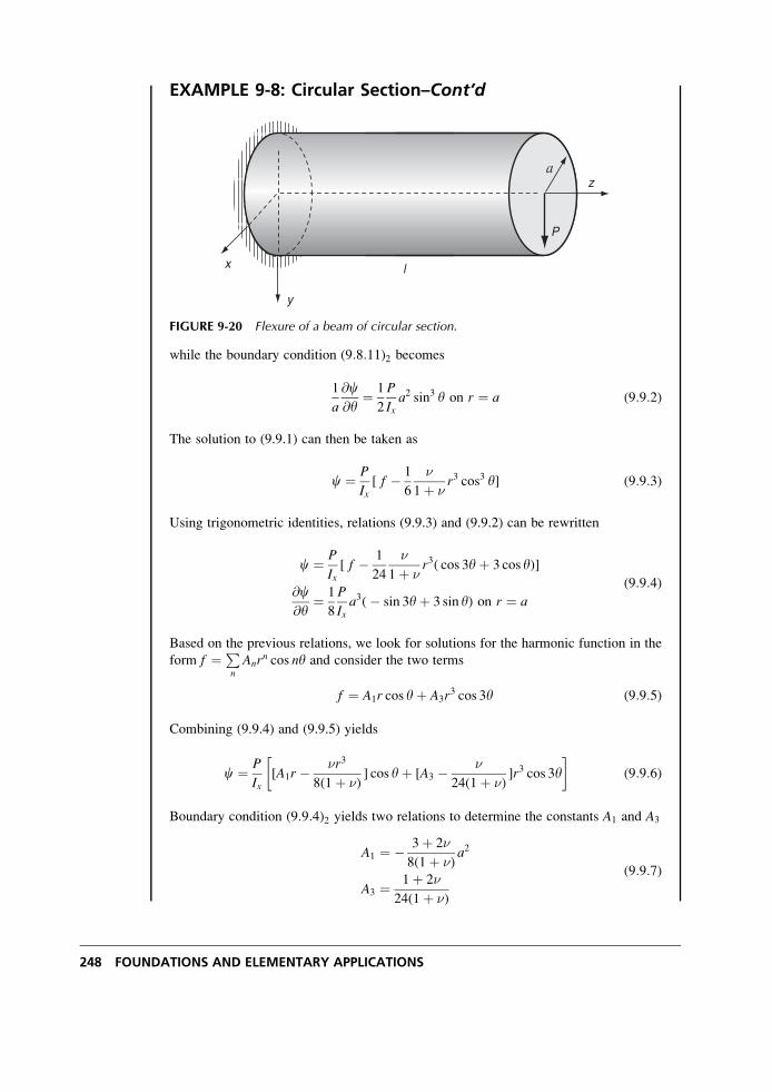
EXAMPLE 9-8: Circular Section–Cont’d
while the boundary condition (9:8:11)2 becomes
1
a
@c@y
¼ 1
2
P
Ixa2 sin3 y on r ¼ a (9:9:2)
The solution to (9.9.1) can then be taken as
c ¼ P
Ix[ f � 1
6
�
1þ �r3 cos3 y] (9:9:3)
Using trigonometric identities, relations (9.9.3) and (9.9.2) can be rewritten
c ¼ P
Ix[ f � 1
24
�
1þ �r3( cos 3yþ 3 cos y)]
@c@y
¼ 1
8
P
Ixa3(� sin 3yþ 3 sin y) on r ¼ a
(9:9:4)
Based on the previous relations, we look for solutions for the harmonic function in the
form f ¼PnAnr
n cos ny and consider the two terms
f ¼ A1r cos yþ A3r3 cos 3y (9:9:5)
Combining (9.9.4) and (9.9.5) yields
c ¼ P
Ix[A1r � �r3
8(1þ �)] cos yþ [A3 � �
24(1þ �)]r3 cos 3y
(9:9:6)
Boundary condition (9:9:4)2 yields two relations to determine the constants A1 and A3
A1 ¼ � 3þ 2�
8(1þ �)a2
A3 ¼ 1þ 2�
24(1þ �)
(9:9:7)
x
y
za
P
l
FIGURE 9-20 Flexure of a beam of circular section.
248 FOUNDATIONS AND ELEMENTARY APPLICATIONS
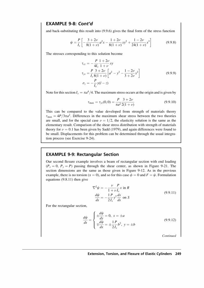
EXAMPLE 9-8: Cont’d
and back-substituting this result into (9.9.6) gives the final form of the stress function
c ¼ P
Ix� 3þ 2�
8(1þ �)a2x� 1þ 2�
8(1þ �)xy2 þ 1� 2�
24(1þ �)x3
(9:9:8)
The stresses corresponding to this solution become
txz ¼ � P
4Ix
1þ 2�
1þ �xy
tyz ¼ P
Ix
3þ 2�
8(1þ �)a2 � y2 � 1� 2�
3þ 2�x2
�z ¼ � P
Ixy(l� z)
(9:9:9)
Note for this section Ix ¼ pa4=4. The maximum stress occurs at the origin and is given by
tmax ¼ tyz(0, 0) ¼ P
pa23þ 2�
2(1þ �)(9:9:10)
This can be compared to the value developed from strength of materials theory
tmax ¼ 4P=3pa2. Differences in the maximum shear stress between the two theories
are small, and for the special case � ¼ 1=2, the elasticity solution is the same as the
elementary result. Comparison of the shear stress distribution with strength of materials
theory for � ¼ 0:1 has been given by Sadd (1979), and again differences were found to
be small. Displacements for this problem can be determined through the usual integra-
tion process (see Exercise 9-24).
EXAMPLE 9-9: Rectangular Section
Our second flexure example involves a beam of rectangular section with end loading
(Px ¼ 0, Py ¼ P) passing through the shear center, as shown in Figure 9-21. The
section dimensions are the same as those given in Figure 9-12. As in the previous
example, there is no torsion (a ¼ 0), and so for this case f ¼ 0 and F ¼ c. Formulation
equations (9.8.11) then give
r2c ¼ � �
1þ �
P
Ixx in R
dcds
¼ � 1
2
P
Ixy2
dx
dson S
(9:9:11)
For the rectangular section,
dcds
¼�dcdy
¼ 0, x ¼ �a
�dcdx
¼ � 1
2
P
Ixb2, y ¼ �b
8>><>>: (9:9:12)
Continued
Extension, Torsion, and Flexure of Elastic Cylinders 249
EXAMPLE 9-9: Rectangular Section–Cont’d
Based on these boundary relations we are motivated to select a solution of the form
c ¼ P
Ix[ f � 1
6
�
1þ �(x3 � a2x)� b2x
2] (9:9:13)
with the harmonic function f satisfying
f (x, y) ¼0, x ¼ �a
�
6(1þ �)(x3 � a2x), y ¼ �b
((9:9:14)
Because we expect tyz to be an even function in x and y, and txz to be odd in y, welook for a harmonic solution for f in the form
f (x, y) ¼X1n¼1
An sinnpxa
coshnpya
(9:9:15)
This form satisfies (9:9:14)1 identically, while (9:9:14)2 implies that
X1n¼1
bn sinnpxa
¼ �
6(1þ �)(x3 � a2x) (9:9:16)
where bn ¼ An cosh (npb=a). Relation (9.9.16) is recognized as a Fourier sine series,
and thus the coefficients follow from standard theory (8.2.28) and are given by
bn ¼ 2�3(� 1)n=(1þ �)n3p3. Putting these results back together gives the final form
of the stress function
c ¼ P
Ix� 1
6
�
1þ �(x3�a2x)� b2x
2þ 2�a3
(1þ �)p3X1n¼1
(� 1)n
n3
sinnpxa
coshnpya
coshnpba
264
375 (9:9:17)
x
y
z
2a
Pl
2b
FIGURE 9-21 Flexure of a beam of rectangular section.
250 FOUNDATIONS AND ELEMENTARY APPLICATIONS
EXAMPLE 9-9: Cont’d
The stresses then follow to be
txz ¼ 2�a2P
(1þ �)p2Ix
X1n¼1
(�1)n
n2
sinnpxa
sinhnpya
coshnpba
tyz ¼ P
2Ix(b2�y2)þ �P
6(1þ �)Ix3x2� a2� 12a2
p2X1n¼1
(�1)n
n2
cosnpxa
coshnpya
coshnpba
264
375
sz ¼ P
Ixy(l� z)
(9:9:18)
The corresponding results from strength of materials gives tyz ¼ P(b2 � y2)=2Ix, andthus the second term of (9.9.18)2 represents the correction to the elementary theory.
Note that if � ¼ 0, this correction term vanishes, and the two theories predict identical
stresses. For the case of a thin rectangular section with b >> a, cosh (npb=a) ! 1,
and it can be shown that the elasticity solution reduces to the strength of materials
prediction. A similar result is also found for the case of a thin section with a >> b.Comparison of the shear stress distribution tyz with strength of materials theory for
� ¼ 1=2 has been presented by Sadd (1979), and differences between the two theories
were found to be sizable. As in the previous example, the maximum stress occurs at
x ¼ y ¼ 0
tmax ¼ tyz(0, 0) ¼ P
2Ixb2 � �Pa2
6(1þ �)Ix1þ 12
p2X1n¼1
(� 1)n
n2sech
npba
" #(9:9:19)
Again, the strength of materials result is given by the first term in relation (9.9.19).
This concludes our brief presentation of flexure examples. Solutions to additional
flexure problems are given by Sokolnikoff (1956) and Timoshenko and Goodier
(1970).
References
Higgins TJ: A comprehensive review of Saint-Venant torsion problem, Amer. Jour. Physics, vol 10,pp. 248-259, 1942.
Higgins TJ: The approximate mathematical methods of applied physics as exemplified by application to
Saint-Venant torsion problem, Jour. Appl. Physics, vol 14, pp. 469-480, 1943.Higgins TJ: Analogic experimental methods in stress analysis as exemplified by Saint-Venant’s torsion
problem, Proc. Soc. Exp. Stress Analysis, vol 2, pp. 17-27, 1945.Kellogg OD: Foundations of Potential Theory, Dover, New York, 1969.
Sadd MH: A comparison of mechanics of materials and theory of elasticity stress analysis, Mech. Eng.News, ASEE, vol 16, pp 34-39, 1979.
Sokolnikoff IS: Mathematical Theory of Elasticity, McGraw-Hill, New York, 1956.
Timoshenko SP, and Goodier JN: Theory of Elasticity, McGraw-Hill, New York, 1970.
Extension, Torsion, and Flexure of Elastic Cylinders 251
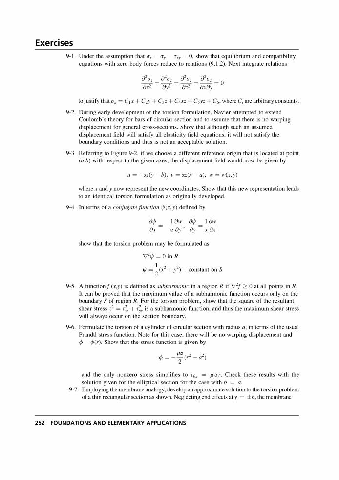
Exercises
9-1. Under the assumption that sx ¼ sy ¼ txy ¼ 0, show that equilibrium and compatibility
equations with zero body forces reduce to relations (9.1.2). Next integrate relations
@2sz@x2
¼ @2sz@y2
¼ @2sz@z2
¼ @2sz@x@y
¼ 0
to justify that sz ¼ C1xþ C2yþ C3zþ C4xzþ C5yzþ C6, whereCi are arbitrary constants.
9-2. During early development of the torsion formulation, Navier attempted to extend
Coulomb’s theory for bars of circular section and to assume that there is no warping
displacement for general cross-sections. Show that although such an assumed
displacement field will satisfy all elasticity field equations, it will not satisfy the
boundary conditions and thus is not an acceptable solution.
9-3. Referring to Figure 9-2, if we choose a different reference origin that is located at point
(a,b) with respect to the given axes, the displacement field would now be given by
u ¼ �az(y� b), v ¼ az(x� a), w ¼ w(x, y)
where x and y now represent the new coordinates. Show that this new representation leads
to an identical torsion formulation as originally developed.
9-4. In terms of a conjugate function c(x, y) defined by
@c@x
¼ � 1
a@w
@y,@c@y
¼ 1
a@w
@x
show that the torsion problem may be formulated as
r2c ¼ 0 in R
c ¼ 1
2(x2 þ y2)þ constant on S
9-5. A function f (x,y) is defined as subharmonic in a region R if r2f � 0 at all points in R.It can be proved that the maximum value of a subharmonic function occurs only on the
boundary S of region R. For the torsion problem, show that the square of the resultant
shear stress t2 ¼ t2xz þ t2yz is a subharmonic function, and thus the maximum shear stress
will always occur on the section boundary.
9-6. Formulate the torsion of a cylinder of circular section with radius a, in terms of the usual
Prandtl stress function. Note for this case, there will be no warping displacement and
f¼ f(r). Show that the stress function is given by
f ¼ �ma2(r2 � a2)
and the only nonzero stress simplifies to tyz ¼ m a r. Check these results with the
solution given for the elliptical section for the case with b ¼ a.9-7. Employing the membrane analogy, develop an approximate solution to the torsion problem
of a thin rectangular section as shown. Neglecting end effects at y ¼ �b, the membrane
252 FOUNDATIONS AND ELEMENTARY APPLICATIONS
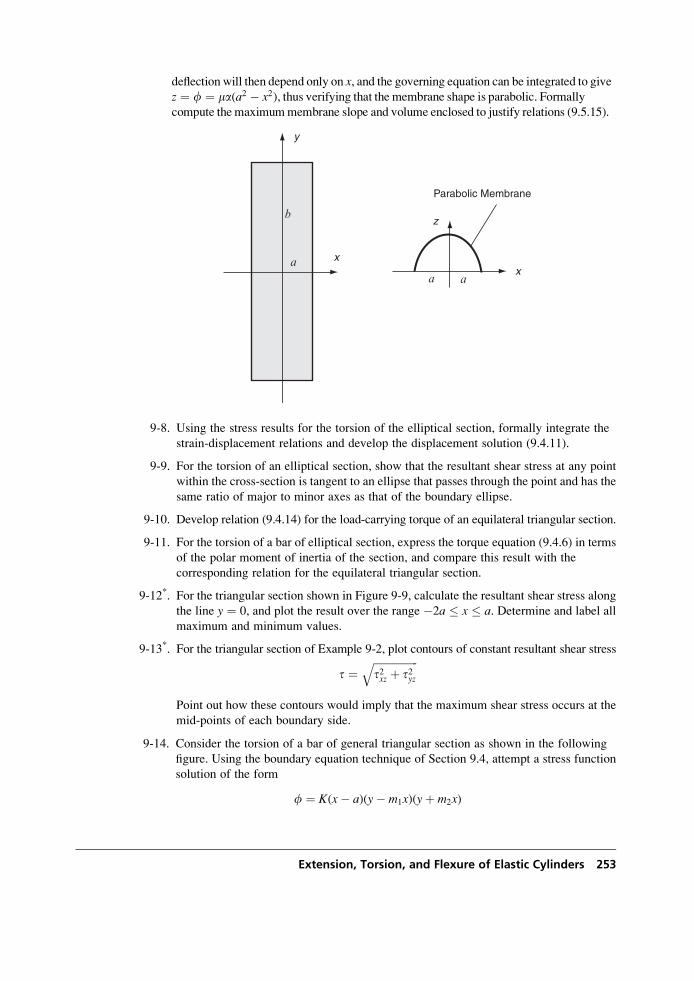
deflection will then depend only on x, and the governing equation can be integrated to givez ¼ f ¼ ma(a2 � x2), thus verifying that the membrane shape is parabolic. Formally
compute the maximummembrane slope and volume enclosed to justify relations (9.5.15).
x
y
a
b
Parabolic Membrane
aax
z
9-8. Using the stress results for the torsion of the elliptical section, formally integrate the
strain-displacement relations and develop the displacement solution (9.4.11).
9-9. For the torsion of an elliptical section, show that the resultant shear stress at any point
within the cross-section is tangent to an ellipse that passes through the point and has the
same ratio of major to minor axes as that of the boundary ellipse.
9-10. Develop relation (9.4.14) for the load-carrying torque of an equilateral triangular section.
9-11. For the torsion of a bar of elliptical section, express the torque equation (9.4.6) in terms
of the polar moment of inertia of the section, and compare this result with the
corresponding relation for the equilateral triangular section.
9-12*. For the triangular section shown in Figure 9-9, calculate the resultant shear stress along
the line y ¼ 0, and plot the result over the range �2a � x � a. Determine and label all
maximum and minimum values.
9-13*. For the triangular section of Example 9-2, plot contours of constant resultant shear stress
t ¼ffiffiffiffiffiffiffiffiffiffiffiffiffiffiffiffiffit2xz þ t2yz
qPoint out how these contours would imply that the maximum shear stress occurs at the
mid-points of each boundary side.
9-14. Consider the torsion of a bar of general triangular section as shown in the following
figure. Using the boundary equation technique of Section 9.4, attempt a stress function
solution of the form
f ¼ K(x� a)(y� m1x)(yþ m2x)
Extension, Torsion, and Flexure of Elastic Cylinders 253
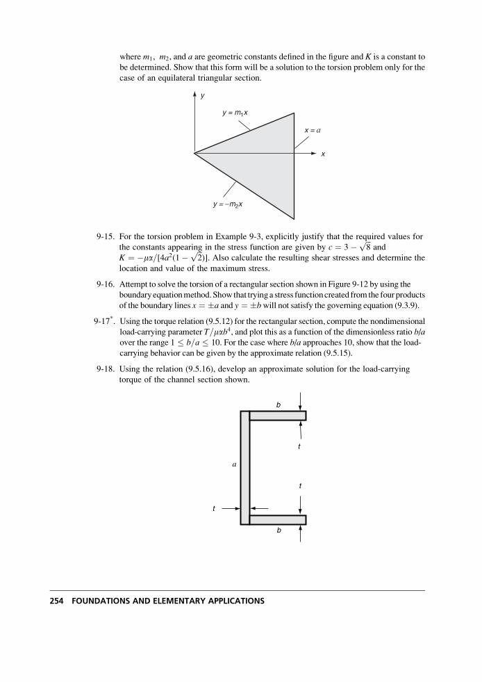
where m1, m2, and a are geometric constants defined in the figure and K is a constant to
be determined. Show that this form will be a solution to the torsion problem only for the
case of an equilateral triangular section.
x = a
y = m1x
y = −m2x
x
y
9-15. For the torsion problem in Example 9-3, explicitly justify that the required values for
the constants appearing in the stress function are given by c ¼ 3� ffiffiffi8
pand
K ¼ �ma=[4a2(1� ffiffiffi2
p)]. Also calculate the resulting shear stresses and determine the
location and value of the maximum stress.
9-16. Attempt to solve the torsion of a rectangular section shown in Figure 9-12 by using the
boundaryequationmethod.Show that tryinga stress functioncreated from the four products
of the boundary lines x ¼ �a and y ¼ �bwill not satisfy the governing equation (9.3.9).
9-17*. Using the torque relation (9.5.12) for the rectangular section, compute the nondimensional
load-carrying parameter T=mab4, and plot this as a function of the dimensionless ratio b/aover the range 1 � b=a � 10. For the case where b/a approaches 10, show that the load-
carrying behavior can be given by the approximate relation (9.5.15).
9-18. Using the relation (9.5.16), develop an approximate solution for the load-carrying
torque of the channel section shown.
a
t
b
t
t
b
254 FOUNDATIONS AND ELEMENTARY APPLICATIONS
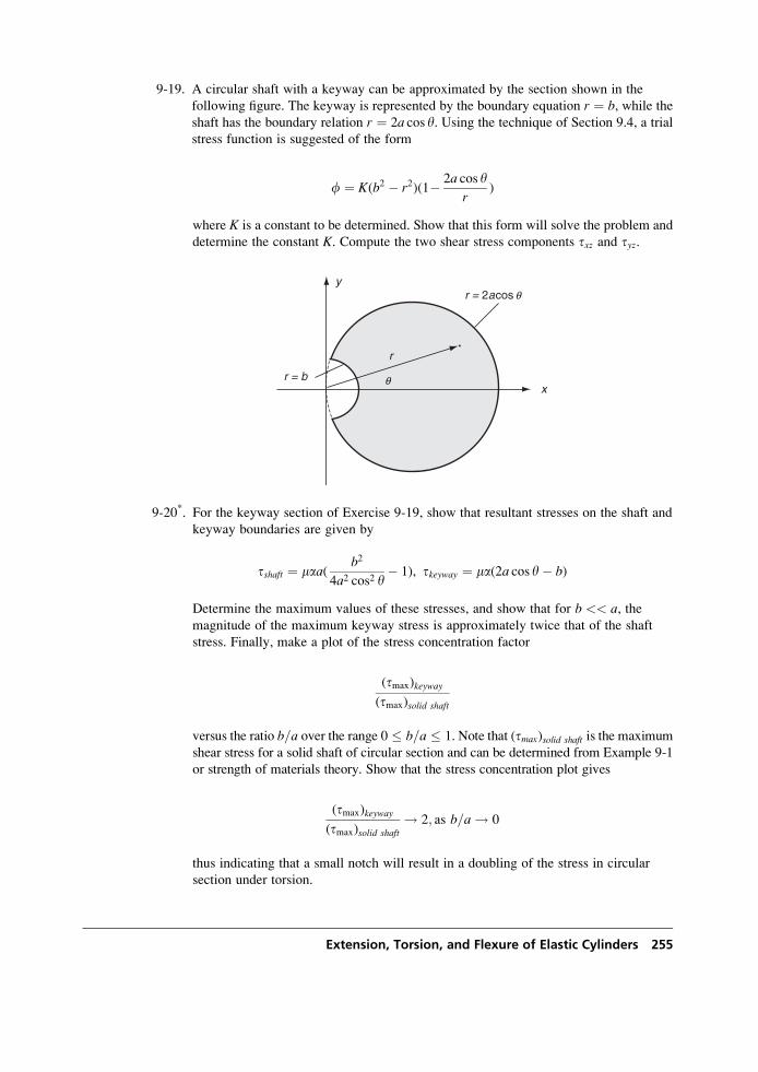
9-19. A circular shaft with a keyway can be approximated by the section shown in the
following figure. The keyway is represented by the boundary equation r ¼ b, while theshaft has the boundary relation r ¼ 2a cos y. Using the technique of Section 9.4, a trial
stress function is suggested of the form
f ¼ K(b2 � r2)(1� 2a cos yr
)
where K is a constant to be determined. Show that this form will solve the problem and
determine the constant K. Compute the two shear stress components txz and tyz.
r = b
r = 2acos q
r
x
y
.
q
9-20*. For the keyway section of Exercise 9-19, show that resultant stresses on the shaft and
keyway boundaries are given by
tshaft ¼ maa(b2
4a2 cos2 y� 1), tkeyway ¼ ma(2a cos y� b)
Determine the maximum values of these stresses, and show that for b << a, themagnitude of the maximum keyway stress is approximately twice that of the shaft
stress. Finally, make a plot of the stress concentration factor
(tmax)keyway
(tmax)solid shaft
versus the ratio b=a over the range 0 � b=a � 1. Note that (tmax)solid shaft is the maximum
shear stress for a solid shaft of circular section and can be determined from Example 9-1
or strength of materials theory. Show that the stress concentration plot gives
(tmax)keyway
(tmax)solid shaft
! 2; as b=a ! 0
thus indicating that a small notch will result in a doubling of the stress in circular
section under torsion.
Extension, Torsion, and Flexure of Elastic Cylinders 255
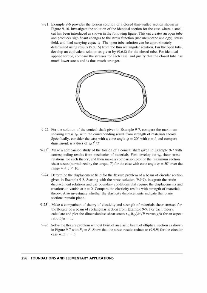
9-21. Example 9-6 provides the torsion solution of a closed thin-walled section shown in
Figure 9-16. Investigate the solution of the identical section for the case where a small
cut has been introduced as shown in the following figure. This cut creates an open tube
and produces significant changes to the stress function (use membrane analogy), stress
field, and load-carrying capacity. The open tube solution can be approximately
determined using results (9.5.15) from the thin rectangular solution. For the open tube,
develop an equivalent relation as given by (9.6.8) for the closed tube. For identical
applied torque, compare the stresses for each case, and justify that the closed tube has
much lower stress and is thus much stronger.
9-22. For the solution of the conical shaft given in Example 9-7, compare the maximum
shearing stress tyz with the corresponding result from strength of materials theory.
Specifically, consider the case with a cone angle j ¼ 20 with z ¼ l, and compare
dimensionless values of tyzl3=T.
9-23*. Make a comparison study of the torsion of a conical shaft given in Example 9-7 with
corresponding results from mechanics of materials. First develop the tyz shear stressrelations for each theory, and then make a comparison plot of the maximum section
shear stress (normalized by the torque, T) for the case with cone angle j ¼ 308 over therange 4 � z � 10.
9-24. Determine the displacement field for the flexure problem of a beam of circular section
given in Example 9-8. Starting with the stress solution (9.9.9), integrate the strain-
displacement relations and use boundary conditions that require the displacements and
rotations to vanish at z ¼ 0. Compare the elasticity results with strength of materials
theory. Also investigate whether the elasticity displacements indicate that plane
sections remain plane.
9-25*. Make a comparison of theory of elasticity and strength of materials shear stresses for
the flexure of a beam of rectangular section from Example 9-9. For each theory,
calculate and plot the dimensionless shear stress tyz(0, y)b2=P versus y=b for an aspect
ratio b=a ¼ 1.
9-26. Solve the flexure problem without twist of an elastic beam of elliptical section as shown
in Figure 9-7 with Py ¼ P. Show that the stress results reduce to (9.9.9) for the circular
case with a ¼ b.
256 FOUNDATIONS AND ELEMENTARY APPLICATIONS
10 Complex Variable Methods
Complex variable theory provides a very powerful tool for the solution of many problems in
elasticity. Such applications include solutions of the torsion problem and most importantly the
plane problem discussed in Chapters 7 and 8. The technique is also useful for cases involving
anisotropic and thermoelastic materials, and these are discussed in subsequent chapters.
Employing complex variable methods enables many problems to be solved that would be
intractable by other schemes. The method is based on the reduction of the elasticity boundary-
value problem to a formulation in the complex domain. This formulation then allows many
powerful mathematical techniques available from complex variable theory to be applied to the
elasticity problem. Such applications were originally formulated by Kolosov (1909), and
additional Russian researchers further expanded the use of this technique. Comprehensive
texts on this solution method include Muskhelishvili (1953, 1963), Milne-Thomson (1960),
Green and Zerna (1968), and England (1971). Additional briefer sources of information can
also be found in Sokolnikoff (1956) and Little (1973). The purpose of this chapter is to
introduce the basics of the method and to investigate its application to particular problems
of engineering interest. We shall first briefly review complex variable theory to provide a
general background needed to develop the elasticity solutions. Further and more detailed
information on complex variables may be found in the mathematical texts by Churchill
(1960) or Kreyszig (1999).
10.1 Review of Complex Variable Theory
A complex variable z is defined by two real variables x and y in the form
z ¼ xþ iy (10:1:1)
where i ¼ ffiffiffiffiffiffiffi�1p
is called the imaginary unit, x is known as the real part of z, that is, x ¼ Re(z),while y is called the imaginary part, y ¼ Im(z). This definition can also be expressed in polarform by
z ¼ r( cos yþ i sin y) ¼ reiy (10:1:2)
259
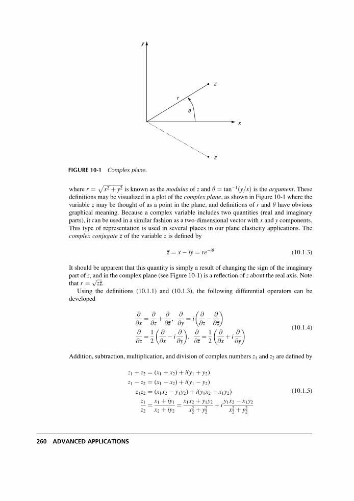
where r ¼ffiffiffiffiffiffiffiffiffiffiffiffiffiffiffix2 þ y2
pis known as the modulus of z and y ¼ tan�1 y=xð Þ is the argument. These
definitions may be visualized in a plot of the complex plane, as shown in Figure 10-1 where thevariable z may be thought of as a point in the plane, and definitions of r and y have obvious
graphical meaning. Because a complex variable includes two quantities (real and imaginary
parts), it can be used in a similar fashion as a two-dimensional vector with x and y components.
This type of representation is used in several places in our plane elasticity applications. The
complex conjugate �zz of the variable z is defined by
�zz ¼ x� iy ¼ re�iy (10:1:3)
It should be apparent that this quantity is simply a result of changing the sign of the imaginary
part of z, and in the complex plane (see Figure 10-1) is a reflection of z about the real axis. Notethat r ¼ ffiffiffiffi
z�zzp
.
Using the definitions (10.1.1) and (10.1.3), the following differential operators can be
developed
@
@x¼ @
@zþ @
@�zz,
@
@y¼ i
@
@z� @
@�zz
� �@
@z¼ 1
2
@
@x� i
@
@y
� �,
@
@�zz¼ 1
2
@
@xþ i
@
@y
� � (10:1:4)
Addition, subtraction, multiplication, and division of complex numbers z1 and z2 are defined by
z1 þ z2 ¼ (x1 þ x2)þ i(y1 þ y2)
z1 � z2 ¼ (x1 � x2)þ i(y1 � y2)
z1z2 ¼ (x1x2 � y1y2)þ i(y1x2 þ x1y2)
z1z2
¼ x1 þ iy1x2 þ iy2
¼ x1x2 þ y1y2x22 þ y22
þ iy1x2 � x1y2x22 þ y22
(10:1:5)
z
r
y
x
z
q
FIGURE 10-1 Complex plane.
260 ADVANCED APPLICATIONS
A function of a complex variable z may be written as
f (z) ¼ f (xþ iy) ¼ u(x, y)þ iv(x, y) (10:1:6)
where u(x,y) and v(x,y) are the real and imaginary parts of the complex function f(z). Anexample of this definition is given by
f (z) ¼ azþ bz2 ¼ a(xþ iy)þ b(xþ iy)2 ¼ (axþ bx2 � by2)þ i(ayþ 2bxy)
thus u(x, y) ¼ axþ bx2 � by2 and v(x, y) ¼ ayþ 2bxy, where we have assumed that a and bare real constants.
The complex conjugate of the complex function is defined by
f (z) ¼ �ff (�zz) ¼ u(x, y)� iv(x, y) (10:1:7)
and thus for the previous example of f (z) ¼ azþ bz2
f (z) ¼ (azþ bz2) ¼ a�zzþ b�zz2
¼ a(x� iy)þ b(x� iy)2
¼ (axþ bx2 � by2)� i(ayþ 2bxy)
Differentiation of functions of a complex variable follows the usual definitions. Let f(z) be asingle-valued continuous function of z in a domain D. The function f is differentiable at pointzo in D if
f 0(zo) ¼ limDz!0
f (zo þ Dz)� f (zo)
Dz
� �(10:1:8)
exists and is independent of how Dz ! 0. If the function is differentiable at all points in a
domain D, then it is said to be holomorphic, analytic, or regular in D. Points where the
function is not analytic are called singular points.Using the representation (10.1.6) with differential relations (10.1.4), the derivative of f can
be expressed by
f 0(z) ¼ @
@z(uþ iv) ¼ 1
2
@u
@xþ @v
@y
� �þ i
1
2
@v
@x� @u
@y
� �(10:1:9)
Because the derivative limit must be the same regardless of the path associated with Dz ! 0,
relation (10.1.9) must be valid for the individual cases of Dx ¼ 0 and Dy ¼ 0, and thus
f 0(z) ¼ 1
2
@u
@x
� �þ i
1
2
@v
@x
� �¼ 1
2
@v
@y
� �þ i
1
2� @u
@y
� �(10:1:10)
Equating real and imaginary parts in relations (10.1.10) gives
@u
@x¼ @v
@y,@u
@y¼ � @v
@x(10:1:11)
Complex Variable Methods 261
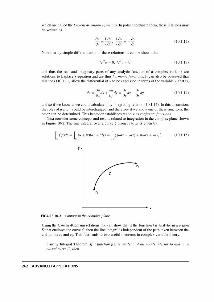
which are called the Cauchy-Riemann equations. In polar coordinate form, these relations may
be written as
@u
@r¼ 1
r
@v
@y,1
r
@u
@y¼ � @v
@r(10:1:12)
Note that by simple differentiation of these relations, it can be shown that
r2u ¼ 0, r2v ¼ 0 (10:1:13)
and thus the real and imaginary parts of any analytic function of a complex variable are
solutions to Laplace’s equation and are thus harmonic functions. It can also be observed that
relations (10.1.11) allow the differential of u to be expressed in terms of the variable v, that is,
du ¼ @u
@xdxþ @u
@ydy ¼ @v
@ydx� @v
@xdy (10:1:14)
and so if we know v, we could calculate u by integrating relation (10.1.14). In this discussion,
the roles of u and v could be interchanged, and therefore if we know one of these functions, the
other can be determined. This behavior establishes u and v as conjugate functions.Next consider some concepts and results related to integration in the complex plane shown
in Figure 10-2. The line integral over a curve C from z1 to z2 is given by
ðC
f (z)dz ¼ðC
(uþ iv)(dxþ idy) ¼ðC
(udx� vdy)þ i(udyþ vdx)ð Þ (10:1:15)
Using the Cauchy-Riemann relations, we can show that if the function f is analytic in a region
D that encloses the curve C, then the line integral is independent of the path taken between the
end points z1 and z2. This fact leads to two useful theorems in complex variable theory.
Cauchy Integral Theorem: If a function f(z) is analytic at all points interior to and on aclosed curve C, then
z2
z1
y
x
C
FIGURE 10-2 Contour in the complex plane.
262 ADVANCED APPLICATIONS
þC
f (z)dz ¼ 0 (10:1:16)
Cauchy Integral Formula: If f(z) is analytic everywhere within and on a closed curve C,and if zo is any point interior to C, then
f (zo) ¼ 1
2pi
þC
f (z)
z� zodz (10:1:17)
The integration over C is to be taken in the positive sense with the enclosed region to the left as
the curve is traversed. Notice that the Cauchy integral formula provides a method to express
the value of an analytic function at interior points of a domain in terms of values on the
boundary.
It is often convenient to express functions of a complex variable in a power series. If f(z) isanalytic at all points within a circle C with center at z ¼ a, then at each point inside C the
function admits the Taylor series expansion
f (z) ¼ f (a)þ f 0(a)(z� a)þ � � � þ f (n)(a)
n!(z� a)n þ � � � (10:1:18)
about point z ¼ a. For the special case where a ¼ 0, the representation is referred to as the
Maclaurin series. These results are useful for expansions in interior regions. A generalization
of series representations for an annular region also exists. If f(z) is analytic on two concentric
circles C1 and C2 and throughout the region between these circles (C1 > C2), then the function
may be expressed by the Laurent series
f (z) ¼X1n¼0
An(z� a)n þX1n¼1
Bn
(z� a)n(10:1:19)
where
An ¼ 1
2pi
þC1
f (z)
(z� zo)nþ1
dz, n ¼ 0, 1, 2, � � �
Bn ¼ 1
2pi
þC2
f (z)
(z� zo)�nþ1
dz, n ¼ 1, 2, � � �(10:1:20)
Recall that points where a complex function is not analytic are called singular points or
singularities. We now wish to discuss briefly one particular type of singularity called a pole.If f(z) is singular at z ¼ a, but the product (z� a)nf (z) is analytic for some integer value of n,then f(z)is said to have a pole of order n at z ¼ a. For this case, the analytic product form can be
expanded in a Taylor series about z ¼ a,
(z� a)nf (z) ¼X1k¼0
Ak(z� a)k
Ak ¼ 1
k!
dk
dzk{(z� a)nf (z)}
����z¼a
Rewriting this series for f(z)
Complex Variable Methods 263
f (z) ¼X1k¼0
Ak(z� a)k
(z� a)n
Integrating this expression around a closed contour C that encloses the point a and using the
Cauchy integral formula reduces the right-hand side to a single term
þC
f (z)dz ¼ 2piAn�1
The quantity An�1 is called the residue of f(z) at the pole z ¼ a, and this result would allow
the calculation of the integral by knowing the residue of the pole inside the contour C. Thus, iff(z) is analytic except for a pole of order n at z ¼ a in a region enclosed by an arbitrary contourC, then the integral of f(z) around C is given by
þC
f (z)dz ¼ 2pi1
(n� 1)!
dn�1
dzn�1(z� a)nf (z)f g
� ����z¼a
�(10:1:21)
If more than one pole exists in the domain enclosed by C, then the integral is evaluated using
relation (10.1.21) by including the summation of the residues of all poles in the domain. This
procedure is called the calculus of residues and is useful to evaluate complex integrals. Using
this scheme along with the Cauchy integral formula, the following useful integral relation may
be developed
1
2pi
þC
1
zn(z� z)dz ¼ 0, n > 0
1, n = 0
�(10:1:22)
where C is the contour around the unit circle and z is inside the circle.Another type of nonanalytic, singular behavior involves multivalued complex functions.
Examples of such behavior are found in the functions z1=2 and log z. Consider in more detail
the logarithmic function
log z ¼ log (reiy) ¼ log r þ iy
It is observed that this function is multivalued in y. This multivaluedness can be eliminated by
restricting the range of y to�p < y � p, and this results in the principal value of log z. For thiscase, the function is single-valued at all points except for the origin and the negative real axis.
The origin is then referred to as a branch point, and the negative real axis is a branch cut. Byrestricting the function to the domain r > 0 and �p < y � p, the singular behavior is avoided,and the function is analytic in the restricted range. Because of the common occurrence of
functions involvingffiffiffiffiffiffiffi( � )n
pand log, branch points and branch cuts are present in many
applications in elasticity.
Consider next the issue of the connectivity of the plane domain. Recall that a simplyconnected region is one where any closed curve can be continuously shrunk to a point without
going outside the region, and for two dimensions this simply means a region with no holes in it.
Figure 10-3 illustrates a multiply connected region D with several internal boundaries Lk. It canbe shown that analytic functions in such multiply connected regions need not be single-valued.
Note, however, that such regions can be made simply connected by making appropriate cuts
joining each of the internal boundaries with the outer boundary.
264 ADVANCED APPLICATIONS
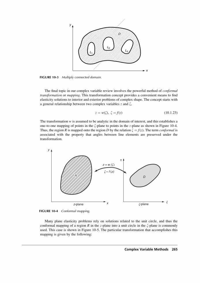
The final topic in our complex variable review involves the powerful method of conformaltransformation or mapping. This transformation concept provides a convenient means to find
elasticity solutions to interior and exterior problems of complex shape. The concept starts with
a general relationship between two complex variables z and z,
z ¼ w(z), z ¼ f (z) (10:1:23)
The transformation w is assumed to be analytic in the domain of interest, and this establishes a
one-to-one mapping of points in the z-plane to points in the z-plane as shown in Figure 10-4.
Thus, the region R is mapped onto the region D by the relation z ¼ f (z). The term conformal isassociated with the property that angles between line elements are preserved under the
transformation.
Many plane elasticity problems rely on solutions related to the unit circle, and thus the
conformal mapping of a region R in the z-plane into a unit circle in the z-plane is commonly
used. This case is shown in Figure 10-5. The particular transformation that accomplishes this
mapping is given by the following:
x
y
L1
L2L3
D
FIGURE 10-3 Multiply connected domain.
z-plane
z = w (z)
z = f (z)
z-plane
D
y
x
R
x
h
FIGURE 10-4 Conformal mapping.
Complex Variable Methods 265
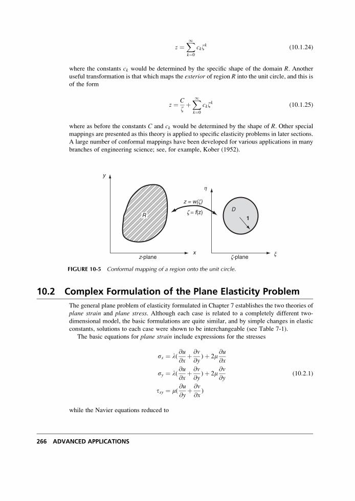
z ¼X1k¼0
ckzk (10:1:24)
where the constants ck would be determined by the specific shape of the domain R. Anotheruseful transformation is that which maps the exterior of region R into the unit circle, and this is
of the form
z ¼ C
zþX1k¼0
ckzk (10:1:25)
where as before the constants C and ck would be determined by the shape of R. Other specialmappings are presented as this theory is applied to specific elasticity problems in later sections.
A large number of conformal mappings have been developed for various applications in many
branches of engineering science; see, for example, Kober (1952).
10.2 Complex Formulation of the Plane Elasticity Problem
The general plane problem of elasticity formulated in Chapter 7 establishes the two theories of
plane strain and plane stress. Although each case is related to a completely different two-
dimensional model, the basic formulations are quite similar, and by simple changes in elastic
constants, solutions to each case were shown to be interchangeable (see Table 7-1).
The basic equations for plane strain include expressions for the stresses
sx ¼ l(@u
@xþ @v
@y)þ 2m
@u
@x
sy ¼ l(@u
@xþ @v
@y)þ 2m
@v
@y
txy ¼ m(@u
@yþ @v
@x)
(10:2:1)
while the Navier equations reduced to
z-plane z-plane
z = w(z)
z = f(z)
y
x
R
h
x
D
1
FIGURE 10-5 Conformal mapping of a region onto the unit circle.
266 ADVANCED APPLICATIONS
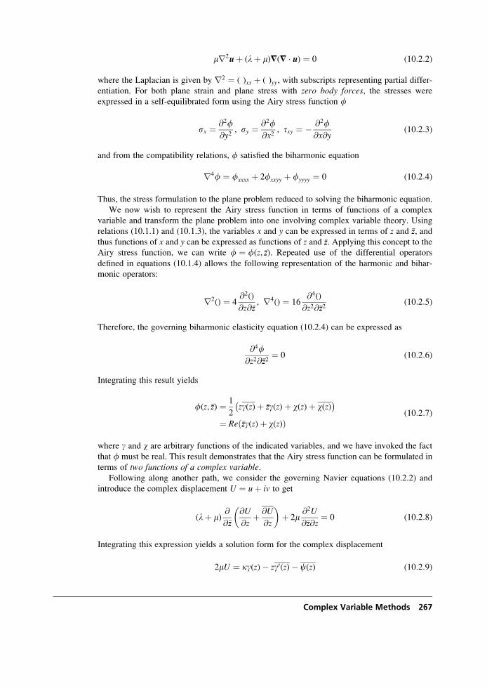
mr2uþ (lþ m)=(= � u) ¼ 0 (10:2:2)
where the Laplacian is given by r2 ¼ ( )xx þ ( )yy, with subscripts representing partial differ-
entiation. For both plane strain and plane stress with zero body forces, the stresses were
expressed in a self-equilibrated form using the Airy stress function f
sx ¼ @2f@y2
, sy ¼ @2f@x2
, txy ¼ � @2f@x@y
(10:2:3)
and from the compatibility relations, f satisfied the biharmonic equation
r4f ¼ fxxxx þ 2fxxyy þ fyyyy ¼ 0 (10:2:4)
Thus, the stress formulation to the plane problem reduced to solving the biharmonic equation.
We now wish to represent the Airy stress function in terms of functions of a complex
variable and transform the plane problem into one involving complex variable theory. Using
relations (10.1.1) and (10.1.3), the variables x and y can be expressed in terms of z and �zz, andthus functions of x and y can be expressed as functions of z and �zz. Applying this concept to the
Airy stress function, we can write f ¼ f(z, �zz). Repeated use of the differential operators
defined in equations (10.1.4) allows the following representation of the harmonic and bihar-
monic operators:
r2() ¼ 4@2()
@z@�zz, r4() ¼ 16
@4()
@z2@�zz2(10:2:5)
Therefore, the governing biharmonic elasticity equation (10.2.4) can be expressed as
@4f@z2@�zz2
¼ 0 (10:2:6)
Integrating this result yields
f(z, �zz) ¼ 1
2zg(z)þ �zzg(z)þ w(z)þ w(z)
¼ Re �zzg(z)þ w(z)ð Þ(10:2:7)
where g and w are arbitrary functions of the indicated variables, and we have invoked the fact
that f must be real. This result demonstrates that the Airy stress function can be formulated in
terms of two functions of a complex variable.Following along another path, we consider the governing Navier equations (10.2.2) and
introduce the complex displacement U ¼ uþ iv to get
(lþ m)@
@�zz
@U
@zþ @U
@z
� �þ 2m
@2U
@�zz@z¼ 0 (10:2:8)
Integrating this expression yields a solution form for the complex displacement
2mU ¼ kg(z)� zg0(z)� c(z) (10:2:9)
Complex Variable Methods 267
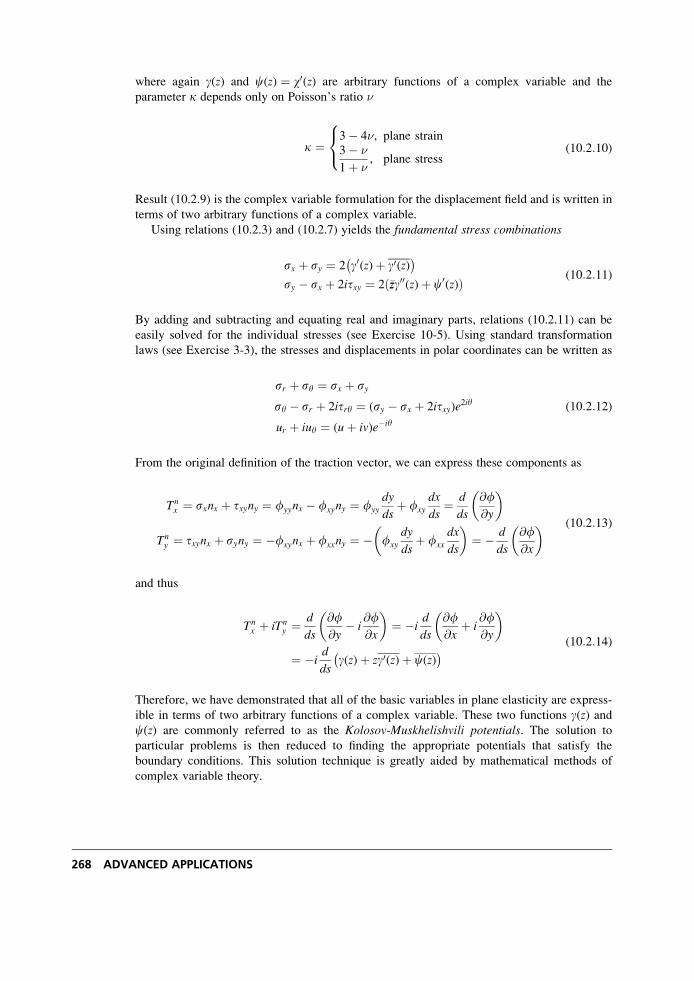
where again g(z) and c(z) ¼ w0(z) are arbitrary functions of a complex variable and the
parameter k depends only on Poisson’s ratio �
k ¼3� 4�, plane strain3� �
1þ �, plane stress
8<: (10:2:10)
Result (10.2.9) is the complex variable formulation for the displacement field and is written in
terms of two arbitrary functions of a complex variable.
Using relations (10.2.3) and (10.2.7) yields the fundamental stress combinations
sx þ sy ¼ 2 g0(z)þ g0(z)
sy � sx þ 2itxy ¼ 2 �zzg00(z)þ c0(z)ð Þ (10:2:11)
By adding and subtracting and equating real and imaginary parts, relations (10.2.11) can be
easily solved for the individual stresses (see Exercise 10-5). Using standard transformation
laws (see Exercise 3-3), the stresses and displacements in polar coordinates can be written as
sr þ sy ¼ sx þ sy
sy � sr þ 2itry ¼ (sy � sx þ 2itxy)e2iy
ur þ iuy ¼ (uþ iv)e�iy
(10:2:12)
From the original definition of the traction vector, we can express these components as
Tnx ¼ sxnx þ txyny ¼ fyynx � fxyny ¼ fyy
dy
dsþ fxy
dx
ds¼ d
ds
@f@y
� �
Tny ¼ txynx þ syny ¼ �fxynx þ fxxny ¼ � fxy
dy
dsþ fxx
dx
ds
� �¼ � d
ds
@f@x
� � (10:2:13)
and thus
Tnx þ iTn
y ¼ d
ds
@f@y
� i@f@x
� �¼ �i
d
ds
@f@x
þ i@f@y
� �
¼ �id
dsg(z)þ zg0(z)þ c(z) (10:2:14)
Therefore, we have demonstrated that all of the basic variables in plane elasticity are express-
ible in terms of two arbitrary functions of a complex variable. These two functions g(z) andc(z) are commonly referred to as the Kolosov-Muskhelishvili potentials. The solution to
particular problems is then reduced to finding the appropriate potentials that satisfy the
boundary conditions. This solution technique is greatly aided by mathematical methods of
complex variable theory.
268 ADVANCED APPLICATIONS
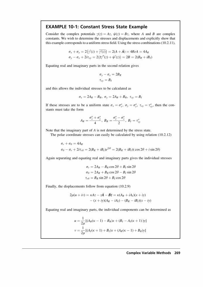
EXAMPLE 10-1: Constant Stress State Example
Consider the complex potentials g(z) ¼ Az, c(z) ¼ Bz, where A and B are complex
constants. We wish to determine the stresses and displacements and explicitly show that
this example corresponds to a uniform stress field. Using the stress combinations (10.2.11),
sx þ sy ¼ 2 g0(z)þ g0(z) ¼ 2(Aþ �AA) ¼ 4ReA ¼ 4AR
sy � sx þ 2itxy ¼ 2 �zzg00(z)þ c0(z)Þ ¼ 2B ¼ 2(BR þ iBI)ð
Equating real and imaginary parts in the second relation gives
sy � sx ¼ 2BR
txy ¼ BI
and this allows the individual stresses to be calculated as
sx ¼ 2AR � BR, sy ¼ 2AR þ BR, txy ¼ BI
If these stresses are to be a uniform state sx ¼ sox , sy ¼ soy , txy ¼ toxy, then the con-
stants must take the form
AR ¼ sox þ soy4
, BR ¼ soy � sox2
, BI ¼ toxy
Note that the imaginary part of A is not determined by the stress state.
The polar coordinate stresses can easily be calculated by using relation (10.2.12)
sr þ sy ¼ 4AR
sy � sr þ 2itry ¼ 2(BR þ iBI)e2iy ¼ 2(BR þ iBI)( cos 2yþ i sin 2y)
Again separating and equating real and imaginary parts gives the individual stresses
sr ¼ 2AR � BR cos 2yþ BI sin 2y
sy ¼ 2AR þ BR cos 2y� BI sin 2y
try ¼ BR sin 2yþ BI cos 2y
Finally, the displacements follow from equation (10.2.9)
2m(uþ iv) ¼ kAz� z �AA� �BB�zz ¼ k(AR þ iAI)(xþ iy)
� (xþ iy)(AR � iAI)� (BR � iBI)(x� iy)
Equating real and imaginary parts, the individual components can be determined as
u ¼ 1
2m[(AR(k� 1)� BR)xþ (BI � AI(kþ 1) )y]
v ¼ 1
2m[(AI(kþ 1)þ BI)xþ (AR(k� 1)þ BR)y]
Complex Variable Methods 269
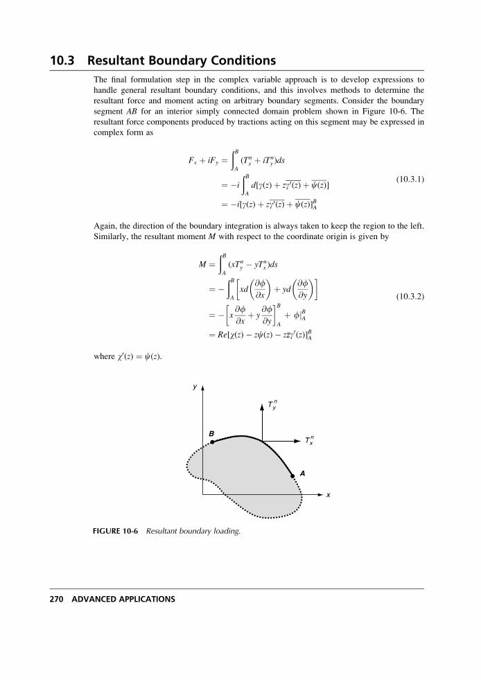
10.3 Resultant Boundary Conditions
The final formulation step in the complex variable approach is to develop expressions to
handle general resultant boundary conditions, and this involves methods to determine the
resultant force and moment acting on arbitrary boundary segments. Consider the boundary
segment AB for an interior simply connected domain problem shown in Figure 10-6. The
resultant force components produced by tractions acting on this segment may be expressed in
complex form as
Fx þ iFy ¼ðBA
(Tnx þ iTn
y )ds
¼ �i
ðBA
d[g(z)þ zg0(z)þ c(z)]
¼ �i[g(z)þ zg0(z)þ c(z)]BA
(10:3:1)
Again, the direction of the boundary integration is always taken to keep the region to the left.
Similarly, the resultant moment M with respect to the coordinate origin is given by
M ¼ðBA
(xTny � yTn
x )ds
¼ �ðBA
xd@f@x
� �þ yd
@f@y
� �� �
¼ � x@f@x
þ y@f@y
� �BA
þ fjBA¼ Re[w(z)� zc(z)� z�zzg0(z)]BA
(10:3:2)
where w0(z) ¼ c(z).
y
x
A
nxT
nyT
B
FIGURE 10-6 Resultant boundary loading.
270 ADVANCED APPLICATIONS
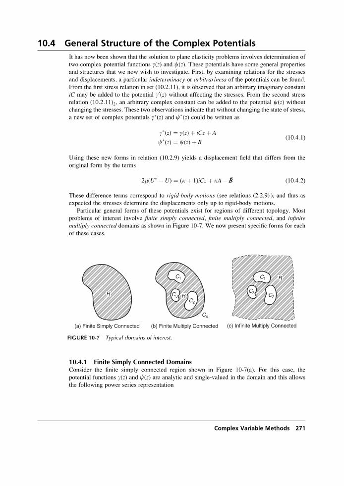
10.4 General Structure of the Complex Potentials
It has now been shown that the solution to plane elasticity problems involves determination of
two complex potential functions g(z) and c(z). These potentials have some general properties
and structures that we now wish to investigate. First, by examining relations for the stresses
and displacements, a particular indeterminacy or arbitrariness of the potentials can be found.
From the first stress relation in set (10.2.11), it is observed that an arbitrary imaginary constant
iC may be added to the potential g0(z) without affecting the stresses. From the second stress
relation (10:2:11)2, an arbitrary complex constant can be added to the potential c(z) withoutchanging the stresses. These two observations indicate that without changing the state of stress,
a new set of complex potentials g�(z) and c�(z) could be written as
g�(z) ¼ g(z)þ iCzþ A
c�(z) ¼ c(z)þ B(10:4:1)
Using these new forms in relation (10.2.9) yields a displacement field that differs from the
original form by the terms
2m(U� � U) ¼ (kþ 1)iCzþ kA� �BB (10:4:2)
These difference terms correspond to rigid-body motions (see relations (2.2.9) ), and thus as
expected the stresses determine the displacements only up to rigid-body motions.
Particular general forms of these potentials exist for regions of different topology. Most
problems of interest involve finite simply connected, finite multiply connected, and infinitemultiply connected domains as shown in Figure 10-7. We now present specific forms for each
of these cases.
10.4.1 Finite Simply Connected DomainsConsider the finite simply connected region shown in Figure 10-7(a). For this case, the
potential functions g(z) and c(z) are analytic and single-valued in the domain and this allows
the following power series representation
(a) Finite Simply Connected (b) Finite Multiply Connected (c) Infinite Multiply Connected
RC1
C2C3R R
Co
C1
C2
C3
FIGURE 10-7 Typical domains of interest.
Complex Variable Methods 271
g(z) ¼X1n¼0
anzn
c(z) ¼X1n¼0
bnzn
(10:4:3)
where an and bn are constants to be determined by the boundary conditions of the problem
under study.
10.4.2 Finite Multiply Connected DomainsFor the general region shown in Figure 10-7(b), it is assumed that the domain has k internal
boundaries as shown. For this topology, the potential functions need not be single-valued, as
can be demonstrated by considering the behaviors of the stresses and displacements around
each of the n contours Ck in region R. For the present case, we shall limit the problem and
assume that the displacements and stresses are continuous and single-valued everywhere.
Multivalued displacements lead to the theory of dislocations, and this is discussed at a later
stage in Chapter 15. The resultant force on a typical internal boundary Ck may be determined
by using relation (10.3.1)
Fk ¼ Xk þ iYk ¼þCk
(Tnx þ iTn
y )ds ¼ i[g(z)þ zg0(z)þ c(z)]Ck(10:4:4)
where [f (z, �zz)]Ckis referred to as the cyclic function of f and represents the change of the
function f around closed contour Ck. Note that in relation (10.4.4), the internal boundary circuit
Ck is traversed with the region on the left, thus leading to a clockwise circuit and a change of
sign from relation (10.3.1). Of course, the cyclic function of a single-valued expression is zero,
and further details on properties of cyclic functions may be found in Milne-Thomson (1960).
Because the resultant force on a given internal boundary will not necessarily be zero, the cyclic
function on the right-hand side of relation (10.4.4) should properly produce this result.
Therefore, the potential functions g(z) and c(z) must have appropriate multivalued behavior.
It can be shown that the logarithmic function previously discussed in Section 10.1 can provide
the necessary multivaluedness, because
[ log (z� zk)]Ck¼ 2pi (10:4:5)
where zk is a pointwithin the contourCk and the cyclic evaluation is taken in the counterclockwise
sense for the usual right-handed coordinate systemwith ymeasured counterclockwise. Including
such logarithmic terms for each of the two complex potentials and employing (10.4.4) for all
contours within the region R in Figure 10-7(b) develops the following general forms:
g(z) ¼ �Xnk¼1
Fk
2p(1þ k)log (z� zk)þ g�(z)
c(z) ¼Xnk¼1
k �FFk
2p(1þ k)log (z� zk)þ c�(z)
(10:4:6)
where Fk is the resultant force on each contour Ck, g�(z) and c�(z) are arbitrary analytic
functions in R, and k is the material constant defined by (10.2.10).
272 ADVANCED APPLICATIONS
10.4.3 Infinite DomainsFor the region shown in Figure 10-7(c), the general form of the potentials is determined in an
analogous manner as done in the previous case. The logarithmic terms in (10.4.6) may be
expanded in the region exterior to a circle enclosing all m contours Ck to get
log (z� zk) ¼ log zþ log 1� zkz
� �¼ log z� zk
zþ 1
2
zkz
� �2þ � � �
� �¼ log zþ (arbitrary analytic function)
Combining this result with the requirement that the stresses remain bounded at infinity gives
the general form for this case
g(z) ¼ �Pmk¼1
Fk
2p(1þ k)log zþ s1x þ s1y
4zþ g��(z)
c(z) ¼kPmk¼1
�FFk
2p(1þ k)log zþ s1y � s1x þ 2it1xy
2zþ c��(z)
(10:4:7)
where s1x , s1y , and t1xy are the stresses at infinity and g��(z) and c��(z) are arbitrary analytic
functions outside the region enclosing all m contours. Using power series theory, these analytic
functions can be expressed as
g��(z) ¼X1n¼1
anz�n
c��(z) ¼X1n¼1
bnz�n
(10:4:8)
An examination of the displacements at infinity would indicate unbounded behavior unless all
stresses at infinity vanish and SFk ¼ S �FFk ¼ 0. This fact occurs because even a bounded strain
over an infinite length will produce infinite displacements. Note that the case of a simply
connected, infinite domain is obtained by dropping the summation terms in (10.4.7).
10.5 Circular Domain Examples
We now develop some solutions of particular plane elastic problems involving regions of a
circular domain. The process starts by developing a general solution to a circular region with
arbitrary edge loading as shown in Figure 10-8. The region 0 � r � R is to have arbitrary
boundary loadings at r ¼ R specified by sr ¼ f1(y) try ¼ �f2(y), which can be written in
complex form as
f ¼ f1(y)þ if2(y) ¼ sr � itryjr¼R (10:5:1)
The fundamental stress combinations and displacements in polar coordinates were given in
relations (10.2.12). The tractions given by (10.2.14) may be expressed in polar form as
Trx þ iTr
y ¼ �id
dsg(z)þ zg0(z)þ c(z) jr¼R (10:5:2)
Complex Variable Methods 273
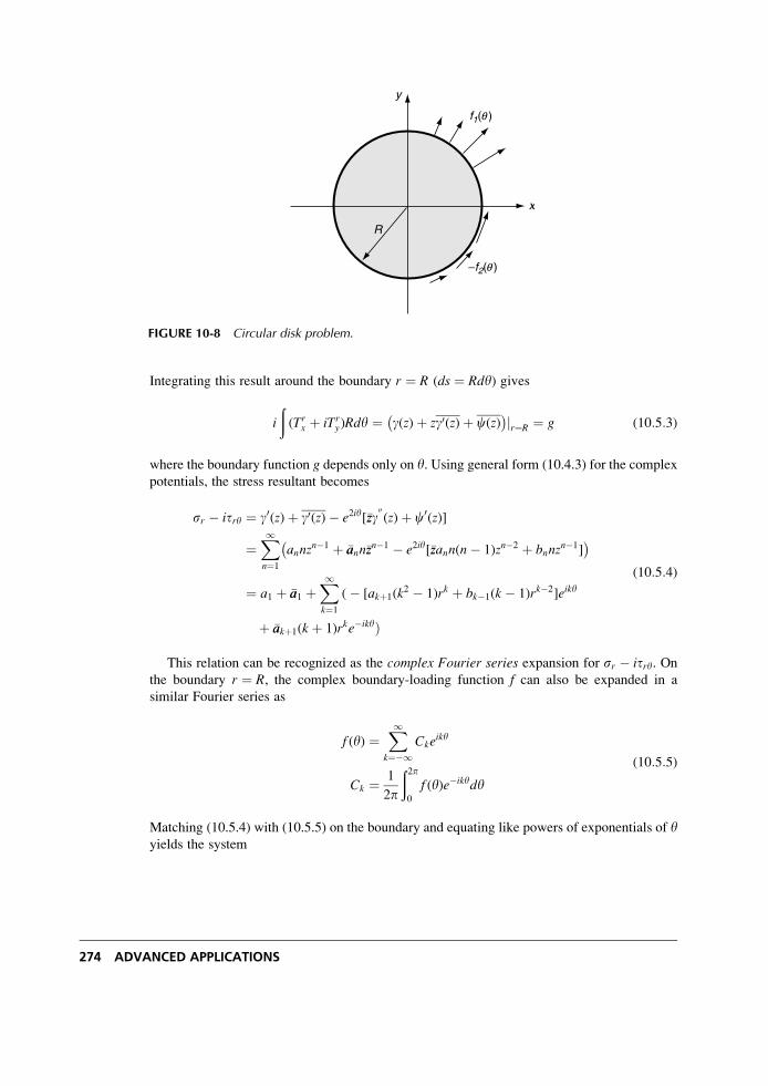
Integrating this result around the boundary r ¼ R (ds ¼ Rdy) gives
i
ð(Tr
x þ iTry)Rdy ¼ g(z)þ zg0(z)þ c(z)
jr¼R ¼ g (10:5:3)
where the boundary function g depends only on y. Using general form (10.4.3) for the complex
potentials, the stress resultant becomes
sr � itry ¼ g0(z)þ g0(z)� e2iy[�zzg00(z)þ c0(z)]
¼X1n¼1
annzn�1 þ �aann�zz
n�1 � e2iy[�zzann(n� 1)zn�2 þ bnnzn�1]
¼ a1 þ �aa1 þX1k¼1
(� [akþ1(k2 � 1)rk þ bk�1(k � 1)rk�2]eiky
þ �aakþ1(k þ 1)rke�ikyÞ
(10:5:4)
This relation can be recognized as the complex Fourier series expansion for sr � itry. Onthe boundary r ¼ R, the complex boundary-loading function f can also be expanded in a
similar Fourier series as
f (y) ¼X1k¼�1
Ckeiky
Ck ¼ 1
2p
ð2p0
f (y)e�ikydy
(10:5:5)
Matching (10.5.4) with (10.5.5) on the boundary and equating like powers of exponentials of yyields the system
y
x
f1(q )
−f2(q )
R
FIGURE 10-8 Circular disk problem.
274 ADVANCED APPLICATIONS
a1 þ �aa1 ¼ Co ¼ 2Re(a1)
�aakþ1(k þ 1)Rk ¼ C�k, (k > 0)
akþ1(k2 � 1)Rk þ bk�1(k � 1)Rk�2 ¼ Ck, (k > 0)
(10:5:6)
Equating real and imaginary parts in relations (10.5.6) generates a system of equations to
determine the constants ak and bk. This solution is essentially the same as the Michell solution
previously discussed in Section 8.3. Note that the annulus (ri � r � ro) and the exterior
(r � R) domain problems may be solved in a similar fashion.
This solution scheme then only duplicates previous methods based on Fourier analysis.
A more powerful use of complex variable techniques involves the application of Cauchy
integral formulae. In order to discuss this method, consider again the circular region with unit
boundary radius. Relation (10.5.3) becomes
g(z)þ zg0(z)þ c(z) jz¼z ¼ g (10:5:7)
where z ¼ zjr¼1 ¼ eiy and �zz ¼ e�iy ¼ 1=z. Multiplying (10.5.7) by 1=2pi (z� z) and integrat-
ing around the boundary contour C (r ¼ 1) yields
1
2pi
þC
g(z)z� z
dzþ 1
2pi
þC
zg0(z)z� z
dz
þ 1
2pi
þC
c(z)z� z
dz ¼ 1
2pi
þC
g(z)z� z
dz
(10:5:8)
Using the Cauchy integral formula, the first term in (10.5.8) is simply g(z). Using the general
series form (10.4.3) for the potentials and employing the integral formula (10.1.22), the
remaining two terms on the left-hand side of (10.5.8) can be evaluated, and the final result
reduces to
g(z)þ �aa1zþ 2�aa2 þ c(0) ¼ 1
2pi
þC
g(z)z� z
dz (10:5:9)
We also find that an ¼ 0 for n > 2, and so g(z) ¼ ao þ a1zþ a2z2. These results can be used to
solve for the remaining terms in order to determine the final form for the potential g(z). Using asimilar scheme but starting with the complex conjugate of (10.5.7), the potential c(z) may be
found. Dropping the constant terms that do not contribute to the stresses, the final results are
summarized as
g(z) ¼ 1
2pi
þC
g(z)z� z
dz� �aa1z, a1 þ �aa1 ¼ 1
2pi
þC
g(z)
z2dz
c(z) ¼ 1
2pi
þC
g(z)z� z
dz� g0(z)z
þ a1z
(10:5:10)
Note that the preceding solution is valid only for the unit disk. For the case of a disk of radius
a, the last two terms for c(z) should be multiplied by a2.We now consider a couple of specific examples using this general solution.
Complex Variable Methods 275
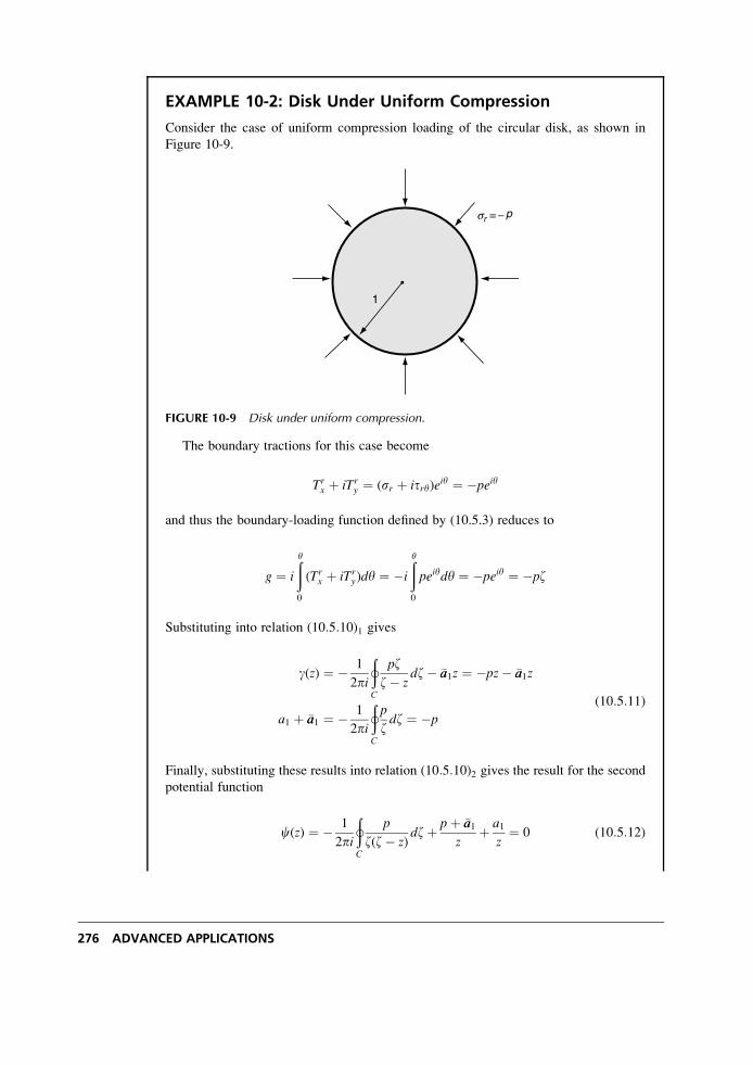
EXAMPLE 10-2: Disk Under Uniform Compression
Consider the case of uniform compression loading of the circular disk, as shown in
Figure 10-9.
sr = −
1
p
FIGURE 10-9 Disk under uniform compression.
The boundary tractions for this case become
Trx þ iTr
y ¼ (sr þ itry)eiy ¼ �peiy
and thus the boundary-loading function defined by (10.5.3) reduces to
g ¼ i
ð�0
(Trx þ iTr
y)dy ¼ �i
ð�0
peiydy ¼ �peiy ¼ �pz
Substituting into relation (10:5:10)1 gives
g(z) ¼ � 1
2pi
þC
pzz� z
dz� �aa1z ¼ �pz� �aa1z
a1 þ �aa1 ¼ � 1
2pi
þC
p
zdz ¼ �p
(10:5:11)
Finally, substituting these results into relation (10:5:10)2 gives the result for the secondpotential function
c(z) ¼ � 1
2pi
þC
p
z(z� z)dzþ pþ �aa1
zþ a1
z¼ 0 (10:5:12)
276 ADVANCED APPLICATIONS
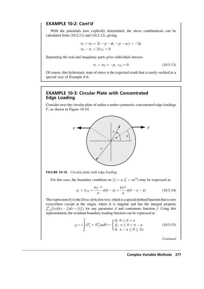
EXAMPLE 10-2: Cont’d
With the potentials now explicitly determined, the stress combinations can be
calculated from (10.2.11) and (10.2.12), giving
sr þ sy ¼ 2(� p� �aa1 � p� a1) ¼ �2p
sy � sr þ 2itry ¼ 0
Separating the real and imaginary parts gives individual stresses
sr ¼ sy ¼ �p, try ¼ 0 (10:5:13)
Of course, this hydrostatic state of stress is the expected result that is easily verified as a
special case of Example 8-6.
EXAMPLE 10-3: Circular Plate with ConcentratedEdge Loading
Consider next the circular plate of radius a under symmetric concentrated edge loadings
F, as shown in Figure 10-10.
F
a
Fr
qa
FIGURE 10-10 Circular plate with edge loading.
For this case, the boundary condition on jzj ¼ a (z ¼ aeiy) may be expressed as
sr þ itry ¼ Fe�ia
ad(y� a)þ Feia
ad(y� p� a) (10:5:14)
The expressiond() is theDirac delta function,which is a special defined function that is zeroeverywhere except at the origin, where it is singular and has the integral propertyÐ d�d f (x)d(x� x)dx ¼ f (x) for any parameter d and continuous function f. Using this
representation, the resultant boundary-loading function can be expressed as
g ¼ i
ð�0
(Trx þ iTr
y)ady ¼0, 0 � y < aif , a � y < p� a0, p� a � y � 2p
((10:5:15)
Continued
Complex Variable Methods 277
EXAMPLE 10-3: Circular Plate with ConcentratedEdge Loading–Cont’d
Thus, using the general solution (10.5.10) then gives
a1 þ �aa1 ¼ F
2p
ðaei(p�a)
aeia
dz
z2¼ � F
2p1
z
�����aei(p�a)
aeia
¼ F
pacos a
and the expressions for the potential functions then become
g(z) ¼ F
2p
ðaei (p�a)
aeia
dzz� z
� �aa1z ¼ F
2plog (z� z)jaei(p�a)
aeia
��aa1z ¼ F
2plog
zþ ae�ia
z� aeia
� �� �aa1z
c(z) ¼ � F
2plog
zþ ae�ia
z� aeia
� �þ Fa3 cos apz(zþ ae�ia)(z� aeia)
þ a1 þ �aa1z
a2 (10:5:16)
The stress resultant then becomes
sr þ sy ¼ 2 g0(z)þ g0(z)
¼ � 2Fa cos ap
1
(zþ ae�ia)(z� aeia)þ 1
(�zzþ aeia)(�zz� ae�ia)þ 1
a2
� �(10:5:17)
Note that for the case with a ¼ 0 (diametrical compression), we get
sr þ sy ¼ sx þ sy ¼ � 2Fa
p1
(z2 � a2)þ 1
(�zz2 � a2)þ 1
a2
� �(10:5:18)
which was the problem previously solved in Example 8-10, giving the stresses specified
in relations (8.4.69). Solutions to many other problems of circular domain can be found
in Muskhelishvili (1963), Milne-Thomson (1960), and England (1971).
10.6 Plane and Half-Plane Problems
Complex variable methods prove to be very useful for the solution of a large variety of full-
space and half-space problems. Full-space examples commonly include problems with various
types of internal concentrated force systems and internal cavities carrying different loading
conditions. Typical half-space examples include concentrated force and moment systems
applied to the free surface and indentation contact mechanics problems where the boundary
conditions may be in terms of the stresses or displacements, or of mixed type over a portion of
the free surface. This general class of problems involves infinite domains and requires the
general solution form given by (10.4.7).
278 ADVANCED APPLICATIONS
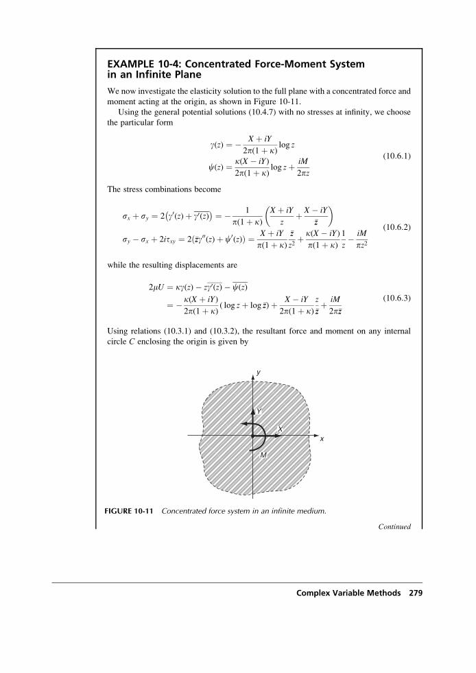
EXAMPLE 10-4: Concentrated Force-Moment Systemin an Infinite Plane
We now investigate the elasticity solution to the full plane with a concentrated force and
moment acting at the origin, as shown in Figure 10-11.
Using the general potential solutions (10.4.7) with no stresses at infinity, we choose
the particular form
g(z) ¼ � X þ iY
2p(1þ k)log z
c(z) ¼ k(X � iY)
2p(1þ k)log zþ iM
2pz
(10:6:1)
The stress combinations become
sx þ sy ¼ 2 g0(z)þ g0(z) ¼ � 1
p(1þ k)X þ iY
zþ X � iY
�zz
� �
sy � sx þ 2itxy ¼ 2 �zzg00(z)þ c0(z)ð Þ ¼ X þ iY
p(1þ k)�zz
z2þ k(X � iY)
p(1þ k)1
z� iM
pz2
(10:6:2)
while the resulting displacements are
2mU ¼ kg(z)� zg0(z)� c(z)
¼ � k(X þ iY)
2p(1þ k)( log zþ log �zz)þ X � iY
2p(1þ k)z
�zzþ iM
2p�zz
(10:6:3)
Using relations (10.3.1) and (10.3.2), the resultant force and moment on any internal
circle C enclosing the origin is given by
Continued
y
x
M
X
Y
FIGURE 10-11 Concentrated force system in an infinite medium.
Complex Variable Methods 279
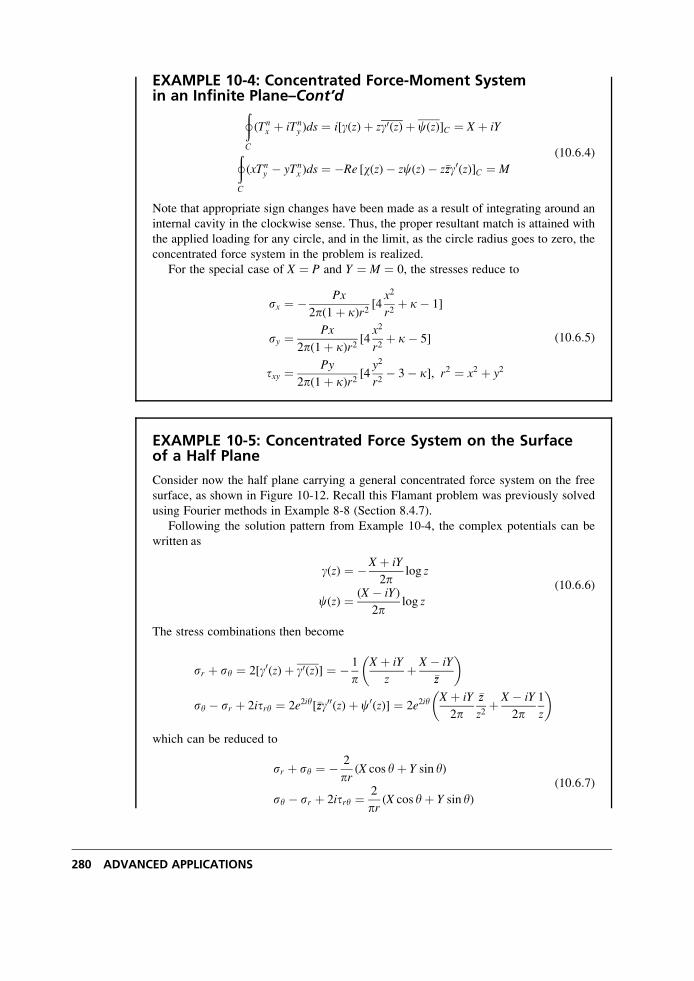
EXAMPLE 10-4: Concentrated Force-Moment Systemin an Infinite Plane–Cont’dþ
C
(Tnx þ iTn
y )ds ¼ i[g(z)þ zg0(z)þ c(z)]C ¼ X þ iY
þC
(xTny � yTn
x )ds ¼ �Re [w(z)� zc(z)� z�zzg0(z)]C ¼ M
(10:6:4)
Note that appropriate sign changes have been made as a result of integrating around an
internal cavity in the clockwise sense. Thus, the proper resultant match is attained with
the applied loading for any circle, and in the limit, as the circle radius goes to zero, the
concentrated force system in the problem is realized.
For the special case of X ¼ P and Y ¼ M ¼ 0, the stresses reduce to
sx ¼ � Px
2p(1þ k)r2[4
x2
r2þ k� 1]
sy ¼ Px
2p(1þ k)r2[4
x2
r2þ k� 5]
txy ¼ Py
2p(1þ k)r2[4
y2
r2� 3� k], r2 ¼ x2 þ y2
(10:6:5)
EXAMPLE 10-5: Concentrated Force System on the Surfaceof a Half Plane
Consider now the half plane carrying a general concentrated force system on the free
surface, as shown in Figure 10-12. Recall this Flamant problem was previously solved
using Fourier methods in Example 8-8 (Section 8.4.7).
Following the solution pattern from Example 10-4, the complex potentials can be
written as
g(z) ¼ �X þ iY
2plog z
c(z) ¼ (X � iY)
2plog z
(10:6:6)
The stress combinations then become
sr þ sy ¼ 2[g0(z)þ g0(z)] ¼ � 1
pX þ iY
zþ X � iY
�zz
� �
sy � sr þ 2itry ¼ 2e2iy[�zzg00(z)þ c0(z)] ¼ 2e2iyX þ iY
2p�zz
z2þ X � iY
2p1
z
� �
which can be reduced to
sr þ sy ¼ � 2
pr(X cos yþ Y sin y)
sy � sr þ 2itry ¼ 2
pr(X cos yþ Y sin y)
(10:6:7)
280 ADVANCED APPLICATIONS
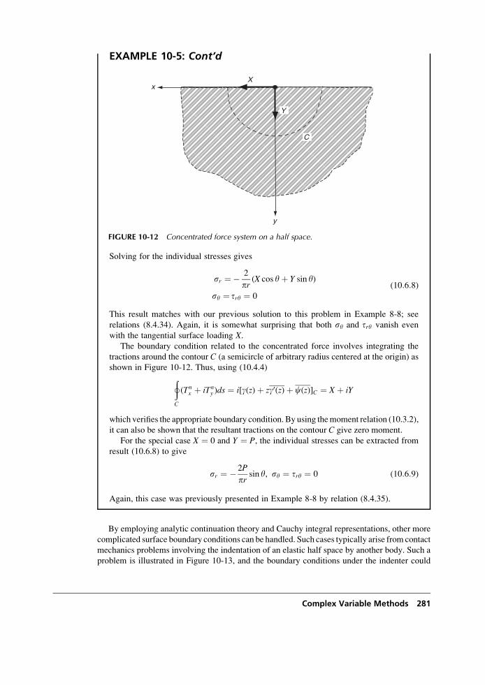
EXAMPLE 10-5: Cont’d
Solving for the individual stresses gives
sr ¼� 2
pr(X cos yþ Y sin y)
sy ¼ try ¼ 0
(10:6:8)
This result matches with our previous solution to this problem in Example 8-8; see
relations (8.4.34). Again, it is somewhat surprising that both sy and try vanish even
with the tangential surface loading X.The boundary condition related to the concentrated force involves integrating the
tractions around the contour C (a semicircle of arbitrary radius centered at the origin) as
shown in Figure 10-12. Thus, using (10.4.4)þC
(Tnx þ iTn
y )ds ¼ i[g(z)þ zg0(z)þ c(z)]C ¼ X þ iY
which verifies the appropriate boundary condition. By using themoment relation (10.3.2),
it can also be shown that the resultant tractions on the contour C give zero moment.
For the special case X ¼ 0 and Y ¼ P, the individual stresses can be extracted from
result (10.6.8) to give
sr ¼ � 2P
prsin y, sy ¼ try ¼ 0 (10:6:9)
Again, this case was previously presented in Example 8-8 by relation (8.4.35).
By employing analytic continuation theory and Cauchy integral representations, other more
complicated surface boundary conditions can be handled. Such cases typically arise from contact
mechanics problems involving the indentation of an elastic half space by another body. Such a
problem is illustrated in Figure 10-13, and the boundary conditions under the indenter could
C
x
y
X
Y
FIGURE 10-12 Concentrated force system on a half space.
Complex Variable Methods 281
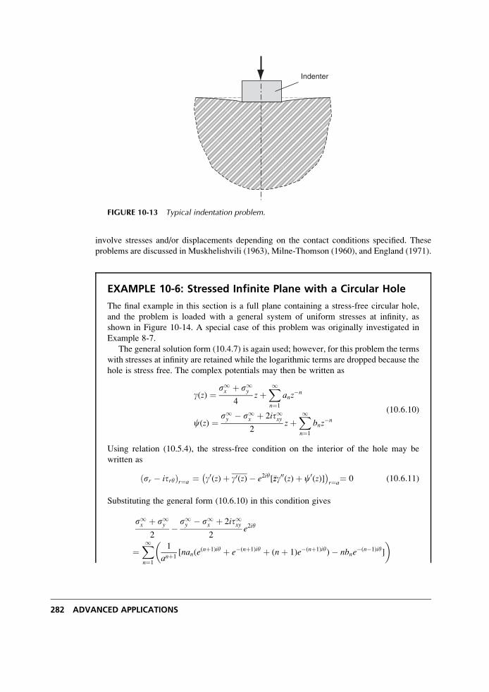
involve stresses and/or displacements depending on the contact conditions specified. These
problems are discussed in Muskhelishvili (1963), Milne-Thomson (1960), and England (1971).
EXAMPLE 10-6: Stressed Infinite Plane with a Circular Hole
The final example in this section is a full plane containing a stress-free circular hole,
and the problem is loaded with a general system of uniform stresses at infinity, as
shown in Figure 10-14. A special case of this problem was originally investigated in
Example 8-7.
The general solution form (10.4.7) is again used; however, for this problem the terms
with stresses at infinity are retained while the logarithmic terms are dropped because the
hole is stress free. The complex potentials may then be written as
g(z) ¼ s1x þ s1y4
zþX1n¼1
anz�n
c(z) ¼ s1y � s1x þ 2it1xy2
zþX1n¼1
bnz�n
(10:6:10)
Using relation (10.5.4), the stress-free condition on the interior of the hole may be
written as
sr � itryð Þr¼a ¼ g0(z)þ g0(z)� e2iy[�zzg00(z)þ c0(z)]
r¼a¼ 0 (10:6:11)
Substituting the general form (10.6.10) in this condition gives
s1x þ s1y2
� s1y � s1x þ 2it1xy2
e2iy
¼X1n¼1
1
anþ1[nan(e
(nþ1)iy þ e�(nþ1)iy þ (nþ 1)e�(nþ1)iy)� nbne�(n�1)iy]
� �
Indenter
FIGURE 10-13 Typical indentation problem.
282 ADVANCED APPLICATIONS
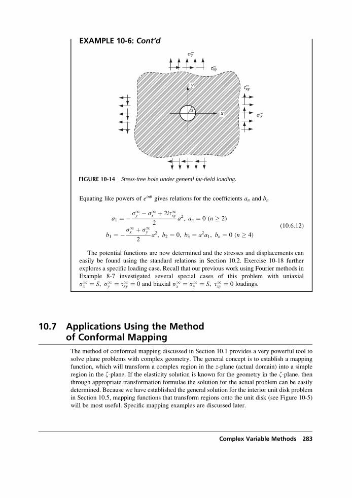
EXAMPLE 10-6: Cont’d
Equating like powers of einy gives relations for the coefficients an and bn
a1 ¼ � s1y � s1x þ 2it1xy2
a2, an ¼ 0 (n � 2)
b1 ¼ �s1x þ s1y2
a2, b2 ¼ 0, b3 ¼ a2a1, bn ¼ 0 (n � 4)
(10:6:12)
The potential functions are now determined and the stresses and displacements can
easily be found using the standard relations in Section 10.2. Exercise 10-18 further
explores a specific loading case. Recall that our previous work using Fourier methods in
Example 8-7 investigated several special cases of this problem with uniaxial
s1x ¼ S, s1y ¼ t1xy ¼ 0 and biaxial s1x ¼ s1y ¼ S, t1xy ¼ 0 loadings.
10.7 Applications Using the Methodof Conformal Mapping
The method of conformal mapping discussed in Section 10.1 provides a very powerful tool to
solve plane problems with complex geometry. The general concept is to establish a mapping
function, which will transform a complex region in the z-plane (actual domain) into a simple
region in the z-plane. If the elasticity solution is known for the geometry in the z-plane, thenthrough appropriate transformation formulae the solution for the actual problem can be easily
determined. Because we have established the general solution for the interior unit disk problem
in Section 10.5, mapping functions that transform regions onto the unit disk (see Figure 10-5)
will be most useful. Specific mapping examples are discussed later.
x
y
ax
y
xy
xy
s∞
s∞
tt∞
t∞
FIGURE 10-14 Stress-free hole under general far-field loading.
Complex Variable Methods 283
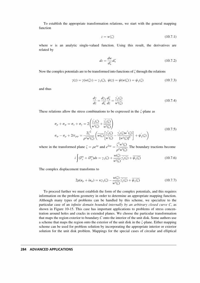
To establish the appropriate transformation relations, we start with the general mapping
function
z ¼ wðzÞ (10:7:1)
where w is an analytic single-valued function. Using this result, the derivatives are
related by
dz ¼ dw
dzdz (10:7:2)
Now the complex potentials are to be transformed into functions of z through the relations
g(z) ¼ g(w(z) ) ¼ g1(z), c(z) ¼ c(w(z) ) ¼ c1(z) (10:7:3)
and thus
dgdz
¼ dg1dz
dzdz
¼ g01(z)w0(z)
(10:7:4)
These relations allow the stress combinations to be expressed in the z-plane as
sr þ sj ¼ sx þ sy ¼ 2g01(z)w0(z)
þ g01(z)
w0(z)
!
sj � sr þ 2itrj ¼ 2z2
r2w0(z)w(z)
g001(z)w0(z)
� g01(z)w
00(z)
[w0(z)]2
� �þ c
01(z)
� � (10:7:5)
where in the transformed plane z ¼ reij and e2ij ¼ z2w0(z)r2w0(z)
. The boundary tractions become
i
ð(Tn
x þ iTny )ds ¼ g1(z)þ
w(z)
w0(z)g01(z)þ c1(z) (10:7:6)
The complex displacement transforms to
2m(ur þ iuj) ¼ kg1(z)�w(z)
w0(z)g01(z)þ c1(z) (10:7:7)
To proceed further we must establish the form of the complex potentials, and this requires
information on the problem geometry in order to determine an appropriate mapping function.
Although many types of problems can be handled by this scheme, we specialize to the
particular case of an infinite domain bounded internally by an arbitrary closed curve C, asshown in Figure 10-15. This case has important applications to problems of stress concen-
tration around holes and cracks in extended planes. We choose the particular transformation
that maps the region exterior to boundary C onto the interior of the unit disk. Some authors use
a scheme that maps the region onto the exterior of the unit disk in the z-plane. Either mapping
scheme can be used for problem solution by incorporating the appropriate interior or exterior
solution for the unit disk problem. Mappings for the special cases of circular and elliptical
284 ADVANCED APPLICATIONS
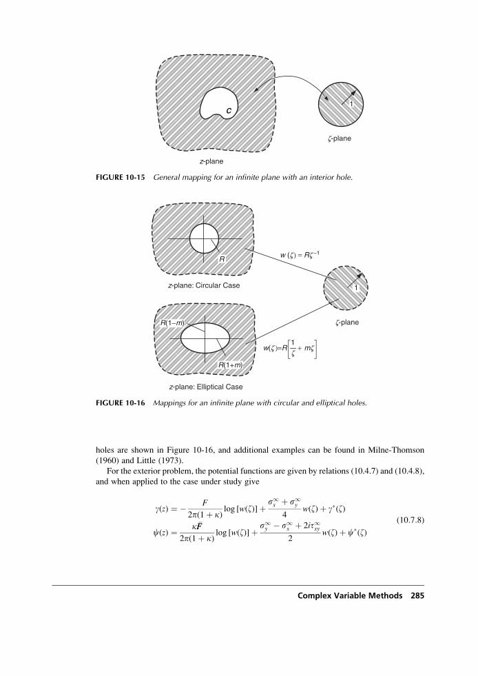
holes are shown in Figure 10-16, and additional examples can be found in Milne-Thomson
(1960) and Little (1973).
For the exterior problem, the potential functions are given by relations (10.4.7) and (10.4.8),
and when applied to the case under study give
g(z) ¼ � F
2p(1þ k)log [w(z)]þ s1x þ s1y
4w(z)þ g�(z)
c(z) ¼ k �FF2p(1þ k)
log [w(z)]þ s1y � s1x þ 2it1xy2
w(z)þ c�(z)(10:7:8)
z-plane
z-plane
1C
FIGURE 10-15 General mapping for an infinite plane with an interior hole.
z-plane
1
w (z ) = Rz −1
+ mzw(z )=R1
z-plane: Circular Case
R
z-plane: Elliptical Case
R(1+m)
R(1−m)
z
FIGURE 10-16 Mappings for an infinite plane with circular and elliptical holes.
Complex Variable Methods 285
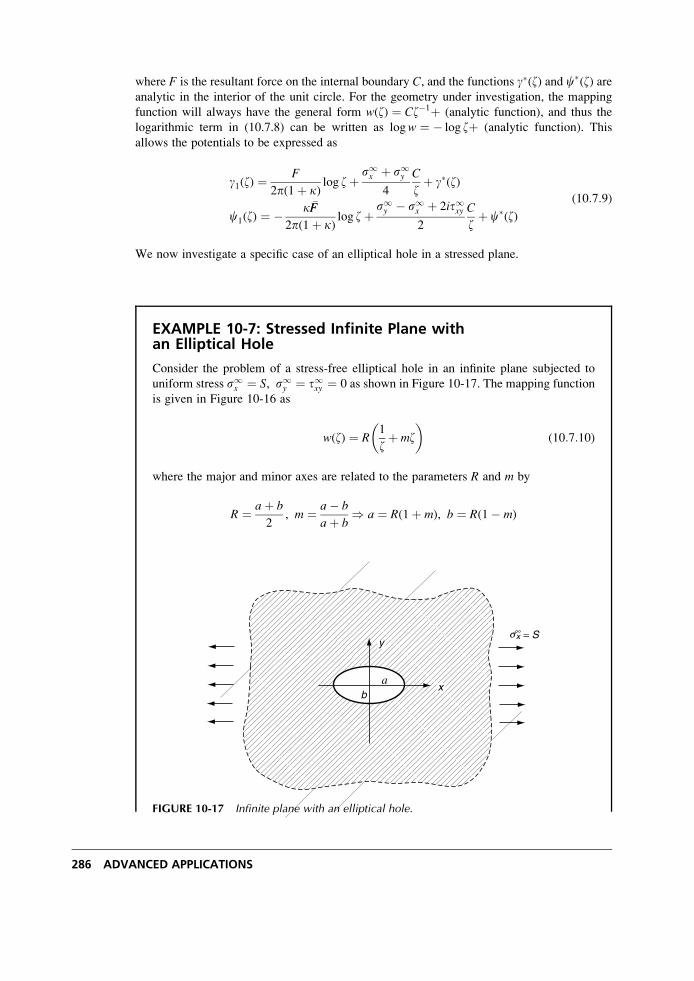
where F is the resultant force on the internal boundary C, and the functions g�(z) and c�(z) areanalytic in the interior of the unit circle. For the geometry under investigation, the mapping
function will always have the general form w(z) ¼ Cz�1þ (analytic function), and thus the
logarithmic term in (10.7.8) can be written as logw ¼ � log zþ (analytic function). This
allows the potentials to be expressed as
g1(z) ¼F
2p(1þ k)log zþ s1x þ s1y
4
C
zþ g�(z)
c1(z) ¼ � k �FF2p(1þ k)
log zþ s1y � s1x þ 2it1xy2
C
zþ c�(z)
(10:7:9)
We now investigate a specific case of an elliptical hole in a stressed plane.
EXAMPLE 10-7: Stressed Infinite Plane withan Elliptical Hole
Consider the problem of a stress-free elliptical hole in an infinite plane subjected to
uniform stress s1x ¼ S, s1y ¼ t1xy ¼ 0 as shown in Figure 10-17. The mapping function
is given in Figure 10-16 as
w(z) ¼ R1
zþ mz
� �(10:7:10)
where the major and minor axes are related to the parameters R and m by
R ¼ aþ b
2, m ¼ a� b
aþ b) a ¼ R(1þ m), b ¼ R(1� m)
x
yx = S
ba
s∞
FIGURE 10-17 Infinite plane with an elliptical hole.
286 ADVANCED APPLICATIONS
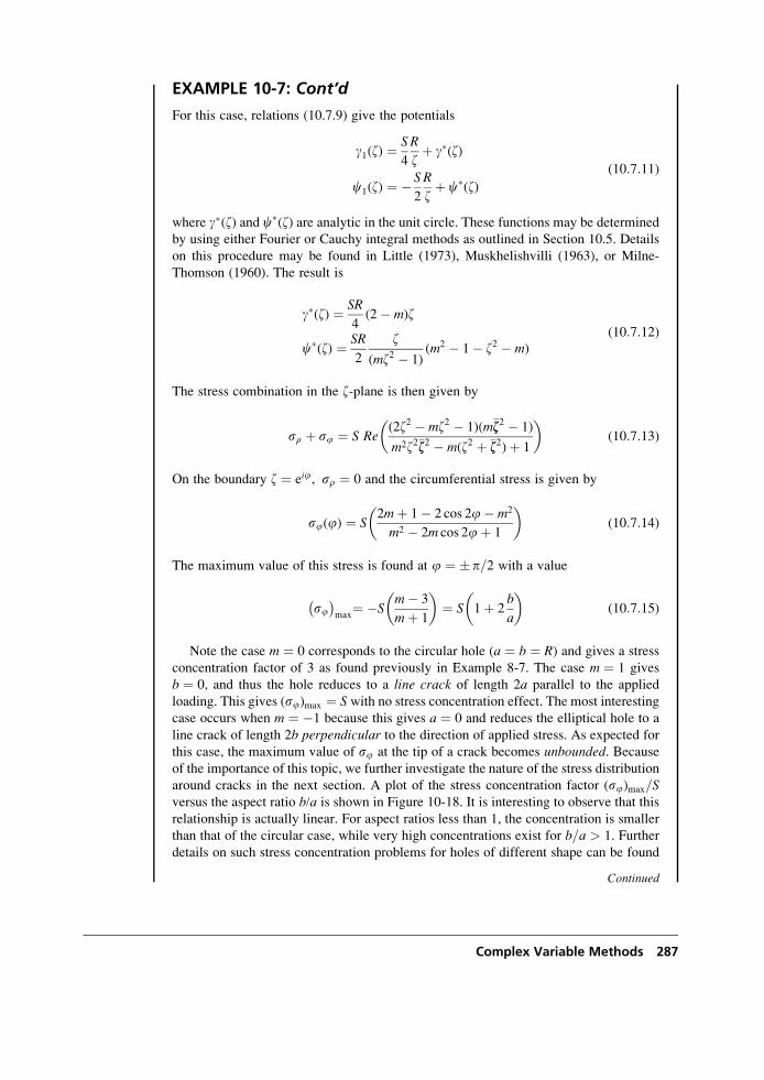
EXAMPLE 10-7: Cont’d
For this case, relations (10.7.9) give the potentials
g1(z) ¼S
4
R
zþ g�(z)
c1(z) ¼ � S
2
R
zþ c�(z)
(10:7:11)
where g�(z) and c�(z) are analytic in the unit circle. These functions may be determined
by using either Fourier or Cauchy integral methods as outlined in Section 10.5. Details
on this procedure may be found in Little (1973), Muskhelishvilli (1963), or Milne-
Thomson (1960). The result is
g�(z) ¼ SR
4(2� m)z
c�(z) ¼ SR
2
z
(mz2 � 1)(m2 � 1� z2 � m)
(10:7:12)
The stress combination in the z-plane is then given by
sr þ sj ¼ S Re(2z2 � mz2 � 1)(m�zz2 � 1)
m2z2�zz2 � m(z2 þ �zz2)þ 1
� �(10:7:13)
On the boundary z ¼ eij, sr ¼ 0 and the circumferential stress is given by
sj(j) ¼ S2mþ 1� 2 cos 2j� m2
m2 � 2m cos 2jþ 1
� �(10:7:14)
The maximum value of this stress is found at j ¼ � p=2 with a value
sj
max¼ �S
m� 3
mþ 1
� �¼ S 1þ 2
b
a
� �(10:7:15)
Note the case m ¼ 0 corresponds to the circular hole (a ¼ b ¼ R) and gives a stress
concentration factor of 3 as found previously in Example 8-7. The case m ¼ 1 gives
b ¼ 0, and thus the hole reduces to a line crack of length 2a parallel to the applied
loading. This gives (sj)max ¼ S with no stress concentration effect. The most interesting
case occurs when m ¼ �1 because this gives a ¼ 0 and reduces the elliptical hole to a
line crack of length 2b perpendicular to the direction of applied stress. As expected for
this case, the maximum value of sj at the tip of a crack becomes unbounded. Becauseof the importance of this topic, we further investigate the nature of the stress distribution
around cracks in the next section. A plot of the stress concentration factor (sj)max=Sversus the aspect ratio b/a is shown in Figure 10-18. It is interesting to observe that this
relationship is actually linear. For aspect ratios less than 1, the concentration is smaller
than that of the circular case, while very high concentrations exist for b=a > 1. Further
details on such stress concentration problems for holes of different shape can be found
Continued
Complex Variable Methods 287
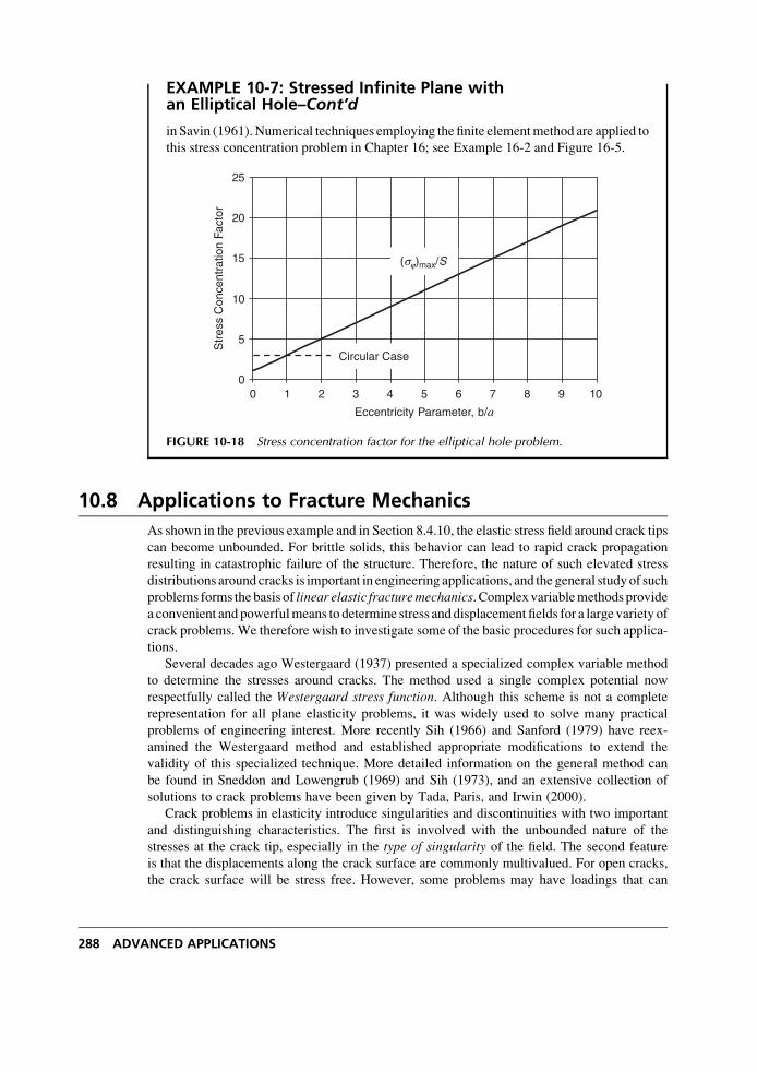
EXAMPLE 10-7: Stressed Infinite Plane withan Elliptical Hole–Cont’d
in Savin (1961).Numerical techniques employing the finite elementmethod are applied to
this stress concentration problem in Chapter 16; see Example 16-2 and Figure 16-5.
0
5
10
15
20
25
Eccentricity Parameter, b/a
Str
ess
Con
cent
ratio
n Fa
ctor
Circular Case
0 1 2 3 4 5 6 7 8 9 10
(sj)max/S
FIGURE 10-18 Stress concentration factor for the elliptical hole problem.
10.8 Applications to Fracture Mechanics
As shown in the previous example and in Section 8.4.10, the elastic stress field around crack tips
can become unbounded. For brittle solids, this behavior can lead to rapid crack propagation
resulting in catastrophic failure of the structure. Therefore, the nature of such elevated stress
distributions around cracks is important in engineering applications, and the general studyof such
problems forms the basis of linear elastic fracturemechanics. Complexvariablemethodsprovide
a convenient and powerfulmeans to determine stress anddisplacement fields for a large variety of
crack problems. We therefore wish to investigate some of the basic procedures for such applica-
tions.
Several decades ago Westergaard (1937) presented a specialized complex variable method
to determine the stresses around cracks. The method used a single complex potential now
respectfully called the Westergaard stress function. Although this scheme is not a complete
representation for all plane elasticity problems, it was widely used to solve many practical
problems of engineering interest. More recently Sih (1966) and Sanford (1979) have reex-
amined the Westergaard method and established appropriate modifications to extend the
validity of this specialized technique. More detailed information on the general method can
be found in Sneddon and Lowengrub (1969) and Sih (1973), and an extensive collection of
solutions to crack problems have been given by Tada, Paris, and Irwin (2000).
Crack problems in elasticity introduce singularities and discontinuities with two important
and distinguishing characteristics. The first is involved with the unbounded nature of the
stresses at the crack tip, especially in the type of singularity of the field. The second feature
is that the displacements along the crack surface are commonly multivalued. For open cracks,
the crack surface will be stress free. However, some problems may have loadings that can
288 ADVANCED APPLICATIONS
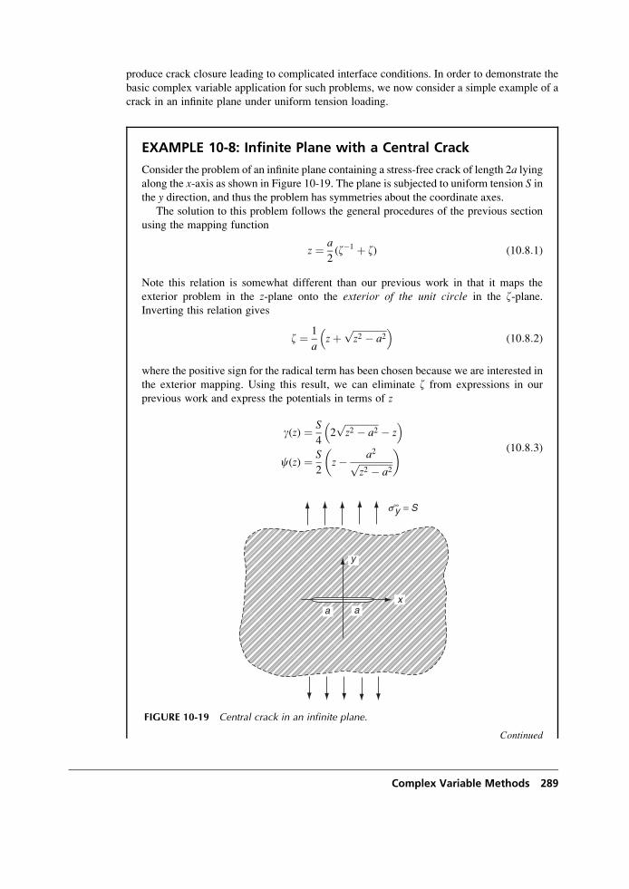
produce crack closure leading to complicated interface conditions. In order to demonstrate the
basic complex variable application for such problems, we now consider a simple example of a
crack in an infinite plane under uniform tension loading.
EXAMPLE 10-8: Infinite Plane with a Central Crack
Consider the problem of an infinite plane containing a stress-free crack of length 2a lyingalong the x-axis as shown in Figure 10-19. The plane is subjected to uniform tension S inthe y direction, and thus the problem has symmetries about the coordinate axes.
The solution to this problem follows the general procedures of the previous section
using the mapping function
z ¼ a
2(z�1 þ z) (10:8:1)
Note this relation is somewhat different than our previous work in that it maps the
exterior problem in the z-plane onto the exterior of the unit circle in the z-plane.Inverting this relation gives
z ¼ 1
azþ
ffiffiffiffiffiffiffiffiffiffiffiffiffiffiz2 � a2
p� �(10:8:2)
where the positive sign for the radical term has been chosen because we are interested in
the exterior mapping. Using this result, we can eliminate z from expressions in our
previous work and express the potentials in terms of z
g(z) ¼ S
42ffiffiffiffiffiffiffiffiffiffiffiffiffiffiz2 � a2
p� z
� �c(z) ¼ S
2z� a2ffiffiffiffiffiffiffiffiffiffiffiffiffiffi
z2 � a2p
� � (10:8:3)
Continued
x
y
y = S
aa
s∞
FIGURE 10-19 Central crack in an infinite plane.
Complex Variable Methods 289
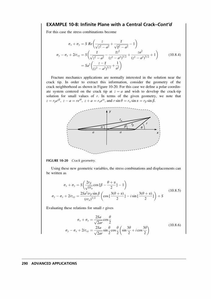
EXAMPLE 10-8: Infinite Plane with a Central Crack–Cont’d
For this case the stress combinations become
sx þ sy ¼ S Rezffiffiffiffiffiffiffiffiffiffiffiffiffiffi
z2 � a2p þ �zzffiffiffiffiffiffiffiffiffiffiffiffiffiffi
�zz2 � a2p � 1
� �
sy � sx þ 2itxy ¼ S�zzffiffiffiffiffiffiffiffiffiffiffiffiffiffi
z2 � a2p � �zzz2
(z2 � a2)3=2þ za2
(z2 � a2)3=2þ 1
� �
¼ Sa2z� �zz
(z2 � a2)3=2þ 1
a2
� � (10:8:4)
Fracture mechanics applications are normally interested in the solution near the
crack tip. In order to extract this information, consider the geometry of the
crack neighborhood as shown in Figure 10-20. For this case we define a polar coordin-
ate system centered on the crack tip at z ¼ a and wish to develop the crack-tip
solution for small values of r. In terms of the given geometry, we note that
z ¼ rbeib, z� a ¼ reiy, zþ a ¼ rae
ia, and r sin y ¼ ra sin a ¼ rb sin b.
r
aa
rra
x
y
a b qb
FIGURE 10-20 Crack geometry.
Using these new geometric variables, the stress combinations and displacements can
be written as
sx þ sy ¼ S2rbffiffiffiffiffiffirra
p cos [b� yþ a2
]� 1
� �
sy � sx þ 2itxy ¼ 2Sa2irb sin b
(rra)3=2
cos [3(yþ a)
2]� i sin [
3(yþ a)2
]
� �þ S
(10:8:5)
Evaluating these relations for small r gives
sx þ sy ¼ 2Saffiffiffiffiffiffiffi2ar
p cosy2
sy � sx þ 2itxy ¼ 2Saffiffiffiffiffiffiffi2ar
p siny2cos
y2
sin3y2þ i cos
3y2
� � (10:8:6)
290 ADVANCED APPLICATIONS
EXAMPLE 10-8: Cont’d
and solving for the individual stresses produces the following:
sx ¼ KIffiffiffiffiffiffiffiffi2pr
p cosy2
1� siny2sin
3y2
� �
sy ¼ KIffiffiffiffiffiffiffiffi2pr
p cosy2
1þ siny2sin
3y2
� �
txy ¼ KIffiffiffiffiffiffiffiffi2pr
p siny2cos
y2cos
3y2
(10:8:7)
where the parameter KI ¼ Sffiffiffiffiffiffipa
pand is referred to as the stress intensity factor. Using
relation (10.2.9), the corresponding crack-tip displacements can be expressed by
u ¼ KI
m
ffiffiffiffiffiffir
2p
rcos
y2
k� 1
2þ sin2
y2
� �
v ¼ KI
m
ffiffiffiffiffiffir
2p
rsin
y2
kþ 1
2� cos2
y2
� � (10:8:8)
As observed in Section 8.4.10, these results indicate that the crack-tip stresses have an
r�1=2 singularity, while the displacements behave as r1=2. The stress intensity factor KI is a
measure of the intensity of the stressfield near the crack tip under the openingmode (mode I)deformation. Two additional shearing modes also exist for such crack problems, and the
crack-tip stress and displacement fields for these cases have the same r dependence but
different angular distributions (seeExercise 8-32). For the central crack problemconsidered
in this example, the stress intensity factor was proportional toffiffiffia
p; however, for other crack
geometries, this factor will be related to problem geometry in a more complex fashion.
Comparing the vertical displacements on the top and bottom crack surfaces indicates
that v(r,p) ¼ �v(r,� p). This result illustrates the expected multivalued discontinuous
behavior on each side of the crack surface under opening mode deformation.
10.9 Westergaard Method for Crack Analysis
As mentioned, Westergaard (1937) developed a specialized complex variable technique to
handle a restricted class of plane problems. The method uses a single complex potential, and
thus the scheme is not a complete representation for all plane elasticity problems. Neverthe-
less, the technique has been extensively applied to many practical problems in fracture
mechanics dealing with the determination of stress fields around cracks. Sih (1966) and
Sanford (1979) have reexamined the Westergaard method and established appropriate modifi-
cations to extend the validity of the specialized technique.
In order to develop the procedure, consider again the central crack problem shown in
Figure 10-19. Because this is a symmetric problem, the shear stresses must vanish on y ¼ 0,
and thus from relation (10.2.11)
Im[�zzg00(z)þ c0(z)] ¼ 0 on y ¼ 0 (10:9:1)
Complex Variable Methods 291
This result can be satisfied by taking
zg00(z)þ c0(z) ¼ A (10:9:2)
where we have used z ¼ �zz on y ¼ 0, and A is a real constant determined by the boundary
conditions. Equation (10.9.2) can be integrated to give the result
c(z) ¼ g(z)� zg0(z)þ Az (10:9:3)
where the constant of integration has been dropped. This provides a relation to express one
potential function in terms of the other, and thus we can eliminate one function for this class of
problem.
Using the stress combination definitions (10.2.11), we eliminate the c potential and find
sx ¼ 2 Re[g0(z)]� 2yIm[g00(z)]� A
sy ¼ 2 Re[g0(z)]þ 2yIm[g00(z)]þ A
txy ¼ �2y Re[g00(z)](10:9:4)
Defining the Westergaard stress function Z(z) ¼ 2g0(z), the stresses can now be written as
sx ¼ ReZ(z)� yImZ0(z)� A
sy ¼ ReZ(z)þ yImZ0(z)þ A
txy ¼ �y ReZ0(z)(10:9:5)
Note that this scheme is sometimes referred to as the modified Westergaard stress functionformulation.
This method can be applied to the central crack problem of Example 10-8. For this case, the
Westergaard function is given by
Z(z) ¼ Szffiffiffiffiffiffiffiffiffiffiffiffiffiffiz2 � a2
p � S
2(10:9:6)
with A ¼ S=2. The stresses follow from equation (10.9.5) and would give identical values as
previously developed.
The Westergaard method can also be developed for skewsymmetric crack problems in
which the normal stress sy vanishes along y ¼ 0. Exercise 10-25 explores this formulation.
References
Churchill RV: Complex Variables and Applications, McGraw-Hill, New York, 1960.
England AH: Complex Variable Methods in Elasticity, John Wiley, New York, 1971.
Green AE, and Zerna W: Theoretical Elasticity, 2nd ed., Oxford Univ. Press, London, 1968.
Kober H: Dictionary of Conformal Representations, Dover, New York, 1952.
Kolosov GV: On the application of complex function theory to a plane problem of the mathematical
theory of elasticity, diss., Dorpat Univ., 1909.
Kreyszig E: Advanced Engineering Mathematics, John Wiley, New York, 1999.
Little RW: Elasticity, Prentice Hall, Englewood Cliffs, NJ, 1973.
292 ADVANCED APPLICATIONS
Milne-Thomson LM: Plane Elastic Systems, Springer Verlag, Berlin, 1960.Muskhelishvili NJ: Singular Integral Equations, trans. JRM Radok and P Noordhoff, Groningen,
The Netherlands, 1953.
Muskhelishvili NJ: Some Basic Problems of the Theory of Elasticity, trans. JRM Radok and P Noordhoff,
Groningen, The Netherlands, 1963.
Sanford RJ: A critical re-examination of the Westergaard method for solving opening-mode crack
problems, Mech. Research Comm., vol 6, pp. 289-294, 1979.Savin GN: Stress Concentration Around Holes, Pergamon, New York, 1961.
Sih GC: On the Westergaard method of crack analysis, Intl. J. Fracture Mech., vol 2, pp. 628-630, 1966.Sih GC, ed: Mechanics of Fracture I Methods of Analysis and Solutions of Crack Problems, NoordhoffInternational, Leyden, The Netherlands, 1973.
Sneddon IN, and Lowengrub M: Crack Problems in the Classical Theory of Elasticity, John Wiley,
New York, 1969.
Sokolnikoff IS: Mathematical Theory of Elasticity, McGraw-Hill, New York, 1956.
Tada H, Paris PC, and Irwin GR: The Stress Analysis of Cracks Handbook, ed 3, American Society of
Mechanical Engineers, New York, 2000.
Westergaard HM: Bearing pressures and cracks, J. Appl. Mech., vol 6, pp. A49-53, 1937.
Exercises
10-1. Derive the relations (10.1.4) and (10.2.5)
@
@x¼ @
@zþ @
@�zz,
@
@y¼ i
@
@z� @
@�zz
� �@
@z¼ 1
2
@
@x� i
@
@y
� �,
@
@�zz¼ 1
2
@
@xþ i
@
@y
� �
r2() ¼ 4@2()
@z@�zz, r4() ¼ 16
@4()
@z2@�zz2
10-2. Formally integrate relation (10.2.6) and establish the result
f(z, �zz) ¼ 1
2zg(z)þ �zzg(z)þ c(z)þ c(z)
¼ Re �zzg(z)þ c(z)Þð
10-3. Starting with the Navier equations (10.2.2) for plane strain, introduce the complex
displacement U ¼ uþ iv, and show that
(lþ m)@
@�zz
@U
@zþ @U
@z
� �þ 2m
@2U
@�zz@z¼ 0
Integrate this result with respect to �zz to get
(lþ m)@U
@zþ @U
@z
� �þ 2m
@U
@z¼ f 0(z)
where f 0(z) is an arbitrary analytic function of z. Next, combining both the preceding
equation and its conjugate, solve for @U=@z, and simplify to get form (10.2.9).
Complex Variable Methods 293
10-4. Establish the relations
@
@�zz[2m(uþ iv)] ¼ �[zg00(z)þ c0(z)] ¼ m(ex � ey þ 2iexy)
where ex, ey, and exy, are the strain components.
10-5. Explicitly derive the fundamental stress combinations
sx þ sy ¼ 2[g0(z)þ g0(z)]sy � sx þ 2itxy ¼ 2[�zzg00(z)þ c0(z)]
Next solve these relations for the individual stresses
sx ¼ 2 Re[g0(z)� 1
2�zzg00(z)� 1
2c0(z)]
sy ¼ 2 Re[g0(z)þ 1
2�zzg00(z)þ 1
2c0(z)]
txy ¼ Im[�zzg00(z)þ c0(z)]
10-6. Develop the polar coordinate transformation relations for the stress combinations and
complex displacements given in equations (10.2.12).
10-7. Determine the Cartesian stresses and displacements in a rectangular domain
(�a � x � a;� b � y � b) from the potentials g(z) ¼ Aiz2, c(z) ¼ �Aiz2 where Ais an arbitrary constant. Discuss the boundary values of these stresses, and show that
this particular case could be used to solve a pure bending problem.
10-8. Determine the polar coordinate stresses corresponding to the complex potentials
g(z) ¼ Az and c(z) ¼ Bz�1 where A and B are arbitrary constants. Show that these
potentials could solve the plane problem of a cylinder with both internal and external
pressure loadings.
10-9. Show that the potentials g(z) ¼ 0, c (z) ¼ A/z will solve the problem of a circular hole
of radius a with uniform pressure loading p in an infinite elastic plane. Determine the
constant A and the stress and displacement fields for r � a.
10-10. Consider the problem geometry described in Exercise 10-9. Show that the suggested
potentials (with different A) can also be used to solve the problem of a rigid inclusion
of radius aþ d, which is forced into the hole of radius a. Determine the new constant Aand the stress and displacement fields for r � a.
10-11. From Section 10.4, the complex potentials
g(z) ¼ � X þ iY
2p(1þ k)log z, c(z) ¼ k(X � iY)
2p(1þ k)log z
would be the appropriate forms for a problem in which the body contains a hole
surrounding the origin (i.e., multiply connected). Show for this case that the complex
displacement U is unbounded as jzj ! 0 and jzj ! 1. Also explicitly verify that the
resultant force across any contour surrounding the origin is X þ iY. Finally, determine
the stress distribution on the circle r ¼ a.
294 ADVANCED APPLICATIONS
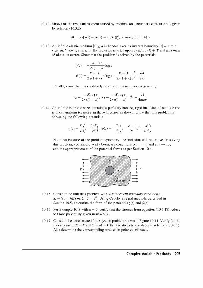
10-12. Show that the resultant moment caused by tractions on a boundary contour AB is given
by relation (10.3.2)
M ¼ Re[w(z)� zc(z)� z�zzg0(z)]BA, where w0(z) ¼ c(z)
10-13. An infinite elastic medium jzj � a is bonded over its internal boundary jzj ¼ a to a
rigid inclusion of radius a. The inclusion is acted upon by a force X þ iY and a momentM about its center. Show that the problem is solved by the potentials
g(z) ¼ � X þ iY
2p(1þ k)log z
c(z) ¼ X � iY
2p(1þ k)k log zþ X þ iY
2p(1þ k)a2
z2þ iM
2pz
Finally, show that the rigid-body motion of the inclusion is given by
uo ¼ �kX log a
2pm(1þ k), v0 ¼ �kY log a
2pm(1þ k), yo ¼ M
4pma2
10-14. An infinite isotropic sheet contains a perfectly bonded, rigid inclusion of radius a and
is under uniform tension T in the x-direction as shown. Show that this problem is
solved by the following potentials
g(z) ¼ T
4z� 2a2
kz
� �, c(z) ¼ �T
2z� k� 1
2za2 þ a4
kz3
� �
Note that because of the problem symmetry, the inclusion will not move. In solving
this problem, you should verify boundary conditions on r ¼ a and at r ! 1,
and the appropriateness of the potential forms as per Section 10.4.
x
y
TT
Inclusion
10-15. Consider the unit disk problem with displacement boundary conditionsur þ iuy ¼ h(z) on C: z ¼ eiy. Using Cauchy integral methods described in
Section 10.5, determine the form of the potentials g(z) and c(z).
10-16. For Example 10-3 with a ¼ 0, verify that the stresses from equation (10.5.18) reduce
to those previously given in (8.4.69).
10-17. Consider the concentrated force system problem shown in Figure 10-11. Verify for the
special case of X ¼ P and Y ¼ M ¼ 0 that the stress field reduces to relations (10.6.5).
Also determine the corresponding stresses in polar coordinates.
Complex Variable Methods 295
10-18. For the stress concentration problem shown in Figure 10-14, solve the problem with
the following far-field loadings s1x ¼ s1y ¼ S, t1xy ¼ 0, and compute the stress
concentration factor. Verify your solution with that given in (8.4.9) and (8.4.10).
10-19. Verify the mappings shown in Figure 10-16 by explicitly investigating points on the
boundaries and the point at infinity in the z-plane.
10-20*. Consider relation (10.7.14) for the circumferential stress sj on the boundary of the
elliptical hole shown in Figure 10-17. Explicitly verify that the maximum stress
occurs at j ¼ p=2. Next plot the distribution of sj vs: j for the cases of
m ¼ 0, � 0:5, � 1.
10-21*. Consider the problem of an infinite plate containing a stress-free elliptical hole with
s1x ¼ s1y ¼ 0, t1xy ¼ S. For this problem, the derivative of the complex potential has
been developed by Milne-Thomson (1960)
dg(z)dz
¼ iS
m� z2
Show that the stress on the boundary of the hole is given by
sj ¼ � 4S sin 2jm2 � 2m cos 2jþ 1
Determine and plot sj vs: j for the cases m ¼ 0, 0:5, and 1. Identify maximum
stress values and locations.
10-22. Verify the crack-tip stress distributions given by (10.8.6) and (10.8.7).
10-23. Verify that the crack-tip displacements are given by (10.8.8).
10-24. Show that the Westergaard stress function
Z(z) ¼ Szffiffiffiffiffiffiffiffiffiffiffiffiffiffiffiffiffiffi(z2 � a2)
p � S
2
with A ¼ S=2 solves the central crack problem shown in Figure 10-19.
10-25. Following similar procedures as in Section 10.9, establish a Westergaard stress
function method for skewsymmetric crack problems. For this case, assume that
loadings are applied skewsymmetrically with respect to the crack, thereby
establishing that the normal stress sy vanishes along y ¼ 0. Show that this leads to
the following relations
sx ¼ 2ReZ(z)� yImZ0(z)sy ¼ yImZ0(z)txy ¼ �ImZ(z)� yReZ0(z)� B
where Z(z) ¼ 2g0(z) and B is a real constant.
296 ADVANCED APPLICATIONS
11 Anisotropic Elasticity
It has long been recognized that deformation behavior of many materials depends upon
orientation; that is, the stress-strain response of a sample taken from the material in one
direction will be different if the sample were taken in a different direction. The term
anisotropic is generally used to describe such behaviors. Early investigators of these phe-
nomena were motivated by the response of naturally occurring anisotropic materials such as
wood and crystalline solids. Today, extensive use of engineered composites (see Jones 1998
or Swanson 1997) has brought forward many new types of fiber-and particle-reinforced
materials with anisotropic response. Thus, knowledge of stress distributions in anisotropic
materials is very important for proper use of these new high-performance materials in
structural applications. Our previous development of the linear elastic stress-strain relations
in Section 4.2 began with the general case of inhomogeneous and anisotropic behavior.
However, this generality was quickly eliminated, and only the homogeneous isotropic
case was subsequently developed in detail. We now wish to go back and further investigate
the anisotropic homogeneous case and develop applications for particular elasticity problems
including torsion and plane problems. Much of the original work in this field was done by
Lekhnitskii (1968, 1981), while Love (1934) and Hearmon (1961) also made early contribu-
tions. More recently, texts by Ting (1996a) and Rand and Rovenski (2005) provide modern
and comprehensive accounts on this subject.
11.1 Basic Concepts
The directional-dependent behaviors found in anisotropic solids normally result from par-
ticular microstructural features within the material. Our previous isotropic model neglected
these effects, thus resulting in a material that behaved the same in all directions. Micro
features commonly arise in natural and synthetic materials in such a way as to produce a
stress-strain response with particular symmetries. This concept is based on the Neumannprinciple (Love 1934) that symmetry in material microgeometry corresponds to identicalsymmetry in the constitutive response. We can qualitatively gain an understanding of this
concept from some simple two-dimensional cases shown in Figure 11-1. The figure illustrates
idealized internal microstructures of two crystalline solids and one fiber composite. The two
297
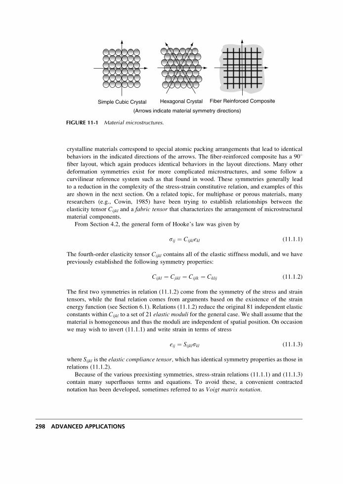
crystalline materials correspond to special atomic packing arrangements that lead to identical
behaviors in the indicated directions of the arrows. The fiber-reinforced composite has a 908fiber layout, which again produces identical behaviors in the layout directions. Many other
deformation symmetries exist for more complicated microstructures, and some follow a
curvilinear reference system such as that found in wood. These symmetries generally lead
to a reduction in the complexity of the stress-strain constitutive relation, and examples of this
are shown in the next section. On a related topic, for multiphase or porous materials, many
researchers (e.g., Cowin, 1985) have been trying to establish relationships between the
elasticity tensor Cijkl and a fabric tensor that characterizes the arrangement of microstructural
material components.
From Section 4.2, the general form of Hooke’s law was given by
sij ¼ Cijklekl (11:1:1)
The fourth-order elasticity tensor Cijkl contains all of the elastic stiffness moduli, and we have
previously established the following symmetry properties:
Cijkl ¼ Cjikl ¼ Cijlk ¼ Cklij (11:1:2)
The first two symmetries in relation (11.1.2) come from the symmetry of the stress and strain
tensors, while the final relation comes from arguments based on the existence of the strain
energy function (see Section 6.1). Relations (11.1.2) reduce the original 81 independent elastic
constants within Cijkl to a set of 21 elastic moduli for the general case. We shall assume that the
material is homogeneous and thus the moduli are independent of spatial position. On occasion
we may wish to invert (11.1.1) and write strain in terms of stress
eij ¼ Sijklskl (11:1:3)
where Sijkl is the elastic compliance tensor, which has identical symmetry properties as those in
relations (11.1.2).
Because of the various preexisting symmetries, stress-strain relations (11.1.1) and (11.1.3)
contain many superfluous terms and equations. To avoid these, a convenient contracted
notation has been developed, sometimes referred to as Voigt matrix notation.
Simple Cubic Crystal Fiber Reinforced CompositeHexagonal Crystal
(Arrows indicate material symmetry directions)
FIGURE 11-1 Material microstructures.
298 ADVANCED APPLICATIONS
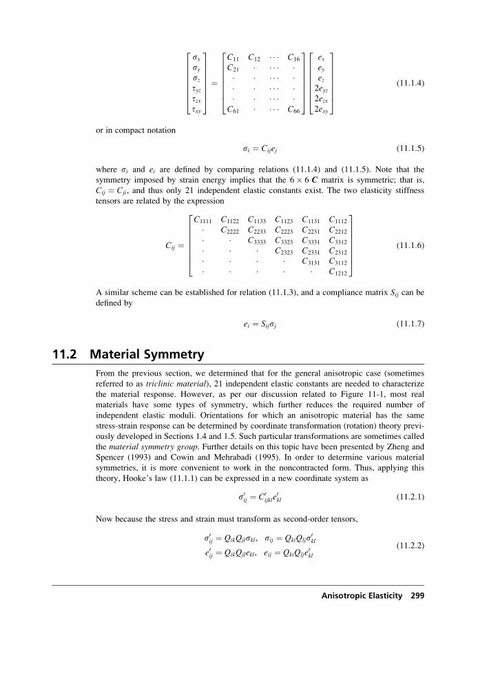
sxsysztyztzxtxy
26666664
37777775¼
C11 C12 � � � C16
C21 � � � � �� � � � � �� � � � � �� � � � � �
C61 � � � � C66
26666664
37777775
exeyez2eyz2ezx2exy
26666664
37777775
(11:1:4)
or in compact notation
si ¼ Cijej (11:1:5)
where si and ei are defined by comparing relations (11.1.4) and (11.1.5). Note that the
symmetry imposed by strain energy implies that the 6� 6 C matrix is symmetric; that is,
Cij ¼ Cji, and thus only 21 independent elastic constants exist. The two elasticity stiffness
tensors are related by the expression
Cij ¼
C1111 C1122 C1133 C1123 C1131 C1112
� C2222 C2233 C2223 C2231 C2212
� � C3333 C3323 C3331 C3312
� � � C2323 C2331 C2312
� � � � C3131 C3112
� � � � � C1212
26666664
37777775
(11:1:6)
A similar scheme can be established for relation (11.1.3), and a compliance matrix Sij can be
defined by
ei ¼ Sijsj (11:1:7)
11.2 Material Symmetry
From the previous section, we determined that for the general anisotropic case (sometimes
referred to as triclinic material), 21 independent elastic constants are needed to characterize
the material response. However, as per our discussion related to Figure 11-1, most real
materials have some types of symmetry, which further reduces the required number of
independent elastic moduli. Orientations for which an anisotropic material has the same
stress-strain response can be determined by coordinate transformation (rotation) theory previ-
ously developed in Sections 1.4 and 1.5. Such particular transformations are sometimes called
the material symmetry group. Further details on this topic have been presented by Zheng and
Spencer (1993) and Cowin and Mehrabadi (1995). In order to determine various material
symmetries, it is more convenient to work in the noncontracted form. Thus, applying this
theory, Hooke’s law (11.1.1) can be expressed in a new coordinate system as
s0ij ¼ C0ijkle
0kl (11:2:1)
Now because the stress and strain must transform as second-order tensors,
s0ij ¼ QikQjlskl, sij ¼ QkiQljs0kle0ij ¼ QikQjlekl, eij ¼ QkiQlje
0kl
(11:2:2)
Anisotropic Elasticity 299
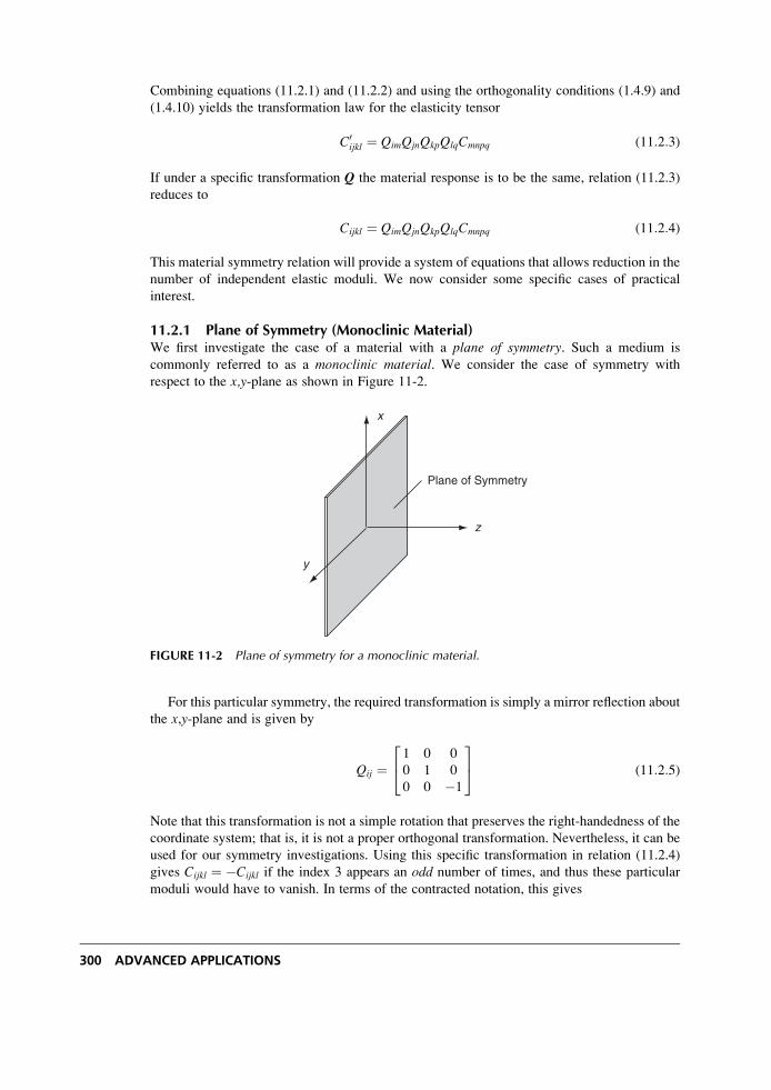
Combining equations (11.2.1) and (11.2.2) and using the orthogonality conditions (1.4.9) and
(1.4.10) yields the transformation law for the elasticity tensor
C0ijkl ¼ QimQjnQkpQlqCmnpq (11:2:3)
If under a specific transformation Q the material response is to be the same, relation (11.2.3)
reduces to
Cijkl ¼ QimQjnQkpQlqCmnpq (11:2:4)
This material symmetry relation will provide a system of equations that allows reduction in the
number of independent elastic moduli. We now consider some specific cases of practical
interest.
11.2.1 Plane of Symmetry (Monoclinic Material)We first investigate the case of a material with a plane of symmetry. Such a medium is
commonly referred to as a monoclinic material. We consider the case of symmetry with
respect to the x,y-plane as shown in Figure 11-2.
For this particular symmetry, the required transformation is simply a mirror reflection about
the x,y-plane and is given by
Qij ¼1 0 0
0 1 0
0 0 �1
24
35 (11:2:5)
Note that this transformation is not a simple rotation that preserves the right-handedness of the
coordinate system; that is, it is not a proper orthogonal transformation. Nevertheless, it can be
used for our symmetry investigations. Using this specific transformation in relation (11.2.4)
gives Cijkl ¼ �Cijkl if the index 3 appears an odd number of times, and thus these particular
moduli would have to vanish. In terms of the contracted notation, this gives
x
y
z
Plane of Symmetry
FIGURE 11-2 Plane of symmetry for a monoclinic material.
300 ADVANCED APPLICATIONS
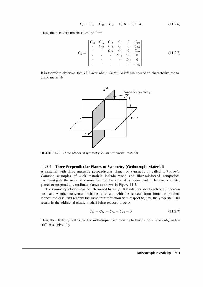
Ci4 ¼ Ci5 ¼ C46 ¼ C56 ¼ 0, (i ¼ 1, 2, 3) (11:2:6)
Thus, the elasticity matrix takes the form
Cij ¼
C11 C12 C13 0 0 C16
� C22 C23 0 0 C26
� � C33 0 0 C36
� � � C44 C45 0
� � � � C55 0
� � � � � C66
26666664
37777775
(11:2:7)
It is therefore observed that 13 independent elastic moduli are needed to characterize mono-
clinic materials.
11.2.2 Three Perpendicular Planes of Symmetry (Orthotropic Material)A material with three mutually perpendicular planes of symmetry is called orthotropic.Common examples of such materials include wood and fiber-reinforced composites.
To investigate the material symmetries for this case, it is convenient to let the symmetry
planes correspond to coordinate planes as shown in Figure 11-3.
The symmetry relations can be determined by using 1808 rotations about each of the coordin-ate axes. Another convenient scheme is to start with the reduced form from the previous
monoclinic case, and reapply the same transformation with respect to, say, the y,z-plane. Thisresults in the additional elastic moduli being reduced to zero:
C16 ¼ C26 ¼ C36 ¼ C45 ¼ 0 (11:2:8)
Thus, the elasticity matrix for the orthotropic case reduces to having only nine independentstiffnesses given by
Planes of Symmetryx
y
z
FIGURE 11-3 Three planes of symmetry for an orthotropic material.
Anisotropic Elasticity 301
Cij ¼
C11 C12 C13 0 0 0
� C22 C23 0 0 0
� � C33 0 0 0
� � � C44 0 0
� � � � C55 0
� � � � � C66
26666664
37777775
(11:2:9)
It should be noted that only two transformations were needed to develop the final reduced
constitutive form (11.2.9). The material also must satisfy a third required transformation
that the properties would be the same under a reflection of the x,z-plane. However, attempting
this transformation would only give relations that are identically satisfied. Thus, for
some materials the reduced constitutive form may be developed by using only a portion of
the total material symmetries (see Ting 1996a for more on this topic). On another issue for
orthotropic materials, vanishing shear strains imply vanishing shear stresses, and thus the
principal axes of stress coincide with the principal axes of strain. This result is of course not
true for general anisotropic materials; see, for example, the monoclinic constitutive form
(11.2.7).
For orthotropic materials, the compliance matrix has similar form but is commonly written
using notation related to isotropic theory:
Sij ¼
1
E1
� �21E2
� �31E3
0 0 0
� �12E1
1
E2
� �32E3
0 0 0
� �13E1
� �23E2
1
E3
0 0 0
� � � 1
m230 0
� � � � 1
m310
� � � � � 1
m12
2666666666666666664
3777777777777777775
(11:2:10)
where Ei are Young’s moduli in the three directions of material symmetry, �ij are the Poisson’sratios defined by �ej=ei for a stress in the i direction, and mij are the shear moduli in the
i, j-planes. Symmetry of this matrix requires that �ij=Ei ¼ �ji=Ej.
11.2.3 Axis of Symmetry (Transversely Isotropic Material)Another common form of material symmetry is with respect to rotations about an axis. This
concept can be specified by stating that a material possess an axis of symmetry of order n whenthe elastic moduli remain unchanged for rotations of 2p=n radians about the axis. This situationis shown schematically in Figure 11-4. The hexagonal packing crystalline case shown in
Figure 11-1 has such a symmetry about the axis perpendicular to the page for n ¼ 6
(608 increments). It can be shown (Lekhnitskii 1981) that the only possible symmetries for
this case are for orders 2, 3, 4, 6, and infinity. The order 2 case is equivalent to a plane of
symmetry previously discussed, and order 6 is equivalent to the infinite case.
The transformation for arbitrary rotations y about the z-axis is given by
302 ADVANCED APPLICATIONS
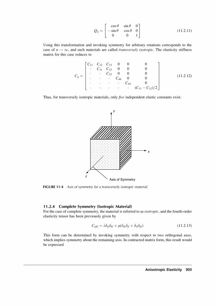
Qij ¼cos y sin y 0
� sin y cos y 0
0 0 1
24
35 (11:2:11)
Using this transformation and invoking symmetry for arbitrary rotations corresponds to the
case of n ! 1, and such materials are called transversely isotropic. The elasticity stiffness
matrix for this case reduces to
Cij ¼
C11 C12 C13 0 0 0
� C11 C13 0 0 0
� � C33 0 0 0
� � � C44 0 0
� � � � C44 0
� � � � � (C11 � C12)=2
26666664
37777775
(11:2:12)
Thus, for transversely isotropic materials, only five independent elastic constants exist.
11.2.4 Complete Symmetry (Isotropic Material)For the case of complete symmetry, the material is referred to as isotropic, and the fourth-orderelasticity tensor has been previously given by
Cijkl ¼ ldijdkl þ m(dikdjl þ dildjk) (11:2:13)
This form can be determined by invoking symmetry with respect to two orthogonal axes,
which implies symmetry about the remaining axis. In contracted matrix form, this result would
be expressed
Axis of Symmetry
x
y
z
FIGURE 11-4 Axis of symmetry for a transversely isotropic material.
Anisotropic Elasticity 303
Cij ¼
lþ 2m l l 0 0 0
� lþ 2m l 0 0 0
� � lþ 2m 0 0 0
� � � m 0 0
� � � � m 0
� � � � � m
26666664
37777775
(11:2:14)
Thus, as shown previously, only two independent elastic constants exist for isotropic
materials. For each case presented, a similar compliance elasticity matrix could be developed.
Our brief presentation does not include all cases ofmaterial symmetry. Based on symmetry planes,
Ting (2003) has proven that there are only eight symmetries for linear anisotropic elastic materials
for the general case. Of course, a large variety of curvilinear material symmetries also exist in
various biological and synthetic materials and these will be discussed further in Section 11.7.
EXAMPLE 11-1: Hydrostatic Compressionof a Monoclinic Cube
In order to demonstrate the difference in behavior between isotropic and anisotropic
materials, consider a simple example of a cube of monoclinic material under hydrostatic
compression. For this case, the state of stress is given by sij ¼ �pdij, and the mono-
clinic Hooke’s law in compliance form would read as follows:
exeyez2eyz2ezx2exy
26666664
37777775¼
S11 S12 S13 0 0 S16� S22 S23 0 0 S26� � S33 0 0 S36� � � S44 S45 0
� � � � S55 0
� � � � � S66
26666664
37777775
�p�p�p0
0
0
26666664
37777775
(11:2:15)
Expanding this matrix relation gives the following deformation field components:
ex ¼ �(S11 þ S12 þ S13)p
ey ¼ �(S12 þ S22 þ S23)p
ez ¼ �(S13 þ S23 þ S33)p
eyz ¼ 0
ezx ¼ 0
exy ¼ � 1
2(S16 þ S26 þ S36)p
(11:2:16)
The corresponding strains for the isotropic case would be given by ex ¼ ey ¼ ez ¼�[(1�2�)=E]p, eyz ¼ ezx ¼ exy ¼ 0. Thus, the response of the monoclinic material is
considerably different from isotropic behavior and yields a nonzero shear strain even
under uniform hydrostatic stress. Additional examples using simple shear and/or bend-
ing deformations can also be used to demonstrate the complexity of anisotropic stress-
strain behavior (see Sendeckyj 1975). It should be apparent that laboratory testing
methods attempting to characterize anisotropic materials would have to be more
involved than those used for isotropic solids.
304 ADVANCED APPLICATIONS
11.3 Restrictions on Elastic Moduli
Several general restrictions exist on particular combinations of elastic moduli for anisotropic
material classes previously discussed. These restrictions follow from arguments based on
rotational invariance and the positive definiteness of the strain energy function.
Consider first the idea of rotational invariance. This concept has already been discussed in
Section 1.6, where it was shown that for all 3� 3 symmetric matrices or tensors there exist
three invariants given by relations (1.6.3). This general concept may be applied to symmetric
square matrices of any order including the general elasticity matrix Cij. One scheme to
generate such invariant relationships is to employ the rotational transformation (11.2.11)
about the z-axis. Using this transformation, we can show that
C044 ¼ C44 cos
2 y� 2C45 sin y cos yþ C55 sin2 y
C055 ¼ C44 sin
2 yþ 2C45 sin y cos yþ C55 cos2 y
Adding these individual equations together gives the simple result
C044 þ C0
55 ¼ C44 þ C55
and thus this sum must be an invariant with respect to such rotations. Other invariants can alsobe found using this type of rotational transformation scheme, and the results include the
following invariant forms:
C11 þ C22 þ 2C12
C66 � C12
C44 þ C55
C13 þ C23
C234 þ C2
35
C11 þ C22 þ C33 þ 2(C12 þ C23 þ C13)
(11:3:1)
Next consider modulus restrictions based on strain energy concepts. In terms of the
contracted notation, the strain energy function can be written as
U ¼ 1
2sijeij ¼ 1
2Cijeiej ¼ 1
2Sijsisj (11:3:2)
Now the strain energy is always positive definite, U � 0 with equality only if the stresses or
strains vanish. This result implies that both the Cij and Sij must be positive definite symmetricmatrices. From matrix theory (see, for example, Ting 1996a,b), it can be shown that for such a
case all eigenvalues and principal minors of Cij and Sij must be positive and nonzero. Recall
that a principal minor pi of a square matrix is the determinant of the submatrix created by
deleting the ith row and column. For the general case, this concept will yield six rather lengthy
relations; however, one simple result from this is that all diagonal elements of each matrix are
positive.
Anisotropic Elasticity 305
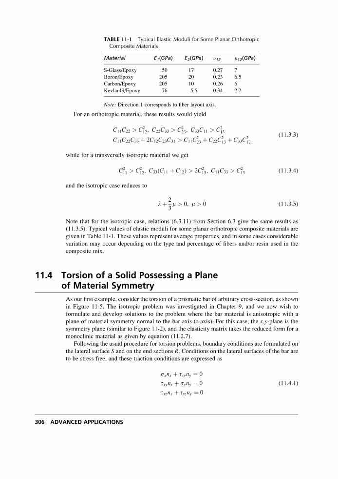
For an orthotropic material, these results would yield
C11C22 > C212, C22C33 > C2
23, C33C11 > C213
C11C22C33 þ 2C12C23C31 > C11C223 þ C22C
213 þ C33C
212
(11:3:3)
while for a transversely isotropic material we get
C211 > C2
12, C33(C11 þ C12) > 2C213, C11C33 > C2
13 (11:3:4)
and the isotropic case reduces to
lþ 2
3m > 0, m > 0 (11:3:5)
Note that for the isotropic case, relations (6.3.11) from Section 6.3 give the same results as
(11.3.5). Typical values of elastic moduli for some planar orthotropic composite materials are
given in Table 11-1. These values represent average properties, and in some cases considerable
variation may occur depending on the type and percentage of fibers and/or resin used in the
composite mix.
11.4 Torsion of a Solid Possessing a Planeof Material Symmetry
As our first example, consider the torsion of a prismatic bar of arbitrary cross-section, as shown
in Figure 11-5. The isotropic problem was investigated in Chapter 9, and we now wish to
formulate and develop solutions to the problem where the bar material is anisotropic with a
plane of material symmetry normal to the bar axis (z-axis). For this case, the x,y-plane is the
symmetry plane (similar to Figure 11-2), and the elasticity matrix takes the reduced form for a
monoclinic material as given by equation (11.2.7).
Following the usual procedure for torsion problems, boundary conditions are formulated on
the lateral surface S and on the end sections R. Conditions on the lateral surfaces of the bar are
to be stress free, and these traction conditions are expressed as
sxnx þ txyny ¼ 0
txynx þ syny ¼ 0
txznx þ tyzny ¼ 0
(11:4:1)
TABLE 11-1 Typical Elastic Moduli for Some Planar OrthotropicComposite Materials
Material E1(GPa) E2(GPa) �12 m12(GPa)
S-Glass/Epoxy 50 17 0.27 7
Boron/Epoxy 205 20 0.23 6.5
Carbon/Epoxy 205 10 0.26 6
Kevlar49/Epoxy 76 5.5 0.34 2.2
Note: Direction 1 corresponds to fiber layout axis.
306 ADVANCED APPLICATIONS
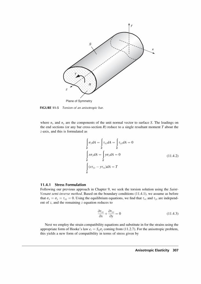
where nx and ny are the components of the unit normal vector to surface S. The loadings on
the end sections (or any bar cross-section R) reduce to a single resultant moment T about the
z-axis, and this is formulated as
ðR
szdA ¼ðR
txzdA ¼ðR
tyzdA ¼ 0
ðR
xszdA ¼ðR
yszdA ¼ 0
ðR
(xtyz � ytxz)dA ¼ T
(11:4:2)
11.4.1 Stress FormulationFollowing our previous approach in Chapter 9, we seek the torsion solution using the Saint-Venant semi-inverse method. Based on the boundary conditions (11.4.1), we assume as before
that sx ¼ sy ¼ txy ¼ 0. Using the equilibrium equations, we find that txz and tyz are independ-ent of z, and the remaining z equation reduces to
@txz@x
þ @tyz@y
¼ 0 (11:4:3)
Next we employ the strain compatibility equations and substitute in for the strains using the
appropriate form of Hooke’s law ei ¼ Sijsj coming from (11.2.7). For the anisotropic problem,
this yields a new form of compatibility in terms of stress given by
x
y
z
S
R
T
Plane of Symmetry
FIGURE 11-5 Torsion of an anisotropic bar.
Anisotropic Elasticity 307
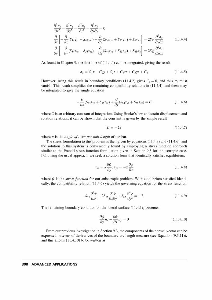
@2sz@x2
¼ @2sz@y2
¼ @2sz@z2
¼ @2sz@x@y
¼ 0
@
@x� @
@x(S44tyz þ S45txz)þ @
@y(S54tyz þ S55txz)þ S63sz
� �¼ 2S13
@2sz@y@z
@
@y� @
@y(S54tyz þ S55txz)þ @
@x(S44tyz þ S45txz)þ S63sz
� �¼ 2S23
@2sz@x@z
(11:4:4)
As found in Chapter 9, the first line of (11.4.4) can be integrated, giving the result
sz ¼ C1xþ C2yþ C3zþ C4xzþ C5yzþ C6 (11:4:5)
However, using this result in boundary conditions (11.4.2) gives Ci ¼ 0, and thus sz must
vanish. This result simplifies the remaining compatibility relations in (11.4.4), and these may
be integrated to give the single equation
� @
@x(S44tyz þ S45txz)þ @
@y(S54tyz þ S55txz) ¼ C (11:4:6)
where C is an arbitrary constant of integration. Using Hooke’s law and strain-displacement and
rotation relations, it can be shown that the constant is given by the simple result
C ¼ �2a (11:4:7)
where a is the angle of twist per unit length of the bar.
The stress formulation to this problem is then given by equations (11.4.3) and (11.4.6), and
the solution to this system is conveniently found by employing a stress function approach
similar to the Prandtl stress function formulation given in Section 9.3 for the isotropic case.
Following the usual approach, we seek a solution form that identically satisfies equilibrium,
txz ¼ a@c@y
, tyz ¼ �a@c@x
(11:4:8)
where c is the stress function for our anisotropic problem. With equilibrium satisfied identi-
cally, the compatibility relation (11.4.6) yields the governing equation for the stress function
S44@2c@x2
� 2S45@2c@x@y
þ S55@2c@y2
¼ �2 (11:4:9)
The remaining boundary condition on the lateral surface (11:4:1)3 becomes
@c@y
nx � @c@x
ny ¼ 0 (11:4:10)
From our previous investigation in Section 9.3, the components of the normal vector can be
expressed in terms of derivatives of the boundary arc length measure (see Equation (9.3.11)),
and this allows (11.4.10) to be written as
308 ADVANCED APPLICATIONS
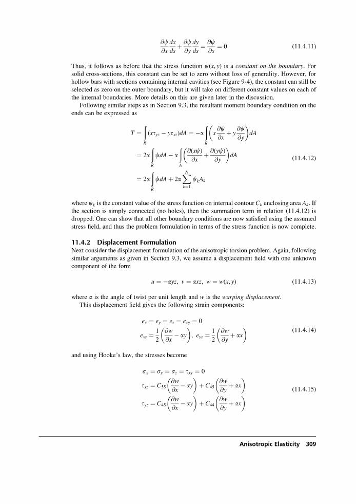
@c@x
dx
dsþ @c
@y
dy
ds¼ @c
@s¼ 0 (11:4:11)
Thus, it follows as before that the stress function c(x, y) is a constant on the boundary. Forsolid cross-sections, this constant can be set to zero without loss of generality. However, for
hollow bars with sections containing internal cavities (see Figure 9-4), the constant can still be
selected as zero on the outer boundary, but it will take on different constant values on each of
the internal boundaries. More details on this are given later in the discussion.
Following similar steps as in Section 9.3, the resultant moment boundary condition on the
ends can be expressed as
T ¼ðR
(xtyz � ytxz)dA ¼ �aðR
x@c@x
þ y@c@y
� �dA
¼ 2aðR
cdA� aðA
@(xc)@x
þ @(yc)@y
� �dA
¼ 2aðR
cdAþ 2aXNk¼1
ckAk
(11:4:12)
where ck is the constant value of the stress function on internal contour Ck enclosing area Ak. If
the section is simply connected (no holes), then the summation term in relation (11.4.12) is
dropped. One can show that all other boundary conditions are now satisfied using the assumed
stress field, and thus the problem formulation in terms of the stress function is now complete.
11.4.2 Displacement FormulationNext consider the displacement formulation of the anisotropic torsion problem. Again, following
similar arguments as given in Section 9.3, we assume a displacement field with one unknown
component of the form
u ¼ �ayz, v ¼ axz, w ¼ w(x, y) (11:4:13)
where a is the angle of twist per unit length and w is the warping displacement.This displacement field gives the following strain components:
ex ¼ ey ¼ ez ¼ exy ¼ 0
exz ¼ 1
2
@w
@x� ay
� �, eyz ¼ 1
2
@w
@yþ ax
� �(11:4:14)
and using Hooke’s law, the stresses become
sx ¼ sy ¼ sz ¼ txy ¼ 0
txz ¼ C55
@w
@x� ay
� �þ C45
@w
@yþ ax
� �
tyz ¼ C45
@w
@x� ay
� �þ C44
@w
@yþ ax
� � (11:4:15)
Anisotropic Elasticity 309
Substituting these stresses into the equilibrium equations yields the following governing
equation for the warping displacement
C55
@2w
@x2þ 2C45
@2w
@x@yþ C44
@2w
@y2¼ 0 (11:4:16)
For this formulation, the boundary conditions on the lateral surface give the result
C55
@w
@x� ay
� �þ C45
@w
@yþ ax
� �� �nx
þ C45
@w
@x� ay
� �þ C44
@w
@yþ ax
� �� �ny ¼ 0
(11:4:17)
and the moment condition on the ends is given by
T ¼ aðR
C44x2 þ C55y
2 � 2C45xyþ C44x@w
@y
�
� C55y@w
@xþ C45 x
@w
@x� y
@w
@y
� ��dA
(11:4:18)
Note that all other boundary conditions in set (11.4.1) and (11.4.2) are satisfied.
Comparison of the stress and displacement formulations for the anisotropic torsion problem
results in similar conclusions found for the isotropic case in Chapter 9. The stress function is
governed by a slightly more complicated nonhomogeneous differential equation but with a
simpler boundary condition. This fact commonly favors using the stress function approach for
problem solution.
11.4.3 General Solution to the Governing EquationThe governing equation for both the stress and displacement formulations of the torsion
problem can be written as
auxx þ 2buxy þ cuyy ¼ d (11:4:19)
where the constants a, b, and c are related to appropriate elastic moduli, and d is either zero
or �2, depending on the formulation. Of course, for the nonhomogeneous case, the general
solution is the sum of the particular plus homogeneous solutions.
To investigate the general solution to (11.4.19) for the homogeneous case, consider
solutions of the form u(x, y) ¼ f (xþ ly), where l is a parameter. Using this form in
(11.4.19) gives
(aþ 2blþ cl2)f 00 ¼ 0
Since f 00 cannot be zero, the term in parentheses must vanish, giving the characteristicequation
cl2 þ 2blþ a ¼ 0 (11:4:20)
310 ADVANCED APPLICATIONS
Solving the quadratic characteristic equation gives roots
l1, 2 ¼ �b�ffiffiffiffiffiffiffiffiffiffiffiffiffiffiffib2 � ac
p
c(11:4:21)
Using these roots, the original differential equation (11.4.19) can be written in operator form as
D1D2 u(x, y) ¼ 0
where Dk ¼ @
@y� lk
@
@x(11:4:22)
It is apparent that the characteristic equation (11.4.20) has complex conjugate rootswhenever b2 < ac. As per our discussion in Section 11.3, elastic moduli for materials possess-
ing a strain energy function must satisfy relations C44C55 > C245 and S44S55 > S245, and this
implies that all roots to (11.4.20) will be complex conjugate pairs of the form l1 ¼ l and
l2 ¼ l. The general solution to (11.4.22) then becomes
u(x, y) ¼ f1(xþ ly)þ f2(xþ ly) (11:4:23)
where f1 and f2 are arbitrary functions to be determined.
Because u(x,y) must be real, f1 and f2 must be complex conjugates of each other, and so
(11.4.23) can be written in the simplified form
u(x, y) ¼ 2Re[ f1(xþ ly)] (11:4:24)
Because l is a complex number, we can introduce the complex variable z* ¼ xþ ly, and the
previous solution form can be written as
u(x, y) ¼ 2Re[ f (z*)] (11:4:25)
This formulation then allows the method of complex variables to be applied to the solution of the
torsion problem. As discussed in the previous chapter, this method is very powerful and can
solve many problems, which are intractable by other schemes. We will not, however, pursue the
formal use of this method for our limited discussion of the anisotropic torsion problem.
These results then provide the general solution for the homogeneous case. To complete our
discussion we need the particular solution to (11.4.19). Using the structure of the equation, a
simple particular solution is given by
up(x, y) ¼ d(x2 þ y2)
2(aþ c)(11:4:26)
EXAMPLE 11-2: Torsion of an Elliptical Orthotropic Bar
Consider the torsion of a bar with elliptical cross-section as shown in Figure 9-7. Recall
that this problem was previously solved for the isotropic case in Example 9-1. Here, we
wish to solve the problem for the case of an orthotropic material. For convenience, the
coordinate system is taken to coincidewith thematerial symmetry axes, and this will yield
the reduced stiffness matrix given in relation (11.2.9). Note that for this case
Continued
Anisotropic Elasticity 311
EXAMPLE 11-2: Torsion of an Elliptical Orthotropic Bar–Cont’d
C45 ¼ S45 ¼ 0. Because of the simple section geometry and the expected correspondence
with the isotropic case, the solution method will not employ the general scheme previously
discussed. Rather, we will use the boundary equation method presented in Section 9.4.
Consider first the solution using the stress function formulation. Using the scheme
for the isotropic case, we choose a stress function form that will vanish on the boundary
of the elliptical cross-section
c ¼ Kx2
a2þ y2
b2� 1
� �
where the constant K is to be determined. Substituting this form into the governing
equation (11.4.9) determines the value of K and gives the final solution
c ¼ a2b2 � b2x2 � a2y2
S55a2 þ S44b2(11:4:27)
The stresses then follow from relations (11.4.8)
txz ¼ � 2aa2yS55a2 þ S44b2
txz ¼ 2ab2xS55a2 þ S44b2
(11:4:28)
which reduce to equations (9.4.8) for the isotropic case with S44 ¼ S55 ¼ 1=m. The load-carrying torque may be determined from result (11.4.12)
T ¼ apa3b3
S55a2 þ S44b2(11:4:29)
The warping displacement again follows from integrating relations (11:4:15)2,3, givingthe result
w(x, y) ¼ b2C55 � a2C44
a2C44 þ b2C55
xy (11:4:30)
which again reduces appropriately to the isotropic case given by (9.4.11). With the
warping displacement determined, the twisting moment can also be calculated from
relation (11.4.18).
11.5 Plane Deformation Problems
We now wish to investigate the solution of two-dimensional problems of an anisotropic elastic
solid. The material is chosen to have a plane of material symmetry that coincides with the plane
of reference for the deformation field. Plane problems were first discussed in Chapter 7, and this
leads to the formulation of two theories: plane strain and plane stress. The assumed displace-
ment field for plane strain was given in Section 7.1, and the corresponding assumptions on
the stress field for plane stress were specified in Section 7.2. These general assumptions still
312 ADVANCED APPLICATIONS
apply for this case with a plane of material symmetry, and each theory produces similar
governing equations for anisotropic materials. Ultimately, a complex variable formulation
similar to that of Chapter 10 will be established. Further details on this formulation can be
found in Milne-Thomson (1960), Lekhnitskii (1981), and Sendeckyj (1975). We begin with the
case of plane stress in the x,y-plane. For this case, the elasticity stiffness matrix is given by
relation (11.2.7) and a similar form would exist for the compliance matrix. Under the usual
plane stress (or generalized plane stress) assumptions sz ¼ txz ¼ tyz ¼ 0, and Hooke’s law
would then read
ex ¼ S11sx þ S12sy þ S16txyey ¼ S12sx þ S22sy þ S26txy
2exy ¼ S16sx þ S26sy þ S66txy
(11:5:1)
For plane strain, the usual assumptions give ez ¼ exz ¼ eyz ¼ 0, and Hooke’s law in terms of
the stiffness matrix would read
ex ¼ B11sx þ B12sy þ B16txyey ¼ B12sx þ B22sy þ B26txy
2exy ¼ B16sx þ B26sy þ B66txy
(11:5:2)
where the constants Bij may be expressed in terms of the compliances Sij by the relations
B11 ¼ S11S33 � S213S33
, B12 ¼ S12S33 � S13S23S33
B22 ¼ S22S33 � S223S33
, B16 ¼ S16S33 � S13S36S33
B66 ¼ S66S33 � S236S33
, B26 ¼ S26S33 � S23S36S33
(11:5:3)
Comparing stress-strain relations (11.5.1) and (11.5.2), it is observed that they are of the same
form, and a simple interchange of the elastic moduli Sij with the corresponding Bij will
transform the plane stress relations into those of plane strain. This is a similar result as
found earlier for the isotropic case. Because of this transformation property, we proceed
only with the plane stress case, realizing that any of the subsequent developments can be
easily converted to plane strain results.
The Airy stress function f(x, y) can again be introduced, and for the case with zero body
forces, we have the usual relations
sx ¼ @2f@y2
, sy ¼ @2f@x2
, txy ¼ � @2f@x@y
(11:5:4)
This stress field automatically satisfies the equilibrium equations, and using this form in
(11.5.1) yields the corresponding strain field in terms of the stress function. As before, the
only remaining nonzero compatibility relation is
@2ex@y2
þ @2ey@x2
¼ 2@2exy@x@y
(11:5:5)
Anisotropic Elasticity 313
and substituting the strain field into this relation gives the governing equation for the
stress function
S22@4�
@x4� 2S26
@4�
@x3@yþ (2S12 þ S66)
@4�
@x2@y2� 2S16
@4�
@x@y3þ S11
@4�
@y4¼ 0 (11:5:6)
The case with nonzero body forces has been given by Sendeckyj (1975).
The general solution to equation (11.5.6) can be found using methods of characteristics as
discussed previously in the torsion problem formulation; see result (11.4.23). The process
starts by looking for solutions of the form f ¼ f(xþ my), where m is a parameter. Using this in
(11.5.6) gives the characteristic equation
S11m4 � 2S16m3 þ (2S12 þ S66)m2 � 2S26mþ S22 ¼ 0 (11:5:7)
The four roots of this equation are related to the elastic compliances by the relations
m1m2m3m4 ¼ S22=S11
m1m2m3 þ m2m3m4 þ m3m4m1 þ m4m1m2 ¼ 2S26=S11
m1m2 þ m2m3 þ m3m4 þ m4m1 þ m1m3 þ m2m4 ¼ (2S12 þ S66)=S11
m1 þ m2 þ m3 þ m4 ¼ 2S16=S11
(11:5:8)
Using this formulation, the governing equation (11.5.6) can be written in operator form
D1D2D3D4f ¼ 0
where Dk ¼ @
@y� mk
@
@x
(11:5:9)
It can be shown (Lekhnitskii 1981) that the roots of the characteristic equation (11.5.7) must
be complex. Because complex roots always occur in conjugate pairs, this leads to two
particular cases:
Case 1: m1 ¼ a1 þ ib1, m2 ¼ a2 þ ib2, m3 ¼ �mm1, m4 ¼ �mm2Case 2: m1 ¼ m2 ¼ aþ ib, m3 ¼ m4 ¼ �mm1
(11:5:10)
With the equality condition, the second case rarely occurs, and it can be shown that it will
reduce to an isotropic formulation. We therefore do not consider this case further. Note for the
orthotropic case, S16 ¼ S26 ¼ 0, and the roots of the characteristic equation become purelycomplex, that is, ai ¼ 0 (see Exercise 11-14).
For the unequal complex conjugate root case, (11.5.9) can be separated into four equations
and integrated in a similar fashion as done to get result (11.4.23). This then leads to the general
solution
f(x, y) ¼ F1(xþ m1y)þ F2(xþ m2y)þ F3(xþ m3y)þ F4(xþ m4y)
¼ F1(xþ m1y)þ F2(xþ m2y)þ F3(xþ �mm1y)þ F4(xþ �mm2y)
¼ 2Re[F1(xþ m1y)þ F2(xþ m2y)]
¼ 2Re[F1(z1)þ F2(z2)], z1 ¼ xþ m1y, z2 ¼ xþ m2y
(11:5:11)
314 ADVANCED APPLICATIONS
where we have used similar arguments as in the development of the torsion solution (11.4.24)
and (11.4.25). Thus, we have now established that the general solution to the anisotropic plane
problem is given in terms of two arbitrary functions of the complex variables z1 and z2.We now wish to express the remaining elasticity equations in terms of these two complex
potential functions. It is generally more convenient to introduce two new complex potentials
that are simply the derivatives of the original pair; that is,
F1(z1) ¼ dF1
dz1, F2(z2) ¼ dF2
dz2(11:5:12)
In terms of these potentials, the in-plane stresses can be written as
sx ¼ 2Re[m21F01(z1)þ m22F
02(z2)]
sy ¼ 2Re[F01(z1)þ F0
2(z2)]
txy ¼ �2Re[m1F01(z1)þ m2F
02(z2)]
(11:5:13)
where primes indicate derivatives with respect to argument. Using Hooke’s law, the strains
may be determined, and the displacements follow from integration of the strain-displacement
relations, giving the result
u(x, y) ¼ 2Re[p1F1(z1)þ p2F2(z2)]
v(x, y) ¼ 2Re[q1F1(z1)þ q2F2(z2)](11:5:14)
where we have dropped the rigid-body motion terms and
pi ¼ S11m2i � S16mi þ S12
qi ¼ S12mi � S26 þ (S22=mi)(11:5:15)
In polar coordinates, the stresses and displacements take the form
sr ¼ 2Re[( sin y� m1 cos y)2F0
1(z1)þ ( sin y� m2 cos y)2F0
2(z2)]
sy ¼ 2Re[( cos yþ m1 sin y)2F0
1(z1)þ ( cos yþ m2 sin y)2F0
2(z2)]
try ¼ 2Re[( sin y� m1 cos y)( cos yþ m1 sin y)F01(z1)
þ ( sin y� m2 cos y)( cos yþ m2 sin y)F02(z2)]
(11:5:16)
ur ¼ 2Re[(p1 cos yþ q1 sin y)F1(z1)þ (p2 cos yþ q2 sin y)F2(z2)]
uy ¼ 2Re[(q1 cos y� p1 sin y)F1(z1)þ (q2 cos y� p2 sin y)F2(z2)](11:5:17)
Next we wish to establish the usual boundary conditions in terms of the complex potentials.
Results developed in the previous chapter, equation (10.2.13), are also valid here, and thus the
traction vector can be written as
Tnx ¼ sxnx þ txyny ¼ d
ds
@f@y
� �
Tny ¼ txynx þ syny ¼ � d
ds
@f@x
� � (11:5:18)
Anisotropic Elasticity 315
Integrating this result over the boundary gives the boundary forces
ðS
Tnx dsþ C1 ¼ @f
@y¼ 2Re[m1F1(z1)þ m2F2(z2)] ¼ px(s)
ðS
Tny dsþ C2 ¼ � @f
@x¼ �2Re[F1(z1)þ F2(z2)] ¼ py(s)
(11:5:19)
where px(s) and py(s) are the prescribed boundary tractions and C1 and C2 are arbitrary constants
of integration that do not affect the stresses, and thus can be chosen as any convenient value.
The displacement boundary conditions follow directly from equations (11.5.14):
u(s) ¼ 2Re[p1F1(z1)þ p2F2(z2)]
v(s) ¼ 2Re[q1F1(z1)þ q2F2(z2)](11:5:20)
where u(s) and v(s) are the prescribed boundary displacements.
Therefore, we have now formulated the plane anisotropic problem in terms of two arbitrary
functions of the complex variables z1 and z2. In regard to the general structure of these complex
potentials, many of the conclusions from the isotropic case covered previously in Section 10.4
would still hold for the anisotropic formulation. We now investigate the use of this formulation
for the solution to several problems of engineering interest.
EXAMPLE 11-3: Uniform Tension of an Anisotropic Sheet
Consider first the simple problem shown in Figure 11-6 of an anisotropic plane under
uniform tension T acting at an angle a measured from the horizontal. For this problem,
we already know the solution, namely a uniform stress field given by
sx ¼ T cos2 a
sy ¼ T sin2 a
txy ¼ T sin a cos a
(11:5:21)
Complex potential functions corresponding to such a constant stress field would take the
form F1(z1) ¼ A1z1,F2(z2) ¼ A2z2, where A1 and A2 are constants that may be com-
plex. Using this form in relations (11.5.13) gives
sx ¼ 2Re[m21A1 þ m22A2]
sy ¼ 2Re[A1 þ A2]
txy ¼ �2Re[m1A1 þ m2A2]
(11:5:22)
Equating (11.5.21) with (11.5.22) gives
T cos2 a ¼ 2Re[m21A1 þ m22A2]
T sin2 a ¼ 2Re[A1 þ A2]
T sin a cos a ¼ �2Re[m1A1 þ m2A2]
(11:5:23)
316 ADVANCED APPLICATIONS
EXAMPLE 11-3: Cont’d
T
T
FIGURE 11-6 Uniform tension of an anisotropic plane.
Because the complex constants A1 and A2 each have real and imaginary parts, the previous
three relations cannot completely determine these four values. Another condition is needed,
and it is commonly chosen as A1 ¼ �AA1. Using this constraint, (11.5.23) can now be solved
to yield
A1 ¼ T( cos aþ m2 sin a)( cos aþ �mm2 sin a)(m1 � �mm2)(m1 � m2)þ (�mm1 � �mm2)(m1 � m2)
A2 ¼ T( cos aþ �mm1 sin a)( cos aþ �mm2 sin a)� (m1 � �mm1)(m1 � �mm2)A1
(m2 � �mm1)(m2 � �mm2)(11:5:24)
EXAMPLE 11-4: Concentrated Force System in an Infinite Plane
Consider next the problem of an infinite anisotropic plane containing a concentrated
force system at the origin, as shown in Figure 11-7. The problem is similar to Example
10-4, which investigated the isotropic case.
FIGURE 11-7 Concentrated force system in an infinite plane.
Continued
Anisotropic Elasticity 317
EXAMPLE 11-4: Concentrated Force System in an InfinitePlane–Cont’d
Guided by our previous isotropic analysis, we choose the logarithmic form for the
complex potentials
F1(z1) ¼ A1 log z1
F2(z2) ¼ A2 log z2(11:5:25)
The stresses from these potentials are
sx ¼ 2Re m21A1
z1þ m22
A2
z2
� �
sy ¼ 2ReA1
z1þ A2
z2
� �
txy ¼ �2Re m1A1
z1þ m2
A2
z2
� � (11:5:26)
Consider the boundary loading on a circle C enclosing the origin. Using the general
result (11.5.19), the resultant loadings are given by
�X ¼þC
Tnx ds ¼ 2Re[m1F1(z1)þ m2F2(z2)]C
�Y ¼þC
Tny ds ¼ �2Re[F1(z1)þ F2(z2)]C
(11:5:27)
where we have dropped the arbitrary constants. Substituting in the complex potentials,
and using the cyclic properties of logarithmic functions (see (10.4.5)), the preceding
relations become
�X ¼ 4pRe[m1A1iþ m2A2i]
�Y ¼ �4pRe[A1iþ A2i](11:5:28)
This system is not sufficient to determine completely the complex constants A1 and
A2, and additional relations can be found by invoking the condition of single-valued
displacements. If the displacements are to be single-valued, then the cyclic function
(defined in Section 10.4) of relations (11.5.14) must be zero
Re[p1F1(z1)þ p2F2(z2)]C ¼ 0
Re[q1F1(z1)þ q2F2(z2)]C ¼ 0(11:5:29)
and for this case gives the result
Re[p1A1iþ p2A2i] ¼ 0
Re[q1A1iþ q2A2i] ¼ 0(11:5:30)
Relations (11.5.28) and (11.5.30) now provide sufficient relations to complete the problem.
318 ADVANCED APPLICATIONS
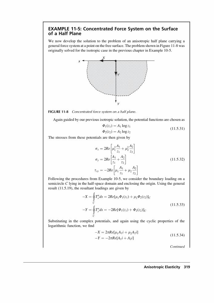
EXAMPLE 11-5: Concentrated Force System on the Surfaceof a Half Plane
We now develop the solution to the problem of an anisotropic half plane carrying a
general force system at a point on the free surface. The problem shown in Figure 11-8 was
originally solved for the isotropic case in the previous chapter in Example 10-5.
FIGURE 11-8 Concentrated force system on a half plane.
Again guided by our previous isotropic solution, the potential functions are chosen as
F1(z1) ¼ A1 log z1
F2(z2) ¼ A2 log z2(11:5:31)
The stresses from these potentials are then given by
sx ¼ 2Re m21A1
z1þ m22
A2
z2
� �
sy ¼ 2ReA1
z1þ A2
z2
� �
txy ¼ �2Re m1A1
z1þ m2
A2
z2
� � (11:5:32)
Following the procedures from Example 10-5, we consider the boundary loading on a
semicircle C lying in the half-space domain and enclosing the origin. Using the general
result (11.5.19), the resultant loadings are given by
�X ¼þC
Tnx ds ¼ 2Re[m1F1(z1)þ m2F2(z2)]C
�Y ¼þC
Tny ds ¼ �2Re[F1(z1)þ F2(z2)]C
(11:5:33)
Substituting in the complex potentials, and again using the cyclic properties of the
logarithmic function, we find
�X ¼ 2pRe[m1A1iþ m2A2i]
�Y ¼ �2pRe[A1iþ A2i](11:5:34)
Continued
Anisotropic Elasticity 319
EXAMPLE 11-5: Concentrated Force System on the Surfaceof a Half Plane–Cont’d
As before this system is not sufficient to determine completely the complex constants
A1 and A2. Additional relations can be found by invoking the stress-free boundary
condition on surface y ¼ 0, giving the result
sy(x, 0) ¼ 2ReA1
z1þ A2
z2
� �����y¼0
txy(x, 0) ¼ �2Re m1A1
z1þ m2
A2
z2
�� ����y¼0
(11:5:35)
Solving relations (11.5.34) and (11.5.35), the constants are found to be
A1 ¼ (X þ m2Y)2ip(m2 � m1)
A2 ¼ (X þ m1Y)2ip(m1 � m2)
(11:5:36)
With the constants determined, the stresses can easily be calculated using (11.5.32).
Using polar coordinates, we can show the surprising result that sy ¼ try ¼ 0, and thus
the stress state will be only radial. This result matches our findings for the correspond-
ing isotropic case given by relations (8.4.34) and/or (10.6.8). Exercise 11-16 computes
and compares sr stress components for orthotropic and isotropic cases, and significant
differences between the two cases are found.
EXAMPLE 11-6: Infinite Plate with an Elliptical Hole
Let us now investigate the solution to a class of problems involving an elliptical hole in an
infinite anisotropic plate, as shown in Figure 11-9. Although we develop solutions only to
a couple of cases in this example, Savin (1961) provides many additional solutions to
problems of this type. We first construct the general solution for arbitrary loading on the
hole surface for the case where the loading produces no net force or moment. Finally, a
specific case of a pressure loading is investigated in detail.
Using the usual conformal mapping concept, consider the mapping function that
transforms the exterior of the ellipse to the exterior of a unit circle
z ¼ w(z) ¼ aþ b
2zþ a� b
2z(11:5:37)
The complex variables z1 and z2 can be expressed in terms of the z and z as
z1 ¼ xþ m1y ¼1
2(1� im1)(xþ iy)þ 1
2(1þ im1)(x� iy) ¼ g1zþ d1z
z2 ¼ xþ m2y ¼1
2(1� im2)(xþ iy)þ 1
2(1þ im2)(x� iy) ¼ g2zþ d2z
(11:5:38)
Continued
320 ADVANCED APPLICATIONS
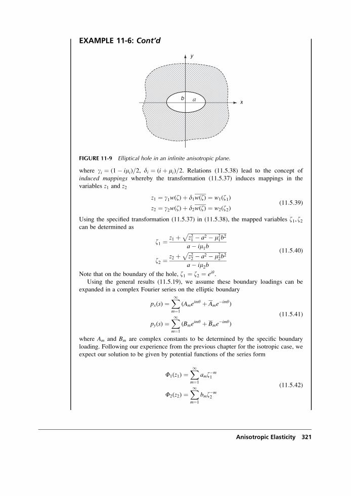
EXAMPLE 11-6: Cont’d
FIGURE 11-9 Elliptical hole in an infinite anisotropic plane.
where gi ¼ (1� imi)=2, di ¼ (iþ mi)=2. Relations (11.5.38) lead to the concept of
induced mappings whereby the transformation (11.5.37) induces mappings in the
variables z1 and z2
z1 ¼ g1w(z)þ d1w(z) ¼ w1(z1)
z2 ¼ g2w(z)þ d2w(z) ¼ w2(z2)(11:5:39)
Using the specified transformation (11.5.37) in (11.5.38), the mapped variables z1, z2can be determined as
z1 ¼z1 þ
ffiffiffiffiffiffiffiffiffiffiffiffiffiffiffiffiffiffiffiffiffiffiffiffiffiffiffiffiffiz21 � a2 � m21b2
pa� im1b
z2 ¼z2 þ
ffiffiffiffiffiffiffiffiffiffiffiffiffiffiffiffiffiffiffiffiffiffiffiffiffiffiffiffiffiz22 � a2 � m22b2
pa� im2b
(11:5:40)
Note that on the boundary of the hole, z1 ¼ z2 ¼ eiy.Using the general results (11.5.19), we assume these boundary loadings can be
expanded in a complex Fourier series on the elliptic boundary
px(s) ¼X1m¼1
(Ameimy þ Ame
�imy)
py(s) ¼X1m¼1
(Bmeimy þ Bme
�imy)
(11:5:41)
where Am and Bm are complex constants to be determined by the specific boundary
loading. Following our experience from the previous chapter for the isotropic case, we
expect our solution to be given by potential functions of the series form
F1(z1) ¼X1m¼1
amz�m1
F2(z2) ¼X1m¼1
bmz�m2
(11:5:42)
Anisotropic Elasticity 321
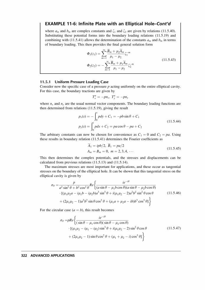
EXAMPLE 11-6: Infinite Plate with an Elliptical Hole–Cont’d
where am and bm are complex constants and z1 and z2 are given by relations (11.5.40).
Substituting these potential forms into the boundary loading relations (11.5.19) and
combining with (11.5.41) allows the determination of the constants am and bm in terms
of boundary loading. This then provides the final general solution form
F1(z1) ¼X1m¼1
Bm þ m2Am
m1 � m2z�m1
F2(z2) ¼ �X1m¼1
Bm þ m1Am
m1 � m2z�m2
(11:5:43)
11.5.1 Uniform Pressure Loading CaseConsider now the specific case of a pressure p acting uniformly on the entire elliptical cavity.
For this case, the boundary tractions are given by
Tnx ¼ �pnx, T
ny ¼ �pny
where nx and ny are the usual normal vector components. The boundary loading functions are
then determined from relations (11.5.19), giving the result
px(s) ¼ �ðs0
pdyþ C1 ¼ �pb sin yþ C1
py(s) ¼ðs0
pdxþ C2 ¼ pa cos y� paþ C2
(11:5:44)
The arbitrary constants can now be chosen for convenience as C1 ¼ 0 and C2 ¼ pa. Usingthese results in boundary relation (11.5.41) determines the Fourier coefficients as
A1 ¼ ipb=2, B1 ¼ pa=2
Am ¼ Bm ¼ 0, m ¼ 2, 3, 4, � � � (11:5:45)
This then determines the complex potentials, and the stresses and displacements can be
calculated from previous relations (11.5.13) and (11.5.14).
The maximum stresses are most important for applications, and these occur as tangential
stresses on the boundary of the elliptical hole. It can be shown that this tangential stress on the
elliptical cavity is given by
sy ¼ p
a2 sin2 yþ b2 cos2 yRe
ie�iy
(a sin y� m1b cos y)(a sin y� m2b cos y)
�� [(m1m2a� im1b� im2b)a
3 sin3 yþ i(m1m2 � 2)a2b2 sin2 y cos y
þ (2m1m2 � 1)a2b2 sin y cos2 yþ (m1aþ m2a� ib)b3 cos3 y] (11:5:46)
For the circular case (a ¼ b), this result becomes
sy ¼pReie�iy
( sin y� m1 cos y)( sin y� m2 cos y)
�� [(m1m2 � im1 � im2) sin
3 yþ i(m1m2 � 2) sin2 y cos y
þ (2m1m2 � 1) sin y cos2 yþ (m1 þ m2 � i) cos3 y] (11:5:47)
322 ADVANCED APPLICATIONS
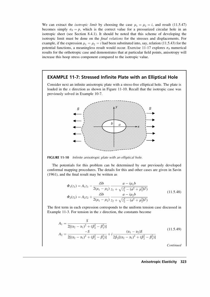
We can extract the isotropic limit by choosing the case m1 ¼ m2 ¼ i, and result (11.5.47)
becomes simply sy ¼ p, which is the correct value for a pressurized circular hole in an
isotropic sheet (see Section 8.4.1). It should be noted that this scheme of developing the
isotropic limit must be done on the final relations for the stresses and displacements. For
example, if the expression m1 ¼ m2 ¼ i had been substituted into, say, relation (11.5.43) for thepotential functions, a meaningless result would occur. Exercise 11-17 explores sy numerical
results for the orthotropic case and demonstrates that at particular field points, anisotropy will
increase this hoop stress component compared to the isotropic value.
EXAMPLE 11-7: Stressed Infinite Plate with an Elliptical Hole
Consider next an infinite anisotropic plate with a stress-free elliptical hole. The plate is
loaded in the x direction as shown in Figure 11-10. Recall that the isotropic case was
previously solved in Example 10-7.
FIGURE 11-10 Infinite anisotropic plate with an elliptical hole.
The potentials for this problem can be determined by our previously developed
conformal mapping procedures. The details for this and other cases are given in Savin
(1961), and the final result may be written as
F1(z1) ¼ A1z1 � iSb
2(m1 � m2)a� im1b
z1 þffiffiffiffiffiffiffiffiffiffiffiffiffiffiffiffiffiffiffiffiffiffiffiffiffiffiffiffiffiffiffiffiz21 � (a2 þ m21b2)
pF2(z2) ¼ A2z2 þ iSb
2(m1 � m2)a� im2b
z2 þffiffiffiffiffiffiffiffiffiffiffiffiffiffiffiffiffiffiffiffiffiffiffiffiffiffiffiffiffiffiffiffiz22 � (a2 þ m22b2)
p (11:5:48)
The first term in each expression corresponds to the uniform tension case discussed in
Example 11-3. For tension in the x direction, the constants become
A1 ¼ S
2[(a2 � a1)2 þ (b22 � b21)]
A2 ¼ �S
2[(a2 � a1)2 þ (b22 � b21)]þ i
(a1 � a2)S
2b2[(a2 � a1)2 þ (b22 � b21)]
(11:5:49)
Continued
Anisotropic Elasticity 323
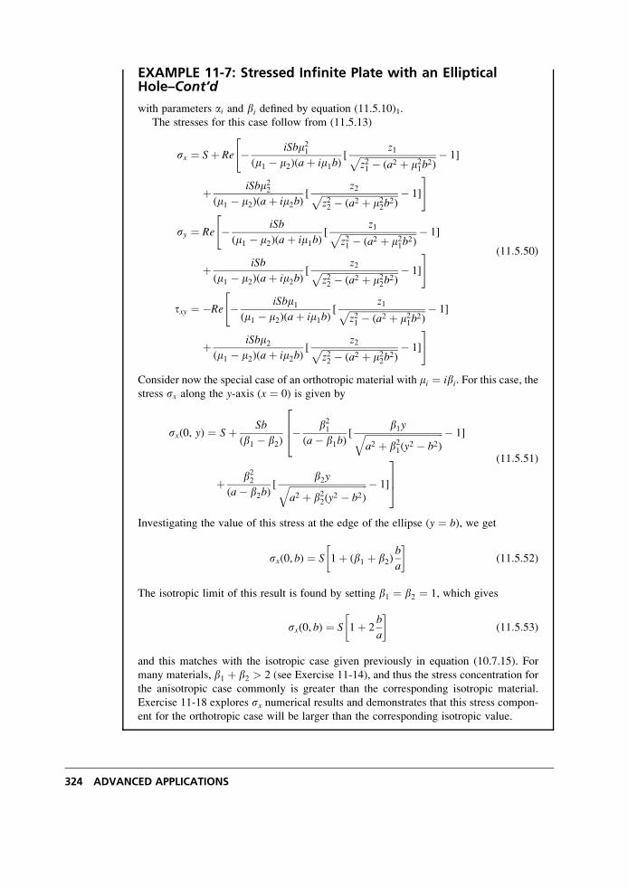
EXAMPLE 11-7: Stressed Infinite Plate with an EllipticalHole–Cont’d
with parameters ai and bi defined by equation (11.5.10)1.
The stresses for this case follow from (11.5.13)
sx ¼ Sþ Re � iSbm21(m1 � m2)(aþ im1b)
[z1ffiffiffiffiffiffiffiffiffiffiffiffiffiffiffiffiffiffiffiffiffiffiffiffiffiffiffiffiffiffiffiffi
z21 � (a2 þ m21b2)p � 1]
"
þ iSbm22(m1 � m2)(aþ im2b)
[z2ffiffiffiffiffiffiffiffiffiffiffiffiffiffiffiffiffiffiffiffiffiffiffiffiffiffiffiffiffiffiffiffi
z22 � (a2 þ m22b2)p � 1]
#
sy ¼ Re � iSb
(m1 � m2)(aþ im1b)[
z1ffiffiffiffiffiffiffiffiffiffiffiffiffiffiffiffiffiffiffiffiffiffiffiffiffiffiffiffiffiffiffiffiz21 � (a2 þ m21b2)
p � 1]
"
þ iSb
(m1 � m2)(aþ im2b)[
z2ffiffiffiffiffiffiffiffiffiffiffiffiffiffiffiffiffiffiffiffiffiffiffiffiffiffiffiffiffiffiffiffiz22 � (a2 þ m22b2)
p � 1]
#
txy ¼ �Re � iSbm1(m1 � m2)(aþ im1b)
[z1ffiffiffiffiffiffiffiffiffiffiffiffiffiffiffiffiffiffiffiffiffiffiffiffiffiffiffiffiffiffiffiffi
z21 � (a2 þ m21b2)p � 1]
"
þ iSbm2(m1 � m2)(aþ im2b)
[z2ffiffiffiffiffiffiffiffiffiffiffiffiffiffiffiffiffiffiffiffiffiffiffiffiffiffiffiffiffiffiffiffi
z22 � (a2 þ m22b2)p � 1]
#
(11:5:50)
Consider now the special case of an orthotropic material with mi ¼ ibi. For this case, thestress sx along the y-axis (x ¼ 0) is given by
sx(0, y) ¼ Sþ Sb
(b1 � b2)� b21(a� b1b)
[b1yffiffiffiffiffiffiffiffiffiffiffiffiffiffiffiffiffiffiffiffiffiffiffiffiffiffiffiffiffiffiffiffiffi
a2 þ b21(y2 � b2)q � 1]
264
þ b22(a� b2b)
[b2yffiffiffiffiffiffiffiffiffiffiffiffiffiffiffiffiffiffiffiffiffiffiffiffiffiffiffiffiffiffiffiffiffi
a2 þ b22(y2 � b2)q � 1]
375
(11:5:51)
Investigating the value of this stress at the edge of the ellipse (y ¼ b), we get
sx(0, b) ¼ S 1þ (b1 þ b2)b
a
� �(11:5:52)
The isotropic limit of this result is found by setting b1 ¼ b2 ¼ 1, which gives
sx(0, b) ¼ S 1þ 2b
a
� �(11:5:53)
and this matches with the isotropic case given previously in equation (10.7.15). For
many materials, b1 þ b2 > 2 (see Exercise 11-14), and thus the stress concentration for
the anisotropic case commonly is greater than the corresponding isotropic material.
Exercise 11-18 explores sx numerical results and demonstrates that this stress compon-
ent for the orthotropic case will be larger than the corresponding isotropic value.
324 ADVANCED APPLICATIONS
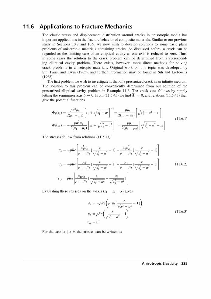
11.6 Applications to Fracture Mechanics
The elastic stress and displacement distribution around cracks in anisotropic media has
important applications in the fracture behavior of composite materials. Similar to our previous
study in Sections 10.8 and 10.9, we now wish to develop solutions to some basic plane
problems of anisotropic materials containing cracks. As discussed before, a crack can be
regarded as the limiting case of an elliptical cavity as one axis is reduced to zero. Thus,
in some cases the solution to the crack problem can be determined from a correspond-
ing elliptical cavity problem. There exists, however, more direct methods for solving
crack problems in anisotropic materials. Original work on this topic was developed by
Sih, Paris, and Irwin (1965), and further information may be found in Sih and Liebowitz
(1968).
The first problem we wish to investigate is that of a pressurized crack in an infinite medium.
The solution to this problem can be conveniently determined from our solution of the
pressurized elliptical cavity problem in Example 11-6. The crack case follows by simply
letting the semiminor axis b ! 0. From (11.5.45) we find A1 ¼ 0, and relations (11.5.43) then
give the potential functions
F1(z1) ¼ pa2m22(m1 � m2)
z1 þffiffiffiffiffiffiffiffiffiffiffiffiffiffiz21 � a2
q� ��1
¼ �pm22(m1 � m2)
ffiffiffiffiffiffiffiffiffiffiffiffiffiffiz21 � a2
q� z1
� �
F2(z2) ¼ � pa2m12(m1 � m2)
z2 þffiffiffiffiffiffiffiffiffiffiffiffiffiffiz22 � a2
q� ��1
¼ pm12(m1 � m2)
ffiffiffiffiffiffiffiffiffiffiffiffiffiffiz22 � a2
q� z2
� � (11:6:1)
The stresses follow from relations (11.5.13)
sx ¼ �pRem21m2
m1 � m2[
z1ffiffiffiffiffiffiffiffiffiffiffiffiffiffiz21 � a2
p � 1]� m1m22
m1 � m2[
z2ffiffiffiffiffiffiffiffiffiffiffiffiffiffiz22 � a2
p � 1]
" #
sy ¼ �pRem2
m1 � m2[
z1ffiffiffiffiffiffiffiffiffiffiffiffiffiffiz21 � a2
p � 1]� m1m1 � m2
[z2ffiffiffiffiffiffiffiffiffiffiffiffiffiffi
z22 � a2p � 1]
" #
txy ¼ pRem1m2
m1 � m2[
z1ffiffiffiffiffiffiffiffiffiffiffiffiffiffiz21 � a2
p � z2ffiffiffiffiffiffiffiffiffiffiffiffiffiffiz22 � a2
p ]
" #(11:6:2)
Evaluating these stresses on the x-axis (z1 ¼ z2 ¼ x) gives
sx ¼ �pRe m1m2[xffiffiffiffiffiffiffiffiffiffiffiffiffiffiffi
x2 � a2p � 1]
� �
sy ¼ pRexffiffiffiffiffiffiffiffiffiffiffiffiffiffiffi
x2 � a2p � 1
� �txy ¼ 0
(11:6:3)
For the case jx1j > a, the stresses can be written as
Anisotropic Elasticity 325
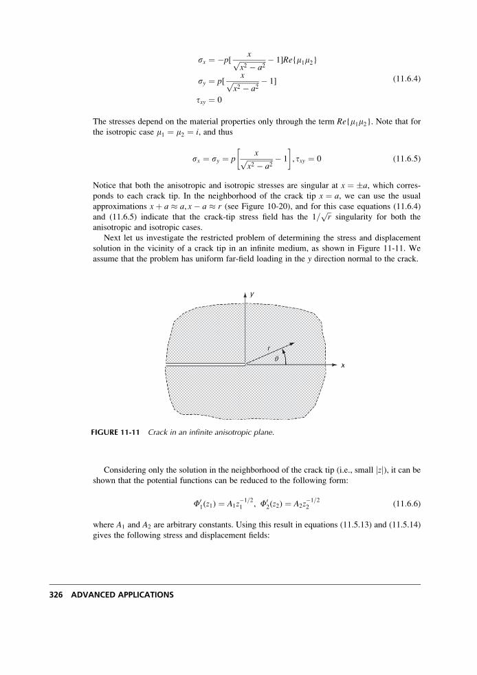
sx ¼ �p[xffiffiffiffiffiffiffiffiffiffiffiffiffiffiffi
x2 � a2p � 1]Re{m1m2}
sy ¼ p[xffiffiffiffiffiffiffiffiffiffiffiffiffiffiffi
x2 � a2p � 1]
txy ¼ 0
(11:6:4)
The stresses depend on the material properties only through the term Re{m1m2}. Note that forthe isotropic case m1 ¼ m2 ¼ i, and thus
sx ¼ sy ¼ pxffiffiffiffiffiffiffiffiffiffiffiffiffiffiffi
x2 � a2p � 1
� �, txy ¼ 0 (11:6:5)
Notice that both the anisotropic and isotropic stresses are singular at x ¼ �a, which corres-
ponds to each crack tip. In the neighborhood of the crack tip x ¼ a, we can use the usual
approximations xþ a � a, x� a � r (see Figure 10-20), and for this case equations (11.6.4)
and (11.6.5) indicate that the crack-tip stress field has the 1=ffiffir
psingularity for both the
anisotropic and isotropic cases.
Next let us investigate the restricted problem of determining the stress and displacement
solution in the vicinity of a crack tip in an infinite medium, as shown in Figure 11-11. We
assume that the problem has uniform far-field loading in the y direction normal to the crack.
Considering only the solution in the neighborhood of the crack tip (i.e., small jzj), it can be
shown that the potential functions can be reduced to the following form:
F01(z1) ¼ A1z
�1=21 , F0
2(z2) ¼ A2z�1=22 (11:6:6)
where A1 and A2 are arbitrary constants. Using this result in equations (11.5.13) and (11.5.14)
gives the following stress and displacement fields:
FIGURE 11-11 Crack in an infinite anisotropic plane.
326 ADVANCED APPLICATIONS
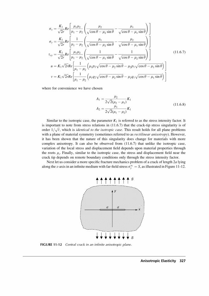
sx ¼ K1ffiffiffiffiffi2r
p Rem1m2
m1 � m2
m2ffiffiffiffiffiffiffiffiffiffiffiffiffiffiffiffiffiffiffiffiffiffiffiffiffiffiffiffiffifficos y� m2 sin y
p � m1ffiffiffiffiffiffiffiffiffiffiffiffiffiffiffiffiffiffiffiffiffiffiffiffiffiffiffiffiffifficos y� m1 sin y
p !" #
sy ¼ K1ffiffiffiffiffi2r
p Re1
m1 � m2
m1ffiffiffiffiffiffiffiffiffiffiffiffiffiffiffiffiffiffiffiffiffiffiffiffiffiffiffiffiffifficos y� m2 sin y
p � m2ffiffiffiffiffiffiffiffiffiffiffiffiffiffiffiffiffiffiffiffiffiffiffiffiffiffiffiffiffifficos y� m1 sin y
p !" #
txy ¼ K1ffiffiffiffiffi2r
p Rem1m2
m1 � m2
1ffiffiffiffiffiffiffiffiffiffiffiffiffiffiffiffiffiffiffiffiffiffiffiffiffiffiffiffiffifficos y� m1 sin y
p � 1ffiffiffiffiffiffiffiffiffiffiffiffiffiffiffiffiffiffiffiffiffiffiffiffiffiffiffiffiffifficos y� m2 sin y
p !" #
u ¼ K1
ffiffiffiffiffi2r
pRe
1
m1 � m2m1p2
ffiffiffiffiffiffiffiffiffiffiffiffiffiffiffiffiffiffiffiffiffiffiffiffiffiffiffiffiffifficos y� m2 sin y
p� m2p1
ffiffiffiffiffiffiffiffiffiffiffiffiffiffiffiffiffiffiffiffiffiffiffiffiffiffiffiffiffifficos y� m1 sin y
p �� �
v ¼ K1
ffiffiffiffiffi2r
pRe
1
m1 � m2m1q2
ffiffiffiffiffiffiffiffiffiffiffiffiffiffiffiffiffiffiffiffiffiffiffiffiffiffiffiffiffifficos y� m2 sin y
p� m2q1
ffiffiffiffiffiffiffiffiffiffiffiffiffiffiffiffiffiffiffiffiffiffiffiffiffiffiffiffiffifficos y� m1 sin y
p �� �
(11:6:7)
where for convenience we have chosen
A1 ¼ m22ffiffiffi2
p(m2 � m1)
K1
A2 ¼ m12ffiffiffi2
p(m1 � m2)
K1
(11:6:8)
Similar to the isotropic case, the parameter K1 is referred to as the stress intensity factor. It
is important to note from stress relations in (11.6.7) that the crack-tip stress singularity is of
order 1=ffiffir
p, which is identical to the isotropic case. This result holds for all plane problems
with a plane of material symmetry (sometimes referred to as rectilinear anisotropy). However,it has been shown that the nature of this singularity does change for materials with more
complex anisotropy. It can also be observed from (11.6.7) that unlike the isotropic case,
variation of the local stress and displacement field depends upon material properties through
the roots mi. Finally, similar to the isotropic case, the stress and displacement field near the
crack tip depends on remote boundary conditions only through the stress intensity factor.
Next let us consider a more specific fracture mechanics problem of a crack of length 2a lyingalong the x-axis in an infinite mediumwith far-field stress s1y ¼ S, as illustrated in Figure 11-12.
FIGURE 11-12 Central crack in an infinite anisotropic plane.
Anisotropic Elasticity 327
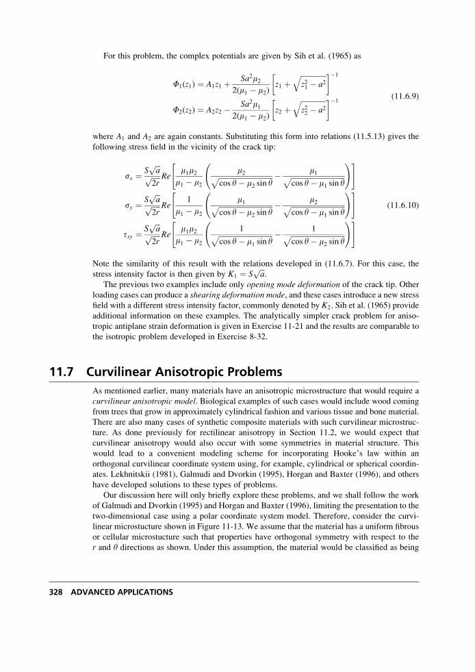
For this problem, the complex potentials are given by Sih et al. (1965) as
F1(z1) ¼ A1z1 þ Sa2m22(m1 � m2)
z1 þffiffiffiffiffiffiffiffiffiffiffiffiffiffiz21 � a2
q� ��1
F2(z2) ¼ A2z2 � Sa2m12(m1 � m2)
z2 þffiffiffiffiffiffiffiffiffiffiffiffiffiffiz22 � a2
q� ��1(11:6:9)
where A1 and A2 are again constants. Substituting this form into relations (11.5.13) gives the
following stress field in the vicinity of the crack tip:
sx ¼ Sffiffiffia
pffiffiffiffiffi2r
p Rem1m2
m1 � m2
m2ffiffiffiffiffiffiffiffiffiffiffiffiffiffiffiffiffiffiffiffiffiffiffiffiffiffiffiffiffifficos y� m2 sin y
p � m1ffiffiffiffiffiffiffiffiffiffiffiffiffiffiffiffiffiffiffiffiffiffiffiffiffiffiffiffiffifficos y� m1 sin y
p !" #
sy ¼ Sffiffiffia
pffiffiffiffiffi2r
p Re1
m1 � m2
m1ffiffiffiffiffiffiffiffiffiffiffiffiffiffiffiffiffiffiffiffiffiffiffiffiffiffiffiffiffifficos y� m2 sin y
p � m2ffiffiffiffiffiffiffiffiffiffiffiffiffiffiffiffiffiffiffiffiffiffiffiffiffiffiffiffiffifficos y� m1 sin y
p !" #
txy ¼ Sffiffiffia
pffiffiffiffiffi2r
p Rem1m2
m1 � m2
1ffiffiffiffiffiffiffiffiffiffiffiffiffiffiffiffiffiffiffiffiffiffiffiffiffiffiffiffiffifficos y� m1 sin y
p � 1ffiffiffiffiffiffiffiffiffiffiffiffiffiffiffiffiffiffiffiffiffiffiffiffiffiffiffiffiffifficos y� m2 sin y
p !" #
(11:6:10)
Note the similarity of this result with the relations developed in (11.6.7). For this case, the
stress intensity factor is then given by K1 ¼ Sffiffiffia
p.
The previous two examples include only opening mode deformation of the crack tip. Other
loading cases can produce a shearing deformation mode, and these cases introduce a new stress
field with a different stress intensity factor, commonly denoted by K2. Sih et al. (1965) provide
additional information on these examples. The analytically simpler crack problem for aniso-
tropic antiplane strain deformation is given in Exercise 11-21 and the results are comparable to
the isotropic problem developed in Exercise 8-32.
11.7 Curvilinear Anisotropic Problems
As mentioned earlier, many materials have an anisotropic microstructure that would require a
curvilinear anisotropic model. Biological examples of such cases would include wood coming
from trees that grow in approximately cylindrical fashion and various tissue and bone material.
There are also many cases of synthetic composite materials with such curvilinear microstruc-
ture. As done previously for rectilinear anisotropy in Section 11.2, we would expect that
curvilinear anisotropy would also occur with some symmetries in material structure. This
would lead to a convenient modeling scheme for incorporating Hooke’s law within an
orthogonal curvilinear coordinate system using, for example, cylindrical or spherical coordin-
ates. Lekhnitskii (1981), Galmudi and Dvorkin (1995), Horgan and Baxter (1996), and others
have developed solutions to these types of problems.
Our discussion here will only briefly explore these problems, and we shall follow the work
of Galmudi and Dvorkin (1995) and Horgan and Baxter (1996), limiting the presentation to the
two-dimensional case using a polar coordinate system model. Therefore, consider the curvi-
linear microstucture shown in Figure 11-13. We assume that the material has a uniform fibrous
or cellular microstucture such that properties have orthogonal symmetry with respect to the
r and y directions as shown. Under this assumption, the material would be classified as being
328 ADVANCED APPLICATIONS
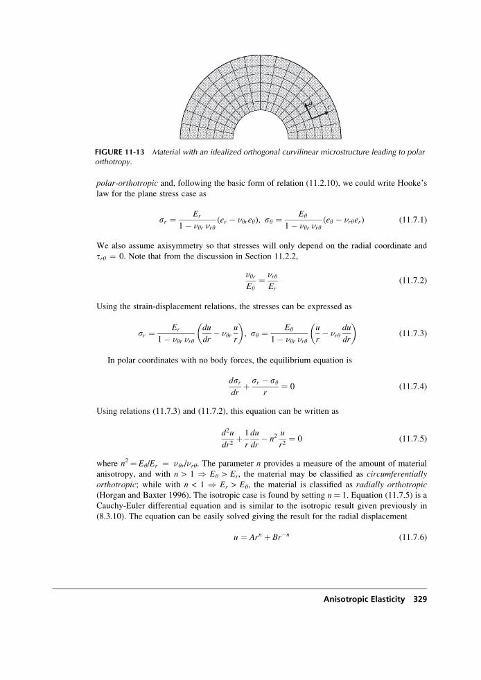
polar-orthotropic and, following the basic form of relation (11.2.10), we could write Hooke’s
law for the plane stress case as
sr ¼ Er
1� �yr �ry(er � �yrey), sy ¼ Ey
1� �yr �ry(ey � �ryer) (11:7:1)
We also assume axisymmetry so that stresses will only depend on the radial coordinate and
try ¼ 0. Note that from the discussion in Section 11.2.2,
�yrEy
¼ �ryEr
(11:7:2)
Using the strain-displacement relations, the stresses can be expressed as
sr ¼ Er
1� �yr �ry
du
dr� �yr
u
r
� �, sy ¼ Ey
1� �yr �ry
u
r� �ry
du
dr
� �(11:7:3)
In polar coordinates with no body forces, the equilibrium equation is
dsrdr
þ sr � syr
¼ 0 (11:7:4)
Using relations (11.7.3) and (11.7.2), this equation can be written as
d2u
dr2þ 1
r
du
dr� n2
u
r2¼ 0 (11:7:5)
where n2¼ Ey/Er ¼ �yr/�ry. The parameter n provides a measure of the amount of material
anisotropy, and with n > 1 ) Ey > Er, the material may be classified as circumferentiallyorthotropic; while with n < 1 ) Er > Ey, the material is classified as radially orthotropic(Horgan and Baxter 1996). The isotropic case is found by setting n¼ 1. Equation (11.7.5) is a
Cauchy-Euler differential equation and is similar to the isotropic result given previously in
(8.3.10). The equation can be easily solved giving the result for the radial displacement
u ¼ Arn þ Br�n (11:7:6)
FIGURE 11-13 Material with an idealized orthogonal curvilinear microstructure leading to polarorthotropy.
Anisotropic Elasticity 329
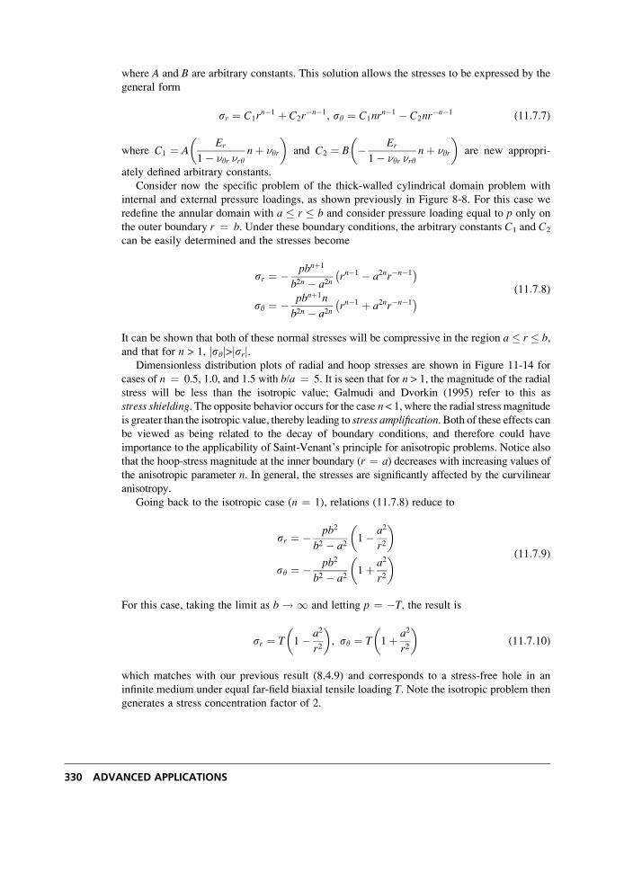
where A and B are arbitrary constants. This solution allows the stresses to be expressed by the
general form
sr ¼ C1rn�1 þ C2r
�n�1, sy ¼ C1nrn�1 � C2nr
�n�1 (11:7:7)
where C1 ¼ AEr
1� �yr �rynþ �yr
� �and C2 ¼ B � Er
1� �yr �rynþ �yr
� �are new appropri-
ately defined arbitrary constants.
Consider now the specific problem of the thick-walled cylindrical domain problem with
internal and external pressure loadings, as shown previously in Figure 8-8. For this case we
redefine the annular domain with a � r � b and consider pressure loading equal to p only on
the outer boundary r ¼ b. Under these boundary conditions, the arbitrary constants C1 and C2
can be easily determined and the stresses become
sr ¼ � pbnþ1
b2n � a2nrn�1 � a2nr�n�1�
sy ¼ � pbnþ1n
b2n � a2nrn�1 þ a2nr�n�1� (11:7:8)
It can be shown that both of these normal stresses will be compressive in the region a � r � b,and that for n > 1, jsyj>jsrj.
Dimensionless distribution plots of radial and hoop stresses are shown in Figure 11-14 for
cases of n ¼ 0.5, 1.0, and 1.5 with b/a ¼ 5. It is seen that for n > 1, the magnitude of the radial
stress will be less than the isotropic value; Galmudi and Dvorkin (1995) refer to this as
stress shielding. The opposite behavior occurs for the case n < 1, where the radial stress magnitude
is greater than the isotropic value, thereby leading to stress amplification. Both of these effects canbe viewed as being related to the decay of boundary conditions, and therefore could have
importance to the applicability of Saint-Venant’s principle for anisotropic problems. Notice also
that the hoop-stress magnitude at the inner boundary (r ¼ a) decreases with increasing values ofthe anisotropic parameter n. In general, the stresses are significantly affected by the curvilinear
anisotropy.
Going back to the isotropic case (n ¼ 1), relations (11.7.8) reduce to
sr ¼ � pb2
b2 � a21� a2
r2
� �
sy ¼ � pb2
b2 � a21þ a2
r2
� � (11:7:9)
For this case, taking the limit as b ! 1 and letting p ¼ �T, the result is
sr ¼ T 1� a2
r2
� �, sy ¼ T 1þ a2
r2
� �(11:7:10)
which matches with our previous result (8.4.9) and corresponds to a stress-free hole in an
infinite medium under equal far-field biaxial tensile loading T. Note the isotropic problem then
generates a stress concentration factor of 2.
330 ADVANCED APPLICATIONS
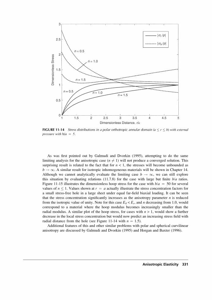
As was first pointed out by Galmudi and Dvorkin (1995), attempting to do the same
limiting analysis for the anisotropic case (n 6¼ 1) will not produce a converged solution. This
surprising result is related to the fact that for n < 1, the stresses will become unbounded as
b ! 1. A similar result for isotropic inhomogeneous materials will be shown in Chapter 14.
Although we cannot analytically evaluate the limiting case b ! 1, we can still explore
this situation by evaluating relations (11.7.8) for the case with large but finite b/a ratios.
Figure 11-15 illustrates the dimensionless hoop stress for the case with b/a ¼ 50 for several
values of n � 1. Values shown at r ¼ a actually illustrate the stress concentration factors for
a small stress-free hole in a large sheet under equal far-field biaxial loading. It can be seen
that the stress concentration significantly increases as the anisotropy parameter n is reduced
from the isotropic value of unity. Note for this case Ey < Er, and n decreasing from 1.0, would
correspond to a material where the hoop modulus becomes increasingly smaller than the
radial modulus. A similar plot of the hoop stress, for cases with n > 1, would show a further
decrease in the local stress concentration but would now predict an increasing stress field with
radial distance from the hole (see Figure 11-14 with n ¼ 1.5).
Additional features of this and other similar problems with polar and spherical curvilinear
anisotropy are discussed by Galmudi and Dvorkin (1995) and Horgan and Baxter (1996).
FIGURE 11-14 Stress distributions in a polar orthotropic annular domain (a � r � b) with externalpressure with b/a ¼ 5.
Anisotropic Elasticity 331
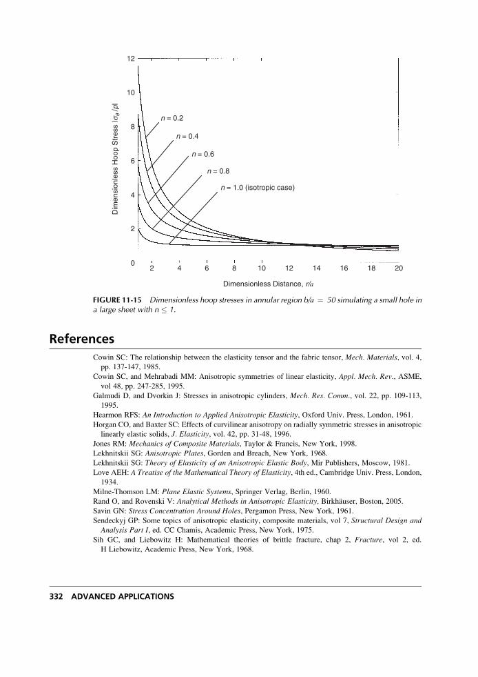
References
Cowin SC: The relationship between the elasticity tensor and the fabric tensor, Mech. Materials, vol. 4,pp. 137-147, 1985.
Cowin SC, and Mehrabadi MM: Anisotropic symmetries of linear elasticity, Appl. Mech. Rev., ASME,
vol 48, pp. 247-285, 1995.
Galmudi D, and Dvorkin J: Stresses in anisotropic cylinders, Mech. Res. Comm., vol. 22, pp. 109-113,1995.
Hearmon RFS: An Introduction to Applied Anisotropic Elasticity, Oxford Univ. Press, London, 1961.
Horgan CO, and Baxter SC: Effects of curvilinear anisotropy on radially symmetric stresses in anisotropic
linearly elastic solids, J. Elasticity, vol. 42, pp. 31-48, 1996.Jones RM: Mechanics of Composite Materials, Taylor & Francis, New York, 1998.
Lekhnitskii SG: Anisotropic Plates, Gorden and Breach, New York, 1968.
Lekhnitskii SG: Theory of Elasticity of an Anisotropic Elastic Body, Mir Publishers, Moscow, 1981.
Love AEH: A Treatise of the Mathematical Theory of Elasticity, 4th ed., Cambridge Univ. Press, London,
1934.
Milne-Thomson LM: Plane Elastic Systems, Springer Verlag, Berlin, 1960.Rand O, and Rovenski V: Analytical Methods in Anisotropic Elasticity, Birkhauser, Boston, 2005.Savin GN: Stress Concentration Around Holes, Pergamon Press, New York, 1961.
Sendeckyj GP: Some topics of anisotropic elasticity, composite materials, vol 7, Structural Design andAnalysis Part I, ed. CC Chamis, Academic Press, New York, 1975.
Sih GC, and Liebowitz H: Mathematical theories of brittle fracture, chap 2, Fracture, vol 2, ed.
H Liebowitz, Academic Press, New York, 1968.
n = 0.2
n = 0.4
n = 0.6
n = 0.8
n = 1.0 (isotropic case)
12
10
8
6
4
Dim
ensi
onle
ss H
oop
Str
ess
|sq
/p|
2
02 4 6 8 10 12
Dimensionless Distance, r/a
14 16 18 20
FIGURE 11-15 Dimensionless hoop stresses in annular region b/a ¼ 50 simulating a small hole ina large sheet with n � 1.
332 ADVANCED APPLICATIONS
Sih GC, Paris PC, and Irwin GR: On cracks in rectilinearly anisotropic bodies, Intl. J. Fracture Mech., vol1, pp. 189-203, 1965.
Swanson SR: Introduction to Design and Analysis with Advanced Composite Materials, Prentice Hall,
Upper Saddle River, NJ, 1997.
Ting TCT: Generalized Cowin-Mehrabadi theorems and a direct proof that the number of linear elastic
symmetries is eight, Intl. J. Solids Structures, vol. 40, pp. 7129-7142, 2003.Ting TCT: Anisotropic Elasticity, Theory and Applications, Oxford Univ. Press, New York, 1996a.
Ting TCT: Positive definiteness of anisotropic elastic constants, Math. Mech. of Solids, vol 1, pp. 301-314, 1996b.
Zheng QS, and Spencer AJM: Tensors which characterize anisotropes, Intl. J. Eng. Sci., vol 31, pp. 679-693, 1993.
Exercises
11-1. From strain energy arguments in Section 6.1, it was found that@sij@ekl
¼ @skl@eij
. Show
that these results imply that Cij ¼ Cji, therefore justifying that only 21
independent elastic moduli are needed to characterize the most general anisotropic
material.
11-2. Using material symmetry through 1808 rotations about each of the three coordinate
axes, explicitly show the reduction of the elastic stiffness matrix to nine
independent components for orthotropic materials. Also demonstrate that after two
rotations, the third transformation is actually already satisfied.
11-3 A transversely isotropic material with an x3-axis of symmetry was specified by the
elasticity matrix given in equation (11.2.12). Under an arbitrary y-rotation about the
x3-axis given by relation (11.2.11), all components of this elasticity matrix should remain
the same. Explicitly show this property for the 55 and 22 components of the C matrix.
Use the translation relation (11.1.6) and the given structure of the C matrix such as
C16 ¼ C1112 ¼ 0, C44 ¼ C55� � �11-4. Verify the inequality restrictions on the elastic moduli for orthotropic, transversely
isotropic, and isotropic materials given by relations (11.3.3), (11.3.4), and (11.3.5).
11-5. For the orthotropic case, show that by using arguments of a positive definite strain
energy function, �2ij < (Ei=Ej). Next, using typical values for E1 and E2 from Table 11-1,
justify that this theory could allow the unexpected result that �12 > 1.
11-6. For the torsion of cylinders discussed in Section 11.4, show that with
sx ¼ sy ¼ sz ¼ txy ¼ 0, the compatibility equations yield
� @
@x(S44tyz þ S45txz)þ @
@y(S54tyz þ S55txz) ¼ C
where C is a constant.
11-7. In terms of the stress function c, the torsion problem was governed by equation
(11.4.9)
S44cxx � 2S45cxy þ S55cyy ¼ �2
Anisotropic Elasticity 333
Show that the homogeneous counterpart of this equation may be written as
@
@y� m1
@
@x
� �@
@y� m2
@
@x
� �c ¼ 0
where m1, 2 are the roots of the characteristic equation
S55m2 � 2S45mþ S44 ¼ 0
11-8. Explicitly justify relationships (11.5.3) between the compliances of the plane stress
and plane strain theories.
11-9. Investigate case 2 (m1 ¼ m2) in equation (11.5.10), and determine the general form
of the Airy stress function. Show that this case is actually an isotropic formulation.
11-10. Determine the roots of the characteristic equation (11.5.7) for S-Glass/Epoxy material
with properties given in Table 11-1. Justify that they are purely imaginary.
11-11. Recall that for the plane anisotropic problem, the Airy stress function was found to be
f ¼ F1(z1)þ F1(z1)þ F2(z2)þ F2(z2)
where z1 ¼ xþ m1y and z2 ¼ xþ m2y. Explicitly show that the in-plane stresses are
given by
sx ¼ 2Re[m21F001(z1)þ m22F
002(z2)]
sy ¼ 2Re[F001(z1)þ F
002(z2)]
txy ¼ �2Re[m1F001(z1)þ m2F
002(z2)]
11-12. For the plane stress case, in terms of the two complex potentials F1 and F2, compute
the two in-plane displacements u and v and thus justify relations (11.5.14).
11-13. Determine the polar coordinate stresses and displacements in terms of the complex
potentials F1 and F2, as given by equations (11.5.16) and (11.5.17).
11-14*. For the plane problem with an orthotropic material, show that the characteristic
equation (11.5.7) reduces to the quadratic equation in m2
S11m4 þ (2S12 þ S66)m2 þ S22 ¼ 0
Explicitly solve this equation for the roots mi, and show that they are purely complex
and thus can be written as m1, 2 ¼ ib1, 2, where
b21, 2 ¼ � 1
2S11�(2S12 þ S66)�
ffiffiffiffiffiffiffiffiffiffiffiffiffiffiffiffiffiffiffiffiffiffiffiffiffiffiffiffiffiffiffiffiffiffiffiffiffiffiffiffiffiffiffiffiffiffi(2S12 þ S66)
2 � 4S11S22
q�
Justify the isotropic case where b1, 2 ¼ 1. Finally, determine b1, 2 for each of the four
composite materials given in Table 11-1.
11-15. Consider an anisotropic monoclinic material symmetric about the x-y-plane(see Figure 11-2) and subject to an antiplane deformation specified by u ¼ v ¼ 0,
334 ADVANCED APPLICATIONS
w ¼ w(x, y). Show that in the absence of body forces, the out-of-plane displacement
must satisfy the Navier equation
C55
@2w
@x2þ 2C45
@2w
@x@yþ C44
@2w
@y2¼ 0
Next looking for solutions that are of the form w¼ F(x þ �y), show that this problem
is solved by
w ¼ 2Re{F(z*)}
txz ¼ 2Re{(mC45 þ C55)F0(z*)}
tyz ¼ 2Re{(mC44 þ C45)F0(z*)}
where z* ¼ x þ �y and m are the roots of the equation C44�2 þ 2C45� þ C55 ¼ 0.
Note that for this case, positive definite strain energy implies that C44C55 > C452;
therefore the roots will occur in complex conjugate pairs.
11-16*. For Example 11-5, consider the case of only a normal boundary load (X ¼ 0), and
assume that the material is orthotropic with mi ¼ ibi (see Exercise 11-14). Show that
the resulting stress field is given by
sr ¼ � Yb1b2(b1 þ b2) sin y
pr( cos2 yþ b21 sin2 y)( cos2 yþ b22 sin
2 y), sy ¼ try ¼ 0
Next compare the stress component sr with the corresponding isotropic value by
plotting the stress contours sr=Y ¼ constant for each case. Use orthotropic material
values for the Carbon/Epoxy composite given in Table 11-1, and compare with the
corresponding isotropic case.
11-17*. Consider the case of the pressurized circular hole in an anisotropic sheet. Using
orthotropic material properties given in Table 11-1 for Carbon/Epoxy, compute and
plot the boundary hoop stress sy as a function of y. Compare with the isotropic case.
11-18*. Investigate the case of a circular hole of radius a in Example 11-7. Use orthotropic
material properties given in Table 11-1 for Carbon/Epoxy with the 1-axis along the
direction of loading. Compute and plot the stress sx(0, y) for y > a. Also compare
with the corresponding isotropic case.
11-19. Consider the elliptical hole problem in Example 11-7. By letting a ! 0, determine the
stress field for the case where the hole reduces to a line crack of length 2b. Demonstrate
the nature of the singularity for this case.
11-20. The potentials
F1(z1) ¼ A1z1 þ Sa2m22(m1 � m2)
z1 þffiffiffiffiffiffiffiffiffiffiffiffiffiffiz21 � a2
q� ��1
F2(z2) ¼ A2z2 � Sa2m12(m1 � m2)
z2 þffiffiffiffiffiffiffiffiffiffiffiffiffiffiz22 � a2
q� ��1
Anisotropic Elasticity 335
were proposed to solve the plane extension of an anisotropic panel containing a crack of
length 2a (see Figure 11-12). Recall that the constants A1 and A2 correspond to the
uniform tension case, and for stress S in the y direction
A1 ¼ (a22 þ b22)S
2[(a2 � a1)2 þ (b22 � b21)]
A2 ¼ (a21 � b21 � 2a1a2)S
2[(a2 � a1)2 þ (b22 � b21)]þ i
[a2(a21 � b21)� a1(a22 � b22)]S
2b2[(a2 � a1)2 þ (b22 � b21)]
a. Determine the general stress field, and verify the far-field behavior.
b. Show that the stress field is singular at each crack tip.
c. Using the limiting procedures as related to Figure 10-20, verify that the crack-tip
stress field is given by (11.6.10).
11-21. Consider the case of a crack problem in an anisotropic monoclinic material under anti-
plane deformation as described in Exercise 11-15. Following relation (11.6.6), choose the
complex potential form as F(z*) ¼ Affiffiffiffiz*
p, where A ¼ � ffiffiffi
2p
K3m=(C55 þ mC45) and K3 is a
real constant. Using this form, show that the nonzero displacement and stresses in the
vicinity of the crack tip (see Figure 11-11) are given by
w ¼ K3
ffiffiffiffiffi2r
pRe
ffiffiffiffiffiffiffiffiffiffiffiffiffiffiffiffiffiffiffiffiffiffiffiffiffiffiffifficos yþ m sin y
pC45 þ mC44
�
txz ¼ � K3ffiffiffiffiffi2r
p Remffiffiffiffiffiffiffiffiffiffiffiffiffiffiffiffiffiffiffiffiffiffiffiffiffiffiffi
cos yþ msin yp�
tyz ¼ K3ffiffiffiffiffi2r
p Re1ffiffiffiffiffiffiffiffiffiffiffiffiffiffiffiffiffiffiffiffiffiffiffiffiffiffiffi
cos yþ msin yp�
Note that the parameter K3 will be related to the stress intensity factor for this case.
Verify that shear stress tyz vanishes on each side of the crack face, y ¼ +p. Theseresults can be compared to the corresponding solution for the isotropic case given in
Exercise 8-32.
11-22. Explicitly develop the governing Navier equation (11.7.5) for the polar orthotropic
problem. Verify that its solution is given by (11.7.6) and show how this leads to the
stress solution (11.7.7). Finally, confirm that the problem with only external pressure
loading is given by (11.7.8).
336 ADVANCED APPLICATIONS
12 Thermoelasticity
Many important stress analysis problems involve structures that are subjected to both mechan-
ical and thermal loadings. Thermal effects within an elastic solid produce heat transfer by
conduction, and this flow of thermal energy establishes a temperature field within the material.
Most solids exhibit a volumetric change with temperature variation, and thus the presence of a
temperature distribution generally induces stresses created from boundary or internal con-
straints. If the temperature variation is sufficiently high, these stresses can reach levels that
may lead to structural failure, especially for brittle materials. Thus, for many problems
involving high temperature variation, the knowledge of thermal stress analysis can be very
important.
The purpose of this chapter is to provide an introduction to thermoelasticity; that is, elasticity
with thermal effects. We develop the basic governing equations for isotropic materials and
investigate several solutions to problems of engineering interest. We have already briefly
discussed the form of Hooke’s law for this case in Section 4.4. More detailed information may
be found in several texts devoted entirely to the subject such as Boley and Weiner (1960),
Nowacki (1962), Parkus (1976), Kovalenko (1969), Nowinski (1978), and Burgreen (1971).
We start our study with some developments of heat conduction in solids and the energy equation.
12.1 Heat Conduction and the Energy Equation
As mentioned, the flow of heat in solids is associated with temperature differences within the
material. This process is governed by the Fourier law of heat conduction, which is the
constitutive relation between the heat flux vector q and the temperature gradient =T. Thistheory formulates a linear relationship that is given by
qi ¼ �kijT, j (12:1:1)
where kij is the thermal conductivity tensor. It can be shown that this tensor is symmetric, that
is, kij ¼ kji. For the isotropic case kij ¼ kdij, and thus
qi ¼ �kT, i (12:1:2)
337
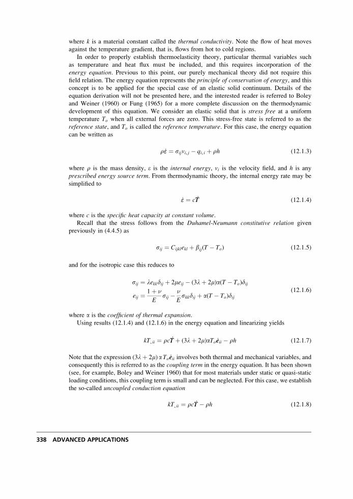
where k is a material constant called the thermal conductivity. Note the flow of heat moves
against the temperature gradient, that is, flows from hot to cold regions.
In order to properly establish thermoelasticity theory, particular thermal variables such
as temperature and heat flux must be included, and this requires incorporation of the
energy equation. Previous to this point, our purely mechanical theory did not require this
field relation. The energy equation represents the principle of conservation of energy, and this
concept is to be applied for the special case of an elastic solid continuum. Details of the
equation derivation will not be presented here, and the interested reader is referred to Boley
and Weiner (1960) or Fung (1965) for a more complete discussion on the thermodynamic
development of this equation. We consider an elastic solid that is stress free at a uniform
temperature To when all external forces are zero. This stress-free state is referred to as the
reference state, and To is called the reference temperature. For this case, the energy equation
can be written as
r _"" ¼ sijvi, j � qi, i þ rh (12:1:3)
where r is the mass density, e is the internal energy, vi is the velocity field, and h is any
prescribed energy source term. From thermodynamic theory, the internal energy rate may be
simplified to
_"" ¼ c _TT (12:1:4)
where c is the specific heat capacity at constant volume.Recall that the stress follows from the Duhamel-Neumann constitutive relation given
previously in (4.4.5) as
sij ¼ Cijklekl þ bij(T � To) (12:1:5)
and for the isotropic case this reduces to
sij ¼ lekkdij þ 2meij � (3lþ 2m)a(T � To)dij
eij ¼ 1þ �
Esij � �
Eskkdij þ a(T � To)dij
(12:1:6)
where a is the coefficient of thermal expansion.Using results (12.1.4) and (12.1.6) in the energy equation and linearizing yields
kT, ii ¼ rc _TT þ (3lþ 2m)aTo _eeii � rh (12:1:7)
Note that the expression (3lþ 2m) aTo _eeii involves both thermal and mechanical variables, and
consequently this is referred to as the coupling term in the energy equation. It has been shown
(see, for example, Boley and Weiner 1960) that for most materials under static or quasi-static
loading conditions, this coupling term is small and can be neglected. For this case, we establish
the so-called uncoupled conduction equation
kT, ii ¼ rc _TT � rh (12:1:8)
338 ADVANCED APPLICATIONS
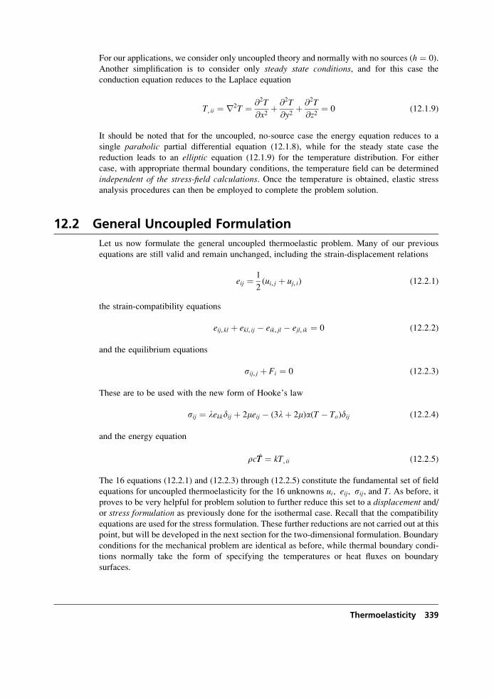
For our applications, we consider only uncoupled theory and normally with no sources (h ¼ 0).
Another simplification is to consider only steady state conditions, and for this case the
conduction equation reduces to the Laplace equation
T, ii ¼ r2T ¼ @2T
@x2þ @2T
@y2þ @2T
@z2¼ 0 (12:1:9)
It should be noted that for the uncoupled, no-source case the energy equation reduces to a
single parabolic partial differential equation (12.1.8), while for the steady state case the
reduction leads to an elliptic equation (12.1.9) for the temperature distribution. For either
case, with appropriate thermal boundary conditions, the temperature field can be determined
independent of the stress-field calculations. Once the temperature is obtained, elastic stress
analysis procedures can then be employed to complete the problem solution.
12.2 General Uncoupled Formulation
Let us now formulate the general uncoupled thermoelastic problem. Many of our previous
equations are still valid and remain unchanged, including the strain-displacement relations
eij ¼ 1
2(ui, j þ uj, i) (12:2:1)
the strain-compatibility equations
eij, kl þ ekl, ij � eik, jl � ejl, ik ¼ 0 (12:2:2)
and the equilibrium equations
sij, j þ Fi ¼ 0 (12:2:3)
These are to be used with the new form of Hooke’s law
sij ¼ lekkdij þ 2meij � (3lþ 2m)a(T � To)dij (12:2:4)
and the energy equation
rc _TT ¼ kT, ii (12:2:5)
The 16 equations (12.2.1) and (12.2.3) through (12.2.5) constitute the fundamental set of field
equations for uncoupled thermoelasticity for the 16 unknowns ui, eij, sij, and T. As before, itproves to be very helpful for problem solution to further reduce this set to a displacement and/or stress formulation as previously done for the isothermal case. Recall that the compatibility
equations are used for the stress formulation. These further reductions are not carried out at this
point, but will be developed in the next section for the two-dimensional formulation. Boundary
conditions for the mechanical problem are identical as before, while thermal boundary condi-
tions normally take the form of specifying the temperatures or heat fluxes on boundary
surfaces.
Thermoelasticity 339
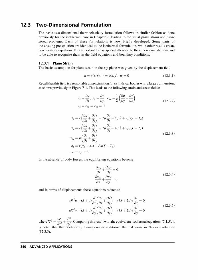
12.3 Two-Dimensional Formulation
The basic two-dimensional thermoelasticity formulation follows in similar fashion as done
previously for the isothermal case in Chapter 7, leading to the usual plane strain and planestress problems. Each of these formulations is now briefly developed. Some parts of
the ensuing presentation are identical to the isothermal formulation, while other results create
new terms or equations. It is important to pay special attention to these new contributions and
to be able to recognize them in the field equations and boundary conditions.
12.3.1 Plane StrainThe basic assumption for plane strain in the x,y-plane was given by the displacement field
u ¼ u(x, y), v ¼ v(x, y), w ¼ 0 (12:3:1)
Recall that this field is a reasonable approximation for cylindrical bodieswith a large zdimension,
as shown previously in Figure 7-1. This leads to the following strain and stress fields:
ex ¼ @u
@x, ey ¼ @v
@y, exy ¼ 1
2
@u
@yþ @v
@x
� �ez ¼ exz ¼ eyz ¼ 0
(12:3:2)
sx ¼ l@u
@xþ @v
@y
� �þ 2m
@u
@x� a(3lþ 2m)(T � To)
sy ¼ l@u
@xþ @v
@y
� �þ 2m
@v
@y� a(3lþ 2m)(T � To)
txy ¼ m@u
@yþ @v
@x
� �sz ¼ v(sx þ sy)� Ea(T � To)
txz ¼ tyz ¼ 0
(12:3:3)
In the absence of body forces, the equilibrium equations become
@sx@x
þ @txy@y
¼ 0
@txy@x
þ @sy@y
¼ 0
(12:3:4)
and in terms of displacements these equations reduce to
mr2uþ (lþ m)@
@x
@u
@xþ @v
@y
� �� (3lþ 2m)a
@T
@x¼ 0
mr2vþ (lþ m)@
@y
@u
@xþ @v
@y
� �� (3lþ 2m)a
@T
@y¼ 0
(12:3:5)
wherer2 ¼ @2
@x2þ @2
@y2. Comparing this resultwith the equivalent isothermal equations (7.1.5), it
is noted that thermoelasticity theory creates additional thermal terms in Navier’s relations
(12.3.5).
340 ADVANCED APPLICATIONS
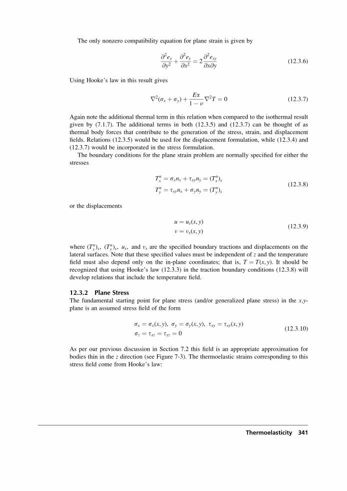
The only nonzero compatibility equation for plane strain is given by
@2ex@y2
þ @2ey@x2
¼ 2@2exy@x@y
(12:3:6)
Using Hooke’s law in this result gives
r2(sx þ sy)þ Ea1� �
r2T ¼ 0 (12:3:7)
Again note the additional thermal term in this relation when compared to the isothermal result
given by (7.1.7). The additional terms in both (12.3.5) and (12.3.7) can be thought of as
thermal body forces that contribute to the generation of the stress, strain, and displacement
fields. Relations (12.3.5) would be used for the displacement formulation, while (12.3.4) and
(12.3.7) would be incorporated in the stress formulation.
The boundary conditions for the plane strain problem are normally specified for either the
stresses
Tnx ¼ sxnx þ txyny ¼ (Tn
x )s
Tny ¼ txynx þ syny ¼ (Tn
y )s(12:3:8)
or the displacements
u ¼ us(x, y)
v ¼ vs(x, y)(12:3:9)
where (Tnx )s, (T
ny )s, us, and vs are the specified boundary tractions and displacements on the
lateral surfaces. Note that these specified values must be independent of z and the temperature
field must also depend only on the in-plane coordinates; that is, T ¼ T(x, y). It should be
recognized that using Hooke’s law (12.3.3) in the traction boundary conditions (12.3.8) will
develop relations that include the temperature field.
12.3.2 Plane StressThe fundamental starting point for plane stress (and/or generalized plane stress) in the x,y-plane is an assumed stress field of the form
sx ¼ sx(x, y), sy ¼ sy(x, y), txy ¼ txy(x, y)
sz ¼ txz ¼ tyz ¼ 0(12:3:10)
As per our previous discussion in Section 7.2 this field is an appropriate approximation for
bodies thin in the z direction (see Figure 7-3). The thermoelastic strains corresponding to this
stress field come from Hooke’s law:
Thermoelasticity 341
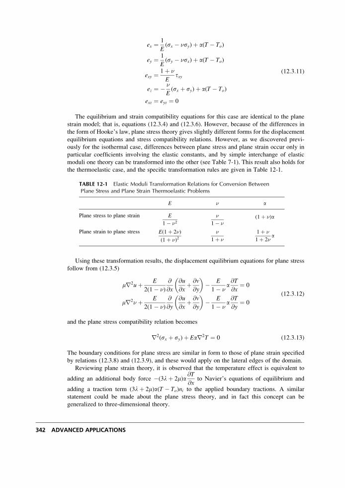
ex ¼ 1
E(sx � �sy)þ a(T � To)
ey ¼ 1
E(sy � �sx)þ a(T � To)
exy ¼ 1þ �
Etxy
ez ¼ � �
E(sx þ sy)þ a(T � To)
exz ¼ eyz ¼ 0
(12:3:11)
The equilibrium and strain compatibility equations for this case are identical to the plane
strain model; that is, equations (12.3.4) and (12.3.6). However, because of the differences in
the form of Hooke’s law, plane stress theory gives slightly different forms for the displacement
equilibrium equations and stress compatibility relations. However, as we discovered previ-
ously for the isothermal case, differences between plane stress and plane strain occur only in
particular coefficients involving the elastic constants, and by simple interchange of elastic
moduli one theory can be transformed into the other (see Table 7-1). This result also holds for
the thermoelastic case, and the specific transformation rules are given in Table 12-1.
Using these transformation results, the displacement equilibrium equations for plane stress
follow from (12.3.5)
mr2uþ E
2(1� �)
@
@x
@u
@xþ @v
@y
� �� E
1� �a@T
@x¼ 0
mr2� þ E
2(1� �)
@
@y
@u
@xþ @v
@y
� �� E
1� �a@T
@y¼ 0
(12:3:12)
and the plane stress compatibility relation becomes
r2(sx þ sy)þ Ear2T ¼ 0 (12:3:13)
The boundary conditions for plane stress are similar in form to those of plane strain specified
by relations (12.3.8) and (12.3.9), and these would apply on the lateral edges of the domain.
Reviewing plane strain theory, it is observed that the temperature effect is equivalent to
adding an additional body force �(3lþ 2m)a@T
@xto Navier’s equations of equilibrium and
adding a traction term (3lþ 2m)a(T � To)ni to the applied boundary tractions. A similar
statement could be made about the plane stress theory, and in fact this concept can be
generalized to three-dimensional theory.
TABLE 12-1 Elastic Moduli Transformation Relations for Conversion BetweenPlane Stress and Plane Strain Thermoelastic Problems
E � a
Plane stress to plane strain E
1� �2�
1� �(1þ �)a
Plane strain to plane stress E(1þ 2�)
(1þ �)2�
1þ �
1þ �
1þ 2�a
342 ADVANCED APPLICATIONS
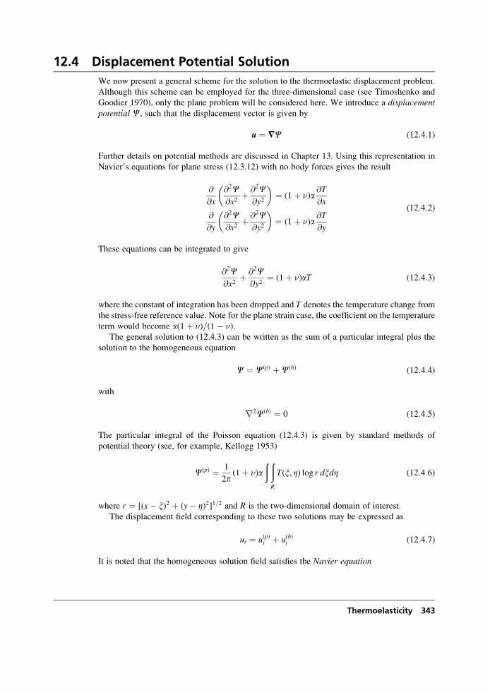
12.4 Displacement Potential Solution
We now present a general scheme for the solution to the thermoelastic displacement problem.
Although this scheme can be employed for the three-dimensional case (see Timoshenko and
Goodier 1970), only the plane problem will be considered here. We introduce a displacementpotential C, such that the displacement vector is given by
u ¼ =C (12:4:1)
Further details on potential methods are discussed in Chapter 13. Using this representation in
Navier’s equations for plane stress (12.3.12) with no body forces gives the result
@
@x
@2C@x2
þ @2C@y2
� �¼ (1þ �)a
@T
@x
@
@y
@2C@x2
þ @2C@y2
� �¼ (1þ �)a
@T
@y
(12:4:2)
These equations can be integrated to give
@2C@x2
þ @2C@y2
¼ (1þ �)aT (12:4:3)
where the constant of integration has been dropped and T denotes the temperature change from
the stress-free reference value. Note for the plane strain case, the coefficient on the temperature
term would become a(1þ �)=(1� �).The general solution to (12.4.3) can be written as the sum of a particular integral plus the
solution to the homogeneous equation
C ¼ C(p) þC(h) (12:4:4)
with
r2C(h) ¼ 0 (12:4:5)
The particular integral of the Poisson equation (12.4.3) is given by standard methods of
potential theory (see, for example, Kellogg 1953)
C(p) ¼ 1
2p(1þ �)a
ð ðR
T(x, Z) log r dxdZ (12:4:6)
where r ¼ [(x� x)2 þ (y� Z)2]1=2 and R is the two-dimensional domain of interest.
The displacement field corresponding to these two solutions may be expressed as
ui ¼ u(p)i þ u(h)i (12:4:7)
It is noted that the homogeneous solution field satisfies the Navier equation
Thermoelasticity 343
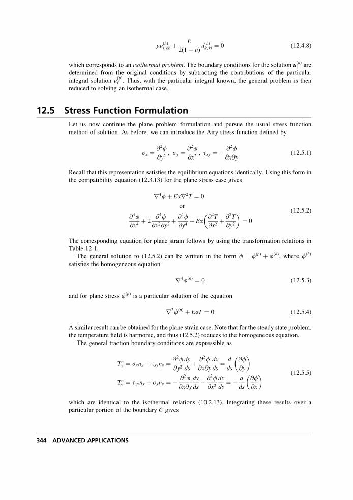
mu(h)i, kk þE
2(1� �)u(h)k, ki ¼ 0 (12:4:8)
which corresponds to an isothermal problem. The boundary conditions for the solution u(h)i are
determined from the original conditions by subtracting the contributions of the particular
integral solution u(p)i . Thus, with the particular integral known, the general problem is then
reduced to solving an isothermal case.
12.5 Stress Function Formulation
Let us now continue the plane problem formulation and pursue the usual stress function
method of solution. As before, we can introduce the Airy stress function defined by
sx ¼ @2f@y2
, sy ¼ @2f@x2
, txy ¼ � @2f@x@y
(12:5:1)
Recall that this representation satisfies the equilibrium equations identically. Using this form in
the compatibility equation (12.3.13) for the plane stress case gives
r4fþ Ear2T ¼ 0
or
@4f@x4
þ 2@4f
@x2@y2þ @4f
@y4þ Ea
@2T
@x2þ @2T
@y2
� �¼ 0
(12:5:2)
The corresponding equation for plane strain follows by using the transformation relations in
Table 12-1.
The general solution to (12.5.2) can be written in the form f ¼ f(p) þ f(h), where f(h)
satisfies the homogeneous equation
r4f(h) ¼ 0 (12:5:3)
and for plane stress f(p) is a particular solution of the equation
r2f(p) þ EaT ¼ 0 (12:5:4)
A similar result can be obtained for the plane strain case. Note that for the steady state problem,
the temperature field is harmonic, and thus (12.5.2) reduces to the homogeneous equation.
The general traction boundary conditions are expressible as
Tnx ¼ sxnx þ txyny ¼ @2f
@y2dy
dsþ @2f@x@y
dx
ds¼ d
ds
@f@y
� �
Tny ¼ txynx þ sxny ¼ � @2f
@x@y
dy
ds� @2f
@x2dx
ds¼ � d
ds
@f@x
� � (12:5:5)
which are identical to the isothermal relations (10.2.13). Integrating these results over a
particular portion of the boundary C gives
344 ADVANCED APPLICATIONS
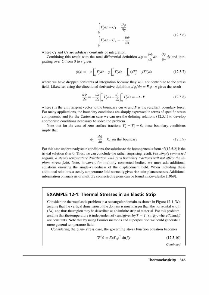
ðC
Tnx dsþ C1 ¼ @f
@yðC
Tny dsþ C2 ¼ � @f
@x
(12:5:6)
where C1 and C2 are arbitrary constants of integration.
Combining this result with the total differential definition df ¼ @f@x
dxþ @f@y
dy and inte-
grating over C from 0 to s gives
f(s) ¼ �x
ðs0
Tny dsþ y
ðs0
Tnx dsþ
ðs0
(xTny � yTn
x )ds (12:5:7)
where we have dropped constants of integration because they will not contribute to the stress
field. Likewise, using the directional derivative definition df=dn ¼ =f � n gives the result
dfdn
¼ � dx
ds
ðs0
Tnx ds�
dy
ds
ðs0
Tny ds ¼ �t � F (12:5:8)
where t is the unit tangent vector to the boundary curve and F is the resultant boundary force.
For many applications, the boundary conditions are simply expressed in terms of specific stress
components, and for the Cartesian case we can use the defining relations (12.5.1) to develop
appropriate conditions necessary to solve the problem.
Note that for the case of zero surface tractions Tnx ¼ Tn
y ¼ 0, these boundary conditions
imply that
f ¼ dfdn
¼ 0, on the boundary (12:5:9)
For this case under steady state conditions, the solution to the homogeneous formof (12.5.2) is the
trivial solution f � 0. Thus, we can conclude the rather surprising result: For simply connectedregions, a steady temperature distribution with zero boundary tractions will not affect the in-plane stress field. Note, however, for multiply connected bodies, we must add additional
equations ensuring the single-valuedness of the displacement field. When including these
additional relations, a steady temperature field normally gives rise to in-plane stresses.Additional
information on analysis of multiply connected regions can be found in Kovalenko (1969).
EXAMPLE 12-1: Thermal Stresses in an Elastic Strip
Consider the thermoelastic problem in a rectangular domain as shown in Figure 12-1.We
assume that the vertical dimension of the domain is much larger than the horizontal width
(2a), and thus the regionmay be described as an infinite strip ofmaterial. For this problem,
assume that the temperature is independent of x andgivenbyT ¼ To sinby,whereTo andbare constants. Note that by using Fourier methods and superposition we could generate a
more general temperature field.
Considering the plane stress case, the governing stress function equation becomes
r4f ¼ EaTob2 sinby (12:5:10)
Continued
Thermoelasticity 345
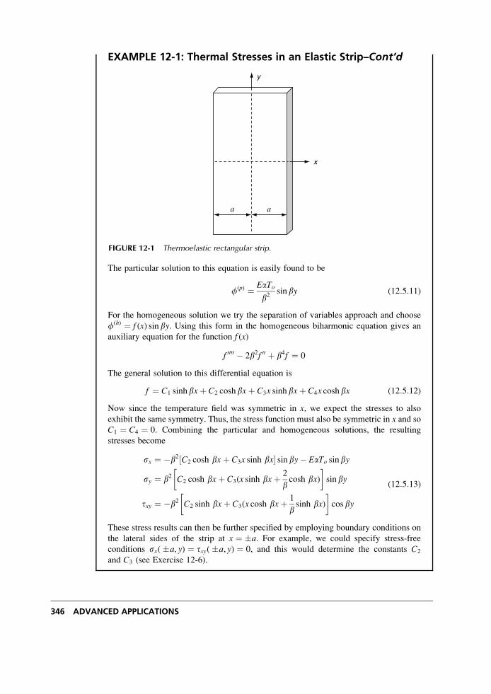
EXAMPLE 12-1: Thermal Stresses in an Elastic Strip–Cont’d
The particular solution to this equation is easily found to be
f(p) ¼ EaTob2
sinby (12:5:11)
For the homogeneous solution we try the separation of variables approach and choose
f(h) ¼ f (x) sin by. Using this form in the homogeneous biharmonic equation gives an
auxiliary equation for the function f (x)
f 0000 � 2b2f 00 þ b4f ¼ 0
The general solution to this differential equation is
f ¼ C1 sinhbxþ C2 cosh bxþ C3x sinh bxþ C4x cosh bx (12:5:12)
Now since the temperature field was symmetric in x, we expect the stresses to also
exhibit the same symmetry. Thus, the stress function must also be symmetric in x and soC1 ¼ C4 ¼ 0. Combining the particular and homogeneous solutions, the resulting
stresses become
sx ¼ �b2 C2 cosh bxþ C3x sinh bx½ � sin by� EaTo sinby
sy ¼ b2 C2 cosh bxþ C3(x sinh bxþ 2
bcosh bx)
� �sin by
txy ¼ �b2 C2 sinh bxþ C3(x cosh bxþ 1
bsinh bx)
� �cos by
(12:5:13)
These stress results can then be further specified by employing boundary conditions on
the lateral sides of the strip at x ¼ �a. For example, we could specify stress-free
conditions sx(�a, y) ¼ txy(�a, y) ¼ 0, and this would determine the constants C2
and C3 (see Exercise 12-6).
x
y
aa
FIGURE 12-1 Thermoelastic rectangular strip.
346 ADVANCED APPLICATIONS

12.6 Polar Coordinate Formulation
We now wish to list the basic plane thermoelastic equations in polar coordinates. Recall that
the isothermal results were previously given in Section 7.6. Following the same notational
scheme as before, the strain-displacement relations are given by
er ¼ @ur@r
, ey ¼ urrþ 1
r
@uy@y
ery ¼ 1
2
1
r
@ur@y
þ @uy@r
� uyr
� � (12:6:1)
For the case of plane stress, Hooke’s law becomes
sr ¼ E
1� �2[er þ �ey � (1þ �)a(T � To)]
sy ¼ E
1� �2[ey þ �er � (1þ �)a(T � To)]
try ¼ E
1þ �ery
(12:6:2)
In the absence of body forces, the equilibrium equations reduce to
@sr@r
þ 1
r
@try@y
þ sr � syr
¼ 0
@try@r
þ 1
r
@sy@y
þ 2tryr
¼ 0
(12:6:3)
The Airy stress function definition now becomes
sr ¼ 1
r
@f@r
þ 1
r2@2f
@y2
sy ¼ @2f@r2
try ¼ � @
@r
1
r
@f@y
� � (12:6:4)
which again satisfies (12.6.3) identically. The governing stress function equation given previ-
ously by (12:5:2)1 still holds with the Laplacian and biharmonic operators specified by
r2 ¼ @2
@r2þ 1
r
@
@rþ 1
r2@2
@y2
r4 ¼ r2r2 ¼ @2
@r2þ 1
r
@
@rþ 1
r2@2
@y2
� �@2
@r2þ 1
r
@
@rþ 1
r2@2
@y2
� � (12:6:5)
Thermoelasticity 347
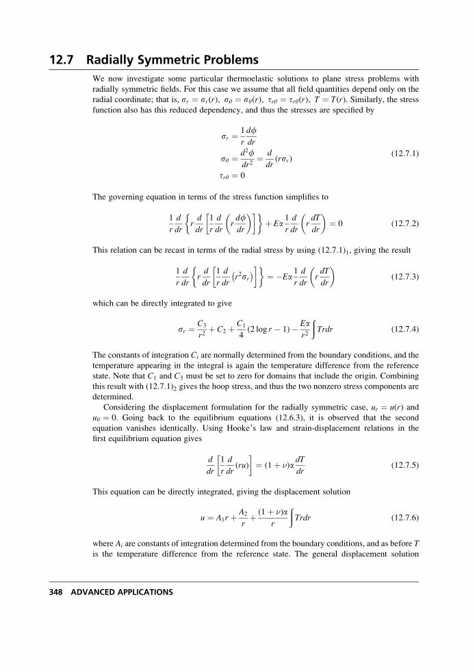
12.7 Radially Symmetric Problems
We now investigate some particular thermoelastic solutions to plane stress problems with
radially symmetric fields. For this case we assume that all field quantities depend only on the
radial coordinate; that is, sr ¼ sr(r), sy ¼ sy(r), try ¼ try(r), T ¼ T(r). Similarly, the stress
function also has this reduced dependency, and thus the stresses are specified by
sr ¼ 1
r
dfdr
sy ¼ d2fdr2
¼ d
dr(rsr)
try ¼ 0
(12:7:1)
The governing equation in terms of the stress function simplifies to
1
r
d
drrd
dr
1
r
d
drrdfdr
� �� �� �þ Ea
1
r
d
drrdT
dr
� �¼ 0 (12:7:2)
This relation can be recast in terms of the radial stress by using (12:7:1)1, giving the result
1
r
d
drrd
dr
1
r
d
drr2sr� � �� �
¼ �Ea1
r
d
drrdT
dr
� �(12:7:3)
which can be directly integrated to give
sr ¼ C3
r2þ C2 þ C1
4(2 log r � 1)� Ea
r2
ðTrdr (12:7:4)
The constants of integration Ci are normally determined from the boundary conditions, and the
temperature appearing in the integral is again the temperature difference from the reference
state. Note that C1 and C3 must be set to zero for domains that include the origin. Combining
this result with (12:7:1)2 gives the hoop stress, and thus the two nonzero stress components are
determined.
Considering the displacement formulation for the radially symmetric case, ur ¼ u(r) anduy ¼ 0. Going back to the equilibrium equations (12.6.3), it is observed that the second
equation vanishes identically. Using Hooke’s law and strain-displacement relations in the
first equilibrium equation gives
d
dr
1
r
d
dr(ru)
� �¼ (1þ �)a
dT
dr(12:7:5)
This equation can be directly integrated, giving the displacement solution
u ¼ A1r þ A2
rþ (1þ �)a
r
ðTrdr (12:7:6)
where Ai are constants of integration determined from the boundary conditions, and as before Tis the temperature difference from the reference state. The general displacement solution
348 ADVANCED APPLICATIONS
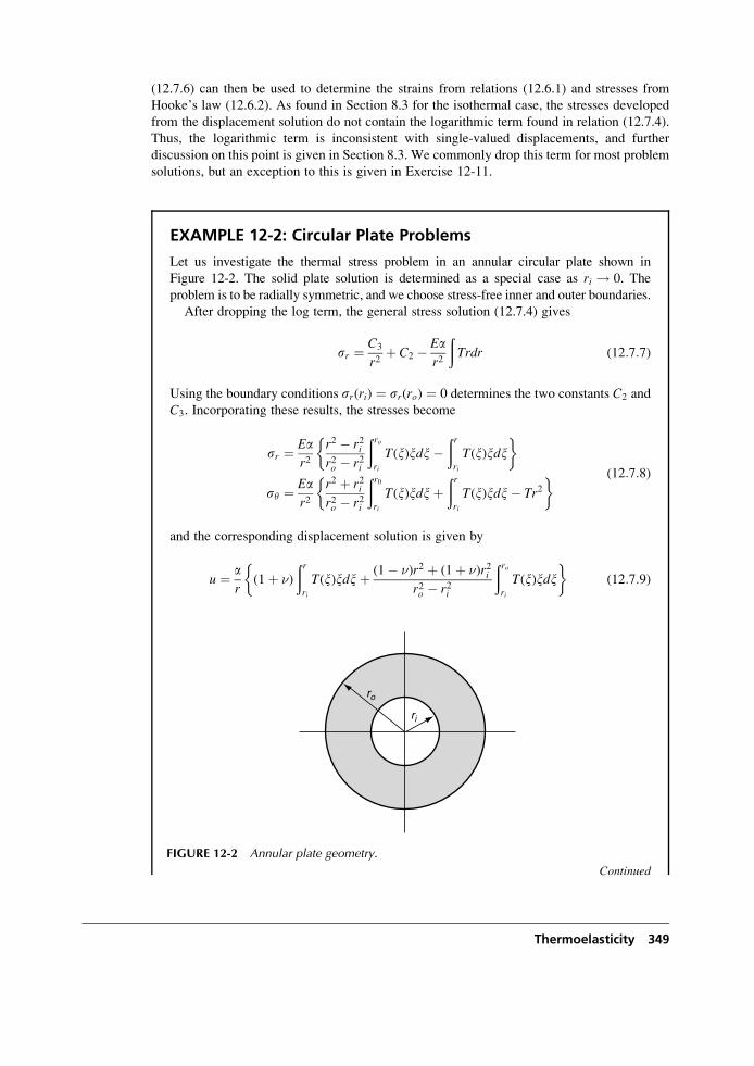
(12.7.6) can then be used to determine the strains from relations (12.6.1) and stresses from
Hooke’s law (12.6.2). As found in Section 8.3 for the isothermal case, the stresses developed
from the displacement solution do not contain the logarithmic term found in relation (12.7.4).
Thus, the logarithmic term is inconsistent with single-valued displacements, and further
discussion on this point is given in Section 8.3. We commonly drop this term for most problem
solutions, but an exception to this is given in Exercise 12-11.
EXAMPLE 12-2: Circular Plate Problems
Let us investigate the thermal stress problem in an annular circular plate shown in
Figure 12-2. The solid plate solution is determined as a special case as ri ! 0. The
problem is to be radially symmetric, and we choose stress-free inner and outer boundaries.
After dropping the log term, the general stress solution (12.7.4) gives
sr ¼ C3
r2þ C2 � Ea
r2
ðTrdr (12:7:7)
Using the boundary conditions sr(ri) ¼ sr(ro) ¼ 0 determines the two constants C2 and
C3. Incorporating these results, the stresses become
sr ¼ Ear2
r2 � r2ir2o � r2i
ðrori
T(x)xdx�ðrri
T(x)xdx� �
sy ¼ Ear2
r2 þ r2ir2o � r2i
ðr0ri
T(x)xdxþðrri
T(x)xdx� Tr2� � (12:7:8)
and the corresponding displacement solution is given by
u ¼ ar
(1þ �)
ðrri
T(x)xdxþ (1� �)r2 þ (1þ �)r2ir2o � r2i
ðrori
T(x)xdx� �
(12:7:9)
Continued
ro
ri
FIGURE 12-2 Annular plate geometry.
Thermoelasticity 349
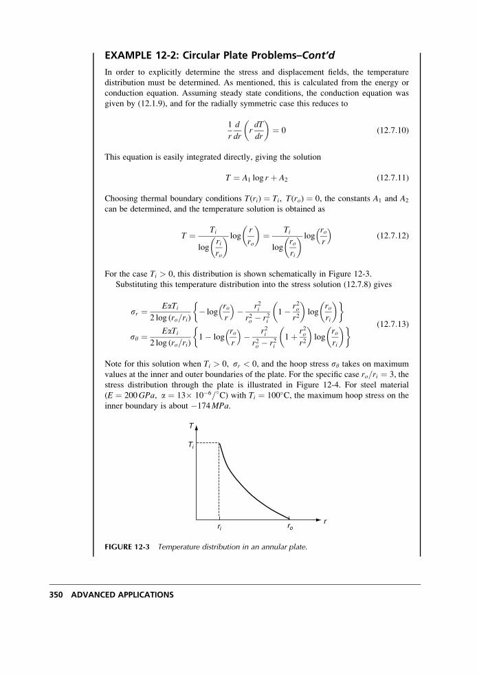
EXAMPLE 12-2: Circular Plate Problems–Cont’d
In order to explicitly determine the stress and displacement fields, the temperature
distribution must be determined. As mentioned, this is calculated from the energy or
conduction equation. Assuming steady state conditions, the conduction equation was
given by (12.1.9), and for the radially symmetric case this reduces to
1
r
d
drrdT
dr
� �¼ 0 (12:7:10)
This equation is easily integrated directly, giving the solution
T ¼ A1 log r þ A2 (12:7:11)
Choosing thermal boundary conditions T(ri) ¼ Ti, T(ro) ¼ 0, the constants A1 and A2
can be determined, and the temperature solution is obtained as
T ¼ Ti
logriro
� � logr
ro
� �¼ Ti
logrori
� � logror
�(12:7:12)
For the case Ti > 0, this distribution is shown schematically in Figure 12-3.
Substituting this temperature distribution into the stress solution (12.7.8) gives
sr ¼ EaTi2 log (ro=ri)
� logror
�� r2ir2o � r2i
1� r2or2
� �log
rori
� �� �
sy ¼ EaTi2 log (ro=ri)
1� logror
�� r2ir2o � r2i
1þ r2or2
� �log
rori
� �� � (12:7:13)
Note for this solution when Ti > 0, sr < 0, and the hoop stress s� takes on maximum
values at the inner and outer boundaries of the plate. For the specific case ro=ri ¼ 3, the
stress distribution through the plate is illustrated in Figure 12-4. For steel material
(E ¼ 200GPa, a ¼ 13� 10�6=�C) with Ti ¼ 100�C, the maximum hoop stress on the
inner boundary is about �174MPa.
T
rrori
Ti
FIGURE 12-3 Temperature distribution in an annular plate.
350 ADVANCED APPLICATIONS
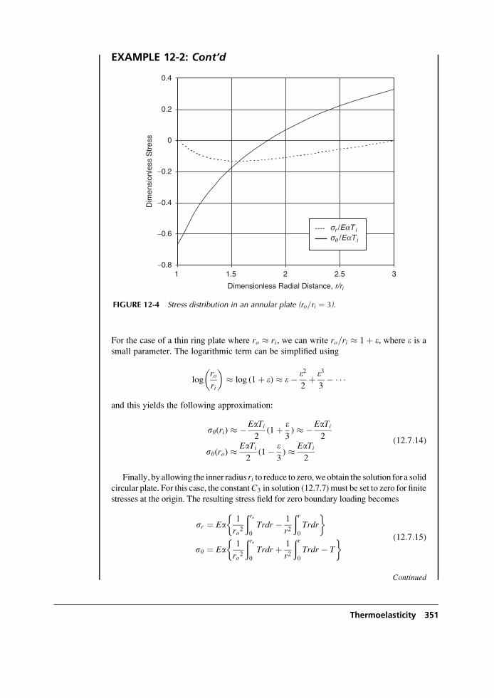
EXAMPLE 12-2: Cont’d
For the case of a thin ring plate where ro ri, we can write ro=ri 1þ e, where e is asmall parameter. The logarithmic term can be simplified using
logrori
� � log (1þ e) e� e2
2þ e3
3� � � �
and this yields the following approximation:
sy(ri) �EaTi2
(1þ e3) �EaTi
2
sy(ro) EaTi2
(1� e3) EaTi
2
(12:7:14)
Finally, by allowing the inner radius ri to reduce to zero,weobtain the solution for a solidcircular plate. For this case, the constantC3 in solution (12.7.7) must be set to zero for finite
stresses at the origin. The resulting stress field for zero boundary loading becomes
sr ¼ Ea1
ro2
ðro0
Trdr � 1
r2
ðr0
Trdr
� �
sy ¼ Ea1
ro2
ðro0
Trdr þ 1
r2
ðr0
Trdr � T
� � (12:7:15)
Continued
−0.8
−0.6
−0.4
−0.2
0
0.2
0.4
Dimensionless Radial Distance, r/ri
Dim
ensi
onle
ss S
tres
s
---- sr /EaT i
sq /EaT i
1 1.5 2 2.5 3
FIGURE 12-4 Stress distribution in an annular plate (ro=ri ¼ 3).
Thermoelasticity 351
EXAMPLE 12-2: Circular Plate Problems–Cont’d
Casual inspection of the integral term1
r2
ðr0
Trdr indicates the possibility of unbounded
behavior at the origin. This term can be investigated using l’Hospital’s rule, and it can
be shown that
limr!0
1
r2
ðr0
Trdr
� �¼ 1
2T(0)
Because we expect the temperature at the origin to be finite, this limit then implies that the
stresses will also be finite at r ¼ 0. Using a temperature boundary condition T(ro) ¼ To,the general solution (12.7.11) predicts a uniform temperature T ¼ To throughout the
entire plate. For this case, relations (12.7.15) give sr ¼ sy ¼ 0, and thus the plate is
stress free. This particular result verifies the general discussion in Section 12.5 that a
steady temperature distribution in a simply connected regionwith zero boundary tractions
gives rise to zero stress. The previous results for plane stress can be easily converted to
plane strain by using the appropriate conversion of elastic constants.
The general thermoelastic plane problem (without axial symmetry) can be developed using
methods of Fourier analysis; see, for example, Boley and Weiner (1960). The results lead to a
similar solution pattern as developed in Section 8.3. Instead of pursuing this development, we
look at the use of complex variable methods for the general plane problem.
12.8 Complex Variable Methods for Plane Problems
We now wish to develop a complex variable technique for the solution to plane problems in
thermoelasticity. As demonstrated in Chapter 10, the complex variable method is a very
powerful tool for solution of two-dimensional problems. Thismethodmay be extended to handle
problems involving thermal stress; see Bogdanoff (1954) and Timoshenko and Goodier (1970).
For the steady state case, the scheme starts by defining a complex temperature
T*(z) ¼ T þ iTI (12:8:1)
where the actual temperature T is the real part of T* and TI is the conjugate of T. As before,these temperatures actually represent the change with respect to the stress-free reference state.
Further define the integrated temperature function
t*(z) ¼ðT*(z)dz ¼ tR þ itI (12:8:2)
Using the Cauchy-Riemann equations,
@tR@x
¼ @tI@y
,@tR@y
¼ � @tI@x
(12:8:3)
Note that these results imply that the temperature can be expressed as
T ¼ @tR@x
¼ @tI@y
(12:8:4)
352 ADVANCED APPLICATIONS
Next decompose the two-dimensional displacement field as
u ¼ u0 þ btR� ¼ iv0 þ btI
(12:8:5)
where b is a constant to be determined. Substituting these displacements into Hooke’s law
(12.3.3) for plain strain yields the following stress field:
sx ¼ l@u0
@xþ @v0
@y
� �þ 2m
@u0
@xþ [2b(lþ m)� a(3lþ 2m)]T
sy ¼ l@u0
@xþ @v0
@y
� �þ 2m
@v0
@yþ [2b(lþ m)� a(3lþ 2m)]T
txy ¼ m@u0
@yþ @v0
@x
� � (12:8:6)
By choosing
b ¼ (1þ �)a, plane strain
a, plane stress
�(12:8:7)
the temperature terms in (12.8.6) are eliminated and thus the problem reduces to the isothermalcase in terms of the displacements u0, v0. This reduction indicates that the general thermo-
elastic plane problem can be formulated in terms of complex variable theory by the relations
sx þ sy ¼ 2 g0(z)þ g0(z)�
sy � sx þ 2itxy ¼ 2 �zzg00(z)þ c0(z)ð Þ2m(uþ iv) ¼ kg(z)� zg0(z)� c(z)þ 2mbt*(z)
Tnx þ iTn
y ¼ �id
dsg(z)þ zg0(z)þ c(z)�
(12:8:8)
where we have used many of the relations originally developed in Section 10.2. The material
parameter k was given by (10.2.10) and b is specified in (12.8.7). Thus, the problem is solved
by superposition of an isothermal state with appropriate boundary conditions and a displace-
ment field given by uþ i� ¼ bt*(z). For the nonsteady case, the temperature is no longer
harmonic, and we would have to represent the complex temperature in the more general
scheme T* ¼ T*(z, �zz).
EXAMPLE 12-3: Annular Plate Problem
Consider again the annular plate problem shown in Figure 12-2. Assume a complex
temperature potential of the form
T*(z) ¼ �C1
z(12:8:9)
Continued
Thermoelasticity 353
EXAMPLE 12-3: Annular Plate Problem–Cont’d
where C is a real constant. The actual temperature field follows as
T ¼ �C Re1
z
� �¼ �C
rcos y (12:8:10)
and it is easily verified that this temperature is a harmonic function, thus indicating a
steady state field. Note that the boundary temperatures on the inner and outer surfaces
for this case become
T(ri) ¼ �C cos yri
, T(ro) ¼ �C cos yro
and this would have to match with the assumed temperature boundary conditions. Of
course, we could use Fourier superposition methods to handle a more general boundary
distribution. Using relation (12.8.5), it is found that this temperature field produces a
logarithmic term in the displacement distribution, and this leads to a discontinuity when
evaluating the cyclic behavior. This displacement discontinuity must be removed by
adding an additional field with the opposite cyclic behavior. Based on our previous
experience from Chapter 10, we therefore choose an additional field with the following
potentials
g(z) ¼ A log zþ go(z)
c(z) ¼ B log zþ co(z)(12:8:11)
where go(z) and co(z) are single-valued and analytic in the domain (ri r ro). Forsingle-valued displacements in the region, we can use equations (12:8:8)3 to evaluate
and set the cyclic displacement to zero, thus giving
kAþ B ¼ 2mbC (12:8:12)
where we have taken A and B to be real.
Again, choosing stress-free boundaries at ri and ro and using results from (10.2.11)
and (10.2.12), we can write
(sr � itry)r¼ri, ro ¼ g0(z)þ g0(z)� e2iy[�zzg00(z)þ c0(z)]�
r¼ri, ro¼ 0 (12:8:13)
and this is satisfied by potentials with the following properties:
A ¼ B
go(z) ¼ �Az2
r2i þ r2o
co(z) ¼ �Ar2i r
2o
z2(r2i þ r2o)
(12:8:14)
Thus, the final form of the potentials becomes
354 ADVANCED APPLICATIONS
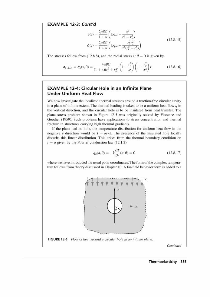
EXAMPLE 12-3: Cont’d
g(z) ¼ 2mbC1þ k
log z� z2
r2i þ r2o
� �
c(z) ¼ 2mbC1þ k
log z� r2i r2o
z2(r2i þ r2o)
� � (12:8:15)
The stresses follow from (12.8.8), and the radial stress at y ¼ 0 is given by
srjy¼0 ¼ sx(x, 0) ¼ 4mbC(1þ k)(r2i þ r2o)
1� r2ix2
� �1� r2o
x2
� �x (12:8:16)
EXAMPLE 12-4: Circular Hole in an Infinite PlaneUnder Uniform Heat Flow
We now investigate the localized thermal stresses around a traction-free circular cavity
in a plane of infinite extent. The thermal loading is taken to be a uniform heat flow q in
the vertical direction, and the circular hole is to be insulated from heat transfer. The
plane stress problem shown in Figure 12-5 was originally solved by Florence and
Goodier (1959). Such problems have applications to stress concentration and thermal
fracture in structures carrying high thermal gradients.
If the plane had no hole, the temperature distribution for uniform heat flow in the
negative y direction would be T ¼ qy=k. The presence of the insulated hole locally
disturbs this linear distribution. This arises from the thermal boundary condition on
r ¼ a given by the Fourier conduction law (12.1.2)
qn(a, y) ¼ �k@T
@r(a, y) ¼ 0 (12:8:17)
where we have introduced the usual polar coordinates. The form of the complex tempera-
ture follows from theory discussed in Chapter 10. A far-field behavior term is added to a
Continued
x
y
q
a
FIGURE 12-5 Flow of heat around a circular hole in an infinite plane.
Thermoelasticity 355
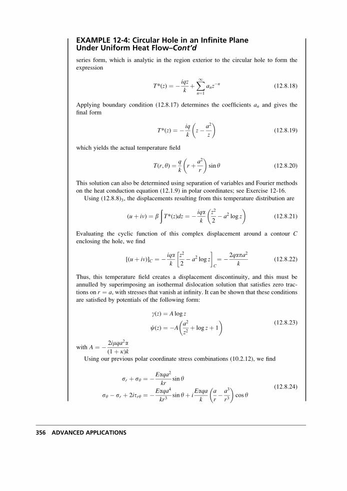
EXAMPLE 12-4: Circular Hole in an Infinite PlaneUnder Uniform Heat Flow–Cont’d
series form, which is analytic in the region exterior to the circular hole to form the
expression
T*(z) ¼ � iqz
kþX1n¼1
anz�n (12:8:18)
Applying boundary condition (12.8.17) determines the coefficients an and gives the
final form
T*(z) ¼ � iq
kz� a2
z
� �(12:8:19)
which yields the actual temperature field
T(r, y) ¼ q
kr þ a2
r
� �sin y (12:8:20)
This solution can also be determined using separation of variables and Fourier methods
on the heat conduction equation (12.1.9) in polar coordinates; see Exercise 12-16.
Using (12:8:8)3, the displacements resulting from this temperature distribution are
(uþ iv) ¼ bðT*(z)dz ¼ � iqa
k
z2
2� a2 log z
� �(12:8:21)
Evaluating the cyclic function of this complex displacement around a contour Cenclosing the hole, we find
[(uþ iv)]C ¼ � iqak
z2
2� a2 log z
� �C
¼ � 2qapa2
k(12:8:22)
Thus, this temperature field creates a displacement discontinuity, and this must be
annulled by superimposing an isothermal dislocation solution that satisfies zero trac-
tions on r ¼ a, with stresses that vanish at infinity. It can be shown that these conditionsare satisfied by potentials of the following form:
g(z) ¼ A log z
c(z) ¼ �Aa2
z2þ log zþ 1
� �(12:8:23)
with A ¼ � 2imqa2a(1þ k)k
Using our previous polar coordinate stress combinations (10.2.12), we find
sr þ sy ¼ �Eaqa2
krsin y
sy � sr þ 2itry ¼ �Eaqa4
kr3sin yþ i
Eaqak
a
r� a3
r3
� �cos y
(12:8:24)
356 ADVANCED APPLICATIONS
EXAMPLE 12-4: Cont’d
and the individual stresses then become
sr ¼ � 1
2
Eaqak
a
r� a3
r3
� �sin y
sy ¼ � 1
2
Eaqak
a
rþ a3
r3
� �sin y
try ¼ 1
2
Eaqak
a
r� a3
r3
� �cos y
(12:8:25)
The largest stress is given by the hoop stress on the boundary of the hole
smax ¼ sy(a, y) ¼ �Eaqak
sin y (12:8:26)
Notice that this expression takes on maximum values of �Eaqa=k at y ¼ �p=2 and
predicts a maximum compressive stress on the hot side of the hole y ¼ p=2 and
maximum tensile stress on the cold side y ¼ �p=2. For the case of a steel plate with
properties E ¼ 200GPa and a ¼ 13� 10�6=�C), and with qa=k ¼ 100�C, the max-
imum stress is 260MPa.
EXAMPLE 12-5: Elliptical Hole in an Infinite PlaneUnder Uniform Heat Flow
Similar to the previous example, we now investigate the localized thermal stresses
around a traction-free elliptical hole (with semiaxes a and b) in a plane of infinite extentas shown in Figure 12-6. The thermal loading is again taken to be a uniform heat flow qin the vertical direction, and the hole is to be insulated from heat transfer. The plane
Continued
x
y
q
ab
FIGURE 12-6 Flow of heat around an elliptical hole in an infinite plane.
Thermoelasticity 357
EXAMPLE 12-5: Elliptical Hole in an Infinite PlaneUnder Uniform Heat Flow–Cont’d
stress solution to this problem again comes from the work of Florence and Goodier
(1960) who solved the more general case of an ovaloid hole with heat flow at an
arbitrary angle. This problem is solved by complex variable methods employing
conformal transformation (see Section 10.7).
As discussed in Chapter 10, conformal mapping provides a very useful tool for this
type of problem, and the appropriate mapping function
z ¼ w(z) ¼ R zþ m
z
� �(12:8:27)
transforms the region exterior to the unit circle in the z-plane onto the region exterior tothe ellipse in the z-plane. The ellipse major and minor axes are related to the mapping
parameters by 2Rm ¼ a� b and 2R ¼ aþ b. As before, in the transformed plane,
z ¼ reiy.From our previous example, the temperature distribution for heat flow around an
insulated circular hole of unit radius in the z-plane may be written as
T ¼ q
kR rþ 1
r
� �sin y (12:8:28)
The complex temperature corresponding to this result is
T*(z) ¼ � q
kiR z� 1
z
� �(12:8:29)
Again, this temperature field creates a dislocation in the displacement. Following
similar steps as in equations (12.8.21) and (12.8.22), the cyclic function of the complex
temperature displacement is given by
[(uþ iv)]C ¼ aðT*(z)dz
� �C
¼ � 2qapR2
k(1þ m) (12:8:30)
where C is the counterclockwise contour around the unit circle enclosing the origin.
Employing conformal transformation, relations (10.7.5) through (10.7.7) can be used
to determine the stresses, displacements, and tractions in the z-plane. As in the previousexample, we now wish to superimpose an isothermal state having equal but opposite
dislocation behavior as (12.8.30), with zero tractions on the hole boundary and vanishing
stresses at infinity. The appropriate potentials that satisfy these conditions are given by
g(z) ¼ A log z
c(z) ¼ �AA log z� A1þ mz2
z2 � m
with A ¼� EaqR2i
4k(1þ m)
(12:8:31)
Using relations (10.7.5), the stresses in the z-plane become
358 ADVANCED APPLICATIONS
EXAMPLE 12-5: Cont’d
sr ¼ � Eaqa2kh(y)
r(r2 þ m)[r4 � r2(1þ m2)þ m2] sin y
sy ¼ � Eaqa2kh(y)
r(r2 þ m){[r4 þ r2(1þ m)2 þ m2] sin y� 2r2m sin 3y}
try ¼ Eaqa2kh(y)
r(r2 � m)[r4 � r2(1þ m2)þ m2] cos y
(12:8:32)
where h(y) ¼ [r4 � 2r2m cos 2yþ m2]2. It can be shown that the circular hole case is
found by setting m ¼ 0, and the stresses will reduce to those given in the previous
example in equations (12.8.25). Another interesting special case is given by m ¼ 1,
which corresponds to the elliptical hole reducing to a line crack of length 2a along the
x-axis. For this case the heat flow is perpendicular to the crack, and the stresses become
sr ¼ � Eaqa2kh(y)
r(r2 þ 1)[r4 � 2r2 þ 1] sin y
sy ¼ � Eaqa2kh(y)
r(r2 þ 1){[r4 þ 4r2 þ 1] sin y� 2r2 sin 3y}
try ¼ Eaqa2kh(y)
r(r2 � 1)[r4 � 2r2 þ 1] cos y
(12:8:33)
with h(y) ¼ [r4 � 2r2 cos 2yþ 1]2. On the surface of the crack (r ¼ 1), the hoop stress
becomes
sy(1, y) ¼ �Eaqa2k
3 sin y� sin 3y(1� cos 2y)2
¼ � Eaqa2k sin y
(12:8:34)
and as expected this stress becomes unbounded at the ends of the crack at y ¼ 0, p.Another interesting result for this case occurs with the shear stress behavior along the
positive x-axis (y ¼ 0)
tpy(r, 0) ¼ Eaqa2k
rr2 � 1
(12:8:35)
We again observe that this stress component becomes infinite at the crack tip when
r ¼ 1. As mentioned, Florence and Goodier (1960) solved the more general problem of
an ovaloid hole for which the elliptical cavity is a special case. Deresiewicz (1961)
solved the general thermal stress problem of a plate with an insulated hole of arbitrary
shape and worked out solution details for a triangular hole under uniform heat flow. For
the anisotropic case, Sadd and Miskioglu (1978) and Miskioglu (1978) have investi-
gated the problem of an insulated elliptical hole in an anisotropic plane under unidirec-
tional heat flow. Sih (1962) has investigated the singular nature of the thermal stresses at
crack tips. He showed that the usual 1=ffiffir
psingularity also exists for this case and that
the stress intensity factors (see Equation (10.8.7)) are proportional to the temperature
gradient.
Thermoelasticity 359
References
Bogdanoff JL: Note on thermal stresses, J. Appl. Mechanics, vol 76, p. 88, 1954.Boley BA, and Weiner JH: Theory of Thermal Stresses, John Wiley, New York, 1960.
Burgreen D: Elements of Thermal Stress Analysis, C. P. Press, Jamaica, NY, 1971.
Deresiewicz H: Thermal stress in a plate due to disturbance of uniform heat flow by a hole of general
shape, J. Appl. Mechanics, vol 28, pp. 147-149, 1961.Florence AL, and Goodier JN: Thermal stress at spherical cavities and circular holes in uniform heat flow,
J. Appl. Mechanics, vol 26, pp. 293-294, 1959.Florence AL, and Goodier JN: Thermal stresses due to disturbance of uniform heat flow by an insulated
ovaloid hole, J. Appl. Mechanics, vol 27, pp. 635-639, 1960.Fung YC: Foundations of Solid Mechanics, Prentice Hall, Englewood Cliffs, NJ, 1965.
Kellogg OD: Foundations of Potential Theory, Dover, New York, 1953.
Kovalenko AD: Thermoelasticity, Noordhoff, Groningen, The Netherlands, 1969.
Miskioglu I: Thermal stresses around an insulated elliptical hole in an anisotropic medium, master’s
thesis, Mississippi State University, 1978.
Nowacki W: Thermoelasticity, Addison Wesley, Reading, MA, 1962.
Nowinski JL: Theory of Thermoelasticity with Applications, Sijthoff-Noordhoff, Groningen, The Nether-lands, 1978.
Parkus H: Thermoelasticity, Springer, New York, 1976.
Sadd MH, and Miskioglu I: Temperatures in an anisotropic sheet containing an insulated elliptical hole,
J. Heat Transfer, vol 100, pp. 553-555, 1978.Sih GC: On the singular character of thermal stresses near a crack tip, J. Appl. Mechanics, vol 29,pp. 587-589, 1962.
Timoshenko SP, and Goodier JN: Theory of Elasticity, McGraw-Hill, New York, 1970.
Exercises
12-1. Using the assumption for isotropic materials that a temperature change produces
isotropic thermal strains of the form a(T � To)dij, develop relations (12.1.6).
12-2. For the general three-dimensional thermoelastic problem with no body forces,
explicitly develop the Beltrami-Michell compatibility equations
sij, kk þ 1
(1þ �)skk, ij þ Ea
1þ �(T, ij þ 1þ �
1� �dijT, kk) ¼ 0
12-3. If an isotropic solid is heated nonuniformly to a temperature distribution T(x, y, z) andthe material has unrestricted thermal expansion, the resulting strains will be eij ¼ aTdij.Show that this case can only occur if the temperature is a linear function of the
coordinates; that is,
T ¼ axþ byþ czþ d
12-4. Express the traction boundary condition (12.3.8) in terms of displacement and
temperature for the plane stress problem.
12-5. Develop the compatibility equations for plane strain (12.3.7) and plane stress (12.3.13).
12-6*. Explicitly develop the stress field equations (12.5.13) in Example 12-1 and determine
the constants C2 and C3 for the case of stress-free edge conditions. Plot the value of sythrough the thickness (versus coordinate x) for both high-temperature ( sin by ¼ 1) and
low-temperature ( sin by ¼ �1) cases.
360 ADVANCED APPLICATIONS
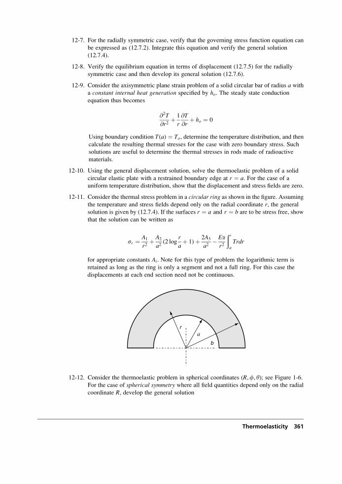
12-7. For the radially symmetric case, verify that the governing stress function equation can
be expressed as (12.7.2). Integrate this equation and verify the general solution
(12.7.4).
12-8. Verify the equilibrium equation in terms of displacement (12.7.5) for the radially
symmetric case and then develop its general solution (12.7.6).
12-9. Consider the axisymmetric plane strain problem of a solid circular bar of radius a with
a constant internal heat generation specified by ho. The steady state conduction
equation thus becomes
@2T
@r2þ 1
r
@T
@rþ ho ¼ 0
Using boundary condition T(a) ¼ To, determine the temperature distribution, and then
calculate the resulting thermal stresses for the case with zero boundary stress. Such
solutions are useful to determine the thermal stresses in rods made of radioactive
materials.
12-10. Using the general displacement solution, solve the thermoelastic problem of a solid
circular elastic plate with a restrained boundary edge at r ¼ a. For the case of a
uniform temperature distribution, show that the displacement and stress fields are zero.
12-11. Consider the thermal stress problem in a circular ring as shown in the figure. Assuming
the temperature and stress fields depend only on the radial coordinate r, the generalsolution is given by (12.7.4). If the surfaces r ¼ a and r ¼ b are to be stress free, showthat the solution can be written as
sr ¼ A1
r2þ A2
a2(2 log
r
aþ 1)þ 2A3
a2� Ea
r2
ðra
Trdr
for appropriate constants Ai. Note for this type of problem the logarithmic term is
retained as long as the ring is only a segment and not a full ring. For this case the
displacements at each end section need not be continuous.
a
b
r
12-12. Consider the thermoelastic problem in spherical coordinates (R,f, y); see Figure 1-6.For the case of spherical symmetry where all field quantities depend only on the radial
coordinate R, develop the general solution
Thermoelasticity 361
uR ¼ 1þ �
1� �a1
R2
ðRTx2dxþ C1Rþ C2
R2
sR ¼ � 2aE1� �
1
R3
ðRTx2dxþ EC1
1� 2�� 2EC2
1þ �
1
R3
sf ¼ sy ¼ aE1� �
1
R3
ðRTx2dxþ EC1
1� 2�þ EC2
1þ �
1
R3� aET1� �
Note that any convenient lower limit may be placed on the integral terms to aid in
problem solution.
12-13. Use the general solution of Exercise 12-12 to solve the thermal stress problem of a
hollow thick-walled spherical shell (a R b) with stress-free boundary conditions.
Assume that the problem is steady state with temperature conditions T(a) ¼ Ti,T(b) ¼ 0, and show that the solution becomes
T ¼ Tia
b� a
b
R� 1
� �
sR ¼ aETi1� �
ab
b3 � a3aþ b� 1
R(b2 þ abþ a2)þ a2b2
R3
� �
sf ¼ sy ¼ aETi1� �
ab
b3 � a3aþ b� 1
2R(b2 þ abþ a2)� a2b2
2R3
� �
For the case of a thin spherical shell, let b ¼ a(1þ "), where " is a small parameter.
Show that using this formulation, the hoop stresses at the inner and outer surfaces
become
sf ¼ sy ¼ aETi2(1� �)
�1� 2
3"
� �
and if we neglect the " term, these values match those of the cylindrical shell given by
relations (12.7.14).
12-14. Explicitly develop relations (12.8.6) and verify that by using the value of b given in
(12.8.7) the temperature terms will drop out of these relations.
12-15. For Example 12-3, verify that the potentials go(z), co(z) given by relations (12.8.14)
satisfy the stress-free boundary conditions on the problem.
12-16. Using separation of variables and Fourier methods, solve the conduction equation and
verify that the temperature distribution (12.8.20) in Example 12-4 does indeed satisfy
insulated conditions on the circular hole and properly matches conditions at infinity.
12-17. For Example 12-4, explicitly develop the stresses (12.8.25) from the complex
potentials given by equation (12.8.23).
12-18*. Plot the isotherms (contours of constant temperature) for Examples 12-4 and 12-5.
12-19. For the elliptical hole problem in Example 12-5, show that by letting m ¼ 0, the stress
results will reduce to those of the circular hole problem given in Example 12-4.
362 ADVANCED APPLICATIONS
12-20*. In Example 12-5, show that the dimensionless hoop stress around the boundary of the
hole is given by
�ssy ¼ syEaqa=k
¼ � (1þ m)[(1þ mþ m2) sin y� m sin 3y](1� 2m cos 2yþ m2)2
For the cases m ¼ 0,� 1⁄2 ,�1, plot and compare the behavior of �ssy versus y(0 y 2p).
12-21. Show that for the plane anisotropic problem, the heat-conduction equation for
uncoupled steady state conditions is given by
kxx@2T
@x2þ 2kxy
@2T
@x@yþ kyy
@2T
@y2¼ 0
Looking for solutions that are of the form T¼ F (x þ ly), show that this leads to the
quadratic characteristic equation
kyyl2 þ 2kxylþ kxx ¼ 0
Using the fact that kxxkyy > kxy2, demonstrate that the two roots to this equation will be
complex conjugate pairs; therefore, since the temperature must be real, the final form
of the solution will be
T ¼ 2Re{F(z*)}
where z*¼ x þ ly. This problem is mathematically similar to Exercise 11-15.
Thermoelasticity 363
13 Displacement Potentialsand Stress Functions
We nowwish to investigate the method of potentials to generate solutions to elasticity problems.
Several different potential techniques have been developed in order to solve problems within
both displacement and stress formulations. Methods related to the displacement formulation
include the scalar and vector potentials from theHelmholtz decomposition,Galerkin vector, andPapkovich-Neuber functions. These schemes provide general solution forms for Navier’s equa-
tions. Potentials used in the stress formulation are those related to theMaxwell andMorera stressfunctions, and these lead toAiry and other common stress functions that we have already used for
the solution of particular elasticity problems. As previously observed, these stress functions
normally satisfy the equilibrium equations identically and when combined with the compatibil-
ity relations they yield a simpler and more tractable system of equations.
For either displacement or stress formulations, these solution schemes bring up the ques-
tion—are all solutions of elasticity expressible by the particular potential representation? Thisissue is normally referred to as the completeness of the representations, and over the past
several decades these theoretical questions have generally been answered in the affirmative.
For many cases these approaches are useful to solve particular three-dimensional elasticity
problems, and we will investigate several such solutions. Some potential methods are also
particularly useful in formulating and solving dynamic elasticity problems involving wave
propagation (see Fung 1965 or Graff 1991).
13.1 Helmholtz Displacement Vector Representation
A useful relation called the Helmholtz theorem states that any sufficiently continuous vector
field can be represented as the sum of the gradient of a scalar potential plus the curl of a vector
potential. Using this representation for the displacement field, we can write
u ¼ =fþ =� w (13:1:1)
where f is the scalar potential and w is the vector potential. The gradient term in the decom-
position has a zero curl and is referred to as the lamellar or irrotational part, while the curl
365
term in (13.1.1) has no divergence and is called solenoidal. Note that this representation
specifies three displacement components in terms of four potential components, and further-
more the divergence of w is arbitrary. In order to address these problems, it is common to
choose w with zero divergence; that is,
= � w ¼ 0 (13:1:2)
It can be easily shown that the volume dilatation W and the rotation vectorv are related to these
potentials by
W ¼ ekk ¼ f, kk, !i ¼ � 1
2ji, kk (13:1:3)
General solutions of these relations can be determined (see Fung 1965), and thus the scalar and
vector potentials can be expressed in terms of the displacement field.
Using representation (13.1.1) in the general three-dimensional Navier equations (5.4.4),
we find
(lþ 2m)=(r2f)þ m=� (r2w)þ F ¼ 0 (13:1:4)
Notice that if the divergence and curl are taken of the previous equation with zero body forces,
the following relations are generated
r2r2f ¼ r4f ¼ 0, r2r2w ¼ r4w ¼ 0 (13:1:5)
and thus we find that both potential functions are biharmonic functions. Further reduction of
(13.1.4) will now be made for specific applications.
13.2 Lame’s Strain Potential
It is noted that for the case of zero body forces, special solutions of (13.1.4) occur with
r2f ¼ constant and r2w ¼ constant. We consider the special case with
r2f ¼ constant, w ¼ 0 (13:2:1)
Because our goal is to determine simply a particular solution, we can choose the constant to be
zero, and thus the potential f will be a harmonic function. For this case, the displacement
representation is commonly written as
2mui ¼ f, i (13:2:2)
and the function f is called Lame’s strain potential. Using this form, the strains and stresses
are given by the simple relations
eij ¼ 1
2mf, ij
sij ¼ f, ij
(13:2:3)
366 ADVANCED APPLICATIONS
In Cartesian coordinates, these expressions would give
u ¼ 1
2m@f@x
, v ¼ 1
2m@f@y
, w ¼ 1
2m@f@z
ex ¼ 1
2m@2f@x2
, ey ¼ 1
2m@2f@y2
, � � �
sx ¼ @2f@x2
, sy ¼ @2f@y2
, txy ¼ @2f@x@y
, � � �
(13:2:4)
Thus, for this case any harmonic function can be used for Lame’s potential. Typical forms of
harmonic functions are easily determined, and some examples include
x2 � y2, xy, rn cos ny, log r,1
R, log (Rþ z)
with r ¼ffiffiffiffiffiffiffiffiffiffiffiffiffiffiffix2 þ y2
p, y ¼ tan�1 y
x, R ¼
ffiffiffiffiffiffiffiffiffiffiffiffiffiffiffiffiffiffiffiffiffiffiffiffix2 þ y2 þ z2
p (13:2:5)
13.3 Galerkin Vector Representation
In the previous sections, the displacement vector was represented in terms of first derivatives
of the potential functions f and w. Galerkin (1930) showed that it is also useful to represent thedisplacement in terms of second derivatives of a single vector function. The proposed repre-
sentation is given by
2mu ¼ 2(1� �)r2V � =(= � V) (13:3:1)
where the potential function V is called the Galerkin vector. Substituting this form into
Navier’s equation gives the result
r4V ¼ � F
1� �(13:3:2)
Note that for the case of zero body forces, the Galerkin vector is biharmonic. Thus, we have
reduced Navier’s equation to a simpler fourth-order vector equation.
By comparing the representations given by (13.1.1) with that of (13.3.1), the Helmholtz
potentials can be related to the Galerkin vector by
f ¼ 1� 2�
2m(= � V), w ¼ � 1� �
m(=� V) ð13:3:3Þ
Notice that if V is taken to be harmonic, then the curl of w will vanish and the scalar potential
f will also be harmonic. This case then reduces to Lame’s strain potential presented in the
previous section. With zero body forces, the stresses corresponding to the Galerkin representa-
tion are given by
Displacement Potentials and Stress Functions 367
sx ¼ 2(1� �)@
@xr2Vx þ �r2 � @2
@x2
� �= � V
sy ¼ 2(1� �)@
@yr2Vy þ �r2 � @2
@y2
� �= � V
sz ¼ 2(1� �)@
@zr2Vz þ �r2 � @2
@z2
� �= � V
txy ¼ (1� �)@
@yr2Vx þ @
@xr2Vy
� �� @2
@x@y= � V
tyz ¼ (1� �)@
@zr2Vy þ @
@yr2Vz
� �� @2
@y@z= � V
tzx ¼ (1� �)@
@xr2Vz þ @
@zr2Vx
� �� @2
@z@x= � V
(13:3:4)
As previously mentioned, for no body forces the Galerkin vector must be biharmonic. In
Cartesian coordinates, the general biharmonic vector equation would decouple, and thus each
component of the Galerkin vector would satisfy the scalar biharmonic equation. However, in
curvilinear coordinate systems (such as cylindrical or spherical), the unit vectors are functions
of the coordinates, and this will not in general allow such a simple decoupling. Equation
(1.9.18) provides the general form for the Laplacian of a vector, and the expression for polar
coordinates is given in Example 1-5 by relation (1:9:21)7. Therefore, in curvilinear coordinatesthe individual components of the Galerkin vector do not necessarily satisfy the biharmonic
equation. For cylindrical coordinates, only the z component of the Galerkin vector satisfies the
biharmonic equation, while the other components satisfy a more complicated fourth-order
partial differential equation; see Exercise 13-8 for details.
Before moving on to specific applications, we investigate a few useful relationships dealing
with harmonic and biharmonic functions. Consider the following identity:
r2(xf ) ¼ xr2f þ 2@f
@x
Taking the Laplacian of this expression gives
r4(xf ) ¼ r2 xr2f� �þ 2
@
@x(r2f )
and thus if f is harmonic, the product xf is biharmonic. Obviously, for this result the coordinate xcould be replaced by y or z. Likewise we can also show by standard differentiation that the
product R2f will be biharmonic if f is harmonic, where R2 ¼ x2 þ y2 þ z2. Using these results,
we can write the following generalized representation for a biharmonic function g as
g ¼ fo þ x f1 þ y f2 þ z f3 þ 1
2R2f4 (13:3:5)
where fi are arbitrary harmonic functions. It should be pointed out that not all of the last four
terms of (13.3.5) are independent.
Consider now the special Galerkin vector representation where only the z component of V is
nonvanishing; that is, V ¼ Vzez. For this case, the displacements are given by
368 ADVANCED APPLICATIONS
2mu ¼ 2(1� �)r2Vzez � =@Vz
@z
� �(13:3:6)
With zero body forces, Vz will be biharmonic, and this case is commonly referred to as Love’sstrain potential. A special case of this form was introduced by Love (1944) in studying solids
of revolution under axisymmetric loading.
For this case the displacements and stresses in Cartesian coordinates become
2mu ¼ � @2Vz
@x@z, 2mv ¼ � @2Vz
@y@z, 2mw ¼ 2(1� �)r2Vz � @2Vz
@z2
sx ¼ @
@z�r2 � @2
@x2
� �Vz, txy ¼ � @3Vz
@x@y@z
sy ¼ @
@z�r2 � @2
@y2
� �Vz, tyz ¼ @
@y(1� �)r2 � @2
@z2
� �Vz
sz ¼ @
@z(2� �)r2 � @2
@z2
� �Vz, tzx ¼ @
@x(1� �)r2 � @2
@z2
� �Vz
(13:3:7)
The corresponding relations in cylindrical coordinates are given by
2mur ¼ � @2Vz
@r@z, 2muy ¼ � 1
r
@2Vz
@y@z, 2muz ¼ 2(1� �)r2Vz � @2Vz
@z2
sr ¼ @
@z�r2 � @2
@r2
� �Vz, try ¼ � @3
@r@y@zVz
r
� �
sy ¼ @
@z�r2 � 1
r
@
@r� 1
r2@2
@y2
� �Vz, tyz ¼ 1
r
@
@y(1� �)r2 � @2
@z2
� �Vz
sz ¼ @
@z(2� �)r2 � @2
@z2
� �Vz, tzr ¼ @
@r(1� �)r2 � @2
@z2
� �Vz
(13:3:8)
We now consider some example applications for axisymmetric problems where the field
variables are independent of y.
EXAMPLE 13-1: Kelvin’s Problem: Concentrated ForceActing in the Interior of an Infinite Solid
Consider the problem (commonly referred to as Kelvin’s problem) of a single concen-
trated force acting at a point in the interior of an unbounded elastic solid. For conveni-
ence we choose a coordinate system such that the force is applied at the origin and acts
in the z direction (see Figure 13-1). The general boundary conditions on this problem
would require that the stress field vanish at infinity, be singular at the origin, and give
the resultant force system Pez on any surface enclosing the origin.
The symmetry of the problem suggests that we can choose the Love/Galerkin
potential as an axisymmetric form Vz(r, z). In the absence of body forces, this function
is biharmonic, and using the last term in representation (13.3.5) with f4 ¼ 1=R gives the
trial potential
Continued
Displacement Potentials and Stress Functions 369
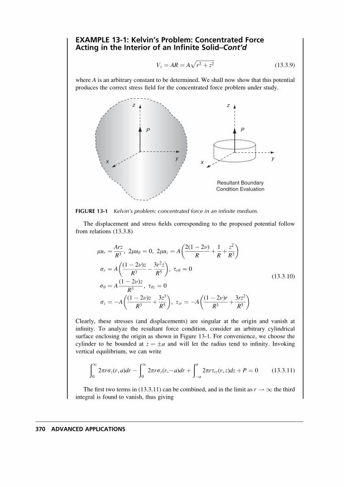
EXAMPLE 13-1: Kelvin’s Problem: Concentrated ForceActing in the Interior of an Infinite Solid–Cont’d
Vz ¼ AR ¼ Affiffiffiffiffiffiffiffiffiffiffiffiffiffir2 þ z2
p(13:3:9)
where A is an arbitrary constant to be determined. We shall now show that this potential
produces the correct stress field for the concentrated force problem under study.
xy
z
P
xy
z
P
Resultant BoundaryCondition Evaluation
FIGURE 13-1 Kelvin’s problem: concentrated force in an infinite medium.
The displacement and stress fields corresponding to the proposed potential follow
from relations (13.3.8)
mur ¼ Arz
R3, 2muy ¼ 0, 2muz ¼ A
2(1� 2�)
Rþ 1
Rþ z2
R3
� �
sr ¼ A(1� 2�)z
R3� 3r2z
R5
� �, try ¼ 0
sy ¼ A(1� 2�)z
R3, tyz ¼ 0
sz ¼ �A(1� 2�)z
R3þ 3z3
R5
� �, tzr ¼ �A
(1� 2�)r
R3þ 3rz2
R5
� �(13:3:10)
Clearly, these stresses (and displacements) are singular at the origin and vanish at
infinity. To analyze the resultant force condition, consider an arbitrary cylindrical
surface enclosing the origin as shown in Figure 13-1. For convenience, we choose the
cylinder to be bounded at z ¼ �a and will let the radius tend to infinity. Invoking
vertical equilibrium, we can write
ð10
2prsz(r, a)dr �ð10
2prsz(r,�a)dr þða�a
2prtrz(r, z)dzþ P ¼ 0 (13:3:11)
The first two terms in (13.3.11) can be combined, and in the limit as r ! 1 the third
integral is found to vanish, thus giving
370 ADVANCED APPLICATIONS
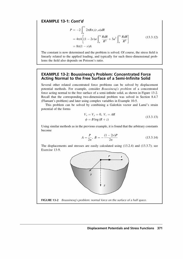
EXAMPLE 13-1: Cont’d
P ¼ �2
ð1a
2pRsz(r, a)dR
¼ 4pA (1� 2�)a
ð1a
RdR
R3þ 3a3
ð1a
RdR
R5
� �¼ 8p(1� �)A
(13:3:12)
The constant is now determined and the problem is solved. Of course, the stress field is
linearly related to the applied loading, and typically for such three-dimensional prob-
lems the field also depends on Poisson’s ratio.
EXAMPLE 13-2: Boussinesq’s Problem: Concentrated ForceActing Normal to the Free Surface of a Semi-Infinite Solid
Several other related concentrated force problems can be solved by displacement
potential methods. For example, consider Boussinesq’s problem of a concentrated
force acting normal to the free surface of a semi-infinite solid, as shown in Figure 13-2.
Recall that the corresponding two-dimensional problem was solved in Section 8.4.7
(Flamant’s problem) and later using complex variables in Example 10-5.
This problem can be solved by combining a Galerkin vector and Lame’s strain
potential of the forms
Vx ¼ Vy ¼ 0, Vz ¼ AR
f ¼ B log (Rþ z)(13:3:13)
Using similar methods as in the previous example, it is found that the arbitrary constants
become
A ¼ P
2p, B ¼ � (1� 2�)P
2p(13:3:14)
The displacements and stresses are easily calculated using (13.2.4) and (13.3.7); see
Exercise 13-9.
FIGURE 13-2 Boussinesq’s problem: normal force on the surface of a half space.
Displacement Potentials and Stress Functions 371
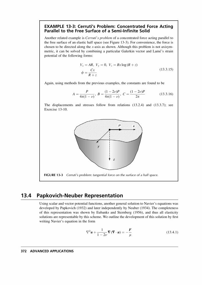
EXAMPLE 13-3: Cerruti’s Problem: Concentrated Force ActingParallel to the Free Surface of a Semi-Infinite Solid
Another related example is Cerruti’s problem of a concentrated force acting parallel to
the free surface of an elastic half space (see Figure 13-3). For convenience, the force is
chosen to be directed along the x-axis as shown. Although this problem is not axisym-
metric, it can be solved by combining a particular Galerkin vector and Lame’s strain
potential of the following forms:
Vx ¼ AR, Vy ¼ 0, Vz ¼ Bx log (Rþ z)
f ¼ Cx
Rþ z
(13:3:15)
Again, using methods from the previous examples, the constants are found to be
A ¼ P
4p(1� �), B ¼ (1� 2�)P
4p(1� �), C ¼ (1� 2�)P
2p(13:3:16)
The displacements and stresses follow from relations (13.2.4) and (13.3.7); see
Exercise 13-10.
13.4 Papkovich-Neuber Representation
Using scalar and vector potential functions, another general solution to Navier’s equations was
developed by Papkovich (1932) and later independently by Neuber (1934). The completeness
of this representation was shown by Eubanks and Sternberg (1956), and thus all elasticity
solutions are representable by this scheme. We outline the development of this solution by first
writing Navier’s equation in the form
r2uþ 1
1� 2�= (= � u) ¼ �F
m(13:4:1)
FIGURE 13-3 Cerruti’s problem: tangential force on the surface of a half space.
372 ADVANCED APPLICATIONS
Using the Helmholtz representation (13.1.1) and relation (13.1.3), this previous equation can
be written as
r2[uþ 1
(1� 2�)=f] ¼ �F
m(13:4:2)
Define the vector term in the brackets as
h ¼ uþ 1
(1� 2�)=f (13:4:3)
We note that
r2h ¼ �F=m, = � h ¼ 2(1� �)
1� 2�r2f (13:4:4)
Using the identity r2(R � h) ¼ R � r2hþ 2(= � h), it can be shown that
= � h ¼ 1
2r2(R � h)þ R � F
m
� �(13:4:5)
Combining results (13.4.5) with (13.4.4) gives
r2 2(1� �)
1� 2�f� 1
2R � h
� �¼ R � F
2m(13:4:6)
Defining the term in brackets by scalar h, we get
r2h ¼ R � F2m
(13:4:7)
Using the definition of h, we can eliminate f from relation (13.4.3) and obtain an expression
for the displacement vector.
Redefining new scalar and vector potentials in terms of h and h, we can write
2mu ¼ A� = Bþ A � R4(1� �)
� �(13:4:8)
where
r2A ¼ �2F, r2B ¼ R � F2(1� �)
(13:4:9)
This general displacement representation is the Papkovich-Neuber solution of Navier’s equa-
tions. For the case with zero body forces, the two potential functions A and B are harmonic.
The four individual functions Ax, Ay, Az, and B, however, are not all independent, and it can
be shown that for arbitrary three-dimensional convex regions, only three of these functions are
Displacement Potentials and Stress Functions 373
independent. Note that a convex region is one in which any two points in the domain may be
connected by a line that remains totally within the region.
Comparing the Galerkin vector representation (13.3.1) with the Papkovich solution
(13.4.8), it is expected that a relationship between the two solution types should exist, and it
can be easily shown that
A ¼ 2(1� �)r2V, B ¼ = � V � A � R4(1� �)
(13:4:10)
As with the Galerkin vector solution, it is convenient to consider the special case of axisym-
metry where
Ar ¼ Ay ¼ 0, Az ¼ Az(r, z), B ¼ B(r, z)
with r2B ¼ 0 and r2Az ¼ 0(13:4:11)
For this axisymmetric case, B and Az are commonly called the Boussinesq potentials, and as
before with zero body forces they are harmonic functions.
EXAMPLE 13-4: Boussinesq’s Problem Revisited
We consider again the problem shown previously in Figure 13-2 of a concentrated
force acting normal to the stress-free surface of a semi-infinite solid. Because the
problem is axisymmetric, we use the Boussinesq potentials defined by (13.4.11).
These potentials must be harmonic functions of r and z, and using (13.2.5), we try the
forms
Az ¼ C1
R, B ¼ C2 log (Rþ z) (13:4:12)
where C1 and C2 are constants to be determined.
The boundary conditions on the free surface require that sz ¼ trz ¼ 0 everywhere
except at the origin, and that the summation of the total vertical force be equal to P.Calculation of these stresses follows using the displacements from (13.4.8) in Hooke’s
law, and the result is
sz ¼ � 3C1z3
4(1� �)R5
trz ¼ r
R3C2 � (1� 2�)
4(1� �)C1 � 3C1z
2
4(1� �)R2
� � (13:4:13)
Note that the expression for sz vanishes on z ¼ 0, but is indeterminate at the origin, and
thus this relation will not directly provide a means to determine the constant C1. Rather
than trying to evaluate this singularity at the origin, we pursue the integrated condition
on any typical plane z ¼ constant
374 ADVANCED APPLICATIONS
EXAMPLE 13-4: Cont’d
P ¼ �ð10
sz(r, z) 2prdr (13:4:14)
Invoking these boundary conditions determines the two constants
C1 ¼ 2(1� �)
pP, C2 ¼ (1� 2�)
2pP (13:4:15)
The results for the displacements and stresses are given by
ur ¼ P
4pmRrz
R2� (1� 2�)r
Rþ z
� �
uz ¼ P
4pmR2(1� �)þ z2
R2
� �uy ¼ 0
(13:4:16)
sr ¼ P
2pR2� 3r2z
R3þ (1� 2�)R
Rþ z
� �
sy ¼ (1� 2�)P
2pR2
z
R� R
Rþ z
� �
sz ¼ � 3Pz3
2pR5, trz ¼ � 3Prz2
2pR5
(13:4:17)
Many additional problems can be solved using the Papkovich method, and some of these
are given in the exercises. This technique also is used in Chapter 15 to generate solutions for
many singular stress states employed in micromechanics modeling.
An interesting connection can be made for the two-dimensional case between the Papko-
vich-Neuber scheme and the complex variable method discussed in Chapter 10. For the case of
plane deformation in the x, y-plane, we choose
Ax ¼ Ax(x, y), Ay ¼ Ay(x, y), Az ¼ 0, B ¼ B(x, y) (13:4:18)
Using the general representation (13.4.8), it can be shown (see Exercise 13-16) that for the
plane strain case
2m(uþ iv) ¼ (3� 4�)g(z)� zg0(z)� c(z) (13:4:19)
with appropriate selection of g(z) and c(z) in terms of Ax, Ay, and B. It is noted that this form
is identical to (10.2.9) found using the complex variable formulation.
Displacement Potentials and Stress Functions 375
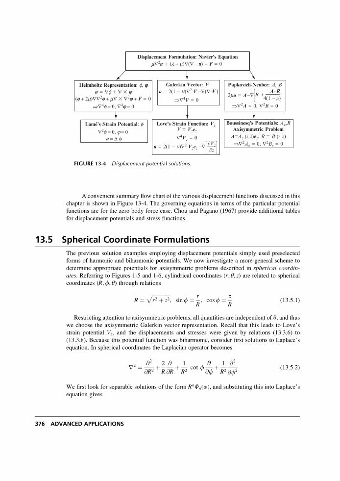
A convenient summary flow chart of the various displacement functions discussed in this
chapter is shown in Figure 13-4. The governing equations in terms of the particular potential
functions are for the zero body force case. Chou and Pagano (1967) provide additional tables
for displacement potentials and stress functions.
13.5 Spherical Coordinate Formulations
The previous solution examples employing displacement potentials simply used preselected
forms of harmonic and biharmonic potentials. We now investigate a more general scheme to
determine appropriate potentials for axisymmetric problems described in spherical coordin-ates. Referring to Figures 1-5 and 1-6, cylindrical coordinates (r, y, z) are related to spherical
coordinates (R,f, y) through relations
R ¼ffiffiffiffiffiffiffiffiffiffiffiffiffiffir2 þ z2
p, sinf ¼ r
R, cosf ¼ z
R(13:5:1)
Restricting attention to axisymmetric problems, all quantities are independent of y, and thuswe choose the axisymmetric Galerkin vector representation. Recall that this leads to Love’s
strain potential Vz, and the displacements and stresses were given by relations (13.3.6) to
(13.3.8). Because this potential function was biharmonic, consider first solutions to Laplace’s
equation. In spherical coordinates the Laplacian operator becomes
r2 ¼ @2
@R2þ 2
R
@
@Rþ 1
R2cot f
@
@fþ 1
R2
@2
@f2(13:5:2)
We first look for separable solutions of the form RnFn(f), and substituting this into Laplace’s
equation gives
Displacement Formulation: Navier’s Equation
Helmholtz Representation: f, jj
Lamé’s Strain Potential: f
Galerkin Vector: V
Love’s Strain Function: VzV = Vzez
∂z∂Vz
Papkovich-Neuber: A, B
4(1 − )2mu = A −∇ A . R
B +
Boussinesq’s Potentials: Az,BAxisymmetric Problem
A=Az (r,z)ez, B = B (r,z)
m∇2u + (l + m)∇(∇ . u) + F = 0
u = 2(1 − )∇2 V −∇(∇.V )
u = 2(1 − )∇2 Vzez −∇
u = ∇f + ∇ � j(f + 2m)∇∇2f + m∇ � ∇2j + F = 0
⇒∇4f = 0, ∇4j = 0⇒∇4V = 0
⇒∇2A = 0, ∇2B = 0
⇒∇2Az = 0, ∇2Bz = 0∇4Vz = 0
∇2f = 0, j = 0u = Δ f
FIGURE 13-4 Displacement potential solutions.
376 ADVANCED APPLICATIONS
1
sinfd
dfsinf
dFn
df
� �þ n(nþ 1)Fn ¼ 0 (13:5:3)
Next, making the change of variable x ¼ cosf, relation (13.5.3) becomes
(1� x2)d2Fn
dx2� 2x
dFn
dxþ n(nþ 1)Fn ¼ 0 (13:5:4)
and this is thewell-known Legendre differential equation. The two fundamental solutions are the
Legendre functions Pn(x) and Qn(x) of the first and second kinds. However, only Pn(x) is
continuous for jxj � 1, (0 � f � p), and so we drop the solution Qn(x). Considering only the
case of integer values of parameter n, the solution reduces to the Legendre polynomials given by
Pn(x) ¼ 1
2nn!
dn(x2 � 1)
dxn(13:5:5)
where P0 ¼ 1, P1 ¼ x, P2 ¼ 12(3x2 � 1), � � �. Putting these results together gives the follow-
ing harmonic solution set:
{RnFn} ¼ 1, z, z2 � 1
3(r2 þ z2), z3 � 3
5z(r2 þ z2), � � �
(13:5:6)
These terms are commonly referred to as spherical harmonics.Our goal, however, is to determine the elasticity solution that requires biharmonic functions
for theLove/Galerkin potential. In order to construct a set of biharmonic functions,we employ the
last term in relation (13.3.5) and thus argue that ifRnFn are harmonic,Rnþ2Fnwill be biharmonic.
Thus, a representation for the Love strain potential may be written as the linear combination
Vz ¼ B0(r2 þ z2)þ B1z(r
2 þ z2)þ B2(2z2 � r2)(r2 þ z2)
þ A0 þ A1zþ A2[z2 � 1
3(r2 þ z2)]þ � � �
(13:5:7)
It can be shown that this solution form is useful for general problems with finite domains.However, for the case involving infinite regions, this form will result in unbounded displace-
ments and stresses at infinity. Therefore, (13.5.7) must be modified for use in regions that
extend to infinity. This modification is easily developed by noting that the coefficient n(nþ 1)
in governing equation (13.5.3) will be the same if we were to replace n by (�n� 1). This
then implies that solution forms R�n�1F�n�1 ¼ R�n�1Fn will also be harmonic functions.
Following our previous construction scheme, another set of biharmonic functions for the
potential function can be expressed as
Vz ¼ B0(r2 þ z2)1=2 þ B1z(r
2 þ z2)�1=2 þ � � �þ A0(r
2 þ z2)�1=2 þ A1z(r2 þ z2)�3=2 þ � � �
(13:5:8)
and this form will be useful for infinite domain problems. For example, the solution to the
Kelvin problem in Example 13-1 can be found by choosing only the first term in relation
(13.5.8). This scheme can also be employed to construct a set of harmonic functions for the
Papkovich potentials; see Little (1973).
Displacement Potentials and Stress Functions 377
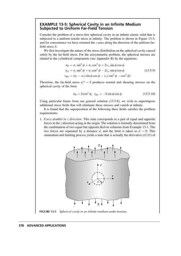
EXAMPLE 13-5: Spherical Cavity in an Infinite MediumSubjected to Uniform Far-Field Tension
Consider the problem of a stress-free spherical cavity in an infinite elastic solid that is
subjected to a uniform tensile stress at infinity. The problem is shown in Figure 13-5,
and for convenience we have oriented the z-axes along the direction of the uniform far-
field stress S.We first investigate the nature of the stress distribution on the spherical cavity caused
solely by the far-field stress. For the axisymmetric problem, the spherical stresses are
related to the cylindrical components (see Appendix B) by the equations
sR ¼ sr sin2 fþ sz cos2 fþ 2trz sinf cosf
sf ¼ sz sin2 fþ sr cos2 f� 2trz sinf cosf
tRf ¼ (sr � sz) sinf cosf� trz( sin2 f� cos2 f)
(13:5:9)
Therefore, the far-field stress s1z ¼ S produces normal and shearing stresses on the
spherical cavity of the form
sR ¼ S cos2 f, tRf ¼ �S sinf cosf (13:5:10)
Using particular forms from our general solution (13.5.8), we wish to superimpose
additional stress fields that will eliminate these stresses and vanish at infinity.
It is found that the superposition of the following three fields satisfies the problem
requirements:
1. Force doublet in z direction: This state corresponds to a pair of equal and opposite
forces in the z direction acting at the origin. The solution is formally determined from
the combination of two equal but opposite Kelvin solutions from Example 13-1. The
two forces are separated by a distance d, and the limit is taken as d ! 0. This
summation and limiting process yields a state that is actually the derivative (@=@z) of
x
y
z
a
S
S
FIGURE 13-5 Spherical cavity in an infinite medium under tension.
378 ADVANCED APPLICATIONS
EXAMPLE 13-5: Cont’d
the original Kelvin field with a new coefficient of �Ad (see Exercise 13-18). This
field’s coefficient is denoted as K1.
2. Center of dilatation: This field is the result of three mutually orthogonal double-
force pairs from the previous state (1) (see Exercise 13-19). The coefficient of this
state is denoted by K2.
3. Particular biharmonic term: A state corresponding to the A1 term from equation
(13.5.8).
Combining these three terms with the uniform far-field stress and using the condition of
zero stress on the spherical cavity provide sufficient equations to determine the three
unknown constants. Details of this process can be found in Timoshenko and Goodier
(1970), and the results determine the coefficients of the three superimposed fields
K1 ¼ � 5Sa3
2(7� 5�)
K2 ¼ S(1� 5�)a3
(7� 5�)
A1 ¼ Sa5
2(7� 5�)
(13:5:11)
Using these constants, the stress and displacement fields can be determined.
The normal stress on the x,y-plane (z ¼ 0) is given by
sz(r, 0) ¼ S 1þ 4� 5�
2(7� 5�)
a3
r3þ 9
2(7� 5�)
a5
r5
� �(13:5:12)
At r ¼ a, this result produces the maximum stress
sz(a, 0) ¼ (sz)max ¼27� 15�
2(7� 5�)S (13:5:13)
Typically, for many metals, � ¼ 0:3, and this would give a stress concentration factor of
(sz)max
S¼ 45
22¼ 2:04 (13:5:14)
It should be noted that in three dimensions the stress concentration factor is generally a
function of Poisson’s ratio. A plot of this general behavior given by equation (13.5.13)
is shown in Figure 13-6. It can be observed that the value of Poisson’s ratio produces
only small variation on the stress concentration. It is also interesting to note that if the
plot were continued for negative values of Poisson’s ratio, further decrease in the stress
concentration would be found. Exercise 13-25 explores this behavior in more detail.
Note that the corresponding two-dimensional case was previously developed in
Example 8-7 and produced a stress concentration factor of 3. Plots of the corresponding
two- and three-dimensional stress distributions are shown in Figure 13-7. For each case
the normal stress component in the direction of loading is plotted versus radial distance
away from the hole. It is seen that the three-dimensional stresses are always less than
Continued
Displacement Potentials and Stress Functions 379
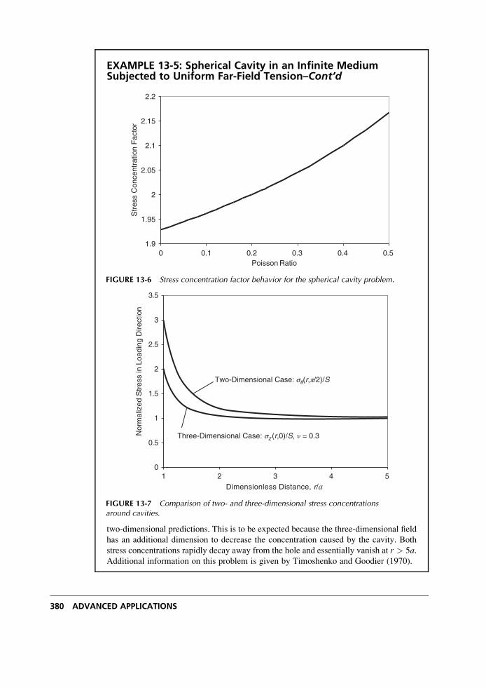
EXAMPLE 13-5: Spherical Cavity in an Infinite MediumSubjected to Uniform Far-Field Tension–Cont’d
two-dimensional predictions. This is to be expected because the three-dimensional field
has an additional dimension to decrease the concentration caused by the cavity. Both
stress concentrations rapidly decay away from the hole and essentially vanish at r > 5a.Additional information on this problem is given by Timoshenko and Goodier (1970).
1.9
1.95
2.05
2
2.1
2.15
2.2
0 0.1 0.2 0.3 0.4 0.5Poisson Ratio
Str
ess
Con
cent
ratio
n F
acto
r
FIGURE 13-6 Stress concentration factor behavior for the spherical cavity problem.
0
0.5
1
1.5
2
2.5
3
3.5
Dimensionless Distance, r/a
Nor
mal
ized
Str
ess
in L
oadi
ng D
irect
ion
Two-Dimensional Case: sq(r,p/2)/S
Three-Dimensional Case: sz (r,0)/S, � = 0.3
1 2 3 4 5
FIGURE 13-7 Comparison of two- and three-dimensional stress concentrationsaround cavities.
380 ADVANCED APPLICATIONS
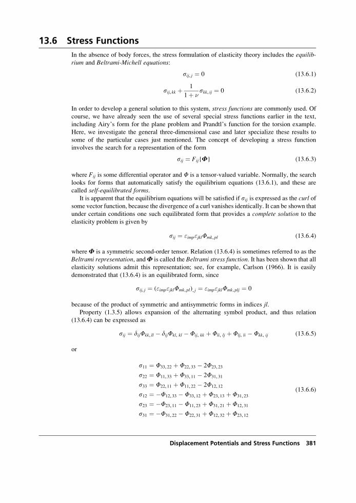
13.6 Stress Functions
In the absence of body forces, the stress formulation of elasticity theory includes the equilib-rium and Beltrami-Michell equations:
sij, j ¼ 0 (13:6:1)
sij, kk þ 1
1þ �skk, ij ¼ 0 (13:6:2)
In order to develop a general solution to this system, stress functions are commonly used. Of
course, we have already seen the use of several special stress functions earlier in the text,
including Airy’s form for the plane problem and Prandtl’s function for the torsion example.
Here, we investigate the general three-dimensional case and later specialize these results to
some of the particular cases just mentioned. The concept of developing a stress function
involves the search for a representation of the form
sij ¼ Fij{F} (13:6:3)
where Fij is some differential operator and F is a tensor-valued variable. Normally, the search
looks for forms that automatically satisfy the equilibrium equations (13.6.1), and these are
called self-equilibrated forms.It is apparent that the equilibrium equations will be satisfied if sij is expressed as the curl of
some vector function, because the divergence of a curl vanishes identically. It can be shown that
under certain conditions one such equilibrated form that provides a complete solution to the
elasticity problem is given by
sij ¼ "imp"jklFmk, pl (13:6:4)
where F is a symmetric second-order tensor. Relation (13.6.4) is sometimes referred to as the
Beltrami representation, andF is called the Beltrami stress function. It has been shown that allelasticity solutions admit this representation; see, for example, Carlson (1966). It is easily
demonstrated that (13.6.4) is an equilibrated form, since
sij, j ¼ ("imp"jklFmk, pl), j ¼ "imp"jklFmk, plj ¼ 0
because of the product of symmetric and antisymmetric forms in indices jl.Property (1.3.5) allows expansion of the alternating symbol product, and thus relation
(13.6.4) can be expressed as
sij ¼ dijFkk, ll � dijFkl, kl � Fij, kk þ Fli, lj þ Flj, li � Fkk, ij (13:6:5)
or
s11 ¼ F33, 22 þ F22, 33 � 2F23, 23
s22 ¼ F11, 33 þ F33, 11 � 2F31, 31
s33 ¼ F22, 11 þ F11, 22 � 2F12, 12
s12 ¼ �F12, 33 � F33, 12 þ F23, 13 þ F31, 23
s23 ¼ �F23, 11 � F11, 23 þ F31, 21 þ F12, 31
s31 ¼ �F31, 22 � F22, 31 þ F12, 32 þ F23, 12
(13:6:6)
Displacement Potentials and Stress Functions 381
The first invariant of the stress tensor then becomes
snn ¼ "nmp"nklFmk, pl
¼ (dmkdpl � dmldpk)Fmk, pl
¼ Fkk, ll � Flk, lk
(13:6:7)
and thus the compatibility equations (13.6.2) can be expressed in terms of the general stress
function as
("imp"jklFmk, pl), nn þ1
1þ �(Fkk, ll � Flk, lk), ij ¼ 0 (13:6:8)
Not all of the six components of Fij are independent. Two alternate ways of generating
complete solutions to the stress formulation problem are developed through the use of reducedforms that include the Maxwell and Morera stress function formulations.
13.6.1 Maxwell Stress Function RepresentationThe Maxwell stress function representation considers the reduced form whereby all off-
diagonal elements of Fij are set to zero; that is,
Fij ¼F11 0 0
0 F22 0
0 0 F33
24
35 (13:6:9)
which yields a representation
s11 ¼ F33, 22 þ F22, 33
s22 ¼ F11, 33 þ F33, 11
s33 ¼ F22, 11 þ F11, 22
s12 ¼ �F33, 12
s23 ¼ �F11, 23
s31 ¼ �F22, 31
(13:6:10)
Notice that the Airy stress function that is used for two-dimensional problems is a special case
of this scheme with F11 ¼ F22 ¼ 0 and F33 ¼ f(x1, x2).
13.6.2 Morera Stress Function RepresentationThe Morera stress function method uses the general form with diagonal terms set to zero;
that is,
Fij ¼0 F12 F13
F12 0 F23
F13 F23 0
24
35 (13:6:11)
This approach yields the representation
382 ADVANCED APPLICATIONS
s11 ¼ �2F23, 23
s22 ¼ �2F31, 31
s33 ¼ �2F12, 12
s12 ¼ �F12, 33 þ F23, 13 þ F13, 23
s23 ¼ �F23, 11 þ F13, 21 þ F12, 31
s31 ¼ �F31, 22 þ F12, 32 þ F23, 12
(13:6:12)
It can be observed that for the torsion problem, the Prandtl stress function (here denoted by j)is a special case of this representation with F12 ¼ F13 ¼ 0 and F23, 1 ¼ j(x1, x2).
References
Carlson DE: On the completeness of the Beltrami stress functions in continuum mechanics, Jour. Math.Anal. Appl., vol 15, pp. 311-315, 1966.
Chou PC, and Pagano NJ: Elasticity Tensor, Dyadic and Engineering Approaches, D. Van Nostrand,
Princeton, NJ, 1967.
Eubanks RA, and Sternberg E: On the completeness of the Boussinesq-Papkovich stress functions, Jour.Rational Mech. Anal., vol 5, pp. 735-746, 1956.
Fung YC: Foundations of Solid Mechanics, Prentice Hall, Englewood Cliffs, NJ, 1965.
Galerkin B: Contribution a la solution generale du probleme de la theorie de l’elasticite dans le cas de trios
dimensions, Comptes Rendus, vol 190, p. 1047, 1930.Graff KF: Wave Motion in Elastic Solids, Dover, New York, 1991.
Lakes RS: Foam structures with a negative Poisson’s ratio, Science, vol 235, pp. 1038-1040, 1987.Little RW: Elasticity, Prentice Hall, Englewood Cliffs, NJ, 1973.
Love AEH: A Treatise on the Mathematical Theory of Elasticity, 4th ed., Dover, New York, 1944.
Neuber H: Ein neurer Censatz zur Losing Raumlicher Probleme der Elastez-etatstheorie, Z. Angew. Math.Mech., vol 14, p. 203, 1934.
Papkovich PF: An expression for a general integral of the equations of the theory of elasticity in terms of
harmonic functions, Izvest. Akad. Nauk SSSR, Ser. Matem. K. estestv. neuk, no. 10, 1932.Timoshenko SP, and Goodier JN: Theory of Elasticity, McGraw-Hill, New York, 1970.
Exercises
13-1. Using the Helmholtz representation, determine the displacement field that corresponds
to the potentials f ¼ x2 þ 4y2, w ¼ R2e3. Next show that this displacement field
satisfies Navier’s equation with no body forces.
13-2. Explicitly show that the dilatation and rotation are related to the Helmholtz potentials
through relations (13.1.3).
13-3. For the case of zero body forces, show that by using the vector identity (1:8:5)9 Navier’sequation can be written as
(lþ 2m)r2uþ (lþ m)=� =� u ¼ 0
Using repeated differential operations on this result, show that the displacement vector is
biharmonic. Furthermore, because the stress and strain are linear combinations of first
derivatives of the displacement, they too will be biharmonic.
13-4. For the case of Lame’s potential, show that strains and stresses are given by (13.2.3).
Displacement Potentials and Stress Functions 383
13-5. Justify that the Galerkin vector satisfies the governing equation (13.3.2).
13-6. Show that the Helmholtz potentials are related to the Galerkin vector by relations
(13.3.3).
13-7. Justify relations (13.3.4) for the stress components in terms of the Galerkin vector.
13-8. For the case of zero body forces, the Galerkin vector is biharmonic. However, it was
pointed out that in curvilinear coordinate systems, the individual Galerkin vector
components might not necessarily be biharmonic. Consider the cylindrical coordinate
case where V ¼ Vrer þ Vyey þ Vzez. Using the results of Section 1.9, first show that
the Laplacian operator on each term will give rise to the following relations:
r2(Vrer) ¼ r2Vr � Vr
r2
� �er þ 2
r2@Vr
@yey
r2(Vyey) ¼ r2Vy � Vy
r2
� �ey � 2
r2@Vy
@yer
r2(Vzez) ¼ r2Vzez
Using these results, show that the biharmonic components are given by
r2r2(Vrer) ¼ r2 � 1
r2
� �2
Vr � 4
r4@2Vr
@y2
" #er þ 4
r2r2 � 1
r2
� �@Vr
@y
� �ey
r2r2(Vyey) ¼ � 4
r2r2 � 1
r2
� �@Vy
@y
� �er þ r2 � 1
r2
� �2
Vy � 4
r4@2Vy
@y2
" #ey
r2r2(Vzez) ¼ r2r2Vzez
and thus only the component Vz will satisfy the scalar biharmonic equation.
13-9. Explicitly show that Boussinesq’s problem as illustrated in Figure 13-2 is solved by the
superposition of a Galerkin vector and Lame’s potential given by relation (13.3.13).
Verify that the Cartesian displacements and stresses are given by
u ¼ Px
4pmRz
R2� 1� 2�
Rþ z
� �, v ¼ Py
4pmRz
R2� 1� 2�
Rþ z
� �, w ¼ P
4pmR2(1� �)þ z2
R2
� �
sx ¼ � P
2pR2
3x2z
R3� (1� 2�)
z
R� R
Rþ zþ x2(2Rþ z)
R(Rþ z)2
� �� �
sy ¼ � P
2pR2
3y2z
R3� (1� 2�)
z
R� R
Rþ zþ y2(2Rþ z)
R(Rþ z)2
� �� �
sz ¼ � 3Pz3
2pR5, txy ¼ � P
2pR2
3xyz
R3� (1� 2�)(2Rþ z)xy
R(Rþ z)2
� �
tyz ¼ � 3Pyz2
2pR5, txz ¼ � 3Pxz2
2pR5
13-10. Show that Cerruti’s problem of Figure 13-3 is solved by the Galerkin vector and
Lame’s potential specified in relations (13.3.15). Develop the expressions for the
Cartesian displacements and stresses
384 ADVANCED APPLICATIONS
u ¼ P
4pmR1þ x2
R2þ (1� 2�)
R
Rþ z� x2
(Rþ z)2
� �� �
v ¼ Pxy
4pmR1
R2� 1� 2�
(Rþ z)2
� �, w ¼ Px
4pmRz
R2þ 1� 2�
Rþ z
� �
sx ¼ Px
2pR3� 3x2
R2þ (1� 2�)
(Rþ z)2R2 � y2 � 2Ry2
Rþ z
� �� �
sy ¼ Px
2pR3� 3y2
R2þ (1� 2�)
(Rþ z)23R2 � x2 � 2Rx2
Rþ z
� �� �
sz ¼ � 3Pxz2
2pR5, tyz ¼ � 3Pxyz
2pR5, txz ¼ � 3Px2z
2pR5
txy ¼ � Py
2pR3� 3x2
R2� (1� 2�)
(Rþ z)2R2 � x2 þ 2Rx2
Rþ z
� �� �
13-11. Explicitly justify that the Papkovich functions A and B satisfy relations (13.4.9).
13-12. For the axisymmetric case, the Papkovich functions reduced to the Boussinesq
potentials B and Az defined by relations (13.5.11). Show that the general forms for the
displacements and stresses in cylindrical coordinates are given by
ur ¼ � 1
2m@
@rBþ Azz
4(1� �)
� �, uu ¼ 0 , uz ¼ 1
2mAz � @
@zBþ Azz
4(1� �)
� �� �
sr ¼ � �
1� 2�r2 Azz
4(1� �)
� �þ �
1� 2�
@Az
@z� @2
@r2Bþ Azz
4(1� �)
� �
sy ¼ � �
1� 2�r2 Azz
4(1� �)
� �þ �
1� 2�
@Az
@z� 1
r
@
@rBþ Azz
4(1� �)
� �
sz ¼ � �
1� 2�r2 Azz
4(1� �)
� �þ �
1� 2�
@Az
@zþ @Az
@z� @2
@z2Bþ Azz
4(1� �)
� �
trz ¼ 2merz ¼ 1
2
@Az
@r� @2
@r@zBþ Azz
4(1� �)
� �
13-13. Using the results of Exercise 13-12, verify that the displacement and stress fields for
the Boussinesq problem of Example 13-4 are given by (13.4.16) and (13.4.17). Note
the interesting behavior of the radial displacement, that ur > 0 only for points where
z=R > (1� 2�)R=(Rþ z). Show that points satisfying this inequality lie inside a cone
f � fo, with fo determined by the relation cos2 fo þ cosfo � (1� 2�) ¼ 0.
13-14*. The displacement field for the Boussinesq problem was given by (13.4.16). For this
case, construct a displacement vector distribution plot, similar to the two-dimensional
case shown in Figure 8-22. For convenience, choose the coefficient P=4pm ¼ 1 and
take v ¼ 0:3. Compare the two-and three-dimensional results.
13-15. Consider an elastic half space with sz ¼ 0 on the surface z ¼ 0. For the axisymmetric
problem, show that the Boussinesq potentials must satisfy the relation Az ¼ 2 @B=@zwithin the half space.
Displacement Potentials and Stress Functions 385
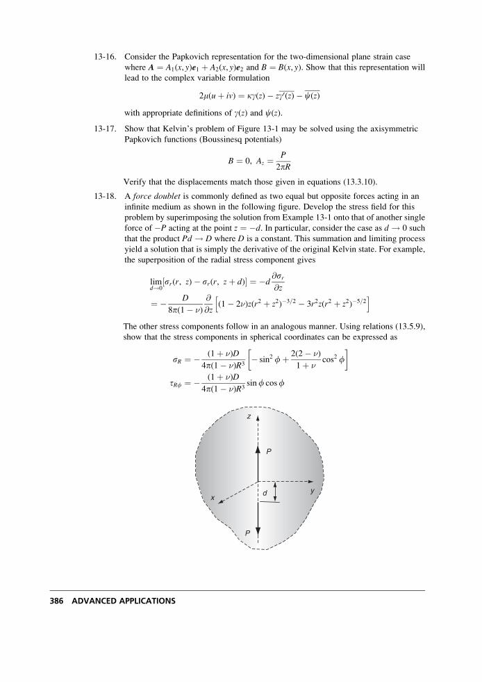
13-16. Consider the Papkovich representation for the two-dimensional plane strain case
where A ¼ A1(x, y)e1 þ A2(x, y)e2 and B ¼ B(x, y). Show that this representation will
lead to the complex variable formulation
2m(uþ iv) ¼ kg(z)� zg0(z)� c(z)
with appropriate definitions of g(z) and c(z).
13-17. Show that Kelvin’s problem of Figure 13-1 may be solved using the axisymmetric
Papkovich functions (Boussinesq potentials)
B ¼ 0, Az ¼ P
2pR
Verify that the displacements match those given in equations (13.3.10).
13-18. A force doublet is commonly defined as two equal but opposite forces acting in an
infinite medium as shown in the following figure. Develop the stress field for this
problem by superimposing the solution from Example 13-1 onto that of another single
force of �P acting at the point z ¼ �d. In particular, consider the case as d ! 0 such
that the product Pd ! D where D is a constant. This summation and limiting process
yield a solution that is simply the derivative of the original Kelvin state. For example,
the superposition of the radial stress component gives
limd!0
sr(r, z)� sr(r, zþ d)½ � ¼ �d@sr@z
¼ � D
8p(1� �)
@
@z(1� 2�)z(r2 þ z2)�3=2 � 3r2z(r2 þ z2)�5=2h i
The other stress components follow in an analogous manner. Using relations (13.5.9),
show that the stress components in spherical coordinates can be expressed as
sR ¼ � (1þ �)D
4p(1� �)R3� sin2 fþ 2(2� �)
1þ �cos2 f
� �
tRf ¼ � (1þ �)D
4p(1� �)R3sinf cosf
xy
z
P
P
d
386 ADVANCED APPLICATIONS
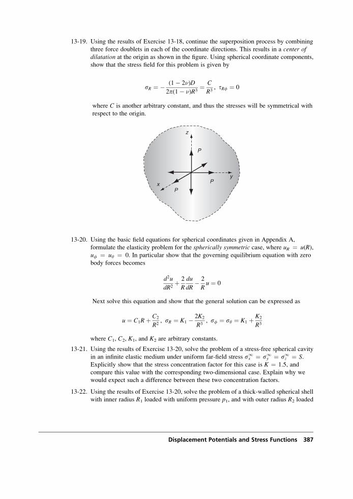
13-19. Using the results of Exercise 13-18, continue the superposition process by combining
three force doublets in each of the coordinate directions. This results in a center ofdilatation at the origin as shown in the figure. Using spherical coordinate components,
show that the stress field for this problem is given by
sR ¼ � (1� 2�)D
2p(1� �)R3¼ C
R3, tRf ¼ 0
where C is another arbitrary constant, and thus the stresses will be symmetrical with
respect to the origin.
x
y
z
P
P
P
13-20. Using the basic field equations for spherical coordinates given in Appendix A,
formulate the elasticity problem for the spherically symmetric case, where uR ¼ u(R),uf ¼ uy ¼ 0. In particular show that the governing equilibrium equation with zero
body forces becomes
d2u
dR2þ 2
R
du
dR� 2
Ru ¼ 0
Next solve this equation and show that the general solution can be expressed as
u ¼ C1Rþ C2
R2, sR ¼ K1 � 2K2
R3, sf ¼ sy ¼ K1 þ K2
R3
where C1, C2, K1, and K2 are arbitrary constants.
13-21. Using the results of Exercise 13-20, solve the problem of a stress-free spherical cavity
in an infinite elastic medium under uniform far-field stress sx1 ¼ sy
1 ¼ sz1 ¼ S.
Explicitly show that the stress concentration factor for this case is K ¼ 1.5, and
compare this value with the corresponding two-dimensional case. Explain why we
would expect such a difference between these two concentration factors.
13-22. Using the results of Exercise 13-20, solve the problem of a thick-walled spherical shell
with inner radius R1 loaded with uniform pressure p1, and with outer radius R2 loaded
Displacement Potentials and Stress Functions 387
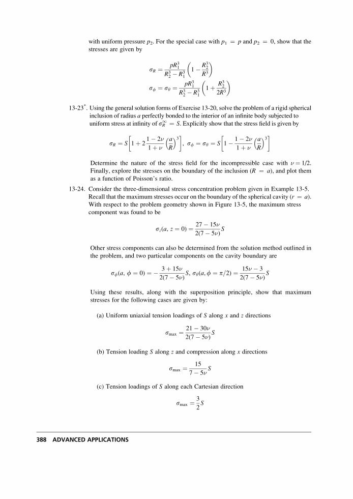
with uniform pressure p2. For the special case with p1 ¼ p and p2 ¼ 0, show that the
stresses are given by
sR ¼ pR31
R32 � R3
1
1� R32
R3
� �
sf ¼ sy ¼ pR31
R32 � R3
1
1þ R32
2R3
� �
13-23*. Using the general solution forms of Exercise 13-20, solve the problem of a rigid spherical
inclusion of radius a perfectly bonded to the interior of an infinite body subjected touniform stress at infinity of sR
1 ¼ S. Explicitly show that the stress field is given by
sR ¼ S 1þ 21� 2�
1þ �
a
R
� �3� �, sf ¼ sy ¼ S 1� 1� 2�
1þ �
a
R
� �3� �
Determine the nature of the stress field for the incompressible case with � ¼ 1/2.
Finally, explore the stresses on the boundary of the inclusion (R ¼ a), and plot them
as a function of Poisson’s ratio.
13-24. Consider the three-dimensional stress concentration problem given in Example 13-5.
Recall that the maximum stresses occur on the boundary of the spherical cavity (r ¼ a).With respect to the problem geometry shown in Figure 13-5, the maximum stress
component was found to be
sz(a, z ¼ 0) ¼ 27� 15�
2(7� 5�)S
Other stress components can also be determined from the solution method outlined in
the problem, and two particular components on the cavity boundary are
sf(a, f ¼ 0) ¼ � 3þ 15�
2(7� 5�)S, sy(a,f ¼ p=2) ¼ 15� � 3
2(7� 5�)S
Using these results, along with the superposition principle, show that maximum
stresses for the following cases are given by:
(a) Uniform uniaxial tension loadings of S along x and z directions
smax ¼ 21� 30�
2(7� 5�)S
(b) Tension loading S along z and compression along x directions
smax ¼ 15
7� 5�S
(c) Tension loadings of S along each Cartesian direction
smax ¼ 3
2S
388 ADVANCED APPLICATIONS
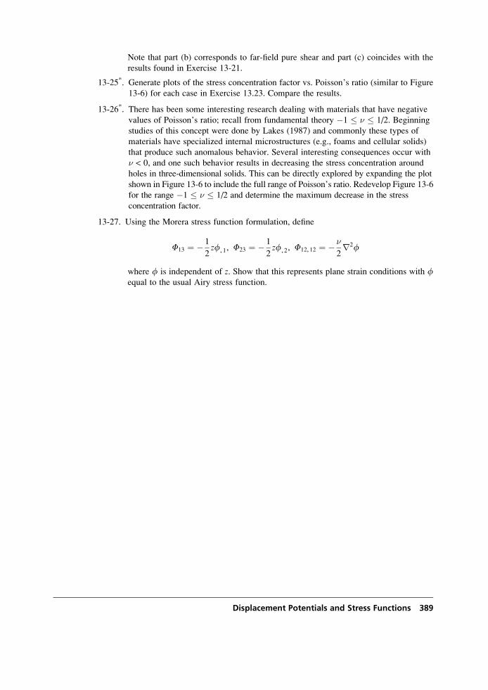
Note that part (b) corresponds to far-field pure shear and part (c) coincides with the
results found in Exercise 13-21.
13-25*. Generate plots of the stress concentration factor vs. Poisson’s ratio (similar to Figure
13-6) for each case in Exercise 13.23. Compare the results.
13-26*. There has been some interesting research dealing with materials that have negative
values of Poisson’s ratio; recall from fundamental theory �1 � � � 1/2. Beginning
studies of this concept were done by Lakes (1987) and commonly these types of
materials have specialized internal microstructures (e.g., foams and cellular solids)
that produce such anomalous behavior. Several interesting consequences occur with
� < 0, and one such behavior results in decreasing the stress concentration around
holes in three-dimensional solids. This can be directly explored by expanding the plot
shown in Figure 13-6 to include the full range of Poisson’s ratio. Redevelop Figure 13-6
for the range �1 � � � 1/2 and determine the maximum decrease in the stress
concentration factor.
13-27. Using the Morera stress function formulation, define
F13 ¼ � 1
2zf, 1, F23 ¼ � 1
2zf, 2, F12, 12 ¼ � �
2r2f
where f is independent of z. Show that this represents plane strain conditions with fequal to the usual Airy stress function.
Displacement Potentials and Stress Functions 389
14 Nonhomogeneous Elasticity
It has been observed that many materials have a spatially varying microstructure that leads to
spatial variation in elastic properties and thus requires a nonhomogeneous model. For example,
in geomechanics studies rock and soil material will commonly have depth-dependent proper-
ties resulting from the overburden of material lying above a given point. Gradations in
microstructure are also commonly found in biological cellular materials such as wood and
bone, where biological adaptation has distributed the strongest microstructure in regions that
experience the highest stress.
Recently, there has been considerable interest in the development of graded materials thathave spatial property variations deliberately created to improve mechanical performance
(Suresh, 2001). Such graded properties can be traced back to surface heat treatments for
swords, knives, and gear teeth. Various composite materials have been constructed using
graded transitions in composition to reduce stress concentrations at interfaces. In the 1990s,
interest in graded materials focused on controlling thermal stresses in structures exposed to
high-temperature applications and to surface contact damage. This work has led to a new class
of engineered materials called functionally graded materials (FGMs) that are developed with
spatially varying properties to suit particular applications. The graded composition of such
materials is commonly established and controlled using advanced manufacturing techniques,
including powder metallurgy, chemical vapor deposition, centrifugal casting, and other
schemes.
Our previous developments have been connected to the formulation and solution of
isotropic and anisotropic elasticity problems. We now wish to go back and investigate the
inhomogeneous isotropic case and explore solutions for a few problems that exist in the
literature. We will focus attention on formulation issues that allow the development of
tractable boundary value problems and will examine the effect of inhomogeneity on the
resulting stress and displacement solution fields. By exploring closed-form solutions to a series
of example problems, we will see that in some cases inhomogeneity produces little effect,
while in others significant and fundamentally different stress and displacement distributions
will occur.
391
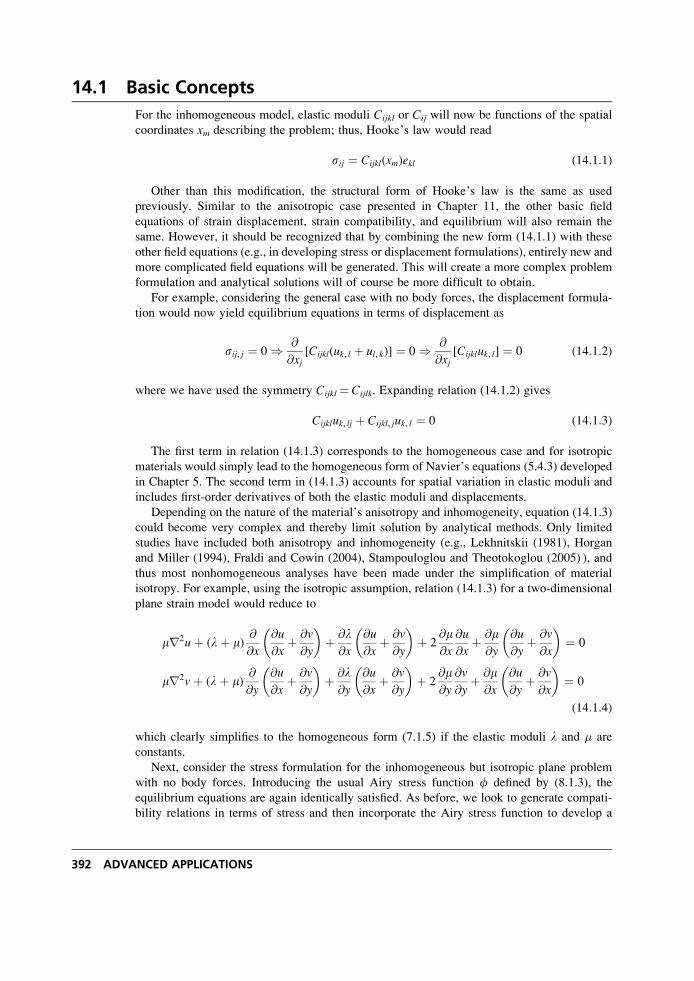
14.1 Basic Concepts
For the inhomogeneous model, elastic moduli Cijkl or Cij will now be functions of the spatial
coordinates xm describing the problem; thus, Hooke’s law would read
sij ¼ Cijkl(xm)ekl (14:1:1)
Other than this modification, the structural form of Hooke’s law is the same as used
previously. Similar to the anisotropic case presented in Chapter 11, the other basic field
equations of strain displacement, strain compatibility, and equilibrium will also remain the
same. However, it should be recognized that by combining the new form (14.1.1) with these
other field equations (e.g., in developing stress or displacement formulations), entirely new and
more complicated field equations will be generated. This will create a more complex problem
formulation and analytical solutions will of course be more difficult to obtain.
For example, considering the general case with no body forces, the displacement formula-
tion would now yield equilibrium equations in terms of displacement as
sij, j ¼ 0 ) @
@xj[Cijkl(uk, l þ ul, k)] ¼ 0 ) @
@xj[Cijkluk, l] ¼ 0 (14:1:2)
where we have used the symmetry Cijkl¼ Cijlk. Expanding relation (14.1.2) gives
Cijkluk, lj þ Cijkl, juk, l ¼ 0 (14:1:3)
The first term in relation (14.1.3) corresponds to the homogeneous case and for isotropic
materials would simply lead to the homogeneous form of Navier’s equations (5.4.3) developed
in Chapter 5. The second term in (14.1.3) accounts for spatial variation in elastic moduli and
includes first-order derivatives of both the elastic moduli and displacements.
Depending on the nature of the material’s anisotropy and inhomogeneity, equation (14.1.3)
could become very complex and thereby limit solution by analytical methods. Only limited
studies have included both anisotropy and inhomogeneity (e.g., Lekhnitskii (1981), Horgan
and Miller (1994), Fraldi and Cowin (2004), Stampouloglou and Theotokoglou (2005) ), and
thus most nonhomogeneous analyses have been made under the simplification of material
isotropy. For example, using the isotropic assumption, relation (14.1.3) for a two-dimensional
plane strain model would reduce to
mr2u þ (l þ m)@
@x
@u
@xþ @v
@y
� �þ @l
@x
@u
@xþ @v
@y
� �þ 2
@m@x
@u
@xþ @m
@y
@u
@yþ @v
@x
� �¼ 0
mr2v þ (l þ m)@
@y
@u
@xþ @v
@y
� �þ @l
@y
@u
@xþ @v
@y
� �þ 2
@m@y
@v
@yþ @m
@x
@u
@yþ @v
@x
� �¼ 0
(14:1:4)
which clearly simplifies to the homogeneous form (7.1.5) if the elastic moduli l and � are
constants.
Next, consider the stress formulation for the inhomogeneous but isotropic plane problem
with no body forces. Introducing the usual Airy stress function f defined by (8.1.3), the
equilibrium equations are again identically satisfied. As before, we look to generate compati-
bility relations in terms of stress and then incorporate the Airy stress function to develop a
392 ADVANCED APPLICATIONS
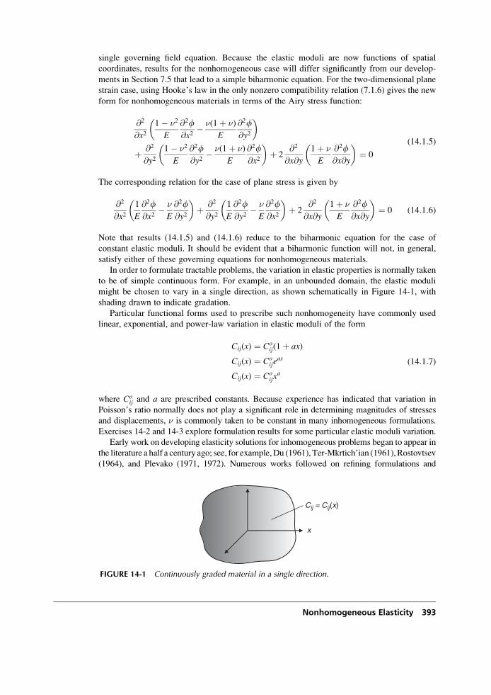
single governing field equation. Because the elastic moduli are now functions of spatial
coordinates, results for the nonhomogeneous case will differ significantly from our develop-
ments in Section 7.5 that lead to a simple biharmonic equation. For the two-dimensional plane
strain case, using Hooke’s law in the only nonzero compatibility relation (7.1.6) gives the new
form for nonhomogeneous materials in terms of the Airy stress function:
@2
@x21� �2
E
@2f@x2
� �(1þ �)
E
@2f@y2
� �
þ @2
@y21� �2
E
@2f@y2
� �(1þ �)
E
@2f@x2
� �þ 2
@2
@x@y
1þ �
E
@2f@x@y
� �¼ 0
(14:1:5)
The corresponding relation for the case of plane stress is given by
@2
@x21
E
@2f@x2
� �
E
@2f@y2
� �þ @2
@y21
E
@2f@y2
� �
E
@2f@x2
� �þ 2
@2
@x@y
1þ �
E
@2f@x@y
� �¼ 0 (14:1:6)
Note that results (14.1.5) and (14.1.6) reduce to the biharmonic equation for the case of
constant elastic moduli. It should be evident that a biharmonic function will not, in general,
satisfy either of these governing equations for nonhomogeneous materials.
In order to formulate tractable problems, the variation in elastic properties is normally taken
to be of simple continuous form. For example, in an unbounded domain, the elastic moduli
might be chosen to vary in a single direction, as shown schematically in Figure 14-1, with
shading drawn to indicate gradation.
Particular functional forms used to prescribe such nonhomogeneity have commonly used
linear, exponential, and power-law variation in elastic moduli of the form
Cij(x) ¼ Coij(1þ ax)
Cij(x) ¼ Coije
ax
Cij(x) ¼ Coijx
a
(14:1:7)
where Coij and a are prescribed constants. Because experience has indicated that variation in
Poisson’s ratio normally does not play a significant role in determining magnitudes of stresses
and displacements, � is commonly taken to be constant in many inhomogeneous formulations.
Exercises 14-2 and 14-3 explore formulation results for some particular elastic moduli variation.
Early work on developing elasticity solutions for inhomogeneous problems began to appear in
the literature a half a century ago; see, for example,Du (1961), Ter-Mkrtich’ian (1961), Rostovtsev
(1964), and Plevako (1971, 1972). Numerous works followed on refining formulations and
Cij = Cij(x)
x
FIGURE 14-1 Continuously graded material in a single direction.
Nonhomogeneous Elasticity 393
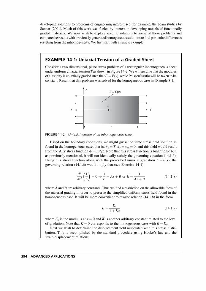
developing solutions to problems of engineering interest; see, for example, the beam studies by
Sankar (2001). Much of this work was fueled by interest in developing models of functionally
graded materials. We now wish to explore specific solutions to some of these problems and
compare the resultswithpreviously generated homogeneous solutions tofindparticular differences
resulting from the inhomogeneity. We first start with a simple example.
EXAMPLE 14-1: Uniaxial Tension of a Graded Sheet
Consider a two-dimensional, plane stress problem of a rectangular inhomogeneous sheet
under uniformuniaxial tensionT as shown in Figure 14-2.Wewill assume that themodulus
of elasticity is uniaxially graded such thatE¼ E(x), while Poisson’s ratiowill be taken to beconstant. Recall that this problem was solved for the homogeneous case in Example 8-1.
x
y
TT
l
E = E(x)
FIGURE 14-2 Uniaxial tension of an inhomogeneous sheet.
Based on the boundary conditions, we might guess the same stress field solution as
found in the homogeneous case, that is, sx¼ T, sy¼ txy¼ 0, and this field would result
from the Airy stress function f¼ Ty2/2. Note that this stress function is biharmonic but,
as previously mentioned, it will not identically satisfy the governing equation (14.1.6).
Using this stress function along with the prescribed uniaxial gradation E¼ E(x), thegoverning relation (14.1.6) would imply that (see Exercise 14-1)
d2
dx21
E
� �¼ 0 ) 1
E¼ Axþ B or E ¼ 1
Axþ B(14:1:8)
where A and B are arbitrary constants. Thus we find a restriction on the allowable form of
the material grading in order to preserve the simplified uniform stress field found in the
homogeneous case. It will be more convenient to rewrite relation (14.1.8) in the form
E ¼ Eo
1þ Kx(14:1:9)
where Eo is the modulus at x¼ 0 and K is another arbitrary constant related to the level
of gradation. Note that K¼ 0 corresponds to the homogeneous case with E¼ Eo.
Next we wish to determine the displacement field associated with this stress distri-
bution. This is accomplished by the standard procedure using Hooke’s law and the
strain displacement relations
394 ADVANCED APPLICATIONS
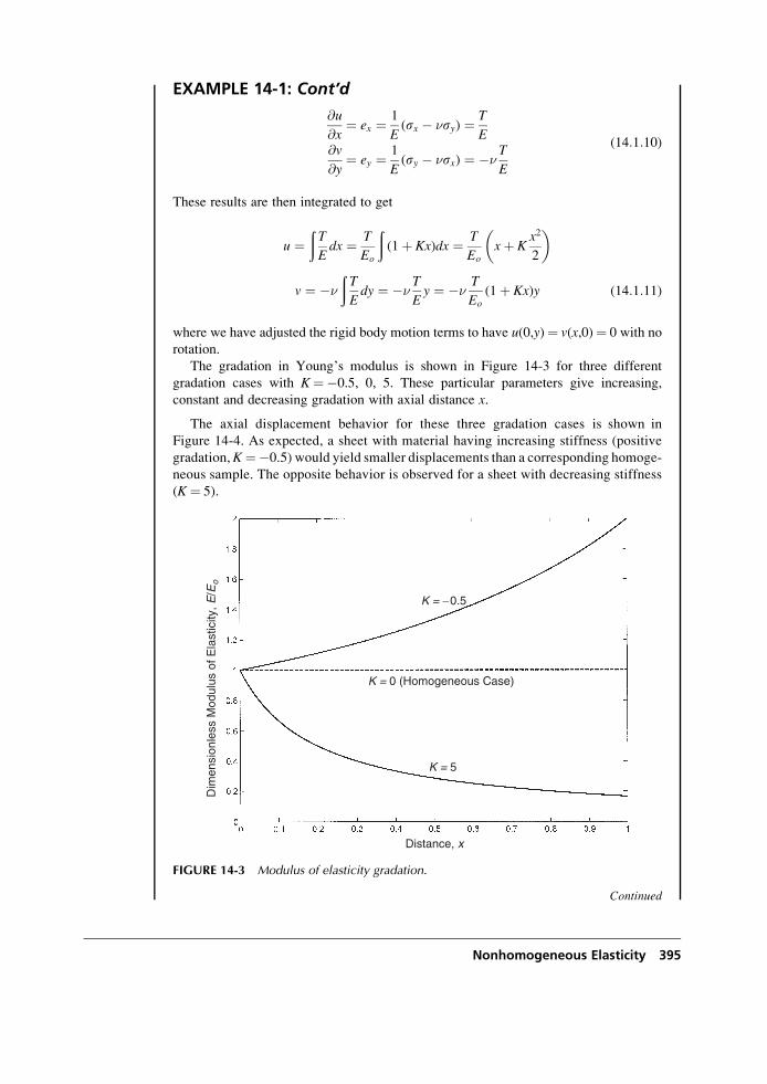
EXAMPLE 14-1: Cont’d
@u
@x¼ ex ¼ 1
E(sx � �sy) ¼ T
E@v
@y¼ ey ¼ 1
E(sy � �sx) ¼ ��
T
E
(14:1:10)
These results are then integrated to get
u ¼ðT
Edx ¼ T
Eo
ð(1þ Kx)dx ¼ T
Eoxþ K
x2
2
� �
v ¼ ��
ðT
Edy ¼ ��
T
Ey ¼ ��
T
Eo(1þ Kx)y (14:1:11)
where we have adjusted the rigid body motion terms to have u(0,y)¼ v(x,0)¼ 0 with no
rotation.
The gradation in Young’s modulus is shown in Figure 14-3 for three different
gradation cases with K¼�0.5, 0, 5. These particular parameters give increasing,
constant and decreasing gradation with axial distance x.
The axial displacement behavior for these three gradation cases is shown in
Figure 14-4. As expected, a sheet with material having increasing stiffness (positive
gradation,K¼�0.5) would yield smaller displacements than a corresponding homoge-
neous sample. The opposite behavior is observed for a sheet with decreasing stiffness
(K¼ 5).
K = 5
K = 0 (Homogeneous Case)
K = − 0.5
Distance, x
Dim
ensi
onle
ss M
odul
us o
f Ela
stic
ity, E
/Eo
FIGURE 14-3 Modulus of elasticity gradation.
Continued
Nonhomogeneous Elasticity 395
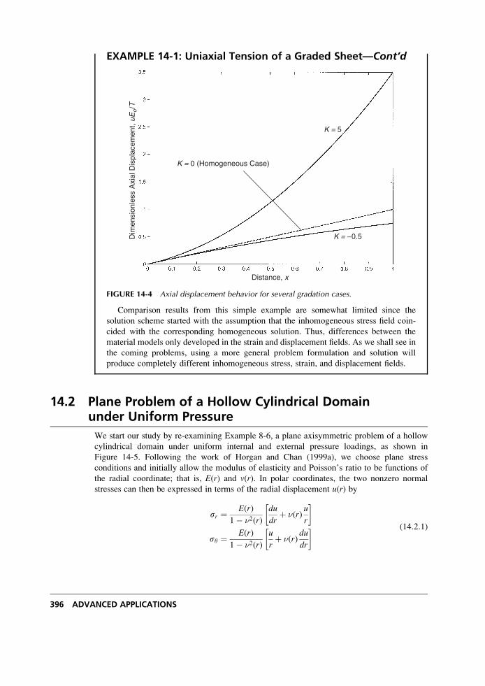
EXAMPLE 14-1: Uniaxial Tension of a Graded Sheet—Cont’d
K = 5
K = 0 (Homogeneous Case)
Distance, x
Dim
ensi
onle
ss A
xial
Dis
plac
emen
t, uE
o/T
K = −0.5
FIGURE 14-4 Axial displacement behavior for several gradation cases.
Comparison results from this simple example are somewhat limited since the
solution scheme started with the assumption that the inhomogeneous stress field coin-
cided with the corresponding homogeneous solution. Thus, differences between the
material models only developed in the strain and displacement fields. As we shall see in
the coming problems, using a more general problem formulation and solution will
produce completely different inhomogeneous stress, strain, and displacement fields.
14.2 Plane Problem of a Hollow Cylindrical Domainunder Uniform Pressure
We start our study by re-examining Example 8-6, a plane axisymmetric problem of a hollow
cylindrical domain under uniform internal and external pressure loadings, as shown in
Figure 14-5. Following the work of Horgan and Chan (1999a), we choose plane stress
conditions and initially allow the modulus of elasticity and Poisson’s ratio to be functions of
the radial coordinate; that is, E(r) and v(r). In polar coordinates, the two nonzero normal
stresses can then be expressed in terms of the radial displacement u(r) by
sr ¼ E(r)
1� �2(r)
du
drþ �(r)
u
r
� �
sy ¼ E(r)
1� �2(r)
u
rþ �(r)
du
dr
� � (14:2:1)
396 ADVANCED APPLICATIONS
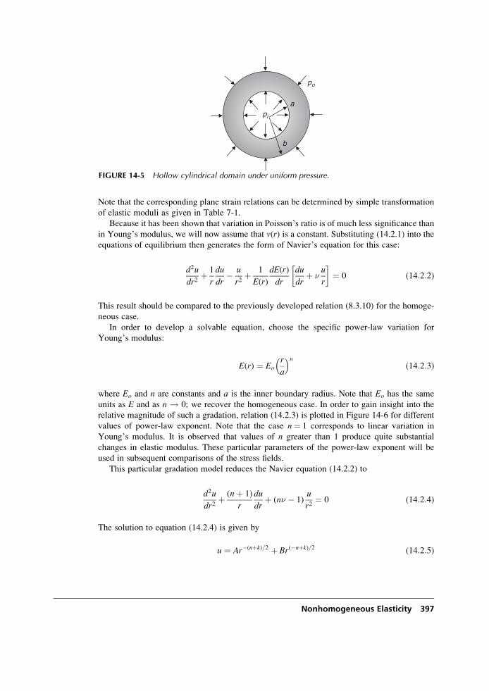
Note that the corresponding plane strain relations can be determined by simple transformation
of elastic moduli as given in Table 7-1.
Because it has been shown that variation in Poisson’s ratio is of much less significance than
in Young’s modulus, we will now assume that v(r) is a constant. Substituting (14.2.1) into the
equations of equilibrium then generates the form of Navier’s equation for this case:
d2u
dr2þ 1
r
du
dr� u
r2þ 1
E(r)
dE(r)
dr
du
drþ �
u
r
� �¼ 0 (14:2:2)
This result should be compared to the previously developed relation (8.3.10) for the homoge-
neous case.
In order to develop a solvable equation, choose the specific power-law variation for
Young’s modulus:
E(r) ¼ Eor
a
� �n(14:2:3)
where Eo and n are constants and a is the inner boundary radius. Note that Eo has the same
units as E and as n ! 0; we recover the homogeneous case. In order to gain insight into the
relative magnitude of such a gradation, relation (14.2.3) is plotted in Figure 14-6 for different
values of power-law exponent. Note that the case n¼ 1 corresponds to linear variation in
Young’s modulus. It is observed that values of n greater than 1 produce quite substantial
changes in elastic modulus. These particular parameters of the power-law exponent will be
used in subsequent comparisons of the stress fields.
This particular gradation model reduces the Navier equation (14.2.2) to
d2u
dr2þ (nþ 1)
r
du
drþ (n� � 1)
u
r2¼ 0 (14:2:4)
The solution to equation (14.2.4) is given by
u ¼ Ar�(nþk)=2 þ Br(�nþk)=2 (14:2:5)
a
b
pi
po
FIGURE 14-5 Hollow cylindrical domain under uniform pressure.
Nonhomogeneous Elasticity 397
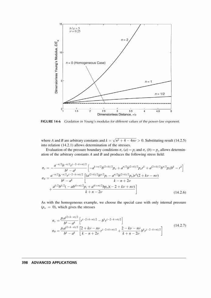
where A and B are arbitrary constants and k ¼ ffiffiffiffiffiffiffiffiffiffiffiffiffiffiffiffiffiffiffiffiffiffiffiffiffiffin2 þ 4� 4n�
p> 0. Substituting result (14.2.5)
into relation (14.2.1) allows determination of the stresses.
Evaluation of the pressure boundary conditions sr (a)¼ pi and sr (b)¼ po allows determin-
ation of the arbitrary constants A and B and produces the following stress field:
sr ¼ � a�n=2b�n=2r(�2�kþn)=2
bk � ak�akþn=2b(2þk)=2po þ an=2b(2þk)=2por
k þ a(2þk)=2bn=2pi(bk � rk
h i
sy ¼ a�n=2b�n=2r(�2�kþn)=2
bk � ak(a(2þk)=2bn=2pi � an=2b(2þk)=2po)r
k(2þ k� � n�)
k � nþ 2�
�
þ ak=2bk=2(� ab(kþn)=2pi þ a(kþn)=2bpo)(� 2þ k� þ n�)
k þ n� 2�
�(14:2:6)
As with the homogeneous example, we choose the special case with only internal pressure
(po ¼ 0), which gives the stresses
sr ¼ pia(2þk�n)=2
bk � akr(�2þkþn)=2 � bkr(�2�kþn)=2h i
sy ¼ pia(2þk�n)=2
bk � ak2þ k� � n�
k � nþ 2�r(�2þkþn)=2 þ 2� k� � n�
k þ n� 2�bkr(�2�kþn)=2
� � (14:2:7)
n = 0 (Homogeneous Case)
n = 2
n = 1
n = 1/2
b / a = 5 = 0.25
FIGURE 14-6 Gradation in Young’s modulus for different values of the power-law exponent.
398 ADVANCED APPLICATIONS
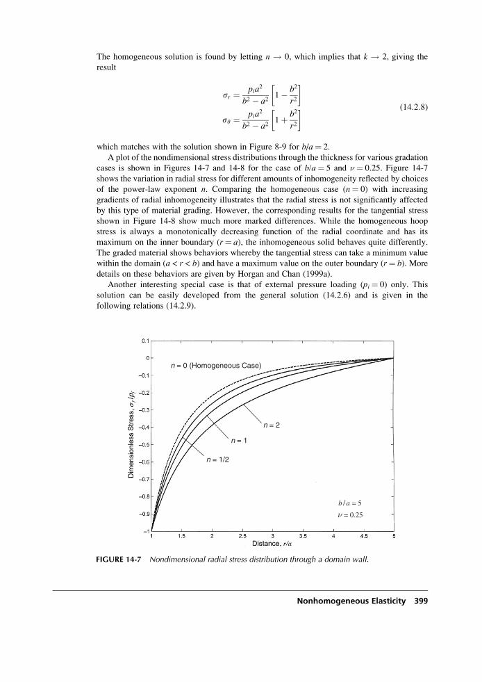
The homogeneous solution is found by letting n ! 0, which implies that k ! 2, giving the
result
sr ¼ pia2
b2 � a21� b2
r2
� �
sy ¼ pia2
b2 � a21þ b2
r2
� � (14:2:8)
which matches with the solution shown in Figure 8-9 for b/a¼ 2.
A plot of the nondimensional stress distributions through the thickness for various gradation
cases is shown in Figures 14-7 and 14-8 for the case of b/a¼ 5 and � ¼ 0.25. Figure 14-7
shows the variation in radial stress for different amounts of inhomogeneity reflected by choices
of the power-law exponent n. Comparing the homogeneous case (n¼ 0) with increasing
gradients of radial inhomogeneity illustrates that the radial stress is not significantly affected
by this type of material grading. However, the corresponding results for the tangential stress
shown in Figure 14-8 show much more marked differences. While the homogeneous hoop
stress is always a monotonically decreasing function of the radial coordinate and has its
maximum on the inner boundary (r¼ a), the inhomogeneous solid behaves quite differently.
The graded material shows behaviors whereby the tangential stress can take a minimum value
within the domain (a < r < b) and have a maximum value on the outer boundary (r¼ b). More
details on these behaviors are given by Horgan and Chan (1999a).
Another interesting special case is that of external pressure loading (pi¼ 0) only. This
solution can be easily developed from the general solution (14.2.6) and is given in the
following relations (14.2.9).
n = 0 (Homogeneous Case)
n = 2
n = 1
n = 1/2
b / a = 5
= 0.25
FIGURE 14-7 Nondimensional radial stress distribution through a domain wall.
Nonhomogeneous Elasticity 399
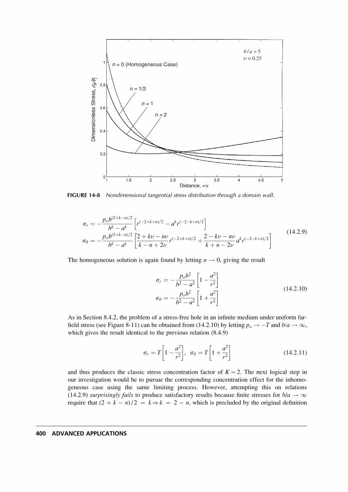
sr ¼ � pob(2þk�n)=2
bk � akr(�2þkþn)=2 � akr(�2�kþn)=2h i
sy ¼ � pob(2þk�n)=2
bk � ak2þ k� � n�
k � nþ 2�r(�2þkþn)=2 þ 2� k� � n�
k þ n� 2�akr(�2�kþn)=2
� � (14:2:9)
The homogeneous solution is again found by letting n ! 0, giving the result
sr ¼ � pob2
b2 � a21� a2
r2
� �
sy ¼ � pob2
b2 � a21þ a2
r2
� � (14:2:10)
As in Section 8.4.2, the problem of a stress-free hole in an infinite medium under uniform far-
field stress (see Figure 8-11) can be obtained from (14.2.10) by letting po !�T and b/a!1,
which gives the result identical to the previous relation (8.4.9)
sr ¼ T 1� a2
r2
� �, sy ¼ T 1þ a2
r2
� �(14:2:11)
and thus produces the classic stress concentration factor of K¼ 2. The next logical step in
our investigation would be to pursue the corresponding concentration effect for the inhomo-
geneous case using the same limiting process. However, attempting this on relations
(14.2.9) surprisingly fails to produce satisfactory results because finite stresses for b/a ! 1require that (2 þ k � n) / 2 ¼ k) k ¼ 2 � n, which is precluded by the original definition
n = 0 (Homogeneous Case)
n = 1/2
n = 1
n = 2
b / a = 5 = 0.25
FIGURE 14-8 Nondimensional tangential stress distribution through a domain wall.
400 ADVANCED APPLICATIONS
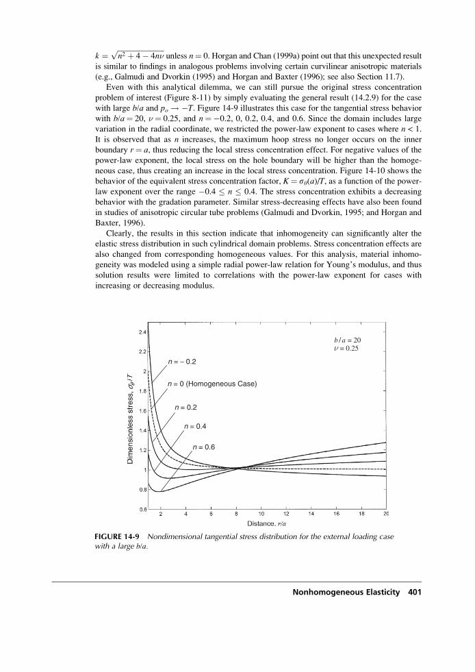
k ¼ ffiffiffiffiffiffiffiffiffiffiffiffiffiffiffiffiffiffiffiffiffiffiffiffiffiffin2 þ 4� 4n�
punless n¼ 0. Horgan and Chan (1999a) point out that this unexpected result
is similar to findings in analogous problems involving certain curvilinear anisotropic materials
(e.g., Galmudi and Dvorkin (1995) and Horgan and Baxter (1996); see also Section 11.7).
Even with this analytical dilemma, we can still pursue the original stress concentration
problem of interest (Figure 8-11) by simply evaluating the general result (14.2.9) for the case
with large b/a and po ! �T. Figure 14-9 illustrates this case for the tangential stress behavior
with b/a¼ 20, � ¼ 0.25, and n¼�0.2, 0, 0.2, 0.4, and 0.6. Since the domain includes large
variation in the radial coordinate, we restricted the power-law exponent to cases where n < 1.
It is observed that as n increases, the maximum hoop stress no longer occurs on the inner
boundary r¼ a, thus reducing the local stress concentration effect. For negative values of the
power-law exponent, the local stress on the hole boundary will be higher than the homoge-
neous case, thus creating an increase in the local stress concentration. Figure 14-10 shows the
behavior of the equivalent stress concentration factor, K¼ sy(a)/T, as a function of the power-
law exponent over the range �0.4 � n � 0.4. The stress concentration exhibits a decreasing
behavior with the gradation parameter. Similar stress-decreasing effects have also been found
in studies of anisotropic circular tube problems (Galmudi and Dvorkin, 1995; and Horgan and
Baxter, 1996).
Clearly, the results in this section indicate that inhomogeneity can significantly alter the
elastic stress distribution in such cylindrical domain problems. Stress concentration effects are
also changed from corresponding homogeneous values. For this analysis, material inhomo-
geneity was modeled using a simple radial power-law relation for Young’s modulus, and thus
solution results were limited to correlations with the power-law exponent for cases with
increasing or decreasing modulus.
n = 0 (Homogeneous Case)
n = 0.2
n = 0.4
n = 0.6
n = − 0.2
b / a = 20 = 0.25
FIGURE 14-9 Nondimensional tangential stress distribution for the external loading casewith a large b/a.
Nonhomogeneous Elasticity 401
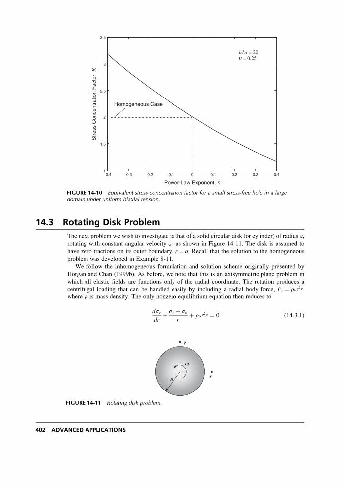
14.3 Rotating Disk Problem
The next problem we wish to investigate is that of a solid circular disk (or cylinder) of radius a,rotating with constant angular velocity !, as shown in Figure 14-11. The disk is assumed to
have zero tractions on its outer boundary, r¼ a. Recall that the solution to the homogeneous
problem was developed in Example 8-11.
We follow the inhomogeneous formulation and solution scheme originally presented by
Horgan and Chan (1999b). As before, we note that this is an axisymmetric plane problem in
which all elastic fields are functions only of the radial coordinate. The rotation produces a
centrifugal loading that can be handled easily by including a radial body force, Fr¼ r!2r,where � is mass density. The only nonzero equilibrium equation then reduces to
dsrdr
þ sr � syr
þ r!2r ¼ 0 (14:3:1)
−0.4 −0.3 −0.2 −0.1 0 0.1 0.2 0.3 0.41
1.5
2
2.5
3
3.5
Power-Law Exponent, n
Str
ess
Con
cent
ratio
n F
acto
r, K
Homogeneous Case
b / a = 20 = 0.25
FIGURE 14-10 Equivalent stress concentration factor for a small stress-free hole in a largedomain under uniform biaxial tension.
x
y
a
w
FIGURE 14-11 Rotating disk problem.
402 ADVANCED APPLICATIONS
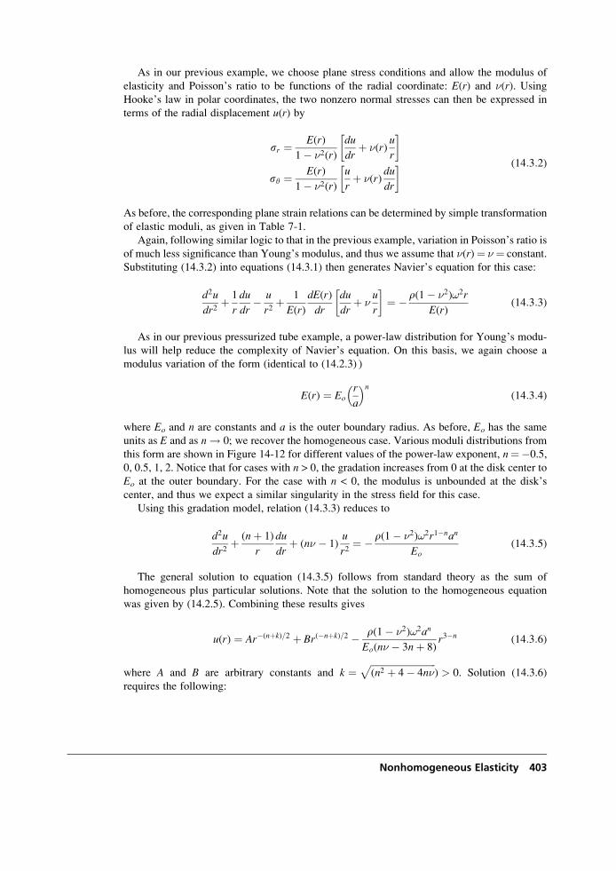
As in our previous example, we choose plane stress conditions and allow the modulus of
elasticity and Poisson’s ratio to be functions of the radial coordinate: E(r) and �(r). UsingHooke’s law in polar coordinates, the two nonzero normal stresses can then be expressed in
terms of the radial displacement u(r) by
sr ¼ E(r)
1� �2(r)
du
drþ �(r)
u
r
� �
sy ¼ E(r)
1� �2(r)
u
rþ �(r)
du
dr
� � (14:3:2)
As before, the corresponding plane strain relations can be determined by simple transformation
of elastic moduli, as given in Table 7-1.
Again, following similar logic to that in the previous example, variation in Poisson’s ratio is
of much less significance than Young’s modulus, and thus we assume that �(r)¼ � ¼ constant.
Substituting (14.3.2) into equations (14.3.1) then generates Navier’s equation for this case:
d2u
dr2þ 1
r
du
dr� u
r2þ 1
E(r)
dE(r)
dr
du
drþ �
u
r
� �¼ �r(1� �2)!2r
E(r)(14:3:3)
As in our previous pressurized tube example, a power-law distribution for Young’s modu-
lus will help reduce the complexity of Navier’s equation. On this basis, we again choose a
modulus variation of the form (identical to (14.2.3) )
E(r) ¼ Eor
a
� �n(14:3:4)
where Eo and n are constants and a is the outer boundary radius. As before, Eo has the same
units as E and as n! 0; we recover the homogeneous case. Various moduli distributions from
this form are shown in Figure 14-12 for different values of the power-law exponent, n¼�0.5,
0, 0.5, 1, 2. Notice that for cases with n > 0, the gradation increases from 0 at the disk center to
Eo at the outer boundary. For the case with n < 0, the modulus is unbounded at the disk’s
center, and thus we expect a similar singularity in the stress field for this case.
Using this gradation model, relation (14.3.3) reduces to
d2u
dr2þ (nþ 1)
r
du
drþ (n� � 1)
u
r2¼ � r(1� �2)!2r1�nan
Eo(14:3:5)
The general solution to equation (14.3.5) follows from standard theory as the sum of
homogeneous plus particular solutions. Note that the solution to the homogeneous equation
was given by (14.2.5). Combining these results gives
u(r) ¼ Ar�(nþk)=2 þ Br(�nþk)=2 � r(1� �2)!2an
Eo(n� � 3nþ 8)r3�n (14:3:6)
where A and B are arbitrary constants and k ¼ffiffiffiffiffiffiffiffiffiffiffiffiffiffiffiffiffiffiffiffiffiffiffiffiffiffiffiffi(n2 þ 4� 4n�
p) > 0. Solution (14.3.6)
requires the following:
Nonhomogeneous Elasticity 403
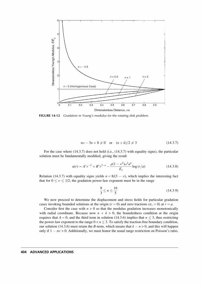
n� � 3nþ 8 6¼ 0 or (nþ k)=2 6¼ 3 (14:3:7)
For the case where (14.3.7) does not hold (i.e., (14.3.7) with equality signs), the particular
solution must be fundamentally modified, giving the result
u(r) ¼ A�r�3 þ B�r3�n � r(1� �2)!2an
Eolog (r=a) (14:3:8)
Relation (14.3.7) with equality signs yields n¼ 8/(3 � �), which implies the interesting fact
that for 0 � � � 1/2, the gradation power-law exponent must be in the range
8
3� n � 16
5(14:3:9)
We now proceed to determine the displacement and stress fields for particular gradation
cases invoking bounded solutions at the origin (r¼ 0) and zero tractions (sr¼ 0) at r¼ a.Consider first the case with n > 0 so that the modulus gradation increases monotonically
with radial coordinate. Because now n þ k > 0, the boundedness condition at the origin
requires that A¼ 0, and the third term in solution (14.3.6) implies that n � 3, thus restricting
the power-law exponent to the range 0 < n� 3. To satisfy the traction-free boundary condition,
our solution (14.3.6) must retain the B-term, which means that k � n > 0, and this will happen
only if 1 � n� > 0. Additionally, we must honor the usual range restriction on Poisson’s ratio,
FIGURE 14-12 Gradation in Young’s modulus for the rotating disk problem.
404 ADVANCED APPLICATIONS
0 � � � 1/2. Collectively these conditions place coupled restrictions on the gradation
parameter n and Poisson’s ratio �, but these can be satisfied. Therefore, we now move forward
with the solution assuming this is the case.
With A¼ 0 in solution (14.3.6), the radial stress follows from relation (14.3.2)1
sr ¼ Ba�nEo
1� �2� þ 1
2(k � n)
� �r(nþk�2)=2 � (3� nþ �)r!2r2
(n� � 3nþ 8)(14:3:10)
Applying the zero-traction boundary condition easily determines the constant B, giving the
final stress results
sr ¼ (3� nþ �)r!2
(n� � 3nþ 8)a3�(nþk)=2r(nþk�2)=2 � r2h i
sy ¼ r!2
(n� � 3nþ 8)
(3� nþ �)[1þ (�=2)(k � n)]
[� þ (k � n)=2]a3�(nþk)=2r(nþk�2)=2
�� [(3� n)� þ 1]r2�
for the case n� � 3nþ 8 6¼ 0
(14:3:11)
Recall that these results were developed under condition (14.3.7). For the case where this
condition is not satisfied, solution form (14.3.8) must be used instead. Similar analysis yields
the stress solutions
sr ¼ r!2 (n� 4)(n� 2)
nr2 log (r=a)
� �
sy ¼ r!2
n8r2 � 3(n� 4)(n� 2)r2 log (r=a)
for the case8
3� n � 16
5
(14:3:12)
The homogeneous case corresponds to n! 0, which means k! 2, and (14.3.11) would reduce
to our previous solution (8.4.81).
Returning now to consider the case where n < 0 (decreasing radial gradation), we find that
the boundedness condition implies that the solution constant A must again be set to 0.
However, no restriction is needed on the power of r in the third term of solution (14.3.6).
Consideration of the special solution (14.3.8) is no longer needed because n� � 3n þ 8 6¼ 0
will always be satisfied. Thus, the solution given by (14.3.11) is also valid for n < 0.
To show details on the stress distribution, we will choose the case � ¼ 0 so that no
restriction is placed on the condition that k � n > 0, and additionally plane stress results
coincide with plane strain values. We also take the case 8� 3n 6¼ 0 and thus relations (14.3.11)
are used to determine the stresses. Results for the radial stress distribution are shown in Figure
14-13 for gradation parameter values n¼�0.5, 0, 0.5, 1, 2. The results indicate very signifi-
cant differences in behavior from the homogeneous case n¼ 0, which has its maximum value
at the disk center (r¼ 0) and decays to 0 at the outer stress-free boundary. For inhomogeneous
cases with positive gradations (e.g., n¼ 0.5, 1, 2 ), the radial stress actually vanishes at r¼ 0
Nonhomogeneous Elasticity 405
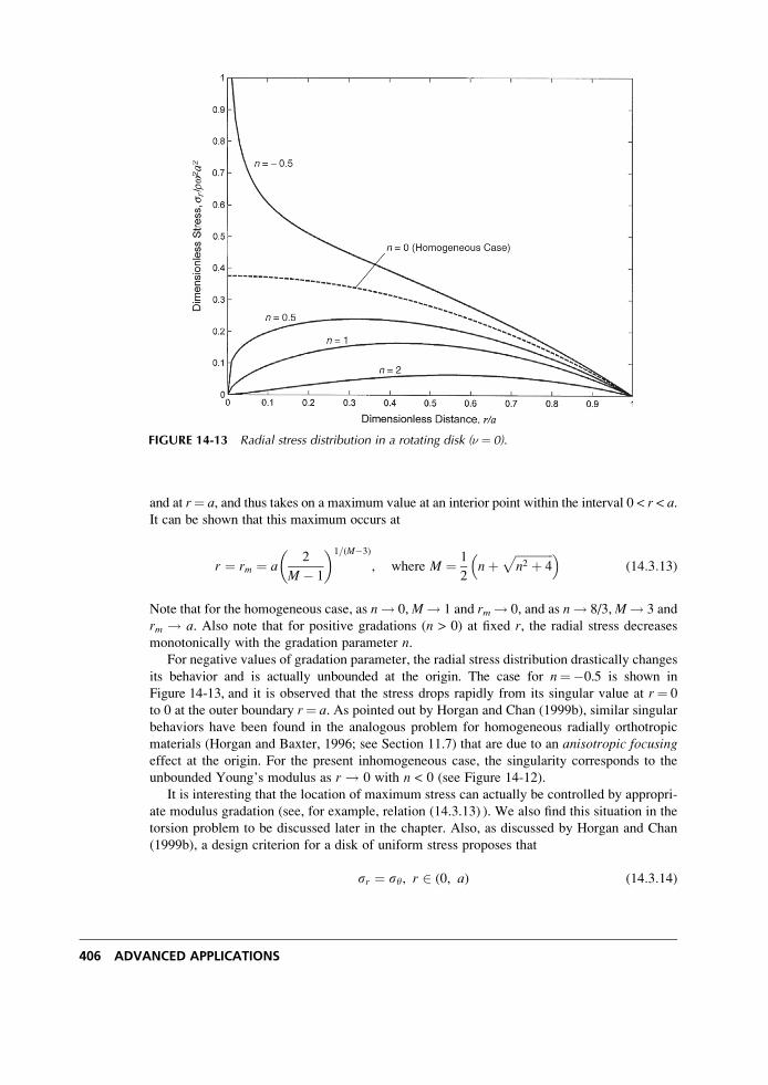
and at r¼ a, and thus takes on a maximum value at an interior point within the interval 0 < r < a.It can be shown that this maximum occurs at
r ¼ rm ¼ a2
M � 1
� �1=(M�3)
, where M ¼ 1
2nþ
ffiffiffiffiffiffiffiffiffiffiffiffiffin2 þ 4
p� �(14:3:13)
Note that for the homogeneous case, as n! 0,M! 1 and rm ! 0, and as n! 8/3,M! 3 and
rm ! a. Also note that for positive gradations (n > 0) at fixed r, the radial stress decreases
monotonically with the gradation parameter n.For negative values of gradation parameter, the radial stress distribution drastically changes
its behavior and is actually unbounded at the origin. The case for n¼�0.5 is shown in
Figure 14-13, and it is observed that the stress drops rapidly from its singular value at r¼ 0
to 0 at the outer boundary r¼ a. As pointed out by Horgan and Chan (1999b), similar singular
behaviors have been found in the analogous problem for homogeneous radially orthotropic
materials (Horgan and Baxter, 1996; see Section 11.7) that are due to an anisotropic focusingeffect at the origin. For the present inhomogeneous case, the singularity corresponds to the
unbounded Young’s modulus as r ! 0 with n < 0 (see Figure 14-12).
It is interesting that the location of maximum stress can actually be controlled by appropri-
ate modulus gradation (see, for example, relation (14.3.13) ). We also find this situation in the
torsion problem to be discussed later in the chapter. Also, as discussed by Horgan and Chan
(1999b), a design criterion for a disk of uniform stress proposes that
sr ¼ sy, r 2 (0, a) (14:3:14)
FIGURE 14-13 Radial stress distribution in a rotating disk (� ¼ 0).
406 ADVANCED APPLICATIONS
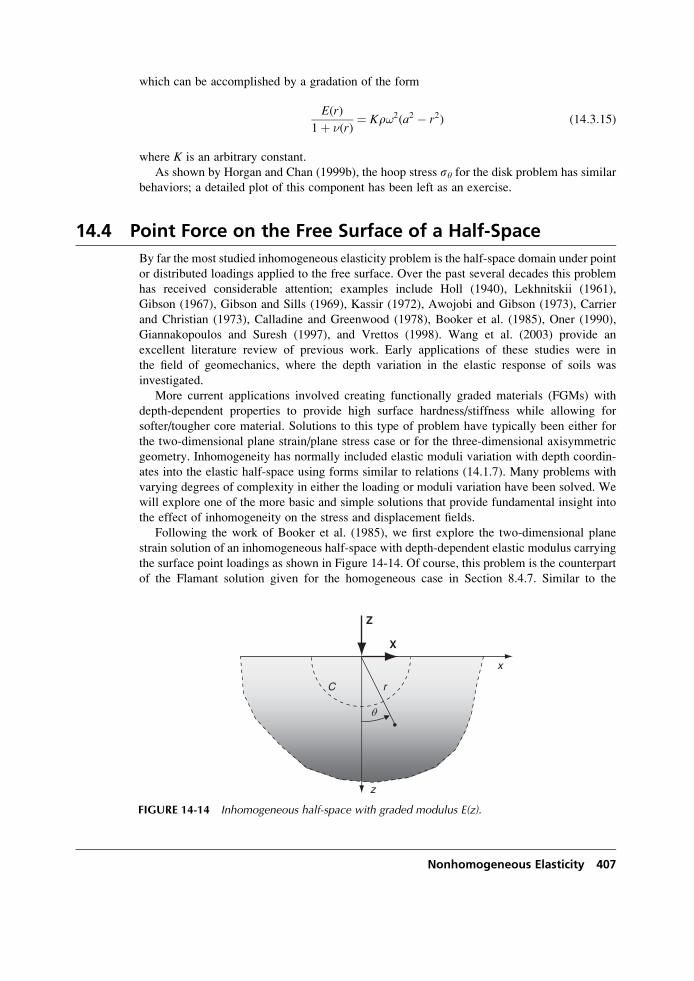
which can be accomplished by a gradation of the form
E(r)
1þ �(r)¼ Kr!2(a2 � r2) (14:3:15)
where K is an arbitrary constant.
As shown by Horgan and Chan (1999b), the hoop stress sy for the disk problem has similar
behaviors; a detailed plot of this component has been left as an exercise.
14.4 Point Force on the Free Surface of a Half-Space
By far the most studied inhomogeneous elasticity problem is the half-space domain under point
or distributed loadings applied to the free surface. Over the past several decades this problem
has received considerable attention; examples include Holl (1940), Lekhnitskii (1961),
Gibson (1967), Gibson and Sills (1969), Kassir (1972), Awojobi and Gibson (1973), Carrier
and Christian (1973), Calladine and Greenwood (1978), Booker et al. (1985), Oner (1990),
Giannakopoulos and Suresh (1997), and Vrettos (1998). Wang et al. (2003) provide an
excellent literature review of previous work. Early applications of these studies were in
the field of geomechanics, where the depth variation in the elastic response of soils was
investigated.
More current applications involved creating functionally graded materials (FGMs) with
depth-dependent properties to provide high surface hardness/stiffness while allowing for
softer/tougher core material. Solutions to this type of problem have typically been either for
the two-dimensional plane strain/plane stress case or for the three-dimensional axisymmetric
geometry. Inhomogeneity has normally included elastic moduli variation with depth coordin-
ates into the elastic half-space using forms similar to relations (14.1.7). Many problems with
varying degrees of complexity in either the loading or moduli variation have been solved. We
will explore one of the more basic and simple solutions that provide fundamental insight into
the effect of inhomogeneity on the stress and displacement fields.
Following the work of Booker et al. (1985), we first explore the two-dimensional plane
strain solution of an inhomogeneous half-space with depth-dependent elastic modulus carrying
the surface point loadings as shown in Figure 14-14. Of course, this problem is the counterpart
of the Flamant solution given for the homogeneous case in Section 8.4.7. Similar to the
x
z
Z
X
r
θ
C
FIGURE 14-14 Inhomogeneous half-space with graded modulus E(z).
Nonhomogeneous Elasticity 407
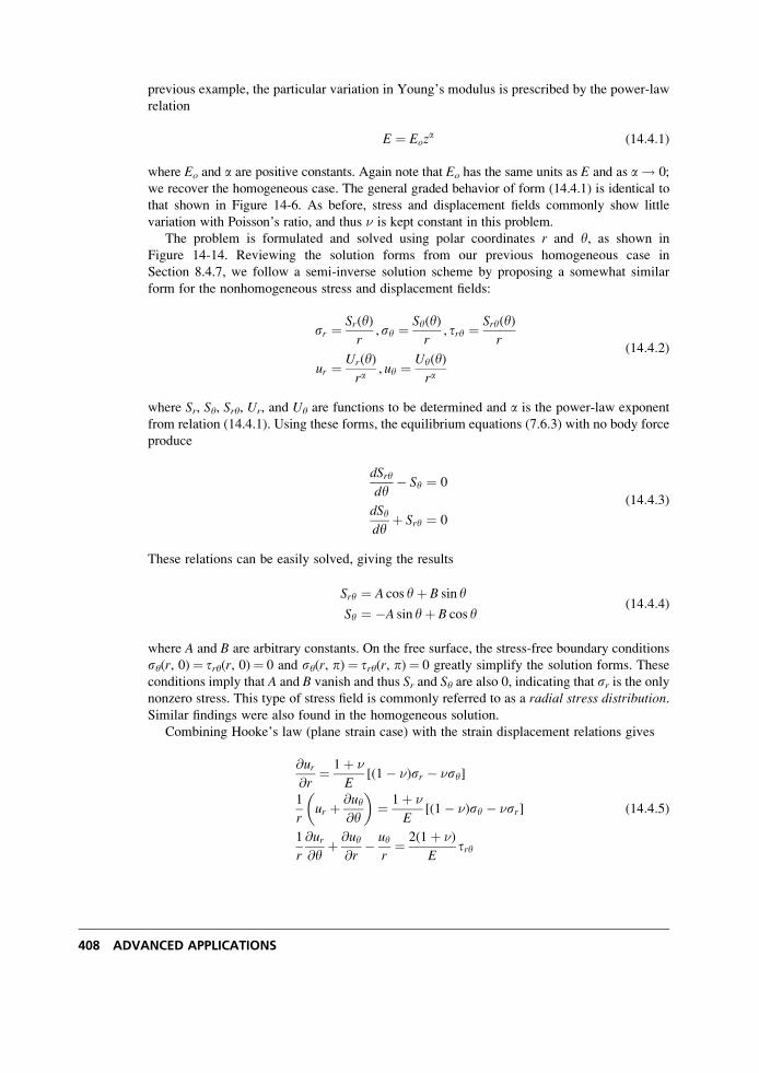
previous example, the particular variation in Young’s modulus is prescribed by the power-law
relation
E ¼ Eoza (14:4:1)
where Eo and a are positive constants. Again note that Eo has the same units as E and as a ! 0;
we recover the homogeneous case. The general graded behavior of form (14.4.1) is identical to
that shown in Figure 14-6. As before, stress and displacement fields commonly show little
variation with Poisson’s ratio, and thus � is kept constant in this problem.
The problem is formulated and solved using polar coordinates r and y, as shown in
Figure 14-14. Reviewing the solution forms from our previous homogeneous case in
Section 8.4.7, we follow a semi-inverse solution scheme by proposing a somewhat similar
form for the nonhomogeneous stress and displacement fields:
sr ¼ Sr(y)r
,sy ¼ Sy(y)r
, try ¼ Sry(y)r
ur ¼ Ur(y)ra
, uy ¼ Uy(y)ra
(14:4:2)
where Sr, Sy, Sry, Ur, and Uy are functions to be determined and a is the power-law exponent
from relation (14.4.1). Using these forms, the equilibrium equations (7.6.3) with no body force
produce
dSrydy
� Sy ¼ 0
dSydy
þ Sry ¼ 0
(14:4:3)
These relations can be easily solved, giving the results
Sry ¼ A cos yþ B sin y
Sy ¼ �A sin yþ B cos y(14:4:4)
where A and B are arbitrary constants. On the free surface, the stress-free boundary conditions
sy(r, 0)¼ try(r, 0)¼ 0 and sy(r, p)¼ try(r, p)¼ 0 greatly simplify the solution forms. These
conditions imply that A and B vanish and thus Sr and Sy are also 0, indicating that sr is the onlynonzero stress. This type of stress field is commonly referred to as a radial stress distribution.Similar findings were also found in the homogeneous solution.
Combining Hooke’s law (plane strain case) with the strain displacement relations gives
@ur@r
¼ 1þ �
E[(1� �)sr � �sy]
1
rur þ @uy
@y
� �¼ 1þ �
E[(1� �)sy � �sr]
1
r
@ur@y
þ @uy@r
� uyr¼ 2(1þ �)
Etry
(14:4:5)
408 ADVANCED APPLICATIONS
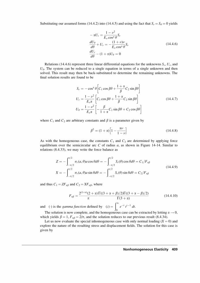
Substituting our assumed forms (14.4.2) into (14.4.5) and using the fact that Sr¼ Sy¼ 0 yields
� aUr ¼ 1� �2
Eo cosa ySr
dUy
dyþ Ur ¼ � (1þ �)�
Eo cosa ySr
dUr
dy� (1þ a)Uy ¼ 0
(14:4:6)
Relations (14.4.6) represent three linear differential equations for the unknowns Sr, Ur, and
Uy. The system can be reduced to a single equation in terms of a single unknown and then
solved. This result may then be back-substituted to determine the remaining unknowns. The
final solution results are found to be
Sr ¼ � cosa y C1 cos byþ 1þ ab
C2 sinby� �
Ur ¼ 1� �2
EoaC1 cos byþ 1þ a
bC2 sin by
� �
Uy ¼ 1� �2
Eoa� b1þ a
C1 sinbyþ C2 cos by� � (14:4:7)
where C1 and C2 are arbitrary constants and b is a parameter given by
b2 ¼ (1þ a) 1� a�1� �
h i(14:4:8)
As with the homogeneous case, the constants C1 and C2 are determined by applying force
equilibrium over the semicircular arc C of radius a, as shown in Figure 14-14. Similar to
relations (8.4.33), we may write the force balance as
Z ¼ �ðp=2�p=2
sr(a, y)a cos ydy ¼ �ðp=2�p=2
Sr(y) cos ydy ¼ C1=Fab
X ¼ �ðp=2�p=2
sr(a, y)a sin ydy ¼ �ðp=2�p=2
Sr(y) sin ydy ¼ C2=Fab
(14:4:9)
and thus C1¼ ZFab and C2¼ XFab, where
Fab ¼ 2(1þa)(2þ a)p
G((3þ aþ b)=2)G((3þ a� b)=2)G(3þ a)
(14:4:10)
and �(�) is the gamma function defined by �(z)¼ð10
e�t tz�1 dt.
The solution is now complete, and the homogeneous case can be extracted by letting a! 0,
which yields b¼ 1, Fab¼ 2/p, and the solution reduces to our previous result (8.4.34).
Let us now evaluate the special inhomogeneous case with only normal loading (X¼ 0) and
explore the nature of the resulting stress and displacement fields. The solution for this case is
given by
Nonhomogeneous Elasticity 409
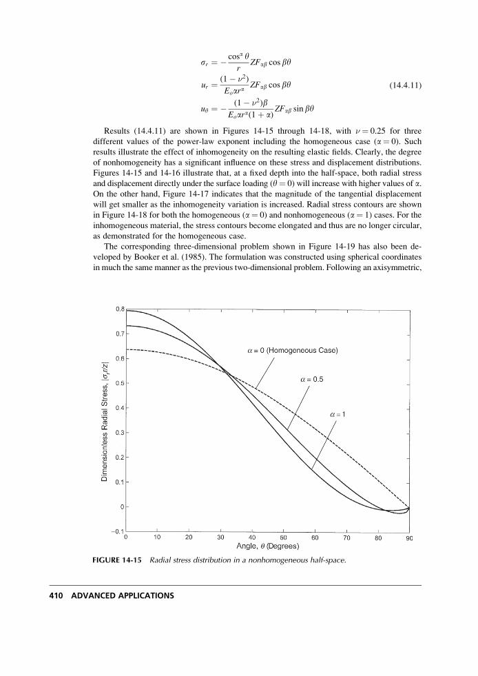
sr ¼ � cosa yr
ZFab cos by
ur ¼ (1� �2)
EoaraZFab cos by
uy ¼ � (1� �2)bEoara(1þ a)
ZFab sinby
(14:4:11)
Results (14.4.11) are shown in Figures 14-15 through 14-18, with � ¼ 0.25 for three
different values of the power-law exponent including the homogeneous case (a¼ 0). Such
results illustrate the effect of inhomogeneity on the resulting elastic fields. Clearly, the degree
of nonhomogeneity has a significant influence on these stress and displacement distributions.
Figures 14-15 and 14-16 illustrate that, at a fixed depth into the half-space, both radial stress
and displacement directly under the surface loading (y¼ 0) will increase with higher values of a.On the other hand, Figure 14-17 indicates that the magnitude of the tangential displacement
will get smaller as the inhomogeneity variation is increased. Radial stress contours are shown
in Figure 14-18 for both the homogeneous (a¼ 0) and nonhomogeneous (a¼ 1) cases. For the
inhomogeneous material, the stress contours become elongated and thus are no longer circular,
as demonstrated for the homogeneous case.
The corresponding three-dimensional problem shown in Figure 14-19 has also been de-
veloped by Booker et al. (1985). The formulation was constructed using spherical coordinates
in much the same manner as the previous two-dimensional problem. Following an axisymmetric,
FIGURE 14-15 Radial stress distribution in a nonhomogeneous half-space.
410 ADVANCED APPLICATIONS
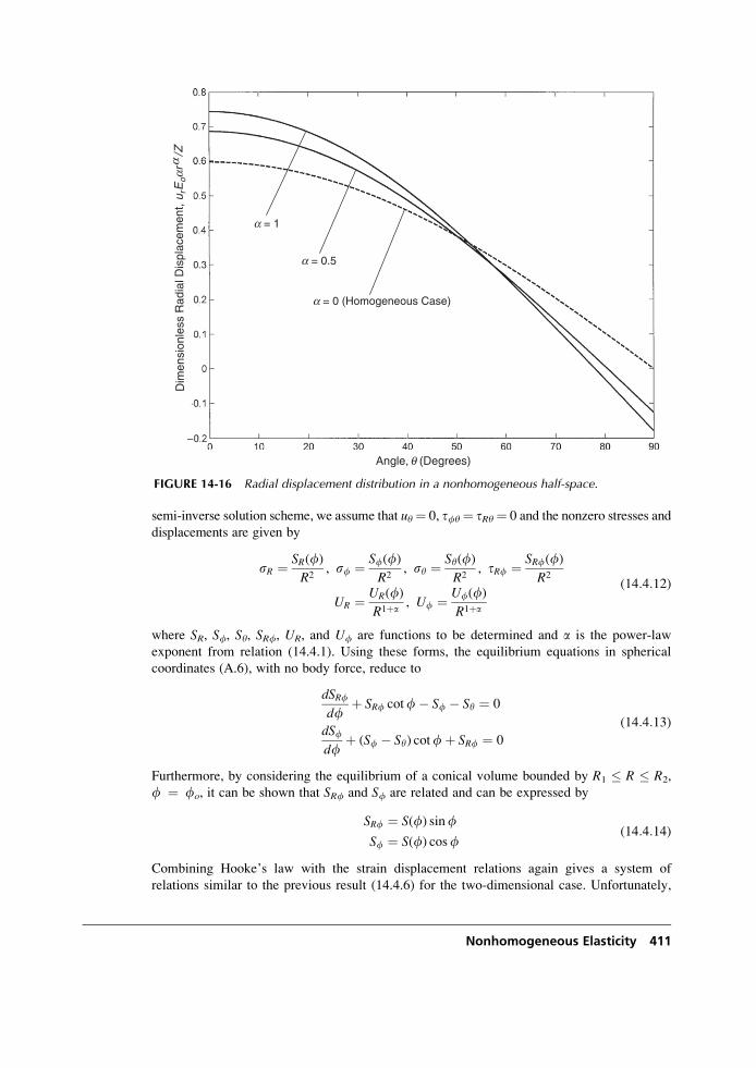
semi-inverse solution scheme, we assume that uy¼ 0, tfy¼ tRy¼ 0 and the nonzero stresses and
displacements are given by
sR ¼ SR(f)R2
, sf ¼ Sf(f)R2
, sy ¼ Sy(f)R2
, tRf ¼ SRf(f)R2
UR ¼ UR(f)R1þa , Uf ¼ Uf(f)
R1þa
(14:4:12)
where SR, Sf, Sy, SRf, UR, and Uf are functions to be determined and a is the power-law
exponent from relation (14.4.1). Using these forms, the equilibrium equations in spherical
coordinates (A.6), with no body force, reduce to
dSRfdf
þ SRf cotf� Sf � Sy ¼ 0
dSfdf
þ (Sf � Sy) cotfþ SRf ¼ 0
(14:4:13)
Furthermore, by considering the equilibrium of a conical volume bounded by R1 � R � R2,
f ¼ fo, it can be shown that SRf and Sf are related and can be expressed by
SRf ¼ S(f) sinf
Sf ¼ S(f) cosf(14:4:14)
Combining Hooke’s law with the strain displacement relations again gives a system of
relations similar to the previous result (14.4.6) for the two-dimensional case. Unfortunately,
Angle, q (Degrees)
Dim
ensi
onle
ss R
adia
l Dis
plac
emen
t, u r
Eoa
ra/Z
a = 0 (Homogeneous Case)
a = 0.5
a = 1
FIGURE 14-16 Radial displacement distribution in a nonhomogeneous half-space.
Nonhomogeneous Elasticity 411
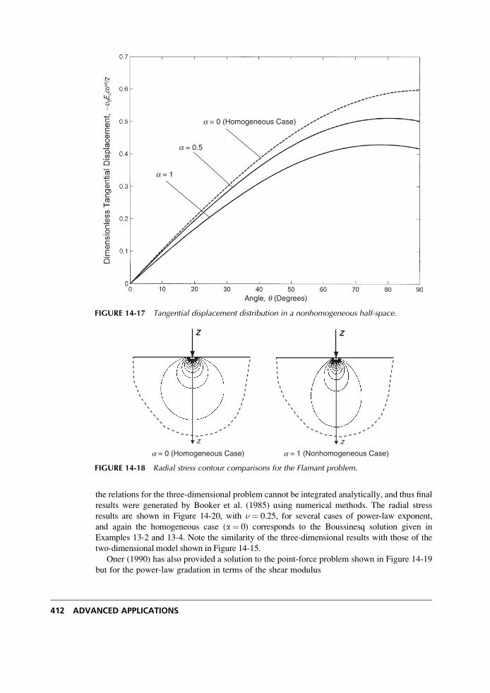
the relations for the three-dimensional problem cannot be integrated analytically, and thus final
results were generated by Booker et al. (1985) using numerical methods. The radial stress
results are shown in Figure 14-20, with � ¼ 0.25, for several cases of power-law exponent,
and again the homogeneous case (a¼ 0) corresponds to the Boussinesq solution given in
Examples 13-2 and 13-4. Note the similarity of the three-dimensional results with those of the
two-dimensional model shown in Figure 14-15.
Oner (1990) has also provided a solution to the point-force problem shown in Figure 14-19
but for the power-law gradation in terms of the shear modulus
a = 0.5
a = 0 (Homogeneous Case)
a = 1
Angle, q (Degrees)
FIGURE 14-17 Tangential displacement distribution in a nonhomogeneous half-space.
z
Z
a = 0 (Homogeneous Case)
z
Z
a = 1 (Nonhomogeneous Case)
FIGURE 14-18 Radial stress contour comparisons for the Flamant problem.
412 ADVANCED APPLICATIONS
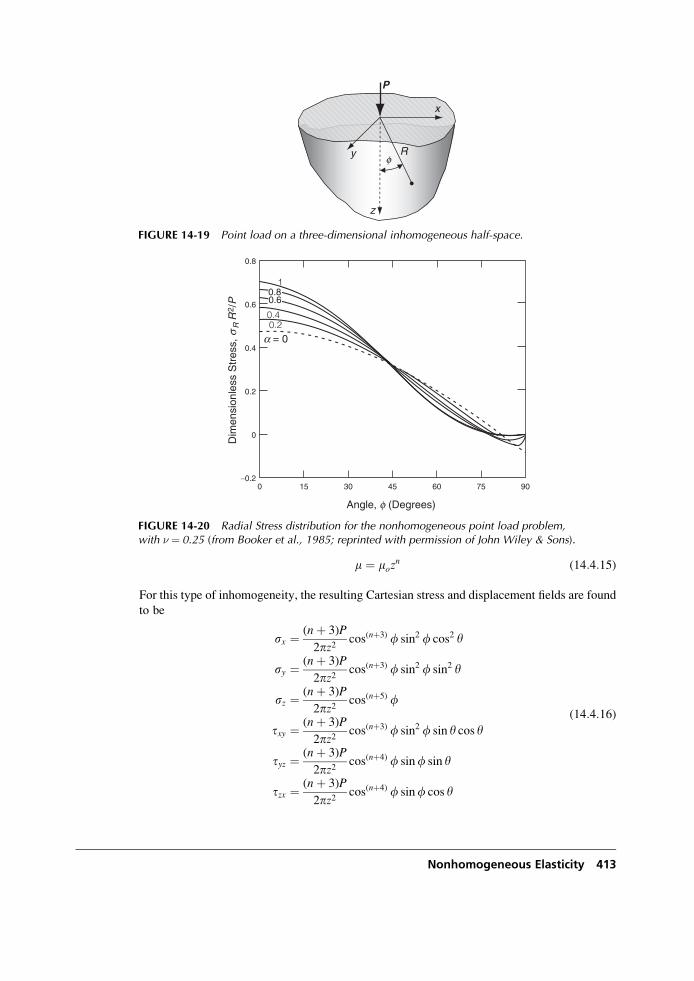
m ¼ mozn (14:4:15)
For this type of inhomogeneity, the resulting Cartesian stress and displacement fields are found
to be
sx ¼ (nþ 3)P
2pz2cos(nþ3) f sin2 f cos2 y
sy ¼ (nþ 3)P
2pz2cos(nþ3) f sin2 f sin2 y
sz ¼ (nþ 3)P
2pz2cos(nþ5) f
txy ¼ (nþ 3)P
2pz2cos(nþ3) f sin2 f sin y cos y
tyz ¼ (nþ 3)P
2pz2cos(nþ4) f sinf sin y
tzx ¼ (nþ 3)P
2pz2cos(nþ4) f sinf cos y
(14:4:16)
x
y
z
P
fR
FIGURE 14-19 Point load on a three-dimensional inhomogeneous half-space.
Angle, f (Degrees)
Dim
ensi
onle
ss S
tres
s, s
R R
2 /P
0.8
a = 00.20.4
1
0.4
0.2
0
0 15 30 45 60 75 90−0.2
0.6 0.60.8
FIGURE 14-20 Radial Stress distribution for the nonhomogeneous point load problem,with � ¼ 0.25 (from Booker et al., 1985; reprinted with permission of John Wiley & Sons).
Nonhomogeneous Elasticity 413
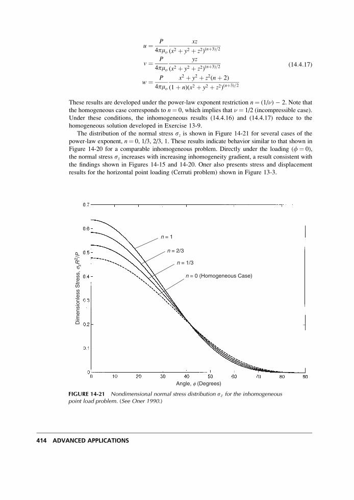
u ¼ P
4pmo
xz
(x2 þ y2 þ z2)(nþ3)=2
v ¼ P
4pmo
yz
(x2 þ y2 þ z2)(nþ3)=2
w ¼ P
4pmo
x2 þ y2 þ z2(nþ 2)
(1þ n)(x2 þ y2 þ z2)(nþ3)=2
(14:4:17)
These results are developed under the power-law exponent restriction n¼ (1/�) � 2. Note that
the homogeneous case corresponds to n¼ 0, which implies that � ¼ 1/2 (incompressible case).
Under these conditions, the inhomogeneous results (14.4.16) and (14.4.17) reduce to the
homogeneous solution developed in Exercise 13-9.
The distribution of the normal stress sz is shown in Figure 14-21 for several cases of the
power-law exponent, n¼ 0, 1/3, 2/3, 1. These results indicate behavior similar to that shown in
Figure 14-20 for a comparable inhomogeneous problem. Directly under the loading (f¼ 0),
the normal stress sz increases with increasing inhomogeneity gradient, a result consistent with
the findings shown in Figures 14-15 and 14-20. Oner also presents stress and displacement
results for the horizontal point loading (Cerruti problem) shown in Figure 13-3.
n = 0 (Homogeneous Case)
n = 1/3
n = 2/3
n = 1
Angle, f (Degrees)
Dim
ensi
onle
ss S
tres
s, s
zR2 /
P
FIGURE 14-21 Nondimensional normal stress distribution sz for the inhomogeneouspoint load problem. (See Oner 1990.)
414 ADVANCED APPLICATIONS
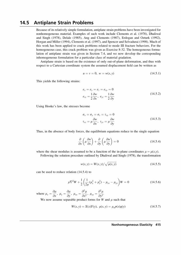
14.5 Antiplane Strain Problems
Because of its relatively simple formulation, antiplane strain problems have been investigated for
nonhomogeneous material. Examples of such work include Clements et al. (1978), Dhaliwal
and Singh (1978), Delale (1985), Ang and Clements (1987), Erdogan and Ozturk (1992),
Horgan and Miller (1994), Clements et al. (1997), and Spencer and Selvadurai (1998). Much of
this work has been applied to crack problems related to mode III fracture behaviors. For the
homogeneous case, this crack problem was given as Exercise 8-32. The homogeneous formu-
lation of antiplane strain was given in Section 7.4, and we now develop the corresponding
inhomogeneous formulation for a particular class of material gradation.
Antiplane strain is based on the existence of only out-of-plane deformation, and thus with
respect to a Cartesian coordinate system the assumed displacement field can be written as
u ¼ v ¼ 0, w ¼ w(x, y) (14:5:1)
This yields the following strains:
ex ¼ ey ¼ ez ¼ exy ¼ 0
exz ¼ 1
2
@w
@x, eyz ¼ 1
2
@w
@y
(14:5:2)
Using Hooke’s law, the stresses become
sx ¼ sy ¼ sz ¼ txy ¼ 0
txz ¼ m@w
@x, tyz ¼ m
@w
@y
(14:5:3)
Thus, in the absence of body forces, the equilibrium equations reduce to the single equation
@
@xm@w
@x
� �þ @
@ym@w
@y
� �¼ 0 (14:5:4)
where the shear modulus is assumed to be a function of the in-plane coordinates m¼ m(x,y).Following the solution procedure outlined by Dhaliwal and Singh (1978), the transformation
w(x, y) ¼ W(x, y)=ffiffiffiffiffiffiffiffiffiffiffiffiffim(x, y)
p(14:5:5)
can be used to reduce relation (14.5.4) to
mr2W þ 1
2
1
2m(m2x þ m2y)� mxx � myy
� �W ¼ 0 (14:5:6)
where mx ¼@m@x
, my ¼@m@y
, mxx ¼@2m@x2
, myy ¼@2m@y2
.
We now assume separable product forms for W and m such that
W(x, y) ¼ X(x)Y(y), m(x, y) ¼ mop(x)q(y) (14:5:7)
Nonhomogeneous Elasticity 415
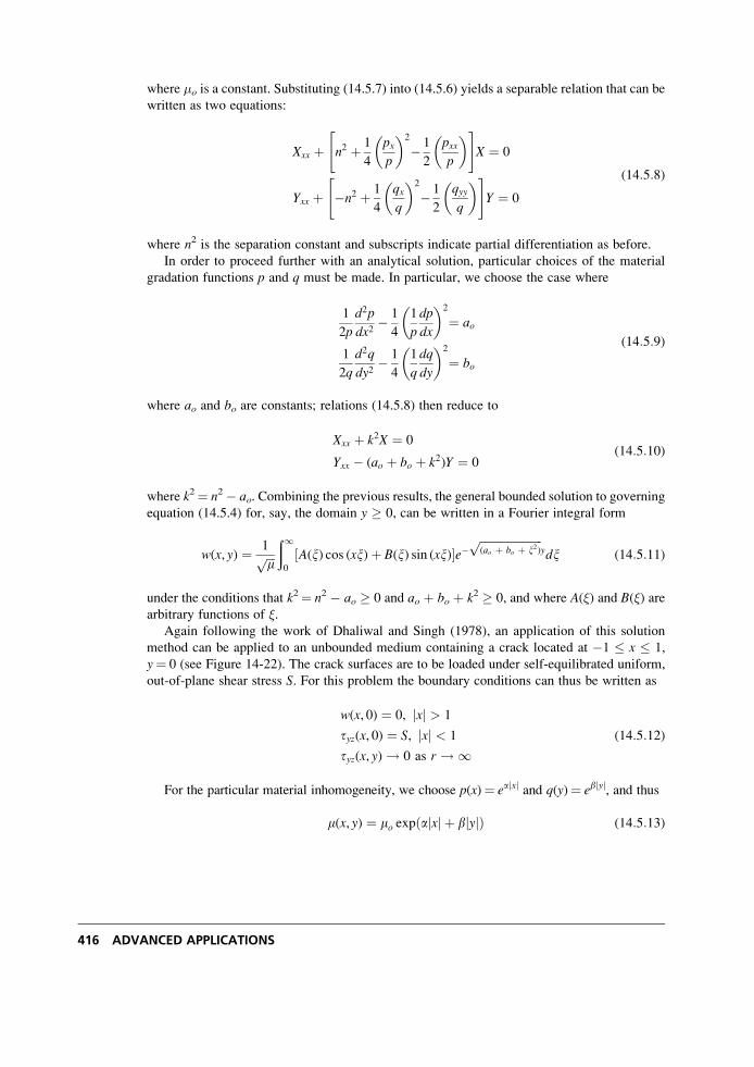
where �o is a constant. Substituting (14.5.7) into (14.5.6) yields a separable relation that can bewritten as two equations:
Xxx þ n2 þ 1
4
pxp
� �2
� 1
2
pxxp
� �" #X ¼ 0
Yxx þ �n2 þ 1
4
qxq
� �2
� 1
2
qyyq
� �" #Y ¼ 0
(14:5:8)
where n2 is the separation constant and subscripts indicate partial differentiation as before.
In order to proceed further with an analytical solution, particular choices of the material
gradation functions p and q must be made. In particular, we choose the case where
1
2p
d2p
dx2� 1
4
1
p
dp
dx
� �2
¼ ao
1
2q
d2q
dy2� 1
4
1
q
dq
dy
� �2
¼ bo
(14:5:9)
where ao and bo are constants; relations (14.5.8) then reduce to
Xxx þ k2X ¼ 0
Yxx � (ao þ bo þ k2)Y ¼ 0(14:5:10)
where k2¼ n2 � ao. Combining the previous results, the general bounded solution to governing
equation (14.5.4) for, say, the domain y � 0, can be written in a Fourier integral form
w(x, y) ¼ 1ffiffiffim
pð10
A(x) cos (xx)þ B(x) sin (xx)½ �e�ffiffiffiffiffiffiffiffiffiffiffiffiffiffiffiffiffiffiffiffiffiffi(ao þ bo þ x2)
pydx (14:5:11)
under the conditions that k2¼ n2 � ao � 0 and ao þ bo þ k2 � 0, and where A(�) and B(�) arearbitrary functions of �.
Again following the work of Dhaliwal and Singh (1978), an application of this solution
method can be applied to an unbounded medium containing a crack located at �1 � x � 1,
y¼ 0 (see Figure 14-22). The crack surfaces are to be loaded under self-equilibrated uniform,
out-of-plane shear stress S. For this problem the boundary conditions can thus be written as
w(x, 0) ¼ 0, jxj > 1
tyz(x, 0) ¼ S, jxj < 1
tyz(x, y) ! 0 as r ! 1(14:5:12)
For the particular material inhomogeneity, we choose p(x)¼ eajxj and q(y)¼ ebjyj, and thus
m(x, y) ¼ mo exp ajxj þ bjyjð Þ (14:5:13)
416 ADVANCED APPLICATIONS
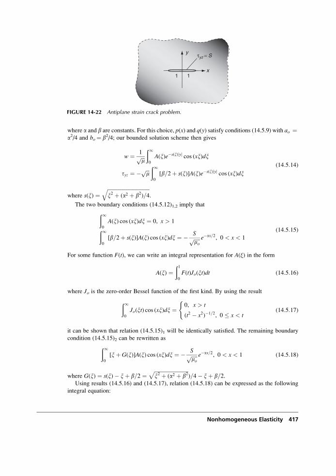
where a and b are constants. For this choice, p(x) and q(y) satisfy conditions (14.5.9) with ao ¼a2/4 and bo¼ b2/4; our bounded solution scheme then gives
w ¼ 1ffiffiffim
pð10
A(x)e�s(x)jyj cos (xx)dx
tyz ¼ � ffiffiffim
p ð10
[b=2þ s(x)]A(x)e�s(x)jyj cos (xx)dx(14:5:14)
where s(x) ¼ffiffiffiffiffiffiffiffiffiffiffiffiffiffiffiffiffiffiffiffiffiffiffiffiffiffiffiffiffiffiffiffiffix2 þ (a2 þ b2)=4
q.
The two boundary conditions (14.5.12)1,2 imply thatð10
A(x) cos (xx)dx ¼ 0, x > 1ð10
[b=2þ s(x)]A(x) cos (xx)dx ¼ � Sffiffiffiffiffimo
p e�ax=2, 0 < x < 1
(14:5:15)
For some function F(t), we can write an integral representation for A(�) in the form
A(x) ¼ð10
F(t)Jo(xt)dt (14:5:16)
where Jo is the zero-order Bessel function of the first kind. By using the result
ð10
Jo(xt) cos (xx)dx ¼ 0, x > t
(t2 � x2)�1=2, 0 � x < t
((14:5:17)
it can be shown that relation (14.5.15)1 will be identically satisfied. The remaining boundary
condition (14.5.15)2 can be rewritten asð10
[xþ G(x)]A(x) cos (xx)dx ¼ � Sffiffiffiffiffimo
p e�ax=2, 0 < x < 1 (14:5:18)
where G(x) ¼ s(x)� xþ b=2 ¼ffiffiffiffiffiffiffiffiffiffiffiffiffiffiffiffiffiffiffiffiffiffiffiffiffiffiffix2 þ (a2 þ b2
p)=4� xþ b=2.
Using results (14.5.16) and (14.5.17), relation (14.5.18) can be expressed as the following
integral equation:
x
y τyz = S
11
FIGURE 14-22 Antiplane strain crack problem.
Nonhomogeneous Elasticity 417
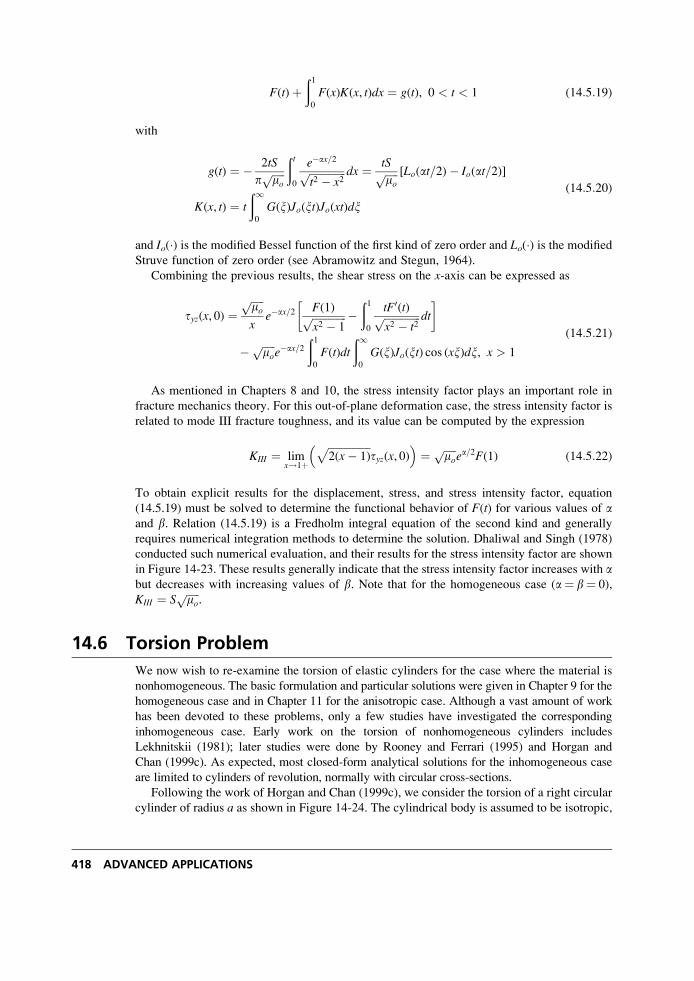
F(t)þð10
F(x)K(x, t)dx ¼ g(t), 0 < t < 1 (14:5:19)
with
g(t) ¼ � 2tS
pffiffiffiffiffimo
pðt0
e�ax=2ffiffiffiffiffiffiffiffiffiffiffiffiffiffit2 � x2
p dx ¼ tSffiffiffiffiffimo
p [Lo(at=2)� Io(at=2)]
K(x, t) ¼ t
ð10
G(x)Jo(xt)Jo(xt)dx
(14:5:20)
and Io(�) is the modified Bessel function of the first kind of zero order and Lo(�) is the modified
Struve function of zero order (see Abramowitz and Stegun, 1964).
Combining the previous results, the shear stress on the x-axis can be expressed as
tyz(x, 0) ¼ffiffiffiffiffimo
px
e�ax=2 F(1)ffiffiffiffiffiffiffiffiffiffiffiffiffix2 � 1
p �ð10
tF0(t)ffiffiffiffiffiffiffiffiffiffiffiffiffiffix2 � t2
p dt
� �
� ffiffiffiffiffimo
pe�ax=2
ð10
F(t)dt
ð10
G(x)Jo(xt) cos (xx)dx, x > 1
(14:5:21)
As mentioned in Chapters 8 and 10, the stress intensity factor plays an important role in
fracture mechanics theory. For this out-of-plane deformation case, the stress intensity factor is
related to mode III fracture toughness, and its value can be computed by the expression
KIII ¼ limx!1þ
ffiffiffiffiffiffiffiffiffiffiffiffiffiffiffiffi2(x� 1)
ptyz(x, 0)
� �¼ ffiffiffiffiffi
mop
ea=2F(1) (14:5:22)
To obtain explicit results for the displacement, stress, and stress intensity factor, equation
(14.5.19) must be solved to determine the functional behavior of F(t) for various values of aand b. Relation (14.5.19) is a Fredholm integral equation of the second kind and generally
requires numerical integration methods to determine the solution. Dhaliwal and Singh (1978)
conducted such numerical evaluation, and their results for the stress intensity factor are shown
in Figure 14-23. These results generally indicate that the stress intensity factor increases with abut decreases with increasing values of b. Note that for the homogeneous case (a¼ b¼ 0),
KIII ¼ Sffiffiffiffiffimo
p.
14.6 Torsion Problem
We now wish to re-examine the torsion of elastic cylinders for the case where the material is
nonhomogeneous. The basic formulation and particular solutions were given in Chapter 9 for the
homogeneous case and in Chapter 11 for the anisotropic case. Although a vast amount of work
has been devoted to these problems, only a few studies have investigated the corresponding
inhomogeneous case. Early work on the torsion of nonhomogeneous cylinders includes
Lekhnitskii (1981); later studies were done by Rooney and Ferrari (1995) and Horgan and
Chan (1999c). As expected, most closed-form analytical solutions for the inhomogeneous case
are limited to cylinders of revolution, normally with circular cross-sections.
Following the work of Horgan and Chan (1999c), we consider the torsion of a right circular
cylinder of radius a as shown in Figure 14-24. The cylindrical body is assumed to be isotropic,
418 ADVANCED APPLICATIONS
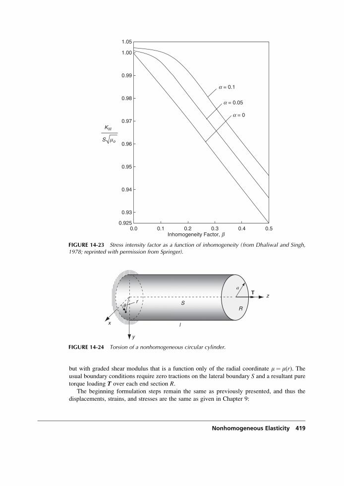
but with graded shear modulus that is a function only of the radial coordinate m¼ m(r). Theusual boundary conditions require zero tractions on the lateral boundary S and a resultant pure
torque loading T over each end section R.The beginning formulation steps remain the same as previously presented, and thus the
displacements, strains, and stresses are the same as given in Chapter 9:
Inhomogeneity Factor, b
S mo
KIII
a = 0
a = 0.05
a = 0.1
1.05
1.00
0.99
0.98
0.97
0.96
0.95
0.94
0.93
0.9250.0 0.1 0.2 0.3 0.4 0.5
FIGURE 14-23 Stress intensity factor as a function of inhomogeneity ( from Dhaliwal and Singh,1978; reprinted with permission from Springer).
x
y
z
aT
l
q•
rR
S
FIGURE 14-24 Torsion of a nonhomogeneous circular cylinder.
Nonhomogeneous Elasticity 419
u ¼ �ayz
v ¼ axz
w ¼ w(x, y)
(14:6:1)
ex ¼ ey ¼ ez ¼ exy ¼ 0
exz ¼ 1
2
@w
@x� ay
� �
eyz ¼ 1
2
@w
@yþ ax
� � (14:6:2)
sx ¼ sy ¼ sz ¼ txy ¼ 0
txz ¼ m@w
@x� ay
� �
tyz ¼ m@w
@yþ ax
� � (14:6:3)
It again becomes useful to introduce the Prandtl stress function, f¼ f(x,y)
txz ¼ @f@y
, tyz ¼ � @f@x
(14:6:4)
so that the equilibrium equations are satisfied identically. We can again generate the compati-
bility relation among the two nonzero stress components by differentiating and combining
relations (14.6.3)2,3 to eliminate the displacement terms. Substituting (14.6.4) into that result
gives the governing relation in terms of the stress function
@
@x
1
m@f@x
� �þ @
@y
1
m@f@y
� �¼ �2a (14:6:5)
where the shear modulus � must now be left inside the derivative operations because the
material is inhomogeneous. Recall that, for the homogeneous case, relation (14.6.5) reduced to
the Poisson equation r2f¼�2�a.Incorporation of the boundary condition that tractions vanish on the lateral surface S leads
to identical steps as given previously by equations (9.3.10) through (9.3.12), thus leading to the
fact that the stress function must be a constant on all cross-section boundaries; that is,
dfds
¼ 0 ) f ¼ constant, on S (14:6:6)
For simply connected sections, the constant may again be chosen as 0. Invoking the resultant
force conditions on the cylinder end planes (domain R), as given by relations (9.3.14), again
yields
420 ADVANCED APPLICATIONS
T ¼ðð
R
(xTny � yTn
x )dxdy ¼ 2
ððR
fdxdy (14:6:7)
and the torsional rigidity J can again be defined by J¼ T/a.Because we wish to use a simple radial shear modulus variation, �¼ �(r), it is more
convenient to use a polar coordinate formulation. For the circular cylinder under study, the
problem reduces to an axisymmetric formulation independent of the angular coordinate and the
warping displacement vanishes. Under these conditions the displacements, strains, and stresses
reduce to
ur ¼ uz ¼ 0, uy ¼ arz
er ¼ ey ¼ ez ¼ erz ¼ ery ¼ 0, eyz ¼ ar2
sr ¼ sy ¼ sz ¼ trz ¼ try ¼ 0, tyz ¼ amr
(14:6:8)
Relations (14.6.4) and (14.6.5) for the stress function formulation then reduce to a system in
terms of only the radial coordinate r
tyz ¼ � dfdr
1
r
d
dr
r
mdfdr
� �¼ �2a
(14:6:9)
with boundary condition f(a)¼ 0.
The governing differential equation (14.6.9) can be easily integrated to give the general
solution
f(r) ¼ �aðrm(r)dr þ C1
ðm(r)r
dr þ C2 (14:6:10)
where C1 and C2 are arbitrary constants. We require that the solution for f remain bounded as
r ! 0, thus implying that each integral term in (14.6.10) be finite at the origin. Restricting
ourselves to the plausible case where the shear modulus is expected to be nonzero but bounded
at the origin, limr!0
Ðrm(r)dr ! 0, while the second integral, lim
r!0
Ð m(r)r
dr, is singular. Based on
these arguments, C1 must be set to 0. Finally, the boundary condition f(a)¼ 0 determines the
final constant C2 and produces the general solution
f(r) ¼ aðar
xm(x)dx (14:6:11)
With this result, the shear stress and torsional rigidity then become
tyz ¼ arm(r)
J ¼ 2pða0
r3m(r)dr(14:6:12)
Nonhomogeneous Elasticity 421
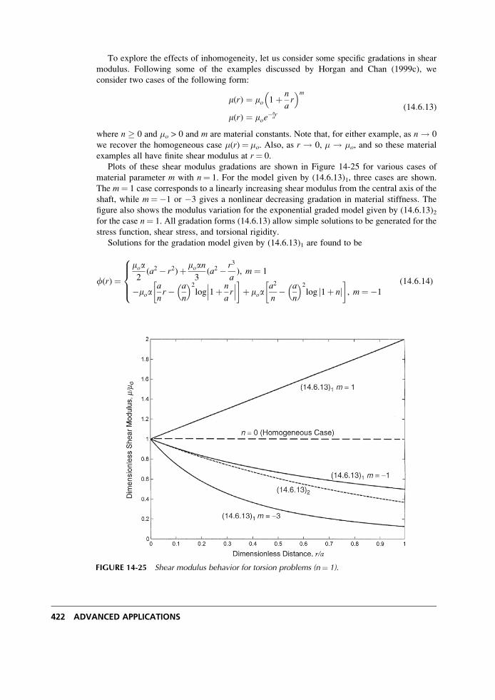
To explore the effects of inhomogeneity, let us consider some specific gradations in shear
modulus. Following some of the examples discussed by Horgan and Chan (1999c), we
consider two cases of the following form:
m(r) ¼ mo 1þ n
ar
� �mm(r) ¼ moe
�nar
(14:6:13)
where n � 0 and �o > 0 and m are material constants. Note that, for either example, as n ! 0
we recover the homogeneous case �(r)¼ �o. Also, as r ! 0, � ! �o, and so these material
examples all have finite shear modulus at r¼ 0.
Plots of these shear modulus gradations are shown in Figure 14-25 for various cases of
material parameter m with n¼ 1. For the model given by (14.6.13)1, three cases are shown.
The m¼ 1 case corresponds to a linearly increasing shear modulus from the central axis of the
shaft, while m¼�1 or �3 gives a nonlinear decreasing gradation in material stiffness. The
figure also shows the modulus variation for the exponential graded model given by (14.6.13)2for the case n¼ 1. All gradation forms (14.6.13) allow simple solutions to be generated for the
stress function, shear stress, and torsional rigidity.
Solutions for the gradation model given by (14.6.13)1 are found to be
f(r)¼moa2
(a2 � r2)þ moan3
(a2 � r3
a), m¼ 1
�moaa
nr� a
n
� �2log 1þ n
ar
��� ���� �þ moa
a2
n� a
n
� �2log j1þ nj
� �, m¼�1
8>><>>: (14:6:14)
FIGURE 14-25 Shear modulus behavior for torsion problems (n¼ 1).
422 ADVANCED APPLICATIONS
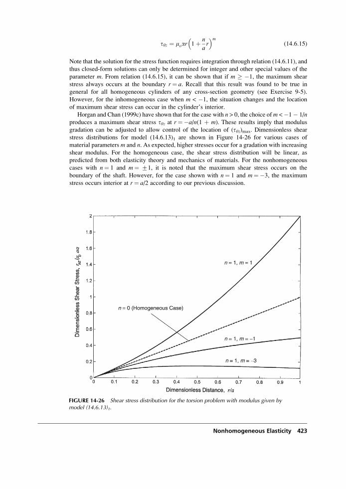
tyz ¼ moar 1þ n
ar
� �m(14:6:15)
Note that the solution for the stress function requires integration through relation (14.6.11), and
thus closed-form solutions can only be determined for integer and other special values of the
parameter m. From relation (14.6.15), it can be shown that if m � �1, the maximum shear
stress always occurs at the boundary r¼ a. Recall that this result was found to be true in
general for all homogeneous cylinders of any cross-section geometry (see Exercise 9-5).
However, for the inhomogeneous case when m < �1, the situation changes and the location
of maximum shear stress can occur in the cylinder’s interior.
Horgan and Chan (1999c) have shown that for the case with n > 0, the choice ofm <�1� 1/nproduces a maximum shear stress tyz at r¼�a/n(1 þ m). These results imply that modulus
gradation can be adjusted to allow control of the location of (tyz)max. Dimensionless shear
stress distributions for model (14.6.13)1 are shown in Figure 14-26 for various cases of
material parameters m and n. As expected, higher stresses occur for a gradation with increasingshear modulus. For the homogeneous case, the shear stress distribution will be linear, as
predicted from both elasticity theory and mechanics of materials. For the nonhomogeneous
cases with n¼ 1 and m¼ +1, it is noted that the maximum shear stress occurs on the
boundary of the shaft. However, for the case shown with n¼ 1 and m¼�3, the maximum
stress occurs interior at r¼ a/2 according to our previous discussion.
FIGURE 14-26 Shear stress distribution for the torsion problem with modulus given bymodel (14.6.13)1.
Nonhomogeneous Elasticity 423
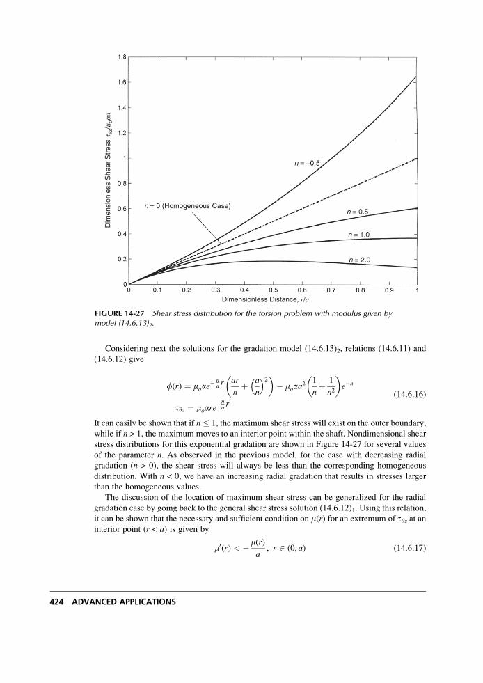
Considering next the solutions for the gradation model (14.6.13)2, relations (14.6.11) and
(14.6.12) give
f(r) ¼ moae� n
a rar
nþ a
n
� �2� �� moaa
2 1
nþ 1
n2
� �e�n
tyz ¼ moare�na r
(14:6:16)
It can easily be shown that if n � 1, the maximum shear stress will exist on the outer boundary,
while if n > 1, the maximum moves to an interior point within the shaft. Nondimensional shear
stress distributions for this exponential gradation are shown in Figure 14-27 for several values
of the parameter n. As observed in the previous model, for the case with decreasing radial
gradation (n > 0), the shear stress will always be less than the corresponding homogeneous
distribution. With n < 0, we have an increasing radial gradation that results in stresses larger
than the homogeneous values.
The discussion of the location of maximum shear stress can be generalized for the radial
gradation case by going back to the general shear stress solution (14.6.12)1. Using this relation,
it can be shown that the necessary and sufficient condition on �(r) for an extremum of tyz at aninterior point (r < a) is given by
m0(r) < �m(r)a
, r 2 (0, a) (14:6:17)
Dimensionless Distance, r/a
Dim
ensi
onle
ss S
hear
Str
ess t q
z/m o
aa
FIGURE 14-27 Shear stress distribution for the torsion problem with modulus given bymodel (14.6.13)2.
424 ADVANCED APPLICATIONS
where the prime indicates differentiation. Furthermore the location ro of this extremum is
specified by
ro ¼ � m(ro)m0(ro)
(14:6:18)
Further analysis to determine the torsional rigidities can also be carried out (see, for example,
Exercise 14-20). Horgan and Chan (1999c) have explored torsional rigidities in detail and have
developed several general results including upper and lower bounding theorems.
It should be noted that the general field equation for the torsion problem (14.6.5) is quite
similar to the corresponding field equation for the antiplane strain problem (14.5.4) discussed
previously. Thus, a transformation scheme similar to (14.5.5) may also help reduce the torsion
field equation into a more tractable relation. Following this concept, we use the transformation
f(x, y) ¼ F(x, y)ffiffiffiffiffiffiffiffiffiffiffiffiffim(x, y)
p(14:6:19)
into (14.6.5) and find the following reduction
r2Fþ F(m)F ¼ �2affiffiffim
p(14:6:20)
where
F(m) ¼ 1
2mr2m� 3
2mj=mj2
� �¼ � ffiffiffi
mp r2(m�1=2) (14:6:21)
Assuming that � > 0 in the domain, boundary condition (14.6.6) implies that
F ¼ 0, on S (14:6:22)
This formulation leads to significant simplification for the case where F(�)¼ 0, which
corresponds to the situation where ��1/2 is harmonic. For such a case, the governing equation
reduces to the Poisson equation
r2F ¼ �2affiffiffim
p(14:6:23)
and standard solution techniques for solving such equations can then be applied.
Another noteworthy area of significant research dealing with graded materials includes
studies of static and dynamic fracture mechanics; see, for example, Parameswaran and Shukla
(1999, 2002). These and other studies have investigated material gradation effects on crack tip
stresses around stationary and moving cracks.
This concludes our exploration into nonhomogeneous elasticity solutions. The examples
given illustrate some of the interesting effects caused by spatial variation of elastic moduli. As
should be evident, problem formulation and solution are more challenging. Solutions to such
problems commonly indicate significant differences in the elastic stress and displacement
fields when compared with corresponding homogeneous solutions. In some cases, material
gradation will reduce maximum stresses and change the spatial location where such max-
imums occur. This provides the possibility of tailoring material variation to achieve desired
stresses in a structure and thus of functionally grading the material. The difficult part of this
concept is how to develop manufacturing techniques that will produce the desired continuous
modulus variation in realistic materials used in engineering applications.
Nonhomogeneous Elasticity 425
References
Abramowitz M, and Stegun IA: Handbook of Mathematical Functions with Formulas, Graphs andMathematical Tables, National Bureau of Standards, 1964.
Ang WT, and Clements DL: On some crack problems for inhomogeneous elastic materials, Int. J. SolidsStructures, vol 23, pp. 1089-1104, 1987.
Awojobi AO, and Gibson RE: Plane strain and axially symmetric problems of a linearly nonhomogeneous
elastic half-space, Q. J. Mech. Appl. Math, vol 21, pp. 285-302, 1973.Booker JR, Balaam NP, and Davis EH: The behavior of an elastic non-homogeneous half-space. Part I.
Line and point loads, Int. J. Num. Anal. Meth. Geomech. vol 9, pp. 353-367, 1985.Calladine CR, and Greenwood JA: Line and point loads on a non-homogeneous incompressible elastic
half-space, J. Mech. Appl. Math., vol 31, pp. 507-529, 1978.Carrier WD, and Christian JT: Analysis of an inhomogeneous elastic half-space, J. Soil Mech Founda-tions Eng., vol 99, pp. 301-306, 1973.
Clements DL, Atkinson C, and Rogers C: Antiplane crack problems for an inhomogeneous elastic
material, Acta Mech., vol 29, pp. 199-211, 1978.Clements DL, Kusuma J, and Ang WT: A note on antiplane deformations of inhomogeneous elastic
materials, Int. J. Eng. Sci., vol 35, pp. 593-601, 1997.Delale F: Mode III fracture of bonded non-homogeneous materials, Eng. Frac. Mech., vol 22,
pp. 213-226, 1985.
Dhaliwal RS, and Singh BM: On the theory of elasticity of a non-homogeneous medium, J. Elasticity, vol 8,pp. 211-219, 1978.
Du CH: The two-dimensional problems of the nonhomogeneous isotropic medium, Problems of Con-tinuum Mechanics: Contributions in Honor of the 70th Birthday of I. Muskehlishvili, pp. 104-108,SIAM, Noordhoff, 1961.
Erdogan F, and Ozturk M: Diffusion problems in bonded nonhomogeneous materials with an interface
cut, Int. J. Eng. Sci., vol 30, pp. 1507-1523, 1992.Fraldi M, and Cowin SC: Inhomogeneous elastostatic problem solutions constructed from stress-associ-
ated homogeneous solutions, J. Mech. Phys. Solids, vol 52, pp. 2207-2233, 2004.Galmudi D, and Dvorkin J: Stresses in anisotropic cylinders, Mech. Res. Comm., vol 22, pp. 109-113,1995.
Giannakopoulos AE, and Suresh S: Indentation of solids with gradients in elastic properties: Part I. Point
force, Int. J. Solids Structures, vol 34, pp. 2357-2392, 1997.Gibson RE: Some results concerning displacements and stresses in a non-homogeneous elastic half space,
Geotechnique, vol 17, pp. 58-67, 1967.Gibson RE, and Sills GC: On the loaded elastic half space with a depth varying Poisson’s ratio, ZAMP,vol 20, pp. 691-695, 1969.
Holl DL: Stress transmission in earths, Proc. Highway Res. Board, vol 20, pp. 709-721, 1940.Horgan CO, and Baxter SC: Effects of curvilinear anisotropy of radially symmetric stresses in anisotropic
linearly elastic solids, J. Elasticity, vol 42, pp. 31-48, 1996.Horgan CO, and Chan AM: The pressurized hollow cylinder or disk problem for functionally graded
isotropic linearly elastic materials, J. Elasticity, vol 55, pp. 43-59, 1999a.Horgan CO, and Chan AM: The stress response of functionally graded isotropic linearly elastic rotating
disks, J. Elasticity, vol 55, pp. 219-230, 1999b.Horgan CO, and Chan AM: Torsion of functionally graded isotropic linearly elastic bars, J. Elasticity,vol 52, pp. 181-199, 1999c.
Horgan CO, and Miller KL: Antiplane shear deformations for homogeneous and inhomogeneous aniso-
tropic linearly elastic solids, J. Appl. Mech., vol 61, pp. 23-29, 1994.Kassir MK: Boussinesq problems for nonhomogeneous solids, J. Eng. Mech., vol 98, pp. 457-470, 1972.Lekhnitskii SG: Radial distribution of stresses in a wedge and in a half-plane with variable modulus of
elasticity, PMM, vol 26, pp. 146-151, 1961.
Lekhnitskii SG: Theory of Elasticity of an Anisotropic Body, Mir Publishers, Moscow, 1981.
426 ADVANCED APPLICATIONS
Oner M: Vertical and horizontal deformation of an inhomogeneous elastic half-space, Int. J. Num. Anal.Meth. Geomech., vol 14, pp. 613-629, 1990.
Parameswaran V, and Shukla A: Crack-tip stress fields for dynamic fracture in functionally gradient
materials, Mech. Materials, vol 31, pp. 579-596, 1999.Parameswaran V, and Shukla A: Asymptotic stress fields for stationary cracks along the gradient in
functionally graded materials, J. Appl. Mech., vol 69, pp. 240-243, 2002.Plevako VP: On the theory of elasticity of inhomogeneous media, PMM, vol 35, pp. 853-860, 1971.
Plevako VP: On the possibility of using harmonic functions for solving problems of the theory of
elasticity of nonhomogeneous media, PMM, vol 36, pp. 886-894, 1972.
Rooney FJ, and Ferrari M: Torsion and flexure of inhomogeneous materials, Comp. Eng., vol 5,
pp. 901-911, 1995.
Rostovtsev NA: On the theory of elasticity of a nonhomogeneous medium, PMM, vol 28, pp. 601-611,
1964.
Sankar BV: An elasticity solution for funtionally graded beams, Comp. Sci. Tech., vol 61, pp. 689-696,2001.
Stampouloglou IH, and Theotokoglou EE: The anisotropic and angularly inhomogeneous elastic wedge
under a monomial load distribution, Arch. Appl. Mech., vol 75, pp. 1-17, 2005.Spencer AJM, and Selvadurai APS: Some generalized anti-plane strain problems for an inhomogeneous
elastic half space, J. Eng. Math., vol 34, pp. 403-416, 1998.Suresh S: Graded materials for resistance to contact deformation and damage, Science, vol 292,
pp 2447-2451, 2001.
Ter-Mkrtich’ian LN: Some problems in the theory of elasticity of nonhomogeneous elastic media, PMM,
vol 25, pp. 1120-1125, 1961.
Vrettos C: The boussinesq problem for soils with bounded non-homogeneity, Int. J. Num. Anal. Meth.Geomech., vol 22, pp. 655-669, 1998.
Wang C.D, Tzeng CS, Pan, E, and Liao, JJ: Displacements and stresses due to a vertical point load in an
inhomogeneous transversely isotropic half-space, Int. J. RockMech.Mining Sci., vol 40, pp. 667-685, 2003.
Exercises
14-1. Show that, for the case of plane stress, the governing compatibility relation in terms of
the Airy stress function is given by (14.1.6)
@2
@x21
E
@2f@x2
� �
E
@2f@y2
� �þ @2
@y21
E
@2f@y2
� �
E
@2f@x2
� �þ 2
@2
@x@y
1þ �
E
@2f@x@y
� �¼ 0
Next determine the reduced form of this equation for the special case E¼ E(x) and
� ¼ constant.
14-2. Consider a special case of equation (14.1.4). Parameswaran and Shukla (1999) presented
a two-dimensional study where the shear modulus and Lame’s constant varied as
�(x)¼ �o(1 þ ax) and l(x)¼ k�(x), where �o, a, and k are constants. For such a material,
show that in the absence of body forces the two-dimensional Navier’s equations become
mo(1þ ax) k@W@x
þ 2@2u
@x2þ @2u
@y2þ @2v
@x@y
� �þ moa kWþ 2
@u
@x
� �¼ 0
mo(1þ ax) k@W@y
þ 2@2v
@y2þ @2v
@x2þ @2u
@x@y
� �þ moa
@u
@yþ @v
@x
� �¼ 0
where W ¼ @u
@xþ @v
@y.
Nonhomogeneous Elasticity 427
14-3. Parameswaran and Shukla (2002) recently presented a fracture mechanics study of non-
homogeneous material behavior related to functionally graded materials. They
investigated a two-dimensional plane stress problem where Poisson’s ratio remained
constant but Young’s modulus varied as E(x)¼ Eoeax, where Eo and a are constants. For
this case, with zero body forces, show that the governing Airy stress function equation is
given by
r4f� 2a@
@x(r2f)þ a2r2f� a2(1þ �)
@2f@y2
¼ 0
This result may be compared with the more general case given by relation (14.1.6). Note
that, when a¼ 0, this result reduces to the homogeneous form r4f¼ 0. The nonho-
mogeneous result is a challenging equation, and its solution was developed for the
limited case near the tip of a crack using asymptotic analysis.
14-4. For the hollow cylinder problem shown in Figure 14-5, use the given boundary
conditions to explicitly determine the arbitrary constants A and B and the stress relations
(14.2.6).
14-5. For the problem in Figure 14-5 with only internal pressure, show that the general stress
field (14.2.6) reduces to relations (14.2.7).
14-6. For the hollow cylinder problem illustrated in Figure 14-5, show that the usual
restrictions on Poisson’s ratio, 0 � � � 1/2, imply that
� 2þ k þ n � 0, � 2� k þ n � 0
2þ k� � n�
k � nþ 2�� 1,
2� k� � n�
k þ n� 2�� 1
Using these results, develop arguments to justify that the stresses in solution (14.2.9)
must satisfy sr < 0 and sy > 0 in the cylinder’s domain. Thus stresses in the nonhomo-
geneous problem have behavior similar to those of the ungraded case.
14-7*. Following procedures similar to those for the homogeneous problem (see Section 8.4.1),
develop the following stress field for a pressurized hole in an infinite nonhomogeneous
medium with moduli variation given by (14.2.3).
sr ¼ �pia
r
� �(2þk�n)=2
sy ¼ pi2� k� � n�
k þ n� 2�
a
r
� �(2þk�n)=2
Plot the dimensionless stress fields for this case using the same parameters � and n used
in Figures 14-7 and 14-8.
14-8. For the inhomogeneous rotating disk problem with � ¼ 0, explore the solution for the
special case of n¼ 3 and show that the stresses reduce to
sr ¼ 0, sy ¼ r!2r2
428 ADVANCED APPLICATIONS
Also determine the displacement solution and show the surprising result that u(0) > 0.
This strange behavior has been referred to as a cavitation at the disk’s center.
14-9*. Using MATLAB or similar software, make a plot similar to Figure 14-13 showing the
behavior of the hoop stress sy for the case with � ¼ 0 and n¼�0.5, 0, 0.5, 1, 2. Discuss
your results.
14-10. Using the design criterion (14.3.14), incorporate the fundamental equations for the
inhomogeneous rotating disk problem to explicitly develop the required gradation
given by relation (14.3.15).
14-11. Rather than using polar coordinates to formulate the inhomogeneous half-space
problem of Section 14.4, some researchers have used Cartesian coordinates instead.
Using the x, z-coordinates as shown in Figure 14-14, consider the plane strain case withinhomogeneity only in the shear modulus such that �¼ �(z) and � ¼ constant. First
show that combining the strain displacement relations with Hooke’s law gives
sx ¼ 2m(z)@u
@xþ ��W
� �
sz ¼ 2m(z)@w
@zþ ��W
� �
txz ¼ m(z)@u
@zþ @w
@x
� �
where W ¼ ekk ¼ @u
@xþ @w
@zis the dilatation and �� ¼ �
1� 2�. Next show that the equi-
librium equations yield
r2uþ (1þ 2��)@W@x
þ h(z)@u
@zþ @w
@x
� �¼ 0
r2wþ (1þ 2��)@W@z
þ 2h(z)@w
@zþ ��W
� �¼ 0
where h(z) ¼ 1
mdmdz. Explore the simplification of these equations for the special inhomo-
geneous case in which �¼ �o eaz, where �o and a are constants.
14-12. Consider the axisymmetric half-space problem shown in Figure 14-19 for the case
where only Poisson’s ratio is allowed to vary with depth coordinate � ¼ �(z). Usingcylindrical coordinates (r, y, z) to formulate the problem, first show that the stress field
can be expressed by
sr ¼ 2m@ur@r
þ ��(z)W� �
sz ¼ 2m@uz@z
þ ��(z)W� �
sy ¼ 2murrþ ��(z)W
� �trz ¼ m
@ur@z
þ @uz@r
� �
Nonhomogeneous Elasticity 429
where W ¼ @ur@r
þ urrþ @uz
@zis the dilatation and ��(z) ¼ �(z)
1� 2�(z). Next show that the
equilibrium equations reduce to
r2 � 1
r
� �ur þ @
@r(1þ 2��)Wð Þ ¼ 0
r2uz þ @
@z(1þ 2��)Wð Þ ¼ 0
14-13. For the antiplane strain problem, verify that transformation (14.5.5) will reduce the
governing equilibrium equation to relation (14.5.6). Next show that the separation of
variables scheme defined by (14.5.7) will lead to the two equations (14.5.8).
14-14. Explicitly show that the inhomogeneity functions p(x)¼ e�ajxj and q(y)¼ e�bjyj, thatwere used for the antiplane crack problem, do in fact satisfy relations (14.5.9) with
ao¼ a2/4 and bo¼ b2/4.
14-15. For the torsion problem discussed in Section 14.6, explicitly justify the reductions in
polar coordinates summarized by relations (14.6.8) and (14.6.9).
14-16. Verify that the general solution to equations (14.6.9) are given by (14.6.11) and
(14.6.12) for the torsion problem.
14-17. For the torsion problem, verify the solutions (14.6.14) and (14.6.15) for the gradation
model (14.6.13)1.
14-18. For the torsion problem, verify the solutions (14.6.16) for the gradation model
(14.6.13)2.
14-19. Investigate the issue of finding the location of (tyz)max for the torsion problem. First
verify the results given by (14.6.17) and (14.6.18). Next apply these general relations to
the specific gradation models given by (14.6.13)1,2, and develop explicit results for
locations of the extrema.
14-20. Show that the torsional rigidity for the exponential gradation case (14.6.13)2 is given by
J ¼ 2pa4mo6
n4� e�n 1
nþ 3
n2þ 6
n3þ 6
n4
� �� �
Next use a Taylor series expansion for small n to show that
J � pa4mo2
1� 4n
5þ O(n2)
� �.
Compare this result with the homogeneous case.
430 ADVANCED APPLICATIONS
15 Micromechanics Applications
In recent years, considerable interest has developed inmicromechanical modeling of solids. This
interest has been fueled by the realization that many materials have heterogeneous microstruc-
tures that play a dominant role in determining macro deformational behavior. Materials where
this occurs include multiphase fiber and particulate composites, soil, rock, concrete, and various
granular materials. These materials have microstructures that occur at a variety of length scales
from meters to nanometers, and general interest lies with the case where the length scale is
smaller than other characteristic lengths in the problem. The response of such heterogeneous
solids shows strong dependence on the micromechanical behaviors between different material
phases. Classical theories of continuummechanics have limited ability to predict such behaviors,
and this has lead to the development of many new micromechanical theories of solids.
Work in this area, initiated almost a century ago by Volterra (1907), began with studies of
elastic stress and displacement fields around dislocations and other imperfections. More
recently, using continuum mechanics principles, theories have been developed in which the
material response depends on particular microscale length parameters connected with the
existence of inner degrees of freedom and nonlocal continuum behavior. By nonlocal behavior
we mean that the stress at a point depends not only on the strain at that point but also on the
strains of neighboring points. Mindlin (1964) developed a general linear elasticity theory withmicrostructure that allowed the stress to depend on both the strain and an additional kinematicmicrodeformation tensor. Related research has led to the development of micropolar and
couple-stress theories; see Eringen (1968). These approaches allow material deformation to
include additional independent microrotational degrees of freedom. Elastic continuum theories
using higher-order gradients have also been developed to model micromechanical behavior of
solids; see, for example, Mindlin (1965), Chang and Gao (1995), Aifantis (1999), and Li et al.
(2004). A general review of modeling heterogeneous elastic solids has been provided by
Nemat-Nasser and Hori (1993). Along similar lines, Cowin and Nunziato (1983) developed
a theory of elastic materials with voids including an independent volume fraction in the
constitutive relations.
Another interesting theory called doublet mechanics (Ferrari, Granik, Imam, and Nadeau
1997) represents heterogeneous solids in a discrete fashion as arrays of points or particles that
interact through prescribed micromechanical laws. Other related work has investigated elastic
materials with distributed cracks; see, for example, Budianski and O’Connell (1976) and
431
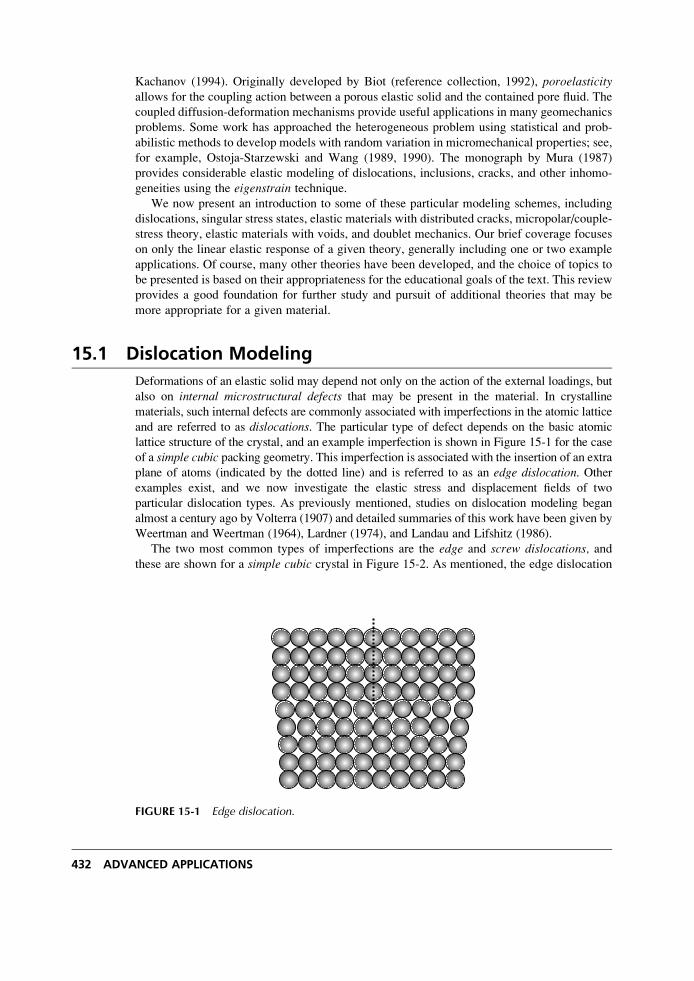
Kachanov (1994). Originally developed by Biot (reference collection, 1992), poroelasticityallows for the coupling action between a porous elastic solid and the contained pore fluid. The
coupled diffusion-deformation mechanisms provide useful applications in many geomechanics
problems. Some work has approached the heterogeneous problem using statistical and prob-
abilistic methods to develop models with random variation in micromechanical properties; see,
for example, Ostoja-Starzewski and Wang (1989, 1990). The monograph by Mura (1987)
provides considerable elastic modeling of dislocations, inclusions, cracks, and other inhomo-
geneities using the eigenstrain technique.
We now present an introduction to some of these particular modeling schemes, including
dislocations, singular stress states, elastic materials with distributed cracks, micropolar/couple-
stress theory, elastic materials with voids, and doublet mechanics. Our brief coverage focuses
on only the linear elastic response of a given theory, generally including one or two example
applications. Of course, many other theories have been developed, and the choice of topics to
be presented is based on their appropriateness for the educational goals of the text. This review
provides a good foundation for further study and pursuit of additional theories that may be
more appropriate for a given material.
15.1 Dislocation Modeling
Deformations of an elastic solid may depend not only on the action of the external loadings, but
also on internal microstructural defects that may be present in the material. In crystalline
materials, such internal defects are commonly associated with imperfections in the atomic lattice
and are referred to as dislocations. The particular type of defect depends on the basic atomic
lattice structure of the crystal, and an example imperfection is shown in Figure 15-1 for the case
of a simple cubic packing geometry. This imperfection is associated with the insertion of an extra
plane of atoms (indicated by the dotted line) and is referred to as an edge dislocation. Otherexamples exist, and we now investigate the elastic stress and displacement fields of two
particular dislocation types. As previously mentioned, studies on dislocation modeling began
almost a century ago by Volterra (1907) and detailed summaries of this work have been given by
Weertman and Weertman (1964), Lardner (1974), and Landau and Lifshitz (1986).
The two most common types of imperfections are the edge and screw dislocations, andthese are shown for a simple cubic crystal in Figure 15-2. As mentioned, the edge dislocation
FIGURE 15-1 Edge dislocation.
432 ADVANCED APPLICATIONS
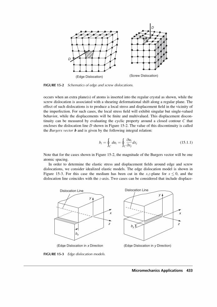
occurs when an extra plane(s) of atoms is inserted into the regular crystal as shown, while the
screw dislocation is associated with a shearing deformational shift along a regular plane. The
effect of such dislocations is to produce a local stress and displacement field in the vicinity of
the imperfection. For such cases, the local stress field will exhibit singular but single-valued
behavior, while the displacements will be finite and multivalued. This displacement discon-
tinuity can be measured by evaluating the cyclic property around a closed contour C that
encloses the dislocation line D shown in Figure 15-2. The value of this discontinuity is called
the Burgers vector b and is given by the following integral relation:
bi ¼þC
dui ¼þC
@ui@xj
dxj (15:1:1)
Note that for the cases shown in Figure 15-2, the magnitude of the Burgers vector will be one
atomic spacing.
In order to determine the elastic stress and displacement fields around edge and screw
dislocations, we consider idealized elastic models. The edge dislocation model is shown in
Figure 15-3. For this case the medium has been cut in the x,z-plane for x � 0, and the
dislocation line coincides with the z-axis. Two cases can be considered that include displace-
(Screw Dislocation)
D
(Edge Dislocation)
D
FIGURE 15-2 Schematics of edge and screw dislocations.
x
z
y
bx
Dislocation Line
(Edge Dislocation in x Direction
x
z
y
by
Dislocation Line
(Edge Dislocation in y Direction)
FIGURE 15-3 Edge dislocation models.
Micromechanics Applications 433
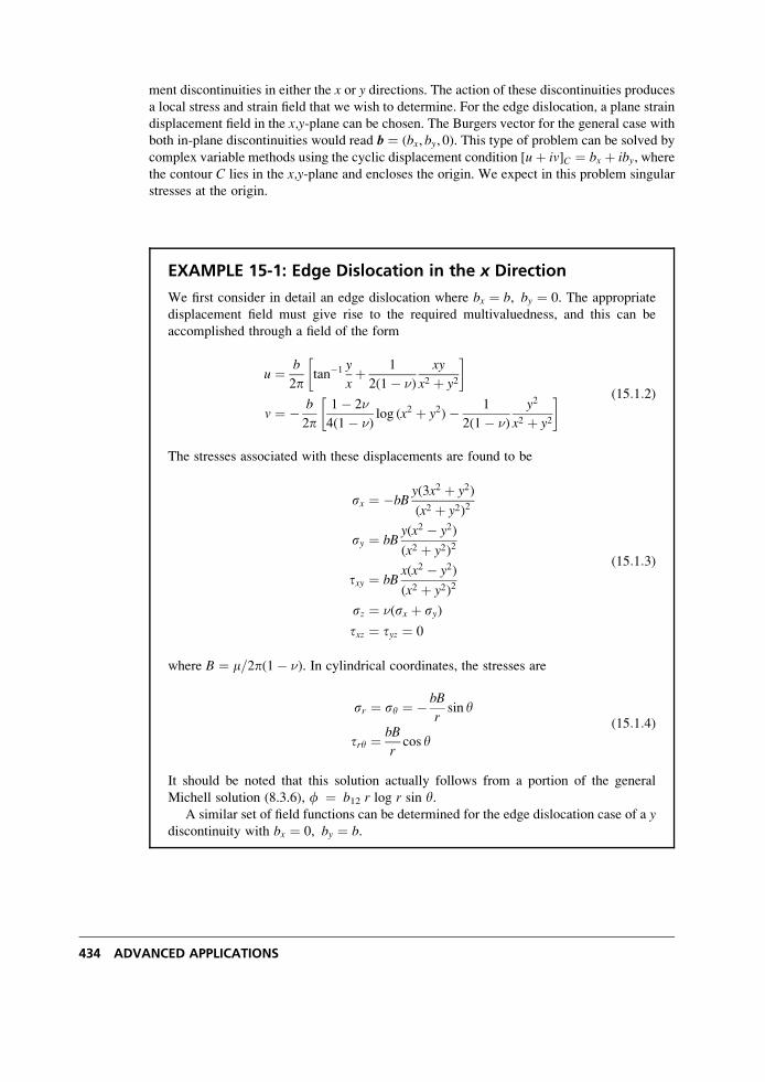
ment discontinuities in either the x or y directions. The action of these discontinuities producesa local stress and strain field that we wish to determine. For the edge dislocation, a plane strain
displacement field in the x,y-plane can be chosen. The Burgers vector for the general case withboth in-plane discontinuities would read b ¼ (bx, by, 0). This type of problem can be solved by
complex variable methods using the cyclic displacement condition [uþ iv]C ¼ bx þ iby, wherethe contour C lies in the x,y-plane and encloses the origin. We expect in this problem singular
stresses at the origin.
EXAMPLE 15-1: Edge Dislocation in the x Direction
We first consider in detail an edge dislocation where bx ¼ b, by ¼ 0. The appropriate
displacement field must give rise to the required multivaluedness, and this can be
accomplished through a field of the form
u ¼ b
2ptan�1 y
xþ 1
2(1� �)
xy
x2 þ y2
� �
v ¼ � b
2p1� 2�
4(1� �)log (x2 þ y2)� 1
2(1� �)
y2
x2 þ y2
� � (15:1:2)
The stresses associated with these displacements are found to be
sx ¼ �bBy(3x2 þ y2)
(x2 þ y2)2
sy ¼ bBy(x2 � y2)
(x2 þ y2)2
txy ¼ bBx(x2 � y2)
(x2 þ y2)2
sz ¼ �(sx þ sy)
txz ¼ tyz ¼ 0
(15:1:3)
where B ¼ m=2p(1� �). In cylindrical coordinates, the stresses are
sr ¼ sy ¼ � bB
rsin y
try ¼ bB
rcos y
(15:1:4)
It should be noted that this solution actually follows from a portion of the general
Michell solution (8.3.6), f ¼ b12 r log r sin y.A similar set of field functions can be determined for the edge dislocation case of a y
discontinuity with bx ¼ 0, by ¼ b.
434 ADVANCED APPLICATIONS
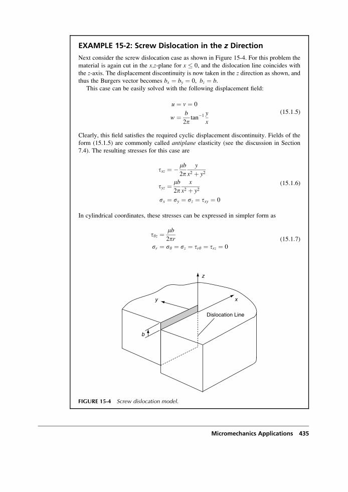
EXAMPLE 15-2: Screw Dislocation in the z Direction
Next consider the screw dislocation case as shown in Figure 15-4. For this problem the
material is again cut in the x,z-plane for x � 0, and the dislocation line coincides with
the z-axis. The displacement discontinuity is now taken in the z direction as shown, and
thus the Burgers vector becomes bx ¼ by ¼ 0, bz ¼ b.This case can be easily solved with the following displacement field:
u ¼ v ¼ 0
w ¼ b
2ptan�1 y
x
(15:1:5)
Clearly, this field satisfies the required cyclic displacement discontinuity. Fields of the
form (15.1.5) are commonly called antiplane elasticity (see the discussion in Section
7.4). The resulting stresses for this case are
txz ¼ �mb2p
y
x2 þ y2
tyz ¼ mb2p
x
x2 þ y2
sx ¼ sy ¼ sz ¼ txy ¼ 0
(15:1:6)
In cylindrical coordinates, these stresses can be expressed in simpler form as
tyz ¼ mb2pr
sr ¼ sy ¼ sz ¼ try ¼ trz ¼ 0
(15:1:7)
Dislocation Line
xy
z
b
FIGURE 15-4 Screw dislocation model.
Micromechanics Applications 435
Notice that the edge and screw dislocation stress fields are singular at the origin. This is
expected because of the nature of the displacement discontinuities associated with each
problem. Other aspects of dislocation modeling include determination of the associated strain
energy (see exercises), effect of external force fields, dislocation interaction, and movement.
These and other modeling issues can be found in Weertman and Weertman (1964), Lardner
(1974), and Landau and Lifshitz (1986).
15.2 Singular Stress States
As discussed in the previous section, elasticity theory can be used to model defects in
solids. Obviously, such studies may involve modeling of imperfections that are not simple
edge or screw dislocations. For example, other defects may include voids and inclusions
of arbitrary shape and distribution. In some cases these defects can produce localized, self-
equilibrated residual stress fields from, say, trapped gases, thermal mismatch associated
with an inclusion, and so forth. For many such problems, elasticity models can be developed
by using solutions from a particular solution class sometimes referred to as singular stressstates. These stress states include a variety of concentrated force and moment systems
yielding stress, strain, and displacement fields that have singular behaviors at particular
points in the domain. Such cases commonly include concentrated forces as developed in the
solution of the Kelvin problem (see Example 13-1). Combinations and superposition of
this fundamental solution are normally made to generate more complex and applicable
solutions. We now develop some basic singular stress states and investigate their fundamental
features.
Define a regular elastic state in a domain D as the set
S(x) ¼ {u, e,s} (15:2:1)
where the displacement vector u and stress and strain tensors s and e satisfy the elasticity fieldequations in D.
We use the Papkovich-Neuber solution scheme from Section 13.4 with redefined scalar and
vector potentials functions to allow the displacement solution to be expressed as
2mu ¼ =(fþ R � c)� 4(1� �)c (15:2:2)
where f is the scalar potential and c is the vector potential satisfying the equations
r2f ¼ � R � F2(1� �)
, r2c ¼ F
2(1� �)(15:2:3)
with body force F. Using elements of potential theory (Kellogg 1953), a particular solution to
equations (15.2.3) in a bounded domain D can be written as
436 ADVANCED APPLICATIONS
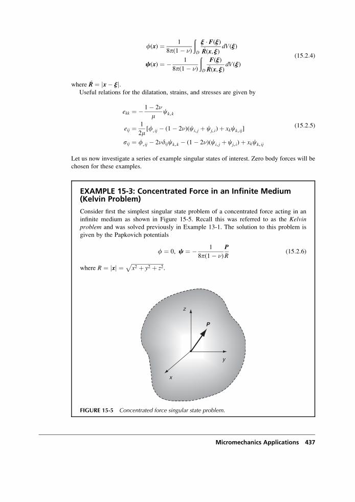
f(x) ¼ 1
8p(1� �)
ðD
j � F(j)RR(x, j)
dV(j)
c(x) ¼ � 1
8p(1� �)
ðD
F(j)
RR(x, j)dV(j)
(15:2:4)
where RR ¼ jx� jj:Useful relations for the dilatation, strains, and stresses are given by
ekk ¼ � 1� 2�
mck, k
eij ¼ 1
2m[f, ij � (1� 2�)(ci, j þ cj, i)þ xkck, ij]
sij ¼ f, ij � 2�dijck, k � (1� 2�)(ci, j þ cj, i)þ xkck, ij
(15:2:5)
Let us now investigate a series of example singular states of interest. Zero body forces will be
chosen for these examples.
EXAMPLE 15-3: Concentrated Force in an Infinite Medium(Kelvin Problem)
Consider first the simplest singular state problem of a concentrated force acting in an
infinite medium as shown in Figure 15-5. Recall this was referred to as the Kelvinproblem and was solved previously in Example 13-1. The solution to this problem is
given by the Papkovich potentials
f ¼ 0, c ¼ � 1
8p(1� �)
P
R(15:2:6)
where R ¼ jxj ¼ffiffiffiffiffiffiffiffiffiffiffiffiffiffiffiffiffiffiffiffiffiffiffiffix2 þ y2 þ z2
p.
x
y
z
P
FIGURE 15-5 Concentrated force singular state problem.
Micromechanics Applications 437
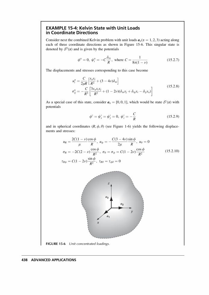
EXAMPLE 15-4: Kelvin State with Unit Loadsin Coordinate Directions
Consider next the combined Kelvin problem with unit loads aa(a ¼ 1, 2, 3) acting along
each of three coordinate directions as shown in Figure 15-6. This singular state is
denoted by Sa(x) and is given by the potentials
fa ¼ 0, cai ¼ �C
diaR
, where C ¼ 1
8p(1� �)(15:2:7)
The displacements and stresses corresponding to this case become
uai ¼C
2mRxaxiR2
þ (3� 4�)daih i
saij ¼ � C
R3
3xaxixjR2
þ (1� 2�)(daixj þ dajxi � dijxa)� � (15:2:8)
As a special case of this state, consider aa ¼ [0, 0, 1], which would be state Sz(x) withpotentials
fz ¼ czx ¼ cz
y ¼ 0, czz ¼ �C
R(15:2:9)
and in spherical coordinates (R,f, y) (see Figure 1-6) yields the following displace-
ments and stresses:
uR ¼ 2C(1� �)
mcosfR
, uf ¼ �C(3� 4�)
2msinfR
, uy ¼ 0
sR ¼ �2C(2� �)cosfR2
, sy ¼ sf ¼ C(1� 2�)cosfR2
tRf ¼ C(1� 2�)sinfR2
, tRy ¼ tfy ¼ 0
(15:2:10)
x
y
z
a3
a2
a1
FIGURE 15-6 Unit concentrated loadings.
438 ADVANCED APPLICATIONS
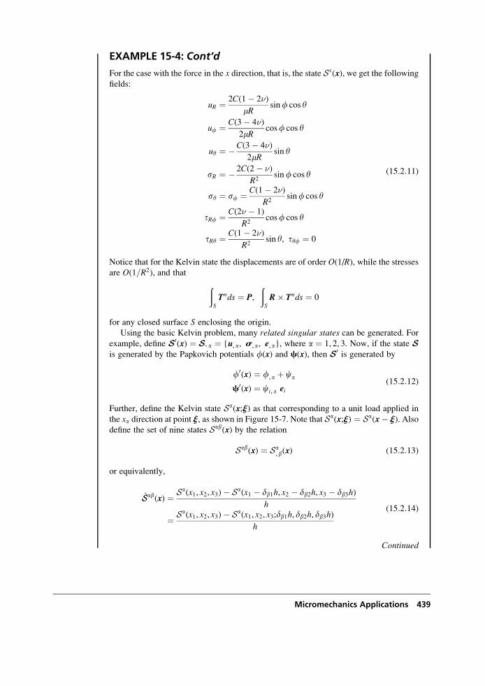
EXAMPLE 15-4: Cont’d
For the case with the force in the x direction, that is, the state Sx(x), we get the followingfields:
uR ¼ 2C(1� 2�)
mRsinf cos y
uf ¼ C(3� 4�)
2mRcosf cos y
uy ¼ �C(3� 4�)
2mRsin y
sR ¼ � 2C(2� �)
R2sinf cos y
sy ¼ sf ¼ C(1� 2�)
R2sinf cos y
tRf ¼ C(2� � 1)
R2cosf cos y
tRy ¼ C(1� 2�)
R2sin y, tyf ¼ 0
(15:2:11)
Notice that for the Kelvin state the displacements are of order O(1/R), while the stressesare O(1=R2), and that ð
S
Tnds ¼ P,
ðS
R� Tnds ¼ 0
for any closed surface S enclosing the origin.
Using the basic Kelvin problem, many related singular states can be generated. For
example, define S0(x) ¼ S, a ¼ {u, a, s, a, e, a}, where a ¼ 1, 2, 3. Now, if the state Sis generated by the Papkovich potentials f(x) and c(x), then S0 is generated by
f0(x) ¼ f, a þ ca
c0(x) ¼ ci, a ei(15:2:12)
Further, define the Kelvin state Sa(x;j) as that corresponding to a unit load applied in
the xa direction at point j, as shown in Figure 15-7. Note that Sa(x;j) ¼ Sa(x� j). Alsodefine the set of nine states Sab(x) by the relation
Sab(x) ¼ Sa, b(x) (15:2:13)
or equivalently,
SSab(x) ¼ Sa(x1, x2, x3)� Sa(x1 � db1h, x2 � db2h, x3 � db3h)h
¼ Sa(x1, x2, x3)� Sa(x1, x2, x3;db1h, db2h, db3h)h
(15:2:14)
Continued
Micromechanics Applications 439
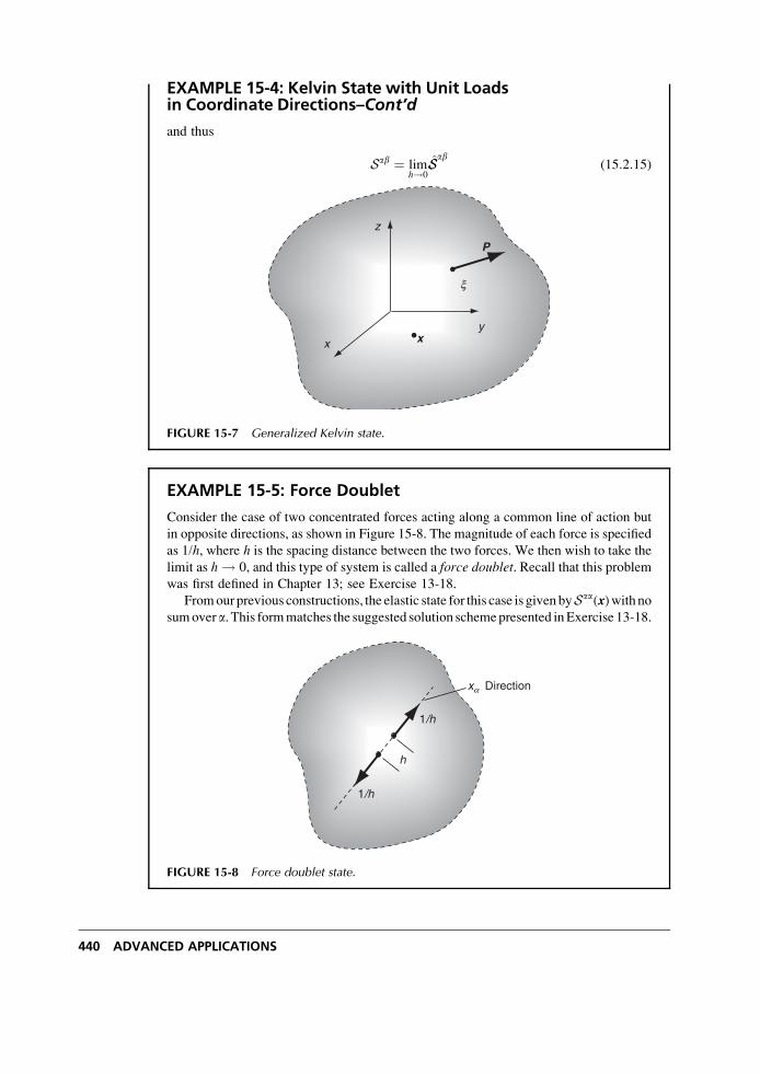
EXAMPLE 15-4: Kelvin State with Unit Loadsin Coordinate Directions–Cont’d
and thus
Sab ¼ limh!0
SSab(15:2:15)
x
y
z
P
x
ξ
FIGURE 15-7 Generalized Kelvin state.
EXAMPLE 15-5: Force Doublet
Consider the case of two concentrated forces acting along a common line of action but
in opposite directions, as shown in Figure 15-8. The magnitude of each force is specified
as 1/h, where h is the spacing distance between the two forces. We then wish to take the
limit as h ! 0, and this type of system is called a force doublet. Recall that this problemwas first defined in Chapter 13; see Exercise 13-18.
Fromour previous constructions, the elastic state for this case is givenbySaa(x)with nosumovera. This formmatches the suggested solution schemepresented inExercise 13-18.
h
xa Direction
1/h
1/h
FIGURE 15-8 Force doublet state.
440 ADVANCED APPLICATIONS
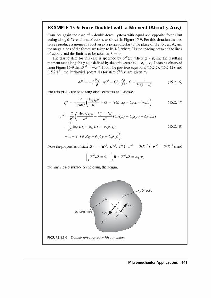
EXAMPLE 15-6: Force Doublet with a Moment (About g-Axis)
Consider again the case of a double-force system with equal and opposite forces but
acting along different lines of action, as shown in Figure 15-9. For this situation the two
forces produce a moment about an axis perpendicular to the plane of the forces. Again,
the magnitudes of the forces are taken to be 1/h, where h is the spacing between the linesof action, and the limit is to be taken as h ! 0.
The elastic state for this case is specified by Sab(x), where a 6¼ b, and the resulting
moment acts along the g-axis defined by the unit vector eg ¼ ea � eb. It can be observedfrom Figure 15-9 that Sab ¼ �Sba. From the previous equations (15.2.7), (15.2.12), and
(15.2.13), the Papkovich potentials for state Sab(x) are given by
fab ¼ �CdabR
, cabi ¼ Cdai
xbR3
, C ¼ 1
8p(1� �)(15:2:16)
and this yields the following displacements and stresses:
uabi ¼ � C
2mR3
3xaxbxiR2
þ (3� 4�)daixb � dabxi � dbixa
� �(15:2:17)
sabij ¼ C
R3
15xaxbxixjR4
þ 3(1� 2�)
R2(daixbxj þ dajxbxi � dijxaxb)
�
� 3
R2(dbixaxj þ dbjxaxi þ dabxixj)
�(1� 2�)(daidbj þ dajdbi þ dijdab)� (15:2:18)
Note the properties of state Sab ¼ {uab, sab, eab}: uab ¼ O(R�2), sab ¼ O(R�3), andðSTabdS ¼ 0,
ðS
R� TabdS ¼ egabeg
for any closed surface S enclosing the origin.
h
xa Direction
1/h
1/hxb Direction
FIGURE 15-9 Double-force system with a moment.
Micromechanics Applications 441
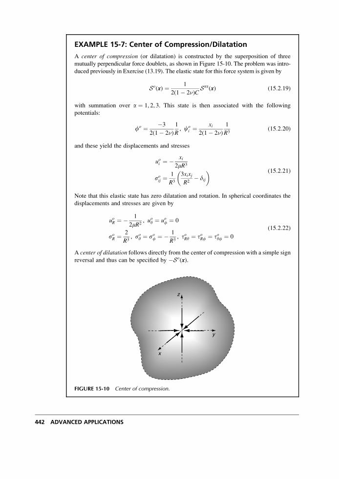
EXAMPLE 15-7: Center of Compression/Dilatation
A center of compression (or dilatation) is constructed by the superposition of three
mutually perpendicular force doublets, as shown in Figure 15-10. The problem was intro-
duced previously in Exercise (13.19). The elastic state for this force system is given by
So(x) ¼ 1
2(1� 2�)CSaa(x) (15:2:19)
with summation over a ¼ 1, 2, 3. This state is then associated with the following
potentials:
fo ¼ �3
2(1� 2�)
1
R, co
i ¼xi
2(1� 2�)
1
R3(15:2:20)
and these yield the displacements and stresses
uoi ¼ � xi2mR3
soij ¼1
R3
3xixjR2
� dij
� � (15:2:21)
Note that this elastic state has zero dilatation and rotation. In spherical coordinates the
displacements and stresses are given by
uoR ¼ � 1
2mR2, uoy ¼ uof ¼ 0
soR ¼ 2
R3, soy ¼ sof ¼ � 1
R3, toRy ¼ toRf ¼ toyf ¼ 0
(15:2:22)
A center of dilatation follows directly from the center of compression with a simple sign
reversal and thus can be specified by �So(x).
x
y
z
FIGURE 15-10 Center of compression.
442 ADVANCED APPLICATIONS
EXAMPLE 15-8: Center of Rotation
Using the cross-product representation, a center of rotation about the a-axis can be
expressed by the state
aS(x) ¼ 1
2eabgSbg(x) (15:2:23)
where summation over b and g is implied. Thus, centers of rotation about the coordinate
axes can be written as
1S(x) ¼ 1
2(S23 � S32)
2S(x) ¼ 1
2(S31 � S13)
3S(x) ¼ 1
2(S12 � S21)
(15:2:24)
Using the solution (15.2.16), the potentials for this state become
af ¼ 0, aci ¼C
2R3eaijxj (15:2:25)
with the constant C defined in relation (15.2.16). The corresponding displacements and
stresses follow as
aui ¼ � 1
8pmR3eaijxj
asij ¼ � 3
8pR5(eaikxkxj þ eajkxkxi)
(15:2:26)
This state has the following properties:ÐSaTdS ¼ 0,
ÐS R� aTdS ¼ daiei, where the
integration is taken over any closed surface enclosing the origin.
In order to develop additional singular states that might be used to model distributed singular-
ities, consider the following property.
Definition: Let S(x;l) ¼ {u(x;l), s(x;l), e(x;l)} be a regular elastic state for each param-
eter l 2 [a, b] with zero body forces. Then the state S� defined by
S�(x) ¼ðba
S(x;l)dl (15:2:27)
is also a regular elastic state. This statement is just another form of the superposition principle,
and it allows the construction of integrated combinations of singular elastic states as shown in
the next example.
Micromechanics Applications 443
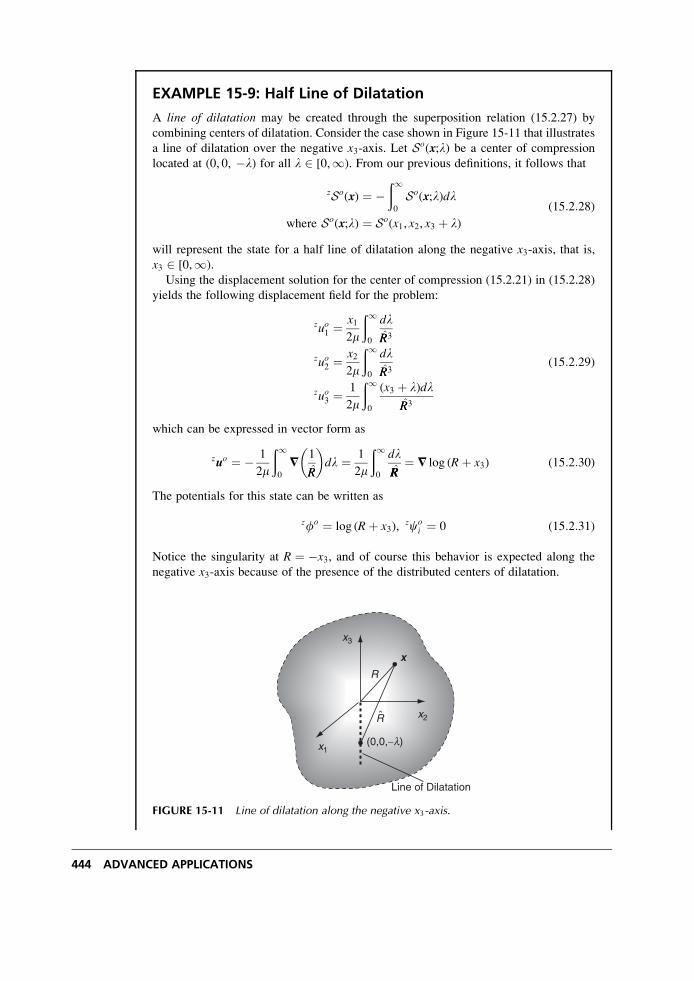
EXAMPLE 15-9: Half Line of Dilatation
A line of dilatation may be created through the superposition relation (15.2.27) by
combining centers of dilatation. Consider the case shown in Figure 15-11 that illustrates
a line of dilatation over the negative x3-axis. Let So(x;l) be a center of compression
located at (0, 0, �l) for all l 2 [0,1). From our previous definitions, it follows that
zSo(x) ¼ �ð10
So(x;l)dl
where So(x;l) ¼ So(x1, x2, x3 þ l)(15:2:28)
will represent the state for a half line of dilatation along the negative x3-axis, that is,x3 2 [0,1).
Using the displacement solution for the center of compression (15.2.21) in (15.2.28)
yields the following displacement field for the problem:
zuo1 ¼x12m
ð10
dl
RR3
zuo2 ¼x22m
ð10
dl
RR3
zuo3 ¼1
2m
ð10
(x3 þ l)dl
RR3
(15:2:29)
which can be expressed in vector form as
zuo ¼ � 1
2m
ð10
=1
RR
� �dl ¼ 1
2m
ð10
dl
RR¼ = log (Rþ x3) (15:2:30)
The potentials for this state can be written as
zfo ¼ log (Rþ x3),zco
i ¼ 0 (15:2:31)
Notice the singularity at R ¼ �x3, and of course this behavior is expected along the
negative x3-axis because of the presence of the distributed centers of dilatation.
x1
x2
x3
Line of Dilatation
(0,0,−l)
R
x
R
FIGURE 15-11 Line of dilatation along the negative x3-axis.
444 ADVANCED APPLICATIONS
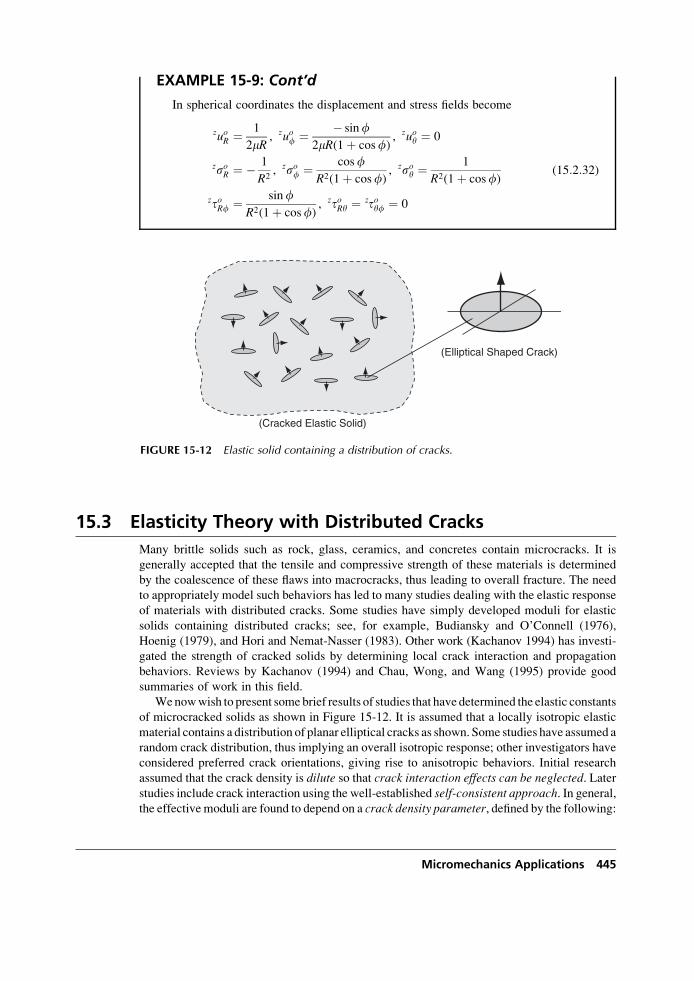
EXAMPLE 15-9: Cont’d
In spherical coordinates the displacement and stress fields become
zuoR ¼ 1
2mR, zuof ¼ � sinf
2mR(1þ cosf), zuoy ¼ 0
zsoR ¼ � 1
R2, zsof ¼ cosf
R2(1þ cosf), zsoy ¼
1
R2(1þ cosf)
ztoRf ¼ sinfR2(1þ cosf)
, ztoRy ¼ ztoyf ¼ 0
(15:2:32)
15.3 Elasticity Theory with Distributed Cracks
Many brittle solids such as rock, glass, ceramics, and concretes contain microcracks. It is
generally accepted that the tensile and compressive strength of these materials is determined
by the coalescence of these flaws into macrocracks, thus leading to overall fracture. The need
to appropriately model such behaviors has led to many studies dealing with the elastic response
of materials with distributed cracks. Some studies have simply developed moduli for elastic
solids containing distributed cracks; see, for example, Budiansky and O’Connell (1976),
Hoenig (1979), and Hori and Nemat-Nasser (1983). Other work (Kachanov 1994) has investi-
gated the strength of cracked solids by determining local crack interaction and propagation
behaviors. Reviews by Kachanov (1994) and Chau, Wong, and Wang (1995) provide good
summaries of work in this field.
Wenowwish to present somebrief results of studies that have determined the elastic constants
of microcracked solids as shown in Figure 15-12. It is assumed that a locally isotropic elastic
material contains a distribution of planar elliptical cracks as shown. Some studies have assumed a
random crack distribution, thus implying an overall isotropic response; other investigators have
considered preferred crack orientations, giving rise to anisotropic behaviors. Initial research
assumed that the crack density is dilute so that crack interaction effects can be neglected. Laterstudies include crack interaction using the well-established self-consistent approach. In general,the effective moduli are found to depend on a crack density parameter, defined by the following:
(Cracked Elastic Solid)
(Elliptical Shaped Crack)
FIGURE 15-12 Elastic solid containing a distribution of cracks.
Micromechanics Applications 445
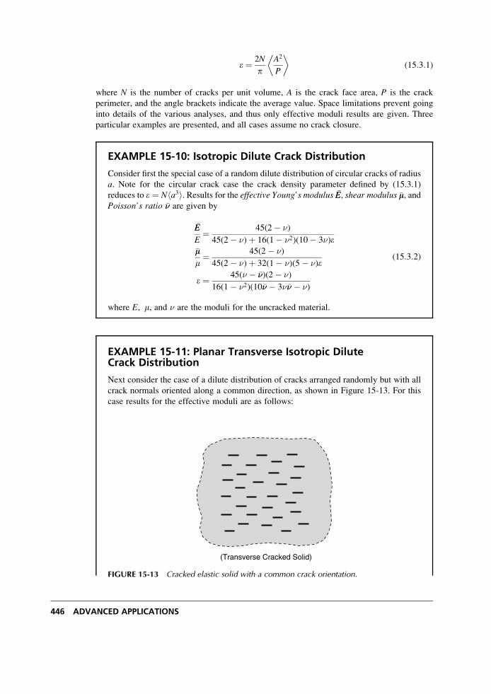
e ¼ 2N
pA2
P
� �(15:3:1)
where N is the number of cracks per unit volume, A is the crack face area, P is the crack
perimeter, and the angle brackets indicate the average value. Space limitations prevent going
into details of the various analyses, and thus only effective moduli results are given. Three
particular examples are presented, and all cases assume no crack closure.
EXAMPLE 15-10: Isotropic Dilute Crack Distribution
Consider first the special case of a random dilute distribution of circular cracks of radius
a. Note for the circular crack case the crack density parameter defined by (15.3.1)
reduces to e ¼ Nha3i. Results for the effective Young’s modulus �EE, shear modulus �mm, andPoisson’s ratio ��� are given by
�EE
E¼ 45(2� �)
45(2� �)þ 16(1� �2)(10� 3�)e�mmm¼ 45(2� �)
45(2� �)þ 32(1� �)(5� �)e
e ¼ 45(� � ���)(2� �)
16(1� �2)(10��� � 3���� � �)
(15:3:2)
where E, m, and � are the moduli for the uncracked material.
EXAMPLE 15-11: Planar Transverse Isotropic DiluteCrack Distribution
Next consider the case of a dilute distribution of cracks arranged randomly but with all
crack normals oriented along a common direction, as shown in Figure 15-13. For this
case results for the effective moduli are as follows:
(Transverse Cracked Solid)
FIGURE 15-13 Cracked elastic solid with a common crack orientation.
446 ADVANCED APPLICATIONS
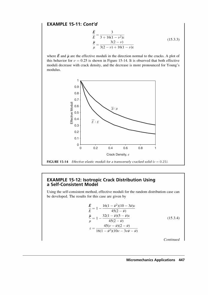
EXAMPLE 15-11: Cont’d
�EE
E¼ 3
3þ 16(1� �2)e�mmm¼ 3(2� �)
3(2� �)þ 16(1� �)e
(15:3:3)
where �EE and �mm are the effective moduli in the direction normal to the cracks. A plot of
this behavior for � ¼ 0:25 is shown in Figure 15-14. It is observed that both effective
moduli decrease with crack density, and the decrease is more pronounced for Young’s
modulus.
EXAMPLE 15-12: Isotropic Crack Distribution Usinga Self-Consistent Model
Using the self-consistent method, effective moduli for the random distribution case can
be developed. The results for this case are given by
�EE
E¼ 1� 16(1� ���2)(10� 3���)e
45(2� ���)�mmm¼ 1� 32(1� ���)(5� ���)e
45(2� ���)
e ¼ 45(� � ���)(2� ���)
16(1� ���2)(10� � 3���� � ���)
(15:3:4)
Continued
0
0.1
0.2
0.3
0.4
0.5
0.6
0.7
0.8
0.9
1
0 0.2 0.4 0.6 0.8 1
Crack Density, e
Effe
ctiv
e M
odul
i
EE /
mm /
FIGURE 15-14 Effective elastic moduli for a transversely cracked solid (� ¼ 0:25).
Micromechanics Applications 447
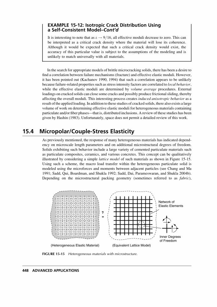
EXAMPLE 15-12: Isotropic Crack Distribution Usinga Self-Consistent Model–Cont’d
It is interesting to note that as e ! 9=16, all effective moduli decrease to zero. This can
be interpreted as a critical crack density where the material will lose its coherence.
Although it would be expected that such a critical crack density would exist, the
accuracy of this particular value is subject to the assumptions of the modeling and is
unlikely to match universally with all materials.
In the search for appropriate models of brittle microcracking solids, there has been a desire to
find a correlation between failure mechanisms (fracture) and effective elastic moduli. However,
it has been pointed out (Kachanov 1990, 1994) that such a correlation appears to be unlikely
because failure-related properties such as stress intensity factors are correlated to local behavior,while the effective elastic moduli are determined by volume average procedures. External
loadings on cracked solids can close some cracks and possibly produce frictional sliding, thereby
affecting the overall moduli. This interesting process creates induced anisotropic behavior as aresult of the applied loading. In addition to these studies of cracked solids, there also exists a large
volume of work on determining effective elastic moduli for heterogeneous materials containing
particulate and/or fiber phases—that is, distributed inclusions. A review of these studies has been
given by Hashin (1983). Unfortunately, space does not permit a detailed review of this work.
15.4 Micropolar/Couple-Stress Elasticity
As previously mentioned, the response of many heterogeneous materials has indicated depend-
ency on microscale length parameters and on additional microstructural degrees of freedom.
Solids exhibiting such behavior include a large variety of cemented particulate materials such
as particulate composites, ceramics, and various concretes. This concept can be qualitatively
illustrated by considering a simple lattice model of such materials as shown in Figure 15-15.
Using such a scheme, the macro load transfer within the heterogeneous particulate solid is
modeled using the microforces and moments between adjacent particles (see Chang and Ma
1991; Sadd, Qui, Boardman, and Shukla 1992; Sadd, Dai, Parameswaran, and Shukla 2004b).
Depending on the microstructural packing geometry (sometimes referred to as fabric),
Network ofElastic Elements
(Heterogeneous Elastic Material)
=?
Inner Degreesof Freedom
(Equivalent Lattice Model)
FIGURE 15-15 Heterogeneous materials with microstructure.
448 ADVANCED APPLICATIONS
this method establishes a lattice network that can be thought of as an interconnect series of
elastic bar or beam elements interconnected at particle centers. Thus, the network represents in
some way the material microstructure and brings into the model microstructural dimensions
such as the grid size. Furthermore, the elastic network establishes internal bending moments
and forces, which depend on internal degrees of freedom (e.g., rotations) at each connecting
point in the microstructure as shown. These internal rotations would be, in a sense, independ-
ent of the overall macro deformations.
This concept then suggests that an elastic continuum theory including an independent
rotation field with concentrated pointwise moments might be suitable for modeling heteroge-
neous materials. Such approaches have been formulated under the names Cosserat continuum;oriented media; asymmetric elasticity; micropolar, micromorphic, or couple-stress theories.The Cosserat continuum, developed in 1909, was historically one of the first models of this
category. However, over the next 50 years very little activity occurred in this field. Renewed
interest began during the 1960s, and numerous articles on theoretical refinements and particu-
lar analytical and computational applications were produced. The texts and articles by Eringen
(1968, 1999) and Kunin (1983) provide detailed background on much of this work, while
Nowacki (1986) presents a comprehensive account on dynamic and thermoelastic applications
of such theories.
Micropolar theory incorporates an additional internal degree of freedom called the micro-rotation and allows for the existence of body and surface couples. For this approach, the newkinematic strain-deformation relation is expressed as
eij ¼ uj, i � eijlfl (15:4:1)
where eij is the usual strain tensor, ui is the displacement vector, and fi is the microrotationvector. Note that this new kinematic variable fi is independent of the displacement ui, and thusis not in general the same as the usual macrorotation vector; that is,
!i ¼ 1
2eijkuk, j 6¼ fi (15:4:2)
Later in our discussion we relax this restriction and develop a more specialized theory that
normally allows simpler analytical problem solution.
The body and surface couples (moments) included in the new theory introduce additional
terms in the equilibrium equations. Skipping the derivation details, the linear and angular
equilibrium equations thus become
sji, j þ Fi ¼ 0
mji, j þ eijksjk þ Ci ¼ 0(15:4:3)
where sij is the usual stress tensor, Fi is the body force, mij is the surface moment tensor
normally referred to as the couple-stress tensor, and Ci is the body couple per unit volume.
Notice that as a consequence of including couple stresses and body couples, the stress tensorsij no longer is symmetric. For linear elastic isotropic materials, the constitutive relations for a
micropolar material are given by
sij ¼ lekkdij þ (mþ k)eij þ mejimij ¼ afk, kdij þ bfi, j þ gfj, i
(15:4:4)
Micromechanics Applications 449
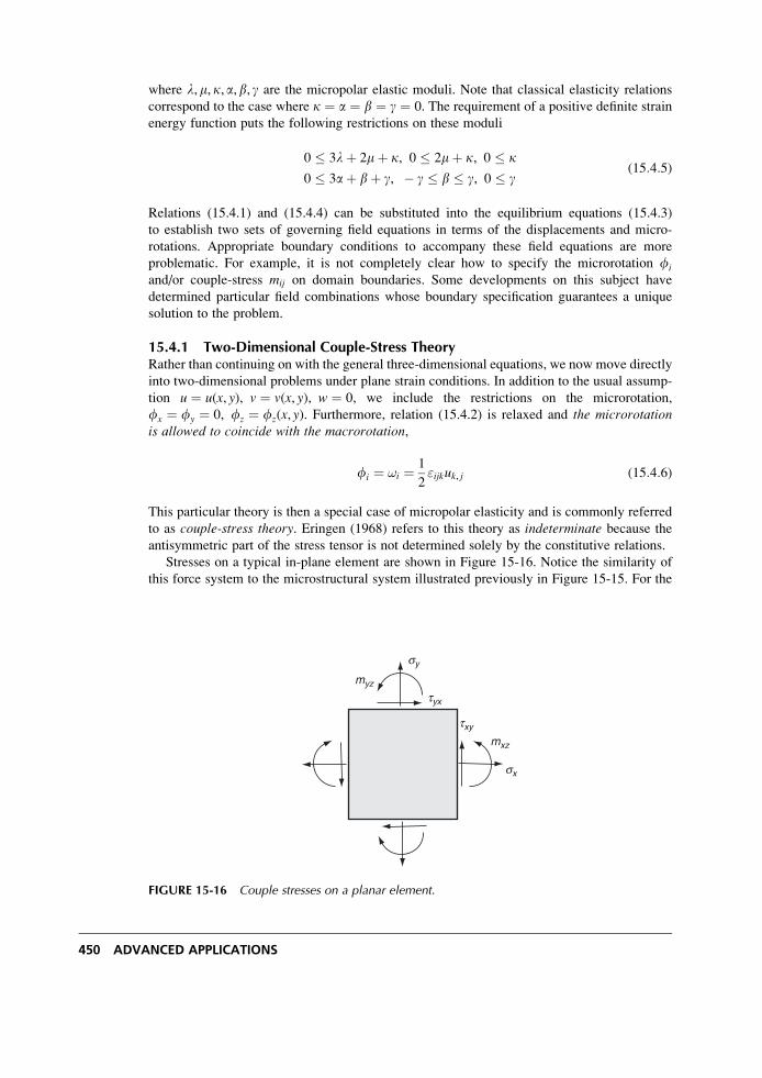
where l,m, k, a,b, g are the micropolar elastic moduli. Note that classical elasticity relations
correspond to the case where k ¼ a ¼ b ¼ g ¼ 0. The requirement of a positive definite strain
energy function puts the following restrictions on these moduli
0 � 3lþ 2mþ k, 0 � 2mþ k, 0 � k
0 � 3aþ bþ g, � g � b � g, 0 � g(15:4:5)
Relations (15.4.1) and (15.4.4) can be substituted into the equilibrium equations (15.4.3)
to establish two sets of governing field equations in terms of the displacements and micro-
rotations. Appropriate boundary conditions to accompany these field equations are more
problematic. For example, it is not completely clear how to specify the microrotation fi
and/or couple-stress mij on domain boundaries. Some developments on this subject have
determined particular field combinations whose boundary specification guarantees a unique
solution to the problem.
15.4.1 Two-Dimensional Couple-Stress TheoryRather than continuing on with the general three-dimensional equations, we now move directly
into two-dimensional problems under plane strain conditions. In addition to the usual assump-
tion u ¼ u(x, y), v ¼ v(x, y), w ¼ 0, we include the restrictions on the microrotation,
fx ¼ fy ¼ 0, fz ¼ fz(x, y). Furthermore, relation (15.4.2) is relaxed and the microrotationis allowed to coincide with the macrorotation,
fi ¼ !i ¼ 1
2"ijkuk, j (15:4:6)
This particular theory is then a special case of micropolar elasticity and is commonly referred
to as couple-stress theory. Eringen (1968) refers to this theory as indeterminate because the
antisymmetric part of the stress tensor is not determined solely by the constitutive relations.
Stresses on a typical in-plane element are shown in Figure 15-16. Notice the similarity of
this force system to the microstructural system illustrated previously in Figure 15-15. For the
sy
sx
txy
tyx
mxz
myz
FIGURE 15-16 Couple stresses on a planar element.
450 ADVANCED APPLICATIONS
two-dimensional case with no body forces or body couples, the equilibrium equations (15.4.3)
reduce to
@sx@x
þ @tyx@y
¼ 0
@txy@x
þ @sy@y
¼ 0
@mxz
@xþ @myz
@yþ txy � tyx ¼ 0
(15:4:7)
The in-plane strains can be expressed as
ex ¼ @u
@x, ey ¼ @v
@y
exy ¼ @v
@x� fz, eyx ¼
@u
@yþ fz
(15:4:8)
while using (15.4.6) gives
fz ¼1
2
@v
@x� @u
@y
� �(15:4:9)
Notice that substituting (15.4.9) into (15:4:8)2 gives the result exy ¼ eyx.The constitutive equations (15.4.4) yield the following forms for the stress components:
sx ¼ l(ex þ ey)þ (2mþ k)exsy ¼ l(ex þ ey)þ (2mþ k)eytxy ¼ (2mþ k)exy ¼ tyx
mxz ¼ g@fz
@x, myz ¼ g
@fz
@y
(15:4:10)
In regard to the last pair of equations of this set, some authors (Mindlin 1963; Boresi
and Chong 2000) define the gradients of the rotation fz as the curvatures. Thus, they establish
a linear constitutive law between the couple stresses and curvatures. This approach is com-
pletely equivalent to the current method. It is to be noted from (15.4.10) that under the
assumptions of couple-stress theory we find the unpleasant situation that the antisymmetric
part of the stress tensor disappears from the constitutive relations. In order to remedy this,
we can solve for the antisymmetric stress term from the moment equilibrium equation
(15:4:7)3 to get
t[xy] ¼ 1
2(txy � tyx) ¼ � 1
2
@mxz
@xþ @myz
@y
� �
¼ � g2r2fz
(15:4:11)
By cross-differentiation we can eliminate the displacements from (15.4.8) and (15.4.9) and
develop the particular compatibility equations for the following case
Micromechanics Applications 451
@2ex@y2
þ @2ey@x2
¼ 2@2exy@x@y
@2fz
@x@y¼ @2fz
@y@x
@fz
@x¼ @exy
@x� @ex
@y
@fz
@y¼ @ey
@x� @exy
@y
(15:4:12)
Using the constitutive forms (15.4.10), these relationsmay be expressed in terms of the stresses as
@2sx@y2
þ @2sy@x2
� �r2(sx þ sy) ¼ @2
@x@y(txy þ tyx)
@mxz
@y¼ @myz
@x
mxz ¼ l2@
@x(txy þ tyx)� 2l2
@
@y[sx � �(sx þ sy)]
myz ¼ 2l2@
@x[sy � �(sx þ sy)]� l2
@
@y(txy þ tyx)
(15:4:13)
where � ¼ l=(2lþ 2mþ k) and l ¼ ffiffiffiffiffiffiffiffiffiffiffiffiffiffiffiffiffiffiffiffiffiffiffiffig=(4mþ 2k)
pis a material constant with units of length.
Notice that this result then introduces a length scale into the problem. If l ¼ 0, the couple-
stress effects are eliminated and the problem reduces to classical elasticity. It should also be
pointed out that only three of the four equations in set (15.4.13) are independent because the
second relation can be established from the other equations.
Proceeding along similar lines as classical elasticity, we introduce a stress function ap-
proach (Carlson 1966) to solve (15.4.13). A self-equilibrated form satisfying (15.4.7) identi-
cally can be written as
sx ¼ @2F@y2
� @2C@x@y
, sy ¼ @2F@x2
þ @2C@x@y
txy ¼ � @2F@x@y
� @2C@y2
, tyx ¼ � @2F@x@y
þ @2C@x2
mxz ¼ @C@x
, myz ¼ @C@y
(15:4:14)
where F ¼ F(x, y) and C ¼ C(x, y) are the stress functions for this case. If C is taken to be
zero, the representation reduces to the usual Airy form with no couple stresses. Using form
(15.4.14) in the compatibility equations (15.4.13) produces
r4F ¼ 0
@
@x(C� l2r2C) ¼ �2(1� �)l2
@
@y(r2F)
@
@y(C� l2r2C) ¼ 2(1� �)l2
@
@x(r2F)
(15:4:15)
452 ADVANCED APPLICATIONS
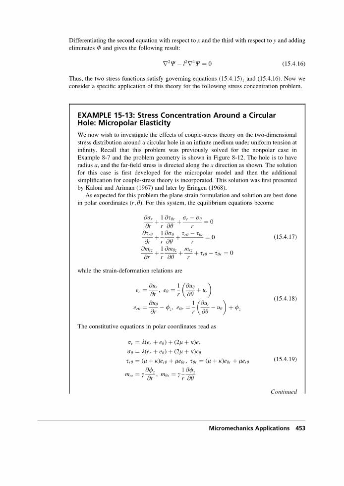
Differentiating the second equation with respect to x and the third with respect to y and adding
eliminates F and gives the following result:
r2C� l2r4C ¼ 0 (15:4:16)
Thus, the two stress functions satisfy governing equations (15:4:15)1 and (15.4.16). Now we
consider a specific application of this theory for the following stress concentration problem.
EXAMPLE 15-13: Stress Concentration Around a CircularHole: Micropolar Elasticity
We now wish to investigate the effects of couple-stress theory on the two-dimensional
stress distribution around a circular hole in an infinite medium under uniform tension at
infinity. Recall that this problem was previously solved for the nonpolar case in
Example 8-7 and the problem geometry is shown in Figure 8-12. The hole is to have
radius a, and the far-field stress is directed along the x direction as shown. The solution
for this case is first developed for the micropolar model and then the additional
simplification for couple-stress theory is incorporated. This solution was first presented
by Kaloni and Ariman (1967) and later by Eringen (1968).
As expected for this problem the plane strain formulation and solution are best done
in polar coordinates (r, y). For this system, the equilibrium equations become
@sr@r
þ 1
r
@tyr@y
þ sr � syr
¼ 0
@try@r
þ 1
r
@sy@y
þ try � tyrr
¼ 0
@mrz
@rþ 1
r
@myz
@yþ mrz
rþ try � tyr ¼ 0
(15:4:17)
while the strain-deformation relations are
er ¼ @ur@r
, ey ¼ 1
r
@uy@y
þ ur
� �
ery ¼ @uy@r
� fz, eyr ¼1
r
@ur@y
� uy
� �þ fz
(15:4:18)
The constitutive equations in polar coordinates read as
sr ¼ l(er þ ey)þ (2mþ k)ersy ¼ l(er þ ey)þ (2mþ k)eytry ¼ (mþ k)ery þ meyr, tyr ¼ (mþ k)eyr þ mery
mrz ¼ g@fz
@r, myz ¼ g
1
r
@fz
@y
(15:4:19)
Continued
Micromechanics Applications 453
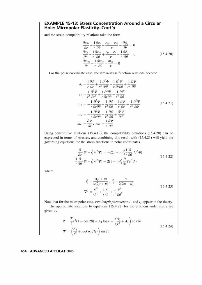
EXAMPLE 15-13: Stress Concentration Around a CircularHole: Micropolar Elasticity–Cont’d
and the strain-compatibility relations take the form
@eyr@r
� 1
r
@er@y
þ eyr � eryr
� @fz
@r¼ 0
@ey@r
� 1
r
@ery@y
þ ey � err
� 1
r
@fz
@y¼ 0
@myz
@r� 1
r
@mrz
@yþ myz
r¼ 0
(15:4:20)
For the polar coordinate case, the stress-stress function relations become
sr ¼ 1
r
@F@r
þ 1
r2@2F
@y2� 1
r
@2C@r@y
þ 1
r2@C@y
sy ¼ 1
r2@2F@r2
þ 1
r
@2C@r@y
� 1
r2@C@y
try ¼ � 1
r
@2F@r@y
þ 1
r2@F@y
� 1
r
@C@r
� 1
r2@2C
@y2
tyr ¼ � 1
r
@2F@r@y
þ 1
r2@F@y
þ @2C@r2
mrz ¼ @C@r
, myz ¼ 1
r
@C@y
(15:4:21)
Using constitutive relations (15.4.19), the compatibility equations (15.4.20) can be
expressed in terms of stresses, and combining this result with (15.4.21) will yield the
governing equations for the stress functions in polar coordinates
@
@r(C� l21r2C) ¼ �2(1� �)l22
1
r
@
@y(r2F)
1
r
@
@y(C� l21r2C) ¼ 2(1� �)l22
@
@r(r2F)
(15:4:22)
where
l21 ¼g(mþ k)k(2mþ k)
, l22 ¼g
2(2mþ k)
r2 ¼ @2
@r2þ 1
r
@
@rþ 1
r2@2
@y2
(15:4:23)
Note that for the micropolar case, two length parameters l1 and l2 appear in the theory.
The appropriate solutions to equations (15.4.22) for the problem under study are
given by
F ¼ T
4r2(1� cos 2y)þ A1 log r þ A2
r2þ A3
� �cos 2y
C ¼ A4
r2þ A5K2(r=l1)
� �sin 2y
(15:4:24)
454 ADVANCED APPLICATIONS
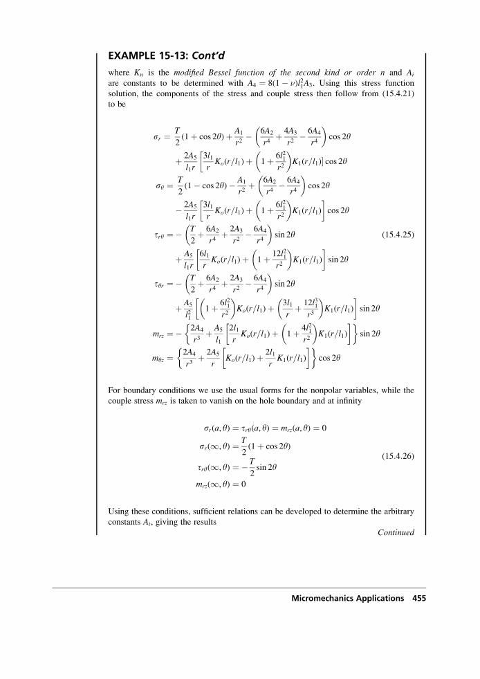
EXAMPLE 15-13: Cont’d
where Kn is the modified Bessel function of the second kind or order n and Ai
are constants to be determined with A4 ¼ 8(1� �)l21A3. Using this stress function
solution, the components of the stress and couple stress then follow from (15.4.21)
to be
sr ¼ T
2(1þ cos 2y)þ A1
r2� 6A2
r4þ 4A3
r2� 6A4
r4
� �cos 2y
þ 2A5
l1r
3l1rKo(r=l1)þ 1þ 6l21
r2
�� �K1(r=l1)� cos 2y
sy ¼ T
2(1� cos 2y)� A1
r2þ 6A2
r4� 6A4
r4
� �cos 2y
� 2A5
l1r
3l1rKo(r=l1)þ 1þ 6l21
r2
� �K1(r=l1)
� �cos 2y
try ¼� T
2þ 6A2
r4þ 2A3
r2� 6A4
r4
� �sin 2y (15:4:25)
þ A5
l1r
6l1rKo(r=l1)þ 1þ 12l21
r2
� �K1(r=l1)
� �sin 2y
tyr ¼� T
2þ 6A2
r4þ 2A3
r2� 6A4
r4
� �sin 2y
þ A5
l211þ 6l21
r2
� �Ko(r=l1)þ 3l1
rþ 12l31
r3
� �K1(r=l1)
� �sin 2y
mrz ¼� 2A4
r3þ A5
l1
2l1rKo(r=l1)þ 1þ 4l21
r2
� �K1(r=l1)
� � sin 2y
myz ¼ 2A4
r3þ 2A5
rKo(r=l1)þ 2l1
rK1(r=l1)
� � cos 2y
For boundary conditions we use the usual forms for the nonpolar variables, while the
couple stress mrz is taken to vanish on the hole boundary and at infinity
sr(a, y) ¼ try(a, y) ¼ mrz(a, y) ¼ 0
sr(1, y) ¼ T
2(1þ cos 2y)
try(1, y) ¼ �T
2sin 2y
mrz(1, y) ¼ 0
(15:4:26)
Using these conditions, sufficient relations can be developed to determine the arbitrary
constants Ai, giving the results
Continued
Micromechanics Applications 455
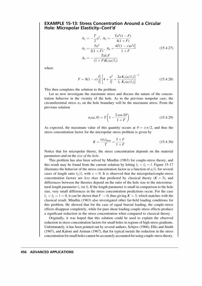
EXAMPLE 15-13: Stress Concentration Around a CircularHole: Micropolar Elasticity–Cont’d
A1 ¼ �T
2a2, A2 ¼ � Ta4(1� F)
4(1þ F)
A3 ¼ Ta2
2(1þ F), A4 ¼ 4T(1� �)a2l22
1þ F
A5 ¼ � Tal1F
(1þ F)K1(a=l1)
(15:4:27)
where
F ¼ 8(1� �)l22l21
4þ a2
l21þ 2a
l1
Ko(a=l1)
K1(a=l1)
� ��1
(15:4:28)
This then completes the solution to the problem.
Let us now investigate the maximum stress and discuss the nature of the concen-
tration behavior in the vicinity of the hole. As in the previous nonpolar case, the
circumferential stress sy on the hole boundary will be the maximum stress. From the
previous solution
sy(a, y) ¼ T 1� 2 cos 2y1þ F
� �(15:4:29)
As expected, the maximum value of this quantity occurs at y ¼ �p=2, and thus the
stress concentration factor for the micropolar stress problem is given by
K ¼ (sy)max
T¼ 3þ F
1þ F(15:4:30)
Notice that for micropolar theory, the stress concentration depends on the material
parameters and on the size of the hole.This problem has also been solved by Mindlin (1963) for couple-stress theory, and
this result may be found from the current solution by letting l1 ¼ l2 ¼ l. Figure 15-17
illustrates the behavior of the stress concentration factor as a function of a=l1 for severalcases of length ratio l2=l1 with � ¼ 0. It is observed that the micropolar/couple-stress
concentration factors are less than that predicted by classical theory (K ¼ 3), and
differences between the theories depend on the ratio of the hole size to the microstruc-
tural length parameter l1 (or l). If the length parameter is small in comparison to the hole
size, very small differences in the stress concentration predictions occur. For the case
l1 ¼ l2 ¼ l ¼ 0, it can be shown that F ! 0, thus giving K ¼ 3, which matches with the
classical result. Mindlin (1963) also investigated other far-field loading conditions for
this problem. He showed that for the case of equal biaxial loading, the couple-stress
effects disappear completely, while for pure shear loading couple-stress effects produce
a significant reduction in the stress concentration when compared to classical theory.
Originally, it was hoped that this solution could be used to explain the observed
reduction in stress concentration factors for small holes in regions of high stress gradients.
Unfortunately, it has been pointed out by several authors, Schijve (1966), Ellis and Smith
(1967), and Kaloni and Ariman (1967), that for typical metals the reduction in the stress
concentration for small holes cannot be accurately accounted for using couple-stress theory.
456 ADVANCED APPLICATIONS
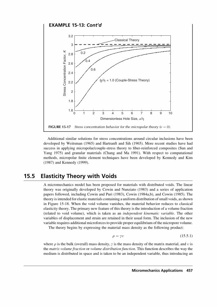
EXAMPLE 15-13: Cont’d
Additional similar solutions for stress concentrations around circular inclusions have been
developed by Weitsman (1965) and Hartranft and Sih (1965). More recent studies have had
success in applying micropolar/couple-stress theory to fiber-reinforced composites (Sun and
Yang 1975) and granular materials (Chang and Ma 1991). With respect to computational
methods, micropolar finite element techniques have been developed by Kennedy and Kim
(1987) and Kennedy (1999).
15.5 Elasticity Theory with Voids
A micromechanics model has been proposed for materials with distributed voids. The linear
theory was originally developed by Cowin and Nunziato (1983) and a series of application
papers followed, including Cowin and Puri (1983), Cowin (1984a,b), and Cowin (1985). The
theory is intended for elastic materials containing a uniform distribution of small voids, as shown
in Figure 15-18. When the void volume vanishes, the material behavior reduces to classical
elasticity theory. The primary new feature of this theory is the introduction of a volume fraction
(related to void volume), which is taken as an independent kinematic variable. The other
variables of displacement and strain are retained in their usual form. The inclusion of the new
variable requires additional microforces to provide proper equilibrium of the micropore volume.
The theory begins by expressing the material mass density as the following product:
r ¼ g� (15:5:1)
where r is the bulk (overall) mass density, g is the mass density of the matrix material, and � is
the matrix volume fraction or volume distribution function. This function describes the way themedium is distributed in space and is taken to be an independent variable, thus introducing an
Classical Theory
l2/l1 = 1.0 (Couple-Stress Theory)
0.6
0.4
0.2
Dimensionless Hole Size, a/l1
Str
ess
Con
cent
ratio
n F
acto
r, K
3.2
3
2.8
2.6
2.4
2.2
2
1.8
1.60 1 2 3 4 5 6 7 8 9 10
FIGURE 15-17 Stress concentration behavior for the micropolar theory (� ¼ 0).
Micromechanics Applications 457
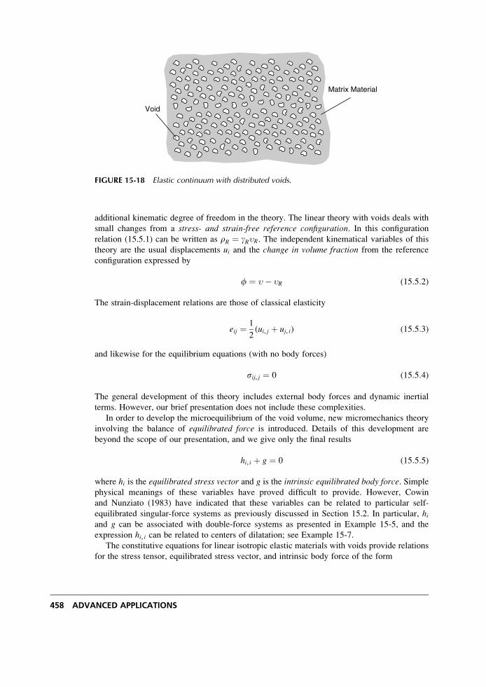
additional kinematic degree of freedom in the theory. The linear theory with voids deals with
small changes from a stress- and strain-free reference configuration. In this configuration
relation (15.5.1) can be written as rR ¼ gR�R. The independent kinematical variables of this
theory are the usual displacements ui and the change in volume fraction from the reference
configuration expressed by
f ¼ �� �R (15:5:2)
The strain-displacement relations are those of classical elasticity
eij ¼ 1
2(ui, j þ uj, i) (15:5:3)
and likewise for the equilibrium equations (with no body forces)
sij, j ¼ 0 (15:5:4)
The general development of this theory includes external body forces and dynamic inertial
terms. However, our brief presentation does not include these complexities.
In order to develop the microequilibrium of the void volume, new micromechanics theory
involving the balance of equilibrated force is introduced. Details of this development are
beyond the scope of our presentation, and we give only the final results
hi, i þ g ¼ 0 (15:5:5)
where hi is the equilibrated stress vector and g is the intrinsic equilibrated body force. Simple
physical meanings of these variables have proved difficult to provide. However, Cowin
and Nunziato (1983) have indicated that these variables can be related to particular self-
equilibrated singular-force systems as previously discussed in Section 15.2. In particular, hiand g can be associated with double-force systems as presented in Example 15-5, and the
expression hi, i can be related to centers of dilatation; see Example 15-7.
The constitutive equations for linear isotropic elastic materials with voids provide relations
for the stress tensor, equilibrated stress vector, and intrinsic body force of the form
Void
Matrix Material
FIGURE 15-18 Elastic continuum with distributed voids.
458 ADVANCED APPLICATIONS
sij ¼ lekkdij þ 2meij þ bfdijhi ¼ af, i
g ¼ �! _ff� xf� bekk
(15:5:6)
where the material constants l,m, a, b, x,! all depend on the reference fraction �R and satisfy
the inequalities
m 0, a 0, x 0, ! 0, 3lþ 2m 0, M ¼ 3lþ 2m
b2 3 (15:5:7)
Note that even though we have dropped dynamic inertial terms, constitutive relation (15:5:6)3includes a time-dependent response in the volume fraction. This fact indicates that the theory
will predict a viscoelastic type of behavior (Cowin 1985) even for problems with time-
independent boundary conditions and homogeneous deformations.
For this theory, the boundary conditions on stress and displacement are the same as those of
classical elasticity. The boundary conditions on the self-equilibrated stress vector are taken to
have a vanishing normal component; that is, hini ¼ 0, where ni is the surface unit normal
vector. Using this with the constitutive statement (15:5:6)2 develops the boundary specificationon the volume fraction
f, ini ¼ 0 (15:5:8)
This completes our brief general presentation of the theory, and we will now discuss the
solution to the stress concentration problem around a circular hole discussed previously in
Example 15-13.
EXAMPLE 15-14: Stress Concentration Around a CircularHole: Elasticity with Voids
Consider again the stress concentration problem of a stress-free circular hole of radius ain an infinite plane under uniform tension, as shown in Figure 8-12. We now outline the
solution given by Cowin (1984b) and compare the results with the micropolar, couple-
stress, and classical solutions. The problem is formulated under the usual plane stress
conditions,
sx ¼ sx(x, y), sy ¼ sy(x, y), txy ¼ txy(x, y), sz ¼ txz ¼ tyz ¼ 0
For this two-dimensional case the constitutive relations reduce to
sij ¼ 2mlþ 2m
(lekk þ bf)dij þ 2meij
g ¼ �! _ff� x� b2
lþ 2m
� �f� 2mb
lþ 2mekk
(15:5:9)
where all indices are taken over the limited range 1,2. Using a stress formulation, the
single nonzero compatibility relation becomes
Continued
Micromechanics Applications 459
EXAMPLE 15-14: Stress Concentration Around a CircularHole: Elasticity with Voids–Cont’d
skk,mm � mblþ m
f,mm ¼ 0 (15:5:10)
Introducing the usual Airy stress function, denoted here by c, allows this relation to be
written as
r4c� mblþ m
r2f ¼ 0 (15:5:11)
For this case, relation (15.5.5) for balance of equilibrated forces reduces to
ar2f� ah2
f� ! _ff ¼ b3lþ 2m
r2c� mblþ m
f� �
(15:5:12)
The parameter h is defined by
ah2
¼ x� b2
lþ m(15:5:13)
and has units of length, and thus can then be taken as a microstructural length measurefor this particular theory.
Relations (15.5.11) and (15.5.12) now form the governing equations for the plane
stress problem. The presence of the time-dependent derivative term in (15.5.12) requires
some additional analysis. Using Laplace transform theory, Cowin (1984b) shows that
under steady boundary conditions, the solutions f and c can be determined from the
limiting case where t ! 1, which is related to taking ! ¼ 0. Thus, taking the Laplace
transform of (15.5.11) and (15.5.12) gives the following
r4�cc� mblþ m
r2�ff ¼ 0
ar2�ff� a�hh2
�ff ¼ b3lþ 2m
r2�cc� mblþ m
�ff� � (15:5:14)
where �ff ¼ �ff(s), �cc ¼ �cc(s) are the standard Laplace transforms of f,c, and s is the
Laplace transform variable. The basic definition of this transform is given by
�ff (s) ¼ð10
f (t)e�stdt
and the parameter �hh is defined bya�hh2
¼ ah2
þ !s. Boundary conditions on the problem
follow from our previous discussions to be
sr ¼ try ¼ @�ff@r
¼ 0 on r ¼ a
For the circular hole problem, the solution to system (15.5.14) is developed in polar
coordinates. Guided by the results from classical elasticity, we look for solutions of the
form f (r)þ g(r) cos 2y, where f and g are arbitrary functions of the radial coordinate.
Employing this scheme, the properly bounded solution satisfying the boundary condi-
tion@�ff@r
¼ 0 at r ¼ a is found to be
460 ADVANCED APPLICATIONS
EXAMPLE 15-14: Cont’d
�ff ¼ �x�ppMb!sþ bx(M � 3)
þ A3(lþ m)m�hh2b
[ �FF(r)� 1] cos 2y
�cc ¼ mblþ m
�hh2�ffþ �ppr2
4þ A1 log r þ A2
r2þ A3 � �ppr2
4
� �cos 2y
� � (15:5:15)
where �FF is given by
�FF(r) ¼ 1þ 4mx�hh2
(lþ m)M!sþ 4mxN1
r2þ 2�hhK2(r=�hh)
a3K02(a=
�hh)
� �(15:5:16)
and �pp is the Laplace transform of the uniaxial stress at infinity, K2 is the modified Bessel
function of the second kind of order 2,
N ¼ lþ m4m
(M � 3) 0
and the constants A1, A2, A3 are determined from the stress-free boundary conditions as
A1 ¼ � 1
2�ppa2, A2 ¼ � 1
4�ppa4, A3 ¼ 1
2�ppa2 �FF(a)
Note in relation (15.5.16) the bar on F indicates the dependency on the Laplace
transform parameter s, and the bar is to be removed for the case where s ! 0 and�hh(s) is replaced by h.
This completes the solution for the Laplace-transformed volume fraction and Airy
stress function. The transformed stress components can now be obtained from the Airy
function using the usual relations
�ssr ¼ 1
r
@�cc@r
þ 1
r2@2�cc
@y2, �ssy ¼ @2�cc
@r2, �ttry ¼ 1
r2@�cc@y
� 1
r
@2�cc@r@y
(15:5:17)
Wenowconsiderthecasewhere thefar-field tensionT isaconstant intime,andthus �pp ¼ T=s.Rather than formally inverting (inverse Laplace transformation) the resulting stress com-
ponentsgenerated fromrelations (15.5.17),Cowindevelops results for thecasesof t ¼ 0and
t ! 1. It turns out that for the initial condition at t ¼ 0, the stressesmatch those found from
classical elasticity (see Example 8-7). However, for the final-value case (t ! 1), which
implies (s ! 0), the stresses are different than predictions from classical theory.
Focusing our attention on only the hoop stress, the elasticity with voids solution for
the final-value case is determined as
sy ¼ T
21þ a2
r2
� �þ cos 2y a2
F00(r)F(a)
� 1þ 3a4
r4
� �� � (15:5:18)
The maximum value of this stress is again found at r ¼ a and y ¼ �p=2 and is given by
(sy)max ¼ sy(a,�p=2) ¼ T 3� a2
2
F00(a)F(a)
� �
¼ T 3þ 2N þ [1þ (4þ L2)N]K1(L)
LKo(L)
� ��1" # (15:5:19)
Continued
Micromechanics Applications 461
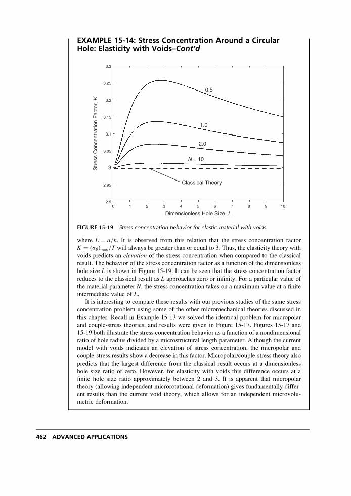
EXAMPLE 15-14: Stress Concentration Around a CircularHole: Elasticity with Voids–Cont’d
Classical Theory
N = 10
0.5
1.0
2.0
Dimensionless Hole Size, L
Str
ess
Con
cent
ratio
n F
acto
r, K
0
3.3
3.25
3.2
3.15
3.1
3.05
3
2.95
2.91 2 3 4 5 6 7 8 9 10
FIGURE 15-19 Stress concentration behavior for elastic material with voids.
where L ¼ a=h. It is observed from this relation that the stress concentration factor
K ¼ (sy)max=T will always be greater than or equal to 3. Thus, the elasticity theory with
voids predicts an elevation of the stress concentration when compared to the classical
result. The behavior of the stress concentration factor as a function of the dimensionless
hole size L is shown in Figure 15-19. It can be seen that the stress concentration factor
reduces to the classical result as L approaches zero or infinity. For a particular value of
the material parameter N, the stress concentration takes on a maximum value at a finite
intermediate value of L.It is interesting to compare these results with our previous studies of the same stress
concentration problem using some of the other micromechanical theories discussed in
this chapter. Recall in Example 15-13 we solved the identical problem for micropolar
and couple-stress theories, and results were given in Figure 15-17. Figures 15-17 and
15-19 both illustrate the stress concentration behavior as a function of a nondimensional
ratio of hole radius divided by a microstructural length parameter. Although the current
model with voids indicates an elevation of stress concentration, the micropolar and
couple-stress results show a decrease in this factor. Micropolar/couple-stress theory also
predicts that the largest difference from the classical result occurs at a dimensionless
hole size ratio of zero. However, for elasticity with voids this difference occurs at a
finite hole size ratio approximately between 2 and 3. It is apparent that micropolar
theory (allowing independent microrotational deformation) gives fundamentally differ-
ent results than the current void theory, which allows for an independent microvolu-
metric deformation.
462 ADVANCED APPLICATIONS
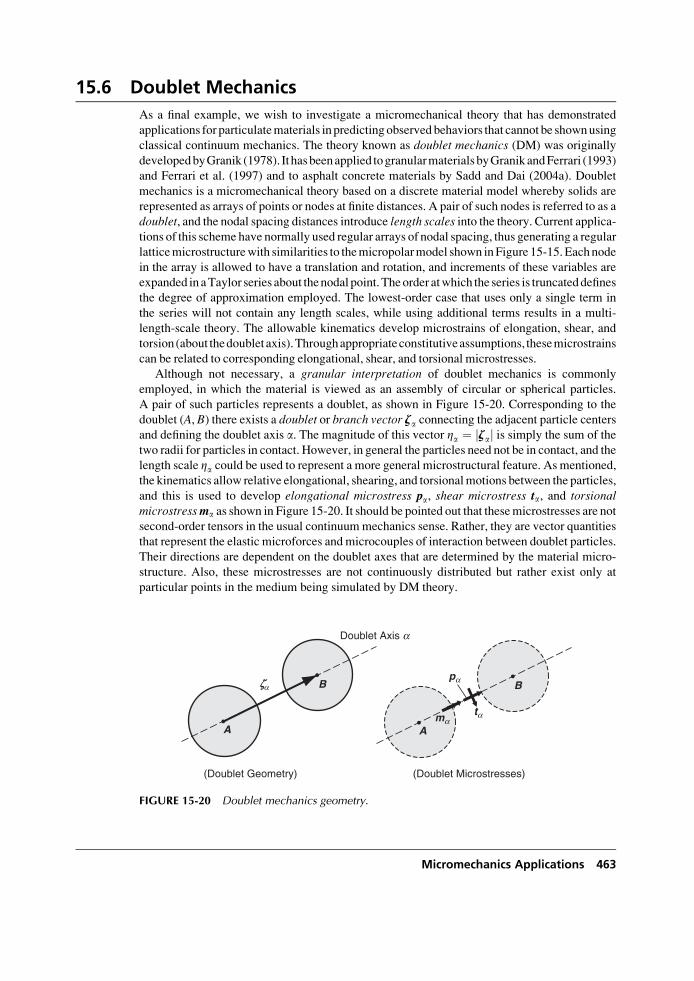
15.6 Doublet Mechanics
As a final example, we wish to investigate a micromechanical theory that has demonstrated
applications for particulatematerials inpredictingobservedbehaviors that cannot be shownusing
classical continuum mechanics. The theory known as doublet mechanics (DM) was originally
developedbyGranik (1978). It hasbeenapplied togranularmaterialsbyGranikandFerrari (1993)
and Ferrari et al. (1997) and to asphalt concrete materials by Sadd and Dai (2004a). Doublet
mechanics is a micromechanical theory based on a discrete material model whereby solids are
represented as arrays of points or nodes at finite distances. A pair of such nodes is referred to as a
doublet, and the nodal spacing distances introduce length scales into the theory. Current applica-tions of this scheme have normally used regular arrays of nodal spacing, thus generating a regular
latticemicrostructurewith similarities to themicropolarmodel shown inFigure 15-15. Eachnode
in the array is allowed to have a translation and rotation, and increments of these variables are
expanded in aTaylor series about thenodal point.Theorder atwhich the series is truncateddefines
the degree of approximation employed. The lowest-order case that uses only a single term in
the series will not contain any length scales, while using additional terms results in a multi-
length-scale theory. The allowable kinematics develop microstrains of elongation, shear, and
torsion (about thedoubletaxis).Throughappropriateconstitutiveassumptions, thesemicrostrains
can be related to corresponding elongational, shear, and torsional microstresses.
Although not necessary, a granular interpretation of doublet mechanics is commonly
employed, in which the material is viewed as an assembly of circular or spherical particles.
A pair of such particles represents a doublet, as shown in Figure 15-20. Corresponding to the
doublet (A, B) there exists a doublet or branch vector za connecting the adjacent particle centersand defining the doublet axis a. The magnitude of this vector Za ¼ jzaj is simply the sum of the
two radii for particles in contact. However, in general the particles need not be in contact, and the
length scale Za could be used to represent a more general microstructural feature. As mentioned,
the kinematics allow relative elongational, shearing, and torsionalmotions between the particles,
and this is used to develop elongational microstress pa, shear microstress ta, and torsionalmicrostressma as shown in Figure 15-20. It should be pointed out that thesemicrostresses are not
second-order tensors in the usual continuummechanics sense. Rather, they are vector quantities
that represent the elastic microforces and microcouples of interaction between doublet particles.
Their directions are dependent on the doublet axes that are determined by the material micro-
structure. Also, these microstresses are not continuously distributed but rather exist only at
particular points in the medium being simulated by DM theory.
A
B
Doublet Axis a
A
B pa
ta ma
(Doublet Geometry) (Doublet Microstresses)
zα
FIGURE 15-20 Doublet mechanics geometry.
Micromechanics Applications 463
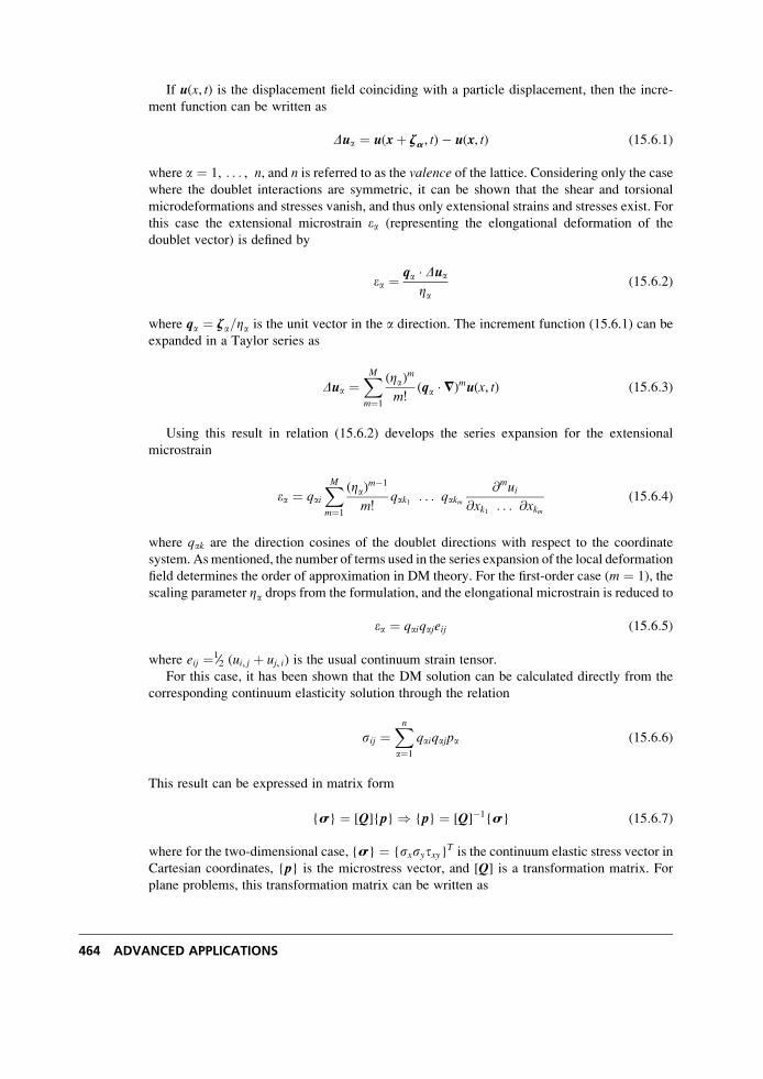
If u(x, t) is the displacement field coinciding with a particle displacement, then the incre-
ment function can be written as
Dua ¼ u(xþ za, t)� u(x, t) (15:6:1)
where a ¼ 1, . . . , n, and n is referred to as the valence of the lattice. Considering only the casewhere the doublet interactions are symmetric, it can be shown that the shear and torsional
microdeformations and stresses vanish, and thus only extensional strains and stresses exist. For
this case the extensional microstrain ea (representing the elongational deformation of the
doublet vector) is defined by
ea ¼ qa � DuaZa
(15:6:2)
where qa ¼ za=Za is the unit vector in the a direction. The increment function (15.6.1) can be
expanded in a Taylor series as
Dua ¼XMm¼1
(Za)m
m!(qa � =)mu(x, t) (15:6:3)
Using this result in relation (15.6.2) develops the series expansion for the extensional
microstrain
ea ¼ qaiXMm¼1
(Za)m�1
m!qak1 . . . qakm
@mui@xk1 . . . @xkm
(15:6:4)
where qak are the direction cosines of the doublet directions with respect to the coordinate
system. As mentioned, the number of terms used in the series expansion of the local deformation
field determines the order of approximation in DM theory. For the first-order case (m ¼ 1), the
scaling parameter Za drops from the formulation, and the elongational microstrain is reduced to
ea ¼ qaiqajeij (15:6:5)
where eij ¼1⁄2 (ui, j þ uj, i) is the usual continuum strain tensor.
For this case, it has been shown that the DM solution can be calculated directly from the
corresponding continuum elasticity solution through the relation
sij ¼Xna¼1
qaiqajpa (15:6:6)
This result can be expressed in matrix form
{s} ¼ [Q]{p} ) {p} ¼ [Q]�1{s} (15:6:7)
where for the two-dimensional case, {s} ¼ {sxsytxy}T is the continuum elastic stress vector in
Cartesian coordinates, {p} is the microstress vector, and [Q] is a transformation matrix. For
plane problems, this transformation matrix can be written as
464 ADVANCED APPLICATIONS
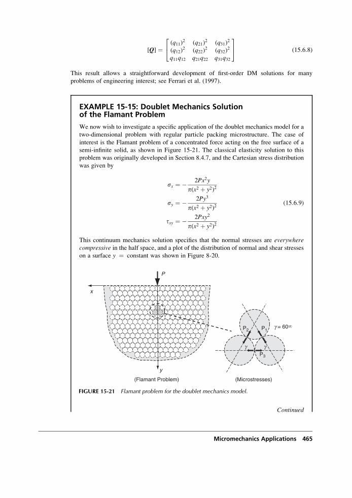
[Q] ¼(q11)
2 (q21)2 (q31)
2
(q12)2 (q22)
2 (q32)2
q11q12 q21q22 q31q32
24
35 (15:6:8)
This result allows a straightforward development of first-order DM solutions for many
problems of engineering interest; see Ferrari et al. (1997).
EXAMPLE 15-15: Doublet Mechanics Solutionof the Flamant Problem
We now wish to investigate a specific application of the doublet mechanics model for a
two-dimensional problem with regular particle packing microstructure. The case of
interest is the Flamant problem of a concentrated force acting on the free surface of a
semi-infinite solid, as shown in Figure 15-21. The classical elasticity solution to this
problem was originally developed in Section 8.4.7, and the Cartesian stress distribution
was given by
sx ¼ � 2Px2y
p(x2 þ y2)2
sy ¼ � 2Py3
p(x2 þ y2)2
txy ¼ � 2Pxy2
p(x2 þ y2)2
(15:6:9)
This continuum mechanics solution specifies that the normal stresses are everywherecompressive in the half space, and a plot of the distribution of normal and shear stresses
on a surface y ¼ constant was shown in Figure 8-20.
Continued
g = 60∞ P1 P2
P3
(Microstresses)
y
x
(Flamant Problem)
P
g g
FIGURE 15-21 Flamant problem for the doublet mechanics model.
Micromechanics Applications 465
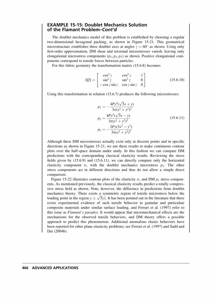
EXAMPLE 15-15: Doublet Mechanics Solutionof the Flamant Problem–Cont’d
The doublet mechanics model of this problem is established by choosing a regular
two-dimensional hexagonal packing, as shown in Figure 15-21. This geometrical
microstructure establishes three doublet axes at angles g ¼ 60 as shown. Using only
first-order approximation, DM shear and torsional microstresses vanish, leaving only
elongational microstress components (p1, p2, p3) as shown. Positive elongational com-
ponents correspond to tensile forces between particles.
For this fabric geometry the transformation matrix (15.6.8) becomes
[Q] ¼cos2 g cos2 g 1
sin2 g sin2 g 0
� cos g sin g cos g sin g 0
24
35 (15:6:10)
Using this transformation in relation (15.6.7) produces the following microstresses:
p1 ¼ � 4Py2(ffiffiffi3
pxþ y)
3p(x2 þ y2)2
p2 ¼ 4Py2(ffiffiffi3
px� y)
3p(x2 þ y2)2
p3 ¼ � 2Py(3x2 � y2)
3p(x2 þ y2)2
(15:6:11)
Although these DM microstresses actually exist only at discrete points and in specific
directions as shown in Figure 15-21, we use these results to make continuous contour
plots over the half-space domain under study. In this fashion we can compare DM
predictions with the corresponding classical elasticity results. Reviewing the stress
fields given by (15.6.9) and (15.6.11), we can directly compare only the horizontal
elasticity component sx with the doublet mechanics microstress p3. The other
stress components act in different directions and thus do not allow a simple direct
comparison.
Figure 15-22 illustrates contour plots of the elasticity sx and DM p3 stress compon-
ents. As mentioned previously, the classical elasticity results predict a totally compres-
sive stress field as shown. Note, however, the difference in predictions from doublet
mechanics theory. There exists a symmetric region of tensile microstress below the
loading point in the region y ffiffiffi3
p jxj. It has been pointed out in the literature that there
exists experimental evidence of such tensile behavior in granular and particulate
composite materials under similar surface loading, and Ferrari et al. (1997) refer to
this issue as Flamant’s paradox. It would appear that micromechanical effects are the
mechanisms for the observed tensile behaviors, and DM theory offers a possible
approach to predict this phenomenon. Additional anomalous elastic behaviors have
been reported for other plane elasticity problems; see Ferrari et al. (1997) and Sadd and
Dai (2004b).
466 ADVANCED APPLICATIONS
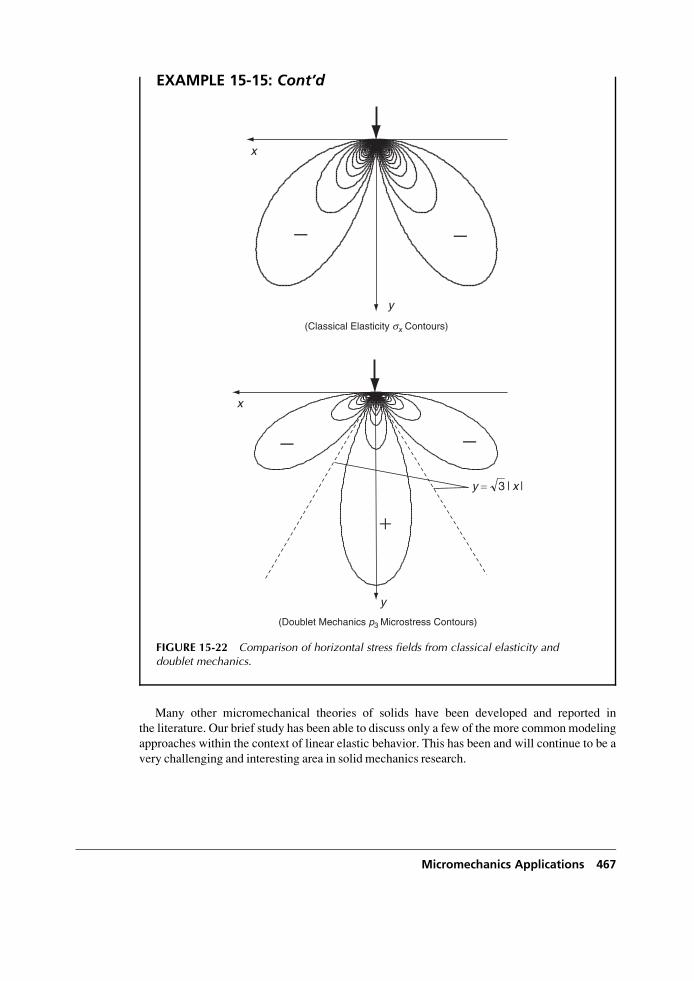
EXAMPLE 15-15: Cont’d
Many other micromechanical theories of solids have been developed and reported in
the literature. Our brief study has been able to discuss only a few of the more commonmodeling
approaches within the context of linear elastic behavior. This has been and will continue to be a
very challenging and interesting area in solid mechanics research.
x
y
(Classical Elasticity sx Contours)
x
y
(Doublet Mechanics p3 Microstress Contours)
||3 xy =
+
--
--
FIGURE 15-22 Comparison of horizontal stress fields from classical elasticity anddoublet mechanics.
Micromechanics Applications 467
References
Aifantis EC: Gradient deformation models at nano, micro, and macro scales, J. Eng. Materials &Technology, vol 121, pp 189-202, 1999.
Biot MA: Twenty-One Papers by M. A. Biot, ed. I Tolstoy, Acoustic Society of America, Woodbury, NY,
1992.
Boresi AP, and Chong KP: Elasticity in Engineering Mechanics, John Wiley, New York, 2000.
Budiansky B, and O’Connell RJ: Elastic moduli of a cracked solid, Int. J. Solids Structures, vol 12, pp. 81-97, 1976.
Carlson DE: Stress functions for plane problems with couple stresses, J. Applied Math. Physics, vol 17,pp. 789-792, 1966.
Chang CS, and Gao J: Second-gradient constitutive theory for granular material with random packing
structure, Int. J. Solids Structure, vol 32, pp. 2279-2293, 1995.Chang CS, and Ma LA: Micromechanical-base micro-polar theory for deformation of granular solids., Int.J. Solids Structures, vol 28, pp. 67-86, 1991.
Chau KT, Wong RHC, and Wang P: Validation of microcrack models by experiments on real and
replicated rocks, Mechanics of Materials with Discontinuities and Heterogeneities, ASME Publication,AMD vol 201, pp. 133-146, 1995.
Cowin SC: A note on the problem of pure bending for a linear elastic material with voids, J. Elasticity,vol 14, pp. 227-233, 1984a.
Cowin SC: The stresses around a hole in a linear elastic material with voids, Quart. J. Mech. Appl. Math.,vol 37, pp. 441-465, 1984b.
Cowin SC: The viscoelastic behavior of linear elastic materials with voids, J. Elasticity, vol 15, pp. 185-191, 1985.
Cowin SC, and Nunziato JW: Linear elastic materials with voids, J. Elasticity, vol 13, pp. 125-147, 1983.Cowin SC, and Puri P: The classical pressure vessel problems for linear elastic materials with voids,
J. Elasticity, vol 13, pp. 157-163, 1983.Ellis RW, and Smith CW: A thin-plate analysis and experimental evaluation of couple-stress effects,
Experimental Mech., vol 7, pp. 372-380, 1967.Eringen AC: Theory of micropolar elasticity, Fracture, vol 2, ed. H Liebowitz, Academic Press,
New York, pp. 662-729, 1968.
Eringen AC: Microcontinuum Field Theories, I Foundations and Solids, Springer-Verlag, New York,
1999.
Ferrari M, Granik VT, Imam A, and Nadeau J: Advances in Doublet Mechanics, Springer, Berlin, 1997.Granik VT: Microstructural mechanics of granular media, Technical Report IM/MGU 78-241, Inst. Mech.
of Moscow State University, in Russian, 1978.
Granik VT, and Ferrari M: Microstructural mechanics of granular media, Mech. of Materials, vol 15,pp. 301-322, 1993.
Hartranft RJ, and Sih GC: The effect of couple-stress on the stress concentration of a circular inclusion,
J. Appl. Mech., vol 32, pp. 429-431, 1965.Hashin Z: Analysis of composite materials—A survey, J. Appl. Mech., vol 50, pp. 481-504, 1983.Hoenig A: Elastic moduli on a non-random cracked body, Int. J. Solids Structures, vol 15, pp. 137-154,1979.
Hori H, and Nemat-Nasser S: Overall moduli of solids with microcracks: load induced anisotropy,
J. Mech. Physics Solids, vol 31, pp. 155-171, 1983.Kachanov M: On the relationship between fracturing of brittle microcracking solid and its effective elastic
properties, Damage Mechanics in Engineering Materials, ASME Publication, ed. JW Ju, D Krajcinovic,
and HL Schreyer, AMD vol 109, pp. 11-15, 1990.
Kachanov M: Elastic solids with many cracks and related problems, Advances in Appl. Mech., vol 30,pp. 259-445, 1994.
Kaloni PN, and Ariman T: Stress concentration effects in micropolar elasticity, J. Appl. Math. Phys.,vol 18, pp. 136-141, 1967.
Kellogg OD: Foundations of Potential Theory, Dover, New York, 1953.
468 ADVANCED APPLICATIONS
Kennedy TC: Modeling failure in notched plates with micropolar strain softening, Composite Structures,vol 44, pp. 71-79, 1999.
Kennedy TC, and Kim JB: Finite element analysis of a crack in a micropolar elastic material, Computersin Engineering, ASME, ed. R Raghavan and TJ CoKonis, vol 3, pp. 439-444, 1987.
Kunin IA: Elastic Media with Microstructure II Three-Dimensional Models, Springer-Verlag, Berlin, 1983.Landau LD, and Lifshitz EM: Theory of Elasticity, Pergamon Press, London, 1986.
Lardner RW:Mathematical Theory of Dislocations and Fracture, Univ. of Toronto Press, Toronto, 1974.Li S, Miskioglu I, and Altan BS: Solution to line loading of a semi-infinite solid in gradient elasticity,
Int. J. Solids Structures, vol 41, pp 3395-3410, 2004.
Mindlin RD: Influence of couple-stress on stress concentrations,Experimental Mech., vol 3, pp. 1-7, 1963.Mindlin RD: Microstructure in linear elasticity, Arch. Rat. Mech. Anal., vol 16, pp. 51-78, 1964.Mindlin RD: Second gradient of strain and surface-tension in linear elasticity, Int. J. Solids Structures,vol 1, pp 417-438, 1965.
Mura T: Micromechanics of Defects in Solids, Martinus Nijhoff, Dordrecht, 1987.
Nemat-Nasser S, and Hori H: Micromechanics: Overall properties of heterogeneous materials, Advancesin Appl. Mech. vol 37, North-Holland, Amsterdam, 1993.
Nowacki W: Theory of Asymmetric Elasticity, Pergamon Press, Oxford, England, 1986.
Ostoja-Starzewski M, and Wang C: Linear elasticity of planar Delaunay networks: random field charac-
terization of effective moduli, Acta Mech., vol 80, pp. 61-80, 1989.Ostoja-Starzewski M, and Wang C: Linear elasticity of planar Delaunay networks part II: Voigt and Reuss
bounds, and modification for centroids, Acta Mech., vol 84, pp. 47-61, 1990.Sadd MH, and Dai Q: A comparison of micromechanical modeling of asphalt materials using finite
elements and doublet mechanics, Mech. of Materials, vol 37, pp 641-662, 2004a.
Sadd MH, Dai Q, Parameswaran V, and Shukla A: Microstructural simulation of asphalt materials:
modeling and experimental studies, J. Materials in Civil Eng., vol 16, pp. 107-115, 2004b.Sadd MH, Qiu L, Boardman WG, and Shukla A: Modelling wave propagation in granular media using
elastic networks, Int. J. Rock Mech. Min. Sci. & Geomech., vol 29, pp. 161-170, 1992.Schijve J: Note of couple stresses, J. Mech. Phys. Solids, vol 14, pp. 113-120, 1966.Sun CT, and Yang TY: A couple-stress theory for gridwork-reinforced media, J. Elasticity, vol 5,
pp. 45-58, 1975.
Volterra V: Sur l’equilibre des corps elastiques multiplement connexes, Ann. Ec. Norm. (Paris) vol 24(Series 3), pp. 401-517, 1907.
Weertman J, and Weertman JR: Elementary Dislocation Theory, Macmillan, New York, 1964.
Weitsman Y: Couple-stress effects on stress concentration around a cylindrical inclusion in a field of
uniaxial tension, J. Appl. Mech., vol 32, pp. 424-428, 1965.
Exercises
15-1. Show that the general plane strain edge dislocation problem shown in Figure 15-3 can be
solved using methods of Chapter 10 with the two complex potentials
g(z) ¼ imb4p(1� �)
log z, c(z) ¼ � im�bb4p(1� �)
log z
where b ¼ bx þ iby. In particular, verify the cyclic property [uþ iv]C ¼ �b, where C is
any circuit in the x,y-plane around the dislocation line. Also determine the general stress
and displacement field.
15-2. Justify that the edge dislocation solution (15.1.2) provides the required multivalued
behavior for the displacement field. Explicitly develop the resulting stress fields given
by (15.1.3) and (15.1.4).
Micromechanics Applications 469
15-3. Show that the screw dislocation displacement field (15.1.5) gives the stresses (15.1.6)
and (15.1.7).
15-4. For the edge dislocation model, consider a cylinder of finite radius with axis along the
dislocation line (z-axis). Show that although the stress solution gives rise to tractions
on this cylindrical surface, the resultant forces in the x and y directions will vanish.
15-5. The stress field (15.1.7) for the screw dislocation produces no tangential or normal
forces on a cylinder of finite radius with axis along the dislocation line (z-axis).However, show that if the cylinder is of finite length, the stress tzy on the ends will notnecessarily be zero and will give rise to a resultant couple.
15-6. Show that the strain energy (per unit length) associated with the screw dislocation
model of Example 15-2 is given by
Wscrew ¼ mb2
4plog
Ro
Rc
where Ro is the outer radius of the crystal and Rc is the core radius of the dislocation.
This quantity is sometimes referred to as the self-energy. The radial dimensions are
somewhat arbitrary, although Rc is sometimes taken as five times the magnitude of the
Burgers vector.
15-7. Using similar notation as Exercise 15-6, show that the strain energy associated with
the edge dislocation model of Example 15-1 can be expressed by
Wedge ¼ mb2
4p(1� �)log
Ro
Rc
Note that this energy is larger than the value developed for the screw dislocation in
Exercise 15-6. Evaluate the difference between these energies for the special case of
v ¼ 1⁄3 .
15-8. For the Kelvin state as considered in Example 15-4, explicitly justify the displacement
and stress results given in relations (15.2.8) and (15.2.10).
15-9. Verify that the displacements and stresses for the center of compression are given by
(15.2.21) and (15.2.22).
15-10. A fiber discontinuity is to be modeled using a line of centers of dilatation along the
x1-axis from 0 to a. Show that the displacement field for this problem is given by
u1 ¼ 1
2m1
RR� 1
R
� �
u2 ¼ 1
2m1
R
x1x2x22 þ x23
� 1
RR
(x1 � a)x2x22 þ x23
� �
u3 ¼ 1
2m1
R
x1x3x22 þ x23
� 1
RR
(x1 � a)x3x22 þ x23
� �
where RR ¼ffiffiffiffiffiffiffiffiffiffiffiffiffiffiffiffiffiffiffiffiffiffiffiffiffiffiffiffiffiffiffiffiffiffiffiffiffiffi(x1 � a)2 þ x22 þ x23
qand R is identical to that illustrated in Figure 15-11.
470 ADVANCED APPLICATIONS
15-11*. For the isotropic self-consistent crack distribution case in Example 15-12, show that
for the case � ¼ 0:5, relation (15:3:4)3 reduces to
e ¼ 9
16
1� 2���
1� ���2
� �
Verify the total loss of moduli at e ¼9⁄16 . Using these results, develop plots of the
effective moduli ratios ���=�, �EE=E, �mm=m versus the crack density. Compare these
results with the corresponding values from the dilute case given in Example 15-10.
15-12. Develop the compatibility relations for couple-stress theory given by (15.4.12). Next,
using the constitutive relations, eliminate the strains and rotations, and express these
relations in terms of the stresses, thus verifying equations (15.4.13).
15-13. Explicitly justify that the stress-stress function relations (15.4.14) are a self-
equilibrated form.
15-14. For the couple-stress theory, show that the two stress functions satisfy
r4F ¼ 0, r2C� l2r4C ¼ 0
15-15. Using the general stress relations (15.4.25) for the stress concentration problem of
Example 15-13, show that the circumferential stress on the boundary of the hole is
given by
sy(a, y) ¼ T 1� 2 cos 2y1þ F
� �
Verify that this expression gives a maximum at y ¼ �p=2, and explicitly show that
this value will reduce to the classical case of 3T by choosing l1 ¼ l2 ¼ l ¼ 0.
15-16. Starting with the general relations (15.5.6), verify that the two-dimensional plane
stress constitutive equations for elastic materials with voids are given by (15.5.9).
15-17. For elastic materials with voids, using the single strain-compatibility equation,
develop the stress and stress function compatibility forms (15.5.10) and (15.5.11).
15-18*. Compare the hoop stress sy(r, p=2) predictions from elasticity with voids given by
relation (15.5.18) with the corresponding results from classical theory. Choosing
N ¼1⁄2 and L ¼ 2, for the elastic material with voids, make a comparative plot of
sy(r, p=2)=T versus r/a for these two theories.
15-19*. For the doublet mechanics Flamant solution in Example 15-15, develop contour plots
(similar to Figure 15-22) for the microstresses p1 and p2. Are there zones where thesemicrostresses are tensile?
Micromechanics Applications 471
16 Numerical Finite and BoundaryElement Methods
Reviewing the previous chapters would indicate that analytical solutions to elasticity problems
are normally accomplished for regions and loadings with relatively simple geometry. For
example, many solutions can be developed for two-dimensional problems, while only a limited
number exist for three dimensions. Solutions are commonly available for problems with simple
shapes such as those having boundaries coinciding with Cartesian, cylindrical, and spherical
coordinate surfaces. Unfortunately, problems with more general boundary shape and loading
are commonly intractable or require very extensive mathematical analysis and numerical
evaluation. Because most real-world problems involve structures with complicated shape
and loading, a gap exists between what is needed in applications and what can be solved by
analytical closed-form methods.
Over the years, this need to determine deformation and stresses in complex problems has
lead to the development of many approximate and numerical solution methods (see brief
discussion in Section 5.7). Approximate methods based on energy techniques were outlined in
Section 6.7, but it was pointed out that these schemes have limited success in developing
solutions for problems of complex shape. Methods of numerical stress analysis normally recast
the mathematical elasticity boundary value problem into a direct numerical routine. One such
early scheme is the finite difference method (FDM) in which derivatives of the governing field
equations are replaced by algebraic difference equations. This method generates a system of
algebraic equations at various computational grid points in the body, and the solution to the
system determines the unknown variable at each grid point. Although simple in concept, FDM
has not been able to provide a useful and accurate scheme to handle general problems with
geometric and loading complexity. Over the past few decades, two methods have emerged that
provide necessary accuracy, general applicability, and ease of use. This has led to their
acceptance by the stress analysis community and has resulted in the development of many
private and commercial computer codes implementing each numerical scheme.
The first of these techniques is known as the finite element method (FEM) and involves
dividing the body under study into a number of pieces or subdomains called elements. Thesolution is then approximated over each element and is quantified in terms of values at special
locations within the element called the nodes. The discretization process establishes an
473
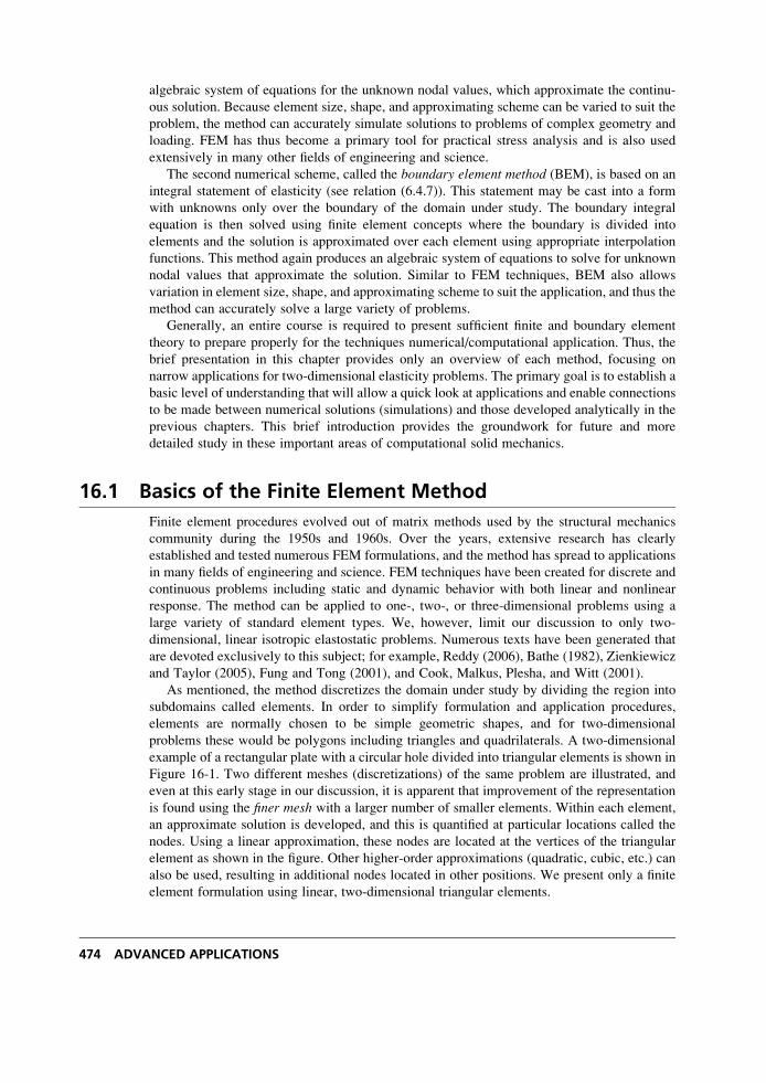
algebraic system of equations for the unknown nodal values, which approximate the continu-
ous solution. Because element size, shape, and approximating scheme can be varied to suit the
problem, the method can accurately simulate solutions to problems of complex geometry and
loading. FEM has thus become a primary tool for practical stress analysis and is also used
extensively in many other fields of engineering and science.
The second numerical scheme, called the boundary element method (BEM), is based on an
integral statement of elasticity (see relation (6.4.7)). This statement may be cast into a form
with unknowns only over the boundary of the domain under study. The boundary integral
equation is then solved using finite element concepts where the boundary is divided into
elements and the solution is approximated over each element using appropriate interpolation
functions. This method again produces an algebraic system of equations to solve for unknown
nodal values that approximate the solution. Similar to FEM techniques, BEM also allows
variation in element size, shape, and approximating scheme to suit the application, and thus the
method can accurately solve a large variety of problems.
Generally, an entire course is required to present sufficient finite and boundary element
theory to prepare properly for the techniques numerical/computational application. Thus, the
brief presentation in this chapter provides only an overview of each method, focusing on
narrow applications for two-dimensional elasticity problems. The primary goal is to establish a
basic level of understanding that will allow a quick look at applications and enable connections
to be made between numerical solutions (simulations) and those developed analytically in the
previous chapters. This brief introduction provides the groundwork for future and more
detailed study in these important areas of computational solid mechanics.
16.1 Basics of the Finite Element Method
Finite element procedures evolved out of matrix methods used by the structural mechanics
community during the 1950s and 1960s. Over the years, extensive research has clearly
established and tested numerous FEM formulations, and the method has spread to applications
in many fields of engineering and science. FEM techniques have been created for discrete and
continuous problems including static and dynamic behavior with both linear and nonlinear
response. The method can be applied to one-, two-, or three-dimensional problems using a
large variety of standard element types. We, however, limit our discussion to only two-
dimensional, linear isotropic elastostatic problems. Numerous texts have been generated that
are devoted exclusively to this subject; for example, Reddy (2006), Bathe (1982), Zienkiewicz
and Taylor (2005), Fung and Tong (2001), and Cook, Malkus, Plesha, and Witt (2001).
As mentioned, the method discretizes the domain under study by dividing the region into
subdomains called elements. In order to simplify formulation and application procedures,
elements are normally chosen to be simple geometric shapes, and for two-dimensional
problems these would be polygons including triangles and quadrilaterals. A two-dimensional
example of a rectangular plate with a circular hole divided into triangular elements is shown in
Figure 16-1. Two different meshes (discretizations) of the same problem are illustrated, and
even at this early stage in our discussion, it is apparent that improvement of the representation
is found using the finer mesh with a larger number of smaller elements. Within each element,
an approximate solution is developed, and this is quantified at particular locations called the
nodes. Using a linear approximation, these nodes are located at the vertices of the triangular
element as shown in the figure. Other higher-order approximations (quadratic, cubic, etc.) can
also be used, resulting in additional nodes located in other positions. We present only a finite
element formulation using linear, two-dimensional triangular elements.
474 ADVANCED APPLICATIONS
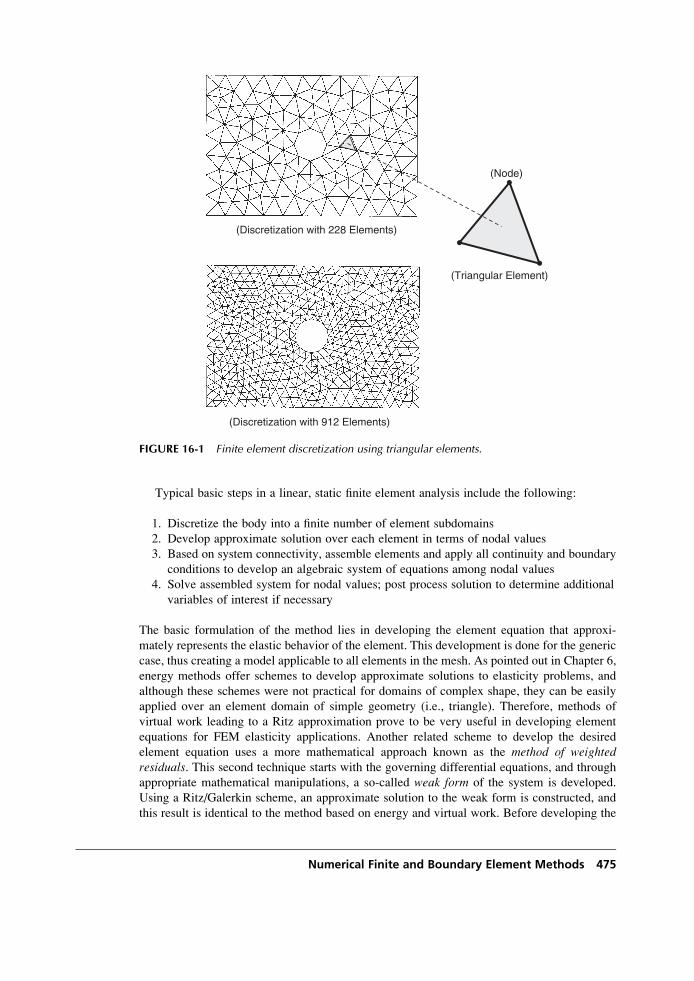
Typical basic steps in a linear, static finite element analysis include the following:
1. Discretize the body into a finite number of element subdomains
2. Develop approximate solution over each element in terms of nodal values
3. Based on system connectivity, assemble elements and apply all continuity and boundary
conditions to develop an algebraic system of equations among nodal values
4. Solve assembled system for nodal values; post process solution to determine additional
variables of interest if necessary
The basic formulation of the method lies in developing the element equation that approxi-
mately represents the elastic behavior of the element. This development is done for the generic
case, thus creating a model applicable to all elements in the mesh. As pointed out in Chapter 6,
energy methods offer schemes to develop approximate solutions to elasticity problems, and
although these schemes were not practical for domains of complex shape, they can be easily
applied over an element domain of simple geometry (i.e., triangle). Therefore, methods of
virtual work leading to a Ritz approximation prove to be very useful in developing element
equations for FEM elasticity applications. Another related scheme to develop the desired
element equation uses a more mathematical approach known as the method of weightedresiduals. This second technique starts with the governing differential equations, and through
appropriate mathematical manipulations, a so-called weak form of the system is developed.
Using a Ritz/Galerkin scheme, an approximate solution to the weak form is constructed, and
this result is identical to the method based on energy and virtual work. Before developing the
(Discretization with 228 Elements)
(Discretization with 912 Elements)
(Triangular Element)
(Node)
FIGURE 16-1 Finite element discretization using triangular elements.
Numerical Finite and Boundary Element Methods 475
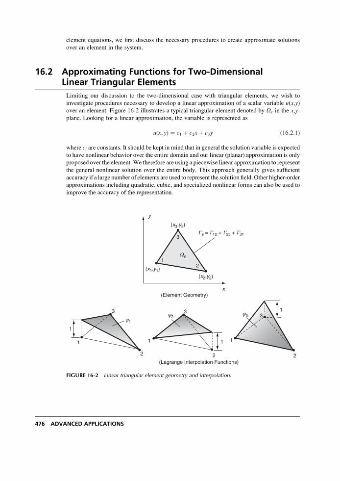
element equations, we first discuss the necessary procedures to create approximate solutions
over an element in the system.
16.2 Approximating Functions for Two-DimensionalLinear Triangular Elements
Limiting our discussion to the two-dimensional case with triangular elements, we wish to
investigate procedures necessary to develop a linear approximation of a scalar variable u(x,y)over an element. Figure 16-2 illustrates a typical triangular element denoted by Oe in the x,y-plane. Looking for a linear approximation, the variable is represented as
u(x, y) ¼ c1 þ c2xþ c3y (16:2:1)
where ci are constants. It should be kept in mind that in general the solution variable is expected
to have nonlinear behavior over the entire domain and our linear (planar) approximation is only
proposed over the element.We therefore are using a piecewise linear approximation to represent
the general nonlinear solution over the entire body. This approach generally gives sufficient
accuracy if a large number of elements are used to represent the solution field. Other higher-order
approximations including quadratic, cubic, and specialized nonlinear forms can also be used to
improve the accuracy of the representation.
12
3
x
y
We
(Element Geometry)
Ge = G12 + G23 + G31
(x1,y1)
(x2,y2)
(x3,y3)
(Lagrange Interpolation Functions)
1
2
3
1
y1
y2y3
1
2
3
1 1
2
31
FIGURE 16-2 Linear triangular element geometry and interpolation.
476 ADVANCED APPLICATIONS
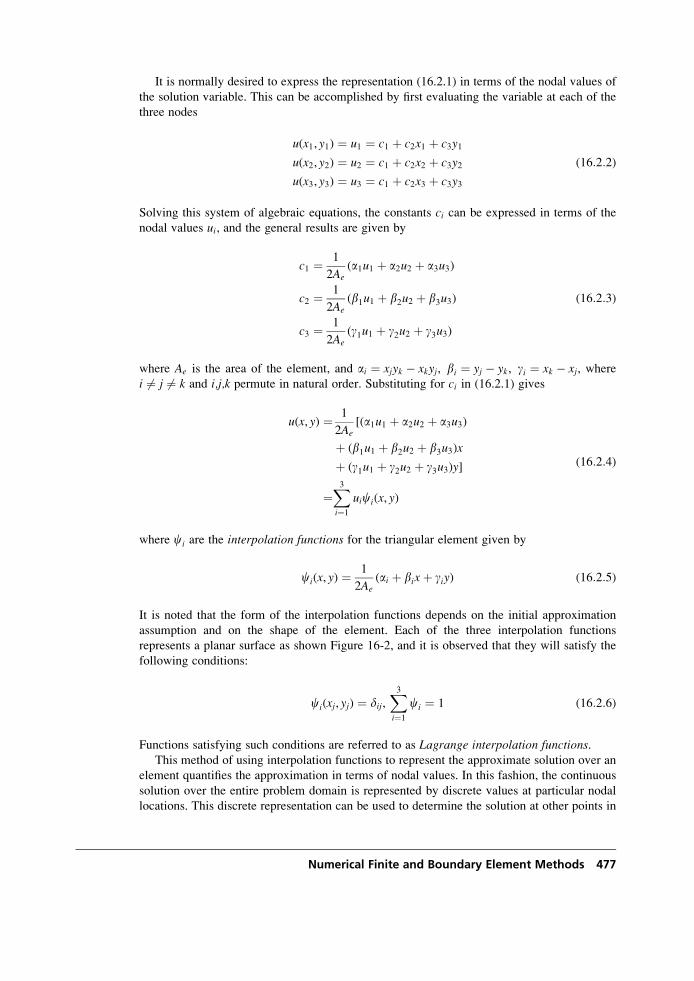
It is normally desired to express the representation (16.2.1) in terms of the nodal values of
the solution variable. This can be accomplished by first evaluating the variable at each of the
three nodes
u(x1, y1) ¼ u1 ¼ c1 þ c2x1 þ c3y1
u(x2, y2) ¼ u2 ¼ c1 þ c2x2 þ c3y2
u(x3, y3) ¼ u3 ¼ c1 þ c2x3 þ c3y3
(16:2:2)
Solving this system of algebraic equations, the constants ci can be expressed in terms of the
nodal values ui, and the general results are given by
c1 ¼ 1
2Ae(a1u1 þ a2u2 þ a3u3)
c2 ¼ 1
2Ae(b1u1 þ b2u2 þ b3u3)
c3 ¼ 1
2Ae(g1u1 þ g2u2 þ g3u3)
(16:2:3)
where Ae is the area of the element, and ai ¼ xjyk � xkyj, bi ¼ yj � yk, gi ¼ xk � xj, wherei 6¼ j 6¼ k and i,j,k permute in natural order. Substituting for ci in (16.2.1) gives
u(x, y) ¼ 1
2Ae[(a1u1 þ a2u2 þ a3u3)
þ (b1u1 þ b2u2 þ b3u3)x
þ (g1u1 þ g2u2 þ g3u3)y]
¼X3i¼1
uici(x, y)
(16:2:4)
where ci are the interpolation functions for the triangular element given by
ci(x, y) ¼1
2Ae(ai þ bixþ giy) (16:2:5)
It is noted that the form of the interpolation functions depends on the initial approximation
assumption and on the shape of the element. Each of the three interpolation functions
represents a planar surface as shown Figure 16-2, and it is observed that they will satisfy the
following conditions:
ci(xj, yj) ¼ dij,X3i¼1
ci ¼ 1 (16:2:6)
Functions satisfying such conditions are referred to as Lagrange interpolation functions.This method of using interpolation functions to represent the approximate solution over an
element quantifies the approximation in terms of nodal values. In this fashion, the continuous
solution over the entire problem domain is represented by discrete values at particular nodal
locations. This discrete representation can be used to determine the solution at other points in
Numerical Finite and Boundary Element Methods 477
the region using various other interpolation schemes. With these representation concepts
established, we now pursue a brief development of the plane elasticity element equations
using the virtual work formulation.
16.3 Virtual Work Formulation for Plane Elasticity
The principle of virtual work developed in Section 6.5 can be stated over a finite element
volume Ve with boundary Se as
ðVe
sijdeijdV ¼ðSe
Tni duidSþ
ðVe
FiduidV (16:3:1)
For plane elasticity with an element of uniform thickness he, Ve ¼ heOe and Se ¼ heGe, and
the previous relation can be reduced to the two-dimensional form
he
ðOe
(sxdex þ sydey þ 2txydexy)dxdy
� he
ðGe
(Tnxduþ Tn
ydv)ds� he
ðOe
(Fxduþ Fydv)dxdy ¼ 0
(16:3:2)
Using matrix notation, this relation can be written as
he
ðOe
dexdey2dexy
8><>:
9>=>;
T sxsytxy
8><>:
9>=>;
0B@
1CAdxdy
� he
ðGe
du
dv
� �T Tnx
Tny
( ) !ds� he
ðOe
du
dv
� �T Fx
Fy
� � !dxdy ¼ 0
(16:3:3)
We now proceed to develop an element formulation in terms of the displacements and choose a
linear approximation for each component
u(x, y) ¼X3i¼1
uici(x, y)
v(x, y) ¼X3i¼1
vici(x, y)
(16:3:4)
where ci(x, y) are the Lagrange interpolation functions given by (16.2.5). Using this scheme
there will be two unknowns or degrees of freedom at each node, resulting in a total of six
degrees of freedom for the entire linear triangular element. Because the strains are related to
displacement gradients, this interpolation choice results in a constant strain element (CST), and
of course the stresses will also be element-wise constant. Relation (16.3.4) can be expressed in
matrix form:
478 ADVANCED APPLICATIONS
u�
� �¼ c1 0 c2 0 c3 0
0 c1 0 c2 0 c3
� �u1�1u2�2u3�3
8>>>>>><>>>>>>:
9>>>>>>=>>>>>>;
¼ [c]{D} (16:3:5)
The strains can then be written as
{e} ¼ex
ey
2exy
8><>:
9>=>; ¼
@=@x 0
0 @=@y
@=@y @=@x
264
375 u
�
� �
¼@=@x 0
0 @=@y
@=@y @=@x
264
375[c]{D} ¼ [B]{D}
(16:3:6)
where
[B] ¼
@c1
@x0
@c2
@x0
@c3
@x0
0@c1
@y0
@c2
@y0
@c3
@y
@c1
@y
@c1
@x
@c2
@y
@c2
@x
@c3
@y
@c3
@x
26666664
37777775
¼ 1
2Ae
b1 0 b2 0 b3 0
0 g1 0 g2 0 g3g1 b1 g2 b2 g3 b3
264
375
(16:3:7)
Hooke’s law then takes the form
{s} ¼ [C]{e} ¼ [C][B]{D} (16:3:8)
where [C] is the elasticity matrix that can be generalized to the orthotropic case (see Section
11.2) by
[C] ¼C11 C12 0
C12 C22 0
0 0 C66
24
35 (16:3:9)
For isotropic materials,
C11 ¼ C22 ¼E
1� �2� � � plane stress
E(1� �)
(1þ �)(1� 2�)� � � plane strain
8>><>>:
C12 ¼E�
1� �2� � � plane stress
E�(1þ �)(1� 2�) � � � plane strain
8><>:
C66 ¼ m ¼ E
2(1þ �)� � � plane stress and plane strain
(16:3:10)
Numerical Finite and Boundary Element Methods 479
Using results (16.3.5), (16.3.6), and (16.3.8) in the virtual work statement (16.3.3) gives
he
ðOe
{dD}T([B]T[C][B]){D}dxdy
� he
ðOe
{dD}T[c]TFx
Fy
� �dxdy� he
ðGe
{dD}T[c]TTnx
Tny
( )ds ¼ 0
(16:3:11)
which can be written in compact form
{dD}T [K]{D}� {F}� {Q}ð Þ ¼ 0 (16:3:12)
Because this relation is to hold for arbitrary variations {dD}T , the expression in parentheses
must vanish, giving the finite element equation
[K]{D} ¼ {F}þ {Q} (16:3:13)
The equation matrices are defined as follows:
[K] ¼ he
ðOe
[B]T[C][B]dxdy � � � stiffness matrix
{F} ¼ he
ðOe
[c]TFx
Fy
� �dxdy � � � body force vector
{Q} ¼ he
ðGe
[c]TTnx
Tny
( )ds � � � loading vector
(16:3:14)
Using the specific interpolation functions for the constant strain triangular element, the [B]matrix had constant components given by (16.3.7). If we assume that the elasticity matrix also
does not vary over the element, then the stiffness matrix is given by
[K] ¼ heAe[B]T[C][B] (16:3:15)
and multiplying out the matrices gives the specific form
[K] ¼ he4Ae
b21C11 þ g21C66 b1g1C12 þ b1g1C66 b1b2C11 þ g1g2C66 b1g2C12 þ b2g1C66 b1b3C11 þ g1g3C66 b1g3C12 þ b3g1C66
� g21C22 þ b21C66 b2g1C12 þ b1g2C66 g1g2C22 þ b1b2C66 b3g1C12 þ b1g3C66 g1g3C22 þ b1b3C66
� � b22C11 þ g22C66 b2g2C12 þ b2g2C66 b2b3C11 þ g2g3C66 b2g3C12 þ b3g2C66
� � � g22C22 þ b22C66 b3g2C12 þ b2g3C66 g2g3C22 þ b2b3C66
� � � � b23C11 þ g23C66 b3g3C12 þ b3g3C66
� � � � � g23C22 þ b23C66
26666664
37777775
(16:3:16)
Note that the stiffness matrix is always symmetric, and thus only the top-right (or bottom-left)
portion need be explicitly written out. If we also choose body forces that are element-wise
constant, the body force vector {F} can be integrated to give
{F} ¼ heAe
3{Fx Fy Fx Fy Fx Fy}
T (16:3:17)
480 ADVANCED APPLICATIONS
The {Q} matrix involves integration of the tractions around the element boundary, and its
evaluation depends on whether an element side falls on the boundary of the domain or is
located in the region’s interior. The evaluation also requires a modeling decision on the
assumed traction variation on the element sides. Most problems can be adequately modeled
using constant, linear, or quadratic variation in the element boundary tractions. For the typical
triangular element shown in Figure 16-2, the {Q} matrix may be written as
{Q} ¼ he
ðG[c]T
Tnx
Tny
( )ds
¼ he
ðG12
[c]TTnx
Tny
( )dsþ he
ðG23
[c]TTnx
Tny
( )dsþ he
ðG31
[c]TTnx
Tny
( )ds
(16:3:18)
Wishing to keep our study brief in theory, we take the simplest case of element-wise
constant boundary tractions, which allows explicit calculation of the boundary integrals. For
this case, the integral over element side G12 is given by
he
ðG12
[c]TTnx
Tny
� �ds ¼ he
ðG12
c1Tnx
c1Tny
c2Tnx
c2Tny
c3Tnx
c3Tny
8>>>>>><>>>>>>:
9>>>>>>=>>>>>>;ds ¼ heL12
2
Tnx
Tny
Tnx
Tny
0
0
8>>>>>><>>>>>>:
9>>>>>>=>>>>>>;
12
(16:3:19)
where L12 is the length of side G12. Note that we have used the fact that along side G12, c1 and
c2 vary linearly and c3 ¼ 0. Following similar analysis, the boundary integrals along sides G23
and G31 are found to be
he
ðG23
[c]TTnx
Tny
� �ds ¼ heL23
2
0
0
Tnx
Tny
Tnx
Tny
8>>>>>><>>>>>>:
9>>>>>>=>>>>>>;
23
, he
ðG31
[c]TTnx
Tny
� �ds ¼ heL31
2
Tnx
Tny
0
0
Tnx
Tny
8>>>>>><>>>>>>:
9>>>>>>=>>>>>>;
31
(16:3:20)
It should be noted that for element sides that lie in the region’s interior, values of the
boundary tractions will not be known before the solution is found; therefore the previous
relations cannot be used to evaluate the contributions of the {Q} matrix explicitly. However,
for this situation, the stresses and tractions are in internal equilibrium, and thus the integrated
result from one element will cancel that from the opposite adjacent element when the finite
element system is assembled. For element sides that coincide with the region’s boundary, any
applied boundary tractions are then incorporated into the results given by relations (16.3.19)
and (16.3.20). Our simplifications of choosing element-wise constant values for the elastic
moduli, body forces, and tractions were made only for convenience of the current abbreviated
presentation. Normally, FEM modeling allows considerably more generality in these choices,
and integrals in the basic element equation (16.3.14) are then evaluated numerically for such
applications.
Numerical Finite and Boundary Element Methods 481
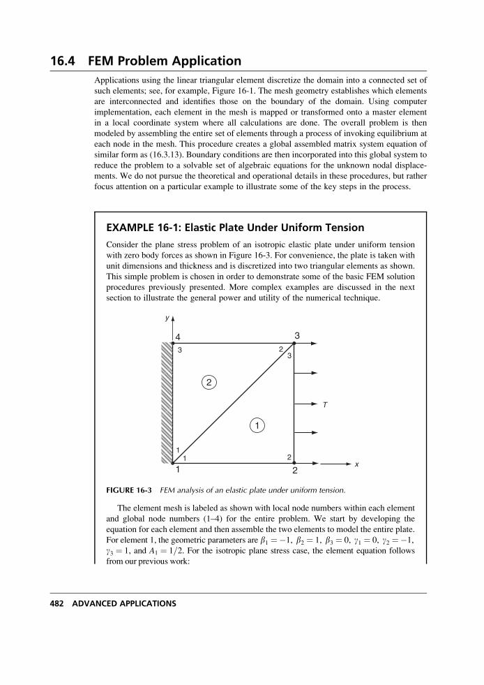
16.4 FEM Problem Application
Applications using the linear triangular element discretize the domain into a connected set of
such elements; see, for example, Figure 16-1. The mesh geometry establishes which elements
are interconnected and identifies those on the boundary of the domain. Using computer
implementation, each element in the mesh is mapped or transformed onto a master element
in a local coordinate system where all calculations are done. The overall problem is then
modeled by assembling the entire set of elements through a process of invoking equilibrium at
each node in the mesh. This procedure creates a global assembled matrix system equation of
similar form as (16.3.13). Boundary conditions are then incorporated into this global system to
reduce the problem to a solvable set of algebraic equations for the unknown nodal displace-
ments. We do not pursue the theoretical and operational details in these procedures, but rather
focus attention on a particular example to illustrate some of the key steps in the process.
EXAMPLE 16-1: Elastic Plate Under Uniform Tension
Consider the plane stress problem of an isotropic elastic plate under uniform tension
with zero body forces as shown in Figure 16-3. For convenience, the plate is taken with
unit dimensions and thickness and is discretized into two triangular elements as shown.
This simple problem is chosen in order to demonstrate some of the basic FEM solution
procedures previously presented. More complex examples are discussed in the next
section to illustrate the general power and utility of the numerical technique.
T
3
21
y
x
4
33
2
2
11
1
2
FIGURE 16-3 FEM analysis of an elastic plate under uniform tension.
The element mesh is labeled as shown with local node numbers within each element
and global node numbers (1–4) for the entire problem. We start by developing the
equation for each element and then assemble the two elements to model the entire plate.
For element 1, the geometric parameters are b1 ¼�1, b2 ¼ 1, b3 ¼ 0, g1 ¼ 0, g2 ¼�1,
g3 ¼ 1, and A1 ¼ 1=2. For the isotropic plane stress case, the element equation follows
from our previous work:
482 ADVANCED APPLICATIONS
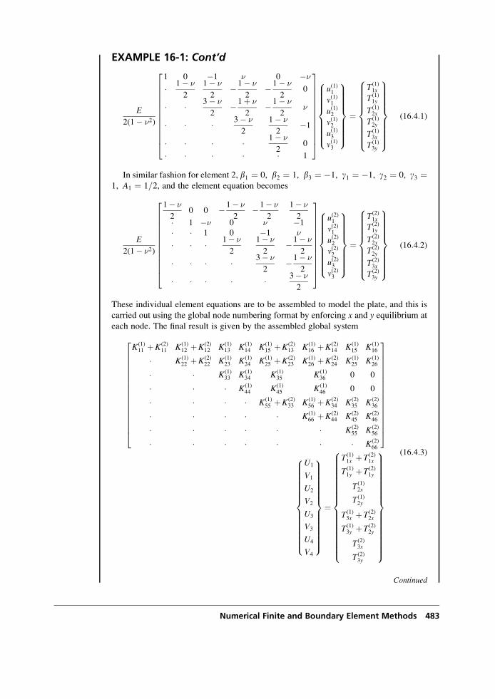
EXAMPLE 16-1: Cont’d
E
2(1� �2)
1 0 �1 � 0 ��
� 1� �
2
1� �
2� 1� �
2� 1� �
20
� � 3� �
2� 1þ �
2� 1� �
2�
� � � 3� �
2
1� �
2�1
� � � � 1� �
20
� � � � � 1
2666666666664
3777777777775
u(1)1
v(1)1
u(1)2
v(1)2
u(1)3
v(1)3
8>>>>>>><>>>>>>>:
9>>>>>>>=>>>>>>>;
¼
T(1)1x
T(1)1y
T(1)2x
T(1)2y
T(1)3x
T(1)3y
8>>>>>>>><>>>>>>>>:
9>>>>>>>>=>>>>>>>>;
(16:4:1)
In similar fashion for element 2, b1 ¼ 0, b2 ¼ 1, b3 ¼ �1, g1 ¼ �1, g2 ¼ 0, g3 ¼1, A1 ¼ 1=2, and the element equation becomes
E
2(1� �2)
1� �
20 0 �1� �
2�1� �
2
1� �
2� 1 �� 0 � �1
� � 1 0 �1 �
� � � 1� �
2
1� �
2�1� �
2
� � � � 3� �
2�1� �
2
� � � � � 3� �
2
2666666666664
3777777777775
u(2)1
v(2)1
u(2)2
v(2)2
u(2)3
v(2)3
8>>>>>>><>>>>>>>:
9>>>>>>>=>>>>>>>;
¼
T(2)1x
T(2)1y
T(2)2x
T(2)2y
T(2)3x
T(2)3y
8>>>>>>>><>>>>>>>>:
9>>>>>>>>=>>>>>>>>;
(16:4:2)
These individual element equations are to be assembled to model the plate, and this is
carried out using the global node numbering format by enforcing x and y equilibrium at
each node. The final result is given by the assembled global system
K(1)11 þK(2)
11 K(1)12 þK(2)
12 K(1)13 K(1)
14 K(1)15 þK(2)
13 K(1)16 þK(2)
14 K(1)15 K(1)
16
� K(1)22 þK(2)
22 K(1)23 K(1)
24 K(1)25 þK(2)
23 K(1)26 þK(2)
24 K(1)25 K(1)
26
� � K(1)33 K(1)
34 K(1)35 K(1)
36 0 0
� � � K(1)44 K(1)
45 K(1)46 0 0
� � � � K(1)55 þK(2)
33 K(1)56 þK(2)
34 K(2)35 K(2)
36
� � � � � K(1)66 þK(2)
44 K(2)45 K(2)
46
� � � � � � K(2)55 K(2)
56
� � � � � � � K(2)66
26666666666666664
37777777777777775
U1
V1
U2
V2
U3
V3
U4
V4
8>>>>>>>>>>>>><>>>>>>>>>>>>>:
9>>>>>>>>>>>>>=>>>>>>>>>>>>>;
¼
T(1)1x þ T(2)
1x
T(1)1y þ T(2)
1y
T(1)2x
T(1)2y
T(1)3x þ T(2)
2x
T(1)3y þ T(2)
2y
T(2)3x
T(2)3y
8>>>>>>>>>>>>>>>><>>>>>>>>>>>>>>>>:
9>>>>>>>>>>>>>>>>=>>>>>>>>>>>>>>>>;
(16:4:3)
Continued
Numerical Finite and Boundary Element Methods 483
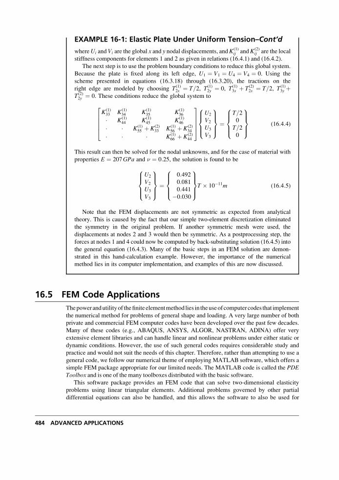
EXAMPLE 16-1: Elastic Plate Under Uniform Tension–Cont’d
whereUi and Vi are the global x and y nodal displacements, andK(1)ij andK(2)
ij are the local
stiffness components for elements 1 and 2 as given in relations (16.4.1) and (16.4.2).
The next step is to use the problem boundary conditions to reduce this global system.
Because the plate is fixed along its left edge, U1 ¼ V1 ¼ U4 ¼ V4 ¼ 0. Using the
scheme presented in equations (16.3.18) through (16.3.20), the tractions on the
right edge are modeled by choosing T(1)2x ¼ T=2, T(1)
2y ¼ 0, T(1)3x þ T(2)
2x ¼ T=2, T(1)3y þ
T(2)2y ¼ 0. These conditions reduce the global system to
K(1)33 K(1)
34 K(1)35 K(1)
36
� K(1)44 K(1)
45 K(1)46
� � K(1)55 þ K(2)
33 K(1)56 þ K(2)
34
� � � K(1)66 þ K(2)
44
26664
37775
U2
V2
U3
V3
8>><>>:
9>>=>>; ¼
T=20
T=20
8>><>>:
9>>=>>; (16:4:4)
This result can then be solved for the nodal unknowns, and for the case of material with
properties E ¼ 207GPa and � ¼ 0:25, the solution is found to be
U2
V2
U3
V3
8>><>>:
9>>=>>; ¼
0:4920:0810:441
�0:030
8>><>>:
9>>=>>;T � 10�11m (16:4:5)
Note that the FEM displacements are not symmetric as expected from analytical
theory. This is caused by the fact that our simple two-element discretization eliminated
the symmetry in the original problem. If another symmetric mesh were used, the
displacements at nodes 2 and 3 would then be symmetric. As a postprocessing step, the
forces at nodes 1 and 4 could now be computed by back-substituting solution (16.4.5) into
the general equation (16.4.3). Many of the basic steps in an FEM solution are demon-
strated in this hand-calculation example. However, the importance of the numerical
method lies in its computer implementation, and examples of this are now discussed.
16.5 FEM Code Applications
Thepowerandutilityof thefinite elementmethod lies in theuseof computer codes that implement
the numerical method for problems of general shape and loading. A very large number of both
private and commercial FEM computer codes have been developed over the past few decades.
Many of these codes (e.g., ABAQUS, ANSYS, ALGOR, NASTRAN, ADINA) offer very
extensive element libraries and can handle linear and nonlinear problems under either static or
dynamic conditions. However, the use of such general codes requires considerable study and
practice and would not suit the needs of this chapter. Therefore, rather than attempting to use a
general code, we follow our numerical theme of employing MATLAB software, which offers a
simple FEM package appropriate for our limited needs. The MATLAB code is called the PDEToolbox and is one of the many toolboxes distributed with the basic software.
This software package provides an FEM code that can solve two-dimensional elasticity
problems using linear triangular elements. Additional problems governed by other partial
differential equations can also be handled, and this allows the software to also be used for
484 ADVANCED APPLICATIONS
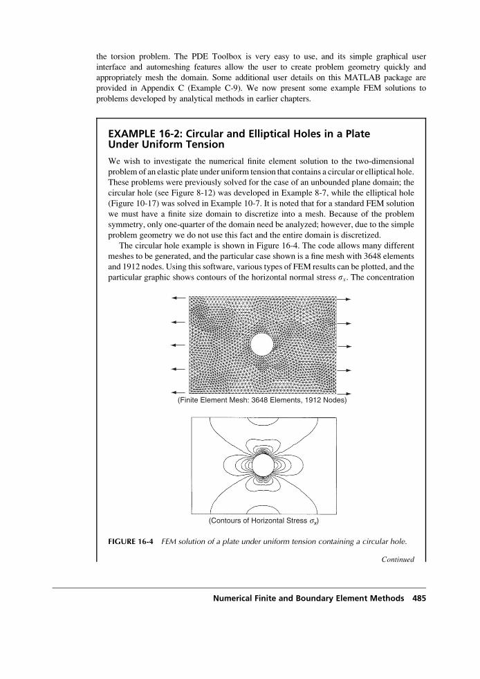
the torsion problem. The PDE Toolbox is very easy to use, and its simple graphical user
interface and automeshing features allow the user to create problem geometry quickly and
appropriately mesh the domain. Some additional user details on this MATLAB package are
provided in Appendix C (Example C-9). We now present some example FEM solutions to
problems developed by analytical methods in earlier chapters.
EXAMPLE 16-2: Circular and Elliptical Holes in a PlateUnder Uniform Tension
We wish to investigate the numerical finite element solution to the two-dimensional
problem of an elastic plate under uniform tension that contains a circular or elliptical hole.
These problems were previously solved for the case of an unbounded plane domain; the
circular hole (see Figure 8-12) was developed in Example 8-7, while the elliptical hole
(Figure 10-17) was solved in Example 10-7. It is noted that for a standard FEM solution
we must have a finite size domain to discretize into a mesh. Because of the problem
symmetry, only one-quarter of the domain need be analyzed; however, due to the simple
problem geometry we do not use this fact and the entire domain is discretized.
The circular hole example is shown in Figure 16-4. The code allows many different
meshes to be generated, and the particular case shown is a fine mesh with 3648 elements
and 1912 nodes. Using this software, various types of FEM results can be plotted, and the
particular graphic shows contours of the horizontal normal stress sx. The concentration
(Finite Element Mesh: 3648 Elements, 1912 Nodes)
(Contours of Horizontal Stress sx)
FIGURE 16-4 FEM solution of a plate under uniform tension containing a circular hole.
Continued
Numerical Finite and Boundary Element Methods 485
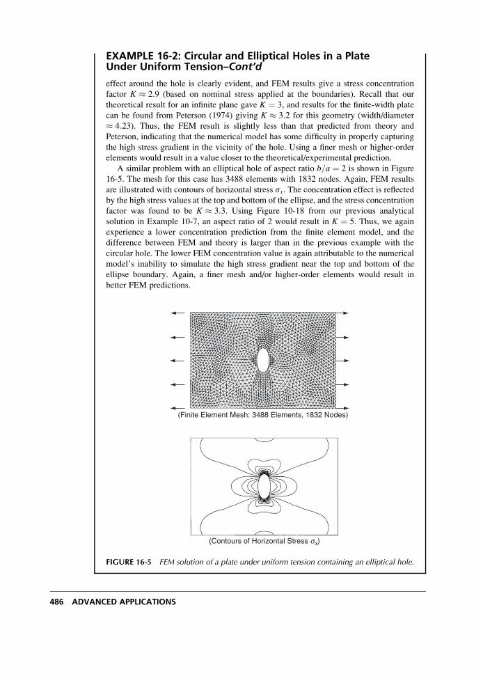
EXAMPLE 16-2: Circular and Elliptical Holes in a PlateUnder Uniform Tension–Cont’d
effect around the hole is clearly evident, and FEM results give a stress concentration
factor K � 2:9 (based on nominal stress applied at the boundaries). Recall that our
theoretical result for an infinite plane gave K ¼ 3, and results for the finite-width plate
can be found from Peterson (1974) giving K � 3:2 for this geometry (width/diameter
� 4:23). Thus, the FEM result is slightly less than that predicted from theory and
Peterson, indicating that the numerical model has some difficulty in properly capturing
the high stress gradient in the vicinity of the hole. Using a finer mesh or higher-order
elements would result in a value closer to the theoretical/experimental prediction.
A similar problem with an elliptical hole of aspect ratio b=a ¼ 2 is shown in Figure
16-5. The mesh for this case has 3488 elements with 1832 nodes. Again, FEM results
are illustrated with contours of horizontal stress sx. The concentration effect is reflectedby the high stress values at the top and bottom of the ellipse, and the stress concentration
factor was found to be K � 3:3. Using Figure 10-18 from our previous analytical
solution in Example 10-7, an aspect ratio of 2 would result in K ¼ 5. Thus, we again
experience a lower concentration prediction from the finite element model, and the
difference between FEM and theory is larger than in the previous example with the
circular hole. The lower FEM concentration value is again attributable to the numerical
model’s inability to simulate the high stress gradient near the top and bottom of the
ellipse boundary. Again, a finer mesh and/or higher-order elements would result in
better FEM predictions.
(Finite Element Mesh: 3488 Elements, 1832 Nodes)
(Contours of Horizontal Stress sx)
FIGURE 16-5 FEM solution of a plate under uniform tension containing an elliptical hole.
486 ADVANCED APPLICATIONS
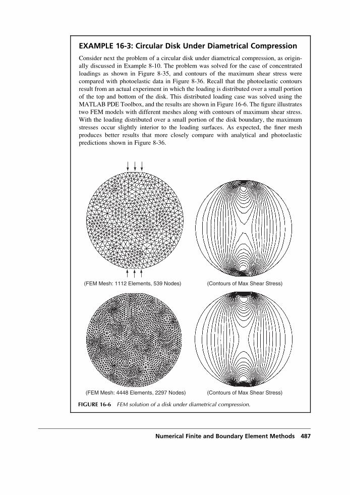
EXAMPLE 16-3: Circular Disk Under Diametrical Compression
Consider next the problem of a circular disk under diametrical compression, as origin-
ally discussed in Example 8-10. The problem was solved for the case of concentrated
loadings as shown in Figure 8-35, and contours of the maximum shear stress were
compared with photoelastic data in Figure 8-36. Recall that the photoelastic contours
result from an actual experiment in which the loading is distributed over a small portion
of the top and bottom of the disk. This distributed loading case was solved using the
MATLAB PDE Toolbox, and the results are shown in Figure 16-6. The figure illustrates
two FEM models with different meshes along with contours of maximum shear stress.
With the loading distributed over a small portion of the disk boundary, the maximum
stresses occur slightly interior to the loading surfaces. As expected, the finer mesh
produces better results that more closely compare with analytical and photoelastic
predictions shown in Figure 8-36.
(FEM Mesh: 1112 Elements, 539 Nodes) (Contours of Max Shear Stress)
(FEM Mesh: 4448 Elements, 2297 Nodes) (Contours of Max Shear Stress)
FIGURE 16-6 FEM solution of a disk under diametrical compression.
Numerical Finite and Boundary Element Methods 487
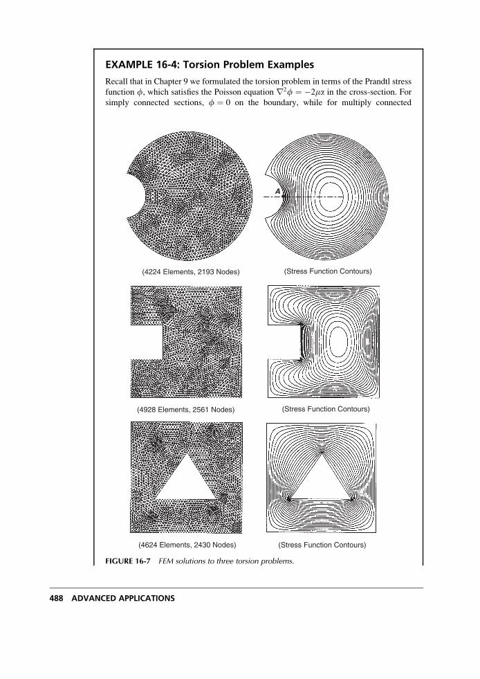
EXAMPLE 16-4: Torsion Problem Examples
Recall that in Chapter 9 we formulated the torsion problem in terms of the Prandtl stress
function f, which satisfies the Poisson equation r2f ¼ �2ma in the cross-section. For
simply connected sections, f ¼ 0 on the boundary, while for multiply connected
(4224 Elements, 2193 Nodes)
(4928 Elements, 2561 Nodes)
(4624 Elements, 2430 Nodes)
(Stress Function Contours)
(Stress Function Contours)
(Stress Function Contours)
A
FIGURE 16-7 FEM solutions to three torsion problems.
488 ADVANCED APPLICATIONS
EXAMPLE 16-4: Cont’d
sections the function could be set to zero on the outer boundary but must be a different
constant on each inner boundary. This two-dimensional problem is easily solved using
finite elements and in particular using the PDE Toolbox. Figure 16-7 illustrates three
sections that have been solved using the MATLAB software with linear triangular
elements. The first problem is that of a circular section with a circular keyway, and this
problem was originally presented in Exercises 9-19 and 9-20. FEM results show stress
function contours over the section, and the slope of these contours gives the shear stress in
the perpendicular direction. It is readily apparent that the maximum shear stress occurs at
the root of the keyway acting tangent to the boundary at point A. The second example
shown is a square section with a square keyway. The stress function contour lines indicate
high-stress regions at the two reentrant corners of the keyway. The final example is a
multiply connected section with a square outer boundary and a triangular inner hole.
Contours for this case show three high-stress regions at each vertex of the triangular
cutout. Countless other torsion examples can be quickly analyzed using this simple FEM
code, and quantitative stress results can also be generated (see Exercise 16-10).
16.6 Boundary Element Formulation
A second numerical method has recently emerged that provides good computational abilities
and has some particular advantages when compared to FEM. The technique known as the
boundary element method (BEM) has been widely used by computational mechanics investi-
gators, leading to the development of many private and commercial codes. Similar to the finite
element method, BEM can analyze many different problems in engineering science including
those in thermal sciences and fluid mechanics. Although the method is not limited to elastic
stress analysis, this brief presentation discusses only this particular case. Many texts have been
written that provide additional details on this subject; see, for example, Banerjee and Butter-
field (1981) and Brebbia and Dominguez (1992).
The formulation of BEM is based on an integral statement of elasticity, and this can be cast
into a relation involving unknowns only over the boundary of the domain under study. This
originally led to the boundary integral equation method (BIE), and early work in the field was
reported by Rizzo (1967) and Cruse (1969). Subsequent research realized that finite element
methods could be used to solve the boundary integral equation by dividing the boundary into
elements over which the solution is approximated using appropriate interpolation functions.
This process generates an algebraic system of equations to solve for the unknown nodal values
that approximate the boundary solution. A procedure to calculate the solution at interior
domain points can also be determined from the original boundary integral equation. This
scheme also allows variation in element size, shape, and approximating scheme to suit the
application, thus providing similar advantages as FEM.
By discretizing only the boundary of the domain, BEM has particular advantages over
FEM. The first issue is that the resulting boundary element equation system is generally much
smaller than that generated by finite elements. It has been pointed out in the literature that
boundary discretization is somewhat easier to interface with computer-aided design (CAD)
codes that create the original problem geometry. A two-dimensional comparison of equivalent
FEM and BEM meshes for a rectangular plate with a central circular hole is shown in
Figure 16-8. It is apparent that a significant reduction in the number of elements (by a factor
of 5) is realized in the BEM mesh. It should be pointed out, however, that the BEM scheme
Numerical Finite and Boundary Element Methods 489
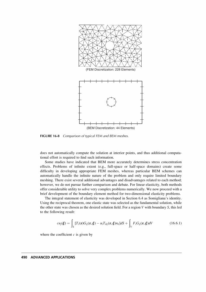
does not automatically compute the solution at interior points, and thus additional computa-
tional effort is required to find such information.
Some studies have indicated that BEM more accurately determines stress concentration
effects. Problems of infinite extent (e.g., full-space or half-space domains) create some
difficulty in developing appropriate FEM meshes, whereas particular BEM schemes can
automatically handle the infinite nature of the problem and only require limited boundary
meshing. There exist several additional advantages and disadvantages related to each method;
however, we do not pursue further comparison and debate. For linear elasticity, both methods
offer considerable utility to solve very complex problems numerically. We now proceed with a
brief development of the boundary element method for two-dimensional elasticity problems.
The integral statement of elasticity was developed in Section 6.4 as Somigliana’s identity.
Using the reciprocal theorem, one elastic state was selected as the fundamental solution, while
the other state was chosen as the desired solution field. For a region V with boundary S, this ledto the following result:
cuj(j) ¼ðS
[Ti(x)Gij(x, j)� uiTikj(x, j)nk]dSþðV
FiGij(x, j)dV (16:6:1)
where the coefficient c is given by
(FEM Discretization: 228 Elements)
(BEM Discretization: 44 Elements)
FIGURE 16-8 Comparison of typical FEM and BEM meshes.
490 ADVANCED APPLICATIONS
c ¼1, j in V12, j on S
0, j outside V
8<: (16:6:2)
Gij(x, j) is the displacement Green’s function that comes from the fundamental solution to
the elasticity equations and corresponds to the solution of the displacement field at point xproduced by a unit concentrated body force e located at point j
uGi (x) ¼ Gij(x;j)ej(j) (16:6:3)
The stresses associated with this state are specified by
sGij ¼ Tijk(x, j)ek ¼ [lGlk, ldij þ m(Gik, j þ Gjk, i)]ek (16:6:4)
and the tractions follow to be
TGi ¼ sGij nj ¼ Tijknjek ¼ pikek (16:6:5)
with pik ¼ Tijknj. Relation (16.6.1) gives the displacement of a given observational point j in
terms of boundary and volume integrals. If point j is chosen to lie on boundary S, then the
expression will contain unknowns (displacements and tractions) only on the boundary. For this
case (j on S), relation (16.6.2) indicates c ¼ 1=2, but this is true only if the boundary has a
continuous tangent (i.e., is smooth). Slight modifications are necessary for the case of non-
smooth boundaries; see Brebbia and Dominguez (1992).
Restricting our attention to only the two-dimensional plane strain case, the Green’s function
becomes (Brebbia and Dominguez 1992)
Gij ¼ 1
8pm(1� �)(3� 4�) ln
1
r
� �dij þ r, ir, j
� �(16:6:6)
where r ¼ jx� jj is the distance between points x and j. Relation (16.6.5) can be used to
determine the traction pij associated with this specific Green’s function, giving the result
pij ¼ Tikjnk ¼ � 1
4p(1� �)r(1� 2�)
@r
@ndij þ r, inj � r; j ni
� �þ 2
@r
@nr, ir, j
� �(16:6:7)
It is convenient to use matrix notation in the subsequent formulation and thus define
G ¼ G11 G12
G21 G22
� �, p ¼ p11 p12
p21 p22
� �
u ¼ u1
u2
� �, T ¼ T1
T2
� �, F ¼ F1
F2
� � (16:6:8)
The boundary integral equation (16.6.1) can then be expressed in two-dimensional form as
ciui ¼ðG[GT � pu]dSþ
ðR
GFdV (16:6:9)
Numerical Finite and Boundary Element Methods 491
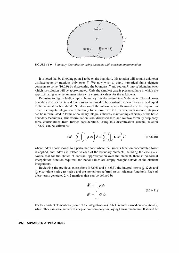
It is noted that by allowing point j to be on the boundary, this relation will contain unknown
displacements or tractions only over G. We now wish to apply numerical finite element
concepts to solve (16.6.9) by discretizing the boundary G and region R into subdomains over
which the solution will be approximated. Only the simplest case is presented here in which the
approximating scheme assumes piecewise constant values for the unknowns.
Referring to Figure 16-9, a typical boundary G is discretized into N elements. The unknown
boundary displacements and tractions are assumed to be constant over each element and equal
to the value at each midnode. Subdivision of the interior into cells would also be required in
order to compute integration of the body force term over R. However, such interior integrals
can be reformulated in terms of boundary integrals, thereby maintaining efficiency of the basic
boundary techniques. This reformulation is not discussed here, and we now formally drop body
force contributions from further consideration. Using this discretization scheme, relation
(16.6.9) can be written as
ciui þXNj¼1
ðGj
p ds
!uj ¼
XNj¼1
ðGj
G ds
!Tj (16:6:10)
where index i corresponds to a particular node where the Green’s function concentrated force
is applied, and index j is related to each of the boundary elements including the case j ¼ i.Notice that for the choice of constant approximation over the element, there is no formal
interpolation function required, and nodal values are simply brought outside of the element
integrations.
Reviewing the previous expressions (16.6.6) and (16.6.7), the integral termsÐGjG ds andÐ
Gjp ds relate node i to node j and are sometimes referred to as influence functions. Each of
these terms generates 2� 2 matrices that can be defined by
AAij ¼ðGj
p ds
Bij ¼ðGj
G ds
(16:6:11)
For the constant element case, some of the integrations in (16.6.11) can be carried out analytically,
while other cases use numerical integration commonly employing Gauss quadrature. It should be
Node j Element Gj
R
Node i
G
FIGURE 16-9 Boundary discretization using elements with constant approximation.
492 ADVANCED APPLICATIONS
noted that the i ¼ j case generates a singularity in the integration, and specialmethods are normally
used to handle this problem.
Relation (16.6.10) can thus be written as
ciui þXNj¼1
AAijuj ¼XNj¼1
BijTj (16:6:12)
and this result specifies the value of u at node i in terms of values of u and T at all other nodes
on the boundary. If the boundary is smooth, ci ¼ 1⁄2 at all nodes. By defining
Aij ¼ AAij, i 6¼ jAAij þ ci, i ¼ j
�(16:6:13)
equation (16.6.12) can be written in compact form as
XNj¼1
Aijuj ¼XNj¼1
BijTj (16:6:14)
or in matrix form
[A]{u} ¼ [B]{T} (16:6:15)
Boundary conditions from elasticity theory normally specify either the displacements or
tractions or a mixed combination of the two variables over boundary G. Using these specified
values in (16.6.14) or (16.6.15) reduces the number of unknowns and allows the system to be
rearranged. Placing all unknowns on the left-hand side of the system equation and moving all
known variables to the right generates a final system that can always be expressed in the form
[C]{X} ¼ {D} (16:6:16)
where all unknown boundary displacements and tractions are located in the column matrix
{X} and all known boundary data have been multiplied by the appropriate influence function
and moved into {D}. Relation (16.6.16) represents a system of linear algebraic equations that
can be solved for the desired unknown boundary information. This BEM system is generally
much smaller than that from a corresponding FEM model. However, unlike the FEM system,
the [C] matrix from (16.6.16) is not in general symmetric, thereby requiring more computa-
tional effort to solve for nodal unknowns. Using modern computing systems, usually this
added computational effort is not a significant factor in the solution of linear elasticity
problems.
Once this solution is complete, all boundary data is known and the solution at any desired
interior point can be calculated reusing the basic governing boundary integral equation. For
example, at an interior point relation (16.6.9) with no body forces will take the form
ui ¼ðGGTdS�
ðGpudS (16:6:17)
Following our previous constant element approximation, this expression can be discretized as
Numerical Finite and Boundary Element Methods 493
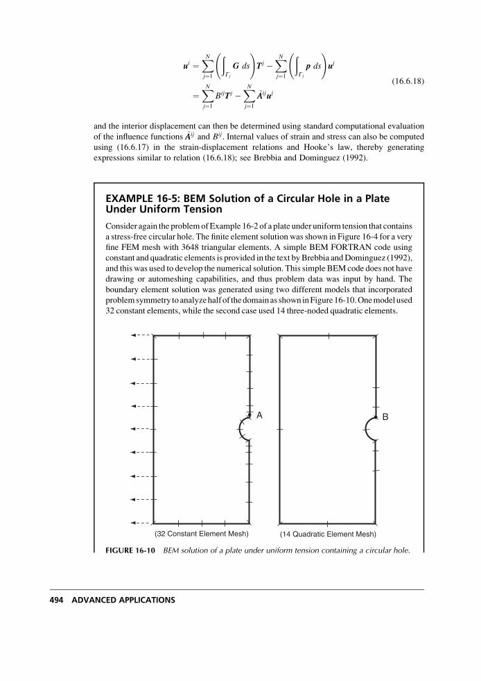
ui ¼XNj¼1
ðGj
G ds
!Tj �
XNj¼1
ðGj
p ds
!uj
¼XNj¼1
BijTj �XNj¼1
AAijuj
(16:6:18)
and the interior displacement can then be determined using standard computational evaluation
of the influence functions AAij and Bij. Internal values of strain and stress can also be computed
using (16.6.17) in the strain-displacement relations and Hooke’s law, thereby generating
expressions similar to relation (16.6.18); see Brebbia and Dominguez (1992).
EXAMPLE 16-5: BEM Solution of a Circular Hole in a PlateUnder Uniform Tension
Consider again the problemofExample 16-2 of a plate under uniform tension that contains
a stress-free circular hole. The finite element solution was shown in Figure 16-4 for a very
fine FEM mesh with 3648 triangular elements. A simple BEM FORTRAN code using
constant and quadratic elements is provided in the text byBrebbia andDominguez (1992),
and this was used to develop the numerical solution. This simple BEM code does not have
drawing or automeshing capabilities, and thus problem data was input by hand. The
boundary element solution was generated using two different models that incorporated
problemsymmetry toanalyzehalf of thedomainas showninFigure16-10.Onemodelused
32 constant elements, while the second case used 14 three-noded quadratic elements.
(32 Constant Element Mesh) (14 Quadratic Element Mesh)
A B
FIGURE 16-10 BEM solution of a plate under uniform tension containing a circular hole.
494 ADVANCED APPLICATIONS
EXAMPLE 16-5: Cont’d
The constant element model is limited to having nodes located at the midpoint of
each element (see Figure 16-9), and thus does not allow direct determination of the
highest stress at the edge of the hole. For this case using the stress value at node A in
Figure 16-10, the stress concentration factor is found to be K � 2:75. The quadratic
element case uses three nodes per element, including nodes located at the element
boundaries. For this case node B in Figure 16-10 is used to determine the highest stress,
and this gives a stress concentration factor of K � 3:02. The particular model has a
width to diameter ratio of 10, and for such geometry, results from Peterson (1974)
would predict a stress concentration of about 3. As expected, the BEM results using
constant elements were not as good as the predictions using quadratic interpolation.
Comparing this BEM analysis with the finite element results in Example 16-2 indicates
that the quadratic boundary element results appear to give a more accurate estimate of
the actual stress concentration using much fewer elements. However, this conclusion is
based on the particular element models for each analysis, and using other element types
and meshes could produce somewhat different results and comparisons.
Many additional FEM and BEM examples can be developed and compared to illustrate
other interesting features of these computational stress analysis methods. Unfortunately, such
an excursion would require developments outside the current scope of the text, and thus we do
not pursue such material. The interested reader is encouraged to consult the chapter references
for additional study.
References
Banerjee PK, and Butterfield R: Boundary Element Methods in Engineering Science, McGraw-Hill,
New York, 1981.
Bathe KJ: Finite Element Procedures in Engineering Analysis, Prentice Hall, Englewood Cliffs, NJ, 1982.Brebbia CA, and Dominguez J: Boundary Elements: An Introductory Course, WIT Press, Southampton,
UK, 1992.
Cook RD, Malkus DS, Witt R, and Plesha ME: Concepts and Applications of Finite Elements inEngineering, John Wiley, New York, 2001.
Cruse TA: Numerical solutions in three-dimensional elastostatics, Int. J. Solids Structures, vol 5,
pp. 1259-1274, 1969.
Fung YC, and Tong P: Classical and Computational Solid Mechanics, World Scientific, Singapore, 2001.
Peterson RE: Stress Concentration Factors, John Wiley, New York, 1974.
Reddy JN: An Introduction to the Finite Element Method, McGraw-Hill, New York, 2006.
Rizzo RJ: An integral equation approach to boundary value problems of classical elastostatics, Quart.Appl. Math., vol 25, pp. 83-95, 1967.
Zienkiewicz OC, and Taylor RL: The Finite Element Method, McGraw-Hill, New York, 2005.
Exercises
16-1. Starting with the general linear form (16.2.1), verify the interpolation relations (16.2.4)
and (16.2.5).
16-2. For the constant strain triangular element, show that the stiffness matrix is given by
(16.3.16).
Numerical Finite and Boundary Element Methods 495
16-3. For the case of element-wise constant body forces, verify that the body force vector is
given by relation (16.3.17) for the linear triangular element.
16-4. Verify boundary relation (16.3.19) for the linear triangular element with constant
boundary tractions Tnx and Tn
y .
16-5. For Example 16-1, show that the element stiffness equations for the isotropic case are
given by relations (16.4.1) and (16.4.2).
16-6. Verify the nodal displacement solution given by (16.4.5) in Example 16-1.
16-7*. Using the MATLAB PDE Toolbox (or equivalent), develop an FEM solution for the
stress concentration problem under biaxial loading given in Exercise 8-22. Compare
the stress concentration factor from the numerical results with the corresponding
analytical predictions.
16-8*. Using the MATLAB PDE Toolbox (or equivalent), develop an FEM solution for the
stress concentration problem under shear loading given in Exercise 8-23. Compare
the stress concentration factor from the numerical results with the corresponding
analytical predictions.
16-9*. Using the MATLAB PDE Toolbox (or equivalent), develop an FEM solution for the
curve beam problem shown in Figure 8-32. At the fixed section, compare numerical
stress results (sx) with analytical predictions (sy) given by equations (8.4.65).
16-10*. Using the MATLAB PDE Toolbox (or equivalent), develop an FEM solution for
the torsion of a cylinder of circular section with circular keyway as shown in Exercise
9-19. Verify the result of Exercise 9-20, that the maximum shear stress on the keyway
is approximately twice that found on a solid shaft. In order to investigate the shear
stress, use the Toolbox plot selection window to plot contours of the variable
abs(grad(u)).
16-11. Verify the traction relation (16.6.7) for the plane strain case.
496 ADVANCED APPLICATIONS
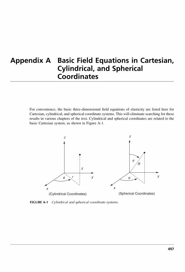
Appendix A Basic Field Equations in Cartesian,Cylindrical, and SphericalCoordinates
For convenience, the basic three-dimensional field equations of elasticity are listed here for
Cartesian, cylindrical, and spherical coordinate systems. This will eliminate searching for these
results in various chapters of the text. Cylindrical and spherical coordinates are related to the
basic Cartesian system, as shown in Figure A-1.
497
z
x
yr
z
(Cylindrical Coordinates)
z
x
y
R
(Spherical Coordinates)
q q
f
FIGURE A-1 Cylindrical and spherical coordinate systems.
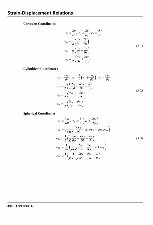
Strain-Displacement Relations
Cartesian Coordinates
ex ¼ @u
@x, ey ¼ @v
@y, ez ¼ @w
@z
exy ¼ 1
2
@u
@yþ @v
@x
� �
eyz ¼ 1
2
@v
@zþ @w
@y
� �
ezx ¼ 1
2
@w
@xþ @u
@z
� �(A:1)
Cylindrical Coordinates
er ¼ @ur@r
, ey ¼ 1
rur þ @uy
@y
� �, ez ¼ @uz
@z
ery ¼ 1
2
1
r
@ur@y
þ @uy@r
� uyr
� �
eyz ¼ 1
2
@uy@z
þ 1
r
@uz@y
� �
ezr ¼ 1
2
@ur@z
þ @uz@r
� �(A:2)
Spherical Coordinates
eR ¼ @uR@R
, ef ¼ 1
RuR þ @uf
@f
� �
ey ¼ 1
R sinf@uy@y
þ sinfuR þ cosfuf
� �
eRf ¼ 1
2
1
R
@uR@f
þ @uf@R
� ufR
� �
efy ¼ 1
2R
1
sinf@uf@y
þ @uy@f
� cotfuy
� �
eyR ¼ 1
2
1
R sinf@uR@y
þ @uy@R
� uyR
� �
(A:3)
498 APPENDIX A
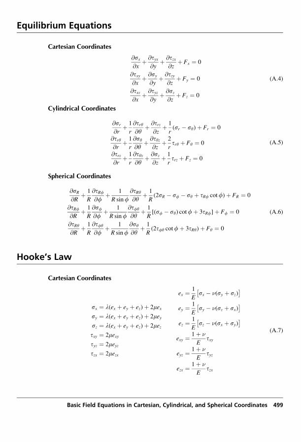
Equilibrium Equations
Cartesian Coordinates
@sx@x
þ @tyx@y
þ @tzx@z
þ Fx ¼ 0
@txy@x
þ @sy@y
þ @tzy@z
þ Fy ¼ 0
@txz@x
þ @tyz@y
þ @sz@z
þ Fz ¼ 0
(A:4)
Cylindrical Coordinates
@sr@r
þ 1
r
@try@y
þ @trz@z
þ 1
r(sr � sy)þ Fr ¼ 0
@try@r
þ 1
r
@sy@y
þ @tyz@z
þ 2
rtry þ Fy ¼ 0
@trz@r
þ 1
r
@tyz@y
þ @sz@z
þ 1
rtrz þ Fz ¼ 0
(A:5)
Spherical Coordinates
@sR@R
þ 1
R
@tRf@f
þ 1
R sinf@tRy@y
þ 1
R(2sR � sf � sy þ tRf cotf)þ FR ¼ 0
@tRf@R
þ 1
R
@sf@f
þ 1
R sinf@tfy@y
þ 1
R[(sf � sy) cotfþ 3tRf]þ Ff ¼ 0
@tRy@R
þ 1
R
@tfy@f
þ 1
R sinf@sy@y
þ 1
R(2tfy cotfþ 3tRy)þ Fy ¼ 0
(A:6)
Hooke’s Law
Cartesian Coordinates
sx ¼ l(ex þ ey þ ez)þ 2mexsy ¼ l(ex þ ey þ ez)þ 2meysz ¼ l(ex þ ey þ ez)þ 2meztxy ¼ 2mexytyz ¼ 2meyztzx ¼ 2mezx
ex ¼ 1
Esx � �(sy þ sz)� �
ey ¼ 1
Esy � �(sz þ sx)� �
ez ¼ 1
Esz � �(sx þ sy)� �
exy ¼ 1þ �
Etxy
eyz ¼ 1þ �
Etyz
ezx ¼ 1þ �
Etzx
(A:7)
Basic Field Equations in Cartesian, Cylindrical, and Spherical Coordinates 499
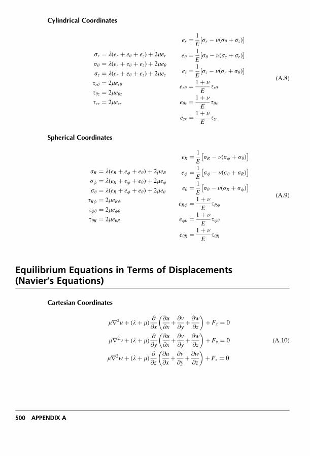
Cylindrical Coordinates
sr ¼ l(er þ ey þ ez)þ 2mersy ¼ l(er þ ey þ ez)þ 2meysz ¼ l(er þ ey þ ez)þ 2meztry ¼ 2merytyz ¼ 2meyztzr ¼ 2mezr
er ¼ 1
Esr � �(sy þ sz)½ �
ey ¼ 1
Esy � �(sz þ sr)½ �
ez ¼ 1
Esz � �(sr þ sy)½ �
ery ¼ 1þ �
Etry
eyz ¼ 1þ �
Etyz
ezr ¼ 1þ �
Etzr
(A:8)
Spherical Coordinates
sR ¼ l(eR þ ef þ ey)þ 2meRsf ¼ l(eR þ ef þ ey)þ 2mefsy ¼ l(eR þ ef þ ey)þ 2meytRf ¼ 2meRftfy ¼ 2mefytyR ¼ 2meyR
eR ¼ 1
EsR � �(sf þ sy)� �
ef ¼ 1
Esf � �(sy þ sR)� �
ey ¼ 1
Esy � �(sR þ sf)� �
eRf ¼ 1þ �
EtRf
efy ¼ 1þ �
Etfy
eyR ¼ 1þ �
EtyR
(A:9)
Equilibrium Equations in Terms of Displacements(Navier’s Equations)
Cartesian Coordinates
mr2uþ (lþ m)@
@x
@u
@xþ @v
@yþ @w
@z
� �þ Fx ¼ 0
mr2vþ (lþ m)@
@y
@u
@xþ @v
@yþ @w
@z
� �þ Fy ¼ 0
mr2wþ (lþ m)@
@z
@u
@xþ @v
@yþ @w
@z
� �þ Fz ¼ 0
(A:10)
500 APPENDIX A
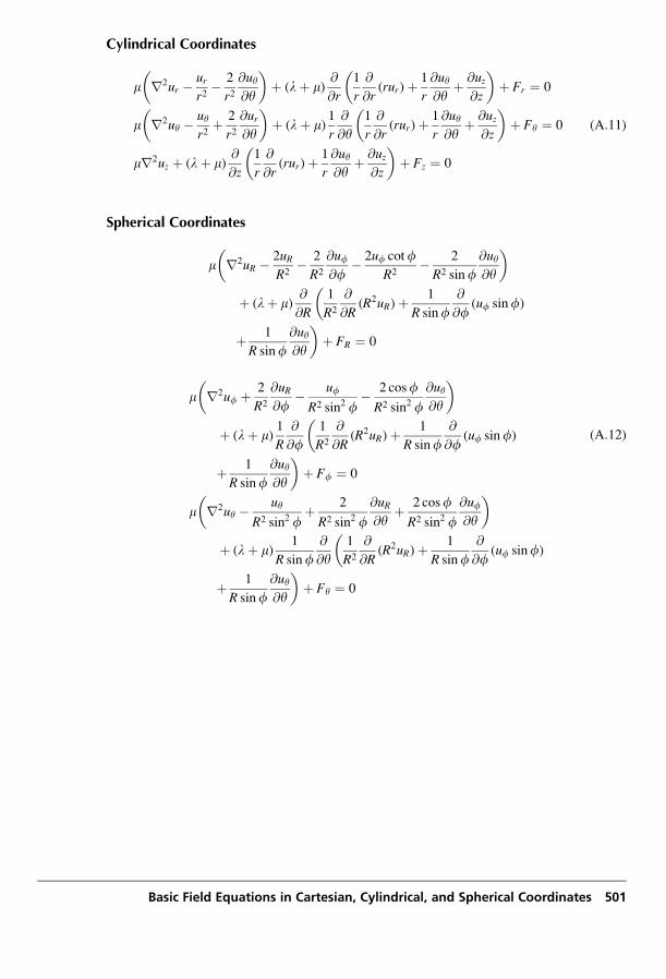
Cylindrical Coordinates
m r2ur � urr2
� 2
r2@uy@y
� �þ (lþ m)
@
@r
1
r
@
@r(rur)þ 1
r
@uy@y
þ @uz@z
� �þ Fr ¼ 0
m r2uy � uyr2
þ 2
r2@ur@y
� �þ (lþ m)
1
r
@
@y1
r
@
@r(rur)þ 1
r
@uy@y
þ @uz@z
� �þ Fy ¼ 0
mr2uz þ (lþ m)@
@z
1
r
@
@r(rur)þ 1
r
@uy@y
þ @uz@z
� �þ Fz ¼ 0
(A:11)
Spherical Coordinates
m r2uR � 2uRR2
� 2
R2
@uf@f
� 2uf cotfR2
� 2
R2 sinf@uy@y
� �
þ (lþ m)@
@R
1
R2
@
@R(R2uR)þ 1
R sinf@
@f(uf sinf)
�
þ 1
R sinf@uy@y
�þ FR ¼ 0
m r2uf þ 2
R2
@uR@f
� uf
R2 sin2 f� 2 cosfR2 sin2 f
@uy@y
� �
þ (lþ m)1
R
@
@f1
R2
@
@R(R2uR)þ 1
R sinf@
@f(uf sinf)
�
þ 1
R sinf@uy@y
�þ Ff ¼ 0
m r2uy � uy
R2 sin2 fþ 2
R2 sin2 f@uR@y
þ 2 cosfR2 sin2 f
@uf@y
� �
þ (lþ m)1
R sinf@
@y1
R2
@
@R(R2uR)þ 1
R sinf@
@f(uf sinf)
�
þ 1
R sinf@uy@y
�þ Fy ¼ 0
(A:12)
Basic Field Equations in Cartesian, Cylindrical, and Spherical Coordinates 501
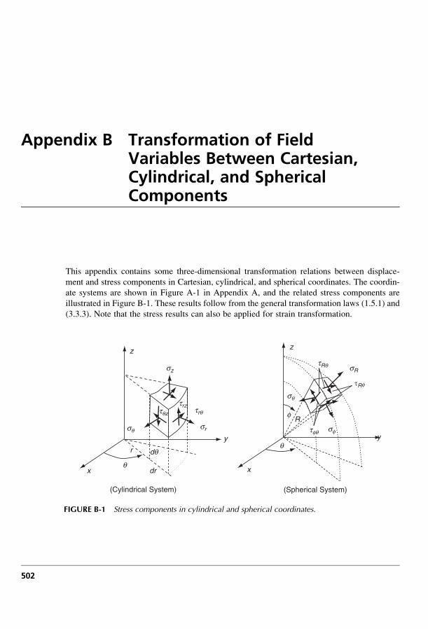
Appendix B Transformation of FieldVariables Between Cartesian,Cylindrical, and SphericalComponents
This appendix contains some three-dimensional transformation relations between displace-
ment and stress components in Cartesian, cylindrical, and spherical coordinates. The coordin-
ate systems are shown in Figure A-1 in Appendix A, and the related stress components are
illustrated in Figure B-1. These results follow from the general transformation laws (1.5.1) and
(3.3.3). Note that the stress results can also be applied for strain transformation.
x
y
r
z
dr
sz
sq sr
trqtrz
tqz
dq
(Cylindrical System) (Spherical System)
sR
sq
sf
z
x
y
R
tRq
τRf
q
f
q
tfq
FIGURE B-1 Stress components in cylindrical and spherical coordinates.
502
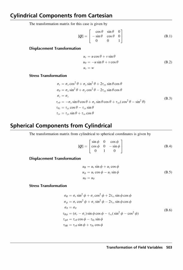
Cylindrical Components from Cartesian
The transformation matrix for this case is given by
[Q] ¼cos y sin y 0
� sin y cos y 0
0 0 1
24
35 (B:1)
Displacement Transformation
ur ¼ u cos yþ v sin y
uy ¼ �u sin yþ v cos y
uz ¼ w
(B:2)
Stress Transformation
sr ¼ sx cos2 yþ sy sin2 yþ 2txy sin y cos y
sy ¼ sx sin2 yþ sy cos2 y� 2txy sin y cos y
sz ¼ sz
try ¼ �sx sin y cos yþ sy sin y cos yþ txy( cos2 y� sin2 y)
tyz ¼ tyz cos y� tzx sin y
tzr ¼ tyz sin yþ tzx cos y
(B:3)
Spherical Components from Cylindrical
The transformation matrix from cylindrical to spherical coordinates is given by
[Q] ¼sinf 0 cosfcosf 0 � sinf0 1 0
24
35 (B:4)
Displacement Transformation
uR ¼ ur sinfþ uz cosf
uf ¼ ur cosf� uz sinf
uy ¼ uy
(B:5)
Stress Transformation
sR ¼ sr sin2 fþ sz cos2 fþ 2trz sinf cosf
sf ¼ sr cos2 fþ sz sin2 f� 2trz sinf cosf
sy ¼ sy
tRf ¼ (sr � sz) sinf cosf� trz( sin2 f� cos2 f)
tfy ¼ try cosf� tyz sinf
tyR ¼ try sinfþ tyz cosf
(B:6)
Transformation of Field Variables 503
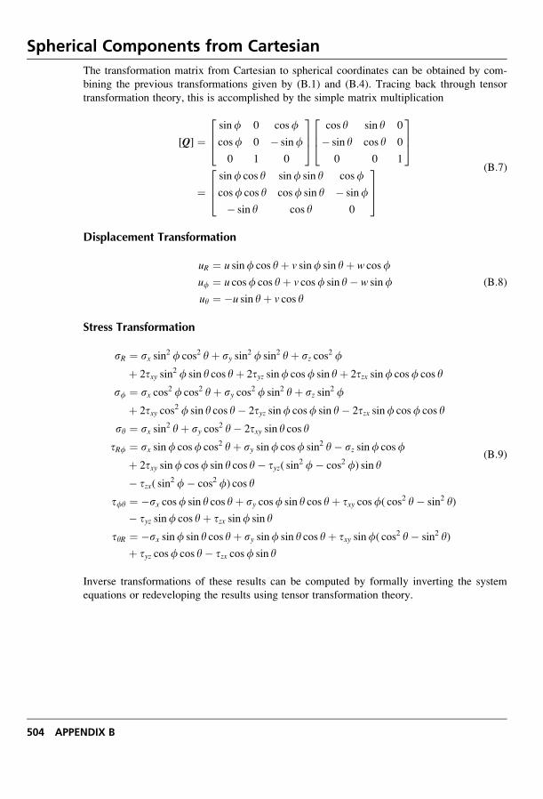
Spherical Components from Cartesian
The transformation matrix from Cartesian to spherical coordinates can be obtained by com-
bining the previous transformations given by (B.1) and (B.4). Tracing back through tensor
transformation theory, this is accomplished by the simple matrix multiplication
[Q] ¼sinf 0 cosf
cosf 0 � sinf
0 1 0
264
375
cos y sin y 0
� sin y cos y 0
0 0 1
264
375
¼sinf cos y sinf sin y cosf
cosf cos y cosf sin y � sinf
� sin y cos y 0
264
375
(B:7)
Displacement Transformation
uR ¼ u sinf cos yþ v sinf sin yþ w cosf
uf ¼ u cosf cos yþ v cosf sin y� w sinf
uy ¼ �u sin yþ v cos y
(B:8)
Stress Transformation
sR ¼ sx sin2 f cos2 yþ sy sin2 f sin2 yþ sz cos2 f
þ 2txy sin2 f sin y cos yþ 2tyz sinf cosf sin yþ 2tzx sinf cosf cos y
sf ¼ sx cos2 f cos2 yþ sy cos2 f sin2 yþ sz sin2 f
þ 2txy cos2 f sin y cos y� 2tyz sinf cosf sin y� 2tzx sinf cosf cos y
sy ¼ sx sin2 yþ sy cos2 y� 2txy sin y cos y
tRf ¼ sx sinf cosf cos2 yþ sy sinf cosf sin2 y� sz sinf cosf
þ 2txy sinf cosf sin y cos y� tyz( sin2 f� cos2 f) sin y
� tzx( sin2 f� cos2 f) cos y
tfy ¼ �sx cosf sin y cos yþ sy cosf sin y cos yþ txy cosf( cos2 y� sin2 y)
� tyz sinf cos yþ tzx sinf sin y
tyR ¼ �sx sinf sin y cos yþ sy sinf sin y cos yþ txy sinf( cos2 y� sin2 y)
þ tyz cosf cos y� tzx cosf sin y
(B:9)
Inverse transformations of these results can be computed by formally inverting the system
equations or redeveloping the results using tensor transformation theory.
504 APPENDIX B
Appendix C MATLAB Primer
Many locations in the text use numerical methods to calculate and plot solutions to a variety of
elasticity problems. Although other options are available, the author has found MATLAB
software ideally suited to conduct this numerical work. This particular software has all of the
necessary computational and plotting tools to enable very efficient and simple applications for
elasticity. MATLAB is a professional engineering and scientific software package developed
and marketed by MathWorks, Inc. In recent years, MATLAB has achieved widespread and
enthusiastic acceptance throughout the engineering community. Many engineering schools
now require and/or use MATLAB as one of their primary computing tools, and it is expected
that it will continue to replace older structured programming methods. Its popularity is because
of a long history of well-developed and tested products, its ease of use by students, and its
compatibility across many different computer platforms (e.g., PC, Mac, and UNIX). The
purpose of this appendix is to present a few MATLAB basics to help students apply particular
software applications for the needs of the text. The software package itself contains an
excellent Help package that provides extensive information on various commands and proced-
ures. Also, many books are available on the software package; see, for example, Palm (2008).
It is assumed that the reader has some prior background and experience with at least one other
programming language, and thus has a basic understanding of programming techniques.
C.1 Getting Started
MATLAB is both a computer programming language and a software environment for using the
language. Under the Microsoft Windows operating system, the MATLAB window appears as
shown in Figure C-1. It is from this window that the Help menu can be accessed, and this provides
extensive information onmost topics. In this commandwindow, the user can type instructions after
the prompt ‘‘�.’’ However, it is much more efficient to create and save application programs
within the editor/debugger window. This window is activated by clicking the File menu in the
Commandwindowand selecting eitherNew to start a new creation orOpen to open an existingfile.
MATLAB files are called m-files and have the extension ‘‘�:m’’. Within the editor/debugger
window, a new application code can be created or an existing one modified. In either case, the
resulting file can then be saved for later use, and the current file can be run from this window.
An example program appearing in the editor/debugger window is shown in Figure C-2.
505
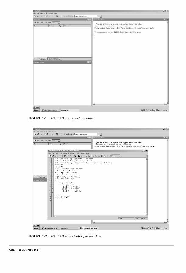
FIGURE C-1 MATLAB command window.
FIGURE C-2 MATLAB editor/debugger window.
506 APPENDIX C
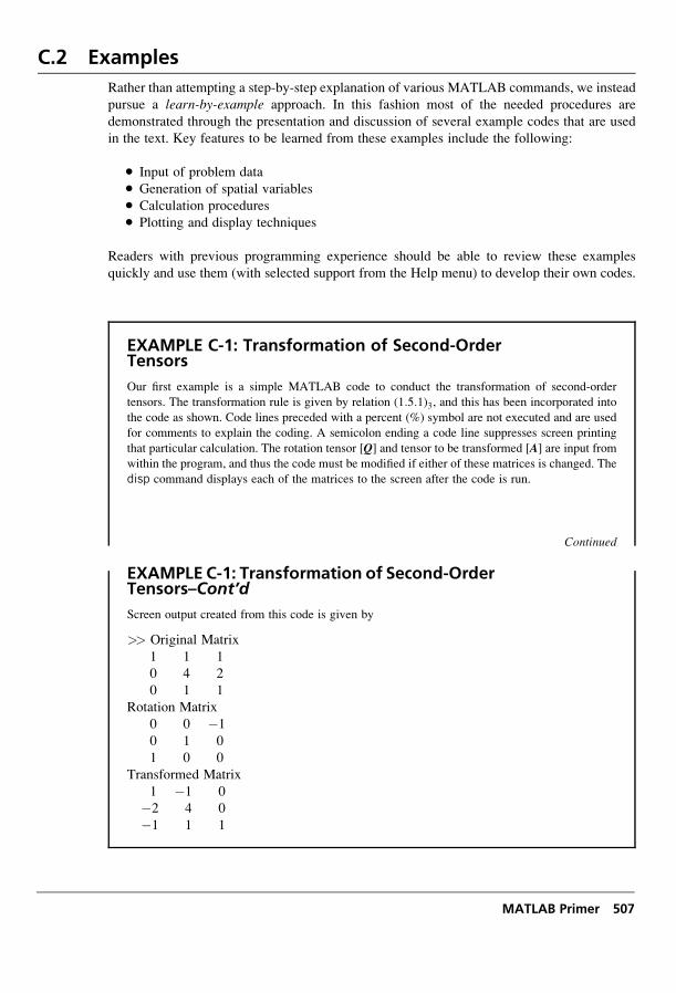
C.2 Examples
Rather than attempting a step-by-step explanation of various MATLAB commands, we instead
pursue a learn-by-example approach. In this fashion most of the needed procedures are
demonstrated through the presentation and discussion of several example codes that are used
in the text. Key features to be learned from these examples include the following:
. Input of problem data
. Generation of spatial variables
. Calculation procedures
. Plotting and display techniques
Readers with previous programming experience should be able to review these examples
quickly and use them (with selected support from the Help menu) to develop their own codes.
EXAMPLE C-1: Transformation of Second-OrderTensors
Our first example is a simple MATLAB code to conduct the transformation of second-order
tensors. The transformation rule is given by relation (1:5:1)3, and this has been incorporated into
the code as shown. Code lines preceded with a percent (%) symbol are not executed and are used
for comments to explain the coding. A semicolon ending a code line suppresses screen printing
that particular calculation. The rotation tensor [Q] and tensor to be transformed [A] are input from
within the program, and thus the code must be modified if either of these matrices is changed. The
disp command displays each of the matrices to the screen after the code is run.
Continued
EXAMPLE C-1: Transformation of Second-OrderTensors–Cont’d
Screen output created from this code is given by
>> Original Matrix
1 1 1
0 4 2
0 1 1
Rotation Matrix
0 0 �1
0 1 0
1 0 0
Transformed Matrix
1 �1 0
�2 4 0
�1 1 1
MATLAB Primer 507

EXAMPLE C-2: Calculation of Invariants, Eigenvalues,and Eigenvectors of a Matrix
MATLAB provides very simple and efficient methods to determine the invariants, principal
values, and directions of second-order tensors (matrices). The basic tool for the eigenvalue
problem is the command eig( ), which will generate both the eigenvalues and eigenvectors. The
following simple code illustrates the basics for the matrix originally given in Example 1-3.
% MATLAB CODE: Example C-2% Elasticity: Theory, Applications and Numerics - Elsevier% M.H. Sadd, University of Rhode Island% Program to Numerically Calculate Invariants, Principal Values% and Directions of a Matrix% Program Uses Matrix from Example 1-3clc;clear all;% Input MatrixA¼ [2,0,0;0,3,4;0,4,-3]% Calculate Invariantsinvariants¼ [trace(A),(trace(A)^2-trace(A�A))/2,det(A)][V,L]¼ eig(A);% Principal Values are the Diagonal Elements of the L Matrixprincipal_values¼ [L(1,1),L(2,2),L(3,3)]% Principal Directions are the Columns of the V Matrixprincipal_directions¼ [V(:,1),V(:,2),V(:,3)]
508 APPENDIX C
MATLAB Primer 509
EXAMPLE C-2: Cont’d
Screen output created from this code is given by
A ¼
2 0 0
0 3 4
0 4 �3
invariants ¼
2 �25 �50
principal_values ¼
�5 2 5
principal_directions ¼
0 1:0000 0
0:4472 0 �0:8944�0:8944 0 �0:4472
EXAMPLE C-3: XY Plotting of Stresses in Figure 8-9
The MATLAB code shown was developed to calculate and plot the radial and circumferential
stresses in a thick-walled cylinder under internal pressure loading from Example 8-6. The
theoretical expressions for the stresses are given by equations (8.4.3), and the plot is shown in
Figure 8-9. The nondimensional radial coordinate r=r2 is conveniently generated from 0.5 to 1,
and the length(r) expression gives the number of terms in the r array, which is used as the limiter
on the looping index. This simple code illustrates the for-end looping and calculation procedure
and the basic XY plot call used to draw the two stress curves. Note the plot formatting used to
label the axes. Additional format control is available through the Help menu, and the plot can also
be edited within the generated plot window.
% MATLAB CODE C-3; Elasticity: Theory, Applications & Numerics% Martin H. Sadd, University of Rhode Island% Calculate and Plot Stresses in Thick-Walled Cylinder Problem Example 8-6% Internal Pressure Loading Case with r1/r2=0.5; Generate Figure 8-9clear;% Generate Nondimensional Radial Coordinate Space: r/r2r=[0.5:0.01:1];% Calculation Loop for Stressesfor i=1:length(r) sr(i)=0.3333*(1-(1/r(i))^2); st(i)=0.3333*(1+(1/r(i)) ^2);end% Plotting Callplot(r,sr,r,st),xlabel(‘Dimensionles Distance, ‘),ylabel(‘Dimensionless Stress’)
EXAMPLE C-4: Polar Contour Plotting of Hoop StressAround a Circular Hole in Figure 8-13
This example illustrates a code used to plot the hoop stresses on the boundary of a circular hole in an
infinite plane under uniform far-field tension (see problem geometry in Figure 8-12). The hoop stress
was given by equation (8.4.15)2, and the plot on the boundary of the hole is shown in Figure 8-13.
Similar to the previous example, this code calculates the necessary stress values and then displays
them in a polar plot. The angular coordinate is generated from 0 to 2�. For this code, the use of thefor-loop is dropped since MATLAB can automatically handle calculations with matrix/vector
arguments. The plotting call used in this example is the polar command that generates Figure 8-13.
Additional formatting can be applied to the polar plot call to control line type, thickness, and so on, and
these can also be edited in the plot window.
% MATLAB CODE: Example C-4% Elasticity: Theory, Applications and Numerics - Elsevier% M.H. Sadd, University of Rhode Island% Calculate and Plot Normalized Hoop Stress on Circular Hole% In Infinite Plane Under Uniform Tension at Infinity: Example 8.7% Nondimensional Plot Generates Figure 8-13clear;% Input (r/a)- Variable and Generate Angular Coordinate Spacer¼ 1;t¼ [0:0.01:2�pi];% Calculation Loopst¼ 0.5�(1þ(1/r)^2)-0.5�(1þ3�(1/r)^4)�cos(2�t);% Plotting Callpolar(t,st)title(‘Nondimensional Hoop stress Around Hole’)
EXAMPLE C-5: Displacement Vector Distribution Plottingin Figure 8-22
Consider next the example of plotting the displacement vectors for the Flamant problem of
Section 8.4.7 shown in Figure 8-19. For the normal loading case, the displacement field is given
by relations (8.4.43), and these are plotted in Figure 8-22 for the near-field case (0 < r < 0:5) with
a Poisson’s ratio of 0.3 and Y=E ¼ 1. Radial coordinates are generated by the logspace command
as explained in the comment line, and this range can easily be changed to investigate other regions
of the half plane. Within the calculation loops, the Cartesian coordinates and displacement
components are changed to reflect the system used in Chapter 8. The plotting is done using the
quiver command, which draws two-dimensional vectors with components ux and uy at locations xand y. Additional details on this type of plotting can be found in the Help menu.
% MATLAB CODE C-5: Elasticity: Theory, Applications & Numerics% Martin H. Sadd, University of Rhode Island% Displacement Vector Distribution Plot for Flamant Problem - Figure 8-19% Normal Loading Case (X=0); Generates Figure 8-22% Input Parameters
510 APPENDIX C
MATLAB Primer 511
EXAMPLE C-5: Cont’d
Y=1; E=1; nu=0.3;% Input Radial Coordinates: logspace(M,N,*) Generates Region 10^M < r< 10^Nr=logspace(-3,-0.5,60);% Input Theta Coordinatest=[0:pi/20:pi];% calculation Loopsfor i=1:length(r) for j=1:length(t) x(i,j)=r(i)*cos(t(j)); y(i,j)=r(i)*sin(t(j)); % Coordinate Change x(i,j)=-x(i,j); y(i,j)=-y(i,j); % Calculate Polar Displacement Components ur(i,j)=Y/(pi*E)*((1-nu)*(t(j)-pi/2)*cos(t(j))-2*log(r(i))*sin(t(j))); ut(i,j)=Y/(pi*E)*(-(1-nu)*(t(j)-pi/2)*sin(t(j))-2*log(r(i))*cos(t(j))-(1+nu)*cos(t(j))); % Calculate Cartesian Displacement Components ux(i,j)=cos(t(j))*ur(i,j)-sin(t(j))*ut(i,j); uy(i,j)=sin(t(j))*ur(i,j)+cos(t(j))*ut(i,j); % Corrdinate Change ux(i,j)=-ux(i,j); uy(i,j)=-uy(i,j); end end clf; hold on; axis equal; % Plotting Call for Vector Distribution quiver(x,y,ux,uy)
EXAMPLE C-6: Plotting of Warping Displacement Contoursin Figure 9-8
The following MATLAB code has been developed to calculate and plot the warping displacements
for the torsion of a cylinder with elliptical section shown in Figure 9-7. This code uses many of the
same commands from the previous examples to input parameters, generate the variable grid space,
and conduct the calculations to determine the warping displacement array. The plotting call uses the
contour command, which generates contours of constantwwithin the grid space that was created to
lie inside the elliptical boundary. The code generates the displacement contours shown in Figure 9-8.
Again, additional formatting details on this plotting command can be found in the Help menu.
% MATLAB CODE C-6: Elasticity: Theory, Applications & Numerics% Martin H. Sadd, University of Rhode Island% Generates 2-D Warping Displacement Contours for% Elliptical Section Under Torsion - Figure 9-8close allclear all
Continued
EXAMPLE C-6: Plotting of Warping Displacement Contoursin Figure 9-8–Cont’d
% Input Geometry and Angle of Twista=1.0; b=0.5; alpha=1.0;% Input Grid Spacer=[0.01:0.05:1]; t=[0:pi/10:2*pi];% Generate Contour DataK=alpha*(b^2-a^2)/(a^2+b^2);for i=1:length(r) for j=1:length(t) x(i,j)=a*r(i)*cos(t(j)); j(i,j)=b*r(i)*sin(t(j)); w(i,j)=K*x(i,j)*y(i,j); endend% Plotting Call with 20 Contourscontour(x,y,w,20);axis equal
EXAMPLE C-7: Plotting a Three-DimensionalWarpingDisplacement Surface in Figure 9-8
This example illustrates how MATLAB can make a three-dimensional surface plot of the warping
displacement for the torsion of an elliptical section. Figure 9-8 shows the surface plot created from
this code. After generating appropriate x- and y-location arrays, the warping displacement values are
calculated and stored in the array w. Using the surf command, the warping surface is then generated
in a three-dimensional system. Numerous viewing parameters can be edited to suit the desired view.
% MATLAB CODE: Example C-7% Elasticity: Theory, Applications & Numerics% Professor Martin H. Sadd, University of Rhode Island% Three Dimensional Plot of Warping Displacement Surface% for Elliptical Section Under Torsionclc;clear all; close allt¼ [0:5:360];r¼ [0:0.05:1];a¼ 1;b¼ 0.5;for i¼ 1:length(r)
for j¼ 1:length(t)th¼ t(j)�pi/180;xc¼ a�r(i)�cos(th);yc¼ b�r(i)�sin(th);w(i,j)¼ -xc�yc;y(i,j)¼ yc;x(i,j)¼ xc;
endendsurfc(x,y,w);colormap grayh¼ findobj(gcf,‘type’,‘patch’);set(h,‘LineWidth’, 1.0, ‘EdgeColor’,‘k’);axis([-1 1 -1 1])axis squareview(20,10)
512 APPENDIX C
MATLAB Primer 513
EXAMPLE C-8: Determination of Roots for OrthotropicMaterials
InChapter 11anisotropic solutions toplane elasticity problems required the roots of thecharacteristic
equation (11.5.7). As indicated in Exercise 11-12, for orthotropic materials this characteristic equa-
tion reduces to a quadratic with roots b1, 2. TheMATLAB code shown calculates these two roots and
writes the results to the screen command window. This code illustrates some of the basic formatting
issues related to inputting names and data and printing calculated information to the screen.
% MATLAB CODE C-8: Elasticity: Theory, Applications & Numerics% Martin H. Sadd, University of Rhode Island% Calculate Beta Parameters of Orthotropic E-Glass Materialclear;% Input Number of Materials,Names and Stiffness ModuliN=1;name(1,:)='E-Glass/Epoxy';e1(1)=38.6; e2(1)=8.3; nu12(1)=0.26; mu12(1)=4.2;% Calculate Compliancesfor i=1:Ns11(i)=1/e1(i); s22(i)=1/e2(i); s12(i)=-nu12(i)/e1(i); s66(i)=1/mu12(i); % Calculate Beta Values From Solution to Quadratic Characteristic Equationb1(i)=sqrt(-(1/(2*s11(i)))*(-(2*s12(i)+s66(i))+sqrt((2*s12(i)+s66(i))^2-4*s11(i)*s22(i))));b2(i)=sqrt(-(1/(2*s11(i)))*(-(2*s12(i)+s66(i))-sqrt((2*s12(i)+s66(i))^2-4*s11(i)*s22(i))));% Print Results to Screenfprintf(1,'\n ')disp(name(i,:))fprintf(i,' beta(1)=%5.3f',b1(i))fprintf(1,' beta(2)=%5.3',b2(i))end
Screen output from this particular case is given by
>> E-Glass/Epoxy beta(1)=0.758 beta(2)=2.845 >>
EXAMPLE C-9: PDE Toolbox: Finite Element Applicationof a Circular Hole in a Plate Under Uniform Tensionfrom Example 16-2
In Chapter 16 the PDE Toolbox was presented as MATLAB application software that could conduct
two-dimensional finite element analysis. We now present some of the basic steps in generating the
solution to the problem of a circular hole in a plate under uniform tension as originally discussed in
Example 16-2. Once properly installed, the PDEToolbox is activated by typing the command pdetoolin theMATLAB commandwindow. This brings up the graphical user interface (GUI) window shown
in Figure C-3.Within this window, the first step is to select the type of problem by choosing one of the
items from the pull-down menu, as shown in Figure C-4. The figure illustrates the selection of
‘‘Structural Mech., Plane Stress.’’ Other useful choices include ‘‘Structural Mech., Plane Strain’’
for plane strain analysis and ‘‘Generic Scalar,’’ which can be used to find numerical solutions to the
torsion problem; see Example 16-4 and Figure 16-7. After selecting the problem type, click the PDE
button to open a window to input the desired values of elastic moduli and body forces.
Continued
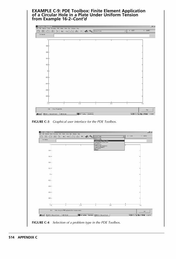
EXAMPLE C-9: PDE Toolbox: Finite Element Applicationof a Circular Hole in a Plate Under Uniform Tensionfrom Example 16-2–Cont’d
FIGURE C-3 Graphical user interface for the PDE Toolbox.
FIGURE C-4 Selection of a problem type in the PDE Toolbox.
514 APPENDIX C
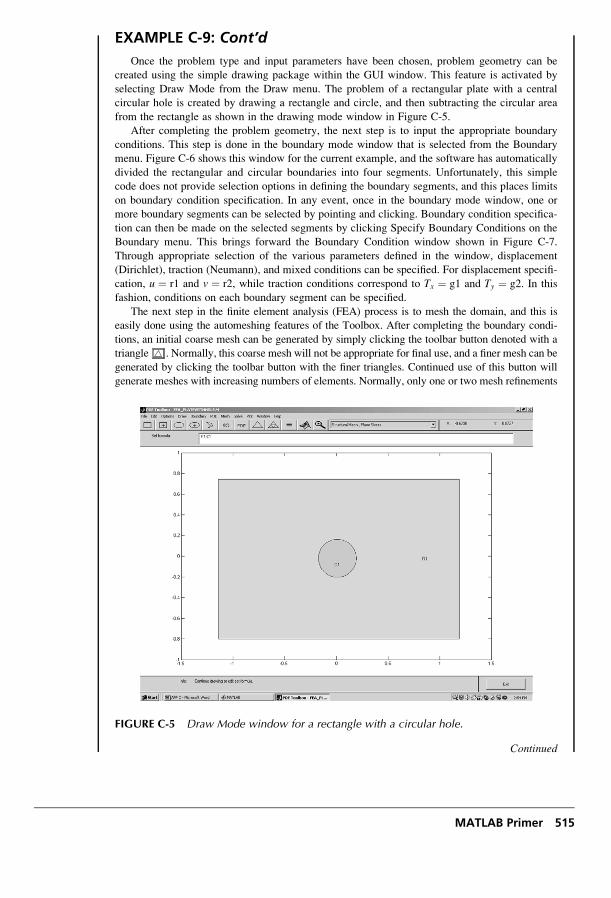
EXAMPLE C-9: Cont’d
Once the problem type and input parameters have been chosen, problem geometry can be
created using the simple drawing package within the GUI window. This feature is activated by
selecting Draw Mode from the Draw menu. The problem of a rectangular plate with a central
circular hole is created by drawing a rectangle and circle, and then subtracting the circular area
from the rectangle as shown in the drawing mode window in Figure C-5.
After completing the problem geometry, the next step is to input the appropriate boundary
conditions. This step is done in the boundary mode window that is selected from the Boundary
menu. Figure C-6 shows this window for the current example, and the software has automatically
divided the rectangular and circular boundaries into four segments. Unfortunately, this simple
code does not provide selection options in defining the boundary segments, and this places limits
on boundary condition specification. In any event, once in the boundary mode window, one or
more boundary segments can be selected by pointing and clicking. Boundary condition specifica-
tion can then be made on the selected segments by clicking Specify Boundary Conditions on the
Boundary menu. This brings forward the Boundary Condition window shown in Figure C-7.
Through appropriate selection of the various parameters defined in the window, displacement
(Dirichlet), traction (Neumann), and mixed conditions can be specified. For displacement specifi-
cation, u ¼ r1 and v ¼ r2, while traction conditions correspond to Tx ¼ g1 and Ty ¼ g2. In this
fashion, conditions on each boundary segment can be specified.
The next step in the finite element analysis (FEA) process is to mesh the domain, and this is
easily done using the automeshing features of the Toolbox. After completing the boundary condi-
tions, an initial coarse mesh can be generated by simply clicking the toolbar button denoted with a
triangle . Normally, this coarse mesh will not be appropriate for final use, and a finer mesh can be
generated by clicking the toolbar button with the finer triangles. Continued use of this button will
generate meshes with increasing numbers of elements. Normally, only one or two mesh refinements
FIGURE C-5 Draw Mode window for a rectangle with a circular hole.
Continued
MATLAB Primer 515
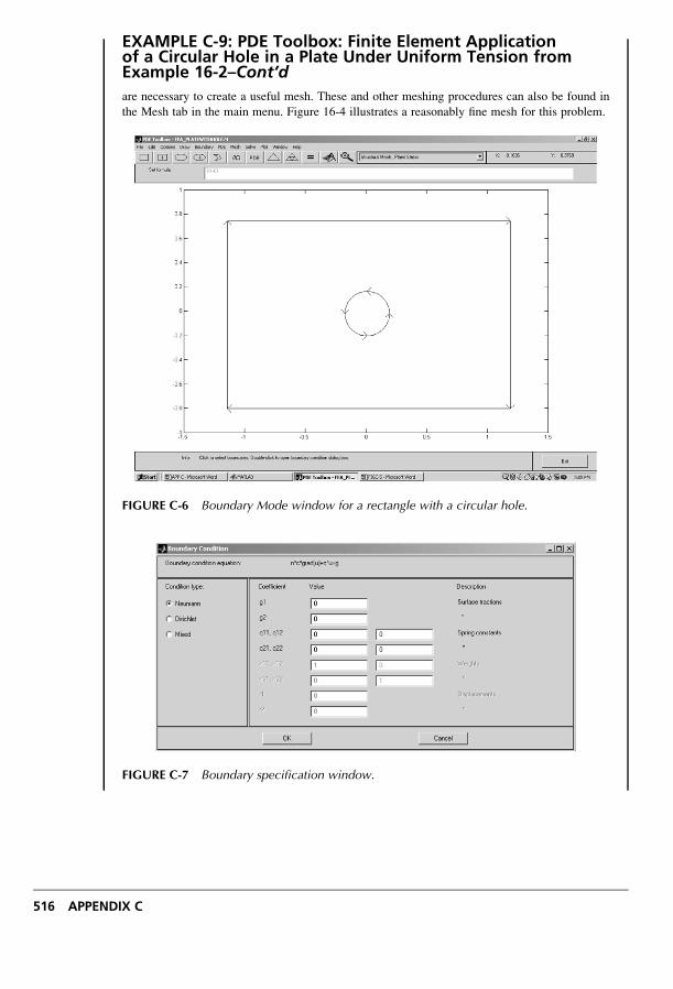
EXAMPLE C-9: PDE Toolbox: Finite Element Applicationof a Circular Hole in a Plate Under Uniform Tension fromExample 16-2–Cont’d
are necessary to create a useful mesh. These and other meshing procedures can also be found in
the Mesh tab in the main menu. Figure 16-4 illustrates a reasonably fine mesh for this problem.
FIGURE C-6 Boundary Mode window for a rectangle with a circular hole.
FIGURE C-7 Boundary specification window.
516 APPENDIX C
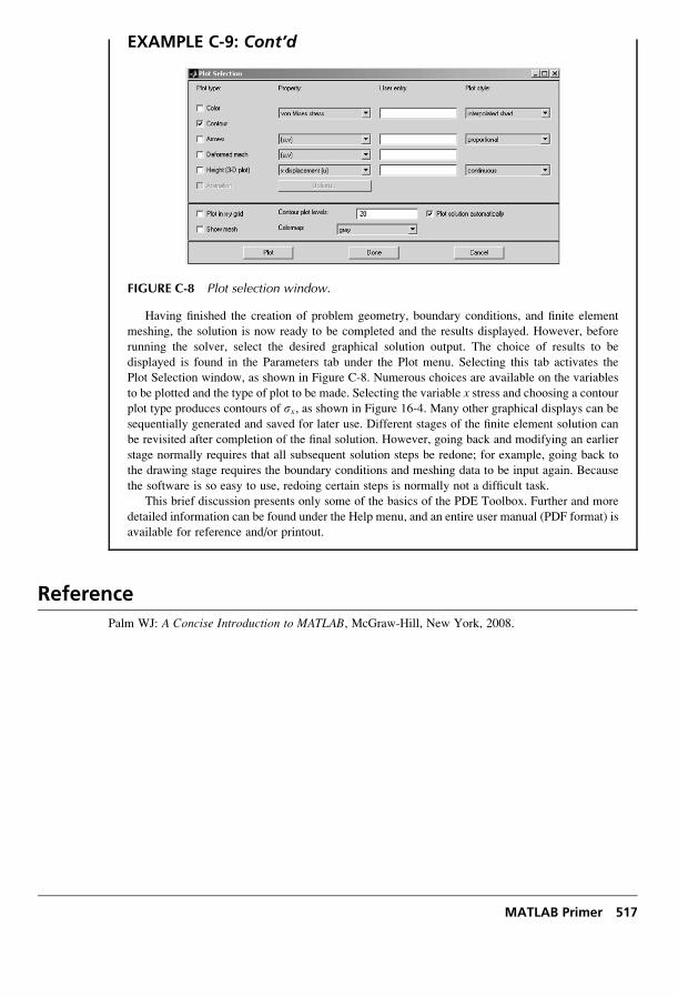
EXAMPLE C-9: Cont’d
FIGURE C-8 Plot selection window.
Having finished the creation of problem geometry, boundary conditions, and finite element
meshing, the solution is now ready to be completed and the results displayed. However, before
running the solver, select the desired graphical solution output. The choice of results to be
displayed is found in the Parameters tab under the Plot menu. Selecting this tab activates the
Plot Selection window, as shown in Figure C-8. Numerous choices are available on the variables
to be plotted and the type of plot to be made. Selecting the variable x stress and choosing a contourplot type produces contours of sx, as shown in Figure 16-4. Many other graphical displays can be
sequentially generated and saved for later use. Different stages of the finite element solution can
be revisited after completion of the final solution. However, going back and modifying an earlier
stage normally requires that all subsequent solution steps be redone; for example, going back to
the drawing stage requires the boundary conditions and meshing data to be input again. Because
the software is so easy to use, redoing certain steps is normally not a difficult task.
This brief discussion presents only some of the basics of the PDE Toolbox. Further and more
detailed information can be found under the Help menu, and an entire user manual (PDF format) is
available for reference and/or printout.
Reference
Palm WJ: A Concise Introduction to MATLAB, McGraw-Hill, New York, 2008.
MATLAB Primer 517
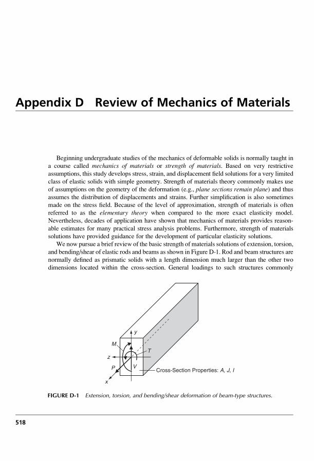
Appendix D Review of Mechanics of Materials
Beginning undergraduate studies of the mechanics of deformable solids is normally taught in
a course called mechanics of materials or strength of materials. Based on very restrictive
assumptions, this study develops stress, strain, and displacement field solutions for a very limited
class of elastic solids with simple geometry. Strength of materials theory commonly makes use
of assumptions on the geometry of the deformation (e.g., plane sections remain plane) and thus
assumes the distribution of displacements and strains. Further simplification is also sometimes
made on the stress field. Because of the level of approximation, strength of materials is often
referred to as the elementary theory when compared to the more exact elasticity model.
Nevertheless, decades of application have shown that mechanics of materials provides reason-
able estimates for many practical stress analysis problems. Furthermore, strength of materials
solutions have provided guidance for the development of particular elasticity solutions.
We now pursue a brief review of the basic strength of materials solutions of extension, torsion,
and bending/shear of elastic rods and beams as shown in Figure D-1. Rod and beam structures are
normally defined as prismatic solids with a length dimension much larger than the other two
dimensions located within the cross-section. General loadings to such structures commonly
x
z
y
P
M
VCross-Section Properties: A, J, I
T
FIGURE D-1 Extension, torsion, and bending/shear deformation of beam-type structures.
518
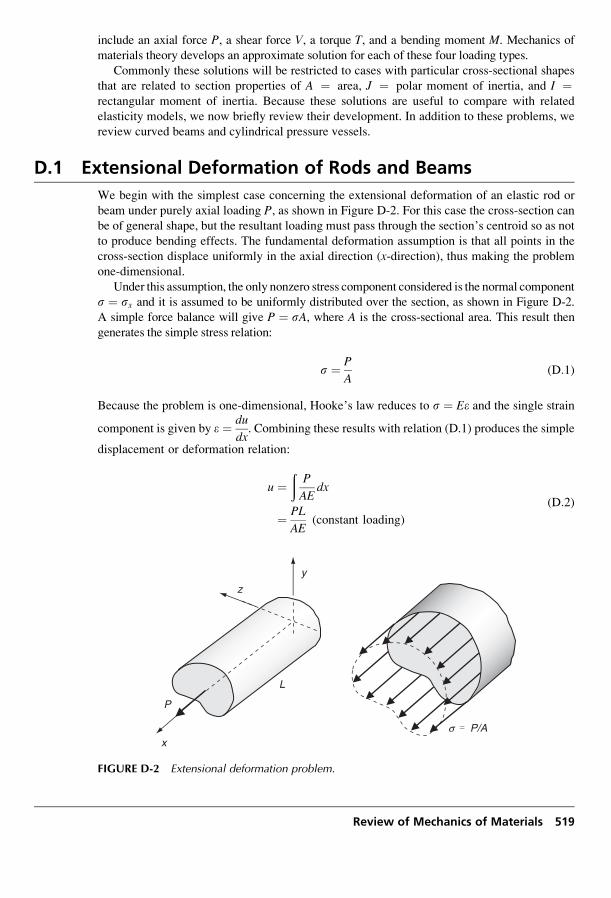
include an axial force P, a shear force V, a torque T, and a bending moment M. Mechanics of
materials theory develops an approximate solution for each of these four loading types.
Commonly these solutions will be restricted to cases with particular cross-sectional shapes
that are related to section properties of A ¼ area, J ¼ polar moment of inertia, and I ¼rectangular moment of inertia. Because these solutions are useful to compare with related
elasticity models, we now briefly review their development. In addition to these problems, we
review curved beams and cylindrical pressure vessels.
D.1 Extensional Deformation of Rods and Beams
We begin with the simplest case concerning the extensional deformation of an elastic rod or
beam under purely axial loading P, as shown in Figure D-2. For this case the cross-section can
be of general shape, but the resultant loading must pass through the section’s centroid so as not
to produce bending effects. The fundamental deformation assumption is that all points in the
cross-section displace uniformly in the axial direction (x-direction), thus making the problem
one-dimensional.
Under this assumption, the only nonzero stress component considered is the normal component
s ¼ sx and it is assumed to be uniformly distributed over the section, as shown in Figure D-2.
A simple force balance will give P ¼ sA, where A is the cross-sectional area. This result then
generates the simple stress relation:
s ¼ P
A(D:1)
Because the problem is one-dimensional, Hooke’s law reduces to s ¼ Ee and the single strain
component is given by e ¼ du
dx. Combining these results with relation (D.1) produces the simple
displacement or deformation relation:
u ¼ð
P
AEdx
¼ PL
AE(constant loading)
(D:2)
x
y
z
P
L
s P/A
FIGURE D-2 Extensional deformation problem.
Review of Mechanics of Materials 519
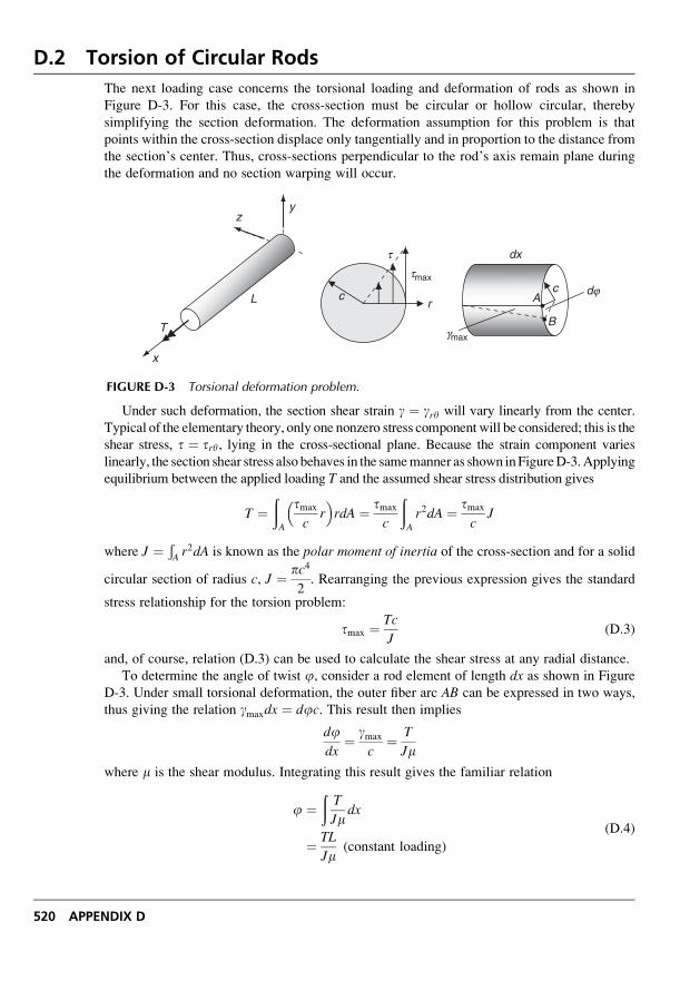
D.2 Torsion of Circular Rods
The next loading case concerns the torsional loading and deformation of rods as shown in
Figure D-3. For this case, the cross-section must be circular or hollow circular, thereby
simplifying the section deformation. The deformation assumption for this problem is that
points within the cross-section displace only tangentially and in proportion to the distance from
the section’s center. Thus, cross-sections perpendicular to the rod’s axis remain plane during
the deformation and no section warping will occur.
Under such deformation, the section shear strain g ¼ gry will vary linearly from the center.
Typical of the elementary theory, only one nonzero stress component will be considered; this is the
shear stress, t ¼ try, lying in the cross-sectional plane. Because the strain component varies
linearly, the section shear stress also behaves in the samemanner as shown inFigureD-3.Applying
equilibrium between the applied loading T and the assumed shear stress distribution gives
T ¼ðA
tmax
cr
� �rdA ¼ tmax
c
ðA
r2dA ¼ tmax
cJ
where J ¼ ÐA r2dA is known as the polar moment of inertia of the cross-section and for a solid
circular section of radius c, J ¼ pc4
2. Rearranging the previous expression gives the standard
stress relationship for the torsion problem:
tmax ¼ Tc
J(D:3)
and, of course, relation (D.3) can be used to calculate the shear stress at any radial distance.
To determine the angle of twist j, consider a rod element of length dx as shown in Figure
D-3. Under small torsional deformation, the outer fiber arc AB can be expressed in two ways,
thus giving the relation gmaxdx ¼ djc. This result then implies
djdx
¼ gmax
c¼ T
Jm
where m is the shear modulus. Integrating this result gives the familiar relation
j ¼ðT
Jmdx
¼ TL
Jm(constant loading)
(D:4)
x
yz
T
L
t
tmax
rc
dx
c
gmax
djA
B••
FIGURE D-3 Torsional deformation problem.
520 APPENDIX D
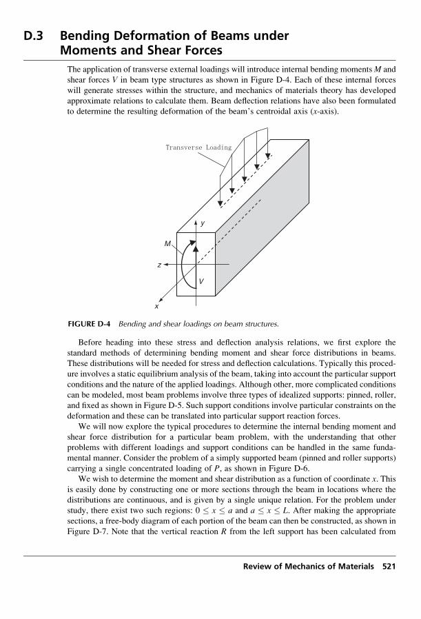
D.3 Bending Deformation of Beams underMoments and Shear Forces
The application of transverse external loadings will introduce internal bending momentsM and
shear forces V in beam type structures as shown in Figure D-4. Each of these internal forces
will generate stresses within the structure, and mechanics of materials theory has developed
approximate relations to calculate them. Beam deflection relations have also been formulated
to determine the resulting deformation of the beam’s centroidal axis (x-axis).
Before heading into these stress and deflection analysis relations, we first explore the
standard methods of determining bending moment and shear force distributions in beams.
These distributions will be needed for stress and deflection calculations. Typically this proced-
ure involves a static equilibrium analysis of the beam, taking into account the particular support
conditions and the nature of the applied loadings. Although other, more complicated conditions
can be modeled, most beam problems involve three types of idealized supports: pinned, roller,
and fixed as shown in Figure D-5. Such support conditions involve particular constraints on the
deformation and these can be translated into particular support reaction forces.
We will now explore the typical procedures to determine the internal bending moment and
shear force distribution for a particular beam problem, with the understanding that other
problems with different loadings and support conditions can be handled in the same funda-
mental manner. Consider the problem of a simply supported beam (pinned and roller supports)
carrying a single concentrated loading of P, as shown in Figure D-6.
We wish to determine the moment and shear distribution as a function of coordinate x. Thisis easily done by constructing one or more sections through the beam in locations where the
distributions are continuous, and is given by a single unique relation. For the problem under
study, there exist two such regions: 0 � x � a and a � x � L. After making the appropriate
sections, a free-body diagram of each portion of the beam can then be constructed, as shown in
Figure D-7. Note that the vertical reaction R from the left support has been calculated from
x
z
y
M
V
FIGURE D-4 Bending and shear loadings on beam structures.
Review of Mechanics of Materials 521
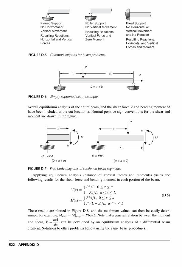
overall equilibrium analysis of the entire beam, and the shear force V and bending moment Mhave been included at the cut location x. Normal positive sign conventions for the shear and
moment are drawn in the figure.
Applying equilibrium analysis (balance of vertical forces and moments) yields the
following results for the shear force and bending moment in each portion of the beam.
V(x) ¼ Pb=L, 0 � x � a
�Pa=L, a � x � L
�
M(x) ¼ Pbx=L, 0 � x � a
Pa(L� x)=L, a � x � L
� (D:5)
These results are plotted in Figure D-8, and the maximum values can then be easily deter-
mined; for example,Mmax ¼ Mjx¼a ¼ Pba=L. Note that a general relation between the moment
and shear, V ¼ dM
dx, can be developed by an equilibrium analysis of a differential beam
element. Solutions to other problems follow using the same basic procedures.
Pinned Support:No Horizontal orVertical Movement
Resulting Reactions:Horizontal and VerticalForces
Roller Support:No Vertical Movement
Resulting Reactions:Vertical Force andZero Moment
Fixed Support:No Horizontal orVertical Movementand No Rotation
Resulting Reactions:Horizontal and VerticalForces and Moment
FIGURE D-5 Common supports for beam problems.
b
P
L = a + b
xa
FIGURE D-6 Simply supported beam example.
a
P
x
V
M
R = Pb/L
x
V
M
R = Pb/L
(0 < x < a) (a < x < L)
FIGURE D-7 Free-body diagrams of sectioned beam segments.
522 APPENDIX D
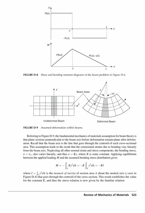
Review of Mechanics of Materials 523
Referring to FigureD-9, the fundamentalmechanics ofmaterials assumption for beam theory is
that plane sections perpendicular to the beam axis before deformation remain plane after deform-
ation. Recall that the beam axis is the line that goes through the centroid of each cross-sectional
area. This assumption leads to the result that the extensional strains due to bending vary linearly
from the beam axis. Neglecting all other normal strain and stress components, the bending stress,
s ¼ sx, also varies linearly, and thus s ¼ Ky, where K is some constant. Applying equilibrium
between the applied loadingM and the assumed bending stress distribution gives
M ¼ �ðA
Ky2dA ¼ �K
ðA
y2dA ¼ �KI
where I ¼ ÐA y2dA is the moment of inertia of section area A about the neutral axis (z-axis inFigure D-4) that goes through the centroid of the cross-section. This result establishes the value
for the constant K, and thus the stress relation is now given by the familiar relation
ax
L
V
Pb/L
−Pa/L
xL
M
Pbx/L Pa(L−x)/L
a
FIGURE D-8 Shear and bending moment diagrams of the beam problem in Figure D-6.
Undeformed Beam Deformed Beam
Beam Axes
x
y
•
r
Δq
FIGURE D-9 Assumed deformation within beams.
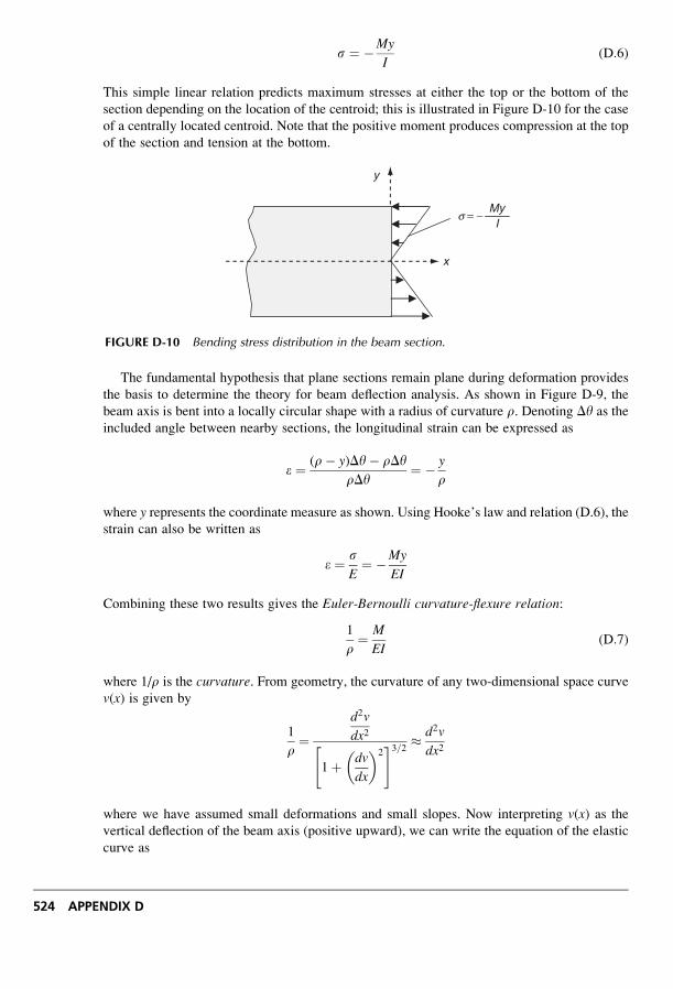
s ¼ �My
I(D:6)
This simple linear relation predicts maximum stresses at either the top or the bottom of the
section depending on the location of the centroid; this is illustrated in Figure D-10 for the case
of a centrally located centroid. Note that the positive moment produces compression at the top
of the section and tension at the bottom.
The fundamental hypothesis that plane sections remain plane during deformation provides
the basis to determine the theory for beam deflection analysis. As shown in Figure D-9, the
beam axis is bent into a locally circular shape with a radius of curvature r. Denoting Dy as the
included angle between nearby sections, the longitudinal strain can be expressed as
e ¼ (r� y)Dy� rDyrDy
¼ � y
r
where y represents the coordinate measure as shown. Using Hooke’s law and relation (D.6), the
strain can also be written as
e ¼ sE¼ �My
EI
Combining these two results gives the Euler-Bernoulli curvature-flexure relation:
1
r¼ M
EI(D:7)
where 1/r is the curvature. From geometry, the curvature of any two-dimensional space curve
v(x) is given by
1
r¼
d2v
dx2
1þ dv
dx
� �2" #3=2 � d2v
dx2
where we have assumed small deformations and small slopes. Now interpreting v(x) as the
vertical deflection of the beam axis (positive upward), we can write the equation of the elastic
curve as
x
y
IMy
s = −
FIGURE D-10 Bending stress distribution in the beam section.
524 APPENDIX D
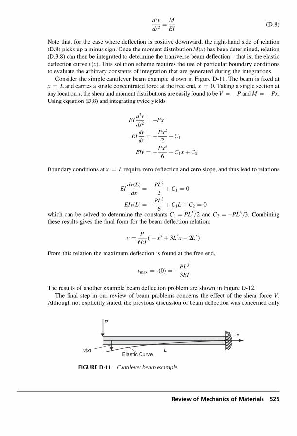
d2v
dx2¼ M
EI(D:8)
Note that, for the case where deflection is positive downward, the right-hand side of relation
(D.8) picks up a minus sign. Once the moment distribution M(x) has been determined, relation
(D.3.8) can then be integrated to determine the transverse beam deflection—that is, the elastic
deflection curve v(x). This solution scheme requires the use of particular boundary conditions
to evaluate the arbitrary constants of integration that are generated during the integrations.
Consider the simple cantilever beam example shown in Figure D-11. The beam is fixed at
x ¼ L and carries a single concentrated force at the free end, x ¼ 0. Taking a single section at
any location x, the shear andmoment distributions are easily found to beV ¼ �P andM ¼ �Px.Using equation (D.8) and integrating twice yields
EId2v
dx2¼ �Px
EIdv
dx¼ �Px2
2þ C1
EIv ¼ �Px3
6þ C1xþ C2
Boundary conditions at x ¼ L require zero deflection and zero slope, and thus lead to relations
EIdv(L)
dx¼ �PL2
2þ C1 ¼ 0
EIv(L) ¼ �PL3
6þ C1Lþ C2 ¼ 0
which can be solved to determine the constants C1 ¼ PL2=2 and C2 ¼ �PL3=3. Combining
these results gives the final form for the beam deflection relation:
v ¼ P
6EI(� x3 þ 3L2x� 2L3)
From this relation the maximum deflection is found at the free end,
vmax ¼ v(0) ¼ �PL3
3EI
The results of another example beam deflection problem are shown in Figure D-12.
The final step in our review of beam problems concerns the effect of the shear force V.Although not explicitly stated, the previous discussion of beam deflection was concerned only
Review of Mechanics of Materials 525
v(x)Elastic Curve
P
L
x
FIGURE D-11 Cantilever beam example.
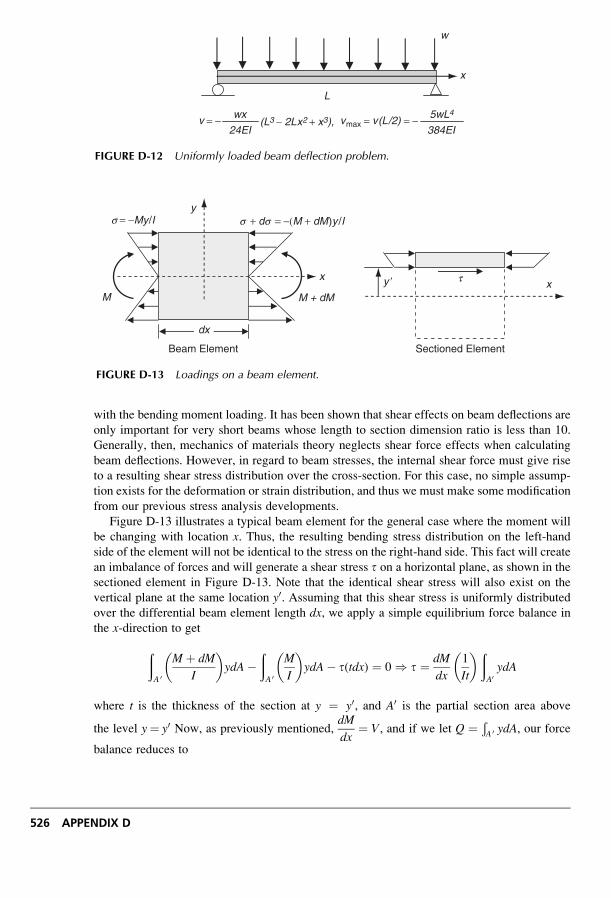
with the bending moment loading. It has been shown that shear effects on beam deflections are
only important for very short beams whose length to section dimension ratio is less than 10.
Generally, then, mechanics of materials theory neglects shear force effects when calculating
beam deflections. However, in regard to beam stresses, the internal shear force must give rise
to a resulting shear stress distribution over the cross-section. For this case, no simple assump-
tion exists for the deformation or strain distribution, and thus we must make some modification
from our previous stress analysis developments.
Figure D-13 illustrates a typical beam element for the general case where the moment will
be changing with location x. Thus, the resulting bending stress distribution on the left-hand
side of the element will not be identical to the stress on the right-hand side. This fact will create
an imbalance of forces and will generate a shear stress t on a horizontal plane, as shown in the
sectioned element in Figure D-13. Note that the identical shear stress will also exist on the
vertical plane at the same location y0. Assuming that this shear stress is uniformly distributed
over the differential beam element length dx, we apply a simple equilibrium force balance in
the x-direction to get
ðA 0
M þ dM
I
� �ydA�
ðA 0
M
I
� �ydA� t(tdx) ¼ 0 ) t ¼ dM
dx
1
It
� �ðA0ydA
where t is the thickness of the section at y ¼ y0, and A0 is the partial section area above
the level y¼ y0 Now, as previously mentioned,dM
dx¼ V, and if we let Q ¼ ÐA 0 ydA, our force
balance reduces to
x
L
w
vmax = v(L/2) = −wxv = −
384EI
5wL4(L3 − 2Lx2 + x3),
24EI
FIGURE D-12 Uniformly loaded beam deflection problem.
x
ys = −My/I
M M + dM
dx
s + ds = −(M + dM)y /I
xty �
Sectioned ElementBeam Element
FIGURE D-13 Loadings on a beam element.
526 APPENDIX D
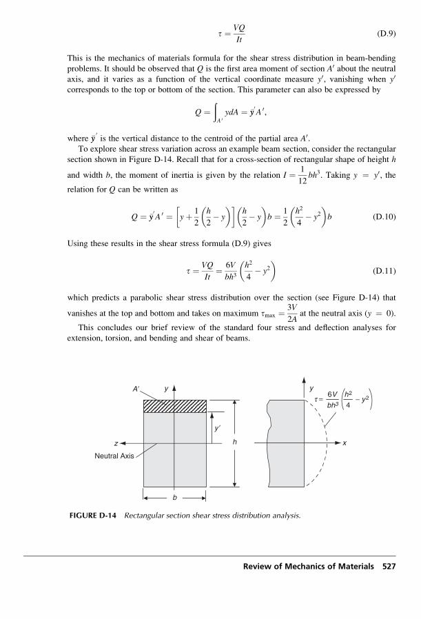
t ¼ VQ
It(D:9)
This is the mechanics of materials formula for the shear stress distribution in beam-bending
problems. It should be observed that Q is the first area moment of section A0 about the neutralaxis, and it varies as a function of the vertical coordinate measure y0, vanishing when y0
corresponds to the top or bottom of the section. This parameter can also be expressed by
Q ¼ðA 0ydA ¼ �yy
0A 0,
where �yy0is the vertical distance to the centroid of the partial area A0.
To explore shear stress variation across an example beam section, consider the rectangular
section shown in Figure D-14. Recall that for a cross-section of rectangular shape of height h
and width b, the moment of inertia is given by the relation I ¼ 1
12bh3. Taking y ¼ y0, the
relation for Q can be written as
Q ¼ �yy0A 0 ¼ yþ 1
2
h
2� y
� � h
2� y
� �b ¼ 1
2
h2
4� y2
� �b (D:10)
Using these results in the shear stress formula (D.9) gives
t ¼ VQ
It¼ 6V
bh3h2
4� y2
� �(D:11)
which predicts a parabolic shear stress distribution over the section (see Figure D-14) that
vanishes at the top and bottom and takes on maximum tmax ¼ 3V
2Aat the neutral axis (y ¼ 0).
This concludes our brief review of the standard four stress and deflection analyses for
extension, torsion, and bending and shear of beams.
z
Neutral Axis
yA�
y�
b
h
y
− y2t =4
6V h2
bh3
x
FIGURE D-14 Rectangular section shear stress distribution analysis.
Review of Mechanics of Materials 527
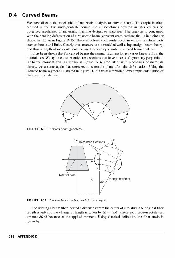
D.4 Curved Beams
We now discuss the mechanics of materials analysis of curved beams. This topic is often
omitted in the first undergraduate course and is sometimes covered in later courses on
advanced mechanics of materials, machine design, or structures. The analysis is concerned
with the bending deformation of a prismatic beam (constant cross-section) that is in a circular
shape, as shown in Figure D-15. These structures commonly occur in various machine parts
such as hooks and links. Clearly this structure is not modeled well using straight beam theory,
and thus strength of materials must be used to develop a suitable curved beam analysis.
It has been shown that for curved beams the normal strain no longer varies linearly from the
neutral axis. We again consider only cross-sections that have an axis of symmetry perpendicu-
lar to the moment axis, as shown in Figure D-16. Consistent with mechanics of materials
theory, we assume again that cross-sections remain plane after the deformation. Using the
isolated beam segment illustrated in Figure D-16, this assumption allows simple calculation of
the strain distribution.
Considering a beam fiber located a distance r from the center of curvature, the original fiber
length is rdy and the change in length is given by (R� r)dc, where each section rotates an
amount dc=2 because of the applied moment. Using classical definition, the fiber strain is
given by
a
b
r
MM
FIGURE D-15 Curved beam geometry.
r
dq
Neutral Axis
R
Deformed Sections 2dy
Elongated Fiber
A
FIGURE D-16 Curved beam section and strain analysis.
528 APPENDIX D
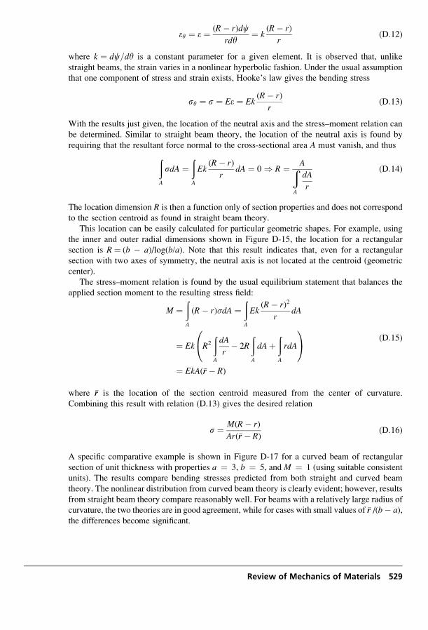
ey ¼ e ¼ (R� r)dcrdy
¼ k(R� r)
r(D:12)
where k ¼ dc=dy is a constant parameter for a given element. It is observed that, unlike
straight beams, the strain varies in a nonlinear hyperbolic fashion. Under the usual assumption
that one component of stress and strain exists, Hooke’s law gives the bending stress
sy ¼ s ¼ Ee ¼ Ek(R� r)
r(D:13)
With the results just given, the location of the neutral axis and the stress–moment relation can
be determined. Similar to straight beam theory, the location of the neutral axis is found by
requiring that the resultant force normal to the cross-sectional area A must vanish, and thusðA
sdA ¼ðA
Ek(R� r)
rdA ¼ 0 ) R ¼ AÐ
A
dA
r
(D:14)
The location dimension R is then a function only of section properties and does not correspond
to the section centroid as found in straight beam theory.
This location can be easily calculated for particular geometric shapes. For example, using
the inner and outer radial dimensions shown in Figure D-15, the location for a rectangular
section is R¼ (b � a)/log(b/a). Note that this result indicates that, even for a rectangular
section with two axes of symmetry, the neutral axis is not located at the centroid (geometric
center).
The stress–moment relation is found by the usual equilibrium statement that balances the
applied section moment to the resulting stress field:
M ¼ðA
(R� r)�dA ¼ðA
Ek(R� r)2
rdA
¼ Ek R2
ðA
dA
r� 2R
ðA
dAþðA
rdA
0@
1A
¼ EkA(�rr � R)
(D:15)
where �rr is the location of the section centroid measured from the center of curvature.
Combining this result with relation (D.13) gives the desired relation
s ¼ M(R� r)
Ar(�rr � R)(D:16)
A specific comparative example is shown in Figure D-17 for a curved beam of rectangular
section of unit thickness with properties a ¼ 3, b ¼ 5, and M ¼ 1 (using suitable consistent
units). The results compare bending stresses predicted from both straight and curved beam
theory. The nonlinear distribution from curved beam theory is clearly evident; however, results
from straight beam theory compare reasonably well. For beams with a relatively large radius of
curvature, the two theories are in good agreement, while for cases with small values of �rr /(b� a),the differences become significant.
Review of Mechanics of Materials 529
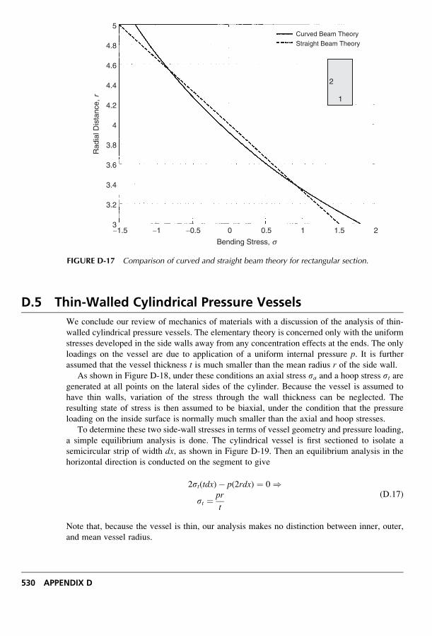
D.5 Thin-Walled Cylindrical Pressure Vessels
We conclude our review of mechanics of materials with a discussion of the analysis of thin-
walled cylindrical pressure vessels. The elementary theory is concerned only with the uniform
stresses developed in the side walls away from any concentration effects at the ends. The only
loadings on the vessel are due to application of a uniform internal pressure p. It is further
assumed that the vessel thickness t is much smaller than the mean radius r of the side wall.As shown in Figure D-18, under these conditions an axial stress sa and a hoop stress st are
generated at all points on the lateral sides of the cylinder. Because the vessel is assumed to
have thin walls, variation of the stress through the wall thickness can be neglected. The
resulting state of stress is then assumed to be biaxial, under the condition that the pressure
loading on the inside surface is normally much smaller than the axial and hoop stresses.
To determine these two side-wall stresses in terms of vessel geometry and pressure loading,
a simple equilibrium analysis is done. The cylindrical vessel is first sectioned to isolate a
semicircular strip of width dx, as shown in Figure D-19. Then an equilibrium analysis in the
horizontal direction is conducted on the segment to give
2st(tdx)� p(2rdx) ¼ 0 )st ¼ pr
t
(D:17)
Note that, because the vessel is thin, our analysis makes no distinction between inner, outer,
and mean vessel radius.
Curved Beam Theory
Straight Beam Theory
5
4.8
4.6
4.4
4.2
4
Rad
ial D
ista
nce,
r
3.8
3.6
3.4
3.2
3−1.5 −1 −0.5 0
Bending Stress, s0.5 1 1.5 2
1
2
FIGURE D-17 Comparison of curved and straight beam theory for rectangular section.
530 APPENDIX D
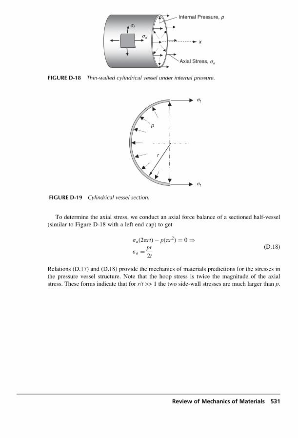
To determine the axial stress, we conduct an axial force balance of a sectioned half-vessel
(similar to Figure D-18 with a left end cap) to get
sa(2prt)� p(pr2) ¼ 0 )sa ¼ pr
2t
(D:18)
Relations (D.17) and (D.18) provide the mechanics of materials predictions for the stresses in
the pressure vessel structure. Note that the hoop stress is twice the magnitude of the axial
stress. These forms indicate that for r/t >> 1 the two side-wall stresses are much larger than p.
st
sa
Internal Pressure, p
Axial Stress, sa
x
FIGURE D-18 Thin-walled cylindrical vessel under internal pressure.
r
p
st
st
FIGURE D-19 Cylindrical vessel section.
Review of Mechanics of Materials 531
Index
A
Airy stress function, 144, 147, 151, 267,
334, 392–393
Alternating symbol, 7
Angle of twist, 218
Analytic function, 261
Angular momentum, 67
Anisotropic elasticity, 80, 297
Antiplane strain, 143, 213, 415
Antisymmetric tensors, 6
Approximate solution methods, 106
Approximating functions (FEM), 476
Axisymmetric problems
plane case, 171
three-dimensional case, 387
B
Basis vectors, 4
Beam problems
pure bending, 155
sinusoidal transverse loading, 162
uniform axial loading, 153
uniform transverse loading, 157
Beltrami-Michell compatibility equations
general equations, 97
plane strain, 137
plane stress, 140
Beltrami stress function, 381
Bending of curved beams, 194
Bessel function, 417–418, 455
Betti-Rayleigh reciprocal theorem, 120–121
Bianchi relations, 51
Biharmonic equation, 145, 147
Biharmonic functions, 145, 366, 368
Biharmonic solutions, 145, 147
Biharmonic vectors, 367, 368, 384
Body couple, 449
Body forces, 55
Body force vector, finite element theory, 480
Boundary conditions, 92–95
Boundary element method, 107, 474, 489
Boundary integral equation, 489
Boussinesq potentials, 374
Boussinesq problem, 371, 374
Brazilian test, 197
Bulk modulus, 84
Burgers vector, 433
C
Calculus of variations, 128
Cartesian coordinate system, 8
Cartesian tensor notation, 10
Castigilianos theorem, 126
Cauchy stress, 60
Cauchy’s integral formula, 263
Cauchy’s integral theorem, 262
Cauchy-Riemann equations, 262
Cellular materials, 389
Center of dilatation, 379, 387, 442
Center of flexure, 247
Center of rotation, 443
Cerruti’s problem, 372
Cesaro integral, 46
Characteristic equation (principal value
problem), 12–16
Circumferentially orthotropic, 329
Clapeyron’s theorem, 120
Coefficient of thermal expansion, 86, 338
Comma notation, 17
Compatibility equations. See Beltrami-
Michell compatibility
equations; Saint-Venant
compatibility equations
Complementary energy, 124–126
Completeness, 365, 372
Complex conjugate, 260
Complex derivative, 261
Complex displacements, 267
Complex Fourier series, 274, 321
Complex potential functions, 271
Complex stresses, 268
Complex temperature, 352
Complex variable, 259
Complex variable methods
anisotropic plane problem, 315
anisotropic torsion problem, 310–311
plane problem, 266–292
thermoelastic plane problem, 352–359
torsion problem, 259
Compliance tensor, 298
Composites, 297, 301, 306
Concentrated force problem
plane problem, 182, 278, 279, 317–320
three-dimensional problem, 370–372,
410–414, 437–440
Conformal mapping/transformations, 265,
283, 320
Conical shaft under torsion, 242
Conjugate functions, 262
Conservation of angular momentum, 67
Conservation of energy, 338
Conservation of linear momentum, 66
Constitutive relations, 77
Contact problems, 189
Continuum mechanics, 3
Contraction of tensors, 5
Conversion between plane strain
and plane stress
isothermal case, 141
thermoelastic case, 342
Convex region, 373
Coordinate systems
Cartesian, 8, 473
cylindrical, 21, 497
general orthogonal curvilinear, 22
polar, 25
spherical, 22, 497
Coordinate transformation, 8
Cosserat continuum, 449
Couple stress tensor, 449
533
Couple stress theory, 56, 448–457
Coupling term (thermoelastic energy
equation), 338
Crack density parameter, 445
Crack problems, 192–193, 287–292,
325–328, 359, 416–418
Cross product, 16
Curl operation, 18, 24
Curved beams, 194–197
Curvilinear anisotropy, 328
Cyclic functions, 272, 318, 319, 356
Cylindrical coordinates, 21, 497
D
Deformation, 31
Degrees of freedom, 478
Del operator, 18
Determinant, 7
Dilatation, 40, 50
Dirac delta function, 277
Direct solution method, 102
Dislocations
edge, 432–434
screw, 52, 432, 435
Displacement formulation, 98–100
Displacement gradient tensor, 33
Displacement potentials, 365
Displacement vector, 32
Divergence operation, 18–20, 24
Divergence theorem, 20
Dot product, 16
Doublet mechanics, 431, 463
Dual vector, 28
Duhamel-Neumann thermoelastic
law, 86, 338
Dyadic notation, 11
E
Eigenvalue problem, 12–16
Elasticity with distributed cracks,
431, 445, 471
Elasticity with voids, 432, 457, 471
Elastic material, 77–79
Elastic limit, 78
Elastic moduli, 80, 82
Element assembly, 482
Elliptical hole problem, 286–288,
320–324, 357–359
Energy equation, 338
Energy methods
minimum complementary energy, 125
minimum potential energy, 124
Engineering strains, 36
Equilibrated body force, 458
Equilibrated force, 458
Equilibrated stress vector, 458
Equilibrium equations, 66
Cartesian, 67, 499
cylindrical, 70, 499
polar, 75
spherical, 70, 499
Essential boundary conditions, 124
Euler-Bernoulli beam theory,
126–128
Eulerian description, 32
Even functions, 166
Extension of cylinders, 216
F
Fabric tensor, 298
Failure criteria (distortional strain
energy), 117
Finite difference method, 107, 473
Finite element method, 107, 473, 474
Fixity conditions, 154, 156, 160, 164
Flamant solution, 182, 280, 407, 465
Flamants paradox, 466
Flexure of cylinders
circular section, 247
general formulation, 243
rectangular section, 249
Force doublet, 378, 386, 440, 441
Fourier integral form, 416
Fourier law of heat conduction, 337
Fourier methods, 105, 161, 233
Fourier series, 165
Fourier integral, 416
Fracture mechanics, 193, 212, 288,
325, 359, 416
Functionally graded materials,
80, 391, 407
Fundamental solution, 121
G
Galerkin vector, 365, 367, 384
Gamma function, 409
Generalized plane stress, 141–142
Global reference system, 482
Graded materials, 391, 393, 394,
399, 407, 425
Gradient operation, 18, 24
Granular materials, 200, 214, 431
Green’s theorem in the plane, 21
Greens function, 121, 491
H
Half-space problems, 181, 280, 319, 371,
372, 407
Harmonic functions, 246, 262, 366, 367
Heat conduction, 337
Heat flux vector, 337
Helmholtz representation theorem, 365
Hollow cylindrical domain, plane problem,
172
Holomorphic functions, 261
Homogeneous materials, 80
Hooke’s law, 79, 81, 298–304, 392–393,
403, 479
Hydrostatic compression (tension), 84
Hyperelastic materials, 117
I
Incompatibility tensor, 51
Incompressibility, 84
Index notation, 4
Indirect tension test, 197
Induced mappings, 321
Infinite space problems, 279, 369,
437–445
Infinitesimal (small) deformations, 32, 34
Inhomogeneous elastic half-space, 407, 413
Inner product, 5
Integral equation, 418
Integral transform methods, 106, 460
Interface conditions,
perfectly bonded interface, 95
slip interface, 95–96
Internal energy, 338
Interpolation functions, 477
Invariants
general tensor, 13
stain, 40
stress, 61
Inverse solution method, 103
Irrotational vector field, 365
Isochromatic fringe patterns, 191,
200, 212, 214
Isotropic materials, 80
Isotropic tensors, 10, 27, 81, 86, 87
K
Kelvin problem, 121, 369,
437–440
Kolosov-Muskhelishvili potentials, 268
Kronecker delta, 7
L
Lagrange interpolation functions, 476
Lagrangian description, 32
Lame’s constant, 81
Lame’s strain potential, 366–367
Lamellar vector field, 365
Laplace equation, 105, 143, 222,
233, 262
Laplace transform, 460
Laplacian operation, 18, 24–26
Laurent series, 263
Legendre differential equation, 377
Legendre functions and polynomials, 377
Length scales, 431, 452, 463
Line integrals, 20, 262–263
Line of dilatation, 444
Loading vector, finite element theory, 480
Local coordinates, 482
Love strain potential, 369
M
Maclaurin series, 263
Material symmetry, 299–304, 306
Material symmetry group, 299
MATLAB, 505
Matrix notation, 16
Matrix products, 16
Maximum shear stress, 63, 72,
191, 200, 211
Maxwell stress function, 365, 382
534 INDEX
Mechanics of materials, 518
Membrane analogy, 225
Mesh (FEM), 474
Michell solution, 169
Micromechanics, 431
Micropolar stress theory, 56, 448, 454
Modulus of elasticity, 82, 84
Mohr’s circle, 63
Monoclinic materials, 301
Morera stress function, 365, 382
Multiply connected regions,
45, 223, 237
Multivaluedness, 46, 264, 272, 433
N
Navier equations
antiplane strain case, 143
general equations, 99, 392, 500–501
plane strain case, 136–137
plane stress case, 140
Natural boundary conditions, 124
Negative Poisson’s ratio, 389
Neumann principle, 297
Nodal displacements, 477, 482
Nodal forces, 480
Nodal points, 473
Nonhomogeneous elasticity
airy stress function, 392–393
antiplane strain problems, 415–418
Hooke’s law, 392
plane hollow cylindrical domain
problem, 396–402
point force on half-space, 407–414
rotating disk problem, 402–407
torsion problem, 418–425
uniaxial tension, 394–396
Nonhomogeneous materials, 80, 391
O
Octahedral plane, 65
Octahedral stress, 65
Odd functions, 166
Orthogonality conditions, 10
Orthotropic materials, 301, 306
P
Papkovich-Neuber solution, 365, 372–376
Permutation symbol, 7
Photoelastic results
contact loadings, 191
crack problem, 212
disk under compression, 200
granular media, 214
Physical components, 23
Piola-Kirchhoff stress, 60
Plane axisymmetric problem, 171, 207
Plane strain
isothermal, 135
thermal 340
Plane stress
isothermal, 138
thermal 341
Point force problem, 182, 280,
407, 465
Poisson equation, 219
Poisson’s ratio, 82, 83
Polar coordinates, 25
Polar coordinate formulation
isothermal, 145
thermoelastic, 347
Polar orthotropic materials, 329
Polynomial solutions, 151
Poroelasticity, 432
Positive definite strain energy form, 116
Potential functions, 365
Potential theory, 223, 343, 436
Power series method for Airy
function, 105, 151
Prandtl stress function, 219, 420
Principal value problem
principal directions, 13
principal values, 12
Proportional limit, 78
Pure shear, 83
Q
Quadratic form of strain energy, 116
R
Radial stress distribution, 408
Radially orthotropic, 329
Rayleigh-Ritz method, 106, 128
Reciprocal theorem, 120–121
Reference temperature, 338
Reissner’s principle, 126, 130
Residues, 264
Restrictions on elastic moduli, 119, 305
Rigid body motion, 31, 34, 37–38
Rosette strain gage, 49
Rotating disk problem
homogeneous, 210–203
nonhomogeneous, 402–407
Rotation tensor, 33
Rotation vector, 34
S
Saint-Venant compatibility equations, 41
Saint-Venant’s principle, 101, 138, 215
Saint-Venant theory, deformation
of cylinders
bending flexure, 215, 243
extension, 215, 216
torsion, 215, 217
Scalar notation, 3
Scale factors, 22
Self-equilibrated forms, 381
Semi-inverse solution method, 104, 215
Shear center, 247
Shear modulus, 81, 83
Shear stress, 58
Simple tension, 82
Simply connected regions, 44, 264
Single-valued displacements, 41
Singular stress states, 436
Singularities
branch points and cuts, 264
general definition, 261
poles, 263
Solenoidal vector field, 366
Somiglianas identity, 121, 490
Specific heat capacity, 338
Spherical coordinate solutions, 361, 376,
387–389
Spherical coordinates, 22, 497
Spherical harmonics, 377
Spherically symmetric problems, 387
Stationary potential energy, 124
Steady-state thermal conditions, 339
Stiffness matrix, 480
Stokes theorem, 20
Strain compatibility, 41–46
Strain displacement relations
Cartesian, 36, 498
cylindrical, 47, 498
polar, 146
spherical, 47, 498
Strain energy, 113
Strain energy forms
distortional, 117
general, 116
volumetric, 117
Strain gage, 49
Strain tensor, 33
deviatoric strain, 41
extensional strain, 35
normal strain, 35
principal strain, 40
shear strains, 36
spherical strain, 41
Strain transformation, 38
Strength of materials theory, 518
Stress concentration factors
anisotropic case, 320–324
BEM solution, 495
elasticity with voids case, 459–462
FEM solutions, 485, 486
micropolar case, 454–457
plane elastic cases, 175, 177–178,
179, 286–288
three-dimensional cases, 378–380,
387–388
Stress functions, 144, 219, 381
Stress intensity factor, 193, 291,
327, 328, 418
Stress-strain curve, 78
Stress tensor (Cuachy), 57–58
deviatoric stress, 65
normal stress, 58
octahedral stress, 65
principal stress, 61
shear stress, 58
spherical stress, 65
von Mises stress, 65
Stress tensor (Piola-Kirchhoff ), 60
Stress transformation, 60
Stress vector, 57
INDEX 535
Summation convention, 5
Superposition principle, 100
Surface forces, 56
Symmetric tensors, 5
T
Taylor’s series, 263
Temperature, 86
Tensor definition, 10
Tensor product, 11
Tensor transformation, 8
Thermal conductivity, 338
Thermal conductivity tensor, 337
Thermal expansion coefficient, 86, 338
Thermal fracture, 359
Thermoelastic displacement potential
solution, 343
Thermoelastic plane strain formulation,
340–341
Thermoelastic plane stress formulation,
341–342
Torsion of cylinders
anisotropic formulation, 306–312
displacement formulation, 222
elliptical section, 227
equilateral triangular section, 230
general formulation, 217
multiply connected sections, 223, 238
rectangular section, 233
stress formulation, 218
thin rectangular sections, 236
thin-walled sections, 239
variable diameter, 241
Torsion problem, 417
Torsional rigidity
homogeneous case, 222
inhomogeneous case, 421
Traction boundary conditions, 92
Traction vector, 57
Transformation matrix, 8
Transformation of field variables, 502
Transversely isotropic materials, 302
Triangular element, 476
Triclinic material, 299
U
Uncoupled conduction equation, 338
Uncoupled thermoelastic formulation, 339
Uniaxial (simple) tension, 82, 119
Uniaxial tension, graded sheet, 394–396
Uniqueness theorem, 118
Unit matrix, 7
V
Variational methods, 128–130
Vector notation, 3
Vector products, 16
Velocity field, 338
Virtual displacements, 122
Virtual work principle, 122
Virtual work formulation for finite element
method, 478
Voigt matrix notation, 298
Volume fraction, 457
Volumetric deformation, 84
von Mises stress, 65
W
Warping displacement, 217, 218
Weak form, 475
Wedge problems, 179
Weighted residual method, 130
Westergaard stress function, 288, 291
Y
Yield point, 78
Young’s modulus, 82, 83, 85
Z
Zero-value theorem, 21
536 INDEX